ARJEN MULDER

Government Dilemmasin the Private Provisionof Public Goods

Government Dilemmas in the Private Provision of Public Goods

Government Dilemmas in the Private Provision of Public Goods

Dilemma’s voor overheden bij het privaat aanbieden van publieke goederen

PROEFSCHRIFT

ter verkrijging van de graad van doctor aan de Erasmus Universiteit Rotterdam

op gezag van de Rector Magnificus

Prof.dr. S.W.J. Lamberts

en volgens besluit van het College voor Promoties.

De openbare verdediging zal plaatsvinden op donderdag 14 oktober 2004 om 13:30 uur

door

Arjen Mulder

geboren te Dordrecht

Promotiecommissie Promotor: Prof.dr. R.J.M. van Tulder Overige leden: Prof.dr.ir. H.W.G.M. van Heck Dr. R. Huisman Prof.dr. J.W. Velthuijsen Erasmus Research Institute of Management (ERIM) Rotterdam School of Management / Rotterdam School of Economics Erasmus University Rotterdam Internet: http://www.erim.eur.nl ERIM Electronic Series Portal: http://hdl.handle.net/1765/1 ERIM PhD Series Research in Management 45 ISBN 90-5892-071-2 Cover illustration: Prophet 3, painting (2002) by William J. Baumol. Reproduced by courtesy of the artist. © Arjen Mulder, 2004. All rights reserved. No part of this publication may be reproduced or transmitted in any form or by any means, electronic or mechanical, including photocopying, recording, or by any information storage and retrieval system, without permission in writing from the author.

v

ACKNOWLEDGEMENTS The worst moment of the writing process of a PhD thesis is the moment you hand in the first complete draft. It is not that you would have wanted to continue with that manuscript (in fact, I couldn’t have cared less for the first few weeks after). What makes ‘handing in’ a disappointing activity, however, is the fact that you realise ‘this is it’. Four laborious years come together in these two or three minutes of printing your manuscript. There is, however, also a joy of these few minutes of printing: they allow you to quickly meditate on the happy moments experienced during the entire process. In writing the current pages, I return to these moments. When assessing my thesis, it seems slightly more economic in nature than truly managerial. I think there are two important reasons for this. First, I must admit that—although the more you learn on economics, the more disappointing the science becomes—my former colleagues at NEI have apparently brainwashed me with their neoclassical economics thinking. Without wishing to mention everybody, I wish to express my greatest admiration of Nol Verster and Gerbert Romijn, by then probably the two brightest people within that firm. In addition, I must admit that Thijs de Ruyter van Steveninck has always surprised me with his neoclassical interpretations of the ordinary things in life, and his (extremely!) broad literary interests. I cannot help but mentioning Holger van Eden, who claimed any problem you discovered to be ‘a market imperfection’. Lastly, there was Willem Molle, who was willing not only to read my first drafts of a research proposal for a PhD thesis, but also expressed sincere interest in the youngsters who had recently joined ‘his’ company. Having swapped NEI for Erasmus Univ. (a big difference in income, but a physical distance of only a few hundreds of meters), I have very good memories of the frequent talks, laughter, and serious discussions with Michael Mol. Mike, I still remember our summer school at Essex—though I’m convinced the A120 was the shortest route to Essex, indeed, I still do believe that it should not have been taken by bicycle. Once Mike had left, I have been fortunate enough to have similar talks with Douglas van den Berghe. Doug, when we returned from that conference in Vienna, and we saw that airplane having an undesirable ignition in one of the engines, it was most pleasant to notice that all we both concluded was that we had some time left for a dessert (although later on, it appeared not to be our plane but the neighbouring one). I acknowledge Hans van Oosterhout, probably the brightest guy at our school, for sharing thoughts and numerous discussions about whatever theme. Hans, ever since I took my methodology/philosophy classes with you, I have had the feeling the topics we discussed were only the top of an iceberg, of which you knew more. From my very first MPhil course onwards, I have been very fortunate to meet bright and enthusiastic fellow PhD students at the Financial Management department, with whom I could not only discuss my little

vi

mathematical and econometric problems, but also transcend the professional level. In this respect I mention Ben Tims, Cyriel de Jong, Gerard Moerman, and Reggy Hooghiemstra. At some lucky moment, Ronald Huisman crossed my path, to whom I owe a debt of gratitude. Ronald, you have not only encouraged me to deepen my corporate finance interests, but also gave me numerous opportunities to present materials for other people—professionals and academics. In the same R2 office, I met Ronald Mahieu, with whom I have started to write some papers. Ronalds, thank you both for inviting me to the Financial Management department! I dedicate a separate note to my thesis advisor, Rob van Tulder. Rob, although the result of this study is not quite what I had in mind when I started, I hope you share my satisfaction. I thank you for giving me the ‘degrees of freedom’ I needed so badly, varying from lecturing my own courses, to the supervision of MSc theses and apprenticeships, to a large body of my thesis. By allowing me sufficient ‘artistic freedom’, you expressed your confidence in both the process and the outcome. It is unbelievable how you have always managed to read everything in time, and how you have helped me to see the broader perspective of all my pieces of writing. In your own (e-mail) terms: Some people deserve a separate note for going beyond the writing process of the current thesis. First, there is Joost van Montfort, and of course Margreet. To both of you, I wish to express my deepest sympathy. Not only have you shown a sincere interest in my first steps on the path of my PhD process, but also it proved possible to maintain and even deepen our friendship at a distance (both at the route Rotterdam-Amsterdam, and at the Netherlands-Latin America). Joost, although I still a share your love for Latin America, I couldn’t help but change my thesis’ topic into something completely different—I hope to make it up by travelling more to ‘your’ continent. Then my two paranymphs. I am very fortunate with close friends, like Paul de Gruyl for an ever-lasting friendship that proved to be able to survive over time, while still remaining intense. I must say I was most surprised that Gertjan de Jong not only proved to be a close friend, but also appeared to share professional interests relating to the topic of this thesis. Gertjan, it’s a big pleasure to have you at the defence ceremony. I thank my parents for their moral support—apparently from a distance, these four years appeared more intense to you than I may remember. Lastly (finally!), a word to my beloved Fatima. Our relationship started in the first year of my time as a PhD student, so in fact you have gone through the same process, albeit from a different perspective. From the very first start, I remember the preciousness of our relationship, and how lovely it is to have you around. I have never seen a happier person, full of positive energy, while always ready for a critical note. Although without having known you I would probably have finished this thesis as well, I am most convinced life would have been less beautiful.

Arjen Mulder, Rotterdam, July 2004.

vii

CONTENTS ACKNOWLEDGEMENTS .......................................................................................... V EXECUTIVE SUMMARY..........................................................................................XI SAMENVATTING (SUMMARY IN DUTCH) .............................................................XII

PART I: INTRODUCTION ................................................................................. 1

1 OBJECTIVES AND ORIENTATION ........................................................ 3

1.1 INSPIRATION FOR THE STUDY .................................................................. 3 1.1.1 The pessimist view on public enterprise .......................................... 5 1.1.2 Privatisation as one possible dimension of all structural reforms .. 6 1.1.3 Expected gains of structural reforms............................................... 7

1.2 CHALLENGES FOR THE PRIVATE SECTOR............................................... 13 1.3 PRIVATE PROVISION OF PUBLIC GOODS: AN OVERVIEW........................ 15 1.4 SOME MECHANISMS FOR INFLUENCING PRIVATE SECTOR INVESTMENTS ........................................................................................ 17 1.5 PROBLEM STATEMENT AND RESEARCH QUESTIONS .............................. 20 1.6 PURPOSE OF THE STUDY ........................................................................ 27 1.7 RELEVANCE OF THE STUDY ................................................................... 27

1.7.1 Societal relevance.......................................................................... 30 1.7.2 Scientific relevance........................................................................ 31 1.7.3 Managerial relevance.................................................................... 32

1.8 ORGANISATION OF THE STUDY .............................................................. 33

PART II: FOUR DILEMMAS ........................................................................... 35

2 THE INFLUENCEABILITY DILEMMA ................................................ 37

2.1 THE CONCEPT OF UNDERINVESTMENT................................................... 38 2.2 SOURCES OF UNDERINVESTMENT: BARRIERS TO CORPORATE INVESTMENT.......................................................................................... 42 2.3 MICRO-LEVEL BARRIERS TO INVESTMENT ............................................ 43

2.3.1 Wrong incentives for managers to invest ...................................... 44 2.3.2 Uncertainty on ROI with an option to wait ................................... 44 2.3.3 Debt-to-equity ratio ....................................................................... 45 2.3.4 Stock market performance of the firm ........................................... 46 2.3.5 Agency approaches to underinvestment ........................................ 48

2.4 SECTOR ANALYSIS AND INVESTMENT BARRIERS................................... 49 2.4.1 Strategic underinvestment and the signalling game...................... 50 2.4.2 Incomplete contracts and the hold-up problem............................. 50 2.4.3 Contract renegotiation and the hold-up problem.......................... 51

viii

2.4.4 The role of competition.................................................................. 53 2.4.5 Declining product-market.............................................................. 55

2.5 THE MACRO-LEVEL CONTEXT................................................................ 57 2.5.1 Savings gap, hyperinflation, and capital flight.............................. 57 2.5.2 Profits and price cap regulation.................................................... 58 2.5.3 Liberalisation, regulatory reforms, and the vertical separation of the value chain........................................................................... 60 2.5.4 Franchise bidding, concessions, and licensing ............................. 61 2.5.5 Policy reforms, and the expropriation risk.................................... 61

2.6 AN INTERMEDIATE SUMMARY AND ANALYSIS ...................................... 62 2.7 MEASUREMENT AND EXISTENCE OF UNDERINVESTMENT ..................... 63

2.7.1 Empirical studies on underinvestment........................................... 63 2.7.2 Some definitions of ‘underinvestment’ .......................................... 68 2.7.3 Popular benchmarks...................................................................... 69 2.7.4 Implications for the current study ................................................. 70

2.8 A DEFINITION OF UNDERINVESTMENT................................................... 72 2.9 GOVERNMENT INSTRUMENTS FOR DISCOURAGING UNDERINVESTMENT............................................................................... 73

3 THE SMART GOVERNANCE DILEMMA ............................................ 77

3.1 THE PARTICIPATION CONSTRAINT AND AN EVALUATION CRITERION.... 77 3.1.1 A note on evaluation criteria and benchmarks.............................. 81

3.2 GOVERNMENT’S EXPENDITURE MINIMISATION PROBLEM AND PARETO EFFICIENCY............................................................................................ 85

3.2.1 Nested optimisation and Nash equilibria ...................................... 86 3.2.2 Underinvestment and governmental valuation of the public good 92

3.3 A PROPOSAL FOR A SMART GOVERNANCE FRAMEWORK....................... 93 APPENDIX 3.A MATHEMATICAL APPENDIX ................................................... 97

4 THE POLICY PORTFOLIO DILEMMA: EMPIRICAL EVIDENCE FROM WIND TURBINES INVESTMENTS ................................................. 107

4.1 INTRODUCTION .................................................................................... 107 4.2 A MODEL.............................................................................................. 108

4.2.1 Ramified Q................................................................................... 109 4.2.2 Discussion of economic instruments............................................ 114

4.3 SOME BASE-CASE DEVELOPMENTS ...................................................... 115 4.3.1 Base-case assumptions ................................................................ 116 4.3.2 Base-case Q ................................................................................. 119

4.4 POLICIES AFFECTING Q........................................................................ 121 4.4.1 Description of green policies....................................................... 121 4.4.2 Present value of green policies.................................................... 131 4.4.3 Q including incentives ................................................................. 132

4.5 INVESTMENT RESPONSE TO GREEN POLICIES....................................... 133

ix

4.5.1 Wind turbine investments over time............................................. 133 4.5.2 From Q to capital stock: Phase diagrams................................... 137 4.5.3 From Q to capital stock: Individual regressions......................... 138 4.5.4 From Q to capital stock: A panel data regression ...................... 143 4.5.5 A note on the ‘barriers to investment’ ......................................... 144

4.6 IMPLICIT GOVERNMENTAL VALUATION OF THE PUBLIC GOOD............ 144 4.7 UNDERINVESTMENT ISSUES................................................................. 145

4.7.1 Barriers to investment ................................................................. 147 4.7.2 Technical underinvestment based on Tobin’s Q.......................... 147 4.7.3 Underinvestment in the context of governmental valuation ........ 148

4.8 CONCLUSIONS...................................................................................... 150 APPENDIX 4.A DATA AND STATISTICAL APPENDIX ..................................... 153

5 THE JOINT OWNERSHIP DILEMMA: INVESTMENT AND EFFICIENCY INCENTIVES IN PUBLIC-PRIVATE PARTNERSHIPS.. 163

5.1 INTRODUCTION .................................................................................... 163 5.2 AN OVERVIEW OF PPP ARRANGEMENTS ............................................. 164 5.3 SOME COMMON MISUNDERSTANDINGS ABOUT PPPS .......................... 166 5.4 WHAT DO WE KNOW ABOUT PPPS? ..................................................... 171

5.4.1 Empirical ‘evidence’ on PPPs..................................................... 172 5.4.2 On the proper scope of government or ‘who should own the project?’ ...................................................................................... 173 5.4.3 On the nature and contractibility of the co-operation................. 176

5.5 INCENTIVES, INVESTMENT, AND ENTREPRENEURIAL ABILITY: A MODEL ............................................................................................. 179

5.5.1 A model........................................................................................ 180 5.5.2 Base-case: Public provision ........................................................ 181 5.5.3 Alternative scenario: Unregulated PPP...................................... 183

5.6 WHEN WOULD A PPP BE PREFERRED OVER PUBLIC PROVISION?......... 188 5.6.1 PPP minimally produces the base-case output quantity ............. 188 5.6.2 PPP produces the same output quantity at lower cost ................ 189 5.6.3 Wrapping up ................................................................................ 190

5.7 DISCUSSION ......................................................................................... 191 APPENDIX 5.A MATHEMATICAL APPENDIX ................................................. 193

PART III: CONCLUSIONS AND POLICY IMPLICATIONS.................... 197

6 CONCLUSIONS........................................................................................ 199

6.1 FOUR DILEMMAS.................................................................................. 199 6.1.1 The Influenceability Dilemma ..................................................... 199 6.1.2 Smart Governance Dilemma ....................................................... 200 6.1.3 Policy Portfolio Dilemma............................................................ 201 6.1.4 Joint Ownership Dilemma........................................................... 202

x

6.2 A PROPOSAL FOR DESIGNING NON-COERCIVE POLICIES ...................... 203 6.2.1 A proposal for a conceptual model: Hypotheses......................... 203 6.2.2 A proposal for a conceptual model: Towards empirical testing . 207

6.3 OVERALL CONCLUSIONS...................................................................... 209 6.4 LIMITATIONS OF THE STUDY AND AVENUES FOR FURTHER RESEARCH 210

6.4.1 How versus why........................................................................... 210 6.4.2 Data limitation............................................................................. 211 6.4.3

7

PART IV: REFERENCES AND SOME ‘ABOUTS’ ..................................... 219

REFERENCES ...................................................................................................... 221 ABOUT THE COVER ILLUSTRATION................................................................... 240 ABOUT THE AUTHOR .......................................................................................... 242 ERASMUS RESEARCH INSTITUTE OF MANAGEMENT (ERIM) ........................ 243

Other avenues for further research ............................................. 212

BEYOND THE STUDY............................................................................ 215

xi

EXECUTIVE SUMMARY The private provision of public goods is a much debated topic, both in the academic and the ‘real life’ literature. From an academic perspective, numerous potential pitfalls exist with respect to funding, willingness-to-pay, and the free rider problem. The logical solution to these problems has therefore always been government provision of public goods. In an era where governments withdraw from the market place as active providers of goods and services, however, there is a renewed interest in the private provision of these activities. This thesis takes a governmental perspective, asking how governments can encourage investments in the private provision of public goods. Since from an economic perspective the so-called ‘coercive’ measures (most noteworthy: regulation) are by definition inefficient, I focus on the non-coercive measures. Therewith, a trade-off is introduced between the efficiency and effectiveness of the government intervention—coercive measures are most predictable in their outcomes, but less efficient, whereas non-coercive measures are most efficient, but less predictable. One of the basic assumptions is that firms will invest in whatever assets, as long as it

‘participation constraint’). Still, however, even though it may be economically interesting to invest in the provision of public goods, there may exist so-called ‘barriers to investment’. Chapter 2 of this study makes an inventory of these barriers, and introduces the concept op ‘underinvestment’. Altogether, the barriers to investment and their consequences in terms of underinvestment define the ‘Influenceability Dilemma’ for a government. Suppose a government has identified the most important barriers to investment, and suppose the non-coercive measures should focus on the economic attractiveness of the investment opportunity. How then, can a government assure herself of a desired response by the private sector on the one hand, whilst not being too generous on the other? This nested optimisation problem (i.e., the private sector faces a profit maximisation problem, whereas government faces an expenditure minimisation problem) forms the basis of the ‘Smart Governance Dilemma’. Chapter 3 proposes a framework, floating on Tobin’s Q as the main evaluation criterion for the private sector’s economic attractiveness of investing. Having proposed a framework, the question arises how to turn a pecuniary transfer into a real policy. Chapter 4 analyses an empirical test of this ‘Policy Portfolio Dilemma’, of which the results suggest that only money matters—not the policy palette through which it is offered. Ultimately, there may exist cases where a government would not want the private sector do the job on its own. In cases of incomplete contracting (such as prisons or hospitals) or naturally monopolistic areas (infrastructure projects as roads), public-private partnerships may form a nice alternative to the measures described above. Chapter 5 analyses this so-called ‘Joint Ownership Dilemma’, and finds that PPPs are not necessarily welfare enhancing.

is economically attractive to do so (i.e., the problem needs to meet the so-called

xii

SAMENVATTING (SUMMARY IN DUTCH) Het privaat aanbieden van publieke goederen is een veelbesproken onderwerp, zowel binnen de academia als in de ‘echte wereld’. Vanuit een wetenschappelijk perspectief bestaan er vele drempels voor het fenomeen, zoals het financieringsprobleem, de bereidheid tot betalen bij eindgebruikers, en het zogenaamde ‘free rider’ probleem. Hierdoor wordt bij publieke goederen de overheid vrijwel altijd als logisch alternatief voor de markt wordt gezien. Met een zich uit de markt terugtrekkende overheid als actieve aanbieder van goederen en diensten, echter, ontstaat er een hernieuwde aandacht voor het thema ‘privaat aanbieden van publieke goederen’. Dit proefschrift beziet het perspectief van een overheid, en onderzoekt hoe overheden de private sector kunnen stimuleren om te investeren in het aanbieden van publieke goederen. Aangezien vanuit een economisch perspectief ‘dwingende’ maatregelen (lees: regulering) per definitie inefficiënt zijn, richt ik mij op de niet-dwingende maatregelen. Hiermee wordt automatisch een uitwisselingsprobleem geïntroduceerd—dwingende maatregelen zijn het meest voorspelbaar qua uitkomsten, maar minder efficiënt, terwijl niet-dwingende maatregelen het meest efficiënt zijn, maar minder voorspelbaar uitpakken. Eén van de centrale vooronderstellingen is dat ondernemingen zullen investeren zo lang het economisch aantrekkelijk is (ofwel, er dient voldaan te worden aan de zogenaamde ‘participatie restrictie’). Desondanks kunnen er echter situaties zijn waarin het wel economisch aantrekkelijk is om te investeren, maar dat zogenaamde ‘investeringsbarrières’ dit verhinderen. Hoofdstuk 2 van dit proefschrift maakt een inventarisatie van deze barrières, en introduceert het begrip ‘onder-investeringen’. Tezamen vormen deze twee begrippen het ‘Beïnvloedbaarheids-dillemma’ voor een overheid. Stel nu dat een overheid heeft geïnventariseerd wat de belangrijkste investeringsbarrières zijn, en dat de niet-dwingende maatregelen zich op de economische aantrekkelijkheid van de investeringsbeslissing kunnen richten. Hoe kan een overheid zich dan enerzijds redelijkerwijs verzekeren van de gewenste respons door de private sector, terwijl ze anderzijds toch ook weer niet té scheutig wil zijn? Dit geneste optimalisatie probleem (de private sector wil winst maximaliseren terwijl een overheid haar uitgaven wil minimaliseren) vormt de basis van het ‘Slimme Bestuursdilemma’. Hoofdstuk 3 doet een voorstel voor een raamwerk, waarbij Tobin’s Q als evaluatiecriterium wordt genomen voor de economische aantrekkelijkheid van de investeringsbeslissing. Gegeven nu zo’n raamwerk, rijst de vraag hoe een overheid een berekende pecuniaire steun dient te vertalen naar concreet beleid. Hoofdstuk 4 maakt een empirische analyse van dit ‘Beleidsinstrumentenmixdilemma’, waarvan de resultaten suggereren dat slechts de hoogte van de pecuniaire steun telt, en niet zozeer de typen van ingezette instrumenten. Tenslotte wordt aandacht gegeven aan gebieden waar het privaat aanbieden niet altijd even gewenst is. Bijvoorbeeld in het geval van incomplete contracten (bijvoorbeeld ziekenhuizen of gevangenissen), of natuurlijke monopolies (infrastructurele projecten als wegen) zouden publiek-private samenwerkingsverbanden een aardig alternatief op bovenstaande arrangementen kunnen vormen. Hoofdstuk 5 analyseert dit zogenaamde ‘Gemeenschappelijk eigendomsdilemma’ en stelt dat PPSen niet per se welvaart creëren.

Part I: Introduction

3

1 OBJECTIVES AND ORIENTATION This book is the result of a study that seeks to identify dilemmas for governments in the private provision of public goods, and to propose solutions to these dilemmas. In an era where governments increasingly withdraw from the economy as active providers of goods and services, and hence increasingly rely on the private sector for these provisions, this study investigates under what circumstances private sector investments coincide with the goals of governments. Though the benefits of a private sector economy is widely acclaimed in product-market combinations with little externalities, it is by no means clear whether more complicated product-market combinations as drinking water provision, environmental protection, or even sewerage or integrated waste management may bear the same fruits from private sector provision as the production of jeans or biscuits. Particularly, it is unclear whether the investment decisions of private sector companies (possibly driven by the short-termism of the capital market) harmonise with the long-term interest of society, especially in cases of highly specific assets, that require large, sunk investments that are usually depreciated over longer time spans than average production equipments—the investments typically needed for the provision of many public goods. Section 1.1 shortly introduces the context of the study. Since the early 1980s, governments around the world tend to withdraw from the economy as active providers of goods and services. Even in product-market combinations where competition is not ‘natural’, such as in the case of utility sectors, most economies try to rely on private sector companies. Section 1.2 signals some challenges for these private sector companies. Section 1.3 briefly reviews the literature on the private provision of public goods. What are the obstacles mentioned in the literature? Section 1.4 gives a short sketch of the mechanisms governments can use to influence the investment behaviour of private firms. These mechanisms will be discussed in more detail in the case study analysis (Part II of this book). Section 1.5 defines the scope and structure of the book by introducing the problem statement and research questions. Lastly, section 1.6 specifies the relevance of the study.

1.1 Inspiration for the study After two decades of structural reforms (embodying privatisation, trade liberalisation, investments liberalisation, and regulatory reforms) theory and practice often still seem to clash. In their seminal article, Kay and Thompson (1986) already complain about the variety of possible goals of the vague concept

4

of privatisation. Consequently, they argue correctly, it is not only understandable that we can observe a large variety of ‘methods’ of privatisation, but it is also understandable that it is difficult to assess ‘the’ outcome of privatisation, since there exist multiple goals that can be achieved. Ramanadham (1989) provides an extensive list of possible privatisation measures, varying from ownership measures (in mainstream economics this is the sole dimension on which privatisation is based), to organisational measures (this is where organisation theory has not contributed substantially until the late 1990s), to even operational measures. Figure 1.1 gives a graphical interpretation of all of these possible interpretations of the concept of ‘privatisation.’ Identifying forms of privatisation is probably the easiest part for understanding the criticism of Kay and Thompson—when it comes to identifying rationales or objectives the hard part begins. Nevertheless, there are two important commonalities amongst the majority of all studies examining privatisation: 1. Virtually all studies embrace an extremely negative view on public enterprise; 2. Virtually all studies posit that there exists one broad spectrum where a public

regulated monopolist appears on the one extreme, and the competitive efficiently operating private enterprise (in a deregulated contestable market) appears on the other extreme.

These commonalities can be criticised as follows. First, what assumptions underlie the negative view on public enterprise? Section 1.1.1 tries to give an answer to that question in order to identify rationales for restructuring. A question related to the second commonality is whether (both in theory and empirical works) privatisation is modelled as a dummy variable (having two values ‘public’ and ‘private’) or

Figure 1.1: Some possible interpretations of 'privatisation' measures Source: Inspired by Ramanadham (1989).

Privatisation

Ownership measures

Organisational measures

Operational measures

•Denationalisation

•Joint venture

•Liquidation

•Org. restructuring

•Internal competition

•Contracting out

•Investment criteria

•Incentive rewards

•Pricing principles

5

whether intermediate forms of organisation and market structures exist, and how these hybrids perform. Section 1.1.2 analyses how privatisation is but one element of market restructuring; section 1.1.3 analyses the expected gains of the reforms.

1.1.1 The pessimist view on public enterprise In general, those adhering to the negative view on public enterprise rely on one (or more) of the following assumptions: Public enterprises are inefficient because they address the objectives of

politicians rather than maximise efficiency (Boycko et al. (1996); Shleifer and Vishny (1994));

Public enterprises produce goods desired by politicans rather than by consumers (Shleifer and Vishny (1994));

Excess employment is typical for state-owned enterprises (SOEs), mainly due to the fear of losing votes of the otherwise fired state-employees, and due to the political bargaining power of trade unions (Boycko et al. (1996); Shleifer and Vishny (1994));

In the absence of the possibility (or threat) of bankruptcy (or take-overs), managers of public firms need not worry about the market value of the firm, and hence lack incentives to improve efficiency (Vickers and Yarrow (1988: 15-26));

Private firm’s management is constrained in its actions by the following actors that usually do not constrain management of public firms (Vickers and Yarrow (1988: 9-11)):

The firm’s shareholders; Other investors or their agents; The firm’s creditors.

Public enterprises are often located in politically desirable locations rather than in economically attractive regions (Shleifer and Vishny (1994)).

Probably this list (without being extensive) can be labelled as ‘shocking’ to the uninitiated, being unfamiliar with the esothericism of mainstream economics. Furthermore, given that these assumptions were true, the uninitiated might ask ‘Why would private enterprise be free of these problems apparently typical to public enterprise?’ Unfortunately, the answer to that latter question is not clear-cut, as the bulk of empirical studies on privatisation shows: in some cases private enterprise is free of the aforementioned plagues, whereas in other cases it is not (see, for example, the extensive survey of Megginson and Netter (2001)). One of the many possible reasons for not finding a clear-cut explanation on the problems plaguing public enterprise is that all of the listed arguments implicitly state that ownership is determinative, whereas the ‘dummy switch’ from ‘public’ to ‘private’ takes place on one dimension only (ownership), and that this switch is costless and has immediate results. This ‘dummy’ view deserves to be nuanced.

6

1.1.2 Privatisation as one possible dimension of all structural reforms A typical way of analysing privatisation is by means of designing one spectrum where the public regulated monopolist is posed on the one extreme, and the private efficient competitive enterprise (operating in a deregulated market) is on the other. This is an inadequate comparison, since in fact some other dimensions have been included in the analysis as well. Apart from the asset transfer on the ownership dimension, for example, private enterprise is assumed to operate efficiently. Ownership is not the determinant of this change. If A hands over her car keys to somebody else (as a symbol of the ownership transfer), that car will not go faster or consume less fuel if the new owner behaves in the same fashion as A does (as a symbol of the performance of the object that has changed from owner). This also holds for public enterprise. In order to change the behaviour and performance of an enterprise that is privatised, additional measures have to be taken. Dependent on the degree of market imperfections in the economy, such additional measures include the establishment of financial institutions as catalysts for entrepreneurship (George and Prabu (2000)), legal protection of investors (La Porta et al. (1998); Shleifer and Vishny (1997)), the ability and necessity to innovate (Shleifer (1998); Baumol (1990)), elimination of corruption (Shleifer and Vishny (1994)), existence of competitive markets (Kole and Mulherin (1997)), external valuation (Shleifer and Vishny (1997)), or internal incentive mechanisms (cf. Prendergast (1999) or Gibbons (1998)). If privatisation encompasses a change of hats but not of tricks, everything else remains equal (except ownership of course).1 Another implicit dimension in the inadequate comparison is the change from a monopoly to a contestable market. Existence of a contestable market requires hit-and-run competition (cf. Baumol et al. (1982)), in which multiple enterprises compete (resulting in increased allocative and productive efficiency). Such change from monopoly to contestability, however, requires that either the monopolist has been fragmentised, or that the market has been liberalised to new entrants. Lastly, it seems inadequate to treat public enterprise as heavily regulated while private enterprise would go unhindered by any regulatory interference. For modelling purposes it is probably easier not to constrain private preferences by external preferences (of government), but for analytical precision one must admit that this is an extra dimension. Figure 1.2 provides an illustration of the common simplification.

1 See Peltzman (1971), who addressed the question ‘If a privately owned firm is socialized, and nothing else happens, how will the ownership alone affect the firm’s behavior.’ Kole and Mulherin (1997) investigated this question for 17 Japanese and German firms located in the US, that were expropriated during WWII by the US government. In spite of the nationalisation, Kole and Mulherin could not find significant difference with the performance of private sector firms operating in the same market during the same era, suggesting that it is the competitiveness of the market that determines corporate performance rather than ownership.

7

Privatisation is but one of the many changes that take place under the label of structural reforms. Since, however, in most cases of privatisation other changes (as liberalisation and regulatory reforms) take place simultaneously, it becomes extremely difficult to isolate benefits that can be attributed to privatisation alone.

1.1.3 Expected gains of structural reforms Traditionally, two types of economic reforms can be distinguished: (1) macroeconomic reforms (as monetary policies, anti-inflation measures, and tax reforms), and (2) structural reforms (as privatisation, trade liberalisation, investments liberalisation, and regulatory reforms). As Rodrik (1996) argues, macroeconomic reforms not only have more solid theoretical rationales justifying change than structural reforms, but also empirical evidence is much more convincing. Mainstream growth theory shows how structural reforms may have a level effect on welfare, whereas macroeconomic reforms have an impact on growth (see, e.g., Krugman and Obstfeld (1994) for an elaboration of how sectoral barriers to trade may have a level effect). Rodrik (1996) extends this point, and shows (by comparing the policies and successes of the ‘Asian tigers’ versus some Latin American economies) how ‘poor’ industrial policies (as import-substitution industrialisation) need not have as dramatic effects as poor macroeconomic policies (as a poor fiscal regime). In the light of the current study, the consequences of Rodrik’s findings are far going—macroeconomic stability becomes a determinant (if not a precondition) for the success of sectoral policies.2 2 Two other important macro-level determinants of the success of structural reforms are the quality of the institutional framework and the efficiency of capital markets. A discussion of both issues is postponed to the next two chapters.

Figure 1.2: Typical analysis of privatisation

Monopolistic market

Public ownership

Contestable marketRegulated market

Deregulated market

Before privatisation

Afterprivatisation

Private ownership

8

Structural reforms consist of privatisation, trade liberalisation, investment liberalisation, and regulatory reforms. Of all of these four measures, the costs and benefits of regulatory reforms seem to be worked out worst (see Hahn (1998) for a discussion for the US case). When assessing studies on the benefits (and costs) of liberalisation, trade liberalisation and investments liberalisation are usually grouped as if they were equal. The expected gains of privatisation may differ widely (since so many measures are grouped under the same denominator), but most authors seem to agree upon the fact that privatisation should increase efficiency. Efficiency, however, is a broad concept too. Kay and Thompson (1986) distinguish between privatisation (as an ownership measure) and liberalisation (as an introduction of competition), and argue that privatisation may increase allocative efficiency (producers satisfying the needs and wants of consumers, while prices equal marginal costs MC of production) whereas liberalisation may increase productive efficiency (whatever the choice of outputs, the total costs TC of production of the entire range of outputs is minimised).3 The combination of allocative and productive efficiency is the so-called ‘Pareto efficient production’. Figure 1.3 may clarify matters. The standard reasoning why allocative efficiency increases after privatisation is that private entrepreneurs will only produce those goods for which there exists a market, and hence consumers are ready to pay. Consequently, scarce resources are

3 Note that other interpretations of the efficiency concept, as dynamic efficiency (with a focus on innovations in products or production methods) are often unmentioned.

Figure 1.3: Potential efficiency gains of privatisation and liberalisation (naturally competitive market)

Pareto efficient production(Efficient producers in contestable market)

• TC are minimal

• P=MC

• TC are minimal

• P>MC

• TC are not minimal

• P=MC

• TC are not minimal

• P>MC

Allocative efficiency

Y N

Prod

uctiv

e ef

fici

ency

YN

9

used only for those goods that society values positively.4 Productive efficiency, on the other hand, increases because price competition encourages firms to produce efficiently over the entire range of outputs. As Megginson and Netter (2001: 23) state: ‘[...] private firms are not necessarily intrinsically more efficient, but [...] market pressures are more effective at weeding out poorly performing firms in the private sector than in the public.’ At a first glance, the potential gains of privatisation and liberalisation seem attractive, but are they universally applicable? For example, do industry characteristics (as sunk costs, or a sub-additive total cost function which gives rise to the so-called natural monopoly) matter? Does any product-market combination fit with the predictions? What happens if firms engage in forms of competition other than price competition? Empirical studies show that these nuances do matter,5 and are most likely to affect the efficiency outcomes of structural reforms.

4 Though Kay and Thompson assume private ownership to be a necessary and sufficient condition for improving allocative efficiency, it seems odd for a private monopolist to set sales prices equal to marginal costs of production— it is much more logical if some competitive pressures would enhance this issue of price setting. Consequently, however, privatisation seems a necessary condition only for improving allocative efficiency (when combined with competition, however, privatisation does become a necessary and sufficient condition for improving allocative efficiency). 5 See, for example, the results of the 1990s ‘laboratory experiment’ of privatisation in Eastern Europe and the former Soviet Union. This privatisation experiment is sometimes labelled a ‘laboratory’ experiment, since it represented one of the few chances economists had to try different arrangements in the macro economy at the same time under similar initial endowments. The results show nice contrasts between, e.g., Poland, the Czech Republic, and Russia. In each of these three countries, a mass privatisation programme was executed under the header of ‘social capitalism’, where ‘the people’ were given the option to buy shares in the former SOEs. The biggest differences lied in the manner of transferring shares to the public, and in the corporate governance systems. In the case of Poland, shares have usually been transferred to the workers, including management (see Hashi (2000)). For small- and medium-sized enterprises, such has proved to be a success, but for larger SOEs the process has become a disaster (Sachs (1992)). These latter firms have indeed seen a shift from ownership going down the hierarchy, but as an effect both managers and workers tend to show myopia, allow wage-increases, asset-stripping, and job-protection rather than long-run restructuring. In the case of Russia, voucher privatisation meant that despite the formal ownership-shift from state to workers (and others), no fundamental restructuring has been promoted with respect to the companies (Nelson and Kuzes (1994)). It appears that, following privatisation, most management teams have remained intact, most workers have retained their pre-privatisation job, and long-overdue modernisation has not begun (ibid.). The apparently initial promising effects of the Czech voucher privatisation scheme call for special attention. In the Czech mass privatisation programme, special investment funds (IFs) were set-up, as an intermediary between the public and the privatised SOEs, and where all Czech citizens were offered the opportunity to purchase vouchers (which entitled them to purchase shares). This

10

Consider the impact of industry characteristics, for example. In some sectors, or elements of a value chain, industry characteristics as sunk cost in specific assets, necessary scale and scope economies, and the presence of a subadditive cost function for total production6 may give rise to the characterisation of a so-called ‘natural monopoly’. In a natural monopoly (usually found in infrastructure ownership and exploitation as rail networks, high-voltage electricity transportation grids, local distribution grids of lower voltage electricity, water distribution networks, natural gas networks) competition does not improve efficiency. For example, given the costs of a network and its enormous impact on urban planning and the environment, the societal benefits of multiple parallel competing networks potentially do not outpace the costs of such enforced competition (see Shah (1992), Gramlich (1994), or Crampes and Estache (1997)). Consequently, other co-ordination mechanisms are applied, as ‘competition for the monopoly’ (as in franchise bidding in privatisation)7, or price or profits regulations. If, however, there exist cases where it is more efficient for a single firm to produce a good or service, then there must exist other interpretations of other market organisation modes that provide Pareto efficient production. Contrasting with figure 1.3 (where the gains of structural reforms were presented for a naturally competitive market), figure 1.4 gives some examples of allocative and productive (in)efficiencies in the case of a naturally monopolistic market. Though the dimensions of allocative and productive efficiency remain equal, a market characterised by natural monopoly has a different solution to the Pareto efficient production—being one based on monopolistic production instead of a contestable market.8 Technical industry characteristics are not the only determinants of market modes; another important dimension that affects the potential for competition or the preference for monopoly is rooted in the nature of the good or service offered. For example, consider the applicability of the competition concept in various product-market combinations. Price competition of suppliers requires marginal utility and pricing—otherwise, consumer valuation would be impossible. Furthermore, consumption must be measurable (otherwise cost of production cannot be attributed to those who have most utility of it) and consumption must be exclusive. So-called private goods share all of these characteristics, and most

programme was most successful, which is often attributed to the superior corporate governance practices (Marikova Leeds (1993)). See also George and Prabu (2000), Guislain (1997), Krueger (2000), Laffont and Tirole (1991), Parker (2000), Perotti (1995), Sappington and Stiglitz (1987), or Shleifer (1998). 6 A subadditive cost function for total cost of production implies that it is more expensive for two or more firms to produce a good than it is for one single firm. 7 More on privatisation and franchise bidding in the following chapters. 8 A comparison would be much more instructive if the other three cells of each matrix would contain ‘real life’ examples. Unfortunately, figures 1.3 and 1.4 are but stylised representations of reality, so that only stylised examples fit the picture.

11

obvious examples are fast-moving consumer goods as jeans or biscuits. Another class of goods are the so-called public goods, where consumption is not exclusive or measurable, and where utility (and associated pricing) is immeasurable. Most classical examples of these goods are defence, and street lighting. A third and last category is formed by the in-between, labelled as mixed goods, sharing characteristics of both worlds.9 When assessing markets, industrial characteristics matter for the possibility of introducing competition. Consider on the one extreme the natural monopoly, which is an industry where it is cheaper if one firm produces total output than if more than one firm would produce that output (cf. the subadditivity concept of Baumol et al. (1982: 17)). Examples of natural monopolies are mainly found in infrastructure. On the other extreme there is natural competition, where an absence of entry and exit barriers leads to ‘hit-and-run’ competition. Figure 1.5 combines the typologies of products and markets. If now either market or product characteristics are unfavourable to competition, how can structural reforms in that product-market combination lead to the aforementioned Pareto efficient production? If second-best solutions are allowed as well, then it may be clear that the striving for Pareto efficient production after privatisation may require more effort in the case of a natural monopoly industry for a club good (for example, the case of waste water transport) than for a naturally competitive market for a pure private good (for example, the case of electricity wholesale). In those cases where competition does not arise spontaneously (and is considered ‘unnatural’), complex combinations of

9 There exist other names for other ‘in-between’ categories, as for example ‘bundled goods, merit goods, or club goods. A further explanation of these goods would transcend the purpose of the current study. For more details on ‘public goods’, see chapter 3.

Figure 1.4: Naturally monopolistic market modes

Pareto efficient production(Efficient monopolist subject to price or profits regulation, or ‘competition for the monopoly’)

• TC are minimal

• P=MC

•TC are minimal

• P>MC

• TC are not minimal

• P=MC• TC are not minimal

• P>MC

Allocative efficiencyPr

oduc

tive

effi

cien

cy

Y NY

N

12

privatisation, liberalisation and regulation arise. An example is the ‘competition for the monopoly’ as in franchise bidding.10 For example, infrastructure projects as motorways, railways, or even high voltage power grids, would normally be classified as ‘naturally monopolistic’. Full private ownership would require heavy regulation, since market entry is not economic. As an alternative, however, a government may opt for concessions, where firms can bid for running the piece of infrastructure for a given period, and where all maintenance, investment, and usage prices are specified beforehand. This ‘competition for the monopoly’ is not only much more complex than the arrangements needed to set up, e.g., a competitive market for biscuits, but also the expectations about the benefits of private ownership are different. Lastly, there may always exist a difference between theoretically normative expectations and empirical realisation. As Baumol et al. (1982) state:

‘[…] it is by no means obvious in advance that actual market behaviour will (tend to) force any particular industry to adopt the market structure that is least costly. For example, an industry that is naturally competitive might conceivably be taken over by an oligopoly. Normatively speaking, then, the industry should be naturally competitive; but in its actual behavior it would be oligopolistic.’ (p. 9)

10 Franchise bidding will be discussed in more detail in the next chapter.

Figure 1.5: Some examples of applicability of competition arguments in some product-market typologies

Pure private good•exclusive consumption•measurable consumption•possibility of marginalutility and pricing

Mixed good•mixed characteristicsof private good andpublic good

Pure public good•non-measurability of marginalconsumption•inability of determining marginalutility and ‘fair’ marginal pricing•non-excludability

Natural monopoly

Natural competition

Electricity distribution

Railways grid

Electricity wholesale

Waste water transportDrinking water suppliesElectricity transport

Water sewerageTrain operations

Bus operations

Street lightingDefence

Jeans, biscuits, etc.

13

Theory alone (and especially theories using one angle only to investigate a problem) may not be capable to predict or explain actual market behaviour or modes of organisation. Context-specific factors and regulatory regimes need to be included in an analysis that understands phenomena otherwise characterised as anomalies.

1.2 Challenges for the private sector Since the 1980s, most utility sectors have faced a dramatic restructuring, with an overall tendency of private sector companies being the providers of goods and services instead of public enterprises. In the same time period, the performance of these restructured utility sectors is questioned as the quality of delivery or the price of the goods or services do not always meet the expectations of the public. Both in developing countries and developed countries, signs of underinvestment in assets, maintenance, or personnel become apparent. Some anecdotic examples include the following: In August 2002, water supplies in the greater Glasgow area were contaminated

by cryptosporidium (which comes from animal faeces) as the 140-year-old water treatment plant of Scottish Water proved incapable to filter the bacteria that entered into the water reservoir after heavy rainfalls. The problem has been blamed to delays in building a new water treatment plant.

By mid-2002, the privatised UK railway network operator Railtrack (once the darling of the stock market) is re-nationalised due to poor performance. The company is not only in serious financial troubles, but improving the network safety and punctuality requires large-scale investments—money not available to Railtrack. Its public successor Network Rail promised to spend some 20% more on operation, maintenance and renewal than Railtrack.

Throughout the early 2000s, the public health system in many EU(15) countries is under attack of criticism. Not only do many countries cope with unacceptable queues for even simple medical treatments, but also prices for drugs are often considered too high.

In the years 2000 to 2002, the Dutch railway operator NS has been heavily criticised for its passenger transport. Not only had the punctuality figures dropped to a historic minimum, but also the vulnerability of the system punctuality for external conditions increased enormously: in the summer, high temperatures caused electrical switches to malfunction; in autumn, fallen leaves on the track caused severe damages to the wheels; throughout the year, road-rail crossings still suffer from collusions. Furthermore, throughout the year the change of obtaining a seat dropped to rock bottom figures, and if these could be obtained for peak hours only, they would become more dramatic even.

14

In all examples, underinvestment in assets, maintenance or operation were mentioned as the major cause. To what extent are the issuing companies to be blamed? First, it must be mentioned that in the case of privatisation, the new private owners inherited assets that frequently suffered from decades of underinvestment, while still under public ownership. For example, before the massive privatisation wave in the UK back in the 1980s, many utility sectors were already in need of large-scale investments, but the government did not have the funds available and hoped the private sector would solve the problem. Neo-classical economic theory predicts sub-optimal investment under public ownership, since the assets must serve social goals apart from a least-cost provision of goods and services (see Laffont and Tirole (1993: Section 1.9 and chapter 17)). Is privatisation the solution to solving underinvestment? Another challenge for the private sector utility firms (both newcomers and privatised incumbents) is a more fundamental one. Utility sectors embody many economic activities that cannot be classified as a product-market combination of ‘pure private goods’ sold in a ‘naturally competitive market’, as shown in figure 1.5. Given furthermore the externalities associated with most utility sector activities, society is likely to have other goals (and another definition of the optimal investment decision) than a private sector investor. Nevertheless, following widespread privatisation and liberalisation, private sector companies do provide goods and services previously considered as ‘mixed’ or even ‘public’. This poses the following fundamental question: Does private provision of public goods or mixed goods lead to

underinvestment relative to the societally desirable levels and directions of investments?

A challenge not investigated in the current study is related to marketing or communicative aspects of the current utility sector business. Under private sector provision of goods and services, it becomes clearer for consumers how much they pay for each service, whereas under public ownership indirect taxation and (cross) subsidisation effects camouflaged the exact price paid for a good or service. While some consumers may argue that the marginal cost of electricity, water, or transport has risen since privatisation, they may remain unconscious of the fact that this may represent the real price for delivering that service, whilst previously prices were distorted through complex social policies. If, however, the price paid directly for using a service or good increases then the expectations about the quality of that good or service may increase as well. For example, if—due to a removal of subsidies—the fare for a railway trip from A to B increases with 25 per cent following privatisation while the quality of the trip (chance of obtaining a seat, punctuality, additional services on board) remains equal, the average train passenger is most likely to be upset. Furthermore, the valuation of the trip might

15

be affected by halo-effects caused by extreme events. As Wil Whitehorn, non-executive director of Virgin Rail Group, says:

‘[…] Due to 30 years of massive underinvestment by successive governments it [the UK railway system, AM] is by no means one of the best systems in the world. Many readers might think it is one of the worst but that is not true. France may have the TGV but many of its regional and commuter services are run with 50-year-old trains on life-expired infrastructure and passenger complaints are at record levels. […] It is not the case that Britain has the worst punctuality record in the world. In fact, we are quite well up in the top half of the international league table. The problem is our best train services are not the best in the world and our worst experiences of the infrastructure are awful. […]11

Another challenge for the private sector is to respond to changing governmental policies, whilst the investments to be made in specific assets require a long-term commitment of private sector investors. Not only the expropriation risk following privatisation matters here, but also a changed attitude towards the externalities produced by the firms. Perotti (1995) shows how policy-sensitive firms have often been privatised gradually, while manufacturing firms have often privatised immediately. Once privatised, however, the risk of changing policies affecting the profitability of investment decisions may defer investments—this is the so-called ‘hold-up risk’ and is explained in more detail in chapter 2. A last challenge for the private sector is to come up with new organisational forms as under public-private partnerships (PPPs). Though the essence of PPPs is that society benefits from projects otherwise not realised (due to budget constraints of government) while the burden of the business opportunities given to private sector parties rests at the taxpayers’ accounts.

1.3 Private provision of public goods: An overview The fundamentals underlying the literature on the private provision of public goods can be summarised as follows. First, since pure public goods are both non-rival in consumption and non-excludable, there exists an ideal incentive for free riders. The bulk of the literature on the private provision of public goods therefore uses non-cooperative game theoretical approaches where the effect of non-provision is examined. Second, most literature on the private provision of public goods assumes voluntary contribution. The rationale behind this assumption is that compulsory action is a limitation to the choice set of consumers, and is unlikely to result in Pareto efficient equilibria. Voluntary contributions thus mimic the individual valuation of the public good, which—from a welfare economic point of

11 ‘Our railways have a real future now’, The Express on Sunday, 21 July 2002.

16

view—is preferred over intervening schemes.12 Third, all consumers are usually assumed to be identical (eliminating the need for investigating demand revelation), and have linear utility in the benefits of the public good and in the cost of contribution (eliminating income effects). Since these assumptions are rather restrictive with respect to their reality content, much of the more recent literature aims at relaxing them. Below, I summarise some of these relaxations. It is important to distinguish between discrete and continuous public goods. A bridge is an example of a discrete public good: it is there, or it is not there. If left uncompleted (e.g., some framework spans a river, but no road has been put on top) the public good cannot be accessed and could be considered worthless. The literature on the provision of costly discrete public goods emphasizes that they are realised if and only if the contributions of the consumers at least equal the costs of provision.13 Continuous goods form a completely different class. For example, the cadastral information on property is a continuous public good: a potential buyer can ask for the most recent purchase price of the desired house, but he can also ask for the registered prices of all property surrounding the object. The information is a public good (the fact that person A asks for it does not preclude person B from obtaining the same information), and it is continuous (everybody can ask for the amount of information he needs). Also, though the consumption of information can be measured, one cannot determine the utility each person derives from the information.14 The notion of discrete public goods (as opposed to continuous ones) is very important for an analysis of underinvestment. In case of discrete public goods, underprovision or underinvestment is equal to non-realisation of the provision of the public good. If the public good were a costly continuous one, its provision (a fraction between nothing and full) is a function of the amount of contributions. Underinvestment then occurs if society is unwilling to contribute as much as the optimum, though here difficult question arises what society should consider as ‘optimal’. Palfrey and Rosenthal (1984) underscore the difference between contribution games and subscription games in the provision of a discrete public good. 12 Though the voluntary contributions are usually treated as if they yield free-rider behaviour, Coase (1974) already argued how in Britain public goods as lighthouses used to be supplied by private firms in the past. A major issue here, however, is that the owners of these lighthouses could couple that public good with a private good—which is the usage of a harbour. Each ship using a harbour paid not only for the harbour, but also had to contribute to the lighthouse. Thus, by coupling the public good with a private good, entrepreneurs tackled the funding problem of public goods in ancient times. 13 If the provision of costly discrete goods would not be dependent on voluntary contributions but on taxation instead, the amount of taxes should optimally equal the cost of providing the public good. 14 Strictly speaking, this is a continuous public good with costly access, since no Registry Office will provide the information for free.

17

Contributors do not get their money back if the public good is not provided, whereas subscribers get their money back if the good is not delivered. This distinction allows limiting contributors in their risk exposure (less risk in case of a subscription game). In their analysis, Palfrey and Rosenthal (1984) show how multiple equilibria exist for both subscription and contribution games, so that efficient provision of a discrete public good is but one possible outcome. Given that they find always at least one pure strategy equilibrium where the public good is provided, regardless of the group size of contributors (subscribers), Palfrey and Rosenthal have difficulty predicting how group size relates to the actual provision of the public good. Gradstein (1998), Pecorino (1999), and Xu (2002) are recent examples of investigating this matter. They all show that with large group sizes, co-operation in the contribution to the public good provision is feasible. One important aspect of voluntary contributions relates to the question of individual payoffs and group payoffs. Dickinson (1998) focuses on the case where, in spite of positive contributions non-provision may occur, provision uncertainty only has a weak effect on the amount of contribution, both at the level of the individual as of a group. Bergstrom et al. (1986) analyse the impact of several wealth transfers, amongst others the effect of government supply on private donations. Bergstrom et al. show how taxation may lead to a ‘crowding out’ of anequal amount of private donations. Hence, though government support may increase the total supply of a continuous public good, it does not necessarily yield an efficient solution. That result is also obtained by Kirchsteiger and Puppe (1997), who conclude that government can only provide an efficient amount of public good if it has complete information about the individual characteristics of the tax-paying consumers (resulting in a non-uniform tax scheme).15 Whilst game theory is concerned with strategic action regarding participation and provision, another category of literature investigates demand revelation for public goods in order to determine social optimums. A discussion of that literature is beyond the purpose of this study.

1.4 Some mechanisms for influencing private sector investments If governments observe or foresee that the private sector is unlikely to provide a public good at a desirable level, basically four classes of mechanisms are available for intervention:16 Ownership related measures: Governments may hold a (golden) share in a

firm, managed by private entrepreneurs. By doing so, they can influence the 15 Menezes et al. (2001), for example, focus on the role of incomplete information in the private provision of a public good. 16 This categorisation is inspired by Turner and Opschoor (1994); Verbruggen (1994); De Savorin Lohman (1994); Bromley (1995); Baumol (1990); Anderson (1995); Vickers and Yarrow (1988); Viscusi et al. (1995); Laffont and Tirole (1993); and Hall (1998).

18

investment behaviour directly by having a say. Examples include PPPs and privatised firms where government keeps a percentage of the shares, or government keeps a golden share.

Change the choice set available to firms: In economic terms, regulatory measures as standards, permits, and quotas alter the choice set available to firms, which may hinder private entrepreneurs to make the most efficient resource allocations. For example, suppose that the most profitable fuels for power generation are (in decreasing order) nuclear, brown-coal, charcoal, and natural gas. Suppose furthermore that renewable energy supplies (RES) is unprofitable if unsupported by subsidies or fiscal measures. Following the profit-maximisation rule, a private power producer would opt for nuclear power production, because it is most profitable. Nevertheless, if the regulation applying to this firm prohibits the use of nuclear inputs and coals, three profitable options are eliminated, and the firm will choose natural gas. If regulation also requires the firm to use a percentage of RES generation, it will have to, and it will see its profits lowered.

Change the costs and benefits associated with the available choices: Contrasting with the aforementioned regulatory measures, economic instruments as taxes or subsidies alter the costs and benefits associated with the choice set available, while leaving the choice set itself intact. From an economic perspective, the advantage of economic instruments is that private entrepreneurs have a better opportunity to optimise resource allocation than under regulation. For example, to avoid that a power producer heavily invests in nuclear power production, a government might tax non-renewable power generation. If investors still wish to invest in coal-fired power plants, they may do so, but then they have to pay an additional amount of taxes (which decreases the attractiveness of this investment option).

Persuasive or voluntary regulatory approaches: This is the ‘softest’ category of instruments available to government. Examples include ‘corporate social responsibility’ (CSR) programmes where firms design their own ‘code of conduct’ in order to avoid governments to intervene. This set of instruments is not further explored in the current study, since they provide too little guarantees for governments in the light of investment decisions in assets. Nevertheless, in other cases as working practices, fraud prevention, location decisions, these voluntary approaches may be very useful. For some good entries into CSR, see Wood (1991); Klassen (1996); Kolk et al. (1999); Van Tulder and Kolk (2001); Kolk and Van Tulder (2002); or Van Tulder and Van Der Zwart (2005).

All classes of mechanisms may help to let firms internalise external preferences, but the way they function differs fundamentally. Without entering into the details of each class of mechanisms here (such is left to Part II of this book), it seems that

19

the choice for an intervening mechanism corresponds to a certain product-market combination. For example, economic instruments as taxes or subsidies are seemingly fine instruments in theory for encouraging investments in a product-market combination where in essence the private sector would be apparent, but the financial attractiveness of the investment decision is not sufficiently high (yet).17 In a similar fashion, governments may want to encourage private sector investments in other product-markets as well, such as in infrastructure or markets characterised by enormous externalities as health care or drinking water supplies. In these cases, the optimal investment decision established by purely microeconomic considerations may not lead to the societally desired outcomes. For example, the aforementioned case of the 140-years-old Scottish drinking water treatment plant that was incapable of filtering certain types of pollution might be a financially attractive asset for the owner, but it is clear that some serious intervention schemes are needed here. Chapters 4 and 5 deal with these issues in more detail.

17 For example, the market for renewable energy production as through wind turbines, photovoltaic cells, or other forms a product-market combination where the product is essentially a private good (electricity is consumed exclusively, the consumption can be measured, and valued). The market for electricity production is naturally competitive—if there is one part of the economic value chain of electricity supplies that is competitive, it must be power generation. At present, however, power production based on renewable energy supplies (RES) is still hardly financially sustainable. Since RES-based power generation have significant positive externalities due to reduced emissions and a reduced demand for depletable resources, governments may want to encourage RES-based power generation. Chapter 4 analyses this case, analyses whether financial and fiscal incentives have boosted private sector investments indeed, and how a healthy and sustainable market for RES-based power generation can be created.

Figure 1.6: Applicability of intervention mechanisms

Economic instruments, possibly combined with measures eliminating uncertainties

Complex regulation with possibilities for ex post governance

Inefficient intervention except for monopolistic industries, where specific arrangements are cheaper than generic regulation or other generic inventions

Public-private partnership with case-specific contractual arrangement that affects the profitability of the outcomes of the entrepreneurial choice set

Private provision of public good

Contractible

Scop

e of

inte

rven

tion

Gen

eric

Spec

ific

Non-contractible

20

As another distinction of the four classes of policy instruments, one can distinguish between generic and specific measures, as well as between the contractibility of the entrepreneurial action, as visualised in figure 1.6. When relating the non-coercive instruments to a particular type of investment that should be encouraged, it is inevitable to distinguish between tasks or services that can easily be specified and the ones that are hard to specify. As shown in figure 1.6, non-contractible tasks or goods are unlikely to be affected by generic economic instruments. In fact, there is no reason a priori to assume generic instruments will ever lead to the desired result in this area, given the nature of incomplete contracts. Thus, the only measures that might work here are complex regulation combined with ex post governance mechanisms. When analysing the case where private sector provision of public goods is contractible, then generic non-coercive instruments can readily be used. The case-specific intervention mechanisms are most likely to arise in industries characterised by a high degree of concentration. For example, if a country has one oil company, or two automobile producers, it is cheaper for government to negotiate environmental standards with these specific companies directly, than to set up a generic regulation. Note that public-private partnerships (PPPs) form a separate class of instruments. By giving private sector parties the opportunity to participate in areas that used to be the exclusive domain of government, PPPs expand the choice set for firms (which is distinct from economic instruments), but compared to coercive instruments (that reduce the choice set), private sector participation is still voluntary.

1.5 Problem statement and research questions Since the 1980s, the dominant trend in economics has been to prefer market-based solutions to government-led ones. Combined with the withdrawal of governments as active providers of goods and services in the market place, one would necessarily conclude that the private sector safely takes over the provision of goods and services in all areas where government used to be active. Also one could assume that the often-claimed success stories on privatisation assure that society will benefit from the shift from public provision to private provision of goods and services. While I do not deny that much progress has been made in this area, I do not share the enthusiasm of the free-market advocates who suggest that the private provision of goods and services always yields the most efficient solution for society. Section 1.1 showed how that claim can be nuanced. In particular, I am concerned with the private provision of public goods. Mainstream economic theory mentions the funding problem as the biggest problem underlying the private provision of public goods (see section 1.3). Also, there seems to be widespread agreement that voluntary contributions to the private provision of a public good is preferred over other forms of funding, since the voluntary

21

mechanism ensures that all individual preferences can be reflected in the individual pecuniary contributions. Therefore, government funding of the private provision of public goods by means of transferring tax money is rejected, for uniform taxation foregoes the differences in individual preferences. Theoretically, this view is logically consistent, and worked out well. Nevertheless, I am very pessimistic regarding its practical applicability. Of all policy instruments available to government (see section 1.4), the ones based on voluntary action are the least predictable with respect to their outcomes. Since this unpredictability holds for both the funding and the desired investment response, imagine how combined voluntarism should work. For example, suppose private sector companies are allowed but not obliged to provide street lighting, and that civilians are kindly asked to donate some money for this service whenever and how much they wish. From the viewpoint of a policy-maker, such situation does not quite sound like a predictable one: it is most likely that firms will not invest if they cannot assure themselves of the funding, but that does not imply the converse. By the same token, civilians may be willing to donate initially, but their willingness to pay for street lighting does not imply that their willingness to accept darkness is absent. Also, preferences may change over time, and the free-rider problem of civilians stopping to donate once the streetlights have been installed, imposes a serious threat on the entrepreneurial willingness to invest. The three remaining categories of policy instruments mentioned in section 1.4 that governments may use for guiding the private provision of public goods are regulation, economic instruments, and ownership related measures. Though regulation (or ‘command-and-control’ measures) has often been popular amongst bureaucrats, economists have developed a deep-grounded scepticism against it. Stavins (1998) mentions multiple reasons why bureaucrats would have preferred regulatory mechanisms over market-based ones. For economists, however, regulatory or ‘coercive’ measures are not preferred because they are not market-based. As a consequence, coercive measures are likely to yield an economically suboptimal outcome.18 Consequently, it would be very challenging to identify non-coercive, market-based policy instruments that (a) result in the desired behaviour, and (b) yield a (near) Pareto efficient solution. This is the central problem for the current study, as reflected in the overall problem statement. Problem statement: How can governments encourage investment in the private provision of public goods by means of non-coercive instruments? This problem statement will be answered by means of a framework based on the overall research model given in figure 1.7. This simple model floats on two basic assumptions, each worked out below. 18 The debate on environmental standards gives a fine example here. See, for example, Hahn (1989), Jaffe et al. (1995), Bromley (1995), Hahn (1998), or Stavins (1998).

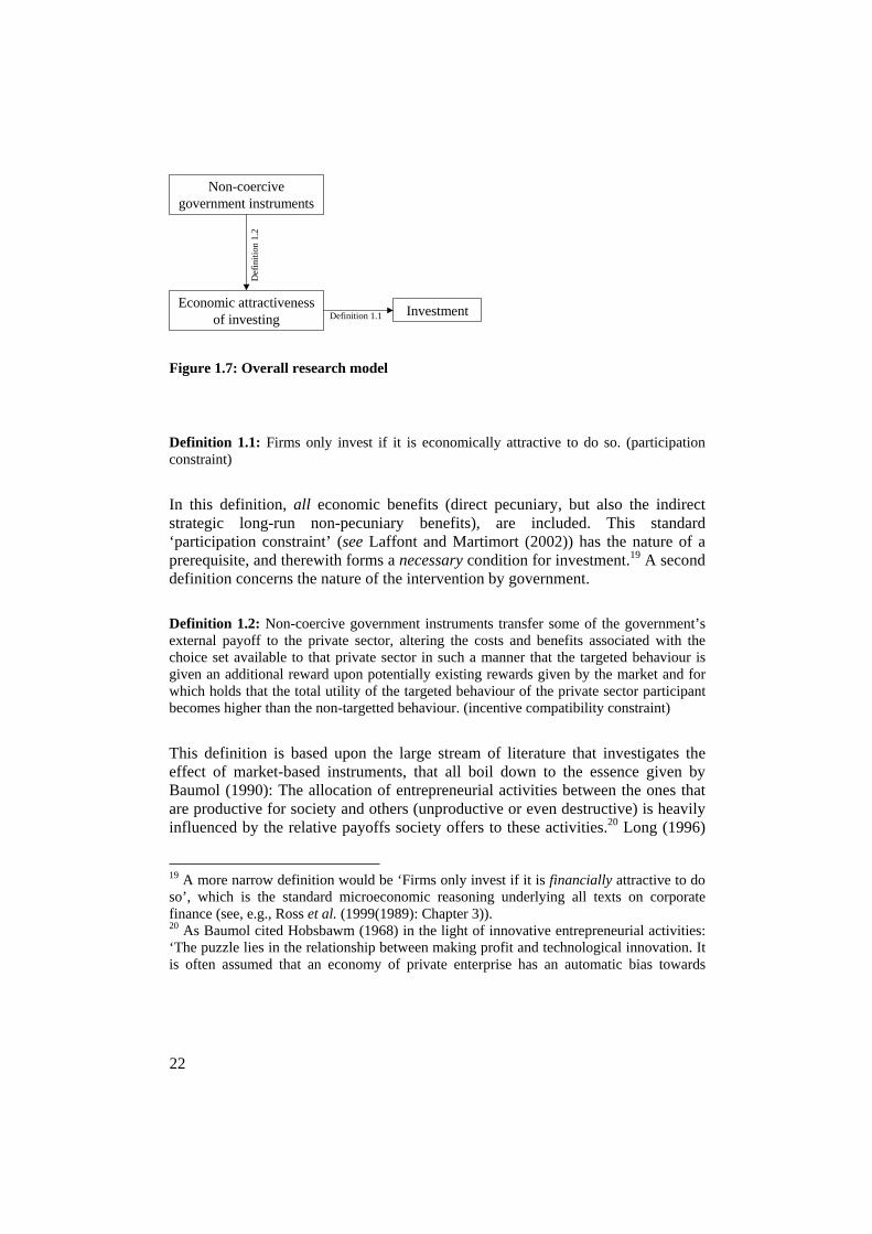
22

Definition 1.1: Firms only invest if it is economically attractive to do so. (participation constraint)

In this definition, all economic benefits (direct pecuniary, but also the indirect strategic long-run non-pecuniary benefits), are included. This standard ‘participation constraint’ (see Laffont and Martimort (2002)) has the nature of a prerequisite, and therewith forms a necessary condition for investment.19 A second definition concerns the nature of the intervention by government.

Definition 1.2: Non-coercive government instruments transfer some of the government’s external payoff to the private sector, altering the costs and benefits associated with the choice set available to that private sector in such a manner that the targeted behaviour is given an additional reward upon potentially existing rewards given by the market and for which holds that the total utility of the targeted behaviour of the private sector participant becomes higher than the non-targetted behaviour. (incentive compatibility constraint)

This definition is based upon the large stream of literature that investigates the effect of market-based instruments, that all boil down to the essence given by Baumol (1990): The allocation of entrepreneurial activities between the ones that are productive for society and others (unproductive or even destructive) is heavily influenced by the relative payoffs society offers to these activities.20 Long (1996)

19 A more narrow definition would be ‘Firms only invest if it is financially attractive to do so’, which is the standard microeconomic reasoning underlying all texts on corporate finance (see, e.g., Ross et al. (1999(1989): Chapter 3)). 20 As Baumol cited Hobsbawm (1968) in the light of innovative entrepreneurial activities: ‘The puzzle lies in the relationship between making profit and technological innovation. It is often assumed that an economy of private enterprise has an automatic bias towards

InvestmentEconomic attractiveness

of investing

Non-coercive government instruments

Definition 1.1

Def

init

ion

1.2

Figure 1.7: Overall research model

23

adds to this argument that the total utility of the recipient must be ‘substantially positive’ (p.80).21 When analysing the impact of the incentive compatibility constraint on the participation constraint, we see that definition 1.2 is not sufficient to ensure 1.1. In words, the fact that government support for private sector investment is positive, and that the firm’s total utility from the targeted behaviour is higher than its utility from the non-targeted behaviour does not imply automatically that this utility is positive (as was used in definition 1.1). The combination of the participation and incentive compatibility constraints, however, does form a logical necessary and sufficient condition for self-enforcing contracts.22 Nevertheless, the choice for non-coercive instruments may be risky: After all, although coercive instruments are inefficient in an economic sense, they seem much more predictable (see, e.g., Stavins (1998)). The fact that the private sector remains with considerable degrees of freedom implies that their behaviour is necessarily unpredictable—at least, up to some extent. Although the game-theoretical literature on incentives provides a logical framework within which contracts almost seem self-enforceable, there may exist other factors at work that prevent firms from making the actions targeted by government.23 Also, the fact that we can calculate payoff structures or even optimal subsidy schemes does not automatically imply that we have a set of operational guidelines. As Drèze (1995) innovation, but this is not so. It has a bias only toward profit. It will revolutionize manufactures only if greater profits are to be made in this way than otherwise.’ (p. 25) 21 Long focuses on total and not marginal utility, since the marginal utility of an incentive is almost always declining. 22 See Laffont and Martimort (2002) for a formal and much more rigorous notation of the participation and incentive compatibility constraints. 23 Here I recall John von Neumann: ‘As a mathematical discipline travels far from its empirical source, or still more, if it is a second and third generation only indirectly inspired from ideas coming from 'reality', it is beset with very grave dangers. It becomes more and more purely aestheticizing, more and more purely l’art pour l’art. This need not be bad, if the field is surrounded by correlated subjects, which still have closer empirical connections, or if the discipline is under the influence of men with an exceptionally well-developed taste. But there is a grave danger that the subject will develop along the line of least resistance, that the stream, so far from its source, will separate into a multitude of insignificant branches, and that the discipline will become a disorganized mass of details and complexities. In other words, at a great distance from its empirical source, or after much ‘abstract’ inbreeding, a mathematical subject is in danger of degeneration. At the inception the style is usually classical; when it shows signs of becoming baroque the danger signal is up. It would be easy to give examples, to trace specific evolutions into the baroque and the very high baroque, but this would be too technical. In any event, whenever this stage is reached, the only remedy seems to me to be the rejuvenating return to the source: the reinjection of more or less directly empirical ideas. I am convinced that this is a necessary condition to conserve the freshness and the vitality of the subject, and that this will remain so in the future.’ (Von Neumann (1947))

24

laments: ‘Few economists will object to the research agenda of developing operational guidelines, but fewer still will pursue it themselves’ (p. 122). Also, when it comes to analysing recent developments already observed in ‘the real world’, the academia is often lagging behind with the theoretical foundations of these empirical phenomena.24 Applying non-coercive instruments raises a number of dilemmas, of which some are specified in the next four research questions. These research questions help to answer the overall problem statement. Research question 1: What factors might prevent firms from making investments in the provision of public goods, even if such investment were financially attractive?(Influenceability Dilemma) Given that non-coercive instruments leave important degrees of freedom for entrepreneurs in their investment process, one might perceive underinvestment as a deliberate strategy of firms. Such need not be the case. In fact, there may exist numerous reasons that can be labelled under the header ‘barriers to investment’. These barriers can act as an intervening variable between ‘financial attractiveness of investing’ and ‘investment’. An inventory and analysis of the relevant barriers to investment improves our understanding of the possibilities for governments to positively affect corporate investment behaviour through non-coercive instruments. I will call this dilemma the Influenceability Dilemma, for it deals with the possibility of the combined definitions 1.1 and 1.2. Chapter 2 will investigate the literature on barriers to investment, underinvestment, and—since underinvestment is an incremental concept—the existing literature on benchmarks. Altogether, the Influenceability Dilemma deals with the effectiveness of policy instruments. A second dilemma deals with the ‘generosity’ of government. How much resources must be sacrificed in order to affect the payoff structure of the entrepreneurial investment process in such a manner that private sector investment meets the goals of government. Research question 2: How can governments determine the minimum level of support needed to make the private sector invest according to government goals, and how can they design such a mixture of policy instruments that meets these criteria?(Smart Governance Dilemma)

24 A nice example here is given by Kay and Thompson (1986) with their article named: ‘Privatisation: A policy in search of a rationale’.

25

Given that potential barriers to investment have been identified, and preferably eliminated or overcome in another manner, the question rises how much support a government should give in order to make the private sector invest. I call this the Smart Governance Dilemma, after Van Tulder (1998) and Van Tulder (1999).25 For example, suppose a government makes investment extremely interesting for the private sector, by providing large subsidies or fiscal arrangements. Even though the measures can then be considered effective (the private sector is most likely to respond according to the plan), one can raise serious doubts regarding the efficiency of these measures. If, however, it is possible to design a policy framework where the trigger of investment is specified in more detail (which is also measurable), then it may become possible to calculate the optimal ‘dose’ of financial support. Chapter 3 proposes a methodological framework for designing a support scheme. Building a general framework implies the use of general instruments—that is, instruments with a generic nature as fiscal measures or subsidies.26 In sum, the Smart Governance Dilemma deals with the efficiency of policy instruments.27 A third dilemma is that—even if it were possible to design a ‘smart’ support scheme and calculate the height of support in pecuniary terms—it is unclear beforehand whether all non-coercive policy instruments yield the same effect. For example, Single (1999) shows that companies investing in developing countries prefer direct cash measures as subsidies to long-term fiscal arrangements. In more volatile, or unstable economies, laws can easily change, just as administrations. Nevertheless, even in stable economies as found in the OECD countries, there is very little empirical evidence that suggests that non-coercive measures work in practice. In addition, even if non-coercive instruments work, it may well be that some instruments work better than others. 28

25 I underscore that I do not refer here to the acronym SMART sometimes found in the literature, where ‘SMART governance’ refers to Simple, Moral, Accountable, Responsive and Transparent governance. 26 A general optimising framework for a specific case would become a logical impossibility. 27 Another, related dilemma here concerns the distributional effects of the measures taken, as well as the distributional effects of the provision of public goods. This is a very technical discussion, largely summarised by Roberts (1987). 28 For example, Bloom et al. (2002) analyse the effects of R&D tax credits, and find that fiscal incentives matter, although they have serious questions regarding the efficiency of these instruments. Pearce and Palmer (2001) analyse public and private spending in environmental protection. Amongst others, they find little evidence for the ‘environmental drag’ hypothesis (where countries with heavy regulatory environmental restrictions scare off firms, so that tighter regulation would negatively affect economic growth). Simultaneously, however, they neither find evidence for a shift from public to private spending on environmental protection, which gives little support for governments that wish to rely on the private provision of such public good. Devereux and Griffith (1998) analyse

26

Research question 3: How do non-coercive instruments work in encouraging the private sector to invest in the provision of a public good, and are there differences in the effectiveness of various different instruments? (Policy Portfolio Dilemma) To answer this question, chapter 4 will make use of the optimisation scheme proposed in chapter 3. As in chapter 3, the empirical tests performed in chapter 4 make use of instruments with general applicability. This research question aims at contributing to the implementability debate of policy instrument. A last dilemma still untouched is the response of firms to more specific non-coercive measures. Whereas research questions 2 and 3 dealt with the more generic measures, still there is much to be investigated in the area of specific measures. In section 1.4, I mentioned ownership-related measures as an alternative non-coercive approach. Public-private partnerships (PPPs) serve as a particular case here. Research question 4: How can governments encourage private sector participants to invest in joint ownership projects as public-private partnerships? (Joint Ownership Dilemma) One the one hand, PPPs seem an attractive instrument to governments, as firms take over a share of the investment costs, as well as a portion of the risks associated with the project, and they may even improve the technical or cost efficiency of the issuing project. In addition, as opposed to measures where the private sector holds full ownership, government retains a stake in the project vehicle, which allows it to exercise power even on those issues that cannot be specified ex ante. Therewith, for more complex product-market combinations or for unique large-scale projects, PPPs seem an interesting alternative to other policy instruments. There exists, however, a big problem: Although many PPPs can be observed in the empirical reality, the academic literature on PPPs is very limited—both in amount and depth. Optimisation-like models, as called for in the Smart Governance Dilemma, are therewith far from our academic reality. Chapter 5 of

whether favourable profit tax regimes affect the decision of US multinationals to invest in production within Europe, and find that there exists a relationship—albeit that the effective average tax rate does influence location choice, it does not affect the choice of whether to invest in Europe. As a last example, Lewis and Mackinnon (1987) have analysed the impact of government loan guarantees in the case of the Canadian Northern Railway. They found that despite of the fact that such loan guarantees did help the railway company in her investment, these guarantees also provided the perverse incentive to over-rely on debt (which ultimately triggered bankruptcy).

27

this study will analyse the status quo of the literature on PPPs, as well as making an attempt in the direction of a smart governance system in this area.

1.6 Purpose of the study Government support for the private provision of public goods has predominantly been worked out in the theoretical literature. Studies in the areas of public economics or public finance have already provided theoretically sound and consistent directions for research in this area. Nevertheless, much still has to be learnt. The four dilemmas sketched in the previous section form a mere example of serious gaps still present in the literature. If at present we do not know how the private sector will respond to government support, and if we cannot pre-specify the optimal policy mix, then it may appear pretentious to provide unambiguous policy descriptions in this study. Rather, it seems more realistic to formulate propositions, and try to specify hypothesis in the last phase of this research. Therewith, the ultimate goal of the study is to formulate testable hypotheses.

1.7 Relevance of the study Since the 1980s, privatisation spreads around the globe.29 Particularly in the utility sectors (as electricity, natural gas, water, rail, or bus services) where either market or product characteristics may form a barrier to competition, the ideas of structural reforms have received far going attention. Private entrepreneurs once established most of these utility firms, as a means of supporting the more productive sectors. During the 1880-1930 era of macroeconomic growth,30 firms internationalised rapidly, and economic activities nowadays classified as ‘industries’ (such as railways, banking system, or energy supplies) were financed by multinational firms in order to improve or secure their ‘core activities’ (see Jones (1996), Miller (1993) or Bulmer-Thomas (1994) for a nice overview). From the 1930s to the 1950s, however, most of these ‘supporting’ activities were nationalised—usually justified by nation-state arguments,31 where a nation had a strong desire for autonomy from other countries with respect to its energy and water supplies, and public transportation. A rival argument for the same era was that the state had to

29 Most studies start with the 1980s as the U-turn in economics (e.g., Megginson and Netter (2001), Krueger (2000), or Oecd (1996)). Sometimes an individual case of the early 1970s is mentioned, such as the (often-praised) privatisation of the Chilean pension funds (see Estache and Rodriguez-Pardina (1998), Cline (1995), or Bates and Krueger (1993)) or the 1979 start of the massive UK privatisation policies (see Parker (2000), Ramanadham (1989), or Jenkinson and Mayer (1988)). 30 Many authors use the 1880-1930 era. Schumpeter (1954), however, lets this era start in 1870. 31 See Galbraith (1994).

28

recover the economy, in a Keynesian sense.32 From 1950 to 1980 (the era Jones (1996) labels ‘Resurgence’) the private sector gradually recuperates from the period Ruigrok and Van Tulder (1995) label the ‘inter-bellum’. In that era, the private sector invests more, and becomes a more dominant ‘player’ in the economy (see Jones (1996), Dunning (1993)). Then comes the modern era of ‘the retreat of the state’ (see Strange (1996)), characterised by massive privatisation. By the change of the millennium, however, the Oecd (2002) signals a decline in privatisation figures:

‘After peaking in 1998, the OECD privatisation proceeds have been declining; however, with the most pronounced drop taking place in 2001. [...] After two decades of privatisation, and in particular following the hectic pace of activity in the 1990s, governments with maturing privatisation programmes are left with assets that are more difficult to sell, both in terms of their regulatory and contracting requirements, and in terms of public preference for retention of state ownership and accountability.’ (pp. 53-4).

This notion is backed by the data given in Megginson and Netter (2001). So if the privatisation peak is over indeed, what is next? The OECD signals that public-private partnerships (PPPs) can readily be seen as an alternative approach to privatisation (Oecd (2002)). When combining these eras, it seems that the movements of private ownership to public ownership, followed by privatisation occur in a wave. This is depicted in figure 1.8.33 From the end of the 20th century onwards, some first signs show that re-nationalisation is a fact for poor performing privatised firms. For example, by mid-1998, the financial crisis in Hong Kong led the Hong Kong government to prevent speculation against its currency peg with the US dollar, and purchased an estimated UCS 15 billion of shares on the Hong Kong stock market.34 By early September 2001, the Mexican government announced to re-nationalise its heavily indebted sugar mills in order to save them from bankruptcy and in a move to force the USA to lift restrictions on sugar imports.35 In October 2001, the UK government announced to re-nationalise

32 As Helm (2000) labels this period the ‘The 1930s Debate’ (pp.26-7), which was a response to the growing economic ‘crisis of capitalism’. The state secured not only welfare (re)distributions, but as Dunning (1993) mentions, since market became increasingly insecure and many firms collapsed, governments became important employers and investors in the economy. See also Keynes (1936). 33 The idea of ‘waves’ in privatisation or nationalisation is not new. For example, the OECD emphasizes the notion of privatisation waves in multiple publications (see, e.g., Oecd (1996), Oecd (2002)). To mention but a few references on the nationalisation wave, see Jones (1996) or Krueger (2000). 34 Financial Times, 04 September 1998. 35 Financial Times, 04 September 2001.

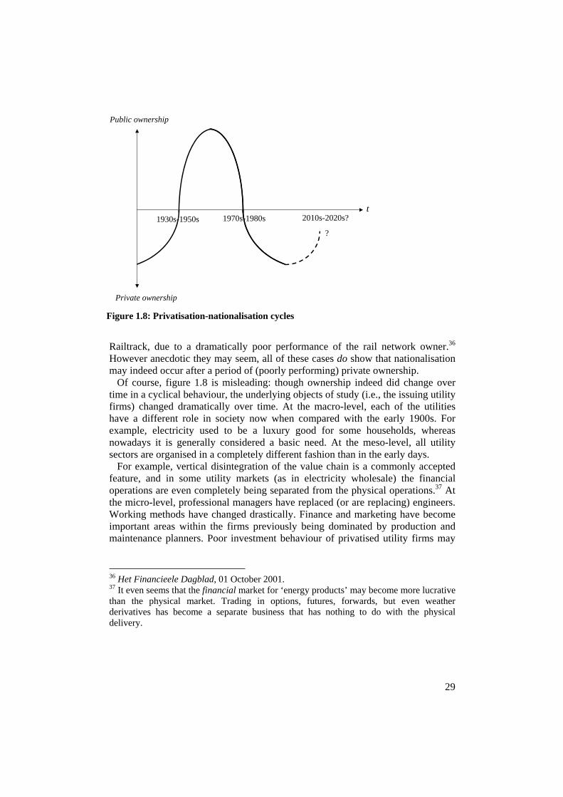
29

Railtrack, due to a dramatically poor performance of the rail network owner.36 However anecdotic they may seem, all of these cases do show that nationalisation may indeed occur after a period of (poorly performing) private ownership. Of course, figure 1.8 is misleading: though ownership indeed did change over time in a cyclical behaviour, the underlying objects of study (i.e., the issuing utility firms) changed dramatically over time. At the macro-level, each of the utilities have a different role in society now when compared with the early 1900s. For example, electricity used to be a luxury good for some households, whereas nowadays it is generally considered a basic need. At the meso-level, all utility sectors are organised in a completely different fashion than in the early days. For example, vertical disintegration of the value chain is a commonly accepted feature, and in some utility markets (as in electricity wholesale) the financial operations are even completely being separated from the physical operations.37 At the micro-level, professional managers have replaced (or are replacing) engineers. Working methods have changed drastically. Finance and marketing have become important areas within the firms previously being dominated by production and maintenance planners. Poor investment behaviour of privatised utility firms may

36 Het Financieele Dagblad, 01 October 2001. 37 It even seems that the financial market for ‘energy products’ may become more lucrative than the physical market. Trading in options, futures, forwards, but even weather derivatives has become a separate business that has nothing to do with the physical delivery.

t1930s-1950s 1970s-1980s 2010s-2020s?

Public ownership

Private ownership

?

Figure 1.8: Privatisation-nationalisation cycles

30

lead to, for example, a loss of consumers, a welfare loss for society in case of disruptions of supplies, takeovers, bankruptcy, or re-nationalisation.

1.7.1 Societal relevance The privatisation literature shows that under specific circumstances society benefits from the private provision of private goods. When it comes to public goods, additional problems arise, of which the existent literature mentions the funding problem as a central one. Of all policy instruments available to government, regulatory (or ‘coercive’) ones have the clear advantage of being quite predictable in terms of outcomes. A major drawback of coercive instruments is, however, their economic inefficiency. Thus, though being effective, the question rises whether these measures are efficient. As Pollit (1995) questioned after studying the efficiency gains following the massive privatisation of the British power industry: Was it worth it? As Michael Pollit concludes, a maximum 5 per cent efficiency gain (most favourable result of various econometric estimation methods) can hardly justify the costs of the whole transition process—instead, he questioned, that money might have been better spent on improving the management skills of the management of the state-owned enterprises. For the use of coercive measures one can ask the same question as Michael Pollit did—would it be worth it to ‘outsource’ the provision of public goods to the private sector, if the use of coercive instruments would eliminate all potential efficiency gains at the macro-level? As an alternative to coercive instruments, mainstream economic theory provides a number of market-based, or ‘non-coercive’ instruments. Instead of changing the choice set available to firms (as coercive instruments do), non-coercive instruments change the costs and benefits associated with the choice set, whilst leaving the set intact. William Baumol provides very interesting insights in this area (see, e.g., Baumol (1990)). Thus, if society pays a high value to certain goods or services whereas the market does not provide sufficient return on investment in these areas, government support or funding for the private provision of these goods or services seems a logical alternative. Unfortunately, the literature summarised in section 1.3 shows reluctance with respect to government support for efficiency reasons. Since uniform taxation (needed to fund the government support measures) is not based upon individual preferences, there is always some degree of macroeconomic inefficiency. The literature summarised in section 1.4 even adds a predictability or effectiveness problem. Since market-led instruments are non-coercive, firms can and must decide themselves whether the offered payoff structure is sufficiently interesting to make investments. This characteristic inherently embodies some degrees of freedom for the private sector that reduce the predictability of the policy instruments in terms of effectiveness.

31

The underinvestment problem is but one of the many ‘worst case scenarios’ that may occur. 38 If the private sector underinvests relative to the societal optimum or relative to the policy target, then the potential benefits of the entire ‘outsourcing process’ are most likely to vanish. From a societal point of view, especially for those goods and services that can reasonably be defined as ‘basic needs’ (such as water, energy, transport, and communications), it is extremely important to gain more insight in the underinvestment phenomenon. If we know better what circumstances encourage underinvestment, then prevention and correction mechanisms are more likely to be effective. For example, not all underinvestment behaviour has to reflect a deliberate corporate strategy—if laws or imperfect capital markets restrict firms in their investment pattern, then who is to blame? The underinvestment problem can also be analysed from a developmental or economic growth perspective. For example, when taking a look at privatised utilities in developing countries, underinvestment is a real fact threatening further economic development of entire regions. Exhibit 1.1 serves as anecdotal evidence for this point.

1.7.2 Scientific relevance The private provision of public goods is a relatively neglected field in the literature. In the light of governments withdrawing from the market place as active

38 Alternative terms to ‘optimal investment’ that can be applied here are societally ‘adequate’ or ‘desirable’ levels of investments, or adequate or desirable investment opportunities.

Exhibit 1.1: Power outage in Buenos Aires In February 1999, a substantial part of Buenos Aires faced an electricity blackout. At this summer peak, some 156,000 people were without electricity for one day, some 60,000 for several days, whereas some tens of thousands of that group were left without electricity for some 10 days. This situation implied no drinking water (water pumps operate on electricity), no refrigerators or air-conditioning working, no elevators, no ATMs operating, no electric security systems, no supermarkets because there were no cashiers functioning, no automated working force since all computers were down, no underground operating, and so on. The cause of this drama was that the Chilean owner of the responsible distribution company EDESUR had not invested enough in cables, wiring, connectors and transformers. In the annual report over the year 1999, the company underscores that it had met the required levels of investments as negotiated in the concession deal with the government—unfortunately, however, that concession did not specify the direction of investments, so that an ‘Internet firewall’ can also be found in the investments categories. A possible cause why the EDESUR drama could have taken place might be rooted in the fact that the regulatory entity had very little power in enforcing repercussions (and did hence not have a ‘credible threat’).

32

providers of goods and services, it can at least be called ‘strange’ that the academia still has to tackle numerous gaps in the literature whilst the empirical reality has already embraced the phenomenon of private provision of public goods. In the entire ‘outsourcing’ process initiated by the massive market restructuring waves of the early 1980s, the early critique of Kay and Thompson (1986) in their article ‘Privatisation: A policy in search of a rationale’ seems to bear generalisable characteristics that can readily be applied to the private provision of public goods. If it is unknown how large the efficiency benefits will be if government uses coercive instruments for streamlining entrepreneurial investment behaviour with policy goals, whilst it is uncertain how the private sector will respond to non-coercive instruments, then it seems a plausible question to ask if we are ready for this outsourcing process. When assessing the literature, at least two important topics of scientific interest seem to be lacking. First, the investment behaviour of private sector companies in the provision of public goods seems virtually absent. Even in the privatisation literature (which is still being enriched) there is limited knowledge about the performance and conduct of privatised enterprises. More general ideas about the willingness and ability of the private sector to invest in projects yielding public goods seem to be lacking. Many questions are still unanswered. For example do government incentives indeed encourage the private sector to invest in the provision of non-private goods? Do these incentives create white elephants or do they vanish over time? A second topic deals with selecting the right policy instruments. Does it matter whether a specific type of instrument is chosen, or is any policy alike? The broader context for this study is about the proper scope of government. Authors as Hart et al. (1997) or Blank (2000) have made interesting steps in answering that question, but still much work has to be done.

1.7.3 Managerial relevance With the withdrawal of governments from many economic activities, all kinds of new market opportunities arise for the private sector. Although one might expect a particular attention from the management sciences in privatisation and its consequences, surprisingly little has been written from an entrepreneurial perspective.39 The same holds for the private provision of public goods, which seems a domain exclusively reserved for scholars of public economic and public finance.40

39 One big exception—albeit a stand-alone one—is the July 2000 issue of the Academy of Management Review, with a special topic forum on ‘Privatization and Entrepreurial Transformation’. 40 In particular, it seems that the debate has predominantly appeared in journals as The Journal of Public Economics and The Economic Journal.

33

It is a pity that the insights of management scholars and practitioners are currently not included in the debate of policy design, the conditions for market functioning, or on the development of new organisational forms as public-private partnerships. Returning to the privatisation debate, economists do not seem to find the ultimate answers to fundamental questions as ‘does privatisation deliver?’ (see Basañes et al. (1999)), since variations in performance are deviations in their models. In management studies, on the other extreme, variances in performance of privatisation are the starting point of analysing sources of comparative or competitive advantages (see Cuervo and Villalonga (2000), or Doh (2000)).

1.8 Organisation of the study The four dilemmas formulated in section 1.5 are interrelated, and worked out in part II of the study (chapters 2 to 5). Chapter 2 investigates the potential effectiveness of non-coercive policy instruments by analysing barriers to investment, as well as the underinvestment dilemma. Chapter 3 proposes a methodological framework for calculating the wealth transfer necessary in the application of non-coercive policies. In chapter 4, I analyse how such a wealth transfer has been translated into concrete policy measures, and analyse whether the type of policy instrument matters in encouraging investment. Chapter 5 analyses investment and efficiency incentives public-private partnerships, and surveys the literature on PPPs. In each chapter, I formulate some hypotheses, and try to come up with additional insights for constructing a smart governance framework for the private provision of public goods. Part III of the book translates the propositions to testable hypotheses, and discusses some—albeit preliminary—policy implications. Chapter 6 proposes the aforementioned hypotheses and smart governance framework, whereas chapter 7 puts the results of the study in a broader perspective.

Part II: Four dilemmas

37

2 THE INFLUENCEABILITY DILEMMA The Influenceability Dilemma lies at the heart of any effectiveness analysis of non-coercive policy instruments. In fact, this dilemma consists of two interrelated issues. First, since non-coercive instruments necessarily leave considerable degree of freedom to the private sector (in this case with respect to the decision to invest or not), there exists a serious risk that the private sector does not respond according to the plan.41 In particular, there exists a serious risk of underinvestment where firms do not invest as much as government would want them to do. The second issue deals with the determinants of underinvestment. Sticking to the logic proposed in hypotheses 1.1 and 1.2, firms would only invest if it were financially attractive to do so. Suppose, however, an investment decision is financially attractive—would this guarantee an investment response? The answer is of course negative, but the question rises why. Any potential barriers to investment must be carefully analysed, and where possible overcome, in order to improve the predictability of non-coercive instruments. The overall purpose of this chapter is to analyse factors that prevent firms from making investments, even if it were financially attractive to make these investments (research question 1). In addition, this chapter analyses the potential effect of these barriers to investment, which is the concept of underinvestment. Efficient production requires an ‘optimal level’ of investments, from which firms can deviate in two directions: overinvestment and underinvestment. Although from a static efficiency point of view it may seem contradictory, firms can rationally decide to overinvest, for example, as an anticipation on future demand, as a strategic ‘signal’ to competitors or potential market entrants, or as a perverse side-effect of regulation (see Averch and Johnson (1962), and Viscusi et al. (1995: 390) for a discussion). In case of overinvestment, productive efficiency is sub-optimal, but output quality and quantity are capable of meeting demand. When investments, however, diverge to the opposite side of the spectrum (i.e., underinvestment), then supplies may not be capable to meet demand. Worst-case scenarios such as the California electricity crisis (with frequent power blackouts above a certain threshold of demand), or the British water sector (where supplies

41 In fact, there still exists a much fundamental debate in the literature that deals with the philosophical question whether incentives work at all. That question is raised at all levels of analysis, from inter-governmental relations to human resources. For a recent overview see for example Beer and Katz (2003) or Bénabou and Tirole (2002). See also Hart (1989). Regarding the specific question ‘do government subsidies increase the private provision of public goods?’ it seems that the answer is a definite ‘yes’ (see Bergstrom and Andreoni (1996), Falkinger et al. (2000), or Bernheim (1986)).

38

are frequently below the socially desirable in terms of both quantity and quality) show how underinvestment by firms can have dramatic impact on society. This chapter gives a survey of the literature on underinvestment. The structure of this chapter is as follows. Section 2.1 puts the concept of underinvestment in perspective. The term ‘underinvestment’ underscores the incremental nature of a concept compared to a benchmark of optimal/adequate/relevant/desirable investment behaviour. If for the sake of simplicity the mainstream term ‘optimal’ is used, then one can think of a maximisation function, some critical assumptions, and worked-out ideas on the preferences behind that investment behaviour. The section shows how these dimensions of characterising investment behaviour differ when applying a different level of analysis (macro, meso, micro). Since this study deals with the investment behaviour of private sector companies, the focus will be on the micro-level interpretation of underinvestment. Section 2.2 investigates the theoretical causes of underinvestment behaviour of firms by categorising determinants from the micro-, meso-, and macro-levels that may constrain corporate investment behaviour. Sections 2.3 to 2.5 work out these determinants at these respective levels of analysis. Since this results in a rather lengthy overview, section 2.6 gives a brief intermediate summary and analysis of the status quo of the theoretical literature on underinvestment. Section 2.7 briefly introduces the empirical concepts of ‘measurement’ and ‘existence’ of underinvestment, and gives an overview of some empirical studies on underinvestment. One of the striking results of that section is that most of the theoretical determinants summarised in sections 2.3 to 2.5 have very little practical value. Virtually all empirical studies reviewed use proxies to ‘determine’ some degree of underinvestment.

2.1 The concept of underinvestment In the previous chapter, definitions 1.1 and 1.2 postulated that firms only invest if it is financially attractive to do so. A first, technical interpretation would then be the following: If current investment yields insufficient levels of public goods, whilst it is financially attractive to invest, then there is underinvestment.

Investment Capital stockAmount of public good

Economic attractiveness of investing

Figure 2.1: Technical interpretation of underinvestment in the provision of a public good

39

Figure 2.1 illustrates the mechanics. Investment yields an amount of capital stock (e.g., a number of wind turbines, computers, or bridges). The amount of that capital stock determines how much public good is produced. The issue of underinvestment in a technical sense would focus on how much firms should have invested, given the attractiveness of the investment. This technical notion is in line with the microeconomic ‘optimal investment decision’ benchmark investigated in this chapter. In the figure, it is the ‘financial attractiveness’ variable that determines this technical interpretation of underinvestment. The feedback loop determines whether there is underinvestment or not –that is, one can assess how much public good there is provided (and ergo, how much capital stock was needed), and how attractive it was to invest. If it was financially attractive to invest, but still the level of public good provided is too low (given another benchmark), then there is underinvestment in a technical sense. This is a first important step in isolating the problem. The next step in analysing underinvestment lies in the recognition of its incremental nature, and that is relative to ‘optimal investment’. Optimal investment, in its turn, is a concept that can be defined at various levels of analysis. This section distinguishes between the firm (or ‘micro’) level, the sectoral (or ‘meso’) level, and the (inter)national (or ‘macro’) level. That distinction underscores the importance of the following points: (a) the different interpretations of ‘optimal investment’; (b) the main assumptions underlying these concepts of ‘optimal investment’; (c) a recognition of the preferences for ‘optimal investment’ and an explicit separation of different goal functions; and (d) the consequences of the aforementioned points for interpreting ‘underinvestment’. Table 2.1 summarises these points. From the mainstream microeconomic point of view, the firm is a set of production possibilities. In a similar fashion, it is assumed that there exists an investment opportunity set, out of which a firm can pick that optimal investment decision that maximises the firm’s profits, or utility (see, e.g., Friedman (1985); Hart (1995); Long and Malitz (1985); Milgrom and Roberts (1992: Chapter 8); Modigliani and Miller (1958); Myers (1984)). Given the existence of an investment opportunity set, the firm (its owners or management) develops ex ante criteria for choosing amongst the opportunities available. In each case, the choice for the optimal investment decision derives from internal preferences that exist within the firm (assuming both the owners and managers as internal decision-makers). At the sectoral or meso level, the optimal investment is not one executed by a single firm, but by the entire population of firms inhabiting the sector. Such optimum is of a much more complex nature, since its optimality depends upon the decisions of multiple, interacting actors. From an economic point of view, the optimal investment decision (of the aggregate) results in both allocative and productive efficiency. Hence, this optimal investment decision is not only placed at a higher level of aggregation, it inevitably becomes constructed as a result of

Tab

le 2

.1: L

evel

s of a

naly

sis i

n 'o

ptim

al in

vest

men

t' an

d 'u

nder

inve

stm

ent'

M

icro

(fir

m) l

evel

M

eso

(sec

tor)

leve

l M

acro

(cou

ntry

) lev

el

Opt

imal

inve

stm

ent

Opt

imal

inve

stm

ent d

ecis

ion

is th

at

one

that

max

imis

es th

e fi

rm’s

util

ity o

r pr

ofits

Opt

imal

inve

stm

ent l

evel

and

dir

ectio

n co

ncer

ns th

e ag

greg

atio

n of

all

inve

stm

ents

of

all p

artic

ipan

ts in

eac

h se

gmen

t of

a va

lue

chai

n, th

at a

ltoge

ther

m

axim

ise

allo

cativ

e an

d pr

oduc

tive

effi

cien

cy

Opt

imal

agg

rega

te in

vest

men

ts

harm

onis

es w

ith c

onsu

mpt

ion,

s.t.

in

the

shor

t-ru

n (a

.o.)

sup

ply

mee

ts

dem

and,

and

in th

e lo

ng-r

un (

a.o.

) m

acro

econ

omic

gro

wth

is b

oost

ed

Max

imis

atio

n fu

nctio

n M

axim

ise

the

prof

its o

f th

e i p

roje

cts

with

in th

e fi

rm’s

inve

stm

ent p

ortf

olio

, gi

ven

cons

trai

nts

Max

imis

e th

e se

ctor

al p

rodu

ctiv

e an

d al

loca

tive

effi

cien

cy, g

iven

(a)

the

cons

trai

nts

to th

ese

conc

epts

, and

(b)

the

inte

ract

ion

in th

e fi

rms’

inve

stm

ent

beha

viou

r

Max

imis

e m

acro

econ

omic

gro

wth

(or

w

ealth

) su

ch th

at n

ot o

nly

toda

y’s

wea

lth is

pre

serv

ed, b

ut a

lso

that

fu

ture

ext

ra w

ealth

is c

reat

ed, g

iven

th

at s

uppl

y sh

ould

mee

t dem

and

in

an e

ffic

ient

way

, giv

en th

at a

ggre

gate

co

nsum

ptio

n an

d in

vest

men

t sho

uld

be b

alan

ced,

and

giv

en

mac

roec

onom

ic c

onst

rain

ts

Mai

n as

sum

ptio

n E

xist

ence

of

a se

t of

(fir

m-s

peci

fic)

in

vest

men

t opp

ortu

nitie

s E

xist

ence

of

allo

cativ

e an

d pr

oduc

tive

effi

cien

cy

Rel

atio

nshi

p be

twee

n in

vest

men

t (in

eq

uipm

ent,

hum

an c

apita

l) a

nd

mac

roec

onom

ic g

row

th

Pref

eren

ces f

or th

e op

timal

inve

stm

ent

deci

sion

Inte

rnal

to th

e fi

rm

Ext

erna

l to

the

firm

; int

erna

l to

the

soci

al p

lann

er

Ext

erna

l to

the

firm

; int

erna

l to

the

soci

al p

lann

er

Und

erin

vest

men

t R

elat

ive

to th

e op

timal

inve

stm

ent

proj

ect f

or a

spe

cifi

c fi

rm

Rel

ativ

e to

sec

tora

l opt

imum

N

egat

ive

spin

-off

of

inve

stm

ents

in

one

sect

or to

oth

er s

ecto

rs in

the

mac

ro-e

cono

my

40

41

interacting individual investment decisions. This underscores a first notion on the problem of underinvestment. Given existence (not to mention measurability) of the Pareto efficient investment decision (where all consumer demand is met in such a way that all consumers face maximum utility, and where all other production allocations would harm at least one consumer in his utility), it becomes clear that the optimal investment decision is one based on the preferences of the social planner (government) which need not match with those of the individual firms. Firms interacting in a market may obtain an equilibrium in, e.g., supply capacity, but the investments used to obtain that equilibrium need not be optimal from the perspective of the social planner. For example, according to game theoretical approaches in the industrial organisation literature, firms may decide to overinvest in certain ‘strategic’ assets for which other market participants can pay high usage tariffs, or decide to overinvest in assets as a signal for potential competitors. On the other hand, these firms may also decide to underinvest if there are no market forces present that encourage them to innovate or expand their asset base. At the macro level, the goal function for maximising utility is again different, due to a different perspective on the most desirable investment behaviour and spin-offs. Here, it is not so much the individual sector that matters, but much more the interaction between the various sectors, and the spin-off effects of aggregate investments to macroeconomic growth. Assuming that there exists a relationship between investments in assets, labour, or equity, and macroeconomic growth, the government tends to balance consumption and investments. The various optima of all sectors together should lead to macroeconomic growth, or wealth in another sense. Furthermore, one can think of optimal investment patterns in a Keynesian sense, where in times of macroeconomic woes, firms (and government) should invest more in order to overcome crises. Such investment pattern certainly serves governmental goals, and in the long-run it will serve the entrepreneurial goals as well, but for a short-run oriented micro-level investor, anti-cyclical investment behaviour need not be optimal. Based on these three interpretations of the optimal investment decision, it becomes clear that at each level of analysis, deviations from the optimum may occur, but also that the sources behind these deviations will differ per aggregation level. When turning to the investment behaviour of private sector companies in the provision of public goods, table 2.1 gives some intuition for the incommensurability of goals of the three levels of analysis. The most profitable investment strategy for a firm need not harmonise with the goals of government or society. Particularly in the case of large externalities associated, such a clash of goals is likely to occur, which is reflected in the free-rider problem of public goods provision. The key problem in choosing an ‘optimal provision’ of the public good is summarised by Drèze (1995). Ideally, there should exist a level or a quantity of public goods provision, for which the marginal cost of provision equals the sum of the individual ‘marginal willingness-to-pay’ of all users. Suppose user charges are based on reported preferences, then there is an incentive to underreport these

42

preferences. Therefore, mainstream economic theory pays considerable attention to revealing the true preferences, but this seems particularly a theoretical, or highly stylised exercise, which is very difficult to put into practice. If the optimal level of public good were independent of reported preferences, then we may come closer to a pragmatic solution, although we have to sacrifice some of the theoretical consistency with respect to Pareto efficiency. As such, this problem is not unique to investigating possibilities for non-coercive government instruments—in fact the same problem holds for regulatory solutions. For example, a popular instrument in environmental economics is the standard (see Cropper and Oates (1992)). To set a standard, however, also depends on some underlying optimum, which inevitably suffers from the same problems as described above. Thus, for the current study, the choice for a benchmark is not a unique problem—instead, it is a problem inherent to public goods analysis. Section 2.7 will explore the issue of benchmarks in more detail.

2.2 Sources of underinvestment: Barriers to corporate investment

Firms may underinvest, but the causes behind underinvestment need not be deliberate corporate action. Sometimes, firms can be constrained on financial grounds, if debt or equity providers are unwilling to provide further cash. Uncertainty about the future may make investments too risky to conduct. On the other hand, underinvestment may be a strategic tool in a bargaining situation with buyers, suppliers, or with government. Figure 2.2 shows how the various ‘barriers to investment’ intervene in the relationship between economic attractiveness to invest and actual investment, which is also reflected in the following hypothesis.

Hypothesis 2.1: Even though it may seem economically attractive to invest for firms (including both pecuniary and non-pecuniary benefits), there may exist barriers to

InvestmentEconomic attractiveness

of investing

Definition 1.1

Barriers to investment

Hyp

othe

sis

2.1

Figure 2.2: The role of barriers to investment

43

investment acting as an intervening variable between ‘economic attractiveness’ and actual ‘investment’ that hamper firms from investing.

The number of potential barriers to investment is large—table 2.2 gives a brief overview of the most important determinants that may constrain corporate investment behaviour. In table 2.2, each row (representing the issuing level of analysis of the causes) is worked out in the associated section, whereas each cell (representing a theoretical cause to underinvestment) is worked out in a separate subsection.

2.3 Micro-level barriers to investment In some cases, internal organisational matters may negatively affect the firm’s investment behaviour. Underinvestment, in this terminology, is investment behaviour relative to other investment possibilities. Hence, the choice for an investment project is conditional upon the other investment opportunities available. In such perspective, the firm has to be seen as a set of possible production functions, or investment projects. This is precisely what neoclassical microeconomics does. In this reasoning, firms (or managers) are assumed to be willing to maximise the firm’s utility (or profits), but they are restricted in obtaining their goals. Hence, though acting rationally, managers do not necessarily

Table 2.2: Barriers to investment

Level of analysis Source of underinvestment Section Wrong incentives for management to invest 2.3.1 Uncertainty on ROI with an option to wait 2.3.2 Debt-to-equity ratio 2.3.3 Stock-market performance of the firm 2.3.4

‘Micro’ or firm level

Agency approaches to underinvestment 2.3.5 Strategic underinvestment and the signalling game 2.4.1 Incomplete contracts and the hold-up problem 2.4.2 Contract renegotiation and the hold-up problem 2.4.3 The role of competition 2.4.4

‘Meso’ or sectoral level

Declining product-market 2.4.5 Savings gap, hyperinflation, and capital flight 2.5.1 Profits and price cap regulation 2.5.2 Liberalisation, regulatory reforms, and the vertical separation of the value chain

2.5.3

Franchise bidding, concessions, and licensing 2.5.4

‘Macro’ or country level

Policy reforms, and the expropriation risk 2.5.5

44

succeed in realising the optimal investment decisions due to certain constraints. On the one hand, these constraints can be analysed at the level of the investment project itself: criteria as a minimally required net present value (NPV) of any investment project, or avoidance of the associated uncertainty may prevent managers from investing in a particular project. Furthermore, constraints may be analysed at the management level: wrong incentives for managers may result in the case where the optimal investment decision for the firm is sub-optimal for the manager involved; furthermore issues of informal organisation may prevent well-willing managers to undertake projects that are optimal for the formal organisation. Common in all of these approaches is that the firm can control for these sources of underinvestment.

2.3.1 Wrong incentives for managers to invest As argued by Jensen and Murphy (1990), managerial compensation can be rather pervasive in providing the right signals to invest. On the one hand, one can advocate aligning management’s interests with those of the shareholders by coupling (part of) managerial pay to the firm’s stock price. Suppose managers will direct their efforts at increasing the firm’s value (which is debatable as argued by Milgrom and Roberts (1992: 441-3)) but simultaneously, they are exposed to non-diversifiable risk, which may cause them to underinvest in risky projects (Jensen and Murphy (1990); Prendergast (1999)). In an Anglo-Saxon perspective, shareholders are usually assumed to be the owners of the firm who wish to see the firm’s profits being maximised, and who have diversified their investments (and hence the associated risks) because they are most likely to hold a portfolio of investments. Consequently, shareholders will be less risk-averse than the manager. The latter has no possibility to diversify the risks of his income (which was performance-based).42

2.3.2 Uncertainty on ROI with an option to wait In real options theory (cf. Dixit and Pindyck (1994); Kogut and Kulatilaka (1994); Trigeorgis (1996); Pindyck (1999); Brennan and Trigeorgis (2000)), waiting has a value. If one invests under uncertainty about the future, then one is likely to obtain more valuable information over time, and is hence more capable of making the right decisions. Meanwhile, risk-averse firms operating in markets too turbulent to invest at present will tend to defer investments. This need not imply underinvestment in the long run, but in the short run it may indeed result in underinvestment. Sources of uncertainty can be (a) systematic (that is, market-

42 For a more detailed discussion, see Mcconaughy and Mishra (1997); or for a somewhat broader discussion on the effect of incentives in order to align management’s interests with those of the owners, see Gibbons (1998); Milgrom and Roberts (1992); Prendergast (1999).

45

specific risk, to which all participants are exposed and which cannot be diversified within that product-market combination), such as changes in a fiscal regime, or (b) unsystematic (that is, firm-specific risk, that can be diversified). Furthermore, next period’s opportunities may be conditional upon the present period’s investments. In this time series view, tomorrow’s chance of obtaining profits depends on today’s investments, which implies that today’s investments may be made under the expectation that they will create profitable opportunities tomorrow, although they are loss making in the current period. Furthermore, there exists no guarantee that indeed current investments do become profitable in a next period. To some extent, firm-specific investments in future opportunities or utility can be compared with investments in intangibles, such as R&D or brand name. The prospects of these investments are often highly unpredictable, and it is hard for investors to observe the chances that lead to profitability. Chan et al. (2001) show how companies with poor past returns (due to high investments in R&D) may earn large excess returns in later periods; how the stock market does value R&D unbiased; but also that R&D intensity is associated with return volatility. Especially the last point underscores the probability range of actually obtaining a positive return on projects for which the next period’s gains are conditional upon the current period’s investments. In this case of R&D expenditures, both the firm and its investors are uncertain about the future profitability of these investments. Acemoglu (1993) looks at the uncertainty part for the firm, where the spin-off of investments is accelerated by the aggregate level of investments in the sector.

2.3.3 Debt-to-equity ratio The capital structure of the firm partially determines the ability to invest. Ever since about the 1960s, a substantial part of the corporate finance literature has been dedicated to the capital structure of the firm, in particular the choice between debt and equity on the firm’s balance sheet. It seems that an unambiguous theory on the choice between debt and equity is still lacking. The most important theories are summarised by Myers (2001): Trade-off theory: Firms trade off the tax deductibility advantages of additional

debt against the associated interest costs; Pecking order theory: Firms usually prefer internal funding, but when internal

cash flows are insufficient to cover financial expenditures, they tend to prefer debt over equity;43

Free cash flow theory: Mature firms are prone to overinvest and diversify, when the operating cash flow exceeds the profitable investment opportunities of the firm;44

43 Section 2.3.4 gives more intuition for the pecking order theory. 44 See also section 2.3.5 on the agency problems related to free cash flows.

46

Efficient market hypothesis: In a perfect and frictionless capital market financing does not matter, so the choice between debt and equity financing has no material effect on the value of the firm or on the cost or availability of capital (cf. Modigliani and Miller (1958)).

Though the Modigliani-Miller propositions are widely accepted, corporate finance and corporate governance research suggests that the capital structure of the firm (and the context within which the firm is located) does matter. For example, not only the leverage aspects of the debt-to-equity ratio are analysed, but also the extent to which the interests of debt- or equity-holders streamline with those of the firm at stake (Friedman (1985)). Following Modigliani and Miller (1958), the market value of the firm is a function of (a) the present value of (earnings generated by) assets-in-place, and (b) the present value of growth opportunities. Myers (1977) first noticed the risk of underinvestment in the light of these two determinants of the market value of firms as follows. Consider a firm with equity-holders and debt-holders. In case of bankruptcy, debt-holders have preference over equity-holders. Furthermore, in case of prosperity of the firm, both debt-holders and equity-holders see a positive return. Hence, equity-holders tend to be more risk-averse towards investing in risky projects than debt-holders. As Mauer and Ott (2000) show, equity-holders tend to underinvest in the growth option of the firm; a problem which can be overcome by partially financing the growth option with a new debt issue that has the same priority in bankruptcy as the currently outstanding debt. As Long and Malitz (1985) show, firms whose assets are weighted in the presence of intangible assets and growth opportunities (e.g., pharmaceuticals for whom the value of the firm predominantly relies on R&D success and on the exploitation of intellectual property rights) on average borrow significantly less than firms holding mostly tangible assets in place (e.g., a hotel chain). This notion confirms the idea that complex debt contracts are effective only when the firm’s investment opportunity set is observable. Long and Malitz therewith turn the underinvestment problem into one of information asymmetry and moral hazard. If a firm faces many firm-specific investment opportunities, owners may relatively easy increase firm risk over time. Since outsiders have more difficulty estimating the risk and return of these investment opportunities, it is almost for debt-holders impossible to monitor such investments (Long and Malitz (1985)).

2.3.4 Stock market performance of the firm Stock market valuation may affect corporate investment behaviour in two ways. First, there exists the information asymmetry between insiders and outsiders on how to value the firm’s investments and associated prospects. This is the valuation problem under asymmetric information (Greenwald et al. (1984)). Second, there may exist a deviation between the allowed time horizons of getting a return on

47

investment between the short-term driven stock market and longer run profitability of investments made by the firm. This is the debate on economic ‘short-termism’ (Laverty (1996)), or on intertemporal choices. The valuation problem (under asymmetric information) is especially worked out for intangibles, such as R&D expenditures, or advertisement campaigns in strengthening corporate brand names. Though in neoclassical economics all firms are alike, and technology is determinative to profits, organisation theory45 assumes that it is the uniqueness of the firm (and hence heterogeneity) that creates a competitive advantage (Barney (2001); Wernerfelt (1984)). Especially the firm-specific assets (of which many are intangibles) contribute to that competitive advantage (Balakrishnan and Fox (1993)). The basic idea behind the valuation problem of intangibles is twofold (Greenwald et al. (1984)): either (a) the firm wishes to leverage more, but is constrained by the willingness of outsiders to provide capital (especially debtholders fear risky projects) which reduces the capital sources available, or (b) those firms that are not credit constrained may face an increase in the effective cost of capital, which reduces their investment possibilities. The leverage problem, which is based upon James Tobin’s seminal article analysing the substitutability of debt and equity (Tobin (1961)), has led to a large stream of corporate finance literature. Amongst others, the ‘pecking order of capital’ (Donaldson (1961); Myers (1977)) shows us how corporate financing and investment behaviour is affected by this information asymmetry (Myers and Maljuf (1984)). Take R&D expenditures. Suppose that an optimal level of R&D expenditures exists for an individual firm (taking the direction of investments as given). The research process inhabits a lot of uncertainty already, but coupled with the information asymmetry (between in- and outsiders) it could have a first-order effect on resource allocation (Jones and Williams (2000)). Given the pecking order of capital, R&D-intensive firms must especially rely upon equity, for which the question arises to what extent the stock market has unbiased beliefs about returns. The empirical evidence on this topic is hampered by the fact that firms are not obliged to report on R&D expenditures, which leaves both investors and researchers with an estimation problem (see, for example, Carey et al. (1998)). Chan et al. (2001) find that firms investing in R&D face similar rates of return compared to firms not investing in R&D, but they also find that on average there exists some volatility of that return for R&D-intensive firms, which may impose a real cost on investors which ultimately may increase the cost of capital for R&D-intensive firms. Lastly, citing Chan et al. (2001), ‘The benefits [of R&D], if any are likely to materialize only much later [than the investment momentum], and the life-cycles of resulting products may be quite short.’ This shifts the attention to the general problem of differences in time horizons. 45 Particularly the resource-based view of the firm and the population ecology streams stress this view.

48

The short-termism problem of stock markets is that short-run investments (with direct spin-off) are preferred over long-run investments (since shareholders would prefer short-run payoff). Therefore, listed firms may become unable to commit themselves to long-run investments that are necessary for the future. In a worst-case scenario, long-run investments are not made, and both manufacturing capabilities and workforce skills enter into a downward spiral. Laverty (1996) investigates this spiral for US firms (as opposed to their Japanese and German counterparts), and mainly comes to the conclusion that the monodisciplinary economic perspective prevails in analyses, but that—if we want to offer managers a solution to overcome the intertemporal choice problem—more angles have to be studied. Bebchuk and Stole (1993) take a different approach and study the impact of management’s informational advantage over the stock market on corporate investment behaviour. They argue that the investment level may be distorted either through underinvestment (when the market has incomplete information about the level of investment undertaken), but also through overinvestment (when the market observes the level of investment, but not its productivity). This approach seems similar to the one applied by Laffont and Tirole (1993: 87), who state that a societally optimal investment level includes a condition that minimises the ex post costs of an investment project through an efficiency parameter. Lastly, there exists a stream of literature that focuses on the role of internal funding of investments. The idea is that imperfect capital markets may drive firms to use internal funds rather than external ones, Goergen and Renneboog (2001) find that a high concentration of control in the hands of executive directors reduces the underinvestment problem.46

2.3.5 Agency approaches to underinvestment In the light of corporate investment behaviour, agency theories may predict both under- and overinvestment. On the one hand, Jensen (1986) shows how managers prefer to overinvest free cash flows into unprofitable assets instead of paying out to stockholders.47 This behaviour leads to the growth of the diversified firm, and to overinvestment. Furthermore, once the diversified firm is reality, the internal capital market of the firm may also lead to inefficient resource allocations, see, for a recent example Whited (2001). On the other hand, Myers and Maljuf (1984), for example, show how agency problems (as asymmetric information, adverse selection, moral hazard, signalling) are in line with the pecking order theory of finance (Myers (2001)), which may put constraints on funding possibilities for investments. In this subsection I will not focus on the free cash flow problem, but on the approaches associated with the pecking order theory instead. 46 For more literature on this topic see Kaplan and Zingales (1997) and Cleary (1999). 47 The assumptions applied here is that the status of a manager depends on the size of the firm he controls—a growth of the firm (in terms of assets) then leads to a growth of the manager’s status.

49

Agency theory states that the higher the variance of the firm’s returns, the less the underinvestment problem, which is explained as follows. Recall the pecking order of capital, as outlined by Donaldson (1961). Firms prefer internal funding for their investments. Target dividend payout ratios are adapted to the investment requirements of the firm. In general, dividend levels are stable, and payout targets are only adjusted gradually to shifts in investment opportunities. If external funding is required, then the safest security (read: debt) is issued first, then come hybrid securities (such as convertible bonds), and then comes equity. Following Myers (1977), the value of a firm (consisting of assets in place and growth opportunities, the latter treated as call options on real assets) funded with risky debt is almost per definition lower than the value of the equity financed firm. Firms will issue risky debt instead of safe debt in case firm-specific investments (including maintenance), intangibles, or other investments hard to value for outsiders. If the firm’s management acts in the interest of its shareholders, then it will not engage in these investments (since these would lower shareholders’ wealth), which might lead to underinvestment in, e.g., maintenance. A logical consequence would be that firms with valuable growth opportunities would never issue risky debt, but unfortunately equity is not a panacea (see Jensen and Meckling (1976)). Another way of avoiding the problem would be to write out complex debt contracts that would require the firm to take on any investment project in all states in which its NPV is positive. For as far as these complex contracts would be feasible at all, a major requirement is that the firm’s investment opportunity set is observable. Long and Malitz (1985) then show that:

‘[…] because intangible, firm-specific, and therefore unobservable growth opportunities reduce the effectiveness of bond covenants, the only way in which owners of firms with a high proportion of intangible investment opportunities can control the agency costs of debt is by limiting the amount of risky debt outstanding’ (p. 326).

It is the type of investment opportunities that determine financial leverage. This is in line with the information asymmetry problems in stock market valuation, as described in section 2.3.4.

2.4 Sector analysis and investment barriers In section 2.3, theoretical determinants of corporate investment behaviour were endogenous to corporate behaviour. When analysing the firm within its competitive space (i.e., the markets within which it operates), corporate behaviour (and hence corporate investment behaviour) becomes subject to external stimuli. This section pays attention to the theoretical determinants deriving from the competitive space that may lead to the underinvestment of an individual firm. In

50

this attempt, interaction effects of competition are analysed (a horizontal dimension of value chain analysis), as well as transactions, contracts, and sales within the vertical value chain.

2.4.1 Strategic underinvestment and the signalling game A dominant firm may deliberately underinvest as a strategy for obtaining a strong bargaining position vis-à-vis, e.g., government. If, for example, government sets the standard for production, and a monopolist responds with poor demand due to a relative underinvestment, then we may apply a ‘signalling game’48 in terms of Gibbons (1992: 183-90) or Tirole (1988: 447-53). Due to the fact that the monopolist has private information on its investment function and associated returns, it may use this information to let government provide more favourable conditions for the firm. Vickers and Yarrow (1988: 88ff) and Vagstad (2001) show how underinvestment may occur if a firm tries to obtain a more favourable regulatory regime. Myers and Maljuf (1984) use the signalling game in the relationship between the firm (needing finance for a new project) and its (existing and potential future) investors. For both applications of the signalling game (other applications include the advertising problem (Martin (1993: 151ff)), or entry deterrence (Dixit (1980))), the informational asymmetry and the two-stage modelling are crucial elements.49 As the next sections will show, information asymmetry lies at the heart of many analyses of potential underinvestment.

2.4.2 Incomplete contracts and the hold-up problem The essence of the hold-up problem (following Williamson (1975) and Joskow (1985)), is that there exists an incentive for firms to commit to long-term contracting or even vertical integration when the transaction between buyer and supplier requires investments in specific assets. In the absence of the aforementioned relationships, the firm that needs to invest in specific assets may (temporarily) hold up investment until more certainty is gained on its long-run profitability. This ‘hold-up’ problem of investments (as shown by Armstrong et al. (1994: 138ff)) can be overcome by, for example, (1) contracting or vertical integration (as aforementioned), or (2) competition (since the presence of multiple buyers and suppliers makes the investing firm less dependent upon its buyer for the specific asset). 48 The basis of a signalling game is information-asymmetry. Whilst in screening games the focus is on how to obtain private information of others (in order to overcome the asymmetry), signalling games deal with communicating your own private information. Heavy investments in specific assets, for example, may ‘communicate’ the willingness and intention of a firm to stay within a market. 49 If the analysis is made in a single time period (stage) only, it is very difficult to check the credibility of a signal. As soon as two or multiple time periods are considered, economic actors build up a reputation, which informs on the credibility of signals.

51

The hold-up problem of transaction-specific investment was first described by Klein et al. (1978) and Williamson (1975). It derives from the transaction cost economics approach where two activities A and B can either be organised within a single firm or in a market. As Williamson (1985) suggests, the choice between markets and hierarchies is especially determined by the transaction frequency, uncertainty, and asset specificity.50 The logic applied is as follows: the higher the levels of uncertainty, and the higher the degree of asset specificity, the more complex is the contract that should safeguard the interests of both parties, and the more likely it is that this ex ante written contract has to be adjusted ex post (after investments and commitments have been made) through a governance mechanism. If the two activities are not integrated within a single firm, then there exists the risk that—due to the inevitable incompleteness of the contract—the party that has to make relation-specific investments that are sunk may hold-up this investment until it has more certainty on the long-run profitability of its investments. In other words, problems typically tend to arise in the case of transaction specific investments: investments that have a smaller value outside the contractual relationship than within that relationship (Grossman and Hart (1986)). A large stream of literature focuses on the question of relying on markets or hierarchies, and aims at setting the boundaries of the firm via a principal-agent framework. Two major critiques can be distinguished with respect to the incomplete contracts approach. First, investment incentives are not provided by ownership alone. As Holmström and Roberts (1998) correctly notice, ‘hold-up problems do not get resolved solely by integration of buyer and seller.’ Though the hold-up problem is real, there exist more motives to alter the boundaries of the firm than described by the principal-agent framework, just as investment incentives can be provided by many other sources than ownership rights. A second critique is that though the hold-up problem (as a special case of underinvestment) typically arises in the incomplete contracts context, incomplete contracts per se need not lead to underinvestment only. As Hart and Moore (1990) show, for example, the fact whether the principal or the agent overinvests or underinvests depends upon, amongst others, whether the investment is more important to the principal or the agent, whether the future benefits for the investor are assured, and whether investments made by both parties are complementary or not.

2.4.3 Contract renegotiation and the hold-up problem Section 2.4.2 discussed the standard model of the hold-up problem, where incomplete contracts were the main cause. In that standard case, the scope of the 50 As Walter Powell argues, the non-co-operative TCE approach of Williamson only focuses on either the market or the hierarchy, whilst the same conditions might as well lead firms into more co-operative forms within a network, based on reciprocity, but also on interdependence and mutual benefits of that co-operation (Powell (1990)).

52

contract was limited in terms of content, due to ex ante information asymmetries inherent in complex transactions. There exists, however, a special case of a limited scope of a contract, where the governance failure does not stem from incomplete content but rather from a limited time scope. This is the case where contracts have a limited life span and are renegotiated after investments have been made and parties have become committed. Contract renegotiation may be necessary if—in order to achieve an efficient resource allocation—the choice process depends on exogenous events that occur after a relationship has started but these events are not themselves verifiable because they are too complex or too multidimensional (Malcomson (1997)). The renegotiation process may reduce transaction costs (by allowing contracts to be renegotiated instead of dedicating too much effort in specifying unverifiable events), but simultaneously renegotiation may adversely affect investment decisions, because at the writing of the contract, parties know ex ante that the rents of the relationship may be redistributed ex post which may reduce their incentives to invest in relation-specific assets (see Aghion et al. (1994) for a discussion on the use of renegotiation for overcoming underinvestment). Virtually all worked-out solutions to this dynamic setting of the contracting approach to the hold-up problem rely on the silent premise that ownership overcomes the hold-up problem. Since uncertainties increase when the time horizon is expanded, dynamic solutions virtually all propose option-like contracts to overcome the side effects of renegotiation. The basic option scheme (without renegotiation) allows the agent to initially have the ownership of an asset, while the principal holds an option-to-own for the period after the agent has made his investments. This gives the agent an incentive to perform in the interest of the principal, because (given the relation-specific investment) otherwise he would be stuck with the investment. To some extent, this seems like the franchise bidding process following privatisation (see Armstrong et al. (1994) or Vickers and Yarrow (1988)). Once, however, renegotiation of the contract terms comes in as a relevant threat, an opportunistic principal will let his option expire or delay investing even when the agent performs well, because then the principal would increase his bargaining power to demand a lower price in the renegotiation process (Edlin and Hermalin (2000)). The agent, however, knows that the principal will exercise his option if the underlying value of that option (i.e., the investment) is at least as high as the negotiated option exercise price. Hence, the threat renegotiation gives the agent incentives to perform well, and the option now even serves guard against overinvestment by the agent (Edlin and Hermalin (2000)). Nöldeke and Schmidt (1998) argue that neither the agent (in the first stage) nor the principal (in the second stage) will overinvest, so that the option contract provides a first-best solution. Edlin and Hermalin (2000) provide more nuances in the assumptions and show that under some conditions, no option contract is efficient at all.

53

2.4.4 The role of competition Competition may affect corporate investment behaviour in two (opposite) ways: (1) an absence of competition may put a firm in a vacuum where little incentives to invest exist, whereas (2) fierce competition (especially on price) may lead companies to save costs, which might imply investments to be reduced. It seems that some competition is needed, but too much of a good thing can have similar effects on corporate investment behaviour. Furthermore, competition not only may affect the investment levels of firms competing in the same market, it also potentially affects the return of the investments made by an individual firm. As a result, firms not only do not know ex ante whether it pays off to try to innovate or imitate (when focusing on R&D investments), or what levels of investments in R&D might be appropriate, but also the potential payoff of these investment depends on the choices (and performance) of other firms (Nelson and Winter (1982: 286)). Competition does seem to matter, but the question how to define causality between competition and corporate investment behaviour (if any) is still unanswered. That question is analysed in the following three cases of (a) no competition, (b) price competition, and (c) other forms of competition on corporate investment behaviour. No competition In mainstream economics, (potential) competition is a powerful tool to provide incentives to firms to innovate, set competitive prices, and so on. In Schumpetarian economics, however, industry concentration is a fine catalyst for investments in innovative activities (such as R&D). Actually, as noticed by Nelson and Winter (1982: 279), Schumpeter ‘stressed the advantages for innovation of large firm size, and was not focused on market structure per se.’ The original idea was that large firms had a better financial position that would enable them to internalise an industrial research laboratory (assumed to be central to the innovation process). The corresponding levels of profitability for large firms were later on associated with industry concentration. Hence, what would matter was firm size, not market power per se (which, by the way, has become an often raised question in the empirical literature). In fact, this idea reflects internal finance hypothesis: large firms (and firms operating in a concentrated market) may obtain larger levels of internal cash availability, which enables them to spend more on, e.g., R&D. As Dasgupta and Stiglitz (1980) notice, ‘if firms are forced to finance their R&D expenditure from internal funds there is a clear presumption that industrial concentration is positively correlated with R&D activity.’ If capital markets work perfectly, however, this presumption may be challenged (as they do in their model). Interesting features in the Dasgupta-Stiglitz model include the attention for the speed with which firms carry out R&D work, and the rapidity with which technological innovations take place, as well as the role of entry barriers and price elasticity of demand.

54

Price competition When firms engage in price competition, their products (or services) must be alike. This assumption usually lies at the heart of mainstream economic analysis: not only are firms alike in terms of technology, but also would they engage in equal R&D activities, for example. In the real world we may question how many firms are actually engaged in competing R&D activities, but the bulk of literature focussing on price competition goes unhindered by this technicality. Stiglitz (1981), for example, assumes that potential market entrants can engage in R&D activity which will result in their having a lower cost or a better product, which relies upon substitutability of the outputs of the issuing firms. Though entry and contestability do affect investment in the price competition literature (Baumol et al. (1982)), more nuances can be found. For example, Joglekar and Hamburg (1989) mention how industries with (a) greater investable resources; (b) greater inter-industry competition; (c) less inter-firm competition; and (d) greater risk aversion, display relatively less underinvestment in their basic research. In its simplest form, (short-run) price competition assumes homogeneity on many dimensions, most noteworthy on the product space (if products were not substitutable, price competition were difficult). In the somewhat more complicated model that does allow for product differentiation, the product may still be physically the same, but other features as sales location may differ (see Tirole (1988: Ch. 5, 7, and 8) for a discussion). In price competition, firms first choose capacity (requiring investments) after which in a later stage they will enter into the price competition game. The following metaphors are used to describe the price competition game. First, there is the idea that identical firms compete for procurement: in the first period, two identical firms invest, they learn about their cost function in the second period, and so does their principal who then grants the contract to the lowest cost firm (see, e.g., Dasgupta (1990), or Tirole (1986)). In fact, this stream derives from the incomplete contracts approach. The second approach also departs from the incomplete contracts approach, but this one assumes that it is the threat of renegotiation in the second period (after the investment has been made) between principal and agent that causes the hold-up problem (see, for example, Malcomson (1997)). A third way of analysing the relation between competition and investment is by changing the level of analysis towards the one of input production factors. This deals with the question to what extent different types of K, L, and M of the Cobb-Douglas function can be substituted (see, for example, Dewan and Min (1997)). A fourth interpretation of the competition issue is located at the level of the individual investment project. That discussion assumes imperfect capital markets external to the firm so that the firm must use internal funding to realise project. Consequently, interdependence is suggested amongst otherwise completely unrelated investment projects that just happened to be executed by the

55

same firm, ands therefore have to compete for the internal funds available (see, for example, Hubbard (1998), Lamont (1997), or Stein (1997)). In the above discussion, the competition element focused on the firms engaging in investments. Price competition can, however, also take place at the supply side of capital, for example if banks (or capital providing intermediaries in general) compete for the borrower. For a recent entry into that literature, see Yanelle (1997). Lastly, recall that other governance mechanisms than the price mechanism can be used in order to streamline investments, such as in the case of (price-) competing firms that (nevertheless) co-operate in innovative activities. The interested reader is referred to Jorde and Teece (1990) or Ciccotello and Hornyak (2000). Other forms of competition From a standard economic point of view, where firms are all alike so that competition automatically implies price competition, any form of non-price competition is related to the case where apparently price competition is impossible as, for example, in the case of regulated prices (see, e.g., Viscusi et al. (1995: 529ff)). In management literature, however, these assumptions of all firms being equal and about price competition being the base case are often defined differently. When looking at the resource-based view of the firm, for example, firms derive their competitive advantage over other firms from the fact that they are not equal. Especially investments in intangibles (such as R&D, human capital, or brand name) may create unique advantages that allow firms to differentiate themselves. In his seminal article on the resource-based view of the firm, Barney (1991) defines a sustained competitive advantage as ‘[…] a value creating strategy not simultaneously being implemented by any current or potential competitors and [for which] these other firms are unable to duplicate the benefits of this strategy’ (emphasis in original work). Hence, what matters for a competitive advantage to be sustainable is to be imperfectly imitable. When assessing the literature on the relationship between competition (or industry structure) and corporate investment, it appears that especially the allocation of resources to these firm-specific assets (as R&D, or human capital) matters.

2.4.5 Declining product-market When expressing a product-market combination in terms of demand, then one possible (and actually quite popular) way of putting things in an evolutionary perspective is by means of the product lifecycle (as in the seminal work of Vernon (1971)). The theory of the product lifecycle states that a product-market combination develops through a sequential path of multiple stages, where the combination is premature, developing, mature, and finally declines. If we combine this cycle with some thoughts about possible forms of product-market competition, then the idea is that in the premature phase, firms compete for setting the standard;

56

in the developing phase, firms compete on quality and other product characteristics; in the mature phase, competition focuses on price; and in the declining phase, firms are pure price takers that try to extract as much profit as they can before they withdraw from this market. In other words, since firms know that demand is declining, the industry starts to face excess supply capacity. Industrial organisation then predicts that such situation would lead to the emergence of a price war (Martin (1993: 127)). In this phase of the lifecycle, some first signs of divestments or even firm closures may be noticed (since this phase may be less interesting or profitable to some market players), up to such level that demand even (temporarily) exceeds supplies. In this phase, one cannot expect firms to invest in improvements of production quality (except for innovations that create new product-market combinations) or in expansions of production facilities. The issuing product-market combination may face underinvestment. In fact, the discussion slightly shifts towards the one on industry dynamics, where on the one hand we can question whether technological progress indeed is the key determinant of industry dynamics (as neoclassical analysis suggests), or how contestability evolves over time. This last question is addressed by Ormerod et al. (2001), who develop a model based on entry over time, where price decrease over time (close towards the competitive minimum), and products become more differentiated (which leaves consumers more choice over time). These price developments are consistent with the findings of Caballero and Pindyck (1996), who find that negative demand shocks decrease price along the existing supply curve, whereas positive demand shocks induce entry or expansion of the incumbents’ supply capacity. In a variety of setting, Ormerod et al. find that there exists no relationship between market price and the number of firms; hence, contestability is and remains a matter of potential entrants (cf. the definition posed by Baumol et al. (1982)). An interesting implication is the following. Given a certain necessary payback period, the threat of entry in an industry characterised by sunk costs declines once the product-market combination approaches the mature phase in the aforementioned model. In fact then, not only competition but also potential competition evolve over time. From the mature phase onwards, a product-market combination may become less attractive to invest in due to the fact that firms may not have the time to recuperate their specific investments. In this dynamic setting, contestability decreases over time; price is still not a first-order determinant, but may then reflect another process, and that is the following. If price declines, then competition has shifted towards ‘price competition’, which (in the aforementioned industry setting) lowers incentives for potential entrants, and hence (as a second-order effect) decreases potential entry (and so contestability). A second paper related to the industry dynamics, is one by Ghosal (2001), who studies firm survival rates and industry structure developments over time, using a model based on sunk costs, uncertainty and real options. He finds that it is not so much technological change being the key driver of industry dynamics, but instead it is (price and profits) uncertainty and sunk costs that play a crucial role.

57

2.5 The macro-level context This section underscores the role of macro-level phenomena that influence corporate investment behaviour. The current section (as the previous) studies phenomena exogenous to the firm. In section 2.4, the theoretical determinants of underinvestment were predominantly the result of the direct (and usually non-co-operative) interaction between firms. The macro-level determinants mentioned in the current section are predominantly outside the direct influence of firms, such as inflation. On the other hand, situations exist where firms may indeed have a direct impact on macro-level phenomena, including regulatory issues, or the shape of structural reforms. Examples of situations can be found in Dunning (1993); Dunning and Narula (1996); Ruigrok and Van Tulder (1995); or Stopford et al. (1991). Before starting, let me state what this section is not about. A first interesting discussion that is nevertheless considered outside the scope of the current chapter concerns the measures to correct the aforementioned macro-level phenomena, such as predominantly found in stabilisation programmes or regulatory or political reforms. Another possible approach in the relationship between macro-level phenomena and corporate investment behaviour which is considered outside the scope of the current chapter is to reverse causality—i.e., the studies that analyse the impact of corporate investment behaviour on macroeconomic performance. The interested read for that relationship is referred to Romer (1996: Chapter 8).

2.5.1 Savings gap, hyperinflation, and capital flight In traditional development economics, three structural gaps constrain macroeconomic growth (see Cline (1995: 156-7) for a discussion): the savings gap (total investments minus domestic savings), the trade gap (total spending on imports minus total earnings from exports), and the fiscal gap (governments revenues minus expenditures). The savings gap indicates that at the macro-level domestic savings cannot finance the need for investments (and hence, that the capital market is imperfect and that access to international capital markets is limited). Usually two phenomena precede the lack of domestic savings: hyperinflation and capital flight. If inflation exceeds certain threshold levels, saving does not pay off (or the financial system does not generate the necessary faith people need before depositing their money). Usually, capital flight is the response: people tend to convert their money into a foreign currency (e.g., the US dollar) or deposit their savings directly on a foreign account. Adding these pieces together, there remains too little capital available domestically, and domestic banks do not have many funds available for lending. Two scenarios seem viable: (1) in the light of an imperfect capital market, the savings gap constrains private

58

sector investments, or (2) deficiencies in the domestic availability are overcome by means of attracting foreign direct investments (FDI). In the former scenario, domestic banks have limited capital available. This implies they are reluctant to lending to risky projects (since they can hardly diversify these risks), and hence tend to lend only to low-risk low-return projects. Examples of such projects are governmental infrastructure projects. If all lending is concentrated in these areas, high-risk high-return projects (i.e., the innovative projects with a high potential spin-off) show underinvestment. In the second scenario mentioned, FDI may be attracted to fill the gap between capital needs and availability (see Dunning (1993); Dunning (1994); Dunning and Narula (1996); Dunning (1997) and Unctad (1999) for a discussion). An alternative explanation for capital flight comes from the so-called ‘tragedy of the commons’: the case where property rights over a productive asset are ill defined or cannot be reinforced (Tornell and Velasco (1992)). The idea is that common access leads to overconsumption and underinvestment. Hence, in a (poor) country with weak property rights, the fruits of private investments may be unintentionally born by third parties. As a consequence, the private investor only captures a fraction of the rents. In contrast, if he would make private investments in a country with strong property rights, then his rents are also private (and presumed to be higher). The role of inflation on corporate investment behaviour is clear. Given a long-term but finite horizon of an investor, the optimal investment portfolio should match the investor’s risk-averseness, whereas the maturity of the investment projects should match the investment horizon. Brennan and Xia (2002) investigate this investment optimisation problem for financial investments (i.e., bonds and stocks). Standard results show that if the risk averseness of the investor increases, then the bond-stock ratio (in the investment portfolio) increases, and the maturity of the optimal bond decreases. An interesting finding is that Brennan and Xia show how risk averseness of the investor affects the optimal investment portfolio (i.e., the constraints used in their empirical model are not binding for large enough risk averseness).

2.5.2 Profits and price cap regulation The regulated firm is a thorn in an economist’s side, since such firm has incorporated external preferences that would normally not be internalised. Consequently, it may react different (relative to the profit-maximising, price-taking firm), and hence may not fit within the standard microeconomic models. Regulation of economic activity can take many forms, varying from regulation on static indicators (as profits, price, etc.) or be it behavioural (e.g., safety regulations, labour conditions). This subsection outlines the effect of two types of static regulation on corporate investment behaviour: price cap regulation, and profits regulation.

59

Price cap regulation Price cap regulation has especially received attention in the UK, where privatised utilities tended to be constrained on their output prices, in order to protect end-users. One of the important rationales for developing an economic regulation different from the US system of profits (or ‘rate-of-return’) regulation, was the pragmatic fact that profits regulation would require too much detailed company specific information (which would be expensive and difficult to check, assess, and interpret). Hence, a different system was developed, where output prices were regulated. This system has become known as the RPI-X regulation, where RPI is the retail price index with which prices are allowed to increase annually, and X an efficiency factor (set by the regulator) by which prices have to decrease per annum. For an excellent overview of the various variants and technicalities, see Armstrong et al. (1994), or Vickers and Yarrow (1988). Since X is set for a certain time period (e.g., five years) we can rationally expect that unforeseen events take place in that time period, which would make it unfair for the regulated firms to meet the X criterion. Consequently, price cap regulation often includes an extra component, e.g., Y (usually indicated with the ‘cost passthrough’) which allows prices to rise due to unexpected events. A major drawback of such extension is, however, that such a pricing formula would signify a step backwards with respect to the incentives for temporal price differentiation, unless accompanied by regulation of the rate structure (Vickers and Yarrow (1988: 287)). Thomadakis (1982) analyses the possible incentives for undercapitalisation of production as a result of price cap regulation, and finds that incentives for underinvestment are especially present in the case where price caps are imposed (or relaxed) after uncertain costs have been revealed. Profits regulation Rate-of-return regulation (or ‘profits regulation’) has especially become popular in the US for regulating firms, whereas in other parts of the world, rate-of-return regulation has especially become popular in regulating networks. The idea here is that the regulator allows firms to make a certain profits rate, whilst firms remain free to set their output prices. Consequently, though regulated, these firms may still enter into a price competition game. An early warning for this type of regulation derives from the famous Averch-Johnson (AJ) thesis, which overinvestment in capital intensive assets, so that (by increasing the costs and investments in the denominator) firms can alter their absolute profits whilst still meeting the relative rate-of-return ceiling (Averch and Johnson (1962)). Hence, profits regulated firms would have an incentive to invest in rent-seeking activities. Though it remains difficult to empirically test for the AJ thesis (Viscusi et al. (1995: 390)), the capital structure of the (profits) regulated firm remains debated topic (see, e.g., Spiegel and Spulber (1994)). In the original, static setting of the AJ thesis, overinvestment in certain assets (at the expense of an underinvestment in

60

other activities) was the result of the rate-of-return regulation. In later studies, the AJ thesis has been reformulated in a dynamic setting, where elements of TCE have been incorporated (especially the role of uncertainty is stressed in a contractual relationship). Usually two parties are considered, where one party has to make an irreversible specific investment, whereas contextual determinants of this investment decision are captured by the contract metaphor. Two broad categories of analysis can be distinguished. First, there is the setting where the other party is the buyer of the investor’s output. Following the investment done by enterprise A, the buyer B shows opportunistic behaviour, and tries to renegotiate the price it has to pay for A’s output. This type of contract-related uncertainty (i.e., price and volume uncertainties) is dealt with in the contract renegotiation literature (see above in the current essay). The second category of analysis deals with policy uncertainty, since A may have made its investments under the silent premise of a current tax regime, environmental regulation, or other. Both categories of analysis can be captured by the intergenerational choice problem: firm A makes an investment at t1 (assuming it can bear the fruits of that investment in a time period between t1 and some tn) but at some moment tk (with k<n) some favourable conditions turn out to become unfavourable. How does A plan its investments under the uncertainty of future contextual conditions? Two possibilities arise: (a) the firm makes full investments before it has resolved uncertainties, or (b) it starts off by making a fraction of all investments, and decides to postpone the remainder until uncertainties have sufficiently been eliminated. The latter case presents a situation with incentives for undercapitalised production.

2.5.3 Liberalisation, regulatory reforms, and the vertical separation of the value chain

An important mechanism to improve the contestability of a market is to vertically disintegrate the sectoral value chain. This separation of the various value-adding elements is particularly an issue in liberalisation measures and regulatory reforms aimed at improving competition. From a TCE perspective we can explain rationales for both horizontal integration (Scherer et al. (1975)) and vertical integration (Joskow (1985)). The rationales that argue for integration usually apply to those (segments of) sectors that are characterised by specific investments (Williamson (1975)), or by natural monopoly (declining marginal costs at increasing scale, where it is cheaper for one producer to supply than for more than one producer, see Baumol et al. (1982: 8)). Some sectors such as the utility sectors combine both elements, and have been characterised by government ownership roughly between the 1930s until the 1980s. In the light of the massive privatisation wave around the globe that started in the 1980s, the question arose whether the benefits of privatisation could be realised by an ownership alone, or that contestability required the large, vertically and horizontally integrated former state-owned enterprise (SOE) to be separated into smaller competing units. This

61

measure is indicated with ‘breaking up the monopoly’, or ‘making the monopoly competitive’. An alternative approach (usually focussed on horizontally integrated firms, such as an infrastructure provider for electricity, rail, or water) leaves the (horizontal) monopoly intact, but aims at making more competitive by allowing private enterprises to operate the firm (hence, ownership remains public) and collect the usufruct, but here government writes a tender (or other form) and lets the private enterprises make competitive offers to operate the integrate firm. This latter approach is dealt with in the next subsection. If the elements of a value chain are disintegrated horizontally or vertically, whereas there existed a natural tendency to be integrated, one can expect that the potential benefits of the realised competition will only be realised at the expense of the abandoned advantages of integration (see D'aveni and Ravenscraft (1994) for a discussion). Horizontal disintegration is essentially a scale economies problem, or even a natural monopoly problem. Vertical disintegration, however, may lead to the classical hold-up problem (see Joskow (1998) for a discussion on the electricity supply industry).

2.5.4 Franchise bidding, concessions, and licensing Especially in utilities, the regulator may decide to let private sector firms ‘compete for the monopoly’ rather than letting the monopoly become competitive. This is the essence of franchise bidding, concessions, and licensing: the regulator invites (directly or through a tender) private firms to make an offer to operate a certain activity. Examples are found in many elements of value chains in utilities, especially there where the natural monopoly argument applies (i.e., in long-distance transport and local distribution of utility products as electricity, water, natural gas, telecommunications through fixed lines, but also harbours and airports can be perceived a basic infrastructure to which the argument applies). The problem with these arrangements lies in the time inconsistency of the commitments: in the absence of security that the concession is continued in the next period, firms tend to invest only in the beginning of their appointment. Hence, here the (potential) hold-up problem arises again, though the underlying reasons differ somewhat from other settings.

2.5.5 Policy reforms, and the expropriation risk Policy reforms may also cause firms to hold up investments as follows. Armstronget al. (1994: 139) argue that if, e.g., a regulator changes environmental policies or changes price caps, while firms are to make irreversible, specific investments that are not optimal in the post-reform context, then they would make a loss (due to the sunk costs). Hence, in times where policy reforms are foreseen, firms may defer investments (see Besanko and Spulber (1992) for a discussion). A special case of the changes in policy is grouped under the so-called ‘expropriation risk.’ In a principal-agent setting, this risk is illustrated as follows.

62

Once the agent has made its sunk investment, the principal may use these investments for other purposes than originally scheduled (cf. Laffont and Tirole (1993: 641)). In a narrower setting, the firm making the investment may lose the ownership rights due to nationalisation or due to badly defined property rights (see Henisz (2000) for a discussion on protection of foreign direct investments, or North (1991) for a general discussion of the role of institutions).

2.6 An intermediate summary and analysis The theoretical barriers to corporate investment vary widely in terms of aggregation level of analysis, and in terms of stream of thought. Given the large number of possible theoretical determinants, it seems useful to recap this section before proceeding. The most important findings of sections 2.3 to 2.5 were the following. 1) Determinants of underinvestment can derive both from within the firm (e.g.,

managerial opportunism, bureaucratic rules leading to inefficient resource allocation), and from the firm’s context. This notion opens the possibility for underinvestment to be a deliberate strategy, or the result of a process exogenous to the firm.

2) Information asymmetry plays a major role. At the level of the investment opportunity, one can think of the valuation problem, where insiders may have an informational advantage over outsiders with respect to the possible profitability and value of an investment opportunity. This is particularly the case for intangibles (such as R&D expenditures, maintenance, and brand name building). At the level of the firm, it may be difficult for outsiders to observe and evaluate the investment opportunity set of the going concern. Since it is the performance of the entire firm and not of the individual investment project that is being evaluated in providing capital, disclosure of relevant financial information may help to mitigate the underinvestment problem too.

3) Credible commitments can prevent the hold-up problem of investments. At the level of the transaction, the incomplete contracts approach, the contract renegotiation problem, and corporate governance issues cover this issue. In the absence of this security (especially in the context of relation-specific investments) there exists an incentive for integration, which would not only give rise to new investment problems (i.e., the resource allocation of the conglomerate), but it might also affect contestability, which in itself may affect the investment behaviour of other market participants. At the institutional level, it is important for firms to have certainty on the endurance and enforceability of regulations, and the securement of property rights.

4) Uncertainty about demand or the profitability of an investment may cause the firm to fragmentise the necessary investment over time. Hence, instead of concentrating an investment at one point in time, it is being spread over

63

multiple discrete moments. Here, the risk preference profile of the investor plays an important role.

5) Asset specificity (in its broadest interpretation) seems to have a patent on meeting most of the aforementioned criteria.

2.7 Measurement and existence of underinvestment This section gives an overview of some recent empirical studies on underinvestment. Though some generalisations could be distilled from the theoretical causes to underinvestment, it remains unanswered to what extent these normative theories are useful for descriptive purposes. Empirical testing is an important and powerful tool to test the usefulness of the theoretical insights, and to obtain a clearer picture of how to prevent or correct underinvestment from happening. A number of questions can immediately be raised. First, the normative theoretical studies reviewed in this chapter do not provide an unambiguous view of what underinvestment really is—other than a deviation from a theoretical benchmark. Section 2.7.2 gives an overview of some definitions. Second, many normative theoretical studies use a benchmark (for example, ‘optimal investment’) with which actual investments are compared. The inevitable question discussed in section 2.7.3 is ‘how to construct a relevant benchmark?’ Third, many normative theoretical studies use variables that are not easily observed or measured, such as ‘managerial incentives’, ‘opportunistic behaviour of management’, ‘strategic underinvestment’, or ‘asset specificity’. If there exist empirical studies using these variables, they are most likely to be replaced by proxies. Though the use of proxies is fine for many empirical research, it is always important to remain conscious of the fact that not the real variable of interest is measured, but the proxy. Also, the proxy used may respond itself to other theories not included in the framework of the particular study. Consequently, we might infer on underinvestment whereas in reality we deal with another phenomenon.

2.7.1 Empirical studies on underinvestment The amount of empirical studies on underinvestment is very low relative to the amount of theoretical studies. In the table below, some recent empirical studies have been outlined. The purpose of that list is not to cover all empirical studies in the field, but rather to give an impression how underinvestment is measured in empirical studies. The rationale behind this interest is that in theoretical studies (as shown in the earlier sections of this chapter), underinvestment may be a function

Tab

le 2

.3: S

ome

rece

nt e

mpi

rica

l stu

dies

on

unde

rinv

estm

ent

Stud

y Sa

mpl

e de

scri

ptio

n, st

udy

peri

od, a

nd

met

hodo

logy

Ty

pe o

f und

erin

vest

men

t pr

oble

m, a

nd b

ench

mar

k Su

mm

ary

of fi

ndin

gs a

nd c

oncl

usio

ns

Mun

ari e

t al.

(200

2)

Four

cas

e st

udie

s of

pri

vatis

ed f

irm

are

dr

awn

from

thre

e se

ctor

s (s

teel

, ele

ctri

city

, an

d te

leco

mm

unic

atio

ns).

Som

e in

dica

tors

(i

nves

tmen

ts in

R&

D a

s pe

rcen

tage

of

sale

s,

etc.

) ar

e qu

antif

ied,

but

the

focu

s is

on

in-

dept

h qu

alita

tive

insi

ghts

.

Lev

el a

nd s

cope

of

inve

stm

ents

in R

&D

, co

mpa

ring

pre

-pri

vatis

atio

n w

ith p

ost-

priv

atis

atio

n er

as.

Priv

atis

atio

n no

t onl

y ch

ange

s co

rpor

ate

goal

s, b

ut a

lso

its in

vest

men

ts in

R&

D

activ

ities

. Ove

rall,

it s

eem

s th

at

inve

stm

ent l

evel

s in

R&

D d

ecre

ase,

a

shif

t tow

ards

mor

e ap

plie

d an

d bu

sine

ss-

orie

nted

pro

ject

occ

urs,

as

wel

l as

a re

stru

ctur

ing

of e

xter

nal c

olla

bora

tions

. W

olf e

t al.

(200

1)

Publ

ic a

nd p

riva

te p

rovi

sion

in a

gric

ultu

ral

econ

omic

info

rmat

ion

syst

ems

in th

e U

S.

Dat

a pa

rtic

ular

ly c

ome

from

a s

urve

y on

va

luat

ion,

hel

pful

ness

, and

the

like

of p

riva

te

and

publ

ic s

ourc

es o

f in

form

atio

n (L

iker

t sc

ales

, etc

.).

Inve

stm

ent i

n th

e tr

ansf

orm

atio

n fr

om r

aw d

ata

to in

form

atio

n.

Priv

ate

sect

or c

ompa

nies

see

m to

un

deri

nves

t rel

ativ

e to

the

publ

ic s

ecto

r,

part

icul

arly

at t

he le

vel o

f ‘n

on-

cust

omis

ed’,

bas

ic in

form

atio

n.

Goe

rgen

and

R

enne

boog

(20

01)

A s

ix-y

ear

pane

l dat

a st

udy

of 2

40 f

irm

s lis

ted

at th

e L

ondo

n St

ock

Exc

hang

e, te

stin

g th

e re

latio

nshi

p be

twee

n co

rpor

ate

inve

stm

ent a

nd f

ree

cash

flo

w.

Peck

ing

orde

r th

eory

sta

tes

that

fir

ms

with

fin

anci

ng

cons

trai

nts

(lac

k of

inte

rnal

fu

nds

and

expe

nsiv

e ex

tern

al

fund

s) u

nder

inve

st. T

his

stud

y co

nfir

ms

this

hy

poth

esis

by

anal

ysin

g ca

sh

flow

sen

sitiv

ities

.

Ove

rall,

no

evid

ence

of

a po

sitiv

e re

latio

nshi

p be

twee

n ‘l

evel

of

inte

rnal

ly

gene

rate

d fu

nds’

and

‘in

vest

men

t sp

endi

ng’.

Com

pani

es w

ith f

inan

cial

co

nstr

aint

s se

em to

und

erin

vest

. C

once

ntra

ted

inst

itutio

nal o

wne

rshi

p re

duce

s th

e re

latio

nshi

p.

Mun

ro a

nd L

eath

er

(200

0)

Qua

litat

ive

inte

rvie

ws

(211

) in

thre

e ci

ties

in

Eng

land

, and

acr

oss

the

Cen

tral

Reg

ion

of

Scho

tland

.

Giv

en e

vide

nce

from

re

peat

ed h

ouse

con

ditio

n su

rvey

s, s

igni

fica

nt a

nd

subs

tant

ial d

isre

pair

pro

blem

s in

ow

ner-

occu

pied

pro

pert

ies

show

und

erin

vest

men

t.

A r

ange

of

mot

ives

are

iden

tifie

d th

at

infl

uenc

e th

e de

cisi

on f

or in

vest

ing

in

real

est

ate,

but

onl

y so

me

of w

hich

are

lik

ely

to b

e ca

pabl

e of

am

elio

ratio

n by

po

licy

actio

n.

64

Stud

y Sa

mpl

e de

scri

ptio

n, st

udy

peri

od, a

nd

met

hodo

logy

Ty

pe o

f und

erin

vest

men

t pr

oble

m, a

nd b

ench

mar

k Su

mm

ary

of fi

ndin

gs a

nd c

oncl

usio

ns

Parr

ino

and

Wei

sbac

h (1

999)

M

onte

Car

lo s

imul

atio

ns o

f 23

US

firm

s,

usin

g C

ompu

stat

198

1-95

dat

a.

Bas

ed o

n pe

ckin

g or

der

theo

ry, ‘

cut-

off’

NPV

s ar

e ca

lcul

ated

for

attr

actin

g st

ockh

olde

r in

vest

men

ts, f

or

each

ris

k le

vel (

vola

tility

) of

an

inve

stm

ent p

roje

ct. A

n es

timat

ion

is m

ade

of th

e w

ealth

tran

sfer

fro

m

shar

ehol

ders

to d

ebth

olde

rs.

Scal

e-ex

pand

ing

proj

ects

are

mor

e lik

ely

to s

how

ove

rinv

estm

ent,

whi

lst

dive

rsif

ying

pro

ject

s m

ay b

e as

soci

ated

w

ith u

nder

inve

stm

ent.

Low

cas

h fl

ow

vola

tility

(as

for

gas

and

ele

ctri

city

fir

ms)

is

not

ass

ocia

ted

with

und

erin

vest

men

t pr

oble

ms.

Shar

pe a

nd T

uzun

(1

997)

In

com

plet

e pa

nel d

ata

set f

or 2

3 A

ustr

alia

n ba

nks

(qua

rter

s 19

89:3

– 1

992:

4) u

sing

off

-ba

lanc

e sh

eet d

irec

t cre

dit s

ubst

itute

s (a

s as

sets

sol

d w

ith r

ecou

rse,

sta

ndby

lette

rs o

f cr

edit,

gua

rant

ees,

etc

.).

As

with

pec

king

ord

er th

eory

, un

deri

nves

tmen

t is

‘sub

-op

timal

inve

stm

ent’

, whi

ch is

an

age

ncy

cost

indu

ced

by

risk

y de

bt. U

nder

inve

stm

ent

acro

ss f

irm

s is

det

erm

ined

by

the

leve

l of

risk

atta

ched

to

outs

tand

ing

debt

.

Stro

ng e

vide

nce

for

supp

ortin

g un

deri

nves

tmen

t hyp

othe

sis

that

hig

h ri

sk

bank

s w

ith r

elat

ivel

y hi

gh p

ropo

rtio

ns o

f lo

ng-m

atur

ity d

ebt m

ake

grea

ter

use

of

off-

bala

nce

shee

t dir

ect c

redi

t sub

stitu

tes

than

low

ris

k ba

nks.

Thi

s hy

poth

esis

fl

oats

on

the

wea

lth tr

ansf

er a

ssum

ptio

n of

the

peck

ing

orde

r of

cap

ital.

Lam

ont (

1997

) E

xam

ines

the

join

t hyp

othe

sis

that

(1)

a

decr

ease

in c

ash/

colla

tera

l dec

reas

es

inve

stm

ent (

hold

ing

fixe

d th

e pr

ofita

bilit

y of

un

deri

nves

tmen

t), a

nd (

2) th

e fi

nanc

e co

sts

of d

iffe

rent

par

ts o

f th

e sa

me

corp

orat

ion

are

inte

rdep

ende

nt. S

ampl

e co

nsis

ts o

f 40

oil-

depe

nden

t oil

firm

s, u

sing

a c

ontr

ol g

roup

of

26 d

iver

sifi

ed o

il-ow

ning

fir

ms,

usi

ng 1

985-

86 C

ompu

stat

cor

pora

te s

egm

ent-

leve

l dat

a.

Und

erin

vest

men

t as

an in

tra-

firm

res

ourc

e al

loca

tion

prob

lem

, med

ian

indu

stry

in

vest

men

t as

the

benc

hmar

k (u

sing

196

1-85

tim

e se

ries

fr

om th

e U

S A

nnua

l Sur

vey

of M

anuf

actu

ring

).

Lar

ge d

ecre

ases

in c

ash

flow

and

co

llate

ral v

alue

dec

reas

e in

vest

men

t. C

orpo

rate

seg

men

ts a

re in

terd

epen

dent

. L

arge

div

ersi

fied

com

pani

es o

veri

nves

t in

, and

sub

sidi

se u

nder

perf

orm

ing

segm

ents

.

Che

n et

al.

(199

7)

Inve

stig

ates

the

effe

ct o

f in

tern

atio

nal

activ

ities

on

the

debt

rat

io o

f m

ultin

atio

nal

and

dom

estic

fir

ms.

Use

s C

ompu

stat

dat

a (1

8,49

5 ob

serv

atio

ns in

per

iod

1984

-199

3).

Und

erin

vest

men

t is

deri

ved

from

the

debt

rat

io, f

loat

ing

on th

e pe

ckin

g or

der

theo

ry

of c

apita

l.

It s

eem

s th

at m

ultin

atio

nal e

nter

pris

es

(MN

Es)

tend

to h

ave

a lo

wer

deb

t rat

ios

and

high

er g

row

th o

ppor

tuni

ties

than

do

mes

tic f

irm

s, c

eter

us p

arib

us.

65

Stud

y Sa

mpl

e de

scri

ptio

n, st

udy

peri

od, a

nd

met

hodo

logy

Ty

pe o

f und

erin

vest

men

t pr

oble

m, a

nd b

ench

mar

k Su

mm

ary

of fi

ndin

gs a

nd c

oncl

usio

ns

Kits

on a

nd M

ichi

e (1

996)

St

udie

s B

rita

in’s

poo

r in

dust

rial

per

form

ance

si

nce

1960

, a p

erio

d ch

arac

teri

sed

by

dein

dust

rial

isat

ion

and

cont

inue

d re

lativ

e ec

onom

ic d

eclin

e. M

acro

econ

omic

m

anuf

actu

ring

gro

ss in

vest

men

t dat

a ar

e an

alys

ed f

or 1

960-

94, a

nd c

ompa

red

amon

gst s

ix c

ount

ries

.

Gro

wth

of

UK

’s

man

ufac

turi

ng g

ross

cap

ital

stoc

k (r

elat

ive

to o

utpu

t) is

co

mpa

red

with

that

rat

io in

ot

her

(ind

ustr

ial)

cou

ntri

es.

Cap

ital s

tock

is c

ateg

oris

ed

into

‘eq

uipm

ent’

, ‘(

infr

a)st

ruct

ures

’, a

nd ‘

tota

l as

sets

’.

Und

erin

vest

men

t in

man

ufac

turi

ng is

ar

gued

to b

e th

e ke

y re

ason

for

the

poor

pe

rfor

man

ce. U

nder

inve

stm

ent i

tsel

f is

ar

gued

to b

e th

e re

sult

of a

lack

of

any

stro

ng m

oder

nisi

ng f

orce

. U

nder

inve

stm

ent c

onst

rain

s te

chno

logi

cal p

rogr

ess

and

the

expa

nsio

n of

dem

and.

Han

son

(199

5)

Dev

elop

s a

mod

el o

f m

odel

of

owne

rshi

p st

ruct

ure

that

min

imis

es h

old-

up r

isks

and

sp

read

s na

tura

l ris

k (v

aria

nce

in th

e st

ate

of

natu

re).

Sub

cont

ract

ing

data

incl

ude

95 f

irm

-le

vel i

nter

view

s an

d in

dust

rial

cen

sus

data

fo

r th

e M

exic

an a

ppar

el in

dust

ry.

A r

isk-

adju

sted

hol

d-up

m

odel

hyp

othe

sise

s th

at th

e le

ss s

tand

ardi

sed

a go

od, t

he

larg

er th

e m

anuf

actu

rer’

s in

vest

men

ts in

des

ign

and

dist

ribu

tion,

whi

ch le

ads

to a

lo

w le

vel o

f su

bcon

trac

ting.

T

his

hypo

thes

is is

bal

ance

d w

ith o

ne w

here

hig

h un

cert

aint

y of

dem

and

stim

ulat

es m

anuf

actu

rers

to

subc

ontr

act m

ore.

Man

ufac

ture

rs d

o su

bcon

trac

t a h

igh

shar

e of

pro

duct

ion

whe

re d

eman

d is

hi

ghly

var

iabl

e an

d a

low

sha

re w

here

th

ey m

ake

larg

e re

latio

n-sp

ecif

ic

inve

stm

ents

. Thi

s m

akes

the

optim

al

owne

rshi

p st

ruct

ure

a fu

nctio

n of

the

rela

tive

impo

rtan

ce o

f pa

rtie

s’

inve

stm

ents

and

par

ties’

rel

ativ

e ri

sk

aver

sion

.

Hen

ders

on (

1993

) T

ests

the

com

petit

ive

impl

icat

ions

of

radi

cal

and

incr

emen

tal i

nnov

atio

n, u

sing

ne

ocla

ssic

al a

nd o

rgan

izat

ion

theo

ries

of

inve

stm

ent b

ehav

iour

in th

e fa

ce o

f in

nova

tion,

in th

e se

mic

ondu

ctor

ph

otol

ithog

raph

ic in

dust

ry, u

sing

fir

m-l

evel

da

ta, w

ith a

196

0-86

sam

ple

peri

od.

Firm

-lev

el d

ata

on p

erso

n-ye

ars

inve

sted

in

deve

lopm

ent d

urin

g th

e fi

rst

thre

e ye

ars

of d

evel

opm

ent

(rel

ativ

e to

the

inve

stm

ent

leve

ls o

f co

mpe

titor

s).

Incu

mbe

nts

appe

ar to

hav

e ra

tiona

lly

antic

ipat

ed le

ss-p

rodu

ctiv

e re

sear

ch

effo

rts

whe

n in

vest

ing

in ‘

radi

cal’

in

nova

tion,

and

hav

e in

vest

ed n

o m

ore

than

ent

rant

s in

thes

e pr

ojec

ts.

Furt

herm

ore,

incu

mbe

nts

inve

sted

mor

e th

an e

ntra

nts

in ‘

incr

emen

tal’

in

nova

tions

.

66

Stud

y Sa

mpl

e de

scri

ptio

n, st

udy

peri

od, a

nd

met

hodo

logy

Ty

pe o

f und

erin

vest

men

t pr

oble

m, a

nd b

ench

mar

k Su

mm

ary

of fi

ndin

gs a

nd c

oncl

usio

ns

Ace

mog

lu (

1993

) D

evel

ops

an e

ndog

enou

s gr

owth

mod

el

whe

re th

e m

argi

nal p

rodu

ct o

f in

vest

men

t for

a

typi

cal f

irm

dep

ends

on

the

tota

l in

vest

men

t in

the

econ

omy,

whe

re la

st

peri

od’s

leve

l of

aggr

egat

e in

vest

men

t in

unob

serv

ed, b

ut a

ggre

gate

out

put i

s ob

serv

able

(so

that

out

put m

ay G

rang

er

caus

e in

vest

men

t). S

ampl

e co

nsis

ts o

f qu

arte

rly

mac

roec

onom

ic d

ata

for

the

US

(196

5:1

to 1

989:

4) a

nd U

K (

1965

:1 to

19

90:3

).

Und

erin

vest

men

t suf

fers

fr

om a

n in

form

atio

nal

exte

rnal

ity. I

f th

is e

xter

nalit

y is

igno

red,

then

inve

stm

ent

wou

ld f

ollo

w a

whi

te n

oise

pr

oces

s ov

er ti

me.

Exi

sten

ce

of e

xter

nalit

ies

and

lear

ning

, ho

wev

er, a

dd to

the

pers

iste

nce

of f

luct

uatio

ns

(add

ing

an M

A te

rm to

in

vest

men

t’s

time

seri

es).

Out

put h

as s

ome

pred

ictiv

e po

wer

for

in

vest

men

t and

em

ploy

men

t (th

ough

the

evid

ence

rem

ains

som

ewha

t mix

ed).

The

U

K d

ata

sugg

est t

hat t

he p

redi

ctiv

e po

wer

of

outp

ut f

alls

as

its v

aria

nce

incr

ease

s.

Bal

akri

shna

n an

d Fo

x (1

993)

In

vest

igat

es th

e im

port

ance

of

spec

ialis

ed

asse

ts a

nd o

ther

uni

que

char

acte

rist

ics

of a

fi

rm in

exp

lain

ing

the

vari

ance

in c

apita

l st

ruct

ure

acro

ss f

irm

s. S

ampl

e co

nsis

ts o

f 29

5 m

inin

g an

d m

anuf

actu

ring

fir

ms,

op

erat

ing

in 3

0 in

dust

ries

for

the

1978

-87

peri

od.

Firm

-spe

cifi

c as

sets

on

the

one

hand

enh

ance

that

fir

m’s

un

ique

ness

and

com

petit

ive

adva

ntag

e, b

ut o

n th

e ot

her

hand

thes

e as

sets

are

mos

tly

inta

ngib

le, d

iffi

cult

to

mea

sure

and

to e

valu

ate.

R

&D

inte

nsity

and

ad

vert

isin

g in

tens

ity a

re s

een

as p

roxi

es f

or f

irm

-spe

cifi

c in

vest

men

ts.

Uni

que

firm

-spe

cifi

c as

sets

and

ski

lls a

re

by f

ar th

e m

ost i

mpo

rtan

t det

erm

inan

ts o

f ca

pita

l str

uctu

re. F

irm

s th

at te

nd to

inve

st

heav

ily in

R&

D w

hich

pot

entia

lly c

reat

es

inta

ngib

le a

nd f

irm

-spe

cifi

c kn

ow-h

ow

find

it m

ore

diff

icul

t to

fund

suc

h in

vest

men

ts w

ith d

ebt.

Firm

s th

at s

pend

m

ore

on r

eput

atio

nal a

sset

s (e

.g.,

bran

d na

me)

that

incr

ease

the

firm

’s u

niqu

enes

s m

ay (

thou

gh in

tang

ible

too)

act

ually

in

crea

se th

at f

irm

’s a

bilit

y to

bor

row

. Sh

ah (

1992

) E

xam

ines

the

role

of

publ

ic in

fras

truc

ture

as

a fa

ctor

of

prod

uctio

n in

stim

ulat

ing

econ

omic

s gr

owth

and

infl

uenc

ing

the

prof

itabi

lity

of p

riva

te b

usin

ess.

Dat

a ar

e us

ed o

f 26

Mex

ican

man

ufac

turi

ng f

irm

s be

twee

n 19

70 a

nd 1

987.

Shad

ow p

rice

s be

ing

high

er

than

ser

vice

pri

ces

(use

r co

st)

indi

cate

s th

e pr

esen

ce o

f un

deri

nves

tmen

t.

Not

foc

used

on

unde

rinv

estm

ent p

er s

e.

67

68

of unobservable or immeasurable variables (such as managerial effort to invest in low-cost highly durable assets). The practical value of these determinants seems rather limited.

2.7.2 Some definitions of ‘underinvestment’ When assessing the empirical studies summarised in table 2.3 at a quick glance, a first preliminary conclusion that can be drawn deals with the definition of ‘underinvestment’. Though all studies deal with ‘underinvestment’ in some way, the definition of ‘investment’ appears to have multiple interpretations. Some studies (Goergen and Renneboog (2001); Parrino and Weisbach (1999); Sharpe and Tuzun (1997); and Chen et al. (1997)) perceive underinvestment as a deviation from the theoretically possible optimum of (anonymous, undefined) investment projects, where the capital order of capital suggests underinvestment. In some other studies (Munari et al. (2002); Henderson (1993); and Balakrishnan and Fox (1993)), a specific form of investments (and hence underinvestment) is considered, such as intangibles as R&D. In another category of studies, underinvestment is not perceived relative to the theoretical optimum, but rather incremental to the investments realised by competitors in other sectors or countries (Lamont (1997) and Kitson and Michie (1996)). The Kitson and Michie study distinguishes some directions of investments in capital stock, as ‘equipment’, ‘(infra)structures’, and ‘total assets’; the Lamont study only deals with anonymous investments as such. The study of Acemoglu (1993) seems a category on its own, since it deals with some time series characteristics of (anonymous) investment levels, based on the efficient market hypothesis.51 Only some studies use qualitative indicators for signalling and defining underinvestment. For example, Munro and Leather (2000) base themselves on house condition surveys in the UK, where ‘substantial disrepair problems’ in houses imply serious underinvestment by the owners. Munari et al. (2002) also use qualitative information for making more explicit statements on underinvestment. As Munari et al. state:

51 In popular terms, the efficient market hypothesis assumes that current prices reflect all (public) information necessary for making (investment) decisions. In that situation, the investments time series would be described by a random walk—that is, today’s observations do not depend on previous ones. As soon as investments would not follow a random walk, but some long or short run memory process instead, the market cannot be efficient, and investments can hence assumed to be suboptimal. This theoretical assumption may perhaps apply to liquid investments in stocks, derivates or currencies, but when considering the investment process and strategy of a firm, then the investments time series may well display a gradual expansion path, where investments in the current period do depend on the previous period’s investments. To state that this is underinvestment seems debatable.

69

‘Studies on the relationship between ownership and organizational actions are generally confined to a macro perspective on firm activities, looking at aggregate economic and financial quantities such as the amount and degree of investments as indicators to evaluate the coherence of managerial decisions with principals interests. Often, however, there is a lack of deeper analysis on the different areas of activities which those decisions affect.’ (p. 33)

It seems that this comment holds for the majority of empirical studies on underinvestment. A good example is Chen et al. (1997), where all firms are equal (except for the distinction between ‘multinational’ and ‘domestic’ firms) and Compustat data or alike seem sufficient for drawing inferences on numerous dimensions, without ever paying attention to context-specific factors, or firm strategies.

2.7.3 Popular benchmarks Within the empirical studies surveyed, the most popular benchmark is definitely the optimal capital structure of the firm (in terms of debt and equity) that puts constraints on capital availability and costs when investing in new projects. In fact, it is the set of assumptions on the costs of capital and on the investment options available that suggest that a firm is restricted in entering into new, more profitable investment opportunities. In fact, this indicator informs about the possibility or likelihood that a firm may invest in new, more interesting projects, rather than informing on contemporary poor performance of that firm, the quality of its goods or services provided, or other output indicators. An alternative benchmark—closer to the intuition of benchmarking—is to compare investment levels of multiple firms. The benchmark can then be put at a sectoral level, a national level, international level, or just an arbitrary control group of ‘similar’ firms. To what extent the benchmark is representative for a specific firm is debatable. In the light of contemporary managerial finance, where outsourcing, leasing, and off-balance sheet funding are the standard, one may question to what extent reported company data provide sufficient information on what is really at stake with the investment behaviour of a particular firm. Therefore, this benchmark can only be used when combined with in-depth analysis for putting things in perspective. The optimal capital structure may inform on future investments; investment behaviour of others may inform on current investments, but still there need not be any evidence of ‘underinvestment’, in a pragmatic sense of the word. The more pragmatic ‘benchmark’ that tries to ‘prove’ existence of underinvestment is the one that signals symptoms of underinvestment. For example, in the UK real estate study of Munro and Leather (2000), disrepair problems would indicate underinvestment in property. Though perhaps such signals hardly form a

70

‘benchmark’,52 this type of studies are the only ones that care for the performance of an asset or a firm. If the asset (or firm) underperforms relatively to a well-specified benchmark, then the suspicion of underinvestment in new assets or in maintenance may arise. This brief assessment of benchmarks may leave the reader with the uncomfortable feeling that—though the concept of underinvestment is by definition incremental—there does not exist clarity on the type of benchmark to be used. Unfortunately, this is true. Probably the largest problem in accepting a standard is not so much rooted in the benchmark per se, but much more in a clear definition of underinvestment. All of the three surveyed benchmarks use proxies.53 Since neither benchmark measures underinvestment directly, they can only suspect underinvestment—not prove it. These suspicions, however, can be categorised into suspected future underinvestment, and suspected contemporary underinvestment. Expected future underinvestment may arise if the agency costs of debt get higher, and firms become constrained in investing in new projects. Expected contemporary underinvestment, on the other hand, may arise if the current investment levels (or those of the very recent past) are substantially below those of the firm’s competitors. Still, however, these suspicions may be sufficient conditions for underinvestment, but are certainly not sufficient and necessary.

2.7.4 Implications for the current study The ‘one million Euros question’ becomes: ‘when do firms underinvest in the provision of a public good?’ Preferably, the answer to that question should provide a benchmark or evaluation criterion, which is both theoretically sound and measurable in practice. In the provision of public goods, the level (or amount) of public good provided is an important benchmark. Here, it is important to recall the difference between discrete and continuous public goods (as highlighted in the previous chapter). If the public good is discrete (for example, a bridge), then the benchmark is straightforward: if the good is there (the bridge functions), then there is no underinvestment. If it is not there (e.g., the bridge remains unfinished and cannot be used yet), then there is underinvestment.54 For continuous public goods, the benchmark criterion becomes much more difficult. Take the example of public information on property transactions as a continuous public good. When would the Registry Office provide sufficient amounts of this public good? The answer ‘once all demand is satisfied’ is not a very economic one, for it would ignore all costs and benefits associated with the provision of the public good. A more subtle answer, however, is difficult to specify in general terms. When analysing the 52 Probably, in this particular case the underlying real benchmark is ‘good condition of a house’, or alike. 53 These proxies were respectively, capital structure of the firm, investment levels of others, and symptoms of neglect. 54 Given that the bridge was desired.

71

benchmarks used in empirical studies, however, some interesting features may be applied in the field of public goods. For example, both the Munari et al. (2002) and the Wolf et al. (2001) studies explicitly deal with public goods. The Munari et al. study takes a longitudinal perspective (comparing the level and scope of R&D investment of two time periods), which has the pragmatic advantage that one can easily compare previously recorded data with current data.55 Nevertheless, when analysed in isolation, these figures need not be that informative. For example, the European Commission complains about the member states’ spending on education:

‘[…] Europe seems to be suffering from under-investment in human resources. Although the EU Member States, like the USA, spend just over 5% of their GDP on publicly funded education and training, there is still a clear deficit in private funding. While private sources have always been regarded as an addition to, rather than a substitute for, public funding in the European social model, an increase in private funding is necessary in view of the new challenges of globalisation. […]’56

Suppose the member states increase their spending on education—no matter whether this concerns public or private spending. Would an increase as such be enough? Of course much depends on the effectiveness of the spending—one might spend millions of Euros extra on education, but that need not improve the status of education as such. Thus, the scope of spending also matters. The comparison between public and private spending (found in the Wolf et al. (2001) study), is also reflected in the above-cited concerns of the EC. Again, these statements can be based on measurable data, comparing two sources of funding at a time.57 All other empirical studies on underinvestment focus on private goods.58 Most of these studies use measurable proxies for inferring on the real but immeasurable variables. The house condition study of Munro and Leather (2000) uses disrepair problems as proxies for the investment behaviour. In fact, these proxies reveal the symptoms of underinvestment; that is, once disrepair problems arise, the investigators had a starting point for suspecting underinvestment. This approach is very workable, although ‘symptoms’ as such cannot easily be generalised. Table

55 The Henderson (1993) study also takes this perspective of longitudinal comparisons. 56 Source: http://europa.eu.int/scadplus/leg/en/cha/c11066.htm 57 This method is also applied by Pearce and Palmer (2001), analysing public and private spending on environmental protection. 58 The last exception is the Shah (1992) study, focusing on the role of public infrastructure as a factor of production. That study, however, is rather technical in the sense of comparing shadow prices with user cost, in order to predict underinvestment.

72

2.4 gives some examples of some underinvestment symptoms in utility sectors—those sectors of the economy where many public goods are present.

2.8 A definition of underinvestment Underinvestment appears to have many interpretations, and there seem to be multiple possibilities for empirically testing for its existence. A good definition of ‘underinvestment’ for the current study, however, seems to be lacking. Since the focus of the study is on exploring the possibilities for governments to fight underinvestment (by private sector companies), let underinvestment be defined from a governmental or societal perspective. Governments do not define ‘underinvestment’ per se, but are more likely to define: Policies where the investment levels and direction are prescribed. This

matches with the notion of ‘changing the choice set available’ of section 1.3. For example, consider the concession for the usufruct of assets as in some forms of privatisation.59 Under a concession, the concessionaire often has the obligation to invest a fixed amount of money per annum in predefined directions (assets, maintenance, etc.). In this case, underinvestment is clearly the negative deviation from the prescribed target, while both ‘observed investment behaviour’ and ‘prescribed investment behaviour’ can be expressed in amounts of money, and are hence directly measurable.

Policies where performance targets are specified. This indirect goal-setting leaves more room for manoeuvre for the private sector entrepreneurs to determine the most profitable and effective resource allocation. It is somewhat comparable to the ‘economic instruments’ approach of section 1.3, in the sense that not all investment behaviour has been prescribed, though still the choice set is affected by this performance target policy too. An example of a performance target policy, is the case where a government specifies the

59 See section 2.5.4 for an explanation of concessions.

Table 2.4: Some examples of underinvestment symptoms in utility sectors

Sector Underinvestment symptoms Motorways Poor surface quality, congestions (due to shortage in road volumes or

lengths) Electricity Power blackouts and brownouts, voltage drops Drinking water Poor taste or chemical contents, interruptions in delivery, drop in water

pressure Telecommunications Poor quality of the (audio or data) signal, disruptions in connections,

inaccessibility of a connection Railways Low change of obtaining a seat, delays, poor coach quality, difficulty

with using one ticket for travelling amongst multiple areas

73

punctuality of a railway system, while it leaves undefined whether the punctuality figures are met due to investments in rails, whether engine drivers are offered specific incentives for being in time, or other. The theoretical advantage of this type of policy (relative to the aforementioned case where government specifies what to invest) is that the fruits of a free market can be borne, since resource allocation is left to private entrepreneurs. A clear disadvantage, however, is that investment behaviour becomes a second-order variable, which makes it more difficult to determine whether there exists ‘underinvestment’ or whether there exists ‘bad luck’, ‘bad management’, or other.

Both policy types have many variants, but what matters for the current study is that underinvestment can be expressed as a function of the applied policy. The advantage of expressing underinvestment as a function of a policy is that it allows policies to vary over different product-market combinations, as well as over space or time. For example, it is most likely that a government prioritises clean drinking water more than rock-bottom telephone rates. Consequently, it will apply a different policy in each sector. Over time, however, priorities and preferences may change—and so may policies. In addition, other determinants as ‘national wealth’ may affect the priorities a government gives to the development of a sector. Here the promotion of environmentally friendly technologies may serve as an example. Though in theory each government should take care of the environment, that care is usually given a lower priority than, for example, economic growth.60 A clear disadvantage of defining underinvestment in terms of government policy is that it may become ambiguous or obsolete—the same observed investment behaviour might simultaneously be classified as ‘underinvestment’ as well as ‘societally desired investment’.

2.9 Government instruments for discouraging underinvestment The purpose of this chapter was to analyse factors that prevent firms from making investments, even if it were financially attractive to make these investments (see research question 1). The previous sections have given an extensive overview of possible barriers to investment, and of the possible consequence: underinvestment. The current section deals with the implications for government intervention in the private sector investment decision. Though there exists at least a semantic difference between ‘discouraging underinvestment’ and ‘encouraging investment’, 60 A fine example here is probably the decision of the US president George W. Bush, early-2001, not to rectify the Kyoto agreement on greenhouse gas reductions, since rectification would be harmful for the US economy. In a press conference, Mr Bush argued: ‘I will not accept anything that will harm our economy and hurt our American workers’ (The Independent, 30 March 2001).

74

the two approaches share one big characteristic: to align investment with policy goals. However obvious this may seem at a glance, it seems useful to introduce the following definition:

Definition 2.1: Policy instruments that encourage investment discourage underinvestment.

For example, if the market underinvests in a certain type of technology, government can only intervene by either encouraging investment, or by restricting firms in their investments in other technologies. Since the latter group of measures affects the choice set, and can therefore not be considered a non-coercive instrument, I will proceed with the former. Having a definition that helps to describe the action government can take, the next step is to determine a benchmark. After all, by definition 2.1 alone, firms can invest up to infinity, but such does not mean that there still exists underinvestment. Section 2.7 has discussed this issue in detail. The essence of all non-coercive instruments is that they change the costs and benefits associated with the choice set available to entrepreneurs, without changing the choice set itself. Though the list of specific instruments is large,61 all instruments nail down to the idea that desirable behaviour should be encouraged through e.g. fiscal benefits (as depreciation allowances etc.) or subsidies (e.g., output-related or fixed amounts) and undesirable behaviour should be discouraged through levies, duties, etc. Table 2.5 illustrates a number of possible non-coercive instruments that may eliminate underinvestment through positive action. In addition to the incentive compatibility problem, however, the Influenceability Dilemma also includes a participation constraint (see Laffont and Martimort (2002)). If governments opt for economic instruments in encouraging investment (ergo, discouraging underinvestment), they must thus affect the costs and benefits associated with the choice set available to firms. Table 2.5 shows how economic instruments may affect the determinants of underinvestment, as analysed in this chapter. For most underinvestment determinants, government has limited possibilities for directly influencing a specific group of companies, or for directly influencing a specific type of investments. The added value then of analysing the hard-to-affect determinants is that they may operate as sufficient conditions—having the nature of a prerequisite. For example, suppose the current government

61 See, for example, the large online database of the OECD at the Internet, listing a large number of economic instruments for the purpose of environmental protection. This database (called the ‘OECD/EEA Economic Instruments Database’) is publicly accessible at the following URL: http://www1.oecd.org/scripts/env/ecoInst/index.htm

75

offers a generous tax holiday for investments in the private provision of public goods. If, however, it is most likely that in the next period a government with opposite ideologies replaces the current government, then the fiscal measures may

Table 2.5: Government instruments for discouraging underinvestment

Source of underinvestment Possible non-coercive government instrument

Wrong incentives for management to invest

Personal income tax measures; budgetary policy increasing purchasing power; corporate social responsibility (CSR) measures

Uncertainty on ROI with an option to wait Influence ROI, reduce uncertainty; monetary measures (e.g., affecting interest rate via Central Bank)

Debt-to-equity ratio Fiscal measures Stock-market performance of the firm Specific measures might help an individual

firm, but these distort competition Agency approaches to underinvestment Measures affecting the costs of debt and

equity Strategic underinvestment and the signalling game

Possible in case of a firm signalling vis-à-vis government; moral appeals to the firms ‘not to cheat’

Incomplete contracts and the hold-up problem

Eliminate (long run) uncertainty with respect to ROI (may require regulation)

Contract renegotiation and the hold-up problem

In case of renegotiation between firm and government (e.g., concession) impose penalties on renegotiation for either party

The role of competition Generic fiscal measures or subsidies on making an investment need not distort competition; specific measures would distort competition

Declining product-market Subsidies or fiscal measures may lengthen the life of a product-market, and therewith provide incentives to continue investing

Savings gap, hyperinflation, and capital flight

Macroeconomic measures (generic); foreign direct investment (FDI) policies

Profits and price cap regulation Macroeconomic measures (generic) Liberalisation, regulatory reforms, and the vertical separation of the value chain

Macroeconomic or sectoral measures (generic)

Franchise bidding, concessions, and licensing

Difficult (see chapter 5); government procurement policies (competitive tendering)

Policy reforms, and the expropriation risk Macroeconomic measures (generic); international treaties; free trade agreements

76

vanish in that subsequent period. Thus, though the absence of near-future policy reforms is not a necessary condition for invoking investments, it can readily be treated as a prerequisite.

77

3 THE SMART GOVERNANCE DILEMMA Given an analysis of all potential barriers to investment hindering the effectiveness of non-coercive instruments, the fundamental question rises how much encouragement a government should provide. I have labelled this the Smart Governance Dilemma, which deals with the efficiency of government policies—if, after all, it appears to be possible to encourage firms to invest with less support than intuitively thought, why should a government be too generous?62 This chapter analyses the possibility to ‘design’ or determine an optimal wealth transfer that (a) is sufficiently generous to encourage the private sector to invest, but also (b) minimizes governmental expenditures in order not to deviate too much from a Pareto efficiency. The aim of this chapter is to propose a ‘smart’ framework that calculates the minimum amount of wealth transfer through non-coercive instruments, which is sufficiently high to encourage private sector investment, but not so high that the wealth transfer becomes very Pareto inefficient. Instead of immediately rushing into a complex debate on the societal valuation of the public good, I will start off with the question of how much monetary support is needed in order to make the private sector invest in a technology that yields a public good. This question is best answered in case of a standard technology, for which the costs and benefits are checked relatively easy.

3.1 The participation constraint and an evaluation criterion Recalling the overall research model in Figure 1.7, it is the economic attractiveness of the investment that determines whether firms invest or not. Chapter 2 has shown that nevertheless some variables may intervene in this process, but these are ignored for the time being (they will return in the next chapter). How can we put this ‘economic attractiveness’ into operation? Both in the general economics literature (see, e.g., Frederick et al. (2002)) as in the corporate finance literature (see, e.g., Ross et al. (1999(1989))),63 the standard evaluation criterion would be the net present value (NPV). In terms of the NPV,

62 One could add here that penny-pinching is unproductive in the long run, since a lack of generosity may also be interpreted as an absent long-run commitment of government to the private sector. 63 Note that the corporate finance literature uses the narrower criterion of ‘financial attractiveness’ instead of the ‘economic attractiveness’.

78

any project for which a nonnegative NPV is obtained should be accepted.64 Although this criterion gives a fine intuition for a ‘single-shot’ investment, it does not capture any long-term sustainability conditions. For example, suppose a firm invests in an asset with an economic lifespan of ten years. Given now a zero NPV (which was considered sufficient), the firm earns exactly enough to recuperate the initial investment as well as all relevant costs during the lifespan of the asset. This implies that during its ten years’ lifespan, the project has not generated any additional penny other than the money needed to recuperate the aforementioned costs. Thus, though the zero NPV criterion suffices for a firm to be in the industry for the duration of one project, it does not help the firm in saving any money for a replacement investment. Suppose, for example, the firm intends to stay in the business. Then the zero NPV criterion implies that at each expiry of an asset, there is considerable uncertainty whether the firm may proceed. After all, since it had no opportunity to save money for any replacements, it has to find funding each time it has fully depreciated an asset. If, however, the firm were allowed not only to recuperate all costs of the asset currently installed, but also to save money for making a replacement investment once the current asset has been written off, then the long-run presence of the firm in that same market is much more predictable. In mathematical terms, this intuition is represented by a maximisation problem subject to a long-run sustainability constraint: The firm is assumed to maximise the (net present) value on its investment, subject to the restriction that this NPV is not only nonnegative, but also covers the replacement costs at the end of the depreciation period. Let Vt be the NPV of an investment It calculated at time t, kt the capital stock at time t, and let be the rate of physical depreciation of the capital stock. The firm’s maximisation problem then becomes:

t,kI

Vtt

max0

, s.t.: 11 ttt kkk .

In this optimisation problem, the firm maximises the NPV of its investment and capital stock, subject to the restriction that this capital stock at least remains equal over time—that is, all physical depreciation of assets already installed must be compensated by installing new ones. This simple and intuitive model is sometimes referred to as the ‘neoclassical investment model’ developed by Hall and Jorgenson (1967). The attractiveness of this model lies in the fact that we now have some (albeit a somewhat simplified) criterion for a government to determine the height of the subsidies or tax incentives necessary to not only let firms invest

64 Since the early 1990s, the theory of ‘real options’ has become increasingly popular as a valuation tool. Though the calculation of a real option price may have some advantages over the traditional NPV analysis (for example, it is easier to include the effects of abandonment or additional investment in continuous time), the essence and intuition remain the same as in the standard NPV analysis. See Dixit and Pindyck (1994), Trigeorgis (1996), or Brennan and Trigeorgis (2000) as some good entries into options pricing.

79

once, but which is also sufficiently high to let them reinvest after depreciation of the installed assets. A second step is to complicate this model, such that it captures all kind of real-life attributes that fine-tune the participation constraint. For example, there may exist cases where not every Euro invested turns into a Euro of capital stock. Imagine an organisation that wishes to invest in a small-scaled fundamentalist religious school (not equal to the dominant religion in that country). It will not meet the same resistance compared to when it wishes to invest in one thousand schools scattered across one province or state. In the latter case, there is no doubt the organisation has to spend more on lobbying or even protective measures to realise the project. Needless to say that in that case, the organisation receives ‘less bricks per Euro’. However hypothetical this example may be, investments in public goods (and religious schools may be included here) not only inhabit positive externalities, but they may also yield negative externalities. A motorway interferes with the quality of life (noise and dirt for inhabitants of surrounding areas), streetlights spoil the darkness overnight (negative impact on flora), and religious schools of an aberrant type may be considered a threat to the standard ones. In each of these cases, the seriousness of these side effects increases exponentially with the size of investments, and the investor may be asked to take preventive measures that mitigate these negative externalities. Uzawa (1969) therefore introduces a so-called ‘capital stock adjustment cost function’, which is visualised in figure 3.1. In this figure, investment It may increase, but the net effect

It

tI

Figure 3.1: Capital stock adjustment cost function

80

is only tI per cent of It. This capital stock adjustment cost function must be

included in the restriction to the above maximisation problem.65 Another important notion is that the replacement cost of the existing capital stock probably varies over time. Investments in the sphere of renewable energy readily provide a good example here: About twenty years after their commercial introduction, both wind turbines and solar panels have seen price drops of about 50 per cent of the introduction price. A smart government policy must take care of this phenomenon, because ignoring the technological progress that decreases the costs and benefits of a standard technology implies over subsidising. One way of combining the two suggested refinements is given by authors as Auerbach (1983) or Hayashi (1982). They combine the Hall-Jorgensonian neoclassical investment model with a modified version of Tobin’s Q. Although the original Q (see Tobin (1961)) has seen many different interpretations, they all approach a ratio where the market value of installed capital stock is divided by price one has to pay for replacing the capital stock.66 One serious problem that has hampered empirical applications for a long time is that Q is based on marginal effects that may be expressed mathematically, but can never be observed empirically.67 Hayashi (1982), however, has shown that under some specific conditions (i.e., a constant-returns-to-scale technology for a firm that is a price-taker), marginal Q equals average Q. This result is very powerful. Also, Hayashi (1982) helps to express ‘Q’ as follows:

tt

t

KmV

Q ,

where Vt is the NPV of the project (including all expected future profits, and subject to the long-run sustainability restriction), mt the price of new investment goods, and Kt the firm’s capital stock,68 all evaluated at time t. This is average Q,

65 Note that in this figure, divestment (i.e., It<0) yields little benefit to the firm. This effect stems from the sunk cost notion, which is extensively discussed in the real options literature (see, e.g., Dixit and Pindyck (1994), Trigeorgis (1996), or Brennan and Trigeorgis (2000)). 66 Examples of these different interpretations vary from the accountancy ‘market-to-book value’ to advanced economic shadow price ratios. 67 In fact, there are two important discussions related to Tobin’s Q. First, the difference between marginal Q (which is derived analytically), and average Q (which is observed); see Hayashi (1982) for a rigorous discussion. The second discussion deals with the unobserved capital stock adjustment cost function. If sunk costs are present, firms cannot decrease their capital stock (divest) costless. In addition, if investments face installation costs (loosely speaking, diminishing returns to scale), I units of gross investment do not necessarily turn into capital, but only a fraction does. See Abel et al. (1996) for a discussion. 68 Alternatively, if one would like to calculate Q for an industry, then K is usually applied the to industry’s capital stock, while k represents the capital stock of the individual firm.

81

which can be observed. The link with the neoclassical investment model of Hall and Jorgenson (1967) is established in the value of the firm, Vt. All government incentives with respect to the investment process can be now readily incorporated in Q. For example, if government provides a tax holiday, Vt will increase, and so does Q. If the firm can obtain an investment subsidy, the costs of new investments mt decreases, so that Q increases. The impact of technological progress (reducing the replacement costs of the capital stock) increases Q. Q not only has a very consistent underlying theoretical framework (see the appendix to this chapter for the references and mathematical derivations), but also does it provide an evaluation criterion that is both simple and intuitive. For example, if Q is bigger than unity, firms should invest—apparently installed capital stock yields more than it costs to install that capital stock. If Q is smaller than one, firms should not invest for the investment costs are bigger than the present value of the revenues.69 At Q equalling unity, firms should be indifferent. It is this criterion that will be used as a central evaluation criterion in fine-tuning the support needed to meet the participation constraint. Given these simple guidelines, governments can readily apply this sort of ‘Q’ to calculate how much money should be transferred to the private sector in order to make them invest. Since the denominator of Q is an NPV, the impact of non-coercive government instruments should also be expressed in terms of an NPV.

3.1.1 A note on evaluation criteria and benchmarks In the above section, where I have explained my choice for a modified version of Tobin’s Q, the reader might get the incorrect impression that my choice for Q would be the only correct one. In order to be complete, I wish to emphasize the

69 Opposing to these simple guidelines offered by the literature, I would like to argue that firms invest as long as Q is nonnegative. Thus, I disagree with the mainstream literature on

values for Q at the 1,0 interval. If the denominator of Q is nothing more than an NPV,

and if a nonnegative NPV suffices for investing, then firms must also invest if Q is nonnegative. These investments would, however, not necessarily be sustainable in the long run (and thus the NPV would not meet its long-run sustainability restriction), and may vanish after the economic lifespan of the first and single investment. The question rises whether this is bad per se (and thus whether the restriction should always be added). For example, one of my best friends has invested in a wind turbine project. Given his background as a tax lawyer, he knew how to fully exploit all fiscal and financial incentives available for this project, and his project has obtained a positive NPV. Just as I am convinced that he enjoys his brand new convertible (bought from the profits of this project) more than the ‘warm glow’ he might have received from positively contributing to the environment, I am also sure his motivation for this project was not to remain in the wind energy market forever. Actually, though the project generates sufficient cash to increase his standard of living, it does not generate sufficient money to meet the long-run sustainability restriction. Nevertheless, I am most convinced he could not care less.

82

limited applicability of Q, and put it in perspective by elucidating some background and alternatives. In any government policy design that aims at stimulating the private sector to undertake some kind of action, one could plausibly argue there exists a so-called ‘level of analysis problem’: government designs and evaluates a policy at the macroeconomic level (and includes externalities of the policy), whereas firms will predominantly be focussed on the microeconomic pecuniary gains that enhance the value of the firm. Not surprisingly, the literature offers distinct evaluation criteria and benchmarks for these two levels of analysis, each summarised below, as well as the gap. Evaluating non-coercive government policies Following the nice illustrations and argumentation given by Baumol (1990), entrepreneurs will engage in those activities that create most value for them. If some activities are unproductive to society (varying from environmental pollution to the destruction of people through the production and sales of weapons), one could plausibly argue there exists a difficulty with the payoff structure of the choices available to these firms. Governments can affect these payoff structures by means of supporting desired activities that currently have an uninteresting payoff, or fining the undesired activities such that firms will internalise the negative externalities of their actions undesired by society. The most popular non-coercive instruments are financial measures (subsidies and fines) and fiscal measures. In the literature on non-coercive policy measures, the effect of subsidies and fines is the simplest one, of which most authors calculate a present value. In environmental economics, for example, the height of the individual fine (times the chance of fining) can be readily compared with (a) the value of negative externality (which gives rise to the currently unsolvable valuation problem), or (b) with the costs of avoiding the externality (such as a filter). Though there is little consensus on the valuation of the externality, there exists a consensus on the logic that if the fine helps to let firms internalise the costs of the externality, then the policy is effective, and firms can still dedicate resources to those activities that are value enhancing. The literature focussing on the effects of fiscal measures is more complex. A popular evaluation criterion asserts that in the base-case (of no tax incentives) firms face a tax burden summarised in the net corporate tax rate. Since fiscal policies may lower the tax burden to firms, they may be evaluated by means of the adjusted net corporate tax rate (see Ec (2001), or Devereux and Griffith (1998) for applications of this methodology). The logic is then that firms will be attracted to those activities for which the net corporate tax rate is lowest.

83

Evaluating the private sector investment decision In corporate finance, the standard evaluation criterion is the NPV.70 In NPV calculations, most of the attention is paid to the discount rate, or ‘cost of capital’. Most academics agree the capital asset pricing model (CAPM) is the most logical choice for determining that discount rate, particularly when uncertainty is introduced into the analysis (see Fama (1996)). As soon as the uncertainty becomes bigger, however, and firms wish to value the optionalities associated with the numerous choices they face at any moment in time (and not only at the end of a fixed period), the NPV rule is a pain in the neck. Here the ideas of the ‘real option theory’ have changed our thinking on valuation dramatically (see Dixit and Pindyck (1994), Trigeorgis (1996), or Brennan and Trigeorgis (2000) as overviews of and entries into this field). Albeit that the computational techniques of real options are more complicated than of the simple NPV (which also puts a burden on the quality of the data necessary to make these computations), the intuition remains the same: any investment must contribute nonnegatively to the value of the firm. Defining the gap At a first glance, the two levels of analysis need not clash—the governmental evaluation of non-coercive policies might be expressed in an NPV, just as the private sector would do. The biggest problems, however, are found in (a) the subject to be maximised as well as the underlying ideas regarding ‘maximisation’, and (b) the discount rate to be used as well as the underlying ideas regarding the analysis of ‘the future’. The entire idea of wealth maximising (whether at the macro or the micro level) stands or falls with the valuation of the output of the activity in which government or firms invest. For firms this exercise is easy—cash is cash, and with a little effort one may even valuate the effects of those actions that do not raise cash immediately (the so-called ‘strategic actions’). For governments, however, the problem is much more difficult (see also chapter 5 of this study on this matter). Even if governments were only concerned with wealth maximisation for society,71 then still we must acknowledge the impossibility to unambiguously valuate the public goods and other positive externalities provided by the public sector (or that arise as a result of the actions supported by governments). For governments to make a full cost-benefit analysis, however, these externalities must be included in the benefits of a public works project, but if we do not know how to valuate these

70 Although the theory prefers the NPV in most situations (see Amaro De Matos (2001)), in practice managers may still use dramatically naive decision rules as the ‘payback period’ (see Graham and Harvey (2001) for a large survey and discussion). 71 Of course, governments are not only concerned with the creation of wealth, but also with its distribution.

84

benefits this exercise remains a very theoretical one.72 As a consequence, it is difficult to come up with an NPV-like criterion, and the use of an adjusted net corporate tax rate suddenly becomes apparent (for it escapes the valuation discussion on the externalities). A big problem with that approach, however, is that is does not easily translate into some benchmark—what tax rate is good? Suppose it were possible to valuate the output of the project from a governmental perspective. Still then, the question arises of how to discount these benefits. Even in the case of publicly provided private goods, the question rises what discount rate should be used (see, e.g, Blomquist and Christiansen (1999) or Munro (1991)). In some works, the erroneous assumption is made that governments may discount at the risk-free interest rate—after all, that rate represents the costs of capital when public works are financed through issuing government bonds. That false assumption completely ignores not only the specific risks associated with the individual project (that should be included in the assessment of that project), but also the fact that governments then use the unlimited collateral of the taxpayers (who should have to compensate for all downside risk, but need not benefit from all upward potential). Different discount rates, however, raise the question whether assets can have a different value in the public or private sectors (cf. Brealey et al. (1997)). Another issue associated with discounted utility (or discounted cash flows) concerns the time horizon and time preferences. At the micro-level, even though it is rational for investors to accept projects with a nonnegative NPV, they need not accept projects that yield a loss for some subsequent years, even though these project would have a positive overall NPV (Frederick et al. (2002)). At the micro-level, this ‘anomaly’ stems from psychological theories, but what about the macro-level? For an elected government starting a project that may be beneficial to society in the long run, but is loss-giving in the first few years, it may readily fear not to be re-elected.73 Also, over time, firms need not adjust their preferences (still they are likely to aim at profit maximisation), but what about governments? Suppose a left-wing government supports a certain policy (say, stimulate public transport) but is not re-elected. its right-wing successor is likely to have other preferences (say, build more motorways) and abolish the previous support programmes. This change of administration represents a regime shift in preferences. When translating that issue to the provision of public goods (of which many have a long-term effect and therewith deal with intergenerational sustainability issues and thus an intergenerational choice problem of how to divide costs and benefits amongst the various generations), discounting becomes a tricky

72 Although it can be very instructive to perform such an exercise, all too many will never be put into operation. 73 Therefore, in the extreme, some authors suggest that unpopular policy measures are easier carried out by dictatorial than by democratic regimes (see Rodrik (1993), Rodrik (1996), Alessina and Drazen (1991), or Fernandez and Rodrik (1991)).

85

business (see Gollier (2002)). When assessing these time dynamics for the private provision of public goods, however, concepts as altruism or a ‘warm glow’ are introduced in order to explain any observed investment pattern (see Myles (1997), or Gradstein (1992)). Bridging the gap Although some authors believe it is possible to obtain a Pareto efficient solution to the private provision of public goods, I am more reluctant on this matter. If, after all, it is so difficult to valuate the public good, it is also virtually impossible to let government maximise its utility. Given my scepticism about governmental utility maximisation—but not about firms’ profit maximisation—I have a difficulty with optimisation techniques that aim at obtaining a Pareto efficient provision of public goods in general, and therewith also in the case of government support for the private provision of public goods. I believe firms may choose their optimal investment, given a payoff structure altered by government (which is exactly in line with Baumol (1990)). Nevertheless, I believe it will be difficult to statically calculate the optimal wealth transfer governments should make. Instead, I think the whole problem might be better served by allowing a little dynamics into the game: Government makes sure it offers a payoff structure to the private sector that meets the participation constraint of the latter, but does not try to be too generous and violate its own expenditure minimisation problem. The methodology proposed above (combining Tobin’s Q with a neoclassical investment model) meets these criteria. There is, however, one big drawback of that framework. Despite its theoretical logical consistency, the number of cases for which Q can also be measured (and hence put into practice) forms only a subset of the entire economy.74

3.2 Government’s expenditure minimisation problem and Pareto efficiency

For a government trying to encourage private sector investment by means of non-coercive instruments, it is very important to know how the private sector will respond to an amount of money offered as a support. That knowledge alone, however, is not enough. In order to achieve some sort of Pareto efficiency, government can use the knowledge on the predicted private sector behaviour as input to its own decision-making. The optimal wealth transfer therewith becomes a nested optimisation problem: first, government analyses how the private sector is likely to respond, and second, it optimises its own goals—in this light of the current study, such will be the maximisation of the provision of a public good. This logic is worked out in two sections (1) an explanation of the game theoretical

74 I described this problem above (in section 3.1).

86

dynamics, and (2) a discussion on the (implicit) governmental valuation of the public good.

3.2.1 Nested optimisation and Nash equilibria Government support for the private provision of public goods will be treated as a nested optimisation problem: government will choose a strategy that is conditional upon the outcome of the strategy played by a rational75 private sector investor. Suppose a government is interested in the provision of a public good Y that can be ‘produced’ by means of a technology that also produces some private good.76 In order to anticipate on the private sector’s investment behaviour, government first learns about the microeconomic attractiveness of the targeted investment decision necessary to provide the public good.77 In section 3.1, I introduced ‘Q’ as the evaluation criterion indicating the economic attractiveness. It is most reasonable to assert that at least the market for the private good is characterised by a downward sloping demand curve.78 As a consequence, increasing investment also increases the capital stock in the market, which will ultimately impose a downward pressure on the price that market offers for the private good. Thus, the economic attractiveness of the investment decision must be a function of the capital stock in that market: KQ . This yields the following proposition:

Proposition 3.1: Due to a downward-sloping demand curve of a ‘normal’ private good, any increase in the installed capital stock of a technology yielding both a private and a public good puts a downward pressure on the market price for the private good—therewith lowering the economic attractiveness of the investment. 75 The usage of the term ‘rational’ may require some explanation. Anyone experienced in a specific card or board game, varying from bridge to chess knows that it is more fun playing such a game with players at a similar level. As soon as an absolute newcomer joins the game, one will observe that the newcomer’s moves may seem totally ‘irrational’, since he or she makes moves that would never have been made by the incumbent players. It may well be that the newcomer is a rational person, but since he or she is unfamiliar with this specific game, his or her movements deviate from the predicted pattern and are usually perceived as ‘irrational’ by the other players. 76 Let a wind turbine serve as an example of this technology: the private good is electricity (which can be sold at a wholesale market) and the public good is clean air (or avoided emissions). 77 This learning is easy: With a standard technology, government can ask—like any other market party can—the manufacturer or other supplier for the investment and operating costs. Assuming that this technology also yields some private good for which we deal with a market where firms are price-takers rather than price-makers (this is in fact a situation beyond Coase (1974)). Then, government can inform on the price the market offers for the private good, and mimic the microeconomic NPV calculations. 78 In section 3.2.2, I will also discuss the limitations to continue providing more and more amounts of public good.

87

The entrepreneur will probably not explicitly calculate the Q introduced in section 3.1—instead, it will calculate the more naive NPV for its individual project. Without entering into the detailed (mathematical) relationships here, let the entrepreneurial NPV (denoted as Vt) simply be the consequence of the economic attractiveness the market offers to new investments, that is: KQVt .

Given now that an entrepreneur will not invest if the NPV on that investment is negative, we know that for all negative values of Vt (whether that NPV benefited from government support or not) the response of the entrepreneur will be ‘no investment.’ The payoff for the entrepreneur of that investment project is then zero, and government (unwilling or unable to invest herself) receives zero utility from the provision of the public good (since no public good is produced). Suppose, however, the market offers already sufficiently to the provision of the private good, such that the base-case NPV for the entrepreneur (no government support) is nonnegative. Our above framework predicts that the entrepreneur should invest, and the payoff for the entrepreneur is its NPV, denoted as Vt. It may well be that this NPV is nonnegative, but not sufficiently high to generate massive investment by the private sector.79 This low economic attractiveness, which is bigger than zero but smaller than the one triggering large investments is denoted by kQVt . In this case, government can either ‘free-ride’ on the private sector

investments (providing no support for additional investment) or it can provide more support. In the ‘free-rider’ case, government enjoys the benefits of some (albeit low) amount of public good, denoted as Y . In case governments wish to boost investment by means of providing support to the private sector, the following payoffs are realised. First, the entrepreneurs must invest more, for which they receive an NPV based on a higher economic attractiveness (due to tax

allowances or subsidies). This NPV is denoted as kQVt . In this strategy, the

government receives more of a public good, which is denoted as Y , but this goes at the expense of the allowances transferred to the private sector. Denoting the pecuniary value of the sum of all fiscal and financial measures by As, where s is the year when the allowance was introduced. The age of the assets that yield the public good then becomes t-s (see Hall and Jorgenson (1967)). Then the present value of all allowances given to the private sector is determined by all capital stock is then given by the sum of all allowances A, initiated in year s, and

applicable to all assets of various ages t-s, which is denoted as dsA sts , . Figure

3.2 visualises these payoffs in a simple matrix.

79 This may be the domain for which 1,0Q .

88

In that matrix, the participation constraint for the entrepreneur is that the NPV on its investment is nowhere negative, which implies that in the case of investing both

0kQVt and 0kQVt . In case the NPV would become negative, the firm

does not invest, so that the NPV of negative strategy becomes zero. Apart from a participation constraint, there must exist an incentive constraint—that is, if government offers some support scheme to the private sector for investing, then this support scheme must inherently contain an incentive to do so. Thus, the NPV for the entrepreneur’s investment must be higher with government support than

without support: kQVkQV tt .80

When analysing the ‘payoffs’ for government, we see that in the South-East corner of the matrix, the private sector does not invest, and government (free-riding under a ‘no support’ strategy) receives no public good. For government, it would be nice if it could free-ride on the private provision of the public good in the strategy plaid in the South-West cell of the matrix (no support, but still ‘receiving’ amount Y of the public good). Suppose government offers some real penny-pinching support programme, which may have some symbolic value but

80 In case of the right-hand side column (where the private sector does not invest), the strategy ‘government support’ does not dominate ‘no government support’, which implies that the incentive constraint does not work here. Such does not matter, for if we would have calculated the NPV of hypothetical investment (which would be negative in both the upper and lower cells), then the upper NPV would probably still be higher than the lower one. Since, however, it is economically unattractive to invest under a negative NPV, the private sector will not respond, and the net effect of the support measures indeed turns out to fail the incentive constraint.

Entrepreneur

Invest

Gov

ernm

ent

Supp

ort

Do

not

supp

ort

Do not invest

kQVdsAY tsts ,,

kQVY t ,

0 ,0

0 ,0

Figure 3.2: Payoff diagram

89

does not help the private sector to obtain a nonnegative NPV on investment (this is the North-East cell in the matrix). In this case, the private sector does not invest, and will hence not make use of the support scheme. Given the net payoff for government (zero public good), it must be indifferent between a lousy support programme and no support programme, if the two result in zero investment by the private sector. Suppose now the private sector already obtains a nonnegative NPV on investment, and government free-rides by receiving some amount of public good, Y . Suppose government finds this amount of Y too low, and wishes to encourage more investment. In that case, it offers such a support programme that that is a serious incentive to invest. Gross, the government ‘receives’ more public good

(being Y ), but this increase from the free-rider strategies yielding Y or 0 public good comes at a cost. That costs equals the present value of all allowances, which

equals dsA sts , . For government to make this an attractive strategy, it must also

meet some criteria:

A participation constraint: 0, dsAY sts , otherwise the support

programme would be loss giving.

An incentive constraint: YdsAY sts, , otherwise offering support

would be more costly for society than the free-rider strategy. Without entering into all the details of Nash equilibria here,81 it is relatively easy to show that the above nested maximisation problem yields a so-called Nash equilibrium.82 In a Nash equilibrium, each player’s strategy choice is a best response to the strategies actually played by his rivals (see Mas-Colell et al. (1995: 246)), and it is easy to show that such is exactly the dynamics of the above ‘game’. First, suppose the government gives no support, and the private sector does not invest (South-East cell). As a consequence of government not helping the private sector, the latter does not invest. Second, if government supports, but the private sector perceives that support as insufficient, it does still not invest. Since section 3.1 has provided a framework that should suffice as a decision tool, it is apparently a deliberate strategy played by government to offer a very unattractive support scheme, and it should know beforehand that the private sector will not invest. Third, if government knows beforehand the private sector will invest (or if it has even observed this already), then it need not offer additional support, as long 81 The literature on game theory, and Nash equilibria in particular is too wide to summarise here. See, for example, Mas-Colell et al. (1995: 246ff), Gibbons (1992: 8ff), Osborne and Rubinstein (1994: 14ff), or Gintis (2000: 12ff). 82 See Bergstrom et al. (1986) for the existence of the Nash equilibrium (in particular, see their Theorem 2).

90

as it perceives Y to be a sufficient amount of the public good. Fourth, if government wishes to encourage investment, since currently there is either zero public good (right-hand side column) or little public good (South-West cell), it offers a support scheme for which the payoff for the private sector becomes

0kQVkQV tt . As a ‘reward’ for playing this strategy, government

enjoys a higher public good production Y , albeit that this goes at the expense of

the pecuniary value of all support measures, dsA sts , . Altogether, for

government it must hold that 0, YdsAY sts .

83 See also the comments at the web pages of the PPP Working Group of the ‘The Office of the First Minister and Deputy First Minister’ at: http://www.ofmdfmni.gov.uk/ppp/mainreport/publicprivate.htm

Exhibit 3.1: Project refinancing In the UK, government tried to stimulate PPPs under the Private Finance Initiative (PFI) programme. Particularly in the case of large-scale greenfield investment projects (where PPPs are typically observed), there exist many types of uncertainty. If private sector participants would join the PPP in the early stages of such projects (when the uncertainty is highest), risk should be compensated by return. As a consequence, the project might become unaffordable for the end-users. Therefore, governments may typically remove some part of the uncertainty by providing all kinds of guarantees, varying from loan guarantees to minimal income. In the UK, the early PFI projects (including the PPPs) could obtain a prespecified, contracted fixed periodic subsidy in order to let the entrepreneurs obtain a nonnegative return on their investments. Once the projects came into operation, however, much of the initial uncertainty (as the time-to-build problem, the question whether the technology would meet demand, etc.) was eliminated. Less uncertainty for a ‘proven project’ implies less risk for the financiers. Not surprisingly, many entrepreneurs arranged a debt renegotiation with their bank consortia. Particularly when assessing a multi-million Euros project, primarily financed with debt, the gains of a lower interest rate of only half a per cent already yields enormous profits for the entrepreneurs. The UK government, having committed herself to a contractually guaranteed fixed support of these projects saw all the gains of the refinancing being privatised, whereas de facto the risks were socialised. The UK Office of Government Commerce (OGC) has learnt from the refinancing debacle, and launched profit sharing arrangements for newly issued projects. For the existing (early stage) projects, however, all it could do was to call upon the private sector for a voluntary profit sharing of the profits of debt renegotiation. These documents can be found at HM Treasury Office at:83 http://www.hm-treasury.gov.uk/documents/public_private_partnerships/ppp_index.cfm

91

Exhibit 3.1 gives an example of a response by the private sector that was not anticipated by the UK government. Now one might argue that the UK government did not make an optimal response, so the support strategy proposed in this chapter would not yield a Nash equilibrium, but that is not true. In the case of the early PFI projects in the UK, government provided a support scheme (including the elimination of much risk by means of guaranteed payments) that was sufficiently attractive to encourage the private sector to invest. Government’s offer was optimal, in the sense that its offer was sufficiently attractive for the private sector to respond. The private sector made an optimal response—not only by investing when such were attractive, but also by realising the gains from refinancing. After some learning period, however, it appeared the private sector could yield a higher profit by means of the refinancing ‘trick’. From an economic point of view, this new situation was sub-optimal for government for it missed the boat on these particular profits of refinancing. From a common-sense point of view, however, government once were willing to provide a support for the realisation of the project, and it succeeded in obtaining it in co-operation with some private sector participants. In that sense, it received a project at the price it was willing to pay for. If, however, government would have wanted to ensure the support scheme represented a stable Nash equilibrium, government should have been able to adjust the terms of support once more, and come to some sort of profit sharing agreement. If the private sector would have known that government were able to change the terms after the refinancing, however, the question rises whether these entrepreneurs would have been able to obtain financing at all. After all, in cases of large uncertainty, guarantees and fixed payments can do miracles. In order to show that the Nash-equilibrium proposed above (not in exhibit 3.1) is efficient,84 consider whether government would be happy under each different outcome. Government implicitly reveals its willingness-to-pay (WTP) for the production of the public good, by means of launching a support programme. That WTP is not only a function of its own valuation of the public good, but will also embed a rational expectation of the response of the private sector. Since the costs 84 I will stick to the qualitative reasoning here, for reasons explained in the next section (i.e., the difficulty to determine the ‘true’ benefits for government). Others, however, have made the effort to enter into the formalisations of this problem. It appears that it is possible to use non-coercive instruments for which the Nash equilibria correspond to Pareto optimality. For example, in analysing iteratively adjusted incentive compatible planning mechanisms, Roberts (1979) distinguishes between policy measures concerned with the final outcome of the game (so-called global measures), and measures where each agent is concerned with her utility per step of the iterative planning procedure (so-called local mechanisms). Roberts shows how locally, Pareto efficiency can be guaranteed, but global mechanisms can impossibly guarantee a Pareto efficient outcome. That result is an extension of the impossibility given by Hurwicz (1979). Note that Drèze and De La Vallee Poussin (1971) also obtain Pareto efficient outcomes for the local mechanism.

92

and benefits of investing in the technology that produces the public good are public information, government can calculate beforehand how much support the private sector needs before it is triggered to invest. The entrepreneur(s) will only invest if it has a reasonable belief that investing is more profitable than not investing. If the support offered by government is insufficient to let the strategy ‘invest’ dominate the strategy ‘not invest’, then government loses nothing. Apparently, however, it did not have a very high valuation of Y either. Otherwise, if government were desperate to increase the production of public good, it would attribute a high value to it, which implies that the increase of utility from zero

public good or Y to Y should easily outpace the pecuniary disutility of all fiscal or

financial allowances (equal to the cost dsA sts , ). What matters, hence, is the

governmental valuation of the public good.85,86

3.2.2 Underinvestment and governmental valuation of the public good

One of the most difficult issues in the research on public goods concerns their valuation. Over time, many different approaches have seen the light, but still valuation remains problematic.87 As Diamond and Hausman (1994) raise the question ‘is some number better than no number?’, one may wonder whether to opt for a theoretically consistent or a pragmatic approach. As Silberston (1995) discusses the limits to the various cost-benefits analyses based on various types of valuations, she favours a more pragmatic approach where a government first sets a target and then selects some instruments to meet that target. Having discussed the details of any cost-benefit analysis in her study on the sustainability of the UK transport policy, she acknowledges that ‘[…] because of the uncertainty about the extent of environmental costs, and how they varied on particular journeys, we saw insuperable difficulties in determining anything approaching optimum charges’ (p. 1277). This comes close to the approach proposed by Groves and Ledyard (1980), who suggest that the chosen level of public goods should equal the quantity

85 Another thing that matters is the credibility of the government commitment. In dynamic games, an opportunistic government might first encourage the private sector to invest, and then abort the support programme. If this lack of commitment is apparent, then the private sector may not invest, even though at the surface it was economically attractive to do so. In fact, this is a barrier to investment, which has been discussed in the previous chapter (‘Policy reforms and the expropriation risk’). 86 In addition to the previous footnote, it must be emphasized that not only the existence and efficiency of Nash equilibria matter, but also their (long-run) dynamic stability. See Schoumaker (1979), and Chen (2003) as nice entries into this topic. 87 For some historic overviews, see Dougherty (2003), or Drèze (1995). See also Bromley (1995).

93

demanded by consumers, after which a taxation system spreads the costs over society.88 Following both Bergstrom et al. (1986) and Kirchsteiger and Puppe (1997), one can seriously doubt to what extent government is capable of determining the right level of investment necessary to yield a targeted level of public goods provision. Therewith, the painful question also arises ‘What is the benchmark for underinvestment?’ If government would not be capable of determining the optimum, and the market is not willing to voluntarily contribute up to the level where all costs are compensated, then the choice of a benchmark may become arbitrary. Assume a benchmark exists. Then the criterion for continuous public goods investments becomes:

Definition 3.1: The private provision of a continuous public good suffers from underinvestment if investment yields a capital stock lower than the selected benchmark. Only if the level of realised capital stock exceeds the benchmark, then there is no underinvestment.

This definition argues that—even though firms respond positively to Q’s bigger than one, and invest—the achieved level of capital stock may still be below the societally desired level. As already indicated in section 2.7, setting a generic benchmark is a difficult thing: though it is possible to detect ‘popular benchmarks’ in empirical works, they are by no means universally applicable. Therefore, I postpone the choice of a benchmark to the specific analyses in chapters 4 and 5.

3.3 A proposal for a smart governance framework This chapter has analysed a possibility for designing an efficient or ‘smart’ government support framework. Government support for private sector investment can readily be treated as a nested optimisation problem, where determines some amount of support it wishes to transfer to the private sector, and where (in the second round) the private sector chooses whether investing is economically interesting (the participation constraint). Given a standard type of technology, government can assume the role of a private sector investor, and analyse the costs and benefits of the investment beforehand. Here, I assumed a technology that is not only ‘standard’, but also yields both a private and a public good. The market then values and rewards the output of the private product, whereas the public good is often not rewarded for—particularly if the investing firms are price-takers in an existing market for the private good.

88 Here, the reader is referred to Zeckhauser and Weinstein (1974) for a rigorous discussion on the structure of preferences for public goods with implicit account of their finance mechanism.

94

So government learns the costs and benefits of an investment, and may calculate the ‘Q’ I proposed in section 3.1. Given Q (which reflected the economic attractiveness of the investment), government can predict or anticipate on the response of the private sector in terms of investment. If Q is smaller than unity (see section 3.1, or the mathematical appendix to this chapter), private sector investment is unsustainable in the long run. Government, however, can increase Q through non-coercive instruments (as subsidies or tax measures), so that it does become economically interesting to invest (read: the participation constraint has been met). Apart from wishing to encourage private sector investment, government would not wish to be too generous. If it would exaggerate the wealth transfer (that has to be financed through taxation) to the investors, the policy instruments are unlikely to yield a (Pareto) efficient solution. Thus, government also faces an expenditure minimisation problem. My suggestion here, is that Q equalling unity should do well.

Hypothesis 3.1: A smart governance solution for encouraging the private sector investment for producing public goods is to let the investor obtain a Q equal to unity.

The question arises of how the dynamics work here, since offering a Q=1 to any investment does not sound like an efficient solution per se. In section 3.2, I have emphasized that in the absence of government valuation tool for the public good that is both generally accepted and logically consistent, a mathematical calculation of the ‘optimal’ amount of government support for the private provision of that public good tends to become irrelevant. I follow Silberston (1995) in her pragmatic approach, and believe more in governments setting a target (expressed in terms of a level or quantity), after which the corresponding policy instruments are selected. Unfortunately, section 3.2.2 showed that even this approach faces difficulties, since one may question to what extent a government is capable of selecting the right level of public goods provision (and hence the right level of investment needed), in the absence of detailed information of the individual preferences of its citizens. This notion hampers the development of a uniform, logically consistent, pragmatic benchmark for determining whether the market underinvests or not (see also sections 2.7 and 2.8 on this matter). Nevertheless, we may explore more of the dynamics of the government valuation of the public goods provision. Definition 1.2 already emphasized the impact of government support on the economic attractiveness of investing. In this chapter I have shown how this may be evaluated by Q. Although it is difficult to come up with a universally valid formula for governmental valuation of public goods (see section 3.2), the relationship as such between governmental valuation (or utility) and the preparedness of providing support for private sector investments must be present.

95

Proposition 3.2: The utility government derives from the (increased) provision of a public good determines the preparedness to support the private sector in investing, which is reflected in the height of the pecuniary value of that support.

Although government valuation of the public good may determine its generosity in supporting the private sector to invest, the utility government derives from increases in the provision of public goods must be downward-sloping. Just as the market for normal private goods is limited and faces lower marginal prices for increasing supply, the utility government derives from the ten thousandth wind turbine must be less than from the one hundredth turbine.89

89 Also, in environmental economics, this is reflected in the relatively high marginal abatement costs of adding an nth piece of equipment for environmental protection. This whole concept is reflected in the Kyoto protocol, where—apart from setting an international environmental standard— the idea of trading pollution rights and green labels nails down to the concept that investing €1m in Sweden for environmental protection is less beneficial for the globe than investing the same amount of money in environmental protection in, e.g., Poland or the Ukraine. Thus, from a macroeconomic perspective, both

Investment Capital stockAmount of public good

Economic attractiveness of investing

Utility derived from the

public good

Prop

ositi

on 3

.3

Proposition 3.2

Proposition 3.1

Non-coercive government instruments

Def

init

ion

1.2

Definition 1.1

Figure 3.3: Combined feedback mechanism

I/k k YQ

U(Y)

Prop

ositi

on 3

.3

Proposition 3.2

Proposition 3.1

Def

initi

on 1

.2

Definition 1.1

dsA sts ,

Figure 3.4: Proposed ‘smart governance’ framework

96

Proposition 3.3: The level of public good provided influences the utility government may derive from any increases in thay level of public good provision, and therewith the governmental valuation of the public good.

Altogether, figure 3.3 gives a combined feedback mechanism, which combines the relationships proposed above. In order to come to a first empirical test, we first have to agree on the operationalisation of the various building blocs of the figure. First, the economic attractiveness of investing can be ‘measured’ by the version of Tobin’s Q, proposed in section 3.1 and worked out in the appendix to this chapter. Second, recalling the last footnote on decreasing returns to additional capital stock yielding more public good, investment should not be measured in levels, but in growth rates instead. Let I denote the level or physical quantity of investment, for which the price of this standard equipment is m, and which contributes to a physical amount of capital stock k. Then I/k gives the investment rate. Altogether, it is the amount of capital stock that determines how much public good Y can be produced. Without entering into the technical valuation here, governmental utility from the public good is given by U(Y). Dependent on how badly government wants the private sector to invest in the provision of that public good, it is prepared to provide some support through non-coercive instruments, of

which the present value is given by dsA sts , . Then, figure 3.4 proposes a

‘workable’ version of the conceptual figure 3.3.

economists and policy-makers acknowledge the limits to increasing efforts of abatement, and acknowledge that money could be better spent. See also the 1999 special issue of The Energy Journal, titled ‘The costs of the Kyoto protocol: A multi-model evaluation’.

97

Appendix 3.A Mathematical appendix The firm’s profit maximisation and Q Suppose an investment project, producing a private good, X, sold at px, and a public good, Y, which stems from a linear relationship with X: (3.1) ttt XY ,

where t is some scalar. Firms investing in this technology are assumed to be price-takers and receive the wholesale market price, px, which is insufficient to make a profit. The production technology yields a net income Rt, net of production costs C(X,k): (3.2) ),()(, ttttttxt kXCkXpR ,

for which the evolution of the firm’s capital stock is described as follows. Let the next-period value of the firm’s capital kt+1 be represented by: (3.3) ttt Ikk )1(1 ,

where is the physical depreciation rate,90 and It the investment in capital goods at time t. Since not all investments It are necessarily turned into capital, Uzawa (1969) introduces the ‘installation function’ tI , which implies that only tI

per cent of investment is turned into capital. Note that, when defining

1ttt kkk , (3.3) can be rewritten as:

(3.3’) ttt Ikk .

Expression (3.3’) is sometimes referred to as the ‘accounting identity’ (see, for example, Poterba and Summers (1982: 143)). I disagree with that interpretation, and I believe that once making an empirical analysis, the true nature of the depreciation is revealed. The capital stock determines the amount of output, as well as the operating costs. If we allow the book value of the capital stock to depreciate per annum, then we either need an alternative interpretation of the production function, or we must accept that production declines in a fashion similar with the depreciation rate. Since the power of Tobin’s Q lies in its use of economic data rather than accounting data, I prefer to list the economic effects of all accounting methods allowed by the regulator under the header ‘allowances’, rather than mixing economic and accounting interpretations in the same analysis.

90 For any 0 , the asset starts to produce less per year due to the damage of use. This process need not be continuous—it may well be that this physical depreciation occurs after expiry of the economic lifespan. At that moment, a firm withdraws the asset, and the aggregate overall capital stock in the industry decreases with one asset. In order to ensure sustainability or continuity here, each withdrawal (either gradual or discrete) must be compensated by a new investment.

98

Then, expression (3.3’) uses delta as a rate of physical depreciation (just as, e.g., Abel (1982: 354) labels it). Therewith, (3.3’) provides the necessary conditions for maintaining a long-run capital stock, constant over time (cf. Gould (1968)). Another critical remark with respect to (3.3’) concerns the dimensions of k, I, and tI . If the capital stock determines output, it must be expressed in physical

units—otherwise, a decrease in the value of the capital stock would cause a decrease in output levels, which is nonsense. As a consequence, investment I must also be expressed in physical quantities; the only question rises whether this is a rate or an absolute figure. Many authors remain vague about this choice. For example, Hayashi (1982) simply refers to ‘investment’, which can be multiplied with a price of investment goods. Implicitly, Hayashi thus expresses I in levels. When having a closer look at (3.3’), it must follow that tI is an absolute

investment figure, for both tk and tk represent absolute figures.

Net income is based on current capital goods. Lastly, let the price mt of a unit investment It, shape the entrepreneur’s dynamic optimisation problem. Let first the initial present value of the entrepreneur becomes:

(3.4) dteV rt

tt

0

0 ,

where t are the after-tax net profits, for which holds:91

(3.5) tttinvtct ImART ,11 ,

where Tc is the corporate tax rate,92 and Ainv,t the rate of investment tax credit for investments made in year t. A little rewriting yields:

(3.4’) dteImzARTV rt

tttttinvtc

0

,0 11 ,

where zt is the present-value of the depreciation deduction on investment after the tax credit (see Hall and Jorgenson (1967)), for which holds:

(3.6) 0

,, dseATz strstdeprstct ,

where Adepr,(t+s) is the depreciation allowance per unit of investment for tax deductions. It is the proportion of the original cost of an asset of age (t+s) that may be deducted from income. The firm’s objective function now becomes: 91 Note that Hayashi includes a term Ds at the right-hand side of this equation, which represents the value (made present) of current and future tax deductions attributable to past investments (at t=t-s). Though highly important for analysing going-concerns, that fiscal allowance may be too advanced for the data used in this study. 92 Though Tc is denoted time-invariant here, such is only done for expositional purposes. In the empirical analysis, it is allowed to vary over both time and geographical space.

99

(3.7) dteImzARTV rt

tttttinvtct

kI tt 0

,,

11 max0

, s.t.:

(i) ttt Ikk .

Since (3.7) is an improper integral I define the following transversality conditions.93 Initial endowments are set equal to zero. Thus the first transversality condition becomes: (3.8) k0=0. The condition for terminal capital stock is determined below. Now the present-value Hamiltonian becomes:

(3.9) rt

tttrt

tttttinvtc

ttttrt

ttttinvtc

ttttt

rt

tttttinvtctt

ekIkeImzART

kIkeImzART

dtkIkdteImzARTIkH

,

,

00

,

11

11

11,

Since the present-value Hamiltonian still contains a nasty exponential which hampers further calculations, it is convenient to transform it into a current-value Hamiltonian as follows.

(3.9’) ttt

rttttttinvtc

rtttttc

kIkeImzART

eIkHIkH

,11

,',

Define now rttt eq , so that (9’) can be rewritten as:

(3.9’’) ttttttttinvtcttc kIkqImzARTIkH ,11,

In this expression, the firm can freely determine the control variable It. The so-called state variable (the one determined by past decisions) is the capital stock kt; the shadow value of the state variable (i.e., the co-state variable) is qt. Before obtaining the first-order conditions (FOCs), I first follow Chiang (1992: Chapter 8), for checking the equations that describe the motion in the state and co-state variables. In optimising the present-value Hamiltonian, the state value would

have appeared as tt Hk / (the partial derivative of (3.9) with respect to the

multiplier, yielding restriction (3.3’)). 93 See Chiang (1992: Chapter 3) for transversality conditions in variable-endpoint problems.

100

Since tctttt qHkIkH // (by means of (3.9’’) and by

the definition of qt) equation (3.3’) describing the motion of the state variable has to be rewritten as:

(3.10)

t

tttt

t

ttt

t

ttttinvt

tt

tttt

t

ttt

t

ttttinv

t

c

qqI

qIq

qIAqqI

mSk

kq

qIqI

qqIA

qqI

mSqH

,

,

1

01

This implies that if net investment is zero ( 0tk ), then (3.10) reduces to:

(3.10’) t

ttt

t

ttt

t

ttttinvt q

qIq

qqIA

qqI

mSI ,1 .

In words, the gross amount of investment is established by the theoretical response of investment to Tobin’s Q (that is, qqI ). That response is called forth by increases in Q. In addition, in optimising the present-value Hamiltonian, the motion of the co-

state variable would have been described by ttkH / .94 When plugging in

the definition for qt, and by differentiating qt in the left-hand side, a little rewriting yields:

rt

t

crtt

rtt

tt e

qH

erqeqkH

,

which can be rewritten as:

(3.11) tt

ct rq

qH

q .

Thus, q is constant 0tq when the user cost of capital trq equals the marginal

revenue product of capital. Lastly, the terminal endpoint transversality condition has to be checked and defined. If the life of the firm would have been capped at t=T, and if the firm

94 For an explanation of the minus sign, see Chiang (1992: Chapters 7 and 8). In particular,

see p.179, note 8. The clue is in the integration by parts of the term

0 dtktt , which

yields: 00000 dtkkkdtkdtk tttttt . Applying the

transversality conditions to the initial state (k0=0) and terminal state (specified later on) further simplifies this expression. By setting the partial derivative of the Hamiltonian equal

to zero, one can find the expression ttkH / .

101

cannot have negative capital stock, the terminal capital stock kT should be zero.95 Since the multipliers t are concerned with the value of capital in period t, it follows from (3.9’) that if at t=T the value of capital stock equals zero, then this is

equal to stating that at T it must hold that 0TTTT kIk . Since it was

defined above that rttt eq , it follows that rt

tt eq . Now, the endpoint

condition can be rewritten as 0TTTrT

T kIkeq . Therefore, in the

limit T , the terminal endpoint transversality condition becomes:

(3.12) 0 limt

tttrt

t kIkeq .

The first-order conditions (FOCs) now become:

(3.13) t

tttinvt

rt

t

tttttinv

t

c

I

mzAqe

II

qmzAIH ,

,

1 01

In words, the marginal user cost of capital qt equals the after-tax marginal purchase price of capital goods divided by the marginal adjustment costs of changing the capital stock.

(3.14) 01t

tt

t

ttt

t

tc

t

c

kk

qkI

qqkR

TkH

Using ttkH / as obtained above, combined with the fact that rttt eq ,

and that tt

ct rq

qH

q , where tt

c kqH

, (3.14) can be simplified to:

(3.14’)

t

t

t

tt

rttt

t

tc

t

tc

t

t

t

tt

rtt

rtt

t

tc

t

t

t

tt

rtt

rtt

t

tc

t

t

t

tt

t

c

kk

kI

qeqrqkR

T

kR

Tkk

kI

qerqeq

kR

Tkk

kI

qerqeq

kR

Tkk

kI

qkH

1

01

01

01

95 Otherwise, the firm would hold valuable capital forever, which one the one hand yields unnecessary opportunity costs, but more important—given the Hamiltonian— the firm would still be able to increase her value by decreasing her capital stock.

102

Hence, the after-tax marginal revenue product of capital stock equals the opportunity costs of capital. The third f.o.c. is the partial derivative of (3.9’’) with respect to the multiplier qt:

(3.15) 0tttt

c kIkqH

This optimality condition is a mere mimicking of (3.3’). Though all optimality conditions have been defined now, there are two problems before turning to an empirical test. First, the exact functional form of the capital adjustment cost function (I) is unknown. Optimality condition (3.7) requires that q is not only based upon the observable component mt, but also on the unobservable part (I). Empirical studies investigating the relationship between q and investment have often tried to fit (I), but found that fitted adjustment costs were so high that they could not be given a reasonable economic interpretation. The second problem for empirical analysis is that the above conditions rely on the unobservable marginal q, whereas only average q is observable. Effect of economic instruments Consider a phase diagram, as illustrated in figure 3.5. Consider a firm that faces an investment opportunity, as described in this appendix. The profit function k of

this investment shows decreasing returns to scale, so that 022 k , whereas

the capital adjustment cost function is convex, so that 0II and

022 II . The logic of the phase diagram is now as follows. For those

values of Q that fall below the line where 0k , incumbents decrease their capital stock. The small horizontal arrows in the figure directed to the left represent this

movement ( 0k ).

103

Thus, if 0k , then tt kI , which says that net investment equals physical

depreciation. Since increases in k lead to higher depreciation, the slope of the line

where 0k must be upwards.96 The line for which 0q is found as follows. Recall that equation (3.11) in this

appendix expressed q as: tt

ct rq

qH

q , implying that q is constant 0tq

when the user cost of capital trq equals the marginal revenue product of

capital.97 Since the marginal revenue product of capital decreases in k, all points

meeting the condition that t

ct qr

Hq also decrease in k, so the line where 0q is

downward-sloping in k. Furthermore, since tc qH decreases in k, it must hold

that q increases in k. Thus, all points above the line where 0q must yield positive increases in Q. The long-run equilibrium point E is obtained at the

96 See Abel (1982) for a full proof of this statement. 97 Note that if the profit function were linear in k, then 022 k . As a consequence,

tqH becomes independent of k, so that the line where 0q would have become a

horizontal one in figure 3.5. See Abel (1982: 365).

Figure 3.5: Phase diagram

Q

k

E

0k

0q

104

intersection of the lines for which 0q and 0k . For the proof that all other points will be attracted by E along the saddle path, I suffice referring to Shone (2001: Chapter 8), Romer (1996: Chapter 8), or Chiang (1992: Chapter 5). The effects of economic instruments as tax incentives or subsidies can now readily be given in another phase diagram. Here, I borrow from Abel (1982) and Romer (1996: Chapter 8). Suppose government gives a permanent capital investment subsidy Sinv, which is a fraction of the purchase price of the capital good. This subsidy reduces the net purchase price mt of investments. Clearly, the

expression shaping the line 0k remains unchanged. To see why the investment subsidy shifts up the line for which 0q , recall that the motion of q was described as:

tt

ct rq

qH

q .

The subsidy increases the profitability of the investment, which yields a higher Hc. Since therewith tc qH also increases, q must decrease in a similar fashion.

Therewith, the line for which 0q shifts upwards.98 This motion is visualised in figure 3.6. In the graph, the initial equilibrium (saddle point) E0 corresponded with the optimal capital stock k0. The investment subsidy (or other economic instrument) increased the marginal profitability of holding a unit of capital, and shifted the equilibrium up to E1. For that situation, the corresponding capital stock is k1. Only a few economic instruments are designed as permanent. What is the effect then of a temporary measure? In general, temporary measures are believed to have a more stimulating effect than permanent ones. Abel (1982) shows how temporary investment credits indeed yield a bigger effect than permanent ones, except for the

case where 022 k . Thus, if the production function of the firm shows decreasing returns to scale, then temporary measures may be more effective than permanent ones. Without entering into the details here with respect to the why and how behind the superiority of temporary measures (see Abel (1982) for a full exposition), the intuition behind the statement is as follows. The shorter-lived the incentive, the shorter time period available to the industry to respond, and hence the smaller the increase in capital stock. Shorter-lived policies, however, cause larger jumps in q, and therewith larger jumps in investments. Since it is investing that is rewarded by the policy analysed by Abel, rather than holding capital, there is an incentive to divest after the policy is removed.

98 As an alternative explanation, the subsidy causes an immediate increase in q. Any orbit in the (K,q) space jumps upward, until it reaches a higher saddle path. It will then gradually move along that saddle path to the new equilibrium.

105

Figure 3.6: Effect of a permanent investment subsidy

Q

k

E0

0k

0q

E1

k0 k1

0q

(Regime 0)

(Regime 1)

107

4 THE POLICY PORTFOLIO DILEMMA: EMPIRICAL EVIDENCE FROM WIND TURBINES INVESTMENTS

However important the analysis underlying the Influenceability Dilemma, or the calculation of the optimal government support for private sector investment may be, these analyses remain empty without a clear policy prescription. This critique follows Drèze (1995), who noticed that few economists make this translation from mathematical analysis to the real world. This chapter provides empirical evidence on (a) the mixture of policy instruments that make the private sector invest indeed, and (b) the efficiency of the support offered by these instruments. I have labelled this dilemma the Policy Portfolio Dilemma.

4.1 Introduction Government support for the private provision of public goods is a much-debated issue in the literature. If voluntary contributions to the public good provision were the base case, then each individual might contribute as much as it values the public good which (ignoring the free rider problem) should yield an efficient outcome. Both the free rider problem and the impossibility of government to impose taxation based upon individual preferences results in inefficient taxation, and therewith in an inefficient private provision of a public good. Kirchsteiger and Puppe (1997), for example, show how taxation may indeed raise the total supply of a public good, but the taxation is unlikely to match the individual utility of the good, a result which can also be found in Lahiri and Raimondos-Moeller (1998). The ‘crowding-out thesis’ even shows how government support on top of voluntary contributions leads to a ‘dollar-to-dollar decrease’ in the voluntary contributions (see e.g. Roberts (1987), Andreoni (1993), or Nyborg and Rege (2003)). In spite of all inefficiencies associated with each possible type of taxation, fiscal and financial support still remain important instruments for encouraging the private provision of public goods. Independent of the economic arguments against taxation and government support, this chapter addresses the question whether government support works in the encouragement of private provision of public goods.99 In a multi-case study, I analyse the effect of green policies of the EU(15) countries on wind turbine

99 Another fundamental debate concerns ‘the other public good’, being the question whether—in this specific case of encouraging the production of renewable energy—the subsidies add to the conservation of the non-renewable energy sources. See Baumol and Wolff (1981) for a discussion.

108

investments in the 1985-2000 period. I evaluate the effects of these policies by means of a uniform hypothetical investment project in a 1 MW wind power plant for which I first derive a ramified version of Tobin’s Q. I address the following specific questions. First, why would government support be necessary? Does the base-case yield sufficient financial attractiveness for private sector investments, or do private sector investors need additional support? Second, what support schemes are offered, and how do they affect the Q of the investment project? Third, does the private sector provide the public good if Q becomes nonnegative? In other words, should Q exceed unity for investors, or are nonegative values sufficient? Given both the present value of the support schemes, and given the response in investments, how have governments implicitly valued the public good? In other words, how much value-for-money have the taxpayers received?

4.2 A model Wind turbines produce a pure private good X, which is electricity, and a continuous, pure public good Y, which is the avoided emission that enhances a cleaner environment.100 The amount of environmental benefits is a direct function of the production of the private good: tititi XY ,,, , where Xi,t is the total amount

of wind power generated in country i at time t, and where i,t indicates the amount of avoided emissions. I concentrate here on the CO2 emissions. Anticipating the fact that no firm-level data on investments were available, this chapter needs a modification of the Tobin’s Q worked out in chapter 3. First, in the ‘standard’ version of Tobin’s Q, all conditions exogenous to the firm (both market conditions and government incentives) are allowed to vary over time. Consequently, firms not only assess whether it is interesting to increase their capital stock, but if market conditions deteriorate, they may decide to decrease their capital stock as well. When assessing the green policies of the EU(15) countries in the period observed, most of the measures taken lasted for a guaranteed time period. Therefore, the profitability of installed capital is almost fixed. Consequently, it seems illogical for incumbents to decrease capital stock if the profitability for newly installed capital drops, whilst the profitability of existing capital stock remains constant. A second ramification of the model worked out in chapter 3 concerns the assumptions underlying the profit function. The maths in appendix 3.A assumed diminishing returns to scale, but for wind turbines that assumption need not hold.

100 Strictly speaking, wind turbines do not produce a public good, but conventional power generating technologies produce a public bad. Since the market prices, however, do not reflect the inclusion of the value the negative externalities of the latter technology, I let renewable energy generating technologies include the production of a public good.

109

Wind turbines, in isolation or grouped as a wind power plant seem to be characterised by constant returns to scale.101 Third, wind turbines do not suffer from the physical depreciation in the sense proposed in Appendix 3.A. Since an important part of the equipment is mechanical, wind turbines do deteriorate when used. Nevertheless, this hardly affects their output quantities during their economic lifespan. Instead, it is more plausible that after their economic lifespan, the costs of maintenance and repair increase dramatically, which is no longer justified by their book value.

4.2.1 Ramified Q Wind turbines produce a private good electricity, X, sold at px, and a public good ‘avoided emissions’, Y, which stems from a linear relationship with X: (4.1) jtjtjt XY ,

where jt represents the avoided emissions in country j during year t. Firms investing in wind turbines only receive the electricity wholesale market price, px, which is insufficient to make a profit. Let wt be the wind regime determining total output of X. The wind regime may vary over time and particularly geographical space. The production technology yields a net income Rt, net of production costs C(X,k): (4.2) ),()(, ttttttttxt kXCwkXwpR ,

for which the evolution of the firm’s capital stock is described as in Appendix 3.A—albeit that the initial value k0 = 0 . Net income is based on current capital goods. Lastly, let the price mt of a unit investment It, shape the entrant’s dynamic optimisation problem. For all transversality conditions, the capital stock adjustment cost function, etc., see Appendix 3.A. Contrasting with the calculations in Appendix 3.A, where all elements affecting Q could change over time, I now restrict the impact of government policies to investments made at a certain time. The aim of this complication is to ensure that changes in economic instruments do not apply retrospectively. I rewrite the initial present value of a firm in a fashion similar to Hayashi (1982) and Hall and Jorgenson (1967):

(4.3) dteV tr

tt

wacc

0

0 ,

where t are the after-tax net profits (discounted at the CAPM-based weighted

average cost of capital, WACC), where:

101 See, for example, a recent World Bank paper ‘Statistical analysis of wind farm costs and policy regimes’, available at the following URL: www.worldbank.org/astae/windfarmcosts.pdf

110

(4.4) dsAImSImDeprDrTRT ststtinvtttttdctct0

,, 11

where Tc is the corporate tax rate,102 ttdc DrT , the tax shield on interest rd (paid for

outstanding debt Dt), and tttc ImDeprT the tax shield on the economic

depreciation Depr—applicable to the initial investment. Investments may be subsidised or given another rebate at rate Sinv. All allowances applicable to past investments of age s are captured in the last integral. Table 4.1 gives the functional form of all allowances analysed in this chapter. As,t-s means the sum of all allowances for investments of age s, concerning the policies initiated at time t-s. The idea behind this notion of age is that changes in policies do not have a retrospective effect. Therefore, all policies that have been guaranteed for a time period equal or close to the economic lifespan of a wind turbine have been listed under this header. All policies with a non-guaranteed character (that are thus time-variant) have been included in the ‘regular’ income stream. For example, only Germany has offered production subsidies that were fixed for a ten years’ time period. All other countries offering production subsidies reserved the right to change them on an annual basis. Without rewriting (4.4) entirely here for all individual allowances, I suffice with defining the firm’s objective function as:

(4.5) dtedsAImSImDeprDrTRTV rt

tststtinvtttttdctct

kI tt 0 0

,,,

11 max0

s.t.

(i) tt Ik .

The current-value Hamiltonian for this problem can now be specified as:

(4.6) tttststtinvtttttdctcc kIqdsAImSImDeprDrTRTH

0

,, 11

The motion of the state variable is described by:

(4.7)

t

tttt

t

ttt

t

ttttinvtct

tt

tttt

t

ttt

t

ttttinvtc

t

c

qqI

qIq

qIAqqI

mSDeprTk

kq

qIqI

qqIA

qqI

mSDeprTqH

1

01

,

,

whereas the motion of the co-state variable in the present-value Hamiltonian yields (see Appendix 3.A):

102 Though Tc is denoted time-invariant here, such is only done for expositional purposes. In the empirical analysis, it is allowed to vary over both time and geographical space.

111

(4.8) tt

ct rq

qH

q .

Note that—given that wind turbines have constant returns to scale—the term

tc qH is decreasing in k.103 Consequently, in a (Q, k) space as given in figure

3.3, the line for which 0q would be a downward sloping one, of the following shape:

(4.9) rqH

qrqqH t

c

ttt

c

Abel (1982: 359) gives an interpretation for this expression. The 0q locus gives, for any value of the capital stock k, the present value (in perpetuity) of the tax-adjusted rental to capital, calculated under the assumption that the capital stock remains constant.

The line for which net investment is zero ( 0k ) is obtained by rewriting (4.7) which yields:

(4.10) t

ttt

t

ttttinvtct q

qIAqqI

mSDeprTI ,1

which says that the gross investment expenditures equal the purchase price of capital stock mt, adjusted for all allowances and subsidies. Also, (4.10) shows how investment is triggered by changes in Q. Figure 4.1 gives the associated phase diagram. Analysing the case for which As,t-s=At, the first f.o.c. for the firm’s optimisation problem now becomes:

(4.11) 01 rt

t

tt

t

ttinvttc

t

c eII

qIA

mSmDeprTIH ,

which yields:

(4.12) t

t

ttinvtc

t IIA

mSDeprTq

1

103 This assumption holds if the demand curve for the industry’s output is downward sloping. Then, optimisation of the present-value Hamiltonian with respect to kt would be downward sloping in k. This is equal to a downward-sloping partial derivative of the current-value Hamiltonian with respect to q. See Appendix 3.A.

112

Table 4.1: Present value of economic instruments

Economic instrument Present value Favourable, guaranteed feed-in tariffs (fixed prices)a

Tstr

ttstsxstsxc dseXwppT f

0

,,,,~1

Production subsidy (per unit of output) dseXwST str

T

stststsoutputcf

0

,,1

Production subsidy (per unit of capacity installed)

dsekST strT

stsstscapacitycf

0

,,,1

Subsidy on capital investment

tttinv ImS ,

Subsidy on interest rates on loans (‘soft loans’)

dseDrrT

dsee

strT

ststssofttdc

Tstrstr

t

wacc

oldwacc

newwacc

0

,,,

0

Tax relief on investments from fiscal profits (percentage deduction of capital investment costs)

stsstsstinvc ImAT ,,,

Reduced corporate tax rate

Ttr

tttttDtreduced

cregular

c dteImDrRTT wacc

0

,

Accelerated depreciation

1

0

,,,

~1

0

,,,

dseImDeprT

dseImDeprT

strstssts

caseBasestsc

strstssts

Accelstsc

wacc

wacc

Note: a In essence, one should treat the guaranteed feed-in prices as a floor, since firms might in theory obtain even higher prices in the market. In this sense, firms actually possess a put option. Since, however, no wholesale prices higher than the guaranteed feed-in prices were observed, I will not complicate matters more by means of options pricing.

113

Note how the long-run equilibrium value for q=1 is clearly justified here: the nominator of (4.12) equals the net benefit of installing an extra unit of capital stock: it includes all tax benefits, subsidies, and allowances, and is corrected for the purchase price of that unit of capital stock. The denominator on the other hand gives the costs of an extra unit of capital stock. Once the nominator and denominator are equal, firms should be indifferent with respect to investing. The second f.o.c. becomes:

(4.13) 01t

tt

t

tt

t

t

t

tc

t

c

kk

qkI

qkA

kR

TkH

which yields:104

(4.13’) t

t

t

tt

rttt

t

ttc k

Ikk

qeqrqkA

RT1

Note that the marginal Q derived in this model is based on firms that are price-takers, whereas the both the production function and installation function are homogeneous. These are exactly the conditions Hayashi (1982) uses for establishing the result that marginal Q equals average Q. The interesting feature of

104 Here, I use the fact that under constant returns-to-scale, kR is a constant, set at R.

Figure 4.1: Phase diagram

Q

k

0k

0q

E1

114

that result is that average Q is observable, whereas marginal Q is not. Expressing average q yields:

(4.14)

dtedsAImSImDeprDrTRTkm

kmV

q

rt

tststtinvtttttdctc

tt

tt

tt

0 0

,, 111

4.2.2 Discussion of economic instruments The effects of the economic instruments listed in table 4.1 are either related to the book value of the investment, or to economic spin-off of an asset. The intuition behind the instruments related to the book value of the investment is that—given a base-case of linear depreciation—firms are allowed to realise a part of the tax shield on depreciation upfront. Since the present value of upfront realisations is higher than under the base-case, so is the present value of the investment. Favourable feed-in tariffs The economic value of ‘favourable’ tariffs is incremental to the market prices at each time period. Since the feed-in tariffs are not only higher than the market prices, but also fixed (they are guaranteed), their after-tax effect is discounted at the risk-free interest rate. Production subsidy Production subsidies are given pre-tax, so that their net effect is still affected by corporate income taxation. Since the production subsidies were guaranteed and fixed for a given time period, their impact is discounted at the risk-free interest rate. Capacity subsidy The capacity subsidy applies to the installed amount of power generating capacity, which is the capital stock. The fixed, guaranteed nature justifies risk-free discounting. Capital investment subsidy Capital investment subsidies are typically given at the end of year 0, when the investment is completed. Due to their realisation in year 0, they are not discounted. Two forms can be observed: a percentage subsidy ( tttinv ImS , ), or a fixed amount

( ttinvt ISm ,

~).

115

Soft loans Though interest expenses are not included in a regular cost-benefit analysis, they do affect the value of the investment in two ways. First, the interest rate determines the tax shield on debt; lower interest payments lower this tax shield, which decreases the value of the project. Second, the lower interest rate paid lowers the weighted average costs of capital, the rwacc. A lower WACC implies that future income is discounted at a lower rate, which increases the value of the project. Tax relief on investments Usually the tax relief on investments consists of a percentage of the investment amount. Suppose 40% of mtIt can be deducted of the fiscal profits at a 35% tax rate. The net advantage then becomes 40%*35%= 14%, which would have been equal to a 21.5% subsidy (=14%/(1-35%)). Note that this tax credit usually occurs in the year when the investment is made, so that it need not be discounted. Reduced corporate tax rate The positive effect of a reduced corporate tax rate lies of course in the increase of the net, after-tax income. Simultaneously, however, the tax shields on debt and on depreciation are reduced. Accelerated depreciation In the base-case, I assumed linear depreciation, for which the depreciation factor

caselBaseDepr is T1 (the economic lifespan of the investment). Under an accelerated depreciation scheme, the tax shield on depreciation increases, since most depreciations are realised upfront (where they are less affected by the

discount rate). In this accelerated scheme, with depreciation rate AccelDepr , the present value of the tax shield on depreciation is calculated over a shorter time

period, AccelDepr1 . For example, suppose the investment may be written off

immediately, that is 1AccelDepr , then and the entire tax shield on depreciation is realised in one year.

4.3 Some base-case developments Since the 1980s, privatisation has taken place in many electricity sectors around the world. With the withdrawal of government as an active provider of electricity, it is either the privatised companies or newcomers on the market that determine the fuel mix. The considerations for choosing a power generating technology will predominantly be based on microeconomics, where only the gains of power

116

generation count—not necessarily the long-run macro-level environmental impact of the technology. Wind turbines have a positive impact on the environment. Instead of using fossil fuels for power generation, wind is transformed into electricity. Unfortunately, relative to the traditional fossil fuel power plants, availability of wind power is uncertain, and the marginal costs of production are still much higher. Since, however, the naked output (free of spin off effects) which is traded (i.e., electricity) has to compete with traditionally generated power, then in a liberalised market there is little incentive to invest in environmentally-friendly power generation.

4.3.1 Base-case assumptions In the base-case I analyse a hypothetical investment project in a 1MW wind power plant. Most of the assumptions outlined below are concerned with the layout of that project. Deviations between these assumptions and ‘real life’ projects roughly have a uniform impact across the various countries, and therewith most potential deviations will cancel out in the comparison. Investment costs and annual costs The costs of wind turbines have decreased rapidly over time. The exact figures vary per manufacturer, but in general terms investment costs have dropped by about 5.5% per annum over the 1985-1995 period, and have decreased with about

Figure 4.2: Estimated investment costs in onshore wind turbines

Estimated investment cost [€/MW]

800,000

1,000,000

1,200,000

1,400,000

1,600,000

1,800,000

2,000,000

1985

1986

1987

1988

1989

1990

1991

1992

1993

1994

1995

1996

1997

1998

1999

2000

117

3% afterwards.105 In concrete terms, the investment costs of a 1 MW wind power plant have dropped from about €1.8m in 1985 to about €900k in the year 2000. Figure 4.2 shows an estimate of this development. Apart from the investment costs, the annual operation and maintenance costs have dropped as well. Simultaneously, however, the average costs of land use have risen over time. Therefore, I assume constant annual operating and maintenance costs (including land rental) of €40k. Financing costs and the use of debt Many wind power projects are fully debt financed.106 Full debt financing not only lowers the discount rate, but also maximises the tax shield from debt. In order to let full debt financing de realistic, I assume a collateral is provided which is uncorrelated with the market value of the installed capital stock, and which is provided at zero cost. Though I assume an annual 6% interest rate, the project may still suffer from some contingencies. Therefore, I will use a somewhat higher discount rate of 7.36 per cent for the analyses.107 Economic lifespan and depreciation The choice for the economic lifespan of a wind turbine varies between 10 and 15 years: commercial banks assume an economic life span of 10 years, whereas advocates of wind power use a longer lifespan. I have used a 15 years’ lifespan. In the base case, I applied a linear depreciation for that lifespan in order to calculate the tax shield on depreciation.

105 This estimate is consistent with the ones reported by Faber et al. (2001), Ec (1997), and Btm (1999)—these sources, however, use a broader bandwidth within which mine fits. See also Uce et al. (2001), for a review of long-run cost projections for onshore and offshore wind farms. At present, the average investment costs are about €900 per kW installed—a number that is expected to drop to about €600 to €800 by the year 2050. 106 If investors wish to maximise the profits from the wind power project, full debt is a logical consequence. Nevertheless, other motives may drive investors to use free cash for investments in renewables. See Bear Stearns (2001) German Wind Farm Developers, European Equity Research. That report describes how D/E ratios of 0.6 to 0.7 provide unique opportunities for investors to deduct the negative income flows from the wind power project from the taxable income of the going concern. By doing so, wind power projects are attractive possibilities for postponing tax payments. It is beyond the scope of the current paper to include these motives in determining a leverage ratio. 107 This discount rate is the result of a risk-adjustment. In CAPM, I used a D/E ratio of 100. This left some minimal amount of equity (less than 1% of D+E), for which the beta increased to almost 70. Though the relative use of equity becomes infinitesimally small in the limit, it does add some points to the WACC. In the limit, the WACC appeared to equal 7.36.

118

Prices and currency For the sake of uniformity, I have expressed all prices, costs, and benefits in Euros.108 Most countries have applied output-related incentives as fixed feed-in tariffs or production subsidies. For the years where no price-related regulation was available (for most countries, this was the 1985-1990 period), I have assumed that wind power producers could sell their electricity at wholesale prices (representing avoided costs of production). Since it proved difficult to obtain wholesale prices for all countries, particularly in the pre-1990 period (most electricity sectors were nationalised) the ex-tax industry price has been used as a proxy. Of course, industry prices may have been subsidised, and do not represent truly avoided costs of production, but in the absence of better data the IEA uses the same methodology.109 For some countries, other specific assumptions have been made. For example, wherever price deflation occurred in Italy, Sweden, Greece, Portugal, and Austria, the electricity retail price index has been used, due to an absent wholesale price deflator for the electricity sector. For Spain, the National Renewable Energy plans (starting back in 1986) regulated favourable buy-back tariffs. The 1998 Royal Decree explicitly gave wind power producers the option to choose between (a) the wholesale price plus a premium, or (b) a fixed price of about €62.6/MWh. For the sake of simplicity, and to avoid the aforementioned problem of obtaining the true wholesale prices, the fixed price has been applied. Since no exact regulated price data could be obtained for the 1986-96 period,110 I have applied the fixed €62.6/MWh price to that entire period. Since in Spain the government has traditionally determined the electricity prices for the different consumer categories, no electricity wholesale price index was available to deflate the fixed tariff. In Greece, the feed-in tariff for independent power producers (IPPs) has been regulated since 1985. Since no historical feed-in tariff data were obtained, the 1994 legislation (where IPPs receive 90% of the grid price) has also been applied to the pre-1994 period (deflated at the wholesale price index). In Portugal, the conditions for IPPs to deliver to the national grid have been regulated since 1988. In 1998, wind power was guaranteed a PTE 10.48/kWh price. Since no historical data were obtained, and since no wholesale price index was available, I have deflated this price using the electricity retail price index.

108 Since the Euro did not exist before 01 January 2002, I have used the following methodology. The German Mark has been used as a reference for calculating the exchange rate with the Euro, ECU, and pre-ECU standard. For 1990 onwards, I have used exchange rates from oanda.com. For the 1985-1989 period, I assumed the DMark to equal about €0.49. For all other currencies, I have used historical exchange rates (IMF data) vis-à-vis the DMark, and then multiplied with the normalisation factor to construct ‘Euros’. 109 See for example the explanatory note at p. 301 of Iea/Oecd (2002). 110 A request at the Spanish regulatory body has not been answered.

119

For Luxembourg, neither industry nor wholesale price data were available, as holds for the price indices. Given the relatively high retail prices, and furthermore the enormous interconnection with the Belgium economy (e.g., during the entire period observed the currencies of both countries were interchangeable) I have applied the data for the Belgium market to the Luxembourg case for the period before specific feed-in tariff regulations occurred (that is, before 1994). For constructing a base-case feed-in tariff, I used the average 1985 ex-tax industry price for the EU(15), deflated by the real energy price index for industrial end-users in OECD Europe. This results in base-case prices varying from €51.9/MWh in the year 1985 (start), via €53.8/MWh in 1990 (highest), to €44.9/MWh in the year 2000 (lowest and last). I applied these prices uniformly to all countries in the sample. The rationale for uniform base-case feed-in tariffs is that it was impossible to obtain wholesale prices for the sample period. Most countries did not have a true wholesale market in that era, and their prices were in fact artefacts determined by law or Parliament. For example, in Spain government set all prices, varying between industries, etc. Industry-specific energy prices have been frequently applied, and have often been (ab)used as some form of subsidies. Therefore, using country-neutral base-case prices may eliminate some part of this implicit subsidisation. As a consequence, however, the present value of the differences between the real-price vectors and base-case price vectors may yield negative subsidies there. Wind regime A crucial factor that affects the profitability of a wind turbine investment project in the various countries is the wind regime. I have used the wind regimes given by Btm (2000), and cross-checked these figures with the data provided by the European Wind Energy Association.111 Fiscal regime I have used the statutory corporate tax rates provided by the Institute of Fiscal Studies (IFS).112 Since the IFS data do not cover Denmark and Luxembourg, I have assumed these corporate tax rates to equal 32% and 37% respectively for the entire sample period.113

4.3.2 Base-case Q Using the above assumptions, the base-case Q’s calculated for investment in wind turbines have steadily remained below unity over time. Figure 4.3 shows the calculated Q’s of an investment in a hypothetical 1MW wind power plant in the1985-2000 period. The base case shows that not a single positive Q (let alone 111 URL: www.ewea.org 112 URL: www.ifs.org.uk, see link to ‘Corporate tax’. 113 These estimates have been based on Ec (2001).

120

one exceeding unity) was calculated. A sensitivity analysis on these results with respect to the assumptions yields the following results. The capital-intensive nature of wind turbine projects by definition makes the outcomes very vulnerable to changes in the level of the initial investment. A change of 10% in the investment costs triggers similar responses in the base-case Qs. Jumping ahead to the net analysis (including fiscal and financial incentives) this sensitivity is smoothened for most of the individual countries, either due to investment subsidies, or due to the tax shield on depreciation, investment reliefs, etc. Changes in the discount rate show a similar pattern. For example, if the debt-to-equity ratio changes from full debt financing to a D/E ratio of one, the WACC slightly increases to 7.9%. More important, however, is the fact that the tax shield from debt decreases. For the base-case, this has a moderate effect. For countries as Denmark and Spain (corporate tax rate comparable to the base-case) the impact is smoothened. In the case of Spain, this is because of the investment subsidy—given a lower capital need, the impact of a change in the finance structure is more limited too. In the case of Denmark, the income is much higher than in the base-case (due to production subsidies and high feed-in tariff), which limits the impact of changes in the tax shield, etc. In the case of Germany, however, the tax benefits

Figure 4.3: Base-case Q's (1MW investment project)

121

drop dramatically, which can be attributed to the high corporate tax rate of 52%. These effects are multiplied for a full equity financed project. If the asset beta is increased from 0.69 to 1.00, the discount rate increases to 8.9%. The base-case Qs then drop slightly, an effect that is replicated in the case of Germany. In Denmark and Spain the increased discount rate hardly has any effect on Q. An increase of the operating costs with 10% (i.e., €4k per annum) is of minor importance to the project. Overall, it appears that the Q calculations are rather stable. The variables most sensitive to changes are related to the capital structure and to the investment amount. Particularly the tax shield from debt has a multiplying effect here.

4.4 Policies affecting Q

4.4.1 Description of green policies Table 4.2 reviews the national policies for encouraging wind turbine investments during the 1985-2000 period. For some countries as Austria, Spain, and Belgium, table 4.2 includes some regional policies as well. These governments have transferred some policies to non-central governments, so that inclusion of these regional policies makes the overview more accurate. Nevertheless, I have predominantly restricted the empirical assessment to the policies at the national level. Legislation that has come into force after 31 December 2000 has not been included in this review, since the available data on installed wind turbine capacity have at least a two years’ time lag before being published, which would hamper an assessment of the effects of these policies. Since the focus is on a 1 MW wind power plant, I have excluded stimuli for households (such as auto-consumption projects for rural areas), as well as niche-market applications of wind power.114 Production subsidies and subsidies on capital investments appear to be the two most popular instruments in the various national policies. Favourable feed-in tariffs have also been a common practice.

114 For example, the combination of wind and solar power, or the use of wind power for the extraction of water from geothermal deposits.

Tab

le 4

.2: C

ount

ry-s

peci

fic fi

scal

and

fina

ncia

l inc

entiv

es fo

r w

ind

ener

gy fo

r le

gal e

ntiti

es

Cou

ntry

Ger

man

y O

ther

fis

cal

mea

sure

s: T

he 1

990

‘Ele

ctri

city

Fee

d-In

Law

’ (i

n fo

rce

in 1

991)

req

uire

s ut

ility

fir

ms

to p

urch

ase

rene

wab

le e

nerg

y ge

nera

ted

from

thi

rd p

artie

s at

pri

ces

betw

een

65-9

0% o

f av

erag

e co

nsum

er e

lect

rici

ty p

rice

s (w

ind

pow

er a

t 90

%).

The

se p

rice

s ha

ve f

luct

uate

d ov

er t

ime.

The

suc

ceed

ing

‘Ren

ewab

le E

nerg

y So

urce

s A

ct’

(01

Apr

il 20

00)

has

sim

ilar

cond

ition

s, a

lbei

t th

at t

he f

eed-

in t

arif

fs a

re n

owad

ays

not

paid

by

the

utili

ty f

irm

s, b

ut b

y th

e gr

id

oper

ator

s. T

he ‘

Ren

ewab

le E

nerg

y So

urce

s A

ct’

guar

ante

es a

€91

/MW

h pr

ice

for

the

firs

t 5 y

ears

of

oper

atio

n, w

here

as

for

the

rem

aini

ng y

ears

a €

61.7

/MW

h pr

ice

was

gua

rant

eed.

Fro

m J

anua

ry 2

002

onw

ards

, the

min

imum

com

pens

atio

n w

ill b

e re

duce

d by

1.5

% p

.a.

for

new

ly c

omm

issi

oned

ins

talla

tions

. Ju

risp

rude

nce

show

s th

at t

his

oblig

atio

n is

NO

T

cons

ider

ed a

sub

sidy

or

stat

e ai

d, b

ut i

nste

ad i

t is

def

ined

as

a no

n-ta

x fis

cal m

easu

re (

sinc

e th

e ta

riff

s pa

id d

o no

t de

rive

fro

m ta

x re

venu

es b

ut f

rom

the

prof

its o

f th

e gr

id o

pera

tors

).

Subs

idy

on c

apita

l inv

estm

ent:

Sin

ce 1

989

(ext

ende

d in

199

1) m

ax o

f 25

% w

ith a

max

of

€46,

016

of to

t inv

cos

t. T

he

last

gra

nts

wer

e ap

prov

ed b

y th

e en

d of

199

6, w

ith la

st p

roje

cts

real

ised

in 1

998.

Su

bsid

ised

inte

rest

rat

es o

n lo

ans:

The

Jun

e 19

89 ‘

100

MW

Win

d Pr

ogra

mm

e’,

as w

ell

as i

ts F

ebru

ary

1991

su

cces

sor

‘250

MW

Win

d Pr

ogra

mm

e’

The

pub

lic D

euts

che

Aus

glei

chsb

ank

gran

ts lo

w-i

nter

est l

oans

up

to 5

0% o

f to

t inv

cos

t, w

ith in

tere

st r

ates

at a

bout

5%

p.

a. f

or 1

0 ye

ars

(for

con

stru

ctio

n pr

ojec

ts u

p to

20

year

s), w

ith 2

-5 s

tart

ing

year

s w

ithou

t cre

dit r

epay

men

t. Pr

oduc

tion

subs

idy:

Sup

port

of

€30.

7/M

Wh

deliv

ered

to th

e gr

id (

star

ting

in 1

989)

und

er th

e 10

0MW

pro

gram

me

and

its s

ucce

ssor

, th

e 25

0MW

Pro

gram

me.

The

clo

sing

dat

e fo

r pr

opos

als

for

the

250M

W p

rogr

amm

e w

as 3

1 D

ecem

ber

1995

, whe

reas

the

last

app

rova

ls c

once

rned

pro

ject

s er

ecte

d in

199

8. T

he p

rogr

amm

e en

ds a

roun

d th

e ye

ar 2

008.

122

Cou

ntry

Den

mar

k O

ther

fisc

al m

easu

res:

In th

e 19

84 ’

10-y

ear

Agr

eem

ent’

, the

Ass

ocia

tion

of D

anis

h E

lect

ric

Util

ities

(D

EF)

agr

eed

to

purc

hase

all

win

d po

wer

del

iver

ed to

the

grid

at 8

5% o

f th

e co

nsum

er e

nd p

rice

(ex

clud

ing

taxe

s), o

n th

e co

nditi

on th

at

the

capi

tal i

nves

tmen

t sub

sidy

wou

ld p

reva

il. E

ven

afte

r th

e re

mov

al o

f th

at c

apita

l sub

sidy

in 1

989,

the

fixe

d pu

rcha

se

pric

e re

mai

ned.

By

the

end

of 2

000,

the

85%

rul

e ha

s be

en t

erm

inat

ed i

n fa

vour

of

a fi

xed

nom

inal

pay

men

t. T

he n

ew

rule

s gu

aran

tee

a m

inim

um p

aym

ent o

f 60

Øre

/kW

h fo

r tu

rbin

es in

stal

led

befo

re 0

1.01

.200

0, w

here

as o

nsho

re tu

rbin

es

inst

alle

d af

ter

01.0

1.20

00 a

re g

uara

ntee

d 43

Øre

/kW

h (w

ides

prea

d cr

itici

sm h

as c

hang

ed t

hese

rul

es a

gain

per

19

.06.

2002

).

Subs

idy

on c

apita

l inv

estm

ent:

As

per

Janu

ary

1985

, gov

ernm

ent

subs

idis

ed 2

5% o

f ca

pita

l in

vest

men

ts (

this

pol

icy

star

ted

in 1

979,

and

pre

viou

s pe

rcen

tage

s fl

uctu

ated

bet

wee

n 30

% a

nd 2

0%).

As

per

June

198

5, th

is p

erce

ntag

e w

as c

ut

to 2

0%.

From

Jan

uary

198

6 un

til t

he e

nd o

f 19

88,

the

perc

enta

ge w

as c

ut t

o 15

% (

unde

r th

e 10

0-M

W A

gree

men

t).

From

Jan

uary

198

9, th

is s

ubsi

dy w

as r

educ

ed to

10%

, and

fin

ally

aba

ndon

ed in

Aug

ust 1

989.

Pr

oduc

tion

subs

idy:

Fro

m 1

984

to t

he e

nd o

f 19

90,

the

Min

istr

y of

Tax

atio

n ha

s su

bsid

ised

RE

S pr

oduc

tion

with

€3

1/M

Wh

(23

Øre

/kW

h).

From

199

1 to

199

9, t

his

subs

idy

was

dif

fere

ntia

ted

into

tw

o di

ffer

ent

prod

uctio

n su

bsid

ies:

(a

) T

he r

eim

burs

emen

t on

CO

2 ta

x of

€13

/MW

h (t

he 1

0 Ø

re/k

Wh

mea

sure

), a

nd (

b) A

n ad

ditio

nal

dire

ct s

ubsi

dy o

f €2

3/M

Wh

(17

Øre

/kW

h) f

or w

ind

hydr

o an

d bi

ogas

ele

ctri

city

, whi

ch w

as n

ot a

pplic

able

to u

tility

fir

ms.

Fro

m 2

000

till

2003

, a

tran

sitio

n pe

riod

is

esta

blis

hed

for

intr

oduc

ing

gree

n la

bels

. T

he e

xpec

ted

valu

e of

a g

reen

lab

el i

s be

twee

n D

DK

100

– 27

0/M

Wh.

As

per

2002

, ele

ctri

city

fro

m n

ew p

lant

s co

nnec

ted

to th

e gr

id a

fter

Jan

uary

200

0 re

ceiv

es D

DK

33

0/M

Wha f

or t

he f

irst

22,

000

full

load

hou

rs (

abou

t te

n ye

ars

of o

pera

tion)

. A

bove

tha

t ca

p, r

emai

ning

ele

ctri

city

is

sold

at

m

arke

t pr

ices

. In

ad

ditio

n (u

ntil

the

gree

n ce

rtif

icat

e m

arke

t ha

s be

en

esta

blis

hed)

pr

oduc

ers

rece

ive

DD

K10

0/M

Wh—

once

gre

en c

ertif

icat

es h

ave

been

est

ablis

hed,

they

rep

lace

this

sub

sidy

.

123

Cou

ntry

Spai

n Ta

x re

lief

on i

nves

tmen

ts:

The

nat

iona

l L

aw 4

3/19

95 (

in f

orce

fro

m 3

0.10

.199

7) p

rovi

des

a 10

% t

ax l

iabi

lity

dedu

ctio

n fo

r in

vest

men

t in

env

iron

men

tally

fri

endl

y ta

ngib

le f

ixed

ass

ets.

The

For

al L

aws

in B

asqu

e co

untr

y (a

ll th

ree

prov

ince

s) p

rovi

de a

15%

ded

uctio

n of

inv

estm

ent

cost

s in

env

iron

men

tally

fri

endl

y fi

xed

asse

ts (

all

in f

orce

by

mid

-199

6). T

he N

avar

ra r

egio

n al

low

s a

15%

ded

uctio

n fr

om t

he c

orpo

ratio

n ta

x lia

bilit

y in

env

iron

men

tally

fri

endl

y fi

xed

asse

ts (

in f

orce

fro

m 0

1.10

.199

7).

Subs

idy

on c

apita

l inv

estm

ent:

The

nat

iona

l ‘E

nerg

y Sa

ving

s an

d E

ffic

ienc

y Pl

an’

prov

ides

cap

ital

subs

idie

s up

to

30%

of

proj

ect

inve

stm

ent

cost

s (1

991-

2000

). T

he r

egio

nal

And

alus

ian

PRO

SOL

pro

gram

me

prom

otes

ren

ewab

le

ener

gy i

nsta

llatio

ns f

or t

he 2

000-

2006

per

iod.

Win

d en

ergy

may

rec

eive

up

to €

893/

MW

ins

talle

d (i

n fo

rce

from

12

.05.

2000

). T

he 3

1.01

.199

7 R

esol

utio

n of

the

Ast

uria

s re

gion

est

ablis

hes

a su

bsid

y of

60%

of

elig

ible

inv

estm

ent

cost

s, w

ith a

max

imum

of

ESP

5 m

illio

n (b

y th

en E

CU

29,

762)

for

sta

nd-a

lone

or

grid

-con

nect

ed w

ind

turb

ines

(in

fo

rce

from

01.

02.1

997)

. T

he L

a R

ioja

reg

ion

offe

rs s

ome

subs

idie

s fo

r de

mon

stra

tion

proj

ects

in

RE

S (i

ncl.

win

d) a

s w

ell

as t

he e

xten

sion

of

ener

gy i

nfra

stru

ctur

es (

in f

orce

fro

m 2

4.11

.200

0 til

l 15

.12.

2000

). T

he B

alea

ric

Isla

nds

have

off

ered

a m

axim

um

subs

idy

of E

SP 3

00/W

inst

alle

d (b

y th

en E

CU

1.7

9) f

or w

ind

turb

ines

(in

for

ce 2

7.04

.199

7 on

ly f

or p

roje

cts

unde

rtak

en

in 1

997)

. The

Cas

tilla

-Leo

n re

gion

pro

vide

s su

bsid

ies

for

win

d en

ergy

(in

for

ce f

rom

01.

01.1

996)

. The

Mur

cia

regi

on

prov

ides

sub

sidi

es f

or R

ES

inve

stm

ents

, up

to 5

0% o

f th

e pr

ojec

t im

plem

enta

tion

budg

et (

in f

orce

fro

m 0

6.05

.199

7).

Prod

uctio

n su

bsid

y:

The

na

tiona

l ‘R

enew

able

E

nerg

y Pl

ans’

(o

f 19

86-8

9,

1989

-90,

an

d 19

91-2

000)

re

gula

te

favo

urab

le b

uy-b

ack

rate

s fo

r re

new

able

ene

rgy

from

fac

ilitie

s sm

alle

r th

an 1

00M

W.

Acc

ordi

ng t

o th

e R

oyal

Dec

ree

2818

/199

8, w

ind

pow

er p

rodu

cers

can

cho

ose

betw

een

rece

ivin

g ei

ther

(a)

The

‘fi

nal

aver

age

hour

ly p

rice

’ on

the

w

hole

sale

mar

ket,

plus

a €

0.02

88/k

Wh

prem

ium

, or

(b)

A f

ixed

pri

ce o

f €0

.062

6/kW

h.

Dec

ree

170/

94 o

f th

e A

rago

n re

gion

gra

nts

subs

idie

s fo

r th

e ex

ploi

tatio

n of

ren

ewab

le e

nerg

y so

urce

s, i

ncl.

win

d (i

n fo

rce

from

30.

07.1

994)

.

124

Cou

ntry

Net

herl

ands

A

ccel

erat

ed d

epre

ciat

ion:

Sin

ce 1

996,

win

d tu

rbin

e in

vest

men

ts a

re a

llow

ed t

o ap

ply

a ‘f

ree

depr

ecia

tion’

und

er t

he

VA

MIL

fac

ility

(V

AM

IL a

lrea

dy e

xist

ed s

ince

199

1). T

his

faci

lity

allo

ws,

for

exa

mpl

e, a

com

plet

e de

prec

iatio

n in

the

fi

rst y

ear

of o

pera

tion.

T

ax r

elie

f on

inve

stm

ents

: Fro

m 0

1.01

.199

7 til

l 01

.10.

2002

the

EIA

(E

nerg

y In

vest

men

t Ded

uctio

n) a

llow

s to

ded

uce

40 to

52%

(de

pend

ent o

n th

e in

vest

men

t am

ount

) fr

om th

e fi

scal

pro

fits

(w

ith a

cap

of

NL

G 5

0 m

ln.,

abou

t €22

.7 m

ln.)

. C

apita

l inv

estm

ent s

ubsid

y: I

n M

ay 1

986,

the

5-ye

ars

last

ing

IPW

(In

tegr

al P

rogr

amm

e W

ind

ener

gy)

was

lau

nche

d.

In 1

986

and

1987

, th

e IP

W s

ubsi

dise

d ab

out

€300

/kW

ins

talle

d. F

rom

198

8 to

199

0, a

per

cent

age

of t

he t

otal

in

vest

men

t co

sts

was

sub

sidi

sed,

with

its

cap

dec

reas

ing

from

50%

(19

88)

to 3

7% (

1990

). I

n 19

86,

the

Min

istr

y of

V

RO

M p

rovi

ded

an a

dditi

onal

sub

sidy

(M

PW—

Env

iron

men

tal

Prem

ium

Win

d en

ergy

) of

€11

5/kW

, an

am

ount

tha

t gr

adua

lly d

ecre

ased

to

€45/

kW i

n 19

90.

From

199

1 to

199

5, t

he T

WIN

pro

gram

me

prov

ided

cap

ital

inve

stm

ent

subs

idie

s, c

appe

d at

35%

of

tota

l in

vest

men

t co

sts.

Dur

ing

1993

and

199

4, t

he t

otal

am

ount

of

subs

idie

s av

aila

ble

decr

ease

d si

gnif

ican

tly. F

or 1

995,

the

max

imum

was

set

at 3

0% o

f to

tal i

nves

tmen

t cos

ts. F

rom

199

6 on

war

ds, t

he C

O2

Red

uctio

n Pl

an p

rovi

des

capi

tal i

nves

tmen

t sub

sidi

es o

f ab

out 5

% o

f to

tal i

nves

tmen

t cos

ts.

Prod

uctio

n su

bsid

y: I

n ad

ditio

n to

all

subs

idie

s, R

ES

prod

ucer

s re

ceiv

e a

stan

dard

buy

-bac

k ta

riff

fro

m t

he r

egio

nal

ener

gy d

istr

ibut

ion

com

pani

es. I

n A

ugus

t 199

4, a

n ar

bitr

agin

g co

mm

ittee

det

erm

ined

tha

t win

d po

wer

sho

uld

rece

ive

a st

anda

rd

tari

ff

of

NL

G0.

079/

kWh—

an

amou

nt

that

pr

oved

di

sapp

oint

ing

to

mos

t w

ind

turb

ine

owne

rs.

Thi

s di

ssat

isfa

ctio

n ha

s le

d to

a r

evis

ion

for

1995

and

199

6. F

or t

urbi

nes

inst

alle

d in

199

5 an

d 19

96,

the

stan

dard

tar

iff

beca

me

NL

G0.

133/

kWh

plus

an

NL

G0.

054/

kWh

subs

idy.

Fro

m 1

997

onw

ards

, th

e m

argi

nal

prod

uctio

n su

bsid

y w

as

repl

aced

by

a tr

ansf

erre

d le

vy (

the

RE

B),

dis

cuss

ed b

elow

. T

he s

tand

ard

buy-

back

tar

iff

rem

aine

d eq

ual.

For

1999

, it

was

NL

G0.

081/

kWh.

Fr

om 1

996

onw

ards

, sm

all

and

med

ium

-siz

ed e

lect

rici

ty c

onsu

mer

s (i

.e.,

hous

ehol

ds a

nd s

mal

l co

mpa

nies

) pa

y a

mar

gina

l le

vy o

n th

eir

pow

er c

onsu

mpt

ion

(RE

B—

Reg

ulat

ory

Ene

rgy

Tax

), w

hich

is

larg

ely

tran

sfer

red

to t

he R

ES

prod

ucer

. Tha

t tra

nsfe

r in

crea

sed

over

tim

e fr

om N

LG

0.02

95/k

Wh

(199

6) to

NL

G0.

0354

/kW

h (2

000)

.

125

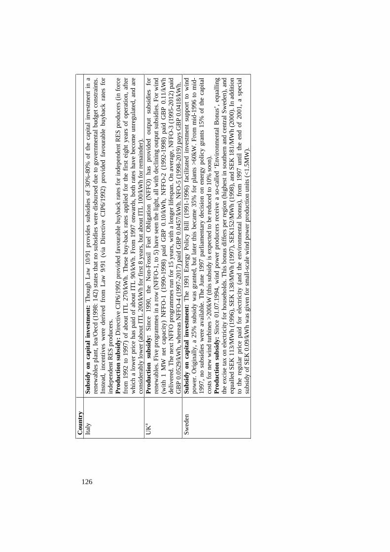
Cou

ntry

Ital

y Su

bsid

y on

cap

ital

inve

stm

ent:

Tho

ugh

Law

10/

91 p

rovi

des

subs

idie

s of

30%

-80%

of

the

capi

tal

inve

stm

ent

in a

re

new

able

s pl

ant,

Iea/

Oec

d (1

998:

142

) st

ates

that

no

subs

idie

s w

ere

disb

urse

d du

e to

gov

ernm

enta

l bud

get c

onst

rain

ts.

Inst

ead,

inc

entiv

es w

ere

deri

ved

from

Law

9/9

1 (v

ia D

irec

tive

CIP

6/19

92)

prov

ided

fav

oura

ble

buyb

ack

rate

s fo

r in

depe

nden

t RE

S pr

oduc

ers.

Pr

oduc

tion

subs

idy:

Dir

ectiv

e C

IP6/

1992

pro

vide

d fa

vour

able

buy

back

rat

es f

or in

depe

nden

t RE

S pr

oduc

ers

(in

forc

e fr

om 1

992

to 1

997)

of

abou

t IT

L 2

70/k

Wh.

The

se b

uy-b

ack

rate

s ap

plie

d fo

r th

e fi

rst

eigh

t ye

ars

of o

pera

tion,

aft

er

whi

ch a

low

er p

rice

has

pai

d of

abo

ut I

TL

90/

kWh.

Fro

m 1

997

onw

ards

, bot

h ra

tes

have

bec

ome

unre

gula

ted,

and

are

co

nsid

erab

ly lo

wer

(ab

out I

TL

200

/kW

h fo

r fi

rst 8

yea

rs, b

ut a

bout

IT

L 1

00/k

Wh

for

rem

aind

er).

U

Ka

Prod

uctio

n su

bsid

y:

Sinc

e 19

90,

the

Non

-Fos

sil

Fuel

O

blig

atio

n (N

FFO

) ha

s pr

ovid

ed

outp

ut

subs

idie

s fo

r re

new

able

s. F

ive

prog

ram

mes

in a

row

(N

FFO

-1, t

o 5)

hav

e se

en th

e lig

ht, a

ll w

ith d

eclin

ing

outp

ut s

ubsi

dies

. For

win

d (w

ith 1

MW

net

cap

acity

) N

FFO

-1 (

1990

-199

8) p

aid

GB

P 0.

10/k

Wh,

NFF

O-2

(19

92-1

998)

pai

d G

BP

0.11

/kW

h de

liver

ed. T

he n

ext N

FFO

pro

gram

mes

run

for

15

year

s, w

ith a

long

er li

fesp

an. O

n av

erag

e, N

FFO

-3 (

1995

-201

2) p

aid

GB

P 0.

0529

/kW

h, w

here

as N

FFO

-4 (

1997

-201

7) p

aid

GB

P 0.

0457

/kW

h. N

FO-5

(19

98-2

019)

pay

s G

BP

0.04

18/k

Wh.

Sw

eden

Su

bsid

y on

cap

ital

inve

stm

ent:

The

199

1 E

nerg

y Po

licy

Bill

(19

91-1

996)

fac

ilita

ted

inve

stm

ent

supp

ort

to w

ind

pow

er.

Ori

gina

lly,

a 25

% s

ubsi

dy w

as g

rant

ed,

but

late

r th

is b

ecam

e 35

% f

or p

lant

s >6

0kW

. Fr

om m

id-1

996

to m

id-

1997

, no

sub

sidi

es w

ere

avai

labl

e. T

he J

une

1997

par

liam

enta

ry d

ecis

ion

on e

nerg

y po

licy

gran

ts 1

5% o

f th

e ca

pita

l co

sts

for

new

win

d tu

rbin

es >

200k

W (

this

sub

sidy

is e

xpec

ted

to b

e re

duce

d to

10%

soo

n).

Prod

uctio

n su

bsid

y: S

ince

01.

07.1

994,

win

d po

wer

pro

duce

rs r

ecei

ve a

so-

calle

d ‘E

nvir

onm

enta

l B

onus

’, e

qual

ling

the

exci

se ta

x on

ele

ctri

city

for

hou

seho

lds.

Thi

s bo

nus

diff

ers

per

regi

on (

high

est i

n so

uthe

rn a

nd c

entr

al S

wed

en),

and

eq

ualle

d SE

K 1

13/M

Wh

(199

6), S

EK

138

/MW

h (1

997)

, SE

K15

2/M

Wh

(199

8), a

nd S

EK

181

/MW

h (2

000)

. In

addi

tion

to t

he r

egul

ar p

rice

pai

d fo

r el

ectr

icity

(an

d th

e en

viro

nmen

tal

bonu

s),

from

199

7 un

til t

he e

nd o

f 20

01,

a sp

ecia

l su

bsid

y of

SE

K 0

.09/

kWh

was

giv

en f

or s

mal

l-sc

ale

win

d po

wer

pro

duct

ion

units

(<1

.5M

W).

126

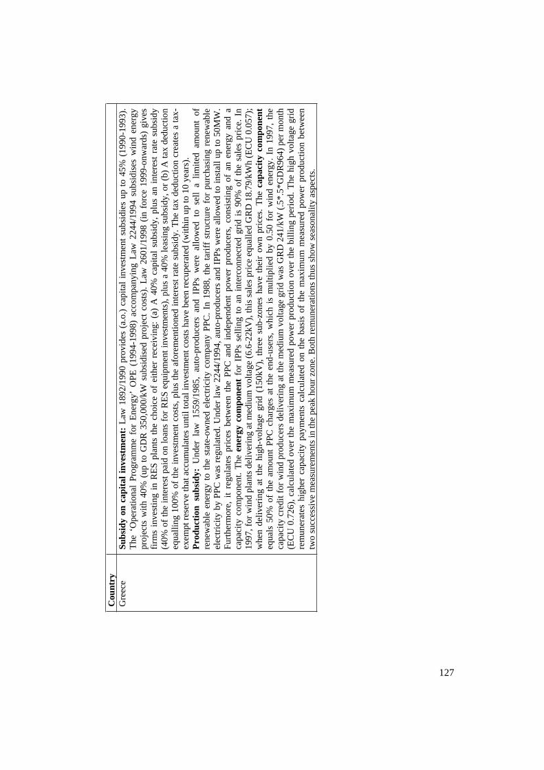
Cou

ntry

Gre

ece

Subs

idy

on c

apita

l inv

estm

ent:

Law

189

2/19

90 p

rovi

des

(a.o

.) c

apita

l in

vest

men

t su

bsid

ies

up t

o 45

% (

1990

-199

3).

The

‘O

pera

tiona

l Pr

ogra

mm

e fo

r E

nerg

y’ O

PE (

1994

-199

8) a

ccom

pany

ing

Law

224

4/19

94 s

ubsi

dise

s w

ind

ener

gy

proj

ects

with

40%

(up

to

GD

R 3

50,0

00/k

W s

ubsi

dise

d pr

ojec

t co

sts)

. L

aw 2

601/

1998

(in

for

ce 1

999-

onw

ards

) gi

ves

firm

s in

vest

ing

in R

ES

plan

ts t

he c

hoic

e of

eith

er r

ecei

ving

: (a

) A

40%

cap

ital

subs

idy,

plu

s an

int

eres

t ra

te s

ubsi

dy

(40%

of

the

inte

rest

pai

d on

loan

s fo

r R

ES

equi

pmen

t inv

estm

ents

), p

lus

a 40

% le

asin

g su

bsid

y, o

r (b

) A

tax

dedu

ctio

n eq

ualli

ng 1

00%

of

the

inve

stm

ent

cost

s, p

lus

the

afor

emen

tione

d in

tere

st r

ate

subs

idy.

The

tax

ded

uctio

n cr

eate

s a

tax-

exem

pt r

eser

ve th

at a

ccum

ulat

es u

ntil

tota

l inv

estm

ent c

osts

hav

e be

en r

ecup

erat

ed (

with

in u

p to

10

year

s).

Prod

uctio

n su

bsid

y: U

nder

law

155

9/19

85,

auto

-pro

duce

rs a

nd I

PPs

wer

e al

low

ed t

o se

ll a

limite

d am

ount

of

rene

wab

le e

nerg

y to

the

sta

te-o

wne

d el

ectr

icity

com

pany

PPC

. In

198

8, t

he t

arif

f st

ruct

ure

for

purc

hasi

ng r

enew

able

el

ectr

icity

by

PPC

was

reg

ulat

ed. U

nder

law

224

4/19

94, a

uto-

prod

ucer

s an

d IP

Ps w

ere

allo

wed

to

inst

all

up t

o 50

MW

. Fu

rthe

rmor

e, i

t re

gula

tes

pric

es b

etw

een

the

PPC

and

ind

epen

dent

pow

er p

rodu

cers

, co

nsis

ting

of a

n en

ergy

and

a

capa

city

com

pone

nt.

The

ene

rgy

com

pone

nt f

or I

PPs

selli

ng t

o an

int

erco

nnec

ted

grid

is

90%

of

the

sale

s pr

ice.

In

1997

, for

win

d pl

ants

del

iver

ing

at m

ediu

m v

olta

ge (

6.6-

22kV

), th

is s

ales

pri

ce e

qual

led

GR

D 1

8.79

/kW

h (E

CU

0.0

57);

w

hen

deliv

erin

g at

the

hig

h-vo

ltage

gri

d (1

50kV

), t

hree

sub

-zon

es h

ave

thei

r ow

n pr

ices

. T

he c

apac

ity c

ompo

nent

eq

uals

50%

of

the

amou

nt P

PC c

harg

es a

t th

e en

d-us

ers,

whi

ch i

s m

ultip

lied

by 0

.50

for

win

d en

ergy

. In

199

7, t

he

capa

city

cre

dit f

or w

ind

prod

ucer

s de

liver

ing

at th

e m

ediu

m v

olta

ge g

rid

was

GR

D 2

41/k

W (

.5*.

5*G

DR

964)

per

mon

th

(EC

U 0

.726

), c

alcu

late

d ov

er t

he m

axim

um m

easu

red

pow

er p

rodu

ctio

n ov

er t

he b

illin

g pe

riod

. The

hig

h vo

ltage

gri

d re

mun

erat

es h

ighe

r ca

paci

ty p

aym

ents

cal

cula

ted

on t

he b

asis

of

the

max

imum

mea

sure

d po

wer

pro

duct

ion

betw

een

two

succ

essi

ve m

easu

rem

ents

in th

e pe

ak h

our

zone

. Bot

h re

mun

erat

ions

thus

sho

w s

easo

nalit

y as

pect

s.

127

Cou

ntry

Irel

and

Acc

eler

ated

dep

reci

atio

n: I

t is

assu

med

(th

ough

this

is d

ebat

ed)

that

inve

stm

ents

in w

ind

turb

ines

may

opt

for

the

15%

ta

x de

prec

iatio

n p.

a. a

llow

ance

for

pla

nts

and

mac

hine

ries

(vi

s-à-

vis

the

4% p

.a. f

or in

dust

rial

bui

ldin

gs).

T

ax r

elie

f on

inve

stm

ents

: Sin

ce 1

980,

a 1

0% t

ax r

ate

appl

ies

to a

spe

cifi

ed r

ange

of

econ

omic

act

iviti

es,

incl

udin

g el

ectr

icity

gen

erat

ion

(the

cur

rent

‘no

rmal

’ ta

x ra

te is

28%

). S

ince

18.

03.1

999

(ope

ratin

g fo

r 2

year

s), t

he 1

998

Fina

nce

Bill

allo

ws

a ta

x re

lief

for

equi

ty in

vest

men

ts in

RE

S pr

ojec

ts u

nder

cer

tain

res

tric

tive

cond

ition

s.

Subs

idy

on c

apita

l inv

estm

ent:

The

AE

R-3

pro

gram

me

offe

red

capi

tal g

rant

s €8

0,00

0 pe

r M

W in

stal

led.

Pr

oduc

tion

subs

idy:

Sin

ce 1

994,

fiv

e ‘A

ltern

ativ

e E

nerg

y R

equi

rem

ent’

(A

ER

) pr

ogra

mm

es h

ave

been

lau

nche

d, o

f w

hich

AE

R-1

AE

R-3

, and

AE

R-5

app

ly t

o w

ind

pow

er. T

he A

ER

s ar

rang

e 15

-yea

rs’

purc

hase

con

trac

ts w

ith t

he I

rish

ut

ility

ESB

; th

e pr

ices

inc

reas

e an

nual

ly w

ith R

PI i

nfla

tion.

The

AE

Rs

regu

late

the

pri

ce c

ap,

but

the

real

pri

ces

are

settl

ed t

hrou

gh a

bid

ding

pro

cess

. U

nder

AE

R-1

(19

94-1

996)

, R

ES

prod

ucer

s w

ere

paid

a f

ixed

tar

iff

for

a 15

-yea

rs’

peri

od o

f IE

P 0.

061-

0.06

4/kW

h du

ring

wee

kday

s (a

bout

EC

U 0

.08)

, an

d IE

P 0.

024-

0.02

5/kW

h du

ring

the

wee

kend

s.

AE

R-3

(19

97-1

999)

reg

ulat

es a

pri

ce c

ap f

or w

ind

ener

gy, w

here

as th

e su

cces

sful

bid

s en

ded

at I

EP

0.02

21/k

Wh

(EC

U

0.02

8), w

hile

the

max

imum

win

d po

wer

pla

nt h

ad b

een

fixe

d at

15

MW

. AE

R-5

has

bee

n an

noun

ced

in A

ugus

t 20

01,

and

is n

ot d

iscu

ssed

her

e.

Port

ugal

Su

bsid

y on

cap

ital i

nves

tmen

t: I

n Po

rtug

al, i

nves

tmen

t sub

sidi

es h

ave

been

con

side

red

the

key

inst

rum

ent t

o pr

omot

e th

e us

e of

RE

S. T

wo

prog

ram

mes

hav

e pr

ovid

ed c

apita

l in

vest

men

t su

bsid

ies:

the

Ene

rgia

Pro

gram

me

and

the

MA

PE/P

OE

Pro

gram

me.

The

Ene

rgia

Pro

gram

me

(199

4-19

99)

gran

ts u

p to

50%

cap

ital

subs

idie

s of

tot

al i

nves

tmen

t co

sts

for

diss

emin

atio

n (c

omm

erci

alis

atio

n) p

roje

cts,

with

a c

ap o

f PT

E 5

0mln

(ab

out E

CU

249

k) f

or w

ind

proj

ects

. Pr

oduc

tion

subs

idy:

The

198

8 D

ecre

e L

aw 1

89 r

egul

ates

con

ditio

ns u

nder

whi

ch I

PPs

may

del

iver

to

the

natio

nal

grid

; it f

urth

erm

ore

incl

udes

pro

visi

ons

for

favo

urab

le p

rice

s. I

n 19

98, t

he p

rice

for

win

d en

ergy

was

PT

E 1

0.48

/kW

h.

128

Cou

ntry

Aus

tria

O

ther

fisc

al m

easu

res:

Sin

ce 0

1.08

.199

5, a

n O

rdin

ance

of

the

Fede

ral M

inst

er o

f Fo

reig

n A

ffai

rs g

uara

ntee

s m

inim

um

pric

es f

or R

ES

pow

er, v

aryi

ng f

rom

AT

S 0.

421/

kWh

to A

TS

0.9/

kWh

(rat

es f

or p

lant

s <

2MW

, dep

endi

ng o

n th

e tim

e of

del

iver

y). T

he 1

998

‘Ele

ctri

city

Bus

ines

s an

d O

rgan

isat

ion

Law

’ (E

LW

OG

, in

forc

e fr

om 1

999

onw

ards

) st

ates

tha

t th

e fe

dera

l pro

vinc

es h

ave

to f

ix th

e fe

ed-i

n ta

riff

s fo

r R

ES

pow

er. F

urth

erm

ore,

ren

ewab

le e

lect

rici

ty m

ay n

ow b

e so

ld

dire

ctly

to

any

cust

omer

. T

hese

fee

d-in

tar

iffs

not

onl

y di

ffer

per

pro

vinc

e, b

ut a

lso

per

seas

on (

sum

mer

or

win

ter)

, w

ithin

wee

ks (

wor

king

day

s or

wee

kend

s), a

nd t

hrou

ghou

t th

e da

y (d

aytim

e or

nig

hts)

. On

aver

age,

the

fee

d-in

tar

iffs

va

ry b

etw

een

€0.0

40/k

Wh

and

€0.0

49/k

Wh.

Su

bsid

y on

cap

ital

inve

stm

ent:

In

the

1992

-96

peri

od,

the

Law

of

Env

iron

men

tal

Prot

ectio

n pr

ovid

ed u

p to

30%

ca

pita

l in

vest

men

t su

bsid

ies.

Sin

ce J

uly

1997

, th

e ‘P

rom

otio

n In

stru

men

t fo

r E

lect

rici

ty f

rom

Ren

ewab

les’

(PI

ER

) pr

ovid

es (

a.o.

) ca

pita

l su

bsid

ies.

The

cap

ital

subs

idie

s ar

e ca

pped

to

prov

ide

not

mor

e th

an a

7%

rat

e of

ret

urn

for

15

year

s.

Prod

uctio

n su

bsid

y: I

n ad

ditio

n to

the

feed

-in

tari

ff, t

he M

inis

try

of E

cono

mic

Aff

airs

sig

ned

a ‘v

olun

tary

agr

eem

ent’

(F

ebru

ary

1994

) w

ith t

he u

tility

fir

ms

of a

ddin

g a

bonu

s to

IPP

s fo

r a

3 ye

ars’

per

iod

afte

r th

e co

nstr

uctio

n of

a R

ES

plan

t (f

or p

lant

s co

nstr

ucte

d be

fore

31.

12.1

996—

thou

gh s

ome

utili

ties

con

tinue

d th

is b

onus

pac

kage

unt

il ea

rly

1998

).

For

win

d po

wer

, thi

s bo

nus

was

100

%. T

his

agre

emen

t ap

plie

d to

the

199

4-19

96 p

erio

d. F

rom

Jul

y 19

97 o

nwar

ds, t

he

PIE

R p

rovi

des

all i

ncen

tives

for

RE

S.

Fran

ceb

Acc

eler

ated

dep

reci

atio

n: S

ince

199

3, p

riva

te c

ompa

nies

inv

estin

g in

RE

S pr

ojec

ts m

ay d

epre

ciat

e th

eir

inve

stm

ents

w

ith 1

00%

in o

ne y

ear.

T

ax r

elie

f on

inve

stm

ents

: Sin

ce 1

993,

pri

vate

com

pani

es in

vest

ing

in R

ES

proj

ects

may

app

ly f

or a

red

uced

cor

pora

te

inco

me

tax

rate

(50

% r

educ

tion)

. O

ther

fis

cal

mea

sure

s: T

houg

h th

e 19

46 l

aw c

once

rnin

g th

e na

tiona

lisat

ion

of e

lect

rici

ty,

and

a 19

55 d

ecre

e es

tabl

ishe

d th

e ba

sis

for

oblig

atin

g E

dF t

o pu

rcha

se e

nerg

y pr

oduc

ed b

y co

-gen

erat

ors,

thi

s m

easu

re p

redo

min

antly

fo

cuss

ed o

n su

rplu

s ca

paci

ties,

and

did

not

pro

vide

par

ticul

ar i

ncen

tives

for

enc

oura

ging

RE

S pr

oduc

tion.

The

refo

re, a

ne

w d

ecre

e w

as p

ut in

pla

ce a

s pe

r N

ovem

ber

1994

, whe

re E

dF w

as o

blig

ed to

pur

chas

e R

ES

elec

tric

ity a

s w

ell.

Prod

uctio

n su

bsid

y: U

nder

the

‘E

OL

E 2

005’

win

d en

ergy

pro

gram

me

(199

6-20

05),

spe

cial

fee

d-in

tar

iffs

are

re

gula

ted

betw

een

EdF

and

IPP

s fo

r 15

-yea

rs’

peri

ods.

Thi

s pr

ogra

mm

e co

nsis

ts o

f 3

stag

es. U

nder

sta

ge 1

(19

96),

the

feed

-in

tari

ff w

as F

FR 0

.38/

kWh

(€0.

058)

. St

age

2 (1

997)

app

lied

an F

FR 0

.34/

kWh

rate

. St

age

3 (2

001)

for

esee

s a

€0.0

838/

kWh

rate

for

the

fir

st 5

yea

rs, a

fter

whi

ch a

low

ered

rat

e is

off

ered

for

the

nex

t 10

yea

rs (

bein

g €0

.030

5/kW

h fo

r ov

er 3

600

hrs.

of

prod

uctio

n, a

nd €

0.08

38/k

Wh

for

less

than

200

0 hr

s.).

129

Cou

ntry

Finl

and

Subs

idy

on c

apita

l inv

estm

ent:

The

199

3 ‘w

ind

ener

gy p

rogr

amm

e’ p

ut a

30%

cei

ling

to c

apita

l inv

estm

ent s

ubsi

dies

. T

he 1

996

Cou

ncil

of S

tate

’s ‘

new

dec

isio

n on

gen

eral

con

ditio

ns f

or g

rant

ing

ener

gy s

uppo

rts’

cap

s th

e in

vest

men

t su

bsid

y to

win

d tu

rbin

e pr

ojec

ts to

40%

(de

cisi

on 5

4/96

).

Prod

uctio

n su

bsid

y: I

n es

senc

e, R

ES

elec

tric

ity r

ecei

ves

the

free

-mar

ket

pric

e. I

n ad

ditio

n, h

owev

er, s

ome

prem

ium

s ha

ve b

een

adde

d. D

urin

g 19

97, w

ind

pow

er r

ecei

ved

a pr

oduc

tion

subs

idy

equa

l to

the

tax

levi

ed to

indu

stri

al e

lect

rici

ty

cons

umpt

ion

of F

IM 0

.025

/kW

h (a

bout

€4.

2/M

Wh)

. A

s pe

r Se

ptem

ber

1998

, th

e su

bsid

y eq

ualle

d th

e ta

x le

vied

to

hous

ehol

d el

ectr

icity

con

sum

ptio

n of

FIM

0.0

41/k

Wh

(abo

ut €

6.9/

MW

h).

Bel

gium

T

ax r

elie

f on

inve

stm

ents

: T

he n

atio

nal

1992

com

pany

tax

cod

e (1

992-

onw

ards

) al

low

s a

pref

eren

tial

dedu

ctio

n fo

r in

vest

men

ts i

n R

ES

to b

e de

duct

ed f

rom

the

pro

fits

. T

his

fisc

al i

nves

tmen

t de

duct

ion

cons

ists

of

a ‘b

ase-

perc

enta

ge’

that

var

ies

per

annu

m (

and

fluc

tuat

ed a

roun

d 3.

5% o

ver

the

last

yea

rs)

plus

a 1

0% s

uppl

emen

tary

ded

uctio

n. A

ltoge

ther

, th

e al

low

ance

has

bee

n ab

out 1

3.5%

ove

r th

e la

st d

ecad

e.

Subs

idy

on c

apita

l inv

estm

ent (

Flan

ders

): U

nder

the

head

er o

f ‘e

colo

gy s

uppo

rt’,

the

Flan

ders

fed

erat

ion

gran

ts 2

0%

capi

tal i

nves

tmen

t sub

sidi

es (

1998

-onw

ards

).

Prod

uctio

n su

bsid

y (F

land

ers)

: T

he ‘

Ele

ctri

city

Gen

erat

ion

Fund

’ (R

EG

) pr

ovid

es a

BE

F 1/

kWh

(€24

.8/M

Wh)

pr

oduc

tion

subs

idy

for

peri

ods

up to

10

year

s, f

or R

ES

prod

uctio

n un

der

the

‘Gre

en F

ranc

Sys

tem

’ (1

995-

onw

ards

). I

n ad

ditio

n, t

he V

IRE

G p

rogr

amm

e (1

996-

onw

ards

) pr

ovid

es a

BE

F 1/

kWh

(€24

.8/M

Wh)

pro

duct

ion

subs

idy

for

win

d,

sola

r, a

nd b

iom

ass

pow

er w

ith a

n in

stal

led

capa

city

10

MW

(as

per

01.

07.1

998,

thi

s su

bsid

y w

as i

ncre

ased

to

BE

F 2/

kWh)

. Su

bsid

y on

cap

ital i

nves

tmen

t (W

allo

on):

Fir

ms

inve

stin

g in

RE

S ca

n ge

t a 1

5% in

vest

men

t gra

nt (

1993

-onw

ards

).

Lux

embo

urg

Acc

eler

ated

dep

reci

atio

n: T

he 2

4.12

.199

6 in

trod

uced

spe

cial

dep

reci

atio

n al

low

ance

s fo

r R

ES

inve

stm

ents

that

allo

w

to d

epre

ciat

e 60

% in

the

firs

t yea

r.

Subs

idy

on c

apita

l inv

estm

ent:

A 1

994

min

iste

rial

reg

ulat

ion

supp

orte

d L

UF

6000

per

kW

(ab

out

€149

) in

stal

led

to

non-

indu

stri

al c

o-ge

nera

tors

(19

94-1

997)

. T

he 2

1.02

.199

7 la

w o

n ec

onom

ic d

evel

opm

ent

and

dive

rsif

icat

ion

allo

ws

a su

bsid

y of

LU

F 30

00 p

er k

W (

abou

t €74

) w

ith a

max

imum

of

LU

F 6m

ln (

€148

,736

) fo

r w

ind

turb

ines

>50

kW.

Prod

uctio

n su

bsid

y: T

he 1

994

Gra

nd D

ucal

reg

ulat

ion

sets

the

buy-

back

tari

ff f

or R

ES

pow

er e

qual

to th

e ta

riff

for

co-

gene

ratio

n. F

or i

nsta

llatio

ns b

etw

een

151

and

1500

kW,

the

day

tari

ff p

aid

aver

ages

LU

F 2.

3/kW

h, w

here

as L

UF

1.2/

kWh

is p

aid

over

nig

hts.

Win

d po

wer

rec

eive

s an

d ad

ditio

nal

prod

uctio

n su

bsid

y of

LU

F 1/

kWh.

The

re e

xist

s an

an

nual

LU

F 45

00/k

W s

ubsi

dy f

or d

eliv

erin

g el

ectr

icity

dur

ing

peak

load

. So

urce

s: B

ased

on

natio

nal

legi

slat

ions

, va

riou

s is

sues

of

the

IEA

cou

ntry

rev

iew

s ‘E

nerg

y P

olic

ies

of…

’, Ie

a/O

ecd

(199

8),

and

tran

slat

ions

and

int

erpr

etat

ions

in

the

EN

ER

-IU

RE

pro

ject

, sup

port

ed b

y th

e E

C. F

or th

e la

tter

sour

ce, s

ee: h

ttp://

ww

w.jr

c.es

/cfa

pp/e

neri

ure/

wel

com

e.ht

ml.

Not

es: a S

peci

fic

mea

sure

s fo

r Sc

otla

nd a

nd N

orth

ern

Irel

and

have

not

bee

n ta

ken

into

acc

ount

in th

is ta

ble;

b Leg

isla

tion

for

over

seas

terr

itori

es is

not

incl

uded

.

130

131

4.4.2 Present value of green policies Figure 4.4 shows the present value of all economic instruments listed in table 4.2, by means of the calculations given in table 4.1. The exact figures are given in table 4.3 in the appendix to this chapter. Any discussion of the financial attractiveness of the different economic instruments should emphasize the fundamental difference between the ‘bidding programme’ countries, and the others. Under a non-bidding programme, firms apply for a subsidy or other incentive, and may increase their capital stock up to the long-run economic equilibrium. The governments of both the UK and Ireland, however, decided to launch bidding programmes for encouraging investments in renewable energy. Under such programme, the number of eligible projects (and therewith the capital stock) is specified beforehand, as is the budget available. Firms can join a tender and demand for subsidies. The firms demanding the lowest subsidies are eligible, whereas all the other projects (demanding too much support) are not. In theory, this is a very nice mechanism. That shield yield efficient outcomes. Particularly when assessing ex post how high the granted support has been in the UK, then it turns out that the NFFO bidding programme was anything but efficient (particularly the 1990-94 period is striking).

Figure 4.4: Present value of economic instruments (1MW investment project)

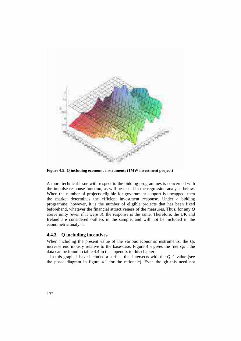
132

A more technical issue with respect to the bidding programmes is concerned with the impulse-response function, as will be tested in the regression analysis below. When the number of projects eligible for government support is uncapped, then the market determines the efficient investment response. Under a bidding programme, however, it is the number of eligible projects that has been fixed beforehand, whatever the financial attractiveness of the measures. Thus, for any Q above unity (even if it were 3), the response is the same. Therefore, the UK and Ireland are considered outliers in the sample, and will not be included in the econometric analysis.

4.4.3 Q including incentives When including the present value of the various economic instruments, the Qs increase enormously relative to the base-case. Figure 4.5 gives the ‘net Qs’; the data can be found in table 4.4 in the appendix to this chapter. In this graph, I have included a surface that intersects with the Q=1 value (see the phase diagram in figure 4.1 for the rationale). Even though this need not

Figure 4.5: Q including economic instruments (1MW investment project)

133

represent the long-run equilibrium value for which 0q (this will be discussed in the next section), it does provide a minimum value for that condition. When analysing the Q values including incentives, it appears that none of the countries in the sample provided positive Qs at the start of the sample period. Also, all countries had nonnegative Qs at the end of the sample period. Though strictly speaking Q should at least be one for a long-run sustainable industry, nonnegative Qs might attract ‘single shot’ investments. These do not generate sufficient income to ensure an infinitely lived industry, but they might attract some investments. Of all countries, the Qs for the UK can safely be labelled excessive. As the present value of the economic instruments already suggested, wind turbine investments were very profitable during the 1990-94 period in the UK. Though some countries provided little incentives, I still obtained relatively high Qs. For example, the Dutch government has hardly provided serious incentives before 1995, but the Qs during the pre-1995 period have not been dramatically low (oscillating around the Q=0 value). Such anomalies are attributed to the favourable wind regimes of such countries, or the relatively low corporate tax rates. On the downside, the Qs obtained for Ireland are dramatically low, and in fact (given the investments in turbines revealed in the next section) I also obtained very low Qs for Denmark. Here, a general comment holds for all countries with low accumulated levels of wind turbines. Usually, when a product-market is in its start-up phase, additional subsidies are available for market development. For renewable energy, both national governments and the EU have specific subsidy programmes. Including these may explain the residual growth observed with currently negative Qs.

4.5 Investment response to green policies

4.5.1 Wind turbine investments over time I have used annual IEA/OECD data on the installed wind turbine capacity per country.115 These data have some limitations. First, since only some countries have reported wind turbine capacity per ownership class (public, NGO, private) whilst these distinctions have not been made from the start, I have decided to treat all countries similarly and use aggregates. As a consequence, even if the calculated Qs would be negative, one may observe growth in investments. This ‘autonomous’ growth is attributed to either (a) public sector investments, since public enterprises are assumed to use another evaluation criterion than micro-level Q, or (b) the fact that for premature markets, additional market development subsidies are often available.

115 The IEA is the International Energy Agency of the OECD.

134

Table 4.2 does not include these kinds of subsidies, which might lead to an underestimate of Qs for markets with low levels of accumulated turbine capacity. A second remark concerns replacements. Since only aggregate figures were available, the data reflect net investments, and should actually be corrected for replacement investments. Therefore, the gross investment figures might be higher. A consequence of this data limitation is that we may now observe a negative growth in turbine capacity in Luxembourg between 1998 and 1999, whilst in reality there might have been a positive gross investment in that period. Figure 4.6 gives an impression of the cumulative investment figures for the four largest investing countries (ranked by their year 2000 capital stock). The data for all countries in the sample can be found in table 4.5 in the appendix to this chapter. Germany, Denmark, and Spain are by large the biggest investors in wind turbines. Particularly when assessing the cumulative year 2000 figures, the gap between these three countries and the rest of the sample becomes even more apparent. When calculating the marginal growth rates of the capital stock in all countries, then it appears that the largest investors in cumulative terms have had their peak in the late 1980s or early-1990s. Ever since, these growth rates have

Figure 4.6: Cumulative installed capacity (Kt) for the four largest wind turbine investing countries

135

been lower than 100 per cent.116 Interpreting declining growth rates (for example in the three largest investing countries) as saturation, it seems that if there is growth to be expected it should come from the smaller wind turbine countries.117 As such, declining growth need not be bad: if an industry approaches its long-run equilibrium, the only investments that should be made are the replacement investments, necessary to cover the depreciation of the existing capital stock. In order to analyse this equilibrium hypothesis, we need to analyse the phase diagrams. Before turning to the phase diagrams, however, I calculate the average Qs, for which I have used two approaches. First, I have assumed that each country was served by a single investor—that is, all investments made in year t represented a single investment project. Under this assumption, the subsidies and tax allowances are capped for a number of countries, limiting the value of Q. Figure 4.7 outlines the results. The most striking Q-values were obtained for the UK (about 5 in 1991), Italy (over 3 in 1995), and Ireland (over 3 in 1996). The only two other countries for which I obtained Qs bigger than one were Belgium (1997) and Germany (1989 and 1993). In the second approach, I have removed the restriction that all investments represented atomistic projects, and allowed the maximum incentives possible. Under this scenario, the Qs had to be bigger, and figure 4.8 shows how much bigger they were. In the remainder, I proceed with the second approach (the higher values for average Q). See table 4.6 in the appendix to this chapter for the data.

116 With an exception for Spain in the 1996-1997 period. 117 See the recent wind energy report of the German Federal Environmental Ministry at http://www.bmu.de/download/dateien/windenergie_studie02.pdf. In this report (in German) the authors argue that particularly in the coastal regions of Germany, there is little space left for new turbines (p. 14).

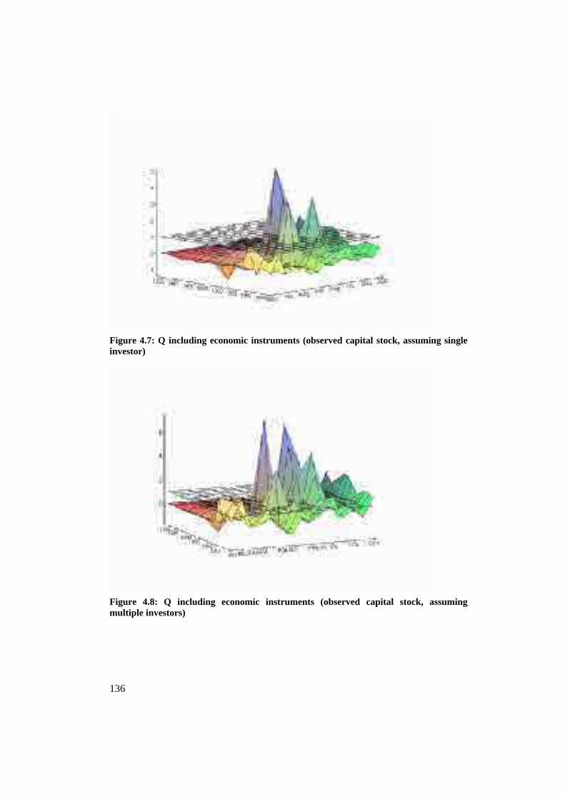
136

Figure 4.7: Q including economic instruments (observed capital stock, assuming single investor)

Figure 4.8: Q including economic instruments (observed capital stock, assuming multiple investors)

137

4.5.2 From Q to capital stock: Phase diagrams Figure 4.1 gave the theoretical relationship between capital stock and Tobin’s Q for wind turbine investment. The data, however, made it very difficult to establish such a nice smooth pattern as in figure 4.1. In figure 4.9, I have depicted the same four countries as in figure 4.6 (Germany, Denmark, Spain, and the Netherlands). At first, the diagram may look fuzzy for it only describes the different pairs of k and Q, without providing any line for which 0q . The reason for omitting these lines is a simple one. Plotting these lines requires complex simulations. Since any line for which 0q embodies a set of unobservable partial derivatives (see equations (4.9) and (4.7)), they can at best be approximated by, for example, Monte Carlo simulation.118

118 Not only should one have a very good estimate of the response of I to Q (for which the panel data response in the next subsection may only represent a first step), but also recall

that qHc was downward sloping because kH c had a downward slope, which

was the result of a downward sloping demand curve. Thus, in addition to the response of I to Q one has to fit the demand curve.

Figure 4.9: Combined diagram of four countries in (k,Q) space

138

An additional reason for not including any line for which 0q is of minor importance and concerns the visual interpretation. In each year, the incentives as well as the economic context (wholesale prices) change per country, resulting in a different Q per country per year. As a consequence, with constantly shifting Qs, the long-run equilibrium and optimal capital stock also change each year. If the combination (k,Q) is an orbit, and the equilibrium the attractor, then the moving attractor causes the system to be in permanent motion. Since it is very unrealistic to assume that the system can move towards its current equilibrium instantaneously, it becomes quite plausible to assert that none of the observed pairs of (k,Q) represent steady states. Now one might try to draw a line for which

0q for each year in order to check how the equilibrium has moved over time, but this gives a very messy picture since these lines never overlap.

4.5.3 From Q to capital stock: Individual regressions Numerous regression models exist for estimating a relationship between Tobin’s Q and corporate investment—varying from relatively simple OLS models to dynamic panel data models using GMM estimates. The common denominator in all econometric models is the problem of the unobservable installation function. Net investments can be observed, but gross investments cannot. It is beyond the scope of this study to come up with a ‘new’ regression model. The only purpose any regression model would have here is to confirm that higher Q’s yield more investments, and that such relationship has a consistent pattern. A simple model that meets these criteria is given by Blundell et al. (1992), which is very similar to the one provided by Hayashi (1982). The intuition is as follows. First, investment is triggered by (4.10) and (4.11), of which the latter yielded:

01 rt

t

tt

t

ttinvttc

t

c eII

qIA

mSmDeprTIH

A little rearranging gives:

(4.15) t

tt

t

ttinvttc I

Iq

IA

mSmDeprT 1

The second step is to recall the Euler equation describing the evolution in q, which was given by (4.13):

01t

tt

t

tt

t

t

t

tc

t

c

kk

qkI

qkA

kR

TkH

A little rearranging of that equation yields:

(4.16) t

tt

t

t

t

tc

t

tt k

Iq

kA

kR

Tkk

q 1

139

Multiplying (4.15) by It and (4.16) by kt, and taking the difference of the resulting equations gives:119

(4.17) tctctinvtttt RTDeprTSImqk )1(1 , .

Here, I follow Poterba and Summers (1982) for the intuition behind (4.17). The left-hand side of the equation gives the market value of I units of additional

investments is tt qk .120 On the right-hand side, we find the market costs of the

additional unit of investment. The direct investment costs mtIt are lowered by the investment subsidies and investment tax credits. With each additional unit of investment also an amount of revenues R are foregone, due to the constant returns to scale and the downward sloping demand curve. Firms will thus invest up to the point where the benefits of an additional unit of investment equal the costs. Following Lucas Jr. (1967), I use the fact that the first derivative of the gross investment function (which is assumed to be homogeneous of degree one) with respect to I can be treated as a function of the ratio I/k. Then (4.15) can be rewritten as:

(4.18)

t

t

t

tttctinv

t

II

IA

mDeprTmS

q 1

1

,

which we can solve for I to obtain the optimal investment rule: (4.19) tt kqI ,~ ,

where tq~ (hereafter referred to as ‘modified Q’) is the left-hand side of (4.18), being:

t

tttctinvtt I

AmDeprTmSqq 1~ .

Since the interest is not so much in the effect of mtIt investment but in It units only, I will use tq as the normalised modified Q:

(4.20) tt

ttcinvtt Im

ADeprTSqq 1 .

119 Since the revenues R were decreasing in k, kR must be negative. After multiplying

(4.16) with k, I have added that negative sign to R. 120 To check this, recall that the multiplied forms of (4.15) and (4.16) with It and kt

respectively yield tt Iq . Since that part equals tt qk , it follows that gross investment

tI turns into the change of capital stock tk —a result identical to the restriction on the

Hamiltonian.

140

In words, (4.20) incorporates an adjustment that is directed at the investment decision only: the only variables that remain in the denominator are the investment subsidy, the tax credit on investment, and the accelerated depreciation of new investment. Once more I follow Hayashi (1982), and reduce (4.19) to:

(4.21) tqkI ~ ,

for which the OLS equation becomes:

(4.22) ititiiit

qkI ~ .

In the appendix to this chapter, table 4.7 gives the I/k ratios, whereas table 4.8 gives modified Q. The scatter plots in figures 4.10 and 4.11 illustrate the effect of the above transformation. Table 4.9 in the appendix gives the results of a simple OLS estimation for a zero year time lag.121 The interest is in the slope estimators , and not so much in finding a perfect model fit. Therefore, only the betas and associated t-statistics and standard errors have been reported. Though for most countries only a few observations were available, the regression does provide ‘significant’ results for nine countries. A few comments should be made. First, both bidding countries (UK and Ireland) show a very significant and positive response of investments to the modified Q. However significant statistically, this result is doubtful. For both countries the number of eligible projects was determined beforehand, and Q was the result of the bidding process rather than of a straightforward relationship between financial attractiveness and investment as in the non-bidding countries. Second, most countries have very few variation in the dependent, which raises a serious question mark with respect to individual series regressions. I will tackle this problem by means of panel data analysis. For some countries, the results need a particular explanation.

121 Blundell et al. (1992) use a GLS estimator, and first check whether Q is independent of the error term. If not, then firms are not the price-takers Hayashi (1982) assumed them to be, and it becomes incorrect to use average Q as being equal to marginal Q. In case of the wind turbines, both wholesale prices and government incentives are exogenous, and so is Q.

141

Figure 4.10: Scatter plot for all (k,Q) pairs

Figure 4.11: Scatterplot for all (I/k, q ) pairs

142

Germany The country with the biggest investment (Germany) has an insignificant slope estimator at a zero year time lag. When increasing the time lag, all slope estimators become insignificant except for Germany and Belgium. The latter result must be spurious (given even less variation in the dependent); the time lag for Germany is attributed to the dreadful red-tape for installing wind power plants. 122 Once that time lag is introduced, however, the sign of the slope estimator changes to minus 0.88 at a two years time lag! However counterintuitive this result may seem at a first glance, a line plot helps to find the rationale. As figure 4.12 shows, though modified Q went up in Germany and has remained high ever since 1989, the growth rate of installed capacity has already decreased from 1987 onwards. If we go back to the absolute figures (see table 4.5 in the appendix), however, then we see that the investment figures in absolute levels are still very impressive and the highest of the entire sample. True that the growth rates are declining, but in absolute levels they still increase. As argued in section 4.5.1, the most logical reason for declining growth rates of capital stock is probably not rooted in the financial attractiveness but rather in the saturation of geographical space.

122 In Germany investors lament over both red tape and local urban planning legislation, since these reduce the speed of implementation.

Figure 4.12: Combined diagram of I/k and modified Q for Germany

143

Denmark Though the data for Denmark should have sufficient variation, the economic instruments included for calculating Q cannot explain the growth in turbine capacity. It must be emphasized here that in Denmark households own about 60 per cent of all wind turbines installed. The economic instruments listed in table 4.2 do not include measures for households, and may hence underestimate the financial attractiveness of turbine investments. Furthermore, households may well have different utility preferences than companies, and may attribute a high value to the ‘warm glow’ of positively contributing to the environment.123

4.5.4 From Q to capital stock: A panel data regression The biggest drawback of the individual time series regressions is that there are many countries with little variation in the dependent. This data limitation can be overcome by means of a panel data regression model. Assuming that all investors respond in a similar fashion to Q, I have estimated a common effects panel data model. Though such strategy eliminates the data problem for the ‘small growth countries’, it cannot solve the parameter restriction problem associated with the bidding programme countries. Therefore, I have excluded the UK and Ireland.124 The simple straight-line common effects panel data model, assuming homogeneity in both the intercept and slope estimators is given by:

(4.23) ititit

QkI

,

which is defined as above (in (4.22)). The regression analysis yields a beta of 0.74, with a standard error of 0.082 and a t-statistic of 8.897. This beta is thus very significant. The Durbin-Watson statistic of 1.89 suggests that there is very little serial correlation in the error term. An important implication of this regression analysis is that it does not seem to matter too much what exact policy instruments are used, as long as the project becomes financially sustainable. Hence, it seems that firms have equal preferences for investment subsidies or tax rebates, as long as they yield the same results. Probably, this result only holds for a macro-context within which macroeconomic and political stability are present, and where government commitment to whatever instrument is guaranteed for a minimum time period. If this were not the case, then the international business literature suggests that entrepreneurs prefer those

123 Glaeser and Shleifer (2001) emphasize that even for-profit entrepreneurs may start a not-for-profit organisation, due to the ‘soft incentives’ associated with that not-for-profit status (as donations). Now it could be possible that some Danish entrepreneurs follow this strategy, but given the size of the wind turbine market, it does not seem plausible. 124 Particularly the inclusion of the UK would lead to a series of outliers—some five observations centred around the €800k values for which hardly any growth is realised (all close to the x-axis).

144

incentives that have immediate spin off, such as an investment subsidy. Other instruments, as production subsidies or tax holidays over a longer time span become less attractive when macroeconomic or political instability increase.125 If the shape of the wealth transfer does not matter, what policy instruments yield a win-win situation? This depends on the preferences of government. In the long run and overall, it would not matter whether government spends on subsidies or faces an opportunity cost due to fiscal incentives. Nevertheless, entrepreneurs are probably more committed to fulfilling long run projects if they receive favourable buyback rates or production subsidies, than an initial investment subsidy.

4.5.5 A note on the ‘barriers to investment’ In section 2.1, I have argued that the barriers to investment (surveyed in chapter 2) may hinder entrepreneurs in their optimal investment decision. Consequently, the observed capital stock may deviate from what we might expect from a technical analysis in (Q,k) space. In the empirical analysis of this chapter, I found for example that in Germany the red tape was hindering entrepreneurs in their turbine instalments. Consequently, it was the only country for which the regression analysis became very significant at a two years’ time lag between modified Q and the investment growth rate. Still I decided not to include (dummy) variables in the regressions for the barriers to investment, for the following two reasons. First, the data I obtained were measured at such a low frequency, that adding extra variables would either dramatically drop the statistical significance or yield spurious results. A second reason is that the data were only reported at the aggregate, national level whereas many barriers to investment take place at the micro-level. Given now this inability to include (dummy) variables in the regression analysis, the inferences on possible underinvestment, and particularly the policy implications become weaker.

4.6 Implicit governmental valuation of the public good Up to here, the focus has been on the investment, and not so much on the public good. In section 4.2.1, I have argued that the avoided emissions of wind power may vary over both time and space. It is striking to see how the average CO2 emissions from power generation differ per country. Figure 4.13 gives an overview for the EU(15) countries during the 1985-99 period; table 4.10 in the appendix gives the underlying data. The differences in the emissions from power generation can be roughly explained as follows. The lowest emissions are found in the countries that predominantly rely on hydropower (Sweden, Austria, Finland), nuclear power

125 See for example Henisz (2000), Jou (2000), Tybout (2000), Single (1999), Clark (1993), Davis and Swenson (1993), or Mcclintock (1988).

145

(Belgium), or a combination of these two (France). For Luxembourg, it must be noted that it primarily depends on electricity import; this also explains the fact that it is the only country for which the emissions per MWh generated can fluctuate so much over time. When calculating the implicit government valuation or utility of wind power, I divided the present value of all economic instruments for a 1MW investment by the product of the average emissions times the wind regime:

(4.24) 0

,

Tw

dtdseAYU

itit

t

trsts

itgov

f

In case of a negative present value of the allowances, I valued this ratio as zero. Figure 4.14 gives the results; table 4.11 in the appendix gives the underlying data. Most estimates of the marginal abatement costs of CO2 vary between zero and some 250 Euros per tonne,126 and my calculations seem to fit fine within these estimates. More important, however, is that this analysis gives a completely different interpretation of the ‘generosity’ of the various governments. In the above analysis of the Tobin’s Q values, countries as the UK seemed to exaggerate their economic incentives. When relating the tax money spent to the avoided emissions in that country over the lifespan of a wind turbine, then it appears that the UK has been generous, but not so much as France (ignoring the environmental costs of nuclear power production in the latter country), or Luxembourg.

4.7 Underinvestment issues Clean air is a continuous public good. Therewith the question regarding underinvestment is one that depends on the benchmark chosen. The empirical analysis in this chapter suggests that the answer is twofold: (1) the reasons underlying underinvestment can occur in a technical, microeconomic sense, or (2) they are rooted in the macroeconomic governmental valuation, indicating societal preferences. In addition, I have observed some ‘barriers to investment’, interfering in the discussion.

126 See, for example, Blok et al. (2001).

146

Figure 4.13: Average emission in national power generation [tonne CO2/MWh]

Figure 4.14: Implicit govermental valuation of a 1MW project [€/tonne CO2]

147

4.7.1 Barriers to investment In section 4.5, I already mentioned the impossibility to test for precise effects of possible ‘barriers to investment’ (as sketched in chapter 2), due to limitations in the data. In terms of figure 3.4, this impossibility implies I cannot test for the statistical importance of these phenomena, so that—if the capital stock remains below the levels desired by government—the policy recommendations for this chapter become weaker. Suppose the main issue in wind turbine investment is a funding constraint, because banks dislike the asset specificity of the investment. In that case, providing loans (not even under ‘soft’ terms) may be a powerful catalyser for investment. When assessing the case of German wind turbine investments, it now seems that high levels of Tobin’s Q, that in addition are stable over time, form as key explanation in the success of the German wind turbine support programme. Meanwhile, however, Germany was the only country where a commercial bank offered soft loans that covered 50 per cent of the capital investment. Since I do not know whether all projects applied for this soft loan, or whether the parental company needed such funding at all, it becomes more difficult to give clear-cut policy advise.

4.7.2 Technical underinvestment based on Tobin’s Q In the microeconomic part of the optimisation problem, the phase diagrams showed how investment and capital stock are related to Tobin’s Q. The panel data regression showed how investments were indeed sensitive to Q, and—except for Denmark, where households own 60 per cent of the wind turbines—how Qs approaching unity or even higher yielded very large investments in Germany and Spain. For all other countries it was difficult to assess the individual time series due to the limited variation in the dependent variable. Underinvestment in this technical sense would occur if Q were above unity but the capital stock would not reach its equilibrium level. Hence, the benchmark here is the observed capital stock, related to Tobin’s Q. In this technical interpretation, the two countries with the largest capital stock are Germany and Spain. For Germany, the observed capital stock steadily exceeds the Q=1 line from 1989 onwards.

148

Independent of the exact position of the locus for which 0q , it seems plausible that the German wind turbine investments will move to their long-run equilibrium. The fact that the growth rates are declining in spite of high values for Q confirms this intuition. For Spain, I had not included regional economic instruments, for they were quite different—both over time and over space. Therewith, my calculations for Q have a downward bias, and the ‘true’ Q should be higher. Since my calculated Qs for Spain are close to unity, I suspect them to be on the Q=1 line. This intuitive conclusion would justify the high levels of capital stock that have rapidly increased since 1995 onwards. I cannot draw any inference on the case of Denmark, since the high levels of capital stock cannot be explained by the Qs calculated for the economic measures listed in table 4.2. Since households own about 60 per cent of the wind turbines in Denmark, different instruments should be analysed here. For all other countries analysed, the majority of the time period there was underinvestment in a technical sense—albeit one spurred by governments. Given that in most countries for most of the time period no Qs exceeding unity were observed, investments remained absent. Here, the private sector cannot be blamed for not investing, but it does show that the funding problem in the private provision of public goods is a serious one.

4.7.3 Underinvestment in the context of governmental valuation Apart from the technical interpretation of underinvestment, it appears that the governmental valuation of the public good ‘clean air’ varies widely over both time and space.

Economicinstruments

Barriers toinvestment

Q I/kEconomic

context

U(Y)

kBenchmark for

underinvestment (technical sense)

Figure 4.15: Technical interpretation of underinvestment

149

Starting off from the premise that no private sector participant will invest in a loss-giving project, the question rises whether government (as a representative of society) is willing to support the private sector in a market where firms are price-takers, and where the wholesale price yields a base-case scenario of negative Qs. In section 4.6 I have related the present value of the economic instruments to the

Economicinstruments

Barriers toinvestment

Q I/kEconomic

context

U(Y)

k

Benchmark for underinvestment

(desirability of public good)

Figure 4.16: Desirability-of-public-good interpretation of underinvestment

Figure 4.17: Scatter for (U(Y), I/k) pairs

150

amount of the public good they would yield. The results were striking in the sense that some countries originally appeared to have given extraordinarily high incentives (e.g., the UK from 1990 to 1994, Germany from 1989 to 1995, or Italy in 1995 and 1996), but when related to the amount of public good provided, they were less dramatic. In fact, for countries where the national power generation hardly yields CO2 emissions (e.g., Sweden or France), the spin-off for the taxpayers is so much lower than in countries as Greece or Ireland. This provides a completely different perspective to the optimisation problem, and therewith to the analysis of potential underinvestment. If society does not value the public good sufficiently high enough, can we blame the private sector for not investing? Although it would be tempting to analyse a relationship between governmental valuation U(Y) and the investment rate I/k or the capital stock k, I do not have a solid criterion that sets the benchmark. In addition, the scatter plot in figure 4.17 shows it will be difficult to interfere on such relationship.

4.8 Conclusions In this chapter, I have analysed the effect of various economic instruments on private sector investments in wind turbines. The main conclusions can be summarised as follows. First, wind turbine investments appear to be very sensitive to higher marginal revenue products of capital. Second, investments do not seem to respond differently to tax incentives or subsidies; what matters is the financial attractiveness of these measures. The most frequently observed instruments were the capital investment subsidy, the production subsidy, and the tax relief on investments. Other measures, including accelerated depreciation, or even soft loans were utilised, but were less frequent. Third, in countries where the national average emissions per unit of electricity output are high, governments provide more generous incentives for renewable energy production. Fourth, the countries with the largest wind turbines investment figures (absolute levels) have faced decreasing growth levels since the mid-1990s. This is attributed to congestion of suitable sites. Fifth, the realized spin-off from the fiscal and financial measures varies widely over both time and space, but it is difficult to obtain a consistent pattern here. A major limitation of the study is rooted in the available data. First, the annualised national wind turbine data did not allow for testing a very extended model, due to the limited variation in the dependent variable. Second, the absence of company-specific data did not allow for testing the effect of ‘barriers to investment.’ It proved very difficult to come up with an unambiguous criterion for checking whether there has been ‘underinvestment’ in the investment in wind turbines. Though theoretically, phase diagrams could do the job, it appears to be extremely difficult to come up with such a diagram in practice. I have tried to overcome this limitation by means of transcending the technical, economic relationship between

151

Tobin’s Q and investment, and focus on the amount of public good a national government receives through the investment in a wind turbine. This I labelled the ‘desirability criterion’. Two problems arise with that approach. First, though a desirability criterion sheds a completely different light on the ‘generosity’ of government support for the private provision of public goods, it does not offer a sound theoretically supported benchmark. As a consequence, it is difficult to assess whether governments offer sufficient support, too little, or even too much. A second drawback is that even if one would go unhindered by a burden of theoretical knowledge, and ‘let the data speak for itself’, then still it is difficult to draw a pattern. If it proved very difficult to test for underinvestment, does that mean this chapter has failed to contribute to answering the problem statement of this study? Definitely not. The literature on the private provision of public goods emphasizes the funding problem, and is sceptical about government support. For example, in the case where the private provision of public goods relies on voluntary donations, government support would ‘crowd out’ these donations. I have shown that in a market where firms are price-takers and where the provision of the public good is coupled with the provision of a private good (the latter combination being a popular setting for most research in the private provision of public goods) government support does encourage firms to invest. Using a framework based on Tobin’s Q, my results suggest that for Qs bigger than unity investments are boosted. Even though this result does not inform whether the private sector underinvests or not, it is very informative on the possibility for governments to intervene in the private sector investment process. In addition, my results suggest that it is the financial attractiveness of that government support which matters, and not so much the mixture of instruments applied.

Appendix 4.A Data and statistical appendix

Tabl

e 4.

3: P

rese

nt v

alue

of t

he e

cono

mic

inst

rum

ents

lite

d in

tabl

e 4.

2 (1

MW

inve

stm

ent p

roje

ct)

G

ER

D

EN

SP

A

NE

T

ITA

U

K

SWE

G

RE

IR

E

POR

FR

A

AU

S FI

N

BE

L

LU

X

1985

0.

29

0.57

0.

18

0.44

-0

.21

0.81

0.

41

-0.2

0 0.

28

-0.2

6 0.

07

-0.2

0 -0

.34

-0.3

5 -0

.35

1986

0.

32

0.39

0.

21

0.07

-0

.26

-0.1

5 -0

.11

-0.1

5 0.

01

-0.1

7 0.

08

-0.2

2 -0

.36

-0.2

8 -0

.28

1987

0.

38

0.29

0.

24

-0.0

1 -0

.30

-0.0

4 -0

.12

-0.0

5 0.

10

-0.0

6 0.

11

-0.2

1 -0

.33

-0.2

5 -0

.25

1988

0.

35

0.24

0.

20

0.66

-0

.27

-0.0

3 -0

.09

-0.0

7 0.

01

0.00

0.

07

-0.2

4 -0

.39

-0.2

3 -0

.23

1989

1.

03

0.18

0.

24

0.59

-0

.21

-0.1

0 -0

.08

-0.1

2 0.

04

-0.2

9 0.

10

-0.1

9 -0

.34

-0.1

1 -0

.11

1990

0.

96

0.00

0.

20

0.37

-0

.16

2.58

-0

.22

0.53

-0

.01

-0.2

7 0.

04

-0.2

2 -0

.34

-0.1

4 -0

.14

1991

1.

56

0.19

0.

58

0.40

-0

.01

2.53

0.

15

0.60

0.

00

-0.1

2 0.

06

-019

-0

.32

-0.1

4 -0

.14

1992

1.

59

0.17

0.

56

0.34

1.

94

2.37

-0

.01

0.54

-0

.01

-0.0

6 0.

63

-0.1

9 -0

.31

-0.0

5 -0

.12

1993

1.

66

0.22

0.

54

0.35

1.

83

2.47

-0

.04

0.46

-0

.01

-0.0

8 0.

62

-0.0

9 0.

08

-0.0

7 -0

.13

1994

1.

74

0.15

0.

56

0.05

1.

70

2.59

0.

11

0.49

0.

29

0.25

0.

64

-0.0

4 0.

11

-0.0

1 0.

65

1995

1.

80

0.24

0.

60

1.21

1.

72

0.42

0.

23

0.60

0.

34

0.32

0.

49

0.01

0.

21

0.07

0.

76

1996

1.

23

0.32

0.

60

1.06

2.

01

0.76

-0

.02

0.67

0.

50

0.34

0.

46

0.31

0.

34

0.60

0.

74

1997

1.

31

0.32

0.

63

0.79

1.

14

0.66

0.

10

0.68

-0

.28

0.34

0.

45

0.27

0.

40

0.61

0.

73

1998

1.

32

0.41

0.

67

0.78

1.

11

0.37

0.

09

0.62

-0

.28

0.35

0.

65

0.31

0.

39

1.26

0.

72

1999

1.

33

0.44

0.

68

0.32

1.

15

0.53

0.

18

0.51

-0

.26

0.34

0.

63

0.34

0.

36

1.27

0.

76

2000

1.

17

0.30

0.

69

0.37

1.

17

0.71

0.

27

0.44

-0

.32

0.10

0.

62

0.35

0.

36

1.28

0.

77

Not

e: A

ll fi

gure

s ex

pres

sed

in m

illio

ns o

f E

uros

.

154

Tab

le 4

.4: Q

incl

udin

g ec

onom

ic in

stru

men

ts (1

MW

inve

stm

ent p

roje

ct)

G

ER

D

EN

SP

A

NE

T

ITA

U

K

SWE

G

RE

IR

E

POR

FR

A

AU

S FI

N

BE

L

LU

X

1985

-0

.02

-0.0

7 -0

.29

-0.0

7 -0

.43

0.23

-0

.16

-0.3

7 -0

.45

-0.3

8 -0

.15

-0.3

9 -0

.39

-0.5

1 -0

.58

1986

0.

01

-0.1

3 -0

.24

-0.2

7 -0

.45

-0.3

1 -0

.30

-0.3

2 -0

.45

-0.3

3 -0

.13

-0.4

3 -0

.40

-0.4

7 -0

.53

1987

0.

06

-0.1

7 -0

.21

-0.3

1 -0

.48

-0.2

4 -0

.31

-0.2

6 -0

.51

-0.3

3 -0

.11

-0.4

3 -0

.47

-0.4

7 -0

.52

1988

0.

07

-0.1

7 -0

.20

0.15

-0

.45

-0.1

7 -0

.27

-0.2

4 -0

.53

-0.2

7 -0

.11

-0.4

6 -0

.50

-0.4

4 -0

.49

1989

0.

56

-0.1

9 -0

.16

0.08

-0

.42

-0.2

4 -0

.23

-0.3

0 -0

.51

-0.5

2 -0

.25

-0.4

5 -0

.48

-0.3

7 -0

.41

1990

0.

53

-0.2

8 -0

.15

-0.0

2 -0

.36

1.78

-0

.39

0.21

-0

.50

-0.4

8 -0

.26

-0.4

6 -0

.54

-0.3

8 -0

.40

1991

1.

05

-0.1

1 0.

20

0.04

-0

.23

1.88

-0

.19

0.31

-0

.47

-0.3

6 -0

.23

-0.4

6 -0

.52

-0.3

8 -0

.40

1992

1.

16

-0.1

0 0.

20

0.03

1.

40

1.90

-0

.30

0.32

-0

.45

-0.3

0 0.

27

-0.4

5 -0

.53

-0.3

0 -0

.37

1993

1.

31

-0.0

2 0.

24

0.07

1.

44

2.38

-0

.30

0.30

-0

.43

-0.3

0 0.

31

-0.3

6 -0

.25

-0.3

0 -0

.37

1994

1.

44

-0.0

7 0.

28

-0.1

9 1.

42

2.38

-0

.17

0.34

-0

.14

0.00

0.

36

-0.3

2 -0

.22

-0.2

4 0.

35

1995

1.

55

0.00

0.

32

0.89

1.

47

0.36

-0

.08

0.44

-0

.12

0.06

0.

18

-0.2

6 -0

.15

-0.1

9 0.

46

1996

1.

07

0.10

0.

36

0.81

1.

85

0.73

-0

.31

0.56

-0

.08

0.11

0.

18

0.05

0.

03

0.36

0.

48

1997

1.

15

0.09

0.

38

0.54

0.

98

0.61

-0

.20

0.56

-0

.73

0.09

0.

16

0.03

0.

07

0.36

0.

47

1998

1.

21

0.20

0.

44

0.55

0.

92

0.34

-0

.20

0.53

-0

.73

0.10

0.

38

0.09

0.

08

1.06

0.

48

1999

1.

23

0.24

0.

47

0.09

0.

99

0.52

-0

.10

0.43

-0

.72

0.09

0.

39

0.11

0.

06

1.11

0.

54

2000

1.

10

0.10

0.

51

0.15

1.

05

0.74

0.

00

0.37

0.

80

0.17

0.

39

0.12

0.

07

1.12

0.

58

155

Tab

le 4

.5: N

et in

vest

men

ts in

win

d tu

rbin

es I i

,t

G

ER

D

EN

SP

A

NE

T

ITA

U

K

SWE

G

RE

IR

E

POR

FR

A

AU

S FI

N

BE

L

LU

X

1985

1

33

0 1

0 0

0 0

0 0

0 0

0 0

0

1986

0

22

0 0

0 0

0 1

0 0

0 0

0 3

0

1987

4

52

0 7

0 0

0 0

0 0

0 0

0 1

0

1988

9

60

7 3

1 4

0 0

0 1

0 0

0 0

0

1989

34

15

3 0

37

2 6

5 0

0 0

0 0

0 1

0

1990

62

70

0

36

1 4

4 0

0 0

1 0

1 0

0

1991

73

45

39

25

3

36

8 15

6

2 0

0 0

0 0

1992

15

1 33

5

26

11

81

9 11

0

5 2

0 4

0 0

1993

30

9 41

24

22

3

22

11

0 0

0 0

0 0

0 0

1994

49

4 84

40

10

0 1

47

27

0 0

0 1

1 1

0 0

1995

42

7 22

6 96

42

48

38

38

0

0 10

3

9 1

0 0

1996

40

2 28

8 24

4 34

50

84

18

0

46

11

5 9

5 0

3

1997

70

6 31

3 37

9 28

44

9

51

11

8 19

8

8 5

1 7

1998

14

66

328

625

48

65

20

22

71

7 9

5 8

21

4 -1

1999

19

57

1043

98

4 33

13

4 54

13

11

7 49

26

31

19

0

4 5

2000

26

17

138

970

38

301

15

84

44

19

42

25

15

1 12

1

Not

e: A

ll fi

gure

s ex

pres

sed

in M

W.

Sour

ce: I

EA

/OE

CD

.

156

Tab

le 4

.6: Q

incl

udin

g ec

onom

ic in

stru

men

ts (o

bser

ved

capi

tal s

tock

)

G

ER

D

EN

SP

A

NE

T

ITA

U

K

SWE

G

RE

IR

E

POR

FR

A

AU

S FI

N

BE

L

LU

X

1985

0.

00

0.39

0.

00

0.00

0.

00

0.00

-0

.16

0.00

0.

00

0.00

0.

00

0.00

0.

00

0.00

0.

00

1986

0.

01

-0.0

4 0.

00

-0.2

7 0.

00

0.00

-0

.30

0.00

0.

00

0.00

0.

00

0.00

0.

00

0.00

0.

00

1987

1.

01

-0.0

5 0.

00

-0.3

6 0.

00

0.00

-0

.31

-0.2

6 0.

00

0.00

0.

00

0.00

0.

00

-0.5

3 0.

00

1988

0.

49

-0.0

9 0.

00

0.31

0.

00

0.00

-0

.27

-0.2

4 0.

00

0.00

0.

00

0.00

0.

00

-0.4

4 0.

00

1989

2.

30

-0.0

9 -0

.16

1.45

-0

.71

-0.3

4 -0

.32

-0.3

0 0.

00

-0.5

2 0.

00

0.00

0.

00

-0.3

8 0.

00

1990

1.

44

-0.2

8 -0

.15

0.18

-0

.39

2.54

-0

.48

0.21

0.

00

-0.4

8 0.

00

0.00

0.

00

-0.3

8 0.

00

1991

1.

86

-0.0

9 2.

74

0.13

-0

.23

6.98

-0

.12

7.37

0.

00

-0.5

5 -0

.23

0.00

-0

.52

-0.3

8 0.

00

1992

2.

25

-0.0

9 0.

25

0.09

3.

92

5.07

-0

.30

0.63

-0

.45

-0.3

8 1.

31

0.00

-1

.56

-0.3

0 0.

00

1993

2.

65

0.00

0.

46

0.12

1.

71

2.79

-0

.31

0.30

-0

.43

-0.3

0 0.

31

0.00

-0

.25

-0.3

0 0.

00

1994

2.

68

-0.0

5 0.

56

-0.1

6 1.

49

3.12

-0

.10

0.34

-0

.14

0.00

0.

56

0.00

-0

.20

-0.2

4 0.

00

1995

2.

19

0.09

0.

80

1.08

5.

04

0.43

0.

05

0.44

-0

.12

0.44

0.

53

-0.1

7 -0

.11

-0.1

9 0.

00

1996

1.

39

0.21

1.

05

0.93

3.

29

1.00

-0

.31

0.56

3.

94

0.33

0.

51

0.34

0.

27

0.36

0.

00

1997

1.

63

0.17

0.

92

0.61

1.

40

0.63

-0

.16

0.84

-0

.77

0.32

0.

46

0.14

0.

24

0.48

2.

19

1998

1.

97

0.29

0.

97

0.67

1.

39

0.37

-0

.19

1.75

-0

.77

0.17

0.

55

0.18

0.

58

1.93

0.

41

1999

1.

90

0.41

0.

88

0.12

1.

72

0.61

-0

.09

1.01

-0

.92

0.25

1.

23

0.31

0.

06

1.66

0.

99

2000

1.

66

0.12

0.

83

0.19

2.

13

0.77

0.

12

0.46

-0

.86

-0.1

1 0.

70

0.23

0.

09

2.38

0.

64

Not

e: I

n ca

se o

f ze

ro o

bser

ved

capi

tal s

tock

, Q=

0 is

rep

orte

d.

157

Tab

le 4

.7: G

row

th r

ates

(Ii,t

/Kt)

G

ER

D

EN

SP

A

NE

T

ITA

U

K

SWE

GR

E

IRE

PO

R

FRA

A

US

FIN

B

EL

L

UX

19

85

.. 1.

43

.. ..

.. ..

0.00

..

.. ..

.. ..

.. ..

.. 19

86

0.00

0.

39

.. 0.

00

.. ..

0.00

..

.. ..

.. ..

.. ..

.. 19

87

4.00

0.

67

.. 7.

00

.. ..

0.00

0.

00

.. ..

.. ..

.. 0.

33

.. 19

88

1.80

0.

46

.. 0.

38

.. ..

0.00

0.

00

.. ..

.. ..

.. 0.

00

.. 19

89

2.43

0.

81

0.00

3.

36

2.00

1.

50

1.67

0.

00

.. 0.

00

.. ..

.. 0.

25

.. 19

90

1.29

0.

20

0.00

0.

75

0.33

0.

40

0.50

0.

00

.. 0.

00

.. ..

.. 0.

00

.. 19

91

0.66

0.

11

5.57

0.

30

0.75

2.

57

0.67

15

.00

.. 2.

00

0.00

..

0.00

0.

00

.. 19

92

0.83

0.

07

0.11

0.

24

1.57

1.

62

0.45

0.

69

0.00

1.

67

2.00

..

4.00

0.

00

.. 19

93

0.93

0.

08

0.47

0.

16

0.17

0.

17

0.38

0.

00

0.00

0.

00

0.00

..

0.00

0.

00

.. 19

94

0.77

0.

16

0.53

0.

64

0.05

0.

31

0.68

0.

00

0.00

0.

00

0.33

..

0.20

0.

00

.. 19

95

0.38

0.

37

0.83

0.

16

2.18

0.

19

0.57

0.

00

0.00

1.

25

0.75

9.

00

0.17

0.

00

.. 19

96

0.26

0.

34

1.16

0.

11

0.71

0.

35

0.17

0.

00

7.67

0.

61

0.71

0.

90

0.71

0.

00

.. 19

97

0.36

0.

28

0.83

0.

08

0.37

0.

03

0.41

0.

41

0.15

0.

66

0.67

0.

42

0.42

0.

20

2.33

19

98

0.55

0.

23

0.75

0.

13

0.40

0.

06

0.13

1.

87

0.12

0.

19

0.25

0.

30

1.24

0.

67

-0.1

0 19

99

0.47

0.

37

0.56

0.

08

0.59

0.

15

0.07

1.

07

0.73

0.

46

1.24

0.

54

0.00

0.

40

0.56

20

00

0.43

0.

06

0.43

0.

09

0.83

0.

04

0.40

0.

19

0.16

0.

51

0.45

0.

28

0.03

0.

86

0.07

N

otes

: In

case

of

divi

ding

by

zero

, a ‘

..’ is

rep

orte

d.

Sour

ce: I

EA

/OE

CD

.

158

Tab

le 4

.8: M

odifi

ed Q

G

ER

D

EN

SP

A

NE

T

ITA

U

K

SWE

GR

E

IRE

PO

R

FRA

A

US

FIN

B

EL

L

UX

19

85

0.00

0.

39

0.00

0.

00

0.00

0.

00

-0.1

7 0.

00

0.00

0.

00

0.00

0.

00

0.00

0.

00

0.00

19

86

0.01

-0

.04

0.00

-0

.27

0.00

0.

00

-0.3

1 0.

00

0.00

0.

00

0.00

0.

00

0.00

0.

00

0.00

19

87

1.05

-0

.05

0.00

-0

.37

0.00

0.

00

-0.3

2 -0

.26

0.00

0.

00

0.00

0.

00

0.00

-0

.54

0.00

19

88

0.51

-0

.10

0.00

0.

32

0.00

0.

00

-0.2

8 -0

.25

0.00

0.

00

0.00

0.

00

0.00

-0

.46

0.00

19

89

2.40

-0

.09

-0.1

7 1.

48

-0.7

3 -0

.35

-0.3

3 -0

.31

0.00

-0

.53

0.00

0.

00

0.00

-0

.40

0.00

19

90

1.49

-0

.29

-0.1

6 0.

19

-0.4

1 2.

59

-0.4

9 0.

22

0.00

-0

.49

0.00

0.

00

0.00

-0

.39

0.00

19

91

1.93

-0

.10

2.81

0.

13

-0.2

4 7.

13

-0.1

2 7.

57

0.00

-0

.57

-0.2

3 0.

00

-0.5

3 -0

.39

0.00

19

92

2.34

-0

.09

0.26

0.

09

4.05

5.

19

-0.3

1 0.

64

-0.4

6 -0

.40

1.61

0.

00

-1.5

9 -0

.33

0.00

19

93

2.76

0.

00

0.47

0.

13

1.77

2.

85

-0.3

2 0.

30

-0.4

4 -0

.31

0.38

0.

00

-0.2

5 -0

.33

0.00

19

94

2.78

-0

.05

0.57

-0

.17

1.55

3.

19

-0.1

0 0.

35

-0.1

5 0.

00

0.68

0.

00

-0.2

0 -0

.26

0.00

19

95

2.28

0.

09

0.82

1.

11

5.22

0.

44

0.05

0.

46

-0.1

2 0.

46

0.63

-0

.18

-0.1

1 -0

.21

0.00

19

96

1.45

0.

22

1.08

1.

12

3.41

1.

02

-0.3

2 0.

57

4.05

0.

34

0.60

0.

38

0.28

0.

39

0.00

19

97

1.69

0.

18

0.94

0.

75

1.45

0.

64

-0.1

6 0.

87

-0.7

9 0.

32

0.55

0.

16

0.25

0.

52

2.48

19

98

2.04

0.

30

1.03

0.

82

1.42

0.

38

-0.1

9 1.

79

-0.8

0 0.

17

0.66

0.

21

0.59

2.

10

0.46

19

99

1.97

0.

42

0.93

0.

15

1.77

0.

62

-0.0

9 1.

04

-0.9

6 0.

26

1.47

0.

34

0.06

1.

80

1.13

20

00

1.72

0.

12

0.88

0.

23

2.19

0.

79

0.12

0.

48

-0.8

9 -0

.11

0.83

0.

25

0.09

2.

59

0.73

N

ote:

In

case

of

zero

obs

erve

d ca

pita

l sto

ck, Q

=0

is r

epor

ted.

159

160

Table 4.9: Individual OLS regressions

Model: ititiiit

qkI ~

i t-statistic standard error

Germany 0.04 0.111 0.317 Denmark -1.62 -1.265 1.281 Spain 1.66 8.719 0.191 The Netherlands -0.39 -0.430 0.901 Italy 0.21 2.215 0.094 UK 0.26 4.196 0.063 Sweden -0.02 -0.025 0.719 Greece 1.95 20.128 0.097 Ireland 1.53 8.932 0.171 Portugal -0.20 -0.384 0.528 Austria -5.06 -1.365 3.708 France 0.96 8.232 0.117 Finland -1.45 -3.382 0.429 Belgium 0.23 6.231 0.037 Luxembourg 0.83 9.89 0.083

Tab

le 4

.10:

Avo

ided

em

issio

n pe

r M

Wh

prod

uced

[ton

ne C

O2/M

Wh]

G

ER

D

EN

SP

A

NE

T

ITA

U

K

SWE

GR

E

IRE

PO

R

FRA

A

US

FIN

B

EL

L

UX

19

85

0.66

0.

93

0.47

0.

56

0.49

0.

68

0.06

0.

91

0.68

0.

30

0.14

0.

16

0.26

0.

30

0.56

19

86

0.67

0.

90

0.44

0.

55

0.48

0.

70

0.05

0.

89

0.71

0.

43

0.10

0.

16

0.26

0.

26

0.57

19

87

0.64

0.

92

0.43

0.

57

0.52

0.

71

0.05

0.

93

0.78

0.

41

0.09

0.

18

0.27

0.

26

0.53

19

88

0.62

0.

91

0.35

0.

59

0.52

0.

67

0.04

0.

91

0.76

0.

35

0.08

0.

17

0.28

0.

26

0.46

19

89

0.62

0.

94

0.43

0.

58

0.54

0.

65

0.03

0.

97

0.73

0.

58

0.10

0.

18

0.26

0.

30

0.49

19

90

0.62

0.

89

0.42

0.

60

0.55

0.

68

0.03

0.

98

0.71

0.

52

0.10

0.

24

0.29

0.

31

0.52

19

91

0.63

0.

87

0.42

0.

58

0.52

0.

66

0.04

0.

94

0.75

0.

52

0.11

0.

24

0.28

0.

31

0.53

19

92

0.60

0.

87

0.47

0.

57

0.51

0.

63

0.04

0.

96

0.75

0.

62

0.09

0.

19

0.25

0.

30

0.62

19

93

0.60

0.

84

0.41

0.

60

0.50

0.

57

0.04

0.

92

0.74

0.

55

0.06

0.

17

0.29

0.

30

0.71

19

94

0.60

0.

80

0.41

0.

58

0.49

0.

53

0.05

0.

92

0.73

0.

50

0.05

0.

18

0.35

0.

32

0.52

19

95

0.59

0.

79

0.41

0.

61

0.52

0.

52

0.04

0.

94

0.75

0.

58

0.06

0.

20

0.32

0.

31

0.31

19

96

0.57

0.

79

0.37

0.

60

0.50

0.

49

0.07

0.

93

0.72

0.

44

0.06

0.

24

0.38

0.

30

0.26

19

97

0.54

0.

76

0.40

0.

57

0.49

0.

46

0.04

0.

83

0.71

0.

47

0.06

0.

21

0.35

0.

27

0.19

19

98

0.54

0.

73

0.38

0.

56

0.48

0.

48

0.04

0.

87

0.71

0.

47

0.08

0.

20

0.27

0.

27

0.07

19

99

0.52

0.

69

0.44

0.

57

0.47

0.

44

0.03

0.

76

0.69

0.

54

0.07

0.

19

0.28

0.

24

0.10

20

00

N

ote:

For

eac

h co

untr

y, th

e to

tal C

O2

emis

sion

s fo

r do

mes

tic th

erm

al p

ower

gen

erat

ion

have

bee

n di

vide

d by

the

tota

l dom

estic

ele

ctri

city

pro

duct

ion.

So

urce

: Bas

ed o

n E

c (2

002)

.

161

Tab

le 4

.11:

Impl

icit

gove

rnm

ent v

alua

tion

of a

void

ed e

miss

ion

per

MW

h w

ind

pow

er [€

/tonn

e C

O2]

G

ER

D

EN

SP

A

NE

T

ITA

U

K

SWE

GR

E

IRE

PO

R

FRA

A

US

FIN

B

EL

L

UX

19

85

16

18

12

25

0 28

22

0

14

0 17

0

0 0

0 19

86

17

13

15

4 0

0 0

0 10

0

26

0 0

0 0

1987

21

9

18

0 0

0 0

0 4

0 40

0

0 0

0 19

88

20

8 18

35

0

0 0

0 0

0 29

0

0 0

0 19

89

59

6 18

32

0

0 0

0 2

0 33

0

0 0

0 19

90

55

0 14

20

0

88

0 14

0

0 14

0

0 0

0 19

91

87

7 44

22

0

89

119

17

0 0

19

0 0

0 0

1992

94

6

38

19

127

87

0 15

0

0 23

5 0

0 0

0 19

93

98

8 42

19

12

2 11

2 0

13

0 0

347

0 10

0

0 19

94

103

6 43

3

116

113

71

14

13

16

430

0 11

0

42

1995

10

8 9

47

63

110

19

184

17

15

19

272

2 22

7

82

1996

77

12

52

56

13

4 36

0

19

23

27

254

43

30

66

95

1997

86

12

50

44

77

33

79

22

0

24

248

43

38

75

128

1998

87

16

56

44

78

18

74

19

0

25

269

52

48

155

345

1999

91

19

49

18

82

28

19

4 18

0

21

301

59

43

176

252

Not

e: R

ound

ed f

igur

es, a

ssum

ing

a 15

yea

rs’

lifes

pan

of th

e w

ind

turb

ines

.

162

163

5 THE JOINT OWNERSHIP DILEMMA: INVESTMENT AND EFFICIENCY INCENTIVES IN PUBLIC-PRIVATE PARTNERSHIPS127

In the previous chapter, the emphasis was put on generic measures. Nevertheless, governments can also enter into more specific non-coercive instruments. Public-private partnerships (PPPs) are amongst these arrangements. Although PPPs can be observed in the empirical reality for quite some time and at a considerable scale, our knowledge on the dynamics underlying PPPs is surprisingly limited. This chapter analyses the status quo of the literature, and then focuses on the investment and efficiency incentives provided by the ownership share in PPPs. I have labelled this dilemma the Joint Ownership Dilemma.

5.1 Introduction Public-private partnerships (PPPs) are a means for governments to let the private sector participate in areas that used to be the exclusive domain of public investment. The applications of PPPs range from areas where the theory of incomplete contracting applies (such as prisons or hospitals) to areas where naturally monopolistic elements would make pure private ownership undesirable unless heavily regulated (e.g., infrastructure projects as roads). The involvement of private sector participants in these areas may stem from different reasons. Take the UK ‘Private Finance Initiative’ (PFI) programme as an example. As Hall (1998) describes, in the early phases of the PFI programme, PPPs were particularly considered an additional means of income. This approach reduces PPPs to a financing vehicle. It was not until the later phases of the PFI programme that the main rationale for the active involvement of entrepreneurs shifted towards an efficiency argument. Assuming that entrepreneurs have superior knowledge and skills regarding efficiency issues, and given that traditional procurement does not necessarily encourage them to fully exploit that knowledge, PPPs may offer new forms of contracting where different incentive structures should induce entrepreneurs to ‘realise more for less’. The first part of the chapter summarises the status quo of the literature on PPPs; the second part focuses on the technical efficiency argument for private sector investments in PPPs. In that second part, we first analytically develop a nested optimisation model where governmental utility maximisation of the PPP’s output is conditional upon the expected entrepreneurial

127 The second part of this chapter draws extensively from Huisman and Mulder (2004).

164

behaviour. Such model floats on the neo-classical corporate investment model in the Hall-Jorgensonian spirit, combined with efficient production frontier models based on technical efficiency (Leibenstein (1978), or Leibenstein (1983)), and on the incentives of the contractual arrangement of the PPP (inspired by, e.g., Laffont and Martimort (2002), Gibbons (1998), or Salanié (1997)).

5.2 An overview of PPP arrangements Figure 5.1 gives an overview of the most popular contractual arrangements of PPPs. In brief,128 PPPs can be classified according to the lifespan of the concession (finite or infinite time period), or to the type of investment (greenfield or rehabilitation). A major difference between finitely lived concessions and infinitely lived ones lies in the incentive structure provided by the salvage value of the entrepreneur’s investment at expiration of the concession. The incentive given by a fixed transfer price dramatically differs from a price conditional upon the project’s output quality or quantity, just as there are major differences between contracts where the end-of-period transfer price is prespecified (conditionally or not) and the ones where the transfer price is determined by a bidding process. By the same token, there are major differences in the incentive structure between an infinitely lived concession and a finitely lived one. Consider, for example, the

128 For more information on PPP contracts, see for example Kahn and Parra (2003: 30-2). See also an extensive glossary and forms of existence of PPPs at the Worldbank Internet pages: www.worldbank.org/privatesector/ppi/ppi_database.htm, which also includes an impressive project list with almost 3,000 projects.

Supply-Operate-Transfer (SOT)

Build-and-Transfer (BT)

Build-Lease-Transfer (BLT)

Build-Operate-Transfer (BOT)

Build-Develop-Operate-Transfer (BDOT)

Build-Operate-Own (BOO)

Rehabilitate-Operate-Transfer (ROT) Rehabilitate-Operate-Own (ROO)

Finite concession period Infinite concession period

Greenfield investment

Rehabilitation project

Figure 5.1: A PPP contracts typology

165

hold-up problem of investments, as noticed by Vickers and Yarrow (1988) back in 1988 in the light of privatisation concessions:

‘The numerous problems of asset valuation and handover perhaps suggest that investment decisions should be left to public authority and that the competition should be simply for an operating franchise. However, operating franchises allow market forces to act only to a limited extent, and the divorce of investment and operating decisions can lead to undesirable losses of coordination.’ (p.113, emphasis in original)

Even if the entrepreneur were guaranteed a fixed end-of-concession amount for its sunk investments, the question arises how to value specific investments as knowledge, managerial practices, etc. Not only does the lifespan of the concession matter, also there is a major difference between a start-up and a restart. To our belief, rehabilitation is closer to privatisation than to our interpretation of a PPP. With a PPP both partners are assumed to interact on the specifications of the project design. With a rehabilitation, it may well be that the entrepreneur is the only party busy with the organisational restructuring, while the goals of the organisation at stake and its embeddedness in society have already been determined in the past. This is important for issues as geographic location, the choice of output and customers, etc. There are two extremes in the roles of public and private parties in PPPs. The most naked version is close to ordinary procurement: government roughly decides what should be done, the private sector develops and builds, and the assets remain or soon become public. This form is often indicated as the Build-Operate-Transfer (BOT) form of PPPs. On the other extreme, both public and private parties are engaged in the design, building, and maintenance and operations of the project—here, the ownership of the assets remains mixed. That form is often indicated as the Build-Operate-Own (BOO) form of PPPs. Without designing a one-dimensional continuum for the in-betweens, and without trying to be complete, the following varieties are often mentioned in the literature (Kahn and Parra (2003)): Supply-Operate-Transfer (SOT): The equipment manufacturer for the project

builds and operates the project, which is transferred to government after a specified time period.

Build-and-Transfer (BT): A construction firm finances and constructs the project. Following completion and acceptance, the project is transferred to government.

Build-Lease-Transfer (BLT): A private sector firm is authorised to finance and construct a project. Upon completion and acceptance, the ownership is transferred to government, after which the entrepreneur enters into a sales and leaseback construction of the project for a fixed time period.

166

Build- Operate-Transfer (BOT): A private sector party delivers a complete and operational project that will be publicly owned. The goal of turnkey contracting is to conserve public funds and lower project costs by overlapping design and construction activities (therefore saving time), and minimising contract change orders (since design and construction activities are contracted with one party only, responsible for all specified tangibles and intangibles).

Build-Develop-Operate-Transfer (BDOT): The private sector party is allowed not only to design and deliver the naked (infrastructure) project, but also to beautify it with additional economic activities. For example, the design and construction of a toll road is not commercially attractive. If, however, some restaurants, advertisement space, etc. are added and operated by the same private sector party, the project may become commercially viable.

Rehabilitate-Operate-Transfer (ROT): An existing asset is sold to a private sector party in order to rehabilitate it, after which it operates and maintains it during a franchise period.

Rehabilitate-Own-Operate (ROO): As in the ROR, an existing asset is transferred to a private sector party. A major difference, however, is the concession period, which is in principle settled in perpetuity.

Build-Operate-Own (BOO): Similar to a BOT contract, albeit that there is no transfer of the project at the end of the concession period. The interesting feature of a BOO contract for governments is that they are released of some part of the liabilities and responsibilities, whereas they remain a stake (and thus a say) in the project.

For all of the abovementioned forms, the owner bears all the risks associated with the assets. For example, in a BOT, the private developer builds, owns and operates a new facility at his own risk, whilst government usually offers a revenue guarantee during the concession period. In a BLT, on the other hand, the private sector party builds a facility at its own risk, but as soon as the leasing begins, government bears the risks of the assets. With a large gamma of forms of existence of PPPs, it is difficult to come up with a uniform criterion for evaluating PPPs on cost efficiency, or on the adequacy of government stimuli to encourage private sector involvement. In addition, it appears that different financing schemes exist, and therewith different costs of capital. Before turning to a more detailed analysis, I will discuss some common misunderstandings surrounding the phenomenon.

5.3 Some common misunderstandings about PPPs In public works projects as infrastructure investments, the general consensus is that governments face lower capital costs than private sector entrepreneurs: since taxpayers provide an unlimited collateral to government, government has the

167

ability to diversify downside risks for these projects over a large group, whereas private sector participants have a limited liability. In fact this reasoning only holds if the aforementioned taxpayers are not remunerated for bearing these risks (see Klein (1997)). Since the true economic costs are not included in advocating government funding, the comparison uses apples and oranges. So, if the project’s risks determine the premium, there is no reason a priori to assume that government’s role would ideally be a funding one. Let me illustrate the discussion by means of the following example. Grout (2003) assumes that government can choose between public provision and a PPP. Let bt,g be the project benefits for government at time t, bt,p the benefits for the private sector party in a PPP, c are the costs for the indicated party, and r is a discount rate. A simple cost-benefit analysis (CBA) would dictate that if the net benefits of public provision outpace the net benefits of the PPP, government would choose the former. In continuous time, a CBA for a project with an infinite lifespan would compare:

(5.1) 0

,

0

,

0

,

0

,,, dtecdtebdtecdteb tr

pttr

pttr

gttr

gtpcbgcb

If government provision resulted in the same quality of the project as a PPP, then from a government perspective the costs of public provision should not exceed the costs of supporting the private sector in case of a PPP (for example, the costs of subsidising, a soft loan, or a revenue guarantee). Hence, the service quantity qt times the unit price of support pt in case of a PPP should be less than direct government provision:

(5.2) 00

, dtepqdtec trtt

trgt

xx ,

where the discount rate rx has still to be determined. Grout (2003) now imposes some restrictions on any competition between public and private parties, i.e., no ex

ante excess profits such that 00

,, dteqpdtec tr

tttr

gtxgc , as well as on the quality

of the output delivery, i.e., an equal product is delivered such that bt,g=bt,p, and that the discount rates of costs and benefits should not differ between public and private parties, i.e., rc,g=rc,p and rb,g=rb,p, but also that a single discount rate should be used for rx=rc,p. Under these assumptions, (5.1) simplifies to:

00

,

0

,

0

,, dteqpdtebdtecdteb tr

tttr

pttr

gttr

gtxbgcb ,

such that:

168

(5.3) 00

,, dteqpdtec tr

tttr

gtxgc .

The assumption that public and private sector investors should apply the same discount rates (rc,g=rc,p) is perfectly justifiable. The idea, however, that the discount rates for government costs under public provision and under a PPP should equal (rx=rc,p) is highly doubtful. As Grout (2003) also states (p. C66):

‘There is no reason to suppose that the risk characteristics are equivalent for these two cash flows; indeed there is every reason to suppose that they are not.’

Another peculiarity of Paul Grout’s formalisation is the decision rule that—given equal quality—if the costs of public provision are smaller than the costs of the wealth transfer to the private sector in case of a PPP, then public provision should be preferred. This is strange. From a pure egocentric perspective, the decision rule might be correct, but for a welfare analysis, the total costs of providing the good or service should also be considered. Suppose the total investment costs of a project under public provision are 100, whereas under a PPP, government would invest 40 and the private sector 70. The aforementioned decision rule of Paul Grout would let government prefer the PPP since such is cheaper for government. In reality, however, we can seriously question whether the PPP (costing 110 instead of 100) could deliver the same output quality at the same price, and still be financially sustainable. The most likely outcome is that either the quality is inferior, or the user price is higher, or the profitability is lower. Assuming that public provision occurs at cost price, the latter outcome means the PPP would be loss giving unless the productive efficiency of the PPP is significantly higher than public provision. When assessing the empirical literature on privatisation, the results are mixed. In their extensive survey, Megginson and Netter (2001) show how in some cases privatisation leads to efficiency improvements, but most literature underscores that it is the combo of privatisation, liberalisation and regulatory reforms that boost efficiency. For a more profound discussion, see Chapter 1 of this study. Grout uses the Gorman polar form as the indirect utility function to illustrate how costs and benefits are related for PPPs. I would like to dedicate some space to his reasoning (including the maths) since it provides a good illustration of the confusion surrounding PPPs. Let the demand for the PPP’s output be described by the Gorman polar form: (5.4) iii mpbpaq )()( ,

where i denotes the individual consumer, p denotes price, ai is price elasticity, mi is the income (wealth) of the individual, and b(p) is the wealth coefficient. Since b(p)

169

lacks the subscript i, aggregate demand does not depend on the distribution of income (wealth). The choice for this utility function probably stems from its attractive aggregation properties, but it seems a highly unrealistic representation of reality. A PPP usually provides a private good or service with significant net positive externalities. For example, infrastructure, ports, but also health care and education can be listed under the header ‘PPP’. In each of these cases, individuals consume the private good for which they are usually asked to pay immediately. For example, using a toll road can be priced per kilometre. The externalities of the road may include social inclusion of distant rural areas, the economic development of some areas, etc. These externalities are also consumed, but not paid for in the Gorman polar form. In fact, even without using the road (and hence paying for it) consumers can benefit from the externalities if their local economy is boosted. My critique to many economic analyses of PPPs is they assume the production of a private good in a naturally competitive market. In reality, however, they usually produce mixed goods or pure public goods in a naturally monopolistic market. In addition, the consumption of the public good by the individual consumer is usually set exogenously. Given a demand function,129 one can express the costs and revenues of the project. Grout establishes the revenues (based on the Gorman polar form) as:

(5.5) i i

ii mppbpapR )()( ,

where p is the price specified in the PPP contract. The costs of the project can similarly be expressed as:

(5.6) i i

ii mpcbpacFC )()( ,

where F is a fixed cost component. What do these expressions say? First, the revenues of the project are limited to the pecuniary ones. This is counterintuitive, because why would government agree on a wealth transfer to the private sector as in (5.2) if all the benefits can be priced and collected? The project generates significant positive externalities, which form the rationale of a wealth transfer in the private provision of public goods. The same argument holds for the costs. Compare electricity production by means of two technologies. The base case technology uses fossil fuels, and hence causes natural resource depletion and toxic emissions. The alternative technology uses wind power, and lacks the negative externalities of the base case technology. Strictly speaking, wind turbines thus provide a pure private good (electricity) that can be priced and collected for. In addition, however, the turbines ‘produce’ a public good, being the omitted emission. The production of the public good comes at a price, for wind power

129 See the appendix to this chapter for an analytically worked out version.

170

technology is still more expensive than traditional power generating technologies. Governments willing to fight the global warming problem may encourage technologies as wind power, and have a good economic rationale for a wealth transfer via subsidies, tax incentives or other, in order to stimulate the private sector to produce the public good as well. A full cost-benefit analysis of the project would either require an estimation of the pecuniary value of the externalities, or a sound justification for the choice of the discount rate. Under public provision, government may use a lower discount rate in order to compensate for the externalities. Under a PPP, however, the discount rate has to reflect the opportunity costs of the capital invested. Given costs and revenues, the riskiness of the project’s profitability can be expressed in terms familiar from the CAPM framework. In CAPM, the ratio of the covariance between the expected returns on an individual investment j and the market portfolio, and the variance of the market portfolio yields:

(5.7) ))(var(

))(),(cov(

m

mjj RE

RErE,

where j measures the relative riskiness of the jth investment. The attractiveness of CAPM lies in the fact that j can now readily be used for determining the discount factor associated with investment j, by using the security market line (SML): (5.8) )()( fmjfj rRrrE .

According to the SML, the expected return on investment j should be E(rj). Since both the market premium (Rm-rf) and the risk free interest rate rf are expressed in percentages, E(rj) is also a percentual discount rate. Professor Grout aims at establishing a similar framework, but does so in a different way. Given the Gorman polar form and linear payments, Grout (2003) establishes:130

(5.9) )()(

)var(

)],)()(cov([

)var(),cov( 2

ppbppb

m

mmppbpap

mmR

m

mii

R .

This result is striking, for the following reasons. First, mathematically speaking, this result can only be obtained if p is independent from m. The economic intuition behind that assumption is difficult to find. I recall that most PPPs have positive 130 To be precise, Grout only writes (p. C66): ‘It is easy to show that the beta for the

revenue cash flow is: i

R pbpm

mR)(

)var(),cov(

.’ Without showing the

intermediate steps, he obtains his result. I have simplified the last summation term, since summing over i does not change b(p).

171

externalities. If these spin-off effects take place, then the externalities should boost m, and hence demand qi. Consequently, R should increase. If we consider a case without positive externalities, then still we can question what p is really about. If p is a marginal wealth transfer from government to the private sector partner, then any increase in domestic wealth may increase demand q. When demand increases, so should p. If p is not marginal but a lump sum payment, then still increased demand will raise the costs (if only the maintenance of a toll road). A higher demand intensity than the contracted one will lead the PPP to ask for a larger government support. A second peculiarity is the independence of p from c. In any case, the marginal price (government support or user charge) should reflect the underlying costs. In many naturally monopolistic activities, where PPPs are often found, the profits are

capped by means of a rate of return regulation. Hence, CCR )( is restricted to,

say, 5 per cent per annum. A third peculiarity of (5.9) is the fact that both R and m are expressed in levels, not in increments. If (5.9) is to represent a measure of riskiness like (5.7), then one should use increments expressed as percentages. The intuition of the CAPM framework is based on opportunity costs: one evaluates the return on an investment with the average market risk, the return on a risk free investment (treasury bond), and investment j. If investment j perfectly replicated the market portfolio, its return should be equal. If it were more risky (indicated by a beta bigger than one), it should earn a higher return. In the contexts of PPPs, one might think that government can either invest in ‘average’ public works (yielding a standard return), or in project j. If it invests in j, the return should reflect the premium associated with the riskiness of that particular project. Let an average public works project yield the benchmark ‘Rm’. This is the increase in wealth due to an average investment, including all non-pecuniary benefits as spin-off effects. What is government would suffice with an ‘Rm’ equalling the risk-free interest rate? In the CAPM framework, it would imply that it would accept any project of any level of riskiness (indicated by any beta), and still the required rate of return for an individual project would be rf. Actually, this notion is in line with Baumol (1968), who noted: ‘There is substantial obscurity and divergence of views in discussions of the implications of differences (if indeed there are any) in the degree of risk that is occurred when a given project is undertaken by a private firm on the one side and by government on the other’ (p. 788).

5.4 What do we know about PPPs? Section 5.3 has illustrated that it may be difficult to recklessly apply standard microeconomic reasoning to PPPs. In the previous chapters, I already indicated how difficult it is to come up with an unambiguous valuation of the public good.

172

Since analysing what we do not know may help us forward in setting a research agenda, this section gives a brief overview of the status quo of the literature on PPPs. Three issues will be discussed: (1) What do we know empirically about PPPs? (2) How can we decide who should own the project? and (3) What can be contracted upon, and what should be left to ex post mechanisms?

5.4.1 Empirical ‘evidence’ on PPPs The literature on PPPs is divided into two extremes: the advocates on the one hand, and the opponents on the other. It seems there is hardly any intermediate position imaginable. The advocates seem to be concentrated in the (supra-)national institutions as the EC, the OECD, and the World Bank, whereas the opponents are often found in the sectors or even organisations where the PPPs have been introduced. Academic research seems to be hampered by a sound theoretical framework for assessing the empirical evidence, and for understanding the underlying dynamics of this particular organisational form. For example, to quote Flinders (2003):

‘[…] PPPs represent a Faustian bargain in that forms of PPP may deliver efficiency gains and service improvements which are, at best, described as minimal and yet involve substantial political and democratic costs. The short-term benefits of PPPs may therefore be outweighed by a number of long-term problems’ (p. 2).

This conclusion comes pretty close to the rigorous analysis of the privatisation of the British power sector by Michael Pollit. He concluded that—using various econometric models—in the most ‘favourable model’, the efficiency of the power generating companies increased by 5 per cent (Pollit (1995)). Given then, he concluded, the enormous costs associated with the transition of the economic system, one might wonder whether that money would not have been better spent on improving the management practices of the public servants. It seems that a similar argument can also be made for PPPs. For example, that the UK Institute for Public Policy Research (IPPR) showed that the realised gains of PPPs relative to public provision yielded the largest efficiency gains in prisons, whereas areas as health and education the results were disappointing (Kelly (2001)). The IPPR concluded that such may have been due to the restrictive nature of the contractual arrangements, but could not be firm on this matter (ibid.). A brief analysis of the realised efficiency gains in the prison ‘sector’, however, shows the dramatic result of efficiency gains varying from ‘negligible’ to a 4.2 per cent maximum.131 In the

131 The report of the UK ‘Public Private Partnerships Working Group’ shows that the cost saving potential is very low indeed (ranging from negligible to a 4.2% saving, whereas these disappointing results are attributed to the contractual arrangement used, see http://www.ofmdfmni.gov.uk/ppp/mainreport/experience.htm).

173

absence of a sound theoretical framework for assessing all benefits of PPPs, it is difficult to conclude whether these efficiency gains justify the costs of writing complex contracts. It would be interesting to see, for example, whether the contracts listed in figure 5.1 fits with certain product-market conditions. For example, it would be interesting to analyse whether BOO contracts are typical for, e.g., infrastructure projects whereas BOT might better suit with non-infrastructure projects. Unfortunately, this distinction cannot easily be derived from the empirical observations. Two difficulties arise. First, there is the often-heard complaint of interest groups that PPPs often lack an obligation for information disclosure. In the grey area of public-private, information is often lacking on the exact organisational structure, the contractual arrangement, the financial performance, but also on the operational performance.132 Due to the limited information, a thorough analysis is virtually impossible. A second obstacle relates to the apparent ‘randomness’ observed in the areas where the various PPP contracts are found in the empirical reality. Although one would expect a pattern, a closer look at these arrangements suggests a serious randomness in applications. For example, the World Bank provides an extensive database with thousands of realised PPPs in developing countries (see section 5.2). In that database, the build-own-operate (BOO) appears in the sectors of telecommunications, electricity, natural gas, sewerage, drinking water provision, seaports, and airports. Though many BOO projects seem to be on an infrastructure nature, the database also shows that the build-own-transfer (BOT) contract overlaps with these areas. In the database, BOT contracts appear in telecommunications, electricity, natural gas, sewerage, drinking water provision, seaports, airports, toll roads, and railways. All BOT and BOO contracts were labelled as greenfield investment projects. Even the private sector ownership percentages vary from 10 per cent to 100 per cent in the case of BOO projects, and from 25 per cent to 100 per cent in the case of BOT projects.

5.4.2 On the proper scope of government or ‘who should own the project?’

For an economist, the fundamental question on the proper scope of government must be answered in terms of costs and benefits.133 Given the difficulty of valuing the public good, such cost-benefit analysis runs the risk of becoming very stylised and hypothetical. In addition, section 5.4.1 showed that even without valuing the public good, it turned out difficult to compare the different contractual arrangements in PPPs. Still, however, two important contributions can be observed in the literature. First, there is the paper of Hart (2003), that takes the impossibility

132 See, for example, the complaints raised by Auerbach (2002). 133 See the classical paper of Becker (1968) here, who revived the economic analysis of prisons.

174

to contract a task as the justification for public provision or government involvement in the case of a PPP. A second paper, by Besley and Ghatak (2001), focuses on the provision of a public good. Besley and Ghatak depart from the relative valuation of the public and private sector parties of the public good, in order to determine who should own the project. Both papers are discussed below. An incomplete contracts approach From an incomplete contract’s approach, government should provide the good if it is very difficult to specify the task or investment in an ‘outsourcing contract’ to the private sector. Hart (2003) distinguishes between ‘bundling’ and ‘unbundling’ of the investment in the case of PPPs. This notion is important in dynamic games, as the Nash bargaining game proposed in this study. After all, if an investment or activity is homogeneous, inseparable, non-stageable, and can be specified, then the dynamics of a Nash bargaining game become relatively simple. The wind turbines discussed in chapter 4 of this study form a good example of this matter. As soon, however, as the investment (or outsourced activity) becomes more complex, the responsibilities—particularly in PPPs—of all parties must be scrutinised. For example, suppose a government and a firm decide to jointly build, operate, and own a hospital. Who constructs the building? Who runs the personnel? Suppose the firm arranges the delivery of qualified personnel, whereas government takes care of the building. It is obvious from the start, that the payoff of the investments of each party is dependent upon the completion of the investment of both herself and its counterpart. In the case of investments yielding private goods only, the unbundling problem can still be solved in a mechanic fashion (see Grossman and Hart (1986), and Hart and Moore (1990)). Even if the investment were inseparable, the presence of externalities in general (or more specifically, the production of a public good) inevitably yields a different bargaining game between two parties.134 If the two parties anticipate on each other’s possible opportunism in this light, it can easily be shown there exists a severe risk of underinvestment (Hart and Moore (1990)). In PPPs, this issue is far from worked out. A recent attempt by Oliver Hart explicitly mentions ‘[…] I use [an incomplete contracts, AM] model to understand the costs and benefits of public-private partnerships. […] [T]his model is extremely preliminary’ Hart (2003).

134 It may seem easy to complicate matters even more. What would happen, for example, if not only the investment were separable, but also the externality? This debate was spurred by Davis and Whinston (1962) who argued that if technological externalities are separable, the classical tax-subsidy prescription may not yield optimal welfare solutions. Baumol (1976), however, showed that even though all sorts of cases approximate separability, they are irrelevant because they fall outside the feasible region of production possibilities.

175

A relative valuation approach Besley and Ghatak (2001) show how ownership matters in the provision of public goods—if contracts are incomplete, then the ownership of the project yielding a public good should lie with a party that valuates the benefits generated by that project more than its counterpart. Although their conclusion may seem natural, the reasoning that yields it deserves some explanation. A first step in determining optimal ownership consists of a bargaining power framework in the light of a non-contractible investment. Following Grossman and Hart (1986), and Hart and Moore (1990), ownership improves investment incentives. When analysing investment that yield public goods, however, the free-rider problem complicates matters. Following the incomplete contracts literature reviewed in Hart (1995), it follows that if neither the investment itself can be specified, nor can the benefits of such investment easily be contracted on. Thus, Besley and Ghatak assume that in a Nash bargaining game, two parties may renegotiate their interests in order to find the optimal owner. Anticipating ex post bargaining affects the ex ante investment incentives for both parties. Also, the disagreement payoff of each player (that is, the payoff when the negotiations are terminated) influences his or its relative bargaining position. To make their point, however, Besley and Ghatak assume initial ownership lies at one of the two parties. If the bargaining game is terminated, ownership returns to the original owner, which might make both parties better off. Therewith, ex ante ownership provides some form of credible commitment to maintain the ownership structure ex post. Changes in the ownership commitments then only occur if such is beneficial for both parties. Besley and Ghatak (2001) then state: ‘Even if the investment of one party is more important for the project than that of the other party, so long as she has a lower valuation she is not optimally the owner’ (p. 1352). Although valuation and bargaining are at the heart of the Besley and Ghatak paper, they also include an efficiency argument. After all, it may well be that one party is capable of running the project more efficiently than the other. Since ownership is assumed to give investment incentives that in turn may affect the efficiency of the project, there exists another rationale for determining the optimal ownership. When combining these two determinants, and when skipping the maths here, figure 5.2 schematically combines the two determinants. On the horizontal axis, the difference in investment productivities (ae-ag) indicates whether the entrepreneur e or government g should own the project. Thus, at the right-hand side of the graph, the entrepreneur is able to run the project more efficiently. Nevertheless, it may well be that government attributes a higher value to the project, and should own it due to the bargaining position approach. Therefore, at the vertical axis, the graph shows the difference in valuations

ge .

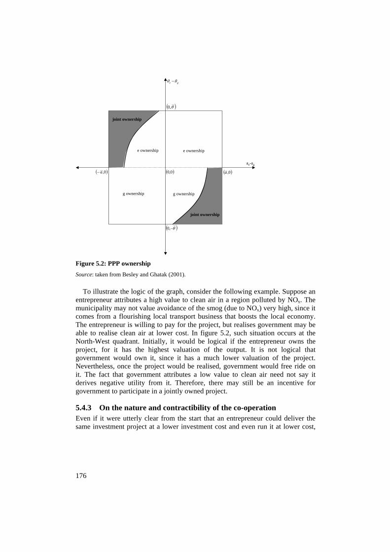
176

To illustrate the logic of the graph, consider the following example. Suppose an entrepreneur attributes a high value to clean air in a region polluted by NOx. The municipality may not value avoidance of the smog (due to NOx) very high, since it comes from a flourishing local transport business that boosts the local economy. The entrepreneur is willing to pay for the project, but realises government may be able to realise clean air at lower cost. In figure 5.2, such situation occurs at the North-West quadrant. Initially, it would be logical if the entrepreneur owns the project, for it has the highest valuation of the output. It is not logical that government would own it, since it has a much lower valuation of the project. Nevertheless, once the project would be realised, government would free ride on it. The fact that government attributes a low value to clean air need not say it derives negative utility from it. Therefore, there may still be an incentive for government to participate in a jointly owned project.

5.4.3 On the nature and contractibility of the co-operation Even if it were utterly clear from the start that an entrepreneur could deliver the same investment project at a lower investment cost and even run it at lower cost,

e ownership e ownership

g ownership g ownership

joint ownership

joint ownership

0,00,a 0,a

ae-ag

,0

,0

ge

Figure 5.2: PPP ownership Source: taken from Besley and Ghatak (2001).

177

still there exists a dilemma for government whether to ‘contract out’ the project to the private sector. Hart et al. (1997) show in their seminal article on prisons how it may still be undesirable for governments to ‘outsource’ sudden activities to the private sector. In the US, following the general strike of prison guard in New York State (see Zimmer and Jacobs (1981) for an analysis), the capacity for prisoners in privately owned houses increases rapidly from about 1200 prisoners in 1985 to almost 50,000 by the end of 1994.135 Initially the debate on private prisons tended to focus on the question whether they could be more efficient at all, but following the first experiences proving they were, critics argued ‘you get what you pay for’,136 and this is exactly what Hart et al. (1997) wish to underscore. Since it is so difficult to define ‘quality’,137 it is also difficult to write a contract on this matter (cf. Grossman and Hart (1986)), and there exists a serious risk that the entrepreneur sacrifices quality for improving efficiency. Prisons are but one example, and the analysis can easily be extended to health provision,138 education139 and so on. In the case of detention, a prison not only keeps somebody off the street, but—whenever possible—should also try to correct somebody’s behaviour as a preparation to his or its return into society. In the case of privately run prisons, this latter correctional task is very difficult to specify. When are inmates ready to return? Let exhibit 5.1 serve as some anecdotal evidence for the opponents of the private provision of public goods in the case of prisons.

135 Data from the testimony by Charles W. Thomas, Director of Private Corrections Project at the Univ. of Florida in Gainesville, before the subcommittee on crime of the US House Committee on the Judiciary, June 8, 1995. 136 Op. cit. 137 See the novel Zen and the Art of Motorcycle Maintenance by Robert M. Pirsiq. 138 In Canada, many hospitals are run on a PPP basis, with mixed results. For the UK, see section 5.4.1. 139 See here the scandal raised in the media on the ‘dual grading system’ at Harvard University: since students paid such a high price for tuition fees, they also ‘expected’ A-grades. So, as former Harvard professor Janine Bempechat said, ‘Students have come to expect if they pay a great deal of money for the education at Harvard, they deserve to have very high grades.’ Harvard professor Harvey Mansfield openly declares that since spring 2001, he has been handing out two sets of grades: ‘ironic grades’ (the marks that will go on public record, replete with A’s and A minuses) and ‘private grades’ (the marks, generally lower and, he says, more accurate, which he gives the students for the same work but which only they and he will ever know). (see ‘Grades row at Harvard’, 14 January 2002, article on BBC World Internet pages).

178

The example shows that on paper, the prisoners are taught some skills, which would facilitate their return into society. In reality, however, there is very little chance they will ever be able to bear the fruits of these skills, since ‘the skills they learn are arguably out-dated’ (Quek (1999)). In addition to recognising the difficulty of contracting all tasks (and therewith the risk of deterioration of quality), Hart et al. (1997) emphasize that problems with corruption and contract enforcement are also severe. Overall, Hart et al. conclude that particularly due the

Exhibit 5.1: How a privately run prison is made profitable ‘For 21 months, at 7:30 every morning, David Harpster would walk, together with about 100 men, onto the assembly floor of Lockhart Technologies Inc (LTI), and start work on computer and electronic components. What was unusual is that this factory is located inside a prison, and Harpster, like all the other men he worked with, were inmates. “It’s like any other job,” says Harpster, “except that all the men are in the same uniform.” LTI, a subsidiary of U.S. Technologies, is the company that contracts the labor from the prison, as well as work from companies such as Dell, IBM, and Texas Instruments. About 100 of the 500 inmates at Lockhart work with LTI. As prison labor moves into the high-tech industry, both prison labor advocates and ex-prisoners disagree over the effectiveness of such an option. Though prisoners are taught technical skills and work for high-tech operations while incarcerated, the skills they learn are arguably out-dated and the salary is little. Meanwhile, other corporations that do not use such low-cost labor may have unfair competition to deal with. Typically, inmates in work programs make license plates for cars or manufacture clothing. But at the Lockhart Work Facility, prisoners learn to build relay cards, upgrade motherboards, make computer cables, circuit boards and other electronic components. The facility also provides the manpower for Chatliffe, a company based in Buda that makes control systems and air-conditioners. The Lockhart facility is owned and run by Wackenhut Corrections Corporation, a subsidiary of Wackenhut Corporation – one of the nation’s largest firms dealing with security. Wackenhut also has private prisons in other countries including the United Kingdom, and has secured contracts providing security for domestic nuclear power plants. The state contracts with private companies like Wackenhut to house and feed the prisoners. U.S. Technologies employs about 100 of the 500 inmates housed at the Lockhart facility, paying the minimum wage to the prison. Lockhart Warden James Black said the prisoners are allowed to keep up to 20 percent of what they make, about $1 per hour. The rest of their income goes to pay for court fees, outstanding loans, Social Security, taxes, a restitution fund for crime victims, child support and to the prison for their stay there. The idea was started to get prisoners to pay for their own incarceration, Black said. Harpster says that he got to keep $2,000 for the time that he was there, and he calculated that prisoners were allowed to keep up to 14 percent of what they earned. A portion of the salary of LTI inmates is paid back to Wackenhut, Black confirms, though he would not comment on the amount. Harpster says that he believes it comes out to between eight to nine percent of their gross salary.’ Source: taken from Quek (1999), emphasis added.

179

difficulty of writing a contract (for activities as the above-described preparations to return to society, but also the clauses for using violence against prisoners) privatisation (in the broad sense) of prisons is undesirable.

5.5 Incentives, investment, and entrepreneurial ability: A model The previous sections have shown that the private sector may be more efficient than the public sector in the provision of a public good.140 This would be a principal added value of the entrepreneur in her venture with a government. Given, however, the problems with some existing PPPs or the cases of full private provision of a public good, the question rises how much ownership should be transferred to the private sector in case of a PPP. That question has not been addressed in the literature yet.141 For example, Besley and Ghatak (2001) do show how ownership matters, but in their analysis there exist but three cases: full governmental ownership, full private ownership, and joint ownership.142 Also, we address the question under what circumstances the PPP may add value. We investigate this matter by means of developing a base-case of public provision, after which some alternative scenarios are presented. The theoretical literature on public-private partnerships, or partnerships in general is limited in amount. Apart from PPPs, there are two categories of studies focussing on collaborative ventures: those on business start-ups (investigating the co-operation between a venture capitalist and an entrepreneur, and assess the

140 The privatisation literature shows that there may exist cases where—on the basis of comparative statics of performance— private sector enterprises outperform public sector organisations. Though in theory there is a strong case for preferring private sector provision in many areas, the empirical evidence is much weaker. The reasons given for this discrepancy differ per study, and are not discussed here. 141 We focus on the rationales for and applicability of entrepreneurial qualities in PPPs. Shleifer (1998), for example, emphasizes that ‘[…] private ownership is the crucial source of incentives to innovate and become efficient […]’ (p. 135). This matches well with the key rationale for private sector involvement in investment projects: eliminating inefficiency through incentives associated with ownership. In this light, Hart et al. (1997) discuss two classes of investment incentives that can be given to the private sector party: those that reduce costs, and those that innovate or improve quality. 142 Section 2.4.3 already indicated that ownership alone is not a sufficient incentive for making investments (see Holmström and Roberts (1998)). It was argued that overinvestment or underinvestment also depended on, amongst others, the relative importance of the investment to either party (see Hart and Moore (1990)). This matches nicely with the analysis of Besley and Ghatak (2001). They show how the choice for public, private, or joint ownership is affected by the relative importance each party assigns to the project.

180

complementarities in ‘entrepreneurial abilities’)143 and those on team production, varying from analysing factory workers to medical group practices.144 Both categories float upon strong assumptions regarding the unobservability of effort, and the difficulty of individual performance verifiability. Inevitably, the interaction and interdependence problems yield very complex contracts, where signalling seems a core activity for both partners. The common solutions offered nail down to game theory, emphasizing the risk of free riders, and apply complex statistics for tracing unobservable variables. In our study, we face one tremendous simplification. If the cost inefficiency of the investment project can be eliminated at all, the entrepreneur must do it. Therewith, both parties are complementary in their abilities. Giving an ownership share to the entrepreneur in a PPP clearly streamlines the interests of both partners, but we will show that ownership is not the panacea to eliminating all possible problems.

5.5.1 A model Consider a government that intends to set up a public-private partnership (PPP) vehicle for the production of a private good X, and a costless continuous public good Y, which is the spin-off of the private good. For this PPP, government invites a private sector participant to buy a share in the PPP. It is government who determines this fraction . Government’s primary interest is in the realisation of the public good, but she also enjoys the additional income on the sales of the private good. Private sector participants are only interested in joining the PPP if the return on their investment is nonnegative. For government, it is attractive to invite an entrepreneur in the PPP vehicle—the entrepreneur, after all, is often praised for possessing superior knowledge and skills to manage and operate an investment project more efficiently than government. Suppose this efficiency argument holds, as supported by numerous comparative and longitudinal studies on privatisation and on the relative performances of public and private enterprise. The optimisation problem here then becomes one of eliminating inefficiencies. These inefficiencies can be both technical and allocative inefficiencies. If the optimal situation is one where the PPP vehicle operates efficiently (both in a technical and allocative sense), whereas pure public provision would be one characterised by inefficiency, then a first crucial step is to find the efficient frontiers of production and cost functions. The ideal PPP should meet these

143 For example, Amit et al. (1990) analyse entrepreneurial ability in the light of venture investments, where both the entrepreneur and the venture capitalist have their specific abilities. 144 For example, Chi (1996) analyses collaborative ventures, where both business partners interact in their setting of effort levels; Lynk (1993) analyses joint production between multiple privatised water authorities; and Gaynor and Pauly (1990) analyse intra-group dynamics in medical teams.

181

frontier conditions, and any deviation can be attributed to a suboptimal exploitation of the entrepreneur’s abilities. The model applied in this chapter differs from the ones used in chapters 3 and 4 with respect to the assumptions regarding time dependencies. In chapters 3 and 4, I assumed a setting where the value of the entrepreneur’s investment was maximised by means of maximising every slice of the integrals applied. Of course, if every slice of an integral is maximised, so is the total integral. In this chapter, such maximisation method is not applied, for it would eliminate all dynamics that are of interest for out analysis.

5.5.2 Base-case: Public provision Consider a project that yields a private good X, and a public good Y. The public good arises at zero additional cost as a spin-off effect from the production of X.145 In our base-case, a government sets up a project individually. We follow the privatization literature here, suggesting the public provision may suffer from some degree of technical or cost inefficiency. Let the cost of public provision of the private good be denoted as XCgov . Demand for the private good, pX , is

downward sloping in price (hence, 0pX ). Government may now either set the monopolist output (maximising her profits on the sales of X) or decide to serve the entire market and maximise the production of Y (taking for granted that the pecuniary income stream is suboptimal. We assume government is particularly interested in the provision of the public good, and is less interested in the pecuniary income stream deriving from X.146 Since Y is defined as a spin-off effect of X, government utility maximisation of Y is essentially equal to maximising the output level of X. End-user price p is the only instrument available to government for this utility maximisation problem, so that (in a one period setting): (5.10) 0, max IXCppXYUYXU

p,

where I0 is the initial investment. The only solution for this government is to set px close to nil, accept the cost inefficiency included in C, the foregone income stream on X*p, and accept the loss on the initial investment I0. This base-case setting is frequently observed in ‘the real world’. For example, motorways provide a private good (usage kilometres of transport) as well as a public good (e.g., the accessibility of regions, or the economic attractiveness of an area). All ‘losses’ identified above are collected through general taxation. An alternative setting would be that government sets such a price for X that the proceeds of the sales of X cover the initial investment, and enjoys the utility of Y

145 In its most simple form, Y=X, for which C(Y)=0, whereas C(X)>0. 146 Thus, one could say U(Y)>U( (X)), where are the pecuniary profits from the sales of X.

182

for free. In such situation, the restriction 00IXCppX is imposed to

(5.10), after which U(X) becomes zero (government neither looses on the proceeds of X, nor does she gain a penny). As a consequence, YUYXU , , and since

pXYU , the ‘optimisation’ is a single-shot (that is, setting p such that the restriction is met), for which:

(5.11) XCpX

Ip

*0*

The maximum possible output for this price is **

0*

pXCpI

pX .

Assuming that government approximately sells at marginal cost, i.e. Cp , then

X . For any price higher than the marginal costs of production, government is ready to accept a lower output quantity (otherwise she would be making profits). Although many governments may be happy with this base-case scenario, they may enter into a partnership with the private sector for two distinct reasons. First, the private sector may use her superior efficiency skills and the project’s costs. Second, the private sector may take over some part of the initial investment I0, and hence reduce the financial burden for government. The first argument (on efficiency) is inspired by the privatisation literature. Though the empirical results on post-privatisation efficiency are mixed (see Megginson et al. (1994), Megginson and Netter (2001), or Dewenter and Malatesta (2001) to name but a few), the economic incentives literatures suggests that ownership may work as an incentive to cutting costs. For example, opposed to traditional procurement (see Laffont and Tirole (1993)), giving away a ‘share of the pie’ gives the incentive to increase the pie (see Laffont and Martimort (2002)), and thus streamline the private sector participant’s interests with the interests of the project’s principal: government. Although the literature on economic incentives is massive in amount, we do not know how these should work in a co-operative agreement between a private and a public sector participant. Neither do we know how they would apply in the specific economic areas where PPPs emerge. The second argument (on sharing the costs) is a straightforward one. Not only may governments be short in cash (as in developing countries), but also may their budget be constrained for other reasons. For example, the European Monetary Union (EMU) restricts the participating countries with respect to their spending on, e.g., infrastructure projects. Even though a government might be willing (and financially able) to invest in new infrastructure projects, she may not spend more than, say, 5 per cent per annum on infrastructure. PPPs may provide an alternative

183

here. Also, when assessing the contracts depicted in figure 5.1, one can imagine leasing contracts enter into this ‘gap’. In our model, we initially focus on the efficiency argument as the rationale underlying a PPP. Therewith, the question rises whether ownership provides sufficient incentives for the entrepreneur to make the PPP more efficient than under public provision. Hence, we will first analyse whether the provision of the public good benefits from the entrepreneurial effort of improving the project’s efficiency.

5.5.3 Alternative scenario: Unregulated PPP In our first scenario alternative to the base-case, we analyse an ‘unrestricted’ PPP in the sense of neither price not output quantity being regulated. Based on the assumption that ownership provides an incentive to improve efficiency, government thus has an alternative steering variable as compared to her maximisation problem proposed in (5.10), being the transfer of some ownership share , which yields:147 (5.12) 01, max IXCppXYUYXU .

Since the entrepreneur cannot privatise the public good Y, its utility can be fully received by society. Since we assume a one-to-one relationship between residual rights and residual control, the entrepreneur buys some share in the project vehicle, for which she receives an equal share of the net benefits of it. Returning to the added value of the entrepreneur, we presume the entrepreneur can make an effort that helps to reduce the inefficiencies of the PPP project. Based on the economic incentives literature, government hopes that ‘giving away’ some share in the PPP provides an incentive for the entrepreneur to raise effort . Thus, we implicitly assume ( ). If such is true, then PPPs can be made efficient by transferring an ownership share only. As chapter 4 suggested that subsidizing the private provision of public goods in a market where firms are price-takers can readily be reduced to a pecuniary transferral problem, the proof of existence of ( ) would have the same implications. In fact, the question of how to run a PPP in a most efficient fashion would boil down to the question of how much ownership share should be sold to the entrepreneur. That problem is a typical nested optimization problem: government should first analyse how high the entrepreneur is likely to set her effort level (given some ), and then offer that . Thus the choice for the optimal from a governmental perspective depends on the optimal effort level from the entrepreneur’s perspective. 147 Note that p is no longer concerned a steering variable, since that would imply a price-regulated PPP.

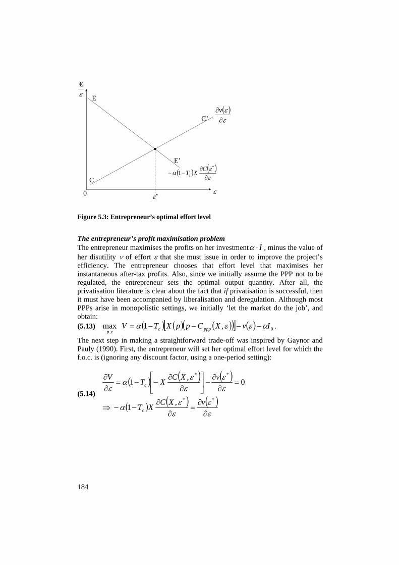
184

The entrepreneur’s profit maximisation problem The entrepreneur maximises the profits on her investment I , minus the value of her disutility of effort that she must issue in order to improve the project’s efficiency. The entrepreneur chooses that effort level that maximises her instantaneous after-tax profits. Also, since we initially assume the PPP not to be regulated, the entrepreneur sets the optimal output quantity. After all, the privatisation literature is clear about the fact that if privatisation is successful, then it must have been accompanied by liberalisation and deregulation. Although most PPPs arise in monopolistic settings, we initially ‘let the market do the job’, and obtain: (5.13) 0

,,1 max IvXCppXTV pppc

p.

The next step in making a straightforward trade-off was inspired by Gaynor and Pauly (1990). First, the entrepreneur will set her optimal effort level for which the f.o.c. is (ignoring any discount factor, using a one-period setting):

(5.14) **

**

,1

0,

1

vXCXT

vXCXT

V

c

c

0

v

€

*

1C

XTc

E

E’

C

C’

*

Figure 5.3: Entrepreneur’s optimal effort level

185

The optimal effort * the entrepreneur puts in the PPP is set such that the marginal disutility of increasing effort equals the net reduction in costs for the entrepreneur. In a graph, this is shown as follows.148 In figure 5.3, the entrepreneur faces decreasing marginal earnings on her effort, which is represented by the line EE’. Also, by (5.14), she faces increasing marginal disutility of effort, represented by the line CC’. The optimal effort level is then given by the intersection of the two lines. In addition to setting an optimal effort level, the entrepreneur also sets an optimal output price:

(5.15)

xx

x

pppxx

x

xc

x

pXX

XXC

XXCp

pX

X

XCpXXCp

ppX

TpV

,,

0,

1,1

*

In words, the optimal price exceeds the marginal cost price C, increases up to the point of optimal scale of production, as well as with the optimal output regarding the price elasticity of demand. Recalling (5.11), this price the entrepreneur would equal the governmental price if:

XCpX

IpX

XXXC

XXC

pp

xx

govxpppx

*0

*,

*,

,,

Here, some interesting cases arise: The PPP operates at equal cost as government: XCXC govppp , . The

PPP’s mark-up (determined by the optimal scale of production, as well as the price elasticity of demand) then would equal the naïve governmental mark-up,

XI 0 .

The PPP applies the same mark-up, but operates at lower costs: XCXC govppp ,

For investigating either case, it is important to first be clear about the base-case. Given the assumptions there, we can explore the circumstances under which a PPP can add value (i.e., either produce more at the same cost, or produce the same quantity at lower cost). Section 5.6 makes a first attempt. 148 Note that—in the absence of a functional form of v— the exact shapes of the lines may differ. The graph should hence only be seen as a support to the formalisation in order to help the intuition.

186

Note that both and Tc show up in the above equations for the optimal effort and price levels. This implies that the government is able to influence the efforts of the entrepreneur by adjusting the share of the PPP given to the entrepreneur and corporate taxes. As effort influences the per-unit costs of X, government indirectly influences the output by the incentives it gives to the entrepreneur through and Tc. Therefore, the response functions of the entrepreneur for effort and output price both depend on and Tc, that is:

(5.16) cTgp ,* cTjpX , *

and:

(5.17) cTh ,*

Therewith, as does affect the optimal effort level *, and as the cost function is determined by the entrepreneur’s effort level, output X (and therewith the public good Y) is indirectly set by via price. Government’s utility maximisation problem We assumed that the government established the PPP to produce a public good Ythat can be obtained by producing a private good X, where Y was a direct spin-off effect of X. Let the amount of Y equal a fraction of the amount of X (i.e., Y= X,

for which ). The utility for the government derived from the PPP equals the sum of Y and the financial revenues. The maximisation problem is essentially reduced to the question of how much ownership share the government transfers to the private sector participant. The utility for the government from the PPP yields:

(5.18) 0**** )1()],([))1(1(, IXCppXTpXYXU c

The first part of the right hand side is the total utility derived from the public good, which we assumed to be X, the second part is the share of the profits from the PPP for the government plus the corporate taxes paid by the entrepreneur over her part of the profit, whereas the third part is the share in the investments paid by the government. Government chooses to maximise the utility from the PPP given the expected response of the entrepreneur. The first order condition yields the following expression.

187

(5.19)

0

,,

),(

11

),(1,

0

****

**

***

I

ppX

XXCXCp

X

XCpp

pX

T

XCppXTp

pXYXU

c

c

which rewrites to:

ppX

XXCXCp

X

XCpp

pX

T

ppX

IXCppXT

c

c

****

**

0***

,,

),(

11

),(1

If both sides of the latter equation are multiplied by we obtain the following result:

(5.20)

ppX

XXCXCp

X

XCpp

pX

T

ppX

IXCppXT

c

c

****

**

0***

,,

),(

11

),(1

The left-hand side of the equation equals the total share of the financial income of the PPP ‘given’ to the entrepreneur. The right-hand side relates to the increase in utility for the government from an increase in production of X and Y due to an increase in the share transferred to the entrepreneur and the cost reduction due to the incentives given to the entrepreneur to increase effort. That is, the optimal share transferred to the entrepreneur, *, is set such that the marginal increase in utility from the public good Y plus the marginal decrease in costs for the government equals the part of the project profits given away to the entrepreneur. Any further worked out version now requires a specific setting.

188

5.6 When would a PPP be preferred over public provision?

5.6.1 PPP minimally produces the base-case output quantity By the above entrepreneurial profit maximisation problem (see (5.15)) we may express the PPP’s optimal output level as

X

XCXXCp

pX

pX pppppp

xppp

,,** .

Recall that by (5.11), government would have delivered:

**0*

govgovgov pXCp

IpX

Suppose government requires the PPP to minimally deliver the same output

level: govppp XX . This restriction requires the PPP to set a lower price (due to

the downward-sloping demand curve), and hence to cut costs. Thus, govppp pp .

Base-case: XCp govgov

If government would sell X at a price higher than marginal cost, govX will be

finite. In this case, Xppp may exceed govX , which implies that:

(5.21)

XCppX

Ip

X

XCXXC

XCppX

IX

XCXXCp

XCpI

X

XCXXCp

pX

govgov

pppppp

ppp

govgov

ppppppppp

govgov

ppppppppp

0

0

0

,,

,,

,,

The right-hand side of this expression clearly gives the ‘room for manoeuvre’ for the PPP: prices, Cgov, and I0 are nonnegative real numbers, whereas pX is negative. Therewith, the right-hand side de facto expresses the governmental mark-up. On the left-hand side, now, the PPP not only faces the marginal costs of production as such, but also the scale economies effect related to output. By

189

setting pppp, also X is determined, and therewith the scale economies effect in the cost function Cppp. In addition, note that in this equality, the larger the price elasticity of demand, the less room for manoeuvre the PPP has. Also, consider the impact of a constant cost of production: if 0XC , then the PPP’s output is demand-driven.

Base-case: XCp govgov Suppose that in the above sketched governmental ‘optimisation’ problem government would have sold X slightly above marginal cost (i.e.,

XCp govgov , resulting in an infinitesimal mark-up). In that case, output must

be maximal to compensate for the initial investment I0 (hence, X ). In such

base case, Xppp can at most equal govX , which implies that:

(5.22) XCp

IX

XCXXCp

pX

govgov

ppppppppp

0,

,

Since, however, XCp govgov is infinitesimal, the right-hand side of this

equation tends to infinity. When transposing the price elasticity of demand from the left to the right-hand side (as in the above exercise), the mechanics of finding a solution become pretty meaningless unless pX is very large. Thus, only when demand is very sensitive to changes in price, (5.22) has a finite solution. Also, recall that if XCp govgov , and if the PPP is required to minimally

produce the same output quantity, it can only make a profit if it is able to cut costs. Stated alternatively, the PPP may only recuperate investment, and minimally produce the same output quantity, and meet the entrepreneur’s profit maximization purpose in the absence of any investments for the PPP (which suggests the entrepreneur should only take over the managerial role of the project, and ensure the project is run more efficiently).

5.6.2 PPP produces the same output quantity at lower cost One of our crucial assumptions regarding the entrepreneur is that she is able to produce at lower costs, due to her superior efficiency skills. Let government’s production costs be denoted by XCg , whereas—due to the entrepreneur’s

efficiency improving effort—can realise a cost function ,XC ppp , for which:

XCXC gppp , . Since the output quantity sold is assumed to be the same

for the PPP and the base-case here, we can readily assume prices are equal as well. Thus, govppp pp , and therewith govppp pXpX . We would now basically

190

derive (5.21), which would probably reduce to the following problem: (5.23) XCXCXT govpppc ,1 ,

which is no more than a participation constraint for the entrepreneur to exert cost-cutting effort.

5.6.3 Wrapping up Suppose YYU , and Y=X. In this specific case, we can make the following comparisons. First, consider the value of the project vehicle. Under public provision, the value created is nil, assuming price equals marginal cost plus a mark-up to recuperate the initial investment (see (5.11)). The PPP, on the other hand, has a value equalling: (5.24) 0, IXCpXV ppppppppp

Therewith, if Vppp is to exceed Vgov, then it immediately follows that:

(5.25) ,0 XCXI

p pppppp

Meanwhile, when assessing government’s utility of the provision of the public good, she would have received (under public provision): govgov pXYYU .

In case of a PPP, this would have been: pppppp pXYYU . Now

YUYU govppp if and only if govppp pXpX , due to a downward-

sloping demand curve for the private good. Combining this (obvious) result with the above requirement for the PPP creating a positive value, it follows that govppp pp , which can only be achieved if

XCXC govppp , . Thus, in our model, the PPP must produce at lower cost

than government, and must sell at a lower price than government in order to add value. In sections 5.5 and 5.6 we have shown some implications. The ultimate question remaining is, ‘if PPPs must operate more efficient than under public provision, and if entrepreneurial effort is the key to achieving that target, does the ownership share of the entrepreneur in the PPP determine the entrepreneur’s effort level?’ To answer this question, recall (5.14), which set the expression for the optimal effort level by the entrepreneur. Given (5.14), the idea

191

now is to analyse the impact of altering , which yields the following comparative statics:149

(5.26)

2

*2

2

22

2

*2

2

22

1

11

vCXX

CCXT

vCXX

CXT

CXT

c

cc

When analysing this expression, we immediately see has an impact on:

The profits for the PPP via 2

2C. This implies that if

2

2C=0, then the

impact of on profits is nil (i.e., transferring ownership does not

provide any incentive for the PPP to operate more efficiently in case ,XC

is a straight line relationship between C and .

The disutility for the entrepreneur via 2

2

.

In the absence of specific functions regarding the various costs and benefits of the project, it is difficult for each of the cases to come up with more specific interpretations of the effect of alpha on effort. This is a clear drawback of trying to keep the analysis at a general level. Hence, further analysis needs to restrict to a number of specific functions.

5.7 Discussion Following the first waves of privatisation, PPPs seemed an attractive alternative for governments to involve the private sector in the provision of public goods. The initial benefits of this new organisational form must have been promising: the private sector could add value by means of taking over risks, improving efficiency, and providing additional funds to tight government budgets. Meanwhile, since government maintained a stake in the project vehicle, PPPs might be attractive in those areas where the investment or output are hard to specify—after all, the more traditional forms of encouraging the private sector (as with subsidies or fiscal measures) can only apply to contractible economic activities. Since changing these regulations is a costly and time-consuming process, PPPs might be interesting since governmental ownership opens the floor for ex post governance mechanisms

149 For notation purposes, the arguments *,X of C have been dropped here.

192

through the residual control rights. The empirical evidence on PPPs, however, shows that public-private partnerships are not the panacea governments might have hoped for. This chapter has analysed the literature and some experiences with PPPs. It appears that, although PPPs exist from the 1990s onwards, the academic literature is very limited. The following ‘gaps’ can be identified. First, it seems unclear under what conditions the various contractual arrangements work best. Though one might expect certain contracts to be designed for specific product-market combinations, the empirical evidence shows that multiple contracts are observed in the same areas. Second, the economic analysis of PPPs seems to ignore fundamental characteristics of the vehicle. Section 5.3 took the paper by Grout (2003) as a dramatic example. Third, it appears that the efficiency gains of realised PPP projects are limited in amount, though this is sometimes blamed to the fact that the specific contractual arrangement puts a cap on the entrepreneurial ability to improve that efficiency. Fourth, though there seems to be a clear case that ownership does provide an incentive to the private sector party to improve efficiency, it is unclear how much ownership the entrepreneur should have in the vehicle in order to improve its efficiency. Given the status quo of the academic literature on PPPs, one can seriously doubt whether it is reasonable at all to expect PPPs to operate smoothly. Sections 5.5 and 5.6 try to spur the literature on PPPs by addressing the question of division of ownership. The model presented in section 5.5 may easily be extended to, for example, analyse the effects of price regulation, zero governmental valuation of the private good, or the effect of a minimum output level for the PPP project. Each of these extensions, just as the basic model proposed in section 5.5, should be perceived as determinants of the feasible set of outcomes for a PPP contract. This is a clear added value of the model, for it enriches our understanding of what an efficient PPP should look like. Section 5.6 shows some conditions under which PPPs can add value relative to a base-case of public provision. Having found some feasible sets for PPPs to operate, however, does not guarantee entrepreneurs will add value indeed. Therefore, for governments to hedge themselves against undesired behaviour, one may explore the impact of additional regulation. For example, the impact of price caps or rate-of-return regulation could be studied, just as the impact of imposing additional non-coercive measures (i.e., governments may try to shift the PPP’s cost curve, or the entrepreneur’s profit curve by relaxing corporate tax rates, awarding productivity or production incentives, and so on). Such extensions, however, are still to be worked out. The question how much ownership should be transferred to yield an optimal entrepreneurial cost-reducing effort depends on the impact of

(see last part of 5.6.3). A precise answer requires the study of a specific case, specified by explicit (and hence less generalisible) functions of costs and benefits.

193

Appendix 5.A Mathematical appendix The demand for a PPP’s output Some authors suggest a PPP may produce Pareto efficiently, since it would be possible to set the marginal rate of substitution (MRS) equal to the marginal rate of technical transformation (MRT). Apart from the fact that it is counterintuitive for the consumer to determine the level of Y to be consumed (such is set exogenously), most of the utility functions applied in the literature also require some rate of substitution (i.e., the MRS) between Y and X. Amiran and Hagen (2003) have made a fine note on this issue of hyper-substitutability, by investigating the limits to ‘willingness to pay’ and ‘willingness to accept’ in the light of public goods provision. With public goods, Amiran and Hagen argue, ‘[…] the additional income can provide full compensation only if the market goods that can be purchased with the additional income are adequate substitutes for the public good whose quantity has been exogenously reduced’ (p. 463). In their article, they illustrate their point by considering a simply asymptotically bounded utility function—without violating any axiom of the neoclassical consumption theory, it becomes possible to show that the hypersubstitutability may yield an allocation that is outside the bounded utility set. Without replicating the whole point and proof of Amiran and Hagen (2003), I will only use some part of their maths as an input to derive the demand functions for both the public good Y and the private good X. After all, if we have the demand functions, then we know when the public good should be produced (i.e., when the willingness to pay exceeds the costs of provision).150 The purpose of these derivations is to show that the PPPs analysed by Grout (2003) are a dramatic simplification since they ignore an explicit utility of Y. Neglecting the utility from the public good (which is at the heart of a PPP) implies neglecting the non-pecuniary benefits of that project vehicle, which was at the heart of the analysis of Besley and Ghatak (2001). Let me consider a Cobb-Douglas utility function of the following form:

150 I deliberately enter into the analytical solution in the appendix to this chapter (since I believe it is fruitless). Although it would be great to obtain an analytical solution, it is far from our empirical reality. As a consequence, there are numerous articles available on how to reveal the WTP for a public good in a both pragmatic and theoretical sense. See, for example, Lockwood (2003), Gary-Bobo and Jaaidane (2000), or Rondeau et al. (1999), as some theoretical contributions, and see Propper (1993), or Bohm (1983) as some empirical applications.

194

(5.27) bY

YaX

XXYU ),(

where X is the private good consumed, Y the public good, and , , a, and b are real positive numbers. If there would exist a competitive equilibrium for providing goods X and Y, then at the optimal level of Y, the marginal utility would at most equal the marginal costs, whilst the total net utility would be maximised. Let the MRS be determined as follows. If U(Y,X) is a constant, k, then marginal utility becomes:

(5.28) 0),(),(

XXYU

YXYU

, or

(5.29) 02

1

2

1

aXa

bYY

aXX

bYb

bYY

aXX

This is equal to expressing the MRS as:

(5.30) YbYXaX

ab

aXa

bYY

aXX

bYb

bYY

aXX

XXYU

YXYU

dYdX

du

2

1

2

1

0),(

),(

which yields the MRS at constant utility.151 Let now pi be the market price for Xi, and i be the theoretical price for ‘consuming’ Yi. Total income w can then be

divided over the private and the public good as I

iii

I

iii pXYw

11

. Suppose

all market clearing conditions are met, then:

151 The constant utility explains the negative sign: Let YUXUYXU , be

constant, then an infinitesimal change in Y yields: YX

XU

YU

0 , which is equal to

stating that the XU

YU

YX

MRS .

195

(5.31) ijjj

iii

ii

jjj p

YbYXaX

a

b

)(

)(, i R.

The demand functions for Y and X can now be found as follows (using the fact that the MRS equals p/ ,152 and substituting for X):

(5.32) )()()(

or ,)()()(

)(

)()()()(

)(

)()()(

)()(

)()(

)()(

)()()(

)()(

)()(

YbaXabwXab

Y

YbaXabYbwXab

YbaXabYb

wXab

YbY

YbaXabYb

YYb

YbaYYb

YXabYb

wXab

YbaYYXabwXab

XaYbY

ba

Yw

pXaYbY

ba

pYw

and in a similar fashion:

(5.33)

XabYbapwYba

X

XabYbapXawYba

XaX

or ,

152 The MRS represents the slope of the highest possible indifference curve of the consumer(s). The price ratio p/ represents the budget line. Utility maximisation now

occurs at the point of tangency between the budget line and the highest possible indifference curve.

196

These are the demand functions for the public good Y and the private good X. Given now these demand functions, one should realise that together they form ‘the’ demand function Grout (2003) uses for output q of a PPP. Not only could we question the hyper-substitutability of X and Y (as Amiran and Hagen (2003) did), but also we should be aware of the explicit demand function for the public good Y. After all, if we would indeed have a demand function, we have a criterion justifying production (that is, if demand at least equals the costs). Even though the literature on public goods shows that there is very little incentive for people to reveal their true preferences, and to contribute up to the point of their individual demand, we might use it as a rule for setting a uniform tax level. Still, then, the PPP would be assured of this income stream fuelled with taxes, and it should be given a different discount factor than the income stream derived from the sales of the private good output.

Part III: Conclusions and policy implications

199

6 CONCLUSIONS In an era where governments increasingly withdraw from the market place as active providers of goods and services, this study has analysed some governmental dilemmas concerning the private provision of public goods. Since the mainstream literature on the private provision of public goods suggests that the funding problem is most severe, one might expect that the biggest governmental dilemma is a pecuniary one: How much money should be transferred to support the private sector? This question, however, embodies some problems and assumptions that are not easily overcome. First, by opting for a support mechanism, governments choose for so-called non-coercive instruments. These have the theoretical advantage that they are better able to yield Pareto-efficient outcomes than coercive instruments, but their effects are less predictable. Second, calculating a support scheme is not equal to designing or selecting policy instruments. Third, not all non-coercive instruments are alike. In this study, for example, the fiscal and financial measures studied in chapter 4 must clearly be distinguished from the public-private partnerships analysed in chapter 5.

6.1 Four dilemmas In section 1.5, I have specified four governmental dilemmas concerning the encouragement of investment in the private provision of public goods by means of non-coercive instruments. Each of them represented a research question, addressed below.

6.1.1 The Influenceability Dilemma Perhaps the biggest fundamental dilemma underlying the use of non-coercive policy instruments is the unpredictable nature of these instruments. Though the game-theoretical literature on incentives provides a logically sound framework for predicting behaviour of one’s counterpart when offering an incentive, there may well exist other factors at work that prevent firms from making the actions targeted by governments. In chapter 2, I have analysed these ‘barriers to investment’ at the level of the firm, industry, and macro-level context. At each of these three levels of analysis, it appears that the theoretical literature readily provides reasons why firms would not invest even if the investment decision were economically attractive. Therewith, the economic attractiveness of an investment decision reduces to being a necessary condition, instead of being a necessary and sufficient condition. If governments wish to use non-coercive instruments, then it would be wise to

200

analyse any potential barrier to investment beforehand, and eventually try to eliminate these in order to increase the predictability of the outcome of the chosen policy. The analysis of barriers to investment has important implications for an analysis of underinvestment. For example, it may well be that firms are willing to invest, but do not invest sufficiently (in the perception of government) due to the aforementioned barriers. It may well be that eliminating these barriers is more effective and even efficient than providing additional support schemes. In the debate on underinvestment, chapter 2 has shown that this is a concept that is difficult to operationalise. Of all empirical studies on underinvestment, multiple interpretations exist of the benchmark (i.e., ‘optimal investment’), so that it becomes very difficult to come up with clear-cut policy prescriptions here.

6.1.2 Smart Governance Dilemma Given an analysis of all potential barriers to investment hindering the effectiveness of non-coercive instruments, the fundamental question rises how much encouragement a government should provide. I have labelled this the Smart Governance Dilemma, which deals with the efficiency of government policies—if, after all, it appears to be possible to encourage firms to invest with less support than intuitively thought, why should a government be too generous? Chapter 3 has analysed the possibility to ‘design’ or determine an optimal wealth transfer that (a) is sufficiently generous to encourage the private sector to invest, but also (b) minimizes governmental expenditures in order not to deviate too much from a Pareto efficiency. The mainstream economic literature on government support for the private provision of public goods would first try to calculate the optimal valuation of the public good in order to then determine an optimal wealth transfer through the support scheme. As shown in section 1.3, however, there are numerous objections to this approach, for government would not be able to include the individual preferences in determining the value of the public good, as well as the difficulty to unambiguously valuate the public good at all. Therefore, I have proposed an alternative framework that uses a nested optimisation model in order to achieve a Nash equilibrium. In that framework, government anticipates the entrepreneurial response by evaluating the latter’s participation constraint. I have proposed to use a framework based on Tobin’s Q and the neoclassical investment model of Hall and Jorgenson. Given the fact that the present value of governmental support for private sector investment facilitates the participation constraint of the private sector, government can minimise her expenditures. Given a standard type of technology, government can assume the role of a private sector investor, and analyse the costs and benefits of the investment beforehand. In my proposed framework, I assumed a technology that is not only ‘standard’, but also yields both a private and a public good. The market then

201

values and rewards the output of the private product, whereas the public good is often not rewarded for—particularly if the investing firms are price-takers in an existing market for the private good. So government learns the costs and benefits of an investment, and may calculate the ‘Q’ I proposed in section 3.1. Given Q (which reflected the economic attractiveness of the investment), government can predict or anticipate on the response of the private sector in terms of investment. If Q is smaller than unity (see section 3.1, or the mathematical appendix to chapter 3), private sector investment is unsustainable in the long run. Government, however, can increase Q through non-coercive instruments (as subsidies or tax measures), so that it does become economically interesting to invest (read: the participation constraint has been met). Apart from wishing to encourage private sector investment, governments would not wish to be too generous. If, after all, they would exaggerate the wealth transfer (that has to be financed through taxation) to the investors, the policy instruments are unlikely to yield a (Pareto) efficient solution. Thus, governments also face an expenditure minimisation problem. The literature suggests that Q equalling unity should do well. When returning to the question of governmental valuation of the public good, we can now revert it—by anticipating the private sector’s participation constraint (through offering such a support that the Q for the investment equals unity), government can now relate the present value of that support to the amount of public good the investments should yield. The ratio then reveals the governmental ‘willingness-to-pay’ for the public good.

6.1.3 Policy Portfolio Dilemma Chapter 4 consists of a multi-case study on government support for investments in wind turbines, analysing the green policies of the EU(15) countries in the 1985-2000 period. In each of these cases, governments used non-coercive instruments (i.e., fiscal and financial measures) to encourage investment in a standard technology that yields both a private good (electricity) and a public good (avoided emissions, or ‘clean air’). Contrasting with ‘the lighthouse in economics’ by Coase (1974), investors in wind turbines are price takers in the market for the private good, and need additional support in order to deliver at the wholesale market. In the empirical test it appears that investments are realised for all nonnegative values of Q. This result is a clear relaxation of the existing literature, which prescribes Qs exceeding unity. As an explanation, I have used the following reasoning. If Q exceeds unity, the economic attractiveness of the investment meets the long-run sustainability restriction imposed on the investment’s NPV. In other words, the investment not only yields sufficient money to payback itself, but also to buy new equipment at the expiry of the economic lifespan of the current asset. There is,

202

however, no reason a priori that investors in wind turbines all have the intention to stay within the industry for an infinite time period. Therewith, it may well be that they are happy with a nonnegative NPV (yielding a nonnegative Q), but do not care if they cannot stay in the wind power business forever. Nevertheless, for Qs exceeding unity, investments spurred up. Another striking result of the wind power case study is that it seems that the exact policy instrument mixture is not important. Even though various mixtures of fiscal and financial instruments have been observed for the 15 countries over a 16 years’ time period, the results suggest that the economic attractiveness of the investment is the main trigger. Unfortunately, I have not been able to include any of the barriers to investment (as surveyed in chapter 2) in this analysis. Also, the data were not sufficiently rich to isolate any effects of individual instruments. Nevertheless, the overall results of this empirical test were very promising for governments in stable economies that wish to support private sector investment in standard technologies.

6.1.4 Joint Ownership Dilemma The fourth and last dilemma analysed in this study is how governments can encourage private sector participants to invest in joint ownership projects, also referred to as public-private partnerships (PPPs). Whilst the more traditional non-coercive instruments as fiscal and financial measures encourage investment in standard technologies at a large scale, PPPs have the potential to operate in ‘atypical’ areas—e.g., in cases of natural monopolies or where the economic activity is hard to contract. Chapter 5 has shown that PPPs occur in many areas, varying from infrastructure (the bulk of the natural monopolies) to hospitals and even prisons (where not all details can easily be specified). In spite of the fact that PPPs would particularly be interesting in the areas subject to the ‘theory of incomplete contracts’, empirical evidence shows that the largest efficiency gains—if ever realised—are observed in infrastructure projects. The disappointing performance indicators are often attributed to the specific contractual arrangement of that case study, which would hamper the entrepreneurs to fully exploit their efficiency skills and experience. Apart from these suggestions, chapter 5 has emphasized that not only the number of realised PPPs is very small, also very little is known on the dynamics of the interaction of the two parties. Though the game theoretical literature offers some avenues for solving the problem of the design of an incentive structure, it appears that particularly the provision of the public good—which is at the heart of a PPP—causes the problem for a sound theoretical analysis. Recent attempts in the literature can at best be considered ‘first steps’ towards a more rigorous analysis. For example, the works of Hart (2003), and Hart et al. (1997) underscore the importance of the theory of incomplete contracts. They clearly show that—as soon as we relax the assumption of an unbundled, homogeneous investment—the

203

negotiations become suspect to opportunism of either side. Given this notion, Besley and Ghatak (2001) include the relative valuation of the project’s output by each party as a key determinant of who should have the ownership. Though that paper highly enriches the debate, it does not provide an answer to how much ownership should be transferred to the counterpart. Section 5.5 proposes an incentive contract that balances the benefits of transferring ownership to the private sector with the foregone income for government of the project vehicle. This model gives a nice trade-off for either party: the entrepreneur must decide an optimal effort level in order to improve the PPP’s efficiency, whereas government—anticipating that optimal effort level—must decide between the efficiency of the PPP vehicle and giving away both some part of the residual rights and claims.

6.2 A proposal for designing non-coercive policies By analysing four dilemmas, it appears that designing a policy based on non-coercive instruments is more than calculating a wealth transfer. Throughout the study, I have proposed elements for building a framework that goes beyond the current literature on economic incentives. Since one PhD study is probably not enough to validate all building blocks of that framework, this section proposes some testable hypotheses that can be used in further research.

6.2.1 A proposal for a conceptual model: Hypotheses Figure 6.1 gives a first step in proposing a model. It outlines the building blocks proposed in the current study. Given this conceptual model, I will try to integrate the results of the previous chapters through discussing the various relationships or arrows in the figure by means of formulating hypotheses.

Investment Capital stockAmount of public good

Economic attractiveness of investing

Utility derived from the

public good

Hyp

othe

sis

6.4

Hypothesis 6.5

Hypothesis 6.6

Non-coercive government instruments

Def

init

ion

1.2

Definition 1.1

Hypothesis 6.1

Barriers to investment

Hyp

othe

sis

6.2

Hypothesis 6.3

Figure 6.1: Proposed conceptual policy design model

204

Hypothesis 6.1: The investment decision is largely influenced by its economic attractiveness, also in the case of providing public goods.

In the mainstream economic literature, no single agent would invest if it were economically unattractive (usually indicated by a negative NPV). Glaeser and Shleifer (2001), however, showed how ‘not-for-profit entrepreneurs’ might invest for ‘the warm glow’. In environmental economics, agents might invest in project initially loss-giving (or yielding foregone profits in the current time period) as some form of intergenerational altruism. Particularly the empirical results of chapter 4 in this study show how nonnegative NPVs (or Qs, in terms of chapters 3 and 4) hardly match with positive investment levels. Therefore, whilst definition 1.1 could be interpreted as a necessary condition only, it may be that—even in the case of public goods—the economic attractiveness of the investment decision is both a necessary and sufficient (‘if and only if’) condition—given that the barriers to investment have been overcome.

Hypothesis 6.2: ‘Barriers to investment’ existing at various levels of analysis potentially decrease the effectiveness of non-coercive policy instruments.

Apart from the question whether incentives work at all, there exists a debate on their effectiveness.153 Usually, economists attribute the ineffectiveness of incentives to ‘market failures.’ As Hubbard and Skinner (1996) recognise in analysing the effects of an incentive policy to stimulate household savings:

‘[…] even cost-benefit analysis […] does not allow one to judge whether saving incentives are a success, by which we mean an improvement in welfare. To make this judgement, one must first isolate potential market failures that cause people to save too little in the first place.’ (p. 74)

Chapter 2 of this study has analysed multiple ‘market failures’ at three levels of analysis. I have labelled these ‘barriers to investment.’ Though much of the barriers to investment have a sound theoretical justification, the empirical research analysing the underinvestment phenomenon (which arises due to either a low payoff of investing or due to barriers to investing) only uses a few. Moreover, it appears that the empirical research on underinvestment (as a specific case of assessing the effectiveness of policy instruments) is hampered by another problem: not only should the ‘market failures’ be investigated, but also it is very difficult to select an unambiguous benchmark.

153 See, for example, Hubbard and Skinner (1996), Jensen and Murphy (1990), or Bond and Guisinger (1985).

205

Hypothesis 6.3: All investment that increases the capital stock increases the amount of public good

At a first glance, it seems obvious that investment in the provision of public goods increases its output. Nevertheless, Uzawa (1969) has made clear remarks regarding the so-called capital stock adjustment cost function (see figure 3.1). By recognising this installation function, we can distinguish between gross and net investment, where only the latter is the ‘productive’ investment.

Hypothesis 6.4: Government’s marginal utility of a public good is declining as the capital stock that yields the public good increases

Although this hypothesis may appear odd for its obviousness, its consequences are far reaching (see the next hypothesis). First, as the private sector responds positively to the investment incentive, the policy may be called successful. Nevertheless, with each instalment of capital stock yielding the targeted public good, government’s marginal utility decreases, and therewith her willingness-to-pay (see the argumentation below the next hypothesis). Suppose the support scheme offered by government does not put a cap on the number of eligible projects, and that it is sufficiently interesting for the private sector to invest. What occurs if the private sector responds massively? Once investments have been made (which were economically unattractive without the government support scheme), the private sector has become dependent upon that support. This dependence may be compared with James Buchanan’s ‘Samaritan’s Dilemma’ (see the reprint of the original 1972 paper in Buchanan (1975)): the Samaritan tries to do good and help people in need, but once the donor’s action increases the amount of need the painful dilemma arises whether to continue helping or to quit.154 A second consequence of this hypothesis is immediately related to the first one, and deals with technological change. In chapter 4, I have analysed the effects of investment policies on private sector investment in wind turbines. The target group of the green policies predominantly consists of (independent) power-producing companies, and chapter 4 has analysed their response (albeit at the aggregated industry level). Nevertheless, the green policies must have had another impact as well: if, after all, the Samaritan decides to gradually reduce her aid (say argumentation below), then there is an increasing pressure on the producers of the targeted technology—in the case of chapter 4, the wind turbine producers—to improve the commercial viability of the equipment. Once investors are ‘locked in’ into a certain market, but government’s subsidies are gradually being reduced,

154 See also Coate (1995).

206

then the suppliers of the technology are asked to compensate for the reduced aid (see the bargaining relationships in Ruigrok and Van Tulder (1995)). This innovation process—which is confirmed by the rapidly declining cost price of wind turbines, see figure 4.2—is an economic activity in itself. Schmookler (1965) lamented on this issue, and claimed that ‘[…] the production of new technology is […] in essence the mobilization of society’s creative energies to relieve the scarcities which existing resources and products cannot’ (p. 335). Though in the short-run, the Samaritan may increase the recipient’s reliance on support, it may escape from that dependence relationship in the long run by indirectly shifting some of the ‘responsibilities’ to the suppliers of the technology.

Hypothesis 6.5: Assessing government’s utility of the public good gives a better understanding of the ‘generosity’ of the non-coercive measures

One important concept related to declining marginal utility is risk aversion. Take an example of a government providing a €1m subsidy for the private clean-up of a lake currently contaminated with phosphates. Suppose furthermore that the current PO4 concentration is 2 p.p.m., which is labelled as ‘excessively high’. Though there is no guarantee at all the €1m investment is sufficient to bring back the water quality to acceptable levels, this government is urged to ‘do something’, and accepts the risk. Having invested €1m, suppose the concentration of PO4 drops from 2 p.p.m. to a 0.1 p.p.m., which is considered ‘moderate’. Suppose, lastly, an additional investment of €1m may either reduce the concentration of phosphates to >0.05 (which would be classified as ‘low’), or it could stay at the moderate level. Since the water quality in the lake is not urgent anymore, it may well turn out that this government becomes risk averse in the sense of the payoff diagram. As a consequence, the Nash bargaining solution of a more risk averse government shifts, and it will be less likely to provide ‘generous’ support (see Gintis (2000) for the implications of risk aversion in Nash bargaining). Chapter 4 provides some first support for this hypothesis—not only did the present value of all government support for wind turbine investments decline after the first serious peak (see figure 4.4) as did the economic attractiveness of investments including that support (see particularly figure 4.9), but also the air emissions declined over time (see figure 4.13). Based on these data, I calculated the implicit governmental valuation of additional investment in the public good (see figure 4.14). Though it turned out very difficult to interpret that valuation, it is clear that the price of further air quality improvements increases as the level of pollution drops. In addition to a decreasing generosity or willingness-to-pay, one may think of the consequences for the choice of policy instruments. If a government becomes more risk averse, but is still destined to increase the level of the public good, will it still opt for non-coercive policy instruments? After all, although the economic

207

theory shows they are probably more efficient, they are also less predictable than coercive instruments. It would therewith be a logical consequence that the choice for a type of policy instruments may vary over time, whilst coercive instruments may come after non-coercive ones as soon as the marginal governmental utility of the public good declines. This notion has not been investigated in the current study, but is very interesting for future research.

Hypothesis 6.6: For public goods being the spin-off of a private good, increases in the capital stock put a downward pressure on the market price for the private good, lowering the economic attractiveness of the investment

This hypothesis is based on the standard downward sloping demand curve for private goods (see Mas-Colell et al. (1995)). If the investors in the targeted technology are price-takers in the market for the private good, whereas that market is competitive,155 then the increased supply must lower the market price. What, however, would happen in the case of price-making firms? Consider ‘the lighthouse in economics’ by Coase (1974). The investors in lighthouses (the public good) could not collect income for that investment directly. Nevertheless, they could add a mark-up on the harbour fees, since they also owned sea harbours. Clearly, if the ‘market for harbours’ had been competitive, with non-lighthouse-owners in the market for harbours only, then this mark-up should vanish over time. Suppose companies compete in offering ferries or other pieces of infrastructure. Since it would be irrational for a monopolist to offer multiple competing ferries as long as there is ‘insufficient’ traffic congestion, each additional ferry operating on the same line puts a downward pressure on the ticket price. By the same token, each additional budget airline departing from some local airport increases the economic attractiveness of the local area (the public good) but also decreases the airfares.

6.2.2 A proposal for a conceptual model: Towards empirical testing However valuable it may be to propose hypotheses, they themselves do not necessarily help the decision-maker in a pragmatic sense.156 Probably the most difficult question is how to make things operational. Of all the ‘building blocks’ of figure 6.1, there are tree decision variables that might be measurable: (1) the economic attractiveness of the investment (as the impetus of the whole process);

155 In the case of the French electricity market, dominated by state-owned EDF, independent power producers may indeed be price-takers. Nevertheless, since their market share is insignificant opposed to EDF’s, their investment can hardly be considered a downward pressure on the wholesale price. 156 See also the comments of Sutton and Staw (1995) and Eisenhardt (1989) on the role of hypothesis.

208

(2) the investment and resulting capital stock (as the response function); and (3) the utility government derives from the public good (justifying the support she has given to the private sector). The amount of public good depends on its nature, and cannot be easily captured on a single dimension. The two remaining blocks (the type of instruments and the barriers to investment) are of a more categorical nature. Economic attractiveness Given definition 1.1 (and hypothesis 6.1), the naïve NPV rule would do fine as a first intuitive evaluation criterion describing the economic attractiveness of an investment decision. Chapter 3, however, showed how the NPV rule lacks a long-run sustainability criterion. As a consequence, it is well imaginable that investors obtaining a nonnegative NPV on their project are unable to save money for replacing their capital stock following depreciation. In chapter 3, I proposed to use an alternative evaluation criterion, based on the naïve NPV rule, but subject to a long-run sustainability restriction.157 That model, based on Tobin’s Q and the neoclassical investment model of Hall and Jorgenson, is theoretically superior to the NPV rule. Also, it is measurable—that is, as long as the theoretically derived ‘marginal Q’ equals average Q. In chapter 3, I have followed Hayashi (1982) on this matter, who merely used two simple but very powerful conditions. First, firms had to be price-takers in their market, for a monopolist would not necessarily face the downward-sloping demand curve that lowers the marginal benefits of additional investment after some optimum. Second, the technology must be characterised by constant returns-to-scale. For both in- and decreasing returns-to-scale, it is impossible to measure the marginal benefits of additional output or capacity. For standardised technologies as the wind turbines analysed in chapter 4, this framework seems to work fine. Once, however, we enter into a more complex setting as PPPs (often operating in naturally monopolistic areas or being price-makers in their ‘market’), the modified version of Tobin’s Q cannot be measured anymore. In fact, it appeared that with the specific case of PPPs the academic literature is still too limited to propose a concrete evaluation criterion for this kind of arrangements. This is considered an avenue for further research. Investment and capital stock Throughout most of the chapters, I assumed that investment would yield capital stock. Implicitly or explicitly, I have assumed that these investments were

157 Note that although sufficient economic attractiveness of the investment (e.g., NPV>0) might even be both a necessary and sufficient condition in the short-run, there is no guarantee at all that firms remain in the industry once their investment has been written off.

209

indivisible, observable, specifiable, and unstageable.158 Nevertheless, chapter 5 has shown that the provision of public goods may sometimes need more complex investments. As soon as that complexity only increases slightly, the (economic) analysis explodes in terms of additional assumptions and formulae.159 In the anecdotal example of ‘outsourcing’ prisons to the private sector, I wanted to illustrate how difficult it is indeed to define certain tasks, and even a joint ownership solution need not be the panacea here. Again, this is an issue that deserves further attention in future research. Government utility from the public good Despite decades of research in public economics or, more specifically, environmental economics, there is still no unambiguous valuation criterion for public goods. In the absence of such a criterion, I have proposed to use a more pragmatic approach (see section 4.6), in which one simply divides the amount of public good by the provided support (yielding a public good per € figure). Though such approach may work well for justifying government expenses ex post, it clearly lacks the precision of the analytical valuation models that attempt to find some optimum. At least in the short run, it is unlikely that further research will yield a commonly accepted, unambiguous answer to the valuation of public goods; therewith it is very difficult to propose any general measurement tool here (other than the pragmatic one).

6.3 Overall conclusions The overall problem statement for this study was how governments can encourage investment in the private provision of public goods by means of non-coercive instruments. In order to answer that problem statement, I have formulated some research questions, each representing a dilemma a government faces when deciding to ‘outsource’ the provision of public goods to the private sector, using non-coercive policy instruments. The individual dilemmas have been discussed in section 6.1; what remains are the overall conclusions. First, it seems that in relatively ‘standard’ settings (as the standardised technology of the wind turbines analysed in chapter 4), the entire problem for governments largely reduces to determining the height of a wealth transfer. A thorough analysis of any potential barriers to investment (‘market failures’) is a crucial step here, in order to particularly improve the effectiveness of the policy. Second, in this ‘standard’ setting, the results of chapter 4 cautiously suggest that the exact mixture of policy measures does not matter. Of course, this result is difficult to generalise, but it seems in the standard setting, investigated in

158 In sum, I focused on first-best solutions. 159 Read: one finds a second-best solution.

210

developed countries, that investment is a straightforward response to economic attractiveness. Third, given a declining marginal governmental utility of the public good, governments might well be suspect to risk aversion. In that case, the fundamental question rises whether the choice for policy instruments depends on the ‘life cycle’ of the particular public good—that is, if a government has already obtained a certain threshold level of the public good, she might become reluctant to lose ‘wealth’ (in the broad sense), and prefer coercive instruments over non-coercive ones. Fourth, as soon as the investment decision or the economic activity to be performed is more complex, it seems that the analytical framework must be sacrificed in order to obtain a pragmatic solution. Given the status quo of the academic literature (e.g., on PPPs), there is still much to be done before governments can optimise (at least, from an academic point of view). Firth, if we still know so little about the more complex situations as PPPs, then these arrangements form risky strategies from a welfare maximising perspective.

6.4 Limitations of the study and avenues for further research Despite all effort one can dedicate to a study, there will always remain interesting themes that have been left unexplored. On the one hand, one may even argue that the more we know about a theme, the more we become aware that our knowledge is limited. On the other hand, however, the more we know about a theme, the more sophisticated will be our diagnosis. The limitations of the study presented here can be perceived as invitations for further research.

6.4.1 How versus why The most difficult issue in any scientific research is to make the step from descriptive to normative research. As Heiner (1983) pointed out in his seminal article, ‘[a]ll sorts of behavior is consistent with or plausibly suggested by optimization models, yet still not predicted by them’ (p. 561). Of all dilemmas analysed in this study, I am convinced any investigation of the ‘Influenceability Dilemma’ dramatically increases our understanding of the ‘why’ question. The fact, however, that I could not test for this issue in chapter 4 was a data limitation—wind turbine investments are only reported at national level.160 160 Nevertheless, I have tried to obtain some national breakdowns. For example, for the Netherlands these can be obtained through the ECN (Energy Policy Research Centre), the energy and environmental subsidies provider NOVEM for the Dutch Ministry of Economic Affairs, etc. For most other countries, however, this was extremely difficult. Now I might have conducted an in-depth analysis of the ‘case of the Netherlands’, but unfortunately, these investments were by far outpaced by the German, Spanish and Danish turbine investments, and provided little variation in the period observed.

211

The ‘Smart Governance Dilemma’ and the ‘Policy Portfolio Dilemma’ are clear examples of optimisation techniques that float on assumptions and evidence regarding the ‘why’ question. Now one may raise Heiner’s critique here, but I have explicitly proposed an investigation into the barriers to investment in section 6.2. The only study where Heiner’s critique must be taken into account is the ‘Joint Ownership Dilemma’, analysed in chapter 5. At present, we neither know about the dynamics underlying PPPs, nor do we know why firms engage in these partnerships. Chapter 5 has shown that the most sound reason for governments to invite entrepreneurs in a PPP are the efficiency skills of the latter, but still other arguments may apply as well (particularly the lack of cash by governments). If the reasons why governments want to start a PPP must affect the contractual arrangement chosen (e.g., a government short in cash may enter into a financial lease construction even though such is more expensive in the long run), then there must exist a similar rationale at the side of the entrepreneur. For example, if a property broker wishes to obtain a strategic position in some part of town, whereas the municipality wants to construct a new shopping centre by means of a PPP, then it is well imaginable the property broker accepts a zero profit on the PPP while anticipating positive spin-off later on.

6.4.2 Data limitation In the case study conducted in chapter 4 (on the impact of fiscal and financial incentives), I could only obtain the IEA/OECD data on wind turbine investments. These data had the drawback that they were annualised (implying very little variation, which hampers regression analysis), and that they were at the national aggregate level only (which made it impossible to discriminate between various categories of investors, who might have different preference structures and therewith different responses to economic instruments). It appears that this limitation is far from unique in analysing public policies (see e.g. the limitations mentioned by Pearce and Palmer (2001)) or investment data in capital stock in general. Though it might have been possible to conduct a study at the micro-level, incorporating company data only, such would have gone at the expense of the cross-sectional insights provided by the comparative analysis amongst multiple countries. Given that it would have been too time-consuming if not impossible to collect micro-level data for a longer time period for multiple countries, I suggest such micro-level analysis might be conducted additionally to the more generic analysis used in the current study. Originally, I wished to conduct an empirical analysis on public-private partnerships (PPPs) in chapter 5. Though many aggregate, and often superficial data are available on PPPs, so little is published at the level of the individual project. I have considered an in-depth analysis of a specific case-study, but I concluded that the theoretical literature on PPPs was too limited in both amount

212

and depth to come to a precise analysis. Here, I believe an empirical test would be very instructive, but requires a careful selection of the projects to be analysed.

6.4.3 Other avenues for further research Of all themes analysed in the current study, public-private partnerships deserve our most urgent attention. We know so little about this organisational form that one may wonder why they have been realised in practice at all. The limited empirical evidence regarding PPPs show that the efficiency benefits are limited, which is often claimed to be the effect of a restrictive contractual arrangement. As long as we cannot discriminate situations as product-market combinations that determine the ‘ideal’ type of contractual arrangement, it will be impossible to optimise welfare. We may then treat PPPs as alternative sources of cash for governments (realising projects otherwise never started up), but the benefits of these projects being realised must be corrected for the welfare losses that occur due to inefficient or ineffective contracts, or the mere socialisation of risks and privatisation of benefits. A second theme that deserves attention in future research is the question whether there exists some sort of ‘life cycle’ in policy instruments, based on the marginal utility a government faces of some public good. I have suggested that governments must face declining marginal utility of a public good, which cannot be decoupled from the game-theoretical ideas of risk-aversion. Since the non-coercive instruments investigated in the current study inevitably embody some degree of uncertainty with respect to their outcomes, it may well be that this class of instruments works best up to a certain level of public goods provision—beyond some threshold, that very same government may become risk-averse and opt for more predictable instruments, shifting towards the coercive ones. That move may occur with an equal preference structure of that government, but spurred only by a declining marginal utility. A third theme that deserves more attention deals with the operationalisation of the ‘economic attractiveness’ of the investment decision. In chapters 3 and 4, I have used a modified version of Tobin’s Q as the evaluation criterion. That Q, however, could only be measured in case of price-taking firms using a constant returns-to-scale technology. For all other cases, whether it concerns price-making firms or industries with increasing returns-to-scale, only marginal Q can be derived analytically, but it remains immeasurable. For PPPs, often operating in some (naturally) monopolistic setting, the Q proposed here is typically immeasurable. Virtually any study focusing on the impact of Tobin’s Q on investment treats the processes and variables in-between Q and capital stock as a black box. Though I acknowledge the presence of intervening variables (see the research model in chapter 3, as well as figure 6.1), I have used these variables as possible explanatory variables for any pitfall in the relationship between Q and k. Since my

213

data were too limited in amount and richness, I could not put these variables into operation, and try to include them in a regression model. Others (e.g., Hubbard et al. (1995), Abel and Eberly (2002), or Hennesy (2004)) have tried to come to a deeper understanding of the dynamics underlying the relationship between Q and k. Empirical tests for the functional forms of these interferences, however, require more high-frequency data than applied in the current study. Though the literature on incomplete contracts is still emerging, it has not come to a point yet where it can tackle the contracting of complex investments—typical caveats are unobservability, stageability, and heterogeneity. Given the typical information asymmetry arising in these situations between government (as the principal) and some entrepreneur (as the agent) can at best yield second-best solutions, which are of course less attractive than first-best ones. Again, particularly in the case of PPPs these types of investments are at the heart of the contractual arrangement, which raises just another question mark with respect to the existing PPPs. A last remark for future research concerns the (governmental) valuation of public goods. As long as there is not an unambiguous valuation criterion, welfare maximisation must work with the abstract U(Y) which is very difficult for pragmatic analysis. This issue has received much attention over the last decades already, but remains difficult to tackle in the near future.

7 BEYOND THE STUDY Two decades of privatisation, liberalisation, and regulatory reforms have clearly enriched the ‘palette’ of policy instruments. As governments have massively withdrawn from the market place as active providers of goods and services in many areas (varying from telecommunications to sewerage), privatisation initially seemed the panacea—of course, the sales of former state-owned enterprises (SOEs) has resulted in an enormous cash injection for many governments, but also it was widely claimed that privatisation would positively contribute to welfare (see the comments of Kay and Thompson (1986) in this light). Unfortunately, the current empirical evidence on the benefits of privatisation can at best be classified as ‘mixed’ (that is, there are just as many opponents as advocates, see Megginson and Netter (2001)). If privatisation ‘works’, then it must be accompanied by liberalisation of trade and investment, as well as regulatory reforms directed at the promotion of competition. Kay and Thompson (1986) argue that privatisation may increase allocative efficiency (producers satisfying the needs and wants of consumers, while prices equal the marginal costs of production), whereas liberalisation (of trade) may increase productive efficiency (minimising the total costs of production of the entire output vector of an industry). Combining allocative and productive efficiencies yields the so-called Pareto efficient production, which is often considered the ultimate goal in economic analyses. When analysing some product-market combinations, one may seriously doubt whether each combo is suitable for this Pareto efficient production—after all, if it is impossible to measure the marginal consumption of each individual, let alone the marginal utility of individual consumers, then marginal pricing becomes impossible, which is crucial for entrepreneurs to fully exploit their efficiency skills. For example, markets for ‘standard’ consumer goods as jeans, beverages, or household electronics, producers can ‘cream skim’ a market by introducing top-line products first, and then downscale the product (at lower sales prices) in order to maximise the sales market. The various contracts for mobile phones form an ideal example of this logic where the wants and needs of each individual customers is met: heavy consumers may pay a higher fixed cost (monthly subscription) but low variable cost (price per minute), whereas the occasional consumer who pays a lower value to mobile telecommunications pays zero fixed costs (by means of a prepaid system) but a high variable cost instead. Can this mainstream mechanism work in any setting where governments were active for so long? In section 1.5, I have expressed my concern for one particular class of goods in the economy—public goods. As opposed to private goods, pure public goods in a Samuelsonian sense are not exclusive (I cannot be excluded from

215

enjoying the benefits of a national defence system), the marginal consumption of the individual cannot be measured (when do I pass a streetlight?), let alone his marginal utility (who says people living in the highlands care for a clean sea).161 Nevertheless, the aforementioned withdrawal of governments from the economy is definitely not restricted to the ‘private good/contestable market’ (see figure 1.5) product-market combination for which the private sector would probably possess superior efficiency skills as compared to governments. In fact, in many of those areas nowadays ‘outsourced’ to the private sector, public goods play an important role. It is in this discipline referred to as ‘the private provision of public goods’ where I am reluctant to embrace the free market dogma I would enthusiastically support in so many other situations. The literature on the private provision of public goods (see section 1.3) has identified the funding problem as the biggest obstacle to be tackled. Therewith, it would be tempting to assume that government support for the private provision of public goods is a matter of calculating a wealth transfer, changing the payoff structure of the investment decision. As Baumol (1990) showed, changing the costs and benefits of an existing choice set for entrepreneurs need not change their preference structures, and let them operate in line with the policy goals. Having analysed some governmental dilemmas associated with the private provision of public goods (see chapter 6 for a recap), the question rises what governments should do. Although of all the possible arrangements I have only analysed a few, it seems that the private sector may indeed be more efficient in markets where the public good is coupled or bundled with the production of a private good. The wind turbines analysed in chapter 4, form a good example of a standard technology where the private good output is sold at a competitive market, and the investors receive support for the public good. However specific this multi-case study may be (constant returns-to-scale homogeneous technology, firms are price-takers), its implications may be transcended and apply to more areas. To make that translation, much depends on what we classify as the public good. For example, a railway connecting a harbour with a remote industrial area clearly boosts the attractiveness of both locations for firms to settle. This spin-off effect of an

161 Although the literature on the private provision of public goods floats on this Samuelsonian interpretation of a ‘public good’, note that some authors have advocated a rival view. Amongst them was the former Nobel laureate James Buchanan, who despised the ‘pure public goods’ interpretation and suggested to classify all goods (even private goods in the sense used in this study) provided by government as public goods (see, e.g., Buchanan (1965), Buchanan (1978), or Buchanan and Kafoglis (1963)). In the current study (and the mainstream contemporary literature) these would, however, be classified as ‘publicly provided private goods’, or ‘publicly provided public goods’. Although I favour the Samuesonian classification, I am aware that the interpretation of Buchanan remains vivid in the debates on ‘what we should consider as public goods.’

216

affordable railway connection may well be considered a public good, for which local governments are willing to pay. The recent April 2004 case of the EU antitrust authorities against budget airline Ryan Air (accused of paying too little for local landing rights, which was considered as illegal subsidising, so that the difference between Ryan’s landing fees and its competitors had to be paid back) illustrates not only that governments have a positive WTP for the public good, but also that this type of private provision fundamentally differs from the more traditional forms of procurement (see Laffont and Tirole (1993)), including the consequences for competition. This issue of competition (or in fact, antitrust) is highly topical in the case of public-private partnerships. At the heart of any public-private partnership lies an investment project with positive spin-off effects for society. Though there are many forms and labels for public-private partnerships (PPPs), they all share one important characteristic that distinguishes them from other forms of governmental investments in the private sector investment decision—under PPPs, both entities co-operate in the entire project lifecycle. This is a clear contrast with, for example, the case of subsidies, fiscal stimuli, or concessions, where government typically designs the project and the private sector is invited or encouraged to realise it given an existing outline. EU internal market commissioner Frits Bolkestein clarified matters as follows.

‘The phenomenon of public-private partnerships confronts the EU procurement law with a major challenge. EU procurement law does not define a public-private partnership, nor does it provide for a specific set of rules covering the procurement of PPP projects. […] In the context of procurement, the terminology ‘public-private partnership’ is commonly used in order to mark the difference with more traditional forms of procurement. In traditional procurement, the government identifies and finances an asset or a service entirely through its own efforts and resources. In PPP, the private partner assumes a much greater role than is the case in traditional forms of procurement, and stays involved over a longer period of time. Typically, the private partner assists the government in the planning and design of the project. Further, the private partner may arrange for the financing of the project, by having recourse to financing techniques available on the private market. Finally, the private partner usually assumes the operational responsibility for the asset or the service involved over a set period of time. […]’ (Speech delivered at the 3rd annual Public-Private Partnership Global Summit, 08 November 2002, Noordwijk, the Netherlands).

217

As with PPPs, cases as Ryan Air may suspiciously look like cases of unfair competition. Suppose it would be necessary to bypass competition for an effective design of a partnership (in the broadest sense), would productive efficiency be served with these arrangements? To me it seems quite difficult to implement a full PPP, starting from scratch, where both partners co-operate in the design, construction, and operations and maintenance without violating antitrust laws. The more novel the project, the higher the uncertainties and risks associated with that project, and the more the individual and mutual payoffs of the two partners requires a close form of commitment. Also, the privatisation literature teaches us that following privatisation, the new owner immediately starts with a reorganisation in order to improve the efficiency (see Zhara et al. (2000), Barberiset al. (1996), Boardman and Vining (1989), Brada (1996), Clark and Soulsby (1995), Jenkinson and Mayer (1988), or Megginson et al. (1994)). Apparently, governments are incapable of designing organisations that allow a full exploitation of the private sector’s superior efficiency skills. That, however, in itself suggests that if a PPP should be more efficient than traditional procurement or public provision (and this is exactly suggested in chapter 5), then some entrepreneur must be involved in the early stages of the project—when there may be too little known to write a competitive tender. A last note concerns the dependence relationships of the different contractual arrangements between public and private parties. It is very intuitive to draw a dependency scale (cf. Ruigrok and Van Tulder (1995)) with on the one extreme public provision, closely followed by regulation. Under these coercive measures, government is independent of the private sector in case of provision through SOEs, but already becomes slightly dependent on them in the case of regulation. In case of non-compliance, government may fine firms, but then still that does not provide the good or activity. Shifting to the other extreme, non-coercive measures as fiscal and financial measures, but also PPPs can be found. In this category, there exists and interdependence, for example illustrated by the Samaritan’s Dilemma in chapter 6. Lastly, and this is the opposite extreme of public provision, one can place voluntary provision by the private sector. Here, government is completely dependent, and the private sector independent. According to the mainstream economic theory, there is no doubt the coercive measures are most predictable for government in terms of outcomes, but the voluntary ones are often the most efficient ones. Bearing in mind the various dilemmas analysed in this study, and accepting that some organisational forms and processes have been practiced long before the academic literature has come to a full understanding of these phenomena, it seems there is one overall fundamental dilemma governments face in the private provision of public goods: the choice between economic efficiency and predictability.

218

Part IV: References and some ‘Abouts’

221

REFERENCES ABEL, ANDREW B. (1982) 'Dynamic effects of permanent and temporary tax

policies in a q model of investment', Journal of Monetary Economics, 9(3), pp. 353-73.

ABEL, ANDREW B., AVINASH K. DIXIT, JANICE C. EBERLY, and ROBERT S. PINDYCK (1996) 'Options, the value of capital, and investment', Quarterly Journal of Economics, 111(3), pp. 753-77.

ABEL, ANDREW B., and JANICE C. EBERLY (2002), 'Q theory without adjustment costs & cash flow effects without financing constraints', (Mimeo).

ACEMOGLU, DARON (1993) 'Learning about others' actions and the investment accelerator', The Economic Journal, 103(417), pp. 318-28.

AGHION, PHILIPPE, MATHIAS DEWATRIPONT, and PATRICK REY (1994) 'Renegotiation design with unverifiable information', Econometrica, 62(2), pp. 257-82.

ALESSINA, ALBERTO, and ALLAN DRAZEN (1991) 'Why are stabilizations delayed?' The American Economic Review, 81(5), pp. 1170-88.

AMARO DE MATOS, JOÃO (2001) Theoretical Foundations of Corporate Finance, Princeton and Oxford: Princeton University Press.

AMIRAN, EDOH Y., and DANIEL A. HAGEN (2003) 'Willingness to pay and willingness to accept: How much can they differ? Comment', AmericanEconomic Review, 93(1), pp. 458-63.

AMIT, RAPHAEL, LAWRENCE GLOSTEN, and EITAN MULLER (1990) 'Entrepreneurial ability, venture investments, and risk sharing', Management Science, 36(10), pp. 1232-45.

ANDERSON, LEE G. (1995) 'Privatizing open access fisheries: Individual transferable quotas', in: BROMLEY, DANIEL W. (Ed.) The Handbook of Environmental Economics, Oxford, UK, and Cambridge, MA: Blackwell, pp. 453-74.

ANDREONI, JAMES (1993) 'An experimental test of the public-goods crowding out hypothesis', American Economic Review, 83(5), pp. 1317-27.

ARMSTRONG, MARK, SIMON COWAN, and JOHN VICKERS (1994) Regulatory Reform: Economic Analysis and British Experience, Cambridge, MA, and London: MIT Press.

AUERBACH, ALAN J. (1983) 'Taxation, corporate financial policy and the cost of capital', Journal of Economic Literature, XXI(3), pp. 905-40.

AUERBACH, LEWIS (2002), 'Issues raised by public-private partnerships in Ontario's health sector', Ottawa, ON (Mimeo).

222

AVERCH, HARVEY, and LELAND L. JOHNSON (1962) 'Behavior of the firm under regulatory constraint', The American Economic Review, 52(5), pp. 1052-69.

BALAKRISHNAN, SRINIVASAN, and ISAAC FOX (1993) 'Asset specificity, firm heterogeneity and capital structure', Strategic Management Journal, 14(1), pp. 3-16.

BARBERIS, NICHOLAS, MAXIM BOYCKO, ANDREI SHLEIFER, and NATALIA TSUKANOVA (1996) 'How does privatization work? Evidence from the Russian shops', Journal of Political Economy, 104(41), pp. 764-90.

BARNEY, JAY B. (1991) 'Firm resources and sustained competitive advantage', Journal of Management, 17(1), pp. 99-120.

——— (2001) 'Is the resource-based "view" a useful perspective for strategic management research? Yes', Academy of Management Review, 26(1), pp. 41-56.

BASAÑES, FEDERICO, EVAMARÍA URIBE, and ROBERT WILLIG (Eds.), (1999) CanPrivatization Deliver: Infrastructure for Latin America, Washington, D.C.: Inter-American Development Bank.

BATES, ROBERT H., and ANNE O. KRUEGER (Eds.), (1993) Political and Economic Interactions in Economic Policy Reform: Evidence from Eight Countries, Oxford, UK, and Cambridge, MA: Blackwell.

BAUMOL, WILLIAM J. (1968) 'On the social discount rate', American Economic Review, 58(4), pp. 788-802.

——— (1976) 'It takes two to tango, or Sind "separable externalities" überhaupt möglich?' Journal of Political Economy, 84(2), pp. 381-88.

——— (1990) 'Entrepreneurship: Productive, unproductive, destructive', TheJournal of Political Economy, 98(5, part 1), pp. 893-922.

BAUMOL, WILLIAM J., JOHN C. PANZAR, and ROBERT D. WILLIG (1982) Contestable Markets and the Theory of Industry Structure, San Diego (etc.): Harcourt Brace Jovanovich.

BAUMOL, WILLIAM J., and EDWARD N. WOLFF (1981) 'Subsidies to new energy sources: Do they add to energy stocks?' Journal of Political Economy, 89(5), pp. 891-913.

BEBCHUK, LUCIAN ARYE, and LARS A. STOLE (1993) 'Do short-term objectives lead to under- or overinvestment in long-term projects?' The Journal of Finance, XLVIII(2), pp. 719-29.

BECKER, GARY S. (1968) 'Crime and punishment: An economic approach', Journal of Political Economy, 76(2), pp. 169-217.

BEER, MICHAEL, and NANCY KATZ (2003) 'Do incentives work? The perceptions of a worldwide sample of senior executives', Human Resource Planning, 26(3), pp. 30-44.

BÉNABOU, ROLAND, and JEAN TIROLE (2002), 'Intrinsic and extrinsic motivation', (Working paper).

223

BERGSTROM, THEODORE, and JIM ANDREONI (1996) 'Do government subsidies increase the private supply of public goods?' Public Choice, 88(3-4), pp. 295-308.

BERGSTROM, THEODORE, LAWRENCE BLUME, and HAL VARIAN (1986) 'On the private provision of public goods', Journal of Public Economics, 29(1), pp. 25-49.

BERNHEIM, B. DOUGLAS (1986) 'On the voluntary and involuntary provision of public goods', American Economic Review, 76(4), pp. 789-93.

BESANKO, DAVID, and DANIEL F. SPULBER (1992) 'Sequential-equilibrium investment by regulated firms', RAND Journal of Economics, 23(2), pp. 153-70.

BESLEY, TIMOTHY, and MAITREESH GHATAK (2001) 'Government versus private ownership of public goods', Quarterly Journal of Economics, 116(4), pp. 1343-72.

BLANK, REBECCA M. (2000) 'When can public policy makers rely on private markets? The effective provision of social services', The Economic Journal, 110(462), pp. C34-C49.

BLOK, CORNELIS, DAVID DE JAGER, CHRIS HENDRIKS, NIKOS KOUVARITAKIS, and LEONIDAS MANTZOS (2001), 'Economic valuation of sectoral emission reduction objectives for climate change: Comparison of 'top-down' and 'bottom-up' analysis for emission reduction opportunities for CO2 in the European Union', Utrecht and Athens: Ecofys and National Technical University of Athens (Memorandum for DG Environment of the EC).

BLOMQUIST, SÖREN, and VIDAR CHRISTIANSEN (1999) 'The political economy of publicly provided private goods', Journal of Public Economics, 73(1), pp. 31-54.

BLOOM, NICK, RACHEL GRIFFITH, and JOHN VAN REENEN (2002) 'Do R&D tax credits work? Evidence from a panel of countries 1979-1997', Journal of Public Economics, 85(1), pp. 1-31.

BLUNDELL, RICHARD, STEPHEN BOND, MICHAEL DEVEREUX, and FABIO SCHANTARELLI (1992) 'Investment and Tobin's Q', Journal of Econometrics, 51(1), pp. 233-57.

BOARDMAN, ANTHONY E., and AIDAN R. VINING (1989) 'Ownership and performance in competitive environments: A comparison of the performance of private, mixed, and state-owned enterprises', Journal of Law and Economics, XXXII(April), pp. 1-33.

BOHM, PETER (1983) 'Revealing demand for an actual public good', Journal of Public Economics, 24(2), pp. 135-51.

BOND, ERIC W., and STEPHEN E. GUISINGER (1985) 'Investment incentives as tariff substitutes: A comprehensive measure of protection', The Review of Economics and Statistics, 67(1), pp. 91-7.

224

BOYCKO, MAXIM, ANDREI SHLEIFER, and ROBERT W. VISHNY (1996) 'A theory of privatisation', The Economic Journal, 106(March), pp. 309-19.

BRADA, JOSEF C. (1996) 'Privatization is transition -Or is it?' Journal of Economic Perspectives, 10(1), pp. 67-86.

BREALEY, R.A., I.A. COOPER, and M.A. HABIB (1997) 'Investment appraisal in the public sector', Oxford Review of Economic Policy, 13(4), pp. 12-28.

BRENNAN, MICHAEL J., and LENOS TRIGEORGIS (Eds.), (2000) Project Flexibility, Agency, and Competition: New Developments in the Theory and Application of Real Options, Oxford (etc.): Oxford University Press.

BRENNAN, MICHAEL J., and YIHONG XIA (2002) 'Dynamic asset allocation under inflation', Journal of Finance, 57(3), pp. 1201-38.

BROMLEY, DANIEL W. (Ed.), (1995) The Handbook of Environmental Economics, Oxford, UK, and Cambridge, MA: Blackwell.

BTM (1999) World Market Update, Ringkøbing: BTM Consult Aps. ——— (2000) World Market Update, Ringkøbing: BTM Consult Aps. BUCHANAN, JAMES M. (1965) 'An economic theory of clubs', Economica,

32(125), pp. 1-14. ——— (1975) 'The Samaritan's Dilemma', in: PHELPS, EDMUND S. (Ed.) Altruism,

Morality and Economic Theory, New York: Russel Sage, pp. 71-85. ——— (1978) 'Markets, states, and the extent of morals (in critique of our

system)', American Economic Review, 68(2), pp. 364-8. BUCHANAN, JAMES M., and MILTON Z. KAFOGLIS (1963) 'A note on public goods

supply', American Economic Review, 53(3), pp. 403-14. BULMER-THOMAS, VICTOR (1994) The Economic History of Latin America since

Independence, Cambridge (etc.): Cambridge University Press. CABALLERO, RICARDO J., and ROBERT S. PINDYCK (1996) 'Uncertainty,

investment and industry evolution', International Economic Review, 37(3), pp. 641-62.

CAREY, MARK, MITCH POST, and STEVEN A. SHARPE (1998) 'Does corporate lending by banks and finance companies differ? Evidence on specialization in private debt contracting', Journal of Finance, LIII(3), pp. 845-78.

CHAN, LOUIS K., JOSEPH LAKONISHOK, and THEODORE SOUGIANNIS (2001) 'The stock market valuation of research and development expenditures', Journal of Finance, LVI(6), pp. 2431-56.

CHEN, CHARLES J.P., C.S. AGNES CHENG, JIA HE, and JAWON KIM (1997) 'An investigation of the relationship between international activities and capital structure', Journal of International Business Studies, 28(3), pp. 563-77.

CHEN, YAN (2003), 'Dynamic stability of Nash-efficient public goods mechanisms: Reconciling theory and experiments', Ann Arbor, MI (Working paper).

225

CHI, TAILAN (1996) 'Performance verifiability and output sharing in collaborative ventures', Management Science, 42(1), pp. 93-109.

CHIANG, ALPHA C. (1992) Elements of Dynamic Optimization, New York (etc.): McGraw-Hill.

CICCOTELLO, CONRAD S., and MARTIN J. HORNYAK (2000) 'Cooperation via contract: An analysis of research and development agreements', Journal of Corporate Finance, 6(1), pp. 1-24.

CLARK, ED, and ANNA SOULSBY (1995) 'Transforming former state enterprises in the Czech Republic', Organization Studies, 16(2), pp. 215-42.

CLARK, PETER K. (1993) 'Tax incentives and equipment investment', BrookingsPapers on Economic Activity, 1993(1), pp. 317-39.

CLEARY, SEAN (1999) 'The relationship between firm investment and financial status', Journal of Finance, LIV(2), pp. 673-92.

CLINE, WILLIAM R. (1995) International Debt Reexamined, Washington, D.C.: Institute for International Economics.

COASE, RONALD H. (1974) 'The lighthouse in economics', Journal of Law and Economics, 17(2), pp. 357-76.

COATE, STEPHEN (1995) 'Altruism, the Samaritan's dilemma, and government transfer policy', American Economic Review, 85(1), pp. 46-57.

CRAMPES, CLAUDE, and ANTONIO ESTACHE (1997) 'Regulatory tradeoffs in designing concession contracts for infrastructure networks', Washington, D.C.: The World Bank, Policy Research Working Papers, 1854.

CROPPER, MAUREEN L., and WALLACE E. OATES (1992) 'Environmental economics: A survey', Journal of Economic Literature, 30(2), pp. 675-740.

CUERVO, ALVARO, and BELÉN VILLALONGA (2000) 'Explaining the variance in the performance effects of privatization', Academy of Management Review, 25(3), pp. 581-90.

DASGUPTA, PARTHA, and JOSEPH STIGLITZ (1980) 'Industrial structure and the nature of innovative activity', The Economic Journal, 90(June), pp. 266-93.

DASGUPTA, SUDIPTO (1990) 'Competition for procurement contracts and underinvestment', International Economic Review, 31(4), pp. 841-65.

D'AVENI, RICHARD A., and DAVID JJ. RAVENSCRAFT (1994) 'Economies of integration versus bureaucracy costs: Does vertical integration improve performance?' Academy of Management Journal, 37(5), pp. 1167-206.

DAVIS, JON S., and CHARLES W. SWENSON (1993) 'Experimental evidence on tax incentives and the demand for capital investments', The Accounting Review, 68(3), pp. 482-514.

DAVIS, OTTO A., and ANDREW WHINSTON (1962) 'Externalities, welfare, and the theory of games', Journal of Political Economy, 70(3), pp. 241-62.

DE SAVORIN LOHMAN, LEX (1994) 'Economic incentives in environmental policy: Why are they white ravens?' in: TURNER, KERRY and HANS OPSCHOOR

226

(Eds.), Economic Incentives and Environmental Policies, Dordrecht: Kluwer Academic, pp. 55-67.

DEVEREUX, MICHAEL P., and RACHEL GRIFFITH (1998) 'Taxes and the location of production: Evidence from a panel of US multinationals', Journal of Public Economics, 68(3), pp. 335-67.

DEWAN, SANJEEV, and CHUNG-KI MIN (1997) 'The substitution of information technology for other factors of production: A firm level analysis', Management Science, 43(12), pp. 1660-75.

DEWENTER, KATHRYN L., and PAUL H. MALATESTA (2001) 'State-owned and privately owned firms: An empirical analysis of profitability, leverage, and labor intensity', The American Economic Review, 91(1), pp. 320-34.

DIAMOND, PETER A., and JERRY A. HAUSMAN (1994) 'Contingent valuation: Is some number better than no number?' Journal of Economic Perspectives, 8(4), pp. 45-64.

DICKINSON, DAVID L. (1998) 'The voluntary contributions mechanism with uncertain group payoffs', Journal of Economic Behavior & Organization, 35(4), pp. 517-33.

DIXIT, AVINASH (1980) 'The role of investment in entry-deterrence', TheEconomic Journal, 90(357), pp. 95-106.

DIXIT, AVINASH K., and ROBERT S. PINDYCK (1994) Investment Under Uncertainty, Princeton, NJ, and Chichester, West Sussex: Princeton University Press.

DOH, JONATHAN P. (2000) 'Entrepreneurial privatization strategies: Order of entry and local partner collaboration as sources of competitive advantage', Academy of Management Review, 25(3), pp. 551-71.

DONALDSON, GORDON (1961) Corporate Debt Capacity: A Study of Corporate Debt Policy and the Determination of Corporate Debt Capacity, Boston: Harvard University, Graduate School of Business Administration, Division of Research.

DOUGHERTY, KEITH L. (2003) 'Public goods theory from eighteenth century political philosophy to twentieth century economics', Public Choice, 117(3-4), pp. 239-53.

DRÈZE, JACQUES H. (1995) 'Forty years of public economics: A personal perspective', Journal of Economic Perspectives, 9(2), pp. 111-30.

DRÈZE, JACQUES H., and D. DE LA VALLEE POUSSIN (1971) 'A tâtonnement process for public goods', Review of Economic Studies, 38(2), pp. 133-50.

DUNNING, JOHN H. (1993) Multinational Enterprises and the Global Economy, Wokingham, UK (etc.): Addison-Wesley.

——— (1994) 'Re-evaluating the benefits of foreign direct investment', Transnational Corporations, 3(1), pp. 23-51.

——— (1997) 'Governments and the macro-organization of economics activity: An historical perspective', Review of International Political Economy, 4(1), pp. 42-86.

227

DUNNING, JOHN H., and RAJNEESH NARULA (Eds.), (1996) Foreign Direct Investment and Governments: Catalysts for Economic Restructuring, London and New York: Routledge.

EC (1997) 'Energy Technology: The Next Steps', Luxembourg: Directorate General for Energy (DG XVII),

——— (2001) 'Company Taxation in the Internal Market', Brussels: Commision of the European Communities, COM(2001)582 Final.

——— (2002) 2001 -- Annual Energy Review, Luxembourg: Office for Official Publications of the European Communities.

EDLIN, AARON S., and BENJAMIN E. HERMALIN (2000) 'Contract renegotiation and options in agency problems', Journal of Law, Economics, & Organization, 16(2), pp. 395-423.

EISENHARDT, KATHLEEN M. (1989) 'Building theories from case study research', Academy of Management Review, 14(4), pp. 532-50.

ESTACHE, ANTONIO, and MARTIN RODRIGUEZ-PARDINA (1998) 'Light and lighting at the end of the public tunnel: The reform of the electricity sector in the Southern Cone', Washington, DC: World Bank.

FABER, THOMAS, JOHN GREEN, MIGUEL GUAL, REINHARD HAAS, CLAUS HUBER, GUSTAV RESCH, WALTER RUIJGROK, and JOHN TWIDELL (2001) 'Promotion strategies for electricity from renewable energy source in EU countries', Vienna: Institute of Energy Economics, Vienna University of Technology.

FALKINGER, JOSEF, ERNST FEHR, SIMON GÄCHTER, and RUDOLF WINTER-EBMER (2000) 'A simple mechanism for the efficient provision of public goods: Experimental evidence', American Economic Review, 90(1), pp. 247-64.

FAMA, EUGENE F. (1996) 'Discounting under uncertainty', The Journal of Business, 69(4), pp. 415-28.

FERNANDEZ, RAQUEL, and DANI RODRIK (1991) 'Resistance to reform: Status quo bias in the presence of individual-specific uncertainty', The American Economic Review, 81(5), pp. 1146-55.

FLINDERS, MATTHEW (2003), 'The politics of public-private partnerships', University of Sheffield (working paper).

FREDERICK, SHANE, GEORGE LOEWENSTEIN, and TED O'DONOGHUE (2002) 'Time discounting and time preference: A critical review', Journal of Economic Literature, XL(June), pp. 351-401.

FRIEDMAN, BENJAMIN M. (1985) 'The substitutability of debt and equity securities', in: FRIEDMAN, BENJAMIN M. (Ed.) Corporate Capital Structures in the United States, Chicago and London: Chicago University Press, pp. 197-233.

GALBRAITH, JOHN KENNETH (1994) A Journey through Economic Time: A Firsthand View, Boston: Houghton Mifflin.

228

GARY-BOBO, ROBERT J., and TOURIA JAAIDANE (2000) 'Polling mechanisms and the demand revelation problem', Journal of Public Economics, 76(2), pp. 203-38.

GAYNOR, MARTIN, and MARK V. PAULY (1990) 'Compensation and productive efficiency in partnerships: Evidence from medical group practice', Journalof Political Economy, 98(3), pp. 544-73.

GEORGE, GERARD, and GANESH N. PRABU (2000) 'Developmental financial institutions as catalysts of entrepreneurship in emerging economies', Academy of Management Review, 25(3), pp. 620-9.

GHOSAL, VIVEK (2001) 'Impact of uncertainty and sunk costs on firm survival and industry dynamics: EUNIP 25th Annual Conference', Vienna:

GIBBONS, ROBERT (1992) Game Theory for Applied Economists, Princeton, NJ: Princeton University Press.

——— (1998) 'Incentives in organizations', Journal of Economic Perspectives, 12(4), pp. 115-32.

GINTIS, HERBERT (2000) Game Theory Evolving: A Problem-Centered Introduction to Modeling Strategic Interaction, Princeton, NJ: Princeton University Press.

GLAESER, EDWARD L., and ANDREI SHLEIFER (2001) 'Not-for-profit entrepreneurs', Journal of Public Economics, 81(1), pp. 99-115.

GOERGEN, MARC, and LUC RENNEBOOG (2001) 'Investment policy, internal financing and ownership concentration in the UK', Journal of Corporate Finance, pp.

GOLLIER, CHRISTIAN (2002) 'Discounting an uncertain future', Journal of Public Economics, 85(2), pp. 149-66.

GOULD, JOHN P. (1968) 'Adjustment costs in the theory of investment of the firm', Review of Economic Studies, 35(1), pp. 47-55.

GRADSTEIN, MARK (1992) 'Time dynamics and incomplete information in the private provision of public goods', Journal of Political Economy, 100(3), pp. 581-97.

——— (1998) 'Provision of public goods in a large economy', Economics Letters, 61(2), pp. 229-34.

GRAHAM, JOHN R., and CAMPBELL R. HARVEY (2001) 'The theory and practice of corporate finance: Evidence from the field', Journal of Financial Economics, 60(2-3), pp. 187-243.

GRAMLICH, EDWARD M. (1994) 'Infrastructure investment: A review essay', Journal of Economic Literature, XXXII(3), pp. 1176-96.

GREENWALD, BRUCE, JOSEPH E. STIGLITZ, and ANDREW WEISS (1984) 'Informational imperfections in the capital market and macroeconomic fluctuations', American Economic Review, 74(2), pp. 194-99.

GROSSMAN, SANFORD J., and OLIVER D. HART (1986) 'The costs and benefits of ownership: A theory of vertical and lateral integration', The Journal of Political Economy, 94(4), pp. 691-719.

229

GROUT, PAUL A. (2003) 'Public and private sector discount rates in public-private partnerships', The Economic Journal, 113(486), pp. C62-8.

GROVES, THEODORE, and JOHN O. LEDYARD (1980) 'The existence of efficient and incentive compatible equilibria of public goods', Econometrica, 48(6), pp. 1487-506.

GUISLAIN, PIERRE (1997) The Privatization Challenge: A Strategic, Legal, and Institutional Analysis of International Experience, Washington, D.C.: The World Bank.

HAHN, ROBERT W. (1989) 'Economic prescriptions for environmental problems: How the patient followed the doctor's orders', Journal of Economic Perspectives, 3(2), pp. 95-114.

——— (1998) 'Government analysis of the benefits and costs of regulation', Journal of Economic Perspectives, 12(4), pp. 201-10.

HALL, JOHN (1998) 'Private opportunity, public benefit?' Fiscal Studies, 19(2), pp. 121-40.

HALL, ROBERT E., and DALE W. JORGENSON (1967) 'Tax policy and investment behavior', American Economic Review, 57(3), pp. 391-414.

HANSON, GORDON H. (1995) 'Incomplete contracts, risk, and ownership', International Economic Review, 36(2), pp. 341-63.

HART, OLIVER (1989) 'An economist's perspective on the theory of the firm', Columbia Law Review, 89(7), pp. 1757-74.

——— (1995) Firms, Contracts, and Financial Structure, Oxford: Clarendon Press.

——— (2003) 'Incomplete contracts and public ownership: Remarks, and an application to public-private partnerships', The Economic Journal, 113(486), pp. C69-76.

HART, OLIVER, and JOHN MOORE (1990) 'Property rights and the nature of the firm', Journal of Political Economy, 98(6), pp. 1119-58.

HART, OLIVER, ANDREI SHLEIFER, and ROBERT W. VISHNY (1997) 'The proper scope of government: Theory and an application to prisons', QuarterlyJournal of Economics, 112(4), pp. 1127-61.

HASHI, IRAJ (2000) 'The Polish National Investment Fund programme: Mass privatisation with a difference?' Comparative Economic Studies, XLII(1), pp. 87-134.

HAYASHI, FUMIO (1982) 'Tobin's marginal q and average q: A neoclassical interpretation', Econometrica, 50(1), pp. 213-24.

HEINER, RONALD A. (1983) 'The origin of predictable behavior', AmericanEconomic Review, 73(4), pp. 560-95.

HELM, DIETER (2000) 'Introduction', in: HELM, DIETER (Ed.) The Economic Borders of the State, Oxford (etc.): Oxford University Press, pp. 9-45.

HENDERSON, REBECCA (1993) 'Underinvestment and incompetence as responses to radical innovation: Evidence from the photolithographic alignment equipment industry', RAND Journal of Economics, 24(2), pp. 248-70.

230

HENISZ, WITOLD J. (2000) 'The institutional environment for multinational investment', The Journal of Law, Economics, & Organization, 16(2), pp. 334-64.

HENNESY, CHRISTOPHER A. (2004) 'Tobin's Q, debt overhang, and investment', Journal of Finance, 59(4), pp. 1717-42.

HOBSBAWM, ERIC J. (1968) Industry and Empire: An Economic History of Britain since 1750, London: Weidenfeld and Nicolson.

HOLMSTRÖM, BENGT, and JOHN ROBERTS (1998) 'The boundaries of the firm revisited', Journal of Economic Perspectives, 12(4), pp. 73-94.

HUBBARD, R. GLENN (1998) 'Capital-market imperfections and investment', Journal of Economic Literature, 36(1), pp. 193-225.

HUBBARD, R. GLENN, ANIL K. KASHYAP, and TONI M. WHITED (1995) 'Internal finance and firm investment', Journal of Money, Credit and Banking, 27(3), pp. 683-701.

HUBBARD, R. GLENN, and JONATHAN S. SKINNER (1996) 'Assessing the effectiveness of saving incentives', Journal of Economic Perspectives, 10(4), pp. 73-90.

HUISMAN, RONALD, and ARJEN MULDER (2004), 'Investment and efficiency incentives in public-private partnerships', Rotterdam (mimeo).

HURWICZ, L. (1979) 'Outcome functions yielding Walrasian and Lindahl allocations at Nash equilibrium points', Review of Economic Studies, 46(2), pp. 217-25.

IEA/OECD (1998) Renewable Energy Policy in IEA Countries, Paris: International Energy Agency & Organisation for Economic Co-operation and Development.

——— (2002) Energy Prices and Taxes: 1st Quarter 2002, Paris: International Energy Agency & Organisation for Economic Co-operation and Development.

JAFFE, ADAM B., STEVEN R. PETERSON, PAUL R. PORTNEY, and ROBERT N. STAVINS (1995) 'Environmental regulation and the competitiveness of US manufacturing: What does the evidence tell us?' Journal of Economic Literature, 33(1), pp. 132-63.

JENKINSON, TIM, and COLIN MAYER (1988) 'The privatisation process in France and the UK', European Economic Review, 32(2,3), pp. 482-90.

JENSEN, MICHAEL C. (1986) 'Agency costs of free cash flow, corporate finance, and takeovers', American Economic Review, 76(2), pp. 323-29.

JENSEN, MICHAEL C., and WILLIAM MECKLING (1976) 'Theory of the firm: Managerial behavior, agency costs, and capital structure', Journal of Financial Economics, 3 pp. 305-60.

JENSEN, MICHAEL C., and KEVIN J. MURPHY (1990) 'Performance pay and top-management incentives', Journal of Political Economy, 48(2), pp. 225-64.

231

JOGLEKAR, PRAFULLA, and MORRIS HAMBURG (1989) 'Industry concentration and allocation of resources to basic research', Management Science, 35(2), pp. 208-25.

JONES, CHARLES, I., and JOHN C. WILLIAMS (2000) 'Too much of a good thing? The economics of investment in R&D', Journal of Economic Growth, 5(March), pp. 65-85.

JONES, GEOFFREY (1996) The Evolution of International Business: An Introduction, London and New York: Routledge.

JORDE, THOMAS M., and DAVID J. TEECE (1990) 'Innovation and cooperation: Implications for competition and antitrust', Journal of Economic Perspectives, 4(3), pp. 75-96.

JOSKOW, PAUL L. (1985) 'Vertical integration and long-term contracts: The case of coal-burning electric generating plants', Journal of Law, Economics, and Organization, 1(1), pp. 33-79.

——— (1998) 'Electricity sectors in transition', The Energy Journal, 19(2), pp. 25-52.

JOU, JYH-BANG (2000) 'Irreversible investment decisions under uncertainty with tax holidays', Public Finance Review, 28(1), pp. 66-81.

KAHN, M. FOUZUL KABIR, and ROBERT J. PARRA (2003) Financing Large Projects: Using Project Finance Techniques and Practices, Singapore (etc.): Prentice Hall / Pearson Education Asia.

KAPLAN, STEVEN N., and LUIGI ZINGALES (1997) 'Do financing constraints explain why investment is correlated with cash flow?' Quarterly Journal of Economics, 112(1), pp. 169-215.

KAY, J. A., and D.J. THOMPSON (1986) 'Privatisation: A policy in search of a rationale', The Economic Journal, 96(381), pp. 18-32.

KELLY, GAVIN (2001) Building Better Partnerships final report: Commission on Public Private Partnerships, London: IPPR (Institute for Public Policy Research).

KEYNES, JOHN MAYNARD (1936) The General Theory of Employment Interest and Money, London: MacMillan.

KIRCHSTEIGER, GEORG, and CLEMENS PUPPE (1997) 'On the possibility of efficient private provision of public goods through government subsidies', Journal of Public Economics, 66(3), pp. 489-504.

KITSON, MICHAEL, and JONATHAN MICHIE (1996) 'Britain's industrial performance since 1960: Underinvestment and relative decline', TheEconomic Journal, 106(434), pp. 196-212.

KLASSEN, ROBERT D. (1996) 'The impact of environmental management on firm performance', Management Science, 42(8), pp. 1199-214.

KLEIN, BENJAMIN, ROBERT A. CRAWFORD, and ARMEN A. ALCHIAN (1978) 'Vertical integration, appropriable rents, and the competitive contracting process', Journal of Law and Economics, 21(2), pp. 297-326.

232

KLEIN, MICHAEL (1997) 'The risk premium for evaluating public projects', OxfordReview of Economic Policy, 13(4), pp. 29-42.

KOGUT, BRUCE, and NALIN KULATILAKA (1994) 'Operating flexibility, global manufacturing, and the option value of a multinational network', Management Science, 40(1), pp. 123-39.

KOLE, STACEY R., and J. HAROLD MULHERIN (1997) 'The government as a shareholder: A case from the United States', Journal of Law and Economics, XL(April), pp. 1-22.

KOLK, ANS, and ROB VAN TULDER (2002) 'Child labor and multinational conduct: A comparison of international business and stakeholder codes', Journal of Business Ethics, 36 pp. 291-301.

KOLK, ANS, ROB VAN TULDER, and CARLIJN WELTERS (1999) 'International codes of conduct and corporate social responsibility: Can transnational corporations regulate themselves?' Transnational Corporations, 8(1), pp. 143-80.

KRUEGER, ALAN B. (2001) 'An interview with William J. Baumol', Journal of Economic Perspectives, 15(3), pp. 211-31.

KRUEGER, ANNE O. (Ed.), (2000) Economic Policy Reform: The Second Stage, Chicago and London: University of Chicago Press.

KRUGMAN, PAUL R., and MAURICE OBSTFELD (1994) International Economics: Theory and Policy, Third Edition, New York: HarperCollins.

LA PORTA, RAFAEL, FLORENCIO LOPEZ-DE-SILANES, ANDREI SHLEIFER, and ROBERT W. VISHNY (1998) 'Law and finance', Journal of Political Economy, 106(6), pp. 1113-55.

LAFFONT, JEAN-JACQUES, and DAVID MARTIMORT (2002) The Theory of Incentives: The Principal-Agent Model, Princeton and Oxford: Princeton University Press.

LAFFONT, JEAN-JACQUES, and JEAN TIROLE (1991) 'Privatization and incentives', The Journal of Law, Economics, and Organization, 7(Spring), pp. 84-105.

——— (1993) A Theory of Incentives in Procurement and Regulation, Cambridge, MA, and London: MIT Press.

LAHIRI, SAJAL, and PASCALIS RAIMONDOS-MOELLER (1998) 'Public good provision and the welfare effects of indirect tax harmonisation', Journal of Public Economics, 67(2), pp. 253-67.

LAMONT, OWEN (1997) 'Cash flow and investment: Evidence from internal capital markets', Journal of Finance, LII(1), pp. 83-109.

LAVERTY, KEVIN J. (1996) 'Economic "short-termism": The debate, the unresolved issues, and the implications for management practice and research', Academy of Management Review, 21(3), pp. 825-60.

LEIBENSTEIN, HARVEY (1978) 'On the basic proposition of X-efficiency theory', American Economic Review, 68(2), pp. 328-32.

——— (1983) 'Property rights and X-efficiency: Comment', American Economic Review, 73(4), pp. 831-42.

233

LEWIS, FRANK, and MARY MACKINNON (1987) 'Government loan guarantees and the failure of the Canadian Northern Railway', The Journal of Economic History, 47(1), pp. 175-96.

LOCKWOOD, BEN (2003) 'Imperfect competition, the marginal cost of public funds and public goods supply', Journal of Public Economics, 87(7-8), pp. 1719-46.

LONG, MICHAEL S., and ILEEN B. MALITZ (1985) 'Investment patterns and financial leverage', in: FRIEDMAN, BENJAMIN M. (Ed.) Corporate Capital Structures in the United States, Chicago and London: University of Chicago Press, pp. 325-48.

LONG, WILLIAM J. (1996) 'Trade and technology incentives in bilateral cooperation', International Studies Quarterly, 40(1), pp. 77-106.

LUCAS JR., ROBERT E. (1967) 'Adjustment costs and the theory of supply', Journalof Political Economy, 75(4(Part 1)), pp. 321-34.

LYNK, E.L. (1993) 'Privatisation, joint production and the comparative efficiencies of private and public ownership: The UK water industry case', Fiscal Studies, 14(2), pp. 98-116.

MALCOMSON, JAMES M. (1997) 'Contracts, hold-up, and labor markets', Journal of Economic Literature, XXXV(4), pp. 1916-57.

MARIKOVA LEEDS, EVA (1993) 'Voucher privatization in Czechoslovakia', Comparative Economic Studies, 15(3), pp. 19-37.

MARTIN, STEPHEN (1993) Advanced Industrial Economics, Malden, MA, and Oxford: Blackwell.

MAS-COLELL, ANDREU, MICHAEL D. WHINSTON, and JERRY R. GREEN (1995) Microeconomic Theory, Oxford (etc.): Oxford University Press.

MAUER, DAVID C., and STEVEN H. OTT (2000) 'Agency costs, underinvestment, and optimal capital structure', in: BRENNAN, MICHAEL J. and LENOS TRIGEORGIS (Eds.), Project Flexibility, Agency, and Competition, New York and Oxford: Oxford University Press, pp. 151-79.

MCCLINTOCK, BRENT (1988) 'Recent theories of direct foreign investment: An institutionalist perspective', Journal of Economic Issues, 22(2), pp. 47784.

MCCONAUGHY, DANIEL L., and CHANDRA S. MISHRA (1997) 'The role of performance-based compensation in reducing the underinvestment problem', Quarterly Journal of Business and Economics, 36(4), pp. 25-37.

MEGGINSON, WILLIAM L., ROBERT C. NASH, and MATTHIAS VAN RANDENBORGH (1994) 'The financial and operating performance of newly privatized firms: An international empirical analysis', The Journal of Finance, 49(2), pp. 403-52.

MEGGINSON, WILLIAM L., and JEFFREY M. NETTER (2001) 'From state to market: A survey of empirical studies on privatization', Journal of Economic Literature, XXXIX(June), pp. 321-89.

234

MENEZES, FLAVIO M., PAULO K. MONTEIRO, and AKRAM TEMIMI (2001) 'Private provision of discrete public goods with incomplete information', Journal of Mathematical Economics, 35(4), pp. 493-514.

MILGROM, PAUL, and JOHN ROBERTS (1992) Economics, Organization and Management, Upper Saddle River, NJ: Prentice-Hall.

MILLER, RORY (1993) Britain and Latin America in the Nineteenth and Twentieth Centuries, London and NNnnnnew York: Longman.

MODIGLIANI, FRANCO, and MERTON H. MILLER (1958) 'The cost of capital, corporation finance and the theory of investment', American Economic Review, XLVIII(3), pp. 261-97.

MUNARI, FEDERICO, EDWARD B. ROBERTS, and MAURIZIO SOBRERO (2002) 'Privatization processes and the redefinition of corporate R&D boundaries', Research Policy, 31(1), pp. 31-53.

MUNRO, ALISTAIR (1991) 'The optimal public provision of private goods', Journal of Public Economics, 44(2), pp. 239-61.

MUNRO, MOIRA, and PHILIP LEATHER (2000) 'Nest-building or investing in the future? Owner-occupiers' home improvement behaviour', Policy & Politics, 28(4), pp. 511-26.

MYERS, STEWART C. (1977) 'Determinants of corporate borrowing', Journal of Financial Economics, 5(2), pp. 147-75.

——— (1984) 'Finance theory and financial strategy', Interfaces, 14(1), pp. 126-37.

——— (2001) 'Capital structure', Journal of Economic Perspectives, 15(2), pp. 81-102.

MYERS, STEWART C., and NICHOLAS S. MALJUF (1984) 'Corporate financing and investment decisions when firms have information that investors do not have', Journal of Financial Economics, 13(2), pp. 187-221.

MYLES, GARETH D. (1997) 'Depreciation and intergenerational altruism in the private provision of public goods', European Journal of Political Economy, 13(4), pp. 725-38.

NELSON, LYNN D., and IRINA Y. KUZES (1994) 'Evaluating the Russian voucher privatization program', Comparative Economic Studies, 36(1), pp. 55-67.

NELSON, RICHARD R., and SIDNEY G. WINTER (1982) An Evolutionary Theory of Economic Change, Cambridge, MA, and London, UK: Belknap Press.

NÖLDEKE, GEORG, and KLAUS M. SCHMIDT (1998) 'Sequential investment and options to own', RAND Journal of Economics, 29(4), pp.

NORTH, DOUGLAS C. (1991) 'Institutions', Journal of Economic Perspectives, 5(1), pp. 97-112.

NYBORG, KARINE, and MARI REGE (2003) 'Does public policy crowd out private provisions to public goods?' Public Choice, 115(3), pp. 397-418.

OECD (1996) 'Recent trends in privatisation', Paris: OECD, OECD Report, Recent Trends in Privatisation: 1995.

235

——— (2002) 'Recent privatisation trends in OECD countries', Paris: OECD, OECD Report, Recent Trends in Privatisation: 2001.

ORMEROD, PAUL, BRIDGET ROSEWELL, and LAURENCE SMITH (2001) 'The evolution of market structure and competition: EUNIP 25th Annual Conference', Vienna:

OSBORNE, MARTIN J., and ARIEL RUBINSTEIN (1994) A Course in Game Theory, Cambridge, MA and London, UK: MIT Press.

PALFREY, THOMAS R., and HOWARD ROSENTHAL (1984) 'Participation and the provision of discrete public goods: A strategic analysis', Journal of Public Economics, 24(2), pp. 171-93.

PARKER, DAVID (Ed.), (2000) Privatisation and Corporate Performance, Cheltenham, UK, and Northampton, MA: Edward Elgar.

PARRINO, ROBERT, and MICHAEL S. WEISBACH (1999) 'Measuring investment distortions arising from stockholder-bondholder conflicts', Journal of Financial Economics, 5(3), pp. 3-42.

PEARCE, DAVID, and CHARLES PALMER (2001) 'Public and private spending for environmental protection: A cross-country policy analysis', Fiscal Studies, 22(4), pp. 403-56.

PECORINO, PAUL (1999) 'The effect of group size on public good provision in a repeated game setting', Journal of Public Economics, 72(1), pp. 121-34.

PELTZMAN, SAM (1971) 'Pricing in public and private enterprises: Electric utilities in the United States', Journal of Law and Economics, 14 pp. 109-47.

PEROTTI, ENRICO C. (1995) 'Credible privatization', The American Economic Review, 85(4), pp. 847-59.

PINDYCK, ROBERT S. (1999) 'The long-run evolution of energy prices', The Energy Journal, 20(2), pp. 1-27.

POLLIT, MICHAEL G. (1995) Ownership and Performance in Electric Utilities: The International Evidence on Privatization and Efficiency, Oxford (etc.): Oxford University Press.

POTERBA, JAMES M., and LAWRENCE H. SUMMERS (1982) 'Dividend taxes, corporate investment, and 'Q'', Journal of Public Economics, 22(2), pp. 135-67.

POWELL, WALTER W. (1990) 'Neither market nor hierarchy: Network forms of organization', Research in Organizational Behavior, 12 pp. 295-336.

PRENDERGAST, CANICE (1999) 'The provision of incentives in firms', Journal of Economic Literature, XXXVII(March), pp. 7-63.

PROPPER, CAROL (1993) 'Constrained choice sets in the UK demand for private medical insurance', Journal of Public Economics, 51(3), pp. 287-307.

QUEK, SAMUEL (1999) 'Lockhart prison locks down labor force', The Working Stiff Journal, 2(2), pp. 1-3.

RAMANADHAM, V.V. (1989) 'Privatisation: The UK experience and developing countries', in: RAMANADHAM, V.V. (Ed.) Privatisation in Developing Countries, London and New York: Routledge, pp. 3-93.

236

ROBERTS, JOHN (1979) 'Incentives in planning procedures for the provision of public goods', Review of Economic Studies, 46(2), pp. 283-92.

ROBERTS, RUSSELL D. (1987) 'Financing public goods', Journal of Political Economy, 95(2), pp. 420-37.

RODRIK, DANI (1993) 'The positive economics of policy reform', The American Economic Review, 83(2), pp. 356-61.

——— (1996) 'Understanding economic policy reform', Journal of Economic Literature, XXXIV pp. 9-41.

ROMER, DAVID (1996) Advanced Macroeconomics, New York (etc.): McGraw-Hill.

RONDEAU, DANIEL, WILLIAM D. SCHULZE, and GREGORY L. POE (1999) 'Voluntary revelation of the demand for public goods using a provision point mechanism', Journal of Public Economics, 72(3), pp. 455-70.

ROSS, STEPHEN A., RANDOLPH W. WESTERFIELD, and JEFFREY JAFFE (1999(1989)) Corporate Finance, 5th Edition, Boston (etc.): Irwin McGraw-Hill.

RUIGROK, WINFRIED, and ROB VAN TULDER (1995) The Logic of International Restructuring, London and New York: Routledge.

SACHS, JEFFREY D. (1992) 'Privatization in Russia: Some lessons from Eastern Europe', The American Economic Review, 82(2), pp. 43-8.

SALANIÉ, BERNARD (1997) The Economics of Contracts: A Primer, Cambridge, MA, and London: MIT Press.

SAPPINGTON, DAVID E.M., and JOSEPH E. STIGLITZ (1987) 'Privatization, information and incentives', Journal of Policy Analysis and Management, 6(4), pp. 567-82.

SCHERER, F.M., ALAN BECKSTEIN, ERICH KAUFER, and R. DENNIS MURPHY (1975) The Economics of Multi-Plant Operation, Cambridge, MA, and London: Harvard University Press.

SCHMOOKLER, JACOB (1965) 'Technological change and economic theory', American Economic Review, 55(1/2), pp. 333-41.

SCHOUMAKER, FRANÇOISE (1979) 'Incentives in planning with private goods', Review of Economic Studies, 46(2), pp. 315-18.

SCHUMPETER, JOSEPH A. (1954) History of Economic Analysis, New York: Oxford University Press.

SHAH, ANWAR (1992) 'Dynamics of public infrastructure, industrial productivity and profitability', The Review of Economics and Statistics, 74(1), pp. 28-36.

SHARPE, IAN G., and TAYFUN TUZUN (1997) 'The underinvestment hypothesis and off-balance sheet direct credit substitutes', Pacific-Basin Finance Journal, 5 pp. 325-44.

SHLEIFER, ANDREI (1998) 'State versus private ownership', Journal of Economic Perspectives, 12(4), pp. 133-50.

237

SHLEIFER, ANDREI, and ROBERT W. VISHNY (1994) 'Politicians and firms', TheQuarterly Journal of Economics, 109(4), pp. 995-1025.

——— (1997) 'A survey of corporate governance', The Journal of Finance, LII(2), pp. 737-83.

SHONE, RONALD (2001) An Introduction to Economic Dynamics, Cambridge, UK (etc.): Cambridge University Press.

SILBERSTON, AUDREY (1995) 'In defence of the Royal Commission report on transport and the environment', The Economic Journal, 105(432), pp. 1273-81.

SINGLE, LOUISE E. (1999) 'Tax holidays and firms' subsidiary location decisions', The Journal of the American Taxation Association, 21(2), pp. 17-34.

SPIEGEL, YOSSEF, and DANIEL F. SPULBER (1994) 'The capital structure of a regulated firm', RAND Journal of Economics, 25(3), pp. 424-40.

STAVINS, ROBERT N. (1998) 'What can we learn from the grand policy experiment? Lessons from SO2 allowance trading', Journal of Economic Perspectives, 12(3), pp. 69-88.

STEIN, JEREMY C. (1997) 'Internal capital markets and the competition for corporate resources', Journal of Finance, LII(1), pp. 111-33.

STIGLITZ, JOSEPH E. (1981) 'Potential competition may reduce welfare', American Economic Review, 71(2), pp. 184-9.

STOPFORD, JOHN, SUSAN STRANGE, and JOHN S. HENLEY (1991) Rival States, Rival Firms: Competition for World Market Shares, Cambridge (etc.): Cambridge University Press.

STRANGE, SUSAN (1996) The Retreat of the State: The Diffusion of Power in the World Economy, Cambridge (etc.): Cambridge University Press.

SUTTON, ROBERT I., and BARRY M. STAW (1995) 'What a theory is not', Administrative Science Quarterly, 40 pp. 371-84.

THOMADAKIS, STAVROS B. (1982) 'Price regulation under uncertainty in an asymmetric decision environment', Quarterly Journal of Economics, 97(4), pp. 689-98.

TIROLE, JEAN (1986) 'Procurement and renegotiation', Journal of Political Economy, 94(2), pp. 235-59.

——— (1988) The Theory of Industrial Organization, Cambridge, MA, and London: MIT Press.

TOBIN, JAMES (1961) 'Money, capital, and other stores of value', AmericanEconomic Review, 51(1), pp. 26-37.

TORNELL, AARÓN, and ANDRÉS VELASCO (1992) 'The tragedy of the commons and economic growth: Why does capital flow from poor to rich countries?' Journal of Political Economy, 100(6), pp. 1208-31.

TRIGEORGIS, LENON (1996) Real Options, Cambridge, MA, and London: MIT Press.

TURNER, KERRY, and HANS OPSCHOOR (1994) 'Environmental economics and environmental policy instruments: Introduction and overview', in:

238

OPSCHOOR, HANS and KERRY TURNER (Eds.), Economic Incentives and Environmental Policies, Dordrecht: Kluwer Academic, pp. 1-38.

TYBOUT, JAMES R. (2000) 'Manufacturing firms in developing countries: How well do they do, and why?' Journal of Economic Literature, XXXVIII(March), pp. 11-44.

UCE, STS, ECN, ECOFYS, and RIVM (2001) 'DACES 2050: Database Clean Energy Supply 2050: Final Report', UCE (Utrecht Centre for Energy Research), ECN (Netherlands Energy Research Foundation), Ecofys Energy and Environment, and RIVM (National Institute of Public Health and the Environment).

UNCTAD (1999) World Investment Report 1999: Foreign Direct Investment and the Chalenge of Development, New York and Geneva: United Nations.

UZAWA, HIROFUMI (1969) 'Time preference and the Penrose effect in a two-class model of economic growth', Journal of Political Economy, 77(4 (Part 2)), pp. 628-52.

VAGSTAD, STEINAR (2001) 'Playing monopoly with the government: Time inconsistency of industrial policy revisited', Bergen: Department of Economics (working paper).

VAN TULDER, ROB (1998) 'Governing with multinationals: Dutch smartness in coping with home-based and host multinationals', Hallinnon Tutkimus (AdminIstrative Studies), 17(3), pp. 160-72.

——— (1999) 'Small, smart and sustainable? Policy challenges to the Dutch model of governance (together) with multinationals', in: HOESEL, ROGER VAN and RAJNEESH NARULA (Eds.), Multinational Enterprises from the Netherlands, London and New York: Routledge, pp. 282-301.

VAN TULDER, ROB, and ANS KOLK (2001) 'Multinationality and corporate ethics: Codes of conduct in the sporting goods industry', Journal of International Business Studies, 32(2), pp. 267-83.

VAN TULDER, ROB, and ALEX VAN DER ZWART (2005) International Business-Society Management, London (etc.): Routledge.

VERBRUGGEN, HARMEN (1994) 'Environmental policy failures and environmental policy levels', in: TURNER, KERRY and HANS OPSCHOOR (Eds.), Economic Incentives and Environmental Policies, Dordrecht: Kluwer Academic, pp. 41-54.

VERNON, RAYMOND (1971) Sovereignty at Bay: The Multinational Spread of US Enterprises, New York: Basic Books.

VICKERS, JOHN, and GEORGE YARROW (1988) Privatization: An Economic Analysis, Cambridge, MA, and London: MIT Press.

VISCUSI, W. KIP, JOHN M. VERNON, and JOSEPH E. HARRINGTON (1995) Economics of Regulation and Antitrust, 2nd edition, Cambridge, MA, and London: MIT Press.

VON NEUMANN, JOHN (1947) 'The mathematician', in: HEYWOOD, R.B. (Ed.) Works of the Mind, Chicago: Chicago University Press, pp. 180-96.

239

WERNERFELT, BIRGER (1984) 'A resource-based view of the firm', StrategicManagement Journal, 5 pp. 171-80.

WHITED, TONI M. (2001) 'Is it inefficient investment that causes the diversification discount?' Journal of Finance, LVI(5), pp. 1667-91.

WILLIAMSON, OLIVER E. (1975) Markets and Hierarchies: Analysis and Antitrust Implications, New York: Free Press.

——— (1985) The Economic Institutions of Capitalism, New York: Free Press. WOLF, STEVEN, DAVID JUST, and DAVID ZILBERMAN (2001) 'Between data and

decisions: The organization of agricultural economic information systems', Research Policy, 30(1), pp. 121-41.

WOOD, DONNA J. (1991) 'Corporate social performance revisited', Academy of Management Review, 16(4), pp. 691-718.

XU, XIAOPENG (2002) 'The relationship between group size and the private provision of public goods', Mathematical Social Sciences, 43(2), pp. 157-63.

YANELLE, MARIE-ODILE (1997) 'Banking competition and market efficiency', Review of Economic Studies, 64(2), pp. 215-39.

ZECKHAUSER, RICHARD J., and MILTON C. WEINSTEIN (1974) 'The topology of Pareto-optimal regions with public goods', Econometrica, 42(4), pp. 643-66.

ZHARA, SHAKER A., R. DUANE IRELAND, ISABEL GUTIERREZ, and MICHAEL A. HITT (2000) 'Privatisation and entrepreneurial transformation: Emerging issues and a future research agenda', Academy of Management Review, 25(3), pp. 509-24.

ZIMMER, LYNN, and JAMES B. JACOBS (1981) 'Challenging the Taylor law: Prison guards on strike', Industrial and Labor Relations Review, 34(4), pp. 531-44.

240

ABOUT THE COVER ILLUSTRATION On one occasion, I wanted to explain a colleague what ‘productive’ meant to an academic. As an illustration, I wanted to show him the CV of William J. Baumol, one of the economists I admire most. When searching for his homepage on this colleague’s computer, we ended up at NYU. What amazed me most was not the fact that Professor Baumol had written over 500 articles, books, and chapters—after all, I had read some limited amount of this material, and knew there were good reasons for his nomination for the 2003 Nobel Prize in economics. What stroke me, was the bright illustration in lovely vivid colours that lightened up the homepage, accompanied by the invitation ‘To see my paintings click Art Gallery’. In 2001, an interview with William Baumol appeared in the Journal of Economic Perspectives. In that interview, Alan Krueger (2001) sketched such a sympathetic impression of a man who was not only brilliant but also a normal person, in some sense maybe a self-made man. Now this person, born in 1912, had not only changed our ideas about Pigouvian taxation, changed our thinking on natural monopolies and contestability, or heavily contributed to public or welfare economics in general, but also he had started painting. Now I must recall I have never seen the original panels, neither do I know the techniques used (in the interview by Alan Krueger, William Baumol declared he did not only scarf wood and paint in the traditional sense, but also used ‘computer painting’), but when going through the ‘Art Gallery’ at his NYU homepage, this man appeared to have developed a style so lovely, that he deserves to be praised for this as well. Friends and colleagues to whom I showed the gallery without telling them the name of the painter came up with all kinds of Spanish and French modern artists, but nobody thought of a brilliant economist. Of all paintings, I thought ‘Prophet 3’ would make a nice match with the current study. I cannot tell what the artist had in mind when making this painting, but I find the seated figure a nice concretisation or personalisation of a government puzzled with a dilemma. Then the object he or she is staring at. Here, I return to the title of the painting, referring to some prophetic scene. Though prophets may tell about the future, it seems this one has a hard nut to crack telling something about the object in the Northwest corner. That is what I liked, for I think the dilemmas described in the current study cannot easily be solved. I might have opted for a Samaritan, but a prophet might also do well. Now William Baumol has painted multiple prophets, given the fact that this one was number three. Actually, number one was also on his website, but I thought the colours of this one made a nicer match with the frame within which the illustration had to fit (all theses

241

published by our research school ERIM have the same banner on the left, and use a uniform style in the layout). Having found a lovely potential cover illustration for my thesis, I have been in doubt for some time whether or not to bother this person with a request to use his painting on my thesis. First of all, I realised somebody with the status of William Baumol, a thesis must be just another thesis, and why would he do some unknown PhD candidate a favour? Second, I might receive no response since my request would come from the R.O.W. (on my first visit to an annual conference of the American Economic Association I learnt that the Urbi et Orbi thinking still exists, albeit that Urbi has shifted to another continent). Nevertheless, I did like the painting very much, and I also had the feeling it could be a nice sort of ‘tribute’ to this emeritus professor to see one of his paintings on a book. So, I decided to write him an e-mail, and asked for his permission to use the painting, and I explained that if he would agree, whether I could please get a high resolution version. Within six (!) hours I received his permission by e-mail and a 1.5mb TIF file in the attachment. Now somebody may take this for normal, but I was flabbergasted. We talk about a world famous economist of 82 years old, still active within the academia, making lovely paintings, and responding e-mails within a few hours (and then still, he might have broken his record if we correct for the time zone difference). There was only one condition for Will Baumol to have me using his painting: He insisted on receiving a copy. Sir, it is both my pleasure and big honour!

Note: The entire gallery can be viewed at: http://www.econ.nyu.edu/user/baumolw/

242

ABOUT THE AUTHOR Arjen Mulder (1970) holds a B.Eng. in Mechanical Engineering (Dordrecht Polytechnic), and an MSc in Business Administration (Rotterdam School of Management, Erasmus University). Following graduation, he has worked as an energy sector economist at the Netherlands Economic Institute (NEI, nowadays Ecorys). At NEI, he became more and more interested in industrial organisation and market working. He started lecturing at the RSM in 1998, and quit his job as an economist to become a PhD student at the Public Management Department (nowadays Department of Business-Society Management) at the RSM in the year 2000. He is currently assistant professor at the Financial Management department of the Rotterdam School of Management, Erasmus University. His research interests have shifted to the economics of contracts, financial contracting, valuation, and incentives in investment, ventures and partnerships.

243

ERASMUS RESEARCH INSTITUTE OF MANAGEMENT (ERIM)

ERIM PH.D. SERIES RESEARCH IN MANAGEMENT

ERIM Electronic Series Portal: http://hdl.handle.net/1765/1

Appelman, J.H., Governance of Global Interorganizational Tourism Networks; Changing Forms of Co-ordination between the Travel Agency and Aviation Sector, Promotors: Prof. dr. F.M. Go & Prof. dr. B. Nooteboom, EPS-2004-036-MKT, ISBN 90-5892-060-7, http://hdl.handle.net/1765/1199

Berens, G., Corporate Branding: The Development of Corporate Associations and their Influence on Stakeholder Reactions, Promotor: Prof. dr. C. B. M. van Riel, EPS-2004-039-ORG, ISBN 90 –5892–065–8, http://hdl.handle.net/1765/1273

Berghe, D.A.F., Working Across Borders: Multinational Enterprises and the Internationalization of Employment, Promotors: Prof. dr. R.J.M. van Tulder & Prof. dr. E.J.J. Schenk, EPS-2003-029-ORG, ISBN 90-5892-05-34, http://hdl.handle.net/1765/1041

Bijman, W.J.J., Essays on Agricultural Co-operatives; Governance Structure in Fruit and Vegetable Chains, Promotor: Prof. dr. G.W.J. Hendrikse, EPS-2002-015-ORG, ISBN: 90-5892-024-0, http://hdl.handle.net/1765/867

Brito, M.P. de, Managing Reverse Logistics or Reversing Logistics Management? Promotors: Prof. dr. ir. R. Dekker & Prof. dr. M. B. M. de Koster, EPS-2004-035-LIS, ISBN: 90-5892-058-5, http://hdl.handle.net/1765/1132

Campbell, R.A.J., Rethinking Risk in International Financial Markets, Promotor: Prof. dr. C.G. Koedijk, EPS-2001-005-F&A, ISBN: 90-5892-008-9, http://hdl.handle.net/1765/306

Chen, Y., Labour Flexibility in China’s Companies: An Empirical Study, Promotors: Prof. dr. A. Buitendam & Prof. dr. B. Krug, EPS-2001-006-ORG, ISBN: 90-5892-012-7, http://hdl.handle.net/1765/307

Daniševská, P., Empirical Studies on Financial Intermediation and Corporate Policies, Promotor: Prof. dr. C.G. Koedijk, EPS-2004-044-F&A, ISBN 90–5892–070–4, http://hdl.handle.net/1765/

244

Delporte-Vermeiren, D.J.E., Improving the Flexibility and Profitability of ICT-enabled Business Networks: An Assessment Method and Tool, Promotors: Prof.mr. dr. P.H.M. Vervest & Prof. dr. ir. H.W.G.M. van Heck, EPS-2003-020-LIS, ISBN: 90-5892-040-2, http://hdl.handle.net/1765/359

Dijksterhuis, M., Organizational Dynamics of Cognition and Action in the Changing Dutch and US Banking Industries, Promotors: Prof. dr. ing. F.A.J. van den Bosch & Prof. dr. H.W. Volberda, EPS-2003-026-STR, ISBN: 90-5892-048-8, http://hdl.handle.net/1765/1037

Fenema, P.C. van, Coordination and Control of Globally Distributed Software Projects, Promotor: Prof. dr. K. Kumar, EPS-2002-019-LIS, ISBN: 90-5892-030-5, http://hdl.handle.net/1765/360

Fleischmann, M., Quantitative Models for Reverse Logistics, Promoters: Prof. dr. ir. J.A.E.E. van Nunen & Prof. dr. ir. R. Dekker, EPS-2000-002-LIS, ISBN: 3540 417 117, http://hdl.handle.net/1765/1044

Flier, B., Strategic Renewal of European Financial Incumbents: Coevolution of Environmental Selection, Institutional Effects, and Managerial Intentionality, Promotors: Prof. dr. ing. F.A.J. van den Bosch & Prof. dr. H.W. Volberda, EPS-2003-033-STR, ISBN: 90–5892–055–0, http://hdl.handle.net/1765/1071

Fok, D., Advanced Econometric Marketing Models, Promotor: Prof. dr. P.H.B.F. Franses, EPS-2003-027-MKT, ISBN: 90-5892-049-6, http://hdl.handle.net/1765/1035

Ganzaroli , A., Creating Trust between Local and Global Systems, Promotors: Prof. dr. K. Kumar & Prof. dr. R.M. Lee, EPS-2002-018-LIS, ISBN: 90-5892-031-3, http://hdl.handle.net/1765/361

Gilsing, V.A., Exploration, Exploitation and Co-evolution in Innovation Networks, Promotors: Prof. dr. B. Nooteboom & Prof. dr. J.P.M. Groenewegen, EPS-2003-032-ORG, ISBN 90-5892-05-42, http://hdl.handle.net/1765/1040

Graaf, G. de, Tractable Morality: Customer Discourses of Bankers, Veterinarians and Charity Workers, Promotors: Prof. dr. F. Leijnse & Prof. dr. T. van Willigenburg, EPS-2003-031-ORG, ISBN: 90–5892–051–8, http://hdl.handle.net/1765/1038

Heugens, P.M.A.R., Strategic Issues Management: Implications for Corporate Performance, Promotors: Prof. dr. ing. F.A.J. van den Bosch & Prof. dr. C.B.M. van Riel, EPS-2001-007-STR, ISBN: 90-5892-009-7, http://hdl.handle.net/1765/358

Hooghiemstra, R., The Construction of Reality, Promotors: Prof. dr. L.G. van der Tas RA & Prof. dr. A.Th.H. Pruyn, EPS-2003-025-F&A, ISBN: 90-5892-047-X, http://hdl.handle.net/1765/871

245

Jong, C. de, Dealing with Derivatives: Studies on the Role, Informational Content and Pricing of Financial Derivatives, Promotor: Prof. dr. C.G. Koedijk, EPS-2003-023-F&A, ISBN: 90-5892-043-7, http://hdl.handle.net/1765/1043

Kippers, J., Empirical Studies on Cash Payments, Promotor: Prof.dr. Ph.H.B.F. Franses, EPS-2004-043-F&A. ISBN 90-5892-069-0, http://hdl.handle.net/1765/

Koppius, O.R., Information Architecture and Electronic Market Performance, Promotors: Prof. dr. P.H.M. Vervest & Prof. dr. ir. H.W.G.M. van Heck, EPS-2002-013-LIS, ISBN: 90-5892-023-2, http://hdl.handle.net/1765/921

Langen, P.W. de, The Performance of Seaport Clusters; A Framework to Analyze Cluster Performance and an Application to the Seaport Clusters of Durban, Rotterdam and the Lower Mississippi, Promotors: Prof. dr. B. Nooteboom & Prof. drs. H.W.H. Welters, EPS-2004-034-LIS, ISBN: 90-5892-056-9, http://hdl.handle.net/1765/1133

Loef, J., Incongruity between Ads and Consumer Expectations of Advertising, Promotors: Prof. dr. W.F. van Raaij & Prof. dr. G. Antonides, EPS-2002-017-MKT, ISBN: 90-5892-028-3, http://hdl.handle.net/1765/869

Mandele, L.M., van der, Leadership and the Inflection Point: A Longitudinal Perspective, Promotors: Prof. dr. H.W. Volberda, Prof. dr. H.R. Commandeur, EPS-2004-042-STR, ISBN 90–5892–067–4, http://hdl.handle.net/1765/1302

Meer, J.R. van der, Operational Control of Internal Transport, Promotors: Prof. dr. M.B.M. de Koster & Prof. dr. ir. R. Dekker, EPS-2000-001-LIS, ISBN:90-5892-004-6, http://hdl.handle.net/1765/859

Miltenburg, P.R., Effects of Modular Sourcing on Manufacturing Flexibility in the Automotive Industry: A Study among German OEMs, Promotors: Prof. dr. J. Paauwe & Prof. dr. H.R. Commandeur, EPS-2003-030-ORG, ISBN 90-5892-052-6, http://hdl.handle.net/1765/1039

Mol, M.M., Outsourcing, Supplier-relations and Internationalisation: Global Source Strategy as a Chinese Puzzle, Promotor: Prof. dr. R.J.M. van Tulder, EPS-2001-010-ORG, ISBN: 90-5892- 014-3, http://hdl.handle.net/1765/355

Muller, A.R., The Rise of Regionalism: Core Company Strategies Under The Second Wave of Integration, Promotor: Prof. dr. R.J.M. van Tulder, EPS-2004-038-ORG, ISBN 90–5892–062–3, http://hdl.handle.net/1765/1272

Oosterhout, J. van, The Quest for Legitimacy: On Authority and Responsibility in Governance, Promotors: Prof. dr. T. van Willigenburg & Prof.mr. H.R. van Gunsteren, EPS-2002-012-ORG, ISBN: 90-5892-022-4, http://hdl.handle.net/1765/362

246

Peeters, L.W.P., Cyclic Railway Timetable Optimization, Promotors: Prof. dr. L.G. Kroon & Prof. dr. ir. J.A.E.E. van Nunen, EPS-2003-022-LIS, ISBN: 90-5892-042-9, http://hdl.handle.net/1765/429

Popova. V., Knowledge Discovery and Monotonicity, Promotor: Prof. dr. A. de Bruin, EPS-2004-037-LIS, ISBN 90-5892-061-5, http://hdl.handle.net/1765/1201

Puvanasvari Ratnasingam, P., Interorganizational Trust in Business to Business E-Commerce, Promotors: Prof. dr. K. Kumar & Prof. dr. H.G. van Dissel, EPS-2001-009-LIS, ISBN: 90-5892-017-8, http://hdl.handle.net/1765/356

Romero Morales, D., Optimization Problems in Supply Chain Management, Promotors: Prof. dr. ir. J.A.E.E. van Nunen & Dr. H.E. Romeijn, EPS-2000-003-LIS, ISBN: 90-9014078-6, http://hdl.handle.net/1765/865

Roodbergen , K.J., Layout and Routing Methods for Warehouses, Promotors: Prof. dr. M.B.M. de Koster & Prof. dr. ir. J.A.E.E. van Nunen, EPS-2001-004-LIS, ISBN: 90-5892-005-4, http://hdl.handle.net/1765/861

Six, F.E., Trust and Trouble: Building Interpersonal Trust Within Organizations, Promotors: Prof. dr. B. Nooteboom & Prof. dr. A.M. Sorge, EPS-2004-040-ORG, ISBN 90–5892–064–X, http://hdl.handle.net/1765/1271

Slager, A.M.H., Banking across Borders, Promotors: Prof. dr. D.M.N. van Wensveen & Prof. dr. R.J.M. van Tulder, EPS-2004-041-ORG, ISBN 90-5892-066–6, http://hdl.handle.net/1765/1301

Speklé, R.F., Beyond Generics: A closer look at Hybrid and Hierarchical Governance, Promotor: Prof. dr. M.A. van Hoepen RA, EPS-2001-008-F&A, ISBN: 90-5892-011-9, http://hdl.handle.net/1765/357

Teunter, L.H., Analysis of Sales Promotion Effects on Household Purchase Behavior, Promotors: Prof. dr. ir. B. Wierenga & Prof. dr. T. Kloek, EPS-2002-016-ORG, ISBN: 90-5892-029-1, http://hdl.handle.net/1765/868

Vis, I.F.A., Planning and Control Concepts for Material Handling Systems, Promotors: Prof. dr. M.B.M. de Koster & Prof. dr. ir. R. Dekker, EPS-2002-014-LIS, ISBN: 90-5892-021-6, http://hdl.handle.net/1765/866

Waal, T. de, Processing of Erroneous and Unsafe Data, Promotor: Prof. dr. ir. R. Dekker, EPS-2003-024-LIS, ISBN: 90-5892-045-3, http://hdl.handle.net/1765/870

Wielemaker, M.W., Managing Initiatives: A Synthesis of the Conditioning and Knowledge-Creating View, Promotors: Prof. dr. H.W. Volberda & Prof. dr. C.W.F. Baden-Fuller, EPS-2003-28-STR, ISBN 90-5892-050-X, http://hdl.handle.net/1765/1036

247

Wijk, R.A.J.L. van, Organizing Knowledge in Internal Networks: A Multilevel Study, Promotor: Prof. dr. ing. F.A.J. van den Bosch, EPS-2003-021-STR, ISBN: 90-5892-039-9, http://hdl.handle.net/1765/347

Wolters, M.J.J., The Business of Modularity and the Modularity of Business, Promotors: Prof. mr. dr. P.H.M. Vervest & Prof. dr. ir. H.W.G.M. van Heck, EPS-2002-011-LIS, ISBN: 90-5892-020-8, http://hdl.handle.net/1765/920

Government Dilemmas in the Private Provision ofPublic GoodsThe private provision of public goods is a much debated topic, both

in the academic and the ‘real life’ literature. From an academic pers-

pective, numerous potential pitfalls exist with respect to funding,

willingness-to-pay, and the free rider problem. The logical solution

to these problems has therefore always been government provision

of public goods. In an era where governments withdraw from the

market place as active providers of goods and services, however,

there is a renewed interest in the private provision of these activi-

ties. This thesis takes a governmental perspective, asking how

governments can encourage investments in the private provision of

public goods. Since from an economic perspective the so-called

‘coercive’ measures (most noteworthy: regulation) are by definition

inefficient, I focus on the non-coercive measures. Therewith, a trade-

off is introduced between the efficiency and effectiveness of the

government intervention–coercive measures are most predictable in

their outcomes, but less efficient, whereas non-coercive measures

are most efficient, but less predictable. The choice for non-coercive

intervention instruments yields a number of dilemmas, illustrating

the complexity of the choices to be made. The four dilemmas

discussed are the Influenceability Dilemma, the Smart Governance

Dilemma, the Policy Portfolio Dilemma, and the Joint Ownership

Dilemma.

ERIMThe Erasmus Research Institute of Management (ERIM) is the

Research School (Onderzoekschool) in the field of management of

the Erasmus University Rotterdam. The founding participants of

ERIM are the Rotterdam School of Management and the Rotterdam

School of Economics. ERIM was founded in 1999 and is officially

accredited by the Royal Netherlands Academy of Arts and Sciences

(KNAW). The research undertaken by ERIM is focussed on the

management of the firm in its environment, its intra- and inter-firm

relations, and its business processes in their interdependent connec-

tions. The objective of ERIM is to carry out first rate research in

management, and to offer an advanced graduate program in

Research in Management. Within ERIM, over two hundred senior

researchers and Ph.D. candidates are active in the different research

programs. From a variety of academic backgrounds and expertises,

the ERIM community is united in striving for excellence and working

at the forefront of creating new business knowledge.

www.erim.eur.nl ISBN 90-5892-071-2