Goddard space flight center contributions to the cospar meeting
310
NASA TECHN c GODDARD SPACE FLIGHT CENTER CONTRIBUTIONS TO THE COSPAR MEETING = MAY 1965 Goddard Space Greenbelt, Md. FZi'ht Center i 1 / / ( 0 \ NATIONAL AERONAUTICS AND SPACE ADMINISTRATION WASHINGTON, D. C. JULY 1966
-
Upload
khangminh22 -
Category
Documents
-
view
1 -
download
0
Transcript of Goddard space flight center contributions to the cospar meeting

N A S A TECHN
c
GODDARD SPACE FLIGHT CENTER CONTRIBUTIONS TO THE COSPAR MEETING = MAY 1965
Goddard Space Greenbelt, Md .
FZi'ht Center
i
1 / /
( 0 \ N A T I O N A L A E R O N A U T I C S A N D SPACE A D M I N I S T R A T I O N W A S H I N G T O N , D . C. JULY 1966

TECH LIBRARY U F B . NM
GODDARD SPACE FLIGHT CENTER
CONTRIBUTIONS T O THE COSPAR MEETING - MAY 1965
Goddard Space Flight Center Greenbelt , Md.
NATIONAL A E RON AUT ICs AND SPACE ADMINISTRATION
For s a l e by t h e C lear inghouse for F e d e r a l Scient i f ic and T e c h n i c a l Information Springfield, V i r g i n i a 22151 - P r i c e $7.00


GODDARD SPACE FLIGHT CENTER
CONTRIBUTIONS TO THE COSPAR MEETING
MAY 1965
FOREWORD
The Committee on Space Research (COSPAR) held its fifth International Space Sciences Symposium in May 1965 in Buenos Aires, Argentina. This volume presents a collection of papers co-authored or presented at the meeting by personnel of NASA's Goddard Space Flight Center, Greenbelt, Maryland.
There has been no attempt to arrange the papers in any par- ticular sequence. Their publication within a single NASA Tech- nical Note, rather than as separate ones, was prompted b y recognition of the growing need for more inter-disciplinary com- munication. It is to be hoped, therefore, that the readers of any of these papers will find material of interest in all of them.
Technical Information Division Goddard Space Flight Center
Greenbelt, Mary land
iii


CONTENTS
Foreword . . . . . . . . . . . . . . . . . . . . . . . . . . . . . . . . . . . . . . . . . . . . . . . . . . . . . . . iii
4
"Relative Advantages of Small and Observatory Type Satellites" G.H.Ludwig . . . . . . . . . . . . . . . . . . . . . . . . . . . . . . . . . . . . . . . . . . . . . . . . . . 1
G "The Nimbus I Meteorological Satellite-Geophysical Observations from a New Perspective"
W.Nordberg . . . . . . . . . . . . . . . . . . . . . . . . . . . . . . . . . . . . . . . . . . . . . . . . . . 13
"Conjugate Intersects to Selected Geophysical Stations" J. G. Roederer, W. N. Hess, E. G. Stassinopoulos . . . . . . . . . . . . . . . . . . . . . . . . . 35
r / "A Summary of Results from the IMP-I Magnetic Field Experiment'' N. F. Ness, C. S. Scearce, J. B. Seek and J. M. Wilcox . . . . . . . . . . . . . . . . . . . . . 133
J "Southern Hemisphere Anomalies" J. G. Roederer . . . . . . . . . . . . . . . . . . . . . . . . . . . . . . . . . . . . . . . . . . . . . . . . 171
v' 7 I'
1 \''The General Fokker-Planck Equation for Trapped Electron Diffusion" > J. G. Roederer and J. A. Welch. 183 . . . . . . . . . . . . . . . . . . . . . . . . . . . . . . . . . . . . .
he Neutron Flux in Space Following a Polar Neutron Event on November 15, 1960" . N. Hess, E. L. Chupp, and C. Curry . . . . . . . . . . . . . . . . . . . . . . . . . . . . . . . . 209
3 "Heat Budget of the Southern Hemisphere" S. I. Rasool and C. Prabhakara . . . . . . . . . . . . . . . . . . . . . . . . . . . . . . . . . . . . . 221
1 "Some Energy Implications of Direct Measurements of Thermosphere Structure"
'dltitudinal . , J Variations of Electron Temperature and Concentration from Satellite Probes" L. H. Brace and B. M. Reddy . . . . . . . . . . . . . . . . . . . . . . . . . . . . . . . . . . . . . . .
N. A. Spencer, L. H. Brace, G. R. Carignan, D. R. Taeusch, and H. Niemann . . . . . . 233 T.
\. 241 . \ \
k' 2 ' L ', ,?'Rocket Observations of the Structure of the Mesosphere"
'.X . W. Nordberg, L. Katchen, J. Theon, W. S. Smith . . . . . . . . . . . . . . . . . . . . . . . . . . ).. 257 J :.P -+-"The In-Situ Detection of the Mid-latitude Sq Current System"
K. Burrows and S. H. Hal l . . . . . . . . . . . . . . . . . . . . . . . . . . . . . . . . . . . . . . . . . 275
t "Rocket Measurements of Midlatitude Sq Currents" T. N. Davis, J. D. Stolarick, and J. P. Heppner . . . . . . . . . . . . . . . . . . . . . . . . . . . 289
"Neutron Stars as X-Ray Sources" 4 H.-Y. Chiu . . . . . . . . . . . . . . . . . . . . . . . . . . . . . . . . . . . . . . . . . . . . . . . . . . . 301
V
RELATIVE ADVANTAGES OF SMALL AND OBSERVATORY TYPE SATELLITES
by G. H. Ludwig
Goddard Space Flight Center
Both the relatively small Explorer and the large Orbiting Observatory classes of scientific satellites have advantages which need to be considered carefully when a new space experiment is to be performed. The small satellite offers grea te r choice in tailoring the orbit to the experiments. The orbital, ori- entation, telemetry, and operational needs of a particular experiment a r e not usually compromised to as large an extent because fewer experiments are in- volved. The smaller s ize simplifies the electrical, magnetic, and radiated interference problem, since fewer operating components a r e involved. It pro- vides greater ease in testing and scheduling, and permits a shorter pre-launch lead time.
The la rger observatory permits the conduct of more complex or la rger numbers of related experiments for the more detailed study of the co-relation- ships between the numerous space phenomena. Since it i s l ess highly integrated, standard experiment/spacecraft interfaces can be defined to simplify the experi- ment design and integration problems. The la rger s ize permits the use of higher capacity and more flexible data systems and more precise active orienta- tion systems. Operational efficiency i s higher, since the data f rom a large number of experiments can be recorded and processed simultaneously. It is concluded that both types should continue to be used to meet the varied require- ments of the space sciences program.
INTRODUCTION
The earth satellites presently being used for space science investigations can be grouped into two broad classes. The first is the relatively small satellite typified by the Explorer series. It includes the Explorer, Vanguard, Solar Radiation (S.R.), Injun, Traac, Starad, Lofti, Rados, and International Program (Ariel , Alouette, and San Marco) satellites. The second class consists of the larger observatories, and includes the Orbiting Solar Observatories (OSO), Orbiting Geophysi- cal Observatories ( O W ) and Orbiting Astronomical Observatories (OAO). An Advanced Orbiting Solar Observatory (AOSO) is also being developed. The relative merits of the two classes have been the subject of many debates. This paper is an attempt to summarize some of the more significant advantages of each type.
1

and third observatories (OW-I and OSO-11) have been launched, and it is becoming possible to discuss statistically significant actual experience and performance. To illustrate some of the arguments, reference will be made to several specific satellites. The Interplanetary Monitoring Platform (IMP-I, 1963-46A, or Explorer XVm) typifies the small Explorer class satellite built within a NASA laboratory. A satellite built at another government laboratory is typified by the Naval Research Laboratory Solar Radiation satellite (1964-01D). The University of Iowa Injun series is the only presently existing satellite series built entirely at a university laboratory, and will be represented by Injun IV (1964-76B). The observatory class will be illustrated by O W - I (1 9 64 -5 4A).
WEIGHT AND VOLUME CAPABILITY
The Explorer c lass satellite weights have ranged from 7 kilograms for the atmospheric drag balloon (Explorer IX) t o 14 kilograms for the early energetic particles Explorers, to 184 kilograms for the Atmospheric Structures Explorer XVII. Only three have weighed more than 120 kilograms as is shown in Figure 1. The observatory weights have ranged from 208 kilograms for OSO-I to 488 kilograms, for OGO-I. The first OAO will weigh about 1600 kilograms. Weight has historically
3 :'f 12
been the primary limiting factor when choosing the experiments for each spacecraft mission because of launch vehicle limitation. The large weight carrying capability of the observatories becomes especially significant if individual ex- periments a r e very heavy, and if it is necessary to conduct a large number of experiments at the same position in space at the same time to cor- relate various space phenomena. -
w I
2 0 20 40 60 80 100 120 140 160 180 200 Z WEIGHT (kilograms)
E 0 ' I I I I I I 1 -
Volume for experiments has always been Figure 1-The number of small scientific satellites SUC- secondary in importance, and will probably - cessfully launched as a function of weight. All space science earth orbiting satellites launched to the end of 1964 for which weights were announced are included. Vanguard I and six tetrahedron satel 1 ites, each weighing
continue to be so, except for experiments re - quiring large optical systems or apertures. Presumably, these large optical, near-opticd,
less than 2.5 kg. are included although they are not normally included in the Explorer class. Communica- tion, navigation,and weather satel lites are not included.
and radio-astronomy experiments can be per- formed only on the larger observatories.
On the other hand, large weight and volume may be a liability for some experiments. When searching for relatively r a r e elementary particles, the large mass of an observatory can create an unacceptable background flux of secondary particles. A large volume may complicate the out- gassing problem, causing a local contamination for atmospheric and ionospheric experiments.
2

r
ATTITUDE CONTROL
Numerous experiments require some form of attitude control. Some of these requirements can be met on both small and large spacecraft, while others are more feasib€e with one class or the other.
There a r e many possible types of attitude control, each having interest for certain c lasses of experiments.
Non-oriented and Random Orientation
Some experiments a r e intended to observe an isotropic field, and therefore require no orienta- tion. It is possible t o perform some measurements of a non-isotropic field if the instantaneous orientation of the non-oriented spacecraft is known. Other experiments may actually prefer a random tumble to obtain data statistically integrated over the entire sphere. These missions are best performed by small satellites, since all se t s of experiments flown on larger observatories will almost always contain sub-sets which require orientation. In addition the problems of pro- viding adequate solar power and acquiring data telemetered to the earth from tumbling spacecraft would be more serious for the larger observatories where higher capacity data systems a r e normally employed.
Spin Orientation
Spin orientation is acceptable or preferable for many experiments, and is easy to achieve for small satellites, since most of the smaller unguided final rocket stages require spinning for sta- bility. A separate spin subsystem would have to be added for the observatories. Observatories can be made to spin satisfactorily as demonstrated by the actual operation of OW-I .
Earth Orientation
Earth orientation is desired for many spacecraft to permit use of high-gain antennas for high- capacity data transmission; and some experiments require earth orientation either toward or away from the earth. Some techniques, such as gravity-gradient stabilization, can be used on either large or small satellites. Others, such as the use of horizon scanners and active torquers of various types, require use of the larger observatories because of their complexity. This results f rom the fact that active attitude control system weights do not, in general, scale linearly with total spacecraft weights. The smallest active earth orientation system has a weight which is too large for the smaller satellites.
Magnetic Field Orientation
Alignment of sensors at an angle fixed relative to the local magnetic field is desirable for certain c lasses of experiments designed to investigate the low energy particles whose motions
3

ll1lll1l1l Ill1 I I I l l l l l l l I I I I I I I I Ill I 1 I
are controlled by the earth's magnetic field. Such experiments can be performed near the earth most easily on small satellites, since the controlling torques are small and can be produced directly by the magnetic field, as was done on the Injun satellites. If experiments of this type are to be performed at higher altitudes, where the earth's field is weaker, active attitude control systems using sensitive magnetic field sensors and active torquing devices would be necessary. The active system would probably require a larger satellite. Actually, these experiments can be performed at the cost of somewhat increased instrumentation and data processing complexity, by appropriate sampling of scanning detectors, i f the direction of the field is measured concurrently.
Direction of Motion Orientation
Orientation with respect t o the direction of motion is desirable for experiments which investi- gate particles whose velocities are lower than or comparable with that of the spacecraft. Of course, some of these experiments can be performed on spinning satellites of all s izes by the use of ap- propriate time sampling techniques, but continuous orientation of the sensors along the satellite velocity vector or in the orbital plane requires the use of an active orientation system in a larger sat ellit e.
Sun Orientation Sun orientation is desirable to simplify the collection of solar energy by solar cel ls or reflec-
tors , and many experiments require solar orientation. A few solar orientation systems, such as a torqued spin-axis system, are suitable for use on small satellites. can be performed by careful timing of the observations from a spinning satellite. It is likely, how- ever, that solar experiments requiring medium to high pointing accuracy or solar disc scanning will continue to be located on the larger observatories to take advantage of their higher capability orientation system.
Some solar experiments
Celestial Inertial Orientation
Many astronomical experiments require orientation toward a fixed point on the celestial sphere, and a capability for moving to a new point between observations. Small spin-stabilized satellites a r e acceptable for some experiments requiring low pointing accuracy, for example, gamma ray astronomy, where the sources a r e very weak and integration over a large solid angle is necessary. Most of these experiments, however, require an active orientation system and, therefore, the larger observatories.
Combinations of several different orientation schemes lead, in general, to greater complexity and larger spacecraft. The OS0 is spin and sun oriented. The OGO employs earth, sun, and orbit plane orientation, while OAO will contain a highly accurate directable celestial inertial system and a low accuracy sun orientation system.
In summary, passive orientation techniques a r e useful on small satellites, and some of them a r e better suited to small satellites than large ones. A few simple active systems a r e being used
4

or considered for small satellites. For example, Iowa has used an active magnetic field orienta- tion system on Injun. Any but the simplest active system requires the use of larger observatories.
DATA HANDLING, STORAGE, AND TELEMETRY
As in the case of the active attitude control systems, data handling, storage, and telemetry systems do not scale linearly with spacecraft weight. Doubling the number of time multiplexer inputs, for example, requires only one additional stage in the multiplexer counter. In addition, the capability of electronics equipment increases roughly with volume, or the cube of linear dimen- sions, while the container and other structural weight increases more nearly as the surface area, or the square of linear dimensions. Therefore, doubling the data-handling system weight permits more than doubling the number of functional circuits. For these reasons, the capability of the data system per pound of experiments tends to be larger for larger spacecraft.
Experiments in space a r e designed to measure fields which may be functions of t ime and position from a location which is, in turn, moving. The ability to make a meaningful mapping of that field depends almost entirely on the information bandwidth, assuming that adequate freedom in selection of sampling formats and t imes exists. With present data systems, this freedom usually exists in both large and small satellites. To illustrate, Figure 2 shows the telemetry format for IMP-I and Figure 3 shows the format for the main commutator in OGO-I. In addition to this main commutator, OGO has a 128-word sub-commutator for slowly varying measurements and a flexible format commutator for a relatively few rapidly varying measurements. Both IMP and OGO a re able, by proper assignment of the many telemetry words to the various experiments, t o meet a very large number of the sampling sequence needs.
Thus, the ability of an experiment to effectively map a field depends most directly on the infor- mation bandwidth available for that experiment. Table 1 is a tabulation of the bandwidth per experi- ment and bandwidth per unit experiment weight for several representative satellites. It can be seen that, from the standpoint of the data system alone, it is presently possible to perform a more com- prehensive and detailed mapping of a property of space on the larger spacecraft.
POWER
The total amount of solar power obtained on a satellite per experiment unit weight is not neces- sarily a function of satellite size. Power available from an array is very nearly a linear function of both array a rea and weight. Non-oriented satellites require more a rea to obtain a given power because the sun does not always illuminate the array normally. On the other hand, the large ac- tively oriented satellites require electrical power to keep the arrays directed toward the sun. Table 2 shows the power available to experiments in the four representative spacecraft.
Since power for long periods of operation has always been expensive in t e rms of spacecraft weight, considerable effort has been expended to design electronic circuits to operate on very low power. The same techniques have been employed on satellites of all sizes.

I I1 I l l l1111llIIllIllll1l II I I1
FRAME NUMBER
0
1
2
3
4
5
6
7
B
9
io
I 1
12
I3
14
15
I
I CHANNEL NUMBER
PLASMA PROBE
PLASMA PROBE B (MU)
FLUX GATE B (GSFC)
/ I l l SYMBOLS:
++- P, -Perfomonce pommeter identificotion- I analog sample per channel
So -Sync OSC. 4.5/16 kc
Digitol m l e r identifiation- I digiml bunt per channel
Analog read o ~ t - c o n t i n u ~ u s 4.80 second bunt
Figure 2-The IMP-I (Explorer XVIII) PFM telemetry data format. This i s a modified tone burst-blank system i n which the tone frequency contains the information. One burst-blank period (0.32 sec) makes one channel. Sixteen channels (5.12 sec) make one frame. Sixteen frames (81.92 sec) makes one sequence. The tone burst i s normally used to send digital information (8 quantizing levels or 3 binary bits per burst) or analog samples (1 % accuracy). In six of the frames the blanks are eliminated so that analog quantities canbe transmitted continuously for 4.80 second periods.
INTERFERENCE TO EXPERIMENTS
Many experiments are susceptible to interference from other experiments and from the space- craft. This includes interference in many forms, such as electrical interference from oscillations and transients in operating systems, magnetic interference from ferromagnetic materials and electrical current loops, mechanical interference from moving masses, radioactive interference f rom calibrating sources, particle interference from secondary interactions of cosmic rays in the mass of the spacecraft, and interference from the gases released from the spacecraft. Obviously, the smaller the spacecraft and the fewer the experiments, the more manageable is the interference problem. Interference is combated on the larger observatories where many diverse experiments
6
.

1139 11148 1115 '116 '117
8 9 ( D ) 10 11111III IIIIIIII I I l T l l l l m
l7 2 /B 18 1'13 I I I I I I r2 r15 j 2 5 5 I I I I I I
/3s10 I4Ol5 l 4 I l3
1 5 5 4 r4 r4 I I I I I I
l ' l I 5 lizlS r 1 3 I I I I I I
1 8 7 1 0 lBe10 r5 IIIIII
lllgl I"c ll"g
I I I I I I
I I I I I I
5 I 10 I IO 27 128 129 130 131
43 P 9 ( D ) 13(D) 18 17 17
59 160 161 62 63
IO 75 76 77
O P E P " 2 SHAFT141 POSITION 13(D) 5
91 ~ 9 2 93
- 16
10
32 I I
48 17 - 64
18 - 80
10
96 I I - I12
17 - 128
12
DIGITAL ONLY 0 ANALOG ONLY DIGITAL OR ANALOG
Figure 3-The OGO-I main frame PCM telemetry data format. corner of each box denotes the word number. OGO-I experiment number using that word. whether the analog or digital option was chosen. words make one frame, and 128 frames (128 sub-commutator words) make one sequence. 1 GOO, 8000, or 64,000 bits per second (1, 8, or 64 sequences per 0.868 second).
The number i n the upper left hand The number i n the center of the box designates the
The letter following some experiment number-s indicates Nine binary bits make one word. A total of 128
Bit rates are
Table I
Telemetry Capabilities of Representative Spacecraft.
Spacecraft Identification
1965-76B, Injun IV
1964-01D, S.R.
1963-4GA, IMP-] :Explorer XVIII)
1964-54A, OGO-
rota1 Spacc- ,raft Weight
(1%)
34.6
45.4
62.5
488
Experiment Weight (kg)
8.4
10.9
16.1
87.0
Experiment/ Spacecraft
Weight Rat io
0.243
0.240
0.258
0.178
Number of M a j o r Espc ri- ments
6
6
7
25
Maximum Renl- Time Equivalent Bit Rate (bits
per sec .)
144
280
23.G
64,000
Max. Bit Rate p e r Cspe r imeiil (BPS per bxpe rimcnt
2G.0 ~
46.7
3.37
M a x . Bit Rate per
E xpe r im en1 Weight (BPI
Per kg)
17.2
25.7
1.47
2560 1 735
Note 1. An acceptable error rate can sti l l be obtained if the Injun IV bit rate is increased by a factor of 8 and the I \ : i ' - ! equivalent bit rate i s by a factor o f 4.
Note 2. T h e maximum telemetry ranges for lnjun IV and solar radiation satel l i tes arc lcss than 4,000 km. The maximum ranges for IMP-I and OGO-I are 200,000 and 150,000 km respectively. ranges in all cases.
The maximum bit rates quoted are usable at the maximum
7

II I IIIIIII I1 Ill1 I I1
Table 2
Experiment Power on Representative Spacecraft.
Spacecraft Identification
1964-01D, S.R.
1963-46A, IMP-I
19G4-54A, OGO-I
Total Spacecraft Power (watts)
5.97
3.39
38.0
260.0
Experiment Power (watts)
2.89
1.89
9.68
60.0
Power per Experiment (watts)
0.482
0.315
1.38
2.40
Power per Ex- periment Weight (watts per kg)
0.344
0.174
0.601
0.690
a r e carr ied by the use of booms to isolate detectors f rom the rest of the observatory, and by care- ful interference engineering and control. With great care, the interference levels on the larger observatories can be made acceptable for a large number of experiments. Some of the most sensitive ones, however, may have to be performed on special small satellites.
PROGRAM COORDINATION AND EASE OF INTEGRATION
Small satellites a r e presently easier to coordinate and integrate, primarily because of the smaller number of individuals involved. The amount of this effort which experimenters a r e obliged
to perform varies considerably, and is influenced strongly by the quality of the design and specifi- cation of the electrical, mechanical, and thermal interfaces between the experiments and space- craft. It is also affected by the interfaces between the operations and data-processing groups and the experimenters. Standardization and careful specification of these interfaces before experiment design begins greatly simplifies the coordination, integration, and operations efforts. In principle, the standard observatory concept could lead to a significant reduction in the liaison requirements, since the same observatory and operational systems a r e used repeatedly, permitting careful specification and development of familiarity with the system by the experimenters. The smaller spacecraft are unable to achieve th is goal because of the continuing pressure to specialize the spacecraft to better meet the needs of the experiments. It is common on these spacecraft t o design the experiments, spacecraft, and data processing systems concurrently, so that the inter- faces evolve in the process of the work. This leads to a significant amount of additional liaison effort.
This advantage of the larger observatories is more or less offset by the fact that they involve much larger numbers of personnel. This tends to lead toward a breakdown of the personal working relationships and a greater formalization of the liaison. Realization of the advantage outlined above for the observatories depends on the degree to which a personal, informal working relationship can be established between the experimenters and integration and operations groups, while main- taining the coordination necessary to ensure that the scientific objectives of any one experiment are not jeopardized by other experiments or the spacecraft.
8

The degree of involvement of the experimenter can lie anywhere between two extremes. In the first, that of an experimenter who completely designs, builds, tests, integrates, and launches his own experiments, these efforts are performed within his own organization by personnel under his direct control. This condition is approached in the conduct of many balloon and sounding rocket programs. In the other extreme, the experimenter designs his experiment according to a carefully written set of interfaie specifications, delivers it t o an integration crew at a central laboratory, and appears there occasionally to check the calibration.
Operation after the launch can be divided into two similar extremes. In the former, the experimenter operates his own receivers and other ground equipment and car r ies his flight records to his own analysis group (or analyzes them completely himself): 'in the latter, a ground system is established and operated by a central laboratory, and the raw data are delivered to the experimenters in directly usable form.
Most actual satellite programs fall somewhere between these two extremes, and a considerable amount of liaison between the experimenters and other groups is necessary. The arrangement which is preferred by various experimenters depends to some extent on those individuals' per- sonalities and the extent of their other responsibilities. Advantages are often cited for both extremes. The advocates of the completely self-contained operation feel that they can directly influence all aspects of the project, and a r e less subject to the whims and shortcomings of a large number of strangers or near strangers. In addition, many of the experimenters located at univer- si t ies feel it desirable to have their students become intimately familiar by direct experience with many different aspects of their projects, including the pre-launch integration and testing and in-flight operations .
The advocates of the central integration, testing, launching, and operations facility, feel that this gives them more time for their primary interest, the development of new experiments and ana- l y s i s of their data. They feel that they a r e able to conduct a larger number of experiments and de- rive more results per unit time than experimenters who concern themselves with all of the techni- cal details of the spacecraft subsystems and ground receiving stations. Since these two different approaches s tem from strongly felt genuine differences of opinion on the parts of the members of the scientific community, it is doubtful whether a single method of operating satellite programs can o r should ever be found. Presently there seems to be a continued acceptance of both general methods of operation as evidenced by the recent approval of the university small satellite program on the one hand and the continued scheduling of the large observatories on the other.
ORBITAL REQUIREMENTS
The small satellite offers a definite advantage in meeting the requirements of the experiments for specific individual orbits. A satellite containing a single experiment can be launched into an optimum orbit for that experiment. A large observatory carrying many experiments must be launched into an orbit which best meets the needs of as many experiments as possible. It will, in general, be optimum for less than the entire set of experiments. In the limit, as the number of
9

spacecraft per year became very large, this distinction would disappear, since large numbers of experiments would require the same orbit. It is doubtful whether this condition will ever be reached. It is true, however, that there are now sufficiently large numbers of experiments requir- ing roughly similar orbits t o justify the use of multi-experiment observatories. But it is also t rue that small satellites are necessary for some experiments requiring specialized orbits.
UTILIZATION OF GROUND FACILITIES
The ground facilities, including tracking and data acquisition stations, control centers, orbital computation facilities, and communications and data relay links can be used more efficiently for larger observatories. It requires considerably more equipment and personnel to acquire data f rom a number of small satellites than from a single large one containing the same experiments. The same holds for tracking and orbit computation. In fact, it may be easier t o compute an accurate orbit for a single large satellite than for a single small one, since the large one can include higher powered and higher performance tracking beacons and transponders. The control center and communications links can be operated for a large observatory with less expenditure of resources than for an equivalent number of small satellites, assuming they have comparable com- mand and other operational capabilities.
The data processing facility utilization is not quite as straightforward. It may be argued that the data processing rate would depend only on the telemetered bit rate, in which case a ranking in t e rms of satellite class would not be meaningful. But this neglects editing, tape evaluation, and computer loading times, which are more nearly proportional t o the number of data acquisition station recordings than to the number of telemetered data bits. Therefore, the observatories with their high data rates also offer an advantage in the utilization of the data processing facilities.
RELIABILITY
The electronic subsystems complexity is higher for large observatories than for small satel- lites. Thus, it might seem that a small satellite would operate longer than an observatory. And it might appear likely that more data would be obtained before failure f rom a number of small satel- l i tes than from the same number of experiments in an observatory. This seeming advantage of the small satellites is offset by several factors.
1. The more complex observatory subsystems can be divided into partially or completely redundant subsystems, such that a large fraction of the goals can be achieved even if a number of failures occurs.
2. A larger observatory can carry a large capability command system, allowing the correc- tion of many problems as they occur.
3. Since an observatory is not tailored to each load of experiments to as large a degree as the small satellites, its subsystems can be used repeatedly without essential modification.
10
The reliability of a system increases as it evolves through a long use history, as weaknesses a r e corrected, and as production, testing, and operational personnel become more familiar with it.
4. Since the observatory systems are designed for repeated use, more effort can be expended per unit complexity in their development.
These factors act in such a manner that there is no clear-cut reliability difference at present between individual small and large observatories. There is some indication, however, that the observatories may emerge as the more reliable of the two.
CONCLUSIONS
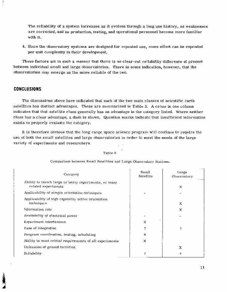
The discussions above have indicated that each of the two main classes of scientific earth satellites has distinct advantages. These a r e summarized in Table 3. A cross in one column indicates that that satellite c lass generally has an advantage in the category listed. Where neither c lass has a clear advantage, a dash is shown. Question marks indicate that insufficient information exists to properly evaluate the category.
It is therefore obvious that the long range space science program wil l continue to require the use of both the small satellites and large observatories in order to meet the needs of the large variety of experiments and researchers .
Table 3
Comparison between Small Satellites and Large Observatory Stations.
Category
Ability to launch large o r heavy experiments, o r many related experiments
Applicability of simple orientation techniques
Applicability of high capability active orientation techniques
Information ra te
Availability of electrical power
Experiment interference
Ease of integration
Program coordination, testing, scheduling
Ability to meet orbital requirements of all experiments
Utilization of ground facilities
Reliability
Small Satellite
-
-
Large Observatory
11
A


THE NIMBUS I METEOROLOGICAL SATELLITE-GEOPHYSICAL OBSERVATIONS FROM A NEW PERSPECTIVE
by W. Nordberg
Goddard Space Flight Center
The Nimbus I meteorological satellite which was launched into a nearly polar sunsynchronous orbit and was fully ear th oriented car r ied a sct of very high res- olution television cameras , a directly transmitting television camera of lesser resolution and a High Resolution Infrared Radiometer. The observations of de- tailed cloud features during daytime, the direct transmission of such observa- tions to local weather station via an Automatic Picture Transmission system and the measurement and pictorial presentation of carth, water and cloud tem- peratures from orbital altitudes a t nighttime with the infrared radiometer have provided geophysical and mcteorological measuremcnts f rom a truly global perspective. Temperatures of ice surfaces of Antarctica and Greenland were presented in high resolution radiation pictures with accuracies of about 12°K. Pictorial maps of cloud cover and of cloud top heights were obtained during nighttime permitting a three-dimensional analysis of the global cloud structure and inferences regarding the dynamics of weather fronts, severe s torms and atmospheric circulation cells. Measurements of s e a surface tcmperatures were made in many areas of the world. Radiation patterns observed over te r ra in in cloudless conditions indicatc the temperatures of the soi l and permit inferences, in certain cases , of these parameters which determine the thermal properties of the soi l , namely moisture, vegetation and rock formations. The data a re availa- ble for further analysis by thc scientific community and a catalog of all Nimbus observations i s contained in Reference 9.
INTRODUCTION
The f i rs t photographs of the earth's surface and of large scale weather systems taken from orbital altitudes have revealed a great deal of new knowledge merely because large scale phenomena which had never been observed in their entirety were now brought within the scope of one single observation. These findings stem from a ser ies of Tiros (Television and Infrared Observation Satellite) satellites launched at the rate of about two per year since April 1960. Tiros satellites were primarily intended to serve the operational needs of the meteorologist in the detection and tracking of storms, frontal systems and similar phenomena by means of the cloud patterns asso- ciated with these weather features. Spaceborne observations of weather have also contributed to
13

fundamental meteorological research. Nimbus I, the f i r s t of NASA's second generation meteoro- logical satellites, has further advanced the potential application of such observations to meteoro- logical research and to other fields of geophysics. The Nimbus I system proved to be an excellent tool for the remote observation of meteorological and geophysical parameters for several reasons: A sun-synchronous, nearly polar orbit, a fully earth oriented, amply powered spacecraft, a set of improved and directly transmitting television cameras and a newly developed high resolution infrared radiometer (Reference 1).
THE NIMBUS I SYSTEM
Nimbus I was launched into a nearly polar orbit on 28 August 1964 from Vandenberg Air Force Base, California. Because of a launch vehicle malfunction, an elliptic orbit (perigee 423 kilometers and apogee 933 kilometers) instead of the planned circular orbit at 900 kilometers, w a s achieved. As planned, the orbital plane was inclined to the equator by 98.7 degrees which caused the orbit to precess around the center of the earth in synchronism with the revolution of the earth around the sun. A s a consequence the relative orientation between the orbital plane and the sun remained essentially constant during the life of the spacecraft. Since at launch the orbit w a s chosen so that the earth-sun line lay in the orbital plane, the satellite passed over most a r eas of the world twice every 24 hours, near local noon and near local midnight. Two stations in the United States, one in North Carolina, the other in Alaska, were used to command the spacecraft and to read out the stored telemetry and sensory data. Of the 14 to 15 orbits in a 24-hour period, eleven were expected to pass within acquisition range of one of the two stations. The eccentricity of the orbit, however, reduced the acquisition capability to fewer than ten orbits per day. Nevertheless, day and night photographs were obtained over 50 to 75 percent of the world on a daily basis.
The entire Nimbus system, including a complex a r r ay of about ten spacecraft subsystems (attitude control, power supplies, telemetry) as well as data transmission and handling facilities on the ground, had been designed to demonstrate the capability of delivering the complete informa- tion sensed by the spacecraft into the hands of the meteorological analyst in a format suited for immediate application. For a period of about four weeks this experiment functioned perfectly. The three-axis, active control system kept the spacecraft axis (sensor axis) oriented toward the center of the earth at all times, generallywithin better than one degree in all three axes; the solar cell power supply continually delivered an average power of about 300 watts to the spacecraft; and the spacecraft data storage and transmission system processed in excess of 50 million items of infor- mation (data words) per orbit. Pictorial presentations of the observations (Figure 1) made either during daytime with television cameras or during the night with a High Resolution Infrared Radio- meter (HRIR) were generally available a t the NASA Nimbus Control Center in Greenbelt, Maryland, within less than 30 minutes after the command for playback of the data was given to the spacecraft. Within these 30 minutes the information recorded in the spacecraft during any previous orbit (nominally 100 minutes of observation) were transmitted to the command station (in Alaska for example), recorded there, then transmitted further via communication circuits to Greenbelt, Maryland, where appropriate geographic referencing (latitudinal and longitudinal grids) as applied
14
60°N
50"N
40°N
30"N
20°N
10°N
EQUATOR
100s
200s \ 30'5 (HRIR) NIGHT
z DAY (AVCS)
40"s
50'5
60'5
70'5
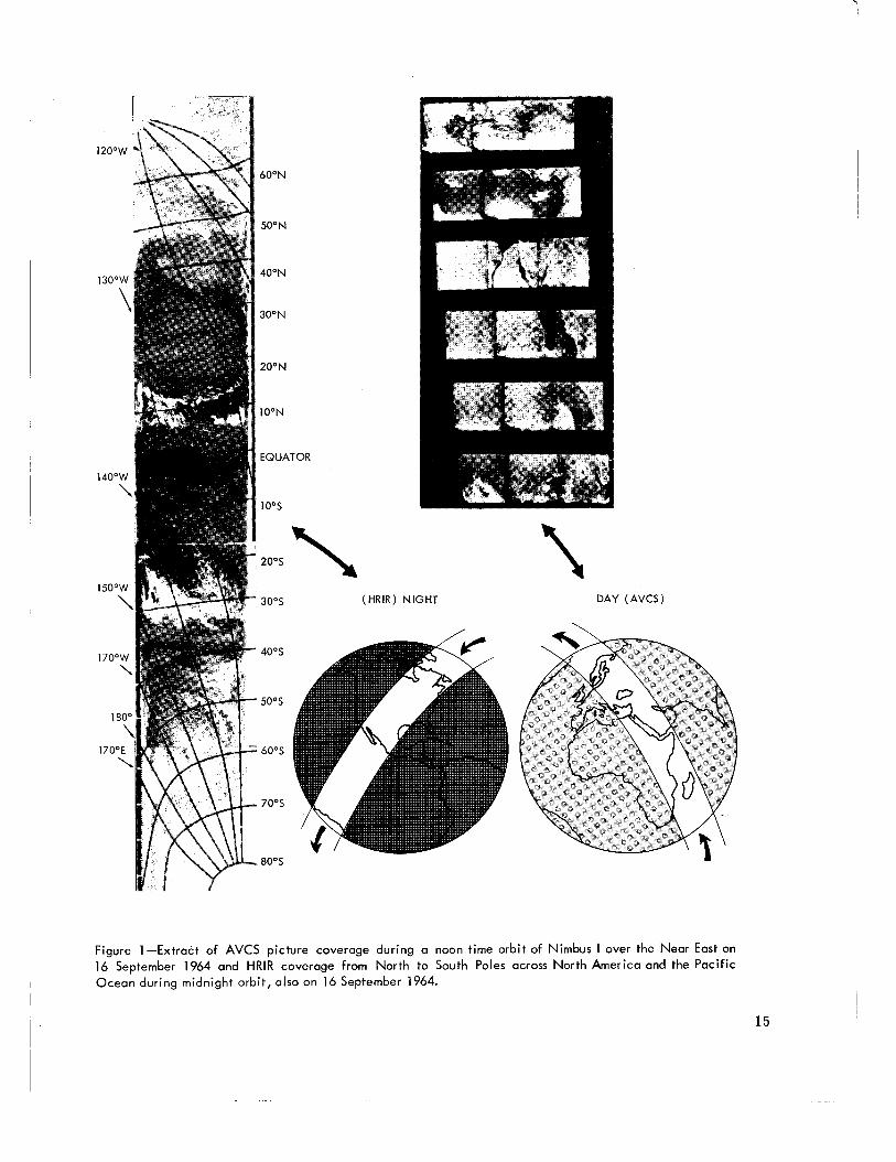
Figure 1-Extract of AVCS picture coverage during a noon time orbit of Nimbus I over the Near East on 16 September 1964 and HRIR coverage from North to South Poles across North America and the Pacific Ocean during midnight orbit, also on 16 September 1964.
15

automatically after which the data were transcribed onto 70 mm photographic film resulting in the s t r ips shown in Figure 1. These s t r ips permit a detailed analysis of weather and surface phenom- ena along the entire globe circling path of the satellite within l e s s than two hours after the observa- tions were taken. For operational meteorological applications an Automatic Picture Transmission (APT) system transmitted television observations instantly to about 50 simple and inexpensive ground stations located all over the globe. These ground stations were operated by the United States Weather Bureau, the meteorological services of the United States Armed Forces, foreign weather services, and, in some cases, by educational institutions.
NIMBUS SENSORS
In the past, television cameras had proved to be the most effective instruments for observations of meteorological features from satellites. Nimbus I carr ied two types of cameras: A set of three very high resolution cameras each with a field of view of about 35 degrees and one camera with lesser resolution but equipped with a photosensitive surface which retained a latent image suffi- ciently long so that images could be transmitted directly via the APT system without intermediate storage on magnetic tape. The resolution obtained with this camera permitted the recognition of cloud and terrain features of l e s s than four kilometers in diameter. The three high resolution television cameras formed the Advanced Vidicon Camera System (AVCS) and yielded considerably greater detail in their pictures. Objects of linear dimensions of less than one-half kilometer could be resolved. This resolution was adequate to observe practically all objects of meteorological significance. The Advanced Vidicon cameras were arranged side by side such that they covered a s t r ip approximately 2000 kilometers wide along the satellite track (Figure 1).
In contrast to the cameras which formed television images of reflected solar radiation during daytime, the High Resolution Infrared Radiometer (HRIR) provided pictorial presentations of emitted, telluric, infrared radiation a t night with high quantitative accuracy (Reference 2). Radiation was sensed in the narrow spectral window between 3.4 and 4.2 microns. A rotating mir ror scanned the earth from horizon to horizon perpendicularly to the orbital path. Due to the satellite motion each successive scan line was advanced by approximately 9 kilometers which is comparable to the linear resolution of the sensor near apogee. Because of the elliptical orbit the resolution near perigee was about 4 kilometers. An entire nighttime half of the orbit was covered by about 2300 contiguous scans (Figure 1). The HRIR has been outstandingly successful not only in providing continuous nighttime cloud cover with a quality comparable to Tiros television pictures, but also in resolving equivalent blackbody temperatures of radiating surfaces at night within about f 1K. The HRIR was a lso capable of imaging cloud patterns during daylight, but the temperature resolution was lost as , in that case, the instrument responded primarilyto reflected solar radiation which masked the telluric emission.
MAPPING BLACKBODY TEMPERATURES WITH HIGH RESOLUTION RADIOMETRY
The principle of mapping cloud and terrain features by means of infrared radiation is quite simple. All objects emit electromagnetic radiation, the spectral distribution and intensity of which
16
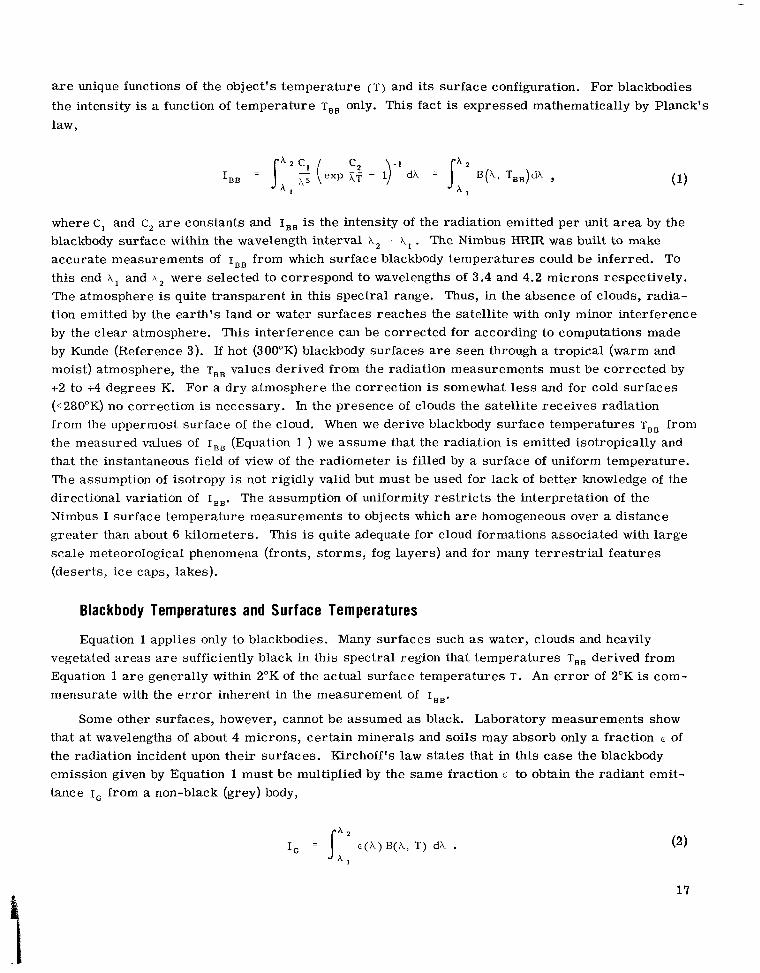
a r e unique functions of the object's temperature ( T ) and i ts surface configuration. For blackbodies the intensity is a function of temperature T,, only. This fact is expressed mathematically by Planck's law,
where C, and C, a r e constants and I,, is the intensity of the radiation emitted per unit area by the blackbody surface within the wavelength interval A, - A, . The Nimbus HRIR was built to make accurate measurements of I,, from which surface blackbody temperatures could be inferred. To this end A, and A, were selected to correspond to wavelengths of 3.4 and 4.2 microns respectively. The atmosphere is quite transparent in this spectral range. Thus, in the absence of clouds, radia- tion emitted by the earth's land or water surfaces reaches the satellite with only minor interference by the clear atmosphere. This interference can be corrected for according to computations made by Kunde (Reference 3). If hot (300°K) blackbody surfaces a r e seen through a tropical (warm and moist) atmosphere, the T,, values derived from the radiation measurements must be corrected by +2 to +4 degrees K. For a dry atmosphere the correction is somewhat less and for cold surfaces (<280"K) no correction is necessary. In the presence of clouds the satellite receives radiation from the uppermost surface of the cloud. When we derive blackbody surface temperatures T,, from the measured values of I,, (Equation 1 ) we assume that the radiation is emitted isotropically and that the instantaneous field of view of the radiometer is filled by a surface of uniform temperature. The assumption of isotropy is not rigidly valid but must be used for lack of better knowledge of the directional variation of I,,. The assumption of uniformity restr ic ts the interpretation of the Nimbus I surface temperature measurements to objects which are homogeneous over a distance greater than about 6 kilometers. This is quite adequate for cloud formations associated with large scale meteorological phenomena (fronts, storms, fog layers) and for many terrestr ia l features (deserts, ice caps, lakes).
Blackbody Temperatures and Surface Temperatures
Equation 1 applies only to blackbodies. Many surfaces such as water, clouds and heavily vegetated a reas a r e sufficiently black in this spectral region that temperatures T,, derived from Equation 1 a r e generally within 2°K of the actual surface temperatures T. An e r ro r of 2°K is com- mensurate with the e r ro r inherent in the measurement of I,,.
Some other surfaces, however, cannot be assumed as black. Laboratory measurements show that a t wavelengths of about 4 microns, certain minerals and soils may absorb only a fraction E of the radiation incident upon their surfaces. Kirchoff's law states that in this case the blackbody emission given by Equation 1 must be multiplied by the same fraction E to obtain the radiant emit- tance I, from a non-black (grey) body,
I, =I"' E ( A ) B ( A , T ) d h . A ,
17

The fraction E is the emissivity of the surface. Defining an average emissivity E within the wave- length 3.4 to 4.2 microns, we may rewrite Equation 2
Using the appropriate values for C, and C, and for A, and A, in Equation 1, we find that at a blackbody temperature of 290"K, which is typical for the earth's surface seen by Nimbus at low latitudes, the value of I,, is about 1.4 x lo-' watts/m2. A reduction of this value by 10 percent corresponds to a T,, value of 288.2"K. This means that a surface of 290°K with an average emis- sivity of 0.9 emits radiation of the same intensity as a blackbody surface of about 288.2"K. Since the minimum temperature change discernible with the HRIR is about 1" to 2"K, the knowledge of E in the derivation of T from I, is important only i f the emissivity is considerably smaller than 0.9.
Surface emissivities can actually be derived from HRIR daytime observations of reflected solar radiation. In this case the measured radiation intensities are not only due to surface tem- peratures but a l so due to the ability of the surfaces to reflect sunlight. The radiation intensity I, sensed by the radiometer during daytime is the sum of the emitted grey body radiation I, and the reflected solar radiation r I s . The reflectivity r of practically all terrestrial surface is given as: 1 - C . Thus, i f we define r as the average reflectivity in the 3.4 to 4.2 micron range, we may write,
-. -
(4 ) I, = I, + r1, = tI,, + (1 - E ) Is .
r S is computed from the solar constant on the basis of purely geometrical considerations. A measurement of I, = I, = 4.17 watts/m2 would result i f the surface were a perfect, 100 percent effective, diffuse reflector for solar radiation at vertical incidence. For a reflectivity T = 0.3, an emissivity F = 0.7 and a surface temperature T = 290°K I,, =0.11 watts/m2 and fIs = 1.25 watts/mz. Hence, i f the surface emissivity is smaller than 0.7, I,, may be neglected and Equation 4 reduces to
-
(5) I, = Is - €IS .
If the surface temperature is less than 290"K, Equation 5 is valid even for emissivities greater than 0.7. In this case the emissivity can be derived from daytime HRIR measurements without any knowledge of surface temperatures. For 7 > 0.7 the emissivity can still be measured very ac- curately provided that the surface temperatures are known. For example i f r = 0.99 and T = 290°K I, = 0.18 watts,",; if E = 1.00 (blackbody) I, = 0.14 watts/m2. The difference of 0.04 watts,", is due to the term TrS in Equation 3 and is equivalent to a blackbody temperature change of about 2°K which is just at the sensitivity threshold of the HRIR. In sunlight emissivities of 0.99 can
18
111 I

therefore easily be discerned from blackbodies and the HRIR,which was in operation during day- time for several orbits of NimbusI, provides a very accurate method to measure large scale surface emissivities at 4 microns.
Preliminary evaluations of these daytime observations indicate that emisivities for most large scale surfaces (oceans, clouds, snow and vegetated regions) are greater than 0.9. Thus, HRIR measurements permit the world wide mapping of actual temperatures of most surfaces during nighttime and the mapping of emissivities of non-blackbody surfaces during daytime. Global measurements of earth surface temperatures (as opposed to air temperatures measured near the ground) are of considerable value in meteorological research since these temperatures can be used as initial values in the numerical analysis and prediction of weather. At polar latitudes HRIR surface temperature maps relate to the morphology of ice formations. Such maps a r e both of practical application to navigation and of fundamental interest to glaciologists. Over oceans, surface temperature differences may indicate the location of areas such as currents and fronts. This suggests the potential use of Nimbus HRIR observations in oceanographic research. Soil moisture content can be derived at least qualitatively from the Nimbus HRIR observations since appreciably higher soil temperatures a r e measured in moist areas . Aircraft observations of emitted infrared radiation over regions of volcanic activity in Hawaii (Reference 4) have shown that underground lava beds can be detected with this technique; therefore, the Nimbus HRIR data were also investigated for this purpose. No definite identification of active volcanic a reas could be made, however, because the spatial resolution of the HRIR is apparently too coarse. Global mapping of emissivity with such coarse resolution is, nevertheless, of geological interest. Maps of emissivity obtained by the satellite might establish a relationship between the small scale emission properties of various minerals and soil constituents measured on samples in the labora- tory and the large scale properties of the same constituents in their natural state where they are blended with impurities, vary in grain s izes and morphology. The satellite observations can be considered very useful in determing whether the distribution of mineral and similar deposits can be mapped by measurement of emitted radiation with low spectral and spatial resolution. Any findings in this a rea may have considerable impact on the expectations for similar measurements of lunar and planetary surfaces.
Cloud Heights
When the HRIR views a cloud covered region and a uniform cloud fills the instantaneous field of view of the radiometer, the average blackbody temperature of the cloud top surface can be derived by means of Equation 1. It is well known that in the troposphere the temperature generally decreases rapidly with altitude. It is also well known that clouds generally do not penetrate to altitudes above the troposphere where temperature increases with height. Thus, blackbody cloud top temperatures can be directly related to height (Figure 2). The deviation of cloud heights from satellite-borne radiometric measurements has been demonstrated previously with Tiros observa- tions (References 5 and 6) but the better spatial resolution of the Nimbus radiometer permits for the first time a detailed pictorial presentation of the vertical structure of cloud tops on a large scale. Figure 3a shows a typical example of such cloud structure over the North Pacific near
19

20 -
-
16 -
-
1 2 - v
+ - I (3 w 8 - I
-
4 - -
TEMPERATURE ( " K )
Figure 2-Typical temperature profile at tropical latitudes illustrating concept of determination of cloud top heights from satellite measurements of cloud top temperatures.
midnight on 20 September 1964. In this photo- graphic s t r ip as in all HRIR presentations high clouds (cold temperatures) are presented as light shades of gray, while low clouds or clear areas (warm temperatures) appear dark. It is immediately apparent that the broken cloud band near the equator consists of the highest clouds
40°N
30"N
20"N
1 O O N
150" W
(a)
140'W
in this picture; clouds in the broad band near 50 degrees N are somewhat lower although still much higher than the large grey mass of clouds covering the North Pacific from 25 to 45 de- grees N. Only a few large, very dark regions indicating clear skies can be seen near 40 degrees N and 140 degrees W. The pictorial presenta- tion of these temperature contrasts permits an instantaneous assessment of the gross features of the meteorological situation. The narrow band of very high clouds near the equator marks the Intertropical Convergence Zone; the broad band near 50 degrees N corresponds to an intense
Figure 3a-Pictorial presentation of cloud and water temperatures over the North Pacific measured by the HRIR at midnight on 20 September 1964. (Dark shades are warm, white shades are cold.)
20

cold front and low lying fog and stratus clouds stretching south of the front, indicated by the dark grey area. Of particular interest is the string of small, very bright (cold) spots near 137 degrees W and 38 to 40 degrees N. These indicate isolated, very high altitude cumulus clouds relating to thunderstorm activity. Normally, the meteorologist would never expect thunderstorm activity under the prevailing situation, especially not near midnight. However, the isolated, very high clouds definitely suggest such activity and, in this case, the validity of this interpretation was confirmed by a report from a single ship which happened to be in that a rea and reported towering cumuli and lightning.
A much more quantitative picture results f rom plotting the numerical temperatdres auto- matically derived by digital computers from the radiation intensities. Extracts of such automatic, numeric presentations a r e shown in Figure 3b. The very highest cloud in the Intertropical Con- vergence Zone (11.5-12 degrees N and 145-146 degrees W) towers to about 16 kilometers, an altitude derived on the basis of Figure 2 from the extremely low temperature of 190°K near the center of the cloud top (Figure 3b). On this basis the fog near 40 degrees N (Figure 3a) gives a surface temperature of 285°K which means it reaches only to about 1 kilometer above sea level; the dark a r e a in the same region corre- sponds to a temperature of about 293°K. The sea surface temperature measured by ships in this region w a s identical to that value which proves that the area was free of clouds. The accuracy of the HRIR cloud height measurements is vividly demonstrated in Figure 4a where the original analog record of one single scan across the center of Hurricane Gladys near midnight on 17 September 1964 over the Atlantic is reproduced. This scan covers a s t r ip of 5 kilometers width across the storm; the observed radiation intensities,
Figure 3b-Automatical ly produced digital
map of cloud surface temperatures for a small portion of Figure 30.
290K -
270K -
250K -
230K - 210K -
I- 0
- 4
6 -
HEIGHT (km)
8 -
Figure 40-Single HRIR scan, from horizon to horizon, across Hurricane Gladys at the location indicated in Figure 4b.
21

expressed in degrees K, are measured along the ordinate. The blackbody temperatures were con- verted to height on the basis of actual temperature soundings performed by balloons in the vicinity of the storm. The corresponding heights a r e shown along the right hand ordinate. The scan indicates temperatures near 300°K outside the s torm and near 290°K in the center of the eye. The temperature of 300°K corresponds to the sea surface temperature over the clear skies out- side the s torm and 290°K corresponds to a height of 2 kilometers over the eye of the hurricane. Over the center of the spiral bands temperatures drop to 200°K corresponding to heights of 14 kilometers. Lower clouds and partially clear skies a r e scanned between the spiral bands. The photographic presentation of the s torm in Figure 4b is composed of a total of about 200 such scans. Detailed analysis of these highly quantitative observations of vertical cloud structure in many cases permit a much better exploration of dynamics of the atmosphere than ordinary cloud photography.
SCAN PATH
w E
Figure 4b-HRIR observation of Hurricane Gladys over the Atlantic near midnight on 17 September 1964. (Dark shades are warm, white shades are cold.)
Sea Surface Temperatures
Since the blackbody assumption for water surfaces is quite valid in the 3.4 to 4.2 micron wave- length range, T,, values derived from the radiation intensities relate directly to water surface temperatures. In cloudless regions the HRIR, therefore, can be used to map globally the surface temperatures of various bodies of water. Figure 5 shows an HRIR picture of the southwestern United States at midnight on 30 August 1964. The darkest region in the right center corresponds to a temperature of 301% for the water surface in the Northern Gulf of California. Applying Kunde's corrections for atmospheric absorption (Reference 3), we obtain a temperature of 303°K for the
22

waters of the Gulf of California which is consid- erably warmer than the Pacific Ocean off the shore of California. There temperatures range from 293% near the coast to about 280% at a distance of about 200 kilometers off shore. The low off shore temperatures indicate the pres- ence of fog o r dense haze, while the temperature of 293% measured just west of Los Angeles is in good agreement with the temperature of 2 9 2 ' K
measured from shipboard by the U. S. Coast Guard. Even small water features such as lakes can be clearly identified and their surface tem- peratures can be determined. The four black (warm) dots in the upper left corner of Figure 5 are mountain lakes in the Sierra Nevada. The
GRAND CANYON
GULF OF CALIFORNIA
Figure 5-HRIR Ocean and terrain temperatures over the southwestern United States near midnight on 1 September 1964. (Dark shades are warm, white shades are cold.)
southwestern most lake is Lake Tahoe; its water surface temperature w a s measured by the HRIR as 283°K. But, for a small body of water such as this there is a question whether the field of view of the radiometer w a s fully covered by the lake. The actual water temperature therefore may be several degrees higher.
The ability of the HRIR to map sea surface temperatures suggests that the course of various ocean currents such as the Gulf Stream, for example, could be detected by the satellite. Unfortu- nately, during the life time of Nimbus I clouds obscured most a r eas of interest. There is, however,
50'N
40°N
1 5OoW 14OOW
Figure 6a-HRIR cloud and water temperatures over the North Pacific near midnight on 30 August 1964. Clear streak of open water can be seen i n the center. (Dark shades are warm, white shades are cold.)
the possibility that certain cloud formations them- selves may be related to ocean temperatures. A suggestion of this can be found in a number of cases for which Figures 6a and 6b a r e typical. Very long and narrow, clear s t reaks of open
30°S
100°E 1 10°E
Figure 6b-HRIR cloud and water temperatures over the Indian Ocean near midnight on 9September 1964. Clear streak of open water can be seen in the center. (Dark shades are warm, white shctdes are cold.)
23

water lie between extensive low altitude s t ra tus cloud decks over the North Pacific in Figure 6a and over the eastern Indian Ocean in Figure 6b. Here the s t reaks are at least 2000 kilo- meters long and about 200 kilometers wide. Although the phenomenon is apparently at- mospheric it is conceivable that the cloud formations and the peculiar clearings may be influenced by ocean surface temperature differences.
Another example of satellite observed variations in sea temperatures can be found in Figure 7 where sea surface temperatures over the Mediterranean are found to range from 297°K off the coast of Africa to 290°K near Corsica. Temperatures of the Adriatic and Tyrrhenian Seas a r e 294%.
Ice Formations
50°N
ALPS
40'N
30"N 10°E 20'E
Figure 7-Temperatures over Europe observed by HRIR near m i d n i g h t o n 14 September 1964. (Dark shades are warm, w h i t e shades are co ld . )
Nimbus I w a s the first weather satellite to provide continuous observations of the polar regions. A great deal of detail in the struc- ture of the inland ice over Antarctica, Green- land, and other a reas w a s observed with the AVCS. High resolution television observations also provided information on the morphology of floating shelf ice, icebergs and similar phenomena (Reference 7). Figure 8 is a typi- cal example of an AVCS picture showing the extent of ice cover and the structure of snow covered mountain ranges over northwestern Greenland. Details in the mountain ranges can be observed because of the pronounced shadows produced by the low elevation of the sun which generally prevails at these high latitudes.
5OoW 82'N
F igu re 8-AVCS p i c t u r e of nor thwestern G r e e n l a n d near noon o n 3 September 1964.
24

Figure 9 is a HFUR presentation of temperatures of Antarctic ice and water surfaces on 29 August 1964. The entire Atlantic sector of the continent is shown to be cloud free and the surface tempera- tures over the interior ice cap near the South Pole were determined numerically as 210-215°K. These extremely low temperatures were observed consistently during the lifetime of Nimbus from late August to late September. Near the edge of the continent surface temperatures increase markedly to about 240°K. The edge of the continent stands out sharply in the infrared picture because a band of apparently open water about 100 kilometers wide in spots stretches along the coast of Queen Maud Land. Maximum temperatures of these spots are about 256°K. This indicates that the full instantaneous field of the radiometer was not viewing an entirely open area of water but that this band probably consists of strongly broken up ice. A wide shelf of floating ice stretches northward into the Wedell Sea and the Atlantic Ocean. The Wedell Sea ice can be easily distinguished from the inland ice because its surface temper- ature of 244°K is about 12°K higher. Very nar- row but distinct lines of warmer temperatures are found crisscrossing the shelf. These lines obviously are due to cracks in the ice and in some cases they a r e over 200 kilometers long. The ice shelf ranges up to 57 degrees where it is bounded by open water of temperatures of about 275°K.
l O O W Figure 10a is an HRIR picture of the Ross
Ice Shelf in the Pacific Sector of Antarctica. Although these observations were made four days after those shown in Figure 9, the temper- atures are nearly the same over the interior ice. Surface temperatures of the Ross Ice Shelf range from 225°K near 85 degrees S to 245°K near 70 degrees S. The latter value compares well with the temperatures of 244°K measured four days earlier over the Wedell Sea (Figure 9). In Figure 10a a number of very isolated high temperature spots can be seen along the coast of Victoria Land. The most pronounced one near 76 degrees S and 165 degrees W has a temperature of 260°K. Since this spot is located near Mt. Erebus it was originally suspected that these isolated warm regions might be r e - lated to volcanic activity. However, as the same regions were observed in subsequent HRIR pictures, it became evident that some of the spots became enlarged and formed small bands along the edge of the continent. Finally
00 10°E 20°E
60'5
70'5
Figure 9-Temperatures over Antarctica observed by HRIR near midnight o n 29 August 1964. (Dark shades are warm, white shcdes are cold.)
25

16OOW 14OOW 120ow
1 80°
7OoS
70'5
80's
80"s SOUTH POLE
( 0 )
Figure loa-Temperatures over Antarctica observed by HRIR near midnight on 1 September 1964. (Dark shades are warm, white shades are cold.)
Figure lob-Digital map of temperature contours over Antarctica for the data presented pictorially in Figure 1 Oa.
on 2 1 September 1964 the spot near Mt. Erebus had enlarged to such an extent that i t filled the entire field of view of the HRIR (Figure l la) and the measured temperature was approximately 270°K. The fact that this is conspicuously close to the temperature of freezing water and that the same spot was photographed 12 hours later in sunlight with the AVCS (Figure l l b ) leads to the definite conclusion that the spots indeed a r e open water. Note the identical shape of the open a rea in Figures l l a and l l b , despite the difference of one order of magnitude in the resolution capabili- ties of the AVCS and HRIR. Figure 10b is a temperature contour map of the Pacific Sector of Antarctica derived from the automatically plotted digital data for the picture shown in Figure loa. The very low temperatures (215°K) over the high plateau surrounding the South Pole a r e obvious. The warm tongue reaching toward the pole near 180 degrees longitude coincides with the Ross Sea where the shelf ice is a t a much warmer temperature than the higher and thicker inland ice. The high clouds seen in Figure 10a to the east of the Ross Ice Shelf show a temperature of about 215°K which corresponds to a cloud top altitude equal to that of the interior plateau, namely about 3000 meters. The 260°K line indicates pockets of broken ice and open water which a r e found in the Pacific Ocean Sector.
An HRIR picture of the Greenland ice cap is shown in Figure 12. Over c lear areas the coldest region of the ice mass shows surface temperatures of about 230°K. Cloud bands can be seen ex- tending over the southwest and eastern portion of the subcontinent. Clouds in this case appear
26

Figure 11 -Comparison of warm spot observed by HRlR (a) and AVCS (b) over Antarctica on 21 September 1964.
darker (warmer) than the underlying ice. The measured cloud temperatures a r e about 20°K warmer than the ice surface temperature. This is plausible in view of the temperature inver- sions which are known to exist over the ice covered polar regions. The inversion means that over a portion of the lower atmosphere, temperatures increase rather than decrease with height, thus deviating from the typical pro- file shown in Figure 2. The darkest portions of the region between Greenland and the large cloud mass to the south indicate clear skies over the waters of Baffin Bay and the Davis Straits. Water surface temperatures of above 280°K were derived from the digital analysis of the data over this area.
Terrain Features and Soil Moisture
80°N
70°N
60°N
5OoW
Figure 12-Temperatures over Greenland observed by HRlR near midnight on 16 September 1964. (Dark shades Land more 'Om-
plex than sea or cloud surfaces. Therefore, are warm, white shades are cold.)
27

under certain conditions, the temperatures derived from radiation intensities measured over land surfaces depend to a large extent not only on terrain heights but a lso on such parameters as heat capacity, conductivity and moisture content. First , a distinction must be made whether the varia- tions in radiation intensity are due to actual ground temperature, or due to variations in emissivity. In the radiation observations with Nimbus I most variations may be ascribed to actual surface temperatures. No cases have been found where variations in surface emissivities could be clearly identified in the HRIR measurements. Indeed, we believe from this experience with Nimbus that effective detection of surface features by means of emissivity measurements from spacecrafts will only be possible i f the spatial and spectral resolutions of radiometric sensors a r e improved by several orders of magnitude over the capability of the Nimbus I instruments. On the other hand, a number of the topographic and geological features mentioned above may be inferred from the measurements of relatively broadband thermal emission performed with the Nimbus I HRIR. For example, the dark streaks in the upper portion of Figure 5 showing the Southwestern United States correspond to blackbody temperatures of about 290°K while the lighter grey in the surrounding regions corresponds to about 275°K. The warm streaks were identified as Death Valley (left) and the Grand Canyon (right). Thus the temperature differences seen by the satellite readily cor re- spond to differences in terrain height. Furthermore, a more quantitative interpretation of the temperatures over Death Valley reveals that the temperature difference of about 15°K measured by the satellite corresponds to an altitude difference of about 1800 meters between the valley floor and the surrounding highlands. The measured temperature decrease with altitude is therefore about 8.3 X/kilometer which is in very good agreement with the expected temperature decrease in the f ree atmosphere (atmospheric lapse rate). This equilibrium between the soil and atmospheric temperatures leads to the conclusion that the heat capacity of the ground in this a rea must be generally very large since only such a large heat capacity will prevent the surface at night from cooling more rapidly by radiation than the overlying atmosphere.
An example where other considerations a r e involved) in addition to topographic height changes, may be seen in Figure 13. Figure 13 shows a very large portion of western South America as seen by the HRIR on 14 September 1964 when much of the region was essentially f ree of clouds except for the Intertropical Convergence Zone north of 10 degrees S, an extensive low altitude layer of s t ra tus clouds along the entire west coast, a high altitude cloud deck off southern Chile, and some smaller clouds along the eastern horizon. The broad, white (cold) band through the center of the picture corresponds to the cold, high altitude mountain ranges of the Andes. Average blackbody temperatures of 255°K a r e measured over the highest elevations between 28 and 32 degrees S. To the northeast there is a remarkably rapid transition from the cold highland with average blackbody temperatures of 270°K to the very warm Amazonas Basin with blackbody temperatures of 290°K. The warm waters of Lake Poop0 (19 degrees S) and Lake Titicaca (16 degrees S) a r e clearly evident in the generally cold highlands. In the plateaus to the east of the mountains (30-35 degrees S) and in northern Chile (24 degrees S) remarkably fine structure in the temperature patterns may be observed. The crescent shaped figure near 23 degrees S corresponds to the Salar de Atacama, a salt flat in northern Chile. The discrete band of warm temperatures (273°K) surrounding the crescent stands out clearly while the center is quite cold (263'13). The topographic map (Figure 14) shows that the entire Salar covers a region of fa i r ly uniform altitude of about 2300 meters. Thus
28

DE
SI PIE
10"s
200s SALAR ATACAMP
ERRA DEL DE PAL0
30'5
40"s
70°W 6OoW
Figure 13-Temperature over South America observed by HRlR near midnight on 13 September 1964. (Dark shades are warm, white shades are cold.)
69' 68OW
Figure 14-Topographic map of Salar de Atacama in northern Chile.
on the basis of terrain height there is no reason to assume the existence of a temperature differ- ence between the center and the rim. Laboratory measurements by Hovis (Reference 8) have shown that of many common minerals tested in this spectral region pure rock salt has the lowest average emissivity. Hovis' measurements give a value of less than 0.5 for T. Therefore, a blackbody temperature of less than 263°K would be measured over pure salt if the actual surface temperature were 273"K, while the periphery of the Salar rock formations at the same altitude and temperature would be detected essentially as
blackbodies and thus produce a T,, measurement which is very close to the actual temperature. The difference of 10°K between the cold center and the warm band in Figure 13 could thus be explained. There is still a question, however, i f the emissivities measured for pure sal ts in the laboratory a r e applicable to naturally impure salt deposits such as this Salar. A more probable interpretation is that the emissivity of the natural salt over the Salar is much greater than 0.5 but that the heat capacity of the salt is considerably less than that of the surrounding rock formations a t the same altitude level. This fact combined with the very high reflectivity of sunlight and the very low heat conductivity of the relatively fine grained salt deposits prevent the storage of large amounts of solar heat over the Salar itself and, after sunset, cause i t to cool very rapidly by radiation resulting in a
29

very low temperature (263°K) at midnight. The rocks along the periphery, however, remain warmer throughout the night (273°K) because of their larger heat capacity and greater conductivity.
A similar case may be observed in Figure 13 near 32 degrees S and 68 degrees W over western Argentina. Here, again, a nearly circu- la r dark band of about 5 kilometers in width and about 40-50 kilometers ip diameter indicates the existence of a high temperature zone along this peculiarly shaped band. The cold tempera- tures (white spot) in the center of the band can easily be explained by topography. The center of the band corresponds to the Pie de Palo mountain shown topographically in Figure 15. The lowest temperature measured in the center of the band is 268°K and corresponds to the highest eleva- tion of about 3000 meters (Figure 15). The temperature along the band is about 280°K which is about 7°K warmer than the temperature of 274°K of the surrounding desert . Since the band around the mountain is certainly not a t a lower altitude than the surrounding deser t
IO 5 o IO 20 30 40 50 60 70 80 plateau (Figure15), the explanation of the warmer m H - M -
KILOMETERS - temperatures must again be found in the differ- ence in heat storage between the deser t sand and the rocks of the Pie de Palo mountains. A visual survey by the author* revealed that the contrast between the Precambrian rock forma- tions of the Pie de Palo mountains and the alluvial
Figure 15-Topographic map of Pie de Palo mountains i n western Argentina.
sand deposits of the surrounding deser t is indeed very striking and extends around the mountains approximately along the 1000 meter contour line (Figure 15). The dar,k band seen by the satellite parallels approximately this 1000 meter contour line. Furthermore, the temperature difference of 12°K between the warm band at 1000 meters and the mountain top rising rapidly to 3000 meters yields an approximate lapse ra te of G"K/kilometers which corresponds much better to the expected adiabatic lapse rate than the temperature difference of 6°K between the deser t plateau a t about 800 meters and the mountain top. That latter difference would yield a rather unrealistic lapse ra te of 3"K/kilometers. Thus, the temperature over the deser t is considerably lower because of the small heat capacity and conductivity of the ground causing a temperature inversion in the air over the
*This survey was made possible by the staff of the University of San Juan, Argentina, espec ia l ly Professor C. V . Cesco who provided valuable background material for this investigation.
30

desert, while the solid rocks again remain considerably warmer resulting in the adiabatically de- creasing temperature from the periphery to the center of the mountain.
HRIR pictures over the deser ts of North Africa and the Near East exhibit similar fine structure in the emitted radiation with inferred temperature variations of 10 to 15°K. Again, we conclude that these gradients a r e due to variations in the thermal properties of the soil rather than due to emis- sivity variations.
In this fashion the satellite HRIR observations on a small scale permit the mapping of geological features which can be distinguished by their thermal properties. On a larger scale these patterns of heat capacity assume meteorological significance since storage of heat in the ground is an im- portant consideration in the numerical description of atmospheric processes.
Moisture content of the soil is also evident in the HRIR observations. It has been very surpris- ing that many r ivers of widths of less than 1 kilometer stand out prominently in the radiation pictures although the linear resolution of the HRIR is generally not better than 5 kilometers. The prominence of the r ivers is apparently due to the fact that the heat capacity of the ground along these r ivers is altered probably by moisture in the ground and that this moisture retains solar heat absorbed during daytime much longer than the adjacent dr ier regions. Several r ivers a r e noticeable to the east of the Andes in Figure 13. Two r ivers a r e particularly prominent by their confluence which is located just to the east of the conspicuous warm band around the Pie de Palo mountains discussed above. These r ivers can be identified as the Rio Zanjon and Rio Bermejo in Northwestern Argentina. Interestingly, dispite their prominence in the radiation pictures these r ivers a r e only less than a few hundred meters wide and except for occasional spring flooding they car ry practically no water. Also, the r ivers do not form any deep canyons or other depressions in this a rea so that their warmer temperatures cannot be explained by height differences. In the course of time, however, their courses have meandered over widths of several kilometers over the deser t plateau. These meanderings have apparently taken place during the flood stages and have altered the terrain to such an extent to create a sufficient contrast in the thermal properties between the desert and the river beds that the nighttime temperature differences could be detected by the satellite radiometer. Of course, such contrasts can only be created where the surrounding terrain is very dry and of very small heat capacity. For example, only vague indications can be found in Figure 13 of the Amazonas River which is much wider than the Bermejo and Zanjon r ivers that stand out so clearly. In the Amazonas Basin the entire region possesses such a large heat capacity due to its moisture and heavy vegetation that a uniform and high temperature is maintained throughout the night. Be- cause of this fact the boundaries between water and land which include the outlines of continents cannot be distinguished in the HRIR observations in tropical regions.
An example of very close equilibrium between soil and air temperatures can be found over the Siberian Tundra as shown in Figure 16. In this Figure a band of clouds, manifesting a cold front, crosses western Siberia near 60 degrees N. Cloudless skies prevail both to the north and south which is indicated by the clearly visible lakes and r ivers on both sides of the front. Blackbody temperatures, however, are markedly different on the two sides. To the south the front, tempera- tures range from 277°K to about 280°K while to the northwest they are about 287°K. Analysis of
31

surface air data provided by the Hydrometeoro- logical Service of the U. S. S. R. shows that sur- face air temperatures in the southern region were about 279°K while in the northwest they ranged from 283" to 288°K. This equivalence with the satellite measured soil temperatures suggests a complete equilibrium between air and soil temperatures over this region. Other HRIR Nimbus observations have been obtained over this same a rea during September 1964 but the temperature contrast was apparent only for this case. This leads to the rather surprising conclusion that the soil temperatures in this case were governed by the temperatures of the overlying air masses.
CONCLUDING REMARKS
A variety of different geophysical and at- mospheric facts can be inferred from the ob- servation of temperature variations over the earth's terrain. Over heavily vegetated regions of the tropics the ground temperature can be measured and because of the larger heat capa- city of this type of terrain i ts effect on air temperatures is similar to that over oceans. The ground acts as a reservoir which heats or cools the air moving over it depending on i ts tempera-
80°N
70°N
60°N
80°E
IOOOE
90"E
Figure 16-Temperature over Siberia observed by HRIR near midnight on 5 September 1964. (Dark shades ai-e warm, white shades are cold.)
ture. A t higher altitudes, especially over dry sandy terrain,the heat capacity of the ground tempera- ture is so small that near midnight when solar radiation is absent, the satellite measured ground temperature is much less than the air temperature demonstrating temperature inversions. Over more solid rock surfaces the satellite measured ground temperatures a r e more equal to the air temperatures. Contrasts in the thermal properties of the surfaces usually exhibit a very pro- nounced fine structure in the satellite observations. In many cases these contrasts can be inter- preted, qualitatively a t least, as a measure of moisture content of the ground, changes in the vegetation or in the geological formation along the ground.
32

REFERENCES
1.
2.
3.
4.
5.
6.
7 .
8.
9.
Nordberg, W., and Press, H., "The NIMBUS I Meteorological Satellite," Bull. Amer. Meteor. SOC. 45(11):684-687, November 1964.
Goldberg, I. L., Foshee, L., Nordberg, W., and Catoe, C. E., "NIMBUS High Resolution Infrared Measurements," in: "Proceedings of the Third Symposium on Remote Sensing of Environment," Ann Arbor: University of Michigan, October 14, 15, 16, 1964.
Kunde, V. G., "Meteorological and Geophysical Observations with the NIMBUS I Satellite," NASA SP, 1965.
Fischer, W., et al. 'Tnfrared Surveys of Hawaiian Volcanoes," Science, 146(3645):733-742, November 6, 1964.
Bandeen, W. R., Kunde, V. G., Nordberg, W., and Thompson, H. P., "TIROS I11 Meteorological Satellite Radiations Observations of a Tropical Hurricane," Tellus, 16(4):481-502, April 1964.
Allison, L. J., Gray, T. I., Jr., and Warnecke, G., "A Quasi-Global Presentation of TIROS 111 Radiation Data," NASA SP-53, 1964.
Popham, R., and Samuelson, R. E., "Meteorological and Geophysical Observations with the NIMBUS I Satellite," NASA SPY 1965.
Hovis, W., "Spectral Reflectivity of Common Minerals," J. Appl. Opt. (to be published).
"NIMBUS I High Resolution Radiation Data Catalog and Users Manual," 1: Greenbelt, Mary- land: Goddard Space Flight Center, 1965.
33


CONJUGATE INTERSECTS TO SELECTED GEOPHYSICAL STATIONS
by J. G. Roederer*
W. N. Hess E. G. Stassinopoulos
Goddard Space Flight Center
Geomagnetic field lines a r e traced into space for more than 500 geophysical stations, using the 48-term Jensen and Cain field expansion for 1960. Total field intensity, magnetic dip, declination, and L-values a r e computed a t each station, and at points 300 and 400 km vertically above the station. Coordinates and B values of the conjugate intersects and of the equatorial (minimum B) points a r e determined for each field line, a s well a s the total a r c length of the line between origin and conjugate intersect.
A general discussion of the resulting tables is given.
Finally, a se r ies of maps showing constant B and L contours a t various levels between surface and 3,000 km a r e reproduced.
INTRODUCTION
In the past few years, the study of propagation of charged particles, electromagnetic radiation and magnetohydrodynamic waves along geomagnetic field lines has become a powerful tool in the search for a better knowledge of the structure of the earth 's magnetosphere.
The determination of the exact shape of a line of force, its change with local time during geo- physical perturbations, and the answer to the question of return to earth of high latitude field lines, a r e of crucial importance to the problem of the interaction of the solar wind with the earth 's mag- netic field. The process of propagation of magnetohydrodynamic and very low frequency electro- magnetic waves along field lines gives information on the electron and ion densities encountered; the study of precipitation of energetic particles down the field lines into the atmosphere hopefully wil l lead to a better understanding of the injection and acceleration mechanisms in the magnetosphere.
Many of these investigations a r e based on ground measurements. Hundreds of IQSY and ex- IGY stations gather information which is being used or which could be used for these studies. These
'National Academy of Sciences - National Research Council, Senior P o s t Doctoral Research Associate , on leave from Facultad de Ciencias Exactas y Naturales and Centro Nacional de Radiacion Cosmica, Buenos Aires, Argentina.
35

measurements a r e particularly valuable, if carried out simultaneously at both "ends" of the same field line. It is, therefore, very useful to know with maximum possible precision, the geometry of the field line which "goes through'' each station, and which intersects the ionosphere at several given vertical altitudes for a given field expansion during normal, quiet geomagnetic conditions.
There are many useful parameters related to this "field line geometry." For this preliminary edition, we have selected the following:
1. Geographic coordinates of the station (or the vertical point at high altitude), henceforth called the origin of the field line;
2. Total field intensity at origin;
3. The magnetic dip at origin;
4. The magnetic declination at origin;
5. L-value corresponding to the origin (and within about 1%. to the whole line);
6 . Geographic coordinates of the conjugate intersect, i.e. the intersection of the field line with the earth 's surface (or a fixed level at the same altitude as the origin), a t the other side;
7. Total field intensity at the conjugate intersect;
8. Geographic coordinates of the equatorial point of the field line (defined as the point where the field intensity attains i ts minimum value on that line);
9. Total field intensity at the equatorial point of the field line;
10. Length of the field line between origin and conjugate intersect.
These quantities, which a r e printed out in the above order in Appendix B, Tables l1 2, and 3 , by no means represent all useful field magnitudes. However, for reasons of space and time, other important quantities a r e not reproduced here.
Stations included in our tables were selected from IQSY lists, as well as extracted more o r less at random from old IGY tables. This selection does not pretend to be complete; we apologize for omissions and possible e r r o r s in name-spelling, coordinates, etc.
A careful analysis of the geographic location of conjugate a reas w a s made. It w a s found that about 380 stations have their conjugates over sea, 140 stations have conjugate intersects over land, in which 16 of them are over Antarctica, and only 22 pairs of stations a r e nearly self-conjugate, either deliberately established as such or by chance. We present a list of these self-conjugate pairs, and give a survey of the geographic location of all other conjugate intersects which fall over land, indicating country, and whenever possible, the nearest town to the intersect.
Finally, for the sake of completeness, we present a ser ies of maps with constant B and L con- tours, for altitudes between sea level and 3,000 km.
36

FIELD LINE PARAMETERS
Selection of Stations
All Stations were selected from lists published in IQSY Notes NO. 4 1963 and No. 11 1965, as well as extracted more or less at random from the IGY Annals. Some stations of this latter group may be at present out of operation.
Whenever a group of stations appeared lumped together in the same geographical area, only one or two of them were picked out (generally the station bearing the name of the nearest greater city, for example: Of the pair of stations Godley Head and Christchurch, only the latter was kept). For practical reasons, stations a r e given in our lists in alphabetical order, according to the first two let ters .
Coordinates
All positions a r e given in geographic coordinates. Latitudes and longitudes a r e in degrees and decinzal fractions; negative latitudes are south, negative longitudes are west, and altitudes and a r c lengths a r e given in kilometers.
Information on altitude over s ea level w a s not available for many stations. In case of doubt, sea level w a s adopted. A test has shown that a change of a few thousand meters in station altitude does not a l ter appreciably the values listed in our tables, except for stations a t very low geomag- netic latitudes.
All calculations were performed for field lines passing through the stations, and through points 300 and 400 km vertically above each. These two levels, which represent typical heights of the F2 layer in its .diurnal variation, were believed to be of interest to ionospheric researchers . They may serve to obtain interpolated values for field line parameters of lines of force passing through other heights than the ones selected here.
Field Parameters
The geomagnetic field used in these calculations is the 48 t e rm expansion by Jensen and Cain (Reference 1). A more recent field expansion by Cain e t al., (Reference 2), which takes into ac- count the oblateness of the earth and updates the field to 1965, w a s applied to several stations for comparison. Differences were very small; conjugate points fell within 20-30 km of the positions given in our tables. For the actual computation of the field, McIlwain's subroutine MAGNET was used.* Values of the field a r e given in gauss in which the e r r o r is expected to be of the order of 2 x gauss.
*MAGNET is parr of INVAR (see footnote page 38).
37
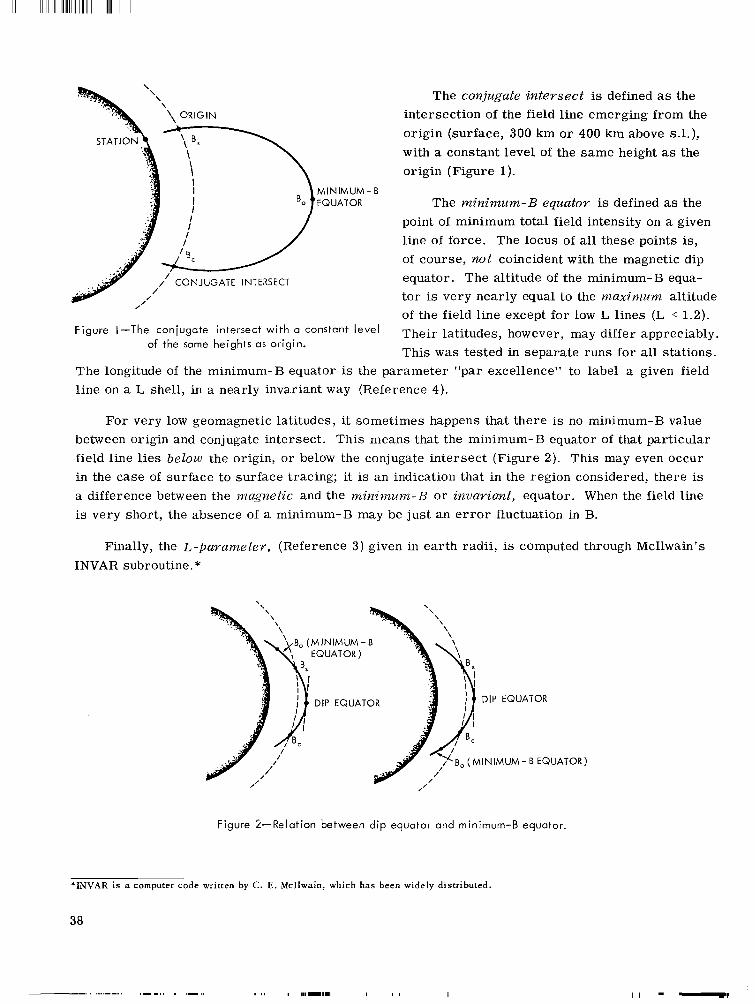
I l l IIIII IIIII l l 1 l l l l 1 1 l l l l l l 1 l l I I IIIII I I
STATION \ *B, 1
The coiijugate intersect is defined as the intersection of the field line emerging from the origin (surface, 300 km or 400 km above SA.), with a constant level of the same height as the origin (Figure 1).
The minimum-B equator is defined as the point of minimum total field intensity on a given line of force. The locus of all these points is, of course, not coincident with the magnetic dip equator. The altitude of the minimum-B equa- tor is very nearly equal to the maximum altitude
, of the field line except for low L lines (L < 1.2).
Figure 1-The conjugate intersect with a constant level of the same heights as origin.
Their latitudes, however, may differ appreciably. This w a s tested in separate runs for all stations.
The longitude of the minimum-B equator is the parameter "par excellence" to label a given field line on a L shell, in a nearly invariant way (Reference 4).
For very low geomagnetic latitudes, it sometimes happens that there is no minimum-B value between origin and conjugate intersect. This means that the minimum-B equator of that particular field line l ies below the origin, or below the conjugate intersect (Figure 2) . This may even occur in the case of surface to surface tracing; it is an indication that in the region considered, there is a difference between the magnetic and the Inininzunz-B or invariant, equator. When the field line is very short, the absence of a minimum-B may be just an e r r o r fluctuation in B.
Finally, the L-parameter, (Reference 3) given in earth radii, is computed through McIlwain's INVAR subroutine.*
MINIMUM-B EQUATOR )
DIP EQUATOR
Figure >-Relation between dip equator and minimum-B equator.
~
*INVAR i s a computer code written by C. E. Mcllwain, which has been widely distributed.
38
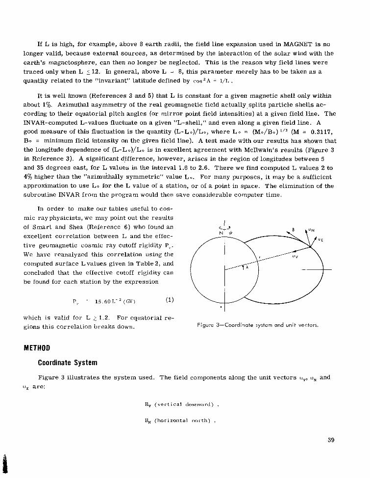
If L is high, for example, above 8 earth radii, the field line expansion used in MAGNET is no longer valid, because external sources, as determined by the interaction of the solar wind with the earth 's magnetosphere, can then no longer be neglected. This is the reason why field lines were traced only when L 5 12. In general, above L = 8, this parameter merely has to be taken as a quantity related to the "invariant" latitude defined by COS * A = 1/L .
It is well known (References 3 and 5) that L is constant for a given magnetic shell only within about 1%. Azimuthal asymmetry of the rea l geomagnetic field actually spli ts particle shells ac- cording to their equatorial pitch angles (or mirror point field intensities) at a given field line. The INVAR-computed L-values fluctuate on a given "L-shell," and even along a given field line. A good measure of this fluctuation is the quantity (L-Lo)/Lo, where L o = (Mo/Bo) lI3 (M = 0.3117, BO = minimum field intensity on the given field line). A test made with our results has shown that the longitude dependence of (L-Lo)/Lo is in excellent agreement with McIlwain's results (Figure 3 in Reference 3). A significant difference, however, arises in the region of longitudes between 5 and 35 degrees east, for L values in the interval 1.6 to 2.6. There we find computed L values 2 to 4% higher than the "azimuthally symmetric" value Lo. For many purposes, it may be a sufficient approximation to use LO for the L value of a station, o r of a point in space. The elimination of the subroutine INVAR from the program would then save considerable computer time.
In order to make our tables useful to cos- mic r a y physicists, we may point out the results of Smart and Shea (Reference 6 ) who found an excellent correlation between L and the effec- tive geomagnetic cosmic ray cutoff rigidity Pc. We have reanalyzed this correlation using the computed surface L values given in Table 2, and concluded that the effective cutoff rigidity can be found for each station by the expression
Pc ~ 1 5 . 6 O L - ' ( G V ) (1) I
which is valid for L 2 1.2. For equatorial re- gions this correlation breaks down. Figure 3-Coordinate system and unit vectors.
Coordinate System
Figure 3 illustrates the system used. The field components along the unit vectors u,, U, and uE are:
B, (vertical downward)
B, (horizontal north) ,
39

Ill1 Ill1 Ill IIIII I
and
BE (horizontal east) .
The equations defining an infinitesimal portion of a line of force are then,
6s is the element of arc , with components - b r , r E A and r cos AS@ along the unit vectors. The coor- dinates of a generic point of a field line originating at r s , A s and 4, a r e then given by
and
where the sign factor u is *1 according to whether one proceeds tracing in the opposite/same di-
rection of the field vector. Notice that i f the origin is in the magnetic Northern hemisphere (Bv > 0), we have to se t u > 0 in order to follow the line to the conjugate intersect* (direction opposite to i).
The total a r c length between origin and a generic point is
s" = h S i
i = l
COMPUTER PROGRAM
Procedure The flow diagram is shown in Figure 4. The altitude level of the origin is determined by an
input parameter which permits one of three internally programmed choices (station altitude, 300
*In our field computations using subroutine MAGNET, w e obtain the w e s t component of the field B , to reverse the sign in Equation 3c. (See listing, Appendix A ) .
= -BE. For this reason we had
40

and 400 km). Control parameters are initial- ized and the station is entered. The L value is computed with McIlwain's INVAR subroutine. The L value is then tested; i f L > 12, no tracing is 'attempted. Before the program returns to read in the next station, it computes the total field, the magnetic dip and the declination at the origin. Then, i f L 5 12, the code proceeds to t race the field line. The "Adams Four Point In- tegration Formula" (Reference ?) for numerical solutions of differential equations is used in this procedure repeatedly at equidistant intervals. The accuracy of this f i t depends on the integra- tion s tep s ize (element of arc length). To in- crease efficiency and to save computer time, the constant step size D for a given field line was fixed as a linear function of L in which
D = SOL - 30 (km) . (5)
Exhaustive testing with several step s izes for fixed L values has shown that Equation 5 is satisfactory with respect to both accuracy and machine time.
Initial conditions for the integration of the dependent variables H (altitude), DLAT and DLON are given, and the total field and its com- ponents are computed. The dip and the declina- tion are calculated only once, on the first pas- sage through the integration loop. A suitable control causes this part of the program to be bypassed thereafter.
Usage and Comments Figure 4-Flow diagram of computer program for
determining conjugate intersects.
The computer code is a FORTRAN I1 monitor controlled program written for the IBM 7090- 7094, Standard o r Moonlight system (Appendix A, Tables 1 and 2).
Execution time varies from fractions of a second for low latitude stations (small L-values) to several seconds for stations at high latitudes (large L-values). For the 511 stations considered in this work, the average time was approximately 2 seconds per station.
41

The choice of altitude levels presently contained in the code has previously been explained. Should other considerations prevail o r different use be made of the routine, new values can easily be substituted in statements number 58 and 59.
An effort has been made to keep the code flexible for diverse usage. Additional quantities con- nected with a field line, such as
1. maximum altitude attained above the earth's surface,
2. geographic coordinates of the intersect with the geographic equator,
3. conjugate mirror-points,
4. curvature at the equator, and
5. field components at origin and conjugate intersect
may become readily available through minor modifications.
The field computing par t of the program has been kept separate in the form of a subroutine. This is practical and advisable, as experience has shown. Since there exist several models de- scribing the geomagnetic field in te rms of a varying number of expansion coefficients and since periodic recomputations of these coefficients a r e necessary due to a gradually better knowledge of the field and its secular changes, this arrangement is most convenient for interchanging or up- dating the various models.
Two cases may a r i se which receive special treatment in the routine,
1. The origin may have an L-value greater than 12, and
2. No minimum-B equator may lie between the origin and the conjugate intersect.
In both, the code wi l l indicate their occurrence by printing relevant comments in place of the reg- ular output. In the tracing process, the location of the minimum-B equator is approximated on the field line with an e r r o r proportional to plus o r minus one integration step, while there a r e no limitations with respect to the number of stations o r the height of the origin. The restriction L imposed on the shell parameter is due to physical (see Field Parameters in the section titled FIELD LINE PARAMETERS) and practical considerations only (to save computer time) and is en- tirely independent of the code itself. Lines with L-values greater than 100 have been traced re- peatedly without any difficulty.
12
In the loop, the following sequence of operations is performed: (a) the total field intensity is tested at every step, and the coordinates and field intensity of the minimum-B point a r e stored; (b) the altitude, latitude and longitude increment parameters a r e evaluated; (c) the (n- 1)th dependent and independent variables a r e stored; (d) and the nth numerical integration is performed.
The integration is terminated whenever the altitude H" is less than or equal to the altitude of the origin H ~ . The total a r c length is then tested; i f S 5 1000 km, the step size is decreased by a fac- tor of 4, and the tracing is repeated for that given field line. This is done in order to obtain a
42

better f i t and to reduce the e r r o r in the location of the conjugate intersect, for low latitude stations. If S > 1000, o r after a second tracing, the coordinates of the conjugate intersect a r e obtained by interpolation, and the field intensity is computed at that point.
Finally, a test is made to determine whether the minimum-B equator l ies between the origin and the conjugate intersect. The results are printed, and the next station is read into the computer.
RESULTS
Table B1 (Appendix B) gives the results of our computations for surface-to-surface tracing for 511 geophysical stations. In column 1, the names of the stations a r e listed. Columns 2 and 3 give the geographical coordinates of the origin; column 4, the total field in gauss; columns 5 and 6, magnetic dip and declination in degrees respectively; and column 7, the L value. Columns 8 and 9 give the coordinates of the conjugate intersect, column 10, the total field at the intersect. Columns 11 and 12 show the coordinates of the equatorial (minimum B) point of the corresponding field line, column 14, the field intensity there, and column 13, the altitude of this point over sea level (almost coincident with the maximum altitude over sea level of that line, except for low L values). Column 15, finally, gives the total a r c length of the field line, between origin and conjugate intersect. All distances a r e in kilometers.
Appendix B, Tables 2 and 3 reproduce the values corresponding to field lines originating 300 and 400 km above each station and intersecting the same altitude as the origin, at the conjugate point. A detailed inspection of the conjugate a reas has revealed several features. F i r s t of all, as expected, the great majority of the stations have conjugate a reas over the sea. There a re , never- theless, 22 pairs of stations which a r e very nearly conjugate to each other and they a r e listed in Appendix C, Table 1. For additional information, the mean L value is given, as well as the per- centage difference in L. With a few exceptions, this difference is not much greater than the intrinsic fluctuation of I,. Another important parameter necessary to judge the "degree of con- jugacy" of two stations, is given by the difference of longitudes of the equatorial points of the field lines passing through both stations. This is indicated in the last column of Table 1. Inspecting this table, one recognizes well-known conjugate pairs, in addition to others. Notice in particular, the European-African group of conjugate pairs.
Appendix C, Table 2 lists stations with conjugate a reas in the Antarctica. Those already listed in Table 1 a r e not shown here.
Finally, in Table 3 we give some information about the conjugate a rea for those stations whose conjugate intersects fall over land, but where there is no other station near by, belonging to our list. In this table, we list the name of the station in alphabetical order, the L value, the name of the city or of the region in the conjugate area, and the country in question.
B AND L CONTOURS The last collection of figures represent constant B and L contours for different altitudes.
They were obtained in the following way: For a given altitude level, a latitude-longitude grid is
43

generated with constant intervals of five degrees for the first and of ten degrees for the latter. At those grid points, the magnetic parameters B and L are computed and stored.
The desired constant B or L contours are then obtained by a l inear interpolation, which is performed separately for both. The resulting positions are then plotted by computer and the curves are drawn manually.
ACKNOWLEDGMENT
We are grateful to Dr. J. C. Cain for many useful discussions and for his advice.
REFERENCES
1.
2.
3.
4.
5.
6.
7.
Jensen, D. C., and Cain, J. C., "An Interim Geomagnetic Field," J. Geophys. Res. 67(9):3568- 3569, August 1962 (Abstract).
Cain, J. C., Hendricks, S., Daniels, W. E., and Jensen, D. C., "Computation of the Main Geo- magnetic Field from Spherical Harmonic Expansions," GSFC Document X-611-64-316, 1964.
McIlwain, C. E., "Coordinates for Mapping the Distribution of Magnetically Trapped Particles," J. Geophys. Res. 66(11):3681-3691, November 1961.
Roederer, J. G., and Welch, J. A., "Calculations of Longitude Dependence of Geomagnetically Trapped Electron Fluxes, Part I, The General Fokker- Planck Equation for Electron Diffusion," GSFC Document X-640-65-149, 1965.
Stone, E. C., "The Physical Significance and Application of L, Bo, and R, to Geomagnetically Trapped Particles," J. Geophys. Res. 68(14):4157-4166, July 1963.
Smart, D. F., and Shea, M. A. , "A Study of the Effectiveness of the McIlwain Coordinates in Computing Cosmic Ray Vertical Cutoff Rigidities," Trans. Am. Geophys. Union, 46(1):63, March 1965 (Abstract).
Slayton, G. R., "Automatic Integration of Differential Equations," IBM, SHARE Distribution, Number 413, 1958.
44

Appendix A
Fortran II Monitor Controlled Program
Table A 1 Arguments and Parameters. Table A2 FORTRAN Listing.
45

Table A1
Arguments and Parameters .
Input: J
BLAT BLON BH NAME
Internal: RAD N L P ITEST D
fixed point parameter controlling start ing altitude; f o r J = 1, 2, 3 altitude is fixed in the code to station height, 300, 400 km, respectively.
geographic latitude of station. geographic longitude of station. height of station above sea level. designation of station.
S H DLAT DLON SGN DECL HM B BN BW BV FAC DH DDLAT DDLON CBN CBW CBV SP DLATP DLONP H P c 2
Output: BB DIP IDECL BEL CLAT C LON CB DLATM DLONM IHM BX DS
conversion factor, radians to degrees. fixed point parameter counting lines per output page. fixed point parameter numbering tracings per line. fixed point parameter controlling dip angle and declination bypass. constant incremental change of independent variable (stepsize of
independent variable: total arc-length. dependent variable: height above sea level. dependent variable: geographic latitude. dependent variable: geographic longitude. sign of vertical field component. magnetic declination a t origin. altitude above sea level of point of minimum B on field line. field strength at generic point. North component of field vector at generic point. West component of field vector a t generic point.* vertical component of field vector a t generic point. factor for increment parameters DDLAT and DDLON. altitude increment parameter. latitude increment parameter. longitude increment parameter. same a s BN at conjugate intersect. same a s BW a t conjugate intersect. same a s BV a t conjugate intersect. (n-1)th reference arclength for conjugate intersect approximation. (n-1)th reference latitude for conjugate intersect approximation. (n-1)th reference longitude for conjugate intersect approximation. (n-1)th reference altitude for conjugate intersect approximation. ratio of B(min) minus B(orig) to B(orig).
integration along field line).
field strength at origin. dip-angle at origin. see DECL magnetic shell parameter L of field line through origin. geographic latitude of conjugate intersect. geographic longitude of conjugate intersect. field strength at conjugate intersect. geographic latitude of minimum B point on field line. geographic longitude of minimum B point on field line. see HM minimum field strength on field line. total arclength between origin and conjugate intersect.
46

47

48

Appendix B
Field Line Parameters for Selected Geophysical Stations
Table B1 Tracing from Surface to Surface. Table B2 Tracing 300 km Above Stations. Table B3 Tracing 400 km Above Stations.
49


Table B1
Tracing from Surface to Surface.
5 1

Table B1 Tracings from Surface to Surface.
I h * * CChJIJGATE I N T E R S . ** P I h I C U V - E E Q U A T 0 K ** ARC S T A T I C h S
AEASHIR I AB I S K O ABERYSTWYTP ACCRA ADEN A O D I S A D A B A ADELA I O € ACAK AGINCOURT AHMEDABAD AIRE-SUR-ACGUR AKRCT I R I AKLAV IK A K I T A ALMERIA ALCAN ALERT ALMA-ATA AL8UQUEROU E A L C I R A h T E GROWN ANCON ANCHGRACE ANTOFAGASTA A P I A APAT I T Y ARKHANGELSK ARCETR I AREGU I P A ARGENTINE I S L A N D ARMIOALE ASSWAN AS 0 ASHKABAD ATHENS BAJA BAGbCAC BANGKOK EAR I BALBOA B A I E S T . P A L L BARTER I S L A K D 6AKER LAKE B A T T L E CREEK BANARAS BANGUI
* * C
L d T .
43.97 6 & . 3 5 52.40
5.63 L2.77
5 . c 3 -34.95
51.90 43 . 80 23.C2 43.70 34.58 68.23 3s.73 36.85 5E.60 82.55 43.20 35.C8
- t 4 . E 8 -11.77
61 .17 -23.65 -13.80
67.55 64.58 43.75
-16 .35 -65.25 -3C. 30
23.S7 3 2 . f 8 37.93 37.97 46.18 32.35 13.75 64.58
e.55 47.43 7C.13 64 .30 42.27 25 .33
R
LCNG.
140.33 18.82 -4.07 - 0 . 2 c 44.97 38.77
138 .53 -176 .65
-79.30 72 .60 -0 .30 32.S5
-135.CO 140 .13 -2.47
125.5C -63.58
76.92 -106 .62
-62.87 -77.15
- 1 4 9 . Y 8 -70.42
-171 .77 33.33 40 .50 11 .25
-71.57 -64.27 151 .40
32.78 131 .02
55 .10 23.72 19.00 44 .38
1CO. 55 -140 .18
-79.57 -70 .50
-143 .67 -96 .08 -85.17
83 .02
I G
0 C I P
0.506 58.4 0 .515 77 .3 0.477 68.0 C.311 -7 .4 0.369 9.7 0.353 -1 .4 0.606 -67.3 0.486 63.4 0.585 74.3 0 .447 32.1 0.452 60.1 C.447 4F.O 0.587 81.3 0 .483 53.7 0 .426 52.4 0 .591 74.6 C.560 85.9 0 .558 62.8 0.536 62.8 0.436 -57.8 0.286 C.5 0 . 5 5 8 74 .1 0.263 -18.4 0.398 -28.8 0.525 71.6 0 .531 76.7 0.457 59.6 C.27C -6.2 0.441 -50.2 0.565 -60 .9 0.390 30.7 0.470 46.7 0.502 56.3 0 .440 52.8 0.471 62.2 0.462 44.0 0.417 9.9 0 .583 81.3 0.387 37.3 0 .579 75.8 C .5@1 8 1 . 1 0.608 86.3 0.5R6 7 3 . 1 0.467 35.3
4.60 18.59 0.332 -16.1
DECL. L L P T .
-8 2
- 9 - 1 1
1 1 7 9
-7 - 1 -6
3 4 0 -7 -7
1.50 5.69 2.57 1.00 C.96 0.96 2.03 2.11 3.33 1.00 1.75 1.25 9.05 1.35 1 .41
-20.5 -59.5 -47.4
11.8 4.7
10.2 53.2
-38.9 -69 .8
-5.3 -32.1 -16.1 -62.8 -22.7 -22.9
LCNG. B L A T . LONG. ALT. B KM
137.8 0.557 64.0 0.482 24.8 0 .321 -1.5 0.323 44 .9 0 .351 38.8 0.355
1 4 3 . 3 0.542 164.8 0.587 -99.9 0.547 -
74.6 0.404 17.3 0 .314 35.6 0.345
167.0 0.661 138.1 0 .531
11.0 0.320
9.17 140.61 3 5 7 1 3.46 33.52 2 9 6 6 9 0.40 7.34 9 4 5 6 6.95 -0.49 15 6.78 44.89 3 c & O M I N I M U M E BETWEEN 9.52 142.68 6 9 4 5 6.03 174.60 7 2 5 3
12.38 -79.11 1 4 7 2 6 7 .81 73.34 4 9 9 2.66 7.23 4447 6.91 33.34 172C 1.29 -162.72 51758 9.03 140.45 2586 3.63 3.74 2 4 9 4
0.092 0.002 0.019 0 .311 0.348
INTERS. 0.037 0.034 O.CO8 0.303 0.059 0.156 o.co0 0.128 0.108
1 3 4 6 1 8 6 8 8 6 30770
7 1 0 9 0 6 1 2 9
2 2 9 9 5 24137 45473
3 5 2 1 1 6 1 8 8
7 7 6 4 147107 10596 1 0 3 2 6
-12 2.61 -39 .4 124.8 0.629 10.24 125.99 10707 0.017 33282 - 8 6 2 4 6 . 0 2 * * N O C O M P U T A T I O N S P E R F O R M E D * +
3 1 3 17
6 27
5 1 2 1 2 15 -2
4 1 8 1 1
2 -5
5 1 1 4 1
38 4
-19 37
4 -0 -0
1.53 -25.7 1.89 -49.1 - 2.31 35.9 1.03 -12.3 4.12 -53 .6 1.08 -3.1 1.05 15.2 - 5.02 -55.7 4.07 -51.7 1.66 -29.0 1.05 -9.8 2.35 36.3 1.65 46.9 1.04 -3.7 1.17 -16 .5 1.37 -22.0 1.36 -19.7 1.79 -31.5 1.23 -16.4 C.92 5.4 9.21 -62.0
82.7 ,128.5 -65 5 -77.2 172.2 -69.7
-106.1 69.4 69.1 24.3
-71.2 -66.0 159 .5
33.1
0.486 0.517 0.534 0.285 0.634
0.342 0.488 0.473 0.324 0 - 2 8 6 0.536 0.474 0 .342
0.313
8.35 77.75 3 8 0 9 0.085 1 3 8 3 4 -7 .94 -114.50 5762 0.045 20036
-12.97 -59.60 8083 0.025 2 7 1 8 1 NO M I N I M U M t3 RETWEEN INTERS. 57 2.95 -168.74 2 0 1 3 9 0 .004 59846
-16 .64 -69 .91 1 7 6 0.248 2373 2.47 -168.55 4 5 6 0.273 3 6 0 6 5.22 43.60 25502 0.002 7 5 1 2 1 5.95 47.44 1 9 4 5 0 0.005 5 8 2 1 9 4.33 16 .30 4042 C.068 1 4 8 9 7 NO M I N I M U M B BETWEEN I N T E R S . 7 2 9
-13.17 -60.30 8 3 1 2 0.024 27818 8.24 156 .83 4392 0.071 1 5 9 7 4 8.14 32.71 466 0.272 3413
30.3 0.493 8.72 131.52 1 5 0 5 0.195 7 2 2 4 59.7 0 .385 6 .68 55.42 2 5 7 3 0.121 1 0 3 4 9 29.3 0.340 6.36 25.48 2316 0.122 9 6 3 6
46 .4 0.353 6.54 44.30 1 6 4 9 0.165 7538 C0.4 0.411 9.06 100.49 40 0.401 932 63.8 0.663 2.52 -168.72 5 2 8 2 6 0.000 150008
31.5 0.327 4 .53 23.15 4 7 9 1 0.056 1 7 0 7 0
1.17 -32.7 -85.2 0.313 -13.60 -81.42 912 0.194 5 5 4 2 4.03 -75.5 -79.2 0.539 -12.46 -64.90 1 9 0 4 4 0.005 5 7 7 0 1 S.05 -61.4 161.9 0.664 3.18 -172.15 51803 0 .000 147162
15.00 * * N U C O M P U T A T I O N S P E R F O R M E D * * 3.01 -65.9 -1C9.6 0.551 -11.79 -87.99 1 2 7 7 6 0.011 3 9 9 1 1 1.02 -6.2 84.7 0.429 8.64 83.62 6 2 9 0.293 4 0 1 5
-5 0.99 17.7 17.5 0.355 9.56 18 .11 98 0 .319 1 5 0 0

Table B1 Tracings from Surface to Surface.
S T A T I C h S * *
BASE R C I bAUOCUIN BANGUIC BELEM BELSK BETTLES BEOFOR0 BERMUDA BECGRAC BIRD BISMARK BJORNOYA BCRCK BOLCGNA BOULOEK BOMBAY EOGCTA BRISEANE BUOAPE ST BUENOS R I R E S BUN I A
CAPRI
CATANIA CAPE CHELYUSK I N CAPE ZHELAhIA CAPE SCHXICT CPMBRICGE UK CARIBOU CALCUTTA CAPE HALLETT
CANBERRA CAP ET 0 H N CAM D EN CAPE CCNAVE'IAL CAPE JONES CEUU CHAMICAL CHURCHILL CHAM B ON- L A - F I1 it E T CH I CAGC CHARLOTTESJILLE C H I T 6 C H I T TAGfl! I!;
BYRO srArIuiU
CASTEL TES I l kU
CibMPeELL ISL.V,UC
Y, w
C R I G
L b T .
-7c .43 16.42 -1.co 51.84 66.90 42.48 32.37 44.eO 56.50 46. E2 74.52 58 .c3 44.50 4c.c3 1s.co 4.63
-27.53 46.68
-34.52 1.53
-7S.98 4c.57 46.C5 37.50 77.72 76.90 68.87 52.22 46.87 22.93
-72.32 - 5 2 .! 5 -35.32 -34.15 -34.08 Zt.40 54.50 1C.33
-3c.33 iE.77 4E.C2 41.43 3e.c3 92.c5 22.35
LCNG. B C I P
23.32 120.5e -49.00 20.8C
-151.84 -71.78 -64.67 20.52 94.20
-1cc. 77 19.02 38.33 11.35
-105.30 72.83
-74.08 152.92 21.27
3 0 . 1 8 - 120.0 2 14.33 11.65 15.07
104.28
-179.46 0.10
-68.02 88.52 178.22 169.15 149.00 18.32
150.68
-79.50 123.90 -66.33 -94.17
2.27 -97.67 -78.22 113.4e Yl.d2
-58.5~
68.60
-a0.60
0.457 -65.0 C.409 19.0 0.298 15.9 0.487 67.3 0.570 77.8 0.569 72.8 0.516 64.4 C.468 6C.8 0.605 75.7 0.599 74.6 0.527 80.1 0.521 72.9 0.459 60.4 0.566 67.9 0.427 23.7
0.546 -57.6 0.475 62.7 0.255 -32.1 C.340 -22.1
0.448 55.9 0.464 62.0 C.437 51.9 0.578 86.2 0.562 83.9 0.560 77.1 C.476 67.7 0.573 75.1 0.455 30.0 0.660 -e3.6 C.635 -76.0 0.596 -66.2
0.359 31.8
0.605 -74.8
0.312 -65.a 0.587 -64.8 C.517 61.4 0.602 E0.9 0.392 6.2 0.260 -27.3 C.613 E3.5 0.466 64.1
0;564 70.1 C.595 70.9 0 . 4 5 3 28.7
0.585 72.5
I
OECL.
-32 0
-14 2
29 - 14 -13
1 2
12 1 11 -2 14 -1
1 10 2 0
-1 70 -1 -1 -1 17 79 10 -7
-21 -0
-87 77 11
-27 12 0
- 1 8 1 5 3
-5 2
-5 -7
h * * CCNJUGATt INTERS. ** CINIMUM-8 E Q U A T 0 R ** ARC
KM LAT. LONG. 8 LAT. LONG. ALT. 8 L
5.21 0.95 1.09 2.24 5.98 3.11 2.04 1.69 2.48 3.38 9.55 2.86 1.71 2.32 0.96 1.13 1.51 1.81 1.20 1.00 7.25 1.48 1.81 1.35 9.36 Y.33 5.16 2.49 3.85 0.98 16 .Ob 4.02 1.99 1.83 1.89 1.77 6.58 0.93 1.14 8.h3 2.07 2.90 2.54 2.00
59.5 -0.8
-17.2 -39.7 -57.1 -70.8 -61.3 -29.4 -38.0 -62.6 -63.7 -45.2 -30.1 -54.4 -1.2
-30.5 43.7 -32.1
7.2 19.7 55.7
-23.Y -32.4 -19.5 -56.4
-52.7 -45.4 -75.3 -3.3
61.7 52.5 45.0 51.0
-53.9
4.7 2.7
-74.4
-64.3 -64.7 -33.5
-58.0
** N
-78.8
-38.0
-31.7 120.1 -44.6 38.8 164.2 -79.3 -60.9 31 -4 101.1
-135.3 77.3 59.3 25.0
-131.9 74.3
-77.2 160.5 33.6
-62.1 30.0
-78.9 24.0 26.5 22.7 113.3 98.4 150.9 26.7
-70.8 8'3.4
0 c o -154.9 158.5 -0.6 160.2 -93.5
-117.7 123.8 -66.6
-152.6 22.9
-113.1 -93.7 115.4
0.516 0.411 0 -247 0.334 0.654 0.511 0.404 0.329 0.585
0.546 0.410
0.552 0.396 0.285 0.454 0.328 0.364 0.375 0.601 0.332
0.336 0.646 0.607 0.657 0.320 0.525 0.427 M P U 0.553 0.507 0.456 0.496 0.442 0.602 0.394 0.342 0 -6 38 0.312 0.552 0.506 0.597
0.592
0.323
0.321
-5.35 7.93
-12.69 4.00 3.62
-12.90 -13.43
4.96 9.80
-E.95 4.23 5.62 4.19
-7.99 7.84
-15.23 8.32 4.79
-16.28 8.70
-12.02 5.20 3.e8 6.05 10.83 9.65 7.15 1.09
-12.21 9.05
T A T I I 3.48 '8.50 2.25 8.26
-12.04 7.32
-16.79 -9.64 1.98
-11.56 -12.98 10.03
-r3.05
-11.56 120.45 -45.60 26.23
-I 74.69 -66.99 -59.01 24.05 95.52
-110.21 40.59 42.80 16.57
-114.16 73.45
-74.97 157.96 25.11
-59.45 29.98
-77.34 18.07 17.23 18.09
104.41 77.70 164.48 10.43
-61.19. 88.87
I N S P -173.05 155.25 7.43
156.90 -82.23 -78.49 123.85 -65.83
-103.74 10.59
-91.62 -78.06 114.70
26283 165 9c
7527 32092 13244 6303 4253 9907 15304 54426 11716 4307 8516 247 605 3487 4964 819 192
39750 3004 4899 225C
53708 53367 26858 8908 17919 425
E R F 19492 6593 4970 5907 4812 35450
17 495
48685 6201 12122 9694 6916
0.002 0.364 0.244 0.029 0.001 0.010 0.036 0.065 0.020 0.008 0.000 0.013 0.063 0.024
0.213 0.093. 0.053 0.183 0.311 0.001 0.094 0.054 0.123 0.000 0.000 o.co2 0.021 0.005 0.327
O R M E 0.005 0.040 0.052 0.047 0.055 0.001 0.388 0.213 0. coo 0.038 0.012 0.C19 C.038
0.345
78127 1986 1913
25000 92780 41532 22148 15473 30963 46711 155251 36681 15683 27777 2383 4414 13394 17559 5412 2114
114912 11 772 17430 9462
152202 151583 78214 29160 54631 3204
D ** 58042 22151 17738 20246 17556
102970 62 5
4049 139215 21324 38040 31436 22646 ~~
-0 0.97 -2.7 92.4 0.428 S.C9 92.04 384 0.336 3029

S T P T I C K S * * c
C H R I S T C H U K C I - C H A C A L T A Y A C L I M A X C L C N C U K H Y CCFjCCRC COOK C O L L E G E CGR I N A L C C C O I M E R A C O N C E P C I C N CORDOBA COLCPEI : cocos I S L A N C C O P E N H A G E N C O R A L H A R H C U R C R A C C k C U R A C A t i cuzco D A V I S D A P A N G C D A L L A S C A U A R D A RW I N- C C I1 ,V A h A R R A O E B R E C C N O E R I L T O E E P R I V E R D E N V E R C E H R A CUN D E L H I O E C E P C I O N D I X O N I S L A i L C O J I B C U T I D J A K A R T A D O 0 A I IRA OOLGOPl lUI I iVPY A O C U R B E S D U N S I N K D U S H E T T I DURHAM D U C C N T C ' U 2 V I L L E D U R B A N E 0 I NBU!? G tI E I G H T S E L L S W O R T H E L I S A B E T H V I L L E
L P T .
-43.57 -16.32
39.37 -2C.67
43.20 -3C.63
64.85 43.63 4C. 22
-36.58 -31.32
6.90 -12.20
55.75 64.20 5c.c5 12.08
-13.52 - b e . 60
32.78 14.66
-12.43 47.48 52.10 4 6 . l C 39.75 3c.23
- 6 2 . $ 8 73.53 11.55 -6.17 36.00 55.94 5 c . 10 53.38 42.1)8 43.08
- 6 6 . t 7 -29.83
55.92 -75.23 -71 .72
i c . e o
z e . 6 3
Table B1 Tracings from Surface to Surface.
R I G I
LCNG. B C I P O E C L .
172.80 -68.15
-1U6.18 140.5C -71.53 130.40
-147 .83 13.00 -8.42
-72.98 -64.22
79 .87 96.90 12.50
- 8 3 . 4 0 19.95
- 6 8 . d4 - 7 1 . 9 8
78.00 0.07
-96 .80 -17 .43 130.Y0
21.65 5.18
-77.50 -105 .00
78 .05 77.2?
-60.72 80.70 43.15
107.00 139.7.0
37 .52 4.6C
-6.33 44.70
-70.Y2 140.02
31.C3 -3.18
-77.17 -41 .13
0.594 -68.9 0 .265 -5.4 0 .561 67.1 0.515 -5C.8 0.571 73.3 0.587 -63.8 0.570 77.0 0.458 59.4 0.440 57.1 0 . 2 9 1 -35.8 0.258 -28.3 0.4CO -6.5 0.470 -45.5 C.488 70.1 0.6CO 85.6 0.482 65.8 0 .404 43.5 0.276 -1.0 0.563 -73.2 C.321 4.2 0.536 62.7 0 .328 20.8 0.465 -39.2 c.477 63.5 0.477 67 .4
0 .565 67.7 0.493 44.8 C.483 42.0 0.416 -56.1 0.575 84.0 0 .363 6.2 0.443 -32.9 0 .465 49.4 0.517 71.4 0.472 65.8 0 .480 68.8 0.498 60.0 0.570 73.2 (3.671 -89.6 0.328 -65.2 0 .485 70.4 C.534 -67.1 C.513 -66.3
0.588 75.8
-11.63 27.42 0 .342 -47.9
2 1 1
1 4 6
-14 4
30 - 1
-10 12
4 - 3 -2 -0
-33 2
- 3 3
- 6 8 -10
9 -13
3 2
-4 -11
1 3 0
-0 15 26 1 2
-6 10 -4
- 1 1 7
-15 -70 -20
-9 3 2
9 -6
h * * C O N J U G A T E I N T E R S . * * M I N I M U M - 8 E Q U A T 0 R * * ARC
L L A T . LCNG. I3 L A T . LONG. A L T . B K M
2.41 1 .06 2.24
3.23 1.74 5.43 1.65 1.62 1.21 1.15 C.92 1.11 2.75
17.14 2.10 1.27 1.05
14.02 1.00 1.86 1.05 1.09 1.87 2.41 3.78 2.30 1.11 1.08 2.16 6.90 0.96 1.00 1.24 2.59 2.23 2.74 1.54 3.20
36.22 1.71 3.04 3.91 4.49 1.17
1.28
53.0 -162.4 0.506 4.19 -174.57 9166 0.023 29497 -10.5 -68.1 0.280 N O M I N I M U M 8 B E T W E E N I N T E R S . 6 4 7 -53.4 -132.1 0.546 -7.73 -115.00 8 0 1 0 0.027 2 6 3 4 9
37.5 142.7 0.463 8.96 142.83 2147 0.149 9 3 1 0 -71.5 -80.3 0.516 -12.65 -67.25 13969 0.009 4 3 5 4 6
48.7 131.8 0 .552 9.53 132.55 5 1 6 5 0.059 17896 -56.9 168.6 0.648 2.94 -169.77 28588 0.002 8 3 1 4 6 -28.5 25.3 0.326 4.46 17.68 3 9 6 0 0.070 1 4 6 4 4 -30.2 9.9 0.309 1.58 -0.05 3 6 7 7 0.073 1 3 9 7 3
9.1 -70.7 0.386 -15.53 -70.51 1042 0.176 6 1 3 4 3.6 -65.2 0.346 -16.70 -64.04 557 0.206 4 3 3 0
12.2 79.5 0.407 8.62 79.76 15 0.398 5 9 1 31.1 96.0 0.506 9.08 96.29 1239 0.226 6 1 4 3
* * N O C O M P U T P T I O N S P E R F O R M E D ' * * -47.0 38.6 0.345 2.70 21.21 10703 0.016 3 4 1 3 7
-37.2 36.1 0.328 4.18 .24.97 6 5 4 6 0.036 22176 -40.3 -70.2 0 ,297 -15.57 -67.87 1402 0.152 7 4 1 9 -12.5 -71.9 0.27Y N O M I N I M U M 6 B E T W E E N I N T E R S . 116
7.3 0.8 0.315 K O M I N I M U M R B E T W E E N I N T E R S . 402 -51.1 -116.8 0.497 -10.10 -102.87 5 5 5 1 0.047 1 9 4 8 5
-4.8 -11.9 0.288 2.42 -14.08 2 1 1 0.265 2 3 6 3 28.4 131.5 0.443 8 .63 131.84 975 0.243 5482
-33.2 34.6 0.328 4.63 25.64 5294 0.049 1 8 5 2 5 -43.5 29.3 0.321 1.91 14.22 8417 0.024 2 7 6 9 9 -72.5 -98.0 0.555 -12.60 -76.09 17572 0.006 53437 -54.3 -131.3 0.550 -8.14 -113.76 8 3 7 8 0.025 2 7 3 9 1 -12.0 80.9 0.440 8.20 78.84 1194 0.223 5 9 8 4 -10.4 79.8 0.431 8.20 78.01 9 9 4 0.244 5 3 1 9
34.1 -64.6 0.524 -13.18 -58.67 7 0 6 9 0.031 24327 -54.2 100.6 0.611 10.10 85.33 37660 0.001 108589
6.4 43.1 0.352 7.03 43.08 7 0.352 574 24.1 107.5 0.459 8.77 107.35 552 0.308 3777
-19.3 137.6 0.508 8.99 139.53 1918 0.163 8 5 8 1 -43.0 56.2 0 .392 5.57 41.40 10008 0.018 3 1 8 8 4 -40.6 26.5 0.315 2.01 13.07 7 1 9 4 0.030 2 4 1 8 4 -49.9 25.0 0.329 -C.23 6.06 ' 1 0 5 1 2 0.016 3 3 8 0 4 -26.2 50.6 0 .360 6.21 45.24 3505 0.086 1 3 1 6 3 -71.5 -78.5 0.513 -12.70 -66.34 1 3 8 0 8 0.009 4 3 1 1 2
* * N O C C M P U T A T I O N S P E R F O R M E D * * 45.1 19.7 0.468 4.82 23.42 4 3 5 8 0.063 1 5 7 8 7
* * N O C O M P U T A T I O N S P E R F O R M E D * *
-52.3 30.4 0.347 0.24 9.53 12446 0.011 3 9 2 4 4 47.0 -69.9 0.577 -12.48 -64.10 18368 0.005 5 5 8 3 5 50.7 -59.9 0.560 -11.09 -48.12 21885 0.003 6 5 8 1 3 31.7 24.5 0.422 7.50 25.46 1 2 1 3 0.189 6 1 3 1

j
Table B1 Tracings from Surface to Surface.
I A * * C C N J U G A T E INTERS. * * VINIMUN-B E Q u A T a R ** A R C S T A T I C h S
E N N A D A I ENUGU E S K O A L E M U I R E S P E R A N Z A E U R E K A F A R E W E L L F A N N I N G I S L A N D F L I N F L C N F O R T Y U K O N F O R T NCKMAN F O R T C H I M O F O R T VCNCCU TH F O R T B E L V C I R F O R T R A N D O L P H F O R T OE F R A N C E F R E E T C k N F R O B I S H E R F R E I B U R G F R O N T R O Y A L F T . C A Y I S GARCHY G A I N E S V I L L E
** C R I G
L P T .
61.30 6.47
55.32 -63.38
8C.CO 62.53
3.52 54.70 6 t . 5 7 64.SC 58.10 4C.25 38.73
5.38 14.10
e.47 63 .75 4e .c5 38 .93 3C.63 47.30 25.63
GENOVA MOluTE C A P E L G E N E R A L B E L G R A N O G E N E R A L SAtL M A R T I N GHANA G I F U G I L G I T GOUGH I S L A K C GODHAVN GOOSE B A Y G O T T I N G E N G R Y T V I K E V G R A Z GROCKA G R A N D B A H L P P GRAHAMSTOWN G R E A T WHALE K I V E R G U L M ARG GUANTANAPC! F A Y GUAM GUAYAQU I L H A M M A S H I R H A C H I J C J I V A H A L L E T T H A R T L A N D
44.55 -77.97 -6e .13
1 C . C C 35.58 35.54
-40.35 6 5 - 2 3 53.32 51.53
-54.27 47 .c7 44 .63 26.67
-33.28 55.27 34.05 19.90 13.45 -2.17 3C.10 3 2 - 1 3
-72.32 5 1 . C O
LCNG. B C I P
-101.20 7.55
-3.20 -56.96 -85 .93
-153 .90 -159.38 -1oz .oc -145.30 -125 .50
-68.43 -74 .02 -77 .13 -79.88 -61.02 -13 .22 -68 .57
7.58 -78.16
-103 .95 3.07
8.95 -38 .80 -67 .43
4.00 137.08
74.3c -9.89
-53.52 -60 .38
9.93 -36.50
15.47 20 .71
-78 .37 26.48
-77.76 74 .40
-75 .15 144 .75 -79 .88
0. 139.80 170.22
-4.48
- az . 3 c
0.613 84.2 0 .321 -9.0 0 .484 70.0 0 .413 -56.1 0 .571 87.5 0.557 74.5 0.333 10.7 0.613 e C . 1 0.576 78.6 0.596 81.3 0.584 80.7 0.566 71.6 0.565 7C.6 0.3YC 37.8 0.405 44.9 c .307 6.0 0 .582 82.7 0.468 63.9 0.567 70.8 0.512 58.7 0.464 63 .4 0.525 62.4 0.458 60.5 0 .513 -66.4 0.469 -60.8 0 .323 0.6 0 .469 49.3 0.521 53.7 0.279 -57.5 0.557 81.6 0.565 76.9 0.4'78 66.9 0.318 -50.9
0.468 60.6 0.506 59.9 0.320 -66.3 0.600 81 .1 0 .511 51.0 0 . 4 6 1 52.9 0 .364 11.9 0 .323 17.9 0 .397 42.4 G.447 45.6
0 .473 66.9
0.470 63.0
0.664 -84.9
DECL. L L A T . LCNG. 8 L A T . LONG. A L T . 8 KM
1 7 9.86 -72.4 -164.6 0.648 -8.02 -116.17 56632 0.000 161017 -9 0.99 13.9 6 .3 0.334 8.54 7.20 27 0.31Y 845 -9 2.95 -51.4 29.4 0 .341 0 .41 9.22 11857 0 .013 37578
6 8 3 1 4 . 7 5 * * N O C O M P U T A T I O N S P E R F O R M E D * * 1 3 2.20 34.7 -63.2 0.523 -13.08 -56.51 7285 0.029 24966
25 10 1 5 3 3 38
-35 -10
-6 4
-9 -14 -46
-3 -5 11 -5
1 - 3
7 22 -9 -6
1 -27 -52 -31
-2 -5 -0 1
-0 -24 -2 1
1 -0
1 5
-7 -5
-77 -9
4.27 0.98 5.54 6.45 8.23 8.40 2.81 2.62 1 .17 1.32 1.02
14 .83 2 .01 2.64 1 .65 1.98 1.82 1.73 4.59 2.65 0.99 1 .23 1.26 1.70
20.97 5 .33 2.30 1.82 1.86 1.68 1.69 1.84 6.99 1.21 1 .44
1 .05 1 .19 1.18
21.59 2.43
0.96
-53.4 168.8 -6.2 -161.2
-68.2 -149.4 -58.8 167.1 -64.2 177 .1 -85.4 -83.9 -68.1 -85.5 -65.7 -91.8 -33.1 -85 .7 -41.5 -55.2
3.2 -11.8
-36.5 26.0 -65.6 -94.1 -45.7 -122.2 -36.6 22.6 -54.5 -96.6 -30.7 23.5
51.2 -59.3 39.2 -67.2
9 .5 4 .1 -18.9 135 .8 -18.4 78.5
34 .7 -34.5
-80.2 -39.9 -41.3 31.4
30.4 -54.0 -33.3 29.9 -29.1 31 .5 -53.0 -89 .3
46.5 10.9 -80.1 -115.6 -16.4 78.2 -47.0 -82.1
1.8 144.3 -20.5 -82.3 -13.3 8.8 -16.7 138.4
-45.3 22.7
* * N O c o
* * N U C O
* * N O C O
0.638 0 .351
0.654 0.656 0.587 0.507 0.507 0.315 0 .271 0.297 M P U 0.316 0.512 0.483 0 .313 0.455 0 .321 0.560 0.550 0.322 0.507 0.450 0.445 M P U 0.532 0.322 0.479 0 .323 0.330 0 - 4 2 3 0.465 0 .601 0 -444 0.365 0.379 0.284 0.322 0 -489 M P U 0.315
0.628
3.44 -172.77 21141 0.004 62592 0.74 -159.94 46 0.328 1154
-8.37 -114.22 29092 0.002 04892 2.68 -169.36 35108 0.001 101129
-1.47 -150.08 46413 0.COl 132451 -11.82 -58.89 46897 0.001 134933 -12.85 -71.50 11384 0.014 36267 -12.83 -76.36 10214 0.017 32919 -13.67 -81 .81 949 0.191 5680 -15.20 -57.03 1 5 7 3 0.138 8075
3.61 -11.90 5 0.297 6 1 1
2.93 14 .65 5942 0 .041 20519 -13.01 -77.91 10339 0.017 33247
2.46 10.93 5803 0.042 20149 -12 .85 -84.46 5192 0.050 18620
3.67 14.72 4392 0.061 15957 -11.03 -47 .21 22518 0.003 67578 -12 .81 -61.47 10288 0.016 33351
NO M I N I M U M B B E T W E E N I N T E R S . 5 7 9.07 137.52 1864 0.167 8397 7.98 75 .11 2103 0.152 8830
-5 .31 -23.04 400C 0.064 15275
-11.05 -48 .01 27230 O.CO2 80636 2.77 17 .61 7754 0.027 25749
-11.64 -44.90 4717 0 .053 17651 4.08 20.54 5227 0.049 18369 4.94 24.23 4190 0.066 15286
-13.32 -79.32 4309 0.062 16140 3.79 16.77 5113 0 .051 18062
-11.99 -75.48 38020 0 .001 110131 7.86 75.22 1767 0.174 7809
8.83 144.60 66 0.353 1 3 1 3 -13.90 -81.20 155 0.267 2131
8.86 140.03 1492 0.192 7257
0.51 6.48 8488 0.023 28003
T A T I O N S P E R F O R M E D * *
-8.42 -110.58 4258 0.067 15760
T A T I O N S P E R F O R M E D * *
-14.19 -75.55 2640 0.102 11249
5 .63 4.26 1210 0.179 6218
T A T I O N S P E R F O R M E D * *
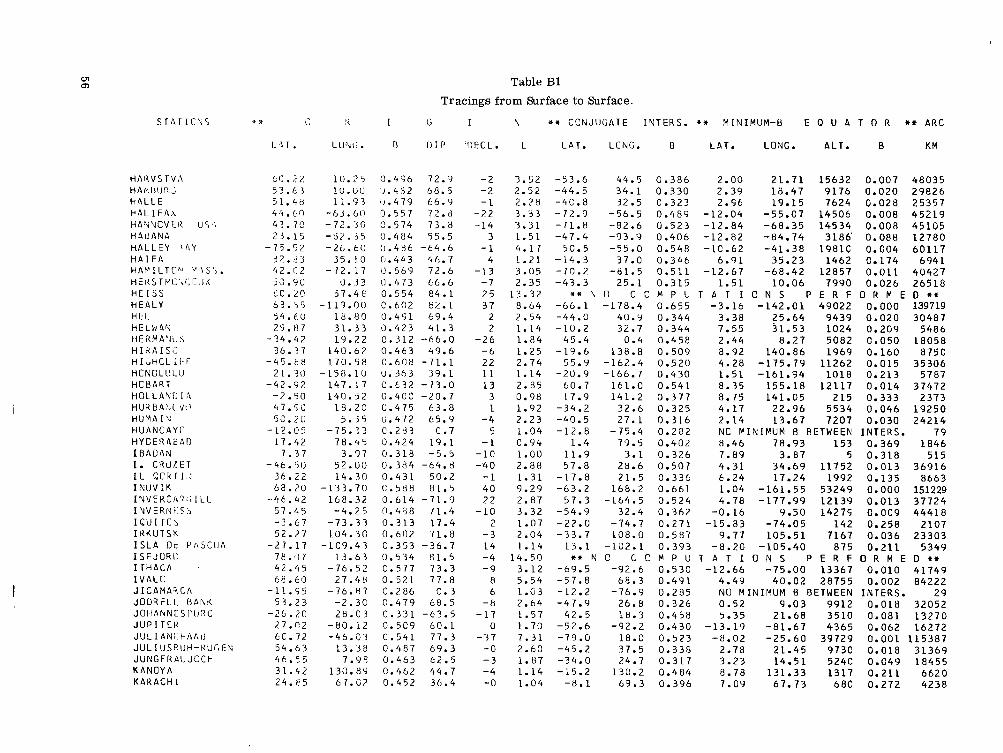
Table B1 Tracings from Surface to Surface.
s r A r 1 c k . S * * i: I< I ti I h * * C C N J I J G A T E I V T E R S . * * M I N I M U M - 8 E Q U A T 0 R ++ A R C
I. r . LUWi;. D O I P ‘OECL. L L A T . LCNG. 8 L A T . LONG. A L T . 8 K M
H A R V S T V ,I H A I*. t 5 I J r< A h 4 L L E H A L I F A A HAYUCVF.II U 5 , \ H4tlANA H A L L E Y H A I F A HAP’ I L T Z h l
HEISS H E A L Y H E L H E L 4 t< ti E RM A Y i J 5 H I R A I SC H I ~ H C L i f - T H C R C L 11 L I1 H C H A R T H O L L A ’ V C I ,A H U I< 8 A Y.1 L V!1 H U Y A I ’ V H U A N C A Y C HY C E H 4 E A I) I R A C A ; \ I I. C K c l L E T
I NIJV I K I N V E R C A 7 ; ; I L L I N V E Rbl i : S
I H K U T S K I S L A C t P n S C I J A I S F J URL I T H A C A I V A L C J I C A M A ’ t C A JODRELL i 3 A h K J OH A h N E 5 1’0 2 G J U P I T C K J U L I U N E H A L d JUL I I J S R IJH-K U i; EX J U NG F I< AU J C C + K A N O Y A K A R A C H I
‘4 .I 5 5 . ti E i( s r P C . ~ C ; c IJ A
IC c c r { r ~ . J
IGUI r c b
c c . 2 % 5 3 . 6 3 5 1 . 4 3
4 ? . 70 23.15
-75.52 3 2 . 3 3 ‘12.C2 5G.90 C C . 2 0 63.35 54.60 29.87
-34 .42 36.37
- 4 5 . t 8 2 1 . 3 0
-42 .92 -2 .50 41.52 52 . Zi)
-12 .05 17.42
1.37 - 4 6 . 5 0
36.22 68 .20
-46 .42 57.45 - ? .67 52.27
-21 .17 78.g17 42 .45 6 8 . 6 0
-11 .55 53.23
- 2 6 . 2 0 27.r l2 6C.72 54.63 46 .55 31.42 24.E5
4 4 . b n
10.25 1U.UO 11.97
-63.611 - 7 2 . 3 0 -92 .35 - 2 6 . 6 0
35.10
u . 33 57 .4e
- 1 1 9 . 0 0 1Y.80 31.33 19.22
1 4 0 . 6 7 170.58
147.17 1 4 0 . 5 2
L8.2C 5 . 3 5
-75.33 7 8 . 4 5
3.77 5 2 . 0 0
-133.70 168.32 -4 .25
-73.33 104:3C
- 1 c 9 . 4 3 13 .63
- 7 6 . 5 2 2 7 . 6 L{
-76 .87 -2 .30 211.03
-80 .12 - 4 6 . 0 3
13 .38 7.9q
130.84 67.C7
- 12.17
- 1 5 8 . i u
14 .30
0 .496 72.9 :J.482 68.5 0 . 4 7 9 t6 .Y 3 .557 72 .6 C.574 73.8 0 . 4 8 4 55.5 (1.486 -64.6 0 . 4 h 3 ‘t h. 7 0 .5h9 72.6 U.473 66.6 0 .554 e4.1 C.602 EZ.1 0 . 4 9 1 69 .4 9 .423 41.3 0.312 -66.0 0 .463 49.6 C.6C11 -71 .1 U.3h3 39.1 C.t-32 - ? 3 . 0 0.4CC -20.7 C.475 63 .8
C.Zd3 C.7 0 . 4 2 4 19 .1 0.318 -5 .5 0 . 3 8 4 -64.8 0 .431 50.2 C.588 81.5 0 . 6 1 4 -71 .9
0 .313 17.4 0.602 71.8 G.353 -36.7 9 .534 Rl.5 C.577 13 .3
C.286 C . 3 0 . 4 7 9 68.5 C . 3 3 1 - 6 ? . 5 0.5C9 60.1 C.541 77.3 0 .487 69.3 0 .463 62.5 0.462 44.7 0 .452 36.4
u.4- rz 65 .9
0 .488 .I L. 4
0 . 5 2 1 7 7 . 8
-2 - 2 -1
-2 2 - 1 4
3 - 1
4 - 1 3
-7 2 5 37
2 2
- 2 6 - 6 2 2 1 1 1 3
3 1
-4 5
- 1 -1C - 4 0 - 1 4 0 2 2
- 1 0 2
- 3 1 4 - 4 - 9
8 6
-8 - 1 7
0 - 7 7
- 0 - 3 - 4 -0
3.52 2.52 2.28 3.33 3.31 1.51 4.17 1 .21 3 .05 2.35
1?.32 8.64 2.54 1 .14 1 .84 1.25 2.74 1.14 2.85 0.911 1 .92 2.23 1 .04 c .94 1.00 2.88 1.31 9.29 2.87 3.32 1 .07 2.04 1.14
14 .50 3 .12 5 .54 1.U3 2 .64 1 .57 1.70 7 .31 2.60 1.87 1.14 1.04
-53.6 -44.5 -4C.8
-71.8 -47 .4
50.5 -14 .3 -70.2 -43.3
-66.1 -44.0 -10.2
45.4 -19.6
55.Y -20.9
60.7 17.9
-34.2 -40.5 -12.8
1 .4 11.9 57.8
-17.8 -63.2
57 .3 -54.9 -22.0 -73.7
13.1
-69.5 -57.8 -12.2 -47.9
42.5 -52 .6 -79.0 -45.2 -34.0 -15.2 -k.l
-72.9
* * h
*I. N
44.5 0 .386 34.1 0 .330
-56.5 0.489 -82.6 0 .523 -93 .9 0 .406 - 5 5 . 0 0.548
37.0 0.346 -81.5 0 . 5 1 1
25.1 0.315 0 C C M P U -178.4 0.655
40 .9 0.344 32.7 0 .344
0.4 0 .458 138.8 0 .509
-162.4 0 .520 -166.7 0 .430
161.0 0 .541 141.2 0 .377
32.6 0 .325 27 .1 0 . 3 1 6
77 .5 0.402
32.5 0.323
-75.4 0.282
3.1 0.326 28.6 0.507 21.5 0.336
168.2 0 . 6 6 1 -164.5 0.524
32.4 0.362 -74.7 0 .271 108.0 0.587
-102.1 0 . 3 9 3 C C C M P U
-92.6 0.53C
-16 .9 0.285 26.8 0 . 3 2 6 18.3 0.458
-92 .2 0.430 18.0 0.523 37.5 0 .338 24.7 0.317
130.2 0 .484 69 .3 0 .396
68 .3 0 .491
2.00 21 .71 1 5 6 3 2 0.007 4 8 0 3 5 2 .39 18.47 9 1 7 6 0 .020 2 9 8 2 6
-12 .04 -55.07 1 4 5 0 6 0.008 4 5 2 1 9 -12.84 -68 .35 1 4 5 3 4 0.008 4 5 1 0 5 -12.82 -84 .74 3186‘ 0.088 1 2 7 8 0
6 .01 35.23 1 4 6 2 0.174 6 9 4 1 -12 .67 -68.42 1 2 8 5 7 0 . 0 1 1 4 0 4 2 7
1.51 10 .06 7 9 9 0 0 .026 2 6 5 1 8
-3 .16 -142.01 4 9 0 2 2 0.000 139719
7.55 31.53 1 0 2 4 0.209 5 4 8 6
8.92 140.86 1 9 6 9 0.160 8 7 5 0 4.28 -175.79 1 1 2 6 2 0.015 3 5 3 0 6 1.51 -161.94 1 0 1 8 0 .213 5 7 8 7
8.75 141.05 2 1 5 0.333 2 3 7 3 4.17 22.96 5 5 3 4 0 . 0 4 6 1 9 2 5 0 2.14 13.67 7 2 0 7 0.030 2 4 2 1 4 N C P I N I H U M A AETWEEK I N T E R S . 7 9 8.46 78.93 1 5 3 0.369 1 8 4 6 7 .89 3.87 5 0.318 515
2.96 19.15 7 6 2 4 0.028 2 5 3 5 7
-1C.62 -41.38 1981C 0.004 6 0 1 1 7
T P T I C N S P E R F O R M E D * +
3.38 25.64 9 4 3 9 0.020 30487
2.44 8.27 5082 0.050 1 8 0 5 8
8.35 155.18 1 2 1 1 7 0 .014 3 7 4 7 2
4 .31 34 .69 1 1 7 5 2 0.013 3 6 9 1 6 6.24 17.24 1 9 9 2 0.135 8 6 6 3 1.04 -161.55 5 3 2 4 9 0.000 151229 4.78 -177.99 1 2 1 3 9 0.013 3 1 7 2 4
-0 .16 9.50 1 4 2 7 5 0.009 4 4 4 1 8 -15.83 -74.05 1 4 2 0.258 2107
9.77 105.51 7 1 6 7 0.036 2 3 3 0 3 - 8 . 2 0 -105.40 8 7 5 0 .211 5 3 4 9
T A T I O N S P E R F O R M E D * * -12 .66 -75.00 1 3 3 6 7 0.010 4 1 7 4 9
4.49 40.02 2 8 7 5 5 0.002 8 4 2 2 2 NU M I N I M U M R B E T W E E N I N T E R S . 2 9 0 . 5 2 9.03 9 9 1 2 0 .018 3 2 0 5 2 5.35 21.68 3 5 1 0 0 .081 1 3 2 7 0
-13.19 -81 .67 4 3 6 5 0.062 L6272 -8.02 -25 .60 3 9 7 2 9 0.001 1 1 5 3 8 7
2.78 21.45 973C 0.018 3 1 3 6 9 3.23 14.51 524C 0 .049 1 8 4 5 5 8.78 131.33 1 3 1 7 0 .211 6 6 2 0 7 .09 67 .73 68C 0.272 4 2 3 8

Table B1 Tracings from Surface to Surface.
I h *I CCFIJUGATE I N T E R S . * * M I N I M U M - H E Q U A T 0 R * * ARC S T A T I C R S *i c
L O T .
K A Z A C H I E K A P T O H I N K A Z A N K A K I C K A K A M P A L A K E K A H A KHARTOUC K H A B A H C V S K K H A R K O V K I E L K I R U N A K I N G SALtNCh K I E V K I N G S T C N KNOB L A K E KCROR I S L A h C K O T L E B U E K C L N KCMURC K O K U R U N J I K O O A I K A N A L K U H L U N C S H C * k K U M A S I K Y D T O L ' AQtJ I L A L A M A C C A L E N A L A H C R E L A P L A T A L A Q U I A C A L A P A L L b E L A CRAU L A H A Y E L E E O S L E I C E S T t l l LERW I C K L EN I NGK 11 E L E 1 c s C H E x r. A :a L E C P C L C I I L L E L I NO AlJ t HA I< L L I SBUA L I T T L E A:.lE,lIC.EI L O C R C k C L C V U Z E ii 0 L C N G Y E A i t n Y E I I LOIdUC'I
7 c . 7 0 7G. 42 55.83 3 6 . 2 3
c . 2 3 21.E4 1 5 . 5 8 48.52 5 C . C O 54.30 67.83 5e. 7 0 5c.45 1 e . c o 54.80
7 .16 &C.E8 50.93 35 .58 35.70 1C.23 54.12
6 .h7 j 5 . c z
42.40 41.22 31.55
-34.Y0 -22.10 -115.48
- 6 I 1 2 43 .10 52.1C 53.80 52.62 60 .13 5s.s5 52.08 -4.?7
3e.77 - 7 8 . 1 8
42.45 67 .$9 7E.22 51.53
51.65
P. I G
L C h G . E C I P
,136.4 C -21 .97
48.82 140.18
32.58 -159.72
32.58 135.12
36.23 10 .10 20.43
-156.7C 30.5C
- 7 6 . 8 0 -66 .92 123.49
- 162.60 6 . 9 2
139.62 139.48
1 1 . 9 3 -1.5e
135.78 13.32
9.40 74.33
-57.90 -65.6C -68 .05 147.11c
6 .00 4 . 3 0
- 1 . 5 5
- 1 . l b 3 c . 7 0
4.38 15.25 10.13 -9 .13
-162.17 -2.50 35.0P 15.67
77.48
- 1 . i c
i). I?,
0.584 G.523 0.536 0.463 0 . 3 4 1 0.363 0 .364 (1.543 0.504
0.515 0.540 0 .496 D.44Y 0 . 5 8 0 0.392 0.561 3.475 0 .464 0.462 C.401 0.4'?5 c . 312 0.469 (1.454 u.447 c.497 (1 .255 6.255 b.265 0 .416 C.452 c.477 (3.480 G.477 0.493 C.513 11.477 t i .330 0.478 c.435 0.642 C.448 0 .528 0 .534 c .475
u .4a4
e1.2 78.8 72.4 49.5
-24.2 33.5 12 .3 64.0 66 .0 69.0 77 .1 71.2 66.7 5c .4 7 8 . 9
76.6 66.5 49.3 49.0
2.2 6d.9 -4.4 43.8 58.0 56.8 47 .2
-32.6 -15.2
-5.7 -28.3
59.0 67.4 6d.9 6e.O 7 3 . 0 73.5 67.4
-34.8 67.0 55.6
-80.2 58.9 77.9 d1.6 67.1
-0.a
D E C L . L L A T .
-11 - 2 9
1 3 -6 -1 L2
1 -10
8 - 2
4 2 2
6 0
-3 1 2
2 2 -3 -6 -6 - 3 -1
-12 -6 -1 -3
0 0 1 1 5
- 4 -5 - 8 -8 - 9
9 -5 - 9 -2
-10 - 7 8
-7 1 3 -2
5.20 -50.3 1C.94 -72.6
2.55 -41.5 1.25 -19.5 1.00 20.3 1.14 -20.8 c.97 5.3 1.73 -30.5 2.02 -35.8 2.59 -45.5 5.43 -58.7 3.31 -49.7 2.07 -36.7 1.38 -44.2 6.35 -82.6 0.93 7.9 5.19 -54.5 2.28 -41.2 1.24 -19.3 1.23 -19.0 2.92 8.5 2.55 -44.8 1.00 10.3 1.22 -18.4 1.58 -26.7 1.54 -25.6 1.14 -13.8 1.20 7.6
1.06 -10.4 1.02 22.3 1.66 -29.2
2.70 -48.5 2.55 -46.5 3.70 -57 .1 3.20 -48.6 2.41 -43.8 1.07 25.1 2 .31 -41.5 1 .56 -28.4
1.08 -5 .1
2.42 -43.8
L C N S . L)
129.0 0 .660 60.3 0.535 6 5 . 1 0.429
138.5 0 .509 32.5 0.381
-168.4 0.433 32.6 0.343
133.1 0.585 48 .8 0.356 3 S . l 0.334 63 .6 0.477
171.3 0.622 44.5 0 .345
-84.2 0.357 -68.9 0.566 123.5 0.392 160.0 0.652
20.8 0.318 138.C 0 . 5 C 8 137.9 0.506
77.6 0.399 36.0 0.334 -2.4 0.318
134.7 0 .504 24.6 0.328 21.2 0.327 17.6 0.435
-61.8 0.366 -65.Y 0.300 -6d.O 0.281
20.5 0 .321 28 .8 0.320 26.0 0.329 26.6 0.322 38.4 0.388 56 .4 0.40d 28.8 0.320 11.5 0.379 31.6 0.322
148.6 0.375
L A r . LGNG. ALT. M KM
9.01 4.78 4.71 7.88
-16.34 -17.51
NO M 8.96 3.65 1 .82 0.77 0.76 0.24 4.63 1.82 e.20 2.86
1C.52 131.91 2 7 1 8 1 -2.25 6.88 6 3 0 2 0
6.44 51.40 9 8 6 2 9.09 140.46 1 9 4 8 8.39 32.41 2 3 4
8.62 32.53 55 9.54 135.70 5053 5.42 38.68 6 3 8 5 2.30 18.83 9 6 7 7 3.48 34.27 2 7 9 0 8 3.76 -172.61 L4956 4.98 33.82 6 6 1 8
-14.07 -77.86 2 2 3 6 -11.60 -57.35 3 3 7 7 %
7.75 123.50 0 5.19 177.60 27084 2.43 15.09 7 5 5 1
9.02 139.79 1 8 6 8 N f l M I N I M U M M UETWEEQ 2.79 20.11 9425 NO M I N I N U M B H E T W E E h
136.25 1 7 8 5
1.00 -163.64 1044
8.96 139.S2 1 9 1 2
17 .64 3553 14 .21 3200 75.15 1 3 8 6
-58.98 0 5 4 -65.55 106
8.4 0.309 1.63 13.10 * * N O c n M P u ~ P T I
1.6Y -31.0 15.0 0 ,313 2.41 5.15 -55.8 71 .0 0.495 5.54
14.42 * * N O C C n P U T b T I -7 2.41 -44.3 25.d 0.317 1.13
0.002 78882
0.019 31326
0.306 2 3 4 6 0 .211 5 8 7 9 0.337 1 1 6 0 0.060 1 7 6 1 7 0 .038 2 1 5 9 0 0.019 31254 o.co2 8 2 2 1 2 0.009 4 5 5 2 6 0.036 22307 0.117 9978 O.CO1 9 8 6 5 4 0.392 83 0.002 78925 0.028 2 5 1 9 0
0.000 179616
0.161 0604
(2.164 8566 0.166 8 4 3 1
I N T E R S . 1Y5 0.020 30512
I N T E R S . 4 1 9 0.173 0144 0.079 1 3 4 2 0 0.085 1 2 6 2 8 0.203 6 6 1 4 0.181 5556 0.249 1 9 4 3
N I M U M H B E T W E E h U T E R S . 148.20 4 3 9 0.293
12.01 397C 0.069 13.54 8481 0.023
9.70 9315 0.020 13.24 17238 0.006 37.28 13807 0.010
9.80 LO296 0.016
13.60 8 4 6 1 0.023 13.34 531 0.251 17.79 7 8 2 0 0.027 -1.00 3279 0.083
O N S P E R F O R M E 5.19 4102 0.065
45.23 26306 0.002 O N S P E R F O R M E
10.17 8 4 2 5 0.023
6 0 2 3520
14722 2 7 8 9 0 33135 30336 5 2 6 6 6 42650 27833
3710 2 5 9 3 3 1 2 7 8 3 0 + * 15185 7 7 3 1 6 0 ++ 27776

Table B1 Tracings from Surface to Surface.
S T A T I C I N S
L O M N I C K Y S T I T L O U R E N C O M A R Q U E S L U N O L U A N O A L U L E A L V O V LW I R O L Y C K S E L E M A K A T E A M A N I L A M A L V E R N M A J U R O I S L A N I ) M A D R I C MACAO M A C R A S MAWSON M A C Q U A R I E I S L A N C M A R I O N I S L A N D
MCMURDO SOUND M E A N C C U MEUOON M E M A M B E T S U M E X I C O E L C E R R I L L O M E L B O U R N E M I O W A Y I S L A A D M I E O Z E S L Y N M I N N E A P O L I S M I R N Y M I N A A G U I L A R M O U L D B A Y M O S H I R I MOCA MOSCCW MOUNT b4ASH I h G T C N MOUNT N D K I K U R A MONT J C L I M U R C H I S C W B A Y MURMANSK MGNCH E N N ARS S A R S S I ! A R N A R Y A N P A R N A T A L N A I R O B I N E U S T R E L I T Z
M A U I 9 K I H E I
* * 0
L A T .
49 .20 -25.97
55.70
65.60 49.82 -2.25 64.62
-16.2U 14.52 52.12
7.08 40.40 22.20 13.C8
-67.40 -54.30 -46.85
2c . eo -77.85
54.62
43.92 15.32
-37.82 6.97
52.17 44.97
-66.57 -23.10
16.20 44.37
3.35 55.47 44.27 36.12 48.60 8C .c5 68 - 9 1 48.13 61 .18 67 50 -5.?3
53.28
-8.82
48.80
-1.28
R I G
LONG. 8 D I P
20 .22 32.60 13.18 13.22 22.12 24.02
18.67 48 .20 21.00 -2.32 71 .13
113.55 80.28 62 .50
158.60 37.87
-156.50 166.62
-113 .33 2.25
144.2C -99.55 144.32 158.22
21.20 -93.23
92.92 -65.70
- 119.40 142.27
8.67 37.32
-71.30 137.55 -68.20
18.30
11.7C -45.42
53.00 - 3 s . 12
36.80
2 8 . 8 0
-3.68
33.08
0 . 4 8 0 65.1 0 .335 -63.0 0.489 70.1 0.329 -42.2 0 .512 76.1 0.486 65.8 0.34C -30.7 0.508 75.5 0 .373 -26.5 0.403 15.1 0.476 67.7 0.340 5.5 0 .440 56.8 0 .443 30.1 0.410 8.5 0.515 -69.5 0.653 -79.1 0.343 -64.6 0 .363 38.8 0 .655 -83.3 0 .603 77.8 0.468 64.8 0.495 57.6 0.439 46.0 0 .614 -69.2 0.350 0.4 0.488 67.6 0.596 74.3 0 .599 -76.8 0 .255 -16.8 0.585 87.5 0.503 58.4 0 .320 -16.6 0.516 11.1 0.573 74.0 0.470 49.9 0.516 76.1 0.539 82.5 0.527 78.2 0.470 64.0 0.541 77.4 0.549 79.1 0 .272 -4.4 0.343 -26.4
I
CECL.
2 -16
-0 -12
5 3
-2 2
1 2 0
-8 10 -8
0 -2
-56 26
-35 11
-36 2 4 -6 -8
9 10
6 3 6
-75 2
7 1 -8 -9 10
-15 -6
-22 - 1 12 -1
-38 21
-18 -0
N ** C O N J U G A T E I N T E R S . it* M I N I M U M - 8 E Q U A T 0 R ** A R C
L L A T .
2.03 -35.9 1.56 42.5 2.73 -46.8 1.13 28.2 4 .61 -56.3 2.05 -36.4 1.03 23.4 4.40 -56.2
0 .94 1.0 2.51 -46.2 0.97 1.7 1.59 -28.4 0.99 -5.3 0.92 6.1 8.63 70.8 5.25 67.3 2.71 55.5 1.13 -21.0
1.04 11.0
L C N G . 8
3 5 - 4 0.327 24.4 0.465 39.0 0.345
7.4 0.391 60.3 0.453 38.8 0.333 28.1 0.388 56.8 0.439
-143.3 0.342 120.6 0.405
25.3 0.319 170.2 0.353
12.7 0.314 l i 2 . 9 0.436
80.7 0 .401 -4.6 0.516
-164.8 0.561 11.8 0.487
-164.9 0.427 34.48 * * N 0 C 0 M P U
4.66 -62.9 -158.0 0.627 2.17 1.50 1.27 2.26 0.96 2.21 3.28
19.55 1.08
37.32 1.52 1.00 2.54 3.40 1.24 4.26
17.28 5.56 1.98 7.50 4.76 1.05 1.01
-39.2 -26.6 -35.2
55.8 6.6
-40.1 -64.6
-4.1
-26.9 17.0
-42.4 -72.5 -19.4 -76.9
-57.0 -35.6 -78.9 -52.3
-1.3 20.8
it* N
** N
* * N
L A T . LONG. A L T . 8 K M
4.35 24.94 6 1 1 2 0.040 2 0 9 1 3
2.76 21.72 10614 0.016 3 3 8 8 1 7.28 10.22 8 6 2 0.213 4 9 7 0 3.80 33.78 22759 0.003 6 7 7 0 0
8.57 28.28 397 0.279 3 1 2 0 3.16 30.59 21357 0.004 6 3 8 6 1
-1.68 -145.41 3 8 8 0.275 3316
0.82 8.54 9066 0.021 2 9 6 3 4 2 0.340 6 0 4 6.92 171.10
2.64 3.69 3 4 9 0 0.078 13362 8.42 113.41 4 4 5 0.322 3 3 6 3 8.62 80.53 27 0.39'6 7 8 0 0.35 19.85 4 8 2 7 7 0.000 138656 5.44 175.72 2 7 3 8 1 0.002 7 9 7 3 1
1.05 -160.31 9 9 5 0.215 5705
-5.57 -128.91 23520 0.003 6 9 3 5 1
5.51 26.84 3 4 9 1 0.082 1 3 1 9 1
4.48 28.23 6 3 5 5 0.038 21596
7.95 120.88 1 0 1 0,375 1542
2.50 20.61 1 0 5 5 3 0.016 3 3 7 2 4
F A T I O N S P E R F O R M E D * +
2.06 10.79 6 6 1 2 0.035 2 2 5 1 6 23.7 0.312 140.9 0.555 9.18 144.11 3 5 2 5 0.093 1 3 3 6 9
-110.4 0.392 -9.10 -103.92 1 7 5 9 0.149 8 3 2 3 153.0 0.533 8.88 150.25 8 3 2 4 0.027 26916
39.4 0.335 4.17 26.63 7 7 1 7 0.028 2 5 5 3 8 158.2 0.351 NO M I N I M U M B B E T W E E N I N T E R S . 4 1
-124.3 0.578 -10.47 -99.66 1 4 5 8 4 0.009 4 4 8 0 7 0 C O M P U T A T I O N S P E R F O R M E D * *
0 C O M P U T A T I O N S P E R F O R M E D * * -66 .0 0.304 -,17.44 -65.62 1 4 1 0.246 2 1 8 1
139.3 0.559 9.25 142.37 3 6 6 1 0.090 1 3 7 3 9 6.5 0.344 8.41 7.80 105 0.306 1581
55.5 0.388 5.39 41.10 9660 0.019 3 0 9 0 5 -80.1 0.522 - f 2 . 6 8 -66.72 15094 0.008 4 6 6 8 5 136.2 0.509 8.93 137.97 1 9 5 1 0.162 8 6 6 0 -72.0 0.537 -12.08 -61.09 2 0 4 9 1 0.004 6 1 7 7 5
71.6 0.502 5.20 44.48 2 8 9 1 1 0.002 8 4 5 5 9 0 C O M P U T A T I O N S P E R F O R M E O * *
28.6 0.319 3.45 17.88 5 8 1 8 0.042 2 0 1 2 4 20.5 0.524 -7.80 -24.59 40947 0.001 1 1 8 7 5 7 80.1 0.526 7 .28 59.32 23990 0.003 7 0 6 0 4
-36.5 0 .283 N O M I N I M U M B B E T W E E N I N T E R S . 476 36.9 0.390 7 .86 36.67 2 8 9 0.300 2 6 2 3
-13.08 0 .482 69.1 -14 2.88 -53.0 21.4 0.336 -1.45 0.84 1 1 4 1 3 0.013 3 6 4 3 5

Table B1
Tracings from Surface to Surface.
S T A T I O N S *it 0
N I A M E Y N I T S A N I M N I I G A r A N I C O S I A N O U V E L L E ACSTEROAM N O V O L A Z A R E V S K A Y A NGRO NORWAY S T A T I O N N O R F O L K I S L A N D NOUMEA N U R M I J P R V I O C E S S A O ' H I G G I N S R I S C P A T R O K I N A W A O L E N E K ONAGAWA OOH I R A ORCAOAS DEL SL;R O S L O K J E L L E H OTTAWA O U L U P A L E S T I N E P A N S K A V E S P A R I S - S A C L A Y P A R I S- B A G K E I! X P A N A G U R I T S C H P A R A M A R I B O PETROPAVLOVSK-ON-K P E A R C E P I C OU M I D I P I L A R P I W N I C E -TORUN P L A I S A N C E POSAGAS P O N Z A P O N T A OELGACO P O T C H E F S T K C C M P O I N T B A R R C h POTSOAM P O I T I E R S PORT ARTHUR PCONA PORO P C I N T PORT AUX F K A N C A I S P O R T S T A N L E Y cn
(0
L P T .
13.50 31.73 37.70 35.17
-37.84 -70.77
81.60 -70.50 -29.C0 -22.30 6C.50 46.78
-63.32 26.50 68.50 38.43 35.62
-6C.73 59.97 45.40 65.00 31.77 5c.53 48.12 48.80 42.52 5.E2
52.98 -31.67 42.93
-31.67 5C.52
-20.43 -27.42 4C. 92 37.77
-26.68 71.13 52.38 46.57 30.00 18.05 16.62
-4s.35
R I G
LUNG. 8 D I P
2.50 34.60 138.82 33.28 77.57 11.85
-16.67 -2.53 167.60
-166.4C 24.65 30.88
-57.YO 128.00 112.4C 141.47 140.50 -44.73 11.1c
-75.75 25.52
-95.63 14.57 2.33 2.32
24. I d -55.22 158.65 115.97 0.25
-63.88 14.57 57.67
-56.10 12.95
-25.65 27.08
-156.77 13.07 0.35
-94.00 73.12
120.28 70.27
0.330 0.437 0.476 0.45C 0.4R6 0.449 0.544 0.439 0.528 0.438 c.5c7 0.487 0.414 0.442 0.597 0.472 0.459 0.373 C. 496 0.584 0.514 0.531 0.478 0.466 0.468 0.465 0.343 0.5C9 0.589 0.449 0.258 0.478 0.378 0.243 0.448 0.443 0.330 0.573 0.482 0.461 0.522 0.423 0.410 0.472
9.2 44.9 51.6 49.9
-67.7 -64.0 83.3
-62.7 -56.4 -41.3 73.5 63.4
-56.1 37.6 112.6 52.0 48.7
-53.9 72.8 75.2 76.0 61.9 66.1 64.2 64.8 58.4 31.1 64.4
-66.4 59.2
-28.7 66.1
-54.3 -24.2 56.3 57.5
-63.8 80.3 67.6 62.8 60.4 21.6 19.4
-68.0 -51.70 -57.85 0.328 -47.0
I K it* C O N J U G A T E I N T E R S . * * M I N I M U M - B E Q U A T 0 R * * ARC
DECL. L L A T . LCNG. 8 L A T . LONG. A L T . 8 KM
-9 3
-6 4
-36 -2 5 -34 -17 14 13 6 5 14 -2 -6 -6 -5 4
-1 -12
7 9
-0 -5 -5 2
-11 -4 -2 -6 4 -0
-15 -4 -1 -16 -18 29 -0 -6 8
-1 0
-4 8 8
1.00 5.6 4.0 0.316 7.75 3.56 29 0.314 900 1.18 -12.9 36.2 0.346 7.17 34.69 1297 0.186 6403 1.29 -20.8 137.2 0.519 9.14 139.21 2208 0.147 9459 1.27 -16.9 36.1 0.345 6.75 33.70 1825 0.150 8098 2.32 54.1 65.5 0.565 7.72 66.95 8628 0.025 27623 4.61 56.3 -37.4 0.519 -6.64 -18.81 22445 0.003 67498 37.39 * * N O C C M P U T A T I O N S P E R F O R M E O * * 3.93 52.2 1.49 40.8 1.16 22.8 3.36 -50.4 1.80 -31.7 2.19 34.6 1.06 -10.7 4.60 -48.3 1.31 -21.5 1.23 -18.9 2.08 33.9 3.45 -53.0 3.64 -72.5 4.37 -55.0 1.81 -50.5 2.18 -38.8 2.08 -38.1 2.16 -39.2 1.56 -25.9 1.18 -29.0 2.02 -35.7 1.86 50.0 1.69 -30.7 1.15 4.0 2.18 -38.7 1.32 36.4 1.13 1.3 1.51 -24.6 1.73 -37.2 1.58 42.7 8.08 -58.9 2.35 -41.9 1.95 -36.3 1.72 -49.4 C.96 -0.2 0.95 -1.0 3.68 63.0 1.58 23.2
-43.5 -179.6 -157.1
53.3 41.2
-63.6 127.4 116.0 139.4 138.8 -58.3 44.5
-93.0 61.0
-1 14.7 33.0 23.0 23.8 32.4
-48.2 149.0 114.4 17.0
-65.0 33.0 53.8
-59.7 23.3 -1.7 16.7
156.1 34.3 20.3
-111.7 74.4
119.8 45.5
-63.0
0.524 0.422 0.369 0.402 0.339 0.523 0.456 0.643 0.522 0.505 0.506 0.383 0.545 0.451 0.489 0.323 0.312 0.312 0.335 0.240 0.598 0.589 0.315 0.348 0.323 0.493 0.326 0.330 0.288 0.457 0.664 0.327 0.311 0.474 0.395 0.412 0.537 0.464
-7.90 6.09 1.37 4.11 5.47
-13.12 8.38 10.56 9.17 8.91
-12.13 2.03
-12.54 4.01
-1C.08 3.35 2.28 1.85 5.74
-15.28 8.60 9.74 2.88
-16.77 3.34 6.56
-16.91 4.93
-2.78 5.03 5.12 2.92 2.22
-10.50 7.78 7.98 6.45
-14.15
-27.C3 174.51
-161.34 32.72 33.25
-57.03 128.21 112.57 141.69 140.74 -49.81 22.22
-73.43 35.97
-101.33 20.89 10.61 10.89 26.62
-51.01 155.34 115.58 7.45
-63.74 20.88 54.01
-57.24 17.03
-14.51 20.44 177.00 20.36 8.59
-99.22 73.71
J20.15 50.86
-58.23
18159 3288 1177 14727 4961 7247 803
23408 2323 1849 6433 15216 16642 21237 5223 6958 6251 6606 3488 568
6815 5970 4145 580
6950 2261 355
3121 4148 3598 45608 8140 5613 4664 20c 172
17008 3278
0.005 0.096 0.200 0.008 0.054 0.029 0.264 0. 003 0.140 0.167 0.035 0.008 0.006 0.004
0.032 0.038 0.035 0.082 0.199 0.038 0.048 0.065 0.204 0.033 0.134 0.218 0.091 0.062 0.078 0.001 0.025 0.044 0.059 0.353 0.363 0.006 0.080
0.051
55583 12894 6340
45308 17497 24852 4847
68408 9830 8383
22596 46861 50892 63426 18560 23414 21462 22503 13178 4409 22771 20000 15280 4434 23393 9414 3466 12135 15591 13541 129999 26831 19616 16974 2130 2031 5 1349 13379
: .
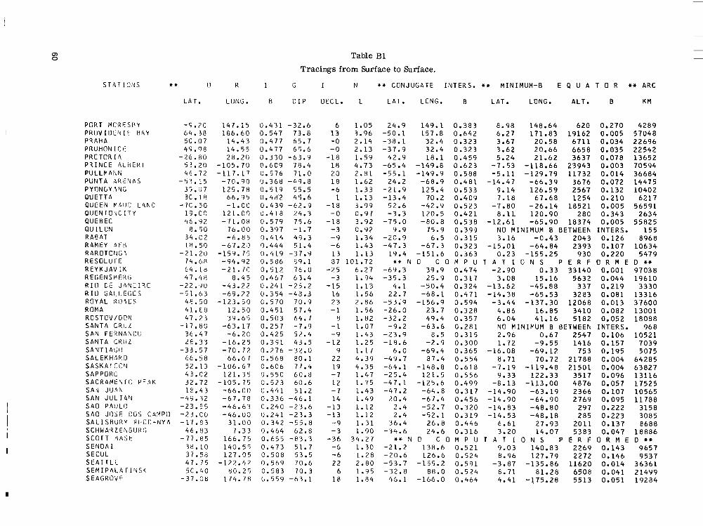
Q, 0 Table B1
Tracings from Surface to Surface.
I
S T A T I O X S * * 0
L A F .
P C K T m x c l s r i Y P R O V I O C ; U I L - R 4 Y P R A H A P R U H O N I C E P R E T O R I 4 P R I N C E A L H E R I P U L L )r A I\ b4 P U N T A B R E 9 A S PYONGY ? & C Q U E T T A Q U E E N V411[: L 4 N C
Q U E H E C Q U I L C N R A B A T RAMEY b F H R A R O T C P J G I R E S O L U T E R E Y K J AV I K R E G E N S H E R G R I O C E J Q N E I ? C R I U G A L L E G i S R O Y A L R O ? C S ROMA ROSTOV/DC!N
S A N F E R N A N C C S A N T A C K l l L S A N T I AGC S A L E K H Q K D S A S K A T C O Y S A P P O R O S A C R A M E Y T C P F A K SAiq JUAN S A N J U L I A ' $ S A 0 PAIJLO
W E N r o u c ITY
SAlVTA CRrJL
-5 .7c 6 4 . 38 5C.07 4S.98
-26.80 5 ! .20 46.72
- 5 3 . 1 5 37.il7 3C.18
-7c .50 19 .co 46.32
e . 5 0 3 4 . C 2 I t ? . 50
-21 .20 7 4 . 6 H 64.18 47.48
- 2 2 . ,90 -51 .63
4E.50 41.E8 4 7 . 7 3
-17.80 36.47 2 e . 3 3
-33.57 6 6 . 5 8 52.13 43.C2 32.72 l e . 4 3
-49.32 -23 .55
S A 0 J O S E C G S C A M P ( ] -23.C0 S A L I S H U R Y PbCI:-IVYA -17.03 S CHW AI7 2 E V 13 I J it G 46.83 S C O r T H A S t -11.85 S E N D A I 33.10 S E O U L 37.58 S E A T T L E 47.75 S E M I P A L A r I Y S K 5C.40
K I G
LONG. B D I P
147.15 1G6.60
14.43 14.55 28.20
-105.70 -117.17
-70.90 125 .78
66.95 -1.oc
121.00 -71.08
76.00 - h . 8 5
- 6.1. 2 :I - 1 5 9 . 1 5
-94 .92 - 2 1 . IC
8.45 -43.22 -69.77
-123 .50 12.50 39.65
-63.17 -6.2C
-16.25 -70.12
66 .67 -106.67
121.35 -105 .75
-66.00 -67.78 -46.63 - 4 6 . U 6
31.00 7 .33
166.75 140.55 127.C5
- 172 . /t 7 80.25
0 .431 -32.6 0.547 73.8 0.477 65.7 0.477 65.6 0.330 -63.Y 0.6C9 78.4 0.576 71.0 c1.368 -49.8 0.519 55.5 0.48'2 45.6 0.439 -62.9 11.418 24.3 0.579 75.6 0.397 -1.7 0.414 49.3 (1.444 51.4 0 . 4 1 9 -37.9 0.5d6 39.1 0 .512 7 0 . 0 0.467 63.4 0 . 2 4 1 -25.2 0.354 -48.3 C.570 70.9 0.451 57.4 0 .503 64.7 0.257 -7.9 0.425 52.4 0 . 3 9 1 43.5 0.276 -32.0 0 .568 80.1 0.6C6 77.4 '1.55C 60.8 0 .523 60.6 0 . 4 4 1 51.2 0.336 -46.1 0.240 -23.6 0 .241 -23.3 0 .342 -55.8 0.464 62.8 0 .655 [email protected] 0 .473 51.7 C.508 53.5 0 .569 70.6 0.583 70.3
I
D E C L .
6 1 3 -0 -0
-18 1 8 20 18 -6
1 -18
-0 - 1 8
-3 - 9 -6 13
N * * C O N J U G A T E I N T E R S . * * M I N I M U M - 8 E Q U A T 0 R +* A R C
L L A T . L C N G . R L A T . LONG. A L T . B K M
1.05 3.96 2.14 2.13 1.59 4.73 2.81 1.62 1.33 1.13 3.99 0.97 3.92 0.92 1.34 1.43 1.13
24.9 -50.1 -38.1 -37.9
42.9 -65 - 4 -55.1
24.2 -21.9 -13.4
52.6 -3.3
-75.0 9 . 9
-20.9 -47.3
19.4
149.1 157.8
32.4 32.4 18.1
-149.8 -149.9
-68.9 125.4
70 .2 -42.9 120.5 -80.8
75.9 6.5
-67.3 -151.6
0.383 0 - 6 4 2 0.323 0.323 0 .459 0 - 6 2 3 0.588 0.481 0.533 0.409 0.523 0.421 0.538 0.399 0.315 0.323 0.363
8.98 148.64 6 2 0
3.67 20.58 6 7 1 1 3.62 20.66 6 6 5 8 5.24 21.62 3637
-7.53 -118.66 23943 -5.11 -129.79 11732
-14.47 -66.39 3676 9.14 126.59 2567 7.18 67.68 1254
8 - 1 1 120.90 280 -12.61 -65.90 18374
N O M I N I M U M 8 BETWEEL 3.16 -0.43 2 0 4 3
-15.01 -64.84 2 3 9 3 0.23 -155.25 930
6.27 171.83 19162
-7.80 -26.14 1 8 5 2 1
0.270
0.034 0.035 0.0'18 0.003 0.014 0.072 0.132 0.210 0.005 0.343
0.005
0.005 I N T E R S .
0.126 0.107 0.220
4 2 8 9 5 7 0 4 8 22696 22542 13652 7 0 5 9 4 3 6 6 8 4 14475 10402
6 2 1 7 5 6 5 9 1
2 6 3 4 5 5 8 2 5
155 8968
1 0 6 3 4 5 4 7 9
8 7 1 0 1 . 7 2 * * N O C O M P U T A T I O N S P E R F O R M E D * * -2 5
-3 -15
16 23 - 1 Y
- 1 -9
- 1 2 9
22 19 -7 12 -7 1 4
-13 -13
-9 - 3
-36 -6 -6 22
6
1.82 -32.2 1.07 -9.2 1.43 -23.9 1.25 -18.6 1.17 6.0 4.39 -49.7 4.35 -64.1 - 1.+7 -25.4
49.4 0.357 -63.6 0.281
-2.9 0.300 8.5 0.315
-69.4 0 .365 - ,148.8 0.618 121.5 0.556
87.4 0.554
6.27 -6Y.3 39.9 0.474 -2.90 0 .33 33140 0.001 9 7 0 3 8 1.94 -35.3 25.9 0.317 3.08 15.16 5 6 3 2 0.044 1 9 6 1 0 1.13 4.1 -50.4 0.324 -13.62 -45.88 337 0.219 3330 1.56 22.7 -68.1 0.471 -14.38 -65.53 3283 0.081 13316 2.86 -53.9 -156.9 0.594 -3.44 -137.30 12068 0.013 3 7 6 0 0 1.56 -26.0 23.7 0.328 4.86 16.85 3410 0.082 13001
6 .04 41.16 5 1 8 2 0.052 18088 NO M I N I M U M B B E T W E E k I N T E R S . 9 6 8 2.96 0.67 2547 0.106 10521 1.72 -9.55 1416 0.157 7 0 3 9 6.08 -69.12 7 5 3 0.195 5075 8.71 70.72 21788 0.004 6 4 2 8 5 7.19 -119.48 2 1 5 0 1 0.004 6 3 8 2 7 9.33 122.33 3517 0.096 13116
1.75 -47.1 -125.6 0.499 -8.13 -113.00 4 8 7 6 0.057 1 7 5 2 5 1.43 -47.2 -64.8 0.317 -14.90 -63.19 2366 0.107 10565
1.12 2.4 -52.7 0.320 -14.83 -48.80 297 0.222 3158 1.49 20.4 -67.4 0.456 -14.90 -64.90 2 7 6 9 0.095 1 1 7 8 8
1.12 2.4 -52.1 0.319 -14.53 -48.18 285 0.223 3085 1 .31 36.4 26.8 0.446 6 - 6 1 27.93 2 0 1 1 0.137 8688 1 - 9 0 -34.6 24.6 0.316 3.20 14.07 5 3 8 3 0.047 1 8 8 8 6
34.27 * + N O C O M P U T A T I O N S P E R F O R M E D * * 1.30 -21.2 138.6 0.521 9.03 140.83 2 2 6 9 0.143 9 6 5 7 1.28 -20.6 126.6 0.524 8.96 127.79 2 2 7 2 0.146 9 5 3 7 2.80 -53.7 -155.2 0 .591 -3.87 -135.86 11620 0.014 3 6 3 6 1 1.95 -32.8 88.0 0.524 8.71 81.28 6 5 0 8 0.041 214Y9
S EAGRO'J E -37.G8 114.78 b.559 -63.1
I
18 1.84 46.1 -166.0 0.464 4.41 -175.28 5 5 1 3 0.051 1 9 2 8 4

Table B1 Tracings from Surface to Surface.
I N * * C O N J U G A T E I N T E R S . * * M I N I M U M - H E Q U A T 0 R * * ARC S T A T I O N S * * 0
SHEPHERD CAY S H I R A Z S H A C K L E T CN S H E F F I E L O SI MOSATC S I OMOU T H S I T K A S I M F E R 0 P (1 L S I N G A P O R E SLOUGH S O O A N K Y L A S O U T H P G L E S R E O N I K A N ST. STEPHEIL S T E L L E N T O S C I S T O C K H O L M STONYHURST
S T A N L E Y ST. S A N T I N - C E - M A U K ST. M I C H E L S T A N F O R U
S U K K E R T f l P P t N S U L P H U K N C U h T A I N S U R L A R I S V C R C L O V S K SWANSEA S W A K T H C 0'1 E SYDNEY
SYOWA B A S E T A M A L E T A S H K E l L r T A M A N R A S S E T T A I P E I T A L A R A T A N A N A R I V C T A H I T I T B I L I S 1 T E N I E N T E Y A T I E n l Z L I T E H R A N T E N E R I F E T EOLOY U C A A T H U L E
ST. L A h R E N L E
sr. JOI-NS
S Y K T Y V K A:<
E T H E P A S
L A T .
68.75 29.63
-17.98 53.43 33.58 5C.68 57.05 44.83 1.32
51.48 67.31
-9C.CO 62.43 67.20
-3?.94 55.3c 53.51 SC.58
-51.70 44.60 43.42 37.43 47.52 65.42 51.10 44.68 56.73 51.63 39.40
-33.60 61.10
-6S.C3 9.42
41.42 22. 80 25.C3 -4.57
-1e.92 -17.48 41.12
-64.97 35.68 2B.CO 15.75 76.55
R I G
L C N ~ ~ . R LIP
-93.15 52.52
-37.11 1.35
75.94 3.22
35.33 34.01 03.82 -0.51 26.65 0.
152.32 -45.20 18.85 18.10 -2.41 1.23
-57.85 20.20 5.72
-122.11 -32. 78 -57.30
-1 15.60 26.25 61.01 -4.00
-13.35 151.10 50.80 39.60 - O . R 9 69.20
121.52 -81.25 47.55
-149.48 44.82
-60.95 51.42
-17.0C
-68.83
5.52
-99. la
c.599 8 e . i 0.459 44.5 0.512 -66.4 0.479 68.5 0.461 46.9 0.413 66.3 C .5 72 74.3 0.481 61.8 0.411 -18.4 0.475 67.1 0.519 71.2 0.599 -75.1
0.545 19.8 C.312 -65.9 0.499 72.5 0.479 68.1 0.412 66.3 0.320 -47.9 0.467 6C.6 (1.454 59.9
0.536 72.0 0.556 8C.3 0.592 14.7 0.415 61.0 0.559 14.1 0.475 67.4 0.567 11.4
0.544 75.1 0.411 -66.3 u.311 1.5 0.540 6 0 . d 0.365 79.2 0.441 35.5 0.312 12.1 0.354 -53.7 0.381 -29.1 0.491 59.7 0.431 -51.5 0.486 53.1 0.389 43.3 0.443 45.7 lr.568 85.4
0.550 13.3
0.518 01.8
0.5~4 -64.3
5 3 . 0 0 -101.30 0.612 7Y.6
D E C L . L L A T . LCNG. B L A T . LCNG. A L T . 8 KM
-18 29.31 * + N U C O M P U T A T I O N S P E R F O R M E D + * 3 1.15 -13.5 54.4 0.364 6.50 52.58 1198 0.204 6075 6 4.61 51.4 -58.9 0.559 -10.96 -46.55 22675 0.003 68021
-6 -5 -5 29 6 2
-7 8
-27
2.61 1.18 2.29 3.91 1.68 c.94 2.42 5.09 13.52
-46.9 -11.1 -41.9 -55.6 - -29.2 11.2
-44.5 -56.9
* 4 N 0 - 8 3.09 -44 13.13 -26 1.82
2 3.22 - 8 2.60 -6 2.31 8 1.58 1 1.68
-4 1.71 17 1.84
-27 3.47 -46 13.06 73 3.62
3 1.68 14 2.62 -9 2.48 -8 2.11 12 1.85 17 3.39
-42 6.16 -11 1.00
4 1.41 -6 1.05 -1 1.03 6 1-04
-10 1.30 12 1.06 6 1.52 16 2.32 5 1.30
-12 1.25 9 1.28
29.0 0.326 1 . 3 3 34.9 0.494 8.94 26.4 0.316 1.95 75.2 0.625 -0.35 42.3 0.342 5.70 04.1 0.427 8.79 25.4 0.317 1.04 65.1 0.477 4.44
C O M P U T A T I -43.8 141.3 0.641
45.0 0.3 0.457 -50.4 47.4 0.381 -48.4 27.1 0.327 -42.4 25.2 0.314 23.2 -63.0 0.464
-29.1 31.0 0.329 -30.5 21.0 0.319 -45.1 -144.5 0.530 -71.6 ' -24.8 0.450
* * N O C C M P U
* * N O C C M P U
11.82 136.36 12.18
-153.53 35.69 104.00 9.64 38.43
~ N S P
9702 1574 7634 18773 4256 147
8449 25897 E R F
0.018 0.188 0.028 0.005 0.067 0.378 0.023 0.002
O R M E
31412 7406
25465 56124 15419 1827
27851 76324 D * *
-5'1.3 -28.3 -41.0 -46.1 -67.4
-41.3 64.0 8.2
-24.6 -3.1 -9.0 -11.4 35.6 12.6
-25.3 36.1
-19.6 -18.7 -35.8
50.4
-154.3 0.610 35.7 0.334 15.7 0.402 23.8 0.317
-88.4 0.509 160.6 0.492 72.4 0.411
-21.2 0.511 -0.6 0.315 75.1 0.452
120.9 0.450 -83.0 0.285 44.1 0.473
-143.7 0.347 50.5 0.360
-64.5 0.532
-3.6 0.298 -113.3 0.396
9.8 0.322
54.d 0.369
8.90 147.92 13723 0.011 41839
2.41 8.10 4949 0.052 17668 3.00 27.14 13785 0.010 42761 0.60 9.00 10158 0.017 32153 1.39 10.68 7714 0.027 25721
-14.15 -58.23 3278 0.080 13379 4.89 23.75 4185 0.066 15274 3.49 11.99 4270 0.063 15615
-4.48 -131.62 5515 0.049 19303 -1'2.03 -39.50 15244 0.007 47421
T A T I O N S P E R F O R M E D * *
T A T I O N S P E R F O R M E D * + -5.24 -129.89 16904 5.26 28.84 4180 7.61 63.01 10480 0.47 7.10 8880
-12.89 -73.55 11111 8.42 157.30 5672 6.63 54.95 15251
-3.14 0.65 32380 NO M I N I M U M 8 RETWEEN 7.70 69.94 337C 7.79 1.75 402 8.40 121.58 678
-13.39 -82.36 7c 6.42 44-77 203C
-1.46 -146.34 402 6.34 45.31 3408
-12.82 -58.02 8122 6-44 51.56 2109 1.41 -10.22 1394
-9.09 -103.59 183Y
0.006 0.067 0.017 0.021 0.014 0.050 0.008 0.001
I N T E R S . 0.096 0.263 0.284
0.142 0.264 0.088 0.024 0.141 0.158 0.144
0.279
51027 15232 32884 29122 35488 19592 46375 94935
143 12609 3184 4341 1463 8730 3741 12874 27309 0960 6977 8580
-78220.13 * * N O C U V P U ATI IONS P E R F O R M E D - 14 5.24 -67.9 -147.1 0.625 -8.34 -112.87 27154 0.002 79540

S T A T I C N S t* C
L P T .
T I H A N Y T I X I E B A Y T I R U C H I R A P A L L I TOR I NO T O T T O R I T O R U N T O M S K T O R R E C H I A H L C C I A T O R T O S A T O L E C C TOYOKAWA T O N A N Z I N T L A T O W N S V I L L E T R U J I L L O TROMSO T R E L E W T R I V A N D K M M T R I N I C A C T S C H O I B A L S A N T S U M E B T U 8 I N G EIU T U C S C N T U C S O N T U C U M A N U J I U L A N F!ATUR U N A L A S K A U N I V E R S I T Y P A R K U P P S A L A U S H U A I A U T S J O K I V A L E N T 1 A V E R K H O Y A N S K V A L C ' C R V I C T O R I A V L A O I V C S T C K V O S T U K WATHERCO WAKKANA I WASH I N G T O N W A L T A I H W E L L E N W E S T F O R D W E I S S E N A l J W E L L I N G T U W
46.89 71.55 10.83 45.20 35.53 5?.08 56.47 42.C3 4C. 82 39.88 35.83 1S.C3
-19.10 -8.10 69.67
-43.20 8.42
1C. 60 48.07
-19.23 48.53 32.23 32.23
-26.90 34.90 47.78 53.E8 40.80 59.80
-54.80 69.75 51.74 61.60 4E.CO 48.40 43.78
-76.48 -3C.32 45.40 38.73
66.17 42.58 47.00
-41.28
17.57,
- ~
- - Table B1
Tracings from Surface to Surface.
~
~ ~
~
R I G I N * * C O N J U G A T E I N T E R S . ** M I N I M U M - 8 E 6) U A T 0 R ++ A R C
L O N G . B D I P D E C L . L L A T . LCNG. 8 L A T . LONG. A L T . 8 K M
17.89 128.90 78.83 7.65
134.22 18.55 84.93 11.83 0.50
-4.05 137.37 -98.30 146.50 -79.03 18.95
-65.30 76.95
-61.20 114.50 17.72 9.07
-110.95 -110.95 -65.40 135.78 106.75
-166.53 -77.77 17.60
-68.30 27.03
-10.25 133.40 -77.8C
-123.40 132.03 106.50 115.88 141.68 -77.13 83.30
-169.84 -71.42
9.50 174.77
0.472 62.8 0.588 82.6 0.403 3.3 0.459 61.2 0.477 49.7 0.487 68.2 0.597 75.5 0.451 57.6 0.442 56.9 0.438 56.2 0.469 49.5 0.440 45.9
0.298 6.8 0.517 77.9 0.297 -40.6 0.398 -2.1 0.383 40.4 0.583 66.9 0.332 -57.2 0.470 64.3 0.510 58.9 0.510 58.9 0.255 -22.5 0.469 48.6 0.589 67.3 0.505 66.1 0.574 72.2 0.499 72.8 0.373 -5C.6 0.523 78.3 0.478 68.0 0.587 79.7 0.593 77.0 0.570 70.9 0.528 59.8 0.627 -79.5 0.582 -65.1 0.510 59.6 0.565 70.6 U.427 18.6 0.555 75.4 0.569 72.9 0.468 63.7 0.580 -66.7
0.498 -48.0
0 1.84 - 1 1 5.55 - 2 0.92 -3 1.78 -6 1.23 2 2.38 7 2.51
- 1 1.57 -6 1.57 -8 1.56 -6 1.24 9 1.27 7 1.24 6 1-03 2 6.29 10 1.33 -3 0.92 -8 1.26 -6 1.73
-16 1.34 -2 2.04 13 1.67 13 1.67 3 1.11
-6 1.21 -3 1.72 15 2.42 -7 2.88 2 3.32 17 1.69 8 6.04
-12 2.64 -13 4.22 -12 4.22 2 3 2.85 -9 1.50 72 103.75 -2 1.76 - 9 1.56 -6 2.62 -1 0.94 16 4.59
-14 3.13 -2 1.97 20 2.15
-32.7 -50.9
8.1 -32.0 -18.9 -41.8 -38.5 -2-6 4 -27.5 -27.8 -19.1 -35.3 35.5
-15.0 -60.5 14.6 10.2
-37.8 -29,9 36.5
-36.8 -44.5 -44.5 -0.5
-18.3 -29.5 -43.1 -67.5 -51.1 25.7
-.5 8.8
-47.5 -74.1 -53.8 -26.2
48.6 -27.8 -65.7
2.0 -52.3 -70.9 -35.6 50.1
-49.5
* * N
31.4 124.9 79.0 23.3
133.2 38.8 94.0 23.3 15.5 12.1
136.0 -109.1 149.8 -79.9 66.7
-66.2 76.8
-56.3 115.9
8.5 27.4
-130.0 -130.0 -65.9 134.7 109.2 169.7 -94.3 47.9
-67.7 70.2 21.0
128.4 -100.9 -156.7 130.'9
0 c o 114.5 138.7 -91.8 84.1
157.7 -79.7 26.9
-162.4
0.325 0.658 0.400 0.319 0.508 0.336 0.562 0.328 0.319 0.315 0.508 0.390 0 -432 0.283 0.496 0.417 0 -400 0.260 0.580 0.428
0.496 0.496
0.503 0.571 0.598 0.523 0.386 0.488 0.503 0.322 0.654 0.566 0.593 0.560 M P U 0.584 0.565 0.507 0 -408 0 -649 0.512 0.318 0.491
0.317
0.323
4-26 22.45 5100 0.051 17982 10.53 125.57 29436 0.002 85087 8.54 78.98 2 0.400 302 3.63 13.83 4687 0.056 16832
3.52 24.88 8376 0.024 27456 9.30 86.30 10034 0.019 31366 4.57 16.38 3467 0.081 13181
8.97 134.76 1875 0.168 8405
3.33 7.09 3438 0.080 13170 2.75 3.25 3352 0.082 12949 8.99 137.80 1902 0.165 8516
-9.39 -102.59 1745 0.149 8285 8.92 149.23 1803 0.167 8316
-14.25 -79.77 9 0.283 776 3.47 34.84 33505 0.001 97492
-15.43 -63.95 1739 0.133 8576 N O M I N I M U M B B E T W E E N I N T E R S . 194
9.75 115.64 5181 0.059 17783 5.62 12.50 2138 0.126 9146
-15.68 -57.82 1147 0.162 6617
2.93 15.97 6113 0.039 21008 -6.76 -118.38 4369 0.066 16061 -6.76 -118.38 4369 0.066 16061
-17.06 -65.23 299 0.230 3122 8s-94 136.25 1767 0.174 8087 9.68 107,82 5146 0.059 17636 4.97 -178.15 9264 0.022 29762
-12.75 -77.09 11840 0.013 37456 3.10 26.98 14395 0.009 44474
4.78 40.63 32002 0.001 93208 2.48 9848 0.018 31959 -0.82
10.38 130.86 20955 0.004 61677 --12.46 -76.34 20382 0.004 61242
-14.26 -64.44 4075 0.064 15668
-3.49 -137.15 11998 0.013 37408 9.26 132.85 3610 0.092 13489
T P T I O N S P E R F O R M E D * * 9.AO 115662 5368 0.056 18311 9.22 141.80 3956 0.082 14577
-12.83 -76.37 10217 0.017 32926 8.87 83.67 146 0.375 1796 6.06 173.13 23209 0.003 68215
-12.87 -67.19 13348 0.010 41819 -3.32 16.04 5742 0.043 19918 4.18 -173.52 7520 0.032 24919
L

Table B1 Tracings from Surface to Surface.
I N * * CCNJUGATE INTERS. ++ MINIMUM-8 E Q U A T 0 R ++ ARC STATIONS
WHITE SANDS WINGST WITTEVEEN WIESE ISLANC WINNIPEG WIEN KCdENZL WILKES WOOMERA WROCLAW WRANGEL I S L P N C YAKUTSK YAMAGAWA YELLOWKNIFE
* * C R I G
LPT. L O N G . 8 C I P
32.40 53.75 52.82 7 s . e 3 49.90 48.27
-66.20 -3C.70
51 .10 71.CO 62.05 31.20 62.40
-106.87 9.07 6.67
76.98 -97.40
16.32 110.35 136.80
17.OH -178.50
129.67 130 .65
-114.40
0.519 60.0
0 .479 68 .0 0.564 e5 .2 0.608 77.5 0.474 64.1 0.640 -81.8 0.584 -63.2 0.482 66.6 0.506 78.8
0 .461 44.4 0.606 82.3
0 .482 68.6
0.589 76.4
YUZHNO-SAKi-ALINSK 46.95 142 .72 0.515 61.0 Z A R I A 11.15 7 .65 0.328 1.9 ZUGSPITZE 41.42 10 .98 0.467 63.3
CECL. L LAT.
1 2 1.72 -46 .3 - -2 2.54 -45.0 -4 2.46 -44.2 3 2 12.00 * + N 0
C N G . B LAT. LCNG. ALT. 8 KM
26.4 0 .497 -7.81 -114.12 4684 0.060 1 6 9 7 3 33.7 0.330 2.33 17.80 9327 0.020 30263 31.1 0.324 2.05 15 .62 8812 0.022 28817
C O M P U T A T I O N S P E R F O R M E D * + 10 4.22 -66.8 -136 .3 0.606 -9.62 -106.33 20587 0.004 61410
0 1 .97 -35.0 31.7 0 .323 4.15 21.53 5748 0.043 19882 - 0 7 ,E 1 7 s L LI n r n u n $ 8 T A T r n hi c n E D c n D Y c n =.. - v 3 > J . L l ' - 4 " u I r " I . I r " I Y , I u I Y J r L n l " R I n L " - -
139.99 5026 0.061 17587 23.02 7 1 9 9 0.031 24086
163.20 33192 0.001 95667 i-,n 3 3 1 2 ~ ~ 7 n n i l / . I E I ?
6 1
12 -13
-4 33 -9 -8 -1
1 .73 48.6 2.20 -39.2 6.15 -54.6 3.07 -42.5 1 .13 -15.0
1 .63 -29.3 0.99 9.6 1.92 -34.7
8.38 -67.2 -
139.8 0 .531 9.28 35.3 0.327 3.73
149.1 0.662 7.21 127 .3 0.641 10.32 130.0 0.483 8.65 173 .4 0.652 -4.59 139.3 0.573 9.30
7.9 0.326 NO M 27.4 0 .319 3.36
N
L L 7 . L 3 L J " " , "."'L T I J I L
131.07 1291 0.213 6533 135.26 47291 0.001 135001 142.67 4421 0.071 15910 MUM B BETWEEN INTERS. 1 7 8
17.12 5516 0.046 19245


Table B2.
Tracing 300 km Above Stations.
65

Table B2
Tracings 300 km Above Stations. r S T A T IONS ** 0 R I " I N ** CONJJGATE I N T E R S . ** Y I N I M U M - 8 E 3 U A T 3 R ++ ARC
L A T . LOVG. 8 DIg OECL. L LAT. LUNG. B LAT. LOVG. ALT. 8 K M
A8 ASH I R I A B I S K O ABEKYSTUYTH ACCRA AOEN AOOIS A B A B A A D E L A I D E AOAK AGINCOURT AHMEOABAO AIRE-SUR-ADOUR AKROT I R I A K L A V I K A K I T A ALMERIA ALOAU ALERT ALMA- A r A ALBUQUERQUE ALMIRA;\ITt BROtiN ANCON ANCHORAGE ANTOFAGASTA A P I A A P A T I TY ARKHANGELSK A R C E T R I AREQUIPA A d G E N T I N t I S L 4 N O ARM I OAL E ASSWAN A S 0 ASHKABAO ATHENS BAJA BAGHDAD B A iV G K 0 K dAR I BALBOA B A I E S T . PAUL t3ARTER I S L A N D BAKER LAKE B A T T L E CREEK BANARAS BANGUI
43.97 68.35 52.40
5.63 12.77
9 . 0 3 -34.95
51.90 43.80 23.02 43.70 34.58 68 .23 39.73 36.85 58.60 82.55 43.20 35.08
-64.88 -11.77
61.17 -23.65 -13.d0
61.55 64.58 43.75
-16.35 -65.25 -30.30
23.97 32.88 37.93 37.97 46.18 33.35 13 .75 69.58
47.43 70 .13 64.30 42.27 25.33
4.60
8.95
140.33 18.82 -4.07 -0.20 44.97 38.77
1 J 8 . 5 3 - 176.6 5 - 19.30
72.60 -0 .30 j2 .95
-135.00 140.13
-2.47 125.50 -63 .58
76.92 -196.62
-62 .87 -77 .15
- 149.9 8 - 70.42
-171.71 33.33 40.50 1 1 - 2 5
-11 .57 -64 .27 151.40
32.78 131.02
55.10 23.72 19 .00 44.38
1110.55 -140.18
-79.57 -70 .50
- 1 +3.6 7 -'16.08 -d5.17
d3.02 18.58
0.437 58.3 0 .457 77.2 0.420 67.7 0 .267 -6.0 0.315 9.8 0.302 -0.8 0.522 - 6 7 . 1 0.427 63.9 0 .503 74.0 0 .381 31.9 0.395 39 .8 0.385 48.7 0 .512 81.2 0 . 4 1 8 53.7 0 . 3 7 1 52.3 0.509 14.0 0.495 86.3 0.477 62 .2 0.462 62.9 0.382 -59 .0 0.250 1.0 0.487 74.3 0.233 -18.4 0 . 3 4 4 -29 .2 0.465 17.4 d.467 76 .4 0.398 59.3 0.237 -6.0 0 . 3 8 6 - 5 9 . 4 0.487 -60.8 0.341 30.9 5 . 4 0 4 46.4 0.430 55 .6 0.387 52.5 0.410 61.8 0.396 48.6 0.357 10.0 U.509 81.2 0 .334 37.4 0.500 75.5 0.507 81.0 0.528 85.6 0.503 72.7 0.398 35.1 0.283 -14.4
- 7 0
-9 -11
1 0 7 10 -6 -0 - 7
3 37 - 5 -8
-10 -a5
3 12 1 6
5 2 5
5 12
9 11 -2
3 1 7 1 1
1 - 4
4 1 0 4 0
36 3
-17 3 5 6
-0 -0 -5
1.57 5.95 2.70 1.06 1.02 1.01 2.13 2.21 3.46 1.06 1.84
9.46 1 .41 1.50 2.70
248.58 1.60 1.98 2.45 1.38 4.33 1.13 1.10 5.22 4.22 1.76 1.10 2.50 1.73 1.10 1.22 1.43 1.44 1.88 1.29 0.97 9.63 1 .22 4.18 9.47
15.35 3.13 1.07 1 .04
1.32
-56.3 -59.4 -48.3 10.8
4.4 9.7
53.3 -39.3 -69.6
-5.5 -33.3 -16.9 -b2.9 -22.5 -24.3 -39.2
-25.7 -4Y. 3
35.4 -12.8 -53.7
-3.2 16.3
-55.6 -51.5 -30.2 -13.0
36.8 45.8 -4.6
-16.1 -22.1 -20.8 -32.4 -16.8
5.2 -62.1 -33.2 -75.2 -51.5
-65.8 -6.5 16.6
* a N
* * V
137.5 0.479 b3.5 0.425 L5.0 0.295 -1.3 0.275
38.8 0 .303 143.8 0.469 l b 4 . 7 0.539 -98.8 0 .469
74.6 3.347
36.3 0.299 167.9 0 .572 137.9 0.456
11 .4 0.278 124.5 0 .541
0 C O M P U 82.7 0.420
-128.3 0.447 -65.6 0 .462 -77.2 0.248 172.2 0.550
45.0 0.333
17.8 0.278
-69.8 0 .271 -166.3 0.300
b9.3 9.430 68.8 0.418 24.9 0.286
-11.3 0.249 -66.2 3 .464 159.8 0.415
33.5 0 .293 130.2 0.423
59.9 3.339 30.0 0.2Y5 32.2 0.292 47.0 0.308
1b0.5 0.352 163.9 0.574
-78.3 0.463 1 6 2 . 0 0 .574
0 C O M P U -108.7 0.473
84.7 0.368 17.5 3 .301
-tr4.9 0.276
9 .31 140.28 4 0 0 9 3.59 34.06 3 1 3 1 1 0.14 7.55 1 0 3 1 7 6.35 -3.36 3 0 8 6.76 44.96 3 3 4 '43 M I V I M U Y 8 BETWEEN 9.32 142.64 7 5 6 2 6.13 174.52 7 9 4 6
-12.28 -79.25 1 5 5 5 3 7.8;) 73.32 8 2 1 2.27 1.46 5 0 4 5 6.56 33.69 2 1 2 1 0.98 -162.58 5 4 3 6 1 9.25 140.17 2 9 8 5 3.09 3.95 2 9 8 8
T A T I 3 Y S P E R F 8.37 77 .87 4 2 1 9
-7.83 -114.38 6 3 7 1 -12 .84 -59.98 9 0 0 9
V O M I Y I M U H 8 BETWEEN 2.78 -168.66 2 1 4 9 2
-16.28 -69.96 4 8 8
5.29 44.21 2 6 7 5 8 5.89 48.05 2 0 4 1 2 3.85 16.63 4 5 9 6
-16 .14 -71.56 3 0 3 -13.36 -60.70 9 2 5 2
8 .24 156.79 4 9 0 6 7 .64 32.93 8 0 6 8.92 131.35 1 8 4 9 6 . 6 4 55.66 2 9 5 5 6.06 25.81 2 7 6 5 4.31 23.52 5 3 6 0 6.53 44.60 2 0 2 0 9.05 100.52 3 4 3
-13 .61 -81.26 1 2 7 4 -12 .21 -65.29 2 0 0 3 0
2.93 -172.10 5 4 5 0 0 T A T I 3 N S P E R F
-11.77 -88 .01 1 3 5 6 3 8.73 83.62 9 6 2 8.86 18.15 3 8 1
10.08 1 2 5 - 6 3 1 1 2 8 6
2.58 -168.51 a02
2.26 -168.63 5 5 5 3 6
0.081 1 4 0 1 1
0.016 32573 0.267 6 1 1
I Y T E R S . 7 6 0 .032 2 4 0 6 4 0.029 2 5 4 0 9 0.007 4 7 1 3 9 0.260 3702 0.051 1 7 2 8 4 0.134 8258 0.000 153685 0.112 1 1 0 2 7 0.092 1 1 1 1 9 0.016 3 4 2 6 1
0.075 1 4 3 3 9 0.039 21103 0.021 29107
I V T E R S . 1 1 6 0.004 6 2 9 6 0
0.235 3892 0.002 77966 0 . 0 0 4 b0255 0.058 1 5 8 6 7 0.237 7 4 0 0.020 29785 O.Obl 1 6 7 4 0
0.170 7481 0.106 1 0 7 6 9 0 .104 1 0 2 8 5 0.048 1 8 0 6 9 0.143 7 9 2 5 0.343 1001
0.168 5872 3 .004 5 9 8 0 1 0.01)O 153994
0.010 4 1 4 6 9 0 .251 4 2 4 3
0.001. 9 0 7 9 9
0.298 978
3 R M E D **
0.218 2473
0.231 3690
0.000 156878
0 R M E 0 *+
0.274 1 4 3 4
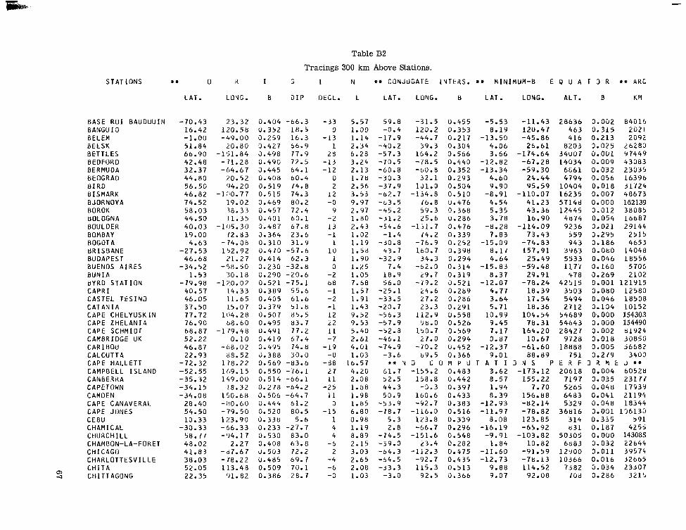
Table B2
Tracings 300 km Above Stations. STATIONS .* 0
BASE R O I BAUOUUIN B A N G U I 0 BELEM BELSK BETTLES BEDFORD BERMUDA EiEOGRAO 81 RD BISMARK BJORNOYA BOROK tiOLOGNA BOUL 0 E R BOMBAY BOGOTA 8R I SBANE BUDAPEST EUENOS A I R E S B U N I A BYRD S T A T I O N C A P R I CASTEL T E S I N D CATAN I A CAPE CHELYUSK I N CAPE Z H E L A N I A CAPE SCHMIDT CAMBRIDGE UK CARIBOU CALCUTTA CAPE HALLETT CAMPBELL I S L A N D CANBERRA CAPETOWN CAMDEN CAPE CANAVERAL CAPE JUNES CEBU CHAMICAL CHURCHILL CHAMBON-LA-FORET CHICAGO CHARLOTTESVILLE C H I T A C H I T T AGONG
LAT.
-70.43 16.42 -1.00 51.84 66.90 42.48 32.37 44.RO 56.50 46.82 74.52 58.03 44.50 40.03 19.00
4.63 -27.53
46.68 -34.52
1.53 -79.98
40.57 46.05 37.50 77.72 76.90
52.22 46.87 22.93
-72.32 -52.55 -35.32 -34.15 -34.08
28.40 54.50 10.33
-30.33 58.77 48.02 41.83 38.03 52.05 22.35
68.87
K I
LOVG. B
23.32 0.404 120.58 3.352 -49.00 0.259
20.80 0.427 -151.84 3.498
-71.28 0.490 -64.67 0.445
20.52 0.408 94.20 0.519
-1:10.77 0.515 19.02 0.469
11.35 0.401 -105.30 0.487
12.83 3.364
38.33 0.457
-14.08 152.92
21.27 -58.50
30.18 .1%0.02
14.33 11.65 15.07
104.28 b8.60
-1 79.48 0.10
-68 .02 t18.52
178.22 169.15 149.00
18.32 150 .68 -30.60 -79.50 1%3.91) -66 .33 -94.17
2.27 -87.67 -78.22 113.48
91.82
-
0.310 31.9 0.470 -57.6 0.414 62.3 0.230 -32.8 0.290 -20.6
0.389 55.6 0.405 61.6 0.379 51.8 0.507 85.5 0.495 83.7 0.491 77.2 0.419 67.4 0.495 74.8 9.388 30.0 0.569 -83.6 0 .550 -76.1 0.514 -66.1 0.278 -64.2 0.506 -64.7 0.444 61.2 0.520 80.5 3.338 5.6
0.521 -75.1
0.233 -27.7 0.530 83.0 0.408 63.8 0.503 72.2 U.485 69.7 0.509 70.1 0.386 28.7
G
D I P
66.3 18.5 16.3 66.9 77.9 72.5 54.1 60.4 74. E3 74.3 80.2 72.4 60.1 67.8 23.6
I
OEGL.
-33 0
-13 1
2 8 -13 -12
0 2
12 -0
9 -2 13 -1
1 10 1 0
-2 68 -1 -2 -1 12 22 11 -7
-19 -0
- 8 8 27 1 1
-25 11
0 -15
1 4 4
-6 2
-4 -6 -0
N t i CONJdGATE I Y T E R S . ** MINIYUM-B E 8 U A T 3 R ** ARC
L LAT. LONG. 8
5.57 1.00 1.14 2.34 6.28 3.24 2.13 1.78 2.56 3.53 Y.Y7 2.97 1.80 2.43 1.02 1.19 1.58 1.90 1.25 1.05 7.68 1.57 1.91 1.43 9.52 9.53 5.40 2.61 4.01 1.03 6.57 4.20 2.38 1.88 1.98 1.85 6.80 0.98 1.19 8.89 2.15 3.03 2.65 2.08 1.03
59.8 -0.4
-17.9 -40.2 -57.3 -70.5 -60.8 -30.3 -37.9 -62.7 -b3.5 -45.2 -51.2 -54.6
-1.4 -50.8
43.7 -32.9
7.4 18.9 56.3
-25.1 -33.5 -20.7 -56.3 -57.9 -52.8 -46.1 -74.9
-3.6
61.7 ~ 2 . 5 44.3 50.9
-53.9 -78.7
5.3 2.8
-74.5 -39.3 -b4.3 -54.5 -33.3
-3.0
*i t N
-31.5 120.2 -44.7
39.3 164.2 -78.5 -60.8
32.1 1J1.0
-134.8 16.8 59.3 25.6
-131.7 14.2
-76.9 163.7
34.3 -62.0
(9 .7 -19.2
24.6 27.2 23.3
112.9 98.0
150.7 27.0
-70.2 b9.5
0 z u -155.2
158.8 -3.3
160.6 -92.7
-116.0 123.8 -66.7
-151.6 23.4
-112.3 -92.7 115.3
92.5
0.455 0.353
0.304 0.566 0.440
0.293 0.504
0.476 0.368 0.286 0.476 0.339 0.252 0.398 0.294
0.319 0.521 0.289 0.286
0.558
0.569 0.294 0.452 0.366 M P U 0.483 0.442 0.397 0.433 0.383 0.516 0.339 0.296 0 .548 0.282 0.475 0.435 0.513 0.366
0.217
0.352
0.510
0.314
0.291
0.526
LAT. LONG. ALT. 8 K M
-5.53 8.19
-13.50 4.06 3.66
-12.82 -13.34
4.60 9.90
-8.91 4.54 5.35 3.78
-8.28 7.83
-15.09 8.17 4.64
-15.83 8.37
-12.07 4.77 3.64 5.71
10.99 9.45 7.17 0.87
-12.37 9.01
A T 1 2 3.62
1.94 R.39
-12.93 -11.97
8.08 -16.19
-9.91 1.84
-11.60 -12.73
9.88 9.07
8.57
-11.43 120.47 -45.86
26.61 -174.64
-67.28 -59.30
24.44 95.59
-1 10.07 41.23 43.36 16.90
-114.09 73.43
-74.83 157.91
25.49 -59.48
29.91 -78.24
18.39 17.54 18.36
104.54 78.31
164.20 13.67
-61.60 88.89
1 4 s P -173.12
155.22 7.70
156.88
-78.82 123.85 -65.92
-103.82 10.82
-91.59 -78.13 114.52
92.08
-82 1 4
28636 463 4 1 6
8203 34U07 1 4 0 3 4
6 8 6 1 4 7 9 4
1 0 4 0 4 1 6 2 3 5 5714d 1 2 4 4 5
4 8 7 4 9 2 3 6
559 9 4 3
3963 5533 1177
470 42515
3503 5494 2712
54689 54643 28427
9728 1 8 8 8 8
7 5 1 E R F 20618
7197 5265 6483 5329
36816 3 1 4 8 3 1
50305 6683
12Y00 1 0 3 6 6
7 3 8 2 1 0 8
0.002 0.315 0.213 3.025 0.OUl 0.009 0.032 0.056 0.018 0.007 0.000 0.012 0.054 3.021 3.295 0.186 0.080 0.046 0.160 0.269 0.001 0.080 0.046 D. 1 3 4 0.. 0 0 0 0.000 0.002 3.016 0.005 0.219
3 3 Y t 0.004 0.035 0.048 0.041 0.048 0.091 0.335 0.187 0.000 0.032 3.011 0.016 0.034 0.286
84016 2021 2092
26283 9 7449 43083 23035 1 6 3 9 6 31724
162139 38085 16687 29144
2515 4653
14048 18556
5706 2102
121Y15 12580 18508 10152 154303 154490 81924 30850 56682
3403 J ** 60528 231 77 17439 21194 1 8 3 4 4
156133 391
4255 143085 22644 39574 32665 23507
3215
40673

m Q, Table B2
Tracings 300 km Above Stations.
.
S T A T I O N S
C H R I S T C H U R C H C H A C A L T A Y A C L I M A X C L O N C U RRY CONCORD COOK C O L L E G t C O R I U A L D O C O I M B R A C O N C E P C I U N C OR 1) 0 8 A COLOMBO COCOS I S L A V O COP E YH A G t N C O R A L H A R a O U R CKACOW C U R AC AC1 C U L C O D A V I S D A P A N G @ D A L L A S O A K A Y OARW I N - C O O N A W A K R A U E O R E C k r J OE B I L T d E E P K I V E R D E N V E R U E H K A DUX D E L H I D E C E P C I ON O I X O N I S L A N D DJ I B O U T I U J A K A R T A D O O A I R A 110 L G 0 P K U U Y AY A U U U R R E b DUNS I NK O U S H E T T I U U R H A M UUMONT D ' U R V I L L E U U R B A N t 0 I N81I R G t I t I G H T S E L L S W O R T H E L I S b B E T H V I L L k
.* 0 ? I G
L A T .
-43.57 -16.32
39.37 -20.67
43.20 -30.63
64 .85 43.63 40.22
-36.58 -31.32
6.90 -12.20
55.75 64.20 50.05 12 .08
-13.52 -68.60
10.80 32.78 14.h6
-12.43 47.40 52.10 46.10. 39.75 30.33 28.63
-62.98 73 .53 11 .55 -6.17 36.00 55.94 5 0 . LO 53.38 42 .00 43 .08
-66.67 -29 .83
55.92 -75.23 -77.72
LONG. B D I P
172.80 -68.15
-1C6.18 140.50 -71 .53 130.40
- 147.8 3 13.00 -8.42
-12.98 -54.22
79.87 96.90 12.50
-83 .40 19.95
-b8 .84 -71.98
78.00 0.07
-96 .80 - 1 7 . 4 3 1 5 0 . 9 0
21.65 5 .18
-17 .50 - 105.00
78.05 77.22
- b o . 7 2 00.70 43.15
107.00 139.20
4.60 -6.33 44.70
-70 .92 140.02
31.03 -3 .18
-77.17 -Q1.13
57.52
0.515 -68.9 0.234 -5.3 0.483 67 .1 0 .444 -50.9
0.505 -63.7 0.498 77.1 0.399 59.1 0 .384 57.0 0 .259 -36.4 0.231 -28.8 0.341 - 6 . 0 0.403 -44.8 0.430 69.7 0.522 85.2 0 .422 65 .4 0.347 43.3 0.242 -0.8 0.491 -74.3 0 .276 5.4 0 . 4 h l b2.8 0.285 21.8 0 . 4 0 1 -39 .6 9.416 63 .1 0 .419 67.1 0.507 75.4 0.486 b 7 - 7 0.420 44.5 0 .411 41.7 U.3h6 -57 .4 0.503 83.5 0.311 6.5 0 .381 -32.7 0.402 49.3 0.452 71.0 0 .414 65.5 0 .423 68.6
0 .491 72.9 U.580 -89 .6 0.292 -63.4 0 . 4 2 8 T0.2 0.462 -67.8 U.446 -67.2
0.492 73.0
0 .429 59.5
-11.63 77 .42 0.294 -45.9
I
OECL.
20 1
1 3 6
-13 3
28 -2
-10 11
3 -3 -2 -1
- 2 5 1
-3 3
-68 -10
9 -13
3 1
-5 - 9 1 3
0 -0 1 4 1 9
1 1
- 4 8
-5 -11
5 -13 -38 - 1 9 -10 31
8 -7
N ++ C O N J U G A T E I q T E R S . ** Y I N I Y U M - 8 E 3 U A T 3 R ** ARC
L L A T . LGNG. 8 L A T . LONG. ALT. 8 K M
2.52 52.9 -1b2.5 0.443 4.33 -174.60 1.10 -10.6 -68.1 0.245 '42 M I l I M U f i B B E 2.35 -53.6 -131.9 0.473 -8.04 -114.94 1.35 37.7 3.36 -71.1 1.83 48.9 5.71 -57.3 1 .74 -29.7 1.72 -31.6 1.27 9.2 1.20 3.7 0.97 11.9 1 - 1 6 3 1 . 3
1 4 3 . 3 0.432 -79.4 0.444 - 132.1 0.474 168.6 0.562
L 6 . 3 0.287 10.3 0.272
-70.9 0.333 - -65.3 0.299 -
79.6 0.347 95.8 0.430
2.88 17.52
2.17 1.33 1.09
1 5 - 2 4 1.05 1.96
1.14 1.96 2.52 3.92
1.17 1.13 2.29 7.03 1.01 1.05 1.30 2.70 2.31
1 .61 3.33
1.75 3.19 4.17 4 .81 1.22
i.11
2.41
2.88
35.99
9 8 9 3 0.020 30870 WtEN I Y T E R S . 6 6 6 8 7 0 4 0.024 2 7 6 4 9
9.17 142.86 2 5 6 7 2.54 -67.55 4 7 8 1
2.90 -169.67 3 0 3 3 4
1.01 0.13 4 2 4 5
6.31 -64.11 8 9 6
9.09 96.20 1 5 7 2
9.61 132.53 5 7 1 3
4.26 17.98 4 5 0 9
5.38 -73.72 1 4 0 4
8.49 79.77 313
0.128 0.008 0.051 0.002 0.060 0.062 0.153
0.340 0.196
0.181
9805 45162 1 8 7 7 4 8 7 3 5 3 1 5 5 9 2 1 4 9 8 8
6 4 4 9 4557
5 8 0 6 3 7 7
-47.3 38.9 0.316 2.46 21.61 1 1 5 5 2 0.013 3 5 8 9 4
-37.8 36.7 0.298 4.02 25.37 7 1 8 4 0.031 2 3 3 6 1 * * Q D C O M P U T A T I 3 N S P E R F 3 R M E D * *
-40.1 -b9.9 0.264 -15 .34 -67.85 1 7 6 6 0.133 1733 -12.7 -11.9 0 .243 V D M I V I M U H B B E T W t E N I V T E R S . 9 +
+ + N O C O M P U T A T I 3 N S P E R F J R M E D + + 6.1 1.3 0.269 6.64 0.92 305 0.269 555
-51.3 -116.4 0.430 -10.01 -102.73 6 1 4 5 0.041 20497 -6.2 -11.5 0.248 1 .72 -13.90 5 4 9 0.225 2 6 5 6 28.8 151.7 0.383 8.82 131.85 1 3 4 4 0.208 5 8 1 9
-34 .0 35.3 0.295 4.62 26.01 5 8 7 6 0.042 1 9 5 5 4 -44.2 Z Y . 7 0 . 2 9 4 1.78 14.50 9 1 9 5 0.020 29273 -72.3 -96.8 0.477 -12.43 -76.30 1 8 4 8 1 0.005 5 5 3 3 1 -54.5 -131.1 0.475 -8.11 -113.63 9 0 8 9 0.022 2 8 7 3 4 -12.2 83.8 0.378 8.31 78 .84 1 5 4 2 0.192 6276 -10.6 19.8 0.370 8 - 0 9 7 8 . 0 1 1 3 3 3 0.210 5585
34.6 -64.7 0.453 -13.02 -59.00 7 9 2 1 0.026 2 6 0 4 8 - 3 4 . 1 1 2 3 . 3 0.529 10.20 8 5 . 7 4 3 8 7 2 1 0.001 1 1 0 3 7 4
6.1 43.1 0.301 6.97 43 .14 3 1 0 0.300 6 3 9 24.2 107.3 0.392 8.75 107.23 077 0.265 3Yb3
-19.3 137.4 0.436 9.11 139.29 2 2 8 8 0.143 8922 -43.3 56.4 0 .353 5.58 41.90 1 0 6 8 7 0.016 3 3 1 4 9
-50.4 25.1 0.302 -0.13 6.17 1 1 4 3 6 0.013 35772
-71.1 -77.7 0.442 -12.60 -66 .65 1 4 6 1 7 0.008 4 4 7 1 9 * + N O L O M P U T A T I J N S P E R F J R M E i l + *
44.4 19.4 0.405 4.86 23.41 4 6 5 7 0.058 1 5 9 9 1 -52.6 33.5 0.317 0.01 9.76 1 3 4 5 6 0.010 4 1 4 4 3
51.2 -59.9 0.488 -11.07 -48.59 2 3 9 3 5 0.093 7 0 8 6 0 30.8 24.2 0.360 7 .26 25.34 1 4 8 5 0.169 6 1 9 2
-41.4 27.0 0.287 ' 2 . 0 6 13.30 7 9 1 8 0.026 2 5 6 1 1
-26.5 51.2 0.321 6.42 45.59 3 9 4 1 0.075 1 3 7 5 2
47.4 -73.1 0.533 -12.30 -64 .74 1 9 9 9 8 0.004 5 9 7 2 0
I

Table B2 Tracings 300 km Above Stations.
STAT IONS t. 0 R I G
ENNADAI t NUGU CSKDALEMUIR ESPERANZA tUREKA FAREWELL FANNING I S L A N D F L I N FLON FORT YUKON FORT NORMAN FORT CHIMO FORT MONMOUTH FORT BELVOIR FORT RANDOLPH FORT DE FRANCE FREETOWN FRO8 I SHEK
FRONT ROYAL FT. DAVI!, GARCHY G A I N E S V I L L E GENOVA MONTE CAPEL GENERAL 8ELGRANO GENERAL SAN MARTIN GHANA G I F U G I L G I T GOUGH ISLANO GO OH A V N GOOSE BAY GOTT I NGEN GRYTVIKEN GKAZ GROCKA GRAND BAHAMA GRAHAMSTOUQ GREAT WHALE R I V E R GULMARG GUANTANAMO BAY GUAM GUAYAQUIL HAMMAGHI K HACHI JOJ IMA HALLETT HARTLANO
FREIBUKG
Q, (0
LAT.
61.30 6.47
55.32 -63.38
80.00 62.53
54.70 66.57 64.90 58.10 40.25 38.73
9.38 14.10
8.47 63.75 48.05 38.93 30.63 47.30 29.63 44.55
-77.97 -68.13
10.00 35.58 35.94
-40.35 69.23 53.32 51.53
-54.27 47.07 44.63 26.67
-33.28 55.27 34.05 19.90 13.45 -2.17 30.10 33.13
-72.32 51.00
3.92
LOYG. 8 O I P
-1 ' . 1.20 7.55
-3.20 -56.98 -35.93
-133.90 -13Y.38 -1u2.00 -145.30 -125.50
-68.43 -74.02 -77.13 4 9 - 8 8
-13.22 - b8. 5 7 7.58
-7M.18 -103.95
3.07 -82.30
8.95 -38 .80 - L7.4 3
4.00 137. 0d
14.30 -9.89
-53.52 -1~0.3R
9.93 - 36-53
15.47 20.77
-78.37
-01.02
26.48 -77.78
14.40 -75.15 144.75 -79.88
0 .
170.22 -4.48
i : 9 . a 0
0.530 0.275 0.427 0.363 0. 503 0.487 0.289 0.528 0.503 0.518 0.508 0.488 0.466 0.336 0.349 0.266 0,508 0.40Y 5.488 0.441 0.406 0.450 0.400 0.446 0.409 0.277 0.405 0.445
0.491 0.492 0.419 0.287 0.41 1 3.437 0.434 0.286 0.51') 0.436 3.396 0.316 0.280 5.344 3.387 J. 573 3.416
0.222
d3.6 -7.5 69.8
-57.4 88.0 74.6
9.8 79.6 78. b 81.1 80.5
70.3 38.0
7.2 82.7 63.6 70.4 59.0 63.1 62.2 60.2
-67.4 -61.9
1.9 49.1 53.2
-56.9 81.9 76.8 66.6
-52.3 62.6 60.3 59.7
-64.6 80.7 50.5
11.7 18.4 42.6 45 .3
-84.8 66.6
11.2
44 . a
52.a
I N ** CONJJGATE I N T E 3 S . + * YIq IMUM-B E 0 U A T 3 2 *+ ARC
U t L L . L LAT. LONL. B LAT. LOVG. ALT. 8 KM
16 10.16 -9 1.34
- 1 0 3.10 12 2.33 7 3 317.06 24 4.49 10 1.03 15 5.75 31 6.77 55 8.58
-31 8.71
-72.5 12.8
-51.8 35.2
-53.6 -5.5
-68.2 -58.9 -64.4 -85.1
.t N
-163.8 0.558 -7.86 6.5 0.284 7.96
29.6 0.313 0.17 -53.2 0.453 -12.95
0 L O M P U T A T I 168.8 0.553 3.30
-1b1.1 0.3U2 0.86 -148.8 0.241 -8.44
167.2 0.567 2.74 177.4 0.567 -1.42 -81.5 0.535 -11.68
-9 2.93 -67.8 -64.6 0.436 -12 -5 2.73 -65.5 -90.8 0.437 -12
3 1.23 -33.5 -&2.4 0.218 -13 -9 1.36 -41.2 -35.5 0.244 - 1 4
-14 1-07 2.0 -11.5 3.254 3 - 4 0 15.36 +* N 0 C 0 M P U T A
-4 2.10 -37.4 26.6 0.285 2
-116.05 7.29 9.44
-56.79 3 4 s P
-172.74 -159.93 -114.10 -169.23 -149.79
-59.54
58502 318
12837 8158
E k F 2 2 5 5 4
342 30402 37132 48635 48857
0.000 165589 0.274 751 0.011 39696 0.024 26744
3.003 6587:) 0.285 1121 0.032 37906 0.031 l d 6 1 0 3 0.000 137980 0.000 139727
3 3 M E D .*
85 -71.70 1 2 1 0 6 0.012 37634 89 -76.47 1 0 9 0 1 0.015 34188
8 0 -57.26 1Y40 0.122 8417 0 4 -11.76 314 3.224 787
77 14.93 6596 0.035 21762
6 9 -81.64 1 3 1 4 0.165 6 ~ 1 7
I I V S P E R F J X M E J + *
- 5 1 1 -6
1 - 3
6 21 - 3 -5
1 - 2 5 -48 -26
- 3 -5 -0
0 -0
-L3 -18
1 - 3
2
-7 -4
-78 - Y
5
2.15 1.74 2.08 1.91 1.82 4.92 2.62 1.04 1.29 1.32 1.76
22.19 5.56 2.40 1.91 1.96 1.77 1.77 1 - 8 9 7.22 1.27 1.51 1.01 1.10 1.27 1.23
22.17 2.54.
-65.4 -Y3.1 0.440 -12.72 -77.99 11032 0.015 54533 -45.3 -122.1 0.419 -8.49 -110.50 4608 0.058 16641 -37.6 23.1 0.282 2.05 11.21 6 4 6 1 0.036 21417 -54.5 -Y5.9 0.394 -12.70 -84.36 5728 0.043 1Y465 -31.9 24.1 0.284 3.56 14.98 4 Y l l 0.052 16993
51.6 -59.3 3.488 -11.05 -47.66 24023 3.OG3 ( 2 i 8 5 39.7 -a7.4 0.476 -12.79 -61.94 11567 0.014 35106
8.4 4.3 0.275 '43 H I V I M U H 8 BETWEEN I \ T E R S . 193 -18.6 125.6 0.435: 9.16 137.28 2 2 2 9 0.146 8722 -18.5 78 .4 3.389 7.90 75.17 2 4 7 1 0.133 9202
54.2 -33.6 0.385 -5.32 -22.55 4570 0.058 15663
-79.8 -40.3 0.459 -11.09 -48.61 28682 0.002 d402U -42.3 31.9 0 .294 2.46 17.97 8483 0.023 27189
5 3 . 8 -53.6 0.414 -11.47 -44.74 5337 0.045 18731 -34.3 30.6 0.290 3.96 23.88 5826 0.042 19454 -33.3 32.2 0.293 4 - 8 6 24.58 4730 0.057 1619Y ->2.9 -88.5 0.367 -13.23 -79.25 4 8 0 1 0.055 16853
45.8 13.9 0.434 3.44 16.93 5416 0.047 18288 -83.3 -113.6 0.516 -11.89 -75.07 39468 0.001 113517 -16.5 i8 .1 0.383 7.91 75.26 2128 0.151 8152 -46.9 -81.4 0.319 -13.98 -75.46 3062 0.089 11753
2.1 144.2 0.328 8.82 144.58 366 0.3U7 133Y -21.2 -b2.2 0.249 -13.79 -81.07 477 0.232 2313 -14.6 Y.1 0,277 4.97 4.45 1 6 2 1 3.151 6731 -16.4 158.2 0.42D 8 - 9 2 139.82 1 8 4 6 0.168 7543
* * ! y o L I j M P U T A T I 3 V S P E R F J X M E U * + -46.1 23.0 0.289 0.30 6.66 9302 0.020 29683
t + N 5 C O M P U T A T I J N S P t R F 3 R M E U r t

Table B2 Tracings 300 km Above Stations.
S T A T I O N S
HARVSTVA HAMBURG HALLE H A L I F A X HANNOVER USA HABAiUA HALLEY BAY H A I F A HAMILTON MASS. HERSTMUNCEUX H E I S S HEALY HEL HELWAN HEKMAVUS H I K A I S O H I GHCL I F F HONOLULU HOBART HOLLANOI A HUH B ANUV U I IUMAIN HUANCAYO HYOERABAD I BADAN I . CROZET I L QOKTIY I N U V I K I NV E RC ARG I L L INVERNESS I QU I TOS IRKUTSK I S L A D E PASCUA I S F J O R D I T H A C A I V A L U JICAMAKCA JOORELL BANK JOHANNESBURG J U P I T E R JULIANEHAAB JULIUSRUH-RUGrN JUNGFRAUJOCH K ANOY A KAKACHI
** 0
L A T .
60.22 53.63 51.48 44.60 43.70 23.15
-75.52 32.83 42.02 50.90 80.20 63.85 54.60 29.87
-34.42 36.37
21.30 -42.92 -2.50 47.90 50.20
-12.05 17.42 7.37
-46.50 36.22 68.20
-46.42 57.45 -3.67 52.27
-27.17 78.07 42.45 68.60
-11.95 53.23
-26.20 27.02 60.72 54.63 46.55 31.42
-45.88
i I " 1
LOVG. 8 D I P OECL.
10.25 10.00 11.93
-63.60 -72.30 -82.35 -26.60 35.10
-72.17 0.33 57.48
-119.00 18.80 31.33 19.22
140.62 110.58
-158.10 147.17 140.52 18.20 5.35
-75.33 78.45 3.97 52.00 14.30
-1 33.70 168.32 -4.25
-73.33 104.30
-1'79.43 13.63
-76.52 27.48
-76.87 -2.30 28.03
-do . 1 2 -46.03 13.38 7.98
130.89
0.438 72.7 0.424 68.2 0.420 66.5 0.482 72.6 0.495 73.4 0.415 55.5 0.424 -65.7 0.381 46.5 0.490 72.3 0.416 66.3 0.490 84.1 0.522 81.8 0.431 69.0 0.364 41.3 0.279 -64.4 0.401 49.6 0.527 -71.1 0.318 38.7 0.546 -72.9 0.346 -21.1 0.415 63.4 0.415 65.5 0.248 1.1 0.361 19.2 0.273 -4.0 0.347 -65.6 U.373 50.1 0.513 81.4 0.532 -71.9 0.432 71.2 U.271 17.6 0.514 71.0 0.307 -36.3 0.474 81.7 0.497 72.9 0.462 77.7 0.249 0.7 0.422 68.2 0.291 -61.6 0.436 59.9 0.476 77.4 0.428 68.9 0.405 62.2 0.397 44.4
24.85 67.02 0.385 36.0
-3 -3 -2
-20 -13
2 -2 3
-12 -7 19 33 1 2
- 2 5 -4 2 2 1 1 13 4 0
-5 4
-1 -10 -38 -2 3 7 2 2
- 1 1 2
-2 14 -6 -8 6 5
-9 -17
0 -35 -1 -3 -3
N ** CONJUGATE I N T E R S . ** MINIMUM-8 E 3 U A T D R ** ARC
KM L LAT. LONG. B LAT. L O i G - ALT. 8
3.69 -53.6 44.5 0.349 1.89 2-63 -45.1 34.5 0.303 2.51 2.37 -41.5 33.0 0.295 3.00 3.47 -72.4 -36.4 0.422 - 2.29 3.44 -71.4 -61.7 0.450 - 2.71 1.59 -47.6 -93.2 0.353 - 2.93 4.47 50.9 -54.9 0.478 -10.63 1.27 -15.1 57.6 0.300 6.76 3.17 -69.9 -&De6 0,440 -12.60 2.45 -44-1 25.5 0.289 1.14
13.64 + * N O C U M P U T A T I 8.98 -66.2 2.66 -44.3 1.20 -11.1 1.89 44.7 1.31 -19.4 2.86 55.8 1.19 -23.4 2.98 60.6 1-03 18.2 2.01 -35.0 2.31 -41.3 1.08 -13.1 1.00 1.1 1.05 13.8 2.99 57.8 1.39 -19.1 9.70 -63.3 3.00 57.2 3.49 -55.1 1.11 -22.3 2.12 -33.6 1.18
15.17 3.25 5.77 1.08 2.77 1.61 1.78 7.69 2.72 1.97
~~
12.4
-59.2 -57.7 -12.7 -48.5 41.7
-52. b -78.8 -45.5 -35.1
** N
-178.0 0.566 41.3 0.315 33.3 0.296 0.7 0.398
138.6 0.438 -162.6 0.455 -166.6 0.369 161.4 0.472 141.3 0.328 33.3 0.293
-75.4 0.246 27.6 0.288
79.4 0.344 3.3 0.278
28.5 0.446 22.1 0.290 168.4 0.572
-164.7 0.459 32.4 0.330
-.74.6 0.238 107.9 0.505
-102.2 0 L O -91.6 67.9
-76.9 27.1 18.1
-91.4 16.5 37.9 25.3
0.337 M P U 0.455 0.433 0.248 0.299 0.396 0.373 0.454 0.310 0.284
22.10 18.77 19.46
-55.50
-84.61 -41.68 35.55
-68.68 10.33
3 N S P
-68.64
16722 9972 8341
15391 15362 3649
2 1702 1848
13630 8763
E R F
0.006 0.018 0.024 0.007 0.007 0.076 0.003 0.149 0.010 0.022
J R M E
50439 31436 26759 47031 46767 13414 b4729 7380
41935 28386 D +*
-3.08 -141.72 51178 0.000- 145071
7.30 31.81 1397 0.178 5883 2.10 8.54 5381 0.046 18269
3.46 26.03 10204 0.017 32004
9.05 140.62 2344 0.139 9105 4.32 -175.86 12074 0.013 36915 1-56 -161.96 1336 0.188 5961 8.38 155.12 12928 0.012 39083 8.74 141.08 535 0.287 2532
2.18 13-91 7929 0.026 25636 NO M I V I M U N 8 BETWEEN I V T E R S . 128
V3 M I V I M U M 8 BETWEEN I V T E R S . 407
4.13 23.32 6138 0.040 20344
8.41 78.92 464 0.314 1970
4.51 35.07 12490 0.012 38340 5.84 17.50 2441 0.114 9314 0.77 -161.40 55888 0.000 157906 4.76 -178.07 12984 0.012 39424
-0.33 9.71 15389 0.007 46887 -15.64 -73.94 457 0.225 2242
9.95 105.44 7628 0.032 23959 -8.33 -105.42 1188 0.186 5487
T A T I J N S P E R F 3 X M E D * + -12.59 -75.18 14152 0.009 43293
4.61 40.62 30222 0.002 07647 NO M I V I M U Y 8 BETWEEN I V T E R S . 86 0.27 9.26 10789 0.015 33899 4.94 21.70 3785 0.074 13408
-13.11 -81.57 4864 0.054 17009 -8.38 -26.10 42206 0.001 121614 2-88' 21.78 10534 0.016 32999 3.09 14.78 5854 0.042 19592
1.19 -14.8 130.1 0.415 8.76 131.17 1653 0.184 6851 -0 1.09 -8.1 69.3 0.341 7.27 67.73 1004 0.235 4433

I Table B2
Tracings 300 km Above Stations.
I N ** COYJJGATE INTERS. ** MINIMUM-8 E P U A T 0 R +* A R C
!
STATIONS
KAZACHIE KAP T O B I N KAZAN KAKIOKA KAMPALA KEKAHA K HART OUM KHABAROVSK KHARKOV K I E L KIRUNA K I N G SALMON K I E V K 1 NGS TON KNOB LAKE KOROR ISLAND KOTZEBUE KOLN KOMURO KOKUBUNJ I KODAIKANAL KUHLUNGSBORN KUMAS I KYOTO L ' AQU I LA LA MAODALENA LAHORE LA PLATA LA 4 U I A C A LA PAZ LA€ LA CRAU LA HAYE LEEDS L E I C E S T E R LERW I CK LENINGRAD LEIDSCHENDAH LEOPOLDVILLE
L I S B O A L I T T L E AMERICA LOGRONO LOVOZ E R O LONGYEARBYEN LONDON
LINOAUIHARZ
.+ 0
LAT.
70.70 70.42 55.83 36.23 0.33
21.84 15.58 48.52 50.00 54.30 67.83 58.70 50 45 18.00 54.80 7.16
66.88 50.93 35.98 35.70 10.23 54.12 6.67
35.02 42.40 41.22 31.55
-34.90 -22.10 -16.48 -6.72 43.10 52.10 53.80 52.62 60.13 59.95 52.08 -4.37 51.65 38.77
-78.18 42.45 67.99 78.22
2 I "
LONG. 8 D I P
136.40 -21.97 48.82 140.18 32.58
-159.72 32.58
135.12 36.23 10.10 20.43
-1 56.70 30.50
-76.80 -66.82 123.48 - 1 62.6 0
6.92 139.62 139.48 77.48 11.93 -1.58 1.35.78 13.32 9.40 14.33
-57.90 -65.60 -68.05 147.00
6.00 4.30
-1.55 -1.10 -1.18 30.70 4.38 15.25 10.13 -9.13
-162.17 -2.50
15.67 35.08
0.509 0.465 0.467 0.401 0.291 0.319
0.467 0.439 0.426 0.457 0.472 0.433 0.386 0.504 0.338 0.491 0.417 0.401 0.400 0.342 0.426 0.268 0.405 0.395 0.389 0.424 0.230
0.233 0.359 0.394 0.419 0.423 0.420 0.437 0.451 0.419 0.281 0.420 0.379 0.553 0.391 0.467 0.475
0.31 1
0.227
80.8 79.0 71.8 49.5
-22.8 39.0 12.9 63.8 66.3 68.7 77.0 71.5 66.3 50.3 78.8 -1.4 76.7 66.1 49.2 48.9 2.5
68.6 -3.0 48.6 57.8 56.5 46.7
-33.3 -15.3 -5.6
-28.5 58.8 67.1 68.6 67.7 72.8 73.1 b7.1
-32.8 66.6 55.5
-80.3 58.7 77.8 81.8
51.53 0.10 0.417 66.8
DELL. L LAT.
-8 -28 10 -4 -1 12 0
-8 6
-3 2
21 5 0
-27 1
2 1 -4 -4 -4 -2 -2
- 1 1 -4 -2 -3 0 0 1 1 5
-4 -5 -8 -8 -9 6
-5 -9 -3
-10 - 79 -8 10 -5
5.35 -50.2 11.62 -72.5 2.64 -41.5 1.31 -19.3 1.06 19.6 1.19 -20.4 1.03 4.5 1.80 -30.3 2.11 -36.1 2.71 -46.0 5.67 -58.6 3.48 -49.8 2.16 -37.1 1.44 -44.3 6.59 -82.2 0.97 8.4 5.46 -54.6 2.37 -42.3 1.30 -19.0 1.29 -18.8 0.97 8.2 2.67 -45.2 1.05 9.2 1.27. -18.1 l.b7 -27.8 1.62 -26.9 1.20 -13.9 1.26 7.8 1.12 -5.1 1.10 -10.5 1-07 22.5 1.75 -33.4 2.53 -44.5
2.68 -47.2 3.97 -57.2 3.33 -48.6 2.53 -44.4 1.12 24.1
1.65 -27.9
2.84 -49.1
2.41 -42.2
LONG. 8 LAT. LONG. ALT. 8 K M
128.6 59.3 65.1 138.2 32.2
-168.3 32.7
132.8 49.3 35.5 b3.2
171.4 45.0
-83.6
123.5 159.9 29.3
137.7 17.6 36.3 -2.1
134.5 25.2 21.8 77.6
-b1.7 -65.9 -be. 9 148.7 21.1 29.2 28.2 26.9 38.5 56.4 29.3 11.5 52.1 8.8
-67.9
137.8
0.569 0.466
0.437 0.324 0.371 0.292 0.533 0.322 0.306 0.421 0.540
0.313 0.487 0.338 0.565 0.291 0.436 0.434 0.343 0.306 0.272 0.432 0.288 0.286 0.374 0.316 0.261 0.245 0.328 0.283 0.294 0.302 0.296 0.351 0.366 0.294 0.323 0.295 0.271
0.382
0.313
10.51 131.51 28170 -2.03 6.88 67347 6.38 51.90 10474 8.98 140.20 2322 8.12 32.32 522 1.87 -163.65 1362
9.58 135.33 5528 5.54 39.12 6949 2.40 19.13 10495
3.49 -172.60 16060
-13.95 -77.73 2646
8-15 32.63 367
3.59 34.81 29532
4.84 34.28 7215
-11.56 -57.93 35327 7.96 123.50 301 5.20 177.53 20770 2.26 15.39 8282 9.07 139.68 2282 9.12 139.55 2236 N 3 M I V I M U Y 8 BETWEEN 2.54 20.49 10220 NO M I Y I M U Y b 8ETWEEiN 9.09 136.03 2145 4.47 17.95 4082 4.33 14.49 3802 7.85 75.17 1736
-15.89 -59.01 1215 -16.85 -65.58 417
N3 M I V I M U Y B 8ETWtEN 8.89 148.23 770
1.68 13.82 9265
0.88 9.86 10161 0.15 13.49 18486
3.43 12.25 4534
0.53 10.04 11190
4.82 37.78 14666 1.68 13.87 9244 7.65 13.40 802 2.52 18.16 8550 1.27 -0.87 3827
0.002 81003 0.000 190926 0.017 32400 0.141 9039 0.264 2354 0.186 6053 0.286 1312
0.034 22546
0.002 85852 0.037 47948 0.031 23363 0.102 10452
0.338 150 0.002 82959 0.024 26639 0.143 8909 0.145 8767
0.017 32126 I 'JTERS. 307 0.151 8453 0.067 14318 '0.073 13503 0.176 6918 0.158 5858 0.220 2033
I Y T E R S . 702 0.253 3729
0.020 29482
0.017 32092 0.005 55507 0.009 44407 0.020 29421 0.221 3703 0.023 27380 0.070 13134
0.053 18281
0.016 32922
0.001 102314
I V T E R S . 238
0.059 15715
0.014 35024
13.73 * * N O C O M P U T A T I 3 V S P f k F J R M E D + * 1.79 -32.3 15.5 0.277 1.93 5.41 4686 0.055 16242 5.34 -55.6 7D.6 0.436 5.62 45.86 27564 0.002 80168 15.07 + * N O G O M P U T A T I J N S P E R F O R M E D + *
-7 2.53 -45.1 26.2 0.291 0.98 10.40 9222 0.020 29403

Table B2
Tracings 300 km Above Stations. S T A T I O Y S
LOMNICKY S T I T LOURENCO MARQUES L U N D LUANDA LULEA LVOV LW I RO LYCKSELE YAKATEA M A N I L A MALVEKN MAJURO MAORI 0 MACAO MAORAS MAWSON MACOUAK MAR I ON
MCMUKOU MEANOOK MEUOON
MAU I s K I
SLAND
E I S L \NO SLAYD € I hUlJ'r10
t* 0
LAT.
49.20 -25.97
55.70 -8.82 65 .60 49.82 -2.25 64.62
-16.20 14 .52 52.12
7.08 40 .40 22.20 13.08
-67.40 -54.30 -46.8 5
20.80 -77 .85
54.62 48.80
MEM AM B E T i U 43.92 M E X I C O EL CERi ! ILLU 19.32 ME L BOU R N t -37.82 MIOW4Y I S L A N D M 1 EO.? E S Z Y N M I N N E A P O L I S M l R N Y M I N A AGUILAR MOULD RAY M U S H I R I MOCA M 0 S C (1 W MUURlr WASHINGTON MOUNT NORIKURA MOYT J O L I MURCHISON RAY MU 33 MAN 5 K MU I C H E '\I 1\1 ARS S AKS L U 4Q !\IA9YAN MAR .\A I AL AAIKOR I VEUSTREL I T L
6.97 52.17 44.97
-66.57 -23.10
76.20 44.37
3.35 55.47 44.27 36.12 48 .60 80.05 68 .97 48.13 61.18 67.50 -5.33 -1.28 53.28
R I G
LONG. B D I P
20.22 32.60 13.18 13.22 22.12 24.02 28 .80 i 8 . 6 7
-148.20 121.00
-2 .32 111.13
-3.68 113.55
80.28 62.50
158.60 37-87
-126.50 106.62
-113.33 2.25
1 4 4 . 2 0 -39 .55 144.32 158.22
/ 1 . 2 0 -93.23
92.92 -65 .70
-119.40 142.27
8.67 17.32
-71.30 137.55 -tr8.20
18.30 33.08 11.70
-95 .42 53 .00
- 35.12 16.80
-13 .08
0.420 64.7 0.295 -61.2 5.430 69.7 0.281 -40.1 0 .454 75.9 0.425 65 .3 0.290 -29 .0 0.450 15.3 0.323 -26.d 3.347 14 .5 0.419 67.4 3.296 4.8 0.384 56.6 0 .379 29.7 0.350 8.8 0.453 -70.8 0.565 -79.1 0.313 -65 .0 0.318 38.3 0.565 -83.4 0 . 5 2 1 77.5 0.410 64.5 0 .429 57.1 0 .380 46.5 0.530 -69.0 0.305 0.1 0.428 67.2 0.512 74.0 0.521 -77.7 0.227 -16.9 0.513 87.3 0.435 58.5 0 .274 -14.9 0.451 70.6 0.495 73.7 0.406 49.7 0.499 75.8 0.479 82.7 0.466 78.1 0.411 63.6 U.476 11.5 0.483 78.8 0.236 -3.0 0.293 -25.1 0.425 69.0
I
D t C L .
1 - 1 6
-1 -12
3 2
- 3 1
12 0
-9 9
- 8 -0 -2
-56 26
- 3 3 11
-38 2 3 -6 -6
9 10
6 1 6
- 74 1
62 -6 - 9
8 -14
-5 -LO
-4 9
-2 - 5 5 16
-1 -17
N ** C O N J J G A I E I N T E R S . ** Y I N I W U M - 6 E 3 U A T 3 8 ** ARC
L LAT. LONG. B
2.10 1.61 2.86 1.18 4.81 2.13 1.08 4.60 1.10 0.99 2.64 1.02 1.68 1.04 0.97 9.31 5.46 2.81 1.18
35.82 4.86 2.22 1.57 1.34 2.36 1.01 2.37 3.42
20.94 1.13
38.84 1.59 1.06 2.64 3.54 1.30 4.43
18.01 5.7f 2.07 7.90 4.90 1.13 1.06
-36.6 41.8
-47.1 27.2
-36.2 -37.3
22.6 -56.1
11.3 1 .4
-46.9 2.4
-29.8 -5.1
5.8 71.3 b7.2 55.3
-20.5
-63.3 -40.2 -26.4 -35.8
55.8 6.8
-40.6 -64.7
-4.1
-26.8 15.9
- 4 2 ; 5 -72.1 -19.1 -16.5
-56.8 r 3 6 . 6 -78.7 -52.2
-2.5 20.2
** N
+* N
* * Y
** ;rl
36.0 24.1 39.2
7.5 60.0 59.4 27.8 56.5
-143.1 120.7
~ 5 . 6 110.3
i 3 . 2 113.1
83.7 -4.7
-154.9 11.9
-164.9
0.297 0.402 0.316 0.333 0.402 0.302 0.330 0 .391 0.300 0.348 0.294 0 .304 0.276 0.374 0 .342 0.460 0 .491
0.367 0.429
~-~ 0 L O M P U -157.6 0.541
24.2 0.283 140.6 0.477
153.4 0.463 158.2 0.305
-123.6 0.497 0 C O M P U
-66.0 0.264 0 C O M P U
139.0 0.480 6.6 0.292
55.7 0.350 -19.2 0.449 156.0 0.438 -71.2 0.462
0 C O M P U
29.2 0.288
79.8 0.460 -36.1 0.243
36.6 0 .331
-110.5 0.344
40.0 0.336
71.2 0 .441
18.9 0.455
LAT.
4.06 5.39 2.52 6.75 3.84 4.33 8.23 3.13
-1.54 8.18 0.59 6.90 2.03 8 .52 8.47 0.58 5 .44 2.35 1.32
LOYG. ALT. B K M
25.35 26.78 22.12 10.31 34.32 28.65 28.18 31.10
-145.33 120.90
8.75 171.10
3.92 113.46
80.53 20.48
175.61
-160.30 20.94
6 7 2 8 3 7 8 1
1 1 4 5 7 1 1 2 7
2 4 0 5 6 6 9 7 0
6 7 8 2 2 6 3 3
718 3 9 8
9 9 0 2 3 0 2
4 0 4 1 7 5 4 3 3 1
5 2 6 7 0 2 8 7 4 2 1 1 1 7 6
1 3 1 3
0.035 0.075 0.014
0.003 0.189
0.033 0.243 0.003 0.238 0.324 0.018 0.296 0.066 0.278 0.338 0.000 0.002 0.014 0.189
2 2 3 4 1 1 3 3 6 6 3 5 6 1 7
7 0 6 6 1 22712
3133 66'166
3529 1 5 5 7
3136B 556
1 4 3 2 8 3482
857 150163 8 2 8 7 3 3 4 8 4 0
5873
4983
T A T I C I N S P E R F J R M E D * * -5.71 -128.71 2 4 7 7 8 0.003 7 2 2 2 0
1.72 11.06 7 3 1 2 0.030 23890 9.07 143.76 3 9 7 2 0.081 1 3 9 4 1
- 9 . 2 1 -103.86 2 1 8 9 0,127 8862 8.84 150.21 8 9 9 4 0.024 2 8 1 3 1 '40 M I V I M U M B BETWEEN I V T E R S . 2 0 3.88 27.08 8397 0.024 2 6 8 3 4
-10.42 - 9 9 , 5 9 1 5 4 5 9 0.008 46612
-16.74 -65.65 4 5 3 0.217 2282
9 - 1 4 142.01 4 1 0 7 0.078 1 4 3 1 3 7.89 3 9 0 0.265 1 5 1 5 7.87
5 - 3 9 41.60 1032.8 0.017 32142 -12.53 -67.03 1 5 9 3 9 0.007 48397
9.04 137.73 2 3 1 6 0.141 8995 - 1 2 - 1 9 -61.53 2 1 5 4 8 0.004 6 4 0 7 1
5.32 45.10 3 0 2 9 2 0.002 8 7 7 5 3 3.25 18.20 6 4 5 3 0.036 21312
-8.16 -25 .09 4 3 5 1 4 0.001 1 2 5 2 3 1 7 .29 59.93 2 4 9 3 6 0.003 72596
T A T I J Y S P E R F 3 R M E D * *
T A T I 3 N S P E R F O R M E D * *
T A T I J N S P E R F O R M E D + +
'43 M I V I M U n B BETWEEN I V T E R S . 353 7 .64 36.55 5.80 0.259 2662
- 1 4 3.04 -53.4 21.4 0.308 -1.73 0.93 1 2 4 0 4 0.011 3 8 5 8 8

Table B2
Tracings 300 km Above Stations.
STATIONS i f 0 n I G I N ** CONJUGATE I N T E R S . ** MINIYUM-E t 2 0 A T 3 1 *I. hRC
LAT. LOUG. 8 DIP OkLL. L LAT. LONL;. B LAT. LOVG. ALT. 8 KM
NIAMEY N I T S A N I H % I I G A T A N I C OS I A NOUVELLE AMSTCRDAM NOVOLAZAREVSK A'f A NORD NORWAY S T A T I O N NORFOLK I S L A N D NOUMEA NURM I JARV I O O E S S A 0 ' H I GG I N 5 R I S UP A I R OKINAUA OLENEK ONAGAWA OOH I RA ORCAOAS IIEL SUR OSLO KJELLER UrTAUA UULU P A L E S T I N E PANSKA V E S PAR IS-S AGL AY PARIS-BAGNEUX PANAGURITSCH PARAMARIBO PETROPAVLOVSK-ON-K PEARCE
P 1 LAR P I W N I C E -TORU!d P L A I S A N C i POSAOAS PONZA PONTA D E C G A O O POTCHEFSTROOH POINT @ARROW POTSDAM POI r I ERS PORT ARTHUR POONA POKO P0I"IT P O R T AlJX F R 4 N L A I b PORT STA;'dLEY
PIC nu M I D I
4 W
13.50 31.73 37.70 35.17
-37.84 -70.77 81.60
-70.50 -29.00 -22.30 60.50 46.78
-63.32 26.50 68.50 38.43 35.h2
-60.73 59.97 45.40 65.00 31.77 50.53 48.12 48.80 42.52 5.82
52.98 -31.67 42.93
-31.h7 50.52
-20.43 -27.42 40.92 37.77
-26.68 71.33 52.38 46.57 30.03 18.05 16.62
-49.35 -51.70
2.50 34.60
158.82 3 3 . 2 8 77.57 11.85
-16.67 -2.53 167.60
-166.40 24.65 30.88
-57.90 128.00 112.40 141.47 140.50 -44.73 11.10
-75.75 i5.52
-?5.63 14.57 2.33 2.32
-55.22 1'18.65 115.97
0.25 -03.88 14.57 'J7.67
-j6.10 12.95
-25.65
7 7 13.07 0.35
-14.05 13.12
120.28 70.27
- 7.8 5
24.18
r7.08 - 1 5 b
0.284 10.3 U.376 44.1 0.411 51.5 0.388 49.6 9.425 -67.7 0.396 -65.4 U.483 83.7 0.387 -64.0 U.456 -56.4 0.378 -41.5 0.447 73.2 0.424 63.0 0.364 -57.4 0.379 37.2 0.518 81.7 0.409 52.0 0.397 48.7 0.331 -55.4 0.438 72.5 0.503 74.8 0.455 75.8 0.457 62.0 0.419 65.7 0.408 63.9 0.410 64.5 0.454 38.1 0.297 31.2 3.445 64.7 0.506 -66.2 0.392 59.0 0.232 -29.2
0.331 -53.4 0.218 -24.4 0.390 96.1 0.387 57.6 U.290 -61.9 0.502 b0.3 3.423 67.2 9.404 b2.6 0.448 60.5 0.360 21.5 0.352 18.9 J.418 -69.3 0.294 -48.5'
3.419 65.1
- 9 3
-5 3
- 3 3 -26 -35 -18 14 14 4 4
12 -2 -4 -5 -4 3
- 2 -11
3 8
-1 -6 -6 1
-11 -3 -2 - 7 3
- 1 - 1 4 -4 -2
-16 - 17 2 8 - 1 -7 7
-1 0
-46 - I
1.05 1.24 1.35 1.34 2.41 4.92
39.86 4.19 1.57 1.22 3.50 1.88 2.33 1.10 4.71 1.37 1.29 2.23 3.62 3.78 4.55 1.90 2.26 2.16 2.22 1.64 1.23 2.12 1.94 1.79 1.20 2.25 1.38 1.18 1.59
1.63 8.4h 2.45 2.35 l.tll 1.31 1.00 3. t i4 1.66
1.83
4.5 4.2 -13.7 j b . 8 -23.6 136.9 -17.6 36.8 >4.2 55.6 56.6 -57.2
52.5 -43.2 43.8 -173.7 23.2 -156.9
-32.3 41.9 35.1 -i3.6
-10.3 127.4 -48.1 115.7 -/L1.3 159.1 -18.7 158.6
-53.1 44.5 -72.2 -91.9 -94.9 50.8 -53.8 -114.4 -39.5 33.6 -39.1 23.5 -43.2 24.2 -26.9 53.2 -L9.3 -48.6 -35.7 148.7 53.3 114.5
-32.3 17.5 4.1 -55.1
-39.5 33.6 36.3 53.5 1.4 -59.5
-25.8 2 3 . 9 -58.7 -1.8 41.3 16.5
-59.3 l>6.1 -42.5 54.8 -37.5 23.8 -49.7 -111.3 -3.4 14.4 -0.5 119.9 63.2 45.6 23.6 -L3.0
* * N O t o
-23 .4 J3.3
34.3 ->a . i
0.270 0.299 0.446 0.300 0.489 3.457 M P U 0.459 0.374 0.326 0.362 0.335
0.391 0.554 0.449 0.434 0.439 3.347 0.469 0.403 0.423 0.235 U.282 0.284 0.295 3.216 0.516 3.534 0.279 3.331 2.294 0.422 0.282
0.258 0.395 3.575 0.299 U.283 0.411 0.338 0.354 0.472 0.432
0.453
0 . 2 ~ ~
7.26 6.98 9.05 6.66 7.98
-6.77 T A T 1
-7.94 6.17 1.53 3.97 5.41
-12.98 8.52
10.83 9.12 9.02
-12.34 2.27
-12.36 4.02
-10.33 3.30 1.87 1.73 5.53
-15.32 8.63 9.76 2.43
-16.15 3.30 6.55
-16.23 4.79
-3.04 4.89 5.23 2.75 1.84
-10.50 7.82 8.22 6.28
-14.11
3.65 34.99 138.94 34.03 67.36
-18.75 J U S P
-27.03 174.47
-161.27 33.24 33.67
-57.33 128.13 112.42 141.41 140.50 -49.84 22.55
-73.68 36.52
-101.23 21.23 13.89 11.12 26.99
-51.30 154.98 115.54
7.68 -63.82 21.23 53.99
-57.27 17.30
-14.61 23.44 176.97 20.73 8.84
-99.09 73.68 123.17 51.59
-58.56
343 167 I 2390 2232 9198
24461 E R F 19826 3 763 1558
15668 5496 81 16 1120
24096 2715 2219 7226
16283 17527 22432 5602 7636 6933 730 7 3987 910 7443 b520 4121 923
7628 2612 684
3631 4/61 3873
48d60
6268 5219 911 471
18956 3630
88 74
3.267 0.159 0.128 0.129 0.022 0.003
J R n E 0.004 0.083 3.172 0.007 0.047 0.025 0.230 0.003 0.122 0.146 3.029 0.007 0.006 0.003 0.044 0.028 3.032 0.030 0.071 0.174 0.033 0.042 0.055 0.179 0.028 0.118 3.192 0.077 9.053 0.072 0.001 0.022 0.057 3.051 0.302
0.006 0.314
0.066
ion1 6ti21 9837 8604
28582 12456 J ** 59574 13553 6733
47295 1838> 26620 4999
69702 1023b 8/21
24162 49195 5 2 1 1 5 66103 19529 24709 L 2 187 23875 13375 4655
23b63 20a9h 16>19 4667
24687 9739 3634
12967 16721 13676
5082 28289 LO871 17tl71 2 2 5 2 2069
53632 14261

Table B2
Tracings 300 km Above Stations.
S T A T I O Y S +* 0 I 1 I G I N *+ C O N J i l G A T E I N T E R S . + + M I N I M U M - 8 E 3 U A T 0 R *+ ARC
L A T . LOYG. 8 D’ IP D t C L . L L A T . LONG. B L A T . LOVG. A L T . 8 K M
P O R T M O R t S B Y P R O V I D E N I E B A Y P R A H A P R U H O N I C E P R E T O R I A P S I N C E A L B E R T P U L L M A N Y PUNTA A R E N A S P Y ONGY 4 N G Q U E T T A Q U E E N MAUO L A N D Q U E N T O N C I T Y Q U E B E C Q U I L O N R A B A T RAMEY A F U R A R O T O N G A R E S O L U T E R E Y K J A V I K R E G E N S B E R G R 1 0 D E J A N E I R O R I O G A L L E G O S R O Y A L ROADS ROMA R O S T O V / O O N S A N T A C R U Z S A N F E R N A N D O S A N T A C R U Z S A N T I AGO S A L E K H A R O S A S K A T O O N S A P P O R O S A C R A M E N T O P E A K S A N JU4N S A N J U L I A N S A 0 P A U L U S A 0 J O S E DOS CAMPO S A L I S B U R Y RHOD-NYA S C H W A R Z E N B U R G S C O T T B A S E S E N D A I S E O U L S E A T T L E S E M I P A L A T I Y S K S E A G R O V E
-9.20 64.38 50.07 49.98
-26.80 53.20 46.72
-53.15 39.07 30.18
- 7 D . S O 19.00 46.92 8.50
34.02 18.50
-2 1.20 74.68 64.18 47.48
-22.90 -51.63 48.50 41.88 47.23
-17.80 36.47 28.33
-33.57 66.58 52.13 43.02 32.72 18.43
-49.32 -23.55 -23.00 -17.83 46.83
-77.85 38.10 37.58 47.75 50.40
-37.08
147.15 186.60 14.43 14.55 28.20
-11’5.70 -117.17 - 10.90 125.78 66.95 -1.00 121.00 -71.08 76.00 -6.85
-67.20 -159.75 -94.92 -21.70
8.45 -43.22 -69.22
-123.50 12.50 39.65
-63.17 -6.20
-70.72 66.67
-106.67 121.35
-105.75 -66.00 -67.78 -46.63 -46.00
31.00 7.33
166.75 140.55 127.05
-122.42 80.25
174.78
-i6.25
0.372 -32.9 0.479 74.0 0.418 65.3 0.418 65.2 0.291 -61.9 0.525 78.0 0.496 71.0 0.326 -51.0 0.445 55.1 0.411 45.0 0.388 -64.1 0.359 23.8 0.500 75.3 0.339 -1.4 0.360 49.4 0.381 51.1 0.363 -38.2 0.514 89.2 0.454 76.1 0.408 63.1 0.215 -24.6 0.314 -49.5 0.492 70.9 0.393 57.2 0.437 64.1 0.227 -7.9 0.369 52.4 0.340 43.8 0.247 -32.5 0.497 79.6 0.522 17.1 0.470 60.3 0.450 60.8 0.379 50.9 0.299 -47.4 0.214 -23.3 0.214 -22.9 0.296 -53.9 0.404 62.5 0.565 -83.3 0.409 51.7 0.435 53.1 0.492 70.6 0.500 69.5 0.484 -63.0
6 13 - 1 -1
-17 17 19 16 -5 1
-19 0
-16 - 3 -9 -6 13
-47 -24 -3
-14 15 2 2 -2 6
-1 -9
-12 9 17 18 -6 12 -6 13
-12 - 1 2 -9 -4
- 3 8 -5 -5 21 5
1 1
1.10 4.16 2.21 2.20 1.63 4.92 2.95 1.71 1.39 1.19 4.25 1.01 4.07 0.97 1-42 1.49 1.18
97.70 6.63 2.04 1.17 1.65 3.00 1. b4 1.90 1.11 1.51 1.33 1.22 4.51 4.53 1.54 1.84 1.49 1.56 1.17 1.17 1.36 2.00
35.64 1.36 1.34 2.93 2.03 1.93
25.1 149.3 0.335 -50.2 157.7 0.557 -38.8 33.0 0.293 -38.7 33.0 0.293 42.1 17.9 0.397
-65.4 -149.3 0.537 -55.2 -149.7 0.538 24.6 -69.1 0.416
-21.6 125.3 0.457 -13.5 10.2 0.353 52.9 -42.6 0.459 -2.9 120.5 0.361
-74.6 - 1 9 . 8 0.463 9.6 75.9 0.340
-22.3 6.9 0.273 -46.9 -67.0 0.286 19.8 -131.4 0.320
-69.2 39.2 0.417 -36.4 26.5 0.285
3.7 -49.9 0.279 23.1 -68.3 0.437
-54.0 -156.7 0.514 -27.2 L4.3 0.288 -32.6 49.9 5.321 -9.2 -63.6 0.245
-25.3 8.9 0.274 -29.1 -2.6 0.263
6.1 -59.6 0.315 -49.5 b7.1 0.482 -64.2 -148.3 0.533 -25.1 121.4 0.477 -47.4 -125.5 0.433 -46.8 -64.6 0.281 20.8 -67.6 0.394 2.1 -52.4 0.275 2.1 -51.8 0.274
35.7 26.3 0.382 -55.7 25.2 0.284
* * N O L O M P U -21.0 138.4 0.447 -20.3 116.4 0.449 -53.8 -155.0 0.511 -32.7 87.9 0.454 46.1 -1b6.l 0.408
* * N O C O M P U
8.96 148.66 961 0.233 4527 6.16 171.64 20458 0.004 60001 3.47 20.95 7377 0.030 23964 3.45 21.02 7322 0.030 23803 4.82 21.65 3914 0.071 13797
-7.66 -118.52 ‘25152 0.003 13329 -5.22 -129.65 12589 0.012 38433
-14.55 -66.75 4248 0.062 15404 9.26 126.39 2942 0.116 10769 7.20 67.71 1595 0.182 6488
-7.85 -26.14 20214 0.004 60656
-12.37 -66.27 19334 0.005 57853
2.81 -0.31 2516 0.107 9687
8.24 120.91 580 0.298 2697
vo MIVIMUM B BETWEEN r v T E x s . 133
-14.67 -64.92 2795 0.094 11063 0.15 -155.21 1296 0.189 5820
T A T I 3 Y S P E R F J R M E O * * -3.24 0.34 35437 0.001 102769 3.06 15.42 6271 0.038 20807
-13.38 -45.78 644 0.194 3416 -14.25 -65.85 3825 0.069 14167 -3.53 -137.13 12948 0.011 39411 4.53 17.15 3933 0.070 13877 5.99 41.60 5690 0.046 18890
-17.14 -63.19 310 0.227 1011 2.45 0.84 3048 0.089 11334 1.13 -9.43 1853 0.132 7650
-15.80 -69.27 1099 0.171 5332 8.64 71.24 22546 0.003 65760
-7.37 -119.34 22648 0.003 66388 9.35 122.13 3915 0.085 13563
-8.12 -112.91 5454 0.049 18483 -14.81 -63.29 2765 0.094 10989 -14.47 -65.19 3276 0.081 12531 -14.40 -48.75 610 0.196 3258 -14.34 -48.09 593 0.197 3176
6.48 27.79 2289 0.124 8799 2.76 14.39 6010 0.040 20060
T A T I 3 M S P E R F D R M E D c r 9.21 140.56 2656 0.125 10051 9.04 127.59 2638 0.128 9813
-3.96 -135.70 12481 0.012 38116 8.85 81.45 6967 0.037 22151 4.52 -175.31 6088 0.044 20228

Table B2 Tracings 300 km Above Stations.
I N ** CONJUGATE INTERS. ++ MINIMUM-8 E 3 U A T il R +* ARC STAT IONS i t 0
SHEPHERD BAY S H I R A L SHACKLETON SHEFF I ELD S I MOSATO S I DMOU r H S I T K A SIMFEROPOL 5 I NGAPORE SLOUGH SOOANKYLA SOUTH POLE SHEDN I KAN S T . STEPHEN STELLENBOSCH STOCKHOLM STONYHURST ST. LAWRENCE STANLEY ST. SANTIN-DE-MAUK ST. MICHEL S T ANFORO S T . JOHNS SUKKERTOPPEN SULPHUR MOUNTAIN SURLARI SVEROLOVSK S WANSEA SWAKTHMORE SYDNEY SYKTYVKAR SYOWA BASE rAMALE TASHKENT TAMANRASSET T A I P E I TALARA TANAMAKIVE T A H I T I T O I L I S 1 T E N I E N T E M A T I t N Z O TEHRAN TENER I F E TEOLOYUCAN THULE 4
Ln THE PAS
LAT.
68.75 29.63
- 17.98 53.43 33.58 50.68 57.05 44.83 1.32
51.48 67.37
-90.00 62.43 67.20
-33.94 59.30 53.51 50.58
-51.70 44.60 43.92 37.43 47.52 65.42 51.10 44.68 56.73 51.63 39.90
-33.60 61.70
-69.03 9.42
41.42 22.80 25.03 -4.57
-18.92 -17.48 41.72
-64.97 35.68 28.00 19.75 76.55
2 I G
LONG. B D I P
-173.7 s 52.52 - 17.17 1.35
135.94 3.22
-135.33 34.07
103.82 -0.57 26.65 0.
152.32 -'t5.20 18.85 18.10 -2.47 1.23
-37.83 20.20 5.72
-122.17 -112.78 -52.90
-115.60 26.25 61.07 -4.00
-75.35 151.10
39.60 -0.89 69.20 5.52
21.52 61.25 47.55 49.48 44.82
-h0.05 51.42
-17.00
-08.83
50.80
-99.18
0.522 87.5 0.392 44.0 0.445 -67.3 0.422 68.2 0.397 46.7 0.415 66.0 0.497 74.3 0.423 61.3 0.357 -18.2 0.417 66.8 0.460 77.0 0.518 -75.7 0.486 73.3 0.481 80.0 0.279 -64.2 0.440 72.2 0.422 68.4 0.415 66.0 0.294 -48.5 0.407 60.2 0.397 59.7 0.448 61.9 0.467 71.9 0.489 80.5 0.511 74.6 0.413 60.6
0.418 67.1 0.488 71.1 0.504 -64.2 0.476 75.7 0.416 -67.7 0.213 2.7 0.462 60.2 0.315 28.8 0.383 35.1 0.271 13.3 9.310 -52.5 0.330 -29.4 0.428 59.1 0.378 -58.8 0.416 52.5 0.339 43.6 0.383 47.1 0.500 85.9
0.486 73.5
53.80 -1U1.30 0.527 79.2
DELL. L LAT. LONG. 8 LAT. LOYG. ALT. 8 KM
-0 2 5
-7 -4 -6 27 4 1
-8 5
- 2 8 -6
-41 -25
0 -9 -7 7 0
-4 16
-25 -42
2 1 2
11 -9 -8 11 13
-43 -11
3 -6 -1 6
-10 12 5
15 4
-1 2 9
-72 14
29.69 1.20 4.95 2.74 1.24 2.39 4.10 1.76 0.99 2.53 5.31
15.25 3.23 13.90 1.87 3.37 2.82 *2.41 1.66 1.77 1.80 1.94 3.63
13.76 3.79 1.76 2.71 2-61 2.88 1.94 3.51 6.61 1.05 1.54 1.11 1.08 1.09 1.35 1.11 1.59 2.47 1.36 1.32 1.35
190.56 5.44
* * V O C O M P U
51.8 -58.9 0.487 -13.6 54.7 0.317
-47.5 29.3 0.300 -16.8 134.7 0.424 -42.7 26.9 0.289 -55.7 -175.0 0.542 -29.7 43.0 0.306 17.2 1G4.0 0.365
-45.3 25.7 0.291 -56.8 65.3 0.422
* + N O C O M P U -43.7 141.0 0.553
* + N O C O M P U 44.3 0.6 0.397
-50.5 47.5 0.345 -49.3 ~7.4 0.301 -43.3 25.6 0.288 23.6 -b3.3 0.402
-33.1 31.8 0.292 -31.7 21.6 0.282 -45.3 -144.5 0.459 -71.3 -25.6 0.393
+ + N O C O M P U -59-4 -154.3 3.528 -23.7 36.4 0.297 -40.9 15.6 0.423 -46.9 24.1 0.292 -67.1 -87.5 0.438 53.3 163.9 0.430
-47.1 72'.2 0.421 64.3 -21.1 0.453 7.0 -3.4 0.269
-24.6 75.1 0.392 -4.3 10.1 0.275 -8.6 1L1.0 0.386
-18.1 -63.0 0.250 35.3 44.3 0.434 13.3 -143.7 0.334
-26.1 51.1 0.320 36.7 -b4.5 0.461
-19.8 55.2 0.325 -23.1 -3.3 0.259 -36.4 -110.4 0.347
-67.9 -146.4 0.538 * * N O C O M P U
T A T I L I N S P E R F O R M E D + + 6.44 52.78 1538 0.177 6350
-10.98 -47.00 24199 0.003 73274
8.98 136.15 1926 0.164 7768 1.75 12.44 8382 0.024 26961
-0.23 -153.29 19993 0.004 58876
8.86 103.93 452 0.325 1904
4.51 39.01 27263 0.002 79473
9.04 147.46 14515 0.009 43565
1.09 12.09 10556 0.016 33191
5.78 36.09 4754 0.058 16198
0.88 9.86 9249 0.020 29488
T A T I D N S P E R F 3 R M E D + *
T A T I L I N S P E R F C I R M E D - 2.10 8.36 5243 0.048 17866 3.21 27.54 14737 0.098 44781 0.35 9.22 11049 0.014 34634 1.48 10.87 8474 0.023 27246
-14.11 -58.36 3830 0.068 14261 4.81 24.10 4726 0.057 16191 3.05 12.28 4847 0.054 16652
-4.36 -131.53 6107 0.042 20300 -10.28 -40.00 16287 0.007 49673
-5.14 -129.66 17943 0.006 53289
7.6'0 63.45 11051 0.016 33846 0.23 7.89 9712 0.018 30848
-12.92 -73.12 11830 0.013 36831 8.27 157.24 6239 0.044 20512
-2.95 0.87 35296 0.001 102373 NO M I Y I M U H B BETWEEN I V T E R S . 283
7.20 7.89 754 0.222 3513 * 8.51 121.56 990 0.247 4476 -13.55 -82.30 384 0.242 1617
6.38 44.63 2356 0.126 8983
6.25 45.68 3838 0.077 13451 -12.72 -50.37 9055 0.020 29258
0.83 -10.10 1830 0.133 7586 -9.21 -103.53 2276 0.124 9137
-8.43 -112.76 28410 0.002 82404
T A T I D M S P E K F J R M E O + +
5.23 29.22 4702 0.058 16090
6.81 55.48 15997 0.007 47816
7.69 70.09 3768 0.084 13079
-1.47 -146.28 818 0.228 3976
6.56 51.81 2482 0.123 9353
T A T I J N S P E R F J R M E D c r

Table B2 Tracings 300 km Above Stations.
S T A T I O N S
r I HANY l I X I E HAY T I R U C H I R A P A L L I T O R I N O T O T T O R I TORUN TOMSK TORRE C H I A K U C Z I A TORTOSA TOLEDO .TOY OK AW A T O N A N Z I N T L A TOWNSVILLE T R U J I L L O TROMSO TRELEH TRIVANDRUM TR I N I OAO TSCHOIHALSAN TSUMEB T U B I N G E N TUCSON TUCSOY TUCUMAN U J I U L A N HATUR UN AL AS K A U N I V E R S I T Y PAItK UPPSALA USHUA I A U T S JOK I VALENT I A V E RK HOY Ai\S K VAL 0 ' 0 4 V I C T O R I A V L A O I V U S r O K VOSTOK W AT H E ROO WAKAANA I WASHINGTON WALTAIR H E L L E N WESTFORO WE I S S E N A U
++ 0
LAT.
46.89 71.55 10.83 45.20 35.53 53.08 56.47 42.03 40.82 39.88 35.83 19.03
-19.10 -8.10 69.67
-43.20 8.42
10.60 48.07
-19.23 48.53 32.23 32.23
-26.90 34.90 47.78 53.88 40.80 59.80
-54.80 69.75 51.94 67.60 48.00 48.40 43.78
-30.32 45.40 38.73 17.57 66.17 42.58 47.80
-76.48
R I G I
L O I G . 8 D I P DELL.
i 7.89 128.90
18.83 7.65
1 34.2 2 18.55 84.93 11.83
0.50 -4.05
137.37 -98.30 146.90 - (9.03
18.95 -65.3i)
16.95 -61.20 114.50
17.72 Y.07
-1 10.95 -1 10.95
-05 .40 135.78 l r i6 .75
-166.53 -77.77
17.60 -68.30
27.03 -10.25 133.40 -17.80 - 123.40 132.03 1 J6.50 115.88 1 4 1.6 8 -77.13
d 3 . 3 0 - 1 r> 9.8 4 - 11.42
9.50
0.412 62.5 0.512 81.9 0.344 3.7 0.401 60.9 0.410 49.5 0.420 67.9 0.513 '14.7 0.393 57.4
U.382 56.1 0.405 49.4 U.380 46.4 0.429 -48.1
3.460 17.9 0.267 -41.7 0.340 -1.8 0 .330 40.2 0.498 66.3 0.286 -55.0 0.411 64.0 0.440 59.1 0.440 59.1 0.228 -22.8 0.404 48.5 0.502 66.6 0 .443 66.6 0.493 71.8 0.441 72.5 0.330 -51.9 0.464 78.2 0.420 67.8 0.510 79.1 0.511 76.6 0.492 70.9 0.454 59.5 3.542 -d0.1 0.500 -64.8 U.441 59.6 0.486 70.3 0.364 18.8 0.486 15.6 3 .491 72.6 0.4G9 63.3
0.385 56.7
u.260 7.4
WELLINGTUN -41.28 174.77 3.503 -b6.7
0 -8 -2 -4 -5
0 6
-2 -7 -8 -5
Y 7 5 0 9
-3 -8 -5
-15 -3 13 1 3
2 -4 -3 15 -6
0 15
5 -12 -10 -10
22 -7
N ++ CONJdGATE I N T E R S . ** M I V I Y U M - B E Q U A T 3 R *+ ARC
L LAT. LUNG. B
1.93 5.70 0.97 1.88 1.29 2.48 2.59 1.55 1.66 1.55 1.29 1.34 1.30 1.08 6.57 1.40 0.97 1.31 1.80 1.39 2.12 1.75 1.75 1.16 1.27 1.79 2.54 3.00 3.47 1.78 6.29 2.17 4.35 4.38 2.99 1.56
I 1 121.37 -2 1.85 -7 1.63 -5 2.73 -1 0.Y9 16 4.82
-13 3.26 -3 2.06 19 2.26
-33.6 -53.8
7.8 -33.1 -18.6 -42.3 -38.4 -27.6 -28.8 -2Y.2 -18.9 -35.9
35.6 -15.6 -60.4
14.9 9.9
-37.6 -29.6
35.5 -37.8 -44.8 -44.8
-3.5 -18.3 - f 9 . 3 -43.2 -67.3 -51.2
26.2 -58.7 -23.1 -47.4 -73.9 -54.0 -25.0
32.1 l i 4 . 5
( 9 . 0 (3.9
133.3 3Y.2 93.9 2 4 . 3 16.0 12.6
155.8 -139.1
153.1 -79.9
&6.2 -66.3
16.9 -56.5 115.7
8.5 23.0
-130.0 -130.0
-65.3 154.5 139.1 1b9.7 -93.4
47.9 -67.9
69.7 21.1
128.0 -99.6
-156.5 159.r
0.291 0.567
0.284 0.436 0.307 0.485 0.287 0.279 0.276 0.436 0.342 0.377 0.247 0.436 3 . 3 6 1 0.341 0.235 0.497 0.368 0.287 0.430 3 . 4 3 0 0.2d3 0 .432 0.490 0.518 0.450 0.349 11.422 0.442 0.296 0.564 0.486 3.513 3.480
0.341
L A [ .
4.12 10.51
8.45 3.29 9.03 3.58 9.43 4.23 2.98 2.09 9.08
-9.52 8.87
-14.23 3.64
-15.05 40 M
-15.27 9.71 5.20 2.72
-7.08 -7.08
-16.61 9.01 9.62 4.85
-12.74 2.95
-13.87 4.53
-0.76 10.26
-12.18 -3.58
9.34
LOVC. ALT. 8 KM
22.80 5 6 8 5 0.044 19028 125.25 3 0 3 6 0 0.002 87033 78.98 304 0.341 353 14.12 5L81 0.048 17913
134.54 2236 0.147 8719 25.26 9097 0.021 28859 86.48 1 0 5 4 0 0.018 32151 16.68 3 9 9 4 0.069 14069
7.29 3982 0.068 14110 3.48 3 8 9 5 0.069 13893
137.56 2 2 6 9 0.144 8847
149.24 2 2 0 3 0.144 8148 -79.70 311 0.246 b 0 1
35.39 3 5 3 1 6 0.001 101869 -64.14 2 1 6 1 0.115 9 0 8 9 MUM B B E T W t E N I V T E d S . 171 -58.32 1 5 3 4 0.142 6 9 0 1 115.47 5 6 1 4 0.052 18343
12.60 2 3 9 4 0.115 9200
102.53 2117 0.128 8828
16.28 6 7 7 1 0.034 2226U -1lB.39 -118.39
-65.28 136.02 107.75
-178.18 -77.22
27.44 -64.78
41.31 2.54
133.45 -76.59
-136.99 132.54
* * V D L O M P U T A T I 48.8 114.6 [).533 9.90
-27.7 158.4 0.466 9.15
1.6 h4.1 0.34Y 8.81 -52.4 l ' ~ 7 . 6 3.562 6.03
-36.6 27.5 0.2db 2.94
-55.5 -90.8 0.437 -12.89
-13.5 -18.9 3.441 -12.78
50 .1 -1b2.5 0.431 4.10
3 N S P 115.57 141.44
83.67 172.97 -6r .47 1b.38
-173.58
-76.48
4 9 2 2 4 9 2 2
6 2 2 2127 5575
1 0 0 6 9 1 2 3 79 1 5 3 7 5
4 6 8 3 3 3 6 0 3 1 0 7 5 1 2 1 7 9 6 2 1 3 7 1 1 2 d 7 6
4'329
0.057 0.057
0.152 0.053 0.019 0.011 0.008 0.055 0.001 0.015 0.004 0.004 0.011 0.081
0 , 2 0 2
E ~ F O Z M E 5d98 0.04Y 4 4 1 2 0.072
10303 0.015 4 5 8 0.319
2 4 6 9 9 0.0~13 1 4 1 4 1 0.009
6 3 8 0 0.037 8181 0.028
16Y48 16948
3276 8394
18189 3 1345 58872 46575 16701 97005 33869 63387 63356 39213 1398'3 0 ++ 19146 15183 34195
1928 71706
21119 26103
43379

Table B2 Tracings 300 km Above Stations.
4 I ti I N +* CONJJGAIE I Y T E 2 S . ** YIYIYUM-B t 3 U A T J 4 ** 4 K t
LONG. 8 U I P L ) t i L . L L A r . LONb. 8 L A T . L O V G . A L T . 8 K M
ST AT I O Y S
U H I T E SANDS AINGST LI I TT EV €EN WIESE I S L A N D W I N N I PFC d I E N KOBENZL v l I L K t S iJOUMERA UROCLAW NRAi'IGEL I S L A N C YAKUTSK YAMAGAWA
** 0
LAT.
32.40 53.75 52.82 79.83 49.90 48.27
-66.20 -30.70
51.10
1. 6.87 9.07 6.67
76.98 - J7.40
16.32 110.35 1 ~ 6 . 8 9
L7.0d
U.447 U.424 0.421 3.49 7 d . 523 0.414 u. 554 0.503 d . 422
60.2 12 bd.5 - 3 67.6 - 4 85.1 2 4 17.1 9 63.7 -0
-82.3 -d1 -63.1 6
b6.2 3
1 .81 2.66 2.28
12.22 4.38 2 . 0 5
30.40 1.81 2.29
-46.6 -125.3 3.431 -45.5 54.1 P.333 -44.8 3 1 . 5 o . 2 r a
* * . I O C f l M P U -56.9 -135.6 0.522 -35.9 32.4 U.LO2
+ * N O C U M P U 4 8 . 8 14'2.3 0.4S8
-39 .8 j 5 .9 1.2911
-7.82 -114.04 5 2 5 3 2.10 18.15 10131 1.85 15.94 9003
-9.40 -106.21 21647 ~ A T J ~ N S P ~ A F
3.74 21.93 6 5 6 4 T A T l J U S P E R F
9.33 133.98 5569 3.42 23.43 7871,
3.052 3.01 I 0.019
3 2 M E 0.094 0.037
J R H E 9.052 0.027
17907 51Y03 10426 3 * * a3732 L l L 1 9 3 *+ 18447 25378 ~~ ~~ ~~
71.00 -118.59 0.496 78.8 13 6 - 4 3 -54.7 1-td.9 'Jmb73 7.31 162.93 34392 0.091 13002J 62.05 129.67 d.SU9 75.9 -11 3.18 -42.4 1L7.0 0.551 10.33 128.83 14333 9.010 rt2733 31.20 150.65 0.597 44.1 - 3 1. lY -14.6 l d9 .9 0.414 8.82 130.92 1626 0.186 6763 62.40 -114.43 U.525 t12.0 >0 8.6'9 -b7.3 -113.0 3 . 5 6 3 -4.52 -135.00 4 9 L 8 1 0.050 139893 YELLOWKNIFF
YUZHNO-SAKHALINSK 46.95 142.72 0.446 '~1.0 -7 1.71 -29.1 139.3 3 . 4 3 3 9.30 142.29 4896 0.003 1 6 5 7 4 L A k 1 A 11.15 7.65 0.282 3.2 - 8 1.04 a.4 d . 1 C' .2?1 ' I O Y I ' I I M U Y 8 BCTWtEIJ I V T E R S . 322 LUGSPITLC 47.42 10.98 0.409 63.0 -2 2.02 -35.7 ~9.0 3.257 3.31 17.41 6136 0.039 ~ 0 5 9 3


Table B3
Tracing 400 km Above Stations.
79

STAT1 ONS
A B A S H I R I ABISKO ABERYSTWYTH ACCRA ADEN A D D I S ABABA A D E L A I D E ADAK AGINCOURT AHMECABAD AIRE-SUR-ADOUR AKROI I R I A K L A V I K A K I T A A L H E R I A ALOAN ALERT ALMA-ATA ALSUQUERQUE ALMIRANTE BROHN ANCON ANCHCRAGE ANTOFAGASTA A P I A APAT I T Y ARKHANGELSK A R C E T R I AREQUIPA ARGENTINE l S L A N D ARM1 GALE ASSWAN AS0 ASHKABAD ATHENS BA JA BAGHCAD BANGKOK BAR I BALBCA
BARTER I S L A N D BAKER LAKE BATTLE CREEK BANARAS BANGUI
B A I E ST. PAUL
4 1 0
LAT.
43.97 68.35 52-40 5.63
12.77 9.03
-34.95 51.90 43.80 23.02 43.70 34.58 68-23 39.73 36.85 58.60 82.55 43.20 35.08
-64.88 -11.77 61.17
-23.65 -13.80 67.55 64.58 43.75
-16.35 -65.25 -30.30 23.97 32.88 37.93 37.97 46-18 33.35 13-75 69.58 8.95
47.43 70.13 64.30 42.27 25.33 4.60
R I G
LONG. B D I P
140.33 18.82 -4.37 -0.20 44.97 38.77
138-53 -176.65 -79.30 72.60 -0.30 32.95
-135.00 140.13 -2.47 125.50 -63.58 76.92
-62.87 -77.15 - 149.98 -70.42
-171.77 33.33 40.50 11.25
-71.57 -64.27 151.40 32.78
131.02 55.10 23.72 19.00 44.38 100.55
-140.18 -79.57 -70.50
-14.3.67 -96.08 -85.17 83. C 2 18.58
-106.62
0.417 58.3 C.440 77.2 0.403 67.6 0.255 -5.5
0.287 -0.6
0.410 64.0 0.480 73.8 0.362 31.8
0.367 48.7 0.490 81.2 0.399 53.7 0.354 52.3 0.485 73.8 0.476 86.4 C.453 62.0 0.440 63.0 0.366 -59.4 C.239 1.1 0.466 74.3 0.224 -18.4 0.328 -29.4 0.446 77.4
C.300 9.8
0-497 -67-1
0.378 59.a
0.448 76.3 0.381 59.2 0.227 -5.9 0.370 -59.8 0.464 -60.8 0.325 30.9 0.385 46.3 0.410 55.4 0.370 52.5 0.393 h1.7 0.377 48.4 0.339 10.1 0.487 81.2 0.318 37.5 0.477 75.4 0.486 81.0 0.504 85.4 0.479 72.6 0.378 35.1 0.269 -13.9
Table B3 Tracings 400 km Above Stations.
I
OECL.
-6 0
-10 -11
0 0 7 10 -6 -0 -7 2
36 -5 -8 -9
N +* CONJUGATE I N T E R S . ** MINIMUM-€3 E 0 U A T 0 R +* ARC
L LAT.
1.59 -26.3 6.03 -59.3 2.75 -48.2 1.07 10.4 1.03 4.4 1.113 9.5 2.16 53.3 2.25 -39.0
1.08 -5.5 3.50 -69.5
1.88 -33.7 1.34 -17.1 9.60 -63.0 1.43 -22.4 1.53 -24.7
LONG. B
137.4 0.456 63.4 0.408 25.1 0.287 -1.2 0.262 45.0 0.286 38.8 0.288
144.0 0.448 164.7 0.485 -98.5 0.447 74.6 0.330 18.0 0.268 36.5 0.286
168.0 0.546 137.8 0.435 11.5 0.266
LAT. LONG. ALT. B
9.21 140.17 4154 3.50 34.25 31863 0.29 7.57 10609
6.79 44.99 436 NO M I N I M U M B BETWEEN
6.18 174.50 8175
6.12 -0.31 405
9.33 142.63 7767
-12.47 -79030 15831 7.80 73-31 928 2.20 7.52 5247 6.59 33.78 2256
9.12 140.07 3118 2.87 4.02 3153
0.8s -162.55 55231
0.017 0.001 0.016 0.254 0 283
I N T E R S . 0.031 0.028 0.007 0.248 0.048 0.127 0.000 0.107 0.087
2.73 -39.2 124.4 0.515 10.16 125.52 11481 0.015 -84252.313 + * N O C O M P U T A T I O N S P E R F O R M E
3 12 16 5
25 5
12 8 10 -2 3 17 10 1
-3 4 0 0 3 0
35 3 - 16
34 h
-0 -0 -5
1.62 2.02 2.51 1.10 4.40 1.14 1.12 5.28 4.27 1.79 1.11 2.55 1.76 1.12 1.24 1.45 1.46 1.91 1.31 0.98 9.78 1.24 4.23 9.61 15-47 3.1d 1.09 1.06
-25.7 82.7 0.401 -49.4 -128.3 0.427 36.6 -65-7 0.441
-12.9 -77.3 0.237
-3.2 -h9.8 0.259 16.2 -165.9 0.288
-51.5 68.7 0.402
-10.1 -71.3 0.238 36.9 -66.2 0.443
-53.8 172.3 0.525
-55.5 68.9 0.413
-30.5 25.1 0.275
46.8 159.9 0.397 -4.8 33.7 0.279
-16.0 130.1 0.402 -22.1 60.0 0.325 -21.1 30.2 0.282 -32.7 32.5 0.282 -16.9 47.1 0.295
5.2 100.5 0.335 -62.2 164.0 0.548 -33.3 -84.8 0.265 -75.1 -78.0 0.442 -61.5 162.0 0.548
+ + N U C O M P U -65.8 -108.4 0.451 -6.6 84.7 0.350 16.3 17.5 0.266
8.24 77.92 4356 0.072 -7.86 -114.35 6580 0.037
-12.95 -60.08 9313 0.019 NO M I N I M U M 8 BETWEEN I N T E R S . 2.61 -168.66 21941 0.004
-16.17 -69.97 592 0.209 2.70 -168.49 917 0.223 5.19 44.42 27181 0.002 5.75 48.26 20736 0.004 3.75 16.73 4783 0.055
-16.08 -71.55 403 0.227 -12.82 -60.83 9562 0.019
8.30 156.79 5077 0.059 7.66 32.99 921 0.219 8.97 131.29 1963 0.163 6.75 55.73 3084 0.101 5.86 25.93 2915 0.099 4.28 23.63 5552 0.046 6.58 44.69 2145 0.136 9.08 100-53 445 0.326 2.17 -168.61 56439 0.000
-13.72 -81.22 1393 0.160 -12.37 -65.40 20362 0.004
2.84 -172.09 55397 0.000 T A T I O N S P E R F O R M E -12.00 -88.03 13826 0.099
8.77 18.15 478 0.262 8 - 6 8 83.62 1072 0.239
KM
14193. 92115.
576. 1003.
59. 24420. 25829.
33181.
47700. 3763.
17653. 8423.
155885. 11171. 11386. 34592.
0 14508. *+
21450. 29741.
63991. 2508. 3985.
78926. 60947. 16193.
744. 30432. 16996. 3784. 7567.
134.
10911. 10503. 18405. 8054. 1022.
159170. 5978.
60509. 156270. 0 ** 41990. 4317. 1411.

W
STATIONS ** 0
BASE R O I BAUDOUIN BANGUI fl 8ELE)r BELSK BETTLES BEDFCRD BERMCDA BEOGHAD B I R D BISHARK BJORNOYA 8OROK BOLOGNA BOULDER BOMBAY BOG0 TA BRISBANE BUDAPEST BUENOS A I R E S BUN1 A BYRD S T A T I O N C A P R I CASTEL T E S I N O C A T A h I A CAPE CHELYUSKIN CAPE ZHELANIA CAPE SCHMIDT CAMBdIDGE UK
CALCUTTA CAPE HALLETT CAMPP,ELL ISLAND CANBERRA CAPE TOWN CANDEN CAPE CANAVERAL CAPE JONES CEBU CHAMICAL CHURCHILL CHAM2ON-LA-FGRET C H I C AGO CHARLGTTESVILLE C H I T A C H I T lAGONG
CAR1 LCIU
LAT.
-70.43 16.42 -1.00 51.84 66.90 42.48 32.37 44.80 56.50 46.82 74.52
44.50 40.03 19.00 4.63
-27.53 46.68
-34.52 1.53
58.03
-79.98 40.57 46.05 37.50 77.72 76.90 68.87 52.22 46.87 22.93
-52.55 -35.32 -34.15 -34.98 28.41) 54.50 10.33
-30.33 58.77 40.32 41.83 38.03
22.35
-72.32
52.95
R I G
LONG. B D I P
Table B3 Tracings 400 km Above Stations.
23.32 120.58 -49.00 20.80
-151.84 -71.28 -64.67 20.52
-100.77 19.02 38.33 11.35
-105.33 72.83
-74.08 152.92 21.27
-58.50 30.10
-120.02 14.33 11.65 15.07
68.60 -179.48
0.10 -68.02 88.52
169.15
18.32
-80.63
123.90 -66.33 -94.17
2.27 -87.67 -70.22 113.48 91.82
94.23
104.28
178.22
149.00
150.68
-79.50
C.388 -66.7 0.335 18.4 0.247 16.5 0.409 66.8 0-477 77.9 0.467 72.4 0.424 64.1 0.390 60.3 0.494 74.6 0.490 74.2 0.451 80.2 0.437 72.3 C.383 60.0 0.464 67.8 0.346 23.5 0.295 31.9 Cj - 448 -57- 6 0.396 62.2 0.222 -33.1 9 276 -20 2 0.497 -75.2 C.372 55.6 0.388 61.5 0.362 51.7 0.485 85.3 0.475 83.7 0.470 77.2 0.402 67.3 0.473 74.7 0.369 30.0 0.543 -83.5 0.525 -76.1 0.490 -66.1 0.268 -63.7 0.483 -64.6 3.423 61.1 0.497 80.3 0.322 5.4 9.225 -27.8 0.506 82.8 0.391 63.7 0.479 72.1 C.462 69.6 0.484 69.9 0.367 28.7
I N ** CONJUGATE INTERS. *i t MINIMUM-8 E Q U A T 0 R ** ARC
OECL. L LAT. LONG. B LAT. LONG. ALT. B KH
-33 0
-13 1
27 -12 -12
0 1
12 -1 8
-2 13 -1 1
10 1 0
-2 68 -1 -2 -1 11 20 11 -8
-18 -0
-88 27 11
-24 11 0
-14 1 4 4
-6 2
-4 -5 -0
5.70 1.01 1.16 2.37 6.37 3.28 2.16 1.81 2.59 3.58
10.11
59.8 -0.2
-18.1 -40.4 -57.3 -70.3 -60.7 -39.6 -37.8 -62.7 -63.5
-31 -4 120.2 -44.7 39.5
164.2 -78.2 -60.8 32.4
-134.6 76.6
100.9
01437 0.337 0.209 0.295 0.541 0.419 0.337 0.282 0.480 0.486 0.456
3.01 -45.2 59.3 0.355 5.51 1.83 -31.6 25.8 0.275 3.69 2.47 -54.6 -131.6 0.454 -8-24 - 1.03 -1.4 74.2 0.323 7.71 1.20 -30.8 -76.8 0.243 -14.92 1.61 43.7 160.8 0.381 8.26 1.93 1.27 1.07 7.82
1.94 1.46 9.57 9.60 5.48
4.06 1.05
1.60
2.65
16.72 4.25 2.12 1.89 2.01 1.88 6.87 0.99 1.20 8.97 2.18 3.07 2.68 2.10 1.04
-33.1 7.4 18.6 56.1
-25.4 -33.8 -21.1 -56.3 -57.8 -52.8 -46 3 -74.7 -3.7
* 4 I 61.6 52.5 44.0 50.9
-53.9 -78.7 5.4 2.8
774.5 -39.3 -64.3 -64.4 -33.2 -3.1
v
34.5 -62.0 29.7
-79.3 24.8 27.4 23.5
112.8 97.8 150.7 27.1
-70 10 89.5
0 C O -155.3 159.0 -0.2 160.7 -92.5
-115.5 123.8 -66.7
-151.3 23.5
-112.0 -92.4 115.2 92.5
0.284
0.302 0.497 0.277 0.276
0.300
0.278 0 532 0.502 0.543 0.285 0.431 0.348 M P U
0.423 0.379
0.462
0.415 0.366 0.492 0.323 0.282 0.522 0.273 0.452 0.415 0.488 0.349
-5.47 -11.41 8.32 120.48
3.83 26.77 -13.48 -45.92
3.55 -174.65 -12 65 -67.37 -13.28 -59.39
4.53 24.56 9.63 95.63
-9.11 -110.07 4-51 41.45
43.50 16.99 14.04 73.43 74.78 57.92
4.63 25.61 -15.61 -59.50
8.15 29-09 -11.95 -78.51
4.88 18.45 3-58 17.64 5.49 18.47 10.91 104.58 9.40 78-50 7.06 164.09 1.01 10.71
-12.15 -61.73
T A T I O N S P 9.00 88.90
3.76 -173.12 8.57 155.21 1.90 7.78
I 8.40 156.86 -32 -96 -82.12 -12.08 -78.93
8.14 123.86 -1 6 24 -6 5 94 -9.58 -103.80 1.90 10.87
-11.47 -91.57 -12.63 -78.15
9.86 114.46 9.08 92.08
29419 563 523
8429 34641 14299 7047 4976 10572 16546 58055 12693 5065 9474 663 1056 4121 5724 1297 573
43432 3673 5694 2866
55047 55088 28946 10006 19214
860 E R F 20991 7398 5368 6675 5500
37281 414 940
50865 7113
13160 10591 7539 815
0.002 0.300 0-203 0.024 0.001 0.009 0.031 01053 0.018 0 007 0.000 0.012 0.051 0.020 0.280 0.176 0.076 0 044 0.154 0.257 0.001 0.076 0.044 0.099 0.000 3.000 0.002 0.017 0.005 0.266
O R H E 0 004 0.033 0.046 0.039 0.046 0.001 0.320 0.179 0.000 0.031 0.011 0.016 0.033 0.272
85971. 2034. 2149.
26712. 98996.
43605. 23333. 16705. 31986. 49328.
164435. 38561. 17025. 29596. 2559. 4730. 14266. 18891. 5804. 2098.
124242. 12851. 18871.
10383. 155094. 155517. 83150. 31420. 57373. 3464.
0 ** 61350. 23519. 18017. 21510. 18605.
107213. 582
4324. 144432. 23088. 40086. 33077. 23531. 3275.

co N Table B3
Tracings 400 km Above Stations.
STATIONS
CHRISTCHURCH CHAC ALT AY A C L I M A X CLONCURRY CONCORD COOK COLLEGE COR1 NALDO COIMERA CONCEPCION CORDOBA COLOPBO COCOS I S L A N D COPERHAGEN CORAL HARBOUR CRACOW CURACAO cuzco D A V I S DAPANGO DALLAS DAKAR DARWIN-COONAWARRA DE BR €C EN D E B I L T DEEP R I V E R DENVER DEHRA DUN DELH I DECE PC I ON
D J I B U U T I DJAKARTA DODA I R A DOLGGPRUDNAYA OOURBES DUNS I N K DUSHET T I DURHAM DUMONT D ' U R V I L L E DURBAN ED I N YURGH E I G H T S ELLSkORTH E L I S A B E T H V I L L E
n Ixok ISLAND
** 0 R I G I
LAT.
-43.57 -16.32
39.37- -20.67
43.20 -30.63
64.85 43.63 40.22
-36.58 -31.32
6.90 -12.20
55.75 64.20 50.05 12.08
-68.60
32.78 14.66
-12.43 47.48 52.10 4 6 - 1 0 39.75 30.33 28.63
-62.98 73.53 11.55 -6.17 36 00 55.94 50.10 53.38 42.08 43.08
-66.67 -29.83
55.92 -75.23 -77.72 -11.63
-13.52
10.80
LONG. B D I P OECL.
172.80 -68.15
-106.18 140.50 -71.53 130.40
-147.83
-8.42 -72.98 -64.22
96.90 12.50
-83.40 19.95
-68 .84 -71.98
78.00 0.07
-96.80 -17.43 130.90
21.65 5.18
-105.00 78.05
-60.72 80.70 43.15
107.00 139.20
37.52 4.60
-6.33 4 4 * 7 0
-70.92 140 .02
31.03 -3.18
-77.17 -41.13
27.42
13.00
79.87
-77.50
77.22
0.492 -68.9 0.224 -5.3 0.460 67.1 0.423 -50.9
0.481 -63.6 0.470 72.9
0.476 77.1 0.381 59.0 0.367 57.0 0.249 -36.6 C.223 -29.0 0.325 -5.9 0.383 -44.7 0.413 69.7 0.499 85 .1 0.404 65.3 0.331 43.2 0.232 -0.7 0.470 -74.6
0.439 62.8
0.382 -39.7 0.398 63.0
0.483 75.3
0.399 44.4 0.391 41.6
0.482 83.3 0.295 6.5 0.362 -32.7 0.383 49.3
0.263 5.7
C.272 22.1
0.402 67.0
0.463 67.6
0.351 -57.7
0.433 70.8 0.397 65.4 0.406 68.5 0.409 59.3 0.468 72.8 0.553 -89.6 0.281 -62 .9 0.411 70.1
0.426 -67.5 0.279 -45.3
0.441 -6x.1
20 1
1 3 6
- 1 2 3
28 -2
-10 11
3 -3 -2 - 2
-23 0
-3 3
-67 -10
8 -13
3 1
-5 -9 1 3
0 -0 1 4 17
0 1
-4 7
-5 -11
5 -13 -28 -19 - 1 0
3 1 7
-7
N ** CONJUGATE I N T E R S . ** MINIMUM-8 E Q U A T 0 R ++ ARC
L LAT. LONG. R LAT. LONG. ALT. B KM
2.56 1.12 2.38 1.37 3.40 1.86 5.80 1.77 1.75 1.28 1.22 0.99 1.18 2.92
17.68 2.21 1.35 1.11
15.64 1.07 1.99
1.16 1.99 2.56 3.97 2.45 1.19 1.15 2.34 7.08 1.03 1.07
2.73 2.35 2.93 1.63 3.37
36.13 1.77 3.24
4.92 1.24
1.13
1 - 3 2
4.25
52.9 -162.6 0.425 -10.6 -68.1 0.234 -53.6 -131.8 0.451
37.7 143.1 0.384 -71.0 -79.2 0 .424
49.0 132.2 0.452 -57.0 168.6 0.536
-32.0 10.4 0.261
3.8 -65.3 0.286
31.0 95.8 0.408
+ + N O C O M P U -38.0 36.9 0.289 -40.0 -69.8 0 .254
-30.0 26.2 0.276
9.2 -71.0 0.317
11.8 79.6 0.329
-47.4 39.0 0.307
-12.8 -71.9 0.233 * + N O C O M P U 5.8 1.1 0.2 5 6
-51.4 -116.3 0 .411
28.9 131.7 0.366 -34.2 35.5 0.285 -44.4 29.9 0.286 -72.2 -96.5 0.454 -54.5 -131.0 0.453 -12.3 80.8 0.360 -10.6 79.8 0.353
-54.0 100.2 0.505
24.2 107.2 0.373
-6.6 -11 .4 0.237
34.7 -64.7 0.433
6.0 43.2 0.286
-19.0 137.3 0.415 -43.0 56.4 0.341 -41.7 27.2 0.279 -50.6 25.2 0.293 -26.6 51.3 0,309
* * N O C O M P U 44.2 19.4 0.387
-52.8 30.5 0.308
51.3 -59 .9 0.467
-71.0 -77.5 0 .421
47.6 -70.2 0.417
30.5 24.1 0.342
4.24 -174.63 10135 0.019
-8.02 -114.89 8936 0.022
-12 .74 -67.64 1 5 0 5 4 0.008
NO M I N I M U M B BETWEEN I N T E R S .
9.11 142.86 2707 0.122
9 - 7 0 132.53 5895 0.048 2.77 -169.67 3 0 9 1 4 0.002 4.16 18.08 4 6 9 3 0.057 0.88 0.18 4 4 3 7 0.059
-15.36 -73.79 1 5 2 4 0.147 -16.12 -64 .14 1 0 1 0 0.173
8.45 79.77 4 1 3 0.323 9.08 96.17 1 6 8 3 0.187 2.63 21.69 11840 0.013
T A T I O N S P E R F O R M E
-15.13 -67 .84 1 8 8 8 0.128 NO M I N I M U M B BETWEEN I N T E R S .
T A T I O N S P E R F O R M E 6.45 0.96 407 0 .256
4.08 25.48 7 4 0 0 0.030
-10.05 -102.70 6 3 4 2 0.039 1.44 -13.83 662 0.213 8.83 131.85 1 4 6 6 0.198 4.32 26.17 6 0 7 0 0.040 1.92 14.56 9 4 5 8 0.019
-12.58 -76.38 1 8 7 8 7 0.005 -8.07 -113.58 9326 0.021
8.28 7 8 - 8 5 1 6 5 8 0.183 8.06 7 8 - 0 1 1 4 4 8 0.200
-13.10 -59.09 8 2 0 1 0.024 10.11 85.87 3 9 0 3 6 0 - 0 0 1
6.89 43 .16 4 1 0 0.285 8.74 107.19 985 0.252 9.19 139.22 2 4 1 1 0.136 5.37 42.09 10915 0.015 1.84 13.41 8 1 6 0 0.025
-0.34 6.25 1 1 7 4 7 0.013 6.34 45.72 4086 0.072
-12.80 -66.74 1 4 8 8 8 0.008 T A T I O N S P E R F O R M E
4 - 5 5 23.45 4 7 5 8 0.056 0.20 9.78 1 3 7 9 8 0.009
-12.52 -64.93 20537 0.004 -11.35 -48.70 24615 0.003
7.13 25.31 1 5 7 6 0,162
31326 . 673
28084. 9969 .
45707 . 19065 . 88743. 15910 . 15329-
6554 . 4633.
578. 6457.
36488.
23760 . 7838.
89 .
608. 20830.
D *+
D +*
2756 . 5930.
19900 . 29804. 55971.
6372 . 5673 .
29181.
26613 . 111023 .
661 .
9035 . 4025 .
33578. 26092. 36436. 13949 . 45260.
D 4 +
1 6 0 6 8 . 42187 . 61004 . 72535 .
6214.

Table B3 Tracings 400 km Above Stations.
I N ** CONJUGATE INTERS. +* MINIMUM-8 E Q U A T 0 R *+ ARC STATIONS ** 0 R I G
ENNAGAI ENUGlJ ESKOALEMUIH ESPERANZA EUR E I( A FASENELL FANNING ISLAND F L I N FLON FORT YUKON FORT NORMAN FORT CHIMO FORT AONMOUTH FORT BELVOIR FORT RANDOLPH FORT DE FRANCE FREE rOWN FROB ISHER
FRONT ROYAL FT. CAVIS GAHCHY G A I N E S V I L L E GENOYA MONTE CAPEL GENEKAL BELGRANO GENERAL SAN MARTIN GHANA G I F U G I L G I T GOUGH ISLAND GODHAVN GOOSE BAY GOTT INGEN GRYTVIKEN GRAZ GKOCAA GRANC 8AHAHA GKAHAMSTOWN GREAT WHALE R I V E R GULMARG GUAN lANAMO B A Y GUAM CUAYAUUIL HANMAtiH I R HACH IJOJ I M A HALLETT HARTLANO
F R E I 2URG
02 w
LAT.
61.30 6.47
55.32 -63.38 80.00 62.53
54.70 66.57 64.90 58.10 40.25 38.73 9.38
14.13 8.47
63.75 48.35 38.93 30.63 47.30 29.63 44.55
-77.97 -68.13 10.00
35.94 -40.35 69.23 53.32 51.53
-54.27
44.63
-33.28 55.27 34.05 19.90 13.45 -2.17 30.10 33.13
-72.32 51.00
3.32
35.58
47.07
26.67
LONG. 8 DIP:
-101.20 7.55
-3.20 -56.98 -85.93
-153.90 -159.38 - 102.0~3 -145.30 -125.50 -68.43 -74.02 -77.13 -79.88 -61.02 -13.22 -68.57
7.58 -78.18 -103.95
3.67 -82.30
8.95 -38.80 -67.43
4.00 137.08 74.30 -9.89
-53.52 -60.38
9.93 -36.50 15.47 20.77
-78.37 26.48
-77.78 74.40
-75.15 144.75 -79.88
0. 139.83 170.22 -4.48
9.506 C.261 0.409 0.349 0.483 0.466 0.277 0.504 0.481 0.495 0.486 0.465 0.463 0.320 13.332 0.254 0.486 0.392 0.465 Q.421 0.389 3.420 3.382 0.427 0.392 0.264 0.386 0.423 C.243 0.471 0.470 5.402 G.277 0.393 0.390 0.413 9.276 0.495 0.414 0.377 0.302 0.267 0.328 0.369 0.546 0.399
83.5 -7.0 69.7
-57.8 88.1 74.7 9.6
79.5 78.6 81.0 80.5 71.1 70.2 38.1 44.7 7.6
82.7 63.5 70.3 59.0 63.0 62.1 60.1
-67.6 -62.2
2.3 49.1 53.0
-56.7 82.0 76.7 66.5
-52.7 62.5 63.2 59.7
-64.2 80.6 50.3 52.7 11.6 18.5 42.6 45.5
-84.8 66.6
DECL. L LAT. LONG- B LAT. LONG. ALTO 8 KM
16 -9
-10 1 2 75 24 10 14 30 34
-30 -9 -5 3
-9 - 14 - 39 -4 -4 11 -6 1
-3 6
20 -9 -4 1
-25 -46 -28 -3 -5 -1 0
-0 -23 -17
1 -0 2 5
-7 -3
-79 -10
10.26 1.06 3.15 2.38
331.26 4.57 1.05 5.82 6.87 8.69 8.82 2.97 2.77 1.25 1.40 1.09
15.54 2.13 2.79 1.77 2.11 1.94 1.85 5.03 2.88 1.06 1.31 1.34 1.78
22.60 5.64 2.43 1.95 1.99 1.80 1.80 1.91 7.30 1.28 1.53 1.02 1.12 1.29 1.25
22.37 2.58
-72.5 -163.6 12.4 6.6
-52.0 29.6 35.4 -63.3
-53.6 168.8 -5.2 -161.1
-68.3 -148.6 -58.9 167.2 -64.4 177.5 -85.0 -80.6 -67.7 -84.3 -65.4 -90.6
-41.1 -55.6 1.6 -11.3
-37.7 26.7 -65.3 -92.8 -46.1 -122.1 -38.0 23.3 -54.5 -95.6 -32.2 24.3 51.7 -59.4 39.9 -67.4 8.0 4.4
-18.6 135.5 -18.5 78.4 34.1 -33.3
-79.7 -40.4 -42.2 32.0 30.9 -53.5
-30.3 32.4 -52.9 -88.3 45.6 10.9
-80.0 -113.1 -16.6 78.1 -46.9 -81.2
2.2 144.2 -21.3 -82.2
-16.3 138.1
-46.3 23.1
* + N O C O
-33.6 -85 3
* * N O C O
* * N O C O
-34.5 30.8
-15.0 9.2
* + N U c n
0.532
0.304 0.433 M P U
0.288 0.515 0.541
0.481 0.416 0.416
0.236 0.242 M P U 0.276 0.420 0.400 0.272
0.274 0.466 0.454 0.261 0.414
0.368 M P U 0.438 0.286 0.396 0.280 0.282 0.351 0.386 0.491 0.365
0.313 0.239 0.264
M P U 0.281
0.270
0.528
0.541
0.267
0.376
0.371
0.306
0.400
-7.94 -116.04 7.71 7.34
-0.01 9.54 -12.71 -56.90
T A T I O N S P 3.51 -172.68 0.80 -159.95
-8.18 -114.02 2.62 -169.22
-1.52 -149.74 -11.77 -59.73 -12.71 -71.75 -12.78 -76-50 -13.57 -81.58 -14.8 1 -57.31
2.77 -11.69 T A T I O N S P
2.52 15.05
-8.57 -110.49 -12.61 -78-01
2.08 11-27 -12.72 -84.33
3.48 15.07 -10.93 -47.81 -12.92 -62.07
NO MINIMUM 8 BE 9.01 137.21 7.92 75.19
-5.35 -22.40 T A T I O N S P -11.23 -48.78
-11.54 -44.67
4.79 24.70
2.59 18.04
3.95 20.98
-13.27 -79.23 3.42 16.96
-11.98 -76.00 7.91 75.27
-14.06 -75.44 8.89 144.58
-13.79 -81.04 4.73 4.52 8.99 139.76
T A T I O N S P 0.09 6.75
59154 0.000 414 0.261
13166 0.010 8446 0.023
E R F O R M E 23021 0.003 &42 0.273
30845 0.002 37804 0.001 49381 0.000 49520 0.000 12349 0.012 11131 0.014 1435 0.158 2071 0.117 417 0.242
E R F O R M E 6815 0.033 11264 0.014 4990 0.055 6684 0.034 5906 0.042 5165 0.050
25326 0.002 11722 0.013
:TWEEN INTERS. 2351 0.140
4495 0.056 E R F O R M E
8730 0.022
6028 0.040 4910 0.054 4964 0.052 5522 0.045
39962 0.001 2249 0.144
2595 0.127
29168 0.002
5541 0.043
3201 0.085 466 0.293 584 0.221
1759 0.143 1964 0.160
E R F O R M E 9575 0.019
167181. 718.
40412. 27329.
66954. 1111.
88927- 107754.
141352.
D +*
139837.
38093. 34614. 6127. 8532. 851.
22180. 34965. 16931. 21835. 19745. 17337. 74514.
D *+
36481.
8830. 9326.
15797.
85156. 27675.
19818. 16505. 17090.
241
0 *+
19086.
18375. 114678.
8265. 11920. 1348. 2367.
7638.
33245.
6933.
0 **

Table B3
Tracings 400 km Above Stations.
STATIONS
HARVSTVA HAMBbRG HALLE H A L 1 FAX HANNGVER USA HABANA HALLEY BAY H A I F A HAM1 LTON MASS. HERSTMONCEUX H F I S S HEALY H E L HELWPN HERMANUS H I R A I S O H I G H C L I F F HONOLULU HOBART HOLLANDIA HURBANOVO H U M A I N HUANCAYO HYDEDABAO I BAD AN
I L Q O R T I N I N U V 1K I N V E P C A R G I L L INVERNESS I P U I 10s I R K U T S K I S L A DE PASCUA I SFJDRD I THACA I V A L O JICAMAKCA JODRELL BANK JOHANNESBURG J U P I T E R J U L I ANEHAAB JULIUSRUH-RUGEN JUNGFRAUJCCH KANOYA KARACHI
I . CPOZET
*+ 0
LAT.
60.22 53.63 51.48
43.70 23.15
-75.52 32.83
44.60
42.02 50.90 80.20 63.85 54.60 29.87
-34.42 36.37
-45.88 21.30
-42.92 -2.50 47.90 50.20
-12.05 17.42 7.37
-46.50 36.22 68.20
-46.42 57.45 -3.67 52.27
78.07 42.45 68.60
53.23
27.02 60.72 54.63 46.55 31.42
-27.17
-11.95
-26.20
R I G I
LONG. B D I P DECL.
10.25 1o.co 11.93
-63.69 -72.30 -82.35
35.10 -72.17
0.33 57.48
-119.C0
31.33
140.62 170.58
-158.10 147.17 140 52 18.20 5.35
-75.33 78.45 3.97
52.00 14.30
-133.70
-26.60
18.80
19.22
168.32 -4.25
-73.33 104.30
-109.43 13.63
-76.52 27.48
-76.87 -2.30 28.03
-80.12 -46.03 13.38 7.98
130.89
9.421 72.6 0.407 68.1 0.403 66.4 0.460 72.5 0.472 73.3 0.396 55.4
0.363 46.4 0.467 72.2 0.399 66.2
C.499 81.7 C.414 68.9 0.346 41.2
0.382 49.6 0.503 -71.1 c.305 38.5 Q.520 -72.8 0.330 -2 1.2
0.406 -66.0
0.471 84.1
0.269 -63.9
0.397 63.3 0.397 65.5
0.343 19.2
C.335 -65.8
0.490 d1.4
0.414 71.2 0.259 17.6 0.489 70.8 0.294 -36.2 0.456 81.8 0.474 72.8 0.444 77.6
0.237 1.2
0.260 -3.6
0.356 50.0
0.508 -71.9
0.239 0.9 0.404 68.2 0.279 -6 1.0 0.416 59.8 0,456 77.5 0.411 68.8 0.388 62.1 0.37% 44.3
24.85 67-02 0.366 35.8
-3 -3 -2
-19 - 12 2
-2 2
-11 -7 1 7 33 0 1
-24 -4 21 11 13 4 0
-5 4
-1 -10 -38 -2 37 21
-11 2
-2 14 -7 -8 5 5
-9 -16
0 -34 -1 -4 -3 -0
N ** CONJUGATE I N T E R S . +* MINIMUM-8 E Q U A T 0 R *+ ARC
L LAT. LONG. R LAT. LONG. A L T O B KW
3.74 2.h7 2.41 3.52 3.49 1.61 4.57 1.29 3.21 2.49 13.75 9.10 2.69 1.22 1.91 1.33 2.90 1.20 3.02 1.05 2.04 2.35 1.10 1.01 1.06 3.03 1.41 9.84 3.05 3.55 1.13 2.14 1.20
15.39 3.29 5.84 1.10 2.82 1.63 1.81 7.82 2.76 2.00 1.21 1.11
-53 6 -45.2 -41.7 -72.3 -71 e3 -47.6
-15.3 -69.8 -44.3
-66.3 -44.5 -11.4 44.4
-19.3 55.8
-20.3 60.6 18.3
-35.3 -41.6 -13.3
1.0 10.4 57.7
-19.5 -63.4 57.2
-55.1 -22.3 -33.5 12.2
-69.2 -57.6 -12.8 -48.7 41.5
-52.6 -78.7 -45.7 -35.4 -14.7 -8.2
51.0
** N
+* N
44.5 0.337 34.7 0.294 33.2 0.287
-56.4 0.403 -81.4 3.429 -93.0 0.338 -54.0 0.457 37.8 0.286
-33.4 0.419 25.6 0.280
0 C O M P U -177.9
41.4 33.5 0.8
138.5 -162.6 -166.6 161.6 141.3 33.5 27.7
-75.4 79.4 3.4
28.5 22.3
168.4 -164.7
32.4 -74.6 107.8
-102.2 0 c o -91.3 67.8
-77 0 27.1 18.0
-91.2 16.0 38.0 25.5 130.1 69.3
0.540 0.305 0.282 0.380 0.417 0.436 0.351 0.452 0.314 0.283 0.279 0,235 0.327 0.264 0.427 0.277 0.546 0 439 0.320 0.229 0.481 0.321 M P U
0.415 0.434
0.237 0.291 0.377 0.357 0.434
0.274
9.325
0.301
0.395
2.11 22.18 17091 0.006 51252. 2.30 18.91 10238 0.017 31980. 2.78 19.60 8582 0.023 27232.
-12.10 -55.65 15688 0.007 47639. -12.53 -68.72 15641 0.007 47327. -13.02 -84.57 3802 0.073 13623. -10.51 -41.79 22331 0.003 66260.
6.78 35.65 1977 0.142 7527. -12.81 -68.76 13889 0.009 42443.
0.92 10.43 9023 0.021 28615. T A T I O N S P E R F O R M E D * *
-3.18 -141.67 51907 0.000 146881. 3.25 26.19 10460 0.016 32516. 7.07 31.90 1521 0.169 6015. 2.08 8.61 5485 0.045 18349. 9.14 140.55 2468 0.133 9223. 4.19 -175.90 12344 0.013 37448. 1.49 -161.99 1443 0.180 6021. 8.62 155.14 13198 0.011 39619. 8.81 141.10 641 0.274 2585. 4.16 23.42 6341 0.038 20711. 1.96 14.03 8170 0.025 26115. NO M I N I M U M B BETHEEN I N T E R S . 143. 8.32 78.92 568 0.299 2011. NO M I N I M U H B BETWEEN I N T E R S . 370. 4.34 35-23 12736 0.011 38817. 5.60 17.60 2591 0.108 9533. 0.67 -161.36 56770 0.000 160141. 4.62 -178.12 13265 0.011 39988.
-0.13 9.73 15765 0.007 47721. -15.40 -73.90 564 0.216 2286.
9.93 105.43 7784 0.031 24181. -8.48 -105.45 1293 0.178 5535. A T I O N S P E R F O R M E D -
-12.80 -75.2'4 14415 0.009 43813. 4.52 40.83 30714 0.002 88800. NO M I N I M U M B BETWEEN I N T E R S . 104. 0.43 9.29 11087 0.014 34522. 4.99 21.68 3882 0.072 13462.
-13.15 -81.55 5030 0.052 17253. -8.08 -26.32 43037 0.001 123697. 2.68 21.93 10804 0.015 33549. 3.0.8 14.86 6063 0.040 19979. 8.81 131.12 1766 0.176 6928. 7.27 67.73 1112 0.224 4498.

Table B3
Tracings 400 km Above Stations.
I N ** CONJUGATE INTERS. ** MINIMUM-B E P U A T 0 R ** ARC :TAT IONS
KAZACHIE
KAZAR KAK I CKA K AM P PL A KEKAHA KHAR TUUM KHA8 AKOV S K KH AR I< OV K I E L KIRUNA K I N G SALMON K I E V K I NG STON KNOB LAKE KOROR ISLAND KOTZ EBUE KOLN KOMURO KUKUI?UNJI KUOAIKANAL KUHLUNGSHORN KUMA 5 I KY OT 0 L ' APUI LA LA MfiDDALENA LAhOllE LA PLATA LA Q I ? I A C A LA PAZ LAE LA C ? A U LA HPYE LEEO; L E I C E S T E R LERW ICK LENIhGRAO LEIDZCHENUAM LEOPGLDVILLE
KAP ~ O E I N
LINDAU9HARZ L I S B C A L I T T L E AMERICA LOGRCNO LUVO ZERO LONGYEAHBYEN LONDCN cn cn
.* 0
LAT.
70.70 70.42 55.83 36.23
0.33 21.84 15.58 48.52 50.9:) 54.30 67.83 58.70 50.45 18.09 54.80
7 - 1 6 66.88 50.93
35.70 10.23 54.12
6.67 35.02 42.485
31.55 -34.90 -22.1.3 -16.48
-6.72 43.10 52.10 53.80 52.62 60.13 59.95 5 2 - 0 3 -4.37 51.65 38.77
-78.18 42.45 67.99 78.22
35.98
41.22
P I G
LONG. 8 D I P
136.40 -21.97
48.82 140.18
-159.72 32.58
135.12 36.23 10.10 20.43
-156.70 30.50
-76.80 -66.82 123.48
6.92 139.62
77.48 11.93 -2.58
135.78 13.32
9.40 74.33
-57.90 -65.60 -68.05 147.00
6.CO 4.33
-1.55 -1.10 -1.18
4.38 15.25 10.13 -9.13
-162.17 -2.53 35.138 15.67
32.58
-162.60
139.48
30.7n
0.487 80.6 0.447 79.1 3.447 71.7 3.383 4Y.5 0.277 -22.3 0.305 38.9 0.296 13.1 C.445 63.7 C.420 66.1 9.409 68.6 0.439 77.0 0.452 71.6 0.414 66.1 3.367 50.3 0.482 78.7 3.322 -1.6 Q.470 76.7 0.400 66.0 3.383 49.2 0.382 48.9 0.325 2.6 0.409 68.5 0.255 -2.6 0.386 48.5 0.378 57.7 0.372 56.5 '3.403 46.6 0.222 -33.5 '7.218 -15.3 0.224 -5.6 0.343 -28.6 0.377 58.7 J.402 67.0 0.406 68.5 C.403 67.6
0.433 73.0 0.402 67.5 0.267 -32.2 0.402 66.6 3.362 55.5 3.527 -80.3 0.374 58.7 0.448 77.7 49.457 81.9
0.420 7 2 - 7
51.53 0.1'3 ! ; .400 66.7
OECL. L LAT.
-7 -28 10 - 4 -2 1 2
0 -8
6 -3 1
21 4 0
- 2 6 1
2 1 - 4 - 4 - 4 -2 -2
-11 - 4 -2 -3
0 0 1 1 5
-5 -5 -9 - A
-10 6
-5 -9 -3
-10 - 8 0
-8 9
-5
5.41 -50.2 11.85 -72.4
2.67 -41.5 1.32 -19.2 1.07 19.4 1.21 -20.2 1.05 4.2 1.82 -30.3 2.14 -36.2 2.76 -46.1 5.75 -58.5 3.54 -49.9 2.19 -37.3 1.4h -44.3 6.67 -82.1 0.99 8.6 5.49 -54.6 2.41 -42.2 1.32 -19.0 1.31 -18.7
2.71 -45.4 1.07 8.9 1.29 -18.0
1.65 -27.3 1 - 2 2 -14.0 1.28 7.9 1.14 -5.1 1 1 2 -10.5 1.09 22.6 1.78 -30.8 2.57 -44.7 2.88 -49.2 2.72 -47.4 4.04 -57.2 3.38 -4A.6 2.56 -44.7 1.13 23.7 2.44 -42.4 1.68 -30.3
0.99 8.1
1 a70 -28 - 2
LONG. 0
128.5 0.542 59.0 0.446
138.2 0.416 32.1 0.307
32.8 0.278 132.7 0.479
49.4 0.312
63.1 0.404 171.4 0.515
65.1 0.368
-168.3 0.354
35.6 0.297
45.2 0.303 -83.4 0.300 -67.5 0.464 123.5 0.322 159.9 0.539
29.5 0.282 137.7 0.415 137.6 0.414
77.6 0.323 36.5 0.298 -2.1 0.258
134.4 0.412 25.4 0.276 22.0 0.274 77.6 0.357
-61.6 0.302 -65.9 0.249 -68.0 0.235
21.3 0.272 29.4 0.285 28.3 0.294 27.0 0.287
56.4 0.354 29.4 '3.285
32.3 0.286
148.8 0.314
3a.5 0.339
11.5 0.306
LAT. LONG. ALT. 8 KM
10.38 131.39 2 8 5 0 6 -2.08 6.91 6 8 7 9 3
6.49 52.04 10681 9.06 140.13 2 4 4 6 7.92 32.29 617 2.00 -163.63 1 4 6 9
9.52 135.21 5 6 8 6 8.15 32.66 4 7 2
5.59 39.26 7 1 3 9 2.20 19.27 1 0 7 6 9 3.50 35.00 3 0 0 5 0 3.66 -172.56 1 6 4 2 6 4.91 34.41 7 4 1 6
-14.04 -77.70 2 7 8 2 -11.67 -58.10 3 5 8 5 0
8.11 123.50 4 0 1 4.95 177.46 29327 2.04 15.52 8527 9.16 139.61 2 4 0 6 8.97 139.47 2 3 6 0 8.22 77.61 4 0 1 2.69 20.57 1 0 4 9 0 NO MINIMUM B BETWEEN 9.16 135.96 2 2 6 5 4.34 1 8 - 0 5 4 2 5 9 4.17 14.58 3 9 7 7 7.83 75.18 1 8 5 3
-15.67 -59.02 1 3 3 6 -16.77 -65.59 5 2 0
NO M I N I M U M B BETWEEN 9.01 148.24 880 3.32 12.33 4 7 2 3 1.47 13.94 9 5 2 8 0.34 10.14 11491 0.68 9.96 10445 0.40 13.52 1 8 9 0 8 4.65 37.97 1 4 9 5 5
7.48 13.41 8 9 2 1.47 13.99 9 5 0 7
2.65 18.23 8 7 9 8
0.002 01000 0.016 0.134 0.252 0.178 0.271 0.051 0.032 0.015 0.002 0.007 0.030 0.098 0.001 0.322 0.002 0.023 0.137 0.139 0.323 0.016
INTERS. 0.145 0.064 0.069 0.168 0.151 0.211
INTERS. 0.242 0.056 0.019 0.013 0.016 0.005 0.008 0.019 0.211 0.022
81730. 194713.
32765. 9151. 2357. 6114. 1363.
18502. 22869. 33486. 87078. 48749. 23719. 10608.
103550. 171.
84292. 27127.
9023. 8879.
252. 32671.
268. 0556.
14617. 13797.
7018. 5959. 2064.
710. 3796.
16049. 30018. 35662. 32684. 56467. 45002. 29957.
27867. 3700.
8.9 0.260 1.11 -0.82 4 0 1 1 0.066 14055.
1.82 -32.7 15.6 0.266 1 - 8 3 5.46 4 8 8 2 0.053 16597. 5.41 -55.6 70.5 0.418 5.52 46.07 27988 0.002 81132.
13.93 + + % U C O M P U T A T I O N S P E R F O R M E D + +
15.29 + * N O C O M P U T A T I O N S P E R F O R M E D * * -7 2.57 -45.3 26.3 0.283 1.12 10.43 9 4 9 1 0.019 29952.

!
STATIONS
LOMNICKY S T I T LOURENCO MARQUES LUND LUANGA LULEA LVOV L W 1 8 0 LYCKSELE MAKA TEA MAN1 LA MALVERN MAJURO I S L A N O MADRID MACAO MADRAS MAWSON HACQUARIE I S L A N O MARICN I S L A N D
MCMURDO SOUND HEANCOK MEUOON MEMAMBETSU
M A U I t K I H E I
Table B3
Tracings 400 km Above Stations.
.* 0 R I G I N ** CONJUGATE I N T E R S . ** MINIMUM-B E Q U A T 0 R ** ARC
LAT. LONG. 8 D I P DECL. L LAT. LUNG. B LAT. LONG. ALT. B KM
49.20 -25.97
55.70 -8.82 6 5 6 0 49.82 -2.25 64.62
-16.20 14.52 52.12
7.08 40.40 22.20 13.08
-67.40 -54.30 -46.85
20.80 -77.85
54.62 48.80
20.22 32.60 13.18 13.22 22.12 24.02 28.80 18.67
-148.20 121.00
-2.32 171.13
-3.68 113.55
80.28 62.50
158.60 37.87
166.62
2.25
-156.50
-1 13.33
0.402 64.5 0.283 -60.6 0.413 69.6 0.267 -39.5 0.436 ,75.9 0.406 65.2 0.276 -28.5 0.433 75 .3 0.309 -26.9 0.330 14.4
0.283 4.7
0.360 29.6 0.332 8.9 0.434 -71.2
0.303 -65.1
0.539 -83.4 0.496 77.4 0.393 64.4
0.402 67.3
0.367 56.6
0- 540 -79.1
0.305 38.2
0 -15 -1
-12 2 2
-3 0
12 0
-9 9
-8 -0 -2
-56 25
-33 1 1
-39 22 -6
2.13 1.62 2.90 1.19 4.88 2.17 1.10 4.66 1.11 1.00 2.68 1.03
1.05 0.99 9.54 5.54 2.84 1.20
36.04 4.92 2.25
1.71
-36.8
-47.2 26.8
-56.2 -37.1
22.3 -56.1
11.4 1.6
-47.1 2.6
-30.2 -5.0
5.7 71.1 67.2 55.2
41.6
-20.4 ** N
-63.0 -40.5
36.2 0.287 23.9 0.383 39.3 0.307
7.5 0.317 59.9 0.387 39.6 0 .292
56.5 0.377 27.7 0.313
-143.0 0.287 120.7 0 .332
25.7 0.285 170.4 0.290
13.3 0.265 113.1 0.356
80.7 0.325 -4.7 0.442
-164.9 0.470 11.9 0.411
-164.9 0.349 O C O M P U -157.5 0.516
24.4 0.275
4.12 5.42 2.69 6.60 3.73 4.38 8.07 3.40
-1.66 8.18 0.38 6.81 1.88 8.55 8.50 0.65 5.58 2.53 1.24
T A T 1 -5.47
1.81
25.46 26.75 22.21 10.34 34.51 28.77 28.15
-145.33 120.90
8.85 171.09
3.98 113.47
80.52 20.68
175.60 21.00
-160.32 U N S P
31.21
-128.60 11.11
6 9 3 7 0.033 3 8 8 1 0.073
1216 0.182 24493 0.003
7 1 7 7 0.031 7 i 2 0.232
11742 0.013
23063 0.003 828 0.227 498 0.309
10182 0.017 4 0 2 0.283
4226 0.063 858 0.265 4 3 2 0.321
54118 0.000 29192 0.002 11388 0.014
1420 0.181 E R F O R M E
7 5 5 0 0.028 25200 0.003
22423. 13431. 36203 .
4987 . 7 1 6 6 0 . 23087.
3138 . 67747 .
3598 . 1562.
31953 . 542 .
14654 . 3522 .
882 . 153955 .
35217 . 5939 .
7 3 1 8 1 .
83907.
D ** 24352.
43.92 144.20 0.410 57.7 -5 1.59 -26.4 140.5 0.454 9.24 143.67 4 1 1 9 0.078 14129 . M E X I C O EL C E R R I L L O 19.32 -99.55 0.362 46.h 9 1.36 -35.9 -110.5 0.330 -9.36 -103.87 2 3 3 2 0.121 9040 . MELBOURNE MIDWAY I S L A N D M I ED ZE SEY N M I N N E A P O L I S H I R N Y M I N A AGUILAR MOULD BAY M O S H I R I MOCA MOSCCW MOUNT WASHINGTON MOUNT NQRIKURA MONT J O L I MURCHISON BAY MURMANSK MU NC HE N NARS SARSSUAQ NARYAN MAR NATAL N A I R O B I N E U S T R E L I T Z
-37.82 6.97
52.17 44.97
-66.57 -23.10
76.20 44.37
3.35 55.47 44.27 36.12 48.60 80.05
48.13 61.18 67.50 -5.33 -1.28 53.28
68.97
144.32 158.22
21.20 -93.23
92.92 -65.70
-119.40 142.27
8.67 37.32
137.55 -68.20
18.30 33.08 11.70
-45.42 53.00
-35.12 3 6 - 8 0
-13.08
-71.30
0.505 -69.0 0.292 -0.0
0.488 73.9 0.498 -77.9 0.218 -17.0
0.410 67.1
0.492 87.2 0.415 58.4 0.260 -14.4 3.432 70.5 0.472 73.6 0.387 49.7 0.476 75.7 0.461 82.8 0.448 78.1 0.394 63.5 0.456 77.6 0.463 78.7 0.226 -2.6
0.408 68.9 0.279 -24.8
10 6 1 6
-73 1
59 -6 -9
7 - 1 3
-4 -19
-5 8
-2 -34 15
-17 -1
-14
2.40 1.02 2.40 3.47
21.39 1.1s
39.08 1.61 1.07 2.68 3.58 1.32 4.48
18.27 5.84 2.10 8.03 4.95 1.12 1.08 3.09
55.8 153.6 0.443
-40.7 4 0 - 1 0.297 -64.7 -123.4 9 .473
* * N O C O M P U -4.1 -66.1 0.253
* * N O C U M P U -26.7 138.9 0.457
15.6 6.7 0.278
-72.0 -78.9 0.428
7.0 158.2 0 .291
-42.5 55.7 0.338
-19.1 135.9 0.417 -76.3 -71.0 0.440
* * N O C U M P U -56.8 71 .1 0.423 - 3 6 - 8 29.4 5.278 -78.7 18.5 0.435 -52.1 79.7 0.441
-2.8 -35.9 0.231 20.1 36.5 0.314
-53.6 21.4 0.299
8.79 150.19 9217 0.023 28536. 7.01 158.22 4 0 0 0.291 5 . 3.99 27.19 8627 0.023 27271.
-10.63 -99.59 15750 01007 47215 . T A T I O N S P E R F O R M E D + +
-16.64 -65.66 557 0.208 2317.
9.32 141.92 4 2 5 5 0.075 14503 . 7.59 7 .94 4 8 4 0.252 1492.
-12.7% -67.13 16225 0.007 48978 . 9.12 137.66 2439 0.135 9107.
T A T I O N S P E R F O R M E D * *
5.52 41.74 10554 0.016 32561 .
-12.35 -61.66 21903 0.003 6 4 8 4 5 . T A T I O N S P E R F O R M E D * *
5.23 45.32 30757 0.002 88826. 3.29 18.29 6 6 6 8 0.035 21713.
-7.86 -25.30 4 4 3 7 3 0.001 127397 . 7.53 60.09 25258 0.003 7 3 2 7 8 . NO M I N I M U M 8 BETWEEN I N T E R S . 309. 7 .46 36.52 676 0.247 2675 .
-1.57 0.91 12739 0.011 39314 .

Table B3 Tracings 400 km Above Stations.
STATIONS ** U R I G I N ** CONJUGATE INTERS. ** MINIMUM-8 E Q U A T 0 R ** ARC
LAT. LUNG. 8 D I P DECL. L LAT. LONG. I3 LAT. LONG. ALT. 8 KM
NIAMEY N I T S A N I H N I I G A T A N I C O S I A NOUVELLE AHSTERDAM NOVQLAZAREVSKAYA NORD NORWAY S T A T I O N NORFOLK I S L A N D NOUMEA NURM I J A R V I ODESSA O ' H I G G I N S RISOPATR O K I N AW A OLENEK ONAGAWA O O H I R A ORCAGAS DEL SUR OSLO KJELLER OTTAYA OULU P A L E S T I N E PANSKA VES P A R I S-SACLAY PARIS-8AGNEUX PANAGURITSCH PARACARIBO PETRCPAVLOVSK-ON-K PEARCE P I C CU M I D I P I L A R P I U N I C E -TORUN P L A I SANCE POSACAS PONZA PONTA DELGADO POTCkEFSTRUOM P O I N T BARROW PUTSCAM P O I T I E R S PORT ARTHUR POONA PORO P O I N T PORT AUX FRANCAIS PORT STANLEY 05
4
13.50 31.73 37.70 35.17
-37.84 -70.77 81.60
-70.50 -29.00 -22.30 60.50 46.78
-63.32 26.50 68.50 38.43 35.62
-60.73 59.97 45.40 65.00 31.77 50.53 48.12 48.80
5.82 52.98
-31.67 42.93
-31.67 50.52
-20.43 -27.42 40.92 37.77
-26.68 71.33
42.52
52.38 46.57 30.00 18.05 16-62
-49.35 -51.70
2.50 34.60 138.82 33.28 77.57 11.85
-16.67 -2.53 167.60
-166.40 24.65 30.88
-57.90 128.00 112.40 141.47 140.50 -44.73 11.10
-75.75 25.52
-95.63 14.57 2.33 2.32
24.18 -55.22 158.65 115.97
0.25 -63.88 14.57 57.67
-56.15 12.95
-25.65 27.08
-156.77 13.07 0.35
-94.09 73.12
120.28 70.27
-57.85
C.270 10.7 0.358 44.7 0.392 51.5 0.370 49.5 0.408 -67.7 0.381 -65.8 0.464 83.8
0.435 -56.4 0.361 -41.6 2.429 73.1 0.405 62.8 0.350 -57.8 0.361 37.0 0.495 81.5 0.390 52.0 0.379 48.6 0.319 -55.8 0.421 72.4 0.480 74.7 0.437 75.7 0.435 62.0 0.402 65.6
0.393 64.4
0.283 31.2 0.426 64.8 0.482 -66.1 0.376 58.9 0.223 -29.4 C.402 65.6 0.317 -53.2 0.211 -24.5 0.372 56.0 0.371 57.7 0.278 -61.3 0.4Rl 65.3 C.405 67.1 0.387 62.5 0.427 60.5 0.342 21.4 0.336 18.8 0.402 -69.2
0.372 -64.4
C.391 63.8
0.386 58.0
0.283 -48.9
-9 1.07 2 1.27
-5 1.36
-32 2.44 -27 5.03 -35 40.66 -18 4.28 14 1.59 14 1.24 3 3.55 4 1.91
12 2.37 -2 1.12 -4 4.75 -5 1.39 -4 1.31 3 2.24
-3 3.67 -10 3.82
4 4.62 8 1.93
-1 2.29 -6 2.19 -6 2.25
1 1.67 -10 1.24 -2 2.15 -2 1.97 -7 1.82 3 1.22
-1 '2.29 -14 1.45 -3 1.19 -2 1.62
-16 1.86 -17 1-64 28 8.59 -1 2.49 -7 2.05 7 1.84
-1 1.53 0 1.01
7 1.69
2 1.36
-45 3.a9
4.1 -13.9 -20.5 -17.9 54.2 56.7
5Zd6 40.9 23.4
-50.4 -32.5 35.3
-10.1 -48.1 -21.3 -18.7 34.5
-53.1 -72.1 -54.8 -50.8 -39.7 -39.4 -40.5 -27.2 -29.4 -35.7 50.3
-32.4 4.1
-39.7 36.3 1.4
-26.1 -39.1 41.7
-59.1 -42.7 -37.8 -49.7 -0.4 -13.4 63.2 23.0
** N
4.3 37.0 136.9 37.0 65.6
-37.1 0 t o -43.2
-179.7 -156.9
53.3 42.1
-63.6 127.4 115.6 139.0 138.5 -58.0 44.5
-91.5 60.7
-114.3 33.8 23.7 24.4 33.4
-48.7 148.6 114.6 17.6
-65.1 33.8 53.4
-59.5 24.1 -1.8 16.4
156.1 35.0 21.0
-111.2 74.4
119.9 45.6
-63.0
0.257 0.285 0.424
0.466
M P U 0.440 0.359 0.313 0.349 0.294
9.372 0.528
0.413 0.419 C.336 0.446 0.385 0.404 0.285 0.273 0.275
0.287
0.438
0.433
0.427
0.283 0.209 0.492 0.479 0.268 0.287 0.285 0.401 0.269 0.276 0.250 0.377 0.549 0.290 0.270 0.392 0.322 (1.337 0.452 0.383
6.91 6.76 9.15 6.45 7.93
-6.69 T A T 1 -8.22 6.25 1.46 3.81 5.39
-12.74 8.56 10.63 9.23 9.10
-12.11 2.12
-12.54 4.28
-10.37 3.40 1.94 1.82 5.38
-14.76 8.66
2.33 -16.19
3.39 6.68
-16.08 4.63
-3.39 4.92 5.17 2.88
9.83
1.54 -10.56
7.72
6.46 -13.83
8.18
3.72 35.10 138.87 34.15 67.49
-18.76 O N S P
-26.99 174.46
-161.27 33.42 33.80
-57.43 128.10 112.38 141.33 140.43 -49.89 22.70
-73.76 36.65
-101.20 21.32 10.94 11.16 27.11
154.87 115.54
7.75 -63.84 21.32 53.97
-57.27 17.40
-51.42
-14.58 20.43
176.93
8.95 -99.05 73.68 120.17 51.77
-58.43
2o.ai
446 1802 2717 2366 9390
25132 E R F 20378 3921 1685
5675 8403 1225
24336 2844 2342 7490
16641 17824 22835 5994 7864 7164 7545 4154 1026 7651 6704 4916 1035 7857 2730 793
3802 4963 3969
48874 9123 6487 5402 614 570
18405 4014
15984
a. 253 G.152 0.123 0.122 0.021 0.002
O R M E 0.004 0.080 0.164 0.007 0.045 0,023 0.220 0.003 0.117 0.139 0.028 0.006 0.005 0.003 0.042 0.027 0.031 0.028 0.067 0.167 0.032 0.040 0.052
0.027 0.171
0.114 0.184 0.073 0.050 0.070 0.000 0.021 0.035 0.048 0.287 0.299 0.005 0.065
1145. 6960. 9962. 8773.
28908. 74103.
60898. 13768. 6865.
18683. 27200. 5050.
70165. 10370. 8833.
24676. 49984. 53331. 67008. 19848. 25146. 23234. 24337. 14242. 4735.
24223. 21195. 16672. 4746.
25123. 9849. 3690. 13247. 17097. 13729.
138197. 28769. 21293. 18166. 2292. 2082.
54385. 14550.
D **
47967.

m W
Table B3
Tracings 400 km Above Stations.
STATIONS
PORT HORESBY P R O V I D E N I E BAY PRAHA PRUHGNICE P R E T G a I A P R I N C E AL8ERT PULLPANN PUNTA ARENAS PY ONCY ANG QUETTA QUEEN MAUD LAND QUENTONC I TY QUEBEC Q U I L C N RABAT RAHEY AFB RAROTONGA RESOLUTE R E Y K J A V I K REGENSBERG R I O L E J A N E I R O R I O GALLEGOS ROYAL ROADS ROHA ROSTCV/DON SANTA CRUZ SAN FERNANDO
SANTIAGO SALEKHARD SASKPTOON SAPPCRO SACRAMENT0 PEAK SAN JUAN SAN J U L I A N S A 0 PAUL0
s m T a CRUZ
** 0
LAT.
-9.20 64.38 50.37 49.98
-26 .80 53.20
-53.15 39.07 30.18
19.00
8.50 34.02 1 8 - 5 9
-21.20 74.68 64.18 47.48
-22.90 -51.63
41.88
-17.80 36.47 28.33
-33.57 66.58 52.13 43.02
46.72
-70.50
46.92
48 .50
47.23
32.72 18.43
-23.55 -49.32
S A 0 JOSE 00s CAMPO SALISBURY RHOC-NYA SCHWARZENBURG SCOTT BASE SENOAI SEOUL SEATTLE S E M I P A L A T I N S K S E AG :' 0 V E
R I G I
LONG. B D I P DECL.
147.15 C.355 -33.9 186.60 0.459 74.1
14.43 0.400 65.2 14.55 0.400 65.1- 28.20 0.279 -61.3
-105.70 0.500 77.9
-23.00 -17.83
46.83 -77.85
38.10 37.58 47.75 50.40
-37.08
-117.17 -70.90 125.78
66.95 -1.012
121.170 -71.08
76.00 -6.85
-67.20 -159.75
-94.92 -21.70
8.45 -43 .22 -69.22
-123.50 12.50 39.65
-63.17 -6.20
-16.25 -70.72
66.h7 -106.67
121.35 -105.75
-66 .00 -67.78 -46.63 -46.00
31.00 7.33
166.75 140.55 127.05
-122.42 80.25
174.78
0.473 70.9 0.313 -51.4 0.423 55.0 0.390 44.9 0.372 -64.5 0.342 23.6 0.477 75.2 0.322 -1.3 0.344 49.4 0.363 51.1 0.346 -35.2 0.492 89.2 3.435 76.1 0.391 63.0 0.207 -24.4 C.302 -49.9 0.470 70.9 3.375 57.1 0.417 64.0 0.218 -7.9 0.353 52.4 0.325 44.0 0.238 -32.6 0.47s 79.4 0.498 77.0 0.447 60.1 0.429 60.8 0.361 50.8 0.288 -47.8 0.206 -23.2 9.206 -22.8 0.283 -53.3 0.389 62.4 0.539 -83 .4 0.390 51.7 0.414 53.0 0.469 70.6 0.476 69.3 0.462 -63.0
6 1 3 -1 -1
-17 17 1 9 1 6 -5
0 - 1 9
0 - 16 -3 -9 -6 13
-36 - 2 4
-3 - 1 4
1 4 21 -2
6 -1 -9
-12 8
16 17 -5 12 -6 13
-11 - 1 2 -10
-4 -39
-5 -5 21 4
N *+ CONJUGATE I N T E R S . t i MINIMUH-B E 4 U A T 0 R ** ARC
L LAT. LONG. B LAT. LONG. ALT. 6 KM
1.12 4.23 2.25 2.24 1.65 4.99 2.99 1.74 1.41 1.21 4.34 1.33 4.12 0.99 1.45 1.51 1.20
95.91 6.75 2.07 1.19 1.67 3.05 1.67
1.13 1.54 1.35 1.24 4.55 4.59 1.56 1.87 1.51 1.59 1.18 1.18 1.37 2.93
36.13 1.38 1.36 2.98 2.05
1.93
25.1 -50.3 -39.1 -38.9
41.9 -65.5 -55.3
24.7 -21.6 -13.5
53.0 -2.7
149.3 157.7
33.2 17.8
-149.1
-69.2 125.2
70.2 -42.5 120.6
33.2
-149.6
0 .321 0.531 9.284 0.284 0.379 0.511 0.485 0.397 0.435 0.337 0.439 0.344
8.91 6.36 3.20 3.18 4.84
-7.44 -5.12
-14.04 9.35 7.19
-8.13 8.33
-74.5 -79.6 0.441 -12.54 9.6 75.9 0.323 NO M I N
-22.8 7.0 0.261 2.59 -46.8 -65.9 0.275 -14.71
20.0 -151.4 0.307 0.29 * * N O C O M P U T A T I O
-69.2 39.0 0.400 -3.35 -36.7 26.7 0.276 2.75
3.6 -49.8 0.265 -13.23 23.2 -68.4 0.388 -14.23
-54.0 -27.6 -32.7
-9.2
-20.5 6.1
-49.5 -64.2 -25.1 -47.4 -46.7
20.9 2.0 2.0
35.4 -36.0
** I -20.9 -20.2 -53.9 -32.7
-25.7
v
-156.7 24.5
-63.6 9.0
-2.5 -69.6
87.0 -148.2
-125.5 -64.5 -67.7 -52.3 -51.7
26.2 25.4
0 c o 130.3 126.4
-155.0 87.9
50 -0
121.3
0.490 0.276 0.310 0.234 0.262 0.248
0.461 0.508 0.454 0.413 0.270 0.376 0.263 0.261 0.363 0.274 H P U 0.426
0.488 0.433
0.301
0.427
-3.77 4.38 5.99
-17.13 2.25 0.92
-15.56 0.49
-7.53 9.48
-14.56 -14.45
-8.18
-14.27 -14.21
6.32
T A T 1 9.07 9.11
-3.85 8.82
2.77
148.67 1 0 7 4 0.223 171.62 2 0 8 8 6 0.004
21.10 7 6 0 0 0.028 21.17 7 5 4 4 0.029 21.64 4 0 1 1 0.069
-118.43 2 5 5 5 8 0.002 -129.57 1 2 8 7 4 0.011
-66.86 4 4 3 6 0.059 126.33 3 0 6 7 0.111
67.73 1 7 0 9 0.174 -26.09 20775 0.004 120.91 6 8 1 0.284 -66.38 1 9 6 5 7 0.004 MUM B BETWEEN INTERS.
-0.25 2 6 7 4 0.101 -64.94 2 9 2 8 0.090 155.17 1417 0.181 N S P E R F O R H E
15.56 6 4 0 4 0.036 9.35 3 6 2 0 9 0.001
-45.76 741 0.186 -65.95 4 0 0 4 0.066
-137.13 1 3 2 4 1 0.011 17.26 4 1 0 8 0.067 41.73 5 8 6 1 0.044
-63.19 4 1 0 0.218 0.90 3 2 1 6 0.085
-9.38 1 9 9 9 0.125 -63.32 1 2 1 6 0.164
71.41 22806 0.003 -119.31 23032 0.003
122.07 4 0 4 8 0.081 -112.89 5645 0.047
-63.33 2 8 9 9 0.091 -65.27 3443 0.077 -48.74 7 1 5 0.188 -48.08 697 0.189
27.75 2382 0.120 14.46 6223 0.038
O N S P E R F O R M E 140.47 2785 0.120 127.54 2760 0.123
-135.63 12767 0.012 81.51 7 1 2 1 0.035
4606 . 60975 . 24391. 24227. 13853 . 7 4 2 4 9 .
15710 . 39013.
10891 . 6578.
62005. 2719.
58537 . 127 .
9931. 11207 .
5932. D ++ 104697 .
21209. 3446 .
14447 , 40013 . 14171 . 19160 .
1026. 11609 .
78570 5418 .
66275 . 67246. 13713 . 18798 .
11132. 12776 .
'3293. 3208. 8839 .
20455. 0 10182 . +*
9988. 38698. 22371.
17 1 - 9 6 46.1 -166.1 0.392 4.52 -175.32 6 2 8 0 0.042 20542.

Table B3
Tracings 400 km Above Stations.
I N ** CONJUGATE INTERS. *+ MINIMUM-8 E P U A T 0 R ** ARC STAT IONS ** 0
LAT.
SHEPtiERD DAY 68.75 S H I R b Z 29.63
S H E F F I E L 0 53.43 SLMOSATO 33.58 S IDMCUTH 50.h8
SHACKLETON -77.98
S I T K A SIMFEROPOL SI NGPPORE SLOUGH SODAQKYLA SOUTh POLE SKEDhIKAN ST. STEPHEN STELLENBOSCH STOCKHOLM STONYHURST
STANLEY ST. LAWRENCE
ST. SANTIN-OE-VAU4 ST. Y ICHEL STANFCRD ST. JOHNS S U KK 'i R T 0 P P E N SULPhUR MOUNfAIN SURL A R 1 S V ER i: LOV S K SWAN \ E A SWAKTHMCRE SYDNtY SYKTYVKAR SYONA BASE TAMALE TASHKENT TAMAkRASSET T A I P E I TALARA TANAhARIVE T A H I I I T B I L I S 1 T t N I E N T E M A T I E \ Z [ I TEHRBN T E N E P I F E TEUL L'YUC AN THUL: THE PAS
57.05
1.32 51.48 67.31
-90.03 62.43 67.20
-33.94 59.30 53.51
-51.70 44.60 43.92 37.43 47.52 65.42
44.68 56.73 51.63 39.90
-33.60 61.70
-69.03
44. a3
50.58
51.10
9.42 41.42 22.80 25.113 -4.57
-18.92
41.72 -64.97
-17.48
35.68 28.00 19.75 76.55 53.80
R I G
LONG. B D I P
-93.75 0.499 87.4
-37.17 5.426 -67.6
135.94 C.379 46.6 3.22 0.393 65.9
52.52 0.373 43.8
1.35 0.405 68.1
-135.33 34.07
-0.57 26.65
0. 152.32 -45.20
18.10 -2.47
1.23 -57.85
20.20 5.72
-122.17 -52.78 -52.90
-115.60 26.25 61.07 -4.90
-75.35 151.10
50.80 39.60
69.20 5.52
121.52 -81.25
47.55
44.82 -60.05
51.42 , -17.G5
-68.83 -101.33
103.82
18.85
-0.89
- 149.48
-99. 18
9.475 74.3 0.404 61.2 0.340 -18.1 0.400 66.7 0.442 77.0 0.494 -75.8 0.465 73.2 C.461 80.1 C.269 -63.7 0.423 72.1 0.405 68.4 0.398 65.9 0.283 -48.9 0.389 60.1 G.379 59.6 0.428 62.0 0.447 71.9 0.469 80.5 C.487 74.5 0.395 69.4 0.464 73.3 G.4S1 67.0 0.465 71.0 0.48C -64.1 0.456 75.5 0.400 -68.1 C.260 3.1 0.43') 60.0 0.301 29.3 0.364 34.9 0.259 13.5 10.297 -52.2 '1.315 -29.5 C.408 5A.9 C.363 -59.2 0.396 52.3 p.324 43.7 C.365 47.3 0.480 86.0 C.503 79.0
DECL. L LAT. LONG. 8 LAT. LONG. ALTO B KH
-5 29.92 2 1.22 4 5.06
-7 2.78 - 4 1.26 -6 2.43 2 7 4.16 4 1 - 7 0 1 1.00
-8 2.57 4 5.38
-29 14.88 -5 3.27
-40 14.17 - 2 4 1.89
0 3.42 -9 2.86 -7 2.45
7 1.69 0 1.80
-5 1.84 1 6 1.97
- 2 4 3.68 - 4 1 13.98
2 1.79 1 0 2.74 -9 2.65 -7 2.92 1 1 1.97 1 2 3.55
-43 6.76 -11 1.07
3 1.56 -6 1.13 -1 1.10
- L O 1.37 1 2 1.13
5 1.62 1 4 2.52
-12 1.35 9 1.38
-70 192.86 13 5.51
2 1 3.84
6 1-10'
4 1.38
0 + + N O c o
-13.6 54.8 51.9 -58.9
-16.7 134.6 -43.0 27.0 -55.8 -175.0 -29.9 43.2
17.1 144.0
-56.7 65.2
-43.7 140.9
44.1 0.7 -50.5 47.5 -49.2 27.4 -43.5 25.8
23.8 -63.0 -30.3 32.0
-45.3 -144.5 -71.2 -25.9
-59.4 -153.9 -30.0 36.6 -40.9 75.6 -47.1 24.1 -67.1 -87.2
50.3 161.0
-47.6 29.4
-45.5 25.8
+ * N O C @
+ * N U C O
-32.1 21.8
+ + Y O c o
-47.1 72.1 64.3 -21.1
6.7 -0.3 -24.6 75.1
-4.7 13.2 -a.5 121.0
-18.3 -83.0 35.2 44.2 13.1 -143.7
-26.2 51.2 36.8 -64.5
-19.8 55.3 -20.6 -3.2 -36.5 -110.4
-68.0 -146.2 * + y Q C C
M P U.
0 - 4 6 6 0.291 0.404 0.280 0.517 0.295 0.347 0.282 0.405 M P U 0.527 M P U
0.334
0.304
0.379
n.292 0.279 0.383 0.281 0 272 0.438 0.376 M P U 0.503 0.286 0.405 0.283
0.412
0.436
0.375 0.262 0.367 0.239
0 .291
0.440 0.311 0.247
M P U
0.418
0.404
0.256
0.384
0.308
0.332
0.512
T A T I O N S P E R F O R M E 6.47 52.84 1 6 5 2 0.169
-10.87 -47.15 2 5 5 0 5 0.002 0.89 12.20 1 0 8 4 3 0.015 9.04 136.09 2 0 4 3 0.157 1.53 12.56 8 6 3 3 0.023
-0.37 -153.25 20399 0.004 5.75 36.22 4 9 2 1 0.055 8.90 103.92 5 5 4 0.309 1.02 9.89 9 5 2 0 0.019 4.41 39.21 27723 0.002
T A T I O N S P E R F O R M E
T A T I O N S P E R F O R M E 9.20 147.33 1 4 8 5 8 0.009
2.08 8.43 5 3 4 6 0.047 3.05 27.71 1 5 0 5 8 0.008 0.51 9.25 1 1 3 5 1 0.014 1.27 10.98 8 7 2 9 0.022
-13.83 -58.43 4 0 1 4 0.065 4.74 24.22 4 9 0 7 0.054 2.96 12.36 5 0 4 2 0.051
-4.39 -131.52 6 3 0 3 0.040 -10.48 -40.14 1 6 6 3 4 0.006
T A T I O N S P E R F O R M E -5.36 -129.54 1 8 2 9 2 0.005
5.16 29.35 4 8 7 7 0.055 7.71 63.58 1 1 2 4 5 0.015 0.37 7 - 1 1 9 9 9 4 0.017
-12.78 -73.76 1 2 0 6 9 0.012 8.29 157.23 6 4 2 8 0.042 7.01 55.62 1 6 2 5 1 0.007
-2.89 0.94 3 6 2 6 1 0.001 NO M I N I M U M B BETWEEN INTERS. 7.81 70.13 3902 ' 0.081 6.84 7.96 8 7 1 0.210
-8.54 121.55 1 0 9 4 0.236 -13.51 -82.26 4 8 9 0.232
6.48 44.57 2 4 6 6 0.121 -1.38 -146.25 9 3 0 0.218
6.45 45.78 3 9 8 4 0.074 -12.82 -58.47 9 3 6 2 0.019
6.65 51.89 2 6 0 8 0.118 0.61 -10.06 1 9 7 5 0.126
-9.36 -103.53 2 4 2 1 0.117 T A T I O N S P E R F O R M E
-8.54 -112.75 2 8 8 3 4 0,002
0 ** 6443.
75019. 33792.
27465. 59790. 16459.
7862.
1931. 30040. 80535. 0 *+ D **
44137.
17943. 45464.
27760. 35269.
14550. 16499. 17000. 20630. 50425.
D ** 54048. 16377. 34175. 31430. 37282. 20819. 48308.
104833. 332.
13236. 3625. 4521. 1666. 9065. 4053.
13645. 29898.
7792. 9319.
9482.
0 *+ 83372.

(0 0
Table B3 Tracings 400 km Above Stations.
STAT IONS
T I HANY T I X I E BAY T I R U C H I R A P A L L I T O R I NO T O T T U R I TORUN TOMSK TORRE C H I A R U C C I A TORTCSA TOLECO TOY OKA W A TONANZ I N T L A TOWNSVIPLE TRUJ I L L 0 TROMSO TRELEW TRIVANDRUM T R I N I D A D TSCHCIBALSAN TSUMEB T U B I h G E N TUCSON TUCSON TUCUPAN UJ I ULAN BATUR UNAL ASKA U N I V E R S I T Y PARK UPPSALA USHUAIA UTS J CK I VALEFUT I A VERKHOYANSK VAL C'OR V IGTOR I A VLAD IVOSTOK VOSTCK WATHEROO W AKK AN A I WASHINGTON WALTAIR WELLEN WESTFGRO WE I S S t NAU WELLINGTON
+it 0
LAT.
46.89 71.55 10.83 45.20 35.53 53.08 56.47 42.03 40.82 39.88 35.83 19.03
-19.10 -8.10 69.67
-43.20
10.60 48.07
-19.23 48.53 32.23 32.23
-26.90 34.90 47.78 53.88 40.80 59.80
-54.80 69.75 51.94
48.00 48.40 43.78
-76.48 -30.32
45.40 38.73 17.57 66.17 42.58 47.80
8.42
67.60
R I G I
LONG. B D I P DECL.
17.89 128.90
78.83 7.65
134.22 18.55 84.93 11.83
0.50 -4.05
137.37 -98.30 146.50 -79.03
18.95 -65.30
-61.20 114.50
17.72 9.07
-110.95 -110.95
-65.40 135.78 106.75
-166.53 -77.77
17.60 -68.30
27.03 -10.25 133.40 -77.80
- 123.40 132.03 106.50
141.68 -77.13
-169.84 -71.42
76.95
115.88
83.30
0.394 62.4 0.490 81.8 0.327 3.7 0.384 60.8 0.391 49 .4 0.410 67.7 0.409 74.5 0.376 57.3 0.368 56.6
0.386 49.4 0.362 46.6
0.248 7.5 0.442 77.9 0.257 -42.1 0.323 -1.7 0.315 40.2 0.473 66.1 0.273 -54.4 0.374 63.9 0.420 59.2 0.420 59.2 0.219 -22.9 0.385 48.4 0.477 66.4 0.425 66.7 0.470 71.7 0.423 72.4 0.317 -52.3 0.446 78.2 0.403 67.7 0.487 79.0 0.487 76.5 0.469 70.9 0.432 59.4 0.518 -80.3
0.421 59.6
0.346 18.8 0.465 75.6 0.468 72.5
0,365 56.1
0.409 -48.1
0.477 -64.0
0.463 70.2
9.50 0.392 63.2 -41.28 174.77 0.480 -66.7
-0 -7 -2 - 4 -4
0 5
-2 -7 -8 -4
9 7 5 0 9
-3 -8 -5
-15 -3 13 1 3
2 -4 -3 15 -6
0 1 5 4
- 13 - 9 -10
2 1 -7
N +* CONJUGATE I N T E R S . ++ MINIMUM-E E Q U A T 0 R +* ARC
L LAT. LONG. 0
1.96 5.75 0.99 1.91 1.30 2.52
1.68 1.69 1.68 1.31 1.36 1.32 1.10 6.66 1.42 0.99 1.33 1.82 1.40 2.16 1.78 1.78 1.17 1.29 1.82 2.59 3.03 3.52 1.81 6.38 2.82 4.40 4.43 3.04 1.58
2.62
-33.9 -50.7
7.7 -33.5 -18.5 -42.5 -38.3 -27.9 -29.2 -29 6 -18.8 -36.1
35.7 -15.7 -60.3
15.0 9.8
-37.6 -29.6
35.3 -38.1 -44.9 -44.9
-0.5 -17.9 -29.3 -43.2 -67.2
26.3 -58.6 -50.3 -47.3 -73.9 -54.0 -25.9
-51.2
7 0 123.06 -2 1.87 -6 1.66 -5 2.77 -1 1.01 16 4.90
-12 3.30 -3 2.09 1 9 2.29
32.3 124.4
79.0 24.1
133.0 39.4 93.9 24.2 16.1 12.7
135.8 -109.1
150.2 -79.9
66.1 -66.3
-56.6 115.7
8.5 28.1
-130.0 -130.0
-66.0 134.4 109.1 169.7 -93.1
48.0 -67.9
69.6 21.2
127.9 -99.2
-156.5 130.6
76.9
0.281 0 5 4 1 0.324 0.273
0.298
0.276
0.265 0.415 0.327 0.361 0.237 0.419 0.344 0.324
0.415
0.463
0.268
0.227 0.473 0.350 0.277 0.410 0.41'3 0.267 0.411 0.466 0.495 0.429 0.330 0.403 0.424 0.288 0.537 0.463 0.490 0.457
+ + N O C O M P U
-27.6 138.3 0.463
1.5 84.1 0.332
-70 .4 -78.6 0.420 -36.9 27.7 0.277 50.1 -162.4 0.413
48.9 114.6 0.475
-65.4 -90.6 0.416
-52 .4 157.6 0.536
CAT.
4.11 10.77
8.38 3.24 9.10 3.36 9.16 4.09 2.83 1.94 9.16
-9.43 8.80
-14.19 3.56
LONG. ALT. B
22.91 125.17
78.98 14.21
134.47 25.42
16 .78 7.36 3.54
137.49 -102.49
149.24 -79.68
35.58
86.55
5 8 8 3 30679
4 0 4 5 4 8 1 2 3 5 6 9 3 3 9
1 0 7 1 1 4 1 7 1 4165 4 0 7 8 2 3 9 1 2 3 2 1 2337
4 1 9 35923
0.042 0.002 0.324 0.046 0.140 0.020 0.017 0.065
0.065 0.138 0.121 0.137 0.236 0.001
0.064
-15.03 -64 .19 2307 0.110 NO M I N I F U M R BETWEEN INTERS.
-15.28 -58.07 1 6 2 1 0.136 9.63 115.42 5 7 5 9 0.051 5.28 12.59 2 4 8 4 0.111 2.83 16.35 6 9 9 3 0.032
-6.87 -118.33 5105 0 .054 -6.87 -118.33 5105 0 .054
-16.47 -65.29 7 2 9 0.194 9.G8 135.96 2 2 4 6 0.146 9.54 107.73 5718 0.051 4.94 -178.16 1 0 3 3 4 0.018
-12.63 -77.25 1 2 8 2 6 0.011 3.16 27.54 15707 0.007
-13.88 -64.88 4 8 8 3 0.052 4.86 41.45 3 4 1 4 1 0.001
-0.98 2.60 1 1 0 5 3 0.014 10.46 130.33 2 2 0 8 1 0.004
-12 .32 -76.67 21705 0.004 -3.83 -136.98 1 3 1 6 7 0.011
9.50 132.45 4168 0.078 T A T I O N S P
9.70 115.56 9.35 141.34
8.73 83.67 -12.77 -76.51
5.89 172.89 -12.61 -67.56
2.99 1 6 - 4 6 4.06 -173.61
E R F O R M E 6 3 7 5 0.047 4 5 6 4 0.069
1 1 1 3 3 0.014 562 0.303
25192 0.003 14407 0.009
6 5 9 6 0.035 8400 0.026
KM
19380 . 87712.
369. 18277 .
8824. 29332. 32421. 14367 . 14427 . 14212 .
8957. 9005. 0892.
914 . 103338 .
9258. 165 .
6996. 18531 .
9 2 2 3 . 22681. 17240 . 17240.
3328.
18375 . 31868 . 39348.
8496 .
47286. 17041 . 98283 . 34513 . 63971 . 64072. 39809 . 14155 .
D *+ 19425 . 15380 . 34621 .
1970 . 7 2 8 5 8 . 43904 . 21523. 26496 .

Table B3
Tracings 400 km Above Stations.
it* 0 R I G I N ++ CONJUGATE INTERS. a* MINIMUM-8 E Q U A T 0 R ** ARC
LAT. LONG. 8 D I P DECL. L LAT. LONG. B LAT. LONG. ALT. 8 KM
STAT IONS
WHITE SANDS WINGST WITTEVEEN WIESF ISLAND W I NN I P E G H I E N KOBENZL U I L K E S WOOMERA WROCLAW WRANGEL I L L A N D YAKUTSK YAMAFAWA
32.45 - 53.75 52.82 79.83 49.90 48.27
-66.20 -30.70
,106.87 9.07 6.67
76.98 -97.40
110.35 136.80
16.32
Q.426 60.2 0.407 68.2 0.404 67.5
0.498 77.0 9.397 63.6 0.529 -82.5 0.479 - 6 3 . 1
~1.477 85.0
12 -3 -4 2 1 9
-0 -81
6
1.84 2.70 2.62
12.30 4.44 2.08
36.85 1.84
-46.7 -126.3 0.411 -7.88 -114.03 5441 0.049 18214. -45.6 34.3 0.294 2.24 18.22 10403 0.016 32457. -45.0 31.6 0.289 1.99 16.00 9870 0.018 30966.
+ + N O C O M P U T A T I O N S P E R F O R M E D * * -66.9 -135.4 0.497 -9.57 -106.21 22003 0.003 64512. -36.1 32.6 0.282 3.78 22.03 6573 0.036 21401.
+ * N O C O M P U T A T I O N S P E R F O R M E D * * 48.8 140.4 0.437 9.41 139.98 5750 0.050 18733.
23.53 8104 0.025 25814. 162.83 35589 0.001 101462. 128.70 14557 0.009 43147. 130.88 1738 0.178 6836.
51.10 17.08 0.404 66.1 -0 2.32 -40.0 36.1 0.289 3.52 71.00 -178.50 0.475 78.8 13 6.52 -54.7 148.8 0.547 7.21 62.05 129.67 6.486 75.7 -10 3.21 -42.3 126.9 0.525 10.12 31.20 130.65 0.378 44.0 -3 1-29 -14.5 129.8 0.394 8.87
YELLCWKNIFE 62-49 -114.40 0.502 81.8 29 8.80 -67.4 -172.9 0.537 -4.62 YUZHMO-SAKHALINSK 46.95 142.72 0.425 61.0 -7 1.73 -29.1 138.9 0.470 9.24 Z A R I A 11.15 7.65 0.268 3.6 -8 1-06 8.0 8.1 0.264 NO M I N ZUGSPITZE 47.42 10.98 0.392 62.9 -2 2.05 -36.0 28.2 0.277 3.32
134.94 49956 0.000 141554. 142.17 5057 0.060 16794. MUM B BETWEEN INTERS. 372. 17.50 6346 0.037 20783.


Appendix C
Conjugates of Stations and Areas
Table C1 Conjugate Pairs of Stations. Table C2 Stations with Conjugate Areas in the Antarctica for L 5. 12. Table C3 Conjugate Areas to Geophysical Stations with 1.1 2 L 5 12.
93

. . .. ... - - I

Table C1
Conjugate Pairs of Stations
Table C2
Stations with Conjugate Areas in the Antarctica, for L 5 12
95

I ~IllIIlllllIll IIlI1l11111 lllllll1l111lllllll I1 II Ill I I
North
Great Whale River Reykjavik Kotzebue Farewell Quebec Lund Unala s ka Bermuda Pet ropavlovs k Caste1 Tesino Aire Sur L'Adour Tschoibalsan Khabarovslc Beograd Panaguritsch L'Aquila Ramey AFB Ashkabad Athens Sendai Baghdad Honolulu
Station
Kap Tobin Bar te r Island For t Chimo Narssarssuaq Julianehaab Cape Jones Knob Lake Goose Bay Mont Jo l i Val D'Or Caribou Deep River For t Monmouth
Table C l
Conjugate Pairs of Stations.
South
Byrd Station Syowa Base MacQuarie Campbell Island Eights Station Marion Island Chris tc hu rch Decepcion Can be rra Graham s town Capetown Watheroo Woomera Durban Lourenqo Marques Potschefstroom San Julian Plaisance Salisbury (Rhod.) Cloncurry Tananarive Noumea
Average
7.12 6.22 5.23 4.17 3.92 2.73 2.41 2.10 2 .oo 1.83 1.79 1.74 1.73 1.70 1.58 1.58 1.46 1.35 1.33 1.29 1.26 1.15
h L L -76
Table C2
Stations with Conjugate Areas in the Antarctica (L 5 12).
10.94 9.05 8.40 7.50 7.31 6.58 6.35 5.33 4.26 4.22 3.86 3.78 2.82
3.6 1.9 1.1 6.0 0.2 0.7 0.3 5.6 1 .G 1.6 4.5 1.8 0.1 0.8 0.1 0.3 3.9 3.6 3.9 1.2 5 .O 2.3
1.85" 0 2 7 1.85 0.26 1.81 1.15 3.57 0.36 0.10 0.41 0.17 0.02 4.29 0.63 0.21 2.77 0.07 1.40 2.46 2 .oo 0.47 0.60
Conjugate Area
Enderby Land Ocean Station (South Pacific Ocean) South Polar Plateau Queen Maud Land Queen Maud Land Near Byrd Station Edith R o m e Land Edith Ronne Land Elsworth Highland Mary Byrd Land Near Eights Station Mary Byrd Land Peter I Island
96

Table C3
Conjugate Areas to Geophysical Stations with 1.1 5 L 5 12.
97
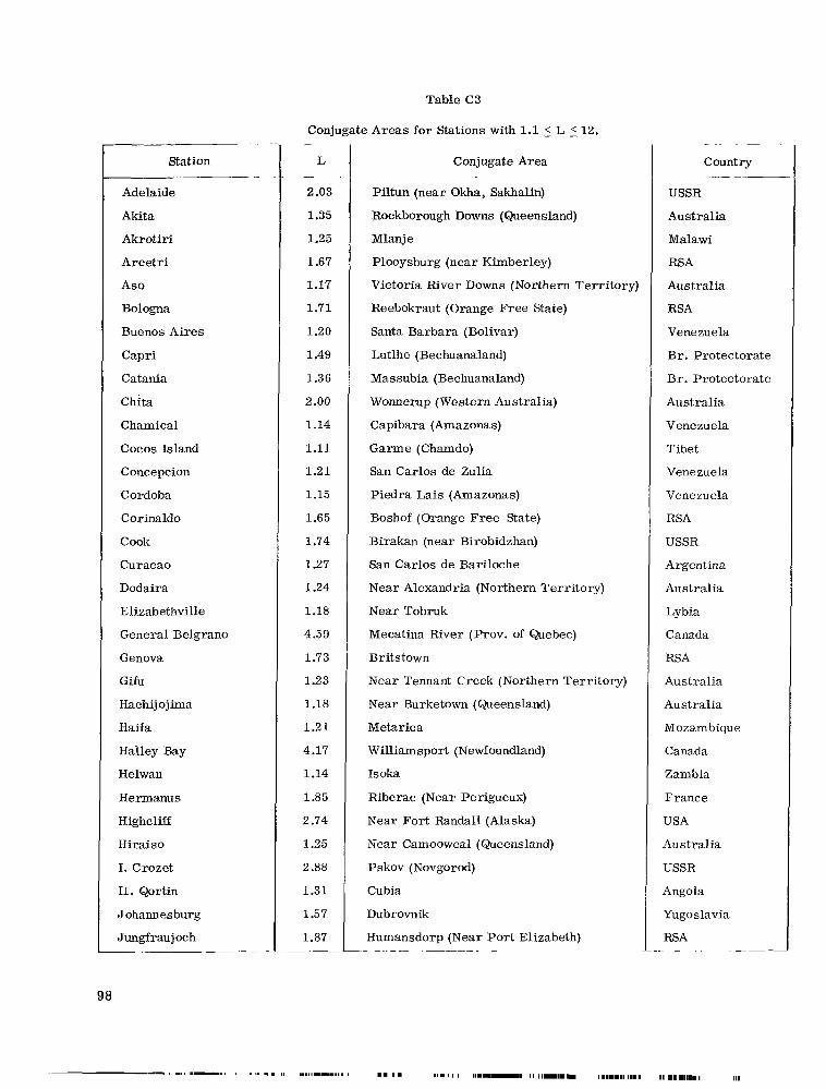
Table C3
Conjugate Areas fo r Stations with 1.1 5 L 5 12. .~ . .
Station
Adelaide
Akita
Akrotiri
Arce t r i
Aso
Bologna
Buenos Aires
Capri
Catania
Chita
Chamical
Cocos Island
Concepcion
Cordoba
Corinaldo
Cook
Curacao
Dodaira
Elizabethville
General Belgrano
Genova
Gifu
Hachijojima
Haifa
Halley Bay
Helwan
Hermanus
Highcliff
Hiraiso
I. Crozet
11. Qortin
Johannesburg
Jungfraujoch _ _
98
-
L
2.03
1.35
1.25
1.67
1.17
1.71
1.20
1.49
1.36
2 .oo 1.14
1.11
1.21
1.15
1.65
1.74
1.27
1.24
1.18
4.59
1.73
1.23
1.18
1.21
4.17
1.14
1.85
2.74
1.25
2.88
1.31
1.57
1.87
- Conjugate Area
Piltun (near Okha, Sakhalin)
Rockborough Downs (Queensland)
Mlanje
Plooysburg (near Kimberley)
Victoria River Downs (Northern Terri tory)
Reebokraut (Orange Free State)
Santa Barbara (Bolivar)
Lutlhe (Bechuanaland)
Massubia (Bechuanaland)
Wonnemp (Western Australia)
Capibara (Amazonas)
Garme (Chamdo)
San Carlos de Zulia
Piedra Lais (Amazonas)
Boshof (Orange Free State)
Birakan (near Birobidzhan)
Sa.n Carlos de Bariloche
Near Alexandria (Northern Terri tory)
Near Tobruk
Mecatina River (Prov. of Quebec)
Britstown
Near Tennant Creek (Northern Terri tory)
Near Burketown (aeens l and)
Metarica
Williamsport (Newfoundland)
Isoka
Riberac (Near Perigueux)
Near For t Randall (Alaska)
Near Camooweal (Queensland)
Pskov (Novgorod)
Cubia
Dubrovnik
Humansdorp (Near Port Elizabeth) _ _ ~
- _ _ ~ -
Country __ -~
USSR
Australia
Malawi
RSA
Australia
RSA
Venezuela
Br . Protectorate
Br . Protectorate
Australia
Venezuela
Tibet
Venezuela
Venezuela
RSA
USSR
Argentina
Australia
Lybia
Canada
RSA
Australia
Australia
Mozambique
Canada
Zambia
France
USA
Australia
USSR
Angola
Yugoslavia
RSA . - _-
Ill ---. . _.. “---.I I m I. .I. I, 1..11..11.1111 I- .I. I I, 11.11 I 1 1 . 1 1 1 1 1 I 1 1 1 1 1 1 . 1 1 11111.11 1111 I1 1111111111.1
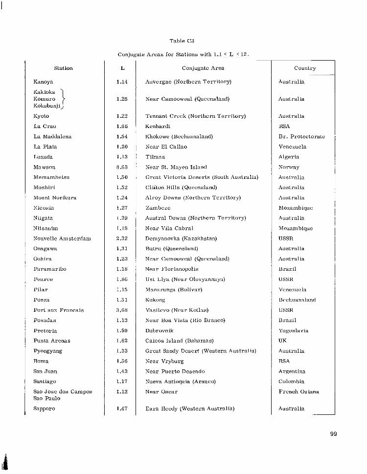
Table C3
Conjugate Areas for Stations with 1.1 5 L 5 12.
Station
Kanoya
Kakioka Komuro Kolubunji
Kyoto
La Crau
La Maddalena
La Plata
Luanda
Mawson
Memambetsu
Moshiri
Mount Norikura
Nicosia
Niigata
Nitsanim
Nouvelle Amsterdam
Onagawa
Oohira
Paramaribo
Pearce
P i l a r
Ponza
Port aux Francais
Po s ada s
Pre tor ia
Punta Arenas
Pyongyang
Roma
San Juan
Santiago
Sao J o s e dos Campos Sao Paulo
Sapporo
L
1.14
1.25
1.22
1.66
1.54
1.20
1.13
8.63
1.50
1.52
1.24
1.27
1.29
1.18
2.32
1.31
1.23
1.18
1.86
1.15
1.51
3.68
1.13
1.59
1.62
1.33
1.56
1.43
1.17
1.12
1.47
Conjugate Area
Auvergne (Northern Terri tory)
Near Camooweal (Queensland)
Tennant Creek (Northern Terri tory)
Kenhardt
Khokowe (Bechuanaland)
Near E l Callao
Tilmas
Near St. Mayen Island
Great Victoria Deserts (South Australia)
Clifton H i l l s (Queensland)
Alroy Downs (Northcrn Terri tory)
Zambeze
Austral Downs (Northern Terri tory)
Near Vila Cabral
Demyanovka (Kazakhstan)
Butru (Queensland)
Near Camooweal (Qucensland)
Near Florianopolis
Ust Llya (Near Olovyannayn)
Mntx~runga (Bolivar)
Kukong
Vasilcvo (Near Kotlas)
N e a r Boa Vista (Rio Branco)
Dubrovnik
Caicos Island (Bahamas)
Great Sandy Desert (Western Australia)
Near Vryburg
Near Puerto Deseado
Nueva Antioquia (Arauco)
Near Oscar
E a r a Heedy (Western Australia)
Country
Australia
Australia
Australia
RSA
Br. Protectorate
Venezuela
Algeria
Norway
Australia
Australia
Australia
Mozambique
Australia
Mozambique
USSR
Australia
Australia
Brazil
USSR
Venezuela
Bechuanaland
USSR
Brazil
Yugoslavia
UK
Australia
RSA
Argentina
Colombia
French Guiana
Australia
99

Station
Seoul
Simosato
Shackleton
Stellenbosch
Torino
Tortosa
Torre Chiaruccia
Tottori
Toyokawa
Trinidad
Tsumeb
Tucuman
Uj i
Vladivostok
Wakkanai
Yamagawa
Yuzhno-Sakhalinsk
Table C3
Conjugate Areas fo r Stations with 1.1 5 L 5 12.
L
1.28
1.18
4.61
1.82
1.78
1.57
1.57
1.23
1.24
1.26
1.34
1.11
1.21
1.50
1.56
1.13
1.64
Conjugate Area
Great Sandy Deser t (Western Australia)
Tanumbirini (Northern Terri tory)
St. Augustine River (Prov. of Quebec)
Saint Martial (Near Bordeaux)
Nelspoort (Near Beaufort West)
Bogenfels (Near Luderitz)
Near Vryburg
Tennant Creek (Northern Ter r i to ry)
Alexandria (Northern Ter r i to ry)
Near Mar del Plata
Tabarka (Near Tunis)
Uaruti (Amazonas)
Tennant Creek (Northern Ter r i to ry)
Great Victoria Deser t s (South Australia)
Eta Dunna (South Australia)
Near Port Keats (Northern Terri tory)
Blanchewater (South Australia)
Country
Australia
Australia
Canada
France
RSA
South West Africa
RSA
Australia
Australia
Argentina
Tunisia
Brazil
Australia
Australia
Australia
Australia
Australia
100

ALTITUDE 0 (km)
101
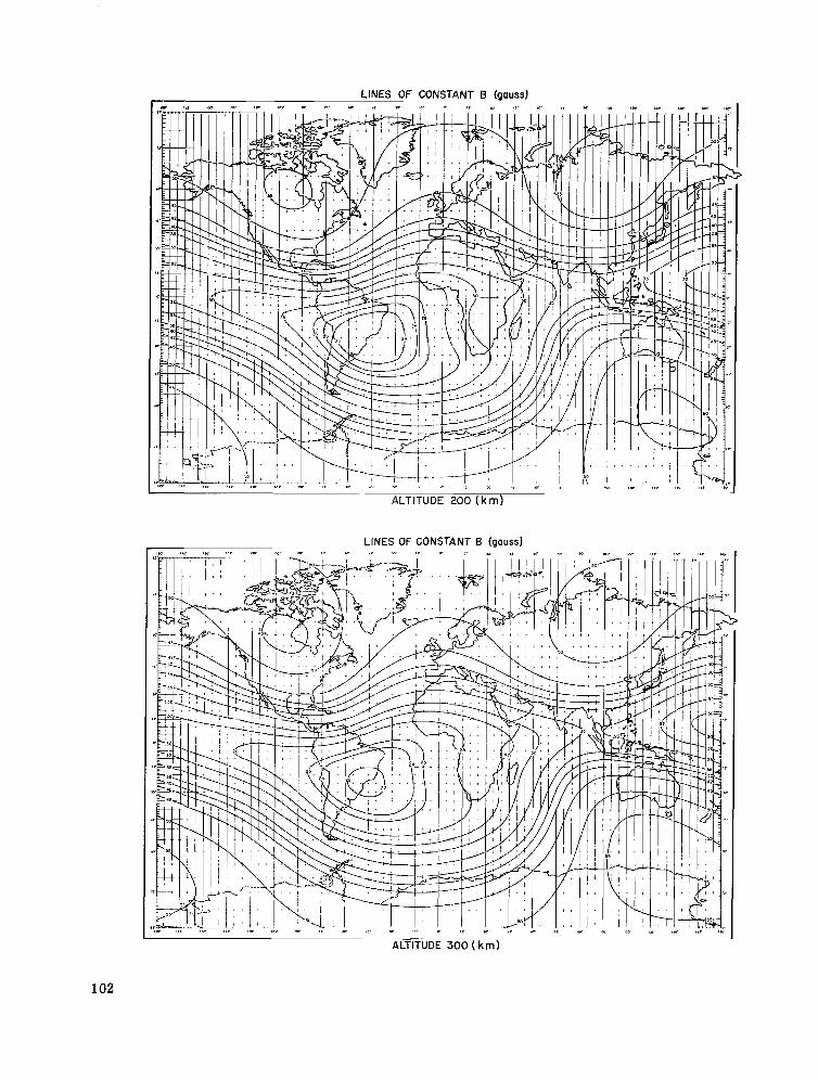
LINES OF CONSTANT B (gauss)
LINES OF CONSTANT B (craussl
102
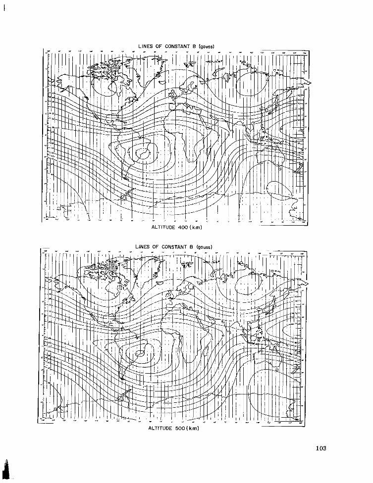
I
.-
ALTITUDE 400 ( k m)
LINES OF CONSTANT B (gauss) I D 1 m I Y ., .I. ~ \,. ,I . ~ .~. I
ALTITUDE 500 ( k m)
103

104
. .

. .
ALTITUDE 900 (km)
105

106

LINES OF CONSTANT B (gauss)
ALTITUDE 1200 ( k m)
LINES OF CONSTANT B (gauss)
ALTITUDE 1300 (km)
107

ALTITUDE 1500 (km)
108

I
LINES OF CONSTANT B (gauss)
2
ALTITUDE 1600 (km)
LINES OF CONSTANT B(gauss1 n /
a
ALTITUDE 1700 (km)
2
109

110
LINES OF CONSTANT B (gauss)
ALTITUDE 1800 ( km)
LINES OF CONSTANT 8 (gauss)

2
LlNtS OF CONSTANT B (g0USSl
7
111

LINES OF CONSTANT B (gauss)
ALTITUDE 2300 (km)
112

LINES OF CONSTANT B (gauss)
ALTITUDE 2400 (km)
LINES OF CONSTANT B(gauss)
ALTITUDE 2500 (km)
113

LINES OF CONSTANT B (gauss)
LINES OF CONSTANT E (gauss)
a
114

ALTITUDE 2800 (km)
LINES OF CONSTANT B (gauss)
ALTITUDE 2900 (km)
115

116
LINES OF CONSTANT B (aauss)
i
ALTITUDE 3000 (km)
LINES OF CONSTANT L (earth radii)
.~ ALTITUDE 0 ( k m)

ALTITUDE 100 (km)
c
ALTITUDE 200 ( k m)
117

Ill I I1 IIIIIII I1 I1 I 1
LINES OF CONSTANT L (earth radii)
118
ALTITUDE 300 (km)
LINES OF CONSTANT L (earth radii)
ALTITUDE 400 (km)

LINES OF CONSTANT L (earth rodid
ALTITUDE 600 (k m)
119

120

LINES OF CONSTANT L (earth radii)
LINES OF CONSTANT L (earth radii)
ALTITUDE 1000 (km)
121

LINES OF CONSTANT L (earth radii)
122

. ..... . . .. .. . . -. .. . . .. . .
ALTITUDE 1300 (k m)
LINES OF CONSTANT L (earth radii)
123
I

124

I
LINES OF CONSTANT L (earth radii)
LINES OF CONSTANT L (earth radii)
125
J

ALTITUDE 1900 (km) LINES OF CONSTANT L (earth radii)
126

LINES OF CONSTANT L (earth radii)
ALTITUDE 2100 (km)
LINES OF CONSTANT L (earth radii)
127

I l l 1 I l l
LINES OF CONSTANT L (earth radii)
7
ALTITUDE 2400 (k m)
128
I

. , . ... , . .. ._. . . __.. . - .. ... . . . . , .. . . . . , .. . - . .. .
LINES OF CONSTANT L (eorfh rodii)
7
LINES OF CONSTANT L (earth radii)
ALTITUDE 2600 ( k m
129

LINES OF CONSTANT L (earth radii)
ALTITUDE 2700 (km) LINES OF CONSTANT L (earth radii)
ALTITUDE 2800 (km)
130

ALTITUDE 2900 (km)
ALTITUDE 3000 ( k m )
131


A SUMMARY OF RESULTS FROM THE IMP-I MAGNETIC FIELD EXPERIMENT
by N. F. Ness , C. S. Scearce, and J. B. Seek
Goddard Space Fl ight Cen ter
and
J. M. Wilcox Space Sc iences Laboratory, Universi ty of California
The Interplanetary Monitoring Platform (IMP-I) launched in November 1963 with an apogee of 31.7 Re, has provided the first accurate measurements of the interplanetary magnetic field, the magnetosphere boundary and the collisionless magnetohydrodynamic shock wave associated with the solar wind interaction with the geomagnetic field. The shape of the magnetosphere i s found to be roughly cylindrical in shape, diameter = 44 Re, with a hemispherical cap with a radius of curvature of approximately 14 Re. The average direction of the interplanetary field i s approximately 140" east of the earth-sun line o r 60" west of the sun.
The interplanetary results confirm the general Archimedean sp i ra l structure of the interplanetary magnetic field. This is a direct result of the radial flux of ionized gas from the so la r corona by super-Alfvenic magnetohydrodynamic ex- pansion as predicted by Parker . The interaction of the super-Alfvhnic plasma flow from the sun with the geomagnetic field leads to the development of a detached bow shock wave and a turbulent transition region in which tangled and rapidly fluctuating magnetic fields are observed.
The experimental detection of an extended magnetic tail on the nighttime side of the earth and an enclosed magnetically neutral sheet represents the most recent important result with respect t o the earth 's outer magnetic field. Significant time variations of the magnetic field in the tail a r e in opposition with the so la r phase of the sudden geomagnetic storms. Thus the tail appears to play a dominant role in various te r res t r ia l phenomena. The neutral sheet is populated with energetic electrons which may be the source of radiation leading to auroral displays and the Van Allen belts.
INTRODUCTION
The Interplanetary Monitoring Platform IMP-I, the first in a ser ies of satellites monitoring the interplanetary medium in cislunar space, w a s launched on 27 November 1963. It carried in- struments to perform detailed measurements of magnetic fields, plasmas, energetic particles, and
133
h

IIIIIII IIIII
solar and galactic cosmic rays. Anumber of publications on the initial results of the magnetic field experiment have already appeared (References 1-6). In addition, some results of other ex- periments carried on board the satellite have appeared in the l i terature (References 7- 12). This paper briefly summarizes and reviews the significant results of the magnetic field experiment and presents certain new aspects of the experimental measurements and their interpretation.
The initial apogee of the satellite was on the sunlit side of the earth at an earth-sun angle of approximately 33" west of the sun at a geocentric distance of 197,616 kilometers = 31.7 earth radii and an initial perigee of 192 kilometers. The period of this highly eccentric orbit is 93.5 hours. Interpretation of the results from the IMP-I satellite w a s initially performed by trans- forming all data obtained into a solar ecliptic coordinate system. This is because the interaction of the solar wind with the geomagnetic field shows a strong day-night asymmetry with apparent cylindrical symmetry about the earth-sun line. The geocentric solar ecliptic coordinate system is defined by an X-axis directed from the earth to the sun, the Y-axis in the plane of the ecliptic, and the Z-axis pointing towards the north ecliptic pole. In this coordinate system, the apparent mo- tion of the satellite apogee is one of westward precession of 4" per orbit as the earth moves about the sun.
Figure 1 shows the variation of the apogee of the satellite in solar ecliptic coordinates. The angle B a is defined as the solar ecliptic latitude and the angle @ a as the solar ecliptic longitude of satellite apogee. The measurements of the magnetic field in space wi l l also be presented in the solar ecliptic coordinate system with 8 and @ defining the direction of the field with magnitude F.
The useful lifetime of the satellite extended over a period of approximately 6 months while satel-
360 - "3
m E m 4 315
n
(3 z
v
W
- ' 270
3
DEC. JAN. FEB. M A R . APR. MAY JUNE I
0 IO 20 30 40 50 ORBIT NUMBER
IJJ -
Figure I-Variation of the apogee (31.7 Re geocentric) of the IMP-I satellite for orbits 1-47 during the time interval 27 November 1963 through 27 May 1964. The two angles tia and represent, respectively, the latitude and longitude of the apogee of the satellite in solar ecl ipt ic coordinates.
lite apogee varied from a solar ecliptic longi- tude of 335" to 155" (Figure 1). This permitted mapping of the boundary of the geomagne'tic field formed by interaction with the solar wind from the subsolar point through the sunrise terminator and far into the nighttime region of the earth.
Apogee w a s sufficiently high (Figure 2) that during the f i r s t 21 orbits direct measurements of the interplanetary medium were possible which were not affected by the earth 's presence and its magnetic field in the supersonic flow of the solar wind. Following orbit 21, measure- ments in cislunar space were limited to that portion associated with the interaction of the solar wind with the geomagnetic field. Finally, subsequent to orbit 31, the measurements were performed while the satellite w a s completely enclosed within the distorted geomagnetic field.
134

The space surrounding the earth is divided into three characteristic physical regions (Fig- ure 2):
1. the intevplanetavy medium,
2. the turbulent transition vegion, and
3. the inagrzetospheve o r distorted geomag- netic field of the earth.
These three regions are separated from each other by two character istic boundaries :
1. The collisionless magnetohydrodynamic shock wave (References 13- 15)
and
2. The m a g n e t o s p h e r e boundary o r inagnetopause.
Repeated t raversals of these two boundaries by IMP-I have yielded extensive measurements de- fining their physical properties and have per- mitted the geometrical description and physical separation of cislunar space into these three characterist ic regions.
30R, /SHOCK WAVE
IMP-I 21 ORBITS
SUN OR, 20 \ i o 7 - i o -20 -3oR,
k ECLIPTIC PLANE
Figure 2-Simp1 i f ied summary of results of mapping the terrestrial magnetosphere boundary with the interplane- tary medium. illustrated on the plane of the ecl ipt ic are the positions of the magnetosphere boundary and the collisionless magnetohydrodynamic shock wave. The shape and position of the detached bow shock wave closelyparallel that observed in supersonic gas dynamics at Mach numbers corresponding to the ratio of the solar wind velocity to the Alfven velocity.
The intevplanetnvy iizediitnz is characterized by a weak magnetic field of approximately 5.1 gammas average magnitude embedded within a radial plasma flux emitted from the surface of the sun, which is referred to as the solar wind (Reference 16). At the earth 's distance of 1 Astronomi- cal Unit (AU) the plasma shows flow velocities between 300 to 700 kilometers per second and densi- t ies between 2 to 20 protons per cubic centimeter. The direction of the magnetic field is variable but the magnitude is impressively constant over long periods of time so that bF/F < 0.1. A general Archimedean spiral structure has been observed in the interplanetary field which can be correlated with the rotational period of the sun and hence corotates with the sun and is suggested to be of solar origin.
The tvansition vegion is observed to be a turbulent, thermalized, magnetized plasma with field strengths varying between 5 and 20 gammas and fluctuations over short time scales of 10 to 20 gammas. No periodic wave forms are readily discernible in the data and the fields are thus described as tangled o r randomly oriented. A thermalized plasma is observed near the stagnation point of the solar wind flow in which the spectrum is considerably broadened and the density in- creases by a factor of approximately 8 (Reference 9). The solar wind is found to resume a super- sonic flow condition around the flanks of the magnetosplzeve.
135

The measurements of the distorted geomagnetic field on the night side of the earth reveal the extension of the geomagnetic field far behind the ear th forming a magnetic tail. Embedded within this magnetic tail, a magnetically neutral surface has been discovered which separates regions of oppositely directed fields over a thin planar region of space. This is referred to as a neutral sheet and can be. correlated with increased particle fluxes illustrating a balance between field and particle pressures.
This paper presents first a summary of the results obtained while the satellite was in inter- planetary space beyond the shock wave during orbits 1 through 21, representing the time interval 27 November 1963 through 17 February 1964 and corresponding approximately to three solar ro- tations, 1784 through 1786. In general, solar activity has remained at a low level throughout the satellite's lifetime. This paper will not discuss any storm-time variations, either of the inter- planetary magnetic field or the earth 's magnetic tail field. Subsequent publications will deal with these transient phenomena in as comprehensive a treatment as possible.
INTERPLANETARY MAGNETIC FIELD RESULTS
After the early suggestions by Biermann (Reference 17) that the sun must be a continual source of a low-energy corpuscular flux or solar plasma, Parker (Reference 18) developed the theory of the solar wind, describing the expansion of solar coronal gases into interplanetary space at super- Alfvenic velocity. A particular distinguishing result of Parker 's model is the twisting of solar photospheric magnetic fields into an Archimedean spiral in the ecliptic plane as a result of the uniform radial flux of coronal gases and the rotation of the sun. This is illustrated in Figure 3 for solar wind velocities as typically measured in the interplanetary medium from 300 to 900 kilom-
e te rs per second (References 9 and 19). It is 180
- 150
E - "7 al
m u - - * 120
360 seen that the angle 4 or 4 ' is approximately 135" or 3154 respectively. Thus the direction of the field is approximately 45" with respect to the
1 earth-sun line. This is a direct result of the approximate equality of radial velocity of solar plasma with the tangential velocity of a radius vector fixed to the sun and rotating with a syn- odic period of 27.3 days.
330 - -0 -
300k
The measurement of the magnetic field on I I I L--. 1 2 7 0 300 600 900 90'
IMP-I was performed for 4.8 seconds every
mat for a consecutive total of 12 such data
SOLAR WIND VELOCITY, V, (km/sec)
Figure 3-Theoretical direction of the interplanetary 20.4 seconds repeatedly within a telemetry for- magnetic field, assumed to be of S o h origin, twisted into an Archimedean spiral by the rotation of the sun and the radial efflux of highly ionized gases. The two di- rections Q and Q' correspond to fields directed essen- minutes in transmission time. These measure-
points distributed Over an Of 5.46
t ia l l y away from or towards the sun along the charac- teristic streaming angle. Note the relative insensitivity of the direction to chanaes in typical solar wind veloci-
ments yielded 12 vector samples of the inter- planetary magnetic field. Individual orthogonal
" I ,
ties from 300 to 700 km/sec. components of the vector field were averaged
156
I

and used to construct an average vecto# magnetic field for the time interval of 5.46 minutes.
t TO ECLIPTIC PLANE
+ C$ = 180°
NORMAL TO t NORTH
ECLIPTIC POLE ECLIPTIC PLANE
I- \ ' ISOTROPIC 'I Y
ECLIPTIC PLANE
- e = 00
+ e = -900
Figure 4-Statistical distribution of the direction of the 5.46-minute component-averaged interplanetary mag- netic f ie ld as observed on IMP-I during solar rotations 1784-1786. The distribution in the plane of the ecl ipt ic indicates a close correspondence with the theoretical model of a continual uniform solar coronal expansion developed by Parker. The f ield distribution normal to the plane of the ecl ipt ic indicates a small but distinct southward-directed component.
The statistical distribution of the direction of the interplanetary magnetic field observed by the IMP-I satellite when beyond the shock wave is shown in Figure 4. A broad but distinct peak in the direction of the field is observed at ap- proximately the angle predicted by Parker 's uniform coronal expansion model. The top of Figure 4 shows the direction of the inter- planetary field projected into the plane of the ecliptic. The bottom view of the figure shows the direction of the field as projected normal to the plane of the ecliptic and without regard to the direction of the field in the piane of the ecliptic.
The magnitude distribution of the inter- planetary magnetic field is shown in Figure 5. It should be noted that extremely stringent re- quirements were placed upon the satellite ex- periment hardware to minimize their magnetic
I M P - I 5.46 MINUTE COMPONENT AVERAGES
" 2 4 6 8 10 12 14
FIELD MAGNITUDE (gammas)
Figure 5-Statistical distribution of the interplanetary magnetic f ield magnitude for the same data correspond- ing to that shown in Figure 4. The uniformity of the distribution with an average value of 5.1 gammas i s in- dicative of average photospheric fields of the sun of a few gauss, according to Parker's model.
137
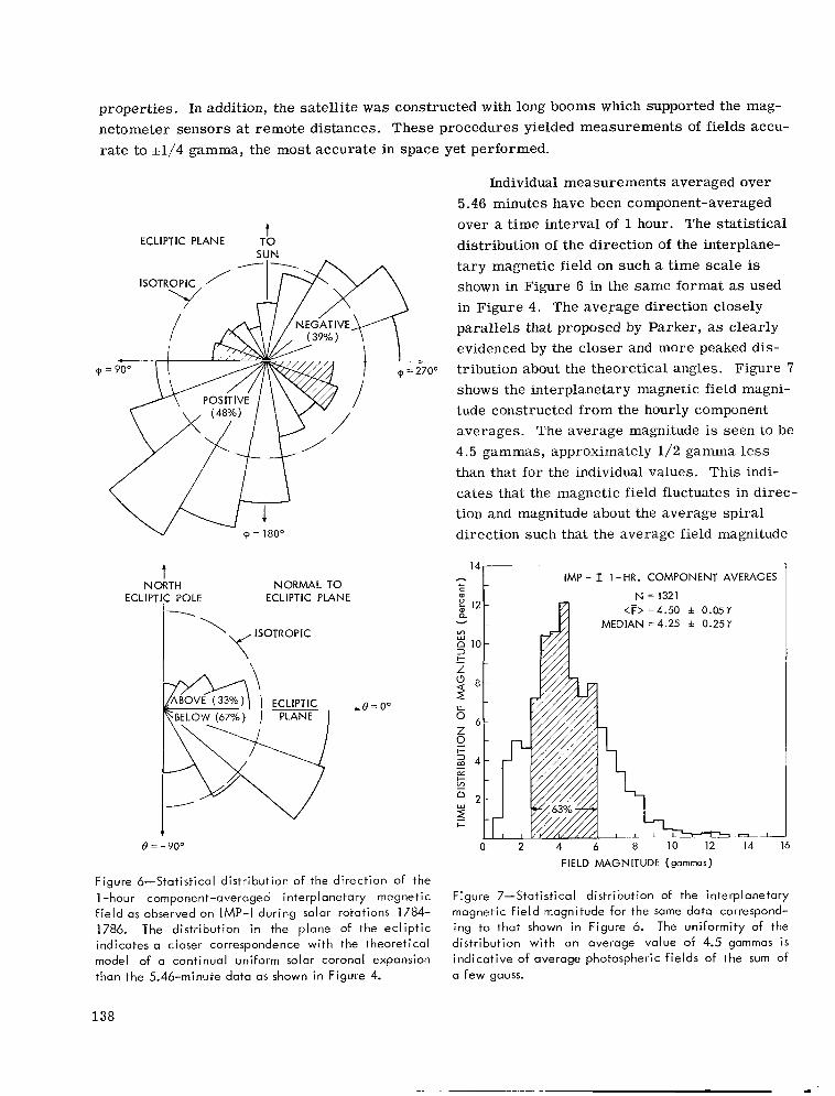
properties. In addition, the satellite w a s constructed with long booms which supported the mag- netometer sensors at remote distances. These procedures yielded measurements of fields accu- ra te to +1/4 gamma, the most accurate in space yet performed.
t ECLIPTIC PLANE T O
SUN
NORMAL TO t
NORTH ECLIPTIC POLE ECLIPTIC PLANE
, e = o o
Figure 6-Statistical distribution of the direction of the 1 -hour component-averaged i nterp I anetary magnetic f ield as observed on IMP-I during solar rotations 1784- 1786. The distribution in the plane of the ecl ipt ic indicates a closer correspondence with the theoretical model of a continual uniform solar coronal expansion than the 5.46-minute data as shown in Figure 4.
Individual measurements averaged over 5.46 minutes have been component-averaged over a time interval of 1 hour. The statistical distribution of the direction of the interplane- tary magnetic field on such a time scale is shown in Figure 6 in the same format as used in Figure 4. The average direction closely parallels that proposed by Parker, as clearly evidenced by the closer and more peaked dis- tribution about the theoretical angles. Figure 7 shows the interplanetary magnetic field magni- tude constructed from the hourly component averages. The average magnitude is seen to be 4.5 gammas, approximately 1/2 gamma less than that for the individual values. This indi- cates that the magnetic field fluctuates in direc- tion and magnitude about the average spiral direction such that the average field magnitude
’“L IMP - I 1 -HR. COMPONENT AVERAGES 1 + g Q 121
N = 1321 <F>=4.50 f 0.05Y I
v MEDIAN =4.25 f 0.25Y Ln
10 3
Z + -
2 8
E 6 Z o_ l-
- 2 4
O 2
2
Di l- 2
Y
+
0 2 4 6 8 10 12 FIELD MAGNITUDE (gammos)
- 14 16
Figure 7-Statistical distribution of the interplanetary magnetic f ield magnitude for the same data correspond- ing to that shown in Figure 6. The uniformity of the distribution with an average value of 4.5 gammas i s indicative of average photospheric fields of the sum of a few gauss.
138

decreases as averages extend over longer time intervals.
Additional statistical characterist ics of the interplanetary magnetic field a r e presented in Figures 8, 9, and 10. These show respectively,
t TO ECLIPTIC PLANE
14 + c -
12- a v
v)
x 10- - 2 Z
3 8:
6 - Z 0 - c - 2 4 - w c - Y n Y 2- 5 - I-
ISOTROPIC
0
k NORMAL TO NORTH ECLIPTIC PLANE
ECLIPTIC POLE
e = 00
Figure 8-Statistical distribution of the direction of the 3-hour component-averaged interplanetary magnetic f ield as observed on IMP-I during solar rotations 1784- 1786. The distribution in the plane of the ecl ipt ic in- dicates a stil I closer correspondence with the theoretical model than shown in Figures 4 and 6 although the lack of 180" symmetry i s clearly evident.
2 2 Y r I- I \, 0
I MEDIAN = 4.25 *0.25 Y
4 6 8 10 12 2
FIELD MAGNITUDE (gammas)
Figure 9-Statistical distribution of the interplanetary magnetic f i e ld magnitude for the same data correspond- ing to that shown in Figure 8. The uniformity of the distribution with an average value of 4.3 gammas i s in- dicative of average photospheric fields of the sun a few gauss according to Parker's model.
IMP-I 3 HR. MAGNITUDE AVERAGES N =455
<F>=5.1Oi 0.05Y
FIELD MAGNITUDE (gammas)
Figure 10-Statistical distribution of the averaged mag- nitudes of the interplanetary magnetic f ield over a 3- hour interval. Th is figure i s to be distinguished from the preceding figure i n which component avei-ages were employed to construct a 3-hour magnitude average. The average value of 5.1 gammas i s identicol to Figure 5 , as i s to be expected.
139
I

the directional distribution of the 3-hour component averages of the interplanetary magnetic field, the average magnetic field magnitude over 3-hour intervals, and finally a magnitude-averaged in- terplanetary magnetic field over a 3-hour time interval. Figure 10 illustrates the differences of averaging the magnetic field components or magnitudes over different time intervals by compari- son with Figure 9.
The description of a vector field which is time-variable in both direction and magnitude is a complex task, since simple component averages may represent an average vector field which does not correspond to one which the "real" field ever showed. Thus in the analysis of the time changes of the magnetic field direction in the following section, recourse was always made to the original 5.46-minute averages. Rather than directly averaging the components of the magnetic field separ- ately and then constructing an average field direction, directional histograms were constructed for time intervals of 3, 6 , 12, and 24 hours, yielding characterist ic directions for the field.
The measurement of 5.1 gamma average magnitude field roughly in the plane of the ecliptic, but with a slight southward component of the field, and directed approximately parallel to the angle predicted by Parker for the field, dramatically confirms the uniform coronal expansion model proposed by him, at least during the years of the quiet sun. It strongly suggests the sun as the origin of the interplanetary magnetic field and ,.ol indeed in the next section this argument will be developed further to illustrate the continuity of field lines from the sun out to 1 AU.
CORRELATION WITH THE PHOTOSPHERIC MAGNETIC FIELD
As shown i n Figures 4, 6, and 8 the direc- tion of the field can be assigned as either posi- tive or negative depending upon whether or not the field appears to be directed away from or towards the sun along the streaming angle. Using the range of @ indicated in Figure 4 as -0.2
0.4
0.2
-0.41 positive o r negative, it is possible to assign a + 1 or - 1 to each 3- hour interval covered by the
-O+ I Y I I I I
interplanetary data on IMP-I. This time ser ies of alternating values shows the changes in di- rection of the field as measured at 1 AU by
0 4 8 12 16 20 24 IMP-I. Construction of the autocorrelation TIME LAG (days)
I 28
function basic tend- Figure 11 -Autocorrelation ofthe direction of the inter-
encies within this time ser ies . Figure 11 pre- sents the normalized autocorre~ation of the di-
planetary magnetic f ield as observed by IMP-I. The di- rection of the f ie ld i s defined to be either positive or negative according to Figure 4. The autocorrelation of
mately 27 days (see text).
Of the magnetic field and this time series yields a significant peak approxi- the results show a statistically significant peak
140
II 11111111111 11111111 II I I II 111 I1111111111.~11111.11111

at a time interval of approximately 27 days. Since this corresponds to the solar synodic rotation period, it is strongly suggestive of a direct connection of the interplanetary magnetic field with magnetic fields originating on the sun.
0.8
0.6
0.4
Z 0 0.2 - 4 w e
0 - ; v) v)
p -0.2 V
-0.4
-0.6
It is possible to directly compare the interplanetary and solar fields by utilizing data obtained with the solar magnetograph at the Mount Wilson Observatory in California (Reference 20). Fig- u r e 12 illustrates the result from the solar magnetograph during the IMP-I lifetime which presents a mapping of the photospheric magnetic field as observed at central meridian passage (CMP) on each day. The magnitude of the line-of-sight component of the photospheric magnetic field is meas- ured by the longitudinal Zeeman effect on one of the Fe lines in the solar spectrum. Consecutive daily measurements at CMP are combined to produce a contour map which shows large a reas on the surface of the sun with magnetic fields in the photosphere which a r e directed either out of or into the sun.
-
-
-
-
-
-
-
-
-
-
-
-
-
-
In aprocess similar to that for the interplanetary data, a time se r i e s w a s constructed for in- dividual latitude bands 10" wide across the sun: the field direction w a s determined within a surface a rea of the solar disk corresponding to a 12-hour longitude interval (equivalent to 6.7" heliographic longitude). With a time ser ies covering the same interval as IMP-I in interplanetary space, it is possible to construct a cross-correlation function between the directions of the inter- planetary magnetic field and the photospheric magnetic field.
This result is shown in Figure 13, in which a statistically significant and coherent peak is
SOLAR LONGITUDE (degrees)
100 80 60 40 20 0 340 320 2 40 N w
I I I I I : ' , I , , , ,
1 2 3 4 5 6 7 8 9 1 0 1 1
DATE, DECEMBER 1963
Figure 12-Representative solar magnetograph obtained from the Mount Wilson Observatory showing the mag- nitude and direction of the line-of-sight component of the photospheric magnetic f ield at CMP on date shown. The contour interval for these data are taken to be 2, 4, 8, 12,and 25 gauss. A solid line indicates f ield directed out of the sun while dashed linesindicate fields directed into the sun.
A - 00
-0 .8 I 1 I I I I I I -8 -4 0 4 8 12 16
TIME LAG (days)
Figure 13-Cross-correlation of the IMP-I interplanetary magnetic f ield data and the photospheric magnetic f ield for three latitudes illustrating the coherent and statisti- cal ly significant peak at 4.5 days. Th is corresponds to a transport velocity of solar lines of flux to 1 AU of ap- proximately 385 km/sec.
141

shown for three separate latitude bands across the solar disk. The time lag of 4.5 days is evi- dent, which corresponds to a transport velocity of lines of flux by the solar wind to l AU of ap- proximately 385 kilometers per second. The uncertainty in the time lag corresponds to the small- est unit of time available, +12 hours, so that the average solar wind velocity from the magnetic field measurements is inferred to be 385 k 45 kilometers per second. The lower limit of this ve- locity, 340 kilometers per second, is very close to the direct measurement of the solar wind veloc- ity by the MIT plasma probe which yielded an average of 320 kilometers per second (Reference 9).
p +++++;+;-\ - -
+++++;-++ +++2+ +-
++++++ + ++ -- / = = + %
. ORBIT NO. 1
20 DEC.
0300 \ - 1 DEC. ' 0300
\ (-1- (-1- f
STORM - 2 DEC.
21 17
4 DEC. 2100
1200
Figure 14-Superposed epoch structure of the interplanetary magnetic f ield direction for solar rotations 1784- 1786. Immediately evident i s the sectoring of the interplanetary f ield into four portions of which three are ap- proximately equal in angular extent. This sector structure co-rotates with the sun and hence observable effects associated with this structure should be detectable at periodic time intervals of approximately 27 days.
142

In addition to investigating the solar origin of the interplanetary magnetic field by the previous method of analysis, it is also possible to superpose the time variations in magnetic field direction in a circular epoch graph as shown in Figure 14. It is seen that the direction of the interplanetary magnetic field is repetitive on a time scale of 27 days in a very dramatic fashion which reveals the existence of four distinct sectors. Within each sector the magnetic field is directed either away from or towards the sun within the entire sector. Three of the sectors have a time interval of approximately 7.6 days, while the third sector shows a time interval correspond- ing to 3.8 days at 1 AU.
This superposed epoch chart also illustrates the characteristic geometrical configuration of the field lines within the interplanetary medium during three solar rotations of the quiet sun. As the sun rotates, this sector structure sweeps past the earth and changes associated with spatial variations within each sector can be associated with changes on the surface of the earth in mag- netic field activity and cosmic ray variations. Figure 15 gives the variation of the planetary mag- netic index K~ within the 2/7 sectors of the interplanetary magnetic field. It is seen that high KP
follows shortly after a sector boundary passes and that low K, values a r e reached towards the end of each sector. There appears to be no significant difference between + and - sectors, at least at the present time.
It should be noted that there i s a close cor- respondence of the orbital period (3.9 days)with the time scale of the sector structure (1/7 sec- tor = 3.8 days). The analyses have been critically reviewed to verify that the sector re- su l t s a r e not an artifact generated in the analysis.
In summary, these results show that during the three solar rotations near the minimum of the solar cycle, the photospheric field is dragged out by the solar wind to form the nearby inter- planetary magnetic field and that a semiper- manent sector structure exists. These conclu- sions a r e consistent with the model suggested by Ahluwalia and Dessler (Reference 21) in which the sense of the field in the sectors is related to the sense of photospheric magnetic field regions.
To interpret the solar wind interaction with the geomagnetic field, it is necessary to have average values of the interplanetary medium available from direct measurements to justify a comparison between supersonic gas dynamics
+ FIELD AWAY FROM SUN ++ - FIELD TOWARD SUN
FIELD AWAY + FIELD TOWARD * O - ep --
- -0
+OD 0
* o -- 0 -- +q* *-
0 -2 0
* o 0
-- o* 0 * -4t_
0000 * -pu
__ 0 -
00 00 _- __ 8
00 -__
+tooo ** O
* o 0000
i V i i i i 7 a POSITION WITHIN 2 /7 SECTORS ( d a y s )
Figure 15-Chat-acteristic variation of the K, index as observed in the combined sectors illustrated in Figure 14. The high KP index follows the change in sense of the directed flux tube from the sun and K, decreases to a minimum at the end of the sector. Implications regard- ing the recurrent M-region storms on the sun are dis- cussed in the text.
143

I I I I I I I I 1 I
and the flow of solar wind. Figure 16 summar- izes the average values of pertinent physical pa- rameters in the interplanetary medium deduced from the magnetic field experiment on IMP-I. The average magnitude of the magnetic field is 5.1 gammas and the directional changes indicate a solar w'ind velocity of 385 kilometers per second, which yields a proton cyclotron radius of 820 kilometers. It has been suggested by Axford (Reference 13) and Kellogg (Reference 15) that this represents the appropriate physical scale unit to utilize in considering the charac- ter is t ics of the interaction of the solar plasma flow with the geomagnetic field. Since the mag- netosphere as shown in Figure 2 is approxi- mately 44 Re in diameter, clearly the plasma flow can be considered as fluid since the proton cyclotron radius is much smaller than the size of the magnetosphere.
MAGNETOSPHERE AND BOUNDARY LAYER RESULTS
PROTON VELOCITY (km /sec )
i o4 200 400 600 800 I I
I I
0.03 cp:
5 1 MAGNETIC FIELD r\
CYCLOTROI / FREQUENCl
I I 1 1 1 1 1 1 I I I l l l l
0.1 0.2 0.4 0.6 1 2 4 6 8 PROTON ENERGY (kev)
Figure 16-Representative values of the interplanetary medium during the quiet sun as observed by IMP-I. The interplanetary magnetic f ield magnitude and velocity, as derived from directional considerations and cross- correlation with the sun, yield a characteristic proton cyclotron radius of 820 kilometers.
Magnetic field measurements by the IMP-I satellite, in comparison with plasma measure- ments, have shown a unique and coherent picture of the termination of the geomagnetic field and the transition to the interplanetary medium. The first t raversal of the magnetosphere and shock wave boundaries by IMP-I is shown in Figure 17 for the magnetic field experiment. The magni- tude, F, and the two angles 0 and 4 describe the vector magnetic field over the 5.46-minute time interval. The root- mean-square deviation of the individual solar ecliptic components is also shown as FX, FY, and 6Z. It is seen that the transition region is one in which both the direction and magnitude of the field vary on short and long time scales. Within the interplanetary medium, magnetic field fluctuations a r e less than the quantization e r r o r s of the telemetry system and cor- respond to a few tenths of a gamma. Thus for the interplanetary medium, the characteristic fluctuations 8 F b are seen to be less than 0.1 while within the transition region, 6Fb varies gen- erally between 0.5 and 2.
An enlarged time scale presentation of the t raversal of the shock wave boundary is shown in Figure 18. Individual measurements at 20.4 second intervals a r e illustrated for the three ortho- gonal components. The motion of the satellite between successive 20.4 second samples corresponds to approximately 40 kilometers in space. The identificationof the shock wave boundary as an abrupt change from a stable, weak, ordered field to a turbulent, stronger field is clear and indicated by the dashed line in the figure.
144

40
F ( yommas)
20
+ 90' 0
e oo -90' 360"
0
6X
6Y
62
TIME (UT) 9 12 15
1 - I
10 15 20 GEOCENTRIC DISTANCE ( R e )
Figure 17-Observed magnetic f ield results on outbound orbit 1 by the IMP-I satellite, 27 November 1963. Clearly evident are the magnetosphere boundary at 11.3 R e and the collisionless shock wave at 16.8 Re. For a definition of these boundaries see text.
SEQUENCE NUMBER
472 yo Y8 4;/6 0 - + 2 0 i - j I I I I
I 1
- 2OLJ 17.373
I 1 I - I 28.295 39.216 50.139
TIME (min)
f igure 18-Detailed variation of the three orthogonal components of the magnetic f ield observed during the first outbound traversal of the shock wave by IMP-I. These data expand the time scale shown in Figure 17 to o distance scale corresponding to satellite motion of ap- proximately 40 kilometers between successive sample points. The gaps in the data correspond to continuous transmission of the rubidium vapor magnetometer data in the telemetry sequence.
On an expanded scale Figure 19 shows the characteristic raw telemetry signals correspond- ing to individual samples of the magnetic field as sampled by the flwgate magnetometers at time intervals of 0.160 second. The individual spin-
modulated segments of the telemetry signal are presented on an enlarged scale but in time sequence. Again the identification of the boundary is evidenced as a transition from a uniform stable field to a turbulent and rapidly fluctuating magnetic field. This characteristic thinness of the shock wave boundary separating stable and turbulent fields w a s not anticipated and is one unique aspect of the magnetic field measurements by IMP-I.
Corresponding to the magnetic field measurements on outbound orbit 1, Figure 20 shows the pertinent plasma measurements from the MIT plasma Faraday Cup (Reference 9). The diagram shows the maximum and minimu'm flux values during each spin period as measured in the channel correspond to protons with energies between 220 and 660 electron volts. A measurement of the extreme fluxes during each satellite spin is an indirect measurement of the anistropy of the plasma flow. Within the transition region, which corresponds perfectly with that defined by the magnetom- eter measurements, the plasma flow is seen to be generally isotropic and other energy channels not shown would indicate a s imilar response characteristic. The MIT plasma measurements have revealed a broad region of turbulent, thermalized plasma flow immediately behind the shock wave
145

FLUXGATE A rT + I SEQUENCE NUMBER 462 1 . ! I 1 1 I 1. I
I
sw -. I p 2 0 . 4 8 s. 4
80 t \
FLUXGATE B
\ FRAME NUMBER f, =6.25 cps \ 4 4.8 SEC. k
SUCCESSIVE RAW FLUXGATE TELEMETRY TRANSMISSIONS
\ \
FILTER NUMBER 4o
Figure 19-Fine detail of the collisionless shock wave thickness as observed on outbound orbit 1 by IMP-I. In- dividual spin-modulated signals observed for time intervals of 4.8 seconds are shown in time sequence. The position of the shock wave and the characteristic differences in the magnetic f ield modulation of the detected f lux gate magnetometer signal are evident.
and enclosing the magnetosphere. The remainder of orbits 2 through 21, which permit sampling of the interplanetary medium, show excellent agreement between plasma and magnetic field meas- urements with respect to the positions of the characterist ic shock wave and magnetosphere bound- aries in cislunar space.
- X 3
Z 2 i o 7
2 2 a
4 x 10⁶
5: 44 7 5 5 8.1 11.5
NOISE LEVEL . 12:05 " 1450 UT 16.5 19.1 DISTANCE ( R E )
Figure 20-Representative results from t h e MIT plosmo probe showing measurements of thermalized plasma by IMP-I during outbound orbit 1. The positions of the boundaries are evidenced by the distinct change to small spin modulation of the observed flux between 11.3 and 16.8 Re compared to measurements beyond these points (Refer- ence 9).
146

Figure 21 presents the inbound orbit 1 magnetic field measurements illustrating the character of the magnetosphere boundary near the stagnation point. The magnetic field interior to the bound- a r y is seen to be increased by approximately a factor of two above that theoretically predicted by extrapolation from the earth’s surface using spherical harmonics. This corresponds to the com- pression of the geomagnetic field by an infinitely conducting plasma and the factor of two is in agreement with theoretical prediction (Reference 22). The direction of the field is seen to be only slightly distorted interior to the magnetosphere boundary. Beyond this a magnetic field turbulent both in direction and magnitude is seen, as shown previously in Figure 17.
/AVE
The energetic particle results for inbound orbit 1 showing electrons with energies greater than 45 kev as detected by the geiger counter experiment of Anderson, Harris, and Paoli (Reference 7 ) are given in Figure 22. An intense flux of particles is observed interior to the magnetosphere boundary to the trapped particles in the outer radiation belts. The termination of the trapping region is seen to coincide with the boundary of the magnetosphere as observed first by Freeman, Van Allen, and Cahill on Explorer XI1 (References 23 and 24). This is a characteristic feature of orbital data obtained near the stagnation point, that is, within 45’ of the earth-sun line. Magnetic fields interior to the magnetosphere boundary in this region of space a r e connected in a distorted but approximately continuous dipole topology which supports trapped particle motion.
ELECTRON FLUX 245 kev
GEOCENTRIC DISTANCE ( R e )
TIME (hrs UT )
180
90
i3
270 *
1 l 8 O 300 200
60 40
Figure 21-Magnetic f ie ld measurements on inbound orbit 1 from the IMP-I satellite on 30 November 1963. The magnetosphere boundary i s observed distinctly a s an abrupt magnitude and direction change at a geocentric distance of 10.8 Re.
10
10 0 2 ‘3; +
2 IO
B 10
0 U +
e v
X 3
= IC 9 Y
U
I-
J Y
10- 111111111.11 14 12 10 8 6 4
GEOCENTRIC DISTANCE ( R e )
Figure 22-Measurements of flux of electrons with energy greater than 45 kev on IMP-I inbound orbit 1 showing coincidence of trapping region boundary with magneto- pause at 10.8 Re.
147

Figure 23 i l lustrates magnetic field measurements obtained on orbit 6 inbound previously reported by Ness, Scearce, and Seek (Reference 1). For this orbit, original determination of the boundary was based upon magnitude measurements and showed a boundary at 10.3 Re. Subsequent re-evaluation of the data has indicated that the termination of the magnetosphere boundary must be determined by the topology of the field; i.e., whether o r not the field is connected to the earth o r to interplanetary space. On the assumption that the change in direction of the field is the perti- nent parameter determining such connection, the boundary of the magnetosphere is identified at a distance of 8.1 Re. That the magnetic field magnitude is continuous across the boundary is an in- teresting aspect which cannot be expanded upon in this brief summary of results.
, .
Figure 24 shows the flux of electrons with energy greater than 45 kev. Again the termination of the trapping region is seen to coincide exactly with the boundary of the magnetosphere even though it has moved in to a distance of 8.1 Re in this particular orbit. No important solar event or related terrestr ia l event has been associated with a boundary as close in as this. The only
GEOCENTRIC DISTANCE ( R e )
- F
+ 90
e - 90
40Y A I
I + -;-- I I . I - I !
OY
360°
180'
1200 TIME (hrs. UT)
Figure 23-Magnetic f ield measurements on inbound orbit 6 from the IMP-I satellite on 20 December 1964 showing the interplanetary magnetic f ie ld beyond approximately 15 Re and magnetosphere boundary at 8.1 Re. This i s determined by the abrupt change i n direction of the f ie ld which i s seen to be not coincident with the magnitude change. This particular orbit shows the magnetosphere boundory i n considerably closer to the earth than generally observed by IMP-I.
148

MAGNETIC LATITUDE (degrees)
I I I I I '
20 DEC 1963 I : I MAGNETOPAUSE
U
0
3
\
U
E
-0
io3 h
I
+
2 B 102 d
X 3
Z
2 LL
9 z I-
2 Y
10'
GEOCENTRIC DISTANCE ( R e )
F i g u r e 2 4 - M e a s u r e m e n t s o f t h e f l u x of e l e c t r o n s w i t h e n e r g y g r e a t e r than 45 k e v o n inbound o r b i t 6 by the IMP-I s a t e l l i t e . C o i n c i d e n c e of the magnetosphere boundory a n d the t r a p p i n g r e g i o n is a g a i n e v i d e n c e d w i t h small e l e c t r o n f luxes b e y o n d the boundary .
ELECTRON FLUX 245 kev (Anderson et a1 ., 1964) MAGNETOPAUSE A N D SHOCK LOCATIONS FROM MAGNETIC FIELD DATA (Ness et al., 1964)
! I 1 1
: I : I . I : I ; I
=
I E l - I - SHOCK
other unique event associated with orbit 6 which possibly might be physically related to it is that during orbit 5, the magnetohydrodynamic wake of the moon w a s detected by the IMP-I satellite while in interplanetary space (Reference 3). Whether or not it is possible for the wake of the moon to disturb the characterist ics in the transition region and thereby effect the position of the mag- netosphere boundary is presently unknown but currently under investigation.
149

- . . . - . .... .-
Continuing in orbital coverage around to the sunrise terminator, Figure 25 shows magnetic field measurements from outbound orbit 11. The boundary of the magnetosphere is discernible as an abrupt change in the direction of the field and in this case is again accompanied by a change in the magnitude of the field. Beyond this boundary the turbulent and tangled magnetic field is observed until the shock wave boundary is detected at 19.7 Re.
Figure 26 shows the flux of energetic electrons greater than 45 kev energy for the same orbit. Here it is seen that the boundary of the trapping region occurs close to the earth at approximately 4 or 5 Re and hence not coincident with the boundary of the magnetosphere.
This is a characteristic feature of the results f rom the IMP-I satellite. The boundary of the trapping region and the magnetosphere boundary a r e coincident near the stagnation point but grad- ually separate towards the sunrise terminator to an appreciable distance on the night side of the earth. This implies that the magnetic field topology within the magnetosphere is such that durably trapped particle motions a r e possible for field lines which a r e approximately dipolar and connected from one hemisphere to the other. However, particles a r e not capable of stably drifting in
GEOCENTRIC DISTANCE ( R e )
10 15 20 25 60Y
40Y F
20Y
+90 OY
e o -90 360"
Q 180"
TIME (hrs UT)
Figure 25-Magnetic f ield measurements on outbound orbit 1 1 from the IMP-I satel l i te on 5 January 1964. The magnetosphere boundary i s observed at a distance of 13.6 Re and the shock wave at a distance of 19.7 Re. The satell i te at this t ime was approximately on the sunrise terminator position with respect to the sun-earth line.
150

, ____ -, . .... . . . . . . . ....
MAGNETIC LATITUDE (degrees)
- 35 - 30 - 25 -20 -17.5 -20
' I ' I I II I
4 - 5 JANUARY 1964 I L SEP = 100' 95O 90°
MAGNETOPAUSE
ELECTRON FLUX 2 45 kev (Anderson et al., 1964)
2 4 6 8 10 12 14 16 18 20 22 24
MAGNETOPAUSE A N D SHOCK LOCATION ( Ness et ai., 1964)
85' I
SHOCK WAVE
GEOCENTRIC DISTANCE ( R e )
Figure 26-Outbound orbit 1 1 from the IMP-I satellite on 5 January 1964, showing flux of electrons with energy greater than 45 kev. The boundary of trapping i s observed at approximately 5 Re while the magnetopause i s not observed until 13.6 Re. The gap in these positions i s associated with a change i n the geomagnetic f ield topology surrounding the earth and iI lustrates the strong day-night asymmetry in the characteristics of the magnetospheric cavity.
longitudes which correspond to field lines beyond approximately 8 Re on the night side of the earth. Although beyond this region of space intense transient fluxes a r e observed on field lines which originate at the surface of the earth, the field lines do not appear to be directly connected to the other hemisphere. Additional discussion of the field topology within the magnetosphere wi l l be presented in the following section.
The last orbit on which interplanetary magnetic field measurements were performed w a s orbit 21. Outbound orbit 2 1 is illustrated in Figure 27 showing the magnetopause at a distance of 18.7 Re. Again the magnetosphere boundary is identified by an abrupt change in the direction of the field. The magnitude of the field is many times larger than that theoretically predicted. The simple model which explains the factor of two increase in magnitude at the stagnation point is no longer applicable on the flanks of the magnetosphere.
The remainder of outbound orbit 21 is shown in Figure 28, where the transition region is seen to consist of intervals in which the field strengths a r e high, when compared to the interplanetary
151

+90
9
- 90
TIME (hrs UT)
Figure 27-Magnetic f ield measurements on outbound orbit21 from the IMP-I satellite on 13 February 1964. The magnetosphere boundary i s not observed until a radial distance of 18.7 R e i s reached. The boundary i s evidenced by an abrupt directional change in the magnetic f ield corresponding to approximately antiparallel fields across the boundary. Characteristic disturbed fields of the turbulent transition region are observed throughout the re- mainder of this data sample.
region, and the directions, reasonably stable, that alternate with regions of fluctuating and weak magnetic fields. This is a feature reminiscent of the Explorer X results near the sunset termina- tor side of the magnetosphere (References 25 and 26). Detailed correlations of these data with the plasma measurements will be necessary to determine whether o r not the boundary of the magneto- sphere has been traversed more than once on this particular orbit. The motion of the boundary of the magnetosphere w a s first deduced in the Explorer X results in 1961 (Reference 27).
A summary of the positions of the magnetosphere boundary and the shock wave is given in Figure 29. Each dot represents either the inner-most or outer-most position of the boundary as observed on each orbit. The boundary terminations on successive orbits a r e connected by solid
152

a500 1200 1800
TIME ( hn UT )
Figure 28-Continued measurements of the magnetic f ield on outbound orbit 21 from the IMP-I satellite on 14 February 1964. The shock wave i s not observed unti l a distance of 30.4 R e i s reached or approximately at satel- l i te apogee. According to the magnetic f ield measurements this represents the last orbit on which the inter- planetary medium was capable of being sampled by the IMP-I satellite.
lines i f no data a r e missing o r no boundary w a s ambiguously defined, and dashed if otherwise. In general it is seen that the magnetosphere is roughly hemispherical on the earth 's sunlit side with a radius of 13.9 R e (Reference 4), but broadens out to approximately a diameter of 44 Re on the flanks. The shock wave boundary is separated from the magnetosphere by a distance of 3-4 Re at the stagnation point and increases to 5-7 Re on the flanks of magnetosphere.
It is possible to consider a comparison of the supersonic gas dynamic analog of the solar wind flow with the magnetosphere, as studied initially by Spreiter and Jones (Reference 28). It is im- portant, however, in this interpretation to attempt to take into account the variable angle of attack which the earth's magnetic dipole presents to the solar wind flow. This is associated with the obliquity to the ecliptic of 23.4" and the 11.7" tilt of the dipole axis of the geomagnetic field to the spin axis of the earth. Figure 30 shows the variation in the angle of attack over the lifetime of the IMP-I satellite. This angle, xS 5 , has been used previously in attempts to rectify the positions of the boundary to the ideal position of impact of the solar wind flux normal to the axis of the earth 's magnetic dipole (Reference 1).
As the angle of attack increases it would normally be expected that the magnetosphere would increase in size, since the magnitude of field at the stagnation point increases. A first-order
153

T O S U N
- 3 0 R e I" ' T U R B U L E N T
- 20 REG ION
- 10
M A G N E T O S P H E R
-1 EARTH
-.
+ - 3/2 0/64
- .-
e
Figure 29-Summary of the magnetopause and shock wave boundary positions as ob- served by the IMP-i satellite. Individual observations have been rotated in a solar ecl ipt ic meridian plane into the ecliptic plane. Successive traversals of the boundary are connected by straight lines i f no gap exists i n the data. Three regions of space are distinguished by these two boundaries: the interplanetary m e d i u m , the t u r b u l e n t t r a n s i t i o n r e g i o n and the m o g n e t o s p h e r e or distorted geomagnetic field.
correction using x, yields the rectified positions of the magnetosphere boundary and shock wave as shown in Figure 31. The inner solid line corresponds to the theoretical predictions by Spreiter and Jones (Reference 28) of the shape of the magnetosphere boundary and assuming an individual particle model with specular reflections, a gas dynamic shock analog has been used to compute the shock wave position and shape using this theoretical magnetosphere. In general. the shape comparison is excellent for the shock wave indicating substantial agreement in the physical model. This is to be expected since in any physical model of a shock wave mass, momentum. and energy must be conserved. netosphere does not appear to correspond well with that predicted. The magnetosphere appears to be broader than was anticipated and indeed is suggested to have a radius of 22 R , ~ . Also, the posi- tion of the shock wave has been adjusted slightly to yield the comparison shown (Reference 1).
It should be noted that the shape of the boundary on the flanks of the mag-
This section has summarized briefly the results of the mapping of the magnetosphere boundary and shock wave by the IMP-I satellite. Detailed discussions of individual experiment results can be found in the literature by other authors. The confining of the geomagnetic field per:nanently by a continual flux of plasma from the sun is a very new aspect in the understanding of the earth 's environment in space, as compared to earlier work on a transient Chapman-Ferraro cavity as re - viewed by Chapman (Reference 29). Equally important are the results obtained on the night side of the earth from IMP-I, which shall be discussed in the following section.
154

TAIL OF THE MAGNETOSPHERE
Detailed measurements of the distorted geomagneticfield on the earth 's night side were performed by the IMP-I satellite on orbits 31 through 47 (Reference 4). A conspicuous and dominant feature of these measurements w a s the direction and strength of the magnetic field when the satellite w a s beyond approximately 10 to 15 Re from the earth. The direction of the field was observed mainly to parallel the earth- sun line with magnitudes of 10 to 20 gammas. A representative orbit illustrat'es these character- istics: In Figure 32 the outbound portion of orbit 41 shows the field paralleling direction of the earth-sunline within a few degrees and with magnitudes many times larger than predicted as shown by the dashed curve. These data ex- tend out to satellite apogee, which corresponds to approximately halfway to the moon.
The inbound portion of orbit 4 1 is shown in Figure 33. In this, a continuation of the char- acterist ic direction of the field is indicated with magnitudes again between 10 and 20 gammas. However, at a distance of 16 R r the magnitude of the field is observed to decrease rapidly while its direction abruptly reverses towards the sun. This change in direction of the field is interpreted to be associated with the magnetic neutral surface in the ear th 's magnetic tail (Reference 30). This surface separates regions of space in which the direction of the distorted geomagnetic field is either away from or towards the sun.
That the direction of the field parallels the earth-sun line appears to be associated with the mechanism for the formation of the tail. Al- though this is not yet understood in detail, it is clearly associated with the interaction of the solar wind with the magnetic field of the earth.
0 m O0 Z z - 30'
.J
' , ,
20 30
Figure 30-Variation of the geomagnetic latitude of the subsolar point during the lifetime of the IMP-I satellite. During the early portion of the satellite the "angle-of- attack" of the solar wind i s seen to have been approxi- mately -10 to -30 degrees.
Figure 31-Comparison of the IMP-I rectified boundary crossings with the high-speed gas dynamic shock model of Spreiter and Jones (Reference 28). The standoff ratio has been adjusted to match the observed measurements. The predicted shape of the shock i s seen to be rather close1 y matched by observations.
155
I

GEOCENTRIC DISTANCE ( R e )
- F
+ 90 e
- 90
Q
GEOCENTRIC DISTANCE ( R e ) APOGEE = 3 1 . 4
I 28 30 40 Y
- - '- _ _ I I
I - I
-
.. - F
-
I +90 O Y
e -90 360'
I
I I 180' Q
00 MAY 1 1800 0000 0600
TIME (hrs UT)
Figure 32-Magnetic f ield measurements of the earth's magnetic tai l by IMP-I on orbit 41 outbound on 30 April, 1-2 May 1964. The apogee of this orbit was approximately at a solar ecl ipt ic longitude of 180". Hence these results correspond to a noon-midnight meridian plane sample. Note the steady direction of the magnetic f ield parallel to the earth-sun line and pointed away from the sun.
Since this parallels the earth-sun line, neglecting the 3"-5" aberration effect, then the direction of the tail and indeed the field direction within the tail can be expected to parallel the earth-sun line. The discovery of the neutral sheet in the earth 's magnetic tail by IMP-I is one of the very signifi- cant results of the experiment. Theoretical treatment of the formation of a magnetic tail of the earth by Piddington (References 31 and 32) w a s on the basis of s torm theory and more recently by Dessler and Juday (Reference 33) and Axford, Petschek and Siscoe (Reference 30) on the basis of limited satellite experimental data (References 25 and 34). This extended magnetic tail represents a change in the concept of the earth's magnetospheric cavity shape.
156

GEOCENTRIC DISTANCE ( R e )
25 20 16 12 08
-
- - F
-
e -
- 9
MAY 3 1800 0000
TIME (hrs UT)
MOO
Figure 33-Magnetic f ield measurements of the earth's magnetic tai l by IMP-I on orbit 41 inbound on 2-4 May 1964 corresponding to the remainder of the orbit shown in Figure 32. The direction of the f i e ld again closely parallels the earth-sun line with a rapid change i n sense at a distance of 16 R e . This i s representative of the traversal of the magnetic neutral sheet i n the earth's magnetic tai l by IMP-I.
A summary of the hourly average components projected on the X-Y plane within the mag- netosphere is shown in Figures 34 and 35. The measurements a r e shown for even hours only for clarity of presentation. The formation of the extended magnetic tail of the earth is dramatically evidenced in this presentation. The c rosses correspond to traversal of the magnetosphere bound- a r y by the satellite and individual orbits a r e distinguished by a continuous pattern of vectors which can be discerned in these figures.
Figure 34 shows the X-Y component of the magnetic field corresponding to positions of the satellite when below the plane with Z s c = -2.5 Re, while Figure 35 corresponds to Zsar > -2.5 R e . In this figure the reversal of direction of the field across the neutral sheet is readily evidenced. In some instances the direction of the field does not change by exactly 180" and the field topology
157

4407t- -2c
S E
1
-40 Re
TO I f SUN4XS E + 10 (Re)
+ =OBSERVED MAGNETOPAUSE POSITION
+10 R ,
Figure 34-Summary of the X-Y hourly average component measurements by the IMP-I satellite for Z,,, 5 -2.5 Re in the earth's magnetic ta i l for orbits 1 through 47. Crosses indicate observed traversals of the magnetosphere boundary. Clearly evident i s the distortion of the geomagnetic f ield forming an extended magnetic ta i l of the earth.
across the neutral sheet is not exactly antiparallel but rather crossed. The thickness of the neutral sheet can be inferred but not accurately determined, since it is not known if the neutral sheet is in motion at the time of t raversal by the satellite. Assuming that the satellite motion is the only pertinent relative velocity, it is then possible to estimate the thickness of the neutral sheet as a fraction of an earth radius over the 14 orbits in which it has been observed. This indicates a very thin, magnetically neutral sheet (on the scale of the magnetosphere) embedded within the earth 's magnetic tail.
An attempt has been made to present a three-dimensional view of the tail field in Figures 36- 39, which show the hourly components projected on X-Z planes for positions of the satellite above and below the plane of the ecliptic and with the Y coordinate greater and less than -3.0 Re. The
158

-30 Re
TO SUN
-
I ZSE = 4 R e
I + = OBSERVED MAGNETOPAUSE POSITION
+10R,
Figure35-Summary of the X-Y hourly average componer SE > -2.5 Re i n the earth's magnetic tail for orbits 1 through 47. Crosses indicate observed traversals of the magnetosphere boundary. Clearly evident i s the distortion of the geomagnetic f ield forming an extended magnetic tail. Abrupt changes in the sense of direction of the ta i l f ield correspond to verticol traversals of the roughly horizontal neutral sheet.
measurements by the IMP-I satellite for
projection of the vector on planes separated by intervals of 2 R? are shown offset in an isometric projection. Careful inspection of Figures 36-39 and also Figures 34 and 35 yields the details of the physical existence and directional characterist ics of the magnetic tail of the earth.
The measurements of the magnetic tail extend over a time interval of approximately 4 months. Thus the earth 's magnetic tail appears to be as permanent a feature of the ear th 's environment as was previously deduced about the confinement of the geomagnetic field by the flow of solar plasma. The original suggestion by Piddington (Reference 31) was for the temporary existence of a magnetic tail of the earth. The characteristics of the neutral sheet are an important aspect of the ear th 's tail and shall be discussed in the following section.
159

zSE THESE PLANES PARALLEL TO X - Z PLANE
Figure 36-Summary of the X-Z hourly average component of the earth's magnetic tai l f ie ld for YsO+ 2 -3.0 Re and Z,,, < 0. The f ie ld i s seen to be parallel to the earth-sun l ine when compared with Figures 34 and 35.
THESE PLANES PARALLEL TO X - Z PLANE z S E =
I t - . + L--- 7-- -18.0Re
10.0
8.0 _ _
I t -- c1 -
Figure 37-Summary of the X-Z hourly average component of the earth's magnetic tai l f ie ld for YS0, 5 -3.0 Re and Z s o t < 0. The f ie ld i s seen to be parallel to the earth-sun line when compared with Figures 34 and 35.
A schematic summary of the cislunar space environment is shown in Figure 40. This shows
the projection of the interplanetary field lines on the plane of the ecliptic as well as the shock wave and magnetosphere boundary. The magnetosphere tail is shown to be filled with lines of force which originate f rom the southern polar cap region. An estimate of the total magnetic flux in the
160

_. . .. . . - - . ._. - . . . . . . - _- .. . . . . .. .. , , . . ... . .
TO S U N
- *I
, c
I
- f l - 8 .
- L I -4 I,
-7 - \r . ySE =
-2.0 Re t s-, ' c
c c ---
I -c
--=e -0
-a
-+2.0
-LJ - 1
c
*:. c
-% a +4.0 - I I -I#:
I b +6.0 -5 - 10 - 15 -20 - 25 9: 30 Re
a , t I I +8.0
: 1 I I -+lO.OR, THESE P L A N E S P A R A L L E L T O X - Z P L A N E
Figure 38-Summary of the X-Z hourly average component of the earth's magnetic ta i l f ie ld for YsOt 1 -3.0 Re and Z s o + > 0. The f ield i s seen to be parallel to the earth-sun l ine when compared with Figures 34 and 35.
T O S U N
M I 0 7 THESE P L A N E 5 P A R A L L E L TO X - Z P L A N E
EARTH XSE
Figure 39-Summary of the X-Z hourly average component of the earth's magnetic to i l f ield for Y S O + 5 -3.0 Re and Z s a t 2 0. The f ield i s seen to be parallel to the earth-sun l ine when compared with Figures 34 and 35.
earth 's magnetic tail can be obtained by integrating over an assumed cylindrical surface. Equating this total flux to that through a polar cap region of colatitude = C ' should yield equivalence i f the total flux in the cap is dragged behind the earth to form the earth 's mag- netic tail.
161
I
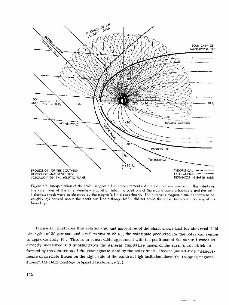
HEMISPHERE MAGNETIC FIELD TOPOLOGY O N THE ECLIPTIC PLANE
EXPERIMENTAL - DISTANCES IN EARTH RADII
Figure 40-interpretation of the IMP-I magnetic f ie ld measurements of the cislunar environment. Illustrated are the directions of the interplanetary magnetic field, the positions of the magnetosphere boundary and the col- lisionless shock wave as observed by the magnetic f ie ld experiment. The extended magnetic tai l as shown to be roughly cylindrical about the earth-sun line although IMP-I did not probe the sunset terminator portion of the boundary.
Figure 41 illustrates this relationship and inspection of the chart shows that for observed field strengths of 20 gammas and a tail radius of 22 Re, the colatitude predicted for the polar cap region is approximately 16". This is in remarkable agreement with the positions of the auroral zones as directly measured and substantiates the general qualitative model of the earth 's tail which is formed by the distortion of the geomagnetic field by the solar wind. Recent low altitude measure- ments of particle fluxes on the night side of the earth at high latitudes above the trapping regions support the field topology proposed (Reference 35).
162

NEUTRAL SHEET CHARACTERISTICS
l , , , , I I I , , ,
Observations of the magnetic neutral sheet in the earth's tail have been performed on 14 of orbits 31 through 47. These have ranged over geocentric distances of 9.9 Re to28 Re. In gen- eral, the early orbits possessed neutral sheet t raversals closer to the ear th than la ter orbits. Analyses have been performed to deduce the orientation of the neutral sheet in the earth's magnetic tail. Indeed, that the neutral surface separating fields of opposite direction is more or less a flat planar feature, as suggested by the word sheet, is one resul t of this particular investigation. The latitude of the positions of crossing of the neutral surface in the earth's magnetic tail has been examined in three coor- dinate systems:
I , I I , , ,
100 80 60
40 v
I- m . 20 Ly n 2 10
S 6 0 4
2
-I Y
U -
1. solar ecliptic
2. geomagnetic
3. solar magnetospheric.
The last system is a recent addition to those coordinates used in interpretation of magnetospheric phenomena. It incorporates the earth-sun line as the X-axis but unlike solar ecliptic, includes a dependence upon the position of the geomagnetic axis rather than the ecliptic plane. The coordinate system is illustrated in Figure 42 showing the X-Z plane as including the magnetic axis of the earth. This implies that the Y-axis in the new coordinate system is always normal to both the earth-sun line and the earth 's magnetic dipole axis.
Previous research workers in the field of magnetosphere physics have suggested that such a coordinate system might be appropriate in the analysis of magnetospheric phenomenona (Refer- ence 33) but until these IMP-I data were avail- able there appeared to be no appropriate need for its consideration. The variation and position of the neutral sheet in the three coordinate sys- tems discussed has been investigated. The best f i t to the equatorial plane in the three coordinate systems occurred in the solar magnetospheric coordinate system. This is shown in Figure 43 in which it is seen that the position of the neutral
GEOMAGNETIC ',SM
OF DIAGRAM) -/
Figure 42-Definition of the solar magnetospheric co- ordinate system used in the interpretation of the position of the neutral sheet as observed in the magnetic ta i l of the earth.
163
I

+ l o o + X s s = GEOMAGNETIC LATITUDE
OF SUBSOLAR POINT
Figure 43-Position of the neutral sheet as observed by the IMP-I magnetic f ie ld experiment while i n the mag- netic ta i l of the earth. The sheet i s observed to be within 5" or 10" of the solar mognetospheric equatorial plane for the 14observed crossings.
+60
+ 40
p +20 E p EQUINOX - 0.
2 -20
- 40
- 60
Figure 44-Illustration of the variation of the t i l t of the equatorial plane of the solar magnetospheric coordinate system with respect to the ecl ipt ic plane. Superimposed is the time interval covered by IMP-I.
surface crossing is always within 5" or 10" of the solar magnetospheric equatorial plane. Thus i t is suggested by these results that the neutral sheet in the earth 's magnetic tail is roughly parallel to the solar magnetospheric equatorial plane and indeed is approximately equivalent to it. The variation in the tilt of the neutral sheet to the ecliptic plane is an important parameter in comparing these results with previous and future satellite measurements. Figure 44 shows the annual variation of the tilt of the neutral sheet with respect to the ecliptic plane when viewed along the earth-sun line. The maximum inclination is k35.4' with an annual seasonal variation.
Measurements in recent years (References 7 and 36-40) have shown enhanced particle fluxes on the night side of the earth. Some of these a r e probably related to the magnetic neutral sheet. Previous measurements by Frank (Refer- ence 36) a r e particularly pertinent in this respect since they revealed the formation of an electron "tail" of the magnetosphere on the night side of the earth with the Explorer 14 satellite. noted by Axford, Petschek and Siscoe (Reference 41), in order that a magnetic neutral sheet exist in the ear th 's magnetic tail, the sheet must be filled with an increased plasma flux which bal- ances the opposing field configurations.
A s
Figure 45 predicts the minimum particle flux necessary to balance a magnetic field in the earth 's tail and superimposes experimental evi-
dence of the neutral sheet. These measurements were not originally interpreted to be indicative of the neutral sheet but with the magnetic field topology of the earth 's tail as measured by the IMP-I satellite, it is possible to place these measurements in a proper perspective. As noted by Van Allen (Reference 42), the measurements by Gringauz (Reference 38) do not necessarily indi- cate a third radiation belt. They now can be reasonably interpreted in te rms of the neutral sheet in the earth 's magnetic tail.
In Figure 46 correlated particle and field measurements performed on IMP-I in the earth 's magnetic tail a r e shown. Precipitous increases in particle fluxes a r e observed coincident with
164

1
ELECTRON FLUX (electrons / cm2 sec)
Figure 45-Assumed pressure balance between vacuum magnetic fields and non- magnetized electron plasma corresponding to idealized model of neutral sheet. Superimposed are particle and plasma observations pertinent to the interpretation of the neutral sheet i n the earth's magnetic tail.
rapid decreases in magnetic field intensity. The interpretation of these time variations is that the total flux of the electrons in the earth 's tail at this time is sufficiently large that the diamagnetic moment of the particles cancels the magnetic field in the earth 's tail, at least locally. Thus the earth 's magnetic tail may at times form a third regime in cislunar space quite unlike that of the interplanetary medium in which plasma energy completely dominates magnetic field energy o r of the radiation belts in which the reverse situation is true. Rather, there is an intimate coupling of the magnetosphere plasma and field in which the P value is close to unity.
The principal problem related to the tail is whether or not it is the source of auroral particles which a r e accelerated from low to high energies by a mechanism acting only in the earth 's tail. Ness (Reference 4) has previously suggested that this mechanism may be related to instabilities of the neutral sheet similar to well-known sheet pinch instabilities studied in the plasma fusion program (Reference 43).
A schematic summary of the geomagnetic field topology and its interaction with the solar wind in the noon-midnight meridian plane is shown in Figure 47. A strong day-night asymmetry is indi- cated in the trapped radiation belts and the neutral sheet is shown as including the earth-sun line. A sample orbit of IMP is shown in the earth 's tail to illustrate the region of space in which mag- netic field measurements revealing the formation of this extended magnetic tail of the earth, were
165
I

80 90c B E .
50 v
W
Z 30-
A- 10 8
9 w U
20
10
0
6 4 2
- 24 1
4 I
, I , I I I I I I I I
- 30 28 26 24 22
MAGNETIC LATITUDE (degrees)
0
MAGITUDE MAGI\ (NESS
, I , , I I I I I ELECTRON FLUX >45 KEV I (ANDERSON ET AL., 1964)
- 20 18 16 14 12
,1964)
50
GEOCENTRIC DISTANCE ( R e )
Figure 46-Correlated electron f lux and magnetic f ield magnitude variations i n the tai l of the magnetosphere observed by IMP-I on orbit 40 inbound 29 April 1964. The sheet was observed during this orbit at a position of 19.8 Re, coincident with an abrupt increase in the electron flux.
performed. Polar regions of the earth a r e as yet unmapped at great distances. The indentations shown on the boundary of the magnetosphere are associated with theoretically suggested neutral points of the earth 's magnetic field in the geomagnetic cavity (Reference 22).
166

---- -
SOLAR WIND ---
-&e '
--__.
-__,--A
PROJECTION OF MAGNETIC FIELD TOPOLOGY ON NOON MIDNIGHT
THEORETICAL
EXPERIMENTAL
V A N ALLEN RADIATION BELTS
MERIDIAN PLANE
Figure 47-Summary iliustration of the interpretation of the IMP-I data perpendicular to the plane of the ecl ipt ic illustrating strong day-night asymmetry i n the radiation belts and the development of the extended magnetic tai l of the earth.
SUMMARY
The continual flux of solar plasma confines the geomagnetic field to a region of space sur- rounding the earth but extending on the night side to a distance as yet unknown. It appears certain that the ear th 's magnetic tail extends beyond the orbit of the moon and thus the moon must t raverse the earth 's magnetic tail once every 29.5 days. The presence of the neutral sheet in the earth 's magnetic tail implies an enhanced particle flux within it to balance the field pressure.
It is possible to view the earth as a magnetic comet i f the earth is considered as a nucleus, the radiation belts as a coma, and the earth 's magnetic tail as a cometary tail with characteristic Type-I cometary tail r ays represented by the earth 's neutral sheet. Certain aspects of this analog a r e currently being investigated and will be reported upon in future publications. At the present time investigation of the earth 's magnetic tail and its association with auroral and radiation belt phenomena present distinct challenges to future space experiments and theory.
ACKNOWLEDGMENTS
The authors gratefully acknowledge the outstanding efforts of the IMP project staff and person- nel at GSFC who so ably assisted us in our efforts to achieve a "magnetically clean" satellite.
167
I

Without their support and cooperation and that of our co-experimenters this work could not have been completed. One of u s (J.M.W.) thanks the Director of the Mt. Wilson Observatory for guest investigator privileges extended him.
REFERENCES
1. Ness, N. F., Scearce, C. S., and Seek, J. B., "Initial Results of the IMP-I Magnetic Field Ex- periment," J. Geophys. Res. 69(17):3531-3569, September 1, 1964.
2. Ness, N. F. and Wilcox, J. M., "The Solar Origin of the Interplanetary Magnetic Field,!' Phys. Rev. Letters 13(15):461-464, October 12, 1964.
3. Ness , N. F., "The Magnetohydrodynamic Wake of the Moon," J. Geophys. Res. 70(3):517-534, February 1, 1965.
4. Ness , N. F., "The Earth 's Magnetic Tail," J. Geophys. Res. 70(13):2989-3005, July 1, 1965
5. Ness , F . and Wilcox, J. M., "Extension of the Photospheric Magnetic Field into Interplane- tary Space," Goddard Space Flight Center Document X-612-65-79, 1965, and Astrophys. J., 14 3 ( 1 ): 2 3 - 3 1, January 196 6.
6. Ness, N. F . and Wilcox, J. M., "Sector Structure of the Quiet Interplanetary Magnetic Field," Science 148(3677): 1592- 1594, June 18, 1965.
7. Anderson, K. A., Harris, H. K., and Paoli, R. J., "Energetic Electron Fluxes in and beyond the Earth 's Outer Magnetosphere," J. Geophys. Res. 70(5):1039-1050, March 1, 1965.
8. Balasubramanyan, V. K., Ludwig, G. H., McDonald, F. B., and Palmeira, R. A. R., "Results f rom the IMP-I GM Counter Telescope Experiment," GSFC Document X-611-65-49, 1965.
9. Bridge, H., Egidi, A., Lazarus, A., Lyon, E . , and Jacobson, L., "Preliminary Results of Plasma Measurements on IMP-A," in: Space Researcli V; Proc. 5th Internat. Space Sei. Symp., Florence, Italy, May 12-15, 1964, ed. by D. G. King-Hele, P. Muller, and G. Righini, Amster- dam: North-Holland Publishing Co.; New York: Interscience Publishers, 1965, pp. 969-978.
10. Fan, C. Y., Gloecker, G., and Simpson, J. A., "Evidence for 30 Kev Electrons Accelerated in the Shock Transition Region beyond the Earth 's Magnetospheric Boundary,'' Phys. Rev. Letters 13(5):149-153, August 13, 1964.
11. McDonald, F. B. and Ludwig, G. H., "Measurement of Low-Energy Primary Cosmic-Ray Pro- tons on IMP-I Satellite," Phys. Rev. Letters 13(26):783-786, December 28, 1964.
12. Serbu, G. P., "Results f rom the IMP-I Retarding Potential Analyser," in: Space Research V; Proc. 5th Internat. Space Sci. Symp., Florence, Italy, May 12-15, 1964, ed. by D. G. King-Hele, P. Muller, and G. Righini, Amsterdam: North-Holland Publishing Co.; New York: Interscience Publishers, 1965, pp. 564-574.
168

13. Axford, W. I., "The Interaction between the Solar Wind and the Earth 's Magnetosphere," J. Geophys. Res. 67(10):3791-3796, September 1962.
14. Harrison, E. R., "The Earth 's Distant Magnetic Field," Geophys. J. 6(4):479-492, June 1962.
15. Kellogg, P. J., "Flow of Plasma around the Earth," J. Geophys. R e s . , 67(10):3805-3811, September 1962.
16. Parker , E. N., "Dynamics of the Interplanetary Gas and Magnetic Field," As t rophys . J. 128(3): 664-676, November 1958.
17. Biermann, L., "Kometenschweife und solare Korpuscularstrahlung," 2. As t rophys . 29(3):274- 286, September 1951.
18. Parker , E. N., "The Hydrodynamic Theory of Solar Corpuscular Radiation and Stellar Winds," As t rophys . J. 132(3):821-866, November 1960.
19. Snyder, C. W. and Neugebauer, M., "Interplanetary Solar Wind Measurements by Mariner 2," in: Space R e s e a r c h Science Sympos ium, 4 th , Wursaw, Poland, June 4-10, 1963, Amsterdam: North-Holland Publisning Co.; New York: Interscience Publishers, 1964.
20. Bdbcock, H. W., "The Solar Magnetograph," As t rophys . J. 118(3):387-396, November 1953.
21. Ahluwahlia, H. S. and Dessler, A. J., "Diurnal Variation of Cosmic Radiation Intensity Pro- duced by a Solar Wind," Planet. Space Sci. 9:195-210, 1962.
22. Beard, D. B., "The Solar Wind Geomagnetic Field Boundary," Rev. Geophys. 2(2):335-365, May 1964.
23. Freeman, J. W., Van Allen, J. A., and Cahill, L. J., "Explorer 12 Observations of the Mag- netospheric Boundary and the Associated Solar Plasma on September 13, 1961," J. Geophys. Res. 68(8):2121-2130, April 15, 1963.
24. Cahill, L. J. and Amazeen, P. G., "The Boundary of the Geomagnetic Field," 6. Geophys. Res . 68(7):1835-1843, April 1, 1963.
25. Heppner, J. P., Ness , N. F., Skillman, T. L., and Scearce, C. S., "Explorer 10 Magnetic Field Measurements," J. Geophys. Res . 68(1):1-46, January 1, 1963.
26. Bonetti, A., Bridge, H. A., Lazarus, A. J . , Rossi, B., and Scherb, F., "Explorer 10 Plasma Measurements," J. Geophys. Res. 68(13):4017-4064, July 1, 1963.
27. Ness, N. F., "Observations of the Geomagnetic Cavity Boundaries," C . U. S y m p o s i u m on P l a s m a s in Space (1963) , Amsterdam: North-Holland Publishing Co., 1965.
28. Spreiter, J . R. and Jones, W. P., "On the Effect of a Weak Interplanetary Magnetic Field on the Interaction between the Solar Wind and the Geomagnetic Field," J. Geophys. Res. 68(12): 3555-3564, June 15, 1963.
169

29. Chapman, S., "Solar Plasma, Geomagnetism and Aurora in Geophysics," in Geophysics: The Eavth's Environment, ed. by C. DeWitt, J. Hieblot, and A. Lebeau, 373-502, New York: Gordon and Breach, Science Publishers, 1963.
30. Axford, W. I., Petschek, H. E., and Siscoe, G. L., "The Tail of the Magnetosphere," J. Geophys. Res. 70(5):1231-1236, March 1, 1965.
31. Piddington, J. H., "The Transmission of Geomagnetic Disturbances Through the Atmosphere and Interplanetary Space," Geopkys. J. 2(3):173- 189, September 1959.
32. Piddington, J. H., "Geomagnetic Storm Theory," J. Geophys. Res. 65(11);93- 106, January 1960.
33. Dessler, A. J . and Juday, R. D., "Configuration of Auroral Radiation in Space," Planet. Space . Sci., 13(1):63-72, January 1965.
34. Cahill. L. J., "Preliminary Results of Magnetic Field Measurements in the Tail of the Geo- magnetic Cavity,'' Intevnat. Geopkys. Bull. No. 79. 11- 15 January 1964.
35. McDiarmid, I. B. and Burrows. J. R., "Electron Fluxes at 1000 Km. Associated with the Tail of the Magnetosphere," J. Geopkys. Res., 70, in press , 1965.
36. Frank, L. A. and Van Allen, J . A., "A Survey of Magnetospheric Boundary Phenomena," in: Res. in Geoplzys. Vol. 1, ed. by H. Odishaw, Cambridge: MIT Press, 1964, pp. 161-185.
37. Freeman, 3. W.. "Electron Distribution in the Outer Radiation Zone," J. Geopkys. Res. 69(9): 1691-1723. May 1, 1964. .
38. Gringauz, K. I., Kurt, V. G., Moroz, V. I., and Shklovskii, I. S., "Results of Observations of Charged Particles Observed out to 100,000 Km with the Aid of Charged-Particle Traps on Soviet Space Probes," Astvon Zk. 37(4):716-735, Jdy-Aiqps t , 19GO; translated in Soliet Astvon. - AJ, 4(4):680-695, January- February, 1961.
39. Montgomery, M. D., Singer, S., Conner, J . P., and Stogsdill. E. E., "Spatial Distribution, Energy Spectra and Time Variations of Energetic Electrons (E Pkys. Rei>. Letters 14(7):209-213, February 15, 1965.
50 Kev) at 17.7 Earth Radii,"
40. Singer, S., Conner, J. P.. Evans, W. D., Montgomery, M. D., and Stogsdill. E. E., "Plasma Observations at l o 5 Km.," in: Space Research V; Pvoc. 5tk Intevnat. Space Sci. S-vmp., Florence, Ztal.v, May 12-15, 1964, ed. by D. G. King-Hele. P. Muller, and G. Righini. Amsterdam: North-Holland Pub. Co.; New York Interscience Publishers, 1965. pp. 546-563.
41. Frank, L. A.. "A Survey of Electrons beyond 5 Earth Radii with Explorer XIV," J. Geophys. Res. 79(7):1593-1626. April 1. 1965.
42. Van Allen. James A.. "Remarks on Accompanying Letter by K. I. Gringauz," J. Geoplzys. Res. 69(5):1011-1013, March 1, 1964.
43. Furth. H. P., Killeen. J., and Rosenbluth. M. N., "Finite Resistivity Instabilities of a Sheet Pinch." Phzls. ~llrin's 6(4):459-484. April 1963.
170

SOUTHERN HEMISPHERE ANOMALIES
by J. G. Roederer*
Goddard Space Flight Center
The eccentricity of the geomagnetic dipole and the presence of multipole perturbations give rise t o a series of phenomena observable in the southern hem- isphere which are important to the physics of the magnetosphere and ionosphere, and to the study of cosmic rays.
In the f i r s t part of this review, the morphology of the geomagnetic field pe- culiarities in the southern hemisphere will be analyzed. In the second part. some of the efforts on cosmic rays , geomagnetically trapped i-adiation and thc ionosphere will be discussed.
INTRODUCTION
Most of the peculiarities of the geophysical behavior of the southern hemisphere ultimately originate in the eccentricity and the asymmetry of the geomagnetic field. both of which lead to particularly strong effects south of the equator. The purpose of this brief review then, is f i rs t to describe the morphology of these geomagnetic peculiarities, and second to summarize some of their effects on several phenomena of ionospheric physics, trapped radiation, and cosmic rays.
PECULIARITIES OF THE GEOMAGNETIC FIELD IN THE SOUTHERN HEMISPHERE
It is well known that the earth 's magnetic field behaves like a centered dipole only in a very first approximation. An improvement in the field description is achieved i f the center of the dipole is displaced about 340 km off the geographic center of the earth, into a direction 6.5 N and 162 E. i.e., roughly towards the East Asian region. This means that field lines of a given dipole shall come "closest" to the earth 's surface over the east coast of South America and over the South Atlantic Ocean. As a result, there is an absolute minimum field intensity over Eastern Brazil.
Figure 1 shows iso-intensity contours of the geomagnetic field: 7 notice the low field intensities in the magnetic equatorial region over South America, and the higher equatorial intensities over
- *National Academy of Sciences - National Research Council, Senior Post-Doctoral Research Associate . on leave from Facultad de
t S e e pages 35 - 131. Ciencias Exactas y Naturales and Cento Nacional d e Radiacion Cosmica, Buenos Aires, Argentina.
171

Figure 1-Contours of constant total f ield intensity.
LONGITUDE (degrees)
Figure 2-Geographic position of the magnetic (dip) equator.
Malaysia. Notice further the different absolute intensities at the geomagnetic poles (North Canada and Antarctica).
These differences, however, cannot be ex- plained by merely displacing the magnetic center. Such a displacement would lead to extreme equatorial values of 0.27 and 0.34 gauss, respec- tively, whereas the observed extreme values a r e 0.24 gauss over the Brazilian east coast and 0.41 gauss over the northeast Indian Ocean. This means that higher multipoles do play a substan- tial role in the field asymmetry. But the net ef- fect is still that the geomagnetic shells come closest to the earth's surface oveY South America and the South Atlantic. 0
The eccentricity and asymmetry of the geo- magnetic field a r e closely associated with the facts revealed in Figure 2, and Figure 3 from
172

Figure 3-Contout-s of constant magnetic dip (from Reference 1).
These variations in the geomagnetic-geographic relationships mean, for instance, that the sun, a t local noon during equinoxes, is farthest a w a y from the magnetic equator in a region over South America. In addition, this region of maximum departure over South America is very narrow in longitude compared to the extension in longitude of the maximum departure region in the northern hemisphere over Africa and South East Asia (Figure 2).
On the other hand, Figure 3 shows that, in general, magnetic field lines are less inclined over the southern geographic polar area than in the northern counterpart. In particular, the "tongue" of low dips invading Antarctica over the Palmer Peninsula is responsible for the existence of a unique
173
I
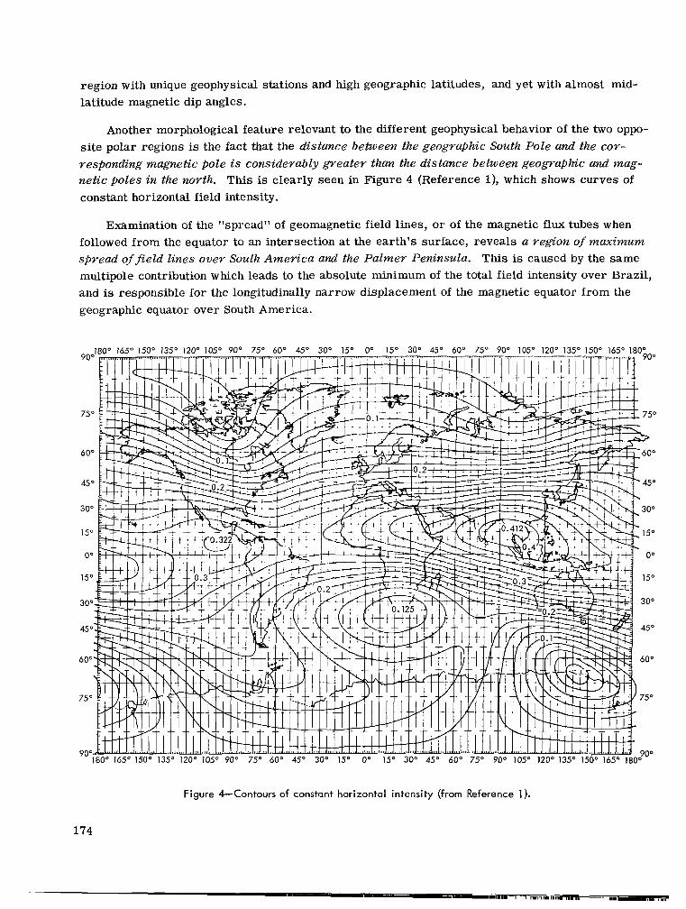
region with unique geophysical stations and high geographic latitudes, and yet with almost mid- latitude magnetic dip angles.
Another morphological feature relevant to the different geophysical behavior of the two oppo- s i te polar regions is the fact that the distance between the geographic South Pole and the COY-
responding magnetic pole i s considerably greater than the distance between geogvaphic and mag- netic poles in the north. This is clearly seen in Figure 4 (Reference l), which shows curves of constant horizontal field intensity.
Examination of the "spread" of geomagnetic field lines, or of the magnetic flux tubes when followed from the equator to an intersection at the earth 's surface, reveals a region of maximum spread of field lines over South America and the Palmer Peninsula. This is caused by the same multipole contribution which leads to the absolute minimum of the total field intensity over Brazil, and is responsible for the longitudinally narrow displacement of the magnetic equator from the geographic equator over South America.
Figure 4-Contours of constant horizontal intensity (from Reference 1).
174

80"
60"
40'
20"
0"
20c
40'
60"
80'
F i
100' 120' 140° 160" I :
This maximum spread can be visualized to some extent by plotting conjugate intersects for a network of field lines (Figure 5 and Ref- erence 2), and is taken into account whenever considering phenomena of plasma flow from the equator toward the poles. It is also ulti- mately responsible for the average longitudinal drift velocity of geomagnetically trapped par- ticles being greater over South America and the Atlantic Ocean.
There are two additional effects, not so well known, but which might play a role in southern hemisphere anomalies. The first of these effects is shown in Figure 6.* Here the
80'
60"
40'
200
0"
200
40"
60'
80'
-ence 2).
EQUATORIAL ALTITUDE OF FIELD LINE
3000 Ij0 km
AMERICAN SECTOR
2000
Figure 6-Equatorial altitude (in km) of a f ield line, as a function of its dip angle at the 400 km level, for the American (dotted curve) regions. The east Asian region curve falls very close to the American curve.
*See pages 35 - 131.
175
\

altitude in kilometers of the equatorial (minimum B) points of a field line is plotted as a function of the dip angles at the northern and southern intersections with a constant altitude surface, for the two longitudinal regions of Africa and America.* A third region in the Far East and the Pacific gives results very close to the American region. Both curves clearly show that for a given dip, field lines attain the lowest equatorial altitude when emerging from South Africa.
The second effect is concerned with the variation of McIlwain's L parameter (Reference 3) along a given field line. Recent calcirlations shozv that the degree of violation of the invariant cltnmctev qf L is higliest f o r field lines startirig south of Capetown, and for L between 1.6 and 2.6.
GEOPHYSICAL EFFECTS OF MAGNETIC FIELD PECULIARITIES IN THE SOUTHERN HEMISPHERE
Geophysical phenomena may be classified as follows: (1) Exclusively field- controlled phenom- ena such as the motion of cosmic rays, solar protons and auroral particles. (2) Field-controlled phenomena influenced by the atmosphere, as in the geomagnetically trapped radiation where mo- tion and storage is field-controlled but diffusion and loss processes are determined by the atmos- phere. (3) Atmosphere-controlled phenomena influenced by the field, as in the variety of ionospheric phenomena where source, loss, and overall motion are controlled by atmosphere but the geomag- netic field determines electric currents, drifts diffusion, etc.
In discussing the groups of phenomena enumerated above, only very general remarks a r e made regarding quiet epochs only. Transient perturbations. as those associated with s torms, a r e not treated.
Examples of the first group of phenomena are two "anomalies" in the equatorial values of vertical effective cut-off rigidities for cosmic ray protons; the highest absolute value of vertical cut-off rigidity (s18 GV) is over the north-east Indian Ocean, and the lowest (213.5 GV) is over South America. In other words, the equatovial cosmic ray flux is highest over South America and has an absolute minimum somewhere over the north-east Indian Ocean.
Indirectly related to the tongue of low dip angles extending from South America over the Palmer Peninsula are the unusually higher cut-off rigidities of cosmic ray observatories like Ushuaia, Ellsworth, and Base General Belgrano in spite of the high geographic latitude of these stations.
An important result of detailed cosmic ray particle orbit calculations by Shea et al. (Reference 4 ) reveals that the structure of so-called shadow cones, i.e., the region in rigidity space where allowed and forbidden zones alternate, is widest and most complicated at points in South America and the adjacent South Atlantic Ocean. Furthermore, discrepancies among different cut-off cal- culations is greatest in this region (Reference 5). Particles impinging on the ear th 's atmosphere
*See pages 35 - 131.
176

over South America feel the multipole perturbations most intensively and possibly cause these anomalies.
The second group of phenomena considers the behavior of the radiation belts. If there were no interactions with the medium (the atmosphere), charged particles would remain trapped on L shells, mirroring at a constant B value. In other words, the "mirror point trajectories" of a par- ticle would be given by a pair of constant B-L rings (intersections of constant B and constant L surfaces), one in each hemisphere. The altitude over the earth 's surface of a B-L ring is not constant; the southern rings get very close to the dense layers of the atmosphere just over the east coast of South America (low L shells), or over the South Atlantic Ocean (high L values). Plots of (southern) B-L ring altitudes as a function of longitude for the L = 1.25 shell (solid curves) a r e displayed in Figure 7.*
The behavior of the B-L rings is responsible for two main effects. First, charged particle fluxes at a given constant altitude (such as measured by a satellite in circular orbit) will be highest
1000 -
900 -
800 -
700 - E
5 600 - Y - !? w
500 - I
400 -
300 -
200 -
100 -
0 w
I 1 1 1 I I 1 I 1 9 1 1 t
140 120 100 80 60 40 20 0 20 40 60 E
GEOGRAPHIC LONGITUDE (degrees)
F i g u r e 7 - A l t i t u d e s i n the km of constant 6-L rings (sol id curves), for L = 1.25. D o t t e d curves: A v e r a g e mirror p o i n t t r a j e c t o r i e s o f 300 k e v e l e c t r o n s d r i f t i n g through the a n o m a l y , subject to C o u l o m b scat ter ing.
- 'See pages 183 - 207.
177

in a region extending from the east coast of South America to the South Atlantic (References 6, 7 and 8). Second, it is here that the satellite wi l l sample trapped radiation at the -lowest B values of a given shell.* This represents the South American anomaly of the radiation belt.
Additionally, since mi r ro r points submerge deepest into the atmosphere in the region of the South American anomaly, this is where scattering and loss processes a r e most intense. Particle precipitation into the atmosphere will be highest in the anomaly (References 9 through 13). A schematic drawing of average trajectories of mi r ro r points of 300 kev electrons (dotted curves) as they drift through the anomaly a r e shown in Figure 7. The enhanced atmospheric scattering causes them to diffuse on the average to higher B values. A certain fraction is lost, precipitating into the lower atmosphere; others manage to "get around" the anomaly, populating the high B region of the shell (which drops below sea level in the anomaly) and surviving just one more turn around the earth.+ This is the "windshield wiper effect."
The study of particle precipitation and its effects on the ionosphere in the South American anomaly is of great importance. The first evidence of electron precipitation through Bremsstrah- lung X-ray measurements with balloons was found by Ghielmetti, e t al. (Reference 14). Its effect on the ionosphere was discussed by De Mendonqa (Reference 15), and the evidence for airglow en- hancement in the South Atlantic was reported by Greenspan and Stone (Reference 16).
Finally, the effect of maximum variation of L along field lines starting out south of Capetown might be relevant to the trapped particle dynamics in the affected L region. Violation of the in- variant character of L means splitting of trapped particle shells according to their mir ror point field intensity (Reference 17). A scattering process, which under normal conditions merely changes the particle's pitch angle to mir ror point, leaving the shell untouched, will now also change the particle 's shell. This change wil l depend on the longitude at which scattering took place. In other words, this effect introduces a radial scattering coupled to each pitch angle scattering process. This might affect substantially the particle density in the corresponding L shells.
The third group of phenomena includes the study of southern hemisphere anomalies in the ionosphere. While a systematic review of this subject is not practical here, a few examples a r e in order .
The position of the sun in relation to the geomagnetic field and also the motion o r sweep of the subsolar point through the field, as viewed from a field-invariant system, a r e likely to be the main factors determining the peculiar behavior of the ionosphere in some regions of the southern hemisphere.
In the case of the equatorial anomaly in f, F2 (References 18 through 22), the facts pointed out in Figure 2 must be considered. The sun, in its annual cycle, scans a different portion of the "critical" field lines (along which the enhanced ionization is found to be aligned) in this South
~ - - *The steady state distribution of trapped particles along a line of force i s always such that the omnidirectional intensity decreases from
+See pages 183 - 207. the equator towards the higher B point.
178

American region than at any other longitude. This effect might explain some of the summer-winter differences in the equatorial anomaly at different longitudes. It should be taken into account in any detailed theoretical description of the equatorial anomaly and its diurnal variations.
The systematic differences between the position (expressed in dip angle o r in magnetic latitude) of the equatorial anomaly maxima in the African and the South American zone (Reference 18) are explained by taking into consideration Figure 6. When transforming dip angle at conjugate inter- sects into altitude of the equatorial point of a field line by means of these curves, the conclusion is reached that the different latitudinal "positions" of northern and southern f, F2 maxima in the South American and African zones, at a given local time, merely correspond to the different posi- tions and dip angles of the conjugate intersects of field lines reaching out to the same geographic altitude at their equatorial point. It appears as if the relevant quantity for the position of the anomaly maxima is given by the maximum altitude of the critical field line for all longitudes.
Several points related to field peculiarities must be considered when studying the processes of the transportation of ionization from the equator to the poles, either along field lines or as drifts in the F region. First, the maximum displacement of low dip angles toward the antarctic geographic polar region and the maximum spread of field lines over the Palmer Peninsula are important in relation to the geographic location of the flow of plasma (Reference 23) and that of its concentration or density, respectively (Reference 24). Second, it must be taken into account that the sun, in its daily cycle, s t a y s for a much shorter period of the day over the magnetic equatorial region in southern summer than in northern summer (Figure 2).
These effects might explain the different behavior of the universal time in control of f,F2 in the Antarctic versus the Arctic regions (References 25 and 26). They also should be connected with the anomalous behavior of the diurnal variation of f,F2 at several South American and Antarc- t ic stations in the a rea where one has a maximum divergence of field lines (Figure 5) and where there is a maximum shift between geographic and magnetic latitudes. In this unique group of stations in southern Argentina, Malvinas Islands, Decepcion, and Palmer Peninsula, there a r e long periods of darkness in winter in spite of their relatively low magnetic latitude. Deeper in the Antarctic terri tory there a r e stations in this range of longitudes which, at magnetic latitudes of only 60 degrees, a r e in constant darkness in winter.
Finally, considering the explanation of the mentioned anomalous variations of f , F2 in the southern polar region (Rqference ,27) in te rms of Dungey's wind shear model for the creation of ionization layers (Reference 28) and the greater distance between the geographic South Pole and the corresponding magnetic pole must be taken into account (Figure 4). Since the field lines a r e on the average more inclined over the southern (geographic) polar region, plasma compression by wind shear should be more effective there. When the effects of electric field (E X (B/B2)) drifts are considered, the same morphological N-S pole field difference must be taken into account, in order t o explain the different behavior of the winter anomaly in the north and south pole regions (Reference 27). It will probably require another solar cycle of ionospheric measurements, es- pecially data obtained with topside sounders (Reference 29), before a clear picture is attained of the very complicated play between geomagnetically and geographically controlled processes which lead to the southern hemisphere anomalies in the ionosphere.
179
I

REFERENCES
1.
2.
3.
4.
5.
6.
7.
8.
9.
10.
11.
12.
Cain, J. C., and Neilon, J. R., "Automatic Mapping of the Geomagnetic Field,",J. Geopkys. Res. 68(16):4689-4696, August 15, 1963.
Vestine, E. H., and Sibley, W. L., "The Geomagnetic Field in Space, Ring Currents and Auroral Isochasms," J. Geopkys. Res. 65(7): 1967- 1980, July 1960.
McIlwain, C. E ., "Coordinates for Mapping the Distribution of Magnetically Trapped Particles," J. Geopkys. Res. 66(11):3681-3691, November 1961.
Shea, M. A., Smart, D. F., and McCracken, K. G., "A Study of Vertical Cut-off Rigidities Using Sixth Degree Simulations of the Geomagnetic Field," J. Geopkys. Res. 70(17):4117-4130, September 1, 1965.
Kenney, J. F., Gauger, J., Smart, D. F., and Shea, M. A., "A Study of the Relative Merits of Various Cosmic-Ray Vertical Cut-off Rigidity Models," Trans. Anzer. Geophys. Union. 46( 1): 62-63, March 1965 (abstract).
Yoshida, S., Ludwig, G. H., and Van Allen, J. A., "Distribution of Trapped Radiation in the Geomagnetic Field," J. Geopkys. Res. 65(3):807-813, March 1960.
Vernov, S. N., Gorchakov, E. V., Logachev, Yu. I., Nesterov, V. E., Pisarenko, N. F., Savenko, I. A., Chudakov, A. E., and Shavrin, P. I., "Investigations of Radiation During Flights of Satel- lites, Vehicles and Rockets,'' J. Pkys. SOC. Japan. l7(supp. A-11): 162-186, January 1962.
Freden, S. C., and Paulikas, G. A., "Trapped Protons at Low Altitudes in the South Atlantic Magnetic Anomoly," J. Geopkys. Res. 69(7):1259-1269, April 1, 1964.
Mann, L. G., Bloom, S. D., and West, H. I., Jr., "Electron Spectrum from 90 to 1200 KeV as Observed on Discoverer Satellites 29 and 31," in: Space Research III; Proc. 3rd Internat. Space Sci. Sympos., Washington, D. C., May 2-S, 1962, ed. by W. Priester, Amsterdam: North-Holland Pub. Co.; New York: Interscience Publishers, Inc., 1963, pp. 447-462. Inc., 1963, pp. 447-462.
Freden, S. C., and Paulikas, G. A., "Precipitation of Energetic Electrons into the Atmosphere," J. Geophys. Res. 69(7):1239-1249, April 1, 1964.
Mihalov, J. D., Mozer, F. S., and White, R. S., "Artificially Injected Electrons at Low Alti- tudes," J. Geopkys. Res. 69(19):4003-4013, October 1, 1964.
MacDonald, W. M., and Walt, M., "Diffusion of Electrons in the Van Allen Radiation Belt. Pt. 2, Particles with Mirroring Points at Low Altitudes," J. Geophys. Res. 67(13):5025-5033, December 1962.
13. Welch, J. A., Jr., Kaufmann, L., and Hess, W. N., "Trapped Electron Time Histories for L = 1.18 to L = 1.30," J. Geophys. Res. 68(3):685-700, February 1, 1963.
180

14. Ghielmetti, H. S., Becerra, N., Godel, A. M., Heredia, H., and Roederer, J. G., "Enhancement of the X-Ray Intensity at Balloon Altitudes in the South American Anomaly," Plzys. Rev. Letters, 12(14):388-390, April 6, 1964.
15. De Mendonqa, F., "Ionospheric Electron Content Measurements in Regions of Low Magnetic Dip Angles and Through the Brazilian Magnetic Anomaly," in: Space Research V; Proc. 5th Internat. Space Sci. Sympos., Florence, May 12-16, 1964, ed. by D. G. King-Hele, P. Muller, and G. Righini, Amsterdam: North-Holland Pub. Co.; New York: Interscience Publishers, 1965, pp. 687-701.
16. Greenspan, J. A., and Stone, C. A., "The Longitudinal Variation of Night Airglow Intensity in the Region of the South Magnetic Anomaly," J. Geophys. Res. 69(3):465-469, February 1, 1964.
17. Stone, E. C., "The Physical Significance and Application of L, Bo, and R , to Geomagnetically Trapped Particles," J. Geophys. Res. 68(14):4157-4166, July 15, 1963.
18. Croom, S., Robbins, A., and Thomas, J. O., "Two Anomalies in the Behavior of the F, Layer of the Ionosphere," Nature, 184(4704):2003-2004, December 26, 1959.
19. Lyon, A. J., and Thomas, L., "The F, -Region Equatorial Anomaly in the African, American and East Asian Sectors during Sunspot Maximum," J. Atoms. Terr. Phys. 25(7):373-386, July 1963.
20. Rao, C. S. R., and Malthora, P. L., "A Study of Geomagnetic Anomaly during IGY," J. Atmos. Terr. Phys. 26(11):1075-1085, November 1964.
21. Bramley, E. N., and Peart, M., "Diffusion and Electromagnetic Drift in the Equatorial F, Region," J. Geophys. Res. 69(21):4609-4616, November 1, 1964.
22. Goldberg, R. A., "The Effect of a Variable Electron Temperature on the Equatorial Electron Density Distribution in the Upper Ionosphere," J. Geoplzys. Res. 70(3):655-665, February 1, 1965.
23. Sato, T., and Rourke, G. F., "F-Region Enhancements in the Antarctic," J. Geophys. Res. 69(21):4591-4607, November 1, 1964.
24. Rastogi, R. G., "Abnormal Features of the F, Region of the Ionosphere at Some Southern High Latitude Stations," J. Geophys. Res. 65(2):585-592, February 1960.
25. King, J. W., Eccles, D., Legg, A. J., Smith, P. A., Galindo, P. A., Kaiser, B. A., Preece, D. M., and Rice, K. C., "An Explanation of Various Ionospheric and Atmospheric Phenomena including the Anomalous Behaviour of the F-Region," Gr. Britain Dept. of Sci. Indus. Res., Radio Re- search Station, Report Number RRS/IM-191, December 1964.
26. Duncan, R. A., "Universal-Time Control of the Arctic and Antarctic F Region," J. Geophys. Res. 67(5):1823-1830, May 1962.
181

27. Hill, G. E., "Anomalous f,F2 Variations in the Antarctic," J. Geopkys . R e s . 65(7):2011-2023, July 1960.
28. Axford, W. I., "The Formation and Vertical Movement of Dense Ionized Layers in the Ionos- phere due to Neutral Wind Shears,'' J. Geopkys . R e s . 68(3):769-779, February 1, 1963.
29. King, J. W., "Investigations of the Upper Ionosphere Deduced from Topside Sounder Data," Nature , 197(4868):639-641, February 16, 1963.
182

THE GENERAL FOKKER-PLANCK EQUATION FOR TRAPPED ELECTRON DIFFUSION
by J. G. Roederer*
Goddard Space Flight Center and
J. A. Welcht
Air Force Systems Command
SUMMARY
A general Fokker-Planck equation is deduced which describes the distri- bution of geomagnetically trapped electrons as a function of longitude, time, energy, and m i r r o r point field intensity. A special variable for the longitudinal position of a particle is introduced.
The physical interpretation of this equation is analyzed for several special cases . In particular, it is found that the usual procedure of averaging over longitude in order to obtain a longitude-independent equation is not valid for the description of electrons mirror ing a t low altitudes. In that case, the longitude dependence cannot be averaged out and a four-dimensional equation must be used.
The coefficients representing longitudinal drift, ionization loss, and multiple, screened Coulomb scattering in the general Fokker-Planck equation a r e de- duced. An approximation is given for a simple model of the field and the at- mosphere in the South American Anomaly. Qualitative conclusions a r e drawn for the m i r r o r point "flow" along lines of force, for a stationary electron dis- tribution drifting through the Anomaly. It is concluded that the region east of the Anomaly, initially depleted by precipitation, is replenished by electrons whose mi r ro r points were situated in a narrow "window" in B , before passing through the Anomaly. A very limited extension of the atmosphere in the region of the Anomaly is responsible for this mechanism of replenishment. A diurnal effect for the electron fluxes in the replenished region controlled by the diurnal variation of the atmosphere in the Anomaly is predicted.
INTRODUCTION
The t ime has come to look with more detail into the latitude dependence of geomagnetically trapped particle fluxes from the theoretical point of view. Until recently, experimental information
*National Academy of Sciences-National Research Council, Senior Post Doctoral Research Associate , on leave from Facultad de
'Major, United States Air Force. Ciencias Exactas y Naturales and Centro Nacional de Radiacion Cosmica, Buenos Aires, Argentina.
183

on this subject was very scarce. It was only after the discovery of the so-called South American Anomaly (Reference 1) and the more detailed surveys with Discoverer satellites by Mann, Bloom, and West (Reference 2), that attention became increasingly focused on the experimental analysis of particle precipitation in the Anomaly and the mechanism of subsequent replenishment of the depleted shell regions. In particular, Imhof and Smith (Reference 3) Paulikas and Freden (Ref- erence 4), and Mihalov, Mozer, and White (Reference 5) have made a careful study of artificially injected electron fluxes measured by various satellites. On the other hand, Freden and Paulikas (Reference 6) and White (Reference 7) have analyzed proton fluxes at low altitudes in the Anomaly and evidence for Bremsstrahlung X-rays from electrons precipitating into the Anomaly was recently found b y Ghielmetti, Becerra, Godel, Heredia and Roederer (Reference 8). It is therefore desirable to set up a theoretical description of the longitudinal behavior of trapped particles and to test by comparison with experimental data, the various assumptions made about interaction processes governing particle diffusion.
Theoretical description of electron trapping, diffusion, and precipitation was so far done only for configurations averaged over all longitudes (References 9-13). In these papers, a time-dependent Fokker-Planck equation w a s set up for the electron distribution function and used to follow the evolution in time of a given, initial electron flux.
In order to study the longitude dependence of the electron distribution on a given magnetic shell, it is necessary to derive a more general diffusion equation which contains an additional variable related to longitude. In this equation the coefficients, which depend upon the atmosphere, will be a function of longitude and local time of day in the Anomaly. One important by-product of the equation derivation will be the identification of an appropriate variable by which to describe the longitudinal dependence. We will call this variable x. It will be used together with the particle energy E, the scalar magnetic field B at the mirror point, and the well-known McIlwain shell pa- rameter L (Reference 14), to describe the space in which particle densities change with time, t .
The main purpose of this paper is to set up such a general equation, to discuss its physical meaning, to compare it with the previously used longitude-averaged equation, and to draw some general, qualitative conclusions about longitude dependence of trapped electrons. Subsequent publications will deal with atmosphere-field configurations to be used in this longitude-dependent description and the results of a numerical integration of the general equation.
Before setting up our equation, let us picture the problem in general terms. Consider the familiar B-L space in which trapped radiation fluxes are usually described (Figure 1). It can be shown that electrons whose mirror points a r e below 100 kilometers cannot remain trapped for more than a few bounces. Thus, it is qualitatively useful to consider the 100-kilometer level as the location of a sink. We shall return to this point in more detail later. At a given longitude the 100 kilometer level can be displayed as a l&us, B, ( L , X) , in B-L space. Essentially no electrons will be found with mi r ro r points above this curve, that is, for mirror point fields larger than Bc (L, x). We have plotted two extreme loci of the 100 kilometer level, corresponding to a longitude (that is, a value of x) right in the "center" of the South American Anomaly and a longitude over the Pacific Ocean, respectively. From Figure 1, one can s e e that for particles of a given energy, the
184

100 kilometer curve, B, (L, X) , "oscillates" with longitudinal drift frequency between these two extreme positions. As B, (L, X ) lowers from its maximum or "Pacific", position, the region in B-L space between the two extreme positions, called the "shadow region'' is wiped clean of particles. As B, (L, X ) rises from its minimum, o r "Anomaly", position, the opportunity ezrists for atmospheric scattering, or any other non- adiabatic process, to repopulate this shadow region. This wiping clean and repopulation has been likened to the action of a windshield wiper.
0.6
0.5
h m
g, 0.4
m
- E 0.3
n x 0.2
Y
v)
2
3 LL
0.1
Satellite observations do, in fact, find par- ticles in the shadow region (Reference 3). This observation means that particles have enough nonadiabatic interaction during one drift around the earth to diffuse into the wiped-out o r
-/ I "SHADOW" REGION
100 km LEVEL IN THE ANOMALY
1: LONGITUDE- INDEPENDENT \ REGION
1 .o 1.5 2.0 L (earth radii )
Figure 1-The "windshield wiper" effect i n 6-L space.
"shadow" region. Our main goal is to study this process of fast replenishment of the shadow region in the case of electrons interacting with the atmosphere by Coulomb scattering and energy loss.
REPRESENTATION OF THE ELECTRON DISTRIBUTION AS A FUNCTION OF LONGITUDE
We shall describe the trapped electrons by the distribution function used by Welch, Kaufmann and Hess (Reference 10). For a given L-shell, we denote by
SN U(B, E , @, t ) b@ SB SE (1)
the number of electrons contained at the time t in a tube of field lines of magnetic flux b@ situated at a longitude @ (for the time being, we shal l use the geographic longitude of the magnetic equatorial point), with mi r ro r points between B and B f 8B, and with kinetic energies between E and E f SE. We shall neglect L-scattering; this is why we do not include explicitly L as a variable in U.
The distribution u is not directly measurable. It is, however, the physical magnitude which most appropriately describes trapped particles. Relations with experimentally accessible quanti- t ies are given in Reference 10. In particular, the number Fn of particles contained in the volume ek?ment FA 8s of a tube at a point where the field is B' and which mi r ro r in the interval dB at B > B '
(Figure 2), is given by

Figure 2-Volume element of & A 6s of a tube at a point where the f ie ld is B'.
The ratio in Equation 2 represents the probability of find- ing a particle of the population of Equation 1 in the volume element 6A 6 s . T,, (B, E, 4) is the half-period of bouncing of these particles, i.e., the time it takes to go from one mir- ror point to its conjugate. In the real geomagnetic field, it depends slightly on longitude. v l I (B' , B, E) = v ( E ) v'm is the particle's velocity parallel to the field line, at the point B' . For a dipole field, the total path of a particle during a bounce period is V T ~ z 2LR (R = radius of earth). The total particle density per unit energy at a given point B ' is therefore
The integration is performed along the field line between the B value at the given point, and some upper cut-off, Bc , beyond which all particles a r e absorbed in the atmosphere. The density (Equation 3) is related to the omnidirectional counting rate C of a spherical detector by
v n A d E , I:: (4)
where A(E) is the effective cross sectional area of the counter for particles of energy E .
Let u s now consider electrons of a given energy, mirroring at the same B, trapped between two neighboring shells labeled 1 and I + 6 1 (Figure 3). I is the second adiabatic invariant (Ref- erence 14) of these particles computed for field lines belonging to the inner shell.
I + 61 is the value of the second invariant, taken along a line of force belonging to the outer shell, between mirror poifits with the same field intensity B. Bo is the field at the equatorial point of a line of force (point of minimum B on a given shell); @ is the geographic longitude of this equatorial point. We call fi, I = ii 61/6y the gradient of I at the equatorial point of a magnetic shell (Fig- u r e s 3 and 4). Northrop and Teller (Reference 15) have shown that the equatorial drift velocity,
186

1 EAST
Figure 3-Shell geometry and elementary flux tube.
averaged over one bounce, is given by
B O
I
61
Figure 4-Unit vectors, mean equatorial drift velocity, and gradient of I.
mv eB: rb
a, I - - u, - ~
(<O for electrons) and r b is the half-period of where p is the particle's momentum, e the charge bouncing. For the different vectors, s ee Figure 4.
W e denote with 8 f = U , ST the distance between equatorial points of two neighboring field lines of a given shell; 8; is then the element of a r c of the shell's equatorial Bo-ring; a r c length along the equator from a given initial point and can be used as a label to locate field lines on a given shell. Evidently
= I d ; is the total
and
where &/a@ is a field-geometric factor (&/d@ = 2n/360 RL for a centered dipole), and @, the geo- graphic longitude of the equatorial point. Let us take a tube of lines of force of equatorial c ross section 8; 8; and magnetic flux B, 8; 8; (Figure 3). By the definition of u (Equation l), the number
187

of electrons in this flux tube, which mirror between B and B -t 6B and with kinetic energy between E
and E + 6E, is given by
We now want to follow the history of these particles as a function of time. Before setting up the Boltzmann-type equation governing the distribution U, we have to introduce a convenient vari- able for the longitude, i.e., a convenient label for the line of force of a given magnetic shell around which a particle is instantaneously spiralling. W e cannot take @ or x (Equation 7) as suitable vari- ables because u is a distribution influx, not in @ o r x. And in the flux expression Bo 6~ 6y interven- ing in Equation 8, not only 6x, but also 6y is a function of longitude for the general geomagnetic field.
In order to find the correct longitudinal variable, we have to transform the flux into an ex- pression 64 = B, 6x 6y, in which 6~ -still related to the radial increment 6y-is now longitude- independent, so that it may be ignored when following the particles during their longitudinal drift. In that case, x would be the correct longitudinal variable, its differential 6X containing complete information about the longitude dependence of the flux 66 of a tube filled with particles as they drift around the earth.
In order to find x and Y, we just have to determine the longitude dependence of 6y, the equatorial distance between two neighboring magnetic shells. Notice that this dependence is a purely geomet- r ic one, independent of the particles' dynamic variables. Let US take McIlwain's definition of L
(Reference 14), which we write here:
- - R 3 L 3 B - (9) M
( R: radius of the earth, L , dimensionless, I , in centimeters). We further consider the relation,
M R3 L3
B o ' - '
only valid within about a few percent, because L actually fluctuates along a line of force (Ref- erences 14 and 16). Combining Equations 9 and 10, and differentiating, we have
- - - 31z F' S I SBO BO R 3 L3
_ -
(9)
for a constant mirror field, B. F' is the derivative of McIlwain's function with respect to its ar- gument. Dividing by b, we obtain, for absolute values
188

Notice that l/Bo SBo/Sy - l/Bo V, B as Sy - 0 , where 8, B is the gradient of I BI taken at the equatorial point. For a current-free magnetic field, l/Bo V1 B is equal to the curvature of the line of force at the point where the normal gradient is taken; in our case, l/Bo 8, B is therefore the curvature at the equatorial point. We shall introduce the dimensionless number
1 - Do B BO
= -3/RL'
which is the curvature of a line of force at the equatorial point in units of the equatorial curvature, 3/mof the corresponding dipole line ( K ~ = 1 for all dipole shells). In the general case, K~ depends on longitude. From Equations 12 and 13, we finally have:
where
is a dimensionless function of the mir ror point field intensity B. Notice that according to Equa- tions 5 and 14, we have
and for the angular drift velocity, taking into account Equation 6,
d d a@
It is important to point out that A(B) (Equation 15) is a "pure dipole function", even in the case of a slightly distorted dipole as the r ea l geomagnetic field (this is not t rue for T ~ ) . It is easy to verify that our function A is identical with l/6E, where E is the function calculated by Hamlin, Karplus, Vik, and Watson (formula 22 in Reference 17). All this of course is valid only within a few percent (fluctuation of L on a magnetic shell). Notice finally that K~ contributes to the longitude dependence of the drift velocity. However, one must not forget that T~ also depends on longitude in the real field. According to Equation 14,
AS I K O
sr; = -
189

I 1 I I
In this relation, the only longitude-dependent quantity is K ~ . W e then introduce the variables y and x in the following way:
‘(19b)
x increases from west to east. Notice that labeling field lines by the coordinate x is equivalent to picking up lines of a shell with a density (number per unit equatorial ring arc length) inversely proportional to the curvature K~ (Equation 13). For a pure dipole fieid, or for the outer shells in the real field, K~ = 1, and X is identical with x (Equation 7). For low L-shells, K,, may differ from 1 as much as *6%. With the new coordinates (Equations 19a and 19b), the flux &@is
in which 6~ is now independent of longitude. Adopting X (Equation 19b) as the appropriate longi- tudinal variable, we can write the number of electrons in a flux tube as
As Bo 8~ is a constant throughout the whole forthcoming discussion, we shall drop it at once when- ever we consider the number of particles in a flux tube.
Finally, it is important to remark that there is a more exact expression for the fundamental relation (Equation 14), which takes into account the fact that in the real geomagnetic field, L differs from I/R (d~,) 1’3
erence 16). This (Equation 10) by a small, longitude-dependent amount, OL = &(L, B, 4) (Ref- relation is given by
However, the correction t e rm RZ. J/JY(AL/L) is expected to be small as compared with K ~ , and the longitude variations of K ~ . On the other hand, the correction term implies the existence of a shell splitting as a function of the mirror point field intensity (Reference 16). But in the whole treatment which follows, this splitting is being neglected and all electrons, initially on a given line of force, are supposed to populate the same shell, regardless of their mirror points.
DERIVATION OF THE FOKKER-PLANCK EQUATION FOR LONGITUDE DEPENDENCE
We are now in condition to set up the general equation governing the distribution of trapped electrons. These electrons will undergo displacements in B, E, and longitude, caused by three types of mutually independent interactions: 190

1. a change in the mir ror point field B, due to the stoclzastic process of multiple Coulomb scattering in the atmosphere;
2. a change in kinetic energy, E, due to ionization slowing-down in the atmosphere, considered here as a non-stochastic process (i.e., neglecting straggling); and
3. a change in longitude due to interaction with the static magnetic field (longitudinal drift), again a non-stochastic process.
All these processes are physically independent of each other, although all intervening parameters are in general functions of the three variables B, E, and longitude.
Let us relate the distribution of electrons as it appears in Equation 20, with the distribution of electrons at a slightly ear l ier time, t - At, at a different longitudinal position. For the time being, we shall forget the non-stochastic character of E and X and t reat all variables as if they were of the same stochastic nature. We write,
U ( B , E . X , t ) U ( B - P , E - € , X-6, t - A t ) n ( B - f i , E - E , X-6, p, 6 , 6, A t ) d / 3 d < d c t Q ( B , E, X, t ) A t . ( 2 1 ) JU In this relation, the distribution of electrons which at the time t a r e at a position X, is linked to the distribution of those electrons which at an ear l ier time, t - A t , were at X - 5 and which happened to scatter, slow down, and drift the right amount in the interval A t in order to become part of the population described by the left hand of Equation 21.
n dp d e d6 is the a priori probability that these electrons have undergone just the right changes in mir ror point field, energy, and longitudinal position, in the time interval A t .
The source te rm Qnt represents the contribution of electrons added by injection to the original bunch of particles during A t .
Expanding all intervening functions in Taylor se r ies in P, E , . < , and A t , we obtain:
1 d 2 d U d d d
Q t higher order terms in c2, c 2 , E P , etc. (22)
The brackets stand for the average per unit time of the enclosed variables,
191

We can now reinstate the non-stochastic character to E and X by taking n as a delta function in energy and longitude,
In this expression, i is the change of energy per unit time due to ionization loss. Evidently
(23) 1 i = - { E }
Tb
where { E } is the energy loss in one half-bounce (path from one mi r ro r point to its conjugate). We have taken { e } and i as positive quantities and evidenced the energy decrease by the sign in the first delta function.
As to $, the drift velocity in the X-coordinate, we have, according to Equations 19b, 16 and 17:
no is the probability f o r a change in the mirror point field due to Coulomb scattering in the interval At. It is evidently given by
where P i s the probability for B-scattering during one half-bounce.
In all this we have implicitly assumed that scattering and slowing down a r e extremely small during one half-bounce of the electron. In other words, we suppose that P << 1 for P # 0 and approxi- mately = 1 for P = 0 (this imposes a limiting condition on the applicability of our discussions when dealing with very high atmospheric densities).
Equation 22 finally becomes, up to the second order in P :
where
with
192

The angular brackets < > are average changes per unit time; the curled brackets { } represent average changes per half-bounce.
We can rewrite the longitude-convection t e rm as a function of ordinary geographic longitude, taking into account Equation 24,
Notice that in a pure, centered dipole, K~ = 1, dx/d@ and 6 constants and the convection term would reduce to & a d d @ .
Equation 26 is the most general Fokker-Planck equation describing the longitude and time dependence of a trapped-particle flux which scatters and slows down in the atmosphere.
The initial condition for Equation 26 is the distribution u given at a certain longitude for a given initial time. There is a "natural" boundary condition at the magnetic equator,
= o for B = B,
At the ends of lines of force in the high atmospheric density region, there i s no physical bound- ary condition for u as a function of B; as particles enter higher densities, they get slowed down by ionization and die away in enevgy space. Therefore, it would be incorrect to impose a condition of the type u = 0 for B, B,. Moreover, Equation 26 is not valid at all near such a fictious boundary (for derivatives and integrals could not be interchanged any more when passing from Equation 21 to Equation 22). Of course, if one is only interested in electron fluxes in B-regions which always remain high up, i.e., fa r away from high atmospheric densities, a boundary condition for u a s a function of B may well be adopted for practical computational reasons.
DISCUSSION OF THE GENERAL EQUATION
Let u s now discuss Equation 26 from the point of view of its physical meaning. First of all, in absence of scattering, slowing down and sources, the right hand of Equation 26 is zero. We then have,
This equation tells u s that a given initial distribution of electrons injected at a time t o at a line labeled xo, will proceed drifting eastwards with speed i, always keeping the electron distribution inversely proportional to the local drift speed i ,
L J ~ = constant.
193

As 2 is energy-dependent, Equation 30 represents a "flight-time spectrometer effect" on the parti- cles after injection. Notice carefully that expression 31 means constancy along the drift path of a given bunch of particles. It is not a constancy in time.
If we now integrate Equation 26 over one complete longitudinal cycle of x, for afixed time t,
the second te rm on the left vanishes. We obtain
Dividing by d X and calling f
f <3> U d X
f U d X
WAV = ___ - -
f <P'> U d X -
< p 2 > A V = f U d X
we obtain the longitude-independent equation
I 194

This equation is formally equivalent to the time-dependent equation used by several authors (Ref- erences 9- 13). Notice, however, the following remarks:
1. The average distribution u,, is computed integrating over the new variable x., which ac- cording to Equation 33a, means that U must be weighted at the different longitudes with the inverse of the equatorial curvature of the field lines.
2. The "coefficients" i,, , (p>,, and (p2),, a r e not simple averages over the new coordinate, but are weighted with the distribution U i t sev . In other words, they are functionals of the '
unknown distribution.
All this leads us to the conclusion that a longitude-average Fokker-Planck treatment of the problem of trapped particle diffision i s not valid unless we restrict our description to only those particles which mir ror high enough at all longitudes so that their distribution function can be ex- pected a priori as very little longitude-dependent. Equation 34 is certainly meaningless as a simple differential equation for that portion of B-L space which descends below about 300 - 350 kilometers in the South American Anomaly. This is precisely the domain where the longitude- independent treatment has so far failed to give numerical results compatible with experimental measurements.
In order to "legalize" the longitude-independent description for such cases in which we know a priori that u wi l l not depend strongly on x, we have to evaluate the coefficients in Equation 33 for a distribution U which has the smallest possible longitude dependence. This dependence is given precisely by Equation 31, Le., for the case of absence of interactions with the atmosphere. In- troducing Equation 31 in Equation 33, and taking into account Equation ficients (independent of U):
24, we obtain "true" coef-
y \P' u, (35)
These expressions a r e formally identical with the longitude-average coefficients used by Hassitt (Reference 18), in which the atmospheric constituents (the only strongly longitude-dependent variables actually contained in i, (P> and (p') a r e weighted inversely proportional to the equa- torial drift velocity a t each longitude.
We must, however, insist again that the use of a longitude-independent Fokker- Planck equation for the description of trapped electron diffusion is not valid at all for those high B values for which the atmospheric interactions in the region of the Anomaly will introduce a notable departure of u f rom the "collisionless" expression 31.
195

Let us now return to Equation 26, for the steady state case dU/dt = 0. This is very nearly t rue for natural radiation belt electrons during quiet solar wind conditions, and even for artificially injected fluxes, provided we are interested in the longitude dependence of the electron distribution at t imes after injection long compared to a typical longitudinal drift period. In that case, we can also neglect the contribution of the natural source t e r m Q. Taking into account Equations 23, 24, and 27, we introduce the distribution function
and the coefficients
which now represent changes per unit longitudinal coordinate X . Notice that the factor
physically represents the "bounce-density," i.e. the number of half-bounces per unit longitudinal coordinate which a particle of mir ror point field B and energy E makes at any position on the shell. Notice that this bounce density is independent of the longitudinal position x.
Using Equations 36 and 37, the steady state form of Equation 26 reads:
This is the fundamental equation which describes the longitude dependence of a stationary, source- f ree electron distribution, now represented by W (Equation 36). It will be the main subject for the r e s t of this work.
A useful concept for a qualitative analysis of Equation 39 is that of the "mirror point flow in B-X space," i.e., the mean change of the mir ror point field intensity of a particle, per unit longitudinal coordinate. Let us consider the following relation,
196
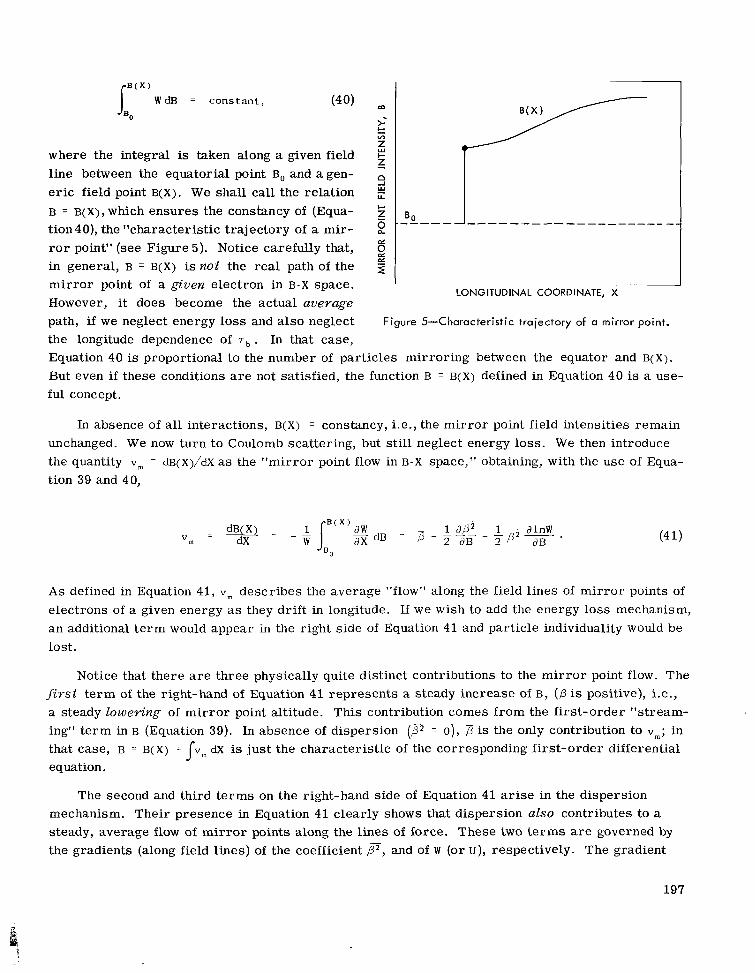
where the integral is taken along a given field line between the equatorial point Bo and a gen- e r ic field point B(X). We shall call the relation B = B(X),which ensures the constancy of (Equa- tion 40), the "characteristic trajectory of a mir- r o r point" (see Figure 5). Notice carefully that, in general, B = B(X) is not the real path of the mir ror point of a given electron in B-X space. However, it does become the actual average path, if we neglect energy loss and also neglect the longitude dependence of -rb. In that case,
LONGITUDINAL COORDINATE, X
Figure 5-Characteristic trajectory of a mirror point.
Equation 40 is proportional to the number of particles mirroring between the equator and B(X).
But even i f these conditions a r e not satisfied, the function B = B(X) defined in Equation 40 is a use- ful concept.
In absence of all interactions, B(X) = constancy, Le., the mir ror point field intensities remain unchanged. We now turn to Coulomb scattering, but still neglect energy loss. We then introduce the quantity vm = dB(X)/dX as the "mirror point flow in B-X space," obtaining, with the use of Equa- tion 39 and 4 0,
A s defined in Equation 41, v m describes the average "flow" along the field lines of mir ror points of electrons of a given energy as they drift in longitude. If we wish to add the energy loss mechanism, an additional t e rm would appear in the right side of Equation 41 and particle individuality would be lost.
Notice that there a r e three physically quite distinct contributions to the mir ror point flow. The first te rm of the right-hand of Equation 41 represents a steady increase of B, ( P is positive), Le., a steady lowering of mir ror point altitude. This contribution comes from the first-order "stream- ing" te rm in B (Equation 39). In absence of dispersion (p = o), is the only contribution to v m ; in that case, B = B(X) = fim dx is just the characteristic of the corresponding first-order differential equation.
The second and third te rms on the right-hand side of Equation 41 a r i se in the dispersion mechanism. Their presence in Equation 41 clearly shows that dispersion also contributes to a steady, average flow of mir ror points along the l ines of force. These two te rms are governed by the gradients (along field lines) of the coefficient p, and of W (or u), respectively. The gradient
197

of p i s always positive, so that the second t e rm in Equation 41 always represents an upward motion of the particle 's mir ror points (back-scattering from the denser atmosphere). If, on the other hand aw/aB< 0, the third t e rm represents a lowering of the mir ror point altitude. If WP2 = constancy along a line of force, the contribution from the two dispersion te rms is zero. The number of mir ror points thrown upwards by the gradient in exactly compensates the num- ber of mir ror points streaming downwards due to the gradient of w. The only mir ror point flow which remains in this case is that of the first order term, v m = P .
DETERMINATION OF THE COEFFICIENTS
In this section we shall obtain expressions for the various coefficients intervening in Equa- tion 39. According to Equation 37, the principal quantities to be found a r e A, { E } , { p } and { p ' } .
With respect to the dimensionless function A defined in Equation 15, we recall that it is in- versely proportional to a dipole-type function computed by Hamlin, Karplus, Vik and Watson (Ref- erence 17). A good approximation of A for the interval 1/4 < B,JB 5 1 is given by
0.384 + O.l28exp(- 35) 1 .
The energy loss per half-bounce { e } is given by the integral
The origin of the field line a r c length is taken at the geomagnetic equator. ds/ i 1 - B' (s)/B is the element of trajectory of the electron at a point s where the field is B ' . Using tables given by Berger and Seltzer (Reference 19), w e obtain the following very good approximation,
where
and
I + 349.0 for E < 470 kev
for E 2 470 kev
(44)
198

is the "effective" atmospheric number density for ionization loss of electrons. As for the time being we a r e interested in low L shells only, we did not include the contribution from atmospheric ions and electrons.
In order to evaluate { p } , the average change of B per half-bounce, we first have to perform the average of collisions over the isotropic azimuthal distribution of scattering angles. Following Welch, Kaufmann, and Hess (Reference 10) and slightly changing their notation, w e obtain
2 is the change in mir ror point field intensity B when the electron's pitch angle scat ters an amount 0 at a field position B' , averaged over all possible azimuthal angles of scattering. Now we have to find the average of s i n 2 0 at the given field point B ' . This will be given by
- where
do. s i n 2 € ' $ dB
is the average contribution from one atom of c lass i. N~ is the number densities of the different atmospheric constituents at the field point B ' ; doi/dt7' a r e the differential c ross sections for screened Coulomb scattering for each constituent. Using Moliere's expression for dci/dti, and following closely Welch, Kaufmann, and Hess (Reference lo), we obtain
0
1 + 0 . 1 6 7 In# (49)
1 mc2 \ m c * '
where
is the effective atmospheric number density for screened Coulomb scattering of electrons. Again, the contribution of atmospheric ions and electrons is excluded.
199

We finally have to perform the integration along the path of a particle from one mir ror point to its conjugate,
Again following Welch, Kaufmann, and Hess (Reference lo), we obtain,
3' 2B2 ($ - 1) s i n 2 B .
Therefore:
If we now call
1 + 0.167 I n )/-F m e 2 m c 2 1
K(B, E ) = 4 x 1 0 - 2 2 B - (gauss c m 2 )
+ 2)
C(E) = h(E) kevcm2 ,
200

we can summarize expressions 51, 53 and 43 in the form
{ E } = a,' (55)
DISCUSSION OF ELECTRON DRIFT AND SCATTERING THROUGH A MODEL FOR THE ANOMALY
Before setting up numerical integrations for low-altitude electrons, it is very helpful to dis- cuss Equation 39 qualitatively, using a simple, approximate model of the atmosphere along field lines in the region of the South American Anomaly, where most of the scattering and energy loss occurs.
We shall res t r ic t ourselves to the region between 250 and 750 km altitude, and to longitudes within about *30 degrees of the center of the Anomaly (supposed at a longitude @ a = 318%). In the present discussion we shall neglect the energy loss te rm and suppose ads@ = constancy and K~ = 1. These latter suppositions lead to a proportionality between x and the longitude @ of the equatorial point of a field line (Equation 19b).
Using the Harr is-Priester atmosphere (Reference 20) for a low solar activity ( s = 70), and Southern Hemisphere geomagnetic field B-L rings as calculated by Stassinopoulos, * we obtain a quite good fit for the effective number density (Equation 50) as a function of B and @, of the type
Due to the supposed proportionality between @ and X , it is easy to convert this expression into a function of x. All this is valid only for very low L values.
For L = 1.25, w e have 1
13 hours local time at the center of the Anomaly:
No = 10" ~ m - ~ , B, = 0 . 2 4 3 gauss, AE3 = 5 . 2 5 ~ gauss, @ = 4.69"
- _ _ _ .- 'Stassinopoulos, E., private communication. tFor higher L shel l s (L 2 1.8), the approximation of Equation 56 becomes very crude. Qualitatively, as L increases, +a shifts to the
e a s t and A + increases considerably.
201
02 hours local t ime at the center:
No = 10" B, = 0.243 g a u s s , DB = 4 . 2 3 ~ g a u s s , &b = 3.78"
For an expression of Equation 56, with a "scale height" AB very small compared to B, the main contribution to the integrals in Equation 54 comes from a region close to that mir ror point which lies in the high atmospheric density end of the line of force. We can therefore approximate:
and
- O B s, - s, = S I B .
dB/ds is the average gradient of B along the field line in the region of interest. Taking into account Equation 55, the following relation between the coefficients { p } and {D'} holds
This is similar to a relation found by Walt and McDonald (Reference 12) for the coefficients of a time-dependent (but longitude- independent) Fokker- Planck equation set up in te rms of mir ror point altitudes, in the region of high atmospheric densities. Relation 59 is expected to hold quite generally in the region of high densities, provided one inserts for AB the value AB = Neff /dNeff /dBI
where the derivation is taken along a line of force.
With Equation 59 and the linear relationship between X and 4, Equation 39 becomes
in which is of the form
K ' is obtained from Equations 37, 54, 55 and 57, and is a slowly varying function of B (slow in com- parison with exp(B/DB).
202

The mir ror point flow (Equation 41) is now
Taking into account (Equation 61) we can approximate
Therefor e,
Physically, the cancellation of the first te rm with the second t e rm in Equation 41 means that the upstream of mir ror points due to diffusion from the denser atmosphere ("backscattering" at lower altitudes) exactly compensates the downstream due to the first order term. What is left is a mir ror point streaming entirely due to diffusion and which may be upwards o r downwards ac- cording to the gradient of the actual electron distribution along a line of force.
In particular, i f dU/dB = 0 for some value B,, there will be no net flow of mir ror points across this B value. An initial distribution of electrons at a longitude @o like the one shown in Figure 6 will therefore keep the maximum at the same B, but wil l broaden towards both sides as the par- ticles drift towards the east (G2 > +, > +o) . This smearing-out wil l be faster at the high-B side (towards lower altitudes), for P is much greater there (see expression (63)). A similar result w a s obtained numerically by MacDonald and Walt (Reference 12).
-
If now W is of the form
3
CT we have a solution of Equation 60, which repre- sents a steady state in longitude. In this case, the mir ror point flow (Equation 63) is approxi- mately equal to P ,
a
Y _I Y
(65)
It can be shown that such a steady state form
- I
g > O
FLUX DENSITY, B
(Equation 64) is attained very Soon Provided the gradient of w along a line of force is negative.
Figure &Qualitative description of the evolution of a mirror point distribution at very low altitudes.
203

It is also easy to verify that Equation 64 is an "equilibrium" configuration: Any small departure of w from Equation 64 will cause mir ror point flows which wil l tend to correct such a departure.
For all these reasons, it is extremely instructive to inspect in detail the motion of mir ror points for such a longitude-independent equilibrium state of Equation 64. Although, of course, all this is only a crude approximation, we expect all qualitative physical features to be valid a lso in the real case. This qualitative analysis will then help us to set up and interpret the tedious numerical calculations.
We shall analyze the characteristic trajectories of mir ror points B = B(X) (Equation 40) through- out the South American Anomaly described approximately by Equation 56, for an equilibrium state electron distribution (Equation 64). First of all, w e will do our discussion in te rms of the more familiar longitude variable 4~ rather than X, which anyway in our description is supposed proportional to the former. In order to obtain the characteristic trajectories in B-@ space, we have to integrate Equation 65, taking into account Equation 61, and the relation of Equation 19b, which now reads
0.24
- 0.23 v)
3 O m
* m 0.22
c 5 0.21 - t l/Y
a -I W
G 0.20
z 2 ~ 0.19
9
I-
ei z
0.18
I _ _ _ _ - - -r------ WEST I EAST
I I
~
298 308 318 328 338OE
LONGITUDE
Figure 7-Charocteristic mirror point trajectories i n the region of the South American Anomaly (model 56) for o steody state distribution of 300 kev electrons of the form 64, and for L = 1.25 (1300 LT in the Anomaly). Elec- trons whose mirror points are in i t ia l l y (i.e., west of the Anomaly) between Bmi, and B,,,, populate the "shadow" region. Those between B,,, and BWE Precipitate eost of
+a; those with B > BW precipitate on the west side. Constant altitude lines for h = 250 and 350 km are shown. Energy loss i s neglected.
Starting from an initial longitude @o well west of the center of the Anomaly, and for a shell L = 1.25, we obtain characterist ic mir ror point trajectories for 300 kev electrons, sche- matically represented in Figure 7. Remember that they correspond to a distribution of the type in Equation 64. In this figure, lines of con- stant altitude for the approximate expression 56 a r e a lso shown. Below 250 kilometers, the N e f f = N e f f (B, @) dependence is still nearly ex- ponential in B and [ @ - @ a 1 , but with a smaller "scale height'' AB. We can safely assume for this discussion, that particles getting below this level wi l l be removed by precipitation. Above 750 kilometers, the scattering effect is ex- tremely small during one drift through the region of interest.
Notice in Figure 7 that there is a narrow "window," Bmin - Bm, , at the initial longitude 6o west of the Anomaly which contains the mir ror points of those electrons that populate the high^ or "shadow" region east of the Anomaly. After one more turn around the earth, all these elec- trons a r e precipitated into the dense layers.
204

A certain portion of these (Bma, - BwE) w i l l manage to get "around" the center of the Anomaly, and precipitate into its eastern side. Electrons mirroring initially at higher altitudes than those cor- responding to the window, wil l lower slightly their mi r ro r points during each passage through the Anomaly until they fall into the critical window. Please remember carefully that all this corre- sponds to an equilibrium distribution of Equation 64, neglecting energy loss and remember that the mir ror point trajectories are average paths, not actual patterns for a given electron.
The most striking result of this analysis, is that if multiple Coulomb scattering i s the only process responsible f o r the replenishment of the shadow region east of the Anomaly, then there is a very limited region of the atmosphere in the South American Anomaly (limited in both longitude and altitude) which entirely governs this replenishing process. We therefore should expect that in the real case, electron fluxes in the shadow are strongly influenced by the instantaneous atmos- pheric structure in this critical region.
In particular, we may expect a diurnal variation of electron fluxes and electron precipitation, determined by the diurnal variation of the atmosphere within about *5' of the center of the Anomaly, between about 250-400 km altitude. We conclude that it would be unrealistic to carry out numeri- cal calculations with a 24-hour averaged atmosphere. Rather, numerical integration should be performed for different local t imes at the Anomaly.
Notice finally, that according to this picture, replenishment occurs right at, or shortly "after," Le., east of the Anomaly. Diffusion into the shadow region far east of the Anomaly is negligible, for Coulomb scattering. We may conclude our discussion by pointing out that in the picture de- scribed above, there is a steady flow of particles out of the lower B-region of a shell towards higher B values and from there into the atmosphere at the Anomaly. In an equilibrium state, this loss must be exactly balanced by a continuous injection from a source mainly effective in the lower B-region. In absence of such a source, i.e., in a nonequilibrium state, this flow and subsequent loss should determine the lifetime of the trapped radiation in question.
A s a numerical example, we have calculated the position of the critical window in B (for the definition of Bmin and B~~~ see Figure 7), for local t imes in the Anomaly as 1300 and 0200. The values obtained for L = 1.25 a r e shown in Table 1. Although the B values differ only very little, remember that they a r e in a region where the distribution U is a very steep function of B.
Table 1
B m i n , B,,, for 1300 and 0200 Local Time, L = 1.25. Crit ical Field Values
1300 Local Time
0200 Local Time
Flux density, B (gauss) at 300 kev
0.198 min.
0.201 max.
0.207 min.
0.210 max.
Flux density,B (gauss) a t 625 kev
0.209 max.
0.216 max.
0.205 min.
0.213 min.
I
205

Detailed quantitative results on electron fluxes can be obtained only by numerical integration of Equation 39. In particular, the energy loss term, neglected in the above discussion, has to be taken into account; this is particularly important if we analyze the behavior of electrons which dip below about 300 kilometers altitude in the Anomaly.
ACKNOWLEDGMENTS
We are indebted to Drs. W. N. Hess, D. Stern, J. Herring and M. Liwshitz for valuable dis- cussions and critical remarks.
REFERENCES
1. Vernov, S. N., Gorchakov, E. V., Logachev, Yu. I., Nesterov, V. E., Pisarenko, N. F., Savenko, I. A., Chudakov, A. E., and Shavrin, P. I . , "Investigations of Radiation During Flights of Satel- lites, Space Vehicles and Rockets," J. Pkys. SOC. Japan, l7(supp. A-11): 162- 186, January 1962.
2. Mann, L. G., Bloom, S. D., and West, H. I., Jr., "Electron Spectrum 90 to 1200 KeV as Ob- served on Discoverer Satellites 29 and 31," in: Space Research III , Proc. 3rd Internat. Space Sci. Sympos., Washington, D. C., May 2-8, 1962, ed. by W. Priester, Amsterdam: North-Holland Pub. Co. and New York: Interscience Publishers, Inc., 1963, pp. 447-462.
3. Imhof, W. L., and Smith, R. V., "Longitudinal Variations of High Energy Electrons at Low Altitudes," J. Geopkys. Res. 70(3):569-577, February 1, 1965.
4. Freden, S. C., and Paulikas, G . A., "Precipitation of Energetic Electrons into the Atmosphere," J. Geopkys. Res. 69(7):1239-1249, April 1, 1964.
5. Mihalov, J. D., Mozer, F. S., and White, R. S., "Artificially Injected Electrons at Low Alti- tudes," J. Geopkys. Res. 69(19):4003-4013, October 1, 1964.
6. Freden, S. C., and Paulikas, G. A., "Trapped Protons at Low Altitudes in the South Atlantic Magnetic Anomaly," J. Geopkys. Res. 69(7):1259-1269, April 1, 1964.
7. White, R. S., Austin, M. M., and Dragt, A. J., "CRAND and SPAND Proton Injection," in:
Space Research V, PYOC. 5th Internat. Space Sci. Sympos., Florence, May 12-15, 1964, ed by D. G. King-Hele, P. Mdler , and G. Righini, Amsterdam: North-Holland Pub. Co. and New York: Interscience Publishers, Inc., 1965, pp. 498-599.
8. Ghielmetti, H. S., Becerra, N., Godel, A. M., Heredia, H., and Roederer, J. G., "Enhancement of the X-Ray Intensity at Balloon Altitudes in the South American Anomaly," Pkys. Rev. Letters, 12(14):388-390, April 6, 1964.
206

9. MacDonald, W. M., and Walt, M., "Distribution Function of Magnetically Confined Electrons in a Scattering Atmosphere,'' Ann. Phys. 15(1):44-62, July 1961.
10. Welch, J. A., Jr., Kaufmann, L., and Hess, W. N., "Trapped Electron Time Histories for L = 1.18 to L = 1.30," J. Geophys. Res. 68(3):685-700, February 1, 1963.
11. MacDonald, W. M., and Walt, M., "Diffusion of Electrons in the Van Allen Radiation Belt. Pt. 1, Treatment of Particles with Mirroring Points at High Altitude," J. Geophys. Res. 67(13):5013- 5024, December 1962.
12. MacDonald, W. M., and Walt, M., "Diffusion of Electrons in the Van Allen Radiation Belt. Pt. 2, Particles with Mirroring Points at Low Altitudes," J. Geophys. Res. 67(13):5025-5033, December 1962.
13. Anderson, A. D., Crane, G. E., Francis, W. E., Newirk, L. L., and Walt, M., "Theoretical Investigation of Geomagnetically Trapped Electrons from High Altitude Nuclear Explosions," Final Report, Sunnyvale, California: Lockheed Missiles and Space Company Report Number 3-24-64-1; AD 612-737, DASA 148, June 1964.
14. McIlwain, C. E., "Coordinates for Mapping the Distribution of Magnetically Trapped Particles," J. Geophys. Res. 66(11):3681-3691, November 1961.
15. Northrop, T. G., and Teller, E., "Stability of the Adiabatic Motion of Charged Particles in the Earth's Field," Phys. Rev. 117(1):215-225, January 1, 1960.
16. Stone, E. C., "Physical Significance and Application of L, Bo, and R, to Magnetically Trapped Particles," J. Geophys. Res. 68(14):4157-4166, July 15, 1963.
17. Hamlin, D. A., Karplus, R., Vik, R. C., and Watson, K. M., "Mirror and Azimuthal Drift Frequencies for Geomagnetically Trapped Particles," J. Geophys. Res. 66(1): 1-4, January 1961.
18. Hassitt, A., "The Drif t of Trapped Particles," J. Geophys. Res. 70(3):535-540, February 1, 1965.
19. Berger, M. J., and Seltzer, S. M., "Tables of Energy Losses and Ranges of Electrons and Protons," NASA SP-3012, 1964.
20. Working Group IV of COSPAR, 1965, CIRA 1965, COSPAR International Reference Atmosphere, 2nd edition, Amsterdam: North Holland Pub. CO., 1965.
207


THE NEUTRON FLUX IN SPACE FOLLOWING A POLAR CAP NEUTRON EVENT ON NOVEMBER 15, 1960
by W. N. Hess
Goddard Space Flight Center
and
E. L. Chupp University of New Hampshire
and
C. Curry University of California
A neutron detector flown on an Atlas pod during the 15 November 1960 solar event measured a la rger neutron flux than another detector flown on a similar vehicle during a quiet solar period. The excess neutron flux at low latitudes obtained by comparing these two measurements is about an order of magnitude higher than expected from the neutron production in the atmosphere by solar protons as deduced from Lingenfelter's calculations and Webber's model for the 15 November event. It i s suggested that most of the discrepancy can be accounted for by considering neutron production by energetic solar alpha parti- cles and lowered geomagnetic cutoffs.
INTRODUCTION
It has been suggested (References 1 and 2) that solar protons bombarding the polar caps could produce a sufficient neutron flux in space (referred to hereafter as a Polar Cap Neutron event o r PCN event) to provide at least part of the source of Van Allen belt protons. This possibility followed the discovery of an anomalous component of protons with energies E > 50 Mev trapped on magnetic field lines with a magnetic shell parameter L > 1.7. Lenchek (Reference 3) has concluded that the observed trapped proton flux is in rough agreement with his theoretical estimates of leakage neutrons from solar proton interactions in the atmosphere. He also concludes that the lifetime of the trapped protons is of the order of 100 years, a time long compared with expected neutron injection from major solar proton events. Thus the anomalous component of trapped protons may be built up by PCN events gradually to its present level by injection over several solar cycles.
209

More recently, Lingenfelter and Flamm (Reference 4) have calculated the neutron leakage flux from solar protons using the exponential rigidity model of Freier and Webber (Reference 5). Their calculations apply only to neutrons with energies E < 10 Mev but provide both the leakage neutron energy spectrum and angular distribution for an arbi t rary solar proton event.
It is the purpose of this paper to present the results of two experiments carried out with neutron detectors on Atlas pods, one of which measured an excess neutron counting rate about four hours after the solar flare at 0207 UT on 15 November 1960. The second experiment provides control data taken one year later. The theory of Lingenfelter and Flamm (Reference 4) is then used along with the solar proton model of Freier and Webber (Reference 5) and the detector character- ist ics to calculate theoretically the expected excess neutron counting rate as a function of position along the trajectory of the Atlas pod. The detector w a s not in the sunlight at any time, so direct solar neutrons could not contribute to the excess counting rate.
DESCRIPTION OF THE SOLAR FLARE EVENT ON 15 NOVEMBER 1960
A t 0207 UT on 15 November 1960 the onset of a great solar flare w a s recorded in Ha. The optical f lare reached a maximum about fourteen minutes later (0221 UT) and ended at 0427 UT.* As eariy as 0233.6 UT the onset of a cosmic ray intensity increase was recorded at the earth (Reference 6), with neutron monitors at sea level and at mountain altitudes. Direct observations of the solar f lare cosmic ray flux were made (Reference 7) using balloon-borne detectors, and indirect observations were made by means of riometers. Pr ior to this solar flare, the interplane- t a ry magnetic field conditions had been altered by a previous f lare on 12 November. A f u l l discus- sion of these two solar f lare cosmic r ay events has been given in l i terature (References 5 and 8), and it is unnecessary to review all the details of the events. For our purposes here it will be sufficient to establish as well as possible the solar cosmic r ay flux time history and spectrum near the earth and the geomagnetic conditions about 0600 to 0630 UT 15 November 1960. This corresponds to the time when the Atlas neutron monitor w a s collecting data.
Ney and Stein (Reference 8) have considered the conditions of the geomagnetic field at the time of the 15 November flare and have concluded that the magnetic field of the earth had returned to its undisturbed condition by late 14 November following the geomagnetic disturbances produced by the solar f lare on 12 November. However, following a solar f lare at 0246 UT on 14 November, a sudden commencement magnetic s torm occurred at 1304 UT on 15 November. The 15 November flare at 0207 produced a sudden commencement at 2200 UT on 15 November. Thus, at the time of the Atlas neutron monitor flight the evidence indicates that the geomagnetic field structure had essentially recovered from its disturbed condition produced by the 12 November flare. Hence, we will first assume that at 0600 on 15 November the normal (Reference 9) cosmic ray threshold rigidities apply.
A t 0500 UT on 15 November, Winckler (Reference 7) made the earliest direct observation of the solar flare particles. On the basis of these observations and neutron monitor records, Freier
*Solar flare data from CRPL Reports, NBS, Boulder.
210

and Webber (Reference 5) have suggested that the spectrum may be best represented at this time by an exponential rigidity spectrum with a characteristic rigidity P, = 350 MeV. A differential power law energy spectrum with exponent n = 3 . 3 does not give as good a f i t as the exponential rigidity spectrum. This spectrum gives a reasonably close fit to the data up to a rigidity of about 3 Bev. These authors have also recommended that this event be best described at all t imes by the differential form
part i c 1 es/cm* - sec-MeV- s t er adi an ,
where (dJ/dP), and Po a r e functions of time during the event. These two parameters a r e simply related by the relation
J o = Po (q0 ,
where J~ is the total flux of charged particles with rigidity greater than P = 0. It has further been found that both the proton and alpha particle fluxes can be represented by this form. The ratio of (dJ/dP), for protons to the same quantity for alpha particles is 1 f 0.5 based on the data of Refer- ence 8 from balloon flights at 1030 to 1230 UT on 15 November. Thus we also assume that the differential flux of protons and alpha particles is the same in any given rigidity interval. Freier and Webber (Reference 5) give, for the time interval covered by this event, the values of J o and Po as a function of time. For the time of interest for our analysis (0600 UT) we have chosen J, = 260 protons/cm2-sec-ster and Po = 355 Mev giving a value for (dJ/dP), of 0.73 protons/cm2- sec-ster-MeV. We make the further assumption that the incoming radiation is isotropic at 0600- 0630 UT.
DESCRIPTION OF ATLAS NEUTRON EXPERIMENT
Moderated Anton BF, proportional counters were flown on an Atlas pod during the solar proton event on 15 November 1960. The general scheme was similar to that described in Reference 10, the pod being cast off from the Atlas after it was aloft. Figure 1 (solid line) shows the pod trajec- tory for the flight which took place at about 0600 UT, about four hours after the start of a large solar f lare and during the time when considerable fluxes of polar cap protons were being detected. A 1-inch B'O F, counter moderated by 2 inches of epoxy w a s used and a similar counter but filled with B" F, w a s flown to indicate counts not due to neutrons. The count rate ratios of the two detectors throughout the flight was consistent with that expected from the ratio of B lo abundance in the two counters indicating that only neutrons were being detected. Individual counts from the detectors were returned to ground by F M telemetry. The count rate history for this detector is shown in Figure 2 as curve a.
211

0 5 10 15 20 TIME FROM POD RELEASE (minutes )
Figure 1-Trajectory of Atlas pod.
-
-
. 24
20
- 1 6 w
: a 4 .12 2 - - 4
- 0
- 4
- a 0.011 , , , , , ,
5 10 15 20 25 TIME FROM POD RELEASE (minutes)
Figure 2-Comparative counting rate histories for neu- tron detectors on Atlas pod flights. The counting rate shown for October 2, 1961 i s 1/10 the actual counting rate since the detector on this fl ight had an efficiency of about 10 times larger than for the other detector.
A nearly identical system of BF3 counters was flown on another Atlas pod on 2 1961 during a relatively quiet solar period. For this flight the detector geometry was the same, but the detectors were replaced by Reuter-Stokes counters filled to a higher pressure and the detectors were moderated with polyethylene; thus the system had higher efficiency than for .the flight on 15 November. The count rate history for this flight for the B'O F, counter is.shown as curve b in Figure 2. The Atlas trajectory for this flight was slightly different than on 15 November 1960, so this data is plotted for comparison with the first flight on Figure 1 as dotted curves. The curves a and b in Figure 2 may not be compared directly except at early t imes because of the large difference in trajectories apparent at late t imes (Figure 1). At late t imes both detectors show an anomalous r i se in counting rate after reaching a minimum following the pod's exit from the radia- tion belt. The minima occur at different t imes following release of the respective pods because of the difference of trajectories but still at nearly the same altitudes and geographic coordinates. We have no explanation for this behavior.
The pod for the second flight was quite similar in geometry to that for the first flight. It was slightly larger and heavier and the location of the components in it was not identical to the first but it was similar enough so that the vehicle produced neutron fluxes should be nearly equal. The approximate weight of the first pod was 65 pounds, and the second pod 100 pounds. An estimate based on the relative masses and distributions of components indicates that the second pod had 20 percent more locally produced neutrons which could be counted by its detector than for the first pod. Thus, the difference in counting rates for the two measurements is a lower limit. That is, any correction for differences in local neutron production would only increase the differences in count- ing rates between the two flights.
The efficiencies of these detectors were measured using standard neutron sources of Sb-Be, Mock Fission and Po-Be. The mean neutron energies for these sources are respectively 25 kev,
212
L

1 Mev and 4 MeV. We feel the detectors and pod trajectories for the two flights a r e sufficiently similar on the ascending portion of the trajectory that it is meaningful to make a direct compari- son of counting ra tes of the two instruments in order to determine what effect the phenomena associated with the solar f lare might have on the neutron flux in space. We make the following assumptions: First, that the differential albedo neutron flux due to galactic cosmic r a y s at both detectors is the same for corresponding detector locations; and, second, that the differential neu- tron flux at both detectors due to neutrons locally produced in the pods and in the detectors are the same in both cases. This, of course, assumes that the charged particle flux at the pod is always the same at corresponding locations in both cases.*
The B'O neutron counting rate for the 15 November 1960 flight and at a particular location is then
where
I1 ( E ) = detector efficiency versus neutron energy (counts-cm2/neutron),
N , ( E ) = the differential neutron flux at the detector associated with the solar flare,
N$ (E) = the differential neutron flux locally produced by the ambient charged particle radia- tion, and
N g (E) = the differential neutron flux produced by the galactic cosmic r ays and returning to space.
In a similar manner we can write the counting rate for the detector flown on the quiet solar day 2 October 1961 as
The detector efficiencies for the 1961 detector compared to the 1960 detector a r e very nearly in the ratio of 10 to 1 at all energies so 2, (E) = 10 x1 ( E ) . A s can be seen in Figure 1, the trajec- tor ies are sufficiently similar at early t imes so that the galactic cosmic r ay flux is the same for both flights, and we assume the t e rm [ N t ( E ) -t Ng (E)] is the same in both cases to *lo percent. This, of course, requires that the cutoff rigidities a r e the same for both flights. The Forbush
* A 3 t solar flare on 28 September 1961 was followed by an SC magnetic storm and associated Forbush decrease on 30 September. By
The solar cyc le variation of galactic cosmic rays the time of the pod flight on 2 October, the galactic cosmic ray intensity bad nearly recovered to its pre-storm level; thus the galactic albedo neutron flux would only be expected to be a few percent lower than normal. a l s o compensates for this effect.
213

decrease associated with the 12 November 1960 event was well over by 15 November and geomag- netic conditions were also normal during the second flight so this assumption is reasonable.
0.4
D z 0 2 0.3 Y)
?; t 8 I) 0.2
c v Q 0.1
Thus the excess counting rate due to the flare is then
-
-
-
-
The integral on the right provides a means of comparing theory with experiment as will be discussed later. Figure 3 shows the experimental values of (AC,) e x p as deduced directly f rom the counting rate data. The estimated absolute e r r o r in (AC,) e x p , the flare associated enhanced neu- tron flux is e30 percent and is mostly due to the detector calibration e r r o r s and counting statistics. Any e r r o r s associated with the assumptions justifying the subtraction of the two sets of data will not produce a large e r r o r in (AC,) e x p since C , >> Cz/lO. We also a r e neglecting the fact that the galactic cosmic ray flux was actually somewhat higher during the second flight but correction for this effect would enhance the experimental value of (AC ,) e x p . Also any correction for differences in local neutron production from galactic cosmic r a y s for the two detectors would increase the value of (Ac,) e x D since the pod containing the second detector was actually somewhat heavier than for the flight following the solar flare. The possibility that an excess of charged particle flux could be present at the detector during the 15 November flight can be ruled out qualitatively from the be- havior of ( A C , ) ~ ~ ~ versus latitude as shown in Figure 3. If solar protons or extra galactic cosmic
b -PO0 IN RADIATION BELT-
0 5 10 15 20 . p 5 TIME FROM POD RELEASE (minutes)
15 NOVEMBER 1960
Figure 3-(a) The flare associated enhanced neutron counting rate ( A C f ) e x p versus time after Atlas pod re- lease. (b) The value of (ACf) theo x 10 according to Lingenfelter's theory. (c) The value of (&f)t, ,eo for a l l cutoffs 80 percent of normal. (d) (Ac,)theo. The theo- retical values are based on neutron production solely by solar protons.
214
rays due to lowered cutoffs were present at the detector and produced a significant flux of locally produced neutrons then (Ac ,) should fall off with t ime (i.e., as the detector pro- gresses to more southern latitudes), but this is contrary to the behavior in Figure 3. This is expected since there would be a higher flux of such leakage charged particles at the ear l ier t imes (Le., higher latitudes) and hence more locally produced neutrons.
Because of the anomalous behavior of the counting rate curves (Figure 2) on the descend- ing portion of the trajectories, it is difficult to have a great deal of confidence in this par t of the data. Since the minima of the counting rates occur at nearly the same location in space and are essentially the same, we take the view that both detectors a r e responding normally here and find the excess counting rate zero within the e r r o r of measurement as shown in Figure 3.
e

ANALYSIS
The flare associated neutron flux enhancement ( A c , ) exp, defined ajove, appears to be due to only one cause. Since solar protons were bombarding the polar cap regions at the time of the Atlas pod flight the most likely extra source of neutrons in space is from the reactions these protons make with atmospheric nuclei. During most of the time of interest during the experiment (when the detector w a s below the radiation belt) par t of those regions of the polar atmosphere accessible to the solar protons were above the horizon for the neutron detector; thus a PCN event of sufficient magnitude could logically explain the flux enhancement. An additional source of extra neutrons is the sun itself, but-the detector was never in the sunlight so this possible source may be excluded.
Generalized theoretical -calculations performed by Lingenfelter and Flamm (Reference 4) give the leakage flux at the top of the atmosphere for neutrons produced by polar cap protons. These results may not be directly compared with the present experimental results since they give only the leakage flux into space from a unit a r ea at the top of the atmosphere. The resudts of.these calculations must be used as a source and the geometrical calculation performed to give the differential flux at the detector location which is changing with time due to the motion of the detector in latitude, longitude and altitude. It has been established above that the best description of the time variation of the flux of solar protons and alpha particles at the earth following the solar f lare of 15 November 1960 is given by an exponential differential rigidity spectrum of the form
- p / p 0 - protons or alphas dP cm2-sec-MeV-steradian
where (dJ/dP), = 0 . 7 3 particles/cm2-sec-MeV-steradian and Po = 355 Mev at the time of the Atlas neutron monitor flight. It is further assumed that the lowest rigidity particle reaching the earth’s atmosphere at a given latitude and longitude is determined by the quiet cosmic r ay vertical cutoff rigidities of Quenby and Wenk (Reference 9). Lingenfelter‘s model also takes the incident charged particle flux as isotropic over the upper hemisphere.
Lingenfelter’s calculations give the equilibrium neutron flux in the atmosphere produced by protons with the above rigidity spectrum using the diffusion theory approximation to neutron trans- port theory. He gives the neutron flux as a function of atmospheric depth for energies up to 10 MeV. In addition the leakage flux from the top of the atmosphere and its angular distribution with respect to the zenith is given for eighteen energy groups. Since all of these calculations have been done for several different values of characteristic rigidity Po and cutoff rigidities, it is a simple geo- metrical problem to calculate the leakage flux at any point in space from a leakage flux source element at a given latitude and longitude.*
*Lingenfelter’s model takes the incident charged particle flux a s isotropic over the upper hemisphere. Since h is leakage flux is normal- ized to a total of 1 proton/cm2 sec-incident the absolute leakage flux value for the conditions of this event is based on 2.rr x .73 = 4.6
protons
cm’sec Mev as the isotropic incident flux.
215

21 Source coordinates: latitude, 8 '"'
/ Longitude, f $ (from observer)
'1 Observer coordinates: Latitude, X Longitude, 6
'"A\ r-R
GEOGRAPHIC
Figure 4-The coordinate system relating the observer coordinates to the source coordinate for a PCN event.
The geometry pertaining to this calcula- tion is shown in Figure 4. It should be noted that only the source elements which are in a direct line of sight (above the horizon) from the detector at a given t ime give contributions to the flux at the detector. Those neutrons whose trajectories a r e modified by the gravita- tional field (En < 10 volts) do not add signifi- cantly to the detector count ra te here.
Referring to Figure 4 the vector flux, or the number of neutrons traveling through a unit a r ea normal to the direction, 6, f rom a source element and into unit solid angle in the direction of the observer is
The te rm A (7, AE i ) * gives the normalized vector flux for a given energy group LEi and zenith angle 7 from Lingenfelter's work for Po = 125 Mev and Pc = O.** The normalization te rm (UrJ,/P,) is required since Lingenfelter's theoretical calculations were normalized to unity for this quantity. The remaining t e rm in brackets, deduced from Lingenfelter's work, is necessary to transform to our specific case of interest where P, = 355 Mev and the cutoff rigidity Pc is defined by the loca- tion of a given source element. For a given energy group then the flux at a particular observer 's location for all source elements above the horizon is
All symbols a r e defined in Figure 4 and cos e dB d+ is the source element of area. The magnitudes of the position vectors and R' a r e expressed in earth radii. J o ( h , 6 , r , mi) is properly defined as the flux through a sphere of unit cross-sectional area at the observer 's location. This calcula- tion has been performed numerically for several detector locations and all energy groups used by Lingenfelter. The integration w a s performed in one degree steps in latitude and longitude over all
*Our values of A 7 , AE. are determined taking into account a correction to Lingenfelter's earlier work a s noted in J. Geophys. Res . , ( 1)
69:4201 (1964).
**Lingenfelter (private communication) has found the dependence of the zenith angle distribution on variation of Po and Pc l e s s than 10 percent.
216

possible source coordinates satisfying the line of sight condition (77 5 W 2 ) . In general the counting rate produced by this differential flux is
E l ( & i ) is the average efficiency corresponding to the energy group DEi. ment between (AC ,) thee and (AC,) e x p ; in fact, the theoretical value is more than an order of magni- tude below the experimental value. Curve b, Figure 3 shows (AC,) thee multiplied by ten. The shape at early t imes follows that for (AC,) e x p indicating that the latter is consistent with a PCN source. verified in (K,) e x p because of the large experimental uncertainty.
There is not good agree-
(K,) thee shows a peak at an altitude of d700 kilometers, but this behavior cannot be
DISCUSSION OF DISCREPANCY
Arguments have been given previously which indicate that the experimental value (AC,) e x p is a lower limit. Further, the behavior of the experimental curve (Figure 3) with latitude is not con- sistent with any significant local production of neutrons. It is not clear how the experimental excess counting rate can be reduced and therefore we wish to inquire how the theoretical prediction can be sign if icantl y increased.
We will consider both the possibility that the absolute leakage flux calculated by Lingenfelter and Flamm (Reference 4) is low for this event; and the effect of changes in the parameters Po and P,. In regard to the first point, Freier and Webber‘s model (Reference 5) indicates that the ratio of alpha particles to protons at the same rigidity is M 1 f 0.5 for the solar flare event on 15 November 1960 and also Po is the same. Lingenfelter and Flamm, however, have only considered protons as the primary neutron producing radiation. Adequate data on neutron production by alpha particles is not available. However, a rough estimate of the extra neutron production from the alpha particles can be found from the following argument: A t a cutoff rigidity of 1 Bev the differential and integral fluxes of protons and alphas is the same but the proton kinetic energy is x435 MeV, while the kinetic energy per nucleon for the alpha is -125 MeV. Now if each of the four nucleons of the alpha particle is as effective in producing neutrons in an air nucleus as a proton of the same energy, then the ratio of the neutron excitation c ross section for alphas to the excitation c ross section for protons is, from Figure 1 (Reference 5)
4a (125 M e v / N u c , u) 4 x . 3 ~ w 2. ~ ( 4 3 5 M e V , P ) - . 6
Thus it seems reasonable that the theoretical absolute neutron leakage flux should be increased by a factor of 3.
217

Lingenfelter's ear l ier work on production of neutrons by galactic cosmic rays is in reasonable agreement with experiment. He has also compared his calculations on neutron production by solar protons with neutron measurements in the atmosphere (Reference 11) following the solar proton event on 18-19 July 1961. Again the agreement is within experimental e r ro r . In both of these cases, however, the ratio of protons to alphas (P/a) is quite high; for galactic cosmic rays at solar min P/a w 7.2(> 4 .5 Bev) and for the event on 18 July 1961 the evidence (Reference 5) indicates that P/a = 6 +_ 1 about ten hours after the associated flare. On the other hand, in the case of the 15 November 1960 event, the evidence indicates that P/a = 1 i 0 .5 about eight hours after the associated flare. At the time of the measurement described here it is therefore possible that alpha particles make a comparable contribution to the excess neutron flux as do the protons, or possibly a larger contribution.
Another factor we suggest that could conceivably increase the expected theoretical flux at the detector concerns the lowered cutoff rigidity for charged particles entering the earth 's atmosphere from the west. The theoretical calculations are based on vertical cutoff rigidities. For a sufficiently steep rigidity spectrum this may significantly enhance the neutron production in the atmosphere for this event.
Freier and Webber (Reference 5) indicate that a geomagnetic cutoff of 80 percent of normal can be deduced from the balloon flight data of WincMer (Reference 7) at 0500 UT, 15 November, about 45 minutes before the Atlas pod measurements. To tes t the effect of reduced cutoffs on the theoretical results, we have made the gross assumption that all cutoffs a r e lowered to 80 percent of normal and recalculated (AC f ) thee. The result is shown as curve c in Figure 3. At the peak of the theoretical curve this increases (AC f ) thee by about a factor of two over the result found as- suming all cutoffs a r e normal. It is possible to get a reasonably close f i t to ( A c ~ ) ~ ~ ~ by further adjusting Po and Pc but there is no evidence to support such modifications to the model used here.
CONCLUSIONS
In summary then we have found a disagreement by afactor of ten to fifteen between theoretical expectations and the measurement of the neutron flux in space from a PCN event following the solar f lare of 15 November 1960. The experimentally observed excess neutron counting rate cannot be decreased by any reasonable argument. There is some inconsistency in the relative response of our detectors when the pods a r e in the trapped radiation, but we believe this can be accounted for by uncertainties in the apogees of the two pod trajectories. The low theoretical result (for the conditions of the experiment) probably should be increased for two reasons. If account is taken of the production of evapo.ration neutrons from the alpha particles accompanying the protons from the flare then the theoretical flux could possibly be increased by a factor of three. Further i f the assumption is made that the geomagnetic cutoff is 80 percent of normal at all latitudes (as was the case at Minneapolis shortly before the experiment) then the theoretical f lux can be increased by another factor of two. If these tentative conclusions stand, then the discrepancy is reduced to a factor of two to three.
218

This experiment has demonstrated the value of a low latitude, ballistic rocket experiment to study a PCN event and provides a basis for planning experiments to study future events. At a representative point in spacp during the 1960 flight the polar cap neutron flux is about 2 neutrons/ cn i2 sec to be compared with a galactic albedo neutron flux of about 0.2 neutrons/cm2 sec. Un- fortunately it was not possible in this experiment to provide any data on the flux of neutrons (En- > 70 Me") which could be related to the high energy trapped protons.
The authors wish to acknowledge several conversations with Dr. R. E. Lingenfelter on theo- retical questions, and discussions with Dr. J. A. Lockwood on several aspects of the solar cosmic rays on 15 November 1960. We are particularly indebted to Mr. Allen Silver for ably carrying out the numerical integrations with the Goddard Space Flight Center computer, and M r . Donald Peters of UCLRL and Mr. Robert Henderson of UCLRL who did the electronic circuit design and me- chanical design, respectively, for the pod experiment. Critical comments by Dr. C. Gilbert of UCLRL in reviewing our analysis are also deeply appreciated.
REFERENCES
1. Armstrong, A. H., Harrison, F. B., Heckman, H. H., and Rosen, L., "Charged Particles in the Inner Van Allen Radiation Belt," J. Geophys. Res. 66(2):351-357, February 1961.
2. Naugle, J. E., and Kniffen, D. A., "Flux and Energy Spectra of the Protons in the Inner Van Allen Belt," Phys. Rev. Letters, 7(1):3-6, January 1961.
3. Lenchek, A. M., "On the Anomalous Component of Low-Energy Geomagnetically Trapped Protons," J. Geophys. Res. 67(6):2145-2157, June 1962.
4. Lingenfelter, R. E., and Flamm, E. J., "Neutron Leakage Flux From Interactions of Solar Protons in the Atmosphere," J. Geophys. Res. 69(11):2199-2207, June 1964.
5. Freier , P. S., and Webber, W. R., "Exponential Rigidity Spectrums for Solar-Flare Cosmic Rays," J. Geophys. Res. 68(6): 1605- 1629, March 1963.
6. Lockwood, J. A., and Shea, M. A., "Variations of the Cosmic Radiation in November 1960," J. Geophys. Res. 66(10):3083-93, October 1961.
7. Winckler, J. R., "Geomagnetic and Interplanetary Effects on Cosmic Rays," J. Phy. SOC. Japan, 17(Suppl. A-II):337-44, January 1962.
8. Ney, E. P., and Stein, W. A., "Solar Protons, Alpha Particles, and Heavy Nuclei in November 1960," J. Geophys. Res. 67(6):2087-2105, June 1962.
9. Quenby, J. J., and Wenk, G. J., "Cosmic Ray Threshold Rigidities and the Earth 's Magnetic Field," Phil. Mag. 7(81):1457-1471, September 1962.
219

10. Hess, W. N. and Starnes, A. J., "Measurement of the Neutron Flux in Space," Phys. Rev. Letters 5(2):48-50, July 15, 1960.
11. Smith, R. V., Chase, L. F., Imhof., W. L., Reagan, J. B., and Walt,M., "Radiation Measure- ments with Balloons," Final Report, Aeromedical Res. Lab., Holloman AFB, New Mexico, ARL-TDR -62 -2, 1962.
220

HEAT BUDGET OF THE SOUTHERN HEMISPHERE
by S. I. Rasool and C. Prabhakara
Goddard Space Flight Center
Analysis has been car r ied out of radiation measurements made by the Ti ros VI1 satellite covering a period ,of one full year. The annual heat budget has been computed separately fo r the northern and southern hemispheres. It i s found that there i s a northward flux of heat across the equator of % 40 x 10 calories/day by transport of water vapor. As the two hemispheres are individually in radia- tive balance with space, this northward flux of heat must therefore be compen- sated by southward transport of heat by ocean cur ren ts and the atmosphere.
Seasonal variations in the intensity of meridional transport of heat in the southern and northern hemispheres have also been examined. It i s found that in the months of December, January and February there i s a large northward flux of heat a t a l l latitudes between 20 degrees S and 90 degrees N. During the other three seasons the flux i s moderate and i s predominantly southward a t all lati- tudes between 15 degrees N and 90 degrees S.
INTRODUCTION
Earl ier studies of the heat budget of the earth have been mainly confined to the northern hemisphere (References 1 and 2). The main reason for this has been the scarcity of temperature and radiation data in the southern hemisphere where 80.9 percent of the surface is covered with oceans. It has therefore been customary to estimate the heat balance of the southern hemisphere by using northern hemisphere data for corresponding latitude and season. This type of analysis is, however, likely to give misleading results because the topography of the southern hemisphere is considerably different from that of the northern hemisphere; also, the albedo, cloud cover, and water vapor amounts in the southern hemisphere, being mostly oceanic, may not necessarily be the same as in the northern hemisphere; and, because of the eccentricity of the earth's orbit around the sun and the inclination of the earth, the solar energy input in the southern hemisphere is 2 6 percent higher in the local summer than in the northern hemisphere.
Since the IGY, however, a considerable amount of data have become available and the subsequent studies of the heat budget of the south polar regions made by Gabites, Rubin and Kort (References 3, 4 and 5) have indicated significant differences in the heat balance of the two poles.
Now, with the availability of data from meteorological satellites, providing uniform coverage over both hemispheres with a frequency of observations never before achieved (a million data
221
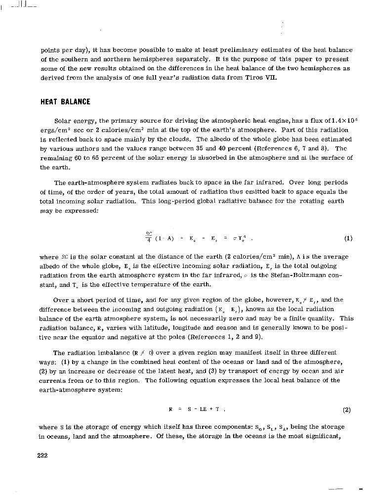
points per day), it has become possible to make at least preliminary estimates of the heat balance of the southern and northern hemispheres separately. It is the purpose of this paper to present some of the new results obtained on the differences in the heat balance of the two hemispheres as derived from the analysis of one full year's radiation data from Tiros VII.
HEAT BALANCE
Solar energy, the primary source for driving the atmospheric heat engine, has a flux of 1 . 4 x 1 0 6
ergs/cm2 sec or 2 calories/cm2 min at the top of the earth's atmosphere. Par t of this radiation is reflected back to space mainly by the clouds. The albedo of the whole globe has been estimated by various authors and the values range between 35 and 40 percent (References 6, 7 a i d 8). remaining 60 to 65 percent of the solar energy is absorbed in the atmosphere and at the surface of the earth.
The
The earth-atmosphere system radiates back to space in the far infrared. Over long periods of time, of the order of years, the total amount of radiation thus emitted back to space equals the total incoming solar radiation. This long-period global radiative balance for the rotating earth may be expressed:
where SC is the solar constant at the distance of the earth (2 calories/cm2 min), A i s the average albedo of the whole globe, Es is the effective. incoming solar radiation, Er is the total outgoing radiation from the earth atmosphere system in the far infrared, u is the Stefan-Boltzmann con- stant, and Te is the effective temperature of the earth.
Over a short period of time, and for any given region of the globe, however, Es # E,., and the difference between the incoming and outgoing radiation ( Es - E,), known as the local radiation balance of the earth atmosphere system, is not necessarily zero and may be a finite quantity. This radiation balance, R , varies with latitude, longitude and season and is generally known to be posi- tive near the equator and negative at the poles (References 1, 2 and 9).
The radiation imbalance (R # 0) over a given region may manifest itself in three different ways: (1) by a change in the combined heat content of the oceans or land and of the atmosphere, (2) by an increase or decrease of the latent heat, and (3) by transport of energy by ocean and air currents from or t o this region. The following equation expresses the local heat balance of the earth-atmosphere system:
where S is the storage of energy which itself has three components: S o , SL, SA, being the storage in oceans, land and the atmosphere. Of these, the storage in the oceans is the most significant,
222

and can have an approximate magnitude of the radiation balance itself (References 10 and 11). S,
and SA are usually 10 percent of so (Reference 10). LE is the net latent heat available in the atmosphere, being the difference between the amount of energy spent in evaporation and that released by condensation in the atmosphere. T is the residual heat available' for transport by ocean currents and by winds.
On an annual basis, within a wide latitudinal zone (%loo), both the storage and the net latent heat t e rms in Equation 2 go to zero, and therefore the latitudinal variations in the annual radia- tion balance are an indicator of the energy transported across the latitudinal c i rc les
In the present study we have attempted to derive, from the meteorological satellite data, the radiation balance of the earth-atmosphere system for one full year, separately for the northern and the southern hemispheres. Also, monthly and latitudinal variations in the radiation balance have been derived. These values a r e combined with climatological estimates of the storage of energy in oceans, land and atmosphere, and of the net latent heat available in the atmosphere. Equation 2 is then solved for T t o obtain the latitudinal and monthly variations in the energy avail- able for transport by oceans and the atmosphere.
RADIATION MEASUREMENTS FROM TIROS SATELLITES
Apart from the now well known television cameras, most of the Tiros ser ies of meteorological satellites were also equipped with medium resolution scanning radiometers. These radiometers have been described in considerable detail by Bandeen and Astheimer (References 12 and 13). They measure the absolute intensities of the emitted terrestr ia l radiation and of the solar radiation a s reflected by the earth. Also, the orbital characteristics of the Tiros VII satellite have been discussed in great detail (References 14 and 15) and therefore will not be repeated here.
For the determination of the radiation balance we have used the data from Channel 2 and Channel 5 (Reference 14). Recent analyses of the radiation data obtained from Tiros VII have indicated that there has been considerable degradation in the instrumental response, thereby intro- ducing an e r r o r in the observed radiation values (Reference 14). Because the Tiros satellites a r e not equipped for on-board calibration, the corrections to these degradations have to be determined indirectly. correction factors for individual channels of the radiometer. These corrections a r e based on the assumption that the quasi-global (60 degrees N - 60 degrees S) mean value of the radiation re- flected in the short wave and emitted in the long wave regions remains constant over long periods of time (several months).
Bandeen (Reference 16) studied th is problem in great detail and has introduced the
SEASONAL AND LATITUDINAL VARIATION OF HEAT BALANCE
Incoming Solar Radiation The incoming radiation, E ~ , in a given 10 degree latitudinal belt for each month, is calculated
from the expression:
Es = E ( l - A ) , (3)
223

where E is the average radiation flux incident at the top of the atmosphere for the month and A is the monthly mean albedo for the latitudinal belt. The values of A a r e based on the Tiros VII measurements in the Channel 5 (0.5 - 0.711) as corrected for the degradation in the response of the radiometer (Reference 14). Figure 1 shows the distribution of the incoming solar radiation as a function of latitude and month between 60 degrees N and 60 degrees S in calories/cmZ day. It is seen that the maximum radiation is received at the subtropical belts during the local summers of the two hemispheres. The values of the effective incoming radiation at 20 degrees - 30 degrees S, during summer, a r e = 10 percent higher than those for the
-
MONTHS
riods of the year (References 17, 18, 19 and 20). 3 2o
northern hemisphere for the corresponding season and latitude. This is both because of
Figure 1-Latitude and time distribution of the incoming solar radiation i n calorieJcm2 day derived from the
- -
albedo measurements made by Tiros VII.
and because slightly more solar radiation (z 6 percent) is incident at the top of the atmosphere during the southern hemisphere summer. The other features of Figure 1 conform with ear l ier studies made using ground-based observations of the incoming radiation (Reference 10).
the larger oceanic regions in the southern hemisphere which have a relatively low albedo
radiation for each10degree latitudinal belt f rom day derived from measurements made by Tiros VII.
224

June 1963 through June 1964. going radiation in calories/cm2 day.
Figure 2 shows the latitudinal and time variations of the total out-
The variation in the outgoing radiation with latitude is small and the change with season is still smaller. The weak highs of outgoing radiation at the subtropical latitudinal belts in both hem- ispheres are to be noted. Also the latitude of the inter-tropical convergence zone (region of the equatorial minimum in the outgoing radiation) changes as expected from 5 degrees S in February t o 210 degrees N in July and August.
Radiation Balance of the Earth-Atmosphere System
Combining Figures 1 and 2, we now obtain the radiation balance of the earth-atmosphere system shown in Figure 3. Because the total outgoing terrestrial radiation does not vary considerably with season and with latitude be- tween 60 degrees N and 60 degrees S, the radi- ation balance of the earth-atmosphere system shows a pattern similar to that of the incoming radiati.on (Figure 1). The main excess of in- coming over outgoing radiation occurs in the latitudes 20 - 40 degrees in both the hemi- spheres in their respective months of summer. In the tropical latitudes between 20 degrees N and 15 degrees S, there is an excess of incom- ing radiation all year round.
J F M A M J J A S O N D MONTHS
Figure 3-Radiation balance of the earth-atmosphere system i n calories/cm2 sec derived fromFigures 1 and 2.
Net Heat Available for Transport
The radiation balance a s shown in Figure 3 gives the net amount of energy deposited by the sun in the earth-atmosphere system. As discussed earlier, a substantial part of th i s energy is stored in the oceans and to some extent also in the land and atmosphere. Also part of this energy is spent in evaporation of water which may later be released in the atmosphere by condensation in the form of clouds. Estimates of the magnitude of energy involved in each of these processes and its varia- tion with time and latitude have recently been made by the authors (Reference 15) and the results a r e shown in Figures 4 and 5. For the source of data and the method of computation on which Fig- u r e s 4 and 5 a r e based, the reader is referred to Reference 15. After accounting for the expenditure of heat in the above-mentioned processes, it is found that there is a finite amount of residual energy at any given time and place. This remaining part is termed as the energy available for transporta- tion across the latitudinal circles, both by the atmosphere (sensible heat) and by the oceans.
By adding the radiation balance (Figure 3), the storages (Figure 4, land and atmosphere storages not shown), and the net latent heat, we obtain Figure 6 which shows the distribution of the
225

I I-
5 Z
h u1
0
E m 73 v
" n 3 + -
I + 3
4 2
I + 5
, z
I + 3
2
MONTHS MONTHS
Figure 4-Latitude and time distribution of the storage of heat in the oceans i n calories/cm2 day; (-) heat gained, (+) heat released (Rosool and Prabhakara, Refer- ence 15).
Figure 5-Latitude and timedistribution of the net latent heat in the earth's atmosphere i n calories/cm2 day; (-) heat lost by the atmosphere by excess of evaporation over precipitation, (+) heat gained by the atmosphere by the excess of precipitation over evaporation (Rasool and Prabhakara, Reference 15).
I + 8 Z
" n 2 + 4
net heat available for transport. It seems difficult t o comment on the accuracy of these quantitative estimates shown in Figure 6. These numbers result from differences of the three large quantities which inherently have some e r r o r s due to the various assumptions made in their evaluation. hoped that the distribution of transportable heat shown in Figure 6 is physically meaning- ful and could be compared with some observed characterist ics of the circulation in the atmos- phere and oceans.
It is, nevertheless,
A large excess of heat in the equatorial latitudes almost throughout the year is indicated in Figure 6. The reason for this is the positive radiation balance (Figure 3) and positive net latent heat (Figure 5) arising from an excess of precipitation over evaporation at these latitudes. The ocean storage (Figure 4) in the equatorial regions is too small to influence the balance.
MONTHS
Figure 6-Latitude and time distribution of the net heat in caIories/cmz day available for transport by the a t m o s p h e r e and oceans across the latitude
circles.
226

In February and March the maximum of this equatorial excess of heat occurs at 10 degrees S, while in July and August, following the thermal equator, the maximum moves to 15 degrees N.
In the subtropical and middle (20 - 40 degree) latitudes, the radiation balance (Figure 3) and net latent heat (Figure 5) appear t o vary in phase with each other, being largest in summer and smallest in winter. to the sum of radiation and the net latent heat, but has an opposite sign. Consequently, in the sub- tropical latitudes, there is little energy available for transport through most of the year. case of the northern hemisphere, Fritz (Reference 11) has already shown that between 20 - 40 degree latitudes, the atmosphere may be in radiative equilibrium throughout the year, in agreement with our results shown in Figure 6. Unlike the northern hemisphere, we find an anomalous feature of high negative values in the southern hemisphere at 40 - 50 degree latitudes in March, April and May. the ocean absorbs heat until the month of May (late fall) (Figure 4) when the radiation balance has already become highly negative. This results in a negative value for transportable heat.
On the other hand, the total heat storage in the oceans is equal in magnitude
In the
This is brought about by the circumstance that at these latitudes in the southern hemisphere,
RESULTS
Seasonal Variations in the Meridional Transport of Heat The flux of heat transported across each
latitudinal circle is derived from Figure 6 by assuming that the flux at the two poles is zero and adopting the values of heat transport given by Gabites (Reference 3) for 72 degrees S and 50 degrees S, respectively. The monthly values of the transportable heat shown in Figure 6 a r e averaged for three monthly periods and added algebraically for each season from 50 degrees S to 50 degrees N. The flux of heat across lati- tude circles is then derived and is shown in Figure 7 for the four seasons. For comparison purposes, we also give the recently published values of sensible heat transport given by Haines and Winston (Reference 21) for the 50 degrees N latitude. The actual values quoted by Haines and Winston were calculated for the atmospheric layer between 500 and 850 millibars. Winston (Reference 22) has suggested that there is a linear relation be- tween the total atmospheric transport and the transport in this layer. The values plotted in Figure 7 are the adjusted values for the total atmosphere.
I - T I r 1 I I
1
I I I I I I I 6050 40 30 20 IO 0 IO 20 30 40 5060 90
SOUTH NORTH LATITUDE (degrees)
Figure 7-Three-monthly mean values of the meridional f lux of heat i n I O l 9 calories/day between 50"N and 5OOS. The values are for the combined transport by ocean currents and the sensible heat i n the atmosphere.
227

It is interesting to note that the northward transport of heat is extremely large in the months of December, January and February. For the rest of the nine months, the transport of heat is south- ward for all latitudes between 20 degrees N and 90 degrees s. The magnitude of the northward f lux in the months of December, January and February is maximum at the latitude of 40 degrees N with a value of Z 3 0 X 10 calories/day. For the remaining nine months, the southward flux maximum is fairly constant in magnitude, s20 x 1019 calories/day,but the latitude of the maximum southward transport var ies f rom 30 degrees S in March, April and May to 10 degrees S in June, July and August. The northward flux of sensible heat in the northern hemisphere is extremely small during these nine months.
calories/day. Also, there is a northward flux across the equator of %23 X l O I 9
Annual The mean annual transport of heat as a function of latitude is shown in Figure 8. It is note-
worthy that on an annual basis the transport of heat by the atmosphere and oceans is much more intense in the southern hemisphere than in the northern hemisphere. Also, a southward flux across the equator of 4 X 10'' calories/day is indicated. This flux of heat balances the net annual north- ward transport of latent heat of water vapor of z 4 X IO1' calories/day. This value is obtained by making a yearly average of the net latent heat from Figure 5 fo r the northern and southern hemi- spheres separately. There appears t o be an excess of evaporation over precipitation in the south- ern hemisphere, implying a northward transport of water vapor.
We have plotted in Figure 9 a summary of the annual heat balance of the earth for the two hemispheres separately. These data a r e based on the Tiros VII measurements of outgoing and
x GABITES
0 BUDYKO 10 WINSTON
90 6050 40 30 20 10 0 10 20 30 40 5060 90
LATITUDE (degrees) NORTH
Figure 8-Mean annual poleward transport of heat as a function of latitude for the northern and southern hem- ispheres (in 1019 calories/day). Values for latitudes >50"N and S are taken from Gabites (Reference 3), Haines and Winston (Reference 20), and Budyko (Refer- ence 22).
228
- 77
- - _ _ _ _ _ c - - O
\ i 94
t ' I OCEANS 8, 1 WATER VAPOR ATMOSPHERE
Figure9-Heat balance of the earth in 10'8 calories/day from Tiros VII. The radiation imbalance i s shown. Com- pared to the magnitude of the total incoming and out- going radiation on the order of 2000x 10l8 calories/day, this imbalance i s negligible.

incoming radiation for one full year, June 19, 1963 through June 7, 1964. It is assumed that on an annual basis the ocean storage and net latent heat values go to zero. The total net radiative balance of the globe between 50 degrees N and 50 degrees S is +175 X calories/day. In order for the whole globe to be in radiative balance with the space over one year, this amount of energy must be radiated back to space from the two polar regions (latitudes > 50 degrees). Several estimates of the net radiative balance of the Arctic and Antarctic have recently become available. Independent analyses by Gabites (Reference 10) and London (Reference 2) give a concurrent value of -55 X 10I8 calories/day for the, annual radiative balance of the north polar latitudes (60 - 90 degrees N). In the case of the southern hemisphere, there is larger disagreement among the various estimates of radiative balance for latitudes >60 degrees S.
From the values given by Gabites, Rubin, and Kort (References 3, 4 and 5) we derive an average value of -69.5 X 10" calories/day for the net radiative energy balance for latitudes between 60 and 90 degrees S. Combining these data for the two poles with the Tiros measured values for the area between 50 degrees N and 50 degrees S, and with Budyko and Kondratiev's estimates of the annual radiation balance of the latitude belts of 50 - 60 degrees N and S (Reference 24), we obtain the radiation balance values for the earth as shown in Figure 9.
It is encouraging to note that the combination of Tiros data which pertains to the major part of the globe (276% of the total surface) with other reliable estimates of the radiation balance of the polar regions gives an almost zero radiation balance for the globe. The actual value derived from Figure 9 is +5.5 X 10" calories/day which is a negligible amount when compared with values of the incoming and outgoing radiation which a r e of the order of 2000 X 10" calories/day. This indicates that, on an annual basis, both the hemispheres a r e in radiative balance, implying that the net transfer of heat across the equator is very small.
However, according to Palmen and Vuorela and Vuorela and Tuominen (References 25 and 26), the net transport of moisture across the equator in June, July and August is northward and amounts to 25.3 X 10" grams/second, while in December, January and February it is southward, but the flux is only 10.0 X 10" grams/second. If we assume that the combination of the summer and winter can give an estimate for the annual transport, we find a net northward transport in the form of latent heat of water vapor, of 73.8 X 1 O I 8 calories/day. Our own computations of the latitudinal and monthly values of evaporation and precipitation for the two hemispheres indicate an excess of evaporation over precipitation in the southern hemisphere (0 - 50 degrees S) corresponding to a net latent heat deficit of x40 X 1 O I 8 calories/day. This has to be compared with the estimate of Budyko who gives a net northward flux of 41 X 10I8 calories/day (Reference 23).
In order that the two hemispheres be in radiative balance, this northward.flux should be com- pensated by a southward transport of heat by the oceans and atmosphere of %40 X 10l8 calories/day. Budyko has obtained similar results on the transport of heat across the equator. There is already a suggestion by Bryan (Reference 27) that there may be a net southward transport of heat across the equator by ocean currents, mainly in the Pacific and Indian Oceans. Our results tend to sub- stantiate Bryan's suggestion and also indicate that this southward transport mainly takes place during the nine months of March through November (Figure 7).
229
I

It is hoped that these resul ts on the meridional transport of heat, which are based on the actual observations of the radiative balance by meteorological satellites, can be usefully employed in the future t o obtain a better understanding of the circulation of the atmosphere and oceans, particularly in the southern hemisphere.
REFERENCES
1. Houghton, H. G., "On the Annual Heat Balance of the Northern Hemisphere," J. Meteor. ll(1):l-9, February 1954.
2.
3.
4.
5.
6.
7.
8.
9.
10.
London, J., "A Study of the Atmospheric Heat Balance," Final Report, New York: New York University College of Engineering, AFCRC TR-57-287, AD-117 227, July 1957.
Gabites, J. F., "The Heat Balance of the Antarctic Through the Year," in: Antarctic Mete- orology; Proceedings of the Symposium Held in Melbourne Australia, February 1959, New York: Pergamon Press , 1960, pp. 370-377.
Rubin, M. J., "Atmospheric Advection and the Antarctic Mass and Heat Budget," in: Antarctic Reseuvch: Mathew Fontuine Maury Memorial Symposium, 10th Pacific Sci. Sympos. Univer- sity of Hawaii, August21 to September 6, 1961, ed. by H. Wexler, M. J. Rubin, and J. E. Caskey, Jr., Washington, D. C., pp. 149-159. Also in: American Geophysical Union, National Research Council pub. 1036, 1962, and A.G.U. Mono. Number 7.
Kort, V. G., "On Heat Exchange of the Antarctic Waters," in: Antarctic Research: Mathew Foniaine M a r y Memom'al Symposium, 10th Pacific Sci. Sympos., University of Hawaii, August 21 to September 6, 1961, ed. by H. Wexler, M. J. Rubin, and J. E. Caskey, Jr., Washington, D. C., pp. 163-167. Also in: American Geophysical Union, National Research Council pub. 1036, 1962, and A.G.U. Mono. Number 7.
Danjon, A., "Nouvelles Recherches sur la Photometrie de la Lumiere Cendree et 1'Albedo de la Terre," Stvasbourg Univ. Observat. Ann. 3(3):139-180, (1936).
Fritz, S., "The Albedo of the Ground and Atmosphere" Bull. Amer. Meteor. SOC. 29(6):303-312, June 1948.
Angstrom, A., "Atmospheric Turbidity, Global Illumination and Planetary Albedo of the Earth," Tellus, 14(4):435-450, November 1962.
Simpson, G. C., "Distribution of Terrestr ia l Radiation," Roy. Meteorol. SOC. Mem. 3:53-78, April 1929.
Gabites, J. F., "Seasonal Variations in the Atmospheric Heat Balance," Ph.D. Thesis, Cambridge, Massachusetts: M.I.T. Press , 1950.
230

11. Fritz, S., "Seasonal Heat Storage in the Ocean and Heating of the Atmosphere," in: Arch. Meteor. , Geophys. Bioklimat., 10(4):291-300, 1958.
12. Bandeen, W. R., "Infrared and Reflected Solar Radiation Measurements f rom the Tiros 11 Meteorological Satellite,'f J. Geophys. Res. 66( 10):3169-3185, October 1961
13. Astheimer, R. W., De Waard, R., and Jackson, E. A., "Infrared Radiometric Instruments on Tiros II," Opt. SOC. Amer. J . 51(12):1386-1393, December 1961.
14. "Tiros VII Radiation Data Catalog and Users' Manual," Goddard Space Flight Center, Green- belt, Maryland Vol. 1, September 1964, Vol. 2, December 1964.
15. Rasool, S. I., and Prabhakara, C., "Radiation Studies from Meteorological Satellites," Geo- physical Sciences Laboratory Report No. 65-1, New York: New York University, 1965.
16. Bandeen, W. R., "A Radiation Climatology in the Visible and Infrared from the Tiros Meteor- ological Satellites," NASA Technical Note D-2534, 1965.
17. Winston, J. S., and Krishna Rao, P., "Preliminary Study of Planetary-Scale Outgoing Longwave Radiation as Derived from Tiros I1 Measurements," Month. Weath. Rev. 90(8):307-310, January 1961.
18. Prabhakara, C., and Rasool, S. I., "Evaluation of Tiros Infrared Data," in: Rocket and Satel- lite Meteorology; Proc. 1st Internat. Synzpos., Washington, D. C., 1962, ed. by H. Wexler and J. W. Caskey, Jr., Amsterdam: North-Holland Pub. Co., 1963, pp. 234-246.
19. Nordberg, W., Bandeen, W. R., Conrath, B. J., Kunde, V., and Persano, I., "Preliminary Results of Radiation Measurements from the Ti ros 111 Meteorological Satellite,'' J. Atmos. Sci. 19(1):20-30, January 1962.
20. House, F., "The Radiation Balance of the Earth from a Satellite," Madison, Wisconsin: Uni- versity of Wisconsin, Ph.D. Thesis, 1965.
21. Haines, D. A., and Winston, J. S., "Monthly Mean Values and Spatial Distribution of Meridional Transport of Sensible Heat," Month. Weather Rev. 91(7):319-328, July 1963.
22. Winston, J. S., "Preliminary Studies of Atmospheric Energy Parameters," Washington, D.C.: U. S. Weather Bureau, Meteorological Satellite Laboratory Report Number 3, 1961.
23. Budyko, M. I., "The Heat Balance of the Earth 's Surface," Washington, D. C.: U. S. Department of Commerce, Weather Bureau, 1958; translated by Nina A. Stepanova.
24. Budyko, M. I., and Kondratiev, K. Y., "The Heat Balance of the Earth," in: Research in Geo- physics; Vol. 2, Solid Earth and Interface Phenomena (ed. by H. Odishaw), Cambridge, Mas- sachusetts: M.I.T. Press , 1964, pp. 529-554.
231

25. Palmen, E., and Vuorela, L. A., "On the Mean Meridional Circulation in the Northern Hemi- sphere during Winter Season," Quart. J. Roy. Meterol. SOC. 89(329):131-138, January 1963.
26. Vuorela, L. A., and Tuominen, I., "On the Mean Zonal and Meridional Circulations and the Flux of Moisture in the Northern Hemisphere during the Summer Season," Pure and Applied Geophys. 57:167-180, 1964.
27. Bryan, K., "Measurements of Meridional Heat Transport by Ocean Currents," J. Geophys. Res. ' 67(9):3403-3414, August 1962.
232

SOME ENERGY IMPLICATIONS OF DIRECT MEASUREMENTS OF THERMOSPHERE STRUCTURE
by N. W. Spencer and L. H. Brace
Goddard Space Flight Center
and
G . R. Carignan, D. R. Taeusch and H. Niemann University of Michigan
Four rocket-borne ejectable instruments (called thermosphere probes), launched into the thermosphere above Wallops Island, have measured the con- centration and temperature of molecular nitrogen and electrons under various atmospheric conditions during the period approaching solar minimum. A fixed- tuned omegatron m a s s spectrometer mounted within an orificed chamber was employed for the N, concentration measurements. The gas temperature was de- rived from the N, scale height, and in some cases measured directly by a velocity scan technique. Cylindrical and hemispherical Langmuir probes were employed fo r the electron temperature and density measurements. The four launchings were car r ied out in the afternoon, a t sunset, a t night, and during the July 20, 1963 so lar eclipse. Calculations of energy deposition confirm earlier experimental and theoretical results which show that so la r extreme ultraviolet i s the major source of electron heating in the daytime F region. This is also c l ea r f rom the factor of two reduction F region electron temperature during the eclipse. The heating observed in the E region can be explained only in part by so la r X-rays, and appears to require an additional source such as an electric field. The gas temperatures agree well with the theoretical model temnerature, but the measured N, concentrations are generally lower than model values by a factor of two. The day to night variation of the height of the thermopause, and i t s rapid fall and low temperature during the eclipse flight, suggests that the thermal conductivity of the thermosphere i s g rea te r than has been assumed. The flights revealed a temporal variation in N, concentration in the lower thermo- sphere (140 kilometers) which may be either diurnal o r seasonal in nature. Assuming that these N, variations are related to temporal variations in the altitude of the effective diffusion level, this level must have been variable by about *5 kilometers over all of the conditions existing at the t imes of these flights.
INTRODUCTION
The thermosphere region of the earth 's atmosphere is characterized by a mixture of gases, predominantly neutral particles, existing principally in thermal and diffusive equilibrium. A fraction of these particles, small in comparison with the neutrals but significant in t e rms of the
233

chemistry of the region, a r e electrons and ions resulting from the absorption of solar radiation by the parent gas. Although all the neutral species are generally believed to have the same temper- ature, this temperature is less than that of the electrons and, at the higher levels, less than that of the ions.
Quantitative determination of these temperatures, and of the density of the various neutral and charged species, permits a direct evaluation of the amount of energy deposited, through the ionization, and other processes, in the atmosphere. This paper briefly describes experiments and results which bear upon the question of energy deposition.
THE EXPERIMENTS
Ideally, direct measurements pf the concentration of the major gases, the electron tempera- tu re (T,) and density (Ne) , the ion temperature (Ti) , and the gas temperature (Tg), are needed to permit an unambiguous computation of the energy deposited, Q. These facts a r e summarized in Equation 1:
where the cooling rates dTe/dt 1 McElroy, Reference 8.
a r e functions of Te, Ti, Tg, N e , as given by Dalgarno and + . N Z , O . *
Equation 2 employs a knowledge of the electron-to-ion and the ion-to-neutral cooling rates to permit computation of the ion temperature for use in Equation 1,
6 x 10⁶N, (Te -Ti) -__ Ti - Tg =
n(O> ~ , 3 / ~
In the experiments discussed herein, it was possible to measure
Te - electron temperature,
Ne - electron density,
T - gas temperature,
and
234
n(N2) - concentration of molecular nitrogen.

The other values required for the computation, the concentrations of the neutrals, have been derived from model atmosphere values (Reference 1). It is important to note, however, that the measured values of the N, concentration and temperature were used to indicate selection of the proper model atmosphere, e.g., one appropriate to the conditions existing at the time of the measurement.
The electron density and temperature measurements were obtained through application of a Langmuir probe technique described in detail (Reference 2) and illustrated in Figure 1. The equip- ments provide a measurement system of two electrodes for immersion in the ionosphere, between which appropriate sweep voltages a r e applied. The resulting currents, and knowledge of the volt- age difference, permit establishment of the volt-ampere relationship of the electrode system, which is determined by the electron temperature, ion density, and electron density of the region probed. Two variations of the Langmuir probe were employed for optimization of the desired measurements.
The molecular nitrogen concentration and temperature measurements were accomplished through use of a small omegatron mass spectrometer (Reference 3) fixed-tuned to mass 28, and
employed in an orificed chamber as illustrated in Figure 1. Figure 2 shows that both Langmuir probes and the omegatron were housed
HEM I S PH ERI CAL / ELECTROSTATIC
PROBE ELECTRODES
CYLINDRICAL ELECTROSTATIC
PROBE
TELEMETRY ANTENNAS
MEGATRON PARTIAL PRESSURE GAUGE
6 INCHES-
Figure 1-Thermosphere probe ejectable instrument em- ploying an omegatron mass spectrometer for molecular nitrogen measurements and Langmuir probes for electron temperature and density measurements.
HEM IS P H E R I CAL COLLECTOR
\
Figure 2-Electrostatic probe experimental arrangement.
235

E J E C T E D T H E R M O S P H E R E P R O B E (TP)
i
\ L \ \ \ \ \ \
I \ Figure 4-A section of omegatron telemetry (labelled 1 i n terms of N, partial pressure) recorded during five 1 consecutive tumble cycles as the TP descended through
the atmosphere. The pressure variations were obtained on the second of eight linear ranges of the current de- tector employed by the omegatron experiment.
in a specially designed, vacuum-tight shell. The instrument, called a thermosphere probe, is ejected f rom the rocket nosecone into the ionosphere, and tumbled as depicted in Figure 3. The resulting N, chamber pressure variation is illustrated in Figure 4, which is a photographic reproduction of a portion of a typical telemetry
I I I 4 1 I
Figure 3-Typical f l ight geometry. At about 125 kilom- eters, the TP i s eiected with a tumble period of 2seconds and a separation velocityof about one meterper second. Measurements are made throughout ascent and descent.
record. From the maxima of such pressure variations, the ambient density is calculated with knowledge of the thermosphere probe trajectory and tumble plane orientation. Because the density of gas of a single mass is measured, the gas temperature can be readily computed fromscale height considerations (Reference 2). A detailed discussion of the computational techniques em- ployed for both the neutral particle and Langmuir probe experiment data is presented in Refer- ences 2 and 4.
RESULTS
A summary of the results obtained from several rocket experiments is presented in Figures 5 through 9 which show profiles of the various structural parameters, both measured and derived. Examination of the data reveal and confirm several interesting facts. Figure 5 shows density profiles f rom four flights which indicate a clearly lower density than the appropriate model values which a r e based on satellite drag data. This difference was also observed in direct measurements by Newton, Reference 4, and has not been explained to date. Various explanations have been sug- gested to explain the generally observed factor of two difference between drag derived and directly measured values; however, the explanations most commonly suggested a r e (a) calibration e r r o r s in the direct measurement data, and (b) incorrect drag coefficient assumption in the drag derived
236

I I I I I111111111 1 1 1 1 1 I I I
35C
300
n
al f 250 - E .- Y
Y
- 2 200 - c -I Q
150
100,
~
N, ( S = l o O ) 1400 HR
6. o(
350 I- f
Y 0 3 c - !i Q
107 108 io9 10'0 NUMBER DENSITY, N, (part ic les/cc)
150 t Figure 5-Composite N, concentration profiles from downlegs of a l l four TP flights, with extremes of diurnal variation given by Harris and Priester model.
UP
\ EXPLORER -y$+ 18 APRIL, 1963
I 16:04 EST, X =60° /
I &UP - LEG 7 DOWN - LEG s =loo
17
LEG
1 I I - '""1
I
0 500 1000 1500 2000 .r data. There appears to be ample evidence at
this time to deny both possibilities. TEMPERATURE ( K )
The eclipse data (Figure 5) show a striking density decrease at the higher altitude (where eclipse totality w a s more nearly realized). This fact implies a very rapid decrease in the tem- perature at the lower altitudes during the brief (few minutes) eclipse time. This decrease seems unexpectedly rapid, although a rapid change of temperature has also been reported by Blamont (Reference 5), in reference to a measure- ment at Churchill.
Figure 6-TN2 and T, measurements from NASA 6.07, with simultaneous Explorer XVl l Te measurement and Harris and Priester model.
Figure 6 presents Te and T, profiles demonstrating the elevation of electron temperature over neutral nitrogen temperature. The point labelled "Explorer 17" represents a simultaneous satellite measurement carr ied out very close (20 kilometers) to the rocket trajectory. Figure 7 shows composite T~ profiles in comparison with day and night model gas temperatures. Clearly evident are three major points: electron temperature above 300 kilometers appears to converge upon a value of 17005(, for day- time and non-eclipse conditions; and (3) the electron temperature during the night (or during eclipse) decreases significantly but remains higher than the gas temperature. This latter fact has been taken as evidence of nighttime energy deposition, but may, in part, reflect electron thermal conduction from much higher altitudes as proposed by Bowhill, Reference 6.
(1) the maximum in Te increases in altitude after noon; (2) the
Figure 8 provides an example of an electron density measurement plotted with a simultane- ously measured ionosonde electron density profile. Good agreement was obtained, and in addition,
237

T, Te 22:oO EST 16:OO EST MEASURED 350.
300.
A .4
ti .- 0
- E 250- .- Y
L u Y
0 3 t c a
200
150
100
d
AFTERNOON
/ /
/ NASA 6.07 18 APR '63 1634 EST W.I. NASA 6.08 20 JULY '63 16:54 EST W.I. NASA 6.09 28 JAN '64 22:OP EST W.I.
- T. MEASURED
-
-
-
T i H AND P MODEL (5 = 100) - _ _ _ I I I I
500 1000 1500 2000
TEMPERATURE ( K )
Figure 7-Composite Te profiles from downlegs of four TP and one Dumbbell f l ight demonstrating the variation in the altitude of the Te maximum. Model values of T, are shown for reference.
300
250 al 0 c
5 5 200 - .-
Y 0 3 t I- < 150
100
H 8. P MODEL S=100
6.08 W.I. 6.06 W.
(ECLIPSE) I !
I I I I I I 500 600 700 800 900
TEMPERATURE ( K )
Figure 9-Composite TN2 profiles from downlegs of the four TP flights, with extremes of T, given by model.
- \
WALLOPS IS., VA. 20 NOVEMBER, 1962 16:41 EST A UP- LEG P DOWN- LEG
*/ .b /
--I I I I I , I I I 1
10 4 6 8 105 2 4
CONCENTRATIONS (electrons/cc)
Figure 8-Ne measurement from NASA 6.06 with iono- sonde Ne profile for time of launch.
topside densities for a height of 100 kilometers above the F, maximum were measured.
Figure 9 shows a summary plot of four neutral particle ( N ~ ) temperature profiles, which, at the higher altitudes, reflect the gross diurnal variation of exosphere temperature. Particularly striking is the fact that the tem- perature of neutrals decreased by about 200% (6.07 curve,assumed representative of a normal atmosphere) during the 85-percent eclipse. Comparison with model values of gas tempera- ture reveals general agreement in all but the 150 to 200-kilometer region.
238

A word of caution is necessary with respect t o the gas temperature during the eclipse. A s noted above, the temperature is derived using scale height concepts which are based upon the as- sumption that the gas is in diffusive equilibrium. This may not be entirely appropriate during the clearly rapidly changing energy input conditions which prevailed during the eclipse. The temper- ature profile does, however, appear generally reasonable considering the rather unusual N, profile f rom which it was derived; and in the absence of a better understanding of the dynamic condition, the derived temperature profile has been accepted as essentially correct.
Figure 10 shows derived and theoretical values of the energy absorbed f rom solar euv and X-rays by the ionosphere electrons. Theoretical studies (Reference 7) indicate that this absorbed energy is rapidly exchanged among electrons by coulomb processes, and lost to the ions through coulomb collisions, and to neutrals by vibrational and rotational excitation of molecular nitrogen and electronic excitation of atomic oxygen. At the higher altitudes, because of the rapidly decreas- ing neutral density and slowly decreasing ion density, a larger share of the energy is lost to the ions gradually raising their temperature above that of the neutrals as suggested by Figure 6.
Figure 10 also shows predicted heating profiles (Reference 8) considering both solar 400
extreme ultraviolet and X-rays for similar solar zenith angles. Comparison of the theoret- ical and experimental values, showing general agreement in both the magnitude and slope, con- f g 300 f i rm that solar euv is the predominant daytime source of electron heating. At the lower alti- .-- tudes, the predicted energy falls rapidly, in 2 contrast to the derived values which increase 5 sharply. Thus, X-rays, which cannot penetrate to the E region significantly when the solar zenith angle nears 90"do not appear adequate to explain E region heating. It has been suggested, however, that E region heating of electrons may
350
L
r% 250
-
20c
lo'
- NASA 6.03, X = Z o o
- MEASURED -
-
-
-
-
/
- 1 l l d 1 1 1 1 1 1 1 1 1 1 I 1 1 1 1 1 1 1 1 I-
be related to electric field acceleration effects 10' 102 i o 3 I o4 i o 5 106
(Reference 9). ENERGY DEPOSITED, Q (eV/cmJ -set)
CONCLUSIONS Figure 10-Comparison of experimental Q profiles with
predicted profiles due to solar ultraviolet and X-ray.
Measured values of electron temperature and density, molecular nitrogen temperature and density, and appropriate model values of the concentration of other neutral particle constituents have permitted the computation of energy deposited in the atmosphere due to photoionization by euv and X-rays. The results demonstrate that euv is the significant source of F region heating in the daytime, but that X-rays alone cannot explain E region heating.
Molecular nitrogen concentrations observed indicate that model values based on satellite drag studies a r e high by approximately a factor of two, whereas model temperature values correspond- ing to the t imes and conditions of the measurements are confirmed.
239

The observed decrease in electron and molecular nitrogen "scale height" temperature during a partial eclipse further supports the concept that euv is the predominant source of F region heat- ing during the daytime.
REFERENCES
1. Harris, I., and Priester , W., "Theoretical Models of the Solar-Cycle Variation of the Upper Atmosphere," J. Geophys. Res. 67(12):4585-4591, November 1962.
2. Spencer, N. W., Brace, L. H., Carignan, G. R., Taeusch, D. R., and Niemann, H., "Electron and Molecular Nitrogen Temperature and Density in the Thermosphere," J. Geophys. Res. 70(11):2665-2698, June 1, 1965.
3. Niemann, H., Kennedy, B. C., "Omegatron Mass Spectrometer for Partial Pressure Measure- ments in the Upper AtmosphereYt' (To be submitted to Rev. Sci. Inst.), 1965.
4. Newton, G. P., Horowitz, R., and Priester, W., "Explorer XVII Pressure Gage Data and In- terpretation," to be published in Planet. Space Sei., 1965.
5. Blamont, J. E., and Lory, M. L., "Sudden Heating of the Ionosphere in the Auroral Zone," Nature, 201(4919):593-595, February 8, 1964.
6. Geisler, J . E., and Bowhill, S. A., ' A n Investigation of Ionosphere- Protonosphere Coupling,'' Urbana, Illinois: University of Illinois Aeronomy Laboratory, Report Number 5, January 1965.
7. Dalgarno, A., McElroy, M. B., and Moffett, R. J., "Electron Temperature in the Ionosphere," Planet. Space Sci. 11(5):463-484, May 1963.
8. Dalgarno, A., McElroy, M. B., to be published in Planet. Space Sei., 1965.
9. Megill, L. R., and Carleton, N. P., "Excitation by Local Electric Fields in the Aurora and Airglow," J. Geophys. Res. 69(1): 101-122, January 1, 1964.
240

I111
LATITUDINAL VARIATIONS OF ELECTRON TEMPERATURE AND CONCENTRATION FROM
SATELLITE PROBES
by L. H. Brace and B. M. Reddy Goddard Space Flight Center
Measurements of electron temperature (T,) and concentration (Ne) have been made by the use of cylindrical electrostatic probes on the Explorer XXII (1964 64A) satellite, which was launched in October 1964. Since the satellite i s an 80 degree inclination, nearly circular orbit a t 1000 kilometers altitude, the latitudinal structure of the ionosphere i s most easily determined. The measure- ments reveal a remarkable symmetry about the magnetic equator which suggests a strong degree of geomagnetic control. In the daytime a maximum of Ne occurs a t the equator ( e 3 - 4 x 304/cc), and Ne decreases to a minimum a t 50-60 de- g rees N and S magnetic latitude ("1 x 10⁴/cc). In the daytime, Te var ies dome- what inversely with Ne, reaching a maximum a t 50-60 degrees (%3000"K), a maximum a t the equator (*2400"K), and decreasing in the polar regions. At night, the equatorial maximum disappears and pronounced maxima develop a t about 35-40 degrees latitude (*3 x 10⁴/cc). A steep gradient a t higher latitudes ends in a deep trough in the aurora l zone (*103/cc). The nighttime Te remains very low (*800"K) a t low and middle latitudes but r i s e s steeply near the auroral trough (z2500"K) and decreases a t higher latitudes. The mean ion mass, inferred from the ion current measurements, suggest that H + i s the dominant ion a t the equator and 0' predominates above 40 degrees magnetic latitude. Small scale fluctuations of the electron cur ren ts to the probes during some of the polar region measurements reveal fine irregularit ies in Ne along the satellite path. These irregularit ies occur primarily in the midnight to sunrise period and have horizontal dimensions of only a few hundred meters and amplitudes of up to 30 percent. Nearly all occur poleward of the auroral zone.
INTRODUCTION
On October 9, 1964, Explorer XXII, the ionosphere beacon satellite (References 1 and 2) was launched into an 80 degree inclination direct orbit which w a s nearly circular at an altitude of 1000 kilometers. The primary mission of the satellite w a s to permit radio propagation studies of the ionosphere on a global scale. The beacon experiment, radiating at 20, 40 and 41 mega- cycles, permits determination of the total electron content in the region between the satellite and an observing station on the ground. Knowledge of the electron density (Ne) at the satellite is very useful in the interpretation of beacon data, and for this reason two cylindrical electrostatic probes
241

Ill I1 IIIIIIIIII I I I
were employed to permit direct in situ measurements of the local plasma. It is the purpose of this paper to describe the probe experiment and to report some of the early results. No attempt will be made here to discuss the detailed implications of these results, since more intensive study of the data is required before this can be done.
TOP PROBE
THE EXPERIMENT l l I- The mounting position of the probes and the
electrical system employed is shown in Figure 1. The satellite is stabilized by a passive magnetic system which causes the spin axis to remain aligned with the local geomagnetic field, some- what like the needle of a compass. Thus, one end of the satellite always points generally
BEACON z D CELLS
northward and the other end points southward.
satellite is moving either north or south, one sensor was each end of the satellite, as shown.
To insure undisturbed measurements when the BOTTOM PROBE
Figure I-Block diagram of cylindrical electrostatic probe experiment on the Explorer XXl l satellite. A sawtooth voltage (V,) i s applied to either of two col- lectors, and the resulting current from the plasma i s measured by either of two linear response current de- tectors whose outputs are telemetered to Earth. The Experimental Arrangement
The experiment is essentially identical to that employed on the Explorer XVII satellite (Ref- erence 3) and several rocket flights (Reference 4). In this application, a 2 cycles per second saw- tooth voltage (-3 to + 5 volts) is applied in ser ies with either of two independent linear current detectors which a r e in turn connected alternately to each of the cylindrical probes. The sensor consists of a 5-inch guard electrode and 9-inch collector of 0.022 inches diameter. The guard prevents the collection of current in the region immediately adjacent to the spacecraft, and there- fore avoids any possible related disturbance of the measurements. The collector dimensions a r e such that the probe operates in an orbital-motion-limited mode in which the simple Langmuir probe equations for a cylinder a r e applicable (Reference 5).
The net current to the collector is the sum of the ion and electron currents and in the sun- light, a small component of photoemission. When the collector is a few volts negative with respect to the plasma, the thermal electrons a r e entirely rejected and the probe is said to be ion saturated. The ion current to a stationary cylindrical probe is given by
2 Ii = AN, e(kTi/2mni)’/’ . - 71 1/2 (1 + eV/kTi)’/’, (eV/kTi ’ 2 ) ,
when
242
I, is the ion current,

A, the probe area,
N, , the ion concentration,
e, the electron charge,
k, the Boltzmann constant,
Ti, the ion temperature,
mi, the ion mass,
V, the potential of the probe relative to plasma.
In the ion saturation region, eV/kTi >> 1 , therefore Equation 1 reduces to
AN, e I, = - 7T (2e~/m,)'/Z .
It is interesting to note that the slope of the ion saturation region depends upon Ni/mi ; i.e.,
(3) Ae
dI /dV = 7 ( e/2V) N l/m , ,
when
so that, when the ion (or electron) concentration is known, the ion mass obtains from the slope of the ion cu'rrent characteristic. It should be pointed out that the existence of a fixed component of photoemission will not affect the ion current slope.
A possible source of e r r o r in applying Equations 2 and 3 to satellite probe data is the high translational velocity of the probe with respect to the plasma. The stationary probe equations a r e most applicable when the ion thermal velocity is comparable to or greater than the translational velocity and this is true only for He' and H'. Until further study of the effects of velocity upon ion current are carried out, the slope of I should be regarded only as an indication of ion mass. Future use of this experiment along with high resolution ion mass spectrometers on the same spacecraft is expected to provide the best evidence for understanding the effects of velocity on the ion current slope.
At the other extreme of the applied voltage sweep, when the probe is driven positive with re - spect to the plasma such that it a t t racts electrons, it is said to be electron saturated, and the saturation equation again applies
a
2 43
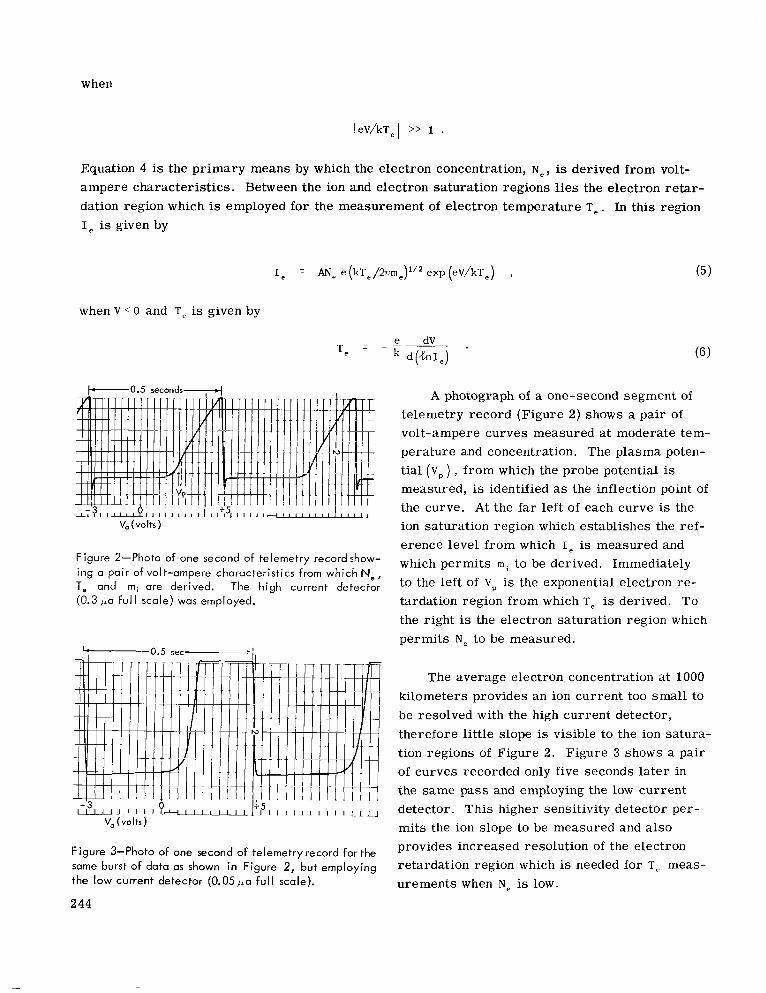
when
Equation 4 is the primary means by which the electron concentration, N ~ , is derived from volt- ampere characteristics. Between the ion and electron saturation regions lies the electron retar- dation region which is employed for the measurement of electron temperature Te . In this region I C is given by
Ie = AN, e(kTe/2mne)1’2 exp(eV/kTe) , (5 )
when V 0 and Te is given by
b-0.5 seconds-/
Figure 2-Photo of one second of telemetry record show- ing a pair of volt-ampere characteristics from which Ne, T, and mi are derived. The high current detector (0.3 pa ful l scale) was employed.
-0.5 sec-,
I l l l l L
n u
V,(VOItS)
Figure 3-Photo of one second of telemetryrecord for the same burst of data as shown i n Figure 2 , but employing the low current detector (0.05pa ful l scale).
e dV ,
d(&Ie) -~
A photograph of a one-second segment of telemetry record (Figure 2) shows a pair of volt-ampere curves measured at moderate tem- perature and concentration. The plasma poten- tial (Vp ) , from which the probe potential is measured, is identified as the inflection point of the curve. At the far left of each curve is the ion saturation region which establishes the ref- erence level from which Ie is measured and which permits m i to be derived. Immediately to the left of Vp is the exponential electron re- tardation region from which TP is derived. To the right is the electron saturation region which permits Ne to be measured.
The average electron concentration at 1000 kilometers provides an ion current too small to be resolved with the high current detector, therefore little slope is visible to the ion satura- tion regions of Figure 2 . Figure 3 shows a pair of curves recorded only five seconds later in the same pass and employing the low current detector. This higher sensitivity detector per- mits the ion slope to be measured and also provides increased resolution of the electron retardation region which is needed for T, meas- urements when Ne is low.
244
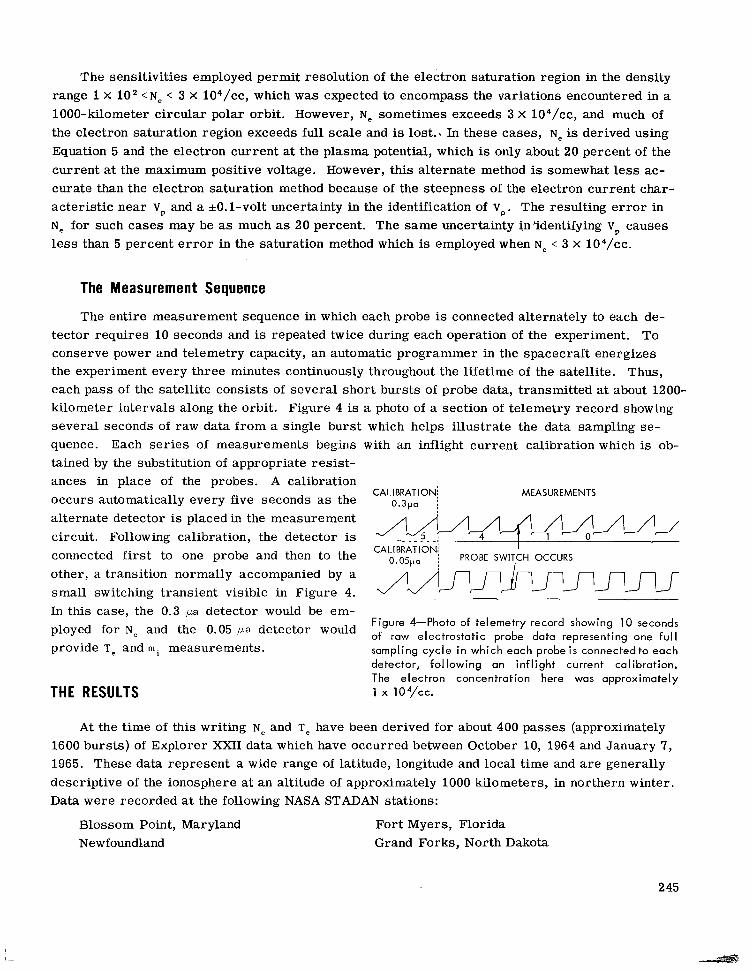
The sensitivities employed permit resolution of the electron saturation region in the density range 1 x l o 2 <N, < 3 x 10⁴/cc, which was expected to encompass the variations encountered in a 1000-kilometer circular polar orbit. However, Ne sometimes exceeds 3 X 10⁴/cc, and much of the electron saturation region exceeds f u l l scale and is lost.. In these cases, N~ is derived using Equation 5 and the electron current at the plasma potential, which is only about 20 percent of the current at the maximum positive voltage. However, this alternate method is somewhat less ac- curate than the electron saturation method because of the steepness of the electron current char- acterist ic near vP and a +O.l-volt uncertainty in the identification of Vp. The resulting e r r o r in Ne for such cases may be as much as 20 percent. The same uncertainty *?identifying Vp causes l e s s than 5 percent e r r o r in the saturation method which is employed when N~ < 3 X 10⁴/cc.
The Measurement Sequence
The entire measurement sequence in which each probe is connected alternately to each de- tector requires 10 seconds and is repeated twice during each operation of the experiment. To conserve power and telemetry capacity, an automatic programmer in the spacecraft energizes the experiment every three minutes continuously throughout the lifetime of the satellite. Thus, each pass of the satellite consists of several short bursts of probe data, transmitted at about 1200- kilometer intervals along the orbit. Figure 4 is a photo of a section of telemetry record showing several seconds of raw data f rom a single burst which helps illustrate the data sampling se- quence. Each ser ies of measurements begins with an inflight current calibration which is ob- tained by the substitution of appropriate resist- ances in place of the probes. A calibration
CALI BRAT ION\ occurs automatically every five seconds as the 0.3pa j
MEASUREMENTS
/JA-/q$-(MJJ alternate detector is placed in the measurement circuit. Following calibration, the detector is ......, ~ ~
connected first to one probe and then to the other, a transition normally accompanied by a small switching transient visible in Figure 4. .-
In this case, the 0.3 pa detector would be em- ployed for Ne and the Ooo5 detector would provide Te and m, measurements.
CALI BRAT ION; I 0.05pa PROBE SWITCH OCCURS
/[email protected] Figure 4-Photo of telemetry record showing 10 seconds of raw electrostatic probe data representing one ful l sampling cycle i n which each probe i s connected to each detector, following an inf l ight current calibration. The electron concentration here was approximately
THE RESULTS 1 1041~~ .
A t the time of this writing N~ and Te have been derived for about 400 passes (approximately 1600 bursts) of Explorer XXII data which have occurred between October 10, 1964 and January 7, 1965. These data represent a wide range of latitude, longitude and local time and a r e generally descriptive of the ionosphere at an altitude of approximately 1000 kilometers, in northern winter. Data were recorded at the following NASA STADAN stations:
Blossom Point, Maryland Newfoundland
Fort Myers, Florida Grand Forks, North Dakota
2 45

College, Alaska Quito, Equador Santiago, Chile Johannesburg, South Africa
Mojave, California Lima, Peru Winkfield, England Woomera, Australia
The polar orbit, and its near circularity, makes the latitudinal structure particularly evident in the resulting measurements. For this reason we have plotted the data as a function of geomag- netic latitude. The behavior of the ionosphere with respect to other variables then appears largely as differences in the latitudinal structure. To minimize the effects of local time, we have plotted only the data corresponding to the relatively stable periods following local noon and midnight.
Actual Data Points
The Ne and Te data points from all longitudes for the period 0000-0330 hours in November and December of 1964 a r e shown in Figures 5 and 6. The individual points from a particular pass are joined by lines to approximate the instantaneous latitudinal structure existing during the pass and
I
I 805
I 1 1 I 1000* 100 km 0000 - 0330 hour: Nov-Dec 1964
\ D
\ \
I .
=+!;-’-. . d d
I I I 605 405 2 os 0 20N 40N 60N 80N
GEOMAGNETIC LATITUDE (degrees)
Figure 5-Raw values of Ne i n the post midnight period at a l l available longitudes. The individual points from single passes are joined by lines to approximate the instantaneous latitudinal profile they represent. The various passes, coded by longitude as discussed in the text, show strong longitudinal dependence superposed on the larger latitudinal variations i n Ne. The pass labelled D corresponds to a magnetically disturbed day.
246

I I I I 1 1000* 100 km
Nov. - Dec. 1964 0000 - 0330 hours
P
I I I ~~
20N 40N 60N 80N I I L I
6 OS 405 20s 0 01 ‘
805
GEOMAGNETIC LATITUDE (degrees)
Figure 6-Raw values of T, for same nighttime passes as employed for Ne data i n Figure 5.
to identify the points as belonging to particular passes. The long and short dashes represent data from the stations along the 75th meridian (50-100W), and only at these longitudes w a s it possible to obtain complete pole to pole coverage. The short dashed lines represent Woomera and some of the College passes (110- 150”E), and the solid lines represent Johannesburg and Winkfield passes (50%-50W). Finally, the long dashes represent data from the western U . S. and Canada recorded at Mojave and College (100-13OW). The ionospheric Ne structure in this range of longitudes w a s sufficiently different from that of the 75th meridian to warrant plotting it separately. It should be stressed that this particular means of sorting the data by longitude a r i ses not so much from the characteristics of the ionosphere but more from the geographic distribution of the various STADAN stations which recorded the data. Indeed most of the spread in Ne within each of the stated ranges remains longitudinal in origin. In at least one pass (labelled D), deviations have been correlated with high values of the 3-hour magnetic index ap. In this case, the disturbance w a s associated with an enhancement of Ne in the equatorial region.
Gross Latitudinal St,ructure
Plots similar toFigures 5 and6 have also been prepared for the daytime data (1200-1530 hours) in November and December of 1964. Figures 7, 8, 9 and 10 summarize the gross latitudinal struc- ture of the ionosphere both day and night at the selected longitudes. These graphs generally outline
247

4
0 0
a3 2 v U Z Z 0 I-
2 2
z 8 U Z
0
Figure 7-Gross latitudinal distribution of electrons in the nighttime ionosphere. The shaded areas represent the range of Ne i n the given longitude ranges.
1OOO-t 100 km 0000 - 0330 hours Nov. -Dec. 1964 3QOO -
w
I 60N
GEOMAGNETIC LATITUDE (degrees)
Figure 8-Gross distribution of T, i n the nighttime ionosphere.
2 48
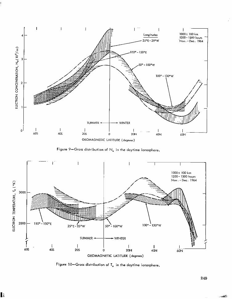
'-[ 3000 w
4 3 5
I-
w R
!-
Z
l2 2000 8 J w
6
I 1 605 405
I I I - - I Longitudes
I - 100Ok 100 km 1200- 1500 hours Nov . - Dec . 1964
SUMMER - I .. 1 . I
20N 40N 60N 1 I
20s 0
GEOMAGNETIC LATITUDE (degrees)
Figure 9-Gross distribution of Ne i n the daytime ionosphere.
- 110°-.1500E f 25' E - 25'W
SUMMER - .~~ 1 1 , 405 20s
I I
1000 f 100 km 1200- 1500 hours
/--- 22% Nov. -Dec. 1964 ,=* e?%.
-WINTER
20N 40N 60N GEOMAGNETIC LATITUDE (degrees)
Figure 10-Gross distribution of T, i n the daytime ionosphere.

I I I I I I I I I I
The ion mass mi derived from the slope of - l5 3
the ion saturation curves with the associated 3 standard deviations of the values is shown in 5 Figure 11. Since the nighttime Ne is too low to Z permit the slope to be determined at all lati- 6 tudes, Figure 11 represents only daytime data. Similar, but preliminary, results have been ob- tained at midlatitudes at night however.
-
-
the extremes of Ne and T, found in the given longitude ranges and a r e intended primarily to convey the predominant features of the ionosphere at 1000 i 100 kilometers during this period.
- *-VY I I .
- - ~
5 -
The Mean Ion Mass
1000* 100 km
l- 50"- 100" W. Longitude - 30'-40' N. Mag. Lat.
K v
0
20 lWO* 100 km Nov. -Dec. 1964
- 2 0
Figure 12-The diurnal variation of T, at northern midlatitudes.
Figure 13-The diurnal variation of Ne and T, at northern mid lat itudes.
250

Longitudinal Behavoir
Although the ionosphere a t t h e 1000- kilometer level appears to reflect primarily local time and latitudinal variations, longitudinal variabilityis also strong in some regions of the globe. The greatest effect is in the 25 degree E - 25 degree W zone where both an equatorial enhancement and a high latitude deficiency are characteristic of the daytime ionosphere. Note that this is in the region just east of the Brazil- ian magnetic anomaly.
4000
5 v
f 3000 W CT
$ 2 6 1000
E 2000 0
I-
CT + E -I Y
0
100Ok 100 km Nov. -Dec. '6~ 3 5 O N: Mag.
Mag. EQUATOR
I I I I I I I I I
0 3 6 9 12 15 18 21 24 LOCAL M E A N TIME (hours)
A second longitudinal irregularity occurs at night in the 50 - 100 degree W zone where the
F i g u r e 1.4-The d i u r n a l v a r i a t i o n o f Te a t m i d l a t i t u d e s a n d a t the e q u a t o r a t the 7 5 t h m e r i d i a n .
southern hemisphere nocturnal maximum is enhanced by nearly a factor of two, and its northern counterpart is depressed and occurs at a somewhat lower latitude. Note that this region is at the western edge of the Brazilian anomaly. It seems probable that these longitudinal irregularities a r e related to the distortion of the earth 's magnetic field in the region of the anomaly and its conjugate.
Small Scale Irregularities
On many occasions when the satellite was north of the auroral zone, the volt-ampere charac- terist ics exhibited rapid fluctuations of the nature shown in Figure 15. When these small scale current variations occurred, they were visible on both detectors and probes. Since the normal operation of the measurement and telemetry systems is evident from the smoothness of the inflight current calibrations, these fluctuations can only be attributed to small scale variations in Ne along the orbit of the satellite. The horizontal dimensions of these irregularities a r e of the order of 300 meters and the magnitude may be as great as 30 percent. Figure 16 shows the locations of these occurrences. They a r e normally found on more than one burst when present at all. With a few exceptions, the irregularities occur above the auroral zone and present statistics suggest that they exist in about lopercent of the passes, with a strong preference for the early morning hours (0000-0600). There appears to be little correlation with magnetic disturbances which were few during this period.
-1 k - 3 0 0 meters
CURRENT TOP PROBE - B O T T O M PROBE
F i g u r e 1 5 - V o l t - a m p e r e character is t ics e x h i b i t i n g r a p i d f l u c t u a t i o n s of Ne a l o n g the o r b i t a l path . T y p i c a l f l u c - tuat ions a r e 100's of meters i n d imension a n d h a v e magni tudes of up t o 30 p e r c e n t .
251

DISCUSSION OF RESULTS
The data reveal that the global structure of the ionosphere at 1000 kilometers exhibits a high degree of variability with respect to lati- tude, longitude and local time.
The Electron Concentration
At midday (Figure 9), Ne exhibits a strong maximum at the magnetic equator, a result which is consistent with the Alouette topside sounder data (Lockwood and Nelms, Reference 6). A general decrease in Ne with increasing latitude extends to a minimum at 60 degrees N and S latitude where Ne is about one third its equatorial value.
Figure 16-Locations ofsmall scale irregularities. Nearly al l occur poleward of the auroral zone and in the early morning hours
A t night (Figure 7), the equatorial maxi- mum has given way to a pair of midlatitude maxima a t 35 degrees N and 35 degrees S. The value of Ne a t the equatorial trough is about one half of that at the maximum. This is not unlike the pattern shown by the Ariel satellite measure- ment of Ne for this altitude during northern summer of 1962 (Sayers, Reference 7). This may therefore be a permanent feature of the nocturnal ionosphere.
These maxima observed a t 35 degrees latitude may be the nighttime counterpart of the equa- torial anomaly present in the daytime at lower altitudes (Goldberg and Schmerling, Reference 8). King* has pointed out that the f , F, data from ground-based sounders show a general poleward movement of the maxima, which constitute the anomaly, through the afternoon and evening. Since the double maximum in the daytime anomaly has merged into a single maximum at the altitude of the Explorer XXII observations, we a r e unable to trace this poleward motion through the day. In- stead, the maxima which we observe at 1000 kilometers seem to emerge in their equilibrium position near 35 degrees latitude within a few hours after sunset.
Attempts to explain behavior of the daytime equatorial anomaly have been based on production and diffusion processes in the F region. The identification of this anomaly as a major feature a t night at higher altitudes suggests rather that the source of particles is in the protonosphere above the equator. Indeed, the daytime equatorial maximum at 1000 kilometers (Figure 9) assures a huge reservoir of electrons at higher altitudes in the protonosphere. At night this reservoir has nearly disappeared (Figure 7), and there seems little doubt that these electrons have diffused downward along the magnetic field lines to form the midlatitude maxima which a r e observed.
*King, J . W., Radio and Space Research Station, Slough, England.
252

At higher latitudes an extraordinarily steep gradient reduces the concentration by nearly two orders of magnitude in less than 20 degrees of latitude. The resulting minimum at 60 degrees North, evident also in Alouette data has been called the "auroral trough" (Muldrew*). This also seems to be a permanent feature of the ionosphere, but is most discernible at night. The fact that the trough occurs at a magnetic latitude of 60 degrees leads one to suspect that this is the same phenomena which produces the "knee whistlers" observed by Carpenter (Reference 9) near mag- netic invariant L = 4. The polar cliff, an enhancement north of the auroral trough noted by Muldrew does not seem to be present at all longitudes (Figure 5).
The high degree of symmetry about the magnetic equator which is evident in these Ne data makes it clear that the magnetic field of the earth exercises strong control over the global distri- bution of electrons, as has been evident to some degree from previous satellite data (References 3, 7 and lo), though the global structure has not been displayed quite so clearly before. The ap- proximate circularity of the orbit combined with its near polar nature, which is a highly advantageous feature of the Explorer XXII, enables a transparent latitudinal exposition of the ionospheric pa- rameters measured without much reduction of the data.
It is interesting that the geomagnetic symmetry remains strong in spite of the extreme de- clination of the sun which w a s near the winter solstice during this period. Only a moderate seasonal asymmetry is evident at midlatitudes where Ne is about a factor of two larger in the summer hemisphere.
The Electron Temperature
A similar and undoubtedly closely related magnetic control is evident in the global distribution of electron,temperature. At midday, Te exhibits broad maxima at 40-50 degrees latitude and a shallow minimum at the equator, variations which a r e generally inversely related to the var- iations in Ne. This is demonstrated best in Figure 17 which shows the daytime latitudinal be- havior of the ionosphere averaged over all longitudes.
At night, the inverse relationship between electron temperature and concentration is lim- ited to the higher latitudes as summarized in Figure 18. Because of the near vertical nature of the magnetic field lines at high latitudes, one expects the same general behavior at lower altitudes also. Explorer XVII data at College, Alaska, indeed show elevated electron temper- a tures accompanied by depressed electron con- centrations in the F, region (Reference 3), and
F 1 O O O i 100km Z 1200 - 1530 hours
I- -r z 2 SUMMER
- 0 6bS 4bS 2bS 0 2AN 4AN 6AN O' 2
GEOMAGNETIC LATITUDE (degrees)
this is strong evidence for a nocturnal heat source there.
F i g u r e 1 7 - M i d d a y v a l u e s of T, and Ne, a v e r a g e d from d a t a a t a l l longitudes.
*Muldrew, D. B. , Defense Radio Telecommunications Establishment, Ottawa, Canada.
253
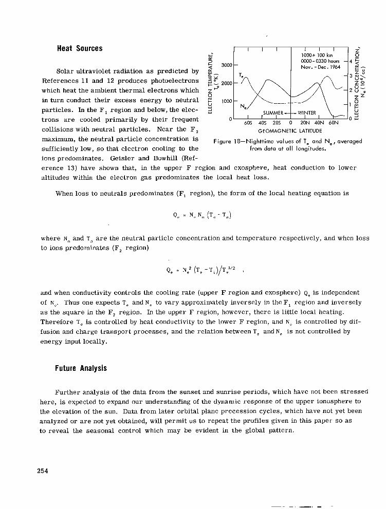
Heat Sources
Solar ultraviolet radiation as predicted by References 11 and 12 produces photoelectrons which heat the ambient thermal electrons which in turn conduct their excess energy to neutral particles. In the F, region and below, the elec- trons a r e cooled primarily by their frequent collisions with neutral particles. Near the F, maximum, the neutral particle concentration is sufficiently low, so that electron cooling to the ions predominates. Geisler and Bowhill (Ref-
I I I I I I Y 1OOO.t 100 km 3 0000 - 0330 hours - I- 3000 Nov. -Dec. 1964
PI
- 2
Y SUMMER -- WINTER
6bS 4bS 2bS 0 20N 40N 60N
GEOMAGNETIC LATITUDE
Figure 18-Nighttime values of Te and Ne, averaged from data a t a l l longitudes.
erence 13) have shown that, in the upper F region and exosphere, heat conduction to lower altitudes within the electron gas predominates the local heat loss.
When loss to neutrals predominates (F, region), the form of the local heating equation is
where Nn and Tn a r e the neutral particle concentration and temperature respectively, and when loss to ions predominates (F, region)
Q, = N: ( T ~ -T~)/T:/, ,
and when conductivity controls the cooling rate (upper F region and exosphere) Q, is independent of Ne. Thus one expects Te and N e to vary approximately inversely in the F, region and inversely as the square in the F, region. In the upper F region, however, there is little local heating. Therefore Te is controlled by heat conductivity to the lower F region, and Ne is controlled by dif- fusion and charge transport processes, and the relation between Te and Ne is not controlled by energy input locally.
Future Analysis
Further analysis of the data from the sunset and sunrise periods, which have not been stressed here, is expected to expand our understanding of the dynamic response of the upper ionosphere to the elevation of the sun. Data from later orbital plane precession cycles, which have not yet been analyzed or a r e not yet obtained, will permit u s to repeat the profiles given in this paper so as to reveal the seasonal control which may be evident in the global pattern.
254

ACKNOWLEDGMENTS
The authors thank James A. Findlay and Tuck Lee for their outstanding efforts in the design and construction of the experiment and its integration into the satellite. We also thank John Sayler, George Dunham, Joseph Johnson and Fred Huie for their dedicated efforts in the reduction of data, and Clyde Freeman, and Don Kennedy for producing the analog records from which the data a r e reduced.
1.
2.
3.
4 .
5.
6 .
7.
8.
9.
10.
11.
12.
13.
REFERENCES
"NASA Schedules October launch for Ionospheric Beacon IMP- 1," Aviation Week and Space Technology, 75(12):30 September 18, 1961.
"More Beacon Explorers Soon," Missiles md Rockets, 15(16): 11 October 19, 1964.
Brace, L. H., Spencer, N. W., and Dalgarno, A., "Detailed Behavior of the Midlatitude F Region from Explorer XVII Satellite," to be published in Planet. Space Sci., 1965.
Spencer, N. W., Brace, L. H., Carignan, G. R., Taeusch, D. R., and Niemann, H., "Electron and Molecular Nitrogen Temperature and Density in the Thermosphere," J. Geophys. Res. 70(11):2665-2698, June 1, 1965.
Mott-Smith, H. M., and Langmuir, I., "Theory of Collectors in Gaseous Discharges," Phys. Rev. 28:727-763, October 1926.
Lockwood, G. E. K., and Nelms, G. L., "Topside Sounder Observations of the Equatorial Anomaly in the 75" Longitude," J. Atmos, Terr. Phys. (5):569-580, May 1964.
Sayers, J., "The Electron Density Distribution in the Topside Ionosphere. I. Magnetic-Field- Alined Strata," Proc. Roy. Soc. 281 A(1387):450-458, 1964.
Goldberg, R. A., and Schmerling, E. R., "The Effect of Diffusion on the Equilibrium Electron Density Distribution in the F Region near the Magnetic Equator," J. Geophys. Res. 68(7):1927- 1936, April 1, 1963.
Carpenter, D. C., "Whistler Evidence of a "Knee" in the Magnetospheric Ionization Density Profile," J. Geophys. Res. 68(6): 1675- 1682, March 15, 1963.
Bowen, P. J., Boyd, R. L. F., Henderson, C. L., and Willmore, A. P., "Electron Temperature in the Upper F-Region,'' Proc. Phys. SOC. 281 A(1387):526-538, October 6, 1964.
Hanson, W. B., "Electron Temperatures in the Upper Atmosphere," in: Space Research 111; Pvoc. 3rd Internat. Space Sei. Sympos., Washington, D. C., May 2-8, 1962, ed. by W. Priester, New York: Interscience, 1963 pp. 282-302.
Dalgarno, A., McElroy, M. B., and Moffett, R. J., "Electron Temperatures in the Ionosphere," Planet. Space Sci. 11(5):463-484, May 1963.
Geisler, J. E., and Bowhill, S. A., "An Investigation of Ionosphere- Protonosphere Coupling,'' Urbana, Illinois: University of Illinois Aeronomy Laboratory, Report Number 5, January 1965.
255


ROCKET OBSERVATIONS OF THE STRUCTURE OF THE MESOSPHERE
by W. Nordberg, L. Katchen, J. Theon and W. S. Smith
Goddard Space Flight Center
Pressure , density, temperature and wind measurements in the upper strat- osphere and in the mesosphere resulted from a total of 53 rocket-grenade sound- ings conducted during the period 1960-1965. Most of the soundings were per- formed over North America (Wallops Island, 38N and Churchill, 59N) but some resul ts were also obtained over the tropical Atlantic (Ascension Island, 8s) and over Northern Europe (Kronogard, 66N). Soundings were carr ied out simul- taneously a t these s i tes and were coordinated with soundings measuring s imi la r parameters over other a reas of the globe.
Seasonal and latitudinal variations in the s t ructure and circulation of this region of the atmosphere were derived from the results. Stratosphere temper- a tures vary with season and latitude in accordance with solar heating ra tes and with established circulation models. Temperatures above 65 km a r e substan- tially warmer in winter than in summer. Average seasonal temperature differ- ences are about 40°K a t 80 km. They a r e very pronounced at midlatitudes (Wallops Island) and become even more extreme a t high latitudes where in sum- m e r mesopause temperatures as low as 140°K were observed. Maximum stratopause temperatures were observed during late winter- early summer. At Wallops Island these maxima of about 280°K coincided with the period of transi- tion from winter to summer circulation. Temperature profiles for all seasons a t all s i tes intersect between 60 and 65 km a t a temperature range of 230 to 240°K.
The strong westerly flow in winter shows two pronounced cores , one per- sistent throughout the winter just above the stratopause, the other somewhat weaker and l e s s persistent near 75 km. Deviations from the zonal flow indicate the existence of meteorological circulation cells on a synoptic scale with the average meridional flow a t Churchill strongly from the north during both sum- m e r and winter and at Wallops Island somewhat weaker from the south during the winter.
INTRODUCTION
After the successful exploration of the structure of the upper stratosphere with rocket-grenade soundings at White Sands, N. Mex., Churchill, Canada, and Guam, Mariana Islands, during the In- ternational Geophysical Year (Reference l), we conducted a ser ies of soundings at various latitudes
257

in the Atlantic and North American region during the period of minimum solar activity. Simul- taneous, seasonal measurements of temperature, pressure, density and winds were planned at four sites: Point Barrow, Alaska (71N); Churchill, Manitoba, Canada (59N); Wallops Island, Virginia (38N); and Ascension Island (8s). While successful soundings were conducted at each of these lo- cations during 1960- 1965, operational difficulties have limited the number of soundings at the various sites, and to date simultaneous observations have been made only at three of the four si tes. These took place recently when three successful soundings were conducted each at Pt. Barrow, Wallops Island and Churchill during January and February 1965. Results f rom this recent se r ies are not yet completely reduced, and only preliminary data f rom the Pt. Barrow soundings were considered in this analysis. The Point Barrow observations are the first known direct measure- ments of the structure of the mesosphere north of "ON. Only four successful acoustic grenade soundings were possible at Ascension Island, one each in January and February and two in August 1964. The August observations were made nearly simultaneously with soundings at Churchill, Wallops Island and at Kronogard, Sweden (66N). Data from Kronogard, however, are , as yet, available only for summer 1963, and only preliminary data f rom the other three s i tes were con- sidered in this analysis. In addition to the grenade soundings in which temperature, pressure, density, and wind a r e derived from observations of the soundwaves generated by the exploding rocket-borne grenades, there were three soundings in February and April 1964 at Ascension Island in which pressure, density, and temperature up to 105 km were measured by the Pitot-static tube technique. Results of these measurements were reported by Horvarth and Simmons (Reference 2) and are included in this analysis.
Acoustic grenade rocket soundings at Churchill were resumed in December 1962 after a fire had destroyed the launch facility there in 1960. A total of 15 soundings were carried out during December 1962, February and March 1963, January, February, April and August 1964 and January and February 1965. All but one of these soundings were conducted nearly simultaneously with soundings at Wallops Island. Data from all soundings up to August 1964 were included in this analysis, although the August 1964 data a r e still of a preliminary nature.
By far the largest number of soundings were obtained at Wallops Island, Virginia since that launch site has been available for the longest period. Forty-two successful soundings were con- ducted at Wallops Island between July 1960 and February 1965. Soundings were taken during every month of the year except October. Results have been analyzed through August 1964.
The times and location of all soundings included in this discussion a r e summarized in Table 1. Space does not permit the presentation here of the complete data from each sounding. However, complete tabulations and graphic presentations of the data for 1960-1963 have been compiled in a report by W. Smith et al. (Reference 3). A similar report for the complete 1964 data is now in preparation.
Only the basic and salient features of the observations will be summarized here with partic- ular emphasis on their latitudinal and seasonal variations and their relationship to the basic physi- cal processes governing the stratosphere and mesosphere. These results are of interest a lso because they permit a comparison between the structure of the mesosphere observed during the
25 8

Date
1960
9 July
1961
14 February 17 February 5 April 5 May 6 May
13 July 14 July 20 July 16 September
1962
2 March 2 March
23 March 28 March 18 April 7 June 8 June 1 December 4 December 6 December 6 December
1963
20 February 20 February 28 February 28 February
9 March 9 March 7 December
Table 1
Dates, Times and Locations of GSFC Meteorological Sounding Rocket Experiments, 1960-65.
Time (GMT)
0359
2350 0226 1257 2300 0454 2207 16 02 1030 2355
0001 1115 2354 0004 0928 0105 0153 2 125 0705 0532 0543
2334 2347 2147 2211 0001 0001 1312
Location
Wallops Island
Wallops Island Wallops Island Wallops Island Wallops Island Wallops Island Wallops Island Wallops Island Wallops Island Wallops Island
Wallops Island Wallops Island Wallops Island Wallops Island Wallops Island Wallops Island Wallops Island Wallops Island Churchill Wallops Island Churchill
Churchill Wallops Island Churchill Wallops Island Wallops Island Churchill Wallops Island
Date
1964
24 January 29 January 29 January 29 January 4 February 4 February 5 February 5 February
13 February 13 February 13 February
15 April 15 April 18 April 18 April
7 March
7 August 8 August
12 August 12 August 16 August 16 August 17 August 18 August 18 August
1965
27 January 4 February 8 February
Time (GMT)
0016 0411 0417 0418 0135* 0146 0040 0320 0430 0430 0455 0245 0122* 1556* 0039 0100 0600 1000 0149 0215 0315 0553 1255 0115 0125
2132 0445 2215
Location
Wallops Island Wallops Island Churchill Ascension Island Ascension Island Wallops Island Churchill Wallops Island Wallops Island Churchill Ascension Island Wallops Island Ascension Island Ascension Island Churchill W a l l o p Island Wallops Island Churchill Wallops Island Churchill Wallops Island Ascension Island Ascension Island Churchill Wallops Island
Point Barrow Point Barrow, Point Barrow
*Al l soundings were rocket grenade experiments except the Pitot-static experiments which are noted with an asterisk (*).
present period of minimum solar activity and during the IGY when solar activity w a s at its maximum.
Results from the large number of wind observations obtained from Meteorological Rocket Net- work soundings analyzed by Webb (Reference 4) were also considered as they overlapped our ob- servations at the lower altitudes.
259

DISCUSSION OF THE OBSERVATIONAL RESULTS
30
2o
10
- X -- - CHURCHILL WINTER
(56-58) - 90 x-x TROPICAL LATITUDE -
(GUAM 58, ASCENSION 64) - 80
l ~ l . l , i , l , . .
26 0
160 180 200 220 240 260 280 - 70 TEMPERATURE ( O K )
Figure 1-Average 1960-64 summer and winter temper- atures for Wallops Island (38N), 1962-64 winter tem- peratures for Churchill (59N), 1964 summer temperatures
60
for Churchill and winter 1964 temperatures for Point Barrow (71N) are compared to average summer and winter temperatures obtained a t Churchill during the IGY (1957-58). The IGY Churchill summer tempera- tures were quite similar to averages from three summer 1964 soundings in Churchill, thus only one profile i s shown. An average temperature profile for tropical lat- itudes obtained in November 1958 at Guam (13N) and in February 1964 at Ascension Island (85) i s shown for comparison. The average profiles are derived from the following number of individual grenade experiment
40
WALLOPS SUMMER (60-64) - WINTER 30 (61 -64)
(62-64) _ _ _ _ _ CHURCHILL SUMMER (64) - WINTER
20 -x- CHURCHILL SUMMER (57) - WINTER (56 - 58)
l 1 l I l I l 1 1 soundings listed in Table 1: Wallops winter-17, Wal- -80 -60 -40 -20 0 20 40 60
. .,... .

instead of 65°C calculated from radiative heating and cooling alone. At lower latitudes (Wallops Island) observed average seasonal temperature variations a r e only about 10°C. Figure 1 shows that latitudinal temperature gradients at the stratopause level are much larger in winter than in summer. This is again in good qualitative agreement with radiatively predicted gradients.
Quantitatively, the discrepancy by about a factor of two between the radiatively predicted and the observed seasonal temperature variations in the stratosphere, especially at high latitudes, re- quires equatorward and poleward energy transport in the summer and winter hemispheres, respec- tively. Dynamic processes which car ry out this energy transport have been postulated by Murgatroyd and Singleton (Reference 6) on the basis of the IGY temperature observations and more recently by Newel1 (Reference 7) on the basis of Meteorological Rocket Network wind observations.
The change from cold winter temperatures to warm summer temperatures in the stratosphere takes place very rapidly during the end of each winter season (March-May, Figure 3). Maximum temperatures occur near 45 km, about 5 km lower than during the period of maximum solar heat- ing in midsummer. Furthermore, many temperature profiles during spring exhibit maximum temperatures equal to or exceeding those reached at 50 km later in the year suggesting the strato- pause to be warmest and lowest during spring. This phenomenon is obvious at Wallops because of the large number of observations at that site, but results from Churchill a r e insufficient to con- f i rm its existence there (Figure 4) . Indications a r e that the warm upper stratosphere in late winter exists also at relativelylow latitudes in the southern hemisphere (Reference 8). It may be expected that these temperature maxima are dynamically induced and are caused by the final break- down of the predominantly cyclonic winter circulation which occurs during the same time period. This phenomenon wil l be considered further in the discussion of the wind observations.
In the lower mesosphere there a r e practically no seasonal and latitudinal temperature varia- tions in the altitude range of about 6 0 to 65 km. Indeed, considering the results reported by Groves (Reference 8) for Woomera, Australia (31S), our ear l ier IGY data (Reference 1) and those shown in Figure 1, one may conclude that temperatures at this altitude range generally between 230 and 240°K over the entire globe during all seasons.
The largest variations in the observed temperature take place in the upper mesosphere and at the mesopause and a r e especially evident at Churchill and Wallops Island (Figure 2) . Average seasonal temperature variations at 80 km during the 1962-64 period a r e about 45°C at Churchill and about 150C at Wallops Island. It must be concluded that this variation diminishes at low lati- tudes since no appreciable seasonal variation can be detected in Groves' (Reference 8) results at Woomera and in our (Reference 1) results at White Sands (33N). At equatorial latitudes, for which an average profile is shown in Figure 1, there have not been sufficient soundings yet to positively deduce any absence of seasonal variations. However, the trend demonstrated in the Churchill, Wallops Island, White Sands and Woomera observations and the fact that at all altitudes the aver- age equatorial temperature profile lies between the summer and winter profiles observed at higher latitudes leaves little doubt that at equatorial latitudes the seasonal variations a r e at a minimum. It should be noted that the variation at Churchill during 1962-64 was only one half the variation ob- served during the IGY (Figure 2). More soundings will have to be made during the next solar max- imum to determine the possible significance of this result.
26 1

1 I I I .I I 30 FEB M A R APR MAY JUN JUL AUG SEP
1961
90 -
80
70
E
5 60 Y - 9 w I
50
40
ISOTHERMS IN O K
I 1 1 1 .I MAR APR MAY JUN JUL
1962
ISOTHERMS IN O K 230
/250 - -- I I I I I. I 1 1 A I
DEC J A N FEB M A R DEC J A N FEB M A R APRIL v AUG 1963 1964
Figure 3-Variation of temperatures in the stratosphere and mesosphere with altitude and season over Wallops Island (38N) during 1961-64. Isotherms are based on 34 grenade soundings listed in Table 1.
262

230 ISOTHERMS IN O K
1 1 I I )EC J A N FEB MAR APR 1962 1963
1 ! I A I I JAN FEB MAR APR AUG
1964
Figure 4-Variation of temperatures in t h e stratosphere a n d mesosphere with a l t i t u d e a n d season over Churchi l l (59N) during 1962-64. Isotherms a r e based on 12 grenade soundings listed in Table 1.
The large average lapse ra tes found during maximum solar heating (high latitude summer), suggest that a very cold upper mesosphere always occurs in conjunction with a warm and high stratopause. The Swedish grenade soundings made during the summer of 1963 (Reference 9) con- f i r m the existence of a warm stratopause (280°K) occurring with a cold mesopause (140°K) at 66N latitude. On the other hand, during minimum solar heating (high latitude winter), the average lapse rate between 50 and 80 km becomes very small, suggesting that a warm upper mesosphere is always found in conjunction with a cold stratopause. Preliminary data from Point Barrow, Alaska (71"N)during January 1965 (Figure 5 ) indicate a more nearly isothermal atmosphere from about 4 0 to 70 km. The seasonal temperature variations which a r e of opposite sign in the stratosphere and upper mesosphere (Figure 2) seem to pivot around the level of nearly constant temperature be- tween 60 and 65 km. These observations disagree both qualitatively and quantitatively with tem- perature distributions computed solely on the basis of radiative properties (Reference 5). The computations require a much colder mesosphere in winter. Radiative heating and cooling alone require winter mesospause temperatures of 190°K and summertime temperatures of 230°K at 60"N. Observations (Figure 1) show 170°K in summer and 220°K in winter at the same latitude. This
263

90
80
70
E
5 60 0
--Y - - u I
50
40
30
~
L
d ? i 1
WIND SPEED IN m/sec
I 1 I . I 1 1 - ..
200 220 240 260 280
TEMPERATURE ( " K )
Figure 5-1965 winter stratosphere and mesosphere average temperature and average wind profiles at Point Barrow (preliminary data).
discrepancy again necessitates a large scale dy- namic mechanism to transport energy merid- ionally and vertically. The mechanism of mean meridional and vertical motions postulated by Murgatroyd and Singleton (Reference 6) produces upward motion in the summer mesosphere, downward motion in the winter mesosphere, and meridional motions from summer to winter pole thus, qualitatively at least, explaining the de- par tures of the observed temperatures from ra- diative equilibrium. Leovy (Reference 10) has developed a quantitative model of such a mean circulation. Our observations agree in general with the temperatures of Leovy's model in the upper mesosphere but disagree quantitatively in the lower mesosphere and at the stratopause. Obviously more sophisticated dynamic models will be needed to conform with the observations.
Heat sources other than solar radiation have been suggested by Kellogg (Reference 11) who pointed out the possibility of heating the polar upper mesosphere by recombination of atomic oxygen transported downward from the ionosphere and by Maeda (Reference 12) who in- vestigated the possibility of heating by auroral particles. The recent simultaneous observa- tions at Churchill and Wallops Island, however, indicate that the warm upper mesosphere is found at both locations and require an explanation
which holds at latitudes outside the polar cap as well as inside. Figure 1 indicates that the obser- vations made during the IGY (Churchill winter 1956-58) show considerably higher temperatures than the most recent observations (Churchill winter 1962-64) obtained during low solar activity. Advocates of the auroral heating concept might be tempted to use this finding as evidence for the existence of a heat source depending on solar activity. But, aside from the scarcity of the data sample which invalidates any such evidence, one would still have to explain the observed low sum- mer temperatures which a r e nearly 100°K colder than those calculated from radiative transfer for 80 km at 60" latitude (Reference 5). Significantly, summer temperatures throughout the mesosphere at Churchill shown in Figure 1 for 1964 a r e practically the same as those observed during the IGY.
Pressure Distributions
The average pressure graphs shown in Figure 6 were obtained by integrating the hydrostatic equation for each of the temperature soundings mentioned in Figure 1, and averaging the resulting
2 64

pressures at each altitude for the appropriate season and location. A measured pressure (usu- a l ly by balloon sondes) at the lower boundary of each temperature profile was used as the initial value in the integration. The pressure profiles a r e very useful to demonstrate the relationship between the seasonal and latitudinal temperature variations and the wind patterns described below.
The stratosphere and mesosphere are dom- inated by very systematic latitudinal and sea- sonal pressure variations (Figure 6 and Table 2). These variations are of considerable mag- nitude throughout the entire region and they converge toward minima at the lower and upper boundaries. Extrapolation of the pressure pro- files in Figure 6 to lower altitudes shows that there is a minimum pressure variation in the lower stratosphere, a fact which can also be de- rived from balloon and Meteorological Rocket Network soundings. It is evident f rom the data shown in Figure 6 that another minimum exists near the mesopause. Average pressure profiles for all seasons at the three sites seem to con- verge toward a common value slightly larger than the 1962 U. S. Standard Atmosphere at 90 km.
In winter, throughout most of the strato- sphere and mesosphere, pressures at Churchill a r e more than 20 percent lower than at Wallops Island, and close to 30 percent lower than at equatorial latitudes where the pressure is closest to the standard. The greatest latitudinal pressure gradient in winter occurs near 55 km. The maximum deviation from the standard at all latitudes takes place in winter at Churchill near 65 km.
The variation of the latitudinal pressure gradient with height in winter is plausible on the basis of the temperature profiles. The much colder winter stratosphere and strato- pause at high latitudes cause the pressure to
90
80
70
h
E 60 Y u
2 (3 2 50
40
3c
20
10
- WALLOPS WINTER (61 -64) M WALLOPS SUMMER (60-64) --- CHURCHILL WINTER (56-58 M CHURCHILL WINTER (62-64) _---- CHURCHILL SUMMER (57, 64) W TROPICAL LATITUDE
(GUAM 58, ASCENSION 64)
, 1 - 1 1 1 I --u -40 -20 0 20 40
PERCENT DEVIATION
Figure 6-Seasonal pressure averages as a function of height for Wallops Island (38N), Churchill (59N), and equatorial latitudes. Averages are based on the same soundings for which average temperature profiles are shown in Figure 1 . Because of their rapid variations with height, observed pressures are shown as deviations from the U. S. Standard Atmosphere, 1962. Absolute values of standard pressures which apply to the zero percent deviation coordinates are shown in Table 2.
Table 2
U. S. Standard Atm.osphere 1962, pressure vs. height. -~ ..
.- Altitude (km)
30 35 40 45 50 55 60 65 70 75 80 85 90
-
Pressure (newton/mZ) - ..
1197.0 574.6 287.1 149.1 79.8 42.8 22.5 11.4 5.5 2.5 1.0 0.4 0.2
265

I 1.1111 111 I II II 1 11. 1 ~ 1 1 1 1 1 1 1 1 I I I II 111 1 1 . 1 . 1 1 . 1 1 1 1 1 1 1 . 1 1 1 1 ~ 1 1 ~ Lf -
decrease with height more rapidly at high latitudes than at low latitudes, resulting in a gradual in- crease of the latitudinal pressure differences above the level of minimum pressure differences at the lower stratosphere. In the mesosphere the warmer temperatures at the higher latitudes bring about a smaller pressure decrease with height than at lower latitudes causing the latitudinal pres- su re differences to decrease above 60 km and to reach a second minimum near 90 km.
In summer, pressures are higher at Churchill than at Wallops Island at all latitudes, but dif- ferences between the two sites are considerably less than in winter. This is because the high latitude summer stratosphere and stratopause are only moderately warmer than their low latitude counterparts. Pressure differences between Wallops Island and Churchill in summer are about one half [of the differences observed in winter. Differences between Wallops Island and tropical latitudes a r e of about equal magnitude during both seasons.
The large seasonal pressure variations of a factor of two between summer and winter at Churc- hill which were reported during the IGY (Reference 1) a r e still prevalent although with a somewhat diminished amplitude (factor of 1.8). At the latitude of Wallops Island, the seasonal variation is considerably l e s s and ranges between a factor of 1.15 and 1.2. At equatorial latitudes, soundings have not been made with sufficient continuity to reach a very definite conclusion, but all observa- tions to date indicate that variations in the average pressure a r e quite small, generally less than the accuracy of the observations which is better than 5 percent.
Wind Patterns
Wind observations in the stratosphere and mesosphere have been more numerous than any other type of observation. The basic features of the general circulation in these regions are, therefore, fa i r ly well understood. A number of publications (References 7 and 10) have recently explored these features in greater detail based on our earlier IGY observations and on the large number of meteorological rocket soundings throughout the stratosphere and into the lower mesosphere which have been regularly con- ducted since 1961. -Our observations are sum- marized in Figures 7 through 12. They confirm that the features observed in the stratosphere by the meteorological network soundings exist throughout the mesosphere, but undergo a major change in the 70 to 80 km region. All observa- tions generally confirm the existence of the ex- pected strong cyclonic circulation around the North Pole in winter and a somewhat weaker anticyclonic motion in summer. Average zonal
WALLOPS WINTER (61 -64) - WALLOPS SUMMER (60-64) CHURCHILL SUMMER (57)
W CHURCHILL SUMMER (64) - CHURCHILL WINTER (62-64) 20 CHURCHILL WINTER (56 -58)
l l L l l l l 20 40 60 80
10 60 40 20 0
FROM EAST (m/sec) FROM WEST
Figure 7-Average zonal wind components vs. altitude for Churchill and Wallops Island. Graphs are based on the same soundings as those shown in Figure 1.
266

wind speeds are considerably greater at almost all altitudes at Wallops Island than at Churchill, both in winter and summer (Figure 7), although occasionally the maximum wind measured at one given altitude in one given sounding at Churchill may exceed the wind speed measured simultane- ously at Wallops Island.
A time cross section of the zonal wind components at Wallops Island (Figure 8) clearly dis- plays two wind maxima during each winter since 1961. One maximum is located very consistently near 55 km in midwinter, but moves gradually to lower altitudes (45 km) toward the end of the winter. This maximum is also obvious in the average zonal wind profile in Figure 7. The second maximum occurs consistently each winter between 70 and 80 km, but it is generally of lesser in- tensity and shorter duration than the lower altitude maximum. Except for 1962,’where no mid- winter data exist, the maximum occurs only during January-February. It is for this reason that the upper maximum does not appear in the average profile in Figure 7. The higher wind speeds throughout the entire winter season in the lower maximum completely overshadow the upper max- imum in the average profile. There is a possibility that the weaker easterl ies occurring in sum- mer also form two cores during midsummer, but they a r e certainly not as pronounced as the two westerly jets. Observations in the mesosphere at this time have not been made with sufficient continuity to determine the persistence in the reversals of the zonal flow from westerly in winter to easterly in summer and vice versa. However, such studies have been made at lower altitudes by Webb (Reference 4) on the basis of Meteorological Rocket Network soundings which showed a very consistent pattern in the seasonal reversals; at low and mid latitudes the reversals always occur during mid-May and September. Figure 8 shows a slope in the springtime zero isotachs from the upper left to the lower right. From this and from the gradual migration of the lower core to lower altitudes, it seems to follow that the winter to summer reversal in the lower cores follows the reversals in the upper cores. Sufficient data do not exist for the f a l l reversals to draw similar conclusions.
In general, the altitude level of maximum average zonal windspeed is higher in summer than in winter. This is consistent with the height of the maximum latitudinal pressure gradient de- scribed above. The comparison of the windspeeds between Wallops Island and Churchill places a steeper latitudinal pressure gradient in the vicinity of Wallops Island than at Churchill. There is complete consistency for the entire region between the average pressures shown in Figure 6 and the average zonal windspeeds in Figure 7. Maximum zonal winds occur at the heights and seasons where maximum latitudinal pressure differences a r e shown, and the average zonal windspeeds a r e smallest at those altitudes where the pressure variations a r e at a minimum.
The time cross section of zonal winds at Wallops Island (Figure 8) a lso shows that the periods of maximum temperature in the upper stratosphere during late winter and early summer (Figure 3) seem to coincide with the seasonal reversal in the zonal winds. Indeed, during 1961 the maxi- mum temperature occurred exactly when the winter westerlies had dropped to zero. In 1962, measurements were made in April and June showing temperatures of 270% during both months. Figure 8 shows that in April the westerlies were still pronounced, while in June easterly circula- tion had already set in and the temperature maximum probably occurred during May again when the zonal winds reversed directions. In 1963, temperatures were already very high in March when
267

9c
80
70
A
E
% 60
Y - (3 Y IT
50
40
30
9(
8(
7(
h
E
2 6C
Y
I? Y I
50
40
30
J I I I I I 1 I I FEB MAR APR M A Y J U N JUL AUG SEP
1961
/ --__--- 60 -*--- - --- - ISOTACHS IN m/sec
I I I I I DEC J A N FEB MAR
1963
/ ISOTACHS IN m/sec
I I I I I MAR APR M A Y J U N
1962
40 20
ISOTACHS IN m/sec
J A N F E B MAR APR AUG I I I 1 -
1964
F i g u r e 8 - V a r i a t i o n of z o n a l w i n d components w i t h a l t i t u d e a n d season over W a l l o p s Is land, 1961-64.
268
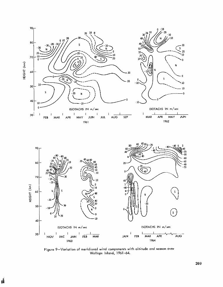
E Y
90
EO
70
- E Y
l- 6 0 -
(3 I
w I
50
40
30
+ I (3 w I
-
-
-
-
-
n -10
ISOTACHS IN m/sec
ISOTACHS IN m/sec
I I 1 - NOV DEC J A N FEB M A R
1963
I I I I MAR APR M A Y J U N
1962
ISOTACHS IN m/sec
1 L I A *
J A N FEB MAR APR " " AUG 1964
Figure 9-Variation of meridional wind components with altitude and season over Wallops Island, 1961-64.
269
I

winds had diminished from their maximum of about 100 m/sec to about 50 m/sec. No temperature measurements exist during April or May for that year, but one may speculate again that the tem- perature continued to r i s e until the zonal winds reversed direction in May.
80
70
60
E - Y v
5 0 - (3 Y - I
40
There is no evidence of any increase in the meridional wind components (Figure 9) o r of any predominance in either the southerly or northerly component during the time of the high late winter temperatures. Zonal circulation simply undergoes maximum changes during these times. Webb (Reference 4) has analyzed the very large number of wind data near the 50-km level resulting from the Meteorological Rocket Network soundings and has found that except for December, January, and February, the average meridional wind components are very small and show no particular in- crease in spring.
-
-
-
-
Webb's analysis a lso shows that average meridional winds a r e from the south during the en- t i re year at all low and mid latitude North American stations. Although the meridional flow is not nearly as well organized as the zonal flow, our soundings do show a consistent average component f rom the south during the winter at all heights up to 70 km at Wallops Island and, with the exception of winter 1957-58, an equally consistent component f rom the north at Churchill during both summer and winter (Figure 10). These average meridional wind components are much larger than the
- WALLOPS WINTER (61-64)
M WALLOPS SUMMER (60-64) CHURCHILL SUMMER (57)
)t---2: CHURCHILL SUMMER (64)
_ _ _ _ -
CHURCHILL WINTER (62-64) CHURCHILL WINTER (56-58)
A 1 40 20 0 20 40
FROM NORTH (m/sec) FROM SOUTH 60
Figure 10-Average meridional wind components vs. a l - titude for Churchill and Wallops Island. Graphs are based on the same soundings as those shown i n Figure 1.
"mean" meridional winds postulated in models such as Murgatroyd and Singleton (Reference 6). One may therefore conclude that the observed winds reflect large scale pressure disturbances at these longitudes and that the data a r e too sparse to derive t rue mean meridional motions. The Churchill meridional winds indicate a more or less permanent position of these pressure disturbances.
These pressure disturbances a r e apparently very deep, reaching well into the mesosphere. They a r e especially pronounced in winter at the very high latitudes. For example, wind data at Wallops indicate a very strong and steady zonal flow from the w e s t during midwinter (Figures 8 and 9), while at the same time at Churchill the westerly wind component is much weaker and a steady northerly component exists in general (Figures 11 and 12). This is also confirmed by the most recent soundings at Point Barrow (Figure 5), suggesting a high pressure cell over the North Pacific and Gulf of Alaska and low pressure over the North Atlantic. This implies that the well-known Aleutian anticyclone may exist up to altitudes of 70 km. A more detailed
27 0

I ISOTACHS IN m/,ec ISOTACHS IN m/sec
1 I 1 I1 1 I I , l I D EC J A N FEB MAR JAN FEB MAR APR AUG
1963 1964
Figure 11-Variation of zonal wind components with altitude and season over Churchill, 1962-64.
analysis of one ser ies of simultaneous soundings at Churchill and Wallops Island by Warnecke and Nordberg (Reference 13) supports this speculation. In contrast to the more recent observations, the averages for the meridional winds for Churchill for 1956-58 show southerly instead of northerly components (Figure 10) because these data a r e dominated by measurements made during January 1958 when a breakdown in the circulation occurred. During that period the high pressure cell lay to the east and low pressure to the west of Churchill (Reference 14). All observations at Churchill since then have displayed northerly winds, leading to the conclusions that, in general, high pres- su re is rather stationary to the west of Churchill and low pressure to the east, and that the 1958 measurements specifically reflected the displacement of the pressure cells during "break down" conditions. It seems somewhat surprising, however, that the average meridional wind components at Churchill are from the same direction during both summer and winter, indicating great per- sistence in the longitudinal position of the pressure cells. Naturally, a much larger number of soundings distributed over a wider range of longitudes would shed some further light on this subject.
27 1

40' ' I 1 1 DEC J A N FEE MAR
1962 1963
I
- ISOTACHS IN m/sec
I 1 I A r. I 1 JAN F E E MAR APR AUG
1964
Figure 12-Variation of meridional wind components with altitude and season over Churchill, 1962-64.
The analysis by Warnecke and Nordberg (Reference 13) of a number of the acoustic grenade soundings supplemented by sodium release wind instruments above 70 km showed that the gen- erally accepted circulation patterns cease to exist above about 75 km. Above that altitude the circulation seems to be governed by variations of much smaller time scales than in the strato- sphere and mesosphere. Tidal phenomena seem to be of much greater importance at those alti- tudes than the synoptic scale pressure variations described here for the lower regions.
CONCLUSIONS
The warm upper mesosphere originally observed at Churchill during the IGY w a s still present at both Churchill and Wallops Island during the recent years of low solar activity. However, at 80 km, winter temperatures during 1962-64 were only about 45°C warmer than summer tempera- tures at Churchill and 15°C warmer at Wallops Island, while during the IGY at Churchill, the cor- responding temperature difference was 70°C. The possibility that the less intense winter warm- ing of the upper mesosphere over Churchill during the IQSY is associated with the solar cycle cannot be sufficiently substantiated by the small data sample. Summer temperatures at the meso- pause at high latitudes were consistently colder than 160°K which does not support the postulation of an additional extraterrestrial heat source to explain the difference between observed and
272

predicted mesosphere temperatures. Dynamic processes can account better for these differences.
In the stratosphere maximum temperatures occurred at Churchill, Wallops Island and tropical latitudes during the end of the winter season. At that t ime the stratopause temperatures at 40-45 km were equal to o r higher than stratopause temperatures at 50-55 km during midsummer. Wal- lops Island data suggest that the stratopause is warmest and lowest during early spring. This phenomenon is probably related to the breakdown of the polar vortex which occurs at the same time of year.
A region of minimum seasonal and latitudinal temperature variation exists at 60 km, while minimum pressure variations occur below 25 km and near 85-90 km. There a r e not sufficient data available to draw any definite conclusions about the seasonal variation of temperature and pressure at the tropics, but indications are that these variations are at a minimum, being probably only a few percent over the entire year.
In midwinter at Wallops Island, the mesophere exhibits two pronounced maxima in the westerly winds at 55 km and 75 km. The upper maximum disapperas usually in February, while the lower maximum migrates toward lower altitudes at the end of the winter. The persistence of meridional flow from the north at Churchill during the entire year indicates fairly permanent large scale pressure systems in the northern latitudes. Preliminary results from Point Barrow show an average temperature profile with the smallest absolute lapse rate yet observed, 0.67"C per km from 40 to 70 km. As at Churchill, a steady northerly component exists, indicating the existence of a high pressure cell over the North Pacific and Gulf of Alaska, and low pressure over the North Atlantic.
ACKNOWLEDGMENTS
The authors gratefully acknowledge the contribution of Philip C. Swartz of GSFC for processing the data to final form; Superior Engineering Company for fabrication and pre-launch preparations of the payload; New Mexico State University's Physical Science Laboratory for rocket trajectory data; and Texas Western College's Schellenger Research Laboratory for sound ranging support.
REFERENCES
1.
2.
3.
Nordberg, W., and Stroud, W. G., "Seasonal, Latitudinal and Diurnal Variations in the Upper Atmosphere," NASA Technical Note D-703, April 1961.
Horvath, J. J., and Simmons, R. W., "Measurements of Upper Atmospheric Parameters by the Pitot-static Technique," Trans. Am. Geophys. Union, 45(4):617, December 1964 (abstract).
Smith, W., Katchen, L., Sacher, P., Swartz, P., and Theon, J., "Temperature, Pressure, Den- sity and Wind Measurements with the Rocket Grenade Experiment, 1960-1963," NASA Tech- nical Report R-211, October 1964.
273
IO

4. Webb, W., "Stratospheric Solar Response," J. Atmos. Sci. 21(6):582-591, November 1964.
5. Leovy, C., "Radiative Equilibrium of the Mesosphere," J. Atmos. Sei. 21(3):238-248, May 1964.
6. Murgatroyd, R. J., and Singleton, F., "Possible Meridional Circulations in the Stratosphere and Mesosphere," Quart. Jour. of the Royal Meteorological Society, 20(3):213-225, May 1963.
7. Newell, R. E., "Preliminary Study of Quasi-Horizontal Eddy Fluxes," J. Atmos. Sei. 20(3):213- 225, May 1963.
8. Groves, G. V., "Meteorological and Atmospheric Structure Studies with Grenades," in: Space Research IV: Proceedings of the 4th International Space Science Symposium, Warsaw, Poland, June 1963, ed. by P. Muller, Amsterdam: North-Holland Pub. Co., 1964, pp. 155-170.
9. Witt, G., Martin-Lof, J., Wilhelm, N., and Smith, W. S., "High Altitude Summer Mesospheric Temperatures and Wind with Particular Regard to Noctilucent Clouds," in: Space Research V: Proceedings of the 5th International Space Science Symposium, Florence, May 12-15, 1964, ed. by D. G. King-Hele, P. Muller, and G. Righini, Amsterdam: North Holland Pub. Co., 1965, pp. 820-821.
10. Leovy, C., "Simple Models of Thermally Driven Mesospheric Circulation," J. Atmos. Sci. 21(4):327-341, July 1964.
11. Kellogg, W. W., "Chemical Heating Above the Polar Mesosphere in Winter," J. Meteor. 18(3):373- 381, June 1961.
12. Maeda, K., "On the Heating of Polar Night Mesosphere," in: Proceedings of the International Symposium on Stratospheric and Mesospheric Circulation, Berlin, Germany, 20 to 31 August 1962, ed. by R. Scherhag, and G. Warnecke, Berlin: Dietrich Reimer, 1963, pp. 451-506.
13. Warnecke, G., and Nordberg, W., "Inferences of Stratospheric and Mesospheric Circulation Systems from Rocket Experiments," in: Space Research V: Proceedings of the 5th Interna- tional Space Science Symposium, Florence, May 12-16, 1964, ed. by D. G. King-Hele, P. Muller, and G. Righini, Amsterdam: North-Holland Pub. Co., 1965, pp. 1026-1038.
14. Teweles, S., "Time Section and Hodograph Analysis of Churchill Rocket and Radiosonde Winds and Temperatures,' ' Monthly Weather Review 89(4):125-136, April 1961.
274

THE IN-SITU DETECTION OF THE MID-LATITUDE Sq CURRENT SYSTEM
by K. Burrows*
and S. H. Hall
Geophysics Department, Imperial College
Two British Skylark research rockets, each carrying a proton magnetom- e te r , were flown f rom the Woomera Rocket Range, South Australia, in March 1964. The f i r s t flight merely recorded an approximately inverse cube law vari- ation of magnetic field with height, but on the second flight a magnetic disconti- nuity of approximately 24y amplitude was recorded. These results a r e consistent with ground observations at the t imes of the two flights and they establish experimentally the existence of an electric current system in the E region of the ionosphere over South Australia. The height and vertical thickness of the current a r e , however, not in close agreement with theoretical predictions.
INTRODUCTION
The generally accepted basis for the explanation of the observed daily variations in the earth 's magnetic field is to be found in the dynamo theory, first postulated by Balfour Stewart in a famous art icle in the 1882 edition of the Encyclopaedia Britannica (Reference 1). His suggestion arose from the observation that the amplitude of the daily variations increased by a factor of 2 o r more during a sunspot maximum, as compared with that during a sunspot minimum. Since this large factor could not be explained in t e r m s of any h o w n physical changes near the surface of the earth, he concluded that the source of the variations must lie in the upper atmosphere and must, therefore, be an electric current. Schuster (Reference 2), Chapman (Reference 3), and other workers later elaborated the dynamo theory and, using magnetograms recorded at various observatories through- out the world, they were able t o represent the complex and changing ar ray of magnetic variations by a relatively simple system of horizontally stratified sheet currents, stationary relative to the sun, but, relative to an observer on the earth, continuously moving westward. and varying in in- tensity with a predominantly 24-hour period.
*Now at the Goddard Space Flight Center, Greenbelt, Maryland.
275
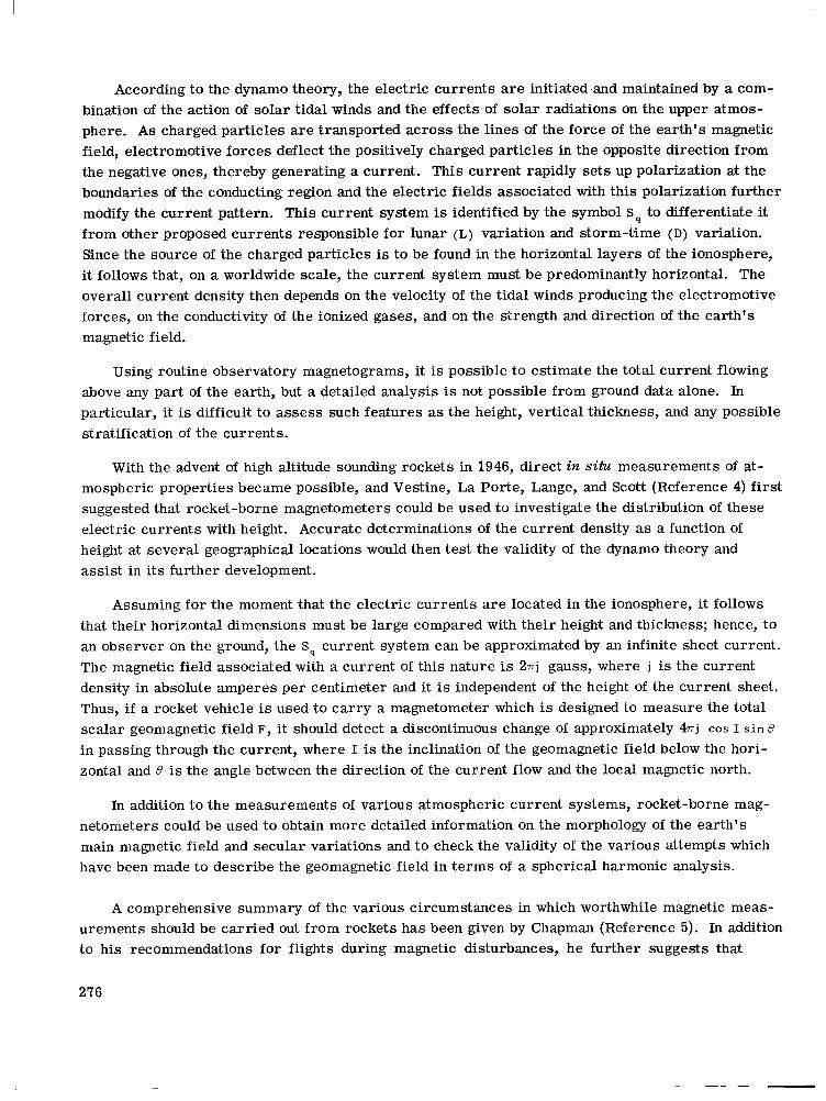
According to the dynamo theory, the electric currents are initiated.and maintained by a com- bination of the action of solar tidal winds and the effects of solar radiations on the upper atmos- phere. As charged particles are transported across the lines of the force of the earth's magnetic field, electromotive forces deflect the positively charged particles in the opposite direction from the negative ones, thereby generating a current. This current rapidly sets up polarization at the boundaries of the conducting region and the electric fields associated with this polarization further modify the current pattern. This current system is identified by the symbol s q to differentiate it from other proposed currents responsible for lunar (L) variation and storm-time (D) variation. Since the source of the charged particles is to be found in the horizontal layers of the ionosphere, it follows that, on a worldwide scale, the current system must be predominantly horizontal. The overall current density then depends on the velocity of the tidal winds producing the electromotive forces, on the conductivity of the ionized gases, and on the strength and direction of the earth's magnetic field.
Using routine observatory magnetograms, it is possible to estimate the total current flowing above any part of the earth, but a detailed analysis is not possible from ground data alone. In particular, it is difficult to assess such features as the height, vertical thickness, and any possible stratification of the currents.
With the advent of high altitude sounding rockets in 1946, direct in situ measurements of at- mospheric properties became possible, and Vestine, La Porte, Lange, and Scott (Reference 4) first suggested that rocket-borne magnetometers could be used to investigate the distribution of these electric currents with height. Accurate determinations of the current density as a function of height at several geographical locations would then test the validity of the dynamo theory and assist in its further development.
Assuming for the moment that the electric currents are located in the ionosphere, it follows that their horizontal dimensions must be large compared with their height and thickness; hence, to an observer on the ground, the S4 current system can be approximated by an infinite sheet current. The magnetic field associated with a current of this nature is 2nj gauss, where j is the current density in absolute amperes per centimeter and it is independent of the height of the current sheet. Thus, i f a rocket vehicle is used to car ry a magnetometer which is designed to measure the total scalar geomagnetic field F, it should detect a discontinuous change of approximately 4nj COS I s i n e in passing through the current, where I is the inclination of the geomagnetic field below the hori- zontal and 8 is the angle between the direction of the current flow and the local magnetic north.
In addition to the measurements of various atmospheric current systems, rocket-borne mag- netometers could be used t o obtain more detailed information on the morphology of the earth's main magnetic field and secular variations and to check the validity of the various attempts which have been made to describe the geomagnetic field in t e rms of a spherical harmonic analysis.
A comprehensive summary of the various circumstances in which worthwhile magnetic meas- urements should be carr ied out from rockets has been given by Chapman (Reference 5). In addition to his recommendations for flights during magnetic disturbances, he further suggests that
276

measurements of the current systems be undertaken in low and middle latitudes during periods of magnetic calm in order to confirm the existence of the S4 current system and to investigate its morphology.
The first in situ detection of an ionospheric current was made in a pioneering rocket flight by Singer, Maple, and Bowen (Reference 6). They installed a total-field flux-gate magnetometer in an Aerobee rocket which reached a height of 105 kilometers at a point very close to the magnetic equator and succeeded in detecting a magnetic discontinuity of 400 * 50r.
Cahill (Reference 7) has reported a further se r ies of equatorial flights using rockoons which were instrumented with proton magnetometers and were launched from ships. Two flights from the vicinity of Jarvis Island reached heights of 120 and 130 kilometers and detected anomalous departures from a dipole field of -1507 and -300r, respectively, the experimental e r r o r in the observations being *20r. The second flight also indicated some stratification of the electrojet into two layers, though the upper layer was not completely penetrated.
Magnetic anomalies of several hundred gammas associated with localized intense electric currents in auroras have also been detected (Reference 8 ) . A number of other rocket flights have taken place in latitudes away from the geomagnetic equator, but the successful detection of the Sq
current system in these latitudes has not been reported (References 9-13).
In consideration of the dynamo theory, the magnetic equator constitutes a special case in which electric fields caused by polarization effects in the ionosphere indirectly result in a con- siderable enhancement of the current density during the middle daylight period in a band approxi- mately 3" of latitude wide; this results in a magnetic discontinuity of magnitude several hundred gamma a s detected by a rocket-borne magnetometer. In midlatitudes, however, the Sq magnetic variations are much smaller, and hence the problem of detecting the postulated ionospheric cur- rents is more difficult.
ESTIMATED GEOMAGNETIC EFFECTS
A rough estimate of the amplitude of a discontinuity, which might be expected in the total scalar force in passing through the postulated electric current above Woomera, can be made as follows:
The rocket launching site at Woomera, from where British Skylark rockets are normally fired, is at latitude 30"56'S, longitude 136"31'E, geomagnetic latitude -41.0".
Figure 1 shows the position of Woomera at local midday and midnight relative to the Sq current system, as given by Chapman and Bartels (Reference 14). It is immediately evident that the focus of the southern pattern passes very close to Woomera. In fact the magnetograms recorded at Gnangara in western Australia (latitude 31"47'S) indicate that the focus passes t o the north of that observatory on about 60 percent of days, to the south on about lo%, and overhead on about
277

Figure 1-The position of Woomera relative to the Sq current system for the equinox of a sunspot minimum (left) at midday as viewed from the sun, and (right) at midnight as viewed from the night hemisphere (after Chapman and Bartels). The f low between adjacent current lines i s 10,000 A.
& NOVEMBER
1 u 0 10 20
Y
Figure 2-Vectorgrams showing the mean hourly variation i n X and Y on the five international quiet days for the months of 1938 at Watheroo, Western Australia. The corresponding monthly means are indicated by crosses.
30 percent.* Normally, therefore, Z , the ver- t ical component of F, shows the greatest diurnal variation at ground level. z is, however, con- tinuous in passing through the current sheet and so cannot contribute appreciably to any discontinuity.
Figure 2 shows the mean monthly variations in x and Y , the horizontal components of F, for quiet days during 1938 at the Watheroo Mag- netic Observatory (30°19'S, 115"53'E, geomag- netic latitude -41.8", longitude 185.6'). Since the observatory at Watheroo (now removed to Gnangara) was at approximately the same magnetic latitude as Woomera, it is reasonable to assume that the magnetograms from an observatory at Woomera would be very similar at corresponding local times. In Figure 2 the E-W component Y shows maximum variation but, since th i s component is almost normal to F, it will contribute very little and hence, it is the variation in x which can be expected to be mainly responsible for any discontinuous
'Private communication from P. M. McGregor, Mundaring Geophysical Observatory, Western Australia.
278

change in^. The maximum value of AX occurs at 0900 f 1 hours in August, when its value is about 20y different f rom the nighttime value. Since at least 25% of this will be due to induced earth cur- rents, the actual discontinuity in X will be roughly 0.75 X 2 X 20 = 30r, and this leads to an estimated discontinuity in F of 30 cos 63 = 147, since the inclination at Woomera is 63". Thus the average discontinuity which might be expected in passing through the S , current over Woomera is about an order of magnitude less than that which has been detected at the geomagnetic equator. The actual effect that might be encountered on any given day could, of course, vary considerably according to the precise location of the focus of the current system and the magnetic conditions prevailing at the time.
INSTRUMENTATION
The magnetometer and data-processing techniques which were used for these flights have been discussed in detail, together with the results of an instrument-proving flight (Reference 15). Although a horizontal component magnetometer would have simplified the problem of detecting an S4 current discontinuity, the Skylark rocket cannot yet be stabilized to the degree required for useful meas- urements of magnetic components; a total force instrument was therefore developed using the principle of nuclear free precession (References 16-19). The data from th is instrument a re in the form of damped sine waves, the frequency of which is an analog of the total scalar magnetic force; it produces approximately one absolute determination of F per second.
In view of the small anticipated magnetic discontinuity, it was essential t o remove the sensing head well out of range of the magnetic field perturbations due to various other rocket instrumenta- tion. In a standard Skylark rocket, the two principal sources of magnetic interference a r e the mild steel tube of the Raven motor and the magnet of the 6-centimeter magnetron used in the Missile Tracking System. Accordingly, the MTS magnetron was enclosed inside a magnetic shield and the magnetometer sensor was mounted on the end of a flexible pneumatic probe.
During the rocket's ascent through the atmosphere, the probe was folded inside a 12-inch diameter canister mounted in the main body of the rocket. After the rocket had passed through the dense atmosphere, the spent motor tube was ejected by means of three pneumatically operated plungers, and the probe was deployed to its full length of 20 feet, at which range the residual magnetic fields associated with the rocket were less than I?. This technique considerably sim- plified the problem of maintaining adequate magnetic cleanliness in other rocket instrumentation.
In the two rocket flights discussed in this paper, the proton magnetometer was classed as a secondary experiment, the primary object of the flights being the measurement of the flux of y rays in the primary cosmic radiation (Southampton University). The rockets also carr ied sporadic E
detectors (University College, London), x-ray cameras (Leicester University), and, for attitude and performance determination, sun slits, f lux gates, rate gyroscopes, and accelerometers (Royal Aircraft Establishment, Farnborough).
In conjunction with the rocket flights, a ground proton magnetometer (Reference 20) was operated to record the diurnal variation in F, and a flux-gate instrument, kindly loaned by the
279
I

I
Bureau of Mineral Resources, Melbourne, recorded H , the horizontal component. H was selected as being that component of the S, variation field which is discontinuous in passing through the postulated current sheet as discussed above.
In flight the rockets were tracked by means of kine-theodolites, radar type FPS 16, and the MTS beacon transmitter, all standard range facilities at Woomera. Each rocket was powered by a combination of a Raven solid fuel motor and a "cuckoo" booster. A full description of the Skylark sounding rocket has been given by Hazel1 and Dorling (Reference 21).
DATA PROCESSING
During flight the proton precession signals were relayed via the standard Skylark 465 telemetry system (Reference 22) and recorded, together with a standard 50-kilocycle reference signal and timing code, on an Ampex multichannel tape recorder.
During playback the signal-to-noise ratio of the raw data was improved by means of a manually controlled tracking filter and the signals were mixed with a suitable reference frequency derived from the 50-kilocycle standard recorded on the same tape. By this means variations in precession
frequency due to tape speed variations were compensated to first order.
A full description of the apparatus and the data reduction technique has been given by Burrows (Reference 15). Figure 3 shows a sample of the beats obtained on flight SL 129 -
by this method recorded together with a 1 millisecozd timing code.
Figure 3-Sample record of beats obtained by processing of raw data (duration of record approximately 0.25 second). The precession frequencies, and hence
magnetic field readings, were computed man- ually by counting the number of beats in a time, measured from the timing code, and adding the beat frequency thereby derived to the accurately known reference frequency. The advantage of this manual technique over a fully automatic approach is that, where the signal is of amplitude com- parable with noise or interference, the regular beats can be seen and random noise rejected.
RESULTS
Ground Data
Figure 4 shows the records of the diurnal variation in F obtained from the ground proton magnetometer at Woomera for seven consecutive days, starting on the date of the first rocket flight. The instrument measures the period of 1024 cycles of the precession signals in units of
seconds and records the last two digits; in the ambientfield atWoomera this corresponds to a
280

w-
). ** . - I . 1, YT:'.,'7";+llpTy??+y& 0 1 2 3 4 5 6 7 8 9 10 1 1 12 13 14 15 16 17 18 19 20 21 22 23 24
TIME (C.S.T. )
Figure &Ground proton magnetometer records, 10-16 March 1964, Woomera. Full-scale deflection of each record i s 143. Timing marks are local time at Woomera (U.T.+9 1/2 hours).
full scale deflection of 1437. Since the first three digits were invariant at 413, the absolute value of the total force of the geomagnetic field was typically 58,2107. In making the records of Figure 4, the instrument was set to take one reading per five minutes. It should be noted that all seven re- cords are similar in general form and amplitude of the peak diurnal variation; indeed all the re- cords taken on magnetically undisturbed days during the three months the instrument was in oper- ation at Woomera are similar in character t o those reproduced in Figure 4.
Figure 5 shows the H magnetograms recorded by the flux-gate magnetometer at Woomera on 10 and 12 March 1964, the days of the two rocket flights. A comparison of Figures 4 and 5 indicates that on 10 and 12 March the diurnal variations in F were very similar in amplitude (21r and 247,
281
SL128 FIRED 12th MARCH 1964
- \ L .I 1 L -.> L 1 , . L L - . L , L j
5 6 7 8 9 10 1 1 12 13 14 15 16 17 18 19 20 21 22 TIME (C.S.T. )
10th MARCH 1964 jL129 FIRED 100 GAMMA
t - I - , \ L \ \ I I L 1 L . L - U L . - L , % ,
respectively), whereas there was a much larger negative variation in H on the second day. This suggests that on 10 March the focus of the Sq current pattern passed nearly overhead at Woomera, whereas on 12 March it was at a significantly lower latitude. Therefore, a much more suitable day for the detection of a magnetic discontinuity at Woomera was 12 March.
Flight Data .
Skylark SL 129 was fired at 02:06 Universal Time (1136 Australian Central Standard Time) on 10 March 1964; it reached a height of 175 kilometers and impacted at a point 77 kilometers down range on a bearing of 326.6"T relative to the launcher. Skylark SL 128 was fired at 02:07 Universal Time (1137 ACST) on 12 March 1964; it reached a height of 175 kilometers and impacted at a point 77 kilometers down range on a relative bearing of 285.7T7 approximately 54 kilometers from the impact point of SL 129. On both flights the proton magnetometers functioned satisfactorily and produced data continuously from the time of probe deployment until the sensing head was torn off as the rockets re-entered the earth's atmosphere.
The accuracy of each reading depends on the attitude of the rocket at the time, as a consequence of the variation of signal amplitude with the angle between the axis of the sensing head and the geomagnetic vector (Reference 15); hence, as the rockets tumbled in flight? the scatter of the read- ings about the mean values varied from less than l y to a maximum of about 10y. All the readings obtained have, however, been used in the computations and discussions which follow. The first one or two readings of each flight a r e of dubious value as, at this time, the probes were still being inflated and the sensing heads were probably still under the influence of the rocket's magnetic fields .
It is well known that rotational motions of a proton-sensing head introduce a frequency modu- lation in the precession signal (References 23 and 24). In practice, however, the flux-gate data showed that Skylarks 129 and 128 precessed with periods of 23 seeonds and 35 seconds, respectively; the e r r o r s from this cause, though detectable, a r e small and have been neglected.
The magnetometer data have been compared with values of magnetic total force calculated on the basis of spherical harmonic analyses using coefficients derived by Leaton, Malin, and Evans (Reference 25), Cain, Shapiro, Stolarik, and Heppner (Reference 26), Cain, Hendricks, Daniels and Jensen (Reference 27), and Cain and Hendricks (Reference 28). The values of measured field minus computed field (defined as DEL) which were obtained from two of the reference fields a r e shown in Figures 6 and 7.
The overall agreement between measured and computed fields depends mainly on the coeffi- cients used, but also there is a second-order difference between the upward and downward sections
282

200
190
180
170
160
150
140
2 130 - v
I-
= 120 2 W I
110
100
90
80
70
60
50 SL129
20 30
+ DOWNWARD FLIGHT
0 UPWARD FLIGHT
1 0
. D
0
4 -
40 50 60 70
MEASURED MINUS COMPUTED FIELD (gamma)
200
190
180
170
160
150
140
4 130
I 120 (3
110
100
90
80
70
60
50
v
f-
W I
+ DOWNWARD FLIGHT
o UPWARD FLIGHT
f
SL128
20 30 40 50 60 70
MEASURED MINUS COMPUTED FIELD (gamma)
Figure 6-Comparison of measured values of total force with computed values as a function of height: left, SL 129; right, SL 128; Leaton et at. coefficients.
of each flight. Thus when April 1964 coefficients a r e used, the values of DEL obtained during the upward flight of SL 128 a r e in close agreement with the downward flight values, but there is a large scatter in the data from flight SL 129; using the Leaton et al. coefficients leads to a better agreement for SL 129, whereas the upward and downward flights can now be resolved in flight SL 128 (Figures 6 and 7). As noted earlier, the trajectories of the two rockets were significantly different, and these secondary discrepancies must reflect the different gradients of the e r r o r s in the two computed fields along the t racks of the two rockets.
In order to provide a quantitative comparison between the abilities of the various reference fields accurately to describe the earth 's main field at the particular location of Woomera, the values of DEL at the apogee of flight SL 128 a r e listed below:
Coefficients DEL
Leaton et al. (Reference 25) Vanguard A (Reference 26)
Vanguard B (Reference 28)
+ 44 f. 3r - 75 f. 3r
April 1964 (Reference 27) -118 * 3~ -992 f 3 y
283

200
190
180
170
160
150
140
5 130 r
- E
+ Q 120 W I
110
100
90
80
70
60
50
SL129 2- .~
-150 -140
. --
+ DOWNWARD
o UPWARD FLIGHT FLIGHT
~~ ~I _ - I J -130 -120 -110 -100
MEASURED MINUS COMPUTED FIELD (gamma)
- 90
DOWNWARD + FLIGHT
0 UPWARD FLIGHT
180
170
160
150 - 140 -
-
-
-
h
E Y
I- - 130 r
-
Q 120 - W I
110
100
90
80
70
-
--
-
-
-
60 c SL128 , ,
c-n I I - L JV
-150 -140 -130 -120 -110 -100 -90
MEASURED MINUS COMPUTED FIELD (gamma)
Figure 7-Comparison of measured values of total force with computed values as a function of height: left, SL 129; right, SL 128; Apri l 1964 coefficients (Reference 28).
In spite of these differences in detail a s between the flight results using different reference fields, the general fo rm of the variation of DEL with height is consistent, regardless of which coefficients a r e used in calculating the reference fields.
IONOSPHERIC CURRENTS
As stated above, Figure 5 shows that the flight of SL 129 took place when the focus of the S q
current system was close to overhead at Woomera and the value of &i recorded at the time of the flight is close to the mean value. It is not therefore surprising that the flight data in Figure 7 (left) do not show any significant discontinuity which could with confidence be attributed to a current sheet.
The flight of SL 128, however, occurred when the magnetic conditions at Woomera were much more favorable for the detection of a discontinuity. As discussed above, at the time of the flight the flux-gate magnetometer recorded a significant departure from the nighttime value (Figure 5).
284
- - - . .. _. . . .. .,. . , I I , I I I 111 I I I I 1111111 11111

The KP index for the appropriate 3-hour period was 4 (Reference 29)) but the proton magnetometer record shows that, at Woomera, the diurnal magnetic variation w a s normal and undisturbed except for minor fluctuations (Figure 4). The reduced data from the rocket-borne magnetometer show an unmistakable change in slope at a height of about 104 kilometers followed by a return to the original slope at about 115 kilometers (Figure 7, right). This indicates that during this t ime the rocket passed through an electric current and the sign of the discontinuity confirms that the current was flowing in a direction having a westerly component. This anomaly is recorded on both the upward and downward par ts of the flight. The absence of any similar discontinuity during the rest of the flight up to apogee indicates that no other current system of comparable magnitude was flowing in this height range at the time of the rocket flight.
i
~
I
In order to measure the amplitude of the magnetic discontinuity and to compare it with that which would be anticipated on the basis of ground data, the upward and downward flight data a r e each plotted separately in Figure 8, since they constitute two independent measurements. The mean relative displacement of the upper and lower par ts of the curves is 24 f 3r. This experimental value can be compared with one calculated on the basis of the ground data, as described above. At the time of the flight, the deviation of H from the undisturbed nighttime value was -35 f 27, the uncertainty being due to the dif- ficulty in selecting the undisturbed value. This leads to an expected discontinuity i n F of be- tween 23 and 26r, making the approximations and the assumptions discussed above.
The magnetic discontinuity which was ob- served in flight therefore agrees very closely, both in amplitude and in sign, with what would be anticipated on the basis of the ground ob- servations at the time. This lends support to the belief that, at the latitude of Woomera, the currents responsible for the normal diurnal magnetic variations a r e concentrated almost entirely in a single layer extending from ap- proximately 104 kilometers up to approximately 115 kilometers in the E-region of the iono- sphere; furthermore, on the basis of the as-
urnal variations are due to induced earth currents, these results also imply that any nighttime ionospheric currents must be much smaller than those which have been demon-
I
I sumption that 25 percent of the observed di-
I strated t o flow ,during the daytime.
18C
170
16C
150
140
130 - E
Y v
g 120 (3 w I
110
100
90
80
70
60 ! 1 1 . 1 I
DEL ( gamma ) 40 60 i
18C
17C
16C
150
140
130 - E
Y z 120 r c? = 110 w
100
90
80
70
60 I I I I I
DEL (gamma ) 40 60 80
Figure 8-Magnet i c discontinuity detected by Sky lark SL 128; left, upward flight; right, downward flight.
285
..I I
18.
19.
20.
21. 1
1
22.
23.
24.
25.
26.
27.
28.
29.
30.
31.
32.
33. 1
34.
35.
288
Waters, G. S., and Francis, P. D., "A Nuclear Magnetometer,I' J. Sci. Instr., 35(3):88-93, March 1958.
Burrows, K., 'I Rocket-borne Magnetometer," J. Brit. IRE, 19(12):769-776, December 1959.
Burrows, K. "Geomagnetic Measurements in a Rocket Vehicle," Ph.D. thesis, London Uni- versity, 1963.
Hazell, J. F., and Dorling, E. B., "British Sounding Rocket-Skylark," in: Sounding Rockets, ed. by H. D. Newell, Jr., New York: McGraw-Hill Book Co., Inc., 1959, pp. 243-251.
Rae, W. M., "The Airborne Sender for 24-channel Telemetry," J. Brit. IRE, 21(1):57-67, January 1961.
Bloom, A. L., "Nuclear Free Precession in a Moving Vehicle," Varian Associates Technical Memorandum, Palo Alto, California, 1955.
Hall, S. H., "The Modulation of a Proton Magnetometer Signal Due to Rotation,'' Geophys. J., 7(1):1-22, September 1962.
Leaton, B. R., Malin, S. R. C., and Evans, J. J., "An Analytical Representation of the Esti- mated Geomagnetic Field and its Secular Change for the Epoch 1965.0," IAGA Symposium on Magnetism of the Earth's Interior, Pittsburgh, Pennsylvania, November 1964.
Cain, J. C., Shapiro, I. R., Stolarik, J. D., and Heppner, J. P., "Measurements of the Geomag- netic Field by the Vanguard 3 Satellite," NASA Technical Note D-1418, October 1962.
Cain, J. C., Hendricks, S., Daniels, W. E., and Jensen, D. C., "Computation of the Main Geo- magnetic Field fromspherical Harmonic Expansions," GSFC DocumentX-611-64-316, October 1964.
Cain, J. C., and Hendricks, S., "Comments on the Vanguard 3 Magnetic Field Data and Analysis," J. Geophys. Res., 69(19):4187-4188, October 1, 1964.
Lincoln, J., "Geomagnetic and Solar Data,'' J. Geophys. Res., 69(15):3283-3296, August 1, 1964.
Baker, W. G., and Martyn, D. F., "Conductivity of the Ionosphere," Nature, 170:1090-1092, December 27, 1962.
Fejer, J. A., "Semidiurnal Currents and Electron Drifts in the Ionosphere," J. Atmospheric Terrest. Phys., 4:184-203, December 1953.
Chapman, S., "The Electrical Conductivity of the Ionosphere: A Review," Nuovo Cimento Suppl. 4( 4) : 13 8 5 - 1 41 2, 19 5 6.
Ratcliffe, J. A., and Weekes, K., "The Ionosphere," in: Physics of the Upper Atmosphere, ed. by J. A. Ratcliffe, New York: Academic Press, 1960, pp. 377-470.
Maeda, K., and Matsumoto, H., "Conductivity of the Ionosphere and Current System," Rept. Ionosphere Space Res. Japan, 16 (Part. 1):l-26, March 1962.
Kochanski, A., "The Circulation in the Stratosphere, Mesosphere, and Lower Thermosphere," WMO Technical Note, ed. by R. J. Murgatroyd, (in press).
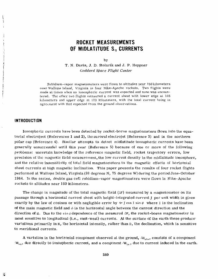
ROCKET MEASUREMENTS OF MIDLATITUDE S, CURRENTS
by T. N. Davis, J. D. Stolarik and J. P. Heppner
Goddard Space Flight Center
Rubidium-vapor magnetometers were flown to altitudes near 150 kilometers over Wallops Island, Virginia in four Nike-Apache rockets. Two flights were made at t imes when no ionospheric cur ren t was expected and none was encoun- tered. The other two flights measured a cur ren t sheet with lower edge at 105 kilometers and upper edge a t 123 kilometers, with the total current being in agreement with that expected from the ground observations.
INTRODUCTION
Ionospheric currents have been detected by rocket-borne magnetometers flown into the equa- torial electroject (References l and 2), the auroral electrojet (Reference 3) and in the northern polar cap (Reference 4). Similar attempts to detect midlatitude ionospheric currents have been generally unsuccessful until this year (Reference 5) because of one o r more of the following problems: uncertain knowledge of the reference magnetic field, rocket trajectory e r rors , low precision of the magnetic field measurement, the low current density in the midlatitude ionosphere, and the relative insensitivity of total field magnetometers to the magnetic effects of horizontal sheet currents at high magnetic inclination. This paper presents the results of four rocket flights performed at Wallops Island, Virginia (38 degrees N, 75 degrees W) during the period June-October 1964. In the series, double gas cell rubidium-vapor magnetometers were flown in Nike-Apache rockets to altitudes near 150 kilometers.
The change in magnitude of the total magnetic field (AF) measured by a magnetometer on its passage through a horizontal current sheet with height-integrated current J per unit width is given exactly by the law of cosines or with negligible e r ro r by 4rr J cos I s i n $ where I is the inclination of the main magnetic field and $ is the horizontal angle between the current direction and the direction of H . Due to the s i n $dependence of the measured AF, the rocket-borne magnetometer is most sensitive to longitudinal (i.e., east-west) currents. At the surface of the earth these produce. variations primarily in H , the horizontal intensity, rather than D, the declination, which is sensitive to meridional currents.
A variation in the horizontal component observed at the ground, AHobs, consists of a component ,*ex, due directly to ionospheric current, and a component AHin , due to current induced in the earth.
289

where J is the height-integrated current per unit width and the inclination I is taken as 70 degrees; AF is the change in the scalar field as the rocket magnetometer passes through the current sheet.
INSTRUMENTATION
This study is the first making use of rubidium vapor magnetometers flown in small rockets to study ionospheric currents. In this magnetometer the Zeeman splitting of atomic energy levels in Rb-85 vapor is detected as resonance absorption of light from a Rb-85 source. The frequency of resonance, the Larmor frequency, is a direct measure of the total scalar magnetic field intensity by the relationship
f (cps) 466744F t (K)359F2
for a one cell magnetometer where F is in gauss andK, usually <0.5, indicates the fraction of the constant with FZ that appears in a given instrument. Here a self-oscillating, cross-coupled, dual cell arrangement is used to largely eliminate the F~ dependence so that the variation with orienta- tion is small, less than &2r at F = 0.5 gauss. Dual (or single) cell rubidium magnetometers have null regions (regions of low signal amplitude) of conical shape centered on the instrument optical axis and in the form of a zone centered on the plane perpendicular t o the optical axis; the instru- ments flown in this study have conical nulls of half-angle near 10 degrees and zonal nulls of half- width 5 degrees or less.
In each rocket the magnetometer sensor was mounted in the forward end of the nose cone with the magnetometer optical axis inclined 45 degrees to the rocket axis. In this orientation and with the rocket spin-stabilized at 5-6 revolutions per second, null regions were avoided since the mag- netic field inclination at Wallops Island, Virginia is 70 degrees.
The Larmor frequency output of each magnetometer was used to phase-modulate a 231.4- megacycle, 2-watt telemetry transmitter fed to a quadrapole antenna located at the base of the payload. Other payload components included a battery pack consisting of 20 HR1 silver cells to supply power for the magnetometer and transmitter, a switching module containing partially- shielded relays for switching operations on the ground, and a DOVAP (doppler) transponder for trajectory determination to supplement and check the radar tracking. The DOVAP transponder was connected to 36.8-megacycle (input) and 73.6-megacycle (output) shroud antennas attached to the Apache rocket motor.
290

Magnetic materials in the payload components were kept to a minimum and care was used to reduce possible current loops in the payload wiring. The greatest possible separation between the magnetometer sensor and the other payload components was maintained. The structural par ts of the payload and the nose cone were constructed primarily of fiberglass t o reduce permanent and induced magnetic fields. As a result, the magnetic contribution of -each payload was 27 o r less as measured at the position of the sensor in a zero ambient field.
It is necessary to maintain the magnetometer sensor lamp bulb and absorption cell tempera- tu res within a narrow range for proper operation. The payloads contained circuits allowing meas- urement and control of the lamp bulb and absorption cell temperatures prior to rocket firing. In flight, the heat output f rom the lamp together with thermal insulation about the sensor sufficed to maintain operating temperatures within allowable limits.
DATA RECOVERY AND REDUCTION
On the ground the Larmor frequency-modulated telemetry signal is received and the Larmor frequency is recorded on magnetic tape together with a reference frequency, time-code and tape- recorder speed-lock reference signal. Using a system designed primarily for reduction of satel- lite data, the rubidium Larmor frequency is counted to an accuracy of one part in 5X10⁶. This accuracy is achieved by use of the rubidium signal to gate the interval over which a 5-megacycle reference signal is counted. Thus, if a sample period of 0.1 second is desired, the Larmor fre- quency can be measured sufficiently accurately t o allow a 0.5 gauss magnetic field to be determined with a precision of 0.1 gamma. Once the Rb-85 Larmor frequency is counted, a value of the scalar magnetic field is found representing the average field over the sampling interval. In a high-speed computer, radar or DOVAP trajectory data are merged with the magnetometer data. At the mid- point of each sampling interval, the location of the rocket is calculated and for that location a ref- erence magnetic field is computed using the coefficients of a spherical harmonic expansion of the geomagnetic field. The computed reference field (B,) is subtracted from the measured field (B,,,);
the value of Bm -Bc is then available for printing or automatic plotting versus time o r spatial parameters.
PRESENTATION OF DATA
Magnetic Conditions
Wallops Island, Virginia l ies to the north of the focus of the equivalent current system derived from the world-wide sq magnetic variations. The normal variations on undisturbed days is typified by the reproduction of the Fredericksburg magnetogram in Figure 1 (Fredericksburg is 180 kilom- e te rs to the west of Wallops Island). The Z component shows minor variation; eastward and west- ward declinations appear in the morning and afternoon hours, respectively, and the maximum neg- ative H deviation occurs one to two hours before local noon. Thus the maximum change in the total field AF measured by a rocket-borne magnetometer on its passage through the ionospheric current sheet is expected just prior to noon when 1 -&I is greatest.
291

FLIGHT 14.156 14h57m39' U. T. 0Oh52"'30' U.T. - w
c 5 0 y 52,8803 Z REFERENCE z+
07 11 115 &L.T. 19 Y, 12 16 00 04 08 I-.: , , t t 1 t . : 1 + - I t 1 I : : I
2o U.T
Figure l-Tracings of the Fredericksburg magnetogram for June 25, 1964 showing the times of flights 14.156 and 14.157. Panel inserts indicate the detailed magnetic variations during each flight: AH from theFredericksburg rapidrun recording; AF from a helium magnetometer operated at Wallops Island. Date i s given for left-hand portion of the diagram.
\ MINUTES / e f i , , A L-v -A+.+L-+L-
t 13F?9,aoy H REFERENCE FLIGHT 14.155 l o m 00' U.T.
52 ,880~ Z REFERENCE .z - - -07 1 1 ! 1; . - I ,L:T.+ 1p 1 ; 5 w 1 + + +--:
12 16 20 U.T. 00 04 08
Figure 2-Tracings of the Fredericksburg magnetogram for June 10, 1964 with a panel insert showing the detailed magnetic variations during f l ight 14.155. See also the t i t le for Figure 1.
One of the flights (Fl. 14.157) was made on the day represented in Figure 1 during an interval in which no ionospheric current was expected on the basis of study of the Freder- icksburg magnetic recordings obtained on the several days preceding the flight. The H ref- erence line of Figure 1 represents the value of H deduced for the condition of no overhead cur- rent. One minute after the commencement of F1.14.157, a small pulsation event occurred; its maximum peak-to-peak amplitude was 5~ in H and 2~ in F (see the upper right panel of Figure 1).
Flight 14.156 was launched earlier in the same local day at a t ime when AH at the ground was -44y, Figure 1. The period represented by Figure 1 was rather quiet magnetically but was not one of the designated 10 quiet days of June 1964; K~ ranged from 1, to 2, and the Fred- ericksburg K-Values were 1 or 2.
A third flight 14.155 was made on June 10, 1964, the most disturbed day in June, Figure 2. At the t ime of the flight K~ was 3, and the Fredericksburg K-Vdue was 2. As in the case of F1.14.156, this flight was made during the pre-noon hours when the maximum westward s, current was expected. Since the flight occurred during a storm period, the horizontal magnetic field was decreased by D s t currents presumed to flow well beyond the ionosphere. Examination of the Fredericksburg magneto- grams taken on the days before and after June 10 indicates that the Dst depression of H
amounted to approximately 14y on that day. That determination accounts for the H reference line on Figure 2 being displaced as compared to that on Figure 1. After removal of the D s t depression there remains on Figure 2 a -35y deviation in H which one expects to be caused by westward ionospheric currents and related earth-induced currents.
A fourth flight (Fl. 14.159) was launched on October 8, 1964 in conjunction with a sodium- release rocket flight during morning twilight. The Fredericksburg magnetogram covering the period of this flight is reproduced in Figure 3. Although this was not one of the designated quiet days in October, 1964, the level of magnetic activity was not high during the first half of October 8;
292

KP ranged from 2, t o 3, and the K-value at Fredericksburg was 2 or 3 . At the t ime of F1. 14.159, the Fredericksburg H -component t race was within 3~ of its quiet-day level so the flight was not expected to encounter ion- ospheric current.
In summary, Fls. 14.157 and 14.159 oc- curred at t imes of minimal AH and were not expected to detect sizable ionospheric current. Flights 14.155 and 14.156 occurred when AH was -33 f 7 y and -42.5 f 2 . 5 ~ ~ respectively; hence these flights should have encountered detect- able ionospheric current.
The horizontal paths of the four rocket flights a r e indicated on a map (Figure 4) show- ing the magnitude of the total magnetic field at the earth surface as computed from the coefficients of the spherical harmonic ex- pansion of the geomagnetic field given by Leaton and Evans (References 6 and 7). Actual departures from the computed surface field a r e indicated in the form of contours drawn at 1OOr intervals. Although the anomaly contours drawn in the upper-left corner of Figure 4 a re based on recent comprehensive data, the anomaly values elsewhere in Figure 4 a r e derived from very few data points obtained over the past 15 years. Consequently, only the gross features of the anomaly map should be considered as meaningful.
AF
~ t l l l * l l l l t t
FLIGHT 14.159 1Oh34"'0OS U.T.
528641-2 BASELINE z+ 1 0 7 1 1
/ , , I , , , 4 , 17 !.?.A 2;3 , -03 i 7, 07 li 16 20 00 U.T. 04 08 12
Figure 3-Tracings of the Fredericksburg magnetogram for October7,1964with a panel insert showing the detailed magnetic variations during f l ight 14.159. See also the t i t le for Figure 1.
38.0 - 0
37 .8 -0 v
37.6
5 = 37 .4 E
2 - 2 37.2
37 .0 2
75.6 75 .2 74 .8 7 4 . 4 74 .0 7 3 . 6 73 .2 LONGITUDE WEST (degrees)
Figure 4-Map showing the horizontal projections of the rocket flights. The parallel lines running from lower left to upper right represent the Leaton and Evans Epoch 1965 reference f ield at the earth's surface and the curved contours represent the surface anomaly f ie ld referenced to the Leaton and Evans field.
The significant features of Figure 4 for our purpose a r e a generally increasing anomaly field from the launch point (upper left) t o the rocket impact points and an isolated region of higher field near the impact point of F1. 14.156. Relative to the magnetic field computed from the Leaton and Evans coefficients, the rocket magnetometers should measure higher fields near the impact points than measured near the launch point. Flight 14.159 is somewhat of an exception in that its impact point is beyond the main anomalous region.
Flight Data
The flight data were sampled over a period equal t o the appropriate rocket roll period (0.17 t o 0.25 seconds). By sampling at this rate, e r r o r s which are dependent upon the angular orientation
29 3

JUNE IO, 1964
*...
, FL. 14.156
20 40
of the rocket measured in the plane perpendicular to its spin axis are averaged out. The result is a meas- urement of the scalar field independ- ent of the spin and which is precise to within a fraction of 17. This measurement gives the magnitude of the vector sum of the local geomag- netic field and the spin-axis compo- nent of the rocket's magnetic field. Flight data above altitude 70 kilom- e te rs from the ascent portions of Fls. 14.155, 14.156 and 14.157 a r e shown in Figure 5. (The ascent portion of F1. 14.159 data is roughly similar to that of F1. 14.157.)
The data points on Figure 5
20 40 20 40
B (MEASURED) - B (COMPUTED) y (GAMMA)
exhibit a sinusoidal variation indi- cating a magnetic contribution along the spin-axis of each rocket and a precessional motion of the rocket
Figure 5-Plots of altitude versus the measured total f ield minus the computed total f ield for ascent portions of three flights. Solid lines represent the data corrected for effects due to vehicle precession.
with a period near 30 seconds. Although each payload is known to possess a very minor magnetic field ( 2 2 ~ ) ~ the overall vehicle (payload and attached Apache stage) showed a magnetic field com- ponent along the spin axis of 30 t o 50r, as measured during re-entry turn-over. This field was due to magnetic elements within the rocket motor or to currents induced by the high spin rates. Due to the smoothness in the variation of the precession period and angle during the upper portion of each flight, it is possible to apply a precession correction to the data of the form c s i n ut.
results of such point by point corrections a r e indicated in Figure 5 by the solid lines drawn through the data points. The shaded regions enclosing the curves for Fls. 14.155 and 14.156 rep- resent a generous estimate of the uncertainty in the precession correction; very little uncertainty exists in the correction applied to F1. 14.157.
The
All flight data taken in the region above 80 kilometers a r e shown in Figure 6 with precession corrections applied. The data obtained below 80 kilometers will be discussed here only to an extent required for the interpretation of the measurements above 80 kilometers. Shortly after launch, when the first stage booster had fallen away, each flight magnetometer measured a field of 100 to 200r l ess than that calculated from the Leaton and Evans reference field. This difference is in accord with that expected from examination of the anomaly map, Figure 4. The ascent portion of each flight shows a steadily increasing value of B~ - B= with altitude; the rate of increase lessens with altitude to the 90 kilometer level. The lessening rate of increase with altitude evidently r e - flects the fall-off with distance of the ground anomaly field. Except for F1. 14.159, the anomaly field appears to have little effect on the ascent data taken above 100 kilometers. As seen in
294

16t
15C
140
- 130 E
Y v
120 i2 t; Q 110
100
90
80
FL. 14.157 -
$
I I 1 40 50 60
FL. 14.159 10h34'"00f U.T.
OCTOBER 8, 1964
{
z
ri I 70 80
-. . '-.
i -.
I I 90 100
FL. 14.155 15h10m00s U.T. JUNE 10, 1964
B : *
. D . * . D
: z .e
FL. 14.156 14h57m39s U.T. JUNE 25, 1964
3 0 z
*e?. 00 .
0 . 0 . .".
9 : 0 .
0 .
D . . : .: * . 0 .
D . D . e . D . - .
0 . e .
0 . e *
2 :
4 I I 20 30 40
B (MEASURED) - B (COMPUTED) y (GAMMA)
Figure 6-Precession corrected ascent (open-circle) and descent (ful I-circle) data above altitude 80 km for all flights.
Figure 4, the descent portions of each flight occur over the region of highest surface anomaly field. This is reflected in the measurements at high altitude by the descent B ~ - B= values generally being higher than those measured during ascent (Figure 6).
Below the 100-kilometer level, the descent portions of Fls. 14.155, 14.156 and 14.157 show monotonically increasing Bm - Bc values to rocket impact, at which points the measured fields were 2007 or more above the Leaton and Evans reference field values. Flight 14.159 passed over the main anomalous region to impact at a point of near-zero surface anomaly and at that point meas- ured a field nearly equal to the reference field value. identical magnetic conditions and along almost identical flight azimuths. between the flights was the higher apogee and shorter horizontal range of F1. 14.157 as compared to F1. 14.159. The characteristics of the high altitude data from these two flights (Figure 6) are very similar. In neither case is there any discontinuity in the region above 80 kilometers that can be attributed to the effect of a current layer in the ionosphere; nor was any expected on the basis of magnetic measurements made on the ground during these flights. In Figure 6, a small change in slope appears near 115 kilometers in the descent portion of the data f rom F1. 14.159, but this is the altitude at which the rocket passed over the greatest anomaly measured on its sub-trajectory path. It is not clear whether or not the 14.157 flight magnetometer detected the small pulsation event occurring during the flight but the flight data, especially those taken during the rocket ascent, do indicate that the amplitude of the event could not have been much if any greater at altitude than that observed on the ground.
Flights 14.157 and 14.159 occurred under The main difference
29 5

I lIIllllIIlIIllI I
The ascent data f rom F1. 14.155 presented in the central panel of Figure 5 show an increase in B~ -Bc of approximately l l y between the altitudes 105 and 123 kilometers, which indicates the existence of westward current in this height region. The F1. 14.155 descent data plot, Figure 6, shows a sharp discontinuity at 105 kilometers and possibly one near 125 kilometers, but evidently the effects of the ionospheric current layer are partially masked by the ground anomaly field. For this flight, a deviation of approximately 147 in IF1 was predicted from the ground observations on the assumption that 0.6 of the observed OH was due t o external currents. Similarly, a deviation in ( F I of 1 7 y was predicted for F1. 14.156. Both the ascent and descent plots, Figures 5 and 6, f rom this flight show discontinuities at 105 and 123 kilometers. The field change in the upward passage through the current sheet was approximately 1 7 ~ and the apparent descent field change was near 1 2 ~ . However as in the case of F1. 14.155, the descent data appear to reflect variations caused both by the ionospheric current and by the ground anomaly.
SUMMARY AND DISCUSSION
A summary of the results of the four flights together with an estimate of the probable e r rors , is given in Table 1. An internally consistent interpretation of the flight data requires magnetic
Table 1
Summary of the Results f rom the Four Flights with an Estimate of the Probable Er ro r s .
r Observed OH At Ground
Predicted AF From Ground Observations,
Assuming f = = 0.6 4 x
obs
OF Observed in Flight
Altitude of Lower Edge of Current Sheet
Altitude of Maximum Current Density
Altitude of Upper Edge of Current Sheet
Total Westward Horizontal Current
296
- ~-
Flight 14.157 OOh 52”’ 30’ U.T
26 June 1964
+3.7 f 2.5Y
+1.5 f ly
Ascent: 0 5 ly Descent: 0 f 21.
Flight 14.159 l o h 34”’ OOs U.T 8 October 1964
__
-3 .w f 2.5y
-1.2 f 17
Ascent: 0 f 27 Descent: 0 i 21
. - ~
Flight 14.155 15h 10” 00” U.T.
10 June 1964
-33.0 f 77
-13.5 f 37
Ascent: -11 f 2y Descent: ?
\scent: 105 * lkm lescent : 104 f lkm
\scent: -116km ( ? : lescent : ( ? )
\scent: 123 5 lkm Iescent: ( ? )
iscent: 25.6 f 1.5 \mpe re s /km Iescent: (?)
Flight 14.156 14h 57”’ 39’ U.T.
25 June 1964 -
-42.5 f 2.5Y
-17.5Y f TY
\scent: -17 f 2y lescent : -12 f 2Y ( ? ;
4scent: 106 f lkm lescent : 105 f lkm
iscent : - l lOkm(?) lescent: -113km(?)
iscent: 123 f lkm Iescent: 123 f lkm
4scent: 39.4 * 1.5 imperes/km Iescent: >26 imperes/km

contributions from both ionospheric current and ground anomalies. The ground anomaly contri- bution t o the ascent data is minor and poses no interpretative problem. However, the descent por- tions of all flights pas s over an appreciable anomaly which has sufficient magnetic contribution at altitude to prevent a quantitative determination of the ionospheric current contribution from the descent data alone. Since the anomaly magnetic field adds vectorially to the geomagnetic field, a quantitative treatment of its effect on the flight data requires more complete knowledge of the surface anomaly field than is available from the sparse observations now in hand.
The data f rom the two flights (Fls. 14.155 and 14.156) which penetrateq a detectable current layer indicate a simple westward current sheet lying between altitudes 105 and 123 kilometers with the altitude of maximum current density between 110 and 116 kilometers. The total current within the sheet is in good agreement with that expected from the ground measurements.
ACKNOWLEDGMENTS
We are grateful to Mr. J. C. Seddon for his efforts in providing final trajectories from the DOVAP data. Mr. G. F. Hinton, United States Navy Oceanographic Office, provided total field magnetic data from a helium magnetometer operated at Wallops Island, Virginia.
REFERENCES
1.
2.
3.
4.
5.
6.
7.
Singer, F. S., Maple, E., and Bowen, W. A., Jr., "Evidence for Ionospheric Currents f rom Rocket Experiments N e a r the Geomagnetic Equator," J. Geophys. Res. 56(2):265-281, June 1951.
Cahill, L. J., "Investigation of the Equatorial Electrojet by Rocket Magnetometer," J. Geophys. Res. 64(5):489-503, May 1959.
Meredith, L. H., Davis, L. R., Heppner, J. P., and Berg, 0. E., "Rocket Auroral Investigations," Annals of the IGY , 12(pt. 2):631-640, 1961.
Cahill, L. J., "Detection of an Electrical Current in the Ionosphere above Greenland," J. Geophys, Res. 64(10):1377-1380, October 1959.
Burrows, K., and Hall, S. H., "ITZ Situ Detection of an Ionospheric Electric Current," Nature, 204(4960):721-722, November 21, 1964.
Leaton, B. R., and Evans, M. J., ?'An Analytical Representation of the Estimated Geomagnetic Field and Its Secular Change for the Epoch 1965.0," presented at the Symposium on Magnetism of the Earth's Interior, Pittsburgh, Nov. 1964.
Cain, J. C., Hendricks, S., Daniels, W. E., and Jensen, D. C., "Computation of the Main Geomagnetic Field from Spherical Harmonic Expansions," GSFC Document X-611-64-316, 1964.
297


Appendix A
Glossary of Terms
B - Total scalar magnetic field
D - Declination of the magnetic field
F - Total magnetic field
H - Horizontal intensity component
I - Inclination of the magnetic field
J - Height-integrated current
K - Instrument constant
s4 - Ionospheric current (daily quiet day variation)
299
A


I
NEUTRON STARS AS X-RAY SOURCES by
H.-Y. Chiu Goddard Institute for Space Studies
The density of neutron s t a r s is approximately 10 l4 g/cm3, with a typical radius of 10 km. At such a high density, the Fermi energy of electrons is of the order of a few hundred MeV, in which the gas is mainly composed of neutrons, thus, nuclei cannot exist. Thought to be a remnant of supernova processes, the neutron s ta r , formed a t a temperature 2 10 lo "K, cools down, in a matter of a few weeks via neutrino processes, to a temperature of about 5 x l o 8 "K. Hence- forth, the loss of energy is through surface blackbody emission with a luminosity in the range of 1 La to l o 3 La. This corresponds to a surface Lempezature of l o6 ' lo7 OK, where most energy is in the wavelength band of 1 A-1OA. Neu- tron s t a r s a re , therefore, potential cosmic x-ray emit ters if they exist.
The radiation characterist ics of neutron s t a r type x-ray sources is also discussed. We have found that the source Scorpius X-1 (ScXR-1) is the most likely selection and further measurements on the angular diameter of this source will be fruitful.
INTRODUCTION
The existence of neutron stars was f i rs t proposed in 1931 by Landau (Reference 1) and Zwicky (Reference 2), in which Zwicky had proposed the formation of neutron stars a s a mechanism for supernovae. The theoretical structure of neutron stars was later studied by Oppenheimer and Volkoff (Reference 3) .
Today, however, there still remain uncertainties in the theory; the main one stems in the neutrino energy loss rate. J. N. Bahcall and R. A. Wolf have suggested a neutrino process, which, if applicable to the density regime of stable neutron stars, will imply that the surface temperature is below lo5 OK and hence, will not penetrate the interstellar medium. The uncertainties in the nuclear many body theory preclude a definite statement if this neutrino loss mechanism will operate in these stars. At present, neutron stars still .remain as theoretically postulated objects, although as we shall see, they may be potential cosmic x-ray sources and may be detectable by space x-ray experiments.
301

STATIC STRUCTURE OF NEUTRON STARS
The existence of neutron stars follows from the theoretical study of general relativity and nuclear physics. Under ordinary density conditions (510" g/cm3 ), neutrons are unstable and will later decay into protons, electrons, and neutrinos with a lifetime of lo3 seconds. As the density of matter is increased, the zero-point energy or Fermi energy of the electrons is increased. Thus, at a density of 107g/cm3, the value of the Fermi energy per electron exceeds 1 Mev and the follow- ing type of inverse beta reactions,
(1) e- + (Z, A) - (2 - 1, A) + v ,
will take place after which the number of electrons will decrease and the nuclei will become more neutron enriched. Whea a density of 101'g/cm3 is reached, the Fermi energy of the electrons will be sufficiently increased enough to cause the complete disintegration of all nuclei, leaving only neutrons to exist, as is the case in the stable form of matter. The decay of neutrons is prevented by the presence of a small amount of electrons.
The typical density of a neutron star is of the order of 10"g/cm3, which is a few times the density of nuclear matter and the radius of one solar mass, corresponding to this density, is around 10 kilometers.
The theory of the formation of these stars is very incomplete because the density is lo8 greater than the highest density observed (-lo6 g/cm 3, which is the density of white dwarfs). It is believed i5at neutron stars are formed during the collapse of a star to become a supernova. This collapse problem must be treated by using the general relativistic hydrodynamical theory. Although no quantitative results a r e yet available, a few theories have been presented (References 4 and 5).
Because of the high concentration of matter in neutron stars, the space-time curvature is large and the general relativity theory must be used to describe the structure. If the space-time curvature is too great, implying too large a mass, then the relativity theory predicts that no light signal may leave the mass concentration. Such a state is referred to as the "Schwarzschild singularity" and as a consequence, the neutron star cannot be observed, hence an upper limit for the mass exists. The numerical value of the upper l imit is a very sensitive function of the detailed interaction among neutrons. At a density of approximately 10"g/cm3, the average distance between neutrons is about 10-'3cm, or equivalent to the s ize of a neutron, thus this interaction cannot be neglected. Figure 1 shows two structures of neutron stars obtained by Cameron* by use of two equations of state. These are ob- tained by two different empirical fits to low energy, nuclear interaction data, within the experimental e r ror . The mass of the neutron s ta r in Figure 1 is expressed as a function of the central density.
*A. G. W. Cameron, private communication.
302
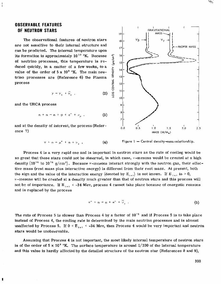
OBSERVABLE FEATURES OF NEUTRON STARS
19
18
17-
The observational features of neutron stars are not sensitive to their internal structure and can be predicted. The internal temperature upon its formation is approximately 10 l o OK. Because 16-
of neutrino processes, this temperature is re- 2 15-
duced quickly, in a matter of a few weeks, to a value of the order of 5 x 10' OK. The main neu- trino processes are (Reference 6) the Plasma 13-
process + 12-
v
14- v, t 2 t
Y " V e + v e > (2) (3
- 1 1 -
10-
and the URCA process
n + n - n + p t e - + U @ 9 (3 1
0 and at the density of interest, the process (Refer-
Figure 1 - Central density-mass relationship. n t n - , u L - -t n + u e . (4)
I I I 1 - GRAVITATIONAL
-
-
9 -
8-
7-
.o 0.5 1 .o 1.5 2 .o 2.5
Process 4 is a very rapid one and is important in neutron stars as the rate of cooling would be so great that these stars could not be observed, in which case, n-mesons would be created a t a high density tive mass ( rest mass plus interactive energy) is different from their rest mass. At present, both the sign and the value of the interaction energy (denoted by E, t ) is not known. If E i n is > 0, n-mesons will be created at a density much greater than that of neutron stars and this process will not be of importance. If E < -34 MeV, process 4 cannot take place because of energetic reasons and is replaced by the process
to 10" g/cm3). Because v-mesons interact strongly with the neutron gas, their effec-
The rate of Process 5 is slower than Process 4 by a factor of lo-' and i f Process 5 is to take place instead of Process 4, the cooling rate is determined by the main neutrino processes and is almost unaffected by Process 5. If 0 < E stars would be unobservable.
< -34 MeV, then Process 4 would be very important and neutron
Assuming that Process 4 is not important, the most likely internal temperature of neutron stars is of the order of 5 x 10' "K. The surface temperature is around 1/100 of the internal temperature and this value is hardly affected by the detailed structure of the neutron star (References 8 and 9),
303
I
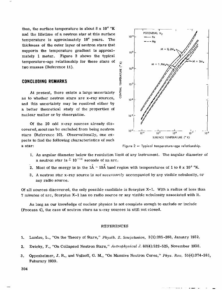
thus, the surface temperature is about 8 x lo6 OK and the lifetime of a neutron star at this surface temperature is approximately io4 years. The thiclmess of the outer layer of neutron stars that supports the temperature gradient is approxi- mately 1 meter. Figure 2 shows the typical temperature-age relationship for these stars of two masses (Reference 11).
CONCLUDING REMARKS
A t present, there exists a large uncertainty as to whether neutron stars a r e x-ray sources, and this uncertainty may be resolved either by a better theoretical study of the properties of nuclear matter or by obserxation.
Of the 20 odd x-ray sources already dis- covered, most can be excluded from being neutron stars (Reference 10). Observationally, one ex- pects to find the following characterist ics of such a star:
104: -, I - . - i o 4 lo5 106 i o
SURFACE TEMPERATURE (" K)
F i g u r e 2 - T y p i c a l tempera ture -age r e l a t i o n s h i p .
I
1. An angular diameter below the resolution l imit of any instrument. The angular diameter of a neutron star is 2 lo-'' seconds of an a rc .
2. Most of the energy is in the 1A - 10A band region with temperatures of 1 to 8 x lo6 OK.
3. A neutron star x-ray source is not necessarily accompanied by any visible nebulosity, o r any radio source.
0 0
Of all sources discovered, the only possible candidate is Scorpius X-1. With a radius of less than 7 minutes of arc, Scorpius X-1 has no radio source or any visible nebulosity associated with it.
As long as our knowledge of nuclear physics is not complete enough to exclude or include (Process 4), the case of neutron stars as x-ray sources is still not closed.
REFERENCES
1. Landau, L., "On the Theory of Stars," Physik. Z . Sowjetunion, 3(1):285-288, January 1932.
2. Zwicky, F., "On Collapsed Neutron Stars," Astrofihysical J. 88(4):522-525, November 1938.
3. Oppenheimer, J. R., and Volkoff, G. M., "On Massive Neutron Cores," Phys. Rev. 55(4):374-381, Feburary 193 9.
304

4. Chiu, H. Y., "Supernovae, Neutrinos and Neutron Stars," Annals of Physics, 26(3):364-410, February 1964.
5. Colgate, S. A., and Johnson, M. H., "Hydrodynamic Origin of Cosmic Rays," Phys. Rev. Letters, 5(6):235-238, September 1960.
6. Chiu, H. Y., and Salpeter, E. E., "Surface X-ray Emission from Neutron Stars," Phys. Rev. Letters, 12(15):413-415, April 1964.
7. Bahcall, J. N., and Wolf, R. A., "Neutron Stars," Phys. Rev. Letters, 14(10):343-346, March 1965.
8. Morton, D., "Neutron Stars as X-ray Sources," Nature, 201(4926): 1308-1309, March 1964.
9. Morton, D. C., "Neutron Stars as X-ray Sources,'' Astrophysical J. 140(2):460-469, August 1964.
10. Finzi, A., "Cooling of a Neutron Star by the 'URCA' Process," Phys. Rev. 137(2B):B472, January 1965.
11. Cameron, A.',G. W. and Tsuruta, S., Private communication.
NASA-Langley, 1966 G-677- 3
\
305
-

“The aeronautical and space activities of the United States shall be conducted so as to contribute . . . to the expansion of human knowl- edge of phenomena in the atmosphere and space. The Administration shall provide for the widest practicable and appropriate dissemination of information concerning its activities and the results thereof .”
-NATIONAL AERONAUnCS AND SPACE ACT OF 1958
NASA SCIENTIFIC AND TECHNICAL PUBLICATIONS
TECHNICAL REPORTS: Scientific and technical information considered important, complete, and a lasting contribution to existing knowledge.
TECHNICAL NOTES: Information less broad in scope but nevertheless of importance as a contribution to existing knowledge.
TECHNICAL MEMORANDUMS: tion because of preliminary data, security classification, or other reasons.
CONTRACTOR REPORTS Technical information generated in connection with a NASA contract or grant and released under NASA auspices.
TECHNICAL. TRANSLATIONS: Information published in a foreign language considered to merit NASA distribution in English.
SPECIAL PUBLICATIONS: Information derived from or of value to NASA activities. Publications include conference proceedings, monographs, data compilations, handbooks, sourcebooks, and special bibliographies.
TECHNOLOGY UTILIZATION PUBLICATIONS: Information on tech- nology used by NASA that may be of particular interest in commercial and other nonaerospace applications. Publications include Tech Briefs; Technology Utilization Reports and Notes; and Technology Surveys.
Information receiving limited distribu-
Details on the availability of these publications may be obtained from:
SCIENTIFIC AND TECHNICAL INFORMATION DIVISION
NATIONAL AERONAUTICS AND SPACE ADMINISTRATION
Washington, D.C. PO546