ORIGINAL ARTICLE

doi:10.1111/j.1558-5646.2012.01591.x

GLOBAL PATTERNS OF LEAF DEFENSESIN OAK SPECIESIan S. Pearse1,2 and Andrew L. Hipp3,4

1Department of Entomology, UC Davis, Davis, California 956162E-mail: ispearse@ucdavis.edu

3The Morton Arboretum, Lisle, Illinois 605324Department of Botany, The Field Museum of Natural History, Chicago, Illinois 60605

Received May 24, 2011

Accepted January 17, 2012

Data Archived: Dryad doi:10.5061/dryad.336n3gt0

Plant defensive traits drive patterns of herbivory and herbivore diversity among plant species. Over the past 30 years, several

prominent hypotheses have predicted the association of plant defenses with particular abiotic environments or geographic regions.

We used a strongly supported phylogeny of oaks to test whether defensive traits of 56 oak species are associated with particular

components of their climatic niche. Climate predicted both the chemical leaf defenses and the physical leaf defenses of oaks,

whether analyzed separately or in combination. Oak leaf defenses were higher at lower latitudes, and this latitudinal gradient

could be explained entirely by climate. Using phylogenetic regression methods, we found that plant defenses tended to be greater

in oak species that occur in regions with low temperature seasonality, mild winters, and low minimum precipitation, and that

plant defenses may track the abiotic environment slowly over macroevolutionary time. The pattern of association we observed

between oak leaf traits and abiotic environments was consistent with a combination of a seasonality gradient, which may relate

to different herbivore pressures, and the resource availability hypothesis, which posits that herbivores exert greater selection on

plants in resource-limited abiotic environments.

KEY WORDS: Biogeography, latitude, macroevolution, Ornstein–Uhlenbeck model, plant–insect interaction, tannins.

Plant defenses drive plants’ associations with herbivores. Plants

with certain life-history traits (such as trees) or habitat affilia-

tions (such as desert plants) often invest more in defenses than

other plants, and it has been the goal of several major theories

of plant defense to understand these correlations (described in

Stamp 2003). The defensive traits that a plant possesses today

are a result of both its evolutionary heritage—the traits and con-

straints it inherited—and more recent adaptation of that plant

species to its biotic and abiotic environment (Gould and Lewontin

1979; Agrawal 2007). Some comparative studies between plant

species have stressed the importance of deep evolutionary history

in driving plant–herbivore interactions (e.g., Mitter et al. 1991;

Weiblen et al. 2006). Others have stressed local adaptation (which

implies rapid evolution of defenses in environments where they

convey a fitness benefit to the plant) (e.g., Fine et al. 2004; Kursar

et al. 2009). Of course, the deep and recent impacts of history

on any adaptive trait are not mutually exclusive (Futuyma and

Agrawal 2009 and papers therein). Modern phylogenetic compar-

ative approaches, such as phylogenetic least-squares methods and

Ornstein–Uhlenbeck (O-U) modeling, allow us to begin to tease

apart the effects of evolutionary history and natural selection in

the evolution of plant defenses.

Selection pressures imposed by different habitat types or

climatic associations are thought to be a major driver of a plant’s

defensive investment (Stamp 2003). For example, studies have

found substantial variation in plant defenses between nutrient-

poor and nutrient-rich habitats as well as between temperate and

tropical regions (Coley and Barone 1996; Fine et al. 2006). One

1C© 2012 The Author(s).Evolution

I . S . PEARSE AND A. L. HIPP

long-standing hypothesis suggests that plant defensive investment

should be greater in regions closer to the equator (Coley and

Barone 1996; Schemske et al. 2009), as biotic interactions such

as herbivory are thought to be stronger in tropical regions near the

equator. This hypothesis has recently been challenged, as some

individual studies find a latitudinal gradient in plant defenses (e.g.,

Rasmann and Agrawal 2011), but larger meta-analyses find no

clear latitudinal gradient (Johnson and Rasmann 2011; Moles et al.

2011). To more carefully approach the geographic variation in

plant defenses, it is necessary to understand the selection pressures

that drive plant defenses.

Optimal defense theory provides expectations of how nat-

ural selection should shape plant defenses (Rhoades and Cates

1976; Stamp 2003). Most simply, plants should invest more in

defenses when the fitness costs of defense are outweighed by the

benefits of reduced herbivory. The benefits of reduced herbivory,

however, are complex: the benefit of defense will be greater to

the plant, (1) the more damage is decreased by the defense, such

as when herbivore pressure is high, and (2) the greater the fitness

loss to the plant is per unit tissue lost, that is, for plants with less

tolerance of herbivory. Theories that predict a plant’s investment

in defense resulting from its habitat affiliation focus on variation

in both of these areas: herbivore pressure and plant tolerance to

herbivory. Coley’s (1985) resource availability hypothesis (RAH)

is the most prominent explanation of abiotic selection pressures

shaping plant defenses, and it uses plant tolerance to herbivory to

explain defensive investment. The RAH states that plant species

that evolve under resource limitation will tend to limit herbivory

through a greater investment in general (and energetically expen-

sive) defenses against herbivores, as resource limitation makes it

costly for the plant to replace tissues lost to herbivory. The RAH

thus uses the plant’s resource budget to predict the evolution-

ary origins of plant defenses and has received substantial support

from studies that compare defensive investment across plants in

resource-rich and resource-poor environments (Coley 1983; Fine

et al. 2006).

Plants in different regions almost certainly experience differ-

ent herbivore pressures, and this side of optimal defense theory has

received less attention recently. For example, herbivore pressure

may be a function of the persistence of plant resources, as plants

with year-round leaves or other resources accrue higher herbivore

loads than plants with a deciduous habit (Karban 2007). At a

broader scale, tropical areas have greater herbivore diversity than

temperate zones, and herbivore species richness has increased

dramatically during periods of global warming throughout Earth’s

history (Coley and Barone 1996; Schemske et al. 2009; Currano

et al. 2010). There is currently debate over whether the greater

diversity of herbivores found in the tropics translates into greater

herbivore pressure for plants (Moles et al. 2011). Herbivore pres-

sure likely varies between habitats, and plants in regions that

experience high herbivore pressure should invest in defenses to

maximize their fitness.

Almost all plant traits that affect herbivory also likely have

other physiological functions (Seigler and Price 1976), so an al-

ternative hypothesis might be that traits linked to herbivore resis-

tance also ameliorate the abiotic environment. Some authors have

suggested that structural plant defenses or phenological avoid-

ance of herbivores have a greater pleiotropic effect than more

herbivore-specific chemical defenses (Carmona et al. 2011). For

example, specific leaf area (SLA) (a physical leaf trait) relates di-

rectly to water use in plants (Knight et al. 2006), but the silencing

of drought-stress pathways in tomato plants had little effect on a

suite of chemical markers of plant defense (Thaler and Bostock

2004).

In this study, we examine the evolutionary history of oaks

(Quercus) and use that phylogeny to investigate how the evolution

of a suite of nine defensive traits correlates with various dimen-

sions of the climatic environment and latitude. An index of these

same traits has independently been shown to reduce the fitness of

a generalist herbivore on oaks (Pearse 2011), and many other stud-

ies support the importance of these traits as leaf defenses against

other herbivores (detailed in section Methods). Our hypothesis is

that leaf defensive traits will evolve more readily in more stressful

environments, as predicted by the resource-availability hypothe-

sis, and in areas with less climatic seasonality, which may corre-

spond with greater herbivore pressure. By comparing information

on the defensive traits, abiotic (climatic) environment, and evolu-

tionary history of oak species, we can begin to assess the relative

importance of optimal defense theories (such as the RAH and

theories that predict higher defense in regions of higher herbivore

persistence) as well as nonoptimal explanations for defensive in-

vestment (such as pleiotropy and evolutionary conservatism) at a

global scale in oaks.

MethodsOAK TAXA AND ASSESSMENT OF PLANT TRAITS

Oaks provide an ideal group of plants to assess global patterns

of defensive traits for several reasons. In oaks, the relationship

between putative defensive traits and actual vulnerability to insect

herbivory is well understood. Pearse (2011) found that indices

of leaf defenses similar to those assayed in the current study

predicted tussock moth caterpillar survival rates on 27 oak species.

Moreover, the effectiveness of traits such as tannins (Feeny 1970;

Forkner et al. 2004), leaf phenology (Karban 2007), and trichomes

(Kitamura et al. 2007) as defenses against herbivores has been

substantiated to varying degrees in oaks. Also, oaks are commonly

planted in arboreta, which represent quasicommon gardens in

which the genetic component of plant traits can be separated from

plasticity.

2 EVOLUTION 2012

GLOBAL PATTERNS OF LEAF DEFENSES IN OAK SPECIES

In the current study, we sample 56 oak taxa, representing

each of the five major oak clades (Manos et al. 1999; Pearse

and Hipp 2009), including representatives from eastern North

America, western North America, Mexico, Europe, and Asia.

Species were selected based on their presence in a 40-year old

stand of oaks at University of California, Davis Arboretum. While

this sample represents less than 15% of the entire genus, it rep-

resents a broad spectrum of the phylogenetic, geographic, and

ecological diversity of the genus. Each taxon was represented

by three individuals except in cases where fewer were present

in the arboretum (Pearse and Hipp 2009). Nomenclature follows

the Oaks Names Database (Trehane 2007). Leaf traits were taken

from previous studies on these same trees (Pearse and Hipp 2009;

Pearse and Baty 2012).

To assess the relationship between defensive traits and en-

vironment, leaf defensive traits were assembled into three de-

fensive indices using principal component analysis (PCA) to de-

rive a chemical traits defensiveness index (DICHEM) composed of

five traits: phenolics, condensed tannins, summer tannins, perox-

idase (POX), and proteins; a physical traits defensiveness index

(DIPHYS) composed of four traits: leaf toughness, SLA, trichome

density on the upper leaf surface, and trichome density on the

lower leaf surface; and an all-traits index (DIALL) composed of all

nine traits. For all three defensiveness indices, we used the first

and second PC. PC1 extracts 33%, 54%, and 42% of the total trait

variance in DIALL, DIPHYS, and DICHEM, respectively. In prelimi-

nary analyses, we found no association between PC2 of DIALL or

DIPHYS and any environmental predictors, so these are not shown.

Preliminary analyses using PC2 of the DICHEM suggested that

this axis (extracting 29% of the variation in DICHEM) showed co-

variation with environmental predictors. These four defensiveness

indices are our primary response variables in the models evaluated

in this study (details under “Comparative methods” below).

ESTIMATION OF CLIMATIC VARIABLES

Oaks occur on every major landmass in the Northern Hemisphere,

so transitions between different habitat types have likely occurred

independently from one another (Manos et al. 1999). Moreover,

niche convergence is well known within oaks, such that each of

the major oak clades has undergone many of the same habitat

transitions (Cavender-Bares et al. 2004). The ranges of most oak

species have been well documented in forestry and herbarium

records, enabling quantitative assessment of climatic niches for

each species in this study by associating fine-scale climatic data

(Hijmans et al. 2005) with numerous herbarium and observational

records for each species.

Herbarium and forestry records of oaks were taken from three

different sources: the Global Biodiversity Information Founda-

tion (GBIF; http://data.gbif.org), the Consortium of California

Herbaria (ucjeps.berkeley.edu/consortium/), and herbarium

sheets housed in the Field Museum Herbarium (F). Erroneous

records were culled from the dataset based on the following crite-

ria. Taxonomically uncertain records were removed, using nomen-

clatural stability according to the Oak Names Database as the

criterion (Trehane 2007). Records that lacked georeferenced co-

ordinates were georeferenced manually when descriptions with

locality information could be confirmed within 5 km. Urban plant-

ings and arboretum records were removed from the dataset, and

records that fell more than 100 km outside of the established

geographic range based on taxonomic literature (Flora of North

America Editorial Committee 1993; le Hardy de Beaulieu and

Lamant 2007) were removed from the dataset. Climate infor-

mation from the WorldClim database (Hijmans et al. 2005) was

associated with each locality at a resolution of 2.5 arc min (about

4.8 km) using the R packages dismo and raster (Hijmans and

Phillips 2010; Hijmans and van Etten 2010). For each oak species,

the mean of each climatic estimate was calculated across the entire

species range as represented by specimen data above and used for

subsequent analyses. Because this approach does not correct for

spatial autocorrelation, the resulting climatic means are weighted

by collection intensity (Fig. 1A). While intraspecific variation in

both climate and traits bears further investigation in oaks, we find

that species identity explains an average of 44%–85% of total vari-

ance in climatic variables, which supports an earlier study in which

leaf physiological traits show strong among-species variance rel-

ative to within-species variance, even across a strong latitudinal

gradient (Cavender-Bares et al. 2011).

We used eight of the 19 WorldClim climatic measures in

our study, as follows: BIO1, mean annual temperature; BIO4,

temperature seasonality, estimated as the standard deviation of

temperature among months; BIO5, maximum temperature (mean

temperature of the warmest month); BIO6, minimum tempera-

ture (mean temperature of the coldest month); BIO12, mean an-

nual precipitation; BIO13, maximum precipitation, estimated as

the mean precipitation of the wettest month; BIO14, minimum

precipitation of the driest month; and BIO15, precipitation sea-

sonality, estimated as the coefficient of variation in precipitation

across months. We use the italicized abbreviations throughout this

article for sake of readability. The eight climatic predictors were

selected a priori from the 19 provided in WorldClim: the excluded

predictors comprise eight that are quantified by quarter rather than

month and three that are based on climatic ranges rather than ex-

tremes or means, and thus are derived from data already reflected

in the eight we included. We also include mean latitude as a pre-

dictor. Among the nine predictors, six pairs exhibited covariance

of |r| > 0.70.

We dealt with covariation among predictor variables in three

ways: first, we condensed all of the eight climatic variables using

PCA. PC1 of these the environmental predictors accounted for

40% of the variance in all eight predictors. Second, to compare

EVOLUTION 2012 3

I . S . PEARSE AND A. L. HIPP

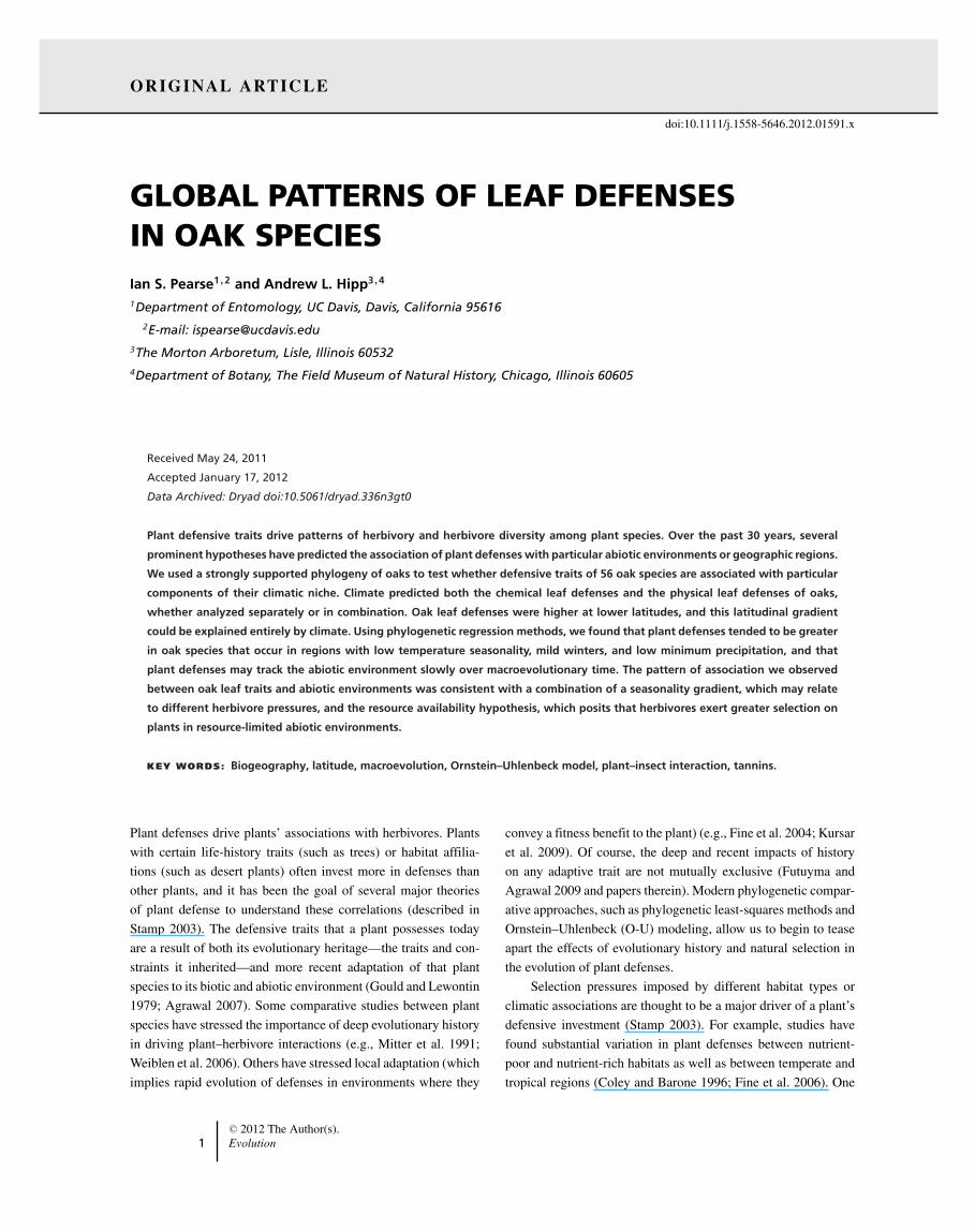
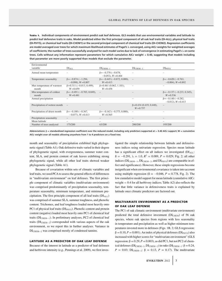
Figure 1. Panel A—a world map, whose background color denotes temperature seasonality (standard deviation of temperature within a

year), and dots represent localities of oak collections used in this study. Dot colors denote the five major subgroups of Quercus. In oaks of

different lineages exit in both seasonal and aseasonal environments multiple times. Panel B—a phylogeny of the 56 oak species used in

this study. Colors of the phylogeny on the left represent an evolutionary reconstruction of a multivariate measure of leaf defenses in oaks.

Colors of the phylogeny on the right represent an evolutionary reconstruction of a PCA ordination of abiotic environment experienced

by oaks, which roughly corresponds to a temperate—tropical/Mediterranean gradient. Estimation of either defense or environment at

deep nodes is likely inaccurate due to multiple transitions in traits within the phylogeny.

the importance of different aspects of the abiotic environment,

we used an information theoretic modeling approach to evaluate

the importance of predictors across a wide range of plausible pre-

dictor combinations, as described below. Third, we used Akaike

information criterion (AIC) to reduce models to avoid problems

of colinearity.

PHYLOGENY

We reconstructed oak phylogenetic relationships based on the

same oak individuals from which we had gathered leaf trait data,

using minimum evolution on an AFLP dataset (Pearse and Hipp

2009). This phylogeny was topologically identical in most partic-

ulars to a phylogeny estimated using Markov chain Monte Carlo

4 EVOLUTION 2012

GLOBAL PATTERNS OF LEAF DEFENSES IN OAK SPECIES

under an asymmetric binary model. To integrate over phylogenetic

uncertainty, a set of 200 minimum evolution bootstrap trees was

used for most analyses presented in this article. Because of the

tendency for AFLP phylogenies to exhibit long terminal branches,

we pruned each bootstrap tree back to the most recent common

ancestor for each species that possessed at least two individuals

per tip. For species with only a single exemplar per tip, tips were

pruned to 50% of their original length. Each resulting tree was

ultrametricized using penalized likelihood with the smoothing pa-

rameter set at 0.1 (Sanderson 2002), and the resulting trees pruned

to include only the taxa for which we could assess leaf traits and

geographic ranges.

PHYLOGENETIC COMPARATIVE METHODS:

OVERVIEW

We present two types of phylogenetic comparative analyses in this

study: generalized least-squares phylogenetic regression models

that assess the relationship between plant traits and environmental

associations and O-U models that specifically model the contri-

bution of phylogenetic inertia and trait adaptation. All variables

throughout the article were rescaled by the standard deviation

of the sample, so regression coefficients reported here are in

estimated-standard deviation units.

PHYLOGENETIC COMPARATIVE METHODS 1.1:

MULTIVARIATE MEASURES OF ENVIRONMENT

AND LATITUDE PREDICTING LEAF DEFENSIVE

INVESTMENT

As an estimate of the combined effects of latitude and climate on

defensive leaf traits in oaks, we used a generalized least squares

(GLS) framework to assess the influence of a multivariate estimate

of environment (PC1 of WorldClim variables) and latitude on a

multivariate estimate of plant defenses (DIALL). We ran these GLS

regressions both in a simple regression and multiple regression

frameworks.

PHYLOGENETIC COMPARATIVE METHODS 1.2:

INDIVIDUAL COMPONENTS OF THE ENVIRONMENT

PREDICTING PARTICULAR LEAF TRAITS

We used an information theoretic approach to estimate the rel-

ative importance of each of the nine potential predictors in ex-

plaining the variance in our three defensive traits indices. First,

we analyzed all possible regression models of 1–4 predictors for

each of the three indices, a total of 255 models for each index.

We corrected for phylogeny using GLS on the minimum evolu-

tion estimate of the optimal phylogenetic tree and calculated the

small-sample AICc weight for each GLS regression. Relative im-

portance of each climatic variable in predicting trait variance was

estimated as the sum of AICc weights for models possessing that

climatic variable. Model weights sum to 1.0 for each analysis,

and all parameters occur in the same number of models, accord-

ing to each parameter equal prior weight and integrating our esti-

mates of parameter importance over model uncertainty (Burnham

and Anderson 2002; cf. discussions in Hipp et al. 2007). From

this analysis (Table A2), we identified those predictors that have

≥ 0.40 evidential support.

In this analysis, we report the R2 for the best-fit model (as-

sessed using AICc weight). Note that while these GLS R2 values

may be interpreted as the total variance explained in the response

variable by the system of predictors, partial r2 values from a GLS

analysis are not readily interpreted and consequently not pre-

sented in this study (Lavin et al. 2008). The R2 are provided from

a single model for purposes of comparison, but we make no at-

tempt in this article to select a single best model or set of models,

as the 95% confidence set of models (estimated using cumulative

reverse-sorted AICc weights on the single minimum evolution

tree [Burnham and Anderson 2002] included 87–208 models for

each response variable (Table A2), with no model receiving more

than 0.105 AICc weight, and all potential predictors appear in at

least one of the models in the confidence set. Rather, our analyses

emphasize the relative importance of the potential predictors in

predicting leaf traits and model-averaged estimates of the effect

strength and direction based on model averaging.

PHYLOGENETIC COMPARATIVE METHODS 1.3:

INDIVIDUAL COMPONENTS OF THE ENVIRONMENT

PREDICTING LEAF DEFENSIVE INVESTMENT

We estimated regression coefficients model averaged over the 255

models for each leaf defensiveness index as well as for each of

the individual leaf traits that contribute to these indices. However,

these regressions condition on a single phylogeny and a Brown-

ian motion model of character evolution, and they include models

that are highly parameter rich in comparison to the size of our

dataset (the largest models include 11 free parameters). Incorrect

phylogeny point estimates, incorrect modeling of the relationship

between branch lengths and trait covariance, and model overpa-

rameterization all have the potential to increase the variance of

parameter estimates (Revell 2010). Consequently, we performed a

second set of analyses aimed at estimating regression coefficients

more precisely. To reduce model complexity, we included in this

analysis only the environmental predictors that were supported

at AICc weights ≥ 0.40 (see Comparative Methods 1 above),

for a maximum of 3–4 predictors for each defensiveness index.

To integrate over phylogenetic uncertainty, each set of regression

models was conducted in a GLS framework over 200 phyloge-

netic trees subsampled from our bootstrap phylogenetic analysis,

with the covariance matrix separately for each tree. Finally, to

relax the assumption that traits evolve according to a Brownian

motion process, the covariance matrix for each model on each tree

was rescaled using Pagel’s λ, a scalar by which all off-diagonal

EVOLUTION 2012 5

I . S . PEARSE AND A. L. HIPP

elements of the covariance matrix are multiplied (Pagel 1999).

All model parameters, including λ and the regression coefficients,

were optimized simultaneously using maximum likelihood in the

gls function of the nlme package in R (Pinheiro et al. 2009). In

this context, λ estimates the phylogenetic signal in the regression

residuals, and rescaling by λ has been found to minimize the

variance of GLS regression coefficients (Revell 2010). Parameter

estimates are presented as means over the bootstrap sample, with

a 95% phylogenetic uncertainty interval on the bootstrap sample

calculated by percentile (empirical).

PHYLOGENETIC COMPARATIVE METHODS 2:

MODELING THE EVOLUTION OF OAK TRAITS AS A

PRODUCT OF BOTH PHYLOGENETIC INERTIA

AND ADAPTATION

It has been noted that the Brownian motion model of character

evolution underlying phylogenetic GLS and phylogenetic inde-

pendent contrasts is a poor model for studying the effects of

natural selection on character evolution, and that an O-U process

more accurately describes the history of traits evolving by nat-

ural selection (Felsenstein 1985; Hansen 1997; Butler and King

2004). Unlike a Brownian motion model, in which trait evolu-

tion is treated as a purely stochastic process, O-U models treat

trait evolution as a result of effectively stochastic evolutionary

processes (e.g., genetic drift or adaptation to a randomly shift-

ing optimum) as well as a deterministic process (e.g., adaptation

to a modeled optimum). In this article, we use Hansen et al.’s

(2008) extension of the O-U model as implemented in SLOUCH

(Hansen et al. 2008), in which the evolution of the predictors (in

our case, variables describing the abiotic environment) is modeled

according to a Brownian process, while the evolution of the traits

(in our case, the all-traits leaf defensiveness index) is modeled

according to an O-U process that tracks an optimum determined

by the predictors. The model is represented by coupled stochastic

differential equations:

dy = −α(y − θ(X ))dt + σydWy, (1)

d X = σx dWx (2)

(Hansen et al. 2008), where y is the response (in our case,

leaf trait or index), X is the system of predictors, θ is the evolu-

tionary optimum of y, and α is the rate of adaptation of y toward θ.

Equation 2 models the evolution of the environmental predictors

according to a multivariate Brownian motion process. Equation

1 models the evolution of the dependent trait, which is taken as

evolving toward an optimum θ that is a function of the environ-

mental predictors, with a rate that is determined by the inherent

rate of adaptation (α) and the distance between the trait value and

its optimum. The “phylogenetic half-life” (Hansen 1997; Hansen

et al. 2008)—the expected time (expressed in the same units that

the tree is scaled to) for a trait to evolve halfway from its ancestral

state to it optimum—is a direct function of the rate of adaptation:

t1/2 = ln(2)/α. At equilibrium, when the dependent trait is fully

adapted to the optimum determined by the predictors in the model,

the residual trait variance is estimated as vy = σy2/2α. The O-U

process is sometimes referred to a “rubber band” process (Hansen

and Martins 1996; Martins et al. 2002) because the rate of evo-

lution toward a trait optimum is a function of the distance of the

trait from that optimum; in other words, natural selection “pulls”

harder on traits that are far from their optimum. Phylogenetic re-

gression parameters, in this case, are equivalent to phylogenetic

GLS regression parameters, and are obtained by multiplying the

coefficients of the optimal regression by a phylogenetic correc-

tion factor ρ (αt) = (1 − (1 − e−αt)/αt), which approaches a limit

of 0 if there is no phylogenetic inertia (i.e., as α goes to ∞) and

1 if there is no effect of adaptation (i.e., as α goes to 0; Hansen

et al. 2008). It is worth noting here that phylogenetic inertia here

denotes “a resistance to or slowness in the adaptation to a specific

optimum,” as contrasted with phylogenetic signal as “any sta-

tistical influence of phylogeny on the trait” (Hansen et al. 1996,

2008). The all-traits defensiveness index was modeled as evolving

in five multivariate environments, chosen for the importance of

their parameters in GLS models: BIO4, BIO4 + BIO5, BIO4 +BIO6, BIO4 + BIO5 + BIO6, and BIO4 + BIO5 + BIO6 +BIO14 (Table 2). For computational reasons, all analyses were

performed on the single best minimum evolution estimate of the

phylogeny. Model coefficients are reported ± standard errors as

estimated using GLS. Confidence intervals around t1/2 and vy

were estimated by plotting the joint likelihood surface from the

maximum likelihood value to two log-likelihood units below the

maximum likelihood value. All parameter estimates are reported

for the separate models evaluated as well as model averaged over

all five models.

All statistical analyses presented in this study were conducted

in R packages APE, NLME, OUCH, VEGAN, and SLOUCH

(Paradis et al. 2004; Hansen et al. 2008; R Core Development

Team 2008; Oksanen et al. 2009; Pinheiro et al. 2009). Trait data

are archived in Dryad (Accession # ___), and phylogenetic data

in TreeBase (S10065).

ResultsDESCRIPTION OF OAK BIOGEOGRAPHY, HABITAT

ASSOCIATION, AND LEAF TRAITS

Oak taxa are separated into the taxonomically defined oak sec-

tions of white oaks (nearctic and paleartic), red oaks (nearctic),

intermediate oaks (nearctic), Cerris “black” oaks (palearctic), and

the Cyclobalanopsis group (palearctic) (Fig. 1A, B, Manos et al.

1999). Climatic variables except for temperature of the hottest

6 EVOLUTION 2012

GLOBAL PATTERNS OF LEAF DEFENSES IN OAK SPECIES

Table 1. Individual components of environment predict oak leaf defenses. GLS models that use environmental variables and latitude to

predict leaf defensive traits in oaks. Model predicted either the first principal component of all oak leaf traits (DI-ALL), physical leaf traits

(DI-PHYS), or chemical leaf traits (DI-CHEM1) or the second principal component of chemical leaf traits (DI-CHEM2). Regression coefficients

are model averaged over trees for which maximum likelihood estimates of Pagel’s λ converged, using AICc weights for weighted averages

of coefficients; the number of trees successfully analyzed for each model varies due to lack of convergence in estimating Pagel’s λ on some

trees. Cells without any information represent parameters for which cumulative AICc weight < 0.40, suggesting that models including

that parameter are more poorly supported than models that exclude the parameter.

Environmentalvariable DIALL DICHEM−1 DICHEM−2 DIPHYS

Annual mean temperature – β=−0.378 (−0.678,−0.052), W=0.404

– –

Temperature seasonality β=−0.874 (−1.294,−0.098), W=0.807

β=−0.445 (−0.872, 0.000),W=0.413

– β=−0.620 (−0.763,−0.004), W=0.892

Max temperature of warmestmonth

β=0.311 (−0.013, 0.499),W=0.659

β=0.461 (0.062, 1.101),W=0.458

– –

Min temperature of coldestmonth

β=−0.491 (−0.703, 0.049),W=0.481

– – β=−0.137 (−0.233, 0.345),W=0.536

Annual precipitation – – – β=−0.140 (−0.282,−0.012), W=0.413

Precipitation of wettest month – – β=0.434 (0.419, 0.448),W=0.757

–

Precipitation of driest month β=−0.180 (−0.367,−0.077), W=0.413

β=−0.162 (−0.375, 0.000),W=0.565

– –

Precipitation seasonality – – – –Mean latitude – – – –Number of trees analyzed 175/200 63/200 200/200 195/200

Abbreviations: β = standardized regression coefficient over the reduced model, including only predictors supported at > 0.40 AICc support; W = cumulative

AICc weight over all models allowing anywhere from 1 to 4 predictors on a fixed tree.

month and seasonality of precipitation exhibited high phyloge-

netic signal (Table A1). Oak defensive traits varied in their degree

of phylogenetic signal, with evergreenness, summer water con-

tent, SLA, and protein content of oak leaves exhibiting strong

phylogenetic signal, while all other leaf traits showed weaker

phylogenetic signal (Table A1).

Because of covariation within sets of climatic variables and

leaf traits, we used PCA to assess the general effects of differences

in “multivariate environment” on leaf defenses. The first princi-

ple component of climatic variables (multivariate environment)

was comprised predominantly of precipitation seasonality, tem-

perature seasonality, minimum temperature, and minimum pre-

cipitation. The first principle component of all leaf traits (DIALL)

was comprised of summer SLA, summer toughness, and phenolic

content. Trichomes, and leaf toughness loaded most heavily onto

PC1 of physical leaf traits (DIPHYS). Phenolic content and protein

content (negative) loaded most heavily onto PC1 of chemical leaf

traits (DICHEM−1). In preliminary analyses, PC2 of chemical leaf

traits (DICHEM−2) corresponded with various aspects of the oak

environment, so we report this in further analyses. Variance in

DICHEM−2 was comprised mostly of condensed tannins.

LATITUDE AS A PREDICTOR OF OAK LEAF DEFENSE

Because of the interest in latitude as a predictor of leaf defenses

and herbivore intensity (e.g., Pennings et al. 2009), we first inves-

tigated the simple relationship between latitude and defensive-

ness indices using univariate regression. Species mean latitude

has a significant effect on all indices we investigated (DIALL:

ß = −0.291, λ = 1.0, R2 = 0.089, P = 0.029, Fig. 2; all other

indices (DICHEM−1, DICHEM−2, and DIPHYS) are comparable in ef-

fect and significance). However, these simple regressions become

insignificant when environmental covariance is taken into account

using multiple regression (ß = −0.046, P = 0.778, Fig. 2). The

low cumulative model support for mean latitude (cumulative AICc

weight < 0.4 for all herbivory indices; Table A2) also reflects the

fact that little variance in defensiveness traits is explained by

latitude once climatic predictors are factored out.

MULTIVARIATE ENVIRONMENT AS A PREDICTOR

OF OAK LEAF DEFENSE

The PC1 of oak climatic environment (multivariate environment)

predicted the total defensive investment (DICHEM) of 56 oak

species, where oak species from regions with less seasonality

in temperature and precipitation as well as higher minimum tem-

peratures invested more in defenses (Figs. 1B, 2; GLS regression:

β = 0.10, P = 0.001). An index of physical defenses (DIPHYS) also

increased with higher scores for “multivariate environment” (GLS

regression: β= 0.29, P = 0.003), as did PC1, but not PC2 of chem-

ical defenses (DICHEM−1, DICHEM−2) in oaks (DICHEM−1: β= 0.24,

P = 0.03; DICHEM−2: β = 0.13, P = 0.17). The multivariate

EVOLUTION 2012 7

I . S . PEARSE AND A. L. HIPP

Ta

ble

2.

Ran

do

mco

vari

ates

Orn

stei

n–U

hle

nb

eck

(O-U

)m

od

elre

sult

s.Th

era

nd

om

cova

riat

esO

-Um

od

elis

are

gre

ssio

nm

od

elas

imp

lem

ente

din

SLO

UC

H.T

he

resp

on

seva

riab

le

for

allm

od

els

isth

eto

tald

efen

sive

ind

ex(D

Iall)

,an

dth

ep

red

icto

rsfo

rea

chm

od

elar

ein

dic

ated

inth

eco

lum

nh

ead

ers.

For

each

pre

dic

tor,

the

evo

luti

on

ary

reg

ress

ion

coef

fici

ent

(±st

and

ard

erro

r)is

pre

sen

ted

,fo

llow

edb

yth

eo

pti

mal

reg

ress

ion

coef

fici

ent±

stan

dar

der

ror

inp

aren

thes

es.T

he

evo

luti

on

ary

reg

ress

ion

coef

fici

ent

isth

ere

gre

ssio

nco

effi

cien

t

taki

ng

ph

ylo

gen

yin

toac

cou

nt,

wh

ileth

eo

pti

mal

reg

ress

ion

coef

fici

ent

esti

mat

esth

ere

lati

on

ship

bet

wee

nth

ep

red

icto

ran

dre

spo

nse

vari

able

sif

ther

ew

ere

no

tp

hyl

og

enet

ic

iner

tia.

The

adap

tive

hal

f-lif

ees

tim

ates

the

amo

un

to

fti

me

(rel

ativ

eto

atr

eele

ng

tho

f1)

req

uir

edfo

rth

ere

spo

nse

vari

able

toev

olv

eh

alfw

ayto

war

dit

sad

apti

veo

pti

mu

m,a

nd

isp

rese

nte

das

the

bes

tes

tim

ate

follo

wed

by

the

two

log

-lik

elih

oo

d-u

nit

con

fid

ence

inte

rval

.Th

est

atio

nar

yva

rian

ceis

the

esti

mat

edva

rian

cein

trai

tva

lue

afte

rth

etr

ait

evo

lved

fully

toit

so

pti

mu

m;s

tati

on

ary

vari

ance

isal

sop

rese

nte

das

the

max

imu

mlik

elih

oo

des

tim

ated

follo

wed

by

the

two

log

-lik

elih

oo

d-u

nit

con

fid

ence

inte

rval

.

Pred

icto

rs

Tem

pera

ture

Max

tem

p.M

inte

mp

Prec

ipita

tion

Mod

elsu

ppor

tM

odel

para

met

ers

seas

onal

ityw

arm

.mon

thco

ldes

tdr

iest

mon

thO

-Um

odel

ln(L

)A

ICc

AIC

cw

iR

2t 1

/2

v y(B

IO4)

(BIO

5)m

onth

(BIO

6)(B

IO14

)

DI A

LL

∼BIO

4−6

5.12

1713

9.02

780.

0789

0.16

420.

72(0

.14,

>20

)1.

00(0

.46,

>20

)−0

.395

±0.1

19(−

1.10

5±0.

333)

−−

−

DI A

LL

∼BIO

4+B

IO5

−63.

7663

138.

7326

0.09

150.

2243

0.54

(0.0

6,>

20)

0.72

(0.3

6,>

20)

−0.5

42±0

.136

(−1.

241±

0.31

1)0.

218±

0.12

0(0

.498

±0.2

74)

−−

DI A

LL

∼BIO

4+B

IO6

−64.

8696

140.

9392

0.03

040.

1776

0.83

(0.1

5,>

20)

1.00

(0.4

3,>

20)

−0.5

31±0

.191

(−1.

649±

0.59

4)−

−0.1

62±0

.181

(−0.

504±

0.56

1)−

DI A

LL

∼BIO

4+B

IO5+

BIO

6−6

1.02

5013

5.76

440.

4035

0.45

310.

14(0

.10,

0.29

)0.

05(0

.01,

0.69

)−1

.418

±0.2

47(−

1.77

4±0.

309)

0.62

1±0.

147

(0.7

77±0

.184

)−0

.731

±0.2

13(−

0.91

5±0.

266)

−

DI A

LL

∼BIO

4+B

IO5+

BIO

6+B

IO14

−59.

7352

135.

8037

0.39

570.

4683

0.17

(0.1

3,0.

49)

0.09

(0.0

1,0.

65)

−1.2

36±0

.285

(−1.

628±

0.37

6)0.

533±

0.15

9(0

.702

±0.2

10)

−0.6

63±0

.219

(−0.

874±

0.28

9)−0

.163

±0.1

19(−

0.21

5±0.

157)

Mod

elav

erag

ed−

−−

−0.

255

0.23

1−1

.158

(−1.

611)

0.48

1(0

.637

)−0

.562

(−0.

730)

−0.0

64(−

0.08

5)

Ab

bre

viat

ion

s:A

ICc

=sm

all-

sam

ple

Aka

ike

info

rmat

ion

crit

erio

nva

lue;

t 1/2

=ad

apti

veh

alf-

life;

v y=

stat

ion

ary

vari

ance

.

8 EVOLUTION 2012

GLOBAL PATTERNS OF LEAF DEFENSES IN OAK SPECIES

Figure 2. Scatter plots showing an index of leaf defenses (DIALL) plotted against latitude and a multivariate estimation of oak en-

vironment: Solid trend lines indicate a significant (P < 0.05) relationship using phylogenetically controlled GLS in a simple regression

framework; bold dotted lines indicate a significant (P < 0.05) relationship using GLS in a multiple regression framework; small dotted

lines indicate the phylogenetic error around simple regression estimates.

environment remained strongly predictive of total defensive in-

vestment of leaves even when analyzed in conjunction with lati-

tude (multiple regression: (ß = 0.35, P = 0.013, Fig. 2).

COMPONENTS OF THE ABIOTIC ENVIRONMENT

THAT EXPLAIN VARIANCE IN LEAF DEFENSIVE

INVESTMENT

Cumulative AICc weights on generalized linear regression models

estimated on a single phylogenetic tree were used to estimate the

importance of environmental predictors (Tables 1, A2). To obtain

a better estimate of regression coefficients for each environmen-

tal variable, we also reduced the model of climatic variables to

include only those with a cumulative AICc weight > 0.4. Model-

averaged standardized regression coefficients from this reduced

model set were estimated using phylogenetic generalized linear

regression models over 200 bootstrap trees and are our best esti-

mate the relative strength and direction of environmental variables

in predicting leaf defensive indices (Table 1). Each index of de-

fense (DIALL, DICHEM−1, and DIPHYS) decreased as temperature

seasonality increased (Table 1). Cumulative AICc weights indi-

cate that DIALL, DIPHYS, and to a lesser degree DICHEM−1 were

strongly influenced by temperature seasonality (cum. AICc =0.807, 0.892, and 0.413, respectively). DIALL and DICHEM−1 in-

creased as the minimum precipitation decreased (βDIall = −0.180,

βDIchem−1 = −0.162), and influence of minimum precipitation was

stronger for DICHEM−1 than for other indices (cum. AICc = 0.565).

DIALL and DICHEM also increased as the maximum temperature

increased (βDIall = 0.311, βDIchem−1 = 0.461), and the influence

of maximum temperature was stronger for DIALL than for other

indices (cum. AICc = 0.659). DIALL and DIPHYS increased as

the minimum temperature decreased (βDIall = −0.491, βDIphys =−0.137). Maximum precipitation had an effect on the second

component of chemical-traits defenses (DICHEM−2), which was

positively correlated with increasing precipitation (βDIchem−2 =0.434, AICc = 0.757). This response is governed chiefly by

condensed tannins, which respond almost as strongly and with

equal support (β = 0.352, cumulative AICc support = 0.762;

Table A2).

COMPONENTS OF THE ABIOTIC ENVIRONMENT THAT

EXPLAIN VARIANCE IN INDIVIDUAL LEAF TRAITS

For the most part, climatic niche is a poorer predictor of

individual leaf traits than combined leaf traits (see R2 values

in Table A2). Striking exceptions among physical traits are

summer SLA and trichome density on the leaf underside, which

correlated negatively with temperature seasonality (ß = −0.360

and −0.350, respectively; Table A2); summer toughness, which

correlated negatively with annual precipitation (ß = −0.264);

and trichome density on the lower and upper leaf surfaces,

which correlated negatively with mean latitude (ß = −0.299

and −0.302, respectively). Among chemical traits, condensed

tannins and protein content were both greater in habitats higher

maximum precipitation (ßcondensedTannins = 0.352) and minimum

precipitation (ßspringProtein = 0.295; Table A2). All of these

individual trait responses are congruent with the responses in

trait indices (Tables 1, A2).

EVOLUTION 2012 9

I . S . PEARSE AND A. L. HIPP

MODELING THE EVOLUTION OF OAK TRAITS AS A

PRODUCT OF BOTH PHYLOGENETIC INERTIA

AND ADAPTATION

If traits evolved without phylogenetic inertia—that is, if ancestral

trait values had no effect on trait values of current-day samples

except through correlation in selective regimes between ances-

tors and descendents—then the phylogenetic regressions we have

already discussed would be the best estimates of the optimal fit

between traits and their environment. The positive side of this

is that phylogenetic inertia provides us with the data needed to

estimate the rate of adaptation, as divergence from Brownian mo-

tion expectations for trait evolution serve as evidence of causal

correlations between traits and environment (Hansen and Martins

1996; Butler and King 2004). While the model we use in this

article (Hansen et al. 2008) does not partition trait variance into

a phylogenetic component and an adaptive component, it does

provide a direct estimate of the effect of phylogeny on our esti-

mates of regression coefficients by translating the phylogenetic

regression into an estimate of the optimal regression, taking into

account the rate of adaptation (α) and phylogenetic autocorrela-

tion in regression residuals.

Regression coefficients estimated in the two best-supported

O-U models (three- and four-predictor models) closely track the

GLS estimates of regression coefficients (cf. Table 1). These mod-

els included temperature seasonality, maximum temperature, min-

imum temperature, and to a lesser degree minimum precipitation.

The variance across O-U models in the estimate of the optimal

regression coefficient is on average 40.0% lower than the variance

across the same models in the phylogenetic regression coefficient

estimates (Table 2), due to the fact that in the current study, the

estimated rate of adaptation (α) increases as the absolute value

of the coefficient estimate increases. The model-averaged esti-

mates of the optimal regression coefficients are on average 33.6%

greater in magnitude than the model-averaged estimates of the

phylogenetic regression coefficients. Under the model-averaged

estimates of optimal relationships, the magnitude of the tempera-

ture seasonality effect (β = −1.611) is 2.2–2.5× greater than the

magnitude of the effect of maximum temperature (β = 0.637) or

minimum temperature in the coldest month (β = −0.730).

The phylogenetic half-life (t1/2, the amount of time required

for leaf defenses to evolve halfway toward their optimum) ranges

from 0.14 in the three-predictor model to 0.72 in the tempera-

ture seasonality model, where t1/2 is scaled in tree-length units

(Table 2). In the one- and two-predictor models, the two log-

likelihood-unit confidence interval extends to a phylogenetic half-

life greater than 20, which suggests that the no-adaptation hy-

pothesis cannot be rejected for those models. However, the best-

supported models are the three-predictor model (AICc weights =0.404, R2 = 0.453) and four-predictor model (AICc weight =0.396, R2 = 0.468), both of which have a narrow confidence in-

terval around t1/2. Both of these well-supported models and the

model-averaged estimate of t1/2 support an important role for both

phylogenetic signal (t1/2 > 0) and adaptation (t1/2 < ∞, although

any t1/2, i.e., substantially greater than the total tree depth [tree

depth is 1.0 in our study] implies that ancestry dominates trait

values).

DiscussionThe magnitude of leaf antiherbivore defenses in oaks tracks the

abiotic environment of oak species’ habitats (Figs. 1B, 2B). Part

of this variation corresponds to a latitudinal gradient in defense

(Fig 2B), but an additional portion of the variation in leaf de-

fenses is explained by environment alone. This is not the case for

the portion of leaf defenses predicted by latitude, as all of the vari-

ation in leaf defenses explained by latitude can also be explained

by environment (Fig 2A). This suggests that there is a latitudinal

gradient in oak defenses and that this gradient driven predom-

inantly by climatic differences between latitudes. Additionally,

climatic differences irrespective of latitude also influence oak

defenses.

In general, oaks from less seasonal and, to a lesser extent,

drier locations invest more in defenses than oaks from more tem-

perate, wetter environments (Fig. 2; Tables 1, 2). In addition,

after correcting for correlation among climatic predictors, tem-

perature seasonality is the climatic variable most predictive of

oak leaf traits (Tables 1, 2). Other aspects of temperature as well

as the precipitation of the driest month also play a role in the

most predictive models of oak leaf defenses (Tables 1, 2). These

comparative patterns might result from any combination of sev-

eral evolutionary processes (Endler 1982). We assess the relative

contribution of two adaptive hypotheses, the resource-availability

hypothesis and gradients in herbivore pressure, and two nonadap-

tive hypotheses (evolutionary conservatism and pleiotropy) in de-

termining the current association of oak defenses with climatic

environments.

EVOLUTIONARY CONSERVATISM OF LEAF DEFENSES

AND CLIMATIC NICHE

Leaf defenses might correlate with climatic niche without be-

ing adapted to climate if there were only infrequent evolutionary

transitions between different leaf defenses and habitat affiliations.

Modern phylogenetic comparative methods were developed pre-

cisely because nonindependence among species can cause such

spurious correlations to appear significant if phylogeny is not

accounted for (Felsenstein 1985). In oaks, however, the paral-

lel evolution of leaf defenses in different lineages (Fig. 1B) and

the strong support for correlations even assuming strong phylo-

genetic autocorrelation (Tables 1, 2, A2; Fig. 2) suggests that

evolutionary conservatism in leaf traits cannot solely account for

1 0 EVOLUTION 2012

GLOBAL PATTERNS OF LEAF DEFENSES IN OAK SPECIES

the association of leaf defenses with particular habitats. Nonethe-

less, groups of extant species tend to have similar leaf defenses

and abicotic habitats (Fig. 1B), and the strong phylogenetic sig-

nal in the residuals of traits regressed on their environmental

predictors suggests that evolutionary conservatism explains a sig-

nificant component of the variance in trait values. The phyloge-

netic lag time suggested by the stochastic linear O-U analyses

(Table 2) along with the significant contribution of rate of adap-

tation as a model parameter suggests that both adaptation and

phylogenetic inertia contribute to the observed interspecific trait

variance.

Similarly, rare, geographically isolated events may drive

current patterns in plant defense. For example, kelps that are

found along the coast of North America consistently have lower

concentrations of phlorotannins and experience less herbivory

than kelps from the coast of Australia, a trend that has been

attributed to top-down limitation of kelp herbivores by sea ot-

ters in North America but not in Australia (Steinberg et al.

1995). We might, then, see a spurious correlation between cli-

matic niche and leaf defenses if oaks had made few transitions

among habitats and levels of herbivore defenses. Oaks, how-

ever, exhibit parallel responses to climatic transitions in multiple

places over multiple continents (Fig. 1A, B) and parallel adapta-

tions to various aspects of their abiotic environment (Cavender-

Bares et al. 2004). It is consequently unlikely that a geographi-

cally isolated event determined the multiple occurrences of plant

defenses.

PLEIOTROPY OF PLANT DEFENSIVE TRAITS AS

TRAITS THAT AMELIORATE HARSH ENVIRONMENTS

A second hypothesis is that leaf traits that confer defense against

herbivores may also ameliorate harsh environments; the corre-

lation between leaf traits and climatic niche, then, might have

nothing to do with herbivore pressure. In any comparative or

correlative study it is impossible to eliminate the possibility of

pleiotropy driving the observed patterns, and that is true here.

Many leaf traits that have been implicated in antiherbivory de-

fense have also been implicated in conveying drought-, ultravi-

olet (UV)-, or heat-tolerance in plants. Flavonoid compounds (a

class of phenolics) protect corn from UV radiation (Stapleton and

Walbot 1994). Similarly, trichomes protect photosynthetically ac-

tive portions of leaves of Q. ilex from UV radiation (Skaltsa et al.

1994). In a common garden of cork oaks (Q. suber) collected from

across Spain, low SLA was associated with drought-tolerant pop-

ulations, and trees showed plasticity in SLA such that SLA was

higher in wetter years (Ramirez-Valiente et al. 2010). Trichomes

may also reduce water loss and contribute to drought tolerance

(Espigares and Peco 1995).

In this study, temperature seasonality has approximately

twice as much effect (estimated by beta coefficients) on the com-

bined defensiveness index (DIALL) as maximum temperature and

minimum temperature in the most extreme months and 5–18 times

the effect of drought intensity (Tables 1, 2). This suggests that

heat-, freezing-, or drought-tolerance alone is not driving the evo-

lution of traits we studied. Rather, the effects of seasonality on

insect intensity or resource limitation have stronger effects on the

evolution of herbivore-resistance traits (Coley et al. 1985; Coley

and Barone 1996; Karban 2007).

RESOURCE LIMITATION SELECTS FOR GREATER

INVESTMENT IN DEFENSIVE TRAITS

The third hypothesis is the RAH (Coley et al. 1985), which ar-

gues that selection for defensive leaf traits should be stronger in

resource-poor environments, as the cost of herbivory is greater for

plants in environments where leaf construction costs are higher.

Our most strongly supported predictor of leaf defensive traits,

temperature seasonality, does not represent an obvious gradient

in resource availability for plants. Along gradients of temperature

and precipitation, however, leaf defensive traits respond in the

direction expected under the RAH. Along the precipitation gra-

dient, physical and chemical leaf defenses increase as minimum

precipitation decreases (i.e., in environments that pose the greatest

drought stress; Tables 1, 2, A2). Likewise, the one chemical trait

that is expected to favor herbivory (leaf protein content) increased

marginally with increasing precipitation in the driest month (ß =0.2950, cumulative AICc weight = 0.6325; Table A2). This is

compatible with the RAH, as water is often a limiting resource

for plants (Shields 1950). Similarly, along temperature gradients,

allocation to leaf defenses increased marginally as minimum

temperature decreases and as maximum temperature increases

(Tables 1, 2, A2). This suggests that temperature extremes select

for increased allocation to leaf defenses, which is also compatible

with the RAH. These dimensions of oaks’ abiotic niche are likely

to affect insect density (discussed below) as well as tree growth,

suggesting that it may be difficult to separate the effects of climate

on insect density from selective gradients on herbivore defenses

that accord with the RAH.

SEASONALITY DRIVES PLANT DEFENSES

In this study, we found that oak defenses were higher in regions

with low seasonality (Tables 1, 2; Fig. 2). Indeed, temperature

seasonality was the most consistent predictor of oak traits and

defense indices in our dataset (Tables 1, 2, A2; Fig. 2). One po-

tential explanation for a greater defensive investment in less sea-

sonal areas would be if there were greater herbivore pressure in

less seasonal areas, as optimal defense theory predicts that plants

that are exposed to high herbivore pressure should invest more in

defenses (Rhoades and Cates 1976; Stamp 2003). Indeed, season-

ality of leaf retention has been shown to strongly affect herbivore

pressure in some systems including oaks (Karban 2007, 2008).

EVOLUTION 2012 1 1

I . S . PEARSE AND A. L. HIPP

Nevertheless, differences in herbivore pressure are difficult to as-

sess at a global scale, as different plant taxa tend to have unique

herbivore associates (Ehrlich and Raven 1964; Weiblen et al.

2006). Some studies have found a robust difference in herbivore

pressure between tropical and temperate zones, which differ in

their temperature seasonality, but others have not (Schemske et al.

2009; Rasmann and Agrawal 2011; but see Moles et al. 2011).

This study shows that temperature seasonality is the strongest

climatic predictor of oak defenses.

ConclusionIn this study, we found a strong latitudinal gradient in oak de-

fenses, where oak species from lower absolute latitudes invested

more in defenses. The latitudinal gradient seems to be driven

by differences in climate, and abiotic climate also explains more

variance in oak defenses than latitude alone (Fig. 1, Table 1).

Specifically, temperature seasonality and to a lesser degree precip-

itation are strong climatic determinants of oak defenses (Table 1).

We cannot entirely identify the selection pressures that drove

the correlation between environment and leaf defense (whether

differences in leaf defenses are driven by pleiotropy, lack of tol-

erance to herbivory in resource-limited habitats, or differences in

herbivore pressure). Explicit models of trait adaptation and evo-

lutionary conservatism suggest that both recent selection as well

as evolutionary history shape the current leaf defenses in oaks.

Our results suggest that differences in herbivore pressure along a

seasonality gradient and differences in resource availability along

a drought gradient are likely factors that have shaped investment

in leaf defenses. Both resource limitation and seasonality may be

involved in driving the global pattern of leaf defenses in oaks.

ACKNOWLEDGMENTSThe UC Davis Arboretum provided technical support for this project.Versions of this manuscript were substantially improved by A. Agrawal,J. Cavender-Bares, P. Fine, R. Karban, J. Rosenheim, S. Strauss, M.Weber, P. Wainwright, and two anonymous reviewers. ISP was supportedby an National Science Foundation (NSF)-Graduate Research FellowshipProgram (GRFP) grant.

LITERATURE CITEDAgrawal, A. A. 2007. Macroevolution of plant defense strategies. Trends Ecol.

Evol. 22:103–109.Burnham, K. P., and D. R. Anderson. 2002. Model selection and multimodel

inference: a practical information-theoretic approach. 2nd ed. Springer-Verlag, New York.

Butler, M. A., and A. A. King. 2004. Phylogenetic comparative analy-sis: a modeling approach for adaptive evolution. Am. Nat. 164:683–695.

Carmona, D., M. J. Lajeunesse, and M. T. J. Johnson. 2011. Plant traits thatpredict resistance to herbivores. Funct. Ecol. 25:358–367.

Cavender-Bares, J., D. D. Ackerly, D. A. Baum, and F. A. Bazzaz. 2004.Phylogenetic overdispersion in Floridian oak communities. Am. Nat.163:823–843.

Cavender-Bares, J., A. Gonzalez-Rodriguez, A. Pahlich, K. Koehler, and N.Deacon. 2011. Phylogeography and climatic niche evolution in liveoaks (Quercus series Virentes) from the tropics to the temperate zone. J.Biogeogr. 38:962–981.

Coley, P. D. 1983. Herbivory and defensive characteristics of tree species in alowland tropical forest. Ecol. Monogr. 53:209–233.

Coley, P. D., and J. A. Barone. 1996. Herbivory and plant defenses in tropicalforests. Annu. Rev. Ecol. Syst. 27:305–335.

Coley, P. D., J. P. Bryant, and F. S. Chapin. 1985. Resource availability andplant antiherbivore defense. Science 230:895–899.

Currano, E. D., C. C. Labandeira, and P. Wilf. 2010. Fossil insect folivorytracks paleotemperature for six million years. Ecol. Monogr. 80:547–567.

Ehrlich, P. R., and P. H. Raven. 1964. Butterflies and plants: a study incoevolution. Evolution 18:586–608.

Endler, J. A. 1982. Problems in distinguishing historical from ecologicalfactors in biogeography. Am. Zool. 22:441–452.

Espigares, T., and B. Peco. 1995. Mediterranean annual pasture dynamics—impact of autumn drought. J. Ecol. 83:135–142.

Feeny, P. 1970. Seasonal changes in oak leaf tannins and nutrients as a causeof spring feeding by winter moth caterpillars. Ecology 51:565–581.

Felsenstein, J. 1985. Phylogenies and the comparative method. Am. Nat.125:1–15.

Fine, P. V. A., I. Mesones, and P. D. Coley. 2004. Herbivores promote habitatspecialization by trees in Amazonian forests. Science 305:663–665.

Fine, P. V. A., Z. J. Miller, I. Mesones, S. Irazuzta, H. M. Appel, M. H. H.Stevens, I. Saaksjarvi, L. C. Schultz, and P. D. Coley. 2006. The growth-defense trade-off and habitat specialization by plants in Amazonianforests. Ecology 87:S150–S162.

Flora of North America Editorial Committee, ed. 1993. Flora of North AmericaNorth of Mexico, New York and Oxford.

Forkner, R. E., R. J. Marquis, and J. T. Lill. 2004. Feeny revisited: condensedtannins as anti-herbivore defences in leaf-chewing herbivore communi-ties of Quercus. Ecol. Entomol. 29:174–187.

Futuyma, D. J., and A. A. Agrawal. 2009. Macroevolution and the biolog-ical diversity of plants and herbivores. Proc. Natl. Acad. Sci. USA106:18054–18061.

Gould, S. J., and R. C. Lewontin. 1979. Spandrels of San Marco and thePanglossian paradigm—a critique of the adaptationist program. Proc. R.Soc. Lond. Ser. B 205:581–598.

Hansen, T. F. 1997. Stabilizing selection and the comparative analysis ofadaptation. Evolution 51:1341–1351.

Hansen, T. F., and E. P. Martins. 1996. Translating between microevolution-ary process and macroevolutionary patterns: the correlation structure ofinterspecific data. Evolution 50:1404–1417.

Hansen, T. F., J. Pienaar, and S. H. Orzack. 2008. A comparative methodfor studying adaptation to a randomly evolving environment. Evolution62:1965–1977.

Hijmans, R. J., and J. van Etten. 2010. Raster: geographic analysis and mod-eling with raster data. R package version 1.0.4. Available at: http://R-Forge.R-project.org/projects/raster/.

Hijmans, R. J., S. E. Cameron, J. L. Parra, P. G. Jones, and A. Jarvis. 2005.Very high resolution interpolated climate surfaces for global land areas.Int. J. Climatol. 25:1965–1978.

Hijmans, R. J., Phillips, S., Leathwick, J., and J. Elith. 2010. Dismo:species distribution modeling. R package version 0.5-4. Available at:http://CRAN.R-project.org/package=dismo.

1 2 EVOLUTION 2012

GLOBAL PATTERNS OF LEAF DEFENSES IN OAK SPECIES

Hipp, A. L., P. E. Rothrock, A. A. Reznicek, and P. E. Berry. 2007.Chromosome number changes associated with speciation in sedges: aphylogenetic study in Carex section Ovales (Cyperaceae) using AFLPdata. Aliso 23:193–203.

Johnson, M. T. J., and S. Rasmann. 2011. The latitudinal herbivory-defencehypothesis takes a detour on the map. New Phytol. 191:589–592.

Karban, R. 2007. Deciduous leaf drop reduces insect herbivory. Oecologia153:81–88.

———. 2008. Leaf drop in evergreen Ceanothus velutinus as a means ofreducing herbivory. Ecology 89:2446–2452.

Kitamura, M., T. Nakamura, K. Hattori, T. A. Ishida, S. Shibata, H. Sato, andM. T. Kimura. 2007. Among-tree variation in leaf traits and herbivoreattacks in a deciduous oak, Quercus dentata. Scand. J. For. Res. 22:211–218.

Knight, C. A., H. Vogel, J. Kroymann, A. Shumate, H. Witsenboer, andT. Mitchell-Olds. 2006. Expression profiling and local adaptation ofBoechera holboellii populations for water use efficiency across a natu-rally occurring water stress gradient. Mol. Ecol. 15:1229–1237.

Kursar, T. A., K. G. Dexter, J. Lokvam, R. T. Pennington, J. E. Richardson,M. G. Weber, E. T. Murakami, C. Drake, R. McGregor, and P. D. Coley.2009. The evolution of antiherbivore defenses and their contribution tospecies coexistence in the tropical tree genus Inga. Proc. Natl. Acad.Sci. USA 106:18073–18078.

Lavin, S. R., W. H. Karasov, A. R. Ives, K. M. Middleton, and T. Garland.2008. Morphometrics of the avian small intestine compared with that ofnonflying mammals: a phylogenetic approach. Physiol. Biochem. Zool.81:526–550.

le Hardy de Beaulieu, A., and T. Lamant. 2007. Guide Illustre des Chenes.Editions du 8eme, Paris.

Manos, P. S., J. J. Doyle, and K. C. Nixon. 1999. Phylogeny, biogeography,and processes of molecular differentiation in Quercus subgenus Quercus(Fagaceae). Mol. Phylogenet. Evol. 12:333–349.

Martins, E. P., J. A. F. Diniz, and E. A. Housworth. 2002. Adaptive constraintsand the phylogenetic comparative method: a computer simulation test.Evolution 56:1–13.

Mitter, C. B., B. Farrell, and D. J. Futuyma. 1991. Phylogenetic studies ofinsect plant interactions—insights into the genesis of diversity. TrendsEcol. Evol. 6:290–293.

Moles, A. T., S. P. Bonser, A. G. B. Poore, I. R. Wallis, and W. J. Foley.2011. Assessing the evidence for latitudinal gradients in plant defenceand herbivory. Funct. Ecol. 25:380–388.

Oksanen, J., R. Kindt, P. Legendre, B. O’Hara, G. Simpson, P. Solymos, M. H.H. Stevens, and H. Wagner. 2009. vegan: Community Ecology Package.Available at: http://CRAN.R-project.org/package=vegan.

Pagel, M. 1999. Inferring the historical patterns of biological evolution. Nature401:877–884.

Paradis, E., J. Claude, and K. Strimmer. 2004. APE: analyses of phylogeneticsand evolution in R language. Bioinformatics 20:289–290.

Pearse, I. S. 2011. Leaf defensive traits in oaks and their role in both prefer-ence and performance of a polyphagous herbivore, Orgyia vetusta. Ecol.Entomol. 36:635–642.

Pearse, I. S., and J. H. Baty. 2012. The predictability of traits and ecologi-cal interactions on 17 different crosses of hybrid oaks. Oecologia, doi:10.1007/s00442-011-2216-5 [Epub ahead of print].

Pearse, I. S., and A. L. Hipp. 2009. Phylogenetic and trait similarity to anative species predict herbivory on non-native oaks. Proc. Natl. Acad.Sci. USA 106:18097–18102.

Pennings, S. C., C. K. Ho, C. S. Salgado, K. Wieski, N. Dave, A. E. Kunza,and E. L. Wason. 2009. Latitudinal variation in herbivore pressure inAtlantic Coast salt marshes. Ecology 90:183–195.

Pinheiro, J., D. Bates, S. DebRoy, D. Sarkar, and The R Core DevelopmentTeam. 2009. nlme: linear and nonlinear mixed effects models. R packageversion 3.1–93.

R Core Development Team. 2008. R. The R Foundation.Ramirez-Valiente, J. A., D. Sanchez-Gomez, I. Aranda, and F. Valladares.

2010. Phenotypic plasticity and local adaptation in leaf ecophysiolog-ical traits of 13 contrasting cork oak populations under different wateravailabilities. Tree Physiol. 30:618–627.

Rasmann, S., and A. A. Agrawal. 2011. Latitudinal patterns in plant defense:evolution of cardenolides, their toxicity and induction following her-bivory. Ecol. Lett. 14:476–483.

Revell, L. J. 2010. Phylogenetic signal and linear regression on species data.Methods Ecol. Evol. 1:319–329.

Rhoades, D. F., and R. G. Cates. 1976. Toward a general theoryof plant antiherbivore chemistry. Recent Adv. Phytochem. 10:168–213.

Sanderson, M. J. 2002. Estimating absolute rates of molecular evolution anddivergence times: a penalized likelihood approach. Mol. Biol. Evol.19:101–109.

Schemske, D. W., G. G. Mittelbach, H. V. Cornell, J. M. Sobel, and K.Roy. 2009. Is there a latitudinal gradient in the importance of bioticinteractions? Annu. Rev. Ecol. Evol. Syst. 40:245–269.

Seigler, D., and P. W. Price. 1976. Secondary compounds in plants—primaryfunctions. Am. Nat. 110:101–105.

Shields, L. M. 1950. Leaf xeromorphy as related to physiological and structuralinfluences. Bot. Rev. 16:399–447.

Skaltsa, H., E. Verykokidou, C. Harvala, G. Karabourniotis, and Y. Manetas.1994. Uv-B protective potential and flavonoid content of leaf hairs ofQuercus ilex. Phytochemistry 37:987–990.

Stamp, N. 2003. Out of the quagmire of plant defense hypotheses. Q. Rev.Biol. 78:23–55.

Stapleton, A. E., and V. Walbot. 1994. Flavonoids can protect maize DNA fromthe induction of ultraviolet-radiation damage. Plant Physiol. 105:881–889.

Steinberg, P. D., J. A. Estes, and F. C. Winter. 1995. Evolutionary conse-quences of food-chain length in kelp forest communities. Proc. Natl.Acad. Sci. USA 92:8145–8148.

Thaler, J. S., and R. M. Bostock. 2004. Interactions between abscisic-acid-mediated responses and plant resistance to pathogens and insects. Ecol-ogy 85:48–58.

Trehane, P. 2007. The Oak Names Checklist. Available at: http://www. oak-names.org. Accessed February 2010.

Weiblen, G. D., C. O. Webb, V. Novotny, Y. Basset, and S. E. Miller. 2006.Phylogenetic dispersion of host use in a tropical insect herbivore com-munity. Ecology 87:S62–S75.

Associate Editor: J. Vamosi

EVOLUTION 2012 1 3

I . S . PEARSE AND A. L. HIPP

Appendix

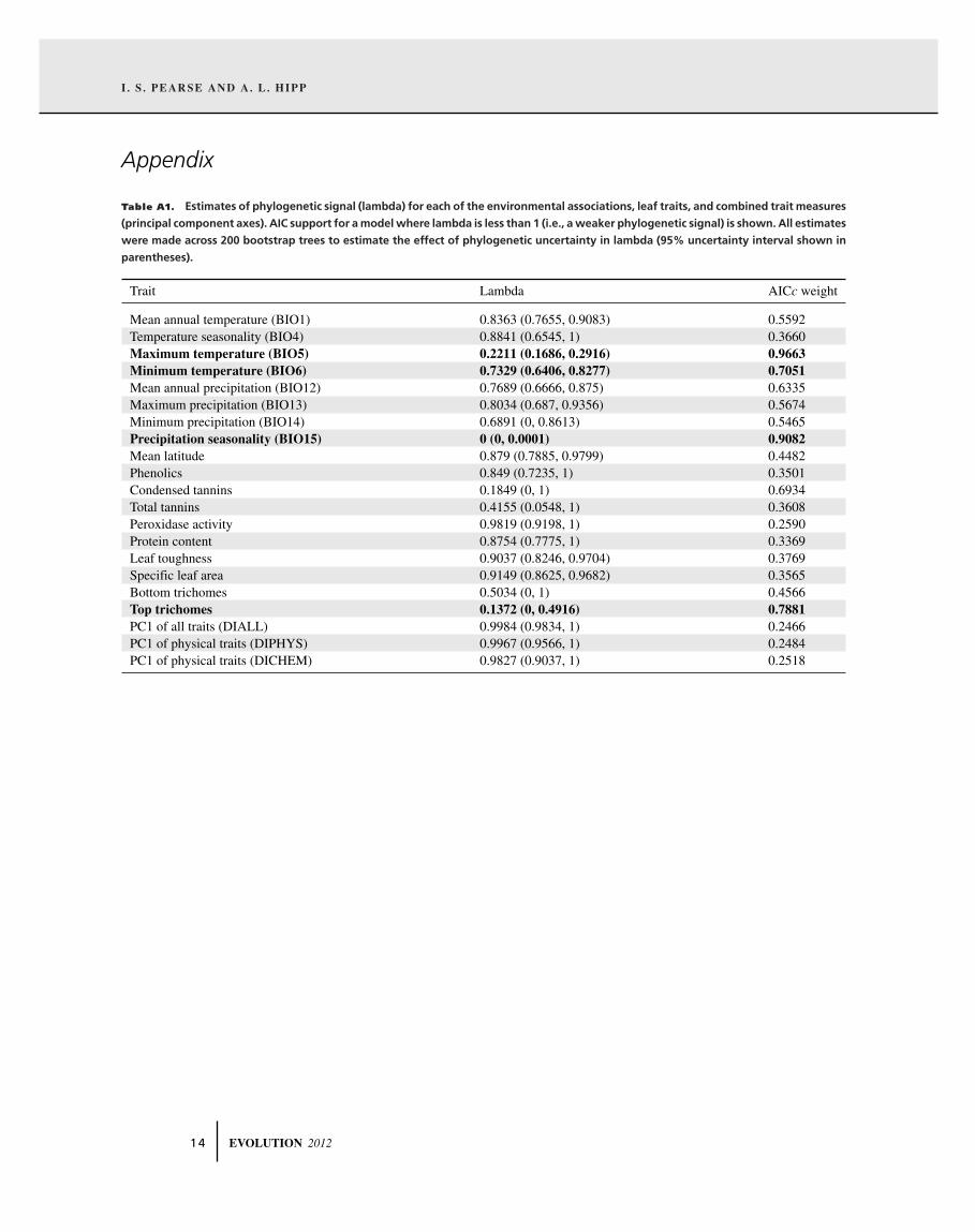
Table A1. Estimates of phylogenetic signal (lambda) for each of the environmental associations, leaf traits, and combined trait measures

(principal component axes). AIC support for a model where lambda is less than 1 (i.e., a weaker phylogenetic signal) is shown. All estimates

were made across 200 bootstrap trees to estimate the effect of phylogenetic uncertainty in lambda (95% uncertainty interval shown in

parentheses).

Trait Lambda AICc weight

Mean annual temperature (BIO1) 0.8363 (0.7655, 0.9083) 0.5592Temperature seasonality (BIO4) 0.8841 (0.6545, 1) 0.3660Maximum temperature (BIO5) 0.2211 (0.1686, 0.2916) 0.9663Minimum temperature (BIO6) 0.7329 (0.6406, 0.8277) 0.7051Mean annual precipitation (BIO12) 0.7689 (0.6666, 0.875) 0.6335Maximum precipitation (BIO13) 0.8034 (0.687, 0.9356) 0.5674Minimum precipitation (BIO14) 0.6891 (0, 0.8613) 0.5465Precipitation seasonality (BIO15) 0 (0, 0.0001) 0.9082Mean latitude 0.879 (0.7885, 0.9799) 0.4482Phenolics 0.849 (0.7235, 1) 0.3501Condensed tannins 0.1849 (0, 1) 0.6934Total tannins 0.4155 (0.0548, 1) 0.3608Peroxidase activity 0.9819 (0.9198, 1) 0.2590Protein content 0.8754 (0.7775, 1) 0.3369Leaf toughness 0.9037 (0.8246, 0.9704) 0.3769Specific leaf area 0.9149 (0.8625, 0.9682) 0.3565Bottom trichomes 0.5034 (0, 1) 0.4566Top trichomes 0.1372 (0, 0.4916) 0.7881PC1 of all traits (DIALL) 0.9984 (0.9834, 1) 0.2466PC1 of physical traits (DIPHYS) 0.9967 (0.9566, 1) 0.2484PC1 of physical traits (DICHEM) 0.9827 (0.9037, 1) 0.2518

1 4 EVOLUTION 2012

GLOBAL PATTERNS OF LEAF DEFENSES IN OAK SPECIES

Ta

ble

A2.

Asu

mm

ary

of

mo

del

sth

atu

seen

viro

nm

enta

lva

riab

les

and

lati

tud

eto

pre

dic

tea

cho

akle

aftr

ait

(or

PCco

mb

inat

ion

of

trai

ts).

GLS

mo

del

sw

ere

con

stru

cted

that

inco

rpo

rate

dal

lp

oss

ible

com

bin

atio

ns

of

up

tofo

ur

envi

ron

men

tal

pre

dic

tors

(n=

255)

.Pa

ram

eter

esti

mat

esan

dcu

mu

lati

veA

ICc

wei

gh

tsw

ere

aver

aged

ove

ral

lm

od

els.

Ad

dit

ion

ally

,th

eb

est-

fit

mo

del

(as

esti

mat

edb

yA

ICc)

was

iden

tifi

ed,a

nd

its

AIC

cw

eig

ht

and

R2

are

sho

wn

.En

viro

nm

enta

lvar

iab

les

wit

hA

ICc.

The

hig

hn

um

ber

of

mo

del

sth

at

fall

wit

hin

the

95%

con

fid

ence

inte

rval

of

mo

del

fit

stro

ng

lysu

gg

ests

that

mo

del

aver

agin

gis

app

rop

riat

e.

Mod

els

inB

est-

fit

Mea

nan

nual

Tem

pera

ture

Max

imum

Min

imum

Mea

nan

nual

Max

imum

Min

imum

Prec

ipita

tion

Lea

fB

est-

fit

95%

AIC

cB

est-

fit

tem

pera

ture

seas

onal

ityte

mpe

ratu

rete

mpe

ratu

repr

ecip

itatio

npr

ecip

itatio

npr

ecip

itatio

nse

ason

ality

Mea

ntr

ait

mod

elco

nfid

ence

set

wei

ght

R2

(BIO

1)(B

IO4)

(BIO

5)(B

IO6)

(BIO

12)

(BIO

13)

(BIO

14)

(BIO

15)

latit

ude

PC1

allt

raits

∼BIO

1+B

IO4+

117/

255

0.10

480.

3687

ß=−0

.197

1,ß=

−0.7

506,

ß=0.

3600

,ß=

−0.3

008,

ß=−0

.007

6,ß=

0.00

20,

ß=−0

.129

7,ß=

0.07

61,

ß=−0

.025

4,(D

IAL

L)

BIO

5+B

IO15

W=0

.389

7W

=0.8

07W

=0.6

593

W=0

.480

9W

=0.1

465

W=0

.116

3W

=0.4

132

W=0

.345

3W

=0.1

646

PC1

phys

.tra

its∼B

IO4+

BIO

6+87

/255

0.04

820.

3867

ß=−0

.020

6,ß=

−0.6

278,

ß=0.

0020

,ß=

−0.2

232,

ß=−0

.092

8,ß=

−0.0

865,

ß=−0

.026

7,ß=

0.01

38,

ß=−0

.117

5,(D

IPH

YS)

BIO

13+l

atM

ean

W=0

.299

1W

=0.8

919

W=0

.273

6W

=0.5

359

W=0

.412

6W

=0.3

873

W=0

.195

1W

=0.1

558

W=0

.378

8

PC1

chem

.tra

its∼B

IO1+

BIO

4+15

1/25

50.

0570

0.21

97ß=

−0.2

227,

ß=−0

.277

8,ß=

0.26

89,

ß=−0

.044

3,ß=

0.06

14,

ß=0.

0243

,ß=

−0.2

324,

ß=0.

0449

,ß=

−0.0

438,

(DIC

HE

M1)

BIO

5W

=0.4

036

W=0

.412

6W

=0.4

581

W=0

.254

4W

=0.2

838

W=0

.237

7W

=0.5

649

W=0

.275

9W

=0.2

284

PC2

chem

.tra

its∼B

IO13

156/

255

0.06

320.

1765

ß=0.

009,

ß=−0

.025

1,ß=

−0.0

111,

ß=0.

0041

,ß=

4×10

−04,

ß=0.

3461

,ß=

0.00

36,

ß=0.

0340

,ß=

−0.0

908,

(DIC

HE

M2)

W=0

.209

2W

=0.2

251

W=0

.212

W=0

.204

4W

=0.3

526

W=0

.756

9W

=0.2

322

W=0

.262

7W

=0.3

51

Phen

olic

s∼B

IO1+

BIO

4+19

1/25

50.

0365

0.13

05ß=

−0.0

853,

ß=−0

.118

8,ß=

0.18

93,

ß=−0

.048

2,ß=

0.01

43,

ß=7×

10−0

4,

ß=−0

.115

5,ß=

−0.0

012,

ß=−0

.034

1,B

IO5

W=0

.305

1W

=0.3

423

W=0

.504

5W

=0.2

710

W=0

.233

6W

=0.2

121

W=0

.421

9W

=0.2

385

W=0

.242

4

Con

dens

edta

nnin

s∼B

IO4+

BIO

1314

6/25

50.

0495

0.28

33ß=

0.01

19,

ß=−0

.093

6,ß=

−0.0

492,

ß=0.

0220

,ß=

0.03

50,

ß=0.

3522

,ß=

0.01

65,

ß=0.

0232

,ß=

−0.1

284,

W=0

.214

8W

=0.3

752

W=0

.311

9W

=0.2

311

W=0

.332

3W

=0.7

618

W=0

.213

5W

=0.2

214

W=0

.412

7

Tota

ltan

nins

∼BIO

1420

8/25

50.

0332

0.04

20ß=

−0.0

849,

ß=−0

.072

9,ß=

0.01

37,

ß=0.

0273

,ß=

−0.0

275,

ß=−0

.044

8,ß=

−0.0

883,

ß=0.

0255

,ß=

0.01

26,

W=0

.32

W=0

.315

5W

=0.2

655

W=0

.260

1W

=0.2

997

W=0

.279

5W

=0.3

863

W=0

.267

7W

=0.2

264

Pero

xida

seac

tivity

∼BIO

1518

8/25

50.

0436

0.10

45ß=

0.03

85,

ß=0.

0635

,ß=

−0.0

454,

ß=−0

.004

6,ß=

−0.1

099,

ß=0.

0213

,ß=

0.16

12,

ß=−0

.115

5,ß=

0.01

95,

W=0

.239

2W

=0.2

709

W=0

.258

0W

=0.2

202

W=0

.351

8W

=0.2

805

W=0

.498

6W

=0.4

489

W=0

.219

9

Prot

ein

cont

ent

∼BIO

6+B

IO13

+14

6/25

50.

0394

0.25

44ß=

0.11

7,ß=

0.10

38,

ß=−0

.159

3,ß=

0.12

54,

ß=−0

.011

6,ß=

−0.1

900,

ß=0.

2950

,ß=

−0.0

418,

ß=0.

0730

,B

IO14

W=0

.318

6W

=0.2

855

W=0

.408

9W

=0.3

979

W=0

.375

1W

=0.4

697

W=0

.632

5W

=0.2

553

W=0

.261

9

Lea

fto

ughn

ess

∼BIO

1215

7/25

50.

0493

0.17

46ß=

−0.0

234,

ß=−0

.132

2,ß=

0.00

98,

ß=−0

.070

1,ß=

−0.2

638,

ß=−0

.031

6,ß=

−0.0

658,

ß=0.

0229

,ß=

0.01

60,

W=0

.248

1W

=0.3

969

W=0

.250

7W

=0.2

883

W=0

.698

5W

=0.3

330

W=0

.319

1W

=0.2

408

W=0

.206

0

Spec

ific

leaf

area

∼BIO

4+B

IO13

+12

4/25

50.

0607

0.32

03ß=

−0.0

455,

ß=−0

.360

3,ß=

−0.0

238,

ß=−0

.018

7,ß=

−0.0

788,

ß=−0

.169

6,ß=

−0.0

336,

ß=0.

1578

,ß=

−2×1

0−04,

BIO

15W

=0.2

43W

=0.7

962

W=0

.253

9W

=0.2

577

W=0

.480

3W

=0.5

017

W=0

.230

1W

=0.5

076

W=0

.150

7

Bot

tom

tric

hom

es∼B

IO5+

latM

ean

124/

255

0.06

720.

2217

ß=−0

.011

,ß=

−0.3

498,

ß=−0

.105

7,ß=

−0.1

513,

ß=0.

0077

,ß=

0.01

60,

ß=0.

0097

,ß=

−5×1

0−04,

ß=−0

.298

5,W

=0.3

197

W=0

.609

1W

=0.4

348

W=0

.382

9W

=0.1

858

W=0

.193

5W

=0.1

837

W=0

.171

4W

=0.6

583

Top

tric

hom

es∼B

IO5+

BIO

13+

163/

255

0.06

560.

2089

ß=−0

.061

6,ß=

−0.1

813,

ß=−0

.147

6,ß=

0.03

53,

ß=−0

.005

4,ß=

−0.1

207,

ß=−0

.015

3,ß=

−0.0

271,

ß=−0

.302

2,la

tMea

nW

=0.2

647

W=0

.457

2W

=0.4

950

W=0

.255

5W

=0.2

270

W=0

.412

6W

=0.1

877

W=0

.206

5W

=0.6

337

EVOLUTION 2012 1 5