Global optimization method for solving the minimum maximal flow problem

Optimization Methods and SoftwareVol. 18, No. 4, August 2003, pp. 395–415

GLOBAL OPTIMIZATION METHOD FOR SOLVINGTHE MINIMUM MAXIMAL FLOW PROBLEM�

JUN-YA GOTOH,a NGUYEN VAN THOAIb,� and YOSHITSUGU YAMAMOTOa,†

aInstitute of Policy and Planning Sciences, University of Tsukuba, Tsukuba 305-8573, Japan;bFB4-Department of Mathematics, University of Trier, 54286 Trier, Germany

(Received 15 October 2002; Revised 5 March 2003; In final form 7 April 2003)

The problem of minimizing the flow value attained by maximal flows plays an important and interesting roleto investigate how inefficiently a network can be utilized. It is a typical multiextremal optimization problem, whichcan have local optima different from global optima. We formulate this problem as a global optimization problem witha special structure and propose a method to combine different techniques in local search and global optimization.Within the proposed algorithm, the advantageous structure of network flow is fully exploited so that the algorithmshould be suitable for handling the problem of moderate sizes.

Keywords: Minimum maximal flow; Global optimization; Optimization over efficient sets; Adjacent vertex search;Branch and bound

1 INTRODUCTION

Consider a directed network N(V , E, s, t, c), where V is the set of m � 2 nodes, E is the set ofn arcs, s is the single source node, t is the single sink node, and c is the vector of arc capacities.A vector x of dimension n is said to be a feasible flow if it satisfies the system of conservationequations and capacity constraints:

Ax � 0� 0 � x � c, (1.1)

where A is the well-known node–arc incidence matrix restricted to the node set V ��s, t�, whosesize is then m � n. We denote by X the set of feasible flows, i.e.,

X � �x � x Rn� Ax � 0� 0 � x � c�. (1.2)

A vector x X is called a maximal flow if there does not exist x � X such that x � x andx � �� x . We denote the set of all maximal flows by X M . Further, let ��(s) and ��(s) denote

� This paper is written during the second author’s stay as a visiting professor at the Institute of Policy and PlanningSciences, University of Tsukuba, Japan.

† Corresponding author. Tel.:�81-29-853-5001/�81-29-853-5202; Fax:�81-29-853-5070; E-mail: [email protected]/[email protected]

ISSN 1055-6788 print; ISSN 1029-4937 online © 2003 Taylor & Francis LtdDOI: 10.1080/1055678031000120191

396 JUN-YA GOTOH et al.

the sets of arcs leaving and entering the source node s, respectively. Then the total amount offlow, called the flow value, of x is given by�

h��(s)

xh ��

h��(s)

xh . (1.3)

The problem to be considered in this article is the minimization of the flow value over the setof all maximal flows, i.e.,

P

��min dx

s.t. x X M ,

where d is an n-dimensional row vector defined as

dh �

��

1 if h ��(s)

�1 if h ��(s)

0 otherwise.

(1.4)

Problem P was considered in Refs. [27,28] and is closely related to the uncontrollableflow raised by Iri [18,19]. It arises from the following situation. Considering the maximumflow problem, we usually take it for granted that each arc flow is controllable, i.e., we can freelyincrease and decrease it as long as the conservation equations and capacity constraints are keptsatisfied. However, in the situation where we are not able or allowed to reduce the given arcflow, we may fail to reach a maximum flow and get stuck in an undesired maximal flow. Withsuch restricted controllability, we may end up with different maximal flows depending on theinitial flow as well as the way of augmentation. Therefore the minimum of the flow values thatare attained by maximal flows will play a prominent role in evaluating how inefficiently thenetwork can be utilized. Note that the problem encompasses the minimum maximal matchingproblem, which is known to be NP-hard, e.g., [14].

Since the set X M is in general nonconvex, Problem P is one of the typical multiextremaloptimization problems. See e.g., Refs. [15,17].Actually, the set X M can be considered as the setof all efficient solutions of the multiple objective programming problem (vector optimizationproblem)

MO

��vector max x

s.t. x X,

so that Problem P is a special case of the class of optimization problems over an efficientset. Solution methods for optimization problems over an efficient set can be found e.g., inRefs. [2,4,5,7,8,11,16,20,23,25,30,32,33,36–38]. A common feature of these methods is, how-ever, that they can be only successfully applied to problems where the underlying multipleobjective programming problem has a small number of objective functions.

In the present article, we first formulate the underlying problem equivalently as a linearprogram with an additional nonconvex constraint, and then propose a method to combinelocal and global optimization techniques for solving the resulting problem in a way that theadvantageous network problem structure will be successfully applied.

The equivalent formulation of Problem P is discussed in the next section. Suitable linearprogram relaxations of this equivalent problem is established in Section 3. Section 4 presentsdifferent local and global optimization techniques which are used for the establishment of thecombination algorithm in Section 5. The convergence of the combination algorithm depends

MINIMUM MAXIMAL FLOW PROBLEM 397

on the branching procedure within a branch and bound scheme for checking global optimality.The case of finite convergence is discussed in Section 4 while establishing the branch andbound method using integral rectangular division for the branching procedure. For the useof simplicial branch and bound procedure, some kind of approximate optimal solutions isintroduced in Section 5 so that the combination algorithm yields an approximate optimalsolution after finitely many iterations. The final section contains an illustrative example andsome conclusions.

2 EQUIVALENT PROBLEM FORMULATIONS

In this paper we denote by Rk and Rk the set of k-dimensional column vectors and the set of

k-dimensional row vectors, respectively. As mentioned in the previous section, the set X M ofmaximal flows is exactly the efficient set of MO. From well-known results in multiple objectiveprogramming, e.g., Refs. [6,26,29,35], there is a compact subset, say �, of Rn�� λ � λ

Rn� λ > 0� such that a point x belongs to X M if and only if it maximizes λx over X for someλ �, i.e.,

X M � �x � x X� λx φ(λ) for some λ ��, (2.1)

whereφ(λ) � max�λy � y X�. (2.2)

In what follows we denote by e the row vector of ones and by Zn the set of n-dimensionalintegral row vectors. The following theorem shows that a finite set of integral points of Rn��

suffices as �.

THEOREM 2.1 �1 � �λ � λ Zn� e � λ � ne� suffices as � in (2.1).

To prove the above theorem we need the following lemmas.Let x R

n be a given maximal flow. Further let F be the index set defined by F �

�h � h E� xh � ch� and F � E�F . Note that F �� . We refer to a directed path from nodei to node j as an i– j path.

LEMMA 2.2 Let G be the graph of node set V and arc set F .

(i) G is acyclic and does not contain an s–t path or a t–s path.(ii) For each node i V ��s, t� at least one of the following two cases occurs:

Case 1: G has neither an s–i path nor a t–i path.Case 2: G has neither an i–s path nor an i–t path.

Proof The assertion (i) is clear from the fact that x is a maximal flow. Let i be an arbitrarynode and suppose that Case 1 of (i) does not occur, i.e., there is either an s–i path or a t–i path.If there is an s–i path, we have by (i) that there is neither an i–s path nor an i–t path, and ifthere is a t–i path, we see that there is neither an i–s path nor an i–t path. These correspondto Case 2. �

Next let a� denote the row of the incidence matrix A of the network corresponding to node� V ��s, t�. Suppose we are given a nonempty subset U of V ��s, t� and let

��E (U)��h � h � (i, j) E� i U � j V �U� (2.3)

��E (U)��h � h � (i, j) E� j U � i V �U�. (2.4)


Then it will be readily seen from the definition of the incidence matrix that

��U

a� ��

k��

E (U )

ek ��

k��

E (U )

(�ek), (2.5)

where ek is the kth unit vector of Rn .

LEMMA 2.3 For each h F it holds that

eh � αh

��Vh

a� ��k�F

βhkek ��

k�E��h�

γhkek (2.6)

for some αh ��1, 1�, Vh � V ��s, t�, βhk �0, 1� and γhk �0, 1�.

Proof Let h � (i, j) and consider the following two cases.

Case 1 Node i satisfies the condition of Case 1 of Lemma 2.2.Let

V�h � �� V � there is an �–i path of G�. (2.7)

Then we see from Lemma 2.2 that s, t, j � V�h and that no arcs of F come into V�

h from

its complement V�h � V �V�

h . Therefore the cut (V�h , V�

h ) consists of the three sets of arcs:��

�F(V�

h ), ��F (V�

h ) and ��F (V�

h ). By (2.5) we obtain

��V�

h

a� ��

k��

�F(V�

h )

ek ��

k��

F (V�

h )

ek ��

k��

F (V�

h )

(�ek), (2.8)

which is rewritten as, since h ��F(V�

h ),

��V�

h

a� � eh ��

k��

�F(V�

h )��h�

ek ��

k��

F (V�

h )

ek ��

k��

F (V�

h )

(�ek). (2.9)

Thus we obtain

eh ��

��V�

h

a� ��

k��

F (V�

h )

ek �

��

k��

F (V�

h )

ek ��

k��

�F(V�

h )��h�

ek

� . (2.10)

Case 2 Node i satisfies the condition of Case 2 of Lemma 2.2.Since node i satisfies the condition of Case 2 and arc h � (i, j) is in F , node j also satisfiesthat condition. Let V�

h � �� V � there is a j–� path of G�. Then we see s, t, i � V�h and

that no arcs of F go from V�h into V�

h � V �V�h , and the cut (V�

h , V�h ) consists of ��

�F(V�

h ),

��F (V�

h ) and ��F (V�

h ). Therefore

��V�

h

a� ��

k��

�F(V�

h )

(�ek)��

k��

F (V�

h )

(�ek)��

k��

F (V�

h )

ek (2.11)

��eh ��

k��

�F(V�

h )��h�

(�ek)��

k��

F (V�

h )

(�ek)��

k��

F (V�

h )

ek . (2.12)


Hence

eh �

��

��V�

h

a�

��

�k��

F (V�

h )

ek �

��

k��

F (V�

h )

ek ��

k��

�F(V�

h )��h�

ek

� . (2.13)

This completes the proof. �

Proof of Theorem 2.1 By Lemma 2.3 we see for each h F

eh ��

k�E��h�

γhkek � αh

��Vh

a� ��k�F

βhkek (2.14)

for some αh ��1, 1�, Vh � V ��s, t�, βhk �0, 1� and γhk �0, 1�. Adding these equationsover h F and the identities eh � eh for h F , we obtain�

k�E

λkek ��

��V��s,t�

δ�a� ��k�F

ζkek, (2.15)

where λk � 1 ��

h�E��k� γhk for k E , ζk ��

h�F βhk � 1 for k F , and δ� is appropri-ately defined for � V ��s, t�. Note that

1 � λk � 1 � (n � 1) � n (2.16)

for k E and ζk 0 for k F . Let λ ��

k�E λkek . Clearly, λ �1. Then for any feasibleflow x it holds that

λ x ��k�E

λkek x ��

��V��s,t�

δ�a� x ��k�F

ζkek x (2.17)

��k�F

ζk xk ��k�F

ζkck (2.18)

�k�F

ζkxk ��

��V��s,t�

δ�a�x ��k�F

ζkekx � λx, (2.19)

meaning that the maximal flow x maximizes λx over the set of feasible flows. �

By the property that φ(αλ) � αφ(λ) for α > 0, any compact subset of Rn�� whose conicalhull contains the conical hull of �1 works as �. Therefore we could replace � by the simplex

�2 �

λ � λ Rn� λ e�

n�i1

λi � M

�(2.20)

if M is sufficiently large.

COROLLARY 2.4 n2 suffices for M defining �2 of (2.20).

Proof Let x be a maximal flow. By Theorem 2.1 it maximizes λx over the feasible flows forsome λ Rn such that 1 � λh � n for each h E . Let λ � (n2/

�h�E λh)λ. Then since n2 �

h�E λh , λ lies in �2 defined for M � n2 and x maximizes λx over the feasible flows. �


Theorem 2.1 implies that Problem P can be solved in theory by the following method.For each integral vector λ �1 identify the optimal face F(λ) of max�λx � x X�, and solvemin�dx � x F(λ)� for a solution x(λ). Note that any point of F(λ) is a maximal flow, and it isreadily seen that x(λ�) such that dx(λ�) � min�dx(λ) � λ �1� is a solution of P . However,the integral points to be considered amount to nn , so that this method is not practical.

Remark 2.5 The optimal face F(λ) is an outer semicontinuous mapping when consideredas a point to set mapping, i.e., for a sequence �λν� converging to λ any cluster point of thesequence �xν� with xν F(λν) is contained in F(λ). See Exercise 1.19 of Rockafellar andWets [24]. Then dx(λ) is a lower semicontinuous function in λ, i.e., lim infν dx(λν) dx(λ)

for any sequence �λν� converging to λ. Therefore for a given ε > 0 each λ has a neighborhoodsuch that dx(λ�) dx(λ)� ε holds for any λ� in the neighborhood. This means that it is verylikely that λ’s with large objective function values dx(λ) make a cluster. Thus the divide andconquer principle or the branch and bound method should work efficiently.

The above arguments yield two different representations of the set X M of maximal flows:

X M ��x � x X� λx φ(λ) for some λ �1� (2.21)

��x � x X� λx φ(λ) for some λ �2�, (2.22)

each of which will in the following sections provide a scheme for solving the problem. NowProblem P is written equivalently as

P

��

min dx

s.t. x X

λx � φ(λ) 0

λ �,

where � is either �1 or �2 with M � n2.

LEMMA 2.6 Assume that each arc capacity ch is a nonnegative integer. Let XV denote the set ofvertices of the polytope X, and let x XV � X M .Then, whenever �x � x X M � dx < d x� �� ,there exists x X M � XV such that dx � d x � 1.

Proof Note first that d is an integral vector. Then this lemma is a direct consequence of thetwo well-known facts that each vertex of X is an integral vector and that Problem P has anoptimal solution in the vertex set of X . �

3 LINEAR PROGRAM RELAXATION

In this section we explain a linear program relaxation of Problem P . For the sake of furtherargument, we consider the following problem with λ restricted to a polytope, say S, containedin �:

P(S)

��

min dx

s.t. Ax � 0

0 � x � c

λx � φ(λ) 0

λ S.


Let (S) � min�φ(λ) � λ S�. (3.1)

Our method for constructing linear program relaxations of Problem P(S) is based on thefollowing result.

LEMMA 3.1 Let �λ1, . . . , λq � be the vertex set of S. Then Problem P(S) is relaxed to thefollowing linear program in variables x� R

n for � � 1, . . . , q �

P(S)

��

minq�

�1

dx�

s.t. Ax� � 0 for � � 1, . . . , q

x� 0 for � � 1, . . . , qq�

�1

x� � c

q��1

λ�x� � (S) 0,

i.e., the optimal value µ(S) of Problem P(S) yields a lower bound of the optimal value ofProblem P(S).

Proof We show that for any feasible solution (x, λ) of Problem P(S) there exists a feasiblesolution (x1, . . . , xq) of Problem P(S) satisfying

dx �

q��1

dx�. (3.2)

Since λ S,

λ �

q��1

β�λ� (3.3)

for some nonnegative numbers β� (� � 1, . . . , q) such that�q

�1 β� � 1. Define

x� � β�x for � � 1, . . . , q. (3.4)

Then clearly�q

�1 x� � x and (x1, . . . , xq) satisfies the first three constraints of P(S).For the last constraint we have

q��1

λ�x� �

q��1

λ�β�x � λx φ(λ) (S), (3.5)

where the last two inequalities follow from the assumption that (x, λ) is feasible toP(S) and from the definition of (S) in (3.1). �

Remark 3.2 If Problem P(S) is infeasible, so is Problem P(S). In this case weset µ(S) � ��.


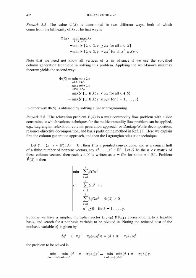
Remark 3.3 The value (S) is determined in two different ways, both of whichcome from the bilinearity of λx . The first way is

(S)�minλ�S

maxx�X

λx

�min�r � λ S� r λx for all x X�

�min�r � λ S� r λx� for all x� XV �.

Note that we need not know all vertices of X in advance if we use the so-calledcolumn generation technique in solving this problem. Applying the well-known minimaxtheorem yields the second way:

(S)�minλ�S

maxx�X

λx

�maxx�X

minλ�S

λx

�max�r � x X� r � λx for all λ S�

�max�r � x X� r � λ�x for � � 1, . . . , q�.

In either way (S) is obtained by solving a linear programming.

Remark 3.4 The relaxation problem P(S) is a multicommodity flow problem with a sideconstraint, to which various techniques for the multicommodity flow problem can be applied,e.g., Lagrangian relaxation, column generation approach or Dantzig-Wolfe decomposition,resource-directive decomposition, and basis partitioning method in Ref. [1]. Here we explainfirst the column generation approach, and then the Lagrangian relaxation technique.

Let Y � �x � x Rn�� Ax � 0�, then Y is a pointed convex cone, and is a conical hull

of a finite number of nonzero vectors, say g1, . . . , gr Rn�. Let G be the n � r matrix of

these column vectors, then each x Y is written as x � Gα for some α Rr�. Problem

P(S) is then ��

minq�

�1

dGα�

s.t.q�

�1

Gα� � c

q��1

λ�Gα� � (S) 0

α� 0 for � � 1, . . . , q.

Suppose we have a simplex multiplier vector (π, π0) Rn�1 corresponding to a feasiblebasis, and search for a nonbasic variable to be pivoted in. Noting the reduced cost of thenonbasic variable α�

i is given by

dgi � (�πgi � π0(λ�gi )) � (d � π � π0λ�)gi ,

the problem to be solved is

min�1,...,q

mini1,...,r

(d � π � π0λ�)gi � min�1,...,q

miny�Y

(d � π � π0λ�)y.


Note that for each �, miny�Y (d � π � π0λ�)y is a shortest path and cycle problem. When theminimum value above is nonnegative, the current basic solution is optimal to P(S).

Next consider the Lagrangian relaxation problem with a multiplier τ 0��

minq�

�1

dx� � τ

� (S)�

q��1

λ�x�

�

s.t. Ax� � 0 for � � 1, . . . , q

x� 0 for � � 1, . . . , qq�

�1

x� � c.

For each j � 1, 2, . . . , n let

λmaxj � max�(λ�) j � � � 1, . . . , q�

and let d �(τ ) Rn be the vector whose j th component d �j (τ ) is defined by

d �j (τ ) � d j � τλmaxj .

Then clearly for a feasible solution (x1, . . . , xq)

q��1

d �(τ )x� �

q��1

(d � τλ�)x�,

so that the above Lagrangian relaxation can be relaxed further by the problem��

minq�

�1

d �(τ )x� � τ (S)

s.t. Ax� � 0 for � � 1, . . . , q

x� 0 for � � 1, . . . , qq�

�1

x� � c,

which is actually equivalent to the following minimum cost network flow problem inn variables:

P(S)

��min d �(τ )x � τ (S)

s.t. Ax � 00 � x � c.

An efficient choice for the multiplier τ can be taken using the well-known parametric linearprogramming technique. See for example Refs. [1,3,10].

The dual problem of P(S), denoted by D(S), is written as

D(S)

��max �vc � z (S)

s.t. u� A � v � zλ� � d for � � 1, . . . , q

(v, z) 0,

where uk Rm , v Rn , z R.


LEMMA 3.5 A nonnegative vector (v, z) satisfies the constraints of D(S) together with someu1, . . . , uq Rm if and only if for any λ S there is u(λ) Rm such that u(λ)A � v � zλ � d .

Proof The ‘‘if’’ part is readily seen by setting u� � u(λ�) for � � 1, . . . , q . To showthe ‘‘only if’’ part, let λ be a given vector of S. Then λ �

�q�1 β�λ� for some nonnega-

tive β�’s with�q

�1 β� � 1. Let u(λ) ��q

�1 β�u�. Then

u(λ)A � v � zλ �

� q��1

β�u�

�A � v � z

� q��1

β�λ�

�

�

q��1

β�(u� A � v � zλ�) � d. �

The lower bound µ(S) has the following properties, which will be utilized within the branchand bound procedure.

LEMMA 3.6 Suppose � �� S2 � S1 � �. Then

�� < µ(S1) � µ(S2). (3.6)

Proof Suppose (v, z) is a feasible solution of D(S1) together with (u1, . . . , uq). Thenby Lemma 3.5, we see that (v,w, z) is a feasible solution of D(S2) with some (u�1, . . . , u�q ).Since the objective function value of D(S) is determined solely by (v, z), we see the mono-tonicity µ(S1) � µ(S2). The fact that�� < µ(S1) is a direct consequence of the boundednessof the feasible region of P(S1). �

We now show that the relaxation problem P(S) can be substantially simplified whenS is a hyper rectangle.

LEMMA 3.7 If λ � λ�, then φ(λ) � φ(λ�).

Proof Let x be a point of X that maximizes λx over X . Since x 0 we have (λ� λ�) x � 0,and hence

φ(λ) � λ x � λ� x � φ(λ�). (3.7)

�

LEMMA 3.8 Let �λ1, . . . , λq � be the vertex set of S � � and suppose λ1 λ� λq

for all � � 1, . . . , q. Then Problem P(S) is equivalent to the problem

P �(S)

��

min dx

s.t. Ax � 0

0 � x � c

λ1x � φ(λq ) 0

in n variables.


Proof Note that λq � λ� for all � � 1, . . . , q implies that λq � λ for all λ S. Thenby Lemma 3.7 we have (S) � φ(λq ).

Let (x1, . . . , xq) be a feasible solution of P(S) and let x ��q

�1 x�. Then clearlyAx � 0 and 0 � x � c. Furthermore, since x� 0 we obtain

λ1x � λ1

q��1

x� �

q��1

λ1x�

q��1

λ�x� (S)

dx �

q��1

dx�.

This means that µ(S) µ�(S), where µ�(S) is the optimal objective function value of P �(S).Let x be a feasible solution of P �(S) and let x1 � x , x2 � � � � � xq � 0. Then (x1, . . . , xq)

clearly satisfies the constraints of P(S), meaning µ(S) � µ�(S). �

From Lemma 3.8 if we take �1 as � and consider a hyper rectangle S � �λ � λ �1� λ �

λ � λ� contained in �1, then, although S has as many as 2n vertices, the relaxation problem P �(S) has only n variables as Problem P(S) does. This might be an advantage of using �1.

However, the simplicity of P �(S) can be to its disadvantage because λx � φ(λ) 0 isa too much relaxed constraint of λx � φ(λ) 0. Therefore we propose below an improve-ment with aid of the concave envelope of the bilinear term λx and an approximation of thefunction φ(λ).

LEMMA 3.9 Let S � �λ � λ �1� λ � λ � λ�, and let V be a nonempty subset of X M � XV .Then the problem

P ��(S, V )

��

min dx

s.t. Ax � 0

0 � x � c

g1k (λk, xk)� tk 0 for k E

g2k (λk, xk)� tk 0 for k E�

k�E

tk � λv 0 for v V

is a relaxation problem of P(S), where

g1k (λk, xk)� ckλk � λk xk � λkck

g2k (λk, xk)� λk xk .

Proof First note that P ��(S, V ) is equivalent to��

min dx

s.t. Ax � 0

0 � x � c�k�E

min�g1k (λk, xk), g2

k (λk, xk)� max�λv � v V �.


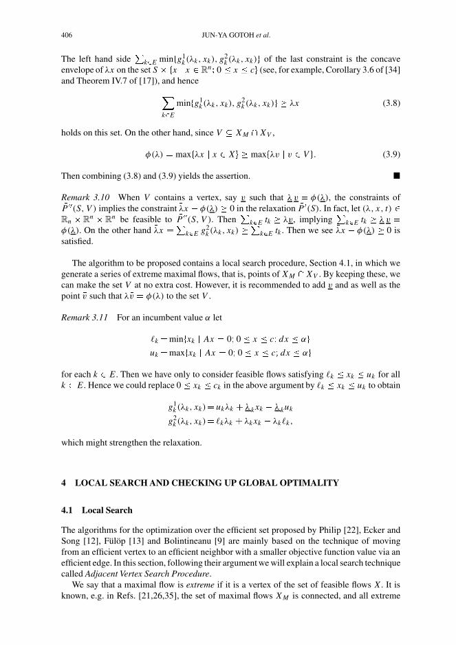
The left hand side�

k�E min�g1k (λk, xk), g2

k (λk, xk)� of the last constraint is the concaveenvelope of λx on the set S � �x � x R

n� 0 � x � c� (see, for example, Corollary 3.6 of [34]and Theorem IV.7 of [17]), and hence�

k�E

min�g1k (λk , xk), g2

k (λk, xk)� λx (3.8)

holds on this set. On the other hand, since V � X M � XV ,

φ(λ) � max�λx � x X� max�λv � v V �. (3.9)

Then combining (3.8) and (3.9) yields the assertion. �

Remark 3.10 When V contains a vertex, say v such that λ v � φ(λ), the constraints of P ��(S, V ) implies the constraint λx � φ(λ) 0 in the relaxation P �(S). In fact, let (λ, x, t)

Rn � Rn � R

n be feasible to P ��(S, V ). Then�

k�E tk λv, implying�

k�E tk λ v �

φ(λ). On the other hand λx ��

k�E g2k (λk, xk)

�k�E tk . Then we see λx � φ(λ) 0 is

satisfied.

The algorithm to be proposed contains a local search procedure, Section 4.1, in which wegenerate a series of extreme maximal flows, that is, points of X M � XV . By keeping these, wecan make the set V at no extra cost. However, it is recommended to add v and as well as thepoint v such that λ v � φ( λ) to the set V .

Remark 3.11 For an incumbent value α let

�k �min�xk � Ax � 0� 0 � x � c� dx � α�

uk �max�xk � Ax � 0� 0 � x � c� dx � α�

for each k E . Then we have only to consider feasible flows satisfying �k � xk � uk for allk E . Hence we could replace 0 � xk � ck in the above argument by �k � xk � uk to obtain

g1k (λk, xk)� ukλk � λ k xk � λ kuk

g2k (λk, xk)� �kλk � λk xk � λk�k,

which might strengthen the relaxation.

4 LOCAL SEARCH AND CHECKING UP GLOBAL OPTIMALITY

4.1 Local Search

The algorithms for the optimization over the efficient set proposed by Philip [22], Ecker andSong [12], Fülöp [13] and Bolintineanu [9] are mainly based on the technique of movingfrom an efficient vertex to an efficient neighbor with a smaller objective function value via anefficient edge. In this section, following their argument we will explain a local search techniquecalled Adjacent Vertex Search Procedure.

We say that a maximal flow is extreme if it is a vertex of the set of feasible flows X . It isknown, e.g. in Refs. [21,26,35], the set of maximal flows X M is connected, and all extreme


maximal flows are connected by paths of edges consisting of maximal flows. Thus, starting froman extreme maximal flow, we could reach an optimal solution of Problem P by a series of pivotoperations in theory. However, we cannot decrease the objective function value monotonicallyalong the path as we trace, i.e., we might be eventually caught by a non-optimal extrememaximal flow none of whose neighboring extreme maximal flows have a smaller objectivefunction value. When this occurs, it is a local minimum solution. See for example Ref. [9].

The Adjacent Vertex Search (AVS) Procedure goes as follows. We denote by �x, x �� theedge of X connecting x and x � for x, x � XV and

NM (x) � �x � � x � XV � X M � �x, x �� X M �.

Adjacent Vertex Search (AVS) Procedure��Initialization��Find x0 XV � X M . If NM (x0) � �, then x0 is an optimal solution of P . Otherwise, setk � 0 and go to Step k.��Step k��

�k1� If �x � x NM (xk)� dx < dxk� �� , choose xk�1 from this set, let k � k � 1 and goto Step k.

�k2� Otherwise, set v � xk and stop.

Note that the initial extreme maximal flow x0 is easily found by choosing an arbitrarypositive vector λ and maximizing λx over X . The AVS Procedure generates a sequence of dis-tinct extreme maximal flows x0, x1, . . . , xk with decreasing objective function values, whichimplies owing to the integrality property that dxk � dx0 � k. When the relaxation problem P ��(S, V ) is used in the branch and bound procedure, we accumulate these extreme maximal

flows as the initial set V .

4.2 Checking Up Global Optimality

We present in this subsection two Branch and Bound (BB) Procedures for handling the follow-ing problem:

CGO(α)

��For a given integer α, find an extreme maximal flow

v X M � XV such that dv � α,

or show that there does not exist such a point.

As shown in Section 2, for the description of the set X M , we can use one of two sets �1and �2. The set �1 defined in Theorem 2.1 consists of all integral vectors contained in therectangle �λ � λ Rn� e � λ � ne�, while the set �2 is an (n � 1)-simplex defined in (2.20).Before presenting two branch and bound procedures for handling Problem CGO(α) accordingto �1 and �2, respectively, we propose here two kinds of division process called integralrectangular division and simplicial division.

4.2.1 Integral Rectangular Division

Let S � �1 be a rectangle with integral bound vectors, which contains more than one integralvector and is defined by

S � �λ � λ Rn� λ � λ � λ�,


where λ and λ are integral vectors of Rn such that λ � λ. Further, let S1, . . . , Sq be rectangleswith integral bound vectors having the following properties:

q�i1

Si � S,

Si � Sj � � for i �� j,q�

i1

(Si � Zn) � S � Zn .

Then we say that �S1, . . . , Sq � is an integral rectangular division of the rectangle S.As a special case of this division, we consider the following integral rectangular bisection.

Let λ� S such that λ� �� λ, and let � �1, . . . , n� such that λ�� < λ�, (note that such an index� exists, whenever S contains more than one integral vector). For each real number t , denotingby �t� the largest integer which is less than or equal to t , we define two rectangles

S1 ��λ � λ S� λ� � �λ��

S2 ��λ � λ S� λ� �λ�� 1�.

Then, it is easy to verify that �S1, S2� is an integral rectangular division of S. We say that S isdivided into �S1, S2� by an integral rectangular bisection using the point λ�.

4.2.2 Simplicial Division

Let S be an (n � 1)-simplex with vertex set SV � �λ1, . . . , λn�. Choose a point λ� S�SV ,which is uniquely represented as

λ� �

n�i1

βiλi , βi 0 (i � 1, . . . , n),

n�i1

βi � 1.

For each i such that βi > 0, construct the simplex Si obtained from S by replacing the vertexλi by λ�, i.e., Si � co�λ1, . . . , λi�1, λ

�, λi�1, . . . , λn�, where coA denotes the convex hull ofa set A. This division is called a radial simplicial division.

When λ� is the midpoint of a longest edge of S, then we obtain two subsimplices. Thisspecial case is called a simplicial bisection.

As discussed in the preceding section, our BB Procedures are based on the linear relaxation P(S) or P ��(S) of the subproblem P(S) with λ restricted to a subset S � �, where � is either

�1 or �2. The branching process subdivides � into finitely many subsets yielding a classof subproblems to be solved. In the algorithm to be proposed we repeatedly apply the AVSProcedure, which provides a local minimum incumbent solution vν , and then one of the BBProcedures to check up the global optimality of vν . The chosen BB procedure starts with thenumber α � dvν � 1 and the class R of subsets S of � such that µ(S) � α, and also with theset V of extreme maximal flows obtained so far. In the BB1 we denote the optimal value ofthe relaxation problem P ��(S, V ) by µ(S) for the simplicity of notation.

Branch and Bound Procedure (BB1) (according to �1)��Initialization��Set k � 0 and R0 � R.��Step k��


�k1� Set µk � min� µ(S) � S Rk� and choose Sk Rk such that µ(Sk) � µk . DivideSk into Sk1, . . . , Skp by an integral rectangular division and set Rk � Rk��Sk� �

�Sk1, . . . , Skp�,�k2� For j � 1, . . . , p do:

(a) If �Skj � Zn � � 1, then do:(i) Set Rk � Rk��Skj �.

(ii) Choose λ Skj � Zn and solve max�λx � x X�, yielding the optimal faceF(λ).

(iii) Solve min�dx � x F(λ)�, yielding a vertex solution x(λ).(iv) Set V � V � �x(λ)�.(v) If dx(λ) � α, then set w � x(λ) and go to �k4�. Otherwise, go to Endfor.

(b) If �Skj � Zn � > 1, then do:(i) Solve P ��(Skj , V ), yielding the optimal value µ(Skj ) and an optimal solution

y if feasible ( µ(Skj ) � �� when infeasible).(ii) If µ(Skj ) > α, then set Rk � Rk��Skj � and go to Endfor.

(iii) If y X M , then identify the minimal face F of X containing y, solve min�dx �

x F� for a vertex solution w and set V � V � �w�.(iv) Go to �k4�.

Endfor�k3� IfRk �� , then set Rk�1 � Rk , k � k � 1 and go to ��Step k��. Otherwise, set R � �

and quit.�k4� Set R � �S � S Rk� µ(S) � dw � 1� and quit.

THEOREM 4.1 Procedure BB1 terminates after finitely many iterations, either yielding anextreme maximal flow with an objective function value being less than or equal to α, orindicating that such a maximal flow does not exist. In other words, Procedure BB1 solvesProblem CGO(α) finitely.

Proof Each subsequence of rectangles, �Sq�, generated throughout Procedure (BB1) suchthat Sq�1 � Sq for all q , must be finite, since every Sq contains at least one element from Zn .

If the procedure terminates at Step �k4�, then the point w is an extreme maximal flowsatisfying dw � α.

If the procedure terminates at Step �k3�, i.e.,R � �, then it follows that each subset S of �1yields a lower bound µ(S) > α, which implies that there does not exist an extreme maximalflow v X M � XV , such that dv � α. �

Branch and Bound Procedure (BB2) (according to �2)��Initialization��Set k � 0 and R0 � R.��Step k��

�k1� (a) Set µk � min� µ(S) � S Rk� and choose Sk Rk such that µ(Sk) � µk .(b) Divide Sk into Sk1, . . . , Skp by a simplicial division and set

Rk � Rk��Sk� � �Sk1, . . . , Skp�,�k2� For j � 1, . . . , p do:

(a) Solve P(Skj ), yielding the optimal value µ(Skj ) and an optimal solution(x1

kj , . . . , xnkj ) if feasible ( µ(Skj ) � �� when infeasible).

(b) If µ(Skj ) > α, then set Rk � Rk��Skj �.(c) Let xkj �

�n�1 x�

kj .


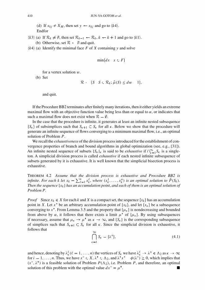
(d) If xkj X M , then set y � xkj and go to �k4�.Endfor

�k3� (a) If Rk �� , then set Rk�1 � Rk , k � k � 1 and go to �k1�.(b) Otherwise, set R � � and quit.

�k4� (a) Identify the minimal face F of X containing y and solve

min�dx � x F�

for a vertex solution w.(b) Set

R � �S � S Rk� µ(S) � dw � 1�,

and quit.

If the Procedure BB2 terminates after finitely many iterations, then it either yields an extrememaximal flow with an objective function value being less than or equal to α, or indicates thatsuch a maximal flow does not exist when R � �.

In the case that the procedure is infinite, it generates at least an infinite nested subsequence�Sκ� of subsimplices such that Sκ�1 � Sκ for all κ . Below we show that the procedure willgenerate an infinite sequence of flows converging to a minimum maximal flow, i.e., an optimalsolution of Problem P .

We recall the exhaustiveness of the division process introduced for the establishment of con-vergence properties of branch and bound algorithms in global optimization (see, e.g., [31]).An infinite nested sequence of subsets �Sκ �κ is said to be exhaustive if �κ1Sκ is a single-ton. A simplicial division process is called exhaustive if each nested infinite subsequence ofsubsets generated by it is exhaustive. It is well known that the simplicial bisection process isexhaustive.

THEOREM 4.2 Assume that the division process is exhaustive and Procedure BB2 isinfinite. For each k let xk �

�n�1 x�

k , where (x1k , . . . , xn

k ) is an optimal solution to P(Sk).Then the sequence �xk� has an accumulation point, and each of them is an optimal solution ofProblem P.

Proof Since xk X for each k and X is a compact set, the sequence �xk� has an accumulationpoint in X . Let x� be an arbitrary accumulation point of �xk�, and let �xκ� be a subsequenceconverging to x�. From Lemma 3.5 and the property that �µκ� is nondecreasing and boundedfrom above by α, it follows that there exists a limit µ� of �µκ�. By using subsequencesif necessary, assume that µκ � µ� as κ ��, and �Sκ � is the corresponding subsequenceof simplices such that Sκ�1 � Sκ for all κ . Since the simplicial division is exhaustive, itfollows that

�κ1

Sκ � �λ��, (4.1)

and hence, denoting by λ�κ (� � 1, . . . , n) the vertices of Sκ we have λ�

κ � λ� �2 as κ ��

for i � 1, . . . , n. Thus, we have x� X , λ� �2, and λ�x� � φ(λ�) 0, which implies that(x�, λ�) is a feasible solution of Problem P(�2), i.e. Problem P , and therefore, an optimalsolution of this problem with the optimal value dx� � µ�. �


5 GLOBAL OPTIMIZATION ALGORITHM AND APPROXIMATEOPTIMAL SOLUTION

Combining Procedure AVS with Procedure BB1 or BB2 in Section 4, we propose the followingalgorithm for globally solving Problem P .

Global Optimization Algorithm (GOA)��Initialization��Compute an extreme maximal flow w0 XV � X M . If NM (w0) � �, then w0 is an optimalsolution of P . Otherwise, set ν � 1, R � �� and go to Iteration ν.�� Iteration ν��

�ν1� Apply AVS to Problem P starting from wν�1 and let vν be the extreme maximal flowobtained. Set αν � dvν � 1 and go to Step ν2.

�ν2� Set R � �S � S R� µ(S) � αν� and apply BB.(a) If an extreme maximal flow wν with dwν � αν is found, set ν � ν � 1 and go to

Iteration ν.(b) If BB terminates with an empty R, then stop (the point vν is an optimal solution

of P).

When BB2 is used in the algorithm GOA, it can be infinite. For the case that Procedure BB2 isinfinite, we introduce the following concept of approximate optimal solutions of Problem P .

DEFINITION 5.1 Given a real numberγ > 0, a flow x is called a γ -optimal solution of ProblemP if it satisfies the following conditions:

(i) There exists λ � such that λx � φ(λ) �γ , and(ii) dx is a lower bound of the optimal value of Problem P.

Using this concept, we modify Procedure BB2 slightly to obtain the finiteness of the globaloptimization algorithm. Recall that λ1

k , . . . , λnk are the vertices of Sk and (x1

k , . . . , xnk ) is an

optimal solution of Problem P(Sk). The modification consists of the following additionalstopping criterion between (a) and (b) at step �k1� �

ifn�

�1

λ�k x�

k � (Sk) �δ, then stop. (5.1)

We will show in Theorem 5.2 below that xk ��n

�1 x�k is an approximate optimal solution

of Problem P in the sense of Definition 5.1.

THEOREM 5.2 Assume that within Procedure BB2 the simplicial division is exhaustive, andthe additional stopping criterion (5.1) is used at Step �k1�. Then

(i) The global optimization algorithm always terminates after finitely many iterations; and(ii) If Procedure BB2 terminates by the additional stopping criterion (5.1), then xk �

�n�1 x�

kis a (δ � nε)-optimal solution of Problem P, where

ε � max�(λ�k � λ��

k )x�k � �, �� 1, . . . , n�. (5.2)


Proof We show that Procedure BB2 is finite. Then the finiteness of GOA follows immediately.Suppose Procedure BB2 could be infinite. Then from Theorem 4.2, it would generate an

infinite sequence �xκ� converging to an optimal solution of Problem P . This implies that thereexists an index κ such that

n��1

λ��κ x�

�κ � (S �κ ) �δ,

Thus, Procedure BB2 must stop at iteration κ.Assume now Procedure BB2 terminates at step �k1� of Iteration k by stopping criterion

(5.1). From (5.2) it follows that for each � � 1, . . . , n and for any λ Sk we have

λ�k x�

k � λx�k � ε,

which implies

λ

n��1

x�k

n��1

λ�k x�

k � nε.

Let now λ� Sk such that φ(λ�) � (Sk). Then

λ�xk � φ(λ�) � λ�n�

�1

x�k � φ(λ�)

n��1

λ�k x�

k � (Sk)� nε,

which implies by (5.1) thatλ�xk � φ(λ�) �(δ � nε).

Note that dxk � µ(Sk) is a lower bound of the optimal value of P by the choice of Sk . Thenby Definition 5.1 xk is a (δ � nε)-optimal solution of Problem P . �

6 AN ILLUSTRATIVE EXAMPLE AND CONCLUSIONS

To illustrate the global optimization algorithm GOA we consider the network with 4 � 2nodes and 10 arcs shown in Fig. 1, where the number attached to each arc is the arc capacityc1, . . . , c10.

FIGURE 1 Network with 6 nodes and 10 arcs.


For this example, Procedure BB1 is chosen for checking up global optimality. Within BB1a lower bound for each rectangle S is computed by solving Problem P ��(S, V ) in Lemma 3.9,and the integral rectangular bisection is performed by the following rule.

Let (x(S), λ(S), t (S)) be an optimal solution of Problem P ��(S, V ). The rectangle S is thendivided into �S1, S2� by the integral rectangular bisection using λ(S) and index � chosen byλ�(S) � max�λi (S) � λi (S) < λi , i � 1, . . . , n�.

��Initialization��An extreme maximal flow is computed: w0 � (7, 3, 1, 4, 2, 1, 6, 1, 2, 8).

�� Iteration ν � 1��

�ν1� Applying AVS we obtain a local optimal solution v1 � (7, 3, 0, 4, 2, 1, 7, 0, 2, 8). Setα1 � dv1 � 1 � 9.

�ν2� BB1 starts with the rectangle S0 � �λ R10 � (1, . . . , 1) � λ � (10, . . . , 10)� and theset V � �w0, v1�. Solving P ��(S0, V ) we obtain

µ(S0)� 7.2706,

x(S0)� (4.2706, 3.0, 0.5591, 4.0, 0.2706, 0.0, 6.7115, 0.2885, 0.0, 7.2706),

λ(S0)� (6.4908, 10.0, 6.0322, 10.0, 2.2177, 1.0, 9.6290, 3.5968, 1.0, 9.1794).

The solution x(S0) is not a maximal flow. We then divide S0 into two subrectangles using λ(S0)

and the index � � 7 chosen by the above rule.At iteration 21 while handling the rectangle S � �λ R10 � (6, 1, 8, 1, 1, 1, 10, 1, 1, 1) �

λ � (7, 10, 8, 10, 10, 10, 10, 10, 10, 5)�, we obtain by solving Problem P ��(S, V )

µ(S)� 9.0,

x(S)� (6.0, 3.0, 1.0, 4.0, 2.0, 0.0, 7.0, 0.0, 1.0, 8.0),

λ(S)� (6.8571, 10.0, 8.0, 10.0, 10.0, 1.0, 10.0, 2.0, 5.5, 5.0).

The point x(S) is a maximal flow with dx(S) � 9 � α1. So, we set w2 � x(S) and go toiteration ν � 2. Procedure BB1 stops here with the set R21 consisting of 21 rectangles.

FIGURE 2 A minimum maximal flow (x�i , cA).


�� Iteration ν � 2��

�ν1� Starting at w1 apply AVS to obtain a local optimal solution v2 � w1. Set α2 � dv2 �

9 � 1 � 8.�ν2� Procedure BB1 continues with R21 and α2 � 8. BB1 terminates at iteration 893 with

R893 � �.

A global optimal solution x� � (6, 3, 1, 4, 2, 0, 7, 0, 1, 8) thus obtained with optimal value 9is shown in Fig. 2, where (x�i , ci ) is given on each arc.

In this article we have combined different techniques in local search and global optimizationto propose the algorithm for solving the minimum maximal flow problem. The characteristicproperty of this algorithm is that the advantageous network flow structure is fully exploited. Adetailed implementation and comparison of different procedures are left for future research.

Acknowledgments

The authors would like to thank DolfTalman,Tilburg University and Maiko Shigeno, Universityof Tsukuba for stimulating discussion. The first author is supported by the Grant-in-Aid forYoung Scientists (B) 14780343, and the second and third authors are supported by the Grant-in-Aid for Scientific Research (B)(2) 14380188 of the Ministry of Education, Culture, Sports,Science and Technology of Japan.

References

[1] P.K. Ahuja, T.L. Magnanti and J.B. Orlin (1993). Network Flows, Theory, Algorithms, and Applications.Prentice Hall, Englewood Cliffs.

[2] H.A. Lethi, D.T. Pham and L.D. Muu (1996). Numerical solution for optimization over the efficient set by d.c.optimization algorithms. Operations Research Letters, 19, 117–128.

[3] K. Belling-Seib, P. Mevet and C. Muller (1988). Network flow problems with one side constraint: a comparisonof three solution methods. Computers and Operations Research, 15, 381–394.

[4] H.P. Benson (1991). An all-linear programming relaxation algorithm for optimizing over the efficient set.Journal of Global Optimization, 1, 83–104.

[5] H.P. Benson (1992). A finite nonadjacent extreme-point search algorithm for optimization over the efficientset. Journal of Optimization Theory and Applications, 73, 47–64.

[6] H.P. Benson (1995). A geometric analysis of the efficient outcome set in multiple objective convex programwith linear criteria functions. Journal of Global Optimization, 6, 213–251.

[7] H.P. Benson and D. Lee (1996). Outcome-based algorithm for optimizing over the efficient set of a bicriterialinear programming. Journal of Optimization Theory and Applications, 88, 77–105.

[8] H.P. Benson and S. Sayin (1994). Optimization over the efficient set: four special case. Journal of OptimizationTheory and Applications, 80, 3–18.

[9] S. Bolintineanu (1993). Minimization of a quasi-concave function over an efficient set. MathematicalProgramming, 61, 89–110.

[10] N. Bryson (1991). Applications of the parametric programming procedure. European Journal of OperationalResearch, 54, 66–73.

[11] J.P. Dauer and T.A. Fosnaugh (1995). Optimization over the efficient set. Journal of Global Optimization, 7,261–277.

[12] J.G. Ecker and J.H. Song (1994). Optimizing a linear function over an efficient set. Journal of OptimizationTheory and Applications, 83, 541–563.

[13] J. Fülöp, (1994). A cutting plane algorithm for linear optimization over the efficient set. In: S. Komlösi,T. Rapcsàk and S. Shaible (Eds.), Generalized Convexity, Lecture Notes in Economics and MathematicalSystems 405, pp. 374–385, Springer-Verlag, Berlin.

[14] M.R. Garay and D.S. Johnson (1979). Computers and Intractability: A Guide to the Theory of NP-Completeness.Freeman, San Francisco.

[15] R. Horst, P. Pardalos and N.V. Thoai (2000). Introduction to Global Optimization, 2nd extended ed. KluwerAcademic Publishers, Dordrecht.


[16] R. Horst and N.V. Thoai (1999). Maximizing a concave function over the efficient or weakly-efficient set.European Journal of Operational Research, 117, 239–252.

[17] R. Horst and H. Tuy (1996). Global Optimization: Deterministic Approach, 3rd, revised and enlarged ed.Springer, Berlin.

[18] M. Iri (1994). An essay in the theory of uncontrollable flows and congestion. Technical Report, Department ofInformation and System Engineering, Faculty of Science and Engineering, Chuo University, TRISE 94–03.

[19] M. Iri (1996). Network flow-theory and applications with practical impact. J. Dolezal and J. Fidler (Eds.),System Modelling and Optimization, pp. 24–36. Chapman & Hall, London.

[20] L.D. Muu. A convex-concave programming method for optimizing over the efficient set. Acta MathematicaVietnamica, 25(1), 67–85.

[21] P.H. Naccache (1978). Connectedness of the set of nondominated outcomes in multicriteria optimization.Journal of Optimization Theory and Applications, 25, 459–467.

[22] J. Philip (1972). Algorithms for the vector maximization problem. Mathematical Programming, 2, 207–229.[23] T.Q. Phong and J.Q. Tuyen (2000). Bisection search algorithm for optimizing over the efficient set. Vietnam

Journal of Mathematics, 28, 217–226.[24] R.T. Rockafellar and R.J-B. Wets (1998). Variational Analysis. Springer-Verlag, Berlin.[25] S. Sayin (2000). Optimizing over the efficient set using a top-down search of faces. Operations Research, 48,

65–72.[26] Y. Sawaragi, H. Nakayama and T. Tanino (1985). Theory of Multiobjective Optimization. Academic Press,

Orland.[27] J.M. Shi and Y. Yamamoto (1997). A global optimization method for minimum maximal flow problem. Acta

Mathematica Vietnamica, 22, 271–287.[28] M. Shigeno, I. Takahashi and Y. Yamamoto (2003). Minimum maximal flow problem – An optimization over

the efficient set. Journal of Global Optimization, 25, 425–443.[29] R.E. Steuer (1985). Multiple Criteria Optimization: Theory, Computation and Application. Wiley, New York.[30] P.T. Thach, H. Konno and D. Yokota (1996). Dual approach to minimization on the set of Pareto-optimal

solutions. Journal of Optimization Theory and Applications, 88, 689–707.[31] N.V. Thoai and H. Tuy (1980). Convergent algorithms for minimizing a concave function. Mathematics of

Operations Research, 5, 556–566.[32] N.V. Thoai (2000). A class of optimization problems over the efficient set of a multiple criteria nonlinear

programming problem. European Journal of Operational Research, 122, 58–68.[33] N.V. Thoai (2000). Conical algorithm in global optimization for optimizing over efficient sets. Journal of

Global Optimization, 18, 321–336.[34] H. Tuy (1998). Convex Analysis and Global Optimization. Kluwer, Dordrecht.[35] D.J. White (1982). Optimality and Efficiency. John Wiley & Sons, Chichester.[36] D.J. White (1996). The maximization of a function over the efficient set via a penalty function approach.

European Journal of Operational Research, 94, 143–153.[37] S. Yamada, T. Tanino and M. Inuiguchi (2000). An inner approximation method for optimization over

the weakly efficient set. Journal of Global Optimization, 16, 197–217.[38] Y. Yamamoto (2002). Optimization over the efficient set: overview. Journal of Global Optimization, 22,

285–317.

Global optimization method for solving the minimum maximal flow problem

Documents

Transcript of Global optimization method for solving the minimum maximal flow problem