Global Financial Conditions, Country Spreads and ...

Board of Governors of the Federal Reserve System

International Finance Discussion Papers

Number 1085

August 2013

Global Financial Conditions, Country Spreads

and

Macroeconomic Fluctuations in Emerging Countries

Ozge Akinci

NOTE: International Finance Discussion Papers are preliminary materials circulated to stimulate discussion and critical comment. References to International Finance Discussion Papers (other than an acknowledgment that the writer has had access to unpublished material) should be cleared with the author or authors. Recent IFDPs are available on the Web at www.federalreserve.gov/pubs/ifdp/. This paper can be downloaded without charge from the Social Science Research Network electronic library at www.ssrn.com.

http://www.federalreserve.gov/pubs/ifdp/

Global Financial Conditions, Country Spreads andMacroeconomic Fluctuations in Emerging Countries∗

Ozge Akinci†

Federal Reserve Board

August 19, 2013

Abstract

This paper uses a panel structural vector autoregressive (VAR) model to investigatethe extent to which global financial conditions, i.e., a global risk-free interest rate andglobal financial risk, and country spreads contribute to macroeconomic fluctuationsin emerging countries. The main findings are: (1) Global financial risk shocks explainabout 20 percent of movements both in the country spread and in the aggregate activityin emerging economies. (2) The contribution of global risk-free interest rate shocksto macroeconomic fluctuations in emerging economies is negligible. Its role, whichwas emphasized in the literature, is taken up by global financial risk shocks. (3)Country spread shocks explain about 15 percent of the business cycles in emergingeconomies. (4) Interdependence between economic activity and the country spread isa key mechanism through which global financial shocks are transmitted to emergingeconomies.

Keywords: Global financial risk; Country risk premium; International business cycles.

JEL classification: F41; G15

∗I am grateful to Martin Uribe and Stephanie Schmitt-Grohe for their support and suggestions. Thanksto Shaghil Ahmed, Bruce Preston, Albert Queralto Olive, Sebastian Rondeau and Jon Steinsson, as wellas participants in the Columbia University Economic Fluctuations Colloquium, for helpful comments andsuggestions. I also thank the two anonymous referees for their valuable comments. The views in this paperare solely the responsibility of the author and should not be interpreted as reflecting the views of the Boardof Governors of the Federal Reserve System or of any other person associated with the Federal ReserveSystem.†Ozge Akinci, Division of International Finance, Federal Reserve Board, 20th and C St. NW, Washington,

DC 20551. Email: [email protected].

1 Introduction

The cost of borrowing that emerging economies face in the international financial markets

is highly correlated with global financial risk. Moreover, this borrowing cost appears to be

more related to global financial risk than it is to a global risk-free real interest rate. These

observations are illustrated in Figure 1, which shows the evolution of the first principal

component of country borrowing spreads of several emerging economies in the international

financial markets, along with U.S. based proxies for global financial risk and a global risk-

free interest rate.1 Periods of higher global financial risk are typically associated with higher

borrowing spreads for emerging economies and times of low risk are often associated with

lower borrowing spreads. However, the relation between the global risk-free real interest rate

and the country spread is not very strong, as depicted in the lower right panel of the figure.

Another important feature of emerging economies is that there is a negative comovement

between the country borrowing spread and real economic activity, as depicted in Figure 2.

The figure shows detrended output and the country spread for several emerging economies

between 1994 and 2011. Periods of low borrowing spreads in the international financial mar-

kets are typically associated with economic expansions. Conversely, phases of high interest

rates are often characterized by depressed levels of aggregate economic activity.2

These two observations suggest that global financial risk shocks might play an important

role in driving country spreads and economic activity in emerging economies. The existing

literature has identified the U.S. risk-free real interest rate as the main global financial factor

affecting country spreads and aggregate fluctuations in emerging markets. The underlying

assumption of such studies is that international lenders are risk neutral, and changes in the

U.S. real interest rate will affect the country interest rate in international markets through

the usual arbitrage relation plus the higher risk premium required for the probability of

default. However, international lenders are indeed risk averse and the actual interest rate that

1Country borrowing spreads are calculated as the difference of returns on dollar-denominated bonds ofemerging countries issued in international financial markets and the U.S. Treasury of the same maturity.The term global financial risk is used to refer to worldwide measures of investors’ appetite for risk.

2The negative comovement between real economic activity and country borrowing rates has been widelydocumented in the literature (see, among others, Neumeyer and Perri (2005) and Uribe and Yue (2006)).

1

sovereigns face in international markets includes not only a default risk premium, but also

an additional premium that compensates international lenders for changes in their appetite

for taking default risk. Nonetheless, the empirical business cycle literature is silent about

the extent to which global financial risk shocks drive business cycle fluctuations in emerging

countries.

Understanding the impact of global financial shocks on business cycle fluctuations in

emerging economies is complicated by the fact that global financial shocks affect aggregate

fluctuations not only directly but also through the interdependence between country spreads

and the domestic economy. This linkage occurs because emerging country spreads react both

to global financial shocks and to domestic macroeconomic variables. In other words, country

spreads serve as a transmission mechanism of global financial conditions. The impact of

global financial shocks on aggregate fluctuations in emerging economies might be amplified

or dampened as country spreads also respond to domestic fundamentals. This complicated

relationship between global financial conditions, country spreads and the domestic activity

makes quantifying the impact of global financial conditions on emerging economy business

cycle fluctuations more difficult.

In this paper, I attempt to disentangle the intricate relationships between country spreads,

global financial risk, the global risk-free real interest rate and business cycles in emerging

economies. I do so by estimating a panel structural vector autoregressive (VAR) model with

quarterly data from several emerging economies. The estimated model in this paper closely

follows the empirical specification in Uribe and Yue (2006), which I augment to incorpo-

rate a global financial risk shock. In particular, the model includes a global risk-free real

interest rate, a proxy for global financial risk, a country spread, and a number of domestic

macroeconomic variables.

The estimated model is used to extract information about three aspects of the data. First,

I identify three structural shocks: a global risk-free interest rate shock, a global financial risk

shock and a country spread shock. A global risk-free interest rate shock is defined as an

identified innovation in U.S. real interest rates. A global financial risk shock is defined as an

2

identified innovation on a measure of investment risk such as U.S. corporate bond spreads.3

The essence of the identification scheme is to assume that (i) global financial variables (i.e.,

U.S. financial risk and the U.S. real interest rate) are exogenous to emerging countries; (ii)

the U.S. real interest rate affects U.S. financial risk contemporaneously, while U.S. financial

risk affects the U.S. real rates with a lag and (iii) innovations in international financial

markets take one quarter to affect real domestic variables, whereas real shocks in domestic

product markets are picked up by financial markets contemporaneously.4 Second, I uncover

the business cycles impact of the identified shocks by computing impulse response functions.

Finally, I measure the importance of the three identified shocks in explaining movements

in domestic macroeconomic variables by performing variance decompositions based on the

estimated structural VAR model.

The main findings of the paper are: (1) Global financial risk shocks explain about 20 per-

cent of movements in aggregate activity in emerging economies at business cycle frequency.

(2) The contribution of the U.S. real interest rate shock to emerging market business cy-

cle fluctuations is negligible. Its role in driving business cycle fluctuations in emerging

economies, which was emphasized in the previous literature (see for example Uribe and Yue

(2006)), is replaced by the global financial risk shock in my model which allows for such

shocks. (3) Country spread shocks explain about 15 percent of business cycle movements in

emerging economies. (4) About 20 percent of movements in country spreads are explained

by global financial risk shocks, 15 percent of fluctuations by real domestic variables, and

5 percent of the movements by the U.S. real interest rate. (5) Global financial risk shocks

affect domestic macroeconomic variables mostly through their effects on country spreads.

When the country spread is assumed not to respond directly to variations in global financial

risk, the variance of output, investment, and the trade balance-to-output ratio explained by

global financial risk shocks is about two-thirds smaller. (6) Based on the empirical model

extended to incorporate a measure of domestic banking sector risk, I find that the country

3I use two other proxies for global financial risk: the U.S. high yield corporate spreads and the U.S. stockmarket volatility index. See section 5.1 for the robustness of the results to the proxies for global financialrisk.

4Identification assumption on the recursivity between the U.S. financial risk and the U.S. real interestrate is released later. See section 5.4.1 for the robustness of results to this assumption.

3

spread shock has a significant impact on the banking sector borrowing-lending spread in

emerging economies. Higher sovereign risk leads to higher banking sector borrowing-lending

spreads and lower economic activity. However, the impact of global financial risk shocks

on the banking sector borrowing-lending spreads is weak, supporting my findings that most

of the impact of the global financial risk is transmitted to emerging economies through its

impact on country spreads.

This paper is related to a growing body of empirical and theoretical research in emerging

economy real business cycle fluctuations. A number of papers (see for example Calvo et al.

(1993) and Calvo (2002)) have observed that emerging market risk premia are correlated

with international factors, in particular worldwide measures of investors’ appetite for risk, for

instance, the spread between the yield on U.S. corporate bonds and that on U.S. Treasuries.

The work by Garcia-Herrero et al. (2006) contributed to the literature by analyzing how

investors’ attitudes toward risk affects Latin American sovereign spreads, by treating the

default risk in emerging economies as purely an exogenous process. The closest paper to

the present study in the literature is an influential paper by Uribe and Yue (2006). They

investigated the relationship between the country interest premium, the U.S. interest rate

and business conditions in emerging markets in a structural panel VAR framework. They

pointed out the importance of the U.S. interest rate shock, the only global financial shock in

the model, in driving macroeconomic fluctuations in emerging markets. Agenor et al. (2008)

studied the effect of external shocks on the banking sector borrowing-lending spreads and

output fluctuations in Argentina during the early 1990s. They did not incorporate any global

variables into the estimation and modeled an external shock as an identified innovation in

the country spread.

The empirical literature on the impact of external shocks to emerging economies is not

restricted to real business cycle models. Empirical monetary models studied the effective-

ness of the inflation targeting regime in coping with external shocks, such as oil price and

exchange rates shocks, in emerging economies (see, among others, Mishkin and Schmidt-

Hebbel (2007)). Studies on the impact of terms of trade shocks mainly focused on the

implications for the choice of exchange rates (see, among others, Broda (2004) and Edwards

4

and Levy Yeyati (2005)). Other empirical monetary models analyzed the impact of U.S.

monetary policy shocks on macroeconomic fluctuations in emerging markets. Canova (2005)

showed that U.S. monetary shocks produce significant fluctuations in Latin American out-

put. Mackowiak (2007) argued that U.S. monetary policy shocks affect interest rates and

the exchange rate in a typical emerging market rather quickly and strongly.

My empirical model in this paper is consistent with theoretical models developed in the

emerging market business cycle literature.5 In particular, the work by Lizarazo (2013), which

develops a quantitative model of debt and default for small open economies that interact with

risk averse international investors, provides a theoretical justification for including global fi-

nancial risk into an empirical model. In the presence of risk averse international investors,

this paper decomposes the risk premium in the asset prices of the sovereign countries into

a base premium that compensates the investors for the probability of default and an ex-

cess premium that compensates them for taking the risk of default. The amplification of

business cycle fluctuations through a feedback loop between country spreads and domestic

fundamentals in emerging economies is theoretically modeled in Mendoza and Yue (2012)

and Akinci (2012). These papers show that introducing microfounded default risk into a

small open economy model helps the model to account for salient characteristics of emerging

market economies, such as countercyclical country borrowing spreads and higher aggregate

consumption volatility relative to real gross domestic product volatility. The theoretical

models of an emerging economy with explicit intermediation sector (see, among others, Ed-

wards and Vegh (1997) and Oviedo (2005)) predict that sovereign risk systematically affects

private-sector borrowing conditions in emerging economies.

Because of the recent financial crises, there has been a renewed interest in understanding

the role of global factors in explaining the variation in the country spreads. According

to Blanchard et al. (2010), an increase in global financial risk was an important channel

5Most models in this literature build on the canonical small open economy real business cycle (SOE-RBC) model presented in Mendoza (1991) and Schmitt-Grohe and Uribe (2003). Neumeyer and Perri (2005)augmented the canonical model with financial frictions. Aguiar and Gopinath (2007) argue that introducingshocks to trend output in an otherwise standard SOE-RBC model can account for the key features offluctuations in emerging countries. Garcia-Cicco et al. (2010) and Chang and Fernandez (Forthcoming)developed and estimated an encompassing model for an emerging economy with both trend shocks andfinancial frictions.

5

through which the crisis was propagated to emerging economies. The empirical evidence in

Longstaff et al. (2011) suggests that global factors explain a large fraction of the variation

in the international interest rate. The recent paper by Gilchrist et al. (2013) also shows the

importance of global financial risk factors in accounting for the movements in sovereign bond

spreads. These studies concentrate mainly on the role of global factors in driving country

spreads; nothing is said about the implications of higher global financial risk on business

cycle fluctuations in emerging economies, which is the focus of the present paper.

The remainder of the paper is organized in five sections. Section 2 presents the model

and discusses the identification of a global risk-free interest rate shock, a global financial risk

shock and a country spread shock. Section 3 analyzes the business cycles implied by these

three sources of uncertainty with the help of impulse responses and variance decompositions.

Section 4 discusses the role of domestic banking sector risk in the transmission of global

financial shocks and country spread shocks to aggregate fluctuations in emerging economies.

Section 5 discusses the robustness of the results. The last section concludes the paper.

2 The Empirical Model

The goal of this section is to lay out the empirical model and to identify shocks to the

global risk-free real interest rate, global financial risk and country spreads. The empirical

model closely follows the model specification in Uribe and Yue (2006):

Ayi,t =

p∑k=1

Bkyi,t−k + ηi + εi,t (1)

where ηi is a fixed effect, i denotes countries, t indicates time period and

yi,t =[

ˆgdpi,t, ˆinvi,t, tbyi,t, R̂USt , ˆGRt, R̂i,t

]εi,t =

[εgdpi,t , ε

invi,t , ε

tbyi,t , ε

RUS

t , εGRt , εRi,t

]

6

gdp denotes real gross domestic product, inv denotes real gross domestic investment, tby

denotes the trade balance-to-output ratio, RUS denotes the gross real U.S. interest rate, GR

is an indicator for global financial risk, which is proxied by the U.S. BAA corporate spread

in the baseline scenario, and R denotes the country specific interest rate.6 A hat on gdp and

inv denotes log deviations from a log-linear trend. A hat on RUS, GR and R denotes the

log. The trade balance-to output ratio, tby, is expressed in percentage points. I measure

RUS as the 3-month gross U.S. Treasury bill rate deflated using a measure of expected U.S.

inflation.7 I measure the U.S. BAA corporate spread as the difference between the U.S.

BAA corporate borrowing rate calculated by Moody’s and long term U.S. Treasury bond

rate. The country borrowing rate in the international financial markets, R, is measured as

the sum of J. P. Morgan’s EMBI+ sovereign spread and the U.S. real interest rate. Output,

investment, and the trade balance are seasonally adjusted. The variables, RUS and GR, are

common across countries included in the sample. More details on the data are provided in

the Appendix.

I note that some measures from the U.S. financial markets are included in the estimation

in order to capture broad changes in the state of the global economy. There are several

reasons for choosing financial variables related to the U.S. economy as the global macroeco-

nomic forces external to small open economies in the sample: (i) the U.S. is not one of the

sovereigns included in my sample; (ii) there is extensive evidence that shocks to the U.S.

financial markets are transmitted globally; (iii) as the largest economy in the world, the U.S.

has a direct effect on the economies and financial markets of many other sovereigns, but

emerging economies are too small to have an impact on the financial system in the U.S..

6Two other measures used as a proxy for global financial risk are the U.S. stock market volatility indexand the U.S. high yield corporate spread.

7I use the method proposed in Schmitt-Grohe and Uribe (2011) to calculate the U.S. real interest rates,RUSt . Specifically, I construct the time series for the quarterly gross real U.S. interest rate as 1 + RUSt =(1 + it)Et

11+πt+1

, where it denotes the 3-month U.S. Treasury bill rate and πt is the U.S. CPI inflation.

Et1

1+πt+1is measured by the fitted component of a regression of 1

1+πt+1onto a constant and two lags. The

results are robust to using higher lags of inflation in calculating real interest rates.

7

2.1 Identification

I obtain structural identification of the empirical model by imposing the restriction that

the matrix A be lower triangular with unit diagonal elements. There are two additional

restrictions in the identifications of structural shocks. First, I assume that global financial

variables, RUS and GR, are exogenous to emerging countries (i.e., they follow a two-variable

VAR process). In particular, I impose the restriction A4,j = A5,j = Bk,4,j = Bk,5,j = 0 for

all j 6= 4, 5 and k = 1, 2, .., p. Second, I assume that innovations in the real U.S. Treasury

bill rate (i.e., a global risk-free real interest rate) have a contemporaneous impact on U.S.

corporate spreads (i.e., global financial risk) but that innovations in U.S. corporate spreads

have no contemporaneous impact on the real U.S. Treasury bill rate. It is reasonable to

assume that changes in the real short-term interest rate contemporaneously affect the risk

premium on longer term borrowing instruments in the U.S., such as U.S. investment grade

corporate bonds. As I discuss in the robustness section 5.4.1, the order of the variables

within the exogenous block does not affect the main results of the paper.8

I note that the standard recursive identification restriction imposed on matrix A assumes

that innovations in global financial conditions and innovations in country spreads affect

domestic real variables with a one-period lag, while real domestic shocks contemporaneously

affect financial markets. This identification strategy is a natural one in order to capture

primarily the exogenous component of the country spread shock.9 It is also reasonable to

assume that financial markets are able to react quickly to news about the state of the business

cycle in emerging economies.

I further note that the country interest rate shock can equivalently be interpreted as a

country spread shock in the VAR system (1). Country borrowing rate, R, is measured as the

8Proxies used for global financial risk (i.e., the U.S. BAA corporate spread, the U.S. stock market volatilityindex and the U.S. high yield corporate spread) are fast moving financial variables. The recent work by Brunoand Shin (2013) modeled the U.S. stock market volatility index as depending on the contemporaneous valuesof the slower moving variables such as the Federal Funds target rate.

9Movements in country spreads depend on changes in the risk premium that international investors chargeto their borrowers; this premium, in turn, reflects changes in the risk of default. To the extent that countrydefault risk tends to vary with the state of the business cycle during recessions, default rates tend to increase,and vice versa. The order of the country spread after domestic macroeconomic aggregates in the VAR model(1) captures the endogenous component of country spreads. But country spreads also move due to exogenousreasons. This behavior is captured by the exogenous component of the country spread shock in my model.

8

sum of J. P. Morgan’s EMBI+ sovereign spread and the U.S. real interest rate. Because R

appears as a regressor in the bottom equation of the VAR system (1), the estimated residual,

εR, would be identical to a country spread shock. Therefore, throughout the paper I refer to

εR as a country spread shock.

2.2 Estimation Method

I estimate the structural VAR (1) by pooling quarterly data from Argentina, Brazil,

Mexico, Peru, South Africa and Turkey using the least square estimator with country specific

dummies. The sample begins in the first quarter of 1994 and ends in the third quarter of

2011. The so-called least square dummy variable estimator (LSDV) or fixed effect estimator

is one of the widely applied techniques to estimate panel VARs from macroeconomic data

with a large time series dimension. The purpose of introducing country specific dummies,

which corresponds to the fixed effect, ηi, in the VAR model (1), is to estimate the country

specific intercept term for each country in the sample. This estimation procedure, however,

imposes that the matrices A and B are the same across the six countries from which I

pool information. The simplifying assumption seems appropriate in light of the fact that

estimations using individual country data yield similar results for the dynamic effects of

global financial shocks and country spread shocks on the macroeconomic aggregates.10 The

exogenous block (the global risk-free interest rate and global financial risk equations) is

estimated by an ordinary least square (OLS) method for the longer time span from 1987Q3

to 2011Q4. Two lags are included in the VAR.11

A potential concern with the panel VAR is the inconsistency of the LSDV estimates due

to the combination of fixed effects and lagged dependent variables (e.g., Nickell (1981)).

However, because the time series dimension of my data is large, the inconsistency problem

10My choice of countries in the baseline estimation is primarily guided by (i) the availability of reliablequarterly data and (ii) my desire to keep the sample of countries close to the Uribe and Yue (2006) samplein order to facilitate the comparison of the results. Individual country estimates are available upon request.

11The Akaike Information Criterion (AIC) is -23.57 for the AR(1) specification, -23.60 for the AR(2)specification, -23.57 for the AR(3) specification, and -23.55 for the AR(4) specification. The likelihood ratio(LR) and Hannan-Quinn (HQ) information criteria chose 2 lags as well. According to the lag exclusion testresult, joint p-value for lag 3 is 0.1241, implying that the third lag can be excluded from the equation, whilejoint p-value for lag 2 is 0.0078, implying that the second lag is significant and should be included in theestimation.

9

is likely not to be a major concern.12 Finally, I note that country spread shocks are assumed

to be independent in the cross section of the emerging markets, a common assumption in

this type of panel VAR models.

3 Estimation Results

In this section I discuss how and by how much global financial risk shocks, global risk-

free real interest rate shocks and country spread shocks affect real domestic variables such

as output, investment and the trade balance in emerging economies. I also investigate how

and by how much country spreads move in response to innovations in emerging country

fundamentals, in the global financial risk and in the global risk-free real interest rate.

3.1 Impulse Responses

The impulse responses following one standard deviation increase in a measure of global

financial risk are shown in Figure 3. The global financial risk shock has a large effect on

emerging economies; when global financial risk rises, output and investment fall and the

trade balance improves. Country spreads in emerging economies also respond strongly to

innovations in global financial risk. In response to an unanticipated one standard deviation

shock to U.S. BAA corporate spreads (0.3 percentage point on an annual basis), the country

spread increases by 0.4 percentage point on an annual basis on impact and stays high for

two quarters after the shock. The U.S. real interest rate increases by 0.6 percentage point

on an annual basis in the two periods following the shock.

Figure 4 displays the response of the variables included in the VAR system (1) to one

standard deviation increase in the U.S. real interest rate. The U.S. real interest rate is used in

the existing literature to identify the impact of global shocks on country spreads and domestic

variables. Under the maintained assumption that global financial risk contemporaneously

12I calculate the bias using a slightly modified version of the methodology proposed in Hahn and Kuer-steiner (2002). The estimated impulse responses using the bias corrected least square dummy variable method(LSDVBC) is very close to those obtained using the LSDV method. Section 5.5 compares the estimatedimpulse response functions predicted by different estimation methods.

10

responds to the U.S. real interest rate shock, global financial risk decreases on impact and

continues to decline two periods after the shock. This result is not in line with what one would

expect. Theoretical models would predict that an increase in the short term real interest

rate leads to an increase in the longer term U.S. credit spreads. This counterintuitive result

is mainly driven by the financial crises period. Once the sample period is restricted to the

pre-crises period (sample ends in 2007Q4), global financial risk increases in response to the

U.S. real interest rate shock, but with a short delay.13

The response of country spreads to innovations in the U.S. interest rate is qualitatively

the same both in the pre-crises sample and in the baseline sample: Country spreads increase

in response to U.S. real interest rates shocks, but with a short delay. Output and investment

improve after a positive shock to U.S. real interest rates but, as argued before, it is mainly

because output and investment respond strongly to changes in global financial risk. If the

sample is restricted to the pre-crises period, output and investment decrease following the

U.S. real interest rate shock but again with a short delay. Overall, it can be argued that

the response of macroeconomic variables to the U.S. real interest rate shock are in line with

what one would expect, but quantitatively its impact is not large. Furthermore, all the

impulse responses due to an innovation in the U.S. real interest rate shock are measured

with a significant error. Both 68 percent and 95 percent error bands are very wide and the

responses of variables in the VAR system (1) are not statistically significant. These results,

combined with impulse responses to the global financial risk shock, show that the role of the

U.S. real interest rate as the main global driving force for emerging economy business cycle

fluctuations is replaced by the global financial risk shock.


standard deviation increase in the country spread shock. In response to an unanticipated

country spread shock, the country spread itself increases and then falls toward its steady

state level. The half-life of the country spread response is about one and a half years.

Output, investment, and the trade balance-to-output ratio respond as one would expect. In

13Interested readers can find impulse responses to the U.S. real interest rate shock for the pre-crises samplein the online appendix of the paper.

11

the two periods following the country spread shock, output and investment fall, and then

recover gradually until they reach their pre-shock level. The trade balance improves in the

two periods following the shock. The trough in the output response following the country

spread shock is about the same in magnitude as the one following the global financial risk

shock.

3.2 Variance Decomposition

Figure 6 displays the variance decomposition of the variables contained in the VAR system

(1) at different horizons. For the purpose of the present discussion, I associate business cycle

fluctuations with the variance of the forecasting error at a horizon of about five years (20

quarters).

According to my estimate of the VAR system given in equation (1), innovations in the

global financial risk explain 18 percent of movements in aggregate activity and the U.S. real

interest rate accounts for about 6 percent of aggregate fluctuations in emerging countries at

business cycle frequency.14

Country spread shocks account for about 18 percent of aggregate fluctuations in these

countries. Therefore, around 40 percent of business cycles in emerging economies is explained

by global financial shocks and country spreads shocks. These disturbances play a smaller

role in explaining movements in the trade balance. In effect, global financial risk shocks

and country spread shocks are responsible for about 15 percent of movements in the trade

balance-to-output ratio in the countries included in our panel. The majority of variance

of the international transaction is explained by the shock to trade balance-to-output ratio

itself and shocks to the real investment. This result suggests that investment specific shocks

could be an important source of the fluctuations in the trade balance-to-output ratio in

emerging economies. Variations in country spreads are largely explained by innovations in

country spreads themselves, the global financial risk, and country specific variables. The

14The impact of U.S. real interest rates on macroeconomic variables is driven mainly by the contempora-neous response of global financial risk to U.S. real interest rates. If the impact effect of the U.S. real interestrate on the global financial risk was eliminated, the variance of output explained by the U.S. real interestrate would significantly decrease (from 6 percent to 2 percent).

12

contribution of domestic macroeconomic variables to fluctuations in sovereign spreads (15

percent) is slightly lower than the contribution of global financial risk (18 percent). These

two sources of uncertainty jointly account for about 35 percent of the fluctuations in sovereign

spreads.15

3.3 The Role of Country Spreads in the Transmission of Global

Financial Shocks

The second largest shock contributing to the fluctuations in country spreads (after the

country spread shock itself) is the global financial risk shock. The natural question to ask in

this context is to what extent the responsiveness of country spreads to global financial shocks

contributes to aggregate fluctuations in emerging countries. This question is addressed by

means of a counterfactual exercise. Without re-estimating the model, I modify the VAR

system given in equation (1) such that the country spread does not directly depend on the

global financial conditions (both global risk-free real interest rates and global financial risk).

Specifically, the country interest rate equation, Rt, in the VAR system (1) is modified by

setting to zero coefficients on RUSt−i and GRt−i for i = 0, 1, 2. I then compute the impulse

response functions and perform variance decomposition based on the modified VAR system.

The variance decomposition of the country specific variables contained in the VAR system

(1) under this counterfactual exercise is shown in Figure 7. When I shut off the response of

the country spread to global financial conditions, the variance of domestic macroeconomic

variables explained by global financial shocks is about two-thirds smaller than in the baseline

scenario. This result is robust to different measures of the global financial risk used in the

estimation of the VAR system (1). Therefore, I conclude that global financial shocks affect

domestic variables mostly through their effects on country spreads.16

15An alternative identification scheme was also explored that allows for real domestic variables to reactcontemporaneously to innovations in financial variables. Global financial shocks and country spread shocksjointly account for about 45 percent of the fluctuations in the domestic activity with this identificationassumption. The contribution of the U.S. interest rate shock is still negligible.

16It is known that this counterfactual exercise is subject to Lucas (1976) critique. A more satisfactoryapproach involves the use of a theoretical model economy in which private decisions change in response toalterations in the country spread process.

13

4 Sovereign Risk, Banking Sector Risk and Business

Cycle Fluctuations

This section investigates the impact of global financial conditions and sovereign risk

on banking sector borrowing-lending spreads and macroeconomic fluctuations in emerging

economies. The banking sector borrowing-lending spread is defined as the difference between

the domestic lending rate by banks to the corporate sector and the deposit rate. It is used as

a proxy for banking sector risk in the present analysis. Sovereign distress has often gone hand

in hand with banking risk in emerging market economies. The linkage between the sovereign

risk and banking sector risk might lead to amplification of emerging economy business cycle

fluctuations driven by global financial shocks.

4.1 Extended Model

I extend the model given in equation (1) to incorporate a measure of banking sector risk.

Ayi,t =

p∑k=1

Bkyi,t−k + ηi + εi,t (2)

where ηi is a fixed effect, i denotes countries, t indicates time period and

yi,t =[

ˆgdpi,t, ˆinvi,t, tbyi,t, R̂USt , ˆGRt, D̂Si,t, R̂i,t

]εi,t =

[εgdpi,t , ε

invi,t , ε

tbyi,t , ε

RUSt , εGR

t , εDSi,t , ε

Ri,t

]

DS denotes the banking sector borrowing-lending spread. All other variables are same as

defined in equation (1).

Movements in the banking sector borrowing-lending spread depend on changes in the

risk premium that banks charge to their borrowers; this premium, in turn, reflects changes

in the (perceived) risk of default. To the extent that default risk tends to vary with the

state of the business cycle during recessions, default rates tend to increase, and vice versa.

The order of the banking sector borrowing-lending spread after domestic macroeconomic

14

aggregates in the VAR model (2) captures the endogenous component of the banking sector

borrowing-lending spreads. But the banking sector borrowing-lending spread also moves due

to exogenous reasons. This behavior is captured by the exogenous component of the banking

sector borrowing-lending spread shock in the extended model.

The contemporaneous comovement between the banking sector borrowing-lending spreads

and the sovereign spreads is interpreted as caused by the banking sector risk in emerging

economies.17 Changes in the sovereign spreads, on the other hand, affect the banking sec-

tor borrowing-lending spreads with a one period lag. The assumption is maintained that it

takes one period for the developments in the financial markets to be effective in real economic

activity.

The structural VAR is estimated by pooling quarterly data from the same group of

countries as in the baseline model: Argentina, Brazil, Mexico, Peru, South Africa and Turkey.

However, the sample period for some of the countries is shorter than the baseline model, based

on the availability of the banking sector borrowing-lending spread data. The sample also

begins in the first quarter of 1994 and ends in the third quarter of 2011. The only difference

is that the sample for Brazil starts from 1999Q3 instead of 1995Q1, and for Turkey from

2003Q1 instead of 1999Q3. I estimate the banking sector borrowing-lending spread, output,

investment, trade balance-to-output ratio and country interest rate equations of the VAR

system (2) by the LSDV method. The exogenous block (the global risk-free real interest

rate and global financial risk equations) is estimated by the OLS method for the longer time

span from 1987Q3 to 2011Q4.

4.2 Estimation Results for the Extended Model

This section focuses on the role of banking sector borrowing-lending spreads in the trans-

mission process of global financial shocks to output. Figure 8 displays the response of the

variables included in the VAR system (2) to one standard deviation increase in the banking

sector borrowing-lending spread shock. In response to an unanticipated one standard de-

17I acknowledge that there might be other reasons for the observed contemporaneous comovement betweenthe banking sector borrowing-lending spread and the country spread. I release this assumption later to studythe robustness of the results to this assumption (see section 5.4.2).

15

viation shock to banking sector borrowing-lending spread (1.3 percentage points annually),

the country spread increases by about 0.5 percentage point on an annual basis and then

falls toward its steady state level. The output and investment fall significantly one period

after the shock and then recover to their steady state level. The trade balance improves

significantly in the year following the shock.


standard deviation increase in the country spread shock. In response to an unanticipated

country spread shock, the country spread itself increases on impact, stays high one period

after the shock and then falls toward its steady state level. The impact of heightened

country risk on the banking sector borrowing-lending spreads is statistically significant. An

0.8 percentage point increase in the country risk premium leads to a 0.4 percentage point

increase in the banking sector borrowing-lending spread in emerging economies. The half-life

of the banking sector borrowing-lending spread is about a year. The country spread shock

has a large effect on domestic macroeconomic aggregates. Output and investment fall, and

the trade balance improves significantly in the three periods following the shock.

Finally, the impulse responses following one standard deviation increase in a measure of

global financial risk is shown in Figure 10. The effect of the global financial risk on banking

sector borrowing-lending spreads is negligible. But, as in the baseline model, the global

financial risk shock has a large effect on macroeconomic aggregates; when global financial

risk rises, output and investment fall and the trade balance improves.

The estimation results for the extended model show that the country spread shock has

a strong effect on the banking sector borrowing-lending spread, but the impact of global

financial risk shock on the banking sector borrowing-lending spread is weak. This finding

supports my earlier findings that most of the impact of the global financial risk is transmitted

to emerging economies through its impact on the country spreads.

16

5 Robustness Analysis

The results in the previous two sections lend support to the view that global financial

risk shocks significantly contribute to the business cycle fluctuations in emerging economies.

This conclusion, however, is reached based on (i) a specific proxy used for global financial

risk; (ii) a specific period of time including recent financial crises; (iii) a specific group of the

emerging market economies; (iv) a particular identification assumption of the VAR system

and (v) a particular panel VAR estimation method. In this section, I analyze whether results

are robust to alternative specifications and to alternative estimation methods.

5.1 Alternative Measures of Global Financial Risk

I estimate the baseline model with the U.S. BAA corporate spreads as a measure of

global financial risk. In this section, I discuss the estimation results of the VAR system

(1) for different measures of the global financial risk, such as U.S. high-yield corporate bond

spreads and the U.S. stock market volatility index, and compare the results with the baseline

estimation results.

As depicted in Figure 11, innovations in the U.S. high yield spreads explain slightly more

than 20 percent of the movements in aggregate activity, while the U.S. stock market volatility

and the U.S. BAA corporate spreads explain slightly less than 20 percent of the aggregate

fluctuations in emerging economies. The robust finding across different measures of the

global financial risk is that the U.S. real interest rate accounts for a negligible portion of the

variance of domestic variables in emerging countries at business cycle frequency. Country

spread shocks account for about 20 percent of the aggregate fluctuations when the U.S.

BAA corporate spread and the U.S. stock market volatility are used, while it accounts

for 15 percent when the U.S. high yield corporate spread is used. Therefore, around 40

percent of the business cycles in emerging economies is explained by disturbances in global

financial conditions and country spreads. These disturbances play a smaller role in explaining

movements in the trade balance-to-output ratio.18

18The responses of the country spread and domestic variables to different measures of global financial risk

17

5.2 Sub-sample Analysis: Pre-crises period

One natural question in this context is whether the results presented in this study are

driven by the global crises in 2008. There is a tendency for comovement in financial markets

indicators to increase during crisis periods. In light of this observation, the baseline VAR

system (1) is re-run for the time period between 1994Q1-2007Q3. I find that global finan-

cial risk is still important in driving sovereign spreads and macroeconomic fluctuations in

emerging economies. The percentage of forecast error variance explained by global financial

risk for output and investment decreases only slightly. The role of the U.S. real interest

rate on business cycle fluctuations of the countries included in the sample is still small. The

contribution of country spreads to the fluctuations in output and investment is unchanged.

5.3 Different country coverage

To study the robustness of the results to the sample of countries used in the estimation,

I augment the sample by adding four more emerging economies: Chile, Colombia, Malaysia,

and the Philippines. I also deepen the sample in the temporal dimension by enlarging the

Argentine sample to the period 1983Q1 to 2001Q3. I find that global financial shocks and

country spread shocks still account for an important fraction of the variance explained in

emerging economies. Around 30 percent of the fluctuations in economic activity is explained

jointly by global financial conditions and country spreads.19

5.4 Alternative Identification Assumptions

5.4.1 Alternative Recursive Order for the Exogenous Block in the Baseline

Model

An alternative identification assumption for global financial shocks is possible. If I assume

that the U.S. real interest rate is ordered after the global financial risk indicators; i.e, the U.S.

are very similar. There is deep recession in emerging economies after a positive shock to global financialrisk, irrespective of the proxy used in the estimation. The figure is presented in the online appendix.

19Forecast error variance decompositions for the pre-crises period and for the ten country sample arepresented in the online appendix.

18

interest rate responds to global financial risk shock contemporaneously but U.S. interest rates

affect global financial risk with one period lag, I find that the contribution of the U.S. interest

rate to aggregate fluctuations is very small, around 2 percent. The contribution of the global

risk shock to aggregate fluctuations in emerging economies, on the other hand, is slightly

higher (up from 18 percent to about 20 percent under the baseline scenario). Therefore, the

result of the paper is strengthened by this alternative identification assumption, but this

recursive identification assumption is harder to justify on theoretical grounds.

5.4.2 Alternative Recursive Order for the Banking Risk in the Extended Model

An alternative identification assumption for the banking sector borrowing-lending spread

shock is possible. If I assume that the banking sector borrowing-lending spread is ordered

after the sovereign spread; i.e, borrowing-lending spreads increase contemporaneously in

response to heightened sovereign spreads but domestic banking sector risk affects sovereign

risk with a one period lag, the results of the extended model do not change.

5.5 Alternative Estimation Methods

The panel VAR model given in equation (1) has additive individual time invariant inter-

cepts (fixed effects) along with parameters common to every country used in the sample. The

LSDV method controls for the fixed effects. A potential concern with the LSDV estimation

of the panel VAR models is the inconsistency of the least squares parameter estimates due

to the combination of fixed effects and lagged dependent variables, but the associated bias

decreases in T; see, Nickell (1981). This section investigates whether the results of the paper

are robust to alternative panel VAR estimation methods.20

One of the methods used in the literature for this purpose is the bias-corrected fixed effects

estimator (LSDVBC) developed by Hahn and Kuersteiner (2002). As depicted in the online

appendix to this paper, the impulse responses predicted by the LSDV and the LSDVBC

turn out to be fairly similar for the panel VAR system given in equation 1. The LSDVBC

20Judson and Owen (1999) and Juessen and Linnemann (2010) compared the performance of widely appliedtechniques to estimate panel VARs from macroeconomic data with the help of Monte Carlo simulations.

19

responses lie within the confidence bands predicted by the LSDV method. Overall, it can be

argued that estimated impulse response functions obtained using the LSDV estimator are

reasonably close to the LSDVBC estimator, though they tend to understate the persistence

of shock effect. Since the time series dimension of my data is significantly larger than the

cross section dimension, the LSDV method produces estimates with a small bias, and when

converted into impulse responses and variance decompositions, the results obtained with the

LSDVBC method are fairly close to the results predicted by the simple LSDV method.21

6 Conclusion

After recent financial crises, there has been a renewed interest in understanding the

role of global factors in explaining the variation in country spreads and in business cycle

fluctuations in emerging economies. This paper has explored the role of global financial

shocks in accounting for the path and volatility of macroeconomic aggregates in emerging

economies. Impulse response and variance decomposition exercises show that global financial

risk shocks explain about 20 percent of movements in economic activity in emerging market

economies, while the contribution of U.S. interest rate shocks is negligible. In other words,

my analysis shows that the role of U.S. interest rate shocks, which was emphasized in the

previous literature, is taken up by global financial risk shocks, when such shocks are allowed.

Country spread shocks explain about 15 percent of business cycles in emerging economies.

But, importantly, country spreads play a significant role in propagating global shocks. For

instance, I find that global financial risk shocks explain about 20 percent of movements

in output. This is a large number. But most of the contribution of global financial risk

to business cycles in emerging markets is due to the fact that country spreads respond

21The other method used in the literature to correct the bias is the GMM method developed by Arellanoand Bond (1991). One would expect the GMM method to yield more persistent impulse responses thanthe LSDV, because the LSDV is biased toward yielding little persistence and the GMM, when correctlyspecified, is unbiased. However, the GMM techniques have been designed for the case of a large cross-sectional dimension relative to the time dimension. In fact, when the VAR model in equation 1 is estimatedby the GMM method, the GMM results show much less persistence than the LSDV results. The substantialnegative bias in the GMM estimations for the panel VAR system 1 translates into impulse response functionsdying out very quickly, in line with the Monte Carlo evidence presented in Juessen and Linnemann (2010).Since the time series dimension is significantly larger than the cross-sectional dimension (i.e., number ofcountries) in the present study, it is reasonable to attach little weight to the GMM results.

20

systematically to variations in this variable. Specifically, if country spreads were independent

of global financial risk, then the variance of emerging countries’ output explained by global

financial risk would fall by about two thirds.

21

Appendix

The dataset includes quarterly data for Argentina, Brazil, Mexico, Peru, South Africa

and Turkey. The sample periods vary across countries. They are: Argentina 1994Q1-2001Q3,

Brazil 1995Q1-2011Q3, Mexico 1994Q1-2011Q3, Peru 1997Q1-2011Q3, South Africa 1994Q4-

2011Q3, and Turkey 1999Q3-2011Q3. The default period in Argentina is excluded from the

analysis, as the country interest rate in that period was not allocative. In total, the dataset

contains 345 observations. My choice of countries and sample period is guided mainly by

data availability. The countries I consider belong to the set of countries included in J. P.

Morgan’s EMBI+ data set for emerging-country spreads. In the EMBI+ database, time

series for country spreads begin in 1994:1 or later.

Quarterly series for GDP, investment and net exports are from the IMF’s International

Financial Statistics. All of these variables are deflated using the GDP deflator. The country

spread is measured using data on spreads from J.P.Morgan’s Emerging Markets Bond Index

Plus (EMBI+). The U.S. real interest rate is measured by the interest rate on three-month

U.S. Treasury bill minus a measure of U.S. expected inflation. EMBI+ is a composite in-

dex of different U.S. dollar-denominated bonds on four markets: Brady bonds, Eurobonds,

U.S. dollar local markets and loans. The spreads are computed as an arithmetic, market-

capitalization-weighted average of bond spreads over U.S. Treasury bonds of comparable

duration. The banking sector borrowing-lending spread in emerging economies is the differ-

ence between the domestic lending rate by banks to the corporate sector and the deposit rate,

as reported in the International Financial Statistics of the International Monetary Fund. The

data for Turkey is from the Central Bank of the Republic of Turkey.

The U.S. stock market volatility index is the monthly (averages of daily values) U.S.

implied stock market volatility (VXO index: Chicago Board of Options Exchange VXO

index of percentage implied volatility, on a hypothetical at the money S&P500 option 30

days to expiration). The U.S. high yield corporate spread is the spread between the yield

of the Merrill Lynch high yield master II index and U.S. 20 year government bond yields.

The U.S. BAA corporate spread is calculated as the difference between U.S. BAA corporate

22

rate and U.S. 20 year government bond yields. The U.S. real interest rate is measured as

the 3-month gross U.S. Treasury Bill rate deflated using a measure of the expected U.S.

inflation (see Schmitt-Grohe and Uribe (2011) for details of the calculation of the expected

U.S. Inflation). I use two lags of inflation when calculating the expected U.S. inflation. The

results are robust to using higher lags of inflation in calculating real interest rates. Sovereign

spreads (EMBI+) are downloaded from Global Financial Data and Bloomberg. The three-

month U.S. Treasury bill rate, the U.S. CPI, the U.S. BAA corporate bond rate and the 20

year government bond yield are obtained from the St. Louis Fed. FRED Database. The

Merrill Lynch high yield master II index is from Bloomberg.

23

References

Agenor, P.-R., Aizenman, J., Hoffmaister, A. W., 2008. External Shocks, Bank Lending

Spreads, and Output Fluctuations. Review of International Economics, Vol. 16, No. 1, pp.

1-20, February 2008. 1

Aguiar, M., Gopinath, G., 2007. Emerging market business cycles: The cycle is the trend.

Journal of Political Economy 115, 69–102.

URL http://ideas.repec.org/a/ucp/jpolec/v115y2007p69-102.html 5

Akinci, O., 2012. Financial frictions and macroeconomic fluctuations in emerging economies.

Mimeo, Federal Reserve Board of Governors. 1

Arellano, M., Bond, S., April 1991. Some tests of specification for panel data: Monte carlo

evidence and an application to employment equations. Review of Economic Studies 58 (2),

277–97.

URL http://ideas.repec.org/a/bla/restud/v58y1991i2p277-97.html 21

Blanchard, O. J., Das, M., Faruqee, H., 2010. The initial impact of the crisis on emerging

market countries. Brookings Papers on Economic Activity 41 (1 (Spring), 263–323.

URL http://ideas.repec.org/a/bin/bpeajo/v41y2010i2010-01p263-323.html 1

Broda, C., May 2004. Terms of trade and exchange rate regimes in developing countries.

Journal of International Economics 63 (1), 31–58.

URL http://ideas.repec.org/a/eee/inecon/v63y2004i1p31-58.html 1

Bruno, V., Shin, H. S., April 2013. Capital flows and the risk-taking channel of monetary

policy. Working Paper 18942, National Bureau of Economic Research.

URL http://www.nber.org/papers/w18942 8

Calvo, G., 2002. Globalization hazard and delayed reform in emerging markets. Journal of

LACEA Economia.

URL http://ideas.repec.org/a/col/000425/008696.html 1

24

http://ideas.repec.org/a/ucp/jpolec/v115y2007p69-102.html

http://ideas.repec.org/a/bla/restud/v58y1991i2p277-97.html

http://ideas.repec.org/a/bin/bpeajo/v41y2010i2010-01p263-323.html

http://ideas.repec.org/a/eee/inecon/v63y2004i1p31-58.html

http://www.nber.org/papers/w18942

http://ideas.repec.org/a/col/000425/008696.html

Calvo, G. A., Leiderman, L., Reinhart, C. M., 1993. Capital inflows and real exchange rate

appreciation in latin america: The role of external factors. Staff Papers - International

Monetary Fund 40 (1), pp. 108–151.

URL http://www.jstor.org/stable/3867379 1

Canova, F., 2005. The transmission of us shocks to latin america. Journal of Applied Econo-

metrics 20 (2), 229–251.

URL http://ideas.repec.org/a/jae/japmet/v20y2005i2p229-251.html 1

Chang, R., Fernandez, A., Forthcoming. On the sources of aggregate fluctuations in emerging

economies. International Economic Review. 5

Edwards, S., Levy Yeyati, E., November 2005. Flexible exchange rates as shock absorbers.

European Economic Review 49 (8), 2079–2105.

URL http://ideas.repec.org/a/eee/eecrev/v49y2005i8p2079-2105.html 1

Edwards, S., Vegh, C. A., October 1997. Banks and macroeconomic disturbances under

predetermined exchange rates. Journal of Monetary Economics 40 (2), 239–278.

URL http://ideas.repec.org/a/eee/moneco/v40y1997i2p239-278.html 1

Garcia-Cicco, J., Pancrazi, R., Uribe, M., 2010. Real business cycles in emerging countries?

American Economic Review 100 (5), 2510–31.

URL http://www.aeaweb.org/articles.php?doi=10.1257/aer.100.5.2510 5

Garcia-Herrero, A., Ortiz, A., Cowan, K., 2006. The role of global risk aversion in explaining

sovereign spreads [with comments]. Economia 7 (1), pp. 125–155.


Gilchrist, S., Yue, V. Z., Zakrajsek, E., 2013. Sovereign risk and financial risk. Mimeo,

Federal Reserve Board of Governors. 1

Hahn, J., Kuersteiner, G., July 2002. Asymptotically unbiased inference for a dynamic panel

model with fixed effects when both n and t are large. Econometrica 70 (4), 1639–1657.

URL http://ideas.repec.org/a/ecm/emetrp/v70y2002i4p1639-1657.html 12, 5.5

25

http://www.jstor.org/stable/3867379

http://ideas.repec.org/a/jae/japmet/v20y2005i2p229-251.html

http://ideas.repec.org/a/eee/eecrev/v49y2005i8p2079-2105.html

http://ideas.repec.org/a/eee/moneco/v40y1997i2p239-278.html

http://www.aeaweb.org/articles.php?doi=10.1257/aer.100.5.2510


http://ideas.repec.org/a/ecm/emetrp/v70y2002i4p1639-1657.html

Judson, R. A., Owen, A. L., October 1999. Estimating dynamic panel data models: a guide

for macroeconomists. Economics Letters 65 (1), 9–15.

URL http://ideas.repec.org/a/eee/ecolet/v65y1999i1p9-15.html 20

Juessen, F., Linnemann, L., 2010. Estimating panel vars from macroeconomic data: Some

monte carlo evidence and an application to oecd public spending shocks. Working Paper

SFB 823, TU Dortmund University. 20, 21

Lizarazo, S. V., 2013. Default risk and risk averse international investors. Journal of Inter-

national Economics 89 (2), 317–330.


Longstaff, F. A., Pan, J., Pedersen, L. H., Singleton, K. J., April 2011. How sovereign is

sovereign credit risk? American Economic Journal: Macroeconomics 3 (2), 75–103.

URL http://ideas.repec.org/a/aea/aejmac/v3y2011i2p75-103.html 1

Mackowiak, B., November 2007. External shocks, u.s. monetary policy and macroeconomic

fluctuations in emerging markets. Journal of Monetary Economics 54 (8), 2512–2520.

URL http://ideas.repec.org/a/eee/moneco/v54y2007i8p2512-2520.html 1

Mendoza, E. G., 1991. Real business cycles in a small open economy. The American Economic

Review 81 (4), pp. 797–818.


Mendoza, E. G., Yue, V. Z., 2012. A general equilibrium model of sovereign default and

business cycles. The Quarterly Journal of Economics 127 (2), 889–946.

URL http://ideas.repec.org/a/oup/qjecon/v127y2012i2p889-946.html 1

Mishkin, F. S., Schmidt-Hebbel, K., January 2007. Does inflation targeting make a differ-

ence? Working Paper 12876, National Bureau of Economic Research.

URL http://www.nber.org/papers/w12876 1

Neumeyer, P. A., Perri, F., March 2005. Business cycles in emerging economies: the role of

26

http://ideas.repec.org/a/eee/ecolet/v65y1999i1p9-15.html


http://ideas.repec.org/a/aea/aejmac/v3y2011i2p75-103.html



http://ideas.repec.org/a/oup/qjecon/v127y2012i2p889-946.html


interest rates. Journal of Monetary Economics 52 (2), 345–380.

URL http://ideas.repec.org/a/eee/moneco/v52y2005i2p345-380.html 2, 5

Nickell, S. J., November 1981. Biases in dynamic models with fixed effects. Econometrica

49 (6), 1417–26.

URL http://ideas.repec.org/a/ecm/emetrp/v49y1981i6p1417-26.html 2.2, 5.5

Oviedo, P. M., May 2005. World interest rate, business cycles, and financial intermediation

in small open economies. Staff General Research Papers 12360, Iowa State University,

Department of Economics.

URL http://ideas.repec.org/p/isu/genres/12360.html 1

Schmitt-Grohe, S., Uribe, M., October 2003. Closing small open economy models. Journal

of International Economics 61 (1), 163–185.


Schmitt-Grohe, S., Uribe, M., March 2011. Pegs and pain. Working Paper 16847, National

Bureau of Economic Research.

URL http://www.nber.org/papers/w16847 7, 6

Uribe, M., Yue, V. Z., June 2006. Country spreads and emerging countries: Who drives

whom? Journal of International Economics 69 (1), 6–36.

URL http://ideas.repec.org/a/eee/inecon/v69y2006i1p6-36.html 2, 1, 2, 10

27


http://ideas.repec.org/a/ecm/emetrp/v49y1981i6p1417-26.html

http://ideas.repec.org/p/isu/genres/12360.html




Figure 1: Global financial risk, the U.S. real interest rate and the country spread

−10

−5

0

5

10

15

20U.S. Stock Market Volatility vs Common Factor of Spreads (Corr:0.52)

−10

−5

0

5

10

15

20U.S. BAA Corporate Spread vs Common Factor of Spreads (Corr:0.30)

−10

−5

0

5

10

15

20U.S.High Yield Corporate Spread vs Common Factor of Spreads (Corr:0.43)

−10

−5

0

5

10

15

20U.S. Real Rate vs Common Factor of Spreads (Corr:0.18)

Jul99 Aug00 Oct01 Nov02 Jan04 Mar05 Apr06 Jun07 Aug08Sep09 Nov10 Jan1210

20

30

40

50

60

70

U.S. Implied Stock Market Volatility(%) −Right Axis


2

4

6

U.S. BAA Corporate Spread (%) − Right Axis


10

20

U.S.High Yield Corporate Spread (%)− Right Axis

Jul99 Aug00 Oct01 Nov02 Jan04 Mar05 Apr06 Jun07 Aug08Sep09 Nov10 Jan12−10

0

10

Common Factor of Spreads (Index) − Left Axis

U.S. Real Rate − Right Axis

Notes: The common factor of spreads is the first principal component based on sovereign spreads of Brazil, Chile, Colombia,Malaysia, Mexico, Peru, the Philippines, South Africa and Turkey. It explains 87 percent of the variation in the countryspreads during the 1998-2011 sample period in this sample of emerging economies. Argentina is excluded from the groupof countries because of sovereign default in 2001. The common factor is measured on the left axis. Restricting the sampleto those countries included in the baseline analysis (Brazil, Mexico, Peru, South Africa and Turkey) yields very similarcorrelation coefficients with U.S. financial market variables. See appendix for the data sources.

28

Figure 2: Country spreads and output in six emerging countries

−0.02

−0.01

0

0.01

0.02Argentina− Correlation Coefficient:−0.71

Q1−94 Q4−95 Q4−97 Q3−99 Q3−01−0.1

−0.05

0

0.05

0.1

−0.02

−0.01

0

0.01

0.02

0.03

0.04Brazil− Correlation Coefficient:−0.14

Q3−99 Q2−02 Q2−05 Q2−08 Q3−11−0.06

−0.04

−0.02

0

0.02

0.04

0.06

−0.05

0

0.05Mexico− Correlation Coefficient:−0.34

Q1−94 Q4−20 Q4−47 Q3−74 Q3−01−0.1

0

0.1

−0.01

0

0.01Peru− Correlation Coefficient:−0.20

Q1−97 Q3−00 Q2−04 Q4−07 Q3−11−0.5

0

0.5

−0.01

−0.005

0

0.005

0.01

0.015

0.02South Africa− Correlation Coefficient:0.30

Q4−94 Q4−98 Q1−03 Q2−07 Q3−11−0.06

−0.04

−0.02

0

0.02

0.04

0.06

−0.02

0

0.02Turkey− Correlation Coefficient:−0.66

Q1−03 Q1−05 Q2−07 Q2−09 Q3−11−0.2

0

0.2

Country Spread − Left Axis GDP − Right Axis

Notes: Output is seasonally adjusted and detrended using a log-linear trend. EMBI+ is an index of country interest rateswhich are real yields on dollar-denominated bonds of emerging countries issued in international financial markets. Datasource: Output, IFS; EMBI+,Global Financial Data.

29

Figure 3: Impulse response to a one standard deviation shock to the global financial risk

0 2 4 6 8 10 12 14 16 18

−0.8

−0.6

−0.4

−0.2

0

a) GDP

quarter

% d

evia

tion

from

tren

d

0 2 4 6 8 10 12 14 16 18

−3

−2.5

−2

−1.5

−1

−0.5

0

b) investment

quarter

% d

evia

tion

from

tren

d

0 2 4 6 8 10 12 14 16 18

0

0.1

0.2

0.3

0.4

c) Trade Balance−to−GDP Ratio

quarter

perc

enta

ge p

oint

0 2 4 6 8 10 12 14 16 18−0.6

−0.4

−0.2

0

0.2

0.4

0.6

0.8

d) U.S. Interest Rates

quarter

perc

enta

ge p

oint

(an

nual

ized

)

0 2 4 6 8 10 12 14 16 18

0

0.1

0.2

0.3

e) Global Risk

quarter

perc

enta

ge p

oint

(an

nual

ized

)

0 2 4 6 8 10 12 14 16 18−0.2

−0.1

0

0.1

0.2

0.3

0.4

0.5

f) Country Spread

perc

enta

ge p

oint

(an

nual

ized

)

quarter

95% Bootstrap Bands68% Bootstrap BandsPoint Estimate−LSDV

Notes: Solid lines with stars show point estimates of impulse responses; and 68% and 95% confidence bands are depictedwith dark-gray and light-gray shaded areas, respectively. The responses of output and investment are expressed in percentdeviation from their respective log-linear trends. The response of the trade balance-to-output ratio, the country spread,the U.S. interest rate and the global financial risk are expressed in (annualized) percentage points. Bootstrap confidencebands are based on 10,000 repetitions. The U.S. BAA corporate spread is used as a proxy for the global financial risk.

30

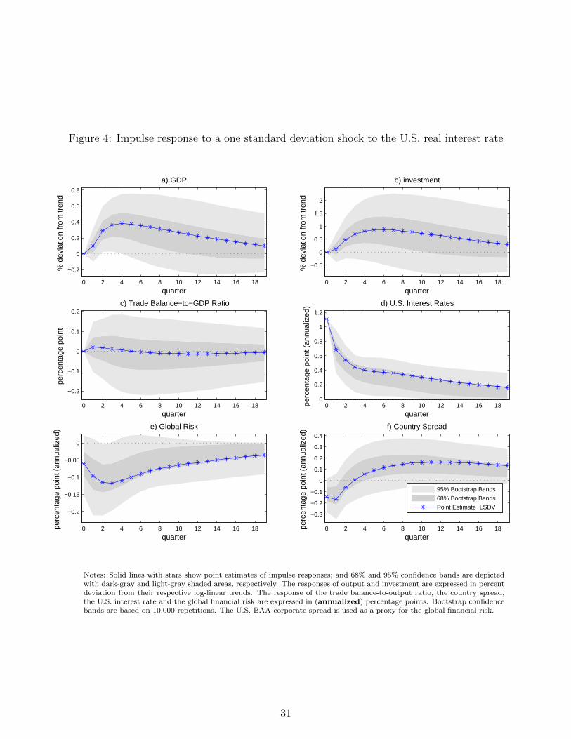
Figure 4: Impulse response to a one standard deviation shock to the U.S. real interest rate

0 2 4 6 8 10 12 14 16 18

−0.2

0

0.2

0.4

0.6

0.8

a) GDP

quarter

% d

evia

tion

from

tren

d

0 2 4 6 8 10 12 14 16 18

−0.5

0

0.5

1

1.5

2

b) investment

quarter

% d

evia

tion

from

tren

d

0 2 4 6 8 10 12 14 16 18

−0.2

−0.1

0

0.1

0.2c) Trade Balance−to−GDP Ratio

quarter

perc

enta

ge p

oint

0 2 4 6 8 10 12 14 16 180

0.2

0.4

0.6

0.8

1

1.2


quarter

perc

enta

ge p

oint

(an

nual

ized

)

0 2 4 6 8 10 12 14 16 18

−0.2

−0.15

−0.1

−0.05

0

e) Global Risk

quarter

perc

enta

ge p

oint

(an

nual

ized

)

0 2 4 6 8 10 12 14 16 18

−0.3

−0.2

−0.1

0

0.1

0.2

0.3

0.4

f) Country Spread

perc

enta

ge p

oint

(an

nual

ized

)

quarter

95% Bootstrap Bands

68% Bootstrap Bands

Point Estimate−LSDV


31

Figure 5: Impulse response to a one standard deviation shock to the country spread

0 2 4 6 8 10 12 14 16 18

−0.8

−0.6

−0.4

−0.2

0a) GDP

quarter

% d

evia

tion

from

tren

d

0 2 4 6 8 10 12 14 16 18

−2.5

−2

−1.5

−1

−0.5

0b) investment

quarter

% d

evia

tion

from

tren

d

0 2 4 6 8 10 12 14 16 180

0.05

0.1

0.15

0.2

0.25

0.3

0.35


quarter

perc

enta

ge p

oint

0 5 10 15 20−1

−0.5

0

0.5

1d) U.S. Interest Rates

quarter

perc

enta

ge p

oint

(an

nual

ized

)

0 5 10 15 20−1

−0.5

0

0.5

1e) Global Risk

quarter

perc

enta

ge p

oint

(an

nual

ized

)

0 2 4 6 8 10 12 14 16 180

0.2

0.4

0.6

0.8

1

f) Country Spread

perc

enta

ge p

oint

(an

nual

ized

)

quarter

95% Bootstrap Bands68% Bootstrap BandsPoint Estimate−LSDV


32

Figure 6: Forecast error variance decomposition at different horizons

0 10 200

0.1

0.2

Output

EpsR

US

0 10 200

0.1

0.2

0.3

EpsG

R

0 10 200

0.1

0.2

0.3

EpsE

MBI

0 10 200

0.1

0.2

Investment

0 10 200

0.1

0.2

0.3

0 10 200

0.1

0.2

0.3

0 10 200

0.1

0.2

Trade Balance-to-GDP Ratio

0 10 200

0.1

0.2

0.3

0 10 200

0.1

0.2

0.3

0 10 200

0.2

0.4

0.6

0.8

Country Spread

0 10 200

0.2

0.4

0.6

0.8

0 10 200

0.2

0.4

0.6

0.8

Notes: Solid lines depict the fraction of the variance of the k-quarter ahead forecasting error explained by the U.S. realinterest rate shocks (shown in the first row), by the global financial risk shocks (shown in the second row) and by thecountry spread shocks (shown in the last row) at different horizons. The U.S. BAA corporate spread is used as a proxy forthe global financial risk.

33

Figure 7: Forecast error variance decomposition at different horizons–counterfactual

0 10 200

0.05

0.1

0.15

0.2Output

EpsU

S

0 10 200

0.05

0.1

0.15

0.2

EpsG

R

0 10 200

0.05

0.1

0.15

0.2Investment

0 10 200

0.05

0.1

0.15

0.2

0 10 200

0.05

0.1

0.15

0.2TBY

0 10 200

0.05

0.1

0.15

0.2

0 10 200

0.2

0.4

0.6

0.8

Country Spread

0 10 200

0.2

0.4

0.6

0.8

CounterfactualBaseline

Notes: Solid lines depict the fraction of the variance of the k-quarter ahead forecasting error explained by the U.S. realinterest rate shocks (shown in the first row) and the global financial risk shocks (shown in the second row). Dashed linesshow the fraction of the variance of the k-quarter ahead forecasting error explained by the U.S. real interest rate shocks(shown in the first row) and by the global financial risk shocks (shown in the second row), when the country spread isassumed not to respond directly to variations in the U.S. financial variables. The U.S. BAA corporate spread is used as aproxy for the global financial risk.

34

Figure 8: Impulse response to a one standard deviation shock to the banking sectorborrowing-lending spread in the extended model

0 5 10 15

−0.5

−0.4

−0.3

−0.2

−0.1

0

0.1

a) GDP

quarter

% d

evia

tion

from

tren

d

0 5 10 15

−1

−0.5

0

0.5

b) investment

quarter

% d

evia

tion

from

tren

d

0 5 10 15

−0.05

0

0.05

0.1

0.15

0.2

0.25

0.3


quarter

perc

enta

ge p

oint

−−

leve

l dev

. fro

m tr

end

0 5 10 15 20−1

−0.5

0

0.5


quarter

perc

enta

ge p

oint

(an

nual

ized

)

0 5 10 15 20−1

−0.5

0

0.5

1e) Global Risk

quarter

perc

enta

ge p

oint

(an

nual

ized

)

0 5 10 150

0.2

0.4

0.6

0.8

1

1.2

1.4f) Domestic Bank Lending Spread

quarter

perc

enta

ge p

oint

(an

nual

ized

)

0 5 10 15 20−0.1

0

0.1

0.2

0.3

0.4

0.5

0.6g) Country Spread

perc

enta

ge p

oint

(an

nual

ized

)

quarter

95% Bootstrap Bands

68% Bootstrap Bands


Notes: Solid lines with stars show point estimates of impulse responses; and 68% and 95% confidence bands are depictedwith dark-gray and light-gray shaded areas, respectively. The responses of output and investment are expressed in percentdeviation from their respective log-linear trends. The response of the trade balance-to-output ratio, the country spread, theU.S. interest rate, the banking sector borrowing-lending spread and the global financial risk are expressed in (annualized)percentage points. Bootstrap confidence bands are based on 10,000 repetitions. The U.S. BAA corporate spread is usedas a proxy for the global financial risk.

35

Figure 9: Impulse response to a one standard deviation shock to the country spread in theextended model

0 5 10 15−0.7

−0.6

−0.5

−0.4

−0.3

−0.2

−0.1

0

a) GDP

quarter

% d

evia

tion

from

tren

d

0 5 10 15

−1.5

−1

−0.5

0

b) investment

quarter

% d

evia

tion

from

tren

d

0 5 10 15

0

0.1

0.2

0.3


quarter

perc

enta

ge p

oint

−−

leve

l dev

. fro

m tr

end

0 5 10 15 20−1

−0.5

0

0.5


quarter

perc

enta

ge p

oint

(an

nual

ized

)

0 5 10 15 20−1

−0.5

0

0.5

1e) Global Risk

quarter

perc

enta

ge p

oint

(an

nual

ized

)

0 5 10 15

0

0.1

0.2

0.3

0.4

0.5

f) Domestic Bank Lending Spread

quarter

perc

enta

ge p

oint

(an

nual

ized

)

0 5 10 15 20−0.2

0

0.2

0.4

0.6

0.8

1


perc

enta

ge p

oint

(an

nual

ized

)

quarter

95% Bootstrap Bands

68% Bootstrap Bands



36

Figure 10: Impulse response to a one standard deviation shock to the global financial riskin the extended model

0 5 10 15

−0.6

−0.4

−0.2

0

a) GDP

quarter

% d

evia

tion

from

tren

d

0 5 10 15

−2

−1.5

−1

−0.5

0

b) investment

quarter%

dev

iatio

n fr

om tr

end

0 5 10 15−0.1

0

0.1

0.2

0.3


quarter

perc

enta

ge p

oint

−−

leve

l dev

. fro

m tr

end

0 5 10 15

−0.5

0

0.5


quarter

perc

enta

ge p

oint

(an

nual

ized

)

0 5 10 15

0

0.1

0.2

0.3

e) Global Risk

quarter

perc

enta

ge p

oint

(an

nual

ized

)

0 5 10 15−0.2

−0.1

0

0.1

0.2

0.3

f) Domestic Bank Lending Spread

quarter

perc

enta

ge p

oint

(an

nual

ized

)

0 5 10 15 20−0.2

0

0.2

0.4


perc

enta

ge p

oint

(an

nual

ized

)

quarter

95% Bootstrap Bands

68% Bootstrap Bands



37

Figure 11: Forecast error variance decomposition at different horizons for alternative mea-sures of the global financial risk

0 10 200

0.1

0.2

0.3

0.4

0.5Output

BAA

0 10 200

0.1

0.2

0.3

0.4

0.5

S.M

.Vol.

0 10 200

0.1

0.2

0.3

0.4

0.5

HY

0 10 200

0.1

0.2

0.3

0.4

0.5Investment

0 10 200

0.1

0.2

0.3

0.4

0.5

0 10 200

0.1

0.2

0.3

0.4

0.5

0 10 200

0.1

0.2

0.3

0.4

0.5TBY

0 10 200

0.1

0.2

0.3

0.4

0.5

0 10 200

0.1

0.2

0.3

0.4

0.5

0 10 200

0.2

0.4

0.6

0.8

1Country Spread

0 10 200

0.2

0.4

0.6

0.8

1

0 10 200

0.2

0.4

0.6

0.8

1

EMBI+GR+USRGR+USRUSR

Notes: Solid lines with circles depict the fraction of the variance of the k-quarter ahead forecasting error explained jointlyby the U.S. real interest rate, the global financial risk and country spread shocks. Solid lines show the fraction of thevariance of the k-quarter ahead forecasting error explained jointly by the U.S. real interest rate and the global financialrisk. Broken lines depict the fraction of the variance of the forecasting error explained by the U.S. real interest rate shock.The first row shows the forecast error variance decomposition at different horizons when the U.S. BAA corporate spread isused as a proxy for the global financial risk. The second row shows the forecast error variance decomposition at differenthorizons when the U.S. stock market volatility index is used as a proxy for the global financial risk. The third row showsthe forecast error variance decomposition at different horizons when the U.S. high yield spread is used as a proxy for theglobal financial risk.

38

Global Financial Conditions, Country Spreads and ...

Documents

Transcript of Global Financial Conditions, Country Spreads and ...