Getting Started with the GARTEUR RECOVER Benchmark

AppendixGetting Started with the GARTEUR RECOVERBenchmark

542 Appendix

1 Introduction

The GARTEUR REconfigurable COntrol for Vehicle Emergency Return(RECOVER) aircraft simulation benchmark was developed to demonstrate, bothoffline and in real-time (piloted) simulation, the performance and viability of newlydesigned fault tolerant flight control algorithms. The software package, based on theDelft University Aircraft Simulation and Analysis Tool DASMAT [2], is equippedwith several simulation and analysis tools, all centered around a generic non-linearaircraft model for six-degrees-of-freedom non-linear aircraft simulations. For highperformance computation and visualisation capabilities, the package has been inte-grated as a toolbox in the computing environment Matlab R©/Simulink R©. The toolsof the RECOVER benchmark include trimming and linearisation for (adaptive)flight control law design, non-linear off-line (interactive) simulations, simulationdata analysis and flight trajectory and pilot interface visualisations. The modularityof the RECOVER software allows customisation by applying user-generated mod-els to the generic package for the simulation of any specific aircraft type or faultscenario. In conjunction with the Matlab R©/Simulink R© Real-Time Workshop R©,the benchmark model is suitable for integration on simulation platforms for pilotedhardware in the loop testing.

The GARTEUR RECOVER benchmark provides enhanced graphical andhigh-resolution aircraft visualisation capabilities, that interface with the Matlab R©environment, to support tool-based advanced flight control system design and eval-uation. This includes, for instance, the visualisation of flight data, the animationof fault or aircraft upset recovery scenarios or (real-time) analysis of flight controlsystem states and performance.

The capabilities of the GARTEUR RECOVER benchmark software are suitablefor any educational or demonstration purposes, providing insight into the design ofadaptive flight control algorithms, aircraft flight dynamics and handling qualitiesand human factors interfaces.

This Appendix provides a practical guide to get started with the GARTEUR RE-COVER Simulation Benchmark software package. It provides the necessary stepsto install the software (Section 3) and get familiar with the model structure (Section5) and the main features of the benchmark environment (Section 6). Some practi-cal examples demonstrate the steps necessary to run a benchmark simulation (Sec-tion 6.2). It is assumed that the user is familiar with the installation and use ofthe Matlab R©/Simulink R© programming environment (references can be found in[13, 14] or on the website of The Mathworks (www.mathworks.com)). For theapplication of the benchmark, the user should have a basic understanding of generalrigid body aircraft dynamics and aircraft simulation modeling. An introduction tothese subjects can be found in several excellent books (e.g. [9, 12]). In this aspect,the GARTEUR RECOVER benchmark is an ideal tool to complement any studieson the introduction of flight control and aircraft simulation modeling using chal-lenging design problems.

The GARTEUR RECOVER benchmark should be regarded as a research toolproviding the flexibility for customisation using a modular structure. As such, the

Getting Started with the GARTEUR RECOVER Benchmark 543

user is encouraged to explore and experiment with the software as much as possibleto obtain insight into the model structure and its features, and adapt it to his or herown research requirements. Names and descriptions of blocks and signal definitionsin the benchmark model provide a guide for the user on the model interfacing re-quirements. An introduction to the RECOVER benchmark, including developmentbackground, software achitecture, the main features and the aircraft operationalcharacteristics has been provided in Chapter 6 of this book. For more details and in-sight into the generic simulation architecture, including the GARTEUR RECOVERbenchmark mathematical models, applied reference frames, variable definitions andsign conventions the user may refer to the references [2, 3, 4, 5, 6, 7, 8, 10].

The GARTEUR RECOVER benchmark is distributed as open source software toaccompany this book on fault tolerant flight control design and simulation for civiltransport aircraft. The software package can be downloaded, after registration, fromthe GARTEUR project website hosted by NLR (www.faulttolerantcontrol.nl). Any updates of the GARTEUR RECOVER benchmark, including documen-tation and release notes, will be made available via the website.

2 System Requirements

The GARTEUR RECOVER benchmark was designed to run under Matlab R© 6.5.1and Simulink R© 5.1 as part of Release 13/Service Pack 1 (R13SP1). This means thatthe benchmark model can also be used with higher versions of Matlab R©/Simulink R©.To install and operate the benchmark model, any PC that complies with the mini-mum hardware requirements to properly run Matlab R©/Simulink R© is suitable. Thewebsite of The Mathworks (www.mathworks.com)) provides further details onthe hardware requirements to install and run Matlab R©/Simulink R©.

The graphical visualisation capabilities of the GARTEUR RECOVER bench-mark, especially the aircraft animation features, require at least a graphics cardthat supports Direct3D. OpenGL compatible hardware acceleration is recommendedto improve the overall graphics quality and hardware performance of the RE-COVER visualisation features. For customisation of the visualisation tool withinMatlab R©/Simulink R©, specifically the inputs that drive the graphical displays, a C-compiler needs to be installed. When running the benchmark within Matlab R© 7.1(Release 14) under Windows XP, the buttons of the benchmark main menu do notdisplay correctly. This graphics issue does not occur in Matlab R© 6.5.1 (R13SP1)and should be solved for later versions of Matlab R© 7.1 (R14).

The GARTEUR RECOVER benchmark was tested under Windows XP and Win-dows VISTA. For the current version of the benchmark (version 2.2) no issues, otherthen those mentioned in this guide, are known under these operating systems.

3 Installation and Initialisation

The GARTEUR RECOVER benchmark software package is distributed via theGARTEUR project site hosted by NLR (www.faulttolerantcontrol.nl).

544 Appendix

After registration, the software can be downloaded as a packed ZIP archive. Thefollowing steps are necessary to download and install the benchmark within theMatlab R© 6.5.1 (R13SP1) environment.

• After registering, download the software package from the GARTEUR projectwebsite (www.faulttolerantcontrol.nl).

• Unzip the package into a temporary directory.• Copy the unzipped package into a suitable destination directory, preferably into

the Toolbox directory of Matlab R©. Make sure that the directory structure ofthe unpacked package is retained.

• Append the RECOVER benchmark directories to the Matlab R© path. TheMatlab R© references provide information on how to configure the path.

• Change the Matlab R© directory to RECOVERv65. Datafiles generated by thebenchmark tools will be made available in the data directory.

• The benchmark can be started by typing recover in the Matlab R© commandwindow which activates the main user menu. This will provide further steps tostart running any simulations or exploring the features and models of the RE-COVER benchmark.

The benchmark can be uninstalled by deleting the directory RECOVERv65.Please make sure that any backup copies are made of the user generated datafiles inthe data directory before deleting.

4 License Agreement

The GARTEUR RECOVER benchmark package is distributed with this book as acollective work. The Matlab R©/Simulink R© models of the benchmark are distributedunder the Open Software License (OSL) version 3 or later, whereas the benchmarkvisualisation tool remains copyrighted by NLR (although freely distributable withthe RECOVER benchmark). The OSLv3 license allows the user of the software tomodify the models according to his or her own requirements and applications andre-distribute the software to other users under the OSLv3 licensing terms and con-ditions and NLR copyright. Any notices and text, including the attribution to theoriginal developers and the book, should remain in the software package and mod-els. To facilitate the development or application by other users, developers that haveadapted the software are required to include an appropriate attribution notice in thesource code to inform new users that the original software has changed. The OSLv3license is available in the file license.txt as part of the GARTEUR RECOVERsoftware package. Please take notice of the licensing terms and conditions beforeusing the software.

5 Model Structure

The aim of the following section is to provide an overview of the main model struc-ture of the GARTEUR RECOVER benchmark. This can be used as a starting point


to further explore the model. Reference [2] provides information on all the submod-els that comprise the generic aircraft simulation in the benchmark including inputand output formats of the individual generic simulation blocks.

The benchmark Matlab R©/Simulink R© environment has been developed in a mod-ular and layered structure using (masked) system blocks and subsystem blocks. Inthis structure, each block has its specific input and ouput formats and signal defi-nitions. When customising the RECOVER benchmark simulation for any particularresearch application, it is important to maintain the model format and signal rela-tionships as much as possible to prevent any inadvertent mismatches between themany subsystems and library components. Due to the complexity of the GARTEURRECOVER benchmark model, it is recommended to always make use of a versioncontrol method to track any changes or revert to a working version of the benchmarkif necessary.

Chapter 6 of this book provides an introduction to the model structure of thebenchmark and its components.

5.1 Model Architecture

The software architecture of the GARTEUR RECOVER simulation benchmark(Fig. 1) comprises a combination of generic aircraft models and aircraft specificmodules including aerodynamics, flight control systems and propulsion systems.For the RECOVER benchmark, the aerodynamic, flight control systems and propul-sion model are representative of the Boeing 747-100/200 aircraft [5, 10]. Throughthe graphical user interface, the user has access to the RECOVER benchmark simu-lation and analysis tools (Section 6).

5.2 GARTEUR RECOVER Benchmark Libraries

The GARTEUR RECOVER benchmark model consists of a combination ofMatlab R© scripts and Simulink R© block diagrams. The Simulink R© block diagramsare built in a layered, modular structure consisting of subsystems with a fixed inter-face definition between the block inputs and outputs ([2]). In order to ensure consis-tency, the top-level models have been built from common blocks that are linked toSimulink R© libraries. All blocks and libraries are contained in the root directory ofthe benchmark called RECOVERv65 (extension v65 referring to Matlab R© version6.5.1 (R13SP1)). The RECOVER benchmark libraries can be regarded as a centralrepository of the main benchmark simulation models. All blocks in the benchmarkthat are linked to a library are automatically updated by any changes of a libraryblock. As such, it is not recommended to change a library block in the benchmarklocally. However, if required, the linked blocks in the benchmark model can bechanged when the link to the library is disabled. This is accomplished by selectingDisable Link in the Matlab R© message dialog window which appears as soon as theuser tries to change the block. In order to change a block in the library, it first needsto be unlocked by selecting Unlock Library in the Matlab R© edit menu. It should

546 Appendix

Fig. 1 GARTEUR RECOVER benchmark software architecture and analysis tools relation-ships

be noted that any changes to the interface definitions of the models in the libraryshould be made carefully. This includes the names of the blocks as the library linksuse the block names as a reference.

A basic library (B747 library.mdl) for the simulation of the B747-100/200aircraft model in the benchmark, contains the basic aircraft, engine and actuatormodels, complete with failure models (Fig. 2). For the GARTEUR RECOVERbenchmark, an additional library was developed (ag16 library.mdl), based onthe basic library, that contains the larger and more extensively modified submodelsout of which the top-level benchmark is built (Fig. 3). This extended library containsmodels of the aircraft, the actuators, the sensors, the classic flight control system andthe benchmark failure generator.

5.3 GARTEUR RECOVER Model Components

The actual benchmark model (b747 auto g.mdl) is depicted in Fig. 4 and isalso described in Chapter 6. The airframe block is the combination of the aircraftaerodynamic model, engines and actuators. It also contains the fault models andthe turbulence and wind models. The inputs to this block are twenty-six separatelycontrollable aerodynamic surfaces and four engine controls. The autoflight block


Fig. 2 GARTEUR RECOVER benchmark basic aircraft simulation library(B747 library.mdl)

represents the implementation of the classic Boeing 747-100/200 autoflight systembased on [7]. This is the block that is to be replaced by any new fault tolerant con-troller design and is intended as a working example of how the new controller issupposed to fit into the aircraft. The classic autoflight system block consists in-ternally of the B747-100/200 hydro-mechanical flight control system model (FCS),which forms the inner control loop, and the autopilot and autothrottle systems whichtogether form the outer control loop.

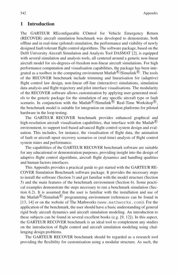
An open-loop simulation model (b747 funpc d.mdl), enabling e.g. real-timeinteractive ‘engineer-in-the-loop’ simulations, is available as part of the benchmarkpackage (Fig. 5). It contains the same aircraft, engine, actuator model and failuregenerator as found in the main benchmark model. The open-loop model is in afunctional form, i.e. it has explicit inputs (12) and outputs (140). The inputs of theopen-loop model consist of the pilot’s controls as found on the Boeing 747 aircraft.The structure of this model is very similar to the model that is used for trimming(b747 trim d.mdl).

To enable real-time ‘engineer-in-the-loop’ simulations, a Simulink R© S-functionblock (sf realtime), which emulates approximate real-time conditions, is included inthe top level of the open-loop model. An additional block library in the RECOVERroot directory (Stick interface library.mdl) provides a Simulink R© stickmanipulator block to interface with the pilot control inputs of the open-loop model.

548 Appendix

Fig. 3 GARTEUR RECOVER benchmark component library (ag16 library.mdl)

Fig. 4 GARTEUR RECOVER benchmark main model components (b747 auto g.mdl)


Fig. 5 GARTEUR RECOVER functional model for open-loop simulation(b747 funpc d.mdl)

Depending on the stick configuration, adaptation of the stick interface model by theuser might be necessary.

Fig. 6, shows the Simulink R© model structure at Level 5 of the benchmarkairframe block. This level shows the main layout of the RECOVER aircraft simu-lation model consisting of the generic simulation models and aircraft specific mod-ules. The aircraft specific modules (Airframe model (AFM) block and Engine framemodel (EFM) block indicated with a blue background) can be customised for anyparticular aircraft taking into account the interface definitions of the blocks.

The blocks that are not specific for any aircraft and that are part of the genericsimulation models ([2]) are displayed with a white background. The generic simu-lation blocks consist of:

AIRDATA blockThe atmospheric and airdata parameters are calculated in this block. The equationsare compiled in a MEX-type Simulink R© S-function ac.atmos.mex.

WIND/TURBULENCE blockIn this block, the wind and gust velocities are calculated based on user-suppliedSimulink R© S-functions of wind and turbulence models. The benchmark simula-tion uses zero wind and zero turbulence conditions by default. The block includes aswitching capability for the selection of a turbulence model based on Dryden spectra

550 Appendix

Fig. 6 GARTEUR RECOVER benchmark Simulink R© block diagram showing main aircraftsimulation model at Level 5 of the airframe system block

or a wind model that includes a wind profile based on meteorological data estimatedat the time of the Flight 1862 aircraft accident.

AFM blockIn this block the forces and moments of both the aircraft aerodynamics and turbu-lence are calculated. The aerodynamic forces and moments are determined from theaircraft specific aerodynamic model.

EFM blockThis block calculates the propulsion forces and moments based on the aircraft spe-cific engine model.

GRAVITY blockThis block calculates the components of the gravity force in the air-path, stability,body and moving earth reference frames. The gravity force is calculated in the mov-ing earth reference frame from the aircraft mass and the altitude varying gravityacceleration.


FM SORT blockIn this block all forces and moments calculated from the aerodynamic model, tur-bulence model, propulsion model and gravity model are combined and added.

EQM blockThis block includes the aircraft equations of motion and are solved resulting in theaircraft states and their derivatives. In addition, the aerodynamic and total forces andmoments and their coefficients are corrected for the α- and β - contributions.

OBSERVATIONS blockThe observation parameters of the RECOVER benchmark are calculated in thisblock. The parameters are arranged in several subgroups, calculated in subblocks,consisting of accelerations, linear velocity time derivatives, flight-path related pa-rameters and measurements outside the center of gravity. A complete list of thebenchmark observation output signal formats is provided in Section 8.

6 Using the GARTEUR RECOVER Benchmark

This section describes the structure and operation of the different (customisable)GARTEUR RECOVER benchmark tools which can be accessed via the RECOVERgraphical user interface. A few user examples are provided demonstrating the proce-dures to conduct a simulation under a particular aircraft condition, perform lineari-sation of the non-linear aircraft model and utilise the aircraft visualisation features.

6.1 Main Menu

The GARTEUR RECOVER benchmark simulation and analysis tools can be ac-cessed via a Matlab R© graphical user interface (Fig. 7). The benchmark main menucan be started by typing recover in the Matlab R© command window. The user op-tions in the menu are divided into three main sections allowing the user to performbenchmark initialisation and simulations (Simulation) and run the analysis tools(Analysis) including aircraft linearisation, plotting of simulation results and flightcontrol assessment criteria and aircraft visualisation. A help section on the mainmenu (Reference) provides a quick reference for operation and customisation of theGARTEUR RECOVER benchmark.

6.1.1 Open-Loop Simulation

The Open-Loop Simulation button (Fig. 8) in the Simulation section of the bench-mark main menu will activate the initialisation of an open-loop simulation of anewly designed control algorithm. During initialisation, the calculation of a (userspecified) trim condition is performed, and a particular test scenario and aircraftfailure mode can be selected. Section 6.2 demonstrates the required steps to per-form a typical open-loop simulation.

552 Appendix

Fig. 7 GARTEUR RECOVER benchmark graphical user interface

Fig. 8 Open-loop simulation initialisation button

6.1.2 Closed-Loop Simulation

The Closed-Loop Simulation button (Fig. 9) in the main menu activates the initiali-sation of a closed-loop benchmark simulation. As with the initialisation of an open-loop simulation, the calculation of a (user specified) trim condition is performed anda particular test scenario and aircraft failure mode can be selected. It should be notedthat the closed-loop simulation is performed using preset test scenarios as specifiedfor the GARTEUR fault tolerant control benchmark (Chapter 6 and 7 of the bookprovide details on the test scenario specifications based on predefined aircraft opera-tional requirements). An example in Chapter 6 describes the initialisation procedureto perform simulations using the closed-loop benchmark model.


Fig. 9 Closed-loop simulation initialisation button

6.1.3 Linearise Aircraft

For control law design purposes, the non-linear aircraft model can be linearised us-ing a basic linearisation routine that is available as part of the RECOVER benchmarktools. The linearisation routine allows a linear model with twelve states and 29 con-trol inputs (25 control surfaces and 4 engines) to be obtained. In the current versionof the benchmark, the linearisation can only be done for the total non-linear modelperturbing all twelve states and 29 control inputs. Separation into a symmetric orasymmetric linear model is an option reserved in the linearisation routine but is notyet implemented. The user may refer to reference [2] for further customisation ofthe benchmark linearisation routine.

To obtain a linearised model, a trimmed flight condition needs to be calculated viathe initialisation of a closed-loop or open-loop simulation. Fig. 10 and 11 illustratethe calculation steps of an example trim condition (TESTlin4.tri).

When a trimmed flight condition is determined, the linearisation of the non-linearaircraft model can be started by using the Linearise Aircraft button in the benchmarkmain menu which activates the linearisation procedure (Fig. 12).

The matrices of the calculated linear model, which is given in state-space form,are available as the variables Alin, Blin, Clin, Dlin in the Matlab R©workspace. Note that the variable Alin is in radians but all control surface de-flections (except for thrust which is in Newtons) in the matrix variable Blin are indegrees. For the purpose of designing a controller, it might be better to convert theBlin matrix back to radians (this can be done by multiplying the columns of Blin,associated with the control surface deflections, with 180/π).

The ordering of the states xlin and the control surfaces ulin of the total linearmodel described by the matrices Alin and Blin are as indicated in equation (1).The spoilers #6 and #7 are ground spoilers and are not used during flight. The10th and 11th columns associated with these control surfaces can therefore be ne-glected during design. Also note that the number of columns of the Blin matrixis 29. The 30th column is associated with the landing gear and has not been in-cluded in the linear model. An example linear model can be accessed through thefile TESTlin4.lin, available in the benchmark data folder, using the commandload -mat TESTlin4.lin in the Matlab R© window.

554 Appendix

Fig. 10 Initialisation of benchmark trim conditions


Fig. 11 Calculation of benchmark trim condition

556 Appendix

Fig. 12 Initialisation and calculation of linearised benchmark model (total model)


Total model:

⎧⎪⎨⎪⎩

xlin =[

pb qb rb VTAS α β φ θ ψ he xe ye]

ulin =[δair δail δaor δaol δsp1−12 δeir δeil δeor δeol δih δru δrl δ f o δ f i δTN1−4

](1)

After the completion of the steps in Fig. 12, the quality of the linearisation routinecan be evaluated by comparing the states (around the trimmed flight condition) be-tween the linear and non-linear model using small actuator deflections. This is doneby running the Simulink R© model called b747 auto g LINcheck.mdl and theplotting routine plotBENCHMARKtestLINandNL.m. The user needs to makea selection of the actuator to be used as perturbation input for the comparison de-pending on which axis is to be tested (e.g. to test the quality of the lateral axis,1.5deg of right aileron and -1.5deg of left aileron can be used). Any control inputfor a particular actuator to excite the linear model can be defined in the airframe forLINEAR comparison test block within the modelb747 auto g LINcheck.mdl.Fig. 13, 14 and 15 show example plot results allowing the comparison of the lin-earised model (TESTlin4.lin) and the non-linear model after a spoiler

Fig. 13 Plots showing actuator deflections (spoilers deflected 1.5 degrees at t=1s) for com-parison of linearised model (TESTlin4.lin) and non-linear model

558 Appendix

Fig. 14 Plots showing longitudinal states for comparison of linearised model(TESTlin4.lin) and non-linear model (NL: non-linear model, lin: linear model)

Fig. 15 Plots showing lateral states for comparison of linearised model (TESTlin4.lin)and non-linear model (NL: non-linear model, lin: linear model)


deflection input of 1.5 degrees. The aircraft states are given in radians while alti-tude (he) and ground distance (xe) are given in meters.

6.1.4 Plot Simulation Results

The Plot Simulation Results button (Fig. 16) activates the plotting function of thebenchmark following a closed-loop or open-loop simulation. The plot function,called via the script plot sim.m, generates additional time responses of the air-craft including the aircraft states, pilot control deflections and specific forces. Ex-ample aircraft simulation responses obtained by the plot function are illustrated inthe user examples (Chapter 6 and paragraph 6.2).

6.1.5 Show Assessment Criteria

Following a simulation (open-loop, closed-loop or via manually controlled inputsin the open-loop functional model (Fig. 5)), the performance of the designed fault

Fig. 16 Simulation time responses activation button

Fig. 17 Benchmark assessment criteria activation button

560 Appendix

Fig. 18 Benchmark assessment criteria plots for Right Turn and Localiser Intercept phaseshowing aircraft states with evaluation criteria

tolerant control algorithms can be evaluated using the benchmark assessment crite-ria. The assessment criteria are provided as plots for each phase of the benchmarkscenario (Chapter 6) and can be generated using the Show Assessment Criteria but-ton (Fig. 17) after a simulation. Fig. 18, 19 and 20 show example plots for the RightTurn and Localiser Intercept phase of the benchmark scenario. Chapters 6 and 7provide further details on the benchmark scenario specifications and definition ofthe assessment criteria parameters as used in the plots.

6.1.6 RECOVER Visualisation

The GARTEUR RECOVER benchmark aircraft visualisation and animation tool(Fig. 22) provides a high-resolution visualisation of the benchmark’s approach andlanding scenario and flight trajectory. The RECOVER visualisation tool is specifi-cally aimed to support interactive (real-time) fault tolerant flight control design andevaluation for civil transport aircraft. The visualisation features include graphic ren-ditions of the aircraft, cockpit flight instrumentation and aircraft geographic environ-ment (Amsterdam Schiphol airport and surroundings). The RECOVER interactivesimulation and visualisation window can be activated via the RECOVER Visualisa-tion button following initialisation of an open-loop or closed-loop simulation.


Fig. 19 Benchmark assessment criteria plots for Right Turn and Localiser Intercept phaseshowing kinematic accelerations in body axes with evaluation criteria

(a) Horizontal trajectory (b) Vertical trajectory

Fig. 20 Aircraft trajectory plots for Right Turn and Localiser Intercept phase

562 Appendix

Fig. 21 Interactive simulation and visualisation activation button

Fig. 22 GARTEUR RECOVER benchmark interactive simulation and visualisation windowshowing aircraft model with separated right-wing engines (Flight 1862 accident scenario)

A graphical pilot interface shows the basic flight instrumentation based on spec-ifications of the electronic flight instrument system (EFIS) displays as found onthe B747-400 aircraft. The RECOVER EFIS displays are configured to show theprimary aircraft state parameters, flight control system state and engine thrust pa-rameters. Additional features on the displays, not found on the standard B747-400instrumentation, are included to assess the human-machine interfacing (HMI) as-pects of new fault tolerant flight control algorithms. For these design applications,the RECOVER benchmark primary flight display (PFD) has the capability to dis-play, for instance, the aircraft’s bank, pitch and airspeed envelope protection limits


as calculated by a new self-adaptive control system. The lower display (Engine In-dicating and Crew Alerting System (EICAS) display) shows the engine parameters,using Engine Pressure Ratio (EPR) as the main thrust setting reference, inboardtrailing edge flap position and landing gear status. Additional aircraft state informa-tion on the EICAS display includes angle-of-attack, sideslip and load factor. TheEICAS display also enables monitoring of the activity of the flight control systemand control law performance by presenting all individual control surface deflec-tions. A basic 3D aircraft model, representing the B747-100/200 aircraft, and theaircraft’s reconstructed flight path in the out-the-window view allows analysis ofthe flight trajectory and maneuvers.

The following features of the interactive simulation window can be controlled bykeyboard and mouse:

• shift -W: switch to aircraft view mode• shift -A: switch to cockpit view mode• shift -C: Activate free viewing (aircraft view mode)• P: Activate/deactivate aircraft flight path (aircraft view mode)• Left mouse/touch pad button: zoom out (aircraft view mode)• Right mouse/touch pad button: zoom in (aircraft view mode)• Mouse or touchpad: Move viewpoint (aircraft view mode)

Fig. 23 shows the information available on the RECOVER benchmark primaryflight display.

Fig. 24 provides a description of the parameters that are available on the RE-COVER benchmark EICAS display.

For a realistic visualisation of the benchmark scenario, the RECOVER visuali-sation tool includes a high-resolution geographic rendition of the Amsterdam areaincluding a detailed layout of the Amsterdam Schiphol Airport runway configura-tions (Fig. 25). Currently, only runway 27 is configured with an instrument landingsystem (ILS) as part of the GARTEUR benchmark scenario. However, further cus-tomisation of the airport approach and landing aids is possible within the benchmarkmodel (e.g. an extension of ILS availability).

The aircraft’s flight trajectory can be visualised by pressing P before starting, orduring, a (real-time) simulation. Fig. 26 and Fig. 27 illustrate the flight path visu-alisation capability in the RECOVER out-the-window view (free viewing mode),following a simulation of a landing test scenario and in-flight maneuver.

Although not part of the GARTEUR benchmark scenario, runway 06 of theSchiphol airport scenery is equipped with approach lighting and a visual approachslope indicator (VASI) (Fig. 28 and 29) to replicate the pilot’s viewpoint during atypical approach and landing test scenario under visual meteorological conditions(VMC).

All parameters presented on the RECOVER flight instrumentation displays andcontrolling the out-the-window view are available as inputs via a Simulink R© in-terface in the output & visualisation block (top system level). The RE-COVER visualisation window input variables, including the signal element number,variable name, dimension and description are summarised in Tables 1 and 2.

564 Appendix

Fig. 23 GARTEUR RECOVER benchmark primary flight display (PFD) elements

1 ILS DME distance 12 Flight director2 Pitch envelope limit 13 Localiser indicator3 Radio altitude 14 Selected heading4 Selected altitude 15 Magnetic heading5 Bank angle envelope limit 16 ILS course6 Altitude 17 Minimum speed (red) and mini-

mum maneuvering speed (yellow)7 Vertical speed 18 Attitude indicator8 Selected altitude 19 Indicated airspeed9 Vertical speed 20 Selected airspeed10 Atmospheric pressure (QNH) 21 Maximum speed (red) and maxi-

mum maneuvering speed (yellow)11 Glideslope indicator 22 Selected airspeed


Fig. 24 GARTEUR RECOVER benchmark engine indicating and crew alerting system(EICAS) display elements

1 Total air temperature 7 Right inboard and outboard elevatorposition

2 Landing gear indicator 8 Stabiliser position3 Commanded and actual inboard

trailing edge flap position9 Left-wing spoilers #1 to #6 position

4 Angle-of-attack (ALFA), sideslip(BETA) and load factor (GLOAD)

10 Left-wing inboard and outboardaileron position

5 Right-wing inboard and outboardaileron position

11 Upper and lower rudder position

6 Right-wing spoilers #7 to #12 posi-tion

12 Engine pressure ratio (EPR) andmaximum EPR

566 Appendix

Fig. 25 GARTEUR RECOVER benchmark geographical rendition of Amsterdam Schipholairport and runway configurations and dimensions


Fig. 26 Aircraft flight path visualisation during approach and landing test scenario

Fig. 27 In-flight maneuver visualisation in free viewing mode

568 Appendix

Fig. 28 Amsterdam Schiphol runway 06 visual landing aids and ground textures

Fig. 29 Visual Approach Slope Indicator (VASI)


Table 1 Aircraft state and navigation input variables for the GARTEUR RECOVER bench-mark visualisation tool (output & visualisation block)

Inputno.

Variable Dimension Description

1 TIMERUN s Simulation time2 VCAS knots Calibrated airspeed3 VSEL knots Selected airspeed4 VGND knots Ground speed5 Reserved input6 MACH – Mach number7 MACHSEL – Selected Mach number8 VSELKTS 1=VSEL /

0=MACHSELSelected speed mode

9 VS feet/min Vertical speed10 VSSEL feet/min Selected vertical speed11 VSSELSET 1=on / 0=off Show selected vertical speed12 VMAX knots Maximum airspeed13 VSTALL knots Stall speed14 WHEELSONGND 1=ground /

0=flightWheels on ground

15 PHI deg Bank angle16 PHILIM deg Bank angle envelope limit17 THETA deg Pitch angle18 THETALIM deg Pitch angle envelope limit19 PSIM deg Magnetic heading angle20 PSI deg True heading angle21 PSISEL deg Selected heading angle22 GHIM deg Magnetic track angle23 GHI deg True track angle24 MAGVAR rad Magnetic variation25 ALFA deg Angle-of-attack26 BETA deg Sideslip angle27 ALTBAROL feet Baro-corrected altitude28 ALTSEL feet Selected altitude29 ALTGND feet Radio altitude30 FDSETL 1=on / 0=off Show flight director31 Reserved input32 FDTHETACOM deg Flight director pitch command33 FDPHICOM deg Flight director roll command34 ILSDMEL NM DME distance ILS35 ILSCOURSEL deg ILS course36 LOCDEVL dot ILS localiser deviation37 GLSDEVL dot ILS glide slope deviation38 LOCSHOWL 1=on / 0=off Show localiser deviation39 GLSSHOWL 1=on / 0=off Show glideslope deviation40 ACLATR rad Aircraft latitude41 ACLONR rad Aircraft longitude42 Reserved input43 Reserved input44 Reserved input45 Reserved input46 Reserved input47 Reserved input48 Reserved input49 Reserved input50 Reserved input51 STATICTEMP K Static air temperature52 Reserved input53 GSTATUS g Load factor

570 Appendix

Table 2 Flight control system and engine state input variables for the GARTEUR RECOVERbenchmark visualisation tool (output & visualisation block)

Inputno.

Variable Dimension Description

54 EPR – Engine pressure ratio #155 EPR – Engine pressure ratio #256 EPR – Engine pressure ratio #357 EPR – Engine pressure ratio #458 EPRMAX – Maximum engine pressure ratio59 Reserved input60 Reserved input61 PITCHTRIM deg Stabiliser trim angle62 DGEAR 1=down / 0=up Landing gear selection63 Reserved input64 DFLAP deg Flap angle (inboard flaps)65 DFLAPCOM deg Demanded flap angle66 AILLINBOARD deg Left inboard aileron deflection67 AILRINBOARD deg Right inboard aileron deflection68 AILLOUTBOARD deg Left outboard aileron deflection69 AILROUTBOARD deg Right outboard aileron deflection70 ELEVLEFT deg Left inboard elevator deflection71 ELEVRIGHT deg Right inboard elevator deflection72 ELEVLEFT2 deg Left outboard elevator deflection73 ELEVLEFT2 deg Right outboard elevator deflec-

tion74 DRUDDER deg Upper rudder deflection75 DRUDDER2 deg Lower rudder deflection76 SPOILLEFT1 deg Spoiler #6 deflection77 SPOILLEFT2 deg Spoiler #5 deflection78 SPOILLEFT3 deg Spoiler #4 deflection79 SPOILLEFT4 deg Spoiler #3 deflection80 SPOILLEFT5 deg Spoiler #2 deflection81 SPOILLEFT6 deg Spoiler #1 deflection82 SPOILRIGHT1 deg Spoiler #7 deflection83 SPOILRIGHT2 deg Spoiler #8 deflection84 SPOILRIGHT3 deg Spoiler #9 deflection85 SPOILRIGHT4 deg Spoiler #10 deflection86 SPOILRIGHT5 deg Spoiler #11 deflection87 SPOILRIGHT6 deg Spoiler #12 deflection88 LEXPSW3 1=engine #3

separated/ 0=en-gine #3 notseparated

Switch to remove engine #3 from3D model (Flight 1862 accidentscenario)

88 LEXPSW4 1=engine #4separated/ 0=en-gine #4 notseparated

Switch to remove engine #4 from3D model (Flight 1862 accidentscenario)


6.1.7 Help RECOVER

The Help RECOVER button (Fig. 30) provides a quick reference guide to start usingand customising the RECOVER benchmark.

Fig. 30 Benchmark help button providing access to quick reference guide

6.2 User Example

In this section, the required steps for a typical open-loop simulation within the GAR-TEUR RECOVER benchmark (b747 funpc d.mdl) are demonstrated for the in-vestigation of the aircraft behaviour under the influence of failures. As an examplefailure mode, the loss of the vertical tail (Chapter 6) is simulated, which makes theaircraft unstable in roll and yaw and also removes the rudder control. Chapter 6of the book describes a user example to conduct a simulation with the closed-loopmodel involving the separation of both right-wing engines (Flight 1862 accidentscenario). The Matlab R© command line scripts are set up to give reasonable defaultvalues for all questions during initialisation of the simulation. The user may enterthe correct data if he wants to deviate from the default values. The user input promptis indicated by a semicolon during initialisation.

Fig. 31: After selecting Open-Loop Simulation in the main menu, the open-loopinitialisation is started in the Matlab R© command window and the first step is todefine the failure model. For this example, the loss of vertical tail failure case ischosen (failure mode #9). The aircraft configuration may then be entered includingthe weight and balance of the aircraft and initial values for the pilot control inputsused for trimming. For the initial trim values of the controls, it is usually sufficientto accept the default values here. For this example, the aircraft is setup in the stan-dard condition (clean configuration, he=2000ft, VTAS=260kts).

Fig. 32: The next step is to choose the flight condition. The straight-and-level trimcondition is chosen and the flight path angle and rate of climb are set at the defaultvalues. This sets up the trim routine.

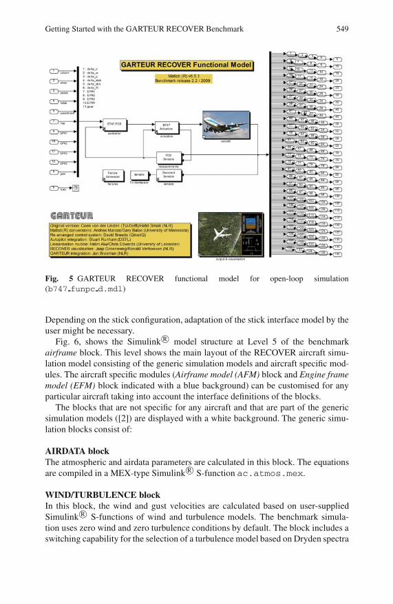
Fig. 33: The program continues with the start of the optimisation to determine thetrim condition. For trimming, the b747 trim d.mdlmodel is used. The trim rou-tine runs and gives a trim result in terms of stabiliser deflection and thrust. If thetrim results are acceptable, the required EPR setting is derived from the thrust in thenext step.

572 Appendix

Fig. 31 Selection of failure mode and aircraft configuration

Fig. 34: After the trim condition is calculated, the user is first asked to define a testinput signal for an open-loop simulation. Note that the test signals are applied to thepilot control inputs and not to the separate control surfaces. The simulation is thenperformed using the open-loop model b747 funpc d.mdl. Any saved inputs andoutputs are located in the data subdirectory.


Fig. 32 Selection of flight condition

Finally, a few time responses can be made to show the results. These plots aregenerated by the plot sim script. Fig. 35 shows the plotted simulation results ofthe aircraft states following an aileron doublet at t=2s . As can be seen in the plots,the aircraft with missing tail becomes unstable in the lateral axis after the ailerondoublet at t=2s. The pilot control inputs are shown in Fig. 36. The calculated specificforces are also plotted and are shown in Fig. 37. The effect of the loss of directionalstability due to the missing vertical tail is clearly visible in the lateral acceleration(Ayb) response.

7 Aircraft and Flight Control System Specifications

Fig. 38 and Table 3 provide aircraft operational data and geometric dimensionsfor both the B747-100/200 and B747-200F (freighter version) as simulated in thebenchmark. The B747-100/200 flight control system characteristics, including ar-rangements and operating limitations, are illustrated in Fig. 39 and Table 4. For thebenchmark simulation, the B747-100/200 hydraulic and flight control system spec-ifications were taken from [5, 10].

8 Signal Formats

This section provides a reference on the signal formats and observation outputs asavailable in the top system level (Level 1) of the closed-loop (b747 auto g.mdl)and open-loop (b747 funpc d.mdl) benchmark models. For all signal formats,the signal number, name, symbol, dimension and a description are provided. TheGARTEUR RECOVER benchmark observation outputs follow the signal formatsas described in reference [2].

574 Appendix

Fig. 33 Optimisation and trim routine results


Fig. 34 Test input signal definition for open-loop simulation (b747 funpc d.mdl)

576 Appendix

Fig. 35 Aircraft state response after an aileron doublet at t=2s with open-loop benchmarkmodel (b747 funpc d.mdl) and loss of vertical tail failure mode

Fig. 36 Pilot control inputs showing aileron doublet as test signal at t=2s


Fig. 37 Aircraft specific forces in body axes after an aileron doublet at t=2s with open-loopmodel (b747 funpc d.mdl) and loss of vertical tail failure mode

Fig. 38 Boeing 747-100/200 large transport aircraft

578 Appendix

Table 3 B747-100/200 series operational data and geometric dimensions

B747-100/200 B747-200F (Freighter)

Wing area 511 m2 511 m2

Wing mean aerodynamic chord (MAC) 8.324 m 8.324 mWing span 59.65 m 59.65 mLength overall 70.66 m 70.66 mHeight overall 19.33 m 19.33 mEngines Pratt & Whitney JT9D-3 Pratt & Whitney JT9D-

7JTakeoff thrust rating (standard day / sealevel)

193 kN (43,500 lb st) 222 kN (50,000 lb st)

Maximum takeoff weight 321,995 kg (710,000 lb) 377,842 kg (833,000 lb)Maximum landing weight 255,782 kg (564,000 lb) 285,763 kg (630,000 lb)Maximum zero fuel weight 238,776 kg (526,500 lb) 267,619 kg (590,000 lb)Load factor range flaps up -1.0/+2.5 -1.0/+2.5Load factor range flaps down 0/+2 0/+2

Fig. 39 Boeing 747-100/200 flight control surface arrangements and body axes and momentdefinitions (L = rolling moment, M = pitching moment, N = yawing moment, p = roll rate,q = pitch rate, r = yaw rate)


Table 4 B747-100/200 flight control surface operating limits (positive sign: surface deflec-tion down / spoiler panel up)

Control surface Symbol Mechanicallimit (deg)

Two hydraulic sys-tem rate (Full boost,deg/sec)

One hydraulic sys-tem rate (Half boost,deg/sec)

Inboard elevator δei +17/-23 +37/-37 +30/-26Outboard elevator δeo +17/-23 +37/-37 +30/-26Stabiliser ih +3/-12 +/-0.2 to +/-0.5 +/-0.1 to +/-0.25Inboard aileron δai +20/-20 +40/-45 +27/-35Outboard aileron δao +15/-25 +45/-55 +22/-45Spoilers #1 - #4 δsp1−4 +45 +75 0Spoilers #9 - #12 δsp9−12 +45 +75 0Spoilers #5, #8 δsp5,δsp8 +20 +75 0Spoilers #6, #7 δsp6,δsp7 +20 +25 0Upper rudder δru +25/-25 +50/-50 +40/-40Lower rudder δrl +25/-25 +50/-50 +40/-40

Table 5 Aircraft states (x)

No. Name Symbol Dimension Description

1 pbody pb rad/s roll rate about body X-axis2 qbody qb rad/s pitch rate about body Y -axis3 rbody rb rad/s yaw rate about body Z-axis4 VTAS VTAS m/s true airspeed5 alpha α rad angle of attack6 beta β rad angle of sideslip7 phi φ rad roll angle8 theta θ rad pitch angle9 psi ψ rad yaw angle10 he he m geometric altitude11 xe xe m horizontal position along earth X-axis12 ye ye m horizontal position along earth Y -axis

Table 6 Aircraft state derivatives (xdot)


13 pbdot pb rad/s2 roll acceleration about body X-axis14 qbdot qb rad/s2 pitch acceleration about body Y -axis15 rbdot rb rad/s2 yaw acceleration about body Z-axis16 VTASdot VTAS m/s2 time derivative of true airspeed17 alphadot α rad/s angle of attack rate18 betadot β rad/s angle of sideslip rate19 phidot φ rad/s roll attitude rate20 thetadot θ rad/s pitch attitude rate21 psidot ψ rad/s heading rate22 hedot he m/s geometric altitude rate23 xedot xe m/s horizontal ground speed along earth X-

axis24 yedot ye m/s horizontal ground speed along earth Y -

axis

580 Appendix

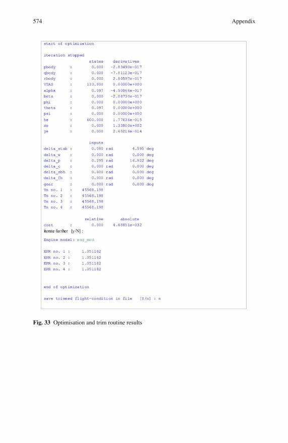
Table 7 Airdata parameters (yair)


25 pstat pa N/m2 ambient pressure26 rho ρ kg/m3 air density27 temp T K ambient temperature28 grav g m/s2 acceleration of gravity29 hpress hp m pressure altitude30 hradio hR m radio altitude31 Hgeopot H m geopotential altitude32 Vsound Vsound m/s speed of sound33 Mach M – Mach number34 qdyn q N/m2 dynamic pressure35 Reynl Re′ – Reynolds number per unit length36 qc qc N/m2 impact pressure37 qrel qrel – relative impact pressure38 ptot pt N/m2 total pressure39 temptot Tt K total temperature40 VEAS VEAS m/s equivalent airspeed41 VCAS VCAS m/s calibrated airspeed42 VIAS VIAS m/s indicated airspeed43 uwindb uwb m/s wind velocity along body X-axis44 vwindb vwb m/s wind velocity along body Y -axis45 wwindb wwb m/s wind velocity along body Z-axis46 uwinde uwe m/s wind velocity along earth X-axis47 vwinde vwe m/s wind velocity along earth Y -axis48 wwinde wwe m/s wind velocity along earth Z-axis49 ug ug – dimensionless gust velocity along nega-

tive body X-axis50 alphag αg rad gust angle of attack51 betag βg rad gust angle of sideslip52 ugdot ˙ug 1/s dimensionless gust velocity derivative

along negative body X-axis53 alphagdot αg rad/s gust angle of attack rate54 betagdot βg rad/s gust angle of sideslip rate55 ugasym ugasym – dimensionless gust velocity along nega-

tive body X-axis, varying along wingspan56 alphagasym αgasym rad gust angle of attack, varying along

wingspan


Table 8 Acceleration parameters (yacc)


57 axb axb g acceleration at c.g. along body X-axis58 ayb ayb g acceleration at c.g. along body Y -axis59 azb azb g acceleration at c.g. along body Z-axis60 anxb anxb g accelerometer output at c.g. along body X-

axis61 anyb anyb g accelerometer output at c.g. along body Y -

axis62 anzb anzb g accelerometer output at c.g. along body Z-

axis63 anxa anxa g accelerometer output at c.g. along airpath

X-axis64 anya anya g accelerometer output at c.g. along airpath

Y -axis65 anza anza g accelerometer output at c.g. along airpath

Z-axis66 anxib anx,ib g accelerometer output at (x,y,z)iacc along

body X-axis67 anyib any,ib g accelerometer output at (x,y,z)iacc along

body Y -axis68 anzib anz,ib g accelerometer output at (x,y,z)iacc along

body Z-axis69 anb anb g normal acceleration at c.g.70 anib an,ib g normal acceleration at (x,y,z)iacc

71 n n g load factor

Table 9 Flight path related parameters (yfp)


72 gamma γ rad flight path angle73 chi χ rad azimuth angle74 gammadot γ rad/s flight path angle rate75 chidot χ rad/s azimuth angle rate76 heacc he m/s2 vertical acceleration77 fpacc f pa m/s2 flight path acceleration

Table 10 Energy related terms (ys)


78 Espec Es m specific energy79 Pspec Ps m/s specific power

582 Appendix

Table 11 Aerodynamic forces and moments (yFMaero)


80 Tbody Tb N aerodynamic tangential force in body ref-erence frame

81 Ybody Yb N aerodynamic sideforce coefficient in bodyreference frame

82 Nbody Nb N aerodynamic normal force in body refer-ence frame

83 MXbody Lb Nm aerodynamic rolling moment in body ref-erence frame

84 MYbody Mb Nm aerodynamic pitching moment in bodyreference frame

85 MZbody Nb Nm aerodynamic yawing moment in body ref-erence frame

Table 12 Forces and moments due to turbulence (yFMgust)


86 Tgbody Tgb N tangential force due to turbulence in bodyreference frame

87 Ygbody Ygb N sideforce coefficient due to turbulence inbody reference frame

88 Ngbody Ngb N normal force due to turbulence in bodyreference frame

89 MXgbody Lgb Nm rolling moment due to turbulence in bodyreference frame

90 MYgbody Mgb Nm pitching moment due to turbulence inbody reference frame

91 MZgbody Ngb Nm yawing moment due to turbulence in bodyreference frame

Table 13 Propulsion forces and moments (yFMt)


92 Ttbody Ttb N propulsion tangential force in body refer-ence frame

93 Ytbody Ytb N propulsion sideforce coefficient in bodyreference frame

94 Ntbody Ntb N propulsion normal force in body referenceframe

95 MXtbody Ltb Nm propulsion rolling moment in body refer-ence frame

96 MYtbody Mtb Nm propulsion pitching moment in body ref-erence frame

97 MZtbody Ntb Nm propulsion yawing moment in body refer-ence frame


Table 14 Aerodynamic force and moment coefficients (yCaero)


98 CDair CDa – aerodynamic drag coefficient in airpathreference frame

99 CYair CYa – aerodynamic sideforce coefficient in air-path reference frame

100 CLair CLa – aerodynamic lift coefficient in airpath ref-erence frame

101 CLLair C�a – aerodynamic rolling moment coefficientin airpath reference frame

102 CMair Cma – aerodynamic pitching moment coefficientin airpath reference frame

103 CNNair Cna – aerodynamic yawing moment coefficientin airpath reference frame

104 CDstab CDs – aerodynamic drag coefficient in stabilityreference frame

105 CYstab CYs – aerodynamic sideforce coefficient in sta-bility reference frame

106 CLstab CLs – aerodynamic lift coefficient in stabilityreference frame

107 CLLstab C�s – aerodynamic rolling moment coefficientin stability reference frame

108 CMstab Cms – aerodynamic pitching moment coefficientin stability reference frame

109 CNNstab Cns – aerodynamic yawing moment coefficientin stability reference frame

110 CTbody CTb – aerodynamic tangential force coefficientin body reference frame

111 CYbody CYb – aerodynamic sideforce coefficient in bodyreference frame

112 CNbody CNb – aerodynamic normal force coefficient inbody reference frame

113 CLLbody C�b – aerodynamic rolling moment coefficientin body reference frame

114 CMbody Cmb – aerodynamic pitching moment coefficientin body reference frame

115 CNNbody Cnb – aerodynamic yawing moment coefficientin body reference frame

584 Appendix

Table 15 Control surfaces (uc)


116 delta air δair rad right inboard aileron deflection117 delta ail δail rad left inboard aileron deflection118 delta aor δaor rad right outboard aileron deflection119 delta aol δaol rad left outboard aileron deflection120 delta sp1 δsp1 rad spoiler #1 deflection121 delta sp2 δsp2 rad spoiler #2 deflection122 delta sp3 δsp3 rad spoiler #3 deflection123 delta sp4 δsp4 rad spoiler #4 deflection124 delta sp5 δsp5 rad spoiler #5 deflection125 delta sp6 δsp6 rad spoiler #6 deflection126 delta sp7 δsp7 rad spoiler #7 deflection127 delta sp8 δsp8 rad spoiler #8 deflection128 delta sp9 δsp9 rad spoiler #9 deflection129 delta sp10 δsp10 rad spoiler #10 deflection130 delta sp11 δsp11 rad spoiler #11 deflection131 delta sp12 δsp12 rad spoiler #12 deflection132 delta eir δeir rad right inboard elevator deflection133 delta eil δeil rad left inboard elevator deflection134 delta eor δeor rad right outboard elevator deflection135 delta eol δeol rad left outboard elevator deflection136 ih ih rad stabiliser deflection137 delta ru δru rad upper rudder deflection138 delta rl δrl rad lower rudder deflection139 delta fo δ f o rad outboard trailing edge flaps deflection140 delta fi δ f i rad inboard trailing edge flaps deflection

Table 16 Pilot control inputs (top level open-loop model b747 funpc d.mdl)


1 delta c δc rad control column position (+12.67deg/-12.5deg)

2 delta w δw rad control wheel position (+88deg/-88deg)3 delta p δp rad rudder pedal position (+14deg/-14deg)4 delta stab δstab rad stabiliser handle position (0-15 units)5 delta sbh δsbh rad speedbrake handle position (0-37deg in-

flight detent)6 delta fh δ f h rad flap handle position (0-30 detent)7 EPR1 EPR1 – EPR engine #1 (0.94-1.62 (Flight 1862

simulation))8 EPR2 EPR2 – EPR engine #2 (0.94-1.62 (Flight 1862



simulation))11 gear gear 0/1 gear handle position


Table 17 Instrument landing system (ILS) parameters (Standard Sensors block)


1 GSdev GSdev rad glideslope deviation2 DME DME m distance to runway threshold3 GSvalid GSvalid 0/1 glideslope signal valid4 LOCdev LOCdev rad localiser deviation5 LOCvalid LOCvalid 0/1 localiser signal valid

9 Contributors

The following persons and organisations contributed to the development of theGARTEUR RECOVER benchmark.

Coen van der Linden (Delft University of Technology)Hafid Smaili (National Aerospace Laboratory NLR)Jan Breeman (National Aerospace Laboratory NLR)Jaap Groeneweg (National Aerospace Laboratory NLR)Ronald Verhoeven (National Aerospace Laboratory NLR)Thomas Lombaerts (Delft University of Technology)Andres Marcos (Deimos Space)Gary Balas (University of Minnesota)Chris Edwards (University of Leicester)Halim Alwi (University of Leicester)David Breeds (QinetiQ)Stuart Runham (DSTL)

Contact information, organisation details and links can be found on the GAR-TEUR project site www.faulttolerantcontrol.nl.

References

1. GARTEUR. GARTEUR RECOVER benchmark quickstart guide, GARTEUR FlightMechanics Action Group 16 ‘Fault Tolerant Control’ (2009)

2. van der Linden, C.A.A.M.: DASMAT- Delft University Aircraft Simulation Model andAnalysis Tool. Report LR-781, Delft University of Technology, Faculty of AerospaceEngineering, Delft, The Netherlands (1996)

3. Smaili, M.H.: Flight data reconstruction and simulation of El Al Flight 1862. Final thesis,Delft University of Technology, Faculty of Aerospace Engineering, Delft, The Nether-lands (1997)

4. Smaili, M.H., Mulder, J.A.: Flight data reconstruction and simulation of the 1992 Ams-terdam Bijlmermeer airplane accident. In: AIAA Modeling and Simulation TechnologiesConference and Exhibit, AIAA-2000-4586, Denver, CO (August 2000)

5. Hanke, C.R.: The simulation of a large transport aircraft. Modeling data, vol. II. NASACR-114494 (September 1970)

586 Appendix

6. Hanke, C.R.: The simulation of a large transport aircraft. Mathematical model, vol. I.NASA CR-1756 (March 1971)

7. van Keulen, R.: Real-time simulation and analysis of the automatic flight control sys-tem of the Boeing 747-200. Final thesis, Delft University of Technology, Faculty ofAerospace Engineering, Delft, The Netherlands (1991)

8. Marcos, A., Balas, G.J.: A Boeing 747-100/200 aircraft fault tolerant and fault diagnosticbenchmark. Technical Report AEM-UoM-2003-1, University of Minnesota, Minnesota(June 2003)

9. EL AL Flight 1862, aircraft accident report 92-11. Netherlands Aviation Safety Board,Hoofddorp, The Netherlands (1994)

10. Boeing 747 Aircraft Operations Manual (1976)11. Stevens, B.L., Lewis, F.L.: Aircraft control and simulation. John Wiley & Sons Inc., New

York (1992)12. Etkin, B., Reid, L.D.: Dynamics of flight - stability and control, 3rd edn. Wiley, New

York (1996)13. Matlab getting started guide. Version 6.5 (Release 13) or later. The Mathworks Inc.,

Natick, MA (USA)14. Simulink user’s guide. Version 5.1 (Release 13SP1) or later. The Mathworks Inc., Natick,

MA (USA)

Lecture Notes in Control and Information Sciences

Edited by M. Thoma, F. Allgöwer, M. Morari

Further volumes of this series can be found on our homepage:springer.com

Vol. 399: Edwards, C.; Lombaerts, T.;Smaili, H. (Eds.):Fault Tolerant Flight Control586 p. 2010 [978-3-642-11689-6]

Vol. 398: Willems, J.C.; Hara, S.;Ohta, Y.; Fujioka, H. (Eds.):Perspectives in Mathematical SystemTheory, Control, and Signal Processing388 p. 2010 [978-3-540-93917-7]

Vol. 397: Yang, H.; Jiang, B.; Cocquempot, V.:Fault Tolerant Control Design forHybrid Systems191 p. 2010 [978-3-642-10680-4]

Vol. 396: Kozlowski, K. (Ed.):Robot Motion and Control 2009475 p. 2009 [978-1-84882-984-8]

Vol. 395: Talebi, H.A.:Neural Network-Based StateEstimation of Nonlinear Systemsappro. 200 p. 2010 [978-1-4419-1437-8]

Vol. 394: Pipeleers, G.; Demeulenaere, B.;Swevers, J.:Optimal Linear Controller Design forPeriodic Inputs177 p. 2009 [978-1-84882-974-9]

Vol. 393: Ghosh, B.K.; Martin, C.F.;Zhou, Y.:Emergent Problems in NonlinearSystems and Control285 p. 2009 [978-3-642-03626-2]

Vol. 392: Bandyopadhyay, B.; Deepak, F.;Kim, K.-S.:Sliding Mode Control Using NovelSliding Surfaces137 p. 2009 [978-3-642-03447-3]

Vol. 391: Khaki-Sedigh, A.; Moaveni, B.:Control Configuration Selection forMultivariable Plants232 p. 2009 [978-3-642-03192-2]

Vol. 390: Chesi, G.; Garulli, A.;Tesi, A.; Vicino, A.:Homogeneous Polynomial Forms forRobustness Analysis of Uncertain Systems197 p. 2009 [978-1-84882-780-6]

Vol. 389: Bru, R.; Romero-Vivó, S. (Eds.):Positive Systems398 p. 2009 [978-3-642-02893-9]

Vol. 388: Jacques Loiseau, J.; Michiels, W.;Niculescu, S-I.; Sipahi, R. (Eds.):Topics in Time Delay Systems418 p. 2009 [978-3-642-02896-0]

Vol. 387: Xia, Y.;Fu, M.; Shi, P.:Analysis and Synthesis ofDynamical Systems with Time-Delays283 p. 2009 [978-3-642-02695-9]

Vol. 386: Huang, D.;Nguang, S.K.:Robust Control for Uncertain NetworkedControl Systems with Random Delays159 p. 2009 [978-1-84882-677-9]

Vol. 385: Jungers, R.:The Joint Spectral Radius144 p. 2009 [978-3-540-95979-3]

Vol. 384: Magni, L.; Raimondo, D.M.;Allgöwer, F. (Eds.):Nonlinear Model Predictive Control572 p. 2009 [978-3-642-01093-4]

Vol. 383: Sobhani-Tehrani E.:Khorasani K.;Fault Diagnosis of Nonlinear SystemsUsing a Hybrid Approach360 p. 2009 [978-0-387-92906-4]

Vol. 382: Bartoszewicz A.;Nowacka-Leverton A.:Time-Varying Sliding Modes for Secondand Third Order Systems192 p. 2009 [978-3-540-92216-2]

Vol. 381: Hirsch M.J.; Commander C.W.;Pardalos P.M.; Murphey R. (Eds.):Optimization and CooperativeControl Strategies: Proceedings of the 8thInternational Conference on CooperativeControl and Optimization459 p. 2009 [978-3-540-88062-2]

Vol. 380: Basin M.:New Trends in Optimal Filtering and Control forPolynomial and Time-Delay Systems206 p. 2008 [978-3-540-70802-5]

Vol. 379: Mellodge P.; Kachroo P.:Model Abstraction in Dynamical Systems:Application to Mobile Robot Control116 p. 2008 [978-3-540-70792-9]

Vol. 378: Femat R.; Solis-Perales G.:Robust Synchronization of Chaotic SystemsVia Feedback199 p. 2008 [978-3-540-69306-2]

Vol. 377: Patan K.:Artificial Neural Networks forthe Modelling and FaultDiagnosis of Technical Processes206 p. 2008 [978-3-540-79871-2]

Vol. 376: Hasegawa Y.:Approximate and Noisy Realization ofDiscrete-Time Dynamical Systems245 p. 2008 [978-3-540-79433-2]

Vol. 375: Bartolini G.; Fridman L.;Pisano A.; Usai E. (Eds.):Modern Sliding Mode Control Theory465 p. 2008 [978-3-540-79015-0]

Vol. 374: Huang B.; Kadali R.:Dynamic Modeling, Predictive Controland Performance Monitoring240 p. 2008 [978-1-84800-232-6]

Vol. 373: Wang Q.-G.; Ye Z.; Cai W.-J.;Hang C.-C.:PID Control for Multivariable Processes264 p. 2008 [978-3-540-78481-4]

Vol. 372: Zhou J.; Wen C.:Adaptive Backstepping Control of UncertainSystems241 p. 2008 [978-3-540-77806-6]

Vol. 371: Blondel V.D.; Boyd S.P.;Kimura H. (Eds.):Recent Advances in Learning and Control279 p. 2008 [978-1-84800-154-1]

Vol. 370: Lee S.; Suh I.H.;Kim M.S. (Eds.):Recent Progress in Robotics:Viable Robotic Service to Human410 p. 2008 [978-3-540-76728-2]

Vol. 369: Hirsch M.J.; Pardalos P.M.;Murphey R.; Grundel D.:Advances in Cooperative Control andOptimization423 p. 2007 [978-3-540-74354-5]

Vol. 368: Chee F.; Fernando T.Closed-Loop Control of Blood Glucose157 p. 2007 [978-3-540-74030-8]

Vol. 367: Turner M.C.; Bates D.G. (Eds.):Mathematical Methods for Robust andNonlinear Control444 p. 2007 [978-1-84800-024-7]

Vol. 366: Bullo F.; Fujimoto K. (Eds.):Lagrangian and Hamiltonian Methods forNonlinear Control 2006398 p. 2007 [978-3-540-73889-3]

Vol. 365: Bates D.; Hagström M. (Eds.):Nonlinear Analysis and SynthesisTechniques for Aircraft Control360 p. 2007 [978-3-540-73718-6]

Vol. 364: Chiuso A.; Ferrante A.;Pinzoni S. (Eds.):Modeling, Estimation and Control356 p. 2007 [978-3-540-73569-4]

Vol. 363: Besançon G. (Ed.):Nonlinear Observers and Applications224 p. 2007 [978-3-540-73502-1]

Vol. 362: Tarn T.-J.; Chen S.-B.;Zhou C. (Eds.):Robotic Welding, Intelligence andAutomation562 p. 2007 [978-3-540-73373-7]

Vol. 361: Méndez-Acosta H.O.; Femat R.;González-Álvarez V. (Eds.):Selected Topics in Dynamics andControl of Chemical andBiological Processes320 p. 2007 [978-3-540-73187-0]

Vol. 360: Kozlowski K. (Ed.):Robot Motion and Control 2007452 p. 2007 [978-1-84628-973-6]

Vol. 359: Christophersen F.J.:Optimal Control of ConstrainedPiecewise Affine Systems190 p. 2007 [978-3-540-72700-2]

Vol. 358: Findeisen R.; AllgöwerF.; Biegler L.T. (Eds.):Assessment and FutureDirections of NonlinearModel Predictive Control642 p. 2007 [978-3-540-72698-2]

Getting Started with the GARTEUR RECOVER Benchmark

Documents

Transcript of Getting Started with the GARTEUR RECOVER Benchmark