
GeRoFan : une architecture et un plan de contrôle ... - CORE
258
GeRoFan : une architecture et un plan de contrˆole bas´ es sur la radio-sur-fibre pour la mutualisation des r´ eseaux d’acc` es mobile de nouvelle g´ en´ eration Ahmed Haddad To cite this version: Ahmed Haddad. GeRoFan : une architecture et un plan de contrˆ ole bas´ es sur la radio-sur- fibre pour la mutualisation des r´ eseaux d’acc` es mobile de nouvelle g´ en´ eration. R´ eseaux et t´ el´ ecommunications [cs.NI]. T´ el´ ecom ParisTech, 2013. Fran¸cais. <NNT : 2013ENST0025>. <tel-01308528> HAL Id: tel-01308528 https://pastel.archives-ouvertes.fr/tel-01308528 Submitted on 28 Apr 2016 HAL is a multi-disciplinary open access archive for the deposit and dissemination of sci- entific research documents, whether they are pub- lished or not. The documents may come from teaching and research institutions in France or abroad, or from public or private research centers. L’archive ouverte pluridisciplinaire HAL, est destin´ ee au d´ epˆ ot et ` a la diffusion de documents scientifiques de niveau recherche, publi´ es ou non, ´ emanant des ´ etablissements d’enseignement et de recherche fran¸cais ou ´ etrangers, des laboratoires publics ou priv´ es.
-
Upload
khangminh22 -
Category
Documents
-
view
1 -
download
0
Transcript of GeRoFan : une architecture et un plan de contrôle ... - CORE

GeRoFan : une architecture et un plan de controle bases
sur la radio-sur-fibre pour la mutualisation des reseaux
d’acces mobile de nouvelle generation
Ahmed Haddad
To cite this version:
Ahmed Haddad. GeRoFan : une architecture et un plan de controle bases sur la radio-sur-fibre pour la mutualisation des reseaux d’acces mobile de nouvelle generation. Reseaux ettelecommunications [cs.NI]. Telecom ParisTech, 2013. Francais. <NNT : 2013ENST0025>.<tel-01308528>
HAL Id: tel-01308528
https://pastel.archives-ouvertes.fr/tel-01308528
Submitted on 28 Apr 2016
HAL is a multi-disciplinary open accessarchive for the deposit and dissemination of sci-entific research documents, whether they are pub-lished or not. The documents may come fromteaching and research institutions in France orabroad, or from public or private research centers.
L’archive ouverte pluridisciplinaire HAL, estdestinee au depot et a la diffusion de documentsscientifiques de niveau recherche, publies ou non,emanant des etablissements d’enseignement et derecherche francais ou etrangers, des laboratoirespublics ou prives.

2013 ENST 0025
T
H
È
S
E
EDITE - ED 130
Doctorat ParisTech
T H È S Epour obtenir le grade de docteur délivré par
Télécom ParisTechSpécialité “Informatique & Réseaux”
présentée et soutenue publiquement par
Ahmed HADDAD
le 26 avril 2013
GeRoFAN: Une architecture et un plan de controle baséssur la radio-sur-fibre pour la mutualisation des réseaux
d’accès mobile de nouvelle génération.Directeur de thèse: Maurice GAGNAIRE
Jury:
M. Leonid G. KAZOVSKY, Professeur, Stanford University, Stanford, CA Rapporteur
M. Josep PRAT, Professeur, Universitat Politècnica de Catalunya (UPC), Barcelona Rapporteur
M. Gérard POGOREL, Professeur, Télécom ParisTech, Paris Examinateur
M. Christophe KAZMIERSKI, Ingénieur, Alcatel-Lucent/Thales III-V Lab, Paris Examinateur
M. Joel MAU, Ingénieur, Institut-Mines Telecom, Paris Examinateur
M. Richard TOPER, Ingénieur, PDG de SETICS, Paris Invité
M. Edouard DOLLEY, Chargé de prospectives, ARCEP, Paris Invité
M. Maurice GAGNAIRE, Professeur, Télécom ParisTech, Paris Directeur de thèse
Telecom ParisTech
Ecole de l’Institut-Mines Télécom - membre de ParisTech
46, rue Barrault - 75634 Paris Cedex 13 - Tél. + 33 (0)1 45 81 77 77 - www.telecom-paristech.fr


GeRoFAN: Une architecture et un plan de controle basés sur la radio-sur-fibre
pour la mutualisation des réseaux d’accès mobile de nouvelle génération.
Résumé: L’architecture actuelle des réseaux d’accès radio n’est pas adaptée en terme de capacité
à supporter l’accroissement continu du trafic dans les systèmes cellulaires 4G et au-delà. L’objectif
de cette thèse est de proposer une architecture réseau générique, GeRoFAN (Generic Radio over Fiber
Access Network) pour la fédération des stations de base des systèmes cellulaires de nouvelle génération
(WiMAX, 4G LTE). Deux innovations technologiques majeures sont utilisées pour l’implémentation de
l’architecture GeRoFAN: la radio-sur-fibre (RoF) et les modulateurs réflexifs éléctro-absorbants.
La thèse vise aussi à concevoir pour l’architecture GeRoFAN un plan contrôle et un canal de signalisa-
tion adapté permettant le basculement des ressources radio, selon la fluctuation du trafic, entre un grand
nombre de cellules réparties à l’échelle métropolitaine. Cependant, il a été bien avéré que la transmission
optique de plusieurs canaux radios en utilisant la RoF analogique est assujettie à des multiples facteurs de
dégradation physique altérant la qualité du signal de ces canaux et induisant une perte dans leur capacité
de Shannon. L’originalité du plan de contrôle de GeRoFAN est de réaliser une affectation optimisée des
canaux radios sur les porteuses optiques, grace au multiplexage par sous-porteuse (SCM), afin d’ajuster
la capacité de Shannon dans chaque cellule radio à la charge de trafic à laquelle elle est soumise. A cet
effet, une connaissance fine des contraintes physiques de la transmission RoF est requise pour le plan de
contrôle. Cette connaissance est acquise par l’élaboration d’un modèle analytique des divers bruits de
transmission du système GeRoFAN. Contrairement à des propositions comparables, le plan contrôle de
GeRoFAN se doit d’être le plus transparent que possible à la technologie des systèmes radio concernés.
Sa nature " MAC radio agnostique " vise à permettre, grâce au multiplexage en longueur d’onde et au
routage optique WDM, la fédération de plusieurs opérateurs utilisant différentes technologies radio sur
la même infrastructure. Plus généralement, avec la mutualisation de l’architecture GeRoFAN, le plan
de contrôle permet de virtualiser les ressources radiofréquences et de promouvoir de nouveaux modèles
économiques pour les opérateurs Télécoms.
Le dernier volet de la thèse se focalise sur la valeur "business" du paradigme GeRoFAN. Les
contours du nouveau éco-system d’affaire promu par GeRoFAN sont définis. Les motivations/attentes
des différentes parties prenantes dans cet éco-system sont esquissées, les contraintes réglementaires et
organisationnelles soulevées sont adressées afin d’assurer un déploiement sans heurts de GeRoFAN.
Bien qu’exigeant un nouveau modèle réglementaire, il s’agit de mettre en évidence l’intérêt économique
de la solution GeRoFAN, tout particulièrement en comparaison à la RoF digitale, à travers des études
technico-économiques chiffrant les couts d’investissement (CapEx), les couts opérationnels (OpEx) et
les possibles retours sur investissement. A cet effet, deux modèles économiques sont proposés mettant
en évidence la valeur ajoutée de GeRoFAN tout au long de la chaine de valeur.
Mots clefs: Féderation des Réseaux d’Accès, Radio-sur-Fibre Analogique, Virtualisation des Radio-
Fréquences, Etude Technico-Economique.
ii
GeRoFAN: An Architecture and a Control Plane based on Radio-over-Fiber for
the Mutualization of Next-Generation Radio Mobile Backhaul.
Abstract:
Current radio access networks architectures are not suited in terms of capacity and back-
hauling capabilities to fit the continuing traffic increase of 4G cellular systems. The objective
of the thesis is to propose an innovative and generic mobile backhauling network architec-
ture, called GeRoFAN (Generic Radio-over-Fiber Access Network), for next generation mobile
systems (WiMAX, 4G LTE). Two major technological innovations are used to implement GeRo-
FAN: analog Radio-over-Fiber (RoF) and reflective amplified absorption modulators.
The aim of this thesis is to design for such an architecture an original Control Plane (CP)
and a signaling channel enabling to balance radio resources between a set of neighboring cells at
the access/metropolitan scale according to traffic fluctuations. The transmission of several radio
frequencies by means of an analog RoF link suffers from several impairments that may degrade
the capacity of the radio system. The originality of the GeRoFAN-CP consists in mapping
radio frequencies with optical carriers by means of Sub-Carrier Multiplexing (SCM) in order to
optimize the Shannon’s capacity within the various cells covered by the system according to the
current traffic load. For that purpose, a deep analysis and modeling of the various physical layer
impairments impacting the quality of the radio signal is carried out. Unlike comparable ap-
proaches, the GeRoFAN-CP is as independent as possible from the radio layer protocols. Thus,
the "radio MAC-agnostic" nature of the GeRoFAN-CP enables to federate multiple operators
using different radio technologies onto the same backhauling optical infrastructure. Subcarrier
and wavelength division multiplexing (SCM/WDM) as well as WDM optical routing capabilities
are exploited onto the GeRoFAN transparent architecture. More globally, the GeRoFAN-CP
enables a form of "radio frequency virtualization" while promoting new business models for
Telecom service providers.
The last part of the thesis focuses on the business value of the GeRoFAN paradigm. The
expectations of the different stake-holders and main regulatory/organizational entities that
could be involved in the deployment of GeRoFAN infrastructures should be addressed in order
to achieve a smooth deployment of this new type of mobile backhauling. Economics of the
GeRoFAN architecture are investigated in terms of OpEx/CapEx valuation and investment
profitability, especially in reference to digitized RoF. Two business models are then proposed
to study how GeRoFAN contributes to enriching the cellular backhauling service value chain.
Keywords: Mobile Backhauling, Analog Radio-over-Fiber, Radio-Frequency Virtualiza-
tion, Backhaul Techno-Economics.

Contents
1 Version courte de la thèse en Français 1
1.1 Introduction . . . . . . . . . . . . . . . . . . . . . . . . . . . . . . . . . . . . . . . 1
1.2 Etat de l’art et evolution des architectures pour l’accès cellulaire . . . . . . . . . 4
1.2.1 Technologies de réseaux d’accès-métro pour la féderation des RANs . . . 4
1.2.2 Modulation Radio-sur-Fibre (RoF) . . . . . . . . . . . . . . . . . . . . . . 6
1.2.3 Des modèles avancés d’architecture réseau d’accès-métro . . . . . . . . . 10
1.2.4 Architecture GeRoFAN . . . . . . . . . . . . . . . . . . . . . . . . . . . . 12
1.3 Limitations physiques de la transmission Radio-sur-Fibre . . . . . . . . . . . . . 13
1.3.1 Catégorie I . . . . . . . . . . . . . . . . . . . . . . . . . . . . . . . . . . . 16
1.3.2 Catégorie II . . . . . . . . . . . . . . . . . . . . . . . . . . . . . . . . . . . 17
1.3.3 Catégorie III . . . . . . . . . . . . . . . . . . . . . . . . . . . . . . . . . . 18
1.3.4 Catégorie IV . . . . . . . . . . . . . . . . . . . . . . . . . . . . . . . . . . 19
1.4 Conception du plan de controle pour GeRoFAN . . . . . . . . . . . . . . . . . . . 22
1.4.1 l’algorithme PaGeO . . . . . . . . . . . . . . . . . . . . . . . . . . . . . . 22
1.4.2 Stratégies alternatives de transport des RFs . . . . . . . . . . . . . . . . . 23
1.5 Performance numérique . . . . . . . . . . . . . . . . . . . . . . . . . . . . . . . . 26
1.5.1 Quelle topologie pour GeRoFAN: boucle ou arbre ? . . . . . . . . . . . . . 26
1.5.2 PaGeO vs. les stratégies alternatives . . . . . . . . . . . . . . . . . . . . . 27
1.6 Conclusion . . . . . . . . . . . . . . . . . . . . . . . . . . . . . . . . . . . . . . . 30
2 General Introduction 33
2.1 Motivation, Objectives and Thesis Outline . . . . . . . . . . . . . . . . . . . . . . 33
2.2 Contributions and Statement of Originality . . . . . . . . . . . . . . . . . . . . . 35
2.3 Publications . . . . . . . . . . . . . . . . . . . . . . . . . . . . . . . . . . . . . . . 37
I GeRoFAN Backhauling Architecture 39
3 RoF-based Mobile Backhauling 41
3.1 Introduction . . . . . . . . . . . . . . . . . . . . . . . . . . . . . . . . . . . . . . . 41
3.2 Cellular backhaul: Current and future trends . . . . . . . . . . . . . . . . . . . . 42
3.2.1 The mobile backhaul section . . . . . . . . . . . . . . . . . . . . . . . . . 42
3.2.2 Evolution of the backhaul protocol stack: Migration paths . . . . . . . . . 51
3.3 Leveraging the fiber at the access: Radio-over-Fiber . . . . . . . . . . . . . . . . 53
3.3.1 Radio-over-Fiber technology . . . . . . . . . . . . . . . . . . . . . . . . . . 54
iv Contents
3.3.2 D-RoF vs. A-RoF: An economic analysis . . . . . . . . . . . . . . . . . . 61
3.4 Generic RoF Access Network . . . . . . . . . . . . . . . . . . . . . . . . . . . . . 70
3.4.1 The Radio Access Unit . . . . . . . . . . . . . . . . . . . . . . . . . . . . . 72
3.4.2 GeRoFAN for multi-operator backhauling . . . . . . . . . . . . . . . . . . 74
3.4.3 GeRoFAN system control plane . . . . . . . . . . . . . . . . . . . . . . . . 75
II Physical Layer Study 79
4 Analog RoF Transmission Limitations in GeRoFAN 81
4.1 Introduction . . . . . . . . . . . . . . . . . . . . . . . . . . . . . . . . . . . . . . . 82
4.2 RoF transceiver . . . . . . . . . . . . . . . . . . . . . . . . . . . . . . . . . . . . . 82
4.2.1 RoF transceiver technology survey . . . . . . . . . . . . . . . . . . . . . . 83
4.2.2 RoF transceiver physical impairments . . . . . . . . . . . . . . . . . . . . 87
4.3 REAMSOA physical impairments . . . . . . . . . . . . . . . . . . . . . . . . . . . 90
4.3.1 REAMSOA working principle . . . . . . . . . . . . . . . . . . . . . . . . . 91
4.3.2 The EAM section . . . . . . . . . . . . . . . . . . . . . . . . . . . . . . . . 92
4.3.3 The SOA section . . . . . . . . . . . . . . . . . . . . . . . . . . . . . . . . 95
4.3.4 Non-linearity and Intermodulation distortions . . . . . . . . . . . . . . . . 98
4.4 ROADM . . . . . . . . . . . . . . . . . . . . . . . . . . . . . . . . . . . . . . . . . 102
4.4.1 FBG-based ROADM . . . . . . . . . . . . . . . . . . . . . . . . . . . . . . 102
4.4.2 OADM noises . . . . . . . . . . . . . . . . . . . . . . . . . . . . . . . . . . 103
4.4.3 Homodyne Crosstalk . . . . . . . . . . . . . . . . . . . . . . . . . . . . . . 104
4.4.4 Heterodyne Crosstalk . . . . . . . . . . . . . . . . . . . . . . . . . . . . . 104
4.5 Fiber impairments . . . . . . . . . . . . . . . . . . . . . . . . . . . . . . . . . . . 108
4.5.1 Chromatic Dispersion . . . . . . . . . . . . . . . . . . . . . . . . . . . . . 108
4.5.2 Polarization Mode Dispersion . . . . . . . . . . . . . . . . . . . . . . . . . 108
4.5.3 WDM Non-linear Effects . . . . . . . . . . . . . . . . . . . . . . . . . . . 109
4.5.4 Rayleigh Back-Scattering . . . . . . . . . . . . . . . . . . . . . . . . . . . 111
4.5.5 Optical Beat Interference . . . . . . . . . . . . . . . . . . . . . . . . . . . 111
4.5.6 Other impairments . . . . . . . . . . . . . . . . . . . . . . . . . . . . . . . 112
4.6 Building a comprehensive QoT-tool . . . . . . . . . . . . . . . . . . . . . . . . . . 114
III GeRoFAN-CP Algorithmic Design 119
5 Impairment-aware CP Design for Static Traffic 121
5.1 Introduction . . . . . . . . . . . . . . . . . . . . . . . . . . . . . . . . . . . . . . . 121
5.2 The cross-layer architecture of the GeRoFAN-CP . . . . . . . . . . . . . . . . . . 122

Contents v
5.3 An exact optimization approach for GeRoFAN-CP . . . . . . . . . . . . . . . . . 123
5.3.1 ILP optimization for GeRoFAN loop . . . . . . . . . . . . . . . . . . . . . 124
5.3.2 ILP optimization for GeRoFAN tree . . . . . . . . . . . . . . . . . . . . . 133
5.4 PaGeO: a heuristic approach for GeRoFAN-CP . . . . . . . . . . . . . . . . . . . 135
5.4.1 PaGeO Algorithm . . . . . . . . . . . . . . . . . . . . . . . . . . . . . . . 137
5.4.2 Numerical performance of PaGeO . . . . . . . . . . . . . . . . . . . . . . 140
5.4.3 Alternative heuristic backhauling policies . . . . . . . . . . . . . . . . . . 142
5.5 Overlaying multiple radio channels per cell site . . . . . . . . . . . . . . . . . . . 146
5.5.1 Equivalent Bandwidth Loss . . . . . . . . . . . . . . . . . . . . . . . . . . 148
5.5.2 QoT analysis . . . . . . . . . . . . . . . . . . . . . . . . . . . . . . . . . . 149
5.6 Summary . . . . . . . . . . . . . . . . . . . . . . . . . . . . . . . . . . . . . . . . 151
6 Differentiated Backhauling Service for Dynamic Traffic 153
6.1 Introduction . . . . . . . . . . . . . . . . . . . . . . . . . . . . . . . . . . . . . . . 153
6.2 Rules to manage A-RoF impairments . . . . . . . . . . . . . . . . . . . . . . . . . 154
6.3 The DBS algorithm . . . . . . . . . . . . . . . . . . . . . . . . . . . . . . . . . . . 157
6.3.1 DBS at traffic load increase (DBS+) . . . . . . . . . . . . . . . . . . . . . 158
6.3.2 DBS at traffic load decrease (DBS−) . . . . . . . . . . . . . . . . . . . . . 159
6.3.3 The Blind-Search Box (BSB) . . . . . . . . . . . . . . . . . . . . . . . . . 160
6.3.4 The Guided-Search Box (GSB) . . . . . . . . . . . . . . . . . . . . . . . . 161
6.4 DBS performance: Numerical results . . . . . . . . . . . . . . . . . . . . . . . . . 161
6.5 Interaction with the RF-broker . . . . . . . . . . . . . . . . . . . . . . . . . . . . 168
6.6 Summary . . . . . . . . . . . . . . . . . . . . . . . . . . . . . . . . . . . . . . . . 173
IV Economics and Business Relevance of GeRoFAN 175
7 GeRoFAN: a Prospective Approach 177
7.1 Introduction . . . . . . . . . . . . . . . . . . . . . . . . . . . . . . . . . . . . . . . 177
7.2 The GeRoFAN operator: a Third party . . . . . . . . . . . . . . . . . . . . . . . 178
7.2.1 Structuring the GeRoFAN eco-system . . . . . . . . . . . . . . . . . . . . 178
7.2.2 Business cases for GeRoFAN . . . . . . . . . . . . . . . . . . . . . . . . . 179
7.3 Economics of the GeRoFAN system . . . . . . . . . . . . . . . . . . . . . . . . . 180
7.3.1 GeRoFAN vs. D-RoF WDM-PON architecture . . . . . . . . . . . . . . . 180
7.3.2 Methodology . . . . . . . . . . . . . . . . . . . . . . . . . . . . . . . . . . 182
7.3.3 Traffic scenario . . . . . . . . . . . . . . . . . . . . . . . . . . . . . . . . . 182
7.3.4 CapEx valuation model . . . . . . . . . . . . . . . . . . . . . . . . . . . . 184
7.3.5 OpEx valuation model . . . . . . . . . . . . . . . . . . . . . . . . . . . . . 184

vi Contents
7.3.6 Economic results and discussion . . . . . . . . . . . . . . . . . . . . . . . 187
7.4 Sharing the business value among stake-holders . . . . . . . . . . . . . . . . . . . 191
7.4.1 A two-tiers business model . . . . . . . . . . . . . . . . . . . . . . . . . . 191
7.4.2 A three-tiers business model . . . . . . . . . . . . . . . . . . . . . . . . . . 195
7.5 Summary and open issues . . . . . . . . . . . . . . . . . . . . . . . . . . . . . . . 201
8 Conclusion 203
8.1 Summary of Thesis Achievements . . . . . . . . . . . . . . . . . . . . . . . . . . . 203
8.2 GeRoFAN in the real world . . . . . . . . . . . . . . . . . . . . . . . . . . . . . . 205
8.3 Areas of future works . . . . . . . . . . . . . . . . . . . . . . . . . . . . . . . . . 207
A Appendix 209
A.1 EAM Analytical Modeling . . . . . . . . . . . . . . . . . . . . . . . . . . . . . . . 209
A.2 EAM chirp analytical modeling . . . . . . . . . . . . . . . . . . . . . . . . . . . . 215
A.3 RBS analytical modeling . . . . . . . . . . . . . . . . . . . . . . . . . . . . . . . . 220
A.3.1 Input RBS noise: . . . . . . . . . . . . . . . . . . . . . . . . . . . . . . . . 221
A.3.2 Output RBS noise: . . . . . . . . . . . . . . . . . . . . . . . . . . . . . . . 221
A.4 OBI analytical modeling . . . . . . . . . . . . . . . . . . . . . . . . . . . . . . . . 222
Index 224
Bibliography 229

List of Figures
1.1 Technologies traditionnelles et émergentes de federations des BS [102]. . . . . . 6
1.2 Benchmark des solutions technologiques de féderations des BSs et directions
strategiques possibles d’évolution pour un opérateur Télécom. . . . . . . . . . . . 7
1.3 Multi-channel radio signal distribution using Radio-over-Fiber (RoF). . . . . . . 8
1.4 Evaluation du CapEx et de la consommation energitique pour les 3 differents
scenarios de trafic. . . . . . . . . . . . . . . . . . . . . . . . . . . . . . . . . . . . 10
1.5 Architecture de GeRoFAN. . . . . . . . . . . . . . . . . . . . . . . . . . . . . . . 13
1.6 Architecture de la RAU pour un trafic sens montant. . . . . . . . . . . . . . . . . 14
1.7 GeRoFAN pour une féderation multi-opérateur/multi-technologique. . . . . . . . 15
1.8 Gestion de la resource radio/optique à court et à moyen terme par le GeRoFAN-CP. 16
1.9 Gain RF de lu modulateur reflexif EAM en fonction de la longueur d’onde du
canal optique. . . . . . . . . . . . . . . . . . . . . . . . . . . . . . . . . . . . . . . 17
1.11 Illustration des différents bruits dans le cas d’une architecture GeRoFAN en arbre. 21
1.10 Illustration des différents bruits dans le cas d’une architecture GeRoFAN en boucle. 21
1.12 Etapes de l’algorithme PaGeO. . . . . . . . . . . . . . . . . . . . . . . . . . . . . 24
1.13 Illustration des étapes clefs de PaGeO. . . . . . . . . . . . . . . . . . . . . . . . . 25
1.14 Comparaison entre l’architecture en boucle et celle en arbre pour GeRoFAN en
terme de taux de rejet (axe à gauche) et de nombre de porteuses optiques requises
(axe à droite). Les valeurs négative de taux de rejet indiquent un excès de capacité
par rapport à la charge de trafic. Les valeurs de taux de rejet indiquées sont des
des moyennes, les STD bars donnent la variance entre les différentes cellules. . . 28
1.15 "Profiling" de la QoT: Part de chaque catégorie de bruit dans la penalité globale. 28
1.16 PaGeO vs. les stratégies de transport alternatives (RCA, FCA, FFCA et IM-free
CA) en terme de taux de rejet et de nombre de porteuses optiques requises. . . . 29
2.1 The current challenge of mobile carriers: Revenues growth rate flatting while
expenditures growth rate are taking off propelled by the traffic increase. How
carriers can bridge the gap and reverse the trend ? . . . . . . . . . . . . . . . . 34
2.2 The four main work-packages structuring the thesis. . . . . . . . . . . . . . . . . 36
3.1 Generic model and subcomponents of the mobile backhaul. . . . . . . . . . . . . 42
3.2 Traditional/emerging backhaul technologies: A big picture view [102]. . . . . . . 43
3.3 Pseudo-Wire Protocol Stack. . . . . . . . . . . . . . . . . . . . . . . . . . . . . . 48
3.4 Backhaul benchmark and telcos’ leverage strategies. . . . . . . . . . . . . . . . . 49

viii List of Figures
3.5 From legacy to prospective backhaul: Evolution of the protocol stack. . . . . . . 52
3.6 Evolution of the Access-Backhaul towards the "Cloud RAN". . . . . . . . . . . . 53
3.7 Analog RoF transport schemes (from [22]). . . . . . . . . . . . . . . . . . . . . . 54
3.8 Digitized RoF transport scheme. . . . . . . . . . . . . . . . . . . . . . . . . . . . 55
3.9 Different RoF-fixed optical broadband integration schemes. . . . . . . . . . . . . 59
3.10 Multi-channel radio signal distribution using Radio-over-Fiber (RoF). . . . . . . 60
3.11 Methodology for A-RoF and D-RoF link modeling. . . . . . . . . . . . . . . . . . 62
3.12 CapEx and power consumption assessment for 3 different traffic mixes. . . . . . . 64
3.13 Power consumption profiling for 3 different traffic mixes. . . . . . . . . . . . . . . 67
3.14 Distributed D-RoF architecture using CPRI. . . . . . . . . . . . . . . . . . . . . 68
3.15 Distributed D-RoF using CPRI: CAPEX and power consumption ratio. . . . . . 69
3.16 Generic Radio-over-Fiber Network Architecture. . . . . . . . . . . . . . . . . . . 71
3.17 Radio-Access Unit (RAU) Architecture (for upstream radio traffic). . . . . . . . . 72
3.18 GeRoFAN accommodating multi-operator and multi-service operation. . . . . . . 73
3.19 GeRoFAN-CP signaling and general frame structure of channel λ⋆. . . . . . . . . 74
3.20 GeRoFAN-CP capacity management at short/long term time-scale. . . . . . . . . 76
4.1 RoF transceiver technology classification. . . . . . . . . . . . . . . . . . . . . . . 83
4.2 EAM quasi-static circuit model . . . . . . . . . . . . . . . . . . . . . . . . . . . . 93
4.3 EAM Optimal Bias Voltage for each optical wavelength. . . . . . . . . . . . . . . 95
4.4 EAM RF Gain as function of the optical wavelength. . . . . . . . . . . . . . . . . 96
4.5 SOA unsaturated gain as function of the optical wavelength. . . . . . . . . . . . . 97
4.6 SOA Saturation optical power as function of the optical wavelength. . . . . . . . 98
4.7 Illustration of clipping using a phasor representation of the SCM signal. . . . . . 100
4.8 ROADM Structure used for GeRoFAN . . . . . . . . . . . . . . . . . . . . . . . . 103
4.9 RF SNR penalty due to OADM Homodyne crosstalk for (a) the ADD path, (b)
the DROP path and (c) the PASS-THROUGH path. . . . . . . . . . . . . . . . . 106
4.10 Crosstalk coefficient of a uniform BFG vs. wavelength tuning. . . . . . . . . . . 107
4.11 Evolution of η with the number of subcarriers and modulation depth. . . . . . . 109
4.12 Impact of CD on optical SNR with 5% OMI at 1.5 GHz. . . . . . . . . . . . . . . 110
4.13 Illustration of the different impairments for a GeRoFAN loop network. . . . . . 114
4.14 Illustration of the different impairments for a GeRoFAN tree network. . . . . . . 115
5.1 The cross-layer architecture of the GeRoFAN-CP. . . . . . . . . . . . . . . . . . . 122
5.2 A 4 frequency reuse planning. . . . . . . . . . . . . . . . . . . . . . . . . . . . . . 123
5.3 Lightpath modeled as a cascade of RAU operating modes. . . . . . . . . . . . . . 124
5.4 SNR penalty vs. the number of Mode-B RAUs. . . . . . . . . . . . . . . . . . . . 126
5.5 SNR penalty when passing through the ROADM. . . . . . . . . . . . . . . . . . . 127

List of Figures ix
5.6 Optimal number of required OCs for a target maximum rejection ratio. . . . . . 132
5.7 GeRoFAN Tree vs. Loop MILP optimization. . . . . . . . . . . . . . . . . . . . . 134
5.8 A 7 frequency reuse planning. . . . . . . . . . . . . . . . . . . . . . . . . . . . . . 135
5.9 The PaGeO algorithm flowchart. . . . . . . . . . . . . . . . . . . . . . . . . . . . 136
5.10 Illustration of the key steps of PaGeO. . . . . . . . . . . . . . . . . . . . . . . . . 137
5.11 Convergence quality analysis of PaGeO. . . . . . . . . . . . . . . . . . . . . . . . 141
5.12 Comparison at different traffic loads between GeRoFAN loop and GeRoFAN tree
in terms of rejection ratio (left axis) and number of required OCs (right axis).
Error bars stand for deviation from the mean value. Negative rejection ratios
indicate excess capacity beyond required by the traffic load. . . . . . . . . . . . . 143
5.13 QoT profiling: Share of each impairment category in the total SNR penalty for
GeRoFAN tree and GeRoFAN Loop. . . . . . . . . . . . . . . . . . . . . . . . . . 143
5.14 A conceptual 2-by-2 matrix positioning of alternative backhauling policies. . . . . 144
5.15 PaGeO vs. Other Policies (RCA, FCA, FFCA, IM-free CA) at different traffic
loads. Error bars stand for deviation from the mean value. Negative rejection
ratio means excess capacity more than the required load. . . . . . . . . . . . . . . 146
5.16 Illustration of both RF planning approaches for 20 cells network (2 RFs/cell). . . 147
5.17 Pie chart of the penalty share of QoT categories for both RF planning approaches.150
6.1 SNR Penalty of MP, IMD-RAM, RBS and CD function of the OC wavelength.
Dashed grey area in each sub-figure highlights the privileged OCs (i.e. with low
penalties.). . . . . . . . . . . . . . . . . . . . . . . . . . . . . . . . . . . . . . . . 155
6.2 OCs ranking for MP, IMD-RAM, RBS and CD impairments. A WDM pool of
24 OCs with 1 nm channel spacing in the C-band is assumed. Y-axis is log-scaled.157
6.3 DBS activation by the GeRoFAN-CP and interaction with the λ-broker. . . . . . 158
6.4 The two variants of the DBS algorithm. . . . . . . . . . . . . . . . . . . . . . . . 162
6.5 Guided and Blind Search Boxes of the DBS algorithm. . . . . . . . . . . . . . . . 163
6.6 An example of the main steps of the BSB and GSB blocks. . . . . . . . . . . . . 164
6.7 Running the DBS algorithm as the load in hot-spots increases. ♣ denotes the
adding of a new OC. Attained Incompressible Capacity ≃ 27%. . . . . . . . . . . 167
6.8 Incompressible excess capacity and critical load vs. the number of hot spot cells
in the cellular network. . . . . . . . . . . . . . . . . . . . . . . . . . . . . . . . . . 168
6.9 DBS enabling the "Pricing for Profit" paradigm as advocated by NSN [135]. . . . 169
6.10 Flowchart of the radio/DBS cross-layer management approach for the case of a
traffic increase. . . . . . . . . . . . . . . . . . . . . . . . . . . . . . . . . . . . . . 170
6.11 Example of RF/DBS cross-layer approach achieved savings. Realistic traffic pro-
file for a mobile network operator. . . . . . . . . . . . . . . . . . . . . . . . . . . 171

x List of Figures
6.12 Gain χ of the RF/DBS cross-layer management approach at various pa values. . 173
7.1 The GeRoFAN new eco-system business model. . . . . . . . . . . . . . . . . . . . 179
7.2 D-RoF WDM-PON network architecture . . . . . . . . . . . . . . . . . . . . . . . 181
7.3 The techno-economic study methodology. . . . . . . . . . . . . . . . . . . . . . . 183
7.4 The three scenarios considered for backhaul capacity evolution. . . . . . . . . . . 184
7.5 Year-by-year discounted cashflow savings achieved by GeRoFAN and D-RoF
WDM-PON for the three traffic scenarios. . . . . . . . . . . . . . . . . . . . . . . 188
7.6 CapEx and OpEx profiling analysis. . . . . . . . . . . . . . . . . . . . . . . . . . 190
7.7 A two-tiers business model . . . . . . . . . . . . . . . . . . . . . . . . . . . . . . . 192
7.8 Methodology of the economic assessment for the two-tiers business model. . . . . 193
7.9 OCs and penalty cost pricing (α, β) for a balanced business value sharing in a
two-tiers model. . . . . . . . . . . . . . . . . . . . . . . . . . . . . . . . . . . . . . 195
7.10 A three-tiers business model. . . . . . . . . . . . . . . . . . . . . . . . . . . . . . 196
7.11 OC leasing price per hour as charged by the GeRoFAN operator to BSP. . . . . . 198
7.12 OCs and penalty pricing of the BSP for each target RoCE. . . . . . . . . . . . . 200
7.13 Revised IRR⋆ for the GeRoFAN operator and Maximum achievable RoCE for
the BSP. . . . . . . . . . . . . . . . . . . . . . . . . . . . . . . . . . . . . . . . . . 201
8.1 Positioning the different players impacted/involved in the GeRoFAN concept. . . 208
A.1 Methodology of EAM-SOA analytical modeling. . . . . . . . . . . . . . . . . . . . 210
A.2 Wave-functions of the QW-EAM for 1550 nm incident light under 0 V . . . . . . 212
A.3 Wave-functions for 1550 nm incident light under −3 V . . . . . . . . . . . . . . . 213A.4 Illustration of a single exciton Stark shift under an applied voltage. . . . . . . . . 214
A.5 MQW-EAM absorption coefficient profile from 1525 nm to 1600 nm. . . . . . . . 216
A.6 Best fit expressions for EAM absorption profiles at 1530 and 1580 nm. . . . . . . 217
A.7 EAM Henry factor (αH) as function of photon wavelength. . . . . . . . . . . . . 218
List of Tables
1.1 Comparatif des technologies de féderation des BS. . . . . . . . . . . . . . . . . . 5
1.2 Modèle de trafic adopté pour les 3 scenarios. . . . . . . . . . . . . . . . . . . . . 8
1.3 Les limitations de transmission physique de GeRoFAN. . . . . . . . . . . . . . . . 20
1.4 Paramètres d’initialisation de PaGeO . . . . . . . . . . . . . . . . . . . . . . . . . 23
1.5 Radio parameters of the simulation. . . . . . . . . . . . . . . . . . . . . . . . . . 27
3.1 Backhaul technologies comparison. . . . . . . . . . . . . . . . . . . . . . . . . . . 47
3.2 Traffic model based on services mix. . . . . . . . . . . . . . . . . . . . . . . . . . 63
3.3 Power consumption model for A-RoF and D-RoF links. . . . . . . . . . . . . . . 66
4.1 RoF transceiver major impairments. . . . . . . . . . . . . . . . . . . . . . . . . . 87
4.2 A comparison between different technologies for GeRoFAN RoF transceiver. . . . . . . 89
4.3 Homodyne Crosstalk Equations for a Tuneable FBG-based ROADM. . . . . . . . 105
4.4 Selection rules of optical channels for each impairment, WDM channels in the
C-band ("+" denotes least penalized OCs, "-" denotes most penalized OCs) . . . 116
4.5 Analog RoF limitations for GeRoFAN loop and tree topologies. . . . . . . . . . . 116
5.1 LTE radio parameters. . . . . . . . . . . . . . . . . . . . . . . . . . . . . . . . . . 123
5.2 Eligible ranges for the first 4 modulations and corresponding average SNR penal-
ties in dB. . . . . . . . . . . . . . . . . . . . . . . . . . . . . . . . . . . . . . . . . 127
5.3 Parameters setting for PaGeO. . . . . . . . . . . . . . . . . . . . . . . . . . . . . 139
5.4 Minimum number of OCs, the lower bound Λmin and ∆Bmin for both approaches.147
6.1 Action levers of each impairment I and rules Rℓ to mitigate its impact. . . . . . 156
6.2 Average rejection ratios, Ψ∗ and required number of OCs |Λ⋆| achieved by DBS+
when 4 hot spot cells experience an increase of the traffic load. DBS ends with
an incompressible excess capacity ξ ≃ 27%. . . . . . . . . . . . . . . . . . . . . . 165
7.1 How to assess project investment profitability ? [45] . . . . . . . . . . . . . . . . 183
7.2 CapEx costs (G: GeRoFAN, D: D-RoF WDM-PON). . . . . . . . . . . . . . . . . 185
7.3 Personnel/staffing overhead cost inspired from [50]. . . . . . . . . . . . . . . . . . 187
7.4 Other yearly recurring OpEx taken from [109]. . . . . . . . . . . . . . . . . . . . 187
7.5 OpEx for a T1/E1 leased-lines backhaul [110]. . . . . . . . . . . . . . . . . . . . . 187
7.6 Financial summary of both investments. . . . . . . . . . . . . . . . . . . . . . . . 189
7.7 Yearly required LTE RF channels per cell, averaged ni and τi for FFCA and DBS.194

xii List of Tables
A.1 Wave-functions and energy levels for each particle at 0 V. . . . . . . . . . . . . . 212
A.2 MQW-EA modulator fitting parameters . . . . . . . . . . . . . . . . . . . . . . . . . 216

Chapter 1
Version courte de la thèse en
Français
Contents
1.1 Introduction . . . . . . . . . . . . . . . . . . . . . . . . . . . . . . . . . . . . . . 1
1.2 Etat de l’art et evolution des architectures pour l’accès cellulaire . . . . . . 4
1.2.1 Technologies de réseaux d’accès-métro pour la féderation des RANs . . . . . . . 4
1.2.2 Modulation Radio-sur-Fibre (RoF) . . . . . . . . . . . . . . . . . . . . . . . . . . 6
1.2.3 Des modèles avancés d’architecture réseau d’accès-métro . . . . . . . . . . . . . 10
1.2.4 Architecture GeRoFAN . . . . . . . . . . . . . . . . . . . . . . . . . . . . . . . . 12
1.3 Limitations physiques de la transmission Radio-sur-Fibre . . . . . . . . . . . 13
1.3.1 Catégorie I . . . . . . . . . . . . . . . . . . . . . . . . . . . . . . . . . . . . . . . 16
1.3.2 Catégorie II . . . . . . . . . . . . . . . . . . . . . . . . . . . . . . . . . . . . . . . 17
1.3.3 Catégorie III . . . . . . . . . . . . . . . . . . . . . . . . . . . . . . . . . . . . . . 18
1.3.4 Catégorie IV . . . . . . . . . . . . . . . . . . . . . . . . . . . . . . . . . . . . . . 19
1.4 Conception du plan de controle pour GeRoFAN . . . . . . . . . . . . . . . . . 22
1.4.1 l’algorithme PaGeO . . . . . . . . . . . . . . . . . . . . . . . . . . . . . . . . . . 22
1.4.2 Stratégies alternatives de transport des RFs . . . . . . . . . . . . . . . . . . . . . 23
1.5 Performance numérique . . . . . . . . . . . . . . . . . . . . . . . . . . . . . . . 26
1.5.1 Quelle topologie pour GeRoFAN: boucle ou arbre ? . . . . . . . . . . . . . . . . . 26
1.5.2 PaGeO vs. les stratégies alternatives . . . . . . . . . . . . . . . . . . . . . . . . . 27
1.6 Conclusion . . . . . . . . . . . . . . . . . . . . . . . . . . . . . . . . . . . . . . . 30
1.1 Introduction
La convergence fixe-mobile et l’ubiquité des services large-bande constituent deux défis majeurs
pour les opérateurs télécoms. L’émergence de nouvelles applications trés consommatrices de
débits et accessibles via les terminaux mobiles de nouvelle génération met d’ores et déjà en

2 Chapter 1. Version courte de la thèse en Français
évidence les limites de capacité des réseaux radio-mobiles actuels (UMTS). Le développement
des réseaux alternatifs 4G confirme cette insuffisance. Une telle technique impose l’utilisation de
fréquences porteuses plus élevées, supérieures, voire très supérieures à 3 GHz pour des réseaux
UWB (autour de 60 GHz) et/ou une réduction drastique de la taille des cellules (désignées
par Node-B en UMTS) pour offrir un plus grand débit par unité géographique. L’architecture
actuelle des réseaux d’accès radio (Radio Access Network ou RAN) fédérant plusieurs Node-Bs
sur un même contrôleur central (ou RNC) n’est pas adaptée à une telle évolution, et ce pour deux
raisons. La première, de type CAPEX, a trait au coût intrinsèque de l’infrastructure à mettre
en place. La montée en débit du trafic transporté dans les futurs réseaux cellulaires ne pourra
pas être satisfaite par les paires de cuivre actuellement utilisés dans le RAN. La multiplication
des équipements radio inhérente à l’accroissement de la densité de Node-Bs pose le problème
de l’investissement à réaliser par les opérateurs pour la mise en place de leur infrastructure. La
seconde, de type OPEX, a trait aux coûts d’exploitation et de maintenance élevés en raison du
grand nombre et de la dispersion géographique des équipements radio à superviser. La gestion du
soft-handover, la minimisation des interférences ou le contrôle dynamique de gain des antennes
dans le cas de pico-cellules d’une centaine de mètres demande une réactivité beaucoup plus
grande du RAN.
Nous proposons dans cette thèse deux approches complémentaires pour répondre à ce chal-
lenge. La première consiste à atteindre la réactivité requise au moyen d’une topologie RAN
simplifiée, faisant appel à des technologies optiques transparentes avancées telles que le mul-
tiplexage en longueurs d’onde (WDM), la modulation par sous-porteuse (SCM), le routage
optique, la transmission par la technologie radio-sur-fibre (RoF) et les modulateurs optiques
réflexifs. La seconde approche consiste en une gestion centralisée de l’intelligence nécessaire
pour l’allocation dynamique des ressources radio, cette centralisation ayant lieu plus en amont
que dans les réseaux actuels. L’originalité de ces deux approches est de viser une mutualisa-
tion multi-opérateurs, multi-technologies de l’infrastructure RAN à une échelle métropolitaine.
L’architecture RAN proposée et le plan contrôle qui sera développé doivent permettre une
transition sans rupture dans le développement des différentes technologies envisagées pour les
réseaux de 4ème génération (4G).
Il y a une quinzaine d’années, la faisabilité du transport point-à-point de fréquences radio
par le biais de porteuses laser a été démontrée. Une telle technique connue sous le nom de
radio-sur-fibre (RoF) permet de déporter les équipements de traitement du signal radio tradi-
tionnellement situés au pied de chaque antenne vers l’autre extrémité de la fibre. L’insensibilité
de la fibre optique aux perturbations électromagnétiques extérieures, sa faible atténuation et
sa très grande bande passante autorisent un déport de plusieurs dizaines de kilomètres entre
les équipements radio et l’antenne elle-même. Des études récentes ont démontré les avantages
tirés des technologies RoF lorsque celle-ci est appliquée à des réseaux radio organisés sous forme

1.1. Introduction 3
de bus, par exemple le long d’une ligne de TGV. Cette approche linéaire a été généralisée au
milieu des années 2000 au cas d’architectures maillées point-à-multipoint incluant une fonction
de routage optique. Très vite, l’intérêt de pouvoir mutualiser les équipements radio, hormis les
antennes, en un point unique est apparu comme un avantage majeur de la RoF pour les opéra-
teurs. Le fait que tous les équipements de traitement du signal radio puissent être co-localisés
chez l’opérateur autorise la mutualisation d’un certains nombre d’équipements tels que les oscil-
lateurs radio à la fréquence intermédiaire ou/et à la fréquence radio. Aujourd’hui, deux usages
de la technique RoF doivent être distingués : indoor et outdoor. Le RoF indoor consiste en une
nouvelle génération de réseaux locaux sans fil à très haut débit, par exemple utilisant l’Ultra
Wideband (UWB) opérant à des fréquences de plusieurs dizaines de GHZ pour du Gbps par
usager. Le RoF outdoor vise quant à lui à fédérer des antennes de type de celles utilisées dans
les réseaux radio-cellulaires. En matière de RoF outdoor, plusieurs projets (USA, Hollande,
UK, Portugal, Espagne etc.) ont été réalisés ou sont en cours, souvent avec la réalisation de
maquettes opérationnelles. Toutefois ces investigations restent très focalisées sur la faisabilité
de ces architectures au niveau de la couche physique. Pour beaucoup de ces projets, la façon
de distribuer les ressources radio aux stations de base fait l’hypothèse a priori de la conception
d’une nouvelle technique d’accès multiple à l’intérieur des cellules. En ce cens, ces propositions
se substituent aux techniques d’accès radio développées pour les systèmes cellulaires. L’une des
originalités de la démarche retenue dans cette thèse pour la conception du plan contrôle et du
canal de signalisation est de ne pas remettre en cause les standards d’accès radio existants. Pour
cela, le plan contrôle ne prend en compte que l’allocation de ressources à l’échelle de la durée
de vie des connexions d’usager vis-à-vis de la capacité globale d’une cellule, voire à l’échelle
des fluctuations macroscopiques de la charge offerte à des cellules géographiquement proches.
L’accès au niveau paquet qui est l’apanage du protocole MAC ne fait pas partie du plan contrôle
et est supposé rester inchangé.
Suivant le type de modulation RoF retenue, soit l’oscillateur à la fréquence intermédiaire (IF)
seul, soit cet oscillateur et l’oscillateur à la fréquence radio (RF) peuvent être déportés du site
où se trouvent les antennes vers le nIJud où est centralisée l’intelligence du plan contrôle. Selon
la modulation adoptée, le niveau de mutualisation des équipements peut varier. Dans les deux
cas, la nouvelle architecture RAN retenue conduit à des économies en matière d’investissement
matériel (CapEx) comme en matière d’exploitation et maintenance (OpEx), les Node-B ne
requérant pratiquement plus d’équipements sensibles sur le terrain.
En résumé, la motivation d’origine de cette thèse part d’un constat simple. La fourniture
de services mobiles large-bande ubiquistes est un objectif clé des réseaux cellulaires de nouvelle
génération. A l’évidence, les usagers ne sont pas ubiquistes dans la mesure où ils se trouvent à
un seul endroit à la fois. Ainsi, plutôt que de dupliquer les ressources radio (les Node-B) dans
leur totalité pour couvrir le territoire comme cela est fait dans les réseaux actuels, il nous parait

4 Chapter 1. Version courte de la thèse en Français
plus judicieux de ne garder que la partie strictement indispensable de ces Node-B sur le terrain,
à savoir les antennes et les démodulateurs RoF. Toute la portion " noble " du Node-B, à savoir
les équipements de traitement du signal radio, les multiplexeurs/démultiplexeurs et les modems
nécessaires à la conception du multiplex à la fréquence intermédiaire et à sa transposition dans
le domaine radio-fréquence sont déportés à la tête du réseau où ils peuvent être mutualisés.
1.2 Etat de l’art et evolution des architectures pour l’accès cel-
lulaire
1.2.1 Technologies de réseaux d’accès-métro pour la féderation des RANs
La federation des stations de base (BS) des réseaux d’accès radio mobile peut se faire par
l’intermédiaire de plusieurs technologies illustrées à travers le panorama dans la Figure 3.2.
Aux Etats-Unis par exemple et selon une étude réalisée par Yankee Group [110], la fédera-
tion des BS par la paire de cuivre (T1/E1) en mode TDM et en utilisant la technologie PDH
représente pres de 90% de l’ensemble du panorama des solutions techniques, suivi par les fais-
ceaux hertziens (FH) point à point ou point à multi-point avec 6% et enfin la fibre optique.
Cependant, d’autres technologies peuvent etre utilisées pour la féderation des BS incluant des
solutions filaires comme les liaisons louées T1/E1 ou la fibre optique, ou des solutions sans-fil
comme les faisceaux hertziens, la communication satellitaire, la technologie FSO (transmission
par des ondes millimétriques à haute capacité avec des lasers directifs), les technologies WiFi
et WiMAX.
Le tableau 3.1 dresse un comparatif des differentes technologies utilisées pour la fédera-
tion des BS. La comparaison est réalisée selon cinq axes differents: la capacité, la distance/la
couverture, Prise en compte des obligations de qualité de service QoS (délai de bout en bout,
gigue, fiabilité de la transmission etc.), synchronisation, cout (déploiement et opérationnel) et
les strategies possibles des operateurs telecoms pour mieux capitaliser du projet du déploiement
de la technologie en question.
Il est evident qu’aucune technologie ne prétend à elle toute seule satisfaire les exigences que
requiert la federation d’un large nombre de BS pour les systemes cellulaires de nouvelle gén-
eration. Plusieurs publications et études de benchmark ont montré que la solution dominante
pour le court terme serait maintenue autour des liens louées (T1/E1) cependant les opérateurs
telecoms sont convaincus de la nécessité de repenser leur architecture de féderation autour d’un
mix-technolgique où des technologies à haute capacité supportant nativement la QoS comme
la fibre s’imposerait progressivement sur le long terme. Dès lors, nous avons réalisé une com-
paraison sous forme de benchmark des differentes technologies decrites avant par rapport à la
solution de réference: la paire de cuivre pour des liaisons louées de type T1/E1. La comparaison

1.2. Etat de l’art et evolution des architectures pour l’accès cellulaire 5
Table 1.1: Comparatif des technologies de féderation des BS.
Capacité Couverture QoS Synchronisation Cout Strategies pour l’opérateur
Te
ch
no
log
ies
Fil
air
es
Lie
ns
cu
ivr
elo
ué
s
faible (∼ 2
Mbps)Suffisante Garantie native
faible CapEx (dejà
existant), mais haut
OpEx (cout de
location du lien aug-
mente linéairement
avec la distance et la
capacité)
Multiplexer plusieurs liens T1/E1 pour
une plus grande capacité. Exploiter la
technologie xDSL sur la meme infrastruc-
ture dejà installée.
Fib
re
"illimitée" Suffisante GarantieTemps d’horloge
fourni
Cout pénalisant de
déploiement, et frais
de maintenance aug-
mentant avec la dis-
tance
Capitaliser sur les réseaux optiques à tres
haut débit de type FFTx. Cloud RAN
basés sur la RoF. Promouvoir la conver-
gence et l’intégration fixe-mobile autour
d’un réseau unifié.
Te
ch
no
log
ies
Sa
ns-fi
l
Fa
isc
ea
ux
He
rtz
ien
s(F
H)
Grande mais
dépendante
de la modu-
lation et les
protocoles
adoptés
LoS requis Garantie Supportée
Cout de déploiement
pouvant etre pé-
nalisant. OpEx:
Frais d’utilisation de
spectre dépendants
de la reglementation
en vigueur.
Diminuer l’OpEx en utilisant des fre-
quences non-reglementées. Partage et mu-
tualisation du site FH par plusieurs opéra-
teurs.
Sa
te
llit
e
MoyenneCouverture
flexible
Fort délai de
propagationSupportée
Plus couteux qu’une
solution à base de
liens louées et à ca-
pacité equivalente
Diminuer le cout d’investissement en util-
isant une politique de facturation du ser-
vice en fonction de son usage. La solu-
tions ultime pour les endroits géneralle-
ment difficilement caccessibles (territoires
éloignées, archipèles isolés etc.)
FS
O
Assez grande
mais dépen-
dante des
conditions de
propagation
LoS
préviligiéeGarantie Supportée
Pas d’investissement
lourd spécialement
requis (vs. fibre).
Garantir des bandes
reglementées avec
des faisceaux direc-
tifs (vs. FH dans des
bandes reglementées
et sans intérference
ou transmission sur
bandes non regle-
mentées mais sujet à
interférence WiFi),
mais haut OpEx (ne-
cessité du stabilité
du systeme)
Promouvoir des solutions hybrides en util-
isant les FHs ne requerant par la condition
LoS comme issue contre les obstrocutions
à travers des configurations topologiques
[42] en boucle ou en bus. FMC: conver-
gence fixe/mobile, FSO utilisé comme ex-
tension de l’Ethernet optique dejà deployé
dans les regions métropolitaines. [128].
WiF
i
Grande LoS requis
Sauf 802.11e,
la QoS est
supportée
Pas assez élaborée
pour son usage pour
la federation des BSs
Faible CapEx grace
à sa maturité tech-
nologique et à la
production de masse.
OpEx faible: us-
age des bandes non-
reglementées.
Offload du trafic packet haut-débit sur
les points de présence WiFi (mechanismes
d’offload avancés à travers: Hot-spot 2.0
[42]). Capitaliser sur les points de présence
WiFi sous la propriété d’une partie tierce
dans les espaces privés [117].
WiM
AX
GrandeLoS ou non-
LoSGarantie
Synchronisation pré-
cise par GPS
Cout de deploiement
du réseau (CapEx),
OpEx: Frais de li-
cence du spectre
Le processus de standarisation devrait
abaisser les couts. Solution de choix pour
les régions rurales et à faible pénetration.

6 Chapter 1. Version courte de la thèse en Français
Figure 1.1: Technologies traditionnelles et émergentes de federations des BS [102].
est réalisée selon deux aspects: un aspect technique (produit de la capacité et de la portée) et
un aspect financier/economique calculé par le cout cumulatif du lancement de la technologie et
son exploitation (TCO: Total Cost of Ownership). Les données et les hypothèses utilisées pour
ce calcul sont tirées des divers rapports et publications suivants: [38], [107], [118], [45] et [122].
La Figure 3.4 présente le positionnement des différentes technologies ainsi que les possibles
directions strategiques que pourraient suivre un opérateur telecom pour faire évoluer son réseau
jusqu’à converger vers la féderation des BSs par la fibre optique comme solution à long terme.
1.2.2 Modulation Radio-sur-Fibre (RoF)
La modulation RoF est considérée comme le moyen le plus adéquat pour fédérer un grand
nombre d’antennes et déplacer les équipements de traitement radio et l’intelligence de la pé-
riphérie vers la tête de l’infrastructure. Suivant le type de modulation choisi, l’emplacement des
oscillateurs locaux (LO IF, LO RF) devrait favoriser plus de mutualisation et un design plus
minimaliste des sites radio. En somme, trois formats de modulation sont identifiés:

1.2. Etat de l’art et evolution des architectures pour l’accès cellulaire 7
10
100
aliz
ed),
log. scale
Wireline Tech.
Wireless Tech.
ADSL 2+
HFC WiMAX
FSO
Build Fiber(EPON)
P2Pmicrowave
Leased Fiber(EPON)
Femto/picos
backhaul
RoF
Cloud RAN
FMC
Incentives to
FMC with
Optical Ethernet
Leverage Cable
FMC
Upgrading
to xDSL
Invest on wireless
first then switch
to fiber
WDM
PON
Reuse
available
ducts
Extending
the fiber to end-user
premises
0 1 10 100 10000
1
Capacity x Coverage Product (Normalized), log. scale
TC
O (
Norm
a
Leased T1/E1 Copper WiFi
(802.11g)
PMPmicro-wave
( )
N xT1/E1
Bonding
Hotspot 2.0
Incentives to
Third-party
Short term relaxing
at low cost
Figure 1.2: Benchmark des solutions technologiques de féderations des BSs et directions strate-
giques possibles d’évolution pour un opérateur Télécom.
• Bande de Base sur fibre (BB-o-F):les oscillateurs LO IF et LO RF sont localisés à chaque
BS.
• Multiplex de fréquence intermédiaire sur fibre (IF-o-F): Seul un LO RF est nécessaire à
chaque BS
• Radiofréquence sur fibre (RF-o-F): Toute la complexité (LO IF, LO RF) est déplacée vers
les sites centraux. Le rôle de la station de base se limite à l’amplification du signal et la
conversion optique/electrique.
Depuis plus d’une décennie, les deux premiers formats de modulation sont bien maitrisés
pour des fréquences allant jusqu’au GHz. La modulation RF-o-F est la solution la plus at-
trayante en terme de coût. Par contre, c’est elle qui présente la plus grande complexité de mise
en IJuvre surtout si l’on considère des systèmes radio dont les fréquences porteuse sont élevées
(fréquences millimétriques ).
Contrairement aux trois variantes de la RoF citées précedémments et qui supposent une
transmission analogique du signal radio, une autre variante de la transmission RoF appelée

8 Chapter 1. Version courte de la thèse en Français
RF BPF
1:N
RF
Sp
litt
er
Analog
Optical
Receiver
(PIN+TIA)
PA1
:N R
F C
ou
ple
r…
RAUHead-end Node
Analog Fiber link
Analog
Optical
Transmitter
(DFB laser)
…
VCO
PA
channel 1
channel N
channel 1
channel N
Do
wn
lin
kd
ata
@ I
F
…@ RF
RF BPFVCO
PA
channel Nchannel N
D
(a) Analog RoF transmission link
RF BPF
1:N
RF
Sp
litt
er
Digital
Optical/
Electrical
Receiver
1:N
RF
Co
up
ler
Digital
Electrical/
Optical
Transmitter
ow
nlin
kd
ata
@ I
F
… …
RRH
Head-end Node
Digitized Fiber link
fsfs
channel 1
channel N
DAC/
DSPPA
PA
channel 1
channel N
… ……
DCImage replicas
@IF@RF
ADC/
DSP
RF BPFDo
PA
channel N
(b) Digitized RoF transmission link
Figure 1.3: Multi-channel radio signal distribution using Radio-over-Fiber (RoF).
Table 1.2: Modèle de trafic adopté pour les 3 scenarios.
Vocal BE Web Multimedia on Web VoD Débit/connexion
Mix1 65% 30% 5% 0% ≃ 38.5 kbps
Mix2 50% 35% 10% 5% ≃ 157 kbps
Mix3 30% 40% 20% 10% ≃ 294 kbps
RoF digitale (D-RoF) se base sur la transmission du flux numerisé des sous porteuses radio
analogiques. En comparaison à la A-RoF, la RoF digitale nécessite toute la chaine de circuit
chargée de la numerisation du signal notamment l’échantillonnage et la quantification dans
les stations de bases. Connue pour etre plus resistante aux effects de degradations physiques
relatives à la transmission analogique, la D-RoF nécessite par contre un cout supplémentaire de
déploiement (cout des numeriseurs) et d’exploitation (l’électronique des numériseurs et les cartes
de traitement associées à base de FPGA ou DSP sont penalisants en terme de consommation
energitique surtout à tres haut-débit). A cet effet, nous avons réalisé une comparaison entre
les deux variantes de la RoF (digitale et analogique) dont la chaine de transmission typique est
illustrée dans la Figure 3.10.
La comparaison entre la A-RoF et la D-RoF se base sur 2 critères de couts: le cout CapEx
(cout d’équipements et d’infrastructure) et le cout OpEx (cout opérationel relatif à la con-

1.2. Etat de l’art et evolution des architectures pour l’accès cellulaire 9
sommation energitique). La comparaison est réalisée selon 3 scenarios de traffic, chacun est
construit comme un mix de 4 services offert par un operateur télécom. Il s’agit du service
de communication vocale (symétrique, temps réel à 16 kbps), du service Best Effort (BE) du
navigation web (non temps réel, asymétrique à 30.5 kbps), service multimedia interactif sur le
web (384 kbps utilisant un codec video de type MPEG-4) et enfin le service de la video à la de-
mande (VoD) (flux continue en temps réel, hautement asymatrique à 2 Mbps). Les 3 scenarios
de traffic sont une pondération des 4 services cités comme le montre le tableau 3.2. Le premier
scenario (Mix1) correspond à un trafic à forte dominante du service vocale. Le second scenario
(Mix2) décrit un profil de trafic du passé proche, c’est à dire un traffic equilibré entre les don-
nées paquets et les connections vocales, enfin le troisième scénario (Mix3) décrit la tendance qui
commence à se profiler actuellement et qui s’accentura prochainement où le trafic géneré par les
utilisteurs mobiles est essentiellement de type paquet. Enfin il est à noter que dans le soucie de
ne pas penaliser le lien D-RoF lors du dimensionnement des équipements requis, la fréquence
d’échantillonage est calculée sur la base de la theorie d’échantillonage passe-bande (Band-Pass
Sampling Theory) qui permet d’échantilloner à des signaux haute-fréquences mais passe-bande
à une fréquence moins elevée ce qui relaxe largement la contrainte sur les numeriseurs requis
pour le lien D-RoF.
Grace à un benchmark sur les couts unitaires des équipments nécessaires pour chacune des
deux variantes RoF ainsi que les données sur leur consommation moyenne energitique, nous
dressons la comparaison entre les deux technologies A-RoF et D-RoF en calculant le rapport
CapEx et OpEx de la D-RoF relativement à la A-RoF pour les 3 scenarios cités en fonction
des nombres de connections dans la cellule. Les résultats de la comparaison sont illustrés dans
la Figure 3.12 . Nous remarquons essentiellement qu’à faible charge (faible nombre de connec-
tions), la A-RoF est plus couteuse que la D-RoF, alors que la tendance s’inverse entre les deux
technologies au fur et à mésure que la charge augmente. En effet, à forte charge, une grande
capacité est requise pour supporter le flux à tres haut débit géneré par l’ensemble des connec-
tions. Avec la D-RoF, le transport d’un si grand débit nécessite des modulateurs digitaux plus
couteux (des transpondeurs optiques à tres haut débit Ethernet 10Gbps voire meme 40Gbps),
des numeriseurs (convertisseurs analogiques/numeriques ADC/DAC) plus rapides et plus précis
(travaillant à des bandes plus larges et avec des fréquences d’échantillonage plus élévées). Par
ailleurs, ces equipements sont de plus en plus consommateurs d’énergie meme si dans l’absolue
l’efficité energitique (c-à-d la consommation energitique par bit par seconde) est plus elevée à
mésure qu’on monte en débit, le bilan de la facture energitique augmente sensiblement avec
l’accroissement du trafic. Ainsi, la technique A-RoF tire avantage de sa transparence optique
pour afficher un OpEx et un CapEx plus faible que la D-RoF surtout à forte charge de trafic.

10 Chapter 1. Version courte de la thèse en Français
3
4
5
6
D R
oF
/ A
Ro
F)
Traffic Mix 1
Traffic Mix 2
Traffic Mix 3
0 100 200 300 400 500
1
2
Number of Connections
Cost
Ratio (
D
(a) Evolution du ratio du CapEx D-RoF/A-RoF avec la charge de trafic.
1.5
2
2.5
Ratio (
D R
oF
/A R
oF
)
Traffic Mix 1
Traffic Mix 2
Traffic Mix 3
0 100 200 300 400 500
0.5
1
Number of Connections
Pow
er
Consum
ptio
n
(b) Evolution du ratio de la consommation energitique ratio avec la charge de
trafic.
Figure 1.4: Evaluation du CapEx et de la consommation energitique pour les 3 differents sce-
narios de trafic.
1.2.3 Des modèles avancés d’architecture réseau d’accès-métro
Depuis les progrès réalisés par les techniques RoF, un intérêt croissant s’est porté vers la déf-
inition d’architecture de réseaux RoF en usage indoor et outdoor. Les conditions difficiles de
propagation du signal (surtout à des fréquences plus élevées) dans un environnement outdoor
orientent principalement les investigations entreprises vers la faisabilité de ces architectures au

1.2. Etat de l’art et evolution des architectures pour l’accès cellulaire 11
niveau de la couche physique. Ces études ont négligé jusqu’ici le design d’un plan de contrôle
pour optimiser l’allocation des ressources radio/optiques sur la base de considération physiques.
Parmi les travaux réalisés dans le conception d’architecture métro outdoor, nous mentionnons
4 approches qui ont retenu notre attention et qui pourraient constituer des entrées utiles pour
la définition de notre architecture générique:
• Dans [11], une architecture optique est proposée à base de A-RoF pour la féderation des
stations de base installées le long d’un train à grande vitesse et destinée à fournir une
connection haut débit aux passagers. Cette solution permet d’exploiter la centralisation
apportée par la A-RoF pour concevoir des BSs à simples configurations et permettre de
gérer depuis la tete du réseau tous les mecanismes liés au handover et aux basculement
de resources en fonction de l’itinéraire du train.
• Dans RoFnet [88], les auteurs proposent l’utilisation de modulateurs réflexifs à chaque
station de base. Ces dernières reçoivent deux longueurs d’onde, la première module le
trafic descendant et la seconde une longueur d’onde continue qui grâce au modulateur
réflexif module le trafic montant de la cellule. Les auteurs de décrivent pas par contre la
topologie adoptée pour leur réseau métropolitain de type RoF. L’apport des modulateurs
réflexifs comme spécifié dans l’architecture de RoFnet pourra inspirer le rôle que devront
jouer ces composants dans notre architecture.
• Dans [146], les auteurs proposent une architecture robuste RoF en anneau pour desservir
différentes stations de base regroupées en sous-anneaux dupliqués. L’architecture pro-
posée implémente des mécanismes d’autoprotection et d’auto-restoration grâce à la struc-
ture d’anneau et la duplication des stations de base dans les sous-anneaux. L’utilisation
de réseaux de Bragg fixes et accordables (T-FBG) permet de jouer sur une relative dy-
namicité dans l’allocation des porteuses optiques. Par contre, aucune logique de contrôle
n’est formalisée pour commander le partage des ressources. D’autre part, l’absence de
modulateurs réflexifs, rend l’architecture plus couteuse et moins transparente que celle
proposée dans cette thèse.
• Dans [132], une architecture à base de A-RoF appelée FUTON permet de féder plusieurs
technologies sur la meme infrastructure optique et grace à la centralisation de la A-RoF
réaliser un traitement de signal et de calcul partagé entre les differents systemes. Le but
étant de tirer le meilleur de chaque systeme tout en mutualisant l’architecture réseau les
supportant. Cependant, contrairement à notre approache, FUTON n’est pas MAC-radio
agnostique et travaille à l’échelle paquet (la connexion individuelle) ce qui réduit l’intéret
d’une architecture génerique visant à etre transparente par rapport au systeme radio servi.

12 Chapter 1. Version courte de la thèse en Français
1.2.4 Architecture GeRoFAN
La Figure 3.16 illustre le type d’architecture hybride radio/fibre que nous proposons dans cette
thèse. Cette architecture se compose de trois éléments principaux:
• le HOLT (Hybrid Optical Line Termination) constitué du noeud final centralisant les
opérations de génération et de maintenance de la porteuse optique et implémentant la
logique de contrôle de basculement dynamique des ressources à travers un porteuse optique
de signalisation λ⋆. Au sein du HOLT, ce noeud est raccordé au routeur AWG chargé
d’exécuter cette allocation dynamique.
• la partie métropolitaine (Feeder Section- FS) composée de sous réseaux tout optiques
connectés aux ports du routeur AWG et déployés chacun sur une zone spécifique de la
métropole. La topologie des sous réseaux pouvant etre une boucle optique, un arbre ou
un bus optique.
• Les RAUs (Radio Access Unit) servant des cellules de type LTE ou WiMAX. Les RAUs
sont équipés de R-OADM pour l’extraction et l’injection des porteuses optiques et de
modulateurs amplifiés à électro-absorption (RAM). La figure ... illustre l’architecture
d’une RAU dans le cas où GeRoFAN sert un seul opérateur/systeme radio. Cependant
l’architecture est aussi adaptée à un service multi-opérateur/multi-technologies radios.
En effet ceci est possible en empilant plusieurs pairs de ROADM/RAM et en utilisant
un commutateur à radio frequence (RF switch) pour distribuer chaque radio frequence
vers son ROADM/RAM associé. De ce fait, plusieurs opérateurs coéxistent dans le meme
réseau GeRoFAN, servant la meme cellule et mutualisant les equipments radio "front-
ends" comme l’antenne et l’amplificateur à faible bruit (LNA) placé avant le commutateur
radio. L’architecture de la RAU multi-service/multi-opérateur (MS-RAU) ainsi que la
HOLT correspondante (M-HOLT) sont montrées dans la Figure 3.18.
Plan de controle: Le plan de controle de GeRoFAN (GeRoFAN-CP) est en charge de gérer
l’allocation des resources radio entre cellules à une echelle temporelle de plusieurs dizaines de
minutes (ce qui correspond à la variation de la charge de trafic agrégée dans la cellule) et/ou la
gestion des resources à la fois radio et optiques entre sous-réseaux à l’échelle multi-horaire. De
ce fait, l’innovation majeure du plan de controle de GeRoFAN est d’etre MAC-radio agnostique
c’est à dire transparent par rapport au système radio servi. Cette transparence permet à
GeRoFAN d’etre utilisé dans un contexte multi-technologique et multi-opérateur. La Figure
3.20 représente la gestion optimisée de la ressource radio et optique entre differents districts
servis par les sous réseaux de GeRoFAN tout au long d’un profile journalier typique du trafic
radio mobile.

1.3. Limitations physiques de la transmission Radio-sur-Fibre 13
pool
RF
Pool
Ge
Ro
FAN
Co
ntr
ol
Pla
ne
Ra
dio
Syst
em
Co
ntr
ol
Pla
ne
RF
LOs
T-
LDs
T-
PDs
RF1 RF2 … RFF
H O L T
Arrayed-Waveguide
(AWG) Router
*
1
2
…
3
W
radio cell RAU
RAU
RAU
Leisure
District
Business
District
Residential
District
Figure 1.5: Architecture de GeRoFAN.
Par ailleurs, le plan de controle de GeRoFAN est en charge de gérer la matrice de placement
des Radio Frequences (RFs) sur les porteuses optiques OCs. L’affectation des ressources radio
sur les porteuses optiques est réalisée d’une manière à consommer le moins que possible des
canaux optiques nécessaires pour le transport tout en gérant les bruits de transmission de la
couche optique ce qui permettra de préserver la capacité de Shannons de ces canaux radio.
On parle ainsi d’un plan de controle intégrant les limitations de la transmission par la RoF
anaogique (QoT-aware Control Plane).
1.3 Limitations physiques de la transmission Radio-sur-Fibre
Comme il a été indiqué dans les sections précedentes, la transmission des signaux radios par
la RoF analogique est soumise à des contraintes de bruit de la couche physique optique qui
risquent de dégrader la qualité de transmission (QoT) du canal radio et de ce fait réduire sa
capacité de Shannon. Le but de cette section est de formaliser mathématiquement les differents
bruits inclus dans la transmission RoF analogique de GeRoFAN.

14 Chapter 1. Version courte de la thèse en Français
cw(+RF)
WDM
channels
in
WDM
channels
out
*
r-CPU
R-OADM
RAU
radio-cell
Modulator
Bias ControlRF
RoFmodulator
Data
Control/Signaling
Figure 1.6: Architecture de la RAU pour un trafic sens montant.
A travers la modélisation analytique des différents bruits, le GeRoFAN-CP détermine la
stratégie optimale de placement des RFs sur les canaux optiques apte à préserver la capacité
radio du système cellulaire et satisfaire la charge dans la cellule. Dans un contexte de trafic
dynamique, où les différentes cellules radio ne sont pas soumises à la meme charge de trafic, il
s’agit de déterminer le rapport Signal sur Bruit (SNR) optimal à chaque cellule qui permettra
d’ajuster la capacité de Shannon dans la cellule à la charge de trafic à laquelle elle est soumise.
Ainsi un SNR trop fort dans une cellule où la charge de trafic est faible conduit à une situation
de gachis de capacité dans la cellule alors qu’un SNR faible dans une cellule soumise à une
forte activité radio conduit à des taux de rejet importants pénalisant la qualité de service
fourni aux utilisateurs mobiles dans cette cellule. Afin d’évaluer l’impact de chaque bruit de la
couche physique sur le SNR final du canal radio nous développons un modèle géneral appelé
QoT-tool (outil de qualité de transmission) analysant les principaux bruits de transmission de
l’archictecture GeRoFAN. Afin de faciliter l’analyse des différents bruits en question nous les
classons en 4 grandes categories:
Categorie I (Cat.I) désigne la penalité de modulation (MP) calculée par la figure de bruit
du modulateur (reflexif) amplifié à electro-absorption (RAM).
Catégorie II (Cat. II) désigne les bruits de distortions dues aux intermodulations entre sous
porteuses portées par le meme canal optique. Symbolisée par IMDs, cette catégorie re-
grouppe 3 sous bruits d’intermodulation principaux: les intermodulations dues au RAM
(IMD-RAM), les intermodulations due à la modulation OFDM des sous-porteuses (IMD-
OFDM) et les intermodulations due aux battements entre canaux optiques (OBI).

1.3. Limitations physiques de la transmission Radio-sur-Fibre 15
RoF
modulator
R-OADM R-OADM R-OADM
r-CPU
…
…
Radio Operator 1 Radio Operator N FTTx Operator
M-RAU
RoF
modulator
WDM
channels
in
WDM
channels
out
*
BB
Bias control
RF Switch
radio-cell
RF1, …, RFN
RF1 RFN
PON
Data
Control/Signaling
(a) M-RAU pour le trafic sens montant.
RF
Pool
N an
e
RF Control plane
RF
LOs
T-
LDs
M- H O L T
BBU 1
RF Control plane
BBU N
RF1/BB RFN/BB…
1
2
3
pool
Ge
Ro
FAN
Co
ntr
ol
PlLDs
T-
PDs
Arrayed-Waveguide
(AWG) Router
*
…
3
W
(b) M-HOLT
Figure 1.7: GeRoFAN pour une féderation multi-opérateur/multi-technologique.
Catégorie III (Cat. III) désigne les bruits due à la propagation par la fibre optique. Ces
bruits sont distribués selon trois sous catégories: Cat. III-A pour le bruit de dispersion
de mode de polarization (PMD) et le bruit RBS. Cat. III-B pour le bruit des effets

16 Chapter 1. Version courte de la thèse en Français
@ 11 H @ 13 H
10
20
30
40
50
60
Lo
ad
(%
)
LeisureBusinessResidential
0 H 9 H 18 H 21 H 24 H@ 11 H @ 13 H
1 2 3
4
5
1
2 3 4
5
1
2 3
4 5
1 2
3
4 5
0 1 2 3 4 5 6 7 8 9 10 11 12 13 14 15 16 17 18 19 20 21 22 230
Time (24 Hours)
Figure 1.8: Gestion de la resource radio/optique à court et à moyen terme par le GeRoFAN-CP.
non-linéaires de la fibre due à la transmission WDM (WDM NLEs). Cat. III-C pour la
dispersion chromatique (CD) de la fibre.
Catérogie IV (Cat. IV) Regrouppe tous les autres bruits du systeme GeRoFAN. Il s’agit
essentiellement du bruit d’intéference (Crosstalk XT) entre canaux optiques dues aux im-
perfections du ROADM et des multiplexeurs WDM dans les AWGs, mais aussi les autres
pénalités du systeme comme: la pénalité du splitter, le bruit des emissions spontannées
des amplificateurs intégrés au modulateur RAM (ASE SOA), bruit des récepteurs et cir-
culateurs etc. Dans la suite, nous détaillons analytiquement l’expression de chacun de ces
bruits.
1.3.1 Catégorie I
La pénalité de modulation (MP) est calculée par la Figure de Bruit (NF) du modulateur qui
dépend aussi du gain RF du lien RoF. Meme si le RAM réalise une fonction d’amplification du
signal optique (par l’amplificateur SOA intégrée à l’EAM), l’efficacité de modulation dépend
du SNR du signal radio modulant et du SNR de la porteuse optique modulée. La pénalité de
modulation est explicitée selon l’équation ci-dessous:

1.3. Limitations physiques de la transmission Radio-sur-Fibre 17
0
2
4
6
8
RF
lin
k g
ain
(dB
)
@ -10 dBm input power
@ 0 dBm input power
1536 1538 1540 1542 1544 1546 1548 1550 1552 1554 1556 1558-10
-8
-6
-4
-2
Optical wavelength (nm)
Modula
tor
R
Figure 1.9: Gain RF de lu modulateur reflexif EAM en fonction de la longueur d’onde du canal
optique.
NF =Nout
k · T K · B · G(1.1)
Given: Nout Le bruit à la sortie du RAM, k La constante de Boltzmann, T K la température
ambiante du systeme en Kélvin and B la largeur de bande de bruit.
La figure 4.4 illustre l’évolution du gain G du lien RoF en fonction de la longueur d’onde
du canal optique à 0 dBm et -10 dBm de puissance optique à l’entrée du modulateur.
1.3.2 Catégorie II
• IMD-RAM: Les intermodulations du modulateur sont dues à la non-linéarité intrinsèque
de la fonction de transfer du modulateur electro-absorbant. On calcule l’amplitude des
intermodulations causées par deux tones ou trois tones en faisant un développement en
série de Taylor de la fonction de transfer f du RAM jusqu’à l’ordre 4, en effet les coefficients
d’intermodulation deviennent negligeables au delà de cet ordre.
N2i±j =3
4· K3
3!· V 3
b · m2i mj · Po (1.2a)
Ni±j∓k =3
2· K3
3!· V 3
b · mimjmk · Po (1.2b)
Avec: mi: l’indice de modulation optique (OMI) du canal radio i; Vb: Tension de bias de
l’EAM; K3 =d3fdV 3
|Vb: 3rd Coefficient de 3eme ordre de la fonction de transfert f calculé à

18 Chapter 1. Version courte de la thèse en Français
la tension de bias et Po: Puissance moyenne reçue par le modulateur RAM.
• IMD-OFDM: Due à la modulation OFDM des sous porteuses radio comme le stipule le
standard LTE ou WiMAX, les canaux radio essuient des intermodulations dues aux batte-
ments entre les sous porteuses OFDM qui les composent. De ce fait, ces intermodulations
dites IMD-OFDM sont calculées suivant l’équation ci-dessous:
I(ℓ) =1
6d2ℓ−1 +
2
3d2ℓ +
1
6d2ℓ+1 (1.3)
Ayant: d2i =(PoK3m2oV 3b )
2
2 · M(Nsc): L’amplitude du bruit relativement crée par les sous
porteuses OFDM composant le canal radio i; mo: OMI d’une seule sous porteuse OFDM;
M(Nsc): Nombre total des produits composites IMD3 produits par le battement des sous
porteuses OFDM également espacées et au nombre de Nsc calculé selon: [101].
• OBI: Dans les arbres optiques ou architectures en étoile comme les réseaux optiques passifs
PONs, les différents canaux optiques à la meme longueur d’onde et modulés par leurs sous
proteuses se rejoignent au niveau de récepteur et sont couplés génerant des interférences
entre les différents canaux. Ces intérferences appelées OBI se manifestent sous forme
d’intermodulations touchant les sous porteuses de la meme manière que les autres formes
d’intermodulation (IMD-RAM, IMD-OFDM).
1.3.3 Catégorie III
• RBS: Le bruit RBS est un bruit observé dans les architectures réseaux reflexifs où le
signal montant et le signal descendant empreintent la meme fibre optique. Due aux
micro-heterogeneités du verre de la fibre optique, une partie du signal est refléchi vers
l’arrière du signal en fonction de sa propagation, ce signal refléchi interfére avec le signal
utile circulant dans le meme sens diminuant le rapport signal à bruit SNR du signal utile.
La pénalité RBS dépend de la longueur d’onde et croit avec la distance parcourue.
• PMD: La dispersion de mode de polarisation est due au décalage entre les deux champs
de polarisation composnant le signal optique au fur et à mésure de sa propagation. Ce
décalage de la PMD induit un affaiblissement de l’amplitude de la sous porteuse une fois
détectée par le récepteur et par la suite diminuant son SNR. Cette pénalité est décrite par
l’équation ci-dessous:
δ = cos(π · f · τ) (1.4)
Avec: τ = βpmd ·√
L: Le délai différentiel de groupe dans la fibre; βpmd: Le coefficient
PMD de la fibre monomode calculé à la longueur d’onde du signal optique.

1.3. Limitations physiques de la transmission Radio-sur-Fibre 19
• CD: La dispersion chromatique est le phénemoène le plus connu dans un systeme WDM
optique. Physiquement, il est du à la différence de délai de propagation entre les différents
canaux optiques due à la différence de leurs vélocités respectives. Ce phénomène est plus
accentué avec une modulation Double Bande Latérale (DSB) adoptée dans l’architecture
GeRoFAN. La modulation DSB est assez courante dans les systemes de transmission à
fréquences faibles ou modérées grace à sa simplicité et son faible cout d’implémentation.
Cependant sur des grandes distances, les deux bandes du spectre du signal DSB ne par-
courent pas la fibre avec la meme vélocité génerant un décalage entre les sous porteuses des
deux bandes, ce décalage se manifeste par un affaiblissement d’amplitude et un déphasage
pouvant induire l’extinction du signal au moment de la détection dans les cas extrèmes.
La penalité de la dispersion chromatique CD est calculée en terme de EVM (error vector
magnitude) qui mésure le décalage entre la position du symbole reçu par rapport à sa po-
sition supposée dans le cas d’une transmission idéale. La pénalité SNR due à la dispersion
étant l’inverse du carrée de l’EVM, celui est exprimée par l’équation ci-dessous:
〈EV M2〉 ≃ 1
Nsc·
(Nsc + 1) +
Nsc/2∑
n=−Nsc/2
η2 cos(ω2n2
− λ2DL
2πc)2 − 2η exp(
−σ2ϕ
2)
Nsc/2∑
n=−Nsc/2
cos(ω2n2
− λ2DL
2πc)
(1.5)
Avec: η = |J1(m)Jo(m) |: L’amplitude relative de la porteuse par rapport à ces deux bandes
latérales dans le cas d’une modulation DSB; Ji: La fonction de Bessel d’ordre i; m: L’OMI
total du signal multiplex transporté par la porteuse optique et exprimé en fonction des
OMIs mi des différents canaux radio; Nsc: Le nombre de sous porteuses OFDM par canal
radio; ωn: la fréquence angulaire de la neme sous porteuse OFDM et σϕ: La puissance de
bruit de phase moyenne d’un canal radio.
1.3.4 Catégorie IV
Cette catégorie inclut essentiellement les bruits d’intérférence WDM qui se manifestent dans
les ROADMs et les multiplexeurs optiques dans les routeurs AWG au niveau du HOLT. Ces
intérférences optiques peuvent etre soit entre canaux optiques de meme longueur d’onde (homo-
dyne crosstalk) ou bien entre canaux optiques à des longueurs d’onde différentes (intérference
héterodyne).
Dans cette catégorie, nous incluons aussi la pénalité due au splitter optique, les bruits du
récepteur, le bruit des émissions spontannées de l’amplificateur intégré SOA au modulateur
electro-absorbant.
Le tableau 4.5 identifie 7 paramètres dont dépendent les différents bruits decrits ci-haut.
Ces paramètres constituent des leviers d’action pour le plan de controle pour pouvoir maitriser

20 Chapter 1. Version courte de la thèse en Français
Table 1.3: Les limitations de transmission physique de GeRoFAN.
Bruit W [λ] λi|1···W NRF/λ [f ] fi|1···F Lopt
Cat.I MP • • • •
Cat.II
IMD-RAM • • • •IMD-OFDM • • • •OBI • • • • •
Cat.III
RBS • • •CD • • • •PMD • • •WDM NLEs • • • • •
Cat.IV
ROADM/AWG XT • • • •SOA ASE • •Penalité du splitter •
la magnitude des bruits correspondants et maximiser par la suite la capacité de Shannon dans
la cellule. Ces paramètres incluent:
• Le canal optique: Representé par la valeur de la longueur d’onde du canal [λ] et le rang
du canal au milieu du multiplex WDM se propageant dans la fibre λi|1···W .
• W : Le nombre total des canaux optiques dans la fibre.
• NRF/λ: Le nombre de canaux radio RF par canal optique.
• La sous porteuse radio f : Représentée par la valeur de sa fréquence radio [f ] et le
rang relatif de la sous porteuse dans le multiplex SCM transporté par la meme porteuse
optique fi|1···F .
• Lopt: La longueur du lien optique reliant la RAU et la HOLT supposée constante une fois
le déploiement est réalisé.
Ces différents bruits intéragissent ensemble pour décider de la pénalité finale au niveau de
chaque canal radio. L’intéraction des différents bruits varie d’une architecture à une autre en
fonction de la topologie du réseau. Nous considérons deux topologies possibles pour GeRoFAN:
une boule optique ou un arbre à l’image des PONs. Certains bruits vont etre associés exlusive-
ment à l’architecture en boucle alors que d’autres bruits sont associés uniquement à la topologie
en arbre (comme la pénalité du splitter). Nous illustrons à travers les deux Figures 4.13 et

1.3. Limitations physiques de la transmission Radio-sur-Fibre 21
WDM DE-MUX
HOLT
Free-running Laser RIN
ROADM XT ROADM XT
DE-MUX XT
Receiver Noise
RAU
SNRf ( @f )
OBI NoiseSplitterPenalty
WDM NLEsCD
PMDRBS
R-EAM
SOA
ROADM
SNRo ( @f )
f
MP
ASE IMD –OFDMChirping
Radio signal
propagation
RAU
RBS
Figure 1.11: Illustration des différents bruits dans le cas d’une architecture GeRoFAN en arbre.
4.14, comment les différents bruits décrits ci-haut intéragissent dans le cas d’une architecture
en boucle et une architecture en arbre.
WDM DE-MUX
HOLT
Free-running Laser RIN
ROADM XT ROADM XT
DE-MUX XT
WDM NLEsCD
PMD
Receiver Noise
RAU
SNRf ( @f )
R-EAM
SOA
ROADM
SNRo ( @f )
f
MP
ASE
IMD EAMIMD –OFDM
ClippingChirping
Radio signal
propagation
RAU
Figure 1.10: Illustration des différents bruits dans le cas d’une architecture GeRoFAN en boucle.

22 Chapter 1. Version courte de la thèse en Français
1.4 Conception du plan de controle pour GeRoFAN
La stratégie optimisée pour le transport des canaux radio fréquence RF par la RoF analogique
peut etre formulée comme un problème d’optimisation résolu par une méta-heuristic multi-
objectifs, appelée PaGeO (Pareto-based Genetic Optimization).
PaGeO est un algorithme d’optimisation multi-objectif utilisant le concept d’algorithme
genetique et l’optimisation par l’approche Pareto. En alliant ces deux concepts, PaGeO tire
avantage de la robustesse des algorithmes genetiques et le compromis réalisé par le front de
Pareto.
1.4.1 l’algorithme PaGeO
Le schema algorithmique de PaGeO et ses paramètres sont fournis dans la Figure 5.9 et le
tableau 5.3. Nous décrivons dans la suite les principales étaps consitutant l’algorithme.
La première étape consiste à classifier les individus d’une population (chromosomes) en
deux groupes: chromosomes faisables et chromosomes non-faisables. Des chromosomes sont
non-faisables quand certaines contraintes sont violées notamment: le nombre maximum de RFs
que peut transporter une porteuse optique, altérer la planification cellulaire, duplication de la
meme fréquence associé à la meme cellule ...
Certains chromosomes seront corrigés afin que le nombre des individus faisables soit large-
ment supérieur aux chromosomes non-faisables. Les deux groupes de chromosomes suivent
ensuite deux processus en parellèle. Pour les chromosomes faisables on evalue leur fonction
objectif en utilisant l’outil QoT (QoT-tool). La fonction objectif est un vecteur de taux de rejet
dans chaque cellule ainsi que le nombre de canaux optiques OC utilisés. Les différents chrom-
somes faisables sont classés en front de dominance Fi, le premier front étant le front de Pareto
est utilisé pour vérifier si les critères de convergence de l’algorithme sont atteintes. Ces critères
incluent le nombre maximum de génerations atteints ou la deviation δ entre la fonction objectif
atteinte et une représentation de la fonction idéale comme indiqué dans l’Equation 5.24. Si les
critères d’arret ne sont pas encore atteintes, un partage de la "fitness" qui réprésente la qualité
de la solution en utilisant la distance Euclidienne est exploité. Parallèlement, les chromosomes
non-faisables sont aussi classés par analogie en fronts infaisables de dominance.
δ = minx∈B|f(x)− f⋆|
|f⋆| (1.6)
La population de la nouvelle géneration est construite en utilisant des procédés d’évolution
des algorithmes génetiques. L’élitisme consiste à séléctionner une proportion des meilleurs
chromosomes pour intégrer la nouvelle population. Des techniques d’évolution permettent de
produire la descendance constituant la nouvelle géneration à partir de la géneration préce-
dente, notamment: le reproduction entre chromosomes (cross-over), et la mutation génetique

1.4. Conception du plan de controle pour GeRoFAN 23
Table 1.4: Paramètres d’initialisation de PaGeO
Taille de la population (℘) 100
Selection des parents Strategie de tourniquet [78]
Taille du pool des parents (M) 50% of ℘
Taux de mutation pm 0.001 [78]
Taux de combinaison (reproduction) pX 0.6 [78]
Proportion des immigrants (ℑ) 25% of ℘
Proportion des élites (ξ) 5% of ℘
Nombre maximum de géneration 1000
(Classification Euclidenne) ncE(x)∑
y∈Pr(y)=r(x)
max
σsh − dE(x, y)
σsh, 0
[23]
(Classification de Hamming) ncH(x)∑
y∈Pr(y)=r(x)
max
1 − dH(x, y)
σsh, 0
Distance Euclidienne dE(x, y)
√√√√|Ψ|+1∑
i=1
(fi(x) − fi(y)
fmaxi − fmin
i
)2[23]
Distance de Hamming dH(x, y)
√√√√|Ψ|∑
i=1
|Λ|∑
j=1
||∑
k=1
(xi,j,k − yi,j,k
)2
Rayon de la niche σsh ≈ 0.44 [78]
Rayon de la niche σsh 2
Seuil de déviation δ⋆ 1%
des chromosomes (mutation) en changeant aléatoirement la représentation matricielle des chro-
mosomes. La population est enrichie par des individus complétement étrangers au processus
ci-dessus, ce procédé s’appelle enrichissement par immigration avec une proportion spécifiée
dans les paramètres de l’algorithme.
Enfin la population est complétée par une sélection aléatoire de la population de la géneration
précedente. Une fois la nouvelle géneration formée, on reprend le meme processus de façon
itérative.
La Figure 5.10 représente une illustation des étapes clefs composant l’algorithme PaGeO.
1.4.2 Stratégies alternatives de transport des RFs
Afin d’évaluer les performances de PaGeO, nous comparons notre algorithme par rapport à
d’autres politiques de transport de RFs sur les OCs par la RoF analogique. Quatres politiques
sont retenues:
• FCA: le canal radio est placé sur le premier canal optique pouvant l’accueillir.
• RCA: le canal radio est placé sur un canal optique pouvant l’accueillir aléatoirement.
• FFCA: Le canal radio est placé sur le premier canal optique pouvant l’accueillir moyennant
un taux de rejet inférieur à un seuil fixé. Si aucun canal optique ne respecte le seuil en

24 Chapter 1. Version courte de la thèse en Français
(1) Ranking & Fitness sharing
Classify the individuals of (Po) into feasible (P) and infeasible (P) individuals
Correct infeasible individuals such that |P| > 4|P|
Evaluate objective value
Dominance-based rankingDominance-based ranking
Evaluate infeasibility measure
feasibleinfeasible
QoT-tool
(1.a)(1.b)
Fitness sharing (Hamming distance)Select F : the Pareto set of P
B : the Pareto set of (F UB)
Stopping criteria reached ?
YesNo
Exit
unfeasible fronts Fi feasible fronts Fi
Fitness sharing (Euclidian distance)
(2) The new population for the next generation
Selecting the mating pool (M ) via binary tournament procedure
Offspring generation (Q) via cross-over operation
Mutation of Q
Elitism: Select elits (i.e., with the best fitness)
Random Immigrants (I)
Complete Q with the remaining individuals randomly from Po\M U
Q Q U U I
Po
Q
E
Figure 1.12: Etapes de l’algorithme PaGeO.

1.4. Conception du plan de controle pour GeRoFAN 25
OCs
RF
Cell
Solution Encoding
cell RF OC
1 2 2
2 1 1
3 2 1
A
B
QoT-
tool
Infeasibility
measure
A
B
Selected
Parents
Obj. 2
Obj. 1
Front 1
Front 2
Front 3
sh
At minimum
hamming
distance
Offsprings
Figure 1.13: Illustration des étapes clefs de PaGeO.

26 Chapter 1. Version courte de la thèse en Français
Algorithm 1: Pseudo-code de l’algorithme FFCA.
input : N : Set of radio-cells. W : OCs Pool.
output: Λ⋆: Selected OCs for backhauling. (ρn)n=1..N : Rejection ratio at each cell.
// Routine initialization ...
1 ρmax ← 0%;
2 Λ⋆ ← ∅;3 n ← 1;
4 while n ≤ N do
5 Ω ← Set of candidate OCs from W able to carry the RFs of cell n;
6 Select the first listed OC λ⋆ ∈ Ω such that: ∀i = 1..n, ρi ≤ ρmax;
7 if λ⋆ Ó= ∅ then // OC λ⋆ is selected to backhaul RFs of cell n
8 n ← n+ 1;
9 Λ⋆ ← λ⋆;
10 else // OC λ⋆ does not exist
11 n ← 1;
12 Λ⋆ ← ∅;13 ρmax = ρmax + 0.1%; // Relaxing the constraint on ρmax
14 end
15 end
question, ce dernier est augmenté afin de relaxer les contraintes sur le placement et le
processus est réitéré de nouveau. Le pseudo code de l’algorithme FFCA est fourni ci-
dessus.
• IM-free CA: Le placement des RFs sur les OCs est réalisé d’une manière à éviter com-
plètement les bruits d’intermodulation IMD3. Le choix du placement, bien que requérant
beaucoup de canaux optiques, est fait selon la regle de Golomb qui assure une assignation
ne génerant aucune combinaison d’intermodulation.
1.5 Performance numérique
Nous conduisons une série de simulations nuémriques afin d’évaluer la performance de PaGeO.
Le scénario consiste à déployer GeRoFAN pour la féderation d’une vingtaine de cellules de type
LTE. Les paramètres du systeme radio utilisé sont résumés dans le tableau 5.1.
1.5.1 Quelle topologie pour GeRoFAN: boucle ou arbre ?
La figure 5.12 montre le taux de rejet par cellule ainsi que le nombre de porteuses optiques OC
requises pour le transport des canaux radio. Les résultats sont évalués à différentes charges de
trafic par cellule. Les résultats numériques indiquent la supériorité des l’architecture GeRoFAN

1.5. Performance numérique 27
Table 1.5: Radio parameters of the simulation.
Fréquence centrale des canaux radios 2.5 GHz
Largeur de bande du canal radio [133] 5 MHz
Puissance radio transmise +10 dBm
Distance inter-RAU√3 · 500 m
Position de l’utilisateur mobile @250 m
Exposant d’affaiblissement 3.65
(Distribution log.) Variance de l’effet de masque 3 dB
Affaiblissement du à la propagation libre 25.5 dB
Gain RF de l’antenne isotropique 15 dBi
Gain RF de l’amplificateur LNA 15 dB
Figure de bruit du LNA 5 dB
Puissance de bruit par sous porteuse OFDM −140 dBm
en arbre sur la topologie en boucle. En termes de taux de rejet, l’architecture arbre atteint un
gain de l’ordre de 25% à forte charge de trafic et jusqu’à 90% de gain à charge modéré. Des gains
significatifs en terme de OCs sont aussi reportés jusqu’à 57% avec la borne inférieure (3 OCs)
atteinte à charge modérée. En effet, le bruit cumulatif dans la boucle penalise le rapport signal
à bruit SNR induisant une perte de la capacité radio du système. Afin de combattre l’impact
des intermodulations IMD et les intérferences optiques, une topologie optique en boucle utilise
plus de porteuses optiques OCs que l’architecture en arbre.
Due à l’accumulation des bruits le long de la boucle optique, on note à travers la figure
5.13, une augmentation significative de la part de la pénalité de modulation MP et les IMDs
dans le profil de pénalité totale pour une boucle plutot qu’un arbre. Par ailleurs, on peut noter
l’abaissement de la part des bruits de la 4eme catégorie (Cat.IV) (16% pour l’arbre et 11% pour
la boucle) alors qu’un splitter n’est requis pour une architecture en boucle, en outre, on note la
contribution marginale (< 1%) des bruits de Cat.III-A (PMD et RBS) pour une boucle optique
due à l’absence du RBS dans le calcul des bruits de transmission.
1.5.2 PaGeO vs. les stratégies alternatives
En démontrant la supériorité de la topologie arbre sur la boucle optique, nous considérons
par la suite uniquement le cas d’une architecture arbre pour le déploiement de GeRoFAN.
Nous comparons les performances de notre algorithme PaGeO avec les stratégies alternatives
de transport RFs FCA, RCA, FFCA et IM-free CA en termes de taux de rejet et de capacité
optique requise pour assurer le transport. Les résultats de cette comparaison sont illustrés dans
la figure 5.15.
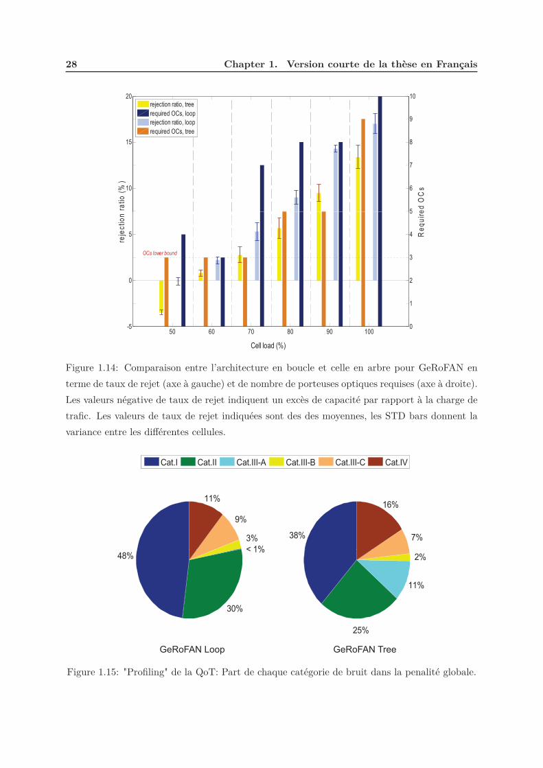
28 Chapter 1. Version courte de la thèse en Français
10
15
20
rati
o (
%)
ed
OC
s
5
6
7
8
9
10rejection ratio, tree
required OCs, loop
rejection ratio, loop
required OCs, tree
-5
0
5
reje
cti
on
Cell load (%)
Re
qu
ire
50 60 70 80 90 1000
1
2
3
4
5
OCs lower bound
Figure 1.14: Comparaison entre l’architecture en boucle et celle en arbre pour GeRoFAN en
terme de taux de rejet (axe à gauche) et de nombre de porteuses optiques requises (axe à droite).
Les valeurs négative de taux de rejet indiquent un excès de capacité par rapport à la charge de
trafic. Les valeurs de taux de rejet indiquées sont des des moyennes, les STD bars donnent la
variance entre les différentes cellules.
< 1%3%
9%
11%
38% 7%
16%
Cat.I Cat.II Cat.III-A Cat.III-B Cat.III-C Cat.IV
48%
30%
< 1%
25%
11%
2%
GeRoFAN TreeGeRoFAN Loop
Figure 1.15: "Profiling" de la QoT: Part de chaque catégorie de bruit dans la penalité globale.

1.5. Performance numérique 29
60% 70% 80% 90% 100%
0
10
20
30
40
Cell traffic load (%)
Re
jec
tion
ra
tio (
%)
PaGeO
IM-free CA
FFCA
FCA
RCA
60% 70% 80% 90% 100%0
5
10
15
20
25
Cell traffic load (%)
Nu
mb
er
of
req
uir
ed
OC
s
-pool size
Lower
Bound
Figure 1.16: PaGeO vs. les stratégies de transport alternatives (RCA, FCA, FFCA et IM-free
CA) en terme de taux de rejet et de nombre de porteuses optiques requises.
En adossant les canaux radio sur le premier canal optique disponible, la politique FCA at-
teint nécessairement le nombre minimum de porteuses optiques par contre cette politique est
réalisée au détriment du taux de rejet dans les cellules. Bien que QoT-agnostique, la politique
RCA combat les contraintes de transmission RoF due à la sélection aléatoire des canaux op-
tiques, cependant ceci est réalisé au prix d’un nombre de porteuses optiques assez élevé (70%
de l’ensemble du pool optique). FFCA peut etre considéré comme la version QoT-intégré du
FCA, FFCA consomme 3 OCs de plus en moyenne par rapport à FCA mais atteint des taux
de rejet plus faibles que FCA (en moyenne 85% plus faible). Les résultats montrent que on
aura besoin de 7 OCs en plus que la borne inférieure pour implémenter la politique IM-free
CA. Cette dernière annule les intermodulations et réduit ainsi le taux de rejet dans les cellules.
Cependant, le taux de rejet résiduel pour la politique IM-free CA spécialement à forte charge
montre qu’en consommant beaucoup de OCs pour annuler les intermodulations n’arrange pas
l’impact d’autres bruits (WDM-NLEs, OADM XT...) dont la pénalité augmente avec le nombre
de porteuses optiques utilisées.

30 Chapter 1. Version courte de la thèse en Français
Enfin pour notre algorithme, PaGeO atteint un compromis excellent par rapport aux autres
politiques de transport entre les deux objectifs: le taux de rejet cellulaire et le nombre de
porteuses optiques requises. En effet, PaGeO consomme en moyenne 2 OCs moins que FFCA,
tout en atteignant à deux reprises la borne inférieure at charge modérée. Par ailleurs, les taux
de rejet atteints par PaGeO sont assez proches de l’algorithme IM-free CA. En effet, les taux
de rejet de l’IM-free CA montrent qu’en se focalisant exclusivement sur les intermodulations
IMDs ne réussit pas seul à diminuer substentiellement les taux de rejet dans les cellules, car de
ce fait la politique IM-free CA ignore les autres bruits qui peuvent se manifester surtout quand
un nombre élevé de OCs est utilisé. Ceci donc premeut plutot une politique de gestion globale
des contraintes de la qualité de transmission RoF plutot qu’une focalisation ciblée sur un seul
bruit plutot qu’un autre.
Enfin, grace à son optimisation multi-objectifs resolu via le front de Pareto, l’algorithme
PaGeO atteint uniformément ses résultats de taux de rejet entre les différentes cellules mieux
que les autres politiques. Ceci peut etre remarqué grace à la longueur des STD bars représentant
la variance des résultats de taux de rejet entre les cellules.
1.6 Conclusion
La montée en débit inhérente à l’utilisation des nouveaux terminaux mobiles (smart-phones)
pose le problème de la capacité inadaptée des réseaux d’accès radio (RAN) actuels. La téléphonie
mobile de 4ème génération (LTE, LTE-advanced) va nécessiter de fait une forte densification des
antennes. Dans ce contexte, l’architecture actuelle des réseaux d’accès radio présente plusieurs
défauts. Elle est très hiérarchique. Elle n’exploite pas la souplesse du multiplexage statis-
tique. Elle ignore les fonctions de protection et de restauration. Elle n’est pas économiquement
adaptable à l’échelle à une densification des stations de base.
Nous avons proposé dans cette thèse une nouvelle architecture appelée GeRoFAN de réseaux
d’accès radio basée sur l’exploitation de réseaux tout-optiques WDM permettant de desservir
des stations de base pouvant être exploitées par différents opérateurs et reposer sur des tech-
nologies distinctes. L’originalité de l’approche proposée consiste en la possibilité d’allouer dy-
namiquement de la ressource radio-fréquence, et donc de la bande passante, au prorata de la
charge de trafic dans des zones géographiques d’activités différentes. Nous exploitons pour cela
les potentialités de la radio-sur fibre (RoF) analogique et de la modulation par sous-porteuse
(SCM). Nous avons introduit les concepts de HOLT (Hybrid Optial Line Termination) et de
RAU (Radio Access Unit). Pour chaque sous réseau optique, une HOLT est située à la tête
du réseau dans les locaux de l’organisme censé gérer dynamiquement l’allocation des ressources
radio (typiquement une collectivité locale). Les RAUs sont quant à elles réparties le long de
chaque sous réseau optique. Typiquement, les têtes de réseau HOLT sont situées au niveau des

1.6. Conclusion 31
actuels commutateur d’accès. Une seule station de base appartenant à un unique opérateur est
connectée à chaque RAU. Par contre, les stations de base raccordées sur les différentes RAUs
d’une même boucle peuvent être opérées par différents opérateurs radio-mobiles. En d’autres
termes, les HOLTs et les infrastructures optiques sont mutualisées entre différents opérateurs
exploitant éventuellement des réseaux radio-mobile de type différents (GSM, WiMAX, LTE,
LTE-advanced etc.). Nous avons proposé en outre la conception d’un plan contrôle permettant
grâce à l’utilisation d’un canal de signalisation, de faire glisser des ressources radio-fréquence
d’une station de base vers une autre, au gré de la dynamique spatio-temporelle du trafic. Ce
plan de controle opère une stratégie de transport des canaux radio par les porteuses optiques
permettant de minimiser les taux de rejet dans chaque cellule tout en consommant moins de por-
teuses optiques que possible. Cette politique optimisée de transport est le fruit d’une stratégie
dérivée par un algorithme génetique basé sur l’optimisation par front de Pareto, appelée PaGeO.
Contrairement aux autres politiques de transport qu’elles intégrent ou ignorent les contraintes
de la qualité de transmission de la RoF analogique, PaGeO assure un excellent compromis entre
l’optimisation de la capacité radio par cellule et la capacité optique requise pour implémenter
la stratégie de transport.
Notre approche est en cohérence avec les concepts de CRAN (Collaborative RAN) et de
Cloud RAN tels qu’ils ont été présentés par des équipementiers et les organismes de standarisa-
tion. Ces concepts visent tous à favoriser une gestion agnostique du spectre radio. Ils préconisent
tous l’utilisation de la technique RoF pour mutualiser à la tête du réseau les équipements de
traitement du signal radio.


Chapter 2
General Introduction
Contents
2.1 Motivation, Objectives and Thesis Outline . . . . . . . . . . . . . . . . . . . . 33
2.2 Contributions and Statement of Originality . . . . . . . . . . . . . . . . . . . . 35
2.3 Publications . . . . . . . . . . . . . . . . . . . . . . . . . . . . . . . . . . . . . . . 37
2.1 Motivation, Objectives and Thesis Outline
The rapid growth of the smart-phones market is at the origin of a strong increase in the
traffic within radio-mobile access systems. Deploying smaller radio cells and/or operating at
higher radio frequencies (greater than 5 GHz) are envisioned to fulfill the increasing need of
capacity per unit area. This advocates for a higher densification of radio cells. Existing Radio
Access Network (RAN) architectures are not economically suited to cope with such an evolution.
In fact, while an unprecedent technological improvement has been made in the radio section and
the core section of the mobile network, the cellular backhaul is left as the weak part threatening
the efficiency of the overall system. More generally, the metro-access area is considered as the
most costly part of public networks because of its low level of mutualization. Today, the biggest
cost challenge facing wireless service providers is the backhaul network– the part of the network
ranging from the base station to the radio network controller. Current backhaul infrastructure
relies mainly on narrow-band Time Division Multiplexing (TDM) systems consisting in leased
copper lines or point-to-point/point-to-multi-point microwave links. As a result, the deployed
network architecture is not optimized to handle the increasing traffic volumes propelled by
packet voice and bandwidth hungry packet data services. Since the last decade, many mobile
operator executives have approved a raising of nearly 15% to 20% in the annual expenditures
[38] dedicated to the backhaul in order to get enough capacity to their cell sites for a high-quality
3G+ and very soon 4G end-user experience. At the mean time, the flat-pricing model adopted
by the mainstream of mobile carriers coupled with an inefficient strategy for the backhaul
consisting in simply leasing additional TDM lines as the capacity grows have generated a gap

34 Chapter 2. General Introduction
flo
w($
)GrowthRate
Backhaul
expenditures
20 – 40% 30 – 40%
Share of the backhaulin the total budget of Telcos
Ca
sh
Time
TDM traffic Era(voice prevailing)
Packet-switched traffic Era(data dominating)
…
Turning
point
revenues
CapEx OpEx
Figure 2.1: The current challenge of mobile carriers: Revenues growth rate flatting while ex-
penditures growth rate are taking off propelled by the traffic increase. How carriers can bridge
the gap and reverse the trend ?
in the operating margin of the mobile operator which increases with the traffic growth as shown
in Figure 2.1.
Considering the heavy weight of backhaul expenditures on mobile carriers total budget1,
it is necessary to rethink current mobile backhauling towards alternative solutions offering a
sustainable high capacity. Fiber optics with its "unlimited" bandwidth and the advances in
opto-electonic/photonic devices are well positioned to contribute in shaping the new cellular
backhaul. To make full benefit of the huge bandwidth and connectivity offered by optical
networks and the mobile features provided by next generation wireless systems, the integration
of wireless and optics by means of Radio-over-Fiber (RoF) technology is an attractive solution
for decreasing the costs and clearing the path for fixed/mobile infrastructure convergence.
The objective of this thesis is to propose an innovative all-optical network infrastructure
called GeRoFAN (Generic Radio-over-Fiber Access Network) and to investigate its potential-
ities. The GeRoFAN architecture aims to backhaul 4G radio access systems (based either on
WiMAX or LTE) by means of analog RoF. Situated at mid-range between optics and wireless,
1According to IDATE [118], mobile operators spend 20 − 40% of their annual CapEx and 30 − 40% of their annual OpEx on cellular
backhauling.

2.2. Contributions and Statement of Originality 35
the main research question in the thesis revolves around the technical and economic require-
ments that have to be addressed to make the GeRoFAN architecture an enabler for a harmonious
wireless-optics integration.
The research conducted in this thesis is structured into four main parts:
• Chapter 2 carries out a comprehensive state of the art on the evolution of the cellular
backhauling and its main future trends. In this chapter, we position the GeRoFAN archi-
tecture within the backhaul solutions constellation and we highlight its main innovative
features.
• The second part of the research is provided by Chapter 3 which focuses on physical layer
impairments modeling of analog RoF transmission. The outcome of this work constitutes
a valuable input for an optimized exploitation of the GeRoFAN system.
• The third part of the research is focused on how the GeRoFAN system intelligence (its
Control Plane) should be designed to achieve an efficient cellular backhauling. More
algorithmic oriented, the third part of the thesis considers successively a static (Chapter
4) and a dynamic traffic context (Chapter 5).
• The last part of the research addresses the economics of the GeRoFAN paradigm and
investigates its business relevance (its added value) through different economic models.
The diagram in Figure 2.2 represents how the different parts of the research are linked
together.
2.2 Contributions and Statement of Originality
The contributions highlighted by this doctoral research are multi-fold and can be itemized as
the following:
• A RoF-based all-optical network architecture (GeRoFAN) is proposed for cellular back-
hauling and the mutualization of next generation radio systems. The originality of GeRo-
FAN is to make use of advanced amplified reflective optical modulators, optical WDM
technologies combined with analog RoF to achieve an elegant integration between optics
and wireless within a unified network infrastructure. At the network design stage, a major
innovation is pointed out by the GeRoFAN solution: its radio MAC-agnostic and analog
RoF impairment-aware control plane (c.f Part I) .
• Thus, unlike the mainstream literature which points out the limitations of analog RoF,
this research offers the opportunity to capitalize on the benefits of analog RoF while
mitigating its Quality-of-Transmission (QoT) limitations; the ultimate aim being to show

36 Chapter 2. General Introduction
Part I Backhauling state of the art
GeRoFAN Architecture(chapter 2)
Part II RoF Physical layer modeling
QoT-tool design(chapter 3)
Part IIIGeRoFAN-CP Algorithmic design
Static traffic context/Dynamic traffic context(chapter 4, chapter 5)Te
chnicalinvestigations
Part IVEconomics and Business relevance of GeRoFAN
(chapter 6, chapter 7)
Economic
investigations
Figure 2.2: The four main work-packages structuring the thesis.
that analog RoF is still an attractive solution to backhaul next generation cellular systems.
At this stage, the main originality of our study consists in providing a deep knowledge
of all physical layer impairments involved in the GeRoFAN network. A comprehensive
analytical modeling of RoF transmission limitations is realized as an essential step to make
the cellular backhauling by GeRoFAN as transparent as possible to the radio system (c.f
Part II).
• The optimization models designed to achieve such a QoT-aware cellular backhauling by
the GeRoFAN-CP constitute the third main originality of this PhD thesis (c.f Part III).
Indeed, a wide range of optimization approaches (exact methods through integer linear
programming, evolutionary algorithms, multi-objective Pareto optimization, greedy algo-
rithms, iterative tabu-search meta-heuristics) are exploited to best-fit the GeRoFAN-CP
requirements. In particular, we show how the GeRoFAN-CP, supported by the knowledge
of the physical layer impairments along with an adapted optimization tool, achieves an
adjusted fine-grained management of the radio system capacity. Such a matching between
the cellular system and GeRoFAN interests gives rise to what is commonly called backhaul
service provisioning.

2.3. Publications 37
• The economic assessment of the GeRoFAN architecture and the business value of its cel-
lular backhaul service constitute the fourth main contribution of the research (c.f part
IV). The key originality highlighted at this stage is to show how the value chain or-
chestrating the cellular backhauling business market could be enriched by the GeRoFAN
solution without shadowing the challenges raised by such a new assumed commercial and
regulatory context.
2.3 Publications
This dissertation consists of an overview and of the following conference and journal publica-
tions:
• "Impairment-aware Control Plane for Next Generation Radio-over-Fiber Access Net-
works", A. Haddad, M. Gagnaire and E.A. Doumith, in IEEE/Proc. of the 2nd Int.
Conf. Network of the Future, Nov. 2011, Paris.
• "Impairment-aware Radio-over-Fiber Control Plane for LTE Antenna Backhauling",
A. Haddad, E.A. Doumith and M. Gagnaire, in IEEE/ Proc. of Int. Conf. on Com-
munications (ICC), June 2012, Ottawa.
• "Next Generation Access Systems Backhauling using Radio-over-Fiber: a Prospective
Approach", A. Haddad and M. Gagnaire, in IEEE/Proc. of Summer Topicals, July 2012,
Seattle, WA.
• "Pareto Optimization for Radio-over-Fiber 4G Base Stations Backhauling", A. Haddad
and M. Gagnaire, in Proc. of the 15th Int. Telecommunications Network Strategy and
Planning Symposium (Networks’12), Oct. 2012, Rome.
• "PaGeO: Pareto-based Genetic Optimization for LTE Radio-over-Fiber Cellular Backhaul-
ing", A. Haddad and M. Gagnaire, in IEEE/Proc. of the 8th Int. Conf. on Wireless and
Mobile Computing, Networking and Communications (WiMob’12), Oct. 2012, Barcelona.
• "Differentiated Radio-over-Fiber-based Backhauling for Dynamic LTE Capacity Provision-
ing", A. Haddad and M. Gagnaire, To appear in IEEE/ACM Transactions on Networking
(ToN) journal, Q1-2013.
• "Optimized Radio-over-Fiber-based Cellular Backhauling Strategy using Genetic Algo-
rithms and Pareto Fronts", A. Haddad and M. Gagnaire, To appear in Special issue of
Telecommunication Systems Journal (TSJ)– Business and Economics Collection, Springer
Ed., 2013.

38 Chapter 2. General Introduction
Publications and a European patent dealing with research not related directly to the work
of this thesis are also enlisted:
• "A Meta-heuristic Approach for Monitoring Trail Assignment in WDM Optical Networks",
A. Haddad, E. A. Doumith and M. Gagnaire, in IEEE/IFIP Proc. of the Int. Congress
on Ultra-modern Telecommunications and Control Systems and Workshops (ICUMT’10),
Oct. 2010, Moscow.
• "A fast and Accurate Meta-heuristic for Failure Localization Based on the Monitoring Trail
Concept", A. Haddad, E. A. Doumith and M. Gagnaire, in Telecommunication Systems
Journal (TSJ)– Business and Economics Collection, Springer Ed., 2011.
• MeMoTA 2.0 Software European Patent (2010), "Meta-heuristic for Monitoring Trail As-
signment: [un algorithme de deploiement de circuits optiques (m-trail) pour la localisation
non-ambigue de pannes dans les reseaux WDM translucides]".

Part I
GeRoFAN Backhauling Architecture


Chapter 3
RoF-based Mobile Backhauling
Contents
3.1 Introduction . . . . . . . . . . . . . . . . . . . . . . . . . . . . . . . . . . . . . . 41
3.2 Cellular backhaul: Current and future trends . . . . . . . . . . . . . . . . . . 42
3.2.1 The mobile backhaul section . . . . . . . . . . . . . . . . . . . . . . . . . . . . . 42
3.2.2 Evolution of the backhaul protocol stack: Migration paths . . . . . . . . . . . . . 51
3.3 Leveraging the fiber at the access: Radio-over-Fiber . . . . . . . . . . . . . . 53
3.3.1 Radio-over-Fiber technology . . . . . . . . . . . . . . . . . . . . . . . . . . . . . . 54
3.3.2 D-RoF vs. A-RoF: An economic analysis . . . . . . . . . . . . . . . . . . . . . . 61
3.4 Generic RoF Access Network . . . . . . . . . . . . . . . . . . . . . . . . . . . . 70
3.4.1 The Radio Access Unit . . . . . . . . . . . . . . . . . . . . . . . . . . . . . . . . . 72
3.4.2 GeRoFAN for multi-operator backhauling . . . . . . . . . . . . . . . . . . . . . . 74
3.4.3 GeRoFAN system control plane . . . . . . . . . . . . . . . . . . . . . . . . . . . . 75
3.1 Introduction
Recently, mobile backhauling has received considerable attention from operators, seeking
to upgrade and even to rethink their existing backhaul infrastructure to meet in a cost-effective
way the increasing demand of bandwidth. This chapter focuses on the salient features and
issues of cellular backhaul with a focus on optical fiber as a promising answer to rising mobile
data traffic.
Chapter 3 is structured as follows. A survey of the various technologies used for backhaul is
carried out in Section 3.2. We spotlight current and upcoming trends of the backhaul network
together with telcos’ strategies. Section 3.3 investigates the opportunities of leveraging the
optical fiber for mobile backhaul through Radio-over-Fiber (RoF) technology. A comparison
between the two main techniques of RoF, analog or digitized, is realized to show the economic
benefit of employing Analog RoF (A-RoF) for broadband mobile backhaul. In Section 3.4, we
describe GeRoFAN (Generic RoF Access Network), an all-optical network architecture relying

42 Chapter 3. RoF-based Mobile Backhauling
on A-RoF, for cellular backhauling. The key features of the GeRoFAN Control Plane (CP) are
introduced at the end of this chapter.
3.2 Cellular backhaul: Current and future trends
3.2.1 The mobile backhaul section
The mobile backhaul section designates the portion of the network that connects the Base
Station (BS) (a.k.a Base Station Transceiver (BTS) in 2G or Node-B in 3G systems) which
communicates with the mobile equipment through the air interface and the radio network con-
troller at the central office (a.k.a Mobile Switching Center (MSC) and Radio Network Controller
(RNC) for 2G and 3G respectively). More generally, the backhaul consists of a group of radio
cell sites aggregated into a hub sites being connected to the edge node of the core network.
Figure 3.1 illustrates the generic model of the backhaul section spanning from the cell site
("Wireless Last Mile" domain) to the core transport network. Three subcomponents constitute
the mobile backhaul: the cell site, the aggregation site, and the Metro network [113].
Core
Core Swtching Node
Metro regional Node
Hub Node
Radio cell site Access
Metro …Core
Access
Aggregation
Figure 3.1: Generic model and subcomponents of the mobile backhaul.

3.2. Cellular backhaul: Current and future trends 43
Figure 3.2: Traditional/emerging backhaul technologies: A big picture view [102].
3.2.1.1 Backhaul technologies at the access/agregation segments
The current backhaul network relies on various technologies to aggregate the radio traffic and
transport it to the network controller. Figure 3.2 shows a big picture of the different technologies
used for current and emerging cellular backhaul.
As it can be noticed, three physical mediums dominate today’s backhaul: copper, optical
fiber and microwave radio links. In the US for instance, leased T1/E1 copper lines reaches up to
90% of backhaul infrastructure followed by microwave radio links (about 6%) and optical fibers
(about 4%)[110]. In the following, we describe the main characteristics of these technologies
and alternative solutions for backhauling either prospective (WiFi,WiMAX) or emerging (circuit
emulation using pseudo-wire).
• Copper: Copper cables constitute the traditional backhaul medium originally used in
GSM system between the BTS and the Base Station Controller (BSC). The traffic between
BTS and BSC is TDM multiplexed and transported in predefined time slots using the Ple-
siochronous Digital Hierarchy (PDH). Two PDH standards are used to transport TDM circuits
over copper cables: the T-carriers and the E-carriers delivering data-rates ranging from 2.048
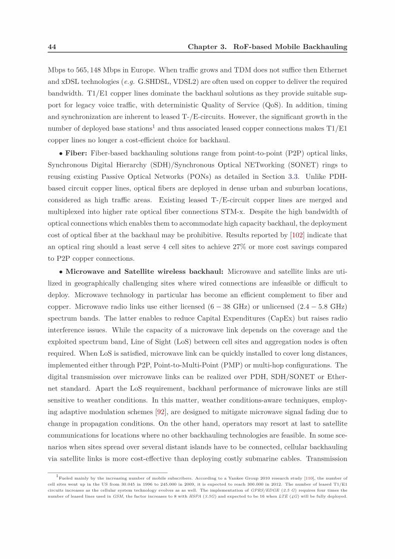
44 Chapter 3. RoF-based Mobile Backhauling
Mbps to 565, 148 Mbps in Europe. When traffic grows and TDM does not suffice then Ethernet
and xDSL technologies (e.g. G.SHDSL, VDSL2) are often used on copper to deliver the required
bandwidth. T1/E1 copper lines dominate the backhaul solutions as they provide suitable sup-
port for legacy voice traffic, with deterministic Quality of Service (QoS). In addition, timing
and synchronization are inherent to leased T-/E-circuits. However, the significant growth in the
number of deployed base stations1 and thus associated leased copper connections makes T1/E1
copper lines no longer a cost-efficient choice for backhaul.
• Fiber: Fiber-based backhauling solutions range from point-to-point (P2P) optical links,Synchronous Digital Hierarchy (SDH)/Synchronous Optical NETworking (SONET) rings to
reusing existing Passive Optical Networks (PONs) as detailed in Section 3.3. Unlike PDH-
based circuit copper lines, optical fibers are deployed in dense urban and suburban locations,
considered as high traffic areas. Existing leased T-/E-circuit copper lines are merged and
multiplexed into higher rate optical fiber connections STM-x. Despite the high bandwidth of
optical connections which enables them to accommodate high capacity backhaul, the deployment
cost of optical fiber at the backhaul may be prohibitive. Results reported by [102] indicate that
an optical ring should a least serve 4 cell sites to achieve 27% or more cost savings compared
to P2P copper connections.
• Microwave and Satellite wireless backhaul: Microwave and satellite links are uti-
lized in geographically challenging sites where wired connections are infeasible or difficult to
deploy. Microwave technology in particular has become an efficient complement to fiber and
copper. Microwave radio links use either licensed (6 − 38 GHz) or unlicensed (2.4 − 5.8 GHz)
spectrum bands. The latter enables to reduce Capital Expenditures (CapEx) but raises radio
interference issues. While the capacity of a microwave link depends on the coverage and the
exploited spectrum band, Line of Sight (LoS) between cell sites and aggregation nodes is often
required. When LoS is satisfied, microwave link can be quickly installed to cover long distances,
implemented either through P2P, Point-to-Multi-Point (PMP) or multi-hop configurations. The
digital transmission over microwave links can be realized over PDH, SDH/SONET or Ether-
net standard. Apart the LoS requirement, backhaul performance of microwave links are still
sensitive to weather conditions. In this matter, weather conditions-aware techniques, employ-
ing adaptive modulation schemes [92], are designed to mitigate microwave signal fading due to
change in propagation conditions. On the other hand, operators may resort at last to satellite
communications for locations where no other backhauling technologies are feasible. In some sce-
narios when sites spread over several distant islands have to be connected, cellular backhauling
via satellite links is more cost-effective than deploying costly submarine cables. Transmission
1Fueled mainly by the increasing number of mobile subscribers. According to a Yankee Group 2010 research study [110], the number of
cell sites went up in the US from 30.045 in 1996 to 245.000 in 2009, it is expected to reach 300.000 in 2012. The number of leased T1/E1
circuits increases as the cellular system technology evolves as as well. The implementation of GPRS/EDGE (2.5 G) requires four times the
number of leased lines used in GSM, the factor increases to 8 with HSPA (3.5G) and expected to be 16 when LTE (4G) will be fully deployed.

3.2. Cellular backhaul: Current and future trends 45
over satellite links are mostly based on PDH circuits. Their short installation times, flexible
coverage and exploitation (using DAMA2 technique for instance) should not mask their major
drawbacks namely their high cost and long propagation delay3.
• Free-Space Optics: Free-Space Optics (FSO) are another means of high bandwidth
backhauling technology capable of 1 Gbps data rate transmission that can be mapped over
SONET/SDH standard (STM-4). FSO is a LoS transmission technology using directive laser
beams to provide optical bandwidth connections. FSO does not require fiber-optic cable or the
securing of spectrum licences for radio-frequency solutions. However, the requirement of hight
stability mounting for FSO and the susceptibility to obstructions and fog attenuation make
them less attractive for large-scale mobile backhaul deployment [128].
• Prospective wireless technologies for backhaul: WiFi and WiMAX
Wireless Fidelity (WiFi) was originally designed for indoor usage based on the IEEE 802.11
standards operating in the 2.4 and 5 GHz unlicensed bands. Recent advances in industry and
academia demonstrated the feasibility to extend the usage scope of WiFi: recently as small
cell-localized WiFi point of presence to offload traffic in 3G radio systems, and prospectively
as an attractive low-cost solution for backhaul which can substitute microwave links. How-
ever, the deployment of WiFi as a backhaul technology poses design challenges relevant to the
achieved throughput, distance, coverage, packet efficiency, timing and synchronization. Several
solutions are proposed to tackle these different issues. For example, the 802.11n standard ex-
ploits MIMO techniques together with frequency reuse to improve the throughput up to 600
Mbps. In addition, to provide long distance outdoor coverage, proprietary modifications of the
MAC protocol are introduced4, while packet overhead is reduced through header compression
techniques. Lastly, as QoS including timing and synchronization is an essential requirement for
mobile backhaul, the 802.11e amendment was introduced to support QoS on WiFi networks.
Wireless interoperability for Microwave Access (WiMAX) was originally designed for out-
door usage and defined through the 802.16 standards. Based on OFDM modulation with higher
spectral efficiency than WiFi, WiMAX provides higher throughput (75 Mbps per single channel
and up to 350 Mbps with channel aggregation) and longer coverage range (up to 50 Km for a
single hop). It operates in both licensed and unlicensed spectrum bands with LoS and non-LoS
connectivity, although data-rate is reduced for a non-LoS transmission. Compared to WiFi,
WiMAX is already used for backhaul thanks to the 802.16-2004 standard designed for fixed
connectivity applications in P2P, PMP, and complex mesh topologies. Unlike standard WiFi,
WiMAX PMP mode supports guaranteed QoS through centralized scheduling mechanisms and
the support of different service classes.
2Demand Assigned Multiple Access (DAMA) dynamically allocates bandwidth resources based on actual requests from the users. DAMA
enables usage-based billing mechanisms which helps reduce the incurred expenses of building a Satellite communication site.3As an illustration, the cost of a transponder for an equivalent bandwidth of full T1-circuit used on a full time basis is 5000$ - 12000$
per month, that is as much as 16 to 40 times the average cost of a single T1 leased link in US as reported by Yankee Group [110].4Involving MAC layer parameters such as: contention window, round-trip time delay and acknowledgment time-out.

46 Chapter 3. RoF-based Mobile Backhauling
• The Pseudo-Wire (PW) framework: The pseudo-wire framework was introduced
as a backhaul technology to transport traditional services (TDM, ATM) over Packet-Switched
Networks (PSN), e.g. Ethernet, IP or MPLS. Such a circuit emulation mechanism is referred to
as "TDM/ATM Pseudo-wire" transport. Compared to legacy circuit switched backhaul based
on T-/E-carriers, pseudo-wire techniques let capitalize on the lower cost per megabit provided
by packet-switched networks which enables to achieve a cost-efficient backhaul and paves the
way for a convergent "all-packet" transport. Several standards have been published by the
IETF5 to address circuit emulation for GSM backhaul and the transport of ATM services
used in UMTS backhaul over packet-switched networks. Figure 3.3 shows the pseudo-wire
protocol architecture activated between two provider edge devices tunneling a TDM or ATM
payload into a PSN. The protocol stack highlights four different layers. The Encapsulation layer
composed of three sub-layers: first the TDM or ATM payload is encapsulated using the payload
convergence sub-layer. The Timing sub-layer provides timing and synchronization within PSN
[102] and the Sequencing sub-layer handles out-of-order packet arrival and packet loss issues.
Depending on the payload (T1/E1 bit streams or ATM cells), the Encapsulation layer decides
the type of processing and the required added headers to form the "pseudo-wire frame". Prior
to packet transport layer, multiple pseudo-wire connections are managed using the Pseudo-wire
mux/demux layer and finally the PSN convergence layer allows pseudo-wires to be independent
of the underlaying PSN type while meeting the service requirements. Although the design of
a PSN-based cellular backhauling poses technical issues relevant to time synchronization, QoS
and packet efficiency, specifications of the Pseudo-wire framework address some of these issues.
Combined with MPLS RSVP-TE, as a connection-oriented switching paradigm, the pseudo-wire
framework enables the provision of an end-to-end QoS with fast packet delivery.
The diversity of aforementioned solutions used for backhaul shows that there is no clear
unique answer to think what is the technology that drives the evolution of backhaul networks. In
fact, although copper T1/E1 leased lines are still today predominant in the backhaul big picture
[110], their incapacity to accommodate cost-efficiently traffic growth makes alternative solutions
worth to consider by telcos. Partially inspired from [102], Table 3.1 synthesizes a comparison
between the different backhaul technologies through five criteria: Capacity, Distance/Coverage,
QoS support (end-to-end delay, jitter, reliability etc.), Timing/Synchronisation, Cost and pos-
sible telcos’ strategies to leverage the backhaul investment.
Telcos’ strategies for selecting the right backhaul technology or/and upgrading their ex-
isting backhaul network are driven by two time-horizon objectives. At the short term, an
operator seeks the immediate benefit of the backhaul technology particularly for coping with
the traffic increase at the cell site, the reference scenario for risk/benefit assessment being the
existing backhaul infrastructure (leased T1/E1 copper). At the medium/long term, the oper-
5Internet Engineering Task Force: RFC 3985, RFC 4385, RFC 5086, RFC 5087 etc.

3.2. Cellular backhaul: Current and future trends 47
Table 3.1: Backhaul technologies comparison.
Capacity Coverage QoS Synchronization Cost Leverage Strategies for Operators
Wir
eli
ne
Te
ch
no
log
ies
Le
ase
dC
op
pe
r
Low (∼ 2
Mbps)
No additional
requirementGuaranteed Natively provided
low CapEx (already
exists), but high
Operational Ex-
penditures (OpEx)
(leasing cost in-
creases linearly
with capacity and
distance)
Bonding multiple T1/E1 lines. Running
xDSL technologies, that can be reused for
femto/pico-cell backhaul.
Fib
er
Very HighNo additional
requirementGuaranteed
Provides timing ref-
erence
High roll-out, CapEx
and maintenance fees
increasing with dis-
tance
Leveraging existing fiber using fixed
broadband xPON technologies (c.f. Sec-
tion 3.3). RoF-based "Cloud RAN" (c.f.
Section 3.2.2 ). Fixed Mobile Convergence
(FMC): Promoting fiber-wireless conver-
gence.
Wir
ele
ss
Te
ch
no
log
ies
Mic
ro
wa
ve
High but
depending
on the fram-
ing protocol
and the
modulation
techniques
LoS require-
mentGuaranteed Provided
High upfront CapEx.
Licence spectrum
fees with high main-
tenance cost.
Lower the OpEx through unlicensed bands
with care to interference. Multi-carrier site
sharing.
Sa
te
llit
e
MediumFlexible cov-
erage
High propaga-
tion delayProvided
More expensive at
an equivalent T1/E1
link.
Usage-based billing to alleviate high in-
vestment cost (Sharing). The ultimate so-
lution for challenging areas (islands, re-
mote locations).
FS
O
Very High but
still depen-
dent on the
propagation
conditions
LoS privi-
legedGuaranteed Provided
No heavy investment
infrastructure (vs.
fiber). Securing
spectrum license
with narrow beam
(vs. interference-free
licensed microwaves
or interference-
subject unlicensed
WiFi), but high
OpEx (mounting sta-
bility, susceptibility
to beam obstruction)
Promoting hybrid solutions by bridging
with non-LoS microwave links to over-
come obstructions through ring and daisy-
chained configurations [42]. FMC: FSO as
an extension of optical Ethernet (already
deployed in metropolitan areas) to mobile
backhaul [128].
WiF
i
High LoS
Excepting
802.11e, QoS
is originally
not supported
Not enough accurate
for backhaul applica-
tions
Low CapEx due to
mass production.
Low OpEx: Unli-
censed spectrum.
Offloading high-bandwidth best-effort
traffic through public hot-spots (Evolved
offloading mechanisms through Hot-
spot 2.0 [42]). Leverage widespread
private/in-building WiFi owned by third
party through incentive micro-payment
technology-based methods [117].
WiM
AX
High
Both LoS and
non-LoS with
multi-hop for
higher cover-
age
Guaranteed
Accurate through
GPS as a reference
clock
CapEx network
building, OpEx:
Licensed spectrum
fee
Standardization drives the total cost down.
Strong candidate for rural and metro areas
deployment.

48 Chapter 3. RoF-based Mobile Backhauling
BS
PSNEthernet,
IP/MPLS
Provider
Edge Device
(pseudo-wire device)
Provider
Edge Device
(pseudo-wire device)
Aggregation point
(MSC/BSC, RNC)
Base Station (BS)
Cell site
TDM (GSM)
ATM (UMTS)
En
cap
sula
tio
n
Payload
Payload convergence(AAL2, AAL5 PDUs)
Timing
Sequencing
PW mux/demux
PSN convergence
PSN Transport (Ethernet, IP, MPLS …)
Figure 3.3: Pseudo-Wire Protocol Stack.The Pseudo-wire protocol stack is implemented at both provider edge devices. The encapsulation layer provides any information needed by the
edge devices to forward packets from the PSN frontier to the TDM/ATM network frontier, and to reconstruct the original TDM/ATM payload
from the received packets. The encapsulation of TDM bit streams is not a mere packetization process since lost packets can cause service
interruption. In fact, usually multiple T1/E1 frames are grouped together into one big frame before encapsulation and only the time slots in
use within each T1/E1 circuit are sent. The encapsulation techniques used by Pseudo-wire rely on AAL (ATM Adaptation Layer) to provide
QoS-compliant transfer of voice-grade channels, data and telephony signaling. Specifically, AAL1 PDUs (Packet Data Unit) for Constant Bit
Rate applications (voice call), AAL2 PDUs for Variable Bit Rate applications (time slots are dynamically assigned, e.g. 2.5G/3G), AAL5 to
handle signaling exchanged between Node-Bs and RNC over the Iub interface in 3G [102].
ator investigates the foreseen Return on Investment (RoI) of the strategy. At this stage, the
operator estimates the potential business value featured by prospective applications that lay
on the upgraded/new backhaul network. Both time-horizon objectives are synthesized through
the schematics in Figure 3.4. We have positioned several backhaul technologies in the diagram
according to two dimensions: the capacity-coverage product and the required Total Cost of
Ownership (TCO), both normalized to the reference scenario of a single leased T1/E1 copper
line. The diagram shows also examples of possible attractive investment strategy paths for an
operator. The techno-economic framework to assess the TCO for the different technologies is
inspired from the economic modeling in [141]. Data and background assumptions used for the
schematics are applied to developed markets and based on recent research consulting/watch
service reports from: [38], [107], [118], [45] and [122].
TCO is evaluated by computing cumulative CapEx (deployment expenses) and OpEx (in-
cluding: maintenance, ongoing leasing cost, licensed spectrum fees) cashflow per cell site over
5 years. The reference scenario of T1/E1-leased copper backhauling assumes a monthly leasing
fee of 300 eper link [110].

3.2. Cellular backhaul: Current and future trends 49
10
100
aliz
ed),
log. scale
Wireline Tech.
Wireless Tech.
ADSL 2+
HFC WiMAX
FSO
Build Fiber(EPON)
P2Pmicrowave
Leased Fiber(EPON)
Femto/picos
backhaul
RoF
Cloud RAN
FMC
Incentives to
FMC with
Optical Ethernet
Leverage Cable
FMC
Upgrading
to xDSL
Invest on wireless
first then switch
to fiber
WDM
PON
Reuse
available
ducts
Extending
the fiber to end-user
premises
0 1 10 100 10000
1
Capacity x Coverage Product (Normalized), log. scale
TC
O (
Norm
a
Leased T1/E1 Copper WiFi
(802.11g)
PMPmicro-wave
( )
N xT1/E1
Bonding
Hotspot 2.0
Incentives to
Third-party
Short term relaxing
at low cost
Figure 3.4: Backhaul benchmark and telcos’ leverage strategies.Several leverage strategy paths are highlighted for Telcos aiming at upgrading their backhaul network with attractive RoI. The first reachable
strategy consists in reusing the already deployed copper infrastructure to run xDSL, ADSL2+ is a cost-effective strategy to backhaul pico-cells
and femtos installed in the subscriber premises. Other operators privileged the low-cost WiFi solution to relax, at short term, the requirement
on backhaul. In general, wireless solutions are considered being more cost-efficient to address short/medium term requirement for backhaul.
Indeed, an analysis carried out by Telecom business consulting companies [107] shows that deploying wireless backhaul (microwave, Enhanced
WiFi, FSO) first then building a fiber network later provides operators with up to 27% of savings, and up to 31% when leasing fiber. More
prospective strategies such as building a high-capacity backhaul network using WDM-PONs are definitely long-term. In fact, the investment
payback of WDM-PON is higher than other strategies and the technology is not yet standardized.
3.2.1.2 Design considerations for evolved packet backhaul
Several studies have pointed out the limitations of the current backhaul especially at the last
mile and the aggregation part to absorb the increasing amount of traffic generated in each
radio cell [110][118]. While the connectivity type offered by the backhaul network is influenced
by the technology used in the RAN and factors such as geographical locations of the cell site,
bandwidth requirements, sustainable investment and local regulations, there is a wide consensus
to rethink the evolved backhaul around the pure packet IP-based switching network. The design
considerations for an all-IP-based mobile backhaul are summarized below [113]:
• VLAN Models: Implementing a Virtual Local Access Network (VLAN) model in the back-
haul enables to separate the traffic either based on services or/and locations through
tagged and untagged frames (original standard defined in IEEE 802.1Q). Overlaying

50 Chapter 3. RoF-based Mobile Backhauling
VLANs on the backhaul enables more efficient management of the traffic in terms of
capacity and QoS. Originally defined as a LAN-based solution for flexible networking of
entreprise business divisions, the model of VLAN is undergoing standards extension efforts
(IEEE 802.1ad and 802.1ah) to meet operators needs for backhaul.
• Class of Services (CoS): The evolved packet-based mobile backhaul network needs to becapable of recognizing the CoS settings of the different traffic streams, doing any re-
marking of packets if required, prioritizing, classifying and scheduling packets. The back-
haul has to be able to support within a unified transport infrastructure the main traffic
streams including voice, video, network signaling/management, and best-effort data while
providing low packet loss.
• Transport and Services: MPLS and pseudo-wire technologies are used as the transport
mechanism in both pure packet and hybrid types of mobile backaul architectures (c.f. see
Subsection 3.2.2). The advantage of using MPLS for transporting pseudo-wires connec-
tions is that it is agnostic to the transport media and more scalable than a traditional
Layer 2 networks. The new extension of the MPLS standard (MPLS-TP) enables to capi-
talize on the maturity of the original protocol and to benefit from its advantages in terms
of protection schemes, faster convergence times and connection-oriented transport. On
the other hand, the PBB-TE (Provider Backbone Bridge-Traffic Engineering) initiative
aims at extending the legacy widespread Ethernet protocol to meet the "carrier-grade" re-
quirements. Both MPLS-TP and PBB-TE rely on the establishment of predefined virtual
connections through the packet transport network by appending labels, computing and
provisioning the required resources.
• Synchronization: Synchronization is a challenging requirement for all-packet backhaul, in-deed unlike TDM, packet transport does not inherently support network synchronization.
In mobile radio systems, synchronization is used to support cellular handoff, interference
management, mobile localization, and the delivery of real-time services like voice and
video streaming. Two major standards namely the IEEE 1588 and the ITU Synchronous
Ethernet (Sync-E) are developed to support clock synchronization for packet-switched
mobile backhaul. Sync-E operates at Layer 1 of the communication stack and thus runs
independently from upper layer transmission protocols.
In Sync-E, each node recovers the clock information from upstream nodes and then dis-
tributes it to downstream nodes after filtering jitter. However, to get implemented, Sync-E
requires hardware support in all devices in the network. The IEEE 1588 protocol runs in
parallel with data traffic. Unlike Sync-E, IEEE 1588 requires only the installation of a
grand master clock at the RNC to get implemented. However, IEEE 1588 is sensitive to

3.2. Cellular backhaul: Current and future trends 51
network congestion, jitter and delay, and in some cases, it complicates traffic engineering
and planning. While much focus has been done on timing and frequency synchroniza-
tion, phase synchronization is an additional requirement in 4G systems that has to be
addressed6. Looking for comprehensive standard, the IETF proposed the TICTOC archi-
tecture –a unified framework for frequency and timing distribution over packet switched
networks, based on existing standards or extensions like the Network Timing Protocol
(NTP) or the IEEE 1588 v2 [102].
• Reliability and Fault Detection: Fault detection mechanisms need to be implemented at
different levels of the backhaul network. Failure detection has to be implemented both at
the Ethernet physical and link layers. MPLS offers for instance protection schemes at the
link and node level with fast failure detection and convergence times.
3.2.2 Evolution of the backhaul protocol stack: Migration paths
Several survey studies conducted with operators [38][118] pointed out the evolution towards
an all-packet backhaul network as a cost-effective investment able to meet in a sustainable
way the traffic increase. Related backhaul evolution steps will be common and the difference
will lie in whether all operators will experience all the transformation stages or whether some
can accelerate or side step one or two of the stages. The challenge of the evolution lies in the
complexity to manage the transition to packet backhaul whilst maintaining existing high quality
of legacy (circuit-switched) services. A smooth transition to pure packet backhaul architecture
involves intermediate steps to set up hybrid approaches where TDM and packet traffic coexist
together within the same backhaul network with different levels of integration. In that matter,
the Pseudo-wire framework combined with MPLS for instance constitutes an attractive and a
mature technology for operators looking for implementing pseudo-wires at the BS to enable an
IP RAN before the IP capability is supported in the BS themselves. The gradual transition
from legacy circuit-switched to prospective pure packet backhaul network is illustrated in Figure
3.5. Hybrid architectures lay at intermediate stages with legacy circuit traffic is increasingly
integrated within packet transport.
The evolution of the backhaul can also be achieved by starting the mutation from the
access part. As detailed in subsection 3.2.1.1, the evolution of the access/aggregation section of
the backhaul consists in making the different underlaying physical technologies as "agnostic" as
possible to handle different transport standards. Meanwhile, the access/last mile section evolves
in-line with the planned mutation of the backhaul depicted in Figure 3.5. A flat architecture of
the RAN highlights such an evolution of the access. Indeed, from 2G/3G to 4G systems, more
6In LTE and WiMAX, the same wireless frequency can be reused in different phases, a capability that enables 4G service providers to
serve more customers on the same frequency range. Hence, a synchronization method supporting phase synchronization is needed. The IEEE
1588 protocol supports phase synchronization which is not the case of Sync-E.

52 Chapter 3. RoF-based Mobile Backhauling
ATM TDM
PDH/SDH
Copper, Fiber,
IP ATM/TDM
SDH
Copper, Fiber,
Ethernet
IP ATM/TDM
PW
Copper, Fiber,
Ethernet
Ethernet
Ethernet
Copper, Fiber,
2G
2.5G
3G
R992G/2.5G
3G
3.5G
4G LTE
WiMAX3G
2G/2.5G3.5G
4G LTE
WiMAX4G LTE
4G LTE-a
WiMAX
IP/MPLS/Ethernet
Micro-Wave,
Satellite, FSO …
Micro-Wave, Satellite,
FSO …
Micro-Wave, Satellite,
FSO …
Micro-Wave,
Satellite, FSO …
Legacy circuit
switchedHybrid Architectures Prospective pure
Packet-switched
Yesterday. Tomorrow ?Today: current and planned migrations …
…
Figure 3.5: From legacy to prospective backhaul: Evolution of the protocol stack.The figure illustrates the main stages describing the evolution of the transport protocols used for backhaul. The migration steps from legacy
circuit switched backhaul towards pure packet transport are achieved along with maintaining backward compatibility to achieve a smooth
transition. Yesterday, legacy circuit transport based on PDH/SDH (SONET) were sufficient to accommodate voice-grade traffic from 2G/2.5G
cellular systems. With the first release of 3G, ATM has been used to handle data traffic requiring higher and variable bandwidth, still the
backhaul remains globally managed through a circuit rationale. Today, it is widely admitted that legacy backhaul could not cope with the
new traffic pattern (bursty, non-deterministic, requiring differentiated QoS). Hybrid architectures describes how backhaul mutates towards a
coexistance between circuit and packet transport. Currently, such a co-existence is achieved by overlaying the ATM/TDM backhaul with the
IP/Ethernet backhaul. Similarly to access where WiFi hot-spots, Distributed antennas and small cells are deployed to offload traffic of the
macro-cell, running both TDM/ATM and IP/Ethernet backhaul networks in parallel could leverage telcos’ investments and achieve scalability.
In that scenario, low-priority high bandwidth traffic can be offloaded from the legacy TDM/ATM network to the new packet backhaul. Planned
hybrid architectures put an emphasis on higher integration of native TDM/ATM traffic into the emerging packet switching network. The
pseudo-wire (PW) technology gains more maturity among backhaul platform vendors and adoption from telcos looking to upgrade their
backhaul network. The hybrid packet/circuit backhaul is implemented either by using an interworking gateway between the BS node and the
BS controller node or running a dual stack TDM/Ethernet on both nodes. Tomorrow, 2G networks will be turned off allowing for the pure
packet transport for mobile broadband (4G, WiMax). The prospective pure packet approach will not become reality until technical challenges
summarized in subsection 3.2.1.2 inherent to packet transport are addressed. Actually, the current "telecom backhaul bubble" promotes two
transport technologies leading the competition for the unified all-packet backhaul: Carrier Grade Ethernet (CGE) and MPLS-TP [118]. CGE
could be the ultimate convergence transport technology but its widespread adoption will depend on the real advantage offered over the more
mature MPLS-based technologies.
efforts have been done in removing intermediate components in the RAN architectural model,
thus reducing signalling and concentrating system intelligence. The BSC used in 2G to middle
the backhaul connection between the cell site (BTS) and the MSC has been removed in 4G
clearing the path for a direct backhaul link between the node-B and the RNC. Meanwhile, more
pico/small cells spring up around the node-B to enhance coverage and bring capacity where
it is actually needed, still control functionalities remain mainly located at the node-B. The
leitmotiv behind such an evolution is dematerializing the access by separating progressively
processing/control functionalities at the cell site from execution functionalities that can be
remotely controlled. An IDATE survey [118] describes the roadmap of the evolution of the
access through three key steps as depicted in Figure 3.6.

3.3. Leveraging the fiber at the access: Radio-over-Fiber 53
Mobile Core
NetworkRNC
Backhaul link(copper, fiber, -wave)
RNC: Radio Network Controller
BS: Base Station
RRH: Remote Radio Head
BBU: Base-Band Unit
BSLegacy
timeline
Mobile Core
NetworkRNC
Backhaul link(fiber, -wave)
BBU
RRH
Mobile Core
Network
Backhaul link(Several Km of fiber)
RRH
Cloud RAN
RRH
RRH
RNC
BBU
BBU
BBU
Today
2015
2020
Figure 3.6: Evolution of the Access-Backhaul towards the "Cloud RAN".The access section is evolving to meet the new backhaul network requirements. At the BS, signal processing and control functionalities a.k.a
BaseBand Unit (BBU) module are decoupled from "passive" radio functionalities called Remote Radio Head (RRH). Today such a splitting
enables to implement cost-efficiently cell sectorization and MIMO techniques by mutualizing the same BBU between several radio heads.
However, the major gain expected by operators from this evolution comes when the BBU is deported more deeply in the backhaul network
leaving only the RRH at the access. Indeed, the closer the radio access point from the end-user, the lower the number of users per unit
area and the radio link performance increases multi-fold. The next stage of the access evolution should focus on the most cost-effective way
to apply the RRH/BBU decoupling at a multi-radio cell site scale. In fact, adding more RRHs or increasing cell densification increases the
throughput per user and most of the times such an approach enables the differentiation between operators. The evolved access architecture
backhauls several distributed RRHs to a pool of BBUs which could be mutualized and used on a job demand basis as envisioned through
"Telecom Cloud"a. Today, several mobile backhaul equipment vendors are launching into the market proven solutions featuring such an
evolution. Alcatel-Lucent’s LightRadio BS model or the collaboration between the chip manufacturer Intel and the Chinese operator ZTE to
merge telecoms and IT cloud expertise highlight the opportunities for operators and equipment vendors alike [145]. Actually, a recent watch
report released by IDATE [118], foresees the "Cloud RAN" as the near future for the access backhaul with an approximate time-line set at
2015− 2020 for first field deployed solutions.
a"Telecom Cloud" is a generic concept aiming at applying the Cloud paradigm for wireless networks.
3.3 Leveraging the fiber at the access: Radio-over-Fiber
With the dramatic increase of throughput at each BS driven by intensive bandwidth mobile
applications and the advances in metro-access optical networks, the use of fiber optics to pro-
vide the required bandwidth for cellular backhauling has been largely investigated [72]. Such
an integration between optics and wireless offers significant advantages while supporting both
optical wire-line and mobile wireless connectivity. To leverage optical fiber investment at the

54 Chapter 3. RoF-based Mobile Backhauling
access, Radio-over-Fiber (RoF) is considered as a key driver technology.
Figure 3.7: Analog RoF transport schemes (from [22]).
3.3.1 Radio-over-Fiber technology
RoF techniques are considered today as very promising to facilitate the backhauling of a large
number of remote antennas. RoF find its application both in indoor and outdoor environments
[22]. RoF consists in transporting the radio signals by means of an optical carrier from the
remote site to the head-end node of the cellular network where it will be processed. The
first investigations dedicated to RoF are dating from the years 90s. These preliminary studies
demonstrated the point-to-point feasibility of RoF transmission.
3.3.1.1 RoF: Transport options
Depending on the frequency of the radio-signal being transported on the optical link, RoF
backhauling prevents the usage of costly IF and/or RF oscillators at the antenna’s site. Two
variants of RoF have been investigated in the literature either the radio channel is transported
as an analog or as a digital signal.
• Analog RoF Transport: The oldest variant known as Analog RoF (A-RoF) has been devel-

3.3. Leveraging the fiber at the access: Radio-over-Fiber 55
Figure 3.8: Digitized RoF transport scheme.This Figure shows a bi-directional multi-wireless signal transmission using digitized RoF. Several Radio Frequencies (RF-1...RF-N) from the
MSC (Mobile Switching Center, the head-end switching node in 2G system) and destined to the BTS are first combined, then digitized and
optically transported over the D-RoF link. At the BTS and upon optical/electrical conversion, the analog multi-wireless signal is recovered
from the digitized stream using an Digital-to-RF converter before power amplification and radiation at the antenna. Note that in TDD
wireless systems (like 2G for instance), where uplink and downlink transmissions are performed at the same radio frequency alternatively, the
D-RoF link requires two wavelengths per BTS to carry the bidirectional traffic. As shown in the figure, WDM mux/demux are also needed
at the edges of the optical link.
oped these last fifteen years. A-RoF features analog optical signal transmission techniques7
like Intensity Modulation Direct Detection (IMDD) for frequencies up to ∼ 30 GHz while
optical heterodyning is privileged for mm-wave signals [70] to mitigate the transmission
limitations due to fiber dispersion at these high frequencies. In general, there are three
possible methods for transporting RF signals over an A-RoF link as depicted in Figure
3.7 namely: RF-over-Fiber, IF-over-Fiber and Baseband-over-Fiber [22].
1. The first approach, RF-over-Fiber, provides a maximum simplification of the BS
configuration, where the RF signal generation and processing is centralized at the
CO. This reduces the network cost and increases its flexibility by including switching
and routing functionality at the CO. In RF-over-Fiber, the RF signal at the BS
intensity-modulates (either directly or externally) an optical channel. It is then
transported through the optical link to the CO (Central Office) where the RF signal
is recovered via direct detection using a photo-detector. Despite its advantages,
there are several drawbacks with RF-over-Fiber transmission; especially formm-wave
frequencies limited by the performance of transceivers (high speed optical modulation
7Apart IMDD (assumed for our modeling in Chapter 4) and optical heterodyning, alternative modulation techniques based on harmonics
generation (optical frequency multiplication) are also reported in [98].

56 Chapter 3. RoF-based Mobile Backhauling
and photo-detection schemes) and the effect of fiber chromatic dispersion on the
detected signal.
2. To tackle the effect of fiber chromatic dispersion and to use low-speed optoelec-
tronic devices, the wireless signal is down-converted to a lower intermediate radio
frequency (IF) at the BS before optical transmission. IF-over-Fiber transmission
may constitute an attractive solution to achieve low cost deployment when combined
with multi-mode optical fibers. However, with IF-over-Fiber, the complexity of the
BS architecture is increased requiring at least a Local Oscillator (LO) and a mixer to
perform signal frequency translation. Such a complexity presents some limitations
when it comes to upgrade/reconfigure the system in order to include additional radio
channels or to modify the wireless frequency.
3. Baseband-over-Fiber modulation refers to the situation where the the radio frequency
is down-converted to Baseband before transmission through the optical link. In
addition of requiring low speed optoelectronic devices, this scheme has the advantage
of using mature and already on-the-shelve electronics for signal processing at the BS.
Furthermore, Baseband-over-fiber transport is independent of the air-interface which
means that the BS must have the intelligence to process the signal before transporting
the baseband information back to the CO.
• Digitized RoF Transport: A more recent version of RoF known as digitized RoF (D-RoF)
has been proposed during these last ten years thanks to the increasing speed of electronics
[2]. Compared to A-RoF, D-RoF produces from the original analog radio signal a sampled
digital serial stream that can be used to modulate an optical channel and detected like any
other digital information. In comparison to A-RoF, D-RoF requires a relocation of the
analog-to-digital (ADC) and digital-to-analog (DAC) functions at the BS and the imple-
mentation of Digital Signal Processing (DSP) functionalities within the transmitter and
the receiver modules. Similarly to A-RoF, it is possible to rebuild directly at destination
the pre-modulated RF signal without the usage of costly RF/IF oscillators. Meanwhile,
in the case of broadband RF signals or applications in the mm-wave frequency bands, the
speed of electronics needed for the design of ADC/DAC may become restrictive. In that
case, it is possible to digitize only the pre-modulated IF signal instead of the RF signal, an
RF oscillator being needed at destination to up-convert the IF signal to the radio carrier
frequency. Figure 3.8 illustrates the basic principle of a P2P D-RoF link.
The main advantage of A-RoF is transparency along the transmission between the CO and
remote BSs. Such a transparency makes the capacity held by A-RoF systems more flexible to
manage, however, as it will be underlined in this thesis A-RoF is more sensitive to physical layer
impairments than D-RoF. Cellular backhauling using A-RoF is particularly simple, cost-effective

3.3. Leveraging the fiber at the access: Radio-over-Fiber 57
and easy to upgrade. The major drawback of A-RoF is the addition of noise and distortions
which limits the dynamic range resulting in a reduced coverage. In fact, unlike D-RoF whose
dynamic range is dependant on receiver sensitivity, the dynamic range of A-RoF decreases
linearly with the fiber length and the number of radio channels [154]. With D-RoF, the signal
distribution inherits the advantages of optical fibre digital transport. With the performance
improvement and cost reduction of ADCs and DACs, it is possible to achieve radio digitization
and reconstruction at the BS. Today available circuitry on the shelves enables narrow-band
radio digitization. The limitation of D-RoF arises when digitizing multiple radio channels or a
wide-band signal such as UWB or mm-wave applications. For instance, a single channel at the
upper band of the LTE FDD system, say 3600 MHz8, would require a sampling rate of at least
7200 MHz according to Shannon’s sampling theorem. Assuming a 9-bit ADC/DAC resolution,
this yields to 64.8 Gbps bit stream, which would not be practical. The line bit-rate reduction
can only be achieved by means of a lower resolution of the ADC/DAC and/or a decrease of the
sampling rate (by frequency shifting or using Band Pass Sampling (BPS) technique as it will
be detailed later) to be massively implementable on remote BS.
3.3.1.2 RoF: Networking options
• Hybrid fiber-radio network architectures:
There are plenty of proposals in the literature aiming at using RoF modulation to realize
hybrid fiber-radio network architectures [89]. In the first level of the multiplexing hierarchy,
several radio channels can be backhauled either using Sub-Carrier Multiplexing (SCM) in A-
RoF, where multiple RFs modulate the same optical carrier, or through TDM in D-RoF to enable
the transport of several digitized radio channels on the same optical carrier. In a second level of
the multiplexing hierarchy, Wavelength-Division Multiplexing (WDM) provides an extra level
of reconfiguration as wavelength can be used as an additional routing dimension. Equipping
the CO with an optical cross-connect functionality would enable the dynamic reconfiguration of
the optical distribution network connecting the different Radio Access Units (RAU) as shown
in [76]. The maturity of wavelength selective optical components such as Optical Add Drop
Multiplexers (OADM) and optical routers makes WDM networking a key factor to boost the
development of advanced RoF network architectures. In addition, the traffic isolation benefit
brought by WDM allows multi-service delivery and multi-operator deployment as recommended
for next generation networks. As discussed later, the use of WDM provides the opportunity
for seamless bridging with broadband fixed networks (FFTx) which speeds-up the realization
of fixed-mobile network convergence.
In [88], a WDM/SCM A-RoF distribution network called RoFnet is proposed to connect
several RAUs to the CO. In RoFnet, two wavelengths are assigned to each RAU: the first one
8Considering LTE FDD Band number 22: 3410− 3500 MHz (uplink)|3510− 3600 MHz (downlink).

58 Chapter 3. RoF-based Mobile Backhauling
being modulated by the downstream traffic and the second one corresponds to a continuous
wavelength which will be used to modulate upstream traffic coming from the radio-cell.
In [146], a hybrid star-ring architecture consisting of a star network on the upper level and
many concatenated ring subnets on the lower level is proposed for SCM radio signals overlaying a
PON. The upper level star network ensures high network capacity and its weakness in reliability
is overcome by the concatenated ring subnets with self-healing capabilities.
Another networking solution has been proposed in [11] where RoF is used for feeding the
RAUs installed along the rail tracks to provide broadband mobile services to train passengers.
Thanks to the intelligence centralization provided by RoF, the system enables the moving cell
concept, where instead of the train moving along a fixed repeated cell pattern, the RoF system
considers a cell pattern that moves together with the train, so that the latter can communicate
on the same frequency during the whole connection, also avoiding most cumbersome handovers.
The EU-Project FUTON [132] proposes an A-RoF-based flexible optical architecture for
wireless systems to jointly process radio signals from different RAUs. A key originality of
the FUTON architecture consists in taking advantage of the transparency of A-RoF to the
modulation format and signal processing centralization at the CO to serve various kinds of
overlaying technologies (WiMAX/LTE, 3G, UWB, WiFi...).
• Integration with fixed broadband PONs:
Given the massive deployment of FFTH networks, an operator can leverage the high capacity
of PONs to achieve an integrated fixed-mobile metro-access optical backbone. The integration
of RAUs through RoF links with fixed broadband PONs can be realized through various ar-
chitectural configurations as the metro-access ring network exposed in [46]. Some PON-radio
system integration schemes are depicted in Figure 3.9. A first intuitive solution consists in shar-
ing blindly the same Optical Network Termination (ONT) between a customer Optical Network
Unit (ONU) and an RAU. However despite its simplicity and unless designing suitable traffic
prioritization techniques, the benefit of such a scheme may be lowered because of occasional
congestion that causes QoS degradation when too numerous RAUs are connected. To manage
efficiently both RAU and fixed broadband traffic, a single integrated ONU-RAU hybrid device
may be required as shown in the proposal of [44] where EPON and WiMAX are merged together
into a single network interface.
When the bandwidth offered by a standard PON network9 is not large enough to meet the
bandwidth requirements to backhaul both fixed broadband terminations and RAUs, a WDM
overlay could be used to provide extra capacity. Such an integration scheme consists in using the
optical capacity of the WDM-PON by separating a group of RAUs from other ONUs through
coarse or dense WDM multiplexing [2].
• Challenges and constraints at the MAC layer:
9With a single upstream/downstream optical channel.

3.3. Leveraging the fiber at the access: Radio-over-Fiber 59
RAU
RAU
RAU
RAU
WDM
Overlay
(WDM-PON)
C
W
D
M
Coarse WDM with passive
splitting is used to separate
RAUs from other customer ONUs
A dedicated wavelength
is assigned to each RAU and
ONU using dense WDM
ONU
ONU
. . .
D
W
D
. . .
CO
OLT
RAU
RAU
RAU
Over Standard
E-PON,
B-PON,
G-PON,
10 GPON …
ONU using dense WDM
Blind sharing: D-RoF/A-RoF
over PON, ONU serving as a
modem to backhaul RAUs
Stand-alone RoF link
ONU-RAU single
hybrid integrated box
ONU
ONU
ONU
D
M
Figure 3.9: Different RoF-fixed optical broadband integration schemes.
For RoF-based PMP radio signal distribution systems, the constraints imposed by upper
layers especially in terms of Round Trip Time (RTT) delays at the MAC level may limit the
maximum RoF link length. By centralizing both signal processing and radio resource manage-
ment at the CO, mobility management and mobile’s medium access delays are also controlled
remotely. As a consequence, to avoid poor performance (data throughput) or failure of the MAC
mechanisms, a special care has to be dedicated to the network design in order to make the RoF
layer not conflicting with the MAC protocol timing constraints [9]. Since RoF technology was
thought initially to federate a high number of RAUs, it’s likely that only short RoF links may
be accommodated with systems where distributed MAC protocols are implemented (like IEEE
802.11 standard). In contrast, centrally controlled MAC protocols such as those used in Hyper-
LAN and WiMAX systems are more suitable for long RoF distribution links. Actually, it turns
out to be difficult to work out a RoF deployment in a PMP configuration without constraining
the link design by MAC considerations.
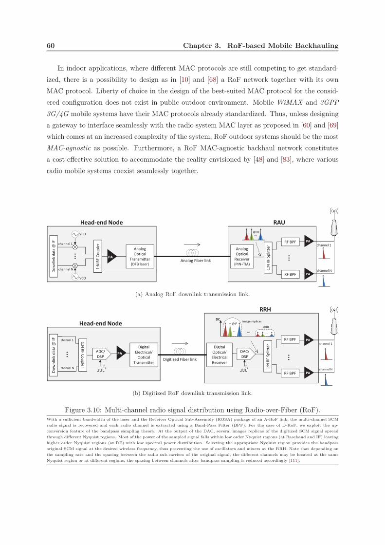
60 Chapter 3. RoF-based Mobile Backhauling
In indoor applications, where different MAC protocols are still competing to get standard-
ized, there is a possibility to design as in [10] and [68] a RoF network together with its own
MAC protocol. Liberty of choice in the design of the best-suited MAC protocol for the consid-
ered configuration does not exist in public outdoor environment. Mobile WiMAX and 3GPP
3G/4G mobile systems have their MAC protocols already standardized. Thus, unless designing
a gateway to interface seamlessly with the radio system MAC layer as proposed in [60] and [69]
which comes at an increased complexity of the system, RoF outdoor systems should be the most
MAC-agnostic as possible. Furthermore, a RoF MAC-agnostic backhaul network constitutes
a cost-effective solution to accommodate the reality envisioned by [48] and [83], where various
radio mobile systems coexist seamlessly together.
RF BPF
1:N
RF
Sp
litt
er
Analog
Optical
Receiver
(PIN+TIA)
PA
1:N
RF
Co
up
ler
…
RAUHead-end Node
Analog Fiber link
Analog
Optical
Transmitter
(DFB laser)
…
VCO
PA
channel 1
channel N
channel 1
channel N
Do
wn
lin
kd
ata
@ I
F
…@ RF
RF BPFVCO
PA
channel Nchannel N
D
(a) Analog RoF downlink transmission link.
RF BPF
1:N
RF
Sp
litt
er
Digital
Optical/
Electrical
Receiver
1:N
RF
Co
up
ler
Digital
Electrical/
Optical
Transmitter
ow
nlin
kd
ata
@ I
F
… …
RRH
Head-end Node
Digitized Fiber link
fsfs
channel 1
channel N
DAC/
DSPPA
PA
channel 1
channel N
… ……
DCImage replicas
@IF@RF
ADC/
DSP
RF BPFDo
PA
channel N
(b) Digitized RoF downlink transmission link.
Figure 3.10: Multi-channel radio signal distribution using Radio-over-Fiber (RoF).With a sufficient bandwidth of the laser and the Receiver Optical Sub-Assembly (ROSA) package of an A-RoF link, the multi-channel SCM
radio signal is recovered and each radio channel is extracted using a Band-Pass Filter (BPF). For the case of D-RoF, we exploit the up-
conversion feature of the bandpass sampling theory. At the output of the DAC, several images replicas of the digitized SCM signal spread
through different Nyquist regions. Most of the power of the sampled signal falls within low order Nyquist regions (at Baseband and IF) leaving
higher order Nyquist regions (at RF) with low spectral power distribution. Selecting the appropriate Nyquist region provides the bandpass
original SCM signal at the desired wireless frequency, thus preventing the use of oscillators and mixers at the RRH. Note that depending on
the sampling rate and the spacing between the radio sub-carriers of the original signal, the different channels may be located at the same
Nyquist region or at different regions, the spacing between channels after bandpass sampling is reduced accordingly [111].

3.3. Leveraging the fiber at the access: Radio-over-Fiber 61
3.3.2 D-RoF vs. A-RoF: An economic analysis
In this section, we focus on the comparison between analog and digital optical transmission for
RF distribution based on RoF technology. Figure 3.10 shows the block diagram (for downlink)
of A-RoF and D-RoF transmission links respectively. Using A-RoF (subfigure 3.10a), several
modulated radio signals generated at the head-end node at Intermediate Frequencies (IF) are
up-converted to their radio-frequencies by means of mixers and Voltage Controlled Oscillators
(VCOs), then power combined to form an SCM RF signal that directly modulates a DFB laser.
Upon reception at the RAU, the analog modulated optical carrier is photo-detected using a
PIN diode implemented with a Trans-Impedance Amplifier (TIA). The recovered SCM signal is
power splitted, each RF is extracted from the multiplex using a stack of BPFs, then amplified
and radiated into the cell. The schematic of multi-channel radio signal transmission using D-
RoF (subfigure 3.10b) is similar to A-RoF but it highlights additional items required for signal
digitization. In the downlink path, several wireless channels at different IFs are electrically
combined at the head-end node before digitization using an ADC locked at a given sampling
frequency (fs). Considering OFDM modulated signals (WiMAX, LTE), the ADC is supported
by a DSP to implement FFT(Fast Fourier Transform)/IFFT (Inverse FFT) processing blocks.
The sampling rate of the ADC is selected based on the Band Pass Sampling theory. BPS
under-samples a modulated signal to achieve frequency shifting by intentionally aliasing the
information bandwidth of the signal. Hence, unlike classical Shannon’s sampling, a significant
reduction of the the sampling rate can be achieved, since BPS is no longer based on the frequency
of the radio carrier but on the occupied bandwidth of the signal [116].
Upon digitization, the serial digital bit stream is processed and transmitted using an optical
digital transmitter. The digital processing at the transmitter includes bit framing, appending
a preamble sequence and additional fields for control and clock management, the details of
these operations depends on the adopted digital transmission technology (PDH/SDH links, P2P
Ethernet). Upon reception by the digital receiver at the RRH, the analog signals including the
image replicas are reconstructed with a DAC. The output analog signal is amplified and power-
splitted into several branches of BPFs. By focusing on the RF spectrum replicas in higher order
Nyquist zones, each filter extracts the desired wireless channel at its radio frequency before
the air-interface. By doing so, the wireless signals are up-converted to their air propagating
microwave frequency without requiring any mixers or local oscillators, which simplifies the
architecture of the RRH. The experimental feasibility of such a frequency relocation scheme
using bandpass sampling theory has been addressed and discussed in [154].

62 Chapter 3. RoF-based Mobile Backhauling
Load
Number of
Connections
Required BWSRC shaping filter
LTE mapping
Mapping BW into
LTE carriersLTE 1 4 20 100 MH
Radio Signal
Processing
Equipment
CAPEX & Power
Consumption
Assessment
Power
Consumption
Model
Capital
Expenditures
Model
Bandwidth
LTE: 1.4, … , 20, 100 MHz
Including guard bands
Bandpass Sampling
Selecting sampling rateBandpass Sampling Theory
Data Line Rate
16x I/Q bit resolution
Overhead ( 20%)Framing, clock management…
Required
ADC/DAC
+DSP
Optical
Digital
Transceivers
Figure 3.11: Methodology for A-RoF and D-RoF link modeling.For each traffic load, the required Bandwidth (BW) is determined assuming a Square-Root Cosine (SRC) filter with a roll-off factor of 0.25
for pulse shaping. BW is mapped according to the standardized radio carrier spacings. Guard bands are also included on both sides of the
RF channel according to the mobile system standard [133]. Using the bandpass sampling theory, the required sampling rate is computed
which enables to target the suitable ADC/DAC for that purpose. In-phase (I) and Quadrature-phase (Q) samples are quantized with 16-bit
resolution. Additional overhead bits are included for framing, control sequences and clock management. The proportion of such an overhead
varies with the adopted transmission protocol. The sampling rate with the overhead bit rate gives the total line rate.
3.3.2.1 Traffic, Cost and Energy consumption models
The comparison scenario between A-RoF and D-RoF assumes four different types of services
whether being symmetric/asymmetric or real-time/non real-time. Using service QoS attributes
detailed in [153], we consider in the following four traffic types, namely: a conversational voice
service (real-time symmetric, 16 kbps, using AMR speech Codec), a Best-Effort (BE) Web
browsing (non real-time asymmetric, 30.5 kbps), an interactive multimedia service on Web (384
kbps with MPEG-4 video Codec) and Video on Demand (VoD) (real-time streaming and highly
asymmetric, 2 Mbps). Then, three traffic-mixes are considered in our model and computed as
a weighted composition of the four aforementioned traffic types. The data-rate of each traffic-
mix and the corresponding service composition are given in Table 3.2. Mix1 corresponds to a
typical service composition when the voice traffic is dominant, Mix2 may describe the recent
past trend in traffic distribution (the overall traffic is equally splitted between voice and data)

3.3. Leveraging the fiber at the access: Radio-over-Fiber 63
Table 3.2: Traffic model based on services mix.
Voice BE Web Multimedia on Web VoD Data-rate/connection
Mix1 65% 30% 5% 0% ≃ 38.5 kbps
Mix2 50% 35% 10% 5% ≃ 157 kbps
Mix3 30% 40% 20% 10% ≃ 294 kbps
Three traffic-mixes are considered to illustrate three key phases of the traffic evolution of mobile users. Mix1: operators still deal with
voice call service as the dominant transported traffic. Mix2: More and more internet applications turns on mobile platforms, voice and data
are equally distributed. Mix3: Data overtook voice-grade traffic, heavy data-rate streaming services (like live or VoD stream) gain more
popularity and challenge the capacity of the backhaul network to cope with.
while Mix3 stands for the current trend observed by operators (with the rapid development
of mobile smart-phones and the widespread of rich-content sharing applications, data overtook
voice traffic) and expected to strengthen for the coming years.
The comparison between A-RoF and D-RoF RF distribution schemes addresses both the
CapEx cost in terms of number and types of required equipment and OpEx cost in terms of
energy consumption. Figure 3.11 depicts the methodology of the simulation scenario. Starting
from a given cell load (number of connections according to traffic-mix Mixi), the required
bandwidth (BW) (including guard bands) is mapped into radio carriers as specified by the
mobile radio system (LTE is assumed in our case) [133]. Then the minimum sampling rate
is computed using bandpass sampling theory. Actually, the choice of the sampling frequency
depends on the minimum fmin and maximum fmax frequencies of the signal. Equation system
3.1 expresses the relationships that must be satisfied to prevent spectral aliasing [62]
2fmax
nz≤ fs ≤ 2 fmin
nz−11 ≤ nz ≤ ⌊fmax
Bs⌋
(3.1)
where nz is an integer, Bs stands for the bandwidth of the passband signal and ⌊•⌋ designatesthe integer floor function. According to the passband sampling theory, the digitized signal in the
spectral domain is replicated at nz multiples of the sampling frequency. On one hand, a higher
nz leads to a lower sampling frequency (which relaxes the requirements on the DAC/ADC) but
produces in the same and narrower Nyquist region more signal images closer to each other.
In fact, studying the performance of multi-channel transmission by D-RoF, it was shown in
[154], that original RF signals that do not belong to the same Nyquist zone (because of a
narrower Nyquist region), the spacing between their replicas falling in the same Nyquist region
is drastically reduced which in turn increases the inter-channel interference and degrades the
Signal to Noise Ratio (SNR) of the recovered RF signals. One the other hand, a lower nz leads
to a higher sampling rate which increases the cost of the required technology of the ADC/DAC.
As in [62], a tradeoff between the aforementioned constraints is achieved by selecting nz at
mid-range and the sampling rate is calculated accordingly. The data-line rate of the digital bit
stream is determined assuming a 16-bit quantization and including processing overhead.

64 Chapter 3. RoF-based Mobile Backhauling
3
4
5
6
D R
oF
/ A
Ro
F)
Traffic Mix 1
Traffic Mix 2
Traffic Mix 3
0 100 200 300 400 500
1
2
Number of Connections
Cost
Ratio (
D
(a) Evolution of CapEx ratio D-RoF/A-RoF with traffic load.
1.5
2
2.5
Ratio (
D R
oF
/A R
oF
)
Traffic Mix 1
Traffic Mix 2
Traffic Mix 3
0 100 200 300 400 500
0.5
1
Number of Connections
Pow
er
Consum
ptio
n
(b) Evolution of power consumption ratio with traffic load.
Figure 3.12: CapEx and power consumption assessment for 3 different traffic mixes.
The total cost of the RoF link is computed through an inventory of the different equipment
involved in the transmission chain. As shown in Figure 3.11, they are deduced at different
stages of the methodology process. RF signal processing equipments (amplifiers, VCO, filters
etc.) are determined at the LTE RF carriers band. The calculated sampling rate determines
the required ADC/DAC and the digital transmission line-rate enables to target the suitable
digital transceiver. Our cost model database uses available price information from suppliers (for
low volumes production). For the digital transmission, a typical T1/E1 LIU framer module10

3.3. Leveraging the fiber at the access: Radio-over-Fiber 65
for instance costs ≈ 400e, while a 1000Base-LX, 10GbE-LR and 40GbE-LR optical Ethernet
transceivers costs ≈ 1000e, ≈ 2000e and ≈ 6800e respectively based on the estimations in
[34]. The cost of digitizers increases with the resolution, the sampling rate and the processed
bandwidth. In our evaluation, the considered ADC/DAC devices operate with 16-bit resolution
and 50 MHz bandwidth. Typical reported costs11 are for instance 850e at 50 MSample/s and
4000e at 250 MSample/s. For the analog case, a typical low noise DFB laser with 2.5 GHz
bandwidth and a ROSA package can comfortably fulfill the required operation; a total cost of
2000e is considered12. A 1 : 2 Power splitter/combiner13, an RF Bandpass cavity filter14 and
a wideband VCO with an up-converter frequency mixer15 cost a total of around 60e. Both
analog and digitized links use amplifiers to boost the signal at the transmitter driver (head-end
node) and to fulfill the cell coverage (RAU, RRH). Based on the analysis in [115], a amplifier
gain of 25 dB is typically required to cover a 100 m cell range. In our model, a wideband RF
amplifier16 with a cost of 50e is assumed.
Both A-RoF and D-RoF transmission links are compared also in terms of power consump-
tion. Data of power efficiency and energy consumption are provided in Table 3.3.
Figure 3.12 illustrates the evolution of the CapEx and power consumption ratios of Digitized
to Analog RoF versus traffic load (expressed in number of connections according to the three
traffic-mixes).
One notices that D-RoF enables lower CapEx than A-RoF only at low traffic loads. The
CapEx advantage of A-RoF over D-RoF increases with traffic evolution which tends to be more
packet-oriented than circuit-oriented. In terms of OpEx, the superiority of D-RoF on A-RoF
is noticeable only under traditional predominant voice traffic. Note that the sawtooth shape
of the OpEx (Figure 3.12b) and the stair-steps shape of the CapEx (Figure 3.12a) costs are
justified by the fact that above a small increment in the number of connections, transmission
equipment of a higher hierarchy (for instance T3/E3 instead of T1/E1 transceivers) are required
for the D-RoF link. Similarly, in Figure 3.12, the cost ratio of D-RoF to A-RoF may decrease
at specific values of traffic loads when the number of connections increases. This is the case for
10Line Interface Unit (LIU) reported from Dell-Sonic Wall Inc.
11Reported from National Instruments Inc.
12Reported from OZ510 datasheet at opticalzonu.com [34]. A total cost of 1600e is also reported in [115]
13RPS-2-30+ wideband (10− 3000 MHz) with 22 dB isolation. Reported from mini-circuits.com.
14SY-BP-2250+, wideband BPF with insertion loss < 1.5 dB at 2 GHz. Reported from mini-circuits.com.
15ROS-2500+, wideband VCO with 20 MHz 3-dB bandwidth, −16 dB 2nd harmonic. SIM-U432H+ for up-converter mixer. Both reported
from mini-circuits.com.16ZX60-2534M-S+ (38.5 dB gain at 2 GHz) reported from mini-circuits.com.
17With GMSK (2G) and 8-PSK (in EDGE) modulations, the PAPR is low regardless of the modulating signal which allows to work closer
to the 1-dB compression point of the PA, thus increasing the power efficiency.18Although not considered for the sake of simplicity in the assessment, a high back-off (due to a high PAPR) degrades the Signal-to-
Quantization Noise Ratio as well, thus lowering the maximum resolution of the ADC/DAC.19Figures of maximum power consumption are average values scaled to a single transmission port. They are based on CISCO
Nexus7000/Juniper EX8216 GigaBit Ethernet transceivers and derived from [73] [147]. The E-circuit standards form part of the PDH/SDH
transmission hierarchy where groups of E1 circuits are bundled onto higher capacity E3 and E5 circuits. Only commonly used E-circuits are
considered in the model.

66 Chapter 3. RoF-based Mobile Backhauling
Table 3.3: Power consumption model for A-RoF and D-RoF links.
Laser DFB laser biased at 40 mA with a drop modulation voltage of 2 V [31] 80 mW
Laser dedicated cooling: Power required to cool the heat dissipated by 1 W [108] ≃ 0.36 W
Laser bias driver 60 mW
PIN
PIN reverse biased at 3 V with a photocurrent of 1 mA [31] 3 mW
Trans-Impedance Amplifier (TIA) 80 mW
LO RF Voltage-Controlled Oscillator (VCO) delivering 12 V with 28 mA supply current. 336 mW
BPF
RF filter with DC power characteristics 5 V and 4 mA. 20 mW
PA
The energy consumption of an amplifier is mainly determined by its efficiency. Such a metric shows how efficiently the
supply DC power is converted to RF power. Broadband electrical amplifiers suffer generally from a poor efficiency compared
to narrow-band Class-A amplifiers. In the RoF link, Power Amplifiers (PA) are introduced at the transmission stage
(transmitter drive amplifier) and at the reception stage (output PA prior to the antenna). For both stages, we consider
a PA with an efficiency of ηmax = 22% at the 1-dB compression point. Unlike 2G/2.5G mobile system radio signals
characterized by constant envelope amplitude over time17, OFDM-modulated LTE/WiMAX radio signals suffer from high
Peak-to-Average Power Ratio (PAPR) that leads to signal clipping. In LTE for instance, a maximum clipping probability
of p = 10−4 leads to a PAPR γ given by: γ = −1
2W
[−6 ln(1 − p)2
π · N2
], where N the number of OFDM subcarriers and W[•]
the Lambert’s W-function [121]. To meet achieve such a PAPR value, a back-off 18 from the 1-dB compression point is
operated which further decreases the efficiency of the amplifier. After back-off, the efficiency of the amplifier is re-evaluated
as: η = ηmax/γ. To compute how much needed supply DC power, we estimate the transmit power at the output of the
PA. For broadband operation, the optical transmitter is considered to have a lossy matching which requires +5 dBm at the
output of the transmitter drive amplifier [31]. The transmit power at the output of the reception stage PA is determined by
the wireless range required to fulfill the radio cell coverage. For instance, based on the propagation model specified in [97],
a transmit power of 2 W is sufficient to cover a pico-cell size of ∼ 100 m
DigitalTransceivers
Each optical digital transceiver is equipped with an optical Small-form Factor Pluggable (SFP) interface (or XFP/SFP+
for bit-rates of 10 Gbps) to perform the optical transmission of the digital stream. Following the approach of [134], the
total power consumption of a transceiver is split into two main parts. The first one is traffic independent and models the
power consumption of the backplane of the transceiver. The second one is line-rate sensitive [124] and has to be related to
the amount of traffic traversing the transceiver interface. The relative influence of these power quantities is regulated by a
weighing parameter α [134]. Thus, given: Pmax the maximum power consumption of the transceiver, Bmax the transceiver
nominal bit-rate and B the transmitted bit-rate, the power dissipated by the transceiver is: Ptr = Pmax ·(
α + (1 − α) BBmax
).
Following are typical reported values of Pmax19 for different transceivers:
E1 line transceiver ≃ 225.28 mW
E3 line transceiver ≃ 1.54 W
E5 line transceiver ≃ 5.65 W
1 Gbit Ethernet Transceiver ≃ 9.31 W
10 Gbit Ethernet Transceiver ≃ 39.18 W
40 Gbit Ethernet Transceiver ≃ 104 W
ADC/DAC
ADC/DAC power consumption Pc increases linearly with the sampler clock frequency fs according to [12]. The energy
required for an ADC/DAC to process a charge sample at a given SNR is: Pc ≃ fs · kT · SNR
(α · VDD)2where: k the Boltzmann’s
constant; T the absolute temperature; α the fractional swing and VDD the supply voltage. It was shown in [111] that for a
high resolution ADC/DAC, the SNR is jitter noise limited. Thus, considering a 16-bit quantization, the SNR is taken to be
∼ 40 dB. Power consumption of the DSP is estimated assuming a single-chip flexible-size FFT/IFFT processor fabricated in
0.25 µm CMOS technology [61]. With 1024-point FFT, the processor dissipates 400 mW at 200 MHz clock frequency, thus
displaying a figure of merit of 2 mW/MHz. Note that the size of the FFT block scales with the radio channel bandwidth.
Losses Cooling loss: Additional cooling required for system equipment [8] ≃ 10%
Loss within power supply system and battery backup [8] ≃ 5%
TDM The power consumption efficiency of a 1 : k TDM MUX evolves approximately as log2(k) times
the consumption efficiency of a 1 : 2 TDM MUX [123].
≃ 0.04 mW/Mbps for
k = 2

3.3. Leveraging the fiber at the access: Radio-over-Fiber 67
instance at 220 connections of traffic Mix3 when the new introduced equipment is very little
mutualized by the traffic connections.
6%
21%
66% 7%
(a) Traffic Mix1
41%
19%
PA ADC/DAC/DSP Transceivers Others
22%
18%
(b) Traffic Mix2
29%
19%
28%
24%
(c) Traffic Mix3
Figure 3.13: Power consumption profiling for 3 different traffic mixes.At all traffic-mixes, the PA is the first major power-consuming, with a share of 66% at Mix1 dropping to 29% at Mix3. The power consumption
of ADC/DAC/DSP evolves considerably as data traffic prevails over voice (Mix2 and Mix3). The power-consumption profiling shows also
the increasing share of power consumption of digital transceivers, at Mix3 the latter occupies 1/4 of the total power consumption. Finally,
one notices the contrast between voice-prevailing traffic mix and data-dominating traffic mix. In fact, at Mix1, the overall share of power
consumption of electronics (34%) remains low compared to the PA consumption, while at Mix3, ADC/DAC/DSP and digital transceivers
taken together amount for nearly half of the total power needed by the D-RoF link.
We depict in Figure 3.13 a profiling of the power consumption of the D-RoF link at the
three traffic-mixes. The profiling addresses the share of the main components of the D-RoF link
(Power Amplifier, Optical Digital Transceivers, ADC/DAC/DSP and other system components)
in the total power consumption.
3.3.2.2 Distributed radio sites using CPRI/OBSAI
Currently two protocols, namely Common Public Radio Interface (CPRI) [55] and the Open
Base Station Architecture Initiative (OBSAI) [103], implement bandpass sampling-based I/Q
digitization with standardized specifications on the sampling rate, the digital line-rate and
a dedicated communication protocol for the transfer of the digitized signal. Both CPRI and
OBSAI aims at making compatible radio equipments between the different vendors by proposing
standardized and at some extent20 open interfaces between radio equipments and between the
radio equipment and radio controller.
• CPRI: In addition to the user plane (containing I/Q digitized data blocks), CPRI protocolspecifies control/management and synchronization signals. Such overheads enable the
digitized flow to be exchanged between the RRH and the radio equipment controller
(head-end node) over a digital (either electrical or optical) serial link. In a distributed
20CPRI reserves a specific-vendor information field at its layer 2 protocol stack [55].
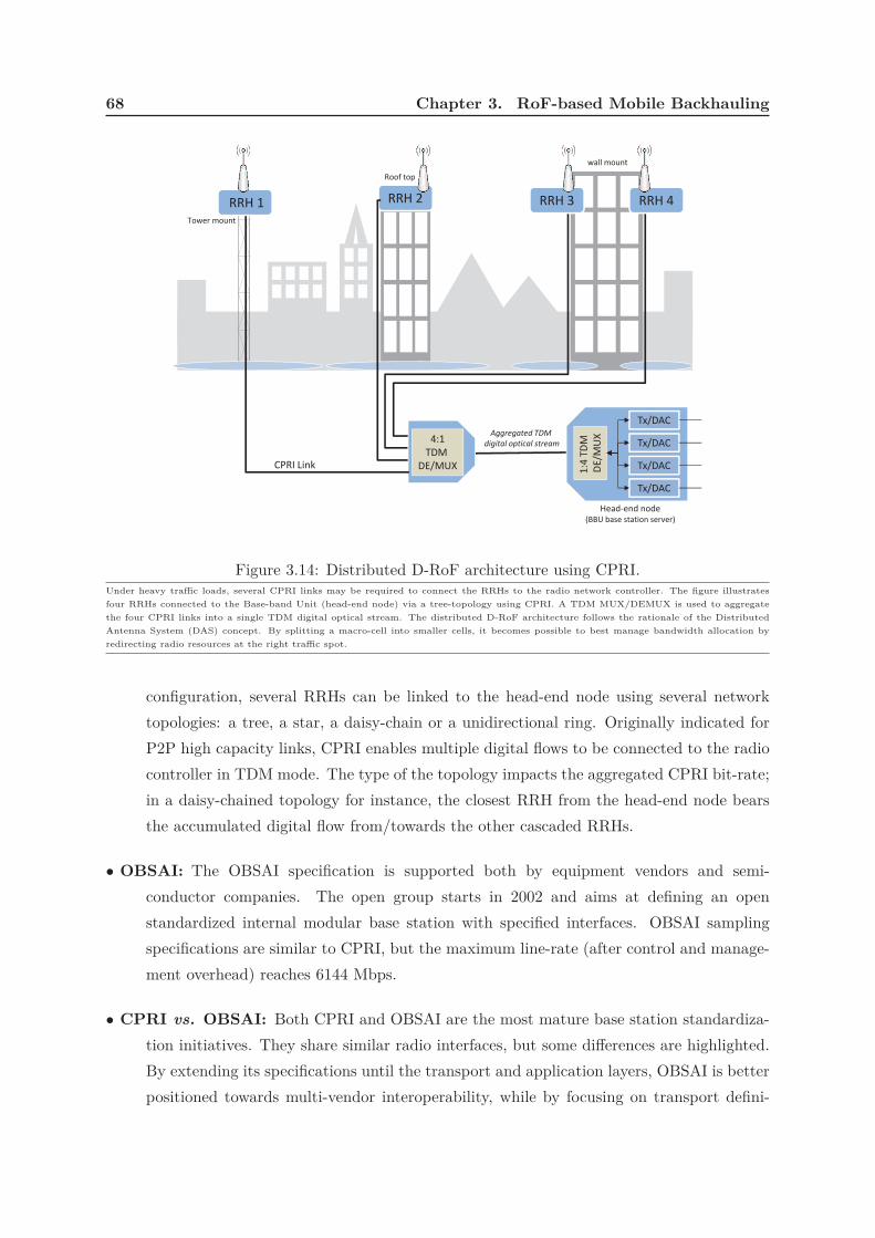
68 Chapter 3. RoF-based Mobile Backhauling
RRH 2 RRH 3 RRH 4RRH 1
wall mount
Roof top
Tower mount
4:1
TDM
DE/MUX
Tx/DAC
1:4
TD
M
DE
/MU
X
Tx/DAC
Tx/DAC
Tx/DAC
CPRI Link
Aggregated TDM
digital optical stream
Head-end node(BBU base station server)
Figure 3.14: Distributed D-RoF architecture using CPRI.Under heavy traffic loads, several CPRI links may be required to connect the RRHs to the radio network controller. The figure illustrates
four RRHs connected to the Base-band Unit (head-end node) via a tree-topology using CPRI. A TDM MUX/DEMUX is used to aggregate
the four CPRI links into a single TDM digital optical stream. The distributed D-RoF architecture follows the rationale of the Distributed
Antenna System (DAS) concept. By splitting a macro-cell into smaller cells, it becomes possible to best manage bandwidth allocation by
redirecting radio resources at the right traffic spot.
configuration, several RRHs can be linked to the head-end node using several network
topologies: a tree, a star, a daisy-chain or a unidirectional ring. Originally indicated for
P2P high capacity links, CPRI enables multiple digital flows to be connected to the radio
controller in TDM mode. The type of the topology impacts the aggregated CPRI bit-rate;
in a daisy-chained topology for instance, the closest RRH from the head-end node bears
the accumulated digital flow from/towards the other cascaded RRHs.
• OBSAI: The OBSAI specification is supported both by equipment vendors and semi-
conductor companies. The open group starts in 2002 and aims at defining an open
standardized internal modular base station with specified interfaces. OBSAI sampling
specifications are similar to CPRI, but the maximum line-rate (after control and manage-
ment overhead) reaches 6144 Mbps.
• CPRI vs. OBSAI: Both CPRI and OBSAI are the most mature base station standardiza-
tion initiatives. They share similar radio interfaces, but some differences are highlighted.
By extending its specifications until the transport and application layers, OBSAI is better
positioned towards multi-vendor interoperability, while by focusing on transport defini-

3.3. Leveraging the fiber at the access: Radio-over-Fiber 69
5
6
7
8
9
(D R
oF
/A R
oF
)
Traffic Mix 1
Traffic Mix 2
Traffic Mix 3
0 100 200 300 400 500
1
2
3
4
Number of Connections
Cost
Ratio (
(a) CAPEX ratio vs. the number of connections.
2
2.5
3
3.5
4
Ratio (
D R
oF
/A R
oF
)
Traffic Mix 1
Traffic Mix 2
Traffic Mix 3
0 100 200 300 400 500
0.5
1
1.5
Number of Connections
Pow
er
Consum
ption
(b) Power consumption ratio vs. the number of connections.
Figure 3.15: Distributed D-RoF using CPRI: CAPEX and power consumption ratio.
tion, CPRI is more open transport oriented. Another main difference between CPRI and
OBSAI lies in protocol implementation. CPRI leverages on higher carrier grade capacity
thanks to air-interface programmable I/Q sample size, while OBSAI has a fixed message
and sample envelope size. To enable flexibility, OBSAI trades with more overhead. For a
3072 Mbps link for instance, CPRI requires less than 7% of protocol overhead (measured
in bytes) while 20% of overhead is necessary for OBSAI [21]. Finally, CPRI requires for
the data-plane a bit-error rate (10−12)21 less stringent than OBSAI (10−15)[55].
21According to CPRI specification 4.2 [http://www.cpri.info], it should be a design goal to avoid Forward Error Correction (FEC) at layer

70 Chapter 3. RoF-based Mobile Backhauling
• Distributed D-RoF architecture using CPRI: Since CPRI is more protocol efficient
than OBSAI, we map the D-RoF link depicted in Figure 3.10b into a CPRI link. In-
deed, the D-RoF link is mapped into several CPRI links when the line-rate exceeds the
maximum line-rate specified by the protocol, i.e 3072 Mbps. The distributed D-RoF sys-
tem architecture is illustrated in Figure 3.14. To backhaul several RRHs using a tree-based
CPRI network, a TDM multiplexer and demultiplexer is used. Cost and power consump-
tion assessments of the distributed CPRI architecture are carried out by following the
same methodology described in Figure 3.11 but including the required CPRI overhead
and selecting the sampling rates as specified by the CPRI standard to backhaul LTE
channels [55]. A 1 : 4 TDM MUX/DEMUX (at 3.072 Gbps) costs 7000e [34] and its
power consumption is given in Table 3.3. Figure 3.15a depicts the evolution of the cost
ratio of D-RoF/A-RoF in the distributed CPRI configuration and the power consumption
ratio with the number of connections (traffic load) for the three traffic-mixes. Compared
to results displayed in Figure 3.12, globally the cost of the distributed D-RoF link based
on CPRI is higher than A-RoF link. The additional equipment needed to implement the
distributed D-RoF network (TDM MUX/DEMUX, as well as more equipment are re-
quired by distributing the antennas22) explains the increase of the D-RoF link cost while
the cost of A-RoF is kept unchanged. The trend is confirmed with the increase of the
power consumption ratio between both RoF backhaul options as depicted in Figure 3.15b.
3.4 Generic RoF Access Network
Economic and power consumption advantages of A-RoF compared to D-RoF, motivate the
proposal of an all-optical cellular backhaul architecture called GeRoFAN (Generic Radio-over-
Fiber Access Network) featuring the transport of RF traffic from/to the RAUs to/from the head-
end node network controller by means of A-RoF links. Figure 3.16 depicts the global architecture
of the GeRoFAN network. Several RAUs, serving 4G system radio cells and deployed across
various geographical districts, are federated via an all-optical network to a head-end node also
called Hybrid Optical Line Transmission (HOLT). The federating optical infrastructure between
the HOLT and RAUs may be based on several optical loops, optical daisy-chains or optical trees.
In this figure, a district refers to a set of neighboring cells corresponding typically to a leisure
district, a residential district or a business district. By a rule of thumb, the number of cells
within a given district is constrained by the power budget of the fiber link.
The usage of reflective optical modulators at the RAUs enables to mutualize all the optical
transceivers at the HOLT and prevents from equipping each remote site with a dedicated costly
1 to reduce overhead and achieve cost-efficiency.22Although the cost of a single equipment at the RRH is lower than the previous case since it works at lower digital rate, such cost saving
is not sufficient enough to make the CapEx of the overall distributed architecture lower than the single D-RoF link considered previously.

3.4. Generic RoF Access Network 71
pool
RF
Pool
Ge
Ro
FAN
Co
ntr
ol
Pla
ne
Ra
dio
Syst
em
Co
ntr
ol
Pla
ne
RF
LOs
T-
LDs
T-
PDs
RF1 RF2 … RFF
H O L T
Arrayed-Waveguide
(AWG) Router
*
1
2
…
3
W
radio cell RAU
RAU
RAU
Leisure
District
Business
District
Residential
District
Figure 3.16: Generic Radio-over-Fiber Network Architecture.
tunable laser diodes and tunable photo-detectors. In addition, thanks to the transparency to
the modulation format, A-RoF enables to co-localize at the HOLT all radio equipment (signals
processors, RF LOs and mixers, ...) leaving the architecture of the RAU as simple as possible.
The GeRoFAN system is supported by an innovative Control Plane (CP).
The CP exploits such a mutualization of radio and optical equipment at the HOLT, to
allocate dynamically Optical Channels (OCs) and RFs according to the traffic fluctuation within
each radio cell or more globally among districts. The GeRoFAN CP manages an RF-onto-
λ switching matrix to control the placement of RFs onto OCs. Optical channels are then
dynamically routed to each covered district by means of an Arrayed Wave-Guide (AWG) optical
router located at the HOLT. AWG routers are cheap and cost-effective to implement in LiNbO3
or InP VLSI chips, however, their flexibility depends on the tunability of light sources [90]. An
AWG router is a passive device made of a set of N monomode waveguides inserted between two
passive optical stars M × N and N × M respectively. The switching mechanism of the AWG
is based on the proprieties of optical interfometry. Assuming an AWG with P ports, if the
AWG input/output ports are indexed by k (k ∈ 0, · · · , P ), the router is designed such that any

72 Chapter 3. RoF-based Mobile Backhauling
cw(+RF)
WDM
channels
in
WDM
channels
out
*
r-CPU
R-OADM
RAU
radio-cell
Modulator
Bias ControlRF
RoFmodulator
Data
Control/Signaling
Figure 3.17: Radio-Access Unit (RAU) Architecture (for upstream radio traffic).
wavelength tuned at index k arriving on port pi exits on output port po following the arithmetic
rule pi + k ≡ po[P ], where x ≡ y[z] means x equals y modulo z.
3.4.1 The Radio Access Unit
The internal architecture of the RAU is depicted in Figure 3.17. We exploit the possibility to re-
place optical light sources at the RAU by a low-power consuming, easy-to-manage and remotely
fed (from the HOLT) colorless RoF modulator23. At an RAU, the OC is dropped from the input
WDM multiplex signal by a Reconfigurable Optical Drop and Add Multiplexer (ROADM). To
distribute downstream traffic, the transported RFs are extracted from their OCs, amplified and
radiated by the antenna into the cell. To backhaul upstream traffic generated within a given
cell, an OC is extracted by the ROADM, modulated by its RFs in the analog RoF modulator
and reinserted into the WDM multiplex. Some colorless RoF transceivers (Semi-conductor am-
plifier, Electro-absorption modulators ...) can perform both detection and modulation functions
within the same device, assuming that the OCs’ wavelengths used respectively for downstream
and uplink traffic are widely separated to avoid interference. In addition, the RAU is equipped
with a remote Control Plane Unit (r-CPU) whose role is depicted in subsection 3.4.3.
23Several options are envisioned based on electro-optic, electro-absorption modulators, injection-locked lasers. As developed in Chapter 4,
the choice of the A-RoF colorless transceiver is a tradeoff between several considerations (cost, energy consumption, modulation performance
...) while privileging high-bandwidth capable modulators.

3.4. Generic RoF Access Network 73
RoF
modulator
R-OADM R-OADM R-OADM
r-CPU
…
…
Radio Operator 1 Radio Operator N FTTx Operator
M-RAU
RoF
modulator
WDM
channels
in
WDM
channels
out
*
BB
Bias control
RF Switch
radio-cell
RF1, …, RFN
RF1 RFN
PON
Data
Control/Signaling
(a) M-RAU (for upstream radio traffic)
RF
Pool
N an
e
RF Control plane
RF
LOs
T-
LDs
M- H O L T
BBU 1
RF Control plane
BBU N
RF1/BB RFN/BB…
1
2
3
pool
Ge
Ro
FAN
Co
ntr
ol
PlLDs
T-
PDs
Arrayed-Waveguide
(AWG) Router
*
…
3
W
(b) M-HOLT
Figure 3.18: GeRoFAN accommodating multi-operator and multi-service operation.

74 Chapter 3. RoF-based Mobile Backhauling
3.4.2 GeRoFAN for multi-operator backhauling
The genericity of the GeRoFAN architecture enables to deal with several services/technologies
or several operators within the same backhauling system. The architecture of the HOLT and
the RAU are enhanced as illustrated in Figure 3.18. In the Multi-service HOLT (M-HOLT) (c.f.
Figure 3.18b), several Base-Band Units (BBUs) process the traffic of different operators/services
either wireless such as 4G WiMAX/LTE, 3G UMTS, Ultra-Wide Band (UWB) or broadband
fixed (FFTx). The internal architecture of the Multi-service RAU (M-RAU) shows a stack of
several RoF-modulator/ROADM modules distributed among the multiple operators serving the
same radio cell. Upstream multi-service radio traffic at an M-RAU is detected by a mutualized
antenna and sent to an RF switch. Thanks to the GeRoFAN-CP, the RF switch is reconfigured to
redirect each radio channel of a given mobile operator to its associated RoF-modulator/ROADM
module. An FFTx operator benefits from the GeRoFAN infrastructure by sharing the same
M-RAU as depicted in Figure 3.18a using an ROADM that drops the right optical channel
modulated with BB users’ data to serve FFTH subscribers of an overlying PON.
…
RAU
m
RF
switching
matrix
config.
Operator 1 RF1 1 Bias 1 Status: On
Operator 2 RF2 2 Bias 2 Status: On
…
Operator N RFN N Bias N Status: On
…
CP (HOLT)
r-CPU (RAU)
• Tuning OADMs
RAU
Beacon
RF switch
matrix config.
Operator
1
Operator
k
Operator
N
Operator
FTTx
Reporting
Monitoring Status…
RAU ID Frame map
…
Bias k k BiasN N FTTx
Frame RAUm-1 Frame RAUm Frame RAUm+1… …
tTDMA
• Adjusting the Bias
• Reconfiguring RF
switching matrix
• Reporting soft/hard
failures
Figure 3.19: GeRoFAN-CP signaling and general frame structure of channel λ⋆.

3.4. Generic RoF Access Network 75
3.4.3 GeRoFAN system control plane
3.4.3.1 System signaling
The direct benefit of traffic processing centralization at the HOLT is the possibility for the CP to
acquire a global view of the load distribution across the cellular network and thus dynamically
managing the bandwidth between RAUs using an out-of-band optical signaling channel λ⋆. The
signaling channel is also used at the RAU level to enable the reconfigurability of the devices
(automatic reconfiguration of the ROADM to drop/add the right OC, change of the bias of
the RoF modulator to achieve optimal performance, reconfiguration of the switching matrix of
the RF switch for M-RAU). The optical channel λ⋆ is accessed by RAUs on a TDMA basis;
reconfiguration information are transported in base-band and processed by the remote CP Unit
(r-CPU) equipping each RAU (c.f. Figure 3.17). Figure 3.19 illustrates the signaling mechanism
between the CP and the r-CPU (at the RAU) using the control information encapsulated into
a TDM λ⋆ frame in the general case where GeRoFAN is used for multi-operator backhauling.
3.4.3.2 Dynamic bandwidth management
To illustrate the dynamicity of the system, one may estimate that the activity of the business
district does not coincide in time with the activity of the residential or leisure district served
by GeRoFAN. The CP reconfigures the devices at the HOLT to dynamically assign, at a multi-
hour scale, RFs and OCs to the district with increasing load. Shorter term horizon of the traffic
fluctuation (i.e, cell localized load variation within the same district) keeps unchanged optical
resources assigned to a given district, but reallocates RFs between the different RAUs within
the same district. Such a reallocation of radio resources is carried out in accordance with radio
cellular planning rules to minimize radio signal interference. Figure 3.20 illustrates how the
GeRoFAN-CP enables optimal bandwidth management by shifting optical and radio resources
at the two aforementioned time-scales.
3.4.3.3 Control plane design requirements
Dynamic bandwidth management realized by the control plane is achieved at a macroscopic
time scale in terms of traffic fluctuations. This means that the GeRoFAN-CP deals with
the aggregated traffic of the cell and ignores the packet time scale (∼ ms) which remains the
focus of the radio mobile operator. Thus, the GeRoFAN system is a radio MAC-agnostic. By
being MAC-agnostic, the GeRoFAN-CP is able to get applied to any radio system technology
without need for costly and complex special engineering adaptations. It operates at time-scales
ranging from few tens of minutes (shorter term traffic variations) to several hours (longer term
variations). Indeed, the bandwidth relocation realized by the CP at the shorter term has to be

76 Chapter 3. RoF-based Mobile Backhauling
@ 11 H @ 13 H
10
20
30
40
50
60
Lo
ad
(%
)
LeisureBusinessResidential
0 H 9 H 18 H 21 H 24 H@ 11 H @ 13 H
1 2 3
4
5
1
2 3 4
5
1
2 3
4 5
1 2
3
4 5
0 1 2 3 4 5 6 7 8 9 10 11 12 13 14 15 16 17 18 19 20 21 22 230
Time (24 Hours)
Figure 3.20: GeRoFAN-CP capacity management at short/long term time-scale.Thanks to A-RoF, GeRoFAN acquires a global view of the traffic evolution. Supported by the CP, GeRoFAN performs dynamic bandwidth
management at the short and medium/long term scales. Considering that GeRoFAN network is serving different functional districts, the CP
exploits the daily pattern of the mobility of users to shift radio/optical resources among districts and cells. At multi-hours scale basis for
instance, the CP shifts OCs from the housing area to the business area during usual working office hours time. At the end of the day, the
CP allocates additional OCs to the leisure district since it becomes more solicited. At the evening, the traffic is more balanced between the
housing and the leisure areas, as a consequence, there is no need to keep higher bandwidth at the business area where the load is decreasing.
The shift of radio resources is achieved by the CP at a shorter time-scale. For instance, at 11a.m, a hot-spot is detected requiring to shift
radio resources from neighboring cells where the load remains low. At the short time-scale, optical resources remain unchanged per district
since the variation of the traffic matrix is triggered by some specific cells and not a set of cells.
achieved within the time-window at which the aggregated load in a given cell reaches its stable
level24.
In addition, as previously specified in Section 3.3, A-RoF transmission systems suffer from
limited dynamic range, with link noise and RF distortions increasing with distance and the
number of backhauled radio channels. In the contributions of [79] and [106] for instance, au-
thors exploit the control centralization of A-RoF to propose optimized management of the
radio/optical resources between RAUs without explicit consideration of physical layer impair-
ments. To not loose the cost-effectiveness benefit of A-RoF (highlighted in Subsection 3.3.2),
the GeRoFAN-CP has to be Quality-of-Transmission(QoT)-aware, to compensate for the
various impairments stemming from A-RoF links. Unlike the compensation approach proposed
in [43], where authors suggest the implementation at the RAU of costly pre-distortion and post-
24Actually the time-window is evaluated by monitoring the evolution of the aggregated traffic distribution based on real operation network.
The time-window depends on the mobility pattern of subscribers, the size of radio cells, the network configuration (sectorization, inter-RAUs
direct traffic pipelining using X2 interface in LTE for instance, type of area covered)...

3.4. Generic RoF Access Network 77
distortion circuits based on adaptive learning algorithms, the QoT-aware CP has to mitigate
RoF impairments through an original approach conducted from the HOLT and based on a deep
knowledge of the physical layer.
In summary, supported by a radio MAC-agnostic and QoT-aware control plane, the GeRo-
FAN architecture provides both an active and a non-intrusive cellular backhauling for the
"hosted" radio system.


Part II
Physical Layer Study


Chapter 4
Analog RoF Transmission
Limitations in GeRoFAN
Contents
4.1 Introduction . . . . . . . . . . . . . . . . . . . . . . . . . . . . . . . . . . . . . . 82
4.2 RoF transceiver . . . . . . . . . . . . . . . . . . . . . . . . . . . . . . . . . . . . 82
4.2.1 RoF transceiver technology survey . . . . . . . . . . . . . . . . . . . . . . . . . . 83
4.2.2 RoF transceiver physical impairments . . . . . . . . . . . . . . . . . . . . . . . . 87
4.3 REAMSOA physical impairments . . . . . . . . . . . . . . . . . . . . . . . . . 90
4.3.1 REAMSOA working principle . . . . . . . . . . . . . . . . . . . . . . . . . . . . . 91
4.3.2 The EAM section . . . . . . . . . . . . . . . . . . . . . . . . . . . . . . . . . . . . 92
4.3.3 The SOA section . . . . . . . . . . . . . . . . . . . . . . . . . . . . . . . . . . . . 95
4.3.4 Non-linearity and Intermodulation distortions . . . . . . . . . . . . . . . . . . . . 98
4.4 ROADM . . . . . . . . . . . . . . . . . . . . . . . . . . . . . . . . . . . . . . . . . 102
4.4.1 FBG-based ROADM . . . . . . . . . . . . . . . . . . . . . . . . . . . . . . . . . . 102
4.4.2 OADM noises . . . . . . . . . . . . . . . . . . . . . . . . . . . . . . . . . . . . . . 103
4.4.3 Homodyne Crosstalk . . . . . . . . . . . . . . . . . . . . . . . . . . . . . . . . . . 104
4.4.4 Heterodyne Crosstalk . . . . . . . . . . . . . . . . . . . . . . . . . . . . . . . . . 104
4.5 Fiber impairments . . . . . . . . . . . . . . . . . . . . . . . . . . . . . . . . . . . 108
4.5.1 Chromatic Dispersion . . . . . . . . . . . . . . . . . . . . . . . . . . . . . . . . . 108
4.5.2 Polarization Mode Dispersion . . . . . . . . . . . . . . . . . . . . . . . . . . . . . 108
4.5.3 WDM Non-linear Effects . . . . . . . . . . . . . . . . . . . . . . . . . . . . . . . 109
4.5.4 Rayleigh Back-Scattering . . . . . . . . . . . . . . . . . . . . . . . . . . . . . . . 111
4.5.5 Optical Beat Interference . . . . . . . . . . . . . . . . . . . . . . . . . . . . . . . 111
4.5.6 Other impairments . . . . . . . . . . . . . . . . . . . . . . . . . . . . . . . . . . . 112
4.6 Building a comprehensive QoT-tool . . . . . . . . . . . . . . . . . . . . . . . . 114

82 Chapter 4. Analog RoF Transmission Limitations in GeRoFAN
4.1 Introduction
Radio signals transmission through A-RoF link is subject to several physical impairments
that degrade the Signal-to-Noise Ratio (SNR) and by consequence the Shannon’s capacity.
Whatever the adopted network topology of the A-RoF system, it is necessary to characterize
each relevant impairment and investigate the main parameters on which the GeRoFAN-CP
could play to keep the Shannon’s capacity as high as possible at the base stations. This chapter
provides in Section 4.2 an overview of the main technological options for the RoF modulator and
justifies the use of a reflective amplified absorption modulator as the most suitable candidate for
GeRoFAN. A comprehensive analytical modeling of undergone physical limitations due to the
different components of the GeRoFAN system is described in Sections 4.3, 4.4 and 4.5. Actually,
several available simulation software tools1 provides the opportunity to model physical layer
impairments of analog optical transmission, however in most cases, these tools lacks the required
genericity to accommodate any network or architecture configuration. Indeed, such tools are
very useful to target a specific noise in a point-to-point network configuration. However, in our
research, we put the focus on the mathematical development of GeRoFAN optical impairments in
a networked configuration in order to understand the salient features of the physical mechanism
behind each transmission noise. Such an approach enables to highlight the key parameters and
variables that can be used by the CP as action levers to achieve an efficient cellular backhauling.
Finally Section 4.6 draws out a big picture of our QoT-tool, a software programm2 packaging the
analytical modeling of GeRoFAN physical impairments. The QoT-tool enables the GeRoFAN-
CP to integrate seamlessly the constraints of the physical layer and refine its backhauling
strategy accordingly.
It is worth noting that the research scope of this chapter focuses only on evaluating the
Shannon’s radio capacity of the system for the upstream traffic3.
4.2 RoF transceiver
The choice of the best transmitter equipping the RAU is subject to stringent requirements that
have to be satisfied without penalizing the investment cost of the overall architecture. These
requirements are summarized through some figures of merits such as: the link gain, the noise
figure, the linearity and the dynamic range of the RoF link [96][34].
1For instance VPI Transmission Maker©, Simulink© or OptiSystem©.2The QoT-tool is a programm developed in Matlab©, it is structured generically into modules, each module represents a specific impairment
based on the mathematical modeling detailed in this Chapter. Depending on the GeRoFAN topology, the QoT-tool calls the different modules
relevant to each step of the signal lightpath and updates the SNR of the optical carrier accordingly.3Managing the radio capacity for upstream traffic is more challenging for a radio operator than the downstream traffic. Indeed, for the
downstream traffic, the mobile operator knows a priori where the capacity would be redirected.

4.2. RoF transceiver 83
4.2.1 RoF transceiver technology survey
A first classification of RoF transmitter candidates can be made on whether these sources are
wavelength-tunable or not. The tunability of the light source is mandatory to enable dynamic
reconfiguration of the system. Thus, we identify two main categories for RoF transceivers at
the RAU subject to whether the optical signal is generated locally or delivered remotely from
the head-end node. Figure 4.1 depicts such a classification and main technologies used for each
category.
4.2.1.1 RAU with locally generated optical signal
Laser Diode + Optical Modulator
ExternalModulation Electro-optic
Modulator (MZM)
RoF transceiver
Local optical
carrier generation
Remote optical
carrier generation
Direct Modulation
Multi-mode Laser(FP, VSCEL, …)
Monomode Laser(DFB, DBR, …)
Electro-absorption Modulator
SemiconductorOptical Amplifier
Injection-lockedFabry Perot laser
Figure 4.1: RoF transceiver technology classification.With rapid wide scale deployment of broadband FFTx networks, remote light generation-based solutions become more attractive. Wavelength
independent upstream transmission is enabled by several colorless components (electro-optic, electro-absorption, injection mode-locked, Semi-
conductor Optical Amplifier (SOA)). The similarity between the different solutions in terms of cost makes the dynamic range and the
transmission performance as the key distinction criterion with respect to the target application.
Early RoF networks are deployed with a dedicated Laser Diode (LD) at the RAU. The
optical signal generated by the LD may be either directly or externally modulated. In both
cases, since each RAU is equipped with a LD, the investment cost of the overall system increases
with the number of deserved remote cells which raises the problem of scalability in areas with
high cell-density.
Two categories of optical sources are considered. Single mode longitudinal laser diodes
(SMLD), DFB or DBR lasers, provide superior performance thanks to their high power, low
intrinsic noise and their very narrow spectrum. They are widely adopted for long reach RoF

84 Chapter 4. Analog RoF Transmission Limitations in GeRoFAN
links with large dynamic range. However, since SMLD are still expensive, it seems economically
not attractive to duplicate this cost at each RAU.
At the opposite, multi-mode laser diodes (MMLD) provide a more economical alternative for
less demanding applications. Their utilization is restricted to short distance RoF links because
of their low output optical power and high intrinsic noise. Fabry Perot (FP) laser diodes are
the most common examples of MMLD. VCSEL MMLD [138] are also developed for remote
antenna feeding and focus a great interest due to their low cost and performance for short range
applications. Current VCSELs are available at 850 nm while DFB and FP lasers are operational
around 1.3 and 1.5 µm [96]. While tunability of standard LDs raises several issues (cooling,
control, cost, power consumption · · · ), Injected Mode-Locked (IML) FP lasers offer an elegant
solution alloying low-cost and tunability. While IML-FP are well established, they suffer from
limited spectral range. Note that the usage of Light Emitting Diodes (LED) has been also
investigated in [71] but their poor performance compared to lasers restricts their utilization.
Operating at higher frequencies intensifies the limitations of direct modulation by approach-
ing the limits of modulation efficiency. Therefore, using an external modulator in conjunction
with the laser is preferable to ensure higher bandwidth with acceptable modulation performance
[30].
4.2.1.2 RAU with remotely generated optical signal
For such a configuration4, the RAU is equipped with an external modulator which is remotely
fed by a high optical power laser diode (DFB) located at the head-end node. In addition to
the RF equipment centralization, this configuration enables light source mutualization between
different RAUs, thus reducing the system cost. Because the modulation at the RAU is carried
out independently from the delivered optical carrier’s wavelength, the RAU are classified as
colorless. Electro-Optic Modulators (EOM) made with polymers, LiNbO3 or III-V materials, are
widely used as external modulators. Particularly, the electro-optic Mach-Zehnder interferometer
Modulator (MZM) is recognized as the industry standard. However, MZMs suffer from some
drawbacks such as non-linearity, low integration with semiconductors, and relative high cost
[30].
Electro-Absorption Modulator (EAM) is an alternative to EOM. EAM relies on the Quan-
tum Confined Stark Effect (QCSE) in quantum wells that leads to a change in the absorption
profile of the incident light dependently on the applied electric field (which stands for the
modulating voltage). Compared to MZM, EAMs have lower drive voltage, larger modulation
bandwidth, and can be packaged with semiconductors through monolithic integration (EAM-
DFB [77]). However, both MZMs and EAMs suffer from the non-linearity of their transfer
function [156]. It is difficult to assess the superiority of one technology on the other due to the
4Also called as Centralized Light Seeding (CLS) configuration.

4.2. RoF transceiver 85
diversity of parameters as well as the continuous technological advances achieved by both of
them. Nevertheless, an extensive comparison can be found in [120] based on a composite figure
of merits.
A third interesting candidate for the RAU transmitter uses a Semiconductor Optical Ampli-
fier (SOA) as a modulator [151]. By varying the bias current according to the RF sub-carrier,
the gain of the SOA is modulated itself, thus modulating the optical carrier at its output. As
opposed to the insertion loss of common external modulators (EAM, MZM), the amplification
functionality of the SOA allows for relatively low power optical signal at its input. However,
SOA modulators suffer from optical noise and non-linearity similar to directly modulated LDs
[40].
Alternatively, monolithic integration can be achieved through EAM-SOA which corresponds
to an amplified EAM. An EAM-SOA cumulates the advantages of the EAM as modulator with
the amplification gain of the SOA. In the EAM-SOA design process, the performance of the
integrated device are improved by shifting the amplification band of the SOA to coincide with
the modulation peak of the EAM [39].
Finally, an Injection Mode-Locked Fabry Pérot (IML-FP) laser diode stands at a particular
position as illustrated by the diagram of Figure 4.1. An IML-FP carries upstream data by direct
modulation, the light is thus locally generated by stimulating the FP laser gain. Meanwhile, an
external remotely generated continuous wave is injected into the FP cavity to lock the laser at
the injected wavelength. The locked FP re-emits at the same wavelength than the injected one.
The locking mechanism suppresses the original multi-mode nature of the FP laser, the locked
device features a strongly single-mode operation with a Side Mode Suppression Ratio (SMSR)
(used to assess how strong is the dominant mode of the laser spectrum) around 40 dB [99] (DFB
laser displays 50 dB SMSR under appropriate bias [96]). Apparently, IML-FP cumulates both
the advantage of the low-cost of the FP laser and the transmission benefits provided by the
locking mechanism, however, the proprieties of the device is strongly dependant on the injected
optical power that requires additional constraints to stabilize the locking mechanism.
4.2.1.3 Advances in external modulators:
• Bulk-based device vs. Quantum Well (QW) structure: For SOA modulators or semi-
conductor LDs, compared to bulk materials, carrier density rises very sharply with the
injected current into the active region which yields to a high differential gain [96]. For
EAMs, the confinement of electrons and holes in the same physical QWs leads to the
creation of excitons which interact with the applied voltage according to the QCSE ef-
fect [33]. In addition, using multiple QWs by piling up thin successive material layers
helps increase both optical and carrier confinement that leads to enhanced performances.
Moreover, multiple QW structures are preferable because the wavelength shift with the

86 Chapter 4. Analog RoF Transmission Limitations in GeRoFAN
temperature is potentially lower than with bulk devices, as well as polarization dependency
[57]
• Traveling Wave (TW) vs. Lumped structure: Lumped devices are subject to RC-time
constant which limits the bandwidth of the modulator at high RFs because the modulating
signal is not constant during the transit time of the optical carrier through the modulator.
For such high RFs, the lumped structure model is no longer valid. Instead, the concept
of TW –where the capacitance is distributed along the modulator electrodes, is proposed.
TW structures provide a broader bandwidth without degrading the modulation efficiency
[156]. However, some design challenges related to velocity-match condition between the
electrical signal and the optical carrier impact the efficiency of the TW modulator [30][96].
• Reflective vs. Non-Reflective device: Reflective modulators (REAM-SOA, RSOA, and
REAM) are designed by adding a highly reflective coating at one side of the device. A
reflective configuration enables to exploit the same single device twice. The RSOA and
REAMSOA amplify both the incident optical carrier and the reflected one. The idea
of a reflective device suits well the deployment of next-generation colorless (WDM)-PON
architectures [20]. However, depending on the modulator length, a reflective configuration
increases the transit time of the optical carrier through the device which may impede its
use at very high data rates. Furthermore, RoF networks using reflective modulators are
sensitive to Rayleigh Back-Scattering (RBS) whose penalty increases with the length of
the fiber [144][59].
4.2.1.4 Full-duplex communication:
Although the modulation process is the most challenging step in the design of RoF link, the
photo-detection process should not be neglected specially for downlink signals. For antenna
remoting of cellular communication systems, all photo-detectors commercially available have
a large bandwidth and a good detector responsivity. The most common receivers are based
on the PIN structure [30]. Although these devices are relatively insensitive to temperature,
some precautions are required in the packaging to minimize the fiber coupling loss and optical
reflections as well as to improve the impedance matching. An additional interesting option for
future RoF networks makes use of the same device to perform simultaneously modulation and
detection functions achieving further cost savings. Besides the modulation functionality, photo-
detection function has been reported for EAM [33] and SOA [143]. Simultaneous full-duplex
operations of EAM and SOA requires balancing between modulation and detection efficiencies.
By using a single device for full-duplex operation, the same bias point is set to satisfy both
modulation and detection functionalities [4]. In-line with the concept of green networks, passive
RAUs equipped with an unbiased electro-absorption transceiver have been proposed. However,
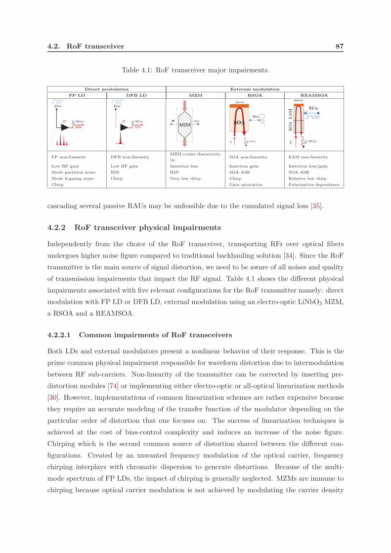
4.2. RoF transceiver 87
Table 4.1: RoF transceiver major impairments.
Direct modulation External modulation
FP LD DFB LD MZM RSOA REAMSOA
RFin
(+RFin)
RFin
(+RFin)
MZM
V biasRF
RFin
mirror
SOA
(+RFin)
EAM
OA
mirror
RFin
SO
(+RFin)
FP non-linearity DFB non-linearityMZM cosine characteris-
ticSOA non-linearity EAM non-linearity
Low RF gain Low RF gain Insertion loss Insertion gain Insertion loss/gain
Mode partition noise RIN RIN SOA ASE SOA ASE
Mode hopping noise Chirp Very low chirp Chirp Relative low chirp
Chirp Gain saturation Polarization dependance
cascading several passive RAUs may be unfeasible due to the cumulated signal loss [35].
4.2.2 RoF transceiver physical impairments
Independently from the choice of the RoF transceiver, transporting RFs over optical fibers
undergoes higher noise figure compared to traditional backhauling solution [34]. Since the RoF
transmitter is the main source of signal distortion, we need to be aware of all noises and quality
of transmission impairments that impact the RF signal. Table 4.1 shows the different physical
impairments associated with five relevant configurations for the RoF transmitter namely: direct
modulation with FP LD or DFB LD, external modulation using an electro-optic LiNbO3 MZM,
a RSOA and a REAMSOA.
4.2.2.1 Common impairments of RoF transceivers
Both LDs and external modulators present a nonlinear behavior of their response. This is the
prime common physical impairment responsible for waveform distortion due to intermodulation
between RF sub-carriers. Non-linearity of the transmitter can be corrected by inserting pre-
distortion modules [74] or implementing either electro-optic or all-optical linearization methods
[30]. However, implementations of common linearization schemes are rather expensive because
they require an accurate modeling of the transfer function of the modulator depending on the
particular order of distortion that one focuses on. The success of linearization techniques is
achieved at the cost of bias-control complexity and induces an increase of the noise figure.
Chirping which is the second common source of distortion shared between the different con-
figurations. Created by an unwanted frequency modulation of the optical carrier, frequency
chirping interplays with chromatic dispersion to generate distortions. Because of the multi-
mode spectrum of FP LDs, the impact of chirping is generally neglected. MZMs are immune to
chirping because optical carrier modulation is not achieved by modulating the carrier density

88 Chapter 4. Analog RoF Transmission Limitations in GeRoFAN
[30]. Nevertheless, MZMs suffer from their non-linear cosine transfer function [3]. While signal
propagation impacts the link gain, RoF transmitter contributes also to the signal loss. Unlike
directly modulated LDs, where link gain only depends on slope efficiencies, the gain of exter-
nally modulated LDs depends quadratically on the optical power, thus the power budget can
be easily improved [30].
4.2.2.2 Specific Impairments of RoF transceivers
The multi-mode nature of FP LDs makes them vulnerable to Optical Beat Interference (OBI)
between the different longitudinal modes, thus the intrinsic noise of the laser (Relative Intensity
Noise (RIN)) is hard to deal with since it includes both mode partition noise and mode hop-
ping noise. At the contrary, DFB LDs are assumed to have lower RIN, higher slope efficiency
and consequently higher link gain. With EAM, a special care is made to select the right bias
voltage and the right operation wavelength to improve the extinction ratio and to minimize the
insertion loss. An SOA modulator suffers from the superposition of both static and dynamic
non-linearities. However, it is shown that the latter kind of non-linearity prevails as static non-
linearity can be suppressed by adjusting the bias [87]. In addition, SOA acts as an amplifier
where the gain profile depends on the optical wavelength. For EAM-based or SOA-based ex-
ternal modulators, the polarization (TE/TM) of the incident light may impact the modulation
performance5, that could be overcome by using Polarization Controllers (PC) or strained (QW)
EAM structures [75].
4.2.2.3 REAMSOA the most suitable RoF transceiver for GeRoFAN
As described earlier, different options of RoF transceiver can be selected to equip GeRoFAN
RAUs, they range from direct vs. external modulation, the type of the light source (MMLD vs.
SMLD) and the type of the modulator. The choice of the best candidate RoF transceiver for
GeRoFAN is the outcome of a compromise between different criteria including:
• Cost: Cost criterion encompasses not only the cost of the device itself but also the cost of
its deployment over all the system.
• The optical power intensity that feeds the RoF modulator or generated by the light source.
• The electrical power driving the device: In a context where designing low-energy consump-
tion networks becomes mandatory, low voltage/current devices are highly privileged.
• High Frequency: This shows the ability of the device to handle high frequency or wideband
modulating signals since GeRoFAN is designed also to support signals with frequencies
above 10 GHz (such as UWB signals).
5Because heavy and light holes in the EAMSOA active region responds differently to incident light polarization.

4.2. RoF transceiver 89
Table 4.2: A comparison between different technologies for GeRoFAN RoF transceiver.
ComparativeCost
Optical ElectricalHF
LinkRIN Chirp
Miniaturization
criteria Power Power Gain Packaging ...
Direct modulation+ - + - - - - - - ++
with FP LD at RAU
Direct modulation- - + + - - - - ++
with DFB LD at RAU
DFB LD at HOLT+ + + + + + - ++
RSOA at RAU
DFB LD at HOLT+ + - - - + ++ ++
MZM at RAU
DFB LD at HOLT+ - + +/- - + +/- +
IML-FP at RAU
DFB LD at HOLT+ + ++ ++ ++ + +/- +
REAMSOA at RAU
• Physical impairments: As explained earlier, while each RoF transceiver has it own spe-
cific transmission limitations, we focus here on 3 major impairments usually cited for
performance comparison: Link gain, RIN and chirp.
• Integration: Significant technological advances have been made to improve the packaging,
the integration and the miniaturization of the different devices.
Supported by the comparative study in [18], RoF transceiver candidates are ranked in Table
4.2 from the most (+) to the least convenient (-) according to the different criteria specified
above.
The comparative ranking depicted in Table 4.2 shows the relative advantage of using REAM-
SOA to equip GeRoFAN RAUs. The compromise achieved by the amplified absorption modu-
lator in terms of cost-size-consumption effectiveness is summarized in the following items:
• In terms of system cost, equipping each RAU with a DFB laser diode is prohibitively
expensive. Instead, the relative low-cost of FP lasers seems more attractive. Meanwhile,
more expenses are required at some parts of the network (adding amplifiers, lineariza-
tion circuits) to overcome the limited dynamic range of FP lasers and their low gain
link. Thanks to RoF, DFB lasers are deported and pooled at the GeRoFAN head-end
node. Remote light generation enables significant cost savings, flexible management and
simplification of the RAU architecture. Size, packaging, required peripheral circuits and
monolithic integration with other optical components, are also additional factors impact-
ing the cost of the RoF transmitter device. LiNbO3-based MZMs are difficult to work with
and virtually impossible to integrate with electronic semiconductors, while a monolithic
integration of EAM with DFB LDs is easily achieved [24]. Still, one of the main challenges
90 Chapter 4. Analog RoF Transmission Limitations in GeRoFAN
with the design of REAMSOA is to benefit from the SOA gain in an effective spectrum
window by detuning the amplifier gain spectrum with respect to the EAM absorption
edge. Design techniques like Selective Area Growth (SAG) have proved their effectiveness
to achieve such a spectrum shift [17].
Currently, REAMSOA technology becomes more and more mature in the market, this
makes the amplified absorption modulator a credible competitor to the emerging RSOA
and the industry standard LiNbO3 MZM. In addition, the same single REAMSOA at
an RAU can be used both for modulation and photo-detection assuming the two signals
belong to distinct bands to avoid interference issues.
• Thanks to the amplification feature provided by the SOA, a REAMSOA can be used for
RoF links with longer reach than FP lasers or EAM external modulators, where an in-line
amplification should be needed to compensate propagation and system components losses.
Compared to a DFB laser diodes, RSOAs requiring relatively high current intensities or
LiNbO3 MZMs, REAMSOA operates with a low voltage (typically 1− 3 V).
• Compared to direct modulation options (FP, DFB LD) and external modulators (MZM
and RSOA), electro-absorption modulators are capable of operating at high frequency and
wide-band radio signals. With IML-FP, increasing the injected optical power consolidates
the locking mechanism, on the contrary, the 3-dB bandwidth of the laser is strongly
reduced.
• The comparison according to the physical impairments criterion is more balanced. In fact,
thanks to the electro-optic mechanism, MZM are very less vulnerable to frequency chirping
than direct modulation and RSOA. However, both REAMSOA and RSOA take advantage
of the integrated amplification functionality to provide relatively higher link gain than
MZM or direct modulation solutions. Finally, the impact of RIN is more serious with
direct modulation (even it is still low with DFB than FP lasers) than external modulation
solutions. Thanks to the injection-locking, the RIN of IML-FP is significantly reduced
(similar to DFB lasers) but the chirp is increased with the injected optical power (chirp
ranges between 1.5 - 4 [99]).
4.3 REAMSOA physical impairments
While the comparative study shown in Table 4.2 highlights definitely the advantage of selecting
REAMSOA as the RoF transceiver for GeRoFAN, a deep insight on its main physical limitations
is required to ensure a proper deployment and exploitation. We develop an analytical model
describing the REAMSOA behavior in order to assess the intensity of the different noises.

4.3. REAMSOA physical impairments 91
4.3.1 REAMSOA working principle
The most crucial part of the REAMSOA stands for the EAM section where the modulation and
photo-detection occur. The EAM is an external optical modulator based on a voltage-controlled
absorption of light. EAMs are promising candidates for ultrahigh speed optical communications,
due to their small size, light weight, relative low power consumption, high-frequency operating
speed and the possibility for monolithic integration with other semiconductor devices. EAM
can be realized using either a bulk semiconductor material or multiple quantum wells (MQW)
positioned within an intrinsic region of a reverse biased p-i-n diode. Bulk and MQW-EAM
rely on different physical quantum effects. While bulk EAM is driven by the Franz-Keldysh
Effect (FKE) characterized by the direct band edge absorption, the working mechanism of a
MQW-EAM is known as the Quantum Confined Stark Effect (QCSE) [150].
The main drawback of EA (Electro-Absorption) modulators consists in their link loss. The
use of EAMs requires a careful adjustment of the bias voltage in order to achieve a low insertion
loss. But, as discussed in the literature [156], the EAM is biased at a particular point leading
to a compromise between the linearity of the modulator and its insertion loss. When an EAM
is used for full duplex communication, the optimal bias voltage is selected as a compromise
between photo-detection and modulation functions as suggested in [32]. To compensate for the
power loss inherent to the modulation, the EAM can be integrated with an SOA to amplify the
optical signal at the output of the modulator. Hence, the use of in-line optical amplifier becomes
useless since the amplification function is already achieved through the new integrated amplified
modulator. However, such integration is still facing some challenges such as maximizing the
fiber coupling efficiency, the sensitivity to light polarization and shifting the amplification region
of the SOA to coincide with the modulation region of the EAM [17][95].
The modulator considered in this study is a MQW-EA amplified modulator made of 10
quantum wells and 11 barriers based on AlGaIn/GaIn layers. One of the main original contri-
butions of this Thesis is the design of a comprehensive analytical model describing the behavior
of the MQW-EA amplified modulator. We provide in the Appendix the detailed description
of the steps composing our methodology. Our analytical modeling of the amplified EAM has
been validated by Mr Christophe Kazmierski, senior researcher within the III-V Labs6 and in-
ternational expert of the domain [104]. Mr Kazmierski estimates that the proposed approach to
describe analytically the behavior of the EAM represents an original and interesting contribu-
tion. The approach is well suited to the description of the Stark effect in quantum wells, even
if exciton effects are not the only ones to be considered to model the EAM behavior, especially
under high reverse bias voltages (around 5 Volts). Meanwhile, at this level of the study, this
remark does not question the final conclusions of following chapters in the manuscript.
6Alcatel-Thales III-V Lab., Alcatel-Lucent Bell Labs France. http//:www.3-5lab.fr/

92 Chapter 4. Analog RoF Transmission Limitations in GeRoFAN
The outcome of the calculations detailed in Appendix enables us to derive the absorption
profile of the EAM with respect to the bias voltage at each optical channel. The absorption
profile of the EAM stands for the transfer function of the device, through which we calculate
the equation of the RF link gain.
4.3.2 The EAM section
The first figure of merit to characterize the performance of a RoF link is the link gain. The link
gain G is defined as the ratio of the microwave output power Pout to the microwave electrical
power Pin injected in the modulator:
G =
∣∣∣∣∣PRF,out
PRF,in
∣∣∣∣∣ (4.1)
For Intensity Modulation Direct Detection (IMDD) link, the link gain strongly depends
on the transmitter device. In [30], the link gain has been evaluated for direct and external
electro-optic modulation in RoF links. The impact of impedance matching on link gain and
noise factor is addressed in [72] with a comparison between direct and external modulation. It
is shown in [34] that for the RoF link gain G (in dB units) is negative (i.e. lossy link) for the
case of direct modulation or external modulation using an EAM, while for the REAMSOA, one
can take advantage from the amplifier functionality featured by the SOA to increase the link
gain.
Like any external modulator, the link gain of EA modulator depends on the injected optical
power and internal parameter of the device (capacitance of the electrodes, internal resistance
etc.). EA modulators suffer from residual loss (residual absorption in the absence of external
electric field) that may decrease the gain. For the case of TW-type EAM, the analysis is carried
out based the mathematical approach developed in [64]. We express in Equation 4.2 the optical
power at the output of the modulator as function of the input optical power, the absorption
coefficient αo of the active layer at 0 Volt, the optical confinement factor Γ of the EAM with
length ℓ and the absorption change α across the modulation section due to the modulating
voltage.
Pout = Pin · ρ · exp (−αoℓ) · exp
(−Γ ·
∫ ℓ
0α(x) dx
)(4.2)
where ρ stands for the optical loss factor at each facet of the modulator (including fiber-
coupling loss). A typical value of 3 dB for ρ is assumed. The applied voltage V to the EAM
is expressed as the sum of its DC part (bias voltage Vb) and its AC part (modulating voltage
VAC). Using small signal approximation, we focus only on the AC part of Equation 4.2 to get:

4.3. REAMSOA physical impairments 93
Rcon
Rs
Lm
gD
Po
st-d
ete
cto
r
Am
plifi
er
ng
Blo
ck
hin
gB
lock
Ro Cm
GDGA
Ma
tch
i
Ma
tch
EAM circuit model
Figure 4.2: EAM quasi-static circuit modelA typical analog RoF link can be represented as a concatenation of an EAM equivalent circuit model, the fiber medium, a photo-detector
equivalent circuit and eventually a post-detector amplifier. Matching blocks are inserted at the input and the output of the link. Impedance
matching between the source and the EAM on one hand, the photo-detector and the amplifier on the other hand minimizes the power loss
due reflection and increases the RF gain.
P ACout = Pin · ρ · exp (−ℓ(αo + Γαb)) · Γ · dα
dV|V=Vb
·∫ ℓ
0VAC(x) dx (4.3)
where αb denotes the absorption coefficient at Vb.
The AC part of the output optical power passes through a PIN photo-detector, the detected
RF output power is:
PRF,out =
(qeη
hf
)2
· ZL · |P ACout |2 (4.4)
where: η the photo-detector quantum efficiency, qe the electron charge, h the Planck con-
stant, f the microwave frequency of the modulating signal and ZL = GD
GA·gD·(1+GDGA
)2the mi-
crowave impedance at the receiver computed through the quasi-static approximated circuit
model of the TW-EA modulator. Parameters gD, GA and GD correspond respectively to the
photodiode admittance, the receiver equivalent impedance seen from both sides of the matching
block as illustrated in Figure 4.2 .
The normalized gain (with respect of the ideal case where no loss is observed) is expressed
in Equation 4.5:
G(f, λ, Vb) =
∣∣∣∣∣T
1− ΓLΓSe−2γuℓ·[
e(βo−γu).ℓ
(βo − γu).ℓ+ ΓL · e−2γuℓ · e(βo+γu).ℓ − 1
(βo + γu).ℓ
]∣∣∣∣∣
2
(4.5)
Given, following the assumptions in [64]:

94 Chapter 4. Analog RoF Transmission Limitations in GeRoFAN
• γu =√
Rcon+2πfLm
Rs+Ro
1+Cm2πfRo
the microwave propagation constant.
• ΓL = ZL−ZmZL+Zm
and ΓS = 1− T are the modulator internal reflection coefficient at the load
and the source ports respectively.
• T = e−Γℓ(αb−αo) the amplitude transmission coefficient of the modulator.
• Zm =√(Rcon + 2πfLm) · (Rs +
Ro1+Cm2πfRo) the modulator impedance.
• βo the wave number associated with the optical-wave group velocity, λ the wavelength of
the optical carrier.
• Lm, Cm, Ro, Rs, Rcon are respectively: the (per-unit length) EAM inductance, capacitance,
equivalent AC resistance, serial resistance and conduction resistance of the equivalent
quasi-static circuit model of the modulator in Figure 4.2. The symbol stands for the
complex number where 2 = −1.
Three main remarks worth to be noticed when analyzing the RF gain of the modulator:
1. The RF gain depends on the waveguide microwave proprieties, the wavelength of the
optical carrier λ and the bias voltage Vb. Therefore, one way to improve the RF gain
should be to focus on enhancing the design parameters of the modulator-waveguide. Such
an approach was followed in the study of [27], where authors investigate the optimal length
of the modulator in order to maximize the RF gain.
2. The importance of the impedance matching between the modulator-waveguide and the
source on one hand, and with the receiver on the other hand. In [72] and [29], the problem
of impedance matching has been worked out through different matching scenarios.
3. The RF gain is proportional to the input EAM optical power squared. It suggests that, at
some extent, one can minimize the link loss by increasing the optical power at the input
of the modulator.
Because of the dependance of T with Vb, the optical bias point at each optical carrier is
selected such that the modulation RF gain is maximized, i.e V ∗b = argmaxVb
G(Vb). Figure 4.3
illustrates the optimal bias voltage V ∗b at different optical channels.
To characterize the performance of the modulator, the noise figure of the RoF link is a
key performance indicator. The Modulation Penalty (MP) (i.e. the noise figure NF of the
modulator) is related to the RF link gain G as expressed by Equation 4.6:
NF =Nout
k · T K · B · G(4.6)

4.3. REAMSOA physical impairments 95
1.4
1.6
1.8
2
2.2
2.4bia
s v
oltage (
-V
* b )
1500 1510 1520 1530 1540 1550 1560 1570 1580 1590 16000.4
0.6
0.8
1
1.2
Optical wavelength (nm)
Revers
e o
ptim
al b
Figure 4.3: EAM Optimal Bias Voltage for each optical wavelength.Unlike electro-optic modulators, EAMs work at smaller bias voltage. Optimal operation (in terms of RF gain) is achieved by biasing the
device in the range −1.8 ∼ −1 V to cover the conventional C-band (cf. squared area in the figure).
Given: Nout the noise power at the output of the amplified modulator, k The Boltzmann’s
constant, T K the Kelvin temperature and B the noise bandwidth.
Figure 4.4 depicts the evolution of the RF link gain of the modulator according to the OC
wavelength at 0 dBm and −10 dBm input optical signal power.
4.3.3 The SOA section
The REAMSOA takes advantage of the amplifier gain provided by the integrated SOA. The
amplification operation is performed twice because of the reflective configuration of the device.
To model the SOA gain profile, we follow the analytical development in [28]. If Gs denotes the
single-pass gain at the operating wavelength λ, the maximum SOA gain expressed in Equation
4.7 is the fiber-to-fiber gain given from the transmittance function of the Fabry-Pérot cavity.
Gmaxsoa (λ) =
(1− R1)(1− R2)Gs
(1− Gs
√R1R2)2 + 4Gs
√R1R2 sin(
2πneff ℓsoa
λ )2(4.7)
Where: ℓsoa the length of the SOA section, R1, R2 Input and output facet reflectivity of
the cavity respectively, neff the effective refractive index of the amplifier waveguide expressed
as in [28] and function of the InGaAsP active region refractive index, the cladding InP region
refractive index and the optical confinement factor Γsoa of the SOA.

96 Chapter 4. Analog RoF Transmission Limitations in GeRoFAN
0
2
4
6
8R
F lin
k g
ain
(dB
)
@ -10 dBm input power
@ 0 dBm input power
1536 1538 1540 1542 1544 1546 1548 1550 1552 1554 1556 1558-10
-8
-6
-4
-2
Optical wavelength (nm)
Modula
tor
R
Figure 4.4: EAM RF Gain as function of the optical wavelength.The RF gain of the modulator is computed at optimal bias voltage and under balanced impedance matching. The figure highlights two
distinct regions of the RF gain: For some optical channels (cf. squared region in the figure), a positive RF link (in dB) is achieved, while at
some other optical channels the RoF link is lossy. By increasing the optical power injected in the modulator, the RF gain increases as well
and the range of optical channels leading to a positive gain is extended.
The single-pass gain depends on the material gain of the device which is in-fine carrier
density dependant. The material gain coefficient gm is estimated with respect to the optical
wavelength and approximated by a parabolic extrapolation as carried out in [85].
Figure 4.5 plots the unsaturated gain of the SOA as function of the optical wavelength.
The gain saturation of the SOA is an important feature included in our analytical modeling.
When the input optical power increases, the optical gain of the amplifier drops. The saturated
gain of the SOA Gsoa is related to the maximum gain according to Equation 4.8:
Gsoa = β · ln(
Gmaxsoa
Gsoa
)(4.8)
The factor β stands for the ratio between the saturation optical power of the SOA (Psat)
and the input optical power.
Equation 4.8 indicates that for a low input optical power, the gain tends to reach its un-
saturated value Gmaxsoa , while at very high optical power, the gain tends to 1 so that the input
optical power equals to the output optical power. Equation 4.8 is solved using the Lambert
W -function.
The saturation power Psat of the SOA is expressed through Equation 4.9:

4.3. REAMSOA physical impairments 97
12.5
13
13.5
14
14.5
15ed S
OA
gain
(dB
)
1.53 1.54 1.55 1.56 1.57 1.58 1.59 1.6
x 10-6
10
10.5
11
11.5
12
Photon wavelength (m)
Unsatu
rate
Figure 4.5: SOA unsaturated gain as function of the optical wavelength.The unsaturated gain of the SOA is calculated assuming a bias of 120 mA and an input optical power of 0 dBm. The effective gain of the
amplifier evolves with respect to the saturation power. When the input optical power is low, the effective gain tends to its unsaturated value,
while at very high power the gain is equal to 1.
Psat =Esat
τc=
hc · witi
τcλ · gm
Nb−No
(4.9)
Given: Esat the saturation energy of the amplifier; τc the spontaneous carrier-life time; h
the Planck constant; wi and ti the width and the thickness of the SOA active layer respectively;
Nb and No the carrier density at bias current Ib and at transparency respectively.
Figure 4.6 illustrates the saturation optical power of the amplifier according to the wave-
length.
The signal amplification by the SOA is accompanied by Amplifier Spontaneous Emission
(ASE) noise. In general the ASE noise is very small (∼ −70 dBm), but it may become a
dominant noise source when numerous in-line amplifiers are inserted along the light-path. The
ASE optical noise is computed through Equation 4.10 [5]:
Pase = 2 · nsp · h · f · (Gsoa − 1) · Bo (4.10)
Assuming: nsp the population inversion parameter of the SOA; fo the optical frequency;
Gsoa the amplifier gain computed according to Equation 4.8 and Bo the equivalent optical
bandwidth.

98 Chapter 4. Analog RoF Transmission Limitations in GeRoFAN
8.7
8.8
8.9
9ic
al p
ow
er
(dB
m)
1.53 1.54 1.55 1.56 1.57 1.58 1.59 1.6
x 10-6
8.3
8.4
8.5
8.6
Photon wavelength (m)
Satu
ratio
n o
pti
Figure 4.6: SOA Saturation optical power as function of the optical wavelength.The saturation power of the SOA is computed assuming a bias of 120 mA and an input optical power of 0 dBm (cf. the C-band is delimited
by the squared area in the figure).
4.3.4 Non-linearity and Intermodulation distortions
Intermodulation (IMD) distortions have been pointed out as the main impairment reducing the
dynamic range of an analog RoF SCM transmission link [154]. Analog signal distortion occurs
when multiple RFs transported by the same optical channel beat together to generate RF mixing
products that may fall on a designated radio channel and degrade its SNR. For a REAMSOA,
the phenomenon of intermodulation distortions is caused by 4 different physical impairments:
Intermodulations proper to the intrinsic non-linearity of the Reflective Amplified Modulator
(IMD-RAM), signal clipping, frequency chirping and specific intermodulations occuring when
RF subcarriers are already OFDM modulated as high-speed WiFi (802.11n/g standard), 4G
LTE and WiMAX signals.
4.3.4.1 IMD-RAM
The transfer function of an EAM is intrinsically nonlinear [67]. Output optical power to input
optical power ratio of the device depends on the absorption coefficient of the active region
α(λ, V ) which varies according to both the applied bias voltage V and the operating optical
wavelength λ. Considering an EAM with an optical confinement factor Γeam and a length ℓeam,
the transfer function f of the modulator is expressed by Equation 4.11:

4.3. REAMSOA physical impairments 99
Pout
Pin= f(V ) = η · e−α(V,λ)·Γeam·ℓeam
(4.11)
Where: η: the fiber coupling loss coefficient.
For a given operating wavelength, we consider V as a superposition of the DC bias voltage
Vb and a variable modulating component Vm (RF modulating signal). We carry out the same
mathematical development detailed in [67] to highlight the non-linear behavior of the device by
expanding Equation 4.11 using Taylor series expansion around Vb:
f(V ) ≃ f(Vb) + Vm ·(df
dV|V =Vb
)+
V 2m
2!·(d2f
dV 2|V=Vb
)+
V 3m
3!·(d3f
dV 3|V=Vb
)+ ...+
V nm
n!·(dnf
dV n|V=Vb
) (4.12)
Under small signal approximation, Equation 4.12 is simplified up to the 3rd order derivative
of f. For sub-octave bandwidth systems, second order IMDs (IMD−2) and third order HarmonicDistortions (HD−3) are not considered since they fall out of the signal band. However, thesedistortions must be considered for the case of multi-service system (for instance, LTE and UWB
signals transported by the same optical channel) [125]. The IMD-3 optical noise generated by 2
tones (i, j) (respectively 3 tones (i, j, k)) that falls at RF l = 2i ± j (respectively l = i ± j ∓ k)
is computed according to Equation 4.13a (respectively 4.13b):
N2i±j =3
4· K3
3!· V 3
b · m2i mj · Po (4.13a)
Ni±j∓k =3
2· K3
3!· V 3
b · mimjmk · Po (4.13b)
Given: mi: Optical Modulation Index (OMI) of RF channel i; Vb: DC bias voltage of the
EAM; K3 =d3fdV 3
|Vb: 3rd order RAM non-linearity parameter computed at bias point and Po:
Average received optical power.
4.3.4.2 Clipping Noise
Restricted for a long time to direct modulations, external modulation links are also subject to
clipping noise. Basically, clipping noise describes the distortion of the optical wave generated at
the output of the modulator when the injection current/voltage overdrives (or under drives) the
device beyond its clipping-free region [72]. Figure 4.7 illustrates through a phasor representation
of the SCM modulating signal, how clipping occurs when some of the signal components get
within clipping region of the modulator. When the signal is clipped, extra-harmonics and
intermodulation products between the modulating subcarriers are generated. The study in [94]
shows that compared to direct modulation systems and assuming the same optical depth and

100 Chapter 4. Analog RoF Transmission Limitations in GeRoFAN
Clipping
region
Clipping-free
region
Resulting
f1
f2f3
fN
Signal
clipped
dc- bias
current…
SCM signal
Figure 4.7: Illustration of clipping using a phasor representation of the SCM signal.When N RF subcarriers modulates an optical channel, the resulting SCM signal will be clipped if the phasor of the signal is pushed within
the clipping region of the modulator. Note that clipping may occur because of some of subcarriers although the phasor of the resulting SCM
signal is outside the clipping region.
frequency planning scheme, externally modulated links suffer from an additional 6 dB clipping
distortion penalty. Several publications have focused on clipping analytical modeling such as
in [6] [137] and [82]. However, a more accurate approach detailed in [58] is followed in our
modeling to assess the impact of clipping. Assuming an input SCM modulating electrical signal
as a multiplex of N subcarriers (f1, ..., fN ) each with OMI mi, the ratio of Carrier-to-Inter-
Modulation Products of order n CIMP (n) computed at frequency fi is expressed in Equation
4.14:
CIMP (n)(fi) =(4N)(n−1) · π · (X(1)n!)2 · exp( 1
µ2)
H2(n−2)(µ/
√2) · D
(n)fi
(4.14)
Given: µ =
√∑N
i=1m2i
2 : the total modulation depth of the RF multiplex signal; D(n)fi: Num-
ber of IMD products of order-n; X(1) = 1−erfc( 1
1√2µ)
2 : The non-linear susceptibility of the
effective transfer function of the modulator assuming to model the input SCM signal as a Gaus-
sian process; H(n−2)(x): the Hermite polynomials of order n − 2. For orders 2 and 3, it can be
written as: 1 and x respectively.

4.3. REAMSOA physical impairments 101
4.3.4.3 Frequency Chirping Noise
Compared to directly modulated lasers, external optical modulators show lower frequency chirp-
ing which makes them very attractive for chirping sensitive optical communication systems.
Chirping is typically between 4 and 6 for semiconductor diode lasers while it ranges between
+1 and −2 for EA modulators [127]. Higher carrier densities are typical for laser diodes and do
not allow for negative chirp factors, while because modulators are reverse biased, they exhibit
a much lower carrier density in the quantum wells [75].
According to [80], there are two possible causes of frequency chirping in external modulators:
one possible reason is the wavelength shift of the semiconductor laser feeding the modulator
due to external reflection outside of the EAM. This kind of chirping can be mainly removed
by adopting optical isolators and reducing the reflection by means of Anti-Reflection coating
to the end-face of the modulator. The second cause of chirping is the phase modulation due to
the refractive index change of medium inside the EAM. In the following analysis, we consider
EAM frequency chirping due to the unwanted phase modulation of the optical signal by the
modulating signal which is inherent to the working mechanism of the EAM. When coupled
with chromatic dispersion, frequency chirping of an EAM, induces distortions of the signal
through the generation of intermodulation products and harmonics. The intensity of these noisy
frequency-dependant components depends on the phase variation with the modulating signal
along the time. To estimate frequency chirping induced signal distortion in multiple quantum
well EAMs (MQW-EAM), we follow the theoretical analysis carried out in [74]. Assuming that
N radio signals at angular microwave frequencies (ω1, ..., ωN ) with OMIs (m1, ..., mN ) modulate
the EAM, the outcome of our calculations (detailed in theAppendix) highlights the expressions
of the optical noise Nopt(ωl) of IMD3 products falling at angular frequency ωl as in Equation
4.15:
Nopt(ωl) ≃ 2Pin10−aL(I2ωl
+Q2ωl) (4.15)
Where: Pin: the optical power at the input of the EAM; a: fiber attenuation coefficient;
L: the optical fiber length; Iωland Qωl
are In-phase and Quadratic-phase chirp-induced IMD3
noise falling at frequency ωl and expressed as the following:
• For IMD3 with 2 tones falling at ωl = 2ωi − ωj :
Ic = a1β2Vb · m2
i mj · (ω2i +ω2j2) + 3a1β
2Vb · m2i mj · ωi(ωj − ωi
2) (4.16a)
Qc = a2β2Vb · m2
i mjωi(ωi − ωj
2) (4.16b)
• For IMD3 with 3 tones falling at ωl = ωi − ωj + ωk:
Ic = a1β2Vb · mimjmk · (ω2i + ω2j + ω2k) + 3a1β
2Vb · mimjmk · (ωjωi + ωjωk − ωiωk) (4.17a)

102 Chapter 4. Analog RoF Transmission Limitations in GeRoFAN
Qc = a2β2Vb · mimjmk · ωi(ωi + ωj + ωk) (4.17b)
Parameters β, a1 and a2 are defined in the Appendix.
4.3.4.4 IMD-OFDM
For a RF OFDM-modulated channel, such as in 4G LTE or WiMAX, the non-linearity of
the modulator generates IMD noises due to beating between OFDM Subcarriers (SCs). The
analytical study in [100] shows that distortions spread out over a bandwidth three times larger
than the RF bandwidth thus penalizing the SNR of the RF channel itself and its adjacent (left
and right) neighbors. The detected intensity of third order IMDs falling at RF channel ℓ is:
I(ℓ) =1
6d2ℓ−1 +
2
3d2ℓ +
1
6d2ℓ+1 (4.18)
Given: d2i =(PoK3m2oV 3b )
2
2 · M(Nsc): The relative amplitude of IMD noises created by OFDM
SCs composing the RF channel i; mo: OMI of single OFDM SC; M(Nsc): total number of IMD3
composite products produced by the beating of Nsc equally-spaced OFDM SCs computed as in
[101].
4.4 ROADM
ROADMs are the second key element in the GeRoFAN system. Substantial developments have
been made on the architecture of ROADM subsystems to improve their tunability and reduce
their insertion loss. A wide range of available ROADM structures are based on Arrayed Waveg-
uide Gratings (AWGs), Fiber Bragg Gratings (FBGs) packaged along with optical switches,
ring resonators, acousto-optic tuneable filters, micro-mirror arrays etc [129].
4.4.1 FBG-based ROADM
FBG-based ROADMs are selected for the GeRoFAN system as they cover a wide range of
proposed OADM structures in the literature, showing relatively low loss compared to their
counterparts (Mach-Zehnder Interfometer, AWG, etc.), low channel spacing. They are mature
technology and available in the market at a relatively low cost [16]. Because tunability is an
important feature to enable further control flexibility of the system, we are specially interested
in tunable FBG based OADM. The tunability is achieved either through thermo-control or
mechanic strain applied to the gratings. While this option may be attractive since it entails one
single FBG, it presents some limitations on the tunability range of the device. To cover a large
range of tunability, a set of gratings at different wavelengths separated by 2×2 optical switchesare connected to each other in cascade within a single device. The switch routes the WDM
signal from the input port through only the gratings at the add/drop wavelengths bypassing

4.4. ROADM 103
…
1 N
Optical 2x2
switches
FBG
IN OUT
A B
A B
B
0P
DROP ADD
AB 0
addP
Figure 4.8: ROADM Structure used for GeRoFANCompared to other technologies, FBG-based OADM is considered as a mature low-cost technology. The reconfigurability of the OADM is
achieved by driving the cross-bar configuration of multiple switches. Such a configuration prevents using filters (difficult to manage) to select
the right optical channel. Each FBG is designed according to the optical wavelength to be dropped. The imperfections of FBGs, circulators,
switches generate homodyne and heterodyne crosstalk which are accurately computed in our modeling.
the gratings at other wavelengths. A tuneable FBG-based OADM model minimizes filtering of
the wavelength channels and subsequent induced signal distortions and eye closure [129].
Figure 4.8 illustrates the model of the Tuneable FBG-based OADM adopted in this study.
Three possible paths of the optical signal are highlighted: a Drop path, an Add path and a
Pass-through path.
4.4.2 OADM noises
OADM may degrade the quality of the optical signal due to the imperfect isolation of its optical
components (optical switches, (de)multiplexers, gratings etc.). The degradation can be modeled
by a leakage power, an optical interference between transiting channels or optical reflections.
The generated crosstalk by these devices is classified either based on the phase difference Φbetween the two optical carriers (Coherent vs. Incoherent Crosstalk) or on their wavelengths
λ (Homodyne vs. Heterodyne Crosstalk) [25].
In-band optical crosstalk (i.e. homodyne crosstalk) occurs if the crosstalk signal is at the
same wavelength as the desired signal, while out-of-band crosstalk (i.e. heterodyne crosstalk)
happens if the crosstalk signal is at a different wavelength. Coherent crosstalk occurs if the
phase difference between the two signals is kept constant, while incoherent crosstalk takes place
when the phase difference between the two signals varies randomly over the range [0, 2π[. We
should notice that the heterodyne crosstalk is definitely non-coherent.

104 Chapter 4. Analog RoF Transmission Limitations in GeRoFAN
4.4.3 Homodyne Crosstalk
Homodyne crosstalk in Tuneable-FBG OADMs results from imperfections in FBGs, interme-
diate switches and circulators. For instance, within the OADM the added optical channel is
reflected by the FBG and transmitted back to the GeRoFAN head-end node. However some of
the added channel leaks through the grating and is received at the drop port of the OADM.
Similarly, some of the dropped optical signal passes through the gratings and continues together
with the added optical signal. Passing through channels are also affected by some power leak-
age. These leakages result either in an incoherent or coherent homodyne crosstalk increasing
the noise level. SNR of the optical channel is also degraded because of a decrease in the power
signal due to connectors or switches loss. To compute the degradation induced by homodyne
crosstalk, we use the analytical model and crosstalk parameters described in [129]. Table 4.3
summarizes homodyne crosstalk equations for each path channel. Assuming an OADM with
N FBGs, the dropped/added/passing-through channel corresponds to the wavelength at FBG
with rank p7.
Figure 4.9 shows the SNR penalty of an RF signal modulating an optical carrier in the
C-band when the considered optical wave is dropped, added and passes-through the ROADM.
Different ROADM structures are simulated assuming 8, 16, 24 and 32 build-in FBGs.
Whatever the path of the optical channel (drop, add or pass-through) through the ROADM,
Figure 4.9 shows the higher the number of build-in FBGs, the higher the SNR penalty. In
addition, least penalized channels differ from one path to another. Channels experiencing the
lowest penalty correspond to longer optical wavelength channels for the ADD path. Short
wavelength channels experience the lowest penalty for the DROP path, while channels located
at the middle of the FBG sequence are the most privileged channels for the PASS-THROUGH
path.
4.4.4 Heterodyne Crosstalk
Out-of-band (i.e. Heterodyne) crosstalk may be removed by adequate filtering at the receiver if
the crosstalk and the desired optical signals are modulated by different subcarriers. When two
optical channels at different wavelengths but modulated by the same radio frequency interfere
with each other, the crosstalk noise depends on the subcarrier phase difference which is related
to the fiber path length of each channel and chromatic dispersion [26]. In our model, the
heterodyne crosstalk occurs within the FBG of the OADM system assuming that the interfered
and the interfering channels are modulated by the same radio subcarrier (this particular kind of
crosstalk noise is accounted only in the case of radio frequency reuse). When the dropped optical
channel is reflected by the grating, a small part of the power of neighboring optical channels is
7p ∈ 1, 2, ..., N
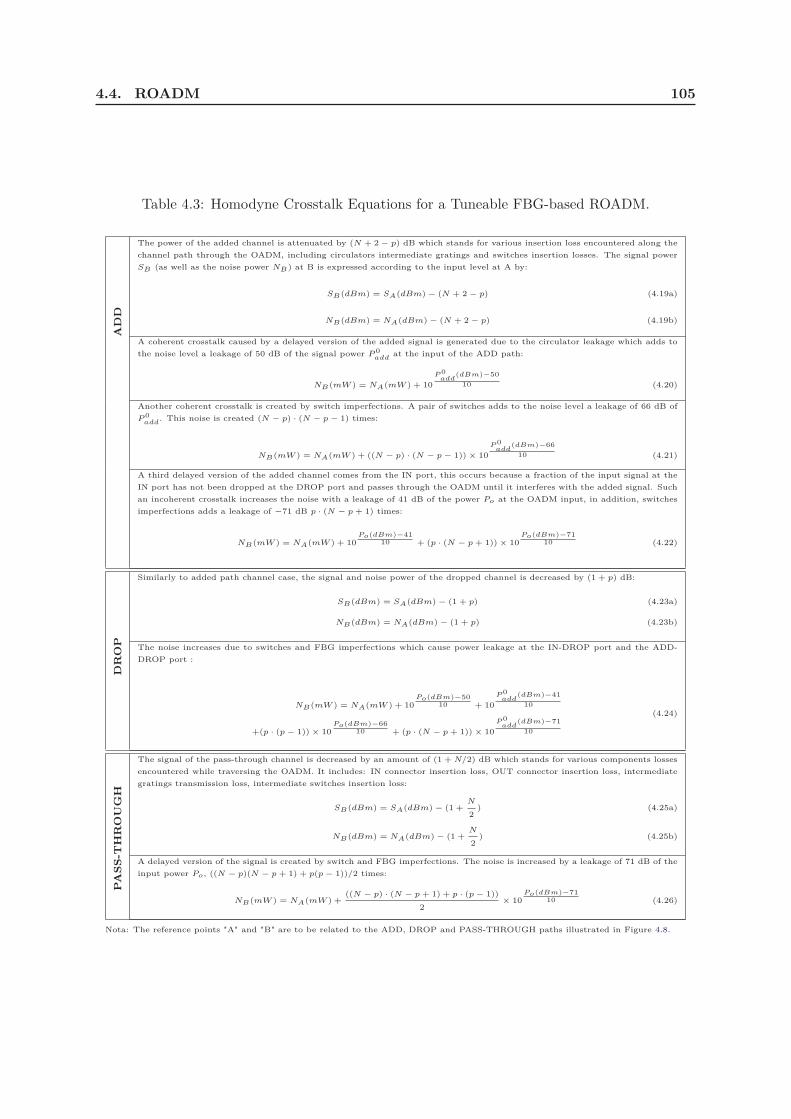
4.4. ROADM 105
Table 4.3: Homodyne Crosstalk Equations for a Tuneable FBG-based ROADM.
AD
D
The power of the added channel is attenuated by (N + 2− p) dB which stands for various insertion loss encountered along the
channel path through the OADM, including circulators intermediate gratings and switches insertion losses. The signal power
SB (as well as the noise power NB) at B is expressed according to the input level at A by:
SB(dBm) = SA(dBm)− (N + 2− p) (4.19a)
NB(dBm) = NA(dBm)− (N + 2− p) (4.19b)
A coherent crosstalk caused by a delayed version of the added signal is generated due to the circulator leakage which adds to
the noise level a leakage of 50 dB of the signal power P 0add
at the input of the ADD path:
NB(mW ) = NA(mW ) + 10
P 0add
(dBm)−50
10 (4.20)
Another coherent crosstalk is created by switch imperfections. A pair of switches adds to the noise level a leakage of 66 dB of
P 0add. This noise is created (N − p) · (N − p − 1) times:
NB(mW ) = NA(mW ) + ((N − p) · (N − p − 1))× 10
P 0add
(dBm)−66
10 (4.21)
A third delayed version of the added channel comes from the IN port, this occurs because a fraction of the input signal at the
IN port has not been dropped at the DROP port and passes through the OADM until it interferes with the added signal. Such
an incoherent crosstalk increases the noise with a leakage of 41 dB of the power Po at the OADM input, in addition, switches
imperfections adds a leakage of −71 dB p · (N − p + 1) times:
NB(mW ) = NA(mW ) + 10Po(dBm)−41
10 + (p · (N − p + 1))× 10Po(dBm)−71
10 (4.22)
DR
OP
Similarly to added path channel case, the signal and noise power of the dropped channel is decreased by (1 + p) dB:
SB(dBm) = SA(dBm)− (1 + p) (4.23a)
NB(dBm) = NA(dBm)− (1 + p) (4.23b)
The noise increases due to switches and FBG imperfections which cause power leakage at the IN-DROP port and the ADD-
DROP port :
NB(mW ) = NA(mW ) + 10Po(dBm)−50
10 + 10
P 0add
(dBm)−41
10
+(p · (p − 1))× 10Po(dBm)−66
10 + (p · (N − p + 1))× 10
P 0add
(dBm)−71
10
(4.24)
PA
SS
-TH
RO
UG
H
The signal of the pass-through channel is decreased by an amount of (1 +N/2) dB which stands for various components losses
encountered while traversing the OADM. It includes: IN connector insertion loss, OUT connector insertion loss, intermediate
gratings transmission loss, intermediate switches insertion loss:
SB(dBm) = SA(dBm)− (1 +N
2) (4.25a)
NB(dBm) = NA(dBm)− (1 +N
2) (4.25b)
A delayed version of the signal is created by switch and FBG imperfections. The noise is increased by a leakage of 71 dB of the
input power Po, ((N − p)(N − p + 1) + p(p − 1))/2 times:
NB(mW ) = NA(mW ) +((N − p) · (N − p + 1) + p · (p − 1))
2× 10
Po(dBm)−7110 (4.26)
Nota: The reference points "A" and "B" are to be related to the ADD, DROP and PASS-THROUGH paths illustrated in Figure 4.8.

106 Chapter 4. Analog RoF Transmission Limitations in GeRoFAN
3
4
5
6
penalty (dB
)
(a) ADD path (SNR
optin = 20 dB, P
optin = 0 dBm)
2.5
3
3.5
4
4.5
alty (dB
)
(b) DROP path(SNRo
ptin = 20 dB)
0.15
0.2
0.25
penalty (dB
)
(c) PASS THROUGH path(SNR
optin = 20 dB)
8 FBGs
16 FBGs
32 FBGs
24 FBGs
8 FBGs
16 FBGs
24 FBGs
32 FBGs
8 FBGs
16 FBGs
24 FBGs
32 FBGs
5 10 15 20 25 300
1
2
3
Rank of the added channel
RF S
NR
p
5 10 15 20 25 300
0.5
1
1.5
2
Rank of the dropped channel
RF S
NR
pena
5 10 15 20 25 300
0.05
0.1
Rank of the passing-through channel
RF S
NR
p
Figure 4.9: RF SNR penalty due to OADM Homodyne crosstalk for (a) the ADD path, (b) the
DROP path and (c) the PASS-THROUGH path.A higher number of optical channels increases the crosstalk penalty. We notice the dependance of the penalty distribution with the rank of the
optical channel. In practice, optical wavelengths are mapped in an ascending order with FBGs from the left to the right side of the OADM.
SNRinopt and P
inopt stand for SNR and signal power at the input of the ROADM (at reference point "A" of the considered path) respectively.
reflected as well, causing interference with the dropped channel. To estimate the level of the
crosstalk noise between reflected and transmitted signals, we focus on the reflectivity spectrum
of the FBG. The choice of the FBG model is conditioned by key spectral characteristics including
the flatness of its pass-band, the severity of pulse distortion related to the phase response of
the grating, the strength of the out-of-band side-lobes and the symmetry of the reflectivity
spectrum [130]. For simplicity, a standard uniform FBG model is assumed in our calculations.
Equation 4.27 expresses the complex reflectivity coefficient ρ of an FBG with respect to the
optical wavelength λ:
ρ(λ) =−κ sinh(α · ℓfbg)
σ sinh(α · ℓfbg) + · α cosh(α · ℓfbg)(4.27)
Given: σ, κ the DC and AC coupling coefficient respectively, ℓfbg FBG length and the
coefficient α =√
κ2 − σ2 [140].
The power of Heterodyne crosstalk noise generated by optical channel j on optical channel
i (modulated by the same radio-frequency f) is given by Equation 4.28:
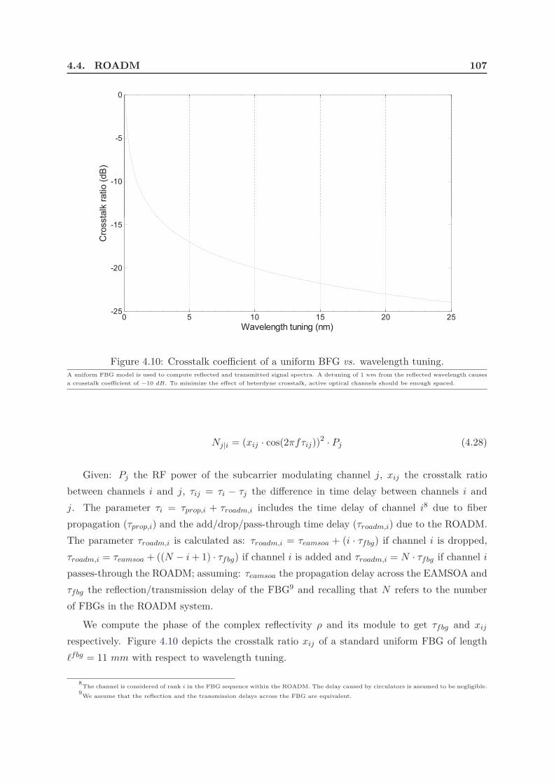
4.4. ROADM 107
-10
-5
0ta
lk r
atio (
dB
)
0 5 10 15 20 25-25
-20
-15
Wavelength tuning (nm)
Cro
sst
Figure 4.10: Crosstalk coefficient of a uniform BFG vs. wavelength tuning.A uniform FBG model is used to compute reflected and transmitted signal spectra. A detuning of 1 nm from the reflected wavelength causes
a crosstalk coefficient of −10 dB. To minimize the effect of heterdyne crosstalk, active optical channels should be enough spaced.
Nj|i = (xij · cos(2πfτij))2 · Pj (4.28)
Given: Pj the RF power of the subcarrier modulating channel j, xij the crosstalk ratio
between channels i and j, τij = τi − τj the difference in time delay between channels i and
j. The parameter τi = τprop,i + τroadm,i includes the time delay of channel i8 due to fiber
propagation (τprop,i) and the add/drop/pass-through time delay (τroadm,i) due to the ROADM.
The parameter τroadm,i is calculated as: τroadm,i = τeamsoa + (i · τfbg) if channel i is dropped,
τroadm,i = τeamsoa + ((N − i+ 1) · τfbg) if channel i is added and τroadm,i = N · τfbg if channel i
passes-through the ROADM; assuming: τeamsoa the propagation delay across the EAMSOA and
τfbg the reflection/transmission delay of the FBG9 and recalling that N refers to the number
of FBGs in the ROADM system.
We compute the phase of the complex reflectivity ρ and its module to get τfbg and xij
respectively. Figure 4.10 depicts the crosstalk ratio xij of a standard uniform FBG of length
ℓfbg = 11 mm with respect to wavelength tuning.
8The channel is considered of rank i in the FBG sequence within the ROADM. The delay caused by circulators is assumed to be negligible.9We assume that the reflection and the transmission delays across the FBG are equivalent.

108 Chapter 4. Analog RoF Transmission Limitations in GeRoFAN
4.5 Fiber impairments
Analog RoF transmission is subject to optical propagation impairments. Both linear and non-
linear fiber transmission limitations are considered in our QoT model. The major impairments
include Chromatic Dispersion (CD), Polarization Mode Dispersion (PMD), Optical Beat Inter-
ference (OBI), Rayleigh Back-Scattering (RBS) and fiber Non-Linear Effects (NLEs).
4.5.1 Chromatic Dispersion
Thanks to its simplicity, GeRoFAN uses double side-bands modulation to modulate the optical
carrier. However, because of CD, the OC, its sidebands, as well as their carried RF channels,
propagate at different velocities. At the photo-detector, when beating the two sidebands of the
optical channel to extract the radio signals, a power fading at each RF channel occurs due to
their velocity mismatch [93]. After transmission over optical fiber of length L and CD coefficient
D at OC λ, CD penalty is measured in terms of average squared Error Vector Magnitude (EVM)
according to [24]:
〈EV M2〉 ≃ 1
Nsc·(Nsc + 1) +
Nsc/2∑
n=−Nsc/2
η2 cos
(ω2n2
− λ2DL
2πc
)2
−
2η · e−σ2ϕ2
Nsc/2∑
n=−Nsc/2
cos
(ω2n2
− λ2DL
2πc
)
(4.29)
Given: η = |J1(m)Jo(m) |: the relative amplitude of the optical carrier to its first-order side-bands;
Ji: the first kind Bessel function of order i; m: the total OMI of the SCM RF signal modulating
the OC expressed with respect to the OMI mi of each RF channel as in Equation 4.14; Nsc:
the number of OFDM SCs of a RF channel; ωn: the angular frequency of the nth OFDM SC
and σϕ: the average RF phase noise power.
The evolution of η with respect to the number of RFs modulating an OC and at different
OMI mi is depicted in Figure 4.11.
Considering the relation between SNR and EVM as SNR = 1/〈EV M2〉, Figure 4.12 illus-trates the effect of CD on optical SNR with weak (2.5%) to moderate (25%) values of η. A
modulation depth of (5%) at 1.5 GHz modulating RF and a phase noise power of σ2ϕ = 5 ‰
are assumed [24].
4.5.2 Polarization Mode Dispersion
In SCM analog optical systems, the composite electrical signal at the receiver is produced
by heterodyne beating between the optical carrier and its subcarriers. To achieve a correct
demodulation, it is necessary to align the State of Polarization (SoP) between the optical carrier

4.5. Fiber impairments 109
40
50
60
70
tive
str
ength
, (
%)
OMI = 5%
OMI = 10%
OMI = 15%
OMI = 20%
5 10 15 20 25 300
10
20
30
Number of subcarriers
Sid
ebands
rela
t
Figure 4.11: Evolution of η with the number of subcarriers and modulation depth.Increasing the modulation depth per subcarrier increases the relative optical sideband intensity. In addition, as one "loads" the optical channel
with more RFs, the velocity mismatch between the carrier and its subcarriers increases. In general, with double sideband modulation, the
carrier absorbs the highest share of the injected optical power in the modulator, but as the number of subcarriers increases more and more
optical power is shifted to the sidebands as shown by the increase of η with the number of RFs.
and its modulating subcarriers. The common birefringence of the optical medium makes the
SoP to walk-off after propagation through the fiber, introducing fading in the beating signal.
According to the analytical modeling in [114], the SNR power penalty δ caused by PMD at
microwave frequency f over an optical link length L is expressed by Equation 4.30:
δ = cos(π · f · τ) (4.30)
Where: τ = βpmd ·√
L: the differential group delay of the fiber; βpmd: the PMD coefficient
of the Single Mode Fiber (SMF).
4.5.3 WDM Non-linear Effects
In a WDM system, increasing the transmitted power to overcome the signal loss accumulated
along the optical path is more prone to multi-channel crosstalk noise arising from fiber non-
linearity. In [131], the impact of fiber non-linearity has been considered in Hybrid Fiber Coaxial-
cable (HFC) system in order to find the optimal optical launch power intended to balance
between receiver sensitivity and optical non-linear effects. Although the impact of NLEs on
systems with optical reach smaller than 100 Km is relatively small [5], the main considered
NLEs are Stimulated Raman Scattering (SRS) and Fourth Wave Mixing (FWM).
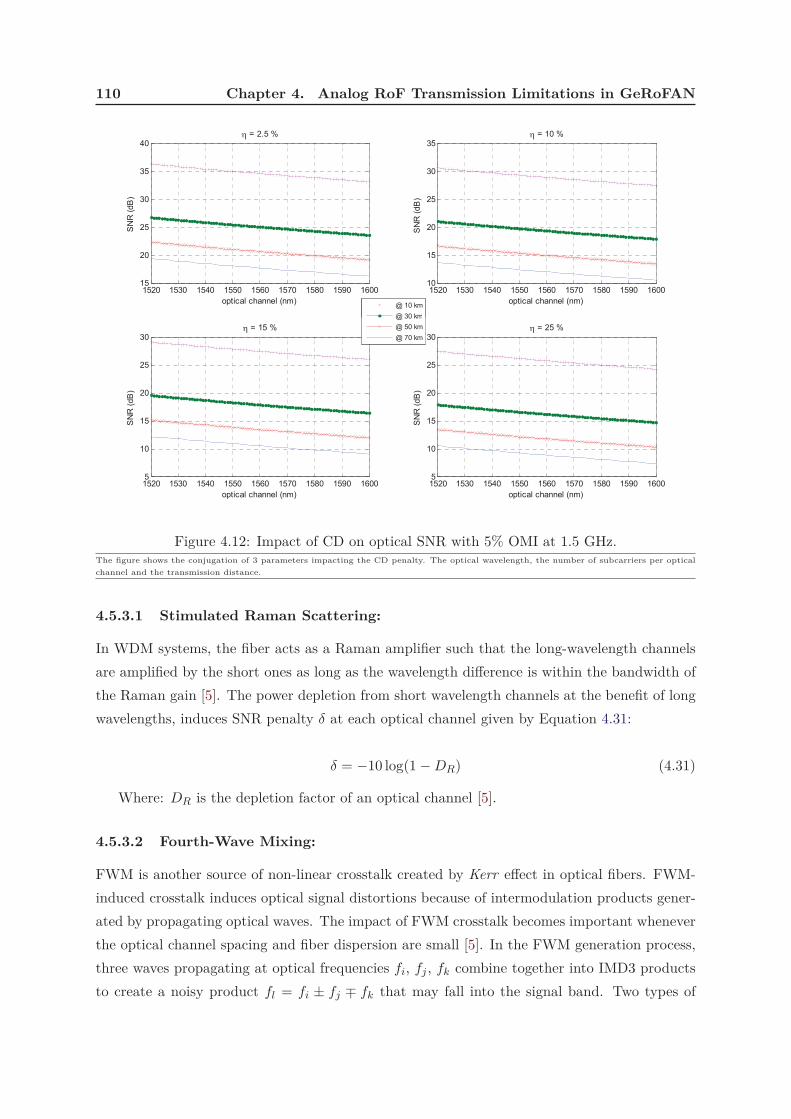
110 Chapter 4. Analog RoF Transmission Limitations in GeRoFAN
1520 1530 1540 1550 1560 1570 1580 1590 160015
20
25
30
35
40
optical channel (nm)
SN
R (
dB
) = 2.5 %
1520 1530 1540 1550 1560 1570 1580 1590 160010
15
20
25
30
35
optical channel (nm)
SN
R (
dB
)
= 10 %
@ 10 km
@ 30 km
1520 1530 1540 1550 1560 1570 1580 1590 16005
10
15
20
25
30
optical channel (nm)
SN
R (
dB
)
= 15 %
1520 1530 1540 1550 1560 1570 1580 1590 16005
10
15
20
25
30
optical channel (nm)
SN
R (
dB
)
= 25 %
@ 30 km
@ 50 km
@ 70 km
Figure 4.12: Impact of CD on optical SNR with 5% OMI at 1.5 GHz.The figure shows the conjugation of 3 parameters impacting the CD penalty. The optical wavelength, the number of subcarriers per optical
channel and the transmission distance.
4.5.3.1 Stimulated Raman Scattering:
In WDM systems, the fiber acts as a Raman amplifier such that the long-wavelength channels
are amplified by the short ones as long as the wavelength difference is within the bandwidth of
the Raman gain [5]. The power depletion from short wavelength channels at the benefit of long
wavelengths, induces SNR penalty δ at each optical channel given by Equation 4.31:
δ = −10 log(1− DR) (4.31)
Where: DR is the depletion factor of an optical channel [5].
4.5.3.2 Fourth-Wave Mixing:
FWM is another source of non-linear crosstalk created by Kerr effect in optical fibers. FWM-
induced crosstalk induces optical signal distortions because of intermodulation products gener-
ated by propagating optical waves. The impact of FWM crosstalk becomes important whenever
the optical channel spacing and fiber dispersion are small [5]. In the FWM generation process,
three waves propagating at optical frequencies fi, fj , fk combine together into IMD3 products
to create a noisy product fl = fi ± fj ∓ fk that may fall into the signal band. Two types of

4.5. Fiber impairments 111
FWM products are distinguished: degenerate (2 tones) and non-degenerate (3 tones) products.
Assuming the worst case scenario where the phase mismatch between optical waves tends to 0,
the variance of a single FWM product is given by [66] and expressed in Equation 4.32:
σF W M2 =
(γ · M · Ddeg
3· 1− exp(−αL)
α
)2
PiPjPk (4.32)
Given: Ddeg: the degeneracy factor equals to 6 and 3 for non-degenerate and degenerate
FWM products respectively; γ, α : the fiber non-linear and attenuation coefficient respectively;
M : the number of traversed SOAs along the optical lightpath; and Pi, Pj , Pk: the average
input optical power at channels i, j and k.
4.5.4 Rayleigh Back-Scattering
Rayleigh Back-Scattering (RBS) is particularly pointed out in bidirectional reflective transmis-
sion systems such as PONs [59]. RBS noise occurs when the Rayleigh back-scattered incident
wave, caused by microscopic non-homogeneities of the fiber material, interferes with the re-
flected modulated optical wave. RBS results in signal power instabilities and in-band crosstalk
causing degradation of the receiver sensitivity. The impact of RBS increases with the propa-
gation inducing a limitation on the fiber length [63]. Some solutions are suggested to reduce
the impact of RBS including: additional phase modulation, polarization scrambling and the de-
ployment of low coherence light sources, while in [144] a proposed method is based on adjusting
the modulator bias current/voltage.
Following the analytical approach in [148], we provide in Equation A.26 the mathematical
expression of RBS Power Spectral Density (PSD) evaluated along an optical link of length L:
Nrbs(f) =10R2
rb(2aL+ e−2aL − 1)
9· F〈|Rεsig |2〉 (4.33)
Given: Rεsig : The autocorrelation function of the signal electric field εsig; a: Fiber attenu-
ation coefficient; Rrb: RBS reflectance of the SMF and F: denotes the Fourier transformation
operator. The mathematical development of Equation A.26 is detailed in the Appendix.
4.5.5 Optical Beat Interference
In a WDM-PON system, two upstream OCs with the same wavelength may be modulated
by distinct radio signals at RFs i and j, then combined at the optical coupler and detected.
Because of the square-law of the detection process, the beating between the OCs generates
IMD-like interference between their subcarrier RF channels that may fall on a designated RF
channel ℓ = 2i±j. The frequency spectrum of the interference term is determined by convolving
the frequency spectra of the OCs. The PSD of the OC at the output of the DFB laser is
approximated by a Lorentzian function with a line-width broadened by the frequency chirp of

112 Chapter 4. Analog RoF Transmission Limitations in GeRoFAN
the RAM. Following the development in [37], we express the Signal to Interference Ratio (SIR)
defined as the ratio of the signal power to the OBI noise power falling within the bandwidth of
RF channel ℓ as:
SIR =12〈m2
ℓP 2o,ℓ〉∫
BℓNij(f) df
(4.34)
The PSD of the OBI noise due to the beating of OCs i and j is provided by Equation 4.35:
Nij(f) = 4√
Po,iPo,j ·√
f(Vi)f(Vj) · | cos(Φ)| · (Si(f)⊗ Sj(f)) · 〈cos2 θij〉 (4.35)
Given: mℓ: the OMI of RF channel ℓ; Bℓ: the bandwidth of RF channel ℓ; Sk(f): The
Lorentzian PSD of the electric field of OC modulated by RF k. Po,k: Received optical power
of OC modulated by RF k; Φ: the phase difference between the two optical carriers; θij : the
difference in polarization angle between fields i and j; ⊗: Convolution operator; 〈·〉: Time
average operator.
The analytical development of the OBI noise is detailed in the Appendix. The optical
power of OBI-induced IMD3 noise falling on frequency fℓ = 2fi − fj is given by Equation A.37:
Nobiℓ =
dgdV
∣∣∣Vb
· d2gdV 2
∣∣∣Vb
4· V 2
b ·√
Po,iPo,j · m2i mj · | cos(Φ)| ·
fℓ+Bℓ/2∫
fℓ−Bℓ/2
F (f − fℓ)df (4.36)
Given: g =√f : the root square of then EAM transfer function f; mi and mj : the OMI
of RF channels i and j respectively; F (·): the Lorentzian distribution function detailed in the
Appendix.
4.5.6 Other impairments
Apart RoF modulator, ROADM and fiber induced impairments, our QoT modeling include also
receiver noises and other miscellaneous system penalties.
4.5.6.1 Receiver noises
Virtually all photo-detectors in use are based on the PIN structure. The main devices are:
Avalanche Photo-Diode (APD) that provides a higher gain due to the avalanche effect, photo-
conductors and direct illumination of phototransistors.
Photo-detectors offer a 3 dB bandwidth that is large enough to accommodate most link
applications ranging from 10 GHz to more than 100 GHz. Meanwhile, such a high bandwidth
comes at the expense of lower fiber-coupled responsivities especially at higher frequencies for
which up to 20.4 dB contribution to the RF link loss is reported [30]. Another tradeoff is be-
tween linearity and optical power. Photodiode non-linearities are due to absorption saturation,

4.5. Fiber impairments 113
electric field screening due to an external circuit effect, or a space charge in the intrinsic layer
[72]. Operating at high optical powers, increases the power density at the photodiode junction
especially for photo-detectors with small illuminated surface, thus increasing the risk of non-
linearities. Although for low-frequencies, photo-detectors are nearly ideal (responsivity, power
handling and linearity), issues raise at higher frequencies. At these frequencies, the conflict
linearity/power density can be reduced either by increasing the bias current or by changing the
illumination geometry of the device as the case in edge-illuminated photo-detectors [30].
In the following, because the target application is remote antenna fiber optic link backhaul-
ing, photodiode non-linearities are neglected [72]. Indeed, at the receiver side, three main noise
sources are expected to degrade the carrier-to-noise ratio: the thermal noise, the shot noise, the
dark noise. While the thermal noise is common to any optoelectronic device, shot noise and
dark noise are specific to the photo detection process of optical receivers.
• Thermal noise: Thermal noise of the receiver is modeled as a white noise process. The
signal is quantified by the modulation depth m and a photocurrent Io. The thermal white
noise is relative to the ambient temperature and the noise factor of the receiver. The noise
factor can be modeled through an equivalent noise current density iN over the bandwidth
Be of the electrical filter. The CNR is expressed according to Equation 4.37:
CNRT h =m2I2o2i2N Be
(4.37)
• Shot noise: Shot noise occurs because the light is composed of discrete packets of energy
bursts of photons. The randomness of the arrival time of each photon generates a random
noisiness in the current at the output of the photodiode. Shot noise can be considered as
a white noise process and its associated CNR is computed through [6]. Let qe stands for
the electron charge. In case of APD diode, qe equals to M times the electron charge since
a single photon is expected to generate M electrons thanks to the avalanche effect. The
expression of the CNR is given by Equation 4.38:
CNRsh =m2I2o2qeIoBe
(4.38)
• Dark noise: Dark noise is constant over the electric bandwidth of the signal. The dark noisecurrent density expressed in A/Hz is specified for a given photo-diode. To get the dark
noise over the signal bandwidth, the noise current density is simply multiplied by the
electrical bandwidth of the RF signal.
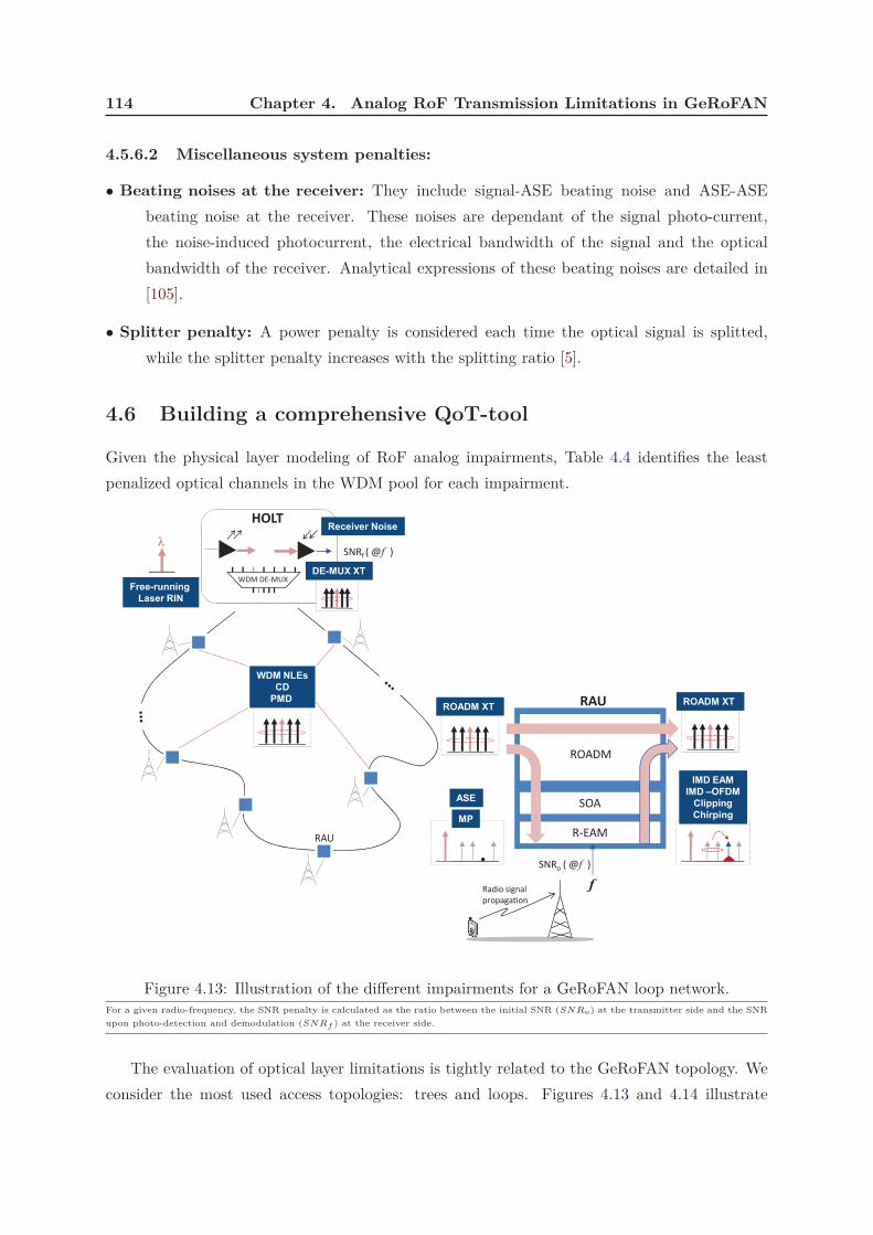
114 Chapter 4. Analog RoF Transmission Limitations in GeRoFAN
4.5.6.2 Miscellaneous system penalties:
• Beating noises at the receiver: They include signal-ASE beating noise and ASE-ASE
beating noise at the receiver. These noises are dependant of the signal photo-current,
the noise-induced photocurrent, the electrical bandwidth of the signal and the optical
bandwidth of the receiver. Analytical expressions of these beating noises are detailed in
[105].
• Splitter penalty: A power penalty is considered each time the optical signal is splitted,
while the splitter penalty increases with the splitting ratio [5].
4.6 Building a comprehensive QoT-tool
Given the physical layer modeling of RoF analog impairments, Table 4.4 identifies the least
penalized optical channels in the WDM pool for each impairment.
WDM DE-MUX
HOLT
Free-running Laser RIN
ROADM XT ROADM XT
DE-MUX XT
WDM NLEsCD
PMD
Receiver Noise
RAU
SNRf ( @f )
R-EAM
SOA
ROADM
SNRo ( @f )
f
MP
ASE
IMD EAMIMD –OFDM
ClippingChirping
Radio signal
propagation
RAU
Figure 4.13: Illustration of the different impairments for a GeRoFAN loop network.For a given radio-frequency, the SNR penalty is calculated as the ratio between the initial SNR (SNRo) at the transmitter side and the SNR
upon photo-detection and demodulation (SNRf ) at the receiver side.
The evaluation of optical layer limitations is tightly related to the GeRoFAN topology. We
consider the most used access topologies: trees and loops. Figures 4.13 and 4.14 illustrate

4.6. Building a comprehensive QoT-tool 115
WDM DE-MUX
HOLT
Free-running Laser RIN
ROADM XT ROADM XT
DE-MUX XT
Receiver Noise
RAU
SNRf ( @f )
OBI NoiseSplitterPenalty
WDM NLEsCD
PMDRBS
R-EAM
SOA
ROADM
SNRo ( @f )
f
MP
ASE IMD –OFDMChirping
Radio signal
propagation
RAU
RBS
Figure 4.14: Illustration of the different impairments for a GeRoFAN tree network.From the RAU until demodulation at the HOLT, the SNR of an uplink radio-frequency is penalized due to several impairments along the
RoF backhauling link.
for each GeRoFAN topology how the different optical impairments considered in our model
cumulate together. Impairments analytical modeling is formulated for both architectures and
packaged into software program called QoT-tool which will be used by the GeRoFAN-CP to
check the SNR relative to a given cellular backhauling strategy. Table 4.5 describes the relevant
QoT impairments for each considered GeRoFAN topology. For each impairment, we highlight
the relevant factors that contribute to impact the SNR. These factors, except Lopt, constitute
the action levers exploited by the control plane of the GeRoFAN system. They include:
• The optical channel: It is represented by its wavelength value [λ] and its relative rank
with respect to the other co-propagating optical channels in the network λi|1···W .
• W : The total number of optical channels per fiber.
• NRF/λ: The number of RF channels transported by the same optical carrier.
• The subcarrier radio channel f : It is represented by its microwave frequency [f ] and
its relative position with respect to other RF channels sharing the same optical carrier

116 Chapter 4. Analog RoF Transmission Limitations in GeRoFAN
Table 4.4: Selection rules of optical channels for each impairment, WDM channels in the C-band
("+" denotes least penalized OCs, "-" denotes most penalized OCs)
Optical carrier (OC) short OCs middle OCs long OCs
Modulation Penalty (MP) - + -
IMD - -/+ +
OADM Homodyne XT, Drop path + +/- -
OADM Homodyne XT, Add path - -/+ +
OADM Homodyne XT, Pass path - + -
Rayleigh Back-Scattering (RBS) + - +
Chromatic Dispersion (CD) + +/- -
WDM NLEs, SRS - -/+ +
Table 4.5: Analog RoF limitations for GeRoFAN loop and tree topologies.
Impairment W [λ] λi|1···W NRF/λ [f ] fi|1···F Lopt Loop Tree
MP10 X X X X X X
IMD11 X X X X X
IMD-OFDM X X X X X X
ROADM-XT12 X X X X X X
OBI X X X X X X
RBS X X X X
CD X X X X X X
NLE13 X X X X X X X
PMD X X X X X
Receiver noises X X X X
Splitter penalty X X
fi|1···F .
• Lopt: The length of the optical link which is constant once the network has been deployed.
Both topologies are subject to common impairments like fiber non-linearities, chromatic
dispersion, polarization mode dispersion and RoF Modulator Penalty (MP). Because of the
cascaded optical carrier modulation in a loop, noise accumulates at each RAU which increases
modulator penalty at each stage. In a tree configuration, a continuous-wave OC is splitted before
getting broadcasted to the RAUs where it will be modulated by RF upstream traffic. Hence
the splitter penalty decreases the SNR of the optical carrier at the input of the modulator. In a
loop topology, RF channels are more prone to interact together within the modulator (through
IMDs) or the ROADM (Heterodyne CrossTalk (XT)). Meanwhile, interaction between RFs in a
10MP designates the noise figure of the RoF link.
11Including IMD-RAM, clipping and chirping. Note that when several RFs modulate the OC at the same RAU, an optical tree topology
is also subject to IMD.12An optical tree is only subject to Homodyne crosstalk.
13Including FWM and SRS impairments.

4.6. Building a comprehensive QoT-tool 117
tree occurs through optical beat interference and eventually within the modulator if several RFs
are present at the same RAU. Finally, only the tree topology may suffer from Rayleigh back-
scattering noise since the incident optical signal and the reflected modulated signal propagate
in opposite directions on the same optical fiber.


Part III
GeRoFAN-CP Algorithmic Design


Chapter 5
Impairment-aware CP Design for
Static Traffic
Contents
5.1 Introduction . . . . . . . . . . . . . . . . . . . . . . . . . . . . . . . . . . . . . . 121
5.2 The cross-layer architecture of the GeRoFAN-CP . . . . . . . . . . . . . . . . 122
5.3 An exact optimization approach for GeRoFAN-CP . . . . . . . . . . . . . . . 123
5.3.1 ILP optimization for GeRoFAN loop . . . . . . . . . . . . . . . . . . . . . . . . . 124
5.3.2 ILP optimization for GeRoFAN tree . . . . . . . . . . . . . . . . . . . . . . . . . 133
5.4 PaGeO: a heuristic approach for GeRoFAN-CP . . . . . . . . . . . . . . . . . 135
5.4.1 PaGeO Algorithm . . . . . . . . . . . . . . . . . . . . . . . . . . . . . . . . . . . 137
5.4.2 Numerical performance of PaGeO . . . . . . . . . . . . . . . . . . . . . . . . . . 140
5.4.3 Alternative heuristic backhauling policies . . . . . . . . . . . . . . . . . . . . . . 142
5.5 Overlaying multiple radio channels per cell site . . . . . . . . . . . . . . . . . 146
5.5.1 Equivalent Bandwidth Loss . . . . . . . . . . . . . . . . . . . . . . . . . . . . . . 148
5.5.2 QoT analysis . . . . . . . . . . . . . . . . . . . . . . . . . . . . . . . . . . . . . . 149
5.6 Summary . . . . . . . . . . . . . . . . . . . . . . . . . . . . . . . . . . . . . . . . 151
5.1 Introduction
As outlined in Chapter 3, the main originality of the GeRoFAN-CP is to be radio MAC-
agnostic to accommodate generically a wide variety of mobile systems. This CP takes into
consideration the impact of signal impairments inherent to RoF transmission. Our objective
is to make the cellular backhauling provided by the GeRoFAN-CP as much as as possible
transparent to the mobile system. In this chapter, we investigate how the backhauling strategy
of the CP can be formulated and solved through an optimization problem. This chapter assumes
a uniform distribution of the traffic load across all cell sites, it is structured as follows. In Section
5.2, we describe the architecture of the GeRoFAN-CP and its interaction with the radio layer.

122 Chapter 5. Impairment-aware CP Design for Static Traffic
Section 5.3 formulates the rationale of the CP through an exact optimization approach. In
Section 5.4, we present an alternative approach based on evolutionary algorithms to solve the
CP optimization problem. Finally, we investigate in Section 5.5 the impact of overlaying several
radio channels per cell site on the system capacity.
5.2 The cross-layer architecture of the GeRoFAN-CP
RF mapping onto
RF cellular planning Mobile
operator
control planeRadio-cell
interference
Ra
dio
mo
bile
te
ch
no
log
y
Optical carrier ( ) selection
RF mapping onto
GeRoFAN
Optical
control plane
IMD/HD
Products
WDM
Crosstalk
in OADMs
ChirpCDSOA
Gain
EAM
MP
Ro
F n
etw
ork
d
om
ain
…
Figure 5.1: The cross-layer architecture of the GeRoFAN-CP.
The GeRoFAN-CP investigates the optimal backhauling strategy that aims at maximizing the
capacity utilization of the optical carrier while minimizing for each RF channel the SNR penalty
that stems from the optical part of the system. Thus, dealing with non-ideal RF front-ends are
out-of-the scope of the GeRoFAN-CP and their effects are assumed to be compensated by the
radio operator at the HOLT. RF front-end devices main impairments include co-channel radio
cellular interference, DC offsets1, I/Q imbalance2, non-linearities of the Power Amplifier (PA),
oscillator frequency drift3 and aperture clock jitter of the ADC/DAC4 [43]. The effects of RF
front-ends can be mitigated from the HOLT by the radio CP through dedicated stabilization
1DC-offset occurs due to self mixing of the signals caused by non-perfect isolation between the LO and the PA at the HOLT for downstream
traffic.2I/Q imbalance denotes the imperfect orthogonality of the in-phase and quadrature components during the complex mixing process. In
today’s commercially available components, the image signal is multiple orders of magnitude weaker than the information carrying signal [43].3Called also Phase Noise, the mixing radio frequency of the LO drifts slightly from its original value due to abrupt small changes of the
controlling voltage, this results in phase distortions of the signal.4In ADC, a clock-driven switch performs the sample-and-hold action by disconnecting quickly the hold capacitor from the input buffer
amplifier. This action requires a short time interval called the aperture time of the ADC. The aperture clock jitter designates commonly the
variation of the aperture time from one sample to another.

5.3. An exact optimization approach for GeRoFAN-CP 123
circuits (DC-offsets, I/Q-imbalance, phase noise of LOs), adequate pre-distortion techniques
(to tackle non-linearities arising from practical PAs5), Peak-to-Average Power Ratio (PAPR)
reduction techniques6 and more efficient radio planning schemes7 (to mitigate radio-cell inter-
ference). Particular coding and bit-interleaving techniques can help compensate RF front-end
impairments. The different aforementioned RF front-end impairment compensation techniques
require either a processing at the level of the individual connection (radio packet scale) or play-
ing with the radio specifications of the cellular system (like those based on power control), which
make them definitely out-of-scope of the GeRoFAN-CP.
Although mitigating radio cellular interference is the responsibility of the radio operator,
the GeRoFAN-CP acquires the quality of the radio channel at the input of the antenna (for
uplink channel) to apply the appropriate optical transport policy. For instance, according to the
Signal to Interference Noise Ratio (SINR) of the uplink RF channel received by the antenna, the
GeRoFAN-CP selects the right OCs and elaborates the optimal mapping of RFs onto OCs such
that the RF channel upon reception at the HOLT undergoes the lowest degradation to guarantee
a successful demodulation. The interaction between the radio layer and the GeRoFAN-CP
(optical) layer is illustrated in Figure 5.1.
f2f1 f3 f4
Figure 5.2: A 4 frequency reuse planning.
Carrier radio frequency 2.5 GHz
Radio channel bandwidth [133] 5 MHz
UE RF transmit power +10 dBm
Inter-RAU distance√3 · 500 m
User location @250 m
Pathloss exponent 3.65
(Log-distr.) Shadowing variance 3 dB
Free-space propagation loss 25.5 dB
Antenna isotropic RF gain 15 dBi
RF amplifier gain 15 dB
RF amplifier noise figure 5 dB
Noise power per OFDM SC −140 dBm
Table 5.1: LTE radio parameters.
5.3 An exact optimization approach for GeRoFAN-CP
To investigate the feasibility and the ultimate gain of the GeRoFAN-CP backhauling strategy, we
propose to formulate the optimal RF-onto-OCs mapping by a Mixed-Integer Linear Programm
(MILP). The MILP performs an exact combinatorial optimization through the finite discrete
search space. While an MILP insures the optimality of the backhauling solution, the main
5Non-linearity of the PA/LNA can be mitigated also by reducing the peak-to-average power ratio of the OFDM signal.6Many methods have been proposed to reduce the PAPR including clipping, constellation extension, and Partial Transmit Sequence (PTS)
with or without feedback side information from the receiver [81].7Like Fractional Frequency Reuse or Two Level Power Control frequency reuse schemes [65].

124 Chapter 5. Impairment-aware CP Design for Static Traffic
difficulty raises from its scalability with the size of the problem due to an increase of the
number of radio-cells, the size of the optical pool or the complexity of the radio planning. To
make the optimization tractable, we consider for this section a 20-cells radio network, with a
cellular planning of four RFs reused regularly across the network as illustrated in Figure 5.2,
while at the optical layer we assume a WDM pool of 11 OCs whose wavelengths range from 1532
nm to 1562 nm with 3 nm channel spacing. The second main challenge raised by the MILP
is the linearity of its constraints to get the problem solved. Since several QoT impairments
modeled in Chapter 4 are intrinsically non-linear, only a subset of these impairments can be
included in the MILP formulation. The MILP considers impairments which are either linear,
linearizable or that can be accounted by their asymptotic values8. In the following subsections,
we provide the MILP formulation when a GeRoFAN loop and tree are considered.
5.3.1 ILP optimization for GeRoFAN loop
5.3.1.1 Modeling RAU operating modes
(+fi, +fk)(+fi)
mode-A RAU
SOA
EAM
ADDDROP
SOAfi fkfi
(+fi)(CW)
mode-C RAU
SOA
EAM
ADDDROP
SOA
fi
(+fi)(+fi)
SOA
EAM
SOA
fi fi
PASS-THROUGH
mode-B RAU
fk fi
(a) Modeling RAU operating modes.
HOLT HOLTmode-B
RAU
mode-B
RAU
mode-B
RAU
mode-C
RAU
mode-B
RAU
mode-B
RAU
mode-A
RAU… … …
fi fk
fi fi fk
(b) An example of lightpath build as cascaded RAUs as seen by RF fi.
Figure 5.3: Lightpath modeled as a cascade of RAU operating modes.
When an optical loop is deployed to backhaul the radio cells, the GeRoFAN system can be
modeled as a cascade of several RAUs connected by fiber segments. At each RAU, the composite
8Unlike the heuristic approach presented later, the MILP uses asymptotic values instead of the exact value of the impairment penalty
because the MILP does not call the QoT-tool during the optimization procedure.

5.3. An exact optimization approach for GeRoFAN-CP 125
radio/optical signal undergoes one of the three operating modes of an RAU as illustrated by
Figure 5.3a. At a given RAU, the SNR penalty can be evaluated as a function of the various
physical impairments and their interaction; the impact of a given impairment being either
magnified or dominated by another impairment. Given the SNR penalty due to each operating
mode, one can estimate the overall penalty of an RF channel along the optical loop. The three
operating modes of an RAU are:
• Passing-through the RAU (Mode-A): An optical carrier λ, previously modulated by fi,
is first dropped by the ROADM before being modulated by an another RF fk and then re-
inserted in the optical loop. In this case, fi is subject to the add/drop penalties of the ROADM
and the absorption/amplification penalties of the REAMSOA.
• Modulation in the RAU (Mode-C): This is the case of fk in the previous example. The
RF fk is subject to the absorption/amplification penalties of the REAMSOA as well as the add
penalty of the ROADM.
• By-passing the RAU (Mode-B): Finally, an optical carrier λ, previously modulated by fi,
may bypass the RAU without any modulation. Only the pass-through penalty of the ROADM
is expected to impact the signal quality of fi.
Figure 5.3b depicts an example where RF fi undergoes the three different operating modes
when it traverses the cascaded RAUs along the loop. It is worth noting that a given radio
channel fi undergoes, along the GeRoFAN optical loop, only a single Mode-C RAU (where
it modulates the OC), but many Mode-B RAUs (where its optical carrier passes-through the
ROADMs) and some few Mode-A RAUs.
5.3.1.2 SNR penalty
When the RAU operates in Mode-C, the impact of the modulator on the RF signal quality
is crucial. Indeed, the SNR degradation due to the REAMSOA is twofold: the penalty due
to the modulation itself and the signal distortion due to the non-linear transfer function of
the modulator. On one hand, the modulation efficiency depends on the SNR of the optical
carrier at the input of the modulator and decreases with the number of hops [99]. On the
other hand, the non-linearity of the REAMSOA induces signal in-band distortions caused by
the beating between the OFDM sub-carriers composing an LTE RF channel [100]. This beating
noise increases with the power of the modulated optical carrier.
In a WDM GeRoFAN loop, a large number of RAUs operate in Mode-B with regard to a
given OC. Thus, we investigate, in a first step, the impact of the number of consecutive Mode-B
RAUs traversed by a given OC before being modulated again at an RAU (Mode-A).

126 Chapter 5. Impairment-aware CP Design for Static Traffic
1.5
2
2.5
en
alty (
dB
)
Overall SNR Penalty
Modulation Penalty
Inband Distortion Penalty
0 1 2 3 4 5 6 7 8 9 10 11 12 13 14 15 16 17 180
0.5
1
Number of "Mode-B" RAUs before RF modulation (@ = 1550nm, 2GHz)
SN
R P
e
Figure 5.4: SNR penalty vs. the number of Mode-B RAUs.
Figure 5.4 illustrates the overall SNR penalty observed by the transported RF channels at the
output of a Mode-A RAU vs. the number of previously traversed Mode-B RAUs. One notices
the non-monotonicity of the overall SNR penalty. This can be explained by the interaction
of the two SNR degradations of the REAMSOA. As the number of traversed Mode-B RAUs
increases, the power and the SNR of the optical carrier, at the input of the modulator of Mode-
A RAU, decrease (no amplification being carried out). On one hand, the modulation penalty
increases as the SNR of the optical carrier decreases. On the other hand, the modulator non-
linear distortion decreases as the optical power decreases. The overall penalty is dominated by
one of the aforementioned penalties with an optimal region where the overall penalty is kept
under a predefined threshold. This region delimitates a range of traversed Mode-B RAUs before
a modulation could be performed. In a second step, we investigate the SNR penalty9 induced
by a single Mode-B RAU with respect to the optical channel rank. GeRoFAN loops with W =
8, 10, 12, and 16 wavelengths respectively are considered and their penalties are illustrated in
Figure 5.5. The lowest penalty is observed at the central wavelength of the considered optical
pool. Moreover, the SNR penalty increases with the number of OCs W .
9The penalty accounts for the homodyne optical crosstalk when the OC passes-through the ROADM.
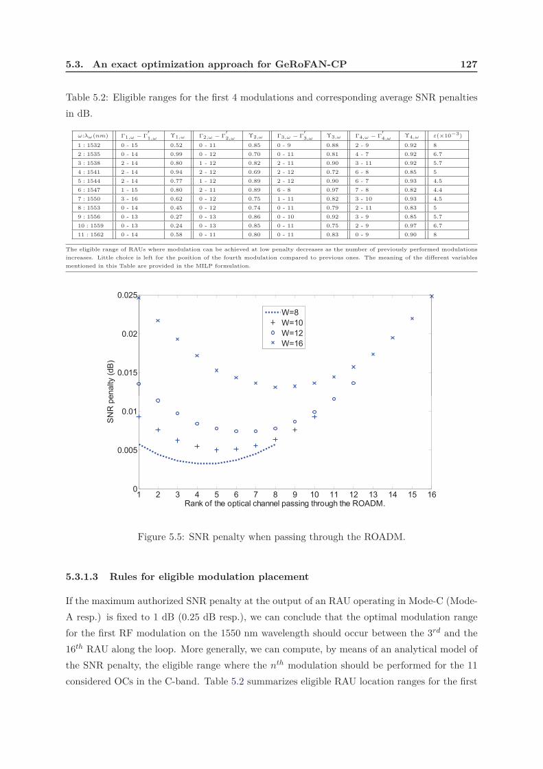
5.3. An exact optimization approach for GeRoFAN-CP 127
Table 5.2: Eligible ranges for the first 4 modulations and corresponding average SNR penalties
in dB.
ω:λω(nm) Γ1,ω − Γ′
1,ωΥ1,ω Γ2,ω − Γ
′
2,ωΥ2,ω Γ3,ω − Γ
′
3,ωΥ3,ω Γ4,ω − Γ
′
4,ωΥ4,ω ε(×10−3)
1 : 1532 0 - 15 0.52 0 - 11 0.85 0 - 9 0.88 2 - 9 0.92 8
2 : 1535 0 - 14 0.99 0 - 12 0.70 0 - 11 0.81 4 - 7 0.92 6.7
3 : 1538 2 - 14 0.80 1 - 12 0.82 2 - 11 0.90 3 - 11 0.92 5.7
4 : 1541 2 - 14 0.94 2 - 12 0.69 2 - 12 0.72 6 - 8 0.85 5
5 : 1544 2 - 14 0.77 1 - 12 0.89 2 - 12 0.90 6 - 7 0.93 4.5
6 : 1547 1 - 15 0.80 2 - 11 0.89 6 - 8 0.97 7 - 8 0.82 4.4
7 : 1550 3 - 16 0.62 0 - 12 0.75 1 - 11 0.82 3 - 10 0.93 4.5
8 : 1553 0 - 14 0.45 0 - 12 0.74 0 - 11 0.79 2 - 11 0.83 5
9 : 1556 0 - 13 0.27 0 - 13 0.86 0 - 10 0.92 3 - 9 0.85 5.7
10 : 1559 0 - 13 0.24 0 - 13 0.85 0 - 11 0.75 2 - 9 0.97 6.7
11 : 1562 0 - 14 0.58 0 - 11 0.80 0 - 11 0.83 0 - 9 0.90 8
The eligible range of RAUs where modulation can be achieved at low penalty decreases as the number of previously performed modulations
increases. Little choice is left for the position of the fourth modulation compared to previous ones. The meaning of the different variables
mentioned in this Table are provided in the MILP formulation.
0.015
0.02
0.025
enalty
(dB
)
W=8
W=10
W=12
W=16
1 2 3 4 5 6 7 8 9 10 11 12 13 14 15 160
0.005
0.01
Rank of the optical channel passing through the ROADM.
SN
R p
e
Figure 5.5: SNR penalty when passing through the ROADM.
5.3.1.3 Rules for eligible modulation placement
If the maximum authorized SNR penalty at the output of an RAU operating in Mode-C (Mode-
A resp.) is fixed to 1 dB (0.25 dB resp.), we can conclude that the optimal modulation range
for the first RF modulation on the 1550 nm wavelength should occur between the 3rd and the
16th RAU along the loop. More generally, we can compute, by means of an analytical model of
the SNR penalty, the eligible range where the nth modulation should be performed for the 11
considered OCs in the C-band. Table 5.2 summarizes eligible RAU location ranges for the first

128 Chapter 5. Impairment-aware CP Design for Static Traffic
four RF modulations and their induced SNR penalties.
5.3.1.4 Mathematical formulation
We formulate the MILP using the following parameters:
• The number N of radio cells and W the maximum number of OCs in the GeRoFAN system.
• The number F of frequencies used in the considered cellular system.
• The maximum number I of RFs that modulate a single OC (I ≤ F ). The value of I is
constrained by the penalties due to the different RAU operating modes of GeRoFAN.
• Subscripts/indices n = 1 · · · N , ω = 1 · · · W , j = 1 · · · F and i = 1 · · · I.
• According to Table 5.2, let Γi,ω and Γ′i,ω be respectively the minimum and maximum number
of operating Mode-B RAUs that OC ω can tolerate after the ith modulation.
• Υi,ω: the SNR penalty incurred by the RF channel modulated onto OC ω as the ith modula-
tion.
• ε: the SNR penalty incurred by any RF modulated onto OC ω when it passes-through an
RAU.
• ξω: the additional SNR penalty incurred by any RF modulated onto ω when it bypasses a
single RAU after the last modulation.
• n,j : a binary parameter representing the radio-mobile cellular deployment. n,j = 1, if the
RF fj is used at cell n. n,j = 0, otherwise.
• A large number M ≫ 1 used to linearize some constraints.
The ILP optimizes the following variables:
• The binary variables yi,n,ω. yi,n,ω = 1, if the RF of the nth cell is modulated onto ω as the
ith modulation. yi,n,ω = 0, otherwise.
• The binary variables ηn,ω. ηn,ω = 1, if the RF of the nth cell is modulated onto ω. ηn,ω = 0,
otherwise.
• The non-negative integer variables xi,ω representing the consecutive number of RAUs that are
bypassed by ω before the ith modulation. If ω is not modulated for the ith time, xi,ω = 0.
• The non-negative integer variables δω representing the consecutive number of RAUs that are
bypassed by the wavelength ω after the last modulation. If ω has never been modulated, δω = 0.
• The binary variables θi,ω. θi,ω = 1, if ω has been dropped at an ROADM for the ith time.
θi,ω = 0, otherwise.

5.3. An exact optimization approach for GeRoFAN-CP 129
• The non-negative integer variables ϑn,ω denoting the number of additional modulations carried
out by ω after the jth cell.
• The binary variables µi,ω and the non-negative real variables n,ω both used for intermediate
calculation.
• The non-negative real variables πn,ω representing the penalty that will be induced by the RF
of the nth cell if it modulates OC ω.
• The non-negative real variables Πn stands for the total SNR penalty computed at the nth
cell.
The ILP is solved subject to the following constraints:
• Each cell must modulate a single OC. ∀n = 1 · · · N ,
I∑
i=1
W∑
ω=1
yi,n,ω = 1 (5.1)
• Constraint 5.1 is consolidated by these redundant equations:
∀n = 1 · · · N W∑
ω=1
yi,n,ω 6 1∀i = 1 · · · I
(5.2)
∀n = 1 · · · N I∑
i=1
yi,n,ω 6 1∀ω = 1 · · · W
(5.3)
I∑
i=1
N∑
n=1
W∑
ω=1
yi,n,ω = N (5.4)
• The relation between ηn,ω and yi,n,ω is given by: ∀n = 1 · · · N , ∀ω = 1 · · · W ,
µn,ω =I∑
i=1
yi,n,ω (5.5)
• The variables θi,ω are related to yi,n,ω by: ∀i = 1 · · · I, ∀ω = 1 · · · W ,
θi,ω =N∑
n=1
yi,n,ω (5.6)
• An OC can not be modulated for the ith time if it was not modulated before.
θi,ω 6 θi−1,ω (5.7)
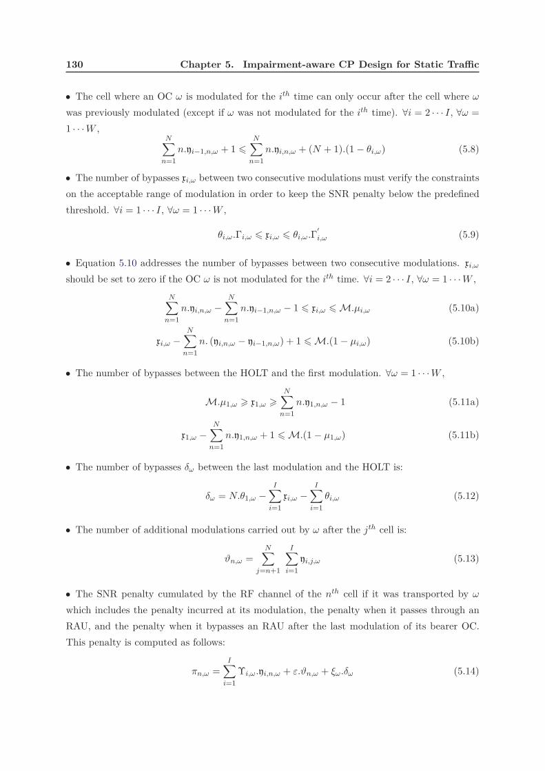
130 Chapter 5. Impairment-aware CP Design for Static Traffic
• The cell where an OC ω is modulated for the ith time can only occur after the cell where ω
was previously modulated (except if ω was not modulated for the ith time). ∀i = 2 · · · I, ∀ω =
1 · · · W ,N∑
n=1
n.yi−1,n,ω + 1 6N∑
n=1
n.yi,n,ω + (N + 1).(1− θi,ω) (5.8)
• The number of bypasses xi,ω between two consecutive modulations must verify the constraints
on the acceptable range of modulation in order to keep the SNR penalty below the predefined
threshold. ∀i = 1 · · · I, ∀ω = 1 · · · W ,
θi,ω.Γi,ω 6 xi,ω 6 θi,ω.Γ′i,ω (5.9)
• Equation 5.10 addresses the number of bypasses between two consecutive modulations. xi,ω
should be set to zero if the OC ω is not modulated for the ith time. ∀i = 2 · · · I, ∀ω = 1 · · · W ,
N∑
n=1
n.yi,n,ω −N∑
n=1
n.yi−1,n,ω − 1 6 xi,ω 6 M.µi,ω (5.10a)
xi,ω −N∑
n=1
n. (yi,n,ω − yi−1,n,ω) + 1 6 M.(1− µi,ω) (5.10b)
• The number of bypasses between the HOLT and the first modulation. ∀ω = 1 · · · W ,
M.µ1,ω > x1,ω >
N∑
n=1
n.y1,n,ω − 1 (5.11a)
x1,ω −N∑
n=1
n.y1,n,ω + 1 6 M.(1− µ1,ω) (5.11b)
• The number of bypasses δω between the last modulation and the HOLT is:
δω = N.θ1,ω −I∑
i=1
xi,ω −I∑
i=1
θi,ω (5.12)
• The number of additional modulations carried out by ω after the jth cell is:
ϑn,ω =N∑
j=n+1
I∑
i=1
yi,j,ω (5.13)
• The SNR penalty cumulated by the RF channel of the nth cell if it was transported by ω
which includes the penalty incurred at its modulation, the penalty when it passes through an
RAU, and the penalty when it bypasses an RAU after the last modulation of its bearer OC.
This penalty is computed as follows:
πn,ω =I∑
i=1
Υi,ω.yi,n,ω + ε.ϑn,ω + ξω.δω (5.14)

5.3. An exact optimization approach for GeRoFAN-CP 131
• The SNR penalty incurred by the RF channel of the nth cell: ∀n = 1 · · · N ,
Πn =W∑
ω=1
n,ω =W∑
ω=1
πn,ω.ηn,ω (5.15)
• The variable n,ω is the product of the two variables πn,ω and ηn,ω, and can be equivalently
expressed as the minimum of πn,ω and M.ηn,ω. This latter expression can be formulated linearly
as: ∀n = 1 · · · N , ∀ω = 1 · · · W ,
n,ω 6 πn,ω (5.16a)
n,ω 6 M.ηn,ω (5.16b)
n,ω − πn,ω > M.(ηn,ω − 1) (5.16c)
• The different cells modulated onto the same OC ω can not have the same frequency. ∀ω =
1 · · · W , ∀j = 1 · · · F ,
N∑
n=1
ηn,ω.n,j 6 1 (5.17)
The objective of the GeRoFAN-CP is to:
• minimize the number of used OCs expressed asW∑
ω=1
θ1,ω,
• and minimize the SNR penalty (Πn)∀n=1..N in each cell which minimizes the rejection ratio
of the radio system.

132 Chapter 5. Impairment-aware CP Design for Static Traffic
5.3.1.5 RF-onto-OCs optimal mapping for a loop
6
7
8
9
10
11
required O
Cs
Moderate Traffic Load (60%)
High Traffic Load (90%)
Lower
Bound
OCs Pool Size
3 4 5 6 7 8 9 10 11 12
1
2
3
4
5
Maximum rejection ratio (%)
Num
ber
of
Figure 5.6: Optimal number of required OCs for a target maximum rejection ratio.
Simulations are carried out assuming the LTE cellular system. The noise due to the radio inter-
face (including signal propagation loss, radio noise and cellular interference) is evaluated using
the analytical fluid-based model10 described in [65]. The MILP is run using Cplex programming
solver11 on a 2 GHz CPU machine. The optimization programm runs until an optimal solution
is found12. The capacity of the RF channel is computed using the Shannon’s capacity which is
based on the SINR of the RF channel accounting for both radio and optical degradations. Once
the cell capacity is derived, the rejection ratio of the system is calculated with respect to the
case where no RoF link is used. For the rejection ratio calculation, we assume a voice connection
requesting 32 kbps13. More generally, radio parameters of the simulation are summarized in
Table 5.1. Figure 5.6 provides the evolution of the number of required OCs to meet the target
maximum (averaged over all cells) rejection ratio at moderate (60%) and high (90%) traffic
loads. It does worth noting that with the assumed 4 RFs regular reuse scheme (c.f Figure 5.2),
the lower bound of the number of required OCs is equal to 6.
10Although originally defined for downlink transmission, some parameters of the model are modified (such as the transmit power and radio
shadowing) to make it valid for uplink transmission.11IBM ILOG Cplex optimizer at: www.ibm.com/software
12The MILP iterates until the gap of optimality equals 0%.
13The assumption of a 32 kbps-voice call connection in our model may not change the performance of the optimization algorithm since we
have been dealing with the Shannon’s capacity.
5.3. An exact optimization approach for GeRoFAN-CP 133
5.3.2 ILP optimization for GeRoFAN tree
The formulation of the optimization problem for the case a GeRoFAN tree is simpler compared
to the GeRoFAN loop formulation since an optical tree does not accumulate noises along RAUs,
thus no particular constraints are required on the minimum and maximum range of modula-
tion. The MILP formulation for a GeRoFAN tree considers the following RoF transmission
impairments: the in-band OFDM distortion penalty occurring at the RF and its neighbors, the
modulation penalty, the ROADM crosstalk and the splitter penalty.
5.3.2.1 Mathematical formulation
Unless specified, we consider the same notations adopted in Subsection 5.3.1.4. In addition, we
introduce the following parameters:
• φωn: in-band OFDM distortion penalty occurring on neighboring channels of the RF modu-
lating the OC ω at cell n.
• ϕωn: includes MP, ROADM optical crosstalk and splitter penalties when OC ω is modulated
at cell n.
For a GeRoFAN tree, the MILP is required to solve for the following variables:
• δω = 1 if OC ω is used. δω = 0 otherwise.
• xωn = 1 if OC ω is dropped at cell n. xω
n = 0 otherwise.
• χωn,m = 1 if OC ω is dropped at both cells n and m. χω
n,m = 0 otherwise.
• ζn: non-negative variable standing for the IMD-OFDM SNR penalty at cell n.
• Πn: non-negative variable standing for the total SNR penalty of RFs at cell n.
The objective of the CP for a tree is the same as the previous MILP, i.e.:
• minimize the number of used OCs expressed asW∑
ω=1
δω and;
• minimize (Πn)∀n=1..N that gives the rejection ratio in each cell.
The specific MILP constraints for a GeRoFAN tree are:
• Each cell must modulate a single OC: ∀n = 1..N ,
W∑
ω=1
xωn = 1 (5.18)

134 Chapter 5. Impairment-aware CP Design for Static Traffic
• An OC cannot be modulated twice by the same RF: ∀ω = 1..W , ∀j = 1..F ,
N∑
n=1
xωn · n,j ≤ 1 (5.19)
• δω are related to xωn by: ∀n = 1..N , ∀ω = 1..W ,
xωn ≤ δω ≤
N∑
n=1
xωn (5.20)
• The IMD-OFDM penalty occurring at the right and the left channels of the RF modulating
cell n is: ∀n = 1..N ,
ζn =N∑
m=1mÓ=n
W∑
ω=1
F∑
j=2n,j=1
n,j−1=1
χωn,m · φω
m +N∑
m=1mÓ=n
W∑
ω=1
F −1∑
j=1n,j=1
n,j+1=1
χωn,m · φω
m (5.21)
• The total SNR penalty at cell n is:
Πn = ζn +W∑
ω=1
xωn · ϕω
n (5.22)
8
10
12
14
ctio
n R
atio
(%
)
GeRoFAN Loop
GeRoFAN Tree
6 7 8 9 10 11 0
2
4
6
Number of OCs
Op
tim
al R
eje
c
Figure 5.7: GeRoFAN Tree vs. Loop MILP optimization.
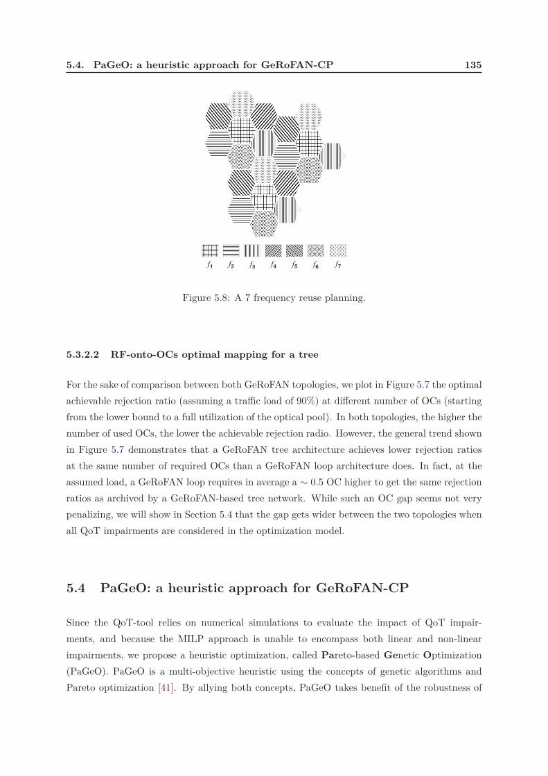
5.4. PaGeO: a heuristic approach for GeRoFAN-CP 135
f1 f2 f3 f4 f5 f6 f7
Figure 5.8: A 7 frequency reuse planning.
5.3.2.2 RF-onto-OCs optimal mapping for a tree
For the sake of comparison between both GeRoFAN topologies, we plot in Figure 5.7 the optimal
achievable rejection ratio (assuming a traffic load of 90%) at different number of OCs (starting
from the lower bound to a full utilization of the optical pool). In both topologies, the higher the
number of used OCs, the lower the achievable rejection radio. However, the general trend shown
in Figure 5.7 demonstrates that a GeRoFAN tree architecture achieves lower rejection ratios
at the same number of required OCs than a GeRoFAN loop architecture does. In fact, at the
assumed load, a GeRoFAN loop requires in average a ∼ 0.5 OC higher to get the same rejection
ratios as archived by a GeRoFAN-based tree network. While such an OC gap seems not very
penalizing, we will show in Section 5.4 that the gap gets wider between the two topologies when
all QoT impairments are considered in the optimization model.
5.4 PaGeO: a heuristic approach for GeRoFAN-CP
Since the QoT-tool relies on numerical simulations to evaluate the impact of QoT impair-
ments, and because the MILP approach is unable to encompass both linear and non-linear
impairments, we propose a heuristic optimization, called Pareto-based Genetic Optimization
(PaGeO). PaGeO is a multi-objective heuristic using the concepts of genetic algorithms and
Pareto optimization [41]. By allying both concepts, PaGeO takes benefit of the robustness of

136 Chapter 5. Impairment-aware CP Design for Static Traffic
evolutionary optimization14 and the compromise ensured by Pareto optimality15.
(1) Ranking & Fitness sharing
Classify the individuals of (Po) into feasible (P) and infeasible (P) individuals
Correct infeasible individuals such that |P| > 4|P|
Evaluate objective value
Dominance-based rankingDominance-based ranking
Evaluate infeasibility measure
feasibleinfeasible
QoT-tool
(1.a)(1.b)
Fitness sharing (Hamming distance)Select F : the Pareto set of P
B : the Pareto set of (F UB)
Stopping criteria reached ?
YesNo
Exit
unfeasible fronts Fi feasible fronts Fi
Fitness sharing (Euclidian distance)
(2) The new population for the next generation
Selecting the mating pool (M ) via binary tournament procedure
Offspring generation (Q) via cross-over operation
Mutation of Q
Elitism: Select elits (i.e., with the best fitness)
Random Immigrants (I)
Complete Q with the remaining individuals randomly from Po\M U
Q Q U U I
Po
Q
E
Figure 5.9: The PaGeO algorithm flowchart.
14Evolutionary optimization are based on the notion of competition between individuals to derive the solution which best-fits the objective
function. Evolutionary algorithms are stochastic meta-heuristics inspired by the same principles of natural evolution, exploiting strategies
like mutation, crossing genes and elitism [41].15The optimal solution for a multi-objective optimization is not a single solution, but a set of solutions called Pareto optimal solutions,
that leaves a greater flexibility for the decision maker to select among the Pareto set, the solution that fits its need. Pareto optimal solutions
represent the compromise solutions between the different conflicting objectives. With the Pareto concept, we do not need to transform the
multi-objective optimization problem into a mono-objective problem by weighing each objective with respect to the other, which like in our
case seems hard to get a fair weighting [41].

5.4. PaGeO: a heuristic approach for GeRoFAN-CP 137
OCs
RF
Cell
Solution Encoding
cell RF OC
1 2 2
2 1 1
3 2 1
A
B
QoT-
tool
Infeasibility
measure
A
B
Selected
Parents
Obj. 2
Obj. 1
Front 1
Front 2
Front 3
sh
At minimum
hamming
distance
Offsprings
Figure 5.10: Illustration of the key steps of PaGeO.
5.4.1 PaGeO Algorithm
The flowchart of PaGeO and its algorithmic parameters are provided in Figure 5.9 and Table
5.3 respectively. In the following, we describe the different steps of the algorithm.
The first population Po is created by generating randomly 100 individuals (i.e. solutions).
A solution x, a.k.a chromosome, is encoded by a 3 dimensional binary matrix [Ψ×Λ×], where
Ψ is the set of cells, Λ the set of OCs and the set of RF channels. The chromosome is defined
as: xi,j,k = 1 if the OC j is used at cell i to transport the RF k; xi,j,k = 0 otherwise.
The multi-objective function that PaGeO optimizes is an objective vector f =

138 Chapter 5. Impairment-aware CP Design for Static Traffic
(f1, ..., f|Ψ|+1
)= ((ρi)i=1..Ψ,Λ⋆ − Λmin) of length |Ψ| + 1, where ρi is the rejection ratio at cell
i, Λ⋆ is the number of used OCs and Λmin is the OCs lower bound.
The randomness of the evolutionary process can lead to some infeasible individuals. Infea-
sible chromosomes are produced each time when the constraints of the optimization problem
(maximum number of RFs carried by an OC, a carrier must not be modulated twice by the
same RF etc.) are violated.
Different strategies are investigated in the literature to handle constraints [78]. In Step
1 of the algorithm, PaGeO splits the current population into two sub-populations: feasible
individuals P and infeasible individuals P. To insure the majority for feasible individuals, some
infeasible chromosomes are corrected by choosing the nearest feasible chromosome according to
the Hamming distance. Feasible chromosomes are treated in Step 1.a by evaluating, via the
QoT-tool developed in Chapter 4, their objective vector. Since several objectives are addressed
at the same time, we use the concept of non-dominated front which is the set of solutions that do
not dominate each other16. This concept is in-line with Pareto optimality. The latter specifies
that for a multi-objective optimization, an improvement on one objective is sacrificed by a
degradation on another one. Following the step-by-step procedure described in [78], different
levels of non-dominated fronts Fi are identified by sweeping iteratively the subpopulation P.
Once solutions are classified into non-dominated fronts, they are ranked according to the
density-based strategy as defined in [78]. To avoid local minima, solutions with the same fitness
(i.e. the same rank) are discriminated using the Euclidian distance-based niche count ncE
(computed as in Table 5.3). A niche count of a given solution is proportional to the number of
solutions located within its immediate neighborhood [23]. Using the niche count, the fitness of
the chromosome is then updated according to Equation (5.23), where y ≻ x denotes chromosome
y dominates x17.
For infeasible chromosomes (Step 1.b), the infeasibility measure, defined as the total number
of violated constraints by an infeasible individual, is used instead of the objective value vector.
Based on the infeasibility measure, infeasible non-dominated fronts Fi are identified and chro-
mosomes are ranked accordingly. To maintain a diverse infeasible population, a niche count
ncH based on the Hamming distance (c.f. Table 5.3) is used to update the ranks of too close
infeasible chromosomes as in Equation (5.23). The population of the next generation is formed
by selecting ξ elite individuals from P. Offsprings Q are produced by crossing, with a probability
pX , the genes of each couple of parents selected from the mating pool M. Individuals of Q are
then mutated with a probability pm. A fraction of immigrants ℑ, made of randomly generatedindividuals, are added to Q in order to increase the diversity of the population.
16Chromosomes x and y do not dominate each other, if and only if, x performs better than y in at least one objective, while y outperforms
x in another one.17Note that y ≻ x, if and only if, fi(y) ≤ fi(x) for i = 1, .., |Ψ| + 1 and fj(y) < fj(x) for at least one objective function j.

5.4. PaGeO: a heuristic approach for GeRoFAN-CP 139
Table 5.3: Parameters setting for PaGeO.
Population size (℘) 100
Parents selection tournament selection strategy [78]
Mating pool (M) size 50% of ℘
Mutation rate pm 0.001 [78]
Cross-over rate pX 0.6 [78]
Immigrants (ℑ) size 25% of ℘
Number of elites (ξ) 5% of ℘
Max. number of generations 1000
Euclidian-based ncE(x)∑
y∈Pr(y)=r(x)
max
σsh − dE(x, y)
σsh, 0
[23]
Hamming-based ncH(x)∑
y∈Pr(y)=r(x)
max
1 − dH(x, y)
σsh, 0
Euclidian distance dE(x, y)
√√√√|Ψ|+1∑
i=1
(fi(x) − fi(y)
fmaxi − fmin
i
)2[23]
Hamming distance dH(x, y)
√√√√|Ψ|∑
i=1
|Λ|∑
j=1
||∑
k=1
(xi,j,k − yi,j,k
)2
Niche radius σsh ≈ 0.44 [78]
Niche radius σsh 2
Threshold δ⋆ 1%
r(x) =
1 +∑
y≻xy∈P
r(y)
ncE(x)if x ∈ P
1 +∑
y≻xy∈P
r(y) +∑
y≻x
y∈P
r(y)
ncH(x)if x ∈ P
(5.23)
The performance of the current generation is evaluated by selecting the Pareto set (F = F1)
of the feasible subpopulation P. A set of Pareto optimal solutions (B) is updated at each
generation with elements of F . Stopping criteria are checked to decide wether to stop or to
continue with the next generation. PaGeO terminates when the maximum generation number
is reached or the lowest relative deviation δ from a targeted objective value vector f⋆18 goes
below a predefined threshold δ⋆. Denoting f the objective function, δ is defined according to
Equation 5.24:
δ = minx∈B|f(x)− f⋆|
|f⋆| (5.24)
The key moments of the PaGeO algorithm are illustrated in Figure 5.10, including: the
representation of the chromosome (genotype: solution encoding), the dispatching of individuals
18The ideal objective vector targets the lower bound in terms of required OCs and the required capacity with an excess ranging from 2%
to 5% as a margin to secure eventual fluctuation of the traffic load.
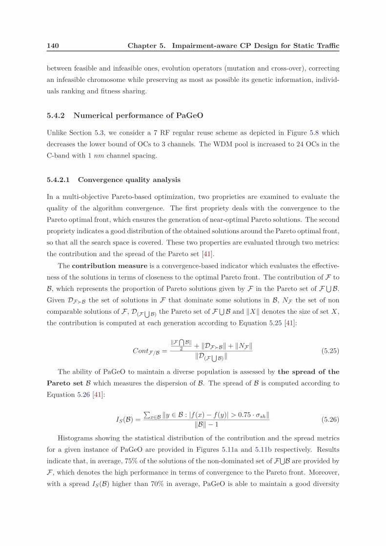
140 Chapter 5. Impairment-aware CP Design for Static Traffic
between feasible and infeasible ones, evolution operators (mutation and cross-over), correcting
an infeasible chromosome while preserving as most as possible its genetic information, individ-
uals ranking and fitness sharing.
5.4.2 Numerical performance of PaGeO
Unlike Section 5.3, we consider a 7 RF regular reuse scheme as depicted in Figure 5.8 which
decreases the lower bound of OCs to 3 channels. The WDM pool is increased to 24 OCs in the
C-band with 1 nm channel spacing.
5.4.2.1 Convergence quality analysis
In a multi-objective Pareto-based optimization, two proprieties are examined to evaluate the
quality of the algorithm convergence. The first propriety deals with the convergence to the
Pareto optimal front, which ensures the generation of near-optimal Pareto solutions. The second
propriety indicates a good distribution of the obtained solutions around the Pareto optimal front,
so that all the search space is covered. These two properties are evaluated through two metrics:
the contribution and the spread of the Pareto set [41].
The contribution measure is a convergence-based indicator which evaluates the effective-
ness of the solutions in terms of closeness to the optimal Pareto front. The contribution of F to
B, which represents the proportion of Pareto solutions given by F in the Pareto set of F ⋃ B.Given DF≻B the set of solutions in F that dominate some solutions in B, NF the set of non
comparable solutions of F , D(F⋃
B) the Pareto set of F ⋃ B and ‖X‖ denotes the size of set X,
the contribution is computed at each generation according to Equation 5.25 [41]:
ContF/B =‖F
⋂B‖
2 + ‖DF≻B‖+ ‖NF‖‖D(F
⋃B)‖
(5.25)
The ability of PaGeO to maintain a diverse population is assessed by the spread of the
Pareto set B which measures the dispersion of B. The spread of B is computed according to
Equation 5.26 [41]:
IS(B) =∑
x∈B ‖y ∈ B : |f(x)− f(y)| > 0.75 · σsh‖‖B‖ − 1 (5.26)
Histograms showing the statistical distribution of the contribution and the spread metrics
for a given instance of PaGeO are provided in Figures 5.11a and 5.11b respectively. Results
indicate that, in average, 75% of the solutions of the non-dominated set of F⋃B are provided by
F , which denotes the high performance in terms of convergence to the Pareto front. Moreover,
with a spread IS(B) higher than 70% in average, PaGeO is able to maintain a good diversity

5.4. PaGeO: a heuristic approach for GeRoFAN-CP 141
of the Pareto set which provides the GeRoFAN manager a large range of (Pareto-)equivalent
solutions.
0.5
0.6
0.7
0.8
0.9
1C
on
t(F
/B)
0 50 100 150 200 250 300 350 400
0.4
Generation Number
(a) PDF of ContF/B. Inset: ContF/B evolving with generations.
0.04
0.05
0.06
0.07
0.08
Inte
nsity
0.5
0.6
0.7
0.8
0.9
1
I S(B
)
0 0.1 0.2 0.3 0.4 0.5 0.6 0.7 0.8 0.9 10
0.01
0.02
0.03
IS(B)
PD
F
0 50 100 150 200 250 300 350 4000.3
0.4
Generation Number
(b) PDF of ISB. Inset: ISB evolving with generations.
Figure 5.11: Convergence quality analysis of PaGeO.

142 Chapter 5. Impairment-aware CP Design for Static Traffic
5.4.2.2 GeRoFAN Tree vs. GeRoFAN Loop
Figure 5.12 shows the rejection ratio achieved by PaGeO as well as the number of required
OCs for GeRoFAN tree and loop topologies. Results indicate the performance superiority of an
optical tree compared to a loop. In terms of rejection ratio, a tree achieves a gain between 25%
at a high traffic load and up to 90% at a moderate load. Significant savings (up to 57%) in terms
of the number of OCs are also reported; with the lower bound of required OCs (equals to 3)
being reached at moderate loads. In fact, the cumulative nature of the noise in an optical loop
induces a higher SNR penalty which leads to a higher loss in the radio capacity. To mitigate
the increasing impact of IMD noises and optical crosstalk, a loop topology has to use more OCs
than a tree.
The comparison between the two topologies is also carried out in terms of QoT profiling
depicted in Figure 5.13. To facilitate the analysis of the share of each physical impairment
in the total SNR penalty for both GeRoFAN topologies, we classify the different noises into
four categories: The first category (Cat.I) designates the modulation penalty (MP), while the
second category (Cat.II) includes all IMDs impairments (IMD-RAM, IMD-OFDM, and OBI).
The third category (Cat.III) gathers all fiber-induced impairments and are sub-categorized as
the following: Cat.III-A for PMD and RBS, Cat.III-B for WDM NLEs and Cat.III-C for CD.
Finally, the fourth category (Cat.IV) encompasses ROADM/AWG optical crosstalk (XT) and
all other GeRoFAN system penalties (mainly the splitter penalty, SOA ASE noise etc.). Figure
5.13 highlights the heavier impact of IMDs on the total SNR penalty in a GeRoFAN loop than
a tree. Due to the cumulative aggregation of noises along RAUs in an optical loop, the QoT
profiling points out a significant increase of the share of MP (Cat.I) and IMDs (Cat.II) in the
total penalty for a loop compared with a tree. Meanwhile, one notices on one hand the decrease
of the share of the fourth category noises (16% for a tree and 11% for a loop) since no splitter
is required for a GeRoFAN loop, and on the other hand the very marginal contribution (< 1%)
of Cat.III-A noises (PMD+RBS) for an optical loop due to the absence of RBS in the SNR
penalty calculations.
5.4.3 Alternative heuristic backhauling policies
Since we demonstrated that a tree topology outperforms a loop topology, the following investi-
gations assumes an optical tree for the GeRoFAN system.
To evaluate the benefit of the cross-optimization achieved by the GeRoFAN-CP, we compare
PaGeO with four cellular backhauling policies, namely:

5.4. PaGeO: a heuristic approach for GeRoFAN-CP 143
10
15
20
rati
o (
%)
ed
OC
s
5
6
7
8
9
10rejection ratio, tree
required OCs, loop
rejection ratio, loop
required OCs, tree
-5
0
5
reje
cti
on
Cell load (%)
Re
qu
ire
50 60 70 80 90 1000
1
2
3
4
5
OCs lower bound
Figure 5.12: Comparison at different traffic loads between GeRoFAN loop and GeRoFAN tree
in terms of rejection ratio (left axis) and number of required OCs (right axis). Error bars stand
for deviation from the mean value. Negative rejection ratios indicate excess capacity beyond
required by the traffic load.
< 1%3%
9%
11%
38% 7%
16%
Cat.I Cat.II Cat.III-A Cat.III-B Cat.III-C Cat.IV
48%
30%
< 1%
25%
11%
2%
GeRoFAN TreeGeRoFAN Loop
Figure 5.13: QoT profiling: Share of each impairment category in the total SNR penalty for
GeRoFAN tree and GeRoFAN Loop.

144 Chapter 5. Impairment-aware CP Design for Static Traffic
Hig
h O
Cs
RCAIM-free CA
QoT- aware QoT-agnostic
Low
OC
s
FFCA FCA
Figure 5.14: A conceptual 2-by-2 matrix positioning of alternative backhauling policies.
• First Channel Assignment (FCA): an RF channel is placed on the first listed available
OC.
• Random Channel Assignment (RCA): an RF channel is placed on a randomly selected
available OC.
• First Fit Channel Assignment (FFCA): an RF channel is assigned to the first listed avail-
able OC that fits the rejection ratio threshold. If no OC is able to meet such a requirement,
the RF placement is iterated with a new relaxed threshold. The pseudo-code of FFCA is
provided in Algorithm 2.
• Intermodulation-free Channel Assignment (IM-free CA): RFs are assigned to the lowest
number of OCs such as IMD3 products are eliminated. To achieve an IMD-free RF
assignment, RF channels are placed according to position marks specified by the Golomb
ruler [13].
Note that FFCA and IM-free CA are QoT-aware backhauling strategies, while FCA and
RCA are QoT-agnostic strategies. Figure 5.14 illustrates the key positioning of the four strate-
gies according to two dimensions: the level of QoT-impairments embedding and the number of
required OCs. In the following, we show how PaGeO gets well positioned at the target square
shadowed in Figure 5.14. The performance of PaGeO are compared with the four backhauling
strategies described previously in terms of rejection ratio and number of required OCs. Numer-
ical results of the comparison are depicted in Figure 5.15 at different network traffic loads. By
bin-packing RFs on the first available channels, FCA achieves by default the lowest number of
required OCs, but at the detriment of the highest level of rejection ratio among all policies. Al-
though being QoT-agnostic, the RCA policy mitigates QoT impairments thanks to the random
selection of OCs and RFs placement, however, this comes at a cost of the highest number of

5.4. PaGeO: a heuristic approach for GeRoFAN-CP 145
Algorithm 2: Pseudo-code of FFCA backhauling policy.
input : N : Set of radio-cells. W : OCs Pool.
output: Λ⋆: Selected OCs for backhauling. (ρn)n=1..N : Rejection ratio at each cell.
// Routine initialization ...
1 ρmax ← 0%;
2 Λ⋆ ← ∅;3 n ← 1;
4 while n ≤ N do
5 Ω ← Set of candidate OCs from W able to carry the RFs of cell n;
6 Select the first listed OC λ⋆ ∈ Ω such that: ∀i = 1..n, ρi ≤ ρmax;
7 if λ⋆ Ó= ∅ then // OC λ⋆ is selected to backhaul RFs of cell n
8 n ← n+ 1;
9 Λ⋆ ← λ⋆;
10 else // OC λ⋆ does not exist
11 n ← 1;
12 Λ⋆ ← ∅;13 ρmax = ρmax + 0.1%; // Relaxing the constraint on ρmax
14 end
15 end
OCs (∼ 70% of the λ-pool). Since it can be considered as the QoT-aware version of FCA, FFCA
consumes in average 3 OCs more than FCA, but at the benefit of lower rejection ratios (up to
85% of decrease compared to FCA). Results show also that we need 7 OCs more than the lower
bound of required OCs to achieve an IM-free RFs backhauling. Compared to FFCA and QoT-
agnostic policies, IM-free CA reduces the rejection ratio by canceling IMDs penalty. However,
the residual values of rejection ratio of IM-free CA, especially at higher loads, show that consum-
ing more OCs to avoid IMDs strengthens some impairments (WDM-NLE, ROADM/DEMUX
XT) whose penalties may increase with the number of used OCs.
Coming to our algorithm, one notices that, among all policies, PaGeO achieves the best
tradeoff between the rejection ratio and the number of required OCs. On one hand, PaGeO
consumes in average 2 OCs lower than FFCA, while achieving 2 times the lower bound (at
moderate load). On the other hand, rejection ratios achieved by PaGeO are close to IM-free
CA. In fact, rejection ratios obtained with IM-free CA show that preventing the occurrence
of IMDs, while ignoring the other impairments (particularly those arising at high number of
OCs), doesn’t suffice to totally preserve the radio capacity. This advocates for a comprehensive
management of all RoF impairments which is achieved by PaGeO while consuming a few of OCs.
Finally, thanks to its multi-objective Pareto optimization, PaGeO achieves its good performance

146 Chapter 5. Impairment-aware CP Design for Static Traffic
60% 70% 80% 90% 100%
0
10
20
30
40
Cell traffic load (%)
Re
jec
tion
ra
tio (
%)
PaGeO
IM-free CA
FFCA
FCA
RCA
60% 70% 80% 90% 100%0
5
10
15
20
25
Cell traffic load (%)
Nu
mb
er
of
req
uir
ed
OC
s
-pool size
Lower
Bound
Figure 5.15: PaGeO vs. Other Policies (RCA, FCA, FFCA, IM-free CA) at different traffic
loads. Error bars stand for deviation from the mean value. Negative rejection ratio means
excess capacity more than the required load.
of rejection ratio more uniformly between radio cells compared to the other policies19.
5.5 Overlaying multiple radio channels per cell site
In the following, we investigate the impact of increasing the number of RFs per radio cell.
Overlaying several radio channels in a cell site is typically observed in real networks when a
mobile operator aims to increase the radio capacity of that cell. However, increasing the number
of radio channels per cell while keeping the same total bandwidth (for instance 5 MHz) in the
cell would not offer more capacity to that cell, instead, doing so provides the mobile operator
with a more flexibility in managing the radio resources between cell sites. In fact, overlaying
more RFs having thinner granularity (smaller bandwidth per RF) within a cell enables to carry
out the radio planning with smaller increments and thus to adjust more suitably the capacity
provided to the cell with respect to its traffic load.
19It can be seen from the length of the standard deviation (STD) bars of PaGeO compared to other policies.
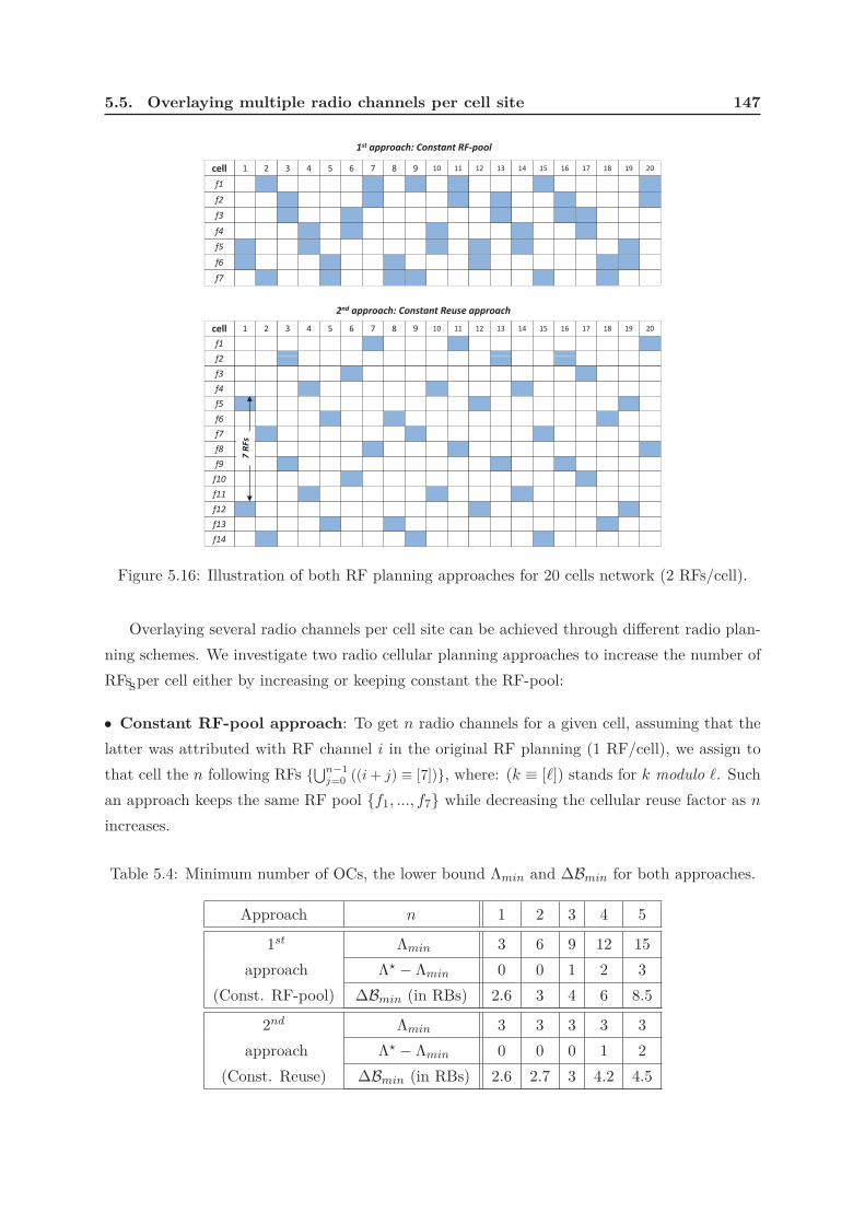
5.5. Overlaying multiple radio channels per cell site 147
1 2 3 4 5 6 7 8 9 10 11 12 13 14 15 16 17 18 19 20cell
f1
f2
f3
f4
f5
f6
f7
1 2 3 4 5 6 7 8 9 10 11 12 13 14 15 16 17 18 19 20cell
f1
f2
1st approach: Constant RF-pool
2nd approach: Constant Reuse approach
f2
f3
f4
f5
f6
f7
f8
f9
f10
f11
f12
f13
f14
7 R
Fs
Figure 5.16: Illustration of both RF planning approaches for 20 cells network (2 RFs/cell).
Overlaying several radio channels per cell site can be achieved through different radio plan-
ning schemes. We investigate two radio cellular planning approaches to increase the number of
RFs per cell either by increasing or keeping constant the RF-pool:s
• Constant RF-pool approach: To get n radio channels for a given cell, assuming that the
latter was attributed with RF channel i in the original RF planning (1 RF/cell), we assign to
that cell the n following RFs ⋃n−1j=0 ((i+ j) ≡ [7]), where: (k ≡ [ℓ]) stands for k modulo ℓ. Such
an approach keeps the same RF pool f1, ..., f7 while decreasing the cellular reuse factor as n
increases.
Table 5.4: Minimum number of OCs, the lower bound Λmin and ∆Bmin for both approaches.
Approach n 1 2 3 4 5
1st Λmin 3 6 9 12 15
approach Λ⋆ − Λmin 0 0 1 2 3
(Const. RF-pool) ∆Bmin (in RBs) 2.6 3 4 6 8.5
2nd Λmin 3 3 3 3 3
approach Λ⋆ − Λmin 0 0 0 1 2
(Const. Reuse) ∆Bmin (in RBs) 2.6 2.7 3 4.2 4.5

148 Chapter 5. Impairment-aware CP Design for Static Traffic
• Constant Frequency Reuse approach: The second approach keeps the same reuse factorwhatever the number of radio channels per cell, but includes new RFs (requested from the radio
broker for instance) thus the size of the RF pool increases as well. To achieve n RFs for a cell
provided with radio channel i in the original RF planning, we assign to that cell the n following
RFs ⋃n−1j=0 (i+ 7× j).
We illustrate both RF cellular planning approaches in Figure 5.16 when two radio channels
are overlaid per cell.
5.5.1 Equivalent Bandwidth Loss
With the increase of RFs per cell, IMDs are expected to increase and radio capacity of the
cell is degraded as well. The capacity loss is converted into bandwidth ∆B, called equivalent
bandwidth loss, which can be interpreted as the amount of "misused" bandwidth [142]. For a
cell with n RF channels each with a bandwidth Bi20, and given ηo
i the spectral efficiency of
the ith RF without RoF and η⋆i the spectral efficiency of the ith RF after the RoF link, EBL is
computed as in Equation (5.27):
∆B =n∑
i=1
Bi · ηoi − η⋆
i
η⋆i
(5.27)
In 4G LTE mobile systems, the concept of Resource Block (RB) is commonly used to
designate the smallest bandwidth unit that can be scheduled for transmission. Given 12 OFDM
SCs (occupying each 15 KHz bandwidth) per RB for LTE uplink transmission, a single RB
occupies thus 180 KHz in the frequency domain [126]. Hence, from a radio operator perspective,
it is more meaningful to express the EBL in terms RBs instead of Hz units
We compare both RF planning approaches by running PaGeO to compute the minimum
number of OCs required to achieve the lowest EBL (∆Bmin).
Results of both approaches, summarized in Table 5.4, show that EBL increases with the
number of RFs per cell. This advocates for reducing the number of RFs per cell to avoid an ex-
cessive EBL, while it’s worth noting that it is easier for an operator to reallocate radio resources
between cells with thin grain RFs capacity. In addition by comparing the two approaches, we
notice a slower increase of the EBL with the number of RFs per cell for the constant RF reuse
approach than the constant RF-pool approach. Since the EBL represents RBs radio spectrum
slices that are definitively lost and cannot longer be allocated to mobile users for traffic trans-
mission, a mobile operator –using GeRoFAN for cellular backhauling– may define a threshold
for the maximum EBL that can be tolerated to achieve a cost-effective network planning. Such
a threshold can be equal to the radio bandwidth overhead specified by the LTE standard which
20Recalling that ∀n,
n∑
i=1
Bi = 5 MHz

5.5. Overlaying multiple radio channels per cell site 149
accounts for the relative guard bands and common/control channels and synchronization for a
given LTE RF channel. Since 5 RBs are required as overhead for a 5 MHz LTE radio channel
according to the LTE standard specifications [133], we deduce that the second approach is more
attractive than the first approach. In fact, with such a threshold, a mobile operator adopting the
constant RF-pool approach can overlay up to 3 RFs per cell while the constant reuse approach
enables to pile up at least 5 RFs per cell without incurring an excessive bandwith loss.
The attractiveness of the second approach compared to the first one is also confirmed by
results of Table 5.4 showing of the evolution of the number of required OCs to achieve∆Bmin. By
increasing the number of RFs per cell, more OCs are needed to achieve the lowest EBL. Unlike
the constant RF pool approach in which the lower bound (Λmin) increases with the number
of RFs per cell, the constant RF reuse approach keeps the same lower bound of required OCs
(Λmin = 3 OCs). We notice also that the number of required OCs increases more slowly for the
second approach than the first approach.
In summary, since a constant RF reuse approach extends the RF-pool to increase the number
of RFs/cell, it is likely to be more expensive for a mobile operator than a constant RF-pool
approach. Meanwhile, as highlighted by the results of Table 5.4 the constant RF reuse approach
is more capacity and OCs-usage efficient than the constant RF-pool approach. Thus, the tradeoff
should lay between both approaches to achieve a cost-effective network planning for the radio
system backhauled by GeRoFAN.
5.5.2 QoT analysis
Figure 5.17 displays the share of each QoT impairment category in the total penalty for the two
approaches. In this figure, the level of the SNR penalty (high penalty or low penalty) is depicted
by the size of its corresponding circle graph for the two RF cellular planning approaches.
In-line with results of Table 5.4, the first approach suffers from higher SNR penalty than
the second one. An increase of the SNR penalty ranging from 12.4% to 83% depending on
the number of RFs/cell is shown in Figure 5.17. For the first approach, MP and 4th category
noises (occupying in average 39% and 24% respectively of the total SNR penalty) are the two
impairments with the highest increase with the number of RFs/cell. In fact, by increasing the
reuse of RFs, the SNR of the RF signal at the input of the RAM is degraded (since radio cellular
interference is increased), increasing de facto the MP. In addition, by requiring more OCs, the
first approach increases NLEs and WDM-XT noises21.
Since it uses lower number of OCs, the second approach packs more RFs onto a single OC,
thus increasing IMD penalty (IMDs contribute with 44.2% in average to the total penalty).
Apart IMDs and although representing only 4.11% of the total pie, CD increases the most
21the increase of the 4th category noises is attributed systematically to ROADM/AWG WDM-XT since the splitter penalty does not
change with the number of RFs/cell.

150 Chapter 5. Impairment-aware CP Design for Static Traffic
38%
2%
7%
16%
Cat. I Cat. II Cat. III-A Cat. III-B Cat. III-C Cat. IV
25%
11%
(a) Basic scenario: A single RF per cell.
35%
5%
22%
31%
2%
6%
14%
27%
8%
3%
5%
39%
9%
(b) Two RFs per cell.
24%
5%
5%
12%38%
24%
48%
7%
24%
5%
6%
3%
(c) Three RFs per cell.
21%
6%
6%
5%
10%
42%
27%
53%
6%
20%
4%
5%
2%
(d) Four RFs per cell.
18%
5%
6%
4%
10%
43%
30%
56%
5%
18%
3%
5%
2%
(e) Five RFs per cell.
Figure 5.17: Pie chart of the penalty share of QoT categories for both RF planning approaches.
significantly with the number of RFs per OC. We note that for both approaches, the most
penalizing factors for radio capacity are: categories I, II and IV, while fiber impairments con-
tribute to less than 10% to the total penalty. Thus, the ROADM and the modulator devices
are more penalizing than the signal propagation. This conclusion can be justified by the very
limited range (∼ 20 Km) of GeRoFAN.

5.6. Summary 151
5.6 Summary
In this Chapter, we proposed an extensive performance evaluation of the control plane of the
GeRoFAN system applied to the backhauling of LTE cell sites. To the best of our knowledge,
the cross-optimization performed by the GeRoFAN-CP–either based on an exact (MILP) or
a heuristic search (PaGeO), is the first approach enabling to mitigate the impact of A-RoF
transmission limitations on cellular capacity while consuming the lowest number of OCs. Both
MILP and PaGeO point out the superiority of a tree topology compared to a loop for GeRoFAN.
Compared to alternative cellular backhauling policies either being QoT-aware (FFCA, IM-
free CA) or QoT-agnostic (FCA, RCA), the GeRoFAN-CP exploiting PaGeO achieves an ex-
cellent tradeoff between preserving the capacity of the radio system while using efficiently the
optical pool. Our numerical results outline that for a given traffic load, for a same total radio
bandwidth per cell (5 MHz), it is preferable to exploit a single RF channel per cell than over-
laying multiple RFs with thinner granularity. Thus, the operator faces a trade-off: overlaying
several radio channels per cell site enables a more flexible management of RFs between cells, but
it comes at the price of a loss in the effective radio capacity because of higher intermodulations
between radio channels.


Chapter 6
Differentiated Backhauling Service
for Dynamic Traffic
Contents
6.1 Introduction . . . . . . . . . . . . . . . . . . . . . . . . . . . . . . . . . . . . . . 153
6.2 Rules to manage A-RoF impairments . . . . . . . . . . . . . . . . . . . . . . . 154
6.3 The DBS algorithm . . . . . . . . . . . . . . . . . . . . . . . . . . . . . . . . . . 157
6.3.1 DBS at traffic load increase (DBS+) . . . . . . . . . . . . . . . . . . . . . . . . . 158
6.3.2 DBS at traffic load decrease (DBS−) . . . . . . . . . . . . . . . . . . . . . . . . . 159
6.3.3 The Blind-Search Box (BSB) . . . . . . . . . . . . . . . . . . . . . . . . . . . . . 160
6.3.4 The Guided-Search Box (GSB) . . . . . . . . . . . . . . . . . . . . . . . . . . . . 161
6.4 DBS performance: Numerical results . . . . . . . . . . . . . . . . . . . . . . . 161
6.5 Interaction with the RF-broker . . . . . . . . . . . . . . . . . . . . . . . . . . . 168
6.6 Summary . . . . . . . . . . . . . . . . . . . . . . . . . . . . . . . . . . . . . . . . 173
6.1 Introduction
Unlike Chapter 5 where static distribution of the traffic is assumed, the PaGeO algorithm
is not suited for the situation where the cell load fluctuates with time, in fact, the convergence
time of PaGeO ranges from 1 hour to 3 hours for instances with a high number of OCs. Such
a long convergence time makes PaGeO impractical for on-line execution. On the other hand,
in a dynamic environment, the new optimal backhauling strategy should not differ completely
from the previous solution which is not the case of PaGeO since it carries out a global opti-
mization. Chapter 6 aims at proposing a new meta-heuristic called Differentiated Backhauling
Service (DBS) intended for on-line execution (fast convergence time) where the new solution
delivered by DBS is build by realizing minor changes to the previous one. The DBS algorithm
is driven by a decision support tool, which consists of a set of rules to manage the impact of
A-RoF impairments on cellular capacity. The DBS algorithm relies on an iterative optimization

154 Chapter 6. Differentiated Backhauling Service for Dynamic Traffic
technique aiming at adjusting the Shannon’s capacity at each cell according to its actual traffic
load, thus preventing either a situation of shortage or useless excess of capacity. The chapter is
organized as follows. Based on the QoT-tool developed in Chapter 4, Section 6.2 formulates the
set of rules which are used as a decision support tool by the GeRoFAN-CP to select optimally
OCs and to assign RFs onto these OCs. Section 6.3 is dedicated to the description of the DBS
algorithm. In Section 6.4, we comment numerical results outlining the efficiency of the DBS
algorithm in the context of 4G LTE backhauling. Finally, in Section 6.5, we describe how the
DBS algorithm can be exploited as a key part of an efficient cross-layer resource management
carried out with the radio broker. Such an interaction with the radio broker enables radio-
frequency virtualization and yields as it will be shown to significant savings in terms of radio
bandwidth usage. In this Chapter and on the basis of the results of Chapter 5, only the tree
topology is considered for GeRoFAN.
6.2 Rules to manage A-RoF impairments
In a dynamic and heterogenous traffic context, where all radio cells are not subject to the same
load, our main challenge consists in determining the optimal SNR at each cell that adjusts the
Shannon’s capacity to the requested bandwidth in the cell. This means that too high SNRs,
thus leading to a higher Shannon’s capacity than required, have to be prevented if they are
achieved at the detriment of insufficient SNR at other radio cells subject to a high traffic load.
To assess the impact of the various RoF impairments on the SNR of an RF channel, we exploit
the QoT-tool, a comprehensive analytical model described in Chapter 4, that packages all noises
inherent to the GeRoFAN system. Figure 6.1 illustrates the penalty of MP, IMD-RAM, RBS
and CD with respect to the optical channel wavelength λ and other relevant factors such as the
number of RFs per OC and the optical link length. For each depicted impairment in Figure 6.1,
we highlight the range of OCs, within the WDM-pool that leads to the lowest penalty.
Based on RoF impairment analytical modeling provided by the QoT-tool, we recall as in-
troduced in Chapter 4, the relevant factors that contribute to noise amplitude. Apart the
length of the optical link that cannot be changed once the GeRoFAN network is deployed, these
factors constitute the action levers the GeRoFAN-CP exploits to mitigate the impact of each
impairment. The action levers are: the wavelength value of the OC [λ], its rank within other
propagating OCs in the fiber λi|1...W , the total number of RFs F , the value of the considered
microwave frequency [f ] and its rank among the other RF channels transported by the same
OC fi|1...F .
From the analytical modeling of each impairment, we get the behavior of its amplitude with
respect to its associated action levers. This enables to derive rules Rℓ in order to manage the
SNR penalty of each impairment. To quantify the degree of compliance of an OC λ to a given
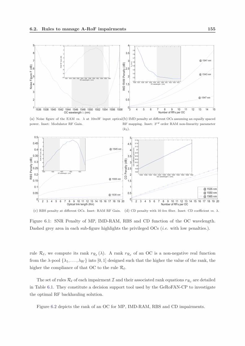
6.2. Rules to manage A-RoF impairments 155
5
6
7
8
9
gu
re F
(d
B)
1536 1538 1540 1542 1544 1546 1548 1550 1552 1554 1556 1558-10
-8
-6
-4
-2
0
2
4
6
RA
M R
F G
ain
(d
B)
1536 1538 1540 1542 1544 1546 1548 1550 1552 1554 1556 15581
2
3
4
OC wavelength (nm)
No
ise
Fi 1536 1538 1540 1542 1544 1546 1548 1550 1552 1554 1556 1558
OC wavelength (nm)
(a) Noise figure of the EAM vs. λ at 10mW input optical
power. Inset: Modulator RF Gain.
2
2.5
3
3.5
4
M P
en
alt
y (d
B)
@ 1543 nm
@ 1541 nm
0.2
0.3
0.4
0.5
0.6
0.7
0.8
0.9
1
k 3 (
a.u
)
3 4 5 6 7 8 9 10 11 12 13 14 150
0.5
1
1.5
Number of RFs per OC
IMD
RA
M
@ 1547 nm
1535 1537 1539 1541 1543 1545 1547 1549 1551 1553 1555 1557 0.1
OC wavelength (nm)
(b) IMD penalty at different OCs assuming an equally spaced
RF mapping. Inset: 3rd order RAM non-linearity parameter
(k3).
0.25
0.3
0.35
0.4
0.45
0.5
en
alty
(d
B)
@ 1545 nm
10
-8
-6
-4
-2
0
2
4
6
RA
M R
F G
ain
(d
B)
1 2 3 4 5 6 7 8 9 10 11 12 13 14 15 16 17 18 19 200
0.05
0.1
0.15
0.2
Optical link length (Km)
RB
S P
e
@ 1555 nm
@ 1535 nm
1535 1540 1545 1550 1555-10
OC wavelength (nm)
(c) RBS penalty at different OCs. Inset: RAM RF Gain.
2.5
3
3.5
4
4.5
5
en
alt
y (
dB
)
19 6
19.8
20
20.2
20.4
20.6
20.8
21
21.2
21.4
21.6
CD
coeff
icie
nt
(ps/n
m.k
m)
1 2 3 4 5 6 7 8 9 10 11 12 13 14 15 16 17 18 19 200
0.5
1
1.5
2
Number of RFs per OC
CD
Pe
@ 1535 nm
@ 1550 nm
@ 1565 nm
1536 1538 1540 1542 1544 1546 1548 1550 1552 1554 1556 1558
19.6
OC wavelength (nm)
(d) CD penalty with 10 km fiber. Inset: CD coefficient vs. λ.
Figure 6.1: SNR Penalty of MP, IMD-RAM, RBS and CD function of the OC wavelength.
Dashed grey area in each sub-figure highlights the privileged OCs (i.e. with low penalties.).
rule Rℓ, we compute its rank rRℓ(λ). A rank rRℓ
of an OC is a non-negative real function
from the λ-pool λ1, . . . , λW into [0, 1] designed such that the higher the value of the rank, thehigher the compliance of that OC to the rule Rℓ.
The set of rules Rℓ of each impairment I and their associated rank equations rRℓare detailed
in Table 6.1. They constitute a decision support tool used by the GeRoFAN-CP to investigate
the optimal RF backhauling solution.
Figure 6.2 depicts the rank of an OC for MP, IMD-RAM, RBS and CD impairments.
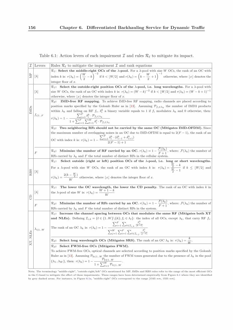
156 Chapter 6. Differentiated Backhauling Service for Dynamic Traffic
Table 6.1: Action levers of each impairment I and rules Rℓ to mitigate its impact.
I Levers Rules Rℓ to mitigate the impairment I and rank equations
MP
[λ]
R1: Select the middle-right OCs of the λ-pool. For a λ-pool with size W OCs, the rank of an OC with
index k is: r(λk) =
(W
2− k
)−2if k < ⌊W/2⌋ and r(λk) =
(k − W
2+ 1
)−1otherwise, where ⌊x⌋ denotes the
integer floor of x.
IMDs
[λ]
R1: Select the outside-right position OCs of the λ-pool, i.e. long wavelengths. For a λ-pool with
size W OCs, the rank of an OC with index k is: r(λk) = (W − k)−2 if k < ⌊W/2⌋ and r(λk) = (W − k + 1)−1
otherwise, where ⌊x⌋ denotes the integer floor of x.
fi|1..F
R2: IMD-free RF mapping. To achieve IMD-free RF mapping, radio channels are placed according to
position marks specified by the Golomb Ruler as in [13]. Assuming Pfi∈λkthe number of IMD3 products
within λk and falling on RF fi, δki a binary variable equals to 1 if fi modulates λk and 0 otherwise, then:
r(λk) = 1 −∑F
i=1δk
i · Pfi∈λk
1 +∑F
i=1
∑W
ℓ=1δℓ
i · Pfi∈λℓ
R3: Two neighboring RFs should not be carried by the same OC (Mitigates IMD-OFDM). Since
the maximum number of overlapping noises in an OC due to IMD-OFDM is equal to 2(F − 1), the rank of an
OC with index k is: r(λk) = 1 −∑F
i=1δk
i · (δki−1 + δk
i+1)
2(F − 1) + 1
FR4: Minimize the number of RF carried by an OC. r(λk) = 1 − F(λk)
F + 1, where: F(λk) the number of
RFs carried by λk and F the total number of distinct RFs in the cellular system.
RBS [λ]
R1: Select outside (right or left) position OCs of the λ-pool, i.e. long or short wavelengths.
For a λ-pool with size W OCs, the rank of an OC with index k is: r(λk) =W2
− k
W2
− 1if k ≤ ⌊W/2⌋ and
r(λk) =2(k − W
2)
Wotherwise, where ⌊x⌋ denotes the integer floor of x.
CD
[λ]
R1: The lower the OC wavelength, the lower the CD penalty. The rank of an OC with index k in
the λ-pool of size W is: r(λk) =W + 1 − k
W
FR2: Minimize the number of RFs carried by an OC. r(λk) = 1 − F(λk)
F + 1, where: F(λk) the number of
RFs carried by λk and F the total number of distinct RFs in the system.
XT,NLEs
λi|1..W
R1: Increase the channel spacing between OCs that modulate the same RF (Mitigates both XT
and NLEs). Defining Ii,k = ℓ ∈ 1..W \k; fi ∈ λℓ: the index of all OCs, except λk, that carry RF fi.
The rank of an OC λk is: r(λk) = 1 −
∑F
i=1
∑ℓ∈Ii,k
δki
|k−ℓ|∑W
j=1
∑F
i=1
∑ℓ∈Ii,j
δj
i|j−ℓ|
R2: Select long wavelength OCs (Mitigates SRS). The rank of an OC λk is: r(λk) =k
W.
R3: Select FWM-free OCs (Mitigates FWM).
To achieve FWM-free OCs, optical channels are selected according to position marks specified by the Golomb
Ruler as in [13]. Assuming Pk∈1..W the number of FWM tones generated due to the presence of λk in the pool
λ1..λW , then: r(λk) = 1 − Pk∈1..W
1 +∑W
ℓ=1Pℓ∈1..W
.
Nota: The terminology "middle-right", "outside-right/left" OCs mentioned for MP, IMDs and RBS rules refer to the range of the most efficient OCs
in the C-band to mitigate the effect of these impairments. These ranges have been determined empirically from Figure 6.1 where they are identified
by grey dashed areas. For instance, in Figure 6.1a, "middle-right" OCs correspond to the range [1545 nm, 1555 nm].

6.3. The DBS algorithm 157
0 5 10 15 20 2510
-3
10-2
10-1
100
OC index
r MP
MP
0 5 10 15 20 2510
-3
10-2
10-1
100
OC index
r IMD
IMD-RAM
0 5 10 15 20 2510
-2
10-1
100
OC index
r RB
S
RBS
0 5 10 15 20 2510
-2
10-1
100
OC index
r CD
CD
Figure 6.2: OCs ranking for MP, IMD-RAM, RBS and CD impairments. A WDM pool of 24
OCs with 1 nm channel spacing in the C-band is assumed. Y-axis is log-scaled.
6.3 The DBS algorithm
The GeRoFAN-CP acquires at the HOLT a global view of the system dynamics (traffic load
distribution). This CP keeps a steady monitoring of the evolution of the aggregated traffic load
at each cell in the network. Upon the observation reported by the traffic load manager, the CP
activates the Differentiated Backhauling Service (DBS) algorithm which is illustrated in Figure
6.3. The DBS algorithm relies on an iterative procedure aiming to adjust the Shannon’s capacity
within each cell according to its actual traffic load. Two variants of the DBS algorithm, namely
DBS− and DBS+, are executed by the CP in case of traffic decrease or increase respectively.
If a traffic load increase and decrease are observed at the same time in two different cells
respectively, the CP averages both magnitudes of these two fluctuations and decides accordingly
to launch the appropriate variant of the DBS. Once DBS achieves the optimal RF-onto-OCs
mapping solution, reconfiguration information are encoded into the signaling OC λ⋆1 and broad-
casted to each RAU.
1The signaling mechanism of GeRoFAN described in Section 3.4.3 of Chapter 3.

158 Chapter 6. Differentiated Backhauling Service for Dynamic Traffic
Traffic load monitor
DBS-
DBS+
DBS
Decrease Increase
Optimal
RF/OC
mapping
Broker Broker
*
Network
broadcasting
Figure 6.3: DBS activation by the GeRoFAN-CP and interaction with the λ-broker.
Assuming ζ = Ck, 1 ≤ k ≤ |ζ| the set of radio cells, F = fi, 1 ≤ i ≤ |F | the set of
distinct RFs used in the cellular planning and Λ = λj , 1 ≤ j ≤ p the set of required OCs
(p ≤ W ), the DBS algorithm investigates the optimal RF-onto-OCs placement solution by
modifying the |F | × p matrix S(p) defined as: S(p)ij = Ck meaning that RF fi assigned to cell
Ck is carried by OC λj . By convention, S(p)ij = 0 means that there is no cell served by RF fi
transported by OC λj . It has to be noted that if multiple RFs are assigned to the same cell
Ck, the value Ck appears several times on the same column of S(p). Since the RF-onto-OCs
remapping has to keep unchanged the cellular RF planning, the modification of S(p) is achieved
by circular shift along the same row of the matrix (i.e. by permutating S(p)ij and S
(p)iℓ ). To
evaluate the impact of the new placement on the capacity provided to each cell, we define
similarly to S(p), the |F | × p matrix ρ. Element ρij expresses the ratio of the gap between the
offered and the required capacities normalized to the required capacity at cell S(p)ij = Ck. In
consequence, ρij > 0 indicates an excess in the offered capacity, while ρij < 0 means that only
a fraction of the offered load is provisioned.
6.3.1 DBS at traffic load increase (DBS+)
The CP runs the DBS+ algorithm when an increase of the traffic load is reported by the traffic
monitor. DBS+ provides hot-spot cells with the needed radio capacity by remapping RFs-onto-
OCs while requesting from the λ-broker, the lowest additional number of required OCs. The

6.3. The DBS algorithm 159
algorithm takes in input the traffic load distribution among cells and the best RF-onto-OCs
mapping solution S(p)∗achieved with p OCs. Considering ζ↑ the set of cells experiencing an
increase of the traffic load, then the quality of a given solution S(p) is evaluated using the
quadratic mean Ω of the radio capacity computed as in Equation 6.1:
Ω =
√√√√∑
(i,j);S(p)ij ∈ζ↑
ρ2ij
|ζ↑| (6.1)
The lower the value of Ω, the better is the RF-onto-OCs mapping solution. The use of the
quadratic mean in Equation 6.1 instead of a simple average makes the minimization of Ω yielded
by the minimization of all its elements |ρij |.As depicted in the flowchart of Figure 6.4a, DBS+ investigates the best mapping solution
that can be achieved with at most p OCs. For that sake, it calls two main algorithmic blocks
namely the Blind Search Box (BSB) and the Guided Search Box (GSB) whose detailed working
is described respectively in subsections 6.3.3 and 6.3.4. Unless BSB or GSB triggers an exit, the
quality of solutions S(p−1)∗ and S(p)∗are compared, making DTS+ either to carry out a new
iteration with an additional OC or to exit with S(p−1)∗ .
6.3.2 DBS at traffic load decrease (DBS−)
When a decrease of the traffic load is reported in some cells, a capacity excess is likely to occur
in that cells. The CP runs the DBS− algorithm which targets to pack RFs more closely together
into the minimum number of OCs. Hence, freshly vacant OCs can be released and given back
to the λ-broker (c.f. Figure 6.3). However, because a dense packing of RFs into OCs is likely
to increase the beating between RFs and thus to degrade their radio capacities, DBS− carries
out the RF packing process iteratively over all used OCs. By doing so, the algorithm ensures
that only the most least penalizing OCs are released. We call least penalizing OCs, those whose
release remains compatible with the satisfaction of the new traffic load. To check the quality
Ω of a given solution S(p), DBS− uses Equation 6.2 which not only focuses on ζ↓, the set of
under-loaded cells, but also includes cells of set ζ = S(p)ij ∈ ζ; ρij < 0 which experience a needin capacity subsequent to the RF packing:
Ω =
√√√√∑
(i,j);S(p)ij ∈ζ↓
⋃ζ
ρ2ij
|ζ↓|+ |ζ|(6.2)
The flowchart of DBS− is depicted in Figure 6.4b. Similarly to DBS+, DBS− calls the BSB
and GSB blocks to search for the best RF-onto-OC mapping. To identify the least penalizing
OC λ that should be released, the algorithm runs a Tabu-search among all OCs using a Tabu

160 Chapter 6. Differentiated Backhauling Service for Dynamic Traffic
list Z. The release of λ is made effective when the quality of the solution S(p−1)∗ (which doesn’t
require λ) is at least equal to the solution S(p)∗(which uses λ). Unless BSB or GSB triggers an
exit, the algorithm stops either when the Tabu list becomes full or the theoretical lower bound
of required number of OCs is achieved.
6.3.3 The Blind-Search Box (BSB)
The DBS algorithm relies on the BSB algorithmic block whose flowchart is illustrated in Figure
6.5a. The rationale of the BSB is to feed cells that need capacity (i.e. cells with ρij < 0) with
the capacity excess observed in under-loaded cells (i.e. cells with ρij > 0). BSB adjusts the
radio capacity to the load level by permutating OCs transporting under-loaded RFs with OCs
carrying overloaded RFs.
BSB starts an iteration t by identifying the cell whose RF i should be relocated from its OC
j to another OC j⋆. If DBS+ is applied, the targeted cell is S(p)ij = S(p)kℓ ∈ ζ↑; maxkℓ
|ρkℓ|,while for DBS− it would be S(p)ij = S(p)kℓ ∈ ζ↓ ⋃
ζ; maxkℓ
|ρkℓ|.
r(λk) =
|ρij − ρik| if S(p)ik Ó= 0
maxℓ=1..|Λ|
r(λℓ) if S(p)ik = 0
(6.3)
To find OC j⋆, BSB ranks all OCs according to Equation 6.3. After rank normalization,
BSB checks whether the rank of the OC j⋆t−1, i.e. the OC selected at the previous iteration
t − 1, equals to maxk=1..|Λ|
r(λk). In that case, ranks are updated as in Equation 6.4 to prevent the
OC j⋆t−1 from being selected at the current iteration t, however if r(λj⋆
t−1) < maxk=1..|Λ|
r(λk) then
there is no need for BSB to update the ranks.
r(λk) = r(λk) +r(λj⋆
t−1)
2(|Λ| − 2)
r(λj⋆t−1) =
r(λj⋆t−1)
2
(6.4)
Equation 6.4 penalizes the rank of OC j⋆t−1 by dividing it by 2 at the profit of the other
OCs (except the original OC j).
We evaluate the capacity matrix ρ of the new RF-onto-OCs mapping solution obtained by
relocating RF i from OC j to the OC j⋆ with the highest rank. Using Equation 6.1 (respectively
Equation 6.2) if DBS+ (respectively if DBS−) is applied, the quality Ω of the new mapping
solution is compared with the best quality achieved Ω∗. The BSB algorithm is iterated once
again, however, it can lead to an exit if Ω∗ achieves a threshold value Ωth, or it moves to the
GSB block if a local counter α attains a threshold value αth.

6.4. DBS performance: Numerical results 161
The example depicted in Figure 6.6 illustrates the working principle of BSB and the GSB
algorithms for a network with 10 cells using 3 radio channels mapped onto 4 optical channels.
6.3.4 The Guided-Search Box (GSB)
The flowchart of the GSB algorithm is presented in Figure 6.5b. GSB identifies the RF i to
relocate similarly to BSB. Nevertheless, unlike BSB, the GSB algorithm relocates RF i from
its OC j to a new OC j⋆ using a guided optimization approach. In fact, supported by the
QoT-tool, GSB quantifies the share of each impairment in the total SNR penalty of RF i in
order to identify the most penalizing impairment I responsible for such a capacity degradation.
Using the rules Rℓ recommended to manage the impairment I in Table 6.1, GSB computes the
rank rRℓ(λk) of each OC k Ó= j. Note that the rank of an OC k is computed after assuming an
RF permutation between OC k and OC j. To prevent the selection of the same OC j, we set
rRℓ(λj) = 0. When L rules are involved for impairment I, we compute the aggregated rank2
r(λk) of an OC k as in Equation 6.5. Once the highest ranked OC has been selected as the OC
j⋆, the algorithm is continued similarly to BSB.
r(λk) =L∏
ℓ=1
rRℓ(λk) (6.5)
6.4 DBS performance: Numerical results
To evaluate the performance of the DBS algorithm, we consider an LTE mobile network with 20
radio cells. We use the same parameters for the radio model provided in Table 5.1 in Chapter 5.
Radio cells are backhauled via the GeRoFAN optical tree by selecting the splitting node at the
center of the cellular network so that all RAUs are uniformly distributed around the splitting
node. The radio spectrum pool is made of 7 radio channels regularly reused among cells as
illustrated in Figure 5.8 of Chapter 5.
2We choose a product instead of a simple normalized sum in order to depict the impact of each rank taken individually on the aggregated
rank. Such a mathematical formulation of the aggregated rank is achieved by analogy with the probability of simultaneous rules (of equal
importance).
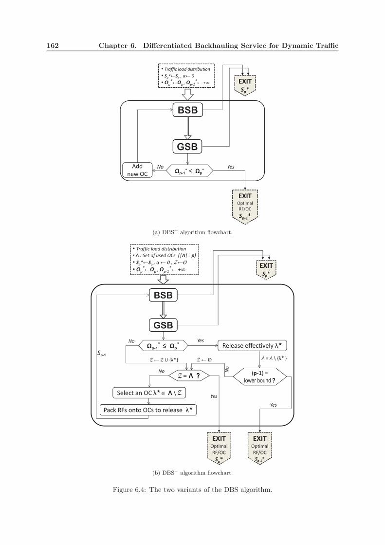
162 Chapter 6. Differentiated Backhauling Service for Dynamic Traffic
BSB
GSB
• Traffic load distribution
• Sp* Sp , 0
• p*
p , p-1*
+ EXIT
Sp*
p-1* < p
*
EXIT
Optimal
RF/OC
Sp-1*
Add
new OC
YesNo
(a) DBS+ algorithm flowchart.
BSB
GSB
• Traffic load distribution
• : Set of used OCs (| |= p)
• Sp* Sp , 0 , Z Ø
• p*
p , p-1*
+EXIT
Sp*
p-1* p
*
EXITOptimal
RF/OC
Sp*
No
Z = ?
Select an OC \ Z
Pack RFs onto OCs to release
Sp-1
Release effectivelyYes
(p-1) =
lower bound ?
Yes
EXITOptimal
RF/OC
Sp-1*
Z Ø
No
No
Yes
= \ Z Z U
(b) DBS− algorithm flowchart.
Figure 6.4: The two variants of the DBS algorithm.

6.4. DBS performance: Numerical results 163
Rank OCs and select OC j with the highest rank
Evaluate the new capacity matrix
Quality check
p vs. p*
+1 0
p* p
= th
*Yes
No
No Yes
improvementNo improvement
optimal p* @ p OCs
RF/OC matrix Sp @ p Ocs
0
A new RF/OC mapping is obtained by RF
permutation between OC j and OC j
Identify the RF i at OC j to relocate
p*th
EXIT
The optimal RF/OC
mapping achieved
with p OCs
To Guided Search
Box (GSB)
0
(a) Blind Search Box (BSB) flowchart.
Identify the RF i at OC j to relocate
identify the most penalyzing impairmentI
Using the rules of I in Table II, compute OCs’
ranks and select OC j with the highest rank.
Evaluate the new capacity matrix
Quality check
p vs. p*
+1 0
improvementNo improvement
From Blind
Search Box (BSB)
0
A new RF/OC mapping is obtained by RF
permutation between OC j and OC j
p* p
= th
p*th
EXIT
The optimal RF/OC
mapping achieved
with p OCs
Yes No
No Yes
To Quality
check with
p-1*
(b) Guided Search Box (GSB) flowchart.
Figure 6.5: Guided and Blind Search Boxes of the DBS algorithm.

164 Chapter 6. Differentiated Backhauling Service for Dynamic Traffic
- 0.9 0.5 1
0.5 5 1
- 0.5 - 0.3 7 3
Normalized
Ranking
Update ranks
( *(t-1) = 3)
matrix (in %)New mapping S4
Blind Search Box (BSB) example
1 2 3 4
f1 1 4 0 7
f2 0 2 6 9
f3 8 5 10 3
S4
(10 cells, F=3, | |= 4 )
1 2 3 4
f1 7 4 0 1
f2 0 2 6 9
f3 8 5 10 3
r( 1) = 0
r( 2) = 0.27
r( 3) = 0.365
r( 4) = 0.365
r( 1) = 0
r( 2) = 0.361
r( 3) = 0.182
r( 4) = 0.456
Identify Impairment I Ranking according to rulesR
matrix (in %)
pe
na
lty
XT/
NLE
CD
RB
S
MP
IMD
s
R1 R2 R3 R4 ( 10-3 )
10.008 1 1 0.5 4.15
20.01 0.7 0.6 0.5 2.1
30.012 0.7 0.25 0.25 0.53
40 0 0 0 0
Guided Search Box (GSB) example
1 2 3 4
f1 7 2 1 4
f2 0 5 6 9
f3 3 0 10 8
2 1 - 0.2 1
- 0.2 3 2
4 1 - 0.4
1 2 3 4
f1 7 2 1 4
f2 0 5 6 9
f3 8 0 10 3
New mapping S4
S4
Figure 6.6: An example of the main steps of the BSB and GSB blocks.
Let consider a network of 10 cells using 3 distinct RFs mapped onto 4 OCs as illustrated by matrix S(4). Assuming that BSB is called during
the execution of DBS+ algorithm, the former identifies RF f1 assigned to cell 1 as the RF to relocate from its OC λ1. The 4 used OCs are
ranked according to Equation 6.3. Since OC λ3 has been selected as OC j⋆ at the previous iteration, BSB updates the ranks according to
Equation 6.4. The updated ranking enables OC λ4 to be selected for RF permutation with OC λ1. With the new RF-onto-OC mapping
solution, BSB exploits the QoT-tool to compute its capacity matrix ρ and to evaluate its quality according to Equation 6.1.
To illustrate the main steps of the GSB algorithm, let consider again the previous case of a 10-cells network using 3 distinct RFs mapped
onto 4 OCs from a λ-pool of W = 24 OCs. As depicted in Figure 6.6, GSB identifies RF f3 of cell 8 as the most degraded RF that should be
relocated from its OC λ4. Supported by the QoT-tool, the algorithm computes the share of each impairment and identifies IMDs as the most
penalizing noise I. According to Table 6.1, 4 rules can be exploited to mitigate IMDs. Once all OCs are ranked with respect to each ruleRℓ, the aggregated rank is computed as in Equation 6.5 while the rank of OC λ4 is set to 0. Showing the highest rank, OC λ1 is selected for
RF permutation with OC λ4. Given the new RF-onto-OC mapping solution, GSB uses the QoT-tool to evaluate its capacity matrix ρ before
computing its quality Ω.
The simulation scenario is initialized by considering that all cells are subject to the same
load set to 50%. As a starting point, RFs are mapped optimally using PaGeO onto the lower
bound of required OCs (equals to 3 OCs). We select randomly 4 radio cells in the network to
emulate hot-spots. The load in hot-spots is increased by an increment of 5% over consecutive
time snapshots3. Such an increment granularity makes the radio cell activity easily tracked by
the traffic load monitor. At each snapshot, the GeRoFAN-CP runs DBS (in this case DBS+) to
investigate the optimal RF-onto-OC mapping solution able to provision the required capacity
with the lowest number of OCs. DBS calculates the optimal RF-onto-OC mapping solution
3The simulation scenario is build through consecutive snapshots. A new snapshot corresponds to an increase of the traffic load in the
hot-spots with an increment of 5%.
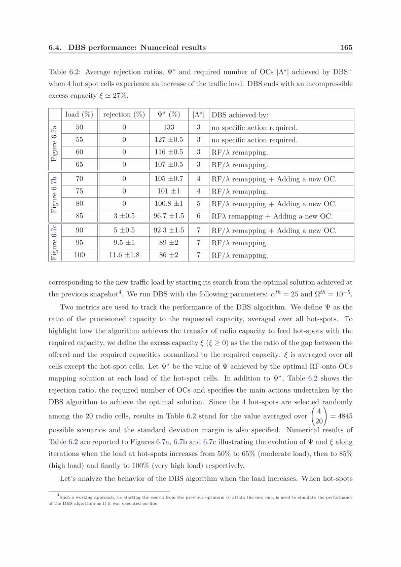
6.4. DBS performance: Numerical results 165
Table 6.2: Average rejection ratios, Ψ∗ and required number of OCs |Λ⋆| achieved by DBS+
when 4 hot spot cells experience an increase of the traffic load. DBS ends with an incompressible
excess capacity ξ ≃ 27%.
load (%) rejection (%) Ψ∗ (%) |Λ⋆| DBS achieved by:
Figure6.7a 50 0 133 3 no specific action required.
55 0 127 ±0.5 3 no specific action required.
60 0 116 ±0.5 3 RF/λ remapping.
65 0 107 ±0.5 3 RF/λ remapping.
Figure
6.7b 70 0 105 ±0.7 4 RF/λ remapping + Adding a new OC.
75 0 101 ±1 4 RF/λ remapping.
80 0 100.8 ±1 5 RF/λ remapping + Adding a new OC.
85 3 ±0.5 96.7 ±1.5 6 RFλ remapping + Adding a new OC.
Figure
6.7c 90 5 ±0.5 92.3 ±1.5 7 RF/λ remapping + Adding a new OC.
95 9.5 ±1 89 ±2 7 RF/λ remapping.
100 11.6 ±1.8 86 ±2 7 RF/λ remapping.
corresponding to the new traffic load by starting its search from the optimal solution achieved at
the previous snapshot4. We run DBS with the following parameters: αth = 25 and Ωth = 10−5.
Two metrics are used to track the performance of the DBS algorithm. We define Ψ as the
ratio of the provisioned capacity to the requested capacity, averaged over all hot-spots. To
highlight how the algorithm achieves the transfer of radio capacity to feed hot-spots with the
required capacity, we define the excess capacity ξ (ξ ≥ 0) as the the ratio of the gap between the
offered and the required capacities normalized to the required capacity. ξ is averaged over all
cells except the hot-spot cells. Let Ψ∗ be the value of Ψ achieved by the optimal RF-onto-OCs
mapping solution at each load of the hot-spot cells. In addition to Ψ∗, Table 6.2 shows the
rejection ratio, the required number of OCs and specifies the main actions undertaken by the
DBS algorithm to achieve the optimal solution. Since the 4 hot-spots are selected randomly
among the 20 radio cells, results in Table 6.2 stand for the value averaged over
(4
20
)= 4845
possible scenarios and the standard deviation margin is also specified. Numerical results of
Table 6.2 are reported to Figures 6.7a, 6.7b and 6.7c illustrating the evolution of Ψ and ξ along
iterations when the load at hot-spots increases from 50% to 65% (moderate load), then to 85%
(high load) and finally to 100% (very high load) respectively.
Let’s analyze the behavior of the DBS algorithm when the load increases. When hot-spots
4Such a working approach, i.e starting the search from the previous optimum to attain the new one, is used to simulate the performance
of the DBS algorithm as if it was executed on-line.

166 Chapter 6. Differentiated Backhauling Service for Dynamic Traffic
are subject to moderate load (i.e. up to 65%), the CP is able to provision the required capacity
by optimizing the placement of RFs onto OCs. The needed capacity in hot-spots is filled at the
detriment of the other cells (subject to lower load) as highlighted by the decrease of the excess
capacity in Figure 6.7a. Note that at 65% traffic load, an excess capacity of 7% can be derived
at hot-spots, while for loads up to 55% no specific action is needed by the CP to satisfy the load
apart reassigning uniformly the excess capacity among hot-spots. However, when the hot-spot
is subject to high load (c.f. Figure 6.7b), it may be necessary to add new OCs when only a
remapping of RF-onto-OCs is not sufficient to provision the required capacity. According to
Table 6.2, first optimal solutions leading to rejection are obtained when the load lies between
80% and 85%. Such a particular value of the load is called critical load. It is worth noting
that when the load at hot-spots attains the critical load, the DBS backhauling solution cannot
"absorb" completely the load. In that case, only providing a new RF (from the radio broker)
is able to provision the capacity required to serve all calls. On Figure 6.7b, we distinguish
the two optimization approaches constituting the DBS algorithm. Under BSB, Ψ increases
as a stair function with small amplitudes and large step iterations, while with GSB this stair
function is characterized by large amplitudes and small steps. Thus, BSB and GSB correspond
respectively to a disruptive and an incremental evolution of Ψ. At very high loads, DBS is
not able to provide the requested capacity as outlined by the values of rejection ratios and
Ψ∗ < 100%. Figure 6.7c shows that for loads higher than 95%, providing a new OC is worthless
while the excess capacity achieves a plateau (equal to ≃ 27%) called the incompressible capacity.
The incompressible excess capacity is the ultimate limit of ξ beyond which the rationale of DBS–
consisting in feeding hot-spots with capacity drawn from the excess of "cold" spot cells, becomes
ineffective.
Figure 6.8 illustrates the incompressible excess capacity (ξ) and the critical load computed
by DBS according to the number of hot-spot cells in the network. Up to 12 hot-spots, an
incompressible excess capacity ranges between 20% and 30% hosted in the other 8 under-
loaded cells. Such an unused capacity could be exploited by the radio operator by applying
promotional fees in under-loaded cells in order to exploit the system at its full capacity. Such
an approach benefits to both mobile users and the radio operator, it is in-line with the Pricing
for Profit paradigm as depicted in Figure 6.9, where the radio operator exploits a dynamic
pricing approach based on patterns of excess capacity. According to a Nokia Siemens Networks
research white paper [135], by combining customers insights and service-capacity knowledge,
Pricing for Profit enables communication service providers to increase revenues by at least 5%.
Critical load vs. the number of hot-spot cells is also depicted in Figure 6.8. If we consider
an operator serving an urban area, such an operator knows a priori the ratio of hot-spots in the
considered area. From the critical load depicted in Figure 6.8, whatever the density of hot-spots
up to 50%, the operator does not need additional RFs than the same RFs already considered. If

6.4. DBS performance: Numerical results 167
90
100
110
120
130
140
io C
apacity
(%
)
for BSB
1 2 3 4 5 6 7 8 9 10 11 12 13 14 15 16 17 1840
50
60
70
80
DBS Iterations
Ave
rage R
ad
load: 60% load: 65%load: 55%
(a) Hot-spots load increasing from 50% to 65%.
70
80
90
100
110
io C
apacity
(%
) for BSB
for GSB
50 100 150 200 25020
30
40
50
60
DBS Iterations.
Ave
rage R
ad
load:
75%
load: 85%load: 80%load: 70%
(b) From 65% to 85%.
60
70
80
90
100
io C
apacity
(%
)
for BSB
for GSB
300 350 400 450 500 55020
30
40
50
DBS Iterations.
Ave
rage R
ad
load: 90%load: 95% load: 100%
(c) From 85% to 100%.
Figure 6.7: Running the DBS algorithm as the load in hot-spots increases. ♣ denotes the adding
of a new OC. Attained Incompressible Capacity ≃ 27%.

168 Chapter 6. Differentiated Backhauling Service for Dynamic Traffic
the hot-spot density is higher than 50% one notices that the probability the operator requests
additional RFs from the RF-broker increases with the number of hot-spots. Since purchasing an
additional RF is very expensive for an operator according to the current regulatory environment,
this highlights the benefit of the DBS algorithm exploited by the GeRoFAN-CP.
1 2 3 4 5 6 7 8 9 10 11 12 13 14 15 16 17 18 19 200
10
20
30
Number of Hot spots
Incom
pre
ssi
ble
E
xcess
Capacity
(%)
1 2 3 4 5 6 7 8 9 10 11 12 13 14 15 16 17 18 19 200
50
100
Number of Hot spots
Critical L
oad (
%)
Figure 6.8: Incompressible excess capacity and critical load vs. the number of hot spot cells in
the cellular network.
6.5 Interaction with the RF-broker
In Sections 6.3 and 6.4, we highlighted the benefit of exploiting the DBS approach by the
GeRoFAN-CP to adjust, at either minimum OCs cost or maximum OCs savings5, the capacity
of the cell to its actual traffic load. However, it was previously shown that at higher loads,
the radio operator would require sooner or later an additional radio channel from the RF-
broker when the DBS technique does not lead to any improvement. When an operator requests
additional RFs due to a load increase, the capacity provided may excess the actual load at
the hot-spot, which constitutes an opportunity for activating the DBS− algorithm to achieve
OCs savings if it is possible. Similarly, when an operator releases some of the overlaying RFs
in under-loaded cells6, the remaining capacity may fall slightly below the required load at
these cold-spots, which requires the activation of the DBS+ algorithm to fulfill the gap at a
minimum optical cost. Both described situations advocate for a cross-layer approach between
the GeRoFAN-CP (exploiting DBS) and the RF broker in order to investigate the best timing
for an operator to request/release a radio channel. The Rf broker "trades" radio resources on-
5Depending on the variant of the DBS algorithm.6Obviously, the radio site is never completely turned off, at least a single RF is maintained in such under-load cells to serve its vegetative
state.

6.5. Interaction with the RF-broker 169
Loa
d,
Ca
pa
city Traffic Load in Hot Spots
Excess Capacity in Cold Spots
Off-PeakTariff
18:00 00:00 06:00 12:00 18:00 00:00 06:00
Incompressible
Excess Capacity Line
ModerateDiscount
HeavyDiscount
ModerateDiscount
time
Figure 6.9: DBS enabling the "Pricing for Profit" paradigm as advocated by NSN [135].As the traffic load in hot spots increases, the excess capacity in underloaded cells decreases. In fact, the DBS algorithm feeds hot spots
cells with capacity derived from the unused capacity in cold spots similar to a water-filling problem in communicating vessels. Depending
on the level of the excess capacity in cold spots, the mobile operator applies different discount schemes (moderate or heavy discounts) that
are advertised instantaneously to mobile users located in these cold spots. The principle of the Pricing for Profit detailed by NSN enables
operators to avoid excess capacity left unexploited and by consequence to increase revenues up to 5% according to the estimations in [135].
This is an example how the DBS strategy fits well the operators need for an accurate and adjusted radio capacity management (a kind of
"lean capacity management") only by acting on the optical layer. Such an optimized capacity management can be further enhanced by well
orchestrating the interaction with the radio broker such that to help the mobile operator with the best timing of requesting/releasing a radio
channel from/to the broker. This is detailed in Section 6.5.
demand with the mobile operator while the GeRoFAN-CP (using DBS) adjusts the provisioned
capacity to the traffic load with an efficient use of optical resources. Figure 6.10 illustrates the
flow-chart of the iterative process performing the radio/DBS cross-layer management approach
for the case of a traffic increase7.
Compared to legacy mobile backhauling8, the cross-layer management approach of the
GeRoFAN-CP offers the mobile operator with bandwidth savings achieved by delaying in time
the systematic need for a additional radio resources from the RF-broker. Such an economic
saving is illustrated through Figure 6.11a. Indeed, in a prospective horizon, mobile operators
trades on-demand radio resources with an RF broker, the latter being a regional or nation-wide
regulator. To price such a spectrum trading, a common discussed approach [112] consists in
multiplying the traded radio channel bandwidth with the elapsed time during which the RF
has been used by the mobile operator. From the mobile operator perspective, the incurred
cost is considered as an OpEx. Thus, we highlight the relevance of the cross-layer management
7The process performing the radio/DBS cross-layer management approach for the case of a traffic decrease follows the same steps with
minor changes: the order of applying the two DBS variants are reversed and the mobile operator releases RFs in under-loaded cells to the
RF-broker.8Not capitalizing on the benefits of A-RoF in terms resources mutualization and flexible management of the bandwidth, enabled by the
GeRoFAN-CP.

170 Chapter 6. Differentiated Backhauling Service for Dynamic Traffic
load monitoring
Load increase // triggering event.
RF/OCs remapping at 0 cost
RF/OCs remappingat + cost
// Calling DBS+ algo.
// Requesting OCs from the -broker.
Capacityfulfilled?
// Keeping aggregated traffic load
monitoring.
……
Yes
…
Not yet
Still needcapacity?
EXIT
NoYes
// Exiting with the optimal RF/OC
mapping.
Add a new RF to the most-needing hot-spot cell.
// Interacting with the RF-broker.
// Also could be relocating RFs
from cold-spots.
RF/OCs remapping at 0 cost
RF/OCs remappingat savings
// Calling DBS- algo.
// Releasing OCs to the -broker.
Capacityfulfilled?
Still needcapacity?
// Tabu list of DBS- is full.
EXIT
// Exiting with the required
number of RFs/cell and optimal
RF/OC mapping.
Not yet
Yes
NoYes
pp g
Figure 6.10: Flowchart of the radio/DBS cross-layer management approach for the case of a
traffic increase.
approach promoted by the GeRoFAN-CP.
To assess the gain achieved by the RF/DBS cross-layer approach, we consider an LTE
network with 20 radio-cells and the same radio model assumed in Chapter 5. The dynamic
traffic model adopted is inspired from the simulation tool in [136]. We highlight in the following
the key features of the model.
For a given simulation instance, k cell sites are selected at random among the 20 radio

6.5. Interaction with the RF-broker 171
Ra
dio
ch
an
ne
lco
nsu
mp
tio
n
f2
1
2
Radio resource management using DBS
Legacy radio resource management
Achieved
savings30%
25% f3
3
Achieved
savings
Achieved
savings
Time
f1 50%
3
(a) Illustrating achieved savings.
0.5
0.6
0.7
0.8
0.9
1
val R
ate
(ca
lls/c
ell/
hour)
5 10 15 20 25 300
0.1
0.2
0.3
0.4
0.5
0.6
0.7
0.8
0.9
1
Time (min)
No
rma
lize
d a
rriv
al c
all
rate
0 1 2 3 4 5 6 7 8 9 10 11 12 13 14 15 16 17 18 19 20 21 22 23 240
0.1
0.2
0.3
0.4
Time (Hours)
Norm
aliz
ed C
all
Arr
iv
(b) Normalized daily radio traffic profile (from [136]).
Figure 6.11: Example of RF/DBS cross-layer approach achieved savings. Realistic traffic profile
for a mobile network operator.Figure 6.11a: The RF/DBS cross-layer management approach enables significant savings in the radio bandwidth consumption compared to
legacy radio resource management (in our case, the cellular backhauling policy is based on FFCA algorithm). When the load increases at hot-
spots, radio bandwidth savings can be achieved by postponing the need for an additional radio channel. As illustrated, during elapsed times
τ1 and τ2, the radio mobile operator exploits the benefits of DBS+ to postpone the need for radio bandwidth ∆f1 and ∆f2 achieving savings
up to 50% and 30% respectively. Similarly, when the load decreases, the cross-layer management approaches exploits DBS to anticipate the
release of some RFs to the radio broker, leading to savings up to 25% as illustrated in the figure.
Figure 6.11b: Typical daily traffic pattern based on real statistics from a mobile operator. Two peak loads are noticed between 9 am and
5 pm. Inset figure illustrates the load activity at the scale of a call. During that time-window, call arrivals are modeled using the Poisson
distribution. A birth/death process is highlighted, while the general trend of the load is increasing from 22% to 25% between 6 and 6.30
am. Note that the GeRoFAN-CP deals only with the aggregated traffic load, i.e the CP remains agnostic to the Poisonous evolution of the
number of calls depicted in Inset Figure.

172 Chapter 6. Differentiated Backhauling Service for Dynamic Traffic
cells to play the role of hot-spots. The simulation scenario is based on successive snapshots.
A snapshot represents the activation/desactivation of user calls. The call arrivals per hot-spot
evolves according to a Poisonous process with an intensity λp9. New calls are generated in a
hot-spot through two different ways. On one hand, calls may be activated due to users mobility
from a cold spot (selected randomly among the neighbors of the hot spot). On the other hand,
activated calls may be emanating from the hot-spot itself. User mobility-induced new calls
occur with a probability pa while hot-spots self-generated new calls occur with a probability
1−pa. Once the hot-spots are clearly identified for a given instance, the simulation is initialized
by assuming 50% of traffic load in cold-spots. The evolution of the aggregated traffic load
in a given hot-spot cell is depicted in Figure 6.11b. The GeRoFAN-CP deals only with the
aggregated traffic and the RF/DBS cross-layer approach depicted in Figure 6.10 is executed at
each 30 min time window. The savings provided by the cross-layer approach is calculated with
respect to a QoT-aware cellular backhauling approach namely FFCA. The FFCA algorithm
presented in Chapter 5, achieves an optimal RF-onto-OCs mapping by assigning RFs to the
first-fit available OC, the same approach is carried out by FFCA when a new RF is solicited
from the radio broker.
Let BW x−layern and ∆τx−layer
n (BW F F CAn and ∆τF F CA
n respectively) be the RF bandwidth
used by the mobile operator and the time duration of its usage in cell n when the cross-layer
approach is exploited (respectively when FFCA is used), the averaged saving χ achieved by the
cross-layer approach is expressed according to Equation 6.6.
χ =1
N·
N∑
n=1
BW x−layern ·∆τx−layer
n
BW F F CAn ·∆τF F CA
n
(6.6)
Figure 6.12 provides the evolution of the achieved gain with the number of hot-spot cells k
among N = 20 for three possible scenarios pa = 1, pa = 0.5 and pa = 0.
Numerical results of Figure 6.12 show that the RF/DBS cross-layer approach of the
GeRoFAN-CP yields to radio bandwidth savings compared to the situation where only FFCA
is used. The gain decreases with the number of hot-spots. In fact, as demonstrated in the
previous section, the benefit of the DBS algorithm is noticed as long as cold-spot cells exist
to feed hot-spots with the required capacity. Figure 6.12 highlights that the highest gain is
achieved with pa = 1 and decreases when pa decreases as well. Indeed, the dynamics of the
transfer of capacity carried out by the DBS algorithm are relevant as long as there is a gap of
traffic load between hot-spots and cold spots. With a high pa, cold-spots become more and more
under-loaded as the new activated calls in hot-spots are due to mobile users originating from
neighboring cold-spots. However, at pa = 0, where all new calls are self-generated within the
hot-spots themselves thus keeping constant the load at cold-spots, a small gain (under 2.5%)
or even no gain at all is reported which confirms the relevance of the cross-layer approach only
9Call holding times are thus exponentially distributed with a mean of 120 sec [136].

6.6. Summary 173
20
25
30
35
40
n (
%)
pa = 1.0
pa = 0.5
pa = 0.0
2 4 6 8 10 12 14 16 18 200
5
10
15
Number of hot-spots (k)
Gain
Figure 6.12: Gain χ of the RF/DBS cross-layer management approach at various pa values.
when there is a gap in the traffic load between cells to favor the transfer of capacity between
them.
6.6 Summary
In this chapter, we demonstrated the GeRoFAN-CP capabilities to perform an efficient cellular
backhauling strategy in a dynamic traffic context. Supported by the QoT-tool, a set of rules
has been derived to manage the impact of A-RoF transmission limitations on cellular capacity.
Such rules constitute a decision support tool for the GeRoFAN-CP that runs a Differentiated
Backhauling Service (DBS) to adjust dynamically the Shannon’s capacity in each radio cell
according to the traffic load by optimizing the RF-onto-OCs mapping. The efficiency of the DBS
approach has been demonstrated through numerical simulation scenarios. Its "fast" convergence
time, ranging from 7 min (for simple instances) to 15 min (for complex instances), makes the
DBS suited to on-line execution10. Given the scarcity of the RF resource and the cost of radio
licences, the GeRoFAN-CP applies an efficient RF/DBS cross-layer management approach to
differ the need for additional RFs for the operators when the load at hot-spots increases thus
helping them leverage on significant cost savings. Our numerical results show that the gain of
the cross-layer approach compared to a classical approach based on the FFCA strategy ranges
between 2.5% and 35%. Results confirm the relevance of the RF/DBS cross-layer approach only
when there is a gap in the traffic load distribution between cells to favor the transfer of capacity
between them. In that sense, an analogy can be found in the rationale of the DBS approach
with the water-filling problem in a system of connecting vessels.
Since it is possible to assign optical channels to different operators and thanks to optical
10Further reductions of the computation time are also possible by optimizing the software implementation of the algorithm.

174 Chapter 6. Differentiated Backhauling Service for Dynamic Traffic
transparency, GeRoFAN can be viewed as an enabler for mobile backhauling mutualization.
Such an environment necessitates an evolution of the regulatory context where the GeRoFAN
infrastructure is managed by a third party (either a regional authority or a private independent
backhaul operator). The next chapter will focus on the economics of the GeRoFAN system
and the integration of business strategies in the DBS in order to facilitate radio resources
mutualization between several operators at the benefit of both the GeRoFAN manager and
radio operators.

Part IV
Economics and Business Relevance
of GeRoFAN

Chapter 7
GeRoFAN: a Prospective Approach
Contents
7.1 Introduction . . . . . . . . . . . . . . . . . . . . . . . . . . . . . . . . . . . . . . 177
7.2 The GeRoFAN operator: a Third party . . . . . . . . . . . . . . . . . . . . . . 178
7.2.1 Structuring the GeRoFAN eco-system . . . . . . . . . . . . . . . . . . . . . . . . 178
7.2.2 Business cases for GeRoFAN . . . . . . . . . . . . . . . . . . . . . . . . . . . . . 179
7.3 Economics of the GeRoFAN system . . . . . . . . . . . . . . . . . . . . . . . . 180
7.3.1 GeRoFAN vs. D-RoF WDM-PON architecture . . . . . . . . . . . . . . . . . . . 180
7.3.2 Methodology . . . . . . . . . . . . . . . . . . . . . . . . . . . . . . . . . . . . . . 182
7.3.3 Traffic scenario . . . . . . . . . . . . . . . . . . . . . . . . . . . . . . . . . . . . . 182
7.3.4 CapEx valuation model . . . . . . . . . . . . . . . . . . . . . . . . . . . . . . . . 184
7.3.5 OpEx valuation model . . . . . . . . . . . . . . . . . . . . . . . . . . . . . . . . . 184
7.3.6 Economic results and discussion . . . . . . . . . . . . . . . . . . . . . . . . . . . 187
7.4 Sharing the business value among stake-holders . . . . . . . . . . . . . . . . . 191
7.4.1 A two-tiers business model . . . . . . . . . . . . . . . . . . . . . . . . . . . . . . 191
7.4.2 A three-tiers business model . . . . . . . . . . . . . . . . . . . . . . . . . . . . . . 195
7.5 Summary and open issues . . . . . . . . . . . . . . . . . . . . . . . . . . . . . . 201
7.1 Introduction
In this chapter, we aim at evaluating the business value of the GeRoFAN network from mobile
carriers’ new regulatory environment perspective. In Section 7.2, we describe the GeRoFAN
eco-system and the crucial role played by the GeRoFAN operator as a third party. As an il-
lustration, we outline in the same section different business cases for GeRoFAN infrastructure
deployment, either short term-oriented or prospective. Based on Capital Expenditures (CapEx)
and Operational Expenditures (OpEx) models, we study in Section 7.3 the economics of the
GeRoFAN architecture. We assess the profitability of GeRoFAN compared to an alternative in-
vestment project backhauling network architecture based on WDM-PON and D-RoF technology

178 Chapter 7. GeRoFAN: a Prospective Approach
considered in the literature as the most credible solution for fiber-based next generation mobile
backhauling. In Section 7.4, we investigate the best-suited business models for GeRoFAN. A
two-tiers and a three-tiers business models are considered to study how the business value of
the cellular backhauling service is shared among the stake-holders of each model. Finally, we
conclude this chapter by summarizing the key findings of our investigations and outlining the
main open issues conditioning the viability of the new business model promoted by GeRoFAN.
7.2 The GeRoFAN operator: a Third party
7.2.1 Structuring the GeRoFAN eco-system
The GeRoFAN architecture assumes a new commercial and regulatory environment in the
metropolitan area in the sense where a third party operator could manage the GeRoFAN infras-
tructure. Thanks to the genericity of the GeRoFAN architecture and the MAC-agnostic feature
of its CP, the GeRoFAN infrastructure can be mutualized by fixed or mobile operators.
The new ecosystem promoted by the GeRoFAN network is depicted in Figure 7.1 and struc-
tured around three functional layers: The resource layer (OC and RF brokers), the telcos’ layer
and the end-users’ layer. The operator of the GeRoFAN infrastructure is positioned at the
upper layer. It provides the optical backhaul infrastructure for the different telecom operators.
In line with the target of a flexible radio spectrum usage achieved through spectrum markets,
we assume that the radio broker allocates on-demand RFs to mobile operators according to the
exploited radio system. Similarly, the GeRoFAN operator acts as an OC-broker in charge of
provisioning dynamically both fixed and mobile operators with the required OCs to transport
their baseband/radio traffic. Two methods are envisioned to manage optical channels for the
OC-broker. The first method consists in dividing the WDM pool into sub-pools, each of them
being used exclusively by a given operator. The borders between these sub-pools could shift
according to the market share of the different operators. The balance between the different
operators while sharing the WDM pool can be determined as the outcome of an auction process
or based on game theory equilibrium1. The second method for optical pool mutualization, con-
sists in sharing the same optical channel by different operators. Such a full sharing approach
offers a more efficient management of the WDM pool. However, we estimate that such an ap-
proach is technically more challenging, a special care being necessary in the placement of the
different traffics (associated to different operators) on the same optical channel in order to avoid
inter-operator interference. The OC-broker implements specific incentives policies2 to encourage
operators to share their assigned OCs with other operators. In addition to the dynamic man-
agement of OCs, the OC-broker dynamically assigns the corresponding ROADM/REAMSOA
1For instance based on a Nash equilibrium assuming a non-cooperative game between the competing operators.2For instance, the higher the rate of sharing of an OC, the lower the leasing price of that OC.

7.2. The GeRoFAN operator: a Third party 179
module to each operator (c.f Section 3.4 of Chapter 3). Thus, another major originality of
GeRoFAN consists in favoring the emergence of an innovative business environment where each
operator can be viewed as a a fixed and/or mobile Virtual Network Operator (VNO). Since
the investment of all operators in the infrastructure is equivalent, service innovation and op-
timization of the traffic management would be the key factors to make the difference in such
commercial competitive multi-tenants environment.
~ 1 - 10 GHz
…
f1
f2
… fm
resource
Layer
(OC,RF)
OC- broker / GeRoFAN manager
WDM pool
…
1 2… n
–leasing Fixed/Mobile
RF broker
RF–leasing RF
… … ……
? ?
…
Full sharingPool partition
into subpools
FTTx
Clients
Op. 2
Clients
Op.1
(FTTx)
Op.2
(4G LTE)
Op.3 (MVNO)
(WiMAX)
Telcos
Layer
End- Users
Layer
fee Backhauling Service
RF: 1 – 10 GHz RF: 1 – 10 GHz
cost
BB: 0 – 10 GHz
RF
… …
Figure 7.1: The GeRoFAN new eco-system business model.
7.2.2 Business cases for GeRoFAN
The successful implementation of the GeRoFAN system requires a full involvement of the dif-
ferent stake-holders. A new regulatory environment is required to encourage the mutualization
of the backhauling infrastructure, the dynamic provisioning of radio and optical resource (the
emergence of RF-broker and OC-broker). Indeed, municipalities,regional authorities or joint-
venture companies set up through a private/public partnership could play the role an OC-broker.
Incumbent operators could benefit from outsourcing the backhaul activity to a third party since

180 Chapter 7. GeRoFAN: a Prospective Approach
such a new environment could help them be more focused on their core competencies (innova-
tive telecom service provisioning, network radio planning etc.). Finally, small operators/new
entrants/VNOs would see GeRoFAN as a springboard to shorten their time-to-market and ex-
pand their business activity. At the time being and since all these requirement are not fulfilled
yet, the deployment of the GeRoFAN system in public outdoor environment is still considered
as a prospective business case. Instead, the GeRoFAN network could be realistic for the short-
term horizon if deployed in semi-private large domains like airports, a major railway station like
in [11], exhibition centers, commercial centers or sports complex. In these domains, multiple
public radio-mobile operators could rent the GeRoFAN infrastructure provided by the private
company that also manages the telecommunications facilities on the whole site. In such do-
mains, significant savings could be achieved in terms of radio resources management (through
RoF mutualization) and power consumption (by shutting down unused equipments) provided
by the GeRoFAN network by correlating the usage of network resources with traffic fluctuations.
For such semi-private large domains, the time3 and space fluctuations of the traffic matrix are
mainly predictable. In an airport [1], the traffic distribution is tightly related to flights depar-
tures and arrivals in the different operating terminals, while in a sports complex facility, the
competition planning determines the time/space variation of the traffic distribution.
7.3 Economics of the GeRoFAN system
In this section, we investigate the economics of the GeRoFAN system. In a comparison with a
WDM-PON architecture exploiting D-RoF technology for cellular backhauling. Both architec-
tures backhaul the same number of radio cells (20 4G LTE radio cells) and are subject to the
same traffic load detailed later.
7.3.1 GeRoFAN vs. D-RoF WDM-PON architecture
The network architecture of the D-RoF WDM-PON is depicted in Figure 7.2 and is taken
from [36]. Several Remote Radio Heads (equivalent to the RAU) are federated to the head-end
node called Main Unit (MU, equivalent to the HOLT) using a WDM-PON infrastructure. An
RRH manages both upstream and downstream radio traffic of its associated LTE cell. The
D-RoF WDM-PON architecture exploits bandpass sampling theory to digitize/reconstruct the
analog signal using an ADC/DAC without needing RF oscillators, thus simplifying the RRH
architecture. The digitized stream is mapped into an Optical Module (OM) port which uses
WDM-PON. The OM is a bidirectional colorless optical transceiver (SFP or SFP+) constituted
by a TOSA (remotely-fed uncooled reflective modulator), a ROSA (High-speed APD) and a
Printed Circuit Board (PCB) implementing in FPGA a high speed path for Inverted Return
3In the range of few tens of minutes as considered in Chapter 5.

7.3. Economics of the GeRoFAN system 181
DWDM
D
W
D
M
OM
OM
OM
…
(joint)
Baseband
Processing
Main Unit (MU)
0-20 Km
Fiber FeederTD
M S
eri
al /
Pa
ralle
l
ADC
DAC OM
DWDM
RRH (cell site)
RRH (cell site)
…
CPRI line
CPRI line
1.25 Gbps
1.25 Gbps
1.25
Gbps
Business
backhaul
Residential
backhaul
CPRI line
…N x 1.25 Gbps
4G radio
cell
4G radio
cell
ADC
DAC OM
Figure 7.2: D-RoF WDM-PON network architecture
to Zero/Return to Zero (IRZ/RZ) translation4. RRH links are aggregated to the MU using a
DWDM multiplexer/demultiplexer. At the MU, each RRH digital link is demodulated using a
dedicated OM. Parallel digital streams are serialized using a high-speed TDM multiplexer and
joint-baseband processed at the CP of the MU.
The GeRoFAN and the D-RoF WDM-PON architectures show several similarities. First,
both systems rely on the centralized light-seeding concept combined with reflective colorless
modulators to facilitate wavelength management and to prevent the need for costly light-sources
at the RRH/RAU. Second, both systems exploit the benefits of the DWDM technology in the
optical distribution network (traffic isolation, transparency, "unlimited" bandwidth etc.). Fi-
nally, both architectures take advantage of the centralization at the head-end node to implement
either joint baseband processing for D-RoF WDM-PON or QoT-aware backhaul and aggregated
capacity management for the GeRoFAN system. However, the main difference between the two
systems is the optical transmission technology used for backhauling: A-RoF for GeRoFAN,
while the alternative architecture relies on D-RoF.
4The PCB translates data coding from IRZ to RZ. The latter is more efficient against the RBS noise which is expected to be one of the
main impairment in high-speed WDM-PON [36].

182 Chapter 7. GeRoFAN: a Prospective Approach
7.3.2 Methodology
The techno-economic study of GeRoFAN and D-RoF WDM-PON systems is carried out follow-
ing the methodology depicted in Figure 7.3. Our methodology is inspired from techno-economic
research studies developed in [109], [51], the economic frameworks presented in [47] and [141]
and the financial model developed for cable television in [149].
Assuming a traffic evolution scenario which depicts the annual increase of the backhaul ca-
pacity per cell site, we determine how the network should be dimensioned to fulfill the projected
capacity. The CapEx cost consists of the infrastructure costs of the network calculated using
the dimensioning model. The CapEx cost includes the infrastructure cost of the head-end node
(HOLT/MU), the infrastructure cost of the RAU/RRH and the outside plant cost (civil works
for fiber deployment, housing/cabinet5 etc.). In addition, we include in the CapEx calculation
the potential savings due to sharing and reuse of existing infrastructure. Substantial proportion
of existing ducts/trenches can be reused for fiber deployment according to a report of Analysys
Masons [7]. The report points out a reuse rate of the infrastructure up to 80% in the distribu-
tion segment near the head-end node (i.e between the HOLT/MU and the fiber node cabinet)
as well as 30% in the final drop near the premises (i.e between the fiber node cabinet and the
RAU/RRH). The OpEx is composed of three major parts: the Installed First Cost (IFC), the
OpEx for a network that is up and running (power consumption cost, diagnosis/repair and
maintenance costs) and the fixed costs for network operation and administration. Once OpEx
and CapEx are calculated for a given traffic scenario, the overall cost of the system is distributed
over the study period fixed at 10 years. To calculate the discounted cashflow savings achieved
by the investment, we evaluate the OpEx cost incurred by the operator if it still relies on the
legacy backhauling strategy based on T1/E1 leased lines. The OpEx incurred by legacy T1/E1-
based backhauling includes the T1/E1 line leasing fee, the line activation fee and the associated
operation and administration expenses.
For the final techno-economic evaluation of the network solution, critical financial indexes,
such as Net Present Value (NPV), Internal Rate of Return (IRR) and Payback period of the
project are calculated in order to decide about the profitability of the investment. The reader
may refer to Table 7.1 which summarizes the definition of the key financial indexes used to
assess the business profitability of the investment.
7.3.3 Traffic scenario
In our study, we use the yearly statistics of the traffic per cell site as reported by Yankee Group
Research [110] from 2000 to 2012. Assuming a study period of 10 years ranging from 2010
to 2020, statistics of the traffic evolution per cell site for the 2012 − 2020 period are derived5The cabinet hosts either the DWDM-MUX or the optical splitter.

7.3. Economics of the GeRoFAN system 183
Traffic evolution scenario
Network design & dimensioning
CAPEX HOLT/MU
CAPEX RAU/RRH
CAPEX
Outside plant
Equipment
Installation
Power
consumption
Diagnosis
Repair
Installed first costs
Equipment enery profile
Equipment failure statistics
Cost reduction over time
Contrated with
the equipment
supplier
OPEX for a
network that is
up and running
T1/E1 lines dimensioning
Leasing fee per
line per month
Activation
fee per line
Operation & p Repair
Maintenance
Operation &
Administration
• Distributing CAPEX, OPEX and legacy OPEX over the study period
• Discounted cashflow financial model (discount rate: 10%)
Final techno-economic evaluation
• Critical financial indexes:
• NPV , IRR, Payback …
• Analysis: Profiling CAPEX and OPEX
Fixed OPEX
(personnel,
staffing ..)
Operation &
Administration
Figure 7.3: The techno-economic study methodology.
Table 7.1: How to assess project investment profitability ? [45]
The Net Present Value (NPV) describes today’s value of the sum of resultant discounted cashflows (CapEx, OpEx,
Revenues, Savings, etc.) by taking into account the time value or opportunity cost of money expressed by the discount rate.
If the NPV is positive, the project is acceptable. The higher the NPV of the investment project, the higher its business
profitability.
The Internal Rate of Return (IRR) gives a good indication of the business value achieved with respect to the money
invested to set up and run the project. is the interest rate resulting from an investment and income (total net discounted
cashflow) that occur over a the study period. To assess the business profitability of a project, we compare the IRR with
the discount rate used for the analysis. The project investment is profitable as long as its IRR is higher than the discount
rate.
The Payback Period is the specific point in the life time cycle of the project when the accumulated discounted cashflow
(cash balance) turns positive. Starting from the first year of investment, the payback period represents the time needed to
recover the required amount of funding.

184 Chapter 7. GeRoFAN: a Prospective Approach
through projections. Three possible scenario projections are considered in our study: the first
scenario assumes a 5% yearly traffic growth rate, the second scenario considers a 10% yearly
growth rate while a rate of 20% is assumed for the third scenario. The three considered traffic
evolution scenarios are shown in Figure 7.4.
800
1000
1200
1400
y p
er
ce
ll site
(M
bp
s)
forecast with 5% growth rate
forecast with 10% growth rate
forecast with 20% growth rate
Actual data from Yankee Group
5
10
15
20
25
30
Ba
ck
ha
ul
ca
pa
cit
y p
er
ce
ll s
ite
(M
bp
s)
HSPA
2G/3G
WiMAX
LTE
00 01 02 03 04 05 06 07 08 09 10 11 12 13 14 15 16 17 18 19 200.5
200
400
600
Year
Ba
ckh
au
l ca
pa
city
00 01 02 03 04 05 06 07 08 09 100
Year
Figure 7.4: The three scenarios considered for backhaul capacity evolution.
7.3.4 CapEx valuation model
For both network architectures, a number of cost components are assigned to different parts
of the network (HOLT/MU, RAU/RRH and Outside plant). Major CapEx components are
detailed in Table 7.2. For all components, we assume that the equipment life time is equal to
10 years. In order to be able to calculate the yearly capital equipment costs, the total cost of
the component is divided by the equipment life-time.
7.3.5 OpEx valuation model
The OpEx cost is the aggregation of four operational costs.
• First, IFC which stands for OpEx associated with equipment installation is determined
together with the CapEx cost of the equipment. For real scenario, the IFC is contracted
as a negotiation with the equipment vendor. For our study, some values of the IFC are
6For instance the Spartan-6 FPGA family from www.xilinx.com

7.3. Economics of the GeRoFAN system 185
Table 7.2: CapEx costs (G: GeRoFAN, D: D-RoF WDM-PON).
Component Cost (e ) IFC (e ) Source G D
HOLT/MU,RAU/RRH
TOSA-DFB-LD @ HOLT/MU 920 276 [115] • •ROSA-APD @ HOLT/MU 700 210 [115] • •FPGA-based RF-onto-OCs switching ma-
trix500 150 Xilinx Corp6. •
High speed TDM S/P 7000 2100 [34] •FPGA PCB for joint Baseband processing 500 150 Xilinx Corp. •DWDM ROADM (25 GHz spacing.) 1500 450 Ciena •TOSA-REAMSOA @ RAU 3000 900 [115] •ROSA-WB APD @ RAU 700 210 [115] •RF duplexer @ RAU/RRH 260 78 [115] • •r-CPU: BOSA (FP-LD/APD) @ RAU 250 75 [115] •r-CPU: FPGA PCB (λ⋆) @ RAU 100 30 Xilinx Corp. •BOSA-EAT WDM-SFP 1GbE @ RRH 3850 1115 [34] •BOSA-EAT WDM-SFP+ 10GbE @ RRH 5000 1500 [34] •BOSA-EAT WDM-XFP/SFP+ 40GbE @
RRH9800 2940 [34] •
ADC/DAC 250MS/sec (8bits) @ RRH 3000 900National Instru-
ments•
ADC/DAC 500MS/sec (8bits) @ RRH 4000 1200National Instru-
ments•
ADC/DAC 1GS/sec (8bits) @ RRH 6000 1800National Instru-
ments•
ADC/DAC 2GS/sec (8bits) @ RRH 10850 3255National Instru-
ments•
OutsidePlant
DWDM MUX/DEMUX (up to 40 λ) 12000 3600 [51] • •Optical Splitter (1:32) 100 - CSMG [109] •Fiber node cabinet/closures 2450 - CSMG [109] • •
Optical Cable24Fiber 1220/Km 900/KmAnalysys Masons
[109]• •
Digging/ducting cost (Urban) 60000/Km - CSMG [109] • •
RAU/RRH site civil work 1000 -Analysys Masons
[109]• •

186 Chapter 7. GeRoFAN: a Prospective Approach
taken from [109] if available, otherwise IFC is estimated as the assumptions in [51] to be
30% of the CapEx costs. Values of IFC for the different components are specified in Table
7.2.
• The second operational cost represents the energy consumption of network components.
Average power consumptions are estimated from the energy consumption model developed
in Section 3.3 of Chapter 3 and from data reported in [73] and [147]. We consider,
according to the assumptions in [51], a price of 0.08 e per KWh to determine the cost of
the energy consumption.
• The third operational cost encompasses the expenditures associated with failure diagno-
sis/monitoring, repair and equipment maintenance. The maintenance cost OpExM of an
equipment is evaluated on a yearly basis according to the following formula in Equation
7.1 reported from [45]:
OpExM i =Vi−1 + Vi
2· (Pi · Rclass + Pl · MTTR
MTBF) (7.1)
where: Vi the equipment volume in year i, Pi the price of the equipment in year i, Rclass
is the maintenance cost percentage for every cost component assumed according to [109]
as 7% of CapEx for the equipment, Pl the hourly cost of the staff in charge of maintaining
the equipment assumed to be 1.5 times the minimum wage. MTTR and MTBF represent
the mean time to repair and the mean time between failures respectively. The first item
between the parenthesis in the Equation represents the cost of repair parts while the
second item stands for the cost of repair work. Nominal values of availability statistics
(MTTR and MTBF ) of the different network components are taken from [51]. The
evolution of the price of a component Pi follows a decreasing trend over years described
by the following learning curve formula taken from [45]:
Pi = P0 ·[1
n(0)·1 + exp
[ln(
1
n(0)− 1)− 2 ln(9)
τ· i
]−1]log2(k)(7.2)
Given: P0 the initial price of the component at the reference year (2010), τ the time re-
quired for the accumulated production volume to grow from 10% to 90% (here assumed to
be 10 years), k is a learning curve coefficient set at 98% [109] and n(0) reflects the relative
cumulative volume taken as 0.5 for components that already exist in the market and their
price is expected to decrease due to aging rather than due to the production volume (RF
duplexers, LD, APD, fiber, splitter etc.), 0.1 for mature components (ROADM, DWDM
MUX, WDM-PON SFP, moderate speed ADC/DACs etc.) and 0.01 for new to very

7.3. Economics of the GeRoFAN system 187
Table 7.3: Personnel/staffing overhead cost inspired from [50].
Activity Overhead
Technical (field) × 2.5
Network Operation Center × 2
Adminstrative/helpdesk × 2
Engineering, R&D × 3
Table 7.4: Other yearly recurring OpEx taken from [109].
OpEx Valuation (e/year)
Site rental for HOLT/MU (urban area) 3000
Housing: cabinets/closures 5% of CapEx for closures
Civil works 3% of CapEx for civil works
new components in the market (WDM-PON XFP/SFP+, very high speed ADC/DACs,
EAT/REAMSOA etc.).
• The last OpEx item stands for Operation and Administration (O&A) costs. The
latter includes the cost of the operational activities (network technical operations,
helpdesk/administrative tasks) calculated as the hourly cost of the employee multiplied
by the average duration required to perform the activity. following the approach of [51],
an overhead factor is included in the salary estimation in order to fully account the cost
of this person for the company. The overhead factor accounts for the tools, transport
and training needed for personnel performing difficult or high qualifying tasks. Table
7.3 provides the personnel cost for each activity type. At this stage of the study, only
administrative/hepldesk and technical field personnel are considered.
• Finally other yearly recurring operation costs are also considered and summarized in Table
7.4.
7.3.6 Economic results and discussion
We investigate the techno-economics of both investment projects and we calculate the discounted
cashflow achieved savings with respect to a legacy backhaul using T1/E1 leased lines. The details
of the OpEx associated with the legacy backhaul are provided in Table 7.5:
Table 7.5: OpEx for a T1/E1 leased-lines backhaul [110].
Leasing fee of a single T1/E1 line 300e/month
Contracted line activation fee 10% of the leasing fee
Required dedicated staff 1 technical, 1 administrative

188 Chapter 7. GeRoFAN: a Prospective Approach
Figure 7.5 provides the evolution of the amount of achieved savings for both architectures
with the three traffic scenarios assuming a 10% discount rate. The evolution of the cashflow
savings shows that the GeRoFAN investment project is more profitable compared to the D-RoF
WDM-PON project at high rate increase of the radio traffic. In fact, at such higher rates, higher
speed electronics and optical transceivers are required for the D-RoF based network architecture.
Regarding the current cost of such components and the high level of power consumed, the
CapEx and OpEx of D-RoF WDM-PON is increased as well which decreases the achievable
savings compared to GeRoFAN. At 5% of the traffic rate increase, results show that the D-RoF
architecture is more cost-effective with a little higher achieved cashflow savings. Such results
are in-line with the results in Chapter 3 where we pointed out the economic advantage of A-RoF
compared to D-RoF only at higher traffic loads.
2010 2011 2012 2013 2014 2015 2016 2017 2018 2019 20200
1
2
3
4
Year
Sa
vin
gs
M
5% traffic growth
3
4
5
gs M
10% traffic growth
€€
2010 2011 2012 2013 2014 2015 2016 2017 2018 2019 2020
1
2
3
Year
Sa
vin
2010 2011 2012 2013 2014 2015 2016 2017 2018 2019 2020
0
2
4
6
8
10
Year
Sa
vin
gs M
20% traffic growth
GeRoFAN
D-RoF WDM-PON
€
Figure 7.5: Year-by-year discounted cashflow savings achieved by GeRoFAN and D-RoF WDM-
PON for the three traffic scenarios.
The trend of cashflow savings shown in Figure 7.5 is confirmed by the financial summary
provided in Table 7.6. Higher IRRs and NPVs as well as lower payback periods are reported for
GeRoFAN compared to D-RoFWDM-PON especially at higher rates of the radio traffic increase.
Particularly, the cost-effectiveness of the GeRoFAN investment is confirmed with the third
scenario (20% of yearly traffic increase rate). Indeed, the D-RoF WDM-PON investment project
shows 94.5% lower NPV, lower IRR (lower than the cost of capital (10%)) and higher payback
period (6× the payback needed by GeRoFAN). Note that all these statistics are subject to

7.3. Economics of the GeRoFAN system 189
Table 7.6: Financial summary of both investments.
Scenario GeRoFAN D-RoF WDM-PON
NP
V
1 1.057 Me 1.104 Me
2 1.280 Me 1.215 Me
3 1.892 Me 103.18 KeIR
R
1 25 % ≃ 30.8 %
2 ≃ 27.7 % ≃ 32.62 %
3 ≃ 34.1 % ≃ 8.5 %
Pa
yb
ack 1 ≃ 1 year, 2 months ≃ 1 year, 2 weeks
2 ≃ 1 year, 3 weeks ≃ 1 year, 1 month
3 ≃ 1 year, 1 month ≃ 6 years, 6 months
modification if substantial technological development is carried out by equipment manufacturers
to lower the cost of high speed opto-electronics required by the D-RoF architecture and increase
the power efficiencies of such devices.
OpEx and CapEx costs are analyzed for both architectures in Figure 7.6. Unlike the D-RoF
WDM-PON architecture, we have noticed no significant change of the OpEx and CapEx cost for
the GeRoFAN architecture at the different traffic scenarios. We can conclude that GeRoFAN
is economically much less sensitive7 to the traffic evolution than D-RoF WDM-PON.
For both investment projects, the outside plant represents the major part of the CapEx cost
(dominated mainly by the deployment cost of the fiber). It’s worth noting that the share of
the outside plant can be significantly reduced by favoring a higher mutualization of network
facilities and cable ducts. Apart the outside plant and excepting the first scenario where the
relatively low traffic increase rate (5%) makes the RRH less expensive, Figure 7.6a shows that
the RRH/RAU captures a major share of the CapEx (at the third scenario, RRHs occupy 29%
of the total network CapEx).
The OpEx profiling illustrated in Figure 7.6b shows that the maintenance/repair cost and
the power consumption are the two major costs constituting the structure of the OpEx. Note
that at higher traffic increase rates (10% and 20%), energy consumption costs over-dominate the
total OpEx (80% of OpEx) for the D-RoF WDM-PON architecture, while the cost structure is
more relatively balanced for GeRoFAN (although energy consumption costs are still prevailing).
These results indicate how the GeRoFAN architecture takes advantage of its higher optical
transparency to lower the OpEx and the share of the energy consumption cost almost driven
by electronics.
7Although a sensitivity analysis is required to assess exactly how much each architecture is economically sensitive to variations of the
used parameters in the model (components cost, T1/E1 leasing fee, the price of a KWh etc.), we expect that such a sensitivity analysis would
not change the results of ours study.

190 Chapter 7. GeRoFAN: a Prospective Approach
5%
16%
6%< 1%
5%
20%
4%
29%
HOLT/MU RAU/RRH Outside Plant (fiber civil work, housing cabinet...)
79% 93% 76% 67%
GeRoFANDRoF WDM
@ 10% traffic growth
DRoF WDM@ 5%
traffic growth
DRoF WDM@ 20%
traffic growth
(a) CapEx Profiling for the two network architectures.
23%
5%
17%30% 38%
10%
2%8% 15%
1%
4%
Maintenance Ongoing OPEX Power consumption Personnel/staffing cost
5%
55%
10%
22% 80% 79%
GeRoFANDRoF WDM
@ 5%traffic growth
DRoF WDM@ 20%
traffic growth
DRoF WDM@ 10%
traffic growth
(b) OpEx Profiling for the two architectures.
Figure 7.6: CapEx and OpEx profiling analysis.

7.4. Sharing the business value among stake-holders 191
7.4 Sharing the business value among stake-holders
After assessing the profitability of the GeRoFAN investment, we investigate in this section the
requirement for an economically attractive exploitation of the GeRoFAN system. As outlined,
the GeRoFAN architecture offers the radio operator the opportunity to outsource the backhaul-
ing activity. Two models are proposed in this section to structure the value chain of the cellular
backhauling activity and to orchestrate the interaction between the different stake-holders.
7.4.1 A two-tiers business model
In the two-tiers model, depicted in Figure 7.7a, the value chain is achieved by two players:
the GeRoFAN operator and the radio mobile operator. The latter outsources the backhauling
activity to the GeRoFAN operator who is in charge of installing and maintaining the GeRoFAN
infrastructure. In addition, the GeRoFAN operator acts also as a Backhaul Service Provider
(BSP) to backhaul the traffic of the radio operator at a given fee and subject to a given Service
Level Agreement (SLA). The SLA of the backhaul service provided by the GeRoFAN operator
is related to the efficiency of the backhauling, i.e the rejection ratio imposed to the mobile
operator due to the physical layer impairments of the backhaul transmission through the GeRo-
FAN network. Thus, the more efficient the backhauling strategy carried out by the GeRoFAN
operator, the higher the compliance with the SLA, but also the more expensive such a strategy
would be to get implemented8. Once the backhauling strategy selected, the non conformity to
the SLA, i.e the loss in the radio system capacity, is translated into a penalty cost that the
GeRoFAN manager refunds back to the radio operator. Our aim is to price the backhauling
service provided by the GeRoFAN operator and its associated penalty cost in order to achieve
a balanced sharing of the business value between the GeRoFAN operator and the radio mobile
operator.
Unlike the techno-economic assessment in Section 7.3 which does not need any assumption
about the backhauling strategy applied by the GeRoFAN operator, the current study requires
the determination of the average number of OCs needed to carry out the considered backhauling
strategy together with its incurred rejection ratio. We assume that the GeRoFAN operator
applies the FFCA backhauling strategy described in Chapter 5. In the following, we describe
the methodology, illustrated in Figure 7.8, to calculate the backhauling fee (α) and the penalty
cost (β).
1. The first step consists in determining the hourly evolution of the traffic per cell site for a
given year i. This is calculated by "modulating" the amount of traffic reported at year i
(considering traffic statistic for an increase rate of 5% in Figure 7.4) with the daily traffic
8Optimal backhauling strategies like those investigated in the previous chapters (DBS, PaGeO, FFCA etc.) are more complex to design
and to implement compared to QoT-agnostic backhauling policies.

192 Chapter 7. GeRoFAN: a Prospective Approach
RadioGeRoFANBackhauling fee
• GeRoFAN infrastructure deployment• GeRoFAN network maintenance
• Backhaul service provisioning
• Needs to backhaulits radio traffic
Radiooperator
GeRoFANoperator
Backhauling service with specified SLA
(a) Interaction between the two business model players.
•GeRoFAN CapEx• GeRoFAN OpEx
• Penalty costpricing
• Backhaulservice fee
• Savings fromlegacy T1/E1
• Received refund(penalty cost)
• Backhaulservice pricing
• Desired profitability(IRR)
Radiooperator
GeRoFANoperator
(b) Sharing the business value between the 2 operators.
Figure 7.7: A two-tiers business model
distribution shown in Figure 6.11b of Chapter 6. To differentiate hot-spot cells from other
cells, the obtained distribution is multiplied by a cell activity factor which equals to 1 for
hot-spots and 0.5 for a non-hot-spot cell.
2. Once the hourly evolution of the traffic per cell site is determined for year i, we deduce
in the second step the required RF bandwidth using the classical Shannon’s formula.
For that sake, we consider the radio spectral efficiency γ calculated from the analytical
radio propagation model of [65] and assuming a regular frequency reuse factor of 7. The
calculated RF bandwidths are mapped into 4G LTE radio channels9.
3. In the third step, we run successively the FFCA algorithm at each hour of the evolution of
the traffic per cell site for an average daily traffic pattern along year i. An LTE network
with 20 cells is considered with 4 hot-spots selected randomly within the radio system
network.
Results of the different FFCA instances (each executed for a given hour) are averaged to
get the number of required OCs per hour (nF F CAi ) and the average rejection ratio per
hour (τF F CAi ) for the considered year i. Values of nF F CA
i and τF F CAi for the investment
9According to the current 3GPP specifications [133], the LTE system supports the deployment of the following bandwidth blocks: 1.4
MHz, 3 MHz, 5 MHz, 10 MHz, 15 MHz and 20 MHz. A radio channel bandwidth of 100 MHz is also possible using the technique of carriers
aggregation.

7.4. Sharing the business value among stake-holders 193
Average daily traffic for year i Daily load traffic profile Activity factorx x
RF bandwidth/cell = Capacity /
OCs dimensioning using FFCA:
ni
, i
Revenue R
i
Penalty
i
CapEx
OpEx_Mi
OpEx_Energyi
OpEx (O&A)i
IFC p _( )i
Yearly cashflow balance
Target IRR
,
Figure 7.8: Methodology of the economic assessment for the two-tiers business model.
study period (10 years) are provided in Table 7.7.
4. The economics of the GeRoFAN system and its backhauling service are evaluated in the
fourth step. CapEx costs (CapEx) (including infrastructure capital cost and IFC) are
evaluated similarly to Section 7.3. As in the previous techno-economic assessment, OpEx
costs at year i (OpExi) aggregates maintenance costs (OpExM i), energy consumption
costs (OpExEi) and operation and adminstration costs (OpEx(O&A)i). However, unlike
the OpEx calculations in Section 7.3, maintenance and energy consumption costs are
evaluated on the basis of effectively activated equipments (i.e nF F CAi OCs), while 2 addi-
tional personnel (sale and Network Operation Center (NOC) personnel) are added to the
operation and adminstration costs.
Given β the penalty cost per hour and due to 1% incurred rejection ratio, we compute
the yearly penalty Πi as: Πi = (24 × 356) × β × τF F CAi . At the same step and using
the calculated average number of required OCs per hour (nF F CAi ), we evaluate the yearly
revenue Ri of the GeRoFAN operator as: Ri = (24× 356)× α × nF F CAi given α the price
of the usage of a single OC per hour10.
10We assume that all OCs are subject to the same price, while in reality, OCs of the WDM pool would be priced differently since they do
not display the same quality as highlighted in the previous chapters.

194 Chapter 7. GeRoFAN: a Prospective Approach
Table 7.7: Yearly required LTE RF channels per cell, averaged ni and τi for FFCA and DBS.
Year 2010 2011 2012 2013 2014 2015 2016 2017 2018 2019 2020
LTE RFs (MHz) 5 15 15, 202×20,10
2×20,10
2×20,10, 3
2×20,15
2×20,15, 3
3×20,1.4
3×20,5
3×20,10
nF F CAi 6.05 6.15 6.6 7.15 7.15 7.6 7.15 7.6 7.6 7.9 8.6
τF F CAi (%) 2.9 3.5 3.6 4.16 4.16 4.48 5 5.57 6.11 6.8 7.53
nDBSi 3.5 3.65 4.15 4.6 4.8 5.17 5 5.5 5.5 5.75 6
τDBSi (%) 0.85 1.06 1.12 1.4 1.4 1.7 2 2.4 2.9 3.5 4.1
Nota: Rejection ratios are computed on the basis of the number of rejected voice calls, each requiring 32 kbps (c.f. Chapter 4
and Chapter 5).
5. Using the yearly cash-inflow and cash-outflow of the project, we compute the cash balance
at year i as: Ri −Πi − OpExi. The question at this stage is how the GeRoFAN operators
should price α and β such that all expenditures can be recovered by the generated revenues
with an additional profit margin. In this context, the IRR is a key indicator to decide about
the profitability of the business project. From an investment perspective, the GeRoFAN
operator estimates the pricing of α and β according to which a desired IRR value (IRR⋆)
is achieved. Analytically, the optimal pricing is decided according to Equation 7.3:
CapEx =10∑
i=1
Ri −Πi − OpExi
(1 + IRR⋆)i(7.3)
The key to implementing the two-tiers business model successfully is aligning the backhauling
fee expectations of the mobile operator with the investment profitability the GeRoFAN operator
is able to achieve. The requirement for a balanced sharing of the business value between the two
stake-holders (GeRoFAN operator and mobile operator) is illustrated in Figure 7.7b. Indeed,
the proposed business model is attractive for the mobile operator as long as the backhauling
service fee is still lower than the received refund (from the GeRoFAN operator as a penalty cost)
added to the estimated yearly cost of legacy backhaul (OpExT1/E1i ) based on leased T1/E1 lines.
Such a requirement is formulated according to Equation 7.4:
10∑
i=1
(Ri −Πi)
(1 + r)i≤
10∑
i=1
OpExT1/E1i
(1 + r)i(7.4)
Figure 7.9 depicts the possible pair solutions (α, β) evolving along the different curves each
of them corresponding to a given targeted IRR⋆ by the GeRoFAN operator. In addition, we
highlight the particular region where a balanced sharing of the business value between the two
operators can be realized. On one hand from the GeRoFAN operator perspective, the investment
is profitable as long as the IRR is higher than the cost of capital (i.e the discount rate of 10%).
On the other hand from the mobile operator perspective, it is worthy to get involved in the
business model as long as the condition expressed in Equation 7.4 is fulfilled, that sets an upper

7.4. Sharing the business value among stake-holders 195
limit on the price of an OC beyond which the backhauling service fee becomes prohibitive.
Thus, the optimal pricing (α, β) within the highlighted eligible region on which both operators
should agree would be the outcome of the business negotiation between the two stake-holders.
100
120
140
160
180
200
pri
cin
g (
)
(
/ h
ou
r)
IRR = 10%
IRR = 20%
IRR = 30%
IRR = 40%
IRR = 50%
IRR = 60%
OpExiT1/E1 +
i = R
i
Unattractive region
for the GeRoFAN
operator
120
130
150
160
180
140€
0 20 40 60 80 100 120 140 160 180 2000
20
40
60
80
OC pricing ( ) ( / hour)
Pe
na
lty c
ost
€
€
Unattractive region
for the radio
operator
80 90 120110100 160130 140 150 170
80
90
110
100
Figure 7.9: OCs and penalty cost pricing (α, β) for a balanced business value sharing in a
two-tiers model.
7.4.2 A three-tiers business model
One may argue that the role of the GeRoFAN operator consists in deploying and maintaining
the optical network infrastructure and leasing it to any potential customer (FTTx operator,
radio mobile operator etc.). Unlike the two-tier model, the new business model assumes a new
player in the market, called Backhaul Service Provider (BSP), who is in charge of provisioning
the traffic backhauling service for a mobile operator subject to a specified SLA. In the three-tiers
model, the BSP is positioned in the value chain as an intermediary player between the mobile
operator and the GeRoFAN operator. Since the value is shared between three stake-holders
instead of only two as described in the previous model, the BSP has to implement an efficient
and cost-effective backhauling strategy to ensure its business viability. Figure 7.10a illustrates
how interactions are orchestrated between the GeRoFAN operator, the mobile operator and the
BSP in the new business model.
Unlike the two-tiers model, the global balance achieved by the players in the three-tiers

196 Chapter 7. GeRoFAN: a Prospective Approach
BSP
• Provides a mobilebackhauling service
Radiooperator
GeRoFANoperator
• GeRoFAN infrastructure deployment• GeRoFAN network maintenance
• Renting the GeRoFAN infrastructure
• Needs to backhaulits radio traffic
BSP
(a) Interaction between the three player in the new business model.
• GeRoFAN CapEx• Revenue ( FFCA)• OpEx ( FFCA)• OpEx_O&A
• Revenue ( DBS)• Business project • Backhauling fee
• Received refund( DBS)
Radiooperator
GeRoFANoperator
BSP
• GeRoFAN OpEx
• Desiredprofitability
(IRR*)
p _• Penalty costpricing ( DBS)
Business projectprofitability
(RoCE)
Backhauling fee( DBS)
( DBS)• Savings fromlegacy T1/E1
(b) Sharing the business value between the 3 stake-holders.
Figure 7.10: A three-tiers business model.
model is constituted by two-sided balances as depicted in Figure 7.10b. Indeed, at the left side
of the model a first balance regulates the interaction between the GeRoFAN operator and the
BSP, while a second balance at the right side ensures that the business is viable for the BSP
and the mobile operator. The complexity of the three-tiers model consists in the fact that the
two balances have to be realized at the same time in order to achieve a balanced sharing of the
business value among the three players.
To solve the two aforementioned balances, we need to understand the motivations and
expectations of each player from getting involved in the business model.
7.4.2.1 The GeRoFAN operator
The GeRoFAN operator rents out the usage of its OCs to the BSP who backhauls the traffic of
its customer (the mobile operator). Hence, the GeRoFAN operator selects the right pricing of

7.4. Sharing the business value among stake-holders 197
the leasing fee (i.e the price of an OC per hour) according to a desired investment profitability
(i.e a target IRR). Similarly to the calculations of the two-tiers model, the GeRoFAN operator
dimensions for each year (along the 10 years project life-time) the average number of OCs
expected to be used per hour by the BSP. Because the GeRoFAN operator does not know a
priori the backhauling strategy the BSP would apply, the GeRoFAN operator estimates the
number of required OCs assuming the FFCA backhauling strategy (i.e nF F CAi ). However,
unlike the calculations carried out by the GeRoFAN operator in the previous model, the latter
does not assume any penalty cost since in the three-tiers model the GeRoFAN operator does
not provide a backhauling service but simply rents the usage of its network infrastructure11.
Thus, by removing the penalty cost represented by Πi, Equation 7.3 is modified as the following
to get the optimal pricing (αF F CA) of an OC that should be charged by the GeRoFAN operator
to the BSP.
CapEx =10∑
i=1
Ri − OpExi
(1 + IRR⋆)i(7.5)
Given: Ri = 24× 356 × (αF F CA · nF F CAi ) and OpExi(n
F F CAi ) the "expected" revenue and
OpEx cost respectively of the GeRoFAN operator for year i. Note that as in the calculations
of the two-tiers model, OpExi(nF F CAi ) depends on the number of "expected" activated OCs
(nF F CAi ) for each year.
Figure 7.11 illustrates the evolution of the leasing price of an OC per hour with respect
to the desired IRR by the GeRoFAN operator. Since the latter targets an IRR at least equal
than the cost of capital, the minimum charged price of an OC would be 50 e per hour. We
notice that this price is roughly 33% lower than the minimum price (75.5 e) of the GeRoFAN
operator determined in the two-tiers model. This is explained by the fact that in the three-tiers
model, the charged price refers only to the cost of the usage of the GeRoFAN infrastructure,
while the two-tiers model pricing reflects both the usage of the infrastructure and the provided
backhauling service12.
7.4.2.2 The BSP
From the BSP perspective, its involvement in the business model is worthy as long as the
business contracted with the mobile operator on one hand and the GeRoFAN operator on the
other hand are profitable. Since the BSP builds up its business without any CapEx (unlike
the case of the GeRoFAN operator in the two tiers model), the business model for the BSP is
profitable if the revenues generated from the backhauling service recover all operational expenses
11This is a key subtle difference between two business models. In the two-tiers model, the GeRoFAN operator acts as both a backhaul
service and infrastructure provider, while in the three-tiers model, the GeRoFAN operator provides only the infrastructure to realize the
backhaul value chain.12By a rule of a thumb, the price of the provided backhauling service can be estimated here to 25.5 e.

198 Chapter 7. GeRoFAN: a Prospective Approach
20
25
30
35
FF
CA (
/hour)
...
€
ractive
regio
n
he G
eR
oFA
N
opera
tor
75
85
95
105
5 10 20 30 40 50 60 70 80 900
5
10
15
Desired IRR (%)
OC
pricin
g
...
Unattr
for
th
o
45
55
65
40
Figure 7.11: OC leasing price per hour as charged by the GeRoFAN operator to BSP.
needed to provide that service. The key competitive advantage of the BSP is to use the DBS
backhauling strategy which carries out the backhauling with lower number of required OCs and
at lower rejection ratio. Similarly to the approach carried out in the two-tiers model for FFCA,
the BSP estimates at each year i the number of required OCs (nDBSi ) and rejection ratio (τDBS
i )
if the DBS is used. Results of nDBSi and τDBS
i are summarized in Table 7.7. Let αDBS the
price of an OC per hour proposed by the BSP, the revenue (RBSPi ) of the BSP at year i will be:
RBSPi = (24×356)×αDBS×nDBS
i . The total yearly OpEx (OpExBSPi ) of the BSP can be defined
as: OpExBSPi = (24×356× βDBS × τDBS
i )+(24×356× αF F CA × nDBSi )+(OpExO&A). Three
major costs constitute the total yearly OpEx of the BSP. The first term between parentheses
stands for the penalty cost paid back to the mobile operator because of the loss of capacity
induced by the DBS backhauling (non conformity to the SLA). The second term stands for the
leasing fee charged by the GeRoFAN operator to the BSP, noting that only effectively used
OCs are charged (i.e nDBSi ). Finally the last term refers to the operation and adminstration
costs assumed to account mainly for the staffing/personnel cost. Unlike FFCA for instance,
the BSP applying the DBS algorithm would support a higher "human" operational cost (high
qualified engineers/R&D team are needed to set up and operate the DBS strategy). Once the
yearly revenue and the OpEx costs are evaluated and discounted13, the BSP uses for instance
the Return on Capital Employed (RoCE) to assess the profitability of its business. Expressed
according to Equation 7.6, RoCE is defined as the ratio of the profit of the business to the
13Since the calculated revenue and OpEx costs are future values, the corresponding cashflows are discounted with a discount rate r of 10%
to determine their present value.

7.4. Sharing the business value among stake-holders 199
amount of capital invested to launch that business14, the result being divided by the overall
study period to get the yearly RoCE.
RoCE =1
10·10∑
i=1
RBSPi − OpExBSP
i
24× 356× αF F CA × nDBSi
(7.6)
From the BSP perspective, the business is theoretically profitable as long as the RoCE is
non-negative. The higher the value of the RoCE, the higher the expected return.
7.4.2.3 The radio mobile operator
Similarly to the two-tiers model, the radio mobile operator finds beneficial to outsource the
backhauling activity to the BSP as long as the backhauling service fee does not overcome the
the potential savings from legacy T1/E1-based backhauling including the refund received from
the BSP in terms of penalty cost. The mobile operator contracts with the BSP as long as the
condition of Equation 7.7 is fulfilled.
24× 356×10∑
i=1
(αDBS
i · nDBSi − βDBS
i · τDBSi
)
(1 + r)i≤
10∑
i=1
OpExT1/E1i
(1 + r)i(7.7)
In Figure 7.12, we illustrate for each IRR targeted by the GeRoFAN operator, the possible
pricing solutions (αBSP , βBSP ) for the BSP to achieve a given RoCE. We note that for each
IRR scenario the range of RoCE is constrained within an eligible region where the pricing couple
should be selected. In fact, the eligible region is delimitated by the mobile operator condition
set by Equation 7.7 (which fixes an upper value on the achievable RoCE) together with the
profitability requirement of the BSP (RoCE ≥ 0). The figure shows also the necessity to reacha compromise between the objective of the GeRoFAN operator to target higher IRRs and the
aim of the BSP to reach higher RoCEs. In fact, the higher the IRR targeted by the GeRoFAN
operator, the lower the maximum bound of RoCE achievable by the BSP. Finally, we note that
the minimum OC pricing proposed by the BSP (i.e the pricing such that RoCE = 0) would
be ∼ 69 e15, this is nearly 8.6% lower than the minimum pricing proposed by the GeRoFAN
operator if it acts as a BSP (c.f in the two-tiers model) which demonstrates the relevance of
the three-tiers model.
The maximum achievable RoCE for the BSP is bounded by the requirement of the mobile
operator expressed in Equation 7.7. Figure 7.13 depicts the evolution of the maximum RoCE
with respect to the target IRR by the GeRoFAN operator. As indicated in the comment of
Figure 7.12, the higher the target IRR (the higher pricing αF F CA charged by the GeRoFAN
14We assume in our study that the amount of capital required by the BSP to launch its business is equal to the OCs leasing fee paid to
the GeRoFAN operator.15We recall that based on the minimum pricing of 75.5 e determined by the GeRoFAN operator in the two-tiers model, we have estimated
by a rule of thumb that the backhaul service (considered separately from the GeRoFAN infrastructure usage price) accounts approximately
for 25.5 e, which is 43.5 e cheaper than the minimum pricing of the BSP in the three-tiers model.

200 Chapter 7. GeRoFAN: a Prospective Approach
0 20 40 60 80 1000
50
100
150
200
BSP ( /hour)
BS
P (
/h
ou
r)
0 20 40 60 80 1000
50
100
150
200
BSP ( / hour)
BS
P (
/h
ou
r)
IRR (GeRoFAN) = 10% IRR (GeRoFAN) = 30%
RoCE = 0
OpExiT1/E1 +
i = R
i
€
€ €
69 €
80 100 120 140 16080 80 100 120 140 16080
100
150
200
250
0
100
150
200
250
0
€
( /hour) ( / hour)
0 20 40 60 80 1000
50
100
150
200
BSP ( / hour)
BS
P
( /h
ou
r)
20 40 60 80 1000
50
100
150
200
BSP ( /hour)
BS
P (
/h
ou
r)
IRR (GeRoFAN) = 50% IRR (GeRoFAN) = 70%
€
€
€ €
80 100 120 140 16080 100 120 140 160
100
150
200
250
0
100
150
200
250
80
0
€
Figure 7.12: OCs and penalty pricing of the BSP for each target RoCE.
operator), the lower the profit margin of the BSP which decreases in turn the maximum RoCE.
Such a result points out the compromise to be found between the GeRoFAN operator and the
BSP in sharing the added value. We illustrate in Figure 7.13 the revised IRR for the GeRoFAN
operator. In fact, the target IRR⋆ was determined by the GeRoFAN operator based on an OC
pricing calculated while assuming the FFCA backhauling strategy. Nevertheless, since the BSP
exploits the DBS algorithm instead of FFCA, the BSP capitalizes on the higher performance of
its innovative backhauling strategy to use actually a lower number of required OCs than planned
by the GeRoFAN operator. Since a lower number than expected of OCs are effectively used,
the benefit margin of the GeRoFAN operator is revised downward as well the target IRR. The
figure shows that the revised IRR values are in average 25.3% lower than the initially planned
IRR. As it can be seen in Figure 7.13, the revised IRR values extends also the unattractive
region for the GeRoFAN operator (the region for which IRR is lower than the cost of capital).
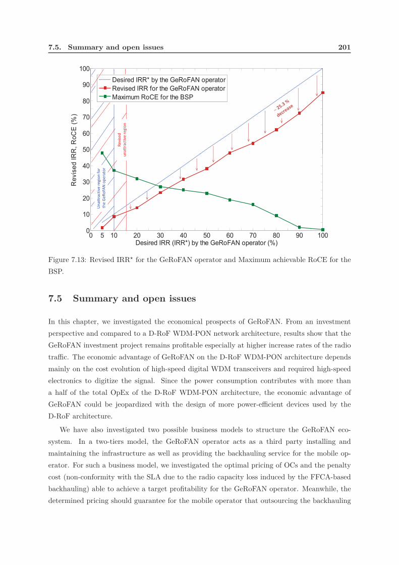
7.5. Summary and open issues 201
50
60
70
80
90
100R
R,
Ro
CE
(%
)Desired IRR* by the GeRoFAN operator
Revised IRR for the GeRoFAN operator
Maximum RoCE for the BSP
Re
vis
ed
na
ttra
ctiv
ere
gio
n
0 5 10 20 30 40 50 60 70 80 90 1000
10
20
30
40
Desired IRR (IRR*) by the GeRoFAN operator (%)
Re
vis
ed
IR
Un
att
ract
ive
reg
ion
for
the
Ge
Ro
FAN
op
era
tor
u
Figure 7.13: Revised IRR⋆ for the GeRoFAN operator and Maximum achievable RoCE for the
BSP.
7.5 Summary and open issues
In this chapter, we investigated the economical prospects of GeRoFAN. From an investment
perspective and compared to a D-RoF WDM-PON network architecture, results show that the
GeRoFAN investment project remains profitable especially at higher increase rates of the radio
traffic. The economic advantage of GeRoFAN on the D-RoF WDM-PON architecture depends
mainly on the cost evolution of high-speed digital WDM transceivers and required high-speed
electronics to digitize the signal. Since the power consumption contributes with more than
a half of the total OpEx of the D-RoF WDM-PON architecture, the economic advantage of
GeRoFAN could be jeopardized with the design of more power-efficient devices used by the
D-RoF architecture.
We have also investigated two possible business models to structure the GeRoFAN eco-
system. In a two-tiers model, the GeRoFAN operator acts as a third party installing and
maintaining the infrastructure as well as providing the backhauling service for the mobile op-
erator. For such a business model, we investigated the optimal pricing of OCs and the penalty
cost (non-conformity with the SLA due to the radio capacity loss induced by the FFCA-based
backhauling) able to achieve a target profitability for the GeRoFAN operator. Meanwhile, the
determined pricing should guarantee for the mobile operator that outsourcing the backhauling

202 Chapter 7. GeRoFAN: a Prospective Approach
to GeRoFAN is still attractive. An alternative innovative three-tiers business model is also
investigated. Such a new business model limits the role of the GeRoFAN operator to an in-
frastructure leaser and introduces a new "unusual" player called BSP in charge of providing
the cellular backhauling service to the mobile operator with an optimized backhauling strategy
(DBS). The BSP brings its added values in the three-tiers business model by capitalizing on
the advantages of the DBS algorithm compared to FFCA, i.e by using lower number of OCs
and offering an improved quality of service for backhaul (lowering the penalty cost thanks to
the lower rejection ratios of DBS).
The key benefit of the three-tiers models consists in enriching the value chain of the back-
hauling service by outsourcing it to a specialized player able to capitalize on its innovation
potential in order to deliver mobile operators with a competitive service (performing higher
QoS at lower cost).
Despite the attractiveness of the three-tiers business model, some issues have to be addressed.
The major issue is related to the complexity of implementing such a model. Indeed the successful
implementation of the tree-tiers model relies on defining exactly the requirments/expectations
of each player and implementing, through a best practice framework, an efficient protocol to
orchestrate a Business-to-Businesses (B2B) cooperative interaction between the involved actors
[91].
The regulation framework needed to support the new business model could get inspired from
similar evolutions initiated either in sectors other than telecom (such as the energy retail market
[119] and the transportation sector) or in activities that are related to telecom (like the study
in [56] that investigates the cost-effectiveness of an outsourced green-power procurement model
for mobile operators and develops a best practice guide to achieve its successful implementation
for the case of the Indian telecom market).

Chapter 8
Conclusion
Contents
8.1 Summary of Thesis Achievements . . . . . . . . . . . . . . . . . . . . . . . . . 203
8.2 GeRoFAN in the real world . . . . . . . . . . . . . . . . . . . . . . . . . . . . . 205
8.3 Areas of future works . . . . . . . . . . . . . . . . . . . . . . . . . . . . . . . . . 207
8.1 Summary of Thesis Achievements
The objective of the research conducted in this thesis is to investigate the potentiality of
GeRoFAN, an all-optical network architecture exploiting A-RoF technology, to backhaul next
generation radio cellular systems.
Thanks to its MAC-agnostic feature and its system flexibility provided by A-RoF, the GeRo-
FAN architecture is suited for multi-technology and multi-radio system backhauling which points
out its genericity. The GeRoFAN architecture takes benefit of equipment centralization at the
head-end node (HOLT) enabled by A-RoF to acquire a global view of the traffic distribution
in the area served by the GeRoFAN system. GeRoFAN is supported by an innovative Control
Plane (CP) exploiting network resources mutualization at the HOLT to carry out a dynamic
bandwidth management according to the space and time variations of the traffic matrix. How-
ever, achieving cellular backhauling using A-RoF is subject to several physical layer impairments
degrading the signal quality and thus the Shannon’s capacity of the radio channel. We outlined
in Chapter 2 that such a limitation can be overcome by designing a QoT-aware CP able to
mitigate RoF transmission impairments and thus preserving the radio system capacity. Doing
so, the key innovation of the GeRoFAN-CP is to make the cellular backhauling as transparent
as possible to the radio system.
Designing an efficient QoT-aware CP for GeRoFAN requires a deep knowledge of the phys-
ical layer impairments inherent to RoF link transmission. For that sake, we conducted in
Chapter 3 an extensive modeling and analysis of the various noises involved in the GeRoFAN
network. Indeed, we proposed a mathematical modeling describing the behavior of the reflective
204 Chapter 8. Conclusion
electro-absorption amplified modulator considered as the key component of the GeRoFAN ar-
chitecture. In addition, we carried out a modeling of the different noise sources inherent to the
GeRoFAN network (fiber transmission impairments, ROADM noises, intermodulation radio
signal distortions and optical crosstalk inherent to SCM/WDM multiplexing used by GeRo-
FAN). Considering two main possible network topologies for GeRoFAN (a tree and a loop),
the outcome of the research was to package the various impairments inherent to each topology
into a comprehensive analytical model called QoT-tool. The latter will be exploited by the
GeRoFAN-CP to set up an optimized cellular backhauling strategy.
Assuming a static and uniform traffic distribution throughout the radio network, we in-
vestigated in Chapter 4 the optimal backhauling strategy operated by the GeRoFAN-CP able
to preserve the radio system capacity while using efficiently the optical pool. Such a cross-
optimization was first solved through an exact MILP formulation. Then we proposed a heuris-
tic approach (PaGeO) based on a genetic algorithm with Pareto optimization. Our numerical
results pointed out the superiority of an optical tree compared to an optical loop for GeRoFAN.
In comparison to alternative backhauling policies either being QoT-aware or QoT-agnostic, the
GeRoFAN-CP exploiting PaGeO achieves an excellent tradeoff between preserving the radio
capacity while using efficiently the optical pool. Moreover, we have investigated the compro-
mise that an operator faces between overlaying several radio channels per cell to enable a more
flexible management of radio resources between cells and the loss in the effective radio capacity
induced by such an overlaying because of the deleterious effect of intermodulation distortions
between radio channels.
The focus of Chapter 5 was to extend the capabilities of the GeRoFAN-CP to perform an
efficient cellular backhauling in a dynamic and non-uniform traffic context. In such a particular
environment, an on-line calculation of the backhauling strategy is required by the CP, a require-
ment that PaGeO is unable to afford despite its good performance. Instead, we designed for
the GeRoFAN-CP a meta-heuristic, called DBS, based on a set of rules exploiting the modeling
of the physical layer impairments provided the QoT-tool. The main originality of the DBS is to
perform a differentiated backhauling policy that aims at adjusting dynamically the Shannon’s
capacity in each radio cell according to its actual aggregated traffic load. We carried out exten-
sive simulations that demonstrated the capability of the GeRoFAN-CP using DBS to achieve
radio capacity virtualization. Indeed, DBS exploits the gap in the traffic load between cells,
inherent to such a dynamic context, to realize a transfer of the radio capacity between them in
a similar way to a water filling problem in a system of communicating vessels. In that sense, the
relevance of the DBS approach is to perform a kind of a lean management of the radio capacity1
of the mobile system by "piping" the required bandwidth where it is needed at the detriment
1By analogy to the lean principle that enables an efficient resource management. The objective of a lean strategy is to avoid either a
waste or a shortage of capacity by designing a flexible workflow process.

8.2. GeRoFAN in the real world 205
of areas where resources are under-used, thus enabling significant savings/gains for the mobile
operator.
The last chapter of the thesis focuses on the business value and the economics of GeRoFAN.
From an investment perspective, we highlighted through a comprehensive CapEx/OpEx valua-
tion model the profitability of the GeRoFAN cellular backhauling system compared to a D-RoF
WDM-PON network architecture. Two business models, namely a two-tiers and a three-tiers
model, structuring the GeRoFAN eco-system were investigated. In both business models, the
cellular backhauling service is outsourced either to the GeRoFAN operator (who also deploys
and maintains the GeRoFAN network infrastructure) or to a specialized third party called BSP
who provides the backhauling service to mobile operators using an optimized backhauling strat-
egy (such as DBS). The economic comparison between the two models showed that the BSP
enriches the business value chain gathering the different stake-holders (mobile operator, BSP
and GeRoFAN operator) by capitalizing on the competitive advantage offered by its backhauling
strategy (DBS) to deliver mobile operators a cellular backhaul with a higher QoS and at lower
cost. We concluded our research study by outlining the main issues conditioning the successful
implementation of the new business model promoted by GeRoFAN.
8.2 GeRoFAN in the real world
The achievements of the thesis find their application for different players, including the following:
• Incumbent operators: Today incumbent operators strive to upgrade their backhauling
network at a low cost in order to cope with the continuous increase of the radio traffic.
As highlighted by the study from the telecom consultancy company Heavy Reading [38],
several mobile carriers across the world are considering the best alternatives to legacy
leased T1/E1 backhaul. While an aggressive shift to microwave-based backhauling is
considered profitable as short-term solution for several operators2, the strategic direc-
tion will certainly be focused on fiber-based backhauling by means of RoF technology as
the most sustainable solution able to accommodate the dramatic increase of the traffic.
Such a strategic direction would open new prospects for a unified broadband fixed/mobile
convergence. In that sense, the GeRoFAN architecture and its innovative control plane
enabling an efficient QoT-aware cellular backhauling is a strong candidate to reinforce the
strategic direction of Telcos to evolve their backhaul.
• Potential new comers/ small operators / MVNOs: The GeRoFAN concept (sys-
tem, architecture and the promoted business model) is by excellence a strong ally for new
telecom operators entering the market as well as MVNOs. Small carriers, new comers
2According to Heavy Reading, such a strategy is strongly applied by Vodafone in UK, Sprint in US, SFR in France.
206 Chapter 8. Conclusion
and virtual operators have lower capabilities (they cannot afford the high CapEx of radio
network deployment) than incumbent operators. Since the GeRoFAN infrastructure in-
vestment is under the responsibility of a third party, the GeRoFAN architecture facilitates
the introduction into the market of such long ago considered small players. Thanks to its
MAC-agnostic feature, different operators serving different radio technologies can be sup-
ported by the GeRoFAN network. Since the investment of all operators (either incumbent
or new comers/MVNOs) in the infrastructure is equivalent, innovation in services offered
to radio mobile subscribers will be the key factor of differentiation in such a commercial
competitive multi-tenants environment.
• Optical network infrastructure provider: Optical network infrastructure providers
like Syringa3 in the US or those promoted by the FFTH Council Europe4 can easily
play the role of a GeRoFAN operator. Instead of simply renting out its optical network
to broadband FFTx operators, the optical infrastructure provider can reuse its optical
network for cellular backhauling as advocated by GeRoFAN. With the current trend of
network component cost evolution, we have demonstrated that investing in GeRoFAN
is more profitable than an alternative D-RoF WDM-PON architecture. As shown in
our research, the optical network infrastructure provider playing the role of a GeRoFAN
operator can either act as a backhaul service provider or simply focus its business on a
backhaul infrastructure provider.
• Backhaul Service Provider (BSP): Several studies like [139] and [38] have pointed out
the increasing role expected from the BSP. As highlighted in the thesis, the nature of the
BSP evolves from a third party who provides backhaul for mobile operators by renting out
its T1/E1 copper line assets to an engineering service company delivering a competitive
backhauling service for radio operators with a higher QoS and at lower cost. Either named,
according to Heavy Reading [38], as a Backhaul Network Optimization Consultancy or
a Backhaul Service Provisioning Company, the BSP is able to enrich the value chain
of the Business-to-Business (B2B) telecom market by outsourcing the backhauling to a
specialized player who acts as a broker between its supplier (the GeRoFAN operator) and
its customers (mobile operators).
• Telecom regulators: As outlined in our research, the GeRoFAN concept supports a new
challenging commercial and regulatory environment, with increased interactions between
the different stake-holders. The key for a successful implementation of the GeRoFAN eco-
system relies on a full involvement of regulatory authorities and institutions to set up the
best practices and implement an efficient legal framework. The role of regulators is crucial
3www.syringanetworks.net4
www.ftthcoucil.eu

8.3. Areas of future works 207
to conceive incentive policies for mutualization according to a suited road-map5. In some
cases, where large incumbent operators are reluctant to take "the GeRoFAN plunge", it is
up to regulators to pave the way for opening the market. In that sense, GeRoFAN could
be an attractive solution to achieve that aim.
• Equipment vendors/Bakchaul technologies suppliers: They are also concerned by
the GeRoFAN solution in particular and the challenges raised by the backhaul in gen-
eral. As shown in the thesis, one of the key components of the GeRoFAN system is
the advantages offered by the reflective electro-absorption amplified modulators. Telecom
equipment companies like the Alcatel-Lucent III-V Lab sitting at mid-range between re-
search/engineering and business are at the front line to promote the quick introduction
into the market of advanced opto-electronic and photonic components able to speed up
the road-map for a real implementation of bold architectures like GeRoFAN.
Regarding their level of involvement in the GeRoFAN concept, the aforementioned players
are positioned in Figure 8.1 within different circles ranging from directly impacted/involved
(inner circles) or indirectly impacted/involved players (outer circles).
8.3 Areas of future works
Thanks to its radio MAC-agnostic CP, the GeRoFAN architecture can be mutualized by several
mobile operators exploiting the same or different radio technologies. In such a multi-operator
environment, the different carriers may serve the same region and compete together to provide
enhanced user-experience for mobile subscribers. Thanks to Cognitive Radio, mobile subscribers
use devices equipped with a multi-technology radio-access card which enables them to get an
instant access to any radio system being sensed6. The different mobile operators compete
not only on the market share, but also on two other resources: radio frequencies managed
dynamically on a leasing-basis by a radio broker, and optical channels from the WDM pool
managed by the GeRoFAN manager. The multi-operator/multi-service GeRoFAN architecture
described in Chapter 2 can be the cellular backhauling network platform for such a multi-
tenants environment. Unlike the research of this PhD that focuses on the interaction between
operators (B2B framework), the future research should include also end-users’ expectations.
Indeed, end-users are willing to shift at the connection basis between operators looking for the
best QoS and the lowest service subscription price. Therefore, the future research deals with
5See the case of the French Telecom regulator ARCEP in the article published in "Le Monde" written by Ce-
cile Ducourtieux (Service Economie) and entitled "Vers une mutualisation des réseaux" [Towards networks mutualization]:
http://www.lemonde.fr/idees/article/2012/06/13/vers-une-mutualization-des-reseaux_1717636_3232.html, accessed 06/13 2012.6The different systems are advertised via their beacon radio signals broadcasted within the cells. As a key enabler of Cognitive Radio,
Software Defined Radio (SDR) implements by software most signal processing tasks usually carried out in hardware. SDR can serve a wide
variety of changing radio protocols in real time and thus enables mobile users to shift seamlessly (even at a connection basis if allowed by the
regulatory environment) from one radio technology/operator to another.

208 Chapter 8. Conclusion
BSP
Incumbentmobile
operators
New entrants
Telecom
Equipmentvendors
Optical network infrastructure
provider Smalloperators
MVNOs
TelecomRegulators
BackhaulTechnologies
Suppliers
Figure 8.1: Positioning the different players impacted/involved in the GeRoFAN concept.
two overlaying interaction frameworks: B2B (interactions between mobile operators/GeRoFAN
manager/Radio broker) and B2C (Business-to-Customer interactions orchestrating the relations
between the mobile operators and their "potential"7 customers). In that sense, the results of the
current research can be exploited as a valuable input together with mathematical models like
Game Theory techniques managing the strategies adopted by the different players involved
in the B2B interaction framework. While Utility Functions enriched with a Learning
Process8 describing the behavior of the mobile users can be used to orchestrate the B2C
framework.
7So called because of their ability to shift from one operator to a competitor (offering a better QoS or/and a more attractive service
price). Hence, operators are constantly challenged to offer a more attractive service in order to retain their customers as long as possible and
thus to lead the competition.8A machine learning process makes utility functions evolve with time. In fact, one can imagine that mobile users are not totally agnostic
during their interactions with the different mobile operators. Indeed, a mobile operator who "disappoints" a given customer for several times,
would be penalized (by appropriately weighing the utility function) in the next round choice of that customer. Although more complicated
to model and implement, Utility function including a learning process enables to translate the perceived QoS (a.k.a Quality of Experience)
by the customer as the latter learns from his/her previous experience and modifies his/her objective accordingly. A learning process-based
Utility function ensures also a minimum stability of the system by avoiding the "ping-pong" effect caused by the excessive move of subscribers
between operators.

Appendix A
Appendix
A.1 EAM Analytical Modeling
Figure A.1 illustrates the methodology followed for EAM analytical modeling. Considering the
case of a Multi-Quantum Well (MQW)-EA modulator, the absorption coefficient α is Volt-
age (V)-dependant and optical carrier (λ)-dependant. For simplicity, only the ground state
heavy/light-hole (E1-(H/L)H1) energy transition is considered in the model since it is expected
to be the major participant in the photo-absorption process [49]. We describe in the following the
different steps to compute α. The mathematical development is inspired from a semi-empirical
model proposed in [84][152] for MQW-based modulators.
First, the unperturbed (ground-state) wave-functions of electrons and holes (heavy/light)
Ψox and their energies Eo
x are computed from the Schrodinger equation, where x denotes the
considered particle (i.e. e, lh and hh for electron, light hole and heavy hole respectively).
Assuming that modulator layers are piled up along the z axis, the unperturbed Hamiltonian
Ho is provided by Equation A.1:
Ho(Ψox) = Eo
x ·Ψox =
−~2
2m∗x,b/w
· −d2Ψox
d2z+ Vx(z) ·Ψo
x(z) (A.1)
Given: m∗x,b/w the effective mass of particle x at the barrier (b) or the well (w); Vx(z) the
electric potential seen by particle x at z and ~ the reduced Planck constant.
Solutions of Equation A.1 for the steady-state are the superposition of two plane-waves,
an incident wave and a reflected wave. Depending on the location of the particle, the wave
expression is:
Ψox(z) =
A · exp (kxz) +B · exp (−kxz) for a well-located particle
A′ · exp (Kxz) +B′ · exp (−Kxz) for a barrier-located barrier(A.2)
Given: kx =√(2mx,w
∗
~2)(Ex
o − Vx(z)) and Kx =√(2mx,b
∗
~2)(Vx(z)− Eo
x) the wave-numbers
for particle x respectively within the well and the barrier; A, B, A′ and B′ are constants and
the complex number (2 = −1).In a QW modulator, a rectangular potential is assumed and expressed as function of the
gap-energy of each quantum layer. Assuming that only an evanescing wave is considered within

210 Appendix A. Appendix
Solving Schrodinger equations
for a eletron, light-hole and heavy-hole
particles located in a quantum well
EAM RF Gain and
Noise Figure using
EAM circuit model
The EAM
Henry factor
Only TE-mode is considered.
Mo
du
lato
r
Pe
na
lty
Dispersive
Fiber
Least-square error double
gaussian fitting of (V, )
The overlapping intergals of electron
and hole wave-functions yields to
EAM absorption profile for each
Particles wave-functions and energy
levels solved using transfer function method for
each particle both under 0V and under a voltage V
Optimal
bias voltage
Derivatives of the
EAMTransfer function
Intermodulation
Distortions (IMDs)
Computing at the incremental
change with respect to V of the real
part ( neff
) and the imaginary part ( )
of the EAM complex refractive index.
SOA maximum gain at SOA Saturation power
- and Input power -dependant
SOA gain using Lambert-W function
SOA noise figure
Non-flat gain
amplification
SOA noise
expansion (ASE)
Maximize RF gain, Extinction ratio of 10 dB
Frequency
Chirping
SOA active region
material gain coefficient
SOA active region
material loss coefficient
SOA single pass gain at
Figure A.1: Methodology of EAM-SOA analytical modeling.We follow a step-by-step modeling methodology inspired from [52] and [28] to get an analytical formulation of the working principle of the
REAMSOA. One of the key aspect of the model is to highlight the dependance with the optical wavelength, that will be exploited for the
optimization carried out by the GeRoFAN control plane. EAMSOA-induced major impairments are also highlighted in blue.

A.1. EAM Analytical Modeling 211
the barrier and only propagating waves within the well, the wave-function is written depending
on the location of the particle as the following Equation system A.3:
Ψo1,x(z) = a · exp (Kxz) z ≤ − ℓw
2
Ψo2,x(z) = b · exp (kxz)± exp (−kxz) − ℓw
2 ≤ z ≤ ℓw2
Ψo3,x(z) = −a · exp (−Kxz) z ≥ ℓw
2
(A.3)
Where: ℓw the width of the quantum well; a and b are real constants.
The equation system A.3 shows the superposition of two possible solutions within the well,
a symmetric (i.e. when: Ψo2,x(z) = b · cos(kxz)) or asymmetric propagating wave (i.e. when:
Ψo2,x(z) = b · sin(kxz)).
In a quantum-well, the energy level is quantized. To compute the discrete energy levels for a
given particle x, we exploit the continuity condition of the wave-function Ψox and its first deriva-
tive dΨox
dz at the well/barrier boundaries (i.e. at z = ±ℓw/2 ), thus leading to Kx = kx · tan(kxℓw2 )
and Kx = −kx · cot(kxℓw2 ) for symmetric solutions and asymmetric solutions respectively. Equa-
tions of wave-numbers for symmetric and asymmetric solutions are solved graphically for each
particle to find energy levels Eox. We use the normalization constraint related to the probability
density function (i.e∫+∞
−∞ |Ψox|2dz = 1) to find the value of constants a and b.
We apply our analytical model on an EAM designed by the joint-venture Alcatel-Thales
III-V Lab [39]. The modulator is made of 10 quantum wells and 11 barriers with the following
features:
• Barrier: Al210Ga190In600As with width ℓb = 9.4 nm.
• Well: Ga517In483As with width ℓw = 9.4 nm.
The band-gap energy Egb,x and Egw,x for particle x in the barrier and well respectively
are computed by taking into account the alloy composition of both well and barrier materials
using the method presented in [54]. Related data at room temperature including the energy
gap of basic elements (Ga, In, Al and As), Luttinger parameters for particle effective masses
in the well and the barrier are extracted from [53]. Wave-functions and energy levels of a given
particle x at each quantum level in the absence of external field (i.e F = 0) are summarized in
Table A.1. Figure A.2 depicts first quantum level unperturbed wave-functions of each particle
for 1550 nm.
Given Ix the number of energy levels of particle x (i.e Ie = 2, Ilh = 2 and Ihh = 4), the set of
wave-functions Ψoxi (1≤i≤Ix)
shown in Table A.1 form a orthonormal basis of a vector sub-space
of L21, i.e. for a given particle x and quantum level i and j,∫+∞
−∞ Ψoxi
·Ψoxjdz = δij
2
With an applied electric field F , the perturbed Hamiltonian is written as in Equation A.4:
1L2: Hilbert space, i.e vector space of 2nd power integrable functions.2
δij stands for the Kronecker notation: δij = 1 if (i = j) and 0 otherwise.

212 Appendix A. Appendix
Table A.1: Wave-functions and energy levels for each particle at 0 V.
xi Eox (eV) Ψo
x(z) (well) Ψox(z) (barrier)
e1 0.4115 1.2206 · 104 · cos(2.361 · 108 · z) 9.5473 · 104 · exp(±6.0993 · 108 · z)
e2 0.567 1.1723 · 104 · sin(4.828 · 108 · z) ±5.323 · 104 · exp(±3.782 · 108 · z)
lh1 −0.3701 1.1212 · 104 · cos(2.0795 · 108 · z) 2.6291 · 104 · exp(±3.0489 · 108 · z)
lh2 −0.4528 7.8696 · 103 · sin(3.673 · 108 · z) ±1.1784 · 104 · exp(±8.848 · 107 · z)
hh1 −0.3623 1.2807 · 104 · cos(8.2099 · 108 · z) −2.7907 · 105 · exp(±7.1579 · 108 · z)
hh2 −0.41334 1.0343 · 104 · sin(1.0557 · 109 · z) ±2.7201 · 104 · exp(±2.124 · 108 · z)
hh3 −0.4524 1.3304 · 104 · cos(2.7906 · 108 · z) 5.0816 · 105 · exp(±1.0647 · 109 · z)
hh4 −0.4781 1.3173 · 104 · sin(5.549 · 108 · z) ±5.673 · 105 · exp(±9.447 · 108 · z)
0.15
0.2
0.25
n a
mplit
ude (
a.u
)
Electron waveform (E1)
Light Hole waveform (LH1)
Heavy Hole waveform (HH1)
Left
Barrier
Well
Right
Barrier
-1 -0.5 0 0.5 1
x 10-8
0
0.05
0.1
Quantum layer axis z (m)
wave-f
unct
ion
Figure A.2: Wave-functions of the QW-EAM for 1550 nm incident light under 0 VAt 0 V , wave-function of particles are confined within the well while evanescing waves at the barrier point out the low probability to find
electrons and holes in that region (tunneling effect through the barrier is neglected). Only first energy level for each particle is illustrated in
the figure.

A.1. EAM Analytical Modeling 213
0.15
0.2
0.25n a
mplit
ude (
a.u
)Light Hole wavefunction (LH1)
Electron wavefunction (E1)
Heavy Hole wavefunction (HH1)
Left
BarrierRight
Barrier
Well
Applied Electric
Field F
-1 -0.5 0 0.5 1
x 10-8
0
0.05
0.1
Quantum layer axis z (m)
wave-f
unct
ion
Figure A.3: Wave-functions for 1550 nm incident light under −3 VBiasing the device creates a perpendicular electric field F that stretches the electron-hole pair. Wave-functions are pushed towards each side
of the barrier. The field-induced electron-hole spatial separation is at the basis of the decrease of the luminescence of the EAM and a change
of its absorption profile (cf. Figure A.4)
Ho(ΨFx ) = EF
x ·ΨFx =
−~2
2m∗x,b/w
· d2ΨF
x
d2z+ (Vx(z)± qeFz) ·ΨF
x (z) (A.4)
Where: qe the electron charge.
Solutions of Equation A.4 can be expressed in their vectorial form: ΨFx =
∑Ixi=1 aF
x,i ·Ψoxi
given the normalization condition:∑Ix
i=1 |ax,i|2 = 1.By substituting the vectorial form of ΨF
xiinto Equation A.4, the mathematical development
leads to the linear system expressed by Equation A.5. Thus, EFx and aF
x,i are respectively the
eigenvalues and the eigenvectors of the Hamiltonian matrix. Figure A.3 illustrates the particles
wave-functions for 1550 nm incident light and under −3 V applied bias voltage.
Eox1+
∫ +∞−∞ Ψo
x1(±qeF z)Ψo
x1dz · · · Eo
x1+
∫ +∞−∞ Ψo
x1(±qeF z)Ψo
xIxdz
.
.
.. . .
.
.
.
EoxIx
+∫ +∞
−∞ ΨoxIx(±qeF z)Ψo
x1dz · · · Eo
xIx+
∫ +∞−∞ Ψo
xIx(±qeF z)Ψo
xIxdz
•
aFx1
.
.
.
aFxIx
= EF
x ·
aFx1
.
.
.
aFxIx
(A.5)
Because two kinds of holes are considered in the model (light/heavy holes), the absorption
process in the quantum well is driven by two coupled excitons called bi-exciton. We characterize
numerically each exciton separately by computing their oscillator strength, their line-width
enhancement and Stark-energy shift (exciton resonance wavelength λex). The exciton resonance

214 Appendix A. Appendix
Decrease of
the oscillator
strength
@ V = 0
@ V 0
Ab
sorp
tio
n p
rofi
le n
orm
ali
zed
Linewidth broadening
Stark shift
Absorption
increase at
Optical wavelength
Figure A.4: Illustration of a single exciton Stark shift under an applied voltage.Applying an external field causes a red shift of the absorption profile of the EAM. The exciton is "stretched" due to the spatial separation
between electrons and holes. The Quantum Confined Stark shift Effect (QCSE) effect is characterized also by a decrease of the oscillator
strength, a broadening of the linewidth and a slight increase of the absorption coefficient at a given optical wavelength. The optimal
performance of the device (higher extinction ratio, higher RF gain) is achieved by adjusting the right bias.
wavelength is related to the QW gap energy Ewg (computed as in [54]) and exciton biding energy
Eb,ex (assumed as in [49]) as: hc/λex = Ewg + EF
e + EFlh/hh − Eb,ex. Following the suggestion of
Miller et al. in [49], we describe the absorption profile of an exciton in a MQW by a Gaussian
shape rather than a Lorentzian. With the approach of [27], the absorption coefficient under
external field F at a given wavelength λ is expressed empirically through Equation A.6:
αFlh/hh(λ) = A · fF
lh/hh · GFlh/hh(λ) + αbulk (A.6)
Where: A: a constant independent of the applied electric field F ; αbulk: background ab-
sorption approximated as the bulk material absorption; fFlh/hh: the oscillator strength of the
exciton (e/lh,e/hh) par unit volume is proportional to overlapping integrals between electron
and hole wave-functions as formulated in Equation A.7; GFlh/hh: The line-shape at an applied
field F modeled at room temperature by a Gaussian function as in Equation A.8.
fFlh/hh =
|Ulh/hh(0)| · | ∫+∞−∞ ΨF
e ·ΨFlh/hhdz|2
ℓw + ℓb· (A.7)
Given: Ulh/hh(0) =√
2πR2B
: the bi-exciton (e/lh, e/hh) envelope function evaluated at the
origin relative coordinate and function of the Bohr radius of the exciton [19].
The absorption coefficient line-shape is given by Equation A.8:

A.2. EAM chirp analytical modeling 215
GFlh/hh(λ) =
√ln 2
π· 1
ΥFlh/hh
· exp
− ln 2 ·
hc(1
λex− 1
λ
)
ΥFlh/hh
2 (A.8)
Given: ΥFlh/hh: The Half-Width Half-Maximum (HWHM) line-width of the (e/lh,e/hh)
exciton when F is applied.
As illustrated by Figure A.4, the effect of an applied field F on the exciton resonance is to
cause a red shift of the absorption curve (i.e shift of λex to longer wavelengths) and a decrease
in the oscillator strength. The line-width of the absorption curve, related to the lifetime of the
excited state, is also broadened due to three mechanisms: on one hand, a homogenous broaden-
ing due to interaction (scattering) with optical phonons, on the other hand, an inhomogeneous
broadening due to well width fluctuations and variations in the electric field from well to well.
Although the homogenous broadening is assumed to be constant with the applied electric field
(estimated to ≃ 6.27 meV according to [52]), the inhomogeneous broadening is modeled analyt-
ically as in [52], while the expression of the exciton energy is deduced from the approximation of
energy shift of the ground state given by the variational calculations carried out by Bastard in
[14]. Although a compressive strain has been applied to the MQW material to achieve optical
polarization independence [95], only TE-mode incident light-waves are considered in the model.
The absorption coefficient in TE-mode under an applied electric field F is expressed according
to Equation A.9 as a weighted sum of the e/lh and e/hh absorption coefficients [75]:
αFT E =
αFhh
4+3 · αF
lh
4(A.9)
Figure A.5 gives the set of absorption curves computed for TE-mode with an incident light
wavelength from 1525 nm to 1600 nm under the application of a reverse bias voltage Vb.
To study the linearity of the modulator, we fit through Equation A.10 the absorption profile
(with respect to Vb) at each optical channel with a double Gaussian fit function of the form:
α(Vb, λ) = Aλ · exp((Vb − Fλ)
2
Bλ
)+ Cλ · exp
((Vb − Gλ)
2
Dλ
)+ Eλ (A.10)
Where: Aλ, Bλ, Cλ, Dλ, Eλ, Fλ and Gλ are λ-dependant fitting parameters
Figure A.6 shows as an example fitted absorption coefficient for 1530 nm and 1580 nm
optical channels. The list of the different fitting parameters of 16 optical channels ranging from
1525 nm to 1600 nm is presented in Table A.2.
A.2 EAM chirp analytical modeling
The refractive index of the EAM is a complex number whose imaginary part stands for the ab-
sorption coefficient determined analytically in Section A.1. The real part of the refractive index

216 Appendix A. Appendix
4
5
6
7x 10
5
on c
oeffic
ient (/
m)
0 0.5 1 1.5 2 2.5 3 3.5 4 4.5 50
1
2
3
Reverse bias voltage (-V)
TE
-mode A
bsorp
tio
1525 nm 1600 nm
(5 nm spacing)
Figure A.5: MQW-EAM absorption coefficient profile from 1525 nm to 1600 nm.The TE-mode absorption profile of the MQW-EAM is a weighted sum of both light hole and heavy hole exciton absorptions. The highest
absorption is achieved at the resonance of the E-LH exciton.
Table A.2: MQW-EA modulator fitting parameters
λ nm Aλ(×105) Bλ(×105) Cλ(×105) Dλ(×105) Eλ(×105) Fλ(×105) Gλ(×105)1525 6.958 -0.4256 2.306 -0.5988 0.161 3.719 2.032
1530 6.48 -0.4143 2.157 -0.6172 0.07529 3.826 2.152
1535 6.006 -0.4063 1.999 -0.6259 0.02996 3.928 2.262
1540 5.544 -0.4065 1.845 -0.6266 0.007714 4030 2.364
1545 5.160 -0.4235 1.699 -0.6198 -0.002244 4.142 2.456
1550 5.004 -0.4797 1.563 -0.6043 -0.005739 4291 2.538
1555 5.808 -0.6681 1.431 -0.5764 -0.005866 4591 2.605
1560 4.880 -0.2055 1.277 -0.5348 -0.004531 6.332 2.649
1565 3.1380 -0.5787 1.164 -0.5366 -0.005158 11.13 2.722
1570 2.4122 -6.714 1.080 -0.5413 -0.005126 12.26 2.797
1575 1.9002 -8.816 0.9871 -0.5311 -0.004546 13.94 2.857
1580 1.647 -3.563 0.8967 -0.5100 -0.003261 7.196 2.904
1585 1.330 -1.749 0.7957 -0.4747 -0.001692 4.985 2.932
1590 07050 -1.129 0.6895 -0.4341 -0.0002721 4.266 2.947
1595 0.6064 -0.9146 0.5766 -0.3919 0.0007817 3.983 2.953
1600 0.5830 -0.7881 0.4934 -0.3615 0.001519 3.871 2.967

A.2. EAM chirp analytical modeling 217
4
5
6
7x 10
5
tion C
oeffic
ient (/
m)
@ 1530 nm: 105 (6.4 e-(V-3.8)2/0.4 + 2.1 e-(V-2.1)
2/0.6 + 7.5)
@ 1580 nm: 105 (16.4 e-(V-7.1)2/3.5 + 0.9 e-(V-2.9)
2/0.5 - 0.003)
0 0.5 1 1.5 2 2.5 3 3.5 4 4.5 50
1
2
3
TE
-mode A
bso
rpt
Reverse Bias Voltage (-V)
Figure A.6: Best fit expressions for EAM absorption profiles at 1530 and 1580 nm.A least-square error double-Gaussian (one for each exciton) function is used to best-fit the absorption coefficient of the modulator [49]. Fitting
parameters are accurately tuned to reproduce faithfully the shape of the absorption profile while ensuring a stable behavior of its derivatives.
of the modulator is computed by taking into account the composite nature of the absorption
material layer of the device. To compute the effective (real part) of the EAM refractive index,
we apply the method depicted in [86]. Including the optical confinement factor Γeamof the EAM
(restricting the analysis only to TE-mode for simplicity), the effective refractive index of the
absorption layer is computed according to Equation A.11:
neff =
√
n2o +
((n2i − n2o) · Γeam
2− Γeam
)(A.11)
Given: no, ni are respectively the refractive index of the cladding layer and the the absorp-
tion layer of the MQW-EAM waveguide.
Frequency chirping is commonly expressed by the line-width enhancement factor (a.k.a
Henry factor αH and chirp parameter) and the modulation waveform. The Henry factor, de-
scribing the sensitivity of the AM-FM conversion chirping phenomenon, is defined as the relative
variation of the real part of the refractive index of the EAM with respect to its imaginary part
[155]. Following the extensive analysis of Yamamoto et al. [152] and using results of energy
levels of electrons and holes under an external field F (see Section A.1), we derive the values of
the Henry factor at different optical channels. We should notice that because of the dependence
of the chirp parameter with the bias voltage (the external electric field F ), the values of αH
that will be assumed for the remaining of the model are those computed at optimal bias V ∗b .

218 Appendix A. Appendix
1
1.5
facto
r H
1.5 1.51 1.52 1.53 1.54 1.55 1.56 1.57 1.58 1.59 1.6
x 10-6
0
0.5
Optical wavelength (m)
Henry
f
Figure A.7: EAM Henry factor (αH) as function of photon wavelength.Compared to semiconductor-based lasers and SOA modulators, EAMs show lower chirp factor (when it is appropriately biased, an EAM can
feature a slightly negative chirp ideal for long haul optical transmission). At optimal bias voltage, the chirp parameter of our EAM varies
within the range 0.7 ∼ 1.2 for the conventional C-band (cf. squared area in the figure).
Figure A.7 illustrates the evolution of αH at V ∗b with optical wavelength.
According to [74], the chirping factor is related to the frequency excursion χ and the optical
power at the output of the modulator Pout as in Equation A.12:
χ =1
2π· dΦdI
=αH
4πPout· dPout
dI(A.12)
Giving that: Pout = fPin, where f the EAM transfer function and V = Zm · I, where Zm the
modulator impedance; the expression of χ is further simplified leading to Equation A.13:
χ =αHZm
4π· f
′(Vb)
f(Vb)(A.13)
The optical field at the output of the modulator is expressed as:
v(t) =√2f(V )Pin cos(wot+Φ(t)) given: V = Vb(1 + x(t)) the AC modulating voltage ex-
pressed with the RF signal x(t); wo the optical carrier angular frequency and Φ(t) the angular
frequency excursion of the optical signal due to chirping. Supported by the analysis in [15] and
the result of Equation A.13, Φ is expressed as: Φ(t) = VbαH2
f′
f
∫t x(ξ)dξ. Following the steps of
the analysis carried out by Betti et al. in [15], the optical field u(t) at the output of the fiber
of impulse response h is given by:
u(t) =√2Pin · ℜ
e((wot+Φ(t))) ·
∫
R
h(τ)√f(V (t − τ))e(−(woτ+Φ(τ)−Φ(t−τ)))dτ
(A.14)

A.2. EAM chirp analytical modeling 219
We expand both√f(V (t − τ)) and
√α(t − τ) into polynomial series up to the third order
(higher terms of the expansion are neglected because of the high bandwidth of the fiber medium).
We introduce H(Ω) = 10−aL2 e
(− βΩ2
2αH Vb)the Fourier transform of h(t) given the coefficient β =
−DLλ2oαHVb
c , the optical wavelength λo, the optical distance L, the fiber attenuation coefficient
a and the fiber dispersion coefficient D. The expression of the output signal becomes:
u(t) =√2Pin · ℜ
e((wot+Φ(τ)))
·(
g(t)H(Ω) + g′(t)dH
d(Ω)+
d2H
d(Ω)2g′′(t) + Φ′′g
2+
d3H
d(Ω)3
) (A.15)
Where: g =√f and g′, g′′ and g′′′ (respectively Φ′, Φ′′ and Φ′′′) first, second and third
derivatives of g (respectively Φ).
Given the dependance of g on V , we derive the expression of the first three derivatives of g
as function of the derivatives of V as the following:
g′ = a1 · V ′ (A.16)
g′′ = a1 · V ′′ + a2 · V ′ (A.17)
g′′′ = a1 · V ′′′ + a2 · V ′′ + a3 · V ′ (A.18)
While the coefficients a1, a2 and a3 are computed at bias point as:
a1 =f′
2g
∣∣∣∣Vb
(A.19)
a2 =f′′f − f′
2g3
∣∣∣∣Vb
(A.20)
a3 =3f′2 − 2f′′f+ 4f′′′f2 − 2f′′f′f
8g5
∣∣∣∣∣Vb
(A.21)
Given that: dnHd(Ω)n = (−1)n
∫R
h(ν)νne−jΩνdν and considering the same assumptions as in
[15] (i.e. e− βΩ2
2αH Vb ≈ 1), we focus along the mathematical development only on the real part of
u(t) which leads to:
u(t) ≃√2Pin · 10−aL
2 ·(
g − βg′x − g′′β2x2
2− Φ′′gβ
4παHVb
−g′′′β3x3
6+3β2x
4· Φ
′′g′ + Φ′′′g3
αHπVb
)· cos(wot) cos(Φ)
(A.22)
To highlight IMD and HD components induced by chirping, we carry out a multi-tone anal-
ysis. The modulating signal x(t) is expressed as a mix of 3 RF signals with angular frequencies

220 Appendix A. Appendix
wi and OMI mi, thus: x(t) =∑3
i=1 mi cos(wit). Substituting the SCM formulation of x into
Equation A.22, we get:
u(t) ≃√2Pin · 10−aL
2 cos(Φ) ·(
DC +
( ∑
i
Ii cos(wit) +Qi sin(wit)
)
+
( ∑
i
I2i cos(2wit) +Q2i sin(2wit)
)+
( ∑
i,j
Ii±j cos(wi ± wjt) +Qi±j sin(wi ± wjt)
)
+
( ∑
i
I3i cos(3wit) +Q3i sin(3wit)
)+
( ∑
i,j
I2i±j cos(2wi ± wjt) +Q2i±j sin(2wi ± wjt)
)
+
( ∑
i,j,k
Ii±j±k cos(wi ± wj ± wkt) +Qi±j±k sin(wi ± wj ± wkt)
)+ · · ·
)
(A.23)
Given: Iℓ and Qℓ are the in-phase and quadrature phase amplitudes of the signal and its
chirp-induced IMD/HDs falling at frequency component ℓ. Specifically, for the case of IMD3
noise we obtain:
• For IMD3 with 2 tones falling at wℓ = 2wi − wj :
I2i−j = a1β2Vb · m2
i mj · (w2i +w2j2) + 3a1β
2Vb · m2i mj · wi(wj − wi
2) (A.24a)
Q2i−j = a2β2Vb · m2
i mjwi(wi − wj
2) (A.24b)
• For IMD3 with 3 tones falling at wℓ = wi − wj + wk:
Ii−j+k = a1β2Vb ·mimjmk · (w2i +w2j +w2k)+3a1β
2Vb ·mimjmk · (wjwi+wjwk −wiwk) (A.25a)
Qi−j+k = a2β2Vb · mimjmk · wi(wi + wj + wk) (A.25b)
The average chirp-induced IMD/HD optical noise power Nopt is computed as: Nopt = 〈|u|2〉,where 〈·〉 the time average operator. Given that: 〈cos(Φ)2〉 ≃ 1, the average optical noise
power Nopt,ℓ of chirp-induced IMD/HD and falling at frequency component ℓ is given by:
Nopt,ℓ ≈ 2Pin · 10−aL · (I2ℓ +Q2ℓ).
A.3 RBS analytical modeling
According to [148], the Power Spectral Density (PSD) of the RBS noise is expressed as:
Nrbs(f) =10R2rb(2αL+ e−2aL − 1)
9· F〈|Rεsig |2〉 (A.26)
Given: Rεsig : The autocorrelation function of the signal electric field εsig; L: The fiber link
length; a: Fiber attenuation coefficient; Rrb: RBS reflectance of the SMF (Rrb = −27 dB forsingle mode fiber [148]) and F: denotes the Fourier transformation operator.

A.3. RBS analytical modeling 221
We distinguish between two kinds of RBS noises. A first RBS noise (N inrbs) called input
RBS is due to the interference of the back-reflected modulated signal with the optical signal
at the input of the modulator. A second RBS noise (Noutrbs ) called output RBS is due to the
interference of the back-reflected continuous-wave signal with the modulated signal at the output
of the modulator.
A.3.1 Input RBS noise:
The PSD of the continuous wave signal εsig at the output of the DFB laser is approximated
by a Lorentzian distribution with a spectral width ∆ν. The Fourier transform of the auto-
correlation of εsig is also a Lorentzian distribution with a spectral width 2∆ν. Then, Equation
A.26 is written as:
N inrbs(f) =
10R2rb(2aL+ e−2aL − 1)9
· 2a∆ν
π(f2 + 4∆ν2)(A.27)
RBS power falling at RF fℓ with a signal bandwidth Bℓ is: P inrbs =
∫fℓ±Bℓ/2 N in
rbs(f)df [148].
A.3.2 Output RBS noise:
The electric field of the signal at the output of the EAM is expressed as function of the input
optical power Pin, the transfer function of the EAM f as:
εsig =√2Pinf(V ) · e2π
∫ t
0γVbx(ξ)dξ (A.28)
With: γ: the EAM chirping efficiency (frequency excursion) expressed in [Hz/V]; x(t) =∑i
mi cos(2πfi) the modulating SCM RF signal.
Introducing g =√f, we exploit the Taylor development of g with respect to V (around the
bias voltage Vb), thus the autocorrelation of εsig is given by:
Rεsig =
[gb + g′
bV (t) + g′′b
V (t)2
2!+ · · ·
]·[gb + g′
bV (t+ τ) + g′′b
V (t+ τ)2
2!+ · · ·
]· e
2πt+τ∫t
γVbx(ξ)dξ
(A.29)
Neglecting higher order terms in A.29, the Fourier transform of Rεsig is expressed as:
F〈|Rεsig |2〉 = F⟨[g2b + g′2
b V 2b (1 +
∑
i
m2i cos(2πfiτ)
2)]2
⟩⊗ F
⟨[cos(2π
t+τ∫
t
γVbx(ξ)dξ)]2⟩
(A.30)
Where: ⊗ stands for the convolution product operator and 〈·〉 the time average operator.Given δ(f) the Dirac distribution function. The first term in Equation A.30 is worked out
leading to:

222 Appendix A. Appendix
F⟨[
g2b + g′2b V 2
b
(1+
∑
i
m2i cos(2πfiτ)
2
)]2⟩=
(g4b + g′4
b V 4b +2g
2b g′2
b + V 2b +
∑i m4
i
8
)· δ(f) (A.31)
For high number of modulating RFs with small OMI, we assume x following a gaussian
distribution, thus the second term of Equation A.30 is computed as:
F⟨[cos(2π
t+τ∫
t
γVbx(ξ)dξ)]2⟩
≃ 1
σf√
πe
−f2
4σ2f (A.32)
given: σf = Vbγ
√∑i
m2i2
Using results of Equations A.31 and A.32, and given that δ(f) is the identity element of the
convolution product, the output RBS noise power falling at RF fℓ with a signal bandwidth Bℓ
is:
Noutrbs =
10R2rb(2aL+ e−2aL − 1)9
·(g4b + g′4
b V 4b +2g
2b g′2
b +V 2b +
∑i m4
i
8
)·fℓ+Bℓ/2∫
fℓ−Bℓ/2
e
−f2
4σ2f
σf√
πdf (A.33)
A.4 OBI analytical modeling
According to the analysis of Desem [37], the PSD of the OBI noise produced by the beating
between two modulated optical carriers i and j is given by the convolution of their respective
PSDs as in Equation A.34:
Nij(f) = 4√
Po,iPo,j ·√
f(Vi)f(Vj) · | cos(Φ)| ·(Si(f)⊗ Sj(f)
)· 〈cos2 θij〉 (A.34)
Given: Si(f) (respectively Sj(f)): The PSD of the electric field of OC modulated by RF
i (respectively j). Po,i (respectively Po,j): Received optical power of OC modulated by RF i
(respectively j); θij : the difference in polarization angle between fields i and j and Φ the phase
difference between the two optical carriers.
The PSD of the continuous-wave signal at the output of the DFB laser is approximated with
a Lorentz distribution showing a linewidth ∆f . For simplicity, we assume that the optical signal
at the output of the modulator keeps also the same distribution but with a broadened linewidth
due to frequency chirping of the EAM. Thus, the power spectrum of OBI is approximately
Lorentzian with a spectral width equal to the sum of the linewidths of the two beating optical
signals [37]:
F (f) =4
π(1 + α2H)∆f·1 +
(f
(1 + α2H)∆f
)2
−1
(A.35)

A.4. OBI analytical modeling 223
The term (1 + α2H) in Equation A.35 denotes the increase of the linewidth due to EAM
chirping, αH being the Henry factor of the modulator [37].
Considering: g =√f, we use the Taylor expansion of g around the bias voltage Vb (higher
orders are neglected) to compute√
f(Vi)f(Vj) as the following:
g(Vi)g(Vj) ≃ g2b+gbg′b·(Vi + Vj)+
gbg′′b
2!·(V 2
i + V 2j
)+
g′bg
′′b
2!·(VjV 2
i + ViV2
j
)+
(g′′
b
2!· ViVj
)2(A.36)
To highlight IMD/HD components produced by the beating between subcarriers of optical
carriers j and j, Equation A.36 is developed by expressing the modulating voltage Vi with OMI
mi and RF angular frequency wi as: Vi = Vb(1 +mi cos(wit)). The mathematical development
leads to the expression of the optical power of OBI-induced IMD3 noise falling on frequency
fℓ = 2fi − fj with signal bandwidth Bℓ as:
Nobiℓ =
g′bg
′′b V 2
b
4·√
Po,iPo,j · m2i mj · | cos(Φ)| ·
fℓ+Bℓ/2∫
fℓ−Bℓ/2
F (f − fℓ)df (A.37)
Where: Φ = wo∆Lc is expressed with the angular optical frequency wo, light velocity in the
vacuum c and ∆L the pathway difference between the two optical carriers.

Index
A-RoF: Analog RoF, 54, 61, 70, 151
Absorption, 84, 90, 92, 209, 214
ADC: Analog Digital Converter, 56, 61, 65, 66
Amplifier, 65, 66, 88, 90, 95, 122
Analytical model, 87, 90, 92, 95, 101, 124, 132,
184, 211, 215, 218, 222
ASE: Amplifier Spontaneous Emissions, 87, 97,
114, 142
AWG: Arrayed Waveguide Grating, 71, 102
B2B: Business-to-Business, 202, 206
B2C: Business-to-Customer, 208
Backhaul (Backhauling), 42, 47, 48, 87
Backhaul value chain, 191, 195, 202
Base-Band, 74
BBU: Base-Band Unit, 53
Bias, 84, 86, 88, 90, 91, 94, 215, 218
BPF: Band Pass Filter, 60, 65
BPS: Band Pass Sampling, 57, 61, 63, 180
Broker, 158, 166, 168, 178, 179, 206
BS: Base Station, 57
BSB: Blind Search Box, 160, 166
BSC: Base Station Controller, 43
BSP: Backhaul Service Provider, 191, 195, 197,
206
BTS: Base Transceiver Station, 42, 55
Business model, 191, 194, 195, 205
Business profitability, 182, 194, 197, 199, 205
Business value, 48, 191, 194, 202, 205
BW: Bandwidth, 62, 84, 86, 112, 148
Capacity, 46, 150, 154, 191, 204
CapEx: Capital Expenditures, 44, 47, 63, 182,
184
CD: Chromatic Dispersion, 87, 108, 149, 155
CGE: Carrier Grade Ethernet, 50, 52
Chirp, 87, 89, 90, 101, 218, 221, 223
Clipping, 98, 99
Cloud RAN, 47, 53
CLS: Centralized Light Seeding, 84, 85
Colorless, 72, 83, 84, 86, 180
Cost, 33, 46, 64, 84, 87, 88, 184, 185, 189
CP: Control Plane, 35, 71, 75, 122, 203
CPRI: Common Public Radio Interface, 67, 68
Critical load, 166
Crosstalk, 104, 126, 145, 149
D-RoF: Digitized RoF, 56, 61, 63, 70, 180
DAC: Digital Analog Converter, 56, 61
Dark noise, 113
DBR: Distributed Bragg Reflector, 83
DBS: Differentiated Backhauling Service, 153,
157, 164, 198, 204
DFB: Distributed Feed-Back, 61, 65, 83, 85, 87
Direct modulation, 83, 87, 101
Discount rate, 183, 188, 194, 198
DSP: Digital Signal Processing, 56, 61, 66
Dynamic, 75, 83, 178
Dynamic range, 84
EAM: Electro-Absorption Modulator, 84, 86,
209
Economics, 182, 187
Electro-absorption, 84, 91
Electro-optic, 84, 87
Exciton, 85, 213, 214

Index 225
External modulation, 84, 85, 87, 101
FBG: Fiber Bragg Grating, 102
FCA: First Channel Assignment, 144
FFCA: First Fit Channel Assignment, 145,
172, 191, 197
Fiber, 5, 43, 44, 47, 49, 189
FMC: Fixed Mobile Convergence, 47
FP: Fabry Perot, 84, 85, 87
FSO: Free Space Optics, 45, 47, 49
FWM: Fourth Wave Mixing, 110
GeRoFAN: Generic RoF Access Network, 70,
88
Golomb ruler, 144, 156
GSB: Guided Search Box, 161, 166
Harmonic Distortion, 219
Heuristic, 135, 151, 157
HOLT: Hybrid Optical Line Termination, 70,
180
IFC: Installed First Cost, 182, 185
IM-free CA: Intermodulation-free Channel As-
signment, 144
IMD: Intermodulation Distortion, 76, 87, 98,
99, 102, 110, 112, 144, 145, 149, 155,
219, 220, 223
IMDD: Intensity Modulation Direct Detection,
55, 92
IML: Injection Mode-Locked, 84, 85, 90
Impairments, 56, 76, 87, 90, 112, 114, 122, 150
Incompressible excess capacity, 165, 166
Incumbent operator, 179, 205
Interference, 122, 149, 178
IRR: Internal Rate of Return, 183, 188, 194
LD: Laser Diode, 83
LED: Light Emitting Diodes, 84
Linearity, 84, 87, 98
Link gain, 85, 87–89, 92, 95
LO: Local Oscillators, 56
Loop, 68, 70, 114, 124, 142
LoS: Line of Sight, 44, 45, 47
MAC-agnostic, 75, 178
Methodology, 91, 182, 183, 193, 209
Microwave, 43, 44, 47, 49
MILP: Mixed Integer Linear Programm, 123,
204
MMLD: Multi-Mode Laser Diode, 84
MP: Modulation Penalty, 94, 142, 155
MQW: Multi-Quantum Well, 85, 209, 214
MTBF: Mean Time Between Failures, 186
MTTR: Mean Time To Repair, 186
MU: Main Unit, 180
Multi-operator, 74, 75, 178, 180, 207
Mutualization, 53, 67, 70, 71, 74, 84, 178, 182,
207
MZM: Mach-Zehnder Modulator, 84, 87
NLE: Non-Linear Effects, 109, 149
Noise, 83, 87, 90, 113
NPV: Net Present Value, 182, 183, 188
Nyquist, 60, 61, 63
OADM: Optical Add Drop Multiplexer, 57, 103
OBI: Optical Beat Interference, 88, 111, 142,
222
OBSAI: Open Base Station Architecture Ini-
tiative, 67, 68
OC: Optical Channel, 71, 108
OFDM: Orthogonal Frequency Division Multi-
plexing, 45, 61, 102, 125
OMI: Optical Modulation Index, 17, 99, 222
OpEx: Operational Expenditures, 47, 63, 169,
182, 184

226 Index
Optimization, 36, 123
Outsourcing, 179, 191, 199, 202, 205
P2P: Point-to-Point, 44, 45, 68
PaGeO: Pareto-based Genetic Optimization,
135, 137, 139, 153, 164, 204
PAPR: Peak to Average Power Ratio, 66, 123
Pareto, 136, 138, 140, 145, 204
Payback period, 182, 183, 188
PCB: Printed Circuit Board, 180
PDH: Plesiochronous Digital Hierarchy, 43, 45
PMD: Polarization Mode Dispersion, 108, 142
PMP: Point-to-Multi-Point, 44, 45, 59
PON: Passive Optical Networks, 44, 49, 58, 74,
86, 180
Power consumption, 63, 66, 180, 186
Pricing, 196, 198, 199
PSD: Power Spectral Density, 111, 220–222
PSN: Packet-Switched Networks, 46, 51, 52
PW: Pseudo-Wire, 46, 51, 52
QCSE: Quantum Confined Stark shift Effect,
84, 85, 91, 214
QoS: Quality of Service, 5, 44, 45, 47, 50, 51,
62
QoT-tool, 91, 115, 124, 138, 154, 204
QoT: Quality of Transmission, 77, 149, 150,
203
r-CPU: remote Control Plane Unit, 72, 75
RAM: Reflective Amplified Modulator, 85, 149
RAN: Radio Access Networks, 33, 49
RAU: Radio Access Unit, 57, 72, 124, 180
RBS: Rayleigh Back-Scattering, 86, 111, 142,
155, 181, 220
RCA: Random Channel Assignment, 144
REAMSOA: Reflective EAM-SOA, 86, 87, 90,
125, 204, 210
Reflective, 86, 111, 180
Refund, 191, 193, 194, 198
Regulation, 178, 202, 206
Rejection, 132, 135, 142, 165, 191, 192
RF-onto-OC mapping, 71, 123, 132, 135, 157
RIN: Relative Intensity Noise, 87–89
RNC: Radio Network Controller, 42, 50
ROADM: Reconfigurable OADM, 72, 74, 102,
125
RoCE: Return on Capital Employed, 198, 199
RoF: Radio-over-Fiber, 34, 54, 61
RoI: Return on Investment, 48, 49
ROSA: Receiver Optical Sub-Assembly, 60, 65,
180
RRH: Remote Radio Head, 53, 60, 61, 180
Sampling, 61–63
SC: Sub-Carrier, 102
SCM: Sub-Carrier Multiplexing, 57, 61
SDH: Synchronous Digital Hierarchy, 44, 45
SFP: Small-form Factor Pluggable, 66, 180
Shot noise, 113
SLA: Service Level Agreement, 191
SMLD: Single Mode Laser Diode, 83
SMSR: Single Mode Suppression Ratio, 85
SNR: Signal to Noise Ratio, 63, 125
SOA: Semiconductor Optical Amplifier, 83, 85,
87, 95, 142
SONET: Synchronous Optical NETworking,
44, 45
Spectrum market, 169, 178
SRC: Square Root Cosine, 62
SRS: Stimulated Raman Scattering, 110
Stake-holders, 191, 195
Strategy, 46, 53, 122, 123, 142, 144, 149, 168,
178, 191, 205, 208
Synchronization, 46, 50
Index 227
T1/E1, 43, 46–48, 64, 65, 187, 206
Tabu-search, 159
TCO: Total Cost of Ownership, 48
TDM: Time Division Multiplexing, 33, 43, 46,
51, 52, 57, 66, 75
Thermal noise, 113
Third party, 178, 201, 206
TIA: Trans-Impedance Amplifier, 61
TOSA: Transmitter Optical Sub-Assembly,
180
Traffic, 62, 65
Transceiver, 83, 87
Tree, 68, 70, 115, 133, 142
Trend, 34, 63
Tunable, 83, 84, 103
TW: Traveling Wave, 86, 92
Utility function, 208
VCO: Voltage Controlled Oscillator, 61, 65
VCSEL: Vertical Cavity Surface Emitting
Laser, 84
Virtualization, 154
VNO: Virtual Network Operator, 179, 206
Wave-function, 209, 211, 213
WDM: Wavelength Division Multiplexing, 57,
109, 178


Bibliography
[1] O. Y. K. Alani A. de Grado Vivero and J. M. H. Elmirghani. Indoor airport radio-over-
fiber network traffic model and performance analysis using load-balancing techniques.
OSA Journal of Optical Networking, 8(3):272–284, Mar. 2009. (Cited on page 180.)
[2] A. Nirmalathas, P. A. Gamage, C. Lim, D. Novak and R. Waterhouse. Digitized radio-
over-fiber technologies for converged optical wireless access network. 28(16):2366–2374,
2010. (Cited on pages 56 and 58.)
[3] A. Sharaiha. Harmonic and intermodulation distorsion analysis by perturbation and
harmonic balance methods for in-line photodetection in a semiconductor optical amplifier.
IEEE/ Photonics Technology Letters, 10(3):421–423, Mar. 1998. (Cited on page 88.)
[4] A. Stohr, K. Kitayama and D. Jager. Full-duplex fiber-optic RF subcarrier transmission
using a dual-function modulator/photodetector. IEEE/ Trans. on Microwave Theory and
Techniques, 47(7):1338–1342, July 1999. (Cited on page 86.)
[5] Agrawal G. P. Fiber-optic communication systems. Third Edition, Canada: Wiley-
Interscience, 2002. (Cited on pages 97, 109, 110 and 114.)
[6] Alameh K. and Minasian R. A. Ultimate limits of subcarrier multiplexed lightwave trans-
mission. Electronic Letters, 27:1260–1262, June 1991. (Cited on pages 100 and 113.)
[7] Analysys-Mason. The cost of deploying fiber-based next generation broadband infrastruc-
ture. Analysys-mason research report, Boradband Stakeholder Group, Cambridge UK,
http://www.analysysmason.com, Jan. 2008. (Cited on page 182.)
[8] Arnold O. et al. Power consumption modeling of different base station types in hetero-
geneous cellular networks. Future Network and Mobile Summit 2010 Conf. proc., (ISBN:
978-1-905824-16-8):1–8, Jan. 2010. (Cited on page 66.)
[9] B.-L. Dang and I. Niemegeers. Analysis of ieee 802.11 in radio over fiber home networks.
IEEE Conf. on Local Computer Networks, pages 744–747, Nov. 2005. (Cited on page 59.)
[10] B.-L. Dang, V.-R. Prasad, and I. Niemegeers. On the mac protocols for radio over fiber
indoor networks. IEEE/ 1st Int. Conf. on Communications and Electronics, ICCE06,
pages 112–117, Oct. 2006. (Cited on page 60.)
[11] M. Pickavet B. Lannoo, D. Colle and P. Demeester. Radio-over-fiber-based solution to
provide broadband internet access to train passengers. IEEE/Communications Magazine,
45(2):56–62, February 2007. (Cited on pages 11, 58 and 180.)

230 Bibliography
[12] B. Murmann. A/d converter trends: Power dissipation, scaling and digitally assisted
architectures. IEEE Custom Integrated Circuits Conference, pages 105–112, January 2008.
(Cited on page 66.)
[13] W.C. Babcock. intermodulation interference in radio systems. Bell Systems Technical
Journal, 1:63–73, Jan. 1953. (Cited on pages 144 and 156.)
[14] Bastard G. et al. Variational calculations on a quantum well in a eletric field. The Amer-
ican Physical Society/ Physical Review B, 28(6):3241–3245, 1983. (Cited on page 215.)
[15] Betti S. et al. Non linear distortions due to the dispersive transmission of SCM optical
signals in the presence of chirping effect: an accurate analysis. IEEE/Photonic Technology
Letters, 10:1640–1643, Dec. 1997. (Cited on pages 218 and 219.)
[16] Mukherjee Biswanath. Optical WDM Networks. Davis: Springer, ISBN: 978-0387-29055-3,
2006. (Cited on page 102.)
[17] Kazmierski C. New colorless 10 gbps remote modulator for wavelength access. In Proc.
of SPIE 10.1117/2.1200802.1084, 2008. (Cited on pages 90 and 91.)
[18] Minot C. Optical microwave interactions in photonic devices. Annales des Telecommuni-
cations, 58:1432–1458, 2003. (Cited on page 89.)
[19] Permarocchi C. Exciton Dynamics in Semiconductor confined Systems. Phd thesis
manuscript, Lausanne, Suisse: Ecole Polytechnique Federale de Lausanne, 1998. (Cited
on page 214.)
[20] C. Kazmierski, P. Chanclou, J. A. Lazaro. Advanced component technologies for colourless
access networks. In Proc. of SPIE 6728.I, 2007. (Cited on page 86.)
[21] C. Lanzani. Open base station architecture: Can standardization enable true innovation.
Technical presentation, Radiocomp. Aps, Oct. 2008. (Cited on page 69.)
[22] C. Lim et al. Fiber-wireless networks and subsystem technologies. IEEE/Journal of
Lightwave Technology, 28(4):390–405, February 2010. (Cited on pages viii, 54 and 55.)
[23] C. M. Fonseca and P. J. Fleming. Genetic algorithm for multiobjective optimization: For-
mulation, discussion and generalization. In Proc. of the fifth IEE Colloquium on Genetic
Algorithms for Control Systems Engineering, May 1993. (Cited on pages 23, 138 and 139.)
[24] C. Sui et al. Impact of electro-absorption modulator integrated laser on MB-OFDM ultra-
wideband signals over fiber systems. IEEE/Journal of Lightwave Technology, 28(24):3548–
3555, Dec. 2010. (Cited on pages 89 and 108.)
Bibliography 231
[25] Castleford et al. Impact of optical crosstalk in fibre-radio systems incroporating WDM. In
Proc. of IEEE/ Int. Top. Meet. Micro. Photon., pages 51–54, 2000. (Cited on page 103.)
[26] Castleford et al. Optical crosstalk in fiber-radio WDM networks. IEEE/ Trans. on
Microwave Theory and Techniques, 49(10):2030–2035, Oct. 2001. (Cited on page 104.)
[27] Chang William S. C. Chin M., Yu P. K. L. Optimization of multiple quantum well struc-
tures for waveguide electroabsorption modulators. IEEE Journal of Quantum Electronics,
27(3):696–701, March 1991. (Cited on pages 94 and 214.)
[28] M. J. Connelly. Wideband semiconductor optical amplifier steady-state numerical model.
IEEE Journal of Quantum Electronics, 37(3):439–447, March 2001. (Cited on pages 95
and 210.)
[29] Cox III et et al. An analytic and experimental comparison of direct and external mod-
ulation in analog fiber-optic links. IEEE/ Trans. on Microwave Theory and Techniques,
38(5):501–509, May 1990. (Cited on page 94.)
[30] Cox III et al. Techniques and performance of intensity-modulation direct-detection analog
optical links. IEEE/Transactions on Microwave Theory and Techniques, 45(8):1375–1383,
Aug. 1997. (Cited on pages 84, 86, 87, 88, 92, 112 and 113.)
[31] Crisp M. et al. Wideband radio over fiber distributed antenna systems for energy efficient
in-building wireless communications. IEEE Conf. on Vehicular Technology, pages 1–5,
May 2010. (Cited on page 66.)
[32] D. Jager and A. Stohr. Optoelectronic components and integration devices: From concepts
to applications. In RTO SET Lecture Series on "Optics Microwave Interactions", pages
1–11, 2002. (Cited on page 91.)
[33] D. Jager, R. Heinzelmann and A. Stohr. Microwave optical interaction devices: From
concept to applications. In Proc. of IEEE/Microwave Conf., pages 1–4, 2000. (Cited on
pages 85 and 86.)
[34] D. Wake, A. Nhansah and N.J. Gomes. Radio-over-fiber link design for next generation
wireless systems. IEEE/JLT, 28(16):2456–2464, Aug. 2010. (Cited on pages 65, 70, 82,
87, 92 and 185.)
[35] D. Wake, D. Johansson and D.G. Moodie. Passive picocell: a new concept in wireless
network infrastructure. In Proc. of IEEE/ Elect. Lett., pages 404–406, 1997. (Cited on
page 87.)

232 Bibliography
[36] S. Dahlfort and K. Laraqui. Exploring the antenna lambda connection. OSA Proc. of
OFC/NFOEC in Los Angeles, CA, pages 1–3, Mar. 2012. (Cited on pages 180 and 181.)
[37] Can Desem. Optical interference in subcarrier multiplexed systems with multiple optical
carriers. IEEE/Journal on Selected Areas in Communications, 8(7):1290–1295, September
1990. (Cited on pages 112, 222 and 223.)
[38] Patrick Donegan. Backhaul strategies for mobile carriers. Watch Service/Consultancy
Report 4, Heavy Reading, http://www.heavyreading.com, March 2006. (Cited on pages 6,
33, 48, 51, 205 and 206.)
[39] Dupuis et al. 10 Gbit/s semi-insutlating buried heterostructure loss-less reflective ampli-
fied modulator for wavelength agnostic networks. In Proc. of Optical Fiber Communica-
tion/ National Fiber Optic Engineers Conference, pages 1–3, 2008. (Cited on pages 85
and 211.)
[40] E. Udvary and T. Broceli. Linearity and chirp investigations on SOA as an external
modulator in SCM systems. In Proc. of the European Microwave Association, pages 217–
222, 2007. (Cited on page 85.)
[41] El-Ghazali Talbi. Metaheuristics: From Design to Implementation. John Wiley & Sons.,
2009. (Cited on pages 135, 136 and 140.)
[42] M. El-Sayed and P. Cagen. Mobile data explosion and planning of heterogeneous networks.
In IEEE, editor, Proc. of 15th Int. Telecommunications Network Strategy and Planning
Symposium (Networks), Rome, Oct. 2012. (Cited on pages 5 and 47.)
[43] A. Hekkala et al. Analysis of and compensation for non-ideal rof links in das. IEEE
Wireless Communications, 17(3):52–59, June 2010. (Cited on pages 76 and 122.)
[44] B. Jung et al. Centralized scheduling mechanism for enhanced end-to-end delay and
qos support in integrated architecture of epon and wimax. IEEE/ Journal of Lightwave
Technology, 28(16):2277–2288, Aug. 2010. (Cited on page 58.)
[45] B.T. Olsen et al. Techno-economic evaluation of the major telecommunication investment
options for european players. IEEE Network Journal, pages 6–15, July 2006. (Cited on
pages xi, 6, 48, 183 and 186.)
[46] M. A. Ali et al. On the vision of complete fixed-mobile convergence. IEEE/ Journal of
Lightwave Technology, 28(16):2343–2357, Aug. 2010. (Cited on page 58.)
[47] M. Kantor et al. General framework for techno-economic analysis of next generation
access networks. IEEE Proc. of Int. Conf. on Transparent Optical Networks (ICTON),
pages 1–4, July 2010. (Cited on page 182.)

Bibliography 233
[48] M.-T. Riaz et al. On radio over fiber for heterogeneous wireless networks. IEEE/IFIP
Conf. on Wireless and Optical Communications Networks, pages 1–4, Apr. 2009. (Cited
on page 60.)
[49] Miller D. A. B. et al. Electric field dependence of optical absorption near the band gap of
quantum well structures. The American Physical Society/Physical Review B, 32(2):1043–
1060, July 1985. (Cited on pages 209, 214 and 217.)
[50] S. Verbrugge et al. Operational expenditures for telecom operators. Proc. of 9th Conf.
on Optical Network Design and Modelling (ONDM05), pages 455–466, Feb. 2005. (Cited
on pages xi and 187.)
[51] S. Verbrugge et al. Methodology and input availability parameters for calculating opex
and capex costs for realistic network scenarios. OSA Journal of Optical Networking,
5(6):509–519, June 2006. (Cited on pages 182, 185, 186 and 187.)
[52] Stevens P. et al. Computer modeling of the electric field dependent absorption spectrum
of multiple quantum well material. IEEE/ Journal of Quantum Electronics, 24(10):2007–
2016, Oct. 1998. (Cited on pages 210 and 215.)
[53] Vurgaftman I. et al. Band parameters for iii-v compound semiconductor and their alloys.
American Institute of Physics/Journal of Applied Physics, 89(11):5815–5875, June 2001.
(Cited on page 211.)
[54] Williams C. K et al. Energy bandgap and lattice constant contours of iii-v quaternary
alloys of the form ax by cz d or abx cy dz. Journal of Electronic Materials, 7(5):689–646,
Jan. 1978. (Cited on pages 211 and 214.)
[55] Ericsson, Huawei, NEC, Nokia Siemens Networks, and Alcatel-Lucent. Common public
radio interface (cpri) specification v4.0; interface specification. Technical specification,
CPRI, http://www.cpri.info, Fab. 2008. (Cited on pages 67, 69 and 70.)
[56] GSMA Mobile for Development. Best practice procurement guide for green energy in
india. White paper, GSMA in partnership with International Finance Corporation (IFC),
http://www.gsma.com, March 2012. (Cited on page 202.)
[57] P. Chanclou F.Payoux and N. Genay. Wdm-pon with colorless onus. In OSA, editor,
OFC/NFOC, number OTuG5, 2007. (Cited on page 86.)
[58] Frigo N. J. A model of intermodulation distortion in non-linear multicarrier systems.
IEEE Transactions on Communications, 42:1216–1222, April 1994. (Cited on page 100.)

234 Bibliography
[59] Fujiwara et al. Impact of back-reflection on upstream transmission in WDM single-fiber
loopback access networks. IEEE/JLT, 24(2):740–746, Feb. 2006. (Cited on pages 86
and 111.)
[60] R. Tucker G. Shen and C.-J. Chae. Fixed mobile convergence architectures for broadband
access: Integration of EPON and WiMAX. IEEE Communications Magazine, 45(1):44–
50, Aug. 2007. (Cited on page 60.)
[61] F. Xu G. Zhong and A.N. Willson Jr. A power-scalable reconfigurable fft/ifft ic based on
a multi-processor ring. IEEE Journal of Solid-State Circuits, 41(2):483–495, feb. 2006.
(Cited on page 66.)
[62] Gamage P. A. et al. Design and analysis of digitized rf-over-fiber links. IEEE/ Journal
of Lightwave Technology, 27(12):2052–2061, June 2009. (Cited on page 63.)
[63] Girault G. et al. 10 gbit/s pon demonstration using a reamsoa in a bidirectional fiber
configuration up to 25 km smf. IEEE/ Proc. of ECOC, 15:212–222, 2008. (Cited on
page 111.)
[64] G.L. Li, C.K. Sun, S.A. Pappert, W.X. Chen and P.K.L. Yu. Ultrahigh-speed traveling-
wave electroabsorption modulator- design and analysis. IEEE/Trans. on Microwave The-
ory and Techniques, 47(7):1177–1183, July 1999. (Cited on pages 92 and 93.)
[65] Godlewski et al. Analytical evaluation of various frequency reuse schemes in cellular
OFDMA networks. In Proc. of the 3rd Int. Conf. on Performance Evaluation Methodolo-
gies and Tools, pages 32:1–32:10, 2008. (Cited on pages 123, 132 and 192.)
[66] Goebel B. et al. On the effect of fwm in coherent optical ofdm systems. OSA/ Optical
Fiber Communications, pages 58–60, March 2008. (Cited on page 111.)
[67] Gyu-Woong Lee and Sang-Kook Han. Linear-dual electro-absorption modulator for analog
optical transmission. Microwave and Optical Technology Letters, 22:369–373, 1999. (Cited
on pages 98 and 99.)
[68] H. B. Kim and A. Wolisz. Performance evaluation of a mac protocol for radio over fiber
wireless lan operating in the 60-ghz band. IEEE Globecom Conf., pages 2659–2663, Dec.
2003. (Cited on page 60.)
[69] H. B. Kim and A. Wolisz. A radio over fiber based wireless access network architecture for
rural areas. IEEE Proc. of the 14th IST Mobile and Wireless Communications Summit,
pages 1–5, June 2005. (Cited on page 60.)

Bibliography 235
[70] Y. Bouslimani H. Chettat, L. M. Simohamed and H. Hamam. RoF networks: A compre-
hensive study. IEEE/Proc. of. 3rd int. symp. on Wireless Pervasive Computing, pages
495–498, May 2008. (Cited on page 55.)
[71] H. Kim and Y.C. Chung. Passive optical network for CDMA-based microcellular commu-
nication systems. IEEE/JLT, 19(3):301–311, Mar. 2001. (Cited on page 84.)
[72] Hamed Al-Raweshidy and Shozo Komaki. Radio-over-Fiber Technologies for Mobile Com-
munications Networks. Artech House Inc., 2002. (Cited on pages 53, 92, 94, 99 and 113.)
[73] W. Van Heddeghem and F. Idzikowski. Equipment power consumption in optical multi-
layer networks Ű source data. Technical Report IBCN-12-001-01, IBBT Ghent University,
http://powerlib.intec.ugent.be/, Jan. 2012. (Cited on pages 65 and 186.)
[74] Iwai et al. Reduction of dispersion-induced distortion in SCM transmission systems by us-
ing predistortion-linearized MQW-EA modulators. IEEE/JLT, 15(2):169–178, Feb. 1997.
(Cited on pages 87, 101 and 218.)
[75] J. Piprek, Y.-J. Chiu and J. E. Bowers. Analysis of multi-quantum well electroabsorption
modulators. In Proc. of SPIE/Physics and simulation of optoelectronic devices, 2002.
(Cited on pages 88, 101 and 215.)
[76] J.C. Attard and J.E. Mitchell. Optical network architectures for dynamic reconfiguration
of full duplex, multi-wavelength, radio-over-fiber. OSA/Journal of Optical Networking,
5(6):435–444, June 2006. (Cited on page 57.)
[77] K. Wakita and I. Kotaka. RF bandwidth capacity and SCM in RoF link employing optical
frequency multiplication. InMicrowave Optic. Technol. Lett., pages 120–128, 1994. (Cited
on page 84.)
[78] K.F. Man, K.S. Tang and S. Kwong. Genetic Algorithms: Concepts and Designs. Springer-
Verlag, 2000. (Cited on pages 23, 138 and 139.)
[79] H. B. Kim and A. Wolisz. A radio over fiber based wireless access network architecture for
rural areas. In IEEE, editor, Proc. of the 14th IST Mobile and Wireless Communications
Summit, Dresden, Germany, June 2008. (Cited on page 76.)
[80] Koyama F. and Iga K. Frequency chirping in external modulators. IEEE/Journal of
Lightwave Technology, 6:87–93, Jan. 1988. (Cited on page 101.)
[81] S.-J. Ku and C.-L. Wang. A new side-information free pts scheme for papr reduction
in ofdm systems. In IEEE, editor, Proc. of the 8th Int. Conf. on Wireless and Mobile

236 Bibliography
Computing, Networking and Communications, Barcelona, Spain, Oct. 2012. (Cited on
page 123.)
[82] Lam C. F. A simplified model for estimating the capacity limit of an optical link in
transporting multichannel m-qam signals. IEEE Photonics Technology Letters, 12:1579–
1581, Nov. 2000. (Cited on page 100.)
[83] K. Lee. Radio over fiber for beyond 3g. IEEE Conf. on Microwave Photonics, pages 9–10,
Oct. 2005. (Cited on page 60.)
[84] Lengyel G. et al. A semi-empirical model for electro-absorption in GaAs/AlGaAs multiple
quantum well modulator structures. IEEE/Journal of Quantum Electronics, 26:296–304,
Feb. 1990. (Cited on page 209.)
[85] Asada M. and Suematsu Y. Density matrix theory of semiconductor lasers with relaxation
broadening model gain and gain suppression in semiconductor lasers. IEEE Journal of
Quantum Electronics, 21(5):434–442, May 1985. (Cited on page 96.)
[86] Saini M. and Sharma K. E. Equivalent refractive index of MQW waveguides. IEEE
Journal of Quantum Electronics, 32(8):1383–1390, Aug. 1996. (Cited on page 217.)
[87] M. A. Ali and G. Metivier. Performance analysis of mutlichannel 16/64-QAM CATV dis-
tribution network using semiconductor optical amplifier as an external modulator. IEEE/
Photonics Technology Letters, 9(5):690–692, May 1997. (Cited on page 88.)
[88] et al. M. C. R. Medeiros. Radio over fiber access network architecture employing reflective
semiconductor optical amplifiers. IEEE/ Conf. proc. of ICTON-MW, pages 1–5, Dec.
2007. (Cited on pages 11 and 57.)
[89] N. Ghazisaidi M. Maier and M. Reisslein. The audacity of fiber-wireless (fiwi) networks.
IEEE/3rd Int. Conf. on Access Networks, AccessNets 2008, 6:16–35, Oct. 2009. (Cited
on page 57.)
[90] M. Maier and M. Reisslein. AWG-based metro WDM networking. Optical Communica-
tions Magazine, 42(11):S19–S26, Nov. 2004. (Cited on page 71.)
[91] Jan Markandahl. Mobile Network Operators and Cooperation. Phd thesis, Kungliga
Tekniska hogskolan (KTH)- Royal Institute of Technology, KTH Communication Systems-
Stockholm, Sweden, Feb. 2011. (Cited on page 202.)
[92] MEF. Microwave technologies for carrier ethernet services. Technical document, Metro
Ethernet Forum, http://metroethernetforum.org, Jan. 2011. (Cited on page 44.)

Bibliography 237
[93] Meslener G. J. Chromatic dispersion induced distortion of modulated monochromatic light
employing direct detection. IEEE/ Journal of Quantum Electronics, QE-20:1208–1216,
Aug. 1984. (Cited on page 108.)
[94] Muys W. and M. F. Mortier. Numerical simulations of clipping induced distortion in
externally modulated lightwave am-scm systems. IEEE Photonics Technology Letters,
6(6):747–750, June 1994. (Cited on page 99.)
[95] Dupuis N. Integration par epitaxie selective d’un modulateur electro-absorbant et d’un
amplificateur otpique a base de puits quantiques algainas. In Metz, France: Universite de
Metz, Ecole doctorale EMMA, PhD Thesis., 2009. (Cited on pages 91 and 215.)
[96] Nadir Dagli. Wide-bandwidth lasers and modulators for RF photonics.
IEEE/Transactions on Microwave Theory and Techniques, 47(7):1151–1171, July
1999. (Cited on pages 82, 84, 85 and 86.)
[97] Technical Specification Group Radio Access Network. TR 36.814- further advancements
for E-UTRA: Physical layer aspects (Release 9). Technical Report 36.814, 3rd generation
partnership project, 2009. (Cited on page 66.)
[98] Anthony Ngoma. Radio-over-Fibre Technology for Broadband Wireless Communication
Systems. Thesis manuscript, Eindhoven University of Technology, June 2005. (Cited on
page 55.)
[99] Nguyen Q.-T. et al. Colorless components for wdm-based optical access networks.
IEEE/Proc. of Int. workshop on Photonics and Applications (IWPA), 6:11–14, Jan. 2008.
(Cited on pages 85, 90 and 125.)
[100] Niiho et al. Transmission performance of multichannel wireless LAN system based
on radio-over-fiber techniques. IEEE/Trans. on Microwave Theory and Techniques,
54(2):980–989, Feb. 2006. (Cited on pages 102 and 125.)
[101] O. K. Tonguz and H. Jung. Personal communications access networks using subcarrier
multiplexed optical links. IEEE/JLT, 14(6):1400–1409, June 1996. (Cited on pages 18
and 102.)
[102] O. Tipmongkolsilp, S. Zaghloul and A. Jukan. The evolution of cellular backhaul tech-
nologies: Current issues and future trends. IEEE Communications Surveys and Tutorials,
13(1):97–113, 2011. (Cited on pages vii, 6, 43, 44, 46, 48 and 51.)
[103] OBSAI. Reference point 3 specification. Technical specification, OBSAI alliance,
http://www.obsai.org, July 2008. (Cited on page 67.)

238 Bibliography
[104] OFC/NFOEC, editor. Remote Amplified Modulators Key Components for 10Gbps WDM
PON, number 1-3. IEEE, Mar. 2010. (Cited on page 91.)
[105] Olshansky R. et al. Subcarrier multiplexed lightwave systems for broadband distribution.
IEEE/Journal of Lightwave Technology, 7(9):1329–1342, Sept. 1989. (Cited on page 114.)
[106] N. L. S. da Fonseca P. H. Gomes and O. C. Branquinho. Optimization of the use of radio
resource of radio-over-fiber access networks. In IEEE, editor, Proc. of IEEE Globecom,
Miami, Dec. 2010. (Cited on page 76.)
[107] Monica Paolini. Crucial economics for mobile data backhaul. White paper, Senza Fili
Consulting, http://www.senzafiliconsulting.com, Nov. 2011. (Cited on pages 6, 48 and 49.)
[108] Cisco White Paper. Ethernet power study of cisco and competitive products. Technical
report, Cisco Systems Inc., 2008. (Cited on page 66.)
[109] J.P. Pareira and P. Ferreira. Infrastructure sharing as an opportunity to promote compe-
tition in local access networks. Hindawi Pusblishing Corp. Journal of Computer Networks
and Communications, pages 1–11, Oct. 2012. (Cited on pages xi, 182, 185, 186 and 187.)
[110] Jennifer M. Pigg. Mobile backhaul evolution. Webinar, Yankee Group- Research
and Consultancy, http://blogs.yankeegroup.com/2010/04/27/webinar-mobile-backhaul-
evolution/, April 2010. (Cited on pages xi, 4, 43, 44, 45, 46, 48, 49, 182 and 187.)
[111] Prasanna A. Gamage et al. Design and analysis of digitized rf-over-fiber links. IEEE/
Journal of Lightwave Technology, 27(12):2052–2061, June 2009. (Cited on pages 60
and 66.)
[112] R. Berry et al. Spectrum markets: Motivation, challenges and implications. IEEE Com-
munications Magazine, 48(11):146–155, Nov. 2010. (Cited on page 169.)
[113] A. D. Kavishwar R. G. Kaduskar. Mobile backhaul network. IACSIT Press/Proc. of Int.
Conf. on Information and Network Technology, 4:211–216, Jan. 2011. (Cited on pages 42
and 49.)
[114] R. Huiet al. Subcarrier multiplexing for high speed optical transmission. IEEE/Journal
of Lightwave Technology, 20(3):417–427, March 2002. (Cited on page 109.)
[115] R. Ngah, T. Prakoso and T. A. Rahman. Coverage range and cost comparison of remote
antenna unit designs for in-building radio-over-fiber technology. ITB J. ICT, 2(1):24–41,
Jan. 2008. (Cited on pages 65 and 185.)
[116] N. Scott R. Vaughan and D. White. The theory of bandpass sampling. IEEE Transactions
on Signal Processing, 39:1973–1984, Sep. 1991. (Cited on page 61.)

Bibliography 239
[117] F. Mao B. Fu R. Zhang, S. Sun and J. Wang. A method to incentivize the third party
devices to contribute in network and content service. In IEEE, editor, Proc. of 15th Int.
Telecommunications Network Strategy and Planning Symposium (Networks), Rome, Oct.
2012. (Cited on pages 5 and 47.)
[118] Tiana Ramahandry. Mobile bachaul: Trends and telcos’ strategies. Innovation reports,
IDATE Consulting and Research- IDATEWatch Services, http://idate-research.com, July
2011. (Cited on pages 6, 34, 48, 49, 51, 52 and 53.)
[119] Louise Van Rensburg. The uk energy retail market review: updated proposals for busi-
nesses. White paper (ref. 134/12), OFGEM: Office of the Gas and Electricity Markets,
http://www.ofgem.gov.uk, Oct. 2012. (Cited on page 202.)
[120] R.G. Walker. High-speed III-V semiconductor intensity modulators. IEEE/ Journal of
Quantum Electronics, 27(3):654–667, 1991. (Cited on page 85.)
[121] Robert J. Baxley et al. Power savings analysis of peak-to-average power ratio reduction
in ofdm. IEEE/ Transactions on Customer Electronics, 50(3):792–798, Aug. 2004. (Cited
on page 66.)
[122] Julius Robson. Small cells deployment strategies and best practice backhaul. White
paper, Cambridge Broadband Networks, http://www.cbnl.com, Aug. 2012. (Cited on
pages 6 and 48.)
[123] Rodney S. Tucker. Green optical communications- part i: Energy limitations in transport.
IEEE/ Journal of Selected Topics in Quantum Electronics, 17(2):245–260, March 2011.
(Cited on page 66.)
[124] Rodney S. Tucker. Scalability and energy consumption of optical and electronic packet
switching. IEEE/ Journal of Lightwave Technology, 29(16):1–12, Aug. 2011. (Cited on
page 66.)
[125] Roselli et al. Analog laser predistortion for multi-service radio-over-fiber systems.
IEEE/JLT, 21(5):1211–1223, May 2003. (Cited on page 99.)
[126] Moray Rumney et al. LTE and the Evolution to 4G Wireless: Design and Measurement
Challenges. Agilent Technologies, July 2009. (Cited on page 148.)
[127] Irmscher S. Design, Fabrication and analysis of InP-InGaAsP Traveling-wave electroab-
sorption modulators. Doctoral thesis, Stockholm: Royal Institute of Technology (KTH),
2003. (Cited on page 101.)
240 Bibliography
[128] M. Gasparroni S. Chia and P. Brick. The next generation for cellular networks: Backhaul.
IEEE Microwave Magazine, 10(5):54–66, Aug. 2009. (Cited on pages 5, 45 and 47.)
[129] S. D. Dods and R. S. Tucker. A comparison of the homodyne crosstalk characteristics of
optical add-drop multiplexers. IEEE/Journal of Lightwave Technology, 19(12):1829–1838,
Dec. 2001. (Cited on pages 102, 103 and 104.)
[130] S. K. Narayankhedkar and R. K. Shevgaonkar. Interchannel crosstalk in fiber bragg
grating based optical add drop multiplexer. Elsevier/Information Sciences, pages 53–59,
May 2003. (Cited on page 106.)
[131] S. L. Woodward and M. R. Phillips. Optimizing subcarrier multiplexed WDM transmis-
sion links. IEEE/Journal of Lightwave Technology, 22(3):773–778, Mar. 2004. (Cited on
page 109.)
[132] et al. S. Pato. On building a distributed antenna system with joint signal processing for
next generation wireless access networks: The futon approach. IEEE/7th Int. Conf. on
Telecommunications, Santa Maria de Feira, Portugal., May. 2009. (Cited on pages 11
and 58.)
[133] S. Sesia, I. Toufik and M. Baker. LTE: The UMTS long-term evolution from theory to
practice. John Wiley & Sons., 2009. (Cited on pages 27, 62, 63, 123, 149 and 192.)
[134] K. Wang A. Vastberg M. Forzati S. Tombaz, P. Monti and J. Zander. Impact of back-
hauling power consumption on the deployment of heterogeneous mobile networks. IEEE/
Proc. of Global Telecommunications Conference (Globecom 2011), pages 1–5, Dec. 2011.
(Cited on page 66.)
[135] J. Brown S. Vakeva, E. Liew and J. Blackney. Pricing for profit. White paper/brochure,
Nokia Siemens Networks, http://nokiasiemensnetworks.com, Jan. 2009. (Cited on
pages ix, 166 and 169.)
[136] G. Salami and R. Tafazolli. Inter-operator dynamic spectrum sharing (analysis, cost and
implications). Int. Journal of Computer Networks, 2(1):47–61, Jan. 2010. (Cited on
pages 170, 171 and 172.)
[137] Saleh A.A.M. Fundamental limit on number of channels in subcarrier multiplexed light-
wave catv systems. Electronic Letters, 25:776–777, June 1989. (Cited on page 100.)
[138] Sauer et al. Radio-over-fiber for picocellular network architectures. IEEE/JLT,
25(11):3301–3320, Nov. 2007. (Cited on page 84.)

Bibliography 241
[139] Eitan Schwartz. Mobile backhaul: challenges and opportunities. White paper, RAD Data
Communications Ltd., http://www.rad.com/21/Mobile-Backhaul, Jan. 2008. (Cited on
page 206.)
[140] S.K. Narayankhedkar and R.K. Shevgaonkar. Nonuniform fiber gratings in optical net-
works. In Proc. of the Pacific Rim Conference on Lasers and Electro-Optics, pages 499–
500, 1999. (Cited on page 106.)
[141] Timo Smura. Techno-economic modelling of wireless network and industry architectures.
Phd dissertation, Aalto University, School of Electrical Engineering, Aalto, Finland,
March 2012. (Cited on pages 48 and 182.)
[142] R. Struzak. On spectrum congestion and capacity of radio links. In Annals of Operations
Research, volume 107, pages 339–347, Jan. 2001. (Cited on page 148.)
[143] Udvary et al. Semiconductor optical amplifier in analog optical links. In Proc. of IEEE/
ICTON, pages 201–206, 2003. (Cited on page 86.)
[144] Urban et al. Rayleigh backscattering-suppression in a WDM access network employing a
reflective semiconductor optical amplifier. In Proc. of IEEE/ LEOS, pages 147–150, 2007.
(Cited on pages 86 and 111.)
[145] Harish Vadada. Cloud ran, radio-over-fiber: Cloud paradigm for wireless networks. Anal-
ysis blog report, Telecom Cloud, http://www.telecom-cloud.net, Sept. 2011. (Cited on
page 53.)
[146] et al. W. P. Lin. The modified star ring architecture for high-capacity subcarrier multi-
plexed passive optical networks. Journal of Lightwave Technology, 19(1):32–38, Jan. 2001.
(Cited on pages 11 and 58.)
[147] W. Van Heddeghem et al. Power consumption modeling in optical multilayer networks.
Springer/ Photonic Network Communications, (24):89–102, Jan. 2012. (Cited on pages 65
and 186.)
[148] Wan P. and Conradi J. . Impact of double rayleigh backscatter noise on digital and analog
fiber systems. IEEE/Journal of Lightwave Technology, 14(3):288–297, March 1996. (Cited
on pages 111, 220 and 221.)
[149] G. Kent Webb. A financial model of cable television with a simulation analysis of the
1993 rate regulations. Springer Telecommunication Systems Journal, 4(11):217–239, Feb.
1995. (Cited on page 182.)

242 Bibliography
[150] Welstand R. B. et al. Combined franz-keldysh and quantum confined stark effect waveg-
uide modulator for analog signal transmission. IEEE Journal of Lightwave Technology,
17(11):497–502, March 1999. (Cited on page 91.)
[151] Won et al. 1.25-Gb/s wavelength-division-multiplexed single wavelength colorless
radio-over-fiber systems using reflective semiconductor optical amplifier. IEEE/JLT,
25(11):3472–3478, Nov. 2007. (Cited on page 85.)
[152] Yamamoto et al. Theory of refractive index variation in quantum well structure and related
intersectional optical switch. IEEE/Journal of Lightwave Technology, 6:1831–1840, Dec.
1988. (Cited on pages 209 and 217.)
[153] Yan Chen et al. Qos requirements of network applications on the internet. IOS Press/
Information-Knowledge-Systems Management, (4):55–76, Jan. 2004. (Cited on page 62.)
[154] Yang Y. et al. Multichannel digitized rf-over-fiber transmission based on bandpass sam-
pling and fpga. IEEE/ Transactions on Microwave Theory and Techniques, 58(11):3181–
3188, Nov. 2010. (Cited on pages 57, 61, 63 and 98.)
[155] Yasunori M. et al. Numerical simulations in the development process of ultrahigh-speed
WDM electro-absorption modulators. IEEE/LEOS Proc. of the third int. conf. on Nu-
merical Simulation of Semiconductor Optoelectronic Devices, 6:11–14, Jan. 2003. (Cited
on page 217.)
[156] Yun et al. Analog performance of multiple-quantum-well electroabsorption modulator.
Springer/Optical and Quantum Electronics, pages 1025–1031, July 2005. (Cited on
pages 84, 86 and 91.)

Bibliography 243