Rochester Institute of Technology Rochester Institute of Technology

RIT Scholar Works RIT Scholar Works

Theses

1991

GENROUTE: A genetic algorithm printed wire board (printed wire GENROUTE: A genetic algorithm printed wire board (printed wire

board (PWB) Router) board (PWB) Router)

Bob Coward

Follow this and additional works at: https://scholarworks.rit.edu/theses

Recommended Citation Recommended Citation Coward, Bob, "GENROUTE: A genetic algorithm printed wire board (printed wire board (PWB) Router)" (1991). Thesis. Rochester Institute of Technology. Accessed from

This Thesis is brought to you for free and open access by RIT Scholar Works. It has been accepted for inclusion in Theses by an authorized administrator of RIT Scholar Works. For more information, please contact ritscholarworks@rit.edu.

Rochester Institute of Technology

Department of Computer Science

GENROUTE:

A Genetic Algorithm Printed Wire Board (Printed Wire Board (PWB) Router)

By

Bob Coward

A thesis, submitted to

The Faculty of the Department of Computer Science,

in partial fulfillment of the requirements for the degree of

Master of Science

Approved by:

Professor John A. Biles

Approved by:

Professor Harvey Rhody

Approved by:

Chairman Peter G. Anderson

:::::c ~\ II'" £;~ ~ )~ k )0

((-e...S:W.;~~--Ji: +eu~ ',-{.~ +-t~

~~{ to l.~-'t"tl c-t<- d-'"\ si-se , (3" kct ~(wJ:: .

t.-~~) /lVJ.t !~ -z.--t;;t

Dedication

This is not a memorial therefore I will not actually dedicate

this to anyone.

However, I do want anyone who accesses this information

to know that I am sincerely grateful to my wife, Caroline,

for working with me to complete this degree. If it were

not for her help and support I would never have

completed this work and you would never have the

opportunity to utilize this research; her unselfishness has

enabled both of us. During my pursuit of the degree she

was extremely patient and supportive of my personal and

singular need to acquire this degree. She carried my

responsibilities to our family for the several years it took to

complete this.

I owe her and our two children, Sean and Robert, a lot

more than I care to describe here. Forwhat it isworth I am

publishing this acknowledgement just as

"Foot prints in the sand

leaves an impression and a change.

Thank you

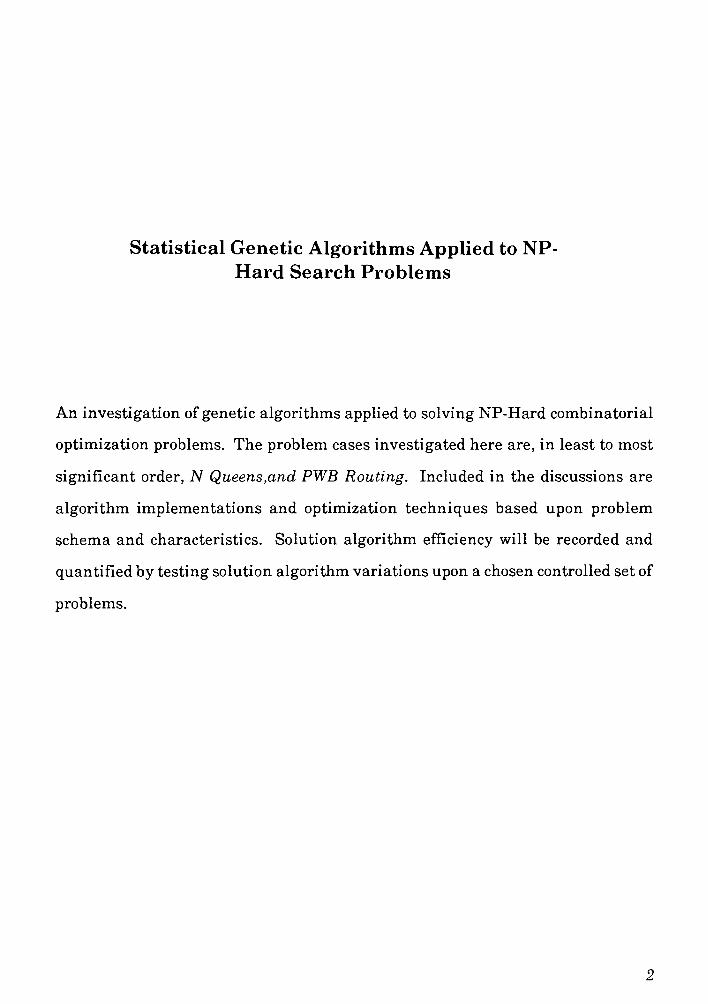
Statistical Genetic Algorithms Applied to NP-

Hard Search Problems

An investigation of genetic algorithms applied to solving NP-Hard combinatorial

optimization problems. The problem cases investigated here are, in least to most

significant order, N Queens,and PWB Routing. Included in the discussions are

algorithm implementations and optimization techniques based upon problem

schema and characteristics. Solution algorithm efficiency will be recorded and

quantified by testing solution algorithm variations upon a chosen controlled set of

problems.

Preface

The major effort of this thesis was to develop an electronic circuit routing system

that utilizes genetic algorithms to perform Printed Wire Board (PWB) routing

rather than brute force exhaustive searching methods. This problem can be

classified as an NP-Hard optimization problem searching a large solution space.

Some desirable characteristics of an electronic routing system are that it:

Minimize the number ofpotential solutions

Minimize the number ofboard layers and tap holes

Minimize trace lengths and the number of"jogs"

Minimize trace cross-talk and the board capacitance

My goal was to develop a system thatwill work for a reasonable but small number

of components (connections) and then investigate and report upon how

characteristics ofmy representation and my heuristics and decision rule functions

affect the efficiency of solution generation. Imeasured efficiency by time required

to converge upon a solution, simplicity of the solution, and the number of

evolutions required to generate the solution.

This routing system is a simulation package developed to gain an understanding

of how genetic algorithms can be applied to solving NP-Hard optimization

problems. With this goal in sight, the system restricted the number of

components it will allow within a design as well as what the components are.

These restrictions imposed to make the task a tractable one. My intent was to

supply the GA routing system with moderate size designs and be able to produce

solutions to the PWB routing problem in a reasonable amount of time.

I iterated the simulation processmany times for a few different electronic designs

in order to learn and evaluate characteristics of genetic solution algorithms. This

enabled me to observe the effects of the heuristic predictors of the decision

algorithm. Features of interest here are annealing techniques and rules applied

to the predictor functions. Additional factors in modifying and testing decision

functions and annealing rules were distances between connections, number of

trace lines in a bus path, the number of junctions / connections per trace, and

neighboring components.

Table of Contents

Statistical Genetic Algorithms Applied to NP-Hard Search Problems 2

Preface 3

Introduction 5

Technical Background 15

2.1 Monte Carlo Theories 15

2.2 How to Measure the Efficiency of an Algorithm. . . . 15

2.3 Fuzzy Cognitive Machines 17

2.4 Annealing Techniques 18

2.5 Probability and Statistical Theory of Optimization 19

2.7 Genetic operators 22

3.0 EXPERIMENTATION INTRODUCTION 23

3.1 N QUEENS PROBLEM 24

3.2 Determining Mean Population Size MPS 32

3.3 Solution Algorithm Description of GeneticOperators 33

3.3.1 Initial Population Generation 34

3.3.2 The NQC() Success Function and the Replication Operator 38

3.3.3 The Mutation Operator 39

3.3.4 The Crossover Operator 40

3.3.5 The Filter Operator 42

3.3.6 Selecting and Adding Parents Back Into the Evolving Population 44

3.3.7 The Average Utility Function AUF 44

3.3.8 The Resample Operator 45

3.3.9 The shuffle Operator 46

3.3.10 The Character Function 48

3.4 N-Queens Solution Algorithm 49

4.0 Routing Problem and GeneticAlgorithm Introduction 50

4.1 Routing Problem Description 51

4.2 PC Board Algorithm Model 52

4.3 Core Population 55

4.4 Fundamental Characteristics of Solution Algorithm 59

4.5 Algorithm Initial Requirements 62

4.6 Genetic Solution Algorithm Functional Flow Description 63

4.8 Genetic Characterization Function ... . 71

4.9 Routing Map Overview 73

5.0 GeneticAlgorithm Routing Equations 81

5.1 Genetic Character Function ..81

5.2 Genetic Utility Function 83

5.3 Genetic Replication Operator 85

5.4 Mean Population Size 86

5.5 Initial Population Generation 87

5.6 Crossover operator 89

5.7 Mutation operator 90

5.8 Neighbor Concept for Evolution ... 93

5.9 Population Growth and Decay ... 96

6.0 Optimum Neighbor Solution Algorithm 99

6.1 Optimum Neighbor Utility Function 99

6.2 Optimum Neighbor Solution Algorithm Character Function 102

6.3 Optimum Neighbor Solution Solution Data 103

6.4 Optimum Neighbor Utility Function of 6.3 with Growth Modification . .. 103

6.5 Optimum Neighbor Utility Function of 6.3 with Fewer Shuffle Operations . 108

7.0 RATNEST SOLUTION TECHNIQUE 118

7 1 Utility function for solution case one . .. 122

7.2 RATNEST Solution Algorithm Solution Data Case One 122

7.3 RATNEST Solution Algorithm Solution Data Case Two 125

7.4 Discussion of Ratnest Algorithm One 127

7.5 Problem with RATNEST solution technique 128

8.0 Restricted Optimum Neighbor Routing Problem 129

8.1 Characteristic Information of Restricted Optimum Neighbor Algorithm 129

8.2 Examples and Description of Prioritization 131

8.3 Extended mutation function 1 34

8.4 Four Layer Board .. 135

8.5 Genetic Operators and Utility Function for the Restricted Neighbor Algorithm

137

8.6 Restricted Neighbor Algorithm Results of the PWB from Chapters six and Seven

138

8.7 Example of 8.6 utilizing the Priority and Cluster option 138

8.8 Example of Two 16 Bit Parity Checker Circuits 143

9.0 Conclusions 148

9.1 Conclusions and Remarks for the Nearest Neighbor routing Algorithm CPT 6 148

9.2 Conclusions and Remarks for the ratnest Algorithm CPT 7 149

9.3 Conclusions and Remarks for the Optimum Neighbor Algorithm CPT 8 .. 150

9.4 Points of interest beyond these experiments 152

9.5 Overall conclusions 1 53

9.6 Applicability to largerscale problems ..155

Introduction

Emphasis of this thesis was the investigation of convergent classes ofGENETIC

ALGORITHMS with finite populations, N operators and M degrees of freedom

applied to NP-Hard combinatorial search space problems. By finite population I

am referring to the entire search space; the complete and exhaustive set of entries

valid within the problem statements and conditions. The algorithms, during

solution generation, may select any proper subset of the population (search space)

to evaluate for convergence to a solution. This subset is sometimes called the

working population. The term convergent, here, means that the algorithm will

iterate through population subsets searching out a solution to a predetermined

accuracy within a reasonable period of time based upon the problem. N operators

refers to the number of functions / operations that an algorithm will apply to

change the search space while converging upon the solution. M degrees of

freedom refer to the number of possible states that each population entry and

condition in the problem can change to. By identifying the algorithm operators

and restricting the possible condition states, we are bounding the possible solution

space to be finite.

Solution algorithms to NP-Hard optimization problems of this nature suffer from

combinatorial explosion in their search space as well asmany other problems, and

are best solved with a strategy that can be referred to as constraint satisfaction,

e.g., how do I identify a set of conditions that, when applied to the population,

leads to a solution even though all conditions sometimes cannot be met.

Generally, it is not easy to identify all of the necessary and sufficient constraints

in order to define an exact solution, let alone test all population entries and

exhaustively search the solution space to converge on an answer. Testing the

union and intersection of problem conditions to identify a solution are typically

the best we can do, but this is usually inadequate to completely isolate a solution

because of the number and complexity of the conditions of the problems.

Because of a problem's complexity and computational restrictions, there is the

need to break down the problem and solution method into more, less complex

components. The problem structure and statement components can be described

as:

1) A crisp problem and problem statement

2) An appropriate problem and computational representation

3) A solution tolerance / accuracy range

4) A graceful failure or fall back scheme

No matter what the solution technique is, I believe all problems require a

rigorous investigation and description ofeach of the four problem categories listed

above. With the growing popularity ofAl techniques being applied to problems,

we are seeing a significant amount of investigation and effort being placed upon

bullets number two and three. These four problem requirements will be referred

to throughout subsequent discussions and example problems.

Adequately describing the four categories required in comprehending a typical

NP-Hard problem is not trivial. Factors as simple as how do we model and

represent 3D objects in 2D spaces may hinder the problem description. Other

difficulties of a problem investigation relate to implementation techniques, which

have constraints within themselves. For example, do you use matrices or vectors

as a data representation model, and should the data be binary or multivalued.

One must also beware of implementation accuracy (are you attempting to get

double precision accuracy out of single precision numbers), resource requirements

and errors introduced by the algorithm itself (invalid population conditions). In

this thesis I intend to investigate and discuss how the above four categories

operate to properly specify a problem and its solution in terms of genetic

algorithms.

In working to solve NP-Hard search space problems and recognizing the above

four conditions, I believe that genetic algorithms are reasonable techniques and

representation models. Inherent in genetic algorithms is the ability to describe

and act upon vectors of complex relationships that allows for convergence upon a

solution without having to represent or search an entire population space. This

modeling and search characteristic of genetic algorithms is a significant asset to

the resource requirement constraints and representation needs of solution

algorithms to NP-Hard problems.

The class of genetic algorithms I intend to investigate here has a strong

foundation based inMonte Carloi and statistical methods2. These techniques lend

themselves very nicely to modeling complex nondeterministic interactions. Other

genetic algorithm modeling characteristics are similar to simulated annealing

techniques described in current neural network research, where there is an ability

to control the amount of"heat"

/ change that occurs over time, given certain

conditions in the solution set. Another feature of the genetic algorithm

representation is that the implementor can incorporate other problem solution

techniques such as greedy algorithm techniques, hill climbing techniques, or

pseudo random search techniques into the GA. The genetic algorithm's inherent

ability to combine multiple problem solution techniques, allows for hybrid

1. SIAM Series #3, Symposium on applied probability and Monte Carlo Methods, 1967

2. Binder, Kurt,Monte Carlo methods in statistical physics, 1/1/79, QC 174 85m64M66

approaches to problem solutions that can work over a wide range of problems

classes.

Genetic Algorithms are well suited for solving NP-Hard optimization problems of

Higher OrderDimensional Spaces (HODS) that can be represented by vectors and

matrixes. An example of an HODS problem could be human interactions,

specifically the complex relations and interactions that occur and regulate our

daily activities. Characteristics such as weather, time of day, place and general

mood have an effect on how individuals act and react to situations. Each

characteristic has many possible conditions (e.g. weather: sunny, damp, ...) and

each condition will act upon an individual differently at different times. All of

these factors and conditions can be represented as a series of vectors andmatrixes

that, when combined, represent a multidimensional, highly complex set of

relationships. If one were to picture / model these relationships, they would have

to be represented in high order dimensions (e.g. contour plots, 3D plots, ...). In this

thesis I intend to investigate and discuss the effects of problem

representation/implementation on algorithm efficiency.

The types of problems that I will be investigating in this thesis are referred to as

NP-Hard combinatorial search space problems. Examples of some are the

Traveling Salesman Problem, Eight Queens problem, and even electronic design

placement and routing algorithms for chip and board designs. Genetic algorithms

also have been applied to applications that perform document storage and

retrieval (Michael Gordon ACM 19883), pattern and feature recognition (Lee

1984), as well as simulations and game treeing problems. These problems all

have large search spaces from which an algorithm must find either a unique

3. Gorden, M., D , Adaptive subject indexing in document retrieval. (PHD dissertation at University of Michigan), Dissertation

abstracts international, 45(2), 61 1 B

8

solution or one ofmany possible solutions within an acceptable tolerance level. In

order for an algorithm to solve these types of problems successfully, it must be

able to search pieces of the solution space and converge upon an answer. A

difficulty with many of these types of problems is the fact that an algorithm

typically does not know the exact, correct answer until that answer is found. This

is because the algorithm must iterate through the search space on a trial and

error basis, applying constraint satisfaction and optimization methods to

determine if a satisfactory solution has been reached. Figure 1.1 is an example of

some simple multi-modal search spaces might look like.

Combinatorial search and optimizations problems have similar characteristics in

that they combine multivariat conditions into complex relationships that

generally need to be represented in higher ordered dimensional space by

sequences ofvectors andmatrices. Thesematrices then can bemanipulated by an

algorithm that will cause them to change to different working sets of the

population and converge upon a solution satisfying the set of solution constraints.

Genetic algorithms are well suited for operating upon problems whose

representation can be vectors and matrices.

The efficient convergence requirement upon optimization problems is the basis for

most of the algorithm research on NP-Hard combinatorial problems . A successful

algorithm must be able to converge to a solution set within the bounds of the

population description, without causing the population to diverge and generate

invalid entries, or to converge to a wrong/false solution. Given that we desire the

algorithm to do something useful, like converge upon a solution, we utilize

constraints by which we measure and rank potential solutions. For example, we

5. Booker, L,B., Improving search in genetic algorithms, L. Davis book on Genetic algorithms and simulated annealing, p 61 -

74, London Press.

fix the working population size to be finite and manageable, but we also must

restrict the number and type of operators applied to the population. Constraints

such as these help us to make the solution algorithm tractable and easier to

manage. Other constraints are accuracy tolerance ranges for solutions or simple

tests such as, does the solution work. Solution algorithms must incorporate an

adequate balance of constraints and degrees of freedom (randomness) because, an

improper amount of either can cause an algorithm never to converge upon a

solution.

DeJong in 19756 published papers investigating the problem of premature

convergence due to inadequate population modeling and prediction trends. In

light of the convergence problem and its criticality to the solution, Holland in

19757 and later Goldberg & Lingle in 19858 published works identifying

reordering procedures specifically for genetic algorithms. Their work attempted

to address convergence problems of stochastic search space algorithms more

adequately. This researches and includes aspects of these and other such studies

in my development and characterization of genetic algorithms so that they

operate effectively and efficiently.

Problems inherent in algorithms that search large spaces and implement

stochastic, non-exhaustive solution methods are not limited to convergence or

divergence problems, but also the effects of randomness on population testing and

backtracking. What I am referring to here by randomness is the measure or rate

of uncontrolled and nondeterministic change in the working population. If there

is too much random change in the population entries, then the solution algorithm

6. DeJong, k., A., An analysis of the behavior of a class of genetic adaptive systems, Dissertation abstracts international

36(10), 5140B.

7. Holland, J., H., Adaptation in natural and artificial systems, University of Michigan Press (1975)

8. Goldberg, D., E., & Lingle, R Alleles, Loci and the traveling salesman problem, Proceedings of an international conference

on genetic algorithms and their applications ppsl 54-1 59

10

may exhibit a thrashing behavior and never converge. Conversely, if there is not

enough randomness, then the algorithm may stagnate or converge on something

other than the solution set. Another type of randomness is that encountered in

the problem itself, not in the solution algorithm. For example, in the human

interaction problem suggested earlier, how do we properly account for

characteristics such as place and time. It is obvious that not all events can occur

in all places or at any arbitrary time. A solution algorithm must successfully

model the valid combinations and omit those that are not.

In NP-Hard problems with solutions containing conflicting requirements, there

must be an acceptable solution accuracy or tolerance in order for algorithms to

function successfully. As mentioned earlier, there are many factors and

characteristics ofNP-Hard problems that require careful control and balance in

order for an algorithm to generate working populations that converge upon a

solution. An example of how one might utilize these controls could be to strictly

regulate the working population size and the accuracy required to describe a

solution. Generally, the larger the population space, the greater amount of

randomness that can be tolerated before thrashing occurs. Utilizing a larger

working population also lowers the probability that it will stagnate or converge

prematurely. Another degree of control typically used in NP-Hard optimization

problems is to impose a tolerance range for acceptable solutions rather than

accepting only one unique solution.

At this point, let me just hint at the extent and complexity of the relationships

that need to be managed in order to achieve a good algorithm. One cannot just

make the working population very large andassume that randomness and other

regulation problems will be masked, because if the population is too large, then

the algorithm execution becomes inefficient andmay never converge. Here we see

11

the need to regulate a working populations size with the amount of randomness

that can be tolerated; otherwise, the algorithm will suffer from premature

convergence or, even worse, divergence. Another subtle problem is a solution's

acceptable tolerance range. If the range is too large, then the solution is of no use;

yet if the range is too small and restrictive, then the algorithm may never

converge or require an inordinate amount of time and resources in order to

converge. As part of the scope of this thesis, I investigated the effects that changes

in population size and randomness have upon an algorithm's ability to converge

upon a solution.

Goldberg & Thomas in 19869 published a work on search problems and machine

learning that investigates solution algorithms accounting for randomness of

population change and the effects of backtracking or thrashing in finite sized

populations. Their research included investigating convergence of large solution

space problems and how, by limiting the population space to be finite, the

problems become tractable. The characteristics of random population changes

(mutation in genetic algorithms), backtracking, and population size can be

likened to techniques known as simulated annealing, feedback, or back

propagation, in Neural Network research.

All of these prior topics were investigated and where appropriate, applied to my

experimentation. The NP-Hard problems I investigated are:8 Queens

PWB routing

The first problem was simple and used as an initial development example in order

to help me focus the development of programming techniques and utilities to

conduct the primary experiment. I utilized thePWB routing task as the primary

9. Goldberg, D., E., & Thomas, A., L., Genetic Algorithms: a bibliography (1962-1 986), TCGA report #86001 , University of

Alabama.

12

experiment. I view the effort exerted in applying some of the investigated and

proven Genetic Algorithm techniques as a method of developing software tools

and utilities that I can expect to complete and be able to demonstrate their

correctness. This ability to prove the tools and effects of some of the algorithm

techniques such as annealing strategies gave me testable / quantifiable positive

feed back on some of the theories that I am investigating and intending to apply to

the highly complex PWB routing problem.

13

Example of a complex 3D search space

where it is possible to arrive at 3 false minima

if the algorithm is incapable of properly traversingthe surface planes during its evaluation

Another example of a complex 3D search space

where it is possible to arrive at 3 false minima

if the algorithm is incapable of properly traversing

the surface planes during its evaluation

Figure 1.1

14

Technical Background

This section introduces characteristics of NP-Hard problems and genetic

algorithm solution techniques utilizing statistical processes.

2.1 Monte Carlo Theories

Monte Carlo methods are typically utilized as a method of statistical integration.

I intend to utilize this theory to aid in the development of the investigated genetic

algorithms. Genetic search algorithms are fundamentally based in statistical

optimization; therefore, I believe that proper application ofMonte Carlo methods

utilized in my genetic algorithms and annealing functions will aid the efficiency

ofmy solution algorithms. The key function of the Monte Carlo theory is to apply

statistical methods to improve optimization algorithms and feedback systems in

order to improve the confidence levels of evolution, predictor functions, and

estimator functions. (Hammersley & Handscomb '651ySLAM 19692

,Binder et.

al'793).

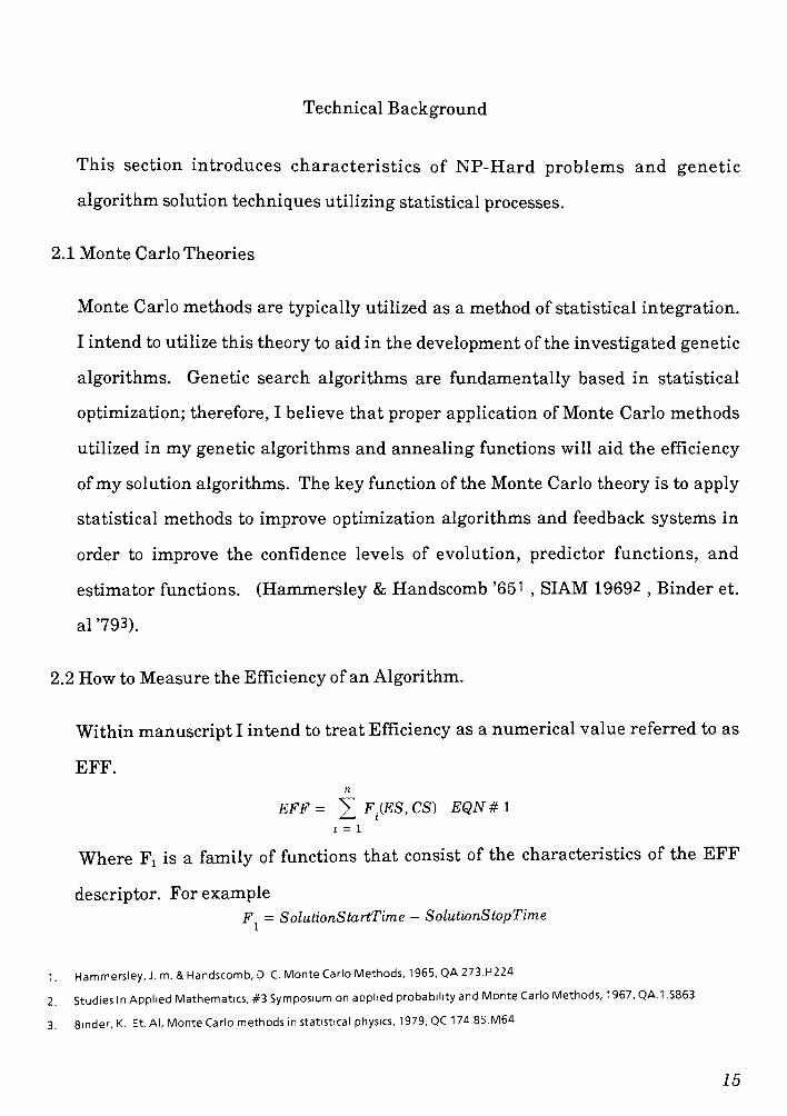
2.2 How toMeasure the Efficiency of an Algorithm.

Withinmanuscript I intend to treat Efficiency as a numerical value referred to as

EFF.

n

EFF= 5^F^ES>CS^ EQN#l

i = l

Where Fi is a family of functions that consist of the characteristics of the EFF

descriptor. For example

F = SolutionStartTime - SolutionStopTime

1 . Hammersley, J. m. & Handscomb, D. C Monte Carlo Methods, 1 965, QA.273.H224

2. Studies In Applied Mathematics, #3 Symposium on applied probability and Monte Carlo Methods, 1967, QA.1 .S863

3. Binder, K. Et.AI,Monte Carlo methods in statistical physics, 1979, QC.1 74.85.M64

15

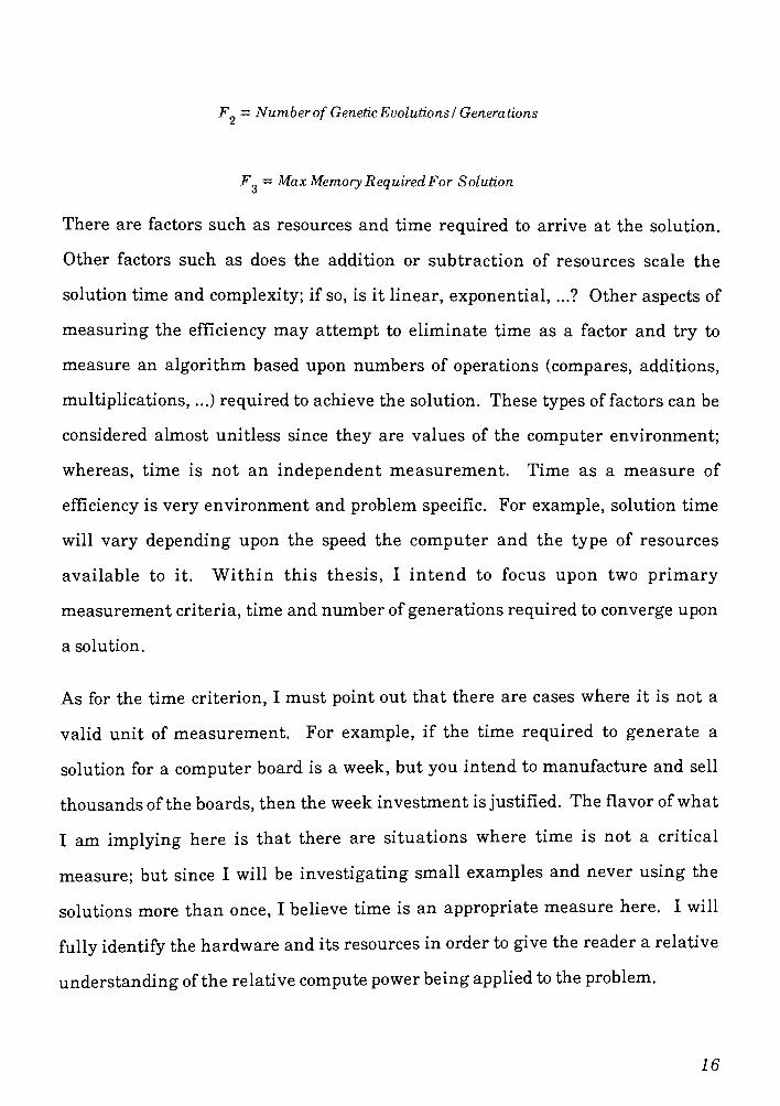
F = NumberofGeneticEvolutions I Generations

F = MaxMemoryRequiredFor Solution

There are factors such as resources and time required to arrive at the solution.

Other factors such as does the addition or subtraction of resources scale the

solution time and complexity; if so, is it linear, exponential, ...? Other aspects of

measuring the efficiency may attempt to eliminate time as a factor and try to

measure an algorithm based upon numbers of operations (compares, additions,

multiplications, ...) required to achieve the solution. These types of factors can be

considered almost unitless since they are values of the computer environment;

whereas, time is not an independent measurement. Time as a measure of

efficiency is very environment and problem specific. For example, solution time

will vary depending upon the speed the computer and the type of resources

available to it. Within this thesis, I intend to focus upon two primary

measurement criteria, time and number ofgenerations required to converge upon

a solution.

As for the time criterion, I must point out that there are cases where it is not a

valid unit of measurement. For example, if the time required to generate a

solution for a computer board is a week, but you intend to manufacture and sell

thousands of the boards, then the week investment is justified. The flavor ofwhat

I am implying here is that there are situations where time is not a critical

measure; but since I will be investigating small examples and never using the

solutions more than once, I believe time is an appropriate measure here. I will

fully identify the hardware and its resources inorder to give the reader a relative

understanding of the relative computepower being applied to the problem.

16

In using the number of generations as an efficiency criterion, I am trying to use

this as a criterion that has units only reflective or contingent on the problem. By

measuring the algorithm based upon the number of generations, I can account for

the factors such as search space size, population size, and number of genetic

operators required to evolve a generation. These types ofmeasurement units are

time and resource independent, which is important since they allow us tomeasure

an algorithm without physical resource implications (size and speed of computer,

efficiency of simulation program, ....). I will attempt to provide the user with an

idea ofhowmany operations occur in a generation cycle.

2.3 Fuzzy Cognitive Machines

These are tools developed as extensions of signal flow graphs of electronic circuits.

The Fuzzy CognitiveMachines FCMs will be used to identify trends of a hardware

system and its components 4 5. The utility of these tools is to be able to imperially,

withminimal overhead and effort, determine where critical and potentially active

paths and devices are within an electronic system. This characteristic

information about the circuit will be incorporated into the solution algorithm to

help efficiently and more directly find solutions to the routing problems.

Part of the measurement criteria is the rate at which the algorithm converges

upon an optimally acceptable solution. This rate (number of iterations /

evolutions) can be reduced or minimized if we can identify a way in which to

restrict the generation of less than optimal population entries.

4. Styblinski, M. A. & Meyer, B. D., Fuzzy Cognitive Maps, Signal Flow Graphs and Qualitative Circuit Analysis, Proc. IEEE Conf

on Neural Networks, 6/87

5. Kosko, B., "Fuzzy Cognitive Maps", International Journal of Man-Machine Studies, Volume 24, pps 65-75, 1/1986.

17

I designed the genetic algorithm to utilize the information from signal flow graphs

to order and rank the importance of possible population entries. This filtering of

population entries can be likened to restricting the evolution process to only

promoting and creating population entries that have or will yield to the highest

possible utility values.

2.4 AnnealingTechniques

This is a concept from neural network research and was adopted into the genetic

algorithm fitness function as a feedback method for adjusting the amount of

randomness / heat applied to the optimization algorithm (Davis '88 6). This

parameter is a means of controlling the mutation rates and thrashing of the

population entries. The genetic algorithm will monitor the rate of progress of the

population (e.g., population fitness value, average population value and its

change rate, ...). The character function discussed in Section 4 is the primary

global status monitor. Population and evolution information will be utilized by

the annealing function to regulate the amountof randomness /mutation thatwill

occur during population evolution. The goal here is to be able to prevent the

population from either stagnating or thrashing while maintaining enough

randomness to be able to effectively explore the solution space.

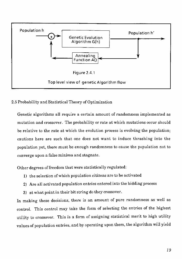
Annealing techniques as implementedwithin thisinvestigation can be thought of

as a system G(h) with feedback A(G(h)) to help regulate both the evolving

population and the evolution algorithms. The feedback A() is the annealing

information that will regulate factors such as population size, mutation,

randomness, etc. A generic diagram of the system could be represented as in

figure 2.4.1.

6 Davis, L. & SteenStrup, M. (1 987). Genetic Algorithms and simulatedannealing: An overview in.

18

Population h

f?r-Popu lation

h'

Genetic Evolution

Algorithm G(h)

v_

M

> 'AnnealingFunction A()

Dp lev flowT(

Figure 2.4.1

el view of genetic Algorii:hm

2.5 Probability and Statistical Theory ofOptimization

Genetic algorithms all require a certain amount of randomness implemented as

mutation and crossover. The probability or rate at which mutations occur should

be relative to the rate at which the evolution process is evolving the population;

cautions here are such that one does not want to induce thrashing into the

population yet, there must be enough randomness to cause the population not to

converge upon a falseminima and stagnate.

Other degrees of freedom thatwere statistically regulated:

1) the selection ofwhich population citizens are to be activated

2) Are all activated population entries entered into the bidding process

3) at what point in their bit string do they crossover.

In making these decisions, there is an amount of pure randomness as well as

control. This control may take the form of selecting the entries of the highest

utility to crossover. This is a form of assigning statistical merit to high utility

values ofpopulation entries, and by operating upon them, the algorithmwill yield

19

resultant population entries of equal or greater value. Hence, there should be

efficient convergence onto a solution.

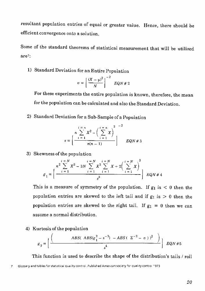
Some of the standard theorems of statistical measurement that will be utilized

are7:

1) Standard Deviation for an Entire Population

(X -

vf

NEQN#2

For these experiments the entire population is known, therefore, the mean

for the population can be calculated and also the Standard Deviation.

2) StandardDeviation for a Sub-Sample of a Population

i = n , i = n^

'l*- (I*

-2

i = 1 i = 1

n(n 1)EQN#3

3) Skewness of the population

i = N i = N i = N , i = N

n2

^ X3-3N JiX2

5i X + 2[ ]T X

S,

i = 1 i=l i=l i = 1

EQN#4

This is a measure of symmetry of the population. If gi is < 0 then the

population entries are skewed to the left tail and if gi is > 0 then the

population entries are skewed to the right tail. If gi = 0 then we can

assume a normal distribution.

4) Kurtosis of the population

ABS( ABS(g2- s-2) -ABS(

Z"2-o))2

gr EQN#5

This function is used to describe the shape of the distribution's tails / roll

7. Glossary and tables for statistical quality control. Published American society for quality control 1973

20

off. If g2 is < 0, then the population distribution plot has shorter tails than

a normal distribution. And if g2 is > 0, then the population distribution

plot has longer tails than a normal distribution. If g2 = 0, then we can

assume a normal distribution.

5) Test of the means of two different populations

(x1 -x2) -(p1 -p2)

z = t = EQN#6<v-x2) -(Pl-p2)

2 2-2

This function will be utilized to compare themean, of two populations (most

likely successive populations).

The previous statistical information was used to determine if the evolution process

was evolving the populations forward towards a solution, backwards away from a

solution, or if the population has stagnated stagnated. I utilized this characteristic

data to modify annealing algorithms, randomness factors, and general population

management. For example the Kurtosis function gave me information that directly

affected the randomness and mutation parameters of the genetic algorithms. If the

population had a kurtosis of g2 less than zero then the genetic algorithm would

increase the randomness and mutation rates. The population having short tails for

distributions means that there were fewer"outlyer"

population entries that could be

involved to cause the population to evolve in a productive positive manner oppositely

it was more likely that the population would stagnate or evolve towards a less

productive path. It was safe to up the mutation rates with out less concern about

causing the population tothrash.

21

2.7 Genetic operators

In the development of my solution algorithms I started with the common basic

genetic operators:

1) Replication: Is the operation of replicating population entries some number of

times based upon their utility value

2) Crossover : The operation of selecting two entries from a replicated

population and merging / crossing over parts of the two input

population entries to generate a new third population entry.

3) Mutation: The operation of randomly changing one or more population

entries simply by changing some value / characteristic of the

entry.

4) Utility: Ameasure of themerit /strength of a population entry.

These standard operators as described by Holland 1975 8 will act as the basis for

my developingOptimized genetic operatorsmore suitable for the class ofNP-Hard

problems that I will be investigatingwithin thisManuscript.

8. Holland, j. H., Adaption of Natural and Artificial systems, AnnArbor: University of Michigan Pres.

22

3.0 EXPERIMENTATION INTRODUCTION

The examples / problems that I have chosen to investigate within the thesis start

out as reasonably simple cases and progress to the main experiment of the thesis.

I am developing the investigation in this form (simple to actual) in order establish

a set ofverified tools and examples from problems which I can expect to solve. By

being assured that I can look at the solution of a moderately sized problem and

empirically evaluate if the answer is correct, I can make inferences as to the

efficiency and correctness of the software tools that I will be utilizing to develop

the solution to the main experiment. This is, in a sense, building a strong

foundation upon which I will grow themain system.

Theminor development problem I will investigate within this thesis is:

1) Eight N Queens

Problem case number one is the challenge of taking an NxN chess board and

placing N queens upon the board, one per rank, such that if any queen were to

make one legitimate chess move she would not capture any other queen upon the

board1. Figure 3.0.1 is an example of an arrangement that is invalid or a failure,

because moving the queen from square (2,3) to square (5,6) will result in the

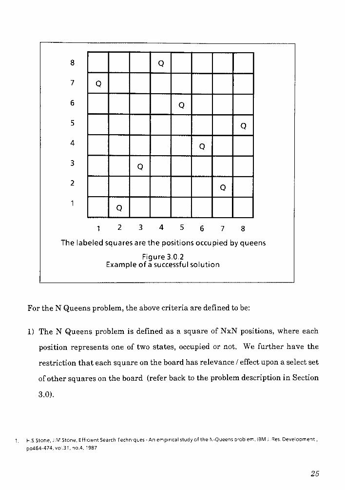
capture of the queen on square of (5,6). Figure 3.0.2 is an example of a correct or

successful placement of 8 queens upon an 8x8 chess board. In Figure 3.0.2 moving

any queen one legitimate chess move will not result in the capture of any other

queen.

23

8

7

6

5

4

3

2

1

Q

Q

Q

Q

Q

Q

Q

Q

1 2 3 4 5 6 7 8

The labeled squares are the positions occupied by queens

Figure 3.0.1

Example of a failed solution

3.1 N QUEENS PROBLEM

If we look back to the criteria of formulating a problem / solution methodology

discussed in the introduction and apply this to the N Queens Problem, we find

that wemust have:

1) A well formed statement ofwhat the problem / question is

2) Criteria for determining an acceptable solution

3) Characteristics of the problem.

24

8

7

6

5

4

3

2

1

Q

Q

Q

Q

Q

Q

Q

Q

1 2 3 4 5 6 7 8

The labeled squares are the positions occupied by queens

Figure 3.0.2

Example of a successful solution

For the N Queens problem, the above criteria are defined to be:

1) The N Queens problem is defined as a square of NxN positions, where each

position represents one of two states, occupied or not. We further have the

restriction that each square on the board has relevance / effect upon a select set

ofother squares on the board (refer back to the problem description in Section

3.0).

1 . H.S.Stone, J.M.Stone, Efficient Search Techniques - An empirical study of the N-Queens problem, IBM J. Res. Development.,

pP464-474, vol.31, no.4, 1987

25

2) A solution is acceptable iff moving any one queen one legitimate chess move,

she does not capture any other queen upon the chess board. All solutions not

satisfying this criteria are invalid. Please note that this problem does not have

a tolerance range for its solution acceptability as some problems do, but there

ismore than one correct / acceptable solution per board.

3) Iwill not detail the problem characteristics here butwill discuss them below as

I work through the solution to the problem.

For this example it was simple enough to assign a one or zero as occupied or not

occupied, respectively. This representation scheme can be implemented as one

location per bit, 8 locations per byte. I selected the bit per position scheme because

it was convenient and saves resource space. Also, by having the board packed in

this manner, I could more easily use boolean operators rather than algebraic

operations to perform some of the genetic functions. I did, however, treat the 8x8

board as a vector of rank(8) bytes and the population as a vector of size P board

vectors. Please refer to Figure 3.1.1 for further explanation.

Having selected a representation scheme, the next item of importance is to

determine if there is any fundamental relationship between the board size and the

ability to solve the problem. In other words, if there is a minimum board size

(NxN), what is it? The goal here is to identify key factors and characteristics of

the problem thatmight relate to implementing an optimal solution algorithm.

By searching for the minimal board, I believe that I can make inferences about

schema 2 3 4 related to larger problem / solution sets. The fundamental /minimum

solution can be utilized as a highly correlated predictor for making statistically

26

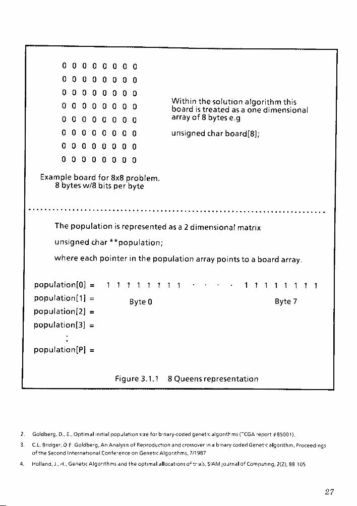
00000000

00000000

00000000

nnnnnnnnWithin the solution algorithm this

uuuuuooo board is treated as a one dimensional

00000000 array of 8 bytes e.g

00000000 unsigned char board[8];

00000000

00000000

Example board for 8x8 problem.8 bytes w/8 bits per byte

The population is represented as a 2 dimensional matrix

unsigned char **population;

where each pointer in the population array points to a board array.

population[0] = 11111111 .... 11111111

population^] =

ByteQ Byte7

population[2] =

population[3] =

populationfP] =

Figure 3.1.1 8 Queens representation

2. Goldberg, D., E., Optimal initial population size for binary-coded genetic algorithms (TCGA report #85001).

3. CL. Bridger, D.E. Goldberg, An Analysis of Reproduction and crossover in a binary coded Genetic algorithm, Proceedings

of the Second International Conference on GeneticAlgorithms, 7/1987

4. Holland, J., H., Genetic Algorithms and the optimal allocations of trials, SIAM journal of Computing, 2(2), 88-105

27

valid assumptions about logical, algebraic, and heuristic rules required to

describe the problem and its solution algorithm.

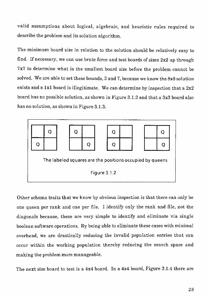
The minimum board size in relation to the solution should be relatively easy to

find. If necessary, we can use brute force and test boards of sizes 2x2 up through

7x7 to determine what is the smallest board size before the problem cannot be

solved. We are able to set these bounds, 2 and 7, because we know the 8x8 solution

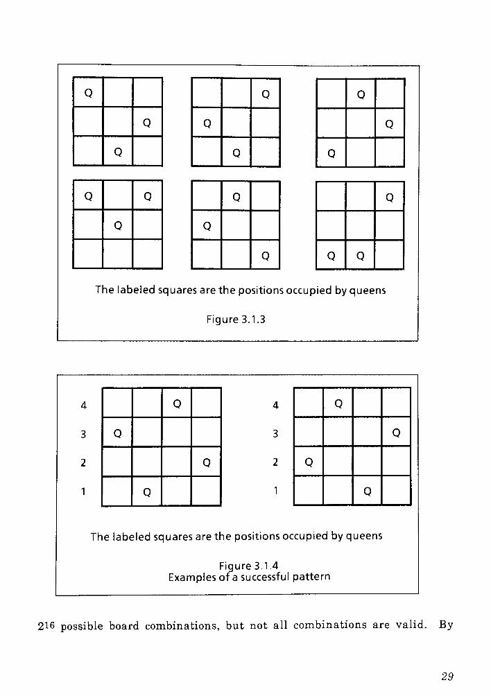
exists and a lxl board is illegitimate. We can determine by inspection that a 2x2

board has no possible solution, as shown in Figure 3.1.2 and that a 3x3 board also

has no solution, as shown in Figure 3.1.3.

Q

Q

Q

Q

Q

Q

Q

Q

The labeled squares are the positions occupied by queens

Figure3.1.2

Other schema traits that we know by obvious inspection is that there can only be

one queen per rank and one per file. I identify only the rank and file, not the

diagonals because, these are very simple to identify and eliminate via single

boolean software operations. By being able to eliminate these cases with minimal

overhead, we are drastically reducing the invalid population entries that can

occur within the working population thereby reducing the search space and

making the problemmoremanageable.

The next size board to test is a 4x4 board. In a 4x4 board, Figure 3.1.4 there are

28

Q : Q Q

Q Q Q

Q Q Q

Q Q Q Q

Q 0

0 Q Q

The labeled squares are the positions occupied by queens

Figure 3.1.3

3

2

Q

Q

! Q

Q

Q I

Q

Q

Q

The labeled squares are the positions occupied by queens

Figure 3.1.4

Examples of a successful pattern

216 possible board combinations, but not all combinations are valid. By

29

eliminating the obvious (trivially identified) board patterns mentioned above for

the 2x2 and 3x3 and 4x4 cases, we can reduce the possible board combinations to

28. Thismakes the search space verymanageable even for brute force algorithms.

This type of search space reductions (an order of magnitude or more) is highly

significant in the case ofNP-Hard problems. In summary we have now identified

the minimal board size for the N Queens problem to be 4x4, this was done by

exhaustive example. Having the minimal board size (4x4) we can now base our

schema design on this and develop optimized genetic evolution algorithms.

One of the reasons for searching for the minimum board size is to help in

determiningwhat the size and characteristics of a schemamight be. The utility of

identifying a set of schema is high because we can then direct the evolution

routines of the genetic algorithm to generate entries that are statistically more

valid6 ~>'

. This kind direct computation is highly efficient and desirable; for

example think of the algorithm for directly computing numbers that are perfect

squares (e.g. 1, 4, 9, 16, 25, ...). The unintelligent method for computing these

values would be to test each whole number to determine if it is the produce of a

perfect square. The exhaustive testing algorithmmight look something like:

1) assign Xi the value 1; by definition this is a perfect square

2) add one to the previously tested value S= Xn + 1

3) Y = round (S/ 2)

4) loop for 2 to Y test cases and test the divisibility ofS

5. Suh, J., Y., &Gucht, D., V., Incorporating heuristic information information into genetic search, Proceedings of the Second

International Conference ofGenetic Algorithms 7/1 987

6. Johnson, K, & Darnell, c, & Burman, J., Feature extraction in the Neocognitron, Proceedings from the conference on

Neural Network

7. Krishnan, G., & Walters, D., Psychologically plausible features for shape recognition in a neural network

30

5) ifS is not divisible then Xn+ i = S

6) loop around to step 2 to test another case

This looping and exhaustive testing of each number is very inefficient. Through

inspection and reasoning we learn that the formula / schema for directly

computing squares is:

1) assign Xi the value 1; by definition this is a perfect square

2) assign Y the value 3

3) Xn+1 = Xn + Y

4) Y = Y + 2

5) Loop to step 3

Please note that the Xn's are the perfect squares

It is these kinds of direct operations based upon the fundamentals of the problem

that help to optimize solution algorithms. I intend to utilize techniques such as

these to facilitate and optimize the genetic algorithms for my test problems (N

Queens, and the PWB routing problem).

From the N queens schema investigation I found that the 4x4 size board is the

smallest possible size with a solution, Figure 3.1.4. Knowing what the minimum

solvable board size is, I then computed several 4x4 solution board sets as well as

numerous 4x4 failure board sets. I then used this information in my evolution

algorithm to filter out population entries that have known failure structures and

promote solution entries with the 4x4 solution schema structure.

This is a simple technique of restricting the search space by rejecting the known

failures and promoting the entries with the most potentials. Having added this

DeJong, K., A., (1981) Adaptive search procedures for large complex spaces., (technical report #81-2), University of

Pittsburgh

31

information to my solution algorithm I was able to cut the number of generations

required to find a solution about in half formost of the tested cases.

3.2 DeterminingMean Population SizeMPS

At this point the problem fundamentals have been reviewed, and I refer the

reader back to Section 3.1 for a discussion on problem characteristics and solution

optimization. This information will be incorporated in both the generation of

boards for the initial population as well as in the evolution functions of the genetic

algorithm.

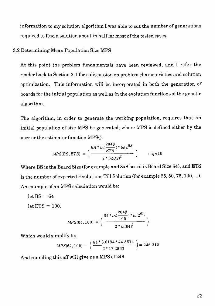
The algorithm, in order to generate the working population, requires that an

initial population of size MPS be generated, where MPS is defined either by the

user or the estimator functionMPS().

2048 Ro

,BS*ln( )*ln(2BS)

MPS(BS,ETS) = : eqnlO

V 2 *IniBST

'

Where BS is the Board Size (for example and 8x8 board is Board Size 64), and ETS

is the number ofexpected Evolutions Till Solution (for example 25, 50, 75, 100, ...).

An example of anMPS calculation would be:

letBS = 64

letETS = 100.

MPS(64, 100) =

Which would simplify to:

2048 ^

6A*ln( )*ln(2n100

2 *Jn(64)2

(64* 3.0194* 44.3614

MPS(64- 100) = ( 2^17^)= 246'312

And rounding this offwill give us aMPS of 246.

32

This function, MPSO, will yield the mean population size. During the evolution

process both the mutation and annealing operators will evaluate the current

population and adjust the Mean Population Size by some percentage. The actual

population size is allowed to fluctuate in order for the genetic algorithm to be able

to control the evolution process. For example, if the population appears to be

stagnating, then the algorithm will increase the population size, hence infusing

"newblood"

into the population to revitalize the evolution.

There are additional factors by which the genetic algorithms would adapt

themselves over the evolution of the population. One example is the Mutation

function, I designed this function to be proportional to the population size as well

as the average changing utility value of the most recent 3 evolution cycles. If the

population size is relatively large (all ormost of the population entries replicate at

10% or better than the CORE population size) then the mutation function will

increase the probability of mutation. The theory here is that as the population

size grows so does it ability to tolerate additional mutation without beginning to

thrash.

3.3 Solution Algorithm Description ofGenetic Operators

The solution algorithm for the N-Queens problem describe earlier is fairly simple

and consistent with its application of standard genetic operators. The operators

known as replication, mutation, and crossover are utilized. The algorithm is

augmented with functions such as a population randomizer, an annealing feed

back scheme, resampling of the population's parents, and a subsampling

technique9 1.

9. Foo, N., Y., & Bosworth, J., L (1972) Algebraic, geometric, and stochastic aspects of genetic operators, (CR-2099)

10. Grefenstette, J., J., Optimization of control parameters for genetic algorithms, IEEE Transactions on Systems, Man and

Cybernetics, SMC-1 6(1), 1 22-1 28

33

The above mentioned genetic operators and functions are applied to the

population at each evolution cycle. Depending upon the annealing temperature

and mutation rate, it is possible that some population entries will not pass

through all of the genetic operators at each evolution cycle. The genetic operators

that are applied to solve this problem in the following order are:

1) Replicate current populationm yielding populations

2) Shuffle*populations

3) Crossover populations yielding populationb

4) Shuffle*populationb

5) Mutate*populationb by < < <%

6) Filter populationb according to valid schema rules yielding populationc

7) Add parents to populationc yielding populationd

8) Shuffle*populationd

9) Mutate*populationd by < <%

10) Resample populationd yielding populationm+ 1 for next generation

* Operation may not occur at each evolution or for every population entry

3.3.1 Initial Population Generation

Now that we can determine the Mean Population Size we know howmany boards

we need to generate to initialize the algorithm. In generating the initial boards

for the population, I incorporated the schema information determined earlier in

Section 3.1. This schema information about minimum valid board sizes and

configurations as well as invalid configurations was captured into two sets. The

set of valid schema configurations were denoted as set A and the invalid schema

configurations were denoted as set x .

34

The set A was generated via the schema processing algorithm and stored.

Example entries are shown in Figure 3.3.1.

The set x was generated from two input sources. One being the capture of invalid

schema output put from the schema algorithmsmentioned in Section 3.1 and the

other being the simple generation of boards that have two or more queen entries

per rank and file. Example entries to this set are shown in Figure 3.3.2.

These two setswere then used in the board generation function BoardQ.

35

These examples will represent the board as it is being stored within thecomputer, a vector of byteswith each bit representing one board location.

For example, the valid chess board of Figure 3.0.2 is represented as:

0 0 0 1 0 0 0 0

1 0 0 0 0 0 0 0

0 0 0 0 1 0 0 0

0 0 0 0 0 0 0 1

0 0 0 0 0 1 0 0

0 0 1 0 0 0 0 0

0 0 0 0 0 0 1 0

0 1 0 0 0 0 0 0

The example boards below are some of the entries in the i set

1 0 0 0 0 0 0 0 0 0 0 0 0 0 0 1 0 0 0 0 0 1 0 0 0 0 0 1 0 0 0 0

0 0 0 0 0 1 0 0 0 1 0 0 0 0 0 0 0 0 1 0 0 0 0 0 0 0 0 0 0 0 1 0

0 0 0 0 0 0 0 1 0 0 0 1 0 0 0 0 0 0 0 0 0 0 1 0 1 0 0 0 0 0 0 0

0 0 1 0 0 0 0 0 1 0 0 0 0 0 0 0 0 0 0 1 0 0 0 0 0 0 0 0 0 0 0 0

0 0 0 0 0 0 1 0 0 0 0 0 0 0 1 0 1 0 0 0 0 0 0 0 0 0 0 0 1 0 0 0

0 0 0 1 0 0 0 0 0 0 0 0 1 0 0 0 0 0 0 0 0 0 0 1 0 1 0 0 0 0 0 1

0 1 0 0 0 0 0 0 0 0 1 0 0 0 0 0 0 1 0 0 0 0 0 0 0 0 0 0 0 1 0 0

0 0 0 0 1 0 0 0 0 0 0 0 0 1 0 0 0 0 0 0 1 0 0 0 0 0 1 0 0 0 0 0

Figure 3.3.1 Example valid board schema

36

The example boards below are some of the entries in the i set

1 0 0 1 0 0 0 0 1 0 0 0 0 0 0 0 0 0 0 0 0 0 0 1 0 0 0 1 0 0 0 0

0 0 0 1 0 0 0 0 0 1 0 0 0 1 0 0 0 1 0 1 0 0 0 0 0 0 0 0 0 0 1 0

0 0 0 0 1 0 0 0 0 0 0 0 1 0 0 0 0 0 1 0 0 0 0 1 0 1 0 0 0 0 1 0

0 0 0 0 0 0 1 0 0 1 0 0 0 1 0 0 0 0 0 0 0 0 1 0 0 0 0 0 1 0 0 0

1 0 0 0 0 0 0 0 0 0 0 1 0 0 0 0 0 0 I 0 1 1 0 0 0 0 0 0 1 0 0 0 0

0 0 0 0 0 1 0 0 1 1 0 0 0 0 0 0 0 0 0 1 0 0 0 0 0 0 1 0 0 0 0 0

0 0 0 0 0 1 0 0 1 0 0 0 0 0 0 1 0 0 0 1 0 0 0 0 0 0 0 0 1 0 0 0

0 1 0 0 0 0 0 0 0 0 0 1 0 0 0 0 0 1 0 0 0 0 1 0 0 0 1 0 0 1 0 0

F igure 3.3.2 example invalid board schema

BOARD({A}, {x}, {F}) = { Vec(S, F) : (Vec(8, F) n x)' * (A Vec(8, F) )} : eqnll

Vec(N, F) function is a random number generator with a filter function that

creates a vector of length n bytes appropriate for the problem.

i = N-l

Vec(N, F)= [J F[Rand(seed)*Rank(F)] : eqn 1 2

i = 0

F is a set ofbytes from which the initial chess boards will be generated. The set F

consists of specially constructed patterns that account for the schema rules

identified earlier in Section 3.1. N in the Vec() function is the rank of one row of

the chess board, for example with an 8x8 board N= 8. Every time the set F is fed

into the Vec() function, it is randomly shuffled to reduce correlations between set

position and data content. This vector Vec() is then utilized by the board

generation function, which will filter out identifiably invalid board formulations

37

based upon the predetermined characteristics and rules of the invalid board

schema sets.

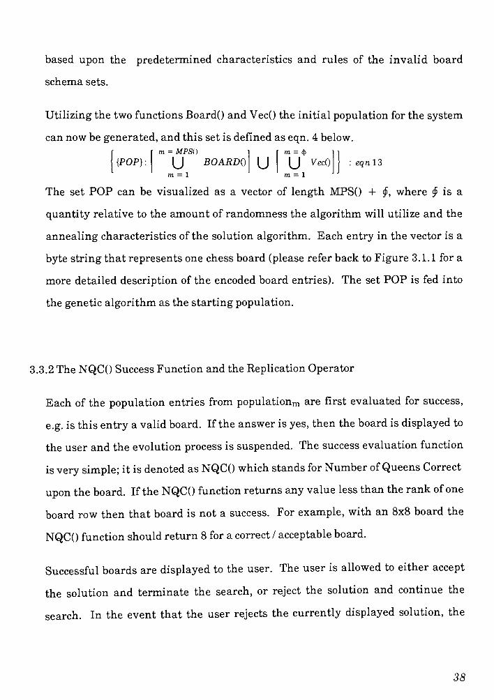
Utilizing the two functions BoardO and Vec() the initial population for the system

can now be generated, and this set is defined as eqn. 4 below.

m = MPSO

{POP} :

m = 1

= Mrm) i r m = $ ii

[J BOARDO \J \J VecQ : eqn 13

m = 1

The set POP can be visualized as a vector of length MPSO + , where <f> is a

quantity relative to the amount of randomness the algorithm will utilize and the

annealing characteristics of the solution algorithm. Each entry in the vector is a

byte string that represents one chess board (please refer back to Figure 3.1.1 for a

more detailed description of the encoded board entries). The set POP is fed into

the genetic algorithm as the starting population.

3.3.2 The NQC() Success Function and the Replication Operator

Each of the population entries from populationm are first evaluated for success,

e.g. is this entry a valid board. If the answer is yes,then the board is displayed to

the user and the evolution process is suspended. The success evaluation function

is very simple; it is denoted as NQCOwhich stands for Number ofQueens Correct

upon the board. If the NQCO function returns any value less than the rank ofone

board row then that board is not a success. For example, with an 8x8 board the

NQCO function should return 8 for a correct / acceptable board.

Successful boards are displayed to the user. The user is allowed to either accept

the solution and terminate the search, or reject the solution and continue the

search. In the event that the user rejects the currently displayed solution, the

38

algorithm will randomly decide to either mutate the board and leave it in the

population or remove the board from the population.

The replication operator is used to replicate the population entries according to a

predetermined function REP().

NQC(POPE)ln(SQRnBS))

REPQ =: eqnlA

3H

Each population entry that fails the NQCO test is passed through the REP()

function to determine how many times the entry should be replicated for the

genetic evolution functions.

For example ifwe evaluate an 8x8 board (BS - 64) with a NQCO of5, we have:

g/n(8)

REP0= = 13.83563

This gives us a REP() = 13.8356, which, when rounded to an integer, indicates

that the population entry should be replicated 14 times going into the evolution

process. These replicated population entries are then added to populations.

3.3.3 TheMutation Operator

This operator is split into several sub-functions that are customized for the

particular problem.

1) Whether tomutate an entry or not.

2) Where tomutate the entry.

3) How tomutate the entry.

Case one, tomutate or not, is a simple Random number generator and a threshold

test. In other words case one is simply a frequency or probability function that

returns true or false based upon user specified values and population conditions.

Case two randomly selects one or more locations on the boardto mutate. Finally,

39

case three selects from a set of allowable mutation operations. For example some

of the possible type of mutation possible are: is the board reordered; do we add

another queen, do we subtract a queen; do we assign one of the valid schema onto

the board, etc.

The reason for mutation cases two and three is to help optimize the evolution

algorithm. By customizing the mutation" operation, I can force the evolution

algorithm to make random changes with some confidence level that the change is

helping to evolve the board in the proper direction towards a solution.

When this operator is invoked, an entire population is passed through the

operation and some percent of the population is changed according to themutation

rules. Below in Figure 3.3.3A is a graph showing the standard mutation success

rate versusmy hybridmutation success rate. Figure 3.3.3B in the appendix is the

corresponding data table to Figure 3.3.3A. The input population was of average

size 40 and the board size was 12x12.

3.3.4 The Crossover Operator

The crossoveroperator^ is also customized for the specific problem as is the

mutation operation. Some of the restrictions of this operation are:

1) Most boards are crossed over at either row or column end points.

2) A board can be crossed overwith itself (e.g. rows or columns are swapped)

3) The crossovermust not leave a row or column without any queens.

Again, the reason for restricting thefunction is to help insure that only valid and

statistically optimalentries are produced for the

populationb

going into the next

evolution cycle.

1 1 Bosworth, J., & Foo, N., & Zeigler, B., P., Comparison of geneticalgorithms with conjugate gradient methods (CR-2093)

National Aeronautics and space administration

40

N

u

m

be

r

of

Que

en

s

Co

rr

ec

t

Fo

r

En

tir

e

Po

pu

lat

io

n

512

480

448

416

384

352

320

288

256

224

192

160

128

96

64

32

0

Hybrid Mutation Number of Queens Correct

Standard Mutation Number of Queens Correct

a i eg i m

12 3 4 5 6 7 8 < 1( 1'

11 M MM 1( 13 1M< 2(2'

2\ 23

Evolution Number

Histogram plot of efficiency of hybrid genetic Mutation operators

Figure 3. 3. 3A

The standard genetic crossover operator is defined such that the cross over point is

a randomly selected location along the string representing a population entry.

This simple definition of crossover does not account for any of the structure of the

12. Goldberg, D., E., (1 987) A note on the disruption due to crossover in a binary coded algorithm, (TCGA report #87001 ).

41

problem or the relationship between the implementation representation and

natural problem structure. My intent is to restrict the crossover operator to

recognize the inherent structure of the problem and its computer representation.

In doing so I contend that I can optimize the crossover operator to combine

population entries and produce more statistically valid entries. Below in Figure

3.3.4A is a graph showing the standard crossover success rate versus my hybrid

crossover success rate. The exact data table for Graph 3.3.4A can be found in the

appendix as Figure 3.3.4B. The input population was of average size 40 and the

board size was 12x12.

3.3.5 The Filter Operator

As intermediate populations are generated, they are passed through a filter

function to insure that the number of obviously invalid population entries are

kept to a minimum. Some of the filter operations that this function implements

are:

1) Checking for greater than 2 queens per row or column

2) Rows and columnsmissing a queen

3) Boards that have a high correlation with the valid schema set A

4) Boards that have a high correlation with the schema set x.

The above set of conditions as well as others are tested for against the population

entries. The boards that have negative characteristics are either passed through

the mutation function, or the algorithm will apply a heuristic and change the

board to be more correlated with characteristics of the A set. The intent here is to

filter out some of the invalid population entries and coalesce them to have a

higher utility values. The filter operation will also promote the board entries that

have high correlations with the set ofvalid schema rules.

42

Aver

age

Num

ber

of

Que

ens

Corr

ect

per

Populati

on

Entr

y

13 Hybrid Crossover Nlumber of Queens Correct ~-

12Standard Crossover l\lumber of Queens Correct

11r r

101 f f 1

9n n n f r ^

8

n nil i7

6 | I ' :: \ | | |

5El pn nif F p r

4n

:

p f: | : 1 | | 1 |

3s w i <. \

: i :. k j : ijj

2

1

::::.

'

i: :; : | i;

.:%'',%'-'%:%< 1 % 1

n ::

; :' i i ':

'

h 1 1 i1 2 3 4 5 6 7 8 5 1(

1*

11 1: lO.MMl 1MS 2(2'

21 23

Crossover Count

Histogram plot of efficiency of hybrid genetic Crossover operators

Figure 3. 3.4A

43

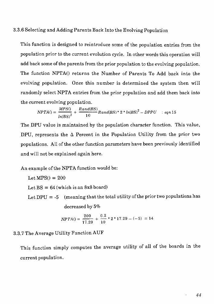
3.3.6 Selecting andAdding Parents Back Into the Evolving Population

This function is designed to reintroduce some of the population entries from the

population prior to the current evolution cycle. In other words this operation will

add back some of the parents from the prior population to the evolving population.

The function NPTAO returns the Number of Parents To Add back into the

evolving population. Once this number is determined the system then will

randomly select NPTA entries from the prior population and add them back into

the current evolving population.

MPSO RandiBS)NPTAO = + RandiBS)

* 2 * ln{BS)Z- DPPU : eqn 15

ln(BS)2 10

The DPU value is maintained by the population character function. This value,

DPU, represents the A Percent in the Population Utility from the prior two

populations. All of the other function parameters have been previously identified

andwill not be explained again here.

An example of the NPTA function would be:

LetMPSO = 200

Let BS = 64 (which is an 8x8 board)

LetDPU =-5 (meaning that the total utility of the prior two populations has

decreased by 5%

200 0 2

NPTAO = +* 2 * 17.29 - (-5) = 14

17.29 10

3.3.7 The Average Utility Function AUF

This function simply computes the average utility of all of the boards in the

current population.

44

i = N

^ NQCiPOPE)

AUF(POP,N) = Eqn: 16N

3.3.8 The Resample Operator

RPS stands for Resample Population Size. This operator performs two tasks^u.

One is to determine how many population entries (X) of the evolving population

will be carried forth into the next population. The second Task is to randomly

sample / select (X) entries from the evolving population and define them to the

next population. In other words populationn is submitted to the genetic operators

and is expanded and evolved; the resample operator selects (X) of the evolved

entries and produces populationn+ 1.

Back in Section 3.2 we defined a function called MPSO for Mean Population Size.

This value is set as the average size of the population through the evolution

process. The exact size of the working population is allowed to fluctuate within

some tolerance range determined by a combination of the genetic classifier

functions such as character function and annealing temperature, population size,

etc.

RPS() represents the number of population entries that will be selected from the

evolving population and used to define the next population. The RPSO function is

defined as:

RPSO = MPSO + NPTAO - AUFQ : eqn 17

Once we have determined the value of RPS, the function then randomly selects

RPS number ofpopulation entries from the evolving population and defines them

13. Wetzel, A., Evaluation of the effectiveness of genetic algorithms in combinatorial optimization, Unpublished manuscript,

University of Pittsburgh (1 983).

14. Booker, L, B., Improving performance of genetic algorithms in classifier systems, Proceedings of an international

conference on genetic algorithms and their applications, pp80-92

45

to be the population for the next set of evolution operations. The output of this

function is the next population or populationn+ 1.

There are advantages with being able to subsample an expanded population as a

separate step, rather than having the population created by the crossover operator

be the input to the next evolution cycle. Some of the advantages are that we can

now easily control the size of the population going into the next generation. This

added control can be utilized as a parameter similar to annealing. The concept is

that as the population begins to stagnate or converge toward false optima, we can

allow the size of the population to grow (increased population size typically allows

for increased mutation probabilities). This has the advantage of increasing the

potential for population entries to converge to the correct answer or at least break

out of the false minimums without the need for increasing the mutation rate such

that the the system begins to thrash.

Another advantage to the post subsampling is that it allows the evolution process

an additional degree of freedom to either statistically, randomly, or by design

select population members that should exist in future generations. For example,

some algorithms may need or find it beneficial to have the parents of certain

children remain in future evolutions.

3.3.9 The shuffle Operator

This operator is a simple shuffle operation. It can be likened to shuffling a deck of

cards prior to dealing the cards for playing. The purpose for designing this

operator is to be able to pass the evolving population through this operator at any

time in the evolution process and randomize the order of the population entries.

46

For example, this is useful for reducing the correlation between sequential

population entries subsequent to the replication operator. The replication

operator simply accepts a population and reproduces the population entries some

determined number of times. In doing so the replicated population contains

groupings of the previous population.

For example:

1) If we let a Xn represent the nth population entry we could describe a

population by the set {Xi, X2, X3, ... , Xm_i, Xm} were there are m entries in

the population. 2) After the population under went replicationmy data

management routines of the population would hold

the replicated population entries as such:

{Xi, Xi, Xi, Xi, Xi, X2, X2, X2, X3, X3, ..., Xm-i,

Xm-l, Xm_i, Xm, Xm}

We can clearly see that the replicated population

now has a positional relationship amongst the

population entries

In order to decorrelate the order of the population entries we simply pass the

replicated population through the shuffle operator, and now the population

entries have no location / position correlation.

For example after the replicated population under goes the shuffle operator the

shuffled populationmight look something like:

{X3, X2, Xi, Xm-i, Xi, X2, Xi, X2, Xm, Xi, ... , Xm, Xm_i, Xi, X3,Xi, Xm.i}

47

3.3.10 The Character Function

For this problem case the function is simple. There are two types of population

information being maintained. One is the average population utility for each

evolution cycle. The second is the annealing temperature for the current

evolution.

For the average population utility this is a simple function that is executed at the

end of every evolution cycle. The result is stored within an array for use by other

genetic operators. The array storage allows for a history of results to be

maintained throughout the solution generation. The Average Utility Function

AUF() is shown below:

i =N

^ NQC(POP.)

AUFO = : eqn 17 AN

Where N is the number of entries in the population. POP is the entire population

for the current evolution. And NQCO is the previously defined function returning

the Number ofQueens Correct for an individual population entry.

48

3.4 N-Queens Solution Algorithm

For this problem case the function is simple. There are two types of population

information being maintained. One is the average population utility for each

evolution cycle. The second is the annealing temperature for the current

evolution.

For this experiment we can conclude that the modified genetic operators are

successful in optimizing the solution algorithm based upon the improved results

shown in the previous figures. We can additionally conclude that the basic

genetic operator functions are correct and can be utilized as building blocks to

investigatemore complex functions.

By way of the successful examples and solutions presented earlier I am also

concluding that the data structures and data management routines developed to

manage the populations are correct and do not adversely effect the solution

algorithm. Factors of concern here were the possible interaction between the

sequential linked lists of population entries. The shuffle operator appears to

minimize / remove detrimental effects of sequential correspondence otherwise I do

not believe thatwe would observe the excellent results.

We can also conclude that the hybrid crossover and hybrid mutation functions

improve the convergence performance of the algorithm. This is demonstrated by

the data of figures 3.3.3A and 3.3.4A.

49

4.0 Routing Problem and GeneticAlgorithm Introduction

In Chapter 3 I developed the genetic algorithm fundamentals as well as several

building blocks for implementing solution algorithms. This work was done using

the N-Queens problem as the focus for development. I selected the N-Queens

problem for ground work because of the magnitude of information available

related to solving the problem, and also because the problem and solution can be

made tractable.

In this Chapter I will begin discussions of the main investigation, Printed Wire

Board (PWB) routing. I intend to utilize and build upon the fundamental

information developed for the N-Queens problem to solve the PWB routing

problem.

Section 4.1 and 4.2 are a brief introduction to the PWB routing problem. In

subsequent Sections I will describe the genetic operators I designed to solve the

PWB routing problem. The genetic operators described will be implemented for

all solution algorithms with only slight modification to the utility function that

tailors it to the individual solution algorithm being implemented and tested.

Chapters 6, 7, 8 will present the specifics of each solution algorithm; each Chapter

describes a new solution algorithm. I attempted to utilize information learned in

the prior experiments to best optimize a final solution algorithm. As the

experiments progressed I enhanced the initial set of genetic programming tools

that I developed to solve PWB routing problem.

50

4.1 Routing ProblemDescription

If we look back at the criteria for formulating a problem / solution methodology

discussed in the introduction, we find that we must have:

1) A well formed statement ofwhat the problem / question is

2) Criteria for determining an acceptable solution

3) Characteristics of the problem.

For the PWB routing problem these criteria are defined as:

1) Characteristics of this investigation is to model a rectangle of MxN cell

positions, where each position represents one of two states, occupied or not.

Each occupied state has a neighbor relationship, "connectedto"

or

"terminator". By connecting carefully selected MxN cells, the algorithm will

route all PWB traces.

2) A solution is acceptable if the algorithm is able to route all of the connections

specified by the netlist or some specified percentage of the connections. Please

note that this problem does have a tolerance range for its solution

acceptability; hence, by definition there is more than one acceptable solution

per net list.

3) For this problem there are three initial requirements.

One: a net list exists for the circuit.

Two: Parts placement has been performed.

Three: a board ofadequate dimension is defined.

51

4.2 PC BoardAlgorithmModel

The first assumption required for all ofmy routing algorithms is that there exists

a net list for the circuit to be routed and that the parts placement has already

occurred. An example netlist is Figure 4.2.1:

This will give me a working board size upon which I can route the traces. I will

treat the PWB as a rectangle of size MxN positions upon a cartesian grid. By

using the analogy of a cartesian grid, I can associate trace starting points, trace

ending points, and the trace path itself as a series of connected (X, Y) coordinates.

Please refer to Figure 4.2.A as a sample board layout and grid overlay. This type

of a layout is similar to the formats utilized in many of the solution algorithms for

the Traveling Salesman problems and the euclidean distance minimization

problems1 2. Examples of a simpler board and its potential trace path routings are

presented in the appendix as figures 4.2.B and 4.2.C.

Having the initial starting data, a netlist, a board size, and parts placement, I

associate each trace starting point with an (X, Y) coordinate and each trace

ending point with an (X, Y) coordinate. With these two data points for each trace,

starting and ending point, thealgorithm knows where the routing paths start and

where they terminate. A routing path is deemed complete when two conditions

are satisfied for the trace. Condition one is that there are a set of (X, Y) coordinate

cells that can be traversed starting from a trace's starting coordinate and ending

at the traces ending coordinate. The second condition is that all of the (X, Y)

coordinates of the trace path are unique to the trace; the coordinates composing

the path are not required or held by any other trace. From these criteria the

algorithm can evaluate with certainty which routing traces are successful,

52

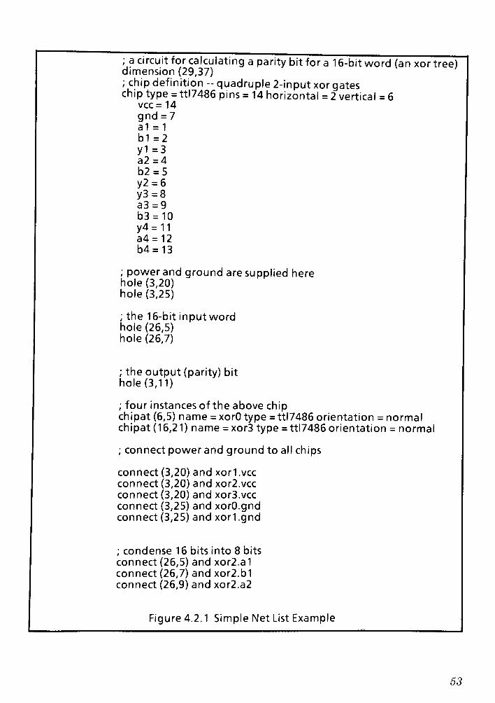
; a circuit for calculating a parity bit for a 1 6-bitword (an xor tree)dimension (29,37); chip definition -

quadruple 2-input xor gateschip type = ttl7486 pins = 14 horizontal = 2 vertical = 6

vcc= 14

gnd = 7

a1 =1

b1=2

y1=3

a2=4

b2 = 5

y2 = 6

y3=8

a3=9

b3 = 10

y4= 11

a4 = 12

b4=13

; power and ground are supplied herehole (3,20)hole (3,25)

; the 16-bit input word

hole (26,5)hole (26,7)

; the output (parity) bithole (3,11)

; four instances of the above chipchipat (6,5) name = xorO type = ttl7486 orientation = normal

chipat (16,21) name = xor3 type =ttl7486 orientation = normal

; connect power and ground to all chips

connect (3,20) and xorl.vccconnect (3,20) and xor2.vcc

connect (3,20) and xor3.vcc

connect (3,25) and xorO.gndconnect (3,25) and xorl .gnd

; condense 16 bits into 8 bits

connect (26,5) and xor2.a1

connect (26,7) and xor2.b1

connect (26,9) and xor2.a2

Figure 4.2.1 Simple Net List Example

53

Y

A

x

i

s

CPU

EPROM

EPROM

SRAM

SRAM

SRAM

SRAM

LED DISPLAY

-^X Axis

Power

Supply

MxN cell PWB board

Board layout for a sample circuit

Figure 4.2.A

Sffi

PPI ::

PPI

incomplete, or unsuccessful. Hence, the algorithm has a mechanism to measure

its progress.

Each of the three algorithms designed and discussed attempt to evolve the

population entries (trace paths) toward acceptable valid solutions. The evolution

process is designed to evaluate, select, and compete for intermediate (X, Y)

coordinates in order to evolve the trace paths to successful completion, connecting

starting point to ending point. A highly active population will have all of its trace

entries advancing one coordinate position per evolution,though it is not expected

that all trace entries will advance during every evolution cycle.

The algorithm monitored and characterized evolving populations. Population

entries that cannot progress any further, those that have either terminally

1. Moopenn, A., &Thakoor, A., P., & Duong, T., A Neural network for Euclidean distance

minimization

2. Van Den Bout, D., E., & Miller, T., K., A traveling Salesman Object function that works, North

Carolina University

54

stagnated or lost all utility, are removed from the evolving population.

Population entries that are demonstrating progress towards completion are

promoted during future evolutions.

To summarize, initial algorithm requirements are:

A netlist exists (Trace starting and ending points are defined)

Parts placement has occurred

PWB size is known

From these initial data points, the algorithm will evolve a population of PWB

traces to successful completion.

4.3 Core Population

Each population entry, hereafter referred to as a POPE, is equated to a trace path

attempting to be routed. The POPE assigned value can be one of three types:

1) (X, Y) trace starting coordinate found in the netlist / placement data.

2) (X, Y) trace ending coordinate found in the netlist / placement data.

3) Set of (X, Y) coordinates that represent a trace's quantized ratnest path.

Please refer to Chapter 7 for definition of a ratnest path.

Prior to the start of the algorithm, a core population is created. The core

population is simply a list of one POPE per PWB trace, as identified in the

circuit's netlist, and is labeled COREPOP. The POPEs of the COREPOP are

considered the start of a family or blood line. POPEs from the core population are

replicated and gathered to form the initial population for the genetic algorithm.

55

This process and the definition of an initial population will be discussed in

Chapter 5, Section 5.2.

I use the notion of family / blood line to connote the relationship of the offspring

that evolve during the evolution process to their parents from the COREPOP.

Each trace entry to be routed represents a family / blood line, and the offspring of

each family work collectively to solve each trace routing path. The two figures

below illustrate what is means by a blood line. The two blackened cells in Figure

4.3.1.A are the two end points of a trace to be routed. The trace end points are

what make up the population entries (POPEs). Figure 4.3. IB show the POPE of

Figure 4.3.1.A after several generation cycles where intermediate cells on the way

towards the trace end point have been captured. Figure 4.3. l.B shows multiple

paths being established that are developing their way towards the single end

point. These multiple trace paths being explored are what I refer to as a POPEs

family / bloodline.

56

Trace IEnding Point

w

Trace

1

1

Starting Poinl

Example of a Blood line for one routing traceFigure4.3.1.A

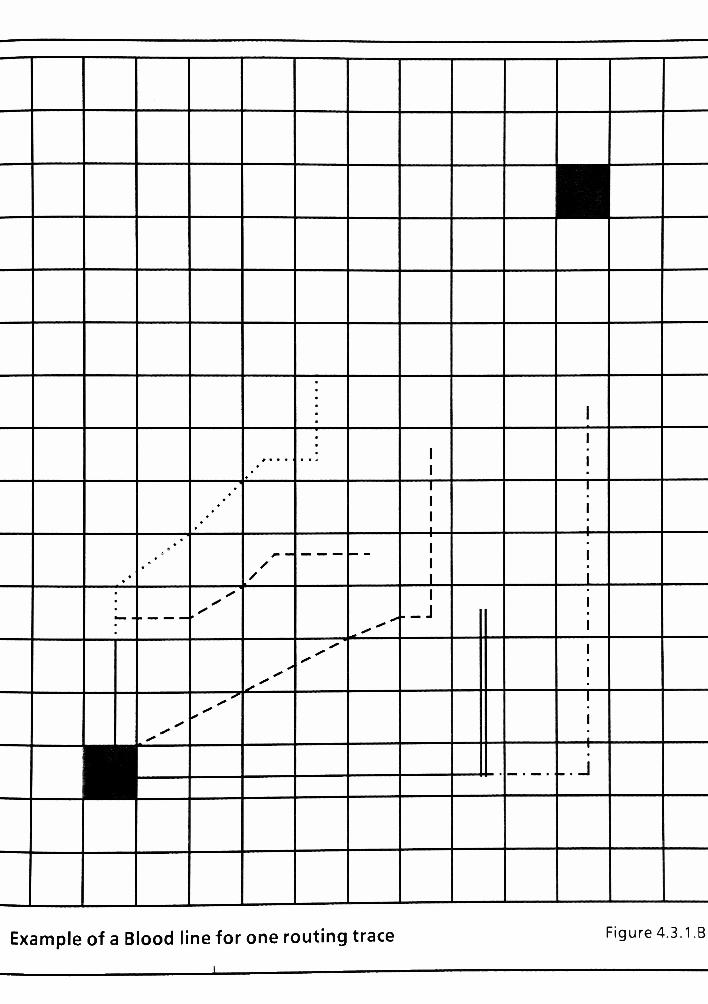
JT

i

9 . i . .'.

y

!--

s

y

y

yy

._J

*

y

yy

?y

i

Example of a Blood line for one routing traceFigure 4.3. 1.B

4.4 Fundamental Characteristics ofSolutionAlgorithm

For the solution algorithms presented here, an initial population of POPEs is

generated from the core population and contains one ormore POPEs for each trace

to be routed. In other words at least one representative for each trace to be routed

is in the initial starting population and is active at all times right from the start.

The algorithm evolves the population towards a solution. During the evolution

process there are only two ways in which a POPE is removed from the population,

by either completing its trace path successfully (finding the trace's end point

coordinate), or failing and dying. No matter what the condition is, success or

failure, at least one single POPE is removed from the evolving population.

Following is a detailed discussion of the two ways in which a POPE can be

removed from the evolving population; they are:

? One, by a POPE successfully completing its routing path.

In the case of success, the POPE's coordinates are marked as routed and

remain unavailable to other POPEs. Upon successful completion, the entire

blood line of the successful POPE is removed from the evolving population. If a

POPE is successful in finding a routing path to its end point, then the POPE is

removed from the active evolution list; its coordinates / trace path are left

marked as a valid trace, and all its other family members are removed from

the active population. This is because there has been a successful path found

and will be preserved; therefore, the other family members are no longer

needed for searching a valid path. Coordinates occupied by the other family

59

members of the successful POPE are freed up and placed upon the available

neighbor list for other POPEs to utilize.

? Two, by a POPE failing to progress during the course of evolution. Failure to

progress is characteristic of a POPE stagnating and / or losing all its utility

value.

The ways in which POPEs die are numerous. For example, a POPE may route

itself into a position where there are no available neighbors and it has not

reached its destination point. In this case, only a single POPE is removed, not

all of its family members. A POPE may bid all of its money / utility away

before reaching its destination. This death is dealtwith similarly to the above

stagnation case.

In the case of failure only the failed POPE is removed from the population, not

its entire blood line, as in the successful case. Also in the case of failure the

POPE's coordinate positions are returned to the available list of neighbors for

the board; other POPEsmay begin to utilize the freed up coordinates.

Solution algorithms investigated within this thesis do not perform any

"backtracking". What I am referring to here is that as POPEs are removed from

the population there are board cells that become available. The algorithms I will

present have nomechanism to go back and reevaluate the merit of freed up board

cells to existing POPEs. The algorithm does not backtrack k through prior

evolutions and reevaluate trace path decisions based upon the newly freed board

cells. However, the newly freed board cells are available for evaluation and use in

future population evolution cycles.

60

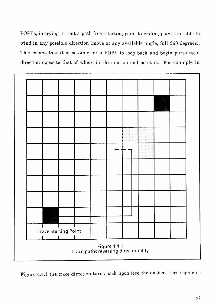
POPEs, in trying to rout a path from starting point to ending point, are able to

wind in any possible direction (move at any available angle, full 360 degrees).

This means that it is possible for a POPE to loop back and begin pursuing a

direction opposite that of where its destination end point is. For example in

Pf

mm

Trace Starting Point

1 1 1

Figure 4.4.1

Trace paths reversing directionality

Figure 4.4.1 the trace direction turns back upon (see the dashed trace segment)

61

itself because forward motion is no longer possible. The shaded squares are

indicate squares that are not available to the current trace path.

At this point we have talked about the board layout and the algorithm

representation of the POPE's. We have also mentioned briefly some of the set up

characteristics of the input population to the algorithm as well as general

characteristics of the individual POPEs.

Another algorithm characteristic is that as POPEs die unsuccessful deaths ( a

trace path can not be routed to any other board cells yet the trace has not

completed in routing path start to finish), they are not restarted into the evolution

process. The potential problem here is that if a family blood line is so unsuccessful

that all the POPEs of the family die of failure, there is no mechanism to retry and

route that trace path. This trace path ismarked as unsuccessful and left out of the

routing process.

Another characteristic of the algorithm is that the total size of the population at

each evolution cycle is allowed to fluctuate within a user or algorithm specified

range. The population entry count fluctuates due to the removal of traces, due

either to success or failure. The adding of a POPE's parents at the end of each

evolution is also a factor in fluctuating the population size. The population is

capable ofgrowing during genetic replication, evolution and resampling stages.

4.5 Algorithm Initial Requirements

? Netlist of the PWB exists.

A net list for a circuit is the listing that describes all of the pin to pin

connections for the system. Refer to Figure 4.2.1

62

? Parts placement for the system is done.

This body of information identifies where all of the circuit components are to

reside on the given PWB. For example the placement information identifies

where all of the power and ground lines are to be. It also identifies where all of

the chips of the circuit are to be placed and what their orientation is to be.

Refer to Figure 4.2.A.

? Sufficient PWB board sizeMxN is defined.

This is the size of the PWB board it self. The only requirement of this value is

that the placed circuit must fit within the given dimensions with1"

surround

on all edges. Refer to Figure 4.2.A.

These initial requirements are essential to all of the solution algorithms

investigated. From this supplied information the user can run the system and

generate solutions to the given routing problem.

4.6 Genetic Solution Algorithm Functional Flow Description

Please refer to the appendix section 11.4.6.X for several drawings of the major

components of the solution algorithm. They are provided to give a high level

description of the components of the solution algorithm and their relationships

within the solution evaluation. The figures 11.4.6.X within the appendix are a

graphical representation of the algorithm flow ofoperation.

Diagram 4.6.1 of the appendix shows the main solution generation routine. This

set ofmodules represents the components of the genetic algorithm that evolve the

population towards a solution. The current population (set {POPE}) is fed through

63

each of the algorithm modules in sequence. One evolution cycle has occurred

every time the currently evolving population has completed a full cycle of the

genetic algorithmmodules (Figure 4.6.1).

The following are high level procedural descriptions for each of the genetic

solution algorithm components. The actual function definitions will be presented

in detail later in Chapter 5:

y Replication Operator.

m = POPE

{{ReplicatedPopulation}] =

_ ReplicateiPOPEJ EQN 18

'm=POPE

This function accepts the current input population and replicates each POPE

some number of times. The actual number of times that any POPE is replicated is

based upon three primary criteria:

1) Utility of the POPEm

2) Characterization of the current POPEm relative to the entire {POPE} set

3) Randomness, some small random factor

The replicate function evaluates the utility and character of each POPE and then

adds a random component to generate the number of times that a POPE is to be

replicated. The POPE is then replicated and inserted into the replicated

population set {POPE}a.

y Crossover Operator:

m

{CrossoverPopulation} = X Crossover({ReplicatedPopulation}) EQN 19

The replicated population set, {POPE}a, is then fed into the crossover operator.

m = Number to crossiPOPE )n

64

This function is implemented in two steps:

? step one is to select two POPEs to be entered into crossover from the

working population set {POPE}a(less any previously selected POPEs).

? Step two is the actual crossover of the two selected POPEs, hence creating a

new POPE, which is placed into the evolving population {POPE}t>.

The actual crossover operation can be one of two types: 1) single point crossover or

2) dual point crossover. Factors considered by the crossover operator are:

1) Purely random selection

2) POPE blood line relationships

3) POPE grid coordinate relationships

The crossover operator evaluates the input population set {POPE}a and selects two

POPEs from the input set based upon POPE relationships, given the above three

categories. By filtering the POPEs to be crossed, we limit the number of invalid

POPEs thatwill be generated or placed into the evolving population. The result is

to focus / direct the solution algorithm to operate primarily upon POPEs that have

a statistically higher correlation with the final solution set ofPOPEs.

This type of restriction of population entries in order to reduce the search space

can be visualized, in terms of set theory, as follows. The entire possible solution

space can bemodeled as shown in Figure 4.6.0:

Knowing the sets that comprise the entire population, we can begin to derive

simple set theory equations that define the population by its entities. For

example, based upon Figure 4.6.0, we can write the following equation for the

entire population:

675

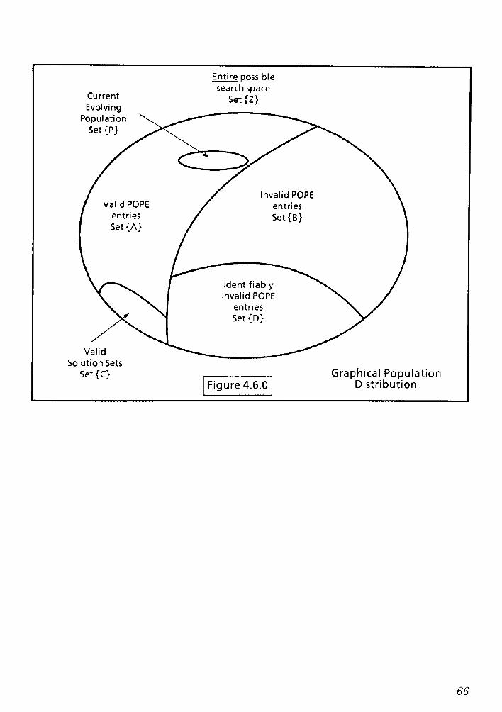
Current

Evolving

Entire possiblt

search space

Set{Z}

alidPOPE

entries

Set{B}

Graphical Population

Distribution

Population \

Set {P} .><

1 Valid POPE

/ entries

| Set {A}

Valid

IdentifiableInvalid POP

entries

Set{D}

Solution Sets

Set{C}Figure 4.6.0

66

Current

EvolvingPopulation

Set {P}

Entire possible

search space

Set{Z}

/ Valid POPE

/ entries /

f Set {A} /

/ InvalidPOPE

entries

Set {B}

Valid

IdentifiableInvalid POP

entries

Set {D}

Solution Sets

Set{C}Figure 4.6.0

Graphical Population

Distribution

Population Set {Z} = {A} U {B} U{C}U {D} EQN20

With out any type ofpopulation / POPE filtering we would not be able to eliminate

some of the invalid POPE entries. Therefore, our working population also would

be required to search the trivially invalid POPE entries, e.g. those of set {D}

within Figure 4.6.0. Hence without filtering, the search space is equivalent to the

size of the entire possible population set {Z}.

Population Set {Z} - {A} U {B} U {C} U {D} = UnalteredAlgorithm Search Space EQN21

With the ability to filter out some of the trivially invalid POPE entries from the

search space we can write the equation below, which describes the possible search

space:

FilteredAlgorithm Search Space {F} = {Z } n {D } EQN22

67

By inspection set {F}, is a smaller set than {Z} hence we are already optimizing the

algorithm by eliminating some of the trivially invalid POPEs.

As discussed earlier in Chapter Three, Section 3, the algorithm designer needs to

be cautious not to cause"inbreeding"

within the evolving populations, which

causes in stagnation of the evolving populations. The way this is prevented is:

1) Allow for purely random crossovers to occur.

2) Monitor the variance of the population and adjust the mutation rates

accordingly

3) Monitor the growth rate of the population via the character function and

dynamically adjust the algorithm parameters to avoid stagnation.

These filters / evolution-monitoring routines are designed to compensate the

abovementioned parameters in order to prevent stagnation or convergence upon a

false minimum. As these filters determine that the evolution algorithm is

stagnating or the rate at which new cells are being captured is declining, etc., the

mutation rate may be increased. Likewise the population size may be increased

and / or additional parents may be added back into the population. All of these

compensations are performed in order to keep the solution algorithm proceeding

towards finding a solution.

? Mutation Operator:

{MutatedPopulation}} = T MutateiPOPEJ EQN23

' onpf

m = {POPEJb

m = POPE,

68

This operator utilizes the trace distance estimator function, population

characterization function, and the annealing function. All of these inputs are

utilized to characterize the state of the evolving population. The mutation

function determines the condition of the current evolving population and the

condition of each individual POPE. It then determines whether the POPE is to be

entered into mutation. In deciding to mutate individual POPEs, the mutation

operator attempts to insure that the population is not stagnating to false

solutions, as well as insuring that the population does not begin to thrash.

For this solution algorithm the mutation operator cannot be simple random bit

flipping. What I did was to design a mutation operation that would introduce

random change in a manner that was more suitable for the problem and its

representation.

For additional descriptive information on the mutation function, refer to Chapter

Five, Section 5.9.

y Resample Operator:

m = POPE

\{ResampledPopulation}] = ][ Resample({POPEJ ) EQN2A

I 'm =

POPEl

The resample operator has twomodes of operation.

1) Purely random resampling

2) Blood line filteringmode

In mode one above the resample operator is fed an entire current working

population set {POPE}c. From this set a predetermined number of POPE entries

are selected, purely at random,and placed into the set {POPE}d. The new set

{POPE}d, is then augmented by adding some ofthe parents from the immediately

69

preceding evolution cycle. This newly formulated set of {POPE}d then becomes

the input population to the next genetic algorithm cycle.

In mode two the resample operator does pseudo-random resampling. The

difference is that in this mode the resample operator will make predetermined

choices as to which POPEs from the set {POPE}c to carry forth into the next set

{POPE}d. The predetermined choices aremade by rules such as:

y Insuring that there are at least two POPEs from each blood line (trace

representative).

? The utility of a POPE relative to the average set {POPE}d utility value, as well

as the statistical correlation of a POPE relative to the set {POPE}d.

? Estimated trace distance to completion (e.g., augment with traces that have

very low estimated completion distances).

? Parents from the previous population set {POPE}a are added back into the set

{POPE}d

These directed selections are done with care so as to not redirect the population

evolution onto false solutions. The basis for directing the resample operator is to

guide / restrict the POPEs that enter into the next evolution cycle to POPEs that

are of high potential and not trivially invalid. I also need to insure that a blood

line does not get lost in the evolution process. This would be a false death, and the

trace would never route.

t Shuffle Operator:

70

!1m = N

{ShuffeledPopulation] = ]T Shuffel({POPEJ) EQN 25

m=POPE1

This operator performs a simple random shuffling of the set of POPEs that are

handed to it, analogous to shuffling a deck of cards. This operation is utilized

because the genetic algorithm, as I implemented it, serially concatenates POPEs

into a list that becomes the next set of {POPEs}n. Because of the way the list is

generated, adjacent entries are highly correlated. This correlation could cause "in

breading,"

which leads the evolving population to stagnate and / or converge to

falseminimums.

4.8 Genetic Characterization Function

For these algorithms I implemented simple population character functions and

individual POPE character functions that monitor vital statistics of the evolving

population. The character function looks at statistics of both individual POPEs

and the population as a whole. Some of the parameters considered for the

character function are:

1) Number ofPOPEs that advanced in the current evolutionary cycle.

2) The average utility of the entire population.

3) Estimated distance required to route the remaining traces.

4) Average number ofevolution cycles for population POPEs.

5) Current and past annealing temperature.

6) Average number ofPOPEs that advance per evolution cycle.

7) Population skew, Kurtosis, and variance.

The character function scans the current population and keeps a history of past

data items, which is utilized to evaluate trends of the population. From data

gathered, the characterization function then sets certain condition flags and

adjusts some of the biasing and randomization constants. These condition

71

variables are used by the other genetic operators such as crossover and mutation

in order to control the evolution algorithm and optimally direct it to converge

upon a solution.

For example, the character function evaluates and compares the mean of past

populations. This information is evaluated and used to monitor the population

growth rate (up, down, stagnate, thrashing). A population can be assumed to be

thrashing if consecutive population means fluctuate by large amounts.

Similarly, a population may be considered to have stagnated if its mean does not

change aftermany evolution cycles.

Other information that is maintained by the character function will be listed in

Chapter 5, Section 5.2. The way in which this information is utilized by the

genetic operators is:

? If a population is negatively skewed, the REP() and NPTAO operators will

modify their characteristic equationsto attempt to compensate for the poor

populations that are evolving.

? If a population's kurtosis is spread too long and or if the variance is too great,

then this is a sign that the evolution algorithm is causing thrashing. The

algorithm is exploiting / thrashing through the solution search space rather

then effectively exploring it for asolution.

The goal is to collect and monitor the characteristic evolution information and

utilize this to optimize the genetic operators. Operators such as annealing,

replication, mutation all are designed to utilize the character function

information to try and adjust theirbehaviors.

72

4.9 RoutingMap Overview

The Routing map is managed as a cartesian grid composed of rectangular cells.

These cells are filled with the primary schema symbols that represent trace path

components, connection pads, trace joints, etc. The solution algorithm selects cells

from the grid according to the genetic algorithm rules. The selected cells then are

filled in with the schema symbols that join together to form the routing trace from

the net list.

? Figure 4.9.1 illustrates the schema symbol set for constructing trace paths in

any of the 90 degree rotations out of the 360 degree circle.

? Figure 4.9.2 illustrates the schema symbol set for constructing trace paths in

any of the 45 degree rotations at 90 degree intervals out of the 360 degree

circle.

? Figure 4.9.3 illustrates the schema symbol set for constructing trace path

mounting holes and connection joints.

? Figure 4.9.4 illustrates the schema symbol set for constructing a trace path

through the edges / corners of cells. These are designed to better utilize cells

when there are diagonal paths through them.

Each of the schema symbol blocks are sized to fit entirely into one cell of the

routing board (a cartesian grid, as discussed earlier). The algorithm is designed to

logically combine the schema blocks in order to build the routing trace paths

required to solve the problem. Figure 4.9.5 through Figure 4.9.12 show example

diagrams ofhow the schema blocks are combined in order to connect a trace path.

73

T

Schema A

Vertical line segment upper halfSchema B

Vertical line segment lower half

Schema C

Horizontal line segment left half

Schema D

Horizontal line segment right half

Figure 4.9.1

In the example ofFigure 4.9.5 our PWB is a 5x6 cell board, and we wish to connect

the three darkened cells. An'animation'

that shows the combining of schema

blocks used to complete a trace routing path isprovided in the appendix as figures

4.9.6 through 4.9.12. This combining of blocks is how the routing algorithm

builds a trace path in order to complete the routingproblem.

74

K

Schema E

Left line

\JSchema G

Right +135line

v\

Schema F

Right+45

line

V-Schema H

Left+225

line

Figure 4.9.2

One caveat that needs to be pointed out here is that there are precautions that

need to be taken when determining the availability of cells for occupancy. For

example, one does not want trace paths to occur as shown in Figures 4.9.13

through 4.9.14. Therefore, in order to insure thatanomalies like this do not occur

75

Schema I

Hole for connection

Schema K

Solder pad for connection

Figure 4.9.3

Schema J

Via for layer transition

O

Schema L

Trace connection joint

the algorithm has multiple evaluations it performs when determining the

eligibility of its neighboring cells for occupancy.

76

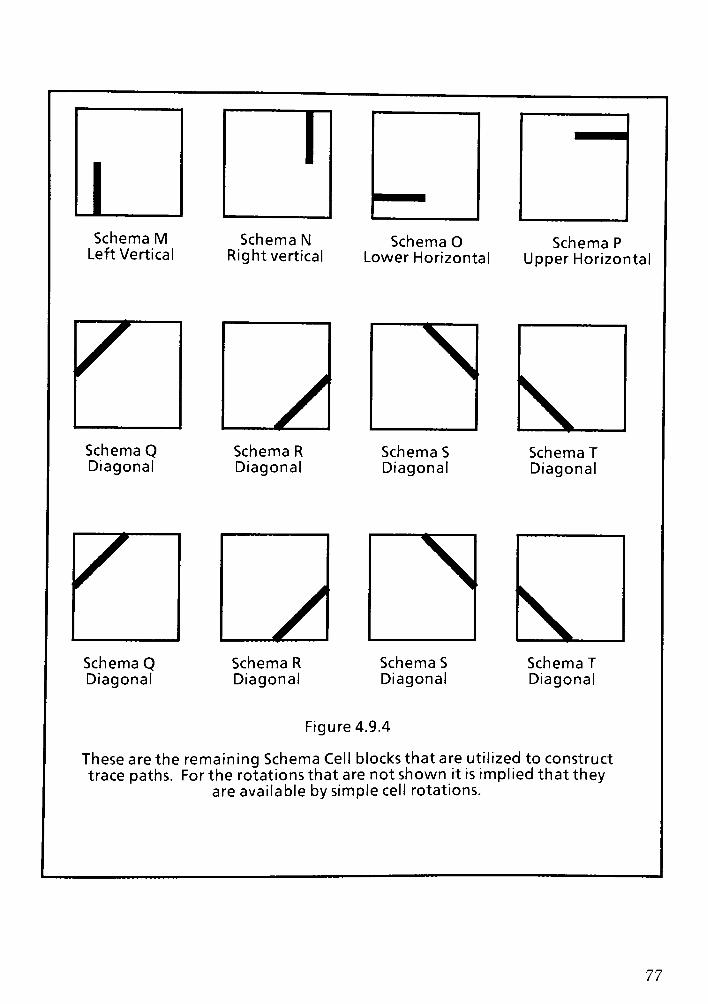
ISchema M

Left Vertical

V

Schema QDiagonal

V

Schema QDiagonal

Schema N

Right vertical

ASchema R

Diagonal

ASchema R

Diagonal

Schema O

Lower Horizontal

N

Schema S

Diagonal

Nl

Schema S

Diagonal

Figure 4.9.4

Schema P

Upper Horizontal

Schema T

Diagonal

kSchema T

Diagonal

These are the remaining Schema Cell blocks that are utilized to construct

trace paths. For the rotations that are not shown it is implied that theyare available by simple cell rotations.

77

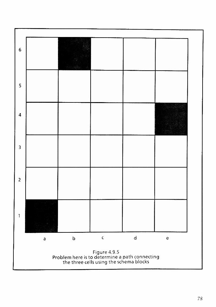
Figure 4.9.5

Problem here is to determine a path connecting

the three cells using the schema blocks

78

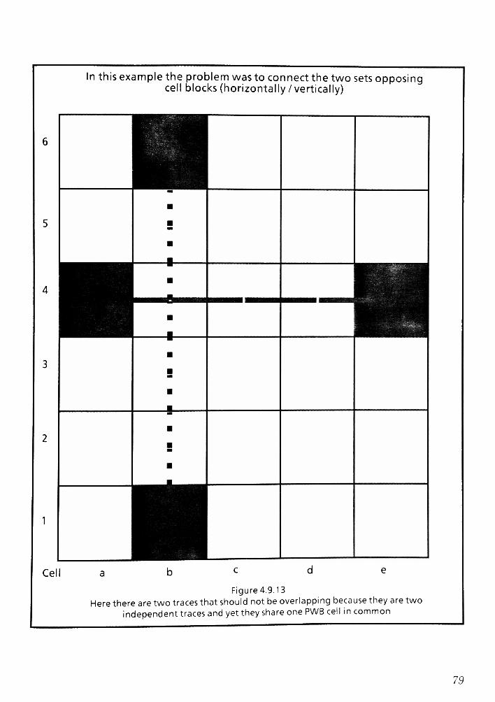
In this example the problem was to connect the two sets opposingcell blocks (horizontally /vertically)

I

e

i

!

Cel

Figure4.9.13

Here there are two traces that should not be overlappingbecause they are two

independent traces and yet they share one PWB cell in common

79

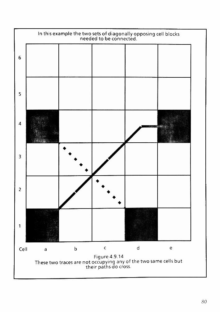
In this example the two sets of diagonally opposing cell blocks

needed to be connected.

Cell

Figure 4.9. 14

These two traces are not occupying any of the two same cells but

their paths do cross.

80

5.0 Genetic Algorithm RoutingEquations

In Chapter Four, I presented a general overview and high level description of the

routing algorithm and genetic operators. In this Chapter I will present the

solution algorithm equations and a description of their function for the routing

problem. The algorithm equations presented here are derivatives of the solution

equations discussed in Chapter Three and Four; I recommend that the reader refer

back to Chapter Three or Four for any additional information on the genetic

operators / functions not repeated here. The solution to the N-Queens problem

served as ground work for the development and characterization of the solution

equations to be utilized for the routing problem.

As in Chapter Four, the functions presented here are utilized for all of the genetic

routing algorithms developed in Chapters, Six, Seven, and Eight.

5.1 Genetic Character Function

This function is utilized to monitor the characteristics of the evolving population.

The specific features of the population that aremaintained / tracked by this utility

are:

? Population average : see Chapter 2 eqn # 2

This information ismaintained as a vector of the last N values for the average

POPE utility, average number of trace jogs, estimated average distance for

trace completion.

? Population standard deviation : see Chapter 2 eqn # 3

81

This information ismaintained as a vector of the last N values for the standard

deviation re: POPE utility, number of trace jogs, estimated distance for trace

completion.

? Population variance : see Chapter 2 eqn # 1

This information ismaintained as a vector of the last N values for the variance

re: POPE utility, number of trace jogs, estimated distance for trace completion.

? Population Skewness : see Chapter 2 eqn # 4

This information is maintained as a vector of the last N values for the

population skewness re: POPE utility, number of trace jogs, estimated distance

for trace completion.

y Population Kurtosis : see Chapter 2 eqn # 5

This information is maintained as a vector of the last N values for the

population Kurtosis re: POPE utility, number of trace jogs, estimated distance

for trace completion.

? Estimated average distance for trace completion

This function is not updated every evolution cycle, the frequency with which

this is updated is either set by the user or defaults to every 5 population

evolution cycles. There are special cases that will force this function to be

updated they are:

1) Three ormore traces complete theirpath

2) The average population utility plateaus and/ or falls for five consecutive

population evolution cycles

82

? AnnealingTemperature

Depending upon how the population average utility grows and the estimated trace

distance to completion falls, this value is updated. If the population is evolving

positively at a steady rate then the annealing temperature is reduced; otherwise it

is increased.

The actual annealing temperature is calculated by the following formula:

AverageEstimatedRema ining TraceDistanceAnneal Temp = EQN 26

AveragePopulation Utility

Most of the mutation and random functions utilize the annealing temperature to

determine just howmuch variability (randomness) the population can tolerate.

In summary, the characterization function is a major data bank that stores

historical characteristic data describing how the evolution is proceeding. Most of

the genetic operators solicit information from this data management function in

order to perform their operations.

5.2 GeneticUtility Function

This algorithm was set up to use a weighting scheme that considered the following

as some of the criteria in order to determine which neighbors to bid for and how

much to bid: the element ofprobability, the merit gained from the prior evolutions

/ biddings, the number of"jogs"

in the path, the general direction (is it towards the

destination or not), how much strength does the entry have to compete with,

current traveled distance, and approximated distance to ending point. All of these

factors plus others are combined as factors into the utility polynomial. This

Polynomial has the form:

83

U = y A. * F (X ) EQN21i '* i mm

m = 1

Where A is a normalizing / scaling constant and Fm( ) is a function that evaluates

and bounds the characteristic. An example of FO could be as simple as a MAX(),

MIN() function, a COS() function, or a polynomial itself. The intent is to be able to

define a function yielding a single value that considers all of the characteristics

required to bid.

As a simple example of this technique, the definition ofUi is:

Bidding criteria for this example will be:

Fi(X) = strlen (X)

F2(X) = Uu

F3(X) = Z * Rand (X)

F4(X) = Rdist (X)

Trace length ofX

Utility of the prior generation

Random percent Z with X as the Seed

Estimate of remaining distance to end point

Please note that not all the string length functions will return the same value at

each iteration. This is because some traces will terminate / complete before others

and some traces will lose entirely in the bidding process; hence, for a given

generation a trace may not advance past its current position. If the latter occurs,

it is known as stagnation, and this genetic algorithm currently will increase the Z

value of the Rand() function. As mentioned earlier the Z value is determined by a

combination of factors; user input data, Kurtosis of the population recent

population average utility trends, etc.. If this enhanced randomness does not

correct the stagnation, then the population entry is removed after a time limit,

and all of its occupied cells become available for other traces to bid for.

84

5 + 10+4 + 12 12.4

The following are examples of population entries over N iterations using the

above utility factor. This series of examples is supplied to show the reader how

this function is implemented.

Example calculation ofUi let:

Fi(X) = strlen (X) = 5 cells

F2(X) = Ui-i = 10

F3(X) = Z * Rand (X) = 10 *(0.4)

F4(X) = Rdist(X) = 12

Then the Ui value would be:

m = 4

U. = I 0.4

m = 1

5.3 Genetic Replication Operator

The replication operator is used to replicate population entries according to a

already defined function REP().

(uTIL(POPE)ln(SQRT(BS))Y2

REPQ = : eqn 28ln(BS)

Each POPE of the population is passed through the REP() function to determine

howmany times the entry should be replicated for the genetic evolution process.

For example ifwe are working on a board of size 100x50 cells (Board Size, BS =

5000) and the UTIL(POPE) function returns a 10 for the supplied POPE, then we

would have:

\-2

ln( 70.71)10

REP0 =~ ' = 15.65

W5000)

This gives us a REPQ = 15.65, which, when rounded to an integer, indicates that

85

the population entry should be replicated 16 times going into the evolution

process. These replicated population entries are then added to the populations.

5.4Mean Population Size

The algorithm requires that an initial population of size MPS (Mean Population

Size) be generated, where MPS is defined by either the user or the estimator

function MPSO. The algorithm's MPSO estimator function is comprised of two

primary components, one being referenced as MPSAO, which utilizes a range of

problem specific characteristic information combined with a small degree of

randomness as well as a normalizing factor. The second major component of the

MPSO function is referenced asMPSB(). This component calculates the estimated

population size based upon two very stable user supplied factors, the PWB board

size and the number ofexpected Evolutions Till Solution (ETS).

The MPSAO function is defined as:

m = RANK(a)

MPSA({a}, {[}}, 0) = ( P X a + (Randil.Q) X a ) : eqn 29

with fi defined as:

m m

m \

6 = EQN30F ln(a )

where alpha a is a set of data containing information describing the current

problem to be solved. For example the set a contains the PWB board size, a

suggested number of generations within which the solution should be found,

information about minimum solution schema, mutation rate, annealing data,

number of traces already routed, number of trace left to be routed, current

population size, etc.

The set P contains real-valued biasing terms,which will scale the estimated value

to within a range for the population size estimator function MPS(). The rank of

86

the p set is equal to the rank of the a set. Each of the terms in the $ set {{Jo, Pi, ...,

Pn} are selected such that they are correlated to the data type in the corresponding

a data set.

TheMPSBO function is defined as:

2048 Ro

BS*ln( )*ln(2Bb)f ETS \

MPSB(BS,ETS) = : eqn 31V ln(BS)2 *

where BS is equal to the Board Size. For example, if the PWB is 100x50 tap holes,

then the Board Size would be defined as 100 times 50 or 5,000

ETS represents the user specified value ofEvolutions Till Solution.

These two equations, MPSAO and MPSBO, are combined and averaged to yield

theMPS value for the working population size. This is given by:

/MPSAO + MPSBO \MPS{MPSAO, MPSBO) = ( J : eqn 32

5.5 Initial Population Generation

The initial population fed into the algorithm is generated by replicating the

POPEs of the core population. The algorithm for determining the number times

each of the core POPEs should be replicated is a combination of the REP() function

discussed in Section 5.5 and the MPSO function from Section 4.5.1.

The first calculation in creating the initial population is to generate the RVEC0

vector. This vector contains one entry for each POPE in the core population. The

RVEC0 function is defined as

i = CPS

II = 1

RVECO) = REPiPOPE.) EQN33

where CPS is the Core Population Size, number ofPOPEs in the core population.

87

The next calculation is to determine the value of RTOT, which is done by

summing all the entries in RVECO. This gives a size for the population according

to the replication function REP() in Section 5.5. The following equation is how the

RTOT value is determined.

i = CPS

RTOT = ^ RVECU) EQN34

i = 1

Having the RTOT value and the MPS value, we now determine the scaling factor

that each of the RVECO entries should be scaled by. The formula to determine the

RSF Replication Scale Factor is given by:

MPSRSF = EQN35

RTOT

The next step is to multiply each entry in the RVECO vector by the RSF scale

factor. This operation adjusts each of the RVECO values to represent the actual

number of times that the corresponding core population POPE's should be

replicated for entry into the initial population. The function to scale the RVECO

vector is defined as:

i = CPS

1 RVECU) = RVECO) *RSF

The RVECO entries now represent the actual number of times the corresponding

POPE from the core population should be replicated for insertion into the initial

population.

The initial population is now generated by cycling through the core population

and replicating each POPE entry by the number of times specified in the RVECO

vector. This can be visualized by:

j = RVECd) ]EQN 36

i = CPS r j = RVECd)

INIT_POP = u \J COREPOPd)

i = 1[

;= 1

S8

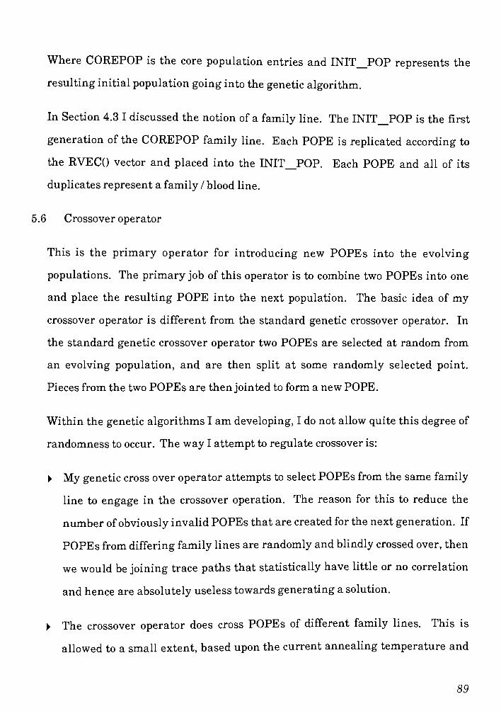
Where COREPOP is the core population entries and INIT_POP represents the

resulting initial population going into the genetic algorithm.

In Section 4.3 I discussed the notion of a family line. The INIT_POP is the first

generation of the COREPOP family line. Each POPE is replicated according to

the RVECO vector and placed into the INIT_POP. Each POPE and all of its

duplicates represent a family / blood line.

5.6 Crossover operator

This is the primary operator for introducing new POPEs into the evolving

populations. The primary job of this operator is to combine two POPEs into one

and place the resulting POPE into the next population. The basic idea of my

crossover operator is different from the standard genetic crossover operator. In

the standard genetic crossover operator two POPEs are selected at random from

an evolving population, and are then split at some randomly selected point.

Pieces from the two POPEs are then jointed to form a new POPE.

Within the genetic algorithms I am developing, I do not allow quite this degree of

randomness to occur. The way I attempt to regulate crossover is:

? My genetic cross over operator attempts to select POPEs from the same family

line to engage in the crossover operation. The reason for this to reduce the

number ofobviously invalid POPEs that are createdfor the next generation. If

POPEs from differing family lines are randomly and blindly crossed over, then

we would be joining trace paths that statistically have little or no correlation

and hence are absolutely useless towards generatinga solution.

? The crossover operator does cross POPEs of different family lines. This is

allowed to a small extent, based upon the current annealing temperature and

89

the current randomness factor. I do need to beware not to cause inbreeding in

the population, insure proper search space exploration, and avoid stagnation.

There is only one occasion when this type of crossover is performed. This is

when a POPE has an (X, Y) coordinate in common with another POPE. This

condition can occur, but is of very low probability. In this function there is a

very small probability that a POPE will be allowed to capture an occupied

neighbor.

? This Crossover operator also performs dual crossovers. This type of crossover

operation is not very common because of the restrictions placed upon the

POPEs that are valid to enter into crossover with each other. In attempting to

perform a dual crossover operation the function will attempt to:

1) Crossover the two current POPEs

2) Crossover one or both of the current POPEs with a member from the

evolving population.

I refer the reader back to Chapter Four Section 4.7 for additional explanation of

this operator.

5.7 Mutation operator

This operation will consult the population character function and determine how

many POPEs are to be mutated from the evolving population. The Mutation

operator then pseudo randomly selects POPEs from the evolving population and

evaluates the utility of each POPE. This utility iscompared against factors in the

population character function, and amutation probability is determined.

90

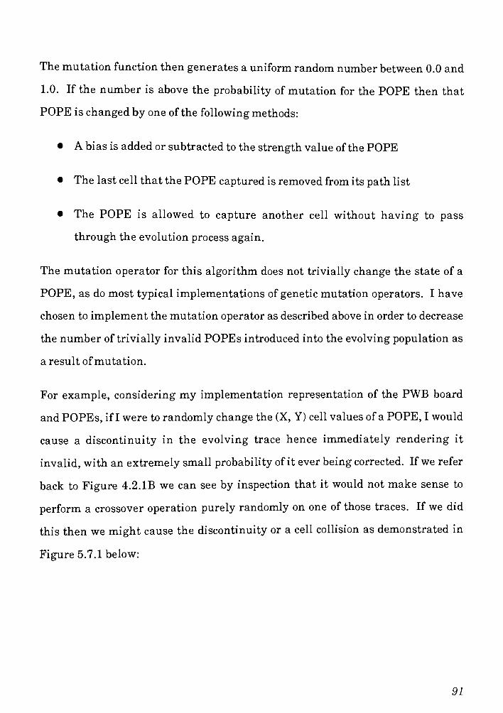
Themutation function then generates a uniform random number between 0.0 and

1.0. If the number is above the probability ofmutation for the POPE then that

POPE is changed by one of the followingmethods:

A bias is added or subtracted to the strength value of the POPE

The last cell that the POPE captured is removed from its path list

The POPE is allowed to capture another cell without having to pass

through the evolution process again.

The mutation operator for this algorithm does not trivially change the state of a

POPE, as do most typical implementations of genetic mutation operators. I have

chosen to implement themutation operator as described above in order to decrease

the number of trivially invalid POPEs introduced into the evolving population as

a result ofmutation.

For example, considering my implementation representation of the PWB board

and POPEs, if I were to randomly change the (X, Y) cell values of a POPE, I would

cause a discontinuity in the evolving trace hence immediately rendering it

invalid, with an extremely small probability of it ever being corrected. Ifwe refer

back to Figure 4.2. IB we can see by inspection that it would not make sense to

perform a crossover operation purely randomly on one of those traces. If we did

this then we might cause the discontinuity or a cell collision as demonstrated in

Figure 5.7.1 below:

91

Pf

1

/

1

S

S

y

/r

1

11

-

**

>

^

._J

*

s**

s

^**

s

i

Example of a Crossover Collision Figure 5.7.1

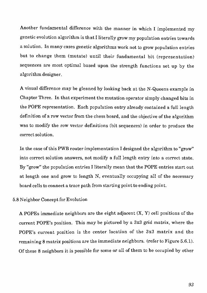
Another fundamental difference with the manner in which I implemented my

genetic evolution algorithm is that I literally growmy population entries towards

a solution. In many cases genetic algorithms work not to grow population entries

but to change them (mutate) until their fundamental bit (representation)

sequences are most optimal based upon the strength functions set up by the

algorithm designer.

A visual difference may be gleaned by looking back at the N-Queens example in

Chapter Three. In that experiment the mutation operator simply changed bits in

the POPE representation. Each population entry already contained a full length

definition of a row vector from the chess board, and the objective of the algorithm

was to modify the row vector definitions (bit sequences) in order to produce the

correct solution.

In the case of this PWB router implementation I designed the algorithm to"grow"

into correct solution answers, not modify a full length entry into a correct state.

By"grow"

the population entries I literallymean that the POPE entries start out

at length one and grow to length N, eventually occupying all of the necessary

board cells to connect a trace path from starting point to ending point.

5.8 Neighbor Concept for Evolution

A POPEs immediate neighbors are the eight adjacent (X, Y) cell positions of the

current POPE's position. This may be pictured by a 3x3 grid matrix, where the

POPE's current position is the center location of the 3x3 matrix and the

remaining 8matrix positions are theimmediate neighbors, (refer to Figure 5.6.1).

Of these 8 neighbors it is possible for some or all of them to be occupied by other

93

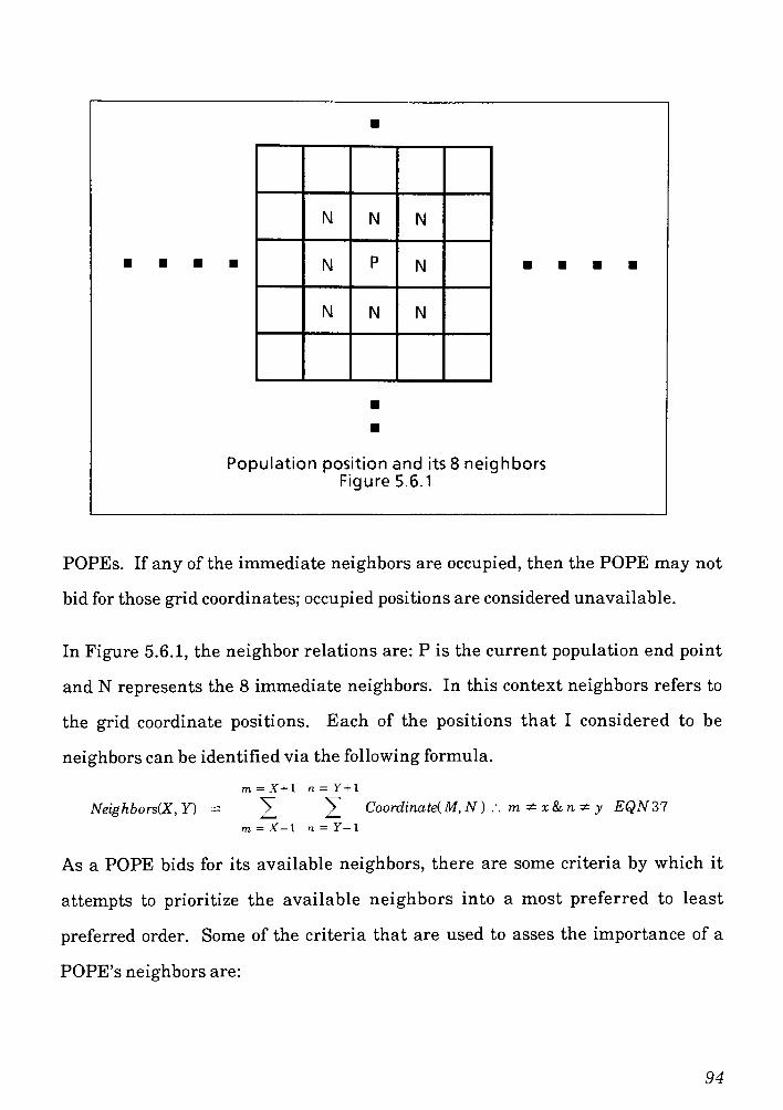
N N N

N P N

N N N

Population position and its 8 neighbors

Figure 5.6.1

POPEs. If any of the immediate neighbors are occupied, then the POPE may not

bid for those grid coordinates; occupied positions are considered unavailable.

In Figure 5.6.1, the neighbor relations are: P is the current population end point

and N represents the 8 immediate neighbors. In this context neighbors refers to

the grid coordinate positions. Each of the positions that I considered to be

neighbors can be identified via the following formula.

Neighbors(X, Y)

m = X+\ n=Y+\

V_

Coordinate(M,N) :. m*x&n*y EQN37

m = X-l n = Y-\

As a POPE bids for its available neighbors, there are some criteria by which it

attempts to prioritize the available neighbors into a most preferred to least

preferred order. Some of the criteria that are used to asses the importance of a

POPE's neighbors are:

94

Will the occupancy of this neighbor introduce more'jogs'

bends into the trace

path? If the answer is yes than this neighbor is less palatable than one that

provides a straight path continuance.

Does the neighbor move the trace closer towards its destination coordinate?

An answer ofyes ismore favorable than no, or further away.

If the POPE were to capture the neighbor cell will the estimated distance until

completion reduce or increase? If the answer is reduce the the neighbor is

considered favorably.

These are some of the primary factors utilized in prioritizing a POPE's neighbor

selection list.

Population evolution occurs by POPEs bidding upon immediate neighboring grid

coordinates, attempting to win and occupy one of the coordinates. Hence, growing

the POPE by one coordinate position towards its end point. In other words each

POPE competes for its immediate neighboring gird positions in its attempt to find

a valid path from starting point to end point. In an evolution cycle if a POPE is

successful in bidding for one of its neighboring positions, the POPE is allowed to

occupy the (X, Y) grid position. This movement / occupancy advances the POPE

by one cell towards its final position. It should be noted that it is possible for a

POPE during an evolution to lose the bidding for any of its neighbors and not

advance in that evolution cycle.

The evolution process is continued until all POPEs have reached their destination

positions or a timeout condition limit is reached.

95

5.9 Population Growth and Decay

The algorithm in attempting to route the POPEs and find a solution to the

problem will grow and shrink the population size MPSO. At any point in time

there are several factors which will regulate what the actual population size is, for

example.

1) POPEs may route successfully and, hence, can be removed from the active

population list.

2) POPEsmay stagnate; all neighbors are occupied and hence can be removed

from the population.

3) POPEsmay simply loose their utility during bidding.

4) The genetic operators are designed to grow and shrink the population from

evolution to evolution based upon current population characteristics.

These and other factors were considered in designing into the evolution algorithm

to try andmaximize its efficiency. Let's consider the case where POPEs complete

their path successfully. They either find the trace end point as in case 1 above, or

stagnate as in case 2 above, or they simply fail and die as in case 3 above. No

matter what the reason for removal is, success or failure, the POPE is removed

from the active population. In the case of success, the POPE's coordinates are

marked as routed and remain permanently unavailable to other POPEs. In the

case of failure, the POPE's coordinate positions are returned to the available list

of neighbors and other POPEs may begin to utilize the freed up coordinates.

These situations produce a shrinkage in the population size.

96

This shrinkage is expected by the algorithm and there are mechanisms to

compensate for the shrinkage. First, however we will discuss more of the details

ofhow and why POPEs are removed from the evolving population.

The way in which a POPE can die are numerous. For example, a POPE may route

itself into a position where there are no available neighbors, but it has not reached

its destination point. In this case, only the single POPE is removed, not all of its

family members. A POPE also may bid all of its money / utility away before

reaching its destination. This death is dealt with similarly to the above

stagnation case; just the one POPE is removed.

If a POPE is successful in finding a routing path to its end point, then this POPE

is removed from the active evolution list; its coordinates / trace path are left

marked as a valid trace, and all its other family members are removed from the

active population. The coordinates occupied by the other family members of the

successful POPE are freed up and placed upon the available neighbor list for other

POPEs to utilize. This is because there has been a successful path found that will

be preserved; therefore, the other family members are no longer needed for

searching a valid path.

Some characteristics worth noting about the algorithm pertaining to the removal

ofPOPEs from the population are:

? POPEs do not back track and attempt to utilize any of the just freed-up

coordinates / neighbors from POPEs being removed from the population.

? As POPEs die of unsuccessful deaths, they are not restarted in the evolution

process. The potential problem here is that if a family blood line is so

unsuccessful that all the POPEs of the family die in failure, there is no

97

mechanism to retry and route that trace path. This trace path is marked as

unsuccessful and left out of the routing process.

? The algorithm is designed to allow the actual population size to fluctuate

within a user / algorithm specified range at each evolution cycle. The

population entry count fluctuates down from the death process of traces,

successful or failure. The population entry count is capable of growing during

genetic replication and resample operations during the evolution cycle.

During the evolution process the REP() function (Section 5.3) and the NPTAO

function (Section 3.3.6) are compensated according the recent changes in the

population size. This relation is established enabling the algorithm to

compensate the size of the evolving population. This information is also utilized

by the resample operator described in section 4.6 to also compensate for changes

in the working population size. All of these interactions are established in order

to optimize the algorithm for finding solutions to the routing problem.

98

6.0 Optimum Neighbor Solution Algorithm

In Chapters 4 and 5 I presented an overview of the routing problem as well as

some specifics of the genetic solution algorithm. In this section I will present one

of the three specific solution algorithms developed for this project. This algorithm

is identified as the Optimum Neighbor Solution Algorithm. The title comes from

the fact that the algorithm investigates a cell's 9 nearest neighbors (see Section

5.6 for definition) in attempting to determine a routing path for each trace in the

netlist.

6.1 OptimumNeighbor Utility Function

Earlier in Section 4.6 I presented the concept of a cell's neighbors and the

association of merit of the neighbors. This algorithm utilizes the concept to

identify neighboring coordinates and rank them in order of most to least

preferable. The way neighbors are ranked is to evaluate the POPE utility

algorithm as if the neighbor is part of the POPE trace path. The path returning

the greatest utility value is considered the highest potential neighbor for success.

Being able to rank the neighboring coordinates allows the algorithm to isolate and

select one or more coordinates which a POPE will bid upon and attempt to

capture, thus advancing the POPE one coordinate further towards its termination

coordinate as indicated in the net list.

This algorithm was set up to use a weighting scheme thatconsidered the following

as the criteria in order to determine which neighbors to bid for and how much to

bid. There was the element of probability, the merit gained from the prior

evolutions / biddings, the number of"jogs"

in the path, the general direction (is it

99

towards the destination or not), how much strength does the entry have to

compete with, current traveled distance and approximated distance to ending

point. All of these factors are combined into the utility polynomial. This

Polynomial has the form:

u. 1m = 1

In A * F (X.

where A is a normalizing / scaling constant, and Fm( ) is a function that evaluates

and bounds the specific characteristic being weighted into a POPEs utility value.

An example of F() could be as simple as a MAX(), MIN() function, a COS()

function, or a polynomial itself. The intent of F() is to define a function yielding a

single value that considers all of the characteristics required to determine a

POPEs utility.

A simple example of this technique is as follows: The definition ofUi

Bidding criteria for this example will be:

+Fi(X) = strlen(X)

+ F2(X) = Ui.i

F3(X) = Z*Rand(X)

+F4(X) = Rdist(X)

-F5(X)= NJogs(X)

F6(X) = APopUtil(X)

F7(X) = SDevPop(X)

Trace length ofX

Utility of the prior generation

Random percent Z with X as the Seed

Estimate of remaining distance to end point

Number ofJogs in this POPE's trace path

A population utility over lastN evolutions

Number ofSTD Deviations this POPE is

Please note that not all the string length functions will return the same value at

each iteration. This is because some traces will terminate / complete before others

and some traces will lose entirely in the bidding process; hence, for a given

generation a trace may not advance past its currentposition. If the latter occurs

100

it is a stagnation, and this genetic algorithm currently will initially increase the Z

value of the RandO function. If this enhanced randomness does not correct the

stagnation, then the population entry is removed after some time limit and all of

its occupied cells become available for other traces to bid for.

Also note that before each function Fn there is a sign. The + operator is

achieved by directly taking the natural log of the function, the operator is

achieved by first performing the (1/X) operation and then taking the natural log.

In all cases, before the natural log operation is performed, a test for zero (0) is

done. When a function returns zero (0) then both the (1/X) and the natural log

function are not performed and zero (0) is added to the POPE's utility value Ui.

The following are examples of population entries over N iterations using the

above utility factor. This series of examples is supplied to show the reader how

this algorithm was designed.

If we look back at the example trace in Figures 5.4.8 and evaluate the utility

function for the trace starting a cell (0,0) and routing towards cell (4,3) we would

get:

Fi(X) = Strlen(X) = 2

F2(X) = Ui-i = 5.101

F3(X) =AT* Rand(X) = 50

* 0.3565 = 17.85

F4(X) = Rdist(X) =* 2

F5(X) = NJogs(X) = 0

F6(X) = APopUtil(X) = 8

F7(X) = SDevPop(X) = -2 which becomes (0.5)

101

The natural log of each of the functions above yields the following results:

ln{Fi(X)} = ln{2} = 0.693

ln{F2(X)} = ln{5.101} = 1.629

ln{F3(X)} = ln{17.85} = 2.880

ln{F4(X)} = ln{2} = 0.693

ln{Fs(X)} = 0 : no operation is performed

ln{F6(X)} = ln{8} = 2.639

ln{F7(X)} = ln{0.5} = -0.693

When we sum all of these terms we get a Ui of 7.841

6.2 OptimumNeighbor SolutionAlgorithm Character Function

For this algorithm I implemented a simple population and individual POPE

character function that was used to adjust the annealing temperature by

monitoring the population's evolution rate. For this character function I would

look at statistics ofboth individual POPEs and the population on a whole. Some of

the parameters considered for the character function were:

1) Number ofPOPEs that advanced in the current evolutionary cycle.

2) The average utility of the entire population.

3) Estimated distance required to route the remaining traces.

4) Number ofevolutions since the POPE Advanced.

5) STD Deviation of the POPE relative to the population.

6) Number of times POPE mutated vs number of times evolved.

7) Instantaneous slope ofPOPEs utility values (increasing / decreasing).

The function would scan the current population as well as keep a history of

selected past data items with which to evaluate the trend of the population. From

102

the data gathered, the characterization function would then set certain condition

flags and adjust some of the biasing and randomization constants. These

condition variables would be used by the other genetic operators such as crossover

and mutation in order to control the evolution algorithm and optimally direct it to

converge upon a solution.

One of the largest problems with this solution algorithm was that it did not

intelligently attempt to back track and incorporate any cells freed-up by traces

that were removed from the population for whatever reason. The freed-up cells

were used by traces only if they could be ofbenefit in their current routing path.

Another problem with this algorithm is that it was extremely difficult to design

the utility function Un such that as time went on and the population grew and

shrank, it was difficult to manage the propagation or negation of prior Ui's and

bids.

6.3 OptimumNeighbor Solution Solution Data

A table can be found in the appendix Table 6.3 that contains the tabular evolution

data having run the genetic algorithm with the previously described evolution

functions. For this simple example the algorithm was able to route all of the

traces.

Graphically the results from the genetic algorithm ofSection 5.7 are shown in the

following charts section 6 results case #1.

6.4 Optimum NeighborUtility Function of 6.3 with GrowthModification

This utility function utilizes all of the characteristic information of the utility

function described in Section 5.7 plus a factor based upon rate ofneighbor growth.

103

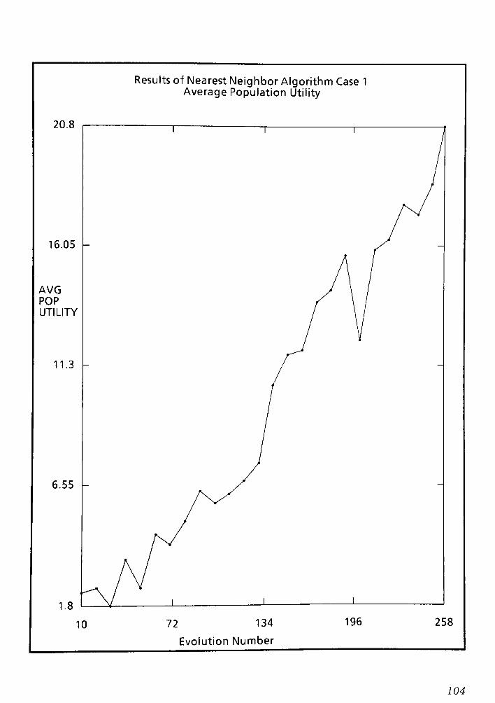
Results of Nearest Neighbor Algorithm Case 1

Average Population Utility

20.8

16.05

AVG

POP

UTILITY

11.3

6.55

1.8

10 72 134

Evolution Number

196 258

104

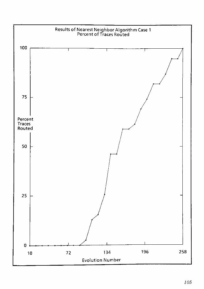
Results of Nearest Neighbor Algorithm Case 1

Percent of Traces Routed

100

75 -

Percent

Traces

Routed

50 -

25 -

0

10 72 134

Evolution Number

196 258

105

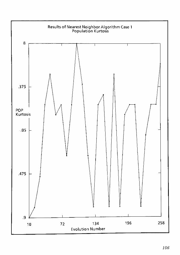
Results of Nearest Neighbor Algorithm Case 1

Population Kurtosis

.375

POP

Kurtosis

.05

.475

.9

10 72 134

Evolution Number

196 258

106

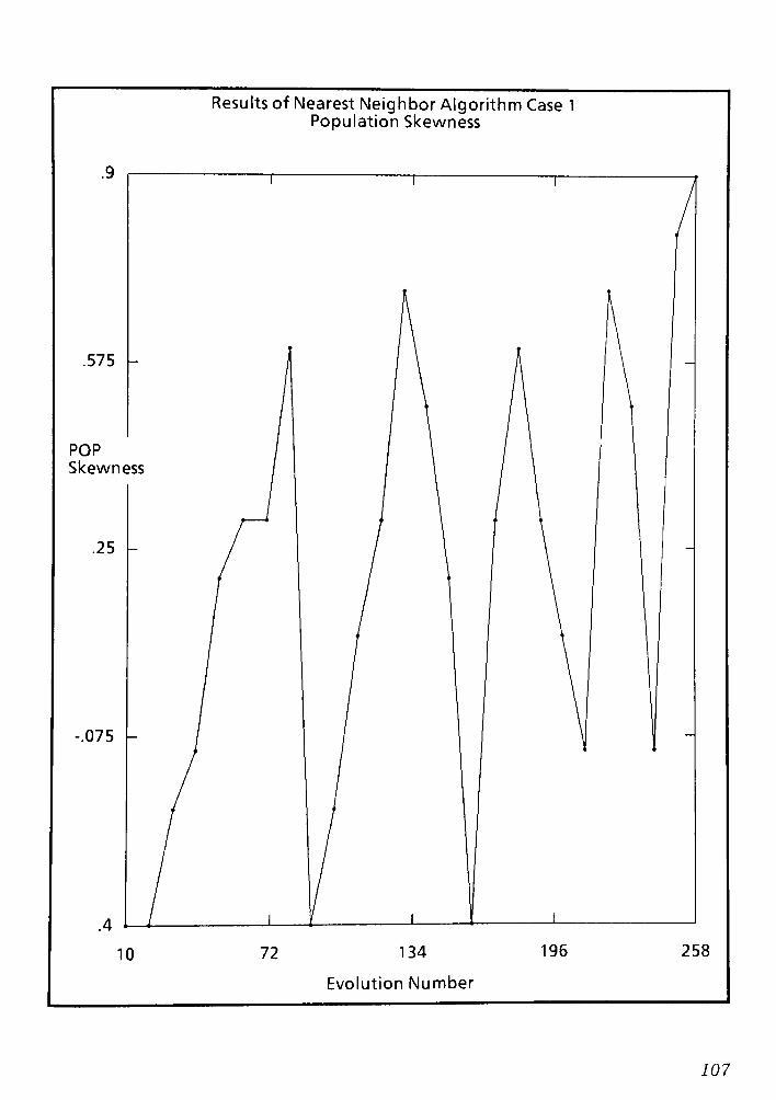
Results of Nearest Neighbor Algorithm Case 1

Population Skewness

.9

.575

POP

Skewness

.25

-.075

10 72 134

Evolution Number

196 258

107

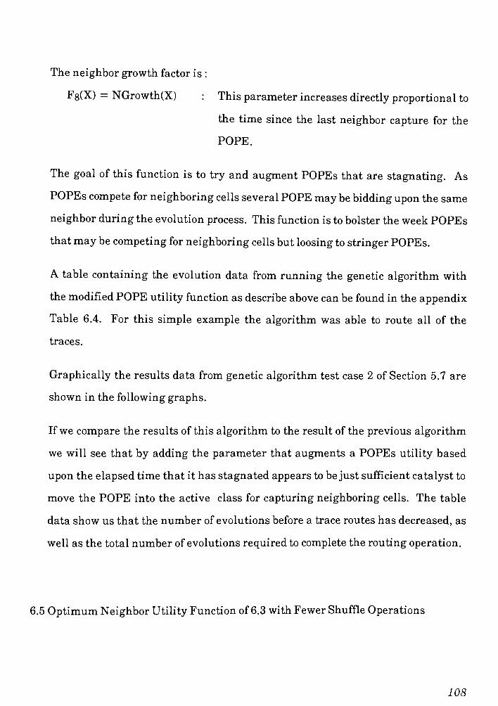
The neighbor growth factor is :

Fs(X) = NGrowth(X) : This parameter increases directly proportional to

the time since the last neighbor capture for the

POPE.

The goal of this function is to try and augment POPEs that are stagnating. As

POPEs compete for neighboring cells several POPE may be bidding upon the same

neighbor during the evolution process. This function is to bolster the week POPEs

thatmay be competing for neighboring cells but loosing to stringer POPEs.

A table containing the evolution data from running the genetic algorithm with

the modified POPE utility function as describe above can be found in the appendix

Table 6.4. For this simple example the algorithm was able to route all of the

traces.

Graphically the results data from genetic algorithm test case 2 of Section 5.7 are

shown in the following graphs.

Ifwe compare the results of this algorithm to the result of the previous algorithm

we will see that by adding the parameter that augments a POPEs utility based

upon the elapsed time that it has stagnated appears to be just sufficient catalyst to

move the POPE into the active class for capturing neighboring cells. The table

data show us that the number of evolutions before a trace routes has decreased, as

well as the total number of evolutions required to complete the routing operation.

6.5 Optimum NeighborUtility Function of6.3 with Fewer Shuffle Operations

108

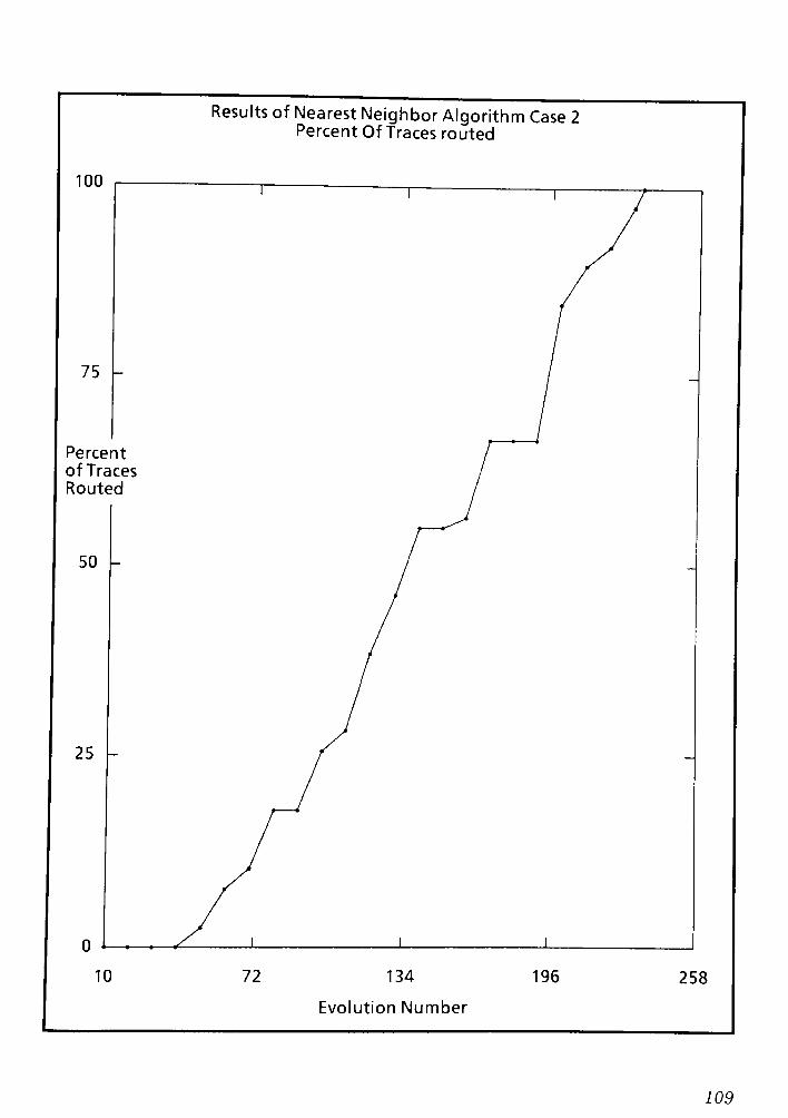
Results of Nearest Neighbor Algorithm Case 2

Percent Of Traces routed

100

75

Percent

of Traces

Routed

50

25

10 72 134

Evolution Number

196 258

109

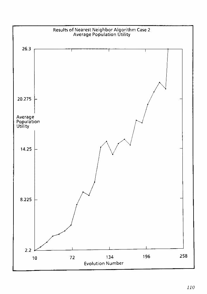
Results of Nearest Neighbor Algorithm Case 2

Average Population Utility

26.3

20.275

Average

Population

Utility

14.25

8.225

2.2

10 72 134

Evolution Number

196 258

110

Results of Nearest Neighbor Algorithm Case 2Population Kurtosis

.9

.55

.2

Population

Kurtosis

-.15

10

_L _L

72 134

Evolution Number

196 258

111

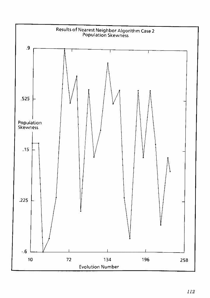
Results of Nearest Neighbor Algorithm Case 2

Population Skewness

.525

Population

Skewness

.15

.225

-

-.6

10 72 134 196

Evolution Number

258

112

This algorithm test case utilizes the utility function of 6.3 exactly as it is shown

earlier. The difference in this test case is that the shuffle operator is not applied to

the population after the replication function. The reason for having the shuffle

operator in the algorithm process after the replication operator is to minimize the

positional correlation between POPEs as they are stored in the data structures.

Itwasmy assumption that the data structures, array vectors and their sequential

loading and unloading tend to lead to negative effects in the evolving population.

By applying the shuffle operator, it was my assumption that the negative

correlation characteristics can be eliminated. In the appendix, Table 6.5 is the

resultant data having removed the shuffle operators. The actual result was to

decrease the number of evolutions required for solution generation. The time

required to produce a solution also decreased.

The time decrease was minimal and is attributed to the fewer operations being

performed to the population entries at every evolution cycle.

The graph of these results is shown in the following four graphs

113

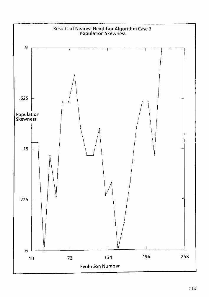
Results of Nearest Neighbor Algorithm Case 3

Population Skewness

.525

Population

Skewness

.225

10 72 134

Evolution Number

196 258

114

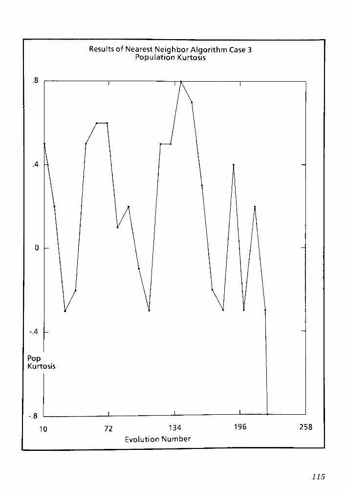
Results of Nearest Neighbor Algorithm Case 3

Population Kurtosis

.4

-

PopKurtosis

10 72 134

Evolution Number

196 258

115

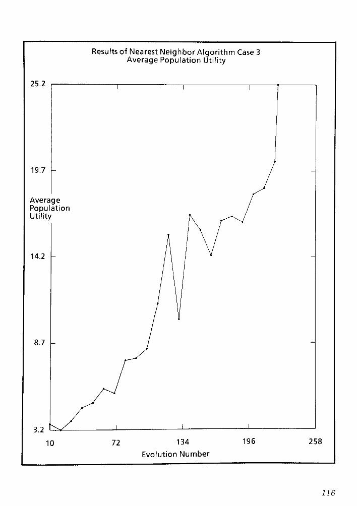
Results of Nearest Neighbor Algorithm Case 3

Average Population Utility

25.2

19.7 -

Average

Population

Utility

14.2

8.7

3.2

10 72 134

Evolution Number

196 258

116

Results of Nearest Neighbor Algorithm Case 3

Percent of Traces Routed

100

75.625 -

Percent

of Traces

Routed

51.25 -

26.875 -

2.5

10 72 134

Evolution Number

196 258

117

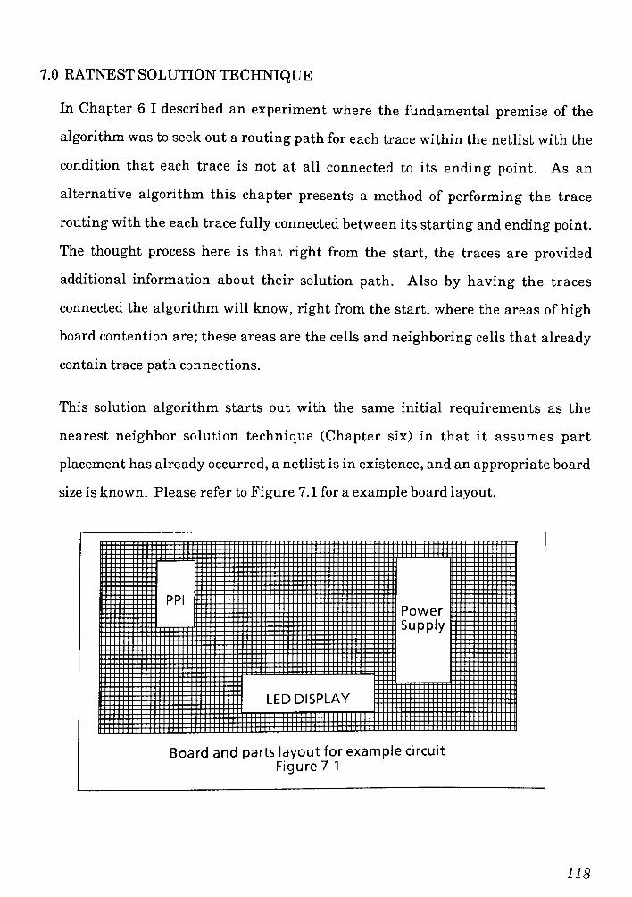
7.0 RATNEST SOLUTION TECHNIQUE

In Chapter 6 I described an experiment where the fundamental premise of the

algorithm was to seek out a routing path for each trace within the netlist with the

condition that each trace is not at all connected to its ending point. As an

alternative algorithm this chapter presents a method of performing the trace

routing with the each trace fully connected between its starting and ending point.

The thought process here is that right from the start, the traces are provided

additional information about their solution path. Also by having the traces

connected the algorithm will know, right from the start, where the areas of high

board contention are; these areas are the cells and neighboring cells that already

contain trace path connections.

This solution algorithm starts out with the same initial requirements as the

nearest neighbor solution technique (Chapter six) in that it assumes part

placement has already occurred, a netlist is in existence, and an appropriate board

size is known. Please refer to Figure 7.1 for a example board layout.

Power

Supply

Board and parts layout for example circuit

Figure 7 1

118

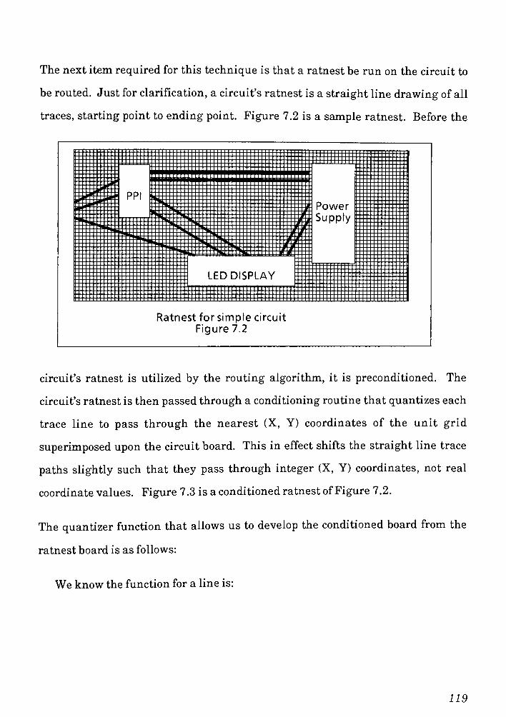
The next item required for this technique is that a ratnest be run on the circuit to

be routed. Just for clarification, a circuit's ratnest is a straight line drawing of all

traces, starting point to ending point. Figure 7.2 is a sample ratnest. Before the

Ratnest for simple circuit

Figure 7.2

circuit's ratnest is utilized by the routing algorithm, it is preconditioned. The

circuit's ratnest is then passed through a conditioning routine that quantizes each

trace line to pass through the nearest (X, Y) coordinates of the unit grid

superimposed upon the circuit board. This in effect shifts the straight line trace

paths slightly such that they pass through integer (X, Y) coordinates, not real

coordinate values. Figure 7.3 is a conditioned ratnest ofFigure 7.2.

The quantizer function that allows us to develop the conditioned board from the

ratnest board is as follows:

We know the function for a line is:

119

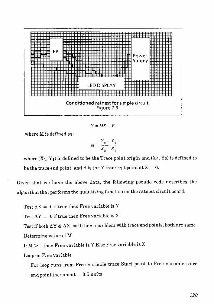
LED DISPLAY

Power

Supply

Conditioned ratnest for simple circuit

Figure 7.3

Y = MX + B

whereM is defined as:

My2-yi

X2~X1

where (Xi, Yi) is defined to be the Trace point origin and (X2, Y2) is defined to

be the trace end point, and B is the Y intercept point at X = 0.

Given that we have the above data, the following pseudo code describes the

algorithm that performs the quantizing function on the ratnest circuit board.

Test AX = 0, if true then Free variable is Y

Test AY = 0, if true then Free variable is X

Test ifboth AY & AX =0 then a problem with trace end points, both are same

Determine value ofM

IfM > 1 then Free variable is Y Else Free variable is X

Loop on Free variable

For loop runs from Free variable trace Start point to Free variable trace

end point increment = 0.5 units

120

Calculate variable

Round both Free variable and variable up to next integer

Set next (X, Y) coordinates to the above corresponding values

End Loop

Result is a vector of conditioned / quantized values for the ratnest trace

path.

There are some unique characteristics of the conditioned ratnest.

? Almost all traces have themaximum number of'jogs'

in them.

? Multiple tracesmay share the same grid coordinates (X, Y).

? Typically each trace length in the conditioned ratnest will be longer than the

trace path in the solution network. By length I refer to the number of (X, Y)

coordinates required to define the trace path.

Aswith the nearest neighbor solution algorithm, the initial core population starts

offwith one entry for each trace defined in the ratnest. Each of these traces are

then replicated some number of times according to their utility values specified by

the replication algorithm.

To restate an important characteristic of this algorithm, each POPE in the CORE

population is greater than length 1. Unlike the Nearest Neighbor algorithm of

Chapter six where each POPE in the core population is equal to length one, a

POPE of the ratnest algorithm contains all of the coordinates required to run a

path from starting point to ending point.

121

The fundamental idea of the ratnest algorithm is to evolve the population by

modifying the POPEs such that they no longer have any of their board cells /

coordinates shared in common with any other POPEs. This is different from the

concept of the nearest neighbor solution. Because the nearest neighbor solution

attempts to evolve its POPEs by growing them in length, capturing / occupying

(X, Y) coordinates towards the traces ending point.

The evolution concept for the ratnest algorithm is for each POPE to identify and

select neighbors of the existing trace path that:

? Eliminate / minimize'jogs'

in the paths, and minimize each trace distance

(number ofcells per trace and geometrical distance).

? Find paths for all traces that do not share (X, Y) coordinate pairs.

Essentially the technique here is to massage the invalid ratnest trace paths such

that they become valid paths not sharing (X, Y) coordinates with other trace

paths.

7.1 Utility function for solution case one

In this experiment I utilized the exact utility and character functions of the

nearest neighbor algorithm, as described in Section 6.2. My intention here was to

be able to hold the genetic operators consistent across the various solution

methods being investigated.

7.2 RATNEST SolutionAlgorithm Solution Data Case One

Within the appendix a table is provided showing the evolution data having run

the genetic algorithm with previously described evolution functions. Please refer

122

to Table 7.2.1. For this simple example, we never achieved an acceptable routing

path solution. After 300 plus evolutions the population percentage of successful

routing paths was extremely low.

As a result of the very poor performance this solution algorithm was abandoned

and the utility function upgraded to be like that of the nearest neighbor algorithm

ofSection 6.4.

123

V

01

u

(13l_

1- oW

o3

+->

o

QC

u1

<U

CL

*N

rou

C

o

oIS)

+->

C+-

(t>

Cd

1 V 1T"

</i

c / *fo

t 0,

(D 3-P \*

N 5 B-^ \< O \ pue. o_ \

\ $ t* a '.

^-.. 1c to5

V-s. -.

-* T> "3>-

c +1 ^^ S 4

\ N 1 i'#

^ > o <?^^ a-

.

l}

< J> >I

^"^

*\^> *

Vt > '>

v# <^

4

1 1

> >

rv if

) *

\ s

( *

1 ^

in

r^rsi

m

cm

o

m

m

LO

CM

or-~

C

o

o>

o>

E3

00

7.3 RATNEST Solution Algorithm Solution Data Case Two

The following table is the evolution data having run the genetic algorithm with

previously described evolution functions. Please refer to the Table 7.2.1 in the

appendix. For this simple example the we never achieved an acceptable routing

path solution. After 400 plus evolutions the population percentage of successful

routing paths is extremely low.

As a result of the very poor performance this solution algorithm was abandoned

and the utility function upgraded to be like that of the nearest neighbor algorithm

Section 5.4. I reran the ratnest algorithm several times, each with an

optimization / change in the algorithm operators.

125

t>

CD

S3

o

CO

CO

cC

cor-l

co

co

u

a

y

fl<D

be

O

cuCO

COr-l

a+j

a

O

cu

'oo

cu

o

ft

CM

7.4 Discussion ofRatnestAlgorithm One

In looking at the data for this technique we see that the percent of completed routing

traces never reached 100%. It plateaued at -40% and then the algorithm's evolution

limit caused the algorithm to stop executing and report a failure. In this experiment

the algorithm stopped executing and declared failure because the evolution exceeded

that of the characterization parameter limit setwithin the character function.

I did rerun this case with the evolution limit set to 9999. Because of the randomness

introduced into the algorithms I am unable to simulate the exact evolution as before,

but on average each rerun should be very similar. Having reset the total number of

evolutions until failure I found no major benefit. The algorithm would progress in a

manner similar to when the limit was 350 and 400 evolutions. The algorithm only

reached about 45% trace completion, and this was achieved at about 400 evolution

cycles. The evolution did eventually plateau at about 75% trace path completion

after about 20,000 evolution cycles.

I reran the algorithm several times attempting to adjust the genetic operators such

that they would achieve a better trace completion rate butwas unsuccessful.

Having performed the experiment several times with various modifications I was left

with a fair amount of data. The data that I focused upon was the trace paths after

competition within each evolution cycle. By competition here I am referring to the

stage at which each trace path bids and attempts to capture neighbors in an attempt

to smooth out the path and no longer share grid cells. If the reader refers back to the

functional flow diagrams ofSection 4.6.4, 1 captured my data just after the "neighbor

evaluation and capturestep"

ofFigure 4.6.4.

127

7.5 Problemwith RATNEST solution technique

Having examined the data from the ratnest routing algorithm I found that there

were several negative conditions that I introduced into the decision algorithm. Two

of themost severe negative conditions be described as 1) local thrashing and 2) a local

versus global optimization contention.

By local versus global optimization contention I am referring to the problem of a

decision beingmade by the genetic algorithm to modify a point on the trace path that

appears to help the local region being evaluated, but causes a negative ripple effect

on second and third level neighbors. To compound the problem, the local decisions

typically did not help to move the trace towards a path that is a"generally"

or "long

distance"

good choice.

Local thrashing is the phenomenon where in one evolution a trace captures a

neighbor that eliminates a jog or shared cell within its path. This appears to be good,

at least in the short term. The induced thrashing problem arises in one of two

situations. The first occurs when in the same evolution cycle a nearby trace captures

a neighboring cell that blocks the previous trace from continuing its path. The

second case occurs where thrashing is induced in the next evolution cycle when a

trace moves to capture a cell that appears to be eliminating a jog in the immediate

neighboring region but causes a jog in an outer region.

128

8.0 Restricted Optimum Neighbor Routing Problem

In Chapter six I presented the nearest neighbor routing algorithm that appeared

to work with only mild success. In Chapter seven I presented a significantly

different approach, the ratnest routing approach, a technique that did notwork at

all. I am now going to presentmy final technique, which I believe was successful.

In the algorithms of Chapter six and seven all of the POPEs were active and

competing at all times. In this technique, Restricted Optimum Neighbor, there

are only a few select POPEs active at any given point in the evolution cycle. For

any given evolution cycle there is typically only one primary POPE and a couple of

immediate neighbors active. The purpose here is to concentrate more effort on

completing a trace path than moving onto the next trace path to be routed. Trace

paths being evolved are denoted by being listed upon the active list. Trace paths

suspended, awaiting to enter into the evolution process, are denoted as being upon

the pending list.

8.1 Characteristic Information ofRestricted Optimum Neighbor Algorithm

Having inspected the manner in which the previous two algorithms operated, I

incorporated some changes to the fundamental operation of this algorithm. These

changeswere:

t The ability to mark traces as priority traces. A trace marked as a priority

trace will be routed before other traces are entered into the evolution cycle.

y The ability to mark traces as being clustered. This was a way of signifying a

series of traces that might be a set of bus paths or address lines. A unique

characteristic of these traces is that they all start from approximately the

same position, e.g. in a row along one of theaxis. Secondly they all terminate

129

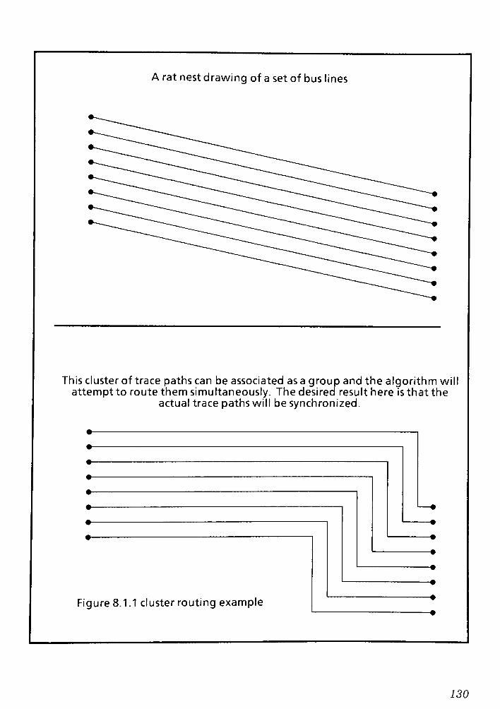
A rat nest drawing of a set of bus lines

This cluster of trace paths can be associated as a group and the algorithm will

attempt to route them simultaneously. The desired result here is that the

actual trace paths will be synchronized.

Figure 8.1.1 cluster routing example

130

in approximately the same position along a row or column at some ending

point. See Figure 8.1.1

? This implementation also utilized signal flow Graph data to help prioritize the

order of the trace path pending list and relative PWB cell values for given

regions.

8.2 Examples and Description ofPrioritization

In the netlist specification the user can utilize the term"priority"

in front of a

trace path definition. Please refer back to Chapter six for other example netlist

files. In the netlist the user would specify priority in front of any of their connect

statements. Please refer to the sample netlist below in Figure 8.2.1

; a circuit for calculating a parity bit for a 16-bitword (an xor tree)

dimension (29,37)

; chip definition- quadruple 2-input xor gates

chip type = ttl 7486 pins= 14 horizontal = 2 vertical = 6

vcc = 1 4

gnd = 7

a1 = 1

b1=2

y1=3

a2 = 4

b2 = 5

y2 = 6

y3 = 8

a3 = 9

b3= 10

y4=11

a4=12

b4=13

; power and ground are supplied here

hole (3,20)

hole (3,25)

; the 16-bit inputword

hole (26,5)

hole (26,7)

hole (26,9)

hole (26,11)

hole (26, 13)

131

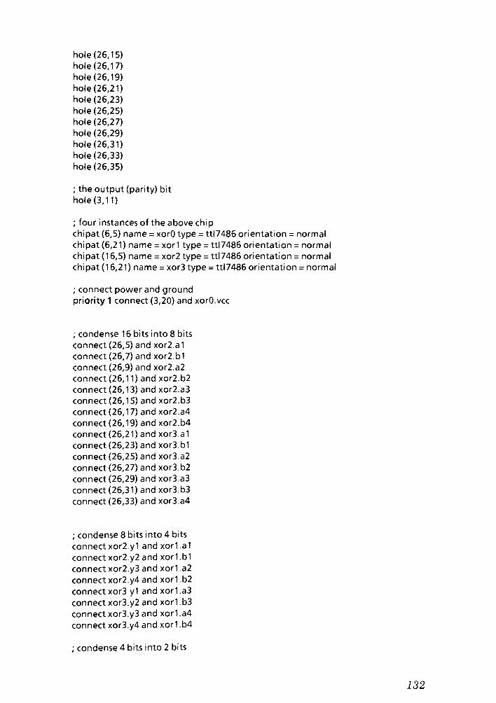
hole (26, 15)

hole (26,17)

hole (26,19)

hole (26,21)

hole (26,23)

hole (26,25)

hole (26,27)

hole (26,29)

hole (26,31)

hole (26,33)

hole (26,35)

; the output (parity) bit

hole (3,11)

; four instances of the above chip

chipat (6,5) name = xorO type = ttl7486 orientation = normal

chipat (6,21) name = xorl type = ttl7486 orientation = normal

chipat (16,5) name = xor2 type = ttl7486 orientation = normal

chipat (16,21) name = xor3 type = ttl7486 orientation = normal

; connect power and ground

priority 1 connect (3,20) and xorO.vcc

; condense 16 bits into 8 bits

connect (26,5) and xor2.a1

connect (26,7) and xor2.b1

connect (26,9) and xor2.a2

connect (26,1 1) and xor2.b2

connect (26, 1 3) and xor2.a3

connect (26, 15) and xor2.b3

connect (26, 1 7) and xor2.a4

connect (26,19) and xor2.b4

connect (26,21) and xor3.a1

connect (26,23) and xor3.b1

connect (26,25) and xor3.a2

connect (26,27) and xor3.b2

connect (26,29) and xor3.a3

connect (26,31) and xor3.b3

connect (26,33) and xor3.a4

; condense 8 bits into 4 bits

connect xor2.y 1 and xorl a 1

connect xor2.y2 and xorl .b1

connect xor2.y3 and xorl a2

connect xor2.y4 and xorl .b2

connect xor3.y1 andxor1.a3

connect xor3.y2 and xorl .b3

connect xor3.y3 and xorl .a4

connect xor3.y4 and xorl .b4

; condense 4 bits into 2 bits

132

connect xorl.yl andxorO.al

connect xorl .y2 and xorO.bl

connect xorl .y3 and xor0.a2

; condense 2 bits into 1 bit

connect xorO.yl and xor0.a3

connect xor0.y2 and xor0.b3

; connect the output (parity) bit

priority 3 connect xor0.y3 and (3, 1 1 )

In the example Figure 8.2.1 1 utilize the priority option for the power and ground

connections. I group the power connections into priority class 1 and the ground

connections into priority class 2. At the bottom of the example file I list the output

bit as priority group 3. In this case where there is only one of them, all I am trying

to signify is that this one should be routed before the rest of the internal traces.

As mentioned earlier this algorithm primarily has only one trace path being

routed at any given time. As the primary trace path is evaluating its neighbors to

determine where to route itself, it is possible that a trace path in a neighboring

cell may become active. The way a primary trace path's neighbor becomes active

is if the neighboring trace path is currently terminated in one of the primary trace

path's neighbor cells, and the neighbor trace path desires to move into one of the

primary trace paths neighboring cells.Please refer to the series of Figures below

8.2.2 through 8.2.9

In Figure 8.2.2 I show the primary trace and its occupied cells. Also shown in

Figure 8.2.2 is the neighbor trace and its occupied cells. In the drawing there is a

neighbor labeled C, which is the cell of contention. Both traces, primary and

neighbor, wish to occupy this cell. The way that the algorithm resolves this

problem is to activate the neighbor trace for this evolution cycle and allow it to

compete for the contention cell. After the evolution cycle is complete the neighbor

133

Current PrimaryTrace \

"

. Neighboring Trace

ghbors

N N

N P

i

N

N C. ..N

?

Population position and its 8 nei

Figure 8.2.2

cell is deactivated, put back onto the pending list and the primary trace resumes

evolution by it self.

8.3 Extendedmutation function

I have programmed the algorithm to extend the mutation function such that the

active trace being routed may be switched with one of the traces on the pending

list. The way in which this swapping process can occur is one of:

? A neighboring trace that has become active, asdescribed above, and has an

estimated completion distance that is less than a threshold found in the

character function. If the primary trace's estimated completion distance is also

less than the threshold it is possible for the primary trace to remain active

rather than be swapped onto the pending que.

134

? It is possible for a primary trace to be placed upon the pending que based upon

sheer random probability. If this is the case, then one trace from the pending

queue is selected at random and placed upon the active queue.

? The third extension to the mutation function is that traces of the same blood

line will crossover at random points along their connection path. There are

two conditions one of which must be satisfied in order for the related traces to

be able to cross over in thismanner.

One is: The two traces have a board cell in common. This is the point at

which the traceswill be crossed.

Two is: The two traces are occupying board cells that are adjacent neighbors

to one another. Please refer to Chapter 4 for a detailed description of

the neighbor concept.

8.4 Four Layer Board

For the experiments in the previous two Chapters I utilized a single layer board in

which all traces were routed upon one side of the board, the top. This last

experiment utilized a four layer board. I will utilize the top and bottom sides for

traces. There will also be two layers sandwiched into the middle of the board.

These two middle layers will be one for power and one for ground. Figure 8.4.1 is

an illustration of a four layer board.

By configuring the PWB in this manner I will be better able to handle congested

areas where many traces were heavily competing for a cell. This configuration

also leads to a lower signal to noise ratio. The two inner layers (power and

ground) act a shielding between the twoouter layers of traces.

135

Figure 8.4.1

Four layers of the PWB

Layer One is for Trace paths and user connections

Layer Two is for ground (0V) connections

Layer Three is for power ( + 5V) connections

Layer Four is for Trace path and trace connections only

Please note that for this system all -5V connections need to be placed on layer One

or Four and routed as a normal signal trace. Please note that it is possible to add

another layer for the -5V into the system.

The way in which I enabled thealgorithm to evaluate and Via / Channel between

layers One and Four, the two trace layers shown inFigure 8.4.1, is through the

center cell of the 3x3 neighbor evaluation grid, Figure 8.4.2. In the prior

algorithms the center cell was considered thecurrent position of the trace being

136

Neighbor evaluation grid

N N N

N V N

N N N

Neighbor layout plus the center (V) for creating Vias Between the

board 's two trace layers

Figure 8.4.2

routed and nothingmore. In this algorithm the center cell is the way in which a

trace can via to the other layer and continue routing.

8.5 Genetic Operators andUtility Function for the Restricted NeighborAlgorithm

All of the operators for this algorithm are the same as the ones defined in

Chapters four and five. Even though I have changed the fundamental operation of

this algorithm as compared to the algorithms of Chapters six and seven, I have

maintained the operators and their functional definitions.

The utility function for this algorithm is exactly a defined in Section 6.1. I have

also utilized the character function from Section 6.2. My intent is to try and keep

as many variables and operations equivalent across the algorithms being

investigated.

137

8.6 Restricted NeighborAlgorithm Results of the PWB from Chapters six and Seven

In Figure 8.2.1 above is a sample of the PWB board definition submitted to the

Restricted Neighbor algorithm. This board is the same board that was submitted

to the algorithms ofChapter six and seven. For this test case I did not utilize the

priority options since they were not available for the algorithms of Chapter six

and seven. Table 8.6.1 found in the appendix is the table of output from the

genetic algorithm. Figure 8.6.2A through 8.6.2D are graph of the results of the

routing. These results can be compared with the results of the algorithms

investigated in Chapters Six and Seven because I utilized the exact same input

netlist for purposes of comparison. The output format for the algorithms of

Chapter 8 is different because of the fundamental way in which the algorithm

works to find a solution is different from that ofChapters six and seven. For this

algorithm I show histograms of the the percent ofboard searched against the trace

being routed. Figures 8.6.2A through 8.6.2D are examples of this. Figure 8.6.4 is

the completed trace diagram. Figure 8.6.5 is the PWB trace routing diagram for

the top layer of the circuit board. Figure 8.6.6 is the PWB trace routing diagram

for the bottom layer of the circuit board. I refer the reader back to Section 8.2 for a

discussion of the circuit board trace and power layers.

As can be seen from the results this new method is highly successful. Each trace

has been routed yet requiring a very small amount of the board to be searched. I

am now going to generate a more complex routing diagram to be feed to the

algorithm for analysis.

8.7 Example of 8.6 utilizing the Priority and Cluster option

For this example I am going to utilize a slightly

138

Summary data Case 1

640

576

512

448

384

320

256

192

128

64

0

Percent of Board Evaluated

Number Traces Closed

Size of Closed List

Size of Open List

ii

1 2 3 4 5 6 7 8 MM 1M. 1MMI 1 11 1! 21 2 2\ 2\ 2' 2! 2l 27Trace

#

139

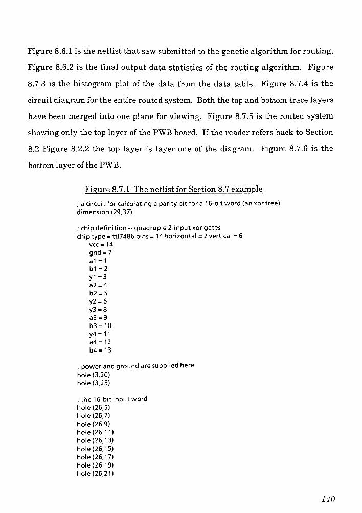
Figure 8.6.1 is the netlist that saw submitted to the genetic algorithm for routing.

Figure 8.6.2 is the final output data statistics of the routing algorithm. Figure

8.7.3 is the histogram plot of the data from the data table. Figure 8.7.4 is the

circuit diagram for the entire routed system. Both the top and bottom trace layers

have been merged into one plane for viewing. Figure 8.7.5 is the routed system

showing only the top layer of the PWB board. If the reader refers back to Section

8.2 Figure 8.2.2 the top layer is layer one of the diagram. Figure 8.7.6 is the

bottom layer of the PWB.

Figure 8.7.1 The netlist for Section 8.7 example

; a circuit for calculating a parity bit for a 1 6-bit word (an xor tree)

dimension (29,37)

; chip definition -quadruple 2-input xor gates

chip type = ttl7486 pins= 14 horizontal = 2 vertical = 6

vcc= 14

gnd = 7

a1 = 1

bl=2

y1=3

a2 = 4

b2 = 5

y2 = 6

y3 = 8

a3 = 9

b3= 10

y4= 11

a4=12

b4=13

; power and ground aresupplied here

hole (3,20)

hole (3,25)

; the 16-bit inputword

hole (26,5)

hole (26,7)

hole (26,9)

hole (26,11)

hole (26, 13)

hole (26, 15)

hole (26, 17)

hole (26,19)

hole (26,21)

140

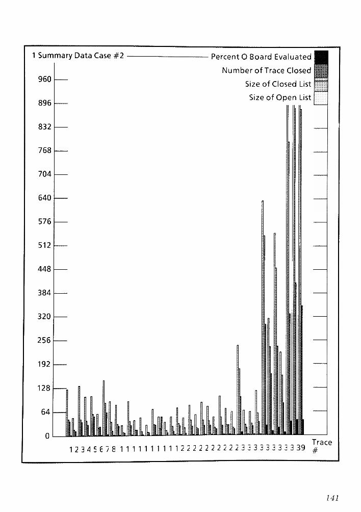
1 Summary Data Case #2 Percent O Board Evaluated

Number of Trace Closed

Size of Closed List

Size of Open List

12 3 4 5 6 7 8 1 1 1 1 1 1 1 1 1 1 2 2 2 2 2 2 2 2 2 2 3 3 3 3 3 3 3 3 3 39#

Trace

141

hole (26,23)

hole (26,25)

hole (26,27)

hole (26,29)hole (26,31)

hole (26,33)

hole (26,35)

; the output (parity) bit

hole (3,11)

; four instances of the above chip

chipat (6,5) name = xorO type = ttl7486 orientation = normal

chipat (6,21) name = xorl type = ttl7486 orientation = normal

chipat (16,5) name = xor2 type = ttl7486 orientation = normal

chipat (16,21) name = xor3 type = ttl7486 orientation = normal

; connect power and ground

priority 1 connect (3,20) and xorO.vcc

priority 1 connect (3,20) and xorO.vcc

priority 1 connect (3,20) and xorO.vcc

priority 1 connect (3,20) and xorO.vcc

priority 2 connect (3,25) and xorO.gnd

priority 2 connect (3,25) and xorO.gnd

priority 2 connect (3,25) and xorO.gnd

priority 2 connect (3,25) and xorO.gnd

; condense 16 bits into 8 bits

connect (26,5) and xor2.a1

connect (26,7) and xor2.b1

connect (26,9) and xor2.a2

connect (26,1 1) and xor2.b2

connect (26,13) and xor2.a3

connect (26,15) and xor2.b3

connect (26,17) and xor2.a4

connect (26,19) and xor2.b4

connect (26,21) and xor3.a1

connect (26,23) and xor3.b1

connect (26,25) and xor3.a2

connect (26,27) and xor3.b2

connect (26,29) and xor3.a3

connect (26,31) and xor3.b3

connect (26,33) and xor3.a4

connect (26,35) and xor3.b4

; condense 8 bits into 4 bits

connect xor2.y1 and xorl.al

connect xor2.y2 and xorl .b1

connect xor2.y3 and xorl .a2

connect xor2.y4 and xorl .b2

connect xor3.y1 andxor1.a3

connect xor3.y2 and xorl ,b3

142

connect xor3.y3 and xorl .a4

connect xor3.y4 and xorl .b4

; condense 4 bits into 2 bits

connect xorl.yl andxorO.al

connect xorl .y2 and xorO.bl

connect xorl .y3 and xor0.a2

connect xorl .y4 and xor0.b2

; condense 2 bits into 1 bit

connect xorO.yl and xor0.a3

connect xor0.y2 and xor0.b3

; connect the output (parity) bit

priority 3 connect xor0.y3 and (3,1 1)

End ofFigure 8.7.1

8.8 Example ofTwo 16 Bit Parity Checker Circuits

In this example I have simply replicated the circuit that was fed into the

algorithm in the example of Section 8.6. I am going to test with a more complex

circuit because as seen by the results of the example in Section 8.6 the circuit is

far too simple for the new algorithm. The new algorithm allows for two layers to

be utilized for the PWB and therefore it is possible to supplymore complex circuits

for the algorithm to route.

If the reader examines the net list back in Figure 8.2.1 and the netlist supplied

below, they will see that I have simply copied the parity circuit a second time.

There are effectively two parallel circuits that are utilizing the same power,

ground, and input connects. This systemshould be fairly rigorous to route, due to

the overlapping nature of the signals.

Figure 8.8.1 below is the netlist. Figure 8.8.2 is the table of results from the

routing algorithm. Figure 8.8.3 is the histogram showing the Graphical

143

representation of the data from the table 8.8.2. Figure 8.8.4 is a print of the entire

circuit. Figure 8.8.5 is a diagram of the top layer of the PWB and Figure 8.8.6 is a

diagram of the bottom layer of the PWB.

Figure 8.8.1 Netlist for circuit ofSection 8.8

; a circuit for calculating a parity bit for a 16-bitword (an xor tree)

dimension (100,100)

; chip definition- quadruple 2-input xor gates

chip type = ttl7486 pins= 14 horizontal = 2 vertical = 6

vcc= 14

gnd = 7

al = 1

b1 =2

y1=3

a2 = 4

b2 = 5

y2 = 6

y3 = 8

a3 = 9

b3=10

y4= 11

a4=12

b4=13

; power and ground are supplied here

hole (3,20)

hole (3,25)

; the 16-bit input word

hole (26,5)

hole (26,7)

hole (26,9)

hole (26,11)

hole (26,13)

hole (26, 15)

hole (26,17)

hole (26,19)

hole (26,21)

hole (26,23)

hole (26,25)

hole (26,27)

hole (26,29)

hole (26,31)

hole (26,33)

hole (26,35)

; the output (parity) bit

hole (3,11)

144

; four instances of the above chip

chipat (6,5) name = xorO type = ttl7486 orientation = normal

chipat (6,21) name = xorl type = ttl7486 orientation = normal

chipat (16,5) name = xor2 type = ttl7486 orientation = normal

chipat (1 6,21 ) name = xor3 type = ttl7486 orientation = normal

chipat (36,35) name = xor4type = ttl7486 orientation = normal

chipat (36,51) name = xor5 type = ttl7486 orientation = normal

chipat (46,35) name = xor6 type = UI7486 orientation = normal

chipat (46,51) name = xor7 type = ttl7486 orientation = normal

; connect power and ground to all chips

priority 1 connect (3,20) and xorO.vcc

priority 1 connect (3,20) and xorl .vcc

priority 1 connect (3,20) and xor2.vcc

priority 1 connect (3,20) and xor3.vcc

priority 2 connect (3,25) and xorO.gnd

priority 2 connect (3,25) and xorl .gnd

priority 2 connect (3,25) and xor2.gnd

priority 2 connect (3,25) and xor3.gnd

; connect power and ground to all chips

priority 1 connect (3,20) and xor4.vcc

priority 1 connect (3,20) and xor5.vcc

priority 1 connect (3,20) and xor6.vcc

priority 1 connect (3,20) and xor7.vcc

priority 2 connect (3,25) and xor4.gnd

priority 2 connect (3,25) and xor5.gnd

priority 2 connect (3,25) and xor6.gnd

priority 2 connect (3,25) and xor7.gnd

; condense 1 6 bits into 8 bits

connect (26,5) and xor2.a1

connect (26,7) and xor2.b1

connect (26,9) and xor2.a2

connect (26,1 1) and xor2.b2

connect (26, 1 3) and xor2.a3

connect (26,1 5) and xor2.b3

connect (26, 1 7) and xor2.a4

connect (26,19) and xor2.b4

connect (26,21) and xor3.a1

connect (26,23) and xor3.b1

connect (26,25) and xor3.a2

connect (26,27) and xor3.b2

connect (26,29) and xor3.a3

connect (26,31) and xor3.b3

connect (26,33) and xor3.a4

connect (26,35) and xor3.b4

; condense 1 6 bits i nto 8 bits

connect (26,5) and xor6.a1

connect (26,7) and xor6.b1

connect (26,9) and xor6.a2

145

connect

connect

connect

connect

connect

connect

connect

connect

connect

connect

connect

connect

connect

(26,11) and

(26, 13) and

(26,1 5) and

(26, 17) and

(26,19) and

(26,21) and

(26,23) and

(26,25) and

(26,27) and

(26,29) and

(26,31) and

(26,33) and

(26,35) and

xor6.b2

xor6.a3

xor6.b3

xor6.a4

xor6.b4

xor7.a1

xor7.b1

xor7.a2

xor7.b2

xor7.a3

xor7.b3

xor7.a4

xor7.b4

; condense 8

connect xor2

connect xor2

connect xor2

connect xor2

connect xor3

connect xor3

connect xor3

connect xor3

; condense 8

connect xor6

connect xor6

connect xor6

connect xor6

connect xor7

connect xor7

connect xor7

connect xor7

bits into 4 bits

y1 and xorl.al

y2and xorl.bl

y3and xor1.a2

.y4and xor1.b2

.y1 and xor1.a3

.y2 and xor1.b3

.y3 and xor1.a4

.y4and xor1.b4

bits into 4 bits

y1 and xor5.a1

y2and xor5.b1

.y3 and xor5.a2

y4and xor5.b2

y1 and xor5.a3

y2and xor5.b3

y3and xor5.a4

y4and xor5.b4

; condense 4 bits into 2 bits

connect xorl.yl and xorO.al

connect xorl .y2 and xorO.bl

connect xorl .y3 and xor0.a2

connect xorl .y4 and xor0.b2

; condense 4 bits into 2 bits

connect xor5.y1 andxor4.a1

connect xor5.y2 and xor4.b1

connect xor5.y3 and xor4.a2

connect xor5.y4 and xor4.b2

; condense 2 bits into 1 bit

connect xorO.yl and xor0.a3

connect xor0.y2 and xor0.b3

; condense 2 bits into 1 bit

connect xor4.y1 and xor4.a3

connect xor4.y2 and xor4.b3

146

; connect the output (parity) bit

priority 3 connect xor0.y3 and (3,1 1)

; connect the output (parity) bit

priority 4 connect xor4.y3 and (3,1 1)

End ofFigure 8.8.1 Netlist listing

147

9.0 Conclusions

The experiments conducted were performed to gain a better understanding ofhow

genetic algorithms could be applied to solving large search space problems. What

I intend to do in this chapter is to draw conclusions from the experiments as well

as propose follow-on investigations.

9.1 Conclusions and Remarks for the NearestNeighbor routingAlgorithm CPT 6

This first attempt to solve the major investigation of this thesis, PWB routing,

was only mildly successful. My solution technique was to make all of the traces

being routed active at all times. I believe thatmy implementation did not attempt

to correlate between the traces properly, and, therefore, I introduced too much

internal competition for board cells. In my opinion the algorithm did not properly

search the solution space; the algorithm exploited it rather than exploring it.

If the reader refers back to Chapter 5, where I present the fundamental genetic

operators utilized for my subsequent experiments, he will find that I did attempt

to utilize schema characteristics of the problem. For example, if the reader refers

back to Section 4.4 where mutation is presented, I restrict the type of mutation

performed on population entries. This is to reduce the number of invalid entries

created during evolution. I make the decisions basedupon a priori knowledge of

the problem andmy solutionrepresentation.

The algorithm also attempts to use a statistical characterization function to

determine how the evolvingpopulation is progressing. Information from the

character function is utilized by the genetic operators at every evolution cycle.

148

This is similar to realtime feedback control systems, where the current state of the

operation ismonitored and utilized to direct the next operation.

Even though the algorithm did produce solutions for the cases tested, it did not

perform very well over all in attempting to generate a solution.

9.2 Conclusions and Remarks for the ratnestAlgorithm CPT 7

This solution algorithm was not successful at all. It almost never reached an

acceptable solution set for the netlists that were presented to it. The algorithm

presented in Chapter 6 worked better than this one.

The core concept of this algorithm is that all of the trace paths to be routed were

connected, then quantized and used as the initial core population. This is the

complete opposite approach to the earlier solution algorithm where traces were

started at length 0 and grown to find their destination, the Ratnest algorithm

started with traces fully connected and tried to massage them until theymet a set

ofvalidation criteria.

The primary reason for failure of this algorithm was the fact that the traces

started out as fully connected paths. This restricted the the areas of the PWB that

the algorithm would search in order to find a solution. Figure 9.4.1 is a sample

initial rat nest that would be fed into the algorithm. Figure 9.4.2, the dashed box,

indicates the primary areas that the algorithm would search in order to find a

solution for the set of trace paths shown . The algorithm would search other areas

of the PWB but the other areas would be explored very infrequently, hence poor

search space exploration and poor algorithm performance.

149

LED DISPLAY

Power

Supply

Conditioned ratnest for simple circuit

Figure 9.2.1

M.

LED DISPLAY

Power

Supply

Conditioned ratnest for simple circuit

Figure 9.2.2

9.3 Conclusions and Remarks for the OptimumNeighborAlgorithm CPT 8

Of the three routing algorithms tested, this algorithm yielded the best results.

The basic concept of this algorithm is that it starts each trace off at length zero

150

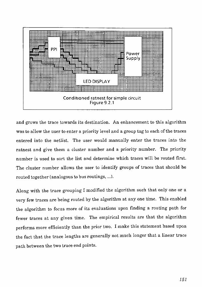
LED DISPLAY

Power

Supply

Conditioned ratnest for simple circuit

Figure 9.2.1

and grows the trace towards its destination. An enhancement to this algorithm

was to allow the user to enter a priority level and a group tag to each of the traces

entered into the netlist. The user would manually enter the traces into the

ratnest and give them a cluster number and a priority number. The priority

number is used to sort the list and determine which traces will be routed first.

The cluster number allows the user to identify groups of traces that should be

routed together (analogous to bus routings, ...).

Along with the trace grouping I modified thealgorithm such that only one or a

very few traces are being routed by the algorithm at any one time. This enabled

the algorithm to focus more of its evaluations upon finding a routing path for

fewer traces at any given time. The empirical results are that the algorithm

performs more efficiently than theprior two. I make this statement based upon

the fact that the trace lengths are generally notmuch longer that a linear trace

path between the two trace end points.

151

9.4 Points of interest beyond these experiments

There are many extrapolations that are of interest beyond the scope of this thesis.

For example: back in Section 9.4 it would be interesting to modify the algorithm

to better explore other areas of the PWB rather than those near the ratnest traces

cells. Such an adjustment might make the algorithm successful and produce

efficient solutions.

Another area of exploration might be to introduce the concept ofback tracking, as

in PROLOG, into all of the algorithms investigated. The ability to back track

might prove beneficial. The thought here is that as cells are freed up due to traces

being removed from the evolving population, some of the currently evolving traces

might either find better, more efficient routing paths, or we might even see a

higher trace completion ratio.

Another experiment that would be of interest would be to increase the number of

traces allowed active for the optimum nearest neighbor algorithm of Chapter 8.

By increasing the active trace count, one could possibly determine when the

efficiency peaks, relative to the algorithm's ability to coordinate inter-trace / cell

relationships.

Another twist on the above investigation would be to vary the mix of traces that

are allowed to be active during the evolution process. What I mean here is that

one could investigate if better solutions of more efficient algorithms are found

when one allows traces ofonly one blood line to be active, if one allows only traces

from a cluster group to be active, or if one allows an arbitrary mixture of traces to

be made active at any give evolution cycle. My thought here are that one might

find the algorithm is able to handle many traces simultaneously as long as they

152

are competing for different areas of the PWB, or if they are all of the same group

number.

9.5 Overall conclusions

I conclude that the overall experiment was a success. I base this statement on the

fact that the final algorithm developed (Modified NearestNeighbor) yielded fairly

optimal PWB routing solutions when comparing the linear distance of each trace

versus the number of board cells required to route the trace. Another perspective

by which I judged the algorithm to be successful is that inmost of the cases tested,

the algorithm routed all of the traces; it was only in the last (most complex) test

case that the algorithm failed to route 4 out of the total 57 traces to be routed.

For the design of this experiment I went back to the basic problem statement, that

being the requirement to route mildly complex PWB circuits. In reviewing the

problem characteristics I found:

1) the problem has no one single solution

2) some solutions are more optimal than others

3) Optimality is primarily judged by the trace lengths and Jogs / trace

I decided to design a solution based on genetic algorithm fundamentals. The first

challenge of the solution algorithm was how to represent the problem. I decided

not to take the classical genetic algorithm approach where each population entry

represented one entire solution. I adapted the classic genetic representation such

that the population represented one PWB solution board and that individual

population entries represented each of the PWB traces to be routed.

153

I selected this representation in order to reduce the overhead of having multiple

replicated boards that the algorithm would be required to manage. My

representation greatly reduced the amount of data that the algorithm was

required to process, hence the algorithm was able to expend extra cycles making

complex evaluations on the individual population entries while evolving them

towards a solution.

Another modification to the classical genetic algorithm representation was the

fact that rather than having traces fully connected by illegitimate paths trying to

converge to a legitimate trace path, I had the trace paths start out as only the path

starting position. The algorithm would evolve each trace path (population entry)

by capturing one of its nearest neighbors and progressing forward towards its end

point. The ramification of this is that each trace path was primarily routing itself

toward completion by pursuing local optima at each evolution cycle. There was a

factor ofpursuing globally optimum solutions as part of the trace routing criterion

(e.g. minimize the overall trace length) but each trace's primary decision criteria

were based upon local trace information.

In developing my solution algorithms I designed some modified problem

representations relative to classic genetic algorithm problem representations.

Finally the last major modification to my genetic solution algorithm for the

modified nearest neighbor algorithm of Chapter 8 was that for most of the

evolution of a solution there was only one trace active at any given time.

Additionally in most cases, except were the proper mutation conditions occurred,

this trace wasmaintained as the active trace until a routing path was found. One

primary ramification of this is that thesolution can now be greatly affected by the

order in which the trace paths were attempted to be routed.

154

Now that the trace path routing order can so greatly affect the solution, I felt it

important to enable the user to enter a routine priority order. I also designed into

the algorithm the ability to presort the trace path to be routed by one of several

mechanisms, one being general trace distance, another being if the trace is a

member of a group / cluster, the third being the traces activity level within the

circuit (refer back to the fuzzy cognitivemachine investigation).

9.6 Applicability to larger scale problems

I believe that this solution technique will scale up reasonably to larger problems.

For example, the solution algorithm lends itself to parallelism in order to

accelerate the solution time. In order to parallelize the solution algorithm the

implementor at a minimum needs only to manage the board space across all of the

fully independent processors. This can be done easily by placing the board itself

into a shared memory region. If this is done, then the problem can scale all the

way up to one processor per trace to be routed. Another paradigm that can be

utilized to parallelize the implementation yet hold the board space as a shared

entity would be to use the Al blackboard paradigm. Each processor could write to

and read from the black board which housed the PWB board. Each access would

be a request as to the condition of the neighboring cells of some trace end point or

the request to capture a board cell for a active trace path.

Amajor algorithm enhancement that should be explored if this algorithm is to be

commercialized is how to couple it to a circuit simulation algorithm and a

placement algorithm. Some important data items that can be learned from the

simulation algorithm are the critical trace paths, those that are most active.

These critical traces can be routed with a higher priority level. The coupling of

the routing algorithm to a placement algorithm and enabling feed back based

155

upon intermediate routing results enables the algorithms to maneuver parts

placement during the routing process that will minimize the number of trace

crossovers, jogs, and inter board vias.

Finally the last modification to the routing algorithm would be to design it to

allow for upwards of 6 to 10 board layers to be investigated rather than the 4

designed into the algorithm. By enabling additional board layers, the

implementor has increased the possible solution space many orders ofmagnitude.

This will result in more optimal trace routing paths and fewer traces not

completing their routing paths for more complex PWBs. There is not just the

simple matter of adding more layers to the solution algorithm. The designer also

should design into the algorithm additional intelligence to route traces upon

certain layers based upon precalculated criteria rather than randomly.

Finally, I believe that if a designer were to add the above functionality /

intelligence to the routing algorithm they would be able to return to the Nearest

Neighbor algorithm of Chapter 6 and find that it produces solution as optimal if

not more optimal than that of the algorithm in Chapter 8. I conclude this based

upon the additional solution space added to the solution algorithm and the

increased intelligence of the routing decision criteria.

156

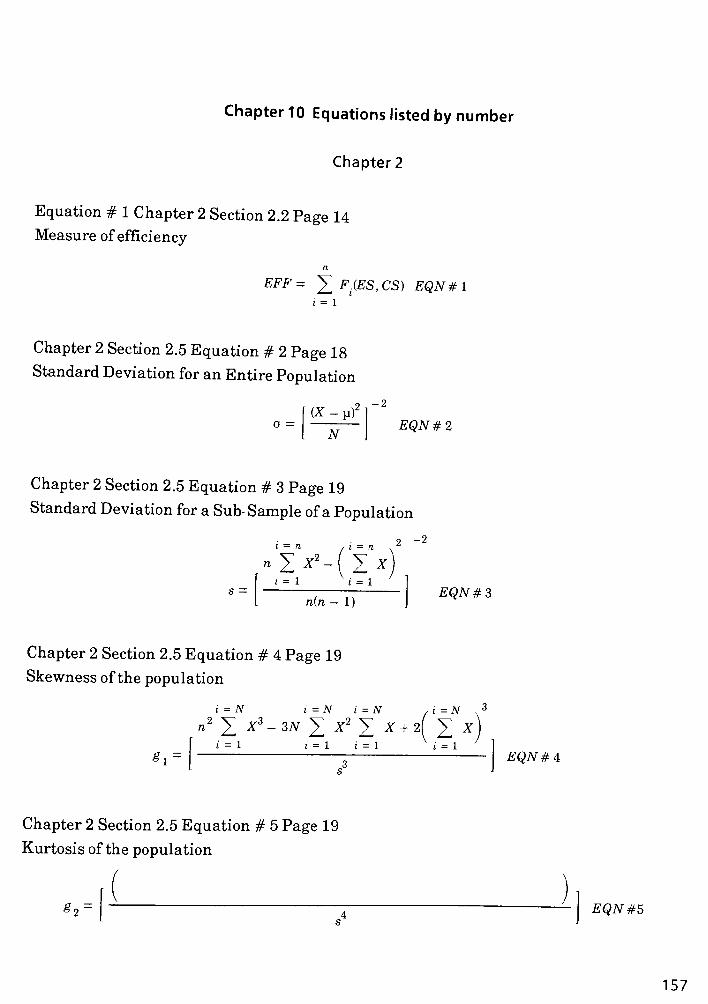
Chapter 10 Equations listed by number

Chapter 2

Equation # 1 Chapter 2 Section 2.2 Page 14

Measure ofefficiency

EFF = ][ F.(ES, CS) EQN# 1

i = 1

Chapter 2 Section 2.5 Equation # 2 Page 18

StandardDeviation for an Entire Population

o =

(X-p)

N

2

EQN#2

Chapter 2 Section 2.5 Equation # 3 Page 19

Standard Deviation for a Sub-Sample of a Population

i = n , i = n

i = l t = 1

rc(n - 1)EQN#3

Chapter 2 Section 2.5 Equation # 4 Page 19

Skewness of the population

= N i = N i = N / i = N

n2

^ X3-3N ^X2

^ X + 2( ][ X

i = 1 i = 1 i = 1 i = l

EQN#4

Chapter 2 Section 2.5 Equation # 5 Page 19

Kurtosis of the population

S, EQN #5

157

Chapter 2 Section 2.5 Equation # 6 Page 19

Test of themeans of two different populations

z = t

iXx-X2)-(^-u^

2 2

-

+-

-2

EQN#6

Chapter 2 Section 2.6 Equation # 7 Page 21

Linear function applied to matrix F

"1=

Nl n2=

N2

Y(mx,m2) = X Z Ftflj.BjJOdij.Bjimj.mj) .EQN#1

.x= 1

n2= 1

Chapter 2 Section 2.6 Equation # 8 Page 22

Matrix Vector transform

n=N2

f = Y N FV EQN#8s~ n n

n = 1

Chapter 2 Section 2.6 Equation # 9 Page 22

VectorMatrix transform

n =

N2

F = Y (N)T

f (V)r

EQN#9

rt = 1

158

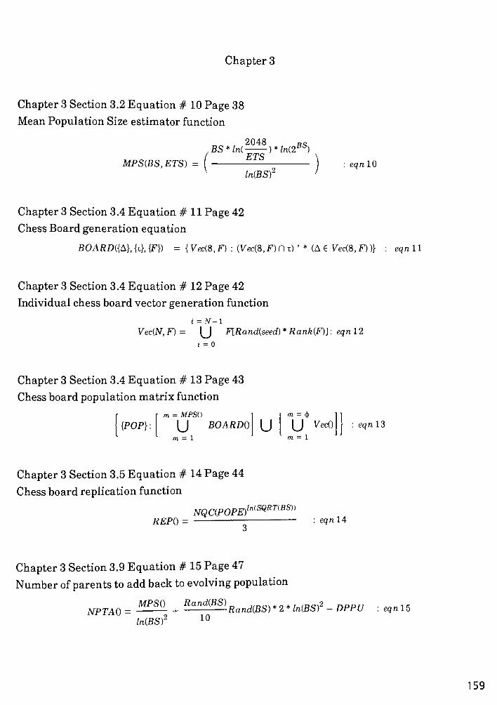
Chapter 3

Chapter 3 Section 3.2 Equation # 10 Page 38

Mean Population Size estimator function

MPS(BS,ETS)

2048

BS*ln( )*ln(2ETS

ln(BS)2

BS,

eqn 10

Chapter 3 Section 3.4 Equation # 11 Page 42

Chess Board generation equation

BOARD({A}, {z}, {F}) = { Vec(8, F) : (Vec(8, F) n i)' * (A <E Vec(8, F))} : eqn 11

Chapter 3 Section 3.4 Equation # 12 Page 42

Individual chess board vector generation function

i = N-l

Vec(N, F)= (J F[Rand(seed)*Rank(F)] : eqn 12

i = 0

Chapter 3 Section 3.4 Equation # 13 Page 43

Chess board population matrix function

{POP} :

m = MPSO("

m = $

|J BOARD0 IJ (J VecO

m = 1 m = 1

eqn 13

Chapter 3 Section 3.5 Equation # 14 Page 44

Chess board replication function

NQC(.POPE)ln(SQRT(BS))

REP0 = : eqnl4

Chapter 3 Section 3.9 Equation # 15 Page 47

Number ofparents to add back to evolving population

MPSO RandiBS)

NPTAO

ln(BSf10

RandiBS)* 2*ln{BSY - DPPU : eqn 15

159

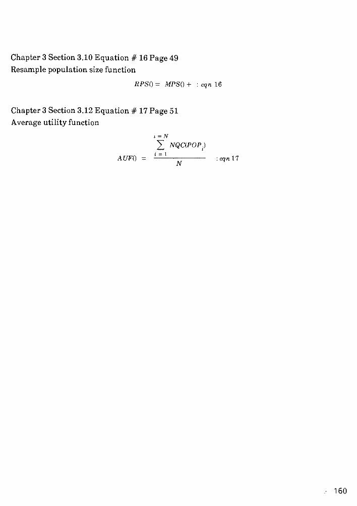
Chapter 3 Section 3.10 Equation # 16 Page 49

Resample population size function

RPS0= MPS0+ : eqn 16

Chapter 3 Section 3.12 Equation # 17 Page 51

Average utility function

i = N

^ NQCiPOP.)

AUFO = : eqn 17N

160

Chapter 4

Chapter 4 Section 4.7 Equation # 18 Page 68

Replication Operator:

m = POPE

{{ReplicatedPopulation}] - ^ ReplicateiPOPEJ EQNli

m = POPE

Chapter 4 Section 4.7 Equation # 19 Page 69

Crossover Operator:

m = Number to crossiPOPE )

{CrossoverPopulation}J = ^T Crossover{{ReplicatedPopulation} ) eqn 19

m = 1

Chapter 4 Section 4.7 Equation # 20 Page 71

Entire possible search space

Population Set {Z} = {A} U {B} U{C}U {D} EQN2Q

Chapter 4 Section 4.7 Equation # 21 Page 71

Population set ofentire possible search space

Population Set {Z} = {A} U {B} U {Q U {>} = UnfilteredAlgorithm Search Space EQN21

Chapter 4 Section 4.7 Equation # 22 Page 71

Filtered search space for population evaluation

FilteredAlgorith Search Space {F} = {Z } D {D} EQN 22

Chapter 4 Section 4.7 Equation # 23 Page 72

Mutation Operator:

m = {POPE }b

{{MutatedPopulation}] = X MutateiPOPEJ EQN23

* Jm=POPE,

161

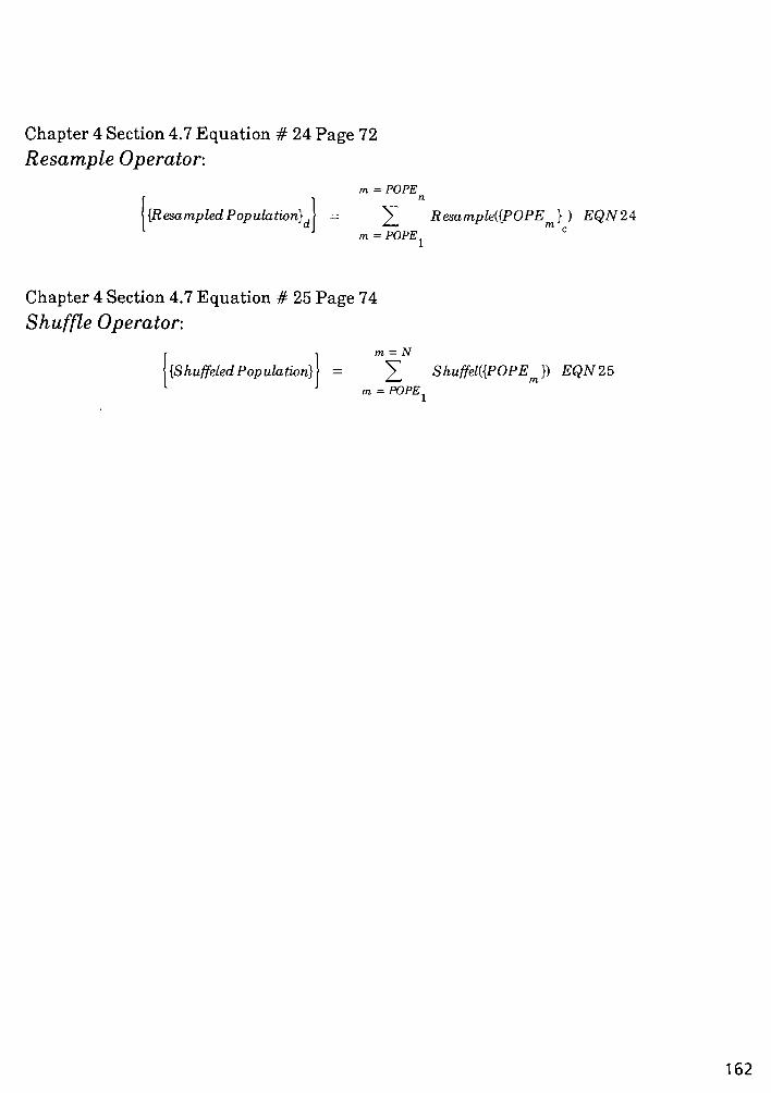
Chapter 4 Section 4.7 Equation # 24 Page 72

Resample Operator:

m = POPE

{{ResampledPopulation}] = V Resample{{POPEm}

) EQN24

m = POPE

Chapter 4 Section 4.7 Equation # 25 Page 74

Shuffle Operator:

!1m = N

{ShuffeledPopulation] = ]T ShuffeWOPEJ) EQN25

m = POPE

162

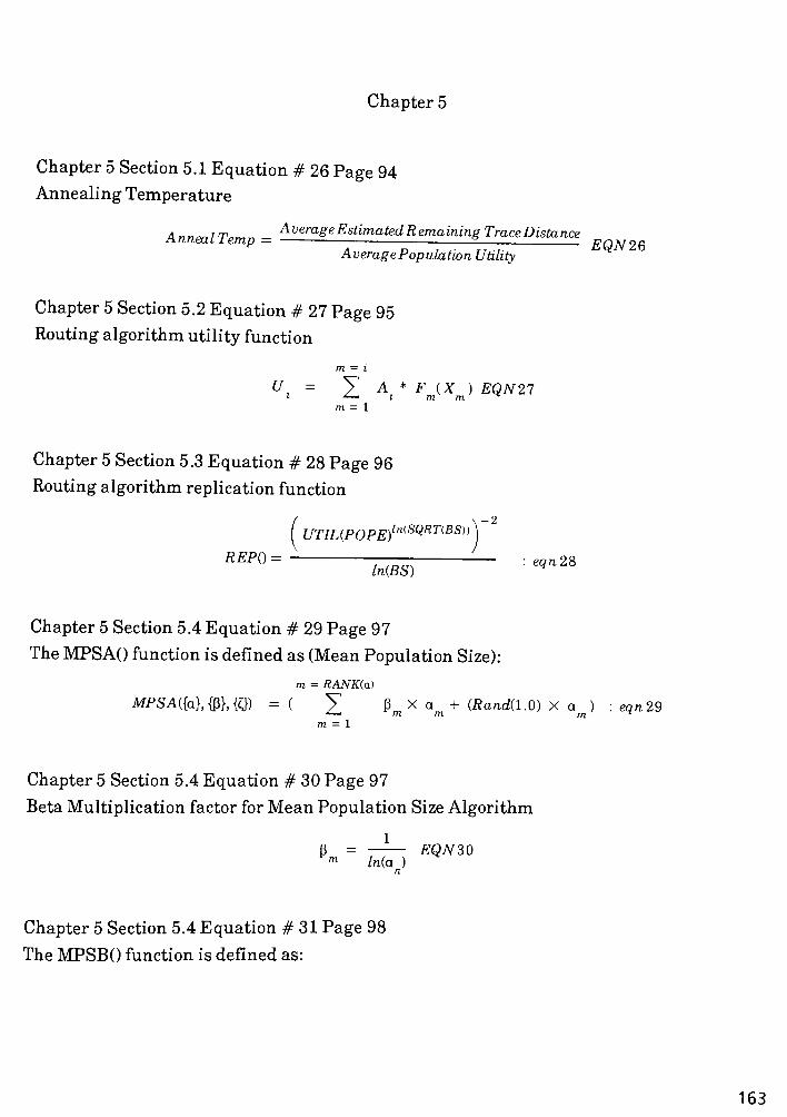
Chapter 5

Chapter 5 Section 5.1 Equation # 26 Page 94

Annealing Temperature

AnnealTemp =AveraSEstimatedRemaining TraceDistance

AveragePopulation Utility'"'''

Chapter 5 Section 5.2 Equation # 27 Page 95

Routing algorithm utility function

U = V A* F (X ) EQN27l * l m m

^

m = 1

Chapter 5 Section 5.3 Equation # 28 Page 96

Routing algorithm replication function

REP0=

wisi

~

:^28

Chapter 5 Section 5.4 Equation # 29 Page 97

TheMPSAO function is defined as (Mean Population Size):

m = RANK(a)

MPSA({a}, {0}, {Q) =(\ (3 Xa + (Randfl.O) X a )^ 772/71 m

eqn. 29

m = 1

Chapter 5 Section 5.4 Equation # 30 Page 97

BetaMultiplication factor forMean Population Size Algorithm

l

P = EQN3Qm ln(a )

Chapter 5 Section 5.4 Equation #31 Page 98

The MPSBO function is defined as:

163

MPSB(BS,ETS) =

2048 Ro

BS*ln( )*ln{2ab)ETS

ln(BS)2

: eqn31

Chapter 5 Section 5.4 Equation # 32 Page 98

Mean Population Size function

/MPSAO + MPSBOMPS(MPSA0,MPSBO) =

Veqn 32

Chapter 5 Section 5.5 Equation # 33 Page 98

Core population replication factor

i = CPS

1i = 1

RVECO) = REPiPOPE: EQN33

Chapter 5 Section 5.5 Equation # 34 Page 99

Total Replication count

i =CPS

RTOT = ^ RVECU) EQN 34

i = 1

Chapter 5 Section 5.5 Equation # 35 Page 99

Replication scale factor

MPSRSF

RTOTEQN 35

Chapter 5 Section 5.5 Equation # 36 Page 100

Core Populatin generation function

i = CPS

INIT_POP = Ui = l

j= RVECU)

(J COREPOPU)

/= i

EQN36

Chapter 5 Section 5.8 Equation # 37 Page 104

Neighbor identification function

164

m = X+l n = 7+1

Neighbors{X,Y) ]T Coordinate{M,N) ;. m * x& n * y EQN31

m =X-l n = 7-1

165

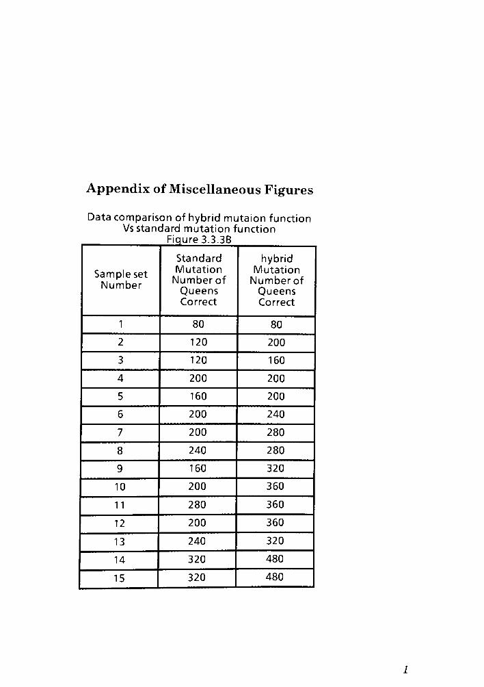
Appendix ofMiscellaneous Figures

Data comparison of hybrid mutaion function

Vs standard mutation function

Figure 3.3.3B

Sample set

Number

Standard

Mutation

Numberof

Queens

Correct

hybrid

Mutation

Numberof

Queens

Correct

1 80 80 |

2 120 200

3 120 160

4 200 200

5 160 200

6 200 240

7 200 280

8 240 280

9 160 320 ;

10 200 360

11 280 360

12 200 360

13 240 320

14 320 480

15 320 480

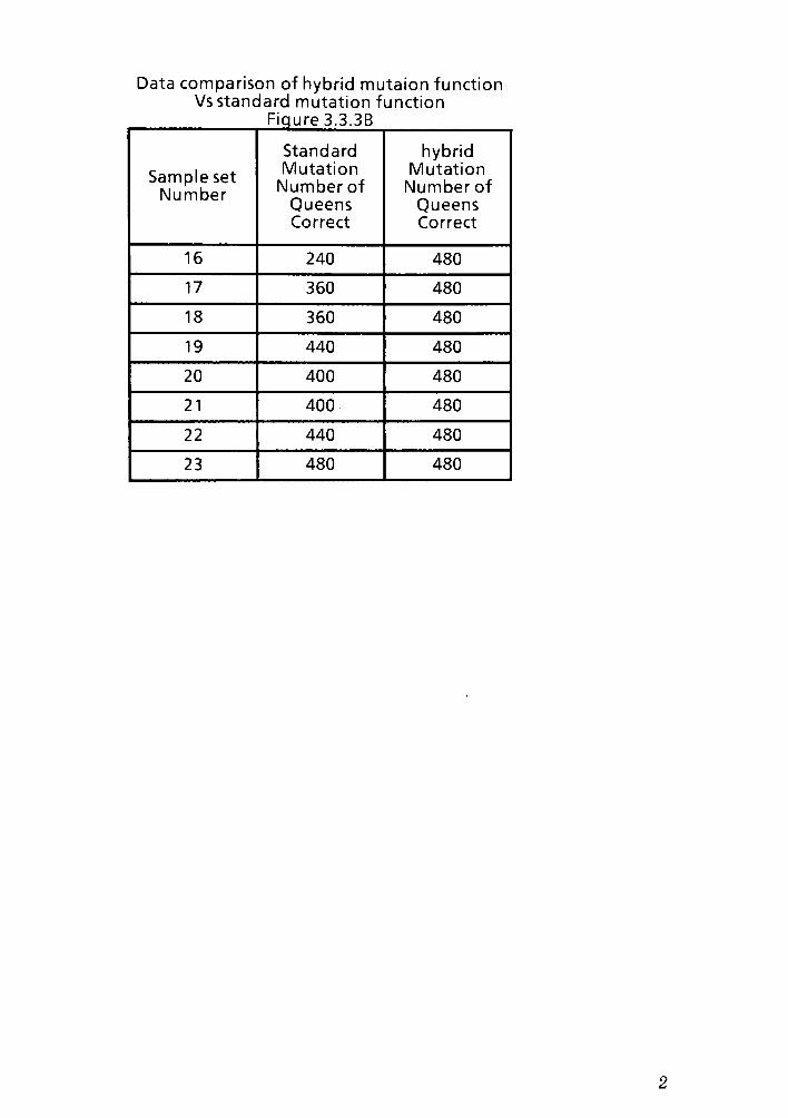
Data comparison of hybrid mutaion function

Vs standard mutation function

Figure 3.3. 3B

Sample set

Number

Standard

Mutation

Numberof

Queens

Correct

hybrid

Mutation

Numberof

Queens

Correct

16 240 480

17 360 480

18 360 480

19 440 480

20 400 480

21 400 480

22 440 480

23 480 480 |

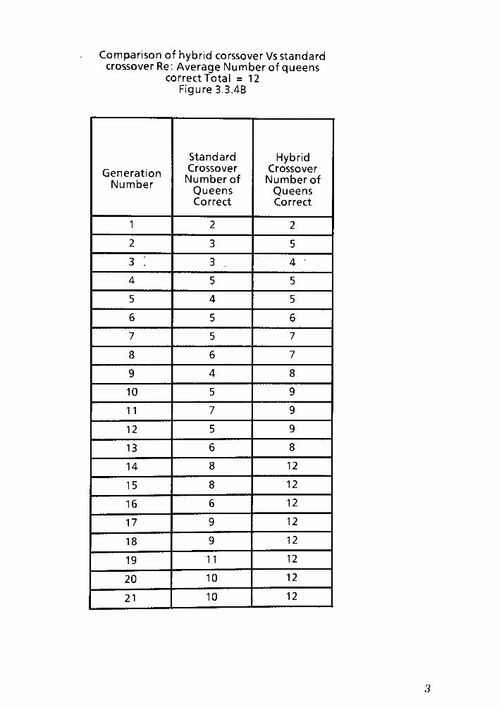
Comparison of hybrid corssover Vs standardcrossover Re: Average Number of gueens

correct Total = 12

Figure 3.3.4B

Generation

Number

Standard

Crossover

Numberof

Queens

Correct

Hybrid

Crossover

Numberof

Queens

Correct

1 2 2

2 3 5 |

3 3 4 |

4 5 5

5 4 5

6 5 6

7 5 7

8 6 7

9 4 8

10 5 9

11 7 9

12 5 9

13 6 8

14 8 12

15 8 12

16 6 12

17 9 12

18 9 12

19 11 12

20 10 12

21 10 12

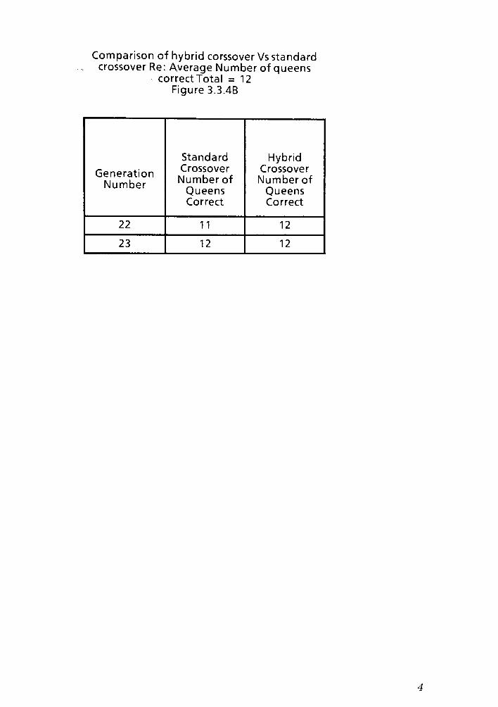
Comparison of hybrid corssover Vs standardcrossover Re: Average Number of gueens

correct Total = 12

Figure 3.3.4B

Generation

Number

Standard

Crossover

Numberof

Queens

Correct

Hybrid

Crossover

Numberof

Queens

Correct

22 11 12

23 12 12

to

c

o

3 E^^

o +^

l/ &_

u o+^ en

cu

c <cu

u

08

c

o

"^ Q.

fO 3

N+*

CU

"aj V)

+

c

s-c

"Co

c

o

o

CU O

sa, 2

cu

3

O

U.

c

.0

c3

CO

c

o*->

3 E_c

o i-"

(/I v.

w O+-> CT>

c <<u

<5

sa rtJ3 v.

4w D>cu aji/>

TifN

03

cO

0 CU

4-> u. V.

CO- 3

N fC Ol

"<5 0i

+-> 4-i

u

c C3u.

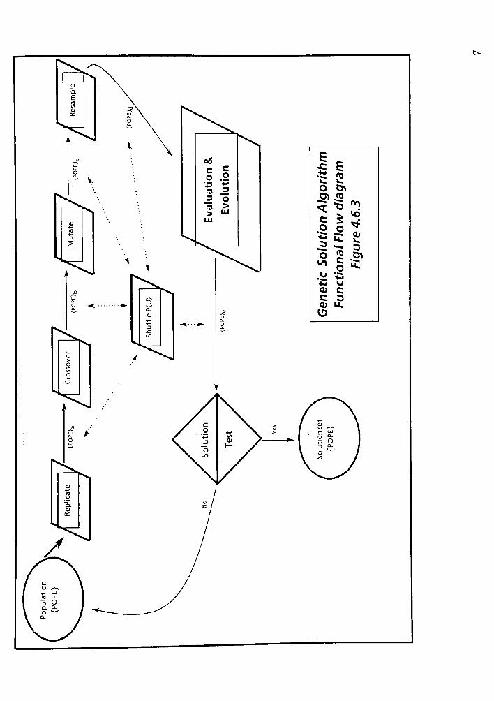
E-c

c=

+-

rov. v.

O 3}en fO

c

.0 O+->

u:CUv.

3 . 3

0<u

0 c

0 LU

.0 4-1

+* u

cu cc 3cu u.

13

00

c

o4-<

3 EJZ

o *>

(/I i_

VJ o

'& o>

c <01

u

c Eo 2+-

en3

"o."J

si-

> vaUj

*QJJ o

cu

Co

u. V-

. 3fTJ cn

4a

<0C

o3

4->

TO u

5. CUj 3

Oi

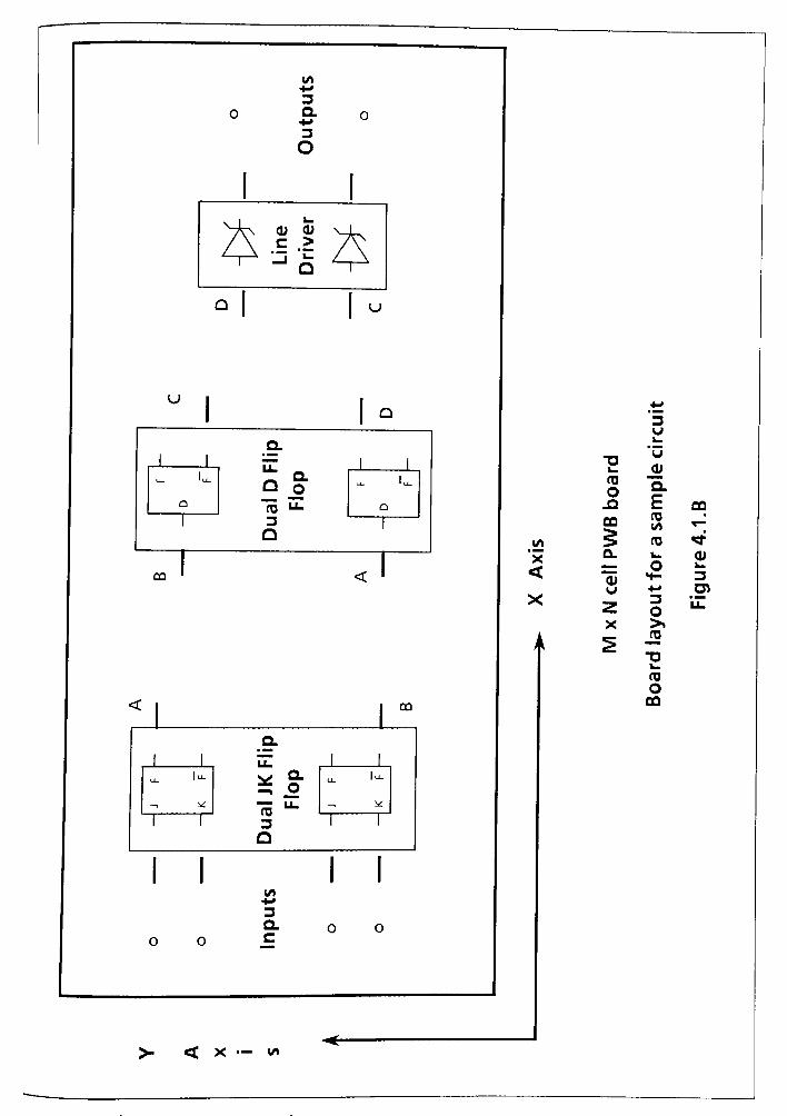
3

CL

3

o

1 i

$ $u

u

Q

1 1

D

i |lli. la.

1 1

00

o

co

<.

1 1QQ

1 i 1 1U-

|u_LL-

lu-

7 1 7 1

'x< = o

3u1_

u

cu

Q.

E COro(^

T-

ro **

i_ cu

3

O

03

OCO

3

cn

I Ito+->

3

a

c

< X />

to

X

<

03

o

CO

<u

3ui

cu

Ql

E uroto

*

ro <fr

u. cuO 1_

*- 3+- cn3

OiZ

5*

J2

D

03

o

CO

< X wo

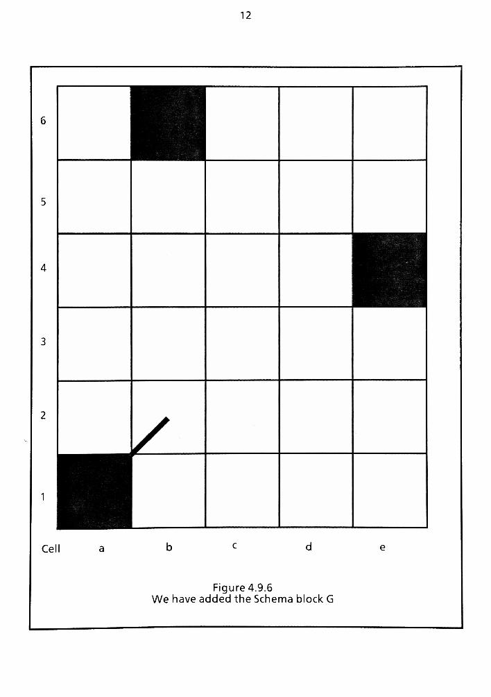
12

6

5

4

3

2

1

Cel I a b c d

Figure 4.9.6

We have added the Schema block G

e

13

gj

s

/

Cell

Figure 4.9.7

We have added the Schema block B

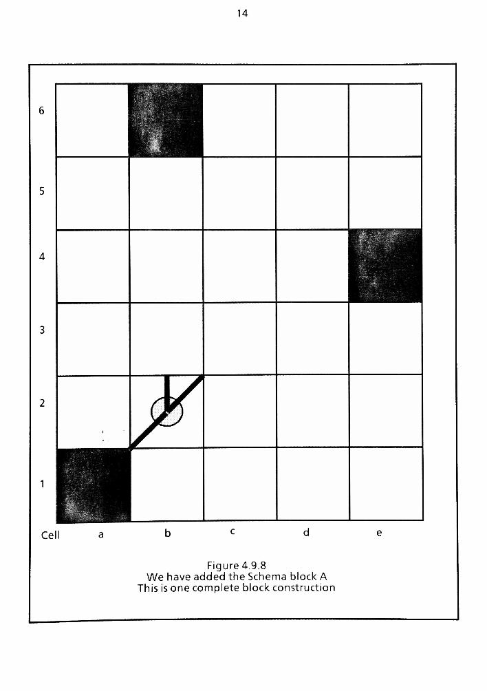
14

^Hi Hi?"

31 V;8HI

Cell

Figure 4.9.8

We have added the Schema block A

This is one complete block construction

15

6

5

4

3

2

1

/

i

1

*

Cel I a b c d

Figure 4.9.9

We have added the Schema blocks G & B

| Thiswas done as one step

e

< j

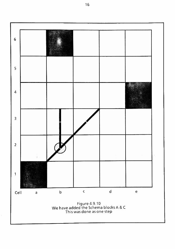
16

6

5

4

3

2

B

/

!

1 K^&pis|

Cel I a b c d

Figure 4.9.10

We have added the Schema blocks A & C

This was done as one step

e

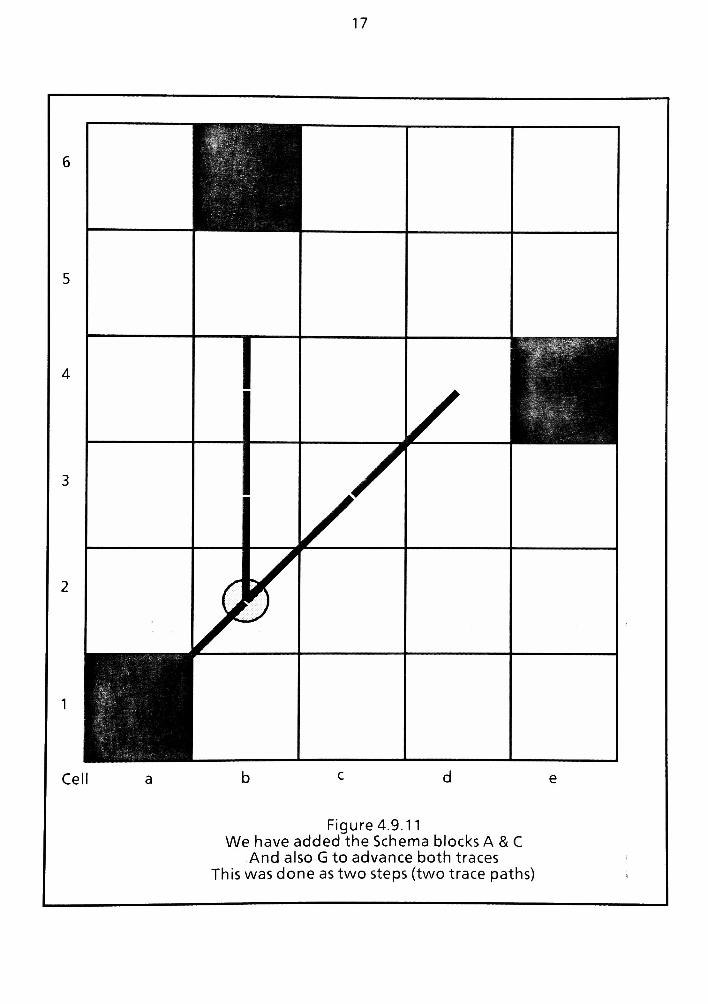
17

Cel

Figure 4.9.1 1

We have added the Schema blocks A & C

And also G to advance both traces

Thiswas done as two steps (two trace paths)

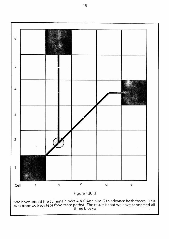
18

^eL,&

Cell

Figure4.9.12

We have added the Schema blocks A & C And also G to advance both traces. This

was done as two steps (two trace paths). The result is thatwe have connected all

three blocks: i

19

Table 6.3 Opt mum Neighbor Solution Data

Dependent

unit:

Evolutions

X10

Average

Population

Utility

Population

Skewness

Population

Kurtosis

Percent of

Traces Routed

10 2.3 -0.4 -0.9 0

20 2.5 -0.4 -0.8 0

30 1.8 -0.2 -0.5 0

40 3.6 -0.1 0.2 0

50 2.5 0.2 0.5 0

60 4.6 0.3 0.1 0

70 4.2 0.3 0.2 0

80 5.1 0.6 -0.3 0

90 6.3 -0.4 0.2 0

100 5.8 -0.2 0.8 2.5 ;

110 6.2 0.1 0.4 12.8

120 6.7 0.3 -0.3 15.3

130 7.4 0.7 -0.8 25.6

140 10.5 0.5 0.2 46.1

150 11.7 0.2 0.3 46.1

160 11.9 -0.4 -0.8 58.9

170 13.8 0.3 0.5 58.9

180 14.3 0.6 -0.8 61.5

190 15.7 0.3 0.1 69.2

200 12.3 0.1 0.2 74.3

210 15.9 -0.1 0.2 82.

220 16.3 0.7 -0.8 82.

230 17.7 0.5 -0.1 87 1 |

240 17.3 -0.1 0.2 94.8

250 18.5 0.8 0.2 94.8

20

Table 6.3 Optimum Neighbor Solution Data

Dependent

unit:

Evolutions

X10

Average

Population

Utility

Population

Skewness

Population

Kurtosis

Percent of

Traces Routed

258 20.8 0.9 0.6 100.0

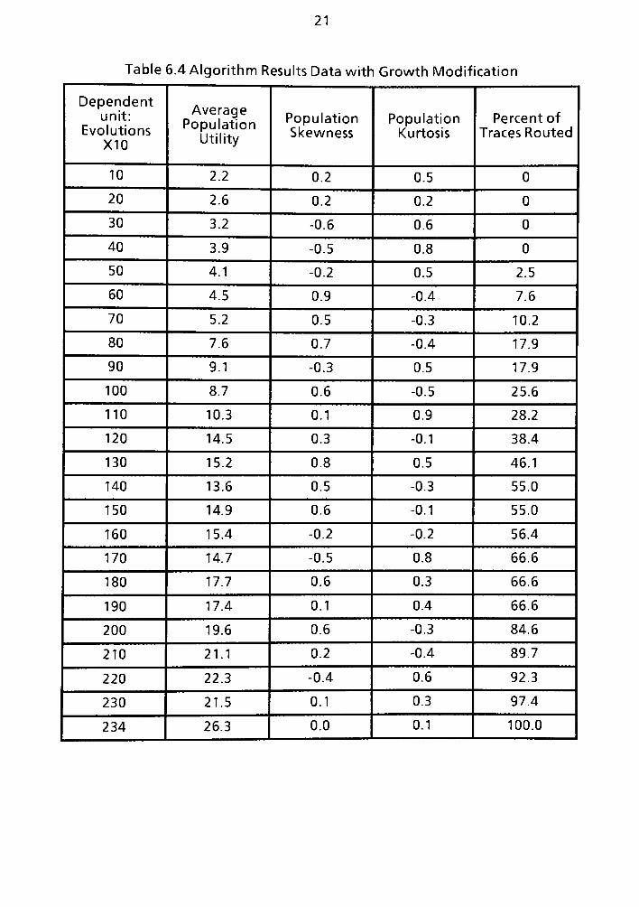
21

Table 6.4 Algorithm Results Data with Growth Modification

Dependent

unit:

Evolutions

X10

Average

Population

Utility

Population

Skewness

Population

Kurtosis

Percent of

Traces Routed

10 2.2 0.2 0.5 0

20 2.6 0.2 0.2 0

30 3.2 -0.6 0.6 0

40 3.9 -0.5 0.8 0

50 4.1 -0.2 0.5 2.5

60 4.5 0.9 -0.4 7.6

70 5.2 0.5 -0.3 10.2

80 7.6 0.7 -0.4 17.9

90 9.1 -0.3 0.5 17.9

100 8.7 0.6 -0.5 25.6

110 10.3 0.1 0.9 28.2 l

120 14.5 0.3 -0.1 38.4

130 15.2 0.8 0.5 46.1

140 13.6 0.5 -0.3 55.0

150 14.9 0.6 -0.1 55.0

160 15.4 -0.2 -0.2 56.4

170 14.7 -0.5 0.8 66.6

180 17.7 0.6 0.3 66.6

190 17.4 0.1 0.4 66.6

200 19.6 0.6 -0.3 84.6

210 21.1 0.2 -0.4 89.7

220 22.3 -0.4 0.6 92.3

230 21.5 0.1 0.3 97.4

234 ; 26.3 0.0 0.1 100.0

22

Table 6.5 Optimum Neighbor Results Data with Reduced Shuffel Operator

Dependent

unit:

Evolutions

X10

Average

Population

Utility

Population

Skewness

Population

Kurtosis

Percent of

Traces Routed

10 3.6 0.2 0.5 2.5

20 3.2 0.2 0.2 5.1

30 3.8 -0.6 -0.3 10.2

40 4.6 0.1 -0.2 12.8

50 4.9 -0.2 0.5 20.5 |60 5.8 0.5 0.6 28.2

70 5.5 0.5 0.6 30.7

80 7.6 0.7 0.1 35.8

90 7.7 0.3 0.2 41.0

100 8.3 0.1 -0.1 43.5

110 11.2 0.1 -0.3 56.4

120 15.6 0.3 0.5 58.9 |130 10.2 -0.2 0.5 61.5

140 16.9 -0.1 0.8 66.6

150 15.9 -0.6 0.7 69.2

160 14.3 -0.4 0.3 74.3 j

170 16.5 -0.1 -0.2 79.4

180 16.8 0.3 -0.3 82.0

190 16.4 0.5 0.4 87 1

200 18.2 0.5 -0.3 92.3

210 18.6 0.1 0.2 94.8

220 20.3 0.8 -0.3 97.4

222 25.2 0.9 -0.8 100

23

Table 7.2.1 RatNest Algorithm Data Test Case 1

Dependent

unit:

Evolutions

X10

Average

Population

Utility

Population

Skewness

Population

Kurtosis

Percent of

Traces Routed

10 2.3 0.5 0.4 0

20 2.5 0.5 0.9 0

30 1.8 0.8 -0.2 0

40 3.6 -0.3 0.2 0 j50 2.5 0.7 -0.8 0

60 4.6 -0.2 -0.3 0

70 4.2 0.3 -0.6 0 |

j 80 5.1 0.6 -0.3 0

90 6.3 0.6 0.5 0

100 5.8 0.8 0.3 2.5

110 6.2 0.8 -0.2 2.5

120 6.7 -0.3 0.7 2.5

130 5.9 -0.1 0.3 5.0 |

140 9.9 -0.9 0.2 5.0

150 3.3 -0.4 -0.3 5.0

160 7.8 0.7 0.4 10.2

170 4.0 -0.3 0.4 10.2

180 11.3 0.2 -0.1 10.2

190 8.7 0.5 -0.8 12.8

200 11.4 0.8 0.2 | 12.8

210 5.9 -0.3 -0.2 | 12.8

220 12.2 -0.6 0.5 10.2

230 | 8.6 0.2 i 0.3 12.8

240 9.3 -0.6 ; 0.6 15.4

250 j 12.5 -0.6 0.1 15.4

260 5.8 -0.4 -0.4 15.4

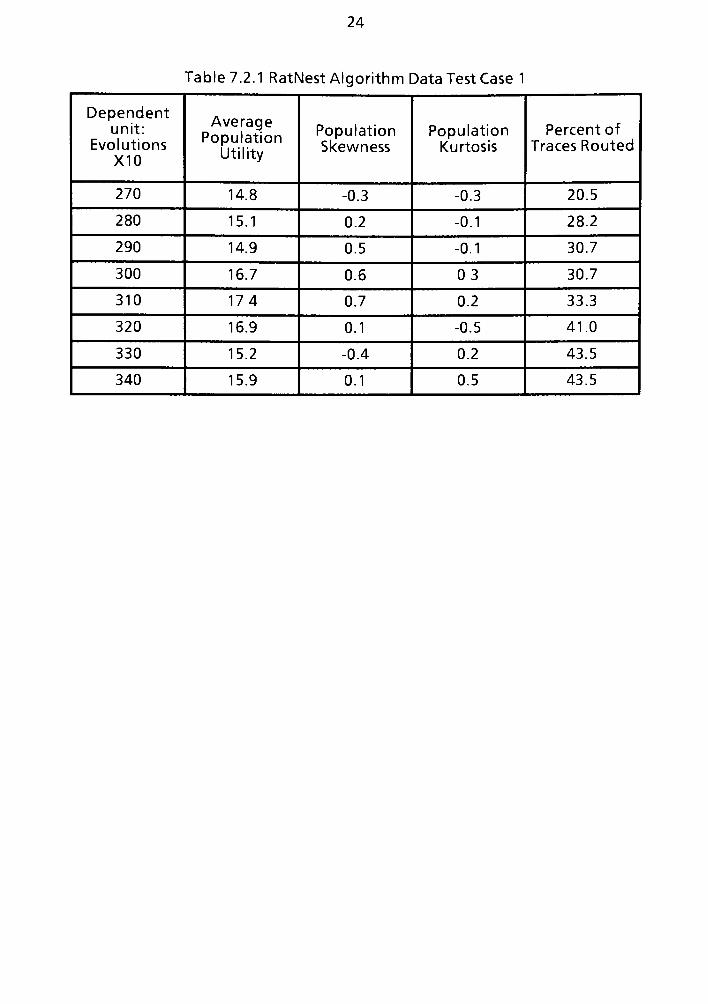
24

Table 7.2.1 RatNest Algorithm Data Test Case 1

Dependent

unit:

Evolutions

X10

Average

Population

Utility

Population

Skewness

Population

Kurtosis

Percent of

Traces Routed

270 14.8 -0.3 -0.3 20.5

280 15.1 0.2 -0.1 28.2

290 14.9 0.5 -0.1 30.7 |

300 16.7 0.6 0.3 30.7

310 174 0.7 0.2 33.3

320 16.9 0.1 -0.5 41.0

330 15.2 -0.4 0.2 43.5

340 15.9 0.1 0.5 43.5

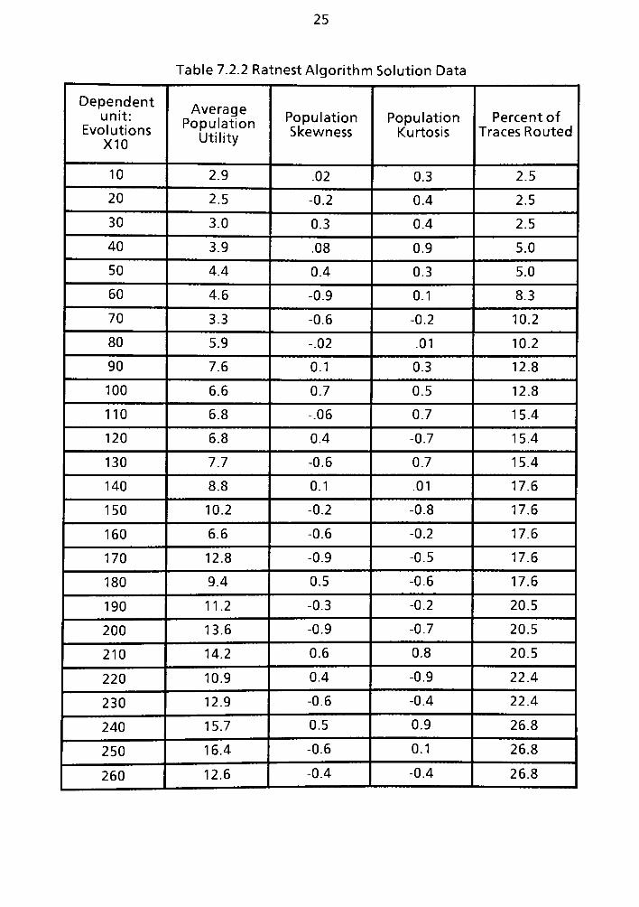
25

Table 7.2.2 Ratnest Algorithm Solution Data

Dependent

unit:

Evolutions

X10

Average

Population

Utility

Population

Skewness

Population

Kurtosis

Percent of

Traces Routed

10 2.9.02 0.3 2.5

20 2.5 -0.2 0.4 2.5

30 3.0 0.3 0.4 2.5

40 3.9.08 0.9 5.0

50 4.4 0.4 0.3 5.0

60 4.6 -0.9 0.1 8.3

70 3.3 -0.6 -0.2 10.2

80 5.9 .02 .01 10.2

90 7.6 0.1 0.3 12.8

100 6.6 0.7 0.5 12.8

110 6.8 .06 0.7 15.4

120 6.8 0.4 -0.7 15.4

130 7.7 -0.6 0.7 15.4

140 8.8 0.1 .01 17.6

150 10.2 -0.2 -0.8 17.6

160 6.6 -0.6 -0.2 17.6 i

170 12.8 -0.9 -0.5 | 17.6

180 9.4 0.5 -0.6 17.6

190 11.2 -0.3 -0.2 20.5

200 13.6 -0.9 -0.7 20.5

210 14.2 0.6 0.8 20.5

220 10.9 0.4 -0.9 22.4

230 12.9 -0.6 -0.4 22.4

240 15.7 0.5 0.9 26.8

250 16.4 -0.6 ; 0.1 26.8

260 12.6 -0.4 -0.4 26.8

26

Table 7.2.2 Ratnest Algorithm Solution Data

Dependent

unit:

Evolutions

X10

Average

Population

Utility

Population

Skewness

Population

Kurtosis

Percent of

Traces Routed

270 17.6 0.6 0.7 28.2

280 14.2 0.2 -0.1 28.2

290 14.9 -0.5 -0.9 30.7

300 16.7 0.6 0.8 30.7

310 17.4 -0.1 -0.3 33.3

320 16.9 -0.1 0.1 33.3

330 15.2 -0.4 0.2 33.3

340 15.9 0.1 0.5 35.8

350 16.0 0.2 0.2 35.8

360 14.8 0.3 0.1 35.8

370 14.2 0.6 0.4 38.4

380 17.5 0.1 -0.2 38.4

390 18.8 -0.4 -0.3 41.0

400 17.4 0.2 0.6 41.0

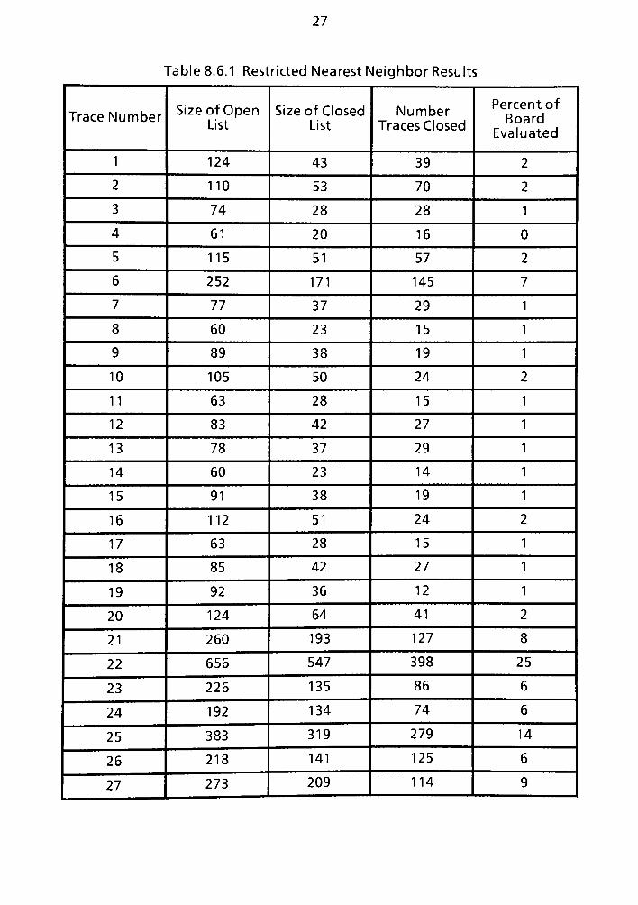
27

fable 8.6.1 Restricted Nearest Neighbor Results

Trace NumberSize ofOpen

List

Size of Closed

List

Number

Traces Closed

Percent of

Board

Evaluated

1 124 43 39 2

2 110 53 70 2

3 74 28 28 1

4 61 20 16 0

5 115 51 57 2

6 252 171 145 7

7 77 37 29

8 60 23 15

9 89 38 19

10 105 50 24 2

11 63 28 15

12 83 42 27

13 78 37 29

14 60 23 14

15 91 38 19

16 112 51 24 2

17 63 28 15

18 85 42 27

19 92 36 12

20 124 64 41 2

21 260 193 127 8

22 656 547 398 25

23 226 135 86 6

24 192 134 74 6

25 383 319 279 14

26 218 141 125 6

27 273 209 114 9

28

Modified Nearest Neighbor Case 1

640

576

512

448

384

320

256

192

128

64

I

Size of Closed List

Size of Open List

1 I1 2 3 4 5 6 7 8 ! 11 1 1i Ii 1' 1! 11 V. 11 V. 21 2 2\ 2. 2< 2! 21 27

Trace Number Being Routed

29

Modified Nearest Neighbor Case 1

25

Percent of Board Evaluated

24

23

22

21

20

19

18

17

16

15

14

13

12

11

10

9

8

7

6

5

4

3

2

1

D nnnnn

Trace Number Being Routed

1 2 3 4 5 6 7 8 ! 11 1 1; 1: 1' 1! 111"

11 1( 21 2 2. 2. 2' 2! 21 27

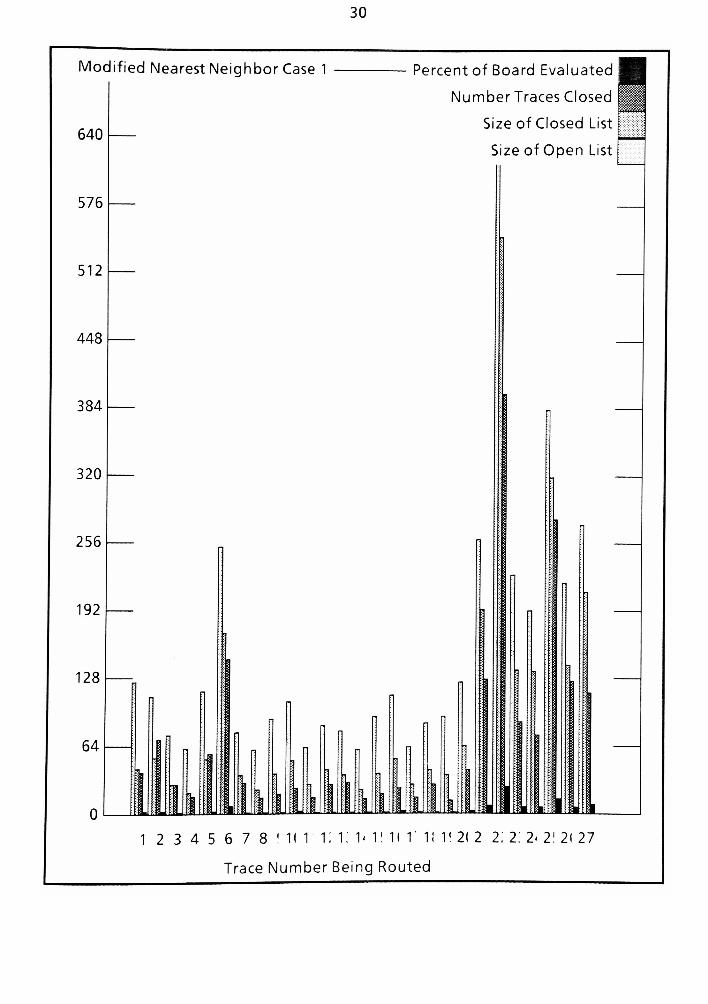
30

Modified Nearest Neighbor Case 1

640

576

512

448

384

320

256

Percent of Board Evaluated

Number Traces Closed

Size of Closed List

Size of Open List

1 2 3 4 5 6 7 8 ' 11 1 1: 1: 1'1' 11

1"

11 1! 2( 2 2. 2. 2> 2! 2l 27

Trace Number Being Routed

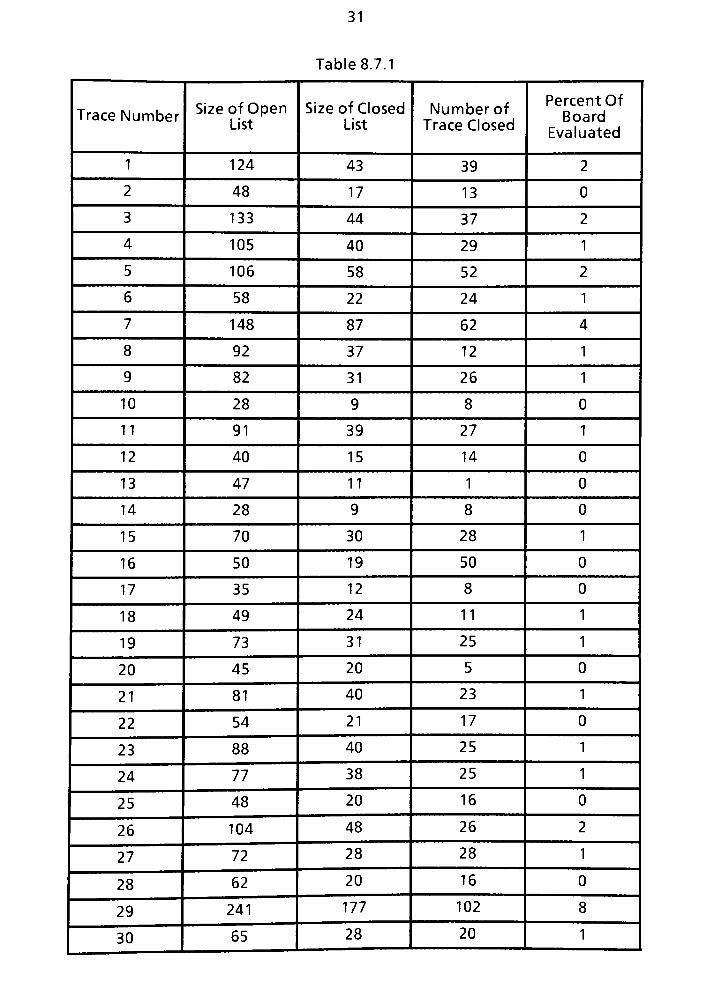
31

Table 8.7.1

Trace NumberSize ofOpen

List

Size of Closed

List

Numberof

Trace Closed

Percent Of

Board

Evaluated

1 124 43 39 2

2 48 17 13 0

3 133 44 37 2

4 105 40 29 1

5 106 58 52 2

6 58 22 24 1

7 148 87 62 4

8 92 37 12 1

9 82 31 26 1

10 28 9 8 0

11 91 39 27 1

12 40 15 14 0

13 47 11 1 0

14 28 9 8 0 !

15 70 30 28 1

16 50 19 50 0

17 35 12 8 0

18 49 24 11 1

19 73 31 25 1

20 45 20 5 0

21 81 40 23 1

22 54 21 17 o !

23 88 40 25 ) 1

24 77 38 25 1 !

25 48 20 16 0

26 104 48 26 2

27 72 28 28 1

28 62 20 16 0

29 241 177 102 8

30 65 28 20 1

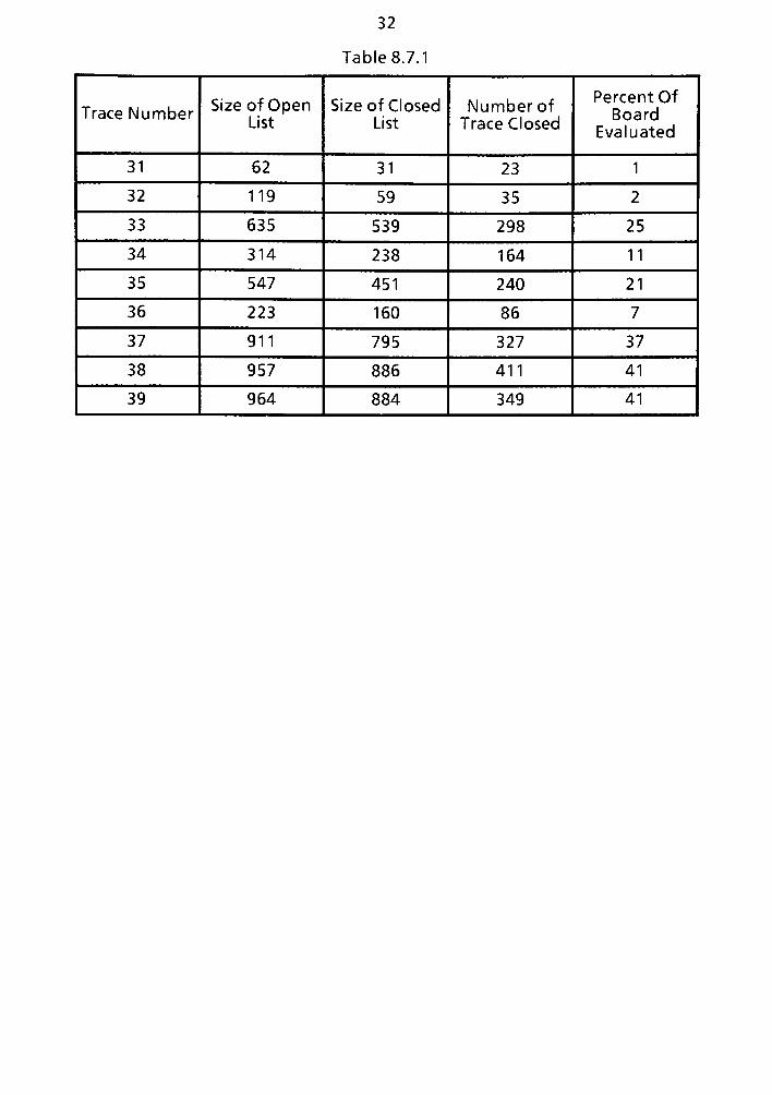
32

Table 8.7.1

Trace NumberSize ofOpen

List

Size of Closed

List

Numberof

Trace Closed

Percent Of

Board

Evaluated

31 62 31 23 1 |

32 119 59 35 2

33 635 539 298 25

34 314 238 164 11

35 547 451 240 21

36 223 160 86 7

37 911 795 327 37 |

38 957 886 411 41

39 964 884 349 41

33

1 Otpimum Nearest Neighbor Case 2

960

920

880

840

800

760

720

680

640

600

560

520

480

440

400

360

320

280

240

200

160

120

80

40

0

Size of Closed List

Size of Open List

*m

Trace Number Being Routed

12345678 11111111112222222222333333333 39

34

1 Modified Nearest Neighbor Case 2

960

896

832

768

704

640

576

512

448

384

320

256

192

128

64

Iklll

Size of Closed List

Size of Open List

11234567811111111112222222222333333333 39

Trace Number being routed

35

Modified Nearest Neighbor Case 2 Percent O Board Evaluated

40

30

20

10

nilnllnn n n nn n nn I In linn

Trace Number Being Routed

12345678 11111111112222222222333333333 39

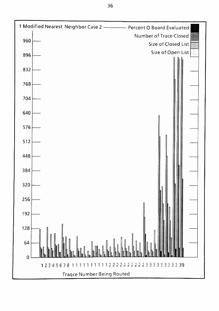
36

1 Modified Nearest Neighbor Case 2 Percent O Board Evaluated

Number of Trace Closed

Size of Closed List

Size of Open List

12345678 1111111111222222222233

Tragce Number Being Routed

3 33 39

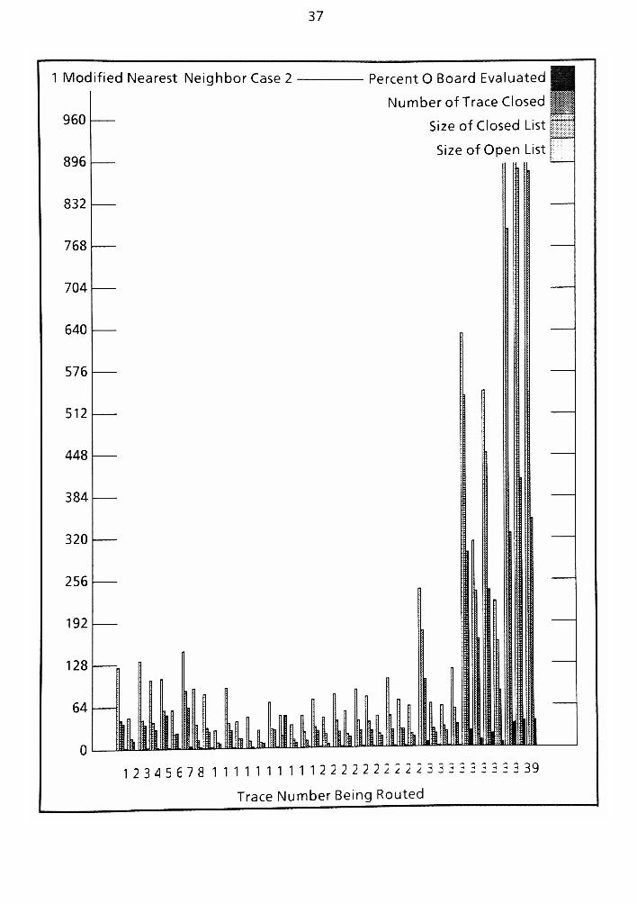
37

1 Modified Nearest Neighbor Case 2

960

896

832

768

704

640

576

512

448

384

320

256

192

128

64

0

Percent O Board Evaluated

Numberof Trace Closed

Size of Closed List T

Size of Open List

12 3 4 5 6 7 8 1 1 1 1 1 1 1 1 1 1 2 2 2 2 2 2 2 2 2 2 3 3 3 3 3 3 3 3 3 39

Trace Number Being Routed

38

Table 8.8.2

Trace NumberSize of Open

List

Size of Closed

list

Numberof

Closed Traces

Percent of

Board

Evaluated

1 124 43 39 0

2 48 17 13 0

3 133 44 37 o ;

4 105 40 29 0

5 559 238 253 1

6 591 211 133 1

7 994 653 535 3

8 794 465 240 2

9 80 43 31 0

10 58 22 24 0 j11 288 203 87 1

12 100 39 33 0 |

13 495 334 194 1

14 220 45 0 0

15 1133 943 461 4

16 2 2 0 0

17 128 80 29 0

18 1511 1396 1212 6

19 28 9 8 0

20 91 39 27 0

21 42 15 16 0

22 56 22 21 0

23 31 12 8 0 I

24 190 128 84 0

25 28 9 8 0

26 71 30 28 0

39

Table 8.8.2

Trace NumberSize of Open

List

Size of Closed

list

Numberof

Closed Traces

Percent of

Board

Evaluated

27 24 9 6 0

28 19218 19218 10625 96

29 49 19 15 0

30 29 12 8 0

31 104 56 34 0

32 73 31 25 0

33 45 20 5 0

34 81 40 23 0

35 54 21 17 0 |

36 64 33 19 0 !

37 339 256 133 1

38 48 20 16 0

39 10 49 22 0

40 74 28 28 0 i

41 62 20 16 0

42 139 82 55 0

43 52 23 20 0

44 61 20 16 0

45 712 614 278 3

46 288 209 76 1

47 492 375 142 1

48 332 218 139 1

49 216 60 57 o

50 ;

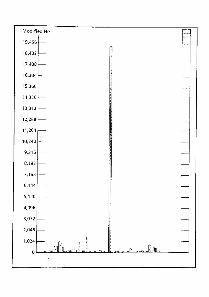
40

Modified Nearest Neighbor Case 3

19,456

18,432

17,408

16,384

15,360

14,336

13,312

12,288

11,264

10,240

9,216

8,192

7,168

6,144

5,120

4,096

3,072

2,048

1,024

0 m '*- ***- Tl- I Vl ITV^-irtki

Size of Closed list

Size of Open List

rhi .r>J la ^aBhPaw yfck.

50Trace #

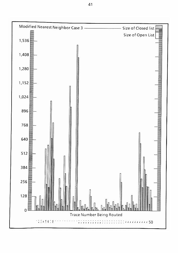
41

Modified Nearest Neighbor Case 3=

1,536

r

1,408n

1,280

1,152==

1,024

896

768

640

512

384

256

128

yym

Size of Closed list

Size of Open List

yMiilUlTrace Number Being Routed

;:^!i;! t4A4.t44*iil 1 1 1 1 1 1 1 1 1 50

42

Modified Nearest Neighbor Case 3

95

Percent of Board Evaluated

90

85

80

75

70

65

60

55

50

45

40

35

30

25

20

15

10

5

0jnnI. In n n _D_ 1nnn

:un:i iiiiiti*ii~-

Tracei L I I i i i L i L 50 #

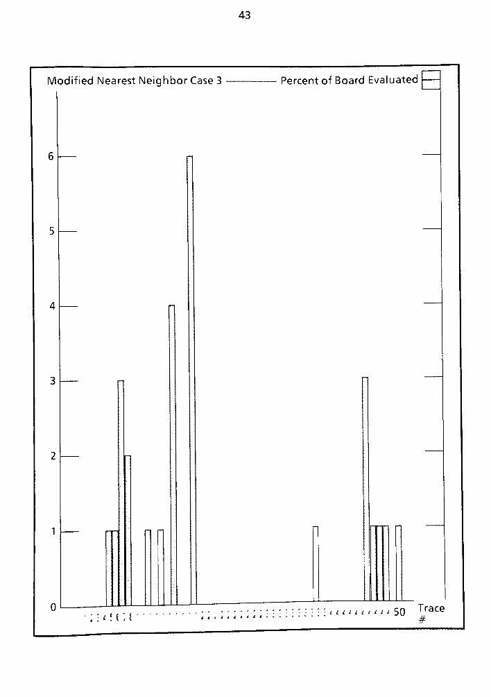
43

Modified Nearest Neighbor Case 3 Percent of Board Evaluated

t lA'AliLlt.lll.il 50

Trace

#

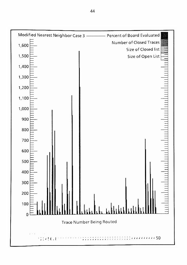
44

Modified Nearest Neighbor Case 3

1,600

1,500

1,400

1,300

1,200

1,100

1,000

900

800

700

600

500

400

300

200

100

0 11 k iik

Percent of Board Evaluated

Number of Closed Traces

Size of Closed list

Size of Open List

l urn

Trace Number Being Routed

'

; i t ! ( , c 4 4 d d 4 I 4i I I L L i L I i I 50

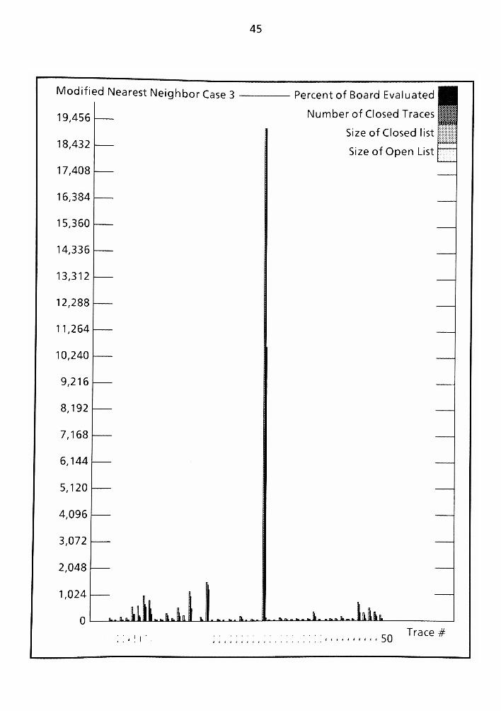
45

Modified Nearest Neighbor Case 3

19,456

18,432

17,408

16,384

15,360

14,336

13,312

12,288

11,264

10,240

9,216

8,192

7,168

6,144

5,120

4,096

3,072

2,048

1,024

a. . L a.

Percent of Board Evaluated

Number of Closed Traces

Size of Closed list

Size of Open List

fc II Urn I* JU naI- . !>.... .. -^ i Ifiahfl-

i i i i i 50Trace #

46

Chapter 12

References

Chapter 1

1. SIAM Series #3, Symposium on applied probability and Monte Carlo

Methods, 1967

2. Binder, Kurt, Monte Carlo methods in statistical physics, 1/1/79, QC

174.85.m64M66

3. Gorden, M., D., Adaptive subject indexing in document retrieval. (PHD

disertation at University of Michigan), Dissertation abstracts

international, 45(2), 61 1B

4. Booker, L., B., Improving search in genetic algorithms, L. Davis book on

Genetic algorithms and simulated annealing, p 61-74, London Press.

5. Dejong, k., A., An alysis of the behacior of a class of genetic adaptive

systems, Dissertation abstracts international 36(10), 5140B.

6. Holland, J., H., Adaptation in natural and artificial systems, University

of Michigan Press (1975)

7. Goldberg, D., E., & Lingle, R., Alleles, Loci and the traveling salesman

problem, Proceedings of an internatinal conference on genetic

algorithms and their appoications ppsl 54-1 59.

8. Goldberg, D., E., & Thomas, A., L., Genetic Algorithms: a bibliography

(1962-1986), TCGA report #86001, University of Alabama.

47

Chapter 2

9. Hammersley, J. m. & Handscomb, D. C. Monte Carlo Methods, 1965,

QA.273.H224

10. Studies In Applied Mathmatics, #3 Symnposium on applied probability

amd Monte Carlo Methods, 1967, QA.1.S863

11. Binder, K. Et. Al, Monte Carlo methods in statistical physics, 1979,

QC.174.85.M64

12. Styblinski, M. A. & Meyer, B. D., Fuzzy Cognitive Maps, Signal Flow

Graphs and Qualatitive Circuit Analysis, Proc. IEEE Conf on Neural

Networks, 6/87

13. Kosko, B., "Fuzzy Cognitive Maps", International Journal of Man-

Machine Studies, Volum 24, pps 65-75, 1/1986.

14. Davis, L. & SteenStrup, M. (1987). Genetic Algorithms and simulated

annealing: An overview in.

15. Glossary and tables for statistical guality control. Published American

society for guality control 1973.

16. William K. Pratt, Digital Image Processing,Wiley-lnterscience, 1978.

48

Chapter 3

17. H.S.Stone, J.M.Stone, Efficient Search Technigues - An emperical study

of the N-Queens problem, IBM J. Res. Development., pp464-474,

vol.31, no.4, 1987

18. Goldberg, D., E., Optimal initial poplation size for binary-coded

genetic algorithms (TCGA report #85001).

19. C.L. Bridger, D.E. Goldberg, An Analysis of Reproduction and crossover

in a binary coded Genetic algorithm, Proceedings of the Second

Intemation Conference on Genetic Algorithms, 7/1987

20. Holland, J., H., Genetic Algorithms and the optimal allocations of

trials, SIAM journal of Computing, 2(2), 88-105

21. Suh, J., Y., & Gucht, D., V., Incorporating heurstic information

information into genetic search, Proceedings of the Swcond

International Conference of Genetic Algorithms 7/1987

22. Johnson, K, & Daniell, c, & Burman, J., Feature extraction in the

Neocognitron, Proceedings from the confrence on Neural Network

23. Krishnan, G., & Walters, D., Psychologically plausible features for

shape recognition in a neural network

24. DeJong, K., A., (1981) Adaptive search procedures for large complex

spaces., (technical report #81-2), Uinversity of Pittsburgh

25. Foo, N., Y., & Bosworth, J., L., (1972) Algebraic, geometric, and

stochastic aspects of genetic operators, (CR-2099)

26. Grefenstette, J., J., Optimization of control parameters for genetic

algorithms, IEEE Transactions on Systems, Man and Cybernetics, SMC-

16(1), 122-128

49

27. Bosworth, J., & Foo, N., & Zeigler, B., P., Comparison of genetic

algorithms with conjugate gradient methods (CR-2093) National

Aeronautics and space administration

28. Goldberg, D., E., (1987) A note on the disruption due to crossover in a

binary coded algorithm, (TCGA report #87001).

29. Wetzel, A., Evaluatin of the effectiveness of genetic algorithms in

combinatorial optimization, Unpublished manuscript, University of

Pittsburgh (1983).

30. Booker, L., B., Improving performance of genetic algorihtms in

classifier systems, Proceedings of an internatinal conference on

genetic algorithms and their applications, pp80-92.

50

Chapter 4

31. Moopenn, A., & Thakoor, A., P., & Duong, T., A Neural network for

Euclidean distance minimization < proceedings from

32. Van Den Bout, D., E., & Miller, T., K., A traveling Salesman Object

function that works, North Carolina University, Proceeding from ACM

[A]

Index

Stochastic Genetic Algorithms Applied to the PWB

Routing Problem

accelerate 155

acceptability 26,51

access 155

ACM 8

activity 155

adapted 153

additionally 49,154

adopted 18

adversely 49

allowable 40

alpha 86

animation 74

annealing 4,7,12-13,15,18,21,33-34,38,45-46,48-49,69,71 -72,83,86,89,102

Annealing Temperature 83

anomalies 75

appendix 40,42,52,63,74,103,108,113,122,125,138

Applicability 155

approximated 83,100

arbitrary 11,152

assumptions 28

AUF 44,48

Average Utility Function 48

[B]

backtrack . 60

backtracking . .10,12,60

behaviors 72

bias 91

biasing . .71,86,103

Biles 1

Binder . . ... . 15

blood33,55-56,59-- 60, 62, 65, 69 - 70, 89, 97, 1 35, 1 52

bloodline . . . 56

Board Size 32

BoardO . . ..... 38

boolean . ...26,28

bounding ... . 5

breading .71

[C]

captures

Carlo

cartesian

catalyst

caveat

cell of contention

cell's

character function

characterization

characterize

charts . . .

Checker .

chipat . . .

circuit's . .

classic

classifier

clustered

coalesce

cognitive . .

combinatorial .

commercialized

compensate . .

compensated

compensations

competes .

concatenates .

concluding . . .

conditioned

configuration

configurations

configuring

conflicting

congested .

connections

constants . .

constraint .

constraints

contention

converge . .

convergence

convergent

converges .

convergingCOREPOP .

correctness

correlate .

correlated

correlation

correlations

cos ....

128

7, 15

52,73

108

75

133

99

102

10,64,69,71,81,83,103, 127.14869

103

143

132, 142,145

55,119

153-154

45

129

42

17,155

2,5,8-9

155

68,72,97-98

98

68

95

71

49

119, 121

135

34

135

11

135

3-4,51,62, 118, 133

71, 103

5,9

5-7,9-10

118,128,133

3,6,9-12,16,19,46,71 -72,103, 154

5,7,9-10,12,20,49,68

5

17

5

55-56,89

13,23

148

26,42,71,87

42,47,65,70-71,89,113

37,42

84,100

[D]

[E]

coupling 155CPS 87

CPT 148-150criteria 16-17,24-26,51-52,64,83-84,94,99-100,

149, 154, 156criterion 16-17, 154

criticality 10

crossover 19,22,33-34,40-42,46,49,64-65,72,89-91,103,135

crossovers 68,90,156customized 39-40

customizing 40

cycling 88

death 60,70,97-98

declining 68

decorrelate 47

DeJong 10

derivatives 81

detrimental 49

deviation 20, 82, 102Deviations 100

diagonals 28

discontinuity ... .91

distributions 20

distributions 21

diverge 9

divergence 10,12

divisibility 30

document 8

DPU 44

drastically 28

dual 65,90

duplicates 89

dynamically 68

EFF 15

Efficiency 15

elapsed 108

eligibility 76

eliminates 128

empirical 151

empirically 23

encoded 38

enhanced 50,84,101

enhancement 151,155

entities 65

entity 155

egn 38,81-82

[F]

eguated 55

Estimated average distance for trace completion 82

estimator 1 5, 32, 69, 86et 15

ETS 32,86-87

euclidean 52

evaluated 38,72,128

evaluates 64-65,72,84,90,100

evaluating 133

evaluation 38, 60, 63, 1 27, 1 36

evaluations 76,151,154

evolution-monitoring 68

evolutionary 71,102

evolutions 3,17,32,46,55,60,83,86-87,99-100,102,108,

113,123,125,127

evolve 17,21,40,54-56,63,122,154

evolves 59

evolving18-19,21,44-46,54-55,59,64-65,68-69,71

72, 81, 83, 89 - 91, 97 - 98, 113, 148, 152, 154

examines 143

executing 127

exhaustive 3,5,30-31

exhaustively 6

expend 154

exploited 148

exploiting 72

exponential 16

extension 135

extensions 17

extrapolations 152

facilitate 31

failures 31

favorably 95

feedback 12,15,18,149

files 131

filter 42

filtering18,65,67,69

filters 68

finite 5,10,12

finite population 5

fitness 18

flipping S! yic R-) 7? ORfluctuate

33,45,62,72,98

fluctuates 62,98

fluctuating62

Jrmw:on. :::::::: ":: l&s. 55.73.83.89.100format 138

formats 52

formulated .70

[G]

[H]

[I]

formulating 24,51

formulations 37

four layer board 135

freed-up 97,103fulfillment 1

functionality 156

fundamentally 15

fundamentals 31-32,50,153

fuzzy 17, 155

Fuzzy Cognitative Machines 17

Fuzzy Cognitive Machines 17

GA 3,7

generates 91

generating 34,89

generic 18

genetic 1-5,7-10,12-13,15,17-19,21-22,26,30-34,

38 - 39, 41 , 45, 48 - 50, 55, 62 - 64, 70 - 73, 81 ,83 -

85,89,91,93,96,98-99, 101, 103, 108, 122, 124-

128,137-138,140, 148,153-154

genetic algorithms .... 7

GENROUTE 1

geometrical 122

gird 95

gleaned 93

global 18,128

globally 154

gnd 131,140,142,144-145

Goldberg 10,12

graphical 63, 143

Graphically 103,108

grid 52,65,73,93-95,119,121,127,136

Hammersley 15

Handscomb 15

heuristic 4,28,42

heuristics 3

Higher Order Dimensional Spaces 8

hinder 6

histogram 140,143

histograms 138

HODS 8

housed 155

hybrid 7,40,42,49

i_<l 84-85, 100-101

dentifiably 37

ff 26

legitimate 28,154

mperially 17

mplement 10,91

mplementation 6,8,42,91,93,131,148,155mplementations 2,91

mplemented 18-19,26,50,65,71,85,93,102

mplementing 26, 50mplementor 7,155-156mplements 42

mplications

mplyingmpose

nbreedingncorporate

17

16

11

68,90

7, 10, 103ncrement 120

nduce 19

nefficient 11,31

nferences 23,26

nfreguently 149

nfusing 33

nherent 7,10,42

INIT 89

initialize 34

initially 101

inordinate 12

69

88

102

69-70

39,85,119, 121

15

103

inputs

insertion

Instantaneous

insuringinteger

integration

intelligentlyintending 13

inter 156

inter-trace 152

interaction 11,49

interactions 7-8,98

intercept 120

invalid 7,9,23,26,28,34-35,37-38,42,65,67-68,70,

89,91,122, 148

investigates 12,99

invoked

isolate .

iterate . .

iterated .

iteration

iterations

40

6,99

5,9

4

84,100

17,85,101

[J]

jog128

jogs ....

junctions

3,81 -83,95,99-100,121 -122,153, 156

4

[K]

[L]

[M]

kurtosis 20-21,71-72,82,84

layout .

likened

limitingLingle .

In

logicallyloopingloosing

M degrees .

m-1

manageable

manipulated

manuallymasked

massage

matrices

matrix .

matrixes

MAX ..

maximize

Mean Population Size

mean population size

mechanisms

merged . . .

merging

methodology

mildlyMIN

minima

minimal . .

minimization

minimize

minimized

minimums . .

modeled . . .

modes ....

modification

modifications

modules ....

monitor

52,62,118

12,18,46

12

10

102

73

31

108

5

47

10,28,30

9

151

11

122, 149

6,9

93

8

84, 100

96

45

32

97,155

140

22

24,51

148,153

84,100

19

17,26,28,30,113

52

3,49, 113,122, 154,156

17

46,71

65

69

50,103,154,156

127

63-64

18,68,71 -72,81

[N]

[0]

monitored 54, 149

monitoring 102

Monte 7, 15Monte Carlo 15

MpS 32 - 33, 38, 44 - 45, 86 - 88, 96MPSA 86-87MPSB 86-87

multi-modal 9

multidimensional 8

multiplications 16

multivalued 6

multivariat 9

mutate 34, 39, 69, 93mutated 90,102

mutation 12,18-19,21-22,33-34,39-40,42,46,49,68-

69,72,83,86,90-91,93, 103, 134-135, 148, 154Mutation function 33

Mutation Operator 68

mutations 19

MxN 51-52,63

N operators 5

N Queens 2,23,25

N-Queens 33,49-50,81,93

negation 103

negatively 72

neighbors 99

netlist 51-52,55,62,99,118,131,138,140,143-144,147,151

netlists 149

neural 7, 12, 18

NGrowth 108

NJogs 100-101

non-exhaustive ....... 10

nondeterministic 7,10

normalizing 84,86,100

NP-Hard 2-3,5-9,11-12,15,22,30

NPTA 44, 72, 98

NQC 38-39,48

Numberof Parents To Add back 44

Number of Queens Correct 38

NxN 23,25-26

occupancy75-76,95

oppositely21

optima 46, 154

optimal 17,26,40,93,153,156

Optimality 153

optimally 17,72,103

optimization 2-3,5,8-9,11,15,18-19,32,125,128optimize 31,40,42,50,72,98optimized 22,30

optimizing 49^68optimum 99,102-103,108,129,150,152,154Optimum Neighbor Solution Algorithm 99option 133,138

options 138

orientation 63,132,142,145outlyer 21

overlay 52

overview 73,81,99

[P]

palatable 95

paradigm 155

parallelism 155

parallelize 155

parameter 18,46,108,127

parameters 21,44,68,71,102,124,126

parity 131-133,140,142-144,147

path's 133

PC 52

pending 129, 131, 134-135

pertaining 97

plateaued 127

plateaus 82

polynomial 83-84,100

POPE 55-56,59-61,63-65,67,69-71,81-82,85,87-

91,93-97,99-100, 102, 108, 121 - 122, 129

POPE'S 59-60,62,88,93-96,100-101

POPEs 55-56,59-62,65,68-71,87,89-91,93-97.100,:..'.. 102,108,113,122,129

Population average ... 81

Population Kurtosis . . 82

Population Skewness . 82

Population standard deviation

Population variance

population's . .

positional

potentially . . .

precalculated . .

preconditioned

predetermined .

predictor

predictors . .

Preface ... .

preferable . .

premature . . .

prematurely . .

premise .

presort

81

82

33,72,102

47, 113

17

156

119

5,38-39,69-70

4, 15,26

4

3

99

10, 12

11

118

155

[Q]

[R]

priori 148

Prioritization 131

prioritize .. 94,131

prioritizing 95

priority 129,131-133,138,142-143,145,147,151,155

priority trace 129

probabilities 46

problem's 6

procedural 64

proceeding 68,83

processor 155

processors 155

programmed 134

programming 12,50

progressed 50

progressing 148,154

PROLOG 152

promoting 18,31

propagation 12,103

proven 13

pseudo 7, 90, 120pseudo-random 70

PWB 1,3,12-13,31,50-52,55,62-63,74,86-87,91,

93,131, 135, 138, 140, 143-144,148-149,152-

153,155

PWB Routing 2

PWBs 156

quadruple 131, 140,144

guantifiable 13

guantified 2

guantized 55,121,149

(quantizer 119

quantizes .

; 119

guantizing120

que 134-135

queen23,26,28,35,40,42

queue 135

ramification 154

Rand84-85,100-101

randomization 71,103

randomize 46

:::.:'

.'.

22,37,39,41,44-46,89-91,156

randomness . 10 - 12, 18- 19, 21, 38, 64, 83

- 84, 86, 89 - 90, 101,

127

ranked 99

rat 149

ratnest 55,118-122,125,127-129,149,151-152Rdist 84-85, 100-101real-valued 86realtime 149

redirect 70

reevaluate 60

referenced 86

reflective 17

reintroduce 44

reject 38

rejecting 31

rejects 38

relevance 25

rendering 91

reordered 40

reordering 10

REP 39,72,85,87-88,98

REPO 39

replicate ,. 33-34,39,64,85

replicated 22,39,47,55,64,85-89,121,143,154

replicates 64

replicating 22,87-88

replication 22,33,38-39,47,62,64,72,85,88,98,113,121

representations ... 154

reproduces 47

reran 125, 127

rerun 127

resample 34,45,69-70,98

Resample Operator .... 69

Resample Population Size 45

resampling 33,62,69-70

researches 10

reset 127

reside 63

resolves 133

restarted 62, 97

restate 121

restrict 10,17,42,70,148

Restricted Neighbor algorithm 138

restricting5,18,31,40

restriction 25, 65

restrictive 12

resultant 20,113

resumes 134

retrieval 8

retry62,98

reviewed 32

reviewing153

revitalize 33

rigorous 6, 143

ripple 128

Rochester 1

Rohdy 1

rotations 73

rout 61

routed 52,55-56,59,62,86,96,119,129,133-135,137-

138,140,148-149,151,153-155router 1# 93routines 30,47,49,68

routing 3,8,12-13,17,31,50-52,56,59,62-63,73-74,81,97-99, 101,103, 108, 1 18 - 1 19, 123, 125, 127 -

129, 137 - 138, 140, 143, 148, 150-156routings 52, 151RPS 45RSF 88

RTOT 88

RVEC 87-89

[S]

sandwiched 135

scaled 88

scaling 84,88,100scans 71

schema 2,26,28,30-31,34-35,37-38,40,42,73-74,86,148

SDevPop 100-101

Secondly 129

selects 39-40,45,65,73,90

sequential 47,49,113

serially 71

shielding 135

shrinkage 96-97

shuffle 34,46-47,49,108,113

shuffle operation .... 46

Shuffle Operator 70

shuffle operator 113

shuffled , 37,47

shuffling 46,71

SIAM 15

signify 133

signifying 129

simulate 127

simulated 7, 12

simulation 3-4,17,155

simulations 8

sized 12,23,73

skew 71

skewed 20, 72

skewness 20, 82

software 13,23,28

solicit 83

solution's 12

solvable 31

specification 131

specifics 50,99

specify 7, 131

[T]

stagnate 11,19,21,46,71-72,96stagnated 21,55,72,108

stagnating 18,33,60,68-69,108stagnation 60,68,84,90,97,101

statistical 2,7,15,19-21,70,148

statistically 19,26,30,40,42,46,65,89

STD 100,102

stochastic 10

strategies 13

stringer 108

strlen 84-85,100-101

sub-functions 39

Sub-Sample 20

subsample 46

subsampling 33,46

subset 5

subsets 5

summarize 55

summing < .-. 88

superimposed . . . .

'

119

swapped 40,134

swapping 134

tabular 103

tailors 50

terminally 54

terminate 38,52,84,100,129

terminated 133

termination 99

terminator 51

testable 13

th 47

theorems - 20

thesis '- 1,3,5,7-8,12,16,23,60,148,152

thrash 21,33,46,69

thrashing11-12,18-19,72,128

timeout 95..,...

tolerance6,9-12,26,45,51

tolerate 33, 83

tolerated 11-12

trace's52,55,59,134,154

tracking152

tractable3,10,12,50

traversed 52

IS9.::::'.:::'.::.: 10,17,71,84

"

V. '.'.'.'.'.'.'.'.. 30,67-68,70,91

ttl7486131-132,140,142,144-145

[U]

[V]

[W]

[X]

unavailable 59,94,96

uncontrolled 10

unintelligent 30

unitless 16

updated 82-83

upgraded 123,125

upwards 156

UTIL 85

utilities 12-13

utility 17-19,22,30,33,42,44,48-50,55,60,64,70-71,81 -85,90,96-97,99-103, 108, 113, 121 -123,125,137

utility function 103

utility polynomial .... 100

utilize Ii 9,11,15,18,31,38,50,60,72-73,83,96-97,131,

133,135,138, 148

utilized 12,15,18,20-21,26,33,37,46,49,52,69,71-72,

81,95,98, 119, 122, 131, 135, 137-138, 143, 148-

149,155

utilizes 3,69,86,99,103,113

utilizing 11,15,23,38,138,143

valid 5,11,16,28-30,34,38,40,42,54,59,90,95,97,

122

validation 149

variability 83

variance 68,71-72,82

vcc 131-132,140,142,144-145

Vec ' 37

Vec() I. 37-38

Vec(N, F) 37

vector26,37-38,81-82,87-89,93,121

vectors 6-9,26,113

verified 23

versus40,42,128,153

vias 156

visualized 38, 65, 88

weighting83,99

workingpopulation 5

xor131,140,144

xorO132-133,142-143,145-147

[Y]

[]

[]

[I]

[1]

xorl 132-133,142-143,145-146

xor2 132,142,145-146

xor3 132,142-143,145-146

xor4 145-147

xor5 145-146

xor6 145-146

xor7 145-146

y1 131-133,140,142-144,146

y2 131-133,140,142-144,146

y3 131-133,140,142-144,146-147

y4 131-132,140,142-144,146

yielded 150,153

yielding 34,84,100

86-87

86-87

l 34-35,42,44,100

iPopUtil 100-101

IX 120

IY 120

34-35,42