Generation of Program Analysis Tools - Frank Tip
220
Generation of Program Analysis Tools Frank Tip
-
Upload
khangminh22 -
Category
Documents
-
view
4 -
download
0
Transcript of Generation of Program Analysis Tools - Frank Tip

Generation of Program Analysis Tools
Frank Tip


Generation of Program Analysis Tools
ILLC Dissertation Series ������
institute for logic, language and computation
For further information about ILLC�publications� please contact
Institute for Logic� Language and ComputationUniversiteit van AmsterdamPlantage Muidergracht ��
�� TV Amsterdamphone� � ���������fax� � ����������e�mail� illc�fwi�uva�nl
Generation of Program Analysis Tools
Academisch Proefschrift
ter verkrijging van de graad van doctoraan de Universiteit van Amsterdam,op gezag van de Rector Magnificus
prof. dr P.W.M. de Meijerten overstaan van een door het college van dekaneningestelde commissie in het openbaar te verdedigen
in de Aula der Universiteit(Oude Lutherse Kerk, ingang Singel 411, hoek Spui),
op vrijdag 17 maart 1995 te 15.00 uur
door
Frank Tip
geboren te Alkmaar.

Promotor� prof� dr P� KlintCo�promotor� dr J�H� FieldFaculteit� Wiskunde en Informatica
CIP�GEGEVENS KONINKLIJKE BIBLIOTHEEK� DEN HAAG
Tip� Frank
Generation of program analysis tools � Frank Tip� �Amsterdam � Institute for Logic� Language andComputation� � Ill� � �ILLC dissertation series � �������Proefschrift Universiteit van Amsterdam�ISBN ������������NUGI ��Trefw�� programmeertalen � computerprogramma�s � analyse�
c� ����� Frank Tip�
Cover design by E�T� Zandstra�Printed by CopyPrint �� Enschede� The Netherlands�
The research presented in this thesis was supported in part by the European Unionunder ESPRIT project �� �� �Compiler Generation for Parallel Machines�COMPARE��

Contents
� Overview �
��� Motivation � � � � � � � � � � � � � � � � � � � � � � � � � � � � � � � � � ���� Source�level debugging � � � � � � � � � � � � � � � � � � � � � � � � � � ��� Program slicing � � � � � � � � � � � � � � � � � � � � � � � � � � � � � � ��� Algebraic speci�cations � � � � � � � � � � � � � � � � � � � � � � � � � � ���� Organization of this thesis � � � � � � � � � � � � � � � � � � � � � � � � ���� Origins of the chapters � � � � � � � � � � � � � � � � � � � � � � � � � �
� Origin Tracking �
��� Introduction � � � � � � � � � � � � � � � � � � � � � � � � � � � � � � � � ������ Applications of origin tracking � � � � � � � � � � � � � � � � � � ������ Points of departure � � � � � � � � � � � � � � � � � � � � � � � � ������ Origin relations � � � � � � � � � � � � � � � � � � � � � � � � � � �
��� Formal de�nition � � � � � � � � � � � � � � � � � � � � � � � � � � � � � ������� Basic concepts for unconditional TRSs � � � � � � � � � � � � � ������� A formalized notion of a rewriting history � � � � � � � � � � � ������ The origin function for unconditional TRSs � � � � � � � � � � ������� Basic concepts for CTRSs � � � � � � � � � � � � � � � � � � � � ������� Rewriting histories for CTRSs � � � � � � � � � � � � � � � � � � ������ The origin function for CTRSs � � � � � � � � � � � � � � � � � � ��
�� Properties � � � � � � � � � � � � � � � � � � � � � � � � � � � � � � � � � ����� Implementation aspects � � � � � � � � � � � � � � � � � � � � � � � � � � ��
����� The basic algorithm � � � � � � � � � � � � � � � � � � � � � � � ������� Optimizations � � � � � � � � � � � � � � � � � � � � � � � � � � � ������ Associative lists � � � � � � � � � � � � � � � � � � � � � � � � � � ������� Sharing of subterms � � � � � � � � � � � � � � � � � � � � � � � � ������ Restricting origin tracking to selected sorts � � � � � � � � � � � ������ Time and space overhead of origin tracking � � � � � � � � � � � �
vii

viii Contents
��� Related work � � � � � � � � � � � � � � � � � � � � � � � � � � � � � � � ��
��� Concluding remarks � � � � � � � � � � � � � � � � � � � � � � � � � � � �
����� Achievements � � � � � � � � � � � � � � � � � � � � � � � � � � �
����� Limitations � � � � � � � � � � � � � � � � � � � � � � � � � � � �
���� Applications � � � � � � � � � � � � � � � � � � � � � � � � � � � � �
� A Survey of Program Slicing Techniques ��
�� Overview � � � � � � � � � � � � � � � � � � � � � � � � � � � � � � � � � �
���� Static slicing � � � � � � � � � � � � � � � � � � � � � � � � � � � �
���� Dynamic slicing � � � � � � � � � � � � � � � � � � � � � � � � � � �
��� Applications of slicing � � � � � � � � � � � � � � � � � � � � � � �
���� Related work � � � � � � � � � � � � � � � � � � � � � � � � � � � �
���� Organization of this chapter � � � � � � � � � � � � � � � � � � �
�� Data dependence and control dependence � � � � � � � � � � � � � � � �
� Methods for static slicing � � � � � � � � � � � � � � � � � � � � � � � � � �
� �� Basic algorithms � � � � � � � � � � � � � � � � � � � � � � � � � �
� �� Procedures � � � � � � � � � � � � � � � � � � � � � � � � � � � � � ��
� � Unstructured control �ow � � � � � � � � � � � � � � � � � � � � ��
� �� Composite data types and pointers � � � � � � � � � � � � � � � �
� �� Concurrency � � � � � � � � � � � � � � � � � � � � � � � � � � � � �
� �� Comparison � � � � � � � � � � � � � � � � � � � � � � � � � � � � ��
�� Methods for dynamic slicing � � � � � � � � � � � � � � � � � � � � � � � �
���� Basic algorithms � � � � � � � � � � � � � � � � � � � � � � � � � �
���� Procedures � � � � � � � � � � � � � � � � � � � � � � � � � � � � � ��
��� Composite data types and pointers � � � � � � � � � � � � � � � �
���� Concurrency � � � � � � � � � � � � � � � � � � � � � � � � � � � � ��
���� Comparison � � � � � � � � � � � � � � � � � � � � � � � � � � � � �
�� Applications of program slicing � � � � � � � � � � � � � � � � � � � � � �
���� Debugging and program analysis � � � � � � � � � � � � � � � � �
���� Program di�erencing and program integration � � � � � � � � � �
��� Software maintenance � � � � � � � � � � � � � � � � � � � � � � �
���� Testing � � � � � � � � � � � � � � � � � � � � � � � � � � � � � � � �
���� Tuning compilers � � � � � � � � � � � � � � � � � � � � � � � � � �
���� Other applications � � � � � � � � � � � � � � � � � � � � � � � � ��
�� Recent developments � � � � � � � � � � � � � � � � � � � � � � � � � � � ��
�� Conclusions � � � � � � � � � � � � � � � � � � � � � � � � � � � � � � � � ��
���� Static slicing algorithms � � � � � � � � � � � � � � � � � � � � � ��
���� Dynamic slicing algorithms � � � � � � � � � � � � � � � � � � � � �
��� Applications � � � � � � � � � � � � � � � � � � � � � � � � � � � � ��
���� Recent developments � � � � � � � � � � � � � � � � � � � � � � � �

Contents ix
� Dynamic Dependence Tracking ���
��� Introduction � � � � � � � � � � � � � � � � � � � � � � � � � � � � � � � � ������� Overview � � � � � � � � � � � � � � � � � � � � � � � � � � � � � ������� Motivating examples � � � � � � � � � � � � � � � � � � � � � � � ������ De�nition of a slice � � � � � � � � � � � � � � � � � � � � � � � � ������� Relation to origin tracking � � � � � � � � � � � � � � � � � � � � ��
��� Basic de�nitions � � � � � � � � � � � � � � � � � � � � � � � � � � � � � � ������� Signatures� paths� context domains � � � � � � � � � � � � � � � ������� Contexts � � � � � � � � � � � � � � � � � � � � � � � � � � � � � � ��
�� Term rewriting and related relations � � � � � � � � � � � � � � � � � � ��� �� Substitutions and term rewriting systems � � � � � � � � � � � � ��� �� Context rewriting � � � � � � � � � � � � � � � � � � � � � � � � � ���� � Residuation and creation � � � � � � � � � � � � � � � � � � � � � ��
��� A dynamic dependence relation � � � � � � � � � � � � � � � � � � � � � �������� Example � � � � � � � � � � � � � � � � � � � � � � � � � � � � � � ���
��� Projections� subreductions � � � � � � � � � � � � � � � � � � � � � � � � ������ Formal properties of slices � � � � � � � � � � � � � � � � � � � � � � � � ���
����� Uniqueness of slices � � � � � � � � � � � � � � � � � � � � � � � � �������� Preservation of topology � � � � � � � � � � � � � � � � � � � � � ������ The relation between Slice� and Project� � � � � � � � � � � � � ������� Soundness and minimality � � � � � � � � � � � � � � � � � � � � ���
��� Nonlinear rewriting systems � � � � � � � � � � � � � � � � � � � � � � � �������� Formal de�nitions for nonlinear systems � � � � � � � � � � � � �� ����� Example� slicing in a nonlinear system � � � � � � � � � � � � � ������� Nonlinear systems and optimality � � � � � � � � � � � � � � � � ���
�� Implementation � � � � � � � � � � � � � � � � � � � � � � � � � � � � � � ����� Related work � � � � � � � � � � � � � � � � � � � � � � � � � � � � � � � ������ Future work � � � � � � � � � � � � � � � � � � � � � � � � � � � � � � � � �
� Parametric Program Slicing ���
��� Introduction � � � � � � � � � � � � � � � � � � � � � � � � � � � � � � � � � ���� Overview � � � � � � � � � � � � � � � � � � � � � � � � � � � � � � � � � � �
����� Motivating example � � � � � � � � � � � � � � � � � � � � � � � � � ����� Slicing via rewriting � � � � � � � � � � � � � � � � � � � � � � � � ���� Term slices and parseable slices � � � � � � � � � � � � � � � � � � ������ More examples � � � � � � � � � � � � � � � � � � � � � � � � � � � �
�� Term rewriting and dynamic dependence tracking � � � � � � � � � � � � ��� �� E�cient implementation of term rewriting � � � � � � � � � � � ��
��� PIM � dynamic dependence tracking � slicing � � � � � � � � � � � � � �������� �C�to�PIM translation � � � � � � � � � � � � � � � � � � � � � � � �������� Overview of PIM � � � � � � � � � � � � � � � � � � � � � � � � � � ������� PIM rewriting and elimination of dependences � � � � � � � � � �������� Reduction of unconstrained and constrained slices � � � � � � � ���

x Contents
����� Slicing and reduction strategies � � � � � � � � � � � � � � � � � ���
����� Slicing at intermediate program points � � � � � � � � � � � � � ��
����� Conditional constraints � � � � � � � � � � � � � � � � � � � � � � ��
���� Complexity tradeo�s � � � � � � � � � � � � � � � � � � � � � � � ���
��� Variations on a looping theme � � � � � � � � � � � � � � � � � � � � � � ���
����� loop execution rules� pure dynamic slicing � � � � � � � � � � � ���
����� � rules� lazy dynamic slicing � � � � � � � � � � � � � � � � � � � ���
���� loop splitting rules� static loop slicing � � � � � � � � � � � � � � ���
����� loop invariance rules� invariance�sensitive slicing � � � � � � � � ���
��� Pragmatics � � � � � � � � � � � � � � � � � � � � � � � � � � � � � � � � ���
����� Properties of graph reduction � � � � � � � � � � � � � � � � � � ���
����� Alternative translation algorithms � � � � � � � � � � � � � � � � ��
���� Chain rules � � � � � � � � � � � � � � � � � � � � � � � � � � � � ��
��� Related work � � � � � � � � � � � � � � � � � � � � � � � � � � � � � � � ���
�� Future work � � � � � � � � � � � � � � � � � � � � � � � � � � � � � � � � ��
� Generation of SourceLevel Debugging Tools ���
��� Introduction � � � � � � � � � � � � � � � � � � � � � � � � � � � � � � � � ��
��� Speci�cation of an interpreter � � � � � � � � � � � � � � � � � � � � � � ���
�� Basic techniques � � � � � � � � � � � � � � � � � � � � � � � � � � � � � � ���
�� �� Origin tracking � � � � � � � � � � � � � � � � � � � � � � � � � � ���
�� �� Dynamic dependence tracking � � � � � � � � � � � � � � � � � � ��
�� � Implementation � � � � � � � � � � � � � � � � � � � � � � � � � � ���
��� De�nition of debugger features � � � � � � � � � � � � � � � � � � � � � � ���
����� Single stepping�visualization � � � � � � � � � � � � � � � � � � � ���
����� Breakpoints � � � � � � � � � � � � � � � � � � � � � � � � � � � � ��
���� State inspection � � � � � � � � � � � � � � � � � � � � � � � � � � ��
����� Watchpoints � � � � � � � � � � � � � � � � � � � � � � � � � � � � ��
����� Data breakpoints � � � � � � � � � � � � � � � � � � � � � � � � � ��
����� Call stack inspection � � � � � � � � � � � � � � � � � � � � � � � ���
��� Dynamic program slicing � � � � � � � � � � � � � � � � � � � � � � � � � ���
����� Pure term slices � � � � � � � � � � � � � � � � � � � � � � � � � � ���
����� Post�processing of term slices � � � � � � � � � � � � � � � � � � ���
��� Practical experience � � � � � � � � � � � � � � � � � � � � � � � � � � � � ���
��� Related work � � � � � � � � � � � � � � � � � � � � � � � � � � � � � � � ���
�� Conclusions and future work � � � � � � � � � � � � � � � � � � � � � � � ���
Conclusions ���
��� Summary � � � � � � � � � � � � � � � � � � � � � � � � � � � � � � � � � ��
��� Main results � � � � � � � � � � � � � � � � � � � � � � � � � � � � � � � � ��
�� Future work � � � � � � � � � � � � � � � � � � � � � � � � � � � � � � � � ��

Contents xi
A PIM details ���
A�� PIM� rules � � � � � � � � � � � � � � � � � � � � � � � � � � � � � � � � � ��A�� PIM�
t equations � � � � � � � � � � � � � � � � � � � � � � � � � � � � � � ��
Bibliography ���
Samenvatting ���


Acknowledgments
Most of the research presented in this dissertation was carried out over the last fouryears in Paul Klint�s �Programming Environments� group at CWI� However� partof this work took place at Mark Wegman�s �Software Environments� group duringa four�month interlude at the IBM T�J� Watson Research Center�
Working for Paul Klint has been a pleasant experience from the very beginning�Paul has always allowed me a lot of freedom in pursuing my own research interests�but was never short of good advice in times of confusion� I am deeply grateful tohim for his continuous support� and for being my promotor�
My time at IBM as a research intern was an extremely useful and pleasant learningexperience� I am especially indebted to my co�promotor� John Field� for taking careof �too� many �administratrivia� that made my stay at IBM possible� I am deeplygrateful to John for actively participating in the realization of this thesis� but hissupport as a friend who pointed out the peculiarities of the American Way of Life isequally much appreciated�
I would like to thank the co�authors of the chapters of this thesis for their part ofthe work� Arie van Deursen �Chapter ��� John Field �Chapters � and ��� Paul Klint�Chapter ��� and G� Ramalingam �Chapter ���
The members of the reading committee�dr Lex Augusteijn� prof� dr Jan Bergstra�prof� dr Tom Reps� and prof� dr Henk Sips�provided many useful comments� I wishto thank them for reviewing this thesis�
In addition to those mentioned above� the following persons made a signi�cantcontribution to this work by commenting on parts of it� Yves Bertot �Chapter ���T�B� Dinesh �Chapter ��� Susan Horwitz �Chapter �� J��W� Klop �Chapter ��� andG� Ramalingam �Chapter ��� Jan Heering deserves a special acknowledgment for hisconstructive comments on various parts of this dissertation� but especially for alwayshaving an open mind �and an open door� to discuss murky research issues�
My colleagues were an essential part of the pleasant environments that I haveworked in� At CWI and the University of Amsterdam� Huub Bakker� Mark van
xiii

xiv Acknowledgments
den Brand� Mieke Brun e� Jacob Brunekreef� Arie van Deursen� Casper Dik� T�B�Dinesh� Job Ganzevoort� Jan Heering� Paul Hendriks� Jasper Kamperman� PaulKlint� Steven Klusener� Wilco Koorn� Elena Marchiori� Emma van der Meulen� JanRekers� Jan Rutten� Susan !Usk!udarl"� Frank Teusink� Eelco Visser� Paul Vriend�and Pum Walters� At the IBM T�J� Watson Research Center� John Field� BarryHayes� Roger Hoover� Chris La�ra� G� Ramalingam� Jim Rhyne� Kim Solow� MarkWegman� and Kenny Zadeck� These persons have in�uenced my work in many ways�
A special word of thanks goes to Frans Vitalis who really �started� this work byexposing me to the mysterious world of computers during visits to my father�s o�ce�
Finally I wish to thank my family and friends for their friendship and support instressful times�
Frank Tip
Amsterdam� The NetherlandsDecember ����
Chapter 1
Overview
1.1 Motivation
In recent years, there has been a growing interest in tools that facilitate the understanding,analysis, and debugging of programs. A typical program is extended and/or modified anumber of times in the course of its lifetime due to, for example, changes in the underlyingplatform, or its user-interface. Such transformations are often carried out in an ad hocmanner, distorting the “structure” that was originally present in the program. Taken togetherwith the fact that the programmers that worked on previous versions of the program maybe unavailable for comment, this causes software maintenance to become an increasinglydifficult and tedious task as time progresses. As there is an ever-growing installed baseof software that needs to undergo this type of maintenance, the development of techniquesthat automate the process of understanding, analyzing, and restructuring of software—oftenreferred to as reverse engineering—is becoming an increasingly important research topic[21, 117].
This thesis is concerned with tools and techniques that support the analysis of programs.Instead of directly implementing program analysis tools, our aim is to generate such toolsfrom formal, algebraic specifications. Our approach has the pleasant property that it islargely language-independent. Moreover, it will be shown that—to a very large extent—the information needed to construct program analysis tools is already implicitly present inalgebraic specifications.
Two particular types of program analysis tools are discussed extensively in the followingchapters—tools for source-level debugging and tools for program slicing.
1.2 Source-level debugging
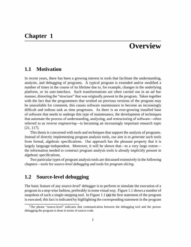
The basic feature of any source-level1 debugger is to perform or simulate the execution of aprogram in a step-wise fashion, preferably in some visual way. Figure 1.1 shows a number ofsnapshots of such a single-stepping tool. In Figure 1.1 (a) the first statement of the programis executed; this fact is indicated by highlighting the corresponding statement in the program
1The phrase “source-level” indicates that communication between the debugging tool and the persondebugging the program is done in terms of source-code.
1

2 Chapter 1. Overview
(a) (b)
(c) (d)
Figure 1.1: Snapshots of a source-level debugging tool.
text. In Figure 1.1 (b), the execution of the next statement is visualized, in this case a callto procedure incr. Figure 1.1 (c) depicts the execution of the statement out := in +1 that constitutes the body of procedure incr. Finally, in Figure 1.1 (d) execution returnsfrom the procedure.
Another common feature of a source-level debugger is state inspection, i.e., allowing theuser to query the current values of variables or expressions whenever execution is suspended.For example, a user might ask for the value of variable in when the execution reaches thepoint shown in Figure 1.1 (c). In reaction to this query, the debugging tool will determinethe value 3.
An extremely useful feature that can also be found in most debugging tools is a breakpoint.In general, a breakpoint may consist of any constraint on the program state that is suppliedby the user. The basic idea is that the user asks to continue execution of the program untilthat constraint is met. Control breakpoints consist of locations in the program (typicallystatements). When execution reaches such a designated location, the debugging tool willreturn control to the user. Control breakpoints can be quite useful to verify whether or not acertain statement in a program is executed or not. Data breakpoints consist of constraints onvalues of expressions. For example, a user may ask the debugging tool to continue execution

1.3. Program slicing 3
read(n);i := 1;sum := 0;product := 1;while i �� n dobeginsum := sum + i;product := product * i;i := i + 1
end;write(sum);write(product)
read(n);i := 1;
product := 1;while i �� n dobegin
product := product * i;i := i + 1
end;
write(product)
read(n);i := 1;
product := 1;while i �� n dobegin
end;
write(product)
(a) (b) (c)
Figure 1.2: (a) Example program. (b) Static slice of the program with respect to the final valueof variable product. (c) Dynamic slice of the program with respect to the final value of variableproduct for input n = 0.
of a program until the values of two designated variables are equal.
1.3 Program slicing
Program slicing [147, 136] is a technique for isolating computational threads in programs.Informally stated, a program slice contains the parts of a program that affect the valuescomputed at some designated point of interest (typically a statement). An alternate viewon the notion of a program slice is that of an executable projection of a program thatreplicates part of its behavior. Traditionally, a distinction between static and dynamicprogram slicing techniques is made in the literature. The former notion involves staticallyavailable information only, i.e., no assumptions regarding the inputs of a program are made.The latter notion, dynamic slicing, assumes a specific execution of the program, i.e., aspecific test-case.
The notion of a program slice is best explained by way of an example. Figure 1.2 (a)shows a simple program that reads a natural number n, and computes the sum and productof the first n numbers. Figure 1.2 (b) shows a (static) slice of this program with respect tothe value of variable product that is computed at statement write(product). Thisslice consists of all statements in the program that are needed to compute the final valueof product in any execution. Observe that neither of the assignments to variable sum ispresent in the slice, because these statements do not have an effect on the computation ofproduct’s value for any value of n. Figure 1.2 (c) shows a dynamic slice of the programin Figure 1.2 (a) with respect to the final value of product for the specific test case n = 0.Note that the entire body of the while loop is omitted from the slice. This is the case becausethe loop body is not executed if n has the value 0—therefore these statements cannot have

4 Chapter 1. Overview
an effect on any value computed by the program, and in particular they cannot have an effecton the final value of variable product. Also observe that the dynamic slice shown inFigure 1.2 (c) is only valid for input n = 0; this is evident from the fact that the slice willnot terminate for any other value of n. Chapters 3, 5, and 6 present several approaches forcomputing program slices such as as the ones shown in Figure 1.2.
The value of program slicing for program understanding (an important aspect of reverseengineering) should be self-evident: it allows a programmer doing software maintenanceto focus his attention on the statements that are involved in a certain computational thread,and to ignore potentially large sections of code that are irrelevant at the point of interest. Ina similar way, slicing can be used to examine the effect of modifications to a program, bydetermining the parts of a program that may be affected by a change.
1.4 Algebraic specifications
As was mentioned previously, our approach will be to generate program analysis toolsfrom formal specifications. More precisely, we will use algebraic specifications2 [23] of alanguage’s semantics as a basis for tool generation. Two important properties of algebraicspecifications that underlie our approach are:
� Algebraic specifications may be executed by way of term rewriting [95] or term graphrewriting [17]. This permits us to model the execution of a program abstractly, as asequence of terms that arise in a rewriting process.
� In Chapters 2 and 4 we will show that algebraic specifications implicitly define originand dynamic dependence relations on the terms that arise in any rewriting processaccording to that specification. These relations are the cornerstones for the generationof various language-specific program analysis tools that will be discussed in Chapters 5and 6.
An algebraic specification consists of a set of (conditional) equations. For specificationsof the semantics of imperative programming languages, these equations typically define the“meanings” of statements in terms of transformations of an “environment” or “store”, whichis a representation of the values computed by the program.
For example, Figure 1.3 shows two conditional equations (taken from an algebraicspecification of an interpreter for a small imperative language that will be presented inChapter 6). Together, these equations define how the execution of an if–then–else-statementcan be expressed in terms of the execution of the statements in the then-branch or theelse-branch of the if, depending on the result of the evaluation of its control predicate.The auxiliary function exec used in the two equations specifies how environments aretransformed by the execution of a list of statements. Figure 1.4 schematically depicts howan application of equation [L16] has the effect of transforming an if-term; dashed lines in
2In this thesis, we will take a rather operational perspective on algebraic specifications by considering theseas an equational high-level programming language.

1.4. Algebraic specifications 5
[L16] exec(if Exp then StatSeq else StatSeq� end;StatSeq��, Env) = exec(StatSeq��, exec(StatSeq, Env))when eval(Exp, Env) �� 0
[L17] exec(if Exp then StatSeq else StatSeq� end;StatSeq��, Env) = exec(StatSeq��, exec(StatSeq�, Env))when eval(Exp, Env) = 0
Figure 1.3: Algebraic specification of the execution of an if-statement.
cond then else
list
list
then
L16
origin relations
env
if
exec
;
exec
exec
env
Figure 1.4: Schematic view of origin relations induced by an application of equation [L16].
the figure indicate the origin relations3 between subterms of the if-term, and the term it isrewritten to. Tracing back origin relations in the sequence of terms for the execution of someprogram is a mechanism for formalizing the notion of a “current locus of execution”. Thisenables us to generate a source-level debugging tool from an algebraic specification of aninterpreter.
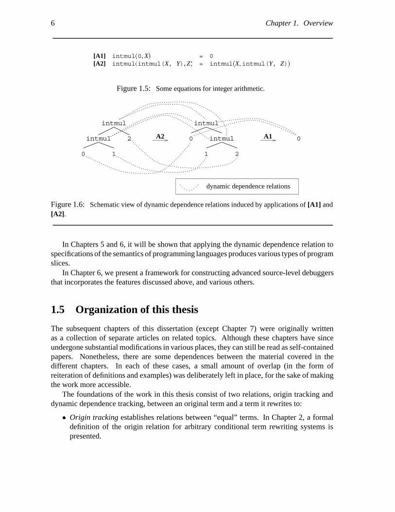
Figure 1.5 shows two simple axioms for integer arithmetic4. Equation [A1] states thatmultiplying the constant 0 with any integer number yields the value 0, and [A2] states thatmultiplication is an associative operation. Figure 1.6 depicts how, according to these tworules, a term intmul�intmul(0, 1)�2� may be rewritten to the constant 0. In thisfigure, dotted lines indicate dynamic dependence relations. Intuitively, dynamic relationsindicate which symbols are necessary for producing certain other symbols. By tracingback dynamic dependence relations from the final term, one may determine which functionsymbols in the initial term were necessary for creating it. Observe that in the examplereduction of Figure 1.6, neither of the constants 1 and 2 in the initial term was necessary forcreating the final term 0.
3The reader should be aware that this depiction is a slight simplification—a formal definition of the originfunction follows in Chapter 2.
4This example is an excerpt of a similar example that occurs in Chapter 6.
6 Chapter 1. Overview
[A1] intmul�0�X� = 0[A2] intmul�intmul(X, Y)� Z� = intmul�X�intmul(Y, Z)�
Figure 1.5: Some equations for integer arithmetic.
A2 A1
intmul
2intmul
0 1
intmul
0 intmul
1 2
0
dynamic dependence relations
Figure 1.6: Schematic view of dynamic dependence relations induced by applications of [A1] and[A2].
In Chapters 5 and 6, it will be shown that applying the dynamic dependence relation tospecifications of the semantics of programming languages produces various types of programslices.
In Chapter 6, we present a framework for constructing advanced source-level debuggersthat incorporates the features discussed above, and various others.
1.5 Organization of this thesis
The subsequent chapters of this dissertation (except Chapter 7) were originally writtenas a collection of separate articles on related topics. Although these chapters have sinceundergone substantial modifications in various places, they can still be read as self-containedpapers. Nonetheless, there are some dependences between the material covered in thedifferent chapters. In each of these cases, a small amount of overlap (in the form ofreiteration of definitions and examples) was deliberately left in place, for the sake of makingthe work more accessible.
The foundations of the work in this thesis consist of two relations, origin tracking anddynamic dependence tracking, between an original term and a term it rewrites to:
� Origin tracking establishes relations between “equal” terms. In Chapter 2, a formaldefinition of the origin relation for arbitrary conditional term rewriting systems ispresented.

1.5. Organization of this thesis 7
A Survey of Program Chapter 7
Slicing Techniques
Dynamic DependenceTracking
Chapter 2
Origin Tracking
Chapter 1
Introduction
Chapter 3
Chapter 4
Generation of Source-LevelDebugging Tools
Parametric Program SlicingChapter 5
Chapter 6
Conclusions
Figure 1.7: Dependences between the chapters in this thesis.
� Dynamic dependence tracking, defined in Chapter 4, determines the symbols of theinitial term that are necessary for producing symbols of the rewritten term. For thecasual reader, the formal definition of dynamic dependence tracking in Chapter 4 couldbe skipped on an initial reading, as Chapters 5 and 6 contain an informal presentationof dynamic dependence tracking that may be more accessible.
These relations will be used for the generation of program analysis tools, in particular forprogram slicing tools. To put our work in context, related work—in the form of an extensivesurvey of the current literature on program slicing and its applications—is presented inChapter 3.
Then, two settings are explored in which these relations are exploited for the generationof tools:
� In Chapter 5, a translational setting is described, in which rewrite rules are used totranslate terms to an intermediate representation called PIM [55]. Then, other rewriterules serve to simplify and execute the resulting PIM term. By using different subsets ofPIM’s simplification and execution rules in combination with the dynamic dependencerelation of Chapter 4, various types of program slices are obtained.
� Chapter 6 describes an interpretive setting, where program terms are directly manip-ulated by a set of rewrite rules. In this setting, the origin relation of Chapter 2 is usedfor the definition of a number of source-level debugging features, and the dynamicdependence relation of Chapter 4 permits the support of dynamic program slicingfeatures.
Finally, in Chapter 7, conclusions and directions for future work are reported. Figure 1.7depicts the main interdependences between the chapters that follow.

8 Chapter 1. Overview
1.6 Origins of the chapters
The subsequent chapters of this thesis are derived from a collection of articles that havepreviously appeared elsewhere.
Chapter 2, ‘Origin Tracking’ is a slightly modified version of a paper5 that appearedin a special issue on ‘Automatic Programming’ of the Journal of Symbolic Computation[47]. This paper was co-authored by Arie van Deursen and Paul Klint. Chapter 3, ‘ASurvey of Program Slicing Techniques’ is an updated version of CWI technical report CS-R9438 [136], and has also been submitted for journal publication. Chapter 4, ‘DynamicDependence Tracking’ is an extended version of a paper6 entitled ‘Dynamic Dependencein Term Rewriting Systems and its Application to Program Slicing’ that was presented atthe Sixth International Symposium on Programming Language Implementation and LogicProgramming held in Madrid, Spain from September 14–16, 1994 [58]. This paper waswritten jointly with John Field. Chapter 5, ‘Parametric Program Slicing’ is an extendedversion of a paper [57] presented at the Twenty-Second ACM Symposium on Principles ofProgramming Languages, in San Francisco, California from January 23–25, 1995. Thispaper was written jointly with John Field and G. Ramalingam. Chapter 6, ‘Generationof Source-Level Debugging Tools’ appeared as CWI technical report CS-R9453, entitled‘Generic Techniques for Source-Level Debugging and Dynamic Program Slicing’ [135], andwill be presented at the Sixth International Joint Conference on the Theory and Practice ofSoftware Development, to be held in Aarhus, Denmark, May 22–26, 1995. Chapter 6 is alsoloosely based on a paper entitled ‘Animators for Generated Programming Environments’ thatwas presented at the First International Workshop on Automated and Algorithmic Debuggingheld in Linkoping, Sweden from May 3–5, 1993 [134].
Some of the papers mentioned above have also appeared as deliverables of the COMPARE
project. For an overview of this project, the reader is referred to [9, 91].
5Academic Press is acknowledged for their permission to reprint parts of this paper.6Springer-Verlag is acknowledged for their permission to reprint parts of this paper.
Chapter 2
Origin Tracking
(joint work with Arie van Deursen and Paul Klint)
Summary
We are interested in generating interactive programming environments from formallanguage specifications and use term rewriting to execute these specifications. Functionsdefined in a specification operate on the abstract syntax tree of programs, and the initialterm for the rewriting process will consist of an application of some function (e.g., atype-checker, evaluator or translator) to the syntax tree of a program. During the termrewriting process, pieces of the program such as identifiers, expressions, or statements,recur in intermediate terms. We want to formalize these recurrences and use them,for example, for associating positional information with messages in error reports,visualizing program execution, and constructing language-specific debuggers. Originsare relations between subterms of intermediate terms and subterms of the initial term.Origin tracking is a method for incrementally computing origins during rewriting.We give a formal definition of origins, and present a method for implementing origintracking.
This chapter is mainly concerned with technical foundations; Chapter 6 will discussin detail how origin tracking can be used for the generation of source-level debuggingtools.
2.1 Introduction
We are interested in generating interactive development tools from formal language defi-nitions. Thus far, this has resulted in the design of an algebraic specification formalism,called ASF+SDF [23, 68] supporting modularization, user-definable syntax, associative lists,and conditional equations, and in the implementation of the ASF+SDF Meta-environment[69, 93].
Given a specification for a programming (or other) language, the Meta-environmentgenerates an interactive environment for the language in question. More precisely, the Meta-environment is a tool generator that takes a specification in ASF+SDF and derives a lexical an-alyzer, a parser, a syntax-directed editor and a rewrite engine from it. The Meta-environmentprovides fully interactive support for writing, checking, and testing specifications—all tools
9

10 Chapter 2. Origin Tracking
are generated in an incremental fashion and, when the input specification is changed, theyare updated incrementally rather than being regenerated from scratch. A central objectivein this research is to maximize the direct use that is made of the formal specification of alanguage when generating development tools for it.
We use Term Rewriting Systems (TRSs) [95] to execute our specifications. A typicalfunction (such as an evaluator, type checker, or translator) is a specification that operateson the abstract syntax tree of a program (which is part of the initial term). During the termrewriting process, pieces of the program such as identifiers, expressions, or statements, recurin intermediate terms. We want to formalize these recurrences and use them, for example,for:
� associating positional information with messages in error reports;� visualizing program execution;� constructing language-specific debuggers.
Our approach to formalize recurrences of subterms consists of two stages. First, wedefine relations for elementary reduction steps ti � ti�1; these relations are described inSection 2.1.3. Then, we extend these relations to compound reduction sequences t0 � t1 ���� � tn. In particular, we are interested in relations between subterms of an intermediateterm ti, and subterms of the initial term t0. We will call this the origin relation. Intuitively, itformalizes from which parts of the initial term a particular subterm originates. The processof incrementally computing origins we will call origin tracking.
2.1.1 Applications of origin tracking
In TRSs describing programming languages terms such as
program(decls(decl(n,natural)), stats(assign(n,34)))
are used to represent abstract syntax trees of programs. A typical type-check function takesa program and computes a list of error messages. An example of the initial and final termwhen type checking a simple program is shown in Figure 2.1.
The program uses an undeclared variable n1, and the result of the type-checker is a termrepresenting this fact, i.e., a term with undeclared-var as function symbol and the namen1 of the undeclared variable as argument. The dashed line represents an origin: it relatesthe occurrence of n1 in the result to the n1 in the initial term. One can use this to highlightthe exact position of the error in the source program. Figure 2.2 shows an application of thistechnique.
Similarly, program evaluators can be defined. Consider for example a rule that evaluatesa list of statements by evaluating the first statement followed by the remaining statements:
[L1] ev-list(cons(Stat,S-list),Env) � ev-list(S-list,ev-stat(Stat,Env))
The variables (Stat, S-list, and Env) are used to pass information from the left to the right-handside. The origins of these variable occurrences in the right-hand side are shown by dashedlines in Figure 2.3.

2.1. Introduction 11
tc
program
decls stats
decl
n natural
assign
n1 34
errorlist� � �
undeclared-var
n1
Figure 2.1: Type-checking a simple program.
Figure 2.2: Highlighting occurrences of errors.

12 Chapter 2. Origin Tracking
ev-list
cons
Stat S-list
Env
ev-list
S-list ev-stat
Stat Env
Figure 2.3: One step in the evaluation of a simple program. Dashed lines indicate how the ruleapplication induces origin relations.
Visualization of program execution is a natural application of origin tracking. The basicidea is that, during execution, the statement currently being executed is highlighted in thesource text. In the sequel, it will be shown how this can be accomplished by matching redexesagainst the pattern ev-stat(Stat, Env); whenever such a match occurs, the origin of thefirst argument of ev-stat indicates the statement that is currently being executed. Dineshand Tip [49, 134] have shown how, by employing multiple patterns, program execution canbe animated in a very fine-grained manner: the execution of any language construct (e.g.,expressions, declarations) can be traced. This is particularly useful for applications such assource-level debugging and tutoring.
In a similar way, various notions of breakpoints can be defined. Source-level debuggersoften have a completely fixed notion of a breakpoint, based on line-numbers, procedure callsand machine addresses. By contrast, the origin relation enables one to define breakpoints ina much more uniform and generic way. For instance, a positional breakpoint can be createdby having the user select a certain point in the source text. The path from the root to thatpoint is recorded and the breakpoint becomes effective when—in this example—the originof the first argument of ev-stat equals that path. Position-independent breakpoints canbe defined by using patterns describing statements of a certain form (e.g., an assignmentwith x as left-hand side). The breakpoint becomes effective when the argument of ev-statmatches that pattern; its origin shows the position in the original program. The definition ofthese, and other debugging concepts will be further explored in Chapter 6.
2.1.2 Points of departure
Before sketching the origin relation (in Section 2.1.3) we briefly state our points of departure:
� No assumptions should be made regarding the choice of a particular reduction strategy.� No assumptions should be made concerning confluence or termination; origins can be
established for arbitrary reductions in any TRS.� The origin relation should be obtained by a static analysis of the rewrite rules.

2.1. Introduction 13
4
3
1 1 2
1. common variables2. common subterms3. redex-contractum4. contexts
Figure 2.4: Single-step origin relations.
� Relations should be established between any intermediate term and the initial term.This implies that relations can be established even if there is no normal form.
� Origins should satisfy the property that if t has an origin t�, then t� can be rewritten tot in zero or more steps.
� The origin relation should be transitive.� An efficient implementation should exist.
These requirements do not lead, however, to a unique solution. We will therefore onlypresent one of the possible definitions of origins, although we can easily imagine alternativeones.
2.1.3 Origin relations
The definition of the origin relation is based on the transitive and reflexive closure of a numberof single-step origin relations for elementary reductions, which will now be studied in somedetail. In the description that follows it is assumed that a rewrite rule r : t1 � t2 is appliedin context C with substitution �, giving rise to the elementary reduction C#t�1 $ �r C#t�2 $.Figure 2.4 depicts the four types of single-step origin relations that occur:
common variables. If a variableX appears in both sides, t1 and t2, of rule r, then relationsare established between each function symbol in the instantiation X� of X in C#t�1 $ and thecorresponding function symbol in each instantiated occurrence of X in C#t�2 $.
Figure 2.5 illustrates how the variable X induces relations between corresponding functionsymbols for a specific application of the rule f(X) � g(X).
The common variables relation becomes a bit more complicated for left-nonlinearrules, i.e., rules where some variable X occurs more than once in the left-hand side, e.g.,plus(X,X) � mul(2, X). In this case, all occurrences of X in the left-hand side give

14 Chapter 2. Origin Tracking
f
h
a b
g
h
a b
Figure 2.5: Relations according to a variable occurrence in both sides of a rule.
append
E empty-list
cons
E empty-list
Figure 2.6: Relations according to common subterms rule.
rise to origin relations. In other words, nonlinearity in the left-hand side may cause non-uniqueness of origins.
common subterms. If a term s is a subterm of both t1 and of t2, then these occurrences ofs give rise to common subterms relations between their instantions. Consider, for example,the following rules that define how an element is appended to the end of a list:
[A1] append(E,empty-list) � cons(E,empty-list)[A2] append(E1,cons(E2,L)) � cons(E2, append(E1,L))
Using the common variables relation, several useful origin relations will be constructed.However, no such relation is present for the constant empty-list that occurs in eitherside of [A1]. This relation is established by the common subterms rule, and is depictedin Figure 2.6. A more elaborate example involving the common subterms relation is theconditional rule [W1] for evaluating while-statements:
[W1] ev-stat(while(Exp,S-list),Env) �ev-stat(while(Exp,S-list),ev-list(S-list,Env))
when ev-exp(Exp, Env) = true
When evaluation of Exp yields true, the same while-statement is evaluated in a modifiedenvironment that is obtained by evaluating the body of the while-statement (S-list) in theinitial environment (Env). The common subterms relation links these while-symbols.
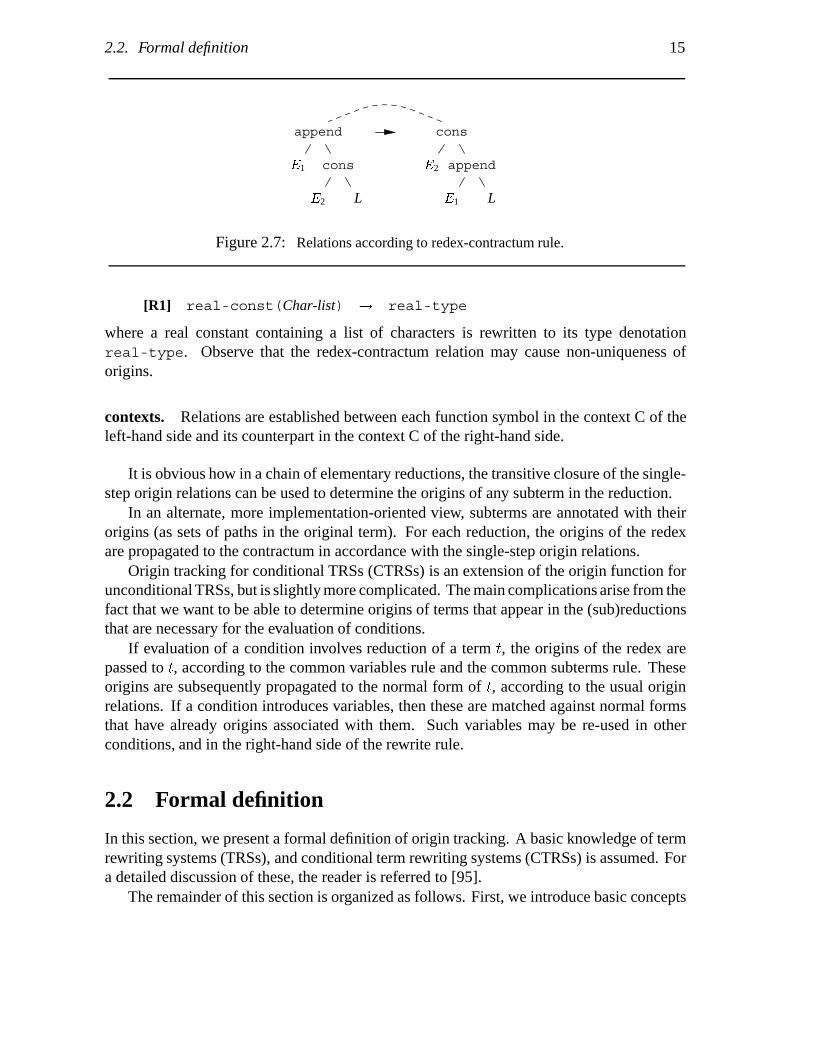
redex-contractum. The top symbol of the redex t�1 and the top symbol of its contractumt�2 are related, as shown in Figure 2.7 for rule [A2]. An essential application of this relationcan be seen in
2.2. Formal definition 15
append
E1 cons
E2 L
cons
E2 append
E1 L
Figure 2.7: Relations according to redex-contractum rule.
[R1] real-const(Char-list) � real-type
where a real constant containing a list of characters is rewritten to its type denotationreal-type. Observe that the redex-contractum relation may cause non-uniqueness oforigins.
contexts. Relations are established between each function symbol in the context C of theleft-hand side and its counterpart in the context C of the right-hand side.
It is obvious how in a chain of elementary reductions, the transitive closure of the single-step origin relations can be used to determine the origins of any subterm in the reduction.
In an alternate, more implementation-oriented view, subterms are annotated with theirorigins (as sets of paths in the original term). For each reduction, the origins of the redexare propagated to the contractum in accordance with the single-step origin relations.
Origin tracking for conditional TRSs (CTRSs) is an extension of the origin function forunconditional TRSs, but is slightly more complicated. The main complications arise from thefact that we want to be able to determine origins of terms that appear in the (sub)reductionsthat are necessary for the evaluation of conditions.
If evaluation of a condition involves reduction of a term t, the origins of the redex arepassed to t, according to the common variables rule and the common subterms rule. Theseorigins are subsequently propagated to the normal form of t, according to the usual originrelations. If a condition introduces variables, then these are matched against normal formsthat have already origins associated with them. Such variables may be re-used in otherconditions, and in the right-hand side of the rewrite rule.
2.2 Formal definition
In this section, we present a formal definition of origin tracking. A basic knowledge of termrewriting systems (TRSs), and conditional term rewriting systems (CTRSs) is assumed. Fora detailed discussion of these, the reader is referred to [95].
The remainder of this section is organized as follows. First, we introduce basic concepts
16 Chapter 2. Origin Tracking
and rewriting histories for unconditional TRSs. Subsequently, the origin function for un-conditional TRSs is defined, and illustrated by way of an example. After discussing basicconcepts and rewriting histories for CTRSs, we consider the origin function for CTRSs.
We have used the formal definition of the origin relation to obtain an executable specifi-cation of origin tracking. The examples that will be given in this section have been verifiedautomatically using that specification.
2.2.1 Basic concepts for unconditional TRSs
A notion that will frequently recur is that of a path (occurrence), consisting of a (possiblyempty) sequence of natural numbers between brackets. Paths are used to indicate subtermsof a term by interpreting numbers as argument positions of function symbols. For instance,(2 1) indicates subterm b of term f(a, g(b, c)). This is indicated by the ‘�’ operator:f(a, g(b, c))�(2 1) = b. The associative operator ‘�’ concatenates paths, e.g., (2) � (1)= (2 1). The operators ‘�’, ‘�’, and ‘j’ define the prefix ordering on paths. The fact that pis a prefix of q is denoted p � q; ‘�’ is the reflexive closure of ‘�’. Two paths p and q aredisjoint (denoted by p j q) if neither one is a prefix of the other.
The set of all valid paths in a term t is O�t�. The set of variables occurring in t is denotedVars�t�. We use t� � t to express that t� appears as a subterm of t; the reflexive closure of‘�’ is ‘’. The negations of ‘�’ and ‘’ are ‘�’ and ‘’, respectively. Finally, Lhs(r) andRhs(r) indicate the left-hand side and the right-hand side of a rewrite rule r.
2.2.2 A formalized notion of a rewriting history
A basic assumption in the subsequent definitions is that the complete history of the rewritingprocess is available. This is by no means essential to our definitions, but has the followingadvantages:
� The origin function for CTRSs can be defined in a declarative, non-recursive manner.We encountered ill-behaved forms of recursion in the definition itself when we exper-imented with more operational definition methods, due to the convoluted structure ofrewriting histories for CTRSs.
� Uniformity of the origin functions for unconditional TRSs and for CTRSs. The lattercan be defined as an extension of the former.
In the case of unconditional TRSs, the rewriting history H is a single reduction sequence S.This sequence consists of a list of sequence elementsSi that contain all information involvingthe ith rewrite-step. Here, i ranges from 1 to jSj where jSj is the length of sequence S.
Each sequence element is a 5-tuple �n� t� r� p� �� where n is the name of the sequenceelement (consisting of a sequence name and a number), t denotes the ith term of sequenceS, r the ith rewrite rule applied, p the path to the redex in t, and � the substitution used inthe application of r. Access functions n�s�, t�s�, r�s�, p�s�, and ��s� are used to obtain thecomponents of s. The last element of a sequence is irregular, because the term associated
2.2. Formal definition 17
with this element is in normal form: the rule, path and substitution associated with SjSjconsist of the special value undefined.
Below, s, s�, and s�� denote sequence elements. Moreover, it will be useful to have anotion H� denoting the history H from which the last sequence element, SjSj, is excluded.For our convenience, we introduce Lhs�s� and Rhs�s� to denote the left-hand side andright-hand side of r�s�. Finally, Succ�H� s� denotes the successor of s, for s in H�, andStart�H� determines the first element of the reduction sequence in H.
2.2.3 The origin function for unconditional TRSs
2.2.3.1 Auxiliary notions
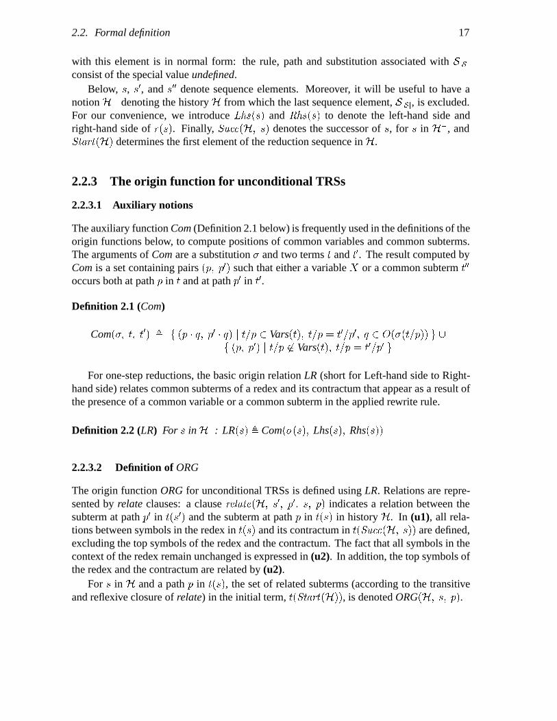
The auxiliary function Com (Definition 2.1 below) is frequently used in the definitions of theorigin functions below, to compute positions of common variables and common subterms.The arguments of Com are a substitution � and two terms t and t�. The result computed byCom is a set containing pairs �p� p�� such that either a variable X or a common subterm t��
occurs both at path p in t and at path p� in t�.
Definition 2.1 (Com)
Com��� t� t�� � f �p � q� p� � q� j t�p � Vars�t�� t�p � t��p�� q � O���t�p�� g �f �p� p�� j t�p � Vars�t�� t�p � t��p� g
For one-step reductions, the basic origin relation LR (short for Left-hand side to Right-hand side) relates common subterms of a redex and its contractum that appear as a result ofthe presence of a common variable or a common subterm in the applied rewrite rule.
Definition 2.2 (LR) For s in H�: LR�s� � Com���s�� Lhs�s�� Rhs�s��
2.2.3.2 Definition of ORG
The origin function ORG for unconditional TRSs is defined using LR. Relations are repre-sented by relate clauses: a clause relate�H� s�� p�� s� p� indicates a relation between thesubterm at path p� in t�s�� and the subterm at path p in t�s� in history H. In (u1), all rela-tions between symbols in the redex in t�s� and its contractum in t�Succ�H� s�� are defined,excluding the top symbols of the redex and the contractum. The fact that all symbols in thecontext of the redex remain unchanged is expressed in (u2). In addition, the top symbols ofthe redex and the contractum are related by (u2).
For s in H and a path p in t�s�, the set of related subterms (according to the transitiveand reflexive closure of relate) in the initial term, t�Start�H��, is denoted ORG�H� s� p�.

18 Chapter 2. Origin Tracking
append
b cons
a empty-list
A2
cons
a append
b empty-list
A1
cons
a cons
b empty-list
t�S1�: t�S2�: t�S3�:
Figure 2.8: History Happ for append(b, cons(a, empty-list)). Dashed lines indicateorigin relations.
Definition 2.3 (ORG) For s in H� and s� in H:
�u1� �q� q�� � LR�s� : relate�H� s� p�s� � q� Succ�H� s�� p�s� � q���u2� p : �p � p�s�� � �p j p�s�� : relate�H� s� p� Succ�H� s�� p�
ORG�H� s� p� �
���������
f p g when s � Start�H�
f p�� j p�� � ORG�H� s�� p���relate�H� s�� p�� s� p� g
when s � Start�H�
In principle, the availability of all relate clauses allows us to determine relationshipsbetween subterms of two arbitrary intermediate terms that occur during the rewriting process.However, we will focus on relations involving the initial term.
2.2.3.3 Example
As an example, we consider the TRS consisting of the two rewrite rules [A1] and [A2] ofsection 2.1.3. Figure 2.8 shows a history Happ, consisting of a sequence S, as obtained byrewriting the term append(b, cons(a, empty)).
Below, we argue how the origin relations shown in Figure 2.8 are derived from Def-inition 2.3. For the first sequence element, S1, we have p�S1� � ��, r�S1� = [A2], and��S1� � f E1 �� b� E2 �� a� L �� empty-list g. As all variable bindings are constantshere, we have: O�E1
��S1�� = O�E2��S1�� = O�L��S1�� = f �� g. From this, we obtain:
LR�S1� � Com���S1�� Lhs�S1�� Rhs�S1�� � f ��1�� �2 1��� ��2 1�� �1��� ��2 2�� �2 2�� g
In a similar way, we compute:
LR�S2� � Com���S2�� Lhs�S2�� Rhs�S2�� � f ��1�� �1��� ��2�� �2�� g

2.2. Formal definition 19
From Definition 2.3 we now derive the following relate relationships. (Note that the lastthree relationships are generated according to (u1) of Definition 2.3.)
relate�Happ� S1� �1�� S2� �2 1�� relate�Happ� S1� �2 1�� S2� �1��relate�Happ� S1� �2 2�� S2� �2 2�� relate�Happ� S1� ��� S2� ���relate�Happ� S2� �2 1�� S3� �2 1�� relate�Happ� S2� �2 2�� S3� �2 2��relate�Happ� S2� ��� S3� ��� relate�Happ� S2� �1�� S3� �1��relate�Happ� S2� �2�� S3� �2��
As an example, we compute the subterms related to the constant a at path (1) in t�S3�:
ORG�Happ� S3� �1�� � f p�� j p�� � ORG�Happ� s�� p��� relate�Happ� s
�� p�� S3� �1�� g� f p�� j p�� � ORG�Happ� S2� �1�� g� ORG�Happ� S2� �1��� f p�� j p�� � ORG�Happ� s
�� p��� relate�Happ� s�� p�� S2� �1�� g
� f p�� j p�� � ORG�Happ� S1� �2 1�� g� ORG�Happ� S1� �2 1��� f �2 1� g
Hence, the constant a at path (1) in t�S3� is related to the constant a at path (2 1) in the initialterm.
We conclude this example with a few brief remarks. First, some symbols in t�S3� arenot related to any symbol of t�S1�. For instance, symbol cons at path (2) in t�S3� is onlyrelated to symbol append in t�S2�; this symbol, in turn, is not related to any symbol int�S1�. Second, we have chosen a trivial example where no origins occur that contain morethan one path. Such a situation may arise when a rewrite rule is not left-linear, or when theright-hand side of a rewrite rule consists of a common variable or a common subterm.
2.2.4 Basic concepts for CTRSs
A conditional rewrite-rule takes the form:
lhs � rhs when l1 � r1� � � � � ln � rn
We assume that CTRSs are executed as join systems [95]: both sides of a condition areinstantiated and normalized. A condition succeeds if the resulting normal forms are syntac-tically equal. It is assumed that the conditions of a rule are evaluated in left-to-right order.As an extension, we allow one side of a condition to introduce variables1; we will referto such variables as new variables (as opposed to old variables that are bound during thematching of the left-hand side, or during the evaluation of a previous condition). To avoidcomplications in our definitions, we impose the non-essential restriction that no conditionside may contain old as well as new variables. New variables may occur in subsequentconditions as well as in the right-hand side. Variable-introducing condition sides are not
1An example CTRS with variable-introducing conditions will be discussed in Section 2.2.6.3 below.
20 Chapter 2. Origin Tracking
normalized, but matched against the normal form of the non-variable-introducing side (fordetails, see [140]). Given the above discussion, conditional term rewriting can be regardedas the following cyclic 3-phase process:
1. Find a match between a subterm t and the left-hand side of a rule r.2. Evaluate the conditions of r: instantiate and normalize non-variable-introducing con-
dition sides.3. If all conditions of r succeed: replace t by the instantiated right-hand side of r.
In will be convenient to introduce some auxiliary notions that formalize the introductionof variables in conditions. Let jrj be the number of conditions of r. For 1 � j � jrj, theleft-hand side and the right-hand side of the jth condition of r are denoted Side�r� j� left�and Side�r� j� right�, respectively. Moreover, let left � right and right � left . Thefunction VarIntro (Definition 2.4) indicates where new variables occur; tuples �h� side� arecomputed, indicating that Side�r� h� side� is variable-introducing.
Definition 2.4 (VarIntro)
VarIntro�r� � f �h� side� j X Lhs�r�� X Side�r� h� side�� j �j � h� side� : X Side�r� j� side�� g
For convenience, we also define a function NonVarIntro (Definition 2.5) that computestuples �h� side� for all non-variable-introducing condition sides.
Definition 2.5 (NonVarIntro)
NonVarIntro�r� � f �h� side� j 1 � h � jrj� side � f left� right g��h� side� � VarIntro�r� g
2.2.5 Rewriting histories for CTRSs
In phase 2 of the 3-phase process sketched in Section 2.2.4 above, each normalization ofan instantiated condition side is a situation similar to the normalization of the original term,involving the same 3-phase process. Thus, we can model the rewriting of a term as a tree ofreduction sequences. The initial reduction sequence named Sinit starts with the initial termand contains sequence elements Sinit
i that describe successive transformations of the initialterm. In addition, H now contains a sequence for every condition side that is normalizedin the course of the rewriting process. Two sequences appear for non-variable-introducingconditions, but for variable-introducing conditions only one sequence occurs in H (for thenon-variable-introducing side).
Formally, we define the history as a flat representation of this tree of reduction sequences.A history now consists of two parts:
� A set of uniquely named reduction sequences. Besides the initial sequence, Sinit,there is a sequence Sk (with k an integer) for every condition side that is normalizedin the course of the rewriting process.As before, a sequence consists of one or more sequence elements, and each sequence

2.2. Formal definition 21
element is a 5-tuple �n� t� r� p� ��, denoting the name, term, rule, path, and substitutioninvolved. As in the unconditional case, access functions are provided to obtain thecomponents of s. A name of a sequence element is composed of a sequence name anda number, permitting us to find out to what sequence an element belongs.
� A mechanism indicating the connections between the various reduction sequences.This mechanism takes the form of a relation that determines a sequence name givena name of a sequence element s, a condition number j, and a condition side side,for all �j� side� � NonVarIntro�s�. E.g., a tuple �n�s�� j� side� sn� indicates that asequence named sn occurred as a result of the normalization of Side�s� j� side�.
Two functions First and Last are defined, both taking four arguments: the history H, asequence element s, a condition number j, and a condition side side. First�H� s� j� side�retrieves the name of s, determines the name of the sequence associated with side side
of condition j of r�s�, looks up this sequence in H, and returns the first element of thissequence. Last�H� s� j� side� is similar: it determines the last element of the sequenceassociated with side side of condition j of r�s�.
Furthermore, H� now denotes the history H from which all last elements of sequencesare excluded, Succ�H� s� now denotes the successor of s in the same sequence, for s in H�,and Start�H� determines the first element of the initial sequence in H. Finally, we introducethe shorthands Side�s� j� side�, VarIntro�s�, and NonVarIntro�s� for Side�r�s�� j� side�,VarIntro�r�s��, and NonVarIntro�r�s��, respectively.
2.2.6 The origin function for CTRSs
2.2.6.1 Basic origin relations
The basic origin relation LR (Definition 2.2) defines relations between consecutive elementss and Succ�H� s� of the same sequence. The basic origin relations LC, CR, and CC definerelations between elements of different sequences. Each of these relations reflects thefollowing principle: common subterms are only related when a common variable or acommon subterm appears at corresponding places in the left-hand side, right-hand side andcondition side of the rewrite rule involved.
Definition 2.6, LC (Left-hand side to Condition side), defines relations that result fromcommon variables and common subterms of the left-hand side and a condition side of a rule.An LC-relation connects a sequence element s to the first element s� of a sequence for thenormalization of a condition side of r�s�. The relation consists of triples �q� q�� s�� indicatinga relation between the subterm at path q in the redex and the subterm at path q� in t�s��.
We do not establish LC-relations for variable-introducing condition sides, because suchrelations are always redundant. To understand this, consider the fact that we disallowinstantiated variables in variable-introducing condition sides. Thus, LC relations wouldalways correspond to a common subterm t of the left-hand side and a variable-introducingcondition side. Then, only if t also occurs in a subsequent condition side, or in the right-handside of the rule can the relation be relevant for the remainder of the rewriting history. But ifthis is the case, this other occurrence of t will be involved in an LC-relation anyway.
22 Chapter 2. Origin Tracking
Definition 2.6 (LC) For s in H�:
LC�H� s� � f �q� q�� s�� j �j� side� � NonVarIntro�s�� s� � First�H� s� j� side���q� q�� � Com���s�� Lhs�s�� Side�s� j� side�� g
In Definition 2.7 and Definition 2.8 below, the final two basic origin relations, CR (Con-dition side to Right-hand side) and CC (Condition side to Condition side) are presented.These relations are concerned with common variables and common subterms in variable-introducing condition sides. In addition to a variable-introducing condition side, theserelations involve the right-hand side, and a non-variable-introducing condition side, respec-tively. The following technical issues arise here:
� There are no CR and CC relations for non-variable-introducing conditions, becauseboth condition sides are normalized in this case, and no obvious correspondence withthe syntactical form of the rewrite rule remains.
� As mentioned earlier, no reduction sequence appears in H for a variable-introducingcondition side. To deal with this issue, the variable-introducing side Side�s� j� side�is used to indicate relations with the term t�Last�H� s� j� side�� it is matched against.
CR-relations are triples �q� q�� s�� indicating that the subterm at path q in t�s�� is relatedto the subterm at path q� in the contractum; CC-relations are quadruples �q� q�� s�� s��� thatexpress a relation between the subterm at path q in t�s�� and the subterm at path q� in t�s���.
Definition 2.7 (CR) For s in H�:
CR�H� s� � f�q� q�� s�� j �j� side� � VarIntro�s�� s� � Last�H� s� j� side���q� q�� � Com���s�� Side�s� j� side�� Rhs�s�� g
Definition 2.8 (CC) For s in H�:
CC�H� s� � f�q� q�� s�� s��� j �j� side� � VarIntro�s�� �h� side�� � NonVarIntro�s��j � h� s� � Last�H� s� j� side�� s�� � First�H� s� h� side����q� q�� � Com���s�� Side�s� j� side�� Side�s� h� side��� g
2.2.6.2 Definition of CORG
The origin function CORG for CTRSs (Definition 2.9) is basically an extension of ORG.Using the basic origin relations LC, CR, and CC, relations between elements of differentreduction sequences are established in (c1), (c2), and (c3). Again, the origin functioncomputes a set of paths in the initial term according to the transitive and reflexive closure ofrelate. For any sequence element s in H, and any path p in t�s�, CORG computes a set ofpaths to related subterms in t�Start�H��.

2.2. Formal definition 23
Definition 2.9 (CORG) For s in H� and s� in H:
�u1� �q� q�� � LR�s� : relate�H� s� p�s� � q� Succ�H� s�� p�s� � q���u2� p : �p � p�s�� � �p j p�s�� : relate�H� s� p� Succ�H� s�� p��c1� �q� q�� s�� � LC�H� s� : relate�H� s� p�s� � q� s�� q���c2� �q� q�� s�� � CR�H� s� : relate�H� s�� q� Succ�H� s�� p�s� � q���c3� �q� q�� s�� s��� � CC�H� s� : relate�H� s�� q� s��� q��
CORG�H� s� p� �
���������
f p g when s� � Start�H�
f p�� j p�� � CORG�H� s�� p���relate�H� s�� p�� s� p� g
when s� � Start�H�
2.2.6.3 Example
We extend the example of section 2.2.3.3 with the following conditional rewrite rules for afunction rev to reverse lists.
[R1] rev(empty-list) � empty-list[R2] rev(cons(E, L1)) � append(E, L2) when L2 = rev(L1)
In rule [R2], a variable L2 is introduced in the left-hand side of the condition. Actually, theuse of a new variable is not necessary in this case: we may alternatively write append(E,rev(L1)) for the right-hand side of [R2]. The new variable is used solely for the sakeof illustration. Figure 2.9 shows the rewriting history Hrev for the term rev(cons(b,empty-list)). Note that besides the initial sequence, Sinit, only one sequence, S1,appears for the normalization of the condition of [R2], because it is variable-introducing.
For sequence elementSinit1 we have p�Sinit
1 � = ��, ��Sinit1 � = f E �� b, L1 �� empty-
list, L2 �� empty-list g. It follows that O�E��Sinit1 �� = O�L1��Sinit1 �� = O�L2
��Sinit1 ��= f �� g. Moreover, VarIntro�Sinit
1 � = f �1� left� g. Consequently, we obtain:
LR�Sinit1 � � f ��1 1�� �1�� g� LC �Hrev� S
init1 � � f ��1 2�� �1�� S1
1 � gCR�Hrev� S
init1 � � f ���� �1�� S1
2 � g� CC �Hrev� Sinit1 � � �
As a result, the following relationships are generated for Sinit1 :
relate�Hrev� Sinit1 � ��� Sinit
2 � ��� relate�Hrev� Sinit1 � �1 1�� Sinit
2 � �1��relate�Hrev� S
init1 � �1 2�� S1
1 � �1�� relate�Hrev� S12 � ��� S
init2 � �2��
In a similar way, the following relate relationships are computed for Sinit2 and S11 :
relate�Hrev� Sinit2 � ��� Sinit
3 � ��� relate�Hrev� Sinit2 � �1�� Sinit
3 � �1��relate�Hrev� S
init2 � �2�� Sinit
3 � �2�� relate�Hrev� S11 � ��� S
12 � ���
relate�Hrev� S11 � �1�� S
12 � ���
Finally, we compute the subterms related to empty-list at path (2) in t�Sinit3 �:

24 Chapter 2. Origin Tracking
rev
cons
b empty-list
append
b empty-list
cons
b empty-list
rev
empty-list
empty-list
R2 A1
R1
t�Sinit1 �: t�Sinit
2 �: t�Sinit3 �:
t�S11 �: t�S1
2 �:
sequence Sinit:
sequence S1:
Figure 2.9: History Hrev for rev(cons(b, empty-list)). Dashed lines indicate originrelations.
CORG�Hrev� Sinit3 � �2�� �
� f p�� j p�� � CORG�Hrev� s�� p��� relate�Hrev� s
�� p�� Sinit3 � �2�� g
� f p�� j p�� � CORG�Hrev� Sinit2 � �2�� g
� CORG�Hrev� Sinit2 � �2��
� � � � � f �1 2� g
Consequently, the constant empty-list in t�Sinit3 � is related to the constant empty-list
in t�S init1 �.
2.3 Properties
The origins defined by CORG have the following property: if the origin of some intermediateterm tmid contains a path to initial subterm torg , then torg can be rewritten to tmid in zero ormore reduction steps. This property gives a good intuition of the origin relations that areestablished in applications such as error handling or debugging.
To see why this property holds, we first consider one reduction step:
Lemma 2.10 Let H be a rewriting history, s� s� arbitrary sequence elements in H, and p� p�
paths. For any relate�H� s� p� s�� p�� we have t�s� � t�s�� or t�s� � t�s��.

2.3. Properties 25
Informally stated, directly related terms are either syntactically equal or one can bereduced to the other in exactly one step. This holds because the context, common variables,and common subterms relations all relate identical terms. Only the redex-contractum relationlinks non-identical terms, but these can be rewritten in one step. Since the origin relationCORG is defined as the transitive and reflexive closure of relate, we now have the desiredproperty:
Theorem 2.11 Let H be a history. For every term t�s� occurring in some sequence elements in history H, and for every path p � O�t�s��, we have:
q � CORG�H� s� p� � t�Start�H���q �� t�s��p
One may be interested in the number of paths in an origin. To this end, we introduce:
Definition 2.12 Let o be an origin, and let joj denote the number of paths in o. Then: o isempty iff joj � 0, non-empty iff joj � 1, precise iff joj � 1, and unitary iff joj � 1.
For some applications, unitary origins are desirable. In animators for sequential programexecution, one wants origins that refer to exactly one statement. On the other hand, whenerror-positioning is the application, it can be desirable to have non-unitary origins, as forinstance in errors dealing with multiple declarations of the same variable (see, e.g., the labeldeclaration in Figure 2.2).
The theorems below indicate how non-empty, precise and unitary origins can be detectedthrough static analysis of the CTRS. In the sequel r denotes an arbitrary rule, j is a numberof some condition in r, and side � fleft � rightg denotes an arbitrary side. In the sequel, aterm that (possibly) contains variables will be referred to as an open term.
Theorem 2.13 (Non-empty origins) Terms with top symbol f have non-empty origins if forall open terms u with top function symbol f :
�1� u Rhs�r� � u Lhs�r��2� u Side�r� j� side� � u Lhs�r�
This can be proven by induction over all relate clauses, after introducing an ordering on allsequence elements. Informally, all terms with top symbol f will have non-empty originsif no f is introduced that is not related to a “previous” f . Note that relations according tovariables have no effect on origins being (non-)empty.
In order to characterize sufficient conditions for precise and unitary origins, we first needsome definitions:
Definition 2.14 Let r be a conditional rewrite rule and u an open term. Then r is anu-collapse rule if Rhs�r� � u, and u Lhs�r�.
Definition 2.15 For open terms t and u, t is linear in u if u occurs at most once in t.
26 Chapter 2. Origin Tracking
Definition 2.16 The predicate LinearIntro�u� r� holds if u has at most one occurrencein either the left-hand side or any variable-introducing condition side. Formally,LinearIntro�u� r� � there is (1) at most one t � fLhs�r�g � fSide�r� h� side� j �h� side� �VarIntro�r�g such that u t, and (2) this t, if it exists, is linear in u.
Theorem 2.17 (Precise origins) Terms with top symbol f have precise origins if the fol-lowing holds for all open terms u having either f as top symbol or solely consisting of avariable:
(1) The CTRS does not contain u-collapse rules(2) u Rhs�r� � LinearIntro�u� r�(3) u Side�r� j� side� � LinearIntro�u� r�
Again, this theorem can be proven by induction over all relates. The crux is that noterm with top function symbol f is introduced in a way that it is related to more than one“previous” term.
Theorem 2.18 (Unitary origins) Since “non-empty” and “precise” implies “unitary”, com-bining the premises of Theorems 2.13 and 2.17 yields sufficient conditions for unitary origins
For many-sorted CTRSs, some special theorems hold. We assume CTRSs to be sort-preserving, i.e., the redex and the contractum belong to the same sort. Hence, CORG issort-preserving. Thus, we have the following theorem (which in the implementation allowsfor an optimization—Section 2.4):
Theorem 2.19 relate can be partitioned into subrelations for each sort.
One may be interested whether all terms of some particular sort S have non-empty, pre-cise, or unitary origins. This happens under circumstances very similar to those formulatedfor the single-sorted case (Theorems 2.13 to 2.18). For precise and unitary origins, however,it is not sufficient to consider only terms of sort S; one also needs to consider sorts T that canhave subterms of sort S (since duplication of T-terms may imply duplication of S-terms).Hence, we define:
Definition 2.20 For two sorts S and T, we write S v T if terms of sort T can containsubterms of sort S.
Using this, we can formulate when terms of sort S have precise or unitary origins. Thisis similar to the single-sorted case (see Theorem 2.17), but in (1) u must be of sort S, and (2)and (3) must hold for all u of sort T such that S v T. Unitary origins of sort S are obtainedby combining the premises for the non-empty origins and precise origins.
We refer to [46] for more elaborate discussions of the above results.
2.4 Implementation aspects
An efficient implementation of origin tracking in the ASF+SDF system has been completed.In this section, we briefly address the principal aspects of implementing origin tracking.

2.4. Implementation aspects 27
2.4.1 The basic algorithm
In our implementation, each symbol is annotated with its origin, during rewriting. Twoissues had to be resolved:
� annotation of the initial term� propagation of origins during rewriting
The first issue is a trivial matter because—by definition—the origin of the symbol at path pis f p g. The second issue is addressed by copying origins from the redex to the contractumaccording to the basic origin relation LR. In a similar way, propagations occur for the basicorigin relations LC, CC, and CR. Observe that no propagations are necessary for the originsin the context of the redex, as the origins of these symbols remain unaltered.
2.4.2 Optimizations
Several optimizations of the basic algorithm have been implemented:
� All positional information (i.e., the positions of common variables and common sub-terms) is computed in advance, and stored as annotations of rewrite rules.
� The rewriting engine of the ASF+SDF system explicitly constructs a list of variablebindings. Origin propagations that are the result of common variables can be imple-mented as propagations to these bindings. When a right-hand side or condition side isinstantiated, all common variable propagations are handled as a result of the instanti-ation. The advantage of this approach is that the number of propagations decreases,because we always propagate to only one subterm for each variable.
� Origins are implemented as a set of pointers to function symbols of the initial term.The advantages are twofold: less space is needed to represent origins, and set unionbecomes a much cheaper operation.
2.4.3 Associative lists
In order to implement origin tracking in the ASF+SDF system, provisions had to be madefor associative lists [69, 140]. Associative lists can be regarded as functions with a variablearity. Allowing list functions in CTRSs introduces two minor complications:
� A variable that matches a sublist causes relations between arrays of adjacent subterms.In the implementation, we distinguish between ordinary variables and list variables,and perform propagations accordingly.
� Argument positions below list functions depend on the actual bindings. Therefore,when computing the positions of common variables and common subterms, posi-tions below lists are marked as relative. The corresponding absolute positions aredetermined during rewriting.
Consider the following example, where l is a list function, and X* is a list variable thatmatches sublists of any length:

28 Chapter 2. Origin Tracking
[L1] f(l(X*, a)) � g(l(X*, a))
When we rewrite the redex f(l(b, c, a)) according to [L1], the contractum is g(l(b,c, a)). Variable X* gives rise to both a relation between the constants b in the redex andthe contractum, and a relation between the constants c in the redex and the contractum.Moreover, constant a appears at path (1 2) in the left-hand side of [L1], but at path (1 3) inthe redex.
2.4.4 Sharing of subterms
For reasons of efficiency, implementations of CTRSs allow sharing of subtrees, thus givingrise to DAGs (Directed Acyclic Graphs) instead of trees. The initial term is represented asa tree, and sharing is introduced by instantiating nonlinear right-hand sides and conditionsides. For every variable, the list of bindings contains a pointer to one of the subterms it wasmatched against. Instantiating a right-hand side or condition side is done by copying thesepointers (instead of copying the terms in the list of bindings). Sharing has the followingrepercussions for origin tracking:
� No propagations are needed for variables that occur exactly once in the left-hand side(and for new variables that occur exactly once in the introducing condition). Thisresults in a radical reduction of the number of propagations.
� Variables that occur nonlinearly in the left-hand side of a rule (and new variablesthat occur nonlinearly in the introducing condition) present a problem. When sharingis allowed in this case, inconsistent origins with respect to the definition may arisebecause different origins may be associated with a shared function symbol when it is“accessed” via different paths. A solution to this problem consists of using a pointerto a copy of the term matched against such a variable in the list of bindings. Thiscorresponds to disallowing sharing in a limited number of situations.
2.4.5 Restricting origin tracking to selected sorts
Often, one is only interested in the origins of subterms of a particular sort. A straightforwardresult of Property 2.19 is the following: to compute the origins of subterms of sort S, onlypropagations for common subterms of sort S, and for common variables of sorts T such thatS v T are necessary.
2.4.6 Time and space overhead of origin tracking
Origins are represented by sets of pointers to symbols of the initial term, and associated withevery symbol is exactly one such set. The size of these sets is bounded by the number offunction symbols in the initial term because, in the worst case, a set contains a pointer toevery symbol in the initial term. Thus, the space overhead of origin tracking is linear in thesize of the initial term. In practice, only small sets arise, resulting in little space overhead.The use of efficient set representations would reduce this overhead even further.
2.5. Related work 29
We have measured the time overhead caused by origin tracking. In all measurements,the run-time overhead lies between 10% and 100%, excluding the costs of pre-computingpositional information.
2.5 Related work
In TRS theory, the notion of descendant [95] (or residual [118, 78]) is used to study propertiessuch as confluence or termination, and to find optimal orders for contracting redexes (see[112] for some recent results). For a reduction t � t� contracting a redex s t, a differentredex s� t may reappear in the resulting term t�. The occurrences of this s� in t� are calledthe descendants of s�.
Descendants are similar to origins, but more restricted. Only relations according tocontexts and common variables are established (Bergstra and Klop [24] also use quasi-descendants linking the redex and contractum as well). Moreover, descendants are definedfor a smaller class of TRSs; only orthogonal (left-linear and non-overlapping) TRSs withoutconditional equations are allowed.
Bertot [27, 26] studies residuals in TRSs and �-calculus, and introduces marking func-tions to represent the residual relation. He provides a formal language to describe compu-tations on these marking functions, and shows how the marking functions can be integratedin formalisms for the specification of programming language semantics (viz. term rewrit-ing systems and collections of inference rules). Bertot works in the realm of left-linear,unconditional TRSs and only considers precise origins.
The ideas of Bertot concerning origins in inference rules have been used in the frameworkof TYPOL [41], a formalism to specify programming languages, based on natural semantics[85]. For compositional definitions of evaluators or type-checkers (in which the meaningof a language construct is expressed in terms of its substructures), the implementation ofTYPOL keeps track of the construct currently processed (the subject). A pointer to the subjectis available in tools derived from the specification, particularly debuggers or error handlers.In addition to automatic subject tracking, TYPOL has been equipped with special languageconstructs to manipulate origins explicitly. This contrasts with our approach, where origintracking is invisible at the specification level.
Berry [25] aims at deriving animators from relational rules (similar to operational se-mantics). He defines a focus that is either equal to the subject (as in TYPOL) or to the resultof the evaluation of some subexpression. The theory he develops uses the concept of aninference tree, a notion similar to our rewriting histories.
In the context of the PSG system [10], a generator for language-specific debuggers wasdescribed. Debuggers are generated from a specification of the denotational semantics of alanguage and some additional debugging functions. Bahlke et al. insist that programs areexplicitly annotated with their position in the initial syntactic structure before running theirsemantic tool.

30 Chapter 2. Origin Tracking
2.6 Concluding remarks
2.6.1 Achievements
Summarizing the results described in this chapter, we have:
� A definition of origins that does not depend on a particular rewrite strategy, nor onthe confluence or strong-normalization of the underlying CTRS. It establishes onlyrelations that can be derived from the syntactic structure of the rewrite rules.
� The property that whenever a term tmid has a subterm torg in the initial term as origin,this term torg can be rewritten to tmid .
� Sufficient criteria that a specification should satisfy to guarantee that an origin con-sisting of at least one, or exactly one path is associated with each subterm of a givensort.
� An efficient implementation method for origin tracking.� A notion of sort-dependent “filtering” of origins, when only the origins of terms of
certain sorts are needed.� A prospect of applying origin tracking to the generation of interactive language-based
environments from formal language definitions. In particular, generic techniques fordebugging and error reporting have been discussed.
2.6.2 Limitations
The current method for origin tracking has limitations, most of which are related to theintroduction of new function symbols. Some typical problem cases are:
� In the context of translating arithmetic expressions to a sequence of stack machineinstructions, one may encounter an equation of the form
trans(plus(E1,E2)) � seq(trans(E1),seq(trans(E2),add))
The plus of the expression language is translated to the add stack-instruction. Itseems intuitive to relate both seq function symbols to the plus symbol at the left-hand side. However, the current origin mechanism do not establish this relation.
� In specifications of evaluators it frequently occurs that the evaluation of one constructis defined by reducing it to another construct, as in
eval(repeat(S,Exp),Env) �eval(seq(S,while(not(Exp),S)),Env)
where the evaluation of the repeat-statement is defined in terms of the while-statement. In this example, seq is a constructor for statement sequences. Here again,the while-statement on the right-hand side does not obtain an origin although therepeat-statement on the left-hand side would be a good candidate for this.
These examples have the flavor of translating terms from one representation to another andthey illustrate that more origin relations have to be established in these cases. In [45, 44], thecompositional structure of primitive recursive schemes [114, 115] (a well-behaved subclassof algebraic specifications) is exploited to establish additional origin relations. An alternative

2.6. Concluding remarks 31
approach would be to allow user-provided annotations in specifications that indicate moreorigin relations.
2.6.3 Applications
The main applications of origin tracking have already been sketched. These applicationscan be summarized as follows:
Animation of program execution: Origin tracking has been used successfully for the con-struction of tools that visualize program execution [49, 134].
Source-level debugging: Chapter 6 describes how origin tracking can be used to generatepowerful source-level debugging tools from algebraic specification of interpreters.
Error reporting: Origin tracking has also been used in conjunction with algebraic spec-ifications of type-checkers [49, 48, 44] in order to obtain positional information oftype-checkers.Experience has shown that the origin function that was described in this chapter isinsufficiently powerful to be applicable to any type-checking specification. A solutionto this problem, in the form of a specialized origin function for primitive recursiveschemes is proposed in [45, 44].


Chapter 3
A Survey of Program Slicing Techniques
Summary
The subsequent Chapters 4, 5, and 6 revolve, in one way or another, around theconcept of program slicing. To put this work in perspective, this chapter presents acomprehensive survey of program slicing and its applications.
A program slice consists of the parts of a program that (potentially) affect the valuescomputed at some point of interest. Such a point of interest is referred to as a slicingcriterion, and is typically specified by a location in the program in combination witha subset of the program’s variables. The task of computing program slices is calledprogram slicing. The original definition of a program slice was presented by Weiserin 1979. Since then, various slightly different notions of program slices have beenproposed, as well as a number of methods to compute them. An important distinctionis that between a static and a dynamic slice. Static slices are computed without makingassumptions regarding a program’s input, whereas the computation of dynamic slicesrelies on a specific test case.
Procedures, unstructured control flow, composite data types and pointers, and con-currency each require a specific solution. Static and dynamic slicing methods foreach of these features are compared and classified in terms of their accuracy and ef-ficiency. Moreover, the possibilities for combining solutions for different features areinvestigated. Recent work on the use of compiler-optimization and symbolic executiontechniques for obtaining more accurate slices is discussed. The chapter is concludedwith an overview of the applications of program slicing, which include debugging,program integration, dataflow testing, and software maintenance.
1 slice n�slısn n 1 : a thin flat piece cut from something 2 : a wedge-shaped blade(as for serving fish) 3 : a flight of a ball (as in golf) that curves in the direction of thedominant hand of the player propelling it2 slice vb sliced; slic-ing 1 : to cut a slice from; also to cut into slices 2 : to hit (a ball)so that a slice results
The Merriam-Webster Dictionary
3.1 Overview
We present a survey of algorithms for program slicing that can be found in the presentliterature. A program slice consists of the parts of a program that (potentially) affect the
33

34 Chapter 3. A Survey of Program Slicing Techniques
values computed at some point of interest. Such a point of interest is referred to as a slicingcriterion, and is typically specified by a pair hprogram point� set of variablesi. The parts ofa program that have a direct or indirect effect on the values computed at a slicing criterionC constitute the program slice with respect to criterion C. The task of computing programslices is called program slicing.
The original concept of a program slice was introduced by Weiser [144, 145, 147].Weiser claims that a slice corresponds to the mental abstractions that people make whenthey are debugging a program, and advocates the integration of program slicers in debuggingenvironments. Various slightly different notions of program slices have since been proposed,as well as a number of methods to compute slices. The main reason for this diversity isthe fact that different applications require different properties of slices. Weiser defined aprogram slice S as a reduced, executable program obtained from a program P by removingstatements, such that S replicates part of the behavior of P . Another common definition ofa slice is a subset of the statements and control predicates of the program that directly orindirectly affect the values computed at the criterion, but that do not necessarily constitute anexecutable program. An important distinction is that between a static and a dynamic slice.The former notion is computed without making assumptions regarding a program’s input,whereas the latter relies on some specific test case. Below, in Sections 3.1.1 and 3.1.2, thesenotions are introduced in some detail.
Features of programming languages such as procedures, unstructured control flow, com-posite data types and pointers, and concurrency each require a specific solution. Static anddynamic slicing methods for each of these features are classified and compared in termsof accuracy and efficiency. In addition, possibilities for integrating solutions for differentlanguage features are investigated. Throughout this survey, slicing algorithms are comparedby applying them to similar examples.
3.1.1 Static slicing
Figure 3.1 (a) shows an example program that asks for a number n, and computes the sumand the product of the first n positive numbers. Figure 3.1 (b) shows a slice of this programwith respect to criterion (10, product). As can be seen in the figure, all computations notrelevant to the (final value of) variable product have been “sliced away”.
In Weiser’s approach, slices are computed by computing consecutive sets of transitivelyrelevant statements, according to data flow and control flow dependences. Only staticallyavailable information is used for computing slices; hence, this type of slice is referred to asa static slice. An alternative method for computing static slices was suggested by Ottensteinand Ottenstein [120], who restate the problem of static slicing in terms of a reachabilityproblem in a program dependence graph (PDG) [101, 53]. A PDG is a directed graphwith vertices corresponding to statements and control predicates, and edges correspondingto data and control dependences. The slicing criterion is identified with a vertex in thePDG, and a slice corresponds to all PDG vertices from which the vertex under considerationcan be reached. Various program slicing approaches discussed below utilize modified andextended versions of PDGs as their underlying program representation. Yet another approach
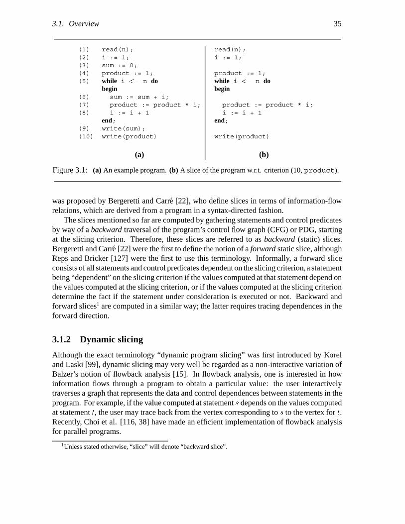
3.1. Overview 35
(1) read(n);(2) i := 1;(3) sum := 0;(4) product := 1;(5) while i �� n do
begin(6) sum := sum + i;(7) product := product * i;(8) i := i + 1
end;(9) write(sum);(10) write(product)
read(n);i := 1;
product := 1;while i �� n dobegin
product := product * i;i := i + 1
end;
write(product)
(a) (b)
Figure 3.1: (a) An example program. (b) A slice of the program w.r.t. criterion (10, product).
was proposed by Bergeretti and Carre [22], who define slices in terms of information-flowrelations, which are derived from a program in a syntax-directed fashion.
The slices mentioned so far are computed by gathering statements and control predicatesby way of a backward traversal of the program’s control flow graph (CFG) or PDG, startingat the slicing criterion. Therefore, these slices are referred to as backward (static) slices.Bergeretti and Carre [22] were the first to define the notion of a forward static slice, althoughReps and Bricker [127] were the first to use this terminology. Informally, a forward sliceconsists of all statements and control predicates dependent on the slicing criterion, a statementbeing “dependent” on the slicing criterion if the values computed at that statement depend onthe values computed at the slicing criterion, or if the values computed at the slicing criteriondetermine the fact if the statement under consideration is executed or not. Backward andforward slices1 are computed in a similar way; the latter requires tracing dependences in theforward direction.
3.1.2 Dynamic slicing
Although the exact terminology “dynamic program slicing” was first introduced by Koreland Laski [99], dynamic slicing may very well be regarded as a non-interactive variation ofBalzer’s notion of flowback analysis [15]. In flowback analysis, one is interested in howinformation flows through a program to obtain a particular value: the user interactivelytraverses a graph that represents the data and control dependences between statements in theprogram. For example, if the value computed at statement s depends on the values computedat statement t, the user may trace back from the vertex corresponding to s to the vertex for t.Recently, Choi et al. [116, 38] have made an efficient implementation of flowback analysisfor parallel programs.
1Unless stated otherwise, “slice” will denote “backward slice”.

36 Chapter 3. A Survey of Program Slicing Techniques
(1) read(n);(2) i := 1;(3) while (i �� n) do
begin(4) if (i mod 2 = 0) then(5) x := 17
else(6) x := 18;(7) i := i + 1
end;(8) write(x)
read(n);i := 1;while (i �� n) dobegin
if (i mod 2 = 0) thenx := 17
else;
i := i + 1end;write(x)
(a) (b)
Figure 3.2: (a) Another example program. (b) Dynamic slice w.r.t. criterion (n = 2, 81, x).
In the case of dynamic program slicing, only the dependences that occur in a specificexecution of the program are taken into account. A dynamic slicing criterion specifies theinput, and distinguishes between different occurrences of a statement in the execution history;typically, it consists of triple hinput� occurrence of a statement� variablei. An alternate viewof the difference between static and dynamic slicing is that dynamic slicing assumes fixedinput for a program, whereas static slicing does not make assumptions regarding the input.A number of hybrid approaches, where a combination of static and dynamic informationis used to compute slices, can be found in the literature. Choi et al. [38], Duesterwaldet al. [51], and Kamkar [87] use static information in order to decrease the amount ofcomputations that have to be performed at run-time. Venkatesh [137], Ning et al. [117], andField, Ramalingam, and Tip (see Chapters 4 and 5) consider situations where only a subsetof the inputs to program are constrained.
Figure 3.2 shows an example program, and its dynamic slice w.r.t. the criterion (n = 2,81, x), where 81 denotes the first occurrence of statement 8 in the execution history of theprogram. Note that for input n = 2, the loop is executed twice, and that the assignmentsx := 17 and x := 18 are each executed once. In this example, the else branch of the ifstatement may be omitted from the dynamic slice since the assignment of 18 to variable x inthe first iteration of the loop is “killed” by the assignment of 17 to x in the second iteration2.By contrast, the static slice of the program in Figure 3.2 (a) w.r.t. criterion (8, x) consists ofthe entire program.
3.1.3 Applications of slicing
The main application that Weiser had in mind for slicing was debugging [144, 145, 147]:if a program computes an erroneous value for some variable x at some program point, the
2In fact, one might argue that the while construct may be replaced by the if statement in its body. This typeof slice will be discussed in Section 3.6.
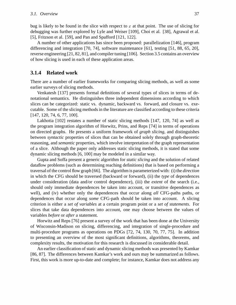
3.1. Overview 37
bug is likely to be found in the slice with respect to x at that point. The use of slicing fordebugging was further explored by Lyle and Weiser [109], Choi et al. [38], Agrawal et al.[5], Fritzson et al. [59], and Pan and Spafford [121, 122].
A number of other applications has since been proposed: parallelization [146], programdifferencing and integration [70, 74], software maintenance [61], testing [51, 88, 65, 20],reverse engineering [21, 82, 81], and compiler tuning [106]. Section 3.5 contains an overviewof how slicing is used in each of these application areas.
3.1.4 Related work
There are a number of earlier frameworks for comparing slicing methods, as well as someearlier surveys of slicing methods.
Venkatesh [137] presents formal definitions of several types of slices in terms of de-notational semantics. He distinguishes three independent dimensions according to whichslices can be categorized: static vs. dynamic, backward vs. forward, and closure vs. exe-cutable. Some of the slicing methods in the literature are classified according to these criteria[147, 120, 74, 6, 77, 100].
Lakhotia [102] restates a number of static slicing methods [147, 120, 74] as well asthe program integration algorithm of Horwitz, Prins, and Reps [74] in terms of operationson directed graphs. He presents a uniform framework of graph slicing, and distinguishesbetween syntactic properties of slices that can be obtained solely through graph-theoreticreasoning, and semantic properties, which involve interpretation of the graph representationof a slice. Although the paper only addresses static slicing methods, it is stated that somedynamic slicing methods [6, 100] may be modeled in a similar way.
Gupta and Soffa present a generic algorithm for static slicing and the solution of relateddataflow problems (such as determining reaching definitions) that is based on performing atraversal of the control flow graph [66]. The algorithm is parameterized with: (i) the directionin which the CFG should be traversed (backward or forward), (ii) the type of dependencesunder consideration (data and/or control dependence), (iii) the extent of the search (i.e.,should only immediate dependences be taken into account, or transitive dependences aswell), and (iv) whether only the dependences that occur along all CFG-paths paths, ordependences that occur along some CFG-path should be taken into account. A slicingcriterion is either a set of variables at a certain program point or a set of statements. Forslices that take data dependences into account, one may choose between the values ofvariables before or after a statement.
Horwitz and Reps [76] present a survey of the work that has been done at the Universityof Wisconsin-Madison on slicing, differencing, and integration of single-procedure andmulti-procedure programs as operations on PDGs [72, 74, 130, 70, 77, 75]. In additionto presenting an overview of the most significant definitions, algorithms, theorems, andcomplexity results, the motivation for this research is discussed in considerable detail.
An earlier classification of static and dynamic slicing methods was presented by Kamkar[86, 87]. The differences between Kamkar’s work and ours may be summarized as follows.First, this work is more up-to-date and complete; for instance, Kamkar does not address any
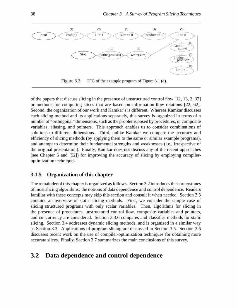
38 Chapter 3. A Survey of Program Slicing Techniques
Start
(10)
read(n) i := 1 sum := 0 product := 1 i <= n
Stop
i := i + 1
sum :=sum+i
product*iproduct :=
write(product) write(sum)
(1) (2) (3) (4) (5)
(6)
(7)
(8)
(9)
Figure 3.3: CFG of the example program of Figure 3.1 (a).
of the papers that discuss slicing in the presence of unstructured control flow [12, 13, 3, 37]or methods for computing slices that are based on information-flow relations [22, 62].Second, the organization of our work and Kamkar’s is different. Whereas Kamkar discusseseach slicing method and its applications separately, this survey is organized in terms of anumber of “orthogonal” dimensions, such as the problems posed by procedures, or compositevariables, aliasing, and pointers. This approach enables us to consider combinations ofsolutions to different dimensions. Third, unlike Kamkar we compare the accuracy andefficiency of slicing methods (by applying them to the same or similar example programs),and attempt to determine their fundamental strengths and weaknesses (i.e., irrespective ofthe original presentation). Finally, Kamkar does not discuss any of the recent approaches(see Chapter 5 and [52]) for improving the accuracy of slicing by employing compiler-optimization techniques.
3.1.5 Organization of this chapter
The remainder of this chapter is organized as follows. Section 3.2 introduces the cornerstonesof most slicing algorithms: the notions of data dependence and control dependence. Readersfamiliar with these concepts may skip this section and consult it when needed. Section 3.3contains an overview of static slicing methods. First, we consider the simple case ofslicing structured programs with only scalar variables. Then, algorithms for slicing inthe presence of procedures, unstructured control flow, composite variables and pointers,and concurrency are considered. Section 3.3.6 compares and classifies methods for staticslicing. Section 3.4 addresses dynamic slicing methods, and is organized in a similar wayas Section 3.3. Applications of program slicing are discussed in Section 3.5. Section 3.6discusses recent work on the use of compiler-optimization techniques for obtaining moreaccurate slices. Finally, Section 3.7 summarizes the main conclusions of this survey.
3.2 Data dependence and control dependence

3.2. Data dependence and control dependence 39
Data dependence and control dependence are defined in terms of the CFG of a program. ACFG contains a node for each statement and control predicate in the program; an edge fromnode i to node j indicates the possible flow of control from the former to the latter. CFGscontain special nodes labeled START and STOP corresponding to the beginning and the endof the program, respectively.
The sets DEF�i� and REF�i� denote the sets of variables defined and referenced at CFGnode i, respectively. Several types of data dependences can be distinguished, such as flowdependence, output dependence and anti-dependence [53]. Flow dependences can be furtherclassified as being loop-carried or loop-independent, depending whether or not they arise asa result of loop iteration. For the purposes of slicing, only flow dependence is relevant, andthe distinction between loop-carried and loop-independent flow dependences can be ignored.Intuitively, a statement j is flow dependent on statement i if a value computed at i is usedat j in some program execution. In the absence of aliasing [105, 104], flow dependencemay be defined formally as follows: there exists a variable x such that: (i) x � DEF�i�, (ii)x � REF�j�, and, (iii) there exists a path from i to j without intervening definitions of x.Alternatively stated, the definition of x at node i is a reaching definition for node j.
Control dependence is usually defined in terms of post-dominance. A node i in the CFGis post-dominated by a node by j if all paths from i to STOP pass through j. A node j iscontrol dependent on a node i if there exists a path P from i to j such that j post-dominatesevery node in P , excluding i and j. Determining control dependences in a program witharbitrary control flow is studied by Ferrante et al. [53]. For programs with structuredcontrol flow, control dependences can be determined in a simple syntax-directed manner[73]: the statements immediately3 inside the branches of an if or while statement are controldependent on the control predicate.
As an example, Figure 3.3 shows the CFG for the example program of Figure 3.1 (a).Node 7 is flow dependent on node 4 because: (i) node 4 defines variable product, (ii)node 7 references variable product, and (iii) there exists a path 4 � 5 � 6 � 7 withoutintervening definitions of product. Node 7 is control dependent on node 5 because thereexists a path 5 � 6 � 7 such that: (i) node 6 is post-dominated by node 7, and (ii) node 5is not post-dominated by node 7.
Many of the slicing approaches that will be discussed in the sequel use the ProgramDependence Graph (PDG) representation of a program [101, 53]. The vertices of the PDGcorrespond to the statements and control predicates of the program, and the edges of a PDGcorrespond to data and control dependences between them. The key issue is that the partialordering of the PDG vertices induced by the dependence edges must be obeyed to preservethe semantics of the program.
In the PDGs of Horwitz et al. [73, 74, 75, 77], a distinction is made between loop-carriedand loop-independent flow dependences, and there is an additional type of data dependenceedges named def-order dependence edges. Horwitz et al. argue that their PDG variant isadequate: if two programs have isomorphic PDGs, they are strongly equivalent. This means
3A statement in a branch of an if statement that occurs within another if statement is only control dependenton the predicate of the inner if statement.

40 Chapter 3. A Survey of Program Slicing Techniques
product*i
Entry
read(n) i := 1 sum := 0 product := 1 while (i <= n) write(sum) write(product)
sum := sum+i i := i + 1product :=
Figure 3.4: PDG of the program in Figure 3.1 (a).
that, when started with the same input state, they either compute the same values for allvariables, or they both diverge. It is argued that the PDG variant of [73] is minimal in thesense that removing any of the types of dependence edges, or disregarding the distinctionbetween loop-carried and loop-independent flow edges would result in inequivalent programshaving isomorphic PDGs. However, for the computation of program slices, only flowdependences and control dependences are necessary. Therefore, only these dependenceswill be considered in the sequel.
As an example, Figure 3.4 shows the PDG of the program of Figure 3.1 (a). In thisfigure, the PDG variant of Horwitz, Reps, and Binkley [77] is used. Thick edges representcontrol dependences4 and thin edges represent flow dependences. The shading of certainvertices in the PDG of Figure 3.4 will be explained in Section 3.3.1.3.
3.3 Methods for static slicing
3.3.1 Basic algorithms
In this section, we will study basic algorithms for static slicing of structured, single-procedureprograms with scalar variables. These algorithms essentially compute the same information,but in different ways.
4The usual labeling of control dependence edges is omitted here, as this is irrelevant for the presentdiscussion. Furthermore, loop-carried flow dependence edges from a vertex to itself will be omitted, as suchedges are irrelevant for the computation of slices.
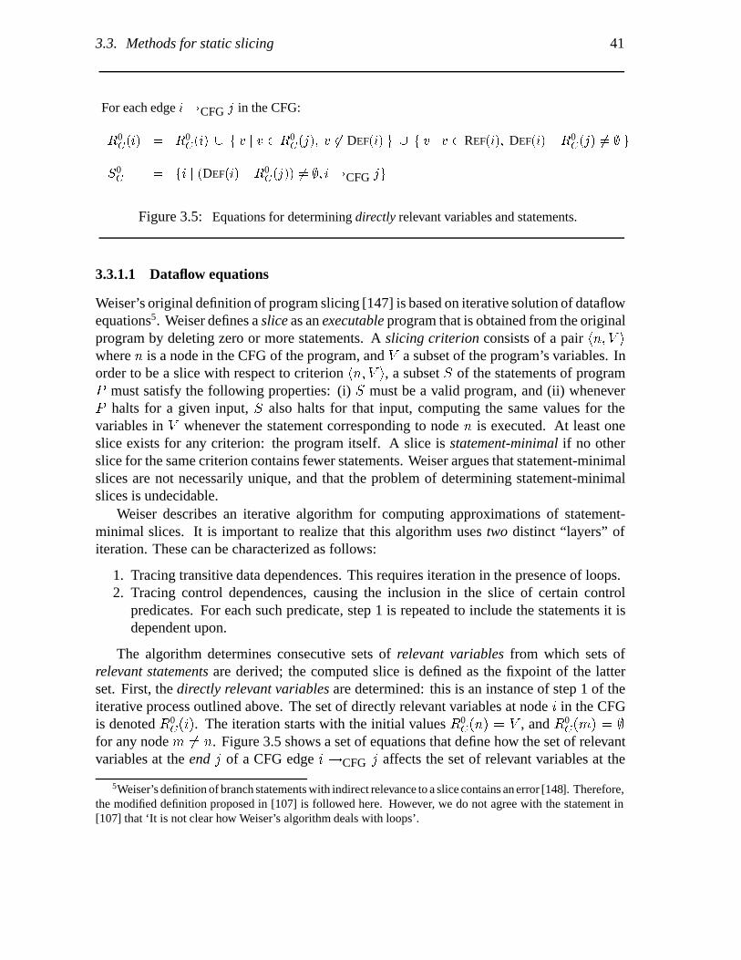
3.3. Methods for static slicing 41
For each edge i�CFG j in the CFG:
R0C�i� � R0
C�i� � f v j v � R0C�j�� v �� DEF�i� g � f v j v � REF�i�� DEF�i� �R0
C�j� �� � g
S0C � fi j �DEF�i� �R0
C�j�� �� �� i�CFG jg
Figure 3.5: Equations for determining directly relevant variables and statements.
3.3.1.1 Dataflow equations
Weiser’s original definition of program slicing [147] is based on iterative solution of dataflowequations5. Weiser defines a slice as an executable program that is obtained from the originalprogram by deleting zero or more statements. A slicing criterion consists of a pair hn� V iwhere n is a node in the CFG of the program, and V a subset of the program’s variables. Inorder to be a slice with respect to criterion hn� V i, a subset S of the statements of programP must satisfy the following properties: (i) S must be a valid program, and (ii) wheneverP halts for a given input, S also halts for that input, computing the same values for thevariables in V whenever the statement corresponding to node n is executed. At least oneslice exists for any criterion: the program itself. A slice is statement-minimal if no otherslice for the same criterion contains fewer statements. Weiser argues that statement-minimalslices are not necessarily unique, and that the problem of determining statement-minimalslices is undecidable.
Weiser describes an iterative algorithm for computing approximations of statement-minimal slices. It is important to realize that this algorithm uses two distinct “layers” ofiteration. These can be characterized as follows:
1. Tracing transitive data dependences. This requires iteration in the presence of loops.2. Tracing control dependences, causing the inclusion in the slice of certain control
predicates. For each such predicate, step 1 is repeated to include the statements it isdependent upon.
The algorithm determines consecutive sets of relevant variables from which sets ofrelevant statements are derived; the computed slice is defined as the fixpoint of the latterset. First, the directly relevant variables are determined: this is an instance of step 1 of theiterative process outlined above. The set of directly relevant variables at node i in the CFGis denoted R0
C�i�. The iteration starts with the initial values R0C�n� � V , and R0
C�m� � �for any node m � n. Figure 3.5 shows a set of equations that define how the set of relevantvariables at the end j of a CFG edge i �CFG j affects the set of relevant variables at the
5Weiser’s definition of branch statements with indirect relevance to a slice contains an error [148]. Therefore,the modified definition proposed in [107] is followed here. However, we do not agree with the statement in[107] that ‘It is not clear how Weiser’s algorithm deals with loops’.

42 Chapter 3. A Survey of Program Slicing Techniques
BkC � fb j i � Sk
C � i � INFL�b�g
Rk�1C �i� � Rk
C�i� �Sb�Bk
C
R0�b�REF�b��
�i�
Sk�1C � Bk
C � fi j DEF�i� �Rk�1C �j� � �� i �CFG jg
Figure 3.6: Equations for determining indirectly relevant variables and statements.
NODE # DEF REF INFL R0C R1
C
1 f n g � � � �2 f i g � � � f n g3 f sum g � � f i g f i, n g4 f product g � � f i g f i, n g5 � f i, n g f 6, 7, 8 g f product, i g f product, i, n g6 f sum g f sum, i g � f product, i g f product, i, n g7 f product g f product, i g � f product, i g f product, i, n g8 f i g f i g � f product, i g f product, i, n g9 � f sum g � f product g f product g10 � f product g � f product g f product g
Table 3.1: Results of Weiser’s algorithm for the example program of Figure 3.1 (a) and slicingcriterion h10� f product gi.
beginning i of that edge. The least fixed point of this process is the set of directly relevantvariables at node i. From R0
C , a set of directly relevant statements, S0C , is derived. Figure 3.5
shows how S0C is defined as the set of all nodes i that define a variable v that is a relevant at
a CFG-successor of i.As mentioned, the second “layer” of iteration in Weiser’s algorithm consists of taking
control dependences into account. Variables referenced in the control predicate of an ifor while statement are indirectly relevant, if (at least) one of the statements in its body isrelevant. To this end, the range of influence INFL�b� of a branch statement b is defined asthe set of statements control dependent on b. Figure 3.6 shows a definition of the branchstatements Bk
C that are indirectly relevant due to the influence they have on nodes i in SkC .Next, the sets of indirectly relevant variables Rk�1
C �i� are determined. In addition to thevariables inRk
C�i�, Rk�1C �i� contains variables that are relevant because they have a transitive
data dependence on statements in BkC . This is determined by performing the first type of
iteration again (i.e., tracing transitive data dependences) with respect to a set of criteriahb�REF�b�i, where b is a branch statement in Bk
C (see Figure 3.6). Figure 3.6 also shows adefinition of the setsSk�1
C of indirectly relevant statements in iteration k�1. This set consistsof the the nodes in Bk
C together with the nodes i that define a variable that is Rk�1C -relevant
to a CFG-successor j.
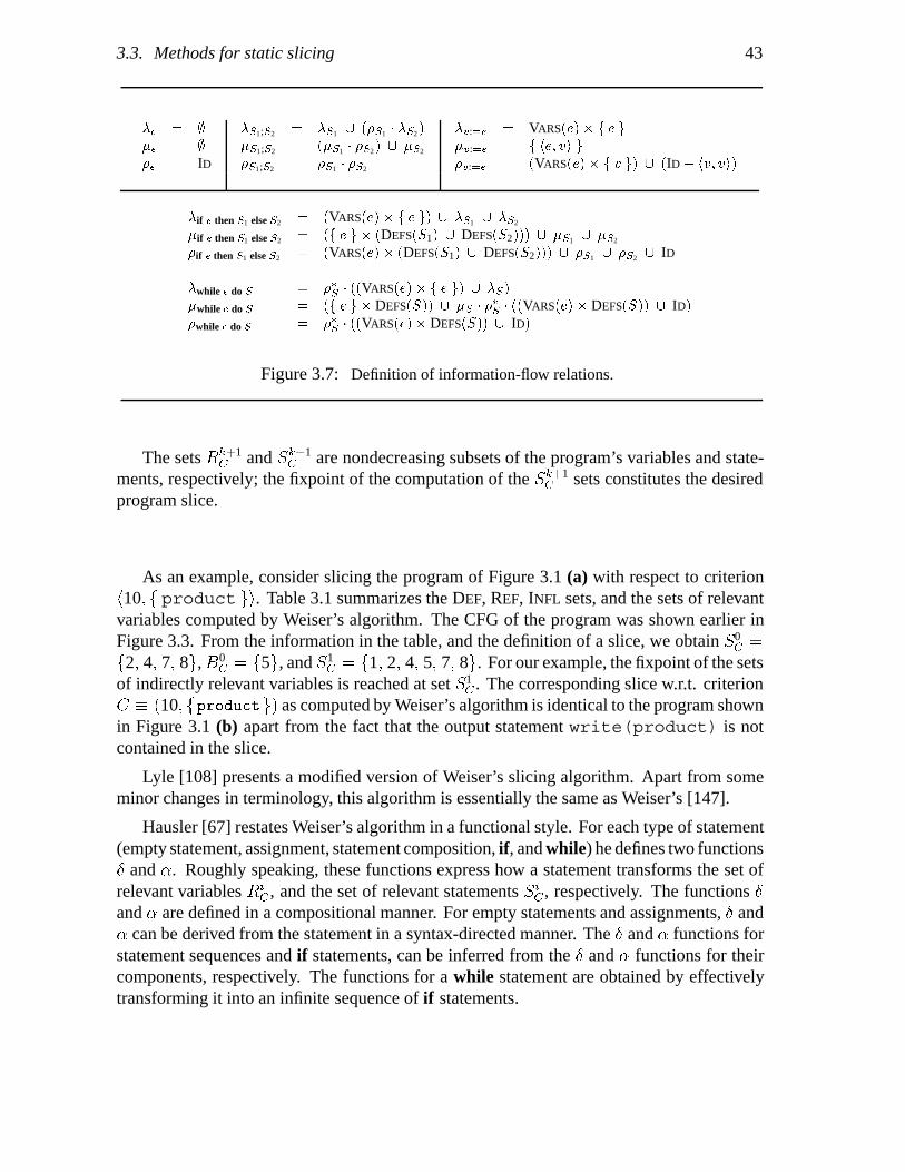
3.3. Methods for static slicing 43
�� � ��� � ��� � ID
�S1;S2 � �S1 � ��S1 � �S2��S1;S2 � ��S1 � �S2� � �S2
�S1;S2 � �S1 � �S2
�v:�e � VARS�e�� f e g�v:�e � f he� vi g�v:�e � �VARS�e�� f v g� � �ID � hv� vi�
�if e then S1 else S2 � �VARS�e�� f e g� � �S1 � �S2
�if e then S1 else S2 � �f e g � �DEFS�S1� � DEFS�S2��� � �S1 � �S2
�if e then S1 else S2 � �VARS�e�� �DEFS�S1� � DEFS�S2��� � �S1 � �S2 � ID
�while e do S � ��S � ��VARS�e�� f e g� � �S��while e do S � �f e g � DEFS�S�� � �S � ��S � ��VARS�e�� DEFS�S�� � ID��while e do S � ��S � ��VARS�e�� DEFS�S�� � ID�
Figure 3.7: Definition of information-flow relations.
The sets Rk�1C and Sk�1
C are nondecreasing subsets of the program’s variables and state-ments, respectively; the fixpoint of the computation of the Sk�1
C sets constitutes the desiredprogram slice.
As an example, consider slicing the program of Figure 3.1 (a) with respect to criterionh10� f product gi. Table 3.1 summarizes the DEF, REF, INFL sets, and the sets of relevantvariables computed by Weiser’s algorithm. The CFG of the program was shown earlier inFigure 3.3. From the information in the table, and the definition of a slice, we obtain S0
C �f2� 4� 7� 8g,B0
C � f5g, and S1C � f1� 2� 4� 5� 7� 8g. For our example, the fixpoint of the sets
of indirectly relevant variables is reached at set S1C . The corresponding slice w.r.t. criterion
C � �10� fproductg� as computed by Weiser’s algorithm is identical to the program shownin Figure 3.1 (b) apart from the fact that the output statement write(product) is notcontained in the slice.
Lyle [108] presents a modified version of Weiser’s slicing algorithm. Apart from someminor changes in terminology, this algorithm is essentially the same as Weiser’s [147].
Hausler [67] restates Weiser’s algorithm in a functional style. For each type of statement(empty statement, assignment, statement composition, if, and while) he defines two functions and . Roughly speaking, these functions express how a statement transforms the set ofrelevant variables Ri
C , and the set of relevant statements SiC , respectively. The functions and are defined in a compositional manner. For empty statements and assignments, and can be derived from the statement in a syntax-directed manner. The and functions forstatement sequences and if statements, can be inferred from the and functions for theircomponents, respectively. The functions for a while statement are obtained by effectivelytransforming it into an infinite sequence of if statements.
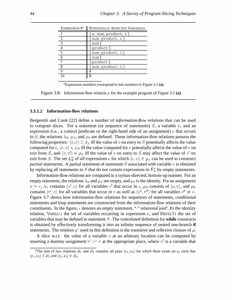
44 Chapter 3. A Survey of Program Slicing Techniques
EXPRESSION #a POTENTIALLY AFFECTED VARIABLES
1 f n� sum� product� i g2 f sum� product� i g3 f sum g4 f product g5 f sum� product� i g6 f sum g7 f product g8 f sum� product� i g9 �10 �
aExpression numbers correspond to line numbers in Figure 3.1 (a).
Figure 3.8: Information-flow relation � for the example program of Figure 3.1 (a).
3.3.1.2 Information-flow relations
Bergeretti and Carre [22] define a number of information-flow relations that can be usedto compute slices. For a statement (or sequence of statements) S, a variable v, and anexpression (i.e., a control predicate or the right-hand side of an assignment) e that occursin S, the relations �S, �S , and �S are defined. These information-flow relations possess thefollowing properties: hv� ei � �S iff the value of v on entry to S potentially affects the valuecomputed for e, he� vi � �S iff the value computed for e potentially affects the value of v onexit from S, and hv� v�i � �S iff the value of v on entry to S may affect the value of v� onexit from S. The set Ev
S of all expressions e for which he� vi � �S can be used to constructpartial statements. A partial statement of statement S associated with variable v is obtainedby replacing all statements in S that do not contain expressions in Ev
S by empty statements.Information-flow relations are computed in a syntax-directed, bottom-up manner. For an
empty statement, the relations �S and �S are empty, and �S is the identity. For an assignmentv := e, �S contains hv�� ei for all variables v� that occur in e, �S consists of he� vi, and �Scontains hv�� vi for all variables that occur in e as well as hv��� v��i for all variables v�� � v.Figure 3.7 shows how information-flow relations for sequences of statements, conditionalstatements and loop statements are constructed from the information-flow relations of theirconstituents. In the figure, � denotes an empty statement, “�” relational join6, ID the identityrelation, VARS�e� the set of variables occurring in expression e, and DEFS�S� the set ofvariables that may be defined in statement S. The convoluted definition for while constructsis obtained by effectively transforming it into an infinite sequence of nested one-branch ifstatements. The relation �� used in this definition is the transitive and reflexive closure of �.
A slice w.r.t. the value of a variable v at an arbitrary location can be computed byinserting a dummy assignment v� :� v at the appropriate place, where v� is a variable that
6The join of two relations R1 and R2 contains all pairs he1� e3i for which there exists an e2 such thathe1� e2i � R1 and he2� e3i � R2.

3.3. Methods for static slicing 45
did not previously occur in S. The slice w.r.t. the final value of v� in the modified programis equivalent to a slice w.r.t. v at the selected location in the original program.
Static forward slices can be derived from relation �S in a way that is similar to the methodfor computing static backward slices from the �S relation.
Figure 3.8 shows the information-flow relation � for the (entire) program of Figure 3.1(a)7. From this relation it follows that the set of expressions that potentially affect thevalue of product at the end of the program are f 1� 2� 4� 5� 7� 8 g. The correspondingpartial statement is obtained by omitting all statements from the program that do not containexpressions in this set, i.e., both assignments to sum and both write statements. The resultis identical to the slice computed by Weiser’s algorithm (see Section 3.3.1.1).
3.3.1.3 Dependence graph based approaches
Ottenstein and Ottenstein [120] were the first of many to define slicing as a reachabilityproblem in a dependence graph representation of a program. They use the PDG [101, 53]for static slicing of single-procedure programs.
In dependence graph based approaches, the slicing criterion is identified with a vertex v inthe PDG. In Weiser’s terminology, this corresponds to a criterion hn� V i where n is the CFGnode corresponding to v, and V the set of all variables defined or used at v. Consequently,slicing criteria of PDG-based slicing methods are less general than those of methods basedon dataflow equations or information-flow relations (the fine-grained PDGs of Jackson andRollins, discussed below, are a notable exception here). However, in Section 3.3.6.2, itwill be shown how more precise slicing criteria can be “simulated” by PDG-based slicingmethods. For single-procedure programs, the slice w.r.t. v consists of all vertices that canreach v. The related parts of the source text of the program can be found by maintaininga mapping between vertices of the PDG and the source text during the construction of thePDG.
The PDG variant of Ottenstein and Ottenstein [120] shows considerably more detailthan that by Horwitz, Reps, and Binkley [77]. In particular, there is a vertex for each(sub)expression in the program, and file descriptors appear explicitly as well. As a result,read statements involving irrelevant variables are not “sliced away”, and slices will executecorrectly with the full input of the original program.
In Figure 3.4 the PDG of the program of Figure 3.1 (a) was shown. Shading is used toindicate the vertices in the slice w.r.t. write(product).
Jackson and Rollins [82] introduce a variation on the PDG that is distinguished by fine-grained dependences between individual variables defined or used at program points. Animportant advantage of this approach is that it allows one to determine more accuratelywhich variables are responsible for the inclusion of a particular statement in a slice.
Each vertex consists of a box that contains a separate port for each variable defined at that
7Bergeretti and Carre do not define information-flow relations for I/O statements. For the purposes of thisexample, it is assumed that the statement read(n) can be treated as an assignment n := SomeConstant,and that the statements write(sum) and write(product) should be treated as empty statements.
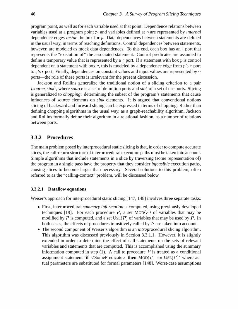
46 Chapter 3. A Survey of Program Slicing Techniques
program point, as well as for each variable used at that point. Dependence relations betweenvariables used at a program point p, and variables defined at p are represented by internaldependence edges inside the box for p. Data dependences between statements are definedin the usual way, in terms of reaching definitions. Control dependences between statements,however, are modeled as mock data dependences. To this end, each box has an � port thatrepresents the “execution of” the associated statement. Control predicates are assumed todefine a temporary value that is represented by a port. If a statement with box p is controldependent on a statement with box q, this is modeled by a dependence edge from p’s portto q’s � port. Finally, dependences on constant values and input values are represented by �ports—the role of these ports is irrelevant for the present discussion.
Jackson and Rollins generalize the traditional notion of a slicing criterion to a pairhsource� sinki, where source is a set of definition ports and sink of a set of use ports. Slicingis generalized to chopping: determining the subset of the program’s statements that causeinfluences of source elements on sink elements. It is argued that conventional notionsslicing of backward and forward slicing can be expressed in terms of chopping. Rather thandefining chopping algorithms in the usual way, as a graph-reachability algorithm, Jacksonand Rollins formally define their algorithm in a relational fashion, as a number of relationsbetween ports.
3.3.2 Procedures
The main problem posed by interprocedural static slicing is that, in order to compute accurateslices, the call-return structure of interprocedural execution paths must be taken into account.Simple algorithms that include statements in a slice by traversing (some representation of)the program in a single pass have the property that they consider infeasible execution paths,causing slices to become larger than necessary. Several solutions to this problem, oftenreferred to as the “calling-context” problem, will be discussed below.
3.3.2.1 Dataflow equations
Weiser’s approach for interprocedural static slicing [147, 148] involves three separate tasks.
� First, interprocedural summary information is computed, using previously developedtechniques [19]. For each procedure P , a set MOD�P � of variables that may bemodified by P is computed, and a set USE�P � of variables that may be used by P . Inboth cases, the effects of procedures transitively called by P are taken into account.
� The second component of Weiser’s algorithm is an intraprocedural slicing algorithm.This algorithm was discussed previously in Section 3.3.1.1. However, it is slightlyextended in order to determine the effect of call-statements on the sets of relevantvariables and statements that are computed. This is accomplished using the summaryinformation computed in step (1). A call to procedure P is treated as a conditionalassignment statement ‘if �SomePredicate� then MOD�P � := USE�P �’ where ac-tual parameters are substituted for formal parameters [148]. Worst-case assumptions

3.3. Methods for static slicing 47
program Main;� � �
while ( � � � ) doP(x1, x2, � � �, xn);x1 := z;x1 := x2;x2 := x3;� � �x�n�1� := xn
end;(L) write(z)
end
procedure P( y1, y2, � � �, yn );beginwrite(y1);write(y2);� � �
(M) write(yn)end
Figure 3.9: A program where procedure P is sliced n times by Weiser’s algorithm for criterionhL� f z gi.
have to be made when a program calls external procedures, and the source-code isunavailable.
� The third part is the actual interprocedural slicing algorithm that iteratively generatesnew slicing criteria with respect to which intraprocedural slices are computed in step(2). For each procedure P , new criteria are generated for (i) proceduresQ called by P ,and (ii) procedures R that call P . The new criteria of (i) consist of all pairs �nQ� VQ�where nQ is the last statement of Q and VQ is the set of relevant variables in P in thescope of Q (formals are substituted for actuals). The new criteria of (ii) consist of allpairs �NR� VR� such that NR is a call to P in R, and VR is the set of relevant variablesat the first statement of P that is in the scope of R (actuals are substituted for formals).
Weiser formalizes the generation of new criteria by way of functions UP�S� and DOWN�S�that map a set S of slicing criteria in a procedure P to a set of criteria in procedures that callP , and a set of criteria in procedures called by P , respectively. The set of all criteria withrespect to which intraprocedural slices are computed consists of the transitive and reflexiveclosure of the UP and DOWN relations; this is denoted �UP � DOWN��. Thus, for an initialcriterion C, slices will be computed for all criteria in the set �UP � DOWN� � �f C g�.
Weiser determines the criteria in this set “on demand” [148]: the generation of newcriteria in step (3) and the computation of intraprocedural slices in step (2) are intermixed; theiteration stops when no new criteria are generated. Although the number of intraproceduralslices computed in step (2) could be reduced by combining “similar” criteria (e.g., replacingtwo criteria hn� V1i and hn� V2i by a single criterion hn� V1 � V2i), Weiser writes that “nospeed-up tricks have been implemented” [147, page 355, col.2]. In fact, one would expectthat such speed-up tricks would affect the performance of his algorithm dramatically. Themain issue is that the computation of the UP and DOWN sets requires that the sets of relevantvariables are known at all call sites. In other words, the computation of these sets relies onslicing these procedures. In the course of doing this, new variables may become relevant

48 Chapter 3. A Survey of Program Slicing Techniques
program Example;begin
(1) a := 17;(2) b := 18;(3) P(a,b,c,d);(4) write(d)
end
procedure P(v,w,x,y);(5) x := v;(6) y := w
end
program Example;begina := 17;b := 18;P(a,b,c,d);
end
procedure P(v,w,x,y);;
y := wend
program Example;begin
;b := 18;P(a,b,c,d);write(d)
end
procedure P(v,w,x,y);;
y := wend
(a) (b) (c)
Figure 3.10: (a) Example program. (b) Weiser’s slice with respect to criterion h4� f d gi. (a) Aslice with respect to the same criterion computed by the Horwitz-Reps-Binkley algorithm.
at previously encountered call sites, and new call sites may be encountered. Consider forexample, the program shown in Figure 3.9. In the subsequent discussion, L denotes theprogram point at statement write(z) and M the program point at the last statement inprocedure P. Computing the slice w.r.t. criterion hL� f z gi requires n iterations of the bodyof the while loop. During the ith iteration, variablesx1� � � � � xi will be relevant at the call site,causing the inclusion of criterion hM� f y1� � � � � yi gi in DOWN�Main�. If no precaution istaken to combine the criteria in DOWN�Main�, procedure P will be sliced n times.
The fact that Weiser’s algorithm does not take into account which output parametersare dependent on which input parameters is a source of imprecision. Figure 3.10 (a)shows an example program that manifests this problem. For criterion h4� f d gi, Weiser’sinterprocedural slicing algorithm [147] will compute the slice shown in Figure 3.10 (b). Thisslice contains the statement a := 17 due to the spurious dependence between variable abefore the call, and variable d after the call. The Horwitz-Reps-Binkley algorithm that willbe discussed in Section 3.3.2.3 will compute the more accurate slice shown in Figure 3.10(c).
Horwitz, Reps, and Binkley [77] report that Weiser’s algorithm for interprocedural slicingis unnecessarily inaccurate, because of what they refer to as the “calling context” problem.In a nutshell, the problem is that when the computation “descends” into a procedure Q thatis called from a procedure P , it will “ascend” to all procedures that call Q, not only P . Thisincludes infeasible execution paths that enter Q from P and exit Q to a different procedure.Traversal of such paths gives rise to inaccurate slices.
Figure 3.11 shows a program that exhibits the calling-context problem. For exam-ple, assume that a slice is to be computed w.r.t. criterion h10�producti. Using sum-mary information to approximate the effect of the calls, the initial approximation of theslice will consist of the entire main procedure except lines 3 and 6. In particular, theprocedure calls Multiply(product, i) and Add(i, 1) are included in the slice,

3.3. Methods for static slicing 49
program Example;begin
(1) read(n);(2) i := 1;(3) sum := 0;(4) product := 1;(5) while i �� n do
begin(6) Add(sum, i);(7) Multiply(product, i);(8) Add(i, 1)
end;(9) write(sum);(10) write(product)
end
procedure Add(a; b);begin
(11) a := a + bend
procedure Multiply(c; d);begin
(12) j := 1;(13) k := 0;(14) while j �� d do
begin(15) Add(k, c);(16) Add(j, 1);
end;(17) c := k
end
Figure 3.11: Example of a multi-procedure program.
because: (i) the variables product and i are deemed relevant at those points, and (ii)using interprocedural data flow analysis it can be determined that MOD�Add� � f a g,USE�Add� � f a, b g, MOD�Multiply� � f c g, and USE�Multiply� � f c, d g.As the initial criterion is in the main program, we have that UP�f h10�producti g� � �,and that DOWN�f h10�producti g� contains the criteria h11� f a gi and h17� f c, d gi.The result of slicing procedure Add for criterion h11� f a gi and procedure Multiply forcriterion h17� f c, d gi will be the inclusion of these procedures in their entirety. Note thatthe calls to Add at lines 15 and 16 cause the generation of a new criterion h11� f a, b giand thus re-slicing of procedure Add. It can now be seen that the example program exhibitsthe “calling context” problem: Since line (11) is in the slice, new criteria are generated forall calls to Add. These calls include the (already included) calls at lines 8, 15, and 16, butalso the call Add(sum, i) at line 6. The new criterion h6� f sum, i gi that is generatedwill cause the inclusion of lines 6 and 3 in the slice. Consequently, the slice consists of theentire program.
It is our conjecture that the calling context problem of Weiser’s algorithm can be fixedby observing that the criteria in the UP sets are only needed to include procedures that(transitively) call the procedure containing the initial criterion8. Once this is done, onlyDOWN sets need to be computed. For an initial criterion C, this corresponds to determiningthe set of criteria DOWN � �UP � �f C g��, and computing the intraprocedural slices withrespect to each of these criteria. Reps [126] suggested that this essentially corresponds tothe two passes of the Horwitz-Reps-Binkley algorithm (see Section 3.3.2.3) if all UP sets arecomputed before determining any DOWN sets.
8A similar observation was made by Jiang et al. [83]. However, they do not explain that this approach onlyworks when a call to procedure p is treated as a conditional assignment if �SomePredicate� then MOD�P �:= USE�P �.

50 Chapter 3. A Survey of Program Slicing Techniques
program P3(x1,x2,x3);begint := 0;P3(x2,x3,t);P3(x2,x3,t);
(L) x1 := x1 + 1end;
P
P
P P
P0
P P
P0
0
P
P P
P0
P P
P0
0
(a) (b)
Figure 3.12: (a) Example program. (b) Exponentially long path traversed by the Hwang-Du-Choualgorithm for interprocedural static slicing for criterion hL�x3i.
Hwang, Du, and Chou [79] propose an iterative solution for interprocedural static slicingbased on replacing (recursive) calls by instances of the procedure body. From a conceptualpoint of view, each iteration comprises of the following two steps. First, procedure calls areinlined, substituting actual parameters for formal parameters. Then, the slice is re-computed,where any remaining procedure call is treated as if it were an empty statement (i.e., it isassumed to have no effect on the flow dependences between its surrounding statements).This iterative process terminates when the resulting slice is identical to the slice computed inthe previous iteration—i.e., until a fixed point is reached. It is assumed that some mappingis maintained between the statements in the various expanded versions of the program, andin the original program.
The approach of Hwang et al. does not suffer from the calling context problem becauseexpansion of recursive calls does not lead to considering infeasible execution paths. However,Reps [125, 128] has shown recently that for a certain family Pk of recursive programs, thisalgorithm takes time O�2k�, i.e., exponential in the length of the program. An example ofsuch a program is shown in Figure 3.12 (a). Figure 3.12 (b) shows the exponentially longpath that is effectively traversed by the Hwang-Du-Chou algorithm.
3.3.2.2 Information-flow relations
Bergeretti and Carre [22] explain how the effect of procedure calls can be approximatedin the absence of recursion. Exact dependences between input and output parameters aredetermined by slicing the called procedure with respect to each output parameter (i.e.,computation of the � relation for the procedure). Then, each procedure call is replacedby a set of assignments, where each output parameter is assigned a fictitious expressionthat contains the input parameters it depends upon. As only feasible execution paths areconsidered, this approach does not suffer from the calling context problem. A call to a side-effect free function can be modeled by replacing it with a fictitious expression containingall actual parameters. Note that the computed slices are not truly interprocedural since noattempt is done to slice procedures other than the main program.
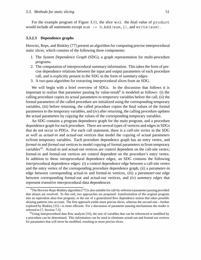
3.3. Methods for static slicing 51
For the example program of Figure 3.11, the slice w.r.t. the final value of productwould include all statements except sum := 0, Add(sum,i), and write(sum).
3.3.2.3 Dependence graphs
Horwitz, Reps, and Binkley [77] present an algorithm for computing precise interproceduralstatic slices, which consists of the following three components:
1. The System Dependence Graph (SDG), a graph representation for multi-procedureprograms.
2. The computation of interprocedural summary information. This takes the form of pre-cise dependence relations between the input and output parameters of each procedurecall, and is explicitly present in the SDG in the form of summary edges.
3. A two-pass algorithm for extracting interprocedural slices from an SDG.
We will begin with a brief overview of SDGs. In the discussion that follows it isimportant to realize that parameter passing by value-result9 is modeled as follows: (i) thecalling procedure copies its actual parameters to temporary variables before the call, (ii) theformal parameters of the called procedure are initialized using the corresponding temporaryvariables, (iii) before returning, the called procedure copies the final values of the formalparameters to the temporary variables, and (iv) after returning, the calling procedure updatesthe actual parameters by copying the values of the corresponding temporary variables.
An SDG contains a program dependence graph for the main program, and a proceduredependence graph for each procedure. There are several types of vertices and edges in SDGsthat do not occur in PDGs. For each call statement, there is a call-site vertex in the SDGas well as actual-in and actual-out vertices that model the copying of actual parametersto/from temporary variables. Each procedure dependence graph has an entry vertex, andformal-in and formal-out vertices to model copying of formal parameters to/from temporaryvariables10. Actual-in and actual-out vertices are control dependent on the call-site vertex;formal-in and formal-out vertices are control dependent on the procedure’s entry vertex.In addition to these intraprocedural dependence edges, an SDG contains the followinginterprocedural dependence edges: (i) a control dependence edge between a call-site vertexand the entry vertex of the corresponding procedure dependence graph, (ii) a parameter-inedge between corresponding actual-in and formal-in vertices, (iii) a parameter-out edgebetween corresponding formal-out and actual-out vertices, and (iv) summary edges thatrepresent transitive interprocedural data dependences.
9The Horwitz-Reps-Binkley algorithm [77] is also suitable for call-by-referenceparameter passing providedthat aliases are resolved. To this end, two approaches are proposed: transformation of the original programinto an equivalent alias-free program, or the use of a generalized flow dependence notion that takes possiblealiasing patterns into account. The first approach yields more precise slices, whereas the second one—furtherexplored by Binkley [31]—is more efficient. For a discussion of parameter passing mechanisms the reader isreferred to [7, Section 7.5].
10Using interprocedural data flow analysis [16], the sets of variables that can be referenced or modified bya procedure can be determined. This information can be used to eliminate actual-out and formal-out verticesfor parameters that will never be modified, resulting in more precise slices.

52 Chapter 3. A Survey of Program Slicing Techniques
The second part of the Horwitz-Reps-Binkley algorithm, computation of summary de-pendences, involves the construction of an attribute grammar that models the calling rela-tionships between the procedures (as in a call graph). Then, the subordinate characteristicgraph for this grammar is computed. For each procedure in the program, this graph containsedges that correspond to precise transitive flow dependences between its input and outputparameters. The summary edges of the subordinate characteristic graph are copied to theappropriate places at each call site in the SDG. Details of the Horwitz-Reps-Binkley algo-rithm for determining summary edges are outside the scope of this survey—for details, thereader is referred to [77].
The third phase of the Horwitz-Reps-Binkley algorithm consists of a two-pass traversalof the SDG. The summary edges of an SDG serve to circumvent the calling context problem.Assume that slicing starts at some vertex s. The first phase determines all vertices from whichs can be reached without descending into procedure calls. The transitive interproceduraldependence edges guarantee that calls can be side-stepped, without descending into them.The second phase determines the remaining vertices in the slice by descending into allpreviously side-stepped calls.
Figure 3.13 shows the SDG for the program of Figure 3.11, where interproceduraldataflow analysis is used to eliminate the vertices for the second parameters of the proceduresAdd and Multiply. In the figure, thin solid arrows represent flow dependences, thick solidarrows correspond to control dependences, thin dashed arrows are used for call, parameter-in,and parameter-out dependences, and thick dashed arrows represent transitive interproceduralflow dependences. The vertices in the slice w.r.t. statement write(product) are shownshaded; light shading indicates the vertices identified in the first phase of the algorithm, anddark shading indicates the vertices identified in the second phase. Clearly, the statementssum := 0, Add(sum, i), and write(sum) are not in the slice.
Slices computed by Horwitz-Reps-Binkley algorithm [77] are not necessarily executableprograms. Cases where only a subset of the vertices for actual and formal parameters arein the slice correspond to procedures where some of the arguments are “sliced away”; fordifferent calls to the procedure, different arguments may be omitted. Two approaches areproposed for transforming such a non-executable slice an executable program. First, severalvariants of a procedure may be incorporated in a slice [77]; this has the disadvantage thatthe slice is no longer a restriction of the original program. The second solution consists ofextending the slice with all parameters that are present at some call to all calls that occur inthe slice. In addition, all vertices on which the added vertices are dependent must be addedto the slice as well. This second approach is pursued by Binkley [30]. Clearly the secondapproach yields larger slices than the first one.
Finally, it is outlined how interprocedural slices can be computed from partial SDGs(corresponding to programs under development, or programs containing library calls) andhow, using the SDG, interprocedural forward slices can be computed in a way that is verysimilar to the previously described method for interprocedural (backward) slicing.

3.3. Methods for static slicing 53
a := a + b
Enter Example
read(n) i := 1 sum := 0 product := 1 while (i <= n) write(sum) write(product)
Add(sum,i)
a_in := sum b_in := i sum := a_out
Add(i,1)
a_in := i b_in := 1 i:= a_out
Mult.(product,i)
c_in := product d_in := i product:=c_out
c := c_in d := d_in
Enter Multiply
c_out := c
j := 1 k := 0 while (j <= d) c := k
Add(j, 1)
a_in := j b_in := 1 j := a_out
Add(k, c)
a_in := k b_in := c k := a_out
Enter Add
a := a_in b := b_in a_out := a
Figure 3.13: SDG of the program in Figure 3.11.
Recently, Reps et al. [129, 128] proposed a new algorithm for computing the summaryedges of an SDG, which is asymptotically more efficient than the Horwitz-Reps-Binkley al-gorithm [77] (the time requirements of these algorithms will be discussed in Section 3.3.6.3).Input to the algorithm is an SDG where no summary edges have been added yet, i.e., a col-lection of procedure dependence graphs connected by call, parameter-in, and parameter-outedges. The algorithm uses a worklist to determine same-level realizable paths. Intuitively, asame-level realizable path obeys the call-return structure of procedure calls, and it starts andends at the same level (i.e., in the same procedure). Same-level realizable paths betweenformal-in and formal-out vertices of a procedure P induce summary edges between thecorresponding actual-in and actual-out vertices for any call to P . The algorithm starts byasserting that a same-level realizable path of length zero exists from any formal-out vertexto itself. A worklist is used to select a path, and extend it by adding an edge to its beginning.Reps et al. [129] also present a demand version of their algorithm, which incrementally

54 Chapter 3. A Survey of Program Slicing Techniques
determines the summary edges of an SDG.
Lakhotia [103] presents an algorithm for computing interprocedural slices that is alsobased on SDGs. This algorithm computes slices that are identical to the slices computed bythe Horwitz-Reps-Binkley algorithm. Associated with every SDG vertex v is a three-valuedtag; possible values for this tag are: “�” indicating that v has not been visited, “�” indicatingthat v has been visited, and all vertices from which v can be reached should be visited, and“�” indicating that v has been visited, and some of the vertices from which v can be reachedshould be visited. More precisely, an edge from an entry vertex to a call vertex shouldonly be traversed if the call vertex is labeled �. A worklist algorithm is used to visit allvertices labeled � before visiting any vertex labeled �. When this process ends, verticeslabeled either � or � are in the slice. Lakhotia’s algorithm traverses performs a single passthrough the SDG. However, unlike the Horwitz-Reps-Binkley algorithm, the value of a tagmay change twice. Therefore it is unclear if Lakhotia’s algorithm is really an improvementover the Horwitz-Reps-Binkley two-pass traversal algorithm.
The dependence graph model of Jackson and Rollins [82] (see Section 3.3.1.3) is “mod-ular”, in the sense that a single box is used for each procedure call. Instead of linkingthe individual dependence graphs for the procedures of the program, Jackson and Rollinsrepresent procedure calls in a more abstract fashion: the internal dependence edges insidea procedure’s box effectively correspond to the summary edges of Horwitz et al. [77, 128].Unlike the previously discussed methods, this algorithm side-steps the calling context prob-lem by only extending slices to called procedures, and not to calling procedures (unlessexplicitly requested by the user). Here, ‘extending a slice to a called procedure’ involvesslicing the (separate) dependence graph for that procedure with respect to the appropriateports of its exit node (i.e., corresponding to the ports at the point of call that occur in theslice).
Whereas for simple statements the internal dependence edges between ports of theassociated box in the dependence graph can be computed in a simple syntax-directed manner,a more elaborate scheme is required for procedures. In the absence of recursion, the internalsummary dependence edges for a procedure are derived from the dependences inside andbetween the boxes for the statements that constitute the procedure body. For recursiveprocedures, Jackson and Rollins briefly discuss a simple iterative scheme for determininginternal dependence edges, and state that their algorithm is essentially an adaptation of thesolution presented by Ernst [52] (see Section 3.6). The essence of their scheme is that theinternal dependence edges for non-recursive calls are determined in the manner sketchedabove, and that there are initially no internal dependence edges for calls in a recursive cycle.In each subsequent step, the transitive dependences between the input parameters and theoutput parameters of a recursive procedure are recomputed by slicing in a graph that containsthe summary edges determined in the previous cycle. Then, summary edges are added to thegraph for those dependences that did not occur in the previous cycle. This iteration processterminates when no more additional transitive dependences can be found.

3.3. Methods for static slicing 55
3.3.3 Unstructured control flow
3.3.3.1 Dataflow equations
Lyle [108] reports that (his version of) Weiser’s algorithm for static slicing yields incorrectslices in the presence of unstructured control flow: the behavior of the slice is not necessarilya projection of the behavior of the program. He presents a conservative solution for dealingwith goto statements: any goto that has a non-empty set of relevant variables associatedwith it is included in the slice.
Gallagher [60] and Gallagher and Lyle [61] also use a variation of Weiser’s method.A goto statement is included in the slice if it jumps to a label of an included statement11.Agrawal [3] shows that this algorithm does not produce correct slices in all cases.
Jiang et al. [83] extend Weiser’s slicing method to C programs with unstructured controlflow. They introduce a number of additional rules to “collect” the unstructured control flowstatements such as goto, break, and continue that are part of the slice. Unfortunately, noformal justification is given for the treatment of unstructured control flow constructs in [83].Agrawal [3] shows that this algorithm may also produce incorrect slices.
3.3.3.2 Dependence graphs
Ball and Horwitz [12, 13] and Choi and Ferrante [37] discovered independently that conven-tional PDG-based slicing algorithms produce incorrect results in the presence of unstructuredcontrol flow: slices may compute values at the criterion that differ from what the originalprogram does. These problems are due to the fact that the algorithms do not determine cor-rectly when unconditional jumps such as break, goto, and continue statements are requiredin a slice.
As an example, Figure 3.14 (a) shows a variant of our example program, which uses agoto statement. Figure 3.14 (b) shows the PDG for this program. The vertices that havea transitive dependence on statement write(product) are highlighted. Figure 3.14(c) shows a textual representation of the program thus obtained. Clearly, this “slice” isincorrect because it does not contain the goto statement, causing non-termination. In fact,the previously described PDG-based algorithms will only include a goto if it is the slicingcriterion itself, because no statement is either data or control dependent on a goto.
The solution of [12, 13] and the first solution presented in [37] are remarkably similar:unconditional jumps are regarded as pseudo-predicate vertices where the “true” branchconsists of the statement that is being jumped to, and the “false” branch of the textuallynext statement. Correspondingly, there are two outgoing edges in the augmented controlflow graph (ACFG). Only one of these edges can actually be traversed during execution;the other outgoing edge is “non-executable”. In constructing the (augmented) PDG, datadependences are computed using the (original) CFG, and control dependences are computed
11Actually, this is a slight simplification. Each basic block is partitioned into labeled blocks; a labeled blockis a subsequence of the statements in a basic block starting with a labeled statement, and containing no otherlabeled statements. A goto is included in the slice if it jumps to a label for which there is some includedstatement in its block.

56 Chapter 3. A Survey of Program Slicing Techniques
read(n);i := 1;sum := 0;product := 1;while true dobegin
if (i > n) thengoto L;
sum := sum + i;product := product * i;i := i + 1
end;L: write(sum);write(product)
read(n);i := 1;
product := 1;while true dobegin
if (i > n) then;
product := product * i;i := i + 1
end;
write(product)
read(n);i := 1;
product := 1;while true dobegin
if (i > n) thengoto L;
product := product * i;i := i + 1
end;L:write(product)
(a) (c) (e)
product*i
Entry
read(n) i := 1 sum := 0 product := 1 while(true) write(sum) write(product)
if (i > n) sum+i i := i +1
goto L
sum := product:=
(b)
sum+i
Entry
read(n) i := 1 sum := 0 product := 1 while(true) write(sum) write(product)
if (i > n)
goto L
i := i +1product:=product*i
sum :=
(d)
Figure 3.14: (a) Program with unstructured control flow, (b) PDG for program of (a), (c) incorrectslice w.r.t. statement write(product), (d) Augmented PDG for program of (a), (e) correct slicew.r.t. statement write(product).

3.3. Methods for static slicing 57
using the ACFG. Slicing is defined in the usual way, as a graph reachability problem. Labelspertaining to statements excluded from the slice are moved to the closest post-dominatingstatement that occurs in the slice.
The main difference between the approach by Ball and Horwitz and the first approach ofChoi and Ferrante is that the latter use a slightly more limited example language: conditionaland unconditional goto’s are present, but no structured control flow constructs. AlthoughChoi and Ferrante argue that these constructs can be transformed into conditional andunconditional goto’s, Ball and Horwitz show that, for certain cases, this results in overlylarge slices. Both groups present a formal proof that their algorithms compute correct slices.
Figure 3.14 (d) shows the augmented PDG for the program of Figure 3.14 (a); verticesfrom which the vertex labeled write(product) can be reached are indicated by shading.The (correct) slice corresponding to these vertices is shown in Figure 3.14 (e).
Choi and Ferrante distinguish two disadvantages of the slicing approach based on aug-mented PDGs. First, APDGs require more space than conventional PDGs, and their con-struction takes more time. Second, non-executable control dependence edges give rise tospurious dependences in some cases. In their second approach, Choi and Ferrante utilize the“classical” PDG. As a first approximation, the standard algorithm for computing slices isused, which by itself produces incorrect results in the presence of unstructured control flow.The basic idea is that for each statement that is not in the slice, a new goto to its immediatepost-dominator is added. In a separate phase, redundant cascaded goto statements are re-moved. The second approach has the advantage of computing smaller slices than the first.A disadvantage of it, however, is that slices may include goto statements that do not occurin the original program.
Yet another PDG-based method for slicing programs with unstructured control flow wasrecently proposed by Agrawal [3]. Unlike the methods by Ball and Horwitz [12, 13] andChoi and Ferrante [37], Agrawal uses unmodified PDGs. He observes that a conditionaljump statement of the form if P then goto L must be included in the slice if predicateP is in the slice because another statement in the slice is control dependent on it. Theterminology “conventional slicing algorithm” is adopted to refer to the standard PDG-basedslicing method, with the above extension to conditional jump statements.
Agrawal’s key observation is that an unconditional jump statement J should be includedin the slice if and only if the immediate postdominator of J that is included in the slice differsfrom the immediate lexical successor of J that is included in the slice. Here, a statementS � is a lexical successor of a statement S if S textually precedes S� in the program12.The statements on which the newly added statement is transitively dependent must also beadded to the slice. The motivation for this approach can be understood by considering asequence of statements S1;S2;S3 where S1 and S3 are in the slice, and where S2 contains anunconditional jump statement to a statement that does not have S3 as its lexical successor.Suppose that S2 were not included in the slice. Then the flow of control in the slicewould pass unconditionally from S1 to S3, though in the original program this need not
12As Agrawal observes, this notion is equivalent to the non-executable edges in the augmented control flowgraphs used by Ball and Horwitz, and Choi and Ferrante.
58 Chapter 3. A Survey of Program Slicing Techniques
always be the case, because the jump might transfer the control elsewhere. Therefore thejump statement must be included, together with all statements it depends upon. Agrawal’salgorithm traverses the postdominator tree of a program in pre-order, and considers jumpstatements for inclusion in this order. The algorithm iterates until no jump statements canbe added; this is necessary because adding a jump (and the statements it depend upon) maychange the lexical successors and postdominators in the slice of other jump statements, whichmay therefore need to be included as well. Although no proof is stated, Agrawal claims thathis algorithm computes correct slices identical to those computed by the Ball-Horwitz andChoi-Ferrante algorithms.
Agrawal’s algorithm [3] may be simplified significantly if the only type of jump thatoccurs in a program is a structured jump, i.e., a jump to a lexical successor. C break,continue, and return statements are all structured jumps. First, only a single traversal ofthe post-dominator tree is required. Second, jump statements have to be added only if theyare control dependent on a predicate that is in the slice. In this case, the statements they aredependent upon are already included in the slice. For programs with structured jumps, thealgorithm can be further simplified to a conservative algorithm by including in the slice alljump statements that are control dependent on a predicate that is in the slice.
Agrawal’s algorithm will include the goto statement of the example program of Fig-ure 3.14 (a) because it is control dependent on the (included) predicate of the if statement.
3.3.4 Composite data types and pointers
Lyle [108] proposes a conservative solution to the problem of static slicing in the presenceof arrays. Essentially, any update to an element of an array is regarded as an update and areference of the entire array.
The PDG variant of Ottenstein and Ottenstein [120] contains a vertex for each sub-expression; special select and update operators serve to access elements of an array.
In the presence of pointers (and procedures), situations may occur where two or morevariables refer to the same memory location—a phenomenon commonly called aliasing.Aliasing complicates the computation of slices because the notion of flow dependencedepends on which variables are (potential) aliases. Even in the intraprocedural case, theproblem of determining potential aliases in the presence of multiple-level pointers is an NP-hard problem [105]. However, slices may be computed using conservative approximations ofdata dependences that are based on approximate alias information. Conservative algorithmsfor determining potential aliases were presented by Landi and Ryder [104], and Choi, Burke,and Carini [36].
Horwitz, Pfeiffer, and Reps [71] present a slightly different approach for computing flowdependences in the presence of pointers. Instead of defining (approximate) flow dependencesin terms of definitions and uses of variables that are potentially aliased, the notion of flowdependence is defined in terms of potential definitions and uses of abstract memory locations.An algorithm is presented that computes approximations of the memory layouts that mayoccur at each program point during execution.
The PDG-based static slicing algorithm proposed by Agrawal, DeMillo and Spafford [4]

3.3. Methods for static slicing 59
implements a similar idea to deal with both composite variables and pointers. Their solutionconsists of determining reaching definitions for a scalar variable v at node n in the flowgraphby finding all paths from nodes corresponding to a definition of v to n that do not containother definitions of v. When composite data types and pointers are considered, definitionsinvolve l-valued expressions rather than variables. An l-valued expression is any expressionthat may occur as the left-hand side of an assignment. Agrawal et al. present a new definitionof reaching definitions that is based on the layout of memory locations potentially denotedby l-valued expressions. Memory locations are regarded as abstract quantities (e.g., thearray a corresponds to “locations” a#1$, a#2$,� � �). Whereas a definition for a scalar variableeither does or does not reach a use, the situation becomes more complex when compositedata types and pointers are allowed. For a def-expression e1 and a use-expression e2, thefollowing situations may occur:
Complete Intersection The memory locations corresponding to e1 are a superset of thememory locations corresponding to e2. An example is the case where e1 defines thewhole of record b, and e2 is a use of b�f .
Maybe Intersection It cannot be determined statically whether or not the memory locationsof a e1 coincide with those of e2. This situation occurs when e1 is an assignment toarray element a#i$ and e2 is a use of array element a#j$. Pointer dereferencing mayalso give rise to Maybe Intersections.
Partial Intersection The memory locations of e1 are a subset of the memory locations ofe2. This occurs for example when some array a is used at e2, and some element a#i$ ofa is defined at e1.
Given these concepts, an extended reaching definition function is defined that traverses theflowgraph until it finds Complete Intersections, makes worst-case assumptions in the caseof Maybe Intersections, and continues the search for the array or record parts that have notbeen defined yet in the case of Partial Intersections.
Lyle and Binkley [110] present an approach for slicing in the presence of pointers that isbased on a variation of symbolic execution. Their algorithm consists of two phases. First, allCFG nodes are determined that introduce addresses (either due to a use of the C ‘&’ operator,or due to the dynamic allocation of a new object). These addresses are propagated throughthe CFG yielding a set of address values for each pointer at each program point. A numberof propagation rules defines how addresses are propagated by assignments statements13. Inthe second phase, the information collected in the first phase is used to determine whichstatements should be included in a slice. This second phase is essentially a generalizationof Lyle’s slicing algorithm [108].
Jiang, Zhou and Robson [83] present an algorithm for slicing C programs with pointersand arrays that is based on Weihl’s notion of dummy variables [142]. The basic idea is thatfor each pointer p, the dummy variable �1�p denotes the value pointed to by p, and for eachvariable x, ��1�x denotes the address of q. Jiang et al. define data dependences in the usualway, in terms of definitions and uses of (dummy) variables. Unfortunately, this approach
13In their definitions, Lyle and Binkley only address straight-line code, and argue that control-dependenceissues are “orthogonal” to the data-dependence issues raised by pointers.

60 Chapter 3. A Survey of Program Slicing Techniques
(1) p = &x;(2) *p = 2;(3) q = p;(4) write(*q)
# DEF REF R0C
1 f p g f (-1)x g �2 f (1)p g f p g f p, (1)q g3 f q g f p g f p, (1)q g4 � f q, (1)q g f q, (1)q g
(1) p = &x;(2) ;(3) q = p;(4)
(a) (b) (c)
Figure 3.15: (a) Example program. (b) Defined variables, used variables, and relevant variablesfor this program. (c) Incorrect slice w.r.t. criterion C � h4� f q, (1)q gi.
appears to be flawed14. Figure 3.15 shows an example program, the DEF, REF, and R0C sets
for each statement, and the incorrect slice computed for criterion C � h4� f q, (1)q gi.The second statement is incorrectly omitted because it does not define any variable that isrelevant at statement 3.
3.3.5 Concurrency
Cheng [35] considers static slicing of concurrent programs using dependence graphs. Hegeneralizes the notions of a CFG and a PDG to a nondeterministic parallel control flow net,and a program dependence net (PDN), respectively. In addition to usual PDG edges, PDNsalso contain edges for selection dependences, synchronization dependences, and commu-nication dependences. Selection dependence is similar to control dependence but involvesnondeterministic selection statements, such as the ALT statement of Occam-2. Synchroniza-tion dependence reflects the fact that the start or termination of the execution of a statementdepends on the start or termination of the execution of another statement. Communicationdependence corresponds to situations where a value computed at one program point influ-ences the value computed at another point through interprocess communication. Static slicesare computed by solving a reachability problem in a PDN. Unfortunately, Cheng does notclearly state the semantics of synchronization and communication dependence, nor does hestate or prove any property of the slices computed by his algorithm.
An interesting point is that Cheng uses a notion of weak control dependence [123] for theconstruction of PDNs. This notion subsumes the standard notion of control dependence; thedifference is that weak control dependences exist between the control predicate of a loop,and the statements that follows it. For example, the statements on lines 9 and 10 of theprogram of Figure 3.1 (a) are weakly (but not strongly) control dependent on the controlpredicate on line 5.
14The counterexample of Figure 3.15 was provided by Susan Horwitz.

3.3. Methods for static slicing 61
3.3.6 Comparison
3.3.6.1 Overview
In this section, the static slicing methods that were presented earlier are compared andclassified. The section is organized as follows: Section 3.3.6.1 summarizes the problemsthat are addressed in the literature. Sections 3.3.6.2 and 3.3.6.3 compare the accuracyand efficiency of slicing methods that address the same problem, respectively. Finally, inSection 3.3.6.4 possibilities for combining algorithms that deal with different problems arediscussed.
Table 3.2 provides an overview of the most significant slicing algorithms that can be foundin the literature. For each paper, the table lists the computation method used and indicates: (i)whether or not interprocedural slices can be computed, (ii) the control flow constructs underconsideration, (iii) the data types under consideration, and (iv) whether or not concurrencyis considered. It is important to realize that the entries of Table 3.2 only indicate theproblems that have been addressed; the table does not indicate the “quality” of the solutions(with the exception that incorrect solutions are indicated by footnotes). Moreover, the tablealso does not indicate which algorithms may be combined. For example, the Horwitz-Reps-Binkley interprocedural slicing algorithm [77] could in principle be combined withany of the dependence graph based slicing methods for dealing with unstructured controlflow [13, 3, 37]. Possibilities for such combinations are investigated to some extent inSection 3.3.6.4. The work by Ernst [52] and by Field et al. (see Chapters 4 and 5) that occursin Table 3.2 relies on substantially different techniques than those used for the static slicingalgorithms discussed previously, and will therefore be studied separately in Section 3.6.
Kamkar [86] distinguishes between methods for computing slices that are executableprograms, and those for computing slices that consist of a set of “relevant” statements. Weagree with the observation by Horwitz et al. [77], that for static slicing of single-procedureprograms this is merely a matter of presentation. However, for multi-procedure programs, thedistinction is significant, as was remarked in Section 3.3.2.3. Nevertheless, we believe thatthe distinction between executable and non-executable interprocedural slices can be ignoredin this case as well, because the problems are strongly related: Binkley [30] describes howprecise executable interprocedural static slices can be obtained from the non-executableinterprocedural slices computed by the algorithm of Horwitz et al. [77].
A final remark here concerns I/O statements. The slices computed by Weiser’s algorithm[147] and the algorithm by Bergeretti and Carre [22] never contain output statements because:(i) the DEF set of an output statement is empty so that no other statement is data dependenton it, and (ii) no statement is control dependent on an output statement. Horwitz and Reps[76] suggest a way for making an output value dependent on all previous output values bytreating a statement write(v) as an assignment output := output || v, whereoutput is a string-valued variable containing all output of the program, and ‘||’ denotesstring concatenation. Output statements can be included in the slice by including outputin the set of variables in the criterion.

62 Chapter 3. A Survey of Program Slicing Techniques
a b c
Met
hod
Com
puta
tion
Inte
rpro
cedu
ral
Solu
tion
Con
trol
Flow
Dat
a
Typ
es
Con
curr
ency
Weiser [147, 107] D yes S S noLyle [108] D no A S, A noGallagher, Lyle [60, 61] D no Ad S noJiang et al. [83] D yes Ad S, A, Pe noLyle, Binkley [110] D no Sf S, P noHausler [67] F no S S noBergeretti, Carre [22] I yesg S S noOttenstein [120] G no S S, A noHorwitz et al. [74, 130, 75] G no S S noHorwitz et al. [77] G yes S S noBinkley [31] G yesh S S noBinkley [32] G yesi S S noJackson, Rollins [82, 81] G yes S S noReps et al. [129, 128] G yes S S noLakhotia [103] G yes S S noAgrawal et al. [4] G no S S, A, P noBall, Horwitz [12, 13] G no A S noChoi, Ferrante [37] G no A S noAgrawal [3] G no A S noCheng [35] G no S S yesErnst [52] O yes A S, A, P noField et al. (Chap. 5) R no S S, P no
aD = dataflow equations, F = functional/denotational semantics, I = information-flow rela-tions, G = reachability in a dependence graph, O = dependence graphs in combination withoptimization techniques (see Section 3.6). R = dependence tracking in term graph rewritingsystems (see Section 3.6).bS = structured, A = arbitrary.cS = scalar variables, A = arrays/records, P = pointers.dSolution incorrect (see [3]).eSolution incorrect (see Section 3.3.4).fOnly straight-line code is considered.gNon-recursive procedures only.hTakes parameter aliasing into account.iProduces slices that are executable programs.
Table 3.2: Overview of static slicing methods.
3.3. Methods for static slicing 63
3.3.6.2 Accuracy
An issue that complicates the comparison of the static slicing methods discussed previouslyis the fact that some methods allow more general slicing criteria than others. For slicingmethods based on dataflow equations and information-flow relations, a slicing criterionconsists of a pair hs� V i, where s is a statement and V an arbitrary set of variables. Incontrast, with the exception of the “modular” PDGs of Jackson and Rollins [82], the slicingcriteria of PDG-based slicing methods effectively correspond to a pair hs�VARS�s�i, wheres is a statement and VARS�s� the set of all variables defined or used at s.
However, a PDG-based slicing method can compute a slice with respect to a criterionhs� V i for arbitrary V by performing the following three steps. First, the CFG node ncorresponding to PDG vertex s is determined. Second, the set of CFG nodesN correspondingto all definitions that reach a variable in V at node n are determined. Third, the set of PDGvertices S corresponding to the set of CFG nodes N is determined; the desired slice consistsof all vertices from which a vertex in S can be reached. Alternatively, one could inserta statement v:�e at the point of interest, where v is some dummy variable that did notoccur previously in the program, and e is some expression containing all variables in V ,re-construct the PDG, and slice with respect to the newly added statement. Having dealtwith this issue, some conclusions regarding the accuracy of static slicing methods can nowbe stated:
basic algorithms. For intraprocedural static slicing, the accuracy of methods based ondataflow equations [147] (see Section 3.3.1.1) information-flow relations [22] (see Sec-tion 3.3.1.2), and PDGs [120] (see Section 3.3.1.3) is essentially the same, although thepresentation of the computed slices differs: Weiser defines his slice to be an executableprogram, whereas in the other two methods slices are defined as a subset of statements ofthe original program.
procedures. Weiser’s interprocedural static slicing algorithm [147] is inaccurate for tworeasons, which can be summarized as follows. First, the interprocedural summary informa-tion used to approximate the effect of a procedure call establishes relations between the setof all input parameters, and the set of all output parameters; by contrast, the approachesof [22, 77, 79, 129, 128] determine for each output parameter precisely which input pa-rameters it depends upon. Second, the algorithm fails to take the call-return structure ofinterprocedural execution paths into account. These problems are addressed in detail inSection 3.3.2.1.
The algorithm by Bergeretti and Carre [22] does not compute truly interproceduralslices because only the main program is being sliced. Moreover, the it is not capable ofhandling recursive programs. Bergeretti-Carre slices are accurate in the sense that: (i) exactdependences between input and output parameters are used, and (ii) the calling-contextproblem does not occur.
The solutions of [79, 77, 129, 128] compute accurate interprocedural static slices, andare capable of handling recursive programs (see Sections 3.3.2.2 and 3.3.2.3). Ernst [52] and

64 Chapter 3. A Survey of Program Slicing Techniques
Jackson and Rollins [82] also present a solution for accurate interprocedural static slicing,but do not present of proof of correctness.
Binkley extended the Horwitz-Reps-Binkley algorithm [77] in two respects: a solutionfor interprocedural static slicing in the presence of parameter aliasing [31], and a solutionfor obtaining executable interprocedural static slices [30].
unstructured control flow. Lyle’s method for computing static slices in the presence ofunstructured control flow is very conservative (see Section 3.3.3.1). Agrawal [3] has shownthat the solutions proposed by Gallagher and Lyle [60, 61] and by Jiang et al. are incorrect[83]. Precise solutions for static slicing in the presence of unstructured control flow havebeen proposed by Ball and Horwitz [12, 13], Choi and Ferrante [37], and Agrawal [3] (seeSection 3.3.3.2). It is our conjecture that these three approaches are equally accurate.
composite variables and pointers. A number of solutions for slicing in the presence ofcomposite variables and pointers were discussed in Section 3.3.4. Lyle [108] presented avery conservative algorithm for static slicing in the presence of arrays. The approach byJiang et al. [83] for slicing in the presence of arrays and pointers was shown to be incorrect.Lyle and Binkley [110] present an approach for computing accurate slices in the presence ofpointers, but only consider straight-line code. Agrawal et al. propose an algorithm for staticslicing in the presence of arrays and pointers that is more accurate than Lyle’s algorithm[108].
concurrency. The only approach for static slicing of concurrent programs was proposedby Cheng (see Section 3.3.5).
3.3.6.3 Efficiency
Below, the efficiency of the static slicing methods that were studied earlier will be addressed:
basic algorithms. Weiser’s algorithm for intraprocedural static slicing based on dataflowequations [147] can determine a slice in O�v � n � e� time15, where v is the number ofvariables in the program, n the number of vertices in the CFG, and e the number of edges inthe CFG.
Bergeretti and Carre [22] report that the �S relation for a statement S can be computedin O�v2 � n�. From �S, the slices for all variables at S can be obtained in constant time.
Construction of a PDG essentially involves computing all data dependences and control
15Weiser [147] states a bound ofO�n� e� log�e��. However, this is a bound on the number of “bit-vector”steps performed, where the length of each bit-vector is O�v�. We have multiplied the cost by O�v� to accountfor the cost of such bit-vector operations. The problem of determining relevant variables is similar to thatof determining possibly-uninitialized variables. Using the transformation technique of Reps et al. [129] thisinformation can be computed in O�v � e� time. The process of determining relevant variables is repeatedat most O�n� times due to the inclusion in the slice of branch statements with indirect relevance. Hence, animproved bound for Weiser’s algorithm is O�v � n� e�.

3.3. Methods for static slicing 65
dependences in a program. For structured programs, control dependences can be determinedin a syntax-directed fashion, in O�n�. In the presence of unstructured control flow, thecontrol dependences of a single-procedure program can be computed in O�e� in practice[40, 84]. Computing data dependences essentially corresponds to determining the reachingdefinitions for each use. For scalar variables, this can be accomplished in O�e� d�, whered is the number of definitions in the program (see, e.g., [129]). From d � n it follows that aPDG can be constructed in O�e� n� time.
One of the self-evident advantages of PDG-based slicing methods is that, once the PDGhas been computed, slices can be extracted in linear time, O�V �E�, where V and E are thenumber of vertices and edges in the slice, respectively. This is especially useful if severalslices of the same program are required. In the worst case, when the slice consists of the entireprogram, V and E are equal to the number of vertices and edges of the PDG, respectively.In certain cases, there can be a quadratic blowup in the number of flow dependence edges ofa PDG, e.g., E � O�V 2�. We are not aware of any slicing algorithms that use more efficientprogram representations such as the SSA form [8]. However, Yang et al. [149] use ProgramRepresentation Graphs as a basis for a program integration algorithm that accommodatessemantics-preserving transformations. This algorithm is based on techniques similar toslicing.
procedures. In the discussion below, Visible denotes the maximal number of parametersand variables that are visible in the scope of any procedure, and Params denotes the maximumnumber of formal-in vertices in any procedure dependence graph of the SDG. Moreover,TotalSites is the total number of call sites in the program; Np and Ep denote the number ofvertices and edges in the CFG of procedure p, and Sitesp the number of call sites in procedurep.
Weiser does not state an estimate of the complexity of his interprocedural slicing algo-rithm [147]. However, one can observe that for an initial criterion C, the set of criteria in(UP � DOWN)*(C) contains at most O�Visible� criteria in each procedure p. An intrapro-cedural slice of procedure p takes time O�Visible � Np � Ep�. Furthermore, computationof interprocedural summary information can be done in O�Globals � TotalSites� time [39].Therefore, the following expression constitutes an upper bound for the time required to slicethe entire program:
O�Globals � TotalSites � Visible2 � Σp�Sitesp �Np � Ep��
The approach by Bergeretti and Carre requires that, in the worst case, the � relation iscomputed for each procedure. Each call site is replaced by at most Visible assignments.Therefore, the cost of slicing a procedure p is O�Visible2 � �n � Visible � Sitesp��, and thetotal cost of computing a slice of the main program is:
O�Visible2 � Σp�n� Visible � Sitesp��
As was discussed in Section 3.3.2.1, the approach by Hwang, Du, and Chou may requiretime exponential in the size of the program.
66 Chapter 3. A Survey of Program Slicing Techniques
Construction of the individual procedure dependence graphs of an SDG takes timeO�Σp�Ep � Np��. The Horwitz-Reps-Binkley algorithm for computing summary edgestakes time:
O�TotalSites � EPDG � Params � TotalSites � Sites2 � Params4�
where Sites is the maximum number of call sites in any procedure, andEPDG is the maximumnumber of control and data dependence edges in any procedure dependence graph. (fordetails, see [77, 128]). The Reps-Horwitz-Sagiv-Rosay approach for computing summaryedges requires
O�P � EPDG � Params � TotalSites � Params3�
time [128]. Here, P denotes the number of procedures in the program. Assuming thatthe number of procedures P is usually much less than the number of procedure callsTotalSites, both terms of the complexity measure of the Reps-Horwitz-Sagiv-Rosay approachare asymptotically smaller than those of the Horwitz-Reps-Binkley algorithm.
Once an SDG has been constructed, a slice can be extracted from it (in two passes) inO�V � E�, where V and E are the number of vertices and edges in the slice, respectively.In the worst case, V and E are the number of vertices and edges in the SDG, respectively.
Binkley does not state a cost estimate of his algorithm for interprocedural slicing in thepresence of parameter aliasing [31]. The cost of his “extension” for deriving executableinterprocedural slices [30] from “non-executable” interprocedural slices is linear in the sizeof the SDG.
Jackson and Rollins [82], who use an adaptation of Ernst’s algorithm for determiningsummary dependences (see Section 3.3.2.3) claim a bound of O�v � n2�, where v denotesthe number of variables, and n the number of ports in the dependence graph. Observe thateach port is effectively a pair hvariable� statementi). In the approach by Jackson and Rollins,extraction of a slice is done in a single traversal of the dependence graph, which requiresO�V � E� time, where V and E denote the number of vertices (i.e., ports) and edges in theslice.
unstructured control flow. Lyle [108] presented a conservative solution for dealing withunstructured control flow. His algorithm is a slightly modified version of Weiser’s algorithmfor structured control flow [147], which requires O�v � n� e� time.
No complexity estimates are stated in [3, 13, 37]. However, the differences betweenthese algorithms and the “standard” PDG-based slicing algorithm are only minor: Ball andHorwitz [13] and Choi and Ferrante [37] use a slightly different control dependence subgraphin conjunction with the data dependence subgraph, and Agrawal [3] uses the standard PDGin conjunction with a lexical successor tree that can be constructed in linear time, O�n�.Therefore it is to be expected that the efficiency of these algorithms is roughly equivalent tothat of the standard, PDG-based algorithm discussed above.
composite variables and pointers. Lyle’s approach for slicing in the presence of arrays[108] has the same complexity bound as Weiser’s solution [147] for scalar variables only,

3.3. Methods for static slicing 67
Proc
edur
es
Con
trol
Flo
w
Uns
truc
ture
d
Com
posi
te
Var
iabl
es
Con
curr
ency
Dataflow Weiser [147, 107] Lyle [108] Lyle [108] —EquationsInf.-Flow Bergeretti, Carre [22] — — —Relations
Horwitz et al. [77] Ball, Horwitz [12, 13] Agrawal et al.[4]a Cheng [35]PDG-based Lakhotia [102] Choi, Ferrante [37]
Reps et al. [129, 128] Agrawal [3]Binkley [30]
aAlgorithms for computing conservative approximations of data dependences in thepresence of aliasing can be used. See Section 3.3.4.
Table 3.3: Orthogonal dimensions of static slicing.
because the worst-case length of reaching definitions paths remains the same.The cost of constructing PDGs of programs with composite variables and pointers ac-
cording to the algorithm proposed by Agrawal et al. [4] is the same as that of constructingPDGs of programs with scalar variables only. This is the case because the worst-caselength of (potential) reaching definitions paths remains the same, and determining MaybeIntersections and Partial Intersections (see Section 3.3.4) can be done in constant time.
Lyle and Binkley do not state a cost estimate for their approach for slicing in the presenceof pointers [110].
It should be remarked here that more accurate static slices can be determined in thepresence of non-scalar variables if more advanced (but computationally expensive) datadependence analysis were performed (see, e.g., [113, 150]).
concurrency. Cheng [35] does not state any complexity estimate for determining selection,synchronization, and communication dependence. The time required for extracting slices isO�V �E�, where V andE denote the number of vertices and edges in the PDN, respectively.
3.3.6.4 Combining static slicing algorithms
Table 3.3 highlights “orthogonal” dimensions of static slicing: dealing with procedures,unstructured control flow, non-scalar variables, and concurrency. For each computationmethod, the table shows which papers present a solution for these problems. In principle,solutions to different problems could be combined if they appear in the same row of Table 3.3

68 Chapter 3. A Survey of Program Slicing Techniques
11 read(n)22 i := 133 i <= n /* 1 <= 2 /*44 (i mod 2 = 0) /* 1 mod 2 = 1 /*65 x := 1876 i := i + 137 i <= n /* 2 <= 2 /*48 (i mod 2 = 0) /* 2 mod 2 = 0 /*59 x := 17710 i := i + 1311 i <= n /* 3 <= 2 /*812 write(x)
DU � f h11� 33i� h11� 37i� h11� 311i�h22� 33i� h22� 44i� h22� 76i�h76� 37i� h76� 48i� h76� 710i�h59� 812i� h710� 311i g
TC � f h33� 44i� h33� 65i� h33� 76i�h44� 65i� h37� 48i� h37� 59i�h37� 710i� h48� 59i g
IR � f h33� 37i� h33� 311i� h37� 33i�h37� 311i� h311� 33i� h311� 37i�h44� 48i� h48� 44i� h76� 710i�h710� 76i g
(a) (b)
Figure 3.16: (a) Trajectory for the example program of Figure 3.2 (a) for input n = 2. (b)Dynamic Flow Concepts for this trajectory.
(i.e., if they apply to the same computation method).
3.4 Methods for dynamic slicing
3.4.1 Basic algorithms
In this section, we will study basic algorithms for dynamic slicing of structured, single-procedure programs with scalar variables.
3.4.1.1 Dynamic flow concepts
Korel and Laski [99, 100] describe how dynamic slices can be computed. They formalize theexecution history of a program as a trajectory consisting of a sequence of “occurrences” ofstatements and control predicates. Labels serve to distinguish between different occurrencesof a statement in the execution history. As an example, Figure 3.16 shows the trajectory forthe program of Figure 3.2 (a) for input n = 2.
A dynamic slicing criterion is specified as a triple hx� Iq� V i where x denotes the inputof the program, statement occurrence Iq is the qth element of the trajectory, and V is asubset of the variables of the program16. Korel and Laski define a dynamic slice with respect
16Korel and Laski’s definition of a dynamic slicing criterion is somewhat inconsistent. It assumes that atrajectory is available although the input x uniquely defines this. A self-contained and minimal definition of adynamic slicing criterion would consist of a triple hx� q� V i where q is the number of a statement occurrencein the trajectory induced by input x.
3.4. Methods for dynamic slicing 69
to a criterion hx� Iq� V i as an executable program S that is obtained from a program Pby removing zero or more statements. Three restrictions are imposed on S. First, whenexecuted with input x, the trajectory of S is identical to the trajectory of P from whichall statement instances are removed that correspond to statements that do not occur in S.Second, identical values are computed by the program and its slice for all variables in V atthe point specified in the criterion. Third, it is required that statement I corresponding tostatement instance Iq specified in the slicing criterion occurs in S. Korel and Laski observethat their notion of a dynamic slice has the property that if a loop occurs in the slice, it istraversed the same number of times as in the original program.
In order to compute dynamic slices, Korel and Laski introduce three dynamic flowconcepts that formalize the dependences between occurrences of statements in a trajectory.The Definition-Use (DU) relation associates a use of a variable with its last definition.Note that in a trajectory, this definition is uniquely defined. The Test-Control (TC) relationassociates the most recent occurrence of a control predicate with the statement occurrencesin the trajectory that are control dependent upon it. This relation is defined in a syntax-directed manner, for structured program constructs only. Occurrences of the same statementare related by the symmetric Identity (IR) relation. Figure 3.16 (b) shows the dynamic flowconcepts for the trajectory of Figure 3.16 (a).
Dynamic slices are computed in an iterative way, by determining successive sets Si
of directly and indirectly relevant statements. For a slicing criterion hx� Iq� V i, the initialapproximation S0 contains the last definitions of the variables in V in the trajectory beforestatement instance Iq, as well as the test actions in the trajectory on which Iq is controldependent. Approximation Si�1 is defined as follows:
Si�1 � Si � Ai�1
where Ai�1 is defined as follows:
Ai�1 � fXp j Xp � Si� hXp� Y ti � �DU � TC � IR� for some Y t � Si� p � q g
where q is the “label” of the statement occurrence specified in the slicing criterion. Thedynamic slice is easily obtained from the fixpoint SC of this process (as q is finite, thisalways exists): any statement X for which an instance Xp occurs in SC will be in the slice.Furthermore, statement I corresponding to criterion Iq is added to the slice.
As an example, the dynamic slice for the trajectory of Figure 3.16 and the criterionhn � 2� 812� f x gi is computed. Since the final statement is not control dependent on anyother statement, the initial approximation of the slice consists of the last definition of x:A0 � f59 g. Subsequent iterations will produce A1 � f37� 48 g, A2 � f76� 11� 33� 311� 44 g,and A3 � f 22� 710 g. From this, it follows that:
SC � f 11� 22� 33� 44� 76� 37� 48� 59� 710� 311� 812 g
Thus, the dynamic slice with respect to criterion hn � 2� 812� f x gi includes every statementexcept statement 5, corresponding to statement 65 in the trajectory. This slice was shownearlier in Figure 3.2 (b).
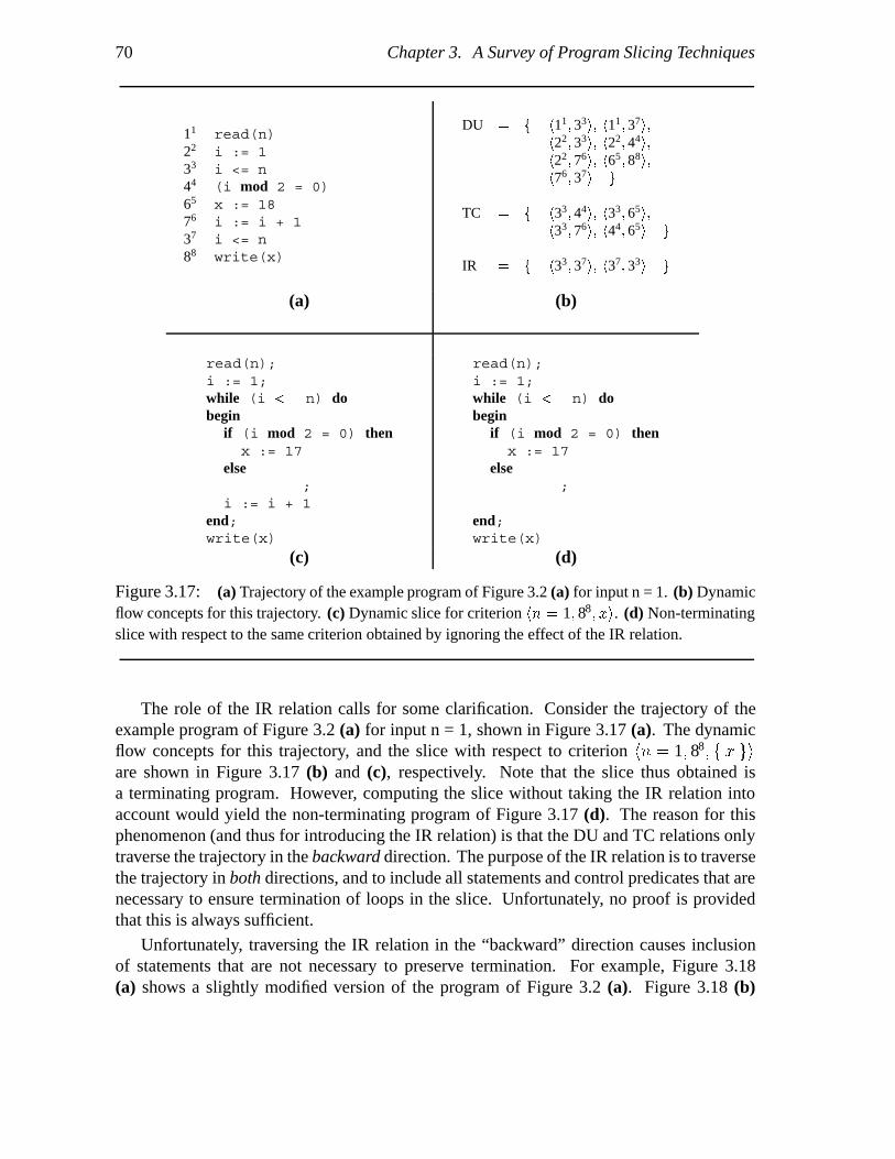
70 Chapter 3. A Survey of Program Slicing Techniques
11 read(n)22 i := 133 i <= n44 (i mod 2 = 0)65 x := 1876 i := i + 137 i <= n88 write(x)
DU � f h11� 33i� h11� 37i�h22� 33i� h22� 44i�h22� 76i� h65� 88i�h76� 37i g
TC � f h33� 44i� h33� 65i�h33� 76i� h44� 65i g
IR � f h33� 37i� h37� 33i g
(a) (b)
read(n);i := 1;while (i �� n) dobegin
if (i mod 2 = 0) thenx := 17
else;
i := i + 1end;write(x)
read(n);i := 1;while (i �� n) dobegin
if (i mod 2 = 0) thenx := 17
else;
end;write(x)
(c) (d)
Figure 3.17: (a) Trajectory of the example program of Figure 3.2 (a) for input n = 1. (b) Dynamicflow concepts for this trajectory. (c) Dynamic slice for criterion hn � 1� 88� xi. (d) Non-terminatingslice with respect to the same criterion obtained by ignoring the effect of the IR relation.
The role of the IR relation calls for some clarification. Consider the trajectory of theexample program of Figure 3.2 (a) for input n = 1, shown in Figure 3.17 (a). The dynamicflow concepts for this trajectory, and the slice with respect to criterion hn � 1� 88� f x giare shown in Figure 3.17 (b) and (c), respectively. Note that the slice thus obtained isa terminating program. However, computing the slice without taking the IR relation intoaccount would yield the non-terminating program of Figure 3.17 (d). The reason for thisphenomenon (and thus for introducing the IR relation) is that the DU and TC relations onlytraverse the trajectory in the backward direction. The purpose of the IR relation is to traversethe trajectory in both directions, and to include all statements and control predicates that arenecessary to ensure termination of loops in the slice. Unfortunately, no proof is providedthat this is always sufficient.
Unfortunately, traversing the IR relation in the “backward” direction causes inclusionof statements that are not necessary to preserve termination. For example, Figure 3.18(a) shows a slightly modified version of the program of Figure 3.2 (a). Figure 3.18 (b)

3.4. Methods for dynamic slicing 71
(1) read(n);(2) i := 1;(3) while (i �� n) do
begin(4) if (i mod 2 = 0) then(5) x := 17
else(6) x := 18;(7) z := x;(8) i := i + 1
end;(9) write(z)
11 read(n)22 i := 133 i <= n44 (i mod 2 = 0)65 x := 1876 z := x87 i := i + 138 i <= n49 (i mod 2 = 0)510 x := 17711 z := x812 i := i + 1313 i <= n914 write(z)
(a) (b)
Figure 3.18: (a) Example program. (b) Trajectory for input n = 2.
shows the trajectory for this program. From this trajectory, it follows that h76� 711i � IR,h65� 76i � DU, and h510� 711i � DU. Therefore, both statements (5) and (6) will be includedin the slice, although statement (6) is neither needed to compute the final value of z nor topreserve termination.
We conjecture that restricting the IR relation to statement instances that correspond tocontrol predicates in the program would yield smaller slices. Alternatively, it would beinteresting to investigate if using a dynamic variation of Podgurski and Clarke’s notion ofweak control dependence [123] could be used instead of the IR relation.
3.4.1.2 Dynamic dependence relations
Gopal [62] describes an approach where dynamic dependence relations are used to computedynamic slices. He introduces dynamic versions of Bergeretti and Carre’s information-flowrelations17 �S , �S , and �S (see Section 3.3.1.2). The �S relation contains all pairs hv� ei suchthat statement e depends on the input value of v when program S is executed. Relation �Scontains all pairs he� vi such that the output value of v depends on the execution of statemente. A pair hv� v�i is in relation �S if the output value of v� depends on the input value of v. Inthese definitions, it is presumed that S is executed for some fixed input.
For empty statements, assignments, and statement sequences Gopal’s dependence rela-tions are exactly the same as for the static case. The (static) information-flow relations fora conditional statement are derived from the statement itself, and from the statements thatconstitute its branches. For dynamic dependence relations, however, only the dependencesthat arise in the branch that is actually executed are taken into account. As in [22], the
17Gopal uses the notation sSv , vSv , and vSs . In order to avoid confusion and to make the relation with Bergerettiand Carre’s work explicit (see Section 3.3.1.2), we will use �S , �S , and �S instead.

72 Chapter 3. A Survey of Program Slicing Techniques
�� � ��� � ��� � ID
�S1;S2 � �S1 � �S1� �S2
�S1;S2� �S1
� �S2� �S2
�S1;S2� �S1
� �S2
�v:�e � VARS�e�� f e g�v:�e � f he� vi g�v:�e � �VARS�e�� f v g� � �ID � hv� vi�
�if e then S1 else S2 �
��VARS�e�� f e g� � �S1
�VARS�e�� f e g� � �S2
if e evaluates to trueif e evaluates to false
�if e then S1 else S2�
��f e g � DEFS�S1�� � �S1
�f e g � DEFS�S2�� � �S2
if e evaluates to trueif e evaluates to false
�if e then S1 else S2�
��VARS�e�� DEFS�S1�� � �S1
�VARS�e�� DEFS�S2�� � �S2
if e evaluates to trueif e evaluates to false
Figure 3.19: Definition of dynamic dependence relations.
EXPRESSION #a AFFECTED VARIABLES
1 f i� n� x g2 f i� x g3 f i� x g4 f i� x g5 f x g6 �7 f i� x g8 �
aExpressions are indicated by the line numbers in Figure 3.2.
Figure 3.20: The � relation for the example program of Figure 3.2 (a) and input n = 2.
dependence relation for a while statement (omitted here) is expressed in terms of depen-dence relations for nested conditionals with equivalent behavior. However, whereas in thestatic case loops are effectively replaced by their infinite unwindings, the dynamic case onlyrequires that a loop be unwound k times, where k is the number of times the loop executes.The resulting definitions are very convoluted because the dependence relations for the bodyof the loop may differ in each iteration. Hence, a simple transitive closure operation, as wasused in the static case, is insufficient.
Figure 3.19 summarizes Gopal’s dynamic dependence relations. Here, DEFS�S� denotesthe set of variables that is actually modified by executing statement S. Note that thisdefinition of DEFS is “dynamic” in the sense that it takes into account which branch of anif statement is executed. Using these relations, a dynamic slice w.r.t. the final value of avariable v is defined as:
�Pv � fe j he� vi � �Pg
Figure 3.20 (a) shows the information-flow relation � for the (entire) program of Fig-

3.4. Methods for dynamic slicing 73
read(n);i := 1;while (i �� n) dobegin
if (i mod 2 = 0) then
elsex := 18;
end;
read(n);i := 1;while (i �� n) dobegin
if (i mod 2 = 0) thenx := 17
else;
z := x;i := i + 1
end;
(a) (b)
Figure 3.21: (a) Non-terminating slice computed for example program of Figure 3.2 (a) withrespect to the final value of x, for input n = 1. (b) Slice for the example program of Figure 3.18(a) with respect to the final value of x, for input n = 2.
ure 3.2 (a)18. From this relation it follows that the set of expressions that affect the value ofx at the end of the program for input n = 2 are f 1� 2� 3� 4� 5� 7 g. The correspondingdynamic slice is almost identical to the one shown in Figure 3.1 (b), the only differencebeing the fact that Gopal’s algorithm excludes the final statement write(x) on line 8.
For certain cases, Gopal’s algorithm may compute a non-terminating slice of a terminat-ing program. Figure 3.21 (a) shows the slice for the program of Figure 3.2 and input n =1 as computed according to Gopal’s algorithm.
An advantage of using dependence relations is that, for certain cases, smaller slices arecomputed than by Korel and Laski’s algorithm. For example, Figure 3.21 (b) shows the slicewith respect to the final value of z for the example program of Figure 3.18 (a), for input n= 2. Observe that the assignment x := 18, which occurs in the slice computed by thealgorithm of Section 3.4.1.1, is not included in Gopal’s slice.
3.4.1.3 Dependence graphs
Miller and Choi [116] were the first to introduce a dynamic variation of the PDG, calledthe dynamic program dependence graph. These graphs are used by their parallel programdebugger to perform flowback analysis [15] and are constructed incrementally, on demand.Prior to execution, a (variation of a) static PDG is constructed, and the object code ofthe program is augmented with code that generates a log file. In addition, an emulationpackage is generated. Programs are partitioned into so-called emulation blocks (typically,a subroutine). During debugging, the debugger uses the log file, the static PDG, and the
18Gopal does not define information-flow relations for I/O statements. For the purposes of this example, itis assumed that the statement read(n) can be treated as an assignment n := SomeConstant, and that thestatements write(sum) and write(product) should be treated as empty statements.

74 Chapter 3. A Survey of Program Slicing Techniques
emulation package to re-execute an emulation block, and obtain the information necessaryto construct the part of the dynamic PDG corresponding to that block. In case the user wantsto perform flowback analysis to parts of the graph that have not been constructed yet, moreemulation blocks are re-executed.
Agrawal and Horgan [6] develop an approach for using dependence graphs to computedynamic slices. Their first two algorithms for computing dynamic slices are inaccurate, butuseful for understanding their final approach. The initial approach uses the PDG as it wasdiscussed in Section 3.3.1.319, and marks the vertices that are executed for a given test set.A dynamic slice is computed by computing a static slice in the subgraph of the PDG that isinduced by the marked vertices. By construction, this slice only contains vertices that wereexecuted. This solution is imprecise because it does not detect situations where there existsa flow edge in the PDG between a marked vertex v1 and a marked vertex v2, but where thedefinitions of v1 are not actually used at v2.
For example, Figure 3.22 (a) shows the PDG of the example program of Figure 3.2 (a).Suppose that we want to compute the slice w.r.t. the final value of x for input n = 2.All vertices of the PDG are executed, causing all PDG vertices to be marked. The staticslicing algorithm of Section 3.3.1.3 will therefore produce the entire program as the slice,even though the assignment x := 18 is irrelevant. This assignment is included in the slicebecause there exists a dependence edge from vertex x := 18 to vertex write(x) eventhough this edge does not represent a dependence that occurs during the second iteration ofthe loop. More precisely, this dependence only occurs in iterations of the loop where thecontrol variable i has an odd value.
The second approach consists of marking PDG edges as the corresponding dependencesarise during execution. Again, the slice is obtained by traversing the PDG, but this timeonly along marked edges. Unfortunately, this approach still produces imprecise slices in thepresence of loops because an edge that is marked in some loop iteration will be present in allsubsequent iterations, even when the same dependence does not recur. Figure 3.22 (b) showsthe PDG of the example program of Figure 3.18 (a). For input n = 2, all dependence edgeswill be marked, causing the slice to consist of the entire program. It is shown in [6] thata potential refinement of the second approach, consisting of unmarking edges of previousiterations, is incorrect.
Agrawal and Horgan point out the interesting fact that their second approach for com-puting dynamic slices produces results that are identical to those of the algorithm proposedby Korel and Laski (see Section 3.4.1.1). However, the PDG of a program (with option-ally marked edges) requires only O�n2� space (n denotes the number of statements in theprogram), whereas Korel and Laski’s trajectories require O�N� space, where N denotes thenumber of executed statements.
Agrawal and Horgan’s second approach computes overly large slices because it does notaccount for the fact that different occurrences of a statement in the execution history maybe (transitively) dependent on different statements. This observation motivates their third
19The dependence graphs of [6] do not have an entry vertex. The absence of an entry vertex does not resultin a different slice. For reasons of uniformity, all dependence graphs shown in this thesis have an entry vertex.

3.4. Methods for dynamic slicing 75
if (i mod 2 = 0)
Entry
read(n) i := 1 while (i <= n) write(x)
i := i + 1
x := 17 x := 18
if (i mod 2 = 0)
Entry
read(n) i := 1 write(z)
z := x i := i + 1
x := 17 x := 18
while (i <= n)
(a) (b)
x := 18
Entry
read(n) i := 1 write(z)
i := i + 1 i := i + 1
z := x z := x
x := 17
while (i <= n) while (i <= n) while (i <= n)
if (i mod 2 = 0)if (i mod 2 = 0)
(c)
Figure 3.22: (a) PDG of the program of Figure 3.2 (a). (b) PDG of the program of Figure 3.18(a). (c) DDG of the program of Figure 3.18 (a).
solution: create a distinct vertex in the dependence graph for each occurrence of a statementin the execution history. This kind of graph is referred to as a Dynamic Dependence Graph(DDG). A dynamic slicing criterion is identified with a vertex in the DDG, and a dynamicslice is computed by determining all DDG vertices from which the criterion can be reached.A statement or control predicate is included in the slice if the criterion can be reached fromat least one of the vertices for its occurrences.
Figure 3.22 (c) shows the DDG for the example program of Figure 3.18 (a). The slicingcriterion corresponds to the vertex labeled write(z), and all vertices from which thisvertex can be reached are indicated by shading. Observe that the criterion cannot be reachedfrom the vertex labeled x := 18. Therefore the corresponding assignment is not in theslice.
The disadvantage of using DDGs is that the number of vertices in a DDG is equal tothe number of executed statements. The number of dynamic slices, however, is in the worstcase O�2n�, where n is the number of statements in the program being sliced. Figure 3.23
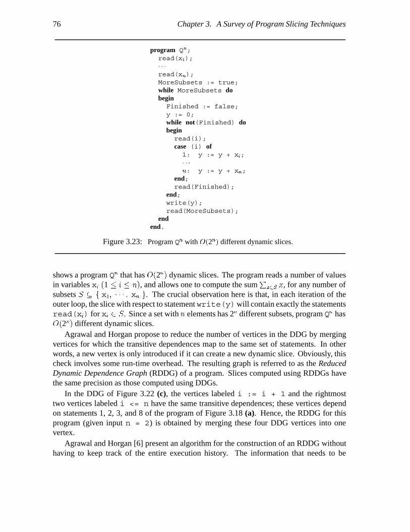
76 Chapter 3. A Survey of Program Slicing Techniques
program Qn;read(x1);� � �read(xn);MoreSubsets := true;while MoreSubsets dobeginFinished := false;y := 0;while not(Finished) dobeginread(i);case (i) of1: y := y + xi;� � �n: y := y + xn;
end;read(Finished);
end;write(y);read(MoreSubsets);
endend.
Figure 3.23: Program Qn with O�2n� different dynamic slices.
shows a program Qn that has O�2n� dynamic slices. The program reads a number of valuesin variables xi �1 � i � n�, and allows one to compute the sum
Px�S x, for any number of
subsets S f x1� � � � � xn g. The crucial observation here is that, in each iteration of theouter loop, the slice with respect to statementwrite(y)will contain exactly the statementsread(xi) for xi � S. Since a set with n elements has 2n different subsets, program Qn hasO�2n� different dynamic slices.
Agrawal and Horgan propose to reduce the number of vertices in the DDG by mergingvertices for which the transitive dependences map to the same set of statements. In otherwords, a new vertex is only introduced if it can create a new dynamic slice. Obviously, thischeck involves some run-time overhead. The resulting graph is referred to as the ReducedDynamic Dependence Graph (RDDG) of a program. Slices computed using RDDGs havethe same precision as those computed using DDGs.
In the DDG of Figure 3.22 (c), the vertices labeled i := i + 1 and the rightmosttwo vertices labeled i <= n have the same transitive dependences; these vertices dependon statements 1, 2, 3, and 8 of the program of Figure 3.18 (a). Hence, the RDDG for thisprogram (given input n = 2) is obtained by merging these four DDG vertices into onevertex.
Agrawal and Horgan [6] present an algorithm for the construction of an RDDG withouthaving to keep track of the entire execution history. The information that needs to be

3.4. Methods for dynamic slicing 77
maintained is: (i) for each variable, the vertex corresponding to its last definition, (ii) foreach predicate, the vertex corresponding to its last execution, and (iii) for each vertex in theRDDG, the dynamic slice w.r.t. that vertex.
3.4.2 Procedures
Agrawal, DeMillo and Spafford [4] consider dynamic slicing of procedures with call-by-value, call-by-reference, call-by-result, and call-by-value-result parameter-passing. A keyproperty of their method is that dynamic data dependences are defined in terms of definitionsand uses of memory locations; this has the advantage that global variables do not requirespecial treatment, and that no alias analysis is necessary. Agrawal et al. describe how eachparameter passing mechanism can be modeled by a set of mock assignments that is insertedbefore and/or after each procedure call. In the subsequent discussion, it is assumed that aprocedure P with formal parameters f1� � � � � fn is called with actual parameters a1� � � � � an.Call-by-value parameter-passing can be modeled by a sequence of assignments f1:�a1;� � �; fn:�an that is executed before the procedure is entered. In order to determine thememory cells for the correct activation record, the USE sets for the actual parameters ai aredetermined before the procedure is entered, whereas the DEF sets for the formal parametersfi are determined after the procedure is entered. For Call-by-value-result parameter-passing,additional assignments of formal parameters to actual parameters have to be performed uponexit from the procedure. Call-by-reference parameter-passing does not require any actionsspecific to dynamic slicing, as the same memory cell is associated with corresponding actualand formal parameters ai and fi.
An alternative approach for interprocedural dynamic slicing was presented by Kamkar,Shahmehri, and Fritzson [90, 89]. This work distinguishes itself from the solution byAgrawal et al. by the fact that the authors are primarily concerned with procedure-levelslices. That is, they study the problem of determining the set of call sites in a program thataffect the value of a variable at a particular call site.
During execution, a (dynamic dependence) summary graph is constructed. The verticesof this graph, referred to as procedure instances, correspond to procedure activations anno-tated with their parameters20. The edges of the summary graph are either activation edgescorresponding to procedure calls, or summary dependence edges. The latter type reflectstransitive data and control dependences between input and output parameters of procedureinstances.
A slicing criterion is defined as a pair consisting of a procedure instance, and an input oroutput parameter of the associated procedure. After constructing the summary graph, a slicewith respect to a slicing criterion is determined in two steps. First, the parts of the summarygraph from which the criterion can be reached is determined; this subgraph is referred to asan execution slice. Vertices of an execution slice are partial procedure instances, because
20More precisely, Kamkar refers to the incoming and outgoing variables of a procedure. This notion alsoapplies to global variables that are referenced or modified in a procedure.

78 Chapter 3. A Survey of Program Slicing Techniques
some parameters may be “sliced away”. An interprocedural program slice consists of allcall sites in the program for which a partial instance occurs in the execution slice.
Three approaches for constructing summary graphs are considered. In the first approach,intraprocedural data dependences are determined statically: this may result in inaccurateslices in the presence of conditionals. In the second approach, all dependences are determinedat run-time. While this results in accurate dynamic slices, the dependences for a procedureP have to be re-computed every time P is called. The third approach attempts to combinethe efficiency of the “static” approach with the accuracy of the “dynamic” approach bycomputing the dependences inside basic blocks statically, and the inter-block dependencesdynamically. In all approaches control dependences21 are determined statically. It is unclearhow useful this third approach is in the presence of composite variables and pointers,where the run-time intra-block dependences cannot be determined statically: additionalalias analysis would have to be performed at run-time.
Kamkar [87] adapts the interprocedural slicing method by Kamkar et al. [90, 89] tocompute statement-level interprocedural slices (i.e., slices consisting of a set of statementsinstead of a set of call sites). In essence, this is accomplished by introducing a vertex foreach statement instance (instead of each procedure instance) in the summary graph. Thesame three approaches (static, dynamic, combined static/dynamic) for constructing summarygraphs can be used.
Choi, Miller and Netzer [38] discuss an approach for interprocedural flowback analysis.Initially, it is assumed that a procedure call may modify every global variable; to this end,the static PDG is augmented with linking edges indicating potential data dependences. In asecond phase, interprocedural summary information is used to either replace linking edgesby data dependence edges, or delete them from the graph. Some linking edges may remain;these have to be resolved at run-time.
3.4.3 Composite data types and pointers
3.4.3.1 Dynamic flow concepts
Korel and Laski [100] consider slicing in the presence of composite variables by regardingeach element of an array, or field of a record as a distinct variable. Dynamic data structuresare treated as two distinct entities, namely the pointer itself and the object being pointed to.For dynamically allocated objects, they propose a solution where a unique name is assignedto each object.
3.4.3.2 Dependence graphs
Agrawal, DeMillo, and Spafford [4] present a dependence graph based algorithm for dynamicslicing in the presence of composite data types and pointers. Their solution consists of
21Kamkar et al. use a notion of termination-preserving control dependence that is similar to Podgurski andClarke’s weak control dependence [123].
3.4. Methods for dynamic slicing 79
expressing DEF and USE sets in terms of actual memory locations provided by the compiler.The algorithm of [4] is similar to that for static slicing in the presence of composite data typesand pointers by the same authors (see Section 3.3.4). However, during the computation ofdynamic reaching definitions, no Maybe Intersections can occur—only Complete and PartialIntersections.
Choi, Miller, and Netzer [38] extend the flowback analysis method by Miller and Choi[116] (see Section 3.4.1.3) in order to deal with arrays and pointers. For arrays, linkingedges are added to their static PDGs; these edges express potential data dependences thatare either deleted, or changed into genuine data dependences at run-time. Pointer accessesare resolved at run-time, by recording all uses of pointers in the log file.
3.4.4 Concurrency
3.4.4.1 Dynamic flow concepts
Korel and Ferguson [98] extend the dynamic slicing method of Korel and Laski [99, 100]to distributed programs with Ada-type rendezvous communication (see, e.g., [18]). For adistributed program, the execution history is formalized as a distributed program path that,for each task, comprises: (i) the sequence of statements (trajectory) executed by it, and (ii)a sequence of triples hA�C�Bi identifying each rendezvous the task is involved in. Here, Aidentifies the accept statement in the task, B identifies the other task that participated in thecommunication, and C denotes the entry call statement in the task that was involved in therendezvous.
A dynamic slicing criterion of a distributed program specifies: (i) the input of each task,(ii) a distributed program path P , (iii) a taskw, (iv) a statement occurrence q in the trajectoryof w, and (v) a variable v. A dynamic slice with respect to such a criterion is an executableprojection of the program that is obtained by deleting statements from it. However, theprogram is only guaranteed to preserve the behavior of the program if the rendezvous in theslice occur in the same relative order as in the program. (Note that not all rendezvous of theprogram need to be in the slice.)
The Korel-Ferguson method for computing slices of distributed programs of is basicallya generalization of the Korel-Laski method, though stated in a slightly different manner. Inaddition to the previously discussed dynamic flow concepts (see Section 3.4.1.1), a notionof communication influence is introduced, to capture the interdependences between tasks.The authors also present a distributed version of their algorithm that uses a separate slicingprocess for each task.
3.4.4.2 Dependence graphs
Duesterwald, Gupta, and Soffa [50] present a dependence graph based algorithm for com-puting dynamic slices of distributed programs. They introduce a Distributed Dependence

80 Chapter 3. A Survey of Program Slicing Techniques
Graph (DDG)22 for representing distributed programs.
A distributed program P consists of a set of processes P1� � � � � Pn. Communica-tion between processes is assumed to be synchroneous and nondeterministic and is ex-pressed by way of send and receive statements. A distributed dynamic slicing criterionhI1� X1i� � � � � hIn� Xni specifies for each process Pi its input Ii, and a set of statements Xi.A distributed dynamic slice S is an executable set of processes P �
1� � � � � P�n such that the
statements of P �i are a subset of those of Pi. Slice S computes the same values at statements
in each Xi as program P does, when executed with the same input. This is accomplishedby: (i) including all input statements in the slice, and (ii) replacing nondeterministic com-munication statements in the program by deterministic communication statements in theslice.
A DDG contains a single vertex for each statement and control predicate in the program.Control dependences between statements are determined statically, prior to execution. Edgesfor data and communication dependences are added to the graph at run-time. Slices arecomputed in the usual way by determining the set of DDG vertices from which the verticesspecified in the criterion can be reached. Both the construction of the DDG and the computa-tion of slices is performed in a distributed manner; a separate DDG construction process andslicing process is assigned to each process Pi in the program; these processes communicatewhen a send or receive statement is encountered.
Due to the fact that a single vertex is used for all occurrences of a statement in the execu-tion history, inaccurate slices may be computed in the presence of loops (see Section 3.4.1.1).For example, the slice with respect to the final value of z for the program of Figure 3.18with input n = 2 will be the entire program.
Cheng [35] presents an alternative dependence graph based algorithm for computingdynamic slices of distributed and concurrent programs. The PDN representation of a con-current program (see Section 3.3.5) is used for computing dynamic slices. Cheng’s algorithmis basically a generalization of the initial approach proposed by Agrawal and Horgan [6]:the PDN vertices corresponding to executed statements are marked, and the static slicingalgorithm of Section 3.3.5 is applied to the PDN subgraph induced by the marked vertices.As was discussed in Section 3.4.1.3, this yields inaccurate slices.
Choi et al. [116, 38] describe how their approach for flowback analysis can be extendedto parallel programs. Shared variables with semaphores, message-passing communication,and Ada-type rendezvous mechanisms are considered. To this end, a parallel dynamic graphis introduced that contains synchronization vertices for synchronization operations (such asP and V on a semaphore) and synchronization edges that represent dependences betweenconcurrent processes. Choi et al. explain how, by analysis of the parallel dynamic graph,read/write and write/write conflicts between concurrent processes can be found.
22This abbreviation ‘DDG’ used in Section 3.4.4.2 should not be confused with the notion of a DynamicDependence Graph that was discussed earlier in Section 3.4.1.

3.4. Methods for dynamic slicing 81
a b
Met
hod
Com
puta
tion
Exe
cuta
ble
Inte
rpro
cedu
ral
Solu
tion
Dat
a
Typ
es
Con
curr
ency
Korel, Laski [99, 100] D yes no S, A, P noKorel, Ferguson [98] D yes no S, A yesGopal [62] I no no S noAgrawal, Horgan [6] G no no S noAgrawal et al. [2, 4] G no yes S, A, P noKamkar et al. [90, 89] G no yes S noDuesterwald et al. [50] G yes no S, A, P yesCheng [35] G no no S yesChoi et al. [116, 38] G no yes S, A, P yesField et al. (Chap. 5, 6) R yes no S, A, P no
aD = dynamic flow concepts, I = dynamic dependence relations, G = reachability ina dependence graph. R = dependence tracking in term graph rewriting systems (seeSection 3.6).bS = scalar variables, A = arrays/records, P = pointers.
Table 3.4: Overview of dynamic slicing methods.
3.4.5 Comparison
In this section, we compare and classify the dynamic slicing methods that were presentedearlier. The section is organized as follows: Section 3.4.5.1 summarizes the problems that areaddressed in the literature. Sections 3.4.5.2 and 3.4.5.3 compare the accuracy and efficiencyof slicing methods that address the same problem, respectively. Finally, Section 3.4.5.4investigates the possibilities for “combining” algorithms that deal with different problems.
3.4.5.1 Overview
Table 3.4 lists the dynamic slicing algorithms discussed earlier, and summarizes the issuesstudied in each paper. For each paper, the table shows: (i) the computation method,(ii) whether or not the computed slices are executable programs, (iii) whether or not aninterprocedural solution is supplied, (iv) the data types under consideration, and (v) whetheror not concurrency is considered. Similar to Table 3.2, the table only shows problems thathave been addressed. It does not indicate how various algorithms may be combined, and italso does not give an indication of the quality of the work. The work by Field et al. (seeChapters 4, 5, and 6) mentioned in Table 3.4 relies on substantially different techniques thanthose used for the dynamic slicing algorithms discussed previously, and will therefore be

82 Chapter 3. A Survey of Program Slicing Techniques
studied separately in Section 3.6.Unlike in the static case, there exists a significant difference between methods that com-
pute executable slices [99, 100, 50, 98], and approaches that compute slices merely consistingof sets of statements [6, 4, 62]. The latter type of slice may not be executable due to theabsence of assignments for incrementing loop counters23. For convenience, we will hence-forth refer to such slices as “non-executable” slices. As was discussed in Section 3.4.1.1,the algorithms that compute executable dynamic slices may produce inaccurate results in thepresence of loops.
Apart from the work by Venkatesh [137], there is very little semantic justification for anyof the methods for computing “non-executable” slices. The algorithms of [116, 6, 90, 35, 89]are graph-reachability algorithms that compute a set of statements that directly or indirectly“affect” the values computed at the criterion. Besides the algorithms themselves, little or noattention is paid to formal characterization of such slices.
3.4.5.2 Accuracy
basic algorithms. The slices computed by Korel and Laski’s algorithm [99, 100] (seeSection 3.4.1.1) are larger than those computed by the algorithms by Agrawal and Horgan[6] (see Section 3.4.1.3) and Gopal [62] (see Section 3.4.1.2). This is due to Korel andLaski’s constraint that their slices should be executable.
procedures. Dependence graph based algorithms for interprocedural dynamic slicing wereproposed by Agrawal, DeMillo, and Spafford [4], and by Kamkar et al. [90, 89] (seeSection 3.4.2). It is unclear if one of these algorithms produces more accurate slices thanthe other.
composite variables and pointers. Korel and Laski [100] (see Section 3.4.1.1), andAgrawal, DeMillo, and Spafford (see Section 3.4.1.3) proposed methods for dynamic slicingin the presence of composite variables and pointers. We are unaware of any difference inaccuracy.
concurrency. Korel and Ferguson [98] (see Section 3.4.4.1) and Duesterwald, Gupta, andSoffa [50] (see Section 3.4.4.2) compute executable slices, but deal with nondeterminismin a different way: the former approach requires a mechanism for replaying rendezvousin the slice in the same relative order as they appeared in the original program, whereasthe latter approach replaces nondeterministic communication statements in the program bydeterministic communication statements in the slice. Cheng [35] and Choi et al. [116, 38](see Section 3.4.4.2) do not address this problem because the slices they compute are notnecessarily executable. The dynamic slicing methods by Cheng and Duesterwald et al. areinaccurate because they are based on “static” dependence graphs in which no distinction
23Of course, such a slice may be executed anyway; however, it may not terminate.

3.4. Methods for dynamic slicing 83
is made between the different occurrences of a statement in the execution history (see thediscussion in Section 3.4.1.3).
3.4.5.3 Efficiency
Since dynamic slicing involves run-time information, it is not surprising that all dynamicslicing methods discussed in this section have time requirements that depend on the numberof executed statements (or procedure calls in the case of [90, 89]) N . All algorithms spendat leastO�N� time during execution in order to store the execution history of the program, orto update dependence graphs. Certain algorithms (e.g., [99, 100, 98]) traverse the executionhistory in order to extract the slice and thus require again at least O�N� time for eachslice, whereas other algorithms require less (sometimes even constant) time. Whenever timerequirements are discussed below, the time spent during execution for constructing historiesor dependence graphs will be ignored. Space requirements will always be discussed in detail.
basic algorithms. Korel and Laski’s solution [99, 100] (see Section 3.4.1.1) requiresO�N� space to store the trajectory, and O�N2� space to store the dynamic flow concepts.Construction of the flow concepts requires O�N � �v � n�� time, where v and n are thenumber of variables and statements in the program, respectively. Extracting a single slicefrom the computed flow concepts can be done in O�N� time.
The algorithm by Gopal [62] (see Section 3.4.1.2) requires O�N� space to store theexecution history and O�n� v� space to store the �S relation. The time required to computethe �S relation for a program S is bounded by O�N2 � v2�. From this relation, slices can beextracted in O�v� time.
As was discussed in Section 3.4.1.3, the slicing method proposed by Agrawal and Horganrequires at most O�2n� space, where n is the number of statements in the program. Sincevertices in an RDDG are annotated with their slice, slices can be extracted from it in O�1�.
procedures. The interprocedural dynamic slicing method proposed by Kamkar et al. [90,89] (see Section 3.4.2) requires O�P 2� space to store the summary graph, where P is thenumber of executed procedure calls. A traversal of this graph is needed to extract a slice;this takes O�P 2� time.
The time and space requirements of the method by Agrawal, DeMillo, and Spafford[4] are essentially the same as those of the Agrawal-Horgan basic slicing method discussedabove.
composite variables and pointers. The algorithms by Korel and Laski [100] (see Sec-tion 3.4.3.1) and Agrawal, DeMillo, and Spafford [4] (see Section 3.4.3.2) for slicing in thepresence of composite variables and pointers are adaptations of the basic slicing algorithmsby Korel and Laski and Agrawal and Horgan, respectively (see the discussion above). Theseadaptations, which essentially consist of a change in the reaching definitions functions that

84 Chapter 3. A Survey of Program Slicing Techniques
Proc
edur
es
Com
posi
te
Var
iabl
es
Con
curr
ency
Dyn. Flow — Korel, Laski [99, 100] Korel, Ferguson [98]ConceptsDyn. Dependence Gopal [62] — —RelationsDependence Agrawal et al. [4] Agrawal et al. [4] Duesterwald et al. [50]Graphs Kamkar et al. [90, 89] Cheng [35]
Choi et al. [116, 38]
Table 3.5: Orthogonal dimensions of dynamic slicing.
are used to determine data dependences, do not affect the worst-case behavior of the algo-rithms. Therefore, we expect the time and space requirements to be the same as in the scalarvariable case.
concurrency. The algorithms by Cheng [35] and Duesterwald et al. [50] are based onstatic PDGs. Therefore, only O�n2� space is required to store the dependence graph, andslices can be extracted in O�n2� time. The distributed slicing algorithm by Duesterwald etal. [50] uses a separate slicing process for each process in the program; the slicing processfor process Pi requires time O�ei�, where ei is the number of edges in the PDG for processPi. The communication overhead between the slicing processes requires at most O�e� time,where e is the number of edges in the entire graph.
3.4.5.4 Combining dynamic slicing algorithms
Table 3.5 displays solutions to “orthogonal” dimensions of dynamic slicing: dealing withprocedures, composite variables and pointers, and communication between processes. Thealgorithms based on dynamic flow concepts for dealing with composite variables/pointers[100], and concurrency [98] may be integrated with little problems. For dependence graphs,however, the situation is slightly more complicated because:
� Different graph representations are used. Agrawal et al. [4], Kamkar et al. [90, 89]and Choi et al. [116, 38] use dynamic dependence graphs with distinct vertices fordifferent occurrence of statements in the execution history. In contrast, Duesterwaldet al. [50] and Cheng [35] use variations of static PDGs.
� The dynamic slicing by Agrawal et al. [4] is based on definition and use of memorylocations. All other dependence graph based slicing methods are based on definitions

3.5. Applications of program slicing 85
and uses of variable names.
Furthermore, it is unclear if the combined static/dynamic interprocedural slicing approach byKamkar et al. [90, 89] is practical in the presence of composite variables and pointers, becausethe intra-block dependences cannot be determined statically in this case, and additional aliasanalysis would be required at run-time.
3.5 Applications of program slicing
3.5.1 Debugging and program analysis
Debugging can be a difficult task when one is confronted with a large program, and fewclues regarding the location of a bug. Program slicing is useful for debugging, because itpotentially allows one to ignore many statements in the process of localizing a bug [108].If a program computes an erroneous value for a variable x, only the statements in the slicew.r.t. x have (possibly) contributed to the computation of that value. In this case, it is likelythat the error occurs in the one of the statements in the slice. However, it need not alwaysbe the case that the error occurs in the slice, as an error may consist of a statement that ismissing inadvertently. However, in situations like this it is probable that more, or differentstatements show up in the slice than one would expect.
Forward slices are also useful for debugging. A forward slice w.r.t. a statement s canshow how a value computed at s is being used subsequently, and can help the programmerensure that s establishes the invariants assumed by the later statements. For example, thiscan be useful in catching off-by-one errors. Another purpose of forward slicing is to inspectthe parts of a program that may be affected by a proposed modification, to check that thereare no unforeseen effects on the program’s behavior.
Lyle and Weiser [109] introduce program dicing, a method for combining the informationof different slices. The basic idea is that, when a program computes a correct value forvariable x and an incorrect value for variable y, the bug is likely to be found in statementsthat are in the slice w.r.t. y, but not in the slice w.r.t. x. This approach is not fail-safein the presence of multiple bugs, and when computations that use incorrect values producecorrect values (referred to as coincidental correctness by Agrawal [2]). The authors claimthat program dicing still produces useful results when these assumptions are relaxed.
Bergeretti and Carre [22] explain how static slicing methods can detect “dead” code,i.e., statements that cannot affect any output of the program. Often, such statements are notexecutable due to the presence of a bug. Static slicing can also be employed to determine usesof uninitialized variables, another symptom of an error in the program. However, there existprevious techniques for detection of dead code and uses of uninitialized variables [7, 150]that do not rely on slicing.
In debugging, one is often interested in a specific execution of a program that exhibitsanomalous behavior. Dynamic slices are particularly useful here, because they only reflect theactual dependences of that execution, resulting in smaller slices than static ones. Agrawal’sthesis [2] contains a detailed discussion how static and dynamic slicing can be utilized for
86 Chapter 3. A Survey of Program Slicing Techniques
semi-automated debugging of programs [6, 4]. He proposes an approach where the usergradually “zooms out” from the location where the bug manifested itself by repeatedlyconsidering larger data and control slices. A data slice is obtained by only taking (staticor dynamic) data dependences into account; a control slice consists of the set of controlpredicates surrounding a language construct. The closure of all data and control slicesw.r.t. an expression is the (static or dynamic) slice w.r.t. the set of variables used inthe expression. The information of several dynamic slices can be combined to gain someinsight into the location of a bug. Several operations on slices are proposed to this end,such as union, intersection, and difference. The difference operation is a dynamic versionof the program “dicing” notion of Lyle and Weiser [109]. Obviously, these operations forcombining slices may produce false leads in the presence of multiple bugs or coincidentalcorrectness. Agrawal, DeMillo, and Spafford [5] discuss the implementation of a debuggingtool that is based on ideas in previous papers by the same authors [2, 4, 6].
Pan and Spafford [121, 122] present a number of heuristics for fault localization. Theseheuristics describe how dynamic slices (variations on the type proposed by Agrawal et al.[6]) can be used for selecting a set of suspicious statements that is likely to contain a bug.The approach of Pan and Spafford consists of two phases. First, the program is executed foran extensive number of test cases, and each test case is classified as being error-revealingor non-error-revealing, depending on the fact whether or not its reveals the presence of abug. The second step consists of the actual heuristic rules for combining the informationcontained in dynamic slices for these test cases in various ways. As an example, one mightthink of displaying the set of statements that occur in every dynamic slice for an error-revealing test-case—such statements are likely to contain the bug. Other heuristics dependon the inclusion frequency or the influence frequency of statements in dynamic slices. Theformer denotes the number of slices in which a particular statement occurs, whereas thelatter notion indicates the number of times that a statement in a particular dynamic sliceis “referred to” in terms of data dependence and control dependence. For example, one ofthe heuristics given by Pan and Spafford consists of selecting the statements with “high”influence frequency in a slice for a selected error-revealing test case. Note that this requires athreshold to be specified by the user that determines the boundary between “high” and “low”frequencies. It is argued that this boundary can be shifted interactively, thereby graduallyincreasing the number of statements under consideration.
Choi, Miller and Netzer [38] describe the design and efficient implementation of adebugger for parallel programs that incorporates flowback analysis, a notion introduced in theseminal paper by Balzer [15]. Intuitively, flowback analysis reveals how the computation ofvalues depends on the earlier computation of other values. The difference between flowbackanalysis and (dependence graph based) dynamic slices is that the former notion allows one tointeractively browse through a dependence graph, whereas the latter consists of the set of allprogram parts corresponding to vertices of the graph from which a designated vertex—thecriterion—can be reached.
Fritzson et al. use interprocedural static [59] and dynamic [90, 87] slicing for algorithmicdebugging [132, 131]. An algorithmic debugger partially automates the task of localizinga bug by comparing the intended program behavior with the actual program behavior. The
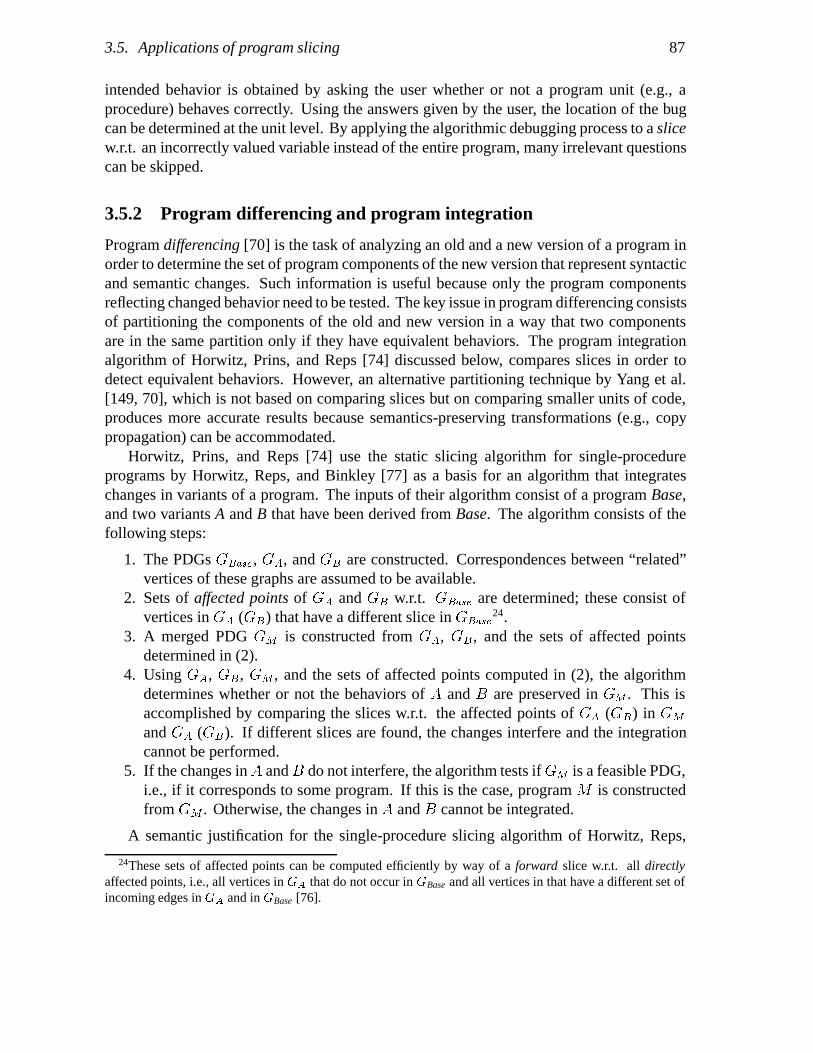
3.5. Applications of program slicing 87
intended behavior is obtained by asking the user whether or not a program unit (e.g., aprocedure) behaves correctly. Using the answers given by the user, the location of the bugcan be determined at the unit level. By applying the algorithmic debugging process to a slicew.r.t. an incorrectly valued variable instead of the entire program, many irrelevant questionscan be skipped.
3.5.2 Program differencing and program integration
Program differencing [70] is the task of analyzing an old and a new version of a program inorder to determine the set of program components of the new version that represent syntacticand semantic changes. Such information is useful because only the program componentsreflecting changed behavior need to be tested. The key issue in program differencing consistsof partitioning the components of the old and new version in a way that two componentsare in the same partition only if they have equivalent behaviors. The program integrationalgorithm of Horwitz, Prins, and Reps [74] discussed below, compares slices in order todetect equivalent behaviors. However, an alternative partitioning technique by Yang et al.[149, 70], which is not based on comparing slices but on comparing smaller units of code,produces more accurate results because semantics-preserving transformations (e.g., copypropagation) can be accommodated.
Horwitz, Prins, and Reps [74] use the static slicing algorithm for single-procedureprograms by Horwitz, Reps, and Binkley [77] as a basis for an algorithm that integrateschanges in variants of a program. The inputs of their algorithm consist of a program Base,and two variants A and B that have been derived from Base. The algorithm consists of thefollowing steps:
1. The PDGs GBase , GA, and GB are constructed. Correspondences between “related”vertices of these graphs are assumed to be available.
2. Sets of affected points of GA and GB w.r.t. GBase are determined; these consist ofvertices in GA (GB) that have a different slice in GBase
24.3. A merged PDG GM is constructed from GA, GB , and the sets of affected points
determined in (2).4. Using GA, GB, GM , and the sets of affected points computed in (2), the algorithm
determines whether or not the behaviors of A and B are preserved in GM . This isaccomplished by comparing the slices w.r.t. the affected points of GA (GB) in GM
and GA (GB). If different slices are found, the changes interfere and the integrationcannot be performed.
5. If the changes inA andB do not interfere, the algorithm tests if GM is a feasible PDG,i.e., if it corresponds to some program. If this is the case, program M is constructedfrom GM . Otherwise, the changes in A and B cannot be integrated.
A semantic justification for the single-procedure slicing algorithm of Horwitz, Reps,
24These sets of affected points can be computed efficiently by way of a forward slice w.r.t. all directlyaffected points, i.e., all vertices in GA that do not occur in GBase and all vertices in that have a different set ofincoming edges in GA and in GBase [76].
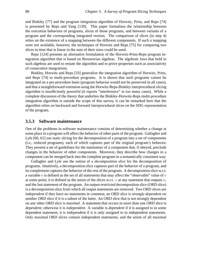
88 Chapter 3. A Survey of Program Slicing Techniques
and Binkley [77] and the program integration algorithm of Horwitz, Prins, and Reps [74]is presented by Reps and Yang [130]. This paper formalizes the relationship betweenthe execution behaviors of programs, slices of those programs, and between variants of aprogram and the corresponding integrated version. The comparison of slices (in step 4)relies on the existence of a mapping between the different components. If such a mappingwere not available, however, the techniques of Horwitz and Reps [75] for comparing twoslices in time that is linear in the sum of their sizes could be used.
Reps [124] presents an alternative formulation of the Horwitz-Prins-Reps program in-tegration algorithm that is based on Brouwerian algebras. The algebraic laws that hold insuch algebras are used to restate the algorithm and to prove properties such as associativityof consecutive integrations.
Binkley, Horwitz and Reps [33] generalize the integration algorithm of Horwitz, Prins,and Reps [74] to multi-procedure programs. It is shown that such programs cannot beintegrated on a per-procedure basis (program behavior would not be preserved in all cases),and that a straightforward extension using the Horwitz-Reps-Binkley interprocedural slicingalgorithm is insufficiently powerful (it reports “interference” in too many cases). While acomplete discussion of the theory that underlies the Binkley-Horwitz-Reps multi-procedureintegration algorithm is outside the scope of this survey, it can be remarked here that thealgorithm relies on backward and forward interprocedural slices on the SDG representationof the program.
3.5.3 Software maintenance
One of the problems in software maintenance consists of determining whether a change atsome place in a program will affect the behavior of other parts of the program. Gallagher andLyle [60, 61] use static slicing for the decomposition of a program into a set of components(i.e., reduced programs), each of which captures part of the original program’s behavior.They present a set of guidelines for the maintainer of a component that, if obeyed, precludechanges in the behavior of other components. Moreover, they describe how changes in acomponent can be merged back into the complete program in a semantically consistent way.
Gallagher and Lyle use the notion of a decomposition slice for the decomposition ofprograms. Intuitively, a decomposition slice captures part of the behavior of a program, andits complement captures the behavior of the rest of the program. A decomposition slice w.r.t.a variable v is defined as the set of all statements that may affect the “observable” value of vat some point; it is defined as the union of the slices w.r.t. v at any statement that outputs v,and the last statement of the program. An output-restricted decomposition slice (ORD slice)is a decomposition slice from which all output statements are removed. Two ORD slices areindependent if they have no statements in common; an ORD slice is strongly dependent onanother ORD slice if it is a subset of the latter. An ORD slice that is not strongly dependenton any other ORD slice is maximal. A statement that occurs in more than one ORD slice isdependent; otherwise it is independent. A variable is dependent if it is assigned to in somedependent statement; it is independent if it is only assigned to in independent statements.Only maximal ORD slices contain independent statements, and the union of all maximal

3.5. Applications of program slicing 89
ORD slices is equal to the original program (minus output statements). The complementof an ORD slice is defined as the original program minus all independent statements of theORD slice and all output statements.
The essential observation by Gallagher and Lyle [61] is that independent statements in aslice do not affect the data and control flow in the complement. This results in the followingguidelines for modification:
� Independent statements may be deleted from a decomposition slice.� Assignments to independent variables may be added anywhere in a decomposition
slice.� Logical expressions and output statements may be added anywhere in a decomposition
slice.� New control statements that surround any dependent statements will affect the com-
plement’s behavior.
New variables may be considered as independent variables, provided that there are no nameclashes with variables in the complement. If changes are required that involve a dependentvariable v, the user can either extend the slice so that v is independent (in a way described inthe paper), or introduce a new variable. Merging changes to components into the completeprogram is a trivial task. Since it is guaranteed that changes to an ORD slice do not affectits complement, only testing of the modified slice is necessary.
3.5.4 Testing
A program satisfies a “conventional” data flow testing criterion if all def-use pairs occur ina successful test-case. Duesterwald, Gupta, and Soffa [51] propose a more rigorous testingcriterion, based on program slicing: each def-use pair must be exercised in a successful test-case; moreover it must be output-influencing, i.e., have an influence on at least one outputvalue. A def-use pair is output-influencing if it occurs in an output slice, i.e., a slice w.r.t. anoutput statement. It is up to the user, or an automatic test-case generator to construct enoughtest-cases such that all def-use pairs are tested. Three slicing approaches are utilized, basedon different dependence graphs. Static slices are computed using static dependence graphs(similar to the PDGs of Horwitz, Reps, and Binkley [77]), dynamic slices are computed usingdynamic dependence graphs (similar to DDGs of Agrawal and Horgan [6], but instances ofthe same vertex are merged, resulting in a slight loss of precision), and hybrid slices arecomputed using dependence graphs that are based on a combination of static and dynamicinformation. In the hybrid approach, the set of variables in the program is partitioned intotwo disjoint subsets in a way that variables in one subset do not refer to variables in theother subset. Static dependences are computed for one subset (typically scalar variables),dynamic dependences for the other subset (typically arrays and pointers). The advantage ofthis approach is that it combines reasonable efficiency with reasonable precision.
Kamkar, Shahmehri, and Fritzson [88] extend the work of Duesterwald, Gupta, and Soffato multi-procedure programs. To this end, they define appropriate notions of interproceduraldef-use pairs. The interprocedural dynamic slicing method by Kamkar et al. [90, 89] is used

90 Chapter 3. A Survey of Program Slicing Techniques
to determine which interprocedural def-use pairs have an effect on a correct output value,for a given test case. The summary graph representation that was discussed in Section 3.4.2is slightly modified by annotating vertices and edges with def-use information. This way,the set of def-use pairs exercised by a slice can be determined efficiently.
Regression testing consists of re-testing only the parts affected by a modification of apreviously tested program, while maintaining the “coverage” of the original test suite. Gupta,Harrold, and Soffa [65] describe an approach to regression testing where slicing techniquesare used. Backward and forward static slices serve to determine the program parts affectedby the change, and only test cases that execute “affected” def-use pairs need to be executedagain. Conceptually, slices are computed by backward and forward traversals of the CFG ofa program, starting at the point of modification. However, the algorithms by Gupta, Harrold,and Soffa [65] are designed to determine the information necessary for regression testingonly (i.e., affected def-use pairs).
Binkley [29] describes an approach for reducing the cost of regression testing of multi-procedure programs by (i) reducing the number of tests that must be re-run,and (ii) decreasingthe size of the program that they must run on. This is accomplished by determining the setof program points affected by the modification, and the set of preserved program points (seeSection 3.5.2). The set of affected points is used to construct a smaller and more efficientprogram that only captures the modified behavior of the original program; all test-cases thatneed to be re-run can be applied to this program. The set of preserved points is used to inferwhich test-cases need not be re-run.
Bates and Horwitz [20] use a variation of the PDG notion of Horwitz, Prins, and Reps[74] for incremental program testing. Testing criteria are defined in terms of PDG notions:i.e., the “all-vertices” testing criterion is satisfied if each vertex of the PDG is exercised by atest set (i.e., each statement and control predicate in the program is executed). An “all-flow-edges” criterion is defined in a similar manner. Given a tested and subsequently modifiedprogram, slicing is used to determine: (i) the statements affected by the modification, and(ii) the test-cases that can be reused for the modified program. Roughly speaking, theformer consists of the statements that did not occur previously as well as any statements thathave different slices. The latter requires partitioning the statements of the original and themodified program into equivalence classes; statements are in the same class if they have thesame “control” slice (a slightly modified version of the standard notion). Bates and Horwitzprove that statements in the same class are exercised by the same test cases.
3.5.5 Tuning compilers
Larus and Chandra [106] present an approach for tuning of compilers where dynamic slicingis used to detect potential occurrences of redundant common subexpressions. Finding sucha common subexpression is an indication of sub-optimal code being generated.
Object code is instrumented with trace-generating instructions. A trace-regenerator readsa trace and produces a stream of events, such as the read and load of a memory location. Thisstream of events is input for a compiler-auditor (e.g., a common-subexpression eliminationauditor) that constructs dynamic slices w.r.t. the current values stored in registers. Larus

3.5. Applications of program slicing 91
and Chandra use a variation of the approach by Agrawal and Horgan [6]: a dynamic sliceis represented by directed acyclic graph (DAG) containing all operators and operands thatproduced the current value in a register. A common subexpression occurs when isomorphicDAGs are constructed for two registers. However, the above situation only indicates that acommon subexpression occurs in a specific execution. A common subexpression occurs inall execution paths if its inputs are the same in all executions. This is verified by checkingthat: (i) the program counter PC1 for the first occurrence of the common subexpressiondominates the program counter PC2 for the second occurrence, (ii) the register containingthe first occurrence of the common subexpression is not modified along any path betweenPC1 and PC2, and (iii) neither are the inputs to the common subexpression modified alongany path between PC1 and PC2. Although the third condition is impossible to verify ingeneral, it is feasible to do so for a number of special cases. In general, it is up to thecompiler writer to check condition (iii).
3.5.6 Other applications
Weiser [146] describes how slicing can be used to parallelize the execution of a sequentialprogram. Several slices of a program are executed in parallel, and the outputs of the slices arespliced together in such a way that the I/O behavior of the original program is preserved. Inprinciple, the splicing process may take place in parallel with the execution of the slices. Anatural requirement of Weiser’s splicing algorithm is that the set of all slices should “cover”the execution behavior of the original program. Splicing does not rely on a particular slicingtechnique; any method for computing executable static slices is adequate. Only programswith structured control flow are considered, because Weiser’s splicing algorithm depends onthe fact that execution behavior can be expressed in terms of a so-called program regularexpression. The main reason for this is that reconstruction of the original I/O behaviorbecomes unsolvable in the presence of irreducible control flow.
Ott and Thus [119] view a module as a set of processing elements that act together tocompute the outputs of a module. They classify the cohesion class of a module (i.e, the kindof relationships between the processing elements) by comparing the slices w.r.t. differentoutput variables. Low cohesion corresponds to situations where a module is partitioned intodisjoint sets of unrelated processing elements. Each set is involved in the computation of adifferent output value, and there is no overlap between the slices. Control cohesion consistsof two or more sets of disjoint processing elements each of which depends on a commoninput value; the intersection of slices will consist of control predicates. Data cohesioncorresponds to situations where data flows from one set of processing elements to another;slices will have non-empty intersection and non-trivial differences. High cohesion situationsresemble pipelines. The data from a processing element flows to its successor; the slices ofhigh cohesion modules will overlap to a very large extent. The paper does not rely on anyspecific slicing method, and no quantitative measures are presented.
Binkley [32] presents a graph rewriting semantics for System Dependence Graphs thatis used for performing interprocedural constant propagation. The Horwitz-Reps-Binkleyinterprocedural slicing algorithm is used to extract slices that may be executed to obtain

92 Chapter 3. A Survey of Program Slicing Techniques
constant values.Beck and Eichmann [21] consider the case where a “standard” module for an abstract
data type module is used, and where only part of its functionality is required. Their objectiveis to “slice away” all unnecessary code in the module. To this end, they generalize the notionof static slicing to modular programs. In order to compute a reduced version of a module,an interface dependence graph (IDG) is constructed. This graph contains vertices for alldefinitions of types and global variables, and subprograms inside a module. Moreover, theIDG contains edges for every def-use relation between vertices. An interface slicing criterionconsists of a module and a subset of the operations of the ADT. Computing interface slicescorresponds to solving a reachability problem in an IDG. Inter-module slices, correspondingto situations where modules import other modules, can be computed by deriving new criteriafor the imported modules.
Jackson and Rollins present a reverse engineering tool called “Chopshop” in [81] thatis based on the techniques of [82] (see Sections 3.3.1.3 and 3.3.2.3). This tool providesfacilities for visualizing program slices in a graphical manner as diagrams. In addition to“chopping” (see Section 3.3.1.3), their tool is capable of “abstracting” slices by eliminatingall non-call-site nodes in a graph and resulting in a graph with only call site vertices andtransitive dependence edges between these vertices.
Ning, Engberts, and Kozaczynski [117] discuss a set of tools for extracting componentsfrom large Cobol systems. These tools include facilities for program segmentation, i.e.,distinguishing pieces of functionally related code. In addition to backward and forwardstatic slices, condition-based slices can be determined. For a condition-based slice, thecriterion specifies a constraint on the values of certain variables.
3.6 Recent developments
This section is concerned with recent work on improving the precision of slicing meth-ods, which relies on the removal of two important restrictions characteristic of the slicingalgorithms discussed previously:
1. The fact that a slice consists of a subset of the statements of the original program,sometimes with the additional constraint that a slice must constitute a syntacticallyvalid program.
2. The fact that slices are computed by tracing data and control dependences.
Both of these “restrictions” adversely affect the accuracy of the computed slices. Moreover,it is important to realize that these issues are strongly interrelated in the sense that, in manycases, dismissing the former constraint is a prerequisite for being able to dismiss the latterone.
Weiser already observed some problems caused by the first constraint in his dissertation[144, page 6], where he states that ‘good source language slicing requires transformationsbeyond statement deletion’. This remark can easily be understood by considering a situationwhere a programming language does not allow if statements with empty branches, but where

3.6. Recent developments 93
read(n);i := 1;if (i > 0) thenn := n + 1
elsen := n * 2;
write(n)
read(n);i := 1;if (i > 0) thenn := n + 1
else;
write(n)
read(n);
n := n + 1
;write(n)
(a) (b) (c)
Figure 3.24: (a) Example program = static slice with respect to statement write(n). (b)Accurate slice obtained by employing constant propagation. (c) Minimal slice.
a slicing algorithm would exclude all statements in such a branch. Taken to the extreme, suchstatements can never be removed from a slice because the result would not be a syntacticallyvalid program. Hwang et al. [80] discuss a number of related problems and conclude that,in practice, statement deletion alone is an inadequate method for deriving slices.
The second constraint—the fact that slices are to be computed by tracing data and controldependences alone—has to be removed as well, if the singular objective is to compute slicesthat are as small as possible. To see this, consider the example program of Figure 3.24(a). Here, the static slice with respect to statement write(n) as computed by any of the“conventional” slicing algorithms consists of the entire program25. However, if constantpropagation [141] or similar optimization techniques could be used in slicing, the resultingslices might be more accurate. In the program of Figure 3.24 (a), for example, one candetermine that the value of i is constant, and that the else branch of the conditional is neverselected. Therefore, computation of the more accurate slice of Figure 3.24 (b) is conceivable.Moreover, if replacement of an entire if statement by one of the statements in its branches isallowed, one can imagine that the minimal slice of Figure 3.24 (c) is determined.
Other compiler optimization techniques26, symbolic execution, and a variety of semantics-preserving operations can also be of use for obtaining more accurate slices. For example,Figure 3.25 (a) shows another example program, which is to be sliced with respect to itsfinal statement write(y). Once again, traditional slicing algorithms will fail to omit anystatements. A more accurate slice for this example can be acquired by “merging” the two ifstatements. The effect of this semantics-preserving transformation is shown in Figure 3.25(b). Clearly, a slicing algorithm that can (conceptually) perform this transformation is inprinciple capable of determining the more accurate slice of Figure 3.25 (c).
Approaches that use optimization techniques for obtaining more accurate slices, such asthe ones shown in Figures 3.24 and 3.25, were presented by Field, Ramalingam, and Tip(see Chapter 5), and by Ernst [52]. At the conceptual level, these slicing approaches rely onthe following components:
25Some algorithms [147, 22] would omit the write statement.26See, e.g., [150] for a comprehensive overview.

94 Chapter 3. A Survey of Program Slicing Techniques
read(p);read(q);if (p = q) then
x := 18elsex := 17;
if (p �� q) theny := x;
elsey := 2;
write(y)
read(p);read(q);if (p = q) then
beginx := 18;y := 2
endelse
beginx := 17;y := x
endwrite(y)
read(p);read(q);if (p = q) then
;elsex := 17;
if (p �� q) theny := x;
elsey := 2;
write(y)
(a) (b) (c)
Figure 3.25: (a) Example program = static slice with respect to the statement write(y). (b)Transformed program. (c) More accurate slice obtained by slicing in the transformed program.
� Translation of the program to a suitable intermediate representation (IR).� Transformation and optimization of the IR.� Maintaining a mapping between the source-text, the original IR, and the optimized IR.� Extraction of slices from the IR.
Field et al. (see Chapter 5) use an intermediate representation for imperative programsnamed PIM [55] as a basis for their slicing approach. Both the translation of a programto its PIM representation, and subsequent optimizations of PIM graphs are defined by anequational logic, which can be implemented by term rewriting [95] or graph rewriting[17]. Correspondences between the source text of a program, its initial PIM graph, andthe subsequently derived optimized PIM graph are automatically maintained by a techniquecalled dynamic dependence tracking (see Chapter 4). This technique, which is defined forarbitrary term rewriting systems, keeps track of the way in which new function symbolsthat are dynamically created in a rewriting process are dependent upon symbols that werepreviously present. These source correspondences are stored in PIM graphs as annotations offunction symbols; in a sense this is similar to the way information is stored in the ReducedDynamic Dependence Graphs of Agrawal et al. [6] (see Section 3.4.1.3). Extracting aslice with respect to a designated expression involves maintaining a pointer to the PIM-subgraph for that expression, and retrieving the dynamic dependence information storedin that PIM-subgraph. For details as to how this is accomplished, the reader is referred toChapter 5.
Both PIM and dynamic dependence tracking have been implemented using the ASF+SDFMeta-environment, a programming environment generator [93] developed at CWI. Recentexperiments have produced promising results. In particular, the (accurate) slices of Fig-ures 3.24 (b) and 3.25 (c) have been computed. Recently, Tip has shown that dynamic

3.6. Recent developments 95
dependence tracking can also be used to compute accurate dynamic slices from a simplealgebraic specification [23] that specifies an interpreter (see Chapter 6).
Ernst [52] uses the Value Dependence Graph (VDG) [143] as an intermediate represen-tation for his slicing technique. The nodes of a VDG correspond to computations, and theedges represent values that flow between computations. The most prominent characteristicsof VDGs are: (i) control flow is represented as data flow, (ii) loops are modeled by recur-sive function calls, and (iii) all values and computations in a program, including operationson the heap and on I/O streams, are explicitly represented in the VDG. The transforma-tion/optimization of VDGs is discussed in some detail in [143]. Ernst refers to the problemof maintaining a correspondence between the VDG and the source code graph throughoutthe optimization process, but no details are presented as to how this is accomplished. Forthe extraction of slices from a VDG, Ernst uses a simple and efficient graph reachabilityalgorithm similar to the one used by Ottenstein and Ottenstein [120].
We are currently unable to provide an in-depth comparison of the approaches by Fieldet al. and by Ernst due to the elaborate optimizations that are involved, and the absence ofany information regarding the “source correspondences” used by Ernst. A few differencesbetween these works are obvious, however:
� The language considered by Ernst is substantially larger than the one studied in Chap-ter 5. Ernst has implemented a slicer for the full C language (including recursiveprocedures—see Section 3.3.2.3), whereas Field et al. do not (yet) address the prob-lems posed by procedures and unstructured control flow.
� The approach by Field et al. permits the use of a number of variations of the PIM logicfor treating loops, corresponding to different “degrees of laziness” in the language’ssemantics. Depending on the selected option, the computed slices will resemble the“non-executable” slices computed by Agrawal and Horgan [6], or the “executable”slices computed by Korel and Laski [100]. It is unclear from Ernst’s paper if hisapproach provides the same degree of flexibility.
� Field et al. permit slices to be computed given any set of constraints on a program’sinputs, and define the corresponding notion of a constrained slice, which subsumes thetraditional concepts of static and dynamic slices. This is accomplished by rewritingPIM graphs that contain variables (corresponding to unknown values) according toPIM-rules that model symbolic execution. Ernst does not discuss a similar capabilityof his slicer.
� Field et al. define slices as a subcontext of (i.e., a “connected” set of function symbolsin) a program’s AST. Statements or expressions of the program that do not occur in theslice are represented by “holes” (i.e., missing subterms) in a context. Although thisnotion of a slice does not constitute an executable program in the traditional sense, theresulting slices are executable in the sense that such as slice can be rewritten to a PIM
graph containing the same value for the expression specified in the slicing criterion,given the same constraints on the program’s inputs.

96 Chapter 3. A Survey of Program Slicing Techniques
*(ptr = &a) = ?A;b = ?B;x = a;if (a < 3)ptr = &y;
elseptr = &x;
if (b < 2)x = a;
(*ptr) = 20;
*( = &a) = ?A;b = ;x = a;if (a < 3)ptr = &y;
else
if ( < )x = a;
(*ptr) = ;
*( = &a) = ?A;b = ;x = ;if (a < 3)
elseptr = &x;
if ( < )x = ;
(*ptr) = 20;
(a) (b) (c)
Figure 3.26: (a) An example program. (b) Constrained slice with respect to the final value of xgiven the constraint ?A :� 2. (c) Conditional constrained slice with respect to the final value of xgiven the constraint ?A � 5.
Figure 3.26 shows an example program (taken from Chapter 5), and some constrainedslices of it obtained using the approach by Field et al.27. The intuition behind these slices isquite simple: a “boxed” expression in a slice may be replaced by any other expression withoutaffecting the computation of the value specified in the slicing criterion, given the specifiedconstraints on the program’s inputs. Although absurdly contrived, the example illustratesseveral important points. By not insisting that a slice be a syntactically valid program,distinctions can be made between assignment statements whose R-values are included butwhose L-values are excluded and vice versa, as Figure 3.26 (b) shows. Observe that it ispossible to determine that the values tested in a conditional are irrelevant to the slice, eventhough the body is relevant. In general, this permits a variety of fine distinctions to be madethat traditional slicing algorithms cannot.
3.7 Conclusions
We have presented a survey of the static and dynamic slicing techniques that can be foundin the present literature. As a basis for classifying slicing techniques we have used thecomputation method, and a variety of programming language features such as procedures,unstructured control flow, composite variables/pointers, and concurrency. Essentially, theproblem of slicing in the presence of one of these features is “orthogonal” to solutions for eachof the other features. For dynamic slicing methods, an additional issue is the fact whether
27In this figure, expressions that begin with a question mark, e.g., ‘?A’, represent unknown values or inputs.Subterms of the program’s AST that do not occur in the slices of Figure 3.26 (b) and (c) are replaced by a box.

3.7. Conclusions 97
or not the computed slices are executable programs that capture a part of the program’sbehavior. Wherever possible, different solutions to the same problem were compared byapplying each algorithm to the same example program. In addition, the possibilities andproblems associated with the integration of solutions for “orthogonal” language featureswere discussed.
3.7.1 Static slicing algorithms
In Section 3.3.6, algorithms for static slicing were compared and classified. Besides listingthe specific slicing problems studied in the literature, we have compared the accuracy and,to some extent, the efficiency of static slicing algorithms. The most significant conclusionsof Section 3.3.6 can be summarized as follows:
basic algorithms. For intraprocedural static slicing in the absence of procedures, unstruc-tured control flow, composite data types and pointers, and concurrency, the accuracy ofmethods based on dataflow equations [147], information-flow relations [22], and programdependence graphs [120] is essentially the same. PDG-based algorithms have the advantagethat dataflow analysis has to be performed only once; after that, slices can be extracted inlinear time. This is especially useful when several slices of the same program are required.
procedures. The first solution for interprocedural static slicing, presented by Weiser [147],is inaccurate for two reasons. First, this algorithm does not use exact dependence relationsbetween input and output parameters. Second, the call-return structure of execution pathsis not taken into account. The solution by Bergeretti and Carre [22] does not computetruly interprocedural slices because no procedures other than the main program are sliced.Moreover, the approach by Bergeretti and Carre is not sufficiently general to handle recursion.Exact solutions to the interprocedural static slicing problem have been presented by Hwang,Du, and Chou [79], Reps, Horwitz and Binkley [77], Reps, Horwitz, Sagiv, and Rosay [129,128], Jackson and Rollins [82], and Ernst [52]. The Reps-Horwitz-Sagiv-Rosay algorithmfor interprocedural static slicing is the most efficient of these algorithms. Binkley studiedthe issues of determining executable interprocedural slices [30], and of interprocedural staticslicing in the presence of parameter aliasing [31].
unstructured control flow. Lyle was the first to present an algorithm for static slicing inthe presence of unstructured control flow [108]. The solution he presents is conservative: itmay include more goto statements than necessary. Agrawal [3] has shown that the solutionsproposed by Gallagher and Lyle [60, 61] and by Jiang et al. [83] are incorrect. Precisesolutions for static slicing in the presence of unstructured control flow have been proposedby Ball and Horwitz [12, 13], Choi and Ferrante [37], and Agrawal [3]. It is not clear howthe efficiency of these algorithms compares.

98 Chapter 3. A Survey of Program Slicing Techniques
composite data types/pointers. Lyle [108] presented a conservative algorithm for staticslicing in the presence of arrays. The algorithm proposed by Jiang et al. in [83] is incorrect.Lyle and Binkley [110] presented an algorithm for static slicing in the presence of pointers,but only for straight-line code. Agrawal, DeMillo, and Spafford [4] propose a PDG-basedalgorithm for static slicing in the presence of composite variables and pointers.
concurrency. The only approach for static slicing of concurrent programs was proposedby Cheng [35]. Unfortunately, Cheng has not provided a justification of the correctness ofhis algorithm.
3.7.2 Dynamic slicing algorithms
Algorithms for dynamic slicing were compared and classified in Section 3.4.5. Due todifferences in computation methods and dependence graph representations, the potential forintegration of the dynamic slicing solutions for “orthogonal” dimensions is less clear thanin the static case. The conclusions of Section 3.4.5 may be summarized as follows:
basic algorithms. Methods for intraprocedural dynamic slicing in the absence of proce-dures, composite data types and pointers, and concurrency were proposed by Korel and Laski[99, 100], Agrawal and Horgan [6], and Gopal [62]. The slices determined by the Agrawal-Horgan algorithm and the Gopal algorithm are more accurate than the slices computed bythe Korel-Laski algorithm, because Korel and Laski insist that their slices be executableprograms. The Korel-Laski algorithm and Gopal’s algorithm require an amount of spaceproportional to the number of statements that was executed because the entire executionhistory of the program has to be stored. Since slices are computed by traversing this history,the amount of time needed to compute a slice depends on the number of executed statements.A similar statement can be made for the flowback analysis algorithm by Choi et al. [116, 38].The algorithm proposed by Agrawal and Horgan based on Reduced Dynamic DependenceGraphs requires at most O�2n� space, where n is the number of statements in the program.However, the time needed by the Agrawal-Horgan algorithm also depends on the number ofexecuted statements because for each executed statement, the dependence graph may haveto be updated.
procedures. Two dependence graph based algorithms for interprocedural dynamic slicingwere proposed by Agrawal, DeMillo, and Spafford [4], and by Kamkar, Shahmehri, andFritzson [90, 89]. The former method relies heavily on the use of memory cells as a basisfor computing dynamic reaching definitions. Various procedure-passing mechanisms canbe modeled easily by assignments of actual to formal and formal to actual parameters atthe appropriate moments. The latter method is also expressed as a reachability problemin a (summary) graph. However, there are a number of differences with the approach of[4]. First, parts of the graph can be constructed at compile-time. This is more efficient,especially in cases where many calls to the same procedure occur. Second, Kamkar et al.

3.7. Conclusions 99
study procedure-level slices; that is, slices consisting of a set of procedure calls rather thana set of statements. Third, the size of a summary graph depends on the number of executedprocedure calls, whereas the graphs of Agrawal et al. are more space efficient due to “fusion”of vertices with the same transitive dependences. It is unclear if one algorithm producesmore precise slices than the other.
unstructured control flow. As far as we know, dynamic slicing in the presence of unstruc-tured control flow has not been studied yet. However, it is our conjecture that the solutionsfor the static case [12, 13, 3, 37] may be adapted for dynamic slicing.
composite data types/pointers. Two approaches for dynamic slicing in the presence ofcomposite data types and pointers were proposed, by Korel and Laski [100], and Agrawal,DeMillo, and Spafford [4]. The algorithms differ in their computation method: dynamicflow concepts vs. dependence graphs, and in the way composite data types and pointers arerepresented. Korel and Laski treat components of composite data types as distinct variables,and invent names for dynamically allocated objects and pointers whereas Agrawal, DeMillo,and Spafford base their definitions on definitions and uses of memory cells. It is unclearhow the accuracy of these algorithms compares. The time and space requirements of bothalgorithms are essentially the same as in the case where only scalar variables occur.
concurrency. Several methods for dynamic slicing of distributed programs have been pro-posed. Korel and Ferguson [98] and Duesterwald, Gupta, and Soffa [50] compute slices thatare executable programs, but have a different way of dealing with nondeterminism in dis-tributed programs: the former approach requires a mechanism for replaying the rendezvousin the slice in the same relative order as they occurred in the original program whereasthe latter approach replaces nondeterministic communication statements in the program bydeterministic communication statements in the slice. Cheng [35] and Choi et al. [116, 38]do not consider this problem because the slices they compute are not executable programs.Duesterwald, Gupta, and Soffa [50] and Cheng [35] use static dependence graphs for com-puting dynamic slices. Although this is more space-efficient than the other approaches, thecomputed slices will be inaccurate (see the discussion in Section 3.4.1.1). The algorithmsby Korel and Ferguson and by Choi et al. both require an amount of space that depends onthe number of executed statements. Korel and Ferguson require their slices to be executable;therefore these slices will contain more statements than those computed by the algorithm of[116, 38].
3.7.3 Applications
Weiser [144] originally conceived of program slices as a model of the mental abstractionsmade by programmers when debugging a program, and advocated the use of slicing indebugging tools. The use of slicing for (automated) debugging was further explored by Lyleand Weiser [109], Choi et al. [38], Agrawal et al. [5], Fritzson et al. [59], and Pan and
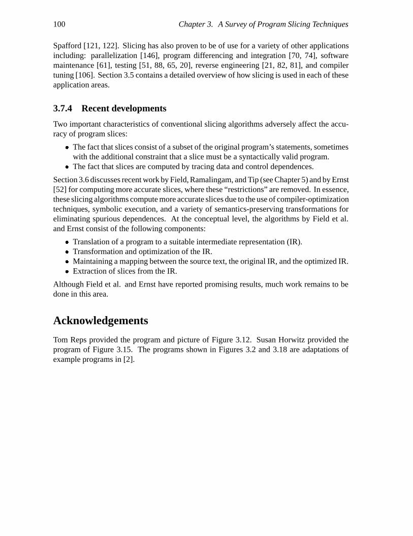
100 Chapter 3. A Survey of Program Slicing Techniques
Spafford [121, 122]. Slicing has also proven to be of use for a variety of other applicationsincluding: parallelization [146], program differencing and integration [70, 74], softwaremaintenance [61], testing [51, 88, 65, 20], reverse engineering [21, 82, 81], and compilertuning [106]. Section 3.5 contains a detailed overview of how slicing is used in each of theseapplication areas.
3.7.4 Recent developments
Two important characteristics of conventional slicing algorithms adversely affect the accu-racy of program slices:
� The fact that slices consist of a subset of the original program’s statements, sometimeswith the additional constraint that a slice must be a syntactically valid program.
� The fact that slices are computed by tracing data and control dependences.
Section 3.6 discusses recent work by Field, Ramalingam, and Tip (see Chapter 5) and by Ernst[52] for computing more accurate slices, where these “restrictions” are removed. In essence,these slicing algorithms compute more accurate slices due to the use of compiler-optimizationtechniques, symbolic execution, and a variety of semantics-preserving transformations foreliminating spurious dependences. At the conceptual level, the algorithms by Field et al.and Ernst consist of the following components:
� Translation of a program to a suitable intermediate representation (IR).� Transformation and optimization of the IR.� Maintaining a mapping between the source text, the original IR, and the optimized IR.� Extraction of slices from the IR.
Although Field et al. and Ernst have reported promising results, much work remains to bedone in this area.
Acknowledgements
Tom Reps provided the program and picture of Figure 3.12. Susan Horwitz provided theprogram of Figure 3.15. The programs shown in Figures 3.2 and 3.18 are adaptations ofexample programs in [2].

Chapter 4
Dynamic Dependence Tracking
(joint work with John Field)
Summary
Program slicing is a useful technique for debugging, testing, and analyzing pro-grams. A program slice consists of the parts of a program that (potentially) affect thevalues computed at some point of interest. With rare exceptions, program slices havehitherto been computed and defined in ad-hoc and language-specific ways. The princi-pal contribution of this chapter is to show that general and semantically well-foundednotions of slicing and dependence can be derived in a simple, uniform way from termrewriting systems (TRSs). Our slicing technique is applicable to any language whosesemantics is specified in TRS form. Moreover, we show that our method admits anefficient implementation.
In Chapter 5, dynamic dependence tracking is “applied to” PIM, an intermediaterepresentation for imperative programs with an accompanying equational logic (whichis implemented by rewriting). It will be shown that this permits the computationof various types of highly accurate program slices. Chapter 6 describes how theapplication of dynamic dependence tracking to algebraic specifications of interpretersyields a useful notion of dynamic program slicing in that context.
4.1 Introduction
4.1.1 Overview
Program slicing is a useful technique for debugging, testing, and analyzing programs.A program slice consists of the parts of a program that (potentially) affect the valuescomputed at some point of interest, referred to as the slicing criterion. As originallydefined by Weiser [147], a slicing criterion was the value of a variable at a particularprogram point and a slice consisted of an “executable” subset of the program’s originalstatements. Numerous variations on the notion of slice have since been proposed, as well asmany different techniques to compute them (see Chapter 3), but all reduce to determiningdependence relations among program components. Unfortunately, with rare exceptions,the notion of “dependence” has been defined in an ad-hoc and language-specific manner,
101

102 Chapter 4. Dynamic Dependence Tracking
resulting in algorithms for computing slices that are notoriously difficult to understand,especially in the presence of pointers, procedures, and unstructured control flow. Thecontributions of this chapter are as follows:
� We define a general notion of slice that applies to any unconditional term rewritingsystem (TRS). Our definition uses a relation on contexts derived from the reductionrelation on terms. This relation makes precise the dynamic dependence of functionsymbols in terms in a reduction sequence on symbols in previous terms in that sequence.Our notion of dependence does not require labeled terms [27, 28, 111, 112], and isdistinguished by its ability to treat (normally problematic) TRSs with left-nonlinearrules.
� Our notion of slicing subsumes most of those defined in previous work on programslicing. The distinction traditionally made between “static” and “dynamic” slicing canbe modeled by reduction of open or closed terms, respectively. Partial instantiationof open terms yields a useful intermediate notion of constrained slicing. AlthoughVenkatesh defines a similar notion abstractly [137], he does not indicate how tocompute such slices.
� We describe an algorithm by which slices can be efficiently computed in practice bysystematically transforming the original TRS to gather dependence information. Theoverhead required to compute this information is linear in the size of the initial term.This algorithm produces minimal slices for left-linear systems, and sound (but notalways minimal) slices for left-nonlinear systems.
Finally, for the case of left-linear systems, we present proofs that our definitions yieldminimal and sound slices.
In Chapter 5, we will show how our techniques can be applied to standard programminglanguages, and compare these techniques to other algorithms in the literature. Chapter 6discusses how the dynamic dependence relation defined in this chapter can be used forproviding dynamic slicing facilities in generated source-level debugging tools. Here, wewill concentrate primarily on technical foundations.
4.1.2 Motivating examples
Consider the program in Figure 4.1 (a) below, written in a tiny imperative programminglanguage, P. The semantics of P are similar to those of many imperative programminglanguages with pointers. A do construct is executed by evaluating its statement list, andusing the computed values to evaluate its in expression. Expressions of the form ‘x’ areatoms, and play the dual role of basic values and addresses that may be assigned to using‘:�’. Addresses are explicitly dereferenced using ‘�’. The distinguished atoms t and frepresent boolean values.
We evaluate P programs by applying the rewriting rules of Figure 4.2 to the termconsisting of the program’s syntax tree until no further rules are applicable. This reductionprocess produces a sequence of terms ending with a normal form that denotes the resultof the evaluation. The program in Figure 4.1 (a) reduces to the normal form ‘result t’.

4.1. Introduction 103
programdo x :� a; w :� x; z :� b;
if w � � � x �then y :� x �else y :� b
in y � � x �
programdo x :� �; w :� x; z :� �;
if w � � � x �then y :� x �else�
in y � � x �
(a) (b)
Figure 4.1: (a) Example P Program. (b) Minimal slice with respect to the entire normal form of(a).
[P1] X � X t[P2] a � b f for all constants a, b such that a �� b
[P3] if t then X else Y X
[P4] if f then X else Y Y
[P5] doX in Y Y[P6] doX in Y � Z �doX in Y � � �doX in Z�[P7] doX ;A :� E in �B �� if �doX ;A :� E in B� � �doX in A�
then �do X inE�else doX in ��do A :� E in B� ��
[P8] doA :� E in �B �� if �doA :� E in B� � A
thenEelse ��doA :� E in B� ��
[P9] doX ; ifA thenB else C in E if �doX in A�then �do X ;B inE�else �doX ;C in E�
[P10] do ifA thenB else C in E ifA then �do B in E� else �do C in E�[P11] doX in if A then B else C if �doX in A�
then �do X inB��doX in C�
[P12] program X result X
Figure 4.2: Rewriting Semantics of P.
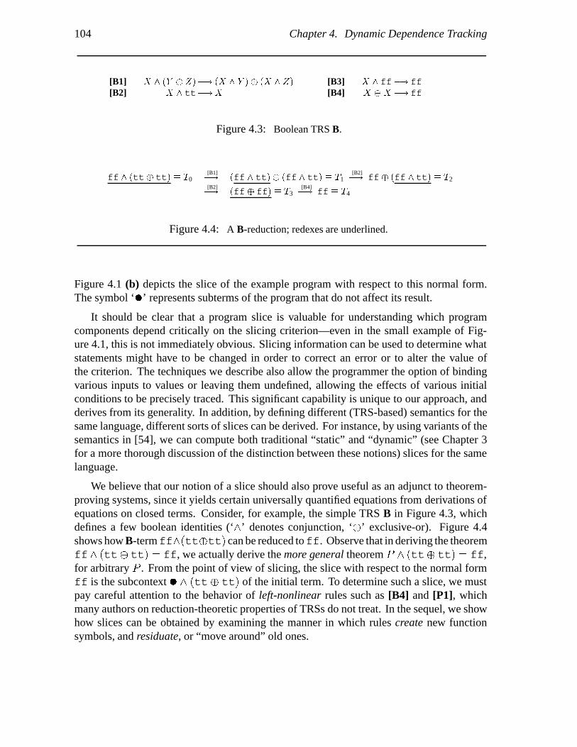
104 Chapter 4. Dynamic Dependence Tracking
[B1] X �Y � Z�� �X Y �� �X Z� [B3] X ff� ff[B2] X tt�X [B4] X �X � ff
Figure 4.3: Boolean TRS B.
ff �tt� tt� � T0[B1]� �ff tt�� �ff tt� � T1
[B2]� ff� �ff tt� � T2
[B2]� �ff� ff� � T3
[B4]� ff � T4
Figure 4.4: A B-reduction; redexes are underlined.
Figure 4.1 (b) depicts the slice of the example program with respect to this normal form.The symbol ‘�’ represents subterms of the program that do not affect its result.
It should be clear that a program slice is valuable for understanding which programcomponents depend critically on the slicing criterion—even in the small example of Fig-ure 4.1, this is not immediately obvious. Slicing information can be used to determine whatstatements might have to be changed in order to correct an error or to alter the value ofthe criterion. The techniques we describe also allow the programmer the option of bindingvarious inputs to values or leaving them undefined, allowing the effects of various initialconditions to be precisely traced. This significant capability is unique to our approach, andderives from its generality. In addition, by defining different (TRS-based) semantics for thesame language, different sorts of slices can be derived. For instance, by using variants of thesemantics in [54], we can compute both traditional “static” and “dynamic” (see Chapter 3for a more thorough discussion of the distinction between these notions) slices for the samelanguage.
We believe that our notion of a slice should also prove useful as an adjunct to theorem-proving systems, since it yields certain universally quantified equations from derivations ofequations on closed terms. Consider, for example, the simple TRS B in Figure 4.3, whichdefines a few boolean identities (‘�’ denotes conjunction, ‘�’ exclusive-or). Figure 4.4shows how B-termff��tt�tt� can be reduced toff. Observe that in deriving the theoremff� �tt� tt� � ff, we actually derive the more general theorem P � �tt� tt� � ff,for arbitrary P . From the point of view of slicing, the slice with respect to the normal formff is the subcontext � � �tt� tt� of the initial term. To determine such a slice, we mustpay careful attention to the behavior of left-nonlinear rules such as [B4] and [P1], whichmany authors on reduction-theoretic properties of TRSs do not treat. In the sequel, we showhow slices can be obtained by examining the manner in which rules create new functionsymbols, and residuate, or “move around” old ones.

4.1. Introduction 105
4.1.3 Definition of a slice
In general, we will define a slice as a certain context contained in the initial term of somereduction. Intuitively, a context may be viewed as a connected (in the sense of a tree) subsetof function symbols taken from a term. For instance, if f�g�a� b�� c� � T is a term, then oneof several contexts contained in T is g��� b� � C. C contains an omitted subterm, or hole1,denoted by ‘�’. This hole results from deleting the subterm ‘a’ of T . We denote the factthat C is a subcontext of T by C v T ; contexts as well as terms may contain subcontexts.
In a slice, holes denote subterms that are irrelevant to the computation of the criterion.Figure 4.1 (b) depicts the minimal subcontext of the original program that yields the slicingcriterion via a “subreduction” of the original reduction. Informally, the holes in the slicecould be replaced by any P-expression and the same criterion could be produced by aP-reduction.
Definition 4.1 below makes precise our notion of slice. We will formalize the notion of“subreduction” of a sequence of reduction steps � using a set Project��, which is a collectionof triples of the form hC� ��� C �i. Informally, such a triple denotes the fact that context Creduces to a context that is isomorphic to C� by a reduction �� derived from rule applicationsthat also occur in �. We discuss Project�� further in Section 4.5. Two contexts are isomorphicif they have the same “structure” (though they may appear at different locations). This notionwill be formalized in Section 4.2.
Definition 4.1 (Slice) Let � : T ��� T � be a reduction. Then a slice with respect to asubcontext C � of T � is a subcontext C of T with the property that there exists a reduction�� such that (i) �� : C ���D� for some D� w E �, (ii) E � and C � are isomorphic, and (iii)hC� ��� D�i � Project��. Slice C is minimal if there is no slice with respect to criterion C �
that contains fewer function symbols.
Definition 4.1 is rendered pictorially in Figure 4.5.The notion of TRS-based slice we define in the sequel can be used for any language
whose operational semantics is defined by a TRS. Many languages whose semantics aretraditionally defined via extended lambda-calculi or using structural operational semanticsalso have corresponding rewriting semantics [1, 54]. In [55], it is shown how many traditionalprogram constructs may be modeled by an appropriate TRS.
4.1.4 Relation to origin tracking
At this point, the reader might wonder why any additional machinery is required beyondthe origin relation that was defined in Chapter 2. Unfortunately, the origin relation does notprovide information that is appropriate for computing program slices. The main reasons forthis being the case are:
� The origin relation was designed with a different objective in mind: to trace recurrencesof the “same” subterm in a term rewriting process. This notion is too “weak” for
1Some authors require that contexts contain exactly one hole; we will not.
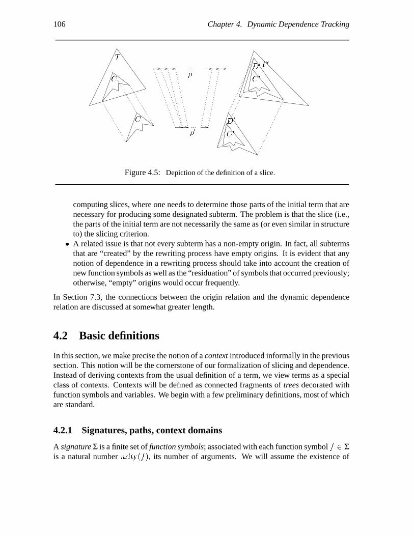
106 Chapter 4. Dynamic Dependence Tracking
D�
�
��
C
C
TT �
C �
C �
D�
Figure 4.5: Depiction of the definition of a slice.
computing slices, where one needs to determine those parts of the initial term that arenecessary for producing some designated subterm. The problem is that the slice (i.e.,the parts of the initial term are not necessarily the same as (or even similar in structureto) the slicing criterion.
� A related issue is that not every subterm has a non-empty origin. In fact, all subtermsthat are “created” by the rewriting process have empty origins. It is evident that anynotion of dependence in a rewriting process should take into account the creation ofnew function symbols as well as the “residuation” of symbols that occurred previously;otherwise, “empty” origins would occur frequently.
In Section 7.3, the connections between the origin relation and the dynamic dependencerelation are discussed at somewhat greater length.
4.2 Basic definitions
In this section, we make precise the notion of a context introduced informally in the previoussection. This notion will be the cornerstone of our formalization of slicing and dependence.Instead of deriving contexts from the usual definition of a term, we view terms as a specialclass of contexts. Contexts will be defined as connected fragments of trees decorated withfunction symbols and variables. We begin with a few preliminary definitions, most of whichare standard.
4.2.1 Signatures, paths, context domains
A signature Σ is a finite set of function symbols; associated with each function symbol f � Σis a natural number arity�f�, its number of arguments. We will assume the existence of

4.2. Basic definitions 107
a denumerable set of variables V such that Σ � V � �. By convention, for each variableX � V , arity�X� � 0. Lower-case letters of the form f� g� h� � � � will denote functionsymbols and upper-case letters of the form X� Y� Z� � � � will represent variables.
A path is a sequence of positive integers that designates a particular function symbol orsubtree by encoding a walk from the tree’s root. The empty path, ‘��’, designates the root ofa tree; path �i1 i2 � � � im� designates the ithm subtree (counted from left to right) of the subtreeindicated by path �i1 i2 � � � i�m�1��. The operation ‘�’ denotes path concatenation. Path p isa prefix of path q, denoted by p � q, if there exists an r such that q � p � r; if r � �� thenp � q.
A context domain P is a set of paths designating a connected fragment of a tree. Thismeans that P must (i) possess a unique root, root�P �� such that for all p � P , root�P � � p,and (ii) have no “gaps,” i.e., for all p� q� r such that p � q � r and p� r � P it must be thecase that q � P .
4.2.2 Contexts
We can now define a context as a total mapping from a context domain to function symbolsand variables:
Definition 4.2 (Context) Let Σ be a signature, V be a set of variables, and P be a contextdomain. Let � be a total mapping from P to �Σ � V� and p be a path. Then a pair hp� �i isa ΣV-context if and only if:
(i) For all q � P and s � Σ � V such that ��q� � s, q � i � P for some i implies thati � arity�s�.
(ii) If P � �, then p � root�P�.
Clause (i) of Definition 4.2 ensures that every child of a function symbol f must have anordinal number less than or equal to the arity of f . Clause (ii) ensures that the root of thecontext is the same as the root of its underlying domain, except when the domain is empty; inthe latter case, we will say that the context is empty. The definition is specifically designedto admit empty contexts, which will be important in the sequel for describing the behavior ofcollapse rules, i.e., rewriting rules whose right hand sides are single variables. Given contextC � hp� �i, root�C� denotes the path p, and O�C� the domain of �. The path correspondingto a “missing child” in a context will be referred to as a hole occurrence; an empty contextis also a hole. The set of hole occurrences in a context C will be denoted by O��C�. Wewill use Cont�Σ�V� to denote the set of all ΣV-contexts.
For any contextC and a path p, p � C denotes an isomorphic context rooted at p obtainedby rerootingC. This notation is used to represent contexts textually; e.g., p � f��� g�a����represents a context rooted at p with two holes (‘�’), binary function symbols f and g and aconstant a. p � � represents an empty context rooted at p. We will say that contexts C andD are isomorphic, written C �
� D, if �� � � C� � �� � � D�A context C is a term if: (i) C has no hole occurrences, and (ii) root�C� � ��. Although
the restriction of root�C� to be �� is not strictly necessary, it results in a definition that agreesmost closely with that used by other authors. We will use Term�� to denote the set of terms

108 Chapter 4. Dynamic Dependence Tracking
over signature Σ. Letters C�D� � � � will generally denote arbitrary contexts, and S� T� � � �terms. Whenever convenient, we ignore the distinction between a variable X and the termconsisting of that variable. Some convenient operations on contexts are introduced next.
For a context C, and S a subset of Σ � V , OS�C� denotes the set of paths to elements ofS in C; Ofsg�C� is abbreviated by Os�C�. The set of variable occurrences in a ΣV-contextC, i.e., OV�C�, is denoted VARS�C�, and Vars1�C� is the set of variables that occur exactlyonce in C.
Two contexts are compatible if all paths common to both of their domains are mapped tothe same symbol. If C and D are compatible, C is a subcontext of D, denoted by C v D, ifand only if one of the following holds: (i) C and D are nonempty and O�C� O�D�, (ii) Cand D are empty and C � D, or (iii) C is empty, D is nonempty, root�C� � q � i � O�D�,and q � O�D�. The third clause states that an empty contextC is a subcontext of a nonemptycontext D only if its root is “sandwiched” between adjacent nodes in D. This property willgreatly simplify a number of definitions in the sequel. Contexts D and E are disjoint if andonly if there exists no context C such that C v D and C v E. If C and D are contextssuch that root�D� � �O�C� � O��C��, C#D$ denotes the context C where the subcontextor hole at root�D� is replaced by D. Note that for all C v D, D#C$ � D. A context C iselementary iff jO�C�j � 1.
A context forest is a set of mutually disjoint contexts. Forest S is a subforest of forestT , denoted S v T , if and only if for all contexts C � S, there exists a context D � Tsuch that C v D. Some convenient set-like operations on context forests can be defined asfollows: Let S and T be compatible context forests. Then their union, denoted by S t T ,is the smallest forest U such that S v U and T v U ; their difference, denoted S � T , is thesmallest forest U such that U v S and S v �T t U�. If P is a set of paths, C �P is theforest containing subcontexts of C rooted at paths in P . The notion of context replacementis easily generalized to a forest S. In the sequel, we allow simple contexts to be used asoperands of context forest operations; such contexts are coerced to singleton forests. Forexample, ‘C tD’ denotes ‘f C g t fD g’.
4.3 Term rewriting and related relations
In this section, we formalize standard term rewriting-related notions using operations oncontexts; we then define the important related ideas of creation and residuation, whichare derived from the rewriting relation. We will first consider only left-linear TRSs; thisrestriction will be removed in in Section 4.7.
4.3.1 Substitutions and term rewriting systems
A substitution is a finite partial map from V to Cont�Σ�V�, where Σ is a signature and V aset of variables. A substitution � is extended to a mapping on contexts by replacing eachsubcontext CX v C consisting solely of a variable X by the context (root�CX� � ��X�),for all X on which � is defined. A term rewriting system R over a signature Σ is a set of

4.3. Term rewriting and related relations 109
pairs hL�Ri such that L and R are terms over Σ, L does not consist of a sole variable, andVARS�R� VARS�L�; hL�Ri is called a rewrite rule and is commonly denoted by L � R.For � L � R � R we define L� � L and R� � R. A rewrite rule is left-linear ifVARS�L�� � Vars1�L��. If R is a TRS, then we define an R-contraction A to be a triplehp� � �i, where p is a path, is a rule of R, and � is a substitution.
We use pA, A, LA, RA, and �A to denote p, , L�A , R�A , and �, respectively. Moreover,LA and RA will denote the contexts �pA � LA� and �pA � RA�, respectively. The R-contraction relation, ��R , is defined by requiring thatT ��R T
� if and only if a contractionA exists such that T � T #�A�LA�$ and T � � T #�A�RA�$, for terms T , T �. The subcontext�A�LA� of C is an A-redex, and the context �A�RA� is an A-reduct; these contexts areabbreviated respectively by RedexA and ReductA. We will feel free to drop the subscript Rof a contraction ��R in cases where it is clear which TRS we are referring to, and simplywrite ��� . For clarity, contraction arrows will frequently be labeled explicitly with the
contraction A that is involved: A�� . As usual, ��� is the reflexive, transitive closure of
�� . A reduction � is a sequence of contractions A1A2 � � �An such that if � is nonempty,there exist terms T0� T1� � � � � Tn where:
T0A1�� T1
A2�� T2 � � �Tn�1An�� Tn
This reduction is abbreviated by � : T0 ��� Tn. A reduction � is a reduction of term T if
there exists T � such that � : T ��� T �. The reduction of length 0 is denoted by �; for allterms T , we adopt the convention that � : T ��� T .
Given the definitions above, the B-reduction depicted in Figure 4.4 may be describedformally by the following sequence of contractions:
h��� �B1�� �X :� ff� Y :� tt� Z :� tt�i; h�1�� �B2�� �X :� ff�i; h�2�� �B2�� �X :� ff�i;h��� �B4�� �X :� ff�i
Most of the new relations defined in the sequel are parameterized with a reduction �A,in which the final contraction is highlighted. Several definitions are concerned with thelast contraction A only; however, when our definitions are generalized in Section 4.7, the“history” contained in � will become relevant. Whenever we define a truly inductive relationon �A, we will append a ‘�’ to the name of the relation.
4.3.2 Context rewriting
In order to generalize term rewriting to context rewriting, a few auxiliary definitions areneeded. A variable instantiation of a context C is a term T that can be obtained from C byreplacing each hole with a variable that does not occur in C. A variable instantiation is alinear instantiation if each hole is replaced by a distinct variable. A context C rewrites toa context C �, denoted C ���C �, if and only if T ��� T �, where T is a linear instantiationof C and T � is a variable instantiation of C �. Note that context reduction is not defined asthe transitive closure of a single-step contraction relation on contexts; this is necessary to
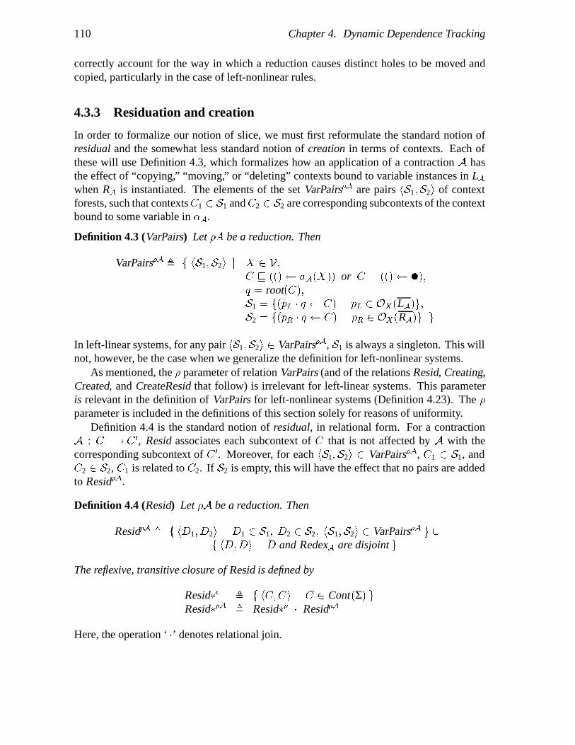
110 Chapter 4. Dynamic Dependence Tracking
correctly account for the way in which a reduction causes distinct holes to be moved andcopied, particularly in the case of left-nonlinear rules.
4.3.3 Residuation and creation
In order to formalize our notion of slice, we must first reformulate the standard notion ofresidual and the somewhat less standard notion of creation in terms of contexts. Each ofthese will use Definition 4.3, which formalizes how an application of a contraction A hasthe effect of “copying,” “moving,” or “deleting” contexts bound to variable instances in LAwhen RA is instantiated. The elements of the set VarPairs�A are pairs hS1�S2i of contextforests, such that contextsC1 � S1 andC2 � S2 are corresponding subcontexts of the contextbound to some variable in A.
Definition 4.3 (VarPairs) Let �A be a reduction. Then
VarPairs�A � f hS1�S2i j X � V�C v ��� � �A�X�� or C � ��� � ���q � root�C��S1 � f�pL � q � C� j pL � OX�LA�g�S2 � f�pR � q � C� j pR � OX�RA�g g
In left-linear systems, for any pair hS1�S2i � VarPairs�A, S1 is always a singleton. This willnot, however, be the case when we generalize the definition for left-nonlinear systems.
As mentioned, the � parameter of relation VarPairs (and of the relations Resid, Creating,Created, and CreateResid that follow) is irrelevant for left-linear systems. This parameteris relevant in the definition of VarPairs for left-nonlinear systems (Definition 4.23). The �parameter is included in the definitions of this section solely for reasons of uniformity.
Definition 4.4 is the standard notion of residual, in relational form. For a contractionA : C��C �, Resid associates each subcontext of C that is not affected by A with thecorresponding subcontext of C�. Moreover, for each hS1�S2i � VarPairs�A, C1 � S1, andC2 � S2, C1 is related to C2. If S2 is empty, this will have the effect that no pairs are addedto Resid�A.
Definition 4.4 (Resid) Let �A be a reduction. Then
Resid�A � f hD1� D2i j D1 � S1� D2 � S2� hS1�S2i � VarPairs�A g �f hD�Di j D and RedexA are disjoint g
The reflexive, transitive closure of Resid is defined by
Resid�� � f hC�Ci j C � Cont�� gResid��A � Resid�� � Resid�A
Here, the operation ‘ �’ denotes relational join.
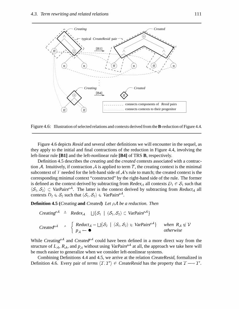
4.3. Term rewriting and related relations 111
.
.
.
Resid pairsconnects components of
connects contexts to their progenitor
ff
tt tttttt ff ff
Creating Created
[B1]
typical CreateResid pair
ff
ff ff
Creating Created
[B4]
Figure 4.6: Illustration of selected relations and contexts derived from the B-reduction of Figure 4.4.
Figure 4.6 depicts Resid and several other definitions we will encounter in the sequel, asthey apply to the initial and final contractions of the reduction in Figure 4.4, involving theleft-linear rule [B1] and the left-nonlinear rule [B4] of TRS B, respectively.
Definition 4.5 describes the creating and the created contexts associated with a contrac-tion A. Intuitively, if contraction A is applied to term T , the creating context is the minimalsubcontext of T needed for the left-hand side of A’s rule to match; the created context is thecorresponding minimal context “constructed” by the right-hand side of the rule. The formeris defined as the context derived by subtracting from RedexA all contexts D1 � S1 such thathS1�S2i � VarPairs�A. The latter is the context derived by subtracting from ReductA allcontexts D2 � S2 such that hS1�S2i � VarPairs�A.
Definition 4.5 (Creating and Created) Let �A be a reduction. Then
Creating�A � RedexA �FfS1 j hS1�S2i � VarPairs�Ag
Created�A �
�ReductA �
FfS2 j hS1�S2i � VarPairs�Ag when RA � V
pA � � otherwise
While Creating�A and Created�A could have been defined in a more direct way from thestructure of LA, RA, and pA without using VarPairs�A at all, the approach we take here willbe much easier to generalize when we consider left-nonlinear systems.
Combining Definitions 4.4 and 4.5, we arrive at the relation CreateResid, formalized inDefinition 4.6. Every pair of terms hT� T �i � CreateResid has the property that T �� T �.

112 Chapter 4. Dynamic Dependence Tracking
The difference between the contraction relation ‘�� ’ and relation CreateResid is that thelatter is derived from the former. Roughly speaking, CreateResid�A may be regarded as the“restriction” of ‘�� ’ to the specific contraction A.
Definition 4.6 (CreateResid) Let �A be a reduction. Then
CreateResid�A � f hC1� C2i j R Resid�A�hC�Di � R and hC�D�i � Resid�A
imply hC�D�i � R�C1 and C2 are contexts such that:C1 � Creating�A t
Ff C j hC�C �i � R g�
C2 � Created�A tFf C � j hC�C �i � R g g
Note that it is impossible to have both hC1� Di � Resid�A and hC2� Di � CreateResid�A, forany nonempty C1� C2� D; these relations may, however, overlap on empty contexts.
4.4 A dynamic dependence relation
In this section, we will derive our dynamic dependence relation, Slice�, using the conceptsintroduced in Section 4.3. For the empty reduction, Slice� is defined as the identity relation.For a criterion D, the inductive case determines the minimal super-context D� w D forwhich there is a C such that hC�D�i � �Resid�A � CreateResid�A�; then the slice for thisC in reduction � is determined.
Definition 4.7 (Slice�) Let �A be a reduction. Then
Slice�� � f hC�Ci j C � Cont�� gSlice��A � Slice�� � f hC�Di j there exists a minimal D� w D
such that hC�D�i � �Resid�A � CreateResid�A� g
Since Resid�A and hC2� Di � CreateResid�A only overlap for empty contexts, it is easy tosee that the slice with respect to any nonempty criterion is uniquely defined. Empty contextsmay have multiple slices, which arise from the application of collapse rules.
4.4.1 Example
In the example that follows, we will frequently use set comprehension to avoid unwieldynotation. We will consider the following B-reduction � = A1A2A3:
S � �ff � �ff � tt�� � ttA1�� �ff � ff� � tt
A2�� ff � ttA3�� ff � T
Note that for contraction A1, we have pA1= (1 2), LA1 = �1 2� � X �tt, RA1 = �1 2� � X ,
RedexA1 = �1 2� � ff � tt, and ReductA1 = �1 2� � ff. This results in the following

4.4. A dynamic dependence relation 113
relations for A1:
VarPairsA1 � f hf �1 2 1� � ff g� f �1 2� � ff gi� hf �1 2 1� � � g� f �1 2� � � gi gResidA1 � f h�1 2 1� � ff� �1 2� � ffi� h�1 2 1� � �� �1 2� � �i�
h�� � �� �� � �i� h�1 2� � �� �1 2� � �i g �f C j C v �� � �ff �� tt g
CreatingA1 � �1 2� � �� tt�CreatedA1 � �1 2� � �
CreateResidA1 � f h�1 2� � �� tt�� �1 2� � �i� h�1� � � �ff tt�� �1� � � ffi�h�1� � ff �ff tt�� �1� � ff ffi�h�� � �� �ff tt�� �� �� � �ff ff� �i�h�� � �� �ff tt�� tt� �� � �ff ff� tti�h�� � �ff �ff tt�� �� �� � �ff ff� �i�h�� � �ff �ff tt�� tt� �� � �ff ff� tti g
For contraction A2, we have pA2= (1), LA2 = �1� � X � ff, RA2 = �1� � ff, RedexA2 =
�1� � ff � ff, and ReductA2 = �1� � ff. Therefore, we have:
VarPairsA1A2 � f hf �1 1� � ff g� �i� hf �1 1� � � g� �i gResidA1A2 � f h�� � �� �� � �i� h�1� � �� �1� � �i g �
f hC�Ci j C v �� � � ff g
CreatingA1A2 � �1� � �� ff�CreatedA1A2 � �1� � ff
CreateResidA1A2 � f h�1� � �� ff�� �1� � ffi� h�� � �� ff� �� �� � ff �i�h�� � �� ff� tt� �� � ff tti g
For the third contraction, A3, we have pA3= (), LA3 = �� � X � tt, RA3 = �� � X ,
RedexA3 = �� � ff � tt, and ReductA3 = �� � ff. The following relations are computedfor A1A2A3:
VarPairsA1A2A3 � f hf �1� � ff g� f �� � ff gi� hf �1� � � g� f �� � � gi gResidA1A2A3 � f h�1� � ff� �� � ffi� h�1� � �� �� � �i� h�� � �� �� � �i g
CreatingA1A2A3 � �� � �� tt�CreatedA1A2A3 � �� � �
CreateResidA1A2A3 � f h�� � �� tt�� �� � �i g
From the above and Definition 4.7 it follows that we have the following dynamic dependencerelations between subcontexts of S and T :
SliceA1A2A3 � f h�1� � � �ff tt�� �� � ffi� h�� � �� �� � �i g

114 Chapter 4. Dynamic Dependence Tracking
Thus, the slice with respect to �� � ff v T is �1� � � � �ff � tt� v S. This is theminimal context for which there exists a subreduction of � that yields the criterion. In thiscase, the projection consists of the first two contractions.
The above example also illustrates why Slice� is defined on contexts rather than oncontext domains: collapse rules require special treatment in order to produce minimal slices.Note that the example exhibits two applications of collapse rule [B2]. Intuitively, the firstone created the criterion, whereas the second one merely affects its location. We achievethis differentiation by: (i) having a collapse rule create an empty context pA � � insteadof the context consisting of the function symbol at path pA (the approach of [94]), and (ii)defining an empty context p � � to be a subcontext of a nonempty context only if the latter“surrounds” the former.
4.5 Projections, subreductions
In this section, we formalize the notion of a projection of a reduction on a subcontext ofits initial term. It will be convenient to define simultaneously the initial context C and thefinal context D to which a projection corresponds along with the projected “subreduction”� itself. We therefore define the set of projection triples as follows:
Definition 4.8 (Projection Triples) Let R be a TRS over signature Σ. Then the set of Rprojection triples is inductively defined as follows:
Project�� � f hB� �� Bi j B � Cont�� g
Project��A � fhB� �A� D�i j hB� �� Ci � Project���hC�Di � CreateResid�A�D� v D g �
(i)
fhB� ��D�i j hB� �� Ci � Project���hC�Di � Resid�A�D� v D g
(ii)
The interesting cases in Definition 4.8 are numbered. Intuitively, these cases behave asfollows:
� In case (i), the context D� that constitutes the third element of the triple is entirelycontained in a context D that is involved in a CreateResid�A–relation. In this case,contraction A is deemed applicable to D�, and the construction continues recursivelywith the context C that contracted to D, and reduction �.
� In case (ii), D� is a subcontext of some context D that residuated from a context C.In this case, contraction A was not applicable to D�, and the construction continuesrecursively with the context C from which D residuated, and reduction �.
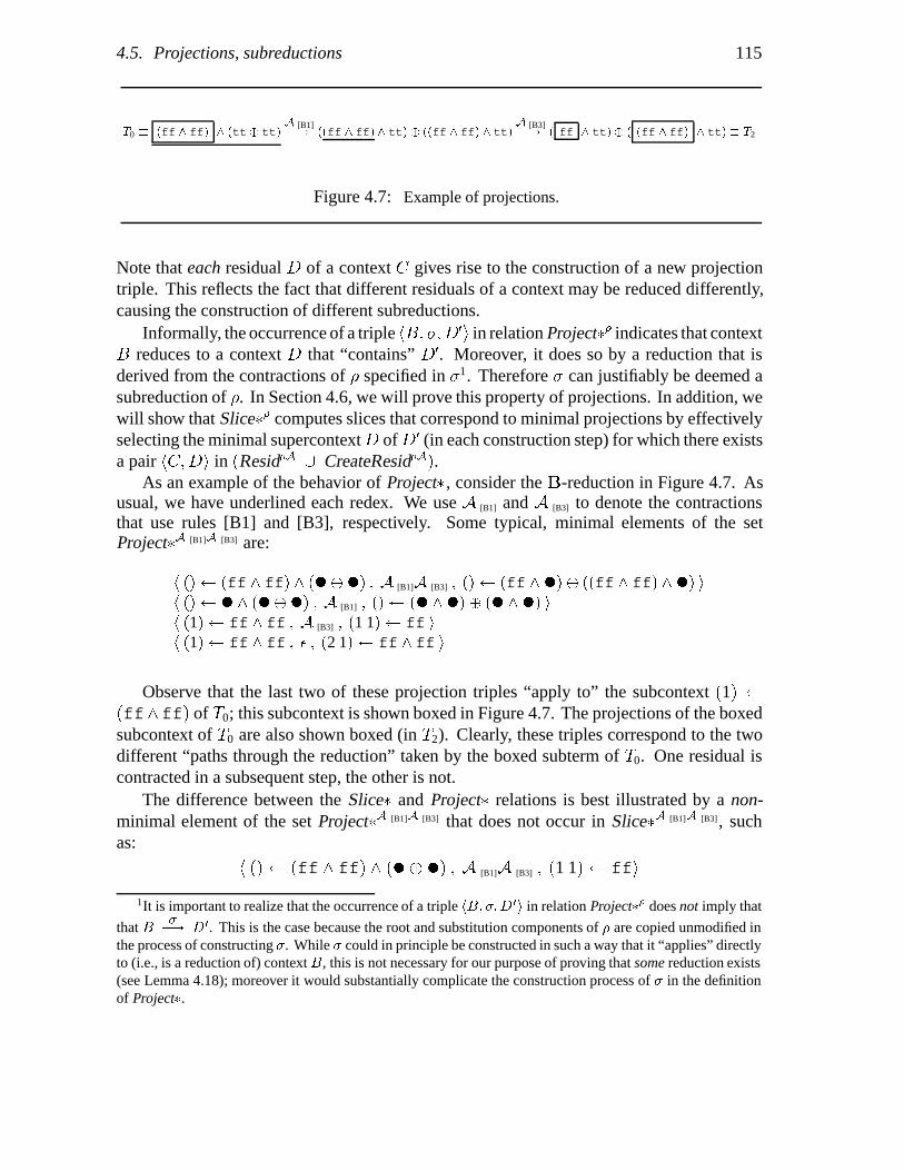
4.5. Projections, subreductions 115
T0 � �ff � ff� � �tt tt�A [B1]�� ��ff � ff� � tt� ��ff � ff� � tt�
A [B3]�� � ff � tt� � �ff � ff� � tt� � T2
Figure 4.7: Example of projections.
Note that each residual D of a context C gives rise to the construction of a new projectiontriple. This reflects the fact that different residuals of a context may be reduced differently,causing the construction of different subreductions.
Informally, the occurrence of a triple hB� ��D�i in relation Project�� indicates that contextB reduces to a context D that “contains” D�. Moreover, it does so by a reduction that isderived from the contractions of � specified in �1. Therefore � can justifiably be deemed asubreduction of �. In Section 4.6, we will prove this property of projections. In addition, wewill show that Slice�� computes slices that correspond to minimal projections by effectivelyselecting the minimal supercontextD ofD� (in each construction step) for which there existsa pair hC�Di in �Resid�A � CreateResid�A�.
As an example of the behavior of Project�, consider the B-reduction in Figure 4.7. Asusual, we have underlined each redex. We use A [B1] and A [B3] to denote the contractionsthat use rules [B1] and [B3], respectively. Some typical, minimal elements of the setProject�A [B1]A [B3] are:
h �� � �ff ff� ����� � A [B1]A [B3] � �� � �ff ��� ��ff ff� �� ih �� � � ����� � A [B1] � �� � �� ��� �� �� ih �1� � ff ff � A [B3] � �1 1� � ff ih �1� � ff ff � � � �2 1� � ff ff i
Observe that the last two of these projection triples “apply to” the subcontext �1� ��ff�ff� of T0; this subcontext is shown boxed in Figure 4.7. The projections of the boxedsubcontext of T0 are also shown boxed (in T2). Clearly, these triples correspond to the twodifferent “paths through the reduction” taken by the boxed subterm of T0. One residual iscontracted in a subsequent step, the other is not.
The difference between the Slice� and Project� relations is best illustrated by a non-minimal element of the set Project�A [B1]A [B3] that does not occur in Slice�A [B1]A [B3] , suchas:
h �� � �ff � ff� � ��� �� � A [B1]A [B3] � �1 1� � ffi
1It is important to realize that the occurrence of a triple hB� ��D�i in relation Project � does not imply that
that B�� D�. This is the case because the root and substitution components of � are copied unmodified in
the process of constructing �. While � could in principle be constructed in such a way that it “applies” directlyto (i.e., is a reduction of) context B, this is not necessary for our purpose of proving that some reduction exists(see Lemma 4.18); moreover it would substantially complicate the construction process of � in the definitionof Project .

116 Chapter 4. Dynamic Dependence Tracking
4.6 Formal properties of slices
We can now state some theorems describing the most important properties of slices. In thesequel, all TRSs are assumed to be left-linear.
4.6.1 Uniqueness of slices
In order to prove that Slice� is a many-to-one mapping for non-empty contexts (that is, eachcontext has a unique slice), we will first prove a few lemmas.
Lemma 4.9 Let B�
��� CA�� D be a reduction. Then for any non-empty D� v D there
is at most one C � v C such that hC �� D�i � Resid�A. Moreover, if it exists, this C � will benon-empty.
Proof. Let D� v D be a non-empty context such that hC�� D�i � Resid�A for some C � v C.There are two cases:
1. root�D�� � root�Created�A� and D� and Created�A are disjoint.Then it follows from Definition 4.4 that C � � D� is the unique subcontext of C suchthat hC �� D�i � Resid�A. This C � is non-empty because D� is non-empty.
2. D� � �pR � q � A� where pR � OX�RA�, A v ��� � �A�X��, and q � root�A� forsome variable X .From left-linearity it follows that there is a unique path pL such that fpL g � OX�LA�.From Definitions 4.3 and 4.4 it follows thatC � � �pL �q � A� is the unique subcontextof C such that hC �� D�i � Resid�A. Since rerooting a context does not affect its (non-)emptyness, C � will be a non-empty context. �
Lemma 4.10 Let B�
��� CA�� D be a reduction. Then for any non-empty D� v D
there is at most one C � v C such that hC �� D�i � CreateResid�A. Moreover, if it exists, thisC � will be non-empty.
Proof. Let D� v D be a non-empty context such that hC�� D�i � CreateResid�A for someC � v C.
From Definition 4.6 it follows that there exists a unique subset R of Resid�A such that:
D� � Created�A tGf E � j hE�E �i � R g
and also that there exists a unique context
C � � Creating�A tGf E j hE�E �i � R g
such that hC �� D�i � CreateResid�A. Since the left-hand side of a rewrite rule is not a singlevariable, Creating�A is non-empty, causing this C � to be non-empty as well. �
Lemma 4.11 Let B�
��� CA�� D be a reduction. It is impossible to have hC1� D
�i �Resid�A and hC2� D
�i � CreateResid�A for any C1� C2 v C and any non-empty D� v D.

4.6. Formal properties of slices 117
Proof. Assume that hC2� D�i � CreateResid�A for some C2 v C, and some non-empty
D� v D. From Definition 4.6 it follows that Creating�A v C2 and Created�A v D�.From Definitions 4.4 and 4.5 it follows that for any pair hC1� D1i � Resid�A withC1 v C,
D1 v D, we have that C1 and Creating�A are disjoint and D1 and Created�A are disjoint.From Creating�A v C2 and Creating�A v C1 it follows that C2 � C1. �
Lemma 4.12 Let � : B��
��� CA�� D be a reduction, and let D�� be a non-empty
subcontext of D. Then there exists a unique minimal D� such that D�� v D� v D andhC �� D�i � �Resid� � CreateResid�� for some non-empty C � v C. Moreover,
hB�� C �i � Slice���
� hB�� D�i � Slice�� � hB�� D��i � Slice��
where B� v B.
Proof. The theorem holds trivially if hC �� D��i � �Resid� � CreateResid��, for someC � v C.Assume that there exists no C � v C such that hC �� D��i � �Resid� � CreateResid��.
From Definitions 4.3 and 4.4, it follows that D�� and Created�A are not disjoint—otherwise,D�� would be involved in a Resid�-relation. From the fact that D�� is not involved in aCreateResid� relation either, we have that one or both of the following hold:
� Created� v D��,� D���Created�A �
FfE � j hE�E �i � R g, for some R � Resid� such that there exist
hA�Bi � R, hA�B�i � Resid� for which hA�B�i � R.
Define:R� � R � f hA�B�i j hA�Bi � R� hA�B�i � Resid� gD� � D� t Created� t f E � j hE�E �i � R� g
Clearly, D� is the minimal supercontext of D�� for which hC �� D�i � CreateResid�, where
C � � Creating� tGf E j hE�E �i � R� g v C
Since Creating� is always non-empty, C � is non-empty as well.From Definition 4.7 it follows that
hB�� C �i � Slice���
� hB�� D�i � Slice�� � hB�� D��i � Slice��
where B� v B. �
Theorem 4.13 (Uniqueness of Slices) Let � : B�
��� D be a reduction, and let D� v Dbe non-empty. Then there exists a unique non-empty B� v B such that hB�� D�i � Slice��.
Proof. By induction on the length of the reduction �.For � � �, we have fB� j hB�� D�i � Slice�� g � fD� g according to Definition 4.7.
For the inductive case, assume that � � ��A such that B��
��� CA�� D, and let
D� v D be a non-empty context. According to Lemma 4.12, we may assume without lossof generality that hC �� D�i � �Resid�
�A � CreateResid��A�, for some C � v C.

118 Chapter 4. Dynamic Dependence Tracking
According to Lemma 4.11, we have either hC�� D�i � Resid��A or hC �� D�i �
CreateResid��A.
Lemmas 4.9 and 4.10 state that both Resid and CreateResid map any non-empty contextD� v D to a unique non-empty C � v C. By induction, there exists a unique non-emptyB� v B such that hB�� C �i � Slice��
�
.From Definition 4.7 it follows that this B� is the unique non-empty subcontext of B such
that hB�� D�i � Slice��. �
Given Theorem 4.13, we will be able to write C � Slice���D� instead of hC�Di �Slice��, for non-empty D.
4.6.2 Preservation of topology
The following lemma states that slices may be computed by repeatedly determining a uniquerelated subcontext of the previous context in the reduction.
Lemma 4.14 Let � : B��
��� CA�� D be a reduction, and let D�� v D be a non-empty
context. Moreover, let D� be the unique minimal super-context of D�� for which there existsa non-empty context C� v C such that hC �� D�i � �Resid� � CreateResid��. Then
Slice���
�C �� � Slice���D��� � Slice���D��
Proof. Follows immediately from Definition 4.7, Lemma 4.12, and Theorem 4.13. �
Lemma 4.15 states that any pair of contexts hC�Di in the Resid relation can be “split”into a set S of pairs of elementary contexts in a way that each pair of elementary contextshC �� D�i in S also occurs in the Resid relation. This result will be used in the proof of theInclusion Lemma, which follows below.
Lemma 4.15 Let C and D be contexts such that hC�Di � Resid�, for some reduction �.Then there exists a set S of pairs of elementary contexts such that all of the following hold:
1.Ff C � j hC �� D�i � S g � C,
2.FfD� j hC �� D�i � S g � D,
3. hC �� D�i � S implies that hC �� D�i � Resid�.
Proof. Follows trivially from Definition 4.4. �
The next lemma and theorem demonstrate that slices effectively preserve the topology oftheir corresponding criteria. This is important in showing that slices are minimal projections.
Lemma 4.16 (Inclusion Lemma) Let �A be a reduction such that B�
��� CA�� D,
and let D�� v D� v D be non-empty contexts such that there exist pairs hC�� D�i ��Resid�A � CreateResid�A�, and hC ��� D��i � �Resid�A � CreateResid�A�. Then C �� v C �.
Proof. There are three cases:
1. hC �� D�i � Resid�A and hC ��� D��i � Resid�A.From Definition 4.4 it follows that there are two cases:

4.6. Formal properties of slices 119
(a) root�D�� � Created�A, D� and Created�A are disjoint, root�D��� � Created�A,and D�� and Created�A are disjoint. Then C � � D� and C �� � D��, and thereforeC �� v C �.
(b) D� � �pR � q� � A��, D�� � �pR � q�� � A��� where pR � OX�RA�, A� v ��� ��A�X��, A�� v ��� � �A�X��, q� � root�A��, q�� � root�A���, for some variableX .From Definitions 4.3 and 4.4 and left-linearity, it follows that there exists a uniqueoccurrence pL of X in LA such that C � � �pL � q� � A��, C �� � �pL � q�� � A���.D�� v D� implies q� � q��, A�� v A� and therefore that C�� v C �.
2. hC �� D�i � CreateResid�A and hC ��� D��i � CreateResid�A.From Definition 4.6 it follows that
D� � Created�A tFf E � j hE�E �i � R� g
D�� � Created�A tFf E � j hE�E �i � R�� g
C � � Creating�A tFf E j hE�E �i � R� g
C �� � Creating�A tFf E j hE�E �i � R�� g
for R�� R�� Resid�A. According to Lemma 4.15, we may assume without loss ofgenerality that for all hE�E�i � R�� R��, bothE andE � are elementary. FromD�� v D�
it follows that R�� R� and therefore that C�� v C �.3. hC �� D�i � CreateResid�A and hC ��� D��i � Resid�A
According to Definition 4.6, we have that
D� � Created�A tFf E � j hE�E �i � R g
C � � Creating�A tFf E j hE�E �i � R g
for some R Resid�A. According to Lemma 4.15, we may assume without loss ofgenerality that for all hE�E�i � R, both E and E � are elementary. From D�� v D�,and the disjointness of Created�A and D�� it follows that there exists a subset R� Rsuch that
D�� �Gf E � j hE�E �i � R� g
Using an argument similar to that in case 1, it follows that
C �� �Gf E j hE�E �i � R� g
Consequently C �� v C �.
Note that the case where hC�� D�i � Resid�A and hC ��� D��i � CreateResid�A is impossible,given D�� v D�. �
Theorem 4.17 (Inclusion Theorem) Let � : B�
��� D be a reduction, let D�� v D� v D,and let D�� be non-empty. Then Slice���D��� v Slice���D��.
Proof. By induction on the length of the reduction �.

120 Chapter 4. Dynamic Dependence Tracking
For � � �, we trivially have:
Slice���D��� � D�� v D� � Slice���D��
For the inductive case, assume that � � ��A such that B��
��� CA�� D, and let
D�� D�� be subcontexts of D such that D�� v D� v D and D�� is non-empty. According toLemmas 4.12 and 4.14 we may assume without loss of generality that there exist non-emptycontexts C �� C �� v C such that
hC �� D�i � �Resid� � CreateResid��� Slice���D�� � Slice���
�C ��
andhC ��� D��i � �Resid� � CreateResid��� Slice���D��� � Slice��
�
�C ���
According to Lemma 4.16, D�� v D� implies C �� v C �. By induction, C �� v C � impliesSlice��
�
�C ��� v Slice���
�C ��. Consequently, it follows that Slice���D��� v Slice���D��. �
4.6.3 The relation between Slice� and Project�
Lemma 4.18 formally justifies the relationship between a reduction and the components ofa projection triple.
Lemma 4.18 Let � be a reduction, and let hB� ��D��i � Project��. Then there exist contextsE � and D such that B ��� D, E � v D, and E � �� D��.
Proof. By induction on the length of �.According to Definition 4.8, hB� ��D��i � Project�� implies that � � � and thatB � D��.
From this it follows trivially that B ��� D, for D � D��.For the inductive case, assume that � � ��A, and hB� ��D��i � Project��. From
Definition 4.8 it follows that two cases can be distinguished:
1. D�� v D�, hC �� D�i � CreateResid�, and hB� ��� C �i � Project��.By induction, there exists a reduction B ��� C for some C w F �, where F � �� C �.
From Definition 4.6 it follows that C � A�� D�. Therefore we have that
B� ��� C � C#F �$ ��� C#E �$ � D
where E� � �root�F �� � D��. Since D� and E� are isomorphic, and D�� v D�, itfollows that D�� �� E �� for some E�� v E � v D.
2. D�� v D�, hC �� D�i � Resid�, and hB� ��� C �i � Project��.By induction, there exists a reduction B ��� C for some C w F �, where F � �� C �.From Definition 4.4 it follows that C � �� D�. Therefore we have that
B� ��� C � C#F �$ � C#E �$ � D
where E� � �root�F �� � D��. Since D� and E� are isomorphic, and D�� v D�, itfollows that D�� �� E �� for some E�� v E v D. �

4.6. Formal properties of slices 121
The lemma below establishes a connection between the relations Slice�� and Project��.
Lemma 4.19 Let � be a reduction such that B�
��� D, and let B� � Slice���D�� for somenon-empty D� v D. Then there exists a triple hB�� ��D�i � Project��.
Proof. By induction on the length of reduction �.Let � � �. From Definition 4.7 it follows that B� � Slice���D�� implies B� � D�.
Moreover, from Definition 4.8 it follows that hB�� �� D�i � Project�� implies B� � D� aswell, so that the lemma trivially holds.
For the inductive case, assume that � � ��A such that B��
��� CA�� D, and let
B� � Slice���D���, for some non-emptyD�� v D. According to Lemmas 4.12 and 4.14 thereexists a unique D� w D�� such that hC �� D�i � �Resid� � CreateResid�� and Slice���D��� �Slice���D�� � Slice��
�
�C �� � B�.By induction there exists a triple hB�� ��� C �i � Project��
�
. From Lemma 4.11, it followsthat there are two cases:
1. hC �� D�i � Resid�. SinceD�� v D� it follows from Definition 4.8 that that hB�� ��� D��i �Project��.
2. hC �� D�i � CreateResid�. Since D�� v D� it follows from Definition 4.8 thathB�� ��A� D��i � Project��. �
4.6.4 Soundness and minimality
The soundness theorem states that the Slice� relation computes slices that comply withDefinition 4.1.
Theorem 4.20 (Soundness) Let � be a reduction such that B�
��� D. Moreover, letB� � Slice���D��� for some non-empty D�� v D. Then there exists a reduction � such that:
1. hB�� ��D��i � Project��, and
2. B��
��� D� such that there exists an E�� v D� for which E�� �� D��.
Proof. Follows immediately from Lemmas 4.18 and 4.19. �
Our final theorem states that a slice is the minimal initial component of some projectiontriple whose final component contains the slicing criterion:
Theorem 4.21 (Minimality) Let � be a reduction, and let B�s � Slice���D�
s� for somenon-empty D�
s. Then hB�p� ��D
�pi � Project�� and D�
p w D�s together imply that B�
p w B�s.
Proof. By induction on the length of reduction �.For � � �, Definition 4.8 states that hB�
p� ��D�pi � Project�� implies � � � andB�
p � D�p.
Moreover, according to Definition 4.7 we have that B�s � Slice���D�
s� implies B�s � D�
s.Therefore D�
p w D�s implies that B�
p w B�s.
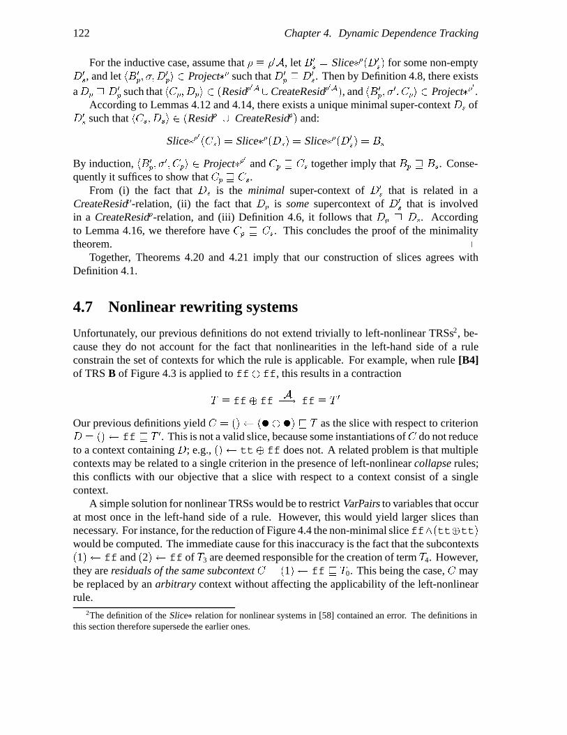
122 Chapter 4. Dynamic Dependence Tracking
For the inductive case, assume that � � ��A, let B�s � Slice���D�
s� for some non-emptyD�s, and let hB�
p� ��D�pi � Project�� such that D�
p w D�s. Then by Definition 4.8, there exists
aDp w D�p such that hCp� Dpi � �Resid�
�A�CreateResid��A�, and hB�
p� ��� Cpi � Project��
�
.According to Lemmas 4.12 and 4.14, there exists a unique minimal super-context Ds of
D�s such that hCs� Dsi � �Resid� � CreateResid�� and:
Slice���
�Cs� � Slice���Ds� � Slice���D�s� � Bs
By induction, hB�p� �
�� Cpi � Project���
and Cp w Cs together imply that Bp w Bs. Conse-quently it suffices to show that Cp w Cs.
From (i) the fact that Ds is the minimal super-context of D�s that is related in a
CreateResid�-relation, (ii) the fact that Dp is some supercontext of D�s that is involved
in a CreateResid�-relation, and (iii) Definition 4.6, it follows that Dp w Ds. Accordingto Lemma 4.16, we therefore have Cp w Cs. This concludes the proof of the minimalitytheorem. �
Together, Theorems 4.20 and 4.21 imply that our construction of slices agrees withDefinition 4.1.
4.7 Nonlinear rewriting systems
Unfortunately, our previous definitions do not extend trivially to left-nonlinear TRSs2, be-cause they do not account for the fact that nonlinearities in the left-hand side of a ruleconstrain the set of contexts for which the rule is applicable. For example, when rule [B4]of TRS B of Figure 4.3 is applied to ff� ff, this results in a contraction
T � ff� ffA�� ff � T �
Our previous definitions yield C � �� � ��� �� v T as the slice with respect to criterionD � �� � ff v T �. This is not a valid slice, because some instantiations ofC do not reduceto a context containing D; e.g., �� � tt� ff does not. A related problem is that multiplecontexts may be related to a single criterion in the presence of left-nonlinear collapse rules;this conflicts with our objective that a slice with respect to a context consist of a singlecontext.
A simple solution for nonlinear TRSs would be to restrict VarPairs to variables that occurat most once in the left-hand side of a rule. However, this would yield larger slices thannecessary. For instance, for the reduction of Figure 4.4 the non-minimal sliceff��tt�tt�would be computed. The immediate cause for this inaccuracy is the fact that the subcontexts�1� � ff and �2� � ff of T3 are deemed responsible for the creation of term T4. However,they are residuals of the same subcontext C � �1� � ff v T0. This being the case, C maybe replaced by an arbitrary context without affecting the applicability of the left-nonlinearrule.
2The definition of the Slice relation for nonlinear systems in [58] contained an error. The definitions inthis section therefore supersede the earlier ones.

4.7. Nonlinear rewriting systems 123
We can account for this fact by modifying the VarPairs relation as follows: if, for a rule, all occurrences of a variable X in L� are matched against a set of “equivalent” contextsS that are residuals of a common context (one that occurs earlier in the reduction sequence),then the contexts in S are deemed to be residuated by (assuming X occurs in R��. Allother cases cause creation: those subcontexts matched against X that are not residuals of acommon context are deemed creating, and the corresponding subcontexts matched againstX in R� are created.
4.7.1 Formal definitions for nonlinear systems
If a context D is created at some point in a reduction, and D has a residual C that occurslater in the reduction, we will say that D is a progenitor of C. This concept will be usefulfor formulating an adequate notion of slice for nonlinear TRSs. Formally, we have:
Definition 4.22 (Progenitor) LetT be a term, � and be reductions such that� : U ��� Tfor some term U , and D be a subcontext of T . Then we will say that a context C is a �� -progenitor of D if hC�Di � Resid�� , and either C v CreateResid� or � � �.
We will say that a context forest S has common �� –progenitor C if for all D � S, D has�� –progenitor C. Note that an empty context may have more than one progenitor, dueto collapse rules, which have the effect of combining existing empty contexts as well ascreating new ones. Also note that the progenitor of a context C created by the last step ofreduction � has �� �–progenitor C.
We can now revise Definition 4.3 to account for common residuals in subterms matchednonlinearly:
Definition 4.23 (VarPairs for nonlinear TRSs) Let �A be a reduction. Then
VarPairs�A � f hS1�S2i j X � V�C v ��� � �A�X�� or C � ��� � ���q � root�C��S1 � f�pL � q � C� j pL � OX�LA�g�S2 � f�pR � q � C� j pR � OX�RA�g�S1 has a common �� –progenitor�� � � g
For linear TRSs, Definition 4.23 reduces to Definition 4.3, since S1 is always a singleton andthus has a trivial common progenitor.
In nonlinear TRSs, certain empty contexts at the “edge” of Creating and Resid have acreating effect that does not occur in the linear case; the definition of Slice� for nonlinearsystems must therefore be modified accordingly. More specifically, in the linear case, theempty contexts between Creating and Resid are irrelevant to the applicability of the redex.However, in the nonlinear case, they are indeed relevant, since if these “glue” contexts werenot empty, the nonlinear match would not occur (unless, as with other contexts matchednonlinearly, the edge contexts have a common progenitor).

124 Chapter 4. Dynamic Dependence Tracking
The following definition computes the union of the slices with respect to relevant edgeempty contexts:
Definition 4.24 (EdgeSlices) Let �A be a reduction. Then
EdgeSlices�A �Ff C j hS1�S2i � VarPairs�A�
�p � �� � �S1 � O��Creating�A���D is a �� –progenitor of �p � ���D is not a common �� –progenitor of S1�hC�Di � CreatedSlice���� � � g
(The relation CreatedSlice�, defined formally below, is a subrelation of Slice� in which thesecond elements are created by the last step of the reduction; this yields a slice specific to theprogenitor in the definition when more than one progenitor exists). Definition 4.24 yieldsthe union of slices with respect to empty context criteria at the “edge” between Creatingand Resid that are not derived from a progenitor common to all the contexts associated witha given variable. Note that EdgeSlices�A is always empty for linear TRSs, since for suchsystems, the forest S1 in the definition is always a singleton.
Our definition of Slice� in the nonlinear case is essentially the same as that for the linearcase, except that we must add the information in EdgeSlices where appropriate:
Definition 4.25 (Slice� for nonlinear TRSs) Let �A be a reduction. Then
Slice�� � f hC�Ci j C � Cont�� gSlice��A � ResidSlice��A � CreatedSlice��A
where
ResidSlice��A � Slice�� � Resid�A
CreatedSlice��A � f hC�Ei j E and Created�A are not disjoint�hC �� Di � Slice���there exists a minimal E� w E such that
hD�E �i � CreateResid�A�C � C � t EdgeSlices�A g
Definition 4.25 is complicated by the necessity of splitting the pure residuation case fromthe creation case—the two cases both apply only when created and residuated informationoverlap exactly; i.e., when A is a collapse rule application.
While Definition 4.25, along with the auxiliary definitions, may appear rather compli-cated, testing whether two contexts have a common progenitor can be performed cheaplyin practice if reduction is implemented using term graph rewriting techniques [17]. Graphrewriting causes terms that are created by contraction of sets of residuals of previous reduc-tions to be shared in a graphical data structure. If such an implementation is used, testingwhether two contexts have a common progenitor reduces to determining whether the contextsare represented by a common shared subgraph.

4.7. Nonlinear rewriting systems 125
4.7.2 Example: slicing in a nonlinear system
Recall the reduction used in the example of Figure 4.4:
ff �tt� tt� � T0A1 � �ff tt�� �ff tt� � T1
A2 � ff� �ff tt� � T2
A3 � �ff� ff� � T3A4 � ff � T4
We have denoted the contractions in the reduction above by A1, A2, A3, and A4. In thesequel, we will abbreviate the reduction sequence A1A2A3 by .
Applying the definitions of the previous section to this example, we find that the mostinteresting step is the contraction A4, which uses nonlinear rule [B4]. In Figure 4.6, thetwo ff subterms in the term matched by contraction A4 have the same progenitor in theinitial term, indicated by dotted lines. Definition 4.23 thus implies that the ff subterms arecomponents of VarPairs. Consequently, the Creating context for the [B4] contraction doesnot include the ff subterms. Taken together, these facts allow us to conclude that the finalterm of the reduction of Figure 4.6 does not depend on the ff subterm of the initial term ofthe reduction.
It is instructive to observe the effect of the formal definitions of Section 4.7.1 with respectto contraction A4. In order to determine whether the contexts bound to the nonlinearlymatched variable X are derived from a common source, we must first consider the commonprogenitors of the contexts in VarPairs�A4 , which are:
f �1� � ff� �2� � ff g v T3 has common �� �–progenitor �1� � ff v T0
f �1� � �� �2� � � g v T3 has common �� �–progenitor �1� � � v T0
Since the contexts bound to the nonlinearly matched variable X (namely, �1� � ff,�2� � ff, �1� � �, and �2� � �) have a common progenitor, they are included in VarPairs:
VarPairs�A4 � f hf�1� � ff� �2� � ffg� �i� hf�1� � �� �2� � �g� �i gResid�A4 � h�� � �� �� � �i
Using VarPairs, we can eliminate the nonlinearly matched contexts from Creating andCreated:
Creating�A4 � �� � ���Created�A4 � �� � ff
However, before we can compute the Slice� relation, we must consider slices with respectto the “edge” empty contexts �1� � � and �2� � �, which separate Creating from elementsof Resid. Their progenitor information is as follows:
�1� � � v T3
�����
has A1A2�A3–progenitorhas A1�A2A3–progenitorhas �� �–progenitor
�1� � � v T2
�1� � � v T1
�1� � � v T0
�2� � � v T3
�����
has �� �–progenitorhas A1�A2A3–progenitorhas �� �–progenitor
�2� � � v T3
�2� � � v T1
�1� � � v T0

126 Chapter 4. Dynamic Dependence Tracking
�1 : �ff � ff� � �tt tt� � T0[B3]�� ff � �tt tt� � T1 ��� ff ff � T4
[B4]�� ff � T5
�2 : �ff � ff� � �tt tt� � T0[B1]�� ��ff � ff� � tt� ��ff � ff� � tt� � T �1
��� �ff � ff� �ff � ff� � T �2[B3]�� ff �ff � ff� � T �3
[B3]�� ff ff � T �4
[B4]�� ff � T �5
Figure 4.8: Sensitivity of nonlinear slicing to reduction strategy.
�1� � � and �2� � � each have three progenitors because the collapse rule [B2] (appliedin contractions A2 and A3) has the effect of combining the empty contexts above and belowthe matched part of the redex, as well as creating a “new” empty context.
For the purpose of computing EdgeSlices�A4 , we need consider only those progenitorsnot common to both �1� � � v T3 and �2� � � v T3. These are: �1� � � v T1,�2� � � v T1, �1� � � v T2, and �2� � � v T3. The CreatedSlice� subrelations relevantto the latter contexts are as follows:
f h�� � � ������ �1� � �i� h�� � � ������ �2� � �i g � CreatedSliceA1
h�� � � �tt���� �1� � �i � CreatedSliceA1A2
h�� � � ��� tt�� �2� � �i � CreatedSliceA1A2A3
Taking the context union of the CreatedSlice� information above, we get:
EdgeSlices�A4 � �� � � ����� t �� � � �tt��� t �� � � ��� tt�� �� � � �tt� tt�
Combining the information computed above and using Definition 4.25, we finally have:
Slice�A4 � f h�� � �� �� � �i� h�� � � �tt� tt�� �� � ffi g
Consequently, the slice � � �tt� tt� v T0 is computed for criterion �� � ff v T4.
4.7.3 Nonlinear systems and optimality
Although the approach to nonlinear slicing developed in the previous section is sound, itdoes not always yield minimal slices. To see this, consider the B reductions in Figure 4.8.
Although both �1 and �2 start and end at the same term, using the definitions of Sec-tion 4.7.1, the slice with respect to criterion T5 is �� � ff� � �tt� tt�, whereas the slicewith respect to criterion T �5 is �ff � ff� � �tt� tt�, i.e., the entire initial term.
The difference in the slices results from the order in which redexes were contracted in thetwo reductions. In �1, the �ff�ff� � S0 subterm of T0 is contracted immediately, and tworesiduals of its contractum, ff, subsequently appear in term T4. In �2, however, S0 is notimmediately contracted. Instead, the reduction produces an intermediate term T �2 containingtwo residuals of S0. These residuals are contracted in subsequent steps, ultimately yielding

4.7. Nonlinear rewriting systems 127
the term T �4. However, unlike T4, the two ff subterms of T �
4 are not residuals of any previousterm. Since theff subterms of T4 have a common progenitor, the definitions of Section 4.7.1allow information common to the slices of the ff subterms of T4 to be omitted when thenonlinear rule [B4] is applied. In the case of T �4, however, the ff subterms have no commonprogenitor, and thus no information can be omitted.
It should be clear from the example of Figure 4.8 that the notion of progenitor is dependentupon reduction order. One way to avoid the problems illustrated by Figure 4.8 is to use aninnermost reduction strategy, in which all redexes are contracted before they are residuated.However, if we do not wish to impose restrictions on allowable reduction strategies, we musttake into account the behavior of reductions such as �2, in which terms that have no commonprogenitor could have had a common progenitor if the redexes were contracted in a differentorder.
Put another way, we must treat sets of terms that are all “derived in the same way” from aset of residuals with a common progenitor as equivalent to sets of terms with a true commonprogenitor. Maranget [111, 112] defines a notion of equivalence modulo permutation ofredexes that could, if extended to non-orthogonal systems, be used for determining whenclasses of terms are or could have been residuals of a common term. However, if reductionis implemented using term graph rewriting techniques, terms that have common progenitorsand terms that could have common progenitors are indistinguishable. In the case of theexample in Figure 4.8, both term T4 and term T �
4 would be represented by identical graphsin which the ff subterms would be shared.
Unfortunately, even graph rewriting does not eliminate the possibility of computingsuboptimal slices for nonlinear systems. Consider, for instance, the following TRS E:
[E1] f�X� � eq�g�X�� h�X�� [E4] k�a� � b[E2] h�X� � k�X� [E5] eq�X�X� � c[E3] g�X� � k�X�
Note in particular that rule [E5] is nonlinear. Now consider the following E-reduction:
� : f�a�[E1] � eq�g�a�� h�a��
[E2] � eq�k�a�� h�a��
[E3] � eq�k�a�� k�a��
[E4] � eq�b� k�a��
[E4] � eq�b� b� � T
[E5] � c
In principle, we ought to be able to determine that the slice with respect to the final term c of� is f���, since we can attain the same final term by omitting the fourth and fifth reductionsteps entirely. However it is difficult to see how any information short of maintaining theentire reduction history could be used to determine that this is the case. In particular, notethat the b subterms of the intermediate term T in � do not have a common progenitor, norare they derived in an “equivalent” way from the sets of residuals. Therefore, we cannotuse information about the derivations of the b subterms in isolation as a means for allowingcommon slice information to be omitted when rule [E5] is applied.
We are led to conclude that short of maintaining information about an entire reductionhistory, the only systematic way to treat nonlinear rules is to eliminate information asso-ciated with nonlinearly-matched subterms possessing a common progenitor (generalized
128 Chapter 4. Dynamic Dependence Tracking
using graph reduction techniques to account for “potential progenitors”). It is conceivable,however, that a restricted class of reduction systems or reduction strategies could eliminatethe problems exhibited in the example of Figure 4.8. We leave it to future work to explorethese possibilities further.
4.8 Implementation
In principle, one could implement slicing by storing information about every step of areduction �, and then computing relation Slice�� based on this information. In practice, suchan approach is infeasible since it would require space and time proportional to the lengthof � for each choice of criterion. Since our reasons for investigating dependence relationsare eminently practical, we use an alternative method that allows slices to be computed as a“side-effect” of the reduction process, in a way that efficiently yields slices with respect toany chosen criterion. During the reduction process, our method maintains (i) the slices forall elementary subcontexts of a term, and (ii) the context union of the slices with respect toany empty context. (Recall that Slice�� is not necessarily single-valued on empty contexts.)The latter information is associated with the non-empty elementary context (i.e., functionsymbol) with the same root. Using this information, a slice with respect to any non-emptycontextD can be determined by computing the context union of the slices with respect to allelementary and empty contexts that are a subcontext of D.
This simple scheme has been implemented in the rewriting engine of the ASF+SDFMeta-environment [93]. Slices for elementary and empty contexts are stored as annotationsof function symbols. More precisely, each function symbol has two slices associated withit: the slice with respect to the elementary context consisting of that function symbol, andthe slice with respect to the empty context “above” that function symbol. Each rewrite stepthat is performed by the rewriting engine has the effect of propagating “slice” informationfrom the symbols in the redex to the symbols in the reduct. These propagations effectivelycompute for each symbol in the reduct the context union of the slices of a set of symbols inthe redex.
The implementation of the Slice� relation for nonlinear rewriting systems is muchsimpler in practice than one might infer from the definitions in Section 4.7. Recall that themain problem addressed in that section consists of defining the notion of a progenitor, anddetermining whether or not two contexts have progenitors in common. As the term rewritingengine of the ASF+SDF Meta-environment actually performs term graph rewriting, thecheck for common progenitors corresponds to testing whether or not two subterms areshared. For certain ill-behaved rewriting systems that feature a combination of nonlinearand collapse rules, our implementation produces sub-optimal results. In practice, this doesnot pose any problems.
Slices are efficiently represented by bit-vectors, whose size is proportional to the size ofthe initial term. Using bit-vectors, set union operations can be performed in time linear inthe length of the vector. The number of unions per reduction step is bounded by the numberof function symbols that need to be matched. Consequently, the overhead per reduction step

4.9. Related work 129
is linear in the size of the initial term. In other words, performing dynamic dependencetracking has the effect of slowing down the execution (i.e., the term rewriting process) by afactor proportional to the size of the initial term. We have implemented dynamic dependencetracking in the ASF+SDF system [93], and conducted some performance measurements. Inour experiments, the term rewriting engine of the ASF+SDF system is never slowed downby more than one order of magnitude.
4.9 Related work
The term “slice” was first coined by Weiser [147], and defined for imperative programminglanguages using dataflow analysis. Subsequent work, beginning with that of Ottenstein andOttenstein [120], has focused on use of program dependence graphs [53] for computingslices. Cartwright and Felleisen [34] and Venkatesh [137] discuss the denotational foun-dations of dependence and slicing, respectively for similar classes of languages; however,they do not provide an operational means to compute slices. Chapter 3 provides a survey ofcurrent work on program slicing.
A number of authors have considered various “labeling” or “tracking” schemes thatpropagate auxiliary information in conjunction with reduction systems; these schemes aresimilar in some respects to the method we will use to implement slicing. Bertot [27, 28]defines an origin function, which is a generalization of the classic notions of residual anddescendant in the lambda-calculus and TRSs. He applies this idea to the implementation ofsource-level program debuggers for languages implemented using natural semantics [85].Van Deursen, Klint and Tip addressing similar problems, define a slightly expanded classof “origin” information for the larger class of conditional TRSs (see Chapter 2). However,slicing is not considered in these works, nor do these “tracking” algorithms propagateinformation appropriate for computing slices.
In [94, page 85], Klop presents a “tracing relation” that is very similar to our dynamicdependence notion, and observes that it can be used to distinguish the needed prefix and thenon-needed part of a term. In our terminology, the needed part is the slice with respect tothe entire normal form, and the non-needed parts correspond to the “holes” in this slice. Inother words, replacing the non-needed parts by arbitrary subterms will result in the samenormal form. There are two main differences with our work. First, Klop’s tracing relation isonly defined for orthogonal TRSs. Second, for collapse rules the top symbol of the reduct isconsidered to be “created”. As we discussed earlier (see the last paragraph of Section 4.4),this gives rise to slices being non-minimal. Finally, Klop does not study the use of tracingrelations for program slicing, nor does he give an algorithm to compute his relation efficientlyin practice.
In certain respects, our technique is the dual of strictness analysis in lazy functionalprogramming languages, particularly the work of Wadler and Hughes [138] using projections.Strictness analysis is used to characterize those subcomponents of a function’s input domainthat are always needed to compute a result; we instead determine subcomponents of aparticular input that are not needed. However, there are significant differences: strictness

130 Chapter 4. Dynamic Dependence Tracking
analysis is concerned with domain-theoretic approximations of values, usually requirescomputation by fixpoint iteration, and rarely addresses more than a few core functionalprimitives. By contrast, we perform exact analysis on a particular input (although we caneffectively perform some approximate analyses by reduction of open terms), compute ourresults algebraically, and can address any construct expressible in TRS form.
Maranget [111, 112] provides a comprehensive study of lazy and optimal reductionsin orthogonal TRSs using labeled terms. Although Maranget’s label information could inprinciple be used to compute slices, he does not discuss such an application, nor does heprovide any means by which such labels could be used to implement slicing. Like Klop,Maranget also only considers orthogonal TRSs. Our approach covers a larger class of TRSs,and provides a purely relational definition of slice that does not require labeling.
4.10 Future work
An important question for future work is to define classes of TRSs for which slices areindependent of the reduction actually used. While orthogonal systems certainly have thisproperty, we believe it should be possible to characterize non-orthogonal systems for whichthis property also holds.

Chapter 5
Parametric Program Slicing
(joint work with John Field and G. Ramalingam)
Summary
Program slicing is a technique for isolating computational threads in programs. Inthis chapter, we show how to mechanically extract a family of practical algorithms forcomputing slices directly from semantic specifications. These algorithms are based oncombining the notion of dynamic dependence tracking in term rewriting systems, whichwas introduced in Chapter 4, with a program representation whose behavior is definedvia an equational logic [55]. Our approach is distinguished by the fact that changesto the behavior of the slicing algorithm can be accomplished through simple changesin rewriting rules that define the semantics of the program representation. Thus, e.g.,different notions of dependence may be specified, properties of language-specific datatypes can be exploited, and various time, space, and precision tradeoffs may be made.This flexibility enables us to generalize the traditional notions of static and dynamicslices to that of a constrained slice, where any subset of the inputs of a program maybe supplied.
5.1 Introduction
Program slicing is an important technique for program understanding and program analysis.Informally, a program slice consists of the program parts that (potentially) affect the valuesof specified variables at some designated program point—the slicing criterion. Althoughoriginally proposed as a means for program debugging [147], it has subsequently been usedfor performing such diverse tasks as program integration and “differencing” [74], softwaremaintenance and testing [61, 51], compiler tuning [106], and parallelization of sequentialcode [146].
In this chapter, we describe how a family of practical slicing algorithms can be deriveddirectly from semantic specifications. The title of this chapter is a triple entendre, in thesense that our technique is “parameterized” in three respects:
� We generalize the traditional notions of static and dynamic slices to that of a con-strained slice. Static and dynamic slices have previously been computed by different
131

132 Chapter 5. Parametric Program Slicing
techniques. By contrast, our approach provides a generic algorithm for computingconstrained slices.
� Given a well-defined specification of a translation from a programming languageto a common intermediate representation called PIM [55], we automatically extracta semantically well-founded language-specific algorithm for computing constrainedslices. An advantage of this approach is that only the PIM translation is languagedependent; the mechanics of slicing itself are independent of the language.
� PIM’s semantics (and thus that of the source language via translation) is defined by a setof rewriting rules. These rules implicitly carry out many techniques used in optimizingcompilers, e.g., conditional constant propagation and dead code elimination. The sliceswe obtain are thus often more precise than those computed by previous algorithms.By choosing different subsets of rules or adding additional rules, the precision of theanalysis, as well as its time and space complexity, may be readily varied. We illustratethe flexible nature of our approach by defining several extensions to PIM’s core logic.These variants describe differing treatments of loop semantics, and consequently definediffering slice behaviors.
One of the primary contributions of this chapter is an algorithm for computing constrainedslices. Despite the myriad variations on the theme of slicing that can be found in theliterature (see Chapter 3), almost all existing slicing algorithms fall into one of two classes:static slicing algorithms, which make no assumptions about the inputs to the program, andconsequently compute slices that are valid for all possible input instances, and dynamicslicing algorithms, which accept a specific instantiation of all inputs, and compute slicesvalid only for that specific case. A constrained slice is valid for all instantiations of the inputsthat satisfy a given set of constraints. In the sequel, we will primarily consider constraintsthat specify the values of some subset of the input parameters of the program.
The relation between constrained slicing, static slicing, and dynamic slicing is straight-forward: a fully constrained slice (with every input a fixed constant) is a dynamic slice,and a fully unconstrained slice is a static slice. We believe that constrained slicing can bemore useful than static or dynamic slicing in helping programmers understand programs,by enabling the programmer to supply a variety of plausible input scenarios that the slicingsystem can exploit to simplify the slice obtained.
While Venkatesh has defined a notion of a quasi-static slice [137] similar to that ofa constrained slice, we know of no previous work that describes how such slices may becomputed. In a recent paper [117], Ning et al. describe a reverse engineering tool thatpermits users to specify constraints on variables and extract conditional slices, but they donot specify how these slices are computed or how powerful the constraints can be. One mightconsider combining partial evaluation of programs with static slicing to compute constrainedslices, but, as will be explained later, this does not lead to satisfactory results.
The feasibility of the ideas in this chapter has been demonstrated by a successful prototypeimplementation of the PIM logic and translators for significant subsets of such disparatelanguages as C and Cobol using the ASF+SDF Meta-environment [93], a programmingenvironment generator based on algebraic specifications.

5.2. Overview 133
5.2 Overview
In this section, we will give a brief overview of our approach using examples. Details willfollow in subsequent sections.
5.2.1 Motivating example
Figure 5.1 (a) shows an example program written in �C, a C subset that we will use for all theexamples in this chapter. �C has the standard C syntax and semantics, with one extension:meta-variables like ?P and ?Q are used to represent unknown values or inputs. All data in�C are assumed to be integers or pointers; we also assume that no address arithmetic is used.When we discuss loops in Section 5.5, we will for simplicity further restrict our analysis toprograms containing only constant L-values.
The example of Figure 5.1 (a) is not entirely trivial, due to manipulation of pointers in aconditional statement. The static slice with respect to the final value of result consists ofthe entire program. The dynamic slice with respect to the final value of result for input p= 5, q = 3 is shown in Figure 5.1 (d); note that it does not immediately reveal the effectof each input. The effect of input p = 5 is illustrated by the constrained slice of Figure 5.1(b); clearly it causes the aliasing of *ptr to y, and thereby makes both assignments to xobsolete. In Figure 5.1 (c), the effect of the other input, q = 3 is shown: the statements inthe first branch of the second if statement become irrelevant. Note that in general, it is notthe case that a slice with respect to multiple constraints consists of the “intersection” of theslices with respect to each constraint.
In examples in the sequel, we will use the double box notation of Figure 5.1 to denotea slicing criterion and the constraints, if any, on meta-variables. We will also use theterminology “slice of P at x [given C]” to denote the slice of P with respect to the finalvalue of variable x [given meta-variable constraints C]. Slicing with respect to arbitraryexpressions at intermediate program points will be discussed in Section 5.4.6.
5.2.2 Slicing via rewriting
PIM [55] consists of a rooted directed acyclic graph program representation1 and an equationallogic that operates on PIM graphs. These graphs can also be interpreted (or depicted) asterms after “flattening”. A subsystem of the full PIM logic defines a rewriting semantics for aprogram’s PIM representation. Rewriting rules can be used not only to execute programs, butalso to perform various kinds of analysis by simplification of a program’s PIM representation;each simplification step consists of the application of a rule of PIM’s logic.
To compute the slice of a program with respect to the final value of a variable x, webegin with a term that “encodes” (i) the abstract syntax tree (AST) of the program, (ii) thevariable x that represents the slicing criterion, and (iii) a (possibly empty) set of additional
1Although loops and recursive procedures admit a PIM graph representation with cycles, we will use asimpler DAG representation for such constructs in this chapter.

134 Chapter 5. Parametric Program Slicing
p = ?P;q = ?Q;if (p > 0)ptr = &y;
elseptr = &x;
if (q < 0) fx = 17;y = 18;
g else fx = 19;y = 20;
gresult = *ptr;
p = ?P;q = ?Q;if (p > 0)ptr = &y;
else;
if (q < 0) f;
y = 18;g else f
;y = 20;
gresult = *ptr;
p = ?P;q = ?Q;if (p > 0)ptr = &y;
elseptr = &x;
if (q < 0)
; else fx = 19;y = 20;
gresult = *ptr;
resultresult
given ?P :� 5result
given ?Q :� 3
(a) (b) (c)
p = ?P;q = ?Q;if (p > 0)ptr = &y;
else;
if (q < 0)
; else f;
y = 20;gresult = *ptr;
p = ?P;q = ?Q;if (p > 0)ptr = &y;
else
if (q < 0) f
g else fx = ;y = 20;
gresult = *ptr;
resultgiven ?P :� 5�?Q :� 3
resultgiven ?P :� 5�?Q :� 3
(d) (d�)Figure 5.1: (a) Example program (= static slice). (b) Constrained slice with ?P :� 5. (c)Constrained slice with ?Q :� 3. (d) Constrained slice with ?P :� 5�?Q :� 3 (= dynamic slice). (d�)Non-postprocessed term slice corresponding to (d).

5.2. Overview 135
translate simplify
dynamic dependence relations
term graph rewriting
slicing criterion
simplified Pim graphabstract syntax tree Pim graphconstraints
extract slice
term slice
parseable slice
post-processingoptional
Figure 5.2: Overview of our approach.
constraints. Next, we translate the AST to a graph comprising its PIM representation. Thistranslation is assumed to be defined by a rewriting system (although it need not necessarilybe implemented that way). The resulting graph is then simplified by repeated applicationof sets of rewriting rules derived from the PIM logic. This reduction process is carried outusing the technique of term graph rewriting [17]. The graph that results from the reductionprocess represents the final value of variable x (in terms of the unconstrained meta-variables).During the reduction process, we maintain dynamic dependence relations (see Chapter 4)that relate nodes of the graph being manipulated to the AST. These relations are definedin a simple way directly from the structure of each rewriting rule, and will be discussed inmore detail in Section 5.3. By tracing the dynamic dependence relations from the simplifiedPIM-graph back to the AST, we finally derive the slice of the AST with respect to x. Thesteps involved in the slicing process are depicted in Figure 5.2.
This basic slicing algorithm is unusually flexible, in that it can be adapted to newlanguages simply by providing a source-to-PIM translator for the language. In addition,simple alterations to the rules or rewriting strategy can be used to affect the kind of sliceproduced, as well as the time or space complexity of the reduction process. The ease withwhich we can handle constrained slices is due principally to the fact that the reductionprocess adapts itself to the presence or absence of information represented by constraints.As more information is available, more rules are applicable that have the potential to furthersimplify the slice.
5.2.3 Term slices and parseable slices
Formally, our slices are contexts derived from the program’s AST, i.e., a connected set ofAST nodes in which certain subtrees are omitted, leaving “holes” behind. By interpretingthese contexts as open terms, all of the slices we compute are “executable” via the PIM
rewriting semantics, in the sense that any syntactically valid substitution for the holes in a

136 Chapter 5. Parametric Program Slicing
term slice yields a program with the same behavior with respect to the slicing criterion2.It is often the case, however, that one wishes obtain a parseable representation of the
slice (i.e., a syntactically well-formed AST without missing subtrees). Therefore, term slicesmay be optionally postprocessed in various ways to obtain parseable programs with identicalbehavior3.
Figure 5.1 (d�) depicts the term slice corresponding to Figure 5.1 (d) before postprocess-ing. Certain fine details are present in this term slice that do not appear in Figure 5.1 (d),e.g., the L-values but not the R-values of certain assignment statements appear in the termslice.
The advantage of term slices is that they have a consistent semantic interpretation, andare oblivious to a language’s syntactic quirks. This is particularly important in a languagelike C, where virtually any expression can have a side-effect, and thus for which some partsof an expression can be relevant to a slice while others are not.
Unfortunately, term slices often introduce a certain amount of “clutter” not present inmore ad-hoc algorithms; thus for the sake of clarity, most of the example slices we use inthe sequel will be minimally postprocessed, primarily by replacing assignments with a holein the right-hand side by empty statements. We will distinguish parseable slices from termslices by using boxes in the latter to represent holes.
5.2.4 More examples
The example in Figure 5.3 illustrates the flexibility of our technique by showing some of thediffering treatments of loops that are possible (loops will be further studied in Section 5.5).Figure 5.3 (b) depicts what we will call a pure dynamic slice at result, given ?N :� 5and ?P :� 1. Note that this slice includes the while loop though it computes no valuerelevant to the criterion. This is the case because the underlying slicing algorithm faithfullyreflects the standard semantics, under which there is a dependence between the while loopand the subsequent assignment to result. This phenomenon is noted in Cartwright andFelleisen’s discussion of demand and control dependence [34]. This notion of dependenceis also closely related to the notion of weak control dependence discussed by Podgurskiand Clarke [123]. The slice in Figure 5.3 (c), similar to the kind computed by Agrawaland Horgan [6], results from adding some simple equational rules to be discussed later.The same variant of the slicing algorithm produces the result in Figure 5.3 (d), thoughthe program is non-terminating for the constraints specified under the standard semantics.Previous dynamic slicing algorithms [6, 100] will not terminate for this input constraint. In
2More precisely, the term “encoding” the original program and the slicing criterion and the term “encoding”the slice (with any syntactically valid substitution for the holes) and the slicing criterion both reduce to thesame term/value.
3Whether or not this is always possible strongly depends on the language under consideration. E.g.,in languages where an if-statement with empty branches is not allowed, removal of all statements fromthe if-branches is clearly a problem. We believe that, in cases like this, term slices are an improvementover “conventional” program slices, as they are capable of conveying more accurate information. A similarobservation was made by Ernst [52].
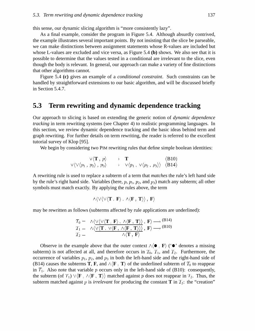
5.3. Term rewriting and dynamic dependence tracking 137
this sense, our dynamic slicing algorithm is “more consistently lazy”.As a final example, consider the program in Figure 5.4. Although absurdly contrived,
the example illustrates several important points. By not insisting that the slice be parseable,we can make distinctions between assignment statements whose R-values are included butwhose L-values are excluded and vice versa, as Figure 5.4 (b) shows. We also see that it ispossible to determine that the values tested in a conditional are irrelevant to the slice, eventhough the body is relevant. In general, our approach can make a variety of fine distinctionsthat other algorithms cannot.
Figure 5.4 (c) gives an example of a conditional constraint. Such constraints can behandled by straightforward extensions to our basic algorithm, and will be discussed brieflyin Section 5.4.7.
5.3 Term rewriting and dynamic dependence tracking
Our approach to slicing is based on extending the generic notion of dynamic dependencetracking in term rewriting systems (see Chapter 4) to realistic programming languages. Inthis section, we review dynamic dependence tracking and the basic ideas behind term andgraph rewriting. For further details on term rewriting, the reader is referred to the excellenttutorial survey of Klop [95].
We begin by considering two PIM rewriting rules that define simple boolean identities:
�hT � pi �� T �B10��h�hp1 � p2i � p3i �� �hp1 � �hp2 � p3ii �B14�
A rewriting rule is used to replace a subterm of a term that matches the rule’s left hand sideby the rule’s right hand side. Variables (here, p, p1, p2, and p3) match any subterm; all othersymbols must match exactly. By applying the rules above, the term
�h�h�hT � Fi � �hF � Tii � Fi
may be rewritten as follows (subterms affected by rule applications are underlined):
T0 � �h�h�hT � Fi � �hF � Tii � Fi�� (B14)
T1 � �h�hT � �hF � �hF � Tiii � Fi�� (B10)
T2 � �hT � Fi
Observe in the example above that the outer context �h� � Fi (‘�’ denotes a missingsubterm) is not affected at all, and therefore occurs in T0, T1, and T2. Furthermore, theoccurrence of variables p1, p2, and p3 in both the left-hand side and the right-hand side of(B14) causes the subterms T, F, and �hF � Ti of the underlined subterm of T0 to reappearin T1. Also note that variable p occurs only in the left-hand side of (B10): consequently,the subterm (of T1) �hF � �hF � Tii matched against p does not reappear in T2. Thus, thesubterm matched against p is irrelevant for producing the constant T in T2: the “creation”
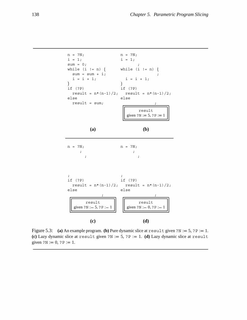
138 Chapter 5. Parametric Program Slicing
n = ?N;i = 1;sum = 0;while (i != n) fsum = sum + i;i = i + 1;
gif (?P)result = n*(n-1)/2;
elseresult = sum;
n = ?N;i = 1;
;while (i != n) f
;i = i + 1;
gif (?P)result = n*(n-1)/2;
else;
resultgiven ?N :� 5�?P :� 1
(a) (b)
n = ?N;;;
;if (?P)result = n*(n-1)/2;
else;
n = ?N;;;
;if (?P)result = n*(n-1)/2;
else;
resultgiven ?N :� 5�?P :� 1
resultgiven ?N :� 0�?P :� 1
(c) (d)
Figure 5.3: (a) An example program. (b) Pure dynamic slice at result given ?N :� 5, ?P :� 1.(c) Lazy dynamic slice at result given ?N :� 5, ?P :� 1. (d) Lazy dynamic slice at resultgiven ?N :� 0, ?P :� 1.

5.3. Term rewriting and dynamic dependence tracking 139
*(ptr = &a) = ?A;b = ?B;x = a;if (a < 3)ptr = &y;
elseptr = &x;
if (b < 2)x = a;
(*ptr) = 20;
*( = &a) = ?A;b = ;x = a;if (a < 3)ptr = &y;
else
if ( < )x = a;
(*ptr) = ;
*( = &a) = ?A;b = ;x = ;if (a < 3)
elseptr = &x;
if ( < )x = ;
(*ptr) = 20;
xgiven ?A :� 2
xgiven ?A � 5
(a) (b) (c)Figure 5.4: (a) An example program. (b) Constrained slice at x given ?A :� 2. (c) Conditionalconstrained slice at x given ?A � 5.
of this subterm T only requires the presence of the matched symbols ‘�’ and ‘T’. Thisobservation is the keystone of our reduction-based slicing technique: We “track” thosesubterms that are relevant to each reduction step; subterms that are relevant to no reductionstep can then be eliminated from the slice.
The tracking process determines not only which subterms are relevant to a given reductionstep, but also how subterms are combined and propagated by the reduction as a whole. Toaccomplish this task, we define for each reduction step that takes a term Ti and yields a newterm Ti�1 the notions of creation and residuation. These are binary relations between thenodes of Ti and the nodes of Ti�1. The creation relation relates the new symbols in Ti�1
produced by the rewriting step to the nodes of Ti that matched the symbols in the left-handside of the rewriting rule (making the rewriting step possible). The residuation relationrelates every other node in Ti�1 to the corresponding occurrence of the same node in theTi�1. The dynamic dependence relation for a multi-step reduction r then consists, roughlyspeaking4, of the transitive closure of creation and residuation relations for the rewritingsteps in r. Figure 5.5 shows all the relations for the example reduction discussed above.
For any reduction r that transforms a term T into a term T �, a term slice with respect tosome subcontextC of T � is defined as the subcontext S of T that is found by tracing back thedynamic dependence relations fromC. The term sliceS satisfies the following properties: (i)
4The notions of creation and residuation become more complicated in the presence of so-called left-nonlinear rules and collapse rules. The exact problems posed by these rules are extensively discussed inChapter 4.

140 Chapter 5. Parametric Program Slicing
F\/
\/
(B14)\/
\/
/\
/\
F
/\
F
/\
T1T0 T2
/\
dynamic dependence relation
F TT F
T
F
F T
(B10)T
creation relation
residuation relation
Figure 5.5: Example of creation and residuation relations.
S reduces to a termC� containing contextC via a reduction r�, and (ii) r� is a subreduction ofr. These properties are rendered pictorially in Figure 5.6, and have the important implicationthat all the slices computed by our technique are effectively “executable” with respect to therewriting semantics.
Our implementation maintains the transitive dependence relations between the nodes ofthe initial term and the nodes of the current term of the reduction by storing with each noden in the current term its term slice, which is the set of nodes in the initial term to which n isrelated. (The dependence relations associated with individual rewriting steps are not stored.)The term slice with respect to a subgraph S of T is then defined as the union of term sliceswith respect to the nodes in S.
Returning to the example of Figure 5.5, we can determine the term slice with respectto the constant T in T2 by tracing back all creation and residuation relations to T0. Byfollowing the transitive relations in Figure 5.5; the reader may verify that this slice consistsof the subcontext �h�hT � �i � �i.
5.3.1 Efficient implementation of term rewriting
We implement term rewriting using the technique of term graph rewriting [17]. Thistechnique extends the basic idea of term rewriting from labeled trees to rooted, labeledgraphs, or term graphs. A term graph may be viewed as a term by traversing it from itsroot and replacing all shared subgraphs by separate copies of their term representations.For clarity, we will frequently depict PIM term graphs or subgraphs in “flattened” form

5.3. Term rewriting and dynamic dependence tracking 141
C
ST
S
r
dynamic dependence relations
T ’ C ’
r ’
C’C
Figure 5.6: The concept of dynamic dependence.
as terms. (The flattened representation of the graph T2 in Figure 5.7, for instance, is�h�hT � Fi � �hT � Tii.)
For certain kinds of rewriting rules, term graph rewriting has the effect of creating sharedsubgraphs where none existed previously. Consider following PIM boolean rule:
�hp1 � �hp2 � p3ii � �h�hp1 � p2i � �hp1 � p3ii (B22)
In rule (B22), the variable p1 appears twice on the right-hand side. Although the left-handside instance of p1 in (B22) matches only a single subterm, the result of the rule applicationmust contain two instances of the subterm matched by p1. Rather than duplicating such aterm, it can be shared, as illustrated by the example in Figure 5.7, in which rule (B22) isapplied to term T0 � �h�hT � Fi � �hF � Tii. We see also from Figure 5.7 that the result ofa single application of reduction rule (here, rule (B10)) inside a shared subterm can also beshared, thus giving the effect of multiple reductions for the price of one.
In general, graph rewriting is performed by replacing the subgraph matched by a rulewith the graph corresponding to the rule’s right hand side. The nodes in a replaced subtermthat are not accessible from elsewhere in the graph are reclaimed by a memory manager.Since the PIM representation of programs contains many shared subgraphs, a graph rewritingimplementation is critical to acceptable performance of the algorithm in practice.
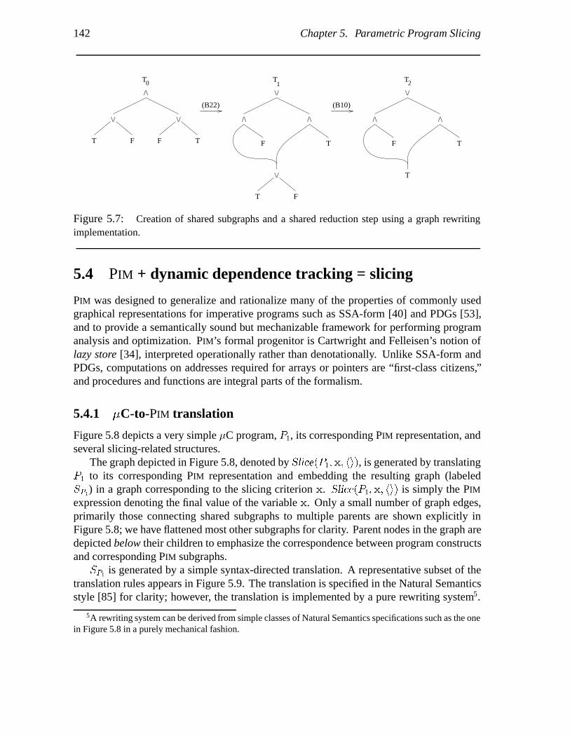
142 Chapter 5. Parametric Program Slicing
\/
FT
\/
\/
/\ /\
\/
FT
F T
/\ \/
T
/\ /\
F T
T
(B10)(B22)
T0 1T T2
F
Figure 5.7: Creation of shared subgraphs and a shared reduction step using a graph rewritingimplementation.
5.4 PIM + dynamic dependence tracking = slicing
PIM was designed to generalize and rationalize many of the properties of commonly usedgraphical representations for imperative programs such as SSA-form [40] and PDGs [53],and to provide a semantically sound but mechanizable framework for performing programanalysis and optimization. PIM’s formal progenitor is Cartwright and Felleisen’s notion oflazy store [34], interpreted operationally rather than denotationally. Unlike SSA-form andPDGs, computations on addresses required for arrays or pointers are “first-class citizens,”and procedures and functions are integral parts of the formalism.
5.4.1 �C-to-PIM translation
Figure 5.8 depicts a very simple �C program, P1, its corresponding PIM representation, andseveral slicing-related structures.
The graph depicted in Figure 5.8, denoted by Slice�P1�x� hi�, is generated by translatingP1 to its corresponding PIM representation and embedding the resulting graph (labeledSP1) in a graph corresponding to the slicing criterion x. Slice�P1�x� hi� is simply the PIM
expression denoting the final value of the variable x. Only a small number of graph edges,primarily those connecting shared subgraphs to multiple parents are shown explicitly inFigure 5.8; we have flattened most other subgraphs for clarity. Parent nodes in the graph aredepicted below their children to emphasize the correspondence between program constructsand corresponding PIM subgraphs.
SP1 is generated by a simple syntax-directed translation. A representative subset of thetranslation rules appears in Figure 5.9. The translation is specified in the Natural Semanticsstyle [85] for clarity; however, the translation is implemented by a pure rewriting system5.
5A rewriting system can be derived from simple classes of Natural Semantics specifications such as the onein Figure 5.8 in a purely mechanical fashion.
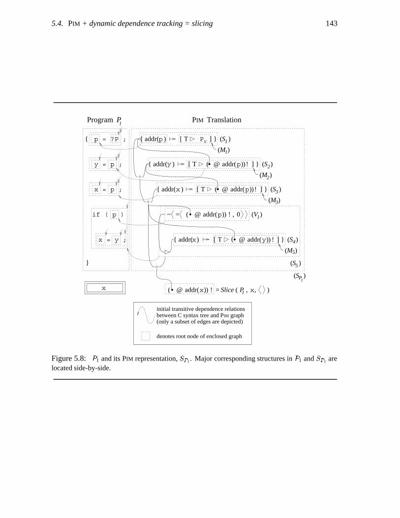
5.4. PIM + dynamic dependence tracking = slicing 143
1P x,, )Slice ()( @ ) !addr(x
VP
))paddr(
S1 )(
S2( )
S3( )
))addr(y S4( )
S5 )(
P1S( )
PIM Translation
PIM
)
}
=x
{ addr( [ T }]
}[ ]T @( !
{ addr( }[ ]T )@ )addr(p( !
~ ,( @ ) !addr( )p= 0
[ ] }
)(V
T @( !
if ( p )
{
x = p ;
p = ?P ;
y = p ;
x = y ;
{ addr(
{ addr(
p )
y )
x )
x)
denotes root node of enclosed graph
between C syntax tree andinitial transitive dependence relations
graph
Program P1
(only a subset of edges are depicted)
(M
(M
1
(M
(M1
2
3)
)
)5
Figure 5.8: P1 and its PIM representation, SP1 . Major corresponding structures in P1 and SP1 arelocated side-by-side.

144 Chapter 5. Parametric Program Slicing
The translation uses several sequent forms corresponding to the principal C syntactic com-ponents. The general form for these sequents is:
s � c � t
Such a sequent may be read as “�C construct c translates to PIM term t, given initial (PIM)store s. ‘�’ is subscripted by ‘Pgm’, ‘Exp’, or ‘LValue’, depending on whether a statement,expression, or L-value (address), respectively, is being translated. Pure expressions (thosehaving no side-effects) and unpure expressions are distinguished in the translation process;subscripts p and u are used to denote the two types. The shared subgraphs in SP1 arise fromrepeated instances of store variables in the antecedents of the translation rules in Figure 5.9,as illustrated in Figure 5.7.
The translation process establishes transitive dependence relations between nodes of theprogram’s AST and the PIM graph SP1 , as described in Section 5.3. Figure 5.8 depicts arepresentative subset of these relations for the root nodes of certain subtrees of the syntaxtree of P1. We have used vestigial arrows in the syntax tree to indicate that nodes are referredto by some set of nodes in the PIM graph. We have also depicted statements of P1 and theircorresponding PIM subgraphs side-by-side.
5.4.2 Overview of PIM
In this section, we briefly outline the function of various PIM substructures using programP1 and its PIM translation, SP1 .
The graph SP1 as a whole is a PIM store structure6, essentially an abstract term representa-tion of memory. SP1 is constructed from the sequential composition (using the ‘ ’ operator)of substores corresponding to the statements comprising P1. The subgraphs accessible fromboxes labeled S1–S4 in Figure 5.8 correspond to the four assignment statements in P1. Thesimplest form of store is a cell such as
S1 � faddr�p� �� #T � PV $g
A store cell associates an address expression (here addr�p�) with a merge structure, (here#T �PV $). Constant addresses such as addr�p� represent ordinary variables. More generally,address expressions are used when addresses are computed, e.g., in pointer references. ‘�s’is used to denote the empty store.
Merge structures are a special kind of conditional construct containing ordered guardedexpressions. The simplest form of merge expression is a merge cell such as #T � PV $,in which some boolean predicate (here, T) guards a value (here, the free PIM variable PVrepresenting the �C meta-variable ?P). The formal consequence of the presence of a freevariable is that any subsequent rewriting-based analysis is valid for any instantiation of thefree variable.
6For clarity, Figure 5.8 does not depict certain empty stores created by the translation process; this elisionwill be irrelevant in the sequel.
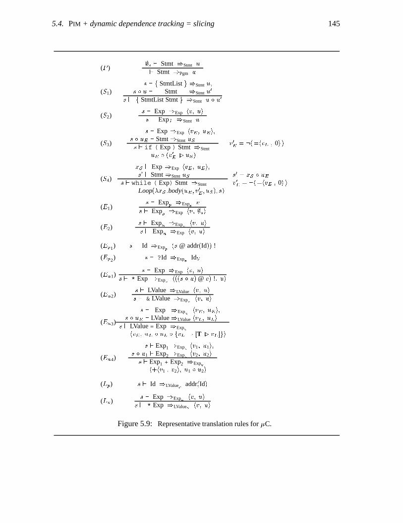
5.4. PIM + dynamic dependence tracking = slicing 145
(P )�s � Stmt �Stmt u
� Stmt �Pgm u
(S1)s � f StmtList g �Stmt u�
s � u � Stmt �Stmt u�
s � f StmtList Stmt g �Stmt u � u�
(S2)s � Exp �Exp hv� uis � Exp; �Stmt u
(S3)
s � Exp �Exp hvE � uEi�s � uE � Stmt �Stmt uSs � if ( Exp ) Stmt �Stmt
uE � �v�E � uS�
v�E � �h�hvE � 0i i
(S4)
xS � Exp �Exp hvE � uEi�s� � Stmt �Stmt uS
s � while ( Exp) Stmt �Stmt
Loop��xS �body�uE � v�E � uS�� s�
s� � xS � uEv�E � �h�hvE � 0i i
(E1)s � Expp �Exp
pv
s � Expp �Exp hv� �si
(E2)s � Expu �Exp
uhv� ui
s � Expu �Exp hv� ui
(Ep1) s � Id �Expp
�s @ addr�Id�� !
(Ep2) s � ?Id �Expp
IdV
(Eu1)s � Exp �Exp hv� ui
s � * Exp �Expuh��s � u� @ v� !� ui
(Eu2)s � LValue �LValue hv� uis � & LValue �Exp
uhv� ui
(Eu3)
s � Exp �ExpuhvE � uEi�
s � uE � LValue �LValue hvL� uLis � LValue = Exp �Exp
u
hvE � uE � uL � fvL � �T � vE �gi
(Eu4)
s � Exp1 �Expuhv1� u1i�
s � u1 � Exp2 �Expuhv2� u2i
s � Exp1 + Exp2 �Expu
h�hv1 � v2i� u1 � u2i
(Lp) s � Id �LValuep addr�Id�
(Lu)s � Exp �Exp
uhv� ui
s � * Exp �LValueu hv� ui
Figure 5.9: Representative translation rules for �C.

146 Chapter 5. Parametric Program Slicing
Merge expressionsm1 andm2 may be composed into ordered lists of the formm1 m m2,in which the rightmost guarded cell takes precedence. Such lists correspond roughly to Lispcond expressions, and represent information similar to SSA-form � nodes [40], particularlythe gated SSA variant of [14]. Unlike normal conditional expressions, however, mergescannot evaluate to values unless they are referred to in a special context represented by theselection operation, ‘!’. Among other places, this operator is used in the translation of everyvariable reference. SP1 contains no non-trivial merge structures, but such structures will arisein the simplification process. �m denotes the null merge structure. In the sequel, we willoften drop subscripts distinguishing related store and merge constructs when no confusionwill arise.
In addition to guards in merge cells, stores such as S5 (which corresponds to the ‘if’statement as a whole) may also be guarded. The guard expression V1 corresponds to theif’s predicate expression. Consistent with standard C semantics, the guard V1 tests whetherthe value of the variable p is nonzero.
The general form for the PIM graph constructed for a slice of program P at x givenconstraints
?X1 :� Exp1� � � � �?Xn :� Expn
isSlice�P�x� h?X1 :� Exp1� � � � �?Xn :� Expni�
� ��SP@addr�x��!� #X1V :� v1� � � � � XnV :� vn$
where SP is the PIM store to which P compiles, the X1V are free variables corresponding tothe meta-variables and the vi are PIM graphs corresponding to the value of the Expi (ignoringside-effects). Slice�P�x� h� � �i� is the PIM representation of the value of x after execution ofP , with substitutions for free variables defined by the constraints.
5.4.3 PIM rewriting and elimination of dependences
PIM’s equational logic consists of an “operational” subsystem, PIM�, plus a set of additionalnon-oriented equational rules for reasoning about operational equivalences in PIM�, in-stances of which can also be oriented for use in analysis. PIM� is confluent and normalizing(assuming an appropriate strategy), thus it can be viewed as defining an operational seman-tics or interpreter for PIM terms. An important subsystem of PIM� that defines the semanticsof programs without loops or procedures, PIM�
t , is canonical, that is, strongly normalizingas well as confluent. PIM� can be enriched with certain oriented instances of rules in (PIM�PIM�) in such a way that confluence is preserved on closed terms, and such that uniquenormal forms for open terms exist up to certain trivial permutations. In the sequel, we willrefer to the enriched rewriting system as COREPIM�. PIM’s rules and subsystem structureare described in detail in [55]; key subsystems are reviewed in Appendix A.
Given a program P and a slicing criterion x, we use normalizing sets of oriented PIM
equations to simplify Slice�P�x� h� � �i� graphs by reducing them to normal (i.e., irreducible)forms. From the point of view of slicing, the goal of this simplification process is to eliminate
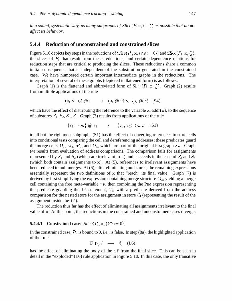
5.4. PIM + dynamic dependence tracking = slicing 147
in a sound, systematic way, as many subgraphs of Slice�P�x� h� � �i� as possible that do notaffect its behavior.
5.4.4 Reduction of unconstrained and constrained slices
Figure 5.10 depicts key steps in the reductions ofSlice�P1�x� h?P :� 0i� andSlice�P1�x� hi�,the slices of P1 that result from these reductions, and certain dependence relations forreduction steps that are critical to producing the slices. These reductions share a commoninitial subsequence that is independent of the substitution generated in the constrainedcase. We have numbered certain important intermediate graphs in the reductions. Theinterpretation of several of these graphs (depicted in flattened form) is as follows:
Graph (1) is the flattened and abbreviated form of Slice�P1�x� hi�. Graph (2) resultsfrom multiple applications of the rule
�s1 s s2� @ v �� �s1 @ v� m �s2 @ v� �S4�
which have the effect of distributing the reference to the variable x, addr�x�, to the sequenceof substores S1, S2, S3, S5. Graph (3) results from applications of the rule
fv1 �� mg @ v2 �� �hv1 � v2i �m m �S1�
to all but the rightmost subgraph. (S1) has the effect of converting references to store cellsinto conditional tests comparing the cell and dereferencing addresses; these predicates guardthe merge cells M1, M2, M3, and M4, which are part of the original PIM graph SP1 . Graph(4) results from evaluation of address comparisons. The comparison fails for assignmentsrepresented by S1 and S2 (which are irrelevant to x) and succeeds in the case of S2 and S4
(which both contain assignments to x). At (5), references to irrelevant assignments havebeen reduced to null merges. At (6), after eliminating null stores, the remaining expressionsessentially represent the two definitions of x that “reach” its final value. Graph (7) isderived by first simplifying the expression containing merge structure M3, yielding a mergecell containing the free meta-variable ?P, then combining the PIM expression representingthe predicate guarding the if statement, V1, with a predicate derived from the addresscomparison for the nested store for the assignment in store S4 (representing the result of theassignment inside the if).
The reduction thus far has the effect of eliminating all assignments irrelevant to the finalvalue of x. At this point, the reductions in the constrained and unconstrained cases diverge:
5.4.4.1 Constrained case: Slice�P1�x� h?P :� 0i�
In the constrained case, PV is bound to 0, i.e., is false. In step (8a), the highlighted applicationof the rule
F �� l �� �� (L6)
has the effect of eliminating the body of the if from the final slice. This can be seen indetail in the “exploded” (L6) rule application in Figure 5.10. In this case, the only transitive
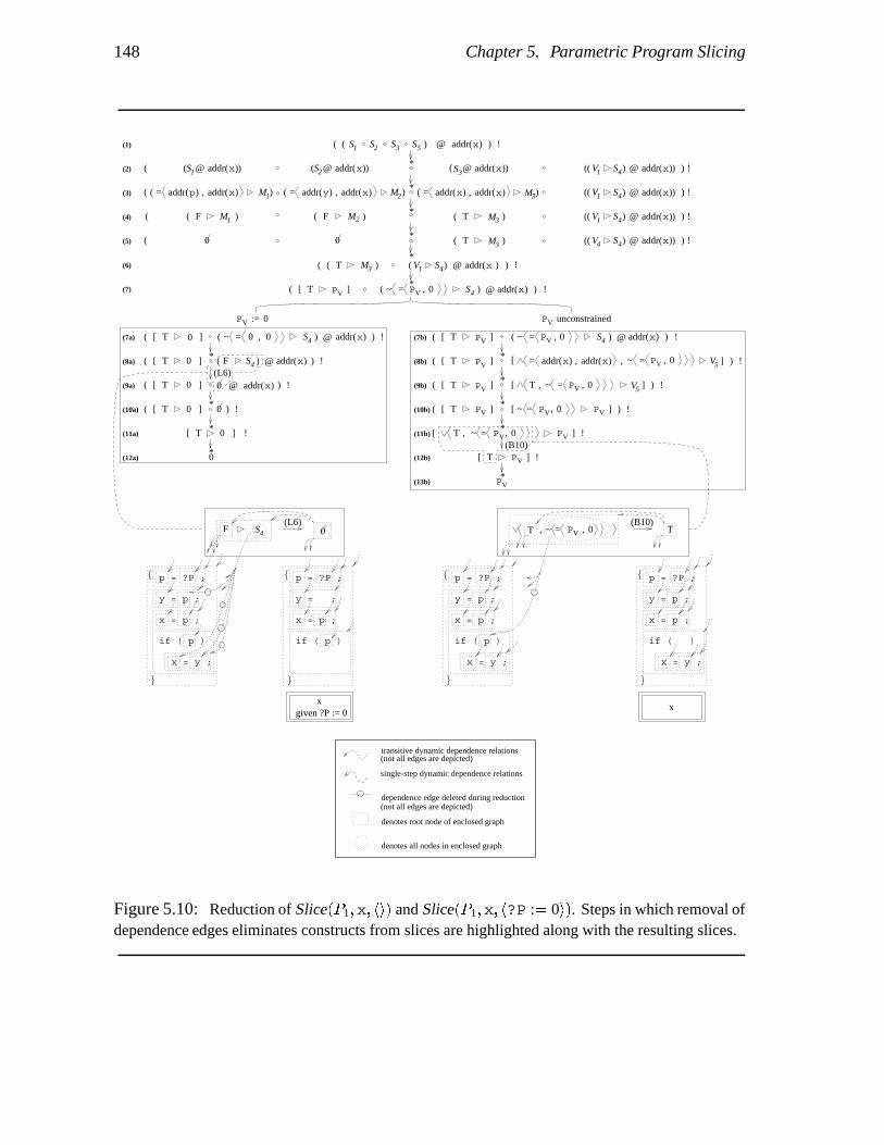
148 Chapter 5. Parametric Program Slicing
*
!x)addr(S1 S2 S3 S5 @( ))(
PV[ ]T xaddr( )S4~ = PV , 0( ) @ ) !(
*
*
*
*
*
0 0
x)addr(S1 @( x)addr(S2 @( ) x)addr(S3 )@(
PV unconstrained
PV[ ]T xaddr( )S4~ = PV , 0( ) @ ) !(
*
*
*
*
PV
PV[ ]T V5~ = PV , 0[ T , ]( ) !
PV[ ]T( PV~ PV, 0=[ ] ) !
~ PV, 0= PV[ T , ] !
PV[ ]T !
*
PV[ ]T V5~ = PV , 0x)addr(= ,)addr(x ,[ ]
dependence edge deleted during reduction
single-step dynamic dependence relations
transitive dynamic dependence relations
denotes root node of enclosed graph
denotes all nodes in enclosed graph
(not all edges are depicted)
(not all edges are depicted)
[ T 0 ] xaddr( )S4 )F( @( ) !
[ T 0 ] 0( ) !
[ T ]0 xaddr( )S400 ,=~ )( @( ) !
*
[ T 0 ] 0 xaddr( )@( ) !
*
*[ T 0 ] !
*
(7a)
(8a)
(9a)
(11a)
(10a)
(12a)
(L6)
0
PV := 0
T(B10)
TPV
x = p ;x = p ;
1
x = p ;
0(L6)
x = p ;
S4
x)addr()addr(p , addr(y addr(x x)addr(addr( )x= ,
)xaddr( )@
)xaddr( )@
)xaddr( )@
)xaddr( )@
xaddr( )@
M
MM
xgiven ?P := 0
x
(1)
(7)
(6)
(5)
(4)
(3)
(2)
( !)
( !)
( !)
)( ) !
(7b)
(8b)
(9b)
(10b)
(11b)
(12b)
(13b)
(B10)
( ) !
, ~ = , 0
{
y = p ;
}
x = y ;
p = ?P ;
if ( )
{
if ( p )
y = p ;
}
x = y ;
p = ?P ;{
if ( p )
}
p = ?P ;
y = ;
F
{
if ( p )
y = p ;
}
x = y ;
p = ?P ;
= ) )= ,(( ) ( )
F( ) F( ) T( )
T( )
( T( )
S4)((
S4)((
S )((
S )(( V4
V
V
V1
1
1 4
4
) !S4)( V1
1) M
M
M
M 32
3
3
M
2
3
Figure 5.10: Reduction of Slice�P1�x� hi� and Slice�P1�x� h?P :� 0i�. Steps in which removal ofdependence edges eliminates constructs from slices are highlighted along with the resulting slices.

5.4. PIM + dynamic dependence tracking = slicing 149
dependence edges linking the constructs in the body of the if statement and the identifierp in the assignment y = p; have their origin in the subgraph S4. When this subgraph iseliminated by the application of (L6), the constructs effectively disappear from the slice.
While it may appear that the slice results entirely from the application of a single rule,this rule is only the last of several rules that eliminate transitive edges from PIM nodes to theomitted constructs inP1. Only when the last edges are eliminated does the construct disappearfrom the slice. Other rules have the effect of combining dependence edges emanating fromseveral intermediate nodes into a single node (as the two single-step dependence edges inthe depiction of rule (L6) illustrate).
5.4.4.2 Unconstrained case: Slice�P1�x� hi�
The unconstrained case is somewhat more interesting than the constrained case: althoughwe do not know the value of PV and thus cannot effectively evaluate the if statement in P1,we discover that the two reaching definitions for x both assign the same value to x, namely,PV . Application of several rules allows us to combine guards of merge cells with the sameguarded value into the disjunctive expression shown in (11b).
The next step, the reduction of (11b) to (12b), discovers that the predicate’s value itselfis irrelevant to the final value of x. As the exploded view of this rewrite step illustrates, thereis no transitive dependence between the predicate p of the source AST and any of the nodesin the resulting term (12b) (or the final term (13b)). Consequently, the unconstrained slicedoes not contain the predicate of the if statement, though it does contain the assignmentstatement within the if statement.
Slices that contain statements from the arms of a conditional statement but not itspredicate, are unusual enough to deserve some discussion. Such slices indicate that thevalue of the predicate itself is irrelevant, even though the conditional statement containssome relevant statement, e.g., an assignment to some relevant variable. Such situations canarise in realistic programs. Consider, for example, the statement
if (P) f(foo); else f(bar);
where the procedure f has some side-effect on some variable x of interest, and wherethis side-effect itself is independent of the argument to the procedure. Here, the two callstatements are relevant to the final value of x, though the predicate itself is irrelevant. Thisreflects a kind of reasoning that programmers do use when analyzing a program backwards,and can result in substantially smaller slices because of the elimination of the statements thatthe predicate itself depends on. The possibilities for computing more precise slices in thisfashion are even greater in the case of constrained slicing.
5.4.5 Slicing and reduction strategies
As PIM� is a confluent rewriting system, reductions may be performed anywhere in a graphwithout affecting the final term produced (assuming the reduction terminates at all). This

150 Chapter 5. Parametric Program Slicing
“stateless” property of reduction systems accommodates a variety of performance tradeoffsderived from varying the reduction strategy. We use an outermost or “lazy” strategy, whichensures that only steps that contribute to a final result are performed. (Note, however, thatthe reduction depicted in Figure 5.10 uses a strategy that is not strictly outermost to betterillustrate the properties of certain intermediate terms). Alternatively, the PIM representationof the entire program could be normalized “eagerly” prior to the specification of any slicingcriterion; those steps specific to the criterion or constraints could be performed later.
Reduction strategies can also have an effect on slices. In the constrained case, both of thereductions depicted in Figure 5.10 are valid, and, consequently both of the slices depicted arealso valid. Slices are therefore not necessarily unique, even when the underlying reductionsystem is confluent. However, our reduction strategy favors the left reduction over the rightone in the constrained case. Intuitively, this favors a “standard” execution semantics thatcorresponds most closely with results of traditional program slicing algorithms.
5.4.6 Slicing at intermediate program points
Although our discussion thus far has concentrated on computing slices with respect to thefinal values of variables, our approach is capable of computing slices with respect to anyexpression at any program point. Conceptually, a slice with respect to a �C expression e(assumed to be side-effect free) at some specific program point can be computed as follows:First, introduce a new variable v and an assignment of the form
v = ophv � ei;
at the program point of interest, where op is an abstract, uninterpreted operator. Then,compute the slice with respect to the final value ofv. Variablevhas the effect of accumulatingthe sequence of values the expression takes on at the desired program point.
In practice, it is not necessary to alter the program in order to compute slices at interme-diate points. An implementation can instead construct and maintain a reference to the PIM
store subgraph sp corresponding to every program point p (note that the graphs representingthese stores will generally have many nodes in common). The slice with respect to the pro-gram point of interest is then computed by normalizing the PIM expression corresponding tothe translation of e in initial store sp.
5.4.7 Conditional constraints
A slice with respect to a conditional constraint such as that depicted in Figure 5.4 (c) can becomputed by constructing a PIM graph roughly equivalent to that which would be producedby inserting the body of the program in a conditional statement where the predicate is theconjunction of all such constraints.
The effectiveness of our slicing algorithm in handling conditional constraints dependsprimarily on its ability to reason about the operations allowed in such constraints. The exten-sible nature of our approach makes it easy to augment the slicing algorithm by incorporating
5.5. Variations on a looping theme 151
sophisticated reasoning capabilities about particular domains into the slicing algorithm, asit only involves adding rewrite rules characterizing the appropriate domains. For example,in the case of Figure 5.4 (c), rudimentary rules for reasoning about arithmetic inequalitiessuffice to compute the slice shown.
5.4.8 Complexity tradeoffs
Use of different normalizing subsets of PIM equations allows various accuracy/time tradeoffsin the analysis process. For instance, pointer-induced alias analysis is NP-complete evenin the absence of loops and procedures [104], although such analysis is usually tractablein practice. By including or excluding appropriate PIM rules, one can effectively choosemore precise (but potentially slow) or more conservative (but guaranteed fast) pointer anal-ysis. For instance, eliminating rule (M3) (see Figure A.1) effectively inhibits propagation ofsymbolic addresses representing pointer values, thus preventing these expressions involvingthese addresses from being resolved or simplified. Rule (L11) has the effect of joining com-mon results of common expression propagation (including address expressions) in differentbranches of a conditional, and can be enabled, disabled, or restricted to prevent or allowsuch propagation.
The result of more accurate pointer analysis in slicing is manifested by elimination ofmore subgraphs of the program representation that are irrelevant to the slicing criterion. Asimilar phenomenon occurs with simplification of boolean predicates involved in condition-als.
5.5 Variations on a looping theme
This section discusses a number of PIM variants suitable for computing slices in loops.These sets of rules may be used as building blocks for generating a variety of differentslicing algorithms without changing the underlying algorithmic framework. In the sequel,we will use COREPIM� to denote those PIM rules that are not loop related and are commonto the slicing variants we will present. While the COREPIM� rules allow addresses to bestored as values and manipulated, the analysis rules presented in this section assume forsimplicity that no pointers are used. The ideas in this section can be adapted easily toproduce conservative slices in the presence of pointers; more precise pointer analysis is alsopossible, but requires more sophisticated rules for reasoning about address equivalence.
5.5.1 loop execution rules: pure dynamic slicing
Loops are represented in PIM by terms of the form
Loop��xS �body�uE� vE� uS�� s�
Informally, uE is a store representing the side-effects of evaluating the loop predicate, vErepresents the value of the predicate, uS is a store representing the side-effects of the loop

152 Chapter 5. Parametric Program Slicing
Loop��xS body�uE � vE � uS�� s� �S�� Y �fL�xS
�uE �s �vE �s �uS �sS�fL �xS �s uE �s uS����� � s� �loop�
(where fL �� �FV�uE� � FV�uS� � FV�vE���
��xf� g � f �x :� g� ���Y f� � f �Y f� �recursion�
Figure 5.11: Loop execution rules.
body, all as functions of the store xS at the beginning of a loop iteration. The secondargument s is the incoming store. The term Loop��xS �body�uE� vE� uS�� s� itself denotesthe store representing the side-effects of executing the loop until the predicate evaluates tofalse. The rewriting rules in Figure 5.11, which we will refer to as loop execution rules,specify this behavior formally. Consider the underlined subterm of the right-hand side of therule (loop). The underlined subterm may be read as: the side-effects of evaluating the looppredicate and—if the predicate evaluates to true, the side-effects of executing the loop bodyonce—composed with the side-effects of executing the same loop with an appropriatelyupdated store, namely, xS s uE s uS . The rest of the term serves to express the recursionusing the recursion combinator Y. f #x :� g$ represents the result of substituting g for freeoccurrences of x in f (with the usual provisos about variable capture and renaming), FV � �is the set of free variables in a term , and ‘S’ is a technicality—a “sort coercion” operatorthat has no semantic content. [54] shows how the � rule and substitution can be encoded aspure rewriting rules.
Utilizing these rules and COREPIM� during the simplification phase leads to a straightfor-ward dynamic slicing algorithm that we call a pure dynamic slicing algorithm. Section 5.2.4discusses an example (Figure 5.3 (b)) of this sort of slice.
5.5.2 � rules: lazy dynamic slicing
Figure 5.12 depicts a set of rules, the � rules, that statically simplify PIM stores generated byloops. The effect of � rules on the PIM representation is essentially to introduce an SSA-form� node [40] for every variable that might be assigned a value inside the loop. In terms ofslicing, these rules have the effect of permitting loops to be removed from slices if it can bedetermined (statically) that the loop cannot assign to any “variable of interest”.
We will refer to the slicing algorithm obtained by using both the loop execution rulesand the � rules in conjunction with COREPIM� as a lazy dynamic slicing algorithm. Thisslicing algorithm computes traditional dynamic slices, such as Figure 5.3 (c), as well as thesomewhat more unusual result in Figure 5.3 (d).
The slices produced by our lazy dynamic slicing algorithm are closer to the slicesproduced by the Agrawal-Horgan algorithm [6] than to the slices produced by the Korel-

5.5. Variations on a looping theme 153
Loop��xS body�uE � vE � uS�� s� �Project� Loop��xS body�uE � vE � uS�� s��
AssignedVars�uE �s uS� � �LA1�
Project�s� fg� � �s �LA2�Project�s� fvg � r� � �v �� s @ v� �s Project�s� r� �LA3�
...rules for computing AssignedVars�s�,
the set of variables assigned to in the store s...
Figure 5.12: � rules.
x = ?X;y = x;if (x < 0)x = -x;
z = x;
x = ?X;;
if (x < 0);
z = x;
zgiven ?X :� 5
(a) (b)
Figure 5.13: (a) Example program. (b) Dynamic slice at z given ?X :� 5.
Laski algorithm [100]. The Korel-Laski slices tend to be larger than the Agrawal-Horganslices since they, unlike the Agrawal-Horgan slices, are executable. Our dynamic slices,though not executable under the “standard semantics”, are executable with respect to thesemantics specified by the rewriting rules.
Figure 5.13 (a) illustrates an important difference between our algorithm and previousdynamic slicing algorithms. Since the if predicate evaluates to false, previous dynamicslicing algorithms exclude the predicate (and any of the statements the predicate evaluationis dependent upon) from the dynamic slice with respect to z. However, as has been observedbefore [100, 121], the predicate does “affect” the final value of z, in the sense that thepredicate must be executed in order to ensure that the value of x, and thus z, is not negated.In other words, the result of the predicate evaluation has an effect on the final result, eventhough the statement guarded by the predicate is not executed. In applications such asdebugging it is useful to include these statements in the slice [121, 122]. In this sense, ourslicing algorithm produces a slice that is semantically more consistent than existing dynamicslicing algorithms.
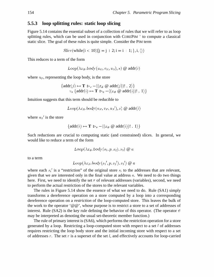
154 Chapter 5. Parametric Program Slicing
5.5.3 loop splitting rules: static loop slicing
Figure 5.14 contains the essential subset of a collection of rules that we will refer to as loopsplitting rules, which can be used in conjunction with COREPIM� to compute a classicalstatic slice. The goal of these rules is quite simple. Consider the PIM term
Slice�while�i � 10�fj � j � 2; i � i � 1; g� i� hi�
This reduces to a term of the form
Loop��xS �body�uE� vE� uS�� s� @ addr�i�
where uS, representing the loop body, is the store
faddr�j� �� T �v �h�xS @ addr�j��! � 2ig s faddr�i� �� T �v �h�xS @ addr�i��! � 1ig
Intuition suggests that this term should be reducible to
Loop��xS �body�uE� vE� uS��� s� @ addr�i�
where uS � is the store
faddr�i� �� T �v �h�xS @ addr�i��! � 1ig
Such reductions are crucial to computing static (and constrained) slices. In general, wewould like to reduce a term of the form
Loop��xS �body�s1� p� s2�� s3� @ a
to a termLoop��xS �body�s1
�� p� s2��� s3
�� @ a
where each si� is a “restriction” of the original store si to the addresses that are relevant,
given that we are interested only in the final value at address a. We need to do two thingshere. First, we need to identify the set r of relevant addresses (variables), second, we needto perform the actual restriction of the stores to the relevant variables.
The rules in Figure 5.14 show the essence of what we need to do. Rule (SA1) simplytransforms a dereference operation on a store computed by a loop into a correspondingdereference operation on a restriction of the loop-computed store. This leaves the bulk ofthe work to the operator ‘@@’, whose purpose is to restrict a store to a set of addresses ofinterest. Rule (SA2) is the key rule defining the behavior of this operator. (The operator �may be interpreted as denoting the usual set-theoretic member function.)
The rule of primary interest is (SA6), which performs the restriction operation for a storegenerated by a loop. Restricting a loop-computed store with respect to a set l of addressesrequires restricting the loop body store and the initial incoming store with respect to a setof addresses r. The set r is a superset of the set l, and effectively accounts for loop-carried

5.5. Variations on a looping theme 155
Loop��xS body�uE � vE � uS�� s� @ v ��Loop��xS body�uE � vE � uS�� s� @@ fvg� @ v �SA1�
�a �� m� @@ l � �a � l� �s �a �� m� �SA2�
�s @@ l � �s �SA3��s1 �s s2� @@ l � �s1 @@ l� �s �s2 @@ l� �SA4��g �s s� @@ l � g �s �s @@ l� �SA5�
r � � l � Demand�vE � xS� � Demand�uE @@ r� xS�� Demand�uS @@ r� xS� � � T
Loop��xS body�uE � vE � uS�� s� @@ l �Loop��xS body�uE @@ r� vE � uS @@ r�� s @@ r� �SA6�
...rules for computing Demand�s� xS�, the set of
addresses dereferencing free instances of xS in s...
Figure 5.14: Loop splitting rules.
dependences. The antecedent of rule (SA6) specifies the condition this set r has to satisfy,namely that the set of variables r should include the set l, the set of variables required tocompute the loop predicate, and the set of variables necessary to compute values assignedto the variables in r within the loop. Put another way, the antecedent of (SA6) ensuresthat the set of variables r is transitively closed with respect to loop-carried dependences.The auxiliary function Demand�t� xS�, roughly, identifies “upwards exposed” variables in t.More formally, given a store or merge t, Demand�t� xS� identifies dereferences of the freestore variable xS in t and collects the address operands of such dereferences.
Rule (SA6) is not a pure rewriting rule, since the variable r in the antecedent of the ruleis not bound in the left-hand side of the rewrite rule. Applying rule (SA6) thus requirescomputing some solution r to the constraint expressed by the antecedent. The computationof the least solution of this constraint can be performed easily using rewriting rules thatcompute an iterative computation of the constraint’s least fixed point.
Rules expressed in a “constraint” style such as (SA6) have the advantage that they canaccommodate analysis algorithms implemented by non-rewriting means (and thus for whichdependence tracking cannot be performed). Observe that (SA6) is valid for every possibleinstantiation of the variable r—thus, one may view (SA6) as a rule schema describinginfinitely many rewriting rules. One may then use any mechanism whatsoever to choose aninstantiation for the rule, treating the instantiation as an ordinary rewriting rule with respectto dependence tracking. This approach ensures that the dependence information is computedcorrectly, notwithstanding the use of an external analysis algorithm.

156 Chapter 5. Parametric Program Slicing
5.5.4 loop invariance rules: invariance-sensitive slicing
We now turn our attention to the final set of rules, which we will refer to as loop invariancerules. We will refer to the slicing algorithm obtained by using these rules, the COREPIM�
rules, and the loop splitting rules, as an invariance sensitive slicing algorithm. If the loopexecution rules are used as well, we obtain a � invariance-sensitive algorithm. The primarydifference between the two algorithms is that the latter will execute (i.e., unfold) a loop aslong as its predicate evaluates to a constant. Figure 5.15 illustrates this behavior. The �invariance-sensitive slicing algorithm, by executing the loop, discovers that two of the threeassignments to y in the loop are irrelevant for the given input constraint ?N :� 5. Thesimpler algorithm avoids unfolding the loop; however, by effectively performing constantpropagation, it discovers that one of the three assignment statements is irrelevant.
We describe the goals of the loop invariance rules below. Consider a store of the form
Loop��xS �body�uE� vE� uS�� s� @ a
The store uS represents the loop body, and free occurrences of xS in uS denote the store atthe beginning of a specific loop iteration. In the presence of loop invariants, one can simplifythe store uS further. For instance, consider the example in Figure 5.15 (c). The store uScompiled for the loop body will contain subterms of the form �xS @ addr�x��!, denoting thevalue of variable x in a particular iteration. Since the value of x is a loop-invariant constant 6(given the constraint ?N :� 5), we would like to replace this term by 6. This replacement, inturn, will allow further simplifications of the store, and ultimately lead to the slice depictedin the figure.
Achieving this kind of simplification requires us to do two things: we must identify theloop-invariant component of the store, and we must specialize the loop body (and the looppredicate) with respect to the loop invariant component of the store. The second task isrelatively trivial. Once the loop invariant component sinv of the store has been identified,we can replace the free occurrences of xS in the loop body by xS s sinv. The rest of PIM
will then take care of the specialization.The rules in Figure 5.16 formalize these intuitions. The most important rule is (IA1),
a conditional rule in the style of rule (SA6) (Figure 5.14). The consequent of the rulespecializes the loop body and loop predicate of a loop-computed store with respect to theloop-invariant part of the store, namely sinv. The antecedent guarding the applicability ofthe rule “defines” what it means for a part of the store to be loop invariant. This definitionis stated in terms of a subsumption relationship ‘!’ between program stores. A store s1
subsumes a store s2, if for every variable x assigned a value v in store s2, x is also assignedthe same value v in store s1. The subsumption relation is concisely defined by the equationalaxiom (IA2). Rules (IA2.1) through (IA2.3) represent a conservative approximation to‘!’ that is more “directly computable,” since it is defined inductively. Less conservativeapproximations to (IA2) can also be defined that allow inference of more complex loopinvariants.
Returning to the notion of a loop-invariant store, the store sinv is considered to be loopinvariant if (i) The incoming store s (the store before the loop begins its first iteration)

5.6. Pragmatics 157
n = ?N; z = ?Z;x = n + 1;i = 1; y = 0;while (i < n) fif (x > 100)y = y + 100;
else if (y < 99)y = y + x;
elsey = y + 50;
z = z + y;i = i + 1;
g
n = ?N; z = ?Z;x = n + 1;i = 1; y = 0;while (i < n) fif (x > 100)
;else if (y < 99)y = y + x;
else;
z = z + y;i = i + 1;
g
n = ?N; z = ?Z;x = n + 1;i = 1; y = 0;while (i < n) fif (x > 100)
;else if (y < 99)y = y + x;
elsey = y + 50;
z = z + y;i = i + 1;
g
zgiven ?N :� 5
zgiven ?N :� 5
(a) (b) (c)
Figure 5.15: (a) Example program. (b) invariance-sensitive slice at z given ?N :� 5. (c)Simple invariance-sensitive slice at z given ?N :� 5.
subsumes sinv, and (ii) The loop body uE s uS, specialized for an incoming store xS s sinvthat subsumes sinv, and then composed with sinv results in a store that subsumes sinv.
As with rule (SA6) discussed in the section on static slicing, rule (IA1) cannot be useddirectly by the dependence tracking system. However, we can use the rule in conjunction withany algorithm for identifying loop invariants, such as the conditional constant propagationalgorithm of Wegman et al. [141].
5.6 Pragmatics
A prototype implementation of our methods has been completed using the ASF+SDF Meta-environment [93]. The results obtained from this prototype have been encouraging, and weare now engaged in implementing a “free-standing” reduction-based slicing system usingthe most efficient possible implementation techniques. In this section, we briefly touch onseveral pragmatic issues that arise in implementing our approach.
5.6.1 Properties of graph reduction
Term graph reduction is a simple technique that can be implemented efficiently when anautomaton-based matching algorithm and outermost reduction strategies are used. This leadsus to believe that it should scale well to relatively large programs. Graph reduction also

158 Chapter 5. Parametric Program Slicing
s � sinv � T�s� � �xS �s sinv��
sinv �s ��uE �s uS��xS :� s��� � sinv � TLoop��xS body�uE � vE � uS�� s� �
Loop��xS body�uE�xS :� s���vE�xS :� s���uS�xS :� s���� s� �IA1�
s1 �s s2 � s1
s1 � s2 � T �IA2�
s � �s � T �IA21�
s � s1 � T� s � s2 � Ts � �s1 �s s2� � T �IA22�
�h�s @ a�! � m!i � Ts � fa �� mg � T �IA23�
Figure 5.16: Loop invariance rules.
has the advantage that results of reductions performed in shared subgraphs are immediatelyavailable to all supergraphs from which they are accessible. This means, e.g., that a slice canbe computed in a subprogram (such as a procedure), and the results later used in computingthe slice with respect to the entire program. It also means that reduction steps that areindependent of a given criterion, but dependent on the program, can be shared and reusedwhen new criteria are supplied.
5.6.2 Alternative translation algorithms
As alluded to in Section 5.2.2, it is not strictly necessary to use a rewriting system to translatea source program to PIM. Any algorithm to perform the translation suffices, provided that thedynamic dependence relations between the source AST and its PIM translation are correctlyinitialized. However, the correctness of these initial relations must be established by hand.
5.6.3 Chain rules
Chain rules in a language’s abstract syntax can be used to distinguish classes of syntacticallyrelated program constructs that have differing semantic properties. For instance, in our Cgrammar, we distinguish between “pure” expressions and those that may have side-effects.Dependences traced by CR-tracking to such nodes can be used to single out a particularproperty of a construct that causes it to be included or excluded from a slice.
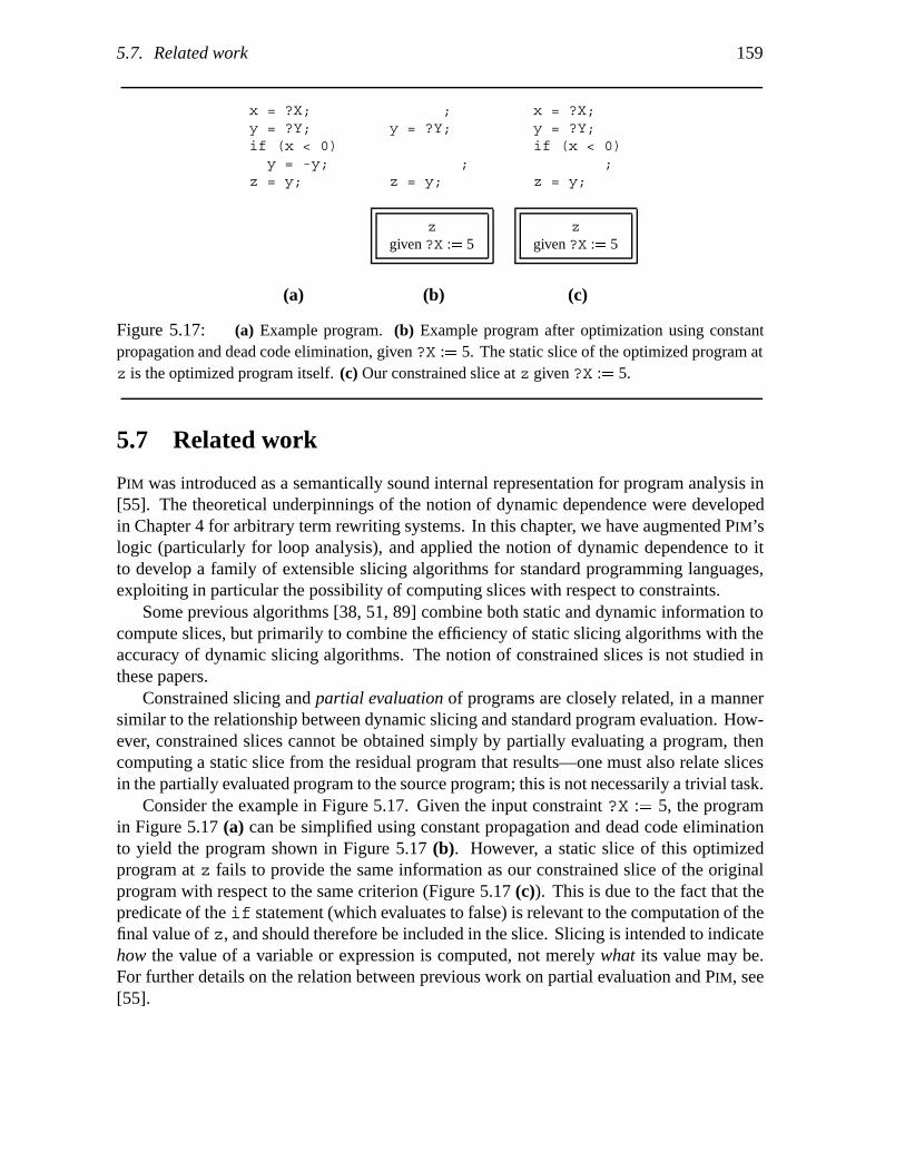
5.7. Related work 159
x = ?X;y = ?Y;if (x < 0)y = -y;
z = y;
;y = ?Y;
;z = y;
x = ?X;y = ?Y;if (x < 0)
;z = y;
zgiven ?X :� 5
zgiven ?X :� 5
(a) (b) (c)
Figure 5.17: (a) Example program. (b) Example program after optimization using constantpropagation and dead code elimination, given ?X :� 5. The static slice of the optimized program atz is the optimized program itself. (c) Our constrained slice at z given ?X :� 5.
5.7 Related work
PIM was introduced as a semantically sound internal representation for program analysis in[55]. The theoretical underpinnings of the notion of dynamic dependence were developedin Chapter 4 for arbitrary term rewriting systems. In this chapter, we have augmented PIM’slogic (particularly for loop analysis), and applied the notion of dynamic dependence to itto develop a family of extensible slicing algorithms for standard programming languages,exploiting in particular the possibility of computing slices with respect to constraints.
Some previous algorithms [38, 51, 89] combine both static and dynamic information tocompute slices, but primarily to combine the efficiency of static slicing algorithms with theaccuracy of dynamic slicing algorithms. The notion of constrained slices is not studied inthese papers.
Constrained slicing and partial evaluation of programs are closely related, in a mannersimilar to the relationship between dynamic slicing and standard program evaluation. How-ever, constrained slices cannot be obtained simply by partially evaluating a program, thencomputing a static slice from the residual program that results—one must also relate slicesin the partially evaluated program to the source program; this is not necessarily a trivial task.
Consider the example in Figure 5.17. Given the input constraint ?X :� 5, the programin Figure 5.17 (a) can be simplified using constant propagation and dead code eliminationto yield the program shown in Figure 5.17 (b). However, a static slice of this optimizedprogram at z fails to provide the same information as our constrained slice of the originalprogram with respect to the same criterion (Figure 5.17 (c)). This is due to the fact that thepredicate of the if statement (which evaluates to false) is relevant to the computation of thefinal value of z, and should therefore be included in the slice. Slicing is intended to indicatehow the value of a variable or expression is computed, not merely what its value may be.For further details on the relation between previous work on partial evaluation and PIM, see[55].
160 Chapter 5. Parametric Program Slicing
Ernst [52] presents an algorithm for static slicing that is similar to our algorithm incertain respects. In particular, Ernst describes how conventional program optimizationtechniques can be used to produce smaller and better slices. The internal representation thatErnst uses, the value dependence graph (VDG), has similarities with PIM, and the processof optimization itself consists of transforming the VDG. Ernst refers to the problem ofmaintaining a correspondence between the VDG and the source code graph throughout theoptimization process, and mentions that this correspondence enables a history mechanismfor explaining the transformations that were performed. No details are presented as to howthis is done, but this aspect of Ernst’s work appears to be the analogue of the notion ofdynamic dependence used in our work to maintain a similar correspondence.
In Chapter 6, it is shown that dynamic dependence tracking can be used to computeaccurate dynamic slices from a simple “interpreter-style” semantics for a language, and thatthese techniques are useful for debugging.
While we have yet to undertake a formal comparison of the complexity of our approachwith that of earlier methods based on dataflow analysis or dependence graphs, informal anal-ysis indicates that for comparable types of slices, our approach should be quite competitivewith previous techniques. One characteristic of our approach that must be kept in mind inany complexity analysis is that aspects of both intermediate representation construction andanalysis using the intermediate representation are combined into reduction steps. For in-stance, in comparing our work with PDG-based algorithms, it is apparent that there is a closecorrespondence between most steps involved in PDG construction and certain PIM rewritingsteps. The computation of the slice itself in PDG-based approaches requires a graph traversalthat corresponds roughly to traversing the set of dynamic dependence relations in a reducedPIM term.
One advantage of our approach over PDG-based methods is that by using an outermost“lazy” graph reduction strategy, the analysis performed is effectively demand-driven. Thusonly those reduction steps directly relevant to the slicing criterion are performed. In thisrespect, our approach has the potential to outperform prior techniques that may eagerlycompute dataflow information that is never used.
5.8 Future work
There are several areas for future research: we are currently exploring the issues involved inextending our techniques to handle arbitrary control flow,arrays, address arithmetic, dynamicmemory allocation, and procedures. We also intend to study various PIM subsystems andreduction strategies in isolation to determine their worst-case complexity versus their abilityto make slices more precise. This study can assist in designing a set of stratified subsystemsthat let the user decide on an appropriate tradeoff between precision and speed. Finally,it would be would be interesting to attempt to extend the notion of dynamic dependenceto more powerful theorem-proving techniques, such as those incorporating higher-order orequational unification or resolution.
There are many areas in which our techniques could be generalized or expanded. Some

5.8. Future work 161
subjects of ongoing research include:
Arbitrary control flow: We are investigating techniques for translating programs with ar-bitrary control flow to PIM, and the effects of such a translation on slicing.
Interprocedural and higher-order slicing: The techniques used for loop analysis (whichare essentially a form of abstract interpretation in disguise) ought to be adaptable tothe more general problem of analysis of procedures and functions.
Arrays, address arithmetic, and dynamic allocation: Proper treatment of these constructsrequires a more complicated model of memory than simple symbolic addresses.
Other symbolic analysis techniques: It would be useful to be able to adapt our notion ofdynamic dependence to more powerful theorem-proving techniques, such as thoseincorporating higher-order or equational unification or resolution.
Complexity of strategies and subsystems: Various PIM subsystems and reduction strate-gies need to be carefully studied in isolation to determine their worst-case complexityversus their ability to make slices precise. A set of stratified subsystems shouldbe designed to enable users to make decisions interactively about tradeoffs betweenprecision and speed.


Chapter 6
Generation of Source-LevelDebugging Tools
Summary
Algebraic specifications have been used successfully as a formal basis for softwaredevelopment. The contribution of this chapter is to show that the origin relation,defined in Chapter 2, and the dynamic dependence relation, defined in Chapter 4, that areimplicitly defined by an algebraic specification can be used to define powerful language-specific tools. In particular, it is shown how tools for source-level debugging anddynamic program slicing can be derived from algebraic specifications of interpreters.
6.1 Introduction
Algebraic specifications [23] have been used successfully for the generation of a varietyof software development tools, such as type-checkers [42], interpreters [49], and programanalysis tools [55] (see also Chapter 5). In this chapter, it is shown how two language-independent techniques, origin tracking (see Chapter 2) and dynamic dependence tracking(see Chapter 4), can be used to derive powerful language-specific debugging tools fromalgebraic specifications of interpreters. In particular, we show that—in addition to “standard”debugger features such as single-stepping, state inspection, and breakpoints—a variation ofdynamic program slicing [6, 100, 89] can be defined with surprisingly little effort. The maincontribution of our work is to show that the information required to construct such debuggingtools is to a very large extent language-independent and implicitly present in a language’sspecification. Hence, we do not require the specification writer to add extensive descriptionsfor constructing them.
It is assumed that specifications are executed as conditional term rewriting systems [95].Specifically, an algebraic specification of an interpreter expresses the execution of a programas the rewriting of a term consisting of a function execute applied to the abstract syntaxtree of that program1. Rewriting this term will produce a sequence of terms that effectivelyrepresent the consecutive internal states of the interpreter. Origin tracking is a method
1Of course, interpreters can be specified in different “styles” than the one used here. However, the approachpursued here is highly suitable for the purpose of origin tracking, and experience has shown that realisticlanguages can easily be specified in this way [49, 134].
163

164 Chapter 6. Generation of Source-Level Debugging Tools
Program ::= declare DeclSeq begin StatSeq endDeclSeq ::= Decl; DeclSeq j dStatSeq ::= Stat; StatSeq j sDecl ::= VarStat ::= Var := Exp j if Exp then StatSeq else StatSeq end j while Exp do StatSeq endExp ::= Constant j Var j � Exp + Exp � j � Exp - Exp � j � Exp * Exp � j � Exp = Exp �
Figure 6.1: Syntax of L.
for tracing occurrences of the same subterm in a sequence of terms, and will be used forthe definition of single-stepping and breakpoints. Dependence tracking establishes certainminimal dependence relations between terms in a rewriting sequence, and will be used toobtain dynamic slices.
We illustrate our ideas by way of a very simple example language whose executionsemantics are defined in Section 6.2. In Section 6.3, origin tracking and dependence trackingare presented in some detail. In Section 6.4 and 6.5, we discuss how language-specific toolsfor debugging and program slicing can be implemented using the language-independenttechniques of Section 6.3. Practical experience with our approach is discussed in Section 6.6.Section 6.7 reviews other generic approaches for obtaining language-specific debuggers.Conclusions and directions for future work are reported in Section 6.8.
6.2 Specification of an interpreter
The techniques of this chapter will be illustrated by way of a simple imperative languageL that features assignment statements, if statements, while statements, and statement se-quences. L-expressions are constructed from constants, variables, arithmetic operators ‘+’,‘-’, and ‘*’, and the equality test operator ‘=’. Figure 6.1 shows a BNF grammar for thelanguage L.
Figure 6.2 shows an algebraic specification that defines the execution of L-programs.The execution of an L-program P corresponds to the rewriting of the term execute(tP)according to the specification of Figure 6.2, where tP is the term that constitutes the abstractsyntax tree (AST) of P . The result of this rewriting process is a term that represents a listcontaining the final value of each variable.
Term rewriting may be regarded as a cyclic process. Each cycle involves determining asubterm t and a rule l � r such that t and l match. This is the case if a substitution � can befound that maps every variable X in l to a term ��X� such that t � ��l� (� distributes overfunction symbols). For rewrite rules without conditions, the cycle is completed by replacingt by the instantiated right-hand side ��r�. A term for which no rule is applicable for anyof its subterms is called a normal form; the process of rewriting a term to its normal form(if it exists) is referred to as normalizing. A conditional rewrite rule (such as [L16]) is onlyapplicable if all its conditions succeed; this is determined by instantiating and normalizingthe left-hand side and the right-hand side of each condition. A positive condition (of the

6.2. Specification of an interpreter 165
/* top-level function for execution of programs */
[L1] execute(declare DeclSeq begin StatSeq end) = exec(StatSeq, create(DeclSeq, e))
/* functions for creation and manipulation of environments */
[L2] create(d, Env) = Env[L3] create(Var;DeclSeq, Env) = create(DeclSeq, Var � 0; Env)[L4] lookup(Var � Constant;Env, Var) = Constant[L5] lookup(Var � Constant;Env, Var�) = lookup(Env, Var�) when Var �� Var�
[L6] update(Var � Constant;Env, Var, Constant�) = Var � Constant�;Env[L7] update(Var � Constant;Env, Var�, Constant�) = Var � Constant; update(Env, Var�, Constant�)
when Var �� Var�
/* evaluation of expressions */
[L8] eval(Constant, Env) = Constant[L9] eval(Var, Env) = lookup(Var, Env)[L10] eval((Exp + Exp�), Env) = intadd(eval(Exp, Env), eval(Exp�, Env))[L11] eval((Exp - Exp�), Env) = intsub(eval(Exp, Env), eval(Exp�, Env))[L12] eval((Exp * Exp�), Env) = intmul(eval(Exp, Env), eval(Exp�, Env))[L13] eval((Exp = Exp�), Env) = inteq(eval(Exp, Env), eval(Exp�, Env))
/* execution of (lists of) statements */
[L14] exec(s, Env) = Env[L15] exec(Var := Exp;StatSeq, Env) = exec(StatSeq, update(Env, Var, eval(Exp, Env)))
[L16] exec(if Exp then StatSeq else StatSeq� end;StatSeq��, Env) = exec(StatSeq��, exec(StatSeq, Env))when eval(Exp, Env) �� 0
[L17] exec(if Exp then StatSeq else StatSeq� end;StatSeq��, Env) = exec(StatSeq��, exec(StatSeq�, Env))when eval(Exp, Env) = 0
[L18] exec(while Exp do StatSeq end; StatSeq�, Env) =exec(while Exp do StatSeq end; StatSeq�, exec(StatSeq, Env))when eval(Exp, Env) �� 0
[L19] exec(while Exp do StatSeq end; StatSeq�, Env) = exec(StatSeq�, Env)when eval(Exp, Env) = 0
Figure 6.2: Algebraic specification of an L-interpreter.

166 Chapter 6. Generation of Source-Level Debugging Tools
declarei; s; p;
begini := 5;s := 0;p := 1;while i dos := (s + i);p := (p * i);i := (i - 1);
end;end
p � 120;s � 15;i � 0;
(a) (b)
Figure 6.3: (a) Example L-program. (b) Environment obtained by executing the program of (a)according to the specification of Figure 6.2.
form t1 � t2) succeeds if and only if the resulting normal forms are syntactically equal, anegative condition (t1 � t2) if they are syntactically different.
The specification of Figure 6.2 is based on the manipulation of an environment, i.e., alist containing the current value for each variable in the program. Rule [L1] defines the top-level function execute in terms of two other functions, create and exec. The former,create, uses the declarations in the program to create an initial environment, where eachvariable is initialized with the value 0 (rules [L2] and [L3])2. The latter, exec, specifiesthe execution of a list of statements; it “uses” the functions lookup (rules [L4]–[L5])for retrieving a value from an environment, and update (rules [L6]–[L7]) for updatingthe value of a variable in an environment. Rules [L8]–[L13] define a recursive functioneval for evaluating L-expressions. The specification of the operations intadd, intsub,intmul, andinteq on integer constants has been omitted. Rule [L14] states that executingan empty list of statements has the effect of leaving the environment unchanged. In rules[L15]–[L19], the cases are specified where the list of statements is non-empty. Rule [L15]defines the execution of an assignment statement in terms of the evaluation of its right-handside expression, and an update of the environment. In [L16]–[L17] the execution of a non-empty list of statements beginning with an if–then–else statement is defined by conditionalrules; [L16] and [L17] correspond to situations where the control predicate evaluates to anynon-zero value and zero, respectively. The execution of a while statement is specified ina similar way (rules [L18]–[L19]). Observe that in the case where the control predicateevaluates to a non-zero value, a new while statement is “generated” by the right-hand sideof the rule.
Figure 6.3 (a) shows an example L-program. By applying the equations of Figure 6.2,the environment of Figure 6.3 (b) is produced.
2This specification assumes that every variable is properly declared.

6.3. Basic techniques 167
6.3 Basic techniques
In this section, we will briefly present the origin and dependence relations that are implicitlydefined by the specification of Figure 6.2. Figure 6.4 depicts some of the relations establishedby origin tracking and dynamic dependence tracking as a result of executing the programof Figure 6.3. The figure shows the initial term S, the final term T and an intermediateterm U that occur in the process of executing the program according to the specification ofFigure 6.2. The intermediate term U corresponds to the situation where the while loop isentered for the first time.
Subterms of U and S that are related by the origin relation are indicated by dashed linesin Figure 6.4.
Also shown in Figure 6.4 is a subcontext S� of S that is related to the subterm U � ofU via the dynamic dependence relation. Observe that S� excludes the right-hand sides oftwo of the assignment statements in the program. One of the key properties of the dynamicdependence relation is that replacing these right-hand sides by any L-expression will yielda term that can be rewritten (via a subreduction of r) to a term that contains a subcontext p�� 1.
Although origin and dependence relations are computed in a similar manner, using similarinformation as input, the nature of these relations is different. This is mainly due to the factthat these relations were designed with different objectives in mind. Origin informationalways involves equal terms. In the example of Figure 6.4, origin tracking establishesrelations between a number of syntactically3 equal terms; in this case corresponding to thestatements of the program. Equality (via convertibility of terms) also plays an importantrole in the notion of dependence tracking. Dynamic dependence relations are in principledefined for any subcontext of any term that occurs in a rewriting process: associated with asubcontext s is the minimal subcontext of the initial term that was necessary for “creating”a term that contains s. In the sequel, we are primarily interested in the dynamic dependencerelations for subcontexts that represent values computed by a program (such as the subtermU � in Figure 6.4). It will be shown below that for these subcontexts, the dynamic dependencerelation will compute information that is similar to the notion of a dynamic program slice.
6.3.1 Origin tracking
In the discussion below, it is assumed that a term S is rewritten to a term T in zero or moresteps: S �� T . In Chapter 2, the origin relation is formally defined as a relation betweensubterms of S and subterms of T ; associated with every subterm T � of T is a set of subterms,OriginOf�T ��, of the initial term S—the origin of T �. The principal properties of the originrelation may be summarized as follows:
3For the purpose of debugging, origin relations rarely involve terms that are not syntactically equal.Examples of origin relations involving terms not syntactically equal are mainly to be found in the area oferror-reporting [49, 48, 44].

168 Chapter 6. Generation of Source-Level Debugging Tools
ee
ee
es
es
es
0
ed
.
;
;
;
;
;
*
S
T
UU’
dynamic dependence relations
origin relations
,
,
,
,
,
,
S’;
;
while
;
;
:=
;
;
while
;
;
:=
:=
:=
:=
+
:=
*
-
+
*
-
execute exec
i ;
s
p
:=
:=i 5
s 0:=
p 1
i
s
s i
p
p i
i
i 1
r
i
s
s i
p
p i
i
i 1
es p 1
s 0
i 5
*
s
p 120
s 15
i
Figure 6.4: Illustration of origin and dynamic dependence relations.

6.3. Basic techniques 169
p
(1)(2)
[L18]
;
while
;
:=
;
while
;
:=
;
:=
(3)
(4)
(5)
(6)
(7)
U V
exec exec
exec
i
s
,
=
1p
i
s
s
,
=
1
Figure 6.5: Origin relations.
� Relations involve equal terms (in the sense of rewriting): for each subterm S� �OriginOf�T �� we have S� �� T �.
� Relations are defined in an inductive manner. For a reduction of length zero, the originrelation is the identity relation; for a multi-step reduction S �� T
r� U , the origin of
a subterm U � of U is defined in terms of the origins of subterms of T , and the structureof the applied rule, r.
As an example, Figure 6.5 partially shows the term U of Figure 6.4, and the term V itrewrites to via an application of [L18]. Dotted lines in the figure indicate origin relations.The relation labeled (1) is the relation between the root ofU and V —such a relation is alwayspresent. Variables that occur in both the left-hand side and the right-hand side of [L18] causemore origin relations to appear—variable Exp gives rise to the relation labeled (6), variableStatSeq to the sets of relations labeled (5) and (7), and variable Env to the relations labeled(4). The relation labeled (3) is caused by the occurrence of a subterm while Exp do StatSeqend in both the left-hand side and the right-hand side of [L18]. Relation (2) is also causedby a common subterm.
Note that the rightmost exec function symbol in term V is not related to any symbolin U—its origin is the empty set. In general, a term will have a non-empty origin if itwas derived directly from a subterm of the initial term (here: the abstract syntax tree of aprogram). In Chapter 2, a number of sufficient constraints on specifications is stated thatguarantee that origin sets of subterms with a specific root function symbol, or of a specificsort, contain at least one, or exactly one element. The specification of Figure 6.2 satisfiesthe constraints necessary to guarantee that each “statement” subterm will have an origin setcontaining exactly one element. For specifications that do not conform to these constraints,the origin relation of [43, Chapter 7] may be used, which is applicable to any specificationof a compositional nature.

170 Chapter 6. Generation of Source-Level Debugging Tools
6.3.2 Dynamic dependence tracking
We introduce dynamic dependence tracking by considering a few simple rules for integerarithmetic:
[A1] intmul�0�X� = 0[A2] intmul�intmul(X, Y)� Z� = intmul�X�intmul(Y, Z)�
By applying these rules, the term intsub(3, intmul(intmul(0, 1), 2)) may berewritten as follows (subterms affected by rule applications are underlined):
T0 � intsub�3�intmul(intmul(0, 1), 2)� �� [A2]
T1 � intsub�3�intmul(0, intmul(1, 2))� �� [A1]
T2 � intsub�3�0�
By carefully studying this example reduction, we can make the following observations:
� The outer context intsub(3,�) of T0 (‘�’ denotes a missing subterm) is not affectedat all, and therefore reappears in T1 and T2.
� The occurrence of variables X, Y, and Z in both the left-hand side and the right-handside of [A2] causes the respective subterms 0, 1, and 2 of the underlined subterm ofT0 to reappear in T1.
� Variable X only occurs in the left-hand side of [A1]. Consequently, the subterm (of T1)intmul(1, 2) matched against X does not reappear in T2. In fact, we can make thestronger observation that the subterm matched against X is irrelevant for producingthe constant 0 in T2: the “creation” of this subterm 0 only requires the presence of thecontext intmul(0, �) in T1.
The above observations are the cornerstones of the dynamic dependence relation that isdefined in Chapter 4. Notions of creation and residuation are defined for single rewrite-steps. The former involves function symbols that are produced by rewrite rules whereas thelatter corresponds to situations where symbols are copied, erased, or not affected by rewriterules4. Figure 6.6 shows all residuation and creation relations for the example reductiondiscussed above.
Roughly speaking, the dynamic dependence relation for a multi-step reduction � consistsof the transitive closure of creation and residuation relations for the individual rewrite stepsin �. In Chapter 4, the dynamic dependence relation is defined as a relation on contexts, i.e.,connected sets of function symbols in a term. The fact that C is a subcontext of a term T isdenoted C v T . For any reduction � that transforms a term T into a term T �, a term slicewith respect to some C � v T � is defined as the subcontext C v T that is found by tracingback the dynamic dependence relations from C�. The term slice C satisfies the followingproperties:
1. C can be rewritten to a term D� w C � via a reduction ��, and
4The notions of creation and residuation become more complicated in the presence of so-called left-nonlinear rules and collapse rules. This is discussed at greater length in Chapter 4.
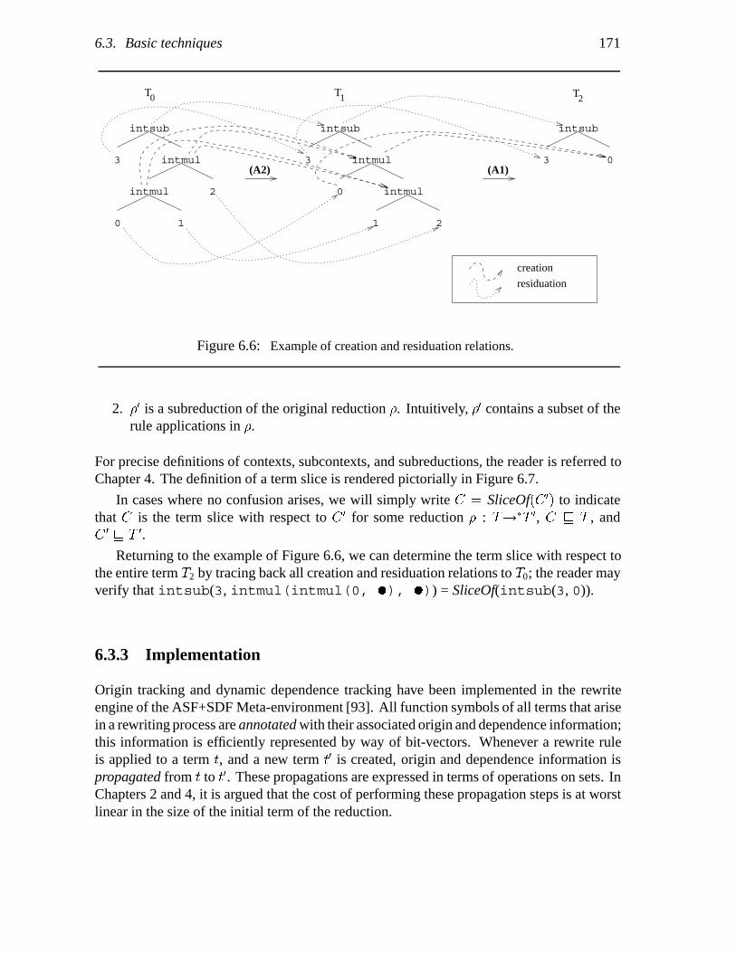
6.3. Basic techniques 171
(A2) (A1)
T1T0 T2
creation
residuation
0
intmul
intmul
intsub intsub
intmul
intmul
intsub
0
3
1
2
3
0
1 2
3
Figure 6.6: Example of creation and residuation relations.
2. �� is a subreduction of the original reduction �. Intuitively, �� contains a subset of therule applications in �.
For precise definitions of contexts, subcontexts, and subreductions, the reader is referred toChapter 4. The definition of a term slice is rendered pictorially in Figure 6.7.
In cases where no confusion arises, we will simply write C � SliceOf�C�� to indicatethat C is the term slice with respect to C � for some reduction � : T��T �, C v T , andC � v T �.
Returning to the example of Figure 6.6, we can determine the term slice with respect tothe entire term T2 by tracing back all creation and residuation relations to T0; the reader mayverify that intsub(3, intmul(intmul(0, �), �)) = SliceOf(intsub(3, 0)).
6.3.3 Implementation
Origin tracking and dynamic dependence tracking have been implemented in the rewriteengine of the ASF+SDF Meta-environment [93]. All function symbols of all terms that arisein a rewriting process are annotated with their associated origin and dependence information;this information is efficiently represented by way of bit-vectors. Whenever a rewrite ruleis applied to a term t, and a new term t� is created, origin and dependence information ispropagated from t to t�. These propagations are expressed in terms of operations on sets. InChapters 2 and 4, it is argued that the cost of performing these propagation steps is at worstlinear in the size of the initial term of the reduction.

172 Chapter 6. Generation of Source-Level Debugging Tools
D�
�
��
C
C
TT �
C �
C �
D�
Figure 6.7: Depiction of the definition of a term slice.
6.4 Definition of debugger features
Below, we describe how a number of debugger features can be defined using the techniques ofthe previous section. We will primarily concentrate on the mechanisms needed for definingdebugger features, and ignore issues related to a debugger’s user-interface.
6.4.1 Single stepping/visualization
Step-wise execution of a program at the source code level is the basic feature of any debugger.Observe that in the specification of Figure 6.2, the execution of a statement corresponds
to the rewriting of a term of the following form:
exec(Stat;StatList, Env)
where Stat represents any statement, StatList any list of statements, and Env any environment.Consequently, the fact that some statement is executed can be detected by matching the abovepattern against the current redex5.
Origin tracking can be used to determine which statement is currently being executed. Weassume that the rewriting process is suspended whenever a redexT matches the above pattern.At this point, the subterm T � of T that is matched against variable Stat is determined. Theorigin ofT �, OriginOf�T ��, will consist of the subtree of the program’s AST that represents thecurrently executed statement. Thus, program execution can be visualized at the source-levelby highlighting this subterm of the AST.
5We will use the term “redex” (short for reducible expression) to denote the subterm that has been matchedagainst some equation. For conditional rules, it is assumed that no conditions have been evaluated yet.

6.4. Definition of debugger features 173
6.4.2 Breakpoints
Another standard feature of source-level debuggers is the breakpoint. The general idea is thatthe user selects a statement s in the program, and execution is continued until this statementis executed.
A breakpoint on a statement s can be implemented as follows. Let Ts be the subterm ofthe AST that corresponds to s. Then the rewriting process should be suspended when: (i)a redex T matches the pattern exec(Stat;StatList, Env) (indicating that some statement isbeing executed), and (ii) Ts � OriginOf�T ��, where T � is the subterm of T matched againstvariable Stat.
6.4.3 State inspection
At any moment that execution is suspended, either while single-stepping or due to a break-point, one may wish to inspect the values of variables or, more generally, arbitrary source-level expressions.
State inspection may be implemented as follows. We assume that execution was sus-pended at the moment that some statement was executed, i.e., a redex T matches the patternexec(Stat;StatList, Env) Let Tz be the subterm of T that was matched against variableEnv. Then an arbitrary source-level expression e (with an AST Te) can be evaluated byrewriting the term eval(Te, Tz) according to the specification of Figure 6.2. The result ofthis rewriting process will be a term representing the “current” value of expression e.
6.4.4 Watchpoints
Watchpoints [133] are a generalization of breakpoints. The user supplies a source-levelexpression e (with AST Te), and execution continues until the value of that expressionchanges.
A watchpoint may be implemented as follows. First, an initial value u (with AST Tu) ofexpression e is computed (using the technique of Section 6.4.3) and stored by the debugger.Whenever a statement is executed, the current value v (with AST Tv) of e is determinedand is compared with u by rewriting a term inteq(Tu, Tv). Execution (i.e., the rewritingprocess) is suspended when this test fails (i.e., yields the value zero).
6.4.5 Data breakpoints
A data breakpoint [139] is yet another variation on the breakpoint theme. A data breakpointon a variable v (with AST Tv) is effective when that variable is referenced (or modified).
Data breakpoints can be implemented by suspending the rewriting process when a redexmatches the pattern lookup(Tv �� Constant;Env, Tv) (for a data breakpoint on a referenceto v), or update(Tv �� Constant;Env, Tv , Constant�) (for a data breakpoint on an update tov).
174 Chapter 6. Generation of Source-Level Debugging Tools
6.4.6 Call stack inspection
In the presence of procedures, the notion of an “environment” needs to be generalized to astack of activation records, where each record contains the values of the local variables andparameters for a procedure call. Call-stack inspection can be defined in way that is similarto the techniques of Section 6.4.3, by visualizing the procedure calls in each record. Onecan easily imagine a tool that allows interactive traversal of the stack of activation records,and enables one to inspect the values of arbitrary source-level expressions in each scope.
6.5 Dynamic program slicing
Myriad variations on the notion of a dynamic program slice [6, 100, 89] can be found inthe literature—see Chapters 3 and 5. For the purposes of this chapter, we define a dynamicslice with respect to the current value of a variable v to be the parts of the program thatare necessary for obtaining the current value of v. To see why dynamic slicing is useful fordebugging, consider a situation where an unintended value is computed for some variablev—only the statements in the dynamic slice with respect to v had an effect on the value ofv. This allows one to ignore many statements in the process of localizing a bug6.
Below we present a two-phase approach for computing dynamic slices. Section 6.5.1discusses the nature of the “raw” information provided by the dynamic dependence relationwe described in Section 6.3.2. In Section 6.5.2, we present an heuristic approach for post-processing this information, in order to obtain dynamic slices similar to those of [6, 100].
6.5.1 Pure term slices
We assume that execution was suspended at a moment that some statement was executed, i.e.,a redex T matches the pattern exec(Stat;StatList,Env). Let Tz be the subterm of T thatwas matched against Env, and let Tp be the subterm of Tz that constitutes the variable-valuepair for variable x. Then, the dynamic dependence relation of Section 6.3.2 will associatewith Tp a minimal set of function symbols, SliceOf�Tp�, in the program’s AST.
Figure 6.8 (a) shows a (textual representation of) the term slice that is determined forthe final value of variable p as obtained by executing the example program of Figure 6.3.Observe that the two holes in this term slice can be replaced by any L-expression withoutaffecting the computation of the value 120 for variable p.
One may wonder why the assignments to variable s are not completely omitted in theterm slice of Figure 6.8 (a). This is best understood by keeping in mind that any hole in aterm slice may be replaced by any syntactically valid L-term. Note that the assignments tos cannot be replaced by any other assignment; e.g., they can certainly not be replaced byany assignment to p. Thus, informally stated, the left-hand sides of the assignments to s arein the slice because they cannot be replaced by assignments to p.
6Even in cases where a statement is missing inadvertently, dynamic slices may provide useful information.In such a case, it is likely that more statements show up in the slice than one would expect.

6.6. Practical experience 175
declarei; s; p;
begini := 5;s := �;p := 1;while i dos := �;p := (p * i);i := (i - 1);
endend
declarei; s; p;
begini := 5;p := 1;while i dop := (p * i);i := (i - 1);
end;end
(a) (b)
Figure 6.8: (a) Term slice with respect to the final value of p. (b) Post-processed slice withrespect to the final value of p.
[P1] Var := � = �
[P2] �;StatSeq = StatSeq
Figure 6.9: Specification for post-processing of term slices.
6.5.2 Post-processing of term slices
While term slices provide information that is semantically sound, they may contain a cer-tain amount of “clutter”, in the form of uninteresting information. An example of suchinformation are the two partial assignments to variable s in the term slice of Figure 6.8 (a).
In order obtain dynamic slices similar to those in [6, 100], one may post-process termslices by: (i) transforming any statement whose right-hand side is irrelevant into an irrelevantstatement (rule [P1]), and (ii) removing irrelevant statements from statement lists (rule [P2]).A specification of this post-processing is shown in Figure 6.9. Rewriting the term slice ofFigure 6.8 (a) according to this specification yields the slice of Figure 6.8 (b).
The specification of Figure 6.9 is minimal—it only removes irrelevant assignments. Inpractice, one would like more sophisticated post-processing that, for example, removes allirrelevant declarations from the program. Post-processing becomes nontrivial in the presenceof procedures, where situations may occur in which different parameters are omitted atdifferent call sites.
6.6 Practical experience
To a large extent, the ideas in this chapter have been implemented using the ASF+SDF Meta-environment [93], a programming environment generator. In particular, origin tracking,

176 Chapter 6. Generation of Source-Level Debugging Tools
(a) (b)
(c) (d)
Figure 6.10: Generated language-specific single-stepping tool.
dynamic dependence tracking, and the matching of language-specific patterns have beenimplemented successfully.
Figure 6.10 shows a snapshots of a language-specific single-stepping tool for the languageCLaX [49, 134], a substantial subset of Pascal that features procedures with nested scopes,unstructured control flow, and multi-dimensional arrays. This tool has been implementedaccording to the techniques of Section 6.4.1.
Figure 6.11 shows a screen dump of a dynamic slicing tool for the language CLaX, thatwas created using the technique of Section 6.5. In this figure, the dynamic slice with respectto the final value of variable ‘product’ is shown, both in pure “term slice” form (here, ‘�?�’indicates a missing subterm), and in post-processed form.
6.7 Related work
The work that is most closely related to ours was done in the context of the PSG system[11]. A generator for language-specific debuggers was described in [10]. Language-specificcompilers are generated by compiling denotational semantics definitions to a functional
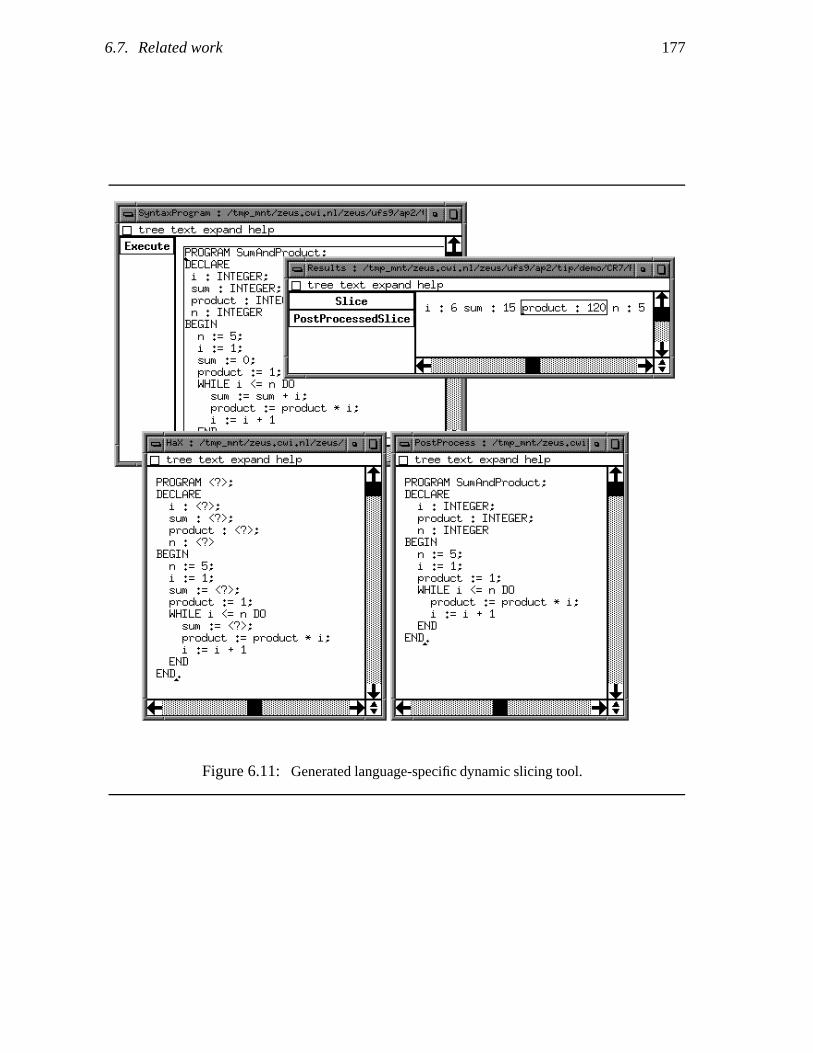
6.7. Related work 177
Figure 6.11: Generated language-specific dynamic slicing tool.

178 Chapter 6. Generation of Source-Level Debugging Tools
language. A standard, language-independent interpreter is used to execute the generatedfunctional language fragments. The behavior of a debugger is specified using a set of built-in debugging concepts. In particular, trace functions are provided for the visualization ofexecution. Other notions enable one to inspect the state of the interpreter, and to definebreakpoints.
Bahlke et al. write that “correspondences between the abstract syntax tree and theterms of the functional language are established in both directions”. These correspondencesare used to determine a language-specific notion of a step. However, the nature of these“correspondences” is not described, making it impossible to conclude how powerful thesecorrespondences are, or what constraints on specifications they imply7. By contrast, ourmethod for keeping track of correspondences, origin tracking (see Chapter 2, is well-defined,and has proven to be sufficiently powerful for realistic languages [134].
A second difference between the work by Bahlke et al. is the information that is usedto define debugger features. In our approach, debugger features are defined in terms ofspecification-level patterns in conjunction with language-independent origin information.That is, the specification of the interpreter and the specification of debugger features areuniform. It is unclear to what extent the debugging concepts of [10] are similar to theinterpreter’s specification.
Finally, Bahlke et al. do not consider more advanced debugger features such as watch-points, data breakpoints, and dynamic slices.
Bertot [26] contributes a technique called subject tracking to the specification languageTypol [85, 41], for animation and debugging purposes. A key property of Typol specificationsis that the meaning of a language construct is expressed in terms of its sub-constructs. Aspecial variable, Subject, serves to indicate the language construct currently processed.This variable may be manipulated by the specification writer when different animation ordebugging behavior is required.
Bertot does not consider other debugger features besides single-stepping, animation, andsimple breakpoints.
Berry [25] presents an approach where animators are generated from structured opera-tional semantics definitions. These specifications are augmented with semantic display rulesthat determine how to perform animation when a particular semantic rule is being processed.Various views of the execution of a program can be obtained by defining the appropriatedisplay rules. Static views consist of parts of the abstract syntax tree of a program, anddynamic views are constructed from the program state during execution. As an example ofa dynamic view, the evaluation of a control predicate may be visualized as the actual truthvalue it obtains during execution.
Although Berry considers highly sophisticated animation features, he does not considerdebugger features such as breakpoints and dynamic program slices.
7The subset of Pascal that is considered in [10] does not contain goto statements. It is unclear whatcomplications these statements would cause.

6.8. Conclusions and future work 179
6.8 Conclusions and future work
We have presented a generic approach for deriving debugging and dynamic program slicingtools from algebraic specifications. The main conclusion of this chapter is that the informa-tion needed for implementing such tools is to a very large extent language-independent andimplicitly present in the language’s specification. The three “building blocks” we used todefine debugger features are:
1. matching of patterns,2. rewriting of terms, and3. computation of origin/dependence information.
The first two items consist of functionality that is, at least in principle, already provided byany rewriting engine. As was described in Section 6.3, the information used in the third itemcan be computed automatically, as a side-effect of rewriting.
The only additional language-dependent information that is required to define debuggingand slicing features consists of the specification of a set of language-specific patterns, andthe actions that should be performed when a match with such a pattern occurs.
The emphasis of this chapter has been on generic techniques for constructing debuggingtools; we have ignored all aspects that have to do with user-interfacing. In the future, we planto develop a formalism in which one can specify such tools together with their user-interfaces.


Chapter 7
Conclusions
7.1 Summary
We have presented an approach to generating program analysis tools from formal specifi-cations. In particular, the generation of tools for source-level debugging and for computingvarious types of program slices has been addressed in detail. We have discussed how suchtools can be of practical use for software maintenance, reverse engineering, and various otherapplications.
Instead of “directly” implementing program analysis tools, we require that a language’ssemantics be formally specified by way of an executable algebraic specification. This permitsus to view the execution of a program as a term rewriting process, or, more abstractly, asa sequence of terms. Two generic, specification-level techniques serve as the cornerstonesof our approach for constructing program analysis tools: origin tracking and dynamicdependence tracking. Origin tracking establishes relations between recurrences of certainterms that occur in a rewriting process, and is used to formalize the notion of a “currentlocus” of program execution. Dynamic dependence tracking establishes certain dependencerelations between terms that occur in a rewriting process, and is used to compute variousnotions of program slices. A crucial property of these techniques is the fact that:
All information needed for computing origin relations and dynamic dependencerelations is implicitly present in the specification of the language’s semantics.
Moreover, these relations can be computed automatically and efficiently, as a side-effect ofterm rewriting.
Once origin and dynamic dependence relations have been computed, only a very smallamount of additional language-specific information is needed to construct program analysistools. This information mainly consists of a small set of language-specific patterns andassociated actions. We have argued that the specification of these patterns and actions isvery similar to the specification of the language’s semantics itself, and therefore easy towrite.
Some prototypes of program analysis tools have been generated according to our tech-niques using the ASF+SDF Meta-environment, a programming environment generator [93].
181

182 Chapter 7. Conclusions
7.2 Main results
The main results of this thesis can be summarized as follows:
� We have presented a generic approach to generating program analysis tools that re-quires very little language-specific information other than a specification of a lan-guage’s semantics, and the language-independent origin and dynamic dependencerelations implicitly defined by that specification.Moreover, the additional information needed for constructing program analysis toolscan be regarded as an extension to the language’s specification (which itself may havebeen developed previously).
� The method for program slicing presented in Chapter 5 subsumes the traditional notionsof static and dynamic program slicing, by allowing arbitrary sets of constraints on theinputs of a program. The precision of the (static) slices computed according to ourapproach compares favorably to that of previous slicing methods.
� We have conducted several experiments with automatically generated program analysistools. Although current performance is rather poor (especially for programs over 50lines), this is mainly due to a combination of two factors:
1. The use of an interpreted term rewriting engine, and2. The fact that origin tracking and dynamic dependence tracking slow down exe-
cution (i.e., the term rewriting process) by a factor proportional to the size of theinitial term.
Current work on compiling specifications to efficient C code [92] is expected toovercome the first problem.Another effort towards greater efficiency is an efficient ML implementation of theslicing approach of Chapter 5 that is currently being developed at the IBM T.J. WatsonResearch Center.
The main contribution of this dissertation has been to explore semantic notions behindprogram slicing and debugging operations. One might justifiably remark that interpretersbased on term rewriting are bound to be much slower than interpreters that are constructedby other means. However, given the recent advances in (rewriting) technology discussedabove and the fact that efficiency is not the primary raison d’etre of interpreters to beginwith, we are mildly optimistic about the practicality of the work presented in this thesis.
7.3 Future work
We foresee a number of directions for extending and applying the work in this thesis:
� For certain applications, (e.g., determining positions of type-errors for type-checkers),different or stronger origin relations are desired [49, 48, 45, 43]. This is an area ofresearch where much work remains to be done.
� Although defined in different ways, the origin relation and the dynamic dependencerelation clearly have many similarities. A more systematic comparison of these

7.3. Future work 183
relations is required. We believe that a potential outcome of such a comparison couldconsist of a generic framework for specifying origin-like relations. One could imaginethat, in such a framework, the origin relation is parameterized with a function definingthe type of relations to be established, and that its properties are expressed in terms ofthis parameter.
� An issue related to the previous one is the fact that the origin relation and the dynamicdependence relation both rely on the combination of a notion of residuation [78] with“other information”. In the case of origin tracking, the latter consists of the relationsbetween redex and contractum, and between common subterms. For dependencetracking, it consists of a notion of “creation”. We conjecture that it should be possibleto redefine origin tracking and dependence tracking in a more consistent way, asrelations that have a “residuation” subrelation in common.
� The dynamic dependence relation defined in Chapter 4 may produce slightly non-optimal results in the presence of left-nonlinear rewriting rules. Although this non-optimality does not seem to pose any problems in practice, we are currently investigat-ing whether an approach based on graph rewriting (see, e.g., [17]) would yield moreaccurate results.
� The dynamic dependence relation is in certain respects similar to the informationthat is used by Field [54, 56] for the purpose of incremental rewriting. It would beinteresting to determine exactly how these different concepts are related.
� We intend to experiment with the application of dynamic dependence tracking to spec-ifications of the static semantics of a language (i.e., specifications of type-checkers).In principle, this would yield a “reduced” program that contains the same type-errors,but excludes all type-correct constructs.
� As was discussed earlier, the information needed for generating language-specificprogram analysis tools is to a very large extent language-independent. However, asmall part of this information (e.g., the patterns and associated actions in Chapter 6)is language-dependent.A logical continuation of the work in this thesis would be the development of a formal-ism/language to express this language-specific information. Ideally, this formalismwould also allow the description of the user-interface of the generated tools. The workby Koorn [96, 97] may be a good starting-point.
� In our current implementation, origin tracking and dynamic dependence tracking areimplemented by way of a modification of the ASF+SDF system’s rewrite engine. Inorder to gain performance, current work in this area includes a compiler of ASF+SDFspecifications to efficient stand-alone C programs [92]. Rather than re-implementingorigin tracking and dynamic dependence tracking in this new setting, it would be inter-esting to compute these relations by way of a systematic transformation on algebraicspecifications.Some experiments in this area have been performed, but were unsuccessful due tothe inefficient implementation of low-level set operations by way of “pure” rewriting.We conclude that an escape-mechanism (such as the hybrid specifications of [140]) isneeded to compute these operations more efficiently.
184 Chapter 7. Conclusions
� In this dissertation, we have mainly explored program slicing for purposes of programanalysis and program understanding. It would be interesting to investigate whetherslicing can be of use for program restructuring as well. The work by Griswold andNotkin [64, 63], who pursue a PDG-based method for program restructuring, may berelevant in this respect.
Appendix A
PIM details
In this appendix, we briefly review the PIM term structure and the most important subsets ofPIM rules. Additional rules used primarily for performing induction are described in [55];these rules are the foundation for the loop analysis rules presented in Section 5.5. In general,PIM is augmented with rules defining the semantics of language-specific data types such asintegers.
PIM terms are constructed over an order-sorted signature. PIM sorts distinguish amongfundamentally incompatible syntactic structures corresponding to observable values, mergestructures, store structures, and lambda expressions; however, sorts should not be interpretedas types in the usual sense.
A.1 PIM� rules
The rules of PIM�t are given in Figure A.1. Variables v, m, s, and f will be used in the rules
to refer to observable values, merge structures, store structures, and lambda-expressions,respectively. Equations (L1)–(L8) are generic to merge or store structures. Thus, each ofthe operators labeled � is to be interpreted as one of s or m. (E1) and (E2) are schemes foran infinite set of equations. Equation (C1) only applies if the argument of ‘S���’ is of sort S.The rules of PIM� consist of those of PIM�
t , along with the rules depicted in Figure 5.11.
A.2 PIM=t equations
The rules of PIM=t are those of PIM�
t along with those given in Figure A.2. As before, � inrules (L9)–(L11) is assumed to be one of m or s. In rule (M9), CV # $ denotes an arbitrarystrict context of value sort; this rule could also be less perspicuously rendered as a family ofrules, one for each value-sorted function symbol.
185
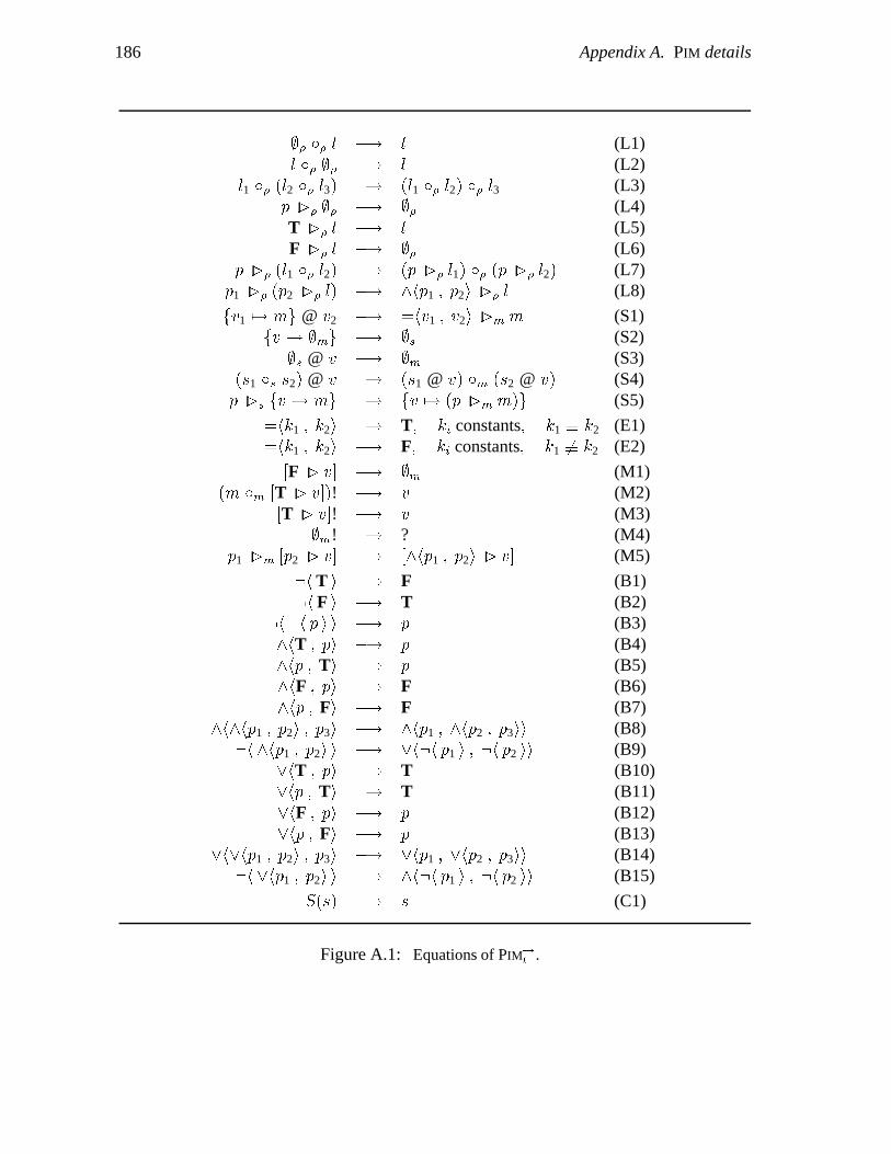
186 Appendix A. PIM details
�� � l �� l (L1)l � �� �� l (L2)
l1 � �l2 � l3� �� �l1 � l2� � l3 (L3)p �� �� �� �� (L4)T �� l �� l (L5)F �� l �� �� (L6)
p �� �l1 � l2� �� �p �� l1� � �p �� l2� (L7)p1 �� �p2 �� l� �� �hp1 � p2i �� l (L8)
fv1 �� mg @ v2 �� �hv1 � v2i �m m (S1)fv �� �mg �� �s (S2)
�s @ v �� �m (S3)�s1 s s2� @ v �� �s1 @ v� m �s2 @ v� (S4)p �s fv �� mg �� fv �� �p �m m�g (S5)
�hk1 � k2i �� T� ki constants� k1 � k2 (E1)�hk1 � k2i �� F� ki constants� k1 � k2 (E2)
#F � v$ �� �m (M1)�m m #T � v$�! �� v (M2)
#T � v$! �� v (M3)�m! �� ? (M4)
p1 �m #p2 � v$ �� #�hp1 � p2i � v$ (M5)
"hT i �� F (B1)"hF i �� T (B2)
"h"h p i i �� p (B3)�hT � pi �� p (B4)�hp � Ti �� p (B5)�hF � pi �� F (B6)�hp � Fi �� F (B7)
�h�hp1 � p2i � p3i �� �hp1 � �hp2 � p3ii (B8)"h�hp1 � p2i i �� �h"h p1 i � "h p2 ii (B9)
�hT � pi �� T (B10)�hp � Ti �� T (B11)�hF � pi �� p (B12)�hp � Fi �� p (B13)
�h�hp1 � p2i � p3i �� �hp1 � �hp2 � p3ii (B14)"h�hp1 � p2i i �� �h"h p1 i � "h p2 ii (B15)
S�s� �� s (C1)
Figure A.1: Equations of PIM�t .

A.2. PIM=t equations 187
�hv � vi � T (E3)
l2 � l1 � l2 � l1 � l2 (L9)
�hp1 � p2i � F�p1 �� l1� � �p2 �� l2���p2 �� l2� � �p1 �� l1� (L10)
�p1 �� l� � �p2 �� l� � ��hp1 � p2i� �� l (L11)
fv �� m1g s fv �� m2g � fv �� �m1 m m2�g (S6)�hv1 � v2i � F
fv1 �� m1g s fv2 �� m2g�fv2 �� m2g s fv1 �� m1g (S7)
�"h p i �m m1 mm2 m #p � v$ �m1 m m2 m #p � v$ (M6)
#p �m!$ � #p � ?$ m �p �m m� (M7)�#T � ?$ m m�! �m! (M8)
CV # m! $ � �m n ��xV�CV # xV $�� !�xV � FV �CV# $� (M9)
�m1 m m2� n f � �m1 n f� m �m2 n f� (M10)#p � v$ n f � #p � �f v�$ (M11)
�m n f � �m (M12)�p �m m� n f � p �m �m n f� (M13)�m n�x�v� n f �m n�x�fv (M14)
�hp1 � p2i � �hp2 � p1i (B16)�hp � pi � p (B17)
�hp � "h p ii � F (B18)�hp1 � p2i � �hp2 � p1i (B19)�hp � pi � p (B20)
�hp � "h p ii � T (B21)�hp1 � �hp2 � p3ii � �h�hp1 � p2i � �hp1 � p3ii (B22)�hp1 � �hp2 � p3ii � �h�hp1 � p2i � �hp1 � p3ii (B23)#p � ��hp � qi�$ � #p � q$ (B24)
Figure A.2: Additional equations of PIM=t .


Bibliography
[1] ACETO, L., BLOOM, B., AND VAANDRAGER, F. Turning SOS rules into equations. In Proc. IEEE Symp.on Logic in Computer Science (Santa Cruz, CA, 1992), pp. 113–124.
[2] AGRAWAL, H. Towards automatic debugging of Computer Programs. PhD thesis, Purdue University,1991.
[3] AGRAWAL, H. On slicing programs with jump statements. In Proceedings of the ACM SIGPLAN’94Conference on Programming Language Design and Implementation (Orlando, Florida, 1994), pp. 302–312. SIGPLAN Notices 29(6).
[4] AGRAWAL, H., DEMILLO, R., AND SPAFFORD, E. Dynamic slicing in the presence of unconstrainedpointers. In Proceedings of the ACM Fourth Symposium on Testing, Analysis, and Verification (TAV4)(1991), pp. 60–73. Also Purdue University technical report SERC-TR-93-P.
[5] AGRAWAL, H., DEMILLO, R., AND SPAFFORD, E. Debugging with dynamic slicing and backtracking.Software—Practice and Experience 23, 6 (1993), 589–616.
[6] AGRAWAL, H., AND HORGAN, J. Dynamic program slicing. In Proceedings of the ACM SIGPLAN’90Conference on Programming Language Design and Implementation (1990), pp. 246–256. SIGPLANNotices 25(6).
[7] AHO, A., SETHI, R., AND ULLMAN, J. Compilers. Principles, Techniques and Tools. Addison-Wesley,1986.
[8] ALPERN, B., WEGMAN, M., AND ZADECK, F. Detecting equality of variables in programs. In ConferenceRecord of the Fifteenth ACM Symposium on Principles of Programming Languages (San Diego, 1988),pp. 1–11.
[9] ALT, M., ASSMANN, U., AND VAN SOMEREN, H. Cosy compiler phase embedding with the cosy compilermodel. In Compiler Construction ’94 (1994), P. A. Fritzson, Ed., vol. 786 of LNCS, Springer-Verlag,pp. 278–293.
[10] BAHLKE, R., MORITZ, B., AND SNELTING, G. A generator of language-specific debugging systems. InProceedings of the ACM SIGPLAN’87 Symposium on Interpreters and Interpretive Techniques (1987),pp. 92–101. SIGPLAN Notices 22(7).
[11] BAHLKE, R., AND SNELTING, G. The PSG system: from formal language definitions to interactiveprogramming environments. ACM Transactions on Programming Languages and Systems 8, 4 (1986),547–576.
189
190 Bibliography
[12] BALL, T. The Use of Control-Flow and Control Dependence in Software Tools. PhD thesis, Universityof Wisconsin-Madison, 1993.
[13] BALL, T., AND HORWITZ, S. Slicing programs with arbitrary control-flow. In Proceedings of the FirstInternational Workshop on Automated and Algorithmic Debugging (1993), P. Fritzson, Ed., vol. 749 ofLecture Notes in Computer Science, Springer-Verlag, pp. 206–222.
[14] BALLANCE, R. A., MACCABE, A. B., AND OTTENSTEIN, K. J. The program dependence Web: Arepresentation supporting control-, data-, and demand-driven interpretation of imperative languages.In Proc. ACM SIGPLAN Conference on Programming Language Design and Implementation (WhitePlains, NY, 1990), pp. 257–271.
[15] BALZER, R. EXDAMS - Extendable Debugging And Monitoring System. In Proceedings of the AFIPSSJCC (1969), vol. 34, pp. 567–586.
[16] BANNING, J. An efficient way to find the side effects of procedure calls and the aliases of variables.In Conference Record of the Sixth ACM Symposium on Principles of Programming Languages (1979),pp. 29–41.
[17] BARENDREGT, H., VAN EEKELEN, M., GLAUERT, J., KENNAWAY, J., PLASMEIJER, M., AND SLEEP, M. Termgraph rewriting. In Proc. PARLE Conference, Vol. II: Parallel Languages (Eindhoven, The Netherlands,1987), vol. 259 of Lecture Notes in Computer Science, Springer-Verlag, pp. 141–158.
[18] BARNES, J. Programming in Ada, second ed. International Computer Science Series. Addison-Wesley,1982.
[19] BARTH, J. A practical interprocedural data flow analysis algorithm. Communications of the ACM 21, 9(1978), 724–736.
[20] BATES, S., AND HORWITZ, S. Incremental program testing using program dependence graphs. In Confer-ence Record of the Twentieth ACM Symposium on Principles of Programming Languages (Charleston,SC, 1993), pp. 384–396.
[21] BECK, J., AND EICHMANN, D. Program and interface slicing for reverse engineering. In Proceedings ofthe 15th International Conference on Software Engineering (Baltimore, 1993).
[22] BERGERETTI, J.-F., AND CARRE, B. Information-flow and data-flow analysis of while-programs. ACMTransactions on Programming Languages and Systems 7, 1 (1985), 37–61.
[23] BERGSTRA, J., HEERING, J., AND KLINT, P., Eds. Algebraic Specification. ACM Press Frontier Series.The ACM Press in co-operation with Addison-Wesley, 1989.
[24] BERGSTRA, J., AND KLOP, J. Conditional rewrite rules: confluence and termination. Journal of Computerand System Sciences 32, 3 (1986), 323–362.
[25] BERRY, D. Generating Program Animators from Programming Language Semantics. PhD thesis,University of Edinburgh, 1991.
[26] BERTOT, Y. Occurrences in debugger specifications. In Proceedings of the ACM SIGPLAN’91 Conferenceon Programming Language Design and Implementation (1991), pp. 327–337. SIGPLAN Notices 26(6).
[27] BERTOT, Y. Une Automatisation du Calcul des Residus en Semantique Naturelle. PhD thesis, INRIA,Sophia-Antipolis, 1991. In French.
[28] BERTOT, Y. Origin functions in lambda-calculus and term rewriting systems. In Proceedings of the 17thColloquium on Trees in Algebra and Programming (CAAP ’92) (1992), J.-C. Raoult, Ed., vol. 581 ofLNCS, Springer-Verlag.
[29] BINKLEY, D. Using semantic differencing to reduce the cost of regression testing. In Proceedings of theIEEE Conference on Software Maintenance (Orlando, Florida, November 1992).

Bibliography 191
[30] BINKLEY, D. Precise executable interprocedural slices. ACM Letters on Programming Languages andSystems 2, 1–4 (1993), 31–45.
[31] BINKLEY, D. Slicing in the presence of parameter aliasing. In Proceedings of the Third SoftwareEngineering Research Forum (Orlando, Florida, November 1993), pp. 261–268.
[32] BINKLEY, D. Interprocedural constant propagation using dependence graphs and a data-flow model. InProceedings of the 5th International Conference on Compiler Construction—CC’94 (Edinburgh, UK,1994), P. Fritzson, Ed., vol. 786 of LNCS, pp. 374–388.
[33] BINKLEY, D., HORWITZ, S., AND REPS, T. Program integration for languages with procedure calls, 1994.Submitted for publication.
[34] CARTWRIGHT, R., AND FELLEISEN, M. The semantics of program dependence. In Proceedings ofthe ACM 1989 Conference on Programming Language Design and Implementation (Portland, Oregon,1989), pp. 13–27.
[35] CHENG, J. Slicing concurrent programs – a graph-theoretical approach. In Proceedings of the FirstInternational Workshop on Automated and Algorithmic Debugging (1993), P. Fritzson, Ed., vol. 749 ofLecture Notes in Computer Science, Springer-Verlag, pp. 223–240.
[36] CHOI, J.-D., BURKE, M., AND CARINI, P. Efficient flow-sensitive interprocedural computation of pointer-induced aliases and side effects. In Conference Record of the Twentieth ACM Symposium on Principlesof Programming Languages (1993), ACM, pp. 232–245.
[37] CHOI, J.-D., AND FERRANTE, J. Static slicing in the presence of goto statements. ACM Transactions onProgramming Languages and Systems 16, 4 (July 1994), 1097–1113.
[38] CHOI, J.-D., MILLER, B., AND NETZER, R. Techniques for debugging parallel programs with flowbackanalysis. ACM Transactions on Programming Languages and Systems 13, 4 (1991), 491–530.
[39] COOPER, K., AND KENNEDY, K. Interprocedural side-effect analysis in linear time. In Proceedings ofthe ACM SIGPLAN’88 Conference on Programming Language Design and Implementation (Atlanta,Georgia, 1988), pp. 57–66. SIGPLAN Notices 23(7).
[40] CYTRON, R., FERRANTE, J., ROSEN, B. K., AND WEGMAN, M. N. Efficiently computing static singleassignment form and the control dependence graph. ACM Transactions on Programming Languagesand Systems 13, 4 (1991), 451–490.
[41] DESPEYROUX, T. Typol: a formalism to implement natural semantics. Tech. Rep. 94, INRIA, 1988.
[42] DEURSEN, A. V. An algebraic specification for the static semantics of Pascal. Report CS-R9129, Centrumvoor Wiskunde en Informatica (CWI), Amsterdam, 1991.
[43] DEURSEN, A. V. Executable Language Definitions—Case Studies and Origin Tracking Techniques. PhDthesis, University of Amsterdam, 1994.
[44] DEURSEN, A. V. Origin tracking in primitive recursive schemes. Report CS-R9401, Centrum voorWiskunde en Informatica (CWI), 1994.
[45] DEURSEN, A. V., AND DINESH, T. Origin tracking for higher-order term rewriting systems. In Proceedingsof the International Workshop on Higher-Order Algebra, Logic and Term Rewriting (Amsterdam,September 1993), J. Heering, K. Meinke, B. Moller, and T. Nipkow, Eds., vol. 816 of LNCS.
[46] DEURSEN, A. V., KLINT, P., AND TIP, F. Origin tracking. Report CS-R9230, Centrum voor Wiskunde enInformatica (CWI), Amsterdam, 1992.
[47] DEURSEN, A. V., KLINT, P., AND TIP, F. Origin tracking. Journal of Symbolic Computation 15 (1993),523–545.

192 Bibliography
[48] DINESH, T. Type checking revisited: Modular error handling. In International Workshop on Semanticsof Specification Languages (1993).
[49] DINESH, T., AND TIP, F. Animators and error reporters for generated programming environments. ReportCS-R9253, Centrum voor Wiskunde en Informatica (CWI), Amsterdam, 1992.
[50] DUESTERWALD, E., GUPTA, R., AND SOFFA, M. Distributed slicing and partial re-execution for distributedprograms. In Proceedings of the fifth workshop on Languages and Compilers for Parallel Computing(New Haven, Connecticut, 1992), pp. 329–337.
[51] DUESTERWALD, E., GUPTA, R., AND SOFFA, M. Rigorous data flow testing through output influences. InProceedings of the Second Irvine Software Symposium ISS’92 (California, 1992), pp. 131–145.
[52] ERNST, M. Practical fine-grained static slicing of optimized code. Tech. Rep. MSR-TR-94-14, MicrosoftResearch, Redmond, WA, 1994.
[53] FERRANTE, J., OTTENSTEIN, K., AND WARREN, J. The program dependence graph and its use inoptimization. ACM Transactions on Programming Languages and Systems 9, 3 (1987), 319–349.
[54] FIELD, J. On laziness and optimality in lambda interpreters: Tools for specification and analysis.In Proceedings of the Seventeenth ACM Symposium on Principles of Programming Languages (SanFrancisco, 1990), pp. 1–15.
[55] FIELD, J. A simple rewriting semantics for realistic imperative programs and its application to programanalysis. In Proceedings of the ACM SIGPLAN Workshop on Partial Evaluation and Semantics-Based Program Manipulation (1992), pp. 98–107. Published as Yale University Technical ReportYALEU/DCS/RR–909.
[56] FIELD, J. A graph reduction approach to incremental rewriting. In Proceedings of the 5th InternationalConference on Rewriting Techniques and Applications (1993), C. Kirchner, Ed., vol. 690 of LNCS,pp. 259–273.
[57] FIELD, J., RAMALINGAM, G., AND TIP, F. Parametric program slicing. In Conference Record of theTwenty-Second ACM Symposium on Principles of Programming Languages (San Francisco, CA, 1995).To appear.
[58] FIELD, J., AND TIP, F. Dynamic dependence in term rewriting systems and its application to programslicing. In Proceedings of the Sixth International Symposium on Programming Language Implementationand Logic Programming (1994), M. Hermenegildo and J. Penjam, Eds., vol. 844, Springer-Verlag,pp. 415–431.
[59] FRITZSON, P., SHAHMEHRI, N., KAMKAR, M., AND GYIMOTHY, T. Generalized algorithmic debuggingand testing. ACM Letters on Programming Languages and Systems 1, 4 (1992), 303–322.
[60] GALLAGHER, K. Using Program Slicing in Software Maintenance. PhD thesis, University of Maryland,1989.
[61] GALLAGHER, K., AND LYLE, J. Using program slicing in software maintenance. IEEE Transactions onSoftware Engineering 17, 8 (1991), 751–761.
[62] GOPAL, R. Dynamic program slicing based on dependence relations. In Proceedings of the Conferenceon Software Maintenance (1991), pp. 191–200.
[63] GRISWOLD, W. G. Direct update of dataflow representations for a meaning-preserving program re-structuring tool. In Proceedings of the ACM SIGSOFT ’93 Symposium on the Foundations of SoftwareEngineering (December 1993), pp. 42–55.
[64] GRISWOLD, W. G., AND NOTKIN, D. Automated assistance for program restructuring. ACM Transactionson Software Engineering and Methodology 2, 3 (July 1993), 228–269.
Bibliography 193
[65] GUPTA, R., HARROLD, M., AND SOFFA, M. An approach to regression testing using slicing. InProceedings of the Conference on Software Maintenance (1992), pp. 299–308.
[66] GUPTA, R., AND SOFFA, M. A framework for generalized slicing. Technical report TR-92-07, Universityof Pittsburgh, 1992.
[67] HAUSLER, P. Denotational program slicing. In Proceedings of the 22nd Hawaii International Conferenceon System Sciences (Hawaii, 1989), pp. 486–494.
[68] HEERING, J., HENDRIKS, P., KLINT, P., AND REKERS, J. The syntax definition formalism SDF - referencemanual. SIGPLAN Notices 24, 11 (1989), 43–75.
[69] HENDRIKS, P. Implementation of Modular Algebraic Specifications. PhD thesis, University of Amster-dam, 1991.
[70] HORWITZ, S. Identifying the semantic and textual differences between two versions of a program. In Pro-ceedings of the ACM SIGPLAN’90 Conference on Programming Language Design and Implementation(White Plains, New York, 1990), pp. 234–245. SIGPLAN Notices 25(6).
[71] HORWITZ, S., PFEIFFER, P., AND REPS, T. Dependence analysis for pointer variables. In Proceedings ofthe ACM 1989 Conference on Programming Language Design and Implementation (Portland, Oregon,1989). SIGPLAN Notices 24(7).
[72] HORWITZ, S., PRINS, J., AND REPS, T. Integrating non-interfering versions of programs. In ConferenceRecord of the ACM SIGSOFT/SIGPLAN Symposium on Principles of Programming Languages (1988),pp. 133–145.
[73] HORWITZ, S., PRINS, J., AND REPS, T. On the adequacy of program dependence graphs for representingprograms. In Conference Record of the Fifteenth Annual ACM Symposium on Principles of ProgrammingLanguages (1988), ACM, pp. 146–157.
[74] HORWITZ, S., PRINS, J., AND REPS, T. Integrating noninterfering versions of programs.ACM Transactionson Programming Languages and Systems 11, 3 (1989), 345–387.
[75] HORWITZ, S., AND REPS, T. Efficient comparison of program slices. Acta Informatica 28 (1991),713–732.
[76] HORWITZ, S., AND REPS, T. The use of program dependence graphs in software engineering. InProceedings of the 14th International Conference on Software Engineering (Melbourne, Australia,1992), pp. 392–411.
[77] HORWITZ, S., REPS, T., AND BINKLEY, D. Interprocedural slicing using dependence graphs. ACMTransactions on Programming Languages and Systems 12, 1 (1990), 26–61.
[78] HUET, G., AND LEVY, J.-J. Computations in orthogonal rewriting systems part I and II. In ComputationalLogic; essays in honour of Alan Robinson, J.-L. Lassez and G. Plotkin, Eds. MIT Press, 1991, pp. 395–443.
[79] HWANG, J., DU, M., AND CHOU, C. Finding program slices for recursive procedures. In Proceedings ofthe 12th Annual International Computer Software and Applications Conference (Chicago, 1988).
[80] HWANG, J., DU, M., AND CHOU, C. The influence of language semantics on program slices. InProceedings of the 1988 International Conference on Computer Languages (Miami Beach, 1988).
[81] JACKSON, D., AND ROLLINS, E. J. Abstraction mechanisms for pictorial slicing. In Proceedings of theIEEE Workshop on Program Comprehension (Washington, November 1994).
[82] JACKSON, D., AND ROLLINS, E. J. A new model of program dependences for reverse engineering. InProceedings of the Second ACM SIGSOFT Conference on Foundations of Software Engineering (NewOrleans, LA, December 1994).
194 Bibliography
[83] JIANG, J., ZHOU, X., AND ROBSON, D. Program slicing for C - the problems in implementation. InProceedings of the Conference on Software Maintenance (1991), pp. 182–190.
[84] JOHNSON, R., PEARSON, D., AND PINGALI, K. The program structure tree: Computing control regionsin linear time. In Proceedings of the ACM SIGPLAN’94 Conference on Programming Language Designand Implementation (Orlando, Florida, 1994), pp. 171–185. SIGPLAN Notices 29(6).
[85] KAHN, G. Natural semantics. In Fourth Annual Symposium on Theoretical Aspects of Computer Science(1987), F. Brandenburg, G. Vidal-Naquet, and M. Wirsing, Eds., vol. 247 of LNCS, Springer-Verlag,pp. 22–39.
[86] KAMKAR, M. An overview and comparative classification of static and dynamic program slicing.Technical Report LiTH-IDA-R-91-19, Linkoping University, Linkoping, 1991. To appear in Journal ofSystems and Software.
[87] KAMKAR, M. Interprocedural Dynamic Slicing with Applications to Debugging and Testing. PhD thesis,Linkoping University, 1993.
[88] KAMKAR, M., FRITZSON, P., AND SHAHMEHRI, N. Interprocedural dynamic slicing applied to inter-procedural data flow testing. In Proceedings of the Conference on Software Maintenance (Montreal,Canada, 1993), pp. 386–395.
[89] KAMKAR, M., FRITZSON, P., AND SHAHMEHRI, N. Three approaches to interprocedural dynamic slicing.Microprocessing and Microprogramming 38 (1993), 625–636.
[90] KAMKAR, M., SHAHMEHRI, N., AND FRITZSON, P. Interprocedural dynamic slicing and its applicationto generalized algorithmic debugging. In Proceedings of the International Conference on ProgrammingLanguage Implementation and Logic Programming, PLILP ’92 (1992).
[91] KAMPERMAN, J., DINESH, T., AND WALTERS, H. An extensible language for the generation of paralleldata manipulation and control packages. In Proceedings of the Poster Session of Compiler Construction’94 (1994), P. Fritzson, Ed. Appeared as technical report LiTH-IDA-R-94-11, Linkoping University.
[92] KAMPERMAN, J., AND WALTERS, H. ARM – Abstract Rewriting Machine. In Computing Science in theNetherlands (1993), H. Wijshoff, Ed. Also appeared as CWI report CS-R9330.
[93] KLINT, P. A meta-environment for generating programming environments. ACM Transactions onSoftware Engineering and Methodology 2, 2 (1993), 176–201.
[94] KLOP, J. Term rewriting systems. Report CS-R9073, Centrum voor Wiskunde en Informatica (CWI),Amsterdam, 1990.
[95] KLOP, J. Term rewriting systems. In Handbook of Logic in Computer Science, Volume 2. Background:Computational Structures, S. Abramsky, D. Gabbay, and T. Maibaum, Eds. Oxford University Press,1992, pp. 1–116.
[96] KOORN, J. Connecting semantic tools to a syntax-directed user-interface. Report P9222, ProgrammingResearch Group, University of Amsterdam, 1992.
[97] KOORN, J. Generating uniform user-interfaces for interactive programming environments. PhD thesis,University of Amsterdam, 1994.
[98] KOREL, B., AND FERGUSON, R. Dynamic slicing of distributed programs. Applied Mathematics andComputer Science 2, 2 (1992), 199–215.
[99] KOREL, B., AND LASKI, J. Dynamic program slicing. Information Processing Letters 29, 3 (1988),155–163.
[100] KOREL, B., AND LASKI, J. Dynamic slicing of computer programs. Journal of Systems and Software 13(1990), 187–195.

Bibliography 195
[101] KUCK, D., KUHN, R., PADUA, D., LEASURE, B., AND WOLFE, M. Dependence graphs and compileroptimizations. In Conference Record of the Eighth ACM Symposium on Principles of ProgrammingLanguages (1981), pp. 207–218.
[102] LAKHOTIA, A. Graph theoretic foundations of program slicing and integration. Report CACS TR-91-5-5,University of Southwestern Louisiana, 1991.
[103] LAKHOTIA, A. Improved interprocedural slicing algorithm. Report CACS TR-92-5-8, University ofSouthwestern Louisiana, 1992.
[104] LANDI, W., AND RYDER, B. A safe approximate algorithm for interprocedural pointer aliasing. InProceedings of the 1992 ACM Conference on Programming Language Design and Implementation (SanFrancisco, 1992), pp. 235–248. SIGPLAN Notices 27(7).
[105] LANDI, W., AND RYDER, B. G. Pointer-induced aliasing: A problem classification. In Proceedings ofthe Eighteenth ACM Symposium on Principles of Programming Languages (January 1991), pp. 93–103.
[106] LARUS, J., AND CHANDRA, S. Using tracing and dynamic slicing to tune compilers. Computer sciencestechnical report #1174, University of Wisconsin-Madison, 1993.
[107] LEUNG, H., AND REGHBATI, H. Comments on program slicing. IEEE Transactions on SoftwareEngineering SE-13, 12 (1987), 1370–1371.
[108] LYLE, J. Evaluating Variations on Program Slicing for Debugging. PhD thesis, University of Maryland,1984.
[109] LYLE, J., AND WEISER, M. Automatic bug location by program slicing. In Proceedings of the SecondInternational Conference on Computers and Applications (Beijing (Peking), China, 1987), pp. 877–883.
[110] LYLE, J. R., AND BINKLEY, D. Program slicing in the presence of pointers. In Proceedings of the ThirdSoftware Engineering Research Forum (Orlando, Florida, November 1993), pp. 255–260.
[111] MARANGET, L. Optimal derivations in weak lambda-calculi and in orthogonal term rewriting systems.In Proceedings of the Eighteenth ACM Symposium on Principles of Programming Languages (1991),pp. 225–269.
[112] MARANGET, L. La Strategie paresseuse. PhD thesis, l’Universite Paris VII, Paris, 1992. In French.
[113] MAYDAN, D., HENNESSY, J., AND LAM, M. Efficient and exact data dependence analysis. In Proceedingsof the ACM SIGPLAN’91 Conference on Programming Language Design and Implementation (1991),pp. 1–14. SIGPLAN Notices 26(6).
[114] MEULEN, E. V. D. Deriving incremental implementations from algebraic specifications. Report CS-R9072, Centrum voor Wiskunde en Informatica (CWI), Amsterdam, 1990.
[115] MEULEN, E. V. D. Deriving incremental implementations from algebraic specifications. In Proceedingsof the Second International Conference on Algebraic Methodology and Software Technology (1992),Workshops in Computing, Springer-Verlag, pp. 277–286.
[116] MILLER, B., AND CHOI, J.-D. A mechanism for efficient debugging of parallel programs. In Proceedingsof the ACM SIGPLAN’88 Conference on Programming Language Design and Implementation (Atlanta,1988), pp. 135–144. SIGPLAN Notices 23(7).
[117] NING, J., ENGBERTS, A., AND KOZACZYNSKI, W. Automated support for legacy code understanding.Communications of the ACM 37, 3 (1994), 50–57.
[118] O’DONNELL, M. Computing in Systems Described by Equations, vol. 58 of Lecture Notes in ComputerScience. Springer-Verlag, 1977.
[119] OTT, L. M., AND THUSS, J. The relationship between slices and module cohesion. In Proceedings of the11th International Conference on Software Engineering (1989), pp. 198–204.

196 Bibliography
[120] OTTENSTEIN, K., AND OTTENSTEIN, L. The program dependence graph in a software developmentenvironment. In Proceedings of the ACM SIGSOFT/SIGPLAN Software Engineering Symposium onPractical Software Development Environments (1984), pp. 177–184. SIGPLAN Notices 19(5).
[121] PAN, H. Software Debugging with Dynamic Intrumentation and Test-Based Knowledge. PhD thesis,Purdue University, 1993.
[122] PAN, H., AND SPAFFORD, E. H. Fault localization methods for software debugging. Journal of Computerand Software Engineering (1994). To appear.
[123] PODGURSKI, A., AND CLARKE, L. A formal model of program dependences and its implications forsoftware testing, debugging, and maintenance. IEEE Transactions on Software Engineering 16, 9(1990), 965–979.
[124] REPS, T. Algebraic properties of program integration. Science of Computer Programming 17 (1991),139–215.
[125] REPS, T. On the sequential nature of interprocedural program-analysis problems. Unpublished report,University of Copenhagen, 1994.
[126] REPS, T. Private communication, 1994.
[127] REPS, T., AND BRICKER, T. Illustrating interference in interfering versions of programs. In Proceedings ofthe Second International Workshop on Software Configuration Management (Princeton, 1989), pp. 46–55. ACM SIGSOFT Software Engineering Notes Vol.17 No.7.
[128] REPS, T., HORWITZ, S., SAGIV, M., AND ROSAY, G. Speeding up slicing. In Proceedings of the SecondACM SIGSOFT Conference on Foundations of Software Engineering (New Orleans, LA, December1994). To appear.
[129] REPS, T., SAGIV, M., AND HORWITZ, S. Interprocedural dataflow analysis via graph reachability. ReportDIKU TR 94-14, University of Copenhagen, Copenhagen, 1994.
[130] REPS, T., AND YANG, W. The semantics of program slicing and program integration. In Proceedingsof the Colloquium on Current Issues in Programming Languages (1989), vol. 352 of Lecture Notes inComputer Science, Springer Verlag, pp. 60–74.
[131] SHAHMEHRI, N. Generalized Algorithmic Debugging. PhD thesis, Linkoping University, 1991.
[132] SHAPIRO, E. Algorithmic Program Debugging. MIT Press, 1982.
[133] STALLMAN, R., AND PESCH, R. Using GDB, A guide to the GNU Source-Level Debugger. Free SoftwareFoundation/Cygnus Support, 1991. Version 4.0.
[134] TIP, F. Animators for generated programming environments. In Proceedings of the First InternationalWorkshop on Automated and Algorithmic Debugging (1993), P. Fritzson, Ed., vol. 749 of LNCS,Springer-Verlag, pp. 241–254.
[135] TIP, F. Generic techniques for source-level debugging and dynamic program slicing. Report CS-R9453,Centrum voor Wiskunde en Informatica (CWI), 1994. Accepted for TAPSOFT’95.
[136] TIP, F. A survey of program slicing techniques. Report CS-R9438, Centrum voor Wiskunde enInformatica (CWI), 1994.
[137] VENKATESH, G. The semantic approach to program slicing. In Proceedings of the ACM SIGPLAN’91Conference on Programming Language Design and Implementation (1991), pp. 107–119. SIGPLANNotices 26(6).
[138] WADLER, P., AND HUGHES, R. Projections for strictness analysis. In Proc. Conf. on FunctionalProgramming and Computer Architecture (Portland, OR, 1987), vol. 274 of LNCS, pp. 385–406.

Bibliography 197
[139] WAHBE, R., LUCCO, S., AND GRAHAM, S. Practical data breakpoints: Design and implementation. InProceedings of the ACM SIGPLAN’93 Conference on Programming Language Design and Implemen-tation (Albuquerque, NM, 1993), pp. 1–12. SIGPLAN Notices 28(6).
[140] WALTERS, H. On Equal Terms, Implementing Algebraic Specifications. PhD thesis, University ofAmsterdam, 1991.
[141] WEGMAN, M., AND ZADECK, F. Constant propagation with conditional branches. ACM Transactionson Programming Languages and Systems 13, 2 (1991), 181–210.
[142] WEIHL, W. Interprocedural data flow analysis in the presence of pointers, procedure variables, andlabel variables. In Conference Record of the Seventh ACM Symposium on Principles of ProgrammingLanguages (1980), pp. 83–94.
[143] WEISE, D., CREW, R., ERNST, M., AND STEENSGAARD, B. Value dependence graphs: Representa-tion without taxation. In Conference Record of the Twenty-First ACM Symposium on Principles ofProgramming Languages (Portland, OR, 1994), pp. 297–310.
[144] WEISER, M. Program slices: formal, psychological, and practical investigations of an automaticprogram abstraction method. PhD thesis, University of Michigan, Ann Arbor, 1979.
[145] WEISER, M. Programmers use slices when debugging. Communications of the ACM 25, 7 (1982),446–452.
[146] WEISER, M. Reconstructing sequential behavior from parallel behavior projections. Information Pro-cessing Letters 17, 3 (1983), 129–135.
[147] WEISER, M. Program slicing. IEEE Transactions on Software Engineering 10, 4 (1984), 352–357.
[148] WEISER, M. Private communication, 1994.
[149] YANG, W., HORWITZ, S., AND REPS, T. A program integration algorithm that accommodates semantics-preserving transformations. In Proceedings of the Fourth ACM SIGSOFT Symposium on SoftwareDevelopment Environments (Irvine, CA, December 1990), pp. 133–143. ACM SIGSOFT SoftwareEngineering Notes Vol.15 No.6.
[150] ZIMA, H., AND CHAPMAN, B. Supercompilers for Parallel and Vector Computers. ACM Press FrontierSeries. ACM Press, New York, 1991.


Samenvatting
Over het onderwerp van dit proefschrift
Het is een bekend fenomeen dat een programma moeilijker te begrijpen wordt naarmatehet “ouder” wordt, en er meerdere malen wijzigingen in zijn aangebracht. Redenen voordergelijke wijzigingen zijn voor de hand liggend:
� Het kan nodig zijn de functionaliteit van een programma uit te breiden.� Programma’s moeten soms worden aangepast wegens overschakeling op een ander
type computer of bedrijfssysteem.� Verbetering van het mens/machine interface kan gewenst zijn.
Helaas wordt dit soort software-onderhoud niet altijd als een volwaardige activiteit be-schouwd, en vindt het plaats onder grote tijdsdruk. Dergelijk programmeerwerk wordt danook veelal op een ad-hoc manier uitgevoerd, waarbij de “structuur” die oorspronkelijk inhet programma aanwezig was grotendeels verloren gaat. Ook worden het ontwerp en dedocumentatie die bij het programma horen vaak niet op adequate wijze aangepast. Eenprogrammeur die met een dergelijk programma wordt geconfronteerd, en de opdracht heeftdaarin nogmaals een wijziging aan te brengen, kan hierdoor grote moeite hebben met hetbegrijpen ervan. Dit geldt in het bijzonder als de programmeurs die betrokken zijn geweestbij eerdere versies van het programma niet meer aanwezig zijn voor tekst en uitleg, en desource-tekst de enige beschikbare informatie omtrent het programma is.
Dit proefschrift gaat over technieken en hulpmiddelen om programma’s automatischte analyzeren, met andere woorden, over hulpmiddelen (“tools”) die het begrijpen vanprogramma’s vergemakkelijken. Hierbij ligt de nadruk op het genereren van programma-analyse tools uit algebraısche specificaties, in plaats van deze direct te implementeren in eenspecifieke programmeertaal. Een belangrijk voordeel van deze aanpak is dat deze grotendeelstaal-onafhankelijk is. De nadruk ligt op twee specifieke technieken voor programma-analyse:source-level debugging en program slicing.
199
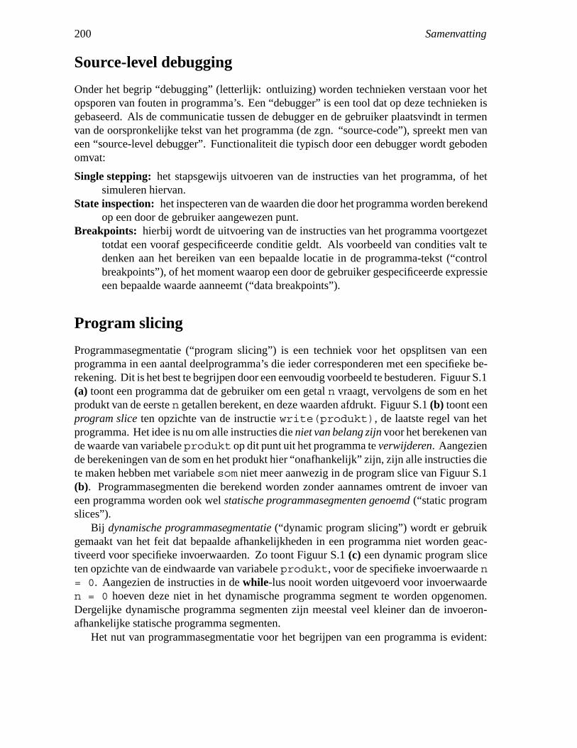
200 Samenvatting
Source-level debugging
Onder het begrip “debugging” (letterlijk: ontluizing) worden technieken verstaan voor hetopsporen van fouten in programma’s. Een “debugger” is een tool dat op deze technieken isgebaseerd. Als de communicatie tussen de debugger en de gebruiker plaatsvindt in termenvan de oorspronkelijke tekst van het programma (de zgn. “source-code”), spreekt men vaneen “source-level debugger”. Functionaliteit die typisch door een debugger wordt gebodenomvat:
Single stepping: het stapsgewijs uitvoeren van de instructies van het programma, of hetsimuleren hiervan.
State inspection: het inspecteren van de waarden die door het programma worden berekendop een door de gebruiker aangewezen punt.
Breakpoints: hierbij wordt de uitvoering van de instructies van het programma voortgezettotdat een vooraf gespecificeerde conditie geldt. Als voorbeeld van condities valt tedenken aan het bereiken van een bepaalde locatie in de programma-tekst (“controlbreakpoints”), of het moment waarop een door de gebruiker gespecificeerde expressieeen bepaalde waarde aanneemt (“data breakpoints”).
Program slicing
Programmasegmentatie (“program slicing”) is een techniek voor het opsplitsen van eenprogramma in een aantal deelprogramma’s die ieder corresponderen met een specifieke be-rekening. Dit is het best te begrijpen door een eenvoudig voorbeeld te bestuderen. Figuur S.1(a) toont een programma dat de gebruiker om een getal n vraagt, vervolgens de som en hetprodukt van de eerste n getallen berekent, en deze waarden afdrukt. Figuur S.1 (b) toont eenprogram slice ten opzichte van de instructie write(produkt), de laatste regel van hetprogramma. Het idee is nu om alle instructies die niet van belang zijn voor het berekenen vande waarde van variabele produkt op dit punt uit het programma te verwijderen. Aangeziende berekeningen van de som en het produkt hier “onafhankelijk” zijn, zijn alle instructies diete maken hebben met variabele som niet meer aanwezig in de program slice van Figuur S.1(b). Programmasegmenten die berekend worden zonder aannames omtrent de invoer vaneen programma worden ook wel statische programmasegmenten genoemd (“static programslices”).
Bij dynamische programmasegmentatie (“dynamic program slicing”) wordt er gebruikgemaakt van het feit dat bepaalde afhankelijkheden in een programma niet worden geac-tiveerd voor specifieke invoerwaarden. Zo toont Figuur S.1 (c) een dynamic program sliceten opzichte van de eindwaarde van variabele produkt, voor de specifieke invoerwaarde n= 0. Aangezien de instructies in de while-lus nooit worden uitgevoerd voor invoerwaarden = 0 hoeven deze niet in het dynamische programma segment te worden opgenomen.Dergelijke dynamische programma segmenten zijn meestal veel kleiner dan de invoeron-afhankelijke statische programma segmenten.
Het nut van programmasegmentatie voor het begrijpen van een programma is evident:

Samenvatting 201
read(n);i := 1;som := 0;produkt := 1;while i �� n dobeginsom := som + i;produkt := produkt * i;i := i + 1
end;write(som);write(produkt)
read(n);i := 1;
produkt := 1;while i �� n dobegin
produkt := produkt * i;i := i + 1
end;
write(produkt)
read(n);i := 1;
produkt := 1;while i �� n dobegin
end;
write(produkt)
(a) (b) (c)
Figuur S.1: (a) Voorbeeldprogramma. (b) Statisch programma segment van het programma tenopzichte van de eindwaarde van variabele produkt. (c) Dynamisch programma segment van hetprogramma ten opzichte van de eindwaarde van variabeleprodukt voor de specifieke invoerwaarden = 0.
het stelt de programmeur in staat de aandacht te concentreren op een bepaalde berekening,en instructies die daar niet mee te maken hebben te negeren. Dynamische programmaseg-mentatie is nuttig als debugging techniek. Als immers een onjuiste waarde wordt berekendop een bepaald punt in het programma, kunnen alleen de instructies in de dynamische sliceten opzichte van dat programma-punt van belang zijn geweest voor de berekening van deonjuiste waarde1. In het algemeen kan worden gesteld dat program slicing nuttig is voor hetbegrijpen van programma’s omdat het het overzicht helpt te vergroten.
Hoofdstuk 3 bevat een uitgebreid overzicht van de huidige vakliteratuur op het gebiedvan program slicing, en de toepassingen daarvan.
Algebraısche specificaties
Zoals eerder genoemd bestaat de aanpak van dit proefschrift uit het genereren vanprogramma-analyse tools uit algebraısche specificaties. Een algebraısche specificatie bestaatuit een verzameling van (conditionele) vergelijkingen die gezamenlijk de “betekenis” vaninstructies en programma’s formeel definieren. Als voorbeeld wordt in Figuur S.2 de exe-cutie van een if-instructie gespecificeerd (dit voorbeeld komt uitgebreid aan de orde inHoofdstuk 6). Gezamenlijk definieren deze twee vergelijkingen hoe de executie van een if-instructie kan worden uitgedrukt in de executie van ofwel de instructies in de then-tak, ofwel
1Zelfs in gevallen waar de fout bestaat uit de afwezigheid van een bepaalde instructie kunnen programma-segmenten van nut zijn. In dergelijke gevallen is het waarschijnlijk dat het segment andere instructies bevatdan men zou verwachten.
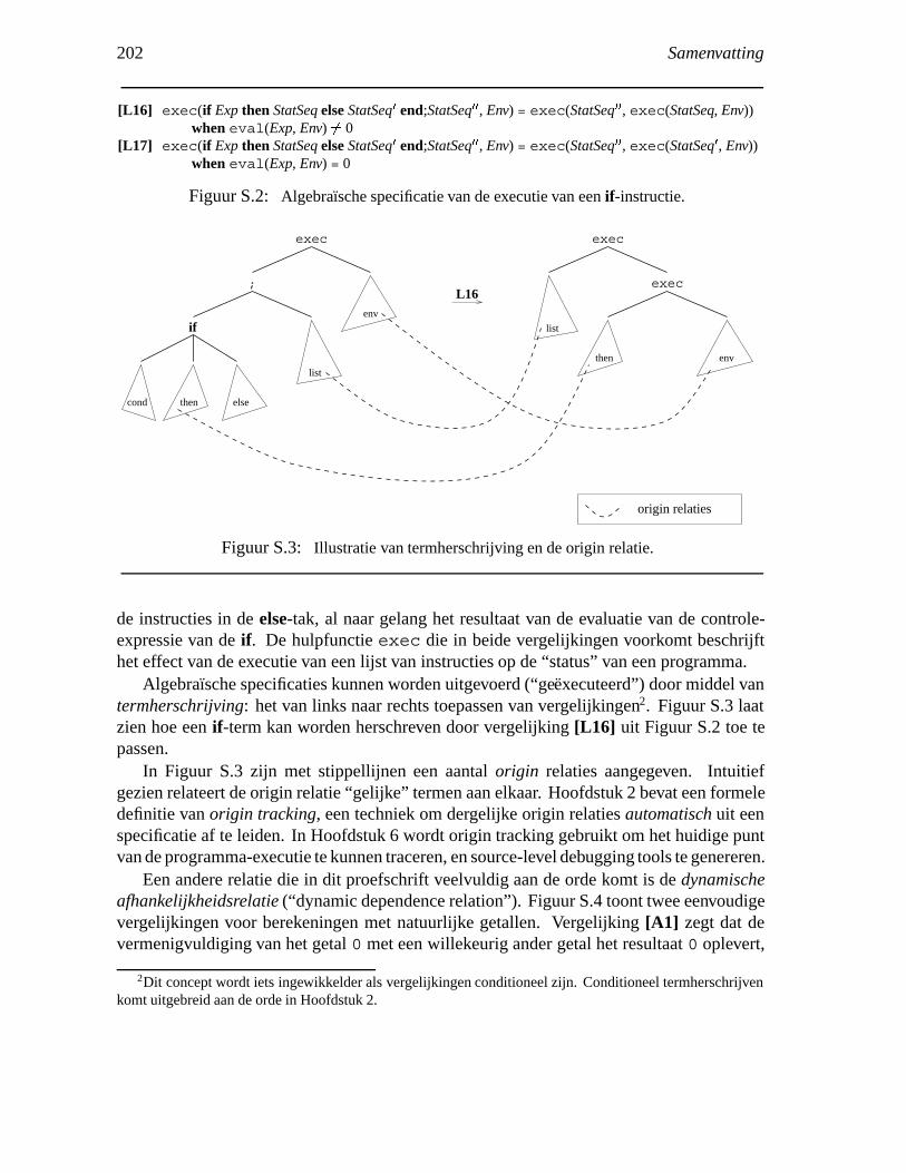
202 Samenvatting
[L16] exec(if Exp then StatSeq else StatSeq� end;StatSeq��, Env) = exec(StatSeq��, exec(StatSeq, Env))when eval(Exp, Env) �� 0
[L17] exec(if Exp then StatSeq else StatSeq� end;StatSeq��, Env) = exec(StatSeq��, exec(StatSeq�, Env))when eval(Exp, Env) = 0
Figuur S.2: Algebraısche specificatie van de executie van een if-instructie.
cond then else
list
list
then
L16
env
if
exec
;
exec
exec
origin relaties
env
Figuur S.3: Illustratie van termherschrijving en de origin relatie.
de instructies in de else-tak, al naar gelang het resultaat van de evaluatie van de controle-expressie van de if. De hulpfunctie exec die in beide vergelijkingen voorkomt beschrijfthet effect van de executie van een lijst van instructies op de “status” van een programma.
Algebraısche specificaties kunnen worden uitgevoerd (“geexecuteerd”) door middel vantermherschrijving: het van links naar rechts toepassen van vergelijkingen2. Figuur S.3 laatzien hoe een if-term kan worden herschreven door vergelijking [L16] uit Figuur S.2 toe tepassen.
In Figuur S.3 zijn met stippellijnen een aantal origin relaties aangegeven. Intuitiefgezien relateert de origin relatie “gelijke” termen aan elkaar. Hoofdstuk 2 bevat een formeledefinitie van origin tracking, een techniek om dergelijke origin relaties automatisch uit eenspecificatie af te leiden. In Hoofdstuk 6 wordt origin tracking gebruikt om het huidige puntvan de programma-executie te kunnen traceren, en source-level debugging tools te genereren.
Een andere relatie die in dit proefschrift veelvuldig aan de orde komt is de dynamischeafhankelijkheidsrelatie (“dynamic dependence relation”). Figuur S.4 toont twee eenvoudigevergelijkingen voor berekeningen met natuurlijke getallen. Vergelijking [A1] zegt dat devermenigvuldiging van het getal 0 met een willekeurig ander getal het resultaat 0 oplevert,
2Dit concept wordt iets ingewikkelder als vergelijkingen conditioneel zijn. Conditioneel termherschrijvenkomt uitgebreid aan de orde in Hoofdstuk 2.

Samenvatting 203
[A1] intmul�0�X� = 0[A2] intmul�intmul(X, Y)� Z� = intmul�X�intmul(Y, Z)�
Figuur S.4: Vergelijkingen voor berekeningen met natuurlijke getallen.
A2 A1
intmul
2intmul
0 1
intmul
dynamische afhankelijkheids relaties
0 intmul
1 2
0
Figuur S.5: Dynamische afhankelijkheidsrelaties die optreden bij toepassing van vergelijkingen[A1] en [A2].
en vergelijking [A2] beschrijft het feit dat vermenigvuldiging een associatieve operatie is.Figuur S.5 laat zien hoe de term intmul(intmul(0, 1), 2) kan worden herschrevendoor toepassing van vergelijkingen [A1] en [A2]. De gestippelde lijnen in Figuur S.5geven dynamische afhankelijkheden weer. Intuıtief gezien beschrijven deze relaties welkefunctiesymbolen in de term hebben geleid tot de “creatie” van een bepaald functiesymbool.Dit kan in het voorbeeld van Figuur S.5 worden ingezien door de afhankelijkheidsrelatiesvanaf het eindresultaat 0 terug te traceren: hieruit blijkt dat het optreden van deze waardeniet afhankelijk is van de waarden 1 en 2 in de beginterm.
Hoofdstuk 4 bevat een formele definitie van “dynamic dependence tracking”, een tech-niek om dynamische afhankelijksrelaties automatisch uit een algebraısche specificatie afte leiden. In Hoofdstuk 5 wordt dynamic dependence tracking gecombineerd met hetformalisme PIM [55], een equationele logica voor het beschrijven van de betekenis vanprogramma’s ontwikkeld aan het IBM T.J. Watson Research Center. In Hoofdstuk 5 wordtuitvoerig beschreven hoe het traceren van de dynamische afhankelijkheden vanuit een waardedie berekend is door een programma, zeer accurate program slices oplevert. In Hoofdstuk 6wordt de dynamische afhankelijkheidsrelatie toegepast op een algebraısche specificatie vaneen interpreter om dynamische programmasegmenten te berekenen.

204 Samenvatting
Resultaten van dit onderzoek
De belangrijkste resultaten van het in dit proefschrift beschreven onderzoek kunnen als volgtworden samengevat:
� Hoofdstukken 2 en 4 bevatten formele definities van respectievelijk de origin relatieen de dynamische afhankelijksheidsrelatie. Verder worden hier een aantal nuttigeeigenschappen van deze relaties bewezen, en wordt aangegeven hoe ze op efficientewijze geımplementeerd kunnen worden.
� In Hoofdstuk 5 wordt de dynamische afhankelijkheidsrelatie “toegepast op” het PIM
formalisme. Dit blijkt overeen te komen met een algemene, flexibele, en zeer preciezevorm van program slicing.
� Hoofdstuk 3 bevat een uitgebreid literatuuronderzoek over het onderwerp programslicing.
� In Hoofdstuk 6 worden de origin relatie en de dynamische afhankelijkheidsrelatietoegepast op algebraısche specificaties van interpreters. Hierbij wordt beschreven hoeop basis van de origin relatie een aantal zeer krachtige debugging concepten op een-voudige wijze kan worden gedefinieerd, en hoe de dynamische afhankelijkheidsrelatiehet mogelijk maakt dynamische programmasegmenten te berekenen.
De technieken die zijn beschreven in dit proefschrift zijn geımplementeerd met behulp vande ASF+SDF Meta-Environment [93], een generator voor programmeeromgevingen dieontwikkeld is door onderzoeksgroepen bij het Centrum voor Wiskunde en Informatica en bijde Universiteit van Amsterdam.

Titles in the ILLC Dissertation Series:
Transsentential Meditations; Ups and downs in dynamic semanticsPaul DekkerILLC Dissertation series 1993-1
Resource Bounded ReductionsHarry BuhrmanILLC Dissertation series 1993-2
Efficient MetamathematicsRineke VerbruggeILLC Dissertation series 1993-3
Extending Modal LogicMaarten de RijkeILLC Dissertation series 1993-4
Studied FlexibilityHerman HendriksILLC Dissertation series 1993-5
Aspects of Algorithms and ComplexityJohn TrompILLC Dissertation series 1993-6
The Noble Art of Linear DecoratingHarold SchellinxILLC Dissertation series 1994-1
Generating Uniform User-Interfaces for Interactive Programming EnvironmentsJan Willem Cornelis KoornILLC Dissertation series 1994-2
Process Theory and Equation SolvingNicoline Johanna DrostILLC Dissertation series 1994-3
Calculi for Constructive Communication, a Study of the Dynamics of Partial StatesJan JasparsILLC Dissertation series 1994-4
Executable Language Definitions, Case Studies and Origin Tracking TechniquesArie van DeursenILLC Dissertation series 1994-5

206 Samenvatting
Chapters on Bounded Arithmetic & on Provability LogicDomenico ZambellaILLC Dissertation series 1994-6
Adventures in Diagonalizable AlgebrasV. Yu. ShavrukovILLC Dissertation series 1994-7
Learnable Classes of Categorial GrammarsMakoto KanazawaILLC Dissertation series 1994-8
Clocks, Trees and Stars in Process TheoryWan FokkinkILLC Dissertation series 1994-9
Logics for Agents with Bounded RationalityZhisheng HuangILLC Dissertation series 1994-10
On Modular Algebraic Prototol SpecificationJacob BrunekreefILLC Dissertation series 1995-1
Investigating Bounded ContractionAndreja PrijateljILLC Dissertation series 1995-2
Relativized Algebras of Relations and Arrow LogicMaarten MarxILLC Dissertation series 1995-3
Study on the Formal Semantics of PicturesDejuan WangILLC Dissertation series 1995-4
Generation of Program Analysis ToolsFrank TipILLC Dissertation series 1995-5


![Frank Sargeson [Norris Frank Davey], 1903 – 1982](https://static.fdokumen.com/doc/165x107/6322013728c44598910594c2/frank-sargeson-norris-frank-davey-1903-1982.jpg)