Generating Readable Proofs: A HeuristicApproach to Theorem Proving With Spider

Diagrams

Jean Flower, Judith Masthoff, and Gem Stapleton

The Visual Modelling GroupUniversity of Brighton, Brighton, UK

www.cmis.brighton.ac.uk/research/vmg{J.A.Flower,Judith.Masthoff,G.E.Stapleton}@bton.ac.uk

Abstract. An important aim of diagrammatic reasoning is to make iteasier for people to create and understand logical arguments. We haveworked on spider diagrams, which visually express logical statements.Ideally, automatically generated proofs should be short and easy to un-derstand. An existing proof generator for spider diagrams successfullywrites proofs, but they can be long and unwieldy. In this paper, wepresent a new approach to proof writing in diagrammatic systems, whichis guaranteed to find shortest proofs and can be extended to incorporateother readability criteria. We apply the A∗ algorithm and develop anadmissible heuristic function to guide automatic proof construction. Wedemonstrate the effectiveness of the heuristic used. The work has beenimplemented as part of a spider diagram reasoning tool.

1 IntroductionIn this paper, we show how readability can be taken into account when generatingproofs in a spider diagram reasoning system. In particular, we show how the A*heuristic search algorithm can be applied.

If diagrammatic reasoning is to be practical, then tool support is essential.Proof writing in diagrammatic systems without software support can be time-consuming and error prone.

In [4] we present a proving environment that supports reasoning with spiderdiagrams. This proving environment incorporates automated proof construction:an algorithm generates a proof that one spider diagram entails another, providedsuch a proof exists. This algorithm usually produces long and somewhat unwieldyproofs. These unnatural proofs suffice if one only wishes to know that there existsa proof. However, if one wishes to read and understand a proof then applyingthe algorithm may not be the best approach to constructing a proof.

Readability and understandability of proofs are important because they:

– support education. The introduction of calculators has not stopped us teach-ing numeracy. Similarly, automatic proof generators will not stop us teachingstudents how to construct proofs manually. An automated proof generatorcan support the learning process, but only if it generates proofs similar tothose produced by expert humans [22].

– increase notational understanding. People will need to write and verify thespecifications (premise and conclusion) given to the automated proof genera-tor. Specification is the phase where most mistakes can be introduced [11]. Agood understanding of the notation used is therefore needed. Reading (andwriting) proofs helps to develop that understanding.

– provide trust in generated proofs. As discussed in [11], automated proofgenerators can themselves contain flaws1 and many people remain wary ofproofs they cannot themselves understand [22].

– encourage lateral thinking. Understanding a proof often leads to ideas ofother theorems that could be proved.

Research has been conducted on how to optimize the presentation of proofs, op-timizing the layout of proofs or annotating proofs with or even translating theminto natural language (see for example [15],[13],[1]). The diagrammatic reason-ing community attempts to make reasoning easier by using diagrams insteadof formulas. For instance, we are working on presenting proofs as sequences ofdiagrams.

In this paper, we enhance the proving environment presented in [4] by de-veloping a heuristic approach to theorem proving in the spider diagram system.We define numerical measures that indicate ‘how close’ one spider diagram is toanother and these measures guide the tool towards rule applications that resultin shorter and, therefore, hopefully more ‘natural’ proofs. In fact, the methodis guaranteed to find a shortest proof, provided one exists. Note that heuristicapproaches have been used in automated theorem provers before, but mainly tomake it faster and less memory intensive to find a proof. This is a nice side effectof using heuristics, but our main reason is readability of the resulting proof.Often heuristics used are not numerical such as ‘in general, this rule should beapplied before that rule’ (e.g. [12]).When numerical heuristics have been used(e.g. [5]), they have usually been used to find a proof quickly rather than tooptimize the proofs.

Many other diagrammatic reasoning systems have been developed, see [9]for an overview. For example, the DIAMOND system allows the constructionof diagrammatic proofs, learning from user examples. The kinds of diagramsconsidered are quite different to spider diagrams.

In [18] Swoboda proposes an approach towards implementing an Euler/Vennreasoning system, using directed acyclic graphs (DAGs). The use of DAGs tocompare diagrams was the focus of [19] in which two diagrams are comparedto assess the correctness of a single diagram transformation. It is possible thatthe work on DAGs, if extended to assess a sequence of diagram transformations,could show some similarity to the measures we give in section 4. The existingDAGs work does not create proofs but rather checks the validity of a proofcandidate.

The structure of this paper is as follows. In Section 2, we introduce a simpli-fied (unitary diagrams only) version of our spider diagram reasoning system. In1 If an algorithm has been proved correct, still the correctness proof or the implemen-

tation could contain errors.

2

Section 3, we discuss the A* heuristic search algorithm that we have applied tothis reasoning system. In Section 4, we describe a so-called admissible heuristicfunction that measures the difference between two spider diagrams. In Section5, we briefly discuss how the heuristic diagrammatic proof generator has beenimplemented, and evaluate its results. We conclude by discussing how the costelement of A* can be used to further enhance understandability (the shortestproof is not necessarily the easiest to understand), how the heuristic can be usedto support interactive proof writing, and what we expect from extending thisapproach to non-unitary spider diagrams and so-called constraint diagrams.

2 Unitary spider diagrams

In this section, we briefly and informally introduce our diagrammatic reasoningsystem. For reasons of clarity, we restrict ourselves in this paper to so-calledunitary spider diagrams and the reasoning rules associated with those. We willbriefly return to non-unitary diagrams in Section 6.

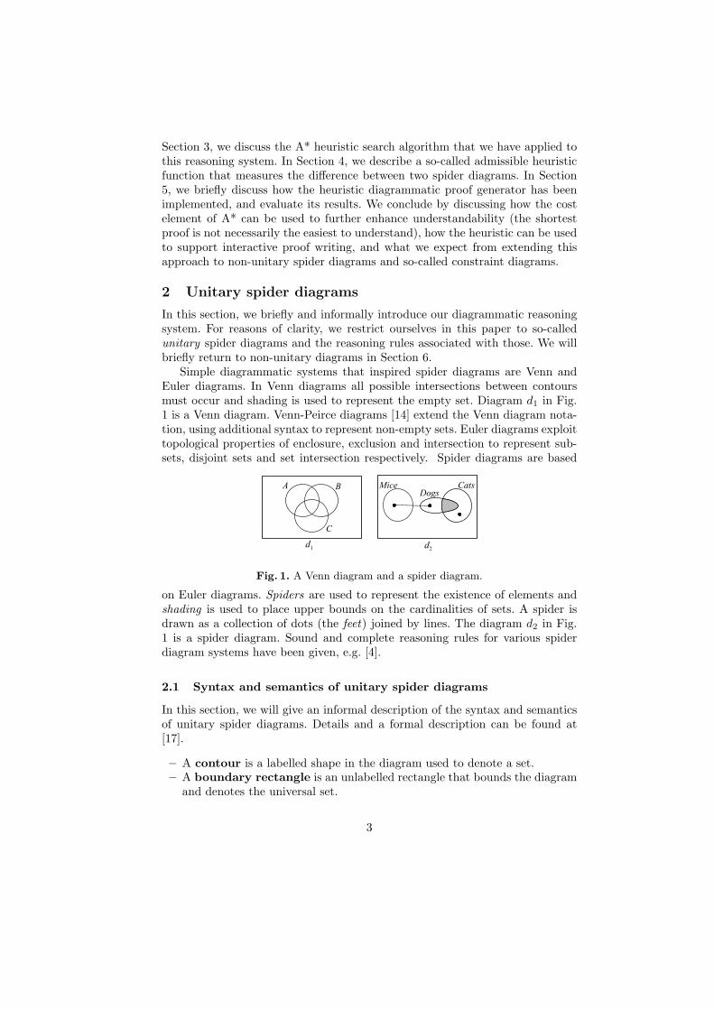
Simple diagrammatic systems that inspired spider diagrams are Venn andEuler diagrams. In Venn diagrams all possible intersections between contoursmust occur and shading is used to represent the empty set. Diagram d1 in Fig.1 is a Venn diagram. Venn-Peirce diagrams [14] extend the Venn diagram nota-tion, using additional syntax to represent non-empty sets. Euler diagrams exploittopological properties of enclosure, exclusion and intersection to represent sub-sets, disjoint sets and set intersection respectively. Spider diagrams are based

C a t sM i c e D o g s

d 2d 1

A B

C

Fig. 1. A Venn diagram and a spider diagram.

on Euler diagrams. Spiders are used to represent the existence of elements andshading is used to place upper bounds on the cardinalities of sets. A spider isdrawn as a collection of dots (the feet) joined by lines. The diagram d2 in Fig.1 is a spider diagram. Sound and complete reasoning rules for various spiderdiagram systems have been given, e.g. [4].

2.1 Syntax and semantics of unitary spider diagrams

In this section, we will give an informal description of the syntax and semanticsof unitary spider diagrams. Details and a formal description can be found at[17].

– A contour is a labelled shape in the diagram used to denote a set.– A boundary rectangle is an unlabelled rectangle that bounds the diagram

and denotes the universal set.

3

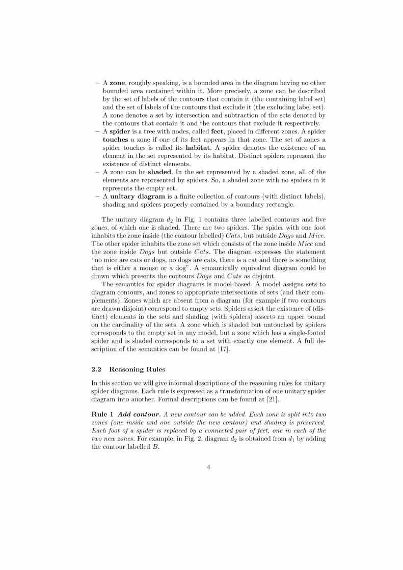
– A zone, roughly speaking, is a bounded area in the diagram having no otherbounded area contained within it. More precisely, a zone can be describedby the set of labels of the contours that contain it (the containing label set)and the set of labels of the contours that exclude it (the excluding label set).A zone denotes a set by intersection and subtraction of the sets denoted bythe contours that contain it and the contours that exclude it respectively.

– A spider is a tree with nodes, called feet, placed in different zones. A spidertouches a zone if one of its feet appears in that zone. The set of zones aspider touches is called its habitat. A spider denotes the existence of anelement in the set represented by its habitat. Distinct spiders represent theexistence of distinct elements.

– A zone can be shaded. In the set represented by a shaded zone, all of theelements are represented by spiders. So, a shaded zone with no spiders in itrepresents the empty set.

– A unitary diagram is a finite collection of contours (with distinct labels),shading and spiders properly contained by a boundary rectangle.

The unitary diagram d2 in Fig. 1 contains three labelled contours and fivezones, of which one is shaded. There are two spiders. The spider with one footinhabits the zone inside (the contour labelled) Cats, but outside Dogs and Mice.The other spider inhabits the zone set which consists of the zone inside Mice andthe zone inside Dogs but outside Cats. The diagram expresses the statement“no mice are cats or dogs, no dogs are cats, there is a cat and there is somethingthat is either a mouse or a dog”. A semantically equivalent diagram could bedrawn which presents the contours Dogs and Cats as disjoint.

The semantics for spider diagrams is model-based. A model assigns sets todiagram contours, and zones to appropriate intersections of sets (and their com-plements). Zones which are absent from a diagram (for example if two contoursare drawn disjoint) correspond to empty sets. Spiders assert the existence of (dis-tinct) elements in the sets and shading (with spiders) asserts an upper boundon the cardinality of the sets. A zone which is shaded but untouched by spiderscorresponds to the empty set in any model, but a zone which has a single-footedspider and is shaded corresponds to a set with exactly one element. A full de-scription of the semantics can be found at [17].

2.2 Reasoning Rules

In this section we will give informal descriptions of the reasoning rules for unitaryspider diagrams. Each rule is expressed as a transformation of one unitary spiderdiagram into another. Formal descriptions can be found at [21].

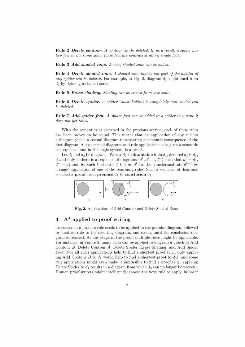
Rule 1 Add contour. A new contour can be added. Each zone is split into twozones (one inside and one outside the new contour) and shading is preserved.Each foot of a spider is replaced by a connected pair of feet, one in each of thetwo new zones. For example, in Fig. 2, diagram d2 is obtained from d1 by addingthe contour labelled B.

4

Rule 2 Delete contour. A contour can be deleted. If, as a result, a spider hastwo feet in the same zone, these feet are contracted into a single foot.

Rule 3 Add shaded zone. A new, shaded zone can be added.

Rule 4 Delete shaded zone. A shaded zone that is not part of the habitat ofany spider can be deleted. For example, in Fig. 2, diagram d3 is obtained fromd2 by deleting a shaded zone.

Rule 5 Erase shading. Shading can be erased from any zone.

Rule 6 Delete spider. A spider whose habitat is completely non-shaded canbe deleted.

Rule 7 Add spider foot. A spider foot can be added to a spider in a zone itdoes not yet touch.

With the semantics as sketched in the previous section, each of these ruleshas been proven to be sound. This means that an application of any rule toa diagram yields a second diagram representing a semantic consequence of thefirst diagram. A sequence of diagrams and rule applications also gives a semanticconsequence, and in this logic system, is a proof.

Let d1 and d2 be diagrams. We say d2 is obtainable from d1, denoted d1 ` d2,if and only if there is a sequence of diagrams 〈d1, d2, ..., dm〉 such that d1 = d1,dm = d2 and, for each k where 1 ≤ k < m, dk can be transformed into dk+1 bya single application of one of the reasoning rules. Such a sequence of diagramsis called a proof from premise d1 to conclusion d2.

A A B

d 1 d 2

A B

d 3

Fig. 2. Applications of Add Contour and Delete Shaded Zone.

3 A* applied to proof writing

To construct a proof, a rule needs to be applied to the premise diagram, followedby another rule to the resulting diagram, and so on, until the conclusion dia-gram is reached. At any stage in the proof, multiple rules might be applicable.For instance, in Figure 2, many rules can be applied to diagram d1, such as AddContour B, Delete Contour A, Delete Spider, Erase Shading, and Add SpiderFoot. Not all rules applications help to find a shortest proof (e.g., only apply-ing Add Contour B to d1 would help to find a shortest proof to d3), and somerule applications might even make it impossible to find a proof (e.g., applyingDelete Spider to d1 results in a diagram from which d3 can no longer be proven).Human proof writers might intelligently choose the next rule to apply, in order

5

to reach the conclusion diagram as quickly as possible. The problem of decid-ing which rules to apply to find a proof is an example of a more general classof so-called search problems, for which various algorithms have been developed(see [10] for an overview). Some of these algorithms, so-called blind-search algo-rithms, systematically try all possible actions. Others, so-called best-first searchalgorithms, have been made more intelligent, and attempt (like humans) to in-telligently choose which action to try first. A∗ is a well known best-first searchalgorithm [6].

A∗ stores an ordered sequence of proof attempts. Initially, this sequence onlycontains a zero length proof attempt, namely the premise diagram. Repeatedly,A∗ removes the first proof attempt from the sequence and considers it. If the lastdiagram of the proof attempt is the conclusion diagram, then an optimal proofhas been found. Otherwise, it constructs additional proof attempts, by extendingthe proof attempt under consideration, applying rules wherever possible to thelast diagram.

The effectiveness of A∗ and the definition of “optimal” is dependent upon theordering imposed on the proof attempt sequence. The ordering is derived fromthe sum of two functions. One function, called the heuristic, estimates how farthe last diagram in the proof attempt is from the conclusion diagram. The other,called the cost, calculates how costly it has been to reach the last diagram fromthe premise diagram. We define the cost of applying a reasoning rule to be one.So, the cost is the number of reasoning rules that have been applied to get fromthe premise diagram to the last diagram (i.e. the length of the proof attempt).The new proof attempts are inserted into the sequence, ordered according to thecost plus heuristic.

A∗ has been proven to be complete and optimal, i.e. always finding the bestsolution (because all reasoning rules have cost 1, this means the shortest proof), ifone exists, provided the heuristic used is admissible [2]. A heuristic is admissibleif it is optimistic, which means that it never overestimates the cost of gettingfrom a premise diagram to a conclusion diagram. As all reasoning rules havecost equal to one, this means that the heuristic should give a lower bound onthe number of proof steps needed in order to reach the conclusion diagram.

The amount of memory and time needed by A∗ depends heavily on the qualityof the heuristic used. For instance, a heuristic that is the constant function zerois admissible, but will result in long and memory-intensive searches. The betterthe heuristic (in the sense of accurately predicting the length of a shortest proof),the less memory and time are needed for the search. In this paper, we presenta highly effective heuristic for A∗ applied to proof writing in a unitary spiderdiagram reasoning system.

4 Heuristic function for unitary diagrams

As discussed above, in order to apply A∗ we need a heuristic function thatgives an optimistic (admissible) estimate of how many proof steps it would taketo get from a premise diagram to the conclusion diagram. In this section, wedevelop various measures between two unitary diagrams. The overall heuristic

6

we use is built from these measures. The heuristic gives a lower bound on thenumber of proof steps required and is used to help choose rule applications whenconstructing proofs in our implementation.

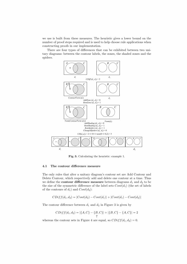
There are four types of differences that can be exhibited between two uni-tary diagrams: between the contour labels, the zones, the shaded zones and thespiders.

d 2

A C

d 1

B C

C D i f f ( d 1 , d 2 ) = 2

d 2

B C

C o n t o u r F o r m ( d 1 )

B C

A d d Z o n e ( d 1 , d 2 ) = 0R e m Z o n e ( d 1 , d 2 ) = 1

V e n n ( d 2 )

B C

V e n n ( C o n t o u r F o r m ( d 1 ) )

B C

A d d S h a d i n g ( d 1 , d 2 ) = 0 R e m S h a d i n g ( d 1 , d 2 ) = 1 R e m S p i d e r s ( d 1 , d 2 ) = 1C h a n g e d S p i d e r s ( d 1 , d 2 ) = 0

d 2

A C

d 1

B CC C B C B C

U H ( d 1 , d 2 ) = 2 + 1 + 0 + 1 + m i n ( 0 + 1 + 0 , 2 ) = 5

Fig. 3. Calculating the heuristic: example 1.

4.1 The contour difference measure

The only rules that alter a unitary diagram’s contour set are Add Contour andDelete Contour, which respectively add and delete one contour at a time. Thuswe define the contour difference measure between diagrams d1 and d2 to bethe size of the symmetric difference of the label sets Cont(d1) (the set of labelsof the contours of d1) and Cont(d2):

CDiff(d1, d2) = |Cont(d2)− Cont(d1)|+ |Cont(d1)− Cont(d2)|

The contour difference between d1 and d2 in Figure 3 is given by

CDiff(d1, d2) = |{A,C} − {B, C}|+ |{B, C} − {A,C}| = 2

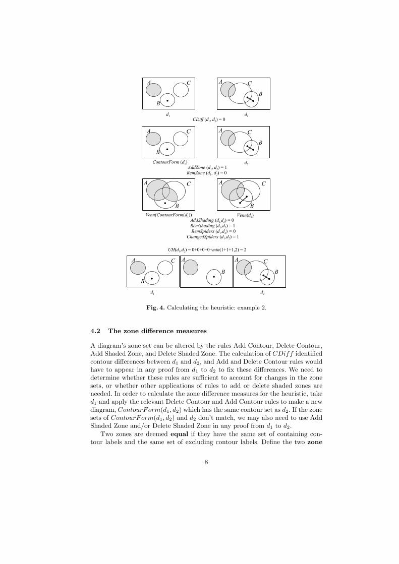
whereas the contour sets in Figure 4 are equal, so CDiff(d1, d2) = 0.7

d 2

A C

d 1

A C

C D i f f ( d 1 , d 2 ) = 0

d 2C o n t o u r F o r m ( d 1 ) A d d Z o n e ( d 1 , d 2 ) = 1R e m Z o n e ( d 1 , d 2 ) = 0

V e n n ( d 2 )

A C

V e n n ( C o n t o u r F o r m ( d 1 ) ) A d d S h a d i n g ( d 1 , d 2 ) = 0 R e m S h a d i n g ( d 1 , d 2 ) = 1 R e m S p i d e r s ( d 1 , d 2 ) = 0C h a n g e d S p i d e r s ( d 1 , d 2 ) = 1

BB

A C

B

A CB

B

A C

B

d 2

A C

d 1

A C

BB

AB

U H ( d 1 , d 2 ) = 0 + 0 + 0 + 0 + m i n ( 1 + 1 + 1 , 2 ) = 2

Fig. 4. Calculating the heuristic: example 2.

4.2 The zone difference measures

A diagram’s zone set can be altered by the rules Add Contour, Delete Contour,Add Shaded Zone, and Delete Shaded Zone. The calculation of CDiff identifiedcontour differences between d1 and d2, and Add and Delete Contour rules wouldhave to appear in any proof from d1 to d2 to fix these differences. We need todetermine whether these rules are sufficient to account for changes in the zonesets, or whether other applications of rules to add or delete shaded zones areneeded. In order to calculate the zone difference measures for the heuristic, taked1 and apply the relevant Delete Contour and Add Contour rules to make a newdiagram, ContourForm(d1, d2) which has the same contour set as d2. If the zonesets of ContourForm(d1, d2) and d2 don’t match, we may also need to use AddShaded Zone and/or Delete Shaded Zone in any proof from d1 to d2.

Two zones are deemed equal if they have the same set of containing con-tour labels and the same set of excluding contour labels. Define the two zone

8

difference measures between diagrams d1 and d2 to be

AddZone(d1, d2) ={

1 if Zones(d2) * Zones(ContourForm(d1, d2))0 otherwise

RemZone(d1, d2) ={

1 if Zones(ContourForm(d1, d2)) * Zones(d2)0 otherwise.

The sum CDiff(d1, d2) + AddZone(d1, d2) + RemZone(d1, d2) is an optimisticestimate of the number of applications of Add Contour, Delete Contour, AddShaded Zone and Delete Shaded Zone which are required in a proof from d1 tod2.

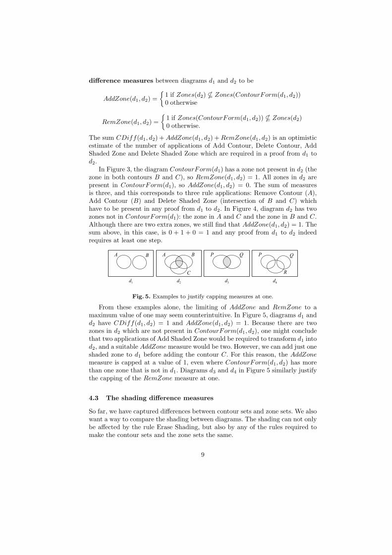
In Figure 3, the diagram ContourForm(d1) has a zone not present in d2 (thezone in both contours B and C), so RemZone(d1, d2) = 1. All zones in d2 arepresent in ContourForm(d1), so AddZone(d1, d2) = 0. The sum of measuresis three, and this corresponds to three rule applications: Remove Contour (A),Add Contour (B) and Delete Shaded Zone (intersection of B and C) whichhave to be present in any proof from d1 to d2. In Figure 4, diagram d2 has twozones not in ContourForm(d1): the zone in A and C and the zone in B and C.Although there are two extra zones, we still find that AddZone(d1, d2) = 1. Thesum above, in this case, is 0 + 1 + 0 = 1 and any proof from d1 to d2 indeedrequires at least one step.

P Q

d 2d 1

A B

C

A B P Q

Rd 3 d 4

Fig. 5. Examples to justify capping measures at one.

From these examples alone, the limiting of AddZone and RemZone to amaximum value of one may seem counterintuitive. In Figure 5, diagrams d1 andd2 have CDiff(d1, d2) = 1 and AddZone(d1, d2) = 1. Because there are twozones in d2 which are not present in ContourForm(d1, d2), one might concludethat two applications of Add Shaded Zone would be required to transform d1 intod2, and a suitable AddZone measure would be two. However, we can add just oneshaded zone to d1 before adding the contour C. For this reason, the AddZonemeasure is capped at a value of 1, even where ContourForm(d1, d2) has morethan one zone that is not in d1. Diagrams d3 and d4 in Figure 5 similarly justifythe capping of the RemZone measure at one.

4.3 The shading difference measures

So far, we have captured differences between contour sets and zone sets. We alsowant a way to compare the shading between diagrams. The shading can not onlybe affected by the rule Erase Shading, but also by any of the rules required tomake the contour sets and the zone sets the same.

9

To measure the difference in shading between d1 and d2, we take the di-agram ContourForm(d1, d2) and add shaded zones until the diagram is inVenn form (every possible zone is present, given the contour label set), giv-ing V enn(ContourForm(d1, d2)). We also add shaded zones to d2 until d2 isin Venn form, giving V enn(d2). The shading difference measures betweendiagrams d1 and d2 are defined to be

AddShading(d1, d2) =

∞ if ShadedZones(V enn(d2))* ShadedZones(V enn(ContourForm(d1, d2)))

0 otherwise

RemShading(d1, d2) =

1 if ShadedZones(V enn(ContourForm(d1, d2)))* ShadedZones(V enn(d2))

0 otherwise.

The allocation of ∞ as the AddShading measure indicates that there is noproof from d1 to d2. In the examples shown in Figures 3 and 4, a proof doesexist between d1 and d2, and in both cases AddShading(d1, d2) = 0. Also, inboth figures, V enn(ContourForm(d1, d2)) has more shading than V enn(d2), soRemShading(d1, d2) = 1. The value of RemShading is capped at 1 for similarreasons to the capping of AddZone and RemZone.

The sum CDiff + AddZone + RemZone + AddShading + RemShading isan optimistic estimate of the number of applications of Add Contour, DeleteContour, Add Shaded Zone, Delete Shaded Zone, and Erase Shading which arerequired in a proof from d1 to d2 (i.e. the sum is a lower bound on the numberof proof steps required).

4.4 The spider difference measures

The rules Delete Spider and Add Spider Foot change the number of spiders ina diagram and the habitats of spiders, respectively. In addition, deleting andreintroducing a contour can also affect the habitats of spiders.

We can see that no rules introduce spiders, so if d2 has more spiders than d1

then we define the spider difference measure to be infinite (in effect, blocking thesearch for proofs between such diagrams). If we have fewer spiders in d2 than d1,then the rule Delete Spider must have been applied and the difference betweenthe numbers of spiders contributes to the heuristic.

If a spider in d2 has a different habitat to all spiders in ContourForm(d1, d2)(i.e. it’s unmatched in d1) then some rule must be applied to change the habitatof a spider in d1 to obtain the spider in d2. That rule could be Add SpiderFoot. Alternatively, the deletion and reintroduction of a contour can changemany spiders’ habitats. We say that n spiders in d2 are unmatched in d1 ifthe bag subtraction Bag(habitats of spiders in d2)−Bag(habitats of spiders inContourForm(d1, d2)) has n elements. Define

RemSpiders(d1, d2) ={∞ if NumSpiders(d1)−NumSpiders(d2) < 0

NumSpiders(d1)−NumSpiders(d2) otherwise

10

ChangedSpiders(d1, d2) = Number of spiders in d2 unmatched in d1.

In Figure 3, there is one spider in d1 and none in d2, so one application ofthe Delete Spider rule is required in any proof from d1 to d2. The measureRemSpiders(d1, d2) = 1, but there are no unmatched spiders in d2, soChangedSpiders(d1, d2) = 0. In Figure 4, d1 and d2 have the same number ofspiders, so RemSpiders(d1, d2) = 0. However, the spider in d2 is unmatched ind1 so ChangedSpiders(d1, d2) = 1.

4.5 The unitary diagram heuristic

We have built seven measures by considering possible differences between thepremise and conclusion diagrams. To give us a lower bound on the length ofa proof with premise d1 and conclusion d2 we take the sum of the measuresdescribed above, but limit the contributions from AddZone, RemShading andChangedSpiders to 2. This is because zones, shading and spiders can changeby applications of Delete Contour followed by Add Contour, as illustrated inFigure 4. Unless we cap the heuristic as shown, it will fail to be admissible, asrequired by the A* algorithm. Define the unitary diagram heuristic betweend1 and d2 to be the sum

UH(d1, d2) = CDiff(d1, d2) + RemZone(d1, d2)+ AddShading(d1, d2) + RemSpiders(d1, d2)

+ min

AddZone(d1, d2) + RemShading(d1, d2)+ChangedSpiders(d1, d2)

2.

Lemma 1. Let d1 and d2 be unitary diagrams. If UH(d1, d2) = ∞ then d1 6` d2.

Theorem 1. Let d1 and d2 be unitary diagrams. If there is a proof with premised1 and conclusion d2 then that proof has length at least UH(d1, d2). That is, theunitary diagram heuristic is optimistic.

The proof strategy uses induction on lengths of proofs. Given a shortest prooflength n between d1 and d2, let dnext be the second diagram in the proof. Theproof from dnext to d2 is length n−1 and so by induction, n−1 ≥ UH(dnext, d2).We consider the seven rules in turn which could have been applied to d1 to obtaindnext. In each case, we find a relationship between UH(d1, d2) and UH(dnext, d2)which allows us to deduce that n ≥ UH(d1, d2).

5 Implementation and Evaluation

The heuristic approach to proof-finding has been implemented in java as partof a proving tool (available at [20]). The user can provide diagrams and ask theprover to seek a proof from one diagram to another. The tool allows the user togive a restriction on the rule-set used. Moreover, in order to assess the benefitsgained from the heuristic defined in section 4, the user can choose between the

11

zero heuristic (ZH) and the unitary diagram heuristic (as defined above). Thezero heuristic simply gives ZH(d1, d2) = 0, for any diagrams d1 and d2. TheA∗ algorithm, when implemented with the zero heuristic, simply performs aninefficient breadth-first search of the space of all possible proof attempts (giventhat we have assumed the cost of each rule application to be 1).

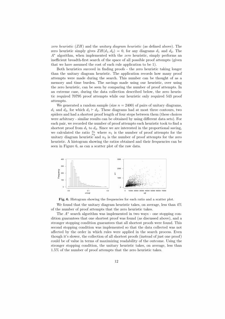
Both heuristics succeed in finding proofs - the zero heuristic taking longerthan the unitary diagram heuristic. The application records how many proofattempts were made during the search. This number can be thought of as amemory and time burden. The savings made using our heuristic, over usingthe zero heuristic, can be seen by comparing the number of proof attempts. Inan extreme case, during the data collection described below, the zero heuris-tic required 70795 proof attempts while our heuristic only required 543 proofattempts.

We generated a random sample (size n = 2400) of pairs of unitary diagrams,d1 and d2, for which d1 ` d2. These diagrams had at most three contours, twospiders and had a shortest proof length of four steps between them (these choiceswere arbitrary - similar results can be obtained by using different data sets). Foreach pair, we recorded the number of proof attempts each heuristic took to find ashortest proof from d1 to d2. Since we are interested in the proportional saving,we calculated the ratio n1

n2where n1 is the number of proof attempts for the

unitary diagram heuristic and n2 is the number of proof attempts for the zeroheuristic. A histogram showing the ratios obtained and their frequencies can beseen in Figure 6, as can a scatter plot of the raw data.

0 . 0 0 . 1 0 . 20

1 0 0

2 0 0

3 0 0

4 0 0

n 1 / n 2

Frequ

ency

0 1 0 0 0 0 2 0 0 0 0 3 0 0 0 0 4 0 0 0 0 5 0 0 0 0 6 0 0 0 0 7 0 0 0 00

1 0 0 0

2 0 0 0

3 0 0 0

n 2

n1

Fig. 6. Histogram showing the frequencies for each ratio and a scatter plot.

We found that the unitary diagram heuristic takes, on average, less than 4%of the number of proof attempts that the zero heuristic takes.

The A∗ search algorithm was implemented in two ways - one stopping con-dition guarantees that one shortest proof was found (as discussed above), and astronger stopping condition guarantees that all shortest proofs were found. Thissecond stopping condition was implemented so that the data collected was notaffected by the order in which rules were applied in the search process. Eventhough it’s slower, the collection of all shortest proofs (instead of just one proof)could be of value in terms of maximizing readability of the outcome. Using thestronger stopping condition, the unitary heuristic takes, on average, less than1.5% of the number of proof attempts that the zero heuristic takes.

12

6 Conclusion and further work

In this paper, we have demonstrated how a heuristic A∗ approach can be usedto automatically generate optimal proofs in a unitary spider diagram reasoningsystem. We regard this as an important step towards generating readable proofs.However, our work has been limited in a number of ways.

The first limitation is that we have assumed the cost of applying each rule tobe equal. This results in the optimal proofs being found by A∗ being the shortestproofs. However, as already indicated in the introduction, the conciseness of aproof does not have to be synonymous with its readability and understandability.The cost element of the evaluation function can be altered to incorporate otherfactors that impact readability. For instance:

– Comprehension of rules. There may be a difference in how difficult each ruleis to understand. This might depend on the number of side effects of a rule.For instance, Delete Spider only deletes a spider without any side effects,while Add Contour does not only add a new contour, but can also add newfeet to existing spiders. This might make an Add Contour application moredifficult to understand. In a training situation, a student might already bevery familiar with some rules but still new to other rules. We can model adifference in the relative difficulty of rules by assigning different costs. Aslong as we keep the minimum cost equal to 1, this would not impact theadmissibility of the heuristic.

– Drawability of diagrams. As discussed in [7] not all diagrams are drawable,subject to some well-formed conditions. These conditions were chosen to in-crease the usability of diagrams, for instance, the diagram with two contourswhich are super-imposed could be hard for a user to interpret, and there is noway of drawing that diagram without concurrent contours, or changing theunderlying zone set. Ultimately, we want to present a proof as a sequence ofwell-formed diagrams with rule applications between them. A proof would beless readable if an intermediate diagram could not be drawn. We can modelthis by increasing the cost of a rule application if the resulting diagram isnot drawable.

Empirical research is needed to determine which other factors might impactreadability, what the relative understandability of the rules is and to what extentthat is person dependent, and how to deal with non-drawable diagrams.

The second limitation is that we have restricted ourselves to discussing thecase of unitary spider diagrams. To enhance the practical usefulness of thiswork, we will need to extend this first to so-called compound diagrams, andnext to the much more expressive constraint diagrams. Compound diagrams arebuilt from unitary diagrams, using connectives t and u to present disjunctiveand conjunctive information. If D1 and D2 are spider diagrams then so areD1tD2 (“D1 or D2”) and D1uD2 (“D1 and D2”). In addition to the reasoningrules discussed in Section 2.2 which operate on the unitary components, manyreasoning rules exist that change the structure of a compound diagram [21].We have started to investigate heuristic measures for compound diagrams. Our

13

implementation (available on [20]) is capable of generating proofs for compounddiagrams, using either the zero heuristic, or a simple heuristic that is derivedonly from the number of unitary components of the diagrams. Two rules wereexcluded, namely D1 ` D1 t D2, and False ` D1. We have defined modifiedversions of the unitary measures, which we expect to be able to integrate intoan effective heuristic for compound diagrams, and we are exploring the use ofadditional structural information.

Constraint diagrams are based on spider diagrams and include further syn-tactic elements, such as universal spiders and arrows. Universal spiders representuniversal quantification (in contrast, spiders in spider diagrams represent exis-tential quantification). Arrows denote relational navigation. In [3] the authorsgive a reading algorithm for constraint diagrams. A constraint diagram reason-ing system (with restricted syntax and semantics) has been introduced in [16].Since the constraint diagram notation extends the spider diagram notation, thisis a significant step towards the development of a heuristic proof writing toolfor constraint diagrams. In [16], the authors show that the constraint diagramsystem they call CD1 is decidable. However there are more expressive versions ofthe constraint diagram notation that may or may not yield decidable systems. Ifa constraint diagram system does not yield a decidable system then a heuristicapproach to theorem proving will be vital if we are to automate the reasoningprocess.

In addition to its use in automatic proof generation, our heuristic measurecan also be used to support interactive proof writing (e.g. in an educationalsetting). It can advise the user on the probable implications of applying a rule(e.g. “If you remove this spider, then you will not be able to find a proof anymore”, or “Adding contour B will decrease the contour difference measure, somight be a good idea”). Possible applications of rules could be annotated withtheir impact on the heuristic value. The user could collaborate with the proofgenerator to solve complex problems. More research is needed to investigate howuseful our heuristic measures are in an interactive setting.

Acknowledgment

Gem Stapleton thanks the UK EPSRC for support under grant number 01800274.Jean Flower was partially supported by the UK EPSRC grant GR/R63516.

References

1. B.I. Dahn and A. Wolf. Natural language presentation and combination of au-tomatically generated proofs. Proc. Frontiers of Combining Systems, Muenchen,Germany, p175-192, 1996.

2. R. Dechter, and J. Pearl. Generalized best-first search strategies and the optimalityof A∗. Journal of the Association for Computing Machinery, 32, 3, p505-536. 1985.

3. A. Fish, J. Flower, and J. Howse. A Reading algorithm for constraint diagrams.Proc. IEEE Symposium on Visual Languages and Formal Methods, New Zealand,2003.

14

4. J. Flower, and G. Stapleton. Automated Theorem Proving with Spider Diagrams.Proc. Computing: The Australasian Theory Symposium, Elsevier science, 2004.

5. C. Goller. Learning search-control heuristics for automated deduction systems withfolding architecture networks. Proc. European Symposium on Artificial Neural Net-works. D-Facto publications, Apr 1999.

6. P.E. Hart, N.J. Nilsson, and B. Raphael. A formal basis for the heuristic determina-tion of minimum cost paths. IEEE Transactions on System Science and Cybernetics,4, 2, p100-107, 1968.

7. J. Flower, and J. Howse. Generating Euler Diagrams. Proc. Diagrams p.61-75,Springer-Verlag, 2002.

8. J. Howse, F. Molina, and J. Taylor. SD2: A sound and complete diagrammaticreasoning system. Proc. IEEE Symposium on Visual Languages (VL2000), IEEEComputer Society Press p.402-408, 2000.

9. M. Jamnik, Mathematical Reasoning with Diagrams, CSLI Publications, 2001.10. G.F. Luger. Artificial intelligence: Structures and strategies for complex problem

solving. Fourth Edition. Addison Wesley: 2002.11. D. MacKenzie. Computers and the sociology of mathemati-

cal proof. Proc. 3rd Northern Formal Methods Workshop, 1998.http://www1.bcs.org.uk/DocsRepository/02700/2713/mackenzi.pdf

12. S. Oppacher and S. Suen. HARP: A tableau-based theorem prover. Journal ofAutomated Reasoning, 4, p69-100, 1988.

13. F. Piroi and B. Buchberger. Focus windows: A new technique for proof presenta-tion. In J. Calmet, B. Benhamou, O. Caprotti, L. Henocque, and V. Sorge, editors,Artificial Intelligence, Automated Reasoning and Symbolic Computation. Proceed-ings of Joint AICS’2002 - Calculemus’2002 Conference, Marseille, France, July 2002.Springer Verlag. http://www.risc.uni-linz.ac.at/people/buchberg/papers/2002-02-25-A.pdf [Accessed August 2003].

14. S.-J. Shin. The Logical Status of Diagrams. Camb. Uni. Press, 1994.15. J. Schumann and P. Robinson. [] or SUCCESS is not enough: Current technol-

ogy and future directions in proof presentation. Proc. IJCAR workshop: Futuredirections in automated reasoning, 2001.

16. G. Stapleton, J. Howse, and J. Taylor. A constraint diagram reasoning system.Proc. International conference on Visual Languages and Computing, Knowledgesystems institute, pp 263-270, 2003.

17. G. Stapleton, J. Howse, J. Taylor and S. Thompson. What can spider diagramssay? Proc. Diagrams 2004.

18. N. Swoboda. Implementing Euler/Venn reasoning systems, In Diagrammatic Rep-resentation and Reasoning, Anderson, M., Meyer, B., and Oliver, P., eds, p.371-386Springer-Verlag, 2001.

19. N. Swoboda and G. Allwein. Using DAG Transformations to Verify Euler/VennHomogeneous and Euler/Venn FOL Heterogeneous Rules of Inference. ElectronicNotes in Theoretical Computer Science, 72, No. 3 (2003).

20. The Visual Modelling Group website. www.cmis.brighton.ac.uk/research/vmg.21. The Visual Modelling Group technical report on spider diagram reasoning systems

at www.cmis.brighton.ac.uk/research/vmg/SDRules.html22. W. Windsteiger. An automated prover for Zermelo-Fraenkel set theory in Theo-

rema. LMCS, 2002.

15