Generalized signal-dependent noise model and parameter ...
13
HAL Id: hal-01915653 https://hal.archives-ouvertes.fr/hal-01915653 Submitted on 19 Mar 2019 HAL is a multi-disciplinary open access archive for the deposit and dissemination of sci- entific research documents, whether they are pub- lished or not. The documents may come from teaching and research institutions in France or abroad, or from public or private research centers. L’archive ouverte pluridisciplinaire HAL, est destinée au dépôt et à la diffusion de documents scientifiques de niveau recherche, publiés ou non, émanant des établissements d’enseignement et de recherche français ou étrangers, des laboratoires publics ou privés. Generalized signal-dependent noise model and parameter estimation for natural images Thanh Hai Thai, Florent Retraint, Rémi Cogranne To cite this version: Thanh Hai Thai, Florent Retraint, Rémi Cogranne. Generalized signal-dependent noise model and parameter estimation for natural images. Signal Processing, Elsevier, 2015, 114, pp.164-170. 10.1016/j.sigpro.2015.02.020. hal-01915653 brought to you by CORE View metadata, citation and similar papers at core.ac.uk provided by Archive Ouverte en Sciences de l'Information et de la Communication
-
Upload
khangminh22 -
Category
Documents
-
view
3 -
download
0
Transcript of Generalized signal-dependent noise model and parameter ...
HAL Id: hal-01915653https://hal.archives-ouvertes.fr/hal-01915653
Submitted on 19 Mar 2019
HAL is a multi-disciplinary open accessarchive for the deposit and dissemination of sci-entific research documents, whether they are pub-lished or not. The documents may come fromteaching and research institutions in France orabroad, or from public or private research centers.
L’archive ouverte pluridisciplinaire HAL, estdestinée au dépôt et à la diffusion de documentsscientifiques de niveau recherche, publiés ou non,émanant des établissements d’enseignement et derecherche français ou étrangers, des laboratoirespublics ou privés.
Generalized signal-dependent noise model andparameter estimation for natural images
Thanh Hai Thai, Florent Retraint, Rémi Cogranne
To cite this version:Thanh Hai Thai, Florent Retraint, Rémi Cogranne. Generalized signal-dependent noise modeland parameter estimation for natural images. Signal Processing, Elsevier, 2015, 114, pp.164-170.�10.1016/j.sigpro.2015.02.020�. �hal-01915653�
brought to you by COREView metadata, citation and similar papers at core.ac.uk
provided by Archive Ouverte en Sciences de l'Information et de la Communication
Generalized Signal-Dependent Noise Model and Parameter Estimation forNatural Images
Thanh Hai Thai, Florent Retraint and, Rémi Cogranne∗∗
ICD - LM2S - University of Technology of Troyes - UMR STMR CNRS12, rue Marie Curie - CS 42060 - 10004 Troyes cedex - France
Abstract
The goal of this paper is to propose a generalized signal-dependent noise model that is more appropriate to describe
a natural image acquired by a digital camera than the conventional Additive White Gaussian Noise model widely used
in image processing. This non-linear noise model takes into account effects in the image acquisition pipeline of a
digital camera. In this paper, an algorithm for estimation of noise model parameters from a single image is designed.
Then the proposed noise model is applied with the Local Linear Minimum Mean Square Error filter to design an
efficient image denoising method.
Keywords: Signal-Dependent Noise Model, Noise Measurement, Noise Parameter Estimation, Denoising.
1. Introduction
Noise has been studied for decades in computer vision, image processing and statistical signal processing because
of its impact in various applications such as image denoising, image segmentation or edge detection. To improve per-
formance in those applications, it is important to identify noise characteristics. Noise models proposed in the literature
can be roughly divided into two groups: signal-independent and signal-dependent. A typical model for the group of
signal-independent noise is the Additive White Gaussian Noise (AWGN) that is widely used in image processing.
However, this signal-independent AWGN model is not relevant due to the dominant contribution of the Poisson noise
corrupting a natural image acquired by imaging device [1, 2]. While signal-independent noise models assume the sta-
tionarity of noise in the whole natural image, regardless original pixel intensity, signal-dependent noise models take
into account the proportional dependence of noise variance on the original pixel intensity. Signal-dependent noise
models include Poisson noise or film-grain noise [3], Poisson-Gaussian noise [4, 5], heteroscedastic noise model
[2, 6], and non-linear noise model [7, 8]. The signal-dependent noise model gives the noise variance as a function
of pixel’s expectation. This function can be linear [4, 5, 2, 6] or non-linear [7, 8]. To identify noise characteristics
∗Corresponding author.∗∗With the financial support from Champagne-Ardenne region, IDENT project.
Email address: [email protected] (Rémi Cogranne )
Preprint submitted to Elsevier March 19, 2019
estimated expectation
estim
ated
vari
ance
0 0.05 0.1 0.15 0.2 0.250
0.4
0.8
1.2
1.6
2 ×10⁻⁵
Nikon D70: Estimated dataNikon D70: Fitted dataNikon D200: Estimated dataNikon D200: Fitted data
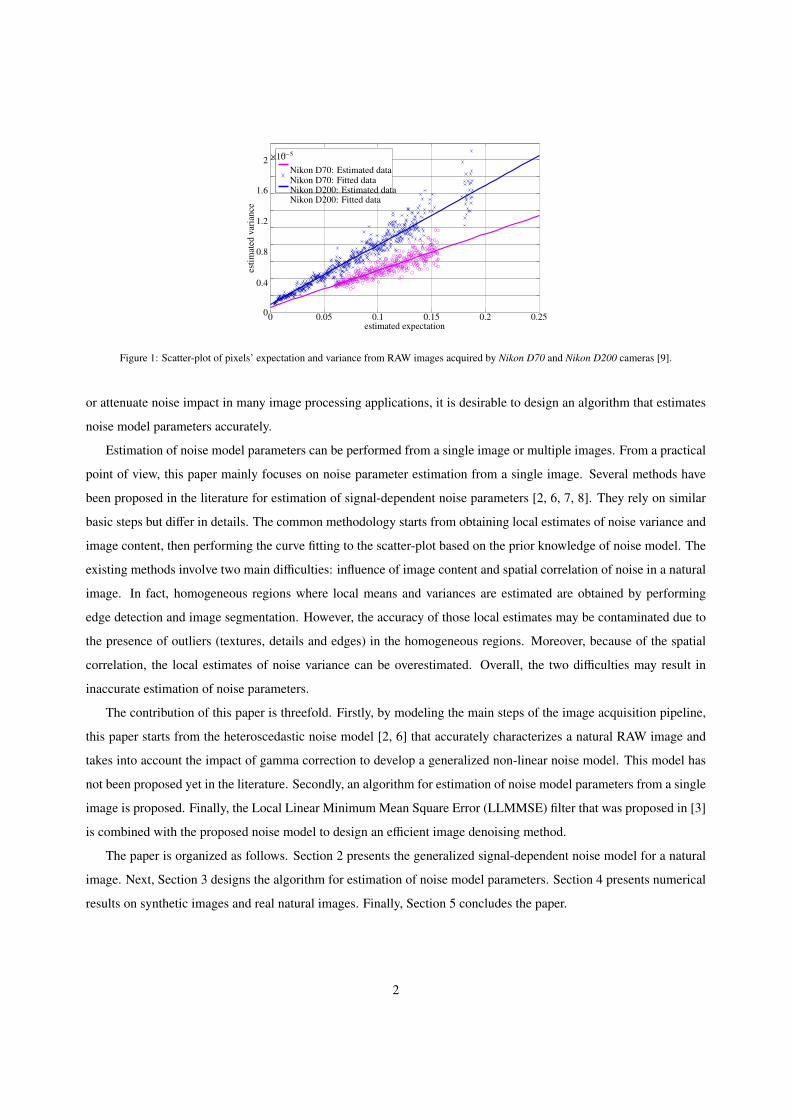
Figure 1: Scatter-plot of pixels’ expectation and variance from RAW images acquired by Nikon D70 and Nikon D200 cameras [9].
or attenuate noise impact in many image processing applications, it is desirable to design an algorithm that estimates
noise model parameters accurately.
Estimation of noise model parameters can be performed from a single image or multiple images. From a practical
point of view, this paper mainly focuses on noise parameter estimation from a single image. Several methods have
been proposed in the literature for estimation of signal-dependent noise parameters [2, 6, 7, 8]. They rely on similar
basic steps but differ in details. The common methodology starts from obtaining local estimates of noise variance and
image content, then performing the curve fitting to the scatter-plot based on the prior knowledge of noise model. The
existing methods involve two main difficulties: influence of image content and spatial correlation of noise in a natural
image. In fact, homogeneous regions where local means and variances are estimated are obtained by performing
edge detection and image segmentation. However, the accuracy of those local estimates may be contaminated due to
the presence of outliers (textures, details and edges) in the homogeneous regions. Moreover, because of the spatial
correlation, the local estimates of noise variance can be overestimated. Overall, the two difficulties may result in
inaccurate estimation of noise parameters.
The contribution of this paper is threefold. Firstly, by modeling the main steps of the image acquisition pipeline,
this paper starts from the heteroscedastic noise model [2, 6] that accurately characterizes a natural RAW image and
takes into account the impact of gamma correction to develop a generalized non-linear noise model. This model has
not been proposed yet in the literature. Secondly, an algorithm for estimation of noise model parameters from a single
image is proposed. Finally, the Local Linear Minimum Mean Square Error (LLMMSE) filter that was proposed in [3]
is combined with the proposed noise model to design an efficient image denoising method.
The paper is organized as follows. Section 2 presents the generalized signal-dependent noise model for a natural
image. Next, Section 3 designs the algorithm for estimation of noise model parameters. Section 4 presents numerical
results on synthetic images and real natural images. Finally, Section 5 concludes the paper.
2
estimated expectation µk
estim
ated
vari
anceσ
2 k
0 50 100 150 200 2500.2
0.4
0.6
0.8
1
1.2
1.4
1.6
1.8
2Nikon D70: Estimated data
Nikon D70: Fitted data
Nikon D200: Estimated data
Nikon D200: Fitted data
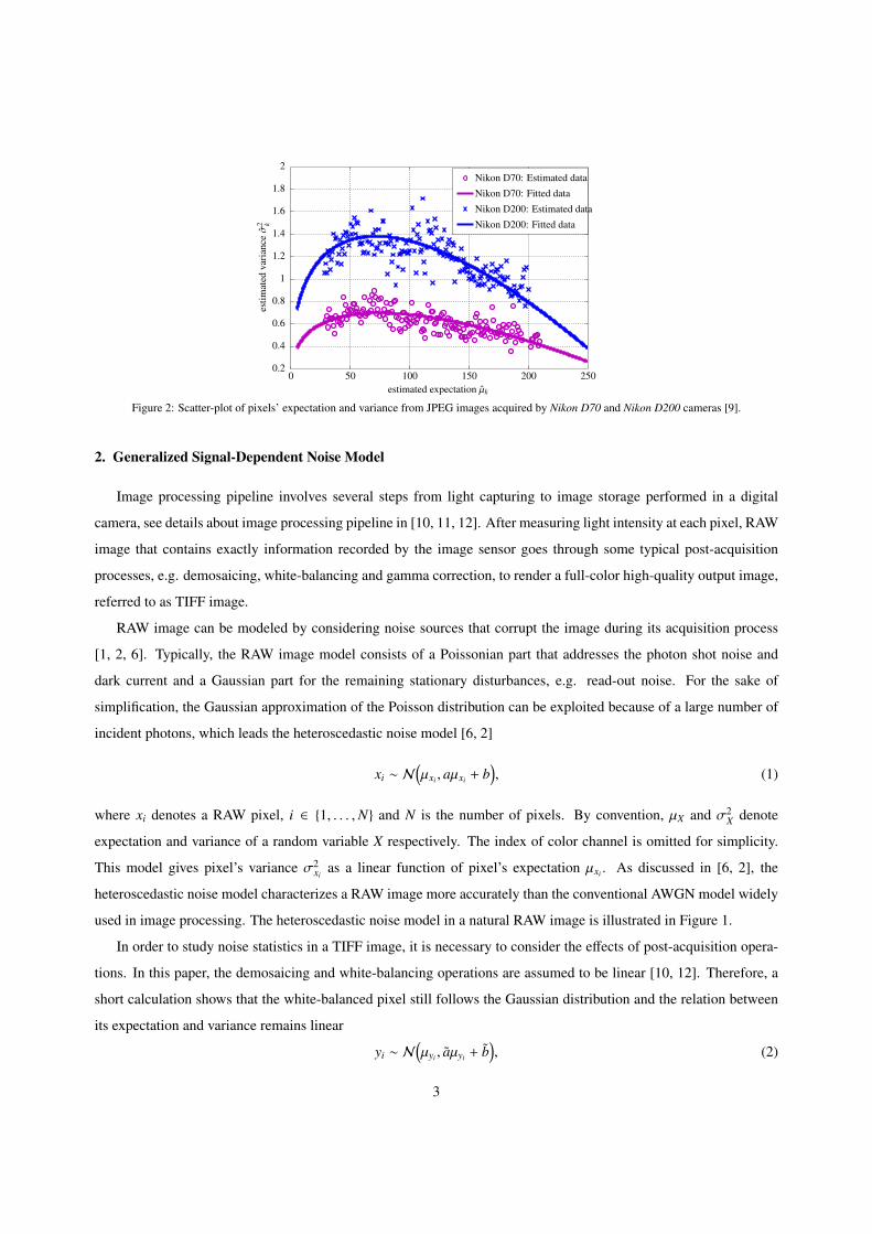
Figure 2: Scatter-plot of pixels’ expectation and variance from JPEG images acquired by Nikon D70 and Nikon D200 cameras [9].
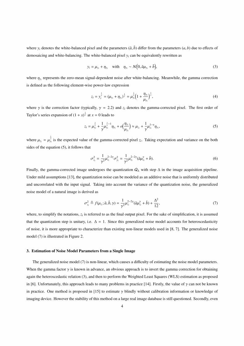
2. Generalized Signal-Dependent Noise Model
Image processing pipeline involves several steps from light capturing to image storage performed in a digital
camera, see details about image processing pipeline in [10, 11, 12]. After measuring light intensity at each pixel, RAW
image that contains exactly information recorded by the image sensor goes through some typical post-acquisition
processes, e.g. demosaicing, white-balancing and gamma correction, to render a full-color high-quality output image,
referred to as TIFF image.
RAW image can be modeled by considering noise sources that corrupt the image during its acquisition process
[1, 2, 6]. Typically, the RAW image model consists of a Poissonian part that addresses the photon shot noise and
dark current and a Gaussian part for the remaining stationary disturbances, e.g. read-out noise. For the sake of
simplification, the Gaussian approximation of the Poisson distribution can be exploited because of a large number of
incident photons, which leads the heteroscedastic noise model [6, 2]
xi ∼ N(µxi , aµxi + b
), (1)
where xi denotes a RAW pixel, i ∈ {1, . . . ,N} and N is the number of pixels. By convention, µX and σ2X denote
expectation and variance of a random variable X respectively. The index of color channel is omitted for simplicity.
This model gives pixel’s variance σ2xi
as a linear function of pixel’s expectation µxi . As discussed in [6, 2], the
heteroscedastic noise model characterizes a RAW image more accurately than the conventional AWGN model widely
used in image processing. The heteroscedastic noise model in a natural RAW image is illustrated in Figure 1.
In order to study noise statistics in a TIFF image, it is necessary to consider the effects of post-acquisition opera-
tions. In this paper, the demosaicing and white-balancing operations are assumed to be linear [10, 12]. Therefore, a
short calculation shows that the white-balanced pixel still follows the Gaussian distribution and the relation between
its expectation and variance remains linear
yi ∼ N(µyi , aµyi + b
), (2)
3
where yi denotes the white-balanced pixel and the parameters (a, b) differ from the parameters (a, b) due to effects of
demosaicing and white-balancing. The white-balanced pixel yi can be equivalently rewritten as
yi = µyi + ηyi with ηyi ∼ N(0, aµyi + b
), (3)
where ηyi represents the zero-mean signal-dependent noise after white-balancing. Meanwhile, the gamma correction
is defined as the following element-wise power-law expression
zi = y1γ
i = (µyi + ηyi )1γ = µ
1γ
yi
(1 +
ηyi
µyi
) 1γ, (4)
where γ is the correction factor (typically, γ = 2.2) and zi denotes the gamma-corrected pixel. The first order of
Taylor’s series expansion of (1 + x)1γ at x = 0 leads to
zi = µ1γ
yi +1γµ
1γ−1yi ηyi + o
(ηyi
µyi
)≈ µzi +
1γµ
1−γzi ηyi , (5)
where µzi = µ1γ
yi is the expected value of the gamma-corrected pixel zi. Taking expectation and variance on the both
sides of the equation (5), it follows that
σ2zi
=1γ2 µ
2−2γzi σ2
yi=
1γ2 µ
2−2γzi (aµγzi + b). (6)
Finally, the gamma-corrected image undergoes the quantization Q∆ with step ∆ in the image acquisition pipeline.
Under mild assumptions [13], the quantization noise can be modeled as an additive noise that is uniformly distributed
and uncorrelated with the input signal. Taking into account the variance of the quantization noise, the generalized
noise model of a natural image is derived as
σ2zi, f (µzi ; a, b, γ) =
1γ2 µ
2−2γzi (aµγzi + b) +
∆2
12, (7)
where, to simplify the notations, zi is referred to as the final output pixel. For the sake of simplification, it is assumed
that the quantization step is unitary, i.e. ∆ = 1. Since this generalized noise model accounts for heteroscedasticity
of noise, it is more appropriate to characterize than existing non-linear models used in [8, 7]. The generalized noise
model (7) is illustrated in Figure 2.
3. Estimation of Noise Model Parameters from a Single Image
The generalized noise model (7) is non-linear, which causes a difficulty of estimating the noise model parameters.
When the gamma factor γ is known in advance, an obvious approach is to invert the gamma correction for obtaining
again the heteroscedastic relation (3), and then to perform the Weighted Least Squares (WLS) estimation as proposed
in [6]. Unfortunately, this approach leads to many problems in practice [14]. Firstly, the value of γ can not be known
in practice. One method is proposed in [15] to estimate γ blindly without calibration information or knowledge of
imaging device. However the stability of this method on a large real image database is still questioned. Secondly, even
4
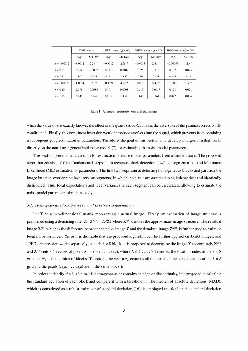
TIFF images JPEG images (Q = 90) JPEG images (Q = 80) JPEG images (Q = 70)
Avg Std Dev Avg Std Dev Avg Std Dev Avg Std Dev
a = −0.0012 −0.0012 2.2e−4 −0.0012 2.5e−4 −0.0013 2.8e−4 −0.00095 4.1e−4
b = 0.11 0.114 0.0097 0.117 0.0102 0.126 0.015 0.132 0.025
γ = 0.8 0.807 0.053 0.811 0.057 0.79 0.058 0.814 0.11
a = −0.0025 −0.0024 3.5e−4 −0.0024 4.2e−4 −0.0026 5.4e−4 −0.0023 5.8e−4
b = 0.20 0.196 0.0084 0.191 0.0098 0.215 0.0117 0.191 0.021
γ = 0.85 0.845 0.049 0.853 0.058 0.845 0.061 0.842 0.086
Table 1: Parameter estimation on synthetic images
when the value of γ is exactly known, the effect of the quantizationQ∆ makes the inversion of the gamma correction ill-
conditioned. Finally, this non-linear inversion would introduce artefacts into the signal, which prevents from obtaining
a subsequent good estimation of parameters. Therefore, the goal of this section is to develop an algorithm that works
directly on the non-linear generalized noise model (7) for estimating the noise model parameters.
This section presents an algorithm for estimation of noise model parameters from a single image. The proposed
algorithm consists of three fundamental steps: homogeneous block detection, level-set segmentation, and Maximum
Likelihood (ML) estimation of parameters. The first two steps aim at detecting homogeneous blocks and partition the
image into non-overlapping level sets (or segments) in which the pixels are assumed to be independent and identically
distributed. Thus local expectations and local variances in each segment can be calculated, allowing to estimate the
noise model parameters simultaneously.
3.1. Homogeneous Block Detection and Level-Set Segmentation
Let Z be a two-dimensional matrix representing a natural image. Firstly, an estimation of image structure is
performed using a denoising filterD: Zapp = D(Z) where Zapp denotes the approximate image structure. The residual
image Zres, which is the difference between the noisy image Z and the denoised image Zapp, is further used to estimate
local noise variances. Since it is desirable that the proposed algorithm can be further applied on JPEG images, and
JPEG compression works separately on each 8 × 8 block, it is proposed to decompose the image Z (accordingly Zapp
and Zres) into 64 vectors of pixels zL = (zL,1, . . . , zL,Nb ), where L ∈ {1, . . . , 64} denotes the location index in the 8 × 8
grid and Nb is the number of blocks. Therefore, the vector zL contains all the pixels at the same location of the 8 × 8
grid and the pixels (z1,B, . . . , z64,B) are in the same block B.
In order to identify if a 8×8 block is homogeneous or contains an edge or discontinuity, it is proposed to calculate
the standard deviation of each block and compare it with a threshold τ. The median of absolute deviations (MAD),
which is considered as a robust estimator of standard deviation [16], is employed to calculate the standard deviation
5
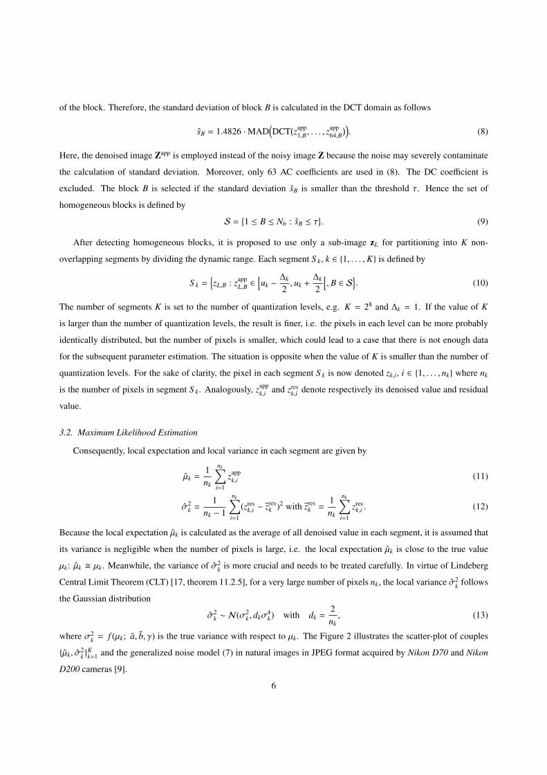
of the block. Therefore, the standard deviation of block B is calculated in the DCT domain as follows
sB = 1.4826 ·MAD(DCT
(zapp
1,B , . . . , zapp64,B
)). (8)
Here, the denoised image Zapp is employed instead of the noisy image Z because the noise may severely contaminate
the calculation of standard deviation. Moreover, only 63 AC coefficients are used in (8). The DC coefficient is
excluded. The block B is selected if the standard deviation sB is smaller than the threshold τ. Hence the set of
homogeneous blocks is defined by
S ={1 ≤ B ≤ Nb : sB ≤ τ
}. (9)
After detecting homogeneous blocks, it is proposed to use only a sub-image zL for partitioning into K non-
overlapping segments by dividing the dynamic range. Each segment S k, k ∈ {1, . . . ,K} is defined by
S k ={zL,B : zapp
L,B ∈[uk −
∆k
2, uk +
∆k
2
[, B ∈ S
}. (10)
The number of segments K is set to the number of quantization levels, e.g. K = 28 and ∆k = 1. If the value of K
is larger than the number of quantization levels, the result is finer, i.e. the pixels in each level can be more probably
identically distributed, but the number of pixels is smaller, which could lead to a case that there is not enough data
for the subsequent parameter estimation. The situation is opposite when the value of K is smaller than the number of
quantization levels. For the sake of clarity, the pixel in each segment S k is now denoted zk,i, i ∈ {1, . . . , nk} where nk
is the number of pixels in segment S k. Analogously, zappk,i and zres
k,i denote respectively its denoised value and residual
value.
3.2. Maximum Likelihood Estimation
Consequently, local expectation and local variance in each segment are given by
µk =1nk
nk∑i=1
zappk,i (11)
σ2k =
1nk − 1
nk∑i=1
(zresk,i − zres
k )2 with zresk =
1nk
nk∑i=1
zresk,i . (12)
Because the local expectation µk is calculated as the average of all denoised value in each segment, it is assumed that
its variance is negligible when the number of pixels is large, i.e. the local expectation µk is close to the true value
µk: µk � µk. Meanwhile, the variance of σ2k is more crucial and needs to be treated carefully. In virtue of Lindeberg
Central Limit Theorem (CLT) [17, theorem 11.2.5], for a very large number of pixels nk, the local variance σ2k follows
the Gaussian distribution
σ2k ∼ N(σ2
k , dkσ4k) with dk =
2nk, (13)
where σ2k = f (µk; a, b, γ) is the true variance with respect to µk. The Figure 2 illustrates the scatter-plot of couples
{µk, σ2k}
Kk=1 and the generalized noise model (7) in natural images in JPEG format acquired by Nikon D70 and Nikon
D200 cameras [9].
6
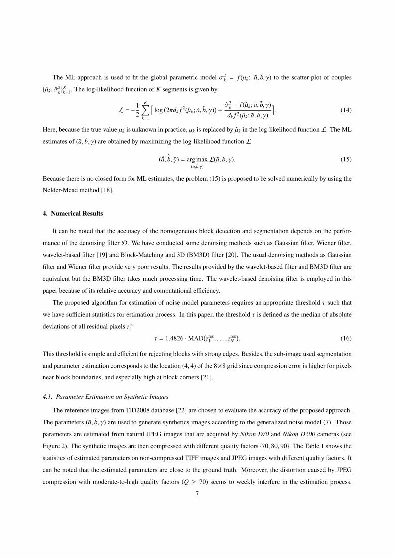
The ML approach is used to fit the global parametric model σ2k = f (µk; a, b, γ) to the scatter-plot of couples
{µk, σ2k}
Kk=1. The log-likelihood function of K segments is given by
L = −12
K∑k=1
[log
(2πdk f 2(µk; a, b, γ)
)+σ2
k − f (µk; a, b, γ)
dk f 2(µk; a, b, γ)
]. (14)
Here, because the true value µk is unknown in practice, µk is replaced by µk in the log-likelihood function L. The ML
estimates of (a, b, γ) are obtained by maximizing the log-likelihood function L
( ˆa, ˆb, γ) = arg max(a,b,γ)
L(a, b, γ). (15)
Because there is no closed form for ML estimates, the problem (15) is proposed to be solved numerically by using the
Nelder-Mead method [18].
4. Numerical Results
It can be noted that the accuracy of the homogeneous block detection and segmentation depends on the perfor-
mance of the denoising filter D. We have conducted some denoising methods such as Gaussian filter, Wiener filter,
wavelet-based filter [19] and Block-Matching and 3D (BM3D) filter [20]. The usual denoising methods as Gaussian
filter and Wiener filter provide very poor results. The results provided by the wavelet-based filter and BM3D filter are
equivalent but the BM3D filter takes much processing time. The wavelet-based denoising filter is employed in this
paper because of its relative accuracy and computational efficiency.
The proposed algorithm for estimation of noise model parameters requires an appropriate threshold τ such that
we have sufficient statistics for estimation process. In this paper, the threshold τ is defined as the median of absolute
deviations of all residual pixels zresi
τ = 1.4826 ·MAD(zres
1 , . . . , zresN
). (16)
This threshold is simple and efficient for rejecting blocks with strong edges. Besides, the sub-image used segmentation
and parameter estimation corresponds to the location (4, 4) of the 8×8 grid since compression error is higher for pixels
near block boundaries, and especially high at block corners [21].
4.1. Parameter Estimation on Synthetic Images
The reference images from TID2008 database [22] are chosen to evaluate the accuracy of the proposed approach.
The parameters (a, b, γ) are used to generate synthetics images according to the generalized noise model (7). Those
parameters are estimated from natural JPEG images that are acquired by Nikon D70 and Nikon D200 cameras (see
Figure 2). The synthetic images are then compressed with different quality factors {70, 80, 90}. The Table 1 shows the
statistics of estimated parameters on non-compressed TIFF images and JPEG images with different quality factors. It
can be noted that the estimated parameters are close to the ground truth. Moreover, the distortion caused by JPEG
compression with moderate-to-high quality factors (Q ≥ 70) seems to weekly interfere in the estimation process.
7
a
b
-0.007 -0.006 -0.005 -0.004 -0.003 -0.002 -0.001 00
0.1
0.2
0.3
0.4
0.5
0.6
0.7Canon Ixus 55Nikon D70Nikon D200Canon Ixus 70
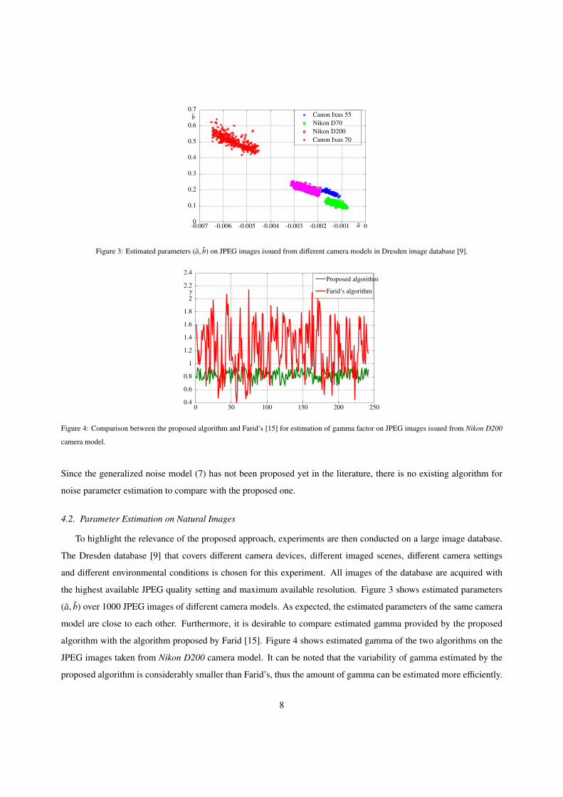
Figure 3: Estimated parameters (a, b) on JPEG images issued from different camera models in Dresden image database [9].
γ
0 50 100 150 200 2500.4
0.6
0.8
1
1.2
1.4
1.6
1.8
2
2.2
2.4Proposed algorithm
Farid’s algorithm
Figure 4: Comparison between the proposed algorithm and Farid’s [15] for estimation of gamma factor on JPEG images issued from Nikon D200
camera model.
Since the generalized noise model (7) has not been proposed yet in the literature, there is no existing algorithm for
noise parameter estimation to compare with the proposed one.
4.2. Parameter Estimation on Natural Images
To highlight the relevance of the proposed approach, experiments are then conducted on a large image database.
The Dresden database [9] that covers different camera devices, different imaged scenes, different camera settings
and different environmental conditions is chosen for this experiment. All images of the database are acquired with
the highest available JPEG quality setting and maximum available resolution. Figure 3 shows estimated parameters
(a, b) over 1000 JPEG images of different camera models. As expected, the estimated parameters of the same camera
model are close to each other. Furthermore, it is desirable to compare estimated gamma provided by the proposed
algorithm with the algorithm proposed by Farid [15]. Figure 4 shows estimated gamma of the two algorithms on the
JPEG images taken from Nikon D200 camera model. It can be noted that the variability of gamma estimated by the
proposed algorithm is considerably smaller than Farid’s, thus the amount of gamma can be estimated more efficiently.
8
4.3. Application to Image Denoising
To highlight the usefulness of the generalized noise model (7), it is proposed to combine it with the LLMMSE
filter [3] to design an efficient image denoising method. The LLMMSE filter is based on the non-stationary mean,
non-stationary variance image model. From (5), the pixel z can be decomposed as
z = u +1γ
u1−γηu, (17)
where u denotes the original pixel and ηu is the zero-mean signal-dependent noise, σ2ηu
= aµγu + b. The index of
pixel is omitted for the sake of clarity. The original pixel u involves non-stationary mean and non-stationary variance.
The non-stationary mean describes the gross structure of an image and the non-stationary variance characterizes edge
information of the image [3]. In the decomposition (17), the quantization noise is assumed to be negligible. As
explained in [3], the LLMMSE filter for any signal-dependent noise model is formulated as
u =(1 −
σ2u
σ2z
)µz +
σ2u
σ2z
z, (18)
where µz and σ2z are respectively local mean and local variance of the pixel z, µu and σ2
u are respectively local mean
and local variance of the original pixel u. Since the noise ηu is zero-mean, it follows from (17) that µz = µu. The
LLMMSE filter (18) is the weighted sum of original signal mean µu and the noisy observation z where the weight is
determined as the ratio of the original signal variance and noise variance. A simple technique to obtain local statistics
µz and σ2z is to calculate over a sliding window of size (2r + 1) × (2c + 1)
µz(m, n) =1
(2r + 1)(2c + 1)
m+r∑i=m−r
n+c∑j=n−c
z(i, j), (19)
σ2z (m, n) =
1(2r + 1)(2c + 1)
m+r∑i=m−r
n+c∑j=n−c(
z(i, j) − µz(m, n))2. (20)
Therefore, it remains to calculate the variance σ2u. From (17), the variance σ2
z can be given by
σ2z = σ2
u +1γ2 E
[u2−2γ]σ2
ηu. (21)
By using the Taylor series expansion of u2−2γ around µu, the expression of E[u2−2γ] can be simplified as
E[u2−2γ] = µ
2−2γu + (1 − γ)(1 − 2γ)µ−2γ
u σ2u. (22)
Combining (21) and (22), the expression of the variance σ2u is derived as
σ2u =
σ2z −
1γ2 µ
2−2γu σ2
ηu
1 + 1γ2 (1 − γ)(1 − 2γ)µ−2γ
u σ2ηu
. (23)
The LLMSSE filter (18) follows immediately.
9
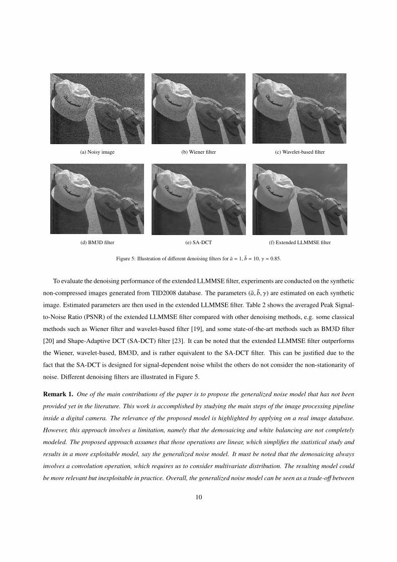
(a) Noisy image (b) Wiener filter (c) Wavelet-based filter
(d) BM3D filter (e) SA-DCT (f) Extended LLMMSE filter
Figure 5: Illustration of different denoising filters for a = 1, b = 10, γ = 0.85.
To evaluate the denoising performance of the extended LLMMSE filter, experiments are conducted on the synthetic
non-compressed images generated from TID2008 database. The parameters (a, b, γ) are estimated on each synthetic
image. Estimated parameters are then used in the extended LLMMSE filter. Table 2 shows the averaged Peak Signal-
to-Noise Ratio (PSNR) of the extended LLMMSE filter compared with other denoising methods, e.g. some classical
methods such as Wiener filter and wavelet-based filter [19], and some state-of-the-art methods such as BM3D filter
[20] and Shape-Adaptive DCT (SA-DCT) filter [23]. It can be noted that the extended LLMMSE filter outperforms
the Wiener, wavelet-based, BM3D, and is rather equivalent to the SA-DCT filter. This can be justified due to the
fact that the SA-DCT is designed for signal-dependent noise whilst the others do not consider the non-stationarity of
noise. Different denoising filters are illustrated in Figure 5.
Remark 1. One of the main contributions of the paper is to propose the generalized noise model that has not been
provided yet in the literature. This work is accomplished by studying the main steps of the image processing pipeline
inside a digital camera. The relevance of the proposed model is highlighted by applying on a real image database.
However, this approach involves a limitation, namely that the demosaicing and white balancing are not completely
modeled. The proposed approach assumes that those operations are linear, which simplifies the statistical study and
results in a more exploitable model, say the generalized noise model. It must be noted that the demosaicing always
involves a convolution operation, which requires us to consider multivariate distribution. The resulting model could
be more relevant but inexploitable in practice. Overall, the generalized noise model can be seen as a trade-off between
10
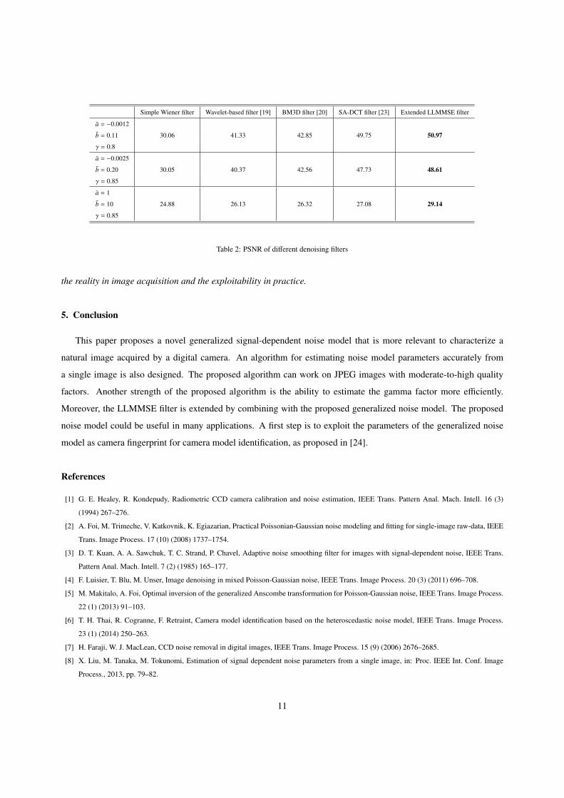
Simple Wiener filter Wavelet-based filter [19] BM3D filter [20] SA-DCT filter [23] Extended LLMMSE filter
a = −0.0012
b = 0.11 30.06 41.33 42.85 49.75 50.97
γ = 0.8
a = −0.0025
b = 0.20 30.05 40.37 42.56 47.73 48.61
γ = 0.85
a = 1
b = 10 24.88 26.13 26.32 27.08 29.14
γ = 0.85
Table 2: PSNR of different denoising filters
the reality in image acquisition and the exploitability in practice.
5. Conclusion
This paper proposes a novel generalized signal-dependent noise model that is more relevant to characterize a
natural image acquired by a digital camera. An algorithm for estimating noise model parameters accurately from
a single image is also designed. The proposed algorithm can work on JPEG images with moderate-to-high quality
factors. Another strength of the proposed algorithm is the ability to estimate the gamma factor more efficiently.
Moreover, the LLMMSE filter is extended by combining with the proposed generalized noise model. The proposed
noise model could be useful in many applications. A first step is to exploit the parameters of the generalized noise
model as camera fingerprint for camera model identification, as proposed in [24].
References
[1] G. E. Healey, R. Kondepudy, Radiometric CCD camera calibration and noise estimation, IEEE Trans. Pattern Anal. Mach. Intell. 16 (3)
(1994) 267–276.
[2] A. Foi, M. Trimeche, V. Katkovnik, K. Egiazarian, Practical Poissonian-Gaussian noise modeling and fitting for single-image raw-data, IEEE
Trans. Image Process. 17 (10) (2008) 1737–1754.
[3] D. T. Kuan, A. A. Sawchuk, T. C. Strand, P. Chavel, Adaptive noise smoothing filter for images with signal-dependent noise, IEEE Trans.
Pattern Anal. Mach. Intell. 7 (2) (1985) 165–177.
[4] F. Luisier, T. Blu, M. Unser, Image denoising in mixed Poisson-Gaussian noise, IEEE Trans. Image Process. 20 (3) (2011) 696–708.
[5] M. Makitalo, A. Foi, Optimal inversion of the generalized Anscombe transformation for Poisson-Gaussian noise, IEEE Trans. Image Process.
22 (1) (2013) 91–103.
[6] T. H. Thai, R. Cogranne, F. Retraint, Camera model identification based on the heteroscedastic noise model, IEEE Trans. Image Process.
23 (1) (2014) 250–263.
[7] H. Faraji, W. J. MacLean, CCD noise removal in digital images, IEEE Trans. Image Process. 15 (9) (2006) 2676–2685.
[8] X. Liu, M. Tanaka, M. Tokunomi, Estimation of signal dependent noise parameters from a single image, in: Proc. IEEE Int. Conf. Image
Process., 2013, pp. 79–82.
11
[9] T. Gloe, R. Bohme, The Dresden image database for benchmarking digital image forensics, in: Proc. ACM Symposium Applied Comput.,
Vol. 2, 2010, pp. 1585–1591.
[10] R. Ramanath, W. E. Snyder, Y. Yoo, M. S. Drew, Color image processing pipeline, IEEE Signal Process. Mag. 22 (1) (2005) 34–43.
[11] T. H. Thai, R. Cogranne, F. Retraint, Statistical model of natural images, in: Proc. IEEE. Int. Conf. Image Process., 2012, pp. 2525–2528.
[12] T. H. Thai, R. Cogranne, F. Retraint, Statistical model of quantized DCT coefficients: Application in the steganalysis of Jsteg algorithm, IEEE
Trans. Image Process. 23 (5) (2014) 1980–1993.
[13] B. Widrow, I. Kollar, M.-C. Liu, Statistical theory of quantization, IEEE Trans. Instrum. Meas. 45 (2) (1996) 353–361.
[14] R. P. Kleihorst, R. L. Lagendiik, J. Biemond, An adaptive order-statistic noise filter for gamma-corrected image sequences, IEEE Trans.
Image Process. 6 (10) (1997) 1442–1446.
[15] H. Farid, Blind inverse gamma correction, IEEE Trans. Image Process. 10 (10) (2001) 1428–1433.
[16] P. J. Rousseeuw, C. Croux, Alternatives to the median absolute deviation, J. Amer. Statist. Assoc. 88 (424) (1993) 1273–1283.
[17] E. L. Lehmann, J. P. Romano, Testing Statistical Hypotheses, 3rd Edition, Springer, New york, 2005.
[18] J. A. Nelder, R. Mead, A simplex method for function minimization, Comput. J. 7 (1965) 308–313.
[19] M. K. Mihçak, I. Kozintsev, K. Ramchandran, Spatially adaptive statistical modeling of wavelet image coefficients and its application to
denoising, in: Proc. IEEE Int. Conf. Acoust., Speech, Signal Process., Vol. 6, 1999, pp. 3253–3256.
[20] K. Dabov, A. Foi, V. Katkovnik, K. Egiazarian, Image denoising by sparse 3-d transform-domain collaborative filtering, IEEE Trans. Image
Process. 16 (8) (2007) 2080–2095.
[21] M. A. Robertson, R. L. Stevenson, DCT quantization noise in compressed images, IEEE Trans. Circuits Syst. Video Technol. 15 (1) (2005)
27–38.
[22] N. Ponomarenko, V. Lukin, A. Zelensky, K. Egiazarian, M. Carli, F. Battisti, TID2008 - a database for evaluation of full-reference visual
quality assessment metrics, Advances Modern Radioelectronics 10 (2009) 30–45.
[23] A. Foi, V. Katkovnik, K. Egiazarian, Pointwise shape-adaptive DCT for high-quality denoising and deblocking of grayscale and color images,
IEEE Trans. Image Process., 16 (5) (2007) 1395–1411.
[24] T. H. Thai, F. Retraint, R. Cogranne, Camera model identification based on generalized noise model in natural images, Signal Processing,
48 (1), (2016) 285–297.
12