Generalization and Localization Based Style Imitation for Grayscale Images

Fatih NAR1, Atılım ÇETİN2

1 Informatics Institute, Middle East Technical University, fatihnar@ii.metu.edu.tr

2 Department of Computer Engineering, Bilkent University, atilim@cs.bilkent.edu.tr

Abstract. An example based rendering (EBR) method based on generalization and localization that uses artificial neural networks (ANN) and k-Nearest Neighbor (k-NN) is proposed. The method involves learning phase and applica-tion phase, which means that once a transformation filter is learned, it can be applied to any other image. In learning phase, error back-propagation learning algorithm is used to learn general transformation filter using unfiltered source image and filtered output image. ANNs are usually unable to learn filter-generated textures and brush strokes hence these localized features are stored in a feature instance table for using with k-NN during application phase. In appli-cation phase, for any given grayscale image, first ANN is applied then k-NN search is used to retrieve local features from feature instances considering tex-ture continuity to produce desired image. Proposed method is applied up to 40 image filters that are collection of computer-generated and human-generated ef-fects/styles. Good results are obtained when image is composed of localized texture/style features that are only dependent to intensity values of pixel itself and its neighbors.

1 Introduction

In recent years, researchers within computer graphics and computer vision com-munities put a great effort on example based rendering, non-photorealistic rendering (NPR), and texture synthesis. They use various methods from other disciplines such as machine learning, and image processing. EBR is an useful tool for creating anima-tions and images for various purposes such as imitation of styles, creating educational softwares for children, and creating video games in cartoon world for entertainment with less human effort [8]. These styles/effects, that are aimed to imitate can be hu-man-generated or computer-generated.

Ultimate aim of EBR is creating an analogous image for a given unfiltered image using unfiltered and filtered image pairs. In short, it is style imitation as seen in Fig-ure 1. Ideally the filter learned from an image pair must be sufficient for creating an analogous image for any image even the filter is a complex or non-linear one such as artistic styles or traditional image filters [6].

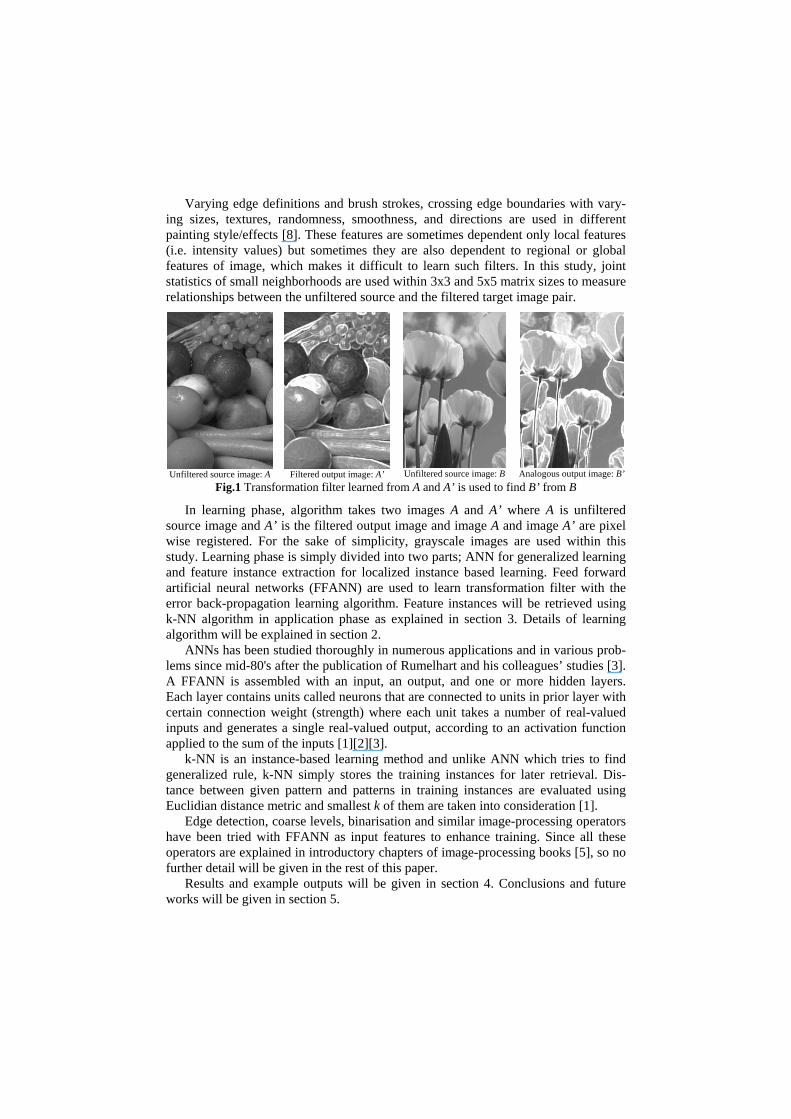
Varying edge definitions and brush strokes, crossing edge boundaries with vary-ing sizes, textures, randomness, smoothness, and directions are used in different painting style/effects [8]. These features are sometimes dependent only local features (i.e. intensity values) but sometimes they are also dependent to regional or global features of image, which makes it difficult to learn such filters. In this study, joint statistics of small neighborhoods are used within 3x3 and 5x5 matrix sizes to measure relationships between the unfiltered source and the filtered target image pair.

Unfiltered source image: A

Filtered output image: A’

Unfiltered source image: B

Analogous output image: B’

Fig.1 Transformation filter learned from A and A’ is used to find B’ from B

In learning phase, algorithm takes two images A and A’ where A is unfiltered source image and A’ is the filtered output image and image A and image A’ are pixel wise registered. For the sake of simplicity, grayscale images are used within this study. Learning phase is simply divided into two parts; ANN for generalized learning and feature instance extraction for localized instance based learning. Feed forward artificial neural networks (FFANN) are used to learn transformation filter with the error back-propagation learning algorithm. Feature instances will be retrieved using k-NN algorithm in application phase as explained in section 3. Details of learning algorithm will be explained in section 2.

ANNs has been studied thoroughly in numerous applications and in various prob-lems since mid-80's after the publication of Rumelhart and his colleagues’ studies [3]. A FFANN is assembled with an input, an output, and one or more hidden layers. Each layer contains units called neurons that are connected to units in prior layer with certain connection weight (strength) where each unit takes a number of real-valued inputs and generates a single real-valued output, according to an activation function applied to the sum of the inputs [1][2][3].

k-NN is an instance-based learning method and unlike ANN which tries to find generalized rule, k-NN simply stores the training instances for later retrieval. Dis-tance between given pattern and patterns in training instances are evaluated using Euclidian distance metric and smallest k of them are taken into consideration [1].

Edge detection, coarse levels, binarisation and similar image-processing operators have been tried with FFANN as input features to enhance training. Since all these operators are explained in introductory chapters of image-processing books [5], so no further detail will be given in the rest of this paper.

Results and example outputs will be given in section 4. Conclusions and future works will be given in section 5.

2 Learning Phase

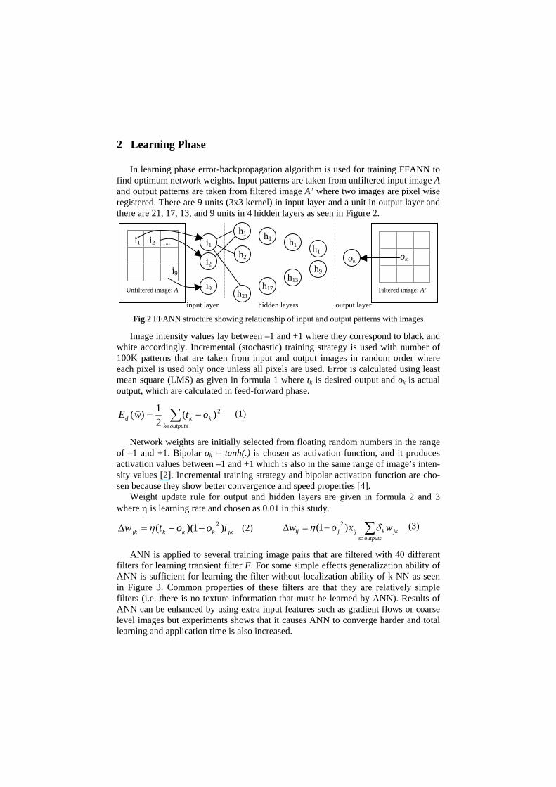
In learning phase error-backpropagation algorithm is used for training FFANN to find optimum network weights. Input patterns are taken from unfiltered input image A and output patterns are taken from filtered image A’ where two images are pixel wise registered. There are 9 units (3x3 kernel) in input layer and a unit in output layer and there are 21, 17, 13, and 9 units in 4 hidden layers as seen in Figure 2.

input layer hidden layers output layer

Unfiltered image: A

Filtered image: A’

i1 i2 ...

i9

ok

i1

i2

i9

h1

h2

h21

ok

h1

h17

h1

h13

h1

h9

Fig.2 FFANN structure showing relationship of input and output patterns with images

Image intensity values lay between –1 and +1 where they correspond to black and white accordingly. Incremental (stochastic) training strategy is used with number of 100K patterns that are taken from input and output images in random order where each pixel is used only once unless all pixels are used. Error is calculated using least mean square (LMS) as given in formula 1 where tk is desired output and ok is actual output, which are calculated in feed-forward phase.

∑∈

−=outputsk

kkd otwE 2)(21)( v (1)

Network weights are initially selected from floating random numbers in the range of –1 and +1. Bipolar ok = tanh(.) is chosen as activation function, and it produces activation values between –1 and +1 which is also in the same range of image’s inten-sity values [2]. Incremental training strategy and bipolar activation function are cho-sen because they show better convergence and speed properties [4].

Weight update rule for output and hidden layers are given in formula 2 and 3 where η is learning rate and chosen as 0.01 in this study.

jkkkkjk iootw )1)(( 2−−=∆ η (2) ∑∈

−=∆outputss

jkkijjij wxow δη )1( 2 (3)

ANN is applied to several training image pairs that are filtered with 40 different filters for learning transient filter F. For some simple effects generalization ability of ANN is sufficient for learning the filter without localization ability of k-NN as seen in Figure 3. Common properties of these filters are that they are relatively simple filters (i.e. there is no texture information that must be learned by ANN). Results of ANN can be enhanced by using extra input features such as gradient flows or coarse level images but experiments shows that it causes ANN to converge harder and total learning and application time is also increased.

Fig.3 Original image and output images (emboss, inverse, solarize) produced by ANN

ANN is good at generalization but provides very weak results at memorization es-

pecially when filter contains extra information such as textures and brush strokes, which cause information-gain in output image. Difference of original image A and filtered image A’ can give us texture information as seen in top right image (D’) in Figure 4. Despite ANN cannot help us to memorize that textural information, it is still valuable tool for extracting this texture information better than simply finding D’. In bottom right image (Figure 4) you can see image D” which is the subtraction of fil-tered image A’ and output image A” that is produced by ANN. This new difference map D”, which acts as texture map for us, is convolved with 5x5 kernel and when-ever the value of middle point in kernel is different than zero (or very near to zero), this pattern is stored in indexes H1 and H2 (intensities that are taken from A”: H1 and intensities that are taken from D, D equals to D’ or D”, itself: H2) for later retrieval with k-NN in application phase. In this pattern, 25 intensity values and position of patterns are kept. As you can see in image D’, total numbers of patterns that will be stored is much more comparing to image D” since image D’ contains much more nonzero intensity values comparing to image D”. Hence memory consumption and query time in application phase is dramatically decreased if image D” is used instead of using image D’ for image pairs A and A’ in Figure 4. So the method proposed in this paper is based on the observation that ANN provides good texture extraction from filtered and unfiltered images for texture synthesis for some cases. In other cases texture map D’ contains more nonzero intensity values comparing to D” so D’ is used instead of D” in such cases.

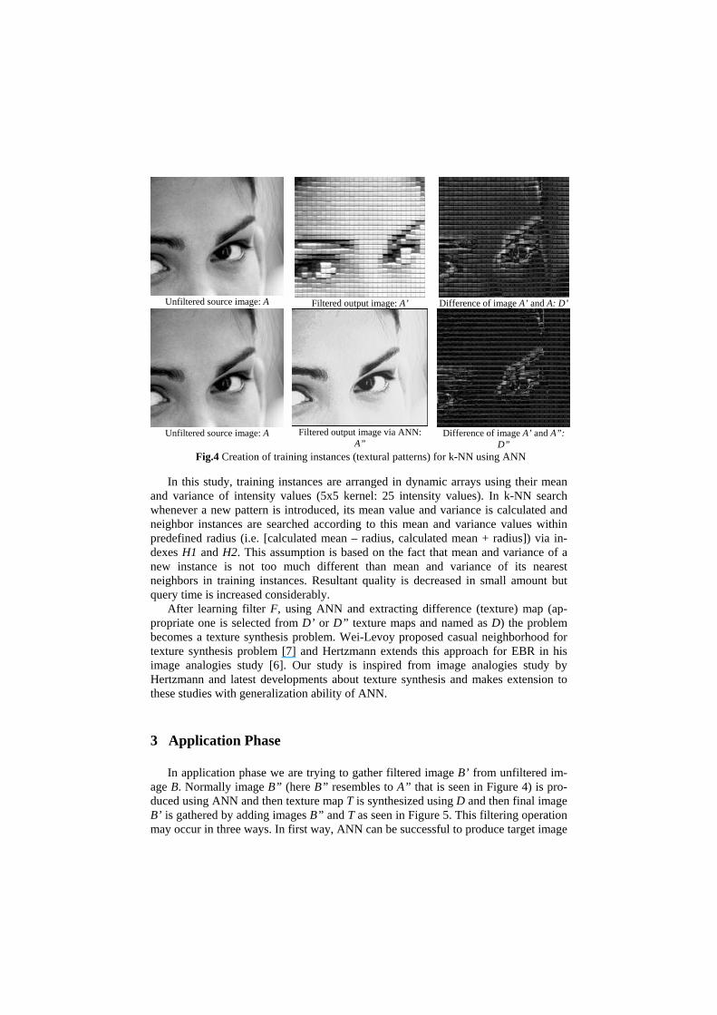
Unfiltered source image: A

Filtered output image: A’

Difference of image A’ and A: D’

Unfiltered source image: A Filtered output image via ANN:

A”

Difference of image A’ and A”:

D” Fig.4 Creation of training instances (textural patterns) for k-NN using ANN

In this study, training instances are arranged in dynamic arrays using their mean

and variance of intensity values (5x5 kernel: 25 intensity values). In k-NN search whenever a new pattern is introduced, its mean value and variance is calculated and neighbor instances are searched according to this mean and variance values within predefined radius (i.e. [calculated mean – radius, calculated mean + radius]) via in-dexes H1 and H2. This assumption is based on the fact that mean and variance of a new instance is not too much different than mean and variance of its nearest neighbors in training instances. Resultant quality is decreased in small amount but query time is increased considerably.

After learning filter F, using ANN and extracting difference (texture) map (ap-propriate one is selected from D’ or D” texture maps and named as D) the problem becomes a texture synthesis problem. Wei-Levoy proposed casual neighborhood for texture synthesis problem [7] and Hertzmann extends this approach for EBR in his image analogies study [6]. Our study is inspired from image analogies study by Hertzmann and latest developments about texture synthesis and makes extension to these studies with generalization ability of ANN.

3 Application Phase

In application phase we are trying to gather filtered image B’ from unfiltered im-age B. Normally image B” (here B” resembles to A” that is seen in Figure 4) is pro-duced using ANN and then texture map T is synthesized using D and then final image B’ is gathered by adding images B” and T as seen in Figure 5. This filtering operation may occur in three ways. In first way, ANN can be successful to produce target image

as seen in Figure 3 so image produced by ANN (B”) is considered as B’ and no fur-ther process is necessary. In second way, ANN is unsuccessful to extract texture so D’ is taken as D and B” is just equals to B, further processes are just same with third way. In third way, image B” is produced using ANN and then texture T is synthe-sized using D (which equals to D” for third way) and then final image B’ is gathered by adding images B” and T as seen in Figure 5.

Image B” is convolved with 5x5 kernel and for each pattern that are taken from B” its k nearest neighbor (k=16) in difference map D is found (using H1 index). T is a texture information which we try to synthesis to merge with B” (by image addition) for producing final image B’. Here we want to make T resembles to D. Since T must contain continuous texture, k neighbor of T itself is found (using H2 index and casual neighborhood [7] as seen in Figure 6) and then T is produced using nearest neighbor of these two k neighbor set. For finding two k neighbor set, similarity measure is intensity values whereas for finding nearest neighbor of these two sets similarity measure is pixels’ positions.

B

B”

T B’

H2D’ or D”

(D)

H1

Fig.5 Process schema of creating image B’ from B using indexes H1, H2 and texture D

Pixel intensity value at P(x, y) in image B’ is B’(x, y) = B”(x, y) + T(x, y) where values less than –1 are set as –1 and values greater than +1 are set as +1. We know the value of B”(x, y) since B” = F(B) or B. Only the value we do not know is T(x, y) and it can be found using the nearest neighbor pattern Pij from set S1 and S2 where distance metric is position of patterns in S1 and S2. S1 is found using k nearest neighbor pattern of B”(x, y) that exits in D(xi, yi) where i<k. S2 is found using k near-est casual neighbor pattern of T(x, y) that exists in T(xj, yj) where j<k.

Fig.6 Casual neighborhood kernel with the size of 7x7 (first 24 pixels are used)

Above in Figure 6, first image is T (target texture map) and other three images are

causal neighborhood kernel images. In casual neighborhood search, intensity value of middle point is taken from the training instance where Euclidian distance is mini-mum. In this study casual neighborhood is used for texture synthesis since it provides texture continuity while preserving pattern similarity [6].

4 Results

Test set is prepared using test images provided by Hertzmann in his web page and using the Adobe Photoshop 6.0.

Fig.7 Example images (Top: Dorotea, Craquelune; Bottom: Sponge, Film Grain) Provided method in this paper renders 256x256 grayscale image in 2-3 minutes

with PIII-800 (Figure 7). Algorithm is successful at most of the styles/effects within test set, which contains 40 styles/effects and about hundred images.

Unfiltered image

Filtered image (patchwork effect)

Fig.8 Kernel size problem in imitation of patchwork effect In Figure 8, patchwork filter is applied that is learned using unfiltered image A and filtered image A’ in Figure 4. Patchwork texture in image D” (Figure 4) is in size of 8x10 and since it is rectangular (well-shaped) and above image uses 5x5 kernel size, it fails to imitate effect in perfect fashion. Patchwork effect is a good example for understanding how the algorithm works and what weaknesses it has got. Since casual neighborhood is used for making texture continuous, in case of texture size is larger than size of the casual neighborhood kernel and texture does not containing curva-tures it naturally fails to find exact neighborhood pixels [9]. Still it can produce simi-lar outputs but error ratio is increases.

5 Conclusions and Future works

Combining ANN and k-NN provides good results since they overcome the weak-ness of each other, however the results indicate that faster and better nearest neighbor search algorithm must be implemented in order to increase the performance of the system (i.e. image pyramids and approximate nearest neighbors) [6]. Proposed method in this paper is based on local features in certain kernel size (i.e. 3x3 and 5x5) hence it produces poor results with textures having large radius or flat shapes like patchwork or effects/styles relying on regional or global features. Iterative texture synthesis methods (based on Markov Random Fields) can be also used for increasing the quality of texture synthesis [9]. Texture continuity versus intensity similarity in texture synthesis process is taken as constant in proposed method and automatic de-tection of these coefficients is leaved as future work. Proposed method is not suitable for series of images (video) since it does not provide continuity within different im-ages. Currently, the method does not work with color images but adaptation is trivial using RGB channels or luminance instead of pixel’s grayscale intensity values. Since only human can quantify the quality of job, success of the proposed algorithm is subjective in some aspects.

Acknowledgments

We would like to thank Ferda Nur ALPASLAN for her guidance and comments and also we would like to thank anonymous reviewers for their valuable suggestions.

References

1. Tom M. Mitchell: Machine Learning, Chapter 4-8. McGraw-Hill series in Computer Sci-ence. (1997)

2. John Hertz, Andres Krogh, Richard G. Palmer: Introduction to The Theory of Neural Com-putation, Chapter 6. Lecture Notes, Vol 1. Santa Fe Institute (1991)

3. D. E. Rumelhart, G.E. Hinton, R. J. Williams: Learning Internal Representations by Error Propagation, pp. 318-362. MIT Press (1986)

4. Dilip Sarkar: Methods to Speed Up Error Back-Propagation Algorithm, Vol 27. ACM Com-puting Surveys (1995)

5. John J. Russ: The Image Processing Handbook, Chapter 4 and 6. CRC Press (1999) 6. Aaron Hertzmann, Charles E. Jacobs, Nuria Oliver, Brian Curless, David H. Salesin: Image

Analogies. Siggraph (2001) 7. Li-Yi Wei, Marc Levoy: Fast Texture Synthesis using Tree-Structured Vector Quantization,

Proceedings of SIGGRAPH, (2000) 8. Barbara J. Meier: Painterly Rendering for Animation. Walt Disney Feature Animation

(1996) 9. Alexei A. Efros, Thomas K. Leung: Texture Synthesis by Non-parametric Sampling. IEEE

International Conference on Computer Vision (1999)