GENERAL MODEL OF DYNAMICS OF HUMAN AND HUMANOID MOTION FEASIBILITY, POTENTIALS AND VERIFICATION

VELJKO POTKONJAK

Faculty of Electrical Engineering, Univ. of Belgrade, Bulevar Kralja Aleksandra 73, 11000 Belgrade, Serbia &Montenegro

potkonjak@yahoo.com

MIOMIR VUKOBRATOVIĆ"Mihajlo Pupin", Volgina 25, 11000 Belgrade, Serbia & Montenegro

vuk@robot.imp.bg.ac.yu

KALMAN BABKOVIĆ, BRANISLAV BOROVACFaculty of Technical Sciences, Univ. of Novi Sad, Trg Dositeja Obradovića 6,

Novi Sad, Serbia & Montenegrobkalman@uns.ns.ac.yu, borovac@uns.ns.ac.yu

This paper elaborates a generalized approach to themodeling of human and humanoid motion. Instead of the usualinductive approach that started from the analysis of differentsituations of real motion (like bipedal gait and running;playing tennis, soccer, or volleyball; gymnastics on the flooror using some gymnastic apparatus; etc.) and tried to make ageneralization, the considered deductive approach started withformulating a completely general problem and derived differentreal situations as special cases. The paper first explains thegeneral methodology. The concept and the software realizationare verified by comparing the results with the ones obtained byusing a "classical" software for one well known particularproblem – biped walk. The applicability and potentials of theproposed method are demonstrated by simulation of a selectedexample. The simulated motion included a landing on one foot(after a jump), the impact, a dynamically balanced single-support phase, and the overturning (falling down) when thebalance is lost. It was shown that the same methodology and thesame software can cover all these phases.

Keywords: ???

1. Introduction

Researchers in biomechanics and robotics have done a lotto investigate different problems in motion of humans andhumanoid robots, like bipedal gait and running; playingtennis, soccer, or volleyball; gymnastics on the floor orusing some gymnastic apparatus; etc. Work [1] suggested a

1

generalization based on a deductive approach: do not baseon existing models of specific tasks, but develop a new,completely general model and then derive different realsituations as special cases. This would be useful forseveral reasons. Besides a purely academic point of viewwhere general methods are always looked for, a commercialaspect is also present. A software package that can covera diversity of motions would be welcome.

However, a decisive argument for such generalizationcomes from the field of humanoid robots that are becomingmore and more human-like in all aspects of theirfunctioning. Since it is expected that they will replacehumans in variety of tasks, it is generally accepted thattheir shape and motion should be based on biomechanicalprinciples. Due to the complexity and high requirementsimposed on such robots, their control system has toutilize the dynamic model. So, the control, the design,and the simulation, strongly require general dynamicmodels that will make humanoid robots capable of handlingthe increasing diversity of expected tasks.

The idea of the work presented in this paper is to checkthe new concept numerically, to show its potential bysimulation, and make a step towards the final target - ageneral-purpose software that could be used for modelingand dynamic analysis of any human-like motion: fromhousehold duties, through the industrial jobs, to sports,and beyond. The authors are well aware of the extremecomplexity of the problem of modeling biological systems,which stems from the complexity of the mechanicalstructure and actuation. The fact that the control of abiological system is still an insufficiently studiedarea, contributes greatly to the significance of theproblem. Because of that, the authors start with thedynamic modeling of the structure of humanoid robots,which yields a solid approximation of dynamics of themechanical aspect of human motion.

2. Principles and Background

2

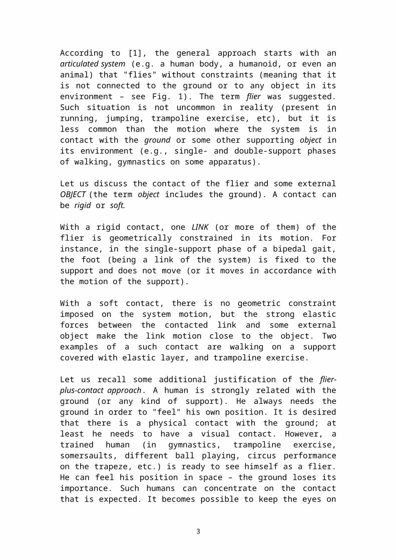
According to [1], the general approach starts with anarticulated system (e.g. a human body, a humanoid, or even ananimal) that "flies" without constraints (meaning that itis not connected to the ground or to any object in itsenvironment – see Fig. 1). The term flier was suggested.Such situation is not uncommon in reality (present inrunning, jumping, trampoline exercise, etc), but it isless common than the motion where the system is incontact with the ground or some other supporting object inits environment (e.g., single- and double-support phasesof walking, gymnastics on some apparatus).

Let us discuss the contact of the flier and some externalOBJECT (the term object includes the ground). A contact canbe rigid or soft.

With a rigid contact, one LINK (or more of them) of theflier is geometrically constrained in its motion. Forinstance, in the single-support phase of a bipedal gait,the foot (being a link of the system) is fixed to thesupport and does not move (or it moves in accordance withthe motion of the support).

With a soft contact, there is no geometric constraintimposed on the system motion, but the strong elasticforces between the contacted link and some externalobject make the link motion close to the object. Twoexamples of a such contact are walking on a supportcovered with elastic layer, and trampoline exercise.

Let us recall some additional justification of the flier-plus-contact approach. A human is strongly related with theground (or any kind of support). He always needs theground in order to "feel" his own position. It is desiredthat there is a physical contact with the ground; atleast he needs to have a visual contact. However, atrained human (in gymnastics, trampoline exercise,somersaults, different ball playing, circus performanceon the trapeze, etc.) is ready to see himself as a flier.He can feel his position in space – the ground loses itsimportance. Such humans can concentrate on the contactthat is expected. It becomes possible to keep the eyes on

3

the object that is to be contacted and thus concentratejust on this relative position. The object may beimmobile (e.g. the ground or a gymnastic horse) or moving(e.g. a ball).

The method that is elaborated in this paper was promotedin [1]. Some of the main explanations and models have tobe repeated here. Other preceding results do not exist.However, there have been some researches that were seenrelevant for this topic and one should mention them. Atthe same time, they support the significance of theproblem elaborated in this paper. The papers [2, 3]address the problem of unconstrained motion of human body(thus, flying), as it appears in a specific task – thesomersaults on the trampoline. The next example ofunconstrained motion and its realization can be found inthe SONY humanoid that is able to run. Running, ofcourse, includes the periods when no foot is in contactwith the support [4]. Very common topic in the work onhuman/humanoid motion is the biped gait. Thus, the theoryof Zero-Moment-Point (ZMP) should be mentioned [5, 6]. Areview of advanced topics in humanoid dynamics ispresented in [7].

3. Free-Flier Motion

We consider a flier as an articulated system consistingof the basic body (the torso) and several branches (head,arms and legs), as shown in Fig. 1. Let there be

4

Fig. 1 Unconstrained system - free flier

independent joint motions described by joint-anglesvector . The terms joint coordinates or internalcoordinates are often used. The basic body is allowed toperform six independent motions in space, described by

, where defines the position ofthe mass center and are orientation angles (roll,pitch, and yaw). Now, the overall number of degrees offreedom (DOFs) for the system is , and the systemposition is defined by

(1)

We now consider the drives. It is assumed that each jointmotion has its own drive – the torque . Note thatthere is no drive associated to the basic-bodycoordinates X. The vector of the joint drives is

, and the augmented drive vector (N-dimensional) is .

The dynamic model of the flier has the general form

(2)or

. (3)

Dimensions of the inertial matrix and its submatricesare: , , , , and

. Dimensions of the vectors containingcentrifugal, Coriolis and gravity effects are: ,

, and .

4. Link Motion and Contact

Let us consider a LINK that has to establish a contactwith some external OBJECT. In one example, it is the footmoving towards the ground and ready to touch (in walkingor running). In the next example, in a soccer game, onemay consider the foot or the head moving towards a ball

5

in order to hit. The external object may be immobile(like ground), an individual moving body (like a ball),or a part of some other dynamic system (even anotherflier, like in a trapeze exercise in the circus). Notethat the contact might be an inner one – involving twolinks of the considered system; the example is a tennisplayer holding the racket with both hands.

In order to express the coming contact mathematically, wedescribe the motion of the considered link by anappropriate set of coordinates. Since the link is a bodymoving in space, it is necessary to use six coordinates.Let this set be and let us call them functionalcoordinates (often referred to as s-coordinates). Functionalcoordinates are introduced as relative ones, defining theposition of the link with respect to the object to becontacted. Several illustrative examples of s-coordinateswere shown in [1]. Each choice was made in accordancewith the expected contact – to support its mathematicaldescription.

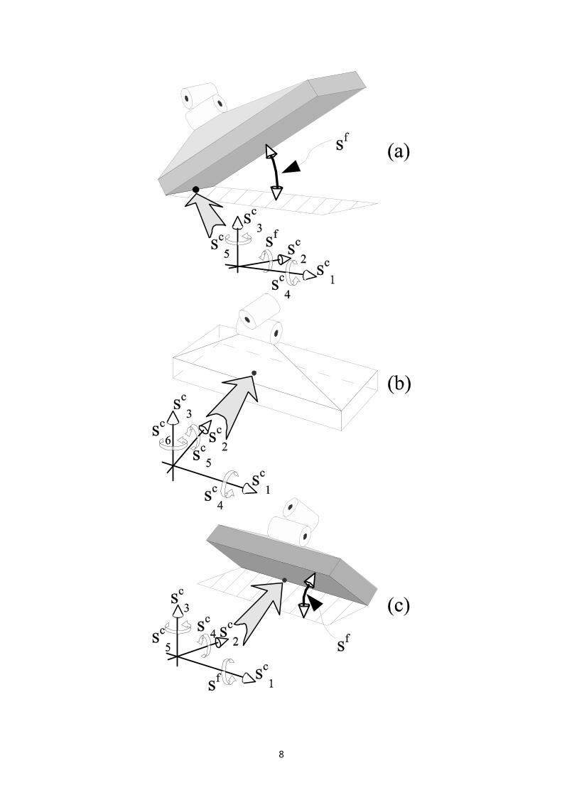
A consequence of the rigid link-object contact is thatthe link and the object perform some motions, along someaxes, together. These are constrained (restricted) directions.Let there be m such directions; m is a characteristic ofa particular contact. Relative position along these axesdoes not change. Along other axes, relative displacementis possible. These are unconstrained (free) directions. Inorder to get a simple mathematical description of thecontact, s-coordinates are introduced so as to describerelative position. Zero value of some coordinateindicates the contact along the corresponding axis. Inthe example, the contact of the robot foot and theground, we may distinguish a few situations (Fig. 2). Theheel contact (Fig. 2a) restricts five s-coordinates,leaving one free (thus, m = 5). The full-foot contact(Fig. 2b) restricts all six coordinates (m = 6). Finally,if the robot is falling down, overturning about the footedge (Fig. 2c), there is again m = 5.

The motion of the external object (to be contacted) hasto be known (or calculated from the appropriate

6

mathematical model), and then the s-frame fixed to theobject is introduced to describe the relative position ofthe link in the most proper way. In the case of an innercontact (two links in contact), one link has to play therole of the object. Thus, in a general case, the s-frameis mobile. As the link is approaching the object, some ofthe s-coordinates reduce and finally reach zero. The zerovalue means that the contact is established. Thesefunctional coordinates (which reduce to zero) are calledrestricted coordinates and they form the subvector ofdimension . The other functional coordinates are freeand they form the subvector of dimension . Now,one may write:

or (4)

where K is a matrix used, when necessary, torearrange the functional coordinates (elements of thevector s) and bring the restricted ones to firstpositions.

7

8

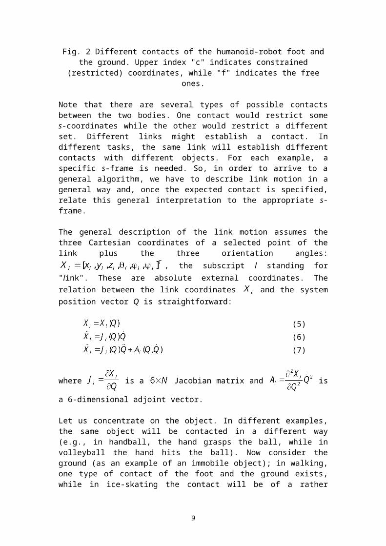
Fig. 2 Different contacts of the humanoid-robot foot andthe ground. Upper index "c" indicates constrained

(restricted) coordinates, while "f" indicates the freeones.

Note that there are several types of possible contactsbetween the two bodies. One contact would restrict somes-coordinates while the other would restrict a differentset. Different links might establish a contact. Indifferent tasks, the same link will establish differentcontacts with different objects. For each example, aspecific s-frame is needed. So, in order to arrive to ageneral algorithm, we have to describe link motion in ageneral way and, once the expected contact is specified,relate this general interpretation to the appropriate s-frame.

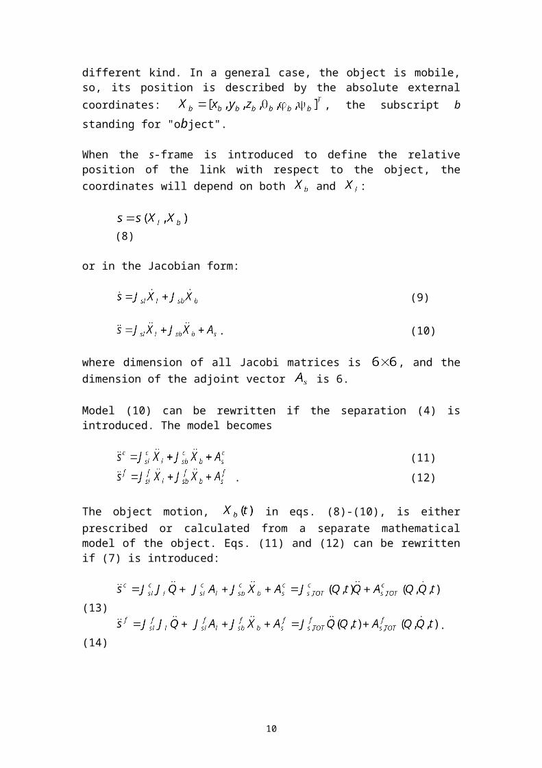
The general description of the link motion assumes thethree Cartesian coordinates of a selected point of thelink plus the three orientation angles:

, the subscript l standing for"link". These are absolute external coordinates. Therelation between the link coordinates and the systemposition vector Q is straightforward:

(5)(6)(7)

where is a Jacobian matrix and is

a 6-dimensional adjoint vector.

Let us concentrate on the object. In different examples,the same object will be contacted in a different way(e.g., in handball, the hand grasps the ball, while involleyball the hand hits the ball). Now consider theground (as an example of an immobile object); in walking,one type of contact of the foot and the ground exists,while in ice-skating the contact will be of a rather

9

different kind. In a general case, the object is mobile,so, its position is described by the absolute externalcoordinates: , the subscript bstanding for "object".

When the s-frame is introduced to define the relativeposition of the link with respect to the object, thecoordinates will depend on both and :

(8)

or in the Jacobian form:

(9)

. (10)

where dimension of all Jacobi matrices is , and thedimension of the adjoint vector is 6.

Model (10) can be rewritten if the separation (4) isintroduced. The model becomes

(11) . (12)

The object motion, in eqs. (8)-(10), is eitherprescribed or calculated from a separate mathematicalmodel of the object. Eqs. (11) and (12) can be rewrittenif (7) is introduced:

(13).

(14)

10

where the model matrices are: ,, ,

When speaking about a moving object one may distinguishtwo cases. The first case assumes that the object motion is given andcannot be influenced by the flier dynamics. Immobile object isincluded in this case. Such situation appears if theobject mass is considerably larger than the flier mass(so, the flier influence may be neglected), or if theobject is driven by so strong actuators that can overcomeany influence on the object motion. An example would bewalking on the ground, i.e. contact between the foot andthe ground. Ground is the immobile object. Anotherexample is walking on a large ship. The ship is a largeobject that moves practically independently of thewalker. The ship is a dynamic system but it cannot beinfluenced by the walker, and so, from the standpoint ofthe walker, the ship motion may be considered as given.Equations (13), (14) apply for this first case.

The other case refers to the object being a "regular" dynamic system, so thatthe flier dynamics can have an effect on it. The example is a handballplayer that catches the ball. The ball is an objectstrongly influenced by the player. The next example isthe walking on a small boat. The boat behavior depends onthe motion of the walker. For this case, eqs. (11), (12)should be combined with the dynamic equations of theobject.

Division of contacts can be done based on the existenceof deformations in the contact zone. If there is nodeformation, i.e. if the motions of the two bodies areequal in the restricted directions, then we talk aboutthe rigid contact. If deformation is possible, then themotions in the restricted directions will not be equal.Theoretically, they will be independent, but in realitythey will be close to each other, due to the action ofstrong elastic forces. In this case, we talk about thesoft contact.

Another division of contacts is also necessary. One class ofcontacts encompasses durable (lasting) contacts. This means that the

11

two bodies (flier and object), after they touch eachother and when the impact is over, continue to movetogether for some finite time. The example is walking.When the foot touches the ground, it will keep thecontact for some time before it moves up again. The nextexample is found in handball playing. When the playercatches the ball, he will keep it for some time beforethrowing.

The other class represents the instantaneous, short-lived contacts. Whenthe two bodies touch each other, a short impact occurs,and after that the bodies disconnect. A good example isthe volleyball player who hits the ball (with his hand).

It is clear that a general theory of impact, includingthe elastodynamic effects, can cover all the mentionedcontacts. However, our intention is to demonstrate thefeasibility and potentials of the proposed method andverify it numerically, and not to explore all the detailsof impact effects. Thus, the discussion of the contacttype is not seen as a primary problem. So, in the presentpaper, we are going to elaborate in detail onerepresentative type of contact – rigid, durable contactinvolving the object that moves according to a given law.1

5. Analysis of the Contact

This section adopts the following:• contact is rigid – allowing no deformation between the twobodies;• object motion is given and cannot be influenced by the flier (thus,

is considered given);• contact is durable – lasting for a finite time after theimpact.

One may recognize the three phases of such contact task[8, 9, 1].

1 Such contact is described in [8]. Some other sort of contact,involving deformation and elastodynamics, are described in [9, 1].

12

Phase 1 is approaching. The link moves towards the object.All functional coordinates are free but some of them(subvector ) gradually reduce to zero.

Phase 2 is the impact. In the preceding phase (approaching),the motion of the link could be planed so as to hit theobject (like in volleyball or in landing after a jump),or it could be planned so as to reach the object with arelative velocity equal to zero (collision-free contact,like in grasping a glass of wine). This is the referencemotion. In the first case, the collision (and the impact)is intentional. In the other case, collision is undesiredbut it still occurs. Namely, the control system producesthe actual motion different from the reference; thetracking error leads to a collision, a non-zero-velocitycontact. The impact forces will affect the system state– after the impact the link state will comply with theobject state and the type of contact.

Phase 3 is the regular contact motion. The contact forces makethe link move according to the character of the contact.

We now elaborate these phases starting with the firstone. The third phase (regular contact motion) will bediscussed before the second phase (impact) since it ismore convenient for the mathematical derivation of themodels.

5.1. Phase 1 - Approaching

From the standpoint of mathematics, approaching is anunconstrained (thus free) motion. Although allcoordinates from the vector s are free, we use theseparation (4) since the subvector is intended todescribe the coming contact. Strictly speaking, therestricted coordinates (elements of ) reach zero one byone. So, a complex contact is established as a series ofsimpler contact effects. Without losing the generalityone may assume that all the coordinates attain zerosimultaneously and establish a complex contactinstantaneously.

13

The dynamics of the approaching is described by the model(2). The model represents the set of N scalar equationsthat can be solved for N scalar unknowns – accelerationvector (thus enabling integration and calculation ofthe system motion ). The link motion in the absoluteexternal frame, , is calculated by using (7). For theapproaching phase, it is more interesting to observefunctional coordinates. Since the object motion isgiven, relation (10) (i.e. (11), (12)) or relations (13),(14), allows one to calculate the link functionaltrajectory .

The reference motion (sign * will be used to denotereference values of a variable) is planned so as to makea zero-velocity contact at the instant : and . Due to the control system, tracking errorwill appear and the actual motion s will differ from thereference. So, it is necessary to monitor the coordinates

and detect the contact as the instant when reduces to zero ( ). It will be , and thecontact velocity will not be zero: .

During the approaching, the integration of the systemcoordinates Q is done. So, at the instant of impact,there will be some system state .

5.2. Phase 3 - Regular Contact Motion

Regular contact motion starts when the transient effectsof the impact vanish. In this phase the restrictedcoordinates are kept zero. So,

(15)

and accordingly

.(16)

14

Now, relation (13) is replaced with

(17)

while relation (14) still holds:

.

In contact problems, the dynamic model has to take careof contact forces. Model (2), derived for a free flier,should be supplemented by introducing contact forces. Acontact force acts along each of the constrained axes.So, there is a reaction force (or torque) for eachcoordinate from the set . There are m independentreactions. Let be the reaction vector. If acoordinate is a linear one (translation) then thecorresponding reaction is a force. For a revolutecoordinate, the corresponding reaction is a torque.

The contact-dynamics model is obtained by introducingreactions into the free-flier model (2):

(18)

Since this model involves N scalar equations and scalar unknowns (vectors and F), it is necessary tosupply some additional conditions. The additionalcondition is the constraint relation (17), containing mscalar equations. So, (18) and (17) describe the dynamicsof a constrained flier, allowing one to calculate theacceleration and reaction F (thus enabling integrationof the equations and calculation of the system motion).

5.3. Phase 2 - Impact

Let be the instant when the contact is established(restricted coordinates reduce to zero and the impactcomes into action) and let be the instant when the

15

impact ends. So, the impact lasts for . Forthis analysis we adopt the infinitely short impact, i.e.

. We also adopt that the m coordinates (forming ) reduce to zero simultaneously.

We now integrate the dynamic model (18) over the shortimpact interval , obtaining:

(19)

where

. (20)

During the approaching phase, the system model wasintegrated and the motion was calculated. Thus,the state at the instant , i.e. , isconsidered known. Since the object motion is also known,it is possible to calculate the model matrices in the equation (19). The position does not change during

, and hence: .

Now, the model (19), contains N scalar equations with scalar unknowns: the change in velocity across the

impact, (dimension ), and the impact momentum (dimension m). The additional equations needed to allowthe solution are obtained rewriting the constraintrelation (17) into the first-order form:

=> , (21)

that contains m scalar conditions. The augmented set ofequations, (19) and (21), allows to solve the impact. Thechange is found and then (20) allows to calculate thevelocity after the impact (i.e. ). So, the newstate (in ) is found starting from the known state in

. The impact momentum is determined as well. Thenew state represents the initial condition for

16

the third phase, the regular contact motion (explained in5.2).

6. Numerical Verification of the GeneralModel

In order to verify the proposed general method, theappropriate software has been developed. Verificationshould be made by comparing the results obtained by usingthe new method with the ones obtained by some "classical"approach. Hence, we will consider a motion task from awell known field - bipedal gait. For modeling suchmotion, there already exist several software packages. Weselect the one developed in Institute "M. Pupin" inBelgrade [5] and it will be referred to as the"classical" method. So, a selected biped gait will beinputted to both the classical software and the new one.The results will be compared.

6.1. Configuration and Task

We consider a humanoid having n = 18 DOFs in its joints(Fig. 3). Definition of joint (internal) coordinates,vector , is presented as well. Mainparameters of the humanoid are given in Appendix.

17

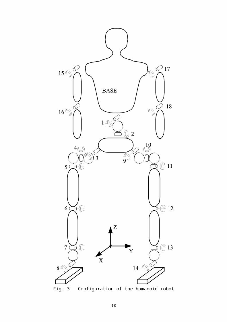
Fig. 3 Configuration of the humanoid robot

18

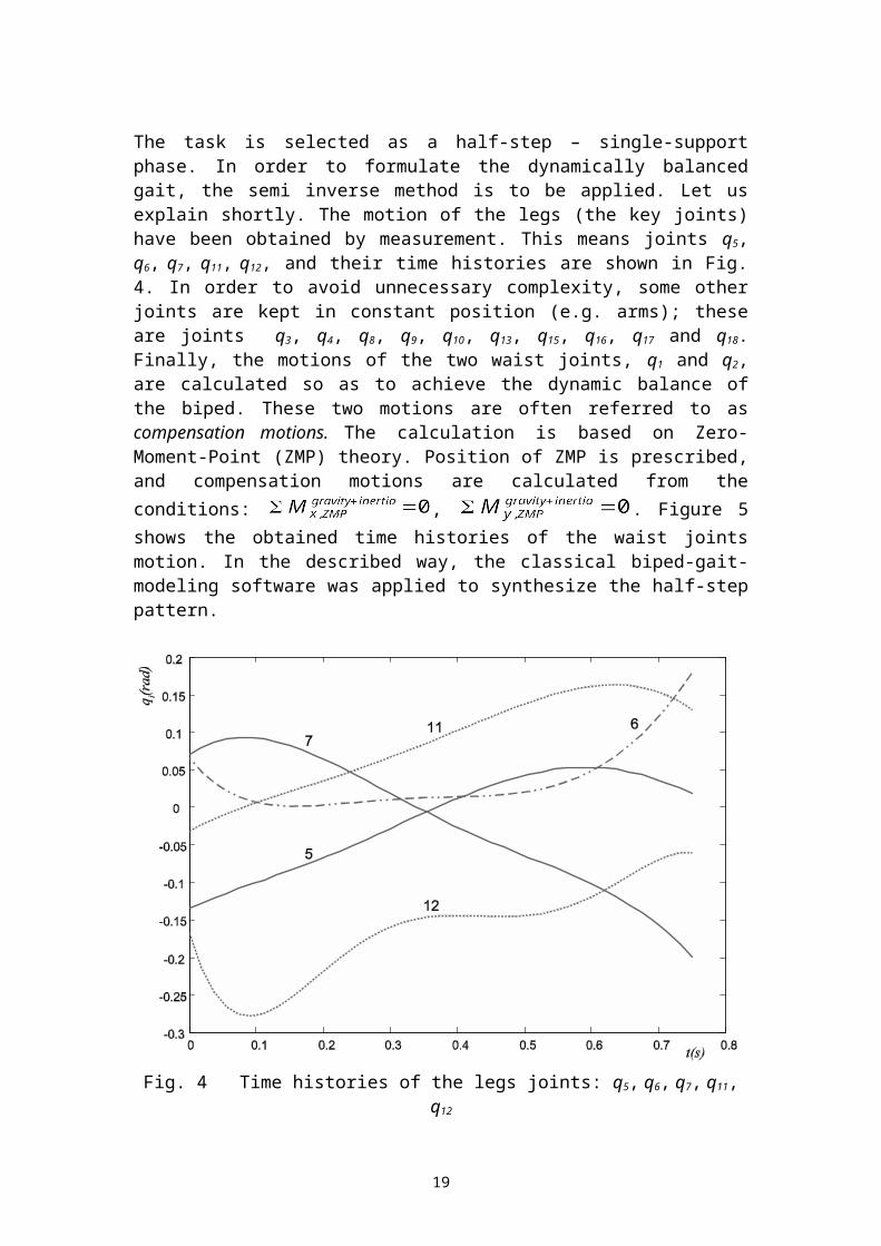
The task is selected as a half-step – single-supportphase. In order to formulate the dynamically balancedgait, the semi inverse method is to be applied. Let usexplain shortly. The motion of the legs (the key joints)have been obtained by measurement. This means joints q5,q6, q7, q11, q12, and their time histories are shown in Fig.4. In order to avoid unnecessary complexity, some otherjoints are kept in constant position (e.g. arms); theseare joints q3, q4, q8, q9, q10, q13, q15, q16, q17 and q18.Finally, the motions of the two waist joints, q1 and q2,are calculated so as to achieve the dynamic balance ofthe biped. These two motions are often referred to ascompensation motions. The calculation is based on Zero-Moment-Point (ZMP) theory. Position of ZMP is prescribed,and compensation motions are calculated from theconditions: , . Figure 5shows the obtained time histories of the waist jointsmotion. In the described way, the classical biped-gait-modeling software was applied to synthesize the half-steppattern.

Fig. 4 Time histories of the legs joints: q5, q6, q7, q11,q12

19

Fig. 5 Time histories of the waist joints: q1 and q2

6.2. Analysis of Results

The synthesized motion is now the input for the newgeneral software. All dynamic variables (like jointtorques, ground reactions, etc.) can be found. In orderto efficiently compare the results of the two methods, wedecided to check the position of ZMP calculated by usingthe two softwares. Let us explain why ZMP position(meaning and ) is used for comparison. ZMPinvolves all the dynamic effects and any incorrectness inthe modeling procedure will reflect in the calculatedposition of ZMP. Thus, ZMP offers the most appropriateway to check a new dynamic model.

The classical method prescribed ZMP. It was prescribedimmobile in the zero position. The new method calculatedthe ZMP position. Figure 6 demonstrates the deviation inZMP. The x-y view of the calculated ZMP position isshown. The foot shape (i.e. the support region) ispresented as well in order to estimate the relativedeviation.

20

One may conclude that results coming out from twodifferent methods agree, thus proving the correctness ofthe new general method.

Fig. 6 Planar (x-y) representation of the ZMP deviation

7. Simulation Example: DemonstratingFeasibility and Potentials of the GeneralMethod

In order to show the applicability of the proposedgeneral method, a complex motion is simulated. Note thatin this example no joint is kept fixed. The humanoidmotion involves rather different situations regarding thecontact between the flier and the ground. Let us explain.

7.1. What Will be Simulated?

21

The flier is a humanoid robot whose configuration wasexplained in Sec. 6.1

The robot falls down from the height of 0.1034m (see Fig.7). This free (unconstrained) motion represents Phase 1of the motion and it ends when the right foot touches theground (support). Due to the configuration of thesupport, the left foot will never make any contact.

The foot establishes the full contact with the ground.The infinitely short impact occurs at the instant ofcontact. The impact represents Phase 2 .

After the impact, the regular contact motion starts,constituting Phase 3. In this phase, the right foot hasthe full contact with the ground and the rectangular footshape defines the support region. Single support is atstake since the left foot does not touch the ground. Forsome time ZMP will be inside the support region ensuringthe dynamic balance. However, the large displacements ofZMP will be observed until ZMP finally reaches the edgeof the support region. This is the end of Phase 3.

22

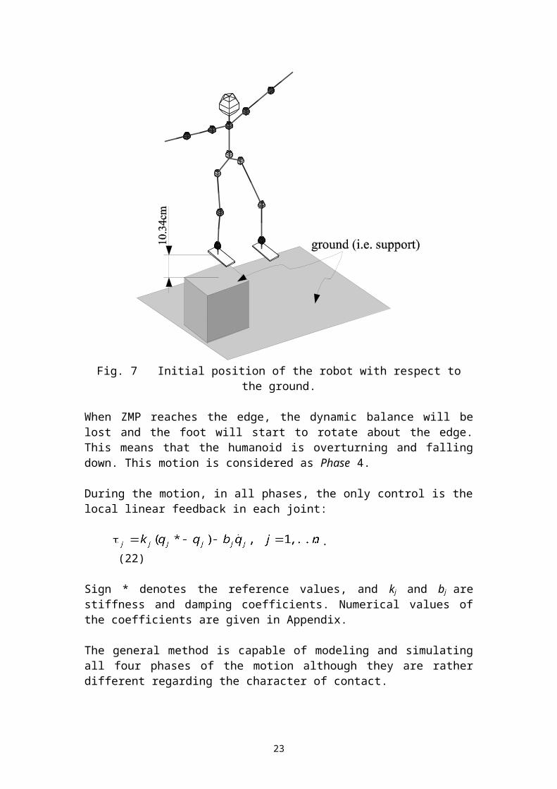
Fig. 7 Initial position of the robot with respect tothe ground.

When ZMP reaches the edge, the dynamic balance will belost and the foot will start to rotate about the edge.This means that the humanoid is overturning and fallingdown. This motion is considered as Phase 4.

During the motion, in all phases, the only control is thelocal linear feedback in each joint:

.(22)

Sign * denotes the reference values, and kj and bj arestiffness and damping coefficients. Numerical values ofthe coefficients are given in Appendix.

The general method is capable of modeling and simulatingall four phases of the motion although they are ratherdifferent regarding the character of contact.

23

● In Phase 1, there is no contact. Theory from Sec. 3 and5.1. is applied for the free motion.

Phase● 2 and Phase 3 concern a full contact of the footand the ground (according to Sec. 5, rigid, durablecontact is assumed). This means that all the sixfunctional coordinates are restricted:

, does not exist, . Thisis shown in Fig. 2b. Theory from Sec. 5.3. is appliedto solve the impact and the theory from 5.2 applies forthe regular contact motion.

Phase● 4 considers a contact that allows one relativerotation, about the edge of the support region (i.e.the foot edge). This means that five coordinates arerestricted. Thus, it holds that: ,

, . This is shown in Fig. 2c. Theory fromSec. 5.3 applies again but with the different characterof the contact.

The proposed method allows calculating all the relevantdynamic effects in all phases of motion

7.2. Simulation Results

The software developed on the basis of the new generalapproach has been used to simulate the entire motion.When switching from one phase to the other, i.e., whenthe character of contact changes, the Jacobean matrixtakes another form as a part of the general algorithm.

Let us discuss the results. Figure 8 shows the “movie” ofthe humanoid motion. Several time instants are selectedand the position of the body presented. Thecharacteristic instants and intervals are the following.► Phase 1 lasts for . At , the freefalling down starts, and at , the right foot touchesthe ground and the impact occurs. This is shown inFigs. 8a-8b.

24

► Phase 2 (the infinitely short impact) accomplishes at (Fig. 8b).

► Phase 3 lasts for . At ,the full-foot contact starts. At , the ZMP positionreaches the edge of the rectangular shaped foot. Thisis shown in Figs. 8b-8i. During this phase, Zero-Moment-Point (ZMP) and Center of Pressure (CoP) areidentical.

► Phase 4 lasts for . At ,the dynamic balance is lost and the foot starts torotate about its edge (we are talking about the left-side edge of the right foot), thus changing thecharacter of the contact. The humanoid overturns andfor such unbalanced motion it is not appropriate totalk about ZMP but rather about CoP only. CoP movesalong the left-side edge and at it reachesthe front edge of the foot. This is shown in Figs. 8i-8k.

► Next phase would take place for . At thatinstant, the foot would change the character of thecontact again, starting to rotate about the left frontcorner of the rectangle. The initial instant of thisphase, , is shown in Fig. 8k, but the simulationstops at that moment. Note that there would be noproblem to continue simulation in this next phase.

25

Fig. 8 The “movie” of the humanoid motion.Characteristic instants defining the phases of motion are

indicated.

26

Figures 9 and 10 show the position coordinates of thehumanoid, , in all four phases of its motion. Fig. 9presents time histories of joint coordinates,

, while Fig. 10 presents thecoordinates of the main body, , ,and . It is evident, as expected, that in Phase 1(free falling) only the vertical coordinate z changes.The others start to change after the contact isestablished. The evident progress in the magnitude of ,and in y and θ as well, shows that even during thebalanced motion in Phase 3 the humanoid tends to overturnwith no chances to keep the balance with the adoptedlocal-control strategy. The absence of possibility toreestablish the balance is rather obvious duringoverturning in Phase 4. Only some radical action of theentire body might help in balancing and preventing thefalling down. However, the control problems are out ofthe scope of this paper. The idea of the paper is todemonstrate the potentials of the new method for dynamicanalysis.

27

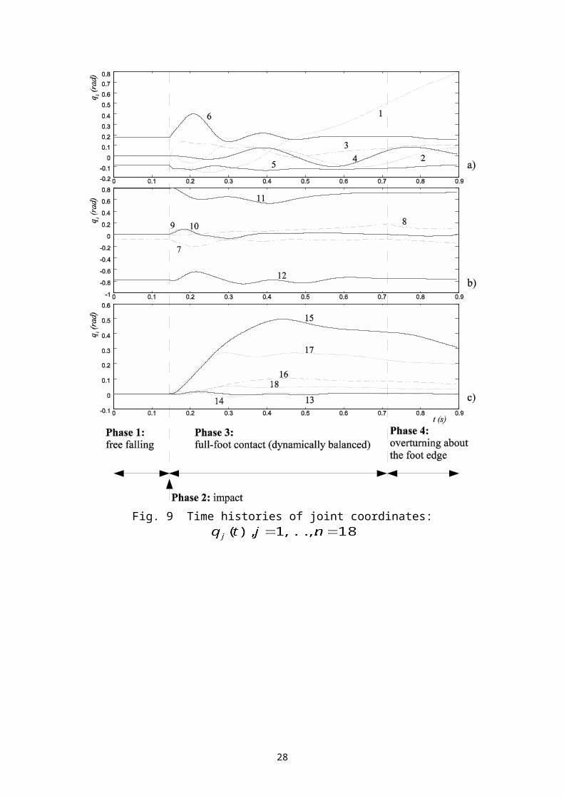
Fig. 9 Time histories of joint coordinates:

28

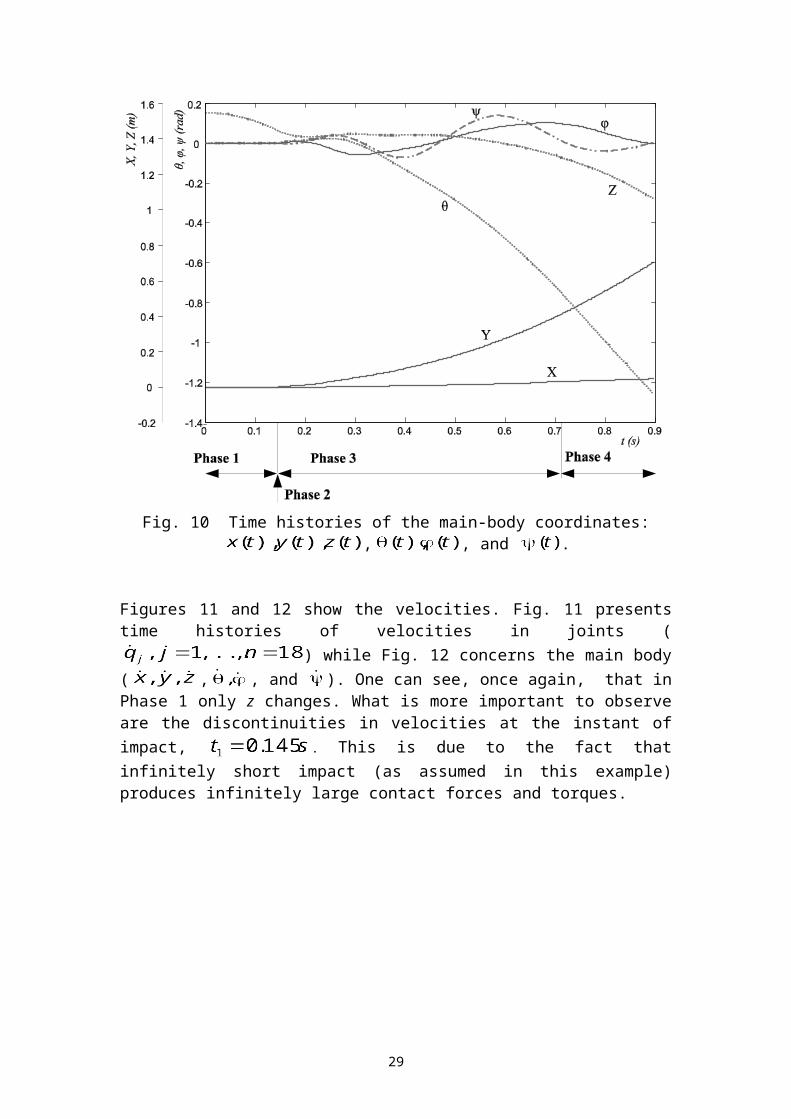
Fig. 10 Time histories of the main-body coordinates: , , and .

Figures 11 and 12 show the velocities. Fig. 11 presentstime histories of velocities in joints (

) while Fig. 12 concerns the main body( , , and ). One can see, once again, that inPhase 1 only z changes. What is more important to observeare the discontinuities in velocities at the instant ofimpact, . This is due to the fact thatinfinitely short impact (as assumed in this example)produces infinitely large contact forces and torques.

29

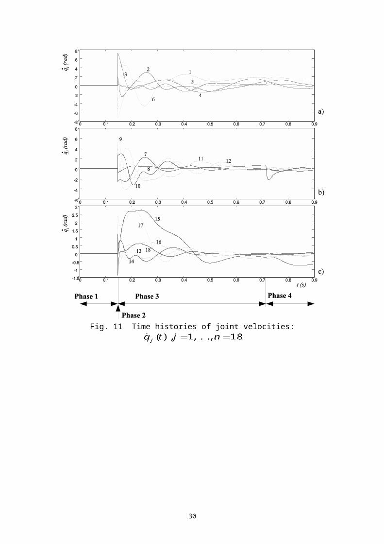
Fig. 11 Time histories of joint velocities:

30

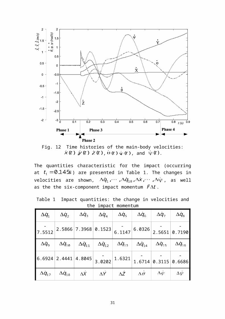
Fig. 12 Time histories of the main-body velocities: , , and .

The quantities characteristic for the impact (occurringat ) are presented in Table 1. The changes invelocities are shown, , as wellas the the six-component impact momentum .

Table 1 Impact quantities: the change in velocities andthe impact momentum

-7.5512 2.5866 7.3968 0.1523 -

6.1147 6.0326 -2.5651

-0.7190

6.6924 2.4441 4.8045 -3.0202 1.6321 -

1.6714-

0.3115-

0.6686

31

2.6331 -2.0934

-0.0081 0.1107 0.2949 0.8735 0.0606 -

0.1523

k 1 2 3 4 5 6

Fk Δt2.6352

-1.1294

27.5154 0.1152 0.1850

-0.0733

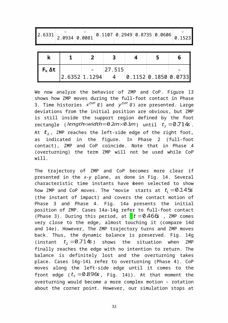
We now analyze the behavior of ZMP and CoP. Figure 13shows how ZMP moves during the full-foot contact in Phase3. Time histories and are presented. Largedeviations from the initial position are obvious, but ZMPis still inside the support region defined by the footrectangle ( ) until .At , ZMP reaches the left-side edge of the right foot,as indicated in the figure. In Phase 2 (full-footcontact), ZMP and CoP coincide. Note that in Phase 4(overturning) the term ZMP will not be used while CoPwill.

The trajectory of ZMP and CoP becomes more clear ifpresented in the x-y plane, as done in Fig. 14. Severalcharacteristic time instants have been selected to showhow ZMP and CoP moves. The “movie” starts at (the instant of impact) and covers the contact motion ofPhase 3 and Phase 4. Fig. 14a presents the initialposition of ZMP. Cases 14a-14g refer to full-foot contact(Phase 3). During this period, at , ZMP comesvery close to the edge, almost touching it (compare 14dand 14e). However, The ZMP trajectory turns and ZMP movesback. Thus, the dynamic balance is preserved. Fig. 14g(instant ) shows the situation when ZMPfinally reaches the edge with no intention to return. Thebalance is definitely lost and the overturning takesplace. Cases 14g-14i refer to overturning (Phase 4). CoPmoves along the left-side edge until it comes to thefront edge ( , Fig. 14i). At that moment theoverturning would become a more complex motion – rotationabout the corner point. However, our simulation stops at

32

, although the method and the software support thesimulation of such next phase of motion.

Fig. 13 Time histories of ZMP coordinates in the phaseof dynamically balanced motion (full-foot contact)

Fig 14 Trajectory of ZMP/CoP for the two phases ofcontact motion

33

(full-foot-contact phase and overturning phase)

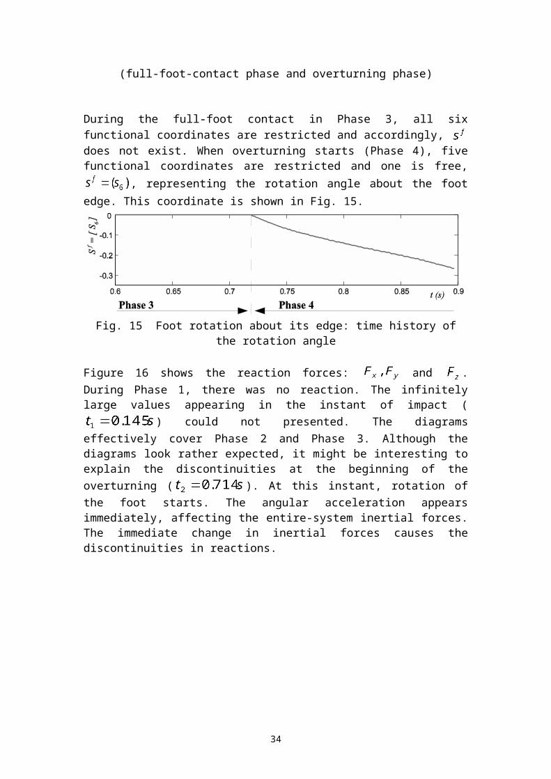
During the full-foot contact in Phase 3, all sixfunctional coordinates are restricted and accordingly, does not exist. When overturning starts (Phase 4), fivefunctional coordinates are restricted and one is free,

, representing the rotation angle about the footedge. This coordinate is shown in Fig. 15.

Fig. 15 Foot rotation about its edge: time history ofthe rotation angle

Figure 16 shows the reaction forces: and .During Phase 1, there was no reaction. The infinitelylarge values appearing in the instant of impact (

) could not presented. The diagramseffectively cover Phase 2 and Phase 3. Although thediagrams look rather expected, it might be interesting toexplain the discontinuities at the beginning of theoverturning ( ). At this instant, rotation ofthe foot starts. The angular acceleration appearsimmediately, affecting the entire-system inertial forces.The immediate change in inertial forces causes thediscontinuities in reactions.

34

Fig. 16 Time histories of the reaction forces

Appendix: Structural and Control Parameters

Table 2 Structural parameters of the humanoid robot

segmentwidth(m)

height(m) mass (kg)

trunk total - pelvis to head top 0.4 0.64 30.85trunk - pelvis to shoulders 0.4 0.4pelvis 0.27 0.15 6.96thigh 0.44 8.41shank 0.42 3.21foot 0.1 0.1 1.53forearm 0.308 2.07upper arm 0.264 1.14total 0.4 1.75 70.53

Table 3 Control parameters (feedback gains)i – joint number 1 2 3 4 5 6 7 8 9ki – stiffness 100 200 120 600 800 400 800 200 120

35

(N/rad) 0 0bi – damping(Ns/rad)

5 5 5 5 5 5 5 5 5

i – joint number 10 11 12 13 14 15 16 17 18ki – stiffness(N/rad)

600 200 200 200 200 20 20 20 20

bi – damping(Ns/rad)

5 5 5 5 5 5 5 5 5

Conclusion

Rapid development of humanoid robots brings about newshifts of the boundaries of Robotics as a scientific andtechnological discipline. It has been finally recognizedthat humanoid robots represent the main direction of workin the entire robotics, being continually present fromthe very beginnings of scientific robotics in sixties andseventies. New technologies of components, sensors,microcomputers, as well as new materials, have allowed tocreate complex, human-like robots with the idea toreplace humans in a variety of job. Hence, it isgenerally accepted that humanoid-robot shape and motionshould be based on biomechanical principles. Due to thecomplexity and high requirements imposed on such robots,their control system has to utilize the dynamic model.So, the control, the design, and the simulation, stronglyrequire general dynamic models that will make humanoidrobots capable of handling the increasing diversity ofexpected tasks.

The work presented in this paper concerned a new generalapproach to modeling human and humanoid motion, allowingto develop different specific practical motions asspecial cases. To promote the approach in a qualifiedmanner, it was necessary to check it numerically and showits potential by simulation on a carefully selectedexample.

In order to check the new method numerically, a well-explored task was chosen – bipedal gait. The resultsobtained by the existing “classical” method and the ones

36

obtained by the new approach have been compared, showingagreement.

To demonstrate the applicability and potentials of themethod by simulation, a motion example was selected whichinvolved different sorts of contact: free (contactless)motion, impact, full-foot contact, and rotation of thefoot about its edge.

As the final target for the future work, a general-purpose software was seen. It would be used for modelingand dynamic analysis of any human-like motion: fromhousehold duties, through the industrial jobs, to sports,and beyond. We mention few interesting examples: sports-man on a trampoline, man on the mobile dynamic platform,running, balanced motion on the foot - a karate kick,playing tennis, soccer or volleyball, gymnastics on thefloor or by using some gymnastic apparatus, skiing -balanced motion with sliding, etc.).

The authors are well aware of the extreme complexity ofthe problem of modeling biological systems, which stemsfrom the complexity of the mechanical structure andactuation. The fact that the control of biological systemis a still insufficiently studied area, contributesgreatly to the significance of the problem. Because ofthat the authors started with the dynamic modeling of thestructure of humanoid robots, which yielded a solidapproximation of dynamics of the mechanical aspect ofhuman motion.

References

[1] V. Potkonjak, M. Vukobratović, A GeneralizedApproach to Modeling Dynamics of Human and HumanoidMotion, Intl. Journal of Humanoid Robotics 2(1) (2005) 1-24.

[2] Blajer, W., Czaplicki, A., Modeling and InverseSimulation of Somersaults on the Trampoline, Journal ofBiomechanics 34 (2001) 1619-1629.

[3] W. Blajer, A. Czaplicki, Contact Modeling andIdentification of Planar Somersaults on theTrampoline, Multibody System Dynamics 10, (2003) 289-312.

37

[4] K. Nagasaka, Y. Kuroki, S. Suzuki, Y. Itoh, and J.Yamaguchi, Integrated Motion Control for Walking,Jumping and Running on a Small Bipedal EntertainmentRobot, in Proceedings of the IEEE International Conference onRobotics, & Automation (ICRA), (New Orleans, USA, 2004),pp. 3189-3194.

[5] M. Vukobratović, B. Borovac, D. Surla, D Stokić,Biped Locomotion: Dynamics, Stability, Control and Application(Springer-Verlag, 1989)

[6] M. Vukobratović, B. Borovac, Zero-Moment Point -Thirty Five Years of its Life, International Journal ofHumanoid Robotics, 1(1) (2004) 157-173.

[7] M. Vukobratović, V. Potkonjak, S. Tzafestas, Humanand Humanoid Dynamics - From the Past to the Future,Journal of Intelligent and Robotic Systems, August issue, 2004.

[8] M. Vukobratović, V. Potkonjak, Applied Dynamics and CADof Manipulation Robots, monograph, (Springer-Verlag,1985).

[9] M. Vukobratović, V. Potkonjak, V. Matijević, Dynamicsof Robots with Contact Tasks, research monograph, (KluwerAcademic Publishers, 2003).

38