Chapter 1

General Introduction

Instructional Objectives

After reading this chapter the student will be able to

1. Differentiate between various structural forms such as beams, plane truss, space

truss, plane frame, space frame, arches, cables, plates and shells.

2. State and use conditions of static equilibrium.

3. Calculate the degree of static and kinematic indeterminacy of a given structure such

as beams, truss and frames.

4. Differentiate between stable and unstable structure.

5. Define flexibility and stiffness coefficients.

6. Write force-displacement relations for simple structure.

Introduction

Structural analysis and design is a very old art and is known to human beings since early

civilizations. The Pyramids constructed by Egyptians around 2000

B.C. stands today as the testimony to the skills of master builders of that civilization.

Many early civilizations produced great builders, skilled craftsmen who constructed

magnificent buildings such as the Parthenon at Athens (2500 years old), the great Stupa at

Sanchi (2000 years old), Taj Mahal (350 years old), Eiffel Tower (120 years old) and

many more buildings around the world. These monuments tell us about the great feats

accomplished by these craftsmen in analysis, design and construction of large structures.

Today we see around us countless houses, bridges, fly-overs, high-rise buildings and

spacious shopping malls. Planning, analysis and construction of these buildings is a

science by itself. The main purpose of any structure is to support the loads coming on it

by properly transferring them to the foundation. Even animals and trees could be treated

as structures. Indeed biomechanics is a branch of mechanics, which concerns with the

working of skeleton and muscular structures. In the early periods houses were constructed

along the riverbanks using the locally available material. They were designed to

withstand rain and moderate wind. Today structures are designed to withstand

earthquakes, tsunamis, cyclones and blast loadings. Aircraft structures are designed for

more complex aerodynamic loadings. These have been made possible with the advances

in structural engineering and a revolution in electronic computation in the past 50 years.

The construction material industry has also undergone a revolution in the last four

decades resulting in new materials having more strength and stiffness than the traditional

construction material.

Here we are mainly concerned with the analysis of framed structures (beam and plane

frame), arches, cables and suspension bridges subjected to static loads only. The methods

that we would be presenting in this course for analysis of structure were developed based

on certain energy principles, which would be discussed here.

Classification of Structures

All structural forms used for load transfer from one point to another are 3- dimensional in

nature. In principle one could model them as 3-dimensional elastic structure and obtain

solutions (response of structures to loads) by solving the associated partial differential

equations. In due course of time, you will appreciate the difficulty associated with the 3-

dimensional analysis. Also, in many of the structures, one or two dimensions are smaller

than other dimensions. This geometrical feature can be exploited from the analysis point

of view. The dimensional reduction will greatly reduce the complexity of associated

governing equations from 3 to 2 or even to one dimension. This is indeed at a cost. This

reduction is achieved by making certain assumptions (like Bernoulli-Euler’ kinematic

assumption in the case of beam theory) based on its observed behavior under loads.

Structures may be classified as 3-, 2- and 1-dimensional (see Fig. 1.1(a) and (b)). This

simplification will yield results of reasonable and acceptable accuracy. Most commonly

used structural forms for load transfer are: beams, plane truss, space truss, plane frame,

space frame, arches, cables, plates and shells. Each one of these structural arrangement

supports load in a specific way.

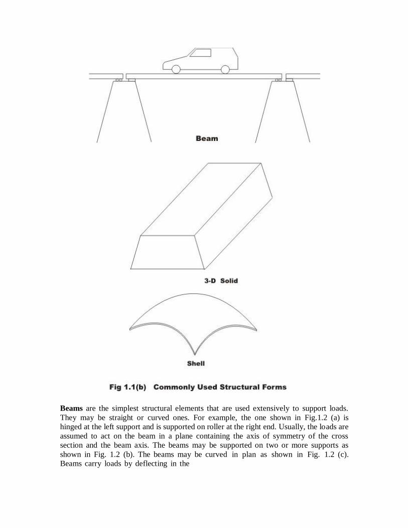
Beams are the simplest structural elements that are used extensively to support loads.

They may be straight or curved ones. For example, the one shown in Fig.1.2 (a) is

hinged at the left support and is supported on roller at the right end. Usually, the loads are

assumed to act on the beam in a plane containing the axis of symmetry of the cross

section and the beam axis. The beams may be supported on two or more supports as

shown in Fig. 1.2 (b). The beams may be curved in plan as shown in Fig. 1.2 (c).

Beams carry loads by deflecting in the

same plane and it does not twist. It is possible for the beam to have no axis of symmetry.

In such cases, one needs to consider unsymmetrical bending of beams. In general, the

internal stresses at any cross section of the beam are: bending moment, shear force and

axial force.

In India, one could see plane trusses (vide Fig. 1.3 (a),(b),(c)) commonly in Railway

bridges, at railway stations, and factories. Plane trusses are made of short thin members

interconnected at hinges into triangulated patterns. For the purpose of analysis statically

equivalent loads are applied at joints. From the above definition of truss, it is clear that

the members are subjected to only axial forces and they are constant along their length.

Also, the truss can have only hinged and roller supports. In field, usually joints are

constructed as rigid by welding. However, analyses were carried out as though they were

pinned. This is justified as the bending moments introduced due to joint rigidity in trusses

are negligible. Truss joint could move either horizontally or vertically or combination of

them. In space truss (Fig. 1.3 (d)), members may be oriented in any direction. However,

members are subjected to only tensile or compressive stresses. Crane is an example of

space truss.

Plane frames are also made up of beams and columns, the only difference being they are

rigidly connected at the joints as shown in the Fig. 1.4 (a). Major portion of this course is

devoted to evaluation of forces in frames for variety of loading conditions. Internal forces

at any cross section of the plane frame member are: bending moment, shear force and

axial force. As against plane frame, space frames (vide Fig. 1.4 (b)) members may be

oriented in any direction. In this case, there is no restriction of how loads are applied on

the space frame.

Equations of Static Equilibrium

Consider a case where a book is lying on a frictionless table surface. Now, if we

apply a force F1 horizontally as shown in the Fig.1.5 (a), then it starts moving in

the direction of the force. However, if we apply the force perpendicular to the book as in

Fig. 1.5 (b), then book stays in the same position, as in this case the vector sum of all

the forces acting on the book is zero.

When does an object move and when does it not? This question was answered by

Newton when he formulated his famous second law of motion. In a simple vector

equation it may be stated as follows:

Fi ma i1

(1.1)

n

where

Fi

i1

is the vector sum of all the external forces acting on the body, m is

the total mass of the body and a is the acceleration vector. However, if the body

is in the state of static equilibrium then the right hand of equation (1.1) must be zero.

Also for a body to be in equilibrium, the vector sum of all external moments

( M 0 ) about an axis through any point within the body must also vanish.

Hence, the book lying on the table subjected to external force as shown in Fig. 1.5 (b) is in static equilibrium. The equations of equilibrium are the direct consequences

of Newton’s second law of motion. A vector in 3-dimensions can be resolved into three

orthogonal directions viz., x, y and z (Cartesian) co- ordinate axes. Also, if the resultant

force vector is zero then its components in three mutually perpendicular directions also

vanish. Hence, the above two equations may also be written in three co-ordinate axes

directions as follows:

Fx 0 ; Fy 0 ; Fz 0 (1.2a)

M x 0 ; M y 0 ; M z 0 (1.2b)

Now, consider planar structures lying in xy plane. For such structures we could

have forces acting only in x and y directions. Also the only external moment that

could act on the structure would be the one about the z -axis.

For planar structures, the resultant of all forces may be a force, a couple or both. The

static equilibrium condition along x -direction requires that there is no net unbalanced

force acting along that direction. For such structures we could express equilibrium

equations as follows:

Fx 0 ; Fy 0 ; M z 0 (1.3)

Using the above three equations we could find out the reactions at the supports in the

beam shown in Fig. 1.6. After evaluating reactions, one could evaluate internal stress

resultants in the beam. Admissible or correct solution for reaction and internal stresses

must satisfy the equations of static equilibrium for the entire structure. They must also

satisfy equilibrium equations for any part of the structure taken as a free body. If the

number of unknown reactions is more than the number of equilibrium equations (as in the

case of the beam shown in Fig. 1.7), then we cannot evaluate reactions with only

equilibrium equations. Such structures are known as the statically indeterminate

structures. In such cases we need to obtain extra equations (compatibility equations) in

addition to equilibrium equations.

n

Static Indeterminacy

The aim of structural analysis is to evaluate the external reactions, the deformed shape

and internal stresses in the structure. If this can be accomplished by equations of

equilibrium, then such structures are known as determinate structures. However, in many

structures it is not possible to determine either reactions or internal stresses or both using

equilibrium equations alone. Such structures are known as the statically indeterminate

structures. The indeterminacy in a structure may be external, internal or both. A structure

is said to be externally indeterminate if the number of reactions exceeds the number of

equilibrium equations. Beams shown in Fig.1.8(a) and (b) have four reaction

components, whereas we have only 3 equations of equilibrium. Hence the beams in Figs.

1.8(a) and (b) are externally indeterminate to the first degree. Similarly, the beam and

frame shown in Figs. 1.8(c) and (d) are externally indeterminate to the 3rd

degree.

Now, consider trusses shown in Figs. 1.9(a) and (b). In these structures, reactions could

be evaluated based on the equations of equilibrium. However, member forces cannot be

determined based on statics alone. In Fig. 1.9(a), if one of the diagonal members is

removed (cut) from the structure then the forces in the members can be calculated

based on equations of equilibrium. Thus,

structures shown in Figs. 1.9 (a) and (b) are internally indeterminate to first degree. The

truss and frame shown in Fig. 1.10 (a) and (b) are both externally and internally

indeterminate.

So far, we have determined the degree of indeterminacy by inspection. Such an approach

runs into difficulty when the number of members in a structure increases. Hence, let us

derive an algebraic expression for calculating degree of static indeterminacy.

Consider a planar stable truss structure having m members and j joints. Let the

number of unknown reaction components in the structure be r . Now, the total number of unknowns in the structure is m + r . At each joint we could write two

equilibrium equations for planar truss structure, viz., Fx 0 and Fy 0 .

Hence total number of equations that could be written is 2 j .

If 2 j m r then the structure is statically determinate as the number of

unknowns are equal to the number of equations available to calculate them. The

degree of indeterminacy may be calculated as

i (m r) 2 j (1.4)

We could write similar expressions for space truss, plane frame, space frame and grillage.

For example, the plane frame shown in Fig.1.11 (c) has 15 members, 12 joints and 9

reaction components. Hence, the degree of indeterminacy of the structure is

i (15 3 9) 12 3 18

Please note that here, at each joint we could write 3 equations of equilibrium for plane

frame.

Kinematic Indeterminacy

When the structure is loaded, the joints undergo displacements in the form of translations

and rotations. In the displacement based analysis, these joint displacements are treated as

unknown quantities. Consider a propped cantilever beam shown in Fig. 1.12 (a). Usually,

the axial rigidity of the beam is so high that the change in its length along axial direction

may be neglected. The displacements at a fixed support are zero. Hence, for a propped

cantilever beam we have to evaluate only rotation at B and this is known as the kinematic

indeterminacy of the structure. A fixed beam is kinematically determinate but statically

indeterminate to 3rd

degree. A simply supported beam and a cantilever beam are

kinematically indeterminate to 2nd

degree.

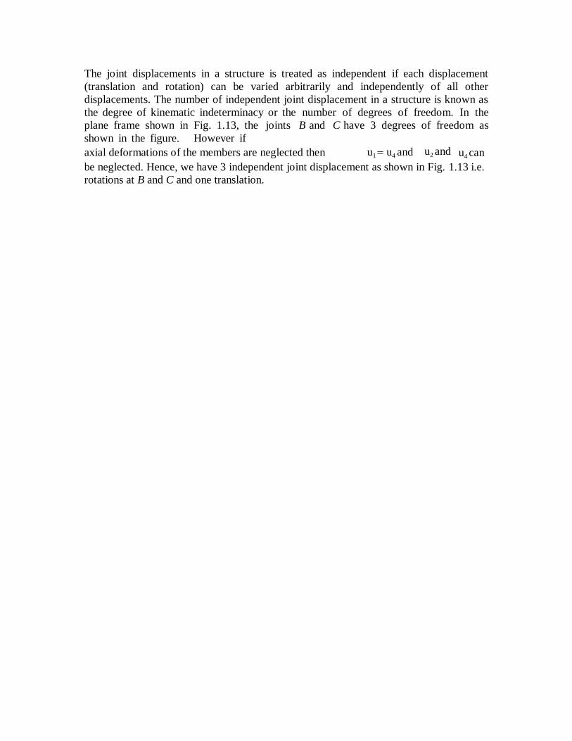
The joint displacements in a structure is treated as independent if each displacement

(translation and rotation) can be varied arbitrarily and independently of all other

displacements. The number of independent joint displacement in a structure is known as

the degree of kinematic indeterminacy or the number of degrees of freedom. In the

plane frame shown in Fig. 1.13, the joints B and C have 3 degrees of freedom as

shown in the figure. However if

axial deformations of the members are neglected then u1 u4 and u2 and u4 can

be neglected. Hence, we have 3 independent joint displacement as shown in Fig. 1.13 i.e.

rotations at B and C and one translation.

Kinematically Unstable Structure

A beam which is supported on roller on both ends ( Fig. 1.14) on a horizontal surface can

be in the state of static equilibrium only if the resultant of the system of applied loads is a

vertical force or a couple. Although this beam is stable under special loading conditions,

is unstable under a general type of loading conditions. When a system of forces whose

resultant has a component in the horizontal direction is applied on this beam, the structure

moves as a rigid body. Such structures are known as kinematically unstable structure.

One should avoid such support conditions.

Compatibility Equations

A structure apart from satisfying equilibrium conditions should also satisfy all the

compatibility conditions. These conditions require that the displacements and rotations be

continuous throughout the structure and compatible with the nature supports conditions.

For example, at a fixed support this requires that displacement and slope should be zero.

Force-Displacement Relationship

Consider linear elastic spring as shown in Fig.1.15. Let us do a simple

experiment. Apply a force P1 at the end of spring and measure the deformation

u1 . Now increase the load to P

2 and measure the deformation u2 . Likewise

repeat the experiment for different values of load P1 , P2 ,...., Pn . Result may be

represented in the form of a graph as shown in the above figure where load is

shown on y -axis and deformation on abscissa. The slope of this graph is known

as the stiffness of the spring and is represented by k and is given by

k P2 P1

P

u2 u1 u

(1.5)

P ku (1.6)

The spring stiffness may be defined as the force required for the unit deformation of the

spring. The stiffness has a unit of force per unit elongation. The inverse of

the stiffness is known as flexibility. It is usually denoted by

displacement per unit force.

'a' and it has a unit of

a 1

k

(1.7)

the equation (1.6) may be written as

P ku

u

1 P aP

k

(1.8)

The above relations discussed for linearly elastic spring will hold good for linearly elastic

structures. As an example consider a simply supported beam subjected to a unit

concentrated load at the centre. Now the deflection at the centre is given by

PL3

48EI u

48EI or P

L3 u (1.9)

The stiffness of a structure is defined as the force required for the unit deformation of the

structure. Hence, the value of stiffness for the beam is equal to

k 48EI

L3

As a second example, consider a cantilever beam subjected to a concentrated load ( P ) at

its tip. Under the action of load, the beam deflects and from first principles the deflection

below the load ( u ) may be calculated as,

PL3

u (1.10) 3EIzz

For a given beam of constant cross section, length L , Young’s modulus E , and

moment of inertia I ZZ

the deflection is directly proportional to the applied load.

The equation (1.10) may be written as

u a P

(1.11)

Where

'a is the flexibility coefficient and is a L3

3EIZZ

. Usually it is denoted by aij

the flexibility coefficient at i due to unit force applied at

beam is

j . Hence, the stiffness of

k11 1

a11

3EI

L3

(1.12)

Summary

In the above discussion we learnt that the structures are classified as: beams, plane truss,

space truss, plane frame, space frame, arches, cables, plates and shell depending on how

they support external load. The way in which the load is supported by each of these

structural systems are discussed. Equations of static equilibrium have been stated with

respect to planar and space structures. A brief description of static indeterminacy and

kinematic indeterminacy is explained with the help simple structural forms. The

kinematically unstable structures are discussed. Compatibility equations and force-

displacement relationships are discussed. The term stiffness and flexibility coefficients

are defined. The procedure to calculate stiffness of simple structure is discussed.

Suggested Text Books for Further Reading

Hibbeler, R. C. (2002). Structural Analysis, Pearson Education (Singapore) Pte. Ltd., Delhi, ISBN 81-7808-750-2

Junarkar, S. B. and Shah, H. J. (1999). Mechanics of Structures – Vol. II, Charotar Publishing House, Anand.

CHAPTER 2

Principle of

Superposition,

Strain Energy

Instructional Objectives

After reading this lesson, the student will be able to

1. State and use principle of superposition. 2. Explain strain energy concept. 3. Differentiate between elastic and inelastic strain energy and state units of

strain energy. 4. Derive an expression for strain energy stored in one-dimensional structure

under axial load. 5. Derive an expression for elastic strain energy stored in a beam in bending.

Introduction

In the analysis of statically indeterminate structures, the knowledge of the

displacements of a structure is necessary. Knowledge of displacements is also

required in the design of members. Several methods are available for the calculation of displacements of structures. However, if displacements at only a

few locations in structures are required then energy based methods are most

suitable. If displacements are required to solve statically indeterminate structures, then only the relative values of EA and EI are required. If actual value of displacement is required as in the case of settlement of supports and temperature stress calculations, then it is necessary to know actual values of E .

In general deflections are small compared with the dimensions of structure but for clarity the displacements are drawn to a much larger scale than the structure

itself. Since, displacements are small, it is assumed not to cause gross displacements of the geometry of the structure so that equilibrium equation can

be based on the original configuration of the structure. When non-linear behaviour of the structure is considered then such an assumption is not valid as the structure is appreciably distorted. In this lesson two of the very important

concepts i.e., principle of superposition and strain energy method will be introduced.

Principle of Superposition

The principle of superposition is a central concept in the analysis of structures.

This is applicable when there exists a linear relationship between external forces

and corresponding structural displacements. The principle of superposition may

be stated as the deflection at a given point in a structure produced by several

loads acting simultaneously on the structure can be found by superposing

deflections at the same point produced by loads acting individually. This is

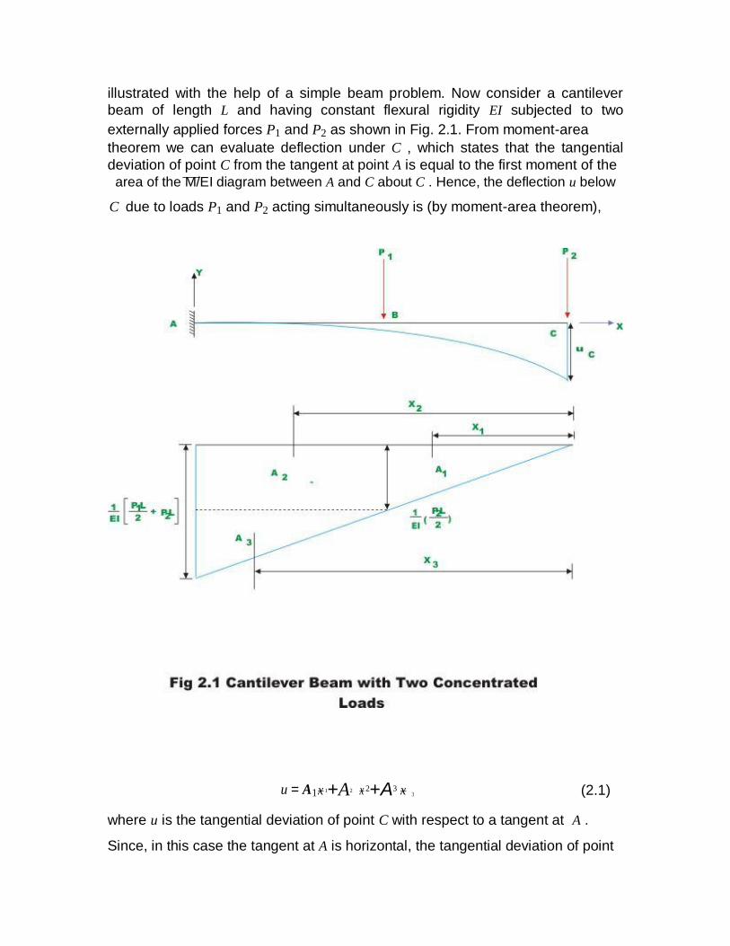
illustrated with the help of a simple beam problem. Now consider a cantilever

beam of length L and having constant flexural rigidity EI subjected to two

externally applied forces P1 and P2 as shown in Fig. 2.1. From moment-area theorem we can evaluate deflection under C , which states that the tangential

deviation of point C from the tangent at point A is equal to the first moment of the

area of the M/EI diagram between A and C about C . Hence, the deflection u below

C due to loads P1 and P2 acting simultaneously is (by moment-area theorem),

u = A1 x 1+A2 x 2+A3 x 3 (2.1)

where u is the tangential deviation of point C with respect to a tangent at A .

Since, in this case the tangent at A is horizontal, the tangential deviation of point

C is nothing but the vertical deflection at C . x1 , x2 and x3 are the distances from

point C to the centroids of respective areas respectively.

x 2 L

x L L

x 2 L L

1 =

2 = + 3 = +

3 2 2 4 3 2 2

A1 = P L2

A2 = P L2

A3 = (PL+P L)L 2

2

1

2

8EI 4EI 8EI

Hence,

u = P L

2 2 L

+ P L

2 L

+ L

+ (PL+P L)L 2 L

+ L

2 2

1 2

(2.2)

8EI 3 2

4EI

2 4 8EI

3 2

2

After simplification one can write,

u = P L

3

+ 5P L

3

(2.3) 2 1

3EI 48EI

Now consider the forces being applied separately and evaluate deflection at C in

each of the case.

u22 = P L

3

(2.4) 2

3EI

where u22 is deflection at C (2) when load P1 is applied at C (2) itself. And,

u21

1 PLL L 2L 5P L3

= 1

+ = 1 (2.5)

2

48EI 22EI 2 3 2

where u21 is the deflection at C (2) when load is applied at B(1) . Now the total deflection at C when both the loads are applied simultaneously is obtained by

adding u22 and u21 .

u = u22 + u21 = P L

3

+ 5P L

3

(2.6) 2 1

3EI 48EI

Hence it is seen from equations (2.3) and (2.6) that when the structure behaves

linearly, the total deflection caused by forces P1 , P2 ,...., Pn at any point in the

structure is the sum of deflection caused by forces P1 , P2 ,...., Pn acting

independently on the structure at the same point. This is known as the Principle

of Superposition. The method of superposition is not valid when the material stress-strain relationship is non-linear. Also, it is not valid in cases where the geometry of

structure changes on application of load. For example, consider a hinged-hinged beam-column subjected to only compressive force as shown in Fig. 2.3(a). Let the compressive force P be less than the Euler’s buckling load of the structure.

Then deflection at an arbitrary point C (say) uc1 is zero. Next, the same beam-

column be subjected to lateral load Q with no axial load as shown in Fig. 2.3(b).

Let the deflection of the beam-column at C be uc2 . Now consider the case when

the same beam-column is subjected to both axial load P and lateral load Q . As

per the principle of superposition, the deflection at the centre uc3 must be the sum

of deflections caused by P and Q when applied individually. However this is not so in the present case. Because of lateral deflection caused by Q , there will be

additional bending moment due to P at C .Hence, the net deflection uc3 will be

more than the sum of deflections uc1 and uc

2 .

Strain Energy

Consider an elastic spring as shown in the Fig.2.4. When the spring is slowly

pulled, it deflects by a small amount u1 . When the load is removed from the

spring, it goes back to the original position. When the spring is pulled by a force, it does some work and this can be calculated once the load-displacement relationship is known. It may be noted that, the spring is a mathematical idealization of the rod being pulled by a force P axially. It is assumed here that

the force is applied gradually so that it slowly increases from zero to a maximum value P . Such a load is called static loading, as there are no inertial effects due

to motion. Let the load-displacement relationship be as shown in Fig. 2.5. Now, work done by the external force may be calculated as,

W

ext

= 1 P u = 1 ( force × displacement) (2.7) 2 2 1 1

The area enclosed by force-displacement curve gives the total work done by the externally applied load. Here it is assumed that the energy is conserved i.e. the

work done by gradually applied loads is equal to energy stored in the structure.

This internal energy is known as strain energy. Now strain energy stored in a spring is

U = 1 Pu (2.8) 2 1 1

Work and energy are expressed in the same units. In SI system, the unit of work and energy is joule (J), which is equal to one Newton metre (N.m). The strain energy may also be defined as the internal work done by the stress resultants in moving through the corresponding deformations. Consider an infinitesimal element within a three dimensional homogeneous and isotropic material. In the most general case, the state of stress acting on such an element may be as

shown in Fig. 2.6. There are normal stresses (σ x ,σ y and σ z ) and shear stresses

(τ xy ,τ yz and τ zx ) acting on the element. Corresponding to normal and shear

stresses we have normal and shear strains. Now strain energy may be written

as,

U = 1 ∫σ T ε dv (2.9)

2 v

in which σ T is the transpose of the stress column vector i.e.,

{σ }T = ( σ x , σ y , σ z , τ xy , τ yz ,τ zx ) and {ε }T = (ε x , ε y , ε z , ε xy , ε yz ,ε zx ) (2.10)

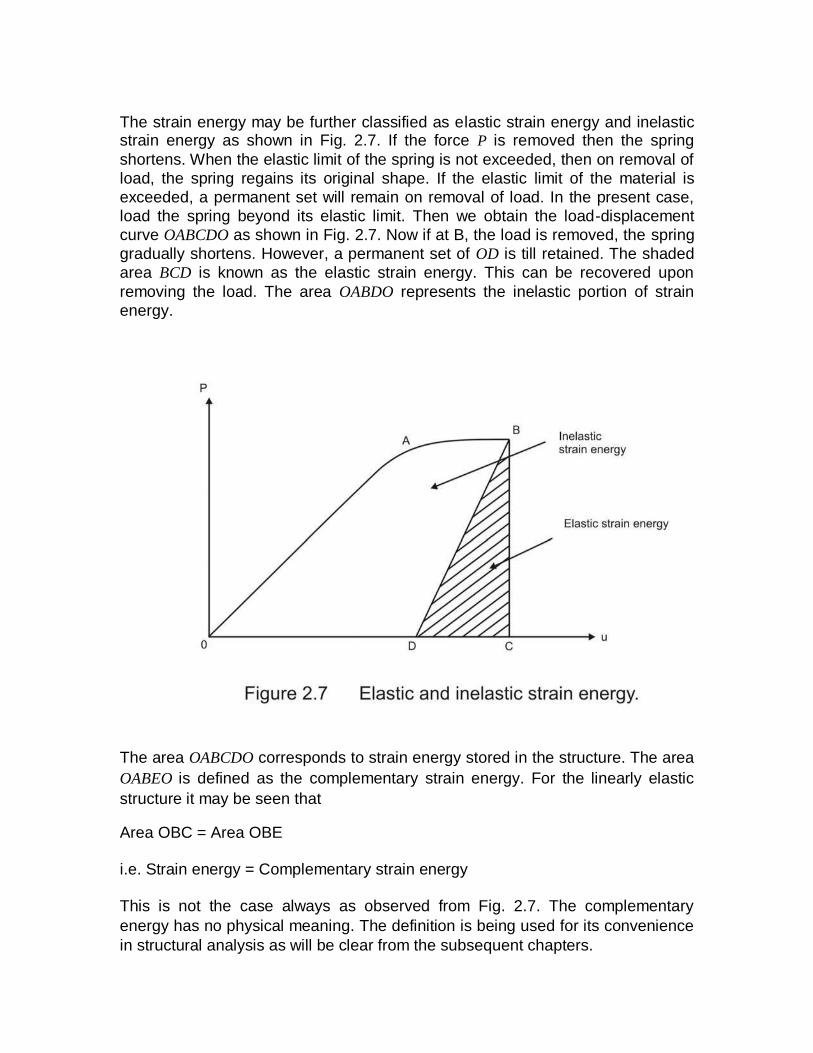
The strain energy may be further classified as elastic strain energy and inelastic strain energy as shown in Fig. 2.7. If the force P is removed then the spring

shortens. When the elastic limit of the spring is not exceeded, then on removal of

load, the spring regains its original shape. If the elastic limit of the material is

exceeded, a permanent set will remain on removal of load. In the present case,

load the spring beyond its elastic limit. Then we obtain the load-displacement

curve OABCDO as shown in Fig. 2.7. Now if at B, the load is removed, the spring

gradually shortens. However, a permanent set of OD is till retained. The shaded

area BCD is known as the elastic strain energy. This can be recovered upon

removing the load. The area OABDO represents the inelastic portion of strain

energy.

The area OABCDO corresponds to strain energy stored in the structure. The area

OABEO is defined as the complementary strain energy. For the linearly elastic

structure it may be seen that

Area OBC = Area OBE

i.e. Strain energy = Complementary strain energy

This is not the case always as observed from Fig. 2.7. The complementary

energy has no physical meaning. The definition is being used for its convenience

in structural analysis as will be clear from the subsequent chapters.

Usually structural member is subjected to any one or the combination of bending moment; shear force, axial force and twisting moment. The member resists these

external actions by internal stresses. In this section, the internal stresses induced in the structure due to external forces and the associated displacements are

calculated for different actions. Knowing internal stresses due to individual forces, one could calculate the resulting stress distribution due to combination of

external forces by the method of superposition. After knowing internal stresses and deformations, one could easily evaluate strain energy stored in a simple beam due to axial deformation and , bending deformation.

Strain energy under axial load

Consider a member of constant cross sectional area A , subjected to axial force P

as shown in Fig. 2.8. Let E be the Young’s modulus of the material. Let the

member be under equilibrium under the action of this force, which is applied

through the centroid of the cross section. Now, the applied force P is resisted by

uniformly distributed internal stresses given by average stress σ = P

A as shown

by the free body diagram (vide Fig. 2.8). Under the action of axial load P applied

at one end gradually, the beam gets elongated by (say) u . This may be

calculated as follows. The incremental elongation du of small element of length dx

of beam is given by,

du = ε dx = σ

E dx = AEP

dx

Now the total elongation of the member of length

integration

L P u = ∫0 AE

dx

(2.11)

L may be obtained by

(2.12)

Now the work done by external loads W = 1

Pu (2.13) 2

In a conservative system, the external work is stored as the internal strain

energy. Hence, the strain energy stored in the bar in axial deformation is,

U = 1

Pu (2.14) 2

Substituting equation (2.12) in (2.14) we get,

L

P 2

U = ∫ dx (2.15)

2AE 0

Strain energy due to bending

Consider a prismatic beam subjected to loads as shown in the Fig. 2.9. The

loads are assumed to act on the beam in a plane containing the axis of symmetry

of the cross section and the beam axis. It is assumed that the transverse cross

sections (such as AB and CD), which are perpendicular to centroidal axis, remain

plane and perpendicular to the centroidal axis of beam (as shown in Fig 2.9).

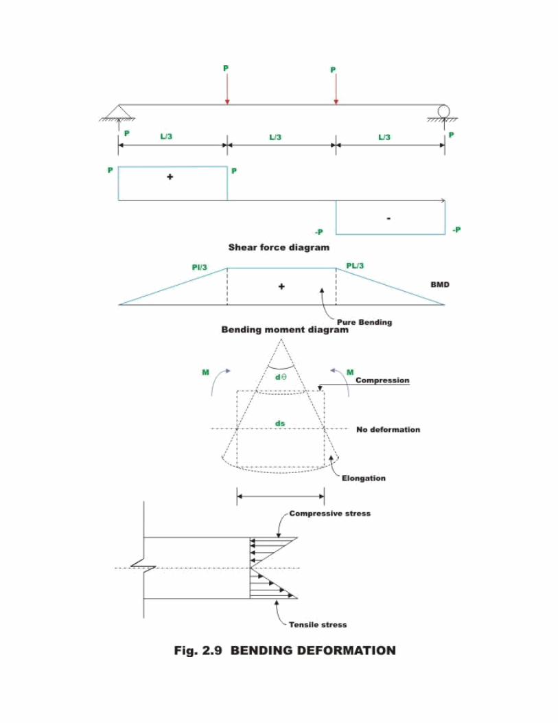
Consider a small segment of beam of length ds subjected to bending moment as

shown in the Fig. 2.9. Now one cross section rotates about another cross section

by a small amount dθ . From the figure,

dθ = 1 ds = M ds (2.16)

EI R

where R is the radius of curvature of the bent beam and EI is the flexural rigidity

of the beam. Now the work done by the moment M while rotating through angle

dθ will be stored in the segment of beam as strain energy dU . Hence,

dU = 1

2 M dθ

Substituting for dθ in equation (2.17), we get, 1 M

2

dU = ds

Now, the energy stored in the complete beam of span

integrating equation (2.18). Thus,

L M 2

U = ∫0 2EI

ds

(2.17)

(2.18)

L may be obtained by

(2.19)

Summary

In this chapter, the principle of superposition has been stated and proved. Also,

its limitations have been discussed. It has been shown that the elastic strain energy stored in a structure is equal to the work done by applied loads in

deforming the structure. The strain energy expression is also expressed for a 3-dimensional homogeneous and isotropic material in terms of internal stresses

and strains in a body. The difference between elastic and inelastic strain energy is explained. Complementary strain energy is discussed. In the end, expressions are derived for calculating strain stored in a simple beam due to axial load and

bending moment.

Chapter 3

Castiglione's Theorems

Instructional Objectives

After reading this lesson, the reader will be able to;

1. State and prove first theorem of Castiglione. 2. Calculate deflections along the direction of applied load of a statically

determinate structure at the point of application of load. 3. Calculate deflections of a statically determinate structure in any direction at a

point where the load is not acting by fictitious (imaginary) load method. 4. State and prove Castiglione’s second theorem.

Introduction

In the previous chapter concepts of strain energy and complementary strain

energy were discussed. Castiglione's first theorem is being used in structural

analysis for finding deflection of an elastic structure based on strain energy of the

structure. The Castiglione's theorem can be applied when the supports of the

structure are unyielding and the temperature of the structure is constant.

Castiglione's First Theorem

For linearly elastic structure, where external forces only cause deformations, the

complementary energy is equal to the strain energy. For such structures, the

Castiglione's first theorem may be stated as the first partial derivative of the strain

energy of the structure with respect to any particular force gives the displacement

of the point of application of that force in the direction of its line of action.

Let P1 , P2 ,...., Pn be the forces acting at x1 , x2 ,......, xn from the left end on a simply

supported beam of span L . Let u1 , u2 ,..., un be the displacements at the loading

points P1 , P2 ,...., Pn respectively as shown in Fig. 3.1. Now, assume that the

material obeys Hooke’s law and invoking the principle of superposition, the work

done by the external forces is given by (vide eqn. 1.8 of lesson 1)

W = 1 P u + 1 P u + .......... + 1 P u (3.1) 2 2

2

1 1 2 2 n n

Work done by the external forces is stored in the structure as strain energy in a

conservative system. Hence, the strain energy of the structure is,

U = 1 P u + 1 P u + .......... + 1 P u (3.2)

2 1 1 2 2 2 2 n n

Displacement u1 below point P1 is due to the action of P1 , P2 ,...., Pn acting at

distances x1 , x2 ,......, xn respectively from left support. Hence, u1 may be expressed

as,

u1 = a11 P1 + a12 P2 + .......... + a1n Pn (3.3)

In general,

ui = ai1 P1 + ai2 P2 + .......... + ain Pn i = 1,2,...n (3.4)

where aij is the flexibility coefficient at i due to unit force applied at j .

Substituting the values of u1 , u2 ,..., un in equation (3.2) from equation (3.4), we

get,

U = 1

2 P1[a11 P1 + a12 P2 + ...] + 12 P2 [a21 P1 + a22 P2 + ...] + ....... +

12 Pn [an1 P1 + an2 P2 + ...] (3.5)

We know from Maxwell-Betti’s reciprocal theorem aij = a ji . Hence, equation (3.5)

may be simplified as,

1 2 2 2 + [ a12 P1 P2 + a13 P1 P3 + .... + a1n P1 Pn ]+ ... U =

+ a 22 P2 + .... + ann Pn 2 a

11 P

1

Now, differentiating the strain energy with any force P1 gives,

∂U = a P + a P + .......... + a P

11 112 2 1n n

∂P1

It may be observed that equation (3.7) is nothing but displacement

loading point. In general,

∂U = u

∂Pn n

(3.6)

(3.7)

u1 at the

(3.8)

Hence, for determinate structure within linear elastic range the partial derivative

of the total strain energy with respect to any external load is equal to the

displacement of the point of application of load in the direction of the applied

load, provided the supports are unyielding and temperature is maintained

constant. This theorem is advantageously used for calculating deflections in

elastic structure. The procedure for calculating the deflection is illustrated with

few examples.

Example 3.1

Find the displacement and slope at the tip of a cantilever beam loaded as in Fig. 3.2. Assume the flexural rigidity of the beam EI to be constant for the beam.

Moment at any section at a distance x away from the free end is given by

M = −Px (1)

L

M 2

Strain energy stored in the beam due to bending is U = ∫ dx (2)

2EI 0

Substituting the expression for bending moment M in equation (3.10), we get,

L

(Px) 2

P 2 3

U = ∫ dx =

L (3)

2EI

6EI 0

Now, according to Castigliano’s theorem, the first partial derivative of strain

energy with respect to external force P gives the deflection uA at A in the

direction of applied force. Thus,

∂U

= uA = PL

3

(4)

3EI ∂P

To find the slope at the free end, we

respect to externally applied moment M

need to differentiate strain energy with

at A . As there is no moment at A , apply

a fictitious moment M 0 at A . Now moment at any section at a distance x away

from the free end is given by

M = −Px − M 0

Now, strain energy stored in the beam may be calculated as,

L (Px + M 0 )2 P 2 L3 M0PL

2 M 0

2 L U = ∫

dx =

+

+

(5) 2EI 6EI 2EI 2EI 0

Taking partial derivative of strain energy with respect to M 0 , we get slope at A .

∂U = θA =

PL2

+ M0 L

(6)

∂M0 2EI

EI

But actually there is no moment applied at A . Hence substitute M 0 = 0 in

equation (3.14) we get the slope at A.

θ A = PL

2

(7) 2EI

Example 3.2 A cantilever beam which is curved in the shape of a quadrant of a circle is loaded as shown in Fig. 3.3. The radius of curvature of curved beam is R , Young’s modulus of the material is E and second moment of the area is I about an axis

perpendicular to the plane of the paper through the centroid of the cross section. Find the vertical displacement of point A on the curved beam.

The bending moment at any section θ of the curved beam (see Fig. 3.3) is given

by

M = PR sinθ (1)

Strain energy U stored in the curved beam due to bending is,

U = ∫s M 2 ds =

π

∫/ 2

P 2 R

2 (sin

2 θ )Rd θ = P2 R3

π = π P2R

3 (2)

0 2EI 0 2 EI 2EI 4 8EI

Differentiating strain energy with respect to externally applied load, P we get

uA = ∂U b = π PR3

(3)

4EI ∂P

Example 3.3

Find horizontal displacement at D of the frame shown in Fig. 3.4. Assume the

flexural rigidity of the beam EI to be constant through out the member. Neglect

strain energy due to axial deformations.

The deflection D may be obtained via. Castigliano’s theorem. The beam

segments BA and DC are subjected to bending moment Px ( 0 < x < L ) and the

beam element BC is subjected to a constant bending moment of magnitude PL .

Total strain energy stored in the frame due to bending

L 2 L 2

U =2∫ (Px) dx + ∫ (PL) dx

After simplifications, 0 2EI 0 2EI

U = P

2L

3

+ P

2L

3

= 5P

2L

3

3EI

2EI

6EI

Differentiating strain energy with respect to P we get,

∂U

= uD = 2

5P L3

=

5P L3

∂P 6EI 3EI

(1)

(2)

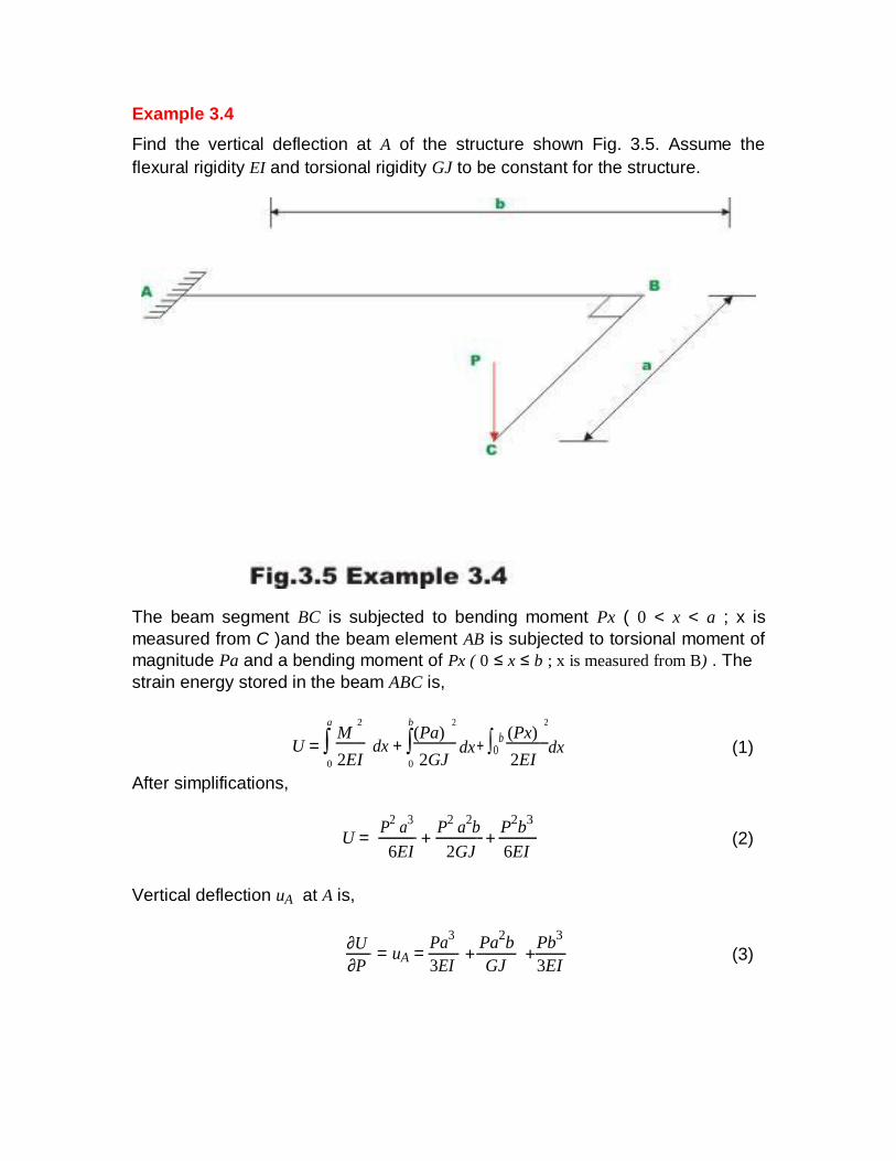
Example 3.4

Find the vertical deflection at A of the structure shown Fig. 3.5. Assume the

flexural rigidity EI and torsional rigidity GJ to be constant for the structure.

The beam segment BC is subjected to bending moment Px ( 0 < x < a ; x is

measured from C )and the beam element AB is subjected to torsional moment of

magnitude Pa and a bending moment of Px ( 0 ≤ x ≤ b ; x is measured from B) . The strain energy stored in the beam ABC is,

a

M 2 b

(Pa) 2

+ ∫0b (Px)

2

U = ∫ dx + ∫

dx

dx (1) 2EI

2GJ 2EI

0 0

After simplifications,

U =

P2 a

3 +

P2 a

2b

+ P

2b

3

(2)

6EI

2GJ

6EI

Vertical deflection uA at A is,

∂U = uA =

Pa3 +

Pa2b

+ Pb

3

(3)

∂P

3EI

GJ

3EI

Example 3.5

Find vertical deflection at C of the beam shown in Fig. 3.6. Assume the flexural

rigidity EI to be constant for the structure.

The beam segment CB is subjected to bending moment Px ( 0 < x < a ) and beam

element AB is subjected to moment of magnitude Pa . To find the vertical deflection at C , introduce a imaginary vertical force Q at C .

Now, the strain energy stored in the structure is,

a

(Px) 2 b

(Pa + Qy) 2

U = ∫ dx + ∫

dy 2EI

2EI

0 0

Differentiating strain energy with respect to Q , vertical deflection at C

∂U b

= uC = ∫ 2(Pa + Qy) y dy

∂Q

0 2EI

uC = 1 b Pay + Qy2 dy

EI

∫0

(1)

is obtained.

(2)

(3)

uC = 1 Pab 2

+ Qb 3

(4)

2

3

EI

But the force Q is fictitious force and hence equal to zero. Hence, vertical

deflection is,

uC = Pab

2

(5) 2EI

Castiglione’s Second Theorem

In any elastic structure having n independent displacements u1 , u2 ,..., un

corresponding to external forces P1 , P2 ,...., Pn along their lines of action, if strain

energy is expressed in terms of displacements then n equilibrium equations may

be written as follows.

∂U = P , j = 1, 2,..., n (3.9)

∂u j j

This may be proved as follows. The strain energy of an elastic body may be

written as

U = 1 P u + 1 P u + .......... + 1 P u (3.10) 2 2

2

1 1 2 2 n n

We know from Lesson 1 (equation 1.5) that

Pi = k i1u1 + k i 2 u 2 + ..... + kin u n , i = 1, 2,..,

n (3.11)

where kij is the stiffness coefficient and is defined as the force at i due to unit

displacement applied at j . Hence, strain energy may be written as,

U = 1 u [ k u + k u + ...] + 1 u [k u + k u + ...] + .......+ 1 u [k u + k u + ...] (3.12)

21111 12 2 2

2 21 1 22 2 2 n n1 1 n2 2

We know from reciprocal theorem k ij = k ji . Hence, equation (3.12) may be

simplified as,

1 2 2 2 + [ k12 u1u 2 + k13 u1u3 + .... + k1 n u1un ] + ... (3.13)

U =

+ k 22 u 2 + .... + k nn u n 2 k

11u

1

Now, differentiating the strain energy with respect to any displacement u1 gives

the applied force P1 at that point, Hence,

∂U = k u + k u + ........ + k u n

(3.14)

2 11 1 12 1n

∂u1

Or,

∂U = P , j = 1, 2,..., n (3.15)

∂u j j

Summary

In this lesson, Castiglione's first theorem has been stated and proved for linearly

elastic structure with unyielding supports. The procedure to calculate deflections

of a statically determinate structure at the point of application of load is illustrated

with examples. Also, the procedure to calculate deflections in a statically

determinate structure at a point where load is applied is illustrated with examples.

The Castiglione's second theorem is stated for elastic structure and proved.