General Features of Our Approach to NESM & NEMD
32
11/25/16 1 General Features of Our Approach to NESM & NEMD Our main goal is to reach an understanding connecting microscopic and mesoscopic models to analogs in the Real World of Macroscopic Physical Phenomena . We strive for simplicity . Our models are mainly classical and nonrelativistic and typically two-dimensional . The main lines of thought we follow can be traced to Abraham , Alder , Ashurst , Bhattacharya , Boltzmann , Bridgman , Bulgac , Debye , De Rocco , Dettmann , Duvall , Euler , Evans , Fermi , Feynman, Ford , Galton , Gauss , Gibbs , Jaynes , Hamilton , Holian , Kawai , Kratky , Krivtsov , Kusnezov , Lagrange , Landau , Lifshitz , Liouville , Lyapunov , Mareschal , Maxwell , the Mayers , Moran , Morriss , Newton , Nosé , Occam , Pars , Patra , Posch , Rahman , Rice , Ruelle , Sommerfeld , Sprott , Steiner , Stell , Stull , Thoreau , Travis , Uhlenbeck , Vineyard , von Neumann, Wainwright , Wojciechowski . Wood , Zwanzig . Feynman’s ideas of pursuing definite examples, along with his and Alder’s efforts toward simplicity are always with us . Most of what you see will be in two dimensions , with graphic illustrations , using FORTRAN and gnuplot and PowerPoint as our main expository tools , not because these are perfect but because we haven’t yet found anything better . In order to teach students rather than course material it is useful to have questions . This is the main job of the student , not just for himself , but for all of us . Let us thank Baidurya Bhattacharya for making this possible .
-
Upload
khangminh22 -
Category
Documents
-
view
1 -
download
0
Transcript of General Features of Our Approach to NESM & NEMD

11/25/16
1
General Features of Our Approach to NESM & NEMDOur main goal is to reach an understanding connecting microscopic and mesoscopic models to analogsin the Real World of Macroscopic Physical Phenomena . We strive for simplicity . Our models are mainlyclassical and nonrelativistic and typically two-dimensional . The main lines of thought we follow can betraced to Abraham , Alder , Ashurst , Bhattacharya , Boltzmann , Bridgman , Bulgac , Debye , De Rocco , Dettmann , Duvall , Euler , Evans , Fermi , Feynman, Ford , Galton , Gauss , Gibbs , Jaynes , Hamilton , Holian , Kawai , Kratky , Krivtsov , Kusnezov , Lagrange , Landau , Lifshitz , Liouville , Lyapunov , Mareschal , Maxwell , the Mayers , Moran , Morriss , Newton , Nosé , Occam , Pars , Patra , Posch , Rahman , Rice , Ruelle , Sommerfeld , Sprott , Steiner , Stell , Stull , Thoreau , Travis , Uhlenbeck , Vineyard , von Neumann, Wainwright , Wojciechowski . Wood , Zwanzig . Feynman’s ideas of pursuing definite examples, along with his and Alder’s efforts toward simplicity are always with us .
Most of what you see will be in two dimensions , with graphic illustrations , using FORTRAN and gnuplotand PowerPoint as our main expository tools , not because these are perfect but because we haven’t yet found anything better .
In order to teach students rather than course material it is useful to have questions . This is the main job of the student , not just for himself , but for all of us .
Let us thank Baidurya Bhattacharya for making this possible .

11/25/16
2
Kharagpur Lecture 3Temperature and Molecular Dynamics
William G. HooverRuby Valley Nevada
December 2016
1. Ideal Gas Thermometer à Temperature/Entropy2. Isokinetic “Gaussian” Molecular Dynamics3. Nosé and Nosé-Hoover Mechanics4. The Boltzmann Equation and Entropy5. The Krook-Boltzmann Equation, h and k6. Direct Simulation Monte Carlo7. Nosé-Hoover Knots from Yang and Wang
1. Ideal Gas Thermometer à Temperature/Entropy

11/25/16
3
Mechanics plus Temperature ( and Heat ) à Thermodynamics .We have the luxury of using the ideal-gas temperature scale
TitaniummeltsatT=3034F.
Temperatureinthesun=15,000,000K.
TemperatureintheHBombisafewtimesgreaterthanthatofthesun.
PlottingPV/Nk atlownumberdensitydefinestheideal-gastemperaturescale.
Ideal-Gas Thermometer: Microscopic Mechanics à ThermodynamicsGibbs’ Statistical Mechanics in the Microcanonical Ensemble *
IdealGas
Fluid
Thermal equilibrium corresponds to maximizing the number of states by varying the fluid energy . The ideal-gas energy states comprise a DN-dimensional hypersphere .Taking the logarithm of the number of states makes the maximization step easy :
Maximizing lnW à ( ∂ lnW I / ∂EI ) = ( ∂ lnW F / ∂E F ) = DN/( 2E ) = ( 1/kT )
This definition of temperature makes thermometry possible and givesthe Zeroth Law of Thermodynamics : T1 = T2 and T1 = T3 à T2 = T3
WI isthenumberofstates,with(dqdp/h)DN corresponding to a “state” àWI+F = WI(E- EF)WF(EF)=WI(EI)WF (E- EI)
* GoodreferencesareMolecularDynamicsandComputationalStatisticalMechanics@williamhoover.info
WIdeal = (1/N!) ∏( ∫ ∫ dq dp/h) µ (V/N)N(E/N)DN/2

11/25/16
4
Next Consider Mechanical Evaluation of Pressure , in 2D
Ly
Lx
vx
Notice that both pressure and temperature can be second-ranktensors. Two directions are involved : [ 1 ] the orientation of the wall on which the force per unit area is measured; and [ 2 ] the direction of the force. At equilibrium the pressure and the temperature are scalars. We will show this for the ideal gas using the Boltzmann equation which à Maxwell-Boltzmann f .
Microscopic Mechanics à ThermodynamicsJ Willard Gibbs’ Statistical Mechanics *
IdealGas
Fluid
Mechanical Coupling à WI+F = WI(V- VF)WF(VF)=WI(VI)WF (V- VI)
Mechanical equilibrium corresponds to maximizing the number of states by varying the fluid volume . The ideal-gas volume states comprise an N-dimensional hypevolume VN . Again ,
taking the logarithm of the number of states makes the maximization step easy :
Maximizing lnW à ( ∂ lnW I / ∂VI ) = ( ∂ lnW F / ∂V F ) = ( N/V ) = ( P/kT )This ideal-gas pressure makes it easy to describe mechanical equilibria and
gives the Zeroth Law of Mechanics/Dynamics if P1 = P2 and P1 = P3 à P2 = P3
* J.W.Gibbs,ElementaryPrinciplesinStatisticalMechanics(Dover,1960),originally1902
( 1839-1903 )
WI = (1/N!) ∏( ∫ ∫ dq dp/h) µ (V/N)N(E/N)DN/2

11/25/16
5
ThermodynamicEntropySCorrespondstoklnW
[1]EntropyisastatefunctiondependinguponEandV.[2]Entropyincreasesintheabsenceofaconstraint.[3]Entropyisanextensivequantityforidentical particles.Foranidealgas(S/Nk)=ln (V/N)+(D/2)ln(E/N)+constant*TdS =dE +PdV (CombinedFirstandSecondLaws).
Themicrocanonical entropyshownheredeviatesonlynegligibly–as(1/N)– fromGibbs’canonicalentropywherethemomentum
integralis(2pmkT)1/2 perdegreeoffreedom.
TheMayers’StatisticalMechanicsexpressesthehypervolume ofaDN-dimensionalhypersphereintermsofGaussianintegrals,whichare“gammafunctions”.
S(p2/2m) = E , a many-dimensional spherical surface with radius (2mE)1/2
What about using the ConfigurationalTemperature from Landau/Lifshitz ?
kT∫ [ ( 2F) e-F/kTdr = ∫ ( F)2e-F/kTdrThis is just an application of integration by parts : ∫du v = - ∫dv u where u = F and v = e-F/kT whereF vanishes at the two endpoints of the integrals .
There is a comprehensive literature detailing ( or obscuring ) what is arelatively simple idea with plenty of generalizations . Unfortunately itappears to be just a dead end . If you would like to read more see CarlosBraga and Karl Travis’ two papers in the Journal of Chemical Physics :123, 134101 (2005) and 124, 104102 (2006) .
D D
D

11/25/16
6
An apparent disadvantage is the occasional vanishing of the denominator .Think about gravitational field forces !
What about using the ConfigurationalTemperature from Landau/Lifshitz ?
An apparent advantage is the lack of dependence on velocity ,where the local velocity might be hard to determine accurately .
Steady rotation increases the forces without increasing temperature so that configurational temperature seems rather unphysical .
2. Isokinetic “Gaussian” Molecular Dynamics
Ordinarily (dK/dt) = - (dF/dt) . The upshot of a classic concept ,Gauss’ “Principle of Least Constraint” , S d(Fc )2 = 0 , is a motion equation of the form (dK/dt) = - (dF/dt) + S F • v as we shall see .Remember that Gauss was famous for “Least Squares” already .
This idea is not a panacea , and gives incorrect results sometimes .
Pars’ text is a good reference for classical variational principles .
11/25/16
7
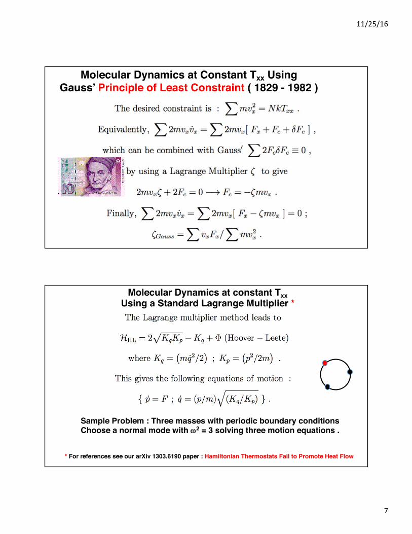
Molecular Dynamics at Constant Txx UsingGauss’ Principle of Least Constraint ( 1829 - 1982 )
Molecular Dynamics at constant TxxUsing a Standard Lagrange Multiplier *
Sample Problem : Three masses with periodic boundary conditionsChoose a normal mode with w2 = 3 solving three motion equations .
* For references see our arXiv 1303.6190 paper : Hamiltonian Thermostats Fail to Promote Heat Flow

11/25/16
8
Sample Problem # 1 : Three masses with periodic boundary conditionsChoose a normal mode with w2 = 3 solving three motion equations .
This moving wave has constant kinetic and potential energies .For this system’s isokinetic problems zGauss = 0 and Kq = Kp .
x, y, and z are the displacements of the particles
Sample Problem # 2 : Two masses in steady rotation with one spring .
Springforceis(1– r)andwithaspeedofunitythecentrifugalforceisr/2à r=2 .Youshouldbeabletoverifythattheinitialvalues
{ x1 = 1 ; y1 = 0 ; px1 = 0 ; py1 = 1 }arethoseforwhichtheradialaccelerationiszero.NoticethatthefourvariablesforParticle2arejustthenegativesofthoseforParticle1.
r12=dsqrt((x1-x2)**2+(y1-y2)**2)fx1 = (x2 - x1)*(r12 - 1)/r12fy1 = (y2 - y1)*(r12 - 1)/r12
RK4solutionof4equationsforParticle1.Thereare628timesteps ofdt =0.01each.Itisn’tnecessarytoaddthecentrifugal
forces{w2r/2}tothespringforces.Thoseforcesariseautomaticallyfromthemotion.
It is also easy to see that the virial theorem is satisfied. Consider the theorem for the x coordinateof Particle 1 . The x coordinate is (r/2)cos(t) = cos(t) à < x �̈� > = < (d/dt) 𝐱�̇� > −< �̇�𝟐 >= 𝟎 − 𝟏 𝟐⁄ .A good way to start on such problems is to write the Lagrangian ( in terms of the coordinates andvelocities ) in order to discover the momenta and the Hamiltonian equations of motion they obey .
r = 2 ••

11/25/16
9
Sample Problem # 3 : Five masses in steady rotation with four springs .
x1 = -19/7.1 ; x2 = -10/7.1 ; x3 = 0 ; x4 = +10/7.1 ; x5 = +19/7.1Initial values of py are equal to the x coordinates à w = 1 .
Springforcesare10(1– r)andcentrifugalforcesarer.Youshouldbeabletoverifythattheinitialvaluesgivenbelowarethoseforwhichalltheradialaccelerationsvanish.
r12 = dsqrt((x1-x2)**2 + (y1-y2)**2)r23 = dsqrt(x2*x2 + y2*y2)fx1 = 10*(x2-x1)*(r12 - 1)/r12fy1 = 10*(y2-y1)*(r12 - 1)/r12fx2 = 10*(x1-x2)*(r12 - 1)/r12fy2 = 10*(y1-y2)*(r12 - 1)/r12fx2 = fx2 + 10*(0-x2)*(r23 - 1)/r23fy2 = fy2 + 10*(0-y2)*(r23 - 1)/r23
RK4solutionof8equationsforParticles1and2.628timesteps ofdt =0.01each.Itisn’tnecessarytoaddthecentrifugalforces{w2r}tothespringforces.Those
Forcesariseautomaticallyfromthemotion.
Potential Energies for Newton, Hoover-Leete, and GaussDynamics with Kinetic Energies initially equal to 7 .
Fourth-Order Runge-Kutta timestep = 0.001 .
F( t )G
HLN

11/25/16
10
3. Nosé and Nosé-Hoover Mechanics *
* Nosé’s 1984 papers [ Molecular Physics + Journal of Chemical Physics ] and mine in Physical Review A .
Shuichi Nosé’s Mechanics for an Oscillator( 1984 )
Two steps are involved here : [ 1 ] Scaling the time with s ( line 2 à line 3 ) and [ 2 ] Redefining the momentum , ( p / s ) à p .
Alternatively one can compute the acceleration .

11/25/16
11
To what extent is the Continuity Equation Obvious ?
dxAn important observation :During the short time dt the flow into the fixed Eulerian bin is fvdt from the left with aloss –fvdt on the right. Evidently the change in fdx during dt becomes -∂(fv/∂x)dtdx sothat the conservation law in one dimension is (∂f/∂t) = -∂(fv)/∂x . There is nothing tostop us from summing up contributions in the x and y and z directions if desired, oreven in all the phase-space directions if we would like to prove Liouville’s Theorem .
The Flag of France
*
* Herefisaconservedquantity,likemassdensityorprobabilitydensity,withavelocityv.
11/25/16
12
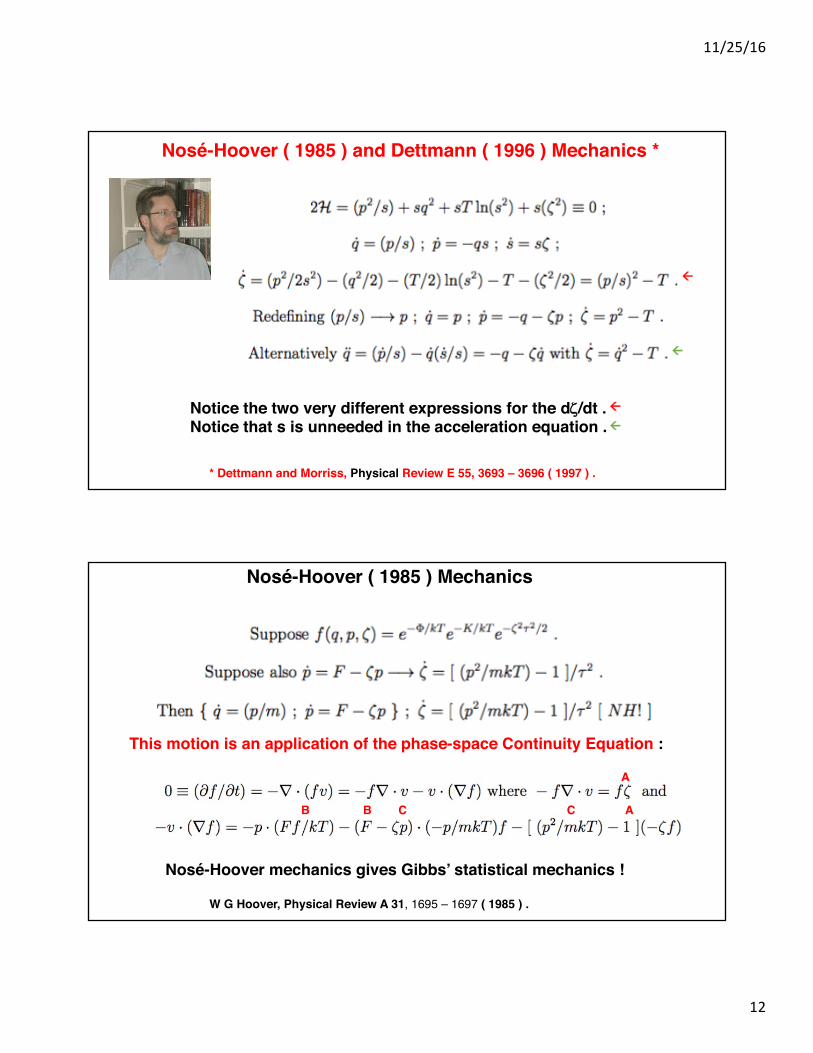
Nosé-Hoover ( 1985 ) and Dettmann ( 1996 ) Mechanics *
Notice the two very different expressions for the dz/dt .Notice that s is unneeded in the acceleration equation .
* Dettmann and Morriss, Physical Review E 55, 3693 – 3696 ( 1997 ) .
ß
ß
ß
ß
Nosé-Hoover ( 1985 ) Mechanics
W G Hoover, Physical Review A 31, 1695 – 1697 ( 1985 ) .
This motion is an application of the phase-space Continuity Equation :
Nosé-Hoover mechanics gives Gibbs’ statistical mechanics !
A
B B C C A
11/25/16
13
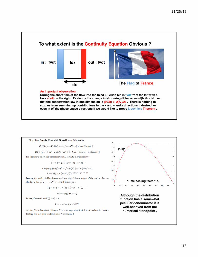
To what extent is the Continuity Equation Obvious ?
dxAn important observation :During the short time dt the flow into the fixed Eulerian bin is fvdt from the left with aloss –fvdt on the right. Evidently the change in fdx during dt becomes -∂(fv/∂x)dtdx sothat the conservation law in one dimension is (∂f/∂t) = -∂(fv)/∂x . There is nothing tostop us from summing up contributions in the x and y and z directions if desired, oreven in all the phase-space directions if we would like to prove Liouville’s Theorem .
The Flag of France
(1/s)s
“Time-scaling factor” s
Although the distribution function has a somewhat peculiar denominator it is
well-behaved from the numerical standpoint .
11/25/16
14
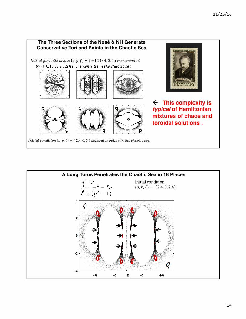
The Three Sections of the Nosé & NH Generate Conservative Tori and Points in the Chaotic Sea
!"#$#%& !"#$%&$' !"#$%& !,!, ! = ±1.2144, 0, 0 !"#$%&%"'%(
!"#$#%& !"#$%&%"# !,!, ! = 2.4, 0, 0 !"#"$%&"' !"#$%& !" !ℎ! !ℎ!"#$% !"# .
ß This complexity istypical of Hamiltonianmixtures of chaos andtoroidal solutions .
-4 < q < +4
A Long Torus Penetrates the Chaotic Sea in 18 Places Initial condition !,!, ! = 2.4, 0, 2.4

11/25/16
15
-4 < q < +4
Initial condition !,!, ! = ±1.6, 0, 0
Two Long Tori Penetrate the Chaotic Sea
-4
-2
0
2
4
-4 -2 0 2 4
Nosé is extremely stiff ( and slow to compute ), here the thick line .Nosé-Hoover is much more efficient, here the thinner projection .
Chaotic starts : (qpsz) = (3310) and (qpz) = (330), both to time = 100 .Fourth-order Runge-Kutta integration with dt = 0.001 and dt = 0.01 .
z
q
OInitialConditionforBothModels
H is 9 here , not 0 !

11/25/16
16
Lyapunov Exponents for Nosé & Nosé-Hoover Mechanics
0.0135
0.0140
0.0145
350000 < time < 750000
λ< λ > = .01414
< λ > = .01392
0.0135
0.0140
0.0145
350000 < time < 750000
λ< λ > = .01414
< λ > = .01392
0.045
0.047
0.049
80000 < time < 180000
λ < λ > = .0475 Nosé
NH2
NH1
< ! >!"#é !"##$%& !"#$ < ! >!" !" ! !"#$%& !" !/< ! >!" = !.!" = < ! ! >! . Initial condition : ( q,p,s, ζ ) = ( 2.4, 0, e-2.88, 0 ) so that H = 0 .
Lyapunov Exponents for Nosé & Nosé-Hoover Mechanics
Dettmann’s Hamiltonian = 0 :( dq/dt ) = ( p/s ) ; ( dp/dt ) = – sq ;
( ds/dt ) = sz ; ( dz/dt ) = ( p/s )2 – 1
Nosé-Hoover Equations :( dq/dt ) = ; ( dp/dt ) = – q – zp; ( dz/dt) = p2 – 1
200 < time < 20 000 000 à 2.3 < log( time ) < 7.3
Lyapunov Exponents for Nosé & Nosé-Hoover Mechanics
< l1(time) >Dettmann’s Hamiltonian = 0 :
( dq/dt ) = ( p/s ) ; ( dp/dt ) = – sq ;
( ds/dt ) = sz ; ( dz/dt ) = ( p/s )2 – 1
Nosé-Hoover Equations :( dq/dt ) = p ; ( dp/dt ) = -q – zp ; ( dz/dt) = p2 – 1
200 < time < 20 000 000 ß-à 2.3 < log( time ) < 7.3
l1 à 0.0138
2 000 000 000 adaptive timesteps

11/25/16
17
4. The Boltzmann Equation and Entropy
When does Boltzmann’s Equation for f(r,p,t) apply ?
[ 1 ] When the density is low so that PV = NKT .[ 2 ] When collisions occur at points ( not Enskog, not Knudsen ) . [ 3 ] When collision orientations are random ( Pxx = Pyy ) .These restrictions are all related to the basic assumption
f(r1, r2, p1, p2) = f(r, p1)f(r, p2) *Remarkably, the Boltzmann Equation obeys the Second Law .That is, the Boltzmann Equation is irreversible and providesquantitative viscosities h and conductivities k .
( ∂f/∂t )collisions is calculated from two-body collisions by combining thecollisional “losses” with reversed-inverse collisions which give “gains”.This expression gives the comoving time derivative following the motion.
* These f( . . . ) functions are all probability densities in phase spaces .

11/25/16
18
Boltzmann’s Treatment of Two-Body Collisions( ∂f/∂t )collisions = “Gain” – “Loss” a [ f3f4 – f1f2 ]For the soft repulsive potential f(r) = ( 1 – r2 )4
a typical pair of collisions is shown below .The “loss” velocities are indicated by arrows .The “gain” collision is inverted in space and time .The “gain” collision begins at the circled blue dots and finishes at the plain end points lacking the dots .
Boltzmann’s Proof of the H-Theorem, (dS/dt) ≥ 0 .
For simplicity we imagine that the system is homogeneous and isolated so that integrating over space is unnecessary . Notice also that f is normalized so that its integral is constant . The collision rates of corresponding gains and losses are identicalas both of them are integrated over the entire velocity space .This irreversible result is surprising as the motion is reversible. Unless ln f is conserved, as in A + Bv + Cv2, the entropy S increases . Evidently equilibrium corresponds to the Maxwell-Boltzmann Gaussian distribution !

11/25/16
19
Boltzmann’s Proof of the H-Theorem, (dS/dt) ≥ 0 .
This irreversible result is surprising as the motion is reversible. Unless ln f is conserved, as in A + Bv + Cv2, the entropy S increases . Evidently equilibrium corresponds to the Maxwell-Boltzmann Gaussian distribution !
The surprise is usually stated as two paradoxes :
Zermélo : If the equations of motion are reversible then anytrajectory obeying the H-Theorem disobeys it if reversed .
Poincaré : If the equations of motion obey Liouville’s Theoremthen any initial state , no matter how odd , will recur in future .
Boltzmann’s Proof of the H-Theorem, (dS/dt) ≥ 0 .
Poincaré : If the equations of motion obey Liouville’s Theoremthen any initial state , no matter how odd , will recur in future .
To prove this consider a small phase volume DW and follow itlong enough that the new volume DW’ does not overlap the old .Call DW” all of the volume ever covered ( in infinitely long time )which was originally in DW’ . Then it must be the case that thelatter includes DW . Otherwise the volume DW + DW” would haveto violate Liouville’s Theorem . This “Recurrence Theorem” is called Poincaré’s Recurrence Paradox . Do not be dismayedthat the time required to recur exceeds the age of the Universefor about a dozen argon atoms at liquid density .
11/25/16
20
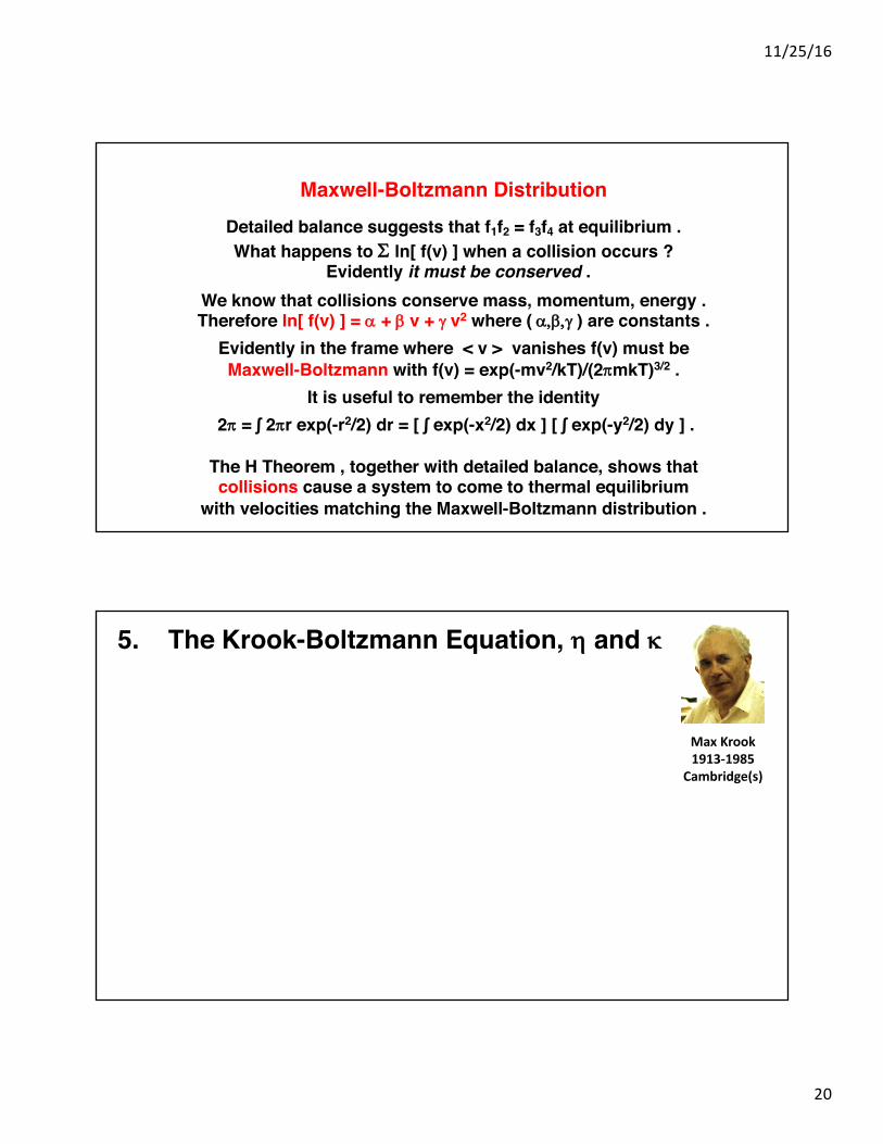
Maxwell-Boltzmann DistributionDetailed balance suggests that f1f2 = f3f4 at equilibrium .What happens to S ln[ f(v) ] when a collision occurs ?
Evidently it must be conserved .We know that collisions conserve mass, momentum, energy .Therefore ln[ f(v) ] = a + b v + g v2 where ( a,b,g ) are constants .
Evidently in the frame where < v > vanishes f(v) must beMaxwell-Boltzmann with f(v) = exp(-mv2/kT)/(2pmkT)3/2 .
It is useful to remember the identity2p = ∫ 2pr exp(-r2/2) dr = [ ∫ exp(-x2/2) dx ] [ ∫ exp(-y2/2) dy ] .
The H Theorem , together with detailed balance, shows thatcollisions cause a system to come to thermal equilibrium
with velocities matching the Maxwell-Boltzmann distribution .
5. The Krook-Boltzmann Equation, h and k
MaxKrook1913-1985
Cambridge(s)

11/25/16
21
The Krook-Boltzmann Equation is Similar and Simpler
(df/dt)=(fLTE – f)/t ,wheret isthecollisiontime.NowtheHTheoremcanbeprovedinasingleline:
(dS/dt)=< – Nk[1+lnf][fLTE – f ] /t =– Nk[ln(f/fLTE)][fLTE – f]>LocalThermodynamicEquilibriummeanshavingexactlythesamedensity,velocity,andenergy.
ForMaxwellmoleculesthisKBapproximationisexact.
Weillustrateitsconsequencesforsimpleshearandforsteadyheatflow.
The Krook-Boltzmann Equation is Similar and Simpler
SupposethatthedistributionfunctionhasalinearincreaseinuwithyandthatPxy =Pyx =– h(du/dy):
This density-independence of viscosity is a major success of the Boltzmann Equation !
11/25/16
22
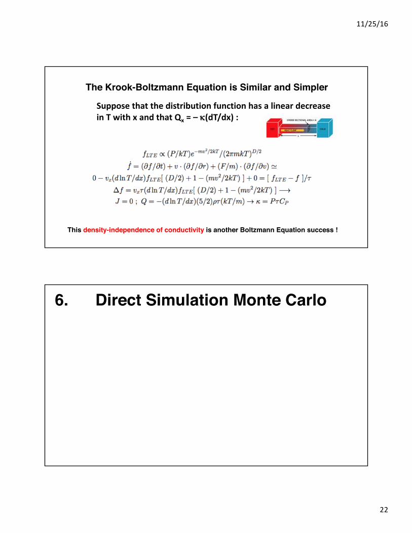
The Krook-Boltzmann Equation is Similar and Simpler
SupposethatthedistributionfunctionhasalineardecreaseinT withxandthatQx =– k(dT/dx):
This density-independence of conductivity is another Boltzmann Equation success !
6. Direct Simulation Monte Carlo

11/25/16
23
Direct Simulation Monte Carlo ( developed by Græme Bird )provides simple solutions, both analytic and numerical .
Divide the space into “zones” or cells, each with several particles .Some cells can act as boundary conditions as in a shock wave .The basic algorithm then advances each particle for a time dt .The number of collisions in each zone is computed from < | vij | > .Pairs of particles in each zone are then selected for collision withThe impact parameters are chosen randomly .The advantages of this method are speed and simplicity .
The Krook-Boltzmann idea would replace a particle with one drawnfrom the LTE ( Local Thermodynamic Equilibrium ) distribution .
Ideal-Gas Thermometry – Massive Particle in a Thermal Bath
The Model :M = 100 with V = 1 and m = 1 witha Maxwell-Boltzmann distribution
Two Solution Methods :1. Expand the Gaussian integrals for the bath in (m/M)1/2 .2. Carry out a simulation along the lines of Krook-Boltzmann :
Algorithm for the Simulation :Choose a Maxwell – Boltzmann bath particle v in 1D, 2D, or 3D .Choose a random “ impact parameter ” in the 2D case .Compute the momentum/energy changes in a collision with V .Weight these changes with the relative speed, | ( v – V ) | .Sum up a million or so collisions .
Simulation is certainly faster and likely more accurate !

11/25/16
24
Reminder : How to Choose a Gaussian random number with rund(intx,inty)random where rund returns a random number in the interval [ 0 to 1 ] .
intx = 0inty = 0
10 vx = 10*dsqrt(T)*(rund(intx,inty) – 0.5d00)Boltz = dexp(-vx*vx/(T+T))If(rund(intx,inty).gt.Boltz go to 10
TheBox-MulleralgorithmisamoresophisticatedmethodforgeneratingGaussianrandomvelocities,asCarolmentioned.SeeWikipediafordetails.
ForthedetailsoftheanalyticapproachaswellastheresultofanelasticcollisionOfMwithVandmwithvseeHHPinPhysicalReviewE48,3196-3198(1993):
DE
Rods
Thermal Equilibration – Energy Change for M = 100 in a bath with m = 1 at T
200 million-collision averages at temperatures 1, 2, . . . 200
0 < kT < 200

11/25/16
25
Two and Three-Dimensional Simulations of the Bath Interaction appear in the Hoovers’Physical Review E 77, 041104 ( 2008 ) : “Nonequilibrium Temperature/Thermometry …”
Some points of interest that could use investigation
Smooth-particleaveragesprovidelocalquantities:
F(r)º S Fjw(r – rj) where w(r) a 1 – 6(r/h)2 + 8(r/h)3 – 3(r/h)4
Computing the local temperature involves a localAverage of two velocity moments : < ( v – < v > )2 > .
An instantaneous recipe would be handy. One ideais to eliminate the “self contribution” to the local temperature . Irving and Kirkwood, and later Hardy,seem to have confused several researchers .
11/25/16
26
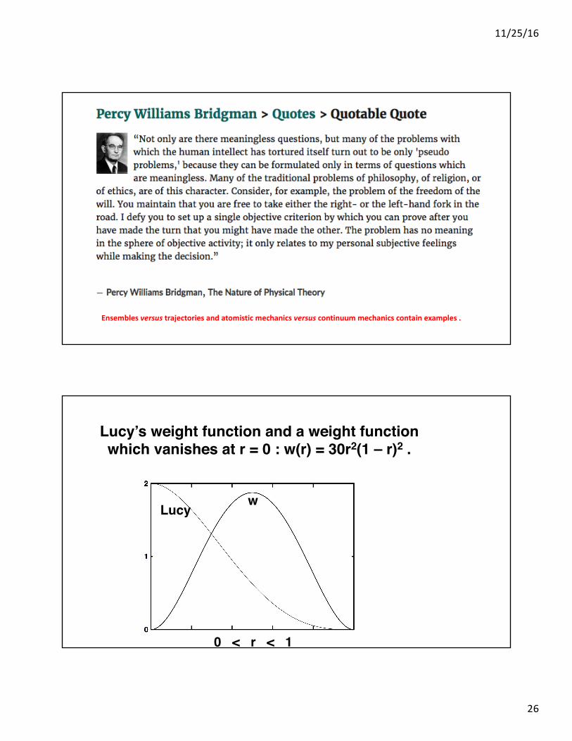
Ensemblesversus trajectoriesandatomisticmechanicsversus continuummechanicscontainexamples.
Lucy’s weight function and a weight functionwhich vanishes at r = 0 : w(r) = 30r2(1 – r)2 .
Lucyw
0 < r < 1
11/25/16
27
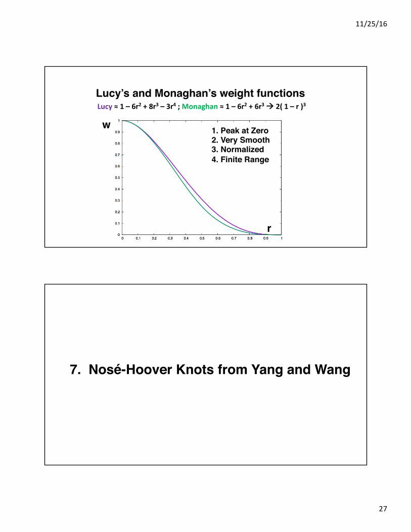
Lucy’s and Monaghan’s weight functionsLucy ≈1– 6r2 +8r3 – 3r4 ;Monaghan ≈1– 6r2 +6r3 à 2(1– r)3
1. Peak at Zero2. Very Smooth3. Normalized4. Finite Range
w
r
7. Nosé-Hoover Knots from Yang and Wang

11/25/16
28
Interlocking Rings in Oscillator Phase Space
z
à( dq/dt ) = p ; ( dp/dt ) = – q – zp ;( dz/dt ) = p2 – T ; T = 1 + e tanh(q)
The topology of knots is fascinating ,even in the case of just three rings .

11/25/16
29
Knots are Everywhere !
Piotr Pieranski’s researchin Poznań, Poland :
He has written software for simplifying, classifying, and
even untying knots by increasing the diameter of the
rope to its maximum .
Trefoil or overhand knot LuxorLas Vegas
“The invariant Tori of Knot Type and the Interlinked Invariant Tori in the Nosé-Hoover System” Lei Wang and Xiao-Song Yang, arXiv 1501.03375
[A somewhat stiffer Nosé-Hoover oscillator : (dq/dt) = p ; (dp/dt) = – q – zp ; (dz/dt) = 10(p2 – 1) ]
Initial(q,p,z)=(-0.72,0,0)and(2.4,0,0)(6x5/2)PairsofToriturnouttobeInterlinked!
q
z

11/25/16
30
Is This a Nosé – Hoover Knot ?Initial condition !,!, ! = 1.6, 0, 0 ! > ! ; ! < !
Is This a Nosé – Hoover Knot ?Initial condition !,!, ! = 2.4, 0, 2.4 ! > ! ; ! < !

11/25/16
31
Is This a Nosé – Hoover Knot ?Initial condition !,!, ! = 2.4, 0, 2.4 ! > ! ; ! < !
Is This a Nosé – Hoover Knot ?
above
below
Initial condition !,!, ! = 1.6, 0, 0 ! > ! ; ! < !

11/25/16
32
Summaryofthingsitwouldbegoodtoknowuptothepresent
1. Temperatureisbestmeasuredwiththeideal-gasthermometer.2. GaussandHoover-Leete algorithmsareisokineticanduseful.3. Nosé mechanicsisunnecessarilystiffandnotveryuseful.*4. Nosé-Hoovermechanicsisconvenientandrobust.5. TheBoltzmannEquationcoversmanyapplicationsbeyondh ,k .6. ThelinearKrook-BoltzmannequationisnearlyasusefulasisB.7. DirectSimulationMonteCarloisasimpletoolforgasproblems.8. Knotsshouldappealtothoseinterestedintopologyandchaos.
* Theseproblemsdemonstratetheusefulnessofadaptiveintegration,alreadyexplainedbyCarol.
Thingsitwouldbegoodtothinkabout:
1. HowtomakeaBoltzmannEquationboundaryconditionforPxy ?2. CanyousolvetheKrook-Boltzmannequationforashockwave?3. Isentropyadynamicalpropertyofasingledynamicalsystem?