Genealogical particle analysis of rare events

arX

iv:m

ath/

0602

525v

1 [

mat

h.PR

] 2

3 Fe

b 20

06

The Annals of Applied Probability

2005, Vol. 15, No. 4, 2496–2534DOI: 10.1214/105051605000000566c© Institute of Mathematical Statistics, 2005

GENEALOGICAL PARTICLE ANALYSIS OF RARE EVENTS

By Pierre Del Moral and Josselin Garnier

Universite de Nice and Universite Paris 7

In this paper an original interacting particle system approach isdeveloped for studying Markov chains in rare event regimes. The pro-posed particle system is theoretically studied through a genealogicaltree interpretation of Feynman–Kac path measures. The algorithmicimplementation of the particle system is presented. An estimator forthe probability of occurrence of a rare event is proposed and its vari-ance is computed, which allows to compare and to optimize differentversions of the algorithm. Applications and numerical implementa-tions are discussed. First, we apply the particle system technique toa toy model (a Gaussian random walk), which permits to illustratethe theoretical predictions. Second, we address a physically relevantproblem consisting in the estimation of the outage probability due topolarization-mode dispersion in optical fibers.

1. Introduction. The simulation of rare events has become an exten-sively studied subject in queueing and reliability models [16], in particularin telecommunication systems. The rare events of interest are long waitingtimes or buffer overflows in queueing systems, and system failure events inreliability models. The issue is usually the estimation of the probability ofoccurrence of the rare event, and we shall focus mainly on that point. Butour method will be shown to be also efficient for the analysis of the cascadeof events leading to the rare event, in order to exhibit the typical physicalpath that the system uses to achieve the rare event.

Standard Monte Carlo (MC) simulations are usually prohibited in thesesituations because very few (or even zero) simulations will achieve the rareevent. The general approach to speeding up such simulations is to acceleratethe occurrence of the rare events by using importance sampling (IS) [16,24]. More refined sampling importance resampling (SIR) and closely relatedsequential Monte Carlo methods (SMC) can also be found in [4, 10]. In

Received May 2004; revised April 2005.AMS 2000 subject classifications. 65C35, 65C20, 60F10, 68U20, 62P35.Key words and phrases. Rare events, Monte Carlo Markov chains, importance sam-

pling, interacting particle systems, genetic algorithms.

This is an electronic reprint of the original article published by theInstitute of Mathematical Statistics in The Annals of Applied Probability,2005, Vol. 15, No. 4, 2496–2534. This reprint differs from the original inpagination and typographic detail.

1

http://arXiv.org/abs/math/0602525v1

http://www.imstat.org/aap/

http://dx.doi.org/10.1214/105051605000000566

http://www.imstat.org

http://www.ams.org/msc/

http://www.imstat.org

http://www.imstat.org/aap/

http://dx.doi.org/10.1214/105051605000000566

2 P. DEL MORAL AND J. GARNIER

all of these well-known methods the system is simulated using a new setof input probability distributions, and unbiased estimates are recovered bymultiplying the simulation output by a likelihood ratio. In SIR and SMCthese ratio weights are also interpreted as birth rates. The tricky part ofthese Monte Carlo strategies is to properly choose the twisted distribution.The user is expected to guess a more or less correct twisted distribution;otherwise these algorithms may completely fail. Our aim is to propose amore elaborate and adaptative scheme that does not require any operationof the user.

Recently intensive calculations with huge numerical codes have been car-ried out to estimate the probabilities of rare events. We shall present atypical case where the probability of failure of an optical transmission sys-tem is estimated. The outputs of these complicated systems result from theinterplay of many different random inputs and the users have no idea of thetwisted distributions that should be used to favor the rare event. This is infact one of the main practical issues to identify the typical conjunction ofevents leading to an accident. Furthermore these systems are so complicatedthat it is very difficult for the user, if not impossible, to modify the codesin order to twist the input probability distributions. We have developed amethod that does not require twisting the input probability distribution.The method consists in simulating an interacting particle system (IPS) withselection and mutation steps. The mutation steps only use the unbiasedinput probability distributions of the original system.

The interacting particle methodology presented in this paper is also closelyrelated to a class of Monte Carlo acceptance/rejection simulation techniquesused in physics and biology. These methods were first designed in the 1950sto estimate particle energy transmission [15], self-avoiding random walks andmacromolecule evolutions [23]. The application model areas of these particlemethods now have a range going from advanced signal processing, includ-ing speech recognition, tracking and filtering, to financial mathematics andtelecommunication [10].

The idea is the following one. Consider an E-valued Markov chain (Xp)0≤p≤n

with nonhomogeneous transition kernels Kp. The problem consists in esti-mating the probability of occurrence PA of a rare event of the form V (Xn) ∈A where V is some function from E to R. The IPS consists of a set of N

particles (X(i)p )1≤i≤N evolving from time p = 0 to p = n. The initial gener-

ation at p = 0 is a set of independent copies of X0. The updating from thegeneration p to the generation p + 1 is divided into two stages:

(1) The selection stage consists in choosing randomly and independently

N particles amongst (X(i)p )1≤i≤N according to a weighted Boltzmann–

Gibbs particle measure, with a weight function that depends on V . Thus,particles with low scores are killed, while particles with high scores aremultiplied. Note that the total number of particles is kept constant.

GENEALOGICAL PARTICLE ANALYSIS OF RARE EVENTS 3

(2) The mutation step consists in mutating independently the particles ac-cording to the kernel Kp. Note that the true transition kernel is applied,in contrast with IS.

The description is rough in that the IPS actually acts on the path level.The mathematical tricky part consists in proposing an estimator of the prob-ability PA and analyzing its variance. The variance analysis will provideuseful information for a proper choice of the weight function of the selectionstage.

The analysis of the IPS is carried out in the asymptotic framework N ≫1 where N is the number of particles, while the number n of mutation–selection steps is kept constant. Note that the underlying process can bea Markov chain (Xp)0≤p≤n with a very large number of evolutionary stepsn. As the variance analysis shows, it can then be more efficient to performselection steps on a subgrid of the natural time scale of the process X . Inother words, it is convenient to introduce the chain (Xp)0≤p≤n = (Xkp)0≤p≤n

where k = n/n and n is in the range 10–100. The underlying process can bea time-continuous Markov process (Xt)t∈[0,T ] as well. In such a situation it

is convenient to consider the chain (Xp)0≤p≤n = (XpT/n)0≤p≤n.Beside the modeling of a new particle methodology, our main contribution

is to provide a detailed asymptotic study of particle approximation models.Following the analysis of local sampling errors introduced in Chapter 9 in theresearch monograph [4], we first obtain an asymptotic expansion of the biasintroduced by the interaction mechanism. We also design an original fluc-tuation analysis of polynomial functions of particle random fields, to derivenew central limit theorems for weighted genealogical tree-based occupationmeasures. The magnitude of the asymptotic variances and comparisons withtraditional Monte Carlo strategies are discussed in the context of Gaussianmodels.

Briefly, the paper is organized as follows. Section 2 contains all the the-oretical results formulated in an abstract framework. We give a summaryof the method and present a user-friendly implementation in Section 3. Weconsider a toy model (a Gaussian random walk) in Section 4 to illustrate thetheoretical predictions on an example where all relevant quantities can beexplicitly computed. Finally, in Section 5, we apply the method to a physicalsituation emerging in telecommunication.

2. Simulations of rare events by interacting particle systems.

2.1. Introduction. In this section we design an original IPS approach foranalyzing Markov chains evolving in a rare event regime.

In Section 2.2 we use a natural large deviation perspective to exhibit natu-ral changes of reference measures under which the underlying process is more


likely to enter in a given rare level set. This technique is more or less wellknown. It often offers a powerful and elegant strategy for analyzing rare de-viation probabilities. Loosely speaking, the twisted distributions associatedto the deviated process represent the evolution of the original process in therare event regime. In MC Markov chain literature, this changes-of-measurestrategy is also called the importance sampling (IS) technique.

In Section 2.3 we present a Feynman–Kac formulation of twisted refer-ence path distributions. We examine a pair of Gaussian models for whichthese changes of measures have a nice explicit formulation. In this context,we initiate a comparison of the fluctuation-error variances of the “pure” MCand the IS techniques. In general, the twisted distribution suggested by thephysical model is rather complex, and its numerical analysis often requiresextensive calculations. The practitioners often need to resort to another“suboptimal” reference strategy, based on a more refined analysis of thephysical problem at hand. The main object of this section is to complementthis IS methodology, by presenting a genetic type particle interpretation ofa general and abstract class of twisted path models. Instead of hand craftingor simplified simulation models, this new particle methodology provides apowerful and very flexible way to produce samples according to any com-plex twisted measures dictated by the physical properties of the model athand. But, from the strict practical point of view, if there exists already agood specialized IS method for a specific rare event problem, then our IPSmethodology may not be the best tool for that application.

In Section 2.4 we introduce the reader to a new developing genealogicaltree interpretation of Feynman–Kac path measures. For a more thoroughstudy on this theme we refer to the monograph [4] and references therein. Weconnect this IPS methodology with rare event analysis. Intuitively speaking,the ancestral lines associated to these genetic evolution models represent thephysical ways that the process uses to reach the desired rare level set.

In the final Section 2.5 we analyze the fluctuations of rare event parti-cle simulation models. We discuss the performance of these interpretationson a class of warm-up Gaussian models. We compare the asymptotic error-variances of genealogical particle models and the more traditional nonin-teracting IS schemes. For Gaussian models, we show that the exponentialfluctuation orders between these two particle simulation strategies are equiv-alent.

2.2. A large deviation perspective. Let Xn be a Markov chain takingvalues at each time n in some measurable state space (En,En) that maydepend on the time parameter n. Suppose that we want to estimate theprobability Pn(a) that Xn enters, at a given fixed date n, into the a-levelset V −1

n ([a,∞)) of a given energy-like function Vn on En, for some a ∈ R:

Pn(a) = P(Vn(Xn)≥ a).(2.1)


To avoid some unnecessary technical difficulties, we further assume thatPn(a) > 0, and the pair (Xn, Vn) satisfies Cramer’s condition E(eλVn(Xn)) <∞ for all λ ∈ R. This condition ensures the exponential decay of the prob-abilities P(Vn(Xn)≥ a) ↓ 0, as a ↑ ∞. To see this claim, we simply use theexponential version of Chebyshev’s inequality to check that, for any λ > 0we have

P(Vn(Xn) ≥ a) ≤ e−λ(a−λ−1Λn(λ)) with Λn(λ)def.= log E(eλVn(Xn)).

As an aside, it is also routine to prove that the maximum of (λa−Λn(λ)) withrespect to the parameter λ > 0 is attained at the value λn(a) determined bythe equation a = E(Vn(Xn)eλVn(Xn)))/E(eλVn(Xn))). The resulting inequality

P(Vn(Xn)≥ a)≤ e−Λ⋆n(a) with Λ⋆

n(a) = supλ>0

(λa−Λn(λ))

is known as large deviation inequality. When the Laplace transforms Λn

are explicitly known, this variational analysis often provides sharp tail es-timates. We illustrate this observation on an elementary Gaussian model.This warm-up example will be used in several places in the further develop-ment of this article. In the subsequent analysis, it is briefly used primarily tocarry out some variance calculations for natural IS strategies. As we alreadymentioned in the Introduction, and in this Gaussian context, we shall derivein Section 2.7 sharp estimates of mean error variances associated to a pairof IPS approximation models.

Suppose that Xn is given by the recursive equation

Xp = Xp−1 + Wp(2.2)

where X0 = 0 and (Wp)p∈N∗ represents a sequence of independent and identi-cally distributed (i.i.d.) Gaussian random variables, with (E(W1),E(W 2

1 )) =(0,1). If we take Vn(x) = x, then we find that Λn(λ) = λ2n/2, λn(a) = a/nand Λ⋆

n(a) = a2/(2n), from which we recover the well-known sharp exponen-

tial tails P(Xn ≥ a)≤ e−a2/(2n).In more general situations, the analytical expression of Λ⋆

n(a) is out ofreach, and we need to resort to judicious numerical strategies. The firstrather crude MC method is to consider the estimate

PNn (a) =

1

N

N∑

i=1

1Vn(Xin)≥a

based on N independent copies (Xin)1≤i≤N of Xn. If is not difficult to check

that the resulting error-variance is given by

σ2n(a) = NE[(PN

n (a)−Pn(a))2] = Pn(a)(1−Pn(a)).

In practice, PNn (a) is a very poor estimate mainly because the whole sample

set is very unlikely to reach the rare level.


A more judicious choice of MC exploration model is dictated by the largedeviation analysis presented above. To be more precise, let us suppose thata > λ−1Λn(λ), with λ > 0. To simplify the presentation, we also assume thatthe initial value X0 = x0 is fixed, and we set V0(x0) = 0. Let Pλ

n be the new

reference measure on the path space Fndef.= (E0 × · · · × En) defined by the

formula

dP(λ)n =

1

E(eλVn(Xn))eλVn(Xn) dPn,(2.3)

where Pn is the distribution of the original and canonical path (Xp)0≤p≤n.By construction, we have that

P(Vn(Xn)≥ a) = E(λ)n [1Vn(Xn)≥a dPn/dP(λ)

n ]

= E(λ)n [1Vn(Xn)≥a e−λVn(Xn)]E[eλVn(Xn)]

≤ e−λ(a−λ−1Λn(λ))P(λ)n (Vn(Xn) ≥ a),

where E(λ)n represents the expectation operator with respect to the distribu-

tion P(λ)n . By definition, the measure P

(λ)n tends to favor random evolutions

with high potential values Vn(Xn). As a consequence, the random paths un-

der P(λ)n are much more likely to enter into the rare level set. For instance,

in the Gaussian example described earlier, we have that

dP(λ)n /dPn =

n∏

p=1

eλ(Xp−Xp−1)−λ2/2.(2.4)

In other words, under P(λ)n the chain takes the form Xp = Xp−1 + λ + Wp,

and we have P(λ)n (Xn ≥ a) = Pn(Xn ≥ a− λn) (= 1/2 as soon as a = λn).

These observations suggest to replace PN (a) by the weighted MC model

PN,λn (a) =

1

N

N∑

i=1

dPn

dP(λ)n

(Xλ,i0 , . . . ,Xλ,i

n )1Vn(Xλ,i

n )≥a

associated to N independent copies (Xλ,in )1≤i≤N of the chain under P

(λ)n .

Observe that the corresponding error-variance is given by

σ(λ)n (a)2 = NE[(PN,λ

n (a)−Pn(a))2]

= E[1Vn(Xn)≥a e−λVn(Xn)]E[eλVn(Xn)]−P 2n(a)(2.5)

≤ e−λ(a−λ−1Λn(λ))Pn(a)−P 2n(a).

For judicious choices of λ, one expects the exponential large deviation termto be proportional to the desired tail probabilities Pn(a). In this case, we


have σ(λ)n (a)2 ≤ KP 2

n(a) for some constant K. Returning to the Gaussiansituation, and using Mill’s inequalities

1

t + 1/t≤ P(N (0,1) ≥ t)

√2πet2/2 ≤ 1

t

which are valid for any t > 0, and any reduced Gaussian random variableN (0,1) (see, e.g., (6) on page 237 in [25]), we find that

σ(λ)n (a)2 ≤ e−a2/(2n)Pn(a)−P 2

n(a) ≤ P 2n(a)[

√2π(a/

√n +

√n/a)− 1]

for the value λ = λn(a) = a/n which optimizes the large deviation inequality(2.6). For typical Gaussian type level indexes a = a0

√n, with large values

of a0, we find that λn(a) = a0/√

n and

σ(λ)n (a)2 ≤ P 2

n(a)[√

2π(a0 + 1/a0)− 1].

As an aside, although we shall be using most of the time upper boundestimates, Mill’s inequalities ensure that most of the Gaussian exponentialdeviations are sharp.

The formulation (2.5) also suggests a dual interpretation of the variance.First, we note that

dPn/dP(λ)n = E[eλVn(Xn)]E[e−λVn(Xn)]dP(−λ)

n /dPn

and therefore

σ(λ)n (a)2 = P(−λ)

n (Vn(Xn)≥ a)E[eλVn(Xn)]E[e−λVn(Xn)]−P 2n(a).

In contrast to P(λ)n , the measure P

(−λ)n now tends to favor low energy states

Xn. As a consequence, we expect P(−λ)n (Vn(Xn) ≥ a) to be much smaller

than Pn(a). For instance, in the Gaussian case we have

P(−λ)n (Xn ≥ a) = Pn(Xn ≥ a + λn)≤ e−(a+λn)2/(2n).

Since we have E[eλXn ] = E[e−λXn ] = eλ2n/2, we can write

σ(λ)n (a)2 ≤ e−a2/ne(a−λn)2/(2n) −P 2

n(a)(2.6)

which confirms that the optimal choice (giving rise to the minimal variance)for the parameter λ is λ = a/n.

2.3. Twisted Feynman–Kac path measures. The choice of the “twisted”

measures P(λ)n introduced in (2.3) is only of pure mathematical interest. In-

deed, the IS estimates described below will still require both the sampling of

random paths according to P(λ)n and the computation of the normalizing con-

stants. As we mentioned in the Introduction, the key difficulty in applyingIS strategies is to choose the so-called “twisted” reference measures. In the


further development of Section 2.4, we shall present a natural genealogicaltree-based simulation technique of twisted Feynman–Kac path distributionof the following form:

dQn =1

Zn

n∏

p=1

Gp(X0, . . . ,Xp)

dPn.(2.7)

In the above display, Zn > 0 stands for a normalizing constant, and (Gp)1≤p≤n

represents a given sequence of potential functions on the path spaces (Fp)1≤p≤n.Note that the twisted measures defined in (2.3) correspond to the (nonunique)choice of functions

Gp(X0, . . . ,Xp) = eλ(Vp(Xp)−Vp−1(Xp−1)).(2.8)

As an aside, we mention that the optimal choice of twisted measure with re-spect to the IS criterion is the one associated to the potential functions Gn =1V −1

n ([a,∞)), and Gp = 1, for p < n. In this case, we have Zn = P(Vn(Xn)≥ a)

and Qn is the distribution of the random paths ending in the desired rarelevel. This optimal choice is clearly infeasible, but we note that the resultingvariance is null.

The rare event probability admits the following elementary Feynman–Kacformulation.

P(Vn(Xn)≥ a) = E

[

g(a)n (X0, . . . ,Xn)

n∏

p=1

Gp(X0, . . . ,Xp)

]

= ZnQn(g(a)n )

with the weighted function defined by

g(a)n (x0, . . . , xn) = 1Vn(xn)≥a

n∏

p=1

G−1p (x0, . . . , xp)

for any path sequence such that∏n

p=1 Gp(x0, . . . , xp) > 0. Otherwise, g(a)n is

assumed to be null.The discussion given above already shows the improvements one might

expect in changing the reference exploration measure. The central idea be-hind this IS methodology is to choose a twisted probability that mimicsthe physical behavior of the process in the rare event regime. The poten-tial functions Gp represent the changes of probability mass, and in somesense the physical variations in the evolution of the process to the rare levelset. For instance, for time-homogeneous models Vp = V , 0 ≤ p ≤ n, the po-tential functions defined in (2.8) will tend to favor local transitions thatincrease a given V -energy function. The large deviation analysis developedin Section 2.2 combined with the Feynman–Kac formulation (2.3) gives someindications on the way to choose the twisted potential functions (Gp)1≤p≤n.


Intuitively, the attractive forces induced by a particular choice of poten-tials are compensated by increasing normalizing constants. More formally,the error-variance of the Qn-importance sampling scheme is given by theformula

σQn (a)2 = Q−

n (Vn(Xn)≥ a)ZnZ−n −Pn(a)2,(2.9)

where Q−n is the path Feynman–Kac measure given by

dQ−n =

1

Z−n

n∏

p=1

G−1p (X0, . . . ,Xp)

dPn.

Arguing as before, and since Q−n tends to favor random paths with low

Gp energy, we expect Q−n (Vn(Xn) ≥ a) to be much smaller than the rare

event probability P(Vn(Xn) ≥ a). On the other hand, by Jensen’s inequal-ity we expect the product of normalizing constants ZnZ−

n (≥ 1) to be verylarge. These expectations fail in the “optimal” situation examined above(Gn = 1V −1

n ([a,∞)), and Gp = 1, for p < n). In this case, we simply note

that Qn = Q−n = Law(X0, . . . ,Xn|Vn(Xn) ≥ a), and Q−

n (Vn(Xn) ≥ a) = 1,and Zn =Z−

n = Pn(a). To avoid some unnecessary technical discussions, wealways implicitly assume that the rare event probabilities Pn(a) are strictlypositive, so that the normalizing constants Zn = Z−

n = Pn(a) > 0 are alwayswell defined.

We end this section with a brief discussion on the competition betweenmaking a rare event more attractive and controlling the normalizing con-stants. We return to the Gaussian example examined in (2.2), and insteadof (2.4), we consider the twisted measure

dQn = dP(λ)n =

1

Z(λ)n

n∏

p=1

eλXp

dPn.(2.10)

In this case, it is not difficult to check that for any λ ∈ R we have Z(λ)n =

e(λ2/2)

∑n

p=1p2

. In addition, under P(λ)n the chain Xn has the form

Xp = Xp−1 + λ(n− p + 1) + Wp, 1 ≤ p≤ n.(2.11)

When λ > 0, the rare level set is now very attractive, but the normalizing

constants can become very large Z(λ)n = Z(−λ)

n (≥ eλ2n3/12). Also notice thatin this situation the first term in the right-hand side of (2.9) is given by

P(−λ)n (Vn(Xn)≥ a)Z(λ)

n Z(−λ)n

≤ e(−1/(2n))(a+λ

∑n

p=1p)2+λ2

∑n

p=1p2

≤ e−a2/ne(1/(2n))(a−λ

∑n

p=1p)2+λ2[

∑n

p=1p2−(

∑n

p=1p)2/n]

.


Although we are using inequalities, we recall that these exponential esti-mates are sharp. Now, if we take λ = 2a/[n(n + 1)], then we find that

P(−λ)n (Vn(Xn)≥ a)Z(λ)

n Z(−λ)n ≤ e−(a2/n)(2/3)(1+1/(n+1)).(2.12)

This shows that even if we adjust correctly the parameter λ, this IS estimateis less efficient than the one associated to the twisted distribution (2.4).The reader has probably noticed that the change of measure defined in(2.10) is more adapted to estimate the probability of the rare level setsVn(Yn) ≥ a, with the historical chain Yn = (X0, . . . ,Xn) and the energyfunction Vn(Yn) =

∑np=1 Xp.

2.4. A genealogical tree-based interpretation model. The probabilistic in-terpretation of the twisted Feynman–Kac measures (2.7) presented in thissection can be interpreted as a mean field path-particle approximation ofthe distribution flow (Qn)n≥1. We also mention that the genetic type se-lection/mutation evolution of the former algorithm can also be seen as anacceptance/rejection particle simulation technique. In this connection, andas we already mentioned in the Introduction, we again emphasize that thisIPS methodology is not useful if we already know a specialized and exactsimulation technique of the desired twisted measure.

2.4.1. Rare event Feynman–Kac type distributions. To simplify the pre-sentation, it is convenient to formulate these models in terms of the historicalprocess

Yndef.= (X0, . . . ,Xn) ∈ Fn

def.= (E0 × · · · ×En).

We let Mn(yn−1, dyn) be the Markov transitions associated to the chain Yn.To simplify the presentation, we assume that the initial value Y0 = X0 = x0

is fixed, and we also denote by Kn(xn−1, dxn) the Markov transitions of Xn.We finally let Bb(E) be the space of all bounded measurable functions onsome measurable space (E,E), and we equip Bb(E) with the uniform norm.

We associate to the pair potentials/transitions (Gn,Mn) the Feynman–Kac measure defined for any test function fn ∈ Bb(Fn) by the formula

γn(fn) = E

[

fn(Yn)∏

1≤k<n

Gk(Yk)

]

.

We also introduce the corresponding normalized measure

ηn(fn) = γn(fn)/γn(1).

To simplify the presentation and avoid unnecessary technical discussions,we suppose that the potential functions are chosen such that

sup(yn,y′

n)∈F 2n

Gn(yn)/Gn(y′n) <∞.


This regularity condition ensures that the normalizing constants γn(1) andthe measure γn are bounded and positive. This technical assumption clearlyfails for unbounded or for indicator type potential functions. The Feynman–Kac and the particle approximation models developed in this section canbe extended to more general situations using traditional cut-off techniques,by considering Kato-class type of potential functions (see, e.g., [19, 22, 26]),or by using different Feynman–Kac representations of the twisted measures(see, e.g., Section 2.5 in [4]).

In this section we provide a Feynman–Kac formulation of rare event prob-abilities. The fluctuation analysis of their genealogical tree interpretationswill also be described in terms of the distribution flow (γ−

n , η−n ), defined as(γn, ηn) by replacing the potential functions Gp by their inverse

G−p = 1/Gp.

The twisted measures Qn presented in (2.7) and the desired rare eventprobabilities have the following Feynman–Kac representation:

Qn(fn) = ηn(fnGn)/ηn(Gn) and P(Vn(Xn)≥ a) = γn(T (a)n (1)).

In the above displayed formulae, T(a)n (1) is the weighted indicator function

defined for any path yn = (x0, . . . , xn) ∈ Fn by

T (a)n (1)(yn) = T (a)

n (1)(x0, . . . , xn) = 1Vn(xn)≥a

∏

1≤p<n

G−p (x0, . . . , xp).

More generally, we have for any ϕn ∈ Bb(Fn)

E[ϕn(X0, . . . ,Xn);Vn(Xn)≥ a] = γn(T (a)n (ϕn))

with the function T(a)n (ϕn) given by

T (a)n (ϕn)(x0, . . . , xn) = ϕn(x0, . . . , xn)1Vn(xn)≥a

∏

1≤p<n

G−p (x0, . . . , xp).(2.13)

To connect the rare event probabilities with the normalized twisted measureswe use the fact that

γn+1(1) = γn(Gn) = ηn(Gn)γn(1) =n∏

p=1

ηp(Gp).

This readily implies that for any fn ∈ Bb(Fn)

γn(fn) = ηn(fn)∏

1≤p<n

ηp(Gp).(2.14)


This yields the formulae

P(Vn(Xn) ≥ a) = ηn(T (a)n (1))

∏

1≤p<n

ηp(Gp),

E(ϕn(X0, . . . ,Xn);Vn(Xn) ≥ a) = ηn(T (a)n (ϕn))

∏

1≤p<n

ηp(Gp),(2.15)

E(ϕn(X0, . . . ,Xn)|Vn(Xn) ≥ a) = ηn(T (a)n (ϕn))/ηn(T (a)

n (1)).

To take the final step, we use the Markov property to check that thetwisted measures (ηn)n≥1 satisfy the nonlinear recursive equation

ηn = Φn(ηn−1)def.=

∫

Fn−1

ηn−1(dyn−1)Gn−1(yn−1)Mn(yn−1, ·)/ηn−1(Gn−1)

starting from η1 = M1(x0, ·).

2.4.2. Interacting path-particle interpretation. The mean field particlemodel associated with a collection of transformations Φn is a Markov chainξn = (ξi

n)1≤i≤N taking values at each time n≥ 1 in the product spaces FNn .

Loosely speaking, the algorithm will be conducted so that each path-particle

ξin = (ξi

0,n, ξi1,n, . . . , ξi

n,n) ∈ Fn = (E0 × · · · ×En)

is almost sampled according to the twisted measure ηn.The initial configuration ξ1 = (ξi

1)1≤i≤N consists of N independent andidentically distributed random variables with common distribution

η1(d(y0, y1)) = M1(x0, d(y0, y1)) = δx0(dy0) K1(y0, dy1).

In other words, ξi1

def.= (ξi

0,1, ξi1,1) = (x0, ξ

i1,1) ∈ F1 = (E0 × E1) can be inter-

preted as N independent copies x0 ξi1,1 of the initial elementary transi-

tion X0 = x0 X1. The elementary transitions ξn−1 ξn from FNn−1 into

FNn are defined by

P(ξn ∈ d(y1n, . . . , yN

n )|ξn−1) =N∏

j=1

Φn(m(ξn−1))(dyjn),(2.16)

where m(ξn−1)def.= 1

N

∑Ni=1 δξi

n−1, and d(y1

n, . . . , yNn ) is an infinitesimal neigh-

borhood of the point (y1n, . . . , yN

n ) ∈ FNn . By the definition of Φn we find

that (2.16) is the overlapping of simple selection/mutation genetic transi-tions

ξn−1 ∈ FNn−1

selection−→ ξn−1 ∈ FNn−1

mutation−→ ξn ∈ FNn .


The selection stage consists of choosing randomly and independently Npath-particles

ξin−1 = (ξi

0,n−1, ξi1,n−1, . . . , ξ

in−1,n−1) ∈ Fn−1

according to the Boltzmann–Gibbs particle measure

N∑

j=1

Gn−1(ξj0,n−1, . . . , ξ

jn−1,n−1)

∑Nj′=1 Gn−1(ξ

j′

0,n−1, . . . , ξj′

n−1,n−1)δ(ξj

0,n−1,...,ξjn−1,n−1)

.

During the mutation stage, each selected path-particle ξin−1 is extended by

an elementary Kn-transition. In other words, we set

ξin = ((ξi

0,n, . . . , ξin−1,n), ξi

n,n)

= ((ξi0,n−1, . . . , ξ

in−1,n−1), ξ

in,n) ∈ Fn = Fn−1 ×En,

where ξin,n is a random variable with distribution Kn(ξi

n−1,n−1, ·). The mu-tations are performed independently.

2.4.3. Particle approximation measures. It is of course out of the scope ofthis article to present a full asymptotic analysis of these genealogical particlemodels. We rather refer the interested reader to the recent monograph [4],and the references therein. For instance, it is well known that the occupationmeasures of the ancestral lines converge to the desired twisted measures.That is, we have with various precision estimates the weak convergenceresult

ηNn

def.=

1

N

N∑

i=1

δ(ξi0,n,ξi

1,n,...,ξin,n)

N→∞−→ ηn.(2.17)

In addition, several propagation-of-chaos estimates ensure that the ancestrallines (ξi

0,n, ξi1,n, . . . , ξi

n,n) are asymptotically independent and identically dis-tributed with common distribution ηn. The asymptotic analysis of regularmodels with unbounded potential functions can be treated using traditionalcut-off techniques.

Mimicking (2.14), the unbias particle approximation measures γNn of the

unnormalized model γn are defined as

γNn (fn) = ηN

n (fn)∏

1≤p<n

ηNp (Gp).

By (2.15), we eventually get the particle approximation of the rare eventprobabilities Pn(a). More precisely, if we let

PNn (a) = γN

n (T (a)n (1)) = ηN

n (T (a)n (1))

∏

1≤p<n

ηNp (Gp),(2.18)


then we find that PNn (a) is an unbiased estimator of Pn(a) such that

PNn (a)

N→∞−→ Pn(a) a.s.(2.19)

In addition, by (2.15), the conditional distribution of the process in the rareevent regime can be estimated using the weighted particle measure

PNn (a,ϕn)

def.= ηN

n (T (a)n (ϕn))/ηN

n (T (a)n (1))

(2.20)N→∞−→ Pn(a,ϕn)

def.= E[ϕn(X0, . . . ,Xn)|Vn(Xn)≥ a].

When no particles have succeeded in reaching the desired level V −1n ([a,∞))

at time n, we have ηNn (T

(a)n (1)) = 0, and therefore ηN

n (T(a)n (ϕn)) = 0 for any

ϕn ∈ Bb(Fn). In this case, we take the convention PNn (a,ϕn) = 0. Also notice

that ηNn (T

(a)n (1)) > 0 if and only if we have PN

n (a) > 0. When Pn(a) > 0,we have the exponential decay of the probabilities P(PN

n (a) = 0) → 0 as Ntends to infinity.

The above asymptotic, and reassuring, estimates are almost sure conver-gence results. Their complete proofs, together with the analysis of extinctionprobabilities, rely on a precise propagation-of-chaos type analysis. They canbe found in Section 7.4, pages 239–241, and Theorem 7.4.1, page 232 in [4].In Section 2.5 we provide a natural and simple proof of the consistency ofthe particle measures (γN

n , ηNn ) using an original fluctuation analysis.

In our context, these almost sure convergence results show that the ge-nealogical tree-based approximation schemes of rare event probabilities areconsistent. Unfortunately, the rather crude estimates say little, as much asmore naive numerical methods do converge as well. Therefore, we need towork harder to analyze the precise asymptotic bias and the fluctuations ofthe occupation measures of the complete and weighted genealogical tree.These questions, as well as comparisons of the asymptotic variances, areaddressed in the next three sections.

We can already mention that the consistency results discussed above willbe pivotal in the more refined analysis of particle random fields. They willbe used in the further development of Section 2.5, in conjunction with asemigroup technique, to derive central limit theorems for particle randomfields.

2.5. Fluctuations analysis. The fluctuations of genetic type particle mod-els have been initiated in [5]. Under appropriate regularity conditions onthe mutation transitions, this study provides a central limit theorem for thepath-particle model (ξi

0, . . . , ξin)1≤i≤N . Several extensions, including Donsker’s

type theorems, Berry–Esseen inequalities and applications to nonlinear fil-tering problems can be found in [6, 7, 8, 9]. In this section we design a


simplified analysis essentially based on the fluctuations of random fields as-sociated to the local sampling errors. In this subsection we provide a briefdiscussion on the fluctuations analysis of the weighted particle measures in-troduced in Section 2.4. We underline several interpretations of the centrallimit variances in terms of twisted Feynman–Kac measures. In the final partof this section we illustrate these general and theoretical fluctuations analy-ses in the warm-up Gaussian situation discussed in (2.2), (2.4) and (2.10). Inthis context, we derive an explicit description of the error-variances, and wecompare the performance of the IPS methodology with the noninteractingIS technique.

The fluctuations of the mean field particle models described in Section 2.4are essentially based on the asymptotic analysis of the local sampling errorsassociated with the particle approximation sampling steps. These local errorsare defined in terms of the random fields WN

n , given for any fn ∈ Bb(Fn) bythe formula

WNn (fn) =

√N [ηN

n −Φn(ηNn−1)](fn).

The next central limit theorem is pivotal ([4], Theorem 9.3.1, page 295). Forany fixed time horizon n ≥ 1, the sequence (WN

p )1≤p≤n converges in law, asN tends to infinity, to a sequence of n independent, Gaussian and centeredrandom fields (Wp)1≤p≤n; with, for any fp, gp ∈ Bb(Fp), and 1 ≤ p ≤ n,

E[Wp(fp)Wp(gp)] = ηp([fp − ηp(fp)][gp − ηp(gp)]).

Let Qp,n, 1 ≤ p ≤ n, be the Feynman–Kac semigroup associated to the dis-tribution flow (γp)1≤p≤n. For p = n it is defined by Qn,n = Id, and for p < nit has the following functional representation:

Qp,n(fn)(yp) = E

[

fn(Yn)∏

p≤k<n

Gk(Yk)|Yp = yp

]

for any test function fn ∈ Bb(Fn), and any path sequence yp = (x0, . . . , xp) ∈Fp. The semigroup Qp,n satisfies

∀1≤ p≤ n γn = γpQp,n.(2.21)

To check this assertion, we note that

γn(fn) = E

[

fn(Yn)∏

1≤k<n

Gk(Yk)

]

= E

[[

∏

1≤k<p

Gk(Yk)

]

× E

(

fn(Yn)∏

p≤k<n

Gk(Yk)|(Y0, . . . , Yp)

)]


for any fn ∈ Bb(En). Using the Markov property we conclude that

γn(fn) = E

[[

∏

1≤k<p

Gk(Yk)

]

×E

(

fn(Yn)∏

p≤k<n

Gk(Yk)|Yp

)]

= E

[[

∏

1≤k<p

Gk(Yk)

]

Qp,n(fn)(Yp)

]

= γpQp,n(fn)

which establishes (2.21). To explain what we have in mind when makingthese definitions, we now consider the elementary telescopic decomposition

γNn − γn =

n∑

p=1

[γNp Qp,n − γN

p−1Qp−1,n].

For p = 1, we recall that ηN0 = δx0 and γ1 = η1 = M1(x0, ·), from which we

find that ηN0 Q0,n = γ1Q1,n = γn. Using the fact that

γNp−1Qp−1,p = γN

p−1(Gp−1)×Φp−1(ηNp−1) and γN

p−1(Gp−1) = γNp (1)

the above decomposition implies that

Wγ,Nn (fn)

def.=

√N [γN

n − γn](fn) =n∑

p=1

γNp (1)WN

p (Qp,nfn).(2.22)

Lemma 2.1. γNn is an unbiased estimate of γn, in the sense that for any

p ≥ 1 and fn ∈ Bb(Fn), with ‖fn‖ ≤ 1, we have

E(γNn (fn)) = γn(fn) and sup

N≥1

√NE[|γN

n (fn)− γn(fn)|p]1/p ≤ cp(n)

for some constant cp(n) < ∞ whose value does not depend on the function

fn.

Proof. We first notice that (γNn (1))n≥1 is a predictable sequence, in

the sense that

E(γNn (1)|ξ0, . . . , ξn−1) = E

(

n−1∏

p=1

ηNp (Gp)|ξ0, . . . , ξn−1

)

=n−1∏

p=1

ηNp (Gp) = γN

n (1).

On the other hand, by definition of the particle scheme, for any 1 ≤ p ≤ n,we also have that

E(WNp (Qp,nfn)|ξ0, . . . , ξp−1)

=√

NE([ηNp −Φp(η

Np−1)](Qp,nfn)|ξ0, . . . , ξp−1) = 0.


Combining these two observations, we find that

E(γNp (1)WN

p (Qp,nfn)|ξ0, . . . , ξp−1) = 0.

This yields that γNn is unbiased. In the same way, using the fact that the

potential functions are bounded, we have for any p ≥ 1 and fn ∈ Bb(Fn),with ‖fn‖ ≤ 1,

E[|[γNn − γn](fn)|p]1/p ≤

n∑

k=1

a1(k)E[|(ηNp −Φp(η

Np−1))(Qp,nfn)|p]1/p

for some constant a1(k) < ∞ which only depends on the time parameter.We recall that ηN

n is the empirical measure associated with a collection ofN conditionally independent particles with common law Φp(η

Np−1). The end

of the proof is now a consequence of Burkholder’s inequality.

Lemma 2.1 shows that the random sequence (γNp (1))1≤p≤n converges in

probability, as N tends to infinity, to the deterministic sequence (γp(1))1≤p≤n.An application of Slutsky’s lemma now implies that the random fields Wγ,N

n

converge in law, as N tends to infinity, to the Gaussian random fields Wγn

defined for any fn ∈ Bb(Fn) by

Wγn(fn) =

n∑

p=1

γp(1)Wp(Qp,nfn).(2.23)

In much the same way, the sequence of random fields

Wη,Nn (fn)

def.=

√N [ηN

n − ηn](fn)(2.24)

=γn(1)

γNn (1)

×Wγ,Nn

(

1

γn(1)(fn − ηn(fn))

)

converges in law, as N tends to infinity, to the Gaussian random fields Wηn

defined for any fn ∈ Bb(Fn) by

Wηn(fn) = Wγ

n

(

1


)

(2.25)

=n∑

p=1

Wp

(

Qp,n

ηpQp,n(1)(fn − ηn(fn))

)

.

The key decomposition (2.24) also appears to be useful to obtain Lp-mean error bounds. More precisely, recalling that γn(1)/γN

n (1) is a uni-formly bounded sequence w.r.t. the population parameter N ≥ 1, and usingLemma 2.1, we prove the following result.


Lemma 2.2. For any p ≥ 1 and fn ∈ Bb(Fn), with ‖fn‖ ≤ 1, we have

supN≥1

√NE[|ηN

n (fn)− ηn(fn)|p]1/p ≤ cp(n)

for some constant cp(n) < ∞ whose value does not depend on the function

fn.

A consequence of the above fluctuations is a central limit theorem for theestimators PN

n (a) and PNn (a,φn) introduced in (2.18) and (2.20).

Theorem 2.3. The estimator PNn (a) given by (2.18) is unbiased, and

it satisfies the central limit theorem

√N [PN

n (a)− Pn(a)]N→∞−→ N (0, σγ

n(a)2)(2.26)

with the asymptotic variance

σγn(a)2 =

n∑

p=1

[γp(1)γ−p (1)η−p (Pp,n(a)2)− Pn(a)2](2.27)

and the collection of functions Pp,n(a) defined by

xp ∈ Ep 7→ Pp,n(a)(xp) = E[1Vn(Xn)≥a|Xp = xp] ∈ [0,1].(2.28)

In addition, for any ϕn ∈ Bb(Fn), the estimator PNn (a,ϕn) given by (2.20)

satisfies the central limit theorem

√N [PN

n (a,ϕn)− Pn(a,ϕn)]N→∞−→ N (0, σn(a,ϕn)2)(2.29)

with the asymptotic variance

σn(a,ϕn)2 = Pn(a)−2n∑

p=1

γp(1)γ−p (1)η−p (Pp,n(a,ϕn)2)(2.30)

and the collection of functions Pp,n(a,ϕn) ∈ Bb(Fp) defined by

Pp,n(a,ϕn)(x0, . . . , xp) = E[(ϕn(X0, . . . ,Xn)− Pn(a,ϕn))1Vn(Xn)≥a|(2.31)

(X0, . . . ,Xp) = (x0, . . . , xp)].

Proof. We first notice that√

N [PNn (a)− Pn(a)] = Wγ,N

n (T (a)n (1))(2.32)

with the weighted function T(a)n (1) introduced in (2.13). If we take fn =

T(a)n (1) in (2.22) and (2.23), then we find that Wγ,N

n (T(a)n (1)) converges


in law, as N tends to infinity, to a centered Gaussian random variable

Wγn(T

(a)n (1)) with the variance

σγn(a)2

def.= E(Wγ

n(T (a)n (1))2)

=n∑

p=1

γp(1)2ηp([Qp,n(T (a)

n (1)) − ηpQp,n(T (a)n (1))]2).

To have a more explicit description of σγn(a) we notice that

Qp,n(T (a)n (1))(x0, . . . , xp)

=

∏

1≤k<p

Gk(x0, . . . , xk)−1

P(Vn(Xn)≥ a|Xp = xp).

By definition of ηp, we also find that

ηp(Qp,n(T (a)n (1))) = P(Vn(Xn)≥ a)/γp(1).

From these observations, we conclude that

σγn(a)2 =

n∑

p=1

γp(1)E

[

∏

1≤k<p

G−k (X0, . . . ,Xk)E(1Vn(Xn)≥a|Xp)

2

]

(2.33)

−Pn(a)2

.

This variance can be rewritten in terms of the distribution flow (η−p )1≤p≤n,since we have

γ−p (fp) = E

[[

∏

1≤k<p

G−(X0, . . . ,Xk)

]

× fp(Xp)

]

= η−p (fp)× γ−p (1)

for any fp ∈ Bb(Ep), and any 1 ≤ p ≤ n. Substituting into (2.33) yields (2.27).Our next objective is to analyze the fluctuations of the particle conditional

distributions of the process in the rare event regime defined in (2.20):

√N [PN

n (a,ϕn)−Pn(a,ϕn)] =ηnT

(a)n (1)

ηNn T

(a)n (1)

×Wη,Nn

(

T(a)n

ηnT(a)n (1)

(ϕn−Pn(a,ϕn))

)

.

Using the same arguments as above, one proves that the sequence of random

variables ηnT(a)n (1)

ηNn T

(a)n (1)

converges in probability, as N → ∞, to 1. Therefore,

letting

fn =T

(a)n

ηnT(a)n (1)

(ϕn −Pn(a,ϕn))


in (2.24) and (2.25), and applying again Slutsky’s lemma, we have the weakconvergence

√N [PN

n (a,ϕn)−Pn(a,ϕn)]1P Nn (a)>0

(2.34)

N→∞−→ Wηn

(

T(a)n

ηnT(a)n (1)

(ϕn −Pn(a,ϕn))

)

.

The limit is a centered Gaussian random variable with the variance

σn(a,ϕn)2def.= E

[

Wηn

(

T(a)n

ηnT(a)n (1)

(ϕn −Pn(a,ϕn))

)2]

.

Taking into account the definition of Wηn and the identities ηnT

(a)n (1) =

Pn(a)/γn(1) and ηnT(a)n (ϕn −Pn(a,ϕn)) = 0, we obtain

σn(a,ϕn)2 = Pn(a)−2n∑

p=1

γp(1)γp([Qp,n(T (a)n (ϕn −Pn(a,ϕn)))]2).(2.35)

To derive (2.30) from (2.35), we notice that

Qp,n(T (a)n (ϕn −Pn(a,ϕn)))(x0, . . . , xp)

= E

[(

∏

p≤k<n

G(X0, . . . ,Xk)

)

1Vn(Xn)≥a

(

∏

1≤k<n

G−(X0, . . . ,Xk)

)

× (ϕn(X0, . . . ,Xn)− Pn(a,ϕn))|(X0, . . . ,Xp) = (x0, . . . , xp)

]

=

(

∏

1≤k<p

G−(x0, . . . , xk)

)

×E[(ϕn(X0, . . . ,Xn)−Pn(a,ϕn))

×1Vn(Xn)≥a|(X0, . . . ,Xp) = (x0, . . . , xp)]

=

(

∏

1≤k<p

G−(x0, . . . , xk)

)

×Pp,n(a,ϕn)(x0, . . . , xp)

from which we find that

γp([Qp,n(T (a)n (ϕn −Pn(a,ϕn)))]2)

= E

[(

∏

1≤k<p

G−(X0, . . . ,Xk)

)

× Pp,n(a,ϕn)(X0, . . . ,Xp)2

]

= γ−p (Pp,n(a,ϕn)2) = γ−

p (1)× η−p (Pp,n(a,ϕn)2).


Arguing as in the end of Section 2.2, we note that the measures η−p tendto favor random paths with low (Gk)1≤k<p potential values. Recalling thatthese potentials are chosen so as to represent the process evolution in therare level set, we expect the quantities η−p (Pp,n(a)2) to be much smaller thanPn(a). In the reverse angle, by Jensen’s inequality we expect the normalizingconstants products γp(1)γ

−p (1) to be rather large. We shall make precise

these intuitive comments in the next section, with explicit calculations forthe pair Gaussian models introduced in (2.4) and (2.10). We end the sectionby noting that

σn(a,ϕn)2 ≤ Pn(a)−2n∑

p=1

γp(1)γ−p (1)η−p (Pp,n(a)2)

for any test function ϕn, with sup(yn,y′n)∈F 2

p|ϕn(yn)−ϕn(y′n)| ≤ 1.

2.6. On the weak negligible bias of genealogical models. In this subsectionwe complete the fluctuation analysis developed in Section 2.5 with the studyof the bias of the genealogical tree occupation measures ηN

n , and the corre-sponding weighted measures PN

n (a,ϕn) defined by (2.20). The forthcominganalysis also provides sharp estimates, and a precise asymptotic descriptionof the law of a given particle ancestral line. In this sense, this study also com-pletes the propagation-of-chaos analysis developed in [4]. The next technicallemma is pivotal in our way to analyze the bias of the path-particle models.

Lemma 2.4. For any n,d ≥ 1, any collection of functions (f in)1≤i≤d ∈

Bb(Fn)d and any sequence (νi)1≤i≤d ∈ γ, ηd, the random products∏d

i=1Wνi,Nn (f i

n) converge in law, as N tends to infinity, to the Gaussian

products∏d

i=1Wνi

n (f in). In addition, we have

limN→∞

E

[

d∏

i=1

Wνi,Nn (f i

n)

]

= E

[

d∏

i=1

Wνi

n (f in)

]

.

Proof. We first recall from Lemmas 2.1 and 2.2 that, for ν ∈ γ, η andfor any fn ∈ Bb(Fn) and p ≥ 1, we have the Lp-mean error estimates

supN≥1

E[|Wν,Nn (fn)|p]1/p < ∞

with the random fields (Wγ,Nn ,Wη,N

n ) defined in (2.22) and (2.24). By theBorel–Cantelli lemma this property ensures that

(γNn (fn), ηN

n (fn))N→∞−→ (γn(fn), ηn(fn)) a.s.


By the definitions of the random fields (Wγ,Nn ,Wγ

n) and (Wη,Nn ,Wη

n), givenin (2.22), (2.23), and in (2.24), (2.25), we have that

Wν,Nn (fn) =

n∑

p=1

cν,Np,n WN

p (f νp,n) and Wν

n(fn) =n∑

p=1

cνp,nWp(f

νp,n)

with

cγ,Np,n = γN

p (1)N→∞−→ cγ

p,n = γp(1),

cη,Np,n = γN

p (1) γn(1)/γNn (1)

N→∞−→ cηp,n = γp(1),

and the pair of functions (fγp,n, fη

p,n) defined by

fγp,n = Qp,n(fn), fη

p,n = Qp,n

(

1


)

.

With this notation, we find that

d∏

i=1

Wνi,Nn (f i

n) =n∑

p1,...,pd=1

[

d∏

i=1

cνi,Npi,n

]

×[

d∏

i=1

WNpi

(f i,νipi,n)

]

,

d∏

i=1

Wνi

n (f in) =

n∑

p1,...,pd=1

[

d∏

i=1

cνi

pi,n

]

×[

d∏

i=1

Wpi(f i,νi

pi,n)

]

.

Recalling that the sequence of random fields (WNp )1≤p≤n converges in law, as

N tends to infinity, to a sequence of n independent, Gaussian and centeredrandom fields (Wp)1≤p≤n, one concludes that

∏di=1Wνi,N

n (f in) converges in

law, as N tends to infinity, to∏d

i=1Wνi

n (f in). This ends the proof of the first

assertion.Using Holder’s inequality, we can also prove that any polynomial function

of terms

Wν,Nn (fn), ν ∈ γ, η, fn ∈ Bb(Fn)

forms a uniformly integrable collection of random variables, indexed by thesize and precision parameter N ≥ 1. This property, combined with the con-tinuous mapping theorem, and the Skorohod embedding theorem, completesthe proof of the lemma.

We first present an elementary consequence of Lemma 2.4. We first rewrite(2.24) as follows

Wη,Nn (fn) = Wγ,N

n

(

1


)

+

(

γn(1)

γNn (1)

− 1

)

×Wγ,Nn

(

1


)


= Wγ,Nn (fn)− 1√

N

γn(1)

γNn (1)

Wγ,Nn (fn)Wγ,N

n (gn)

with the pair of functions (fn, gn) defined by

fn =1

γn(1)(fn − ηn(fn)) and gn =

1

γn(1).

This yields that

NE[ηNn (fn)− ηn(fn)] =−E

[

γn(1)

γNn (1)

Wγ,Nn (fn)Wγ,N

n (gn)

]

.

Since the sequence of random variables (γn(1)/γNn (1))N≥1 is uniformly bounded,

and it converges in law to 1, as N tends to infinity, by Lemma 2.4 we con-clude that

limN→∞

NE[ηNn (fn)− ηn(fn)] = −E[Wγ

n(fn)Wγn(gn)]

(2.36)

= −n∑

p=1

ηp(Qp,n(1)Qp,n(fn − ηn(fn)))

where the renormalized semigroup Qp,n is defined by

Qp,n(fn) =Qp,n(fn)

ηpQp,n(1)=

γp(1)

γn(1)Qp,n(fn).

We are now in position to state and prove the main result of this subsection.

Theorem 2.5. For any n≥ 1 and ϕn ∈ Bb(Fn), we have

NE[(PNn (a,ϕn)−Pn(a,ϕn))1P N

n (a)>0]

N→∞−→ −Pn(a)−2n∑

p=1

γp(1)γ−p (1)η−p [Pp,n(a)Pp,n(a,ϕn)]

with the collection of functions Pp,n(a), Pp,n(a,ϕn) ∈ Bb(Fp) defined, respec-

tively, in (2.28) and (2.31).

Proof. The proof is essentially based on a judicious way to rewrite(2.34). If we define

f (a)n =

T(a)n

ηnT(a)n (1)

(ϕn − Pn(a,ϕn)) and g(a)n =

T(a)n (1)

ηnT(a)n (1)

,


then, on the event PNn (a) > 0, we have

N [PNn (a,ϕn)−Pn(a,ϕn)]

= N [ηNn (f (a)

n )− ηn(f (a)n )]− 1

ηNn (g

(a)n )

Wη,Nn (f (a)

n )Wη,Nn (g(a)

n ).

By Lemma 2.4 and (2.36) we conclude that

NE[(PNn (a,ϕn)−Pn(a,ϕn))1P N

n (a)>0]

N→∞−→ −E[Wηn(f (a)

n )Wηn(g(a)

n )]−E

[

Wγn

(

f(a)n

γn(1)

)

Wγn

(

1

γn(1)

)]

.

On the other hand, using (2.25) we find that

E[Wηn(f (a)

n )Wηn(g(a)

n )]

=n∑

p=1

(γp(1)/γn(1))2E[Wp(Qp,n(f (a)n ))Wp(Qp,n(g(a)

n − 1))]

=n∑

p=1

(γp(1)/γn(1))2ηp(Qp,n(f (a)n )Qp,n(g(a)

n − 1)).

Similarly, by (2.23) we have

E

[

Wγn

(

f(a)n

γn(1)

)

Wγn

(

1

γn(1)

)]

=n∑

p=1

γp(1)2 E

[

Wp

(

Qp,nf

(a)n

γn(1)

)

Wp

(

Qp,n1

γn(1)

)]

.

It is now convenient to notice that

E

[

Wp

(

Qp,nf

(a)n

γn(1)

)

Wp

(

Qp,n1

γn(1)

)]

= γn(1)−2E[Wp(Qp,n(f (a)n ))Wp(Qp,n(1))]

= γn(1)−2 × ηp(Qp,n(f (a)n )Qp,n(1)).

This implies that

E

[

Wγn

(

f(a)n

γn(1)

)

Wγn

(

1

γn(1)

)]

=n∑

p=1

(γp(1)/γn(1))2ηp(Qp,n(1)Qp,n(f (a)n ))

from which we conclude that

NE([PNn (a,ϕn)− Pn(a,ϕn)]1P N

n (a)>0)(2.37)

N→∞−→ −n∑

p=1

(γp(1)/γn(1))2ηp(Qp,n(f (a)n )Qp,n(g(a)

n )).


By the definition of the function T(a)n (ϕn) we have ηnT

(a)n (1) = Pn(a)/γn(1)

and for any yp = (x0, . . . , xp) ∈ Fp

Qp,n(T (a)n (ϕn))(x0, . . . , xp)

=

[

∏

1≤k<p

G−k (x0, . . . , xk)

]

× E[ϕn(X0, . . . ,Xn)1Vn(Xn)≥a|(X0, . . . ,Xp) = (x0, . . . , xp)].

By the definition of the pair of functions (f(a)n , g

(a)n ), these observations yield

Qp,n(f (a)n )(x0, . . . , xp) =

γn(1)

Pn(a)

[

∏

1≤k<p

G−k (x0, . . . , xk)

]

×Pp,n(a,ϕn)(x0, . . . , xp),

Qp,n(g(a)n )(x0, . . . , xp) =

γn(1)

Pn(a)

[

∏

1≤k<p

G−k (x0, . . . , xk)

]

Pp,n(a)(x0, . . . , xp).

To take the final step, we notice that

Qp,n(f (a)n )(x0, . . . , xp)×Qp,n(g(a)

n )(x0, . . . , xp)× (Pn(a)/γn(1))2

=

[

∏

1≤k<p

G−k (x0, . . . , xk)

2

]

Pp,n(a,ϕn)(x0, . . . , xp)Pp,n(a)(x0, . . . , xp).

This implies that

γp(Qp,n(f (a)n )Qp,n(g(a)

n ))× (Pn(a)/γn(1))2

= E

([

∏

1≤k<p

G−k (X0, . . . ,Xk)

]

× Pp,n(a,ϕn)(X0, . . . ,Xp)Pp,n(a)(X0, . . . ,Xp)

)

= γ−p (Pp,n(a,ϕn)Pp,n(a)) = γ−

p (1)× η−p (Pp,n(a,ϕn)Pp,n(a)).

Using the identity γp = γp(1)ηp and substituting the last equation into (2.37)completes the proof.

2.7. Variance comparisons for Gaussian particle models. Let (Xp)1≤p≤n

be the Gaussian sequence defined in (2.2). We consider the elementaryenergy-like function Vn(x) = x, and the Feynman–Kac twisted models as-sociated to the potential functions

Gp(x0, . . . , xp) = exp[λ(xp − xp−1)] for some λ > 0.(2.38)


Arguing as in (2.4), we prove that the Feynman–Kac distribution η−p is thepath distribution of the chain defined by the recursion

X−p = X−

p−1 + Wp and X−k = X−

k−1 − λ + Wk, 1 ≤ k < p,

where X0 = 0, and where (Wk)1≤k≤p represents a sequence of independentand identically distributed Gaussian random variables, with (E(W1),E(W 2

1 )) =(0,1). We also observe that in this case we have

γp(1)γ−p (1) = E[eλXp−1 ]2 = eλ2(p−1).(2.39)

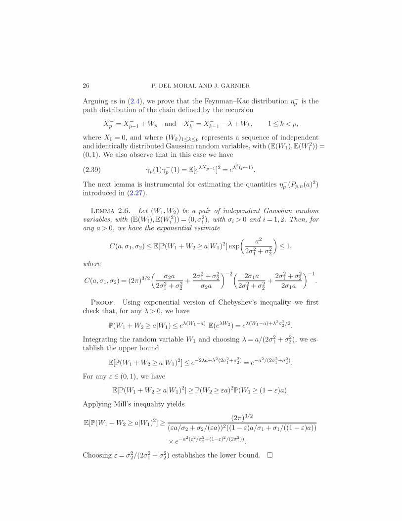
The next lemma is instrumental for estimating the quantities η−p (Pp,n(a)2)introduced in (2.27).

Lemma 2.6. Let (W1,W2) be a pair of independent Gaussian random

variables, with (E(Wi),E(W 2i )) = (0, σ2

i ), with σi > 0 and i = 1,2. Then, for

any a > 0, we have the exponential estimate

C(a,σ1, σ2) ≤ E[P(W1 + W2 ≥ a|W1)2] exp

(

a2

2σ21 + σ2

2

)

≤ 1,

where

C(a,σ1, σ2) = (2π)3/2(

σ2a

2σ21 + σ2

2

+2σ2

1 + σ22

σ2a

)−2( 2σ1a

2σ21 + σ2

2

+2σ2

1 + σ22

2σ1a

)−1

.

Proof. Using exponential version of Chebyshev’s inequality we firstcheck that, for any λ > 0, we have

P(W1 + W2 ≥ a|W1)≤ eλ(W1−a) E(eλW2) = eλ(W1−a)+λ2σ22/2.

Integrating the random variable W1 and choosing λ = a/(2σ21 + σ2

2), we es-tablish the upper bound

E[P(W1 + W2 ≥ a|W1)2]≤ e−2λa+λ2(2σ2

1+σ22) = e−a2/(2σ2

1+σ22).

For any ε ∈ (0,1), we have

E[P(W1 + W2 ≥ a|W1)2] ≥ P(W2 ≥ εa)2P(W1 ≥ (1− ε)a).

Applying Mill’s inequality yields

E[P(W1 + W2 ≥ a|W1)2] ≥ (2π)3/2

(εa/σ2 + σ2/(εa))2((1− ε)a/σ1 + σ1/((1− ε)a))

× e−a2(ε2/σ22+(1−ε)2/(2σ2

1)).

Choosing ε = σ22/(2σ

21 + σ2

2) establishes the lower bound.


From previous considerations, we notice that

η−p (Pp,n(a)2) = E[P(W1 + W2 ≥ (a + λ(p− 1))|W1)2],

where (W1,W2) are a pair of independent and centered Gaussian randomvariables, with (E(W 2

1 ),E(W 22 )) = (p,n− p). Lemma 2.6 now implies that

η−p (Pp,n(a)2)≤ exp[−(a + λ(p− 1))2/(n + p)].(2.40)

Substituting the estimates (2.39) and (2.40) into (2.27), we find that

σγn(a)2 ≤

n∑

p=1

[eλ2(p−1)−(a+λ(p−1))2/(n+p) −Pn(a)2]

=∑

0≤p<n

[e−a2/ne(p+1)/(n(n+p+1))[a−λ(np)/(p+1)]2+λ2p/(p+1) −Pn(a)2].

For λ = a/n, this yields that

σγn(a)2 ≤

∑

0≤p<n

[e−a2/nea2/n2(1−1/(n+p+1)) −Pn(a)2]

(2.41)≤ n(e−(a2/n)(1−1/n) − Pn(a)2).

We find that this estimate has the same exponential decay as the one ob-tained in (2.6) for the corresponding noninteracting IS model. The onlydifference between these two asymptotic variances comes from the multipli-cation parameter n. This additional term can be interpreted as the numberof interactions used in the construction of the genealogical tree simulationmodel. We can compare the efficiencies of the IPS strategy and the usualMC strategy which are two methods that do not require to twist the in-put probability distribution, in contrast to IS. The IPS provides a variancereduction by a factor of the order of nPn(a). In practice the number n ofselection steps is of the order of ten or a few tens, while the goal is theestimation of a probability Pn(a) of the order of 10−6–10−12. The gain isthus very significant, as we shall see in the numerical applications.

Now, we consider the Feynman–Kac twisted models associated to thepotential functions

Gp(x0, . . . , xp) = exp(λxp) for some λ > 0.(2.42)

Arguing as in (2.11), we prove that η−p is the distribution of the Markovchain

X−p = X−

p−1 + Wp and X−k = X−

k−1 − λ(p− k) + Wk, 1≤ k < p,

where X0 = 0, and where (Wk)1≤k≤p represents a sequence of independentand identically distributed Gaussian random variables, with (E(W1),E(W 2

1 )) =(0,1). We also notice that

γp(1)γ−p (1) = E[e

λ∑

1≤k<pXk ]2 = e

λ2∑

1≤k<pk2

.(2.43)


In this situation, we observe that

η−p (Pp,n(a)2) = E

[

P

(

W1 + W2 ≥ a + λ∑

1≤k<p

k|W1

)2]

,

where (W1,W2) are a pair of independent and centered Gaussian randomvariables, with (E(W 2

1 ),E(W 22 )) = (p,n− p). As before, Lemma 2.6 now im-

plies that

η−p (Pp,n(a)2)≤ exp

[

− 1

n + p

(

a + λp(p− 1)

2

)2]

.(2.44)

Using the estimates (2.43) and (2.44), and recalling that∑

1≤k≤n k2 = n(n+1)(2n + 1)/6, we conclude that

σγn(a)2 ≤

n∑

p=1

[e(1/6)λ2(p−1)p(2p−1)−(a+λp(p−1)/2)2/(n+p) −Pn(a)2]

=n∑

p=1

[e−(a2/n)ep/(n(n+p))[a−λn(p−1)/2]2+(1/12)λ2(p−1)p(p+1) −Pn(a)2].

If we take λ = 2a/[n(n − 1)], then we get

σγn(a)2 ≤

n∑

p=1

[e−a2/nea2/(n2(n−1)2)[np/(n+p)(n−p)2+(p−1)p(p+1)/3] −Pn(a)2]

=n∑

p=1

[e−a2/ne(a2/n)n2/(n−1)2[θ(p/n)−p/(3n3)] −Pn(a)2]

with the increasing function θ : ε ∈ [0,1] −→ θ(ε) = ε (1−ε)2

(1+ε) + ε3

3 ∈ [0,1/3].

From these observations, we deduce the estimate

σγn(a)2 ≤ n[e−(a2/n)(2/3)(1−1/(n−1)) −Pn(a)2].(2.45)

Note that the inequalities are sharp in the exponential sense by the lowerbound obtained in Lemma 2.6. Accordingly we get that the asymptoticvariance is not of the order of Pn(a)2, but rather Pn(a)4/3. As in the firstGaussian example, we observe that this estimate has the same exponentialdecays as the one obtained in (2.12) for the corresponding IS algorithm.But, once again, the advantage of the IPS method compared to IS is that itdoes not require to twist the original transition probabilities, which makesthe IPS strategy much easier to implement.


Conclusion. The comparison of the variances (2.41) and (2.45) showsthat the variance of the estimator PN

n (a) is much smaller when the potential(2.38) is used rather than the potential (2.42). We thus get the importantqualitative conclusion that it is not efficient to select the “best” particles(i.e., those with the highest energy values), but it is much more efficient toselect amongst the particles with the best energy increments. This conclusionis also an a posteriori justification of the necessity to carry out a path-spaceanalysis, and not only a state-space analysis. The latter one is simpler butit cannot consider potentials of the form (2.38) that turn out to be moreefficient.

3. Estimation of the tail of a probability density function. We collectand sum up the general results presented in Section 2 and we apply them topropose an estimator for the tail of the probability density function (p.d.f.)of a real-valued function of a Markov chain. We consider an (E,E)-valuedMarkov chain (Xp)0≤p≤n with nonhomogeneous transition kernels Kp. In afirst time, we show how the results obtained in the previous section allow usto estimate the probability of a rare event of the form V (Xn) ∈ A:

PA = P(V (Xn) ∈ A) = E[1A(V (Xn))],(3.1)

where V is some function from E to R. We shall construct an estimatorbased on an IPS. As pointed out in the previous section, the quality ofthe estimator depends on the choice on the weight function. The weightfunction should fulfill two conditions. First, it should favor the occurrenceof the rare event without involving too large normalizing constants. Second,it should give rise to an algorithm that can be easily implemented. Indeedthe implementation of the IPS with an arbitrary weight function requiresrecording the complete set of path-particles. If N particles are generatedand time runs from 0 to n, this set has size (n+1)×N ×dim(E) which mayexceed the memory capacity of the computer. The weight function shouldbe chosen so that only a smaller set needs to be recorded to compute theestimator of the probability of occurrence of the rare event. We shall examinetwo weight functions and the two corresponding algorithms that fulfill bothconditions.

Algorithm 1. Let us fix some β > 0. The first algorithm is built withthe weight function

Gβp (x) = exp[βV (xp)].(3.2)

The practical implementation of the IPS reads as follows.


Initialization. We start with a set of N i.i.d. initial conditions X(i)0 ,

1 ≤ i≤ N , chosen according to the initial distribution of X0. This set is com-

plemented with a set of weights Y(i)0 = 1, 1 ≤ i ≤ N . This forms a set of N

particles: (X(i)0 , Y

(i)0 ), 1≤ i≤N , where a particle is a pair (X, Y ) ∈ E×R+.

Now, assume that we have a set of N particles at time p denoted by

(X(i)p , Y

(i)p ), 1≤ i≤ N .

Selection. We first compute the normalizing constant

ηNp =

1

N

N∑

i=1

exp[βV (X(i)p )].(3.3)

We choose independently N particles according to the empirical distribution

µNp (dX, dY ) =

1

NηNp

×N∑

i=1

exp[βV (X(i)p )]δ

(X(i)p ,Y

(i)p )

(dX, dY ).(3.4)

The new particles are denoted by (X(i)p , Y

(i)p ), 1 ≤ i≤ N .

Mutation. For every 1 ≤ i ≤ N , the particle (X(i)p , Y

(i)p ) is transformed

into (X(i)p+1, Y

(i)p+1) by the mutation procedure

X(i)p

Kp+1−→ X(i)p+1,(3.5)

where the mutations are performed independently, and

Y(i)p+1 = Y (i)

p exp[−βV (X(i)p )].(3.6)

The memory required by the algorithm is N dim(E) + N + n, whereN dim(E) is the memory required by the record of the set of particles, N isthe memory required by the record of the set of weights and n is the memoryrequired by the record of the normalizing constants ηN

p , 0 ≤ p ≤ n− 1. Theestimator of the probability PA is then

PNA =

[

1

N

N∑

i=1

1A(V (X(i)n ))Y (i)

n

]

×n−1∏

k=0

ηNp .(3.7)

This estimator is unbiased in the sense that E[PNA ] = PA. The central limit

theorem for the estimator states that√

N(PNA −PA)

N→∞−→ N (0,QA)(3.8)


where the variance is

QA =n∑

p=1

E

[

EXp[1A(V (Xn))]2p−1∏

k=0

G−1k (X)

]

E

[ p−1∏

k=0

Gk(X)

]

(3.9)−E[1A(Xn)]2.

Algorithm 2. Let us fix some α > 0. The second algorithm is builtwith the weight function

Gαp (x) = exp[α(V (xp)− V (xp−1))].(3.10)

Initialization. We start with a set of N i.i.d. initial conditions X(i)0 ,

1 ≤ i≤ N , chosen according to the initial distribution of X0. This set is

complemented with a set of parents W(i)0 = x0, 1 ≤ i ≤ N , where x0 is

an arbitrary point of E with V (x0) = V0. This forms a set of N particles:

(W(i)0 , X

(i)0 ), 1 ≤ i≤ N , where a particle is a pair (W , X) ∈ E ×E.

Now, assume that we have a set of N particles at time p denoted by

(W(i)p , X

(i)p ), 1 ≤ i≤ N .

Selection. We first compute the normalizing constant

ηNp =

1

N

N∑

i=1

exp[α(V (X(i)p )− V (W (i)

p ))].(3.11)

We choose independently N particles according to the empirical distribution

µNp (dW , dX) =

1

NηNp

N∑

i=1

exp[α(V (X(i)p )− V (W (i)

p ))]

(3.12)× δ

(W(i)p ,X

(i)p )

(dW , dX).

The new particles are denoted by (W(i)p , X

(i)p ), 1≤ i≤ N .

Mutation. For every 1 ≤ i ≤ N , the particle (W(i)p , X

(i)p ) is transformed

into (W(i)p+1, X

(i)p+1) by the mutation procedure X

(i)p

Kp+1−→ X(i)p+1 where the mu-

tations are performed independently, and W(i)p+1 = X

(i)p .

The memory required by the algorithm is 2N dim(E) + n. The estimatorof the probability PA is then

PNA =

[

1

N

N∑

i=1

1A(V (X(i)n )) exp(−α(V (W (i)

n )− V0))

]

×[

n−1∏

k=0

ηNp

]

.(3.13)


This estimator is unbiased and satisfies the central limit theorem (3.8).Let us now focus our attention to the estimation of the p.d.f. tail of V (Xn).

The rare event is then of the form V (Xn) ∈ [a, a + δa) with a large a andan evanescent δa. We assume that the p.d.f. of V (Xn) is continuous so thatthe p.d.f. can be seen as

p(a) = limδa→0

1

δapδa(a), pδa(a) = P(V (Xn) ∈ [a, a + δa)).

We propose to use the estimator

pNδa(a) =

1

δa× PN

[a,a+δa)(3.14)

with a small δa. The central limit theorem for the p.d.f. estimator takes theform

√N(pN

δa(a)− pδa(a))N→∞−→ N (0, p2

2(a, δa)),(3.15)

where the variance p22(a, δa) has a limit p2

2(a) as δa goes to 0 which admitsa simple representation formula:

p22(a) = lim

δa→0

1

δaE

[

1[a,a+δa)(V (Xn))n−1∏

k=0

G−1k (X)

]

E

[

n−1∏

k=0

Gk(X)

]

.(3.16)

Note that all other terms in the sum (3.9) are of order δa2 and are thereforenegligible. This is true as soon as the distribution of V (Xn) given Xp forp < n admits a bounded density with respect to the Lebesgue measure.Accordingly, the variance p2

2(a) can be estimated by limδa→0(δa)−1QN[a,a+δa),

where QNA is given by

QNA =

[

1

N

N∑

i=1

1A(V (X(i)n ))(Y (i)

n )2]

×[

n−1∏

k=0

ηNp

]2

(3.17)

for Algorithm 1, and by

QNA =

[

1

N

N∑

i=1

1A(V (X(i)n )) exp(−2α(V (W (i)

n )− V0))

]

×[

n−1∏

k=0

ηNp

]2

(3.18)

for Algorithm 2. The estimators of the variances are important becauseconfidence intervals can then be obtained.

The variance analysis carried out in Section 2.7 predicts that the secondalgorithm [with the potential (3.2)] should give better results than the Algo-rithm 1 [with the potential (3.10)]. We are going to illustrate this importantstatement in the following sections devoted to numerical simulations.

From a practical point of view, it can be interesting to carry out severalIPS simulations with different values for the parameters β (Algorithm 1)


and α (Algorithm 2), and also one MC simulation. It is then possible toreconstruct the p.d.f. of V (Xn) by the following procedure. Each IPS or MCsimulation gives an estimation for the p.d.f. p (whose theoretical value doesnot depend on the method) and also an estimation for the ratio p2/p (whosetheoretical value depends on the method). We first consider the differentestimates of a 7→ p2/p(a) and detect, for each given value of a, which IPSgives the minimal value of p2/p(a). For this value of a, we then use theestimation of p(a) obtained with this IPS. This method will be used inSection 5.

4. A toy model. In this section we apply the IPS method to computethe probabilities of rare events for a very simple system for which we knowexplicit formulas. The system under consideration is the Gaussian randomwalk Xp+1 = Xp + Wp+1, X0 = 0, where the (Wp)p=1,...,n are i.i.d. Gaussianrandom variables with zero mean and variance 1. Let n be some positiveinteger. The goal is to compute the p.d.f. of Xn, and in particular the tailcorresponding to large positive values.

We choose the weight function

Gαp (x) = exp[α(xp − xp−1)].(4.1)

The theoretical p.d.f. is a Gaussian p.d.f. with variance n:

p(a) =1√2πn

exp

(

− a2

2n

)

.(4.2)

The theoretical variance of the p.d.f. estimator can be computed from (3.16):

p22(a) = p2(a)×

√2πn exp

(

α2 n− 1

n+

(a−α(n− 1))2

2n

)

.(4.3)

When α = 0, we have p22(a) = p(a), which is the result of standard MC. For

α 6= 0, the ratio p2(a)/p(a) is minimal when a = α(n − 1) and then p2(a) =p(a) 4

√2πn exp(α2(n− 1)/(2n)). This means that the IPS with some given α

is especially relevant for estimating the p.d.f. tail around a = α(n− 1).Let us assume that n≫ 1. Typically we look for the p.d.f. tail for a = a0

√n

with a0 > 1 because√

n is the typical value of Xn. The optimal choice isα = a0/

√n and then the relative error is p2(a)/p(a) ≃ 4

√2πn.

In Figure 1 we compare the results from MC simulations, IPS simulationsand theoretical formulas with the weight function (4.1). We use a set of2 × 104 particles to estimate the p.d.f. tail of Xn with n = 15. The agree-ment shows that we can be confident with the results given by the IPS forpredicting rare events with probabilities 10−12.

We now choose the weight function

Gβp (x) = exp(βxp).(4.4)


We get the same results, but the explicit expression for the theoretical vari-ance of the p.d.f. estimator is

p22(a) = p2(a)×

√2πn exp

(

β2 n(n2 − 1)

12+

(a− βn(n− 1)/2)2

2n

)

.(4.5)

When β = 0, we have p22(a) = p(a), which is the result of standard MC.

For β 6= 0, the ratio p2(a)/p(a) is minimal when a = βn(n − 1)/2 and thenp2(a) = p(a) 4

√2πn exp(β2n(n2 − 1)/24). This means that the IPS with some

given β is especially relevant for estimating the p.d.f. tail around a = βn(n−1)/2.

Let us assume that n≫ 1. Typically we look for the p.d.f. tail for a = a0√

nwith a0 > 1. The optimal choice is β = 2a0/n

3/2 and then the relative erroris p2(a)/p(a) ≃ (2πn)1/4 exp(a2

0/6) = (2πn)−1/12p(a)−1/3. The relative erroris larger than the one we get with the weight function (4.1). In Figure 2we compare the results from MC simulations, IPS simulations and the the-oretical formulas with the weight function (4.4). This shows that the weightfunction (4.4) is less efficient than (4.1). Thus the numerical simulationsconfirm the variance comparison carried out in Section 2.7.

5. Polarization mode dispersion in optical fibers.

5.1. Introduction. The study of pulse propagation in a fiber with ran-dom birefringence has become of great interest for telecommunication appli-cations. Recent experiments have shown that polarization mode dispersion(PMD) is one of the main limitations on fiber transmission links becauseit can involve significant pulse broadening [13]. PMD has its origin in the

Fig. 1. (a) P.d.f. estimations obtained by the usual MC technique (squares) and by theIPS with the weight function (4.1) with α = 1 (stars). The solid line stands for the theo-retical Gaussian distribution. (b) Empirical and theoretical ratios p2/p.


Fig. 2. (a) P.d.f. estimations obtained by the usual MC technique (squares) and by theIPS with the weight function (4.4) with β = 0.15 (stars). The solid line stands for thetheoretical Gaussian distribution. (b) Empirical and theoretical ratios p2/p.

birefringence [27], that is, the fact that the electric field is a vector field andthe index of refraction of the medium depends on the polarization state (i.e.,the unit vector pointing in the direction of the electric vector field). Randombirefringence results from variations of the fiber parameters such as the coreradius or geometry. There exist various physical reasons for the fluctuationsof the fiber parameters. They may be induced by mechanical distortions onfibers in practical use, such as pointlike pressures or twists [21]. They mayalso result from variations of ambient temperature or other environmentalparameters [2].

The difficulty is that PMD is a random phenomenon. Designers want toensure that some exceptional but very annoying event occurs only a verysmall fraction of time. This critical event corresponds to a pulse spreadingbeyond a threshold value. For example, a designer might require that such anevent occurs less than 1 minute per year [3]. PMD in an optical fiber varieswith time due to vibrations and variations of environmental parameters.The usual assumption is that the fiber passes ergodically through all possiblerealizations. Accordingly requiring that an event occurs a fraction of time p isequivalent to requiring that the probability of this event is p. The problem isthen reduced to the estimation of the probability of a rare event. Typicallythe probability is 10−6 or less [3]. It is extremely difficult to use eitherlaboratory experiments or MC simulations to obtain a reliable estimate ofsuch a low probability because the number of configurations that must beexplored is very large. Recently IS has been applied to numerical simulationsof PMD [2]. This method gives good results; however, it requires very goodphysical insight into the problem because it is necessary for the user to knowhow to produce artificially large pulse widths. We would like to revisit thiswork by applying the IPS strategy. The main advantage is that we do not


need to specify how to produce artificially large pulse widths, as the IPSwill automatically select the good “particles.”

5.2. Review of PMD models. The pulse spreading in a randomly bire-fringent fiber is characterized by the so-called square differential group delay(DGD) τ = |r|2. The vector r is the so-called PMD vector, which is solutionof

rz = ωΩ(z)× r + Ω(z),(5.1)

where Ω(z) is a three-dimensional zero-mean stationary random processmodeling PMD.

5.2.1. The white noise model. Simplified analytical models have beenstudied. In the standard model [12, 13, 20, 27] it is assumed that the processΩ is a white noise with autocorrelation function E[Ωi(z

′)Ωj(z)] = σ2δijδ(z′−

z). In such a case the differential equation (5.1) must be interpreted as astochastic differential equation:

dr1 = σωr3 dW 2z − σωr2 dW 3

z + σ dW 1z ,(5.2)


z + σ dW 2z ,(5.3)


z + σ dW 3z ,(5.4)

where stands for the Stratonovich integral and the W j ’s are three indepen-dent Brownian motions. It is then possible to establish [12] that the DGDτ is a diffusion process and in particular that τ(ω, z) obeys a Maxwelliandistribution if r(0) = (0,0,0)T . More precisely the p.d.f. of τ(ω, z) is

p(τ) =τ1/2

√2π(σ2z)3/2

exp

(

− τ

2σ2z

)

1[0,∞)(τ).

5.2.2. Realistic models. The white noise model gives an analytical for-mula for the p.d.f. of the DGD, which in turns allows us to compute exactlythe probability that the DGD exceeds a given threshold value. However, ithas been pointed out that the p.d.f. tail of the DGD does not fit with theMaxwellian distribution in realistic configurations [1]. Various numerical andexperimental PMD generation techniques involve the concatenation of bire-fringent elements with piecewise constant vectors Ω [18]. Equation (5.1) canbe solved over each segment, and continuity conditions on the segmentsjunctions give a discrete model for the PMD vector r. The total PMD vec-tor after the (n + 1)st section can then be obtained from the concatenationequation [14]

rn+1 = Rn+1rn + σΩn+1,(5.5)


where σ is the DGD per section, Ωn = Ω(θn) with

Ω(θ) = (cos(θ), sin(θ),0)T .

Rn is a matrix corresponding to a rotation through an angle φn about theaxis Ωn. Explicitly Rn = R(θn, φn) with

R(θ,φ) =

cos2(θ) + sin2(θ) cos(φ) sin(θ) cos(θ)(1− cos(φ)) sin(θ) sin(φ)sin(θ) cos(θ)(1− cos(φ)) sin2(θ) + cos2(θ) cos(φ) − cos(θ) sin(φ)

− sin(θ) sin(φ) cos(θ) sin(φ) cos(φ)

.

From the probabilistic point of view, the angles φn are i.i.d. random vari-ables uniformly distributed in (0,2π). The angles θn are i.i.d. random vari-ables such that cos(θn) are uniformly distributed in (−1,1) [2]. Accordingly,(rn)n∈N is a Markov chain. Let us assume that the fiber is modeled as theconcatenation of n segments and that the outage event is of the form |rn|> afor some fixed threshold value a. In the case where a is much larger than theexpected value of the final DGD |rn|, the outage probability is very small,and this is the quantity that we want to estimate.

5.3. Estimations of outage probabilities.

5.3.1. Importance sampling. In [2] IS is used to accurately calculate out-age probabilities due to PMD. As discussed in the Introduction, the keydifficulty in applying IS is to properly choose the twisted distribution forthe driving process (θp, φp)1≤p≤n. The papers [2, 11, 17] present differenttwisted distributions and the physical explanations why such distributionsare likely to produce large DGD’s. As a result the authors obtain with 105

simulations good approximations of the p.d.f. tail even for probabilities ofthe order of 10−12. The main reported physical result is that the probabilitytail is significantly smaller than the Maxwellian tail predicted by the whitenoise model.

5.3.2. Interacting particle systems. In this subsection we apply our IPSmethod and compare the results with those obtained by MC and IS. To geta reliable estimate of the outage probability of the event, it is necessary togenerate realizations producing large DGD’s. The main advantage of theIPS approach is that it proposes a “blink” method that does not requireany physical insight. Such a method could thus be generalized to more com-plicated situations. Here the Markov process is the PMD vector (rn)n∈N atthe output of the nth fiber section. The state space is R3, the initial PMDvector is r0 = (0,0,0)T , the Markov transitions are described by (5.5) andthe energy-like function is V (r) = |r|. We estimate the p.d.f. p(a) of |rn| byimplementing the IPS with the two weight functions

Gβp (r) = exp(β |rp|)(5.6)


parameterized by β ≥ 0, and

Gαp (r) = exp[α(|rp| − |rp−1|)](5.7)

parameterized by α ≥ 0. We have implemented Algorithms 1 and 2 as de-scribed in Section 3. Before presenting and discussing the results, we wouldlike to underline that we have chosen to perform a selection step at the out-put of each segment, because the number of segments is not very large. Ifthe number of segments were very large, it should be better to perform aselection step every two or three or n0 segments.

In Figure 3(a) we plot the estimation of the DGD p.d.f. obtained bythe IPS method with the weight function Gβ

n defined by (5.6). The fiberconsists in the concatenation of n = 15 segments. The DGD per section isσ = 0.5. We use a set of N = 2 × 104 interacting particles. This result canbe compared with the one obtained in [2], which shows excellent agreement.The difference is that our procedure is fully adaptative, it does not requireany guess of the user, and it does not require to twist the input probabilitydensity. The variance p2

2 of the estimator of the DGD p.d.f. is plotted inFigure 3(b). This figure is actually used to determine the best estimator ofthe DGD p.d.f. by the procedure described at the end of Section 3.

In Figure 4(a) we plot the estimation of the DGD p.d.f. obtained by theIPS method with the weight function Gα

p defined by (5.7). It turns out thatthe estimated variance of the estimator is smaller with the weight functionGα

p than with the weight function Gβp [cf. Figures 4(b) and 3(b)]. This ob-

servation confirms the theoretical predictions obtained with the Gaussianrandom walk.

Fig. 3. (a) Segments of the DGD p.d.f. obtained by the usual MC technique (squares)and by the IPS with the weight function Gβ

n with β = 0.33 (triangles) and β = 1 (stars).The solid line stands for the Maxwellian distribution obtained with the white noise model.The Maxwellian distribution fails to describe accurately the p.d.f. tail. (b): Ratios p2/p.The quantity p2 is the standard deviation of the estimator of the DGD p.d.f. In the IPScases, the standard deviations are estimated via the formula (3.17).


Fig. 4. (a) Segments of the DGD p.d.f. obtained by the usual MC technique (squares)and by the IPS with the weight function Gα

p with α = 2.0 (triangles) and α = 6.0 (stars).The solid line stands for the Maxwellian distribution obtained with the white noise model.(b) Ratios p2/p. The quantity p2 is the standard deviation of the estimator of the DGDp.d.f. In the IPS cases, the standard deviations are estimated via (3.18).

Fig. 5. Conditional expectations D1a,a+δa(p,n) of the intermediate DGD at p = 4, 8, 12,

given that the final DGD lies in the interval (a,a + δa) with n = 15, δa = 0.18, and ( fromtop to bottom) a = 7, a = 6.1, a = 5.2. The error bars are obtained from the estimations ofthe conditional variances.

The IPS approach is also powerful to compute conditional probabilitiesor expectations given the occurrence of some rare event. For instance, wecan be interested in the moments of the intermediate DGDs given that thefinal DGD lies in the rare set (a, a + δa):

Dqa,a+δa(p,n) = E[|rp|q||rn| ∈ [a, a + δa)].

This information gives us the typical behaviors of the PMD vectors alongthe fiber that give rise to a large final DGD. We use the estimator (2.20)


based on the IPS with the weight function (5.7). As shown by Figure 5, thetypical conditional trajectory of the DGD is close to a linear increase witha constant rate given by the ratio of the final DGD over the length of thefiber. The conditional variances are found to be small, which shows thatfluctuations are relatively small around this average behavior.

REFERENCES

[1] Biondini, G., Kath, W. L. and Menyuk, C. R. (2001). Non-Maxwellian DGD dis-tribution of PMD emulators. In Proc. OFC 2001 ThA5 1–3.

[2] Biondini, G., Kath, W. L. and Menyuk, C. R. (2002). Importance sampling forpolarization-mode dispersion. IEEE Photon. Technol. Lett. 14 310–312.

[3] Bulow, H. (1999). Limitation of optical first-order PMD compensation. In Proc.

ECOC 1999 WE1 74–76.[4] Del Moral, P. (2004). Feynman–Kac Formulae, Genealogical and Interacting Par-

ticle Systems With Applications. Springer, New York. MR2044973[5] Del Moral, P. and Guionnet, A. (1999). A central limit theorem for nonlin-

ear filtering using interacting particle systems. Ann. Appl. Probab. 9 275–297.MR1687359

[6] Del Moral, P. and Jacod, J. (2001). Interacting particle filtering with discreteobservations. In Sequential Monte Carlo Methods in Practice (N. J. Gordon, A.Doucet and J. F. G. de Freitas, eds.) 43–75. Springer, New York. MR1847786

[7] Del Moral, P. and Jacod, J. (2002). The Monte Carlo method for filtering with

discrete-time observations: Central limit theorems. In Numerical Methods andStochastics, Fields Inst. Commun. 34 29–53. Amer. Math. Soc., Providence, RI.

[8] Del Moral, P. and Ledoux, M. (2000). On the convergence and the applicationsof empirical processes for interacting particle systems and nonlinear filtering.J. Theoret. Probab. 13 225–257. MR1744985

[9] Del Moral, P. and Tindel, S. (2003). A Berry–Esseen theorem for Feynman–Kacand interacting particle models. Publications de l’Institut Elie Cartan 44. Univ.Henri Poincare, Nancy.

[10] Doucet, A., de Freitas, N. and Gordon, N. (2001). Sequential Monte Carlo Meth-ods in Practice. Springer, New York. MR1847783

[11] Fogal, S. L., Biondini, G. and Kath, W. L. (2002). Multiple importance samplingfor first- and second-order polarization-mode dispersion. IEEE Photon. Technol.Lett. 14 1273–1275.

[12] Garnier, J., Fatome, J. and Le Meur, G. (2002). Statistical analysis of pulsepropagation driven by polarization-mode dispersion. J. Opt. Soc. Amer. B 19

1968–1977.[13] Gisin, N., Pellaux, J. P. and Von der Weid, J. P. (1991). Polarization mode

dispersion for short and long single-mode fibers. J. Lightwave Technol. 9 821–827.

[14] Gordon, J. P. and Kogelnik, H. (2000). PMD fundamentals: Polarization-mode

dispersion in optical fibers. Proc. Nat. Acad. Sci. U.S.A. 97 4541.[15] Harris, T. E. and Kahn, H. (1951). Estimation of particle transmission by random

sampling. Natl. Bur. Stand. Appl. Math. Ser. 12 27–30.[16] Heidelberg, P. (1995). Fast simulation of rare events in queueing and reliability

models. ACM Transactions on Modeling and Computer Simulation 5 43–85.

http://www.ams.org/mathscinet-getitem?mr=2044973






[17] Lima, I. T., Jr., Biondini, G., Marks, B. S., Kath, W. L. and Menyuk, C.R. (2002). Analysis of PMD compensators with fixed DGD using importancesampling. IEEE Photon. Technol. Lett. 14 627–629.

[18] Marcuse, D., Menyuk, C. R. and Wai, P. K. A. (1997). Application of theManakov-PMD equation to studies of signal propagation in optical fibers withrandomly varying birefringence. J. Lightwave Technol. 15 1735–1746.

[19] Nagasawa, M. (1991). Stochastic Processes in Quantum Physics. Birkhauser, Boston.MR1739699

[20] Poole, C. D. and Wagner, R. E. (1986). Phenomenological approach to polarizationdispersion in long single-mode fibers. Electron. Lett. 22 1029–1030.

[21] Rashleigh, S. C. (1983). Origins and control of polarization effects in single-modefibers. J. Lightwave Technol. 1 312–331.

[22] Reed, M. and Simon, B. (1975). Methods of Modern Mathematical Physics. II.Fourier Analysis, Self Adjointness. Academic Press, New York. MR493420

[23] Rosenbluth, M. N. and Rosenbluth, A. W. (1955). Monte Carlo calculations ofthe average extension of macromolecular chains. J. Chem. Phys. 23 356–359.

[24] Rubinstein, R. Y. (1981). Simulation and the Monte Carlo Method. Wiley, NewYork. MR624270

[25] Shorack, G. R. (2000). Probability for Statisticians. Springer, New York. MR1762415[26] Sznitman, A. S. (1998). Brownian Motion, Obstacles and Random Media. Springer,

New York. MR1717054[27] Wai, P. K. A. and Menyuk, C. R. (1996). Polarization mode dispersion, decorre-

lation, and diffusion in optical fibers with randomly varying birefringence. J.Lightwave Technol. 14 148–157.

Laboratoire de Mathematiques J. A. Dieudonne

Universite de Nice

Parc Valrose

06108 Nice Cedex 2

France

e-mail: [email protected]

Laboratoire de Probabilites

et Modeles Aleatoires

and Laboratoire Jacques-Louis Lions

Universite Paris 7

2 Place Jussieu

75251 Paris Cedex 5

France

e-mail: [email protected]






mailto:[email protected]

mailto:[email protected]

Genealogical particle analysis of rare events

Documents

Transcript of Genealogical particle analysis of rare events