RESEARCH REPORT

Gaze motion clustering in scan-path estimation

Anna Belardinelli Æ Fiora Pirri Æ Andrea Carbone

Received: 25 April 2007 / Accepted: 8 February 2008 / Published online: 20 March 2008

� Marta Olivetti Belardinelli and Springer-Verlag 2008

Abstract Visual attention is considered nowadays a

paramount ability both in Cognitive Sciences and in Cog-

nitive Vision to bridge the gap between perception and

higher level reasoning functions, such as scene interpreta-

tion and decision making. Bottom-up gaze shifting is the

main mechanism used by humans when exploring a scene

without a specific task. In this paper we investigated which

criteria allow for the generation of plausible fixation clus-

ters by analysing experimental data of human subjects. We

suggest that fixations should be grouped in cliques whose

saliency can be assessed through an innovation factor

encompassing bottom-up cues, proximity, direction and

memory components.

Introduction

Research on human attention has widely spread in the last

century, providing understanding of cognitive processes

related to vision (Kramer et al. 2007) and leading to the

formulation of several computational models accounting

for oculomotor behaviour and fixations distribution. Ear-

liest models rely on Posner’s one (1980) and Treisman’s

Feature Integration Theory (Treisman and Gelade 1980),

according to which several separable basic features, such as

intensity, color, shape, edge orientations, and conjunctions

of them, that pop out in the field of view, drive eyes to

those locations displaying them.

In this sense attention has been categorized into bottom-

up, i.e. exogenous, stimulus-driven, and top-down, i.e.

endogenous, biased by the subject’s knowledge and

intentions. Most of computational models so far rely on

bottom-up cues, since they are more general and detectable

via image-processing techniques and image statistics (see

Itti and Koch 2001; Tsotsos et al. 1995; and derived

models by Frintrop et al. 2006; Shokoufandeh et al. 2006).

These approaches compute feature maps of the whole

image at different scales with Gabor filters and Gaussian

pyramids, and then conspicuity maps are obtained by

means of the center-surround mechanism, which returns

locations that contrast with local context. A single saliency

map is derived combining the conspicuity maps and a

WTA net selects the point to fixate.

These models are concerned with defining a relation

between fixation deployment and image properties in the

viewed scene. Saliency is mostly determined by processing

selected features known to have correspondent receptors in

biological visual systems. Established architectures so far

have usually not encompassed motor data of the perceiving

subject. Nevertheless, when freely moving in an open

environment the head, eye and body behaviour is condi-

tioned to serve the visual system, which, being foveated,

calls for the production of a meaningful scanpath to gain

high resolution on informative zones. To this end humans

have developed precise scanning strategies in everyday

routines as well as in specific tasks, like search, surveil-

lance or driving. A deeper understanding of these strategies

would lead to the design of effective sensorimotor behav-

iours in artificial vision systems. In this sense some work

A. Belardinelli (&) � F. Pirri � A. Carbone

Dipartimento di Informatica e Sistemistica, ALCOR, Sapienza

University, via Ariosto 25, 00185 Rome, Italy

e-mail: belardinelli@dis.uniroma1.it

F. Pirri

e-mail: pirri@dis.uniroma1.it

A. Carbone

e-mail: carbone@dis.uniroma1.it

123

Cogn Process (2008) 9:269–282

DOI 10.1007/s10339-008-0206-2

relating fovea eccentricity to image statistics in contrast

perception during scanpath and visual search tasks has

been presented in Raj et al. (2005), and Najemnik and

Geisler (2005). Highlighting scanpath primary function and

allowing for decreasing resolution as eccentricity from the

fovea increases, Renninger et al. (2005) defined an eye

movement strategy maximizing sequential information in

silouhette observing. Bruce and Tsotsos (2006) propose a

bottom-up strategy relying on a definition of saliency

aimed at maximizing Shannon’s information measure after

ICA decomposition. Anyway, again saliency is given by

objective properties of the observed scene, not taking into

account data of the attentional behaviour adopted by the

subject. In this paper we present a model to analyse

scanpaths during motion basing on the extraction of salient

features, both objective and subjective (in the sense of the

subject’s motion). We carried out some experiments aimed

at eliciting scanpath mechanisms driven by bottom-up

factors when a walking subject lets her gaze glide over a

scene. Of course top-down factors are present as well in the

form of influence of the subject’s knowledge or experience

but since they cannot emerge directly from sensorymotor

data, we focused on bottom-up and oculomotor features as

data for learning a saliency estimation that could be

implemented on a robotic platform in a straightforward

way. To interpret correlation among several features we

apply factor analysis to the training set of fixations, gath-

ered from the subject by means of a gaze tracker device.

This step helps reducing feature space dimensionality and

combining both temporal and spatial aspects. We propose a

method to cluster fixations related to single saccadic cycles

(see Fig. 1) by introducing a suitable distance measure to

apply to data transformed into the factor space. The use-

fulness of clustering is twofold: on the one hand spatially

and temporally close fixations are usually related to distinct

objects or salient zones inspected, that is, they can denote

higher level functions such as recognition and inference.

On the other hand, clustering can help relating or com-

paring different scanpaths, simplifying data analysis and

discarding outliers (Turano et al. 2003). In Santella and

Decarlo (2003) meanshift clustering with a Gaussian kernel

is proposed to cluster fixations, considering only spatial

location and time.

Finally we introduce an innovation factor modulated by

an Inhibition of Return component, in order to describe the

increase of saliency between consecutive cycles.

Experimental tools

The device used to acquire eye and head displacement data

is an improved version of the one presented in Belardinelli

et al. (2006, 2007). The gaze-machine is made of a helmet

upon which sensors are embedded. A stereo rig and an

inertial platform are aligned along a stripe mounted on the

helmet (see Fig. 2, on the left). Two more cameras, that is,

two microcameras C-mos are mounted on a stiff prop and

point at the pupils. Each eye-camera provides two infrared

LEDs, disposed along X and Y axes near the camera centre.

Fig. 1 Example of some fixations groupings

Fig. 2 On the left, both the gaze machine and the calibration are shown. On the right the detected pupil center, bottom the pupil is detected while

blinking

270 Cogn Process (2008) 9:269–282

123

All cameras were pre-calibrated using the well-known

Zhang camera calibration algorithm (Zhang 1999) for

intrinsic parameter determination and lens distortion cor-

rection. Extrinsic and rectification parameters for stereo

camera were computed too, and standard stereo correlation

and triangulation algorithms used for scene depth estima-

tion. An inertial sensor is attached to the system to correct

errors due to involuntary movements that occur during the

calibration stage. The scene camera frames are suitably

paired with the eye-camera frames for pupil tracking. The

data stream acquired from these instruments is collected at

a frame rate of 15 Hz and it includes the right and left

images of the scene, the cumulative time, the right and left

images of the eyes, and the head angles, in degrees,

accounting for the three rotations: the pitch (the chin up

and down), the roll (the head inclined towards the shoul-

ders) and the yaw (the head rotation left and right),

obtained by the inertial system (see Fig. 3).

In order to correctly locate the Point of Regard of the

user, an eye-camera calibration phase, relative to the two

pairs of cameras and the eyes, is required before using the

system. Calibration is, indeed, necessary to correctly pro-

ject the line of sight on the scene taking into account

several factors such as:

1. Light changes, because light is specularly reflected at

the four major refracting surfaces of the eye (anterior

and posterior cornea and anterior and posterior lens),

and the specularly reflected light is image forming.

2. Head movements, displacing the line of sight also

according to the three rotations pitch, yaw and roll.

3. The unknown position of the eye w.r.t. the stereo rig and

the two C-mos, as they depend on the user head and height.

4. The three reference frames constituted by the three

pairs of vision systems: the stereo rig, i.e. the scene

cameras, the C-mos, i.e. the eye-cameras, and the eyes.

We shall not describe here the eye-camera calibration

process nor the preliminary camera calibrations. A phase of

the eye-camera calibration, using a chess board of 81

squares, projected on the wall plane, is illustrated in Fig. 2,

while the results of pupil tracking are shown in the same

figure on the right. The output of the calibration process is

a transformation matrix mapping the current pupil center,

at time t, on the world point the user is looking at. To

correctly project the world point with respect to a reference

frame common to the whole scanpath, we need to

determine the current position of the user. Indeed, by

calibration, the position of the fixations, at each time step t,

is only known with respect to the subject and not with

respect to a reference frame common to all the fixations.

Since the subject is moving in open space, and, in the

system described, her position cannot be determined if the

environment is completely unknown, we have to put some

restrictions on the environment. Therefore for the experi-

ments described in the paper we have been considering a

relatively small lane whose map is depicted in Fig. 3 and it

is known in advance. Different landmarks have been cho-

sen in order to localize the subject on the map and to

determine fixation point coordinates in the inertial refer-

ence frame, as described below.

According to the eye-camera calibration and the data

from the inertial sensor at each time step t the orientation R

of the head–eye system is known. Hence, following the

notation illustrated in Fig. 3 (left), we are given the current

head–eye orientation R, at time step t, by the three rotations

Fig. 3 On the left a scheme of

the exploration path using

known landmarks, showing the

computation of the subject

position at time t. On the right

the map of the lane in which the

experiments were conducted.

Blue landmarks indicate gates

edges, red landmarks lamps,

green landmarks trees. These

are the landmarks used to

localize the subject

Cogn Process (2008) 9:269–282 271

123

pitch, yaw and roll of the head and the two eye-rotations hand u, indicating the pitch and yaw of the eye. Note that

the head rotations are given with respect to the initial

orientation in t0, which is taken as reference frame for all

the successive rotations, while eye rotations are given with

respect to the observation axis (i.e. the pupillary axis). Yet

the current position of the subject is unknown. We assume

that at each time step t three landmarks are visible in the

image. Thus, given the landmarks Li ¼ ðxi; yi; ziÞ>; Lj ¼ðxj; yj; zjÞ> and Lk ¼ ðxk; yk; zkÞ>; their coordinates

ðxq; yq; zqÞ>; q 2 fi; j; kg; with respect to the reference

frame W0, are known. Furthermore, by stereo triangulation,

the three relative distances di, dj and dk from Vt to Li, Lj and

Lk are determined. In the hypothesis that the landmarks are

correctly localized, but for an error e, the position of the

subject at time t, is obtained resolving the following system

of equations with constraints, for ðx0; y0; z0Þ>; the coordi-

nates of the position of V at time t.

d2i ¼ ðxi � x0Þ2 þ ðyi � y0Þ2 þ ðzi � z0Þ2:

d2j ¼ ðxj � x0Þ2 þ ðyj � y0Þ2 þ ðzj � z0Þ2:

d2k ¼ ðxk � x0Þ2 þ ðyk � y0Þ2 þ ðzk � z0Þ2:

ðx0; y0; z0Þ> ¼ arg minVtdðVt ;Vt�1Þ; with ðx0 [ 0; y0 [ 0; z0 [ 0Þ:

8>>><

>>>:

ð1Þ

Indeed, we can always choose a fixed reference frame such

that the coordinates ðxq; yq; zqÞ> 2 R3 are always positive.

Once the Vt coordinates of the subject, w.r.t. the fixed

reference frame W0 are known, then also the distance dV

from Vt to W0 is determined.

Hence to localize the point of fixation in world coordi-

nates with respect to the reference frame W0 we have

FVtt ¼ RtðFW0

t � VtÞ; and thus FW0t ¼ R>t FVt

t þ Vt: Here

FW0t are the coordinates of the fixation, at time t, with

respect to W0, while FVtt are the local coordinates, at time t,

with respect to Vt.

Now, when t = t0 there are two possibilities: (1) the

subject orientation is parallel to the fixed reference frame,

possibly translated; (2) the subject has an unknown initial

orientation. In any case the eye rotations are h = u = 0,

because in t0 being the eyes aligned with the C-mos, the

rotation angles w.r.t. the pupillary axis are zero. In the first

case, R is RW0; at time t0, and the translation is obtained as

above.

In the second case we note the following useful facts: (1)

the distance between Vt0 and the real world point PC,

projection of the image center C, whose coordinates are

given in the subject reference frame, is known. (2) PC is on

the Z-axis of the subject reference frame. (3) The distance

between PC and the three landmarks is known. (4) The W0

coordinates of the position Vt0 of the subject can be esti-

mated as in (Eq. 1), likewise those of the three landmarks,

for the above remarks. Now, using these facts and the tri-

angles with vertices PC, Lk, Lj and PC, Lk, V0 and PC, V0,

W0 it is possible to estimate the coordinates of PC in W0

coordinates, by constrained optimization, hence the initial

orientation R of the subject in relation to the fixed reference

frame W0. In fact, once the W0 coordinates of PC are

determined the direction cosines of PC, w.r.t. W0 return the

orientation of the Zt0 axis of the head–eye reference frame.

On the other hand the Xt0 axis passes through Vt0 and it is

orthogonal to Zt0 and the Yt0 axis is the cross product of the

first two. Finally, we note that a dynamic estimation of the

rotations, for times steps t = 1, 2, ..., N, given the above-

stated measurements, can be used to correct the head–eye

system of the subject orientation, as the movements are

slow and smooth. We shall not discuss further these aspects

here.

We have, thus, obtained the fixation point Ft, for each

time step, given both the transformation matrices, from the

calibration phases, for projecting the line of sight in real

world coordinates, and the position of the subject in space.

Therefore we have the following data structure F which is

made available for further processing at each time step t:

F :

I ¼ RGB image of the scene;M ¼ depth image of the scene;eL ¼ intensity image of the left eye;eR ¼ intensity image of the right eye;T ¼ time elapsed from the beginning of the experiment;

H ¼ ða; b; cÞ ¼ head rotations; where alpha is the pitch rotation of the head

b is the yaw rotation of the head and

c is the roll rotation of the head;ER ¼ ðu; hÞ ¼ eye rotations, where u is the pitch rotation of the eye and

h is the yaw rotation of the eye. Both rotations are determined w.r.t. the pupillary axis coinciding with the observation axis of the C-mos;pC ¼ pupil center;F ¼ fixation point, obtained by the projection of the line of sight with respect to a fixed reference frame W0;V ¼ current position of the subject, with respect to a fixed reference frame W0;R ¼ rotation matrix giving the orientation of the head�eye system, with respect to a fixed reference frame W0;

8>>>>>>>>>>>>>>>>>>>>>><

>>>>>>>>>>>>>>>>>>>>>>:

ð2Þ

272 Cogn Process (2008) 9:269–282

123

At this point we can give a preliminary definition of gaze

scanpath as follows. A gaze scanpath is the set of all points

Ft, t = 1, ..., N, in real world coordinates, with respect to a

fixed reference frame W0, elicited by the fixations of a

subject, wearing the gaze machine and moving in a known

environment, labelled with landmarks.

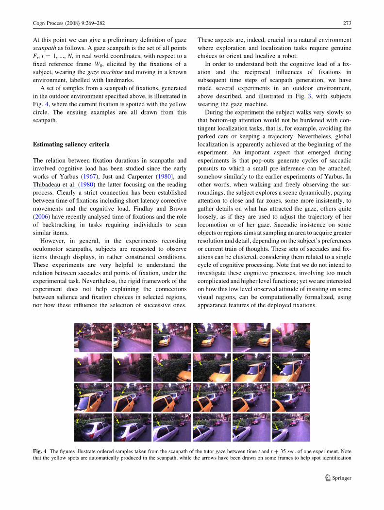
A set of samples from a scanpath of fixations, generated

in the outdoor environment specified above, is illustrated in

Fig. 4, where the current fixation is spotted with the yellow

circle. The ensuing examples are all drawn from this

scanpath.

Estimating saliency criteria

The relation between fixation durations in scanpaths and

involved cognitive load has been studied since the early

works of Yarbus (1967), Just and Carpenter (1980], and

Thibadeau et al. (1980) the latter focusing on the reading

process. Clearly a strict connection has been established

between time of fixations including short latency corrective

movements and the cognitive load. Findlay and Brown

(2006) have recently analysed time of fixations and the role

of backtracking in tasks requiring individuals to scan

similar items.

However, in general, in the experiments recording

oculomotor scanpaths, subjects are requested to observe

items through displays, in rather constrained conditions.

These experiments are very helpful to understand the

relation between saccades and points of fixation, under the

experimental task. Nevertheless, the rigid framework of the

experiment does not help explaining the connections

between salience and fixation choices in selected regions,

nor how these influence the selection of successive ones.

These aspects are, indeed, crucial in a natural environment

where exploration and localization tasks require genuine

choices to orient and localize a robot.

In order to understand both the cognitive load of a fix-

ation and the reciprocal influences of fixations in

subsequent time steps of scanpath generation, we have

made several experiments in an outdoor environment,

above described, and illustrated in Fig. 3, with subjects

wearing the gaze machine.

During the experiment the subject walks very slowly so

that bottom-up attention would not be burdened with con-

tingent localization tasks, that is, for example, avoiding the

parked cars or keeping a trajectory. Nevertheless, global

localization is apparently achieved at the beginning of the

experiment. An important aspect that emerged during

experiments is that pop-outs generate cycles of saccadic

pursuits to which a small pre-inference can be attached,

somehow similarly to the earlier experiments of Yarbus. In

other words, when walking and freely observing the sur-

roundings, the subject explores a scene dynamically, paying

attention to close and far zones, some more insistently, to

gather details on what has attracted the gaze, others quite

loosely, as if they are used to adjust the trajectory of her

locomotion or of her gaze. Saccadic insistence on some

objects or regions aims at sampling an area to acquire greater

resolution and detail, depending on the subject’s preferences

or current train of thoughts. These sets of saccades and fix-

ations can be clustered, considering them related to a single

cycle of cognitive processing. Note that we do not intend to

investigate these cognitive processes, involving too much

complicated and higher level functions; yet we are interested

on how this low level observed attitude of insisting on some

visual regions, can be computationally formalized, using

appearance features of the deployed fixations.

Fig. 4 The figures illustrate ordered samples taken from the scanpath of the tutor gaze between time t and t + 35 sec. of one experiment. Note

that the yellow spots are automatically produced in the scanpath, while the arrows have been drawn on some frames to help spot identification

Cogn Process (2008) 9:269–282 273

123

Several factors, actually, concur to produce a scanpath

and some of them are difficult to discriminate. More pre-

cisely, it is difficult to discriminate which factor is

prevailing in each time step, directing the gaze toward a

location rather than another. In the described experiments

we wanted to verify whether the general criteria reported

below could make sense of the elicited fixations grouping

and help giving an insight into the mechanisms underlying

the scanpath strategy.

More specifically, we wanted to show that the saliency

of a saccadic cycle, related to a spatial area, is delineated

by two main components, that is, inhibition of return and

innovation at the current time step. Indeed, innovation

accounts for the strength of unexpected, outstanding and

unattended stimuli (see Itti and Baldi 2006; for discussion

on the surprise effect).

The structure of scanpaths experiments

The purpose of an experiment is to model the structure of

the dynamic features emerging from a scanpath and to

understand the nature of the paths followed by the gaze. At

the same time we are interested in characterizing both a

gaze scanpath and the experiment supporting it. Our goal is

to learn a model that could allow us to automatically

generate a scanpath, although we shall not face the issue of

automatic scanpath generation here.

An experiment EP is defined to be the collection of data

F t¼1;...;N ; as described in (Eq. 2), including a scanpath, that

is, the collection of fixations Ft, plus the data obtained by

suitably transforming the original data to obtain more

precise and detailed information on the gaze path, as

described below.

In particular, the depth map M is the set of coordi-

nates of points in space of each pixel in I : Let us

consider these coordinates aligned as (XV, YV, ZV), with

XV ¼ ðx1; x2; . . .; xnÞ>; YV ¼ ðy1; y2; . . .; ynÞ> and ZV ¼ðz1; z2; . . .; znÞ>; we note that these coordinates are relative

to the viewer V at time t, i.e. in position Vt. Given the

rotation matrix Rt these components can be rotated with

respect to the fixed reference frame W0, hence the rotated

coordinates are:

ðXW0; YW0

; ZW0Þ ¼ R>ðXV YV ZVÞ>

h i>þ1nV>t

� �

ð3Þ

Furthermore from the elapsed time T we want to infer the

time spent on each fixation. It is, thus, necessary to com-

pute the velocity of the gaze around each fixation, given

that each frame is acquired at 15 Hz.

For example, suppose that at time 25, the subject is

looking at point ð70; 80; 270Þ>; given in cm and W0

coordinates, and at time 25.067 she is looking at point

ð69; 81; 271Þ>: The time elapsed is 1/15 s. during which

the eye could have moved quite far from the first fixation.

Instead the distance between the two fixations isffiffiffi3p

cm.

Now, if we consider 0.03 s. before the first fixation and

0.03 s. after the second, then we could estimate the

velocity of the gaze for this fixation to be 0.1 m/s and the

time of fixation, that is d t, to be 2/15. Therefore the time of

fixation is given by either defining a threshold on the

velocity of the gaze or by introducing a threshold on the

distance between k C 2 fixations.

For the combined rotation of head and eyes we assume

that the eyes anticipate the head positions, but their

movements are never contrasting. Therefore, we can con-

sider an algebraic sum of the angles of rotation.

On these bases we can specify two new concepts, that is,

proximity and following-a-direction.

Proximity accounts for surround inhibition, that is, the

decrease of visual acuity when eccentricity from the fovea

increases. Stimuli that are salient but peripheral with

respect to the current fixation point are less likely to be

noticed and attended. Let Bt be the disk centred in Ft,

with some radius r, and Y its projection on the image

plane. We need two data to assess proximity. First the

distance of point b in Bt from the fixation Ft, in world

coordinates. Further, we need the luminance of the point,

projected on the image, compared to the luminance of the

whole foveated region. The proximity value of a point b

is a function of the luminance contrast of its projection on

the image and its distance from the fixation. Let b be a

point in Bt and y the luminance of its projection on the

image plane. Let l be the mean luminance value of Y, rits standard deviation, and let d be the distance of b from

Ft. We have:

PðbÞ ¼ ððy� lÞ=ðrðd þ 1ÞÞÞ2: ð4Þ

Observe that this coordinate evaluates the scanpath opti-

mization, that is, the restraint to jumping between distant

fixations overlooking what is in the middle.

Following-a-direction is an optimization aspect stem-

ming from the consideration that when a subject explores a

scene she follows a scanning strategy which, possibly, goes

from one side to the other, moving her head, in a cyclic way.

The subject, namely, tries to stay on her scanning route as

long as other factors do not prevail. A biological justification

can be found in the attentional momentum, an effect

described in Spalek and Hammad (2004) which, more spe-

cifically than the IOR (Inhibition Of Return) mechanism,

shows that attention tends to explore new locations. In par-

ticular, attention does not only disregard just attended

locations in favour of unvisited ones, but in doing so it shifts

along the same direction. To allow for this effect we designed

a factor considering the shift between three consecutive

fixations Ft - 1, Ft, Ft + 1. Given the vectors vt�1:t ¼ Ft�1Ft���!

and vt:tþ1 ¼ FtFtþ1���!

; the following-a-direction factor for the

274 Cogn Process (2008) 9:269–282

123

fixation at time t + 1 is given by the cosine of the angle kbetween the two vectors:

DðFtþ1Þ ¼ � cosðkt�1:tþ1Þ

¼ � jvt�1:tj2 þ jvt:tþ1j2 þ jvt�1:t � vt:tþ1j2

2jvt�1:tjjvt:tþ1jð5Þ

It is easy to see that the function takes a maximal value of 1

when the vectors are parallel and with same direction and a

minimal value of -1 when parallel and with opposite

direction. Proximity and following-a-direction factors are

exemplified in Fig. 5.

We consider the set of meaningful features defined

above relative to a region surrounding the projection of the

fixation point Ft, at time t, on both the RGB image I and

the rotated depth image M (see Eq. 3).

For each fixation Ft a square of r2 pixels, whose centre is

the fixation, is sampled (in most experiments we have used

r = 5).

An experiment is gathered into a matrix X, where each

column denotes an observation and each row denotes one

of the physical properties mentioned above, processed at

each time t, during the experiment. Therefore for each

fixation there are r2 observations

n observations ¼ r2 �#fixations

15 features ¼

Obs1 Obs2 � � � Obsn

R

G

B

depth

� � � � � � � � � � � � � � �elapsed

8>>>>>>><

>>>>>>>:

ð6Þ

Specifically, the coordinates of the matrix X of observations

data are the following 15 features: colours (R,G,B), depth (Z),

positions gradient (dX,dY,dZ), where the coordinates

ðXW0; YW0

; ZW0Þ are with respect to W0, proximity, eye rota-

tions (yaw,pitch), combined with the analogous head rotations,

and head roll rotation, velocity, distance between two suc-

cessive fixation points, cumulative time at fixation, estimated

time at fixation. The whole set is formed by 15 features.

To model the generation of the subject scanpath we shall

take the following steps on the data gathered by the

experiments:

1. Use factor analysis, earlier developed in psychometrics

(see Mardia et al. 1979) to decorrelate the data

deducing the latent factors which interpret the main

components of saliency.

2. Infer the structure of cycles of fixations from a suitable

metric on the latent factors.

3. Specify the two core behaviours, that is, inhibition of

return and innovation, this last as a function of

inhibition of return, given the cycles.

In the next section we shall illustrate how to obtain the

latent factors defining saliency.

Latent factors

As shown in the previous section all the features gathered

are obtained by measurements of the subject head–eye

movements and of the colour and space variations obtained

from the three pairs of frames (eyes and scene) of the video

sequences at time t = 1, ..., N. These data can be viewed as

indirect measurements of the real source of attention.

Therefore the meaning of the measurements lies in the

correlation structure that accounts for most of the variation

of the features and explains saliency.

The idea behind the use of factor analysis is to find the

common patterns accounting for the specific roots of

saliency.

Let X be a matrix (p 9 n) of n observations and p

features, we first want to infer the latent factors that

influence saliency and discuss them.

Given an observation X ¼ ðX1; . . .;XpÞ> (i.e. a (p 9 1)

array), taking into account all of the above-mentioned

coordinates, by factor analysis we can reduce the coordi-

nates into common factors, such that

X ¼ ASþ �þ l ð7Þ

where A is a (p 9 k) matrix of the loadings of the factors

S(k 9 1), representing the common latent elements among

the observation coordinates, � is a (p 9 1) matrix of the

specific factors, that is, it is a vector of random variables

interpreting the noise relative to each coordinate, and l is the

mean of the variables. In factor reduction it is assumed that

E(S) = 0 and its variance is the identity, furthermore

Eð�Þ ¼ 0, while the variance of � is W ¼ diagðw11; . . .;wppÞ;also called the specific variance. Finally the covariance of S

and � is also 0.

The component Xj of the observation X can be specified,

in terms of common factors as:

Xk

i¼1

ajiSi þ �j þ lj; j ¼ 1; . . .; p ð8Þ

The variance of the observation can be specified as follows:

RXX ¼ EðXX>Þ � EðXÞEðXÞ> ¼ EðX � lÞðX � lÞ>

¼ EðASþ �ÞðASþ �Þ>

¼ EðASS>A> þ �S>A> þ AS�> þ ��>Þ¼ AEðSS>ÞA> þ Eð�S>ÞA> þ AEðS�>Þ þ Eð��>Þ¼ AA> þW

ð9Þ

Since Eð�S>Þ ¼ EðS�>Þ ¼ 0; EðSS>Þ ¼ varðSÞ ¼ I and

Eð��>Þ ¼ W; as noted above. Therefore the variance rXjXj

of the jth component is:

Cogn Process (2008) 9:269–282 275

123

Xk

i¼1

a2ji þ wjj; j ¼ 1; . . .; p ð10Þ

here wjj is the variance of the factor �j as introduced above.

On the other hand the covariance of X and the factors S is:

RXS ¼ EðXS>Þ � EðXÞEðSÞ> ¼ EðX � lÞS>

¼ EððASþ �ÞS>Þ ¼ AEðSS>Þ þ Eð�S>Þ¼ AI þ 0 ¼ A

ð11Þ

Therefore the variance rXjSiof the jth component and ith

factor is:

Xk

i¼1

aji; j ¼ 1; . . .; p ð12Þ

The estimation of the factor model amounts to find an

estimate A of the loadings and an estimate W of the specific

variance, from which the latent factors can be obtained (see

Hardle and Hlavka 2007).

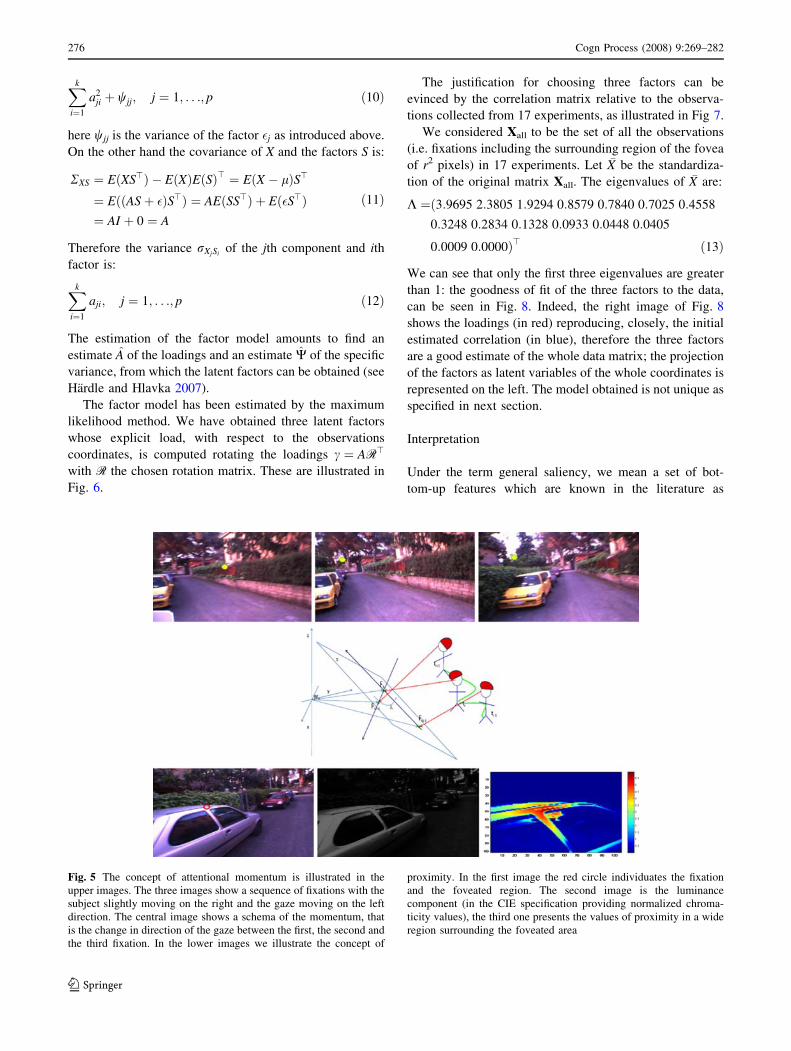
The factor model has been estimated by the maximum

likelihood method. We have obtained three latent factors

whose explicit load, with respect to the observations

coordinates, is computed rotating the loadings c ¼ AR>

with R the chosen rotation matrix. These are illustrated in

Fig. 6.

The justification for choosing three factors can be

evinced by the correlation matrix relative to the observa-

tions collected from 17 experiments, as illustrated in Fig 7.

We considered Xall to be the set of all the observations

(i.e. fixations including the surrounding region of the fovea

of r2 pixels) in 17 experiments. Let �X be the standardiza-

tion of the original matrix Xall. The eigenvalues of �X are:

K ¼ð3:9695 2:3805 1:9294 0:8579 0:7840 0:7025 0:4558

0:3248 0:2834 0:1328 0:0933 0:0448 0:0405

0:0009 0:0000Þ> ð13Þ

We can see that only the first three eigenvalues are greater

than 1: the goodness of fit of the three factors to the data,

can be seen in Fig. 8. Indeed, the right image of Fig. 8

shows the loadings (in red) reproducing, closely, the initial

estimated correlation (in blue), therefore the three factors

are a good estimate of the whole data matrix; the projection

of the factors as latent variables of the whole coordinates is

represented on the left. The model obtained is not unique as

specified in next section.

Interpretation

Under the term general saliency, we mean a set of bot-

tom-up features which are known in the literature as

Fig. 5 The concept of attentional momentum is illustrated in the

upper images. The three images show a sequence of fixations with the

subject slightly moving on the right and the gaze moving on the left

direction. The central image shows a schema of the momentum, that

is the change in direction of the gaze between the first, the second and

the third fixation. In the lower images we illustrate the concept of

proximity. In the first image the red circle individuates the fixation

and the foveated region. The second image is the luminance

component (in the CIE specification providing normalized chroma-

ticity values), the third one presents the values of proximity in a wide

region surrounding the foveated area

276 Cogn Process (2008) 9:269–282

123

causing a pop-out effect, such as colour, luminance and

depth (see. e.g. Itti and Koch 2001). Wherever these

features are highly contrasted with respect to the sur-

rounding area, the correspondent location stands out. This

is the most basic mechanism of visual attention and,

although most of time top-down attention is affecting the

selective tuning of attention, bottom-up attention is nev-

ertheless always ‘on’, particularly when exploring a scene

without a specific task.

The extracted latent factors shed a new light on the

structuring components of general saliency, especially with

respect to motion.

The loadings for the first factor highlight a strong

influence of depth and variation in the Y and Z directions,

while velocity, following-a-direction and the roll move-

ment of the head seem to be less significant. This is

coherent with those studies stressing the role of cortical

mechanisms in detecting focal orientation.

Fig. 6 The figure on the left

illustrates the load of each

extracted factor (rotated) with

respect to the coordinates, the

figure on the right the

contribution of each factor on

160 fixations of a scanpath

of 27 s, interpolants and the

polynomial degree is used to

indicate the behaviour

Fig. 7 The figure illustrates the

correlation matrix of Xall,

colours highlight meaningful

correlations

Fig. 8 The figure on the left

illustrates the weights of each

extracted factor (rotated) with

respect to the coordinates. The

plot on the right shows the

correspondence between the

estimated correlation of the data

gathered during the experiments

and those obtained by AA> þW

Cogn Process (2008) 9:269–282 277

123

On the other hand, it is interesting to note that the three

colour channels are collected in the second component,

whose behaviour (see Fig. 6) is in antiphase with respect to

the first component, this means that luminance and colour

not only are stand alone components of saliency, not

influenced by orientation and motion, but their behaviour

contrasts orientation, like if while orientation pop out is

active colour pop out is inhibited.

The last component can be identified with motion. The

loadings select first head–eye movements having, indeed,

highest weight, then elapsed time and finally proximity.

Note that the third component behaviour (see Fig. 6) is in

between the other two components.

The self-motion component, in attention modelling, is a

novelty and it is faced in our approach thanks to the sac-

cades collection, while the subject is walking, so that the

head is naturally in movement and the body coordination,

during slow steps on the road, contributes significantly in

the pop out.

The correlation-decorrelation of the fifteen chosen fea-

tures introduces, thus, a new insight in the general notion of

saliency. We suggest that it is exactly a bottom-up stimulus

that arouses pre-attentive vision and consequent redirection

of attention determining, as we shall discuss further, a

cyclic structure of attention.

We shall call the three latent factors, composing the

saliency, orientation saliency, luminance-colour saliency

and motion saliency.

Given the observations Xall obtained from the subject

scanpaths in a set of experiments EP, the saliency model,

estimated from the experiments, is given by the following

parameters:

ðA; S;WÞ ð14Þ

Here A are the loadings, S the latent factors, W is the

variance of the random noise �. The model, as noted above,

is not unique and the degrees of freedom are d = (1/2)(p-

k)2-(1/2)(p + k) = 63. However, choosing a rotation that

best fits the correlation of the common factors, the matrix A

of the loadings can be fixed. Hence we shall refer to the

model that best interprets the parameters given the rotation

R: We note that the rotation is chosen so as to maximize

the sum of the variances of the squared loadings within

each column of A. The model, given the rotation is thus:

M ¼ ðA; S;W;RÞ ð15Þ

Now, considering the model estimated by the set of

experiments, we have the following numbers:

1. The set of fixations F ¼ fFtjt ¼ 1; . . .;Ng; and the

regions Xt surrounding the fixations, each of size r2.

Therefore the matrix of all the data has size r2N 9 p,

with p = 15.

2. The array of factors S. As we have chosen 3 factors,

then S has size r2N 9 3.

3. The matrix A of the loadings, having size p 9 3.

4. The diagonal matrix W of the specific variance, having

size p 9 p.

5. The rotation matrix R which has size 3 9 3.

In the next section we shall discuss how to use the

correlation structure induced by the common factors to

define a metric on the space of fixations, and introduce the

concept of cycle.

Metric on latent factors: cycles of fixations

In this section we analyse how cycles of saccades can be

inferred from a scanpath and how, given two observations

Yi, Yj from the visual array we can induce that they belong

to the same cycle.

A cycle of local saccades is a set of fixations that must

be close in time and space (first and third factors) but not

necessarily similar in colour, unless we think only of

luminance. Nevertheless, there must be also some mean-

ingful aspect related to colour that we have not yet

observed in the experiments, and that we shall face in

future research. In this paper we shall consider colour only

through the latent factors (in our case the second factor).

Given two specific regions Yi and Yj, their relative dis-

tance can be specified with respect to the model

ðA; S;W;RÞ: In other words, we assume that the model

correctly specifies the correlation amongst the parameters,

through the latent factors explaining the saliency, hence the

similarity of two regions can be interpreted, in terms of

saliency, as the relative distance of their predicted factors

from the model.

Now, let Yi and Yj be two foveated regions of the

visual array at some specified time steps t and t0, that is,

two (r 9 r) squares of pixels centred in two fixation

points, then the factors predicted by the regions should

approximate those predicted by the model. If we consider

the vector ½Yq S�>; q 2 fi; jg as normally distributed, then

according to the model (see Eqs. 9, 11) its parameters

are:

NlY

lS

� �

;AA> þW A

A> I3

� �� �

ð16Þ

Here, note that the variance of the factors is the identity,

that is, in our case I3(3 9 3), the mean of the

factors lS = 03, and the other values are as given in

(Eqs. 9, 11). The expectation of the latent factor S; given

the specific observation Y, and being the distribution of S,

conditional on the observation Y(p 9 1), the above-defined

k-variate Gaussian (by hypothesis), is:

278 Cogn Process (2008) 9:269–282

123

EðSjY ¼ YqÞ ¼ A>ðAA> þWÞ�1ðY � lYÞ ð17Þ

This is the estimated individual factor score for the

observation Y = Yq. On the other hand, the variance of

the latent factor array, given the observation Y is, for k = 3

(in our case):

varðSjY ¼ YqÞ ¼ Ik � A>ðAA> þWÞ�1A ð18Þ

Therefore the conditional distribution is:

f ðSjY ¼ YiÞ�NðA>ðAA> þWÞ�1ðY � lYÞ; Ik �A>ðAA> þWÞ�1AÞ

ð19Þ

Despite the underlying correlation structure, the influence

of an observation on a group of factors differs from the

influence of another observation. Therefore, the affinity of

two observations can be drawn considering the impact of

each observation on the latent factors.

One way to deal with the distance between regions, in

terms of the predicted latent factors, is to compute the

Mahalanobis distance between observations, that is DM ¼ðH varðSjXÞ�1 H>Þ1=2; with H the mean of the region

centred in Ft, hence DM is a distance matrix of dimension

N 9 N and the distance between region i and j is readily

observed in row i and column j.

Another method consists in computing the correlation

matrix of all the factors and observations, that is, HCH>;with C the correlation, and then considering the distance

DC ¼ IN � HCH>: Also in this case DC is a distance

matrix of dimension N 9 N.

However, if we consider the space of parameters X,

associated with the space of fixations, that is, the space

including the factor model M ¼ ðA; S;WÞ 2 X; but also the

factors predicted by one, two or n regions, then the distance

could be defined in this space. Let us define Hi the

parameters estimated by the observations in region Yi and

fi ¼ f ðSjY ¼ Yi;HiÞ the conditional distribution given the

local parameters and fM the conditional distribution given

the model M: Then we have:

D2ðfi; fjÞ ¼1

2

Z

X

ðf 1=2i � f

1=2M Þ

2dx

0

@

1

A

þZ

X

ðf 1=2j � f

1=2M Þ

2dx

0

@

1

A ð20Þ

This is the mean Hellinger distance between the estimated

model and the local models, which is a real distance

measure (see Bishop 2006).

Now, given the above-defined distance we have to

delimit a cycle CY according to a neighbourhood of

fixations. Consider the lattice generated by D where,

instead of all the observations in the experiment, i.e. (r2 N),

we have N values obtained by estimating the mean of each

(r 9 r) square, surrounding the fixations.

It is interesting to note that, because of both time and

space, this is a block matrix, except when return to a pre-

viously visited cycle happens after a certain amount of

time. At this point we can define the neighbourhood sys-

tem, based on the above-defined distance between

fixations, as follows. Let qi = (x,y) be the pixel position of

the observation Yi, in the current frame (fixation):

Ni ¼ qjjDðfi; fjÞ\q; i 6¼ j� �

ð21Þ

Here, given a weight w [ 0, e.g w = 1/5, and given that

the number of fixations is M, q is defined as:

q ¼ w

ðwþ 1Þminj2M

Dðfi; fjÞ� �

þ 1

Mðwþ 1Þ

� �

�XM

j¼1

Dðfi; fjÞ �minj2M

Dðfi; fjÞ

Note that q is defined for each neighbourhood, as it

depends from the chosen observation Yi. Then a cycle Ci is

defined to be the set of neighbours for which D satisfies:

ðqi; qjÞ 2 Ci iff ðqi; qjÞ 2 Ni^8qrðqj; qrÞ 2 Ci ! Dðfi; frÞ� q

ð22Þ

It is easy to see that all points in a sequence of fixations

satisfying the above conditions form a clique.

We have verified that the above-defined distance is suf-

ficient to capture the cycles performed by the subjects in the

experiments. Results of the definition can be observed in

Fig. 9 which are relative to the scanpath illustrated in Fig. 4.

The above-defined distance has been suitably verified in

all the experiments, leading to natural cycles that are

approximately correct (in empirical terms, by comparison

with the subjects resolution effort). That is, the obtained

cycles, as illustrated in Fig. 9, capture what the subject

marked as an attempt to augment the resolution of an inter-

esting region, and are consistent with time and distance.

Now, if we were given two random observations Yi and

Yj in the visual array, and a model M ¼ ðA;F;W;RÞ;which has been learned from the matrix X of data gathered

by the subject’s experiments, then Yi and Yj would be in the

same cycle if the distance Dðfi; fjÞ of their obtained factors,

from (17), satisfies the above conditions.

Furthermore it is possible to show, although we will not

do it here that, apart from later returns and random exits

from the cycle, a cycle is consistent in time and space, as

there is a continuity of back and forth gaze steps inside the

cycle, among fixations.

Cogn Process (2008) 9:269–282 279

123

Inhibition of return and Innovation

Given the model M ¼ ðA;F;W;RÞ; the factor estimate and

an observation Yi we shall introduce the concept of inhibition

of return and innovation for a random observation, that will

allow predicting whether an observation is promising or not.

Let us assume that a cycle C; initiated by a random

observation Y, has been given. Since, as observed above,

a cycle is consistent in time and space, we say that the

time spent inside the cycle is TC:

We can now introduce the concept of inhibition of

return to a cycle, which accounts for the interest shown for

a region and the way elements of the visual array pop out

far or near a specific cycle.

Inhibition of return ðIORCÞ

The inhibition of return accounts for the time delay in

returning to a visited region. This mnemonic component

tells that we will pay no further attention to a zone recently

sampled through fixations and saccadic movements, at least

for a certain amount of time (see, e.g. Klein 2000).

Someone who is walking observes closer objects already

glanced at a distance. In this sense there is a return which,

though, is not immediate.

Now, let C ¼ ðY1; . . .YmÞ be a cycle of foveated regions,

we expect that inside the cycle there is backtracking,

i.e. the gaze goes back and forth between the fixations, and

the time spent in the cycle is TC: However, once the gaze

has abandoned the cycle it will not return to it in a lapse of

time which depends on TC: Therefore, a recently visited

region (included in the convex hull of a cycle) will receive

a higher value of inhibition. Now, if tC is the exit time of

the cycle C, t is the time step of a current fixation Ft, with

Yt 62 C; and TC the time spent in the cycle C, then tC B t

and TC � tC: Hence we define the inhibition of return as:

IORCðtÞ ¼ a expT2

Cðt � tcÞðt þ 1Þ2

!

ð23Þ

Here a is a normalization factor to ensure that IORC � 1. It

is easy to see that the inhibition of return IORC to a cycle

C first increases and then, as the time passes, it decreases

again leaving attention free to go back to an already visited

region (see Fig. 10).

At this point we are ready to introduce the concept of

innovation.

Innovation ðGÞ

Consider the current cycle C, at time t, and suppose that the

time spent in C, so far, is TC: Let Y be a random obser-

vation, now Y could be in C or not, depending on whether

the predicted factor, from the local region estimate (see Eq.

20), is more or less distant from the factor predicted in the

Fig. 9 The figures illustrate the cycles, including returns after a while, obtained by computing the cliques as in Eq. (22), using the distance

measure defined in Eq. (20). Note that the red circles have been added to emphasise the groups of yellow stars indicating observations

280 Cogn Process (2008) 9:269–282

123

current cycle. However, if the distance is less than the

threshold q it might be the case that the cycle is inhibited

by the IORC. Therefore, these two facts have to be taken

into account in the definition of innovation.

In other words, we consider innovation as a function of

the current observed region Y, such that, given a cycle C at

time step t

GðC; Y ; tÞ � 0 if Y 62 Ct

\0 otherwise

ð24Þ

If innovation is positive then the attention is stimulated to

jump out of the cycle and to remain in it otherwise.

Now, given a cycle C and the current observation Yi, an

estimate of the latent factor S is (17), that is, the conditional

expectation extended to C = Ct, E(S| C = Ct). This is the

regression function of S on C = Ct and E(S0| Y = Yi) is the

regression function of S0 on Y = Yi. Therefore, the distance

according to (20), is DðC;YÞ: If DðC; YÞ � q\0 it follows

that we expect Y to belong to C, having thus low innovation

value, unless C is already inhibited by the IORC: Hence

innovation should be like IORCðtÞ; but weighted by the

distance between the current observation and the consid-

ered cycle:

GðC; Y ; tÞ ¼ IORCðtÞlogDðC; YÞqþ 1

� �� �

ð25Þ

Consider the following cases: if DðC; YÞ\q then innova-

tion rapidly decreases because it expects that the current

fixation is within a cycle further, because of the influence

of the inhibition of return, it will increase again, still

remaining negative. On the other hand, if DðC; YÞ� q then

innovation rapidly increases, to drive the gaze towards new

regions, but then according to inhibition of return it will

decrease and, unless other factors will not contribute it,

approximates IORCðtÞ (see Fig. 10).

Conclusions

Attention is a fundamental component in modelling cog-

nitive architectures as it fosters learning and development

of complex behaviours. Features accounting for selection

of fixation points are not only related to appearance but

should also allow for head and eye movement underlying

strategies. In our research endeavour to investigate and

model psycho-physiological mechanisms of attention

deployment during scene perception, we conducted

experiments in outdoor environments, letting the subject

perform a natural task which would not overwhelm visual

and cognitive resources but just help basic factors emerg-

ing. We designed a framework to extract features from

fixations performed by a subject: some features were taken

as raw measures, others, such as following-a-direction and

proximity, were obtained by processing specific data to

make sense of oculomotor behaviour. We provided a

methodology to group data according to correlated features

so to make them more easily interpretable and comparable.

This made possible to cluster fixations close in appearance,

space and time, according to a distance measure defining

neighbourhoods on observations. We devised a model of

saliency of a cluster, defined as innovation, relying on the

obtained factors and similarity with the current cycle of

fixations. Results showed that a tendency to prefer new

regions anytime a cycle has been going on for a certain

amount of time. This effect was modelled in the innovation

measure by the IOR factor.

The proposed framework was tested on collected

sequences, validating the procedure. Although preliminary

this work will be further expanded in order to make

acquisition and interpretation of data as easy and reliable as

possible, for example by removing the constraints on

known environments and localization through landmarks.

0 200 400 600 800 1000 1200 1400 1600 1800 2000−2

−1

0

1

2

3

4

t

Inno

vatio

nInnovation for different distances D(Y,C)

D=0.5<ρD=7<ρD=12>ρD=18>ρ

0 500 1000 1500 2000 25000

0.1

0.2

0.3

0.4

0.5

0.6

0.7

0.8

0.9

t

IOR

C

IOR of a cycle C taken at different time steps, with TC varying from 0 to 0.5sec.

TC=0

TC=0.1

TC=0.3

TC=0.5

y max

y mean

Fig. 10 The figures illustrate on the left the IORC ; taken with different times of permanence and on the right the innovation taken for different

distances

Cogn Process (2008) 9:269–282 281

123

Further, we are currently working on the definition of a

priming factor, aimed at assessing influence or causality of

a selected region on next selection. Moreover interpretation

and classification of gaze cycles will be used as a tool for

defining and modelling visual strategies and, lastly, object

recognition in a way that can be learnt by robots or artifi-

cial vision systems. Development of this architecture will

hence lead to production of autonomous and meaningful

scanpaths.

Acknowledgments The authors would like to thank the reviewers

for their worthwhile suggestions. This research has been supported by

the European Union 6th Framework Programme Project Viewfinder.

References

Belardinelli A, Pirri F, Carbone A (2006) Spatial discrimination in

task-driven attention. In: Proceedings of IEEE RO-MAN’06.

Hatfield, UK, pp 321–327

Belardinelli A, Pirri F, Carbone A (2007) Bottom-up gaze shifts and

fixations learning by imitation. IEEE Trans Syst Man Cybern B

37:256–271

Bishop CM (2006) Pattern recognition and machine learning.

Springer, Heidelberg

Bruce NDB, Tsotsos JK (2006) Saliency based on information

maximization. Adv Neural Inf Process Syst 18:155–162

Findlay JM, Brown V (2006) Eye scanning of multi-element displays:

I scanpath planning. Vis Res 46:179–195

Frintrop S, Jensfelt P, Christensen H (2006) Attentional landmark

selection for visual slam. In: Proceedings of the IEEE/RSJ

international conference on intelligent robots and systems

(IROS’06)

Hardle W, Hlavka Z (2007) Multivariate statistics: exercises and

solutions. Springer, Heidelberg

Itti L, Baldi P (2006) Bayesian surprise attracts human attention. In:

Advances in neural information processing systems, vol 19

(NIPS*2005). MIT Press, Cambridge, pp 1–8

Itti L, Koch C (2001) Computational modeling of visual attention. Nat

Rev Neurosci 2(3):194–203

Just M, Carpenter P (1980) A theory of reading. Psychol Rev 87:329–

354

Klein RM (2000) Inhibition of return. Trends Cogn Sci 4:138–147

Kramer AF, Wiegmann DA, Kirlik A (2007) Attention. From theory

to practice. Oxford University Press, Oxford

Mardia K, Kent J, Bibby J (1979) Multivariate analysis. Academic

Press, London

Najemnik J, Geisler WS (2005) Optimal eye movement strategies in

visual search. Nature 434:387–391

Posner MI (1980) Orienting of attention. Q J Exp Psychol 32-A:3–25

Raj R, Geisler WS, Frazor RA, Bovik AC (2005) Contrast statistics

for foveated visual systems: fixation selection by minimizing

contrast entropy. J Opt Soc Am 22(10):2039–2049

Renninger LW, Coughlan J, Verghese P, Malik J (2005) An

information maximization model of eye movements. Adv Neural

Inf Process Syst 17:1121–1128

Santella A, Decarlo D (2003) Robust clustering of eye movement

recordings for quantification of visual interest. In ETRA 2004.

New York, pp 23–34

Shokoufandeh A, Sala PL, Sim R, Dickinson SJ (2006) Landmark

selection for vision-based navigation. IEEE Trans Rob

22(2):334–349

Spalek TM, Hammad S (2004) Supporting the attentional momentum

view of ior: Is attention biased to go right? Percept Psychophys

66(2):219–233

Thibadeau R, Just M, Carpenter P (1980) Real reading behaviour. In:

Proceedings of the 18th annual meeting on association for

computational linguistics, Morristown, NJ, USA. Association for

Computational Linguistics, pp 159–162

Treisman A, Gelade G (1980) A feature-integration theory of

attention. Cogn Psychol 12:97–136

Tsotsos JK, Culhane S, Wai W, Lai Y, Davis N, Nuflo F (1995)

Modeling visual attention via selective tuning. Artif Intell

78:507–547

Turano KA, Geruschat DR, Baker FH (2003) Oculomotor strategies

for the direction of gaze tested with a real-world activity. Vis

Res 43:333–346

Yarbus AL (1967) Eye movements and vision. Plenum Press, New

York

Zhang Z (1999) Flexible camera calibration by viewing a plane from

unknown orientations. In: The Proceedings of the seventh IEEE

international conference on Computer vision, 1999, vol 1, pp

666–673

282 Cogn Process (2008) 9:269–282

123