Games strategies and decision making
587
Transcript of Games strategies and decision making


This page intentionally left blank

Games, Strategies, andDecision Making
Joseph E. Harrington, Jr.Johns Hopkins University
Worth Publishers

Senior Publisher: Craig BleyerAcquisitions Editor: Sarah DorgerSenior Marketing Manager: Scott GuileMarket Research and Development: Steven RigolosiDevelopmental Editor: Carol Pritchard-MartinezConsulting Editor: Paul ShensaAssociate Editor: Matthew DriskillPhoto Editor: Bianca MoscatelliArt Director: Babs ReingoldPhoto Researcher: Julie TesserSenior Designer, Cover Designer: Kevin KallInterior Designer: Lissi SigilloAssociate Managing Editor: Tracey KuehnProject Editors: Dana Kasowitz
Dennis Free, Aptara®, Inc.Production Manager: Barbara Anne SeixasComposition: Aptara®, Inc.Printing and Binding: RR Donnelley
Library of Congress Control Number: 2008925817
ISBN-13: 978-0-7167-6630-8ISBN-10: 0-7167-6630-2
© 2009 by Worth Publishers
All rights reserved
Printed in the United States of America
First printing
Worth Publishers41 Madison AvenueNew York, NY 10010www.worthpublishers.com

Games, Strategies, andDecision Making

To Colleen and Grace,who as children taught me love,
and who as teenagers taught me strategy.

This page intentionally left blank

vi
Joseph E. Harrington, Jr., is Professor of Economics at Johns HopkinsUniversity. He has served on various editorial boards, including those of theRAND Journal of Economics, Foundations and Trends in Microeconomics, andthe Southern Economic Journal. His research has appeared in top journals ina variety of disciplines, including economics (e.g., the American EconomicReview, Journal of Political Economy, and Games and Economic Behavior), po-litical science (Economics and Politics, Public Choice), sociology (AmericanJournal of Sociology), management science (Management Science), and psy-chology (Journal of Mathematical Psychology). He is a coauthor of Economicsof Regulation and Antitrust, which is in its fourth edition.

Brief Contents
Preface . . . . . . . . . . . . . . . . . . . . . . . . . . . . . . . . . . . . . . . . . . . . . . . . . . . . . . . . . . . . . . . . . . . . . . . . . . . . xv
C H A P T E R 1
Introduction to Strategic Reasoning . . . . . . . . . . . . . . . . . . . . . . . . . . . . . 1
C H A P T E R 2
Building a Model of a Strategic Situation . . . . . . . . . . . . . . . . . . . 17
C H A P T E R 3
Eliminating the Impossible: Solving a Game whenRationality Is Common Knowledge . . . . . . . . . . . . . . . . . . . . . . . . . . . . . 55
C H A P T E R 4
Stable Play: Nash Equilibria in Discrete Games with Two or Three Players . . . . . . . . . . . . . . . . . . . . . . . . . . . . . . . . . . . . . . . . . . . 89
C H A P T E R 5
Stable Play: Nash Equilibria in Discrete n-Player Games . . . . . . . . . . . . . . . . . . . . . . . . . . . . . . . . . . . . . . . . . . . . . . . . . . . . . . . . . . . 117
C H A P T E R 6
Stable Play: Nash Equilibria in Continuous Games . . . 147
C H A P T E R 7
Keep ’Em Guessing: Randomized Strategies . . . . . . . . . . . . . . 181
C H A P T E R 8
Taking Turns: Sequential Games with Perfect Information . . . . . . . . . . . . . . . . . . . . . . . . . . . . . . . . . . . . . . . . . . . . . . . . . . . . 219
C H A P T E R 9
Taking Turns in the Dark: Sequential Games withImperfect Information . . . . . . . . . . . . . . . . . . . . . . . . . . . . . . . . . . . . . . . . . . . . . . . . 255
vii

BRIEF CONTENTS viii
C H A P T E R 1 0
I Know Something You Don’t Know: Games with Private Information . . . . . . . . . . . . . . . . . . . . . . . . . . . . . . . . 291
C H A P T E R 1 1
What You Do Tells Me Who You Are: Signaling Games . . . . . . . . . . . . . . . . . . . . . . . . . . . . . . . . . . . . . . . . . . . . . . . . . . . . . . . . . 325
C H A P T E R 1 2
Lies and the Lying Liars That Tell Them: Cheap Talk Games . . . . . . . . . . . . . . . . . . . . . . . . . . . . . . . . . . . . . . . . . . . . . . . . . . . . . . 359
C H A P T E R 1 3
Playing Forever: Repeated Interaction with Infinitely Lived Players . . . . . . . . . . . . . . . . . . . . . . . . . . . . . . . . . . . . . . . 391
C H A P T E R 1 4
Cooperation and Reputation: Applications of RepeatedInteraction with Infinitely Lived Players . . . . . . . . . . . . . . . . . . . . 423
C H A P T E R 1 5
Interaction in Infinitely Lived Institutions . . . . . . . . . . . . . . . . . 451
C H A P T E R 1 6
Evolutionary Game Theory and Biology: Evolutionarily Stable Strategies . . . . . . . . . . . . . . . . . . . . . . . . . . . . . . . . . 479
C H A P T E R 1 7
Evolutionary Game Theory and Biology: Replicator Dynamics . . . . . . . . . . . . . . . . . . . . . . . . . . . . . . . . . . . . . . . . . . . . . . . . . . 507
Answers to “Check Your Understanding” Questions . . . . . . . . . . . . . . . . . . . . . . S-1
Glossary . . . . . . . . . . . . . . . . . . . . . . . . . . . . . . . . . . . . . . . . . . . . . . . . . . . . . . . . . . . . . . . . . . . . . . . . . . G-1
Index . . . . . . . . . . . . . . . . . . . . . . . . . . . . . . . . . . . . . . . . . . . . . . . . . . . . . . . . . . . . . . . . . . . . . . . . . . . . . . I-1

ix
Competition for Elected Office . . . . . . . . . . . . . . . . . . . . . 38The Science 84 Game . . . . . . . . . . . . . . . . . . . . . . . . . . . . . 39
2.6 Moving from the Extensive Form andStrategic Form . . . . . . . . . . . . . . . . . . . . . . . . . . . . . . . . . . 39
Baseball, II . . . . . . . . . . . . . . . . . . . . . . . . . . . . . . . . . . . . . . . . 39Galileo Galilei and the Inquisition, II . . . . . . . . . . . . . . . . 40Haggling at an Auto Dealership, II . . . . . . . . . . . . . . . . . 41
2.7 Going from the Strategic Form to the Extensive Form . . . . . . . . . . . . . . . . . . . . . . . . 422.8 Common Knowledge . . . . . . . . . . . . . . . . . . . . . 432.9 A Few More Issues in Modeling Games . . . . . . . . . . . . . . . . . . . . . . . . . . . . . . . . . . . . . . . . . . . . . 45Summary . . . . . . . . . . . . . . . . . . . . . . . . . . . . . . . . . . . . . . . . . . 48Exercises . . . . . . . . . . . . . . . . . . . . . . . . . . . . . . . . . . . . . . . . . . . 49
References . . . . . . . . . . . . . . . . . . . . . . . . . . . . . . . . . . . . . . . . 54
C H A P T E R 3
Eliminating the Impossible:Solving a Game when
Rationality Is CommonKnowledge 55
3.1 Introduction . . . . . . . . . . . . . . . . . . . . . . . . . . . . . . . . 553.2 Solving a Game when Players Are Rational . . . . . . . . . . . . . . . . . . . . . . . . . . . . . . . . . . . . . 563.2.1 Strict Dominance . . . . . . . . . . . . . . . . . . . . . . . . . . . 56
White Flight and Racial Segregation in Housing . . . . . . . . . . . . . . . . . . . . . . . . . . . . . . . . . . . . . . . 59
Banning Cigarette Advertising on Television . . . . . . . . . . . . . . . . . . . . . . . . . . . . . . . . . . . . . . . . 60
3.2.2 Weak Dominance . . . . . . . . . . . . . . . . . . . . . . . . . . 64Bidding at an Auction . . . . . . . . . . . . . . . . . . . . . . . . . . . . . 64The Proxy Bid Paradox at eBay . . . . . . . . . . . . . . . . . . . . 66
3.3 Solving a Game when Players AreRational and Players Know that Players Are Rational . . . . . . . . . . . . . . . . . . . . . . . . . . . . . . . . . . . . . 68
Team-Project Game . . . . . . . . . . . . . . . . . . . . . . . . . . . . . . . . 68
Preface . . . . . . . . . . . . . . . . . . . . . . . . . . . . . . . . . . . . . . . . . . . . . . xv
C H A P T E R 1
Introduction to StrategicReasoning 1
1.1 Who Wants to Be a Game Theorist? . . . 11.2 A Sampling of Strategic Situations . . . . . 31.3 Whetting Your Appetite: The Game ofConcentration . . . . . . . . . . . . . . . . . . . . . . . . . . . . . . . . . . . . . 51.4 Psychological Profile of a Player . . . . . . . 81.4.1 Preferences . . . . . . . . . . . . . . . . . . . . . . . . . . . . . . . . . . . 8
1.4.2 Beliefs . . . . . . . . . . . . . . . . . . . . . . . . . . . . . . . . . . . . . . 11
1.4.3 How Do Players Differ? . . . . . . . . . . . . . . . . . . . 12
1.5 Playing the Gender Pronoun Game . . . 13References . . . . . . . . . . . . . . . . . . . . . . . . . . . . . . . . . . . . . . . . 14
C H A P T E R 2
Building a Model of a StrategicSituation 17
2.1 Introduction . . . . . . . . . . . . . . . . . . . . . . . . . . . . . . . . 172.2 Extensive Form Games: PerfectInformation . . . . . . . . . . . . . . . . . . . . . . . . . . . . . . . . . . . . . . . 18
Baseball, I . . . . . . . . . . . . . . . . . . . . . . . . . . . . . . . . . . . . . . . . . 21Galileo Galilei and the Inquisition, I . . . . . . . . . . . . . . . . 22Haggling at an Auto Dealership, I . . . . . . . . . . . . . . . . . 24
2.3 Extensive Form Games: ImperfectInformation . . . . . . . . . . . . . . . . . . . . . . . . . . . . . . . . . . . . . . . 27
Mugging . . . . . . . . . . . . . . . . . . . . . . . . . . . . . . . . . . . . . . . . . . . 29U.S. Court of Appeals for the Federal Circuit . . . . . . . 30The Iraq War and Weapons of Mass Destruction . . . 32
2.4 What Is a Strategy? . . . . . . . . . . . . . . . . . . . . . . . 342.5 Strategic Form Games . . . . . . . . . . . . . . . . . . . 36
Tosca . . . . . . . . . . . . . . . . . . . . . . . . . . . . . . . . . . . . . . . . . . . . . . 37
Contents

Existence-of-God Game . . . . . . . . . . . . . . . . . . . . . . . . . . . . 70Boxed-Pigs Game . . . . . . . . . . . . . . . . . . . . . . . . . . . . . . . . . . 71
3.4 Solving a Game when Rationality IsCommon Knowledge . . . . . . . . . . . . . . . . . . . . . . . . . . . 733.4.1 The Doping Game: Is It Rational for Athletes to Use Steroids? . . . . . . . . . . . . . . . . . . . . . . . . 73
3.4.2 Iterative Deletion of Strictly DominatedStrategies . . . . . . . . . . . . . . . . . . . . . . . . . . . . . . . . . . . . . . . . . 76
Summary . . . . . . . . . . . . . . . . . . . . . . . . . . . . . . . . . . . . . . . . . . 78Exercises . . . . . . . . . . . . . . . . . . . . . . . . . . . . . . . . . . . . . . . . . . . 79
3.5 Appendix: Strict and Weak Dominance . . . . . . . . . . . . . . . . . . . . . . . . . . . . . . . . . . . . . . . 843.6 Appendix: Rationalizability (Advanced) . . . . . . . . . . . . . . . . . . . . . . . . . . . . . . . . . . . . . . . 84References . . . . . . . . . . . . . . . . . . . . . . . . . . . . . . . . . . . . . . . . 87
C H A P T E R 4
Stable Play: Nash Equilibria in Discrete Games with Two
or Three Players 89
4.1 Defining Nash Equilibrium . . . . . . . . . . . . . . 894.2 Classic Two-Player Games . . . . . . . . . . . . . . 92
Prisoners’ Dilemma . . . . . . . . . . . . . . . . . . . . . . . . . . . . . . . . 93A Coordination Game—Driving Conventions . . . . . . . 95A Game of Coordination and Conflict—Telephone . . 95An Outguessing Game—Rock–Paper–Scissors . . . . . 97Conflict and Mutual Interest in Games . . . . . . . . . . . . . 99
4.3 The Best-Reply Method . . . . . . . . . . . . . . . . . 994.4 Three-Player Games . . . . . . . . . . . . . . . . . . . . 101
American Idol Fandom . . . . . . . . . . . . . . . . . . . . . . . . . . . 101Voting, Sincere or Devious? . . . . . . . . . . . . . . . . . . . . . . 102Promotion and Sabotage . . . . . . . . . . . . . . . . . . . . . . . . . 106
4.5 Foundations of Nash Equilibrium . . . 1094.5.1 Relationship to Rationality Is CommonKnowledge . . . . . . . . . . . . . . . . . . . . . . . . . . . . . . . . . . . . . . . 109
4.5.2 The Definition of a Strategy, Revisited . 110
Summary . . . . . . . . . . . . . . . . . . . . . . . . . . . . . . . . . . . . . . . . . 111Exercises . . . . . . . . . . . . . . . . . . . . . . . . . . . . . . . . . . . . . . . . . 112
4.6 Appendix: Formal Definition of Nash Equilibrium . . . . . . . . . . . . . . . . . . . . . . . . . 116References . . . . . . . . . . . . . . . . . . . . . . . . . . . . . . . . . . . . . . . 116
C H A P T E R 5
Stable Play: Nash Equilibria in Discrete n-Player
Games 117
5.1 Introduction . . . . . . . . . . . . . . . . . . . . . . . . . . . . . . 1175.2 Symmetric Games . . . . . . . . . . . . . . . . . . . . . . . 118
The Sneetches . . . . . . . . . . . . . . . . . . . . . . . . . . . . . . . . . . . 119Airline Security . . . . . . . . . . . . . . . . . . . . . . . . . . . . . . . . . . . 122Operating Systems: Mac or Windows? . . . . . . . . . . . . 125Applying for an Internship . . . . . . . . . . . . . . . . . . . . . . . . 128
5.3 Asymmetric Games . . . . . . . . . . . . . . . . . . . . . 130Entry into a Market . . . . . . . . . . . . . . . . . . . . . . . . . . . . . . 130Civil Unrest . . . . . . . . . . . . . . . . . . . . . . . . . . . . . . . . . . . . . . . 134
5.4 Selecting among Nash Equilibria . . . 137Summary . . . . . . . . . . . . . . . . . . . . . . . . . . . . . . . . . . . . . . . . . 141Exercises . . . . . . . . . . . . . . . . . . . . . . . . . . . . . . . . . . . . . . . . . 141
References . . . . . . . . . . . . . . . . . . . . . . . . . . . . . . . . . . . . . . . 145
C H A P T E R 6
Stable Play: Nash Equilibria in Continuous Games 147
6.1 Introduction . . . . . . . . . . . . . . . . . . . . . . . . . . . . . . 1476.2 Solving for Nash Equilibria without Calculus . . . . . . . . . . . . . . . . . . . . . . . . . . . . . . 148
Price Competition with Identical Products . . . . . . . . . 149Neutralizing Price Competition with
Price-Matching Guarantees . . . . . . . . . . . . . . . . . . . . . 152Competing for Elected Office . . . . . . . . . . . . . . . . . . . . . 154
6.3 Solving for Nash Equilibria withCalculus (Optional) . . . . . . . . . . . . . . . . . . . . . . . . . . . 157
Price Competition with Differentiated Products . . . . . . . . . . . . . . . . . . . . . . . . . . . . . . . . . . . . . . . .160
Tragedy of the Commons—The Extinction of the Woolly Mammoth . . . . . . . . . . . . . . . . . . . . . . . . . . . . . . . . . . . . . . 164
Charitable Giving and the Power of Matching Grants . . . . . . . . . . . . . . . . . . . . . . . . . . . . . 169
Summary . . . . . . . . . . . . . . . . . . . . . . . . . . . . . . . . . . . . . . . . . 174Exercises . . . . . . . . . . . . . . . . . . . . . . . . . . . . . . . . . . . . . . . . . 175
References . . . . . . . . . . . . . . . . . . . . . . . . . . . . . . . . . . . . . . . 179
x CONTENTS

C H A P T E R 7
Keep ’Em Guessing:Randomized Strategies 181
7.1 Police Patrols and the Drug Trade . . . . . . . . . . . . . . . . . . . . . . . . . . . . . . . . . . . . . . . . . . . . 1817.2 Making Decisions under Uncertainty . . . . . . . . . . . . . . . . . . . . . . . . . . . . . . . . . . . . . 1827.2.1 Probability and Expectation . . . . . . . . . 182
7.2.2 Preferences over Uncertain Options . . . 185
7.2.3 Ordinal vs. Cardinal Payoffs . . . . . . . . . 186
7.3 Mixed Strategies and Nash Equilibrium . . . . . . . . . . . . . . . . . . . . . . . . . . . . . 1877.3.1 Back on the Beat . . . . . . . . . . . . . . . . . 187
7.3.2 Some General Properties ofa Nash Equilibrium in Mixed Strategies . . . . . 191
7.4 Examples . . . . . . . . . . . . . . . . . . . .192Avranches Gap in World War II . . . . . . . . . . . . . . . 193Entry into a Market . . . . . . . . . . . . . . . . . . . . . . . 197
7.5 Advanced Examples . . . . . . . . . . . . 198Penalty Kick in Soccer . . . . . . . . . . . . . . . . . . . . . 198Slash ’em Up: Friday the 13th . . . . . . . . . . . . . . . 201Bystander Effect . . . . . . . . . . . . . . . . . . . . . . . . . . 204
7.6 Games of Pure Conflict and Cautious Behavior . . . . . . . . . . . . . 207Summary . . . . . . . . . . . . . . . . . . . . . . . . . . . . . . . . . . . . . . . . . 211Exercises . . . . . . . . . . . . . . . . . . . . . . . . . . . . . . . . . . . . . . . . . 212
7.7 Appendix: Formal Definition of Nash Equilibrium in Mixed Strategies . . . . . . . . . . . . . . . . . . . . . . .215References . . . . . . . . . . . . . . . . . . . . . . . . . . . . . . . . . . . . . . . 216
C H A P T E R 8
Taking Turns: SequentialGames with Perfect
Information 219
8.1 Introduction . . . . . . . . . . . . . . . . . . . . . . . . . . . . . . 2198.2 Backward Induction and SubgamePerfect Nash Equilibrium . . . . . . . . . . . . . . . . . . . 221
8.3 Examples . . . . . . . . . . . . . . . . . . . . . . . . . . . . . . . . . . 225Cuban Missile Crisis . . . . . . . . . . . . . . . . . . . . . . . . . . . . . . 225Enron and Prosecutorial
Prerogative . . . . . . . . . . . . . . . . . . . . . . . . . . . . . . . . . . . . . 227Racial Discrimination and Sports . . . . . . . . . . . . . . . . . 229
8.4 Waiting Games: Preemption and Attrition . . . . . . . . . . . . . . . . . . . . . . . . . . . . . . . . . . . 2358.4.1 Preemption . . . . . . . . . . . . . . . . . . . . . . . . . . . . . . . 236
8.4.2 War of Attrition . . . . . . . . . . . . . . . . . . . . . . . . . . 238
8.5 Do People Reason Using Backward Induction? . . . . . . . . . . . . . . . . . . . . . . . . 2398.5.1 Experimental Evidence and Backward Induction . . . . . . . . . . . . . . . . . . . . . . . . . . . . . 239
8.5.2 A Logical Paradox with Backward Induction . . . . . . . . . . . . . . . . . . . . . . . . . . . . . .242
Summary . . . . . . . . . . . . . . . . . . . . . . . . . . . . . . . . . . . . . . . . . 243Exercises . . . . . . . . . . . . . . . . . . . . . . . . . . . . . . . . . . . . . . . . . 244
References . . . . . . . . . . . . . . . . . . . . . . . . . . . . . . . . . . . . . . . 254
C H A P T E R 9
Taking Turns in the Dark: Sequential
Games with Imperfect Information 255
9.1 Introduction . . . . . . . . . . . . . . . . . . . . . . . . . . . . . . 2559.2 Subgame Perfect Nash Equilibrium . . . . . . . . . . . . . . . . . . . . . . . . . . . . . . . . . . . . . 257
British Intelligence . . . . . . . . . . . . . . . . . . . . . . . . . . . . . . . . 260
9.3 Examples . . . . . . . . . . . . . . . . . . . . . . . . . . . . . . . . . . 263OS/2 . . . . . . . . . . . . . . . . . . . . . . . . . . . . . . . . . . . . . . . . . . . . . 264Agenda Control in the Senate . . . . . . . . . . . . . . . . . . . . 268
9.4 Commitment . . . . . . . . . . . . . . . . . . . . . . . . . . . . . . 2709.4.1 Deterrence of Entry . . . . . . . . . . . . . . . . . . . . . . 270
9.4.2 Managerial Contracts and Competition: East India Trade in the Seventeenth Century . . . . . . . . . . . . . . . . . . . . . . . . 277
Summary . . . . . . . . . . . . . . . . . . . . . . . . . . . . . . . . . . . . . . . . . 280Exercises . . . . . . . . . . . . . . . . . . . . . . . . . . . . . . . . . . . . . . . . . 281
References . . . . . . . . . . . . . . . . . . . . . . . . . . . . . . . . . . . . . . . 289
CONTENTS xi

C H A P T E R 1 0
I Know Something You Don’tKnow: Games with Private
Information 291
10.1 Introduction . . . . . . . . . . . . . . . . . . . . . . . . . . . . 29110.2 A Game of Incomplete Information: The Munich Agreement . . . . 29110.3 Bayesian Games and Bayes–Nash Equilibrium . . . . . . . . . . . . . . . . . . . . 296
Gunfight in the Wild West . . . . . . . . . . . . . . . . . . . . . . . . 298
10.4 When All Players Have PrivateInformation: Auctions . . . . . . . . . . . . . . . . . . . . . . . . 301
Independent Private Values and Shading Your Bid . . . . . . . . . . . . . . . . . . . . . . . . . . . . . . . 302
Common Value and the Winner’s Curse . . . . . . . . . . . 304
10.5 Voting on Committees and Juries . . . . . . . . . . . . . . . . . . . . . . . . . . . . . . . . . . . . . . 30710.5.1 Strategic Abstention . . . . . . . . . . . . . . . . . . . . 307
10.5.2 Sequential Voting in the Jury Room . . . 309
Summary . . . . . . . . . . . . . . . . . . . . . . . . . . . . . . . . . . . . . . . . . 312Exercises . . . . . . . . . . . . . . . . . . . . . . . . . . . . . . . . . . . . . . . . . 313
10.6 Appendix: Formal Definition of Bayes–Nash Equilibrium . . . . . . . . . . . . . . . . 31810.7 Appendix: First-Price, Sealed-Bid Auction with a Continuum of Types . . . . . . . . . . . . . . . . . . . . . . . . . . . . . . . . . . . . . . . . 31910.7.1 Independent Private Values . . . . . . . . . . . . 319
10.7.2 Common Value . . . . . . . . . . . . . . . . . . . . . . . . . 321
References . . . . . . . . . . . . . . . . . . . . . . . . . . . . . . . . . . . . . . . 323
C H A P T E R 1 1
What You Do Tells Me WhoYou Are: Signaling Games 325
11.1 Introduction . . . . . . . . . . . . . . . . . . . . . . . . . . . . 32511.2 Perfect Bayes–Nash Equilibrium . . . .326
Management Trainee . . . . . . . . . . . . . . . . . . . . . . . . . . . . . 329
11.3 Examples . . . . . . . . . . . . . . . . . . . . . . . . . . . . . . . . 333Lemons and the Market for Used Cars . . . . . . . . . . . 333
Courtship . . . . . . . . . . . . . . . . . . . . . . . . . . . . . . . . . . . . . . . . 337Brinkmanship . . . . . . . . . . . . . . . . . . . . . . . . . . . . . . . . . . . . 343
Summary . . . . . . . . . . . . . . . . . . . . . . . . . . . . . . . . . . . . . . . . . 346Exercises . . . . . . . . . . . . . . . . . . . . . . . . . . . . . . . . . . . . . . . . . 348
11.4 Appendix: Bayes’s Rule and Updating Beliefs . . . . . . . . . . . . . . . . . . . . . . . . 354References . . . . . . . . . . . . . . . . . . . . . . . . . . . . . . . . . . . . . . . 357
C H A P T E R 1 2
Lies and the Lying Liars That Tell Them: Cheap
Talk Games 359
12.1 Introduction . . . . . . . . . . . . . . . . . . . . . . . . . . . . . 35912.2 Communication in a Game-Theoretic World . . . . . . . . . . . . . . . . . . . . . . 36012.3 Signaling Information . . . . . . . . . . . . . . . . 363
Defensive Medicine . . . . . . . . . . . . . . . . . . . . . . . . . . . . . . 363Stock Recommendations . . . . . . . . . . . . . . . . . . . . . . . . . 367
12.4 Signaling Intentions . . . . . . . . . . . . . . . . . . 37412.4.1 Preplay Communication in Theory . . . . . 374
12.4.2 Preplay Communication in Practice . . . . 379
Summary . . . . . . . . . . . . . . . . . . . . . . . . . . . . . . . . . . . . . . . . . 381Exercises . . . . . . . . . . . . . . . . . . . . . . . . . . . . . . . . . . . . . . . . . 382
References . . . . . . . . . . . . . . . . . . . . . . . . . . . . . . . . . . . . . . . 388
C H A P T E R 1 3
Playing Forever: RepeatedInteraction with Infinitely
Lived Players 391
13.1 Trench Warfare in World War I . . . . . 39113.2 Constructing a Repeated Game . . . 39313.3 Trench Warfare: Finite Horizon . . . . 39813.4 Trench Warfare: Infinite Horizon . . . . . . . . . . . . . . . . . . . . . . . . . . . . . . . . . . . . . . . . . 40113.5 Some Experimental Evidence for the Repeated Prisoners’ Dilemma . . . 406Summary . . . . . . . . . . . . . . . . . . . . . . . . . . . . . . . . . . . . . . . . . 410Exercises . . . . . . . . . . . . . . . . . . . . . . . . . . . . . . . . . . . . . . . . . 411
xii CONTENTS

13.6 Appendix: Present Value of a Payoff Stream . . . . . . . . . . . . . . . . . . . . . . . . . . . 41613.7 Appendix: Dynamic Programming . . . . . . . . . . . . . . . . . . . . . . . . . . . . . . . . . . 420References . . . . . . . . . . . . . . . . . . . . . . . . . . . . . . . . . . . . . . . 422
C H A P T E R 1 4
Cooperation and Reputation:Applications of Repeated
Interaction with Infinitely Lived
Players 423
14.1 Introduction . . . . . . . . . . . . . . . . . . . . . . . . . . . . 42314.2 A Menu of Punishments . . . . . . . . . . . . . 42414.2.1 Price-Fixing . . . . . . . . . . . . . . . . . . . . . . . . . . . . . 424
14.2.2 Temporary Reversion to Moderate Rates . . . . . . . . . . . . . . . . . . . . . . . . . . . . . . . . . 427
14.2.3 Price Wars: Temporary Reversion to Low Rates . . . . . . . . . . . . . . . . . . . . . . . . . . . . . . . . . . . . 428
14.2.4 A More Equitable Punishment . . . . . . . . . 430
14.3 Quid-Pro-Quo . . . . . . . . . . . . . . . . . . . . . . . . . . 431U.S. Congress and Pork-Barrel Spending . . . . . . . . . 431Vampire Bats and Reciprocal Altruism . . . . . . . . . . . . 434
14.4 Reputation . . . . . . . . . . . . . . . . . . . . . . . . . . . . . . 437Lending to Kings . . . . . . . . . . . . . . . . . . . . . . . . . . . . . . . . . 437Henry Ford and the $5 Workday . . . . . . . . . . . . . . . . . 439
14.5 Imperfect Monitoring and Antiballistic Missiles . . . . . . . . . . . . . . . . . . . . . . . . . 441Summary . . . . . . . . . . . . . . . . . . . . . . . . . . . . . . . . . . . . . . . . . 444Exercises . . . . . . . . . . . . . . . . . . . . . . . . . . . . . . . . . . . . . . . . . 445
References . . . . . . . . . . . . . . . . . . . . . . . . . . . . . . . . . . . . . . . 450
C H A P T E R 1 5
Interaction in Infinitely Lived Institutions 451
15.1 Introduction . . . . . . . . . . . . . . . . . . . . . . . . . . . . 45115.2 Cooperation with OverlappingGenerations . . . . . . . . . . . . . . . . . . . . . . . . . . . . . . . . . . . . 452
Tribal Defense . . . . . . . . . . . . . . . . . . . . . . . . . . . . . . . . . . . 453Taking Care of Your Elderly Parents . . . . . . . . . . . . . 456Political Parties and Lame-Duck Presidents . . . . . . 458
15.3 Cooperation in a Large Population . . . . . . . . . . . . . . . . . . . . . . . . . . . . . . . . . . . . . . 463
eBay . . . . . . . . . . . . . . . . . . . . . . . . . . . . . . . . . . . . . . . . . . . . . 464Medieval Law Merchant . . . . . . . . . . . . . . . . . . . . . . . . . . 469
Summary . . . . . . . . . . . . . . . . . . . . . . . . . . . . . . . . . . . . . . . . . 473Exercises . . . . . . . . . . . . . . . . . . . . . . . . . . . . . . . . . . . . . . . . . 474
References . . . . . . . . . . . . . . . . . . . . . . . . . . . . . . . . . . . . . . . 478
C H A P T E R 1 6
Evolutionary Game Theory and Biology: Evolutionarily
Stable Strategies 479
16.1 Introducing Evolutionary Game Theory . . . . . . . . . . . . . . . . . . . . . . . . . . . . . . . . . . 47916.2 Hawk–Dove Conflict . . . . . . . . . . . . . . . . . . 48116.3 Evolutionarily Stable Strategy . . . . . . . . . . . . . . . . . . . . . . . . . . . . . . . . . . . . . . . . . 484
“Stayin’ Alive” on a Cowpat . . . . . . . . . . . . . . . . . . . . . 488
16.4 Properties of an ESS . . . . . . . . . . . . . . . . . 491Side-Blotched Lizards . . . . . . . . . . . . . . . . . . . . . . . . . . . . 493
16.5 Multipopulation Games . . . . . . . . . . . . . . 496Parental Care . . . . . . . . . . . . . . . . . . . . . . . . . . . . . . . . . . . . 497
16.6 Evolution of Spite . . . . . . . . . . . . . . . . . . . . 499Summary . . . . . . . . . . . . . . . . . . . . . . . . . . . . . . . . . . . . . . . . . 501Exercises . . . . . . . . . . . . . . . . . . . . . . . . . . . . . . . . . . . . . . . . . 502
References . . . . . . . . . . . . . . . . . . . . . . . . . . . . . . . . . . . . . . . 505
C H A P T E R 1 7
Evolutionary Game Theory and Biology: Replicator
Dynamics 507
17.1 Introduction . . . . . . . . . . . . . . . . . . . . . . . . . . . . 50717.2 Replicator Dynamics and theHawk–Dove Game . . . . . . . . . . . . . . . . . . . . . . . . . . . . 50817.3 General Definition ofthe Replicator Dynamic . . . . . . . . . . . . . . . . . . . . . 512
CONTENTS xiii

17.4 ESS and Attractors of the Replicator Dynamic . . . . . . . . . . . . . . . . . . . . . . . . . . 51317.5 Examples . . . . . . . . . . . . . . . . . . . . . . . . . . . . . . . . 515
Stag Hunt . . . . . . . . . . . . . . . . . . . . . . . . . . . . . . . . . . . . . . . . 515Handedness in Baseball . . . . . . . . . . . . . . . . . . . . . . . . . . 517Evolution of Cooperation . . . . . . . . . . . . . . . . . . . . . . . . 521
Summary . . . . . . . . . . . . . . . . . . . . . . . . . . . . . . . . . . . . . . . . . 529
Exercises . . . . . . . . . . . . . . . . . . . . . . . . . . . . . . . . . . . . . . . . . 530
References . . . . . . . . . . . . . . . . . . . . . . . . . . . . . . . . . . . . . . . 532
Answers to “Check Your Understanding”Questions . . . . . . . . . . . . . . . . . . . . . . . . . . . . . . . . . . . . . . . . . S-1
Glossary . . . . . . . . . . . . . . . . . . . . . . . . . . . . . . . . . . . . . . . . . . G-1
Index . . . . . . . . . . . . . . . . . . . . . . . . . . . . . . . . . . . . . . . . . . . . . . . . I-1
xiv CONTENTS
xv
Preface
For Whom Is This Book Intended?When I originally decided to offer an undergraduate course on game theory,the first item on my to-do list was figuring out the target audience. As a pro-fessor of economics, I clearly wanted the course to provide the tools and ap-plications valuable to economics and business majors. It was also the case thatmy research interests had recently expanded beyond economics to include is-sues in electoral competition and legislative bargaining, which led me tothink, “Wouldn’t it be fun to apply game theory to politics, too?” So, the targetaudience expanded to include political science and international relations ma-jors. Then I thought about the many fascinating applications of game theoryto history, literature, sports, crime, theology, war, biology, and everyday life.Even budding entrepreneurs and policy wonks have interests that extendbeyond their majors. As I contemplated the diversity of these applications, itbecame more and more apparent that game theory would be of interest to abroad spectrum of college students. Game theory is a mode of reasoning thatapplies to all encounters between humans (and even some other members ofthe animal kingdom) and deserves a place in a general liberal arts education.
After all of this internal wrangling, I set about constructing a course (andnow a book) that would meet the needs of majors in economics, business, po-litical science, and international relations—the traditional disciplines to whichgame theory has been applied—but that would also be suitable for the generalcollege population. After 15 years of teaching this class, the course remains asfresh and stimulating to me as when I taught it the first time. Bringing togethersuch an eclectic student body while applying game theory to a varied terrain ofsocial environments has made for lively and insightful intellectual discourse.And the enthusiasm that students bring to the subject continues to amaze me.This zeal is perhaps best reflected in a class project that has students scour real,historical, and fictional worlds for strategic settings and then analyze themusing game theory. Student projects have dealt with a great range of subjects,such as the Peloponnesian War, patent races among drug companies, the tele-vision show Survivor, accounting scandals, and dating dilemmas. The qualityand breadth of these projects is testimony to the depth and diversity of stu-dents’ interest in game theory. This is a subject that can get students fired up!
Having taught a collegewide game theory course for 15 years, I’ve learnedwhat is comprehensible and what is befuddling, what excites students andwhat allows them to catch up on their sleep. These experiences—though hum-bling at times—provided the fodder for the book you now hold in your hands.
How Does This Book Teach Game Theory?Teaching a game theory course intended for the general college population raisesthe challenge of dealing with a diversity of academic backgrounds. Althoughmany students have a common desire to learn about strategic reasoning, they dif-fer tremendously in their mathematics comfort zone. The material has to be
presented so that it works for students who have avoided math since high school,while at the same time not compromising on the concepts, lest one cheat thebetter prepared students. A book then needs to both appeal to those who caneffortlessly swim in an ocean of mathematical equations and those who woulddrown most ungracefully. A second challenge is to convey these concepts whilemaintaining enthusiasm for the subject. Most students are not intrinsicallyenamored with game-theoretic concepts, but it is a rare student who is not en-tranced by the power of game theory when it is applied to understanding humanbehavior. Let me describe how these challenges have been addressed in this book.
Concepts Are Developed Incrementally with a Minimum of MathematicsA chapter typically begins with a specific strategic situation that draws in thereader and motivates the concept to be developed. The concept is first intro-duced informally to solve a particular situation. Systematic analysis of theconcept follows, introducing its key components in turn and gradually build-ing up to the concept in its entirety or generality. Finally, a series of examplesserve to solidify, enhance, and stimulate students’ understanding. Althoughthe mathematics used is simple (nothing more than high school algebra), thecontent is not compromised. This book is no Game Theory for Dummies or TheComplete Idiot’s Guide to Strategy; included are extensive treatments of gamesof imperfect information, games of incomplete information with signaling (in-cluding cheap-talk games), and repeated games that go well beyond simplegrim punishments. By gradually building structure, even quite sophisticatedsettings and concepts are conveyed with a minimum of fuss and frustration.
The Presentation Is Driven by a Diverse Collection of Strategic ScenariosMany students are likely to be majors from economics, business, political sci-ence, and international relations, so examples from these disciplines are themost common ones used. (A complete list of all the strategic scenarios and ex-amples used in the text can be found on the inside cover.) Still, they make uponly about one-third of the examples, because the interests of students (eveneconomics majors) typically go well beyond these traditional game-theoretic set-tings. Students are very interested in examples from history, fiction, sports, andeveryday life (as reflected in the examples that they choose to pursue in a classproject). A wide-ranging array of examples will hopefully provide somethingfor everyone—a feature that is crucial to maintaining enthusiasm for the sub-ject. To further charge up enthusiasm, examples typically come with rich con-text, which can be in the form of anecdotes (some serious, some amusing),intriguing asides, empirical evidence, or experimental findings. Interestingcontext establishes the relevance of the theoretical exercise and adds real-worldmeat to the skeleton of theory. In this book, students do not just learn a cleveranswer to a puzzle, but will acquire genuine insights into human behavior.
To assist students in the learning process, several pedagogical devices aredeployed throughout the book.
■ Check Your Understanding exercises help ensure that students areclear on the concepts. Following discussion of an important concept,students are given the opportunity to test their understanding by solving
xvi PREFACE
a short Check Your Understanding exercise. Answers are provided at theend of the book.
■ Boxed Insights succinctly convey key conceptual points. Althoughwe explore game theory within the context of specific strategic scenar-ios, often the goal is to derive a lesson of general relevance. Such lessonsare denoted as Insights. We also use this category to state general resultspertinent to the use of game theory.
■ Boxed Conundrums are yet-to-be-solved puzzles. In spite of the con-siderable insight into human behavior that game theory has delivered,there is still much that we do not understand. To remind myself of thisfact and to highlight it to students, peppered throughout the book arechallenging situations that currently defy easy resolution. These are ap-propriately denoted Conundrums.
■ Chapter Summaries synthesize the key lessons of each chapter.Students will find that end-of-chapter summaries not only review the keyconcepts and terms of the chapter, but offer new insights into the big pic-ture.
■ Exercises give students a chance to apply concepts and methods ina variety of interesting contexts. While some exercises revisit examplesintroduced earlier in the book, others introduce new and interesting sce-narios, many based on real-life situations. (See the inside cover of thetext for a list of examples explored in chapter exercises.)
How Is This Book Organized?Let me now provide a tour of the book and describe the logic behind its struc-ture. After an introduction to game theory in Chapter 1, Chapter 2 is aboutconstructing a game by using the extensive and strategic forms. My experienceis that students are more comfortable with the extensive form because it mapsmore readily to the real world with its description of the sequence of deci-sions. Accordingly, I start by working with the extensive form—initiating ourjourney with a kidnapping scenario—and follow it up with the strategic form,along with a discussion of how to move back and forth between them. A virtueof this presentation is that a student quickly learns not only that a strategicform game can represent a sequence of decisions, but, more generally, how theextensive and strategic forms are related.
Although the extensive form is more natural as a model of a strategic situ-ation, the strategic form is generally easier to solve. This is hardly surprising,since the strategic form was introduced as a more concise and manageablemathematical representation. We then begin by solving strategic form gamesin Part 2 and turn to solving extensive form games in Part 3.
The approach taken to solving strategic form games in Part 2 begins by lay-ing the foundations of rational behavior and the construction of beliefs basedupon players being rational. Not only is this logically appealing, but it makes fora more gradual progression as students move from easier to more difficult con-cepts. Chapter 3 begins with the assumption of rational players and applies it tosolving a game. Although only special games can be solved solely with the as-sumption of rational players, it serves to introduce students to the simplestmethod available for getting a solution. We then move on to assuming that eachplayer is rational and that each player believes that other players are rational.
PREFACE xvii

These slightly stronger assumptions allow us to consider games that cannot besolved solely by assuming that players are rational. Our next step is to assumethat each player is rational, that each player believes that all other players arerational, and that each player believes that all other players believe that all otherplayers are rational. Finally, we consider when rationality is common knowl-edge and the method of the iterative deletion of strictly dominated strategies(IDSDS). In an appendix to Chapter 3, the more advanced concept of rational-izable strategies is covered. Although some books cover it much later, this isclearly its logical home, since, having learned the IDSDS, students have the rightmind-set to grasp rationalizability (if you choose to cover it).
Nash equilibrium is generally a more challenging solution concept for stu-dents because it involves simultaneously solving all players’ problems. WithChapter 4, we start slowly with some simple 2 ! 2 games and move on togames allowing for two players with three strategies and then three playerswith two strategies. Games with n players are explored in Chapter 5. Section5.4 examines the issue of equilibrium selection and is designed to be self-contained; a reader need only be familiar with Nash equilibrium (as describedin Chapter 4) and need not have read the remainder of Chapter 5. Games witha continuum of strategies are covered in Chapter 6 and include those that canbe solved without calculus (Section 6.2) and, for a more advanced course, withcalculus (Section 6.3).
The final topic in Part 2 is mixed strategies, which is always a daunting sub-ject for students. Chapter 7 begins with an introductory treatment of proba-bility, expectation, and expected utility theory. Given the complexity of workingwith mixed strategies, the chapter is compartmentalized so that an instructorcan choose how deeply to go into the subject. Sections 7.1–7.4 cover the basicmaterial. More complex games, involving more than two players or whenthere are more than two strategies, are in Section 7.5, while the maximin strat-egy for zero-sum games is covered in Section 7.6.
Part 3 tackles extensive form games. (Students are recommended to re-view the structure of these games described in Sections 2.2–2.4; repetition of theimportant stuff never hurts.) Starting with games of perfect information,Chapter 8 introduces the solution concept of subgame perfect Nash equilibriumand the algorithm of backward induction. The definition of subgame perfectNash equilibrium is tailored specifically to games of perfect information. Thatway, students can become comfortable with this simpler notion prior to facingthe more complex definition in Chapter 9 that applies as well to games of im-perfect information. Several examples are provided, with particular attention towaiting games and games of attrition. Section 8.5 looks at some logical and ex-perimental sources of controversy with backward induction, topics lendingthemselves to spirited in-class discussion. Games of imperfect information areexamined in Chapter 9. After introducing the idea of a “game within a game”and how to properly analyze it, a general definition of subgame perfect Nashequilibrium is provided. The concept of commitment is examined in Section 9.4.
Part 4 covers games of incomplete information, which is arguably themost challenging topic in an introductory game theory class. My approach isto slow down the rate at which new concepts are introduced. Three chaptersare devoted to the topic, which allows both the implementation of this incre-mental approach and extensive coverage of the many rich applications involv-ing private information.
xviii PREFACE

Chapter 10 begins with an example based on the 1938 Munich Agreementand shows how a game of imperfect information can be created from a game ofincomplete information. With a Bayesian game thus defined, the solution con-cept of Bayes–Nash equilibrium is introduced. Chapter 10 focuses exclusively onwhen players move simultaneously and thereby extracts away from the moresubtle issue of signaling. Chapter 10 begins with two-player games in which onlyone player has private information and then takes on the case of both playerspossessing private information. Given the considerable interest in auctionsamong instructors and students alike, both independent private-value auctionsand common-value, first-price, sealed-bid auctions are covered, and an optionalchapter appendix covers a continuum of types. The latter requires calculus andis a nice complement to the optional calculus-based section in Chapter 6. (In ad-dition, the second-price, sealed-bid auction is covered in Chapter 3.)
Chapter 11 assumes that players move sequentially, with the first player tomove having private information. Signaling then emerges, which means that,in response to the first player’s action, the player who moves second Bayesianupdates her beliefs as to the first player’s type. An appendix introduces Bayes’srule and how to use it. After the concepts of sequential rationality and consis-tent beliefs are defined, perfect Bayes–Nash equilibrium is introduced. Thisline of analysis continues into Chapter 12, where the focus is on cheap talkgames. In Section 12.4, we also take the opportunity to explore signaling one’sintentions, as opposed to signaling information. Although not involving agame of incomplete information, the issue of signaling one’s intentions natu-rally fits in with the chapter’s focus on communication. The material on sig-naling intentions is a useful complement to Chapter 9—as well as toChapter 7—as it is a game of imperfect information in that it uses mixed strate-gies, and could be covered without otherwise using material from Part 4.
Part 5 is devoted to repeated games, and again, the length of the treat-ment allows us to approach the subject gradually and delve into a diverse col-lection of applications. In the context of trench warfare in World War I,Chapter 13 focuses on conveying the basic mechanism by which cooperationis sustained through repetition. We show how to construct a repeated gameand begin by examining finitely repeated games, in which we find that coop-eration is not achieved. The game is then extended to have an indefinite or in-finite horizon, a feature which ensures that cooperation can emerge. Crucialto the chapter is providing an operational method for determining whether astrategy profile is a subgame perfect Nash equilibrium in an extensive formgame with an infinite number of moves. The method is based on dynamic pro-gramming and is presented in a user-friendly manner, with an accompanyingappendix to further explain the underlying idea. Section 13.5 presents empir-ical evidence—both experimental and in the marketplace—pertaining to coop-eration in repeated Prisoners’ Dilemmas. Finally, an appendix motivates anddescribes how to calculate the present value of a payoff stream.
Chapters 14 and 15 explore the richness of repeated games through a seriesof examples. Each example introduces the student to a new strategic scenario,with the objective of drawing a new general lesson about the mechanism bywhich cooperation is sustained. Chapter 14 examines different types of pun-ishment (such as short, intense punishments and asymmetric punishments),cooperation that involves taking turns helping each other (reciprocal altruism),and cooperation when the monitoring of behavior is imperfect. Chapter 15
PREFACE xix

considers environments poorly suited to sustaining cooperation—environ-ments in which players are finitely lived or players interact infrequently.Nevertheless, in practice, cooperation has been observed in such inhospitablesettings, and Chapter 15 shows how it can be done. With finitely lived players,cooperation can be sustained with overlapping generations. Cooperation canalso be sustained with infrequent interactions if they occur in the context of apopulation of players who share information.
The book concludes with coverage of evolutionary game theory inPart 6. Chapter 16 is built around the concept of an evolutionarily stable strat-egy (ESS)—an approach based upon finding rest points (and thus analogousto one based on finding Nash equilibria)—and relies on Chapter 7’s coverageof mixed strategies as a prerequisite. Chapter 17 takes an explicitly dynamicapproach, using the replicator dynamic (and avoids the use of mixed strate-gies). Part 6 is designed so that an instructor can cover either ESS or the repli-cator dynamic or both. For coverage of ESS, Chapter 16 should be used. Ifcoverage is to be exclusively of the replicator dynamic, then students shouldread Section 16.1—which provides a general introduction to evolutionarygame theory—and Chapter 17, except for Section 17.4 (which relates stableoutcomes under the replicator dynamic to those which are an ESS).
How Can This Book Be Tailored to Your Course?The Course Guideline (see the accompanying table) is designed to provide somegeneral assistance in choosing chapters to suit your course. The Core treatmentincludes those chapters which every game theory course should cover. The BroadSocial Science treatment covers all of the primary areas of game theory that areapplicable to the social sciences. In particular, it goes beyond the Core treatmentby including select chapters on games of incomplete information and repeatedgames. Recommended chapters are also provided in the Course Guidelinefor an instructor who wants to emphasize Private Information or RepeatedInteraction.
If the class is focused on a particular major, such as economics or politicalscience, an instructor can augment either the Core or Broad Social Sciencetreatment with the concepts he or she wants to include and then focus onthe pertinent set of applications. A list of applications, broken down by disci-pline or topic, is provided on the inside cover. The Biology treatment recog-nizes the unique elements of a course that focuses on the use of game theoryto understand the animal kingdom.
Another design dimension to any course is the level of analysis. Althoughthis book is written with all college students in mind, instructors can still varythe depth of treatment. The Simple treatment avoids any use of probability,calculus (which is only in Chapter 6 and the Appendix to Chapter 10), and themost challenging concepts (in particular, mixed strategies and games of incom-plete information). An instructor who anticipates having students prepared fora more demanding course has the option of offering the Advanced treatment,which uses calculus. Most instructors opting for the Advanced treatment willelect to cover various chapters, depending on their interests. For an upper-leveleconomics course with calculus as a prerequisite, for example, an instructor canaugment the Advanced treatment with Chapters 10 (including the Appendices),11, and 13 and with selections from Chapters 14 and 15.
xx PREFACE

COURSE GUIDELINE
BroadSocial Private Repeated
Chapter Core Science Information Interaction Biology Simple Advanced
1: Introduction to Strategic Reasoning ✔ ✔ ✔ ✔ ✔ ✔ ✔
2: Building a Model of a Strategic Situation ✔ ✔ ✔ ✔ ✔ ✔ ✔
3: Eliminating the Impossible: Solving a Game when Rationality Is Common Knowledge ✔ ✔ ✔ ✔ ✔ ✔ ✔
4: Stable Play: Nash Equilibria in Discrete Games with Two or Three Players ✔ ✔ ✔ ✔ ✔ ✔ ✔
5: Stable Play: Nash Equilibria in Discrete n-Player Games ✔ ✔
6: Stable Play: Nash Equilibria in Continuous Games ✔
7: Keep ’Em Guessing: Randomized Strategies ✔ ✔ ✔ ✔
8: Taking Turns: Sequential Games with Perfect Information ✔ ✔ ✔ ✔ ✔ ✔ ✔
9: Taking Turns in the Dark: Sequential Games with Imperfect Information ✔ ✔ ✔ ✔ ✔ ✔ ✔
10: I Know Something You Don’t Know: Games with Private Information ✔ ✔
11: What You Do Tells Me Who You Are: Signaling Games ✔ ✔
12: Lies and the Lying Liars That Tell Them: Cheap Talk Games ✔
13: Playing Forever: Repeated Interaction with Infinitely Lived Players ✔ ✔ ✔ ✔
14: Cooperation and Reputation: Applications of Repeated Interaction with Infinitely Lived Players ✔ ✔ 14.3 ✔
15: Interaction in Infinitely Lived Institutions ✔
16: Evolutionary Game Theory and Biology: Evolutionarily Stable Strategies ✔
17: Evolutionary Game Theory and Biology: Replicator Dynamics ✔ ✔
PREFACE xxi

Resources for InstructorsTo date, supplementary materials have been relatively minimal to the instruc-tion of game theory courses, a product of the niche nature of the course and theever-present desire of instructors to personalize the teaching of the course totheir own tastes. With that in mind, Worth has developed a variety of productsthat, when taken together, facilitate the creation of individualized resourcesfor the instructor.
Instructor’s Resources CD-ROMThis CD-ROM includes
■ All figures and images from the textbook (in JPEG and MS PPT for-mats)
■ Brief chapter outlines for aid in preparing class lectures (MS Word)■ Notes to the Instructor providing additional examples and ways to
engage students in the study of text material (Adobe PDF)■ Solutions to all end-of-chapter problems (Adobe PDF)
Thus, instructors can build personalized classroom presentations or enhanceonline courses using the basic template of materials found on the Instructor’sResource CD-ROM.
Companion Web Site for InstructorsThe companion site http://www.worthpublishers.com/harrington is anotherexcellent resource for instructors, containing all the materials found on theIRCD. For each chapter in the textbook, the tools on the site include
■ All figures and images from the textbook (in JPEG and MS PPT for-mats)
■ Brief chapter outlines for aid in preparing class lectures (MS Word)■ Notes to the Instructor providing additional examples and ways to en-
gage students in the study of text material (Adobe PDF)■ Solutions to all end-of-chapter problems (Adobe PDF)
As with the Instructor’s Resource CD-ROM, these materials can be used by in-structors to build personalized classroom presentations or enhance onlinecourses.
AcknowledgmentsBecause talented and enthusiastic students are surely the inspiration for anyteacher, let me begin by acknowledging some of my favorite game theory stu-dents over the years: Darin Arita, Jonathan Cheponis, Manish Gala, IgorKlebanov, Philip London, and Sasha Zakharin. Coincidentally, Darin and Igorwere roommates, and on the midterm exam Igor scored in the mid-90s whileDarin nailed a perfect score. Coming by during office hours, Igor told me inhis flawless English tinged with a Russian accent, “Darin really kicked ass onthat exam.” I couldn’t agree more, but you also “kicked ass,” Igor, and so didthe many other fine students I’ve had over the years.
When I was in graduate school in the early 1980s, game theory was in theearly stages of a resurgence, but wasn’t yet part of the standard curriculum.
xxii PREFACE

Professor Dan Graham was kind enough to run a readings course in game the-ory for myself and fellow classmate Barry Seldon. That extra effort on Dan’spart helped spur my interest in the subject—which soon became a passion—and for that I am grateful.
I would like to express my appreciation to a superb set of reviewers whomade highly constructive and thoughtful comments that noticeably improvedthe book. In addition to a few who chose to remain anonymous, the reviewerswere Shomu Bannerjee (Emory University), Klaus Becker (Texas TechUniversity), Giacomo Bonanno (University of California, Davis), Nicholas J.Feltovich (University of Houston), Philip Heap (James Madison University),Tom Jeitschko (Michigan State University), J. Anne van den Nouweland(University of Oregon and University of Melbourne), Kali Rath (University ofNotre Dame), Matthew R. Roelofs (Western Washington University), JesseSchwartz (Kennesaw State University), Piotr Swistak (University of Maryland),Theodore Turocy (Texas A&M University), and Young Ro Yoon (IndianaUniversity, Bloomington).
My research assistants Rui Ota and Tsogbadral (Bagi) Galaabaatar did asplendid job in delivering what I needed when I needed it.
The people at Worth Publishers were simply terrific. I want to thank CharlieVan Wagner for convincing me to sign with Worth (and my colleague LarryBall for suggesting it). My development editor, Carol Pritchard-Martinez, wasa paragon of patience and a fount of constructive ideas. Sarah Dorger guidedme through the publication process with expertise and warmth, often pushingme along without me knowing that I was being pushed along. Matt Driskillstepped in at a key juncture and exhibited considerable grit and determinationto make the project succeed. Dana Kasowitz, Paul Shensa, and Steve Rigolosihelped at various stages to make the book authoritative and attractive. Thecopy editor, Brian Baker, was meticulous in improving the exposition and,amidst repairing my grammatical faux pas, genuinely seemed to enjoy thebook! While I dedicated my doctoral thesis to my wife and best friend, Diana,my first textbook to my two wonderful parents, and this book to my two lovelyand inspiring daughters, I can’t help but mention again—24 years after sayingso in my thesis—that I couldn’t have done this without you. Thanks, Di.
PREFACE xxiii

This page intentionally left blank
Games, Strategies, andDecision Making

This page intentionally left blank
Man’s mind, once stretched by a new idea, never regains its originaldimensions. —OLIVER WENDELL HOLMES
1.1 Who Wants to Be a Game Theorist?April 14, 2007: What’s this goo I’m floating in? It’s borrrriiiing being here bymyself.
May 26, 2007: Finally, I get out of this place. Why is that woman smiling atme? I look like crud. And who’s that twisted paparazzo with a camera?
June 1, 2007: Oh, I get it. I cry and then they feed me. I wonder what else Ican get them to do. Let’s see what happens when I spit up. Whoa, lots of at-tention. Cool!
September 24, 2019: Okay, this penalty kick can win it for us. Will thegoalie go left or right? I think I’ll send it to the right.
January 20, 2022: I have got to have the latest MP5 player! sugardaddy37has the high bid on eBay, but how high will the bidding go? Should I bidnow or wait? If I could only get around eBay’s new antisniping software!
December 15, 2027: This game theory instructor thinks he’s so smart. Iknow exactly what he’s asking for with this question. Wait, is this a trick?Did he think I would think that? Maybe he’s not so dumb, though he surelooks it; what a geek.
May 7, 2035: If I want that promotion to sales manager, I’ve got to top thecharts in next quarter’s sales. But to do that, I can’t just do what everyoneelse does and focus on the same old customers. Perhaps I should take achance by aggressively going after some new large accounts.
August 6, 2056: If my son keeps getting lousy grades, he’ll never get into agood college. How do I motivate him? Threaten to ground him? Pay forgrades? Bribe him with a car?
February 17, 2071: This transfer to the middle of nowhere is just a way toget me to quit. Maybe I can negotiate a sweet retirement deal with my boss.I wonder how badly she wants me out of here.
October 17, 2089: That guy in room 17 always gets to the commons roomfirst and puts on that stupid talk show. Since when did he own this nursinghome? Tomorrow, I’ll wake up early from my nap and beat him there!
FROM WOMB TO TOMB, life is a series of social encounters with parents, siblings,classmates, friends, teammates, teachers, children, neighbors, colleagues, bosses,baristas, and on and on. In this book, we explore a myriad collection of such
1
1
Introduction to Strategic Reasoning

2 CHAPTER 1: INTRODUCTION TO STRATEGIC REASONING
interactions and do so with two objectives. One objective is to understand themanner in which people behave—why they do what they do. If you’re a socialscientist—such as a psychologist or an economist—this is your job, but manymore people do it as part of everyday life. Homo sapiens is a naturally curiousspecies, especially when it comes to each other; just ask the editors of People andNational Enquirer. Our second objective is motivated not by curiosity, but by ne-cessity. You may be trying to resolve a conflict with a sibling, engaging in asporting contest, competing in the marketplace, or conspiring on a reality TVshow. It would be useful to have some guidance on what to do when interactingwith other people.
In the ensuing chapters, we’ll explore many different kinds of human en-counters, all of which illustrate a situation of strategic interdependence. Whatis strategic interdependence? First, consider a situation in which what oneperson does affects the well-being of others. For example, if you score the win-ning goal in a soccer game, not only will you feel great, but so will your team-mates, while the members of the other team will feel lousy. This situation il-lustrates an interdependence across people, but strategic interdependence issomething more. Strategic interdependence is present in a social situationwhen what is best for someone depends on what someone else does. For ex-ample, whether you kick the ball to the right or left depends on whether youthink the goalkeeper will go to the right or left.
The presence of strategic interdependence can create a formidable chal-lenge to figuring out what to do. Suppose Greg and Marcia arrive at a museumtogether, but are later separated. Because Greg’s cell phone battery is dead,each must independently decide where to meet. Since Greg wants to go wherehe thinks Marcia will go, he needs to think like Marcia. “Where would I go ifI were Marcia?” Greg asks himself. But as soon as he begins thinking that way,he realizes that Marcia will go where she thinks Greg will go, which meansthat Marcia is asking herself, “Where would I go if I were Greg?” So Gregdoesn’t need to think about what Marcia will do; he needs to think about whatMarcia thinks Greg will do. And it doesn’t stop there. As portrayed in FIGURE 1.1,each person is thinking about what the other person is thinking about what theother person is thinking about what the other person is thinking. . . . This prob-lem is nasty enough to warrant its own name: infinite regress.
Infinite regress is a daunting property that is exclusively the domain of thesocial sciences; it does not arise in physics or chemistry or any of the otherphysical sciences. In their pioneering book Theory of Games and EconomicBehavior, John von Neumann and Oskar Morgenstern recognized the singu-larity of strategic situations and that new tools would be needed to conquerthem:
The importance of the social phenomena, the wealth and multiplicity of theirmanifestations, and the complexity of their structure, are at least equal tothose in physics. It is therefore to be expected—or feared—that mathemati-cal discoveries of a stature comparable to that of calculus will be needed inorder to produce decisive success in this field.1
Game theory provides a method to break the chain of infinite regress sothat we can stop banging our heads against the wall and say something useful(assuming that we haven’t banged our heads for so long that we’ve lost any ca-pacity for intelligent thought). Showing how game theory can be used to ex-plore and understand social phenomena is the task this book takes on.

1.2 A Sampling of Strategic Situations 3
1.2 A Sampling of Strategic SituationsSINCE ITS DISCOVERY, game theory has repeatedly shown its value by sheddinginsight on situations in economics, business, politics, and international rela-tions. Many of those success stories will be described in this book. Equally ex-citing has been the expansion of the domain of game theory to nontraditionalareas such as history, literature, sports, crime, medicine, theology, biology, andsimply everyday life (as exemplified by the chapter’s opening monologue). Toappreciate the broad applicability of game theory, the book draws examplesfrom an expansive universe of strategic situations. Here is a sampling to giveyou a taste of what is in store for you:
Price-matching guarantees Surf on over to the website of Best Buy,and you’ll see the following statement: “If you’re about to buy at a BestBuy store and discover a lower price than ours, let us know and we’llmatch that price on the spot.” A trip to Circuit City’s website reveals asimilar policy: “If you’ve seen a lower advertised price from another local
FIGURE 1.1 Infinite Regress in Action

4 CHAPTER 1: INTRODUCTION TO STRATEGIC REASONING
store with the same item in stock, we want to know about it. Bring it toour attention, and we’ll gladly beat their price by 10% of the difference.”Although these policies would seem to represent fierce competition, suchprice-matching guarantees can actually raise prices! How can that be?
Ford and the $5-a-day wage In 1914, Henry Ford offered the unheard-ofwage of $5 a day to workers in his automobile factories, more than doublethe going wage. Although we might conclude that Henry Ford was just beinggenerous with his workers, his strategy may actually have increased the prof-its of the Ford Motor Company. How can higher labor costs increase profits?
Nuclear standoff Brinkmanship is said to be the ability to get to theverge of war without actually getting into a war. This skill was pertinentto a recent episode in which the United States sought to persuade NorthKorea to discontinue its nuclear weapons program. Even if Kim Jong-Ilhas no desire to go to war, could it be best for him to take actions whichsuggest that he is willing to use nuclear weapons on South Korea? And ifthat is the case, should President Bush take an aggressive stance andthereby call a sane Kim Jong-Il’s bluff, but at the risk of inducing a crazyKim Jong-Il to fire off nuclear weapons?
Jury room After the completion of a trial, the 12 jurors retire to the juryroom. On the basis of their initial assessment, only 2 of them believe thatthe defendant is guilty. They start their deliberations by taking a vote. Inturn, each and every juror announces a vote of guilty! How can this hap-pen? And is there an alternative voting procedure that would have avoidedsuch an unrepresentative outcome?
Galileo and the Inquisition In 1633, the great astronomer and scientistGalileo Galilei was under consideration for interrogation by the Inquisition.The Catholic Church contended that Galileo violated an order not to teachthat the earth revolves around the sun. Why did Pope Urban I referGalileo’s case to the Inquisitors? Should Galileo confess?
Waiting at an airport gate Some airlines have an open seating policy,which means that those first in line get a better selection of seats. If thepassengers are comfortably seated at the gate, when does a line startforming and when should you join it?
Helping a stranger Studies by psychologists show that a person is lesslikely to offer assistance to someone in need when there are several otherpeople nearby who could help. Some studies even find that the more peo-ple there are who could help, the less likely is any help to be offered! Howis it that when there are more people to help out, the person in need ismore likely to be neglected?
Trench warfare in World War I During World War I, the Allied andGerman forces would engage in sustained periods of combat, regularlylaunching offensives from their dirt fortifications. In the midst of thisbloodletting, soldiers in opposing trenches would occasionally achieve atruce of sorts. They would shoot at predictable intervals so that the otherside could take cover, not shoot during meals, and not fire artillery at theenemy’s supply lines. How was this truce achieved and sustained?
Doping in sports Whether it is the Olympics, Major League Baseball, orthe Tour de France, the use of illegal performance-enhancing drugs such
1.3 Whetting Your Appetite: The Game of Concentration 5
as steroids is a serious and challenging problem. Why is doping so ubiqui-tous? Is doping inevitable, or can it be stopped?
Extinction of the wooly mammoth A mass extinction around the endof the Pleistocene era wiped out more than half of the large mammalspecies in the Americas, including the wooly mammoth. This event coin-cided with the arrival of humans. Must it be that humans always havesuch an impact on nature? And how does the answer to that question pro-vide clues to solving the problem of global climate change?
1.3 Whetting Your Appetite: The Game of ConcentrationTHE VALUE OF GAME THEORY in exploring strategic situations is its delivery of abetter understanding of human behavior. When a question is posed, the toolsof game theory are wielded to address it. If we apply these tools appropriately,we’ll learn something new and insightful. It’ll take time to develop the tools sothat you can see how that insight is derived—and, more importantly, so thatyou can derive it yourself—but you are certain to catch on before this courseis over. Here, I simply offer a glimpse of the kind of insight game theory hasto offer.
Game theory can uncover subtly clever forms of strategic behavior. To seewhat I mean, let’s consider the common card game of Concentration thatmany of you undoubtedly have played. Through your own experience, youmay already have stumbled across the strategic insight we’ll soon describe.The beauty of game theory is that it can provide insight into a situation beforeyou’ve ever faced it.
The rules of Concentration are simple. All 52 cards are laid face down ona table. Each player takes turns selecting 2 cards. If they match (e.g., if bothare Kings), then the player keeps the pair and continues with her turn. Ifthey do not match, then the cards are returned face down and the turn goesto the next player. The game is played until all the cards are off the table—26 matched pairs have been collected—and the player with the most pairswins.
What does it take to win at Concentration? A bit of luck helps. Early in thegame, players have little choice but to choose randomly. Of course, the firstplayer to move is totally in the dark and, in fact, has less than a 6% chance ofmaking a match. But once the game gets rolling, luck is trumped by a goodmemory. As cards fail to be matched and are turned back over, rememberingwhere those cards are will lead to future matches. So memory and luck aretwo valuable traits to possess (to the extent that one can possess luck). Andthen there is, of course, strategy. Strategy, I say? Where is the role for strategyin Concentration?
To focus on the strategic dimension to Concentration, we’ll neutralize therole of memory by assuming that players have perfect memory.2 For those ofyou who, like me, lack anything approaching such an enviable trait, considerinstead the following modification to the game: When two cards are turned upand don’t match, leave them on the table turned up. So as not to confuse our-selves, we’ll now speak of a player “choosing” a card, and that card may al-ready be turned up (so that all know what card it is), or it may be turned down(in which case the card is yet to be revealed).

6 CHAPTER 1: INTRODUCTION TO STRATEGIC REASONING
Suppose two players—Angela and Zack—are playing Concentration and facethe following array of cards on the board:
Board 1
There are six remaining cards, of which one is known to be a queen. Of the fiveunknown cards, one is another queen; assume that the others are two kings andtwo 10’s.
It’s Angela’s turn, and suppose she chooses one of the unknown cards, whichproves to be a king. The board now looks as follows, with the selected cardnoted.
Board 2
What many people are inclined to do at this point is choose one of the fourunknown cards with the hope of getting another king, rather than select thecard known to be a queen. But let’s not be so hasty and instead explore the pos-sible ramifications of that move. If Angela flips over one of the other four un-known cards, there is a one-in-four chance that it is the other king, because, ofthose four cards, one is a king, one is a queen, and two are 10’s. Similarly, thereis a one-in-four chance that the card is a queen and a one-in-two chance that itis a 10.
What happens if it is a king? Then Angela gets a match and gets to chooseagain. If it is instead a queen, then Angela doesn’t get a match, in which case itis Zack’s turn and he faces this board:
Board 3

1.3 Whetting Your Appetite: The Game of Concentration 7
Notice that Zack is sure to acquire one pair by choosing the two Queens; hecould get more if he’s lucky. Finally, suppose the second card Angela selectsturns out to be a 10. Then Zack inherits this board:
Now Zack gets all three remaining pairs! If he chooses any of the three re-maining unknown cards, he’ll know which other card to select to make a match.For example, if he chooses the first card and it is a king, then he just needs tochoose the fourth card to have a pair of kings. Continuing in this manner, he’llobtain all three pairs.
TABLE 1.1 summarizes the possibilities when Angela has Board 2—having justgotten a king—and chooses one of the four remaining unknown cards as hersecond card. She has a 25% chance of getting a pair (by getting a king), a 25%chance of Zack getting at least one pair (by Angela’s getting a queen), and a 50%chance of Zack getting all three remaining pairs (by Angela’s getting a 10).
Board 4
TABLE 1.1 OUTCOMES WHEN ANGELA CHOOSES AN UNKNOWN CARDAFTER GETTING A KING
Identity of Second Number of Pairs for Number of Pairs for Card Chosen Chances Angela on This Round Zack on Next Round
King 25% 1 (maybe more) 0 (maybe more)
Queen 25% 0 (for sure) 1 (maybe more)
10 50% 0 (for sure) 3 (for sure)
Having randomly chosen her first card and found it to be a king, what, then,should Angela select as her second card? Game theory has proven that the bestmove is not for her to choose one of the four remaining unknown cards, but insteadto choose the card that is known to be a queen! It will take us too far afield for meto prove to you why that is the best move, but it is easy to explain how it could bethe best move. Although selecting the queen means that Angela doesn’t get a pair(because she’ll have a king and a queen), it also means that she doesn’t deliver asattractive a board to Zack. Instead, Zack would receive the following board:
Board 5

8 CHAPTER 1: INTRODUCTION TO STRATEGIC REASONING
Notice that Zack is no longer assured of getting a pair. If, instead, Angela hadchosen one of the four unknown cards, there is a 25% chance that she’d havegotten a pair, but a 75% chance that Zack would have gotten at least one pair.
What this analysis highlights is that choosing an unknown card has bene-fits and costs. The benefit is that it may allow a player to make a match—something that is, obviously, well known. The cost is that, when a playerchooses a card that does not make a match (so that the revealed card remainson the board), valuable information is delivered to the opponent. Contrary toaccepted wisdom, under certain circumstances it is optimal to choose a cardthat will knowingly not produce a match in order to strategically restrict theinformation your opponent will have and thereby reduce his chances of col-lecting pairs in the next round.
Generally, the value of game theory is in delivering insights of that sort. Evenwhen we analyze a decidedly unrealistic model—as we just did with playerswho have perfect memory—a general lesson can be derived. In the game ofConcentration, the insight is that you should think not only about trying tomake a match, but also about the information that your play might reveal tothe other player—a useful tip even if players’ memories are imperfect.
1.4 Psychological Profile of a PlayerI think that God in creating Man somewhat overestimated his ability.—OSCAR WILDE
A STRATEGIC SITUATION IS described by an environment and the people who inter-act in that environment. Before going any further, it is worth discussing whatdefines a person for the purposes of our analysis. If you are asked to describesomeone you know, many details would come to your mind, including the per-son’s personality, intelligence, knowledge, hair color, gender, ethnicity, familyhistory, political affiliation, health, hygiene, musical tastes, and so on. In gametheory, however, we can ignore almost all of those details because, in most sit-uations, understanding or predicting behavior requires knowing just twocharacteristics: preferences and beliefs.
1.4.1 PreferencesWith her current phone contract expired, Grace is evaluating two cell phoneproviders: Verizon and AT&T. The companies differ in terms of their pricingplans and the phones that they offer. (Especially enticing is AT&T’s supportfor the iPhone.) A key assumption in this book is that a person can always de-cide; that is, when faced with two alternatives, someone is able to say whichshe likes more or whether she finds them equally appealing. In the context ofcell phone providers, this assumption just means that Grace either prefersVerizon to AT&T, prefers AT&T to Verizon, or is indifferent between the twoplans. Such a person is said to have complete preferences. (Thus, we areruling out people with particular forms of brain damage that cause abulia,which is an inability to decide; they will be covered in Volume II of thisbook—yeah, right.)
A second assumption is that a person’s preferences have a certain type ofconsistency. For example, if Grace prefers AT&T to Verizon and Verizon toSprint, then it follows that she prefers AT&T to Sprint. Let’s suppose, however,
刁新艳
1.4 Psychological Profile of a Player 9
that were not the case and that she instead prefers Sprint to AT&T; her prefer-ences would then be as follows:
AT&T is better than Verizon.
Verizon is better than Sprint.
Sprint is better than AT&T.
Let’s see what trouble emerges for a person with such preferences.If Grace started by examining Verizon and comparing it with AT&T, she
would decide that AT&T is better. Putting the AT&T plan alongside the onefrom Sprint, she thinks, “Sprint has a better deal.” But just as she’s about tobuy the Sprint plan, Grace decides to compare Sprint with Verizon, and lo andbehold, she decides that Verizon is better. So she goes back and comparesVerizon and AT&T and decides, yet again, that AT&T is better. And if she wereto compare AT&T and Sprint, she’d go for Sprint again. Her process of com-parison would keep cycling, and Grace would never decide! To rule out suchtroublesome cases, it is assumed that preferences are transitive. Preferencesare transitive if, whenever option A is preferred to B and B is preferred to C,it follows that A is preferred to C.
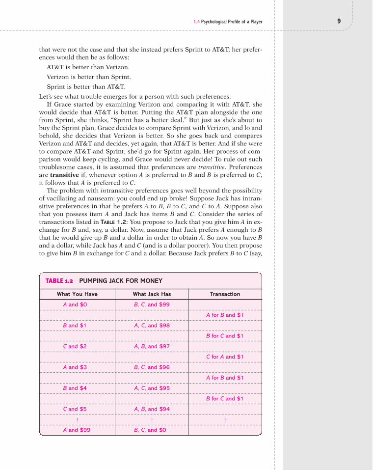
The problem with intransitive preferences goes well beyond the possibilityof vacillating ad nauseam: you could end up broke! Suppose Jack has intran-sitive preferences in that he prefers A to B, B to C, and C to A. Suppose alsothat you possess item A and Jack has items B and C. Consider the series oftransactions listed in TABLE 1.2: You propose to Jack that you give him A in ex-change for B and, say, a dollar. Now, assume that Jack prefers A enough to Bthat he would give up B and a dollar in order to obtain A. So now you have Band a dollar, while Jack has A and C (and is a dollar poorer). You then proposeto give him B in exchange for C and a dollar. Because Jack prefers B to C (say,
TABLE 1.2 PUMPING JACK FOR MONEY
What You Have What Jack Has Transaction
A and $0 B, C, and $99
A for B and $1
B and $1 A, C, and $98
B for C and $1
C and $2 A, B, and $97
C for A and $1
A and $3 B, C, and $96
A for B and $1
B and $4 A, C, and $95
B for C and $1
C and $5 A, B, and $94
! ! !
A and $99 B, C, and $0

10 CHAPTER 1: INTRODUCTION TO STRATEGIC REASONING
by more than a dollar), Jack will make the trade. Now you possess C and twodollars. The next step is to offer C in exchange for A and a dollar. Since Jackprefers A to C (say, by at least a dollar), he’ll make the trade. Now you have Aand three dollars, whereas if you recall, you started with A and no money.Trading with Jack is a money pump! It gets even better: you can continue toexecute this sequence of trades while accumulating three dollars in eachround. Eventually, you’ll have taken all of Jack’s money. Such is the sad life ofsomeone whose preferences are not transitive, so take this cautionary tale toheart and always have your preferences be transitive!
If a person’s preferences are complete and transitive, then there is a way inwhich to assign numbers to all of the feasible items—where the associatednumber is referred to as an item’s utility—so that a person’s preferences canbe represented as choosing the item that yields the highest utility. To be moreconcrete, suppose there are four cell phone providers available to Grace:AT&T, Verizon, Sprint, and T-Mobile. Her preferences are as follows:
AT&T is better than Verizon. Verizon is better than Sprint.
Sprint and T-Mobile are equally appealing.
This set of preferences implies the following ordering ofplans: AT&T is best, Verizon is second best, and Sprintand T-Mobile are tied for third best. The next step is to as-sign a utility to each of these choices so that choosing theplan with the highest utility is equivalent to choosing themost preferred plan. Such an assignment of utilities isshown in TABLE 1.3.
We can now describe Grace’s behavior by saying thatshe makes the choice which yields the highest utility. If allfour plans are available in her area, we know by her pref-
erences that she’ll choose AT&T. If we say that she chooses the plan with thehighest utility, it means that she chooses AT&T, because the utility of choos-ing AT&T is 10, which is higher than 6 from Verizon and 2 from either Sprintor T-Mobile. Now suppose that AT&T is unavailable in her area, so she canchoose only between Verizon, Sprint, and T-Mobile. Her preferences rankVerizon higher than the other two, so that is what she will buy. ChoosingVerizon is also what maximizes her utility—it delivers utility of 6—when shecan choose only between Verizon, Sprint, and T-Mobile.
To ensure that choosing the option with the highest utility is equivalent tochoosing the most preferred option, numbers need to be assigned so that theutility of option A is greater than the utility of option B if and only if A is pre-ferred to B and the utility of A is equal to that of B if and only if the individ-ual choosing is indifferent between A and B. Note that there is no unique wayto do that. Rather than assigning 10, 6, 2, and 2 to AT&T, Verizon, Sprint, andT-Mobile, respectively, it would have worked just as well to have used 14, 12,11, and 11 or 4, 3, 0, and 0. As long as the utility is higher for more preferreditems, we’ll be fine.
There is nothing deep about the concept of utility. The idea is that peopleare endowed with preferences which describe how they rank different alter-natives. If preferences are complete and transitive, then there is a way inwhich to assign a number to each alternative that allows a person’s behaviorto be described as making the choice with the highest utility. A list of options
TABLE 1.3 GRACE’S UTILITY FUNCTION
Cell Phone Provider Utility
AT&T 10
Verizon 6
Sprint 2
T-Mobile 2

1.4 Psychological Profile of a Player 11
and their associated utilities—such as Table 1.3—is known as a utility func-tion. A person’s utility function captures all of the relevant information aboutthe person’s preferences.
Writing down a person’s preferences begs the question of where they comefrom. Why does someone prefer rock and roll to opera? cats to dogs? stripesto solids? pizza to General Tso’s chicken? Preferences could be determined bygenes, culture, chemicals, personal experience, and who knows what else.Where preferences come from will not concern us. We’ll be content to takepreferences as given and explore what they imply about behavior.
1.4.2 BeliefsIn many situations, the utility received by a person depends not just on thechoices the person makes, but also on the choices of others. For example, manycell phone providers have designed their plans to create an interdependence be-tween the choices that people make. For most plans, the price charged perminute is lower if you are calling someone on the same network (i.e., someonewho has chosen the same provider) than if you are calling someone on anothernetwork. What this means is that the best provider for someone may well de-pend on the providers used by the people whom they call.
With this in mind, consider Grace’s deciding on a cell phone plan, knowingthat she spends most of her time calling her best friend Lisa. Although Gracereally likes AT&T (because then she can have an iPhone), it is most critical toher that she choose the same network as Lisa. A utility function consistentwith these preferences for Grace is shown in TABLE 1.4. Note that Grace’s mostpreferred provider is always the provider that Lisa chooses. If Lisa choosesSprint, then Sprint yields the highest utility for Grace. (Compare 6 fromSprint, 5 from AT&T, and 3 from Verizon.) If Lisa chooses Verizon, thenVerizon maximizes Grace’s utility. Given that Grace really likes AT&T, herhighest utility comes when both she and Lisa choose AT&T.
To make the best choice, Grace will need to form beliefs as to which planLisa will choose. This condition leads us to the second key personal attribute
TABLE 1.4 GRACE’S UTILITY FUNCTION WHEN IT DEPENDS ON LISA’S PROVIDER
Grace’s Provider Lisa’s Provider Grace’s Utility
AT&T AT&T 10
AT&T Verizon 5
AT&T Sprint 5
Verizon AT&T 3
Verizon Verizon 8
Verizon Sprint 3
Sprint AT&T 2
Sprint Verizon 2
Sprint Sprint 6

12 CHAPTER 1: INTRODUCTION TO STRATEGIC REASONING
that is relevant to game theory: a person’s capacity to form beliefs as to whatothers will do. While we’ll assume that people are endowed with preferences,such as those described in Table 1.4, they are not endowed with beliefs.Indeed, a major function of game theory is to derive reasonable beliefs re-garding what other players will do.
There are two processes from which these beliefs might emerge, one smartand one dumb. The dumb process is simply experience, which is referred toas experiential learning. By interacting again and again, a person comes toexpect—rightly or wrongly—that another person will do what he’s done in thepast. This process has great universality, as it can be practiced by small kidsand many species in the animal kingdom.
The smart process for forming beliefs is called simulated introspection.Introspection is the examination of one’s own thoughts and feelings, while insimulated introspection a person is simulating the introspective process ofsomeone else in order to figure out what that individual will do. Simulated in-trospection is the default method of belief derivation in this book, althoughsome of what we’ll say can be derived through experiential learning. Becausesimulated introspection is subtle and complex, let’s discuss what demands itputs on a person.
To have the capacity to simulate the reasoning of others, a person musthave self-awareness, which means being aware of your own existence. It isnot enough to think; a person must be capable of thinking about thinking.Thinking is, then not just a process, like digestion, but also a mental state. Ofcourse, thinking about how you think doesn’t necessarily get you closer to fig-uring out what someone else is thinking; we also need what psychologists calla theory-of-mind mechanism (ToMM). Possession of a ToMM means thatyou attribute thinking to others and attribute a ToMM to others, which meansthat you attribute to them the possibility of thinking about you thinking, justas you can think about them thinking. A ToMM is essential to strategizing andis what produces the endlessly slippery slope of infinite regress.
A ToMM is a fascinating capacity and is the basis for all that underlies thisbook. It has been argued that a ToMM is so useful for social animals that it isnatural to think of it as the product of evolution. Surviving and thriving in acommunity would surely have been enhanced by being able to predict whatothers would do.3 Given the advantage that a ToMM bestows, it is natural toask whether other primates possess it. Although indirect tests have been con-ducted on apes and chimpanzees, the evidence is mixed. Interestingly, somescientists believe that the absence of a ToMM is a feature of autism, in whichcase it is possible to be an intelligent human, yet lack a ToMM.
1.4.3 How Do Players Differ?Thus far, we’ve discussed how people are similar: they have well-defined prefer-ences, self-awareness, and a theory-of-mind mechanism. But how do theydiffer? Three forms of individual heterogeneity are especially relevant to gametheory. First, although each person is assumed to have complete and transitivepreferences, those preferences can vary across people. For instance, Grace mayprefer AT&T, while Lisa prefers Verizon. Tony may like the Red Sox and detestthe Yankees, while Johnny is just the opposite. Second, people can have differ-ent options and opportunities. For example, a wealthy bidder at an auction hasa different set of options than another bidder with lower net worth. Third, people

1.5 Playing the Gender Pronoun Game 13
can have different information. Thus, the bidder with less wealth may have abetter evaluation of the item being auctioned off than the wealthier bidder.
One last trait that deserves mention is skill, which is required both in figuringout what to do in a strategic encounter and in then executing a plan. Skill em-bodies many elements, including originality, cleverness, composure, and, asdescribed by Winston Churchill, that “element of legerdemain, an original andsinister touch, which leaves the enemy puzzled as well as beaten.”4 How skillfulare players presumed to be, and how much are they allowed to vary in their skill?
FIGURE 1.2 depicts a range of intellects drawn from fiction. Players aren’tpresumed to be brilliant like James Bond or Albert Einstein, nor are theygoing to be in the “dumb and dumber” category like Curly or Mr. Bean. We’renot out to explain how the Three Stooges would behave when faced with a nu-clear standoff. We will presume that players have at least a modicum of goodsense and guile and, overall, that they are intelligent.
Are people presumed to be logical like Mr. Spock from Star Trek, or can theydraw upon their emotions in decision making? While our analysis will be anexercise in logic, that does not preclude the possibility that people use emo-tions or “gut feelings” to arrive at a decision. In many cases, we will not be re-producing how people actually make decisions; rather, we will be describingwhat the end result of that process may be. A person may reach a decisionthrough cold logic or on the basis of emotions rooted in past experiences.5
The more intriguing issue is whether we allow for variation in the skill ofour players. Can we explore SpongeBob battling wits with Star Wars’ SenatorPalpatine? Or have Mr. Bean and Voldemort exercise their “gray matter” inconflict? Although it would be exciting to explore such possibilities, they willnot be considered here. A key assumption throughout this book is that peoplehave comparable levels of skill. The strategic moves considered will take place ona level playing field. Although a player may have an advantage because she hasmore options or better information, no player will be able to “outsmart” an-other. (In principle, game theory can handle such possibilities, but that line ofinquiry is largely undeveloped.)
1.5 Playing the Gender Pronoun GameBEFORE GOING ANY FURTHER in our quest to learn the logic of game theory, thereis a sociopolitical–legal issue that my publisher, priest, and barista haveurged me to raise with you: the use of gender pronouns. Any textbook that
FIGURE 1.2 A Range of Intellect
Dumb Smart
THE
KOBA
L CO
LLEC
TIO
N
© U
NIV
ERSA
L/CO
URTE
SYEV
ERET
T CO
LLEC
TIO
N
© S
ON
Y PI
CTU
RES/
COU
RTES
YEV
ERET
T CO
LLEC
TIO
N
© C
ORB
IS

14 CHAPTER 1: INTRODUCTION TO STRATEGIC REASONING
discusses people in the abstract—such as a book on game theory—must ex-plain how it intends to use gender pronouns and provide the rationale forthat usage. While this matter is typically discussed in a book’s preface, peo-ple don’t tend to read the preface (apparently, “preface” means “ignore” inlots of languages), and every reader needs to know where I stand on this con-tentious issue.
To the chagrin of “stupid white men”—as filmmaker Michael Moore de-scribes them—the people who live in this book are not all males. If they were,where would the next generation of players come from for my second edition?Yes, women do live in the abstract world of game theory and will live along-side men. But allowing cohabitation between the covers of this book stillleaves a decision of how to allocate men and women across our many exam-ples. I remember a scholarly piece on crime in which the male pronoun wasused to refer to criminals (because most criminals are men) while judges, ju-rors, attorneys, witnesses, and victims were female. (To be accurate, mostcriminals who are caught are men; perhaps women are better about gettingaway with it.) Such an approach is disturbing. Might not an impressionableboy be led to believe that he should turn to a life of crime because that is whatmales do? And should we really convey the impression to a girl that crime istoo risky for the female half of the species? Contrary to that approach, thisbook will allow both men and women to be deviants, sociopaths, and yourrun-of-the-mill perverts.
An alternative strategy is to deploy tactics utilized in the Gender PronounGame. This is the conversational game by which a person seeks to hide thegender of his partner. Instead of using “he” or “she” and “him” or “her”, oneeither avoids the use of pronouns or uses plural pronouns such as “they” and“them”. In the heterosexual world, a gay person might strive to avoid reveal-ing that her partner is of the same gender, and analogously, someone in thegay community (who is perhaps bisexual) might hide a heterosexual relation-ship. But these gender-neutral plural pronouns can become awkward (anddrive my editor crazy), which leads me to another strategy: invent somegender-neutral pronouns. There is no shortage of worthy attempts, including“shis”, “shim”, “shey”, “shem”, “sheir”, “hisorher”, “herorhis”, and—my per-sonal favorite—“h’orsh’it” (a colorful blend of “he”, “she”, and “it”).
After long hours of monklike contemplation with my subconscious in syncwith the Fox Network, I have decided to deal with this issue by mimicking reallife. Just as our species is made up of both men and women, so will the play-ers occupying the pages of this book. If there is a two-player game, then oneplayer will be male and the other female. More generally, I’ll just mix themup—a male here, a female there, a hermaphrodite when I’m getting bored.Admittedly, I have not counted their respective numbers to ensure an evengender balance. You the reader are welcome to do so, and once having beeninformed of your findings, I would be glad to replace an X chromosome witha Y or a Y with an X as is needed. In the meantime, I will do my best to begender neutral and avoid stepping in h’orsh’it.
REFERENCES1. John von Neumann and Oskar Morgenstern, Theory of Games and
Economic Behavior (Princeton: Princeton University Press, 1944), p. 6.

References 15
2. This discussion is based on Uri Zwick and Michael S. Patterson, TheMemory Game (Coventry, U.K.: Mathematics Institute, University ofWarwick, March 1991). It was reported in Ian Stewart, “MathematicalRecreations”, Scientific American, October 1991, pp. 126–28.
3. Nicholas Humphrey, The Inner Eye (Oxford, U.K.: Oxford University Press,2003).
4. Winston S. Churchill, The World Crisis (New York: Charles Scribner’s Sons,1923) vol II, p. 5.
5. On the role of emotions in social decision making, the interested reader isreferred to Antonio R. Damasio, Descartes’ Error: Emotion, Reason, and theHuman Brain (New York: Avon Books, 1994).

This page intentionally left blank

If the human mind was simple enough to understand, we’d be too simpleto understand it. —EMERSON PUGH
2.1 IntroductionTHEY SPEAK OF “DELIVERABLES” in the corporate world as the end product thatis—well, delivered to a customer. So for those who are trying to understandsocial phenomena—such as economists, political scientists, and nosy neigh-bors—or those trying to determine how to behave—such as policymakers,business owners, and teenagers—game theory has two deliverables. First, itprovides a framework for taking a complex social situation and boiling itdown to a model that is manageable. Second, it provides methods for extract-ing insights from that model regarding how people do behave or how theyshould behave. This chapter focuses on using game theory to model a strate-gic situation; the next chapter begins our journey solving such models.
Human behavior typically occurs in an environment that is highly complex,and this complexity poses a challenge in modeling social phenomena. Decidingon what to put in a model is like trying to pack for college: there’s just no wayto shove everything you want into that suitcase. In that light, it is useful to dis-tinguish between literal and metaphorical models. A literal model is a modelthat is descriptively accurate of the real-world setting it is intended to repre-sent. Other than for board games and a few other settings, a literal model of asocial situation would be a bloody mess. In contrast, a metaphorical model isa vast simplification—a simplified analogy—of the real-world situation; it isnot meant to be descriptively accurate. With a metaphorical model, we try tosimulate the real world in essential ways, not replicate it. The “essential” waysare those factors thought to be critical to the problem of interest. Factors thatare presumed to be secondary are willfully ignored. Most of the models in thisbook and most of the models constructed to understand social phenomena aremetaphorical. Done right, a metaphorical model can yield insights into humanbehavior that are applicable to much richer and more realistic situations.
Whether literal or metaphorical, game theory offers a scaffolding aroundwhich a model can be constructed, and in this chapter we review the two pri-mary types of scaffolding. The extensive form is a description of the sequenceof choices faced by those involved in a strategic situation, along with whatthey know when they choose. In Section 2.2, we consider extensive formgames of perfect information, in which a person always knows what has thusfar transpired in the game. Situations with imperfect information are de-scribed in Section 2.3, and these models allow a person to lack knowledgeabout what other people have chosen so far. The central concept of a strategy
2Building a Model of a Strategic Situation
17

is introduced in Section 2.3, and this concept provides the foundation for de-scribing the strategic form of a game in Section 2.4—the second type of scaf-folding. Though more abstract than the extensive form, the strategic form ismore concise and easier to work with. Common knowledge is a concept perti-nent to both methods of modeling a strategic situation and is covered inSection 2.5. Common knowledge deals with what a person knows about whatothers know.
Before we move forward, let me remind you that this chapter is aboutbuilding a game. Solving a game will begin with the next chapter, so be pre-pared for some delayed gratification.
2.2 Extensive Form Games: Perfect InformationIN SPITE OF ITS NAME, game theory can deal with some fairly dire subjects, oneof which is the criminal activity of kidnapping for ransom. This is a sufficientlyserious and persistent problem in some countries—such as Colombia, Mexico,and Russia—that companies have taken out insurance against their executivesbeing held for ransom. Building a model of kidnapping can involve factoringin a great many considerations. The focus of our task, however, is not so muchon gaining insight into kidnapping, but on learning how to construct a game-theoretic model.
Because the objective of game theory is to derive implications about be-havior, a model should focus on those individuals who have decisions to make.Our attention will accordingly be on the kidnapper, whom we’ll call Guy, andthe victim’s wife, Vivica, who has been contacted to pay ransom. Although thevictim (whom we’ll name Orlando) is surely affected by what transpires, weare presuming that the victim has no options. In describing the situation, ourmodel should address the following questions: When do Guy and Vivica get toact? What choices are available when they get to act? What do they know
when they get to act? More information willbe needed to derive predictions about behav-ior, but the information obtained by answer-ing these questions is sufficient for starters.
The model is represented by what isknown as a decision tree, such as thatshown in FIGURE 2.1. A decision tree is readfrom top to bottom. (It can also be depictedto be read from left to right.) Each of the dotsis called a decision node, which represents apoint in the game at which someone has adecision to make. Coming out of a decisionnode is a series of branches, where eachbranch represents a different action avail-able to the decision maker. Choosing abranch is equivalent to choosing an action.
At the top of the decision tree, Guy is tomake the initial decision, and his choices arekidnap (Orlando) and do not kidnap.* If he
18 CHAPTER 2: BUILDING A MODEL OF A STRATEGIC SITUATION
FIGURE 2.1 Extensive Form of the Kidnapping Game
Guy
Guy 3
Vivica 5 Pay ransom
Vivica
4
1
5
3
2
2
1
4
Do not kidnap
Do not pay ransom
Kidnap
Guy
Kill KillRelease Release
Guy
*The name of an action or strategy will typically be italicizedin this book.

2.2 Extensive Form Games: Perfect Information 19
chooses the latter, then the tree comes to an end, which represents “gameover.” If, instead, he chooses to kidnap Orlando, then Vivica is informed of thekidnapping and decides whether to pay the ransom. In response to Vivica’s de-cision, Guy decides whether to release Orlando or kill him. The assumption isthat Guy observes whether ransom is paid prior to making this choice. (Howto handle a simultaneous exchange will be discussed later in the chapter.)
There is a total of five outcomes to this game, each of which corresponds toa path through the decision tree or, equivalently, a sequence of actions. Theseoutcomes are listed in TABLE 2.1. One outcome is for there not to be a kidnap-ping. If there is a kidnapping, there are four possible outcomes, depending onwhether ransom is paid and whether Orlando is killed or released.
TABLE 2.1 KIDNAPPING GAME AND PAYOFFS
Outcome Guy (Violent) Guy Vivica
No kidnapping 3 3 5
Kidnapping, ransom is paid, Orlando is killed 4 5 1
Kidnapping, ransom is paid, Orlando is released 5 4 3
Kidnapping, ransom is not paid, Orlando is killed 2 2 2
Kidnapping, ransom is not paid, Orlando is released 1 1 4
The objective of our model is to make some predictions about how Guyand Vivica will behave. Although solving a game won’t be tackled until thenext chapter, in fact we don’t have enough information to solve it even if weknew how. To describe how someone will behave, it’s not enough to knowwhat they can do (e.g., kill or release) and what they know (e.g., whether ran-som has been paid); we also need to know what these people care about.What floats their boat? What rings their bell? What tickles their fancy? Youget the idea.
A description of what a player cares about takes the form of a ranking ofthe five outcomes of the game. Suppose Guy is someone who really just wantsthe money and kills only out of revenge for the ransom not being paid. ThenGuy’s best outcome is to perform the kidnapping, Vivica pays the ransom, andhe releases Orlando. Because we assume that he is willing to kill in exchangefor money, his second-best outcome is to perform the kidnapping, have theransom paid, and kill Orlando. The third-best outcome is not to kidnapOrlando, since Guy prefers not to run the risk of kidnapping when ransom isnot to be paid. Of the two remaining outcomes, suppose that if he kidnapsOrlando and ransom is not paid, then he prefers to kill Orlando (presumablyout of spite for not receiving the ransom). The least preferred outcome is thenthat there is a kidnapping, ransom is not paid, and Orlando is released.
To concisely include Guy’s preferences in our description of the game, we’llassign a number to each outcome, with a higher number indicating a morepreferred outcome for a player. This ranking is done in Table 2.1 under the col-umn labeled “Guy.” These numbers are referred to as payoffs and are in-tended to measure the well-being (or utility, or welfare, or happiness index) ofa player. For example, the highest payoff, 5, is assigned to the best outcome:the kidnapping takes place, ransom is paid, and Orlando is released. The worst

20 CHAPTER 2: BUILDING A MODEL OF A STRATEGIC SITUATION
outcome—the kidnapping takes place, ransom is not paid, and Orlando is re-leased—receives the lowest payoff, 1.
Suppose, contrary to what was just assumed, that Guy felt that his chancesof getting caught would be less if Orlando were dead, so that he now alwaysprefers killing Orlando to releasing him. Then Guy’s payoffs would be asshown in the column “(Violent) Guy.” The highest payoff is now assigned tothe outcome in which Guy kidnaps and kills Orlando and the ransom is paid.
What about Vivica? If she cares about Orlando more than she cares aboutmoney, then her most preferred outcome is no kidnapping, and we’ll assignthat the highest payoff of 5. Her least preferred outcome is that Orlando is kid-napped and killed and ransom is paid, so it receives the lowest payoff of 1. Thepayoffs for the other outcomes are shown in the table.
To ensure that the depiction in Figure 2.1 contains all of the relevant infor-mation, the payoffs have been included. Each terminal node corresponds to aparticular outcome of the game, and listed below a terminal node are the pay-offs that Guy and Vivica assign to that outcome; the top number is Guy’s pay-off and the bottom number is Vivica’s payoff. While we could also listOrlando’s payoffs—he is surely not indifferent about what happens—thatwould be extraneous information. Because our objective is to say somethingabout behavior, and this model of kidnapping allows only the kidnapper andthe victim’s kin to act, only their payoffs matter.
This step of assigning a payoff to an outcome is analogous to what wasdone in Chapter 1. There we began with a person’s preferences for certainitems (in our example, it was cell phone providers), and we summarized thosepreferences by assigning a number—known as utility—to each item. A per-son’s preferences were summarized by the resulting utility function, and herbehavior was described as making the choice that yielded the highest utility.We’re performing the same step here, although game theory calls the numbera payoff; still, it should be thought of as the same as utility.
The scenario depicted in Figure 2.1 is an example of an extensive formgame. An extensive form game is depicted as a decision tree with decisionnodes, branches, and terminal nodes. A decision node is a location in the treeat which one of the players has to act. Let us think about all of the informa-tion embodied in Figure 2.1. It tells us which players are making decisions(Guy and Vivica), the sequence in which they act (first Guy then, possibly,Vivica, and then Guy again), what choices are available to each player, andhow they evaluate the various outcomes of the game. This extensive formgame has four decision nodes: the initial node at which Guy decides whetherto kidnap Orlando, the decision node at which Vivica decides whether to payransom, and Guy’s two decision nodes concerning whether to kill or releaseOrlando (one decision node for when Vivica pays ransom and one for whenshe does not). Extending out of each decision node are branches, where abranch represents an action available to the player who is to act at that deci-sion node. More branches mean more choices.
We refer to the decision node at the top of the tree as the initial node (thatis where the game starts) and to a node corresponding to an end to the gameas a terminal node (which we have not bothered to represent as a dot in thefigure). There are five terminal nodes in this game, since there are five possi-ble outcomes. Terminal nodes are distinct from decision nodes, as no playeracts at a terminal node. It is at a terminal node that we list players’ payoffs,

2.2 Extensive Form Games: Perfect Information 21
Orioles' manager
Yankees' manager
MR
1
3
3
1
2 Orioles' manager
2 Yankees' manager
JG
RJ
JL
where a payoff describes how a player evaluates an outcome of the game, witha higher number indicating that the player is better off.
! SITUATION: BASEBALL, I
Good pitching will always stop good hitting and vice-versa. —CASEY STENGEL
One of the well-known facts in baseball is that right-handedbatters generally perform better against left-handed pitch-ers and left-handed batters generally perform betteragainst right-handed pitchers. TABLE 2.2 documents thisclaim.1 If you’re not familiar with baseball, batting averageis the percentage of official at bats for which a batter getsa hit (in other words, a batter’s success rate). Right-handedbatters got a hit in 25.5% of their attempts against a right-handed pitcher, or, as it is normally stated in baseball, theirbatting average was .255. However, against left-handedpitchers, their batting average was significantly higher, namely,.274. There is an analogous pattern for left-handed batters, who hit .266 againstleft-handed pitchers but an impressive .291 against right-handed pitching. Let’sexplore the role that this simple fact plays in a commonly occurring strategicsituation in baseball.
It is the bottom of the ninth inning and the game is tied between the Oriolesand the Yankees. The pitcher on the mound for the Yankees is Mariano Rivera,who is a right-hander, and the batter due up for the Orioles is Javy Lopez, whois also a right-hander. The Orioles’ manager is thinking about whether to sub-stitute Jay Gibbons, who is a left-handed batter, for Lopez. He would prefer tohave Gibbons face Rivera in order to have a lefty–righty matchup and thus abetter chance of getting a hit. However, the Yankees’ manager could respondto Gibbons pinch-hitting by substituting the left-handed pitcher RandyJohnson for Rivera. The Orioles’ manager would rather have Lopez faceRivera than have Gibbons face Johnson. Of course, the Yankees’ manager hasthe exact opposite preferences.
The extensive form of this situation isshown in FIGURE 2.2. The Orioles’ managermoves first by deciding whether to substituteGibbons for Lopez. If he does make the substi-tution, then the Yankees’ manager decideswhether to substitute Johnson for Rivera.Encompassing these preferences, the Orioles’manager assigns the highest payoff (which is3) to when Gibbons bats against Rivera andthe lowest payoff (1) to when Gibbons batsagainst Johnson. Because each manager ispresumed to care only about winning, whatmakes the Orioles better off must make theYankees worse off. Thus, the best outcome forthe Yankees’ manager is when Gibbons batsagainst Johnson, and the worst is whenGibbons bats against Rivera.
TABLE 2.2
Batter Pitcher Batting Average
Right Right .255
Right Left .274
Left Right .291
Left Left .266
FIGURE 2.2 Baseball

22 CHAPTER 2: BUILDING A MODEL OF A STRATEGIC SITUATION
! SITUATION: GALILEO GALILEI AND THE INQUISITION, I
In 1633, the great astronomer and scientist Galileo Galilei was under consid-eration for interrogation by the Inquisition. The Catholic Church contendsthat in 1616 Galileo was ordered not to teach and support the Copernicantheory, which is that the earth revolves around the sun, and furthermore thathe violated this order with his latest book, The Dialogue Concerning the TwoChief World Systems. The situation to be modeled is the decision of theCatholic Church regarding whether to bring Galileo before the Inquisitionand, if it does so, the decisions of Galileo and the Inquisitor regarding whatto say and do.
The players are Pope Urban VIII, Galileo, and the Inquisitor. (Althoughthere was actually a committee of Inquisitors, we’ll roll them all into oneplayer.) The extensive form game is depicted in FIGURE 2.3. Urban VIII ini-tially decides whether to refer Galileo’s case to the Inquisition. If he declinesto do so, then the game is over. If he does refer the case, then Galileo isbrought before the Inquisition, at which time he must decide whether to con-fess that he did indeed support the Copernican case too strongly in his recentbook. If he confesses, then he is punished and the game is over. If he does notconfess, then the Inquisitor decides whether to torture Galileo. If he chooses
FIGURE 2.3 Galileo Galilei and the Inquisition
Urban VIII
Urban VIII 3
Galileo 5
Inquisitor 3
Galileo
Galileo
Do not confess
Do not confess
Do not torture
Confess
Confess
Inquisitor5
3
4
2
4
2
4
1
5
1
2
1
Do not refer
Refer
Torture

2.2 Extensive Form Games: Perfect Information 23
To complete the extensive form game, payoff numbers are required. Thereare five outcomes to the game: (1) Urban VIII does not refer the case; (2)Urban VIII refers the case and Galileo initially confesses; (3) Urban VIII refersthe case, Galileo does not initially confess, he is tortured, and then he con-fesses; (4) Urban VIII refers the case, Galileo does not initially confess, he istortured, and he does not confess; and (5) Urban VIII refers the case, Galileodoes not initially confess, and he is not tortured.
In specifying payoffs, we don’t want arbitrary numbers, but rather onesthat accurately reflect the preferences of Urban VIII, Galileo, and theInquisitor. Galileo is probably the easiest. His most preferred outcome is thatUrban VIII does not refer the case. We’ll presume that if the case is referred,then Galileo’s preference ordering is as follows: (1) He does not confess andis not tortured; (2) he confesses; (3) he does not confess, is tortured, and doesnot confess; and (4) he does not confess, is tortured, and confesses. Galileowas a 69-year-old man, and evidence suggests that he was not prepared to betortured for the sake of principle. Urban VIII is a bit more complicated, be-cause although he wants Galileo to confess, he does not relish the idea of thisgreat man being tortured. We’ll presume that Urban VIII most desires a con-fession (preferably without torture) and prefers not to refer the case if it doesnot bring a confession. The Inquisitor’s preferences are similar to those ofUrban VIII, but he has the sadistic twist that he prefers to extract confessionsthrough torture.
So, what happened to Galileo? Let’s wait until we learn how to solve such agame; once having solved it, I’ll fill you in on a bit of history.
not to torture him, then, in a sense, Galileo has won, and we’ll consider thegame ended. If the Inquisitor tortures poor Galileo, then he must decidewhether to confess.
Galileo before the Inquisitor
HU
LTO
N A
RCH
IVE/
GET
TY IM
AG
ES

24 CHAPTER 2: BUILDING A MODEL OF A STRATEGIC SITUATION
! SITUATION: HAGGLING AT AN AUTO DEALERSHIP, I
Donna shows up at her local Lexus dealership looking to buy a car. Cominginto the showroom and sauntering around a taupe sedan, a salesperson,Marcus, appears beside her. After chatting a bit, he leads the way to his cu-bicle to negotiate. To simplify the modeling of the negotiation process, sup-pose the car can be sold for three possible prices, denoted pL, pM, and pH,and suppose pH > pM > pL. (H is for “high,” M is for “moderate,” and L is for“low.”)
The extensive form game is depicted in FIGURE 2.4. Marcus initially decideswhich of these three prices to offer Donna. In response, Donna can either ac-cept the offer—in which case the transaction is made at that price—or reject it.If it is rejected, Donna can either get up and leave the dealership (thereby end-ing the negotiations) or make a counteroffer. In the latter case, Donna can re-spond with a higher price, but that doesn’t make much sense, so it is assumed
Accept Reject A R
A R A R A R
A R
A R
Leave
DonnaDonna Donna
Donna
Donna
Donna
Marcus
Marcus
Donna
0
Marcus Marcus Marcus
Marcus0
0
0
0
0
0
0
0 0
2(pM " pL)
0
0 0
2(pM " pL)
0
00
2(pM " pL)
2(pH " pL)
pM " pL
0
pM " pL pM " pL
0
pM " pH
pL pM
pLLeavepL pM
pM
pH
FIGURE 2.4 Haggling at an Auto Dealership

2.2 Extensive Form Games: Perfect Information 25
that she selects among those prices which are lower than what she was ini-tially offered (and turned down). For example, if Marcus offers a price of pH,then Donna can respond by asking for a price of either pM or pL. If Donna hasdecided to counteroffer, then Marcus can either accept or reject her counterof-fer. If he rejects it, then he can counteroffer with a higher price (though it mustbe lower than his initial offer). This haggling continues until either Donnaleaves, or an offer is accepted by either Donna or Marcus, or they run out ofprices to offer.
In terms of payoffs, assume that both Marcus and Donna get a zero payoffif the game ends with no sale. (There is nothing special about zero, by the way.What is important is its relationship to the other payoffs.) If there is a trans-action, Marcus’s payoff is assumed to be higher when the sale price is higher,while Donna’s payoff is assumed to be lower. More specifically, in the event ofa sale at a price p, Donna is assumed to receive a payoff of pM " p and Marcusgets a payoff of 2(p " pL). (Why multiply by 2? For no particular reason.)
Think about what this is saying. If Marcus sells the car for a price of pL,then his payoff is zero because 2(pL " pL) # 0. He is then indifferent betweenselling it for a price of pL and not selling the car. At a price of pM, his payoffis positive, which means that he’s better off selling it at that price than notselling it; and his payoff is yet higher when he sells it for pH. For Donna, sheis indifferent between buying the car at a price of pM, and not buying it,since both give the same payoff (of zero). She prefers to buy the car at aprice of pL, as that price gives her a payoff of pM " pL > 0; she is worse off(relative to not buying the car) when she buys it at a price of pH, since thatgives her a payoff of pM " pH < 0. (Yes, payoffs can be negative. Once again,what is important is the ordering of the payoffs.) These payoffs are shown inFigure 2.4.
To be clear about how to interpret this extensive form game, consider whatcan happen when Marcus initially offers a price of pH. Donna can eitheraccept—in which case Marcus gets a payoff of 2(pH " pL) and Donna gets apayoff of pM " pH—or reject. With the latter, she can leave or counteroffer witheither pL or pM. (Recall that we are allowing her to counteroffer only with aprice that is lower than what she has been offered.) If Donna chooses thecounteroffer of pL, then Marcus can accept—resulting in payoffs of zero forMarcus and pM " pL for Donna—or reject, in which case Marcus has only oneoption, which is to counteroffer with pM, in response to which Donna can ei-ther accept or reject (after which there is nothing left to do). If she insteadchooses the counteroffer pM, then Marcus can accept or reject it. If he rejects,he has no counteroffer and the game ends.
It is worth noting that this extensive form game can be represented alter-natively by FIGURE 2.5. Rather than have the same player move twice in a row,the two decision nodes are combined into one decision node with all of theavailable options. For example, in Figure 2.4, Donna chooses between acceptand reject in response to an initial offer of pM from Marcus, and then, if shechooses reject, she makes another decision about whether to counteroffer withpL or leave. Alternatively, we can think about Donna having three options(branches) when Marcus makes an initial offer of pM: (1) accept; (2) reject andcounteroffer with pL; and (3) reject and leave. Figure 2.5 is a representationequivalent to that in Figure 2.4 in the sense that when we end up solving thesegames, the same answer will emerge.

26 CHAPTER 2: BUILDING A MODEL OF A STRATEGIC SITUATION
FIGURE 2.5 Simplifying the Extensive Form of the Haggling Game
Accept Reject
A Leave
A
A
R
DonnaDonna Donna
A R
Marcus
Marcus
Donna
0
Marcus Marcus Marcus0
0
0
0pM " pH
0
0
A R
Donna
pM " pL
pL pM
pM
pL A LeavepL pM
pH
0
2(pM " pL) 2(pH " pL)
0
00
00
0pM " pL
0
pM " pL
2(pM " pL)
0
00
2(pM " pL)
Consider a two-player game in which a father chooses between actions yes, no, andmaybe. His daughter moves second and chooses between stay home and go to the mall.The payoffs are as follows:
Outcome Father’s Payoff Daughter’s Payoff
yes and stay home 8 3
yes and go to the mall 5 9
no and stay home 4 1
no and go to the mall 1 5
maybe and stay home 7 2
maybe and go to the mall 2 7
2.1 CHECK YOUR UNDERSTANDING*
Write down the extensive form game for this strategic situation.
*All answers to Check Your Understanding are in the back of the book.

2.3 Extensive Form Games: Imperfect Information 27
2.3 Extensive Form Games: Imperfect InformationRETURNING TO THE KIDNAPPING SCENARIO, suppose we want to model Guy (the kid-napper) and Vivica (the victim’s kin) as making their decisions without knowl-edge of what the other has done. The extensive form game in Figure 2.1 as-sumes that Guy learns whether ransom has been paid prior to deciding whatto do with Orlando (the victim). An alternative specification is that Guy de-cides what to do with Orlando at the same time that Vivica decides about theransom. You could imagine Guy deciding whether to release Orlando some-where in the city while Vivica is deciding whether to leave the ransom at anagreed-upon location. How do you set up an extensive form game with thatfeature?
The essential difference between these scenarios is information. InFigure 2.1, Guy knew what Vivica had done when it was time for him tomake his decision, whereas Vivica did not know what was to happen toOrlando when she had to decide about paying the ransom. Vivica’s lack ofknowledge was represented by having Vivica move before Guy. Now wewant to suppose that at the time he has to decide about killing or releasingOrlando, Guy is also lacking knowledge about what Vivica is to do or hasdone. Well, we can’t make a decision tree in which Vivica moves after Guyand Guy moves after Vivica.
To be able to represent such a situation, the concept of an information setwas created. An information set is made up of all of the decision nodes thata player is incapable of distinguishing among. Every decision node belongsto one and only one information set. A player is assumed to know which in-formation set he is at, but nothing more. Thus, if the information set hasmore than one node, then the player is un-certain as to where exactly he is in the game.All this should be clearer with an example.
FIGURE 2.6 is a reformulation of the Kid-napping game with the new assumption thatGuy doesn’t get to learn whether Vivica haspaid the ransom when he decides what to dowith Orlando. In terms of nodes andbranches, the trees in Figures 2.1 and 2.6 areidentical. The distinctive element is the boxdrawn around the two decision nodes associ-ated with Guy choosing whether to release orkill Orlando (which are denoted III and IV).The nodes in that box make up Guy’s infor-mation set at the time he has to decide whatto do with Orlando. Guy is assumed to knowthat the game is at either node III or node IV,but that’s it; he doesn’t know which of thetwo it is. Think about what this means. Notto know whether the game is at node III ornode IV means that Guy doesn’t knowwhether the sequence of play has been “kid-nap and ransom is paid” or “kidnap and ran-som is not paid.” Well, this is exactly what wewanted to model; Guy doesn’t know whether
FIGURE 2.6 Kidnapping Game When the ExchangeIs Simultaneous. The Box Around NodesIII and IV Represents the Information Setat the Point That Guy Has to DecideWhat to Do with Orlando
Guy
II
I II I
I I II I I IVIV
Guy 3
Vivica 5 Pay ransom
Vivica
4
1
5
3
2
2
1
4
Do not kidnap
Do not pay ransom
Kidnap
Guy
Kill KillRelease Release

28 CHAPTER 2: BUILDING A MODEL OF A STRATEGIC SITUATION
the ransom is to be paid when he must decide whether to release or killOrlando. The way this situation is represented is that Guy doesn’t know ex-actly where he is in the game: Is he at node III or node IV?
In any extensive form game, a player who is to act always has an informa-tion set representing what he knows. So what about when Vivica moves? Whatis her information set? It is just node II; in other words, she knows exactlywhere she is in the game. If we want to be consistent, we would then put a boxaround node II to represent Vivica’s information set. So as to avoid unneces-sary cluster, however, singleton information sets (i.e., an information set witha single node) are left unboxed. In Figure 2.6, then, Guy has two informationsets; one is the singleton composed of the initial node (denoted I), and theother comprises nodes III and IV.
Returning to Vivica, since she is modeled as moving before Guy decidesabout Orlando, she makes her decision without knowing what has hap-pened or will happen to Orlando. Do you notice how I’m unclear about thetiming? Does Vivica move chronologically before, after, or at the same timeas Guy? I’ve been intentionally unclear because it doesn’t matter. What mat-ters is information, not the time of day at which someone makes a decision.What is essential is that Vivica does not know whether Guy has released orkilled Orlando when she decides whether to pay ransom and that Guy doesnot know whether Vivica has paid the ransom when he decides whether torelease or kill Orlando. In fact, FIGURE 2.7 is an extensive form game equiv-alent to that in Figure 2.6. It flips the order of decision making betweenVivica and Guy, and the reason it is equivalent is that we haven’t changedthe information that the players have when they move. In both games, we’llsay that Vivica and Guy move simultaneously (with respect to the ransomand release-or-kill decisions), which is meant to convey the fact that their
FIGURE 2.7 Extensive Form Equivalent to Figure 2.6
Guy
Guy 3
Vivica 5Kill
Guy
4
1
2
2
5
3
1
4
Do not kidnap
Release
Kidnap
Vivica
Pay ransom
Do not pay ransom
Pay ransom
Do not pay ransom

2.3 Extensive Form Games: Imperfect Information 29
information is the same as when they make their decisions at the exactsame time.
An extensive form game in which all information sets are singletons—such as the games in Figures 2.1–2.5—is referred to as a game of perfectinformation, since players always know where they are in the game whenthey must decide. A game in which one or more information sets are notsingletons, such as the game in Figure 2.6, is known as a game of imper-fect information.
! SITUATION: MUGGING
Notorious for being cheap, the comedian Jack Benny would tell the fol-lowing story: “I was walking down a dark alleyway when someone camefrom behind me and said, ‘Your money or your life.’ I stood there frozen.The mugger said again, ‘Your money or your life.’ I replied, ‘I’m thinking, . . .I’m thinking.’”
Simon is walking home late at night when suddenly he realizes that there issomeone behind him. Before he has a chance to do anything, he hears, “I havea gun, so keep your mouth shut and give me your wallet, cell phone, andiPod.” Simon doesn’t see a gun, but does notice that the mugger has his handin his coat pocket, and it looks like there may be a gun in there. If there is nogun, Simon thinks he could give the mugger a hard shove and make a run forit. But if there is a gun, there is a chance that trying to escape will result inhim being shot. He would prefer to hand over his wallet, cell phone, and evenhis iPod than risk serious injury. Earlier that evening, the mugger was engag-ing in his own decision making as he debated whether to use a gun. Becausethe prison sentence is longer when a crime involves a gun, he’d really like toconduct the theft without it.
The mugging situation just described is depicted as the extensive formgame in FIGURE 2.8. The mugger moves first in deciding between three options:not to use a gun; bring a gun, but not show it to the victim; and bring a gun
FIGURE 2.8 Mugging
Mugger
Mugger
Simon
3
2
5
4
2
6
6
3
Gun & show Gun &
hide
No gun
SimonSimon
Resist Do not resist Resist Do not
resist
3
2
4
5
Resist Do not resist

30 CHAPTER 2: BUILDING A MODEL OF A STRATEGIC SITUATION
and show it to the victim. In response to each of these actions, Simon has todecide whether to resist the mugger by doing the “shove and run” (resist) orby complying with the mugger’s instructions (do not resist). Simon has two in-formation sets. One is a singleton and is associated with the mugger’s havingand showing a gun. The other information set comprises two nodes, one cor-responding to the mugger’s having a gun, but not showing it, and the other tothe mugger’s not having a gun. With the latter information set, Simon isn’tsure whether the mugger’s pocket contains a gun.
In specifying the payoffs, the best outcome for Simon is that the muggerdoes not use a gun and Simon resists; the worst outcome is that the muggerhas a gun and Simon resists. For the mugger, the best outcome is that Simondoes not resist and the mugger doesn’t use a gun in the robbery. The worst out-come is that he doesn’t use the gun and Simon resists, as then the muggercomes away empty handed.
! SITUATION: U.S. COURT OF APPEALS FOR THE FEDERAL CIRCUIT
When the U.S. Court of Appeals for the Federal Circuit hears a case, apanel of 3 judges is randomly selected from the 12 judges on the court.After a case is filed, the parties submit written briefs stating their argu-ment. If the court decides to hear oral arguments, each party’s lawyer isgiven between 15 and 30 minutes. The panel of 3 judges then decides thecase. Let us model a simplified version of this judicial setting when thereis no oral argument.
One side of the case is represented by attorney Elizabeth Hasenpfeffer,while attorney Joseph Fargullio represents the other party. Prior to their ap-pearance, each attorney decides on a legal strategy and writes a brief based onit. For Ms. Hasenpfeffer, let us denote the strategies as A and B; for Mr. Fargullio,they’ll be denoted I and II. The briefs are submitted simultaneously, in thesense that each attorney writes a brief not knowing what the other has writ-ten. This situation is reflected in FIGURE 2.9, in which Ms. Hasenpfeffer movesfirst and Mr. Fargullio moves second, but with an information set that en-compasses both the node in which Ms. Hasenpfeffer chose A and the one inwhich she chose B.
After reading the two briefs, the three members of the court then vote eitherin favor of Ms. Hasenpfeffer’s argument or in favor of Mr. Fargullio’s argu-ment. This vote is cast simultaneously in that each judge writes down a deci-sion on a piece of paper. For brevity, the judges are denoted X, Y, and Z. Asdepicted, each judge has four information sets, where an information set cor-responds to the pair of legal strategies selected by the attorneys. Judge Xmoves first and thus doesn’t know how judges Y and Z have voted. Judge Ymoves second and thus doesn’t know how Judge Z has voted (since Z is de-scribed as moving after him), but she also doesn’t know how Judge X hasvoted because of the structure of the information sets. Each of Judge Y’s in-formation sets includes two decision nodes: one for Judge X voting in favor ofMs. Hasenpfeffer and one for Judge X in favor of Mr. Fargullio. Turning toJudge Z, we see that each of her information sets comprises the four nodesthat correspond to the four possible ways that Judges X and Y could have

FIGURE 2.9 U.S. Court of Appeals
EH
JF
X
Y
Z
1
0
2
2
2
1
0
2
2
1
H F
1
0
2
1
2
0
1
2
1
1
H F
1
0
1
2
2
0
1
1
2
1
H
Z
F
0
1
1
1
2
0
1
1
1
1
H F
H F
Y
X
H F
H F
JF
EH
I I II I
A B
I I II I
1
0
1
1
1
1
0
1
1
2
H F
1
0
1
2
1
0
1
1
2
2
H F
1
0
2
1
1
0
1
2
1
2
H
Z
F
0
1
2
2
1
0
1
2
2
2
H F
H F
Y
X
H F
H F
1
0
1
1
1
1
0
1
1
2
H F
1
0
1
2
1
0
1
1
2
2
H F
1
0
2
1
1
0
1
2
1
2
H
Z
F
0
1
2
2
1
0
1
2
2
2
H F
H F
Y
X
H F
H F
1
0
2
2
2
1
0
2
2
1
H F
1
0
2
1
2
0
1
2
1
1
H F
1
0
1
2
2
0
1
1
2
1
H
Z
F
0
1
1
1
2
0
1
1
1
1
H F
H F
Y
X
H F
H F
31

32 CHAPTER 2: BUILDING A MODEL OF A STRATEGIC SITUATION
voted. Although the judges are depicted as moving sequentially, in fact eachvotes without knowledge of how the other two have voted; in other words, thejudges vote simultaneously.
! SITUATION: THE IRAQ WAR AND WEAPONS OF MASS DESTRUCTION
Now let’s take on some recent history: the situation faced by Iraq, the UnitedNations, and the United States that culminated in the U.S. invasion of Iraqon March 20, 2003. At issue is whether Sadaam Hussein has weapons ofmass destruction (WMD). As shown in FIGURE 2.10, Iraq is modeled as hav-ing a choice of possessing or not possessing WMD. Without knowledge ofIraq’s choice, the United Nations decides whether to request inspections ofIraq. The United Nations then has one information set, which includes bothof Iraq’s feasible actions: the one when it has WMD and the other when itdoes not. If the United Nations chooses not to request inspections, then theUnited States decides whether or not to invade Iraq, at which point we’llconsider the game done. If the United Nations does request inspections, thenthe move goes back to Iraq. If Iraq does not have WMD, then it can chooseto deny inspections or allow them. If, instead, Iraq has WMD, then it candeny inspections, allow inspections, or allow inspections and hide the WMD.With the last option, suppose Iraq succeeds in preventing inspectors fromfinding WMD. Assume that when Iraq does have WMD and does not hidethem from the inspectors, the WMD are found. After Iraq moves in responseto the request for inspections by the United Nations, and the outcome of theinspections is revealed, the United States moves again regarding whether toattack Iraq.
The United States has four information sets. The information set de-noted I includes the two nodes associated with (1) Iraq having WMD andthe United Nations not choosing inspections, and (2) Iraq not having WMDand the United Nations not choosing inspections. Although the UnitedStates doesn’t get to observe Iraq’s choice, it does get to observe the UN de-
cision. Information set II corresponds to the scenario inwhich inspections are requested by the United Nationsand allowed by Iraq, but WMD are not found, either be-cause Iraq does not have them or because it does havethem but has successfully hidden them from the in-spectors. Information set III denotes the situation inwhich the United Nations requests inspections, butthey are refused by Iraq; once again, the United Statesdoesn’t know whether Iraq has WMD. The lone single-ton information set for the United States is node IV,
which is associated with Iraq’s having WMD, the United Nation’s having re-quested inspections, and Iraq’s having allowing unobstructed inspections,in which case WMD are found. A similar exercise can be conducted todescribe the one information set of the United Nations and the three in-formation sets of Iraq (all of which are singletons, as Iraq is the only onehiding something).
Now let us return to the Mugging game andsuppose that the mugger not only chooseswhether to use a gun and whether to show it,but also whether to load the gun with bullets. IfSimon sees the gun, he doesn’t know whether itis loaded. Write down the extensive form of thisstrategic situation. (You can ignore payoffs.)
2.2 CHECK YOUR UNDERSTANDING

FIGURE 2.10 Iraq War and WMD. The Abbreviations W and NW Represent War and No War, Respectively
II
I II I
IVIVI I II I I
Iraq
Iraq Iraq
Iraq
UN
UN
1
10
11
11
14 5US
US
War No warNo war
2
6
10
13
13 6
War No war No warDeny
NO WMD WMD
Allow
Inspect InspectDo not inspect
Do not inspect
Deny AllowAllow & hide
7
1
12
7
9 1
War
3
5
9
14
12 7
War
5
2
13
8
8 2
W NW
6
3
14
9
10 3
W NW
4
4
8
12
4 11
W NW
US
US
US
33

34 CHAPTER 2: BUILDING A MODEL OF A STRATEGIC SITUATION
2.4 What Is a Strategy?Victorious warriors win first and then go to war, while defeated warriorsgo to war first and then seek to win. —SUN TZU2
WHAT DO YOU THINK the preceding quote from Sun Tzu means? One interpreta-tion is that, to be victorious, you should develop a detailed plan prior to goingto battle and then, once in battle, execute that plan. Rather than trying to fig-ure out a plan over the course of the battle, perform all of your thinking be-fore one arrow is flung or one cannon is fired.
The notion of a strategy is central to game theory, and its definition is ex-actly what Sun Tzu had in mind. A strategy is a fully specified decision rulefor how to play a game. It is so detailed and well specified that it accounts forevery contingency. It is not a sequence of actions, but rather a catalog of con-tingency plans: what to do, depending on the situation. As was well expressedby J. D. Williams in an early book on game theory, a strategy is “a plan so com-plete that it cannot be upset by enemy action or Nature; for everything that theenemy or Nature may choose to do, together with a set of possible actions foryourself, is just part of a description of the strategy.”3
As a conceptual device, we imagine a player choosing a strategy before thegame begins. This strategy could, in principle, be written down as a set of in-structions and given to another person to play. In other words, having a strat-egy means doing all of the hard thinking (utilizing intelligence, judgment,cleverness, etc.) prior to playing the game. The actual play is nothing morethan following the instructions provided by the strategy selected. Of course,this description of a strategy is an abstraction, since, in practice, surely judg-ment and acumen are applied in the midst of a strategic situation. However,you’ll need to accept this definition of strategy if you are to make headway intogaining insight into strategic situations. It is one of those basic postulates thatis valuable in practice because of its purity in form.
To be more concrete as to the nature of a strategy in game theory, let us re-turn to the Kidnapping game in Figure 2.1. What is a strategy for the kidnap-per? As we’ve just said, a strategy is a complete decision rule—one that pre-scribes an action for every situation that a player can find himself in. Guy (thekidnapper) can find himself in three situations: (1) contemplating whether tokidnap Orlando (i.e., the initial node); (2) having kidnapped Orlando, with ran-som having been paid by Vivica, and deciding whether to kill or releaseOrlando; and (3) having kidnapped Orlando, with ransom not having been paidby Vivica, and deciding whether to kill or release Orlando. It is not coinciden-tal that Guy can find himself in three scenarios and he has three informationsets: A “situation” for a player is defined as finding himself at an informationset; hence, a strategy assigns one action to each of a player’s information sets.
A template for Guy’s strategy is, then,
At the initial node, _____ [ fill in kidnap or do not kidnap].
If a kidnapping occurred and ransom was paid, then _____ [ fill in killor release].
If a kidnapping occurred and ransom was not paid, then _____ [ fill in killor release].
There are as many strategies as ways in which to fill in those three blanks.Exhausting the possibilities, we have eight feasible strategies:

2.4 What Is a Strategy? 35
1. At the initial node, kidnap.If a kidnapping occurred and ransom was paid, then release.If a kidnapping occurred and ransom was not paid, then kill.
2. At the initial node, kidnap.If a kidnapping occurred and ransom was paid, then release.If a kidnapping occurred and ransom was not paid, then release.
3. At the initial node, kidnap.If a kidnapping occurred and ransom was paid, then kill.If a kidnapping occurred and ransom was not paid, then release.
4. At the initial node, kidnap.If a kidnapping occurred and ransom was paid, then kill.If a kidnapping occurred and ransom was not paid, then kill.
5. At the initial node, do not kidnap.If a kidnapping occurred and ransom was paid, then release.If a kidnapping occurred and ransom was not paid, then kill.
6. At the initial node, do not kidnap.If a kidnapping occurred and ransom was paid, then release.If a kidnapping occurred and ransom was not paid, then release.
7. At the initial node, do not kidnap.If a kidnapping occurred and ransom was paid, then kill.If a kidnapping occurred and ransom was not paid, then release.
8. At the initial node, do not kidnap.If a kidnapping occurred and ransom was paid, then kill.If a kidnapping occurred and ransom was not paid, then kill.
Analogously, we can define a strategy template for Vivica:
If a kidnapping occurred, then _____ [fill in pay ransom or do not pay ransom].
Since Vivica has just one information set, her strategy is just a single action.With only two feasible actions and one information set, she then has two fea-sible strategies:
1. If a kidnapping occurred, then pay ransom.2. If a kidnapping occurred, then do not pay ransom.
The strategy set for a player is defined to be the collection of all feasiblestrategies for that player. In this example, the strategy set for Guy comprisesthe eight strategies just listed for him, and the strategy set for Vivica is madeup of two strategies. There are then 16 possible strategy pairs for this game.
As previously mentioned, all of the hard thinking goes into choosing a strat-egy, and once one is chosen, play arises from the implementation of that strat-egy. To see this point more clearly, suppose Guy chooses the following strategy:
At the initial node, kidnap.
If a kidnapping occurred and ransom was paid, then release.
If a kidnapping occurred and ransom was not paid, then kill.
Suppose also that Vivica chooses the following strategy:
If a kidnapping occurred, then pay ransom.
So what will happen? According to Guy’s strategy, he kidnaps Orlando. Vivicathen pays the ransom (as instructed by her strategy), and in response to the

36 CHAPTER 2: BUILDING A MODEL OF A STRATEGIC SITUATION
ransom being paid, Guy releases Orlando (reading from his strategy). Similarly,you can consider any of the 16 possible strategy pairs and figure out what theensuing sequence of actions is. It’s just a matter of following instructions.
Before moving on, notice a peculiar feature about some of Guy’s strategies,namely, that strategies 5 through 8 prescribe do not kidnap and then tell Guywhat to do if he chose kidnap. In other words, it tells him to do one thing, butalso what to do if he doesn’t do what he should have done. In spite of how
strange that might sound, we’ll allow for this possibility ina player’s strategy set, for three reasons. First, it’s simplerto define a strategy as any way in which to assign feasibleactions to information sets than to try to come up with amore complicated definition that rules out these “silly”strategies. Second, inclusion of the silly strategies is, at
worst, some harmless detritus that won’t affect the conclusions that we draw.And the third reason, which is the most important, I can’t tell you now. It’s notthat I don’t want to, but you’ll need to know a bit about solving games beforeyou can understand what I want to say. I’ll clue you in come Chapter 4.
2.5 Strategic Form GamesTHE EXTENSIVE FORM IS one type of scaffolding around which a game can be con-structed. Its appeal is that it describes (1) a concrete sequence with whichplayers act, (2) what actions they have available and what they know, and (3)how they evaluate the outcomes, where an outcome is a path through the de-cision tree. In this section, we introduce an alternative scaffolding that,though more abstract, is easier to work with than the extensive form. In thenext section, we’ll show how you can move back and forth between these twogame forms so that you may work with either one.
A strategic form game (which, in the olden days of game theory, was referredto as the normal form) is defined by three elements that address the followingquestions: (1) Who is making decisions? (2) Over what are they making deci-sions? and (3) How do they evaluate different decisions? The answer to the firstquestion is the set of players, the answer to the second question is the players’strategy sets, and the answer to the third question is players’ payoff functions.
The set of players refers to the collection of individuals who have decisionsto make. The decision is with regard to a strategy, which is defined exactly asin the previous section. A player’s strategy set is the collection of strategiesfrom which he can choose. Finally, a player’s payoff function tells us how theplayer evaluates a strategy profile, which is a collection of strategies, one foreach of the players. A higher payoff means that a player is better off, and whenwe get to solving a game, the presumption will be that each player tries tomaximize his or her payoff.
Although a player does not intrinsically value strategies—for they are justdecision rules, and you can’t eat, wear, caress, or live in a decision rule—astrategy profile determines the outcome of the game (e.g., whether there is akidnapping), and a player does care about the outcome. One final piece of jar-gon before we move on: The term n-tuple refers to n of something—for ex-ample, an n-tuple of strategies in a game with n players. Two of something isa pair, three of something is a triple, and n of something is an n-tuple. With allof this jargon, you can now talk like a game theorist!
For the revised Kidnapping game in Figure 2.6,write down the strategy sets for Guy and Vivica.
2.3 CHECK YOUR UNDERSTANDING

2.5 Strategic Form Games 37
! SITUATION: TOSCA
The force of my desire has two aims, and the rebel’s head is not the more pre-cious. Ah, to see the flames of those victorious eyes smoulder, aching withlove! Caught in my arms, smouldering with love. One to the gallows, theother in my arms! —BARON SCARPIA FROM THE OPERA TOSCA
Giacomo Puccini was arguably the last great operatic composer. He died in1924 after a career that produced such spectacular successes as La Bohème(the plot of which was recycled for the Broadway musical Rent), MadameButterfly, and Turandot. Puccini’s music is the type that leads you to hum orwhistle it after you leave the theater. It clearly runs counter to the popular def-inition of opera as two heavy-set people 6 inches apart screaming at the top oftheir lungs.
One of his most popular operas is Tosca, which is a story of love, devotion,corruption, lechery, and murder—in other words, perfect fodder for learninggame theory!4 The main characters are Baron Vitellio Scarpia, the local chiefof police; an attractive woman named Floria Tosca; and Mario Cavaradossi,her lover. Scarpia has lustful designs on Tosca and has devised a diabolicalplot to act on them. He first has Cavaradossi arrested. He then tells Tosca thatCavaradossi is to go before the firing squad in the morning and he (Scarpia)can order the squad to use real bullets—and Cavaradossi will surely die—orblanks—in which case Cavaradossi will survive. After then hearing Scarpia’ssexual demands, Tosca must decide whether or not to concede to them.
Scarpia and Tosca meet that evening after Scarpia has already given his or-ders to the firing squad. Tosca faces Scarpia and—knowing that Scarpia hasdecided, but not knowing what he has decided—chooses between consentingto his lustful desires or thrusting the knife she has hidden in her garments intothe heart of this heartless man.
In writing down the strategic form game, we have our two players, Scarpiaand Tosca. The strategy set for Scarpia has two strategies—use real bullets oruse blanks—while Tosca can either consent or stab Scarpia. As de-picted in FIGURE 2.11, the two strategies for Tosca correspond tothe two rows, while the two strategies for Scarpia correspond tothe two columns. Thus, Tosca’s choosing a strategy is equivalentto her choosing a row.
The final element to the strategic form game are the payoffs.The first number in a cell is Tosca’s payoff and the second num-ber is Scarpia’s payoff. (We will use the convention that the rowplayer’s payoff is the first number in a cell.) For example, if Toscachooses stab and Scarpia chooses blanks, then Tosca’s payoff is 4and Scarpia’s payoff is 1. We have chosen the payoffs so thatTosca ranks the four possible strategy pairs as follows (going from best toworst): stab and blanks, consent and blanks, stab and real, and consent andreal. Due to her love for Cavaradossi, the most important thing to her is thatScarpia use blanks, but it is also the case that she’d rather kill him than con-sent to his lascivious libido. From the information in the opening quote,Scarpia’s payoffs are such that his most preferred strategy pair is consent andreal, as he then gets what he wants from Tosca and eliminates Cavaradossi asa future rival for Tosca. His least preferred outcome is, not surprisingly, staband blanks.
FIGURE 2.11 Tosca
2,2 4,1
1,4 3,3Tosca
Scarpia
Stab
Consent
Real Blanks
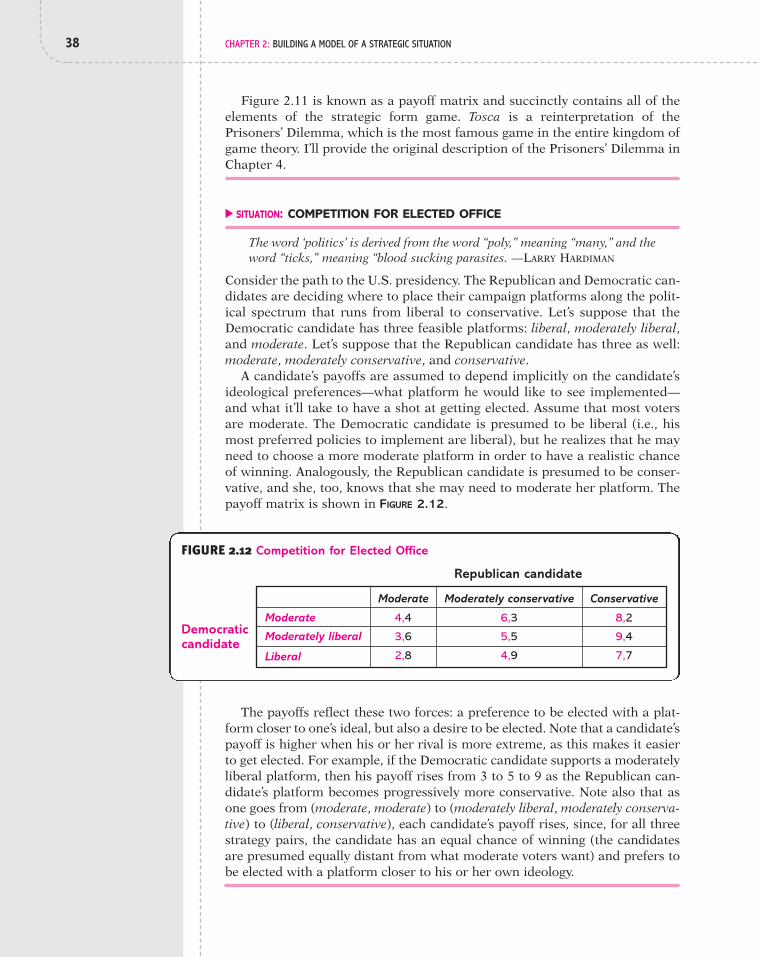
38 CHAPTER 2: BUILDING A MODEL OF A STRATEGIC SITUATION
Figure 2.11 is known as a payoff matrix and succinctly contains all of theelements of the strategic form game. Tosca is a reinterpretation of thePrisoners’ Dilemma, which is the most famous game in the entire kingdom ofgame theory. I’ll provide the original description of the Prisoners’ Dilemma inChapter 4.
! SITUATION: COMPETITION FOR ELECTED OFFICE
The word ‘politics’ is derived from the word “poly,” meaning “many,” and theword “ticks,” meaning “blood sucking parasites. —LARRY HARDIMAN
Consider the path to the U.S. presidency. The Republican and Democratic can-didates are deciding where to place their campaign platforms along the polit-ical spectrum that runs from liberal to conservative. Let’s suppose that theDemocratic candidate has three feasible platforms: liberal, moderately liberal,and moderate. Let’s suppose that the Republican candidate has three as well:moderate, moderately conservative, and conservative.
A candidate’s payoffs are assumed to depend implicitly on the candidate’sideological preferences—what platform he would like to see implemented—and what it’ll take to have a shot at getting elected. Assume that most votersare moderate. The Democratic candidate is presumed to be liberal (i.e., hismost preferred policies to implement are liberal), but he realizes that he mayneed to choose a more moderate platform in order to have a realistic chanceof winning. Analogously, the Republican candidate is presumed to be conser-vative, and she, too, knows that she may need to moderate her platform. Thepayoff matrix is shown in FIGURE 2.12.
FIGURE 2.12 Competition for Elected Office
4,4 6,3 8,2
3,6 5,5 9,4
2,8 4,9 7,7
Republican candidate
Democratic candidate Moderately liberal
Liberal
Moderate
Moderately conservativeModerate Conservative
The payoffs reflect these two forces: a preference to be elected with a plat-form closer to one’s ideal, but also a desire to be elected. Note that a candidate’spayoff is higher when his or her rival is more extreme, as this makes it easierto get elected. For example, if the Democratic candidate supports a moderatelyliberal platform, then his payoff rises from 3 to 5 to 9 as the Republican can-didate’s platform becomes progressively more conservative. Note also that asone goes from (moderate, moderate) to (moderately liberal, moderately conserva-tive) to (liberal, conservative), each candidate’s payoff rises, since, for all threestrategy pairs, the candidate has an equal chance of winning (the candidatesare presumed equally distant from what moderate voters want) and prefers tobe elected with a platform closer to his or her own ideology.

2.6 Moving from the Extensive Form and Strategic Form 39
! SITUATION: THE SCIENCE 84 GAME
The magazine Science 84 came up with the idea of running the following con-test for its readership: Anyone could submit a request for either $20 or $100.If no more than 20% of the submissions requested $100, then everybodywould receive the amount he or she requested. If more than 20% of the sub-missions asked for $100, then everybody would get nothing.
The set of players is the set of people who are aware of the contest. Thestrategy set for a player is made up of three elements: do not send in a request,send in a request for $20, and send in a request for $100. Let us suppose thateach player’s payoff is the amount of money received, less the cost of submit-ting a request, which we’ll assume is $1 (due to postage and the time it takesto write and mail a submission).
In writing down player i’s payoff function, let x denote the number of play-ers (excluding player i) who chose the strategy send in a request for $20 and ydenote the number of players (excluding player i) who chose send in a requestfor $100. Then player i’s payoff function is:
0 if i chooses do not send in a request
19 if i chooses send in a request for $20 and $ .2y
x % y % 1
99 if i chooses send in a request for $100 and $ .2y % 1
x % y % 1
"1 if i chooses send in a request for $20 and .2 &y
x % y % 1
"1 if i chooses send in a request for $100 and .2 &y % 1
x % y % 1
For example, if player i requested $20, and no more than 20% of the submis-sions requested $100 (i.e., $ .2), then she receives $20 from Science 84,from which we need to subtract the $1 cost of the submission.
Although it would be great to know what happened, Science 84 never ranthe contest, because Lloyd’s of London, the insurer, was unwilling to provideinsurance for the publisher against any losses from the contest.
2.6 Moving from the Extensive Form and Strategic FormFOR EVERY EXTENSIVE FORM GAME, there is a unique strategic form representationof that game. Here, we’ll go through some of the preceding examples and showhow you can derive the set of players (that one’s pretty easy), the strategy sets,and the payoff functions in order to get the corresponding strategic form game.
! SITUATION: BASEBALL, II
Consider the Baseball game in Figure 2.2. The strategy set of the Orioles’ man-ager includes two elements: (1) Substitute Gibbons for Lopez and (2) retainLopez. As written down, there is a single information set for the Yankees’ man-ager, so his strategy is also a single action. His strategy set comprises (1) sub-stitute Johnson for Rivera and (2) retain Rivera. To construct the payoff ma-trix, you just need to consider each of the four possible strategy profiles anddetermine to which terminal node each of them leads.
yx % y % 1
⎞⎪⎪⎪⎬⎟⎪⎪⎠

40 CHAPTER 2: BUILDING A MODEL OF A STRATEGIC SITUATION
If the strategy profile is (retain Lopez, retain Rivera), then the payoff is 2 forthe Orioles’ manager and 2 for the Yankees’ manager, since Lopez bats againstRivera. The path of play, and thus the payoffs, are the same if the profile is in-stead (retain Lopez, substitute Johnson), because substitute Johnson means“Put in Johnson if Gibbons substitutes for Lopez”. Since the latter event doesn’toccur when the Orioles’ manager chooses retain Lopez, Johnson is not substi-tuted. When the strategy profile is (substitute Gibbons, retain Rivera), Gibbonsbats against Rivera and the payoff pair is (3,1), with the first number being thepayoff for the Orioles’ manager. Finally, if the strategy profile is (substituteGibbons, substitute Johnson), Gibbons bats against Johnson and the payoffpair is (1,3). The payoff matrix is then as depicted in FIGURE 2.13.
FIGURE 2.13 Strategic Form of Baseball Game
2,2 2,2
3,1 1,3Orioles' manager
Yankees' manager
Retain Lopez
Substitute Gibbons
Retain Rivera Substitute Johnson
FIGURE 2.14 Strategic Form of the Galileo and Inquisition Game
Pope Urban VIII —Refer Pope Urban VIII—Do Not Refer
3,4,5 3,4,5
3,4,5 3,4,5
1,5,4 4,2,2
2,1,1 4,2,2
Galileo
Inquisitor
C/C
C/DNC
DNC/C
DNC/DNC
Torture Do not torture
5,3,3
5,3,3
5,3,3
5,3,3
5,3,3
5,3,3
5,3,3
5,3,3
C/C
C/DNC
DNC/C
DNC/DNC
Torture Do not torture
Galileo
Inquisitor
! SITUATION: GALILEO GALILEI AND THE INQUISITION, II
Referring back to Figure 2.3, we see that Galileo has two information sets: one as-sociated with Pope Urban VIII’s referring the case to the Inquisitor and the otherfor the situation when it is referred, Galileo does not confess, and the Inquisitortortures Galileo. A strategy for Galileo is, then, a pair of actions. We’ll let C/DNC(Confess/Do Not Confess) denote the strategy for Galileo in which he confesses atthe first information set and does not confess at the second. The other three strate-gies—C/C, DNC/C, and DNC/DNC—are defined analogously. The Inquisitor hasone information set—when the Pope refers the case and Galileo does not con-fess—and two actions, all of which gives him two strategies: torture and do not tor-ture. Urban VIII also has one information set, which is the initial node, and as hecan either refer the case or not, he has two strategies: refer and do not refer.
As shown in the payoff matrix in FIGURE 2.14, Galileo chooses a row, theInquisitor chooses a column, and the Pope chooses a matrix. The first number

2.6 Moving from the Extensive Form and Strategic Form 41
in a cell is Galileo’s payoff, the second is the Inquisitor’s payoff, and the third isthe Pope’s payoff. In filling out the matrix, consider, for example, the strategyprofile (Refer, DNC/C, Do not torture). The ensuing path is that the Pope refersthe case, Galileo does not confess, and the Inquisitor does not torture Galileo.The payoffs are (4,2,2), as shown in the figure. Note that if the Pope choosesnot to refer the case, then the payoffs are (5,3,3), regardless of the strategieschosen by Galileo and the Inquisitor, since they don’t get a chance to act.Similarly, if the Pope refers and Galileo initially confesses (by choosing eitherstrategy C/C or strategy C/DNC), then the payoffs are the same whether theInquisitor intends to torture or not, because Galileo’s confession means that theInquisitor doesn’t get the opportunity to move.
! SITUATION: HAGGLING AT AN AUTO DEALERSHIP, II
This game is more complicated than the ones we have considered thus far.Consider the version in Figure 2.5. Marcus has four information sets: (1) the ini-tial node, (2) the node associated with his having offered pM and Donna’s havingrejected it and made a counteroffer of pL, (3) the node associated with his havingoffered pH and Donna’s having rejected it and made a counteroffer of pM, and (4)the node associated with his having offered pH and Donna’s having rejected it andmade a counteroffer of pL. Marcus’s strategy template is then as follows:
At the initial node, offer _____ [fill in pL, pM, or pH].
If I offered pM and Donna rejected it and offered pL, then _____ [fill inaccept or reject].
If I offered pH and Donna rejected it and offered pM, then _____ [fill inaccept or reject].
If I offered pH and Donna rejected it and offered pL, then _____ [fill inaccept or reject and offer pM].
If you write them all out, you will see that there are 24 distinct strategies forMarcus—in other words, 24 different ways in which to fill out those four blanks.
Donna has four information sets, and her strategy template is the following:
If Marcus offered pL, then _____ [fill in accept or reject].
If Marcus offered pM, then _____ [fill in accept, reject and offer pL, or rejectand leave].
If Marcus offered pH, then _____ [fill in accept, reject and offer pL, rejectand offer pM, or reject and leave].
If Marcus offered pH, I rejected and offered pL, and Marcus rejected andoffered pM, then _____ [fill in accept or reject].
Donna has 48 strategies available to her. These are a lot of strategies, but keepin mind the complete nature of a strategy: no matter where Donna finds her-self in the game, her strategy tells her what to do.
Suppose Marcus and Donna chose the following pair of strategies. For Marcus:
At the initial node, offer pH.
If I offered pM and Donna rejected it and offered pL, then reject.
If I offered pH and Donna rejected it and offered pM, then accept.

42 CHAPTER 2: BUILDING A MODEL OF A STRATEGIC SITUATION
If I offered pH and Donna rejected it and offered pL, then reject and offer pM.
For Donna:
If Marcus offered pL, then accept.
If Marcus offered pM, then accept.
If Marcus offered pH, then reject and offer pL.
If Marcus offered pH, I rejected and offered pL, and Marcus rejected andoffered pM, then accept.
With this strategy pair, let us determine the sequence of play that logically fol-lows and thereby the associated payoffs. At the initial node, Marcus offers aprice of pH, as prescribed by his strategy. According to Donna’s strategy, sherejects the offer and counters with a price of pL. In response to that offer,Marcus’s strategy tells him to reject it and counteroffer with pM (reading fromthe bottom line of his strategy). Finally, Donna’s strategy has her accept theoffer of pM. The path of play that emerges is then as follows: Marcus offers aprice of pH, Donna rejects the offer and proposes a price of pL, Marcus rejectsand counters with a price of pM, and Donna accepts. The transaction is thenmade at a price of pM. For this strategy pair, the associated payoffs are (pM " pM)or zero, for Donna and 2(pM " pL), for Marcus.
2.7 Going from the Strategic Form to the Extensive FormALTHOUGH EVERY EXTENSIVE FORM GAME has a unique strategic form game associ-ated with it, the same strategic form game can be associated with more thanone extensive form game. This means that when we move from the extensiveform to the strategic form, we lose some information, but, as we’ll explain, thelost information is irrelevant.
Shown in FIGURE 2.15 are two extensive form games, both of which gener-ate the strategic form game in Figure 2.11. In the game in Figure 2.15(a),
FIGURE 2.15 Two Extensive Form Games That Generate the Same Strategic Form Game
(a) (b)
Scarpia
Tosca
Scarpia
2
2
Real
4
1
1
4
3
3
Blanks
Tosca
Stab StabConsent Consent
2
2
4
1
1
4
3
3
Tosca
Scarpia
Tosca
Scarpia
Real Blanks Real Blanks
Stab Consent

2.8 Common Knowledge 43
Scarpia moves first and then Tosca moves, but Tosca has only one informationset, which indicates that she doesn’t know what Scarpia chose when she de-cides between stab and consent. By this time, it ought to be straightforward toshow that this extensive form game produces the strategic form game depictedin Figure 2.11.
The game in Figure 2.15(b) is the same as that in Figure 2.15(a), except thatthe sequencing of players has been reversed; still, it produces the same strate-gic form game, and it makes sense that it does. We’ve pre-viously argued that what matters is not the chronologicalorder of moves, but rather what players know when theyact. In both of these extensive form games, Scarpia doesn’tknow Tosca’s move when he acts; in the game in Figure2.15(a), it is because he moves first, and in the game inFigure 2.15(b), it is because his information set includes both of Tosca’s ac-tions. Similarly, in both games, Tosca doesn’t know what Scarpia has told thefiring squad when she makes her choice.
2.8 Common KnowledgeJACK AND KATE ARE TO meet at the French restaurant Per Se in New York City.Jack has since learned that the restaurant is closed today, so he e-mails Kate,suggesting that they meet at 7 P.M. at Artie’s Delicatessen, their second-favoriteplace. Kate receives the e-mail on her BlackBerry and e-mails back to Jack,saying she’ll be there. Jack receives her confirmation. Kate shows up at Artie’sat 7 P.M. and Jack is not there. She wonders whether Jack received her reply.If he didn’t, then he might not be sure that she had received the message, andthus he may have gone to Per Se with the anticipation that she would go there.It’s 7:15, and Jack is still not there, so Kate leaves to go to Per Se. It turns outthat Jack was just delayed, and he’s surprised to find that Kate is not at Artie’swhen he arrives there.
The problem faced by Jack and Kate is what game theorists call a lack ofcommon knowledge. Jack knows that Per Se is closed. Kate knows that Per Se isclosed, because she received Jack’s message telling her that. Jack knows thatKate knows it, since he received Kate’s confirmation, and obviously, Kate knowsthat Jack knows it. But Kate doesn’t know that Jack knows that Kate knows thatPer Se is closed, because Kate isn’t sure that Jack received her confirming mes-sage. The point is that it need not be enough for Jack and Kate to both knowthat the restaurant is closed: they may also need to know what the other knows.
To be a bit more formal here, I’m going to define what it means for an event(or a piece of information) to be common knowledge. Let E denote this event.In the preceding example, E is “Per Se is closed and meet at Artie’s.” E is com-mon knowledge to players 1 and 2 if
■ 1 knows E and 2 knows E.■ 1 knows that 2 knows E and 2 knows that 1 knows E.■ 1 knows that 2 knows that 1 knows E and 2 knows that 1 knows that 2
knows E.■ 1 knows that 2 knows that 1 knows that 2 knows E and 2 knows that 1
knows that 2 knows that 1 knows E.■ And so on, and so on.
Write down the strategic form game for theMugging game in Figure 2.8.
2.4 CHECK YOUR UNDERSTANDING
44 CHAPTER 2: BUILDING A MODEL OF A STRATEGIC SITUATION
Are we there yet? No, because this goes on ad infinitum. Common knowl-edge is like the infinite number of reflections produced by two mirrors facingeach other. Here, the “reflection” is what a player knows. Common knowledge,then, is much more than players knowing something: it involves them know-ing what the others know, and knowing what the others know about what theothers know, and so forth.
The concept of common knowledge is quite crucial because an underlyingassumption of most of what we do in this book is that the game is commonknowledge to the players. Each player knows that the game that is beingplayed, each knows that the others know that the game that is being played,and so on.
Of course, here we are talking about an abstraction, for is anything evertruly common knowledge? Even if we’re sitting beside each other watching tel-evision, and a weather bulletin flashes along the bottom of the screen, am Isure that you saw it? Probably. But can I be sure that you saw me watching thebulletin? Possibly. But can I be sure that you saw me watching you watchingthe bulletin? Perhaps not. Although, in reality, knowledge may not hold for theentire infinite levels of beliefs required to satisfy common knowledge, it maynot be a bad approximation for a lot of settings, in the sense that people act“as if” something is common knowledge.
Before we move on, let me describe an intriguing puzzle that conveys thepower of common knowledge. A group of recently deceased individuals standbefore the pearly gates to heaven. St. Peter is waiting for them there. (Bearwith me if you don’t buy into the whole St. Peter shtick.) He tells them thatonly saints may enter right away, and a saint is demarcated with a halo overthe head. Those who are not saints, but who try to enter, will be banished tohell. Those who are not saints and do not try to enter will go to purgatory fora while and then enter heaven. There is one problem in determining whetheryou are a saint: No one sees whether there is a halo over his or her own head,though each sees the halos over the heads of others. St. Peter provides one lastpiece of information: he announces that there is at least one saint in the group.
St. Peter begins by inviting anyone to walk through the gates. If no onedoes, he then asks again, and so forth. Will the saints be able to figure out whothey are? They can if it is common knowledge that there is at least one saintamong them.
To see how the argument operates, suppose that there is, in fact, exactly onesaint. This is not initially known; everyone knows only that there is at least onesaint. The person who is that singular saint will look around and see no halosover the heads of the others. Since he knows that there is at least one saint, heconcludes that he must have a halo over his head. He then enters heaven.Admittedly, that was easy and, in fact, didn’t require common knowledge, butonly knowing that there is at least one saint.
Now suppose there are instead two saints in the group, and let’s name themTyrone and Rita. During the first calling by St. Peter, each person looks aroundand sees at least one person with a halo. (Those who are not saints will see twopeople with halos.) No one can conclude that he (or she) is a saint, so no onewalks through the gates. Let us remember that each person knows that theothers know that there is at least one saint. That no one walked through thegates must mean that each person must have seen at least one other personwith a halo, for if the person hadn’t, then she could infer that she is a saint.

2.9 A Few More Issues in Modeling Games 45
Since everyone, including a person with a halo, saw at least one person witha halo, there must be at least two saints. Since Tyrone sees exactly one otherperson with a halo (Rita), and he knows that there are at least two saints,Tyrone concludes he, too, must have a halo. By an analogous logic, Rita drawsthe conclusion that she has a halo. They both walk through the gates on thesecond calling.
Okay, we could solve the problem when there are two saints. But can we doit when there are three saints? Most definitely, and what allows us to do so isthat each person knows that there is at least one saint, each person knows thateveryone else knows that there is at least one saint, and each person knowsthat everyone else knows that everyone else knows that there is at least onesaint. Do you dare follow me down this daunting path of logic?
Suppose the group has three saints, and their names are Joan, Miguel, andTamyra. As in the case when there are two saints, no one can initially concludethat he or she is a saint. Because each person sees at least two halos (Joan,Miguel, and Tamyra each see two, and everyone else sees three), knowing thatthere is at least one saint doesn’t tell you whether you have a halo. So no oneenters during the first calling. Since no one entered then, as we argued before,everyone infers that everyone must have seen a halo, which means that theremust be at least two saints. So what happens in the second calling? Since thereare in fact three saints, everyone sees at least two halos during the second call-ing, in which case no one can yet conclude that he or she is a saint. Now, whatcan people infer from the absence of anyone entering heaven during the sec-ond calling? Everyone concludes that everyone, including those folks whohave halos, must have seen at least two halos. Hence, there must be at leastthree saints. Since Joan sees only two halos—those above the heads of Migueland Tamyra—Joan must have a halo. Thus, she walks through the gates on thethird calling, as do Miguel and Tamyra, who deploy the same logic. The threesaints figure out who they are by the third calling.
Suppose there are n saints? The same argument works to show that no oneenters until the nth calling by St. Peter, at which time all n saints learn whothey are and enter. To derive that conclusion, it takes n levels of knowledge:everyone knows that there is at least one saint, everyone knows that everyoneknows that there is at least one saint, everyone knows that everyone knowsthat everyone knows that there is at least one saint, and so on, until the nthlevel. Hence, if it is common knowledge that there is at least one saint, thenthe saints can always eventually figure out who they are.
It is said that, in order to succeed, it’s not what you know, but whom youknow. However, game theorists would say that it’s not what you know, butwhat you know about what others know, and what you know about what oth-ers know about what you know, and. . . .
2.9 A Few More Issues in Modeling Games■ Can a player forget?
In the movie Memento, the character Leonard Shelby suffers from an in-ability to create long-term memories due to psychological trauma associatedwith his wife’s murder. In spite of this handicap, he is in pursuit of the killer.Some of the things he learns he writes down so that he’ll have the information

46 CHAPTER 2: BUILDING A MODEL OF A STRATEGIC SITUATION
later, and the really important stuff he learns he has tattooed on himself.Whatever information is not written down will be forgotten. Leonard is thuscognizant of his memory deficiency and, in fact, uses it strategically. At onepoint, he writes down the name of someone as the murderer, even though heknows that that person is not the murderer. But he also knows that he’ll readit in a few minutes and believe what his note says, because he will have for-gotten that it is not true. In this way, he is committing himself to soon believ-ing that he’s found the killer, which will allow him to experience the satisfac-tion of vengeance when he murders him.
In the parlance of game theory, Leonard Shelby has imperfect recall, inthat he does not necessarily know things that he previously knew. Althoughgame theory can allow for that possibility, our attention in this book will belimited to the case of perfect recall, so a player who knows something at onepoint in the game will know it at any later stage of the game. For example, inthe Iraq WMD game, when Iraq decides whether to refuse inspections (whenrequested by the United Nations), it remembers whether it had WMD (a movemade at the start of the game). Similarly, in the game involving haggling at theauto dealership, if Marcus initially made an offer of pH, and Donna refused itand counteroffered with pL, Marcus remembers that he had originally offeredpH when he decides whether to accept Donna’s offer of pL or reject it and coun-teroffer with pM. A situation in which you might want to allow for imperfectrecall is the game of Concentration discussed in Chapter 1, since, in fact, theimperfect memories of players constitute an essential feature of the game.Alas, that is not a matter we will take on in this book.
■ Can a player change the game?
Consider the kidnapping situation in the movie Ransom. Mel Gibson playsthe character Tom Mullen, whose son, Sean, is kidnapped by a corrupt policeofficer named Jimmy Shaker. Initially, the situation operates like a standardkidnapping. Shaker demands a 2 million dollar ransom. While going to makethe ransom drop, Tom Mullen becomes convinced that the kidnappers have nointention of releasing his son. He then decides to go to the local television sta-tion and is filmed live making the following announcement:
The whole world now knows my son, Sean Mullen, was kidnapped, for ran-som, three days ago. This is a recent photograph of him. Sean, if you’rewatching, we love you. And this is what waits for the man that took him.This is your ransom. Two million dollars in unmarked bills, just like youwanted. But this is as close as you’ll ever get to it. You’ll never see one dol-lar of this money, because no ransom will ever be paid for my son. Not onedime, not one penny. Instead, I’m offering this money as a reward on yourhead. Dead or alive, it doesn’t matter. So congratulations, you’ve just becomea 2 million dollar lottery ticket, except the odds are much, much better. Doyou know anyone that wouldn’t turn you in for 2 million dollars? I don’tthink you do. But, this is your last chance, if you return my son, alive, un-injured, I’ll withdraw the bounty. With any luck, you can simply disappear.Understand. You will never see this money. Not one dollar. So you still havea chance to do the right thing. If you don’t, well, then, God be with you, be-cause nobody else on this Earth will be.
It is clear that Tom Mullen had a “brainstorm” of converting the ransominto a bounty. Furthermore, it is natural to suppose that this possibility was

2.9 A Few More Issues in Modeling Games 47
not one that Jimmy Shaker had considered. In a way, the players started withthe game looking like that in Figure 2.1, but then Tom Mullen “changed” thegame to something else. Unfortunately, game theory does not allow for suchchanges or innovations. A key assumption of game theory is that the game isinitially understood and agreed upon by the players; the rules of the game arecommon knowledge.
What we can do, however, is modify the game to that in FIGURE 2.16. JohnMullen now has the option of paying the ransom, offering a bounty, or doingnothing, in response to each of which Jimmy Shaker has the two options ofreleasing or killing Sean Mullen. This game is understood by the players whenthey start it and thus does not allow for the possibility of Tom Mullen “sur-prising” Jimmy Shaker by offering a bounty. True innovation is not a featurethat current game theory can encompass. Thus, the answer is that players arenot allowed to change the game. However, we can always enrich the game andgive players more options.
FIGURE 2.16 Extensive Form for the Film Ransom
John Mullen
7
Kill
3
Jimmy Shaker
Jimmy Shaker
JS JS JS
John Mullen
6
4
Release
Do not pay ransom
Pay ransom
Offer bounty
5
Do not kidnap
Kidnap
7
4
Kill
1
3
6
Release
1
Kill
2
2
5
Release
■ Does the game have to be factually accurate?
If our objective in formulating and then solving a game is to understand be-havior, then what matters is not what is factually or objectively true, but ratherwhat is perceived by the players. Their behavior will be driven by their pref-erences and what they believe, whether those beliefs are in contradiction withreality or not. Thus, a game ought to represent players’ environment as it isperceived by them.

48 CHAPTER 2: BUILDING A MODEL OF A STRATEGIC SITUATION
If a player is a member of a Native American tribe in the 19th centurywhich believes that a tribal leader has magical powers, we need to recog-nize that belief—regardless of whether or not it is true—if we are to under-stand their behavior. Or if a player in the 21st century believes that flying aplane into a building can improve his well-being in the afterlife, then weneed similarly to recognize that belief, no matter how wrong or misguidedit may be.
SummaryWhen the French Impressionist painter Claude Monet viewed a Londonbuilding, a French cathedral, or a lily pond in his backyard, he painted, notreality, but his impression of it. Modeling real-life encounters between peo-ple is similarly an art form, though admittedly not one worth framing andhanging on your wall. Real life is complicated, nuanced, and messy, and asocial scientist who wants to understand it must distill its essential featuresif he is to construct a simple and parsimonious model. Doing so requires cre-ativity, insight, and judgment. While game theory cannot bring those attrib-utes to the table, it can provide the tools for the intelligent observer who hassuch traits to build a model that will shed light on why people do the thingsthey do.
In this chapter, we have reviewed the two frameworks for constructing agame-theoretic model of a strategic situation. An extensive form gameuses a tree structure to depict the sequence in which players make decisionsand describes the circumstances surrounding those decisions, including theactions available to a player and what the player knows regarding what hashappened in the game. That knowledge is represented by an informationset which encompasses all those paths in the game that a player is in-capable of distinguishing among. The concept of an information set allowsus to model the many different contexts in which decisions are made whilewe lack relevant facts. An information set can embody a situation of per-fect information, in which a player knows all that has transpired thus farin the game, or one of imperfect information, in which a player has someuncertainty in regard to what other players have done. Key to describingbehavior is knowing what players care about, so an extensive form gamealso describes the well-being, or payoff, that a player assigns to an outcomeof the game.
A strategic form game has a more concise format than the extensive formgame has. A strategic form game is defined by the set of players, the strategyset of each player, and the payoff function of each player. A player’s decisionmaking involves the selection of a strategy from his or her strategy set, wherea strategy is a fully specified decision rule for how to play a game. A payofffunction tells us how a player evaluates any collection of strategies (one foreach of the players in the game).
As will be revealed in the ensuing chapters, crucial to both predicting be-havior and prescribing behavior is knowing what each player knows aboutthe other players, and this knowledge includes what each player believesabout the other players. A central underlying assumption is that the game iscommon knowledge to the players. This means not only that players agree

1. The countries of Oceania and Eurasia are at war.5 As depicted in FIGURE
PR2.1, Oceania has four cities—Argula, Betra, Carnat, and Dussel—andit is concerned that one of them is to be bombed by Eurasia. Thebombers could come from either base Alpha, which can reach the citiesof Argula and Betra, or base Beta, which can reach either Carnat orDussel. Eurasia decides which one of these four cities to attack. Oceaniadoesn’t know which one has been selected, but does observe the basefrom which the bombers are flying. After making that observation,Oceania decides which one (and only one) of its four cities to evacuate.Assign a payoff of 2 to Oceania if it succeeds in evacuating the city thatis to be bombed and a payoff of 1 otherwise. Assign Eurasia a payoff of1 if the city it bombs was not evacuated and a zero payoff otherwise.Write down the extensive form game.
EXERCISES
Exercises 49
Oceania
Argula
Betra
BetaAlpha
Dussel
Carnat
FIGURE PR2.1
2. Player 1 moves initially by choosing among four actions: a, b, c, and d.If player 1 chose anything but d, then player 2 chooses between x and y.Player 2 gets to observe the choice of player 1. If player 1 chose d, thenplayer 3 moves by choosing between left and right. Write down the ex-tensive form of this setting. (You can ignore payoffs.)
on the game that is being played, but also that each player knows what theother players believe about the game, and so forth. Common knowledge islike the perfect circle; it is a concept that does not exist in reality, but nev-ertheless is a useful abstraction for understanding the world within whichwe live.

50 CHAPTER 2: BUILDING A MODEL OF A STRATEGIC SITUATION
3. Consider a setting in which player 1 moves first by choosing among threeactions: a, b, and c. After observing the choice of player 1, player 2 choosesamong two actions: x and y. Consider the following three variants as towhat player 3 can do and what she knows when she moves:a. If player 1 chose a, then player 3 selects among two actions: high and
low. Player 3 knows player 2’s choice when she moves. Write downthe extensive form of this setting. (You can ignore payoffs.)
b. If player 1 chose a, then player 3 selects among two actions: highand low. Player 3 does not know player 2’s choice when she moves.Write down the extensive form of this setting. (You can ignore pay-offs.)
c. If player 1 chose either a or b, then player 3 selects among two ac-tions: high and low. Player 3 observes the choice of player 2, but notthat of player 1. Write down the extensive form of this setting. (Youcan ignore payoffs.)
4. Return to the game involving the U.S. Court of Appeals in Section 2.2.a. Suppose, at the start of the game, it is known by all that Judge Z will
read only the brief of Ms. Hasenpfeffer. Write down the correspon-ding extensive form game. You may exclude payoffs.
b. Suppose, at the start of the game, it was known by all that Judge Xwould vote first and reveal his vote to Judges Y and Z before they votesimultaneously. Write down the corresponding extensive form game.You may exclude payoffs.
5. The city council is to decide on a proposal to raise property taxes.Suppose Ms. Tuttle is the chair and the Council’s other two members areMr. Jones and Mrs. Doubtfire. The voting procedure works as follows:Excluding the chair, Mr. Jones and Mrs. Doubtfire simultaneously writedown their votes on slips of paper. Each writes either for or against thetax increase. The secretary of the city council then opens the slips ofpaper and announces the vote tally. If the secretary reports that both slipssay for, then the tax increase is implemented and the game is over. If bothvote against, then the tax increase is not implemented and, again, thegame is over. However, if it is reported that the vote is one for and oneagainst, then Ms. Tuttle has to vote. If she votes for, then the tax increaseis implemented, and if she votes against, then it is not. In both cases, thegame is then over. As to payoffs, if the tax increase is implemented, thenMrs. Doubtfire and Mr. Jones each receive a payoff of 3. If the tax in-crease proposal fails, then Mrs. Doubtfire has a payoff of 4 and Mr.Jones’s payoff is 1. As for Ms. Tuttle, she prefers to have a tax increase—believing that it will provide the funds to improve the city’s schools—butwould prefer not to be on record as voting for higher taxes. Her payofffrom a tax increase when her vote is not required is 5, her payoff from atax increase when her for vote is required is 2, and her payoff from taxesnot being increased is zero (regardless of whether or not she voted). Writedown the extensive form of the game composed of Ms. Tuttle, Mr. Jones,and Mrs. Doubtfire.
6. Consider a contestant on the legendary game show Let’s Make a Deal.There are three doors, and behind two doors is a booby prize (i.e., a prizeof little value), while behind one door is a prize of considerable value, suchas an automobile. The doors are labeled 1, 2, and 3. The strategic situationstarts when, prior to the show, host Monty Hall selects one of the threedoors behind which to place the good prize. Then, during the show, a

Exercises 51
contestant selects one of the three doors. After its selection, Monty opensup one of the two doors not selected by the contestant. In opening up adoor, a rule of the show is that Monty is prohibited from opening the doorwith the good prize. After Monty Hall opens a door, the contestant is thengiven the opportunity to continue with the door originally selected orswitch to the other unopened door. After the contestant’s decision, the re-maining two doors are opened.a. Write down an extensive form game of Let’s Make a Deal up to (but
not including) the stage at which the contestant decides whether tomaintain his original choice or switch to the other unopened door.Thus, you are to write down the extensive form for when (1) MontyHall chooses the door behind which the good prize is placed, (2) thecontestant chooses a door, and (3) Monty Hall chooses a door toopen. You may exclude payoffs.
b. For the stage at which the contestant decides whether or not toswitch, write down the contestant’s collection of information sets. Indoing so, denote a node by a triple, such as 3/2/1, which describes thesequence of play leading up to that node. 3/2/1 would mean thatMonty Hall put the good prize behind door 3, the contestant initiallyselected door 2, and Monty Hall opened door 1.
7. For the Iraq War game in Figure 2.10, write down the strategy sets forthe three players.
8. For the extensive form game in FIGURE PR2.8, derive its correspondingstrategic form.
5
2
2
2
1
1
15
0
0 Player 1
0 Player 2
10
5
c2
a2
a1
b2
b1
d2
c1 d1
20
3
4
1
c2 d2
FIGURE PR2.8

52 CHAPTER 2: BUILDING A MODEL OF A STRATEGIC SITUATION
9. Write down the strategic form game for the extensive form game inFIGURE PR2.9.
Player 1Player 2
2
1
1
3
4
2
a b c d
x y x y x y x y
2
2
0
6
3
1
4
2
1
5
0
0
FIGURE PR2.9
10. Write down the strategic form game for the extensive form game inFIGURE PR2.10.
11. Three extensive form games are shown in FIGURE PR2.11. State which ofthem, if any, violate the assumption of perfect recall. Explain your answer.
Player 1
Player 2
Player 3
2
3
4
1
a b c
x y x y r s
1
1
6
0
2
3
1
0
02 1 3 5 6
3
1
2
FIGURE PR2.10

Exercises 53
FIGURE PR2.11
(b)
0
1
1
1
x y x y
c dc d c d c d
0
0
1
0
1
0
1
1
1
0
0
1
2
1
1 1
(c)
0
1
1
1
x y x y
c dc d c d c d
0
0
1
0
1
0
1
1
1
0
0
1
2
1
1
(a)
0
1
1
1
a b
x y x y
c dc d c d c d
0
0
1
0
a b
a b
1
0
1
1
1
0
0
1
2 2
1
1 11

54 CHAPTER 2: BUILDING A MODEL OF A STRATEGIC SITUATION
REFERENCES1. John Thorn and Pete Palmer, The Hidden Game of Baseball (New York:
Doubleday/Dolphin, 1985). The seasons analyzed were 1974–77.
2. Sun Tzu, The Art of War, translated by Thomas Cleary, Shambhala, 1998.For an examination of Sun Tzu’s writings using the lens of game theory, seeEmerson M. S. Niou and Peter C. Ordeshook, “A Game-TheoreticInterpretation of Sun Tzu’s The Art of War,” Journal of Peace Research, 31(1994), 161–74.
3. J. D. Williams, The Compleat Strategyst (New York: McGraw Hill, 1954), p. 16.
4. This application of game theory was first suggested by Anatol Rapoport,“The Use and Misuse of Game Theory,” Scientific American, 207(6): 108–18.
5. These fictitious countries appear in the George Orwell novel 1984. Ifdystopia is not your bag, then you can use Freedonia and Sylvania in theirplace, which are fictional nations from the 1933 Marx Brothers’ movieDuck Soup.

How often have I said to you that when you have eliminated the impossible, whatever remains, however improbable, must be thetruth? —SHERLOCK HOLMES IN A STUDY IN SCARLET, BY ARTHUR CONAN DOYLE
3.1 IntroductionIN CHAPTER 2, WE LEARNED how to construct a game, in both the extensive andstrategic forms. But having built a game, what do we do with it? I say, Let’splay amateur sleuth and investigate people’s behavior in strategic scenarios.To do so, we need to know how to solve a game, which is what this chapter isall about.
FIGURE 3.1 presents the strategic form of the kidnapping situation whose ex-tensive form was illustrated in Figure 2.1. Recall that Guy, the kidnapper, hasfour strategies. He can either not kidnap Orlando, but in the event that hedoes, then kill him (Do not kidnap/Kill); not kidnap Orlando, but in the eventthat he does, then release him (Do not kidnap/Release); kidnap Orlando andkill him (Kidnap/Kill); or kidnap Orlando and release him (Kidnap/Release).Vivica, who is Orlando’s kin, can either pay the ransom or not. The first num-ber in a cell is the row player’s payoff (Guy’s payoff), and the second numberis the column player’s payoff (Vivica’s payoff). Recall that payoff numbers arerank ordered from the least to the most preferred outcome.
3
55
Eliminating the Impossible:Solving a Game when Rationality Is Common Knowledge
FIGURE 3.1 Strategic Form of the Kidnapping Game
3,5 3,5
3,5 3,5Guy (kidnapper)
Vivica (kin of victim)
Pay ransom Do not pay ransom
4,1 2,2
5,3 1,4
Do not kidnap/Kill
Do not kidnap/Release
Kidnap/Kill
Kidnap/Release
Will there be a kidnapping? If so, will ransom be paid? Will Orlando sur-vive? Solving this game means answering these questions by selecting amongthe eight possible pairs of strategies. We need to weed out unreasonable andimplausible strategy profiles and, ideally, identify a unique compelling one.The fewer solutions there are, the more precise is our prediction about be-havior. To derive a solution, we’ll need to assume something about how a

player selects among his or her various strategies. Of course, what makes thistask challenging (and results in a long textbook!) is the fact that how a playerselects a strategy may well depend on how she thinks other players are select-ing. This is a complex undertaking not quickly dispensed with, and it is bestthat we start at the beginning and start simple.
The plan is to progressively make more assumptions about players and ex-plore what we can say about how they’ll behave. We begin with assuming thatplayers are rational (Section 3.2), then further assume that each player be-lieves that all players are rational (Section 3.3), and then assume on top of thatthat each player believes that all players believe that all players are rational(Section 3.3). We conclude the chapter by generalizing this sequence of solu-tion techniques in Section 3.4.
3.2 Solving a Game when Players Are RationalIN MODELING A PLAYER’S SELECTION of a strategy, we’ll begin by assuming that play-ers are rational. A player is rational when she acts in her own best interests.More specifically, given a player’s beliefs as to how other players will behave,the player selects a strategy in order to maximize her payoff. Note that ration-ality has nothing to say about what are reasonable beliefs to hold regardingwhat others will do; rationality just says that a player chooses the strategy thatmaximizes her payoff, given her beliefs as to the strategies of other players.
Is it reasonable to assume that people act only in their self-interest? Doesthis assumption mean that people are selfish? Although rationality does meanpursuing your own interests, it places few restrictions on what those interestsmight be. It can encompass Ebenezer Scrooge either before Christmas Eve—when all he cares about is money—or after that momentous night—when hecares about his fellow human beings. Rationality is a church that welcomes allpeople, from the egotistical to the altruistic. To be rational means only to pur-sue your interests, however they are defined.
Initially, we will assume a particular implication of rationality: A player willnot use a strategy (call it ) when there is another strategy (call it ) that al-ways produces a strictly higher payoff, regardless of what strategies are usedby the other players. Thus, a strategy is never the right thing to do, as willalways outperform . It would then be rather stupid to play (whetheryou’re Mother Teresa or Paris Hilton). We’ll go even further and assume thateach player believes that other players avoid stupid strategies, that each playerbelieves that other players believe that players avoid such strategies, and soforth. In other words, it is common knowledge among players that a player willnot use a particular strategy when there is another strategy that is alwaysstrictly better.
In Appendix 3.5, we consider the concept of rationalizability, which is astronger implication of rationality being common knowledge. Rationalizabilityis closer to the essence of what it means to be rational, although, because it isa rather subtle and complex concept, we make it optional here and leave it forthe more adventuresome student (or the more exacting instructor).
3.2.1 Strict DominanceLet’s revisit Puccini’s opera Tosca, the strategic form game of which is repro-duced in FIGURE 3.2. Recall from Section 2.5 that Baron Scarpia, the chief of
s¿s¿s–s¿
s–s¿
56 CHAPTER 3: ELIMINATING THE IMPOSSIBLE: SOLVING A GAME WHEN RATIONALITY IS COMMON KNOWLEDGE

3.2 Solving a Game when Players Are Rational 57
police, has condemned Floria Tosca’s lover Mario Cavaradossi todeath. Scarpia tells Tosca that he’ll have the firing squad useblank cartridges in exchange for sexual favors from Tosca.Scarpia first tells the firing squad to use real or blank cartridges,and then he meets Tosca, at which point she must decide whetherto consent to Scarpia’s demands or stab him. Soon thereafter,Cavaradossi is brought before the firing squad. Both Tosca andScarpia move without knowing what the other has chosen. Thepayoffs reflect that Tosca cares foremost that her lover survivesand secondarily that she not consent to Scarpia, and that Scarpia longs tohave relations with Tosca and only secondarily desires to execute Cavaradossi.
Can we say what these two operatic characters willdo if all we assume is that they are rational? Well, con-sider Tosca. If Scarpia chooses real, then Tosca’s payofffrom choosing stab is 2 and from choosing consent is 1.(See FIGURE 3.3.) Thus, she clearly prefers to stabScarpia if she expects him to have ordered the firingsquad to use real cartridges. What about if she expectshim to have chosen blank cartridges? Her payoff is 4from stab and 3 from consent, so, once again, sheprefers stab. Thus, regardless of what Tosca believesScarpia will do, stab gives Tosca a strictly higher payoffthan consent. Therefore, Tosca should most definitely not choose consent.Since she has to do something, she has nothing left to do but to stab Scarpia.To see this another way, stab is superior to consent regardless of what Scarpiawill do, so a rational Tosca should most surely choose stab.
By a similar argument, the rationality of Scarpia implies that he will choosereal. If Tosca chooses stab, he earns a payoff of 2 from killing Cavaradossi andonly 1 from not doing so. If Tosca chooses consent, then the payoff from realis 4, which once again exceeds that from blanks (which is 3). Hence, regard-less of what he thinks Tosca will do, Scarpia should have the firing squad usereal bullets. In conclusion, game theory makes a very clear (and bloody) pre-diction that Tosca will stab Scarpia and Scarpia will see that Cavaradossi diesat the hands of the firing squad.
The strategy consent is said to be strictly dominated by the strategy stab forTosca, which just means that stab delivers a higher payoff than consent for anystrategy of Scarpia.
✚ DEFINITION 3.1 A strategy strictly dominates a strategy if thepayoff from is strictly higher than that from for any strategies chosenby the other players.*
A strategy that strictly dominates every other strategy for a player is said tobe a dominant strategy. Obviously, with only two strategies, if consent isstrictly dominated for Tosca, then stab must be the dominant strategy.
✚ DEFINITION 3.2 A strategy is the dominant strategy if it strictly domi-nates every other strategy.
s–s¿s–s¿
FIGURE 3.2 The Tosca Game
2,2 4,1
1,4 3,3Tosca
Scarpia
Stab
Consent
Real Blanks
FIGURE 3.3 Tosca’s Payoffs in the Event ThatScarpia Chooses Real Bullets
2 ,2 4,1
1 ,4 3,3Tosca
Scarpia
Stab
Consent
Real Blanks
*A more formal mathematical presentation of Definitions 3.1 and 3.2 is provided in Section 3.5, which isan appendix to this chapter.

If a strategy is strictly dominated, then it is not optimal for any beliefs re-garding what other players will do; thus, a rational player will avoid usingsuch a strategy. Furthermore, if a player has a dominant strategy, then, if he isrational, he will use it. When each player has a dominant strategy, the uniquereasonable solution is that each player uses his or her dominant strategy.
A rational player never uses a strictly dominated strategy. A rationalplayer always uses a dominant strategy.
Before we apply these new tools to a few other games, take note of an in-teresting property of the outcome of Tosca. When Tosca stabs Scarpia andScarpia has Cavaradossi killed, they each receive a payoff of 2. Now considerthe alternative strategy pair in which Tosca consents and Scarpia has the fir-ing squad use blanks, so that Cavaradossi survives. Now Tosca and Scarpiaeach earn a payoff of 3; they are both better off!
We see in the Tosca situation an important distinction between individualrationality and collective rationality: It is individually rational for Tosca tostab Scarpia (because it is her dominant strategy), and it is individually ra-tional for Scarpia to use real bullets (because it is his dominant strategy);however, it is collectively rational—in the sense that everyone would be bet-ter off—if Tosca and Scarpia were to commit, respectively, to consenting andusing blanks. Thus, what may be in an individual’s best interests need not bein the best interests of the group. (We’ll have more to say on this matter laterin the book.)
So, what happens in the opera? Tosca stabs Scarpia and Scarpia uses realbullets, so that both Cavaradossi and Scarpia die. When she learns thatCavaradossi is dead, Tosca jumps to her death from the castle’s ramparts. Inspite of the carnage, love wins out over lechery. Or, if this was a tennis match,the score would be love: 15, lechery: love.
58 CHAPTER 3: ELIMINATING THE IMPOSSIBLE: SOLVING A GAME WHEN RATIONALITY IS COMMON KNOWLEDGE
Tosca Having Stabbed Scarpia
© 2
00
6 J
ACK
VA
RTO
OG
IA/F
RON
T RO
W P
HO
TOS

3.2 Solving a Game when Players Are Rational 59
! SITUATION: WHITE FLIGHT AND RACIAL SEGREGATION IN HOUSING
What do you think you are going to gain by moving into a neighborhoodwhere you just aren’t wanted and where some elements—well—people can getawful worked up when they feel that their whole way of life and everythingthey’ve ever worked for is threatened. —THE (WHITE) KARL LINDER SPEAKING
TO THE (BLACK) YOUNGER FAMILY IN RESPONSE TO LENA YOUNGER’S PURCHASE OF
A HOME IN HIS NEIGHBORHOOD, IN A RAISIN IN THE SUN, BY LORAINE HANSBERRY
The renting or sale of homes and apartments in an all-white neighborhoodto African-Americans was a contentious racial issue in the 1960s. The term“white flight” refers to the exodus of white families upon the arrival of a fewblack families, making the neighborhood “tip” from being all white to allblack. Could white flight occur even if both blacks and whites prefer to havea racially integrated neighborhood?1
Suppose that a black family is willing to pay higher rent than a white fam-ily to live in what is currently an all-white neighborhood. A willingness to payhigher rent could reflect fewer options for blacks when it comes to attractivehomes and good schools. For a scenario in which there are eight identicalhomes in a certain neighborhood, TABLE 3.1 lists the monthly rent that a blackfamily and a white family are hypothetically willing to pay, depending on howmany black families are in the neighborhood. Notice that both blacks andwhites are willing to pay the highest rent for a (somewhat) racially integratedneighborhood.
TABLE 3.1 RENT IN THE HOUSING MARKET
No. of Black Rent Paid by a Black Rent Paid by a WhiteFamilies Family Family Total Rent
0 — 100 800
1 110 105 845
2 115 110 890
3 120 100 860
4 110 90 800
5 100 75 725
6 90 75 690
7 85 70 665
8 80 — 640
The column entitled “Total rent” is the sum of the monthly rents collectedby the landlords of the eight homes. For example, if there are three black fam-ilies, then each black family pays $120/month and each of the five white fam-ilies pays $100/month, for a total collected monthly rent of $860. Note that thelandlords’ rent is maximized at $890, when two of the homes are rented toblack families.
The game of interest is not between black and white families, but rather be-tween the landlords who own the eight homes. Suppose that each home is

owned by a different person and the payoff of a landlord equals the rent col-lected. Then, in deciding to whom to rent their property, will the landlords se-lect strategies that result in a racially integrated neighborhood? Or will theirdecisions cause the neighborhood to “tip” from being all white to all black?
The concept of strict dominance allows us to say what will happen.Consider the decision faced by an individual landlord, and suppose the otherseven landlords are currently renting to only white families. Then the firstlandlord will earn $10 more a month ($110 versus $100) by renting to a blackfamily. Hence, he will prefer to rent to a black family when the other sevenhomes are rented to white families. Now suppose instead that, of the otherseven homes, six are rented to white families and one to a black family. Thenif the landlord in question rents to a black family, he’ll earn $115 (since thereare now two black families in the neighborhood), an amount of money thatexceeds what he can earn by renting to a white family, which is only $105(when there is only one black family). It is thus to the landlord’s advantage torent to a black family when six of the other seven houses are rented to whitefamilies. Continuing in this manner, you can show that, regardless of what theother seven landlords are doing (in terms of the race of their tenants), an in-dividual landlord makes more money by renting to a black family. In otherwords, renting to a black family strictly dominates renting to a white family.
The monetary benefit applies to each of the landlords, so if each uses his orher dominant strategy, then each will rent to a black family. As a result, theneighborhood shifts from being all white to all black. Notice, however, that ifall the houses are rented to black families, then the landlords end up with alower total rent of $640, compared with the $800 they got when they were allrenting to white families. Sadly, then, landlords are poorer and racial integra-tion is not achieved.
! SITUATION: BANNING CIGARETTE ADVERTISING ON TELEVISION
Winston tastes good like a cigarette should!*
If you grew up in the 1960s, you would know that popular jingle from tele-vision commercials for Winston cigarettes. In fact, it was so common thatmany people (like me!) remember it even though it hasn’t been broadcast formore than 30 years. Since a federally mandated ban went into effect in 1971,no advertisements for tobacco products have either been seen or heard on tel-evision or radio in the United States.
Typically, a government-imposed restriction is something that a companydisdains. Taking away options usually means limiting avenues for achievinghigher profit. In a game-theoretic setting, however, losing options is not al-ways bad. Is it possible that the TV and radio ban might have increased theprofits of the tobacco manufacturers?
Consider Philip Morris and R. J. Reynolds, which were (and still are) thelargest cigarette manufacturers. Most people know their Marlboro andWinston brands of cigarettes. In considering how much advertising is needed,it is critical to understand how advertising affects the number of packs of
60 CHAPTER 3: ELIMINATING THE IMPOSSIBLE: SOLVING A GAME WHEN RATIONALITY IS COMMON KNOWLEDGE
*In response to complaints about grammar from language mavens, Winston responded with a new slogan:“What do you want, good grammar or good taste?”

3.2 Solving a Game when Players Are Rational 61
cigarettes sold. Some studies by economists show that advertising doesn’thave much of an impact on the number of smokers and instead just shifts theexisting set of smokers among the different brands. But then there is other ev-idence that advertising dissuades smokers from stopping and lures nonsmok-ers (in particular, youth) into trying smoking. To keep our model simple, let usassume that advertising doesn’t affect the total number of packs sold and justshifts smokers among the different brands.
Suppose the annual demand for cigarettes is 1,000,000,000 (one billion)packs and that the market share of a company depends on how much itspends on advertising relative to what its rival spends. Let ADVPM denotethe advertising expenditures of Philip Morris (PM) and ADVRJR denote the
COU
RTES
Y O
F TH
E A
DV
ERTI
SIN
G A
RCH
IVES

advertising expenditures of R. J. Reynolds (RJR). Assume that the marketshare of PM equals
This quotient says that PM’s share of all packs sold equals its share of adver-tising. Such a model is overly simplistic, but all that we really need to assumeis that sales are higher when more is spent on advertising. The total numberof packs sold by PM is then
1,000,000,000 !
and by a similar argument, the corresponding number for RJR is
1,000,000,000 !
If each pack sold generates a profit of 10 cents (remember, we’re back in1971), then the profit that PM gets from spending ADVPM dollars is
0.1 ! 1,000,000,000 !
or
100,000,000 !
Analogously, RJR’s profit is
100,000,000 !
Our objective is to say something about how much these companiesadvertise. To keep things simple, assume that there are just three levels ofadvertising: $5 million, $10 million, and $15 million. In that case, the pay-off matrix is as shown in FIGURE 3.4 (where strategies and payoffs are in millions
a ADVRJR
ADVPM % ADVRJRb " ADVRJR.
a ADVPM
ADVPM % ADVRJRb " ADVPM.
a ADVPM
ADVPM % ADVRJRb " ADVPM,
a ADVRJR
ADVPM % ADVRJRb .
a ADVPM
ADVPM % ADVRJRb ,
ADVPM
ADVPM % ADVRJR.
62 CHAPTER 3: ELIMINATING THE IMPOSSIBLE: SOLVING A GAME WHEN RATIONALITY IS COMMON KNOWLEDGE
FIGURE 3.4 The Cigarette Advertising Game
45,45 28,57
57,28 40,40Philip Morris
R. J. Reynolds
Spend 5 Spend 10 Spend 15
60,20 45,30
20,60
30,45
35,35
Spend 5
Spend 10
Spend 15

Now suppose the ban on TV and radio adver-tising is put into effect and it has the impact ofmaking it infeasible for the cigarette companiesto spend $15 million on advertising. That is, themost that a company can spend using the re-maining advertising venues is $10 million. Inthe context of this simple game, each company’sstrategy set is then constrained to comprise thechoices of spending $5 million and spending$10 million, as shown in FIGURE 3.5.
The solution to this game is that both companies spend moderately on ad-vertising, since spending $10 million strictly dominates spending 5 million.And what has this intrusive government policy done to their profits? Theyhave increased! Each company’s profit rises from $35 million to $40 million.
In the original game, each company had a dominant strategy of spending$15 million. This heavy advertising tended to cancel out, so each ended upwith 50% of the market. If they both could have restrained their spending to$10 million, they would each still have had half of the market—thus leavingthem with the same gross profits—and would have spent less on advertising,which translates into higher net profit.
By reducing the options for advertising, the TV and radio ban served to re-strain competition, reduce advertising expenditures, and raise company profits.
of dollars). For example, if PM spends $5 million and RJR spends $15 million,then PM’s market share is 5/(5 % 15), or 25%. PM then sells 250 millionpacks (0.25 multiplied by 1 billion) and, at 10 cents per pack, makes a grossprofit of $25 million. Once we net out the cost of advertising, PM’s profit (orpayoff) is $20 million.
TABLE 3.2 shows that a strategy of spending $15 million strictly dominatesspending either $5 million or $10 million. For example, if RJR spends $5 mil-lion, then PM earns $60 million from spending $15 million (and gets 75% ofthe market), while PM earns $57 million with an advertising budget of $10million and only $45 million by matching RJR’s paltry expenditure of $5 mil-lion. Similarly, a budget of $15 million for PM outperforms the other two op-tions when RJR spends $10 million and when it spends $15 million. Thus, PMprefers the heavy advertising campaign regardless of what RJR chooses, soheavy advertising is a dominant strategy for PM. Because the same can beshown for RJR, the prediction is that both cigarette companies inundate ourtelevision sets with attractive men and women spewing forth smoke.
3.2 Solving a Game when Players Are Rational 63
TABLE 3.2 SPENDING 15 IS A DOMINANT STRATEGYFOR PM
RJR PM Payoff PM Payoff PM PayoffStrategy from 15 from 10 from 5
Spend 5 60 > 57 > 45
Spend 10 45 > 40 > 28
Spend 15 35 > 30 > 20
FIGURE 3.5 Cigarette Advertising Game When TVand Radio Commercials Are Excluded
45,45 28,57
57,28 40,40Philip Morris
R. J. Reynolds
Spend 5
Spend 10
Spend 5 Spend 10

Of course, there’s nothing wrong with that if that is indeed what happened, sincethe objective of the ban was to reduce smoking, not lower companies’ profits.
A rational player never smokes cigarettes. (Okay, I’m making thatone up.)
3.2.2 Weak DominanceNot to be absolutely certain is, I think, one of the essential things in rationality. —BERTRAND RUSSELL
Returning to the world of Italian opera yet again, suppose wenow assume that Scarpia, upon being stabbed by Tosca, does notcare whether Cavaradossi is killed. The resulting payoff matrix isshown in FIGURE 3.6. Although stab continues to be the dominantstrategy for Tosca (indeed, we haven’t changed her payoffs),using real bullets no longer strictly dominates using blanks forScarpia. Nevertheless, real would seem the reasonable course ofaction for Scarpia. If Tosca consents, then Scarpia strictly prefersto have used real bullets; he receives a payoff of 4 as opposed to3. If Tosca stabs him, then he doesn’t care, as his payoff is 2 re-
gardless of what he chooses. Thus, he can’t be any worse off by using real bul-lets, and he might just be better off. We say that the strategy real weakly dom-inates the strategy blanks.
✚ DEFINITION 3.3 A strategy weakly dominates a strategy if (1) thepayoff from is at least great as that from for any strategies chosen bythe other players; and (2) there are some strategies for the other playerswhereby the payoff from is strictly greater than that from .*
Because most people are cautious and lack absolute confidence as to whatother players will do, it seems prudent to avoid weakly dominated strategies.Doing so means that you can never be any worse off and you just might endup being better off. There’ll be no regrets by avoiding weakly dominatedstrategies. And if there is a weakly dominant strategy—which means that itweakly dominates all other strategies—it would be wise to use that strategy.
A rational and cautious player never uses a weakly dominatedstrategy. A rational and cautious player always uses a weakly dominantstrategy.
3.2.3 Bidding at an AuctionIt’s been 20 years since you’ve graduated from college, and you’ve just soldyour Internet company for a cool $50 million. With all this cash on hand, youdecide to indulge your passion for modern art. An auction house is selling anAndy Warhol piece that you’ve been coveting for some time. The rules are thatall interested parties must submit a written bid by this Friday at 5 P.M.Whoever submits the highest bid wins the Warhol piece and pays a price equalto the bid—a format known as the first-price auction.
s–s¿
s–s¿s–s¿
64 CHAPTER 3: ELIMINATING THE IMPOSSIBLE: SOLVING A GAME WHEN RATIONALITY IS COMMON KNOWLEDGE
*A more formal mathematical definition is provided in Section 3.5, which is an appendix to this chapter.
FIGURE 3.6 Revised Tosca Game
2,2 4,2
1,4 3,3Tosca
Scarpia
Stab
Consent
Real Blanks

3.2 Solving a Game when Players Are Rational 65
The Warhol piece is worth $400,000 to you. If you win the item, your pay-off equals $400,000 less the price you paid, while if you don’t win, your payoffis zero. Hence, if you end up paying $400,000, you’re no better off, whileyou’re better (worse) off if you get it for less (more) than $400,000.
You’ve just learned that there is only one other bidder: your old college girlfriend, who has recently cashed in stock options after being CEO for a bio-medical company. You know that she values the piece at $300,000, and fur-thermore, she knows that you value it at $400,000. (In Chapter 10, we’ll ex-plore the more realistic case when each bidder’s valuation is known only tohim or her.)
The auctioneer announces that bids must be inincrements of $100,000 and that the minimumbid is $100,000. We’ll also assume that the maxi-mum bid is $500,000. If the bids are equal, theauctioneer flips a coin to determine the winner.The strategic form of the first-price auction isshown in FIGURE 3.7, where strategies and payoffsare in hundreds of thousands of dollars. For ex-ample, if you bid 3 and she bids 1, then you winthe auction, pay a price of 3, and receive a payoffof 1 (# 4 " 3). If you both bid 1, then there is a50% chance that you’re declared the winner—inwhich case your payoff is 3 (from paying a priceof 1)—and a 50% chance that you’re not the win-ner—in which case your payoff is zero; the ex-pected payoff is then . (We’ll explain more about expected payoffs in Chapter7, so if you don’t understand, trust me.)
How much should you bid? Since bidding 5—which is in excess of what thepiece is worth to you—is strictly dominated by bidding 4, then, clearly, youdon’t want to bid that much. Also, you probably don’t want to bid 4—which isyour valuation of the item—since that is weakly dominated by any lower bid.If you bid your valuation, you’re assured of a zero payoff, regardless ofwhether you win. Thus, it would be better to bid lower and have a chance ofgetting a positive payoff. You can then rule out bidding at or above your valu-ation. The minimum bid of 1 is also weakly dominated. We’ve then eliminatedbids 1, 4, and 5 because they are either strictly or weakly dominated. Can wesay more? Unfortunately, no. Either a bid of 2 or 3 may be best, depending onwhat the other bidder submits. If you think she’ll bid 1, then you want to bid2. If you think she’ll bid 3, then you’ll want to match that bid. You want toshade your bid below your valuation, but how much to shade depends on whatyou think the other bidder will bid.
That you’d want to shade your bid is not that surprising, since, at a first-priceauction, you want to bid just high enough to win the item (all the while makingsure that the bid is below your valuation). Which bid achieves that objective de-pends on the other bids submitted. However, a slight modification in the auctionformat results in the surprising finding that a bidder’s optimal bid is independentof how others bid. Devised by Nobel Laureate William Vickrey, the modified for-mat is like the first-price auction in that the bidder with the highest bid wins, butit differs from the first-price auction in that the winner pays, not his bid, but thesecond-highest bid. Thus, this format is known as the second-price auction.
32
FIGURE 3.7 First-Price Auction
You
Her
1
2
3
4
5
0,0
0,0
0,0
"1,0
0,"1
0,"1
0,"1
"1,0
0
0,0
0,1
"1,0
1,
1,
2 3 41
"0,"
12
12
12
2,0
1,0
0,0
"1,0
32,1
,0
"
0,"2
0,"2
0,"2
0,"2
5
"112,

The strategic form game for the second price auctionis illustrated in FIGURE 3.8. For example, if you bid 3 andshe bids 2, then you win the item and pay a price of 2,because that is the second-highest bid. In that case, yourpayoff is 2 (# 4 " 2). In fact, your payoff is 2 whetheryou bid 3, 4, or 5, because the price you pay is not yourbid, but the other bidder’s bid. Your bid only influenceswhether or not you win. If you were to bid 1, then, sinceshe is bidding 2, your payoff would be affected—it isnow zero—since your low bid causes you to lose theauction.
Inspection of Figure 3.8 reveals that a bid of 4 weaklydominates every other bid for you. It would then makesense for you to bid 4, regardless of how you think yourformer girl friend will bid. As for her, a bid of 3 weakly
dominates every other one of her bids. Note that for each of you, the weaklydominant bid equals your valuation. This is not coincidental: in every second-price auction, bidding your valuation weakly dominates every other bid!
In the first-price auction, the motivation for shading your bid below yourvaluation is to lower the price you pay in the event that you win. That strat-egy doesn’t work in the second-price auction, since the price you pay is notwhat you bid, but what someone else bid. Bidding below your valuation onlyreduces your chances of winning at a price below your valuation, and that’sa bad deal.
Figuring out your optimal bid at a second-price auction is a piece of cake.A bidder just needs to determine what the item is worth and bid that value.There is no need for a certified psychologist to help you evaluate the psyche ofother bidders! There is no need for the services of a well-trained game theoristto tell you how to bid! You just need to know yourself.
! SITUATION: THE PROXY BID PARADOX AT eBAY
Have you ever bid for an item at eBay? Since an auction typically take days,eBay was smart enough to provide a mechanism that doesn’t require a bidderto hang out online 24/7; instead, you can enter a proxy bid, which works as fol-lows: As long as the highest bid of the other bidders is below your proxy bid,you’ll be the top bidder, with a bid equal to the highest bid of the other bid-ders plus the minimum bid increment. As soon as the highest bid of the otherbidders exceeds your proxy bid, you drop out of the bidding (although you canalways return with a higher proxy bid).
So what should your proxy bid be? Note that if, at the end of the auction,you submitted the highest proxy bid, then you win the item and pay a priceequal to the second-highest proxy bid (plus the minimum bid increment). Inthis way, the eBay auction has the property of a second-price auction, andaccordingly, you should submit a proxy bid equal to your valuation.Furthermore, once you’ve submitted such a bid, you can just return to the auc-tion site at its completion to find out whether you’ve won. How simple!
This argument for setting your proxy bid equal to your valuation is hit witha full body slam when it gets in the ring with reality. Contrary to what the the-ory prescribes, people frequently change their proxy bid over the course of an
66 CHAPTER 3: ELIMINATING THE IMPOSSIBLE: SOLVING A GAME WHEN RATIONALITY IS COMMON KNOWLEDGE
FIGURE 3.8 Second-Price Auction
You
Her
1
2
3
4
5
2 3 41 5
3,0
3,0
3,0
3,0
32,1
1,0
0,2
0,1
1,0
12,0
"0,"
0,2
0,1
0,0
0,0
12
2,0
2,0
2,0
0,2
1, 12
" "1
0,"1
0,2
0,1
0,0
12,

3.2 Solving a Game when Players Are Rational 67
eBay auction. For example, say Dave enters a proxy bid of $150 for a ticket toa Rolling Stones concert and, coming back a day later, sees that the highestbid has reached $180 (so that it exceeds his proxy bid). Dave then changes hisproxy bid to $200. But if it was originally worth $200 to Dave to see MickJagger and his buddies, why didn’t he just submit a proxy bid of $200 at thestart? Why mess around with this lower proxy bid?
Because the phenomenon of bidders changing their proxy bids happensfairly often, we cannot summarily dismiss it as “stupid bidding.” The phe-nomenon represents systematic behavior, and as social scientists, our ob-jective is to understand it, not judge it. If we accept the idea that the bid-ders are doing exactly what they intend to do, it’s the theory that’s stupid—or, to say it more eloquently, our auction model is missing some relevantfactors.
What could be missing? Several possibilities have been identified, but wehave space to discuss only one. A potentially significant departure betweenthe model and reality is that eBay runs multiple auctions for the same item.Think about how this could alter someone’s bidding strategy. Perhaps theStones concert is worth $200 to you, which means that you would prefer topay anything less than $200 than not get a ticket. But if you’re bidding for aticket at an eBay auction, losing the auction doesn’t necessarily mean notgetting a ticket; you might instead participate in another auction for aStones ticket.
To see what difference this new information makes, imagine that you’reparticipating at an auction that ends two weeks prior to the concert. If youwin the auction at a price of $199, your payoff is then $1, which is your val-uation less the price. Although $1 is higher than your payoff from not havinga ticket, which is zero, it may not be higher than your expected payoff fromparticipating in another auction. You might prefer not to win at $199 in orderto have the option of winning at a lower price in a later auction.
It isn’t hard to see how this scenario could cause you tochange your proxy bid over time. Suppose that you arecurrently watching two auctions and auction I ends to-morrow and auction II ends in two days. Suppose alsothat you have a proxy bid in auction II, but you’re keepingtrack of the price in auction I. As just argued, your proxybid is not your valuation, but instead something thatdepends on what kind of price you think you would needto pay to win at another auction. If auction I closes at ahigher price than you expected, you may conclude that theremaining tickets will go for higher prices, and this con-clusion could cause you to raise your proxy bid at auctionII. Your optimal proxy bid changes over time as you learnwhat these tickets are selling for at other eBay auctions.
The gap between the theory’s prediction and actual be-havior at eBay auctions indicates a problem, not withgame theory, but rather with the particular game-theoreticmodel. Game theory is immensely flexible and, whencombined with an observant and clever mind, can offercogent explanations of many social phenomena.
For the game in FIGURE 3.9, find the strategiesthat are strictly dominated and those which areweakly dominated.
FIGURE 3.9
3.1 CHECK YOUR UNDERSTANDING*
3,2 1,1
1,3
1,0
2,1
2,0
0,1
3,0Player 1
Player 2
a
b
c
d
x
4,3
2,1
1,2
2,4
y
3,5
4,0
1,0
4,2
w z
*Recall that all answers to Check Your Understanding are atthe back of the book.

3.3 Solving a Game when Players Are Rationaland Players Know That Players Are Rational
[Saddam Hussein] starts out with a very menacing image. It sets you backa bit. I remember looking at my hands, and I was sweating. I was consciousthat he knew what his reputation was. And he knew that I knew his reputa-tion. —BILL RICHARDSON
IN A SECOND-PRICE AUCTION, a player’s optimal bid could be determined withoutfiguring out what bids others would submit. However, in a first-price auction,how much a bid should be shaded below your valuation depends on how ag-gressively you think other bidders will bid. Games commonly require the kindof thinking that goes into bidding in a first-price auction, in that a player mustprognosticate what others will do.
In this section, we begin our journey into solving that problem by consid-ering some games for which it’s not enough to assume players are rational.However, if we assume just a bit more—such as the assumption that eachplayer knows that the other players are rational—then reasonable conclusionscan be drawn about how players will behave, at least in some situations.
! SITUATION: TEAM-PROJECT GAME
Stanford is sort of a big, incredibly smart high school, the high school thatwe never had. We’ve got the jocks, the nerds, the sorority girls, the frat boys,the indie kids, the preps, the `whatever’ college kids. . . . —TAM VO IN THE
STANFORD DAILY
Consider a college class with a diverse array of students, and let’s indulgeourselves with a few stereotypes. Some of the students are underachievingjocks who, as long as it means minimal studying, are content to get a grade ofC (fondly known as the “hook”—for looking like one—at my alma mater, theUniversity of Virginia). Then there are the frat boys and sorority girls who aresatisfied with a B, but are willing to work hard to avoid a lower grade and thedissatisfaction of their parents. And let us not forget the overachieving nerdswho work hard to get an A and find that the best place for their nose is buriedin a book. (Is there anyone I have not offended?)
Determining how much effort a student will exert is fairly straightforwardwhen it comes to an individual assignment such as an exam. The nerd will studyhard, the frat boy will study moderately, and the jock will study just enough topass. But what happens when they are thrown together in a team project? The
quality of the project (and thereby the grade) dependson what all of the team members do. How much efforta student should exert may well depend on how hardother team members are expected to work.
To keep things simple, let’s consider two-personteam projects and initially examine a team made up ofa nerd and a jock. The associated payoff matrix isshown in FIGURE 3.10. Each student has three levels ofeffort: low, moderate, and high. The grade on the proj-ect is presumed to increase as a function of the effortof both students. Hence, a student’s payoff is always
68 CHAPTER 3: ELIMINATING THE IMPOSSIBLE: SOLVING A GAME WHEN RATIONALITY IS COMMON KNOWLEDGE
FIGURE 3.10 Team-Project Game with a Nerdand a Jock
3,1 4,2
2,2
1,3 2,4
3,3Jock
Nerd
Low
Moderate
High
ModerateLow High
5,3
3,5
4,4

3.3 Solving a Game when Players Are Rational and Players Know That Players Are Rational 69
increasing with the effort of the other student, as an increasing effort by theother student means a better grade without having to work harder.
Jocks strongly dislike academic work, so their payoffs are ordered to reflecta distaste for effort. Regardless of the effort exerted by her nerdy partner (yes,there are female jocks!), the jock’s payoff is lower when she works harder. Forexample, if the nerd exerts a moderate effort, then the jock’s payoff falls from 4to 3 to 2 as her effort goes from low to moderate to high. You can confirm thatlow is the jock’s dominant strategy, since exerting a low effort yields a higherpayoff than any other strategy, regardless of the effort chosen by her partner.
What about the nerd? The nerd’s payoff increases with effort. Regardless ofthe effort of his partner, a nerd prefers to work harder in order to improve theproject’s grade. Thus, a high effort is the dominant strategy for the nerd. Theoutcome of the game in Figure 3.10 is then clear: If students are rational (andsober), then the jock will exert a low effort and the nerd will exert a high ef-fort. The jock gets a payoff of 5—she does great because she’s matched up withsomeone who is willing to work hard—and the nerd gets a payoff of 3 (whilemuttering “stupid lazy jock” under his breath).
Next, consider a frat boy and a nerd being matched up. The payoff matrix ispresented in FIGURE 3.11. As before, the nerd’s pay-offs increase with effort. The frat boy is a bit morecomplicated than the nerd and the jock. He wants areasonably good grade and is willing to work hard toget it if that is what is required, but he isn’t willingto work hard just to go from a B to an A. The fratboy then lacks a dominant strategy. If his partner islazy, then the frat boy is willing to work hard inorder to get that B. If his partner “busts his buns,”then the frat boy is content to do squat, as he’ll stillget the B. And if the partner exerts a moderate effortthen the frat boy wants to do the same.
Simply knowing that the frat boy is rational doesn’t tell us how he’ll behave.Can we solve this game if we assume more than just that players are rational?Remember that the game is characterized by common knowledge: the frat boyknows that he’s matched up with a nerd. (It’s pretty apparent from the tapearound the bridge of his glasses.) Suppose the frat boy not only is rational, butknows that his partner is rational. Since a rational player uses a dominant strat-egy when he has one, the frat boy can infer from his partner’s being rational(and a nerd) that he will exert a high effort. Then, given that his partner exertsa high effort, the frat boy should exert a low effort. Thus, when a nerd and a fratboy are matched, the nerd will hunker down and thefrat boy will lounge about. In order to derive thisconclusion, we needed to assume that the nerd andthe frat boy are rational and that the frat boy knowsthat the nerd is rational.
Finally, suppose the frat boy is matched upwith his female counterpart, the sorority girl. Thepayoff matrix is given in FIGURE 3.12. Assumingthat the players are rational and that each playerknows that the other is rational is not enough tosolve this game. The trick that solves the game
FIGURE 3.11 Team-Project Game with a Nerdand a Frat Boy
0,1 2,2
1,2
2,3 3,4
4,3Frat boy
Nerd
Low
Moderate
High
Low Moderate High
6,3
3,5
5,4
FIGURE 3.12 Team-Project Game with a FratBoy and a Sorority Girl
0,0 2,1
1,2
2,6 3,5
4,4Frat boy
Sorority girl
Low
Moderate
High
ModerateLow High
6,2
3,3
5,3

between the frat boy and the nerd won’t work here, as neither player has adominant strategy. Learning how to solve this situation will have to waituntil Chapter 4.
! SITUATION: EXISTENCE-OF-GOD GAME
It is as impossible for man to demonstrate the existence of God as it wouldbe for Harry Potter to demonstrate the existence of J. K. Rowling.—AN UPDATING OF A QUOTE BY FREDERICK BUECHNER
Philosophers have wrestled with the issue of whether God exists for a verylong time. One of the most famous approaches was developed in the mid-17thcentury by Blaise Pascal (1623–1662). Pascal was a highly talented mathe-matician who, at a point in his life, threw aside mathematics to dedicate hislife to the Lord. His take on the issue of belief in God has come to be knownas Pascal’s wager. It goes like this: Suppose you’re not sure about the existenceof God. Then if you fail to believe in God and it turns out God does exist, thepenalty will be mighty severe. (Think of white-hot pitchforks and endlessBrady Bunch reruns.) However, if you believe in God and God does not exist,the cost to you is rather minimal. Pascal then argues that one should play itsafe and believe in God in order to avoid the excruciatingly horrible outcome.
There have been many critiques of Pascal’s wager. Can one really “choose”one’s beliefs? Does God reward beliefs as opposed to actions? Should belief inGod be based, not on faith or love, but on the cold, calculating logic of wagers?But this is not a text on philosophy or theology; rather, it is about game the-ory. So my criticism of Pascal’s wager is that the problem, as cast, involvesonly one decision maker. Shouldn’t we allow God to be a player? In particular,suppose we allow God to decide whether or not to reveal Her existence toMan. What will God do and what will Man do in that instance?2
God then has two strategies: reveal Herself to Man and hide Her existence.Man has the two strategies laid out by Pascal: believe in God and do not believe inGod. In describing payoffs, suppose Man cares most about having his belief (or
disbelief) confirmed. If he believes in God, he wants to seeevidence of God’s existence. If he doesn’t believe in God, hesurely doesn’t want to see evidence of God. Secondarily, Manprefers to believe in God’s existence. As for God, She caresmost about Man believing in God and secondarily prefersnot revealing Herself. The strategic form of the game is re-vealed (yes, pun intended) in FIGURE 3.13.
There is no dominant strategy for Man. If God intends toreveal Her existence, then Man wants to believe in God. IfGod does not intend to reveal Her existence, then Man
doesn’t want to believe in God. Knowing that Man is rational isn’t enough to tellus what Man will do. In contrast, God does have a dominant strategy: regard-less of Man’s belief or disbelief in God, God prefers to hide Her existence. Doingso yields a payoff of 4 versus 3 for when Man believes in God and a payoff of 2versus 1 when Man does not. A rational God will then hide Her existence.
If Man believes that God is rational, then Man knows that God will hide Herexistence, since that is a dominant strategy for God. Given that God hides Herexistence, Man’s optimal strategy is not to believe in God. We conclude that
70 CHAPTER 3: ELIMINATING THE IMPOSSIBLE: SOLVING A GAME WHEN RATIONALITY IS COMMON KNOWLEDGE
FIGURE 3.13 Existence-of-God Game
3,4 1,1
4,2 2,3God
Man
Reveal
Hide
Believe Do not believe

3.3 Solving a Game when Players Are Rational and Players Know That Players Are Rational 71
the answer to the riddle is that Man should not believe in God and God shouldhide Her existence from Man.*
! SITUATION: BOXED-PIGS GAME
While this book aims to show how game theory can be used to understandhuman behavior, it can explain the behavior of lesser animals as well (which weexplore more fully in Chapters 16 and 17). Let’s consider an experiment in whichtwo pigs—one large and one small—are placed in a cage. At one end of the cageis a lever and at the other end is a food dispenser. When the lever is pressed, 10units of food are dispensed at the other end. Suppose either pig incurs a utilitycost of 2 units (measured in food) from pressing the lever. How the 10 units ofdispensed food is divvied up depends on both who gets to the food dispenserfirst and a pig’s size. If the large pig is there first, then it gets 9 units and thesmall pig gets only 1 unit. The large pig not only has heft, but also positioning.(Imagine Shaquille O’Neal posting up against Michael Jackson on the basketballcourt.) If, instead, the small pig is there first, it gets 4 of the 10 units, as it con-sumes some before the large pig arrives to shove it out of the way. If both pigsget there at the same time, the small pig is presumed to get 3 of the 10 units (per-haps mostly from eating the food that falls out of the large pig’s mouth).
Each pig decides whether to press the lever or wait at the dispenser. Thoseare the two strategies in their strategy sets. Assuming that a pig’s payoff is thenumber of units of food consumed less any disutility from pressing the lever,the strategic form of the game is shown in FIGURE 3.14.
FIGURE 3.14 The Boxed-Pigs Game
1,5 "1,9
4,4 0,0Small pig
Large pig
Press lever
Wait at dispenser
Press lever Wait at dispenser
Does the large pig rule the room by being the one that gets to wait at thedispenser? Actually, no. In this setting, “weakness is strength,” as it is the largepig that presses the lever while the small pig waits at the dispenser to startconsuming the food. How does that outcome emerge?
Key to the outcome is that the small pig has a dominant strategy. If the largepig presses the lever, it is preferable for the small pig to wait at the dispenser,since it gets more food then and avoids the disutility from pressing the lever;its payoff is 4 from waiting at the dispenser, compared with 1 from also press-ing the lever. If, instead, the large pig waits at the dispenser, then the small pigdoesn’t get enough food to justify the bother of pressing the lever. It gets only 1unit of food, and the cost of pressing the lever is 2 units, so its payoff is "1. It
*Don’t get sidetracked on such matters as whether rationality—a concept intended for Man—is applicableto God, or how Man can play a game against someone he’s not sure exists, or whether the result is blas-phemous because it says that Man should not or will not believe in God. This example is just intended tobe a thought-provoking application of game theory.

would prefer not to press the lever and get a zero payoff. Thus, if the small pigis rational (that might sound a bit odd) then it waits at the dispenser regardlessof what the large pig does.
The large pig does not have a dominant strategy. It prefers to wait at the dis-penser if the small pig is going to press the lever, but it prefers to press the leverif the small pig is going to wait at the dispenser. If the large pig believes thatthe small pig is rational (now, that most definitely sounds odd!), then the largepig knows that the small pig will wait at the dispenser. That the small pig won’tget enough food to make it worth its while to press the lever serves to make itcredible that it won’t press the lever. The large pig then has no choice but topress the lever, even though this means that the small pig has the advantage ofbeing at the food first. Of course, once the large pig gets there, it can be assuredof getting enough food to justify having pressed the lever. Thus, if pigs are ra-tional and each pig believes that the other pig is rational, then the solution isfor the large pig to press the lever and the small pig to wait at the dispenser.
Is saying “if pigs are rational” like saying “if pigs could fly”? It actually is per-fectly reasonable to assume that pigs are rational, since this just means that pigsact in their own best interests; don’t all species? More problematic is assuming thatpigs believe that other pigs are rational; that’s dicey. But before you dismiss this so-lution, let’s see if it works by comparing the solution with how pigs actually behave.
The experiment was conducted in a cage measuring about 2.8 meters by 1.8meters.3 To ensure a strong desire to eat, the pigs were not fed for 24 hours.Each pig was initially put in a cage by itself in order for it to learn that press-ing the lever resulted in food being dispensed. Rather than focus on size as thedetermining factor, the experimenters determined dominance by putting thetwo pigs together in a room with a bowl of food. A pig was classified as dom-inant if it spent a higher fraction of the time feeding singly from the bowl.
The results are shown in FIGURE 3.15. On the vertical axis is the number oftimes the lever was pressed per 15 minutes. On the horizontal axis is the trial
72 CHAPTER 3: ELIMINATING THE IMPOSSIBLE: SOLVING A GAME WHEN RATIONALITY IS COMMON KNOWLEDGE
FIGURE 3.15 Experimental Results in the Boxed-PigsGame. The Graphs Record the AverageNumber of Presses of the Lever (After 10Trials) During a 15-Minute Period byDominant and Subordinate Animals After 24Hours Without Food when Tested (a)Separately and (b) Together
0 1 5 10 105Tests
(a) (b)
Resp
onse
s pe
r 1
5 m
inut
es
50
100
150
Dominant
Subordinate

3.4 Solving a Game when Rationality Is Common Knowledge 73
number. Up through trial 10, the pigs were in separatecages and the dominant pig pressed the lever slightlymore. Starting with trial 10, they were placed in thesame cage—and the results are striking: the dominantpig increasingly was the one to press the lever.
I am not claiming that the pigs achieved this outcomeby each pig thinking about what the other pig was think-ing. A more likely explanation is that they got to itthrough trial and error. Indeed, note that their behaviorgets closer and closer to the predicted outcome over time.Perhaps a few times in which the submissive pig pressesthe lever and ends up with nothing but crumbs could wellinduce it to stop pressing the lever, and at that point, thedominant pig learns that the only way it’ll eat anything isif it presses the lever. Experience can be a substitute forclever reasoning.
3.4 Solving a Game when Rationality Is Common Knowledge
Man in Black: All right: where is the poison? The battle of wits has begun.It ends when you decide and we both drink and find out who is right andwho is dead.
Vizzini: But it’s so simple. All I have to do is divine from what I know ofyou. Are you the sort of man who would put the poison into his own goblet,or his enemy’s? Now, a clever man would put the poison into his own gob-let, because he would know that only a great fool would reach for what hewas given. I’m not a great fool, so I can clearly not choose the wine in frontof you. But you must have known I was not a great fool; you would havecounted on it, so I can clearly not choose the wine in front of me.—FROM THE MOVIE THE PRINCESS BRIDE
3.4.1 The Doping Game: Is It Rational for Athletes to Use Steroids?On August 7, 2007, baseball player Barry Bonds hit his 756th career home run,surpassing the career record of 755 home runs by Henry Aaron. Although thisshould be a time of awe and praise for Bonds, the achievement continues tobe tainted by allegations that his stellar performance was partially due to nei-ther skill nor hard work, but instead to performance-enhancing steroids. A re-cent book entitled Game of Shadows claims that Bonds engaged in significantsteroid use beginning in 1998.
Regardless of whether Bonds is guilty or innocent, it is well recognized thatdoping is a serious problem in not only professional, but also amateur sports.The societal challenge is to design a system that deters athletes from usingsteroids. Such a system would be good not only for fans, but, more impor-tantly, the athletes themselves. Taking steroids is intended to give an athlete arelative advantage over other athletes, but if all athletes use them, then the ad-vantage is lost. Although the benefit evaporates, the cost remains, because ath-letes still suffer the health consequences. Game theory can be useful for
For the game shown in FIGURE 3.16, find thestrategies that are consistent with the playersbeing rational and each player believing that theother player is rational.
FIGURE 3.16
3.2 CHECK YOUR UNDERSTANDING
3,2 1,1
1,3
1,0
2,1
2,0
0,1
3,0Player 1
Player 2
a
b
c
d
x
4,3
2,1
1,2
2,4
y
3,5
4,2
1,0
1,5
w z

investigating how to structure a system of monitoring and punishments toprovide the right incentives.4
Although we’ll not take on that challenging task here, we can at least iden-tify the temptations faced by players and how they can affect their behavior.Consider a setting with three competitive athletes; think of world-class sprint-ers. They are assumed to differ in both innate skill and their propensity to takesteroids (which could be determined by their desire to win). On the raw-skilldimension, suppose Maurice is faster than Carl and Carl is faster than Ben. Asto the propensity to take steroids, Ben is more inclined to use them than Carl,and Carl is more inclined than Maurice. More specifically, Ben will takesteroids regardless of whether Carl and Maurice do. Carl will not take steroidsif no one else does, but in order to remain competitive, he’ll take them if eitherBen or Maurice (or both) does so. Maurice, who is the fastest without per-formance-enhancing drugs, won’t take steroids unless both Ben and Carl do so.
These preferences are embodied in the strategic form game illustrated inFIGURE 3.17, where the first number in a cell is Ben’s payoff and the secondnumber is Carl’s payoff. Maurice chooses a row, Carl chooses a column, andBen chooses a matrix.
74 CHAPTER 3: ELIMINATING THE IMPOSSIBLE: SOLVING A GAME WHEN RATIONALITY IS COMMON KNOWLEDGE
FIGURE 3.17 The Doping Game
Ben chooses steroids
2,3,3 3,1,5
1,4,5 5,2,6Maurice
Carl
Steroids
No steroids
No steroidsSteroids No steroids
Maurice
Carl
Steroids
No steroids
Steroids
Ben chooses no steroids
3,4,1 4,2,2
5,5,2 6,6,4
FIGURE 3.18 Steroids Is Ben’s Dominant Strategy
Ben chooses steroids
Carl
Steroids
No steroids
No steroidsSteroids
4,2, 2
6,6, 4
3,4, 1
5,5, 2
2,3, 3
1,4, 5
3,1, 5
5,2, 6Maurice
Ben chooses no steroids
Carl
Steroids
No steroids
No steroidsSteroids
Maurice
What will these athletes do? Rationality doesn’t shed any light on what Carland Maurice will do, as their usage depends on what the other athletes are ex-pected to do. However, Ben has a dominant strategy of taking steroids, as shownin FIGURE 3.18. If neither Carl nor Maurice uses steroids, then Ben’s payoff fromsteroid use is 6, which exceeds his payoff of 4 from abstaining. If one of theother athletes uses steroids (either Carl or Maurice), then steroid use for Benmeans a payoff of 5, versus a payoff of 2 from staying off of them. Finally, if bothCarl and Maurice take steroids, then Ben’s payoff from using steroids is 3, ver-sus 1 from abstention. Thus, rationality implies that Ben will use steroids.

3.4 Solving a Game when Rationality Is Common Knowledge 75
Let us assume not only that these athletes are ra-tional, but also that each believes that the other twoathletes are rational. This assumption implies thatboth Carl and Maurice believe that Ben will usesteroids, since the rationality of Ben implies steroiduse. From the perspective of Carl and Maurice, thegame then looks like that shown in FIGURE 3.19, wherewe’ve eliminated the no steroids strategy for Ben. Carlnow has a dominant strategy of taking steroids. Giventhat he knows that Ben is going to use them (becauseCarl knows that Ben is rational and that steroids is thedominant strategy for Ben), it follows that Carlshould do so as well, because it is the best strategy for him, regardless ofwhether Maurice uses steroids. Maurice still lacks a dominant strategy.
Thus far, we know that Ben will use steroids—because he isrational—and that Carl will use steroids—because Carl is ra-tional and Carl knows that Ben is rational. So, what willMaurice do? Let us make the assumption that each athleteknows that athletes know that athletes are rational. What thisassumption buys us is that Maurice knows that Carl knowsthat Ben is rational. Hence, Maurice knows that Carl knowsthat Ben will use steroids, and, therefore, Maurice knows thatCarl will use steroids. Thus, Maurice eliminates no steroids forCarl so the situation Maurice faces is as shown in FIGURE 3.20.Given that Maurice then expects both Ben and Carl to resort totaking steroids, Maurice finds it optimal to use steroids aswell, since it gives a payoff of 2 as opposed to 1.
We conclude that if (1) all athletes are rational, (2) each athlete believes thatthe other athletes are rational, and (3) each athlete believes that the other ath-letes believe that the other athletes are rational, then all three of the athletesuse steroids. What is depressing about this conclusion is that two of the threeathletes don’t even want to take steroids and do so only because others are tak-ing them. Ben’s strong temptation to enhance his performance through chem-icals results in the other two athletes succumbing as well. This is the challengethat sports faces today.
This solution has a ring of truth to it. In Game of Shadows, the authorscontend that Bonds turned to taking steroids only after the 1998 season,when Mark McGwire and Sammy Sosa were center stage, battling to breakRoger Maris’s single-season home-run record of 61. Both McGwire and Sosadid in fact surpass 61 home runs; McGwire, who has since been accused ofbeing “juiced” with steroids, set the new record of 70 home runs. Three yearslater, Bonds broke that record with 73 dingers. If Bonds did take steroids, wasit a reaction to remaining competitive with the other top home-run hitters inbaseball?
Suppose each of the athletes is rational and each believes thatthe others believe that he is rational. However, each athlete is unsure whetherthe other athletes are rational. For example, Carl is rational and believes thatMaurice and Ben believe he is rational, but Carl isn’t sure whether Maurice andBen are rational. Do these beliefs make sense? What can you say about whateach athlete will do?
FIGURE 3.19 Doping Game when Ben Will UseSteroids. Maurice Can NowDeduce That Carl’s DominantStrategy Is to Use Steroids
Maurice
Carl
Steroids
No steroids
No steroidsSteroids
2, 3 ,3
1, 4 ,5
3, 1 ,5
5, 2 ,6
FIGURE 3.20 Doping Game whenBoth Ben and CarlChoose to Use Steroids
2,3,3
1,4,5Maurice
Steroids
No steroids
Steroids

3.4.2 Iterative Deletion of Strictly Dominated StrategiesUp to now, we have progressively used additional levels of knowledge about ra-tionality in order to solve games. The Tosca game was solved with only the as-sumption that players are rational. The Existence-of-God game required notonly that the players were rational, but also that each player believed that allplayers were rational. (Specifically, we needed God and Man to be rational andMan to believe that God is rational). And with the Doping game, the athletes’decisions regarding steroid use could be derived only when all the players wereassumed to be rational, each player believed that all players were rational, andeach player believed that all players believed that all players were rational.These are all examples of a more general procedure for solving a game—a pro-cedure known as the iterative deletion of strictly dominated strategies (IDSDS).
The IDSDS algorithm is defined by the following series of steps:
Step 1 Delete all strictly dominated strategies from the original game.(This step is predicated on the assumption that players are ra-tional.)
Step 2 Delete all strictly dominated strategies from the game derived afterperforming step 1. (This step is predicated on the assumption thateach player believes that all players are rational.)
Step 3 Delete all strictly dominated strategies from the game derivedafter performing step 2. (This step is predicated on the assump-tion that each player believes that all players believe that all play-ers are rational.)
Step 4 Delete all strictly dominated strategies from the game derivedafter performing step 3. (This step is predicated on the assump-tion that each player believes that all players believe that all play-ers believe that all players are rational.)
.
.
.
Step t Delete all strictly dominated strategies from the game derivedafter performing step t " 1.
The procedure continues until no more strategies can be eliminated. In agame with an infinite number of strategies for each player, the procedurecould go on forever, but that is not typical. Usually, after a finite number ofsteps, no more strategies can be eliminated. What remains are the strategiesthat are said to survive the IDSDS.
Returning to the chapter-opening quote of SherlockHolmes, we see that IDSDS eliminates the “impossible,” andthen whatever remains is what is possible. If only one strategyremains for each player (note that at least one strategy mustsurvive), then the game is dominance solvable and theIDSDS delivers a unique prediction regarding behavior.
Let’s go through an example to make sure that we under-stand the procedure. Consider the two-player game illustratedin FIGURE 3.21.
For step 1, consider first player 1. Does she have anystrictly dominated strategies? To answer this question, you
76 CHAPTER 3: ELIMINATING THE IMPOSSIBLE: SOLVING A GAME WHEN RATIONALITY IS COMMON KNOWLEDGE
FIGURE 3.21 Applying the IDSDS
3,2 4,1
4,4
5,1
1,3
3,1
3,1
2,5Player 1
Player 2
a
b
c
d
2,3
2,3
3,1
1,2
0,4
1,4
4,2
0,4
w x y z

3.4 Solving a Game when Rationality Is Common Knowledge 77
could consider each strategy and determine whether there is another strategythat produces a strictly higher payoff for every strategy of player 2. A shortcutis to first determine which strategies are optimal for player 1 for some strat-egy of player 2. Those strategies cannot be strictly dominated, since they arebest in some circumstances.
In deploying the tactic of first identifying optimal strategiesfor player 1, note that if player 2 uses strategy w, then strat-egy d is optimal for player 1 (giving her a payoff of 5, whichexceeds the payoff from any other strategy). Thus, d cannot bestrictly dominated. If player 2 uses x, then a is best for player1, so a cannot be strictly dominated. When player 2 uses y,then c is best, so it is not strictly dominated either. Finally, ifplayer 2 uses z, then c is best, but we already know that c isnot strictly dominated. Thus far, we’ve learned that a, c, and dare not strictly dominated for player 1. This leaves only oneremaining strategy to consider, which is b. In fact, b is strictlydominated by d. So, since player 1 is rational, player 1 willavoid using b. Thus, as depicted in FIGURE 3.22, we can deletestrategy b from the game in Figure 3.21.
We’re not finished with step 1, as the same exercise has to be performed onplayer 2. Working again with the game in Figure 3.21, we see that if player 1uses strategy a, then z is best for player 2, in which case z is not strictly dom-inated. If player 1 uses b, then x is best for player 2, so x is not strictly domi-nated. If player 1 uses c, then w is optimal for player 2, so w is not strictlydominated. And if player 1 uses d, then z is again optimal for player 2. Hence,strategies w, x, and z are not strictly dominated. The remaining strategy, y, is,however, strictly dominated by z. Since player 2 is rational, we conclude thathe will not use y. We can then scratch out strategy y. (See FIGURE 3.23.)
Turning to step 2, we show the reduced game in FIGURE 3.24, where strategyb has been eliminated for player 1 and strategy y has been eliminated forplayer 2. Are there any strictly dominated strategies that we can eliminatefrom this game? None are strictly dominated for player 1. (Convince yourself.)For player 2, z strictly dominates x. Note that x was not strictly dominated byz in the original game, because it produced a higher payoff than z (and anyother strategy) when player 1 used b. However, since b is strictly dominatedfor player 1, player 2 doesn’t think that player 1 will use it, because player 2
FIGURE 3.22 Eliminating Player 1’sStrictly DominatedStrategy
3,2 4,1
4,4
5,1
1,3
3,1
3,1
2,5Player 1
Player 2
a
b
c
d
2,3
2,3
3,1
1,2
0,4
1,4
4,2
0,4
w x y z
FIGURE 3.23 Eliminating Player 2’sStrictly DominatedStrategy
3,2 4,1
4,4
5,1
1,3
3,1
3,1
2,5Player 1
Player 2
a
b
c
d
2,3
2,3
3,1
1,2
0,4
1,4
4,2
0,4
w x y z
FIGURE 3.24 Reduced GameAfter One Roundof IDSDS
3,2 4,1
5,1
1,3
3,1
3,1Player 1
Player 2
a
c
d
0,4
1,4
4,2
w x z

believes that player 1 is rational. Hence, b has been eliminated and, along withit, the reason for keeping x around as a possibly useful strategy. Player 2’sother strategies remain undominated.
Since a strategy was eliminated in step 2, the procedure is not over, and wemove to step 3. With the elimination of strategy x for player 2, the game is asshown in FIGURE 3.25. Recall that no strategies were eliminated for player 1.Examining Figure 3.25, note that d strictly dominates a for player 1, while cand d remain undominated. Of course, w and z are still not strictly dominated:They were not strictly dominated in step 2, and the strategies for player 1 instep 3 are the same as those in step 2.
After deleting strategy a, we find that the reduced game is as in FIGURE 3.26,which brings us to step 4. At this point, no strategy is strictly dominated. Since
we can’t delete any more strategies, the procedure iscompleted. Our conclusion is that strategies c and d forplayer 1 and strategies w and z for player 2 survive theIDSDS. Thus, assuming that rationality is commonknowledge is insufficient to deliver a unique prediction,but it does allow us to eliminate 12 of the 16 possible
strategy pairs. All we can say right now is that player 1 will use c or d andplayer 2 will use w or z.
78 CHAPTER 3: ELIMINATING THE IMPOSSIBLE: SOLVING A GAME WHEN RATIONALITY IS COMMON KNOWLEDGE
FIGURE 3.25 Reduced Game AfterTwo Rounds of IDSDS
3,2
5,1
1,3Player 1
Player 2
a
c
d
0,4
1,4
4,2
w z
FIGURE 3.26 Reduced Game AfterThree Rounds of IDSDS
5,1
1,3Player 1
Player 2
c
d 1,4
4,2
w z
SummaryThis chapter outlines methods for solving a game when players are rational,players know that players are rational, players know that players know thatplayers are rational, and so on, and so on. We emphasize the implication thata rational player will not use a strictly dominated strategy. A strategy isstrictly dominated when another strategy yields a higher payoff, regardless ofwhat the other players do. Thus, no matter what beliefs a player holds con-cerning the other players’ strategies, it is never optimal for him to use a strictlydominated strategy. A dominant strategy is surely the unique compelling wayto play a game, as it strictly dominates every other strategy.
It is also prudent to avoid playing a weakly dominated strategy. A strategyis weakly dominated when the use of another strategy is better some of thetime (i.e., for some strategies of the other players) and is at least as good all ofthe time. You may end up regretting using a weakly dominated strategy, andyou’ll never regret having avoided it. In some games—such as the second-price
For the game in Figure 3.16, find the strategiesthat survive the IDSDS.
3.3 CHECK YOUR UNDERSTANDING

Exercises 79
auction—the presence of a weakly dominant strategy is a good choice for thecautious player.
A procedure known as the iterative deletion of strictly dominated strate-gies (IDSDS) builds on the idea that a rational player does not use a strictlydominated strategy. The key assumption of IDSDS is that it is common knowl-edge that players are rational and thus common knowledge that players avoidusing strictly dominated strategies. The IDSDS procedure eliminates eachplayer’s strictly dominated strategies from the game, resulting in a game withfewer strategies (if some strategies are indeed strictly dominated and thus canbe deleted). In this smaller game, strictly dominated strategies are again elim-inated. A strategy that may not be strictly dominated in the original game maybecome strictly dominated in the smaller game after some of the other players’strategies are eliminated. This procedure continues—eliminating strictly dom-inated strategies and then doing the same for the game that remains—untilnone of the remaining strategies are strictly dominated. Strategies that survivethe IDSDS represent the set of possible solutions.
For some games, such as Tosca, a unique strategy profile can be derived as-suming only that the players are rational. For that to be the case, each playermust have a dominant strategy. In other games, like the Existence-of-Godgame, the derivation of a unique solution requires not only that all players berational, but also that all players know that all players are rational. Othergames, such as the Doping game, require yet more: all players know that allplayers know that all players are rational. Of course, this procedure of itera-tively eliminating stupid (that is, strictly dominated) strategies has tractiononly if, in the original game, some strategies are indeed stupid. In fact, thereare many games in which no strategies are stupid (we’ll start seeing them inthe next chapter), in which case the iterative deletion of strictly dominatedstrategies is incapable of eliminating any of the possible strategy profiles.
This chapter has delivered some of the subtle insights that game theory of-fers. In the Tosca game, we showed how players acting in their own best in-terests can make everyone worse off. In the Cigarette Advertising game, play-ers having fewer options can make themselves better off. And in the BoxedPigs game, a weaker player can outperform a stronger one. The ensuing chap-ters will provide many more insightful lessons.
The observant reader will have noticed that we did not solve the game inFigure 3.1 that led off the chapter. Figuring out what happens in the kidnap-ping scenario is not feasible with the methods of this chapter, because nostrategies are strictly dominated. Fortunately, game theory has many moretools up its sleeve, and the next chapter will pull another one out. Like theshow business adage says, “Always leave them wanting more.”
Sections 3.5 and 3.6 provide additional insight into strict and weak domi-nance and the advanced topic of rationalizability.
1. Derive the strategic form of the Mugging game in Figure 2.8 of Chapter2 (page 29), and determine whether any strategies are either strictlydominated or weakly dominated.
EXERCISES

80 CHAPTER 3: ELIMINATING THE IMPOSSIBLE: SOLVING A GAME WHEN RATIONALITY IS COMMON KNOWLEDGE
2. In the Dr. Seuss story “The Zax,” there is a North-Going Zax and aSouth-Going Zax who, on their trek, come to find themselves facingeach other. Each Zax must decide whether to continue in their currentdirection or move to the side so that the other may pass. As the story re-veals, neither of them moves and that stalemate perpetuates for manyyears. Write down a strategic form game of this situation.
3. For the Team-project game, suppose a jock is matched up with a soror-ity girl as shown in FIGURE PR3.3.a. Assume that both are rational and that the jock knows that the soror-
ity girl is rational. What happens?b. Assume that both are rational and that the sorority girl knows that
the jock is rational. What happens?
3,0 4,1
2,2
1,6 2,5
3,4Jock
Sorority girl
Low
Moderate
High
ModerateLow High
5,2
3,4
4,3
FIGURE PR3.3
4. Consider the strategic form game shown in FIGURE PR3.4.a. Assume that both players are rational. What happens?b. Assume that both players are rational and that each believes that the
other is rational. What happens?c. Find the strategies that survive the iterative deletion of strictly domi-
nated strategies.
FIGURE PR3.4
1,3 1,1
0,2
3,1
1,2
2,2Player 1
Player 2
a
b
c
0,2
3,0
1,0
x y z
5. For the strategic form game shown in FIGURE PR3.5, derive the strategiesthat survive the iterative deletion of strictly dominated strategies.
FIGURE PR3.5
5,2 3,4
4,4
2,3
3,5
1,5
4,4
3,2Player 1
Player 2
a
b
c
d
2,1
3,0
0,4
3,3
x y z

Exercises 81
6. Two Celtic clans—the Garbh Clan and the Conchubhair Clan—are set tobattle. (Pronounce them as you’d like; I don’t speak Gaelic.) Accordingto tradition, the leader of each clan selects one warrior and the two war-riors chosen engage in a fight to the death, the winner determining whichwill be the dominant clan. The three top warriors for Garbh are Bevan(which is Gaelic for “youthful warrior”), Cathal (strong in battle), andDuer (heroic). For Conchubhair, it is Fagan (fiery one), Guy (sensible),and Neal (champion). The leaders of the two clans know the followinginformation about their warriors, and each knows that the other leaderknows it, and furthermore, each leader knows that the other leaderknows that the other leader knows it, and so forth (in other words, thegame is common knowledge): Bevan is superior to Cathal against Guyand Neal, but Cathal is superior to Bevan against Fagan. Cathal is supe-rior to Duer against Fagan, Guy, and Neale. Against Bevan, Guy is best.Against Cathal, Neal is best. Against Duer, Fagan is best. Against Bevan,Fagan is better than Neal. Against Cathal, Guy is better than Fagan.Against Duer, Guy and Neal are comparable. Assuming that each leadercares only about winning the battle, what can you say about who will bechosen to fight?
7. Consider the two-player strategic form game depicted in FIGURE PR3.7.a. Derive the strategies that survive the iterative deletion of strictly dom-
inated strategies.b. Derive the strategies that survive the iterative deletion of weakly dom-
inated strategies. (The procedure works the same as the iterative dele-tion of strictly dominated strategies, except that you eliminate allweakly dominated strategies at each stage.)
FIGURE PR3.7
1,2 0,5
1,3
3,4
2,3
2,1
4,0
5,2Player 1
Player 2
a
b
c
d
2,2
4,0
3,3
5,3
4,0
7,5
6,2
2,0
w x y z
8. Consider the three-player game shown in FIGURE PR3.8. Player 1 selects arow, either a1, b1 or c1. Player 2 selects a column, either a2 or b2. Player3 selects a matrix, either a3 or b3. The first number in a cell is player 1’spayoff, the second number is player 2’s payoff, and the last number isplayer 3’s payoff. Derive the strategies that survive the iterative deletionof strictly dominated strategies.
FIGURE PR3.8
0,3,1
1,0,2
3,1,0
1,1,0
1,2,1
2,3,1a1
b1
c1
a3
a2 b2
2,0,2
1,1,1
3,1,1
2,2,1
0,2,0
1,3,2a1
b1
c1
b3
a2 b2

82 CHAPTER 3: ELIMINATING THE IMPOSSIBLE: SOLVING A GAME WHEN RATIONALITY IS COMMON KNOWLEDGE
9. A gang controls the drug trade along North Avenue between MarylandAvenue and Barclay Street. The city grid is shown in FIGURE PR3.9a. Thegang leader sets the price of the drug being sold and assigns two gangmembers to place themselves along North Avenue. He tells each of themthat they’ll be paid 20% of the money they collect. The only decision thateach of the drug dealers has is whether to locate at the corner of NorthAvenue and either Maryland Avenue, Charles Street, St. Paul Street,Calvert Street, or Barclay Street. The strategy set of each drug dealer isthen composed of the latter five streets. Since the price is fixed by theleader and the gang members care only about money, each memberwants to locate so as to maximize the number of units he sells.
Maryland Avenue
Charles Street
St. Paul Street
Calvert Street
Barclay Street
North Avenue
FIGURE PR3.9a
For simplicity, assume that the five streets are equidistant from eachother. Drug customers live only along North Avenue and are evenly dis-tributed between Maryland Avenue and Barclay Street (so there are nocustomers who live to the left of Maryland Avenue or to the right ofBarclay Street). Customers know that the two dealers set the same price,so they buy from the dealer that is closest to them. The total number ofunits sold on North Avenue is fixed. The only issue is whether a customerbuys from drug dealer 1 or drug dealer 2. This means that a drug dealerwill want to locate so as to maximize his share of customers. We can thenthink about a drug dealer’s payoff as being his customer share. FIGURE
PR3.9b shows the customer shares or payoffs. Let us go through a few sothat you understand how they were derived. For example, suppose dealer1 locates at the corner of Maryland and North and dealer 2 parks hiswares at the corner of Charles and North. All customers who live betweenMaryland and Charles buy from dealer 1, as he is the closest to them,while the customers who live to the right of St. Paul buy from dealer 2.Hence, dealer 1 gets 25% of the market and dealer 2 gets 75%. Thus, wesee that ( , ) are the payoffs for strategy pair (Maryland, St. Paul). Now,3
414
FIGURE PR3.9b Drug Dealer’s Payoffs Based on Location
Dealer 1's location
Dealer 2's location
Maryland
Charles
St. Paul
Calvert
Barclay
Maryland Charles St. Paul Calvert Barclay
12
12
,78
18
,34
14
,58
38
,12
12
,
18
78
,12
12
,58
38
,12
12
,38
58
,
14
34
,38
58
,12
12
,38
58
,14
34
,
38
58
,12
12
,58
38
,12
12
,18
78
,
12
12
,58
38
,34
14
,78
18
,12
12
,

Exercises 83
suppose instead that dealer 2 locates at Charles and dealer 1 at Maryland.The customer who lies exactly between Maryland and Charles will be in-different as to whom to buy from. All those customers to his left will pre-fer the dealer at Maryland, and they make up one-eighth of the street.Thus, the payoffs are ( , ) for the strategy pair (Maryland, Charles). Iftwo dealers locate at the same street corner, we’ll suppose that customersdivide themselves equally between the two dealers, so the payoffs are( , ). Using the iterative deletion of strictly dominated strategies, findwhere the drug dealers locate.
10. Two students are to take an exam, and the professor has instructed themthat the student with the higher score will receive a grade of A and theone with the lower score will receive a B. Student 1’s score equals x1 %1.5, where x1 is the amount of effort she invests in studying. (That is, I as-sume that the greater the effort, the higher is the score.) Student 2’s scoreequals x2, where x2 is the amount of effort she exerts. It is implicitly as-sumed that student 1 is the smarter of the two, in that, if the amount ofeffort is held fixed, student 1 has a higher score by an amount of 1.5.Assume that x1 and x2 can take any value in {0,1,2,3,4,5}. The payoff tostudent i is 10 " xi if she gets an A and 8 " xi if she gets a B, i # 1, 2.a. Derive the strategies that survive the iterative deletion of strictly dom-
inated strategies.b. Derive the strategies that survive the iterative deletion of weakly dom-
inated strategies. (The procedure works the same as the iterative dele-tion of strictly dominated strategies, except that you eliminate allweakly dominated strategies at each stage.)
11. Groucho Marx once said, “I’ll never join any club that would have me fora member.” Well, Groucho is not interested in joining your investmentclub, but Julie is. Your club has 10 members, and the procedure for ad-mitting a new member is simple: Each person receives a ballot that hastwo options: (1) admit Julie and (2) do not admit Julie. Each person cancheck one of those two options or abstain by not submitting a ballot. ForJulie to be admitted, she must receive at least six votes in favor of ad-mittance. Letting m be the number of ballots submitted with option 1checked, assume that your payoff function is
1 if m # 6, 7, 8, 9, 10
0 if m # 0, 1, 2, 3, 4, 5.
a. Prove that checking option 1 (admit Julie) is not a dominant strategy.b. Prove that abstaining is a weakly dominated strategy.c. Now suppose you’re tired at the end of the day, so that it is costly for
you to attend the evening’s meeting to vote. By not showing up, youabstain from the vote. This is reflected in your payoff function havingthe form
1 if m # 6, 7, 8, 9, 10 and you abstained
if m # 6, 7, 8, 9, 10 and you voted
0 if m # 0, 1, 2, 3, 4, 5 and you abstained
if m # 0, 1, 2, 3, 4, 5 and you voted
Prove that abstaining is not a weakly dominated strategy.
"12
12
12
12
78
18
e
µ

3.5 Appendix: Strict and Weak DominanceCONSIDER A GAME WITH n players: 1, 2, . . ., n. Let Si denote player i’s strategy set,and read as “strategy is a member of ” Let be composed of (n " 1)-tuples of strategies for the n " 1 players other than player i. Finally, letVi( , ) be the payoff of player i when his strategy is , and the other playersuse # ( , . . ., , , . . . ). Then we have the following definitions:
1. Strategy strictly dominates if and only if
In other words, yields a strictly higher payoff than , regardless of thestrategies used by the other n " 1 players.
2. is the dominant strategy if and only if
That is, strictly dominates every other strategy for player i.
3. Strategy weakly dominates if and only if
That is, yields at least as high a payoff as for all strategies of theother players and yields a strictly higher payoff for some strategies ofthe other players.
3.6 Appendix: Rationalizability (Advanced)WE BEGAN THIS CHAPTER with the statement that a rational player would not usea strictly dominated strategy. Since rationality means choosing what is best,given expectations of other players’ strategies, and since the existence of astrictly dominated strategy implies the existence of another strategy thatgives a strictly higher payoff regardless of what the other players’ strategiesare, it logically follows that a rational player will not use a strictly dominatedstrategy. If, in addition, all players believe that all players are rational, theneach player believes that no other player will use any strictly dominatedstrategies. This logic led us to eliminate strictly dominated strategies from
si¿s–i
Vi(si–, s"i) 7 Vi(s¿i, s"i) for some s"i ! S"i.Vi(si–, s"i) ' Vi(s¿i, s"i) for all s"i ! S"i, and
si¿s–i
s–i
Vi(si–, s"i) 7 Vi(si, s"i) for all s"i ! S"i, for all si ( si–.
s–i
si¿s–i
Vi(si–, s"i) 7 Vi(si¿, s"i) for all s"i ! S"i.
si¿s–i
sn¿si¿%1si¿"1s1¿s"i¿si¿s"i¿si¿
S"iSi.si¿s¿i ! Si
84 CHAPTER 3: ELIMINATING THE IMPOSSIBLE: SOLVING A GAME WHEN RATIONALITY IS COMMON KNOWLEDGE
12. Derive all of the rationalizable strategies for the game shown in FIGURE
PR3.12.
FIGURE PR3.12
0,4 1,1
3,2
1,1
0,0
2,2Player 1
Player 2
a
b
c
2,3
1,4
0,0
x y z
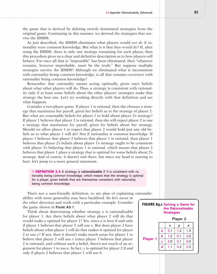
3.6 Appendix: Rationalizability (Advanced) 85
the game that is derived by deleting strictly dominated strategies from theoriginal game. Continuing in this manner, we derived the strategies that sur-vive the IDSDS.
As just described, the IDSDS eliminates what players would not do if ra-tionality were common knowledge. But what is it that they would do? If, afterusing the IDSDS, there is only one strategy remaining for each player, thenthis procedure gives us a clear and definitive description as to how players willbehave. For once all that is “impossible” has been eliminated, then “whateverremains, however improbable, must be the truth.” But suppose multiplestrategies survive the IDSDS? Although we eliminated what is inconsistentwith rationality being common knowledge, is all that remains consistent withrationality being common knowledge?
Remember that rationality means acting optimally, given one’s beliefsabout what other players will do. Thus, a strategy is consistent with rational-ity only if at least some beliefs about the other players’ strategies make thatstrategy the best one. Let’s try working directly with that definition and seewhat happens.
Consider a two-player game. If player 1 is rational, then she chooses a strat-egy that maximizes her payoff, given her beliefs as to the strategy of player 2.But what are reasonable beliefs for player 1 to hold about player 2’s strategy?If player 1 believes that player 2 is rational, then she will expect player 2 to usea strategy that maximizes his payoff, given his beliefs about her strategy.Should we allow player 1 to expect that player 2 would hold just any old be-liefs as to what player 1 will do? Not if rationality is common knowledge. Ifplayer 1 believes that player 2 believes that player 1 is rational, then player 1believes that player 2’s beliefs about player 1’s strategy ought to be consistentwith player 2’s believing that player 1 is rational, which means that player 2believes that player 1 plays a strategy that is optimal for some beliefs about 2’sstrategy. And of course, it doesn’t end there, but since my head is starting tohurt, let’s jump to a more general statement.
✚ DEFINITION 3.4 A strategy is rationalizable if it is consistent with ra-tionality being common knowledge, which means that the strategy is optimalfor a player, given beliefs that are themselves consistent with rationalitybeing common knowledge.
That’s not a user-friendly definition, so my plan of explaining rationaliz-ability with more generality may have backfired. So let’s move inthe other direction and work with a particular example. Considerthe game shown in FIGURE A3.1.
Think about determining whether strategy a is rationalizablefor player 1. Are there beliefs about what player 2 will do thatwould make a optimal for player 1? Yes, since a is best if and onlyif player 1 believes that player 2 will use x. But does player 2 havebeliefs about what player 1 will do that makes it optimal for player2 to use x? If not, then it doesn’t make much sense for player 1 tobelieve that player 2 will use x (since player 1 believes that player2 is rational), and without such a belief, there’s not much of an ar-gument for player 1 to use a. In fact, x is optimal for player 2 if andonly if player 2 believes that player 1 will use b.
1,3
3,3
5,0
2,0
3,1
1,2
1,1
2,0Player 1
Player 2
a
b
c
d
1,2
4,2
3,1
0,1
yx z
FIGURE A3.1 Solving a Game forthe RationalizableStrategies

Let’s summarize thus far: It makes sense for player 1 to use a if she believesthat player 2 will use x. It makes sense for player 1 to believe that player 2 willuse x if player 2 believes that player 1 will use b. But then, this just begs anotherquestion: Is it reasonable for player 2 to believe that player 1 will use b? If b is apoor strategy for player 1, then the belief supporting player 2’s using x is under-mined and, with it, the argument for player 1 to use a. In fact, b is strictly dom-inated by c for player 1. If player 1 believes that player 2 believes that player 1is rational, then player 1 should not believe that player 2 believes that player 1will use b, and thus we cannot rationalize player 2’s using x and thus cannot ra-tionalize player 1’s using a. Strategy a is not rationalizable, because it is not op-timal for player 1 on the basis of beliefs that are themselves consistent with ra-tionality being common knowledge.
Now consider strategy c, and let us argue that it is rationalizable. Strategyc is optimal for player 1 if she believes that player 2 will use z. But is z opti-mal for player 2, given some beliefs about what player 1 will do? We need thatto be the case in order for player 1 to believe that player 2 will use z, because,recall that player 1 believes that player 2 is rational and rational players onlyuse a strategy that is optimal, given their beliefs. If player 2 believes thatplayer 1 will use d, then playing z is indeed best for player 2. But is it reason-able for player 2 to believe that player 1 will use d? Yes it is, because d is opti-mal if player 1 believes that player 2 will play y. Hence, it is reasonable forplayer 1 to believe that player 2 believes that player 1 will play d when player1 believes that player 2 believes that player 1 believes that player 2 will play y.But is that belief consistent with rationality being common knowledge? (Youmight think that this could never end, but just hang in there for one moreround of mental gymnastics.) If player 2 believes that player 1 will play c, thenplaying y is optimal for player 2. Hence, it is reasonable for player 1 to believethat player 2 believes that player 1 believes that player 2 will play y whenplayer 1 believes that player 2 believes that player 1 believes that player 2 be-lieves that player 1 will play c. Now, what about that belief? Well take note thatwe’re back to where we started from, with player 1 playing c. We can then re-peat the argument ad infinitum:
1. Player 1’s playing c is optimal when player 1 believes that player 2 willplay z.
2. Player 2’s playing z is optimal when player 2 believes that player 1 willplay d.
3. Player 1’s playing d is optimal when player 1 believes that player 2 willplay y.
4. Player 2’s playing y is optimal when player 2 believes that player 1 willplay c.
5. Player 1’s playing c is optimal when player 1 believes that player 2 willplay z.
6. Repeat steps 2–5.
After intense use of our “little gray cells” (as the detective Hercule Poirotwould say), we conclude that strategy c is rationalizable for player 1 because it isoptimal for player 1 given beliefs as to what 2 will do and those beliefs are con-sistent with rationality being common knowledge. Furthermore, all strategies in
86 CHAPTER 3: ELIMINATING THE IMPOSSIBLE: SOLVING A GAME WHEN RATIONALITY IS COMMON KNOWLEDGE

References 87
that cycle are rationalizable using those beliefs. For example, z is optimal for 2 if2 believes 1 will use d, and 1 using d is optimal if 1 believes 2 will use y, and y isoptimal for 2 if 2 believes 1 will use c, and 1 using c is optimal if 1 believes 2 willuse z, at which point we’re back where we started from. Hence, strategies c andd are rationalizable for player 1 and y and z for player 2. In fact, one can showthat these are the only rationalizable strategies.
If you were to apply the IDSDS to this game, you’d find that those strate-gies which survive the IDSDS are exactly the same as the rationalizablestrategies just derived. Interesting? Coincidence? Not quite. First note that arationalizable strategy also survives the IDSDS because being rational impliesnot using a strictly dominated strategy. But can a strategy survive the IDSDSand not be rationalizable? Yes, it is possible, although the technical nature ofthat difference is not one that will concern us in this book. Furthermore, in awide class of circumstances, the two concepts deliver the same answer. As youcan imagine, the IDSDS is vastly easier to understand and use, which are goodenough reasons for me to make it the focus of our attention. Nevertheless, itis important to keep in mind that it is the concept of rationalizability thatdirectly encompasses what it means for a strategy to be consistent with ra-tionality being common knowledge.
REFERENCES1. This application is based on Eugene Smolensky, Selwyn Becker, and
Harvey Molotch, “The Prisoner’s Dilemma and Ghetto Expansion,” LandEconomics, 44 (1968), 419–30.
2. This game is from Steven Brams, Superior Beings (New York: Springer-Verlag, 1983). Brams has established himself as one of the most creativeusers of game theory.
3. B. A. Baldwin and G. B. Meese, “Social Behaviour in Pigs Studied by Meansof Operant Conditioning,” Animal Behaviour, 27 (1979), 947–57.
4. See, for example, Edward J. Bird and Gert G. Wagner, “Sport as a CommonProperty Resource: A Solution to the Dilemmas of Doping,” Journal ofConflict Resolution, 41 (1997), 749–66.

This page intentionally left blank

Nothing in the world is so powerful as an idea whose time has come. —VICTOR HUGO
4.1 Defining Nash EquilibriumDreamWorks initially threw down the gauntlet in the clash of the ’toon titansway back in June 2002, claiming a release date of November 5, 2004 forSharkslayer. . . . The studio’s staking out of the November date was seen as aslap at Disney, which has traditionally released its Pixar pictures that month.Disney . . . kicked up the brinkmanship factor, announcing that Sharkslayeror no, The Incredibles would also open on November 5. . . . DreamWorks[then] blinked [as it] moved the release date for its film . . . [to] October 1.1
IN SPITE OF ITS REFERENCE to a nonlethal passive fowl, Chicken is a dangerousgame. In its classic form, it begins with two cars facing each other in duel-likefashion (and typically occupied by male teenagers in pursuit of testosterone-inspired adventures). As the cars come hurtling towards one another, eachdriver is frantically deciding whether to swerve to avoid a collision or to hangtough (hoping that the other will swerve). The goal is to avoid being the firstto swerve, although if both hang tough, then the result is a mangled mess ofmetal and flesh. Chicken has been played in many contexts, including contestsbetween movie executives (with release dates) and between the leaders of theUnited States and the former Soviet Union (with nuclear weapons). TABLE 4.1lists a few other games of Chicken that have arisen in fact and fiction.
4
89
Stable Play: Nash Equilibria in DiscreteGames with Two or Three Players
TABLE 4.1 CHICKEN IN ACTION
Mode Description
Tractors Footloose (1984, movie)
Bulldozers Buster and Gob in Arrested Development (2004, TV)
Wheelchairs Two old ladies with motorized wheelchairs in Banzai (2003, TV)
Snowmobiles “[Two adult males] died in a head-on collision, earning a tie in the game of chicken theywere playing with their snowmobiles.” <www.seriouslyinternet.com/278.0.html>
Film release dates Dreamworks and Disney–Pixar (2004)
Nuclear weapons Cuban Missile Crisis (1963): “Since the nuclear stalemate became apparent, the Governmentsof East and West have adopted the policy which Mr. Dulles calls ‘brinksmanship.’ This is apolicy adapted from a sport which, I am told, is practised by some youthful degenerates. Thissport is called ‘Chicken!’ ” (Bertrand Russell, Common Sense and Nuclear Warfare, 1959)

90 CHAPTER 4: STABLE PLAY: NASH EQUILIBRIA IN DISCRETE GAMES WITH TWO OR THREE PLAYERS
FIGURE 4.1 provides a strategic form representationof Chicken.* Because neither player has a strictly dom-inated strategy, the iterative deletion of strictly domi-nated strategies (IDSDS, Section 3.4.2) won’t help ussolve this game. But don’t forsake hope, as game the-ory has many more game-solving tricks to offer.
If you’ve either read the book or seen the movie ABeautiful Mind, then you know about the brilliantschizophrenic mathematician John Nash. In his
doctoral thesis at Princeton University, Dr. Nash made two striking game-theoretic advances—one of which became known as Nash equilibrium—thatresulted in his winning the Nobel Prize in Economics more than 40 years later.
To understand what Nash equilibrium is and why it is an appropriatemethod for solving a game, let us return to the discussion of the previouschapter. In the context of a game, a player is rational when he chooses a strat-egy to maximize his payoff, given his beliefs about what other players will do.The tricky part is figuring out what is reasonable for a player to believe aboutthe strategy another player will select. Chapter 3 used the assumption that ra-tionality is common knowledge among the players to derive those beliefs. Forexample, if player 2 has a dominant strategy and player 1 believes that player2 is rational, then player 1 believes that player 2 will use her dominant strat-egy. In this manner, we derived player 1’s beliefs regarding player 2’s strategy.
The approach of Nash equilibrium maintains the assumption that playersare rational, but takes a different approach to nailing down beliefs. What Nashequilibrium does is require that each player’s beliefs about other players’ strate-gies be correct. For example, the strategy that player 1 conjectures that player 2will use is exactly what player 2 actually does use. The definition of Nash equi-librium is then made up of two components:
1. Players are rational: Each player’s strategy maximizes his payoff, givenhis beliefs about the strategies used by the other players.
2. Beliefs are accurate: Each player’s beliefs about the strategies used bythe other players are true.
Condition (1) is innocent enough; it’s condition (2) that is tougher to swallow.It requires that players be effective prognosticators of the behavior of others. Insome settings, that may be a reasonable assumption; in others, it may not.Combining the assumptions about behavior—that it is always rational—and be-liefs—that they are always true—gives us the definition of Nash equilibrium.
✚ DEFINITION 4.1 A strategy profile is a Nash equilibrium if each player’sstrategy maximizes his or her payoff, given the strategies used by the otherplayers.
With n players, there are, then, n conditions that must be satisfied in orderfor a strategy profile to be a Nash equilibrium—one condition for each player
FIGURE 4.1 The Game of Chicken
2,2
3,1
1,3
0,0Driver 1
Driver 2
Swerve
Hang tough
Swerve Hang tough
*You might be tempted to put large negative numbers for the strategy pair in which both participantschoose hang tough, since this means certain injury and possible death. You can do so, but it’ll make no dif-ference as regards the solution. As long as the payoffs when both hang tough are less than all the otherpayoffs in the matrix, our conclusions regarding behavior will be the same. This condition reflects theproperty that what matters is the ranking of the payoffs, not their actual values.

4.1 Defining Nash Equilibrium 91
which ensures that a player’s strategy is optimal, given the other players’ strate-gies. Thus, all players are simultaneously doing their best. A violation of one ormore of those conditions means that a strategy profile is not a Nash equilib-rium. Unlike the game of horseshoes, you don’t come “close to a Nash equilib-rium” by having all but one of the conditions satisfied; it’s either all or nothing.
An appeal of Nash equilibrium as a solution concept is that it identifiesstrategy profiles that are stable in the sense that each player is content to dowhat she is doing, given what everyone else is doing. Consider, for instance, astrategy profile that is not a Nash equilibrium because, say, player 3’s strategyis not best for her, given what the other players are up to. We would then ex-pect player 3 to change her strategy once she discovers that it is not optimal.In contrast, a Nash equilibrium is not subject to such second-guessing, be-cause players are happy with what they are doing.
To be more concrete on this point, imagine that players play the same gameover and over. If they are not currently acting according to a Nash equilibrium,then, after one of the game’s interactions, there will be a player who will learnthat his strategy is not the best one available, given what others are doing. Hewill then have an incentive to change his strategy in order to improve his pay-off. In contrast, if players are behaving according to a Nash equilibrium, theyare satisfied with their actions after each round of interactions. Behavior gen-erated by a Nash equilibrium is then expected to persist over time, and socialscientists are generally interested in understanding persistent behavior (notnecessarily because unstable behavior is uninteresting, but rather because itis just much harder to explain).
Hopefully having convinced you that Nash equilibrium is a worthy solutionconcept (and if not, bear with me), let’s put it to use with the game of Chicken.We begin by considering the four strategy pairs and asking whether each is aNash equilibrium.
■ (hang tough, hang tough). If driver 2 chooseshang tough, then driver 1’s payoff from swerveis 1 and from hang tough is 0. (See FIGURE 4.2.)Thus, driver 1 prefers to swerve (and live witha few clucking sounds from his friends) thanto hang tough (and learn whether or not thereis an afterlife). Thus, hang tough is not best forplayer 1, which means that player 1’s Nashequilibrium condition is not satisfied. Hence,we can conclude that (hang tough, hang tough)is not a Nash equilibrium. (It is also true thatdriver 2’s strategy of hang tough is not best forher either, but we’ve already shown this strat-egy pair is not a Nash equilibrium.)
■ (swerve, swerve). If driver 1 chooses swerve,then driver 2’s payoff from swerve is 2 andfrom hang tough is 3. (See FIGURE 4.3.) Driver 2thus prefers hang tough if driver 1 is going tochicken out. Since swerve is not the best strat-egy for driver 2, (swerve, swerve) is not a Nashequilibrium either.
FIGURE 4.3 Chicken: Highlighting Driver 2’sPayoffs when Driver 1 ChoosesSwerve
Driver 1
Driver 2
Swerve
Hang tough
Swerve Hang tough
2, 2 3,1
1, 3
0,0
FIGURE 4.2 Chicken: Highlighting Driver 1’sPayoffs when Driver 2 ChoosesHang Tough
2,2
3,1
1 ,3
0 ,0Driver 1
Driver 2
Swerve
Hang tough
Swerve Hang tough

92 CHAPTER 4: STABLE PLAY: NASH EQUILIBRIA IN DISCRETE GAMES WITH TWO OR THREE PLAYERS
■ (swerve, hang tough). If driver 2 chooses hang tough, swerve is the beststrategy for driver 1, as it produces a payoff of 1 compared with 0 fromhanging tough. Consequently, the requirement that driver 1’s strategy isbest for him is satisfied. Turning to driver 2, we see that hang tough is bestfor her, because it yields a payoff of 3, rather than 2 from swerve. The con-dition ensuring that driver 2’s strategy is optimal for her is satisfied aswell. Because each driver is choosing the best strategy, given what theother driver is expected to do, (swerve, hang tough) is a Nash equilibrium.
■ (hang tough, swerve). By logic similar to that in the preceding case, thisstrategy pair is a Nash equilibrium, too.
Summing up, there are two Nash equilibria in this game: (swerve, hangtough) and (hang tough, swerve). Both predict that there will be no car crashand, furthermore, that one and only one driver will swerve. However, Nashequilibrium doesn’t tell us which driver will swerve.
Perhaps the best way to play Chicken is to com-mit to not swerving by eliminating swerve from yourstrategy set and, most importantly, making thisknown to the other driver. FIGURE 4.4 illustrates whatthe game would look like if driver 1 were to elimi-nate swerve from his strategy set. The game now hasonly one Nash equilibrium: driver 1 hangs toughand driver 2 chickens out.
A tactic similar to that illustrated in Figure 4.4was taken in a naval encounter about 20 years ago.
Let’s listen in on the radio conversation between the two participants.2
1: “Please divert your course 15 degrees to the north to avoid a collision.”
2: “Recommend that you change your course 15 degrees to the south toavoid a collision.”
1: “This is the captain of a U.S. navy ship. I say again, divert your course.”
2: “No, I say again, divert your course.”
1: “This is the aircraft carrier Enterprise; we are a large warship of the U.S.navy. Divert your course now!”
2: “This is a lighthouse. Your call.”
We have several tasks ahead of us in this chapter. Having defined Nash equilib-rium, we want to learn how to solve games for Nash equilibria and begin to ap-preciate how this concept can be used to derive an understanding of human be-havior. Our analysis commences in Section 4.2 with some simple two-player gamesthat embody both the conflict and mutual interest that can arise in strategic situa-tions. To handle more complicated games, the best-reply method for solving forNash equilibria is introduced in Section 4.3 and is then applied to three-playergames in Section 4.4. Finally, Section 4.5 goes a bit deeper into understanding whatit means to suppose that players behave as described by a Nash equilibrium.
4.2 Classic Two-Player GamesTHE MAIN OBJECTIVE OF this chapter is to get you comfortable both with the con-cept of Nash equilibrium and with deriving Nash equilibria. Let’s warm upwith a few simple games involving two players, each of whom has at most
FIGURE 4.4 Chicken when Driver 1 HasEliminated Swerve as a Strategy
3,1 0,0Driver 1
Driver 2
Hang tough
Swerve Hang tough

4.2 Classic Two-Player Games 93
three strategies. As we’ll see, a game can have one Nash equilibrium, severalNash equilibria, or no Nash equilibrium. The first case is ideal in that we pro-vide a definitive statement about behavior. The second is an embarrassmentof riches: we cannot be as precise as we’d like, but in some games there maybe a way to select among those equilibria. The last case—when there is noNash equilibrium—gives us little to talk about, at least at this point. Althoughin this chapter we won’t solve games for which there is no Nash equilibrium,we’ll talk extensively about how to handle that problem in Chapter 7.
You may be wondering whether there is an “easy-to-use” algorithm for solvingNash equilibria. Chapter 3, for example, presented an algorithm for findingstrategies consistent with rationality being common knowledge: the iterativedeletion of strictly dominated strategies (IDSDS). Unfortunately, there is no suchmethod for solving Nash equilibrium. For finite games—that is, when there is afinite number of players and each player has a finite number of strategies—theonly universal algorithm is exhaustive search, which means that one has tocheck each and every strategy profile and assess whether it is a Nash equilibrium.We will, however, present some shortcuts for engaging in exhaustive searches.
A useful concept in deriving Nash equilibria is a player’s best reply (or bestresponse). For each collection of strategies for the other players, a player’sbest reply is a strategy that maximizes her payoff. Thus, a player has not justone best reply, but rather a best reply for each configuration of strategies forthe other players. Furthermore, for a given configuration of strategies for theother players, there can be more than one best reply if there is more than onestrategy that gives the highest payoff.
✚ DEFINITION 4.2 A best reply for player i to (s1, . . ., si"1, si%1, . . ., sn)is a strategy that maximizes player i’s payoff, given that the other n " 1players use strategies (s1, . . ., si"1, si%1, . . ., sn).
A Nash equilibrium can be understood as a strategy profile which ensuresthat a player’s strategy is a best reply to the other players’ strategies, for eachand every player. These are the same n conditions invoked by Definition 4.1,but we’re just describing them a bit differently.
! SITUATION: PRISONERS’ DILEMMA
During the time of Stalin, an orchestra conductor was on a train reading a mu-sical score. Thinking that it was a secret code, two KGB officers arrested theconductor, who protested that it was just Tchaikovsky’s Violin Concerto. Thenext day, the interrogator walks in and says, “You might as well confess, aswe’ve caught your accomplice Tchaikovsky, and he’s already talking.”
The Prisoners’ Dilemma, which we previously considered under the guiseof the opera Tosca, is the most widely examined game in game theory. Twomembers of a criminal gang have been arrested and placedin separate rooms for interrogation. Each is told that if onetestifies against the other and the other does not testify, theformer will go free and the latter will get three years of jailtime. If each testifies against the other, they will both besentenced to two years. If neither testifies against the other,each gets one year. Presuming that each player’s payoff ishigher when he receives a shorter jail sentence, the strate-gic form is presented in FIGURE 4.5.
FIGURE 4.5 The Prisoners’ Dilemma
2,2
1,4
4,1
3,3Criminal 1
Criminal 2
Testify
Silence
Testify Silence

94 CHAPTER 4: STABLE PLAY: NASH EQUILIBRIA IN DISCRETE GAMES WITH TWO OR THREE PLAYERS
This game has a unique Nash equilibrium, which is that both players choosetestify. Let us first convince ourselves that (testify, testify) is a Nash equilibrium.If criminal 2 testifies, then criminal 1’s payoff from also testifying is 2, while itis only 1 from remaining silent. Thus, the condition ensuring that criminal 1’sstrategy is optimal is satisfied. Turning to criminal 2, we see that, given thatcriminal 1 is to testify, she earns 2 from choosing testify and 1 from choosingsilence. So, the condition ensuring that criminal 2’s strategy is optimal is alsosatisfied. Hence, (testify, testify) is a Nash equilibrium.
Let us make two further points. First, the Prisoners’ Dilemma is an exampleof a symmetric game. A two-player game is symmetric if players have the samestrategy sets, and if you switch players’ strategies, then their payoffs switch.For example, if the strategy pair is (testify, silence), then the payoffs are 4 forcriminal 1 and 1 for criminal 2. If we switch their strategies so that the strat-egy pair is (silence, testify), the payoffs switch: now criminal 1’s payoff is 1while criminal 2’s payoff is 4. A trivial implication of the symmetric conditionis that players who choose the same strategy will get the same payoff.
An important aspect of symmetric games is that if a symmetric strategyprofile—such as (testify, testify)—is optimal for one player, it is also optimal forthe other player. If criminal 1’s strategy is optimal (given what criminal 2 isdoing), then it must also be the case that criminal 2’s strategy is optimal (givenwhat criminal 1 is doing). By the symmetry in the game and the considerationof a symmetric strategy profile, the equilibrium conditions for the players areidentical. Thus, for a symmetric strategy profile in a symmetric game, eitherall of the Nash equilibrium conditions hold or none do. Now that we know thisproperty, it is sufficient to show that if testify is optimal for criminal 1 (giventhat criminal 2 chooses testify), testify must also be optimal for criminal 2.
For a symmetric strategy profile in a symmetric game, if one player’sstrategy is a best reply, then all players’ strategies are best replies.
Note also that testify is a dominant strategy. Regardless of what the othercriminal does, testify produces a strictly higher payoff than silence. With a littlethought, it should be clear that if a player has a dominant strategy, then a Nashequilibrium must have her using it. For a player’s strategy to be part of a Nashequilibrium, the strategy must be optimal, given the strategies used by theother players. Because a dominant strategy is always the uniquely best strategy,then it surely must be used in a Nash equilibrium. It follows that if all playershave dominant strategies—as in the Prisoners’ Dilemma—the game has aunique Nash equilibrium in which those dominant strategies are used. Thus,(testify, testify) is the unique Nash equilibrium in the Prisoners’ Dilemma.
© S
COTT
AD
AM
S/D
IST.
BY
UN
ITED
FEA
TURE
SYN
DIC
ATE,
INC.
Dilbert/Scott Adams

If a player has a dominant strategy, a Nash equilibrium requires thatthe player use it. If all players have a dominant strategy, then there is a uniqueNash equilibrium in which each player uses his or her dominant strategy.
! SITUATION: A COORDINATION GAME—DRIVING CONVENTIONS
We next look at an example of a coordination game, which has the propertythat players have a common interest in coordinating their actions. A coordi-nation game that most adults engage in every day is the choice of the side ofthe road upon which to drive. It’s not really that important whether everyonedrives on the left (as in England and Japan) or on the right (as in the UnitedStates and Chile), but just that we agree to a standard.
The game between two drivers is represented inFIGURE 4.6. It is easy to verify that there are twoNash equilibria. One has both Thelma and Louisedriving on the left, and the other has both drivingon the right. If Louise drives on the left, thenThelma’s payoff from doing the same is 1, while it is"1 from driving on the right. Thus, left is indeedbest for Thelma, given that Louise is choosing left.The same argument verifies that Louise’s driving onthe left is best, given that Thelma drives on the left.In fact, since this is a symmetric game, I can invoke the magic words—“bysymmetry”—to conclude that Louise’s strategy of left is optimal as well. Thismakes (left, left) a Nash equilibrium. An analogous argument allows us toconclude that (right, right) is a Nash equilibrium.
In contrast, (left, right) is not a Nash equilibrium. Given that Louise is driv-ing on the right, Thelma’s payoff from driving on the left is "1, while she cando better by driving on the right and getting a payoff of 1. It is straightforwardalso to argue that (right, left) is not a Nash equilibrium.
Nash equilibrium doesn’t tell us which standard a population of drivers willsettle upon; instead, it tells us only that they will settle upon some standard.History shows that societies do settle upon a driving convention, and which sideof the road it is can vary across time and space. It is estimated that about 75% ofall roads have the custom of driving on the right.3 Although today everyone con-forms to a driving convention because it’s the law, conventions developed longbefore they were legislated (and, indeed, long before automobiles came on thescene). Generally, the law just codified a custom that had developed on its own.
Suppose an American driver and an English driver are drivingtowards each other on neutral ground. Each is driving a car from her owncountry. All of this is common knowledge. On which side of the road will eachdrive? Will it turn into a game of Chicken? Is Nash equilibrium a good predictor?
! SITUATION: A GAME OF COORDINATION AND CONFLICT—TELEPHONE
In the driving conventions game, there were two Nash equilibria and the play-ers were indifferent between them: driving on the right was just as good asdriving on the left. Now let us consider a setting that also has two equilibria,but the players rank them differently.
4.2 Classic Two-Player Games 95
FIGURE 4.6 Driving Conventions
1,1
1,1!1,!1
!1,!1Thelma
Louise
Drive left
Drive right
Drive left Drive right

96 CHAPTER 4: STABLE PLAY: NASH EQUILIBRIA IN DISCRETE GAMES WITH TWO OR THREE PLAYERS
Colleen is chatting on the phone with Winnie and suddenlythey’re disconnected. Should Colleen call Winnie or shouldWinnie call Colleen? Colleen and Winnie are the players, and theyhave a strategy set composed of call and wait. Each is willing tocall the other if that is what it takes to continue the conversation,but each would prefer the other to do so. If they both try to callback, then the other’s phone is busy and thus they don’t reconnect.Obviously, if neither calls back, then they don’t reconnect either.The strategic form game is shown in FIGURE 4.7.*
The strategy pair (call, call) is not a Nash equilibrium, since, forexample, Colleen earns 0 from call, but a higher payoff of 3 from wait. Thus,Colleen’s strategy of call is not optimal should Winnie choose call. Nor is (wait,wait) a Nash equilibrium, since, for example, Winnie earns 1 from choosingwait and a higher payoff of 2 from choosing call should Colleen choose wait.Thus, Winnie’s strategy is not optimal, given what Colleen is doing.
A strategy pair that is a Nash equilibrium has one player calling back whilethe other waits. Consider the strategy pair (call, wait), so that Colleen is tocall. Given that Winnie is waiting for Colleen’s call, Colleen prefers to call, asit delivers a payoff of 2 while waiting has a payoff of only 1. And if Winnie an-ticipates that Colleen will call her, then Winnie prefers to wait for Colleen’scall. For Winnie, waiting delivers a payoff of 3, whereas should she call, thepayoff is 0.
If the telephone game is symmetric (and it is), we can infer by symmetry from(call, wait) being a Nash equilibrium that (wait, call) is also a Nash equilibrium(where now it is Winnie who is to call). To see why, first convince yourself thatthis is a symmetric game. If the strategy pair is (call, wait), then Colleen gets apayoff of 2 and Winnie gets 3. If we switch the strategies so that the strategy pairis (wait, call), then Colleen now gets a payoff of 3 and Winnie gets 2.Furthermore, they have the same payoff when they choose the same strategy.This symmetry implies that the Nash equilibrium condition for Winnie at strat-egy pair (wait, call) is the same as the Nash equilibrium condition for Colleen at(call, wait), and the Nash equilibrium condition for Colleen at (wait, call) is thesame as the Nash equilibrium condition for Winnie at (call, wait). Thus, if, at(call, wait), Colleen finds it optimal to choose call, then Winnie must find it op-timal to choose call at strategy pair (wait, call); the conditions are exactly thesame. Either both conditions hold or neither does. Similarly, if, at (call, wait),Winnie finds it optimal to choose wait, then Colleen must find it optimal tochoose wait at (wait, call).
In sum, by virtue of the game being symmetric, either both (wait, call )and (call, wait) are Nash equilibria or neither are. Since we’ve shown that(call, wait) is a Nash equilibrium, then, by symmetry, (wait, call ) is a Nashequilibrium.
If a game is symmetric, but the equilibrium is asymmetric, howdo players coordinate? How would you coordinate in the telephone game?
0,0
3,2
2,3
1,1Colleen
Winnie
Call
Wait
Call Wait
FIGURE 4.7 The Telephone Game
*This is the same game as the well-known “Battle of the Sexes,” though recast in a more gender-neutralsetting. The original game was one in which the man wants to go to a boxing match and the woman wantsto go to the opera. Both would prefer to do something together than to disagree.

4.2 Classic Two-Player Games 97
! SITUATION: AN OUTGUESSING GAME—ROCK–PAPER–SCISSORS
Lisa: Look, there’s only one way to settle this: Rock–Paper–Scissors.
Lisa’s Brain: Poor predictable Bart. Always picks rock.
Bart’s Brain: Good ol’ rock. Nothin’ beats that!
(Bart shows rock, Lisa shows paper)
Bart: Doh!—FROM THE EPISODE “THE FRONT,” OF THE SIMPSONS.
How many times have you settled a disagreement by usingRock–Paper–Scissors? In case you come from a culture that doesn’t use thisdevice, here’s what it’s all about. There are two people, and each person moveshis hands up and down four times. On the fourth time, each person comesdown with either a closed fist (which signals her choice of rock), an open hand(signaling paper), or the middle finger and forefinger in the shape of scissors(no explanation required). The winner is determined as follows: If one personchooses rock and the other scissors, then rock wins, since scissors break whentrying to cut rock. If one person chooses rock and the other paper, then paperwins, as paper can be wrapped around rock. And if one person chooses paperand the other scissors, then scissors wins, since scissors can cut paper. If thetwo players make identical choices, then it is considered a draw (or, more typ-ically, they play again until there is a winner).
If we assign a payoff of 1 to winning, "1 to losing, and0 to a draw, then the strategic form game is as describedin FIGURE 4.8. Contrary to Bart’s belief, rock is not a dom-inant strategy. While rock is the unique best replyagainst scissors, it is not the best reply against paper. Infact, there is no dominant strategy. Each strategy is abest reply against some strategy of the other player.Paper is the unique best reply against rock, rock is theunique best reply against scissors, and scissors is theunique best reply against paper.
Without any dominated strategies, the IDSDS won’tget us out of the starting gate; all strategies survive the IDSDS. So, being goodgame theorists, we now pull Nash equilibrium out of our toolbox and go towork. After much hammering and banging, we chip away some of these strat-egy pairs. We immediately chip off (rock, rock), as Bart ought to choose paper,not rock, if Lisa is choosing rock. Thus, (rock, rock) now lies on the floor, hav-ing been rejected as a solution because it is not a Nash equilibrium. We turn to(paper, rock), and while Bart’s strategy of paper is a best reply, Lisa’s is not, sincescissors yields a higher payoff than rock when Bart is choosing paper. Hence,(paper, rock) joins (rock, rock) on the floor. We merrily continue with our work,and before we know it, the floor is a mess as everything lies on it! None of thenine strategy pairs is a Nash equilibrium.
You could check each of these nine strategy pairs and convince yourself thatthat claim is true, but let me offer a useful shortcut for two-player games.Suppose we ask whether Lisa’s choice of some strategy, call it y, is part of aNash equilibrium. (I say “part of,” since, to even have a chance at being a Nashequilibrium, there must also be a strategy for Bart.) For y to be part of a Nashequilibrium, Bart must choose a strategy (call it c) that is a best reply to Lisa’s
FIGURE 4.8 Rock–Paper–Scissors
Bart
Lisa
Rock
Paper
Scissors
PaperRock Scissors
0,0
1,!1
!1,1 0,0
1,!1
!1,10,0
1,!1
!1,1

98 CHAPTER 4: STABLE PLAY: NASH EQUILIBRIA IN DISCRETE GAMES WITH TWO OR THREE PLAYERS
choosing y. Choosing such a strategy ensures that Bart’s Nash equilibrium con-dition is satisfied. To ensure that Lisa is also acting optimally, we then need toderive her best reply to Bart’s choosing c (which, recall, is his best reply to Lisa’schoosing y). Now suppose that Lisa’s best reply to c is actually y, which is thestrategy we started with for Lisa. Then we have shown that y is indeed part ofa Nash equilibrium and the equilibrium is, in fact, (c, y). However, if Lisa’s bestreply to Bart’s choosing c is not y, then we conclude that y is not part of anyNash equilibrium. In that case, in one fell swoop we’ve eliminated all strategyprofiles involving Lisa’s choosing y. Putting it pictorially, this is what we needto happen for Lisa’s playing y to be part of a Nash equilibrium:
Lisa plays y S Bart’s best reply to y is c S Lisa’s best reply to c is y.
To put this algorithm into action, let us ask whether Lisa’s choosing rock ispart of a Nash equilibrium. If Bart thinks that Lisa is going to choose rock, thenhe wants to choose paper. Now, if Bart chooses paper, then Lisa wants to choosescissors. Since this option is different from what we initially assumed that Lisawould choose, which was rock, we conclude that there is no Nash equilibriumin which Lisa chooses rock. Hence, none of the strategy profiles in which Lisachooses rock—namely, (rock, rock), (paper, rock), and (scissors, rock)—are Nashequilibria. Now let’s do the same trick on the strategy paper for Lisa in order todetermine whether her choosing paper is part of an equilibrium. If Lisa choosespaper, Bart’s best reply is scissors, and Lisa’s best reply to Bart’s selection of scis-sors is rock, not paper. Hence, Lisa’s using paper is not part of any Nash equilib-rium, so we can eliminate (rock, paper), (paper, paper), and (scissors, paper) asNash equilibria. Finally, using the same method, we can show that Lisa’s choos-ing scissors is not part of any Nash equilibrium. In this manner, we’ve proventhat there is no Nash equilibrium for the game of Rock–Paper–Scissors.
Rock–Paper–Scissors is an example of an outguessing game. In an out-guessing game, maximizing your payoff requires that you outguess the otherplayer (or players). That is, you want to do what they don’t expect. If the otherplayer thinks that you’re going to play strategy x, and she responds by playingb, then you don’t want to play x in response to her playing b; instead, you wantto respond with something else. For example, if Lisa thinks that Bart is goingto play rock, then she’ll play paper, in which case Bart doesn’t want to do as Lisaexpects. Instead, he should play scissors, not rock. (Unfortunately, Bart isn’tthat smart, but you have to blame Matt Groening for that, not game theory.)
As it turns out, outguessing games arise in many situations. Sports and mil-itary conflicts are two prominent examples; we’ll investigate them quite ex-tensively in Chapter 7. However, be forewarned: if you intend to enter the USARock–Paper–Scissors League (yes, there is such a thing), game theory reallycan’t help you design a winning strategy.
That Rock–Paper–Scissors is not just a kid’s game was recently demonstratedby the two leading auction houses: Christie’s and Sotheby’s. The owner of an artcollection worth in excess of $20 million decided to determine which auctionhouse would sell his collection—and, consequently, earn millions of dollars incommissions—on the basis of the outcome of a round of Rock–Paper–Scissors.4
Rather than play the game in the traditional way, however, with physical handmovements, an executive for Christie’s and an executive for Sotheby’s eachwrote down one of the three strategies on a piece of paper. Christie’s won, choos-ing rock to beat Sotheby’s scissors.

4.3 The Best-Reply Method 99
CONFLICT AND MUTUAL INTEREST IN GAMES
Rock–Paper–Scissors is a game of pure conflict. What do I mean by that?Well, take note of an interesting property of the payoff matrix in Figure 4.8:Players’ payoffs always sum to the same number (which happens to bezero). For example, if both Bart and Lisa choose rock, then each gets zero,so the sum of their payoffs is zero. If Bart chooses paper and Lisa choosesrock, then Bart gets 1 and Lisa gets "1, which once again sums to zero. Forevery strategy pair, the sum of their payoffs is zero. This type of game isknown as a constant-sum game, because the payoffs always sum to thesame number. When that number happens to be zero, the game is called azero-sum game.
So think about what this implies. Since payoffs must sum to the same num-ber, if some strategy pair results in a higher payoff for Bart, then it must re-sult in a lower payoff for Lisa. Thus, what makes Bart better off has to makeLisa worse off, and analogously, what makes Lisa better off has to make Bartworse off. It is in that sense that Rock–Paper–Scissors is a game of pure con-flict. In fact, all constant-sum games have this property.
Contrast this game with driving conventions. Here we have the opposite ofRock–Paper–Scissors, in the sense that there is no conflict at all. A strategypair that makes driver 1 better off—such as (left, left) compared with (left,right)—also makes driver 2 better off; they both get a payoff of 1 rather than0. This is a game of mutual interest, as the rankings of strategy pairs by theirpayoffs coincides for the players.
Chicken and the telephone game lie between these two extremes. Thosestrategic settings do provide grounds for mutual interest. In Chicken, bothplayers want to avoid (hang tough, hang tough); they both prefer (swerve, hangtough) and (hang tough, swerve). But there is also room for conflict, as theydisagree as to how they rank (swerve, hang tough) and (hang tough, swerve);driver 1 prefers the latter and driver 2 prefers the for-mer. Similarly, with the telephone game, both Colleenand Winnie agree that one of them calling is preferableto either both of them waiting or both calling, but theydisagree as to who should call. Colleen prefers that it beWinnie, while Winnie prefers it to be Colleen. Theyshare a common interest in coordinating on exactly oneperson calling, but their interests depart—they are inconflict—when it comes to who that person should be.
Knowing whether players’ interests are entirely inconflict, partially in conflict, or entirely in common canprovide some insight into which strategy profiles areNash equilibria. So, when you come to a game, thinkabout the interests of the players before launching intoa robotic search for solutions. Your ruminations mayoffer some valuable shortcuts.
4.3 The Best-Reply MethodAS THE CELEBRATED TV chef Emeril Lagasse would say, “Let’s kick it up a notch!”by adding a third player to the mix. But before doing so, I’ll share a usefulshortcut with you for deriving Nash equilibria.
For the game in FIGURE 4.9, find all Nashequilibria.
FIGURE 4.9
4.1 CHECK YOUR UNDERSTANDING
0,1 0,1
1,2
3,0
2,1
1,0
0,1
2,2Player 1
Player 2
a
b
c
d
1,0
1,1
1,2
4,0
3,2
3,1
1,0
0,2
w x y z

100 CHAPTER 4: STABLE PLAY: NASH EQUILIBRIA IN DISCRETE GAMES WITH TWO OR THREE PLAYERS
Recall that a player’s best reply is a strategy that maximizes his pay-off, given the strategies used by the other players. We can then think ofa Nash equilibrium as a strategy profile in which each player’s strategyis a best reply to the strategies the other players are using. Stemmingfrom this perspective, the best-reply method offers a way of finding allof the Nash equilibria. Rather than describe it in the abstract, let’s walkthrough the method for the two-player game in FIGURE 4.10.
For each strategy of Diane, we want to find Jack’s best replies. If Dianeuses x, then Jack has two best replies—b and c—each of which gives apayoff of 2 that exceeds the payoff of 1 from the other possible strategy,a. If Diane uses y, then Jack has a unique best reply of a. And if Diane uses
z, then c is Jack’s only best reply. To keep track of these best replies, circle those ofJack’s payoffs associated with his best replies, as shown in FIGURE 4.11.
Next, perform the same exercise on Diane by finding her best replies in re-sponse to each of Jack’s strategies. If Jack uses a, then both x and y are Diane’sbest replies. If Jack uses b, then Diane’s best reply is x. Finally, if Jack uses c,then y is Diane’s best reply. Circling the payoffs for Diane’s best replies, we nowhave FIGURE 4.12.
FIGURE 4.10 Jack and Diane’sStrategies
1,1
2,1
2,3
2,1
1,2
0,2Jack
Diane
a
b
c
2,0
3,0
2,1
x y z
FIGURE 4.12 Diane’s and Jack’s BestReplies (Circled). TwoStrategy Pairs Are NashEquilbria: (b,x) and (a,y)
FIGURE 4.11 Jack’s Best Replies(Circled)
1,1 2 ,1
2 ,1
2 ,3
1,2
0,2Jack
Diane
a
b
c
2,0
3 ,0
2,1
x y z
Jack
Diane
a
b
c
x y z
2,0
3 ,0
2,1
1, 1
2 ,1
2 , 3
2 , 1
1, 2
0,2
Since a Nash equilibrium is a strategy pair in which each player’s strategyis a best reply, we can identify Nash equilibria inFigure 4.12 as those strategy pairs in which both pay-offs in a cell are circled. Thus, (b,x) and (a,y) are Nashequilibria. We have just used the best-reply method toderive all Nash equilibria.
Before we explore how the best-reply method isused in three-player games, let’s deploy it in Rock–Paper–Scissors. Marking each of Lisa’s and Bart’s bestreplies, we have FIGURE 4.13. For example, if Lisachooses rock, then Bart’s best reply is paper, so we cir-cle Bart’s payoff of 1 earned from the strategy pair(paper, rock). Note that no cell has two circled payoffs,indicating that there is no Nash equilibrium; this isthe same result we derived earlier.
FIGURE 4.13 Best Replies (Circled) for Bartand Lisa’s Game of Rock–Paper–Scissors. There Is NoNash Equilibrium
Bart
Lisa
Rock
Paper
Scissors
PaperRock Scissors
0,0
1 ,!1
!1, 1
0,0
1 ,!1
!1, 1
0,0
1 ,!1
!1, 1

4.4 Three-Player Games 101
4.4 Three-Player Games! SITUATION: AMERICAN IDOL FANDOM
Alicia, Kaitlyn, and Lauren are ecstatic. They’ve just landed tickets to attendthis week’s segment of American Idol. The three teens have the same favoriteamong the nine contestants that remain: Ace Young. They’re determined totake this opportunity to make a statement. While IMing, they come up with aplan to wear T-shirts that spell out “ACE” in large letters. Lauren is to wear aT-shirt with an big “A,” Kaitlyn with a “C,” and Alicia with an “E.” If they pullthis stunt off, who knows—they might end up on national television! OMG!
While they all like this idea, each is tempted to wear instead an attractivenew top just purchased from their latest shopping expedition at Bebe. It’s nowan hour before they have to leave to meet at the studio, and each is at hometrying to decide between the Bebe top and the lettered T-shirt. What shouldeach wear?
In specifying the strategic form of this game, we assign a payoff of 2 if theyall wear their lettered T-shirts (and presumably remember to sit in the rightsequence). This payoff is higher than the one they get from wearing the Bebetop, which is 1. Finally, wearing a lettered T-shirt when one or both of theother girls do not yields a payoff of 0, as the wearer realizes the worst of allworlds: she doesn’t look alluring and they don’t spell out ACE.
The strategic form is shown in FIGURE 4.14.* Lauren’s choice is representedas selecting a row—either wearing the T-shirt with the letter “A” or her Bebetop—while Kaitlyn chooses a column and Alicia chooses a matrix.
FIGURE 4.14 American Idol Fandom
Alicia chooses E Alicia chooses Bebe
2,2,2 0,1,0
1,0,0 1,1,0Lauren
Kaitlyn
A
Bebe
BebeC
Lauren
Kaitlyn
0,0,1 0,1,1
1,0,1 1,1,1
A
Bebe
BebeC
Using the best-reply method to solve this game, consider the situation facedby Lauren. If Alicia wears her T-shirt with E and Kaitlyn wears hers with C,then Lauren’s best reply is to do her part and wear the T-shirt with A. So, wecircle Lauren’s payoff of 2 in the cell associated with strategy profile (A, C, E),as shown in FIGURE 4.15. If, instead, Kaitlyn chooses Bebe and Alicia wears E,then Lauren’s best reply is to wear her Bebe top and receive a payoff of 1, sowe circle that payoff for Lauren. If Alicia wears her Bebe top and Kaitlynwears C, then Lauren’s best reply is again to wear her Bebe top, so we circleLauren’s payoff of 1. Finally, if both of the other two girls choose their Bebe
*This game is a 21st-century teen girl version of the Stag Hunt game due to Jean-Jacques Rousseau in Onthe Origins and Foundations of Inequality among Men (1755). In that setting, hunters can work together tocatch a stag (rather than spell out ACE) or hunt individually for hare (rather than wear a Bebe top).

102 CHAPTER 4: STABLE PLAY: NASH EQUILIBRIA IN DISCRETE GAMES WITH TWO OR THREE PLAYERS
tops, then Lauren optimally does so as well, which means that we now circleLauren’s payoff of 1 in that instance. Performing this same exercise for Kaitlynand Alicia, we end up with Figure 4.15.
Examining the figure, we find that there are two Nash equilibria—that is,two strategy profiles in which all three payoffs are circled—signifying that allthree teens are choosing best replies. One equilibrium is when Lauren wears A,Kaitlyn wears C, and Alicia wears E, which, to the delight of Ace Young, spellsout his name on American Idol. The other equilibrium occurs when each tossesher lettered T-shirt aside and instead wears that eye-catching top from Bebe.
Note that the players rank the Nash equilibria the same: all prefer wearingthe T-shirts spelling out ACE than wearing Bebe shirts. The situation differsfrom that pertaining to driving conventions, in which players are indifferentamong equilibria, and also from that in the Chicken and telephone games, inwhich players ranked equilibria differently.
! SITUATION: VOTING, SINCERE OR DEVIOUS?
A company has three shareholders. Shareholder 1 controls 25% of the shares,shareholder 2 controls 35%, and shareholder 3 controls 40%. The companyhas offers from two other companies, denoted A and B, to purchase it. Thereis also a third option, which is to decline both offers. Shareholder 1 ranks thethree choices, from the most to least preferred, as follows: accept A’s offer, ac-cept B’s offer, and accept neither offer (which we’ll denote option C).Shareholder 2’s ranking is B, then C, then A; and shareholder 3’s ranking is C,then B, then A. The rankings are summarized in TABLE 4.2.
Assume that a shareholder gets a payoff of 2 if his most preferred choice isimplemented, a payoff of 1 for his second choice, and a payoff of 0 for his third
TABLE 4.2 SHAREHOLDERS’ PREFERENCES
Shareholder 1st Choice 2nd Choice 3rd Choice
1 A B C
2 B C A
3 C B A
FIGURE 4.15 The Best-Reply Method Applied to American Idol Fandom. ThereAre Two Nash Equilibria (Two Strategy Profiles in Which all ThreePayoffs Are Circled)
Lauren
Kaitlyn
A
Bebe
Bebe
0,1,0
1 , 1 ,0
C
2 , 2 , 2
1,0,0 1 , 1 , 1
Alicia chooses E
Lauren
Kaitlyn
A
Bebe
C
0,0,1
1 ,0, 1
Bebe
0, 1 , 1
Alicia chooses Bebe

4.4 Three-Player Games 103
choice. The three shareholders cast their votes simultaneously. There are 100votes, allocated according to share ownership, so shareholder 1 has 25 votes,shareholder 2 has 35 votes, and shareholder 3 has 40 votes. Shareholders arerequired to allocate their votes as a bloc. For example, shareholder 1 has to castall of her 25 votes for A, B, or C; she cannot divvy them up among the projects.The strategy set for a player is then composed of A, B, and C. Plurality votingis used, which means that the alternative with the most votes is implemented.
To derive the payoff matrix, let us first determine how votes translate into aplurality winner. For example, if shareholders 1 and 2 vote for alternative B,then B is the winner, with either 60 votes (if shareholder 3 votes instead for Aor C) or 100 votes (if 3 votes for B as well). FIGURE 4.16 shows the plurality win-ner for each of the 27 different ways in which the three players can vote.
The next step is to substitute the associated payoff vector for each alterna-tive in a cell in Figure 4.16. For example, if B is the winner, then shareholder1’s payoff is 1 (since B is his second choice), shareholder 2’s payoff is 2 (sinceB is his first choice), and shareholder 3’s payoff is 1 (since B is his secondchoice). Substitution, then, gives us FIGURE 4.17.
In making statements about how these shareholders might vote, a naturalpossibility to consider is what political scientists call sincere voting. The term
FIGURE 4.17 Strategic Form ofthe Voting Game
FIGURE 4.16 Plurality Winners
3 votes for A
1
2
A
B
C
A
A
A
A
B
A
A
A
C
BA C
3 votes for B
1
2
A
B
C
A
B
B
B
B
B
B
B
C
BA C
3 votes for C
1
2
A
B
C
A
C
C
C
B
C
C
C
C
BA C
3 votes for A
1
2
A
B
C
2,0,0
BA C
2,0,0
2,0,0
1,2,1
2,0,0
2,0,0
2,0,0
2,0,0
0,1,2
3 votes for B
1
2
A
B
C
2,0,0
BA C
1,2,1
1,2,1
1,2,1
1,2,1
1,2,1
1,2,1
1,2,1
0,1,2
3 votes for C
1
2
A
B
C
2,0,0
BA C
0,1,2
0,1,2
1,2,1
0,1,2
0,1,2
0,1,2
0,1,2
0,1,2

104 CHAPTER 4: STABLE PLAY: NASH EQUILIBRIA IN DISCRETE GAMES WITH TWO OR THREE PLAYERS
is used when a voter casts his vote for his first choice. In this case, it wouldmean that shareholder 1 casts her 25 votes for A, shareholder 2 casts his 35votes for B, and shareholder 3 casts her 40 votes for C. As a result, choice Cwould be approved, since it received the most votes. But is sincere voting aNash equilibrium? Is it optimal for shareholders to vote sincerely? Actually,no. Note that shareholder 1 prefers choice B over C. Given that shareholders2 and 3 are voting sincerely, shareholder 1 can instead engage in (shall we callit) devious voting and vote for choice B rather than A. Doing so means that Bends up with 60 votes—being supported by both shareholders 1 and 2—andthus is approved. Shifting her votes from her most preferred alternative, A, toher next most preferred alternative, B, raises shareholder 1’s payoff from 0 to 1.Hence, sincere voting is not a Nash equilibrium for this game.
Although it can be shown that it is always optimal to vote sincerely whenthere are only two alternatives on the ballot, it can be preferable to vote forsomething other than the most preferred option when there are three or moreoptions, as we just observed. The intuition behind this assertion is that the mostpreferred option may not be viable—that is, it won’t win, regardless of how youvote. In the event that your first choice can’t win, its reasonable to start think-
ing about which remaining choices could prevail, depend-ing on various voting scenarios, and, among those choices,vote for the one that is most preferred. In the case we havejust examined, with shareholders 2 and 3 voting for B andC, respectively, shareholder 1 can cause B to win (by cast-ing her votes for B) or cause C to win (by casting her votesfor either A or C). The issue, then, is whether she prefers Bor C. Since she prefers B, she ought to use her votes strate-gically to make that option the winner.
Having ascertained that sincere voting does not pro-duce a Nash equilibrium, let’s see if the best-reply methodcan derive a strategy profile that is a Nash equilibrium.Start with shareholder 1. If shareholders 2 and 3 vote forA, then shareholder 1’s payoff is 2, whether she votes forA, B, or C. (This statement makes sense, since alternativeA receives the most votes, regardless of how shareholder 1votes.) Thus, all three strategies for shareholder 1 are bestreplies, and in FIGURE 4.18 we’ve circled her payoff of 2 inthe column associated with shareholder 2’s choosing Aand the matrix associated with shareholder 3’s choosingA. If shareholder 2 votes for B and shareholder 3 votes forA, then shareholder 1’s best reply is to vote for A or C(thereby ensuring that A wins); the associated payoff of 2is then circled. If shareholder 2 votes for C and share-holder 3 votes for A, then, again, shareholder 1’s bestreplies are A and . Continuing in this manner for share-holder 1 and then doing the same for shareholders 2 and3, we get Figure 4.18.
Now look for all strategy profiles in which all three pay-offs are circled. Such a strategy profile is one in whicheach player’s strategy is a best reply and thus each player isdoing the best he or she can, given what the others players
FIGURE 4.18 Best-Reply Method Appliedto the Voting Game. ThereAre Five Nash Equilibria
3 votes for A
1
2
A
B
C
BA C
2 , 0 , 0
2 ,0,02 ,0,0
1, 2 , 1
2 , 0 ,0
2 ,0,0
2 , 0 ,0
2 ,0,0 0, 1 , 2
3 votes for B
1
2
A
B
C
BA
2 ,0, 0
1, 2 ,1
1, 2 ,11 , 2 , 1
1 , 2 ,1
1 , 2 ,1
C
1 , 2 ,1
1 , 2 ,1
0,1, 2
3 votes for C
1
2
A
B
C
BA C
2 ,0, 0
0,1, 2
0, 1 , 21 , 2 , 1
0, 1 , 2
0, 1 , 2
0 ,1, 2
0 , 1 , 2
0 , 1 , 2

4.4 Three-Player Games 105
are doing; in other words, it is a Nash equilibrium. Inspecting Figure 4.18, wesee that there are five strategy profiles for which all three players are using bestreplies and thus are Nash equilibria: (A, A, A), (B, B, B), (C, C, C), (A, C, C), and(B, B, C). Note that the equilibria lead to different outcomes: (A, A, A) results inoffer A’s being accepted, since all are voting for A. (B, B, B) and (B, B, C) resultin offer B’s being accepted, and (C, C, C) and (A, C, C) lead to C’s being chosen.
We have rather robotically derived the set of Nash equilibria. Although use-ful, it is more important to understand what makes them equilibria. Considerequilibrium (A, A, A). Why is it optimal for shareholders 2 and 3 to vote fortheir least preferred alternative? The answer is that neither shareholder is piv-otal, in that the outcome is the same—alternative A wins—regardless of howeach votes. Now consider shareholder 2. If she votes for A, then A wins with 100votes; if she votes for B, then A still wins (though now with only 65 votes); andif she votes for C, then A still wins (again with 65 votes). It is true that share-holders 2 and 3 could work together to achieve higher payoffs: if they both votefor B, then B wins and shareholders 2 and 3 get payoffs of 2 and 1, respectively,which is better than 0 (which is what they get when A wins). But such coordi-nation among players is not permitted. Nash equilibrium requires only thateach player, acting independently of others, can do no better.*
Equilibrium (A, A, A) has another interesting property: shareholders 2 and 3are using a weakly dominated strategy in voting for A. As shown in TABLE 4.3, vot-ing for A is weakly dominated in voting for B for shareholder 2: all of the payoffsin the column “2 votes for B” are at least as great as those in the column “2 votesfor A,” and in some of the rows the payoff is strictly greater. So, regardless of howshareholders 1 and 3 vote, voting for B gives shareholder 2 at least as high a pay-off as does voting for A. Of course, when shareholders 1 and 3 vote for A—as theydo at Nash equilibrium (A, A, A)—a vote for A and a vote for B result in the samepayoff of 0 for shareholder 2, so she is acting optimally by voting for A. However,
*Note that, in each of the five Nash equilibria, at least one shareholder is not pivotal. With (B, B, B) and(C, C, C), all three players are not pivotal, just as with (A, A, A). With (A, C, C), shareholder 1 is not piv-otal, although shareholders 2 and 3 are pivotal, since each could result in A’s winning if they voted for A.With (B, B, C), shareholder 3 is not pivotal, although shareholders 1 and 2 are.
TABLE 4.3 PAYOFFS TO PLAYER 2
1’s Strategy 3’s Strategy 2 Votes for B 2 Votes for A
A A 0 # 0
A B 2 ) 0
A C 1 # 0
B A 2 ) 0
B B 2 # 2
B C 2 ) 1
C A 0 # 0
C B 2 # 2
C C 1 # 1

106 CHAPTER 4: STABLE PLAY: NASH EQUILIBRIA IN DISCRETE GAMES WITH TWO OR THREE PLAYERS
there are other votes by shareholders 1 and 3 (e.g., when one of them votes for Aand the other for B) for which shareholder 2 does strictly better by voting for Brather than A.
We then find that a player using a weakly dominated strategy is not ruledout by Nash equilibrium. Though voting for B always generates at least as higha payoff for shareholder 2 as does voting for A (and, in some cases, a strictlyhigher payoff), as long as A gives the same payoff that voting for B does for thestrategies that shareholders 1 and 3 are actually using, then A is a best replyand thereby consistent with Nash equilibrium.
A Nash equilibrium does not preclude a player’s using a weaklydominated strategy.
! SITUATION: PROMOTION AND SABOTAGE
Suppose you are engaged in a contest in which the person with the highestperformance wins a prize. Currently, you’re in second place. What can you doto improve your chances of winning? One thought is to work hard to improveyour performance. But what might prove more effective is engaging in a “dirtytricks” campaign to degrade the performance of the current front-runner. Thegoal is to end up on top, and that can be done either by clawing your way upor by dragging those ahead of you down.
Such destructive forms of competition arise regularly in the political arena.The next time the U.S. presidential primaries roll around, pay attention to thecampaigning. Candidates who are behind will talk about not only what a goodchoice they are for President, but also what a bad choice the front-runner is.They generally don’t waste their time denigrating the other candidates—justthe one who is currently on top and thus is the “one to beat.” It has been sug-gested that sabotage by weaker competitors has arisen as well in nondemo-cratic governments. For example, although Zhao Ziyang appeared destined tobecome the leader of the Chinese Communist Party after Deng Xiao-Ping diedin 1997, two more minor figures—Jiang Zemin and Li Peng—took control in-stead. Sabotage may have been at work.
To explore when and how a front-runner can be dethroned through dirtytricks, consider a setting in which three players are competing for a promotion.5
Whoever has the highest performance is promoted. Each contestant has one unitof effort that she can allocate in three possible ways: she can use it to enhanceher own performance (which we’ll refer to as a “positive” effort) or to denigrateone of the two competing players (which we’ll refer to as a “negative” effort).
Before the competition begins, player i’s performance equals vi. If a player ex-erts a positive effort, then she adds 1 to her performance. If exactly one player ex-erts a negative effort against player i, then player i’s performance is reduced by1. If both players go negative against her, then player i’s performance is reducedby 4. Hence, the marginal impact of a second person’s being negative is moredetrimental than the impact of one person’s being negative. This idea seems plau-sible, since one person making negative remarks may be dismissed as a fabrica-tion, but two people saying the same thing could be perceived as credible.
How effort affects performance is summarized in TABLE 4.4. For example, ifplayer i exerts a positive effort and the other two players exert a negative effort

4.4 Three-Player Games 107
against her, then her final performance is vi " 3, going up 1 through her posi-tive effort, but down 4 by the two units of negative effort directed against her.
Suppose players care intrinsically, not about performance, but rather aboutpromotion. More specifically, a player’s payoff is specified to be the probabilitythat she is promoted. If a player ends up with a performance higher than thoseof the other two players, then she is promoted with probability 1, so her payoffis 1. If her performance is highest, but she is tied with one other player, theneach has probability of being promoted, and thus each has a payoff of . If allthree players end up with the same performance, then each receives a payoffof . Finally, if a player’s performance is below that of another player, then herpayoff is 0, since her probability of gaining the promotion is 0.
Assume that v1 # 2 and v2 # 0 # v3 so that player 1 is the front-runner. Tostart the analysis, let’s be a bit idealistic and consider the “no dirty tricks”strategy profile, in which each player exerts a positive effort, so that player i’sfinal performance is vi % 1. This scenario translates into a final performanceof 3 for player 1 (since she began with 2) and 1 for both players 2 and 3 (sinceeach of them began with 0). Hence, player 1 is promoted. We see, then, that ifall exert a positive effort in order to boost their own performances, then theplayer who was initially ahead will end up ahead and thus be promoted. Let’snow assess whether this is a Nash equilibrium:
■ Player 1: First note that player 1’s strategy is clearly optimal, since herpayoff is 1 (recall that it is the probability of being promoted) and that isthe highest feasible payoff. Thus, there can’t be a strategy for player 1that delivers a higher payoff.
■ Player 2: Player 2’s payoff from a positive effort is 0, since he is definitelynot promoted, as his performance of 1 falls short of player 1’s perform-ance of 3. Alternatively, he could exert a negative effort against player 3,but that isn’t going to help, since the real competition for player 2 isplayer 1 and going negative against 3 doesn’t affect 1’s performance. Thefinal alternative is for player 2 to exert a negative effort against player 1,in which case player 1’s performance is 2 instead of 3, while player 2’sperformance is 0 instead of 1 (since he is no longer exerting a positive ef-fort on his own behalf). In that case, player 2 is still not promoted. Wethen find that player 2 is indifferent among all three of his strategies,since all deliver a zero payoff. Thus, because there is no strategy that
13
12
12
TABLE 4.4 PERFORMANCE OF PLAYER i
Amount of Positive Amount of NegativeEffort by i Effort Against i Performance
0 0 vi
0 1 vi " 1
0 2 vi " 4
1 0 vi % 1
1 1 vi
1 2 vi " 3

yields a strictly higher payoff, player 2 is satisfied with exerting a posi-tive effort.
■ Player 3: The situation of player 3 is identical to that of player 2. Theyface the same payoffs and are choosing the same strategy. Thus, if goingpositive is optimal for player 2, then it is optimal for player 3.
■ In sum, all three players choosing a positive effort is a Nash equilibriumand results in the front-runner gaining the promotion.
In now considering a strategy profile in which some negative effort is ex-erted, let’s think about the incentives of players and what might be a naturalstrategy profile. It probably doesn’t make much sense for player 2 to thinkabout denigrating player 3, because the “person to beat” is player 1, as she is inthe lead at the start of the competition. An analogous argument suggests thatplayer 3 should do the same. Player 1 ought to focus on improving her own per-formance, since she is in the lead and the key to winning is maintaining that lead.
Accordingly, let us consider the strategy profile in which player 1 promotesherself, while players 2 and 3 denigrate player 1. The resulting performance is"1 for player 1 (because her performance, which started at 2, is increased by 1due to her positive effort and lowered by 4 due to the negative effort of theother two players) and 0 for players 2 and 3 (since no effort—positive ornegative—is directed at them, so that their performance remains at its initiallevel). Because players 2 and 3 are tied for the highest performance, the pay-offs are 0 for player 1 and each for players 2 and 3. Now let’s see whether wehave a Nash equilibrium:
■ Player 1: Unfortunately for player 1, there’s not much she can do abouther situation. If she exerts a negative effort against player 2, then shelowers 2’s performance to "1 and her own to "2. Player 3’s performanceof 0 results in her own promotion, so player 1 still loses out. An analo-gous argument shows that player 1 loses if she engages instead in a neg-ative effort targeted at player 3: now player 2 is the one who wins thepromotion. Thus, there is no better strategy for player 1 than to exert apositive effort.
■ Player 2: If, instead of denigrating player 1, player 2 goes negative againstplayer 3, then player 1’s performance is raised from "1 to 2, player 2’s per-formance remains at 0, and player 3’s performance is lowered from 0 to"1. Since player 1 now wins, player 2’s payoff is lowered from to 0, soplayer 2’s being negative about player 1 is preferred to player 2’s being neg-ative about player 3. What about player 2’s being positive? This does raisehis performance to 1, so that he now outperforms player 3 (who still has aperformance of 0), but it has also raised player 1’s performance to 2, sinceonly one person is being negative against her. Since player 1 has the high-est performance, player 2’s payoff is again 0. Thus, player 2’s strategy ofbeing negative against player 1 is strictly preferred to either player 2’sbeing negative against player 3 or player 2’s being positive.
■ Player 3: By an argument analogous to that used for player 2, player 3’sstrategy of being negative against player 1 is optimal.
■ In sum, player 1’s going positive and players 2 and 3 denigrating player1 is a Nash equilibrium. Doing so sufficiently lowers the performance of
12
12
108 CHAPTER 4: STABLE PLAY: NASH EQUILIBRIA IN DISCRETE GAMES WITH TWO OR THREE PLAYERS

4.5 Foundations of Nash Equilibrium 109
player 1 (Zhao Ziyang?) such that the promotion goes to either player 2(Jiang Zemin?) or player 3 (Li Peng?). The front-runner loses. As WayneCampbell, of Wayne’s World, would say, “Promotion . . . denied!”
The promotion game, then, has multiple Nash equilibria (in fact, there aremany more than we’ve described), which can have very different implications.One equilibrium has all players working hard to enhance their performance,and the adage “Let the best person win” prevails. But there is a darker solu-tion in which the weaker players gang up against the favorite and succeed inknocking her out of the competition. The promotion then goes to one of thoseweaker players. Perhaps the more appropriate adage in that case is the one at-tributed to baseball player and manager Leo Durocher: “Nice guys finish last”.
For the game in FIGURE 4.19, find all Nash equilibria.
FIGURE 4.19
4.2 CHECK YOUR UNDERSTANDING
Player 3: I
Player 1
Player 2
a
b
c
yx z
2,1,2
0,3,1
1,1,1
2,2,4
0,0,2
3,2,1
3,1,0
1,2,3
2,2,2
Player 3: II
Player 1
Player 2
a
b
c
yx z
2,1,3
1,2,1
1,2,1
3,3,3
1,0,3
1,0,0
1,1,1
1,0,4
2,1,2
4.5 Foundations of Nash EquilibriumTHUS FAR, WE’VE OFFERED two approaches to solving a game: iterative deletion ofstrictly dominated strategies and Nash equilibrium. It is natural to wonderhow they are related, so we’ll address this issue next. Then there is the matterof how a strategy is interpreted in the context of Nash equilibrium. As it turnsout, a strategy plays double duty.
4.5.1 Relationship to Rationality Is Common KnowledgeTo explore the relationship between those strategies which survive the itera-tive deletion of strictly dominated strategies (IDSDS) and Nash equilibria, let’sstart with an example. Consider a Nash equilibrium for a three-player game inwhich player 1 uses strategy x, player 2 uses strategy y, and player 3 uses strat-egy z. Do these strategies survive the IDSDS? It’s pretty easy to argue that noneare eliminated on the first round: Since x is a best reply against player 2’susing y and player 3’s using z, x is most definitely not strictly dominated.Analogously, since y is a best reply for player 2 when player 1 uses x and player3 uses z, y is not strictly dominated. Finally, since z is a best reply for player 3when players 1 and 2 use x and y, respectively, z is not strictly dominated.Thus, x, y, and z are not eliminated in the first round of the IDSDS.

What will happen in the second round? Although some of player 2’s andplayer 3’s strategies may have been eliminated in the first round, y and z werenot, and that ensures that x is not strictly dominated. The same argument ex-plains why y is still not strictly dominated for player 2 in the second round andwhy z is still not strictly dominated for player 3. Thus, x, y, and z survive tworounds. Like the Energizer Bunny, this argument keeps going and going . . . itworks for every round! Thus, if (x, y, z) is a Nash equilibrium, then thosestrategies survive the IDSDS. Although we have demonstrated this propertyfor a three-player game, the argument is general and applies to all games.
While every Nash equilibrium is consistent with IDSDS, can a strategy sur-vive the IDSDS, but not be part of a Nash equilibrium? Absolutely, and in fact,this chapter is loaded with examples. In the American Idol fandom game, all ofthe strategies survive the IDSDS, since none are strictly dominated. Thus, theIDSDS says that any of the eight feasible strategy profiles could occur. In con-trast, only two strategy profiles—(A, C, E) and (Bebe, Bebe, Bebe) (try sayingthat real fast!)—are Nash equilibria. Another example is Rock–Paper–Scissors,in which all strategy profiles are consistent with IDSDS, but none are Nashequilibria. Nash equilibrium is a more stringent criterion than IDSDS, sincefewer strategy profiles satisfy the conditions of Nash equilibrium.
All Nash equilibria satisfy the iterative deletion of strictlydominated strategies and thereby are consistent with rationality’s beingcommon knowledge. However, a strategy profile that survives the IDSDS neednot be a Nash equilibrium.
FIGURE 4.20 depicts how Nash equilibria are a subset ofthe strategy profiles that survive the IDSDS, which arethemselves a subset of all strategy profiles. However, forany particular game, these sets could coincide, so that, forexample, the set of Nash equilibria might be the same asthose strategy profiles which survive the IDSDS, or thestrategies that survive the IDSDS might coincide with theset of all strategy profiles.
4.5.2 The Definition of a Strategy,RevisitedTo better understand the role of a strategy in the contextof Nash equilibrium, think about specifying both a strat-egy for player i—denoted si and intended to be his deci-sion rule—and a conjecture that player i holds regardingthe strategy selected by player j—denoted sj(i)—which rep-resents what i believes that j is going to play. A strategyprofile ( , . . ., ) is then a Nash equilibrium if, for all i,
1. maximizes player i’s payoff, given that he believesthat player j will use sj(i), for all j i.
2. sj(i) # , for all j i.
is then playing a dual role in a Nash equilibrium. As specified in condition1, it is player i’s decision rule. In addition, as described in condition 2, isplayer j’s (accurate) conjecture as to what player i will do.
s¿is¿i
(s¿j
(si¿
sn¿s1¿
110 CHAPTER 4: STABLE PLAY: NASH EQUILIBRIA IN DISCRETE GAMES WITH TWO OR THREE PLAYERS
FIGURE 4.20 Relationship Between NashEquilibria and the StrategiesThat Survive the IDSDS
Nashequilibria
All strategy profiles
IDSDS strategy profiles
Summary 111
Recall from Section 2.3 that we required that a strategy specify what aplayer should do at every possible information set; that is, a strategy mustspecify behavior even at an information set that cannot be reached, given theprescribed behavior for some preceding information set. For example, in thekidnapping game, the kidnapper’s strategy had to specify whether to release orkill the victim, even if at the initial node that strategy prescribed that he notperform the kidnapping. A strategy must meet this requirement because of thedual role of an equilibrium strategy. A player will have a conjecture as to howanother player is going to behave, even if that player did not behave as pre-dicted. For example, the victim’s kin will have a conjecture as to whether thekidnapper will release or kill the victim, even if the kin originally predictedthat the kidnapper would not perform the kidnapping. Just because a playerdid not behave as you expected doesn’t mean that you don’t have beliefs as towhat will happen in the future.
At a Nash equilibrium, a strategy has two roles—decision rule and conjec-ture—in which case it’s important that the strategy be fully specified; it mustspecify behavior at every information set for a player. A Nash equilibriumstrategy both prescribes—being a player’s decision rule—and describes—beinganother player’s conjecture about that player’s decision rule.
SummaryA rational player chooses a strategy that maximizes her payoff, given her be-liefs about what other players are doing. Such an optimal strategy is referredto as a best reply to the conjectured strategies of the other players. If we fur-thermore suppose that these conjectures are accurate—that each player is cor-rectly anticipating the strategy choices of the other players—then we have aNash equilibrium. The appeal of Nash equilibrium is that it identifies a pointof “mutual contentment” for all players. Each player is choosing a strategythat is best, given the strategies being chosen by the other players.
In many games, the iterative deletion of strictly dominated strategies(IDSDS) has no traction, because few, if any, strategies are strictly dominated.Nash equilibrium is a more selective criterion; thus, some games might haveonly a few Nash equilibria while having many more strategy profiles that sur-vive the IDSDS. Generally, Nash equilibrium is a more useful solution concept,for that very reason. Nevertheless, as we found out by way of example, a gamecan have many Nash equilibria, a unique Nash equilibrium, or none at all.
In deriving the Nash equilibria for a game, one can approach the problemalgorithmically, but also intuitively. The best-reply method was put forth asa procedure for deriving Nash equilibria, even though it can be cumbersomewhen players have many strategies to choose from. Intuition about the play-ers’ incentives can be useful in narrowing down the set of likely candidates forNash equilibrium.
Games can range from pure conflict to ones where players have a mutualinterest. Constant-sum games involve pure conflict, because something thatmakes one player better off must make other players worse off. An example isthe children’s game Rock–Paper–Scissors, which is also an example of an out-guessing game whereby each player is trying to do what the other playersdon’t expect. At the other end of the spectrum are games in which the interestsof the players coincide perfectly, so that what makes one player better offmakes the others better off as well. This property describes driving conventions,

a coordination game in which players simply want to choose the same ac-tion. Then there are games that combine conflict and mutual interest, such asthe telephone game, Chicken, and American Idol fandom. In these games, un-derstanding the incentives of a player—how best a player should react to whatanother player is going to do—can provide insight into what strategy profilesare apt to be Nash equilibria.
112 CHAPTER 4: STABLE PLAY: NASH EQUILIBRIA IN DISCRETE GAMES WITH TWO OR THREE PLAYERS
1. One of the critical moments early on in the The Lord of the Rings trilogy isthe meeting in Rivendale to decide who should take the ring to Mordor.Gimli the dwarf won’t hear of an elf doing it, while Legolas (who is an elf)feels similarly about Gimli. Boromir (who is a man) is opposed to either ofthem taking charge of the ring. He is also held in contempt, for it was hisancestor who, when given the opportunity to destroy the ring millenniaago, chose to keep it instead. And then there is Frodo the hobbit, who hasthe weakest desire to take the ring, but knows that someone must throw itinto the fires of Mordor. In modeling this scenario as a game, assume thereare four players: Boromir, Frodo, Gimli, and Legolas. (There were more, ofcourse, including Aragorn and Elrond, but let’s keep it simple.) Each ofthem has a preference ordering, shown in the following table, as to whoshould take on the task of carrying the ring.
EXERCISES
Of the three nonhobbits, each prefers to have himself take on the task.Other than themselves and Frodo, each would prefer that no one takethe ring. As for Frodo, he doesn’t really want to do it and prefers to doso only if no one else will. The game is one in which all players simulta-neously make a choice among the four people. Only if they all agree—aunanimity voting rule is put in place—is someone selected; otherwise,no one takes on this epic task. Find all symmetric Nash equilibria.
2. Consider a modification of driving conventions, shown in FIGURE PR4.2, inwhich each player has a third strategy: to zigzag on the road. Suppose, if aplayer chooses zigzag, the chances of an accident are the same whether theother player drives on the left, drives on the right, or zigzags as well. Letthat payoff be 0, so that it lies between "1, the payoff when a collision oc-curs for sure, and 1, the payoff when a collision does not occur. Find allNash equilibria.
PREFERENCE RANKINGS FOR THE LORD OF THE RINGS
Person First Second Third Fourth Fifth
Boromir Boromir Frodo No one Legolas Gimli
Gimli Gimli Frodo No one Boromir Legolas
Legolas Legolas Frodo No one Gimli Boromir
Frodo Legolas Gimli Boromir Frodo No one

Exercises 113
3. Return to the team project game in Chapter 3, and suppose that a frat boyis partnered with a sorority girl. The payoff matrix is shown in FIGURE
PR4.3. Find all Nash equilibria.
4. Consider the two-player game illustrated in FIGURE PR4.4.a. For each player, derive those strategies which survive the iterative
deletion of strictly dominated strategies.b. Derive all strategy pairs that are Nash equilibria.
5. Consider the two-player game depicted in FIGURE PR4.5.a. Derive those strategies which survive the iterative deletion of strictly
dominated strategies.b. Derive all strategy pairs that are Nash equilibria.
1,1
0,0
0,0
0,0
0,0
!1,!1 1,1
0,0
!1,!1Drive left
Drive right
Zigzag
Drive rightDrive left Zigzag
FIGURE PR 4.2 Modified Driving Conventions Game
FIGURE PR4.3 Team Project
0,0 2,1
1,2
2,6 3,5
4,4Frat boy
Sorority girl
Low
Moderate
High
Low Moderate High
6,2
3,4
5,3
FIGURE PR4.4
4,0 2,1
2,3
2,2
1,2
3,4Player 1
Player 2
a
b
c
3,2
0,3
0,1
x y z
FIGURE PR4.5
1,2 1,2
4,0
0,2
3,1
0,1
2,1
1,3Player 1
Player 2
a
b
c
d
0,3
2,4
1,2
0,2
x y z

114 CHAPTER 4: STABLE PLAY: NASH EQUILIBRIA IN DISCRETE GAMES WITH TWO OR THREE PLAYERS
6. Return to the “white flight” game in Chapter 3. Now suppose that four ofthe eight homes are owned by one landlord, Donald Trump, and the otherfour are owned by a second landlord, John Jacob Astor. A strategy is thenumber of black families to whom to rent. Construct the payoff matrix andfind the set of Nash equilibria. (Although you’re surely familiar withDonald Trump, John Jacob Astor has the noteworthy property of possiblybeing the first millionaire in U.S. history. Centuries before The Donald ar-rived on the real-estate scene in New York, Astor was wealthy beyond be-lief due to his New York City landholdings.)
7. Return to the kidnapping game, whose strategic form is shown in FIGURE
PR4.7. Find all of the Nash equilibria.
FIGURE PR4.7 Kidnapping
3,5 3,5
3,5 3,5Guy (kidnapper)
Vivica (kin of victim)
Pay ransom Do not pay ransom
4,1 2,2
5,3 1,4
Do not kidnap/Kill
Do not kidnap/Release
Kidnap/Kill
Kidnap/Release
8. Queen Elizabeth has decided to auction off the crown jewels, and thereare two bidders: Sultan Hassanal Bolkiah of Brunei and Sheikh Zayed BinSultan Al Nahyan of Abu Dhabi. The auction format is as follows: TheSultan and the Sheikh simultaneously submit a written bid. Exhibitingher well-known quirkiness, the Queen specifies that the Sultan’s bid mustbe an odd number (in hundreds of millions of English pounds) between 1and 9 (that is, it must be 1, 3, 5, 7, or 9) and the Sultan’s bid must be aneven number between 2 and 10. The bidder who submits the highest bidwins the jewels and pays a price equal to his bid. (If you recall fromChapter 3, this is a first-price auction.) The winning bidder’s payoff equalshis valuation of the item less the price he pays, while the losing bidder’spayoff is zero. Assume that the Sultan has a valuation of 8 (hundred mil-lion pounds) and the Sheikh has a valuation of 7.a. In matrix form, write down the strategic form of this game.b. Derive all Nash equilibria.
9. Find all of the Nash equilibria for the three-player game in FIGURE PR4.9.
10. Return to the game of promotion and sabotage in Section 4.4.a. Determine whether the following strategy profile is a Nash equilib-
rium; (i) player 1 is negative against player 2, (ii) player 2 is negativeagainst player 3, and (iii) player 3 is negative against player 1.
b. Find a Nash equilibrium in which player 2 wins the promotion withcertainty (probability 1).
11. When there are multiple Nash equilibria, one approach to selectingamong them is to eliminate all those equilibria which involve one ormore players using a weakly dominated strategy. For the voting game inFigure 4.17, find all of the Nash equilibria that do not have players usinga weakly dominated strategy.
12. Recall the example of Galileo Galilei and the Inquisition in Chapter 2.The strategic form of the game is reproduced in FIGURE PR4.12. Find allof the Nash equilibria.

Exercises 115
FIGURE PR4.9
Player 3 : A
Player 1
Player 2
a
b
c
yx z
1,1,0
3,2,1
2,0,0
1,2,3
2,0,0
0,2,3
0,1,2
2,0,0
3,1,1
Player 3 : B
Player 1
Player 2
a
b
c
yx z
2,0,0
1,2,0
0,1,2
1,2,1
0,0,1
2,2,1
1,2,1
2,1,2
2,1,0
Player 3 : C
Player 1
Player 2
a
b
c
yx z
2,0,0
0,1,1
3,1,2
1,2,1
0,1,2
0,1,2
0,1,2
0,1,2
1,1,2
FIGURE PR4.12
Pope Urban VIII : Refer
3,4,5 3,4,5
3,4,5 3,4,5
1,5,4 4,2,2
2,1,1 4,2,2
Galileo
Inquisitor
C/C
C/DNC
DNC/C
DNC/DNC
Torture Do not torture
Pope Urban VIII: Do Not Refer
5,3,3
5,3,3
5,3,3
5,3,3
5,3,3
5,3,3
5,3,3
5,3,3
Galileo
Inquisitor
C/C
C/DNC
DNC/C
DNC/DNC
Torture Do not torture

116 CHAPTER 4: STABLE PLAY: NASH EQUILIBRIA IN DISCRETE GAMES WITH TWO OR THREE PLAYERS
13. Find all of the Nash equilibria for the three-player game shown in FIGURE PR4.13.
FIGURE PR4.13
Player 3: A
Player 1
Player 2
a
b
c
yx z
2,0,4
3,2,3
1,0,2
0,1,0
1,1,1
0,0,3
2,1,0
1,2,3
3,1,1
Player 3: B
Player 1
Player 2
a
b
c
yx z
2,0,3
1,3,2
0,0,0
2,2,2
4,1,2
3,0,3
0,4,3
1,1,2
2,1,0
4.6 Appendix: Formal Definition of Nash EquilibriumCONSIDER A GAME WITH n players: 1, 2, . . . , n. Let Si denote player i’s strategy set,and read as “strategy is a member of Si.” Let S"i be composed of all (n " 1)-tuples of strategies for the n " 1 players other than player i, and letVi(s*i, s*"i) be the payoff of player i when his strategy is and the other play-ers use s*"i # (s*1, . . ., s*i"1, s*i%1, . . ., s*n). Then for all i # 1, 2, . . ., n, a strategyprofile (s*
1, . . ., s*n) is a Nash equilibrium if s*
i maximizes player i’s payoff, giventhat the other players use strategies (s*
1, . . ., s*i"1, s*
i%1, . . ., s*n). More formally,
(s*1, . . ., s*
n) is a Nash equilibrium if and only if for all i # 1, 2, . . ., n,
Vi(s*1, . . ., s*
n) Vi(s*1, . . ., s*
i"1, si, s*i%1, . . ., s*
n) for all si Si.
REFERENCES1. “Disney Out-‘Sharks’ DreamWorks,” by Marcus Errico (Aug. 18, 2003)
<www.eonline.com>. Sharkslayer later had its title changed to Shark Tale.
2. A transcript of this conversation was reportedly released by the U.S. Chiefof Naval Operations <www.unwind.com/jokes-funnies/militaryjokes/gamechicken.shtml>.
3. <www.brianlucas.ca/roadside/>.
4. Carol Vogel, “Rock, Paper, Payoff: Child’s Play Wins Auction House an ArtSale,” New York Times, Apr. 29, 2005.
5. This game is based on Kong-Pin Chen, “Sabotage in PromotionTournaments,” Journal of Law, Economics, and Organization, 19 (2003),119–40. That paper also provides the anecdote regarding the ChineseCommunist Party leadership.
!'
s¿i
s¿is¿i ! Si

5.1 IntroductionIN THIS CHAPTER, WE GO beyond two- and three-player games to consider a richerarray of settings. This means examining not only games with more than threeplayers, but also games with an unspecified number of players. By the latter,I mean that there are n players, where n could be 2, 3, 10, 50, . . . you name it.But whatever its value, n is fixed and known to the players. In some games,the equilibrium looks the same regardless of the value that n takes, while inother games the number of players drastically alters their behavior.
Before embarking on the next leg of our voyage on the sea of strategic rea-soning, it is helpful to know where our ship is heading. In the games of thischapter, all players have the same strategy sets and thus face the same choices.In Section 5.2, players also have identical payoff functions, which means thatthe game is symmetric. Then, in Section 5.3, players are allowed to have dif-ferent tastes, as reflected in distinct payoff functions. Whether symmetric orasymmetric, in some games equilibrium behavior may mean that all playersact the same. In other games—even symmetric ones—players act differently.In fact, a symmetric game need not have a symmetric equilibrium (i.e., allplayers choosing the same strategy). Similarly, an asymmetric game need nothave an asymmetric equilibrium.
Two important forces, tipping and congestion, can determine whether play-ers make identical or different choices when faced with the same type of de-cision. Tipping reflects the tendency of a player to be increasingly attracted toa strategy when more players choose it. For example, suppose you are ateenager (which shouldn’t be difficult for some of you) who, in deciding whatto wear, wants to “fit in.” In comparing clothes from Abercrombie & Fitch andThe Gap, the more of your friends who opt for the former, the more appealingthat choice becomes to you. In a game, when enough players choose a partic-ular strategy, it can “tip the balance” so that all (or most) players want tochoose that same strategy (hence the term “tipping”). At some point in recentyears, tipping in the teenage fashion world caused The Gap to lose its positionas the leading clothing chain to other retailers, such as Abercrombie & Fitch(which, by the time of the publication of this book, might have lost its appeal).When players’ payoffs have this tipping property, extreme equilibria—wherebya high fraction of all players choose the same strategy—are frequently ob-served. The adage “The more, the merrier” reflects tipping at work.1
Congestion is the opposite of tipping: The more people who use a strategy,the less attractive it becomes. Each workday, commuters engage in a gamewith congestion when they decide on the route to take to work. The more peo-ple who take a particular route, the slower is traffic on that route, and thus the
5
117
Stable Play: Nash Equilibria in Discreten-player Games
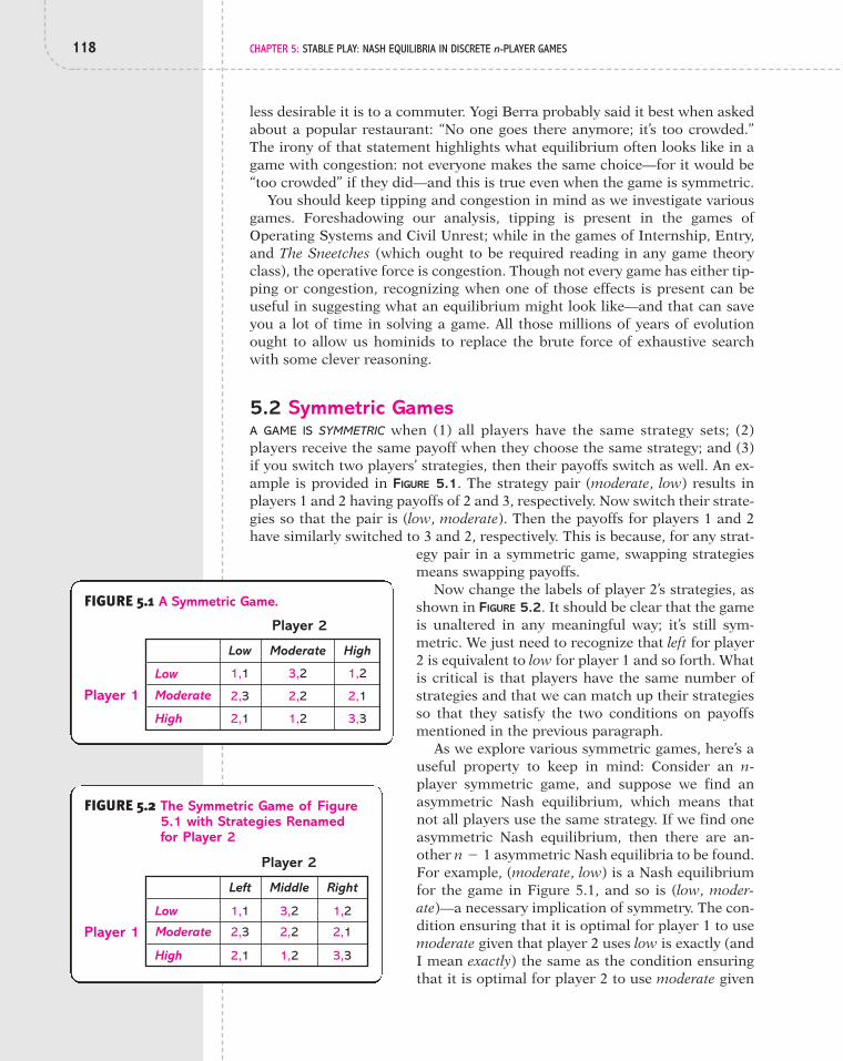
118 CHAPTER 5: STABLE PLAY: NASH EQUILIBRIA IN DISCRETE n-PLAYER GAMES
less desirable it is to a commuter. Yogi Berra probably said it best when askedabout a popular restaurant: “No one goes there anymore; it’s too crowded.”The irony of that statement highlights what equilibrium often looks like in agame with congestion: not everyone makes the same choice—for it would be“too crowded” if they did—and this is true even when the game is symmetric.
You should keep tipping and congestion in mind as we investigate variousgames. Foreshadowing our analysis, tipping is present in the games ofOperating Systems and Civil Unrest; while in the games of Internship, Entry,and The Sneetches (which ought to be required reading in any game theoryclass), the operative force is congestion. Though not every game has either tip-ping or congestion, recognizing when one of those effects is present can beuseful in suggesting what an equilibrium might look like—and that can saveyou a lot of time in solving a game. All those millions of years of evolutionought to allow us hominids to replace the brute force of exhaustive searchwith some clever reasoning.
5.2 Symmetric GamesA GAME IS SYMMETRIC when (1) all players have the same strategy sets; (2)players receive the same payoff when they choose the same strategy; and (3)if you switch two players’ strategies, then their payoffs switch as well. An ex-ample is provided in FIGURE 5.1. The strategy pair (moderate, low) results inplayers 1 and 2 having payoffs of 2 and 3, respectively. Now switch their strate-gies so that the pair is (low, moderate). Then the payoffs for players 1 and 2have similarly switched to 3 and 2, respectively. This is because, for any strat-
egy pair in a symmetric game, swapping strategiesmeans swapping payoffs.
Now change the labels of player 2’s strategies, asshown in FIGURE 5.2. It should be clear that the gameis unaltered in any meaningful way; it’s still sym-metric. We just need to recognize that left for player2 is equivalent to low for player 1 and so forth. Whatis critical is that players have the same number ofstrategies and that we can match up their strategiesso that they satisfy the two conditions on payoffsmentioned in the previous paragraph.
As we explore various symmetric games, here’s auseful property to keep in mind: Consider an n-player symmetric game, and suppose we find anasymmetric Nash equilibrium, which means thatnot all players use the same strategy. If we find oneasymmetric Nash equilibrium, then there are an-other asymmetric Nash equilibria to be found.For example, (moderate, low) is a Nash equilibriumfor the game in Figure 5.1, and so is (low, moder-ate)—a necessary implication of symmetry. The con-dition ensuring that it is optimal for player 1 to usemoderate given that player 2 uses low is exactly (andI mean exactly) the same as the condition ensuringthat it is optimal for player 2 to use moderate given
n " 1
FIGURE 5.1 A Symmetric Game.
2,1 1,2
Player 1
Player 2
Low
Moderate
High
Low Moderate High
1,1 3,2 1,2
3,3
2,3 2,2 2,1
FIGURE 5.2 The Symmetric Game of Figure5.1 with Strategies Renamedfor Player 2
1,1 3,2
2,3
2,1 1,2
2,2Player 1
Player 2
Left Middle Right
1,2
3,3
2,1
Low
Moderate
High

5.2 Symmetric Games 119
that player 1 uses low. And the condition ensuring that it is optimal forplayer 2 to use low given that player 1 uses moderate is the same conditionensuring that it is optimal for player 1 to use low given that player 2 usesmoderate. Thus, if (low, moderate) is a Nash equilibrium, then so is (moder-ate, low).
In a symmetric game, if a strategy profile is a Nash equilibrium, thenso is a strategy profile that has players swap strategies. That is, in a two-playersymmetric game, if (s , s ) is a Nash equilibrium, then so is (s , s ). And in asymmetric three-player game, if (s , s , s ) is a Nash equilibrium, then so are (s , s , s ), (s , s , s ), (s , s , s ), ( s , s , s ), and (s , s , s ).
With this piece of insight, the discovery of one asymmetric equilibrium ina symmetric game tells you that there are other asymmetric equilibria andeven tells you what they look like. Not a bad trick, eh?
! SITUATION: THE SNEETCHES
Now, the Star-Belly Sneetches
Had bellies with stars.
The Plain-Belly Sneetches
Had none upon thars.2
Dr. Seuss’ story “The Sneetches” starts out with some ofthese fictional creatures having a star on their belly andthe others not. The star-bellied sneetches were esteemed—reveling in frankfurter roasts—and those without stars leda morose life. Though perhaps unfair, the sneetches’ worldwas stable: neither the haves nor the have-nots sought toupset the status quo. But stability turned to turmoil whenSylvester McMonkey McBean rolled into town with hismachine that could put stars on and take them off. Do yourecall what happened? How McBean’s machine changedthe equilibrium in the land of sneetches?
To explore this Seussian world, let us suppose thatthere are n sneetches and n is odd. Suppose also thatinitially less than half of the sneetches have stars. Withthe arrival of Sylvester McMonkey McBean and his Star-Off and Star-On machines, each sneetch must decide what to do with his orher belly.* Each of the sneetches who were born with stars must decidewhether to retain the star or have it taken off. Likewise, each of the sneetcheswith “none upon thars” must decide whether to have a star put on or remainstarless.
The story is unclear as to why a star bestows esteem upon its wearer—indeed,the point of the story is that what determines status can be quite arbitrary—but
¿–‡–¿‡¿‡–‡¿––‡¿‡–¿
¿––¿
*The gender pronoun issue here is particularly dicey, as I don’t even know if sneetches have different gen-ders and, if so, how many. Perhaps sneetches are hermaphrodites or asexual, or, like some amphibians,they change their gender during their lifetime. Or perhaps I should stop trying to be so politically correctand just get on with the story.
FRO
M T
HE
SNEE
TCH
ES A
ND
OTH
ER S
TORI
ES B
Y D
R. S
EUSS
, CO
PYRI
GH
TTM
& C
OPY
RIG
HT
© B
Y D
R. S
EUSS
EN
TERP
RISE
S, L
.P. 1
953, 1
954,
1961, R
ENEW
ED 1
989. U
SED
BY
PERM
ISSI
ON
OF
RAN
DO
M H
OUSE
CHIL
DRE
N’S
BO
OKS
, A D
IVIS
ION
OF
RAN
DO
M H
OUSE
, IN
C.
Star-Bellied Sneetches Show Off Their Stars

120 CHAPTER 5: STABLE PLAY: NASH EQUILIBRIA IN DISCRETE n-PLAYER GAMES
we’ll assume that whatever is rarer is prized. Let m denote the number ofsneetches with stars on their bellies at the end of the day. If then hav-ing a star is esteemed (since fewer sneetches have stars than don’t), and in thatcase, each sneetch with a star gets a payoff of 1 and each lacking a star gets apayoff of 0. If, instead, then not having a star is esteemed, so eachsneetch with a star gets a payoff of 0 and each without one gets a payoff of 1.Contrary to the story, suppose Sylvester McMonkey McBean provides his serv-ices for free.*
Note that a sneetch’s payoff depends only on whether or not she has a starand how many sneetches altogether have stars. Also since the use of the Star-On and Star-Off machines is free, it actually doesn’t matter whether a sneetchwas born with a star. The payoffs are summarized in TABLE 5.1.
n/2 6 m,
m 6 n/2,
*In the story, McBean initially charged the sneetches without a star $3 to have a star put on and thencharged the original star-bellied sneetches $10 to have a star removed. After that, I suspect the price con-tinued to rise. An exercise at the end of the chapter has you derive equilibrium when a price is charged.
TABLE 5.1 PAYOFF TO A SNEETCH
What’s on the Sneetch’s Total Number of Sneetches Belly? with Stars (m) Payoff
Star 1
Star 0
Nothing 0
Nothing 1n2 6 m
m 6 n2
n2 6 m
m 6 n2
What is a stable configuration in this society? That is, when are allsneetches content with their bellies? To answer this question requires derivingNash equilibria. We can think of each sneetch’s strategy set as including starand nothing, and the objective is to find a strategy profile whereby each andevery sneetch cannot do better by doing something different.
Accordingly, consider a strategy profile whereby so that fewerthan half of the sneetches choose to be star bellied. For those sneetches whochoose to have a star, each is clearly acting optimally, since its payoff is 1 andthat’s the highest payoff there is. But what about the sneetches whohave chosen not to have a star? Well, they each have a zero payoff. To deter-mine whether they can do better, there are two cases to consider.
In the first case, the number of sneetches with stars is not only less thann/2, but also less than That is, or, equivalently,
An example is the top row in FIGURE 5.3 where andA sneetch who originally planned not to have a star would increase
the number of star-bellied sneetches from m to if, instead, she got astar. This situation is shown in the bottom row in Figure 5.3. Since we havesupposed that it is still the case that star-bellied sneetches arein the minority. (Again, see Figure 5.3.) This means that a sneetch without astar can go from being one of the majority without a star (and earning a pay-off of 0) to being one of the minority with a star (and earning a payoff of 1).
m % 1 6 n/2,
m % 1m # 2.
n # 7m % 1 6 n/2.m 6 (n/2) " 1,(n/2) " 1.
n " m
m 6 n/2,

5.2 Symmetric Games 121
Because any of the starless sneetches would then prefer to have a star, thiscase is not a Nash equilibrium. In sum, if, at the end of the day, the numberof star-bellied sneetches is less than then this strategy profile isnot a Nash equilibrium.
In the second case, we continue to suppose that so that star-belliedsneetches are rarer, but now assume that their number exceeds thatis, Since we are then assuming both and
these inequalities can be combined to yield But this just means that we are supposing that the number m of star-belliedsneetches equals (Recall that n is odd.) That is, m is the highest in-teger less than half of n. An example is shown in the top row of FIGURE 5.4,where and, therefore, So, is this case an equilibrium? We alreadyknow that the sneetches with stars can’t do any better. A sneetch without a staris getting a zero payoff, since more than half of the sneetches have chosen notto have stars. But because if one of those starless sneetchesnow chooses to have a star, then there would be or sneetches with stars. With one sneetch having changed her mind, there wouldbe more sneetches with stars than without, which would mean the star-belliedsneetches now have a zero payoff. This becomes clear if we move from the topto the bottom row in Figure 5.4. Since having a star doesn’t raise the sneetch’spayoff, the sneetch is content not to have a star. In other words, when (n " 1)/2
(n % 1)/2,((n " 1)/2) % 1,m # (n " 1)/2,
m # 3.n # 7
(n " 1)/2.
(n/2) " 1 6 m 6 n/2.m 6 n/2,(n/2) " 1 6 m(n/2) " 1 6 m.
(n/2) " 1;m 6 n/2,
(n/2) " 1,
FIGURE 5.3 A Starless Sneetch Gets a Star (n " 7, m " 2)
FIGURE 5.4 A Starless Sneetch Gets a Star (n " 7, m " 3)

122 CHAPTER 5: STABLE PLAY: NASH EQUILIBRIA IN DISCRETE n-PLAYER GAMES
sneetches have a star and don’t, a starlesssneetch is “damned if she does and damned if she does-n’t”: the sneetch will be in the majority, regardless of whatshe does. A starless sneetch can then do no better than toremain starless.
In conclusion, there is a Nash equilibrium in whichsneetches have stars. By an analogous argu-
ment, there is also a Nash equilibrium in whichsneetches have stars. (Convince yourself.) We
then have two stable configurations for a society ofsneetches: either have stars (and it is the star-bellied sneetches who are esteemed), or havestars (and it is the starless sneetches who are esteemed).
! SITUATION: AIRLINE SECURITY
Security is only as strong as its weakest link. And so if they get on in a foreignair carrier or if they target a foreign air carrier, it is going to be—could be a ter-rible tragedy again. So we need to make sure that there is a uniform raising ofthe level of security in a way that makes sense. —KENNETH QUINN, FEDERAL
AVIATION ADMINISTRATION COUNSEL AND CHAIR OF THE PAN AM 103 TASK FORCE.3
An airline’s security is dependent not just on what security measures ittakes but also on the measures taken by other airlines, because bags that aretransferred will have been checked by another airline. When Pam Am 103blew up over Lockerbie, Scotland, in 1988, the suitcase containing the bombhad been checked in Malta and transferred in Frankfurt and London, when itwas then placed on the Pam Am jet. The bag had not been screened in eitherthe Frankfurt Airport or Heathrow.4
As the opening quote suggests, a major challenge to airport security is thatit is only as good as its weakest point. If every airline but one has tight secu-rity, then it is going to be that one deficient airline which determines the air-port’s safety. A game known as the weakest link coordination game capturessome of the incentives faced by airlines in such a situation. Let’s explore it.
Suppose there are airlines and each has the strategy set {1,2,3,4,5,6,7},where each number represents a level of security expenditure by an airline anda higher number means more resources put into security. Let denote thestrategy of airline i, and suppose the cost associated with its security measuresis Naturally, more intense security measures are more expensive.
Although the cost of those measures is incurred only by the airline that paysfor them, the benefit provided may be shared by all airlines, for the reasonsjust described. We will assume that the overall level of security is deter-mined by the “weakest link” and, more specifically, is measured by
where min is the smallest (or minimum) of thesen numbers. Airline i’s payoff is then this common benefit less its personal cost:
Before trying to find Nash equilibria, let’s first understand the incentives ofairlines. Suppose min so that airline i doesn’t have the low-5s1, . . . , sn6,si 7
50 % 20 ! min5s1, . . . , sn6 " 10 ! si.
5s1, . . . , sn6min5s1, . . . , sn6, 50 % 20 !
10 ! si.
si
n ' 2
(n % 1)/2(n " 1)/2
(n % 1)/2
(n " 1)/2
(n % 1)/2
Now suppose there are two tattoos that can beplaced on a sneetch’s belly: a star or a bar.There are seven sneetches in total, and theysimultaneously decide whether to have a star, abar, or nothing on their belly. There can now beas many as three cliques in Sneetchland: thosewith stars, those with bars, and those with noth-ing. Assume that a sneetch’s payoff is 1 whenthe size of the clique of which he is a memberis no larger than the clique to which any othersneetch belongs. Otherwise, the payoff is 0. Forexample, if there are two sneetches with stars,two with nothing, and three with bars, thenthose with a star or nothing have a payoff of 1.Find as many Nash equilibria as you can.
5.1 CHECK YOUR UNDERSTANDING

5.2 Symmetric Games 123
est security expenditure. Then if airline i reduces its expenditure by one unit(from to the overall security level is unaffected, sincemin is unchanged (because airline i did not initially have theweakest security). However, the airline’s cost is now reduced by 10 from
to which means that its payoff is higher by 10. So, whenan airline does not have the lowest security expenditure, it can always raise itspayoff by reducing its measures by one unit. Doing so lowers its cost withoutaltering the effective security level. This principle leads us to the conclusionthat it is not optimal for an airline to have higher security measures than theleast secure airline. Hence, at a Nash equilibrium, all airlines must have theminimum level of security expenditure, which means that all must have thesame level of expenditure. If there are any Nash equilibria, they must then besymmetric. (Note that we have not yet shown that there are symmetric equi-libria, only that there are no asymmetric equilibria.)
Understanding that we need to focus on symmetric strategy profiles, sup-pose each airline chooses the same security measures and let denote thiscommon strategy. Since the decision problem is the same for all airlines, wecan focus just on airline 1. Airline 1’s payoff from choosing given that allother airlines choose is
The issue is whether airline 1 can do better by having more stringent or lessstringent security measures than
Suppose airline 1 were to choose a higher level of security, denoted Then the minimum security level among all airlines remains at so airline 1’spayoff is
which is necessarily lower than This formula is just a repetition ofwhat we showed earlier. An airline doesn’t want to spend more on security thananother airline, because doing so results, not in more security, but just highercost.
Next, suppose airline 1 considers weaker security measures—say, whereThe minimum security level then declines from to , and airline 1’s
payoff is
This payoff is less than (since which is what airline 1 getsby instead choosing Thus, an airline has no incentive to set its securitymeasures below the common security level of the other airlines.
We conclude that it is a Nash equilibrium for all airlines to choose .Offering more intense security than raises an airline’s cost without increas-ing actual security, while offering weaker measures reduces actual securitybelow which swamps any cost savings. Since can be any element of anairline’s strategy set, there are, then, seven Nash equilibria, one for each of theseven possible strategies.
s¿s¿,
s¿s¿
s¿.s0 6 s¿),50 % 10s¿
50 % 20 ! min5s0, s¿, . . . , s¿6 " 10 ! s0 # 50 % 20s0 " 10s0 # 50 % 10s0.
s0s¿s0 6 s¿.s0,
50 % 10s¿.
# 50 % 10s¿" 10(s–" s¿),50 % 20 ! min5s–, s¿, . . . , s¿6" 10 ! s–# 50 % 20s¿" 10s–
s¿,s–(7 s¿).
s¿.
50 % 20 ! min5s¿, . . . , s¿6 " 10 ! s¿ # 50 % 20s¿ " 10s¿ # 50 % 10s¿.
s¿,s¿,
s¿
10 ! (si " 1),10 ! si
5s1, . . . , sn6si " 1),si

124 CHAPTER 5: STABLE PLAY: NASH EQUILIBRIA IN DISCRETE n-PLAYER GAMES
What is both interesting and disturbing about this result is that Nash equi-librium can mean either that all airlines choose the strictest security measuresor that they choose the slackest security measures. Furthermore, the airlinesare not indifferent among these equilibria. All are jointly better off with anequilibrium that has each airline spend more on security. The payoff to an air-line when all choose security measures is and this payoff is in-creasing in If then each airline’s payoff is 60, while the payoff is 120when
Economists have conducted laboratory experiments with college studentsto learn how people actually behave in such a setting.5 The payoff is exactly asjust specified and is measured in cents. For example, if all of the studentschoose strategy 5, then each receives a payoff of $1.00. If all but one choosestrategy 7 and one chooses strategy 3, then those with strategy 7 each earn 40cents and the one with strategy 3 earns 80 cents. For a given set of students(drawn from Texas A&M undergraduates), the game was played for 10 rounds(so each student has an opportunity to earn as much as $12.00). There werebetween 14 and 16 subjects in a trial (so n is 14, 15, or 16).
Aggregating across the seven trials conducted (each with a different pool ofsubjects), TABLE 5.2 reports the distribution of choices in the first and last(10th) rounds. There is a variety of choices in the first round, which is not un-expected. Different students could have different initial beliefs about whichequilibrium is the relevant one. One student might believe that other studentswill have a minimum choice of 6 and thus choose 6 himself, while a less opti-mistic student might assume that others would choose a minimum of 4, inwhich case she’ll choose 4.
s¿ # 7.s¿ # 1,s¿.
50 % 10s¿,s¿
TABLE 5.2 EXPERIMENTAL RESULTS FOR THE WEAKEST LINKCOORDINATION GAME
Round 1, Percent of Subjects Round 10, Percent of SubjectsAction Choosing that Action Choosing that Action
7 31% 7%
6 9% 0%
5 32% 1%
4 16% 2%
3 5% 2%
2 5% 16%
1 2% 72%
In the initial round, 31% of the students chose the highest strategy, and 88%chose strategy 4 or higher. Only 2% chose the lowest strategy. By way of com-parison, had the students simply made random choices, each strategy would beselected 14.3% of the time. (There are seven strategies, and Higherstrategies were chosen more frequently than randomness would suggest. That’sencouraging. But as the game was played again and again, it became a “race tothe bottom.” There was a gradual movement to lower strategies, so that by the
17 # .143.)

5.2 Symmetric Games 125
end of the fourth round, the minimum choice in every trialwas strategy 1. By round 10, strategy 1 was selected by 72%of the students. Their behavior was converging to the worstequilibrium.*
! SITUATION: OPERATING SYSTEMS: MAC OR WINDOWS?
Well, the idea that the more users you get, the more valuablesomething is, is even stronger today when it’s so easy forpeople to connect up and build communities. I do think itgoes back [to Windows]. As more people used Windows itbecame sort of a standard thing that people would learn; aspeople used Office they would do add-ons. Everyone who had an Office-for-matted document who wanted to exchange it as an attachment with some-body else was kind of encouraging that person. And so these network effects,that was really [the] business model that created Microsoft. —BILL GATES6
Since the early 1980s, most consumers in developed countries have had tomake a choice between doing their computing on a Windows-based PC or ona product of Apple. The PC was originally developed by IBM, with micro-processors built by Intel and an operating system designed by Microsoft (firstDOS and then Windows). In contrast, Apple supplied both hardware and soft-ware components, initially with Apple II and then with the Mac. Apple hit themarket before IBM, but eventually the PC would dominate. Today, about 95%of personal computers run the Windows operating system.
Although most product markets are not dominated by a single product—unlike the market for operating systems—dominance is not uncommon whenthere are network effects. A product has network effects if its value to a con-sumer is greater when more consumers use it. Classic examples are commu-nication networks such as telephone and e-mail. For example, e-mail is not ofmuch value if no one else has it, and furthermore, its value increases as moreand more people can be accessed with it. The case of operating systems is amore indirect version of network effects, but no less important. As more peo-ple use an operating system, more applications are written for it—word pro-cessing, spreadsheets, games, etc.—that increase the value a consumer attachesto using the operating system.
The decision as to which operating system to buy is a game played not amongtwo, or ten, or even a hundred people, but millions of people. Nevertheless, thechoice has all of the essential ingredients of a strategic setting, in that the bestoperating system for someone depends on what she thinks other consumers willdo. No consumer wants to use an operating system that is “stranded” with fewapplications.
Suppose, then, that there are people contemplating which operatingsystem to purchase. Each has a strategy set composed of Mac and Windows.The payoff to buying a Mac is assumed to be where m is thenumber of people who choose Mac. The payoff for choosing Windows is
100 % 10 ! m,
n ' 2
*Before you cancel that airline reservation, keep in mind that an important departure from reality in theseexperiments is that the participants were not allowed to communicate with one another. Permitting suchcommunication prior to play could make it more likely that players would coordinate on the best equi-librium, in which all choose strategy 7.
Assume that the effective security level is nowdetermined by the highest (not the lowest)security measures chosen by airlines. Lettingmax{s1, . . . , sn} denote the highest of the airlines’strategies, we find that airline i’s payoff is now
50 % 20 ! max{s1, . . . , sn} " 10 ! si.
Assuming the same strategy sets, find all Nashequilibria.
5.2 CHECK YOUR UNDERSTANDING

126 CHAPTER 5: STABLE PLAY: NASH EQUILIBRIA IN DISCRETE n-PLAYER GAMES
where w is the number of consumers who buy Windows. Assume forsimplicity that everyone buys one or the other, so that
Note that the value of an operating system is higher when more people buyit. The part of a consumer’s payoff that depends on how many people buy thegood—which is for a Mac and for Windows—measuresthe network effect. A second property is that the Mac is presumed to havesuperior features, and they are worth 100 in terms of payoff.
One Nash equilibrium has every consumer buying the superior Mac sys-tem, and that system then becomes the standard. To prove this claim, considerthe strategy profile in which everyone buys a Mac. Given that the other consumers buy a Mac, a consumer receives a payoff of fromdoing so, but a payoff of only from buying Windows. Since
it is optimal to buy a Mac. Because both the game and thestrategy profile are symmetric, this conclusion applies to each and every con-sumer. It is then a Nash equilibrium for every player to choose Mac.
It can also be a Nash equilibrium, however, for the inferior Windows sys-tem to prevail. If all other consumers buy Windows, then the payoff to a con-sumer from doing likewise is while the payoff from buying a Mac is110 (since, in that case, If
10 ! n ' 110, or equivalently, n ' 11,
then it is better to do as everyone else does and buy Windows. When there areat least 11 consumers, the advantage that Windows has from a bigger networkeffect exceeds the additional value coming from the superior Mac technology.Hence, every consumer then chooses Windows.
In sum, there is always a Nash equilibrium in which all consumers use aMac, but if then there is also a Nash equilibrium in which all con-sumers use Windows. That equilibrium outcomes are extreme—either all go withthe Mac or all go with Windows—is because network effects are a form of tipping.To see this more clearly, assume that there are 20 people FIGURE 5.5(n # 20).
n ' 11,
m # 1).10 ! n,
100 % 10 ! n 7 10,10(# 10 ! 1)
100 % 10 ! nn " 1
10 ! (n " m)10 ! m
w # n " m.10 ! w,
FIGURE 5.5 Mac vs. Windows
20 4 6 8 10 12 14 1615 2018
Payo
ff
w
100
140160
200
300
150160
Payoff from Mac
Payoff from Windows

5.2 Symmetric Games 127
shows the relationship between payoff and the number of users of a system.On the horizontal axis is the number of adopters of Windows; a value for wcorresponds to w consumers choosing Windows and buying a Mac.The vertical axis measures the associated payoff for a Windows user and aMac user. For example, if then the payoff for using Windows is
and for using a Mac is Reflecting net-work effects, as the number of Windows users rises, then the payoff for usingWindows increases and for using a Mac declines.
Suppose now that, of the other 19 consumers, 15 have chosen Windows. Aconsumer then gets a payoff of 160 from also choosing Windows (because, withher choice of Windows, there are now 16 Windows users) and a payoff of 150from choosing a Mac. The consumer will then prefer Windows. The logic forWindows is even more compelling if, instead, 16 of the other 19 consumers useWindows. Now Windows delivers a payoff of 170, while the payoff from choos-ing Mac is only 140. In Figure 5.5, the gap between the Windows payoff and theMac payoff rises as the number of Windows users goes from 16 to 17 and so on.
As long as a consumer thinks that at least 15 other consumers will chooseWindows, she’ll choose Windows as well. If all consumers reason this way,then, in fact, all 20 consumers will buy Windows, and it will become the dom-inant operating system. However, if a consumer believes that only 14 otherconsumers will buy Windows, then he will prefer a Mac. Figure 5.5 showsthat, with 14 users of Windows, the Mac payoff is 160, while the Windows pay-off is 150 (because, with this consumer, there are now 15 buying Windows).Since fewer consumers are expected to buy Windows, the relative attractive-ness of a Mac rises: as indicated in Figure 5.5, the gap between the Mac pay-off and the Windows payoff gets larger as w shrinks.
The tipping point is 15. If, on the one hand, each consumer believes that 15 ormore other consumers will buy Windows, then each and every consumer will buyWindows. If, on the other hand, each consumer believes that 14 or fewer otherconsumers will buy Windows, then each and every consumer will buy a Mac.Depending on those beliefs, the market can tip to one standard or the other.
Consumers’ expectations are, then, critical when a product has network ef-fects. If most consumers come to believe that most consumers will buy a par-ticular product, then those beliefs will prove self-fulfilling, as all will, indeed,buy that product. So how does a company convince consumers that its prod-uct will be the popular one? Although advertising can help, it isn’t sufficient:a consumer who is swayed by an advertisement must also know that manyother consumers are being thus swayed. That is, one wants to make it com-mon knowledge that the product is compelling. Junk mail—of either the paperor electronic variety—won’t do the trick. It may reach a lot of people, but thosepeople who are reached don’t know how many other people have been simi-larly contacted.
Perhaps the best generator of common knowledge in the United States is acommercial during the Super Bowl.7 It is not simply that the Super Bowl isthe most widely watched program, but that almost everyone knows that al-most everyone is watching it. During the 1986 Super Bowl, the Discover cardwas advertised extensively, and it is a classic case of a product with networkeffects. Retailers will accept the Discover card only if many consumers use it,and many consumers will use it only if many retailers accept it. Thus, themore consumers who use the card, the more retailers will accept it, which will
160(# 100 % 6 ! 10).140(# 14 ! 10)w # 14,
20 " w

128 CHAPTER 5: STABLE PLAY: NASH EQUILIBRIA IN DISCRETE n-PLAYER GAMES
induce yet more consumers to use it, which will induce more retailers to ac-cept it, and so on. Better yet, the Mac was introduced with a 60-second com-mercial during the 1984 Super Bowl.
! SITUATION: APPLYING FOR AN INTERNSHIP
It’s the middle of the spring semester, and you’re thinking about applying for asummer internship. You’ve narrowed your prospects down to two investmentbanking firms: JP Morgan (JPM) in New York and Legg Mason (LM) inBaltimore. You, as well as everyone else, prefer the JPM internship, but you arehesitant to apply for two reasons. First, there is only one summer intern posi-tion at JPM for someone from your school, while there are three at LM. Second,you know that everyone else finds the JPM internship more attractive, and thisis likely to make it harder to land a position. Suppose, due to time constraints,you can apply to only one of the internships. Which one should you choose?
Suppose 10 students from your school are interested in an investmentbanking internship at either JPM or LM. Everyone has the same preferences,and each assigns a value of 200 to a JPM internship and a value of 100 to anLM internship. A student’s payoff from applying for a JPM internship is 200only if she is assured of getting it, which is the case only if she is the lone per-son to apply. The payoff is lower than 200 when more than one apply and gen-erally decreases the more that apply. Analogously, a student’s payoff from ap-plying for an LM internship is 100 only if she is assured of getting it, which isthe case only if no more than three people apply. (Recall that there are threeopenings at LM.) When there are more than three applicants, the payoff fromapplying decreases with an increasing number of applicants.
The payoffs for the internship game are listed in TABLE 5.3 and plotted inFIGURE 5.6. The more students who apply to JPM, the lower is the payoff to each
TABLE 5.3 PAYOFFS FOR THE INTERNSHIP GAME
Number of Applicants Payoff to a JPM Payoff to an LMto JPM Applicant Applicant
0 — 30
1 200 35
2 100 40
3 65 45
4 50 50
5 40 60
6 35 75
7 30 100
8 25 100
9 20 100
10 15 —

5.2 Symmetric Games 129
of those applicants. Since more applicants to JPM means fewer applicants toLM, the payoff for applying to LM increases with the number of students com-peting for a position at JPM. Contrast this game with the Operating Systemsgame. As shown in Figure 5.5, the more consumers who choose Windows, thehigher is the payoff to each of them. Thus, although tipping is at work in theOperating Systems game, congestion characterizes the Internship game.
To derive a Nash equilibrium, let’s first suppose that no one applies to JPM.Then the payoff to each of those 10 LM applicants is 30, which is considerablyless than the payoff for being the lone JPM applicant, which is 200. Hence, allstudents applying to LM is not an equilibrium. Next, consider a strategy pro-file in which 1 student applies to JPM and the other 9 apply to LM. Again, anyof those LM applicants would do better by applying to JPM: Applying to JPMraises the payoff from 35 (the payoff to an LM applicant when there is onlyone JPM application) to 100 (the payoff to a JPM applicant when there are twoJPM applicants).
More generally, in considering a strategy profile in which m students applyto JPM, a student who is intending to apply to LM is comparing the payoff frombeing one of applicants to LM and one of applicants to JPM. Asdepicted in Figure 5.6, when the payoff for applying to JPM is higher,in which case it is not optimal for this applicant to apply to LM. As long as thenumber of applicants to JPM is less than 4, we do not have an equilibrium.
Now let’s start with the other extreme: suppose all 10 students apply toJPM. Then each has a payoff of 15, which falls well short of the payoff of 100from applying to LM. Indeed, as long as more than 4 students apply to JPM,an applicant to JPM would do better by applying to LM. If the strategy profilehas m students applying to JPM, then, when the payoff for being oneof m applicants to JPM is less than the payoff for being one of ap-plicants to LM, in which case a JPM applicant ought to switch his application.
We’ve shown that any strategy profile in which fewer than 4 or more than4 students apply to JPM is not a Nash equilibrium. This leaves one remaining
10 " m % 1m 7 4,
m 6 4,m % 110 " m
FIGURE 5.6 Payoffs to Applying to JP Morgan and to LeggMason
Payo
ff
200
180
160
140
120
100
80
60
40
20
0 1 2 3 4 5 6 7 8 9 10
Payoff to JPM applicant
Payoff to LM applicant
Number of applicants to JPM

130 CHAPTER 5: STABLE PLAY: NASH EQUILIBRIA IN DISCRETE n-PLAYER GAMES
possibility: exactly 4 students apply to JPM and 6 apply to LM. In that case,the payoff to both a JPM applicant and an LM applicant is 50. If one of thestudents who is intending to apply to JPM switches to LM, then her payoff de-clines to 45 (see Figure 5.6), and if one of those students who is intending toapply to LM switches to JPM, then his payoff declines to 40. Thus, because anystudent is made worse off by changing her strategy, exactly 4 students apply-ing to JPM is a Nash equilibrium.
Hence, in this scenario, although all students have the same options and thesame preferences, they make different choices in the equilibrium situation.Four students apply to JP Morgan—and compete for the one available posi-tion—and 6 apply to Legg Mason—and compete for the three available slotsthere. Asymmetric behavior emerges from a symmetric game because of con-gestion effects. The more students who apply for a position, the tougher it isto land a position (as reflected in a lower payoff), and thus the less attractiveit becomes to apply.
5.3 Asymmetric GamesA GAME CAN BE ASYMMETRIC because players have distinct roles and thus differ-ent strategy sets. In a kidnapping scenario (such as that explored in Chapter 2),the kidnapper’s choices are whether to release or kill the victim, while the vic-tim’s kin has to decide whether or not to pay ransom. Even when all playersface the same set of alternatives, a game can be asymmetric because the play-ers have different payoffs. For example, in choosing between operating sys-tems, all consumers face the same choices, but they may differ in how theyevaluate them. Some may attach a lot of value to a Mac, while others put a lotof weight on having the most popular system, whatever that might be. That isthe source of asymmetry we explore in this section: players have different pay-offs, while facing the same choices and the same information. Let’s see whatdifference preferences can make.
! SITUATION: ENTRY INTO A MARKET
During the dot-com boom of the late 1990s, the online retailing scene wasgrowing by leaps and bounds. More and more consumers were going online,and at the same time, new online services were popping up. Representative ofthese dynamics is FIGURE 5.7, which reports the growth in the number of B2Bexchanges (i.e., sites that acted as an intermediary between businesses want-ing to buy and businesses wanting to sell products or services).8 Initially, thenumber of exchanges rose at an increasing rate. Then, beginning around 2001,there was a sharp downturn in the number of B2B exchanges. This pattern isquite typical for an industry in its incipiency. FIGURE 5.8 shows the same pat-tern among automobile manufacturers in the early part of the 20th century—a sharp rise and then a decline.9
Although explaining why the number of companies rises and then falls re-quires a model too complicated for this book, we can at least explore the de-cision to enter a market and the determination of how many sellers there areonce all of the entry and exit settles down.

5.3 Asymmetric Games 131
Consider a new market that has just opened up—for example, the online bookmarket in the mid-1990s. (Amazon.com began selling books online in July 1995.)Assume that there are five firms that might enter the market; let us uncreativelylabel them companies 1, 2, 3, 4, and Jeff (okay, actually 5). To operate in this mar-ket, a firm must incur the cost of entry, which you can think of as the cost of cre-ating a website, putting together a fulfillment structure, and advertising the site.
FIGURE 5.7 B2B Online Exchanges, 1993–2004N
umbe
r of
B2B o
nlin
e ex
chan
ges
1,750
1,500
1,250
1,000
750
500
250
0 1993 1994 1995 1996 1997 1998 1999 2000 2001 2002 2003 2004Years
FIGURE 5.8 Automobile Manufacturers, 1895–1938
20
40
60
80
100
120
140
160
180
200
220
240
260
01895 1900 1905 1910 1915 1920
Years1925 1930 1935 1940
Num
ber
of a
utom
obile
man
ufac
ture
rs

132 CHAPTER 5: STABLE PLAY: NASH EQUILIBRIA IN DISCRETE n-PLAYER GAMES
As shown in TABLE 5.4, the prospective entrants face differentcosts of entry. Company 1 is the most efficient, in that its entry costis only 100,* while company 5 is the least efficient, with an entrycost of 210. A company may have a lower entry cost because theowner can do his own programming or the company is a subsidiaryto a conventional retailer (like bn.com, which entered as part ofBarnes & Noble), allowing it to draw on some of the fulfillmenttechnology already in place.
Having described the cost of entry, let’s now consider the benefitof entering the market. Each retailer anticipates earning a profitupon entry. However, that profit is lower when there are more com-peting sites. Assume that all retailers would earn the same gross
profit (i.e., the profit before netting out the cost of entry).TABLE 5.5 reports the gross profit that each would earn andshows how it depends on how many retailers there are. Ifonly one company enters the market, then that company hasa monopoly (“mono” from Latin for “alone” or “single”) andearns a profit of 1,000. If, instead, two companies enter (sothat we have a duopoly), then each earns 400. Note that totalindustry profit has declined from 1,000 to 800 with the pres-ence of a second retailer. This is because, not only do tworetailers have to share the market, but competing for con-sumers will lead them to reduce their prices and, with it,their profit. If there are three retailers (a “triopoly”), theneach company earns 250, and so forth.
As these firms simultaneously decide whether to enter the market, eachcompany’s strategy set is composed of enter and do not enter. A company’s pay-off is zero if it does not enter and is its net profit (gross profit minus the costof entry) if it enters. For example, if company 2 enters and, say, two other com-panies enter, then company 2’s payoff is Using the informa-tion in Tables 5.4 and 5.5, TABLE 5.6 reports the various payoffs.
Note that no strategy is strictly dominated, although, for company 1, enterweakly dominates do not enter. The former strategy delivers a strictly higherpayoff when three or fewer other companies enter and the same payoff when
90(# 250 " 160).
*Never mind the units—they could be thousands of dollars, millions of shekels, billions of lekë.
TABLE 5.4 HETEROGENEOUSCOST OF ENTRY
Company Entry Cost
1 100
2 160
3 180
4 200
5 210
TABLE 5.5 COMMON GROSS PROFIT
Number of Profit per Total IndustryCompanies Company Profit
1 1,000 1,000
2 400 800
3 250 750
4 150 600
5 100 500
TABLE 5.6 PAYOFF TO A COMPANY FROM ENTRY
Number of Other Companies that Enter
Company 0 1 2 3 4
1 900 300 150 50 0
2 840 240 90 #10 #60
3 820 220 70 #30 #80
4 800 200 50 #50 #100
5 790 190 40 #60 #110

5.3 Asymmetric Games 133
four other companies enter. For each of the other companies, enter is thebest reply when two or fewer companies enter, but do not enter is the bestreply when three or four other companies enter. Thus, for each company, ei-ther strategy is a best reply for some strategy configuration of the other fourcompanies.
Let’s find the set of Nash equilibria. Rather than consider a particular strat-egy profile, suppose we start by thinking about how many entrants there willbe at a Nash equilibrium:
■ Is there a Nash equilibrium with no entrants? No, because the grossprofit for the first entrant is 1,000 and that exceeds all companies’ entrycosts. Thus, if all of the other companies chose do not enter, then enterwould be optimal for a company. Hence, it cannot be a Nash equilibriumfor all companies to choose do not enter.
■ Is there a Nash equilibrium with only one entrant? Once again, the an-swer is “no,” since the gross profit for the second entrant is 400 and thatexceeds all companies’ entry costs. Thus, if we consider a strategy profilein which one company enters and the other four do not, any of thoseother four companies could increase its payoff by entering. Hence, it isnot an equilibrium for only one of the firms to enter.
■ Is there a Nash equilibrium with two entrants? Again, the answer is “no,”by the same argument (although we’re getting “warm”). Consider a strat-egy profile in which two companies choose enter and the other threechoose do not enter. Then each of the latter earns zero. Now examine col-umn 2 in Table 5.6. All of the payoffs are positive, so, regardless of whichthree companies chose do not enter, a company can earn a positive pay-off from also entering.
■ Is there a Nash equilibrium with three entrants? There is, indeed. In fact,there are six of them: (1) companies 1, 2, and 3 enter; (2) companies 1, 2,and 4 enter; (3) companies 1, 2, and 5 enter; (4) companies 1, 3, and 4enter; (5) companies 1, 3, and 5; and (6) companies 1, 4, and 5 enter.Consider the first strategy profile. Each of those entrants earns a positivepayoff from entering; company 1 earns 150, company 2 earns 90, andcompany 3 earns 70. Entry is then optimal. As for companies 4 and 5—which have chosen do not enter—if you examine column 3 in Table 5.6,you can see that entry would result in a negative payoff: for company4 and for company 5. Thus, the strategy profile in which companies1, 2, and 3 enter and companies 4 and 5 stay out is a Nash equilibrium.One can similarly confirm each of the other five strategy profiles, as wellas confirm that any other strategy profile that has three companies enter(such as companies 3, 4, and 5) is not a Nash equilibrium.
How did I figure out that those six strategy profiles are equilibria? It wasnot through exhaustive search (I’m far too lazy for that), but from thinkingabout the companies’ incentives. First, note that it cannot be an equilibriumto have three companies enter and not to have company 1 be one of them. Ifcompany 1 is not one of the three entrants, then its payoff is zero, but it canthen earn 50 by entering. Hence, if there is a Nash equilibrium with three en-trants, company 1 must be one of them. Next, note that any of the other fourcompanies earns a positive payoff from entry when there are two other
"60"50

134 CHAPTER 5: STABLE PLAY: NASH EQUILIBRIA IN DISCRETE n-PLAYER GAMES
entrants (all of the payoffs are positive in column 2) and that each earns anegative payoff from entry when there are three other entrants (excluding thepayoff to company 1, all of the payoffs are negative in column 3). From thisstate of affairs, we can conclude that any strategy profile in which company 1enters and two other companies enter is a Nash equilibrium.
■ Is there a Nash equilibrium with more than three entrants? The grossprofit for a company when there are four entrants is 150, but only onecompany has an entry cost that doesn’t exceed 150. Hence, if four com-panies enter, then at least one of them must have a negative payoff,which means that it is better for it to not enter. This logic is also appar-ent from Table 5.6, in which only one company has a nonnegative pay-off under column 3 or column 4. There is, then, no Nash equilibriumwith more than three entrants.
An interesting property of equilibrium is that the most efficient companiesneed not be the ones that enter. The most efficient equilibrium is the one in
which companies 1, 2, and 3 enter, since they have thelowest entry costs. However, there are also equilibria inwhich companies 4 and 5 enter instead of companies 2and 3. Given that companies 4 and 5 are anticipated en-tering (along with company 1), entry becomes unprof-itable for companies 2 and 3, even though if they were tochange places with companies 4 and 5, they would makemore money than 4 and 5.
! SITUATION: CIVIL UNREST
How is it that a small group of people can oppress a large population?Having the support of the military is certainly important, as is having con-trol of the media and economic resources. But what is arguably most im-portant is coordination failure. In a nondemocratic society, the controllingfaction is always a small fraction of a country’s population. If the populacewere to rise up and oppose the ruling body, few dictatorships could survive.The challenge is having people coordinate so that mass demonstrationshappen.
Suppose a country is composed of 500 citizens, each of whom is decidingwhether to protest. The benefit to protesting is where m is the num-ber of citizens who participate in the protest. This specification captures thereasonable notion that a bigger protest will be more influential. The benefit ofprotesting is shared by all those who protest and is the feeling of empower-ment that it yields.
The cost of protesting is a personal one—for example, the risk of being im-prisoned. Here, we’ll suppose that people are different as to how they weighthis cost. To keep things simple, suppose there are three types of individualsin this society (see TABLE 5.7.) There are 100 radicals in the country, and theyhave the lowest cost of protesting, namely, 6,000. The progressives, who alsonumber 100, each incur a cost of 8,000 by protesting. Finally, there are 300bourgeois who, while still desiring revolt, are not too bad off and have the
50 ! m,
Eliminate company 1 from the Entry game so thatonly companies 2, 3, 4, and 5 simultaneously decide whether to enter. The payoffs are still asstated in Table 5.6. Find all Nash equilibria.
5.3 CHECK YOUR UNDERSTANDING

5.3 Asymmetric Games 135
most to lose from a failed revolution. To them, the cost of participating indemonstrations is 20,000.
The payoff to a citizen equals zero if he doesn’t protest and is the benefit,less his cost if he does protest. This means that a radical will protest
if and only if
Solving this expression for m, we find that Thus, if a radical believesthat another 120 people will protest, then she’ll protest as well and receive apayoff of 50 (If 119 other people are expected to protest,then her payoff from protesting is zero and she’s indifferent between protest-ing or not.) Analogously, a progressive will protest when she expects m to belarge enough to satisfy the inequality
or equivalently,
Hence, due to the higher cost incurred, a progressive requires a bigger antici-pated demonstration to draw him out than does a radical. Finally, it takes ananticipated protest size of 400 to induce the bourgeois to protest:
or equivalently,
The minimum protest size necessary to induce a person to attend demonstra-tions will be referred to as her critical mass. The relevant information is shownin Table 5.7.
In solving for Nash equilibria, a useful property to note is that if it is op-timal for a progressive to protest, then it is also optimal for a radical to doso. In other words, you won’t see progressives at a demonstration withoutalso seeing radicals. To establish this claim, recall that a progressive willfind it optimal to protest when he expects 160 people to protest, while ittakes only 120 people to induce a radical to protest. Thus, if there areenough people to bring out the progressives, there also are enough to drawout the radicals. Intuitively, a progressive and a radical realize the samebenefit, but since the latter has a lower cost, a radical will always protestwhen a progressive does. Using the same type of argument, we can seethat if a bourgeois finds it optimal to protest, then so do radicals andprogressives.
From the preceding scenario, the candidates for Nash equilibrium are that(1) no one protests, (2) only radicals protest, (3) only radicals and progressives
m ' 400.50 ! m " 20,000 ' 0
m ' 160.50 ! m " 8,000 ' 0,
(# 50 ! 121 " 6,000).
m ' 120.
50 ! m " 6,000 ' 0.
50 ! m,
TABLE 5.7 CIVIL UNREST
Type of Citizen Number of Citizens Personal Cost Critical Mass
Radicals 100 6,000 120
Progressives 100 8,000 160
Bourgeois 300 20,000 400

136 CHAPTER 5: STABLE PLAY: NASH EQUILIBRIA IN DISCRETE n-PLAYER GAMES
protest, and (4) everyone protests. The case of no one protesting is clearly anequilibrium: if a radical expects no one to participate, then his payoff fromprotesting is which is worse than the zero payofffrom staying home. Protesting is even less attractive to a progressive and abourgeois.
What about only radicals protesting? If all radicals protest, then there is atotal of 100 protestors, so each radical’s payoff is That’s not good enough to make protesting optimal: there just aren’t enough rad-icals in society to sustain an equilibrium protest with only their participation.However, if both radicals and progressives protest, then a progressive’s payoff is
Hence, all of the progressives are out there demon-strating, and we know that the radicals will be out there with them. By contrast,a bourgeois wants no part of such a demonstration, as his payoff from protest-ing is It is then an equilibrium for only radicalsand progressives to protest.
Finally, it is also an equilibrium for everyone to protest. If a bourgeois ex-pects all other citizens to participate, the payoff from joining them is
which makes protesting optimal. It is then opti-mal for the radicals and progressives to participate as well.
In sum, equilibrium can involve the total absence of demonstrations, amodest demonstration with 40% of the citizens, and massive demonstrationswith full participation. How deep into a society a protest will draw depends onthe citizens’ expectations. If they expect a massive protest, then there’ll be one;if they expect no turnout, then that is what there will be. It is all about expec-tations and, from the citizens’ perspective, about coordinating on the beliefthat there will be a high level of participation.
Some of the issues just raised were central to the mass protests that ledto the collapse of the authoritarian regime of the German DemocraticRepublic (GDR).10 Amidst increasing dissatisfaction with the quality of lifeand the absence of basic freedoms, the people of the GDR city of Leipziglaunched a growing series of protests beginning in September 1989. Theyall took place on Monday because, around 6:00 in the evening, peoplewould come out of church after religious services. They would then crossthe central square of Karl-Marx-Platz and pick up more people as theywalked through the city. On September 25, more than 6,000 people partici-pated and called for political liberalization. By the following Monday, theprotests had risen to almost 18,000. Then came the critical protest theMonday after that:11
On October 9 a third demonstration took place against the background ofan ominous rumor that spread quickly through Leipzig (and was later con-firmed): [general secretary Erich] Honecker himself had signed theSchießbefehl (order to shoot) for a Chinese solution to the protest. . . . At5:45 P.M., just fifteen minutes before the end of the peace prayers, the po-lice and the military withdrew, and about sixty thousand unarmed, fright-ened, and yet determined people demonstrated peacefully. . . . The demon-stration broke the back of the regime. . . . Over 100,000 people demon-strated on October 16; 245,000 on October 23; about 285,000 on October30; and 325,000 on November 6. Meanwhile, mass demonstrationserupted all over the GDR.
5,000(# 50 ! 500 " 20,000),
"9,950(# 50 ! 201 " 20,000).
2,000(# 50 ! 200 " 8,000).
"1,000(# 50 ! 100 " 6,000).
"5,950(# 50 ! 1 " 6,000),

5.4 Selecting among Nash Equilibria 137
TABLE 5.8 shows the growth of protests throughout the GDR. These protestshad no leader and were the creation of many people acting on their own, butpresumably with the anticipation that others would do the same. The powerof the people ruled the day, as these protests led to the fall of the Berlin Walland the unification of East and West Germany.
A Mass Demonstration at the Berlin Wall
TABLE 5.8 PUBLIC PROTESTS IN GDR, SEPTEMBER 1989–FEBRUARY 1990
Date Number of Events Turnout Average Turnout
September 1989 7 16,500 3,300
October 1989 32 1,431,500 49,347
November 1989 28 3,268,900 136,204
December 1989 21 903,082 5,443
January 1990 26 1,782,567 81,026
February 1990 20 464,346 35,719
5.4 Selecting among Nash EquilibriaMANY OF THE GAMES examined in this chapter have multiple Nash equilibria.Multiplicity is problematic because the more equilibria there are, the less pre-cise are our statements about behavior. This is a matter that has drawn mucheffort within the game theory community and will continually draw our
LAN
GEV
IN J
ACQ
UES
/CO
RBIS
SYG
MA

138 CHAPTER 5: STABLE PLAY: NASH EQUILIBRIA IN DISCRETE n-PLAYER GAMES
*The section is designed to be read without having read what precedes it in Chapter 5. References togames in Chapter 5 have been placed in clearly demarcated digressions.
**The economist Joel Sobel suggested that, in practice, it should be the person who makes the initial callwho calls back, because that person is assured of having the other person’s phone number.
attention in this book. In this section, we raise some general issuesregarding how to handle multiple equilibria.*
It is important to distinguish various types of multiplicity, sincesome are innocuous and some are not. Consider first the multiplic-ity of Nash equilibria in the telephone game (Section 4.2), which isreproduced in FIGURE 5.9. This game has two Nash equilibria, one inwhich Colleen calls (and Winnie waits) and the other with Winniecalling (and Colleen waiting). The outcome of the game is the samefor the two equilibria in the sense that one person calls and the otherperson waits, although the roles played by the players varies. Such a
multiplicity is not of great concern to us (with one caveat, discussed shortly),because the general description of the outcome is the same across equilibria.Other games with a similar type of multiplicity include Chicken (Section 4.1)and driving conventions (Section 4.2).
This same type of multiplicity arose in The Sneetches and theInternship game. In the latter, any strategy profile with 4 students applying toJP Morgan and 6 to Legg Mason is a Nash equilibrium. There are, in fact, 210Nash equilibria, since there are 210 ways to allocate 10 students so that 4 applyto JP Morgan. Both of these games have a congestion effect, and indeed,multiple asymmetric Nash equilibria are typical in symmetric games withcongestion effects. Because the payoff for using a strategy decreases with thenumber of players that use it, it is often the case that there is an asymmetricequilibrium—and in a symmetric game, if there is one asymmetric equilibrium,then there are more, all with the same mix of strategies (so many players usestrategy 1, so many use strategy 2, etc.) and all differing only in terms of whichplayer uses which strategy.
Multiplicity of Nash equilibria in which the distribution of strategies is thesame—just the identity of the player using the strategy varies—does raise onesource of concern, however: How do players coordinate on a particular Nashequilibrium when there are more than one? How do Colleen and Winnie co-ordinate as to who calls?** How do the drivers in Chicken coordinate on whoswerves? If players were to play this game again and again, some common setof beliefs might develop and would result in play converging on a particular
Nash equilibrium. But that approach doesn’t help us if ourtask is to predict behavior the first time that they play. Thereis no resolution of this issue at this time.
Now consider the modified driving conventions gameshown in FIGURE 5.10 between two drivers who are accus-tomed to driving on the right side of the road. There are twoNash equilibria—both drivers drive on the right and bothdrivers drive on the left—but the outcomes are different interms of the payoffs they deliver. Both drivers would prefer todrive on the right, though driving on the left is also an equi-librium. Multiplicity also arose in the American Idol fandom
DIGRESSION
FIGURE 5.9 Telephone
Colleen
Winnie
Call Wait
Call
Wait
0,0
3,2
2,3
1,1
FIGURE 5.10 Driving Conventions withTwo American Drivers
Driver 1
Driver 2
Right Left
5,5
1,1
1,1
2,2
Right
Left

5.4 Selecting among Nash Equilibria 139
and voting games (Section 4.4), and, similarly, it made a big difference in theoutcome. In these cases, different equilibria have quite different predictions.
This type of multiplicity tends to occur in games with tipping.It can be an equilibrium for all players to choose one particular strategy andan equilibrium for them all to choose some other strategy, because much ofwhat influences the attractiveness of a strategy is its popularity. Such is thecase in the operating systems game: Everyone choosing Windows is anequilibrium, as is everyone choosing a Mac; consumers, however, prefer thelatter equilibrium.
When equilibria have different implications, gametheory offers a few tricks that can, in some such games,result in a selection from the set of Nash equilibria.Consider the game illustrated in FIGURE 5.11. This gamehas three Nash equilibria: one with both Scooter andBrownie choosing low, a second with Scooter choosinghigh and Brownie choosing medium, and a third withScooter choosing medium and Brownie choosing high.Before you are tempted to select (low, low) because itis symmetric—and the game is symmetric—take notethat the strategy low is weakly dominated by the strat-egy high. Thus, a cautious player ought to avoid low.
One selection device is to give preference to undominated Nash equilib-ria: Nash equilibria in which players are not using weakly dominated strate-gies. This approach results in the elimination of (low, low), although there arestill two Nash equilibria that remain. Returning to the voting game (Section4.4), we see that it had five Nash equilibria, but all but one of them had oneor more voters using a weakly dominated strategy. In that game, there is aunique undominated Nash equilibrium, and it has shareholders 1 and 2 vot-ing for option B and shareholder 3 voting for C. As practice, I’d recommendgoing back to the voting game and verifying that claim.
Another selection criterion commonly used is based upon payoff dominanceand what economists call the Pareto criterion. A strategy profile satisfies pay-off dominance if there is no other strategy profile for which each player hasa strictly higher payoff. Although Nash equilibrium is based upon individualrationality—in that each player is doing what is best for him, given what oth-ers are doing—payoff dominance is based upon collective rationality—in thatit involves choosing a strategy profile that is best for everyone. The selectioncriterion is that one use payoff dominance in conjunction with Nash equilib-rium. To only use the former could mean choosing a strategy profile that vio-lates individual rationality. The proposed criterion is called equilibrium pay-off dominance, which means focusing on Nash equilibria for which there isno other Nash equilibrium in which each player has a strictly higher payoff.An equilibrium satisfying this property is called a payoff-dominant Nashequilibrium.
Equilibrium payoff dominance tells us to focus on the equilibrium (right,right) for the game in Figure 5.10, because it results in a higher payoff for bothdrivers relative to the equilibrium (left, left). By this criterion, the unique so-lution in the American Idol fandom game is that all three girls wear the let-tered T-shirts.
DIGRESSION
FIGURE 5.11
2,2 1,1
1,1
2,0 4,1
3,3Scooter
Brownie
Low
Medium
High
Low Medium High
0,2
0,0
1,4

140 CHAPTER 5: STABLE PLAY: NASH EQUILIBRIA IN DISCRETE n-PLAYER GAMES
The equilibrium payoff dominance criterion has a lot of powerin the airline security game. That game has seven Nash equilibria, which can beranked in terms of payoffs. The equilibrium with all airlines choosing the mostintense security measures has the highest payoff for each player among all ofthe Nash equilibria. This criterion can also be used to yield a unique solution inthe operating systems game.
One rationale for the use of equilibrium payoff dominance is that if playerswere to meet beforehand and communicate, it would be in their mutual in-terest to coordinate on an equilibrium with that property. They know thatagreeing on anything but Nash equilibrium is not credible; that is, one ormore players would diverge from the agreement. Players should then be real-istic and consider only those agreements that are self-enforcing, which meansthat it is in each player’s interest to comply and thus doesn’t require institu-tions such as the courts and the police to enforce it. Among all the self-enforcing agreements (i.e., the Nash equilibria), all players can agree that theyshould focus on the payoff-dominant ones.
The game in FIGURE 5.12 has two Nashequilibria: (top, left) and (bottom, right). (top, left) is the payoff-dominant Nash equilibrium. However, bottom weakly dominatestop for player 1, and right weakly dominates left for player 2, so(bottom, right) is the undominated Nash equilibrium. Whichequilibrium do you think is more compelling?
In his 1961 landmark book, Strategy of Conflict, Nobel LaureateThomas Schelling introduced the concept of a focal point. Likepornography and jazz, a focal point is difficult to formally de-fine. As Justice Potter Stewart said in a judicial decision, “I can’t
define it for you, but I know pornography when I see it,” and as the legendarytrumpeter Louis Armstrong proclaimed, “If you have to ask what jazz is, you’llnever know.” In spite of a focal point not being easily definable, it is a power-fully compelling concept.
To understand what is meant by a focal point and how it can help with theselection of a Nash equilibrium, one must first recognize that games do notoccur in a vacuum; they occur with rich societal context. The players are peo-ple with a history, and some of this history is common knowledge to them.Although strategies may be assigned labels such as “top” and “bottom,” in ac-tual contexts they have concrete descriptions, like “Meet at the train station”and “Meet at the ballpark.” In terms of who the players are and what strate-gies they might adopt, there may be one prominent Nash equilibrium, whichthereby becomes an obvious selection, or focal point. But for players to set-tle upon it, it’s not sufficient that each player perceive it as conspicuous: theconspicuousness itself must be common knowledge.
To see how this idea might work, let’s return to our driving conventionsgame, but now suppose the issue is on which side of thesidewalk to walk. In London, since the law is to drive onthe left, the focal point would be to walk on the left.Indeed, that is what seems to be the case, and I have hadmany awkward moments on London pavements toprove it!
DIGRESSION
FIGURE 5.12 Payoff Dominance vs.Weak Dominance
Player 1
Player 2
Left Right
Bottom 3,1 2,2
1,33,3Top
Find the payoff-dominant Nash equilibria in thegame of Civil Unrest.
5.4 CHECK YOUR UNDERSTANDING

Exercises 141
SummaryThis chapter has tackled games in which all players face the same choice,whether it be a consumer choosing the type of computer system to buy, a citi-zen deciding whether to protest, a sneetch contemplating having a star tattoo,or a company deciding whether to enter a market. Much of the analysis wasdone without specifying exactly how many players there are. Some strategy pro-files (such as buying a Mac) are equilibria regardless of how many players thereare, while others (such as buying Windows) depend on the number of players.
If, in addition to all players having the same choice, it is assumed that theyall have the same payoffs, then the game is symmetric. A symmetric gameneed not imply that equilibrium play has everyone doing the same thing. Also,the presence of a symmetric equilibrium can depend on whether payoff func-tions have the property of tipping or congestion. In tipping, the relative at-tractiveness of using a strategy is greater when more players use it, while incongestion, a strategy is less attractive when more players use it. Games withtipping tend to result in equilibria in which everyone (or almost everyone)does the same thing. For example, if enough people buy a Mac, then it’ll bemore attractive to also be a Mac user, there will be lots of software written forthe Mac, and you can easily exchange files with other users. An equilibriumthen has everyone being Mac people. Similarly, if enough people buyWindows, then that’ll be the preferred operating system. By contrast, whencongestion is present, identical people can make different choices. For in-stance, students applying for an internship don’t all want to apply to the sameinvestment banking firm, because the competition will then be fierce.Equilibrium entails students applying to different companies. Though facedwith the same situation, people may act differently.
Multiplicity of Nash equilibria is a common property of the games examinedin this chapter. Indeed, each had more than one Nash equilibrium. More gen-erally, multiplicity is routinely encountered in game theory. We explored a fewcriteria for selecting among multiple equilibria with the goal of identifying aunique solution. Among the criteria that have been proposed are to give pref-erence to undominated Nash equilibria—thereby ruling out equilibria inwhich players use weakly dominated strategies—and to give preference topayoff-dominant Nash equilibria—thereby dropping equilibria for whichthere is another equilibrium that delivers a higher payoff to every player. Insome games a unique solution emerges, but in many games that is not the case.
Identifying a criterion that always delivers a unique solution is the “holygrail” of game theory. Some game theorists find this task unrealistic and sug-gest that pursuing it turns one into a Don Quixote, while others see it as a chal-lenge of the first order and worthy of King Arthur. Regardless of your view, allgame theorists would prize such a criterion because yielding precise predic-tions and explanations is ultimately what game theory is all about.
1. The magazine Science 84 planned to announce a contest in which any-one could submit a request for either $20 or $100. If fewer than 20% ofthe submissions requested $100, then everybody would receive what
EXERCISES

142 CHAPTER 5: STABLE PLAY: NASH EQUILIBRIA IN DISCRETE n-PLAYER GAMES
they requested. If 20% or more asked for $100, then everybody would getnothing. Although the magazine wound up not running the contest, be-cause Lloyds of London was unwilling to insure against losses, we canstill analyze what equilibrium would predict. Suppose 100,000 peoplemight participate in the contest, and assume that payoffs are measuredin money.a. Assume that every possible participant submits a request for either
$20 or $100. Find a Nash equilibrium.b. Now suppose that a request form comes only with the purchase of
Science 84 and that the magazine costs $21.95. Then each person’sstrategy set has three elements: do not buy the magazine, buy the mag-azine and submit a request for $20, and buy the magazine and submita request for $100. Suppose zero value is attached to the magazine.Find a Nash equilibrium.
c. Consider again the situation described in part (b), but now supposethe magazine costs $19.95. Find a Nash equilibrium.
2. Someone at a party pulls out a $100 bill and announces that he is goingto auction it off. There are other people at the party who are po-tential bidders. The owner of the $100 bill puts forth the following pro-cedure: All bidders simultaneously submit a written bid. Everyone (notjust the highest bidder) pays his bid, and the bidder with the highest bidgets the $100 bill (assuming that the highest bid is positive). If m peoplesubmit the highest bid, then each receives a share of the $100. Eachperson’s strategy set is so bidding can go as high as$1,000. If denotes the bid of player j and is the max-imum (or highest) of the n bids, then the payoff to player i is
where m is the number of bidders whose bid equals Find all Nash equilibria.
3. It is the morning commute in Congestington, DC. There are 100 drivers,and each driver is deciding whether to take the toll road or take the backroads. The toll for the toll road is $10, while the back roads are free. Indeciding on a route, each driver cares only about income, denoted y, andhis travel time, denoted t. If a driver’s final income is y and his traveltime is t, then his payoff is assumed to be (where we have made thedollar value of one unit of travel time equal to 1). A driver’s income atthe start of the day is $1,000. If m drivers are on the toll road, the traveltime for a driver on the toll road is assumed to be m (in dollars). In con-trast, if m drivers take the back roads, the travel time for those on theback roads is 2m (again, in dollars). Drivers make simultaneous deci-sions as to whether to take the toll road or the back roads.a. Derive each player’s payoff function (i.e., the expression that gives us
a player’s payoff as a function of her strategy profile.)b. Find a Nash equilibrium.
4. Return to The Sneetches in Section 5.2. Of the n sneetches, let k denote the number of sneetches born with starsand assume Now suppose Sylvester McMonkey McBean chargesa price of p to either get a star removed (if the sneetch was born
k 6 n2.
y " t
max5b1, . . . , bn6."bi if bi 6 max5b1, . . . , bn6100m " bi if bi # max5b1, . . . , bn6
max5b1, . . . , bn6bj
50, 1, 2, . . . , 1,0006, 1m
n ' 2

Exercises 143
with one) or added (if the sneetch was born without one). Assume thatA sneetch’s payoff is as described in Table 5.1, except that
you have to subtract p if he used either the Star-On or Star-Off machine.Find all Nash equilibria.
5. Suppose several friends go out to dinner with the understanding that thebill will be divided equally. The problem is that someone might ordersomething expensive, knowing that part of the cost will be paid by oth-ers. To analyze such a situation, suppose there are n diners and, for sim-plicity, they have the same food preferences. The accompanying tablestates the price of each of three dishes on the menu and how much eachperson values it. Value is measured by the maximum amount the personwould be willing to pay for the meal.
0 6 p 6 1.
DINING DILEMMA
Dish Value Price Surplus
Pasta Primavera $21.00 $14.00 $7.00
Salmon $26.00 $21.00 $5.00
Filet Mignon $29.00 $30.00 #$1.00
Surplus is just the value assigned to the meal, less the meal’s price. Thepasta dish costs $14 and each diner assigns it a value of $21. Thus, if adiner had to pay for the entire meal, then each diner would buy the pastadish, since the surplus of $7 exceeds the surplus from either salmon orsteak. In fact, a diner would prefer to skip dinner then to pay the $30 forthe steak, as reflected by a negative surplus. A player’s payoff equals thevalue of the meal she eats, less the amount she has to pay. The latter isassumed to equal the total bill divided by the number of diners. For ex-ample, if there are three diners and each orders a different meal, thenthe payoff to the one ordering the pasta dish is
the payoff for the person ordering the salmon is
and the payoff to whoever is ordering the steak is
Not surprisingly, the people who order the more expensive meal do bet-ter, since all pay the same amount.a. Suppose there are two diners What will they order (at a Nash
equilibrium)?b. Suppose there are four diners What will they order (at a
Nash equilibrium)?(n # 4).
(n # 2).
29 " a14 % 21 % 303
b # 7.33.
26 " a14 % 21 % 303
b # 4.33,
21 " a14 % 21 % 303
b # 21 " 21.67 # "0.67,

144 CHAPTER 5: STABLE PLAY: NASH EQUILIBRIA IN DISCRETE n-PLAYER GAMES
6. Consider again the entry game from Section 5.3, but now suppose thefive potential entrants are identical in that each faces the same entry costof $300. Given the total number of companies in the market, the accom-panying table reports a company’s net profit (or payoff) if it enters. As be-fore, the payoff from staying out of the market is zero, and each companycan choose either enter or do not enter. Find all Nash equilibria.
ENTRY GAME WITH IDENTICAL COMPANIES
Number of Firms Gross Profit per Firm Net Profit per Firm
1 1,000 700
2 400 100
3 250 #50
4 150 #150
5 100 #200
7. There is a rough neighborhood with residents. Each resident hasto decide whether to engage in the crime of theft. If an individualchooses to be a thief and is not caught by the police, he receives a pay-off of W. If he is caught by the police, his payoff is Z. If he chooses notto commit theft, he receives a zero payoff. Assume that Alln residents simultaneously decide whether or not to commit theft. Theprobability of a thief being caught equals , where m is the number ofresidents who choose to engage in theft. Thus, the probability of beingcaught is lower when more crimes are committed and the police havemore crimes to investigate. The payoff from being a thief, given that
other people have also chosen to be thieves, is then
Find all Nash equilibria.
8. Consider the game in FIGURE PR5.8.a. Find all Nash equilibria.b. Provide an argument for selecting among those equilibria.
9. Consider the game in FIGURE PR5.9.a. Find all Nash equilibria.b. Provide an argument for selecting among those equilibria.
am " 1m
b W % a 1mb Z.
m " 1
1m
W 7 0 7 Z.
n ' 2
2,2 1,2
0,0
2,1
3,1
2,2Player 1
Player 2
0,0
0,0
1,3
x y z
a
b
c
FIGURE PR5.8 FIGURE PR5.9
1,0 1,2
1,2
0,0
1,1
2,1Player 1
Player 2
0,1
0,1
3,3
x y z
a
b
c

References 145
10. Consider a country with n citizens, and let be the value that citizen i at-taches to protesting. Enumerate the citizens so that citizen 1 attachesmore value to protesting than citizen 2, who attaches more value than cit-izen 3, and so forth: where citizen n attaches novalue to protesting. Assume that the cost of protesting is the same for allcitizens and is where and m is the number of protestors. Then thepayoff to citizen i from protesting is while the payoff from notprotesting is zero. Assume that Find all Nash equilibria.
11. n pre-med students are planning to take the MCAT. Each student mustdecide whether to take a preparatory course prior to taking the test. Let
denote the choice of student i, where indicates that she will nottake the course and indicates that she will take the course. A stu-dent cares about her ranking in terms of her MCAT score and whetheror not she took the prep course. Let denote student i‘s MCAT score and
denote the ranking of student i among the n students who took thetest. Specifically, equals 1 plus the number of students who scoredstrictly higher than student i. To clarify this specification, here are threeexamples: If for all then (In other words, if nobody’sscore is higher than that of student i, then her rank is 1.) If for all
then (In other words, if student i has the lowest score, thenher rank is n.) Finally, if then
Now, assume that student i’s payoff equals where Note that taking the prep course entails a cost to
a student equal to c. Note also that a student adds to her payoff by anamount b if her rank increases by 1. Student i’s score is assumed to bedetermined from the formula where and isrelated to the innate ability of the student and is what she would scoreif she did not take the prep course. If she takes the prep course, she addsto her score by an amount z. Assume that
This means that student 1 is, in a sense, smarter than student 2, student 2is smarter than student 3, . . . , student is smarter than student and students and n are equally smart. The final assumption is
In this game, there are n students simultaneously deciding whether ornot to take the MCAT preparatory course. Derive a Nash equilibrium.
ai%1 % z 7 ai for all i # 1, 2, . . . , n " 1.
n " 1n " 1,n " 2
a1 7 a2 7 p 7 an"1 # an.
aiz 7 0.ai 7 0si # ai % xiz,
b 7 c 7 0.xic,b(n " ri) "r3 # r4 # 3, r5 # 5.
r1 # 1, r2 # 2,s1 7 s2 7 s3 # s4 7 s5,ri # n.j ( i,
si 6 sj
ri # 1.j ( i,si ' sj
ri
ri
si
xi # 1xi # 0xi
v1 " c 6 0.vi " ( c
m),c 7 0c
m
v1 7 v2 7 p 7 vn(# 0),
vi
REFERENCES1. The phenomenon of tipping is investigated more broadly in Malcolm
Gladwell, The Tipping Point: How Little Things Can Make a Big Difference(Boston: Little, Brown, 2000).
2. This quote and the ensuing quotes in this example are from Dr. Seuss,“The Sneetches,” in The Sneetches and Other Stories (New York: RandomHouse, 1961).
3. NewsHour with Jim Lehrer, December 24, 2001. <www.pbs.org/newshour>

4. Howard Kunreuther and Geoffrey Heal, “Interdependent Security,”Journal of Risk and Uncertainty, 26 (2003), 231–49.
5. The results that follow are from John B. Van Huyck, Raymond C. Battalio,and Richard O. Beil, “Tacit Coordination Games, Strategic Uncertainty,and Coordination Failure,” American Economic Review, 80 (1990), 234–48.
6. Remarks at Microsoft MIX06 Conference, Las Vegas, Nevada, Mar. 20,2006. <http://www.microsoft.com/billgates/speeches/2006/03-20MIX.asp>
7. This insightful observation was made in Michael Suk-Young Chwe,Rational Ritual: Culture, Coordination, and Common Knowledge (Princeton,NJ: Princeton University Press, 2001).
8. Figure 5.7 is from G. Day, A. Fein, and G. Ruppersberger, “Shakeouts inDigital Markets: Lessons from B2B Exchanges,” California ManagementReview, 45 (2003), 131–50.
9. Figure 5.8 is from Homer B. Vanderblue, “Pricing Policies in theAutomobile Industry,” Harvard Business Review, 39 (1939), 385–401.
10. This discussion is based on Susanne Lohmann, “The Dynamics ofInformational Cascades: The Monday Demonstrations in Leipzig, EastGermany, 1989–91,” World Politics, 47 (1994), 42–101.
11. Lohmann (1994), pp. 70–71.
146 CHAPTER 5: STABLE PLAY: NASH EQUILIBRIA IN DISCRETE n-PLAYER GAMES

6.1 IntroductionIN THE GAMES EXAMINED thus far in this book, the number of strategies has beenseverely limited. In some contexts, this is quite natural: A driver decides whetherto drive on the right or left (the driving conventions discussed in Chapter 2) orwhether to swerve or hang tough (the game of Chicken in Chapter 2); a citizeneither joins a protest or not (the game of Civil Unrest in Chapter 5); and a com-pany either enters a market or not (Chapter 5). In other contexts, a large arrayof options is more natural. For example, when we explored bidding at an auc-tion (Chapter 2), a bidder was restricted to choosing from among five possiblebids, but in reality, there are many feasible bids. Similarly, in the Team Projectgame (Chapter 3), there were three levels of effort that a student could exert—low, medium, and high—but if we measure effort by the amount of time spenton a project, there are, in fact, many possible levels. In particular, when a per-son is choosing an amount of money or an amount of time, she’ll typically havemany options available.
In this chapter, we explore games that allow for many strategies. What dowe mean by “many”? The numerical system of the Bushmen of the Botswanacontains the numbers one through six, with numbers in excess of six lumpedinto the category of “many.”1 That notion of “many” will hardly suffice for ourpurposes. Our interpretation of “many” will far exceed seven; in fact, it will beinfinity! Of course, an infinite number of strategies can be rather complicatedto keep track of, so we’ll assume that strategies have the property that they canbe ordered from lowest to highest; more specifically, a strategy set is a set ofnumbers. A number may represent a price, how many hours to work, or evensomething less obviously quantifiable, such as the quality of a company’sproduct. As long as we can rank the various options—for example, from lowto high quality—we can then assign numbers to them, where, say, a highernumber means higher quality.
One example of an infinite set of numbers is the set of natural numbers: 1,2, 3, . . . . However, the notion of “many” that we want to assume has the ad-ditional property that between any two strategies is a third strategy. This prop-erty is not a property of the natural numbers; for example, there is no naturalnumber between 73 and 74. A set of numbers that does have this property isthe real numbers—for instance, all of the numbers (not just the integers) be-tween 2 and 10. Denoted as [2,10], this interval includes such numbers as5.374, 8/3 and (i.e., 3.141592653589793238462643383279502884197 . . .).
The real numbers comprise both the rational and the irrational numbers. Arational number is any number that can be represented by a fraction of two
p
6
147
Stable Play: Nash Equilibria in Continuous Games

148 CHAPTER 6: STABLE PLAY: NASH EQUILIBRIA IN CONTINUOUS GAMES
integers.* For example, is a rational number, as is 1.712, which is the sameas the fraction An irrational number is a number that cannot be repre-sented by a fraction, which means that it has a decimal expansion that neitherterminates nor is periodic.** is an irrational number. Combining all rationaland irrational numbers gives us the set of real numbers.
In this chapter, a strategy set will be either an interval of real numbers or theentire set of real numbers. We use what is referred to as a continuous strategyset, which has no gaps—no missing numbers. You might wonder why we needso many strategies. The reason is that, although the set of rational numbers iscertainly large, it is a clunky set to work with because it contains lots of gaps.The greatest value of having a strategy set be an interval of real numbers, how-ever, is that it allows us to wield the 17th-century mathematical miracle of cal-culus. This we do in Section 6.3 with great efficacy, although the games inSection 6.2 do not need or use calculus.
In Section 6.2, we consider two classic competitive models, one from eco-nomics—stores competing for customers’ business through the prices theycharge—and the other from politics—candidates competing for elected officethrough their campaign platforms. Alhough you might imagine that searchingfor a few Nash equilibria amidst an infinite number of strategy profiles isharder than trying to find a needle in a haystack, a bit of clever reasoning willallow us to quickly dispense with all but a few possibilities. But the pièce de ré-sistance of this chapter occurs in Section 6.3, where we show how calculus canbe used to easily derive Nash equilibria. In that optional section, first the gen-eral method is described, together with the conditions that a game must satisfyin order for the method to work. Then the method is applied to explore marketcompetition and to understand how the actions of human beings might haveled to the extinction of the woolly mammoth. Finally, we investigate the logicbehind matching grants and how they can increase charitable donations.
6.2 Solving for Nash Equilibria Without CalculusWITH AN INFINITE NUMBER of strategies, an exhaustive search for Nash equilibriawill not work. Considering each strategy profile and asking whether it is aNash equilibrium will take . . . well, forever! We need to be cleverer than that.Although there is no universal algorithm for solving games with infinite strate-gies—no “plug and chug” method that will always work—there are steps wecan take that can, in certain instances, make our task vastly easier.
The trick is to focus on understanding the decision problem faced by aplayer in a game. We need to get “inside the head” of a player and figure outhis incentives. If you were that player, what would you do? How can a playerimprove his payoff? How does a player best respond to what other players aredoing? Once you’ve gained some understanding of a player’s situation, youmay have the insight to begin lopping off lots and lots of strategy profiles.
To gain that understanding, one method that often works is to “dive into theproblem.” Choose a strategy profile—any strategy profile—and ask whether it
p
17121000.
13
*The use of the term “rational” here is totally different from how we’ve been using it with respect tobehavior.**For example, equals .25, which terminates, and equals .142857142857142857 . . . , which repeats thesequence 142857.
17
14

6.2 Solving for Nash Equilibria Without Calculus 149
is a Nash equilibrium. Unless you’re extraordinarily lucky, it will not be anequilibrium. What you then need to do is understand why it is not an equilib-rium, for the answer you get may be applicable to many other strategy pro-files. Though this approach may seem rather mystical, you’ll have a better ap-preciation for it when you see it at work in a few examples.
! SITUATION: PRICE COMPETITION WITH IDENTICAL PRODUCTS
Suppose you’re vacationing in Niagara Falls and figure that it’s time to pick upa few souvenirs for family and friends. You wander over to the string of sou-venir shops at Clifton Hill, all selling basically the same stuff: Niagara Fallspens (tilt it and the person in the barrel goes over the falls), Niagara Falls re-frigerator magnets, Niagara Falls snow globes—you name it. As you browsefrom store to store, you notice that they charge pretty much the same price.Coincidence? Collusion? Competition? What’s up?
To analyze this situation, suppose there are two souvenir shops offering thesame products. To keep things simple, we’ll focus on just one of those prod-ucts. Each shop orders the product from the same manufacturer in China ata per-unit cost of $10. For example, if Wacky Tacky Souvenir Shop (or shop 1,for short) sells 13 units of the item, then its total cost is $130. TastelessTrinkets (aka shop 2) faces the same cost.
Shoppers survey both stores and, since thegoods are identical, buy from the one with thelowest price (although a shopper may not buy atall if prices from both stores are too high).Assume that the lower the price, the greater isthe number of shoppers who will buy. The rela-tionship between price and the number of unitssold is summarized in the concept of a marketdemand curve, which is plotted in FIGURE 6.1. Ifthe lowest price among the two shops is thenthe number of units sold is
The next step is to define the demand for anindividual shop. Since consumers base theirdecision only on price, if shop 1 has a lowerprice than shop 2 then all con-sumers buy only from shop 1, so shop 1 sells
units. If, however, shop 1’s price ishigher than shop 2’s price then noshoppers buy from shop 1, so it doesn’t sell any units. Finally, if both shops setthe same price, then total demand is assumed to be split equally between them.For example, if both charge $40, then shoppers want to buy 60 units and each shop sells 30 units. Summarizing this description, we notethat shop 1’s demand curve, denoted takes the form
Shop 2’s demand curve is analogously defined.
D1(p1, p2) # •100 " p1 if p1 6 p2
(12)(100 " p1) if p1 = p2
0 if p2 6 p1
.
D1(p1, p2),
(# 100 " 40)
(p2 6 p1),100 " p1
(p1 6 p2),
100 " p.p,
FIGURE 6.1 The Market Demand Curve for Souvenirs
Pric
e ($
)
100
40
0 60 100
100 # p
Number of units

150 CHAPTER 6: STABLE PLAY: NASH EQUILIBRIA IN CONTINUOUS GAMES
Let’s look more closely at shop 1’s demandcurve by plotting it when shop 2 charges aprice of 40. (See FIGURE 6.2.) Notice the jumpin the curve at a price of 40. For a priceslightly above 40, shop 1 sells nothing; for aprice slightly below 40, it sells all 60 unitsbeing demanded. At the same price of 40, itgets half of market demand, or 30 units, rep-resented by the colored dot (as opposed tothe open circles).
In specifying a shop’s strategy set, a strat-egy is a price, and prices are allowed to takeany value in the interval [0,100]. Finally, sup-pose that each shop cares only about howmuch money it makes. Shop 1’s profit equalsthe revenue shop 1 collects—which is theprice it charges times the number of unitsit sells, or —minus its cost,which equals 10 times the number of units it
sells, or Shop 1’s payoff (or profit) function is then
which is plotted in FIGURE 6.3 when Shop 2’s payoff function is analo-gously defined:
This game is known as the Bertrand price game, because it was developed byJoseph Bertrand in 1883.
A candidate for Nash equilibrium is anypair of prices from the interval [0,100]. Let’ssee if we can start eliminating some possibili-ties. If a firm prices the product below its costof 10 and sells any units, then its payoff is neg-ative. Such a price cannot be optimal, be-cause, by pricing at 10, a shop can always en-sure a zero payoff, regardless of the othershop’s price. Thus, if the lowest price beingcharged is less than 10, the shop with the low-est price is not pricing optimally. From this ar-gument, we can conclude that any strategypair in which either of the shops price below10 is not a Nash equilibrium.
We just managed to eliminate an infinitenumber of strategy pairs as candidates for a
•0 if p1 6 p2
(12)(p2 " 10)(100 " p2) if p1 = p2
(p2 " 10)(100 " p2) if p2 6 p1
.
p2 # 40.
• (p1 " 10)(100 " p1) if p1 6 p2
(12)(p1 " 10)(100 " p1) if p1 = p2,
0 if p2 6 p1
10 ! D1(p1, p2).
p1 ! D1(p1, p2)
FIGURE 6.2 Shop 1’s Demand Curve when Shop 2Charges a Price of 40
Pric
e ($
)
100
40
0 60 70 80 9030 40 5010 20 100Number of units
D1(p1, p2 " 40)
FIGURE 6.3 Shop 1’s Payoff Function when Shop 2Charges a Price of 40
Payo
ff
0
0 40 50 60 70 80 9010 20 30 100p
1

Nash equilibrium! The only problem is thatwe’re still left with an infinite number: allprice pairs for which price is at least as greatas 10. To simplify matters, from here on we’lllimit our attention to symmetric strategypairs—strategy pairs in which both shopscharge the same price.
Consider any symmetric strategy pair ex-ceeding 10. Suppose, for example, both shopsprice the product at Then the payofffunction faced by shop i is depicted in FIGURE
6.4 when the other shop charges a price of In that case, shop i earns a positivepayoff of since itsells units at a per-unit profit of
Let’s compare this with a price ofwhere When is really small, the profit earned from each unit
sold is about the same between pricing at and at (cf., e.g., andHowever, with a price of the number of units sold is al-
most twice as large (cf. and As a result, the pay-off from pricing at exceeds that from pricing at when is really small:
The preceding argument identifies a powerful incentive for a shop to under-cut the price of its rival: doing so allows it to double its demand comparedwith matching its rival’s price, with almost no reduction in its profit per unit.But as long as one shop undercuts, the other shop is not going to be content,since it’ll then have zero sales. Thus, any symmetric price pair in which theprice exceeds a cost of 10 is not a Nash equilibrium, since both firms have anincentive to charge a slightly lower price instead.
To summarize, we first argued that a symmetric price pair below 10 is nota Nash equilibrium and then argued that a symmetric price pair above 10 isnot a Nash equilibrium. This leaves only one possibility: both shops price at10. Is that a Nash equilibrium? By symmetry, we need only consider one of theshops, so let it be shop 1. With its rival pricing at 10, shop 1 sells 45 units byalso pricing at 10, but its payoff is zero because it is selling at cost. It can in-stead price above 10, but then it doesn’t sell any units—since all shoppers buyfrom shop 2—so shop 1’s payoff is again zero. It can price below 10 and cap-ture the entire market, but now it is losing money on each unit it sells, whichmeans that its payoff is negative. Thus, shop 1 cannot do any better than toprice at cost, given that its rival does the same. We have aNash equilibrium!
What is striking about this result is that competition isincredibly intense even though there are only two shops. Aprice equal to cost of 10 is the lowest level consistent withthem operating. If the price were below 10, then a shopwould prefer to shut down than to incur losses. This sce-nario is a consumer’s dream world! However, life is not al-ways so grand for consumers: in Chapter 14, we’ll see how,
3 (p¿ " e) " 10 4 3100 " (p¿ " e) 4 7 a12b(p¿ " 10)(100 " p¿).
ep¿p¿ " e100 " (p¿ " e)).(1
2)(100 " p¿)p¿ " e,p¿ " e " 10).
p¿ " 10p¿ " ep¿ee 7 0.p¿ " e,
p¿ " 10.(12)(100 " p¿)
(12)(p¿ " 10)(100 " p¿),
p¿.
p¿ 7 10.
6.2 Solving for Nash Equilibria Without Calculus 151
FIGURE 6.4 Shop i ’s Payoff Function when theOther Shop Charges a Price of p$
Payo
ff
0
0 40 50 60 70 80 9010 20 30 100p
i
p$#! p$
Now suppose there are three shops in Clifton Hill,all selling the same product. The game is exactlyas just specified, with the addition that if all threeshops set the same price, each receives one-thirdof market demand. Find both symmetric andasymmetric Nash equilibria.
6.1 CHECK YOUR UNDERSTANDING

152 CHAPTER 6: STABLE PLAY: NASH EQUILIBRIA IN CONTINUOUS GAMES
in a more realistic description of the environment, stores can get around com-petition and sustain a much higher price.
If you go to the online sporting goods sites of Dick’s SportingGoods, <www.dickssportinggoods.com>, Fogdog.com <www.fogdog.com>, andSports Authority <www.sportsauthority.com>, you’ll notice that the productshave not only identical prices (competition at work!), but also identical storeproduct numbers (say what?). What is going on here? (This is one conundrumfor which there is an answer.2)
! SITUATION: NEUTRALIZING PRICE COMPETITION WITH PRICE-MATCHINGGUARANTEES
Best Buy: “Store Price Guarantee—If you’re about to buy at a Best Buystore and discover a lower price than ours, let us know and we’ll match thatprice on the spot.”3
Circuit City: “Price Guarantee—If you’ve seen a lower advertised price from an-other local store with the same item in stock, we want to know about it. Bringit to our attention, and we’ll gladly beat their price by 10% of the difference.”4
Some retail stores have the policy that if you can find one of their productscheaper elsewhere, they’ll match that lower price. This practice—known as aprice-matching guarantee—has been used by electronics stores, office super-stores, supermarkets, tire dealers, and many more retailers. On the surface, thepractice seems like highly competitive behavior. Won’t it drive prices down? Infact, it can drive prices up! A bit of game theory ought to convince you.
Consider the same two shops that were competing to sell identical goods inthe previous example. Suppose these stores have each instituted a price-matching guarantee. This means that shop 1 will sell at a price of when
(so that its sticker price is not higher than its rival’s sticker price), butwill charge only when (so that the low-price guarantee kicks in).Although shop 1 may choose to price the good at the good may actually sellfor the lower of the two shops’ prices, which is denoted for theminimum of and
Shop 1’s payoff function is then
and similarly for shop 2:
With the low-price guarantee, note that both shops end up selling at thesame price—lowest one posted—and each gets 50% of sales. This certainlysounds like it ought to result in low prices. But before jumping to conclu-sions, we need to carefully consider a store’s incentives when it comes to set-ting prices.
It’ll prove useful to first derive how a shop would price if it were the onlyshop on the street. In that case, its payoff function would be
,(p " 10)(100 " p)
3min5p1, p26 " 10 4a12b3100 " min5p1, p26 4 .
3min5p1, p26 " 10 4a12b3100 " min5p1, p26 4 ,
p2.p1
min5p1, p26,p1,p1 7 p2p2
p1 $ p2
p1

which is plotted in FIGURE 6.5. Notice that the payoff function is hill shapedand reaches its highest level at a price of 55. A shop that is a monopolist wouldthen price at 55, sell 45 units, and make a profit of or2,025.
Let’s focus on deriving symmetric Nashequilibria and consider a strategy pair inwhich both stores price at where
so that the price lies betweenthe cost and the monopoly price. FIGURE 6.6depicts the payoff function faced by shop 1when The blue curve is shop 1’sprofit when it is a monopolist, and the redcurve is shop 1’s profit given that shop 2 pricesat When (i.e., shop 1’s price is nothigher than shop 2’s price), shop 1 sells at and gets half of the total profit of
the red curve is half thedistance between the blue curve and zero.(Recall that shop 2 will be selling at as wellbecause of the low-price guarantee.) When
shop 1 sells at (matching shop 2’sprice because of its guarantee), and its payoffis The payoff func-tion is flat in that case, because, regardless ofthe sticker price shop 1 ends up selling the good for shop 2’s lower price of
Notice in Figure 6.6 that any price at or above is a best reply for shop 1,as its payoff is then maximized. In particular, is a best reply. Since the strat-egy pair is symmetric and the game is symmetric, it is also the case that isa best reply for shop 2. Thus, both shops charging a price of is a Nash equi-librium, regardless of whether is 10, 55, or any price in between.
There are, then, many symmetric Nash equilibria when shops are commit-ted to price-matching guarantees. However, if we focus on payoff-dominantNash equilibria, then the solution is that both shops charge 55, because that
p¿p¿
p¿p¿
p¿p¿.p1,
(12)(p¿ " 10)(100 " p¿).
p¿p1 7 p¿,
p1
(p1 " 10)(100 " p1);
p1
p1 $ p¿p¿.
10 6 p¿ 6 55.
10 $ p¿ $ 55,p¿,
(55 " 10)(100 " 55),
6.2 Solving for Nash Equilibria Without Calculus 153
FIGURE 6.5 A Shop’s Payoff Function If It Were theOnly Shop on Clifton Hill
Payo
ff
0
2,025
0 40 50
55
60 70 80 9010 20 30 100p
FIGURE 6.6 The Blue Curve Is the Total Profit IfBoth Shops Priced at p1 (or If Shop 1Were a Monopolist), and the Red CurveIs Shop 1’s Profit when Shop 2 Prices atp$ and Both Shops Have Price-MatchingGuarantees
Payo
ff
0
0 40 50
55
60 70 80 9010 20 30 100
(p1 # 10) (100 # p1)
p1
p"

154 CHAPTER 6: STABLE PLAY: NASH EQUILIBRIA IN CONTINUOUS GAMES
is the Nash equilibrium that yields the highest payoff to both players. But no-tice that 55 is the monopoly price! With price-matching guarantees, competi-tion between shops evaporates, and they end up charging the same price aswhen there is only one shop.
To understand this surprising result, go back to the previous model withoutprice-matching guarantees and consider stores’ incentives. Charging an iden-tical price above cost wasn’t an equilibrium for the two shops, because eachhad an incentive to undercut its rival’s price. Undercutting would double astore’s sales with only a trivial fall in profit per unit sold. But with price-matching guarantees, undercutting doesn’t work. Even if shop 1 sets a lowerprice than shop 2, customers who would have bought from shop 2 still do so,since shop 2 will match shop 1’s lower price. All that shop 1 has done by un-dercutting is to cause it to sell at a lower price to the same set of shoppers.Thus, price-matching guarantees destroy the incentive to undercut a rival’sprice and allow shops to sustain higher prices. What appears to enhance com-petition actually destroys it!
One study of the adoption of price-matching guarantees by supermarketsfound that the practice did indeed raise prices.5 In 1983, Big Star, a NorthCarolina grocer, introduced a price-matching policy and published a weeklycircular (known as the Price Finder) that listed the prices of over 9,000 prod-ucts. For these products, Big Star guaranteed to match the prices of FoodLion, its primary rival. In 1985, another competitor, Winn-Dixie, introduced asimilar policy, once again promising to match the prices of Food Lion. Thetheory predicts that the prices for the products listed in the Price Finder shouldgo up more than the prices for those not listed in the Price Finder, because theformer, but not the latter, were subject to price-matching guarantees. Well,that is what occurred. Although the average effect was not large—it was about2%—it was there; and some items were affected considerably. For example,prior to the adoption of price matching, Maxwell House Coffee sold for $2.19at Food Lion, $2.29 at Winn-Dixie, and $2.33 at Big Star. After its adoption, allthree were selling Maxwell House for $2.89.
! SITUATION: COMPETING FOR ELECTED OFFICE
Earlier this week, I watched the last of the presidential debates, and by theend of it I was ready to change the channel in disgust. Neither George Bushnor John Kerry seemed to be saying anything original, or anything that had-n’t been heard before. By the end of it, I couldn’t help but feel like I waswatching Tweedle-Dum and Tweedle-Dee dancing around in Alice &Wonderland, except here, maybe we’d be better off calling them Tweedle-Dumb and Tweedle-Dumber.6
Candidates running for elected office compete in many ways—advertisingon television, gaining endorsements, giving stump speeches—but perhaps themost significant method of competition lies in the positions they take on theissues. To model this form of competition, suppose there is just one issue anda position on that issue is represented by a number in the interval [0,1]. Forexample, the issue could be taxes, where a higher number indicates a highertax rate. Or it could be how funds are allocated between welfare programs anddefense expenditures, with a higher number corresponding to more defense

6.2 Solving for Nash Equilibria Without Calculus 155
and less welfare. Or we could imagine that candidates aren’t so much takingpositions, but rather conveying their ideology. A position of 0 could corre-spond to the “far left” (very liberal) and of 1 to the “far right” (very conserva-tive), with a moderate position being represented by
In describing the strategic form of this game, the players are candidatesD(emocratic) and R(epublican), and each has a strategy set of [0,1]. Let de-note the position (or strategy) of candidate Taking a rather cynicalview, let us assume that candidates care only about being elected and notabout the positions they take. To write down a candidate’s payoff function, wethen need to describe how strategies (i.e., positions of the two candidates) de-termine the electoral outcome. Doing this will take a bit of work.
Suppose each voter has an ideal position from the position space [0,1].Furthermore, suppose there are many voters evenly distributed over [0,1] interms of their ideal positions. In other words, the number of voters whosemost preferred position is .3 is the same as the number whose most preferredposition is .72, and so forth. Assume that all voters vote and cast their votesfor the candidate whose announced position is closest to their ideal one. Thereis then no question about the credibility of a candidate’s announced position:voters believe what is said. Perhaps this idealistic assumption offsets the cyn-ical one about the candidates’ preferences!
Now, consider the case when candidate D’sposition is to the left of candidate R’s: (See FIGURE 6.7.) Voters who lie to the left of can-didate D’s position (i.e., their ideal position islower than vote for her, since is closer totheir ideal than is Analogously, those voterswho lie to the right of vote for candidate R.What about the voters between and (Pundits refer to them as “swing voters.”)Consider the voter who is smack-dab in the mid-dle—the one located at Since the voter at is equidis-tant between the two candidates’ positions, he’s indifferent between them.Thus, swing voters who lie to the left of are closer to and votefor candidate D. Analogously, those who are to the right of votefor candidate R.*
With this information, we can figure out how positions determine an elec-toral outcome. If then candidate D’s share of the vote is as all voters to the left of vote for D. Hence, if then less than half of the voters vote for candidate D, and candidate R wins.If, instead, then more than half of the voters vote for candi-date D, and candidate D wins. If , then the preceding argument appliesif one switches around the two candidates. Finally, if then, since thecandidates have taken identical positions, the vote is split equally.
In writing down candidates’ payoff functions, assume that the payoff towinning the election is 2 while the loser’s payoff is 0. What if both candidatesreceive the same number of votes? This happens when either both candi-dates take the same position or In those situations, we’ll(xD % xR)/2 # 1
2.
xD # xR,xR 6 xD
12 6 (xD % xR)/2,
(xD % xR)/2 6 12,(xD % xR)/2
(xD % xR)/2,xD 6 xR,
(xD % xR)/2xD(xD % xR)/2
(xD % xR)/2(xD % xR)/2.
xR?xD
xR
xR.xDxD)
xD 6 xR.
i # D, R.xi
12.
*Although the voter located at is indifferent, it doesn’t matter what he does, since there is an infi-nite number of voters.
xD % xR
2
FIGURE 6.7 The Determination of a Winner in theCampaign
Vote for D Vote for R
xRxD0 1xD % xR
2

156 CHAPTER 6: STABLE PLAY: NASH EQUILIBRIA IN CONTINUOUS GAMES
assume that each candidate has an equal chance of winning, so the associ-ated payoff is 1.
Using the preceding analysis that describes how positions affect vote totals, wecan now write down a payoff function. If then candidate D’s payoff is
and if then
The payoff function for candidate R is analogously defined.As an initial step toward understanding the incentives of candidates, con-
sider the pair of positions shown in FIGURE 6.8. The two candidatesshown are relatively liberal—both are located to the left of —but candidate Dis more liberal than candidate R: Voters vote as described at thebottom of Figure 6.8, with all voters whose ideal position is to the right of
voting for candidate R. Candidate R then wins by garnering morethan half of the vote. If candidate D instead took a position between and (say, in the figure), she would gather more than half of the votes and thusraise her payoff from 0 to 2; this is the voting outcome described at the top ofFigure 6.8. Thus, is not a Nash equilibrium, since candidate D can dobetter than to espouse x¿D.
(x¿D, x¿R)
x0D
12x¿R
(x¿D % x¿R)/2
x¿D 6 x¿R 6 12.
12
(x¿D, x¿R)
µ 2 if 12 6xD % xR
2 and xR 6 xD
1 if xD % xR
2 = 12 or xD = xR.
0 if xD % xR
2 6 12 and xR 6 xD
xR $ xD,
µ 0 if xD % xR
2 6 12 and xD 6 xR
1 if xD % xR
2 = 12 or xD = xR,
2 if 12 6xD % xR
2 and xD 6 xR
xD $ xR,
FIGURE 6.8 A Candidate Does Better by Locating Between the OtherCandidate’s Position and When Candidate D ChoosesVoting Is Described at the Bottom. When Candidate DChooses Voting Is Described at the Topx0
D,
x$D,12.
Vote for D Vote for R
x"D x"Rx0
D
0 1x"D % x"R2
12
Vote for DVote for R
More generally, if, say, candidate D is taking a position different from then candidate R can ensure victory by locating between and candidate D’sposition. But this means that candidate D loses for sure. However, a strategythat results in certain loss is clearly not optimal for candidate D, because shecan always gain at least a tie (with a payoff of 1) by taking the exact same po-sition as candidate R. We then conclude that if either or both candidates arelocated away from the pair of positions is not a Nash equilibrium.1
2,
12
12,

6.3 Solving for Nash Equilibria with Calculus (Optional) 157
We have managed to eliminate all strategypairs but one: In that case, thecandidates split the vote and each receives apayoff of 1. Now, consider candidate D’schoosing a different position, say, in FIGURE
6.9. This results in her share of the vote drop-ping from to which means thather payoff declines from 1 to 0. This argu-ment works as well for candidate R, so bothcandidates locating at constitutes a uniqueNash equilibrium.
Even though there are two candidates, electoral competition results in vot-ers having no choice: both candidates support the same position! What at-tracts candidates to that moderate position is that it is the most preferred po-sition of the median voter; half of the voters are more liberal than the medianvoter and half are more conservative. A candidate who strays from the medianvoter is taking an unpopular stance that the other candidate can capitalize onto ensure victory. This result is known as policy convergence, since the candi-dates converge on the same platform.
As is typically the case with a simple model, the result it delivers is extreme.In reality, candidates do not offer identical or even near-identical positions. Thedeparture of reality from theory is at least partly due to some important ele-ments that are absent from the model. Most candidates don’t just care aboutwinning; they also care about the policies they would implement if elected.Also, we assumed that all voters vote but, in fact, voter turnout can well dependon the positions taken. A candidate may take an extreme position to induce vot-ers with similar views to turn out. In spite of these weaknesses of the model,still it delivers the insight that, in trying to win an election, there is a forcedrawing candidates closer together in their positions. That general tendency iswell apt to be true even if it doesn’t result in full policy convergence.
6.3 Solving for Nash Equilibria with Calculus (Optional)IN THIS SECTION, GAMES are considered in which calculus can be used to solve forNash equilibria. We’ll start with a general treatment of the subject and thenmove on to a few examples. Some students will prefer this sequence, whileothers may find it more user friendly to first have a concrete example beforetaking on the more abstract. My suggestion is to read through this section, butdon’t fret if it doesn’t all make sense. If, indeed, that is the case, then, afterreading the first example, come back and reread this material.
Recall that a player’s best reply function describes a strategy that maxi-mizes his payoff, given the strategies of the other players. In formally defininga best-reply function, let represent player i’s payoff function inan n-player game. Once you plug a strategy profile into outpops a number which is the payoff that player i assigns to that strategy pro-file. A best reply for player i to other players using is a strategy that maximizes
A player can have more than one best reply to a particular configuration ofother players’ strategies; it just means that there is more than one strategy that
Vi(s1, . . . , sn).(s1, . . . , si"1, si%1, . . . , sn)
Vi(s1, . . . , sn),Vi(s1, . . . , sn)
12
(x¿D % 12)/2,1
2
x¿D
xD # 12 # xR. FIGURE 6.9 Both Candidates Choosing Is the
Unique Nash Equilibrium
12
Vote for D Vote for R
x"D0 1# xR1 2x"D %
2
1 2

158 CHAPTER 6: STABLE PLAY: NASH EQUILIBRIA IN CONTINUOUS GAMES
generates the highest payoff. In the games analyzed in this section, a player al-ways has a unique best reply. So let
denote the unique best reply for player i, given the strategies chosen by theother players. If we let denote the strategy set of player i, then sat-isfies the following condition:*
BRiSin " 1
BRi(s1, . . . , si"1, si%1, . . . , sn)
*Recall that is read as “ is a member of ”.Sisisi ! Si
[6.1]for all si ! Si.Vi(s1, . . . , si"1, BRi, si%1, . . . , sn) ' Vi(s1, . . . , si"1, si, si%1, . . . , sn)
The strategy profile is a Nash equilibrium when each player’sstrategy is a best reply to the strategies of the other players:
A Nash equilibrium is then a strategy profile that satisfies the preceding nequations. Solving for a Nash equilibrium means solving these n equations forn unknowns, There may be no solution, one solution, a finite num-ber of solutions, or even an infinite number of solutions.
To pursue this solution method, each player’s best-reply function must firstbe derived by solving Equation (6.1) for Suppose, then, that [0,1], sothat choosing a strategy means choosing a number from the interval [0,1].Suppose further that takes the shape shown in FIGURE 6.10. Here we are fix-ing the strategies of all players but i at
and then plotting how player i’s payoff depends on It is not difficult to seethat player i’s best reply is
A key property of in Figure 6.10 is that it is hill shaped, with being itsacme. Now, here’s the critical observation: The slope of the payoff function at
is zero, as shown by the flat tangent. Generally, when the payoff func-tion is hill shaped, the optimal strategy is the point at which the slope of thepayoff function is zero. Let’s convince ourselves of this claim before showinghow we can use this property.
Consider a strategy, such as where the slope is positive. A positiveslope means that the payoff function is increasing in Thus, cannot bea best reply, because player i earns a higher payoff with a slightly biggerstrategy. Now consider a strategy where the slope is negative, such as ins–i
s¿isi.s¿i,
si # s0i
s0iVi
s0i # BRi(s¿1, . . . , s¿i"1, s¿i%1, . . . , s¿n).
si.
(s1, . . . , si"1, si%1, . . . , sn) # (s¿1, . . . , s¿i"1, s¿i%1, . . . , s¿n)
Vi
Si #BRi.
s*1, . . . , s*
n.
s*n # BRn(s*
1, . . . , s*n"1).
o
s*2 # BR2(s*
1, s*3, . . . , s*
n)
s*1 # BR1(s*
2, . . . , s*n)
(s*1, . . . , s*
n)

6.3 Solving for Nash Equilibria with Calculus (Optional) 159
Figure 6.10. Since the payoff function is decreasing in i’s strategy, cannotbe a best reply, because player i earns a higher payoff with a slightly smallerstrategy. It is only at the point where the slope is zero that the payoff ismaximized.
It is at this stage that we introduce the wonder developed by GottfriedWilhelm Leibniz and Sir Issac Newton in the late 17th century. Calculus pro-vides an easy way in which to derive the slope of a function. That slope is sim-ply the function’s first derivative, which is denoted symbolically as
By the previous argument, the best reply for player i is defined as the strategythat makes the derivative equal to zero:
More generally, for any strategies of the other players, the best-reply func-tion, is the solution of the following equation:
Remember that this equation determines the best reply if the payoff functionfor player i is hill shaped. For those who can’t get enough of calculus, a con-dition which ensures that the payoff function is hill shaped is that the secondderivative of the payoff function is always negative:
02Vi(s1, . . . , sn)
0s2i
6 0.
0Vi(s1, . . . , si"1, BRi, si%1, . . . , sn)0si
# 0.
BRi(s1, . . . , si"1, si%1, . . . , sn),
0Vi(s¿1, . . . , s¿i"1, s0i , s¿i%1, . . . , s¿n)
0si# 0.
0Vi(s1, . . . , sn)0si
.
s–i
Payo
ff
0 1s*i
Vi(s"i, . . . , s"i#1, si, s"i%1, . . . , s"n)
s0isi
s*i*
FIGURE 6.10 The Relationship Between Player i ’s Payoff and when the Strategies of All Players But i Are Fixed at(s1, . . . , si"1, si%1, . . . , sn) # (s$1 . . . , s$i"1, s$i%1, . . . , s$n)
si
160 CHAPTER 6: STABLE PLAY: NASH EQUILIBRIA IN CONTINUOUS GAMES
When this last condition holds, the payoff function is said to be strictly con-cave. If all this is a bit too abstract for you, it ought to become clearer as welook at two examples.
But before moving to these examples, it is worth noting that, with infinitestrategy sets, a Nash equilibrium is assured of existing under certain condi-tions. Assume that each player’s strategy set is an interval of real numbers witha lowest value and a highest value—for example, the interval [0,10]. Assumealso that players’ payoff functions are smooth (the curves representing themhave no kinks), continuous (the curves have no jumps), and hill shaped (tech-nically speaking, the curves are strictly concave). The first two conditions en-sure that the derivative we are seeking exists. Then, under the stated assump-tions, there always exists a Nash equilibrium. Furthermore, if the game issymmetric, then a symmetric Nash equilibrium exists.
Note that the method described here will not work with the games inSection 6.2. To take a derivative, a function has to be differentiable, whichrequires that it be continuous and have no kinks. The payoff function forthe situation of price competition with identical products is not continu-ous: there is a jump when a shop matches the price of its competitor.Although there are no jumps in the payoff functions in the Price-MatchingGuarantees game, there is a kink when one shop matches the other’s price.(See Figure 6.6.) Nevertheless, calculus can still be handy even in thosegames. We’ll observe the truth of the latter statement in the last example inthis section, which explores the power of matching grants in generatingcharitable donations.
! SITUATION: PRICE COMPETITION WITH DIFFERENTIATED PRODUCTS
Our first example in this chapter was the case of shops selling the same goods.In that simple setting, consumers cared only about price, so if one storecharged a lower price, they would all buy from it. In most markets, however,companies offer distinct products. You can buy Coke only from Coca-Cola, aBig Mac just from McDonalds, and a Dell computer from Dell alone. Ofcourse, you can buy similar products from other companies, such as a Pepsi,a Whopper, and an HP computer. Nevertheless, even if a Big Mac costs morethan a Whopper, some people will choose to buy a Big Mac because they pre-fer its flavor and shape. Similarly, there are those who prefer the Whopper andwould buy it even if it were more expensive. These are markets in which prod-ucts are said to be differentiated.
So let us explore price competition between Dell and HP in the PC market.*Taking account of the properties just mentioned, assume that the demand forDell computers (i.e., how many units it sells) is of the following form:
Let’s think about the properties of this formula. The higher the price of a DellPC, the fewer of them are sold. This makes sense, as some people decide not
DDell(PDell, PHP) # 100 " 2PDell % PHP.
*To model the PC market properly, one would need to include all manufacturers, as well as relevant sub-stitutes, such as the Mac (not to be confused with the Big Mac). To keep things simple, we’ll focus on justtwo suppliers in that market.

6.3 Solving for Nash Equilibria with Calculus (Optional) 161
to buy a PC or switch from buying a Dell to an HP. Furthermore, the higherthe price of an HP, the more PCs Dell sells, since some prospective HP buyerschoose instead to buy a Dell.
The revenue that Dell earns is equal to the number of units it sells multi-plied by the price it charges:
Finally, assume the cost of manufacturing and distributing a Dell PC is 10 perunit. Dell then makes a profit of for each unit it sells, so its totalprofit (and payoff) is
[6.2]
We define HP’s total profit analogously, but assume that HP has a higher costof 30:
[6.3]
The strategic form of the game is as follows: There are two players—Delland HP—and a strategy is a price. Let the common strategy set be the in-terval [0,100]. The payoff functions are as described in Equations (6.2)and (6.3).
To find the Nash equilibria, we’ll derive each firm’s best-reply function.Take the case of Dell. FIGURE 6.11 plots Dell’s payoff function in relation toDell’s price if Note that Dell’s best reply is 45, as that is the price thatPHP # 60.
VHP(PDell, PHP) # (PHP " 30)(100 " 2PHP % PDell).
VDell(PDell, PHP) # (PDell " 10)(100 " 2PDell % PHP).
(PDell " 10)
PDell ! DDell(PDell, PHP) # PDell ! (100 " 2PDell % PHP).
FIGURE 6.11 Dell’s Payoff Function when HP Prices at 60
Payo
ff
0 25 26
2,450
2,2882,250
1,728
1,650
5445 55
V Dell(pDell, 60)
pDell

162 CHAPTER 6: STABLE PLAY: NASH EQUILIBRIA IN CONTINUOUS GAMES
maximizes Dell’s payoff (which reaches a level of 2,450). Note also that theslope of the payoff function is zero at Contrast this scenario withDell’s charging a price of, say, 25, where the slope of the payoff function is pos-itive. This means that Dell’s payoff is increasing. For example, raising from 25 to 26 raises Dell’s payoff from 1,650 to 1,728. Thus, the best reply can-not be anywhere that the payoff function is increasing. Nor can it be optimalto choose a price where the slope is negative. For example, lowering the pricefrom 55 to 54 raises the payoff from 2,250 to 2,288. Thus, the best reply iswhere the slope is zero, so that a higher payoff cannot be had by either rais-ing or lowering the price.
What we know thus far is that Dell’s best reply is the price at which theslope of the payoff function is zero. Since the slope of a function is simply itsfirst derivative, the payoff-maximizing price is that price which makes the firstderivative equal to zero:
Solving this equation for yields Dell’s best-reply function:
Voilà! Just as a check, substitute 60 for the price of an HP PC, and you’ll findthat the answer shown in Figure 6.11.
FIGURE 6.12 plots Dell’s best-reply function against the price charged by HP.Note that it increases as a function of HP’s price: The higher the HP price, thegreater is the number of consumers that want to buy Dell and stronger demand
PDell # 45,
PDell #120 % PHP
4 or BRDell # 30 % .25PHP.
PDell
# 120 " 4PDell % PHP # 0.
0VDell(PDell, PHP)
0PDell# 100 " 2PDell % PHP " 2PDell % 20 # 0
PDell
PDell # 45.
30
45
0 60pHP
pDel
l
30 % .25pHP
FIGURE 6.12 Dell’s Best-Reply Function PlottedAgainst the Price Charged by HP

6.3 Solving for Nash Equilibria with Calculus (Optional) 163
for its product allows Dell to charge a higher price. Dell is able to extract moremoney out of consumers because their alternative—buying an HP computer—is not as attractive when is higher.
Performing the same series of steps, we derive the best-reply function for HP:
Add a dash of algebra to this stew of best-reply functions, and we can con-coct a meal of Nash equilibrium. A price pair is a Nash equilib-rium when both computer manufacturers are simultaneously choosing bestreplies:
[6.4]
[6.5]
There are two equations and two unknowns. We want to find the pair of pricesthat satisfies both equations. The pair of prices we seek is depicted in FIGURE 6.13as the intersection of the two best-reply functions. At that price pair, each com-pany’s price is a best reply.
Algebraically, we can solve the simultaneous equations (6.4) and (6.5) asfollows. Substitute the right-hand side of (6.5) for in (6.4):
P̂Dell # 30 % .25(40 % .25P̂Dell).
P̂HP
P̂HP # 40 % .25P̂Dell.
P̂Dell # 30 % .25P̂HP,
(P̂Dell, P̂HP)
BRHP # 40 % .25PDell.
PHP #160 % PDell
4
# 160 " 4PHP % PDell # 0
0VHP(PDell, PHP)
0PHP # 100 " 2PHP % PDell " 2PHP % 60 # 0
PHP
42.67
0 50.67pHP
pDel
l
40 % .25pDell
30 % .25pHP
FIGURE 6.13 The Nash Equilibrium Is Where the TwoBest-Reply Functions Intersect

164 CHAPTER 6: STABLE PLAY: NASH EQUILIBRIA IN CONTINUOUS GAMES
Now we have one equation in one unknown. Next, perform a few algebraicmanipulations:
Rounding up, the equilibrium price of a Dell com-puter is 42.67. Substituting this price into HP’sbest-reply function gives us the price for HP:
There is, then, a unique Nash equilibrium—since there is only one solution to the pair of
equations (6.4) and (6.5)—and it has Dell pricing at 42.67 and HP pricing at50.67. Newton and Leibniz, take a bow.
! SITUATION: TRAGEDY OF THE COMMONS—THE EXTINCTION OF THE WOOLLY MAMMOTH
At the end of the Pleistocene era, there was a mass extinction of more than half ofthe large-mammal species in the Americas, including the woolly mammoth. Oneprominent hypothesis is that the extinction was caused by hunting. Evidence of alarge human population in the Americas dates to around 13,400 years ago, and itwas roughly only 1,200 years later that the wave of extinctions occurred.
P̂HP # 50.67.
P̂HP # 40 % .25 ! 42.67,
P̂Dell # 42.67.
P̂Dell(1 " .0625) # 40,
P̂Dell # 30 % 10 % .0625P̂Dell,
Now assume that both Dell and HP have a marginal costof 20. Dell’s payoff function is
while HP’s payoff function is
Find all Nash equilibria.
VHP(PDell, PHP) # (PHP " 20)(100 " 2PHP % PDell).
VDell(PDell, PHP) # (PDell " 20)(100 " 2PDell % PHP),
6.2 CHECK YOUR UNDERSTANDING
Hunting a Woolly Mammoth
THE
GRA
NG
ER C
OLL
ECTI
ON
, NEW
YO
RK

6.3 Solving for Nash Equilibria with Calculus (Optional) 165
A recent computer simulation modeling the interaction between primitivehumans and their environment supports this hypothesis.7 One of those simu-lations is shown in FIGURE 6.14; the thick black line represents the size of thehuman population, and each of the other lines represents a species hunted byhumans. Most of those species saw their population size go to zero—whichmeans extinction—and the median time between human beings’ arrival andextinction was 1,229 years, strikingly close to the evidence.
FIGURE 6.14 The Size of the Human Population (Thick Black Line) and Prey Species (Thin Gray Lines)
To explore how humans may have hunted species into extinction, let’s goback in time to the ice age and see what mischief primitive hunters can getinto. Suppose there are n hunters and each hunter decides how much effort toexert in hunting woolly mammoths. Let denote the effort of hunter i, and as-sume that so that the strategy set comprises all nonnegative (real) num-bers. (One could imagine that effort is the number of hours exerted, in whichcase putting some upper bound on the strategy set would be appropriate.)
The total number of mammoths that are killed depends on how much ef-fort is exerted by all hunters. Letting denote the com-bined effort of all hunters, we find that the total number of mammoths killed(measured, say, in pounds) is which is plotted in FIGURE 6.15.Note that E increases and then decreases with total effort. There are twoforces at work here. For a given population size of mammoths, more effort byhunters means more dead mammoths. However, because there are then fewermammoths to reproduce, more effort also results in a smaller population ofmammoths to kill. When total effort is sufficiently low slightly(E 6 500),
E(1,000 " E),
E # e1 % e2 % p % en
ei ' 0ei
FIG
URE
1A
FRO
M J
OH
N A
LRO
Y, A
MU
LTIS
PECI
ES O
VER
KILL
SIM
ULA
TIO
N O
F TH
E EN
D-P
LEIS
TOCE
NE
MEG
AFA
NU
AL
MA
SSEX
TIN
CTIO
N, S
CIEN
CE, 2
92
(2
00
1),
18
93
–18
96

166 CHAPTER 6: STABLE PLAY: NASH EQUILIBRIA IN CONTINUOUS GAMES
more effort means more mammoth meat; the first force is then bigger than thesecond one. When total effort is sufficiently high slightly more ef-fort means less mammoth meat, so the second force is the dominant one. Atotal effort exceeding 500 is a point of overexploitation: humans are killingmammoths faster than they can replenish themselves.
What we’ve described thus far is how total effort determines the total num-ber of kills. There is still the matter of how the meat is allocated among thehunters. An egalitarian approach would be for each hunter to get the sameshare, Some might say that a more equitable approach wouldbe for a hunter who exerts more effort to get more meat. This approach couldbe carried out by the judgment of the tribal leader, assuming that he observesall the hunters’ efforts. Alternatively, suppose that hunters are acting individ-ually (or in small groups) and consume the meat of the mammoths they actu-ally kill, in which case a hunter who exerts more effort kills more and thus eatsmore.
Going with the equitable approach, we find that the fraction of meat re-ceived by hunter i is assumed to equal his fraction of the total effort:
Total output is and i’s share of it is Finally, we need to netout the personal cost of effort to hunter i, which is assumed to equal Ahunter’s payoff function is then
Fixing the effort of the other hunters, we portray the payoff function forhunter i in FIGURE 6.16. Note that it is hill shaped.*
n " 1
Vi(e1, . . . , en) # ei 31,000 " (e1 % e2 % p % en) 4 " 100ei.
100ei.ei/E.E(1,000 " E)
aei
Eb E(1,000 " E) # ei(1,000 " E).
E(1,000 " E)/n.
(E 7 500),
Poun
ds
0 500 1,000E
E(1,000 # E )
FIGURE 6.15 The Relationship Between Effort inHunting Woolly Mammoths and theAmount of Mammoth Meat
*Note also that 02Vi(e1, . . . en)/0e2i # "2 6 0.

6.3 Solving for Nash Equilibria with Calculus (Optional) 167
With the game now constructed, the next step is to derive a hunter’s best-reply function. We can do this by taking the derivative of his payoff functionwith respect to his effort and setting that derivative equal to zero:
[6.6]
Next, we solve equation (6.6) for to get the best-reply function:
A Nash equilibrium is n effort levels that satisfy the n equations which en-sure that each hunter is maximizing his payoff:
[6.7]
Notice that the best-reply function has the same form for all hunters; it is 450minus half of the total effort of all other hunters. Since the game is symmet-ric, this result is not surprising. Let’s then make our life easier by looking fora symmetric Nash equilibrium.
A symmetric Nash equilibrium is a common effort level, call it wherebyif the other hunters choose then it is optimal for hunter i to do so ase*,n " 1
e*,
e*n # 450 " a1
2b(e*
1 % p % e*n"1).
o
e*2 # 450 " a1
2b(e*
1 % e*3 % p % e*
n)
e*1 # 450 " a1
2b(e*
2 % p % e*n)
BRi # 450 " a12b(e1 % e2 % p % ei"1 % ei%1 % p % en).
ei
# 900 " (e1 % e2 % p % ei"1 % ei%1 % p % en) " 2ei # 0.
0Vi(e1, . . . , en)
0ei# 1,000 " (e1 % e2 % p % en) " ei " 100 # 0
Payo
ff
0
0 ei
Vi
FIGURE 6.16 The Payoff Function for Hunter i

well. Substituting for in Equation (6.7), we have n identical equa-tions, all of the form
Now we have to solve only one equation in one unknown:
A Nash equilibrium, then, has each hunter exert an effort of For example, if there are 9 hunters, then a hunter chooses an effort of 90. Notethat a hunter’s effort is less when there are more hunters. If there are 10hunters rather than 9, then each exerts only about 82 units of effort. Less ef-fort is exerted because more hunters are chasing the same set of mammoths.A hunter might then find it more productive to hunt smaller game, such asrabbits, or gather vegetables.
It is also interesting to consider the combined effort of all hunters, whichis and thus equals This combined effort is plotted in FIGURE
6.17, where one can see that it increases with the number of hunters.*Although each hunter hunts less when there are more hunters, the addition
of another hunter swamps that effect, so the totaleffort put into hunting goes up. Furthermore,there is overexploitation of the resource of mam-moths; that is, collectively, hunters hunt past thepoint that maximizes mammoth meat. Meat pro-duction is maximized when the total effort is 500.(See Figure 6.15.) However, the total equilibriumeffort exceeds that value as long as there are atleast two hunters:
n 7 1.2
400n 7 500
900n 7 500n % 500
900nn % 1
7 500
900n/ (n % 1).ne*
900/(n % 1).
e* #900
n % 1.
e*a2 % n " 12
b # 450
e* c1 % a12b(n " 1) d # 450
e* # 450 " a12b(n " 1)e*
e* # 450 " a12b(n " 1)e*.
e*1, . . . , e*
ne*
168 CHAPTER 6: STABLE PLAY: NASH EQUILIBRIA IN CONTINUOUS GAMES
Poun
ds
900
0 4 5 6 7 8 91 2 3Number of hunters (n)
900nn % 1
FIGURE 6.17 The Relationship Between theNumber of Hunters and the TotalAmount of Effort when All HuntersChoose Their Equilibrium Level ofEffort
*This can be shown as follows:
0ne*
0n #900(n % 1) " 900n
(n % 1)2#
900
(n % 1)27 0.

6.3 Solving for Nash Equilibria with Calculus (Optional) 169
The resource of woolly mammoths is overexploited by hunters. The exces-sive hunting of mammoths is an example of what Garrett Hardin dubbed thetragedy of the commons.8 A tragedy of the commons is a situation in whichtwo or more people are using a common resource and exploit it beyond thelevel that is best for the group as a whole. Overfishing Chilean sea bass, exces-sive deforestation of the Amazon jungle, and extracting oil too fast from a com-mon reservoir are examples of the tragedy of the commons. Interdependencebetween players (and what economists call an “externality”) is at the heart ofthis problem. When a hunter kills a woolly mammoth, he doesn’t take into ac-count the negative effect his action will have on the well-being of other hunters(i.e., they’ll have fewer mammoths to kill). As a result, from the perspective ofthe human population as a whole, each hunter kills too many mammoths.
Surely the most important current example of the tragedy of the commonsis global climate change. According to the U.S. Environmental ProtectionAgency, “Since the beginning of the industrial revolution, atmospheric con-centrations of carbon dioxide have increased by nearly 30%, methane concen-trations have more than doubled, and nitrous oxide concentrations have risenby about 15%.”9 During that same period, the average surface temperature ofthe planet has increased by to 1 degree Fahrenheit and sea level has risen 4–8inches. Those are the facts about which there is little disagreement. Wherecontroversy lies is whether the atmospheric changes have caused the rise intemperature. If, indeed, it has, then the only way to solve this tragedy of thecommons is through coordinated action that limits behavior, such as was pro-posed with the Kyoto Accord.
! SITUATION: CHARITABLE GIVING AND THE POWER OF MATCHING GRANTS
In this final example, payoff functions are not hill shaped and, in fact, are noteven continuous. This means that the method used in the previous two exam-ples will not work here. So why do I present this example? First, it is a re-minder that you should not willy-nilly use the calculus-based approach de-scribed at the start of Section 6.3. Such an approach requires that the payofffunction be differentiable (continuous and with no kinks) and hill shaped. Youmust make sure that it satisfies those properties before applying that method.Second, even when the method cannot be used, calculus can still be useful inderiving a player’s best reply function.
Suppose a philanthropist wants to raise $3,000,000 for his favorite charity.Though he is quite wealthy, this sum is too much even for him. In order tospur others to contribute, he establishes a matching grant whereby he’ll do-nate $1,000,000 if $2,000,000 is raised from other donors. Anything less than$2,000,000, and he’ll contribute nothing. This is hardly a novel scheme, asmany charities and nonprofit organizations use it. Indeed, National PublicRadio often uses similar schemes during its fund drives. Game theory showshow matching grants can generate more donations.
Suppose there are 10 prospective donors who are simultaneously decidinghow much to contribute. Let denote the donation of donor i and be thesum of all donations excluding that of donor i:
s"i # s1 % p % si"1 % si%1 % p % s10.
s"isi
12

170 CHAPTER 6: STABLE PLAY: NASH EQUILIBRIA IN CONTINUOUS GAMES
Assume that a donor’s strategy set is the interval from 0 to 500,000, measuredin dollars. The donor i’s payoff is specified as
and is made up of two parts: is the benefit derived from moneygoing to a worthy cause and depends only on the total contribution; is thepersonal cost for making a contribution.
If there were no matching grant, would any contributions be made?Without a matching grant, donor 1’s payoff function is
This payoff function is not hill shaped with respect to a donor’s strategy. Infact, it is much simpler than that. Taking the first derivative of with respect to we have
A donor’s payoff, then, always decreases with her contribution. For each dollar shecontributes, the personal cost to her is $1 and the benefit she attaches to it is only20 cents. Thus, her payoff declines by 80 cents (or of a dollar) for every dollarshe contributes; the more she gives, the worse she feels. Contributing nothing isthen optimal. Since this is true regardless of the other donors’ contribution, a zerocontribution is the dominant strategy. Finally, because donor 1 is no different fromthe other nine donors, they have a zero contribution as a dominant strategy aswell. There is then a unique Nash equilibrium in which all 10 donors contributenothing. Our fund-raising campaign is off to a rather inauspicious start.
Now suppose there is a matching grant. Then donor 1’s payoff functionlooks like this:
45
0V1(s1, . . . , sn)0s1
# "45
.
s1,V1(s1, . . . , sn)
V1(s1, . . . , sn) # a15b(s1 % p % s10) " s1.
"si
(15)(s"i % si)
a15b(s"i % si) " si
V1(s1, . . . , sn) # e (15)(s1 % p % s10) " s1 if s1 % p % s10 6 2,000,000
(15)(s1 % p % s10 % 1,000,000) " s1 if 2,000,000 $ s1 % p % s10
.
If total contributions fall short of 2,000,000, then the payoff is the same aswithout a matching grant. However, if they reach that 2,000,000 threshold,then each donor’s payoff jumps by the amount or 200,000. Atthis jump, the payoff function is not continuous and thus not differentiable,so we can’t just start taking derivatives. A bit more care is required, but calcu-lus will still come in handy.
Let’s derive a donor’s best-reply function. (Since the game is symmetric,donors have the same best-reply function.) Consider donor 1, and let
denote the sum of the contributions of the other 9donors. First note that if then the matching grant occurs re-gardless of donor 1’s contribution, so her payoff is
a15b(s1 % s"1 % 1,000,000) " s1
s"1 ' 2,000,000,s"1(# s2 % p % s10)
(15) ! 1,000,000,

6.3 Solving for Nash Equilibria with Calculus (Optional) 171
for all values of The derivative of this expression with respect to is thus, donor 1’s payoff always decreases with her donation. Hence, the optimalcontribution is the lowest feasible contribution, which is zero.
Now suppose so the other donors are not contributingenough to get the matching grant. As long as donor 1’s contribution results intotal contributions falling short of the 2,000,000 threshold—that is, if
—then donor 1’s payoff is
the derivative of which is so her payoff strictly decreases with her contribu-tion. Consequently, if donor 1 is not going to give enough to get the matchinggrant, then she ought to give zero. Next, suppose her contribution is sufficientto achieve the matching grant—that is, Her payoff is then
Again, the derivative is so her payoff is higher when she contributes less.Thus, conditional on giving enough to get the matching grant, donor 1 wouldfind it best to give the smallest amount that does so, which is
To summarize, if then donor 1’s best reply is either zero orthe minimum amount required to get total contributions to 2,000,000. A cou-ple of examples should solidify the logic behind this statement. Suppose
so that donor 1’s payoff function is as shown in FIGURE 6.18.If then total contributions fall short of the 2,000,000 goal, andin that range donor 1’s payoff is
a15b(s1 % 1,900,000) " s1 # 380,000 " a4
5b s1.
s1 6 100,000,s"1 # 1,900,000,
s"1 6 2,000,000,2,000,000 " s"1.
"45,
a15b(s1 % s"1 % 1,000,000) " s1.
s1 % s"1 ' 2,000,000.
"45,
a15b(s1 % s"1) " s1,
s1 % s"1 6 2,000,000
s"1 6 2,000,000,
"45;s1s1.
Payo
ff
500,000
400,000380,000
300,000
200,000
100,000
0 100,000s1
FIGURE 6.18 Donor 1’s Payoff Function If HerOptimal Donation Is 100,000, Which Results in the1,000,000 Matching Grant Kicking In
s#1 # 1,900,000.

172 CHAPTER 6: STABLE PLAY: NASH EQUILIBRIA IN CONTINUOUS GAMES
When hits 100,000, the payoff jumps to 500,000 as the 1,000,000 matchinggrant kicks in:
s1
Payo
ff
250,000
300,000
350,000330,000
200,000
150,000
100,000
50,000
0 350,000s1
FIGURE 6.19 Donor 1’s Payoff If HerOptimal Donation Is Zero
s#1 # 1,650,000.
a15b(100,000 % 1,900,000 % 1,000,000) " 100,000 # 600,000 " 100,000 # 500,000.
For donor 1’s payoff is decreasing once more:
As Figure 6.18 indicates, donor 1’s optimal donation is 100,000, which is theminimum amount required to get the matching grant.
Now suppose instead that In this case, it’ll take a donationof 350,000 from donor 1 to get the matching grant. As depicted in FIGURE 6.19,donor 1 then prefers to contribute nothing. As before, her payoff declines untilit reaches a level such that total contributions equal 2,000,000. At that point,it jumps from a payoff of 50,000 to 250,000 and again declines thereafter.Donor 1’s payoff is maximized with a zero contribution. A donation of 350,000to get the matching grant is just too much for any donor.
s"1 # 1,650,000.
a15b(s1 % 1,900,000 % 1,000,000) " s1 # 580,000 " a4
5b s1.
s1 7 100,000,
When the other donors have not given enough to get the matching grant,we have narrowed a donor’s optimal contribution to being either zero or theminimum amount needed to get the grant. The next step is to compare thesetwo options and determine when one is preferred over the other. Assumingthat we calculate that donor 1 prefers to contribute so thattotal contributions just reach 2,000,000 rather than contribute zero when
a15b 3,000,000 " (2,000,000 " s"1) ' a1
5b s"1.
s"1 6 2,000,000,

6.3 Solving for Nash Equilibria with Calculus (Optional) 173
The left-hand side of this inequality is the payoff from contributingand the right-hand side is that from contributing zero.
Solving the inequality for we get
Thus, if then donor 1 optimally donates andsecures the matching grant. If then donor 1 contributeszilch. She is indifferent between those two options when (andwe will suppose she contributes 250,000).
By symmetry, this argument works for any donor. Thus, the best-reply func-tion for donor i is
as depicted in FIGURE 6.20.
BRi # •0 if s"i 6 1,750,0002,000,000 " s"i if 1,750,000 $ s"i 6 2,000,000,0 if 2,000,000 ' s"i
s"1 # 1,750,000s"1 6 1,750,000,
2,000,000 " s"1s"1 7 1,750,000,
a45b s"1 ' 1,400,000 or s"1 ' 1,750,000.
s"1,2,000,000 " s"1,
FIGURE 6.20 The Best-Reply Function for Donor i
2,000,000
200,000
0 2,000,000
1,800,000
1,750,000s"i
si
BRi
Using the best-reply function, let’s focus on finding symmetric Nash equi-libria. We want to find a donation amount such that if the other 9 donors do-nate that amount, then it is optimal for an individual donor to do likewise.Figure 6.20 shows that one symmetric equilibrium is a zero donation. If eachof the other 9 donors contribute zero, then and, according to donor i’sbest-reply function, his optimal donation is similarly zero.
Is there an equilibrium in which donors make a nonzero donation? Recallthat if a donor contributes, her optimal contribution is the minimum amountnecessary to achieve the 2,000,000 threshold in total donations. With 10donors and given our focus on a symmetric strategy profile, this means that
s"i # 0

174 CHAPTER 6: STABLE PLAY: NASH EQUILIBRIA IN CONTINUOUS GAMES
each donor contributes 200,000. In that case, (as the other 9donors are each giving 200,000), and we can see in Figure 6.20 that an indi-vidual donor finds it optimal to respond with 200,000 as well. Hence, it is aNash equilibrium for each donor to contribute 200,000 and thereby ensurethat the matching grant kicks in.
Without the presence of a matching grant, the only equilibrium has no con-tributions being made. Thus, by offering to donate 1,000,000 if at least 2,000,000in donations is raised, there is now an equilibrium in which donors contributea total of 2,000,000 in order to get the matching grant. What the matching grantdoes is juice up the marginal impact of a donation. Given that the other donorscontribute 1,800,000 in total, a contributor who gives 200,000 actually increasescontributions by 1,200,000, so the matching grant induces her to contribute.Since this logic applies to all donors, each sees himself as making that incre-mental donation which brings forth the matching grant.
SummaryThis chapter explored games with continuous strategy sets, as representedby an interval of real numbers. With an infinite number of strategy profiles,the exhaustive search is not a viable method for finding Nash equilibria. InSection 6.2, we showed how you can eliminate many strategy profiles as can-didates for Nash equilibria by understanding players’ incentives. In the exam-ple of price competition with identical products, each firm has an incentiveto slightly undercut its rival’s price when that price exceeds the firm’s cost forthe product. Because this undercutting incentive is present as long as shopsprice above cost, no strategy profile with price above cost is a Nash equilib-rium. Using this idea allowed us to eliminate many possibilities and ulti-mately led us to the conclusion that shops pricing at cost is the unique Nashequilibrium.
In Section 6.3, we introduced a method for using calculus to solve for Nashequilibria. When a player’s payoff function is differentiable (continuous andwith no kinks) and hill shaped, his best reply is that strategy at which the firstderivative of his payoff function (with respect to his strategy) is zero. If the de-rivative is positive (negative), then a player can increase his payoff by raising(lowering) his strategy. Only when the derivative is zero is that not possibleand thus the payoff is maximized. This realization gave us an equation thatcould be easily solved for a player’s best-reply function. All the players’ best-reply functions could then be used to solve for a Nash equilibrium.
The calculus-based method just described was used to solve for Nash equi-librium in two games—first, when companies offer differentiated productsand compete by choosing price, and second, when primitive humans exert aneffort in hunting. An example exploring charitable donations reminded us thatif we are to deploy the calculus-based method, it must first be determined thatthe payoff function is differentiable and hill shaped.
A common feature of Nash equilibria is that they are not payoff dominantamong the set of all strategy profiles. That is, all players could be made bet-ter off relative to a Nash equilibrium if they all changed their strategies in aparticular way. This is because, while each player individually maximizesher own payoff, she ignores the consequences of her strategy selection forthe payoffs of other players. Players then do not act in their best collective
s"i # 1,800,000

Exercises 175
interests, as represented by the tragedy of the commons, in which a re-source is overexploited from a joint perspective (e.g., animals are hunted tothe point of extinction, congestion on the roads leads to a traffic jam, andair pollutes the environment). A remedy for this tragedy is for players to co-ordinate in reducing their use of a resource. Although such coordination isinconsistent with Nash equilibrium for the games examined in this chapter,we’ll see later in Chapters 13–15 how a richer formulation can allow such co-ordination to occur.
Exercises 7–12 require calculus.
1. A game theorist is walking down the street in his neighborhood andfinds $20. Just as he picks it up, two neighborhood kids, Jane and Tim,run up to him, asking if they can have it. Because game theorists aregenerous by nature, he says he’s willing to let them have the $20, butonly according to the following procedure: Jane and Tim are each tosubmit a written request as to their share of the $20. Let t denote theamount that Tim requests for himself and j be the amount that Jane re-quests for herself. j and t are required to be chosen from the interval[0,20]. If then the two receive what they requested, and theremainder, is split equally between them. If, however,
then they get nothing, and the game theorist keeps the $20.Tim and Jane are the players in this game. Assume that each of them hasa payoff equal to the amount of money that he or she receives. Find allNash equilibria.
2. In some presidential elections, there is a serious third-party candidate.In 1992, Ross Perot, running as an independent against Democraticnominee Bill Clinton and Republican nominee George Bush, garnered arespectable 19% of the vote. More recent third-party presidential at-tempts were made by Ralph Nader as the Green Party nominee in 2000and 2004. In light of such instances, consider a model of electoral com-petition with three candidates, denoted D, R, and I(ndependent). As inSection 6.2, each candidate chooses a position from the interval [0,1]. Acandidate receives a payoff of 1 if he receives more votes than the othertwo candidates (so that he wins for sure), a payoff of if he is tied withone other candidate for the most votes, a payoff of if all three candi-dates share the vote equally, and a payoff of zero if his share of the voteis less than another candidate’s (so that he loses for sure). Assume thatvoters vote for the candidate whose position is nearest their own. Is it aNash equilibrium for all three candidates to locate at
3. Return to the Price Competition with Identical Products game ofSection 6.2. Now assume that shop 2 has a cost of 15, while shop 1 stillhas a cost of 10. Make the (admittedly arbitrary) assumption that if bothshops set the same price, then all shoppers buy from shop 1. Shop 1’spayoff function is
e (p1 " 10)(100 " p1) if p1 $ p2
0 if p2 6 p1,
12?
13
12
j % t 7 20,20 " j " t,
j % t $ 20,
EXERCISES

176 CHAPTER 6: STABLE PLAY: NASH EQUILIBRIA IN CONTINUOUS GAMES
while shop 2’s payoff function is
Find all Nash equilibria.
4. Return to the Price-Matching Guarantees game of Section 6.2.a. Suppose both shops set the same price and the price exceeds 55. Is
this situation a Nash equilibrium?b. Suppose both shops set the same price and the price is less than 10.
Is this situation a Nash equilibrium?c. Derive all undominated symmetric Nash equilibria.
5. Two manufacturers, denoted 1 and 2, are competing for 100 identicalcustomers. Each manufacturer chooses both the price and quality of itsproduct, where each variable can take any nonnegative real number. Let
and denote, respectively, the price and quality of manufacturer i’sproduct. The cost to manufacturer i of producing for one customer is
Note in this expression that the cost is higher when the qualityis higher. If manufacturer i sells to customers, then its total cost is
Each customer buys from the manufacturer who offers thegreatest value, where the value of buying from manufacturer i is
higher quality and lower price mean more value. A man-ufacturer’s payoff is its profit, which equals If onemanufacturer offers higher value, then all 100 customers buy from it. Ifboth manufacturers offer the same value, then 50 customers buy frommanufacturer 1 and the other 50 from manufacturer 2. Find all symmet-ric Nash equilibria.
6. For the Charitable Donations game in Section 6.3, find all Nash equilibria.
7. For a two-player game, the payoff function for player 1 is
and for player 2 is
Player 1’s strategy set is the interval [0,100] and player 2’s strategy set isthe interval [0,50]. Find all Nash equilibria.
8. An arms buildup is thought to have been a contributing factor to WorldWar I. The naval arms race between Germany and Great Britain is par-ticularly noteworthy. In 1889, the British adopted a policy for maintain-ing naval superiority whereby they required their navy to be at least two-and-a-half times as large as the next-largest navy. This aggressive stanceinduced Germany to increase the size of its navy, which, according toBritain’s policy, led to a yet bigger British navy, and so forth. In spite ofattempts at disarmament in 1899 and 1907, this arms race fed on itself.By the start of World War I in 1914, the tonnage of Britain’s navy was2,205,000 pounds, not quite 2.5 times that of Germany’s navy, which, asthe second largest, weighed in at 1,019,000 pounds.10 With this scenarioin mind, let us model the arms race between two countries, denoted 1and 2. The arms expenditure of country i is denoted and is restrictedxi
V2(x1, x2) # x2 % 20x1x2.
V1(x1, x2) # x1 % 10x1x2
qi(pi " 10 " 5xi).1,000 % xi " pi;
qi(10 % 5xi).qi
10 % 5xi.
xipi
e0 if p1 $ p2
(p2 " 15)(100 " p2) if p2 6 p1.

Exercises 177
to the interval [1,25]. The benefit to a country from investing in armscomes from security or war-making capability, both of which depend onrelative arms expenditure. Thus, assume that the benefit to country 1 is
so it increases with country 1’s expenditure relative to totalexpenditure. The cost is simply so country 1’s payoff function is
and there is an analogous payoff function for country 2:
These payoff functions are hill shaped.a. Derive each country’s best-reply function.b. Derive a symmetric Nash equilibrium.
9. Players 1 and 2 are playing a game in which the strategy of player i is de-noted and can be any nonnegative real number. The payoff functionfor player 1 is
and for player 2 is
These payoff functions are hill shaped. Find all Nash equilibria.
10. The wedding anniversary of a husband and wife is fast approaching, andeach is deciding how much to spend. Let denote the amount that thehusband spends on his wife and the amount the wife spends on herhusband. Assume that they have agreed that the most each can spend is500. A players’ strategy set is then the interval [0,500]. A spouse enjoysgiving a bigger gift, but doesn’t like spending money. With that in mind,the husband’s payoff function is specified to be
The payoff function can be understood as follows: The benefit from ex-changing gifts is captured by the term Since “men areboys with bigger toys,” this benefit increases with the size of the wife’s gift:
The “warm glow” the husband gets from giving his wife a gift is reflectedin the term which increases with the size of his gift:
0(50gH % (14)gHgW)
0gH# 50 % a1
4b gW 7 0.
50gH % (14)gHgW,
0(50gH % (14)gHgW)
0gW# a1
4b gH 7 0.
50gH % (14)gHgW.
VH(gH, gW) # 50gH % a14b gHgW " a1
2b(gH)2.
gW
gH
V2(z1, z2) # (80 " z1 " z2)z2.
V1(z1, z2) # (100 " z1 " z2)z1
zi
V2(x1, x2) # 36 a x2
x1 % x2b " x2.
V1(x1, x2) # 36 a x1
x1 % x2b " x1,
x1,36(
x1x1 % x2
),

178 CHAPTER 6: STABLE PLAY: NASH EQUILIBRIA IN CONTINUOUS GAMES
Alas, where there are benefits, there are costs. The personal cost to thehusband from buying a gift of size is represented by the term
or in his payoff function. Thus, we subtract this costfrom the benefit, and we have the husband’s payoff function as de-scribed. The wife’s payoff function has the same general form, thoughwith slightly different numbers:
These payoff functions are hill shaped.a. Derive each spouse’s best-reply function and plot it.b. Derive a Nash equilibrium.c. Now suppose the husband’s payoff function is of the same form as the
wife’s payoff function:
Find a Nash equilibrium. (Hint: Don’t forget about the strategy sets.)
11. Players 1, 2, and 3 are playing a game in which the strategy of player i isdenoted and can be any nonnegative real number. The payoff functionfor player 1 is
for player 2 is
and for player 3 is
These payoff functions are hill shaped. Find a Nash equilibrium.
12. Players 1, 2, and 3 are playing a game in which the strategy of player i isdenoted and can be any nonnegative real number. The payoff functionfor player 1 is
for player 2 is
V2(y1, y2, y3) # y2 % y1y2 " (y2)2,
V1(y1, y2, y3) # y1 % y1y2 " (y1)2,
yi
V3(x1, x2, x3) # x1x2x3 "12
(x3)2.
V2(x1, x2, x3) # x1x2x3 "12
(x2)2,
V1(x1, x2, x3) # x1x2x3 "12
(x1)2,
xi
VH(gH, gW) # 50gH % 2gHgW " a12b(gH)2.
VW (gH, gW) # 50gW % 2gHgW " a1
2b (gW)2.
"(gH)2,"gH ! gH,gH

References 179
and for player 3 is
These payoff functions are hill shaped. Find a Nash equilibrium. (Hint:The payoff functions are symmetric for players 1 and 2.)
V3(y1, y2, y3) # (10 " y1 " y2 " y3)y3.
REFERENCES1. Graham Flegg, Numbers: Their History and Meaning (New York: Schoken
Books, 1983).
2. The answer is that these three sites and many more are all operatedby the same company, GSI. For details, go to the website of GSI(www.gsicommerce.com/partners/index.jsp). When searching amongthese different sites, you may think that you’re comparison shopping—but think again!
3. Website of Best Buy, (www.bestbuy.com) (Mar. 1, 2007).
4. Website of Circuit City, (www.circuitcity.com) (Mar. 1, 2007).
5. James D. Hess and Eitan Gerstner, “Price-Matching Policies: An EmpiricalCase,” Managerial and Decision Economics, 12 (1991), 305–315.
6. Blog of the Mad Canuck, (www.madcanuck.com) (Oct. 17, 2004).
7. John Alroy, “A Multispecies Overkill Simulation of the End-PleistoceneMegafaunal Mass Extinction,” Science, 292 (2001), 1893–1896.
8. Garrett Hardin, “The Tragedy of the Commons,” Science, 162 (1968),1243–48.
9. Website of the Environmental Protection Agency, <yosemite.epa.gov/oar/globalwarming.nsf/content/climate.html> (Mar. 1, 2007)
10. Niall Ferguson, The Pity of War (New York: Basic Books, 1999).

This page intentionally left blank

“Obviously the Intruder had acted at night first, then had come out intothe open during the day, when Roberto remained awake in his cabin.Should he now revise his plans, giving the impression of sleeping in thedaytime and staying awake at night? Why? The other would simply alterhis strategy. No, Roberto should instead be unpredictable, make theother unsure, pretend to be asleep when he was awake while he wasasleep. . . . He had to try to imagine what the other thought he thought,or what the other thought he thought the other thought he thought. . . .”1
7.1 Police Patrols and the Drug TradeDETERMINED TO CRACK DOWN on the drug trade, a city mayor puts more officersout on patrol to disrupt the business of drug dealers. A drug dealer in a neigh-borhood can work his trade either on a street corner or in the park. Each day,he decides where to set up shop, knowing that word about his location willtravel among users. Because a good snitch is lacking, word does not travel tothe police. The police officer on the beat then needs to decide whether she willpatrol the park or the street corners, while not knowing where the drug dealeris hanging out that day.
The decisions of the officer and the dealer determine the extent of drugtrades that day. Assume that, without disruption by the police, 100 trades willoccur. A dealer’s payoff equals the number of trades he consummates. For theofficer, her payoff is the number of trades she disrupts (which is simply 100minus the number of trades that occur). If they both end up in the park—theofficer patrolling there and the drug dealer selling there—only 40 trades occur,which means that 60 trades are disrupted. Given the size of the park, there isstill a fair amount of activity. As shown in FIGURE 7.1, the officer’s payoff is then60 and the dealer’s payoff is 40. If the drug dealer is in the park, but the offi-cer is out on the streets, then 100 drug deals go down, so the officer’s payoff iszero and the dealer’s is 100. If the officer is patrolling the streets and the dealer
7
181
Keep ’Em Guessing:Randomized Strategies
FIGURE 7.1 Police Patrol and the Drug Trade
80,20 0,100Police officer
Drug dealer
Street corner
Street corner Park
10,90 60,40Park

182 CHAPTER 7: KEEP ’EM GUESSING: RANDOMIZED STRATEGIES
is out on a street corner, then only 20 trades occur. Finally, if the dealer is ona street corner, but the officer is patrolling the park, then 90 trades occur.(Some drug traffic is disrupted due to patrolling police cars.) All of these pay-offs are illustrated in Figure 7.1.
There is no Nash equilibrium in this game. For example, if the drug dealer isplanning to be in the park, then that is where the officer will go. But if the offi-cer is expected to be in the park, then the drug dealer will take to the streets.
This game is an example of an outguessing game, which was introduced inChapter 4. Each player wants to choose a location that is unanticipated by theother player. A drug dealer would not want to always go to the park, becausesuch predictability would induce the police officer to patrol the park and dis-rupt the dealer’s business. For the same reason, the dealer would not want toalways be on a street corner. What seems natural is for the drug dealer toswitch his location around—sometimes be on a corner, sometimes in the park.But can we say exactly how he should switch his locations? And given that thedealer is moving his location around, what should the officer do? Clearly, anofficer doesn’t want to be predictable either, for if she is always in the park,then the dealer can conduct a brisk business by staying on a street corner.
The objective of this chapter is to learn how to solve outguessing gamesand, more generally, to derive solutions in which players randomize their be-havior. To achieve that objective, we’ll need to know how to model decisionmaking under uncertainty, which is analyzed in the next section. With thatknowledge, we then return in Section 7.3 to the drug trade situation and showhow to solve it. Further examples, along with some tips for arriving at a solu-tion, are provided in Section 7.4, while more challenging games are solved inSection 7.5. In Section 7.6, a special property of solutions with randomizedplay is derived for games of pure conflict.
7.2 Making Decisions under UncertaintyIF THE DRUG DEALER IS making a random decision between going to the park andselling on a street corner, a police officer who is deciding where to patrol facesan uncertain outcome. If she patrols the park, the extent of her success in dis-rupting the drug traffic depends on whether the dealer plies his trade in thepark that day. To determine an optimal strategy, the police officer has to eval-uate options when the outcome is uncertain. Figuring out an approach tomodeling decision making under uncertainty is the task of this section.
The first step is to quantify the uncertainty. This is done through the con-cepts of probability and expectation, which are covered in Section 7.2.1. Theseconcepts are then applied in Section 7.2.2, in a method for comparing alter-natives under uncertainty. Finally, in Section 7.2.3, we discuss the importantissue of the interpretation of a payoff (or utility) when there is uncertainty.
7.2.1 Probability and ExpectationThe intelligence community has jargon to describe the likelihood of differentevents.2 To say that an event—such as a country’s developing a nuclearweapon in the next five years—is of the lowest likelihood is to call the event“conceivable.” To assert that the event is more likely, but the chance of it hap-pening is less than 50%, is to describe the event as “possible.” The event is“probable” if its occurrence is just over 50%, and it is “likely” when it is in the

7.2 Making Decisions under Uncertainty 183
60–70% range. At around 80%, the event is “almost certain,” and to convey thehighest likelihood, one says that there is “no doubt” that the event will occur.
In spite of the appeal of such terms, we’ll need to quantify uncertainty moreprecisely. For this purpose, the concept of probability comes in rather handy.To learn what probability is, let’s visit Las Vegas and play some roulette.(Although, since you’ll need to use probability throughout this chapter, whatyou learn in Vegas cannot stay in Vegas.)
An American roulette wheel has 38 numbers: 0, 00, and 1 through 36. A ballspins around in the roulette wheel and will eventually land in one of 38 com-partments, each having a different number.* The number that “is hit” on a par-ticular spin is considered a random event, which means that it is effectivelyunpredictable. Of course, in principle, a person might be able to predict wherethe ball will land on the basis of the strength with which it was propelled, howfast the wheel was turning, and where the ball started from. (The keen gam-bler might also want to bring in other variables, such as the temperature andhumidity of the room.) But, in effect, the ball’s landing spot is beyond humanand even machine control.
Although we can’t predict where the ball lands, we can observe what hap-pens. So, let’s watch the roulette wheel and keep track of how often a numberis hit. After 1,000 trials, suppose that number 17 has been hit 30 times. Thenthe frequency with which 17 has been hit is 30, and its relative frequency—its frequency relative to the total number of spins—is or .03. In the next1,000 spins, we find that 17 is hit 24 times, for a relative frequency of .024 forthose second 1,000 spins, giving a relative frequency of .027 for the first 2,000spins. Let’s just keep spinning the wheel and writing down what happens. Asthe number of spins goes to infinity, we call the relative frequency with which17 is hit to be the probability of 17 occurring. If this roulette wheel is “fair”—each number has the same chance of occurring—then the relative frequencyof 17 after many trials is close to (recall that a roulette wheel has 38 num-bers) and is the probability of 17 occurring.
Hence, the probability of an event is the frequency of that event over an in-finite number of trials. Thus defined, probability is an abstract concept, becausewe cannot conduct an infinite number of trials and truly measure it. The prob-ability distribution for a random event is the collection of probabilities for allof the possible outcomes of the random event. In the roulette example, the ran-dom event is a particular number being hit, the possible outcomes are the 38numbers, and the probability distribution is a collection of 38 probabilities.
A legitimate probability distribution satisfies two properties. First, eachprobability lies between 0 and 1, where 0 denotes that there is no chance ofthe event in question occurring and 1 denotes that it is certain to occur.Second, the sum of the probabilities over all possible events equals 1. Thinkabout the roulette wheel; the ball must fall somewhere. Thus, if we add up theprobabilities of all of the numbers, they must sum to 1. If that weren’t true—suppose they summed to .98—then we’re saying that there is a 2% chance thatthe number is neither 0, nor 00, nor 1, nor 2, . . . , nor 36. But this doesn’t makesense, since we stipulated at the outset that the ball has to fall on one of the
138
301,000
*Because the casino pays off only when the ball lands on one of the nonzero numbers, this approach givesthe house a 5.26% advantage. By contrast, the European roulette wheel has only 37 numbers, just one ofwhich is zero, giving the house only a 2.70% advantage.
184 CHAPTER 7: KEEP ’EM GUESSING: RANDOMIZED STRATEGIES
38 numbers on the wheel. Of course, you might say that the ball could fly outof the wheel and land on the floor, which is a physical possibility. In that case,we should expand the set of possible outcomes to include “landing on thefloor” as well as the 38 numbers. Once that outcome is taken account of, thesum of the probabilities over those (now) 39 events must equal 1. In otherwords, something has to happen, and if we’ve properly specified the feasibleset of events, then it must be one of those 39 events.
Two (or more) random events are said to be independent when the out-come of one event has no bearing on the likelihood of the outcome of the otherevent. Let’s consider an example. Suppose we have two roulette wheels, oneAmerican and one European, both of which are fair. We define two events: thenumber hit with the American wheel and the number hit with the Europeanwheel. What is the probability of getting a 9 on the ball spun in the Americanwheel and a 23 on the ball spun in the European wheel? Because what hap-pens on the American wheel doesn’t affect what happens on the Europeanwheel (and vice versa), these events are independent, and the probability dis-tribution for the number hit on the European wheel is the same regardless ofthe number hit on the spin of the American wheel.
When two events are independent, the joint probability of those two eventsis simply the probability of each event multiplied together. For example, theprobability of getting a 9 on the American wheel and a 23 on the Europeanwheel equals the probability of getting a 9 on the American wheel multipliedby the probability of getting a 23 on the European wheel, or
But events are not always independent. Suppose, for example, two people aregoing to take a test. A person’s score on the test is the random event of interest.If they are strangers, their scores will probably be independent; that is, one per-son’s score provides no information about the score of the other. But supposethey are friends and they studied together, choosing to focus on the same mate-rial. In that case, their scores would not be independent. If one of them scoreswell, it may indicate that he studied the right material, and since the other per-son studied the same material, she is likely to have gotten a good score, too.
A random variable is a random event that takes numerical values.Tomorrow’s high temperature is a random variable, as is the closing value ofthe Dow Jones Index. The expected value (or expectation) of a random vari-able is the weighted sum of the possible realizations of that random variable,where the weight attached to a realization is the probability of that event. Forexample, suppose you lay wagers of $10 on number 14 and $5 on number 32at the roulette table. The random variable of interest is the amount of yourwinnings. With an American roulette wheel, because the house pays out $36for each dollar wagered on an individual number, the expected value of theamount of winnings is
( 138) ! ( 1
37).
#54038
" 14.21.a 138b ! 10 ! 36 % a 1
38b ! 5 ! 36 % a36
38b ! 0 # a 1
38b ! 360 % a 1
38b ! 180
The probability is that the wheel comes up 14, in which case you win $360(having bet $10), and with probability , the wheel comes up 32 and you win$180. With the remaining probability of , the number is neither 14 nor 32,and you receive zero. Thus, the expected value of your winnings is .540
38
3638
138
138

7.2 Making Decisions under Uncertainty 185
In light of the definition of probability, the expected value of a random vari-able can be thought of as the average value after an infinite number of trials.If you make the preceding wager once, you’ll end up with either nothing, $180,or $360. If you repeat the wager for many spins of the wheel, then your aver-age winnings will be , or about $14.21. Since this amount is less than youraverage bet of $15, you can expect to lose money, and that is how a casinomakes money.
7.2.2 Preferences over Uncertain OptionsIt’s Saturday night and Diana is trying to decide where to go to dinner. Shecould go to the usual place—Furio’s Grill—which serves reliable food at a mod-est price. She’s been there many times and knows what it’s like. Or she couldtry the new upscale restaurant Tapenade, which was given a great review by thelocal food critic. But she’s not sure whether it’ll be as great as the review sug-gests. She could end up with an overpriced meal or a meal to remember.
TABLE 7.1 lists Diana’s payoff (or utility) from each of the possible restaurantexperiences. (For the present, ignore the column labeled “alternative pay-offs.”) Furio’s Grill rates a payoff of 100; she’s gone there many times and it’sa known entity. If Tapenade lives up to the review, the payoff is 180. IfTapenade turns out to be overpriced and pretentious, the payoff is only 60. Onthe basis of past experience with this food critic, Diana believes that there is a60% chance that Tapenade will deliver a spectacular meal.
54038
TABLE 7.1 DIANA DECIDING ON A RESTAURANT
Restaurant Quality of Meal Probability Payoffs Alternative Payoffs
Furio’s Grill Solid 1.0 100 100
Tapenade Good but overpriced 0.4 60 60
Tapenade Spectacular 0.6 180 120
So, what will Diana choose? Answering that question requires a theory ofhow people make choices when there is uncertainty. If faced with three certainchoices—a meal at Furio’s Grill, a good meal at Tapenade, and a spectacularmeal at Tapenade—Diana’s choice would be a spectacular meal at Tapenade,as it delivers the highest payoff: 180. But those are not her choices. She can ei-ther go to Furio’s Grill and get a sure thing of a meal or “roll the dice” atTapenade and leave either elated or ripped off.
Recall from Chapter 1 that when a person’s preferences are complete andtransitive, her behavior can be described as choosing the option with the high-est payoff (or utility).* Under uncertainty, there is a related axiom: For a par-ticular set of conditions (which we will implicitly assume, but I will not de-scribe), a person’s choice can be described as choosing the outcome with thehighest expected payoff. Since the payoff is a random variable, the expectedpayoff can be calculated with the formula illustrated in Section 7.2.1. The
*Preferences are complete when a person can always say which of two alternatives is preferred or that theyare equally good; preferences are transitive when, if A is preferred to B and B is preferred to C, then A ispreferred to C.

186 CHAPTER 7: KEEP ’EM GUESSING: RANDOMIZED STRATEGIES
expected payoff from Furio’s Grill is simply 100, since there is no uncertainty.For Tapenade, it is Thus, by the expected-payoffcriterion, Diana chooses Tapenade over Furio’s Grill.
We will always assume that, when faced with alternatives involving randomoutcomes, a player will choose the alternative that delivers the highest ex-pected payoff.
7.2.3 Ordinal vs. Cardinal PayoffsIn the situations explored in Chapters 2 through 6, a player’s choice dependedonly on the ranking of her alternatives. For example, let’s return to the situa-
tion in Tosca (Section 2.5), reproduced here as FIGURE 7.2. Tosca’spayoff is 4 when she stabs Scarpia and he has the firing squaduse blanks (allowing her lover Cavaradossi to survive), 3 whenshe consents to Scarpia’s sexual demands and he uses blanks, 2when she stabs Scarpia and he uses real bullets (killingCavaradossi), and 1 when she consents and he uses real bullets.In Chapter 2, we concluded that Tosca stabs Scarpia because thatstrategy is a dominant one. If Scarpia chooses blanks, Tosca’spayoff is 4 from choosing stab and only 3 from choosing consent.If Scarpia chooses real, then, again, stab is better, since its payoff
is 2, as opposed to 1 from consent.For current purposes, what’s important to note is that the optimality of stab
for Tosca doesn’t change when we alter her payoffs, as long as we keep theranking of the outcomes the same. For example, if the payoff of 3 from theoutcome (consent, blanks) is changed to 3.99, Tosca would still find it best tostab Scarpia. Or if the payoff of 2 from (stab, real) for Tosca is lowered to1.001, stab is still a dominant strategy.
Payoffs are said to be ordinal when the only information they contain is howa person ranks the various alternatives. In particular, no meaning is attached tothe relative magnitude of the payoffs. That 3.99 is closer to 4 than 3 is to 4 is ofno significance. Being that these are ordinal payoffs, all that matters is that 3.99is less than 4 (just as 3 is less than 4), and thus Tosca prefers the outcome (stab,blanks) to (consent, blanks). To make reasonable predictions of Tosca’s behavior,we just need to have the correct ranking of outcomes for her.
When choices involve uncertain outcomes, it is no longer sufficient to knowhow a player ranks the various outcomes. To see why, it is best to start with anexample. Returning to Table 7.1, consider the “alternative payoffs” for Diana.They differ from the original payoffs only in the payoff associated with a spec-tacular meal at Tapenade, which is now 120 rather than 180. The two sets ofpayoffs yield the same ranking. Whether Diana attaches a payoff of 120 or 180to having a spectacular meal at Tapenade, having a meal there is her firstchoice. Now let’s consider the choice between Furio’s Grill and Tapenade whenthere is uncertainty as to the quality of the meal at Tapenade. With the originalpayoffs, the expected payoff from Tapenade was 132, so Diana went there. Withthe alternative payoffs, the expected payoff is now and since this is less than 100, she chooses Furio’s Grill. The change in the pay-off attached to a spectacular meal at Tapenade altered Diana’s choice, eventhough we left the ranking unchanged.
The take-away from that example is that, when we are faced with uncertainprospects, the payoff levels matter, not just the ranking of outcomes implied
.4 ! 60 % .6 ! 120 # 96,
.4 ! 60 % .6 ! 180 # 132.
FIGURE 7.2 Tosca
2,2 4,1Tosca
Scarpia
Stab
Real Blanks
1,4 3,3Consent

7.3 Mixed Strategies and Nash Equilibrium 187
by them. Payoffs indicate not just the ranking, but also the intensity of prefer-ence. Reducing Diana’s payoff from 180 to 120 reduces the intensity of her de-sire for a spectacular meal at Tapenade. At 120, it is not quite as compelling,compared with a meal at Furio’s. When the relative magnitudes of payoffshave information, the payoffs are said to be cardinal.
When we are trying to write down reasonable ordinal payoffs for a player,we just need to get the ranking “right” in the sense that it is an accurate de-scription of how such a player would actually order the outcomes. But whenwe’re dealing with cardinal payoffs—which we are when there is uncer-tainty—the task before us is considerably more demanding. Now we need toget the relative sizes of the payoffs right if we are to properly describe the in-tensity of a person’s preferences.*
7.3 Mixed Strategies and Nash EquilibriumEQUIPPED WITH A METHOD for making choices under uncertainty, we return inSection 7.3.1 to the conflict between the police officer and the drug dealer, in-troducing a solution method that allows players to randomize. Some generalproperties of this solution method are then presented in Section 7.3.2.
7.3.1 Back on the BeatArmed with the expected-payoff criterion, we can return to exploring what thepolice officer and the drug dealer will do. The payoffs in Figure 7.1 are nowinterpreted to be cardinal and thus reflect intensities of preferences. Becausethe dealer’s payoff is assumed to equal the number of drug deals that go down,a bigger number does indeed mean a more desirable outcome. The officer, too,attaches greater value to a bigger number, since her payoff is the number oftrades prevented.
To derive a solution when players are allowed to randomize their behavior,the first step is to redefine the game to allow for this possibility. Recall thateach player has two strategies: streets and park. We will now call these purestrategies. Each player has the option of drawing upon his pure strategies atrandom, something we call a mixed strategy. More specifically, for this gamea mixed strategy is a real number from the interval [0,1], where this numberis the probability of choosing streets.** For the police officer, let p denote theprobability that she patrols the streets and let be the probability thatshe is in the park. Analogously, a mixed strategy for the drug dealer is repre-sented by the probability d of choosing streets, and the probability ofchoosing park.
1 " d
1 " p
*Any affine transformation of payoffs will leave unaltered the behavior implied by the expected payoff cri-terion. An affine transformation is a transformation arrived at by the addition of a constant to each andevery payoff and/or a multiplication of each and every payoff by a positive number. For example, if weadded 63 to each of Diana’s three payoffs, then her choice of restaurant under uncertainty would notchange. Or if we multiplied each of her three payoffs by 71, then the choice would again not change. Ineffect, changing the scale doesn’t affect what happens. If payoffs are measured in dollars, than measuringthem in pennies (so that they are multiplied by 100) has no effect on one’s choice. Scale changes of thissort are like those with temperature: it doesn’t matter whether the temperature is measured in Fahrenheitor Celsius; one feels just as hot or cold. It is the same with payoffs.**If you skipped Chapter 6 and you’re unfamiliar with the set of real numbers—of which the interval rang-ing from 0 to 1 is an example—then you should read Section 1 of that chapter. It’s quick, easy, and math-ematically exciting!

188 CHAPTER 7: KEEP ’EM GUESSING: RANDOMIZED STRATEGIES
TABLE 7.2 OUTCOMES IN THE POLICE PATROL AND DRUG TRADE GAME
Officer’s Dealer’s Officer’s Dealer’sChoice Choice Probability Payoff Payoff
streets streets p ! d 80 20
streets park p ! (1 " d ) 0 100
park streets (1 " p) ! d 10 90
park park (1 " p) ! (1 " d ) 60 40
To complement these new strategy sets, we need to redefine how strategiesare evaluated. First, we replace the payoffs in Figure 7.1 with expected pay-offs. To derive expected payoffs, we begin by writing down the probabilities as-signed to the various outcomes, given a strategy pair (p, d). These probabili-ties are shown in TABLE 7.2. Because the randomization by the police officerand the drug dealer are independent, the probability of, say, the joint event ofboth going to the park is the probability that the police officer patrols the parkmultiplied by the probability that the drug dealer operates in the park.
# 60 " 60p " 50d % 130pd.
VPO(p, d) # p ! d ! 80 % p ! (1 " d) ! 0 % (1 " p) ! d ! 10 % (1 " p) ! (1 " d) ! 60
For example, with probability both the police officer and the drugdealer are on the streets, in which case the officer’s payoff is 80. Turning to thedrug dealer, his expected payoff is
p ! d,
# 40 % 60p % 50d " 130pd.
VDD(p, d) # p ! d ! 20 % p ! (1 " d) ! 100 % (1 " p) ! d ! 90 % (1 " p) ! (1 " d) ! 40
To summarize, we’ve changed the game in Figure 7.1 in two ways. First, a strat-egy is now a randomization over the two pure strategies—known as a mixedstrategy—and the strategy set is all of the different ways to allocate probabilityacross those pure strategies. Second, a mixed strategy profile is evaluated accord-ing to the expected payoff it generates. This transformed game is referred to asthe randomized version of the game. So, what do we gain from this transfor-mation? The answer is that although there is no Nash equilibrium for the origi-nal game in Figure 7.1, there is a Nash equilibrium for its randomized version.
To derive the solution to the randomized version, let’s first plot the expectedpayoffs to the police officer from her two pure strategies and show their de-pendence on a value for d (i.e., on the drug dealer’s mixed strategy). Note thata pure strategy is just the special (and degenerate) case of a mixed strategy.Thus, the pure strategy streets corresponds to the condition and the purestrategy park to the condition In that case,
VPO(1, d) # 60 " 60 " 50d % 130d # 80d.
p # 0.p # 1
Given a strategy pair (p, d), the expected payoff to the police officer, denotedis thenVPO(p, q),

7.3 Mixed Strategies and Nash Equilibrium 189
This expected payoff is plotted in FIGURE 7.3 alongwith the expected payoff for choosing park,namely,
Using Figure 7.3, we can derive the police of-ficer’s best-reply function that describes her op-timal value for p for each value of d. As is clearfrom that figure, when she prefers to pa-trol the park (i.e., the expected payoff from exceeds that from In other words, if thedrug dealer is sufficiently unlikely to ply histrade on the streets (specifically, thenthe police officer prefers to patrol the park.
Thus far, we’ve shown that if thenis preferred to Next, we want to
show that if then is also preferredto any other value of p; that is,
[7.1]
To do so, we rearrange the police officer’s expected payoff as follows:
VPO(0, d) 7 VPO(p, d) for all p 7 0.
p # 0d 6 613,
p # 1.p # 0d 6 6
13,
d 6 613),
p # 1).p # 0
d 6 613,
VPO(0, d) # 60 " 50d.
FIGURE 7.3 Expected Payoffs for the Police Officer
40
20
d
60
80
100
0 1
VPO(0, d)
VPO(1, d)
6 13
The last line of this equation says that her expected payoff from strategy pequals the probability of patrolling the streets multiplied by the expected pay-off from being on the streets, plus the probability of patrolling thepark multiplied by the expected payoff when she does so. Figure 7.3tells us that when ,
[7.3]
Now we perform a few algebraic manipulations on equation (7.3):
The last line is exactly equation (7.1) and what we wanted to show.This result should not be surprising. Since is a weighted average
of and (see equation (7.2)), if exceeds then exceeds a weighted average of and . Toconclude, if then yields a strictly higher expected payoff thanany and thus is the unique best reply for the police officer.p 7 0
p # 0d 6 613,
VPO(0, d)VPO(1, d)VPO(0, d)VPO(1, d),VPO(0, d)VPO(0, d)VPO(1, d)
VPO(p, d)
VPO(0, d) 7 VPO(p, d).
VPO(0, d) 7 (1 " p) ! VPO(0, d) % p ! VPO(1, d),
p ! VPO(0, d) 7 p ! VPO(1, d),
VPO(0, d) 7 VPO(1, d),
VPO(0, d) 7 VPO(1, d).
d 6 613
VPO(0, d)VPO(1, d)
[7.2]
# p ! VPO(1, d) % (1 " p) ! VPO(0, d).
# p ! 3d ! 80 % (1 " d) ! 0 4 % (1 " p) ! 3d ! 10 % (1 " d) ! 60 4 VPO(p, d) # p ! d ! 80 % p ! (1 " d) ! 0 % (1 " p) ! d ! 10 % (1 " p) ! (1 " d) ! 60

190 CHAPTER 7: KEEP ’EM GUESSING: RANDOMIZED STRATEGIES
By the same brand of logic, we can show that if then (choos-ing streets for sure) not only yields a strictly higher expected payoff than but does so also for any and thus is the unique best reply for the policeofficer. Intuitively, if the drug dealer is sufficiently likely to be on the streets,then that is where the police officer wants to be.
The sole remaining case is when In that situation, the expected payofffrom choosing the pure strategy streets and the pure strategy park are the same.Furthermore, the expected payoff is the same for any value of p. This is so because
Recall that so the secondterm on the second line is zero. Since is the same for all p, every value for p in [0,1] is abest reply.
Pulling together the preceding results, we plotthe police officer’s best reply in FIGURE 7.4. Thehorizontal line running from 0 to 1 at in-dicates that all values for p are best replies inthat case.
The drug dealer’s best reply can be derivedanalogously and is plotted in FIGURE 7.5, alongwith the best reply of the police officer. (As prac-tice, go ahead and derive it.) When thepure strategy of selling on the streets isthe unique best reply for the drug dealer. If it issufficiently unlikely that the police will be pa-trolling the streets, then that is where the drugdealer wants to be. If then the pure strat-
egy of being in the park is the uniquebest reply. And when the drug dealeris indifferent between his two pure strate-gies, which implies that any value for d is abest reply.
Recall that a strategy profile is a Nashequilibrium when each player’s strategy is abest reply to the other players’ strategies.Letting and denote thebest replies of the police officer and the drugdealer, respectively, we see that is aNash equilibrium when
This is nothing more than the intersection ofthe two best-reply functions, which is de-picted in Figure 7.5. Given that the drugdealer chooses the mixed strategy themixed strategy is a best reply for the policep*
d*,
p* # BRPO(d*) and d* # BRDD(p*).
(p*, d*)
BRDD(p)BRPO(d)
p # 513,
(d # 0)p 7 5
13,
(d # 1)p 6 5
13,
d # 613
VPO(p, 613)
VPO(1, 613) # VPO(0, 6
13),
# VPO(0, 613)
# VPO(0, 613) % p ! 3VPO(1, 6
13) " VPO(0, 613) 4 VPO(p, 6
13) # p ! VPO(1, 613) % (1 " p) ! VPO(0, 6
13)
d # 613.
p 6 1p # 0,
p # 1d 7 613,
FIGURE 7.4 Best Reply for the Police Officer
1
0 1p
d
BRPO(d)
6 13
FIGURE 7.5 Nash Equilibrium for the Police Patrol andDrug Trade Game
1
0 1
p
d
BRPO(d)
BRDD(d)
d* # 6 13
p* # 5 13

7.3 Mixed Strategies and Nash Equilibrium 191
officer.* Furthermore, given that the police officerchooses the mixed strategy the mixed strategy is abest reply for the drug dealer. It is clear from Figure 7.5that there is a unique Nash equilibrium, and it has thepolice officer patrolling the streets of the time and thedrug dealer on the streets of the time.
7.3.2 Some General Properties of a NashEquilibrium in Mixed StrategiesLet’s review what we just covered. For a given game,let denote the number of pure strategies of playeri. In formulating the randomized version of a game, astrategy is a randomization of a player’s pure strate-gies. Thus, a mixed-strategy for player i assigns a probability to each of her
pure strategies. The mixed-strategy set comprises every -tuple of num-bers that lie in the interval [0,1] and sum to 1. In other words, the mixed-strategy set encompasses all ways over which the player’s pure strategiescan be randomized. Note that the mixed-strategy set includes pure strate-gies as well. Each player evaluates a particular mixed-strategy profile byusing the associated expected payoff. A Nash equilibrium for the random-ized version of a game is a mixed-strategy profile whereby each player’smixed strategy maximizes her expected payoff, given the other players’mixed strategies.**
Before moving on to some applications—since that is where all of theexcitement is—a few general points on mixed-strategy Nash equilibriaare worth noting. The first point is credited to John Nash, whom we orig-inally met back in Chapter 4. Recall that a finite game is a game with afinite number of players and, for each player, a finite number of (pure)strategies.
Existence of a Nash Equilibrium: Every finite game has a Nashequilibrium in mixed strategies.3
This is a highly useful property. It tells us that it is always worth looking for aNash equilibrium in mixed strategies because, if we’ve conducted the analysiscorrectly, we’re sure to find one. It may be an equilibrium in pure strategies orone that has at least one player randomizing.
Having established that there is always at least one Nash equilibrium,we note the next point, which was contributed by Robert Wilson ofStanford University and tells us something about how many equilibriathere are.
Number of Nash Equilibria: In almost all finite games, there is afinite, odd number of Nash equilibria in mixed strategies.4
mimi
mi
613
513
d*p*,
Find a Nash equilibrium in mixed strategies forthe game in FIGURE 7.6.
FIGURE 7.6
7.1 CHECK YOUR UNDERSTANDING
8,2 1,6
3,5 4,1Player 1
Player 2
Top
Bottom
Left Right
*That there are many other best replies for the police officer is not relevant. Recall that Nash equilibriumrequires only that there be no other strategy that gives a strictly higher payoff. There can be other strate-gies that give the same payoff.**A more precise, but notationally intensive, treatment of the preceding discussion is provided in the ap-pendix to this chapter.

192 CHAPTER 7: KEEP ’EM GUESSING: RANDOMIZED STRATEGIES
For all but a few peculiar finite games, the number of Nash equilibria isodd. Whoa, now this property buries the needle on the weirdometer! Weird,but again useful: Unless you happen to be working with one of those pecu-liar games, then, if you’ve found, say, two equilibria, you know that theremust be at least one more lurking about. For example, we previously foundtwo pure-strategy Nash equilibria for the driving conventions game inSection 4.2. Wilson’s insight suggests that there are probably more, and, infact, one can show that there is a third Nash equilibrium in which Thelmaand Louise randomize.
7.4 ExamplesTHIS SECTION PRESENTS SOME examples to help you become more comfortablewith deriving mixed-strategy Nash equilibria—which is admittedly no easyfeat—and to show their relevance in yielding solutions for a variety of strate-gic contexts. Let’s begin with a few tips on solving for mixed-strategy Nashequilibria.
For the Drug Trade game, equilibrium had the drug dealer on the streetswith probability and in the park with probability While it seems reason-able for the drug dealer to randomize so as to keep the police off balance, inanother respect you have to wonder how it can be optimal to let some randomdevice determine how he behaves. How can it be optimal to let a flip of a coindetermine what you should do?
Although it is generally the case that flipping a coin is not the best way tomake a decision, there is an exception: It is perfectly reasonable to randomizeover a collection of options when you are indifferent among those options. Ifbeing on the streets and being in the park deliver the same expected payoff,then the drug dealer doesn’t care which he does and is perfectly content to leta random device determine his fate. Well, that is exactly the case with a Nashequilibrium in which players randomize. When the police officer is patrollingthe street corners with probability the drug dealer’s payoff is from eitherof his pure strategies:
Drug dealer’s payoff from streets:
Drug dealer’s payoff from park:
In that case, choosing to be on a street corner with probability is quite op-timal for the drug dealer (as is any other mixed strategy).
If it is optimal to randomize over some collection of pure strategies,then a player must receive the same expected payoff from each of those purestrategies.
This piece of insight gives us a valuable method for finding mixed-strategyNash equilibria. If the drug dealer is to randomize, then the police officermust choose a mixed strategy that makes the dealer indifferent between his al-ternatives. That is, the equilibrium strategy for the police officer is that valuefor p which equates the dealer’s expected payoff from his two pure strategies:
p ! 20 % (1 " p) ! 90 # p ! 100 % (1 " p) ! 401 p # 513.
613
( 513) ! 100 % ( 8
13) ! 40 # 82013 .
( 513) ! 20 % ( 8
13) ! 90 # 82013 ,
82013
513,
713.6
13

7.4 Examples 193
To then find the drug dealer’s equilibrium strategy, you need to derive the valuefor d that makes the police officer indifferent between her two pure strategies:
Admittedly, it may seem a bit strange that we are using the police officer’spayoffs to determine the drug dealer’s equilibrium strategy and the drugdealer’s payoffs to determine the police officer’s equilibrium strategy. But it isimportant to keep in mind the nature of a Nash equilibrium in mixed strate-gies. A player randomizes optimally only when he is indifferent toward thestrategies to be randomized. This method thus calls for finding a strategy fora player that makes the other player indifferent among his own pure strategies(or some subset of pure strategies).
Since solving for Nash equilibria in mixed strategies can entail lots of annoy-ing algebra, any trick that simplifies the game is worth learning. Here is onetrick that works for some games: If a player has a strictly dominated (pure)strategy, then it must be assigned zero probability by a Nash equilibrium mixedstrategy. For remember, a player is never committed to doing what the randomdevice suggests that he do. Thus, for it to be optimal to do as prescribed by therandom device, the pure strategy must give the highest payoff among all purestrategies, which cannot be so if the strategy is strictly dominated.
Prior to trying to solve for mixed-strategy Nash equilibria, we should deleteall strictly dominated strategies. The set of mixed-strategy Nash equilibria forthat reduced game will then be the same as the set for the original game, sinceall we’ve done is delete the pure strategies that aren’t going to be used (i.e., aregoing to be assigned zero probability). By the same argument, if there is nowa strictly dominated strategy in that reduced game, a Nash equilibrium strat-egy must assign it zero probability, since, given the strategies that might beused by the other players, the strictly dominated strategy is inferior to someother pure strategy. Thus, a Nash equilibrium mixed strategy assigns zeroprobability to strategies that are strictly dominated for the game derived byfirst deleting all strictly dominated strategies from the original game. This,then, gives us a potentially yet smaller game upon which we can apply thesame argument to conclude that strictly dominated strategies for it will be as-signed zero probability. Following this line of logic, we see that strategieswhich do not survive the iterative deletion of strictly dominated strategies(IDSDS) must be given zero probability by a Nash equilibrium strategy.
If a pure strategy does not survive the iterative deletion of strictlydominated strategies, then a Nash equilibrium strategy assigns it zeroprobability.
Our recommendation, then, is first to apply the IDSDS to eliminate allthose strategies which will be assigned zero probability anyway, and then,upon the game that remains, look for mixed-strategy Nash equilibria.
! SITUATION: AVRANCHES GAP IN WORLD WAR II
One of the most momentous events in twentieth-century military historywas the invasion of Normandy in 1944. Instrumental in the defeat of Nazi
d ! 80 % (1 " d) ! 0 # d ! 10 % (1 " d) ! 601 d # 613.

194 CHAPTER 7: KEEP ’EM GUESSING: RANDOMIZED STRATEGIES
Germany, it has been described in many books and portrayed in numerousfilms, including Stephen Spielberg’s Saving Private Ryan. Strategy had acentral role in what was known by its code name of Operation Overlord,particularly with regard to its date and location. The Germans anticipatedthat there would be an invasion; the question was when and where. Usingdouble agents and radio communications they knew would be interceptedby the Germans, the Allied command deceived the Germans into thinkingthat the invasion would occur elsewhere in France (at Pas de Calais) and inNorway.
Strategy was at work not only at this grand level, but at the local level, withmany commanding officers facing individual strategic situations as the battleunfolded. One of these strategic situations arose in the Avranches Gap, a partof the French coast, and involved General Omar Bradley, who was command-ing the U.S. First Army, and Field Marshall Gunther von Kluge of the GermanSeventh Army.5
The particular issue that’ll concern us is what Bradley should do with a re-serve of four divisions south of the gap. Bradley saw himself as having two op-tions. First, he could use the troops to reinforce the gap and thus make it moredifficult for the German Army to break the gap if the Germans chose to attack.Second, he might move the reserves eastward, with the intent of harassing theGermans. In his own words,6
Either we could play safe on the hinge by calling back those last four divi-sions to strengthen Hodges’ defenses at Mortain and thus safeguard thelifeline of our Brittany forces, or we could take a chance on an enemy break-through at Mortain and throw those four divisions against his open flank inan effort to destroy the German Seventh Army.
Allied Troops Near Avranches
BET
TMA
NN
/CO
RBIS

7.4 Examples 195
As for General von Kluge, we don’t know what was going on in his mind,but two reasonable options were to attack the gap and to withdraw. This ishow Bradley described it:7
[T]he German Command was faced with a perplexing decision . . . Either hecould withdraw the loose left flank, straighten his north–south line, and holdit intact for an orderly retreat to the Seine, or he could gamble an Army bystriking for Avranches in an effort to close our gap and peg the loose end ofhis line back to the sea. . . .
The geography of the situation, along with the four possible outcomes, is de-picted in FIGURE 7.7.
FIGURE 7.7 Possible Troop Deployments at the Avranches Gap
GAP HOLDS WEAK PRESSURE ON GERMAN WITHDRAWAL
Bradley: Reserve to reinforce gap.von Kluge: Attack gap.Estimated Outcome: U.S. forces would repulse attack tohold gap.
Bradley: Reserve to reinforce gap.von Kluge: Withdraw.Estimated Outcome: U.S. forces would be deployed forattack which did not come.
Bradley: Order reserve eastward.von Kluge: Withdraw.Estimated Outcome: U.S. forces ideally deployed forharassment of German withdrawal.
Bradley: Order reserve eastward.von Kluge: Attack gap.Estimated Outcome: Germans may break through to cut gapand cut off the U.S. Third Army.
Avranches
Reserve
Avranches
AvranchesAvranches
GAP CUT
Reserve
Reserve Reserve
U.S.ThirdArmy
U.S.FirstArmy
GermanNinthArmy
BritishArmy U.S.
FirstArmy
GermanNinthArmy
U.S.ThirdArmy
BritishArmy
GermanNinthArmy
U.S.First Army
U.S.ThirdArmy
BritishArmy
GermanNinthArmy
U.S.First Army
U.S.ThirdArmy
BritishArmy
STRONG PRESSURE ON GERMAN WITHDRAWAL
FRO
M O
MA
R N
. BRA
DLE
Y, A
SO
LDIE
R’S
STO
RY,N
EW Y
ORK
, HO
LT &
CO
., 1
95
1, P
. 37
4

196 CHAPTER 7: KEEP ’EM GUESSING: RANDOMIZED STRATEGIES
A payoff matrix associated with this strategic settingis shown in FIGURE 7.8. The best outcome for Bradley isfor von Kluge to withdraw and Bradley to send thetroops eastward to harass the German forces. Theworst outcome for Bradley—and consequently the bestfor von Kluge—is to send the troops eastward whilevon Kluge attacks, since Bradley’s troops would then beunavailable for repelling the attack. Von Kluge’s worstoutcome is to attack when Bradley has kept the re-
serves there to reinforce the gap, because von Kluge’s defeat then becomesquite likely.*
It should not be difficult to see that there is no Nash equilibrium in purestrategies for this game. If von Kluge is expected to choose attack, thenBradley’s best reply is reinforce. But if Bradley is expected to choose reinforce,then von Kluge prefers withdraw. If, instead, von Kluge is expected to choosewithdraw, then Bradley would like to choose eastward, but if that is so, thenvon Kluge should attack, not withdraw. There is no stable pair of pure strate-gies in which each commander is choosing optimally, given what the othercommander is to do.
To look for a Nash equilibrium in mixed strategies, let r denote the probabil-ity that Bradley chooses reinforce and be the probability that he chooseseastward. For von Kluge, a denotes the probability that he chooses attack and
is the probability that he chooses withdraw. If von Kluge is to randomize,then he must be indifferent between his two pure strategies, which means that
where the left-hand expression is the expected payoff from attack and theright-hand expression is the expected payoff from withdraw. Solving thisequation for r gives us Thus, if Bradley allocates equal probability tosending the troops eastward and using them to reinforce his position, thenvon Kluge’s expected payoff is the same from either attacking or withdrawing.
If Bradley is to find it optimal to randomize—whether it is to send thetroops eastward with probability or some other probability—he must be in-different between his two pure strategies:
Hence, if von Kluge attacks with probability then Bradley’s expected payoffis indeed the same whether or not he sends the troops eastward. Thus, if then is a best reply (as is any other mixed strategy for Bradley).Furthermore, is a best reply to since we already showed that vonKluge is content to randomize when Bradley is as likely to send the troopseastward or not. In sum, and is a Nash equilibrium, so both com-manders are randomizing.
So, what is the rest of the story? Well, it’s a bit more complicated than ouranalysis suggests (since there proved to be a third player). Von Kluge chose to
a # 25r # 1
2
r # 12,a # 2
5
r # 12
a # 25,
25,
a ! 3 % (1 " a) ! 2 # a ! 0 % (1 " a) ! 41 a # 25.
12
r # 12.
r ! 0 % (1 " r) ! 5 # r ! 3 % (1 " r) ! 2,
1 " a
1 " r
FIGURE 7.8 The Situation at Avranches Gap
3,0 2,3
0,5 4,2Bradley
von Kluge
Reinforce
Eastward
Attack Withdraw
*Although these are reasonable ordinal payoffs, it isn’t clear that they are reasonable cardinal payoffs.However, our primary purpose in presenting this game is to learn how to use the solution concept ofmixed-strategy Nash equilibrium, so let’s not dwell on this issue.

7.4 Examples 197
withdraw, but then was overruled by Adolf Hitler, who insisted that he attack.Von Kluge did as ordered, the attack failed, and, in retreat, von Kluge commit-ted suicide. But the story doesn’t end there. Recently, it was revealed thatBradley may have known of von Kluge’s plans because of the Allied force’sability to intercept and decipher secret German messages.8 A proper analysisof the Avranches Gap awaits a yet more subtle and complex model.
! SITUATION: ENTRY INTO A MARKET
Suppose a new market has just opened up and four prospective companiesare contemplating entry into it. The cost of entry to a company varies acrossthe companies and is listed in TABLE 7.3. Once they have entered,all companies earn the same gross profit, which depends only onhow many competitors there are; the companies’ gross profits arelisted in TABLE 7.4. A company’s payoff from choosing enter is itsgross profit minus the cost of entry. The payoff from do not enteris zero.
Before beginning to derive mixed-strategy Nash equilibria, weshould determine whether the game can be simplified. One way to dothat is to check for strictly dominated strategies, since we know thatsuch strategies are assigned zero probability by a Nash equilibriumstrategy. In fact, do not enter is strictly dominated by enter for com-pany 1: Regardless of how many other companies decide to enter themarket, company 1’s payoff from entry is positive, since its grossprofit is never less than 150 and its cost of entry is only 100. Thus,any Nash equilibrium will give zero probability to do not enter forcompany 1, which means that company 1 will use the pure strategyenter. In other words, enter is a dominant strategy for company 1.
Next, note that if company 1 enters, then company 4’s payofffrom entry is negative regardless of what companies 2 and 3 do.Even if the latter two companies don’t enter, company 4’s payoff is
which is less than the payoff from staying outof the market. At a Nash equilibrium, company 4 uses the pure strat-egy do not enter.
Having just gone through two rounds of the iterative deletion ofstrictly dominated strategies, we have then surmised that, at a Nashequilibrium, company 1 chooses enter andcompany 4 chooses do not enter. The gamewhich remains is that faced by companies 2and 3, and is described in FIGURE 7.9.
This game has two pure-strategy equilib-ria: (enter, do not enter) and (do not enter,enter). To sum up, the four-player game hastwo pure-strategy Nash equilibria: (1) com-panies 1 and 2 enter, and companies 3 and 4stay out; and (2) companies 1 and 3 enter,and companies 2 and 4 stay out.
Recall that, for most finite games, there is a finite and odd number of Nashequilibria. Thus far, we’ve found two equilibria; there should be more. Moreover,
"100(# 400 " 500),
TABLE 7.3 HETEROGENEOUSCOST OF ENTRY
Firm Entry Cost
1 100
2 300
3 300
4 500
TABLE 7.4 COMMON GROSSPROFIT
Number of Gross ProfitEntrants per Entrant
1 1000
2 400
3 250
4 150
FIGURE 7.9 Entry Game After the IDSDS
"50,"50 100,0
0,100 0,0Company 2
Company 3
Enter
Enter Do not enter
Do not enter

198 CHAPTER 7: KEEP ’EM GUESSING: RANDOMIZED STRATEGIES
since all of the pure-strategy equilibria have been found, any remaining Nashequilibria must entail one or more companies randomizing.
Returning to Figure 7.9, suppose companies 2 and 3 randomize in theirentry decisions, and let be the probability that firm chooses enter.Then the value for that makes company 2 indifferent between entering andnot entering is defined by
[7.4]
where the left-hand expression is the expected payofffrom enter and the right-hand value of zero is the payofffrom do not enter. If company 3 enters, which occurs withprobability then entry by company 2 means that thereare three companies in the industry (don’t forget thatcompany 1 also enters), in which case company 2’s pay-off is With probability company 3 doesn’tenter, so company 2’s payoff from entering is 100. Solvingequation (7.4) for we get Also, because the sit-uations faced by companies 2 and 3 are symmetric, thesame exercise can be conducted to show that if then company 3 is indifferent between its two strategies.
We have thus discovered a third Nash equilibrium inwhich company 1 enters for sure, companies 2 and 3each enter with probability and company 4 does notenter. We see, then, that a Nash equilibrium can have
some, but not all, players randomizing.
7.5 Advanced ExamplesTHE PRECEDING EXAMPLES ALL came down to solving for mixed-strategy equilibriawhen there are two players and each player has two strategies. In this section,we take on some more challenging games that, hopefully, are sufficientlythrilling scenarios to warrant the challenge. The first example is a classic whenit comes to mixed strategies: the penalty kick in soccer. Retaining the assump-tion of two players—here, it is a goalkeeper and a kicker—we now allow forthree pure strategies: The kicker can send the ball to the left, to the middle, orto the right, while the keeper can dive to the left or to the right or stay in the cen-ter. A popular setting for an outguessing situation arises in “slash ’em-up”films—films in which the killer is in pursuit of his next victim. Modeling theclassic teenager gore fest Friday the 13th, we assume that there are three play-ers: the killer and two teenagers. The teenagers decide whether to try to escapethrough the front or back door, and the killer decides whether to lurk near thefront or back door. The final example examines what psychologists call the “by-stander effect” and does so in a model with an arbitrary number of players. Thisis not an outguessing game, and in fact, there are asymmetric Nash equilibriain pure strategies, but the only symmetric equilibrium is in mixed strategies.
! SITUATION: PENALTY KICK IN SOCCER
After 120 minutes of play, the 2006 World Cup Final between France and Italycame down to penalty kicks (or PKs). With Italy leading 4–3 in PKs, Fabio
23,
e2 # 23
e3 # 23.e3,
1 " e3,"50.
e3,
e3 ! ("50) % (1 " e3) ! 100 # 0,
e3
i(# 2, 3)ei
Find a Nash equilibrium in mixed strategies forthe game in FIGURE 7.10.
FIGURE 7.10
7.2 CHECK YOUR UNDERSTANDING
3,1
4,2
2,0
1,5
3,0
1,3
a
b
c
2,2
4,1
2,6
0,4
2,5
5,2
Player 1
Player 2
w x y z

7.5 Advanced Examples 199
Grosso of Italy was poised 12 yards away from French goalkeeper FabienBarthez, who crouched along the goal line, ready to defend. Grosso steppedinto the ball and sent it rocketing to the right corner of the goal, while Barthezguessed wrong and dove to the left. Italian players rejoiced, while the Frenchplayers dropped to the field in disbelief and disappointment.
At the heart of this situation is the mind game between the kicker and thegoalkeeper. Where does the kicker kick the ball? Where does the goalkeeperlunge? This strategic situation is far from unique to soccer and takes analogousforms in many other sports. In baseball, what type of pitch does the pitcherthrow (fast ball, splitter, curve ball, slider, etc.) and what type of pitch does thebatter prepare for? In football, does the defense blitz and does the offense calla play anticipating a blitz? In tennis, does the server put the ball down the mid-dle or down the line and what direction does the other player anticipate? Theseare all outguessing games that make strategy, and not just skill, relevant.
In modeling the penalty kick in soccer, suppose thekicker and the goalkeeper are exclusively deciding on di-rection: In what direction should the kicker kick the ball,and in what direction should the keeper dive. The possi-bilities are left, center, and right, where all directions arefrom the perspective of the kicker. (For the goalkeeper,center means not diving.) Assume that the payoff to thekicker is the probability of scoring and the payoff to thegoalkeeper is the probability of the kicker not scoring.The payoff matrix is shown in FIGURE 7.11.
Roughly speaking, these frequencies of success areconsistent with actual play.9 If the goalkeeper guesseswrong—for example, going to the right when the kicker sends the ball to theleft—a goal is scored about 95% of the time. If the goalkeeper dives in the correctdirection, then about 35% of the time a goal is not scored. Both players going tothe center is a fairly rare occurrence, and we round down by assuming that a goalis not scored for sure in that instance.
A Penalty Kick in the 2006 World Cup Final
FIGURE 7.11 Penalty Kick
.65,.35
.95,.05
.95,.05
Left
Center
Right
.95,.05
0,1
.95,.05
.95,.05
.95,.05
.65,.35
Kicker
Goalkeeper
Left Center Right
OD
D A
ND
ERSE
N/A
FP/G
ETTY
IMA
GES

200 CHAPTER 7: KEEP ’EM GUESSING: RANDOMIZED STRATEGIES
It is clear that this game does not have a pure-strat-egy Nash equilibrium. For example, if Barthez alwaysdove to the right, then a kicker such as Grosso wouldknow to kick the ball to the center or left. But if Grossowas expected to do that, then Barthez would not want todive to the right. TABLE 7.5 shows the actual frequency ofoutcomes between the kicker and goalkeeper; not sur-prisingly, they both tend to mix it up in their choices.The key to success here is not to be predictable.
A mixed strategy for the kicker is a probability ofgoing left (denoted a probability of going center (de-noted and a probability of going right (denoted Since values for and nail down amixed strategy for the kicker, with Analogously, let and denote the probability ofthe goalkeeper going to the left, center, and right, re-spectively. Then values for and define a mixed strat-egy for the goalkeeper, with
A Nash equilibrium could entail the kicker random-izing either over two of his strategies (say, left and right)or over all three. Let us conjecture that there is a Nashequilibrium with each player assigning positive proba-bility to all three of their pure strategies. For that to bethe case, the kicker’s expected payoffs from shooting to
the left, center, and right must be the same. Following are each of thoseexpected payoffs:
gc # 1 " gl " gr.grgl
grgc,gl,kc # 1 " kl " kr.
krklkl % kc % kr # 1,kr).kc),
kl),
TABLE 7.5 ACTUAL CHOICES OF KICKERSAND GOALKEEPERS*
Frequency Kicker Goalkeeper (Percent)
Left Left 19.6
Left Center 0.9
Left Right 21.9
Center Left 3.6
Center Center 0.3
Center Right 3.6
Right Left 21.7
Right Center 0.5
Right Right 27.6
*Recall that “right” means that the kicker sent the ball in his naturaldirection and “left” means that he sent it opposite to his naturaldirection. For example, 19.6% of outcomes are listed as left/left.This means that 19.6% of outcomes had a right-footed kicker sendthe ball to the left or a left-footed kicker send it to the right and, inboth instances, the goalkeeper went in the same direction as the ball.
We want to find a strategy for the goalkeeper—that is, values for and —whereby all three payoffs for the kicker are equal. Equating equations (7.5) and(7.7), we see that the payoffs from choosing left and right must be the same:
Thus, at a Nash equilibrium, the goalkeeper must dive to the left and to the rightwith equal probability. In other words, if the kicker is to be indifferent betweenkicking the ball to the left and to the right, then the goalkeeper must have equalprobability of diving to the left and to the right. Let this common probability bedenoted g; Substituting g for and in equations (7.5)–(7.7), wefind that the kicker’s payoff is now from choosing either left or rightand is 1.9g from choosing center. The payoff for left (or right) and center must bethe same if the kicker is to be indifferent among his three choices:
In sum, a Nash equilibrium strategy has the goalkeeper go to the left withprobability .43, go to the right with probability .43, and remain in the center
.95 " .3g # 1.9g1 g #.952.2
" .43.
.95 " .3ggrglgl # g # gr.
.95 " .3gl # .95 " .3gr1 gl # gr.
grgl
Payoff to kicker from left: [7.5]
Payoff to kicker from center: [7.6]
Payoff to kicker from right: [7.7]gl ! .95 % (1 " gl " gr) ! .95 % gr ! .65 # .95 " .3gr.
gl ! .95 % (1 " gl " gr) ! 0 % gr ! .95 # .95(gl % gr),
gl ! .65 % (1 " gl " gr) ! .95 % gr ! .95 # .95 " .3gl,

7.5 Advanced Examples 201
with probability .14. Only with those probabilities is the kicker indifferent asto where he sends the ball.
Of course, for the goalkeeper to find it optimal to randomize among histhree alternatives, each of them must produce the same expected payoff. Thesame sequence of steps can be used to derive the strategy for the kicker thatwill make the keeper indifferent. Doing so reveals that the kicker sends the ballto the left with probability .43, to the right with probability .43, and to the cen-ter with probability .14.
With these equilibrium strategies, the probability that a goal is scored canbe calculated as follows:
The first of the three terms says that the goalkeeper dives to the right withprobability .43. In that event, if the kicker also goes to the right (which occurswith probability .43), then a goal is scored 65% of the time; if the kicker goesto the center (which occurs with probability .14), then a goal is scored 95% ofthe time; and if the kicker goes to the left (which occurs with probability .43),then a goal is scored 95% of the time. The second and third terms pertain towhen the goalkeeper stays in the center and dives to the left, respectively. Oursimple theory then predicts that a goal is scored about 82% of the time.
Another prediction of this theory is that the probability of scoring is equal-ized between the various options. A kicker is content to randomize betweenkicking the ball to the left and kicking it to the right only if the chances ofmaking a goal are approximately the same. A study supports the prediction ofequalization:10 For 22 different kickers, the frequency of scoring when the ballwas kicked in a kicker’s natural direction was 82.68%, where “natural direc-tion” means that a right-footed kicker kicks it to the right or center and a left-footed kicker kicks it to the left or center. Kicking it in the other direction (forexample, a right-footed kicker kicks it to the left) resulted in a goal beingscored 81.11% of the time. Statistically speaking, 82. 8% and 81.11% are in-distinguishable. As predicted, the likelihood of scoring is the same regardlessof the direction.
! SITUATION: SLASH ’EM UP: FRIDAY THE 13TH
In Friday the 13th, a young boy named Jason Voorhees drowned in 1957 whileattending Crystal Lake Camp. Two camp counselors were then mysteriouslymurdered the next year. The camp has now reopened in 1979 after havingbeen closed for many years. The village wacko warns that there will be mur-ders, but no one listens. Will he prove to be right? Jason, attired with hockeymask and confidently gripping a large, sharp knife, is stalking two of the campcounselors, Beth and Tommy, in the main house. Will they survive, or willJason do them in?
Beth and Tommy are separated in the main house and thus must independ-ently decide whether to make a run for the front door or hightail it for the
# .82044.
% .43 ! (.43 ! .95 % .14 ! .95 % .43 ! .65)
.43 ! (.43 ! .65 % .14 ! .95 % .43 ! .95) % .14 ! (.43 ! .95 % .14 ! .0 % .43 ! .95)
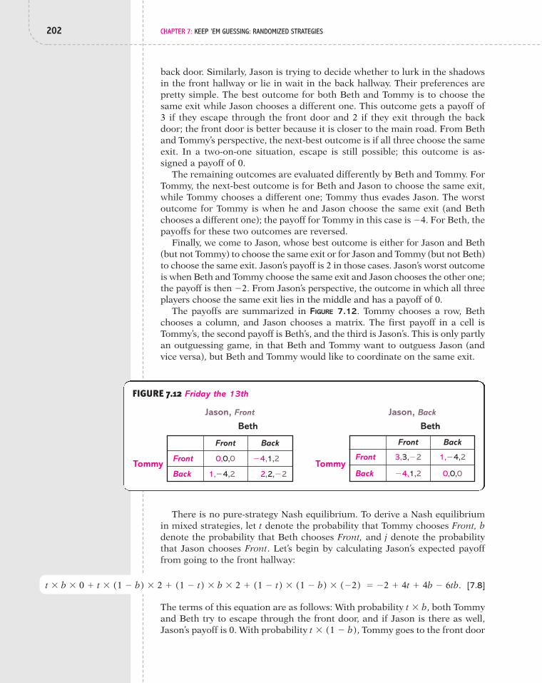
202 CHAPTER 7: KEEP ’EM GUESSING: RANDOMIZED STRATEGIES
back door. Similarly, Jason is trying to decide whether to lurk in the shadowsin the front hallway or lie in wait in the back hallway. Their preferences arepretty simple. The best outcome for both Beth and Tommy is to choose thesame exit while Jason chooses a different one. This outcome gets a payoff of3 if they escape through the front door and 2 if they exit through the backdoor; the front door is better because it is closer to the main road. From Bethand Tommy’s perspective, the next-best outcome is if all three choose the sameexit. In a two-on-one situation, escape is still possible; this outcome is as-signed a payoff of 0.
The remaining outcomes are evaluated differently by Beth and Tommy. ForTommy, the next-best outcome is for Beth and Jason to choose the same exit,while Tommy chooses a different one; Tommy thus evades Jason. The worstoutcome for Tommy is when he and Jason choose the same exit (and Bethchooses a different one); the payoff for Tommy in this case is "4. For Beth, thepayoffs for these two outcomes are reversed.
Finally, we come to Jason, whose best outcome is either for Jason and Beth(but not Tommy) to choose the same exit or for Jason and Tommy (but not Beth)to choose the same exit. Jason’s payoff is 2 in those cases. Jason’s worst outcomeis when Beth and Tommy choose the same exit and Jason chooses the other one;the payoff is then From Jason’s perspective, the outcome in which all threeplayers choose the same exit lies in the middle and has a payoff of 0.
The payoffs are summarized in FIGURE 7.12. Tommy chooses a row, Bethchooses a column, and Jason chooses a matrix. The first payoff in a cell isTommy’s, the second payoff is Beth’s, and the third is Jason’s. This is only partlyan outguessing game, in that Beth and Tommy want to outguess Jason (andvice versa), but Beth and Tommy would like to coordinate on the same exit.
"2.
FIGURE 7.12 Friday the 13th
0,0,0
1,"4,2
"4,1,2
2,2,"2
Front Tommy
BethJason, Front
Front Back
3,3,"2
"4,1,2
1,"4,2
0,0,0
Front Tommy
BethJason, Back
Front Back
BackBack
There is no pure-strategy Nash equilibrium. To derive a Nash equilibriumin mixed strategies, let t denote the probability that Tommy chooses Front, bdenote the probability that Beth chooses Front, and j denote the probabilitythat Jason chooses Front. Let’s begin by calculating Jason’s expected payofffrom going to the front hallway:
[7.8]# "2 % 4t % 4b " 6tb.t ! b ! 0 % t ! (1 " b) ! 2 % (1 " t) ! b ! 2 % (1 " t) ! (1 " b) ! ("2)
The terms of this equation are as follows: With probability both Tommyand Beth try to escape through the front door, and if Jason is there as well,Jason’s payoff is 0. With probability Tommy goes to the front doort ! (1 " b),
t ! b,

7.5 Advanced Examples 203
and Beth to the back door, in which case Jason can attack Tommy, for whichJason’s payoff is 2. The third term is the analogous situation in which Jasonfinds Beth instead of Tommy in the front hallway. Finally, with probability
both Beth and Tommy escape out the back as Jason waitsat the front, so Jason’s payoff is Jason’s expected payoff from lurking inthe back hallway is similarly defined:
[7.9]
If Jason is to randomize between waiting in the front and waiting in theback, his payoff from those two alternatives must be the same. Equating equa-tions (7.8) and (7.9) and solving, we have
[7.10]
Thus, at a Nash equilibrium, the probability of Tommy going to the front plusthe probability of Beth going to the front must sum to 1 if randomizing is tobe optimal for Jason.
Turning to Tommy, his expected payoff from trying to escape through thefront door is
It, instead, he goes for the back door, his expected payoff is
For Tommy to find it optimal to randomize, it must be true that
[7.11]
Since the situations faced by Tommy and Beth are symmetric, an analogouscondition is derived for her:
[7.12]
Combining equations (7.10), (7.11), and (7.12), is a Nash equilib-rium if
If those three conditions hold, then all three players are content to randomize.The last two conditions imply that Combining this equation with the firstcondition, yields Thus, Tommy and Beth are equallyt* # 1
2 # b*.t* % b* # 1,t* # b*.
7j* " 6t* % t*j* # 1.
7j* " 6b* % b*j* # 1,
t* % b* # 1,
(t*, b*, j*)
7j " 6t % tj # 1.
7j " 6b % bj # 1.1 % 2b " 5j % 2bj # "4b % 2j % 3bj1
"4b % 2j % 3bj.b ! j ! 1 % (1 " b) ! j ! 2 % b ! (1 " j) ! ("4) % (1 " b) ! (1 " j) ! 0 #
1 % 2b " 5j # 2bj.b ! j ! 0 % (1 " b) ! j ! ("4) % b ! (1 " j) ! 3 % (1 " b) ! (1 " j) ! 1 #
"2 % 4t % 4b " 6tb # 2t % 2b " 6tb1 t % b # 1.
2t % 2b " 6tb.t ! b ! ("2) % t ! (1 " b) ! 2 % (1 " t) ! b ! 2 % (1 " t) ! (1 " b) ! 0 #
"2.(1 " t) ! (1 " b),

204 CHAPTER 7: KEEP ’EM GUESSING: RANDOMIZED STRATEGIES
likely to make a mad dash for the front and for the back. Given this equal likeli-hood, we can use equation (7.12) to derive Jason’s equilibrium strategy:
Jason then goes to the front hallway with probability So, what is the probability that both Tommy and Beth escape? It is the prob-
ability that both go to the front door and Jason is hiding at the back door, or
plus the probability that Tommy and Beth go to the back door and Jason is atthe front door, or
Since this sum is , there is a 25% chance that both Tommy and Beth get outof the house unharmed—but even if they do, there is always Friday the 13th,Part 2.
! SITUATION: BYSTANDER EFFECT
There is an infamous episode in 1964 in which Kitty Genovese was attackednear her apartment building in New York City. In spite of her screams report-edly having been heard by 38 people, no one came to her aid. Although shock-ing, the lack of response is not entirely surprising and has come to be calledthe bystander effect. Laboratory and field studies by psychologists have shownthat a person is less likely to offer assistance to someone in need when the per-son is in a group than when alone. All those people who heard KittyGenovese’s cries knew that many others heard them as well. Some studieseven find that the more people there are who could help, the less likely help isto occur.11 Let us show that these observations are consistent with equilibriumbehavior in a simple game-theoretic model.12
Suppose there are people who are faced with the decision of whetherto help someone in need of assistance. Each simultaneously chooses betweenhelping the victim (help) and ignoring the victim (ignore). We presume thatpeople are like minded and that each person cares about whether the victimis helped, but also that helping is personally costly. A person’s payoffs can takefour possible values, as shown in FIGURE 7.13.
n ' 2
1560
(1/2) ! (1/2) ! (8/15) #8
60.
(1/2) ! (1/2) ! (7/15) #7
60,
5.
7j* " 6 !12
%12
! j* # 11 j* #8
15.
a c
d bPlayer's choice
Other players' choices
Helps
All ignore At least one helps
Ignores
FIGURE 7.13 Payoff to a Player in the Bystander Game

7.5 Advanced Examples 205
Unlike what we assumed in previous games, we’re not saying exactly whatthe payoffs are; we just represent them symbolically by letters. a, b, c, and dare allowed to take any numerical values, as long as they satisfy two condi-tions: and For example, and is fine,while and is ruled out.
What do these assumptions on payoffs imply about preferences? First,means that a person prefers to help a victim if no one else intends to do
so. However, since , a person prefers not to help if someone else intendsto do so. People are then willing to help, but they don’t want to bother doingso if someone else will do it.
This game has n pure-strategy Nash equilibria, each of which has one per-son helping and the other people staying out of the fray. There are equilibria because they differ by the identity of the person who does the help-ing. For example, consider a strategy profile in which player 1 helps and play-ers ignore. By helping, player 1’s payoff is a, and by not helping, hispayoff is lower, at d, since his lack of help means that the victim receives noassistance, given that the other players are not intending to help. Thus,player 1’s strategy is optimal. Turning to any one of the other players, her pay-off from ignore is b, and that exceeds the payoff from helping, which is c. Thisis then, indeed, a Nash equilibrium.
These equilibria are, of course, asymmetric in that the entirety of the bur-den of helping falls on one person. A more symmetric solution can be foundby deriving an equilibrium in mixed strategies. Suppose each person choosesto help with some common probability p. A symmetric equilibrium is a valuefor p—call it —such that if each of the other players help with proba-bility then it is optimal for a player also to help with probability Thismeans that if each of the other players helps with probability then aplayer is indifferent between helping and ignoring and thus is content to ran-domize with any probability, including
Given that the other players each help with probability p, the ex-pected payoff to a player from helping is as follows:
Expected payoff from help [7.13]
Since each of the other players ignores with probability and since theirchoices are independent, the probability that all of them ignore is multiplied times, or In the event that none of the otherplayers help, this player receives a payoff of a from helping. With probability
at least one of the other players helps, and the payoffto this player from also helping is only c.* This explains the expected payoffin (7.13).
What is the payoff if this player instead chooses to ignore the victim?
Expected payoff from ignore [7.14]
Again, given their mixed strategies, all of the other players ignore with proba-bility If this player also chooses ignore, then the payoff is only d,(1 " p)n"1.
# (1 " p)n"1 ! d % 31 " (1 " p)n"1 4 ! b.
n " 11 " (1 " p)n"1,
(1 " p)n"1.n " 11 " pn " 1
1 " p,
# (1 " p)n"1 ! a % 31 " (1 " p)n"1 4 ! c.
n " 1p*.
p*,n " 1p*.p*,
n " 1p*
n " 1
2, . . . , n
nn " 1
b 7 ca 7 d
d # 1c # 4,b # 3,a # 5,d # 1c # 2,b # 3,a # 4,b 7 c.a 7 d
*Note that either the victim is helped by at least one of the other players, or the victim is helped bynone of them. Hence, the sum of the probabilities of these two events must equal 1. Since the probabilityof the latter event is the probability of the former event must be 1 " (1 " p)n"1.(1 " p)n"1,
n " 1

because he feels bad for the victim’s having been neglected. With probabilityat least one of the other players helps, so the payoff for ignore
is b.The equilibrium strategy is then the value for p that equates equations
(7.13) and (7.14) so that a player is content to randomize:
Performing some algebraic manipulations on this equation, we can solve forthe symmetric equilibrium mixed strategy:
To analyze the properties of this equilibrium, assume that and so that the expression in (7.15) is
This equilibrium probability is plotted in FIGURE 7.14 against the number ofplayers in the game. The probability that a personhelps is lower when there are more people who canhelp, which is the first property from the psychologi-cal studies that we wanted to show.
Although each person is less likely to help, there arealso more people who could help. Accordingly, it isn’timmediately clear whether having a bigger groupmakes it more or less likely that at least one person of-fers assistance. To answer this question, however, wejust need to calculate the probability that at least oneof the n players will help, which is or
and is plotted in FIGURE 7.15. Quite amaz-ingly, more people make it less likely that the victim ishelped!*
1 " (14)
nn"1,
1 " (1 " p*)n,
p* # 1 " (14)
1n"1.
d # 1,c # 2,b # 3,a # 4,
p* # 1 " c b " c(a " d) % (b " c)
d 1n"1
.
1 " p* # c b " c(a " d) % (b " c)
d 1n"1
,
3 (1 " p*)n"1 4 1n"1 # c b " c
(a " d) % (b " c)d 1
n"1
,
(1 " p*)n"1 #b " c
(a " d) % (b " c),
(1 " p*)n"1 3 (a " d) % (b " c) 4 # b " c,
(1 " p*)n"1a % c " (1 " p*)n"1c # (1 " p*)n"1d % b " (1 " p*)n"1b,
(1 " p*)n"1a % 31 " (1 " p*)n"14 c # (1 " p*)n"1d % 31 " (1 " p*)n"1 4 b,
(1 " p*)n"1a % 31 " (1 " p*)n"1 4 c # (1 " p*)n"1d % 31 " (1 " p*)n"1 4 b.
p*
1 " (1 " p)n"1,
206 CHAPTER 7: KEEP ’EM GUESSING: RANDOMIZED STRATEGIES
n
1
1 2 3 4 5 6 7 8 9 100
FIGURE 7.14 Probability of a Person Helping
*It is worth noting that these two properties hold for any values of a, b, c,and d, as long as and b 7 c.a 7 d
[7.15]

7.6 Games of Pure Conflict and Cautious Behavior 207
7.6 Games of Pure Conflict and Cautious BehaviorRECALL THAT A TWO-PLAYER constant-sum game is a game in which the two play-ers’ payoffs always sum to a constant. Since this property implies that achange in behavior which raises one player’s payoff must lower the otherplayer’s payoff, constant-sum games are situations of pure conflict. In otherwords, what is good for one player is bad for the other.
Consider the situation faced by Sherlock Holmes and his arch-nemesis,Professor Moriarty, in Sir Arthur Conan Doyle’s story The Final Solution.Holmes inflicted serious and perhaps irreparable damage upon Moriarty’scrime ring and Moriarty is in hot pursuit to wreak vengeance. Holmes’s initialescape route was to proceed by train from London to Dover and from there tothe continent. As the train pulls out, he notices Moriarty on the platform.Holmes rightly infers that his adversary, who has similarly seen Holmes, willsecure a special train to overtake him. Holmes is faced with the decision of ei-ther going to Dover or disembarking at Canterbury, which is the only interme-diate station. Moriarty, whose intelligence allows him to recognize these pos-sibilities, has the same set of options.
Holmes believes that if they should find themselveson the same platform, it is likely that he’ll be killed byMoriarty. If Holmes reaches Dover unharmed, he canthen make good his escape. Even if Moriarty guessescorrectly, Holmes prefers Dover, as then, if Moriartydoes fail, Holmes can better escape to the continent.The strategic form of the game is shown in FIGURE 7.16.Note that it is a game of pure conflict, since the payoffsalways sum to 100.
If you have read many Sherlock Holmes stories,you know that he is both brilliant and arrogant.*
n
1
1 2 3 4 5 6 7 8 9 100
FIGURE 7.15 Probability of at Least One Person Helping
*Well, . . . “self-assured,” Holmes might say.
20,80 90,10
70,30 10,90Holmes
Moriarty
Dover
Canterbury
Dover Canterbury
FIGURE 7.16 The Final Solution

208 CHAPTER 7: KEEP ’EM GUESSING: RANDOMIZED STRATEGIES
While it would be uncharacteristic of him to take a conservative tack in han-dling a strategic situation, he is smart enough to know that Moriarty maywell be his match. So, rather than think about Holmes formulating a conjec-ture about what Moriarty would do and then choosing a best reply, let us pre-sume that he takes a more cautious route in selecting a strategy.
Suppose, then, that Holmes believes that whatever strategy he selects,Moriarty will have foreseen it and will act so as to minimize Holmes’ expectedpayoff. That he anticipates his payoff being minimized may reflect Holmes’s pes-simism about the situation, but also keep in mind that, since this is a constant-sum game, Moriarty minimizing Holmes’s payoff is equivalent to Moriartymaximizing his own payoff. Having anticipated this response from Moriarty,Holmes then wants to choose the mixed strategy that maximizes his own ex-pected payoff. In other words, he exercises caution by optimizing against hispessimistic beliefs. What we’ve just described Holmes as choosing is what isknown as his maximin strategy. More generally, a maximin strategy maxi-mizes a player’s payoff, given that the other players are expected to respond bychoosing strategies to minimize that player’s payoff.
To derive Holmes’s maximin strategy, a bit of notation is required. Letbe Holmes’s expected payoff should he choose a mixed strategy of
(where is the probability that he goes to Dover) and Moriarty choosesthe pure strategy (which is that Moriarty goes to either Dover orCanterbury).* The maximin strategy for Holmes is a mixed strategy that solvesthe following problem: Choose to maximize when is chosento minimize , given what is. If we let be the value for that minimizes , then Holmes’ problem can be restated as choosing
to maximize Thus, in choosing Holmes anticipates thatMoriarty will use and thereby minimize Holmes’s expected payoff.Whatever Holmes does, Moriarty will anticipate it and act accordingly.
To solve this problem, first consider Holmes’s expected payoff whenMoriarty chooses to go to Dover:
If Moriarty chooses Canterbury, Holmes’s expected payoff is
The expected payoffs are plotted in FIGURE 7.17 for all of the feasible values forRecall that we’re presuming that whatever value for that Holmes
chooses, Moriarty will figure it out and choose the station that minimizesHolmes’s expected payoff. Consequently, Holmes faces the lower envelope ofthe two lines shown, which is the bold line. For example, if Holmes sets
then he anticipates an expected payoff of sinceMoriarty’s choosing Canterbury will minimize Holmes’s payoff.
There is a clear maximum for Holmes in Figure 7.17, and it occurs wherethe two lines intersect. We can then solve for his maximin strategy as follows:
70 " 50pH # 10 % 80pH1 pH # 613.
10 % 80 ! (14) # 30,pH # 1
4,
pHpH.
VH(pH, Canterbury) # pH ! 90 % (1 " pH) ! 10 # 10 % 80pH.
VH(pH, Dover) # pH ! 20 % (1 " pH) ! 70 # 70 " 50pH.
b(pH)pH,VH(pH, b(pH)).pH
VH(pH, sM)sMb(pH)pHVH(pH, sM)
sMVH(pH, sM)pH
sM
pHpH
VH(pH, sM)
*In looking at Holmes’s problem, there is no loss of generality in supposing that Moriarty is limited tochoosing a pure strategy.

7.6 Games of Pure Conflict and Cautious Behavior 209
Thus, is the mixed strategy that maxi-mizes Holmes’s expected payoff, given that what-ever mixed strategy Holmes chooses, Moriartyresponds so as to minimize Holmes’s expectedpayoff. is called the maximin strategybecause it maximizes Holmes’s minimum pay-off, as depicted in Figure 7.17.
Before moving on, note that our cautiousHolmes strictly prefers to randomize, which wasnever the case with the noncautious play of aNash equilibrium. If a player randomizes at aNash equilibrium—say, with respect to Doverand Canterbury—then his expected payoff fromthat mixed strategy is the same as he gets fromchoosing the pure strategy Dover, the pure strat-egy Canterbury, or indeed any other randomiza-tion over the two pure strategies. With a Nashequilibrium, a player is choosing a strategy, hold-ing the other player’s strategy fixed. That is not thesituation with the cautious play associated with a maximin solution. Holmesis not taking Moriarty’s strategy as fixed; rather, he expects Moriarty to re-spond to Holmes’s choice of a mixed strategy by choosing that which mini-mizes Holmes’s expected payoff. If another player is able to anticipate whatyou are going to do, then it may be strictly preferable to randomize.
If this point isn’t clear yet, imagine that Holmes chose Dover. Then Moriartywould choose Dover and Holmes’ payoff would be 20. If Holmes choseCanterbury, then, in minimizing Holmes’s payoff, Moriarty would chooseCanterbury and Holmes’s payoff would be 10. Now consider Holmes flipping a faircoin between Dover and Canterbury so that each is chosen 50% of the time. FromFigure 7.17, we can see that Moriarty would choose Dover (when andHolmes’ expected payoff is Thus, Holmes does better to ran-domize than to use either pure strategy. Randomizing has Moriarty catchingHolmes in Dover 50% of the time, in which case Holmes’ payoff is 20, but 50% ofthe time Holmes gets off at Canterbury and earns a payoff of 70 by escapingMoriarty. Some unpredictability is desirable here and a mixed strategy delivers it.
Having solved for Holmes’s maximin strategy, now suppose Moriarty is sim-ilarly cautious, so that he chooses a mixed strategy, denoted (the probabil-ity that he goes to Dover), that maximizes his expected payoff, given that heanticipates Holmes choosing Dover or Canterbury so as to minimizeMoriarty’s expected payoff. Then if Holmes goes to Dover, Moriarty’s expectedpayoff from is
and if Holmes goes to Canterbury, it is
Plotting these equations in FIGURE 7.18, we find that Moriarty’s expected pay-off (given that Holmes chooses between Dover and Canterbury so as to make
pM ! 30 % (1 " pM) ! 90 # 90 " 60pM.
pM ! 80 % (1 " pM) ! 10 # 10 % 70pM,
pM
pM
70 " 50 ! (12) # 45.
pH # 12)
pH # 613
pH # 613
40
50
70
90
20
30
10
60
80
100
0 1
Moriarty chooses Dover
Moriarty chooses Canterbury
pH
6 13
1 2
FIGURE 7.17 Deriving Holmes’s Maximin Solution

210 CHAPTER 7: KEEP ’EM GUESSING: RANDOMIZED STRATEGIES
Moriarty as worse off as possible) is the boldline. The maximin strategy for Moriarty is then
Summing up, if both Holmes and Moriartyare not as cocky as they seem and have the cau-tious mind-set we have hypothesized them tohave, then Holmes will go to Dover with proba-bility while Moriarty will go to Dover withprobability This strategy pair is the maximinsolution to the game.
Now we come to the interesting part. Supposewe instead look for a Nash equilibrium in mixedstrategies. That is, Holmes chooses a mixedstrategy to maximize his expected payoff, giventhat he correctly anticipates Moriarty’s mixedstrategy, and similarly, Moriarty chooses a mixedstrategy to maximize his expected payoff, giventhat he correctly anticipates Holmes’s mixedstrategy. Then, using the method described pre-
viously in this chapter, we can show that the unique mixed-strategy Nash equi-librium has Holmes go to Dover with probability and Moriarty go to Doverwith probability For example, given that Moriarty uses this mixed strategy,Holmes’s expected payoff from going to Dover is
and from going to Canterbury is
Thus, Holmes is indifferent between the two pure strategies and between anyrandomization over them. It follows that Holmes’s going to Dover with prob-ability is a best reply to Moriarty’s going to Dover with probability , andone can show the same for Moriarty.
Note, then, that the Nash equilibrium is exactly the same as the maximin so-lution! Both players acting cautiously results in them choosing the best strat-egy under correct beliefs about what the other will do. In other words, there isno cost to being cautious, because a player who acts in that manner ends upusing a best reply to what the other player is doing. This is no coincidence.
Maximin Property: For any two-player game of pure conflict, themaximin solution is a Nash equilibrium. Furthermore, if a two-player game ofpure conflict has a Nash equilibrium in which both players randomize (i.e., theydon’t use pure strategies), then each player’s Nash equilibrium strategy is alsohis maximin strategy.
The articulation of the maximin property is credited to John von Neumann,one of the great mathematicians of the twentieth century. His contributions
813
613
a 813b ! 70 % a 5
13b ! 10 #
61013
.
a 813b ! 20 % a 5
13b ! 90 #
61013
813.
613
813.
613,
pM # 813.
40
50
70
90
20
30
10
60
80
100
0 1
Holmes chooses Dover
Holmes chooses Canterbury
pM
813
FIGURE 7.18 Deriving Moriarty’s Maximin Solution

Summary 211
span far beyond pure mathematics to include physics and computer science.Particularly dear to our hearts is that in 1944, he, along with OskarMorgenstern, wrote the first classic book in game theory, Theory of Games andEconomic Behavior.
SummaryPrior to this chapter, a player was modeled as deterministically choosing howto behave as reflected in his choice of a pure strategy. In some contexts, how-ever, it is natural to consider the possibility of randomized play. To encompasssuch an option, the randomized version of a game was developed. A strat-egy for a player is now a mixed strategy, which assigns a probability to eachof the player’s pure strategies. In evaluating a profile of mixed strategies, aplayer calculates the expected payoff using the probabilities implied by themixed strategies and the payoffs from the original game. An attractive prop-erty of the randomized version of a game is that it always has a solution; thatis, there is always a Nash equilibrium in mixed strategies.
We explored two classes of games in which randomized play is especiallyappealing. One class is outguessing games—games in which a player wantsto do what is unanticipated by other players. Because a player wants to beunpredictable, randomly selecting a pure strategy is one method for accom-plishing that goal. Examples of outguessing games are adversarial situa-tions such as those which arise in sports (Penalty Kick), crime (PolicePatrol and Drug Trade), war (Avranches Gap), and summer camp (Fridaythe 13th).
A second class of situations is symmetric games with congestion—games inwhich a strategy becomes increasingly less attractive the more players whochoose it. Examples of these games in this chapter are Market Entry and theBystander Game. Although games with congestion may have asymmetricpure-strategy Nash equilibria, they typically do not have symmetric pure-strat-egy equilibria. In light of the symmetry of the game, a symmetric solution hassome appeal, and these games often have a symmetric Nash equilibrium withmixed strategies.
At a Nash equilibrium, a player who uses a mixed strategy is necessarily in-different among the pure strategies over which she randomizes. All of the purestrategies assigned positive probability must yield the highest expected payoff,and it is for that reason that a player is content to let a random device deter-mine how she behaves. If that weren’t the case, then, after performing the ran-domization, a player might decide to ignore what was recommended andchoose a better strategy. This equilibrium property of indifference is highlyuseful in solving for mixed-strategy Nash equilibria.
A player’s maximin strategy was defined to be that strategy which max-imizes his payoff when he makes the highly cautious assumption that,whatever strategy he chooses, the other players will act in the worst waypossible for him. For two-player games of pure conflict, a maximin solu-tion, whereby both players use a maximin strategy, is also a Nash equilib-rium. Thus, regardless of whether a player is pessimistic (thinking that theother player has outsmarted him) or optimistic (thinking that he has cor-rectly anticipated the other player’s strategy), the proper behavior is thesame.

212 CHAPTER 7: KEEP ’EM GUESSING: RANDOMIZED STRATEGIES
1. Reproduced in FIGURE PR7.1 is the telephone game from Section 4.2.Find all Nash equilibria in mixed strategies.
2. The count is three balls and two strikes, and the bases are empty. Thebatter wants to maximize the probability of getting a hit or a walk, whilethe pitcher wants to minimize this probability. The pitcher has to decidewhether to throw a fast ball or a curve ball, while the batter has to de-cide whether to prepare for a fast ball or a curve ball. The strategic formof this game is shown in FIGURE PR7.2. Find all Nash equilibria in mixedstrategies.
EXERCISES
3. It’s spring break and you’re traveling south on Interstate 95, heading to-ward Fort Lauderdale. Do you travel the legal limit of 65 miles per hour,or do you crank it up to 80 and hope that there’s no speed trap? Andwhat about the state police? Do they set a speed trap or instead head intotown and find out whether the “Hot and Fresh” neon sign is lit up at theKrispy Kreme? (Ouch, that’s a cheap shot!) The police like to nab speed-ers, but they don’t want to set a speed trap if there aren’t going to be anyspeeders to nab. A strategic form for this setting is shown in FIGURE
PR7.3. The driver can either go the legal limit of 65 mph or speed at 80mph. The police officer can set a speed trap or head into town and grabsome of those delicious high-carb doughnuts. The best outcome for thedriver is that she speeds and isn’t caught; the payoff for that case is 70.The worst outcome is that she speeds and is nailed by the police, forwhich the payoff is 10. If she chooses to drive the legal limit, then herpayoff is 40 and is the same regardless of what the state police do. (Inother words, the driver doesn’t care about the caloric intake of thetrooper.) As for the police officer, his best outcome is setting a speed trapand nailing a speeder, giving him a payoff of 100. His worst outcome issitting out there in a speed trap and failing to write a ticket; this outcomedelivers a payoff of only 20. His payoff is 50 when he chooses to go tothe Krispy Kreme. Find all Nash equilibria in mixed strategies.
0,0 2,3
3,2 1,1Colleen
Winnie
Call
Wait
Call Wait
FIGURE PR7.1 The TelephoneGame
.35,.65
.2,.8
.3,.7
.5,.5Batter
Pitcher
Fastball
Curveball
Fastball Curveball
FIGURE PR7.2 Baseball
FIGURE PR7.3 Speed Trap and Doughnuts
10,100
40,20
70,50
40,50Driver
State police officer
80 mph
65 mph
Speed trap Krispy Kreme

Exercises 213
4. A mugger and a victim meet on a dark street. The mugger previously de-cided whether to bring a gun and, if he did, whether to show it duringthe robbery. If the mugger does not show a gun—either because he doesn’thave one or has one and hides it—then the victim has to decide whetherto resist. (Note that if the mugger does have a gun and shows it, then thevictim’s payoff is 5 regardless of the strategy chosen, because the victim’sstrategy is what to do if no gun is shown.) The strategic form of this sit-uation is shown in FIGURE PR7.4. Note that all payoffs have been speci-fied, except for the mugger’s payoff when he chooses to have a gun andshow it. Find a condition on x whereby there is a Nash equilibrium inwhich the mugger randomizes over the two pure strategies gun, hide andno gun and the victim randomizes over resist and do not resist.
FIGURE PR7.4
2,6
3,2
x,5
6,3
5,4
x,5
Mugger
Victim
No gun
Gun, hide
Gun, show
Resist Do not resist
Player 1
Player 2
a 3,2
b
d 6,1
2,3
5,1
4,2
3,7
1,4
2,3
1,3
4,6c 5,4
1,2
x y z
FIGURE PR7.6
5. For the Penalty Kick game in Section 7.5, find a Nash equilibrium inwhich the kicker randomizes only over the pure strategies left and right,so that zero probability is given to center.
6. For the game illustrated in FIGURE PR7.6, find all mixed-strategy Nashequilibria.
7. Find all Nash equilibria in mixed strategies for the game shown in FIGURE
PR7.7.
FIGURE PR7.7
2,2
1,3
3,1
0,0
3,0
2,3
Player 1
Player 2
Top
Middle
Bottom
Left Middle
1,3
1,0
2,2
Right

214 CHAPTER 7: KEEP ’EM GUESSING: RANDOMIZED STRATEGIES
8. It is the closing seconds of a football game, and the losing team has justscored a touchdown. Now down by only one point, the team decides togo for a two-point conversion that, if successful, will win the game. Theoffense chooses between three possible running plays: run wide left, runwide right, and run up the middle. The defense decides between defend-ing against a wide run and a run up the middle. The payoff to the de-fense is the probability that the offense does not score, and the payoff tothe offense is the probability that it does score. Find all mixed-strategyNash equilibria. (See FIGURE PR7.8.)
FIGURE PR7.8 Two-Point Conversion
.6,.4Defense
Offense
Defend againstwide run
Run wide left Run up middle Run wide right
.6,.4
Defend againstrun up middle 3,.7 .5,.5
4,.6
3,.7
9. The childhood game of Rock–Paper–Scissors is shown in FIGURE PR7.9.(If you’re unfamiliar with this game, see Section 4.2.) Show that eachplayer’s assigning equal probability to his or her three pure strategies isa symmetric Nash equilibrium.
10. Each of three players is deciding between the pure strategies go andstop. The payoff to go is where m is the number of players thatchoose go, and the payoff to stop is 55 (which is received regardless ofwhat the other players do). Find all Nash equilibria in mixed strategies.
11. A total of companies are considering entry into a new market. Thecost of entry is 30. If only one company enters, then its gross profit is200. If more than one company enters, then each entrant earns a grossprofit of 40. The payoff to a company that enters is its gross profit minusits entry cost, while the payoff to a company that does not enter is 60.Find a symmetric Nash equilibrium in mixed strategies.
12. Sadaam Hussein is deciding where to hide his weapons of mass destruc-tion (WMD), while the United Nations is deciding where to look forthem. The payoff to Hussein from successfully hiding WMD is 5 andfrom having them found is 2. For the UN, the payoff to finding WMD is9 and from not finding them is 4. Hussein can hide them in facility X, Y,or Z. The UN inspection team has to decide which facilities to check.
n ' 2
120m ,
FIGURE PR7.9 Rock–Paper–Scissors
1,"1 0,0 Bart
Lisa
0,0 "1,1Rock
Paper
Rock Paper
1,"1
"1,1
0,0
Scissors
"1,1 1,"1Scissors

7.7 Appendix: Formal Description of Nash Equilibrium in Mixed Strategies 215
Because the inspectors are limited in terms of time and personnel, theycannot check all facilities.a. Suppose the UN has two pure strategies: It can either inspect facili-
ties X and Y (both of which are geographically close to each other) orinspect facility Z. Find a Nash equilibrium in mixed strategies.
b. Suppose the UN can inspect any two facilities, so that it has threepure strategies. The UN can inspect X and Y, X and Z, or Y and Z. Finda Nash equilibrium in mixed strategies.
7.7 Appendix: Formal Definition of Nash Equilibrium in Mixed StrategiesCONSIDER ANY FINITE GAME—a game in which there are a finite number of play-ers and each player has a finite number of (pure) strategies. If player i haspure strategies, then let her set of pure strategies be represented by
Now consider the randomized version of that game so that a(mixed) strategy for a player assigns a probability to each of her pure strate-gies. Let denote the probability player i assigns to pure strategy A mixedstrategy is then numbers, each of which lies in the interval [0,1] and whosesum equals 1. In other words, is a mixed strategy as long as
Player i’s (mixed) strategy set consists of all of the values for thatsatisfy the preceding conditions. Let Pi denote the (mixed) strategy set forplayer i. Remember that a pure strategy is a special case of a mixed strategy,so we’ve added to what is possible with randomization.
Another key specification of the randomized version of a game is that aplayer evaluates a mixed-strategy profile by calculating the expected payoff.Let us generally define this payoff for a two-player game. representsthe payoff to player 1 when she chooses pure strategy and player 2 choosespure strategy With this representation, we can define her expected payoffwhen player 1 uses mixed strategy and player 2 uses mixed strat-egy *
For player 2, the expected payoff is
When players randomize as a part of using mixed strategies, the presumptionis that the two random events—the pure strategy selected by player 1 and the
am1
j#1am2
k#1pj
1 ! pk2 ! V2(sj
1, sk2).
am1
j#1am2
k#1pj
1 ! pk2 ! V1(sj
1, sk2)
(p12, . . ., pm2
2 ).(p1
1, . . ., pm11 )
sk2.
sj1
V1(sj1, sk
2)
(p1i , . . ., pmi
i )
pji ' 0 for all j # 1,2, p , mi and p1
i % p % pmii # 1.
(p1i , . . ., pmi
i )mi
sji.pj
i
5s1i , . . ., smi
i 6.mi
* is shorthand for the summation of these m terms, so equals x1 % x2 % p % xm.am
j# 1xjam
j#1xj

216 CHAPTER 7: KEEP ’EM GUESSING: RANDOMIZED STRATEGIES
pure strategy selected by player 2—are independent. That is why the probabil-ity that player 1 uses and player 2 uses is
With this notation, we can now formally define the conditions for a Nashequilibrium in mixed strategies. For a two-player game, the mixed strategypair and is a Nash equilibrium if the following con-ditions are satisfied:
[7.16]
and
[7.17]
Equation (7.16) is the condition which ensures that player 1’s mixed strategyis optimal, and equation (7.17) is the condition guaranteeing that player 2’smixed strategy is optimal. For example, (7.16) says that, given that player 2uses there is no other mixed strategy which gives a higher ex-pected payoff than for player 1.
REFERENCES1. Umberto Eco, The Island of the Day Before (London: Vintage Books, 1994),
p. 198. Quoted on the back cover of the Journal of Political Economy, 109(2001), no. 3.
2. William Safire, “On Language,” New York Times Magazine, Nov. 19, 1995.
3. John F. Nash, Jr., “Noncooperative Games,” Annals of Mathematics, 54(1951), 289–95.
4. Robert Wilson, Computing Equilibria, SIAM Journal of AppliedMathematics, 21 (1971), 80–87.
5. The ensuing description and analysis is based on O. G. Haywood, Jr.,Military Decision and Game Theory, Operations Research, 2 (1954),365–85.
6. Omar N. Bradley, A Soldier’s Story (New York: Holt & Co., 1951), p. 372.
7. Ibid., p. 369.
8. This argument is reviewed in Itzhak Ravid, “Military Decision, GameTheory and Intelligence: An Anecdote,” Operations Research, 38 (1990),260–64.
9. The numbers come from Ignacio Palacios-Huerta, “Professionals PlayMinimax,” Review of Economic Studies, 70 (2003), 395–415. His data arefor penalty kicks during 1995–2000 and come largely from professionalgames in England, Italy, and Spain. All data in this section are based onthat study. The numbers are adjusted so as to refer to directionality in thefollowing sense: A right-footed (left-footed) kicker’s natural direction is tokick the ball to the right (left). When the reported data refer to “right,” that
(p̂11, . . ., p̂m1
1 )(p̂1
2, . . ., p̂m22 ),
am1
j#1am2
k#1p̂j
1p̂k2V2(sj
1, sk2) ' a
m1
j#1am2
k#1p̂ j
1 pk2V2(sj
1, sk2) for all (p1
2, . . ., pm22 ) ! P2.
am1
j#1am2
k#1p̂ j
1 p̂k2V1(sj
1, sk2) ' a
m1
j#1am2
k#1pj
1 p̂k2V1(sj
1, sk2) for all (p1
1, . . ., pm11 ) ! P1
(p̂12, . . ., p̂m2
2 )(p̂11, . . ., p̂m1
1 )
pj1 ! pk
2.sk2sj
1

References 217
means a kicker’s natural direction; “left” means the direction oppositefrom his natural direction.
10. Ibid.
11. For a review of this work, see Bibb Latané and Steve Nida, “Ten Years ofResearch on Group Size and Helping,” Psychological Bulletin, 89 (1981),308–24.
12. This analysis is based on Joseph E. Harrington, Jr., “A Simple Game-Theoretic Explanation for the Relationship between Group Size andHelping,” Journal of Mathematical Psychology, 45 (2001), 389–92.

This page intentionally left blank

8.1 IntroductionTHE FOCUS OF THE PRECEDING chapters has been solving strategic form games. Wenow turn to handling extensive form games, such as Chapter 2’s Kidnappinggame, which is reproduced here as FIGURE 8.1. As a bit of refresher on the ex-tensive form, recall that each dot is a decision node and, at each of them, aplayer has to make a choice among the branches (or actions) coming out ofthat node. In games of perfect information, which is what we explore in thischapter, a strategy for a player assigns an action to each decision node. Thus,for Guy, a strategy is a triple of actions, since he has three decision nodes,while for Vivica a strategy is a single action.*
The concept of Nash equilibrium can be applied directly to the extensiveform, but it’s easier to first derive its strategic form and then derive the Nash
8
219
Taking Turns: Sequential Games with Perfect Information
*Recall that an information set is a collection of decision nodes whereby a player knows that she is at oneof those decision nodes, but knows nothing more. In a game of perfect information, each information setis made up of a single decision node, so a player always knows where she is in a game when it is time forher to move. Hence, we will use the terms “decision node” and “information set” interchangeably in thischapter. For further review on extensive form games of perfect information, reread Sections 2.1 to 2.3.
Guy
Guy 3
Vivica 5 Pay ransom
Vivica
4
1
5
3
2
2
1
4
Do not kidnap
Do not pay ransom
Kidnap
Guy
Kill KillRelease Release
Guy
FIGURE 8.1 The Extensive Form of the KidnappingGame (from Chapter 2)

220 CHAPTER 8: TAKING TURNS: SEQUENTIAL GAMES WITH PERFECT INFORMATION
equilibria for it. Since the Nash equilibria for the extensive form and for thestrategic form coincide, this is a legitimate way to proceed.
Pursuing that approach, we show the strategic form corresponding toFigure 8.1 in FIGURE 8.2. In stating a strategy for Guy, we let the first action(kidnap or do not kidnap) be what he does at the initial node, the second ac-tion (kill or release) be what he does when Vivica pays ransom, and the thirdaction (kill or release) be what he does when Vivica does not pay ransom.
3,5
3,5
3,5
3,5
4,1
4,1
5,3
5,3
3,5
3,5
3,5
3,5
2,2
1,4
2,2
1,4
Do not kidnap/Kill/Kill
Do not kidnap/Kill/Release
Do not kidnap/Release/Kill
Do not kidnap/Release/Release
Kidnap/Kill/Kill
Kidnap/Kill/Release
Kidnap/Release/Kill
Kidnap/Release/Release
Guy (kidnapper)
Vivica (kin of victim)
Pay ransom Do not pay ransom
FIGURE 8.2 The Strategic Form for the Kidnapping Game
Considering each of the 16 strategy pairs, we find that there are five pure-strategy Nash equilibria. (Kidnap/Release/Kill, Pay ransom) is one of them, andit has Orlando being kidnapped, Vivica paying ransom, and Orlando beingreleased. Then there are four Nash equilibria in which no kidnappingtakes place: (1) (Do not kidnap/Kill/Kill, Do not pay ransom); (2) (Do notkidnap/Kill/Release, Do not pay ransom); (3) (Do not kidnap/Release/Kill, Do notpay ransom); and (4) (Do not kidnap/Release/Release, Do not pay ransom). Ineach of these cases, Guy chooses not to kidnap Orlando because Vivica has nointention of paying ransom. These four equilibria differ only in terms of whatGuy’s strategy prescribes later in the game in the event that he performs a kid-napping which, in equilibrium, he does not.
For the Kidnapping game, Nash equilibrium isn’t particularly precise. Itpredicts that there could be a kidnapping or not; that is, some equilibria haveOrlando being kidnapped, and others do not. But are all Nash equilibria cre-ated equal? In fact, there is something troublesome about the four equilibriathat result in no kidnapping. They all involve Vivica’s making a not very cred-ible threat and Guy’s believing it. Guy doesn’t kidnap Orlando because he be-lieves that Vivica will not pay the ransom. However, Vivica’s strategy is opti-mal only because Guy doesn’t engage in a kidnapping, so her payoff is thesame regardless of what her strategy is. But suppose, contrary to Guy’s strat-egy, he did end up kidnapping Orlando. Would Vivica persist with the threatnot to pay ransom? She knows Guy’s preferences—specifically, that Guyprefers to kill Orlando when ransom is not paid (the payoff is 2, versus 1 fromreleasing him) and that he prefers to release Orlando when ransom is paid

8.2 Backward Induction and Subgame Perfect Nash Equilibrium 221
(the payoff is 5, versus 4 from killing him). Thus, it would seem to be in herbest interest to pay the ransom and thereby induce the release of Orlando.Now, Guy knows all this as well, so, regardless of what Vivica says she woulddo, he ought to believe that she would pay ransom if Orlando were kidnapped,as that is the only way to induce Guy to release Orlando.
To sum up, the four Nash equilibria sustaining the “no kidnapping” out-come aren’t very convincing. They are predicated upon Guy’s believing thatVivica would act irrationally by not paying ransom in the event of a kidnap-ping. But Vivica is only bluffing that she would not pay ransom, and Guyshould call that bluff. The lone equilibrium that results in a kidnapping doesnot call for Vivica to make an irrational move or for Guy to believe that shewould make an irrational move. We are then inclined to conclude that themost compelling Nash equilibrium is (Kidnap/Release/Kill, Pay ransom).
This and the ensuing chapter are concerned with solving extensive formgames and, in particular, ruling out those Nash equilibria which are sustainedby believing that another player would make an irrational move, or what gametheorists call an incredible threat (but where “incredible” means “not credi-ble,” as opposed to “awesome”). This chapter focuses on games involving per-fect information and a solution concept which formalizes the argument thatled us to eliminate the four Nash equilibria in the kidnapping game. Morespecifically, we will learn about backward induction, a method for solving agame whose solution is known as subgame perfect Nash equilibrium.
8.2 Backward Induction and Subgame Perfect Nash EquilibriumRECALL THAT A STRATEGY is a contingency rule that prescribes an action for eachinformation set for a player. Nash equilibrium requires that each player’s strat-egy be optimal, given the other players’ strategies. Of course, what a strategycalls for at a decision node that is not reached cannot matter for a player’s pay-off; the action assigned to a contingency matters only if one is called upon toimplement it. Thus, a Nash equilibrium does not require that the prescribedaction be optimal for all contingencies, but rather only for those reached overthe course of equilibrium play (i.e., the sequence of play that occurs whenplayers use their equilibrium strategies).
To make this point more concrete, consider the strategy profile(Kidnap/Release/Kill, Pay ransom). Equilibrium play involves a kidnapping oc-curring, in which case Vivica’s strategy must prescribe the best action in re-sponse to a kidnapping (which is to pay ransom). Since the contingency inwhich Vivica pays ransom also occurs, Guy’s strategy must prescribe what isbest in that case (which is to release Orlando). Now contrast this strategy pro-file with the strategy profile (Do not kidnap/Kill/Kill, Do not pay ransom), forwhich equilibrium play predicts no kidnapping. Vivica’s strategy, which pre-scribes what she does in the event of a kidnapping, is not required to call foran optimal action in that event, because a kidnapping doesn’t occur whenGuy’s equilibrium strategy assigns do not kidnap at the initial node. Note thatVivica’s payoff is the same regardless of her strategy. (Check if you’re not con-vinced.) Similarly, Guy’s strategy doesn’t have to call for an optimal decisionin the event of a kidnapping and Vivica paying ransom, since that contingencydoesn’t occur either.

222 CHAPTER 8: TAKING TURNS: SEQUENTIAL GAMES WITH PERFECT INFORMATION
The key point here is that Nash equilibrium does not require that a strategyprescribe an optimal action for those decision nodes which are not reachedduring the course of equilibrium play. If a particular contingency is never re-alized, then it doesn’t make any difference to a player what strategy is assignedfor that contingency. What Nash equilibrium does require is that each player’sstrategy prescribe an optimal action for all decision nodes that are reachedduring equilibrium play.
A Nash equilibrium strategy, then, is optimal only in a restricted sense. Theidea behind a subgame perfect Nash equilibrium is to extend the required op-timality of a player’s action to all contingencies, not just those which occuralong an equilibrium path. So, for example, subgame perfect Nash equilib-rium would require Vivica’s behavior to be optimal in the event that there is akidnapping, even if Guy’s strategy is, say, Do not kidnap/Kill/Release, whichleads to no kidnapping during equilibrium play.
Subgame Perfect Nash Equilibrium for Games of Perfect Information: For a gameof perfect information, a strategy profile is a subgame perfect Nash equilibrium if,at each decision node, it assigns an action that maximizes a player’s payoff.*
A more formal definition of subgame perfect Nash equilibrium is providedin the next chapter, which covers games of both perfect and imperfect infor-mation. Here and now, we focus on games of perfect information. Our ap-proach is to build a strategy for a player piece by piece while presuming thatother players act optimally. Recall that a strategy assigns an action to each ofa player’s information sets. The strategy template for Guy is
At the initial node, ______ [fill in kidnap or do not kidnap].
If a kidnapping occurred and ransom was paid, then ______ [fill in kill orrelease].
If a kidnapping occurred and ransom was not paid, then ______ [fill in killor release].
A particular strategy, then, fills in the preceding three blanks. Vivica’s strategytemplate is
If a kidnapping occurred, then _______ [fill in pay ransom or do not payransom].
The method of backward induction involves filling in each player’s strategytemplate by starting at the game’s final decision node(s), deriving optimal be-havior, and then continuing to work backward up the tree to the initial node.In this manner, a subgame perfect Nash equilibrium is constructed. It is easi-est to understand the method with an example.
For the game of Kidnapping, go to the final two decision nodes associatedwith Guy’s deciding whether to kill or release Orlando. For each of thosenodes, determine Guy’s optimal action. For the decision node associated withVivica’s having paid ransom, Guy’s best action is release; and for the decisionnode associated with Vivica’s having not paid ransom, Guy’s best action is kill.We have then derived Guy’s actions at those two decision nodes, thereby hav-ing filled in the bottom two blanks in Guy’s strategy template.
*Why this solution concept is called “subgame perfect Nash equilibrium” will be explained in Chapter 9.

8.2 Backward Induction and Subgame Perfect Nash Equilibrium 223
The next step is, for each of those two decision nodes, to replace the tree thatcomes out of it (which consists of the branches kill and release in either case) withthe payoffs associated with Guy’s optimal action. This replacement process is de-picted in FIGURE 8.3. The presumption is that when each of those decision nodesis reached Guy will choose the optimal action, so we might as well just replacethose branches with the payoffs associated with Guy’s making such a choice.
Guy
Guy 3
Vivica 5 Pay ransom
Vivica
4
1
5
3
2
2
1
4
Do not kidnap
Do not pay ransom
Kidnap
Guy
Kill KillRelease Release
Guy
Guy
Guy 3
Vivica 5 Pay ransom
Vivica
5
3
2
2
Do not kidnap
Do not pay ransom
Kidnap
FIGURE 8.3 The Procedure of Backward Induction
The process is then repeated for Vivica’s decision node. We compare the pay-offs associated with her paying and not paying ransom. We then see thatVivica’s optimal action is to pay ransom. Thus, we’ve foundVivica’s best action for her lone decision node and thereby haveher subgame perfect Nash equilibrium strategy. Substituting thetree coming out of Vivica’s decision node with the payoffs in-duced by derived behavior then gives us the game in FIGURE 8.4.The game has thus been solved backwards such that there is onedecision node remaining, which is whether Guy kidnaps. Guy’soptimal action is to kidnap.
As just constructed, a subgame perfect Nash equilibrium(which happens to be the unique one for this game) has Guychoose kidnap at the initial node, release at the information setassociated with Vivica’s having paid ransom, and kill at the in-formation set associated with Vivica’s having not paid ransom.For Vivica, her subgame perfect Nash equilibrium strategy ispay ransom. Thus, the unique subgame perfect Nash equilib-rium is (Kidnap/Release/Kill, Pay ransom) which is what we previously arguedis the compelling Nash equilibrium—that is, the lone one not reliant uponVivica’s incredible threat not to pay ransom.
Guy
Guy 3
Vivica 5
5
3
Do not kidnap Kidnap
FIGURE 8.4 Solving ThroughBackward Induction Upto Guy’s Initial Choice

224 CHAPTER 8: TAKING TURNS: SEQUENTIAL GAMES WITH PERFECT INFORMATION
We have just gone through the solution method of backward induction.Working backward through the extensive form, we used inductive reasoning tolead us to the solution.
The Backward Induction Algorithm for Games of Perfect Information:
1. For each of the final decision nodes, solve for optimal behavior.
2. For each of those decision nodes, replace the part of the tree beginning withthat decision node with the associated payoffs, assuming optimal play.
3. Repeat steps 1 and 2 for this reduced game until the initial decision nodeis reached.
Implicit in subgame perfect Nash equilibrium is the idea that a player an-ticipates that other players will subsequently act optimally. For example, whenwe solved for Vivica’s optimal action using the game in Figure 8.3, we assumedthat she implicitly anticipates that, whatever she does, Guy will respond opti-mally. Specifically, when she thinks about paying ransom, she expects Guy torelease Orlando; when she thinks about not paying ransom, she expectsOrlando to be killed. In both cases, this is what would be best for Guy. Thus,incredible threats are eliminated by always presuming that a player does whatis best, regardless of where he or she is in the game.
For a game of perfect information, this procedure always delivers an an-swer. At each decision node, there is always an optimal action, which meansthat you can always identify the payoffs you should use to replace that part ofthe tree. Because at no point does the procedure get stuck, you can alwayssolve the game back to the initial node. Put another way, backward inductionrecovers all subgame perfect Nash equilibria and there always exists at leastone subgame perfect Nash equilibrium.
Existence of a Subgame Perfect Nash Equilibrium: In a game of perfect information, there is atleast one subgame perfect Nash equilibrium.
Although the existence of a subgame perfect Nashequilibrium is assured for a game of perfect information,that equilibrium is unique is not assured: multiple sub-game perfect Nash equilibria may exist when, at a givendecision node, there is no single optimal action. This sit-uation arises in the game of Racial Discrimination andSports (Section 8.3.4).
The following property is worth noting:
Every subgame perfect Nash equilibrium is a Nash equilibrium, but not every Nash equilibrium is asubgame perfect Nash equilibrium.
This is another way of saying that requiring a subgameperfect Nash equilibrium is a more stringent criterionthan requiring a Nash equilibrium. A Nash equilibriumrequires that prescribed behavior be optimal for those
For the game in FIGURE 8.5, solve for the sub-game perfect Nash equilibria.
8.1 CHECK YOUR UNDERSTANDING
Player 1
Player 2
Player 3
1
4
3
x
a b
y
8
1
5
1
6
2
c d
2
0
3
2 3
1
FIGURE 8.5
8.3 Examples 225
decision nodes reached along the equilibrium path, but a subgame perfect Nashequilibrium requires, in addition, that prescribed behavior be optimal for thosedecision nodes which are not reached. By way of example, (Kidnap/Release/Kill,Pay ransom) is both a subgame perfect Nash equilibrium, and a Nash equilib-rium, but the other four Nash equilibria are not subgame perfect Nash equilibria.
8.3 ExamplesTO ASSIST US IN GAINING some fluency in using backward induction, this sectionprovides a range of examples involving misconduct. In the first example, theCuban Missile Crisis, the Soviet Union’s misconduct is planting nuclear mis-siles in Cuba. The issue is how the United States can get the missiles out ofthere without starting a nuclear war. In the second case, we explore howEnron executives are manipulated by a prosecutor through the strategic useof a plea bargain. In the last example, the misbehavior of a racially biasedbaseball team owner is shown to be penalized by the strategizing of an astuteracially neutral owner when it comes to drafting amateur athletes.
! SITUATION: CUBAN MISSILE CRISIS
Meeting of Joint Chiefs of Staff (JCS), 10:00 A.M. on October 16, 1962:1
Chairman, JCS, says he will see the President at 11:45.
General McKee: Once the missile sites become operational, Castro canthreaten retaliation for any offensive move by the U.S. delaying action untilthe missiles are set up could touch off nuclear war.
General Shoup: Soviets might be attempting to pose a nuclear threat to theU.S. without running a risk of nuclear retaliation against the Soviet Union.
JCS agrees the threat is so serious as to require the U.S. to take out the mis-siles by military effort.
General Wheeler favors air attack without warning, to be followed by invasion.
General McKee foresees a possibility of avoiding the need for invasion by ef-ficient application of air strikes and naval blockade.
On October 14, 1962, the United States confirmed the presence of Soviet nu-clear missiles in Cuba. It was the time of the Cold War, and the United Statesand the Soviet Union (U.S.S.R.) were archrivals, each with the capacity to wreakdestruction on an unprecedented scale. The Soviet Union had now placed theseweapons less than 100 miles from the U.S. coastline. FIGURE 8.6 shows the rangeof Soviet SS-4 medium-range ballistic missiles (MRBMs) and SS-5 intermediate-range ballistic (IRBMs). The strategic challenge for President John F. Kennedyand his advisers was to get the missiles out of Cuba before they became opera-tional, which the CIA estimated would be in about 10 days.2
The sequence of decisions facing the U.S. and Soviet leaders is shown inFIGURE 8.7.3 The U.S. initially decides whether to blockade the island—so as toprevent any additional Soviet ships from reaching Cuba—or to perform an airstrike to destroy the missiles before they become operational. If the latter op-tion is taken, then the strategic situation is over, while the choice of a block-ade throws the decision to the U.S.S.R., which must then decide between re-taining the missiles or withdrawing them. If it chooses the latter, then theUnited States again decides whether to perform an air strike.
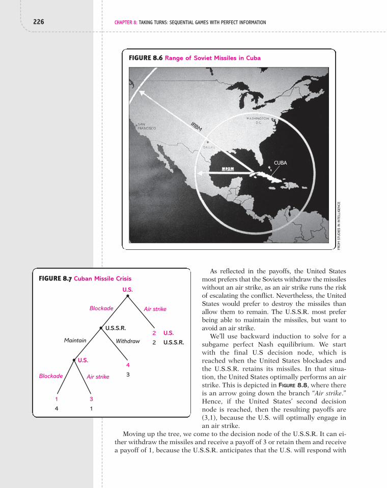
As reflected in the payoffs, the United Statesmost prefers that the Soviets withdraw the missileswithout an air strike, as an air strike runs the riskof escalating the conflict. Nevertheless, the UnitedStates would prefer to destroy the missiles thanallow them to remain. The U.S.S.R. most preferbeing able to maintain the missiles, but want toavoid an air strike.
We’ll use backward induction to solve for asubgame perfect Nash equilibrium. We startwith the final U.S decision node, which isreached when the United States blockades andthe U.S.S.R. retains its missiles. In that situa-tion, the United States optimally performs an airstrike. This is depicted in FIGURE 8.8, where thereis an arrow going down the branch “Air strike.”Hence, if the United States’ second decisionnode is reached, then the resulting payoffs are(3,1), because the U.S. will optimally engage inan air strike.
Moving up the tree, we come to the decision node of the U.S.S.R. It can ei-ther withdraw the missiles and receive a payoff of 3 or retain them and receivea payoff of 1, because the U.S.S.R. anticipates that the U.S. will respond with
226 CHAPTER 8: TAKING TURNS: SEQUENTIAL GAMES WITH PERFECT INFORMATION
CUBA
IRBM
FIGURE 8.6 Range of Soviet Missiles in Cuba
1
4
Blockade Air strike
Maintain Withdraw
U.S.
U.S.
U.S.S.R.
U.S.S.R.
U.S.
3
1
4
3
2
2
Blockade Air strike
FIGURE 8.7 Cuban Missile Crisis
FRO
M S
TUD
IES
IN IN
TELL
IGEN
CE

8.3 Examples 227
an air strike. Since withdrawing the missilesyields a higher payoff, an arrow is placed alongthat action. Finally, we come to the initial deci-sion node. If the United States chooses a block-ade, then, as indicated by the arrows, theU.S.S.R. will respond by withdrawing the mis-siles. The payoff for the United States from ablockade is then 4. Because an air strike deliversa payoff of 2, the United States optimally per-forms a blockade.
There is, then, a unique subgame perfectNash equilibrium in which the U.S. strategy is toblockade and, if the U.S.S.R. does not withdrawthe missiles, then destroy them with an airstrike. The optimal Soviet strategy is, however,to withdraw the missiles if the United Statesblockades Cuba.
In reality, the United States did construct anaval blockade and the U.S.S.R. backed down byremoving the missiles. But that is not all thattook place during the crisis. On October 26,Soviet leader Nikita Khrushchev sent a letter that proposed removing the mis-siles if the United States pledged not to invade Cuba. But then, the next day,Khrushchev made a new demand that the United States also withdraw itsJupiter missiles from Turkey, which, analogously to the case of Cuba, werewithin close reach of the U.S.S.R. The standard historical view is that RobertKennedy, the president’s brother and close advisor (as well as attorney gen-eral), made a trollop ploy* by ignoring Khrushchev’s second demand and in-forming him that the United States accepted his (original) demand not to in-vade Cuba. However, with the recent declassification of documents, it is nowbelieved that use of the trollop ploy was an invention by the Kennedy admin-istration to cover up the fact that it did acquiesce to the second demand andremoved U.S. missiles from Turkey.4
! SITUATION: ENRON AND PROSECUTORIAL PREROGATIVE
Founded in 1985 by Kenneth Lay, Enron was lauded by Forbes as one of themost innovative companies in the country. With (reported) revenue exceed-ing $100 billion, it was seventh on the Fortune 500 list in 2000. News aboutfinancial improprieties then began seeping out, and eventually it was re-vealed that Enron was a financial house of cards kept afloat through sleightof hand and chicanery. Enron stock, which hit a high in excess of $90 pershare in August 2000, had fallen below $1 by late 2001 as the company en-tered into bankruptcy proceedings. Indictments soon began, and numerous
1
4
Blockade Air strike
Maintain Withdraw
U.S.
U.S.
U.S.S.R.
U.S.S.R.
U.S.
3
1
4
3
2
2
Blockade Air strike
FIGURE 8.8 Subgame Perfect Nash Equilibriumfor the Cuban Missile Crisis
∗In nineteenth-century London, trollop was the name given to a streetwalking prostitute. As a gentlemanwalked by, trollops would drop their handkerchiefs and the gentleman would pick up the handkerchief ofthe one he desired. In this manner, communication was indirect and is referred to as a “trollop ploy.” Inthe Cuban Missile Crisis, Khrushchev “dropped” two demands and the Kennedy administration “pickedup” the one they liked best.

228 CHAPTER 8: TAKING TURNS: SEQUENTIAL GAMES WITH PERFECT INFORMATION
company executives either pled guilty or were convicted, including CEOJeffrey Skilling and Lay. While waiting to appeal the decision, Lay died of aheart attack at the age of 64. Enron remains a notable case in the history ofwhite-collar crime.5
In pursing a complex case like this one, prosecutors adopted a strategy of“dealing” their way up the corporate ladder. In exchange for testimonyagainst higher level executives, an implicated employee would “cut a deal.”For example, David Delainey, who was a midlevel executive, was indictedand, in exchange for leniency, cooperated with prosecutors. He reportedlyprovided information relevant to the prosecution of Chief Financial OfficerAndrew Fastow, who was the mastermind (and beneficiary) of much of thefinancial shenanigans. Fastow then pled guilty—agreeing to a 10-year prisonsentence—and provided evidence against Skilling, among others. In doing so,he avoided a trial with the risk of a much longer sentence. Residing at the topof the corporate hierarchy, Skilling and Lay had no one more significant tosell out.
The extensive form of this situation is shown in FIGURE 8.9 and involves theprosecutor, Delainey, and Fastow as players. The prosecutor moves first by de-ciding whether to offer a deal to Delainey, offer a deal to Fastow, or make nodeal at all. If she does offer a deal, then the person to whom the deal is madedecides whether to accept it. If the deal goes to Fastow, then the game is over.If the deal goes to Delainey and he rejects it, then the game is over (because
5
2
2
Accept Reject
Fastowdeal
Fastowdeal
No deal
No deal
Fastow
Delainey
Prosecutor
Prosecutor
3
2
1
4
2
1
1
1
3
Delainey
Fastow
Prosecutor1
1
3
Accept Reject
Fastow
1
1
3
6
0
2
Accept Reject
Delainey deal
FIGURE 8.9 Prosecution of Enron Officers

8.3 Examples 229
the prosecutor just goes to trial). If Delainey accepts the deal, then the prose-cutor decides whether to propose a deal with Fastow. Keep in mind that theprosecutor is in a better position vis-à-vis Fastow, since he now has Delainey’stestimony. The game ends with Fastow accepting or rejecting the proposeddeal. The payoffs are based on the prosecution attaching more importance toconvicting higher level executives and thus being willing to agree to shorterprison sentences if that is what is required. The executives are driven by min-imizing their jail time and thus will provide evidence if that is what it takes.In other words, there is “no honor among thieves.”
This game can be solved with the use of backward induction, as follows(because we derive optimal behavior, you might find it helpful to add arrowsto Figure 8.9 in the manner done with Figure 8.8):
1. At the final decision node, Fastow decides whether to accept or rejectthe deal. Since his payoff from accepting is 2 and from rejecting is 1, itis optimal for him to “cut a deal.”
2. Moving up the tree, we see that the prosecutor’s decision is whether tooffer Fastow a deal (given that she already offered one to Delainey andit was accepted). Her payoff from offering a deal is 5 (under the implicitassumption that Fastow will optimally accept it) and from not doing sois 4. Hence, she makes a deal with Fastow in exchange for his testimony.
3. At the decision node in which Delainey is offered a deal, he will opti-mally accept it, since it delivers a payoff of 2 whereas declining has apayoff of 1. (Note that Delainey’s payoff from accepting the deal is actu-ally the same regardless of what subsequently happens, because all hecares about is his own prison sentence and not whether Fastow cuts adeal.)
4. At the decision node in which Fastow is initially offered a deal, he opti-mally declines it. Doing so delivers a payoff of 3, whereas taking the dealhas a payoff of 2. (Without Delainey having cut a deal at this stage, theprosecutor’s case against Fastow is too weak, in Fastow’s view.)
5. At the initial decision node, the prosecutor offers either a plea toDelainey (which has a payoff of 5), a plea to Fastow (which has a pay-off of 1, since it’ll be declined by Fastow), or a plea to neither (with apayoff of 1). She optimally proposes a deal to Delainey. Implicit in herdoing so is that Delainey will accept it, which will induce Fastow to cuta deal.
The sequence of play associated with subgame perfect Nash equilibrium isthen for the prosecutor to offer a deal to Delainey, who accepts it, where uponthe prosecutor offers a deal to Fastow, who accepts it. In this way, the case isbuilt to prosecute Skilling and Lay.
! SITUATION: RACIAL DISCRIMINATION AND SPORTS
Until the Brooklyn Dodgers chose to play Jackie Robinson in 1947, major leaguebaseball was devoid of African-Americans. Effectively barred from playing, tal-ented black baseball players would play in the Negro Leagues. The breaking ofthe racial barrier gave the Dodgers an advantage in terms of talent—with such

230 CHAPTER 8: TAKING TURNS: SEQUENTIAL GAMES WITH PERFECT INFORMATION
black ballplayers as Roy Campanella, Joe Black, and Don Newcombe in addi-tion to Robinson—and induced other teams to similarly draw upon the great tal-ent pool that was being neglected. Nevertheless, it was only in 1959 that the lastmajor league baseball team—the Boston Red Sox—finally integrated when itplayed Pumpsie Green at second base.
To explore some implications of racial bias, consider a situation that allmajor sports annually experience: the draft of amateur athletes, typically freshout of high school or college.6 Suppose there are two teams, the Dodgers and
Jackie Robinson’s Hall of Fame Plaque
BET
TMA
NN
/CO
RBIS

8.3 Examples 231
the Red Sox, and four ballplayers to be drafted, denoted 1, 2, 3, and 4.Ballplayers are distinguished by race and talent (which is summarized with a“skill rating”), as reported in TABLE 8.1. In terms of talent, ballplayer 1 is bet-ter than ballplayer 2, who is better than ballplayer 3, who is better thanballplayer 4. Ballplayers 1 and 4 are black, while ballplayers 2 and 3 are white.Each team is interested in drafting players so as to maximize the sum of theirvalue to the team. The Dodgers are race blind, as they attach higher value toa ballplayer who is more skilled, irrespective of race. In contrast, let’s assumethat the Red Sox care about both race and talent. They attach the highestvalue to the two best white ballplayers.
TABLE 8.1 SKILL AND RACE OF BASEBALL PLAYERS
Ballplayer Skill Rating Race Value to Dodgers Value to Red Sox
1 30 Black 30 20
2 25 White 25 25
3 22 White 22 22
4 20 Black 20 10
The draft has the two teams take turns choosing players, as depicted in theextensive form game in FIGURE 8.10. This year, the Dodgers get to pick first andcan choose any of the four ballplayers. Among the three remaining ballplay-ers, the Red Sox choose one. Among the two remaining ballplayers, theDodgers select one and the Red Sox get the final ballplayer.
Although the extensive form may have many more branches than previousgames have had in this chapter, the method of backward induction works thesame. Consider the final 12 decision nodes associated with the Dodgers mak-ing their second selection. At that stage of the draft, optimal play meanschoosing the most skilled remaining ballplayer. (However, as we’ll see, thisneed not be true earlier in the draft.) At the decision node associated with theDodgers having chosen ballplayer 1 in the first round and the Red Sox havingchosen ballplayer 2, the Dodgers can choose between ballplayers 3 and 4. Theyoptimally select ballplayer 3, as this means that they end up with ballplayers1 and 3, for a payoff of 52 (which is the sum of the two ballplayers’ values),while the Red Sox get ballplayers 2 and 4 and thus a payoff of 35. We then sub-stitute for that part of the tree with the payoffs (52, 35) as shown in FIGURE
8.11(a). This procedure is repeated for the other 11 decision nodes of theDodgers.
Given the game in Figure 8.11(a), the Red Sox have four decision nodes andwe need to solve for optimal play for each of them. Consider the decision nodeassociated with the Dodgers having chosen ballplayer 2 in the first round.Then the Red Sox’s optimal play is to choose either ballplayer 3 or ballplayer 4,as both deliver a payoff of 32. If they choose ballplayer 3, then the Dodgerschoose ballplayer 1 in the next round, in which case the Red Sox end up withballplayers 3 and 4. If the Red Sox instead choose ballplayer 4, then theDodgers choose ballplayer 1 in the next round, so again the Red Sox end up

52
35
50
47
3
2 3 4
4
55
32
50
47
2 4
55
32
52
35
2
2
Dodgers
Dodgers
Red Sox
3
47
30
45
42
3
1 3 4
4
55
32
45
42
1 4
55
32
47
30
1
1
3
3
47
30
42
45
2
1 2 4
4
52
35
42
45
1 4
4
52
35
47
30
1 2
45
42
42
45
2
1 2 3
3
50
47
42
45
1 3
50
47
45
42
1 2
FIGURE 8.10 The Baseball Draft
232

8.3 Examples 233
with ballplayers 3 and 4. With either choice, the payoffs are the same: 55 forthe Dodgers and 32 for the Red Sox. Doing the same exercise with the otherthree decision nodes, we derive the game in FIGURE 8.11(b).
We have now solved the game up to the point at which the Dodgers need tomake their initial selection. Figure 8.11(b) shows that they could chooseballplayer 1, which will induce the Red Sox to respond optimally by selectingballplayer 2 (the most talented white ballplayer), after which the Dodgers selectballplayer 3. By initially choosing the most talented ballplayer (ballplayer 1),the Dodgers end up with ballplayers 1 and 3, for a payoff of 52. If they chooseballplayer 2 in the first round, then the Red Sox will respond by choosing 3,followed by the Dodgers selecting ballplayer 1.* In that case, the Dodgers end
47
30
52
35
55
32
55
32
2 3 4
2
Dodgers
Red Sox
(a)
1 3 4
55
32
55
32
1 3 4
47
30
52
35
52
35
1 2 4
45
42
50
47
50
47
1 2 3
52
35
52
35
55
32
50
47
(b)
2
Dodgers
1 3 4
FIGURE 8.11 Backward Induction in the Baseball Draft Game
*This is one sequence of equilibrium play. There is another in which the Red Sox respond by choosingballplayer 4 instead of ballplayer 3.

234 CHAPTER 8: TAKING TURNS: SEQUENTIAL GAMES WITH PERFECT INFORMATION
up with the two most skilled ballplayers and a higher payoff of 55. By choos-ing ballplayer 3 in the first round, the Dodgers’ payoff is 52 and by choosingballplayer 4, their payoff is 50. Hence, the optimal choice for the Dodgers is tochoose, not the most skilled ballplayer in the first round, but rather the mostskilled white ballplayer.
Although it might appear that the Dodgers are racially prejudiced—for theyinitially chose an inferior white ballplayer—in fact they are racially blind.They are not blind, however, to the fact that the Red Sox are racially biased,and being strategically astute, the Dodgers use that bias to their advantage:The Dodgers end up with the two most talented ballplayers by first draftingthe best white ballplayer, knowing that the most talented ballplayer will stillbe available later in the draft, since the Red Sox will pass him by because he’sblack. Thus, the Dodgers are taking advantage of the biases of the Red Sox tosecure a more talented team. That may be the best way to battle racial bias:Make those who have it suffer from it.
It is worth noting that there are multiple subgame perfect Nash equilibria.Without writing down the entire strategy profile (it is a 13-tuple for theDodgers and a 4-tuple for the Red Sox), we can see that this multiplicitycomes from the absence of a unique optimal action at some information sets.For example, there is one subgame perfect Nash equilibrium that has the RedSox choose ballplayer 3 after the Dodgers chose ballplayer 2 in the firstround, and there is another subgame perfect Nash equilibrium that has theRed Sox choose ballplayer 4 after the Dodgers chose ballplayer 2 in the first
round. However, all subgame perfect Nash equi-libria result in the Dodgers ending up withballplayers 1 and 2.
Long after the racial barrier in baseball hadbeen breached, was racism absent from the deci-sions of teams? If, in fact, baseball managementwere devoid of racial bias, we would expect blackand white ballplayers to have the same averageperformance. In contrast, if there was a biasagainst black athletes, then an owner or generalmanager would choose a black ballplayer onlywhen he was sufficiently better than a whiteballplayer. It follows that a telltale sign of racialbias is that black ballplayers perform better thanwhite ballplayers.
Evidence from 1947 to 1975 shows that, onaverage, black players did tend to be better per-formers. TABLE 8.2 reports statistics for threeperiods of play. If you’re not familiar with base-ball, a higher number in any of these categoriesis an indicator of better performance. Evenin the early 1970s, 25 years after JackieRobinson’s arrival, black hitters had a higherbatting average, hit with greater power, andstole more bases. Performance measures forpitchers tell a similar story. Although there maybe another explanation for this performance
For the game in FIGURE 8.12, solve for the sub-game perfect Nash equilibria.
8.2 CHECK YOUR UNDERSTANDING
FIGURE 8.12
0
0
1
1 x y
a b a b
4
2
5
2
3
6
Player 1
Player 2
1
3
L M R
1
22
1

8.4 Waiting Games: Preemption and Attrition 235
differential, it is supportive of the hypothesis that racial bias in baseball haspersisted.
8.4 Waiting Games: Preemption and Attrition“The average American spends two to three years of his or her life waitingin line.”7
HARRY POTTER AND THE Half-Blood Prince is opening in your town, and you’re de-ciding when to show up at the theater. You want to make sure that you getboth a ticket and a good seat, but you don’t enjoy standing in line. How earlyshould you arrive? Now suppose you’re in the theater waiting in line yet again,though at the concession counter. The movie is about to start. Do you continuewaiting—hoping some people in front of you will bail out—or do you give upand go to your seat without popcorn and drink in hand? The setting nowmoves to the airport, where you are waiting at the gate to board your flight onSouthwest Airlines. Because Southwest has open seating (“first come, firstserved”), you’re debating whether to get in the queue or remain comfortablyseated. Now suppose you’re online at home watching an item up for auctionat eBay. The auction closes in one hour, and you’re deciding whether to placeyour bid now or hold off and bid near the close.
All of these situations are common in that the decision is about timing.When do you get in line? When do you get out of line? When do you bid? Theseare inherently strategic situations, as your decision depends on what you thinkothers are going to do. If you think that a lot of intense Harry Potter fans willbe going to the theater, then you’ll be inclined to show up earlier. If the peoplein front of you in that concession line are chatting about having missed lunch,you’ll be more inclined to give in and go to your seat. If you look around theSouthwest Airlines gate and see many people comfortably engaged in conver-sation, you’ll be more inclined to hold out longer before getting in line.
In this section, we consider strategic situations in which players are decid-ing about timing. These situations can vary according to whether it is advan-tageous to move earlier than other people—as the case of getting in line at themovie theater—or to move later—as you’re bidding at eBay. The first situation
TABLE 8.2 PERFORMANCE AND RACE IN BASEBALL
Batting Slugging Home StolenYears Race Average Average Hits* Runs* Bases*
1947–1960 White .261 .393 144 13 4
Black .280 .455 154 20 10
1961–1968 White .251 .380 138 14 4
Black .269 .421 148 17 14
1969–1975 White .251 .369 138 12 5
Black .272 .419 149 16 16
*Average per 550 at bats. Source: Kolpin and Singell (1993).

236 CHAPTER 8: TAKING TURNS: SEQUENTIAL GAMES WITH PERFECT INFORMATION
is known as a preemption game, since the objective is to try to preempt othersby moving before them. More specifically, a preemption game is a game inwhich each player decides when to take an action and a player’s payoff ishigher when (1) acting before others and (2) waiting longer before acting. For
example, with open seating at Southwest Airlines, one would like tosit as long as possible and then be first in line. There is a tension,however, in that the longer one holds off, the more likely it is thatsomeone will preempt you and act first. As we’ll see, equilibriumplay involves players acting impatiently in the sense that they don’twait long enough before acting.
In contrast, a war of attrition is a timing game in which aplayer’s payoff is higher when (1) other players act earlier and (2) ac-tions are taken earlier. In particular, if a player is to act, he prefersthat he do it earlier. In the concession line, you prefer other peopleto act first by leaving the line, but if you are to leave the line emptyhanded, you’d prefer that it be done now rather than later. Again,there is a tension in that the longer one holds off waiting for some-
one else to act, the more costly it is. Equilibriumplay involves players being too patient, waitingtoo long before acting.
8.4.1 PreemptionConsider the open-seating scenario withSouthwest Airlines. Although the waiting gameat the airport gate involves many passengers,we’ll keep it simple by having just two passen-gers who sequentially decide whether to stayseated or get in line. Assume that as soon as onepassenger gets in line, the other follows. (Sheanticipates yet more passengers, whom we arenot modeling, getting in line.) The value to beingfirst in line is 30 and being second is 20. Thecost associated with staying in line is shown inTABLE 8.3. The longer one waits, the higher is thecost. Furthermore, the cost of another unit oftime is greater the longer one has been waiting.For example, if one has been waiting for oneunit, then the cost of a second unit is
while if one has been waiting fortwo units, then the cost of a third unit is
A passenger’s payoff is the valueattached to his or her place in line, less the costof waiting in line.
The extensive form is in FIGURE 8.13 and haspassenger 1 initially deciding between acting(i.e., getting in line) and waiting. If she acts,then the game is over and the payoffs are for her (the value to being first, 30, less the wait-ing cost of 45) and for passenger 2 (20, lessthe waiting cost of 45). If passenger 1 waits,
"25
"15
9(# 21 " 12).
7(# 12 " 5),
TABLE 8.3 COST OF WAITINGIN LINE
Units of Time Spent in Line Cost
1 5
2 12
3 21
4 32
5 45
FIGURE 8.13 Waiting Game
#15
#25
1
2
Act Wait
#12
#2
Act Wait
9
#1
Act Wait
8
18
Act Wait
25
15
Act Wait
20
30
25
25
Act Wait
1
1
1
2
2
2

8.4 Waiting Games: Preemption and Attrition 237
then passenger 2 decides whether or not to act. If he waits, then it is passen-ger 1’s turn again, and so forth. This sequence of events continues for at mostfive rounds. If, at the final decision node, passenger 2 decides to wait, then wewill assume that the person to be first in line is randomly determined, inwhich case each passenger’s payoff is (where thereis no waiting cost).
Now, let us solve this game by using backward induction. If everyone hasheld off getting in line, so that passenger 2 is at his final decision node, thenhe’ll scurry to be first in line, with a payoff of 30, rather than wait and haveonly a 50% chance of being first (which has a payoff of 25). In light of that an-ticipated behavior, at her final decision node passenger 1 will get in line, sincedoing so delivers a payoff of 25 as opposed to waiting and ending up secondin line (with a payoff of 20). By the backward induction argument, passenger1 recognizes that if she waits then passenger 2 will optimally jump up and getin line. Going back to passenger 2’s second decision node, he’ll act and get apayoff of 18 rather than wait, in which case passenger 1 gets ahead of him inthe next round. At passenger 1’s second decision node, she can get in line andget a payoff of 9 or wait and get a payoff of 8, so she acts. At passenger 2’s firstdecision node, he actually chooses to wait, with a payoff of rather than getin line, with a payoff of "2. The additional cost of waiting in line for fourunits, rather than three units, is sufficiently great to deter him from getting inline even though he knows that passenger 1 will be first in line. At passenger1’s initial decision node, she clearly wants to wait. Whether she gets in linenow or waits, she ends up first in line because passenger 2 will wait in the nextround. Thus, she prefers to wait so as to reduce to the amount of time shespends in line. The unique subgame perfect Nash equilibrium play is for pas-sengers to wait during the first two rounds and the line to start forming inround 3 with passenger 1.
The preceding scenario exhibits a general property of equilibrium play inpreemption games: players act too soon. In equilibrium, the payoffs are 9 forpassenger 1 and for passenger 2. Contrast these payoffs with those re-ceived when they wait five rounds and passenger 2 is first in line. He’ll be bet-ter off with a payoff of 30, but so will passenger 1, who has a payoff of 20,since she avoids waiting in line. This inefficiency—not waiting long enough—arises because each passenger has a tendency to “jump the gun,” which leadsthem to form the line too early.
An astounding example of this preemption effect arose in the market for med-ical interns and residents. Since around the start of the 20th century, hospitalshave hired medical school graduates as medical interns, thereby providing cheaplabor for the hospitals and training for the students. Hospitals were frequentlygrabbing the best students by preempting other hospitals:
One form in which this competition manifested itself was that hospitals at-tempted to set the date at which they would finalize binding agreements withinterns a little earlier than their principal competitors. As a result, the dateat which most internships had been finalized began to creep forward fromthe end of the senior year of medical school. This was regarded as costly andinefficient both by the hospitals, who had to appoint interns without know-ing their final grades or class standings, and by the students and medicalschools, who found that much of the senior year was disrupted by theprocess of seeking desirable appointments.8
"1
"1,
25 # (12) ! 30 % (1
2) ! 20

By the early 1940s, the timing of the market had advanced to the start ofthe junior year! Hospitals were signing employment contracts a full two yearsin advance of when the medical students were to work as interns. This pre-emption inefficiency was rectified only when the hospitals jointly agreed to acommon calendar for this market in the late 1940s.
8.4.2 War of AttritionAs the name suggests, a war of attrition is derived from a type of military con-flict. Two sides are engaged in continual warfare, and each is hanging on withthe hope that the other will soon retreat or surrender; each strives to outlastthe other. A classic example is the Western Front in World War I, where op-
posing armies were dug into their trenches, the German Armyon one side and the British and French armies on the other.This theater was characterized by little movement, battles thatlasted for months, and a steady stream of casualties. Each sideincurred heavy costs as it waited for the enemy to capitulate.
A two-player war of attrition is shown in FIGURE 8.14. Thevalue to acting first is zero, while the value to having the otherplayer act first is 100. There is also a cost of 10 for each roundthat no one acts. Analogously to the modeling of preemption, ifno one has acted by the end of the game, then the payoffs arebased on a random determination of who must act.*
Using backward induction, notice that at each decision nodethe subgame perfect Nash equilibrium has a player wait ratherthan act. For example, at his second decision node, player 1 waitswith the anticipation that player 2 will wait—which brings fortha payoff of 10—rather than act and get a payoff of All of thiswaiting, however, results in much of the value to the strategic sit-uation—which is 100—being frittered away to the point wherethe total payoff is only 20 (with each player receiving 10).
This is a common property of equilibrium play in wars ofattrition: Players wait too long, as each holds out rather thanbe the one to make the move. A more desirable outcomewould be for them to flip a coin to decide who should act, andthen, once the decision is made, the person should act imme-diately. This approach would give them an expected payoff of
which greatly exceeds the equilibrium payoff of 10,the difference being the cost of waiting. The problem with the “flip the coin”scheme is that it is not enforceable. If the coin flip had, say, player 1 act, thenplayer 1 would say “The heck with it” and wait, according to equilibrium play.
The owners and players in Major League Baseball have engaged in a war ofattrition on several occasions. Having failed to reach an agreement on a laborcontract, baseball players engaged in a work stoppage that resulted in the can-cellation of 86 games in 1972, 712 games in 1981, and 938 games in1994–1995.9 In spite of these ongoing economic costs, each side held out withthe hope that the other side would make the necessary concessions for a new
50 # (12) ! 0 % (1
2) ! 100,
"20.
238 CHAPTER 8: TAKING TURNS: SEQUENTIAL GAMES WITH PERFECT INFORMATION
FIGURE 8.14 Preemption Game
0
100
1
2
Act Wait
90
#10
Act Wait
#20
80
Act Wait
70
#30
10
10
Act Wait
1
1
2
2
*Since players would have waited through four rounds, each player’s expected payoff when no one acts isas a player receives a payoff of (0 less the cost of waiting, 40) when he
is forced to act and a payoff of when he is not.60(# 100 " 40)"4010 # (1
2) ! ("40) % (12) ! 60,
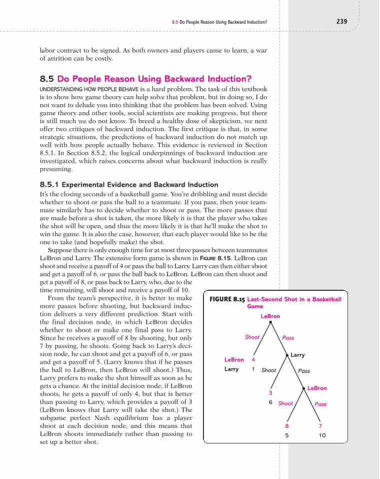
8.5 Do People Reason Using Backward Induction? 239
labor contract to be signed. As both owners and players came to learn, a warof attrition can be costly.
8.5 Do People Reason Using Backward Induction?UNDERSTANDING HOW PEOPLE BEHAVE is a hard problem. The task of this textbookis to show how game theory can help solve that problem, but in doing so, I donot want to delude you into thinking that the problem has been solved. Usinggame theory and other tools, social scientists are making progress, but thereis still much we do not know. To breed a healthy dose of skepticism, we nextoffer two critiques of backward induction. The first critique is that, in somestrategic situations, the predictions of backward induction do not match upwell with how people actually behave. This evidence is reviewed in Section8.5.1. In Section 8.5.2, the logical underpinnings of backward induction areinvestigated, which raises concerns about what backward induction is reallypresuming.
8.5.1 Experimental Evidence and Backward InductionIt’s the closing seconds of a basketball game. You’re dribbling and must decidewhether to shoot or pass the ball to a teammate. If you pass, then your team-mate similarly has to decide whether to shoot or pass. The more passes thatare made before a shot is taken, the more likely it is that the player who takesthe shot will be open, and thus the more likely it is that he’ll make the shot towin the game. It is also the case, however, that each player would like to be theone to take (and hopefully make) the shot.
Suppose there is only enough time for at most three passes between teammatesLeBron and Larry. The extensive form game is shown in FIGURE 8.15. LeBron canshoot and receive a payoff of 4 or pass the ball to Larry. Larry can then either shootand get a payoff of 6, or pass the ball back to LeBron. LeBron can then shoot andget a payoff of 8, or pass back to Larry, who, due to thetime remaining, will shoot and receive a payoff of 10.
From the team’s perspective, it is better to makemore passes before shooting, but backward induc-tion delivers a very different prediction. Start withthe final decision node, in which LeBron decideswhether to shoot or make one final pass to Larry.Since he receives a payoff of 8 by shooting, but only7 by passing, he shoots. Going back to Larry’s deci-sion node, he can shoot and get a payoff of 6, or passand get a payoff of 5. (Larry knows that if he passesthe ball to LeBron, then LeBron will shoot.) Thus,Larry prefers to make the shot himself as soon as hegets a chance. At the initial decision node, if LeBronshoots, he gets a payoff of only 4, but that is betterthan passing to Larry, which provides a payoff of 3(LeBron knows that Larry will take the shot.) Thesubgame perfect Nash equilibrium has a playershoot at each decision node, and this means thatLeBron shoots immediately rather than passing toset up a better shot.
FIGURE 8.15 Last-Second Shot in a BasketballGame
4
1
LeBron
Larry
Shoot Pass
3
6
Shoot Pass
8
5
7
10
Shoot Pass
LeBron
LeBron
Larry

240 CHAPTER 8: TAKING TURNS: SEQUENTIAL GAMES WITH PERFECT INFORMATION
The basketball situation is a variant of a game known as Centipede.10
Drawing its extensive form horizontally as in FIGURE 8.16, we see that the re-sulting figure is shaped like a centipede, and therein lies the source of itsname. The game starts with two piles of money. Player 1 decides betweengrabbing the large pile—in which case player 2 gets the small pile and thegame is over—or leaving it there. If the large pile is left there, more money isadded to both piles and it is now player 2’s turn to make the same decision:grab the large pile or leave it there. In Figure 8.16, the large pile initially has40 cents and the small pile has 10 cents. If the large pile is left there, theamount of money is doubled, so, at the second decision node, the large pilehas 80 cents and the small pile has 20 cents. Each time the money is left onthe table, the amounts are doubled. With the version shown in Figure 8.16, thegame goes on for at most six moves. If, at the final decision node, player 2leaves the money, then it doubles one last time and player 1 automatically getsthe larger pile. (For the time being, ignore the percentages listed on the grabbranches.)
Player 1
Player 2
0.40
0.10
0.20
0.80
1.60
0.40
0.80
3.20
6.40
1.60
3.20
12.80
Grab
(1%)
Leave
1 2 1 2 1 2 25.60 6.40
Leave Leave Leave Leave Leave
Grab
(21%)
Grab
(6%)
Grab
(53%)
Grab
(85%)
Grab
(73%)
FIGURE 8.16 Centipede Game
Assume that a player’s payoff is measured by how much money she re-ceives, and we’ll use backward induction to solve the game. At the final deci-sion node, player 2 will grab the large pile, as he prefers $12.80 to $6.40.Moving back to the penultimate decision node, player 1 can either grab thelarge pile and receive $6.40, or leave it there and get $3.20. That she would get$3.20 presumes that player 1 believes that player 2 will act optimally and grabthe large pile at the next node. Continuing to work backwards, we find that itis always optimal for a player to take the large pile when given the chance.Thus, backward induction implies that player 1 grabs the 40 cents at the startof the game and there it ends.
Backward induction offers a precise solution for the Centipede game. Theonly problem is that people don’t act that way—or at least not exactly that way.The game shown in Figure 8.16 was conducted 281 times with real money andreal-live undergraduate students as subjects.11 Of the trials that reached the ith
node, the percentage listed on the grab branch in Figure 8.16 indicates howoften the person took the money rather than leave it there. For example, at thefirst decision node, player 1 took the 40 cents in only 2 of the 281 trials, which

8.5 Do People Reason Using Backward Induction? 241
is about 1% of the trials. Of the 279 trials that reached the second decisionnode, player 2 grabbed the money in 18 of them, which is about 6% of thetime.
The theory predicts that a player will grab the large pile of money whenevergiven the opportunity. This prediction implies that player 1 will grab the 40cents at the first decision node, but that actually occurred in fewer than 1% ofthe trials. However, the frequency with which the large pile is grabbed steadilyincreases as the game progresses, so the observed behavior gets closer to whatis predicted when there are fewer nodes left. By the fifth decision node, player1 grabs the large pile 73% of the time. However, even at the last decision node,when player 2 is choosing between $12.80 and $6.40, the latter is chosen in15% of the trials!
Should we then conclude that people don’t use backward induction in theirreasoning? Not necessarily: backward induction is just one ingredient in ourtheory, and the incongruity between prediction and practice may be due tosome other poorly chosen ingredient. Let’s consider some of the possible sus-pects. But before doing so, let me ask, Why do you think people act differentlyfrom what the theory predicts? Give that some thought before continuing toread.
It is certainly possible that people don’t deploy backward induction or thatthey are limited in the extent to which they use it. It is noteworthy that whenthere are only two decision nodes left, 73% of the trials conform to the theory’sprediction that player 1 will grab the $6.40, which is not a bad performancefor the theory. In that situation, player 1 has to look forward only one move—prognosticating what player 2 will do—in order to figure out her optimalmove. When there are three decision nodes left, player 2 has to look forwardtwo moves, which is a more challenging exercise. At that node, only 53% ofthe trials conform to the theory. The more decision nodes that remain, the big-ger is the departure from what people do and what the theory predicts.Perhaps people engage in some limited backward induction.
Another ingredient of the theory that is worthy of reevaluation is the pay-offs. The experimenter controls how much money is at stake, but not the ac-tual payoffs of players. The theory is based on the assumption that a personcares only about how much money is received, but suppose people have dif-ferent preferences? Suppose they care about more than money? On this point,it is rather telling that some people—though not many—chose not to grab themoney at the final decision node even though that meant choosing $6.40 over$12.80. Either they made a mistake, or these dollar amounts do not accuratelyreflect the payoffs.
One thought is that people care not only about how much money they re-ceive, but also about how much money the other person receives. The possi-bility that some people are altruists—they like other people receiving moremoney (or feel bad about taking advantage of someone else)—may have impli-cations even for people who are not altruists. Suppose you are unsure ofwhether the person with whom you are matched is an altruist. If she is an al-truist, then she won’t grab the money in the next round, which behooves younot grab it in this round, since you can let it build up and then grab it. Hence,a selfish backward-induction reasoner will let the money lie on the table forsome number of rounds if she is uncertain as to whether she is matched withsomeone like herself or someone who is altruistic.

242 CHAPTER 8: TAKING TURNS: SEQUENTIAL GAMES WITH PERFECT INFORMATION
8.5.2 A Logical Paradox with Backward InductionLet’s put aside the experimental evidence and reexamine the logic of the backward-induction argument. Suppose the game is properly specified and is as describedin Figure 8.16. Then, according to the argument of backward induction, oncethe fifth decision node is reached, player 1 will grab the $6.40 because if hedoesn’t, then player 2 will grab the money in the next round and leave player 1with only $3.20. But why does player 1 expect player 2 to grab it? Because player1 believes that player 2 is rational and that is what a rational player would do.Now let’s move back to the fourth decision node. If player 2 doesn’t grab the$3.20, she expects player 1 to grab it in the next round. The reason is that player2 believes that player 1 believes that player 2 is rational, so player 2 believes thatplayer 1 believes that player 2 will grab the large pile of money at the sixth de-cision node. With such a belief, player 2 expects player 1 to grab it at the fifthdecision node because player 2 believes that player 1 is rational and thus prefers$6.40 to $3.20. Hence, player 2 will act at the fourth decision node and acquire$3.20. Continuing with this logic, rationality is common knowledge among play-ers 1 and 2 implies that player 1 will grab the 40 cents at the start of the game.
Now comes the conundrum. In arguing that player 1 should grab the largepile once it has reached $6.40, a key premise is that player 1 believes that player2 is rational and thus that player 2 would grab the large pile if it were allowedto grow to $12.80. But if rationality is common knowledge, then how did thegame get all the way to the fourth decision node? Rationality is common knowl-
edge implies that it shouldn’t get past the first deci-sion node, much less get to the fourth. So isn’t thefact that the large pile exceeds 40 cents evidencethat rationality is not common knowledge? And ifso, why, then, is it reasonable to suppose that player1 believes that player 2 is rational? Player 2 haspassed up the money before—otherwise, player 1wouldn’t be faced with the decision of whether totake the $6.40 pile—so might she not pass it upagain if it were $12.80? And if she would, thenshouldn’t player 1 pass it up when it is $6.40, so thathe can end up with $25.60?
This paradox is especially self-evident in the ex-tensive form game illustrated in FIGURE 8.17. Jonmoves first, and if he chose b, then Jane gets tomove, after which Jon moves again. In deriving heroptimal strategy, Jane needs to forecast what Jonwould do if she chose x and what Jon would do ifshe chose y. Using backward induction, she predictsthat Jon will play d in response to Jane’s playing x—which results in Jane’s payoff being 5—and that Jonwill play c in response to Jane’s playing y—whichresults in Jane’s payoff being 3. Hence, Jane willchoose x if Jon chose b at the initial decision node.
Note, however, that Jon earns 10 by choosing a,while his payoff can’t be higher than 8 by choosingb, and in fact, it is only 6 when the ensuing play isoptimal. In other words, any strategy that assigns a
4
7
6
5
Jon
Jane10
3
Jon
Jane
c
a b
x y
d
8
3
2
9
Jon
Jon
c d
FIGURE 8.17 Is Backward Induction Consistentwith Rationality Being CommonKnowledge?

Summary 243
to Jon’s initial decision node strictly dominates any strategy that assigns b.Thus, if the game reaches Jane’s decision node, then she knows that Jon chosea strictly dominated strategy. In that case, should Jane anticipate that Jon willrespond in an optimal manner to what Jane does?
One argument in favor of the backward-induction solution starting fromJane’s decision node is that Jon intended to act rationally, but simply made amistake at the initial decision node; he meant to choose a, but chose b in error.If we think that further mistakes are unlikely, then Jane’s best model of howJon will respond to her actions is that he will respond optimally. But perhapsmore mistakes are likely. Maybe Jon is drunk or off of his medication, and thatis why he chose b, in which case further mistakes may occur. What are yourthoughts on this conundrum?
SummaryThis chapter began by pointing out a deficiency in Nash equilibrium as a solu-tion concept. In an extensive form game, Nash equilibrium requires only thata player’s strategy prescribe an optimal action for those information sets (or, ina game of perfect information, decision nodes) which are reached during thecourse of equilibrium play. Since a player’s payoff depends solely on actions im-plemented, there is no cost to assigning an inappropriate action to a contin-gency that isn’t expected to occur. In other words, it is costless to make a bluffthat is not called. A Nash equilibrium strategy could then assign a nonoptimalaction to a decision node that is not reached during equilibrium play. The con-cern this creates is that a strategy profile could be a Nash equilibrium only be-cause of incredible threats. That is, a player’s strategy is optimal only becauseof what another player threatens to do, but if that player’s bluff were called, itwould not be optimal for him to go through with the threat.
This inadequacy led us to consider a more stringent solution concept whichwould rule out Nash equilibria that are dependent on incredible threats. For agame of perfect information, subgame perfect Nash equilibrium extends the re-quirement of optimality from those decision nodes reached during the course ofequilibrium play to all decision nodes. The algorithm of backward induction pro-vides a method for deriving subgame perfect Nash equilibria by solving for opti-mal behavior at the final decision node(s) and then working one’s way up the tree,all along presuming that later play is optimal. In a game of perfect information,this algorithm always produces at least one subgame perfect Nash equilibrium.
A general class of sequential games involving timing was considered inwhich players face a series of decisions regarding whether to act or wait.Examples include when to queue up at an airport gate and when a labor unionshould call off a work stoppage. In a game of preemption, there is an advan-tage to moving before other players do, but it is also the case that it is costlyto move earlier in time. The best outcome for a player would be to wait untilthe end and then be the first to move. The temptation that each player has topreempt others results in a payoff-dominated outcome in which players movetoo soon. In contrast, a war of attrition is characterized by a second-moveradvantage. A player wants the others to move first, but in waiting for that tohappen, the player incurs a cost. In that situation, the ideal outcome for theplayer is for others to act immediately. The temptation to wait in the hope thatothers will move results in all players waiting too long.

244 CHAPTER 8: TAKING TURNS: SEQUENTIAL GAMES WITH PERFECT INFORMATION
In spite of the appeal of backward induction in that it rules out what seemto be unreasonable Nash equilibria, two criticisms have been leveled at themethod and at subgame perfect Nash equilibria. First, in some experiments—such as those conducted on the Centipede game—people are observed to actcontrary to equilibrium predictions. Although this lack of agreement betweentheory and reality may be due to other elements of the model (such as what weassume about peoples’ preferences), it may be the case that their reasoningprocess does not fully conform to backward induction. Second, there is a logi-cal inconsistency with backward induction. In applying the concept, you areengaged in a thought experiment concerning what is best for a player if a cer-tain point in the game is reached. In determining what is best, the presumptionis made that other players will subsequently act optimally. However, it is possi-ble that the only way the game could have reached its current point is throughnonoptimal play. This thought experiment may then require maintaining twoalmost contradictory ideas: only nonoptimal play could have brought the gameto the current point, yet we presume that future play will be optimal. TheAmerican novelist F. Scott Fitzgerald once said, “The test of a first-rate intelli-gence is the ability to hold two opposed ideas in mind at the same time and stillretain the ability to function.” With that in mind, let us note that, in spite of itswarts, backward induction is a compelling prescription for how one shouldplay a game and is currently our best description of how people actually play.
1. Return to the situation described in Chapter 2 in which Galileo Galileimight be confronted by the Inquisition. Let us describe what actually tran-spired. First, Pope Urban VIII referred Galileo to the Inquisition, and he wasbrought to trial on April 12, 1633. After verbal persuasion from the com-missary general of the Inquisition, Galileo confessed that he had gone toofar in supporting the Copernican theory in one of his books (even thoughhe hadn’t). Galileo was then given an “examination of intention,” which in-volves showing the instruments of torture to the accused. The final hearingby the Inquisition was held on June 22, 1633, at which time the 69-year-oldGalileo pleaded for mercy because of his “regrettable state of physical un-wellness.” With the threat of torture and imprisonment lurking in the back-ground, the Inquisitors forced Galileo to “abjure, curse, and detest” hiswork. Galileo complied in every way and was convicted and sentenced tolife imprisonment and religious penances. Due to his age (and possibly hisfame), the sentence was commuted to house arrest. He was allowed to re-turn to his villa near Florence, where he would remain for the last years ofhis life. That is history, and now we turn to our simple modeling of it. Theextensive form game in Figure 2.3 is reproduced here as FIGURE PR8.1.a. Find all Nash equilibria. (Hint: First derive the strategic form game.)b. Find all of the subgame perfect Nash equilibria.c. For each Nash equilibrium that is not a subgame perfect Nash equi-
librium, explain why it is not a subgame perfect Nash equilibrium.
2. There were still pirates in the 1980s, although they tended to appear incorporate boardrooms rather than the open seas. These swashbucklingfinanciers would engage in a “hostile takeover” by acquiring a company
EXERCISES

Exercises 245
through the purchase of shares on the open market and against the willof the target company’s existing management (thus making the takeover“hostile”). Such investors were known as “raiders” and included peoplesuch as T. Boone Pickens, Sir James Goldsmith, Henry Kravis, andVictor Posner. All this was fictionalized in the movie Wall Street, withMichael Douglas portraying the raider Gordon Gekko, who famously es-poused “Greed is good.” The time was full of jocular jargon, as manage-ment could consume a “poison pill” by taking on a costly financial struc-ture that would make it difficult to consummate a hostile takeover. Insome cases, a raid could be fought against by buying a raider’s sharesback at a premium; this tack became known as “greenmail,” a takeoff onblackmail. To get a gist of the strategizing that occurred between araider and management, consider FIGURE PR8.2. The raider makes an ini-tial stock purchase, in response to which management decides whetherto buy the shares back at a premium (pay greenmail) or not. If no green-mail is paid, then the raider decides whether to purchase additionalshares in order to take control of the target company.a. Find all subgame perfect Nash equilibria.b. Find a Nash equilibrium that is not a subgame perfect Nash equilib-
rium, and explain why it is not a subgame perfect Nash equilibrium.
3. Return to the Kidnapping game from the film Ransom (first discussedin Chapter 2), which is reproduced here as FIGURE PR8.3. Solve for allsubgame perfect Nash equilibria.
Urban VIII
Urban VIII 3
Galileo 5
Inquisitor 3
Galileo
Galileo
Do not confess
Do not confess
Do not torture
Confess
Confess
Inquisitor5
3
4
2
4
2
4
1
5
1
2
1
Do not refer
Refer
Torture
FIGURE PR8.1 Galileo Galilei and the Inquisition

246 CHAPTER 8: TAKING TURNS: SEQUENTIAL GAMES WITH PERFECT INFORMATION
FIGURE PR8.2 Greenmail
Raider
Raider 10
Management 10
Management
No greenmail
Do not take over
Greenmail
Raider15
7
6
11
8
4
Do not buy
Buy
Take over
FIGURE PR8.3 Extensive Form for the Film Ransom
John Mullen
7
Kill
3
Jimmy Shaker
Jimmy Shaker
JS JS JS
John Mullen
6
4
Release
Do not payransom
Pay ransom
Offer bounty
5
Do not kidnap
Kidnap
7
4
Kill
1
3
6
Release
1
Kill
2
2
5
Release

Exercises 247
4. Benjamin Franklin once said, “Laws too gentle are seldom obeyed; toosevere, seldom executed.” To flush out what he had in mind, the game inFIGURE PR8.4 has three players: a lawmaker, a (typical) citizen, and ajudge. The lawmaker chooses among a law with a gentle penalty, one witha moderate penalty, and a law with a severe penalty. In response to thelaw, the citizen decides whether or not to obey it. If she does not obey it,then the judge decides whether to convict and punish the citizen. Usingsubgame perfect Nash equilibrium, find values for the unspecified pay-offs (those with letters, not numbers) that substantiate Franklin’s claimby resulting in a lawmaker’s choosing a law with a moderate penalty.
5. Nobel Laureate Thomas Schelling once proposed a solution to theproblem of how a kidnappee can induce his kidnapper to release himafter the kidnappee has learned the identity of the kidnapper. Let’s re-turn to the kidnapping scenario, but instead have the players be Guy(kidnapper) and Orlando (kidnappee). The problem is that one wouldexpect Guy to be inclined to kill Orlando once Orlando sees Guy’sface, since then Orlando, if released, would be able to help the policecapture Guy. The situation is as depicted in FIGURE PR8.5. Guy starts
FIGURE PR8.4 Punishments: Severe or Gentle?
Lawmaker
Citizen
Judge
10
4
8
Lawmaker
Judge
Citizen
10
4
8
10
4
8
Do not convictConvict
8
a
c
6
b
d
Do not convictConvict
8
e
g
6
f
h
Do notconvictConvict
8
i
k
6
j
l
Do not obeyObey
Gentle Moderate Severe
Do not obeyObey Do not
obeyObey

248 CHAPTER 8: TAKING TURNS: SEQUENTIAL GAMES WITH PERFECT INFORMATION
off by deciding whether to kidnap Orlando. Orlando then decideswhether to reveal some incriminating details about himself that areunknown to the rest of the world. (Perhaps Orlando stole funds fromhis church or had an affair unbeknownst to his wife.) Then Guy de-cides whether to kill or release Orlando. If he releases Orlando, thenOrlando has to decide whether to inform the police of his kidnapper’sidentity. If he does, and if Orlando revealed his dirty secret to Guy,Guy must then decide whether to share that secret with the world.Find the unique subgame perfect Nash equilibrium, and you’ll findSchelling’s proposed solution.
FIGURE PR8.5 Revised Kidnapping Situation
Guy
Do nottellTell
2
1
1
3
Do nottell
Tell police
5
2
1
4
Orlando
Orlando
Orlando
Do nottell
Tell police
5
2
4
0
4
0
GuyGuy
Guy
Orlando
3
5
ReleaseKillReleaseKill
Do not tell dirty secret
Tell dirty secret
Guy
KidnapDo not kidnap

Exercises 249
6. In 1842, the Sangamo Journal of Springfield, Illinois, published lettersthat criticized James Shields, the auditor of the State of Illinois. Althoughthe letters were signed “Rebecca,” Shields suspected that it was state leg-islator Abraham Lincoln who penned the letters. As shown in FIGURE
PR8.6, Shields considered challenging Lincoln to a duel, and, as historyrecords, Shields did challenge Lincoln. In response to a challenge,Lincoln could avoid the duel, or, if he chose to meet Shields’s challenge,he had the right to choose the weapons. We will also allow Lincoln to de-cide whether to offer an apology of sorts. (Actually, it proved to be a bitmore complicated than that, so allow me some poetic license here. An“apology of sorts” means making some remarks that could provide anhonorable retreat for Shields—something which Lincoln ultimately did.)If he decides to go forward with a duel, then Lincoln has four choices:propose guns, propose guns and offer an apology, propose swords, andpropose swords and offer an apology. (Shields was known to be a goodshot, so Lincoln chose cavalry broadswords of the largest size, as it gavethe, 6-foot, 4-inch, Lincoln a sizable advantage against the much shorterShields.) In response to any of the four choices, Shields must decide toeither go forward with the duel or stop the duel. (In the latter case,Shields accepts Lincoln’s apology if, indeed, Lincoln offered one.) Find allsubgame perfect Nash equilibria. As a closing note, Lincoln once said, “Ifall the good things I have ever done are remembered as long and as wellas my scrape with Shields, it is plain I shall not be forgotten.”
7. An infamous event that came to be known as the Saturday NightMassacre took place during the second term of the presidential admin-istration of Richard Nixon. Though no one was fired upon, many wereeffectively fired from their high-level positions in the federal govern-ment. The Nixon White House was in the midst of covering up crimes
Shields
Shields Shields
Lincoln
5
6
Lincoln
Challenge
Do not challenge
Stop Stop
Avoid Guns Swords Swords& apology
Guns& apology
0
5
10
1
8
2
StopGo
6
4
8
2
StopGo
0
5
2
3
Go Go
6
4
2
3
FIGURE PR8.6 Lincoln–Shields Duel

250 CHAPTER 8: TAKING TURNS: SEQUENTIAL GAMES WITH PERFECT INFORMATION
committed by close aides to the president. As part of the investigation,Attorney General Elliot Richardson (who was not part of the cover-up)named Harvard Law professor Archibald Cox as a special prosecutor.During the investigation, President Nixon was acutely concerned withCox’s investigation and contemplated ordering Richardson to fire Cox(expressed as the initial decision node in FIGURE PR8.7). When Nixon’s in-tent was expressed to Richardson, the latter conveyed that if he did fireCox, he might feel compelled to resign, but also that he might be in-clined not to fire Cox and, in that case, might also resign. Richardson’sfour possible combinations of firing Cox or not and resigning or not are
FIGURE PR8.7 Saturday Night Massacre
Nixon
Richardson
Ruckelshaus
2
12
12
Do not fire & Resign
Ruckelshaus
Nixon
Nixon
Richardson
Do not fire & Do not resign
Fire & Do not resign
Fire & Resign
4
9
8
7
4
3
8
3
1
3
7
7
1
11
11
Do not fire & Resign
Do not fire & Resign
Ruckelshaus
Do not fire & Do not resign
Do not fire & Do not resign
Fire & Do not resign
Fire & Do not resign
Fire & Resign
Fire & Resign
6
10
10
9
6
4
10
5
2
5
8
9
12
1
5
11
2
6
Do not order
Order

Exercises 251
depicted in the extensive form. If Richardson did choose to resign and notfire Cox, then Nixon would still be left with the matter of getting rid of Cox.And if Richardson chose not to fire Cox and did not resign, then Nixonwould have to decide whether to fire Richardson. Upon Richardson’s de-parture, Deputy Attorney General William Ruckelshaus would assume theposition of acting attorney general and would face the same four optionsas Richardson. If Ruckelshaus also chose to resign and not fire Cox, thenSolicitor General Robert Bork would become acting attorney general, andagain, he would have the same four choices. To simplify matters, we’ll notmodel Bork, even though what happened was that Richardson refused tofire Cox and resigned and Ruckelshaus did the same, at which point Borkcame in and did fire Cox and did not resign. Find all subgame perfect Nashequilibria.
8. Seven goblins are deciding how to split 100 galleons. The goblins are namedAlguff, Bogrod, Eargit, Griphook, Knadug, Ragnuk, and Uric, and they’vebeen rank-ordered in terms of magical power, with Alguff the weakest andUric the strongest. The game starts with Alguff, who proposes an allocationof the 100 galleons coins, where an allocation is an assignment of anamount from {0,1, . . . , 100} to each goblin and where the sum across gob-lins equals 100. All goblins then vote simultaneously, either “yea” or “nay,”on the allocation. If at least half of them vote in favor of the allocation, thenit is made and the game is over. If less than half vote for the proposed allo-cation, then the other goblins perform a spell on Alguff and transform himinto a house elf for a week. In that event, it is Bogrod’s turn to put forth anallocation for the remaining six goblins. Again, if at least half vote in favor,the allocation is made; if not, then Bogrod is made into a house elf for aweek and it is Eargit’s turn. This procedure continues until either an alloca-tion receives at least half of the votes of the surviving goblins or all but Urichave been transformed into house elfs, in which case Uric gets the 100galleons. Assume that the payoff to a goblin is if he is made into ahouse elf and that it equals the number of galleons if he is not. Using the so-lution concept of subgame perfect Nash equilibrium, what happens? (Focuson subgame perfect Nash equilibria in which a goblin votes against an allo-cation if he is indifferent between voting for it and against it.)
9. Consider the four-player game displayed in FIGURE PR8.9. Find all subgameperfect Nash equilibria.
10. Their rich uncle left 100 pounds of gold to Todd and Steven. The negotiat-ing process for allocating the treasure between them was also laid out intheir uncle’s will. They have three rounds by which to come to an agree-ment. In an odd (even) round, Todd (Steven) is required to propose an al-location. (Isn’t it clever how Todd moves in odd rounds and Steven movesin even rounds?) In response to a proposal, the other nephew can accept orreject it. If he accepts the proposal, the process is ended and the proposedallocation is made. If he rejects the proposal, the game moves to the nextround. Failure to agree by the end of the third round means that all of thegold goes to charity, so none of it lands in the pockets of Todd and Steven.Furthermore, at the end of each round in which an agreement has not beenreached, a fraction of the allotment of gold is given to charity, where
Thus, there are 100d pounds of gold at the beginning of round2 (after an agreement was not reached in the first round) and only pounds of gold at the beginning of round 3 (after an agreement was notreached in the first two rounds). In other words, there is a cost to delayingagreement and, of course, a cost to ever failing to agree. Each nephew’s
100d20 6 d 6 1.
1 " d
"1,000

252 CHAPTER 8: TAKING TURNS: SEQUENTIAL GAMES WITH PERFECT INFORMATION
payoff equals the number of pounds of gold he ends up with, so neithercares about the other or about their uncle’s favorite charity. For nota-tional purposes, assume that a proposal in round t is a value for where is the share of the remaining amount of gold for Todd and,therefore, Steven’s share is Note that and thus is anynumber between 0 and 1 inclusive. Find a subgame perfect Nash equi-librium.
11. Consider the following passage from Midnight in the Garden of Good andEvil:12
There’s a woman here, a grande dame at the very apex of society and oneof the richest people in the Southeast, let alone Savannah. She owns acopper mine. She built a big house in an exclusive part of town, areplica of a famous Louisiana plantation house with huge whitecolumns and curved stairs. You can see it from the water. Everybodygoes ‘Oooo, look!” when they pass by it. I adore her. She’s been like amother to me. But she’s the cheapest woman who ever lived! Someyears ago she ordered a pair of iron gates for her house. They weredesigned and built especially for her. But when they were delivered she
0 $ xt $ 11 " xt.xt
xt,
d1 e1
2
1
3
2
3
4
1
1
d1 e1
5
4
0
0
1
2
3
1
a3 b3
0
4
2
1
6
1
2
3
a2
a1 b1 c1
b2 a4 b4
1
3
1
0
4
1
2
3
1
2
11
3 4
FIGURE PR8.9

Exercises 253
pitched a fit, said they were horrible, said they were filth. “Take themaway,” she said, “I never want to see them again!” Then she tore up thebill, which was for $1,400—a fair amount of money in those days. Thefoundry took the gates back, but they didn’t know what to do withthem. After all, there wasn’t much demand for a pair of ornamentalgates exactly that size. The only thing they could do was to sell the ironfor its scrap value. So they cut the price from $1,400 to $190. Naturally,the following day the woman sent a man over to the foundry with $190,and today those gates are hanging on her gateposts where they wereoriginally designed to go. That’s pure Savannah. And that’s what I meanby cheap. You mustn’t be taken in by the moonlight and magnolias.There’s more to Savannah than that. Things can get very murky.
Using backward induction, can you explain where the foundry went wrong?
12. The haggling game from Chapter 2 is reproduced as FIGURE PR8.12. Solvefor all subgame perfect Nash equilibria for which a player chooses ac-cept whenever that is an optimal action. That is, if a player’s payoff ismaximized by either choosing accept or choosing some other action, heor she chooses accept.
Accept Reject
A Leave
A
A
R
DonnaDonna Donna
A R
Marcus
Marcus
Donna
0
Marcus Marcus Marcus0
0
0
0pM " pH
0
0
A R
Donna
pM " pL
pL pM
pM
pL A LeavepL pM
pH
0
2(pM " pL) 2(pH " pL)
0
00
00
0pM " pL
0
pM " pL
2(pM " pL)
0
00
2(pM " pL)
FIGURE PR8.12 Haggling at the Auto Dealer

254 CHAPTER 8: TAKING TURNS: SEQUENTIAL GAMES WITH PERFECT INFORMATION
REFERENCES1. “Notes Taken from Transcripts of Meetings of the Joint Chiefs of Staff,
October–November 1962” <www.gwu.edu/~nsarchiv/nsa/cuba_mis_cri/docs.htm>.
2. For a classic treatment of this crisis, see Graham T. Allison, The Essenceof Decision: Explaining the Cuban Missile Crisis (Boston: Little, Brown andCompany, 1971).
3. The game-theoretic analysis provided here is based on Steven J. Brams,Rational Politics: Decisions, Games, and Strategy (Boston: Academic Press,1985).
4. Sheldon M. Stern, “The Cuban Missile Crisis Myth You Probably Believe,”History News Network </hnn.us/articles/7982.html>.
5. If you want to learn more about the Enron scandal, you can read BethanyMcLean and Peter Elkind, The Smartest Guys in the Room (New York:Portfolio, 2004), and Kurt Eichenwald, Conspiracy of Fools: A True Story(New York: Broadway Books, 2005).
6. The ensuing analysis is based on Van Kolpin and Larry D. Singell, Jr.,“Strategic Behavior and the Persistence of Discrimination in ProfessionalBaseball,” Mathematical Social Sciences, 26 (1993), 299–315.
7. News & Notes with Ed Gordon, Jan. 6, 2005, <www.npr.org>.
8. Alvin E. Roth, “The Evolution of the Labor Market for Medical Interns andResidents: A Case Study in Game Theory,” Journal of Political Economy, 92(1984), 991–1016.
9. Darren Rovell, “Work Stoppage 101: The Issues,” ESPN.com, August 12,2002; espn.go.com (Aug. 26, 2007).
10. Centipede was developed in Robert W. Rosenthal, “Games of PerfectInformation, Predatory Pricing and the Chain-Store Paradox,” Journal ofEconomic Theory, 25 (1981), 92–100.
11. Richard McKelvey and Thomas Palfrey, “An Experimental Study of theCentipede Game,” Econometrica, 60 (1992), 803–36.
12. John Berendt, Midnight in the Garden of Good and Evil (New York:Random House, 1994), p. 10. Quoted on the back cover of the Journal ofPolitical Economy, 107 (1999), no. 1.

9.1 IntroductionIT IS NOW TIME TO consider games with imperfect information. Recall that theseare games in which a player is not always sure as to what has transpired whenit is time to make a decision. In technical jargon, in a game with imperfect in-formation, some information sets contain more than one decision node. Similarto what we discovered in Chapter 8, a Nash equilibrium for a game with imper-fect information can be unreasonable because it has a player believing an in-credible threat (i.e., the threat by a player to act against her best interests). As ingames with perfect information, our goal towards identifying a compelling so-lution is to rule out Nash equilibria predicated upon incredible threats.
The approach is to extend the solution concept introduced in Chapter 8 sothat it can be applied to games with imperfect information. Achieving this endwill prove to be a bit more complicated, given the richer information structureof a game with imperfect information. We’ll first illustrate the approach withan example and then more formally generalize the method in Section 9.2. Thereader who needs a refresher on games with imperfect information should re-turn to Section 2.3 before proceeding.
Let us return to the Kidnapping game, inwhich the kidnapper (Guy) and the victim’skin (Vivica) move simultaneously when de-ciding, respectively, whether to release thekidnappee (Orlando) and whether to payransom. The extensive form from Chapter 2is reproduced here as FIGURE 9.1.
Were the algorithm introduced in Chapter8 to be applied, we’d need to derive optimalbehavior for Guy at his last two decisionnodes. Consider, however, the following diffi-culty: The decision node associated with Guyhaving performed a kidnapping and Vivicahaving paid ransom, denoted node III, is partof an information set that also includes nodeIV. Therefore, Guy doesn’t know whether he’sat node III or node IV (i.e., he doesn’t knowwhether or not Vivica has paid ransom), andit isn’t clear what are reasonable beliefs forGuy to have as to where he is in the game.
So that we may better understand the dif-ficulty we face, examine FIGURE 9.2, which
9
255
Taking Turns in the Dark: SequentialGames with Imperfect Information
Guy
II
I II I
I I II I I IVIV
Guy 3
Vivica 5 Pay ransom
Vivica
4
1
5
3
2
2
1
4
Do not kidnap
Do not pay ransom
Kidnap
Guy
Kill KillRelease Release
FIGURE 9.1 The Kidnapping Game with SimultaneousRansom and Release Decisions

The strategic form for the game in Figure 9.3 is provided in FIGURE 9.4 tohelp us solve for a Nash equilibrium. This game has a unique Nash equilib-rium in which Vivica does not pay ransom and Guy kills Orlando. Thus, ifthere is a kidnapping, then ransom will not be paid and Orlando will bekilled.
Moving back to the initial node (at which Guyis contemplating the idea of a kidnapping), wesee that Guy can expect not to receive ransomand that he’ll murder Orlando. He then antici-pates a payoff of 2 if he performs the kidnapping,which presents him with the situation depicted inFIGURE 9.5. It’s clear that he’ll prefer not to kidnapOrlando and instead receive a payoff of 3. By thepreceding analysis, the solution to the game inFigure 9.1 is the strategy profile (Do notkidnap/Kill, Do not pay ransom).
256 CHAPTER 9: TAKING TURNS IN THE DARK: SEQUENTIAL GAMES WITH IMPERFECT INFORMATION
carves out the part of the game that we’re currently investigating. Thiscarved-out game “starts” with an information set that is not a singleton.The game commences with something having transpired—what Vivicahas done—but we don’t know just what has happened. Game theory isnot well suited to handling such murkiness, and indeed, the “game” inFigure 9.2 doesn’t look like anything we’ve seen before.
At this stage, let’s throw up our hands and admit that we can’t solvefor behavior starting at Guy’s information set. Accepting defeat, weclimb up the tree to consider Vivica’s information set at node II.Because node II is a singleton, none of the problems just discussedarise. Also, because we haven’t solved for Guy’s ensuing play (whetherhe kills or releases the victim), solving for Vivica’s behavior will requiresolving for Guy’s at the same time. This will not pose a problem, since
this part of the game, which is shown in FIGURE 9.3, is recognizable as a game.
I I II I I
4
1
5
3
Guy
Kill Release
FIGURE 9.2 Guy’s Situationat Node III
I II IPay ransom
Vivica
4
1
5
3
2
2
1
4
Do not pay ransom
Guy
Kill KillRelease Release
Pay ransom
Vivica
4,1
5,3
2,2
1,4
Do not pay ransom
GuyKill
Release
FIGURE 9.4 The Strategic Form of the SituationFaced by Vivica and Guy
FIGURE 9.3 The Situation Faced by Vivica andGuy After the Kidnapping
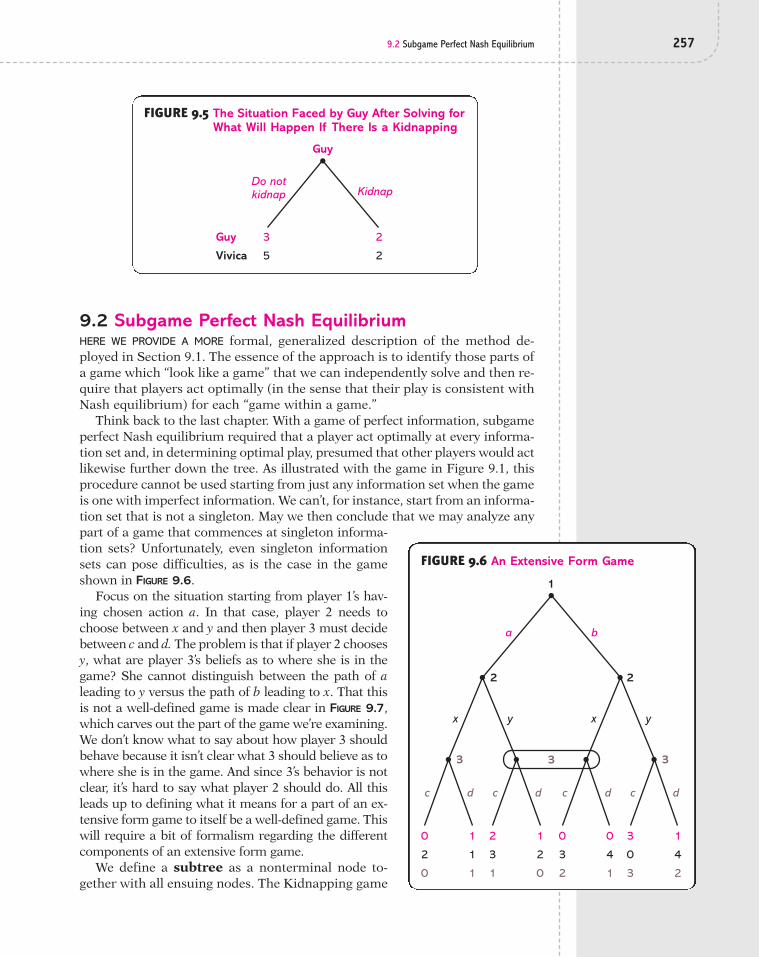
9.2 Subgame Perfect Nash Equilibrium 257
9.2 Subgame Perfect Nash EquilibriumHERE WE PROVIDE A MORE formal, generalized description of the method de-ployed in Section 9.1. The essence of the approach is to identify those parts ofa game which “look like a game” that we can independently solve and then re-quire that players act optimally (in the sense that their play is consistent withNash equilibrium) for each “game within a game.”
Think back to the last chapter. With a game of perfect information, subgameperfect Nash equilibrium required that a player act optimally at every informa-tion set and, in determining optimal play, presumed that other players would actlikewise further down the tree. As illustrated with the game in Figure 9.1, thisprocedure cannot be used starting from just any information set when the gameis one with imperfect information. We can’t, for instance, start from an informa-tion set that is not a singleton. May we then conclude that we may analyze anypart of a game that commences at singleton informa-tion sets? Unfortunately, even singleton informationsets can pose difficulties, as is the case in the gameshown in FIGURE 9.6.
Focus on the situation starting from player 1’s hav-ing chosen action a. In that case, player 2 needs tochoose between x and y and then player 3 must decidebetween c and d. The problem is that if player 2 choosesy, what are player 3’s beliefs as to where she is in thegame? She cannot distinguish between the path of aleading to y versus the path of b leading to x. That thisis not a well-defined game is made clear in FIGURE 9.7,which carves out the part of the game we’re examining.We don’t know what to say about how player 3 shouldbehave because it isn’t clear what 3 should believe as towhere she is in the game. And since 3’s behavior is notclear, it’s hard to say what player 2 should do. All thisleads up to defining what it means for a part of an ex-tensive form game to itself be a well-defined game. Thiswill require a bit of formalism regarding the differentcomponents of an extensive form game.
We define a subtree as a nonterminal node to-gether with all ensuing nodes. The Kidnapping game
Guy
3
5
Guy
Vivica
2
2
Do not kidnap Kidnap
FIGURE 9.5 The Situation Faced by Guy After Solving forWhat Will Happen If There Is a Kidnapping
FIGURE 9.6 An Extensive Form Game
3
2
1
2
0
2
0
1
1
1
c
x
a b
y x y
d
3
2
3
1
1
2
0
c d
0
3
2
0
4
1
c d
3
3
0
3
1
4
2
c d

in Figure 9.1 has four subtrees, which are circled in FIGURE
9.8. A regular subtree is a type of subtree—specifically,one that contains all information sets that have at least onenode in the subtree. To be a regular subtree, a subtree thatincludes one node of an information set must include allnodes of that information set. For the game in Figure 9.1,there are two regular subtrees, which are circled in FIGURE
9.9. Subtree 3 in Figure 9.8 is not a regular subtree, be-cause it includes node III but not node IV; that is, it in-cludes some, but not all, nodes of Guy’s information set. Foranalogous reasons, subtree 4 is not a regular subtree. Asubgame is a regular subtree together with the associatedpayoffs.
A subgame looks like a game; it is a “game within a game.”The key to avoiding ill-defined games (such as those shown inFigures 9.2 and 9.7) is to limit our attention to a part of agame that is sufficiently encompassing such that if it includes
258 CHAPTER 9: TAKING TURNS IN THE DARK: SEQUENTIAL GAMES WITH IMPERFECT INFORMATION
FIGURE 9.7 An Ill-Defined Part of theExtensive Form Game
3
2
0
2
0
1
1
1
c
x y
d
3
2
3
1
1
2
0
c d
FIGURE 9.8 Four Subtrees in the Kidnapping Game
Guy
Subtree 1
Subtree 2
Subtree 3 Subtree 4
II
I II I
I I II I I IVIV
Guy 3
Vivica 5 Pay ransom
Vivica
4
1
5
3
2
2
1
4
Do not kidnap
Do not pay ransom
Kidnap
Guy
Kill KillRelease Release
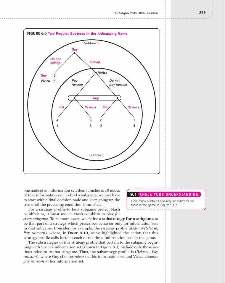
9.2 Subgame Perfect Nash Equilibrium 259
one node of an information set, then it includes all nodesof that information set. To find a subgame, we just haveto start with a final decision node and keep going up thetree until the preceding condition is satisfied.
For a strategy profile to be a subgame perfect Nashequilibrium, it must induce Nash equilibrium play forevery subgame. To be more exact, we define a substrategy for a subgame tobe that part of a strategy which prescribes behavior only for information setsin that subgame. Consider, for example, the strategy profile (Kidnap/Release,Pay ransom), where, in FIGURE 9.10, we’ve highlighted the action that thisstrategy profile calls forth at each of the three information sets in the game.
The substrategies of this strategy profile that pertain to the subgame begin-ning with Vivica’s information set (shown in Figure 9.3) include only those ac-tions relevant to that subgame. Thus, the substrategy profile is (Release, Payransom), where Guy chooses release at his information set and Vivica choosespay ransom at her information set.
How many subtrees and regular subtrees arethere in the game in Figure 9.6?
9.1 CHECK YOUR UNDERSTANDING
FIGURE 9.9 Two Regular Subtrees in the Kidnapping Game
Guy
Guy 3
Vivica 5 Pay ransom
Vivica
4
1
5
3
2
2
1
4
Do not kidnap
Do not pay ransom
Kidnap
Guy
Kill KillRelease Release
Subtree 1
Subtree 2
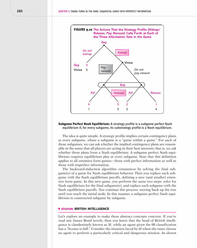
Subgame Perfect Nash Equilibrium: A strategy profile is a subgame perfect Nashequilibrium if, for every subgame, its substrategy profile is a Nash equilibrium.
The idea is quite simple. A strategy profile implies certain contingency plansat every subgame, where a subgame is a “game within a game.” For each ofthose subgames, we can ask whether the implied contingency plans are reason-able in the sense that all players are acting in their best interests; that is, we askwhether those plans form a Nash equilibrium. A subgame perfect Nash equi-librium requires equilibrium play at every subgame. Note that this definitionapplies to all extensive form games—those with perfect information as well asthose with imperfect information.
The backward-induction algorithm commences by solving the final sub-game(s) of a game for Nash equilibrium behavior. Then you replace each sub-game with the Nash equilibrium payoffs, defining a new (and smaller) exten-sive form game. In this new game, you perform the same two steps: solve forNash equilibrium for the final subgame(s), and replace each subgame with theNash equilibrium payoffs. You continue this process, moving back up the treeuntil you reach the initial node. In this manner, a subgame perfect Nash equi-librium is constructed subgame by subgame.
! SITUATION: BRITISH INTELLIGENCE
Let’s explore an example to make these abstract concepts concrete. If you’veread any James Bond novels, then you know that the head of British intelli-gence is clandestinely known as M, while an agent given the 00 classificationhas a “license to kill.” Consider the situation faced by M when she must choosean agent to perform a particularly critical and dangerous mission. As shown
260 CHAPTER 9: TAKING TURNS IN THE DARK: SEQUENTIAL GAMES WITH IMPERFECT INFORMATION
FIGURE 9.10 The Actions That the Strategy Profile (Kidnap/Release, Pay Ransom) Calls Forth at Each ofthe Three Information Sets in the Game
Guy
Guy 3
Vivica 5
Vivica
4
1
5
3
2
2
1
4
Do not kidnap
Do not pay ransom
Kidnap
Pay ransom
Guy
Kill Kill ReleaseRelease
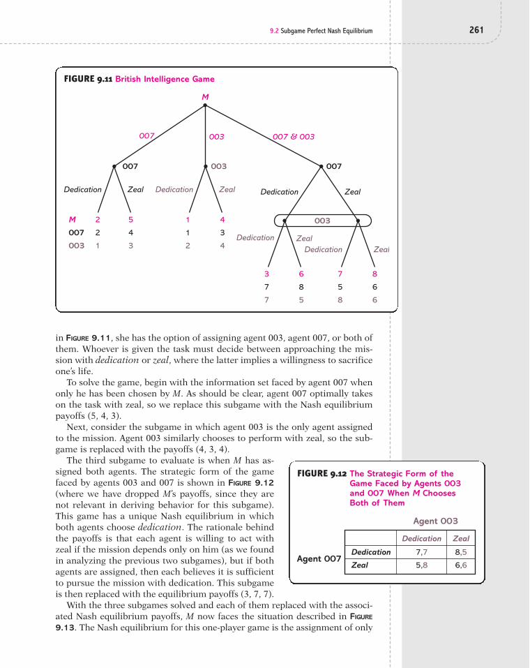
9.2 Subgame Perfect Nash Equilibrium 261
in FIGURE 9.11, she has the option of assigning agent 003, agent 007, or both ofthem. Whoever is given the task must decide between approaching the mis-sion with dedication or zeal, where the latter implies a willingness to sacrificeone’s life.
To solve the game, begin with the information set faced by agent 007 whenonly he has been chosen by M. As should be clear, agent 007 optimally takeson the task with zeal, so we replace this subgame with the Nash equilibriumpayoffs (5, 4, 3).
Next, consider the subgame in which agent 003 is the only agent assignedto the mission. Agent 003 similarly chooses to perform with zeal, so the sub-game is replaced with the payoffs (4, 3, 4).
The third subgame to evaluate is when M has as-signed both agents. The strategic form of the gamefaced by agents 003 and 007 is shown in FIGURE 9.12(where we have dropped M’s payoffs, since they arenot relevant in deriving behavior for this subgame).This game has a unique Nash equilibrium in whichboth agents choose dedication. The rationale behindthe payoffs is that each agent is willing to act withzeal if the mission depends only on him (as we foundin analyzing the previous two subgames), but if bothagents are assigned, then each believes it is sufficientto pursue the mission with dedication. This subgameis then replaced with the equilibrium payoffs (3, 7, 7).
With the three subgames solved and each of them replaced with the associ-ated Nash equilibrium payoffs, M now faces the situation described in FIGURE
9.13. The Nash equilibrium for this one-player game is the assignment of only
M
M
007
003
1
1
2
4
3
4
007 003 007 & 003
007 007003
Dedication Zeal
2
2
1
5
4
3
Dedication Zeal
3
7
7
6
8
5
Dedication
Dedication
Zeal
7
5
8
8
6
6
Dedication Zeal
Zeal
003
FIGURE 9.11 British Intelligence Game
FIGURE 9.12 The Strategic Form of theGame Faced by Agents 003and 007 When M ChoosesBoth of Them
Dedication
Agent 003
7,7
5,8
8,5
6,6
Zeal
Agent 007Dedication
Zeal

262 CHAPTER 9: TAKING TURNS IN THE DARK: SEQUENTIAL GAMES WITH IMPERFECT INFORMATION
agent 007. As reflected in M’s payoffs, he prefers agent 007 to agent 003 (per-haps the former is more skilled), and he prefers to have a single agent with zealto two agents operating at a less intense level.
In sum, there is a unique subgame perfect Nash equilibrium, and it is de-scribed by the following strategy profile: M assigns agent 007 to the mission, 007attacks the problem with zeal if he is the only one assigned and with dedicationif agent 003 is also assigned, and 003 goes at it with zeal if he is the only one as-signed and with dedication if agent 007 is also assigned.
It might help in understanding the concept of subgame perfect Nash equi-librium if we also show how a Nash equilibrium can fail to be a subgame per-fect one. For this purpose, consider the strategy profile (007 & 003, Dedica-tion/Dedication, Dedication/Dedication), which is a Nash equilibrium, butnot a subgame perfect Nash equilibrium. Let us begin by convincing ourselvesthat it is a Nash equilibrium.
At this strategy profile, M’s payoff is 3. If she instead had chosen only agent007, then her payoff would be 2, as 007 chooses dedication whether he is the onlyagent assigned or not. If she had chosen only agent 003, then her payoff wouldbe 1, as 003 would choose dedication. Thus, M’s strategy of choosing both agentsis indeed optimal. Now, if M chooses both agents, then 007’s payoff from dedica-tion/dedication is 7, from zeal/dedication is 7 (since it calls for the same actionwhen M is assigning both agents), and from either dedication/zeal or zeal/zeal is5. Thus, agent 007’s strategy also is optimal. Analogously, one can show thatagent 003 strictly prefers dedication/dedication to dedication/zeal and zeal/zeal,while zeal/dedication yields the same payoff. Accordingly, because each player’sstrategy is optimal given the other two players’ strategies, then (007 & 003, Ded-ication/Dedication, Dedication/Dedication) is a Nash equilibrium.
To show that (007 & 003, Dedication/Dedication, Dedication/Dedication)is not a subgame perfect Nash equilibrium, it is sufficient to find one subgamewhereby the substrategy profile (007 & 003, Dedication/Dedication, Dedica-tion/Dedication) for that subgame is not a Nash equilibrium. Toward that end,consider the subgame in which M assigns only agent 003. This is a one-playergame involving 003, and the relevant substrategy of Dedication/Dedicationhas him choose dedication. However, dedication yields a payoff of 2, whilechoosing zeal results in a payoff of 4. In other words, agent 003’s strategy
FIGURE 9.13 The Situation Faced by M After the ThreeFinal Subgames Have Been Solved forEquilibrium Choices
M
M
007
003
4
3
4
3
7
7
007 003 007 & 003
5
4
3

9.3 Examples 263
has him choose dedication in the event that he is the only agent assigned tothe task but, in fact, it would be optimal for him to choose zeal.*
Finally, note that it is only because M believes the incredible threat thateach agent would not choose zeal if he were the only agent assigned thatmakes it optimal for M to use both agents. If M instead believed that agent 007would act optimally by choosing zeal if he were the only agent on the job, thenM would assign only agent 007. Indeed, this is what happens at the uniquesubgame perfect Nash equilibrium that we just derived.
*This same argument can be used to show that agent 007’s substrategy at the subgame in which he is theonly agent working is also not optimal. That would also have sufficed to prove that (007 & 003, Dedica-tion/Dedication, Dedication/Dedication) is not a subgame perfect Nash equilibrium.
The Mugging game from Chapter 2 is reproduced here as FIGURE 9.14. The muggerfirst decides between having a gun and, if he chooses to have one, whether or notto show it to the victim, who is Simon. Upon either seeing a gun or not, Simon de-cides whether or not to resist the mugger. Find all subgame perfect Nash equilibria.
FIGURE 9.14 The Mugging Game
9.2 CHECK YOUR UNDERSTANDING
Mugger
Mugger
Simon
3
2
5
4
2
6
6
3
Gun & show Gun &
hide
No gun
SimonSimon
Resist Do not resist Resist Do not
resist
3
2
4
5
Resist Do not resist
9.3 ExamplesBEFORE MOVING ON TO some examples, let’s consider briefly the question ofwhether a subgame perfect Nash equilibrium will always exist in games withimperfect information and, if so, whether there may be more than one. Recallfrom Chapter 8 that subgame perfect Nash equilibria exist for every game withperfect information. Unfortunately, no such claim can be made with respectto games with imperfect information. If a subgame has no Nash equilibrium(in pure strategies), there can be no subgame perfect Nash equilibrium (inpure strategies). However, analogously to what was covered in Chapter 7, if weallow players to randomize, then there will be a subgame perfect Nash equi-librium in mixed strategies.

264 CHAPTER 9: TAKING TURNS IN THE DARK: SEQUENTIAL GAMES WITH IMPERFECT INFORMATION
On the issue of the number of equilibria, we know that a game with perfectinformation has multiple subgame perfect Nash equilibria when, at some de-cision node, two actions produce the same maximal payoff. The problem ofmultiplicity of equilibria is more acute in games with imperfect information.Multiple subgame perfect Nash equilibria can occur even when all actions re-sult in different payoffs, as we’ll observe in the OS/2 game. This situation,however, is nothing new to us, because, back in Chapters 4 and 5, we foundmultiple Nash equilibria for many games. And since the multiplicity of Nashequilibria can carry over to subgames, multiple subgame perfect Nash equilib-ria are not uncommon.
When, in fact, there are multiple subgame perfect Nash equilibria, they canall be derived by repeatedly using the method described in the previous sec-tion. Thus, if a subgame is reached for which there are multiple Nash equilib-ria, you should choose one of those equilibria and replace the subgame withthe associated equilibrium payoffs. Then you march up the tree until youreach the initial node. The process gives you just one of the subgame perfectNash equilibria. You must then return to the subgame that has multiple Nashequilibria, select another one of those equilibria, and repeat the exercise. Thenext example shows how this is done.
! SITUATION: OS/2
I suppose this poor fellow has been dead for a long time, but perhaps nobodyremembered to pick up the corpse. . . . OS/2 died from neglect and lack ofwill. And yes, backing away from OS/2 was a pragmatic move, since IBMcould not compete with Microsoft or its tactics. But how amazing to see acompany that large cowed into submission by a bunch of whippersnappersin Washington who already had taken IBM to the cleaners when they con-vinced the Goliath to let them own PC-DOS at the outset. The death of OS/2must be humiliating for IBM.1
When IBM decided to enter the personal computer (PC) market in 1981, itwas determined to make its product the industry standard. Because there werealready home computers on the market, IBM pursued a plan of getting its prod-uct to the market quickly, before some other home computer became the stan-dard. Rather than develop the PC all in-house, which was the company’s moretypical approach, IBM outsourced key components, including the microproces-sor and operating system. For the latter, IBM turned to a small company namedMicrosoft operated by Paul Allen and Bill Gates.
To meet IBM’s needs, Microsoft purchased QDOS (“Quick and Dirty OperatingSystem”) from Seattle Computer Products for $50,000, performed a few modifi-cations, and delivered the resulting product to IBM as MS-DOS (“Microsoft DiskOperating System”). Then, in arguably the worst business decision of the twenti-eth century, IBM allowed Microsoft to retain the copyright to MS-DOS. IBM fore-cast that money would come from the sale of PCs rather than the operating sys-tem itself. History, however, saw it differently: the PC became somewhat of acommodity—with easy entry and many competitors producing highly similarproducts—while Microsoft became the dominant firm in the software market byvirtue of the network effects generated by its operating system.*
*For more on network effects, go to “Situation: Operating Systems: Mac or Windows?” in Section 5.2.

9.3 Examples 265
Once recognizing its blunder, IBM began to develop its own operating sys-tem—initially in conjunction with Microsoft—which was released under thename OS/2 in 1987. At that point, Microsoft had introduced early versions ofWindows, which represented the main competition for OS/2. In spite of IBM’sbeing the leading PC manufacturer, and even though OS/2 ran faster and wasmore stable than Windows, few consumers wanted to buy a PC with OS/2 ifthere was little software available to run on it; most software at that time hadbeen developed to run on Windows. Promoting OS/2 when its competitorWindows had a large stock of compatible software was a big challenge for IBM.
To get a sense of the strategic situation that IBM faced in deciding whetherto develop its own operating system, consider the extensive form game shownin FIGURE 9.15. IBM initially decides whether or not to develop OS/2. If it chooses
FIGURE 9.15 The OS/2 Game
IBM
Company 1
Company 2
Company 3
0
0
0
0
20
3
3
3
15
1
1
0
D
D
Develop software
Develop OS/2
Do not develop OS/2
D = Develop softwareDND = Do not develop software
Do not develop software
DND
DND D DND
D DND
15
1
0
1
"2
"1
0
0
15
0
1
1
"2
0
"1
0
D DND D DND
"2
0
0
"1
"3
0
0
0
Company 3
Company 2
Company 1
IBM

To solve for the subgame perfect Nash equilibria, first consider the three-player subgame that follows from IBM’s having developed OS/2. The strategicform of this game is shown in FIGURE 9.16, where the first payoff is for softwarecompany 1, the second payoff for company 2, and the last for company 3. Wehave dropped IBM’s payoffs because it does not make a decision in this subgame.
There are two Nash equilibria (in pure strategies); onehas all three companies developing software for OS/2,and the other has none of them doing so.
With two Nash equilibria for this subgame, a deri-vation of all subgame perfect Nash equilibria requiressolving for the remainder of the game twice. Begin bysupposing that the Nash equilibrium is the one inwhich all three companies develop software to run onOS/2. The situation faced by IBM is then as shown inFIGURE 9.17. It can choose not to develop OS/2, inwhich case its payoff is zero, or develop it and earn apayoff of 20 based on the anticipation of plenty ofsoftware being written for it. IBM’s optimal decisionis obviously to develop OS/2. The strategy profile(Develop OS/2, Develop, Develop, Develop) is thenone subgame perfect Nash equilibrium.
Now consider the other Nash equilibrium at thethree-player subgame that has the three companiesnot develop applications for OS/2. The situationfaced by IBM is as shown in FIGURE 9.18, and the
266 CHAPTER 9: TAKING TURNS IN THE DARK: SEQUENTIAL GAMES WITH IMPERFECT INFORMATION
to do so, then three software companies are assumed to simultaneously decidewhether or not to develop software to run on OS/2. Implicit in the payoffs is thatOS/2 will be appealing to consumers if there are at least two applications. Thus,the success of OS/2 depends on enough compatible software being written.
FIGURE 9.16 The Situation Faced by Software Companies1, 2, and 3 After OS/2 Is Developed by IBM
Develop
Company 2Company 3, Develop
3,3,3
0,1,1
1,0,1
0,0,"1
Do not develop
Company 1Develop
Do not develop
Develop
Company 2Company 3, Do not develop
1,1,0
0,"1,0
"1,0,0
0,0,0
Do not develop
Company 1Develop
Do not develop
FIGURE 9.17 The Situation Faced by IBM Whenthe Three Companies DevelopSoftware for OS/2
20
3
3
3
IBM
Company 1
Company 2
Company 3
0
0
0
0 Develop OS/2
Do not develop OS/2
IBM

9.3 Examples 267
Nash equilibrium for this one-player game is not todevelop OS/2. This gives us a second subgame per-fect Nash equilibrium: (Do not develop OS/2, Donot develop, Do not develop, Do not develop).
Subgame perfect Nash equilibrium play can thenresult in two quite distinct outcomes: One has IBMintroducing OS/2 in anticipation of all three compa-nies developing applications for it, which they do;the other has IBM ditching the operating systemsproject because it doesn’t expect applications to bewritten for OS/2.
What actually happened? IBM introduced OS/2,but as time revealed, few applications were writtenfor it. In spite of its heft in the computer industry,even IBM could not shake the dominant position ofWindows and the business acumen of Microsoft.Although history then runs counter to either sub-game perfect Nash equilibrium, equilibrium playwill conform to history if we allow players to usemixed strategies.*
Suppose we start with the three-player subgame among the software devel-opers, and let us conjecture that it has a symmetric Nash equilibrium in whicheach company randomizes. Let d denote the probability that a company choosesto develop software. For software company 1 to find it optimal to randomize, itmust receive the same expected payoff from either of its pure strategies, developand do not develop. Suppose companies 2 and 3 each develop software withprobability d. Hence, with probability both of them develop software; withprobability neither develops software; and with probability one of them develops software.** The expected payoff to company 1 from devel-oping software is then
Equating this payoff to 0, which is the payoff from not developing software,we solve for d and find that Thus, each of the three software companieschoosing develop with probability is a symmetric Nash equilibrium.
Given this Nash equilibrium in the three-player subgame, the expected pay-off to IBM from developing OS/2 is***
Because the payoff for not developing OS/2 is 0, IBM finds it optimal to de-velop OS/2. However, in doing so, IBM is uncertain as to how much software
a14b3 ! 20 % 3 a1
4b2a3
4b ! 15 % 3 a1
4ba3
4b2 ! ("2) % a3
4b3 ! ("3) #
2064
.
14
d # 14.
d2 ! 3 % 2d(1 " d) ! 1 % (1 " d)2 ! ("1) # 4d " 1.
2d(1 " d),(1 " d)2,d2,
FIGURE 9.18 The Situation Faced by IBMWhen the Three Companies DoNot Develop Software for OS/2
#3
0
0
0
IBM
Company 1
Company 2
Company 3
0
0
0
0 Develop OS/2
Do not develop OS/2
IBM
*The remainder of this example requires knowledge of the material in Chapter 7.**With probability , company 2 develops software and company 3 does not, and with probability
company 2 does not develop software and company 3 does. Thus, the probability that only oneof them develops software is the sum of those two probabilities, or ***The probability that two companies develop software is the sum of the probability that companies 1and 2 do, that companies 1 and 3 do, and that companies 2 and 3 do; each of those probabilities is and their sum is 3(1
4)2(34).
(14)2(3
4),
2d(1 " d).(1 " d)d,
d(1 " d)

268 CHAPTER 9: TAKING TURNS IN THE DARK: SEQUENTIAL GAMES WITH IMPERFECT INFORMATION
will be written for it. If at least two companies write applications that run onOS/2, an event that occurs with probability , then OS/2 will succeed.* Butwith probability , fewer than two applications are written, and OS/2 will fail.History, as we know, has given us the latter realization.
! SITUATION: AGENDA CONTROL IN THE SENATE
The U.S. Senate is considering three alternative versions of a bill, which we’lldenote A, B, and C. The preferences of the 100 senators are shown in TABLE 9.1.Ten senators prefer bill A and have bill B as their second choice. Bill B is thefirst choice of 44 senators, whose second choice is bill C. Finally, 46 senatorsrank bill C first and bill A second.
5064
1064
TABLE 9.1 PREFERENCES OF THE SENATORS
Type of Number ofSenator 1st Choice 2nd Choice 3rd Choice Senators
I A B C 10
II B C A 44
III C A B 46
The procedure for selecting a bill for passage is a three-stage process:
■ Stage 1: The leader of the Senate sets the agenda by selecting two billsfor a vote. His choice is then either A and B, A and C, or B and C.
■ Stage 2: Given the pair of bills selected by the Senate leader, the 100members vote simultaneously.
■ Stage 3: Whichever bill receives more votes in stage 2 is then matchedwith the third bill, and the Senate votes simultaneously on those twobills, with the majority winner being the bill that is passed.
For example, suppose the Senate leader chooses bills A and C. Then, in stage2, each Senator votes for either A or C. If A draws more votes, then A is matchedwith B in stage 3. If A receives a majority of votes in stage 3, then A is passed,while if B receives a majority of votes, then B becomes law. With 100 players,the extensive form game is far too massive to write down in tree format, so we’llhave to be satisfied with the preceding description. Finally, assume that a sen-ator’s payoff equals 2 if his most preferred bill is passed, 1 if his second-mostpreferred bill is passed, and 0 if his least preferred bill is passed.
Our focus is on deriving subgame perfect Nash equilibria for which it is opti-mal for senators to vote sincerely; that is, in deciding between two bills, a Senatorvotes for the bill he ranks higher. For example, if A and C are the two bills on thefloor, then a type I senator votes for A and type II and III senators vote for C.
A stage 3 subgame has the 100 senators simultaneously cast votes for the twobills under consideration (where one of the bills won a majority in stage 2 andthe other is the one that was excluded by the Senate leader in stage 1). These
*The probability that three applications are written is and the probability that two applicationsare written is so the sum of the probabilities is .10
643(14)2(3
4) # 964,
(14)3 # 1
64,

9.3 Examples 269
final subgames are distinguished by the path that led to them, which is definedby two things: the Senate leader’s initial selection of which two bills to considerand how Senators cast their votes between the two bills. Although there aremany such subgames, all that is important for deriving an equilibrium is know-ing which two bills were proposed in stage 1 and which bill received more votesin stage 2 (and, for the sake of simplicity, let us ignore ties). Accordingly,
■ Consider a stage 3 subgame in which the Senate leader proposed bills Aand B in stage 1 . . .— . . . and A received more votes in stage 2. Then the senators must nowdecide between A and C in stage 3. With sincere voting, C wins, as 90Senators prefer it. (See Table 9.1.) Note that sincere voting is optimal,since the bill that passes is independent of how an individual senatorvotes and, therefore, so is his payoff.— . . . and B received more votes in stage 2.* Then the senators must decidebetween bills B and C. With sincere voting, B wins, as 54 senators prefer it.
■ Consider a stage 3 subgame in which the Senate leader proposed bills Aand C in stage 1 . . .— . . . and A received more votes in stage 2. Then, with sincere votingwith respect to bills A and B, A wins by a vote of 56–44.— . . . and C received more votes in stage 2. Then, with sincere votingwith respect to bills B and C, B wins by a vote of 54–46.
■ Consider a stage 3 subgame in which the Senate leader proposed bills Band C in stage 1 . . .— . . . and B received more votes in stage 2. Then, with sincere votingwith respect to bills A and B, A wins by a vote of 56–44.— . . . and C received more votes in stage 2. Then, with sincere votingwith respect to bills A and C, C wins by a vote of 90–10.
With these Nash equilibrium outcomes to the stage 3 subgames, let us moveback to the stage 2 subgames. As already reasoned, sincere voting is optimal.Hence, if the Senate leader initially selected bills A and B, then A wins with 56votes; if he selected bills A and C, then C wins with 90 votes; and if it were billsB and C that were first up for a vote, then B wins with 54 votes.
With all this in mind, we now go back to the first stage of the game, whichis when the Senate leader chooses the pair of bills to be voted upon. In lightof the preceding analysis, this is what will transpire, depending on his choice:
■ If bills A and B are put on the agenda in stage 1, then A wins by a vote of56–44 (as derived). Then, in stage 3 (or the second round of voting), billA goes against bill C, and C prevails by a vote of 90–10 (as derived).Hence, bill C ultimately passes if the Senate leader initially puts bills Aand B on the agenda.
■ If bills A and C are put on the agenda in stage 1, then C wins by a vote of90–10. Then, in the second round of voting, bill C goes against bill B, andB prevails by a vote of 54–46. Hence, bill B ultimately passes if the Senateleader initially puts bills A and C on the agenda.
*If Senators voted optimally in stage 2, then B should not have received more votes than A. But remem-ber that we have to be sure that play is consistent with Nash equilibrium for every subgame.

270 CHAPTER 9: TAKING TURNS IN THE DARK: SEQUENTIAL GAMES WITH IMPERFECT INFORMATION
■ If bills B and C are put on the agenda in stage 1, then B wins by a voteof 54–46. Then, in the second round of voting, bill B goes against bill A,and A prevails by a vote of 56–44. Hence, bill A ultimately passes if theSenate leader initially puts bills B and C on the agenda.
What is optimal behavior for the Senate leader depends on his preferences.If he has type I preferences, then he most desires bill A to pass, in which casehe’ll first have the Senate vote between bills B and C. The outcome will be thatC loses out, and then B will lose in stage 3 to bill A. If, instead, the Senateleader has type II preferences, then he’ll have bills A and C duke it out in stage2. Bill C will win, but then will lose to bill B. And if the Senate leader has typeIII preferences, he’ll put bills A and B on the agenda. Although A will win, itwill lose to C in stage 3.
Regardless of the Senate leader’s preferences, then, subgame perfect Nashequilibrium results in his most preferred bill passing by virtue of clever ma-nipulation of the agenda. Whatever is his most preferred bill, he should ini-tially have the Senate vote between the other two bills and then have the win-ner of that vote go against his preferred bill. That strategy will always result inthe latter’s being approved. Note that this approach works even if the Senateleader has type I preferences, which are shared by only nine other membersof the Senate. You have just witnessed the power of controlling the agenda.
9.4 CommitmentAS PART OF EVERYDAY LIFE, we often try to avoid commitments. Commitmentmeans limiting future options, in which case it is reasonable to either post-pone or avoid them altogether. That logic does not always apply in a strategicsetting, however: commitment can be desirable because it limits or constrainswhat you can or will do in the future. The benefit arises not from how it af-fects your behavior, but rather in how others respond to knowing that youhave bound yourself to act in a certain way.
In this section, we flesh out the value of commitment in two business set-tings. The first situation is faced by many a successful entrepreneur: now thather enterprise has succeeded, how does she keep others from imitating whatshe’s done and eroding her business’ profitability? The second situation dealswith a historical puzzle: why were Dutch traders more active than Britishtraders in the East India trade in the seventeenth century? As we will argue, itwas due, not to ships or technology, but rather to contracts that committedDutch traders to being more aggressive.
9.4.1 Deterrence of EntryConsider a market in which a single company is operating profitably. Perhapsit is a new market and this company was the first to enter. The challenge tothe established company is to deter the entry of competitors. Let’s see howcommitment can achieve that goal.
If the established company were to continue to enjoy a monopoly, let ussuppose it would expect to earn a profit (or a payoff) of 1,000. Eyeing this mar-ket is a lone potential entrant that, if it chose to enter, would face the compet-itive environment described by FIGURE 9.19. For simplicity, each company canchoose to set its price at one of three levels: low, moderate, or high. Nash

9.4 Commitment 271
equilibrium predicts that both companies will choose a moderate price (infact, this is a dominant strategy) and each earns a profit of 400.
In deciding whether to enter this market, a prospective company must takeaccount of not only the anticipated profit it would make—which has just beenshown to be 400—but also the cost of entry, which is assumed to be 350. This350 may represent the cost of building a manufacturing plant or setting up astore. An entrant can then expect to earn a net profit of 50, which is the post-entry (gross) profit of 400 less the cost of entry of 350. Assuming that thisprospective company would earn zero from not entering the market, it wouldbe optimal for it to enter, since, if it anticipated that companies would price inaccordance with Nash equilibrium, it would find entry profitable.
The preceding description of events is embodied in the extensive formgame shown in FIGURE 9.20. The potential entrant moves first, deciding
FIGURE 9.19 Post-Entry Game (Gross Profit)
Low
New company
300,300
325,350
250,400
350,325
400,400
325,500
400,250
500,325
450,450
Moderate High
Establishedcompany
Low
Moderate
High
FIGURE 9.20 The Entry Game
300
"50
350
"25
400
"100
L M H L M H
325
0
400
50
500
"25
L
Enter Do not enter
M H
250
50
325
150
450
100
1,000
0
L M H
Potential entrant
Potential entrant
Established companyEstablished company
Potential entrant

272 CHAPTER 9: TAKING TURNS IN THE DARK: SEQUENTIAL GAMES WITH IMPERFECT INFORMATION
whether to enter the market. If it chooses do not enter, then the establishedcompany earns a monopoly profit of 1,000 and the potential entrant earns zero.If the potential entrant instead chooses enter, then the two companies make si-multaneous price decisions. (The potential entrant is now the “new company”in Figure 9.19.) Note that the payoffs to the entrant in Figure 9.20 are the valuesfrom Figure 9.19 after subtracting the entry cost of 350.
In describing how companies will behave, we implicitly used the method ofbackward induction. That is, we derived Nash equilibrium behavior for the sub-game that followed the entry of the potential entrant; this subgame had bothcompanies choosing a moderate price. We then replaced that subgame with theNash equilibrium payoffs: 400 for the established company and 50 for the po-tential entrant. This leaves us with a one-player game in which the potential en-trant decides whether to enter. It has a Nash equilibrium of enter. Thus, theunique subgame perfect Nash equilibrium is (Enter/Moderate, Moderate).
Entry of the potential entrant is most unfortunate for the established com-pany, since its profit is only 400, compared with 1,000 if it could somehow man-age to prevent the potential entrant from entering. Interestingly, there is a Nashequilibrium in which entry is deterred: the strategy profile (Do not enter/Moder-ate, Low). Given that this strategy has the potential entrant not enter, the payoffto the established company is 1,000 regardless of its strategy, since its strategystates the price to set if there is entry. Thus, a plan to set a low price in the post-entry game is an optimal strategy for the established company. Given that theestablished company is to price low in response to the potential entrant’s actu-ally entering the market, the potential entrant’s highest payoff if it were to enteris (which requires setting a moderate price). Because this payoff is lowerthan the payoff from not entering, Do not enter/Moderate is optimal for the po-tential entrant (as are Do not enter/Low and Do not enter/High).
Thus, we have a Nash equilibrium in which entry is deterred by the threat oflow pricing by the established company. However, this threat is not credible andthus ought not to be believed by the potential entrant. In other words, although(Do not enter/Moderate, Low) is a Nash equilibrium, it is not a subgame perfectNash equilibrium. The substrategy profile for the subgame in which companiescompete in price, namely, (Moderate, Low), is not itself a Nash equilibrium. Onlya poorly trained game theorist—one versed in Nash equilibrium, but not in sub-game perfection—would recommend that the established company deter entryby making the (idle) threat of pricing low.
Breaking outside of the model described in Figure 9.20, we ask, Is there a wayin which entry can be deterred? One suggestion comes from the New Yorkgarbage-hauling business, in which the established companies were controlled byorganized crime. Soon after a company began to enter the market, an employeefound a dog’s severed head in his mailbox with the note “Welcome to New York.”2
But let us think of a more legitimate and less gruesome manner of discouragingentry, preferably one that is approved by the New York State Bureau of Tourism.
Another avenue is for the established company to figure out how to commititself to pricing aggressively if entry occurs. If the entrant were to anticipate alow price for the established company, then it would not enter the market, be-cause the resulting gross profit of 325 would be insufficient to cover the cost ofentry. So, how might the established company convince the new company thatit would set a low price?
Well, let us suppose there is a new production technology that, though expen-sive at a cost of 500, serves to significantly lower the cost of producing each unit
"25

9.4 Commitment 273
by, for example, requiring fewer inputs (such as less energy). If the establishedcompany were to adopt this new technology, then if the potential entrant ac-tually entered the market, the competitive environment would be as describedin FIGURE 9.21. This environment differs from that of Figure 9.19 because ofthe lower cost of production for the established company. (Note that the pay-offs shown in Figure 9.21 have not subtracted the cost of the investment; weshall do this in a moment.) The gross profit of the new company is the sameas before, since it is not directly affected by the production cost of the estab-lished company; it is affected only by the price that the established companycharges. The gross profit of the established company is uniformly higher, sincethe established company produces at a lower cost.
The key difference between the post-entry situations in Figures 9.19 (with-out investment) and 9.21 (with investment) is that the established company ismore inclined to price low having made the cost-reducing investment de-scribed. Without the investment, the dominant strategy for the establishedcompany was to choose a moderate price. Now it prefers to price low whenthe new company prices either low or moderately (while it still prefers a mod-erate price when the new company prices high). The Nash equilibrium for thepost-entry game in Figure 9.21 has the established company setting a lowprice and the new company setting a moderate price.
The possibility that the established company can invest in the new technol-ogy is taken into account in the extensive form game depicted in FIGURE 9.22.The established company moves first by either making the cost-reducing in-vestment or not. The potential entrant observes that decision prior to decidingwhether it ought to enter. If it does not enter, then the established companyearns 1,000 (if it did not invest) or 700 (if it did invest).* If the new companyenters the market, then the two companies compete by simultaneously choos-ing a price. Note that the payoff for the potential entrant is its gross profitminus the cost of entry (if it entered) and the payoff for the established com-pany is its gross profit minus the cost of investment (if it invested).
To solve for the subgame perfect Nash equilibria for the game shown inFigure 9.22, we first solve for the Nash equilibria for each of the final two sub-games in which the two companies compete in price. Doing so and replacingthe subgames with the (unique) Nash equilibrium payoffs gives us the situa-tion portrayed in FIGURE 9.23. Solving for the final two subgames in the treeshows that the potential entrant will enter if the investment was not made—preferring a payoff of 50 to 0—and will not enter if the investment was made—
FIGURE 9.21 The Post-Entry Game After Investment(Gross Profit)
Low
New company
475,300
425,350
325,400
525,325
500,400
400,500
575,250
600,325
525,450
Moderate High
Establishedcompany
Low
Moderate
High
*It is presumed that cost-reducing investment raises gross monopoly profit from 1,000 to 1,200—becauseof the lower production cost—but the investment cost of 500 needs to be netted out. This gives us 700.

FIGURE 9.22 The Entry–Investment Game
!25
!50
25
!25
75
!100
L M H L M H
!75
0
0
50
100
!25
L
Enter Do notenter
M H
!175
50
!100
150
25
100
700
0
L M H
Potential entrant
Potential entrant
Potential entrant
1,000
0 Potential entrantEstablished company
Enter Do notenter
300
!50
350
!25
400
!100
L M H L M H
325
0
400
50
500
!25
L M H
250
50
325
150
450
100
L M H
Established company
Established company
Invest Do notinvest
Established company
274

9.4 Commitment 275
preferring a payoff of 0 to Working back up to the established company’sdecision, the established company can expect to earn a payoff of 400 by notinvesting—since entry has occurred and both companies price at a moderatelevel—but a payoff of 700 by investing—since the potential entrant’s entry isdeterred.
In sum, the unique subgame perfect Nash equilibrium is as follows: The es-tablished company invests. If the potential entrant then enters the market, theestablished company sets a low price. Had the established company not in-vested and the potential entrant entered, then the established company wouldhave set a moderate price. Turning to the potential entrant’s strategy, we seethat if the established company invested, then the potential entrant would notenter, but if, by mistake, it does enter, then it sets a moderate price. If the es-tablished company did not invest, then the potential entrant enters and stillsets a moderate price.
The key to this entry deterrence strategy is credibly conveying to the poten-tial entrant that the established company will price low in response to the po-tential entrant’s entry; thus, the potential entrant can expect entry to be unprof-itable. The way the established company makes an aggressive pricing policycredible is by altering its preferences for low prices. Adopting a technology thatlowers its production cost makes lower prices more appealing. Hence, invest-ment changes the established company’s preferences in the post-entry situation,and in this manner it is credibly committed to pricing low in response to entry.
Now suppose, in contrast to the previous game, the established company’sinvestment was not observed by the potential entrant at the time of its entrydecision (though it is observed after entry). This game is depicted in FIGURE
9.24 (in which we’ve already substituted the price subgames with their Nashequilibrium payoffs). Now do not invest strictly dominates invest for the es-tablished company, and the Nash equilibrium is for there to be no investmentand entry occurs. If, then, investment is to deter entry, it is essential that the
"25.
FIGURE 9.23 The Entry–Investment Game After Having Solved for the FinalTwo Subgames
Enter Do notenter
700
0
400
50
25
#25
Potentialentrant
1,000
0 Potential entrantEstablished company
Enter Do notenter
Invest Do notinvest
Established company
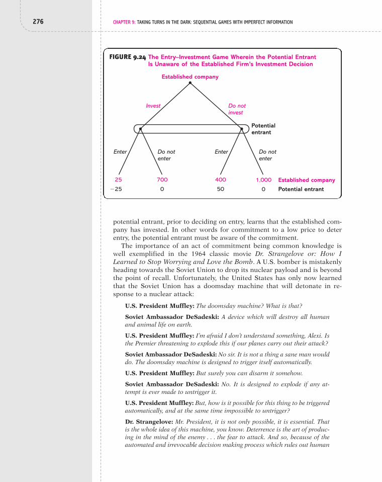
276 CHAPTER 9: TAKING TURNS IN THE DARK: SEQUENTIAL GAMES WITH IMPERFECT INFORMATION
potential entrant, prior to deciding on entry, learns that the established com-pany has invested. In other words for commitment to a low price to deterentry, the potential entrant must be aware of the commitment.
The importance of an act of commitment being common knowledge iswell exemplified in the 1964 classic movie Dr. Strangelove or: How ILearned to Stop Worrying and Love the Bomb. A U.S. bomber is mistakenlyheading towards the Soviet Union to drop its nuclear payload and is beyondthe point of recall. Unfortunately, the United States has only now learnedthat the Soviet Union has a doomsday machine that will detonate in re-sponse to a nuclear attack:
U.S. President Muffley: The doomsday machine? What is that?
Soviet Ambassador DeSadeski: A device which will destroy all humanand animal life on earth.
U.S. President Muffley: I’m afraid I don’t understand something, Alexi. Isthe Premier threatening to explode this if our planes carry out their attack?
Soviet Ambassador DeSadeski: No sir. It is not a thing a sane man woulddo. The doomsday machine is designed to trigger itself automatically.
U.S. President Muffley: But surely you can disarm it somehow.
Soviet Ambassador DeSadeski: No. It is designed to explode if any at-tempt is ever made to untrigger it.
U.S. President Muffley: But, how is it possible for this thing to be triggeredautomatically, and at the same time impossible to untrigger?
Dr. Strangelove: Mr. President, it is not only possible, it is essential. Thatis the whole idea of this machine, you know. Deterrence is the art of produc-ing in the mind of the enemy . . . the fear to attack. And so, because of theautomated and irrevocable decision making process which rules out human
FIGURE 9.24 The Entry–Investment Game Wherein the Potential Entrant Is Unaware of the Established Firm’s Investment Decision
Enter Do notenter
700
0
400
50
25
"25
Potentialentrant
1,000
0 Potential entrantEstablished company
Enter Do notenter
Invest Do notinvest
Established company

9.4 Commitment 277
meddling, the doomsday machine is terrifying. It’s simple to understand.And completely credible, and convincing. (Turning to DeSadeski.) But thewhole point of the doomsday machine is lost if you keep it a secret! Why didn’tyou tell the world, eh?
Soviet Ambassador DeSadeski: It was to be announced at the PartyCongress on Monday. As you know, the Premier loves surprises.
9.4.2 Managerial Contracts and Competition: East India Trade in the Seventeenth CenturyThe importation of spices and silk from East India to Europe was a lucrativebusiness in the seventeenth century.3 Even with the high cost of transportation—about 7% of voyages never returned—profit margins were high, as these itemscould be sold for five times their cost. Trade was dominated by the British andDutch, which is not surprising given their general superiority in naval affairs atthe time. What is puzzling is why the Dutch were noticeably more active than theBritish. For example, in 1622 the Dutch transported 2.28 million pounds of pep-per, exceeding Britain’s supply of 1.615 million pounds by more than 40%.
Dutch East India Company
One intriguing hypothesis is that the difference rested in contracts—in howthe British and Dutch traders were compensated for their services. The argu-ment is that the manner in which the Dutch traders were rewarded not onlyled them to send out more ships on the East India trade route, but becausethey were more aggressive, British traders were induced to send out fewerships. To see the argument behind this hypothesis, let me put forth a simplemodel for your consideration.
THE
GRA
NG
ER C
OLL
ECTI
ON
, NEW
YO
RK

278 CHAPTER 9: TAKING TURNS IN THE DARK: SEQUENTIAL GAMES WITH IMPERFECT INFORMATION
Suppose the shareholders of British trading companies and those of Dutchtrading companies care only about profit—about how much money is made.A trading company, however, is not directly operated by the shareholders, butrather by a manager, and what determines the manager’s behavior is how heis compensated. If his compensation is a share of the company’s profit, thenhe’ll try his best to maximize profit, because the more profit there is, thehigher is his salary. What is interesting is that, in a strategic situation, it couldbe in the best interests of profit-seeking shareholders to have their managersnot care about profit! Only in the subtle and surprising world of strategic rea-soning could such a statement prove true.
In this game, suppose there are just two shipping companies, one that isBritish and one that is Dutch. In each company, shareholders decide on a con-tract to give to their manager. Suppose that there are two feasible contracts: (1)a manager’s pay equals some fraction of the company’s profit; (2) his pay equalssome fraction of the company’s revenue. Revenue—how much money is collectedfrom the sale of a good—equals, say, the price per pound times the number ofpounds sold. Profit equals revenue minus cost, where cost is what the companyhad to pay out to get the items to Europe. Cost includes the cost of buying theitems in India and the cost of transporting them back to Europe. Profit is whatshareholders get and thus is what they are interested in maximizing.
Now, suppose further that once contracts are given to the managers (andpresumably agreed to by them), they are known to both managers. While eachmanager then knows whether the other manager is paid a fraction of profit orof revenue, the amount of compensation is not yet determined. At that point,each manager decides on the number of voyages his company will undertake,which then determines the supply of the good, say, pepper. For simplicity, as-sume there are just three supply levels: low, moderate, and high. The profit andrevenue from each of the nine possible strategy pairs is shown in TABLE 9.2.For example, if the British choose a moderate number of voyages and theDutch a high number, then the British company earns profits of 60,000 on rev-enue of 112,500 (hence, its cost is 52,500), while the Dutch company earnsprofits of 67,500 on revenue of 135,000.
TABLE 9.2 PROFIT AND REVENUE IN THE EAST INDIA TRADE
British British Dutch Dutch British Dutch Profit Revenue Profit Revenue
Low Low 80,000 120,000 80,000 120,000
Low Moderate 70,000 110,000 87,500 137,500
Low High 62,500 100,000 85,000 150,000
Moderate Low 87,500 137,500 70,000 110,000
Moderate Moderate 75,000 125,000 75,000 125,000
Moderate High 60,000 112,500 67,500 135,000
High Low 85,000 150,000 62,500 100,000
High Moderate 67,500 135,000 60,000 112,500
High High 57,500 120,000 57,500 120,000

9.4 Commitment 279
Now suppose both the British and Dutch managers are compensated on thebasis of profit and, to be concrete, each receives a wage equal to 1% of profit.Then the game faced by managers is as shown in FIGURE 9.25, where their pay-offs are presumed to equal their monetary compensation.* This game has aunique Nash equilibrium in which both managers choose to launch a moder-ate number of voyages. Each manager earns pay of 750, and each tradingcompany earns a profit of 75,000 (referring back to Table 9.2).**
FIGURE 9.25 The East India Trade Game When Each Manager’sPayoff Equals 1% of Profit
Low
Dutch manager (profit maximizer)
800,800
875,700
850,625
700,875
750,750
675,600
625,850
600,675
575,575
Moderate High
British manager (profit maximizer)
Low
Moderate
High
Now suppose the Dutch manager’s pay is a share of revenue—specifically, of 1% of revenue. The British manager continues to receive pay equal to 1%of profit. Thus, the Dutch manager ignores the cost of buying and transport-ing the goods. He determines the number of voyages so as to generate thehighest revenue from selling imported items in Europe. The new strategicform game faced by the two companies’ managers is shown in FIGURE 9.26.***This game has a unique Nash equilibrium whereby the British managerchooses a low number of voyages and the Dutch manager chooses a high num-ber of voyages. The British trading company then earns a profit of 62,500 (on100,000 of revenue), and the Dutch company earns a profit of 85,000 (on150,000 of revenue).
12
FIGURE 9.26 The East India Trade Game When the Dutch Manager’sPayoff Equals of 1% of Revenue and the BritishManager’s Payoff Equals 1% of Profit
12
Low
Dutch manager (revenue maximizer)
800,600
875,550
850,500
700,687.5
750,625
675,562.5
625,750
600,675
575,600
Moderate High
British manager (profit maximizer)
Low
Moderate
High
*The payoffs, then, equal 1% of the profit entries in Table 9.2.**To be correct, shareholders receive 75,000, less the 750 paid to the manager. However, the amount ofmanagerial compensation is very small in this example, and our conclusions are unaffected if we chooseto ignore it, which we will.***The payoffs for the British manager are the same as in Figure 9.25, while the payoffs for the Dutchmanager equal of 1% of the revenue entries in Table 9.2.1
2

280 CHAPTER 9: TAKING TURNS IN THE DARK: SEQUENTIAL GAMES WITH IMPERFECT INFORMATION
A couple of interesting points are worth noting. First, not only do the Dutchearn more revenue than the British, but they also make more profit, eventhough the Dutch manager is interested in revenue, not profit. Furthermore,the Dutch company earns more money than when the manager was concernedabout profit. For the game in Figure 9.25, when the Dutch manager cared onlyabout profit (because his pay was a share of profit), the Dutch companyearned a profit of 75,000, but now it earns 85,000 with a manager who caresonly about revenue (because his pay is a share of revenue). The Dutch share-holders thus earn more profit by having their manager import an amount thatmaximizes revenue, not profit. How can this be?
The sleight of hand that led to this striking result is how the British tradingcompany responds to the Dutch manager’s caring about revenue, not profit.Were the British to continue to make a moderate number of voyages, thenswitching the Dutch manager to a revenue-based contract would lead to toomuch being imported and lower profit. Given that the British managerchooses moderate, Dutch profit would go from 75,000 to 67,500 when therevenue-driven Dutch manager chooses high rather than moderate. But, for-tunately for the Dutch, the British know that the Dutch manager will importa lot, so they pull back on how much they import in order not to flood the mar-ket and depress prices. This is why the new Nash equilibrium has the Britishimport a low amount, given that the Dutch import a high amount. The com-mitment to import a lot—which is made credible by having the Dutch man-ager be compensated by how much he imports (not how much money hemakes for shareholders)—induces the British to import less, and that serves toraise the profit of the Dutch trading company.
In a strategic setting, a player can be better off by committinghimself to some future behavior if this commitment is made known to the otherplayers.
SummaryIn solving a game, the task is always to find the most compelling strategy pro-file: what we think intelligent players would do. As originally pointed out inChapter 8, Nash equilibrium need not always be compelling, in spite of eachplayer using a strategy that is best, given other players’ strategies. The opti-mality of a player’s strategy could depend on the belief that if the player didsomething different, then another player would respond in an irrational man-ner. The anticipation of an irrational move was referred to as an incrediblethreat, and it was argued that Nash equilibria predicated upon incrediblethreats are not compelling because a player whose bluff was called would notfind it optimal to go through with the threatened response. In that case, sucha threat should not be believed by other players.
The more stringent solution concept of subgame perfect Nash equilibriumrules out Nash equilibria involving incredible threats, initially introduced forgames with perfect information in Chapter 8. In the current chapter, we pro-vided a generalized definition of subgame perfect Nash equilibrium that ap-plies to extensive form games with perfect or imperfect information.
Implementing subgame perfect Nash equilibrium is a two-step process.First, you must identify the parts of a game that are themselves a well-defined

Exercises 281
1. For the game in FIGURE PR9.1, derive all subgame perfect Nash equilibria.
EXERCISES
2. In FIGURE PR9.2, a variant of the OS/2 game is provided that differs in thestructure of information sets as well as in some of the payoffs. Now ifIBM develops OS/2, software company 1 moves first in deciding whether
FIGURE PR9.1
3
2
1
2
0
2
0
1
1
1
c
x
a b
y x y
d
3
2
3
1
1
2
0
c d
0
3
2
0
4
1
c d
3
3
0
3
1
4
2
c d
game. A “game within a game” is called a subgame. For the second step, wedefined a substrategy profile as the part of a strategy profile that pertains toa subgame, and then we required that the substrategy profile form a Nashequilibrium for that subgame. Thus, subgame perfect Nash equilibrium man-dates that players act optimally at every subgame, even those that are notreached if everyone were to act according to the subgame perfect Nash equi-librium. In this manner, when a player considers the ramifications of a partic-ular move, she presumes that all players will respond in their best interests,not according to some idle threat.
In a game-theoretic context, commitment refers to a decision with somepermanency that has an impact on future decision making. It may mean mak-ing an investment that influences the payoffs from various future actions orconstraining the actions that can be chosen in the future. Commitment can bevaluable in a strategic setting because of how it affects what other players do.A publicly observed commitment can bind a player to act a certain way in thefuture and can thereby induce other players to adjust their behavior in a waythat may be desirable from the perspective of the player making the commit-ment. Understanding how commitment functions is a valuable piece of insightthat game theory delivers.

282 CHAPTER 9: TAKING TURNS IN THE DARK: SEQUENTIAL GAMES WITH IMPERFECT INFORMATION
to develop an application, and then, after its choice has been revealed,companies 2 and 3 act simultaneously.a. Derive all subgame perfect Nash equilibria.b. Derive a Nash equilibrium that is not a subgame perfect Nash equilib-
rium, and explain why it is not a subgame perfect Nash equilibrium.
3. “I can’t come with you,” said Hermione, now blushing, “because I’m al-ready going with someone.” “No, you’re not!” said Ron. “You just said thatto get rid of Neville.” “Oh, did I?” said Hermione, and her eyes flashed dan-gerously. “Just because it’s taken you three years to notice, Ron, doesn’tmean no one else has spotted I’m a girl”4
It is the week before the Yule Ball Dance, and Victor and Ron are eachcontemplating whether to ask Hermione. As portrayed in FIGURE PR9.3,
FIGURE PR9.2 Revised OS/2 Game
IBM
Company 1
Company 2
Company 3
0
0
0
0
5
2
2
2
3
1
1
0
D
D
Develop
Develop OS/2
Do not develop OS/2
D = DevelopDND = Do not develop
Do notdevelop
DND
DND D DND
D DND
3
1
0
1
"2
"1
0
0
3
0
1
1
"2
0
"1
0
D DND D DND
"2
0
0
"1
"3
0
0
0
Company 3
Company 2
Company 1
IBM

Exercises 283
Victor moves first by deciding whether or not to approach Hermione.(Keep in mind that asking a girl to a dance is more frightening than a roguebludger). If he gets up the gumption to invite her, then Hermione decideswhether or not to accept the invitation and go with Victor. After Victor (andpossibly Hermione) have acted, Ron decides whether to conquer his caseof nerves (perhaps Harry can trick him by making him think he’s drunkFelix Felicis) and finally tell Hermione how he feels about her (and also in-vite her to the dance). However, note that his information set is such thathe doesn’t know what has happened between Victor and Hermione. Rondoesn’t know whether Victor asked Hermione and, if Victor did, whetherHermione accepted. If Ron does invite Hermione and she is not going withVictor—either because Victor didn’t ask, or he did and she declined—thenHermione has to decide whether to accept Ron’s invitation. At those deci-sion nodes for Hermione, she knows where she is in the game, since she isfully informed about what has transpired. The payoffs are specified so thatHermione would prefer to go to the dance with Ron rather than withVictor. Both Ron and Victor would like to go with Hermione, but bothwould rather not ask if she is unable or unwilling to accept. Use the con-cept of subgame perfect Nash equilibrium to find out what will happen.
FIGURE PR9.3 Yule Ball Dance
Hermione
Hermione
Victor
Ron
Hermione
8
3
6
7
6
5
Ask Do not ask
Ask Do not ask
1
8
8
3
2
4
Yes No
Yes No
2
5
3
Ask Do not ask
Ron
5
4
1
Ask Do not ask
Hermione
4
7
7
6
1
2
Yes No
Victor

284 CHAPTER 9: TAKING TURNS IN THE DARK: SEQUENTIAL GAMES WITH IMPERFECT INFORMATION
4. For Exercise 3 on the Yule Ball Dance, now assume that, before he de-cides whether to ask Hermione, Ron observes whether or not Victorasked her. However, if Victor does invite Hermione, Ron does not knowher answer to Victor when he decides whether to invite her himself.a. Write down the extensive form game.b. Derive all subgame perfect Nash equilibria.
5. In Tom Clancy’s novel Hunt for Red October, the Soviet Union has devel-oped a submarine named Red October that can run “silently” andthereby escape detection. On its maiden voyage, the ship’s captain,Marko Ramius, has decided to defect, because he believes that this tech-nology risks war by destroying the balance of power between the UnitedStates and the U.S.S.R. He has put together a set of officers who areloyal to him and have agreed to defect as well. However, the captain isconcerned that an officer may change his mind during the voyage and,furthermore, that an officer may be more inclined to change his mind ifhe thinks that other officers will do so. The captain is then consideringwriting a letter—to be delivered to the Soviet government after the sub-marine has departed from its base—stating his plan to defect. The exten-sive form of this game is shown in FIGURE PR9.5.
FIGURE PR9.5 Hunt for Red October
Ramius
Borodin
7
4
4
Ramius
Borodin
Melekhin
3
2
3
Defect
Send letter Do not send lettter
Renege
Renege
Defect Renege
Defect Renege
Defect Renege
Defect RenegeDefect
3
3
2
1
1
1
8
8
8
6
6
5
Melekhin
6
5
6
4
7
7
The captain initially decides whether or not to send the letter. After re-vealing his decision to his officers (once they are all out to sea), the offi-cers, which, for the sake of parsimony, are limited to Captain SecondRank Borodin and Lieutenant Melekhin, simultaneously decide betweencontinuing with the plan to defect or reneging on the plan and insistingthat the submarine return to the Soviet Union. The payoffs are such thatall three players would like to defect and would prefer that it be done

Exercises 285
without the letter being sent (which results in the Soviet governmentsending out another submarine to sink Red October).a. Derive all subgame perfect Nash equilibria.b. Explain why the captain would send the letter.
6. Let us return to examining the competition occurring for the East Indiatrade.a. Consider the game faced by the British and Dutch managers when
both are given contracts that compensate them with of 1% of rev-enue. The strategic form game is shown in FIGURE PR9.6. Find theNash equilibria.
12
FIGURE PR9.6 Revised East India Trade Game
Low
Dutch manager (revenue maximizer)
600,600
687.5,550
750,500
550,687.5
625,625
675,562.5
500,750
562.5,675
600,600
Moderate High
British manager (revenue maximizer)
Low
Moderate
High
b. Now consider the game between the British and Dutch shareholdersas to what kind of contracts to give their managers. Assume that theysimultaneously choose between a contract that gives the manager 1%of profit and one that gives him of 1% of revenue. Assume, as be-fore, that the shareholders’ payoff is profit (and we ignore the trivialamount that they pay to their managers). After a pair of contracts isselected, the two contracts are revealed to both managers, and themanagers then choose between supply levels of low, moderate, andhigh. Find all subgame perfect Nash equilibria.
7. Consider the extensive form game shown in FIGURE PR9.7. The top payoff ata terminal node is for player 1. Find all subgame perfect Nash equilibria.
12
1
2
1
2
4
3
4
1
c1
a2
a1
a2b2
b1
b2 c2
d1 c1 d1 c1 d1 c1 d1 c1 d1
1
2
4
5
2
2
3
3
2
1
1
4
3
3
1
0
2
3
1
FIGURE PR9.7

286 CHAPTER 9: TAKING TURNS IN THE DARK: SEQUENTIAL GAMES WITH IMPERFECT INFORMATION
8. Consider the extensive form game portrayed in FIGURE PR9.8. The topnumber at a terminal node is player 1’s payoff, the middle number isplayer 2’s payoff, and the bottom number is player 3’s payoff.a. Derive the strategy set for each player. (Note: If you do not want to list
all of the strategies, you can provide a general description of a player’sstrategy, give an example, and state how many strategies are in thestrategy set.)
b. Derive all subgame perfect Nash equilibria.c. Derive a Nash equilibrium that is not a subgame perfect Nash equilib-
rium, and explain why it is not a subgame perfect Nash equilibrium.
3
2
3
0
0
0
2
2
a3 b3 a3 b3
a2 b2
3
1
2
2
1
1
1
1
1
2
0
2
2
a2 b2
1 1
2
2
1
0
1
2
1
d1 e1 d1 e1
a2 b2
3
0
3
1
1
1
1
a1 b1 c1
FIGURE PR9.8
9. Consider the extensive form game shown in FIGURE PR9.9. The top num-ber at a terminal node is player 1’s payoff and the bottom number isplayer 2’s payoff.a. Describe the general form of each player’s strategy.b. Derive all subgame perfect Nash equilibria.
10. Consider the extensive form game in FIGURE PR9.10. The top number ata terminal node is player 1’s payoff, the second number is player 2’s pay-off, the third number is player 3’s payoff, and the bottom number isplayer 4’s payoff.a. Derive the strategy set for each player or, alternatively, state a repre-
sentative strategy for a player.b. Derive all subgame perfect Nash equilibria.
11. One of the most exciting plays in baseball is the “suicide squeeze.” Thesituation involves a runner on third base and fewer than two outs. Assoon as the pitcher is in his windup and committed to throwing the ballto home plate, the runner makes a mad dash for home plate. The batter’s
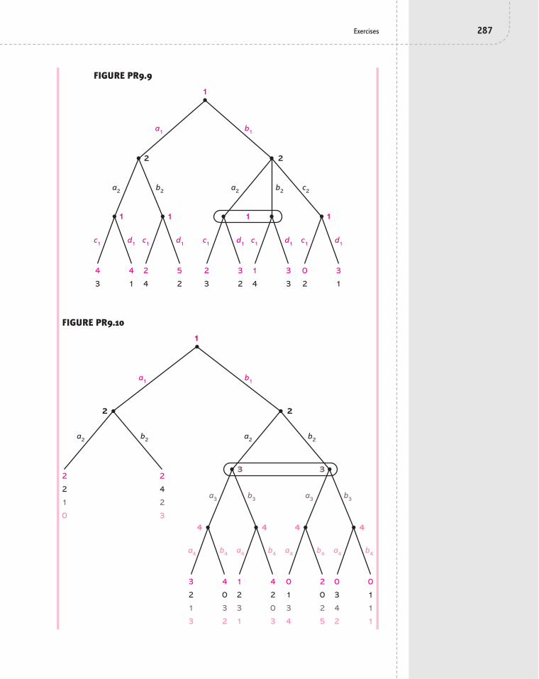
Exercises 287
1
2
1
2
4
3
4
1
c1
a2
a1
a2b2
b1
b2 c2
d1 c1 d1 c1 d1 c1 d1 c1 d1
1
2
4
5
2
2
3
3
2
1
1
4
3
3
1
0
2
3
1
FIGURE PR9.9
2
1
a2
a1 b1
b2
2
2
1
0
3
2
1
3
4
0
3
2
1
2
3
1
4
2
0
3
0
1
3
4
2
0
2
5
0
3
4
2
0
1
1
1
2
4
2
34
2
3
a4 b4 a4 b4 a4 b4 a4 b4
a3
a2 b2
b3 a3 b3
3
4 4 4
FIGURE PR9.10

288 CHAPTER 9: TAKING TURNS IN THE DARK: SEQUENTIAL GAMES WITH IMPERFECT INFORMATION
task is to square up and bunt the ball away from home plate so that noone has the chance to field the ball and tag the runner out. The otherteam can obstruct this play by performing a “pitchout”: the pitcher in-tentionally throws a pitch so wide off the plate that the batter is inca-pable of getting his bat on the ball. The catcher, knowing that thepitchout is coming, steps over to catch the pitch and easily tags the run-ner out coming from third base. Of course, the manager for the team atbat may sense that a pitchout is planned and call off the suicide squeeze.If the other manager does call for a pitchout, but there is no suicidesqueeze, he has put the pitcher in a more difficult situation, because thebatter’s count of balls and strikes will now be more to the batter’s favor.
Suicide Squeeze in Baseball
Let’s consider such a situation as faced by two excellent and strate-gic-minded managers: Tony LaRussa (who is an avid believer in theplay) and Joe Torre. The situation is as depicted in FIGURE PR9.11. Tosimplify matters, we’ll assume that the current count on the batter is,say, two balls and one strike, so that Torre, whose team is pitching, can(realistically) call at most one pitchout. Initially, the two managersmove simultaneously, with Torre deciding whether to call for apitchout and LaRussa deciding whether to execute a suicide squeeze.If there is a pitchout and a suicide squeeze, the outcome will be disas-trous for LaRussa and spectacular for Torre; the latter gets a payoff of10, the former 0. If there is a pitchout and no suicide squeeze, thenLaRussa’s payoff is 8 and Torre’s is 2. If there is a suicide squeeze andno pitchout, then the outcome is exactly as LaRussa wants, and hispayoff is 9, with Torre receiving 1. Finally, if there is no pitchout andno suicide squeeze, then the strategic situation is presumed to con-tinue with the next pitch, when again Torre can call for a pitchout andLaRussa can execute a suicide squeeze. Find a subgame perfect Nashequilibrium in mixed strategies.
AP
PHO
TO/D
AVID
J. P
HIL
LIP

References 289
REFERENCES1. John C. Dvorak, “Obituary: OS/2,” PC Magazine, Dec. 16, 2002.
<http://www.pcmag.com/article2/0,4149,767456,00.asp>
2. The Economist, Mar. 12, 1994; pp. 33–34.
3. The ensuing discussion is based on Douglas A. Irwin, “Mercantilism asStrategic Trade Policy: The Anglo–Dutch Rivalry for the East India Trade,”Journal of Political Economy, 99 (1991), 1296–1314. The original theory isdue to Chaim Fershtman and Kenneth L. Judd, “Equilibrium Incentives inOligopoly,” American Economic Review, 77 (1987), 927–40.
4. J. K. Rowling, Harry Potter and the Goblet of Fire (New York: ScholasticPress, 2000), p. 400.
Pitchout
Torre
Torre
LaRussa
10
0
2
8
1
9
No pitchout
LaRussa
Suicide squeeze
No suicide squeeze
Suicide squeeze
No suicide squeeze
Pitchout
Torre
9
1
4
6
3
7
5
5
No pitchout
LaRussa
Suicide squeeze
No suicide squeeze
Suicide squeeze
No suicide squeeze
FIGURE PR9.11 The Suicide Squeeze Game

This page intentionally left blank
“Who knows what evil lurks in the hearts of men?” —THE SHADOW
10.1 IntroductionIN MODELING A STRATEGIC SITUATION as a game, a key assumption is that the gameis common knowledge to the players. Each player knows who is participating,what their options are, and how they evaluate outcomes. While such a descrip-tion is a good approximation for some contexts—such as the strategic gameplayed with your siblings in the race to the bathroom in the morning—thereare many other contexts in which common knowledge is violated in a blatantmanner and, furthermore, this lack of knowledge can be quite influential indetermining behavior. For example, suppose you walk into an auto dealershipto negotiate with a salesperson. What price you should offer depends not onlyon how much the car is worth to you, but on how much you think the dealer-ship is willing to sell it for. The problem is that you don’t know the lowest priceat which they’re willing to sell, and they don’t know the highest price you’rewilling to pay. This is a scenario in which some information is private to theplayers.
There are many real-world settings in which people have some informationthat is known only to them. Modeling and solving such strategic settingsproved intractable until a brilliant Hungarian mathematician named JohnHarsanyi made a major breakthrough in the late 1960s. Harsanyi figured outhow to take a situation in which players had private information and convert itinto a game that is common knowledge without losing the private-informationaspect, thereby transforming it from something we don’t know how to solveinto something we do. Sounds like magic, doesn’t it? As with most magictricks, however, it becomes obvious once it is explained. Nonetheless, its obvi-ousness does not diminish its value.
10.2 A Game of Incomplete Information: The Munich AgreementBEFORE MAKING THE CONTRIBUTION to game theory for which he received theNobel Prize in Economics, Harsanyi had already revealed himself to be a per-son of great resourcefulness and courage. As a Hungarian Jew in 1944, he es-caped from a train station and thereby avoided deportation to a Nazi concen-tration camp. Then, as the Hungarian government was becoming increasinglyoppressive, he illegally emigrated in 1950 by escaping across relatively un-guarded marshy terrain. In light of such personal challenges and triumphs, it
10
291
I Know Something You Don’t Know:Games with Private Information

292 CHAPTER 10: I KNOW SOMETHING YOU DON’T KNOW: GAMES WITH PRIVATE INFORMATION
is only appropriate that we first apply the methods he pioneered to analyze animportant diplomatic event preceding World War II.
Let us turn back the clock to 1938. Nazi Germany had annexed Austria, andit was believed that Adolf Hitler was considering a similar action againstCzechoslovakia’s Sudetenland. With the Great War (now known as World War I)a recent memory, Europeans feared a repeat of such misery and horror. In aneffort to preserve the peace, Prime Minister Neville Chamberlain of GreatBritain traveled to Munich, Germany, to reach an agreement with Hitler. OnSeptember 28, 1939, Chamberlain and Hitler signed the Munich Agreement,giving Germany the Sudetenland in exchange for Hitler’s promise that hewould go no further. A chunk of Czechoslovakia had been delivered as a con-cession to forestall war. Of course, peace proved to be an illusion. Germanywould enter Prague the following spring and invade Poland a year later, start-ing World War II.
In deciding whether to propose and then sign this agreement, Chamberlainwas uncertain as to the ultimate intentions of Hitler. Was Hitler only seekingadditional lebensraum (“living space”) for the German people? If so, then per-haps a concession such as the Sudetenland would placate him and indeedavoid war. Or was Hitler concocting a more grandiose plan to invade much ofEurope?
The situation in Munich can be cast as the extensive form game in FIGURE
10.1. Chamberlain moves first by deciding whether to offer concessions orstand firm. The presumption is that Hitler will accept the concessions, and ourattention will focus on the decision regarding the pursuit of war. The prefer-ences of Chamberlain are clear: His most preferred outcome is to stand firmwhereupon Hitler avoids war, while his least preferred outcome is to provideconcessions but then Hitler goes to war. Having been offered concessions,Hitler is given more time to prepare his war machine; thus, we shall supposethat Chamberlain finds that outcome less desirable than standing firm andgoing to war.
War No war War No war
3
?
2
?
1
?
HitlerHitler
4
?HitlerChamberlain
Concessions Stand firm
Chamberlain
FIGURE 10.1 The Munich Agreement Game with Unknown Payoffs for Hitler

10.2 A Game of Incomplete Information: The Munich Agreement 293
The challenge with analyzing this situation lies with Hitler’s payoffs. WhileHitler is presumed to know them, Chamberlain does not. And without know-ing Hitler’s payoffs, how can Chamberlain determine what Hitler will do?
As we ponder a solution to this conundrum, let us contemplate the possi-bilities that might have been racing through Chamberlain’s mind. One thoughtis that Hitler is amicable, as reflected in the payoffs presented in FIGURE 10.2(a).We refer to Hitler as amicable because his most preferred outcome is to gainconcessions and avoid war. Note, however, that if Chamberlain stands firm,Hitler will go to war in order to gain additional land. Thus, if Chamberlain re-ally did face an amicable Hitler and knew this fact, then he ought to provideconcessions.
Hitler (far right) and Chamberlain (far left) Meeting in Munich
CORB
IS

294 CHAPTER 10: I KNOW SOMETHING YOU DON’T KNOW: GAMES WITH PRIVATE INFORMATION
The other possibility is that Hitler is belligerent, as summarized by the pay-offs in FIGURE 10.2(b). Here, Hitler has a dominant strategy of going to war, al-though he prefers to do so after receiving concessions. If this is the gameChamberlain is playing, then he would do better to stand firm.
In actuality, Chamberlain was uncertain as to whether he was playing thegame described in Figure 10.2(a) or the one in Figure 10.2(b). This situationis known as a game of incomplete information. Recall that a game of imper-fect information is a game in which players know the game they’re playing,but at some point in the game, a player does not know where he is in the game;that is, he doesn’t know the past choice of some player. In contrast, a game ofincomplete information is a game in which players do not know the game theyare playing; some aspect of the game is not common knowledge. Although thisgame could take various forms, in this chapter we’ll generally limit our atten-tion to when it pertains to lack of information about another player’s payoffs.
The trick to solving a game of incomplete information is to convert it to agame of imperfect information—that is, transform it from something we don’tknow how to solve into something we do know how to solve!1 This is done byintroducing a new player referred to as Nature. Nature is intended, not to referto trees, fleas, and bees, but rather random forces in players’ environment.Nature takes the form of exogenously specified probabilities over various ac-tions and is intended to represent players’ beliefs about random events. In thecontext at hand, Nature determines Hitler’s preferences (or payoffs) and thusthe game that is being played, as is shown in FIGURE 10.3.
Nature is modeled as moving first by choosing whether Hitler is amicableor belligerent. This move by Nature is not observed by Chamberlain—therebycapturing his lack of knowledge as to what Hitler’s payoffs are—but is ob-served by Hitler—since Hitler knows his own preferences. It is important toassume that the probabilities assigned by Nature to these two possibilities are
(a)
War No war War No war
3
4
2
2
1
3
HitlerHitler
4
1HitlerChamberlain
Concessions Stand firm
Chamberlain
(b)
War No war War No war
3
2
2
3
1
4
HitlerHitler
4
1HitlerChamberlain
Concessions Stand firm
Chamberlain
FIGURE 10.2 (a) The Munich Agreement Game When Hitler Is Amicable. (b) The Munich AgreementGame When Hitler Is Belligerent

10.2 A Game of Incomplete Information: The Munich Agreement 295
common knowledge, and here we assume that there is a 60% chance thatHitler is amicable and a 40% chance that he is belligerent.*
The extensive form game in Figure 10.3 is a well-defined game of imperfectinformation. This game is common knowledge, although when Chamberlainmoves, he lacks knowledge of Nature’s choice. To solve it for Nash equilibria,first note that a strategy for Hitler is a quadruple of actions, since he has fourinformation sets describing what has been done by Nature and Chamberlain:(amicable, concessions), (amicable, stand firm), (belligerent, concessions), and(belligerent, stand firm). A strategy for Hitler is then of the following form:
If I am amicable and Chamberlain offered concessions, then ____ [fill inwar or no war].
If I am amicable and Chamberlain stood firm, then ____ [fill in war orno war].
If I am belligerent and Chamberlain offered concessions, then ____ [fill inwar or no war].
If I am belligerent and Chamberlain stood firm, then ____ [fill in war orno war].
War No war
3
4
1
3
Hitler
HitlerChamberlain
Chamberlain
War No war
4
1
2
2
Hitler
Concessions Stand firm
Hitler—amicable Probability = .6
Hitler—belligerent Probability = .4
Nature
War No war
3
2
1
4
Hitler
War No war
4
1
2
3
Hitler
Concessions Stand firm
FIGURE 10.3 The Munich Agreement Game When Nature Determines WhetherHitler Is Amicable or Belligerent
*Game theory doesn’t tell us what these probabilities ought to be, so here we make an arbitrary assump-tion in order to get onto the business of learning how to solve a game of incomplete information. Onecould imagine these probabilities being formed on the basis of a person’s education, life experiences, par-enting, and other factors.

296 CHAPTER 10: I KNOW SOMETHING YOU DON’T KNOW: GAMES WITH PRIVATE INFORMATION
This means that Hitler’s strategy set is made up of 16 strategies: all of the waysin which to fill in those four blanks with his two feasible actions.
Hitler’s optimal strategy is straightforward to derive. If he is amicable (aschosen by Nature), then he should choose no war when Chamberlain offersconcessions and war when Chamberlain stands firm. If Hitler is belligerent,then he should go to war regardless of what Chamberlain does. Thus, the op-timal strategy for Hitler is (No war, War, War, War).
What should Chamberlain do, given this strategy for Hitler? A strategy forChamberlain is a single action, as he has only one information set. GivenChamberlain’s uncertainty as to Hitler’s preferences, he isn’t sure how Hitlerwill respond to his action. Thus, Chamberlain will need to calculate expectedpayoffs in evaluating his two strategies.*
Chamberlain’s expected payoff from providing concessions is
With probability .6, Nature chose Hitler to be amicable, in which case Hitler—as prescribed by his optimal strategy—will avoid war if Chamberlain offersconcessions; Chamberlain’s payoff is 3 in that event. With probability .4, Hitleris belligerent—which, according to his strategy, means that he’ll go to war—sothe payoff to Chamberlain is 1 from providing concessions. The calculationsresult in an expected payoff of 2.2 by appeasing Hitler with the Sudetenland.If, instead, Chamberlain stands firm, his expected payoff is
Standing firm causes both Hitler types to go to war, so the payoff is 2.Chamberlain’s optimal strategy, then, is to offer concessions, since the ex-pected payoff is higher at 2.2. In sum, we contend that a solution to this gamehas Chamberlain offer concessions, in which case Hitler avoids war if he isamicable and goes to war if he is belligerent.
10.3 Bayesian Games and Bayes–Nash EquilibriumIN THIS SECTION, WE DESCRIBE somewhat more systematically how to solve a gameof incomplete information. As we saw in Section 10.2, the idea is to convert agame of incomplete information into a game of imperfect information, whichis known as a Bayesian game. A Bayesian game modifies a standard game byhaving an initial stage at which Nature determines the private information heldby players. The recipe for this transformation involves three easy steps.
Constructing a Bayesian Game
Step 1: In a game of incomplete information, a player lacks some relevantinformation about the person with whom she is interacting. A firststep in the construction of a Bayesian game is to specify the pos-sible answers to the question, “Who is this player?” Informationthat is private information to a player (and thus not known byother players) is referred to as the player’s type, and the collection
.6 ! 2 % .4 ! 2 # 2.
.6 ! 3 % .4 ! 1 # 2.2.
*Expected payoffs were discussed in Section 7.2.

10.3 Bayesian Games and Bayes–Nash Equilibrium 297
of feasible types is the type space. Typically, a player’s type is hispayoffs, in which case the type space is the collection of possiblepayoffs for that player. In the Munich Agreement game, the Hitlertype space included two payoff configurations that we labeled am-icable and belligerent.*
Step 2: Having specified the type space, the next step is to determine eachplayer’s type. Of course, the player’s type has already been set be-fore you meet him; Hitler was either amicable or belligerent whenChamberlain showed up in Munich. However, in a Bayesian game,we need to “turn back the clock” to when a player did not knowhis type (i.e., prior to learning the information that is private tohim). The game must begin with a player as a tabula rasa (blankslate). At that stage, random forces (Nature) determine eachplayer’s type and “write” on that blank slate. A probability is as-signed to each type, and that probability measures the likelihoodof Nature choosing that type for a player. We assume that theseprobabilities are common knowledge to the players.
Step 3: The third step in constructing a Bayesian game is to define strat-egy sets. Recall that a strategy is a completely specified decisionrule chosen before the game begins. A strategy in a Bayesian gameis conceived as being selected before Nature moves. Because astrategy prescribes an action for each situation in which a playercan find himself, a strategy states what to do, given Nature’schoice as to the player’s type and whatever else a player may know(with regard to whatever actions have been chosen by other play-ers). The situation is analogous to planning your reincarnation:What will I do if I come back as a horse or a snake or a dung fly?(Oh, please don’t let me come back as a dung fly!)
You might wonder about Step 3. Hitler is of a particular type—in fact, weknow now that he was belligerent—so why does he need to develop a strategyfor his amicable self? This step is really designed to assist Chamberlain in hisdecision making. Chamberlain must calculate the strategy Hitler uses if he isamicable and the strategy he uses if he is belligerent. With such a calculation,and with beliefs about whether Hitler is amicable or belligerent, Chamberlaincan formulate beliefs about what Hitler will do and thus be able to devise anoptimal strategy.
Having performed the necessary modifications to a game of incomplete in-formation in order to convert it into a Bayesian game of imperfect informa-tion, we next seek to solve the game. A commonly used solution method isBayes–Nash (or Bayesian) equilibrium, which is a strategy profile that pre-scribes optimal behavior for each and every type of a player, given the otherplayers’ strategies, and does so for all players.
To distinguish Bayes–Nash from Nash equilibrium, recall that a strategy pro-file is a Nash equilibrium when each player’s strategy is optimal, given the otherplayers’ strategies. This requirement gives us a total of n conditions, one for each
*Private information can be about more than payoffs; it can be about strategy sets, about the set of play-ers, or even about a players’ beliefs. However, we will focus our attention on private information aboutpayoffs.

298 CHAPTER 10: I KNOW SOMETHING YOU DON’T KNOW: GAMES WITH PRIVATE INFORMATION
of the n players. Now consider a Bayesian game, and let denote the numberof types of player i. Then, for player i’s strategy to be part of a Bayes–Nash equi-librium, it must be optimal for each of those types. That is, for each type ofplayer i, the prescribed behavior must be optimal. There are then conditionsthat must be satisfied if we are to conclude that player i’s strategy is optimal.Whatever type a player proves to be, the prescribed behavior must be optimal.
The preceding is an introductory description of Bayes–Nash equilibrium; amore formal definition is provided in an appendix at the end of the chapter. Ifyou prefer not to venture into “notationland,” a few stimulating examples oughtto elucidate the concept with less pain. It is to those examples that we now turn.
! SITUATION: GUNFIGHT IN THE WILD WEST
It is 1875 in Dodge City, Kansas, and there is a dispute in the local saloon.Marshal Wyatt Earp arrives to restore order when one of the men steps backand pulls his hand away from his body as if he’s ready to draw. The decisionfaced by Earp and the stranger is whether to draw immediately or instead waitand draw only in response to the other’s pulling out his gun. The shooting tal-ents of Earp are known, but Earp doesn’t know the skill of the stranger. Is hea gunslinger or just a plain cowpoke?
If, in fact, the stranger is a gunslinger and Earp knows it, then both Earpand the stranger would see themselves as playing the game depicted in FIGURE
10.4(a). Because Earp would like to avoid a shootout, his most preferred out-come is that he and the stranger choose wait so that a gunfight is avoided. Hisleast preferred outcome is that the stranger draw and Earp has waited. Giventhat the stranger is a gunslinger, Earp is apt to be killed. Note that Earp’s bestreply is to match what he thinks the stranger will do: wait if he thinks thestranger will not draw and draw if he thinks the stranger will draw. In con-trast, the stranger has a dominant strategy, which is draw. He surely wants todo so if he thinks Earp will draw, but he wants to do so even if Earp doesn’tdraw, as he can then add to his reputation as a gunslinger (which obviously isnot sufficiently well established, since Earp doesn’t know who he is).
mi
mi
mi
FIGURE 10.4 (a) The Gunfight Game When the Stranger Is a Gunslinger. (b) The Gunfight Game When the Stranger Is a Cowpoke
Draw
Stranger (gunslinger)
2,3
1,4
3,1
8,2
Wait
Wyatt EarpDraw
Wait
(a)
Draw
Stranger (cowpoke)
5,2
6,3
4,1
8,4
Wait
Wyatt EarpDraw
Wait
(b)
Alternatively, suppose the stranger is a cowpoke. Then, under complete in-formation, the two men would be playing the game in FIGURE 10.4(b). In thatgame, Earp’s dominant strategy is wait. Even if the stranger draws, Earp be-lieves that he could fire first if the stranger is a cowpoke. In this situation, hedefends himself without being seen as having provoked the stranger. The cow-poke recognizes that his skill is not as great as Earp’s and will draw only if he

10.3 Bayesian Games and Bayes–Nash Equilibrium 299
thinks Earp is planning to do so. The cowpoke’s optimal strategy is to do what-ever he thinks Earp will do.
This game is a game of incomplete information, because Earp doesn’t knowif he’s playing the game in Figure 10.4(a) or the one in Figure 10.4(b). Withoutknowledge of whom he’s facing, it’s hard to say what Earp should do. Similarly,it’s hard to say what the stranger should do if he’s a cowpoke, for what is bestfor a cowpoke is to match what Earp is to do. But Earp’s uncertainty as towhom he is facing means that the cowpoke is uncertain as to what he believesEarp will think he’ll do and thus the cowpoke is uncertain as to what Earp willchoose.
To settle matters, Sheriff Harsanyi rolls into town and converts this gameof incomplete information into a game of imperfect information. (See FIGURE
10.5.) Nature moves first to determine whether the stranger is a gunslinger—an event that is assumed to occur with probability .75—or a cowpoke, whichoccurs with probability .25. Earp does not observe Nature’s move, and in thisway we capture the fact that Earp is uncertain as to the stranger’s skills andintentions. Earp has a single information set; thus, his strategy set includesdraw and wait. As for the stranger, he does get to observe Nature—a featurewhich captures the fact that the stranger knows whether he’s a gunslinger ora cowpoke—but does not get to observe Earp’s action; Earp and the strangermove simultaneously. The stranger has two information sets, one for whenNature makes him a gunslinger and the other for when he is a cowpoke. Thestranger’s strategy set encompasses four strategies: (draw, draw), (draw, wait),
FIGURE 10.5 A Bayesian Gunslinger Game
Earp
3
1
2
3StrangerEarp 8
2
1
4
4
1
5
2
8
4
6
3
Draw Wait Draw Wait Draw Wait
Draw DrawWait Wait
Gunslinger Probability = .75
CowpokeProbability = .25
Nature
Draw Wait
Stranger Stranger

300 CHAPTER 10: I KNOW SOMETHING YOU DON’T KNOW: GAMES WITH PRIVATE INFORMATION
(wait, draw), and (wait, wait); the first action is what to do if he is a gunslinger,the second is what to do if he is a cowpoke.
In deriving a Bayes–Nash equilibrium, note that it must have thestranger choosing draw when he is a gunslinger, because that is a dominantmove in that case. Since we can then eliminate (wait, draw), and (wait,wait) for the stranger, there are four remaining candidates for Bayes–Nashequilibria:
A. Earp chooses draw and the stranger chooses (draw, wait).
B. Earp chooses wait and the stranger chooses (draw, wait).
C. Earp chooses draw and the stranger chooses (draw, draw).
D. Earp chooses wait and the stranger chooses (draw, draw).
Strategy profile A is clearly not a Bayes–Nash equilibrium. If Earp is todraw, then the stranger—whether a gunslinger or a cowpoke—will want todraw. Yet, (draw, wait) has the stranger draw only if he is a gunslinger. Notethat neither is strategy profile D, a Bayes–Nash equilibrium: If Earp waits, thenthe stranger wants to wait if he is a cowpoke. We have thus ruled out strategyprofiles A and D.
Next, consider strategy profile B, in which Earp waits and the strangerdraws if he is a gunslinger and doesn’t draw if he is a cowpoke. The followingare the three conditions that need to be satisfied for strategy profile B to be aBayes–Nash equilibrium:
1. Earp’s choosing wait maximizes his expected payoff, given that thestranger chooses draw with probability .75 (because, with probability.75, he is a gunslinger and, according to the stranger’s strategy of (draw,wait), he’ll draw) and the stranger chooses wait with probability .25(because, with probability .25, he is a cowpoke and, according to thestranger’s strategy of (draw, wait), he’ll wait).
2. If the stranger is a gunslinger, then draw maximizes his payoff, giventhat Earp chooses wait.
3. If the stranger is a cowpoke, then wait maximizes his payoff, given thatEarp chooses wait.
Condition 1 ensures that Earp’s strategy is optimal, and conditions 2 and 3ensure that the stranger’s strategy is optimal for both possible types. First,note that condition 2 is indeed satisfied: The gunslinger prefers to draw (re-gardless of what Earp does). Next, note that condition 3 is satisfied, because,when he is a cowpoke, the stranger wants to avoid a gunfight with Earp, so hewaits, since he expects Earp to wait.
Turning to condition 1, Earp’s expected payoff from drawing is
With probability .75, the stranger is a gunslinger—in which case he draws(according to the stranger’s strategy)—and the payoff to Earp is 2. With prob-ability .25, the stranger is a cowpoke—in which case he waits—and Earp’s pay-off is 4 from drawing. His expected payoff from waiting is instead
.75 ! 1 % .25 ! 8 # 2.75.
.75 ! 2 % .25 ! 4 # 2.5.

Condition 3 is then satisfied, since the expected payofffrom waiting exceeds the expected payoff from drawing.
In the Munich Agreement game, it was unnecessary forHitler to know what Chamberlain believed about Hitler’spayoffs. This was because Hitler observed Chamberlain’smove, and all Hitler needed to know to make an optimalchoice was his type and what Chamberlain chose. Hence, solving that game onlyrequired specifying Chamberlain’s beliefs as to Hitler’s type. The Gunfight gameis different. Since Earp and the stranger move simultaneously and the stranger’soptimal move depends on what he thinks Earp will do, specifying Earp’s beliefsabout the stranger’s type is insufficient. The cowpoke needs to know what Earp’sbeliefs are so that he can figure out what Earp will do. In this setting, it is im-portant that we make the assumption that the probabilities assigned to thestranger’s type are common knowledge between Earp and the stranger.
10.4 When All Players Have Private Information: AuctionsTHUS FAR, WE’VE EXPLORED SITUATIONS in which only one player has private infor-mation: Chamberlain did not know Hitler’s true preferences, but Hitler knewall about Chamberlain; Earp did not know the stranger’s skill and intentions,whereas the stranger knew all about Earp. However, there are many situationsin which all players have private information. It is to such settings we turn forthe remainder of the chapter.
A classic situation in which these informational conditions arise is an auc-tion. Each bidder knows how much she is willing to pay, but does not knowhow high other bidders are willing to go. In deciding how to bid, a bidder mustprognosticate how others will bid, and that depends on the valuation they at-tach to the good, which is known only to them. Here, we will model this situa-tion as a Bayesian game and draw some implications about bidding behavior.
Our exploration will take place within the confines of the first-price, sealed-bid auction. Recall that, in a first-price, sealed-bid auction, bidders simultane-ously submit written bids and the one who submits the highest bid wins theitem and pays a price equal to her bid. This type of auction will be explored intwo distinct informational settings. The first setting is known as independentprivate values and assumes that the value of the good is unrelated across bid-ders. That is, each bidder shows up with a valuation, and that valuation iswhat the item is worth to her if she wins it. A bidder’s type is her valuation.The game is called a game of independent private values because each value isprivate or specific to a bidder and bidder’s values are independent random vari-ables. The second informational setting is known as common value and as-sumes that all bidders value the item equally, but when they are bidding, theyare uncertain about what that value is. Each bidder has his own signal or es-timate of its value, and that is what he knows when he bids. A bidder’s type isthen his signal of this common value. An example would be a group of artdealers bidding on some work of art with the intent of reselling it. The truevalue is what it’ll sell for in the future, and that is the same for all bidders.
We explore these two informational settings here in an introductory way. Aricher model of equilibrium-bidding behavior (one that requires the use of cal-culus) is included in an appendix at the end of the chapter.
10.4 When All Players Have Private Information: Auctions 301
Determine whether strategy profile C is aBayes–Nash equilibrium.
10.1 CHECK YOUR UNDERSTANDING

302 CHAPTER 10: I KNOW SOMETHING YOU DON’T KNOW: GAMES WITH PRIVATE INFORMATION
! SITUATION: INDEPENDENT PRIVATE VALUES AND SHADING YOUR BID
On November 11, 1994, Bill Gates bought a piece of scientific history at auc-tion: the Codex Leicester. This oddly named item is a folio of scientific obser-vations written by Leonardo da Vinci almost a half a millennium ago. It wasthe property of the Earl of Leicester and his descendants from 1717 until 1980,when the industrialist Armand Hammer purchased it. After Hammer’s death,his estate put it up for auction. Gates’s winning bid of $30,800,000 set a recordprice for a nonliterary manuscript.
So let us suppose that an object—perhaps the Codex Leicester—is up forauction and there are two bidders: Bill and Charlene. The auctioneer uses afirst-price, sealed-bid auction requiring bidders to submit written bids simul-taneously, with the highest bidder winning the item and paying a price equalto her bid. Let us suppose that if the bidders submit the same bid, the auction-eer flips a coin to determine the winner.
A player’s type is his valuation of the item up for auction, and to keep the sit-uation simple, we’ll assume that there are just two possible types: a valuationof 50, with probability .6; and a valuation of 100, with probability .4. Nature be-gins by choosing each bidder’s type. Given that their types are independent,there is a 36% chance that both Bill and Charlene have the low valuation of 50(since a 16% chance that both have the high valuation of 100,and a 48% chance that one of the bidders has the low valuation and the otherhas the high valuation. Each bidder learns only his or her own valuation, andthen the two players submit their bids simultaneously. We’ll assume that a bidcomes in increments of tens: 10, 20, 30, . . . . If he wins the auction, a bidder’spayoff is his valuation less his bid (which, with a first-price, sealed-bid auction,is the price of the item), while his payoff is zero if he loses the auction.
A strategy is a pair of bids that assigns a bid in the event that a bidder’s val-uation is 50 and a bid in the event that the valuation is 100. Suppose both bid-ders use the following strategy: Bid 40 if the valuation is 50, and bid 60 whenthe valuation is 100. Let us determine whether this symmetric strategy pair isa Bayes–Nash equilibrium. Toward that end, let us derive beliefs that, say, Billholds regarding Charlene’s bid. Given that Bill believes that Charlene will usethe preceding strategy, and given that Bill thinks that there is a 60% chance thatCharlene has a low valuation, then Bill believes that there is a 60% chance thatCharlene will submit a bid of 40 and a 40% chance that she will submit a bidof 60. With these beliefs about Charlene’s bids, we can assess the optimality ofBill’s bidding strategy.
Suppose Bill’s valuation is 50. He knows that Charlene will bid either 40 or 60.His strategy prescribes a bid of 40, which results in an expected payoff of
This expression is derived as follows: With probability .6, Charlene has a lowvaluation and bids 40. Because Bill is submitting the same bid, he then has a50% chance of winning the auction. (Recall that the auctioneer flips a coinwhen both bidders submit the same bids.) In that event, his payoff is or 10, since his valuation is 50 and he pays a price of 40. With probability .4,Charlene has a high valuation and bids 60, which means that she outbids Bill’sbid of 40.
50 " 40,
.6 ! .5 ! (50 " 40) % .4 ! 0 # 3.
.36 # .6 ! .6),

10.4 When All Players Have Private Information: Auctions 303
Thus, for a bid of 40 to be optimal when the valuation is 50, the expectedpayoff from any other bid must not exceed 3. If bidder 1 bids below 40, thenhe is sure to lose, in which case his payoff is zero. If he bids 50, then his pay-off is again zero, because he either loses or wins, but pays a price equal to hisvaluation. And if he bids above 50, his payoff is either zero (if he loses) or neg-ative (if he wins). Thus, a bid of 40 is optimal if Bill’s valuation is 50.
Now suppose Bill’s valuation is 100. His prescribed bid is 60, which yieldsan expected payoff of
Optimality then requires that any other bid generate a payoff no higher than32. Let us begin by showing how we can quickly dismiss bids below 40 andabove 70. If Bill bids below 40, then he is sure to lose (since Charlene bids ei-ther 40 or 60) and his payoff is zero, a strategy that is clearly inferior to bid-ding 60 and getting an expected payoff of 32. If Bill bids 70, then he is sure towin—because Charlene never bids higher than 60—and thus his payoff is 30.A bid above 70 only lowers his payoff, since the probability of winning is nohigher—it is already equal to 1 from a bid of 70—and a higher bid just meanspaying a higher price.
The preceding analysis leaves us with bids of 40, 50, and 70 as possibly at-tractive alternatives to the prescribed bid of 60. The associated expected pay-offs are as follows:
Note that all of these expected payoffs fall short of the expected payoff of 32from bidding 60. Hence, if bidder 1’s valuation is 100, then a bid of 60 is in-deed optimal. By symmetry, the analysis also applies to Charlene. Therefore,it is a Bayes–Nash equilibrium for a bidder to bid 40 when the bidder’s valua-tion is 50 and to bid 60 when the bidder’s valuation is 100.
The most interesting behavior here occurs when a bidder has a high valua-tion, for then a bid of 60 is submitted and it is well below the valuation of 100.Bidding below your valuation is called “shading your bid.” By bidding lower, abidder raises the payoff in the event that she has the highest bid and wins theauction. However, a lower bid also reduces the chances of having the highestbid. The trade-off between these two factors determines a bidder’s optimal bid.
This trade-off is depicted in TABLE 10.1 for a bidder with a valuation of 100.A bid of 40 has a 30% chance of winning because there is a 60% chance thatthe other bidder has a low valuation and bids 40 as well,in which case the auctioneer flips a coin to determine thewinner. At 60 the payoff in the event of win-ning is quite high. If, instead, the bid is higher, at 50, thepayoff in the event of winning falls to 50, but the chanceof winning rises to 60% (as now the bidder wins for surewhen the other bidder has a low valuation). As a result,the expected payoff is higher, at 30, with a bid of 50,
(# 100 " 40),
Expected payoff from a bid of 70 # .6 ! (100 " 70) % .4 ! (100 " 70) # 30.
Expected payoff from a bid of 50 # .6 ! (100 " 50) % .4 ! 0 # 30.
Expected payoff from a bid of 40 # .6 ! .5 ! (100 " 40) % .4 ! 0 # 18.
.6 ! (100 " 60) % .4 ! .5 ! (100 " 60) # 32.
For the Bayesian game just described, considera symmetric strategy profile in which a bidderbids 40 when the valuation is 50 and bids 70when the valuation is 100. Determine whetherthis strategy pair is a Bayes–Nash equilibrium.
10.2 CHECK YOUR UNDERSTANDING

304 CHAPTER 10: I KNOW SOMETHING YOU DON’T KNOW: GAMES WITH PRIVATE INFORMATION
compared with an expected payoff of 18 from a bid of 40. The optimal bid is60, and note that it maximizes neither the probability of winning nor the pay-off in the event of winning. Rather, it balances these two factors in such a wayas to produce the highest expected payoff.
! SITUATION: COMMON VALUE AND THE WINNER’S CURSE
Imagine that you are a senior manager of an oil company, such as Texaco, andyou’re considering the purchase of an oil lease that would give Texaco the rightto extract oil from some location in the Gulf of Mexico. In order to get an esti-mate of the amount of oil in the ground, and thus of the value of the lease, youdecide to hire an engineering firm. There are two available firms: GeologicalConsultants and Acme Engineering. Through the industry grapevine, you’velearned that one of them consistently provides optimistic estimates and theother pessimistic estimates, although you don’t know which is which, so youassign equal probability to each firm’s being the optimistic one. Thus, withprobability , Geological Consultants overestimate the true amount of oil inthe ground and Acme Engineering underestimates it, and with probability ,the underestimate comes from Geological Consultants and the overestimatefrom Acme Engineering.
Let v denote the true value of the oil lease, and suppose v lies in {10,11, . . . , 100}. Then the optimistic firm is assumed to provide an estimate, orsignal, of the value of the oil lease, while the pessimistic firm pro-vides a signal Suppose you choose Geological Consultants and re-ceive a signal s. Since you don’t know whether Geological Consultants is theoptimistic or pessimistic firm, you know that there is a 50% chance that thetrue value is (when Geological Consultants is actually the optimisticfirm) and a 50% chance that the true value is (when GeologicalConsultants is actually the pessimistic firm). For example, if the signal is 10,then the true value of the lease is 12 with probability and 8 with probabil-ity . More generally, your beliefs on the true value after having received asignal s are as follows:
Prob˛(v˛|˛˛s) # e if v # s " 2
if v # s % 2.
12
12
s % 2s " 2
s # v " 2.s # v % 2
12
12
TABLE 10.1 SHADING YOUR BID, HIGH-VALUATION BIDDER
Probability of Payoff If the ExpectedBid Winning Bidder Wins Payoff
30 0 70 0
40 .3 60 18
50 .6 50 30
60 .8 40 32
70 1 30 30
80 1 20 20
1212
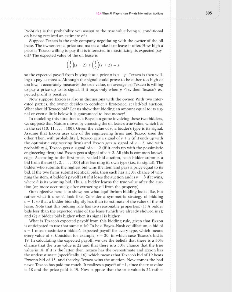
10.4 When All Players Have Private Information: Auctions 305
Prob is the probability you assign to the true value being v, conditionalon having received an estimate of s.
Suppose Texaco is the only company negotiating with the owner of the oillease. The owner sets a price and makes a take-it-or-leave-it offer. How high aprice is Texaco willing to pay if it is interested in maximizing its expected pay-off? The expected value of the oil lease is
so the expected payoff from buying it at a price p is Texaco is then will-ing to pay at most s. Although the signal could prove to be either too high ortoo low, it accurately measures the true value, on average, so Texaco is willingto pay a price up to its signal. If it buys only when then Texaco’s ex-pected profit is positive.
Now suppose Exxon is also in discussions with the owner. With two inter-ested parties, the owner decides to conduct a first-price, sealed-bid auction.What should Texaco bid? Let us show that bidding an amount equal to its sig-nal or even a little below it is guaranteed to lose money!
In modeling this situation as a Bayesian game involving these two bidders,we suppose that Nature moves by choosing the oil lease’s true value, which liesin the set {10, 11, . . . , 100}. Given the value of v, a bidder’s type is its signal.Assume that Exxon uses one of the engineering firms and Texaco uses theother. Then, with probability , Texaco gets a signal of (if it ends up withthe optimistic engineering firm) and Exxon gets a signal of , and withprobability , Texaco gets a signal of (if it ends up with the pessimisticengineering firm) and Exxon gets a signal of All this is common knowl-edge. According to the first-price, sealed-bid auction, each bidder submits abid from the set {1, 2, . . . , 100} after learning its own type (i.e., its signal). Thebidder who submits the highest bid wins the item and pays a price equal to itsbid. If the two firms submit identical bids, then each has a 50% chance of win-ning the item. A bidder’s payoff is 0 if it loses the auction and is if it wins,where b is its winning bid. Thus, a bidder learns the true value after the auc-tion (or, more accurately, after extracting oil from the property).
Our objective here is to show, not what equilibrium bidding looks like, butrather what it doesn’t look like. Consider a symmetric strategy of bidding
so that a bidder bids slightly less than its estimate of the value of the oillease. Note that this bidding rule has two reasonable properties: (1) A bidderbids less than the expected value of the lease (which we already showed is s);and (2) a bidder bids higher when its signal is higher.
What is Texaco’s expected payoff from this bidding rule, given that Exxonis anticipated to use that same rule? To be a Bayes–Nash equilibrium, a bid of
must maximize a bidder’s expected payoff for every type, which meansevery value of s. Consider, for example, in which case Texaco’s bid is19. In calculating the expected payoff, we use the beliefs that there is a 50%chance that the true value is 22 and that there is a 50% chance that the truevalue is 18. If it is the latter, then Texaco has the overestimate and Exxon hasthe underestimate (specifically, 16), which means that Texaco’s bid of 19 beatsExxon’s bid of 15, and thereby Texaco wins the auction. Now comes the badnews: Texaco has paid too much. It realizes a payoff of since the true valueis 18 and the price paid is 19. Now suppose that the true value is 22 rather
"1,
s # 20,s " 1
s " 1,
v " b
v % 2.v " 21
2
v " 2v % 21
2
p 6 s,
s " p.
a12b(s " 2) % a1
2b(s % 2) # s,
(v˛|˛s)

306 CHAPTER 10: I KNOW SOMETHING YOU DON’T KNOW: GAMES WITH PRIVATE INFORMATION
than 18. Since Texaco has a signal of 20, Exxon must have a signal of 24 andthus bids 23, a bid that exceeds Texaco’s bid of 19. So Texaco loses the auction.
Summing up these two cases, we see that Texaco’s expected payoff from abid of 19 (when its signal is 20) is
More generally, the expected payoff (conditional on signal s) when both play-ers use this bidding rule is
Thus, on average, an oil company loses money even though it is bidding belowits signal and the signal is expected to be equal to the value of the oil lease!
When Texaco was the only prospective buyer, paying a price below its sig-nal meant a positive expected payoff, since it was then paying a price belowthe expected value of the oil lease. At the end of the day, it might end up witha positive profit (if its estimate turned out to be low) or a negative profit (ifit turned out to be high), but Texaco expected to earn a positive profit. If, in-stead, Texaco is participating in an auction, then, as we have just shown,bidding below its signal can mean either zero profit (if it loses the auction)or a negative profit (if it wins the auction), so that expected profit is nega-tive. At work here is one of the most dreaded forces in the auction world: thewinner’s curse.
The winner’s curse refers to the phenomenon by which winning an auc-tion can be bad news. It can arise whenever the value of the good is commonto all bidders and each bidder receives an inexact estimate of that value. If bid-ders use the same bidding rule, and it always increases a bidder’s estimate,then the fact that a bidder won means that he had the highest estimate amongall bidders. Thus, unbeknownst to the bidder when he was bidding, the act ofwinning reveals that he had the rosiest forecast of the item’s value, which, onaverage, will prove to exceed the true value. (In the current example, winningmeans learning that you used the engineering firm that overestimates inwhich case your signal exceeds the true value for sure.) Winning the auctiontells you that your estimate of the true value was excessively high, and thereinlies the bad news.
Fortunately, game theory offers a cure for the winner’s curse. The trick is tobid under the assumption that your signal is the highest signal among all bid-ders, for that is exactly the situation in which you’ll find yourself in the eventthat you win the auction. Thus, you want to determine the expected value ofthe object if it turns out that your signal is the highest among all bidders’ sig-nals, and then you want to bid appropriately, given that expected value. In thepreceding example, this strategy implies that a bidder should not bid above
For if you prove to have the higher signal, then you hired the optimisticengineering firm, in which case the true value is Bidding above thatvalue is sure to result in losses. Exactly what you should bid is a harder ques-tion and is dealt with in Appendix 10.7, which describes a different formula-tion of the common-value auction.
In practice, do bidders suffer from the winner’s curse? One study investi-gated whether major oil companies such as Exxon, British Petroleum, and
s " 2.s " 2.
a12b ! 3 (s " 2) " (s " 1) 4 # "
12
.
a12b ! (18 " 19) % a1
2b ! 0 # "
12
.

10.5 Voting on Committees and Juries 307
Texaco fall prey to it or instead are strategically astute in their bidding.2 Upfor auction were the mineral rights to properties that lay 3 to 200 miles off-shore and were owned by the U.S. government. These properties were typi-cally auctioned off in tracts of about 5,000 acres, and companies bid on themwith the intent of extracting oil. The evidence shows that executives at most ofthe companies are indeed well trained in strategic reasoning, as they generallydid manage to avoid the winner’s curse. Their bids were about one-third of theexpected value of the oil lease, conditional on their estimate of its value beingthe largest estimate among all bidders. This meant that, conditional on sub-mitting the highest bid and winning the auction, their bid generated a positiveexpected profit. One notable exception was Texaco, whose bidding behaviornot only suffered from the winner’s curse, but also resulted in a bid that washigher then the estimated value of the oil lease! In our simple example, it is asif Texaco bid above its signal s, a strategy that, winner’s curse aside, is assuredof incurring losses! Hopefully, Texaco has either replaced those executives orenrolled them in a remedial game theory course.
10.5 Voting on Committees and JuriesANOTHER COMMON SETTING INVOLVES private information when a group of peoplehas to reach some joint decision. Each person comes to a meeting with someparticular information that is known only to her, and a common device forreaching a decision is voting. First we consider some strategic issues in a com-mittee when people have different amounts of information and they vote si-multaneously. Then we explore a jury setting in which jurors have differentopinions about the defendant’s guilt and engage in sequential voting to deter-mine an outcome.
10.5.1 Strategic AbstentionThey say it is your civic duty to vote. But does voting always result in the mostdesired social outcome? Could it actually be best for society that you loungein a cafe on Election Day, never exerting your democratic voice? As we willshow, in some instances it can be in both your interests and those of societyfor you to be politically lethargic.
Consider a committee of three people who have to decide whether to main-tain the current (status quo) policy or adopt a new policy that has been pro-posed.3 The three committee members have the same preferences in the sensethat, if they had full information about the new policy, they would either all befor or all be against its adoption. The problem is that some or all members arenot fully informed as to the efficacy of the proposed policy. If the committeechooses the policy that proves to be best, then each member receives a payoffof 1, while if they choose the wrong policy, then the payoff is 0.
Each member can be one of two types: informed and uninformed. An un-informed member is uncertain as to which policy is best and, more specifi-cally, assigns probability p to the status quo being better, where Thus, without any further information, an uninformed member prefers thestatus quo, as it delivers an expected payoff of or p, whilethe new policy’s expected payoff is or If, instead,the member is informed, then she knows which policy is better.
1 " p.p ! 0 % (1 " p) ! 1,p ! 1 % (1 " p) ! 0,
12 6 p 6 1.

308 CHAPTER 10: I KNOW SOMETHING YOU DON’T KNOW: GAMES WITH PRIVATE INFORMATION
Nature moves first by determining which policy is best and, also, eachmember’s knowledge. To ensure that an uninformed member has beliefs con-sistent with the inclination of Nature, suppose that, with probability p, Naturechooses the status quo as the better policy. After the better policy is deter-mined, then, with probability q, the identity of that policy is revealed to amember. Hence, with probability q, a member is an informed type. With prob-ability she is uninformed and thus uncertain as to which policy is best,but thinks it is more likely that the status quo is best (assigning probability pto that being the case).
After Nature makes these four moves—determining the best policy and thethree members’ types—those members simultaneously vote. Each member caneither vote for the status quo, vote against the status quo, or abstain. If a ma-jority of votes is against the status quo, then the new policy is adopted; other-wise, the status quo is maintained. (Hence, the status quo wins in the case of atie.) After the policy is implemented, members learn whether they made theright choice (and get a payoff of 1) or the wrong choice (and get a payoff of 0).
In this Bayesian game, a strategy is a pair of actions: whether and how tovote when one is informed and whether and how to vote when one is unin-formed. A symmetric Bayes–Nash equilibrium is a strategy that maximizes aplayer’s expected payoff when she is informed and maximizes it when she isuninformed, given that the other two members use the same strategy andgiven beliefs as to the other members’ knowledge about which policy is better.
Let us begin by arguing that it is weakly dominant for a member to vote forthe policy that is best when she is informed. By voting for the policy that isbest, member 1 either doesn’t change the outcome—as when members 2 and3 both vote the same—or causes her preferred policy to pass when it wouldn’totherwise—in the case when members 2 and 3 split their votes between thestatus quo and the new policy. In the first case, member 1’s payoff is no lowerby voting in favor of the better policy (compared with voting against it or ab-staining), and in the latter case her payoff is strictly higher. We conclude thatit is weakly dominant for an informed member to participate and vote for thepolicy she thinks is best.
Now we come to the interesting scenario. Suppose a member is unin-formed as to which policy is best. Is it always optimal to vote? Or can it bebest to abstain?
Let us first consider a symmetric strategy profile in which, when informed,a member votes for the best policy and, when uninformed, she votes for thestatus quo. (Recall that an uninformed member thinks the status quo is morelikely to be best.) This means that member 1 anticipates members 2 and 3 al-ways voting (regardless of whether they are informed). It follows that member1’s vote makes a difference only when the other two members split their votes,one voting for the status quo and the other against it. However, this scenariomeans that someone is voting for the alternative, which implies that that per-son must be informed that it is the best policy. (Recall that we are consideringa symmetric strategy profile in which uninformed voters vote for the statusquo.) Thus, if member 1, when uninformed, votes for the status quo, then thewrong policy is implemented. He would have done better by instead voting forthe alternative policy. Hence, it cannot then be optimal for an uninformedvoter to participate and vote for the status quo. That is, if members 2 and 3vote for the status quo when uninformed, then it is not optimal for member 1
1 " q,

10.5 Voting on Committees and Juries 309
to vote for the status quo when uninformed. This bit of reasoning proves thatit is not a symmetric Bayes–Nash equilibrium for a member to vote for the sta-tus quo when uninformed, in spite of the fact that she thinks it is more likelythat the status quo is best.
Another candidate for a Bayes–Nash equilibrium is the symmetric strategyprofile in which, when uninformed, a member votes against the status quoand, when informed, votes for the best policy. However, this can also be shownnot to be a Bayes–Nash equilibrium. The proof is similar to the one just given.
The remaining candidate for a symmetric Bayes–Nash equilibrium is for anuninformed member to abstain when uninformed and, when informed, votefor the best policy. Suppose member 1 follows this strategy and anticipates theother two members doing so as well. If member 2 or member 3 (or both) votes,then, according to their strategies, they must be informed. In that case, thebest policy is implemented, in which case member 1 gets the maximal payoffof 1 by abstaining. If neither member 2 nor member 3 votes, then both are un-informed. Then, by abstaining, member 1 ensures the status quo (since that iswhat happens when there is a tie). If member 1 were to vote, it would be op-timal for her to vote for the status quo, since she thinks it is more likely to bethe best policy. Hence, the status quo results whether member 1 abstains ornot. Thus, abstention is optimal when the member is uninformed, given thatthe other two members also abstain when uninformed.
In sum, for a committee member to abstain when uninformed and to votefor the best policy when informed is the unique symmetric Bayes–Nash equi-librium in this game. In spite of voting being costless, it can be optimal not tocast a vote. The reasoning behind this statement is simple: When a member isuninformed, it is better to abstain and let the informed members determinethe outcome. Thus, only the uninformed should be entitled to avoid the polls,which means that if you’re going to hang out in a café on Election Day, youshould be reading People and not the New York Times.
10.5.2 Sequential Voting in the Jury RoomNow suppose you’re on a jury. The trial has ended, and you and the other ju-rors retire to the jury room. The foreperson begins the deliberations by takinga vote. The jurors are collected around a table, and, in turn, each announces avote of guilty or not guilty. Let’s number jurors by their order in the sequence,so that juror 1 declares her vote first, then juror 2, and so forth until we reachjuror 12.4
On the basis of what transpired during the trial, each juror enters the juryroom with an assessment of the guilt or innocence of the defendant. This as-sessment—which they realize is an inexact signal of the truth—is a juror’stype.* Now, suppose that, in casting her vote, a juror wants to do so on thebasis of everything she knows at the time. For juror 1, all she knows is her ownassessment from the trial. In contrast, by witnessing how juror 1 voted, juror2 may be able to infer juror 1’s assessment. If so, then juror 2 not only has hisown assessment, but also juror 1’s assessment. Similarly, juror 3 may be able
*To properly define this game as a Bayesian game, we would need to assign a probability to a juror’s beingof the “guilty” type (i.e., he enters the jury room believing that the defendant is guilty) or of the “innocent”type. It turns out that our analysis holds regardless of what those probabilities are, so we don’t bother tospecify them.

310 CHAPTER 10: I KNOW SOMETHING YOU DON’T KNOW: GAMES WITH PRIVATE INFORMATION
to infer the assessments of jurors 1 and 2 and thus would have three assess-ments. Assume that a juror prefers to (1) vote guilty if the number of guilty as-sessments exceeds the number of innocent assessments, (2) vote not guilty ifthe number of innocent assessments exceeds the number of guilty assess-ments, and (3) vote according to her own assessment when the number ofguilty assessments equals the number of innocent assessments. By (3), a jurorgives her own assessment more weight in this evaluation process.*
A Bayesian strategy for juror 1 assigns a vote—guilty or not guilty—that de-pends on her assessment (or type): guilty or innocent. A strategy for juror 2 as-signs a vote that depends on his assessment and the vote of juror 1. A strategyfor juror 3 assigns a vote that depends on his assessment and the votes of ju-rors 1 and 2, and so forth. Let us now construct a Bayes–Nash equilibrium.
Juror 1’s optimal strategy is easy, because she has only her own assessmentto weigh. If she comes out of the trial believing that the defendant is guilty, thenshe votes guilty; if she believes that he is innocent, then she votes not guilty.
Juror 2 observes juror 1’s vote and, furthermore, is presumed to know juror1’s strategy. Although he does not observe juror 1’s assessment—which is privateto juror 1—he is able to infer it, since, according to juror 1’s strategy, she votesin line with her assessment. Thus, if juror 1 voted guilty, then juror 2 infers thatjuror 1’s assessment is that the defendant is guilty. Now suppose juror 2’s inde-pendent assessment is that the defendant is guilty. Then juror 2 should clearlyvote guilty, since he has two guilty assessments. If, instead, juror 2’s independ-ent assessment is innocent, then he has one guilty assessment (that of juror 1)and one assessment of innocence (his own). As specified, a juror prefers to voteaccording to his own assessment in those circumstances and thus votes notguilty. Regardless of how his assessment lines up with juror 1’s inferred assess-ment, we see that juror 2’s Bayes–Nash equilibrium strategy is to vote accordingto his own assessment. How juror 1 votes doesn’t influence what juror 2 does.
So far, nothing is surprising: The first two jurors vote guilty if and only iftheir individual assessments of the testimony and evidence are that the defen-dant is guilty. Is there much to be learned by examining juror 3’s optimal be-havior? Indeed, there is. Juror 3 observes the votes of jurors 1 and 2, and ac-cording to the equilibrium strategies just derived for them, each casts a voteconsistent with her or his independent assessment. There are two situationsto consider: jurors 1 and 2 voted the same, and jurors 1 and 2 voted differently.Let us examine each situation in turn:
■ Suppose that jurors 1 and 2 voted differently. Juror 3 should then voteaccording to her own independent assessment. For example, supposejuror 1 voted guilty and juror 2 voted not guilty. Juror 3 then infers thatjuror 1’s assessment is of guilt and juror 2’s is of innocence. If juror 3’sassessment is guilty, then there are two assessments that say guilty, sojuror 3 should vote guilty. If juror 3’s assessment is innocent, then thereare two assessments that say innocent, so juror 3 should vote not guilty.Thus, when jurors 1 and 2 split their votes, juror 3 should vote accord-ing to her own independent evaluation.
*Although we have not explicitly mentioned payoffs, they can be easily introduced. For example, supposea juror’s payoff when the number of assessments of guilt exceeds the number of assessments of innocenceis 10 if she votes guilty and 5 if she votes not guilty. Hence, a vote of guilty in those circumstances maxi-mizes her payoff.

10.5 Voting on Committees and Juries 311
■ Suppose now that jurors 1 and 2 voted the same. If they both votedguilty, then, using her conjecture of the two jurors’ strategies, juror 3 in-fers that each of them believes that the defendant is guilty on the basisof her own and his own assessment of the trial. If juror 3’s own assess-ment is also guilty, then, clearly, she should vote guilty. But even if juror3’s assessment is innocent, she’ll vote guilty because there are two guiltyassessments and only one of innocence. More generally, if jurors 1 and 2voted the same, then juror 3 should cast the same vote because the twoindependent assessments of those jurors override juror 3’s assessment.Juror 3 should ignore her own personal evaluation in voting.
Juror 3’s Bayes–Nash equilibrium strategy then has her vote depend on thevotes cast by jurors 1 and 2 when they voted the same. Only when they voted dif-ferently is it optimal for juror 3 to use her own evaluation when casting her vote.
Continuing in this manner, we can construct the Bayes–Nash equilibriumvoting rule for jurors 4 through 12. But let us instead jump to a striking anddisturbing implication. Suppose that when the 12 jurors enter the jury roomafter the trial, 10 of them believe that the defendant is innocent and only 2 be-lieve that he is guilty of the crime of which he has been accused. Then, in spiteof the preponderance of belief in favor of innocence, the initial vote could haveall 12 jurors voting guilty! And this is in spite of each juror voting conscien-tiously on the basis of the best information available!
The argument is as follows: Suppose the two jurors who believe that the de-fendant is guilty happen to be jurors 1 and 2, who vote before the others. Letus use the equilibrium voting strategies we have just derived. Juror 1 votesguilty, obviously. Juror 2 also votes guilty, because, as we have derived it, hisoptimal strategy is to vote in line with his evaluation, uninfluenced by juror 1’svote. When it comes to juror 3, she’ll vote guilty, as is prescribed by her strat-egy. She is able to infer from the first two jurors’ votes that each of them be-lieves that the defendant is guilty, and those two assessments override her ownassessment. Thus, she votes guilty, irrespective of her evaluation of the testi-mony and evidence. When it comes to juror 4, he’ll know that juror 3 has ig-nored her own assessment, because that is what juror 3’s strategy has her dowhen jurors 1 and 2 vote the same. Thus, all that juror 4 can infer is that ju-rors 1 and 2 hold guilty assessments. Juror 4 is then in the same situation asjuror 3 and consequently will vote guilty. This argument works for jurors 5through 12 as well, so we end up with all 12 jurors voting guilty! However,those 12 votes are not based on 12 independent evaluations, because jurors 3through 12 ignored their evaluations when voting. The guilty verdict is duesolely to the first two jurors believing that the defendant is guilty!
Are jurors 3 through 12 nothing more than sheeple?* To the contrary, theydid not mindlessly mimic how the first two jurors voted. They engaged inrather sophisticated reasoning when they drew inferences about the evalua-tions of the jurors that preceded them. Those 10 jurors voted on the basis ofthe best information they had at the time. To do so required that they drawupon the independent evaluations of jurors who voted before them to the ex-tent that those evaluations could be properly inferred from those jurors’ votes.
*This term is a blend of “sheep” and “people” and is used to refer to someone who simply does what oth-ers do, without thinking.

312 CHAPTER 10: I KNOW SOMETHING YOU DON’T KNOW: GAMES WITH PRIVATE INFORMATION
This phenomenon is known as an informational cascade or informationalherding. It refers to a situation in which people act sequentially and the infor-mation revealed by the behavior of the first few people overrides the signal thateach person has, so that their behavior becomes independent of that privatesignal; instead, their behavior is determined solely by the information revealedby the behavior of those who acted previously. Once a player ignores his owninformation, his behavior provides no additional information and applies to allensuing players. Thus, we find that highly uniform behavior—such as all jurorscasting guilty votes—can rest on only a small number of signals. In our exam-ple, that behavior rests on the signal that the first two jurors truly believe thatthe defendant is guilty on the basis of the testimony and evidence.
An important conclusion here is that the voting procedure can matter a lot.For example, suppose that, instead of voting sequentially, the foreperson hadthe jurors vote simultaneously by writing their votes on a slip of paper. Eachjuror’s optimal voting strategy is to vote according to his or her own assess-ment right after the trial. Then, since we assumed that 10 jurors believed thatthe defendant was innocent, the vote will be 10–2 in favor of not guilty—aquite different outcome from a guilty verdict!
SummaryThis chapter considers a common and crucial feature of many strategic set-tings: A person may know something about him- or herself that others do notknow. This scenario frequently arises in the form of a player’s payoffs beingprivate information. As originally cast, the game is not common knowledge,because, for example, one player doesn’t know another player’s payoffs. Werefer to such a game as having incomplete information. The trick to solvinga game of incomplete information is to convert it into a game of imperfect in-formation. The initial move in the game is now made by random forces, la-beled Nature, that determine each player’s type, where a type encompasses allthat is privately known to a player. This Nature-augmented game, which isknown as a Bayesian game, is common knowledge, since, at its start, noplayer knows his type and thus has no private information. What is commonlyknown is that Nature will determine players’ types. What also is commonlyknown are the probabilities used by Nature in assigning a player’s type.
The solution concept used for Bayesian games in this chapter isBayes–Nash equilibrium. Analogous to Nash equilibrium, it posits that eachplayer’s strategy is required to maximize his expected payoff, given other play-ers’ strategies, but this definition is supplemented in two ways. First, a playerdoesn’t know other players’ types and thus doesn’t know what other playerswill do. However, if a player (accurately) conjectures another player’s strategyand has beliefs about the other player’s type, he can then form beliefs regard-ing how another player will behave. Second, given those beliefs, a player’sstrategy must prescribe an optimal action, and it must do so for every possibletype of that player.
Examples of equilibrium behavior explored in this chapter included a gun-fight in which one gunfighter does not know the skill of the other, negotiationsin which a person does not know the ultimate objectives of the person on theother side of the table, committees in which a member does know how informedother committee members are, and auctions in which a person’s valuation of the

Exercises 313
object up for auction is known only to him. These are only a few of the variousstrategic situations characterized by private information. You face many suchscenarios everyday.
It is worth noting that the last game examined, involving sequential votingin the jury room, was distinctive in an important dimension. In all of the othergames in this chapter, a player with private information either moved at thesame time as other players (the auction) or moved after other players (theMunich Agreement). This meant that other players did not have an opportu-nity to infer the player’s private information from his behavior. But in the juryroom game, a juror who observed another juror’s vote prior to having to casther own vote might be able to infer what that other juror believes. It is exactlythat kind of informational setting which will occupy us in the next chapter.Fascinating nuances and subtleties are introduced, as you’ll soon learn.
1. Greg is deciding whether to ask Marcia out on a date. However, Gregisn’t sure whether Marcia likes him, and he would rather not ask if heexpects to be rejected. Whether Marcia likes Greg is private informationto her. Thus, her preferences regarding Greg constitute her type. Gregdoes not have any private information. Assume that there is a 25%chance that Marcia likes Greg. The Bayesian game is shown in FIGURE
PR10.1. Should Greg ask Marcia? Find a Bayes–Nash equilibrium thatanswers this question.
EXERCISES
FIGURE PR10.1
Yes No
Invite Do not invite
2
2
3
4
10
7Marcia
Marcia
Greg
Greg
Marcia likes GregProbability = .25
Marcia doesn't like GregProbability = .75
Nature
Yes No
Invite Do notinvite
2
3
3
4
8
1
Marcia
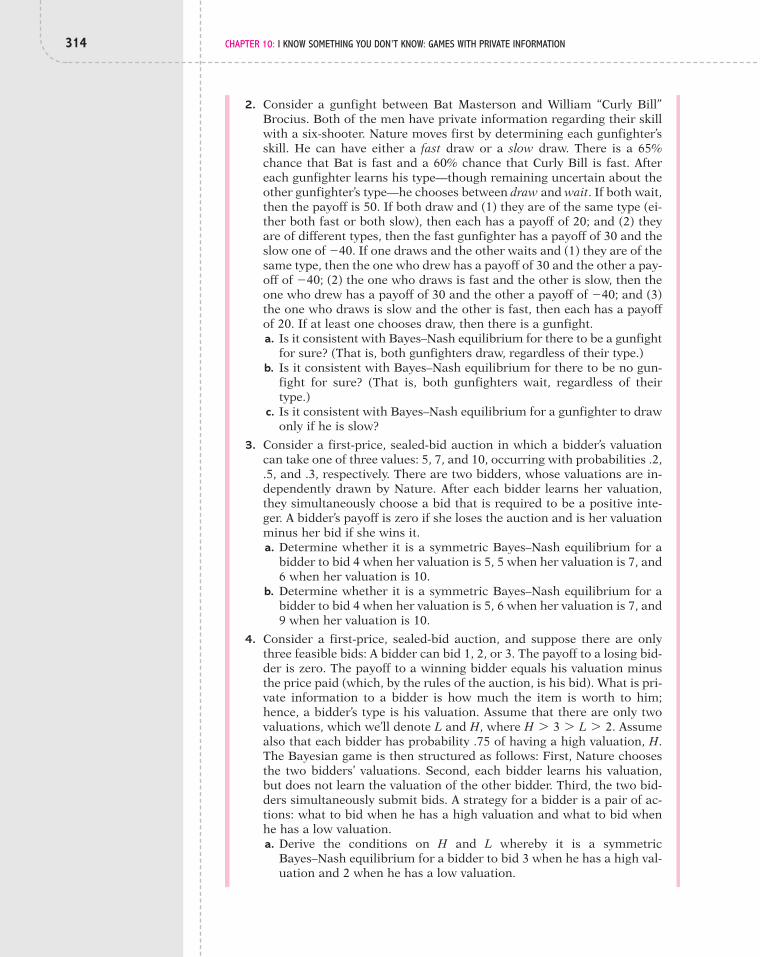
314 CHAPTER 10: I KNOW SOMETHING YOU DON’T KNOW: GAMES WITH PRIVATE INFORMATION
2. Consider a gunfight between Bat Masterson and William “Curly Bill”Brocius. Both of the men have private information regarding their skillwith a six-shooter. Nature moves first by determining each gunfighter’sskill. He can have either a fast draw or a slow draw. There is a 65%chance that Bat is fast and a 60% chance that Curly Bill is fast. Aftereach gunfighter learns his type—though remaining uncertain about theother gunfighter’s type—he chooses between draw and wait. If both wait,then the payoff is 50. If both draw and (1) they are of the same type (ei-ther both fast or both slow), then each has a payoff of 20; and (2) theyare of different types, then the fast gunfighter has a payoff of 30 and theslow one of If one draws and the other waits and (1) they are of thesame type, then the one who drew has a payoff of 30 and the other a pay-off of (2) the one who draws is fast and the other is slow, then theone who drew has a payoff of 30 and the other a payoff of and (3)the one who draws is slow and the other is fast, then each has a payoffof 20. If at least one chooses draw, then there is a gunfight.a. Is it consistent with Bayes–Nash equilibrium for there to be a gunfight
for sure? (That is, both gunfighters draw, regardless of their type.)b. Is it consistent with Bayes–Nash equilibrium for there to be no gun-
fight for sure? (That is, both gunfighters wait, regardless of theirtype.)
c. Is it consistent with Bayes–Nash equilibrium for a gunfighter to drawonly if he is slow?
3. Consider a first-price, sealed-bid auction in which a bidder’s valuationcan take one of three values: 5, 7, and 10, occurring with probabilities .2,.5, and .3, respectively. There are two bidders, whose valuations are in-dependently drawn by Nature. After each bidder learns her valuation,they simultaneously choose a bid that is required to be a positive inte-ger. A bidder’s payoff is zero if she loses the auction and is her valuationminus her bid if she wins it.a. Determine whether it is a symmetric Bayes–Nash equilibrium for a
bidder to bid 4 when her valuation is 5, 5 when her valuation is 7, and6 when her valuation is 10.
b. Determine whether it is a symmetric Bayes–Nash equilibrium for abidder to bid 4 when her valuation is 5, 6 when her valuation is 7, and9 when her valuation is 10.
4. Consider a first-price, sealed-bid auction, and suppose there are onlythree feasible bids: A bidder can bid 1, 2, or 3. The payoff to a losing bid-der is zero. The payoff to a winning bidder equals his valuation minusthe price paid (which, by the rules of the auction, is his bid). What is pri-vate information to a bidder is how much the item is worth to him;hence, a bidder’s type is his valuation. Assume that there are only twovaluations, which we’ll denote L and H, where Assumealso that each bidder has probability .75 of having a high valuation, H.The Bayesian game is then structured as follows: First, Nature choosesthe two bidders’ valuations. Second, each bidder learns his valuation,but does not learn the valuation of the other bidder. Third, the two bid-ders simultaneously submit bids. A strategy for a bidder is a pair of ac-tions: what to bid when he has a high valuation and what to bid whenhe has a low valuation.a. Derive the conditions on H and L whereby it is a symmetric
Bayes–Nash equilibrium for a bidder to bid 3 when he has a high val-uation and 2 when he has a low valuation.
H 7 3 7 L 7 2.
"40;"40;
"40.

Exercises 315
b. Derive the conditions on H and L whereby it is a symmetricBayes–Nash equilibrium for a bidder to bid 2 when he has a high val-uation and 1 when he has a low valuation.
c. Derive the conditions on H and L whereby it is a symmetricBayes–Nash equilibrium for a bidder to bid 3 when he has a high val-uation and 1 when he has a low valuation.
d. Derive the conditions on H and L whereby it is a symmetricBayes–Nash equilibrium for a bidder to bid 1 when he has either ahigh valuation or a low valuation.
5. Consider the Bayesian game in FIGURE PR10.5. Nature chooses the type ofplayer 1, where type H occurs with probability p and type L with proba-bility Player 1 learns his type and then chooses either action x oraction y. Simultaneously, player 2 chooses either action a or action b.a. Assume that Find a Bayes–Nash equilibrium.b. For each value of p, find all Bayes–Nash equilibria.
p # .75.
1 " p.
FIGURE PR10.5
a b
x y x y
1
3
3
1Player 2Player 1
a b
5
2
2
1
a b
1
2
2
3
a b
4
0
3
1
Nature
1 1
2
H Probability = p
LProbability = 1 – p
6. Two U.S. senators are considering entering the race for the Democraticnomination for U.S. president. Each candidate has a privately knownpersonal cost to entering the race. Assume that the probability of havinga low entry cost, is p and the probability of having a high entry cost,
is Thus, the type space has just two values. A candidate’s pay-off depends on whether he enters the race and whether the other sena-tor enters as well. Let be a candidate’s payoff when he enters and theother senator does as well (so that there are two candidates), be a can-didate’s payoff when he enters and the other Senator does not (so that
v1
v2
1 " p.fHfL,

316 CHAPTER 10: I KNOW SOMETHING YOU DON’T KNOW: GAMES WITH PRIVATE INFORMATION
there is one candidate), and 0 be the payoff when he does not enter.Assume that
a. Derive the conditions whereby it is a symmetric Bayes–Nash equilib-rium for a candidate to enter only when she has a low personal costfrom doing so.
b. Derive the conditions whereby it is a symmetric Bayes–Nash equilib-rium for a candidate to enter for sure when she has a low personalcost and to enter with some probability strictly between 0 and 1 whenshe has a high personal cost.
c. Find some other Bayes–Nash equilibrium distinct from those de-scribed in (a) and (b).
7. Assume that two countries are on the verge of war and are simultane-ously deciding whether or not to attack. A country’s military resourcesare its type, and their relevance is summarized in a parameter which in-fluences the likelihood that they would win a war. Suppose the typespace is made up of two values: and where Acountry is type with probability q and type with probability Consider a country of type p (which equals either or If it choosesto attack and it attacks first, then it believes it’ll win the war with prob-ability xp, where x takes a value such that If the two coun-tries both attack, then the probability that a type p country wins is p. Ifa type p country does not attack and the other country does attack, thenthe probability of victory for the type p country is yp, where y takes avalue such that Finally, if neither country attacks, thenthere is no war. A country is then more likely to win the war the higheris its type and if it attacks before the other country. A country’s payoffwhen there is no war is 0, from winning a war is W, and from losing awar is L. Assume that a. Derive the conditions for it to be a symmetric Bayes–Nash equilib-
rium for a country to attack regardless of its type.b. Derive the conditions for it to be a symmetric Bayes–Nash equilib-
rium for a country to attack only if its type is
8. Consider a first-price, sealed-bid auction with three bidders. The payoffto a bidder is 0 when he does not win the item at auction and is the valueof the item less his bid (which is the price he pays) when he is the win-ner. If two or more bidders submit the highest bid, then the winner israndomly determined. Assume that the item has the same value to allthree bidders, but they receive different signals as to its value. Nature de-termines the true value, which is denoted v and can take three possiblevalues: 4, 5, and 6. Each of these values is chosen with probability Thesignals sent to the three bidders are v, and that is, one bid-der receives a signal that is too low another receives a signalthat is too high and the third receives a signal that is “just right”(v). Each bidder learns only his own signal, which is the bidder’s type. If
then one bidder is given a signal of 3, another bidder is given av # 4,
(v % 1),(v " 1),
v % 1;v " 1,
13.
p–.
W 7 0 7 L.
0 6 yp 6 p.
p 6 xp 6 1.
p–).p¿1 " q.p¿p–
0 6 p¿ 6 p– 6 1.p–,p¿
v1 " fH 7 0.
v2 " fL 7 0 7 v2 " fH,
fH 7 fL 7 0,
v1 7 v2 7 0,

Exercises 317
signal of 4, and the last bidder is given a signal of 5. If then onebidder is given a signal of 4, another bidder is given a signal of 5, andthe last bidder is given a signal of 6. If then one bidder is given asignal of 5, another bidder is given a signal of 6, and the last bidder isgiven a signal of 7. Thus, if a bidder’s signal is, say, 5, then he doesn’tknow if the true value is 4 (in which case he has the highest signal), 5 (inwhich case he has the accurate signal), or 6 (in which case he has thelowest signal). Given the value, each bidder has an equal chance of re-ceiving one of the three signals. Assume that the minimum increment inbidding is 1, so that the set of feasible bids is {0, 1, . . . , 10}.a. Show that the following symmetric strategy profile is a Bayes–Nash
equilibrium:
v # 6,
v # 5,
b. Show that there is no symmetric Bayes–Nash equilibrium in which abidder’s bid is strictly increasing. That is, if b(s) is a bidder’s bid, giventhat her signal is s, and if
then this strategy is not a symmetric Bayes–Nash equilibrium.
9. The Newlywed Game was a popular game show broadcast from 1966 to1974. On this show, four recently married couples are queried about oneanother to see how well each spouse knows the other. Each of the hus-bands is asked a series of questions while his wife is offstage in a sound-proof room. The wives would then return, and each would be asked thesame questions. The objective is for the answers of the husband and wifeto match. In the second round, they would reverse roles. The couple withthe most matched answers wins. Questions asked ran along these lines:What animal does your mother-in-law remind you of? Would yourspouse say that your last kiss was ho hum; so so; or ooh, la la? In whatroom of the house does your spouse most like making whoopee? Let usnow suppose the husband is asked the question, What drink would bestdescribe your wife on your wedding night: a sloe gin fizz, a ShirleyTemple, or a zombie? The husband responds with one of those threechoices, and when she is asked the same question, the wife respondswith one of the same three choices. If their choices match, ahusband–wife pair has a payoff of 100; if they don’t match, the pair hasa payoff of 0. In casting this as a Bayesian game, suppose the husband’stype is which one he believes is true: sloe gin fizz, Shirley Temple, orzombie, where the associated probabilities are and respectively.The wife’s type is which one she believes is true: sloe gin fizz, ShirleyTemple, or zombie. The sloe gin fizz occurs with probability the1
2,
14,1
2,14,
b(7) 7 b(6) 7 b(5) 7 b(4) 7 b(3),
Signal Bid
3 4
4 4
5 4
6 4
7 5
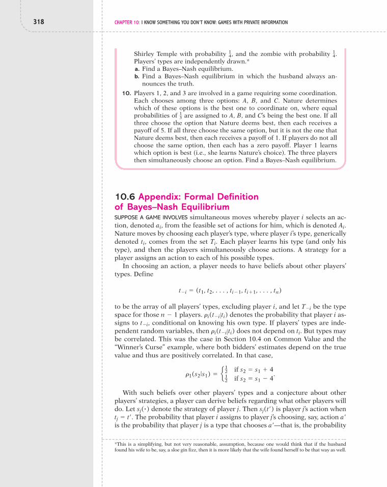
318 CHAPTER 10: I KNOW SOMETHING YOU DON’T KNOW: GAMES WITH PRIVATE INFORMATION
Shirley Temple with probability and the zombie with probability Players’ types are independently drawn.*a. Find a Bayes–Nash equilibrium.b. Find a Bayes–Nash equilibrium in which the husband always an-
nounces the truth.
10. Players 1, 2, and 3 are involved in a game requiring some coordination.Each chooses among three options: A, B, and C. Nature determineswhich of these options is the best one to coordinate on, where equalprobabilities of are assigned to A, B, and C’s being the best one. If allthree choose the option that Nature deems best, then each receives apayoff of 5. If all three choose the same option, but it is not the one thatNature deems best, then each receives a payoff of 1. If players do not allchoose the same option, then each has a zero payoff. Player 1 learnswhich option is best (i.e., she learns Nature’s choice). The three playersthen simultaneously choose an option. Find a Bayes–Nash equilibrium.
13
14.1
4,
10.6 Appendix: Formal Definition of Bayes–Nash EquilibriumSUPPOSE A GAME INVOLVES simultaneous moves whereby player i selects an ac-tion, denoted from the feasible set of actions for him, which is denoted Nature moves by choosing each player’s type, where player i’s type, genericallydenoted comes from the set Each player learns his type (and only histype), and then the players simultaneously choose actions. A strategy for aplayer assigns an action to each of his possible types.
In choosing an action, a player needs to have beliefs about other players’types. Define
to be the array of all players’ types, excluding player i, and let be the typespace for those players. denotes the probability that player i as-signs to conditional on knowing his own type. If players’ types are inde-pendent random variables, then does not depend on But types maybe correlated. This was the case in Section 10.4 on Common Value and the“Winner’s Curse” example, where both bidders’ estimates depend on the truevalue and thus are positively correlated. In that case,
With such beliefs over other players’ types and a conjecture about otherplayers’ strategies, a player can derive beliefs regarding what other players willdo. Let denote the strategy of player j. Then is player j’s action when
The probability that player i assigns to player j’s choosing, say, action is the probability that player j is a type that chooses —that is, the probabilitya¿
a¿tj # t¿.sj(t¿)sj(&)
r1(s2˛|˛s1) # e 12 if s2 # s1 % 412 if s2 # s1 " 4
.
ti.ri(t"i˛#˛ti)t"i,
ri(t"i˛#˛ti)n " 1T"i
t"i # (t1, t2, . . . , ti"1, ti%1, . . . , tn)
Ti.ti,
Ai.ai,
*This is a simplifying, but not very reasonable, assumption, because one would think that if the husbandfound his wife to be, say, a sloe gin fizz, then it is more likely that the wife found herself to be that way as well.

10.7 Appendix: First-Price, Sealed-Bid Auction with a Continuum of Types 319
that takes a value whereby Combining beliefs about anotherplayer’s type with a conjecture regarding that player’s strategy allows the deri-vation of beliefs about that player’s action.
Given the types of the players and the actions selected, let player i’s payoffbe denoted In many examples, a player’s payoff dependsonly on the actions of players and his own type, but here we also allow for thepossibility that it depends directly on other players’ types. Of course, it de-pends indirectly on other players’ types, since another player’s type determinesthe action selected.
is a Bayes–Nash equilibrium if and only if
means the summation of V over all of the values for in ForT"i.t"ia t"i!T"i
for all ai ! Ai, for all ti ! Ti, for all i.
' at"i!T"i
Vi(s*1(t1), . . . , s*
i"1(ti"1), ai, s*i%1(ti%1), . . . s*
n(tn); ti, t"i)r(t"i˛#˛ti)
at"i!T"i
Vi(s*1(t1), p , s*
n(tn); ti, t"i)r(t"i#ti)
(s*1(&), . . . , s*
n(&))
Vi(a1, . . . , an; ti, t"i).
sj(tj) # a¿.tj
each type of player i, the action assigned by his strategy is required to max-imize his expected payoff, where the expectation is over other players’ types(and thereby their actions). This condition must hold for all players.
10.7 Appendix: First-Price, Sealed-Bid Auction with a Continuum of TypesPREVIOUSLY, WE CONSIDERED SOME simple formulations of the first-price, sealed-bid auction when bidders’ values are independent of each other and when theyare common. In this appendix, we enrich the models by assuming that thereis an infinite number of valuations that a bidder might have. Allowing for acontinuum of bidder types will permit us to use calculus to derive equilibriumbidding rules.
10.7.1 Independent Private ValuesAssume that there are bidders, and let denote how much bidder i val-ues the good.5 If bidder i wins the item and pays a price p, then her payoff is
Each bidder’s value is a random draw from the interval [0,1] accordingto the uniform cumulative distribution function
[10.1]
Thus, each valuation in [0,1] has equal likelihood, and the probability that abidder’s valuation is less than or equal to is or A bidder’s valuationis private information, but it is common knowledge that each bidder’s value isdrawn from [0,1] according to a uniform distribution.
The Bayesian game proceeds as follows: Nature simultaneously chooses nvaluations for the n bidders and reveals only to bidder i. Then the bidderssimultaneously submit bids. The winning bidder is the one who submitted thehighest bid, and she pays a price equal to her bid.
vi
v¿.F(v¿),v¿
F(v) # •0 if v 6 0v if 0 $ v $ 1.1 if 1 6 v
vi " p.
vin ' 2
s*i

320 CHAPTER 10: I KNOW SOMETHING YOU DON’T KNOW: GAMES WITH PRIVATE INFORMATION
Consider the following symmetric strategy profile in which a bidder whosevaluation is v submits a bid
Let us prove that this is a symmetric Bayes–Nash equilibrium. That is, if each ofthe other bidders’ valuations are drawn from a uniform distribution over [0,1]and bidder j bids then it is optimal for bidder i to bid Thiscondition must hold for all values of (i.e., all types of bidder i). Since the gameis symmetric, if the condition holds for one bidder, then it holds for all bidders.
To verify this claim, consider bidder i’s expected payoff, which we denote assince it depends on his valuation and bid. His expected payoff equals
the probability that he wins, multiplied by the payoff in the event that he wins;that is,
[10.2]
where is the probability that bidder i outbids allother bids. (We need not worry about ties, as they’ll occur with zero probabil-ity.) Given that bidder j uses the bidding rule we can substitute
for in the probability expression in (10.2):
Since bidders’ valuations are independent draws, it follows that
[10.3]
Using (10.1), we have
Inserting this result into (10.3) yields
Finally, putting this expression into (10.2), we have derived bidder i’s expectedpayoff, given the strategies used by the other bidders and the probability dis-tribution over their valuations:
pi(bi, vi) # c a nn " 1
b bi d n"1(vi " bi).
Prob aa nn " 1
b bi 7 vj for all j ( ib # c a nn " 1
b bi d n"1.
Prob aa nn " 1
b bi 7 vjb # a nn " 1
b bi.
! Prob aa nn " 1
b bi 7 vi%1b ! p ! Prob aa nn " 1
b bi 7 vnb .# Prob aa n
n " 1b bi 7 v1b ! p ! Prob aa n
n " 1b bi 7 vi"1b
Prob aa nn " 1
b bi 7 vj for all j ( ib # Prob aa n
n " 1b bi 7 vj for all j ( ib .
Prob(bi 7 bj for all j ( i) # Prob abi 7 an " 1nb vj for all j ( ibbj(n " 1
n )vj
(n " 1n )vj,
Prob(bi 7 bj for all j ( i)
pi(bi, vi) # Prob(bi 7 bj for all j ( i) ! (vi " bi),
pi(bi, vi),
vi
(n " 1n )vi.(n " 1
n )vj,
b*(v) # an " 1nb v.

10.7 Appendix: First-Price, Sealed-Bid Auction with a Continuum of Types 321
To find bidder i’s optimal bid, we just need to derive the first-order condition:*
*For a review of this principle, return to Section 6.3. The validity of the approach relies on the payoff beinghill shaped with respect to the player’s bid, which is indeed true here.
[10.4]0pi(bi, vi)0bi
# " c a nn " 1
b bi d n"1% (n " 1)a n
n " 1b c a n
n " 1b bi d n"2
(vi " bi) # 0.
The optimal bid for bidder i is that value for which satisfies (10.4).Simplifying and rearranging (10.4), one can solve for
This is exactly what we wanted to show. If all other bidders use this biddingrule, then it is optimal for bidder i to use it as well.
Each bidder then proportionately shades her bid by Clearly, a bidderdoesn’t want to bid her valuation, since, even if she wins the auction, she paysa price equal to what it is worth to her; her payoff is then zero whether or notshe wins. By instead bidding below her valuation, either she loses—in whichcase her payoff is 0—or she wins—in which case her payoff is positive. Hence,her expected payoff is positive if she bids below her valuation, which is betterthan bidding her valuation. The issue is how much to shade one’s bid belowone’s valuation. The lower the bid, the higher is the payoff in the event that onewins but the lower is the probability that one wins. The equilibrium solutionis for each bidder to submit a bid equal to a fraction of his valuation.Since is increasing in n, the more bidders there are, the higher is a bid-der’s bid. This makes sense, since more bidders mean more competition, inwhich case a bidder doesn’t want to shade her bid as much, in order to have areasonable chance of winning.
10.7.2 Common ValueSuppose there are bidders. The true value of the object being auctionedis v and is the same for all bidders. Each bidder gets a noisy (or inexact) sig-nal of v that is chosen by Nature from the interval [0,1] according to a uniformdistribution. The cumulative distribution function on bidder i’s signal, de-noted is
The signal of bidder i is known only to him; thus, a bidder’s signal is his typeand the type space is [0,1]. It is common knowledge that each bidder’s signalis independently drawn from [0,1] according to F. Finally, it is assumed thatthe true value is randomly determined by Nature in that it is assumed to equalthe average of all bidders’ signals:
[10.5]v # a1nban
j#1sj.
F(si) # •0 if si 6 0si if 0 $ si $ 1.1 if 1 6 si
si,
n ' 2
n " 1n
n " 1n
1n.
bi # an " 1nb vi.
bi:bi

322 CHAPTER 10: I KNOW SOMETHING YOU DON’T KNOW: GAMES WITH PRIVATE INFORMATION
Bidders participate in a first-price, sealed-bid auction, which means that ifbidder i wins, then his realized payoff is where is his bid, though hedoesn’t learn v until after he has won.
In deriving a Bayes–Nash equilibrium, let us conjecture that it is linear in abidder’s signal. That is, there is some value for such that
[10.6]
Bidder i’s expected payoff is the probability that he wins (i.e., his bid is higherthan all other bids) times his expected payoff, conditional on having submit-ted the highest bid:
[10.7]
is bidder i’s expected valuation, conditional notonly on his signal, but also on knowing that he submitted the highest bid. Thislatter fact says something about the signals of the other bidders and thusabout the true value of the object.
Now let us use the property that the other bidders are conjectured to usethe bidding rule in (10.6). Substitute for in (10.7):
Next, substitute the expression for v from (10.5):
# Prob abi
a7 sj for all j ( ib ! eE cv˛|˛si,
bi
a7 sj for all j ( i d " bi f .
Prob(bi 7 asj for all j ( i) ! 5E 3v˛#˛si, bi 7 asj for all j ( i 4 " bi6bjasj
E 3v˛|˛si, bi 7 bj for all j ( i 4Prob(bi 7 bj for all j ( i) ! 5E 3v˛#˛si, bi 7 bj for all j ( i 4 " bi6.
bj # asj.
a 7 0
biv " bi
# Prob abi
a7 sj for all j ( ib ! e asi
nb % a1
nb a
j(iE c sj ` bi
a7 sj d " bi f .
# Prob abi
a7 sj for all j ( ib ! e asi
nb % a1
nb E c a
j(isj ` bi
a7 sj for all j ( i d " bi f
Prob abi
a7 sj for all j ( ib ! eE c a1
nb asi % a
j(isjb ` si,
bi
a7 sj for all j ( i d " bi f
The second line follows from the fact that bidder i knows so that but does not know The third line is due to signals being independent ran-dom variables. Using the uniform distribution on we see that bidder i’s ex-pected payoff becomes
[10.8]
where*
E c sj ` bi
a7 sj d #
bi
2a.
abi
abn"1 c asi
nb % an " 1
nb a bi
2ab " bi d ,
sj,sj.
E 3si 4 # si,si,
*This does presume that Since we will show that for some value of it follows that bia $ 1a,bi # asi
bia $ 1.
is equivalent to or which is true by assumption.si $ 1,asia $ 1,

References 323
Bidder i chooses to maximize (10.8). The first-order condition isbi
0&0bi
# (n " 1)a1ababi
abn"2 c asi
nb % an " 1
nba bi
2ab " bi d % abi
abn"1an " 1 " 2an
2anb # 0.
Solving this equation for we obtain
[10.9]
Recall that we conjectured that the symmetric equilibrium bidding rule isfor some value of Equation (10.9) is indeed linear, and furthermore,
we can now solve for by equating to the coefficient multiplying in (10.9):
Solving this equation for we get
In conclusion, a symmetric Bayes–Nash equilibrium has a bidder using the rule
REFERENCES1. As mentioned earlier, this trick is due to John Harsanyi and is reported in a
series of papers: “Games with Incomplete Information Played by ‘Bayesian’Players,” Management Science, 14 (1967–68), 159–82, 320–34, 486–502.
2. Kenneth Hendricks, Joris Pinske, and Robert H. Porter, “EmpiricalImplications of Equilibrium Bidding in First-Price, Symmetric, CommonValue Auctions,” Review of Economic Studies, 70 (2003), 115–45.
3. This analysis is based on Timothy J. Feddersen and Wolfgang Pesendorder,“The Swing Voter’s Curse,” American Economic Review, 86 (1996), 408–24.
4. The ensuing discussion is based on Sushil Bikhchandani, David Hirshleifer,and Ivo Welch, “A Theory of Fads, Fashion, Custom, and Cultural Changeas Informational Cascades,” Journal of Political Economy, 100 (1991),992–1026.
5. This analysis is from William Vickrey, “Counterspeculation, Auctions, andCompetitive Sealed Tenders,” Journal of Finance, 16 (1961), 8–37.
bi # an % 22nb an " 1
nb si.
a #(n % 2)(n " 1)
2n2 .
a,
a # a 2a2an " (n " 1)
b an " 1nb .
siaa
a.bi # asi
bi # a 2a2an " (n " 1)
b an " 1nb si.
bi,

This page intentionally left blank

“For there is nothing covered that shall not be revealed; neither hid, thatshall not be known.” —THE BIBLE, KING JAMES VERSION: LUKE, CHAPTER 12.
11.1 IntroductionIN MANY STRATEGIC SITUATIONS, a player knows something that another playerwould like to know. When Neville Chamberlain was negotiating with AdolfHitler, he would have liked to have known Hitler’s true intentions. When WyattEarp was deciding whether to draw his weapon, he would have liked to haveknown the skill of the stranger he was facing. When bidding at an auction, abidder would like to know how much the item is valued by other bidders (andthus how high they might bid). A player makes the best decision she can inlight of the information she has, but she would sure like to know more aboutthose on the other side of the strategic divide.
In some scenarios, a player may have the opportunity to learn somethingabout what another player knows. For example, suppose Hitler had been un-certain about Chamberlain’s payoffs in terms of his willingness to go to war.Although Hitler cannot read Chamberlain’s mind, he can observe whetherChamberlain offers concessions, and that could provide some insight intoChamberlain’s payoffs. Or consider a bargaining scenario that might occur atan auto dealer. How badly the buyer wants to buy the car may be unknown tothe seller, but the seller may be able to infer something from the initial offerthat the buyer makes. Why do you think car dealers often ask what you’re will-ing to pay for the car? They want you to reveal information about your will-ingness to pay, while concealing information about the price at which they’rewilling to sell the car.
In this and the ensuing chapter, we model and analyze such scenarios. Thebasic model is known as a signaling game and involves two players: the senderand the receiver. The sender’s type is private information to her and is thus un-known to the receiver. The sender chooses an action and may thereby be “signal-ing” or “sending” information to the receiver. The receiver observes the sender’saction and then chooses an action himself. However, what action is best for thereceiver depends on the sender’s type. (It may also depend on the sender’s action.)
To see what kind of mischief can occur in a signaling game, consider a sit-uation that you’re apt to find yourself in upon graduation. A person accepts aposition as a management trainee. On the basis of a period of close observa-tion, a manager decides whether to permanently hire the trainee. One of theattributes to be learned during this training period is how hard someone iswilling to work. To keep matters simple, imagine there are two types ofworker: lazy and industrious. A lazy person is inclined to put in the standard
11
325
What You Do Tells Me Who You Are:Signaling Games

326 CHAPTER 11: WHAT YOU DO TELLS ME WHO YOU ARE: SIGNALING GAMES
40-hour workweek, while the industrious person’s natural tendency is to putin a more intense 60 hours.
Suppose the manager wants to retain only an industrious employee. Of course,whether she is lazy or industrious, the trainee would like to be permanently hired.So what should she do to enhance the chances of that happening if she is, in fact,lazy? Although she is not willing to work 60 hours a week every week, even a lazyperson may be willing to put in extra time during the training period if it will con-vince her manager that she is industrious and thus worthy of permanent employ-ment. Now, suppose a lazy employee does work long hours. The manager, beingat least as clever as a lowly trainee, should recognize that a management traineewho works 60 hours a week is not necessarily industrious, but could in fact be alazy person masquerading as industrious. In that case, the manager cannot inferthe worker’s type from her effort during the training period.
Now consider a trainee who is industrious. If she is clever, she’ll realize thateven a lazy type will put in 60 hours in order to avoid conveying the fact thatshe is lazy. So, what should an industrious person do? Work 80 hours! The in-dustrious employee may have to go overboard to distinguish herself from alazy type. For the manager to infer from an 80-hour workweek that the traineeis indeed industrious, it is critical that a lazy type not be willing to work 80 hours,even if it means being hired.
Signaling games tend to involve a lot of subtle strategies. In our example, alazy trainee is trying to fool the manager, while an industrious trainee is trying todistinguish herself from someone who is lazy, and the manager is trying to sortall this out in an attempt to determine which employee he should retain. The pri-mary goal of this chapter is to learn how to solve for situations involving signal-ing and draw insights into behavior. In the next section, we review a solutionmethod for signaling games, and we apply it to the management trainee scenario.In Section 11.3, we’ll consider diverse scenarios involving signaling, from used-car markets, to being on the brink of nuclear war, to entering into marriage.
11.2 Perfect Bayes–Nash EquilibriumTHERE ARE THREE STAGES to a signaling game:
Stage 1: Nature chooses the sender’s type.
Stage 2: The sender learns her type and chooses an action.
Stage 3: The receiver observes the sender’s action, modifies his beliefs aboutthe sender’s type in light of this new information, and chooses anaction.
A strategy for the sender assigns an action to each possible type, and a re-ceiver’s strategy assigns an action to each possible action of the sender. Theproposed method for solving such a game goes under the grandiose title ofperfect Bayes–Nash equilibrium. The reason for such a moniker is that perfectBayes–Nash equilibrium is to Bayes–Nash equilibrium as (subgame) perfectNash equilibrium is to Nash equilibrium (which sounds like an answer to aquestion on the SAT).
Perfect Bayes–Nash equilibrium is founded on two key concepts: sequentialrationality and consistent beliefs. Sequential rationality means that, at eachpoint in a game, a player’s strategy prescribes an optimal action, given her beliefsabout what other players will do. Wherever she finds herself in the game, a

11.2 Perfect Bayes–Nash Equilibrium 327
player acts to maximize her expected payoff, given her beliefs, just as is speci-fied with subgame perfect Nash equilibrium. In the particular context of a sig-naling game, sequential rationality requires that a sender’s strategy be optimalfor each of her types (just as with Bayes–Nash equilibrium) and that a receiver’sstrategy be optimal in response to each of the sender’s possible actions.
Note that sequential rationality requires optimal behavior, given beliefs. Asyou can imagine, beliefs can’t be just any old thing, but rather should be clev-erly derived in light of the strategic behavior of other players. In a signalinggame, a receiver starts with a set of beliefs about a sender’s type—which arereferred to as his prior beliefs and are the probabilities given by Nature—andthen he gets to observe the sender’s action before having to act himself.Because the sender’s action may contain information about the sender’s type,the receiver then modifies his original beliefs to derive a set of posterior beliefs(or beliefs conditional on the sender’s action). A receiver has consistent beliefsif his posterior beliefs are consistent with the sender’s acting in her own bestinterests. In other words, a receiver should ask, “Having observed the sender’sbehavior, what types of sender would act in such a way?”
To flesh out the concept of consistent beliefs, FIGURE 11.1 presents three dif-ferent strategies for a sender. In this example, there are four sender types, la-beled greedy, frugal, miserly, and generous. The prior beliefs of the receiver as-sign probability .2 to the sender being greedy, .4 to being frugal, .1 to beingmiserly, and .3 to being generous. Suppose the available actions for the senderare A, B, C, D, E, and F.
FIGURE 11.1 (a) Separating Strategy. (b) Pooling Strategy. (c) Semiseparating (or Semipooling)Strategy
greedy
frugal
miserly
generous
(a)
A
B
C
D
E
F
{miserly}
{greedy}
{frugal}
{generous}
greedy
frugal
miserly
generous
A
B
C
D
E
F
{greedy, frugal, miserly, generous}
(b)
greedy
frugal
miserly
generous
A
B
C
D
E
F {generous}
{greedy, frugal, miserly}
(c)
With the strategy in Figure 11.1a, a greedy type chooses action B, a frugaltype chooses D, a miserly type chooses A, and a generous type chooses E.Knowing (or conjecturing) that this is the sender’s strategy and havingobserved the sender’s action, what can the receiver infer? Well, if the receiverwitnesses action A, then he knows that the sender must be miserly, since,

328 CHAPTER 11: WHAT YOU DO TELLS ME WHO YOU ARE: SIGNALING GAMES
according to the sender’s strategy, only a miserly type chooses A. Similarly, ifthe receiver observes action B, then the sender must be a greedy type, and soforth. As each type chooses a distinct action, when it is observed, the actionperfectly reveals the sender’s type. This is an example of a separating strat-egy—a strategy that assigns a distinct action to each type of player. Hence, thereceiver can “separate out” each player’s type from her observed play.
Behavior is not always so revealing, however, for consider the pooling strat-egy in Figure 11.1b. In this case, the sender’s strategy prescribes the same ac-tion regardless of her type: She chooses action E whether she is greedy, frugal,generous, or miserly. The receiver learns nothing about the sender’s type fromher behavior. With a pooling strategy, all sender types “pool together” inchoosing the same action, regardless of the sender’s actual type.
Figure 11.1c offers something in between the extremes of separating and pool-ing strategies. The sender chooses action C whenever she is greedy, frugal, ormiserly, and she chooses action F only when she is generous. If the receiver ob-serves action F, he is then able to infer that the sender is generous. If the receiverobserves action C, then he can eliminate the possibility that the sender is gener-ous, but nothing more; the receiver is left with the possibilities that the sender isgreedy, that the sender is frugal, and that the sender is miserly. The sender’s be-havior then provides partial, but not full, information as to her type. This strategyis an example of a semiseparating strategy or semipooling strategy (dependingon whether you find the glass half full or half empty), which is a strategy that nei-ther has each type chose a distinct action nor has all types chose the same action.
At a minimum, consistent beliefs require that a receiver’s posterior beliefsassign zero probability to types that would not have chosen the observed ac-tion. Then there is still the matter of assigning probabilities to the remainingtypes that are consistent with the observed behavior. This assignment is trivialwith a separating strategy (such as that shown in Figure 11.1a), since, aftereliminating all types inconsistent with the observed action, we see that a sin-gle type remains. In that situation, the receiver assigns a probability of 1 tothat type. For example, if the receiver observes action B, then the receiver’sposterior beliefs assign a probability of 1 to the sender’s being a greedy type.
It is also rather straightforward to derive consistent beliefs for when thesender uses a pooling strategy, such as that depicted in Figure 11.1b. Becausethere is no information in the sender’s behavior—all types choose the same ac-tion—the receiver’s posterior beliefs are the same as his prior beliefs, whichare the probabilities that Nature attached to the various sender types.
The least obvious case arises with a semiseparating strategy, like that in Figure11.1c. If the receiver observes the sender choosing action C, he should assignprobability zero to the sender’s being generous. But how should he distribute theprobabilities across the three types—greedy, frugal, and miserly—that are antic-ipated to choose C? To answer that question, we bring in the wonderfully usefulresult developed by Reverend Thomas Bayes in the eighteenth century.*
Suppose the receiver starts by believing that a sender may be one of n pos-sible types, {1, 2, . . . , n}, and he assigns the prior probability to the sender’sbeing of type i. The receiver then learns that the sender’s type lies in a subset T
pi
*Described next is a special case of Bayes’s rule for when the information received is that a sender is or isnot of a particular type. The more general description of the rule is provided in an appendix, where youwill also learn why you should always switch curtains when you are on Let’s Make a Deal. In this chapter,familiarity with the more general version is needed only for the Brinkmanship game.

11.2 Perfect Bayes–Nash Equilibrium 329
of {1, 2, . . . , n}. In the example, T is {greedy, frugal, miserly}, as the receiverlearned that the sender is not the generous type. For each type not in T, the re-ceiver’s posterior beliefs are given zero probability. For a type i in T, Bayes’srule has the posterior probability equal the prior probability, divided by thesum of the probabilities for all of the types in T. In the example, the sum ofthe probabilities is .7 so the posterior probability of thesender’s being greedy is or to being frugal is and to being miserly is Note that Bayes’s rule leaves the relative probabilities unchanged. For exam-ple, with the prior beliefs, the probability of the sender’s being frugal wastwice as large as her being greedy (.4 versus .2). Having learned that the senderis not generous, the receiver assigns posterior probabilities of and forgreedy and frugal, so it is still the case that it is twice as likely that the senderis frugal than greedy. This makes sense, since all the receiver has learned isthat the sender is not the generous type; otherwise, he has learned nothingabout the relative likelihood of her being greedy, frugal, or miserly.
Because sequential rationality requires that a receiver’s strategy be optimalin response to any action selected by the sender, it is then necessary to specifyposterior beliefs for the receiver, for every action of the sender. That this can bea dicey issue becomes clear upon a consideration of the strategy in Figure 11.1a.What are consistent beliefs for the receiver if he observes the sender chooseaction F? The problem is that, according to the receiver’s conjecture of thesender’s strategy, no sender type should choose F. The receiver can’t assignzero probability to all sender types, as the sender must be of some type. Insuch a situation, the requirement of consistency places no restriction on be-liefs. The beliefs we will write down for such “surprising events” are admit-tedly arbitrary, since we have nothing to guide us in the matter.
To sum up, a perfect Bayes–Nash equilibrium for a signaling game is de-fined by a strategy for the sender, a strategy for the receiver, and a set of be-liefs for the receiver (beliefs about the sender’s type, conditional on the ob-served action of the sender) that satisfy the following conditions:
■ For each type of the sender, the sender’s strategy prescribes an actionthat maximizes the sender’s expected payoff, given how the receiver willrespond.
■ For each action of the sender, the receiver’s strategy prescribes an actionthat maximizes the receiver’s expected payoff, given the receiver’s poste-rior beliefs about the sender’s type.
■ The receiver’s beliefs about the sender’s type, conditional on having ob-served the sender’s action, are consistent with the sender’s strategy andwith Bayes’s rule. This condition applies only to those actions which, ac-cording to the sender’s strategy, she chooses for some type.
! SITUATION: MANAGEMENT TRAINEE
Let’s take this solution concept out for a spin by returning to the managementtrainee scenario. To do so, we’ll need to be more specific about payoffs and be-liefs. Suppose the payoff to the trainee from being hired is 130 and from notgetting a position is 70. She has three options in terms of the amount of effort—40, 60, and 80 hours—and the personal cost to her depends on her type, as ex-pressed in TABLE 11.1. The trainee’s payoff is the value of being hired (or not),less the personal cost of effort. For example, if a lazy type works 60 hours and
47
27
17.4
7,27,.2
.7,(# .2 % .4 % .1),
pi,

330 CHAPTER 11: WHAT YOU DO TELLS ME WHO YOU ARE: SIGNALING GAMES
gets the position, then her payoff is while her payoff if shedoesn’t get the position is The manager’s payoff is 100 from hir-ing an industrious worker, 25 from hiring a lazy worker, and 60 from hiring noone. Thus, he’d prefer to leave the position open than to hire someone who is lazy.
Prior to observing the trainee’s effort, the manager assigns probability .75that the trainee is lazy and .25 that she is industrious. These beliefs have theimplication that, unless the manager is able to acquire more informationabout the trainee’s type, he’ll not hire her: The expected payoff from hiring heris which is less than the payoff of 60 from leav-ing the position open. Finally, note that a strategy for the trainee assigns anaction—work 40, 60, or 80 hours—to each possible type—lazy or industri-ous—while a strategy for the manager assigns an action—hire or fire—to eachpossible action of the trainee—work 40, 60, or 80 hours. This Bayesian gameis depicted in FIGURE 11.2.
.75 ! 25 % .25 ! 100 # 43.75,
"5 (# 70 " 75).55 (# 130 " 75),
TABLE 11.1 PERSONAL COST OF EFFORT
Type 40 Hours 60 Hours 80 Hours
Lazy 50 75 120
Industrious 30 50 80
FIGURE 11.2 The Management Trainee Game
Nature
Hire
40 60 80 40 60 80
Fire Hire Fire Hire Fire
20
60
80
25
Manager
Trainee
ManagerTrainee !5
60
55
25
!50
60
10
25
Hire Fire Hire Fire Hire Fire
40
60
100
100
20
60
80
100
!10
60
50
100
Lazy Probability = .75
Industrious Probability = .25

11.2 Perfect Bayes–Nash Equilibrium 331
To learn how to apply the solution of perfect Bayes–Nash equilibrium, con-sider the following collection of strategies and beliefs:
■ Trainee’s strategy:If lazy, then work 40 hours.If industrious, then work 80 hours.
■ Manager’s strategy:If the trainee worked 40 or 60 hours, then do not hire her.If the trainee worked 80 hours, then hire her.
■ Manager’s beliefs:If the trainee worked 40 hours, then assign a probability of 1 to her beinglazy.If the trainee worked 60 hours, then assign a probability of .6 to her beinglazy and .4 to her being industrious.If the trainee worked 80 hours, then assign a probability of 1 to her beingindustrious.
To determine whether this is a perfect Bayes–Nash equilibrium, start withthe trainee’s strategy. Given the manager’s strategy, the payoffs from variousactions are shown in TABLE 11.2. For example, if the trainee is lazy and works60 hours, her payoff is since she incurs a personal cost of 75 and is nothired (as dictated by the manager’s strategy). Given that the trainee is lazy, itis indeed optimal for her to work 40 hours, as a payoff of 20 exceeds that of
and that of However, if the trainee is industrious, she should work80 hours. Doing so means a payoff of 50—since she is hired—and working lessresults in a lower payoff because she is not hired. Thus, the trainee’s strategyis optimal for both of her types, given the manager’s strategy.
10."5
"5,
TABLE 11.2 TRAINEE’S PAYOFF (GIVEN THE MANAGER’SRESPONSE)
Type 40 Hours 60 Hours 80 Hours
Lazy 20 "5 10
Industrious 40 20 50
With regard to assessing the optimality of the manager’s strategy, let usfirst convince ourselves that his beliefs are consistent. If the trainee worked40 hours, the manager’s beliefs assign a probability of 1 to her being lazy,which is indeed consistent with the trainee’s strategy, since only a lazy traineeworks 40 hours. If he observed her work 80 hours, then, again, his beliefs areon target by assigning a probability of 1 to her being industrious, because, ac-cording to the trainee’s strategy, only an industrious type works 80 hours.Finally, when the trainee is observed to work 60 hours, beliefs can be any-thing, since such behavior is in contradiction to the trainee’s strategy.Arbitrarily, we suppose that the manager assigns a 60% chance to the trainee’sbeing lazy.

332 CHAPTER 11: WHAT YOU DO TELLS ME WHO YOU ARE: SIGNALING GAMES
The next step is to use those consistent beliefs to deter-mine whether the manager’s strategy is sequentially ra-tional. Consider each of the possible actions by thetrainee. If the trainee worked 40 hours, then, given thatthe manager believes that she is lazy for sure, his payofffrom hiring her is 25 and from firing her is 60, so heprefers to fire her, as his strategy prescribes. If, instead,the trainee worked 60 hours, then, on the basis of themanager’s posterior beliefs, his expected payoff from hir-ing her is and from firing her is60. So far, so good; it is indeed optimal to fire the traineeif she worked 40 or 60 hours. Finally, if the traineeworked 80 hours, then the manager believes that she isindustrious, in which case it is better to hire her—andearn a payoff of 100—than to fire her—and earn a payoffof 60. The manager’s strategy is then optimal for eachpossible action of the trainee. Accordingly, this scenariois a perfect Bayes–Nash equilibrium.
Notice that the perfect Bayes–Nash equilibrium dis-cussed in this example is a separating equilibrium, sincethe sender’s type is revealed through the action chosen.Working 80 hours reveals that the trainee is industrious,and putting in a modest 40 hours indicates that she islazy. Another separating strategy is for the industrioustype to work 60 hours while the lazy type works only 40,
a scenario that is considered in Check Your Understanding 11.2. However, thisis not a perfect Bayes–Nash equilibrium, because the lazy type would preferto work 60 hours and mimic an industrious type in order to be hired. Then, toeffectively signal his type, the industrious trainee needs to work 80 hours.
To effectively signal her type, a sender who is of an attractive type(such as being industrious) may need to distort her behavior in order to preventbeing mimicked by a less desirable type (such as being lazy).
The game in Figure 11.2 also has a pooling equilibrium in which the traineeworks the same, regardless of her type. Consider the following strategy profileand set of beliefs:
■ Trainee’s strategy: Work 40 hours whether lazy or industrious.■ Manager’s strategy: Do not hire her (regardless of how hard she worked).■ Manager’s belief: Assign a probability of .75 to the trainee being lazy (re-
gardless of how hard she worked).
Given that the manager won’t hire her in any case, it is clearly best for thetrainee to put in the minimum 40 hours. Note that the manager’s posterior be-liefs are the same as his prior beliefs. When he observes the trainee put in a40-hour workweek, these beliefs are consistent with the trainee’s strategy,since both trainee types work only 40 hours. Because no information is re-vealed by the trainee’s effort, beliefs remain unchanged. When the traineeworks 60 or 80 hours, beliefs can be anything, and we arbitrarily have decidedto make them the same as the prior beliefs. The last matter is the sequential
.6 ! 25 % .4 ! 100 # 55
Consider again the previous strategy profile, butnow suppose that when the manager observesthat the trainee works 60 hours, he assignsprobability p to her being the lazy type. (In thepreceding analysis, we supposed that p # .6.)Find all values of p such that this strategy pro-file and set of beliefs is a perfect Bayes–Nashequilibrium.
11.1 CHECK YOUR UNDERSTANDING
Consider a strategy profile in which the industri-ous type works 60 hours and the lazy typeworks 40 hours. The manager hires the traineeif she works at least 60 hours and fires her ifshe works 40 hours. The manager assigns aprobability of 1 to the trainee’s being lazy whenshe works 40 hours and a probability of zero toher being lazy if she works 60 or 80 hours.Show that this situation is not a perfectBayes–Nash equilibrium.
11.2 CHECK YOUR UNDERSTANDING

11.3 Examples 333
rationality of the manager’s strategy. Given his beliefs, it is indeed optimal notfor him to hire the trainee if and only if
The left-hand side is the value of not hiring her, and the right-hand side is theexpected payoff from hiring her. Thus, it is also an equilibrium for bothtrainee types to pool by working the minimum amount.
11.3 ExamplesTHE REMAINDER OF THE CHAPTER considers a series of examples of increasing diffi-culty. The Lemons game considers the market for used cars and permits thesender (who is an owner of a car) to be of three possible types (correspondingto the true quality of the car). The Courtship game allows for both the senderand receiver to have private information. Finally, the possibility of a senderusing a mixed strategy is considered in the Brinkmanship game. Besides show-ing you how to solve signaling games, these applications will draw out somegeneral lessons about strategic behavior in information-deprived environments.
! SITUATION: LEMONS AND THE MARKET FOR USED CARS
A ubiquitous source of private information in any economy is that betweenthe owner of a product, such as an automobile or a house, and a prospectivebuyer. Although a buyer can physically inspect the product, such inspectionsoften fail to uncover flaws known to the seller. Indeed, a concern for aprospective buyer of, say, an automobile, is that the seller is choosing to sell itbecause she knows that it is a “lemon.” A buyer may then be stuck with an in-ferior car, not by accident, but by the seller’s mischievous design. An impor-tant issue is whether this asymmetric information between a buyer and aseller may prevent worthwhile transactions from taking place. Let us use a bitof game theory to delve into the functioning of the used-car market.1
Suppose the car for sale can be one of three quality levels: low, moderate, orhigh. The seller knows the true quality, but the buyer does not; thus, a seller’stype is the car’s quality.* The buyer initially believes that there is a 20% chancethat the car is of high quality, 50% that it is of moderate quality, and 30% thatit is of low quality. Using these probabilities, Nature determines the seller’stype. The seller then decides whether to put the car up for sale and, if so, whatprice to set (which can take any positive integer). If the car is for sale, thebuyer observes the price and decides whether or not to buy it. For simplicity,the usual give-and-take of negotiating is not modeled; the seller instead makesa take-it-or-leave-it offer. A seller’s strategy, then, assigns a price to each qual-ity of the car. A buyer’s strategy tells him whether to accept or decline eachpossible price (in the event that the car is for sale).
If the car is sold, the seller’s payoff is the price paid. If the car is not sold,then the seller’s payoff is the value she attaches to the car, which is listed in
60 ' .75 ! 25 % .25 ! 100 # 43.75.
*Keep in mind that the car’s quality is not observable to the buyer. We are then considering a particularyear and model of a car, and what the buyer doesn’t know is whether there are any problems with, say, thetransmission or brakes.

334 CHAPTER 11: WHAT YOU DO TELLS ME WHO YOU ARE: SIGNALING GAMES
TABLE 11.3. If the buyer purchases the car, the buyer’s payoff is the value of thecar to him, minus the price paid. The value of the car to the buyer depends onthe car’s true quality, which is revealed only upon using the car after purchase.Thus, the buyer may not know the car’s value to him at the time of the pur-chase. If he doesn’t buy the car, then his payoff is zero.
Table 11.3 tells us that, with complete information, there is always a basisfor a sale to be made, in that the buyer values the car more than the sellerdoes. If the car is of high quality, the buyer values it at 24,000 while the sellervalues it at only 20,000. If the car is of moderate quality, the buyer values it at
more than the seller does, and if it is of low qual-ity, the buyer values it at more than the seller does.The question is whether asymmetric information between the buyer and sellerwill prevent a sale from taking place.
A natural first question to ask is whether higher quality cars sell for more.For example, consider a separating strategy in which the owner of a car postsa price of when the car is of high quality, a price of when the car is ofmoderate quality, and a price of when the car is of low quality, where
Given this strategy for the seller, consistent beliefs for thebuyer would assign a probability of 1 to the car’s being of high quality whenhe sees a price of a probability of 1 to the car’s being of moderate qualitywhen he sees a price of and a probability of 1 to the car’s being of lowquality when he sees a price of The buyer is then willing to buy at the highprice if (so that the price of the car inferred to be of high qualityis no higher than the value of a high-quality car to the buyer), at the moderateprice if and at the low price if For example, if
and then the buyer will buy at each ofthose prices.
Now we come to the dilemma. The seller’s strategy is not optimal. Theowner of a low-quality car sells it for 10,500—as such a low price signals alow-quality car—and reaps a payoff of 10,500, but if she instead posted a priceof 22,000, so as to mislead the buyer into thinking that the car is of high qual-ity, she raises her payoff to 22,000.
What we have just shown is that higher quality cars cannot sell for more.The intuition is simple: If a higher quality car sold for more then the owner ofa low-quality car would mimic the pricing behavior of the owner of a high-quality car in order to mislead buyers and sell it for a higher price. It is just aseasy for the owner of a low-quality car to post a high price as it is for theowner of a high-quality car. The lesson to learn is that, in the used-car market,price is not a credible signal of quality.
Pl # 10,500,Pm # 17,000,Ph # 22,000,Pl $ 12,000.Pm $ 18,000,
Ph $ 24,000Pl.
Pm,Ph,
Ph 7 Pm 7 Pl.Pl
PmPh
2,000 (# 12,000 " 10,000)3,000 (# 18,000 " 15,000)
TABLE 11.3 USED-CAR MARKET
Quality Probability Value to Seller Value to Buyer
High .20 20,000 24,000
Moderate .50 15,000 18,000
Low .30 10,000 12,000

11.3 Examples 335
Another possibility is that all cars sell for the same price. To explore thiscase, consider a pooling strategy in which the seller sets the same price—denote it —whether the car is of low, moderate, or high quality:*
■ Seller’s strategy: Price at whether the car is of low, moderate, or highquality.
■ Buyer’s strategy:—If then buy the car.—If then do not buy the car.
■ Buyer’s beliefs: For any price, the car is believed to be of low quality withprobability .3, moderate quality with probability .5, and high quality withprobability .2.
The objective is to find a price for a used car—that is, a value for —wherebythe preceding scenario is an equilibrium. Beginning with the buyer’s beliefs, theconsistency requirement applies only when the observed price is becausethat is the only price ever selected, according to the seller’s strategy. And sincea seller charges regardless of the car’s quality, the buyer’s posterior beliefsmust be the same as his prior beliefs. Thus, these beliefs are consistent. When
beliefs can be anything, and we’ve made them the same as the buyer’sprior beliefs. The buyer then learns nothing about the car’s quality from theprice that the seller charges.
Turning now to the buyer’s strategy, we see that it is optimal to buy at aprice of if and only if
[11.1]
For example, with probability .2, the car is of high quality, in which case thecar is valued at 24,000 by the buyer and her payoff is Solving(11.1) for we find that That is, the expected value of the car tothe buyer, which is 17,400, must be at least as great as the price she is paying.Thus, if this state of affairs is to be an equilibrium, the seller’s price must notexceed 17,400, or the buyer will not buy.
To complete the analysis, we need to determine whether the seller’s strategyis optimal. According to the seller’s strategy, his payoff is For each sellertype, this payoff must be at least as great as the car’s value to the seller:
This sequence of inequalities corresponds to when the car is of high, moder-ate, and low quality, respectively. Thus, must be at least as great as 20,000.
Houston, we have a problem: For the seller to be willing to sell the car whenit is of high quality, the price must be at least 20,000; for the buyer to be will-ing to buy the car when she’s unsure whether it is of low, moderate, or high qual-ity, the price cannot exceed 17,400. One doesn’t need a Ph.D. in mathematics toknow that there is no number that both exceeds 20,000 and is less than 17,400.The conclusion to draw is that there is no value for such that it is a perfectBayes–Nash equilibrium for all quality types to sell at the same price.
P
P
P ' 20,000, P ' 15,000, and P ' 10,000.
P.
P $ 17,400.P,24,000 " P.
.2 ! (24,000 " P) % .5 ! (18,000 " P) % .3 ! (12,000 " P) ' 0.
P
P ( P,
P
P,
P
P 7 P,P $ P,
P
P
*It can be shown that if this is not an equilibrium for some value of then there is no pooling equilibrium.P,

336 CHAPTER 11: WHAT YOU DO TELLS ME WHO YOU ARE: SIGNALING GAMES
To summarize, we’ve shown that cars cannot sell for different prices (ourfirst result) or for the same price (our second result). What are we left with?Recall that a seller has an option not to sell his car at all. So consider a semi-separating strategy for the seller and the following candidate for a perfectBayes–Nash equilibrium:
■ Seller’s strategy:—If the car is of low or moderate quality, then price it at —If the car is of high quality, then do not put the car up for sale.
■ Buyer’s strategy:—If then buy the car.—If then do not buy the car.
■ Buyer’s beliefs:*—If then the car is believed to be of low quality with probability
.375, moderate quality with probability .625, and high quality withprobability 0.
—If then the car is believed to be of low quality with probability 1.
This time, let’s start with the seller. A seller with a moderate-quality carfinds it optimal to sell if and only if since only then is he gettinga price at least as high as what the car is worth to him. Note that if
then an owner of a low-quality car also finds it optimal to sell.If the car is of high quality, it is optimal to keep the car off the market ifand only if Summing up, the seller’s strategy is optimal when
As to the buyer’s beliefs, if she sees a car on the market at a price of then,according to the seller’s strategy, the car must be of low or moderate quality.Consistency then requires that a probability of zero be attached to high qual-ity, and, using Bayes’s rule, we find that the posterior probability that the caris of low quality is and that it is of moderate quality is
Given those beliefs, the buyer’s strategy of buying at aprice is optimal if and only if
or, equivalently, **Summing up, a buyer—who knows only that the car is of low or moderate
quality—is willing to pay a price as high as 15,750, while a seller is willing tosell the car when it is of moderate quality if the price is at least 15,000. Thus,if takes a value between 15,000 and 15,750—for example, 15,499—then thepreceding strategy profile and set of beliefs do indeed constitute a perfectBayes–Nash equilibrium. Houston, we’ve fixed the problem!
P
P $ 15,750.
.625 ! (18,000 " P) % .375 ! (12,000 " P) ' 0,
P.625 (# .5/(.3 % .5)).
.375 (# .3/(.3 % .5))
P,15,000 $ P $ 20,000.
P $ 20,000.
P ' 15,000,
P ' 15,000,
P 7 P,
P $ P,
P 7 P,P $ P,
P.
*Technically, we should also specify the buyer’s beliefs about quality conditional on the event that the caris not up for sale. Note that consistency implies that those beliefs assign a probability of 1 to the car’s beingof high quality, since, according to the seller’s strategy, only an owner of a high-quality car would keep itoff the market. However, since the buyer has no action to take in the event that there is no car to be sold,there is little point in writing those beliefs down.**For completeness, we also need to check that the buyer’s strategy is optimal when the price is differentfrom It is straightforward to show that it is.P.

11.3 Examples 337
There is an insightful lesson here about the implica-tions of asymmetric information for the efficient func-tioning of a market. Under complete information, thesale of a high-quality car to a buyer can make bothsides of the transaction better off. For example, at aprice of 21,000, the buyer gets a car that is worth24,000 to her (thus, she is better off by an amount of 3,000) while the sellerreceives a price that is 1,000 more than it is worth to him. Unfortunately,there is no equilibrium in which high-quality cars are sold. They are kept offthe market because the seller is unable to sell them for a high enough price.Since all cars on the market must sell for the same price, the presence oflower quality cars reduces the price that a buyer is willing to pay, but at thatprice, the owner of a high-quality car doesn’t want to sell it. In this way, asym-metric information between buyers and sellers results in bad cars drivinggood cars out of the market.
! SITUATION: COURTSHIP
One of the most significant rituals in human society is courtship: the processof becoming familiar and, in some cases, intimate with another with the in-tent to establish a long-term relationship.
A socially and biologically significant dimension to courtship is the role andtiming of sexual relations. Does it occur before the engagement? Between thetime of the engagement and the wedding? Only after the wedding? Social andethical norms have historically defined acceptable sexual behavior incourtship. Mid-twentieth century U.S. norms generally did not include sexualrelations before marriage. In fact, until the pioneering Kinsey Reports of the1940s, the general perception in the United States was that sexual relationsgenerally did not take place prior to marriage. The Kinsey surveys revealed tothe contrary, however, that nearly half of engaged parties in the United Stateshad sexual relations.
Acting on impulses to be sexually intimate prior to marriage carried a costfor a woman at a time when chastity was a perceived requirement of a bride.That premarital sexual relations were fairly common suggests that the prom-ise or likelihood of marriage (through engagement) lessened the risk for thewoman. But what prevented a man from announcing his intent to marry inorder to have sexual relations, but then not follow through with marriage?And what about the man who actually was sincere in his intent to marry? Howcould he signal his sincerity credibly? It would have had to have been a signalthat an insincere man would not mimic. We’ll use the tools of game theory toexplore these and other serious social questions.2
The private information in this setting is whether the man—whom we shallcall Jack—cares deeply about the woman—whom we shall call Rose—andthus would like to marry her, and, similarly, whether Rose cares deeply aboutJack and would like to marry him. Only each person knows whether he or shetruly loves the other, and this love occurs with probability p, where Thus, the probability that they are “meant for each other” is or —thatis, the probability that Jack loves Rose and Rose loves Jack. Note that we areenriching the usual signaling game, since the receiver in this case, Rose, also
p2p ! p,0 6 p 6 1.
Find a perfect Bayes–Nash equilibrium wherebyonly low-quality cars are sold.
11.3 CHECK YOUR UNDERSTANDING

338 CHAPTER 11: WHAT YOU DO TELLS ME WHO YOU ARE: SIGNALING GAMES
has private information. The methods we will develop will work for bothreceivers and senders.*
Jack and Rose face the following sequence of decisions: Jack starts by de-ciding whether to propose being intimate. However, since words are cheap,we’ll suppose that Jack offers a gift at the time he makes this request. In re-sponse to the offer of a gift, Rose either accepts or declines, where it is under-stood that accepting the gift means having intimate relations. After this se-quence of events plays out, they either marry (if they love each other) or not(if one or both does not love the other). The marriage decision—which will notbe explicitly modeled and instead is implicit in the payoffs—is assumed to beindependent of whether the couple has sexual relations.
The payoffs to the array of possible outcomes are shown in TABLE 11.4.Jack’s payoff depends on whether his gift is accepted (and they have sexualrelations) and whether they love each other (and thus marry). Jack wants tobe intimate with Rose regardless of whether he loves her. The gain in hispayoff from having sexual relations is The cost of the gift to Jack is
(which is incurred only if it is accepted by Rose). However, if he endsup marrying her, he will receive some pleasure from her having the gift, sothe net cost to him is only in that event. If he and Rose prove to be in loveand thus marry, Jack assigns a value of to marriage. Summing up, ifhe has sexual relations with Rose and they marry (because it turns out thatthey love each other), then his payoff is If he has sexual rela-tions, but marriage does not ensue, then his payoff is If he marrieswithout premarital intimacy, then his payoff is m. Finally, if he neither hassexual relations nor marries, then his payoff is zero. Remember that mar-riage occurs only when they both love each other; it is determined by fate,not choice.
s " c.m % s " c
2.
m 7 0
c2
c 7 0s 7 0.
*The game is then made up of three stages: (1) Nature chooses both the sender’s type and the receiver’stype; (2) the sender learns his type and chooses an action; and (3) the receiver learns her type, observesthe sender’s action, modifies her beliefs in light of this new information, and chooses an action. A strat-egy for the sender assigns an action to each possible type, while the receiver’s strategy assigns an actionto each possible pair consisting of receiver type and sender action.
TABLE 11.4 PAYOFFS IN THE COURTSHIP GAME
Jack Loves Rose Loves Jack’s Rose’s Gift and Sex? Rose? Jack? Payoff Payoff
Yes Yes Yes m % s % v
Yes Yes No s # c v # u
Yes No Yes s # c v # u
Yes No No s # c v # u
No Yes Yes m m
No Yes No 0 0
No No Yes 0 0
No No No 0 0
m % s # c2

11.3 Examples 339
Like Jack, Rose values their being in love and marrying by an amount m.But she would like to avoid being intimate with someone for whom marriageis not in their future. Rose’s payoff from accepting the gift and having sexualrelations with Jack and then marrying him is where is thevalue of the gift. However, her payoff from having sexual relations and thennot marrying Jack (which occurs either if she doesn’t love him and/or he does-n’t love her) is where which can be considered the cost of beingunchaste. Her payoff is zero from no intimacy and no marriage.
Note that the preferences of Jack and Rose differ with respect to sexual re-lations and the gift. The gift is a cost to Jack and a benefit to Rose. As to sex-ual relations, Jack desires intimacy regardless of whether he and Rose proveto be in love, while Rose prefers having relations only if they are to marry(which occurs only if they are in love).
The Bayesian game is shown in FIGURE 11.3. Nature moves first by deter-mining whether Jack loves Rose and whether Rose loves Jack. As reflected in
u 7 0,v " u,
v 7 0m % s % v,
FIGURE 11.3 The Courtship Game
Rose loves Jack Probability " p
Jack loves Rose Probability " p
Jack does notlove Rose Probability " 1 # p
Rose does not love Jack Probability " 1 # p
Nature
Nature
Accept
Gift No gift Gift No gift
Decline
m
m
m
m
s " c
Rose
RoseJack
Jack
v " u
Accept Decline
0
0
0
0
0
0
0
0
Rose loves Jack Probability " p
Rose does not love Jack Probability " 1 # p
Accept
GiftNo gift Gift No gift
Decline
s " c
v " u
s " c
v " u
Accept Decline
0
0
0
0
m % s "
m % s % v
c2

340 CHAPTER 11: WHAT YOU DO TELLS ME WHO YOU ARE: SIGNALING GAMES
their information sets, Jack knows whether he loves Rose when he decideswhether to propose that they be intimate, but he doesn’t know Rose’s feelings.If Jack proposes, Rose doesn’t know Jack’s true feelings (does he really loveme?) when she must decide whether to be intimate with him, although shedoes know how she feels about Jack.
Consider, then, the following strategy profile and set of beliefs:
■ Jack’s strategy:—If I love Rose, then offer her a gift.—If I do not love Rose, then do not offer her a gift.
■ Rose’s strategy:—If I love Jack and he offers me a gift, then accept it.—If I do not love Jack and he offers me a gift, then do not accept it.
■ Rose’s beliefs:—If Jack offers a gift, then he loves me with a probability of 1.—If Jack does not offer a gift, then he does not love me with a probabil-
ity of 1.
To determine whether the preceding scenario is a perfect Bayes–Nash equi-librium, first consider Jack’s strategy. If he does not love Rose, his strategy hashim not offer a gift, which is an optimal strategy when
[11.2]
The payoff from not offering a gift is zero, since in this case he isn’t intimatewith her and, in addition, he doesn’t marry her (since he doesn’t love her). Ifhe offers a gift, then, with probability p, Rose loves him, in which case she’llaccept the gift (according to her strategy), although again, they won’t marry(because Jack doesn’t love her). His payoff is then which is the value at-tached to sexual relations less the cost of the gift. With probability she’lldecline the gift because she doesn’t love him, and his payoff is then zero. Thus,not offering a gift when he doesn’t love her is optimal for Jack when the gift istoo expensive:
Now suppose Jack loves Rose. His strategy has him offer a gift, which is op-timal when
[11.3]
The expression on the left of the inequality is the expected payoff from of-fering a gift, and the expression on the right of the inequality is the payofffrom not doing so. By Rose’s strategy, she accepts the gift only when sheloves Jack. Thus, if the gift is offered, it is accepted with probability p, andJack’s payoff is as he gets s from being intimate and m frommarrying Rose (they are in love), and is the net cost of the gift. With prob-ability Rose doesn’t love him, and because she declines the gift andthere is no wedding, Jack’s payoff is zero. If he does not offer a gift, he’ll stillmarry Rose in the event that she loves him—which occurs with probability
1 " p,
c2
m % s " (c2),
or, equivalently, 2s ' c.
p ! am % s "c2b % (1 " p) ! 0 ' p ! m % (1 " p) ! 0,
c ' s.
1 " p,s " c,
0 ' p ! (s " c) % (1 " p) ! 0, or, equivalently, c ' s.

11.3 Examples 341
p—and receive zero otherwise. Thus, if Jack loves Rose, then offering her agift is optimal when it is not too expensive:
Combining equations (11.2) and (11.3), we see that perfect Bayes–Nashequilibrium requires that If the gift is too expensive, then Jackwon’t be willing to give it just to have sexual relations with Rose. If the gift issufficiently inexpensive, he is willing to offer it to his future bride in exchangefor being intimate prior to marriage.
Now let’s consider Rose’s strategy. First, note that her beliefs are consistent.Given Jack’s strategy, she perfectly infers his feelings from his behavior; shebelieves that Jack would offer the gift only if he loves her. Thus, if Rose lovesJack and is offered a gift from him, she optimally accepts when
which is indeed true (since both s and v are positive). The offering of a gift sig-nals that he loves her, and given that she loves him, she receives a payoff of
from accepting the gift and having sexual relations (recognizingthat they will marry). If she declines and still expects to marry him, her pay-off is m. She then chooses to accept the gift.
Now suppose Rose does not love Jack. Her strategy has her decline the gift,which is indeed optimal when
The payoff from declining is zero. By accepting, her payoff is since shevalues the gift v but is left an unchaste single woman (which incurs a cost of u).For it to be optimal to turn Jack down, we must have The gift cannotbe too valuable to Rose, because if it were, then she would accept it even if shehad no intent of marrying Jack.
In sum, it is a perfect Bayes–Nash equilibrium for Jack to offer the gift toRose only if he loves her and for Rose to accept it only if she loves him. Thisis so when (1) Jack would not be willing to pay for the gift just to have sex
(2) the gift is not too expensive, so Jack would be willing to give it toRose if he expects her to be his wife and (3) Rose does not value thegift so much that she would be willing to accept it without the expectation ofmarriage The gift, then, should be expensive, but not too expensive,and also should be extravagant (so that Rose doesn’t value it too much).
Let us explore when these conditions hold. First, note that Jack desires in-timacy with Rose regardless of whether he loves her; his payoff rises by s fromsuch intimacy. What differs between the two types of Jack (sincere or insin-cere) is what that intimacy costs him. For an unloving (or insincere) Jack, thecost is the price c of the gift. For a loving (or sincere) Jack, the cost is lower,at , since he knows that Rose will accept the gift only if she loves him as well,and he derives value from a gift going to his future bride. FIGURE 11.4 plots thecost c of the gift to the insincere Jack, and its cost to the sincere Jack for var-ious values of c. Also plotted is the value s of intimacy.
The difference between the cost of the gift to an insincere Jack and to a sin-cere Jack is the vertical distance between the lines c and ; in the figure, forexample, that difference is depicted when the price of the gift is Note thatthe differential in the cost rises with the price tag of the gift, c. When the gift
c¿.c2
c2
c2
(v $ u).
(c $ 2s),(c ' s),
v $ u.
v " u,
0 ' v " u, or, equivalently, u ' v.
m % s % v
m % s % v ' m, or, equivalently, s % v ' 0,
2s ' c ' s.
c $ 2s.

342 CHAPTER 11: WHAT YOU DO TELLS ME WHO YOU ARE: SIGNALING GAMES
is not sufficiently pricey (i.e., then there is no separating equilibrium.The problem is that Jack—whether sincere or not—would be willing to offer agift to Rose if it would induce her to be intimate. The gift from an insincereJack, however, is too cheap to signal Jack’s love credibly. However, if the gift ispricey (but not too pricey), the difference between the cost of the gift to an in-sincere Jack and to a sincere Jack is sufficiently great that only the sincereJack would be willing to give it, which occurs when *
There is a general lesson here about what it takes for there to be a separat-ing equilibrium. What is important is not that the gift be expensive, but ratherthat it be more expensive to Jack when he doesn’t love Rose than when hedoes. It is the differential cost between the types of Jack that matters. Contrastthis game with the Used Car game, in which the value of posting a higher priceis the same regardless of the seller’s type. In that case, the impact of the seller’sprice on his payoff did not vary with the car’s quality, so the owner of a low-quality car would be just as inclined to post a high price as the owner of ahigh-quality car. Due to the ease with which mimicking occurs, a separatingequilibrium did not occur.
s $ c $ 2s.
c 6 s),
FIGURE 11.4 The Cost of Signaling One’s Love with a Gift
c (Insincere Jack)
c (Price of the gift)
Gift is tooinexpensive
Gift ispriced just
right
Gift is too expensive
Differential costof a gift priced
at c9
c2 (Sincere Jack)
0
s
2ss c"
Pers
onal
cos
t of
the
gift
*When the gift is really expensive then neither type of Jack offers it, so, again, there is no sepa-rating equilibrium.
(c 7 2s),

11.3 Examples 343
A sender of a particular type can effectively distinguish himself fromother types by choosing an action that is relatively more costly for the othertypes, so that they would prefer not to choose that action. It is then importantfor signaling that the cost of an action vary with the sender’s type.
The personal cost that a woman incurred with a sham engagement was realenough that, in the United States, many states had laws regarding “breach ofpromise” in which a woman could sue a fiancé who had broken off their en-gagement.3 The threat of a lawsuit may well have deterred some sham engage-ments. However, these laws began being repealed in the 1930s, so that a jiltedwoman could not sue—and it is rather interesting that it was around that timethat the custom of offering a diamond engagement ring arose. A diamond ringmay have been that expensive and extravagant gift in our model which al-lowed premarital sexual relations to occur, as documented by the KinseyReports. (It is indeed interesting that it is the engagement ring, not the wed-ding ring, that has precious stones.) A man intent on marriage may be contentto provide the diamond ring to a woman whom he intends to be his wife, buta man who is interested only in having a sham engagement would find a dia-mond ring an excessively steep price to pay.
! SITUATION: BRINKMANSHIP
But behind the love of luxury, say North Korea watchers, lies a savvy dicta-tor schooled in the art of brinkmanship. “The guy is not irrational. TheNorth Koreans always carefully map these things out in advance,” says for-mer U.S. diplomat Joel Wit, who negotiated nuclear issues with the North.Indeed, the North plays up its erratic image when useful. “They’re trying toconvince us they’re the nuttiest people on Earth and that they’ll put 1 mil-lion men into the DMZ tomorrow,” says a senior U.S. official.4
John Foster Dulles, who was secretary of state in the 1950s, commentedthat the ability to get to the verge without getting into war is the necessary artof brinkmanship. With the United States struggling to control the developingnuclear weapons program of North Korea, it is as much a necessary art in2006, as in 1956, as in 1456. Of concern to the United States is that NorthKorea might actually use such weapons on South Korea or some other coun-try. Although no sane leader would do that—for doing so would bring massiveretaliation from far greater powers—indeed, that is the question: Is Kim Jong-ilsane? How should the United States act in light of such uncertainty? While wecan’t provide an answer that could be used by an American president, we cannevertheless set the scene by using game theory and thereby identify some rel-evant considerations.*
The players are U.S. President George W. Bush and North Korean dictatorKim Jong-il. The sequence of decisions they face is described in FIGURE 11.5.Nature begins by determining whether Kim is sane or crazy, where the proba-bility that he is crazy is .25. After learning his mental state, Kim decideswhether to stand firm in developing nuclear weapons or to cave to the demandsof the United States and the United Nations. If he caves, then the crisis (and
*This example will require having mastered the general form of Bayes’s rule described in the appendix.
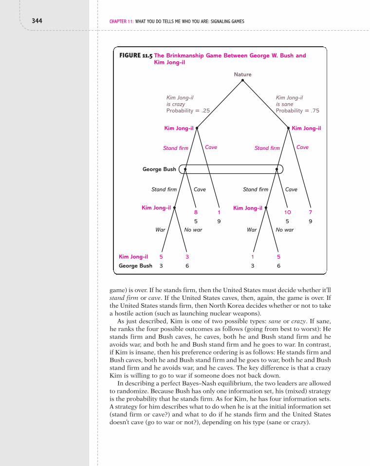
344 CHAPTER 11: WHAT YOU DO TELLS ME WHO YOU ARE: SIGNALING GAMES
game) is over. If he stands firm, then the United States must decide whether it’llstand firm or cave. If the United States caves, then, again, the game is over. Ifthe United States stands firm, then North Korea decides whether or not to takea hostile action (such as launching nuclear weapons).
As just described, Kim is one of two possible types: sane or crazy. If sane,he ranks the four possible outcomes as follows (going from best to worst): Hestands firm and Bush caves, he caves, both he and Bush stand firm and heavoids war, and both he and Bush stand firm and he goes to war. In contrast,if Kim is insane, then his preference ordering is as follows: He stands firm andBush caves, both he and Bush stand firm and he goes to war, both he and Bushstand firm and he avoids war, and he caves. The key difference is that a crazyKim is willing to go to war if someone does not back down.
In describing a perfect Bayes–Nash equilibrium, the two leaders are allowedto randomize. Because Bush has only one information set, his (mixed) strategyis the probability that he stands firm. As for Kim, he has four information sets.A strategy for him describes what to do when he is at the initial information set(stand firm or cave?) and what to do if he stands firm and the United Statesdoesn’t cave (go to war or not?), depending on his type (sane or crazy).
FIGURE 11.5 The Brinkmanship Game Between George W. Bush and Kim Jong-il
Kim Jong-il is crazy Probability " .25
Kim Jong-il is sane Probability " .75
Nature
War
Stand firm
Stand firm
Cave
Cave
No war
Kim Jong-il Kim Jong-il
Kim Jong-il
George Bush
Kim Jong-il
George Bush
5
3
3
6
8
5
1
9War
Stand firm
Stand firm
Cave
Cave
No war
Kim Jong-il
1
3
5
6
10
5
7
9

11.3 Examples 345
Consider a strategy pair of the following form:
■ Kim Jong-il’s strategy:—If crazy, then choose stand firm, and if both North Korea and the
United States chose stand firm, then choose war.—If sane, then choose stand firm with probability k, and if both
North Korea and the United States chose stand firm, then chooseno war.
■ George Bush’s strategy: Choose stand firm with probability b.
Since beliefs need to be part of the specification of a perfect Bayes–Nashequilibrium, let us derive beliefs for Bush that are consistent with Kim’s strat-egy. Suppose Bush observes him stand firm. Then, if Bush cannot inferthe dictator’s type, because although Kim will stand firm for sure if he’s crazy,he’ll stand firm with probability k even when he’s sane. Here, we need to de-ploy Bayes’s rule to tell us what Bush’s beliefs should be. By that rule, we have(where “sf” denotes “stands firm”)
Prob(Kim is crazy given that he stood firm)
k 7 0,
#.25 ! 1
.25 ! 1 % .75 ! k#
.25.25 % .75k
.
#Prob(crazy) ! Prob(sf given that he is crazy)
Prob(crazy) ! Prob(sf given that he is crazy) % Prob(sane) ! Prob(sf given that he is sane)
If a sane Kim never chooses to stand firm (i.e., then
so that Bush can perfectly infer that Kim is crazy from the North Koreandictator’s having stood firm. As k rises, so that it is more likely that a saneleader stands firm, then the probability that the North Korean leader issane, given that he stood firm, goes up. It reaches its maximum value of .75when Not coincidentally, this value equals the prior probability, be-cause if Kim chooses to stand firm for sure, regardless of his type, then thefact that he stood firm provides no information as to his mental state. Inthat situation, Bayes’s rule has the posterior beliefs being identical to theprior beliefs.
If, instead, Bush observes that Kim caved, then his posterior beliefs put aprobability of 1 on the leader’s being sane, since a crazy leader never caves.This result follows from Bayes’s rule as well:
Prob(Kim is crazy given that he caved)
k # 1.
.25.25 % .75 ! 0
# 1,
k # 0),
#.25 ! 0
.25 ! 0 % .75 ! (1 " k)# 0.
#Prob(crazy) ! Prob(caves given that he is crazy)
Prob(crazy) ! Prob(caves given that he is crazy) % Prob(sane) ! Prob(caves given that he is sane)
346 CHAPTER 11: WHAT YOU DO TELLS ME WHO YOU ARE: SIGNALING GAMES
These consistent beliefs are then added to the given strategy pair:
■ George Bush’s beliefs:—If Kim Jong-il chose stand firm, then he is crazy with probability
—If Kim Jong-il chose cave, then he is crazy with probability 0.
Now let us find values for b and k such that the given strategy pair, alongwith the preceding beliefs, form a perfect Bayes–Nash equilibrium. Given thatNorth Korea has stood firm, Bush is content to randomize if and only if
[11.4]
He receives a payoff of 5 from caving (regardless of Kim’s type). From stand-ing firm, he gets a payoff of 3 if Kim is crazy (since war then ensues) and apayoff of 6 if Kim is sane (because war is avoided). Solving (11.4) for k, we ob-tain Thus, if Kim chooses to stand firm with probability .67 when heis sane (and always stands firm when he is crazy), then Bush receives the sameexpected payoff whether he caves or stands firm.
Finally, we turn to Kim’s strategy. It is easy to show that his strategy is op-timal when he is crazy. Initially caving gives him his lowest payoff; thus, it isclearly preferable for him to stand firm. In the event that Bush responds bystanding firm, then going to war results in a higher payoff of 5 than the pay-off of 3 from avoiding war.
Now suppose Kim is sane. If he finds himself having to decide about war—if both he and Bush stood firm—then it is indeed optimal for him to avoid warand get a payoff of 5 (compared with a payoff of 1 from going to war). Theonly remaining information set to consider is when Kim must decide betweenstanding firm and caving. Recall that we are supposing that he randomizes atthat information set. (In particular, we’ve shown that he must stand firm withprobability .67 for Bush to be willing to randomize.) For that to be optimal forKim, it must be true that
[11.5]
The left-hand side expression is Kim’s payoff from caving, and the right-handside expression is his expected payoff from standing firm (which depends onthe likelihood that Bush stands firm or caves). Solving (11.5) for b, we find that
Equilibrium then requires that Bush has a 60% chance of standing firm.To sum up, the equilibrium prediction is that Kim Jong-il will stand firm
for sure if he is crazy, and if he is sane, there is still a 67% chance of him doingso. In response to North Korea’s standing firm, there is a 60% chance thatGeorge Bush will stand firm. In response to a standoff—that is, neither coun-try has caved—only a crazy Kim Jong-il goes to war.
SummaryThis chapter has focused on encounters with two important features: Peoplehave private information and they move sequentially. The significance of se-quential moves is that a person who moves first may reveal information about
b # .6.
7 # b ! 5 % (1 " b) ! 10.
k # .67.
5 # a .25.25 % .75k
b ! 3 % a .75k.25 % .75k
b ! 6.
.25.25 % .75k.

Summary 347
what it is she knows that other players do not. A player who moves secondmay then be able to glean information about a player’s type from her observedbehavior and use that information in deciding what to do. But if that is whatis going on, then the player who moves first may adjust her behavior with theintent to mislead those who are drawing inferences from it. An objective of thechapter was to sort out these various forces and identify solutions in which allplayers are acting in their best interests and no players are fooled. This doesn’tnecessarily mean that a player can figure out what another player knows, butit does mean that he won’t be duped into believing something false.
This analysis was conducted in the context of a signaling game, which is thesimplest structure that embodies these various features. A signaling game in-volves a player, known as the sender, who has some private information andmoves first by choosing an action. The action is observed by a second player,known as the receiver, who, after updating his beliefs as to the first player’s pri-vate information, selects an action as well. The solution concept utilized was aperfect Bayes–Nash equilibrium. Roughly speaking, a strategy pair and a pos-terior set of beliefs for the receiver regarding the first player’s private informa-tion constitute a perfect Bayes–Nash equilibrium if each player (1) is actingoptimally, given her beliefs (sequential rationality) and (2) the receiver’s pos-terior beliefs, which are conditional on the sender’s action, take proper accountof the optimal behavior of the sender (consistent beliefs). In other words, thereceiver recognizes the incentives the sender has to mislead him when he up-dates his beliefs in response to the sender’s observed behavior.
An equilibrium may entail the sender’s behavior (1) perfectly revealing allthat she knows (known as a separating equilibrium), (2) partially revealingwhat she knows (semiseparating, or semipooling, equilibrium), or (3) re-vealing nothing at all (pooling equilibrium). A separating equilibrium arisesin the Courtship game, in which the offering of an expensive gift by a suitorreveals to his fiancé that he truly loves her, and in the Management Traineegame, in which a trainee’s level of effort reveals how hardworking she is. Asemiseparating equilibrium occurs in the Used Car game in that an ownerputs her car up for sale only if it is of low or moderate quality. Because theseller’s price is independent of quality, the buyer does not know whether thecar’s quality is low or moderate, but does know that it is not of high quality,since an owner of a high-quality car chooses not to put it on the market.Partial information is also revealed in the Brinkmanship game, as Kim Jong-il’s standing firm in response to American threats reveals neither that he iscrazy nor that he is sane, but allows President Bush to update his beliefs andraise the probability that Kim is crazy.
What general lessons emerge from this analysis about signaling? One lessonis that whether there is an equilibrium whereby the sender’s behavior is inform-ative depends on how the sender’s type influences his preferences regarding ac-tions. A separating equilibrium is unlikely to exist when the sender’s action hasthe same impact on his payoff irrespective of his type. For example, selling ata higher price is of equal value to an owner of a high-quality car and one of alow-quality car; in both cases, the seller’s payoff is the price at which the carsells. Hence, an owner of a low-quality car is inclined to mimic the price set byan owner of a high-quality car. We then found that the price posted for the usedcar is independent of the car’s quality and thus is uninformative of its quality.In comparison, in the Courtship game, giving an expensive gift to a woman is

348 CHAPTER 11: WHAT YOU DO TELLS ME WHO YOU ARE: SIGNALING GAMES
less costly to a man if he loves her and thus anticipates marrying her. In thatsetting, the gift is a credible signal of his love.
This analysis leads us to a second lesson: For a player to successfully signalher type, she may need to distort her behavior in order to prevent other typesfrom imitating her behavior. Thus, in the Management Trainee game, an in-dustrious worker had to work harder than usual in order to distinguish her-self from a lazy worker. Indeed, an industrious type has to work so hard thata lazy worker would choose not to mimic her even if it meant that the man-ager was fooled into thinking that the lazy worker was industrious.
1. Return to the Lemons game in Section 11.3, and consider the samestructure, except suppose there are just two quality levels: low and high.The buyer initially assigns probability q to a car’s being of high qualityand probability to its being of low quality. If the seller sells the car,then her payoff is the price the buyer paid. If the car is not sold, assumethat it is worth $10,000 to the seller if it is of high quality and $6,000 ifit is of low quality; those are the payoffs. The value of the car to thebuyer is $12,000 if it is of high quality and $7,000 if it is of low quality.If the buyer purchases the car, then the buyer’s payoff is the car’s value—which is 12,000 or 7,000—less the price paid; his payoff is zero if he doesnot buy the car. Find values for q such that there is a perfect Bayes–Nashequilibrium with pooling.
2. For the Courtship game in Section 11.3, find a pooling perfectBayes–Nash equilibrium.
3. A retailer sells a product that is either of low or high quality, where qual-ity is measured by the likelihood that the product works. Assume thatthe probability that the high-quality product functions properly is h andthat the probability that the low-quality product functions properly is l,where A manufacturer’s type is the quality of its prod-uct—low or high—where the consumer attaches a probability r to theproduct’s being of high quality, Both quality types cost the re-tailer an amount c (which is a cost incurred only if the product is sold).After Nature determines the quality of the retailer’s product, the retailermakes two simultaneous decisions: the price to charge and whether tooffer a money-back warranty. A retailer’s price can be any nonnegativenumber. The warranty has the feature that if the product doesn’t work—which occurs with probability for a high-quality good and proba-bility for a low-quality good—then the retailer must return to theconsumer what she paid for the good. A retailer’s payoff is his expectedprofit. Thus, if he sells the good at a price p without a warranty, then hispayoff is If he sells it with a warranty, then his expected payoff is
if the product is of high quality and if it is of lowquality. After observing the product’s price and whether or not it has amoney-back warranty, a lone consumer decides whether to buy it. Inspecifying the consumer’s payoff, first note that if the product works,then the consumer realizes a value of while if it doesn’t work,then the product is of zero value. If she buys it at a price p, then her pay-off is (1) if the product works, (2) if the product doesn’t work"pv " p
v 7 0,
l ! p " ch ! p " cp " c.
1 " l1 " h
0 6 r 6 1.
0 6 l 6 h 6 1.
1 " q
EXERCISES
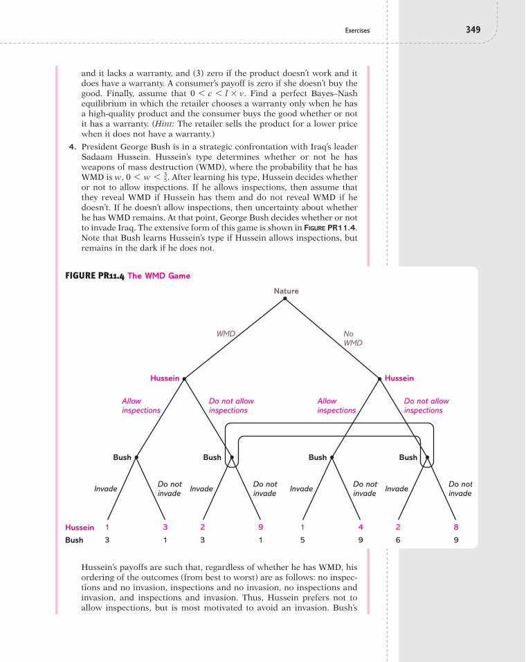
Exercises 349
and it lacks a warranty, and (3) zero if the product doesn’t work and itdoes have a warranty. A consumer’s payoff is zero if she doesn’t buy thegood. Finally, assume that Find a perfect Bayes–Nashequilibrium in which the retailer chooses a warranty only when he hasa high-quality product and the consumer buys the good whether or notit has a warranty. (Hint: The retailer sells the product for a lower pricewhen it does not have a warranty.)
4. President George Bush is in a strategic confrontation with Iraq’s leaderSadaam Hussein. Hussein’s type determines whether or not he hasweapons of mass destruction (WMD), where the probability that he hasWMD is w, After learning his type, Hussein decides whetheror not to allow inspections. If he allows inspections, then assume thatthey reveal WMD if Hussein has them and do not reveal WMD if hedoesn’t. If he doesn’t allow inspections, then uncertainty about whetherhe has WMD remains. At that point, George Bush decides whether or notto invade Iraq. The extensive form of this game is shown in FIGURE PR11.4.Note that Bush learns Hussein’s type if Hussein allows inspections, butremains in the dark if he does not.
0 6 w 6 35.
0 6 c 6 l ! v.
Hussein’s payoffs are such that, regardless of whether he has WMD, hisordering of the outcomes (from best to worst) are as follows: no inspec-tions and no invasion, inspections and no invasion, no inspections andinvasion, and inspections and invasion. Thus, Hussein prefers not toallow inspections, but is most motivated to avoid an invasion. Bush’s
Nature
Invade
Allow inspections
WMD No WMD
Do not allow inspections
Do not invade
3
1
1
3
Bush
BushHussein
Hussein
Invade Do not invade
9
1
2
3
Bush
Invade
Allow inspections
Do not allow inspections
Do not invade
4
9
1
5
Bush
Hussein
Invade Do not invade
8
9
2
6
Bush
FIGURE PR11.4 The WMD Game

350 CHAPTER 11: WHAT YOU DO TELLS ME WHO YOU ARE: SIGNALING GAMES
preference ordering depends very much on whether Hussein has WMD.If Hussein has WMD, Bush wants to invade; if he does not, then heprefers not to invade. Find consistent beliefs for Bush and values for band h, where and such that the following strategypair is a perfect Bayes–Nash equilibrium:
■ Hussein’s strategy:—If I have WMD, then do not allow inspections.—If I do not have WMD, then allow inspections with probability h.
■ Bush’s strategy:—If Hussein allows inspections and WMD are found, then invade.—If Hussein allows inspections and WMD are not found, then do
not invade.—If Hussein does not allow inspections, then invade with proba-
bility b.
5. We’ll now show how a college degree can get you a better job even if itdoesn’t make you a better worker. Consider a two-player game betweena prospective employee, whom we’ll refer to as the applicant, and an em-ployer. The applicant’s type is her intellect, which may be low, moderate,or high, with probability and respectively. After the applicantlearns her type, she decides whether or not to go to college. The personalcost in gaining a college degree is higher when the applicant is less in-telligent, because a less smart student has to work harder if she is tograduate. Assume that the cost of gaining a college degree is 2, 4, and 6for an applicant who is of high, moderate, and low intelligence, respec-tively. The employer decides whether to offer the applicant a job as amanager or as a clerk. The applicant’s payoff to being hired as a man-ager is 15, while the payoff to being a clerk is 10. These payoffs are in-dependent of the applicant’s type. The employer’s payoff from hiringsomeone as a clerk is 7 (and is the same regardless of intelligence andwhether or not the person has a college degree). If the applicant is hiredas a manager, then the employer’s payoff increases with the applicant’sintellect, from 4, to 6, to 14, depending on whether the applicant has low,moderate, or high intellect, respectively. Note that the employer’s payoffdoes not depend on whether or not the applicant has a college degree.The extensive form of this game is shown in FIGURE PR11.5. Find a per-fect Bayes–Nash equilibrium in which students of low intellect do not goto college and those of moderate and high intellect do.
6. The owner of a new restaurant is planning to advertise to attract cus-tomers. In the Bayesian game, Nature determines the restaurant’s qual-ity, which is either high or low. Assume that each quality occurs withequal probability. After the owner learns about quality, he decides howmuch to advertise. Let A denote the amount of advertising expenditure.For simplicity, assume that there is a single consumer. The consumer ob-serves how much advertising is conducted, updates her beliefs about thequality of the restaurant, and then decides whether or not to go to therestaurant. (One can imagine that A is observed by noticing how manycommercial spots are on local television and how many ads are in thenewspaper and on billboards.) Assume that the price of a meal is fixedat $50. The value of a high-quality meal to a consumer is $85 and of alow-quality meal is $30. A consumer who goes to the restaurant andfinds out that the food is of low quality ends up with a payoff of "20,
16,1
2,13,
0 6 h 6 1,0 6 b 6 1

Exercises 351
which is the value of a low-quality meal, 30, less the price paid, 50. If thefood is of high quality, then the consumer receives a value of 35
Furthermore, upon learning of the high quality, a consumeranticipates going to the restaurant a second time. Thus, the payoff to a con-sumer from visiting a high-quality restaurant is actually 70 For the restaurant owner, assume that the cost of providing a meal is 35whether it is of low or high quality. If the restaurant is of high quality,the consumer goes to the restaurant, and the restaurant spends A in ad-vertising, then its profit (and payoff) is If the restaurant is of low quality, the consumer goes to the restaurant,and the restaurant spends A in advertising, then its profit is
These payoffs are summarized in the followingtable. If the consumer does not go to the restaurant, then her payoff iszero and the owner’s payoff is "A.
(50 " 35) " A # 15 " A.
2 ! (50 " 35) " A # 30 " A.
(# 2 ! 35).
(# 85 " 50).
Low Moderate High
Nature
Manager
College No college
Clerk
Manager Clerk
4
7
9
4
Employer
Applicant
EmployerApplicant 10
7
15
4
Manager
College No college
Clerk
Manager Clerk
6
7
11
6
10
7
15
6
Manager
College No college
Clerk
Manager Clerk
8
7
13
14
10
7
15
14
FIGURE PR11.5 The College Signaling Game
RESTAURANT GAME: PAYOFFS WHEN A CONSUMER GOES TO THE RESTAURANT
Restaurant Quality Owner’s Payoff Customer’s Payoff
Low 15 # A #20
High 30 # A 70

352 CHAPTER 11: WHAT YOU DO TELLS ME WHO YOU ARE: SIGNALING GAMES
a. Find a separating perfect Bayes–Nash equilibrium.b. At a separating perfect Bayes–Nash equilibrium, what is the maxi-
mum amount of advertising that a restaurant conducts? What is theminimum amount?
c. Find a pooling perfect Bayes–Nash equilibrium.d. At a pooling perfect Bayes–Nash equilibrium, what is the maximum
amount of advertising?
7. Consider the signaling game in FIGURE PR11.7. Nature chooses one ofthree types for the sender, and after learning her type, the senderchooses one of three actions. The receiver observes the sender’s action,but not her type, and then chooses one of two actions. Find a semisepa-rating perfect Bayes–Nash equilibrium in which the sender chooses thesame action when her type is or and chooses a different action whenher type is t3.
t2t1
Nature
a b a b
x y z
a b a b a ba b a b a ba b
2
0
7
1
Receiver
Sender
ReceiverSender 2
0
4
1
3
0
2
1
x y z
1
1
4
1
1
0
6
1
5
0
3
1
x y z
4
1
2
0
1
1
3
0
5
1
5
0
t1
Probability " 14 t2
Probability " 12
t3
Probability " 14
FIGURE PR11.7
8. For the signaling game in FIGURE PR11.8, find all separating perfectBayes–Nash equilibria.
9. Consider the signaling game in FIGURE PR11.9.a. Find all separating perfect Bayes–Nash equilibria.b. Find all pooling perfect Bayes–Nash equilibria.

Nature
a
x
Type s Probability " .75
Type t Probability " .25
y x y
b ab a b a b
5
0
3
2
Receiver
ReceiverSender
Sender
0
1
2
3
6
4
1
1
2
3
4
2
FIGURE PR11.8
FIGURE PR11.9
Nature
a
x
Type s Probability " .5
Type t Probability " .5
y x y
b ab a b a b
2
2
3
4
Receiver
ReceiverSender
Sender
1
2
5
7
0
5
2
4
5
6
4
3
353

354 CHAPTER 11: WHAT YOU DO TELLS ME WHO YOU ARE: SIGNALING GAMES
11.4 Appendix: Bayes’s Rule and Updating BeliefsCONSIDER A COLLEGE WITH 4,000 students: 2,100 women and 1,900 men. TABLE
A11.1 breaks down the student body in terms of gender and the generalarea of their major, of which there are four categories: undeclared, human-ities, social sciences, and physical sciences. The categories are mutually ex-clusive, which means that a person falls into exactly one category—nomore, no less.
TABLE A11.1 POPULATION OF STUDENTS AT A COLLEGE
Social PhysicalUndeclared Humanities Sciences Sciences Total
Male 250 350 600 700 1,900
Female 150 450 900 600 2,100
Total 400 800 1,500 1,300 4,000
The table can be used to assign probabilities to the characteristics of a ran-domly selected student. For example, the probability that a randomly selectedstudent is a woman is as there are 2,100 female students out of astudent body of 4,000. Similarly, the probability that a randomly selected stu-dent has a major in the social sciences is as there are 1,500 socialscience majors out of 4,000.
Now suppose you meet a female student at the gym and want to start upa conversation with her. With that goal in mind, it would be useful to makean intelligent guess as to her major. So, what is the probability that hermajor is in the physical sciences? That is, what is the probability that thisstudent’s major is in the physical sciences, conditional on knowing that sheis a woman?
To answer this question, first note that asking “What is the probabilitythat a student’s major is in the physical sciences, given that she is a woman”is the same as asking “What is the probability that a randomly selected stu-dent from the population of female students has a major in the physical sci-ences.” Thus, we want to focus on the population of female students; hence,look at the middle row in Table A11.1. From the entries in this row, we canconclude that the answer is That is, out of 2,100 female stu-dents, 600 have a major in the physical sciences, and since it is assumedthat each female student has an equal chance of being at the gym, there isa 28.6% chance that the student you met has a major in the physicalsciences.
You have unknowingly just deployed Bayes’s rule. To be a bit more formalabout matters, let x and y be two random events. In the preceding example,the random events are a student’s gender and a student’s major. Let denote the probability that (e.g., the probability that a student is a fe-male), denote the probability that and (e.g., the prob-ability that a student is a female and the student’s major is in the physical
y # y¿x # x¿Prob(x¿, y¿)x # x¿
Prob(x¿)
6002,100 # .286.
.375 (1,5004,000),
.525 (2,1004,000),

11.4 Appendix: Bayes’s Rule and Updating Beliefs 355
sciences), and denote the probability that conditional on(e.g., the probability that a student’s major is in the physical sciences,
given that the student is a female). Bayes’s rule describes the following rela-tionship between these three probabilities:
[11.6]
This is exactly what we have already calculated, where
Prob( y¿#˛˛x¿) #Prob(x¿, y¿)
Prob(x¿).
x # x¿y # y¿,Prob(y¿#˛˛x¿)
so that
Prob(student is a female) #2,1004,000
Prob(student is a female and student’s major is in the physical sciences) #600
4,000
Prob(student’s major is in the physical sciences, given that student is a female) #
6004,0002,1004,000
#600
2,100.
In using Bayes’s rule, the following properties may prove useful. Supposethere are only two possible values for y: and First note that
[11.7]
This equation is due to mutual exclusivity. When either orbecause y takes on only those two values. Substitute the right-hand
side of (11.7) into the denominator of (11.6):
[11.8]
We can flip around the roles of x and y in (11.6) so that we are now examiningthe probability that conditional on
Multiply both sides by
[11.9]
Perform the exact same steps for
[11.10]Prob(y–) ! Prob(x¿|y–) # Prob(x¿, y–).
y # y–:
Prob(y¿) ! Prob(x¿|˛y¿) # Prob(x¿, y¿).
Prob( y¿):
Prob(x¿|˛y¿) #Prob(x¿, y¿)
Prob(y¿).
y # y¿:x # x¿
Prob(˛y¿|x¿) #Prob(x¿, y¿)
Prob(x¿, y¿) % Prob(x¿, y–)
y # y–y # y¿x # x¿,
Prob(x¿) # Prob(x¿, y¿) % Prob(x¿, y–).
y–.y¿

356 CHAPTER 11: WHAT YOU DO TELLS ME WHO YOU ARE: SIGNALING GAMES
Now substitute (11.9) and (11.10) into the denominator of (11.8):
This is an alternative formula for calculating with Bayes’s rule.Bayes’s rule is handy not only when you meet people at the gym, but also if
you should be a contestant on Let’s Make a Deal. On this show, a contestant se-lects one of three doors. Behind one of the doors is a great prize—say, a brand-new automobile—while behind the other two doors are mediocre or even un-wanted prizes (such as an ornery donkey). Although the show’s host, MontyHall, knows what’s behind each door, the contestant does not. Prior to theshow, the car was randomly placed behind one of the doors, so the contestantinitially assigns probability to (its being behind) Door Number 1, to DoorNumber 2, and to Door Number 3.
The contestant begins by selecting a door. Because she is indifferent as towhich one she selects, we can suppose it is Door 1. However, before Door 1is opened, Monty Hall opens up one of the two doors not selected. Now,here’s a crucial fact: Monty Hall never opens up the door with the car. Thismeans that if Door 2 has the car, then Monty opens Door 3, and if Door 3has the car, then he opens Door 2. If Door 1 has the car, he can open eitherDoor 2 or 3 (and we’ll assume that each has an equal chance of beingopened).
Suppose Monty opens Door 2. He then makes an offer that has stymiedmany a contestant: Do you want to keep Door 1 or instead switch to Door3? After that selection is made, the doors are opened and the contestantlearns what she has won. The contestant wants to switch only if it is morelikely that the car is behind Door 3. So, what should she do? If this contest-ant had read Section 11.4, she would know that the answer is obvious:Switch doors!
To prove this claim, let’s start with the unconditional probabilities regardingwhere the car lies:
13
13
13
Prob(y¿|˛x¿)
Prob( y¿|˛x¿) #Prob( y¿) ! Prob(x¿|˛y¿)
Prob( y¿) ! Prob(x¿|˛ y¿) % Prob( y–) ! Prob(x¿|˛y–).
To determine whether the contestant ought to change doors, it is necessary tocalculate the probability that Door 1 has the car, conditional on Monty’s havingopened Door 2. Here we can use Bayes’s rule:
[11.11]
The denominator can be represented as
[11.12]% Prob(Monty opens Door 2 and Door 3 has car)
# Prob(Monty opens Door 2 and Door 1 has car)Prob(Monty opens Door 2)
#Prob(Monty opens Door 2 and Door 1 has car)
Prob(Monte opens Door 2)
Prob(Door 1 has car, given that Monty opens Door 2)
Prob(Door 1 has car) #13
, Prob(Door 2 has car) #13
, Prob(Door 3 has car) #13
.

References 357
Next, let us calculate each of those two terms in the sum:
[11.13]
#12
!13
#16
.
# Prob(Monty opens Door 2, given that Door 1 has car) ! Prob(Door 1 has car)Prob(Monty opens Door 2 and Door 1 has car)
Note that, in the previous calculation, if Door 1 has the car, then Monty opensDoor 2 with probability and Door 3 with probability
Next, note that if Door 3 has the car, then Monty has to open Door 2 by therule that he never opens a door with the grand prize. Using this fact, we have
12.1
2
Substituting (11.13) and (11.14) into (11.12) yields
[11.15]
Finally, substitute (11.13) and (11.15) into (11.11):
After Monty Hall opens Door 2, the contestant knows that the car is behindeither Door 1 or Door 3. Since we’ve just shown that Door 1 is given a condi-tional probability of it follows that Door 3 has a conditional probability of
Thus, the contestant should always switch doors! There is information inthe fact that Monty avoided Door 3. If Door 3 has the prize, Monty must avoidit, and that he did avoid it is encouraging information about Door 3. All thatis intuitive, but the beauty of Bayes’s rule is that it tells us exactly how to usethat information in updating our beliefs.
REFERENCES1. This analysis is based on the work of George Akerlof that resulted in him
cowinning the 2001 Nobel Prize in Economics: “The Market for ‘Lemons’ :Qualitative Uncertainty and the Market Mechanism,” Quarterly Journal ofEconomics, 84 (1970), 488–500.
23.
13,
Prob(Door 1 has car, given that Monty opens Door 2) #
1612
#13
.
#16
%13
#12
.
% Prob(Monty opens Door 2 and Door 3 has car)# Prob(Monty opens Door 2 and Door 1 has car)
Prob(Monty opens Door 2)
[11.14]
# 1 !13
#13
# Prob(Monty opens Door 2, given that Door 3 has car) ! Prob(Door 3 has car)Prob(Monty opens Door 2 and Door 3 has car)

358 CHAPTER 11: WHAT YOU DO TELLS ME WHO YOU ARE: SIGNALING GAMES
2. The ensuing model is inspired by Peter D. Sozou and Robert M. Seymour,“Costly but Worthless Gifts Facilitate Courtship Gifts,” Proceedings of theRoyal Society B, 2005. In light of current American society, this discussionmay sound quaint at best and sexist at worst. The intent is not to describewhat should be, but rather what is (in some societies) and what was (inother societies).
3. The ensuing discussion draws on Margaret F. Brinig, “Rings and Promises,”Journal of Law, Economics, and Organization, 6 (1990), 203–15, p. 205.
4. Thomas Omestad, “Man of mystery: Contrary to his image, North Koreandictator Kim Jong-il isn’t crazy. So, what’s his game?” U.S. News and WorldReport, January 13, 2003.

“Talk is cheap, it don’t cost nothin’ but breath.”1
12.1 IntroductionTHE PREVIOUS CHAPTER CONSIDERED situations in which an individual’s behaviorcould signal information that was known only to him. A suitor can crediblysignal his love for a woman by offering her an expensive and extravagant gift.A management trainee can credibly signal how industrious she is by workinglong hours. A company can credibly signal the quality of its product by offer-ing a money-back warranty. In all of these cases, behavior conveyed informa-tion because the action chosen was costly and its cost varied with a player’stype. A diamond ring signaled true love because only someone in love wouldbe willing to spend so much. Working long hours signaled a trainee’s workethic because someone who was innately lazy would find that too distasteful.And a company which knew that its product was of low quality would find ittoo expensive to offer a warranty, since it would have to return a customer’smoney far too frequently.
Signaling scenarios will be covered in this chapter as well, but to keep youintrigued, we’ll make one important twist: The action taken is costless. By“costless,” we mean that it doesn’t affect the payoff of the player who is choos-ing it (or any other player, for that matter). It is then necessarily the case thatthe cost of an action is the same across player types, since it is zero for all ac-tions and all player types.
Although your initial reaction might be to wonder how a costless actioncould make any darn difference, in fact we use costless actions every day to in-fluence the behavior of others. What are these magical costless actions?Words. It may be a commercial on television trying to convince you to buy acar. Or the campaign promises of a candidate for electoral office. It could bethe repair work that the auto mechanic says needs to be done or something asmundane as the text message sent to a friend to coordinate a time and placefor dinner. It could even be that e-mail from the wife of a recently deposedgeneral in Nigeria.**
A costless action is referred to as a message, and signaling games with mes-sages have been dubbed cheap talk games. The key assumption is that there isno cost to sending misleading messages (“lying”); thus, we make no presumption
12
359
Lies and the Lying Liars That Tell Them:*Cheap Talk Games
*This is the title of Al Franken’s book of political satire. He is also known for the pithy, sardonic, and ex-istential treatise Rush Limbaugh is a Big Fat Idiot.**According to the Internet Complaint Center, people continue to be duped by this ruse and suffer an av-erage loss in excess of $5,000 per person. As P. T. Barnum said, “There’s a sucker born every day.”

360 CHAPTER 12: LIES AND THE LYING LIARS THAT TELL THEM: CHEAP TALK GAMES
that messages are truthful. Because talk is cheap, one may wonder when mes-sages are informative. Addressing that issue is the primary objective of this chap-ter. When should you buy a stock on the basis of an analyst’s recommendation?When should you believe a presidential candidate’s campaign pledge not to raisetaxes? When can you believe an auto mechanic who says that your car needs anew transmission? Informative messages can have a significant impact on howpeople behave, but when they are devoid of substantive content, they are indeednothing more than breath.
There are two distinct scenarios in which messages may make a differ-ence—a message can “signal information” or “signal intention.” The first isof the sort explored in Chapter 11: A player has private information about,say, payoffs and sends a message that may influence other players’ beliefsabout those payoffs and thus how they act. A second class of situations dealsinstead with games of complete information. Here, a player’s message doesnot convey anything about the game itself; features of the game are knownto all players. Instead, what the message may signal is a player’s intendedplay. This is especially relevant in games with multiple Nash equilibria. Forexample, recall the telephone game from Chapter 4, in which Colleen andWinnie are cut off during their phone conversation and have to decidewhether to call the other back or wait for the other to call. Each would likethe other to do the dialing, but is willing to call back if that is what it takesto reconnect. In that game, there were two pure-strategy Nash equilibria:Colleen calls back and Winnie waits; and Winnie calls back and Colleenwaits. Communication at the start of the original call can help the playerssettle on one of those equilibria. There is also a symmetric mixed-strategyNash equilibrium in which each player randomizes. Although the latterequilibrium has the appeal of treating players symmetrically, it may period-ically result in their failing to coordinate. As we’ll see, cheap talk precedingthe telephone game may allow each player to signal her intentions andthereby coordinate better on an outcome.
In the next section, we consider what it means to communicate in a game-theoretic world (which is a bit different from the real world). Section 12.3 thenexplores the content of messages when players attempt to signal information.The role of communication in signaling intentions is examined in Section12.4. We also explore how the predictions of theory match up with experimen-tal evidence. It turns out that the predicted effects of allowing players to com-municate are strongly supported by how people actually behave.
12.2 Communication in a Game-Theoretic WorldWhile campaigning, Ohio Senator Tom Corwin was asked at a rally, “Whatabout the tariff question?” Senator Corwin replied, “Glad you asked that,mister. I know some in this audience are for a high tariff and others areagainst a high tariff. After considerable thought on the subject, I want every-one in this hall to know—so am I!”2
THIS SECTION HAS THREE basic points. First, a message is not limited to words;just about anything that one player can do which is observable by others canbe a message. Second, the information content of a message need not coincidewith the literal meaning of the message. A message’s meaning is to be derived,

12.2 Communication in a Game-Theoretic World 361
not presumed. Third, although a player may desire to deceive others, there isno lying when players are at an equilibrium. The desire to deceive does not re-sult in deception, but it can prevent information from being revealed. Thesepoints will be fleshed out in the ensuing applications.
What is communication? Communication involves one player “sending amessage” to another player. A message can take many forms. It could involvethe spoken or written word. If you are in a Chinese restaurant in New Yorkand you want to order kung pao chicken, you’ll say to the server, “I’ll havekung pao chicken.” If you’re in Shanghai and you don’t understand Chinese(and the server doesn’t understand English), you can still, of course, say “I’llhave kung pao chicken” but it is unlikely to have the intended effect. If, how-ever, the menu is in both Chinese and English, you could point to the item onthe menu. The physical gesture of pointing is a message.
A message can be any (costless) action that one person can take and an-other person can perceive (i.e., be made aware of through one’s senses). A mes-sage can be spoken (and thus heard) or involve a physical gesture (and thus beseen or felt). In the film The Sting, members of a confidence ring would signalto each other with a flick of a finger along their nose. Similarly subtle handgestures have been set up between a bidder and an auctioneer in order for abidder to signal his acceptance of a bid without tipping off other bidders inthe room as to whom is making the bid. Or the message could be placing ahanger on your dorm room door so that your roommate knows you have“company.” The space of messages encompasses a wide array of utterancesand gestures that have the capacity to convey information.
A message sent is not necessarily information delivered, however. Thisbrings us to the issue of the meaning of a message. Of course, words have aliteral meaning—just look it up in a dictionary—but we know that words canbe deliberately chosen to be vague, misleading, and even downright deceptive.A person can say one thing while knowing something quite different. For suc-cessful communication to occur, two conditions must be met. First, theremust be a shared understanding of the literal meaning of the message. For ex-ample, in the United States, shaking one’s head from side to side is a gesturewith a literal meaning of “no.” But in some parts of India, the exact same phys-ical gesture means “yes.” When I first communicated with a graduate studentfresh from India (who went on to become a superb game theorist), communi-cation was far from perfect, as we lacked that shared understanding.
A common language—that is, a shared understanding of the literal mean-ing of a message—is a necessary, but not sufficient, condition for informationto traverse from one person to another. This fact leads us to the second condi-tion: that there is no incentive for the sender of a message to deceive the re-ceiver. When running for office in 1988, George H. W. Bush made an unam-biguous pledge: “Read my lips . . . no new taxes!” Though linguistically crystalclear, what this message implied about future behavior was far murkier, be-cause voters suspected that Bush might make such an utterance regardless ofhis true intentions. This suspicion was revealed in a contemporaneous Galluppoll in which 68% of those surveyed believed that he would raise taxes ifelected. Apparently, voters were trying to read his mind, not just his lips.
Information, then, is conveyed when two people have a common languageand lack the desire to deceive each other. Deception is central to this chapter.We’ll be interested in understanding when deception is at work and how it

362 CHAPTER 12: LIES AND THE LYING LIARS THAT TELL THEM: CHEAP TALK GAMES
influences the information content of messages conveyed. The most importantpoint for you to recognize at this stage is that the meaning of a message issomething to be solved as part of a game’s solution.
Messages that are linguistically clear can be uninformative, and messagesthat are far removed from formal languages can be teeming with juicy infor-mation. To highlight how messages can be quite arbitrary and yet informative,the absence of words can convey information. When the U.S. Congress heldhearings on steroid use in Major League Baseball®, one of the witnesses wasMark McGwire, who had been accused by a former teammate of having usedsteroids. His silence on the matter spoke volumes:
In a room filled with humbled heroes, Mark McGwire hemmed and hawedthe most. His voice choked with emotion, his eyes nearly filled with tears,[and] time after time he refused to answer the question everyone wanted toknow: Did he take illegal steroids when he hit a then-record 70 home runsin 1998—or at any other time?3
Neither denying nor confirming it, he led many people to believe that he hadtaken steroids. His failure to deny the charges was informative: If he had nottaken steroids, it would have been in his best interest to say so.
The final question we want to address here is, What does it mean to lie? Tofib? To equivocate? To prevaricate? According to Webster’s, “to lie” is “to makean untrue statement with intent to deceive.” The issue is not what is literallyso, but what is the intended inference to be drawn by others. Let me offer anexample close to home (in fact, my home!). In response to certain questions,my younger daughter replies “maybe” when the true answer is “no.” For ex-ample, if I asked her, “Have you done your chores?” she would invariably re-spond “maybe.” But I clearly took that as a “no” because, if she had donethem, she would have said “Yes, Dad, now quit buggin’ me.” When my daugh-ter says “maybe,” she is not lying, because it is common knowledge betweenus that it means “no,” which is the truthful answer to my question. To lie, onemust intend to mislead with the anticipation of success.
In the game-theoretic models we’ll explore, there is often an incentive todeceive, so a player would like to lie. However, in equilibrium, there will beno lying, because, in equilibrium, any such incentive is taken account of bythe other players. Although our analysis will not allow a player to be duped,that doesn’t mean that the truth is revealed: The incentive to deceive can pre-vent information from being revealed. If a detective asks a murder suspectwhether he committed the crime, his answer is unlikely to be informative: Ifthe suspect did not do it, he’ll say he didn’t do it; but if the suspect did do it,he’ll also say he didn’t do it. The detective is not deceived, although he re-mains in the dark.
The absence of the phenomenon of lying in game-theoretic models is unfor-tunate, for people in real life often do succeed with deception. Sadly, game the-ory can shed no light on lying, as our players are just too smart for that. It can-not, for example, explain a critical moment in Shakespeare’s King Lear. KingLear is the aging king of Britain and is deciding what to do with his kingdom.He asks each of his three daughters to tell him how much she loves him.Flattering answers are put forth by the two older ones, Goneril and Regan,while Cordelia remains silent, for she lacks the words to describe how muchshe loves her father. Lear’s response is to disown Cordelia and give his kingdom

12.3 Signaling Information 363
to Goneril and Regan. Soon he learns that the flattering responses were lies andthat silence hid true love. Now, while King Lear might not learn about eachdaughter’s love at a game-theoretic equilibrium, neither will he be duped.
12.3 Signaling InformationFlorence, Italy—Italy’s leading designers may soon learn to their sorrow thatnoisy applause doesn’t mean a jingling cash register. Of the 50 Americanbuyers at the Pitti Palace show of spring fashions, several admitted off therecord that they never clap for the haute couture creations that they like best.They don’t want their competitors to know what they will order. At the sametime, these buyers confessed they applauded enthusiastically for sportswear,boutique items and gowns that they wouldn’t consider featuring in theirown stores.4
A CHEAP TALK GAME has three stages:
Stage 1: Nature chooses the sender’s type.
Stage 2: The sender learns her type and chooses a message.
Stage 3: The receiver observes the sender’s message, modifies his beliefsabout the sender’s type in light of this new information, andchooses an action.
What makes this a cheap talk game rather than any other type of signalinggame is that the message chosen by the sender affects neither the sender’s pay-off nor the receiver’s payoff. Their payoffs are determined only by the sender’stype and the receiver’s action. Of course, a message can indirectly affect pay-offs, influencing the receiver’s action by altering her beliefs about the sender’stype. For that to happen, though, the sender’s type must influence the re-ceiver’s payoff—and not just the sender’s payoff. We shall assume that to be thecase in our examples.
! SITUATION: DEFENSIVE MEDICINE
In a recent survey of physicians, 93% reported altering their clinical behav-ior because of the threat of malpractice liability. Of them, 92% used “assur-ance behavior” such as ordering tests, performing diagnostic procedures,and referring patients for consultation; and 43% reported using imagingtechnology in clinically unnecessary circumstances.5
A common situation in which cheap talk appears is when we rely upon ad-vice from an expert. An auto repair shop says that your car needs a major re-pair. Your stockbroker recommends a stock. Your doctor tells you that youneed a diagnostic test. When should you follow this advice? When is the ex-pert truthfully conveying what she knows? And when is she instead trying toinduce you to do something in her best interests and not yours?
Consider a patient who has a particular symptom and goes to his doctor foran examination.6 The doctor evaluates the patient and then decides whether ornot to recommend an expensive test—or example, an MRI (magnetic resonanceimaging). If it is not recommended, then the patient has no decision to make. Ifan MRI is recommended, then the patient must decide whether to get it. The pa-tient recognizes that the test may be beneficial, but also that it is personally costly,

364 CHAPTER 12: LIES AND THE LYING LIARS THAT TELL THEM: CHEAP TALK GAMES
perhaps because it is not fully covered by insurance or it requires taking time offfrom work or is uncomfortable. The doctor cares about the patient, though per-haps not exclusively. She might recommend the test even when it is near useless,because doing so serves to avoid potential malpractice suits. The patient is awareof the possibility that his doctor will engage in such defensive medicine.
The Bayesian game’s extensive form is shown in FIGURE 12.1. Nature movesfirst by determining the value of the test to the patient. With probability thepatient’s condition is such that the test is beneficial; with probability the testis useless. The value of the test is known only to the doctor, who learns it afterexamining the patient. Upon determining the value of the test to the patient, thedoctor decides whether to recommend it. If she does not, then the patient de-cides whether to take the test. If she does, then the patient decides whether topursue the recommendation.
23,
13,
Nature
Doctor Doctor
Recommendstest
Does notrecommendtest
Does notrecommendtest
Recommendstest
Patient Patient Patient Patient
Test Test Test TestNotest
Notest
Notest
Notest
a % 5
5
a % 5
5
a " 5
"5
a " 5
"5
0
0
0
0
0
0
0
0PatientDoctor
Test isbeneficialProbability " 1
3
Test isuselessProbability " 2
3
FIGURE 12.1 The Doctor–Patient Game
If he takes the test, the patient’s payoff is 5 when it is beneficial and whenit is not. If he doesn’t take the test, then his payoff is zero. Thus, the patientwants to take the test only when it is beneficial, although figuring out whenthat is the case requires assessing the veracity of the doctor’s recommendation.The doctor’s payoff from conducting the test is where v is the value ofthe test to the patient and If the test is beneficial to the patient, thena ' 0.
a % v,
"5

12.3 Signaling Information 365
if it is not beneficial, then a is the value of the test to the doctorfrom a malpractice standpoint. If then the interests of the patient andthe doctor coincide and their payoffs are identical; thus, the doctor wants toconduct the test if and only if it is in the patient’s best interests. However, if
then there may be a conflict of interest, in that the doctor may preferthat the test be conducted even when it is not beneficial to the patient. Finally,assume that the payoff to the doctor is zero if the test is not conducted.
First note that there is a pooling perfect Bayes–Nash equilibrium in whichthe doctor should not be believed:
■ Doctor’s strategy: Recommend the test whether or not it is beneficial tothe patient.
■ Patient’s strategy: Ignore the doctor’s recommendation.■ Patient’s beliefs: Whether or not the doctor recommends the test, the test
is beneficial with probability .
This equilibrium is known as a babbling equilibrium: The doctor’s message isno more informative than inane babble. A babbling equilibrium is a poolingequilibrium in a cheap talk game. Given that the doctor’s strategy has hermake the same recommendation—“Take the test”—regardless of her type, hermessage is entirely uninformative. The patient’s beliefs are then consistent, asthey are the same as his prior beliefs. With those beliefs, the expected payofffrom taking the test when it is recommended is
which is less than the payoff from not taking the test. Since the patient is notgoing to take the test, the doctor’s payoff is zero whether or not she recom-mends it, in which case recommending the test is just as good as not doing so.This equilibrium is not very heartening, as the doctor’s advice is worthless (be-cause it doesn’t depend on the patient’s true condition)—and, of course, theadvice is appropriately ignored by the patient.
In fact, every cheap talk game has a babbling equilibrium. If the receiverbelieves that the sender’s message is independent of the sender’s type, then thereceiver will ignore the message and just use his prior beliefs in deciding howto behave. But if the receiver acts in such a manner—ignoring the sender’smessage—then the sender is indifferent as to what is said, since it doesn’t in-fluence the receiver’s behavior (and all messages have the same cost, which iszero). Any message for any type will suffice, including sending the same mes-sage for all types.
For every cheap talk game, there is always a babbling equilibrium.
The interesting issue is whether there is also an equilibrium in which mes-sages actually contain information. Let us then consider the following candi-date for a separating perfect Bayes–Nash equilibrium:
■ Doctor’s strategy: Recommend the test if and only if it is beneficial to thepatient.
■ Patient’s strategy: Follow the doctor’s recommendation.
a13b ! 5 % a2
3b ! ("5) # "
53
,
13
a 7 0,
a # 0,v # "5.v # 5;

366 CHAPTER 12: LIES AND THE LYING LIARS THAT TELL THEM: CHEAP TALK GAMES
■ Patient’s beliefs:If the doctor recommends the test, then the test is beneficial with proba-bility 1.If the doctor does not recommend the test then the test is useless withprobability 1.
This strategy profile results in a desirable outcome, as the doctor alwaysmakes the recommendation that is best for the patient and the patient truststhe doctor. What we need to assess is when it is an equilibrium. It should beapparent that the patient’s beliefs are consistent. (If it is not apparent, youshould schedule some office hours with your instructor.) Given that the test isrecommended only when it is beneficial, the patient’s strategy is clearly opti-mal. This statement leaves us assessing the sequential rationality of the doc-tor’s strategy. Suppose, in fact, that the test is beneficial. Then the doctor’s pay-off from recommending the test is because, according to the patient’sstrategy, the patient will follow the doctor’s recommendation. Since the payoffis zero from not recommending the test, the doctor’s strategy is optimal if andonly if which is indeed true (because Not surprisingly, if thetest benefits the patient and protects against malpractice, the doctor clearlywants to recommend it. The problematic scenario is when the test is not ben-eficial to the patient. The strategy has the doctor not recommend it then, soher payoff is zero. Recommending it yields a payoff of so not recom-mending it is optimal when
When an equilibrium with truthful recommendations exists (asdoes a babbling equilibrium). When, instead, there is only a babblingequilibrium, so the doctor’s recommendations are necessarily uninformative.There is a general principle at work here. When the doctor’s interestscoincide perfectly with those of the patient, in that the doctor wants him totake the test only when it makes the patient better off. However, as a in-creases, the interests of the doctor and the patient increasingly diverge be-cause the doctor’s recommendation is driven more and more by avoidingmalpractice, while the patient is interested solely in the efficacy of the test.Thus, when a is small (i.e., the doctor cares chiefly about the patient’swell-being and her recommendations are truthful. When, instead, a is large(i.e., the doctor’s interests are dominated by malpractice concernsand she makes recommendations that do not inform the patient about hiscondition.
Generally, the more the interests of the parties coincide, the more likely itis that there is an equilibrium in which messages are informative. When theirinterests are perfectly coincident, what is good for the sender is good for thereceiver, in which case the sender has no incentive to mislead the receiver; in-deed, it would be like misleading oneself. That intuition continues to workeven when interests are not perfectly coincident, as long as they are not toodisparate. Now consider a setting in which interests are totally opposite, suchas a zero-sum game. In that setting, something that is better for the sender isnecessarily worse for the receiver. The sender will then try to mislead the re-ceiver, in which case the receiver should not believe the sender’s message.Since, in equilibrium, no one is misled, the result is that messages aren’t be-lieved. More generally, if interests are sufficiently different, then messages areuninformative.7
a 7 5),
a $ 5),
a # 0,
a 7 5,a $ 5,
0 ' a " 5, or a $ 5.a " 5,
a ' 0).a % 5 ' 0,
a % 5,

12.3 Signaling Information 367
The more coincident the interests of the sender and the receiver are,the more likely it is that messages are informative. When their interests aresufficiently similar, there is an equilibrium in which messages are informative.When their interests are sufficiently dissimilar, all equilibria have uninformativemessages.
For the cheap talk game in FIGURE 12.2, find two separating equilibria and two babbling equilibria.
12.1 CHECK YOUR UNDERSTANDING
Nature
NiceProbability " .4
MeanProbability " .6
Tom Tom
Stop Go GoStop
Jessica Jessica Jessica Jessica
Run RunHide Hide Run Hide Run Hide
2
3
2
3
3
1
3
1
1
1
1
1
5
2
5
2JessicaTom
FIGURE 12.2
! SITUATION: STOCK RECOMMENDATIONS
In recent years, a controversial issue in the securities industry is the conflictof interest which arises within a company that provides both investment ad-vice and investment banking. At any point in time, a company like Starbuckswill be covered by investment firms such as Merrill Lynch, whose analysts willprovide a recommendation of “buy,” “hold,” or “sell” to their clients. IfStarbucks wants to raise financial capital by issuing and selling stock, it may

Nature
0
0
"b " 1
"1
a % 1
1Investor
Analyst
Analyst
Investor
Buy
Buy
Hold Hold Hold
Hold
Sell
Sell
0
0
"b " 1
"1
a % 1
1
Buy Sell
0
0
"b " 1
"1
a % 1
1
Buy BuySell
1
1
"b
0
a
0
1
1
"b
0
a
0
1
1
"b
0
a
0
Buy
Hold Hold Hold
Hold
Sell
Sell
Buy Sell Buy BuySell
0
0
1 " b
1
a " 1
"1
0
0
1 " b
1
a " 1
"1
0
0
1 " b
1
a " 1
"1
Buy
Hold Hold Hold
Hold
Sell
Sell
Buy Sell Buy Sell
Outperform
Probability " 13
Neutral
Probability " 13
Underperform
Probability " 13
FIGURE 12.3 The Analyst–Investor Game
368

12.3 Signaling Information 369
use the investment banking services of such a company. Because Starbucksdoesn’t like to have a sell recommendation placed on its stock, will MerrillLynch instruct its analysts not to make a sell recommendation in order to winover Starbucks’s investment banking business?*
To explore this issue, consider the game depicted in FIGURE 12.3.8 Naturemoves first by determining whether the security analyst believes, as a result ofhis research, that the stock will outperform, underperform, or be neutral rela-tive to the rest of the stock market. Suppose each of these events occurs withprobability If an analyst were investing his own money, he would buy thestock if it was to outperform, hold it if it was expected to be neutral, and sellit if it was expected to underperform. Once learning the expected performanceof the stock, the analyst announces a recommendation: Buy, hold, or sell. Thisrecommendation is cheap talk. The investor or client (who is the receiver inthis game) learns the analyst’s recommendation, although doesn’t know whatthe analyst truly believes. She’ll draw inferences from the recommendation,update her beliefs as to the stock’s quality, and then decide whether to buy,hold, or sell. (Assume that she already owns some of the stock.)
Depending on the true quality of the stock and what the investor does, thepayoffs to the analyst and the investor are shown in TABLE 12.1. The investor’spayoff is 1 from pursuing the best action, which means buying when the stockis predicted to outperform, holding when it is predicted to move with the mar-ket, and selling when it is predicted to underperform. Her payoff is fromchoosing the least desirable action, which means selling when the stock is pre-dicted to outperform and buying when it is predicted to underperform. Herpayoff is zero otherwise. The analyst’s payoff equals the investor’s payoff, plusa when the investor buys and less b when she sells, where That theanalyst’s payoff moves with the investor’s payoff reflects the fact that the ana-lyst’s compensation is higher when his client’s portfolio performs better. The
a, b 7 0.
"1
13.
*By the way, I chose Starbucks as an example because I am sitting in one right now as I write the first draftof this chapter. If I should ever refer to a strip club or an opium den in this text, please do not infer that Iwas sitting in one at the time. That would be quite absurd, for I never bring my laptop to those places.
TABLE 12.1 PAYOFFS IN STOCK RECOMMENDATION GAME
State Action Analyst’s Payoff Investor’s Payoff
Outperform Buy a % 1 1
Outperform Hold 0 0
Outperform Sell #b # 1 #1
Neutral Buy a 0
Neutral Hold 1 1
Neutral Sell #b 0
Underperform Buy a # 1 #1
Underperform Hold 0 0
Underperform Sell 1 # b 1

370 CHAPTER 12: LIES AND THE LYING LIARS THAT TELL THEM: CHEAP TALK GAMES
additional term—either adding a or subtracting b—is motivated by investmentbanking considerations. The analyst (and his company) are harmed whenclients are induced to sell a stock and benefited when they are induced to buy.Consistent with a cheap talk game, payoffs do not depend directly on the an-alyst’s recommendation.
Let us begin the analysis by considering a strategy profile and beliefs thathave recommendations be fully informative. In this scenario, the analystmakes an accurate recommendation and the investor believes that recommen-dation and acts accordingly:
■ Analyst’s strategy:Recommend buy when the stock will outperform.Recommend hold when the stock will be neutral.Recommend sell when the stock will underperform.
■ Investor’s strategy: Follow the analyst’s recommendation.■ Investor’s beliefs:
When the analyst recommends buy, the stock will outperform with prob-ability 1.When the analyst recommends hold, the stock will be neutral with prob-ability 1.When the analyst recommends sell, the stock will underperform withprobability 1.
It should be obvious that the investor’s beliefs are consistent with the analyst’sstrategy. Also, it is trivial to show that the investor’s strategy is optimal, giventhe investor’s beliefs. The only matter that is not so obvious is the optimalityof the analyst’s strategy. Suppose the analyst believes that the stock will out-perform. Then his strategy has him put forth a buy recommendation, whichyields a payoff of because it induces the investor to take the right action(to which the analyst attaches a value of 1) and buy the stock (which the ana-lyst values at a). If he instead makes a hold recommendation, then the ana-lyst’s payoff is zero and would be yet lower, at with a sell recommen-dation. Clearly, then, it is optimal for the analyst to put out a buy recommen-dation when he thinks that the stock will outperform.
Now suppose the true quality of the stock is that it is a neutral. Then a holdrecommendation yields a payoff of 1 for the analyst. That is clearly better than asell recommendation, which results in a payoff of Since the payoff from abuy recommendation is a, a hold recommendation is optimal when
Finally, consider what happens when the stock is a dog. In that case, the an-alyst’s strategy has him put a sell on it, which brings home a payoff of he benefits by giving good advice to his clients, but is harmed by inducingthem to sell. In comparison, a hold on the stock results in a payoff of zero forthe analyst, and a buy produces Equilibrium requires that (soa sell is better than a hold) and also that (so a sell is better thana buy). These two conditions are equivalent to and
Summing up, we see that there are three conditions for the analyst’s strat-egy to be optimal for all types of stock quality: and Since the last condition is satisfied whenever the first two are, this is a perfectBayes–Nash equilibrium when and If the investment bankingb $ 1.a $ 1
a % b $ 2.b $ 1,a $ 1,
2 ' a % b.1 ' b1 " b ' a " 1
1 " b ' 0a " 1.
1 " b;
a $ 1."b.
"b " 1,
a % 1

12.3 Signaling Information 371
component is very important—that is, if the benefit ofinducing stock purchases is sufficiently great or the costof inducing clients to dump the stock is sufficientlydetrimental (or both)—then a or b (or both) is large, soit is not an equilibrium for recommendations to be fullyinformative. If, however, analysts largely care just abouttheir clients—so that a and b are small—then an in-vestor can believe the recommendations announced.FIGURE 12.4 depicts the values for a and b whereby it is anequilibrium for recommendations to be fully informative.
Now suppose so that it is highly detrimental toinduce clients to sell. It is then no longer an equilibriumfor an analyst always to reveal the truth. But can his rec-ommendations be at least partially informative?Towards addressing that question, consider the follow-ing semiseparating strategy profile:
■ Analyst’s strategy:Recommend buy when the stock will outperformor be neutral.Recommend hold when the stock will underper-form.
■ Investor’s strategy:Buy when the analyst recommends buy.Sell when the analyst recommends hold or sell.
■ Investor’s beliefs:When the analyst recommends buy, assign probability to outperformand to neutral.When the analyst recommends hold, assign probability 1 to underperform.When the analyst recommends sell, assign probability 1 to underperform.
Start with the investor’s beliefs. Because the analyst recommends buy when thestock either will outperform or will be neutral, the investor should assign proba-bility zero to the stock’s underperforming. Given that the prior probabilities of out-perform and neutral were both in each case, the posterior probability of each is
according to Bayes’ rule. When, instead, the analyst makes a hold recommen-dation, the investor is correct in assigning probability 1 to the stock’s under-performing, since the analyst announces a hold only when the stock is ex-pected to underperform. Beliefs, then, are consistent with respect to the ana-lyst’s recommending buy or hold. When the recommendation is a sell, consis-tency places no restrictions on beliefs, since, according to the analyst’s strat-egy, he never issues a sell recommendation. In that case, we’ve supposed thatthe investor believes that the stock will underperform.
12
#
13a1
3b % a1
3b,
13
12
12
b 7 1,
FIGURE 12.4 The Information Content ofStock Recommendations
b
2
1
0 1 2a
Partially informativemessages
a % b " 2
Fullyinformativemessages

372 CHAPTER 12: LIES AND THE LYING LIARS THAT TELL THEM: CHEAP TALK GAMES
Given that the investor’s beliefs are consistent, we turn next to examiningher strategy. It says that she should buy when there is a buy recommendation.Her expected payoff from doing so is
The payoff is 1 if the stock outperforms and is zero if the stock proves neutral.The expected payoff for holding the stock is
and to selling it is
Buying the stock, then, is indeed optimal (although holding it is just asgood). When the analyst says hold or sell, the investor believes that the stockwill underperform, and her strategy appropriately calls for her to sell. Theinvestor’s strategy is then optimal in response to all recommendations of theanalyst.
Finally, consider the analyst’s strategy. If the stock will outperform, his pay-off is from putting out a buy recommendation, and that is better thaneither a hold or a sell, both of which yield a payoff of When the stockwill be neutral, his strategy has him also make a buy recommendation, forwhich the payoff this time, though, is only a. If he instead recommends holdor sell, the payoff is which is even lower. Finally, if the stock will under-perform, a hold (or a sell) recommendation yields a payoff of because itinduces the investor to sell. That payoff is required to be higher than which is the payoff from issuing a buy recommendation. Hence, we need
or As long as it is an equilibrium for the analyst to put out a buy
recommendation when the stock will outperform or be neutral and a hold rec-ommendation when it will underperform; and for the investor to buy whenthere is a buy recommendation and to sell when the recommendation is a holdor a sell. Note that the condition is weaker than the conditions fora fully separating equilibrium, which are that and the satisfactionof which obviously implies that Of course, it is possible that
but either or as is depicted in Figure 12.4. For exam-ple, if and then a separating equilibrium exists, since and
But if more investment banking business is lost from inducing investorsto sell—for example, suppose now that —then a separating equilibriumdoes not exist (because but a semiseparating equilibrium exists (be-cause
When b (or a) is higher, the interests of the analyst and investor diverge toa greater degree, as the analyst is more concerned about the impact of pur-chases and sales of a company’s stock on its investment banking business. This
a % b # .6 % 1.2 $ 2).b 7 1),
b # 1.2b $ 1.
a $ 1b # .8,a # .6b 7 1,a 7 1a % b $ 2
a % b $ 2.b $ 1,a $ 1
a % b $ 2
a % b $ 2,a % b $ 2.1 " b ' a " 1
a " 1,1 " b
"b,
"b " 1.a % 1
12
! ("1) %12
! 0 # "12
.
12
! 0 %12
! 1 #12
12
! 1 %12
! 0 #12
.

12.3 Signaling Information 373
concern makes it more difficult for the analyst to provide truthful recommen-dations to his investors. Of course, there is no deception—for example, clientsknow that a hold recommendation means that one should dump the stock—but the information content of a recommendation deteriorates. Now, a buyrecommendation indicates that the stock either will outperform or will beneutral, and the client doesn’t know which is true.
The information content of analyst’s recommendations has been a legiti-mate concern on Wall Street. TABLE 12.2 reports findings from one of the earlystudies of the subject. The lopsidedness in recommendations is startling:Although more than 15% of recommendations were strong buys, there wasnot a single strong sell, and almost 95% of recommendations were a hold, buy,or strong buy.
TABLE 12.2 ACTUAL STOCK RECOMMENDATIONS*
Recommendation Frequency Cumulative Percentage
Strong buy 38 15.2%
Buy 128 66.4%
Hold 70 94.4%
Sell 14 100.0%
Strong sell 0 100.0%
Even more fascinating is how the meaning of a stock recommendation hasevolved to the point where investors have come to learn that a hold recom-mendation is really a recommendation to sell:
[A]nalysts are uncomfortable making sell recommendations on particularstocks. Often the analysts will cop out with a euphemism: the hold rating.But now hold is getting such a bad name that different terminology isgaining favor on the Street. Like strong hold. . . . Just what does stronghold mean? Since most investors assume a hold is really a polite way tosay sell, does strong hold actually mean strong sell? . . . [An analyst wasquoted:] I think some people read the wrong thing into downgrades; theyreally think it’s a sell recommendation and sometimes it is, and some-times it’s not. In the case of Cracker Barrel, I just wanted to confirm andstress that I view it as a wonderful long-term investment and not a sell.It’s a “true hold.” 9
And language continues to evolve with the introduction of new terms suchas “swap” and “avoid,” which, because they were the lowest recommendationthe securities firm had, effectively meant “sell” without the firm’s coming outand saying it. As Sir Walter Scott wrote two centuries ago, “Oh what a tangledweb we weave, When first we practise to deceive!”
*Amitabh Dugar and Siva Nathan, “The Effect of Investment Banking Relationships on Financial Analysts’Earnings Forecasts and Investment Recommendations,” Contemporary Accounting Research, 12 (1995),131–160.

374 CHAPTER 12: LIES AND THE LYING LIARS THAT TELL THEM: CHEAP TALK GAMES
12.4 Signaling IntentionsTHE PREVIOUS SECTION CONSIDERED games of incomplete information, in whichcase the role of a message was to convey private information about the envi-ronment faced by the players. Now we suppose the environment is commonknowledge to the players, but that uncertainty remains as to what a player willdo, even when players are expected to choose their equilibrium strategies. Toexplore the role of messages in enhancing coordination by players, this strate-gic situation is amended by having it preceded by a stage of preplay commu-nication in which both players have the opportunity to convey their intendedplay through cheap talk messages.
12.4.1 Preplay Communication in TheoryThe preceding applications showed how information private to a player couldbe credibly conveyed to another player before actions are taken. However,these are not the only situations in which preplay communication might be
For the cheap talk game in FIGURE 12.5, consider a semiseparating strategy profile in which Leslie sends the message nowwhen she is type low or medium and sends the message later when she is type high and Gary responds with the action upwhen the message is now and the action down when the message is later. Show that, with appropriately specified beliefs,this is a perfect Bayes–Nash equilibrium.
12.2 CHECK YOUR UNDERSTANDING
Nature
Up
Now Later Later Later
Down
Up Down
1
1
Gary
Leslie
GaryLeslie 1
1
2
2
2
2
Up
Now Now
Down
Up Down
3
2
4
3
3
2
4
3
Up Down
Up Down
4
2
2
1
4
2
2
1
LowProbability " 1
6
HighProbability " 1
2MediumProbability " 1
3
FIGURE 12.5

12.4 Signaling Intentions 375
useful. Consider the game of complete informationin FIGURE 12.6.* Matt and Fiona are deciding whetherto see an action movie, such as Gladiator, or a chickflick, such as How to Lose a Guy in Ten Days.Although Matt craves an action movie and Fionadigs a chick flick, each cares most about going tothe theater together. Matt’s most preferred outcomeis that they both go to an action movie, and Fiona’smost preferred outcome is that they both go to achick flick. Suppose the plan is for them to meetafter work at the theater. However, since they failed to come to an agreementbeforehand, each has decided which theater to go to while hoping that theother will choose the same one.
The game has two pure-strategy Nash equilibria. One has both of themgoing to the chick flick, in which case Fiona receives her highest payoff of 3and Matt gets 2, and the other has both of them going to an action movie,when it is now Matt who realizes his highest payoff. Though both of the out-comes are equilibria, it is unclear whether Matt and Fiona will end up coordi-nating on one of them. For this reason, some game theorists find the mixed-strategy equilibrium a more compelling solution. Not only does it not arbitrar-ily favor one of the players, but it also allows for the realistic possibility thatthey do not coordinate on the same film.
Using the methods from Chapter 7, let us derive the mixed strategy forFiona that makes Matt indifferent between his two pure strategies. Let f (forFiona) denote the probability that Fiona goes to the chick flick. Then Matt’sexpected payoffs from choosing the chick flick (the left-hand expression) andchoosing the action movie (the right-hand expression) are equal when
Solving this equation for f, we find that Thus, if there is a 75% chancethat Fiona goes to the chick flick, Matt is indifferent between his two choices.
Of course, for Fiona to be content to randomize, she must also be indiffer-ent between her two choices. If m (for Matt) denotes the probability that Mattgoes to the chick flick, then the expected payoffs to Fiona from going to thechick flick and going to the action movie are the same when
which implies that There is then a mixed-strategy Nash equilibrium in which Matt goes to the
action movie with probability and Fiona goes to the chick flick with proba-bility The probability that they both end up in the same theater is
34
!13
%14
!23
#5
12# .42,
34.
23
m # 13.
m ! 3 % (1 " m) ! 0 # m ! ("1) % (1 " m) ! 2,
f # 34.
f ! 2 % (1 " f) ! 0 # f ! 1 % (1 " f) ! 3.
*This game is also known as the Battle of the Sexes, which we reviewed in Section 4.2 in the guise of thetelephone game.
2,3
1,0
0,"1
3,2Matt
Fiona
Chick flick
Action movie
Chick flick Action movie
FIGURE 12.6 Battle of the Films
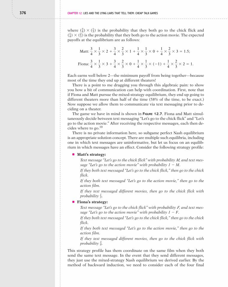
376 CHAPTER 12: LIES AND THE LYING LIARS THAT TELL THEM: CHEAP TALK GAMES
where is the probability that they both go to the chick flick andis the probability that they both go to the action movie. The expected
payoffs at the equilibrium are as follows:
Each earns well below 2—the minimum payoff from being together—becausemost of the time they end up at different theaters!
There is a point to me dragging you through this algebraic pain: to showyou how a bit of communication can help with coordination. First, note thatif Fiona and Matt pursue the mixed-strategy equilibrium, they end up going todifferent theaters more than half of the time (58% of the time, to be exact.)Now suppose we allow them to communicate via text messaging prior to de-ciding on a theater.
The game we have in mind is shown in FIGURE 12.7. Fiona and Matt simul-taneously decide between text messaging “Let’s go to the chick flick” and “Let’sgo to the action movie.” After receiving the respective messages, each then de-cides where to go.10
There is no private information here, so subgame perfect Nash equilibriumis an appropriate solution concept. There are multiple such equilibria, includingone in which text messages are uninformative, but let us focus on an equilib-rium in which messages have an effect. Consider the following strategy profile:
■ Matt’s strategy:Text message “Let’s go to the chick flick” with probability M, and text mes-sage “Let’s go to the action movie” with probability If they both text messaged “Let’s go to the chick flick,” then go to the chickflick.If they both text messaged “Let’s go to the action movie,” then go to theaction film.If they text messaged different movies, then go to the chick flick withprobability
■ Fiona’s strategy:Text message “Let’s go to the chick flick” with probability F, and text mes-sage “Let’s go to the action movie” with probability If they both text messaged “Let’s go to the chick flick,” then go to the chickflick.If they both text messaged “Let’s go to the action movie,” then go to theaction film.If they text messaged different movies, then go to the chick flick withprobability
This strategy profile has them coordinate on the same film when they bothsend the same text message. In the event that they send different messages,they just use the mixed-strategy Nash equilibrium we derived earlier. By themethod of backward induction, we need to consider each of the four final
34.
1 " F.
13.
1 " M.
Fiona: 34
!13
! 3 %34
!23
! 0 %14
!13
! ("1) %14
!23
! 2 # 1.
Matt: 34
!13
! 2 %34
!23
! 1 %14
!13
! 0 %14
!23
! 3 # 1.5;
(14) ! (2
3)(3
4) ! (13)
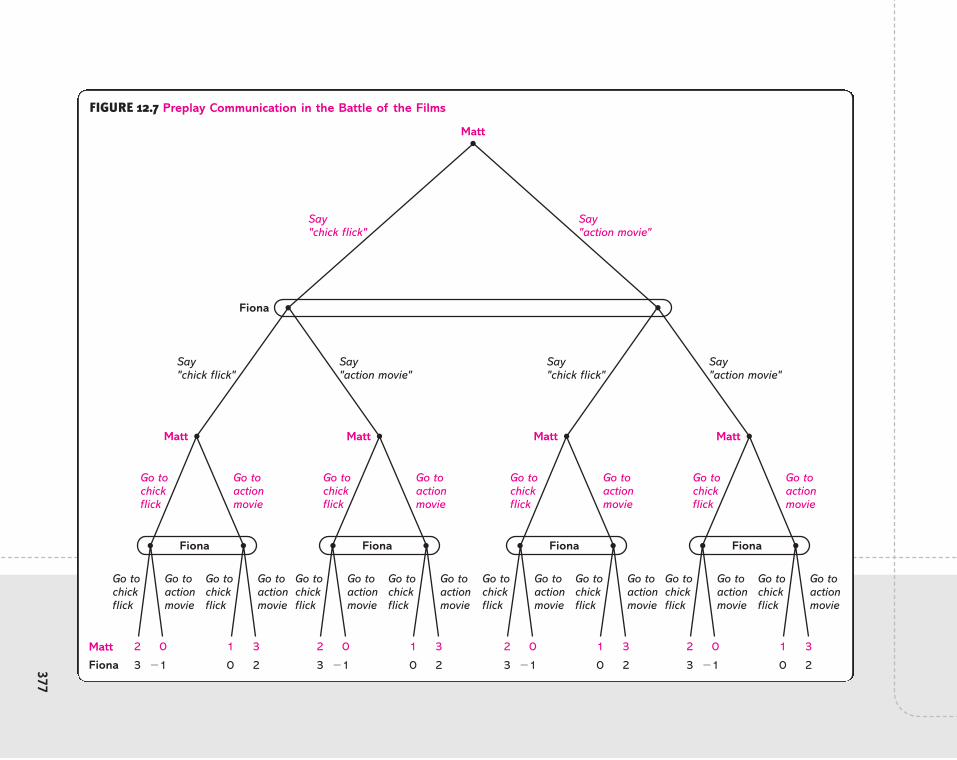
FionaMatt
Matt
Matt
Go to chick flick
Say "chick flick"
Say "chick flick"
Go to chick flick
Go to action movie
0
"1
2
3
Fiona
Fiona
Go to chick flick
Go to action movie
Say "action movie"
Go to action movie
3
2
1
0
Matt
Go to chick flick
Go to chick flick
Go to action movie
0
"1
2
3
Fiona
Go to chick flick
Go to action movie
Go to action movie
3
2
1
0
Matt
Go to chick flick
Say "chick flick"
Go to chick flick
Go to action movie
0
"1
2
3
Fiona
Go to chick flick
Go to action movie
Say "action movie"
Say "action movie"
Go to action movie
3
2
1
0
Matt
Go to chick flick
Go to chick flick
Go to action movie
0
"1
2
3
Fiona
Go to chick flick
Go to action movie
Go to action movie
3
2
1
0
FIGURE 12.7 Preplay Communication in the Battle of the Films
377

378 CHAPTER 12: LIES AND THE LYING LIARS THAT TELL THEM: CHEAP TALK GAMES
subgames. (See Figure 12.7.) First, consider the one associated with both hav-ing text messaged “Let’s go to the chick flick.” Their strategies then have themboth go to the chick flick, which is indeed a Nash equilibrium. For the sub-game in which they text messaged “Let’s go to the action movie,” they are togo to the action movie, and again, this is a Nash equilibrium. For the two sub-games in which their text messages are different, Matt goes to the chick flickwith probability and Fiona goes to it with probability and we already knowthat this substrategy pair is a Nash equilibrium.
Substituting each subgame with its associated equilibrium payoffs, wederive the game in FIGURE 12.8. It will be easier, however, to work with itsstrategic form, which is shown in FIGURE 12.9. For this game, we want tosolve for the equilibrium values of M and F. In the usual manner, M must
34,1
3
Matt
Say "chick flick"
Say "chick flick"
Fiona
Say "action movie"
FionaMatt 2
3
1.5
1
1.5
1
3
2
Say "chick flick"
Say "action movie"
Say "action movie"
FIGURE 12.8 Battle of the Films after Solving the Final Subgames
2,3
1.5,1
1.5,1
3,2Matt
Fiona
"Let's go to the chick flick"
"Let's go to the action movie"
"Let's go to the chick flick" "Let's go to the action movie"
FIGURE 12.9 Strategic Form of the Extensive Form Game in Figure 12.8

12.4 Signaling Intentions 379
result in Fiona’s being indifferent between her two feasible text messages;that is,
Solving this equation gives us The value for F must make Matt simi-larly indifferent:
Solving this equation yields Thus, the strategy profile presented is asubgame perfect Nash equilibrium when and
Given this equilibrium, let’s calculate the probability of Fiona and Mattending up at the same theater. That’ll happen if either they send the same textmessage (and thereby coordinate at the message stage) or they send differentmessages but luck out by going to the same theater. The former event occurswith probability or Even if their text messages do notmatch, which occurs with probability or when they come to actu-ally choose where to go, the probability that they end up in the same place is
(which we derived earlier). The probability that they send different mes-sages but still go to the same theater is then or The total prob-ability that they end up watching the same film is the sum of these two prob-abilities, or
When there was no opportunity to engage in preplay communication, theprobability that Fiona and Matt go to the same theater was .42. Allowing themto first text message each other raises the probability to .66. In this way, pre-play communication can be useful even when there is no private information.It provides players with an opportunity to signal their intentions, and that canhelp players to coordinate their actions. It is important that this is a setting inwhich players do have a certain degree of commonality of interest; that way,there is a basis for wanting to coordinate. If, however, Fiona was trying tobreak up with Matt, then her text message would end up being uninformative.
12.4.2 Preplay Communication in PracticeAlthough the preceding analysis suggests that a round of commu-nication may help with coordination, it would be more convincingto observe actual behavior. Let’s then review some experimentalevidence.11 For the payoffs used in the experiment (which areshown in FIGURE 12.10), the mixed-strategy Nash equilibrium hasthe two players coordinate 37.5% of the time when there is nopreplay communication.* The game with preplay communicationis as we just modeled it, but with the addition of a third message:Each player can either signal his intent to play x, signal his intentto play y, or say nothing.
Predictions were taken from the equilibrium for which players anticipate(1) both playing x when either both signaled their intent to play x or one playersignaled an intent to play x and the other remained silent; (2) both playing y
( 512) % ( 35
144) # 95144 " .66.
35144.( 7
12) ! ( 512),
512
712,1 " ( 5
12),
512.(3
4) ! (13) % (1
4) ! (23),
M # 13.F # 3
4
F # 34.
F ! 2 % (1 " F) ! 1.5 # F ! 1.5 % (1 " F) ! 3.
M # 13.
M ! 3 % (1 " M) ! 1 # M ! 1 % (1 " M) ! 2.
* .
,
,
,
,Player 1
Player 2
x
y
x y
FIGURE 12.10 Battle of the Sexes
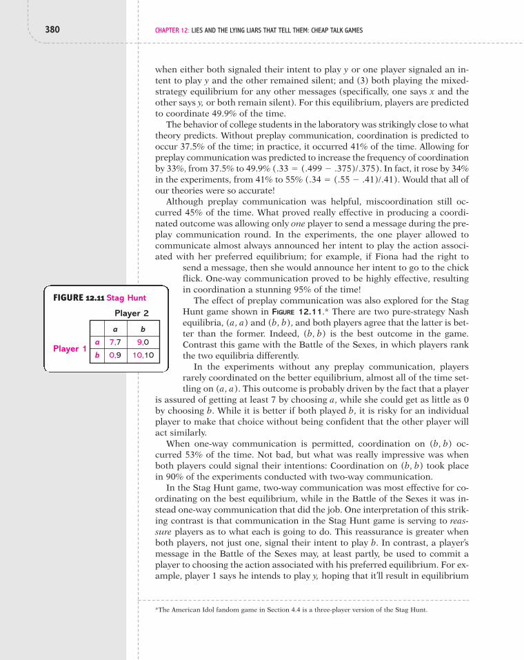
380 CHAPTER 12: LIES AND THE LYING LIARS THAT TELL THEM: CHEAP TALK GAMES
when either both signaled their intent to play y or one player signaled an in-tent to play y and the other remained silent; and (3) both playing the mixed-strategy equilibrium for any other messages (specifically, one says x and theother says y, or both remain silent). For this equilibrium, players are predictedto coordinate 49.9% of the time.
The behavior of college students in the laboratory was strikingly close to whattheory predicts. Without preplay communication, coordination is predicted tooccur 37.5% of the time; in practice, it occurred 41% of the time. Allowing forpreplay communication was predicted to increase the frequency of coordinationby 33%, from 37.5% to 49.9% In fact, it rose by 34%in the experiments, from 41% to 55% Would that all ofour theories were so accurate!
Although preplay communication was helpful, miscoordination still oc-curred 45% of the time. What proved really effective in producing a coordi-nated outcome was allowing only one player to send a message during the pre-play communication round. In the experiments, the one player allowed tocommunicate almost always announced her intent to play the action associ-ated with her preferred equilibrium; for example, if Fiona had the right to
send a message, then she would announce her intent to go to the chickflick. One-way communication proved to be highly effective, resultingin coordination a stunning 95% of the time!
The effect of preplay communication was also explored for the StagHunt game shown in FIGURE 12.11.* There are two pure-strategy Nashequilibria, and and both players agree that the latter is bet-ter than the former. Indeed, is the best outcome in the game.Contrast this game with the Battle of the Sexes, in which players rankthe two equilibria differently.
In the experiments without any preplay communication, playersrarely coordinated on the better equilibrium, almost all of the time set-tling on This outcome is probably driven by the fact that a player
is assured of getting at least 7 by choosing a, while she could get as little as 0by choosing b. While it is better if both played b, it is risky for an individualplayer to make that choice without being confident that the other player willact similarly.
When one-way communication is permitted, coordination on oc-curred 53% of the time. Not bad, but what was really impressive was whenboth players could signal their intentions: Coordination on took placein 90% of the experiments conducted with two-way communication.
In the Stag Hunt game, two-way communication was most effective for co-ordinating on the best equilibrium, while in the Battle of the Sexes it was in-stead one-way communication that did the job. One interpretation of this strik-ing contrast is that communication in the Stag Hunt game is serving to reas-sure players as to what each is going to do. This reassurance is greater whenboth players, not just one, signal their intent to play b. In contrast, a player’smessage in the Battle of the Sexes may, at least partly, be used to commit aplayer to choosing the action associated with his preferred equilibrium. For ex-ample, player 1 says he intends to play y, hoping that it’ll result in equilibrium
(b, b)
(b, b)
(a, a).
(b, b)(b, b),(a, a)
(.34 # (.55 " .41)/.41).(.33 # (.499 " .375)/.375).
*The American Idol fandom game in Section 4.4 is a three-player version of the Stag Hunt.
7,7
0,9
9,0
10,10Player 1
Player 2
a
b
a b
FIGURE 12.11 Stag Hunt

Summary 381
being played. But since players have different preferences regarding equi-libria, these messages may fail to result in any coordination, as player 1 signalshis intent to play y and player 2 signals her intent to play x. If, instead, only oneplayer can send a message, then there is no possibility for conflicting signals atthe preplay communication stage, and coordination becomes more likely.
SummaryThe ability to communicate in a rich manner is a distinctive trait of humanity.Although vervet monkeys have the capacity to communicate whether it is asnake, hawk, or a tiger in the vicinity, animal communication doesn’t getmuch more sophisticated than that. The human lexicon is rich not only inwords, but also in gestures. Indeed, people can create a language that capturesthe specifics of a particular situation, such as teenagers IM’ing PIR (“parent inroom”) or a couple making eye contact at a boring dinner party, signaling eachother that it’s time to head home. However, although a rich shared language isnecessary for communication, it need not be sufficient to result in informationbeing transmitted: The intelligence that allows for such sophisticated lan-guages also produces an ability to deceive, which can seriously deteriorate thesubstantive content of the messages we send to each other.
This chapter explored communication in the context of a cheap talk game,which is a signaling game in which the sender’s choice is a message (i.e., acostless action in the sense that it does not directly affect players’ payoffs).Although there always exists a babbling equilibrium with wholly uninforma-tive messages, whether there is an equilibrium with informative messagesrests on the commonality of interests between the sender and receiver of amessage. If those interests are sufficiently similar, then messages can be in-formative. For example, if a pitcher signals to a catcher that he intends tothrow a fast ball, the catcher is correct in believing him, because the pitcherand catcher have a common interest in striking out the batter. However, if theinterests of the two parties are sufficiently divergent, then messages containno informative content. For example, if the catcher whispers to the batter thatthe pitcher will throw a curve ball, the batter should ignore such a message.For if the batter were to believe the message, then the catcher would instructthe pitcher to throw a fast ball instead. The problem is that the catcher wantsthe batter to strike out, while the batter wants to get a hit. With such diamet-rically opposed interests, what is said cannot be believed. Messages are thenuninformative.*
Our exploration of the role of communication prior to play was conductedfor two types of scenarios. In a game of incomplete information, a messagehas the potential to convey what one player knows about the game itself, suchas payoffs. For instance, in the Stock Recommendations game, a stock analysthas an expectation about how a stock will perform, and his buy, hold, or sellrecommendation may convey what he knows and what his client does not.
(y, x)
*Now, if you’ve seen the film Bull Durham, you might say, “Wait a minute. In that movie, the catcher doestell the batter what pitch is coming, and the batter believes him.” You would be right, but this is actuallyyet more confirmation of the lessons of this chapter. In the situation shown in the film, the catcher wasmiffed at the pitcher and wanted the batter to get a hit. Since the catcher’s and batter’s interests were coin-cident (and the batter knew this), the batter could believe the catcher when he told him that the pitcher wasgoing to throw a curve ball. That is indeed what was thrown, and the batter drilled the ball out of the park.

382 CHAPTER 12: LIES AND THE LYING LIARS THAT TELL THEM: CHEAP TALK GAMES
This action was referred to as “signaling information.” Preplay communica-tion can also be useful in a game of complete information, in which playershave common knowledge about the game. In that case, the role of a messageis to convey a player’s intended play. “Signaling intentions” can allow playersto coordinate. In the Battle of the Films game, Fiona and Matt needed to co-ordinate on a theater, and exchanging text messages beforehand increased thechances of that happening.
1. For the game in FIGURE PR12.1, find a separating perfect Bayes–Nashequilibrium.
EXERCISES
2. Consider a cheap talk game in which Nature moves by choosing asender’s type, where the type space has four elements: 1, 2, and 3,each occurring with equal probability of The sender learns his typeand chooses one of three possible messages: bumpy, smooth, and slick.The receiver observes the sender’s message and then chooses one ofthree actions: 0, 5, and 10. The sender’s payoff equals his type multipliedby the receiver’s action. The receiver’s payoff equals the sender’s typemultiplied by twice the receiver’s payoff.
14.
"1,
Nature
a
x y x y x y x y
b a b
3
2
2
1
2 2 2 2
Player 2Player 1
1 1
3
2
2
1
1
0
2
1
1
0
2
1
Type sProbability " 1
2
Type tProbability " 1
2
FIGURE PR12.1

Exercises 383
a. Find a separating perfect Bayes–Nash equilibrium.b. Find a semiseparating perfect Bayes–Nash equilibrium.
3. Consider a cheap talk game in which Nature chooses the sender’s typeand there are three feasible types: x, y, and z, which occur with proba-bility and respectively. The sender learns her type and then choosesone of four possible messages: or The receiver observesthe sender’s message and chooses one of three actions: a, b, or c. Thepayoffs are shown in the table below.
m4.m3,m2,m1,
12,1
4,14,
a. Suppose the sender’s strategy is as follows: (1) if the type is x, thenchoose message and (2) if the type is y or z, then choose message
The receiver’s strategy is the following: (1) if the message is then choose action a; (2) if the message is then choose action b;and (3) if the message is or then choose action a. For appro-priately specified beliefs for the receiver, show that this strategy pairis a perfect Bayes–Nash equilibrium.
b. Find a separating perfect Bayes–Nash equilibrium.
4. Return to the Stock Recommendation game, and consider again the semi-separating strategy profile, but let the analyst’s strategy now be as follows:Recommend buy when the stock will outperform or be neutral; and recom-mend sell when the stock will underperform. Show that if thenthis strategy pair is part of a perfect Bayes–Nash equilibrium.
5. FIGURE PR12.5 is a cheap talk game in which the sender has two possibletypes—denoted and —and can choose one of two possible mes-sages—denoted and After observing the sender’s message, the re-ceiver chooses from amongst three possible actions: a, b, and c.a. Find a separating perfect Bayes–Nash equilibrium.b. Find a pooling perfect Bayes–Nash equilibrium.c. Suppose the probability that the sender is type is p and the proba-
bility that the sender is type is Find the values for p such thatthere is a pooling perfect Bayes–Nash equilibrium in which the re-ceiver chooses action b.
1 " p.t2
t1
m2.m1
t2t1
a % b $ 2
m4,m3
m2,m1,m2.
m1,
Sender’s Receiver’s Sender’s Receiver’sType Action Payoff Payoff
x a 3 3
x b 2 1
x c 1 2
y a 4 1
y b 5 3
y c 3 4
z a 3 2
z b 9 1
z c 10 0

384 CHAPTER 12: LIES AND THE LYING LIARS THAT TELL THEM: CHEAP TALK GAMES
6. Suppose Grace and Lisa are to go to dinner. Lisa is visiting Grace fromout of town, and they are to meet at a local restaurant. When Lisa livedin town, they had two favorite restaurants: Bel Loc Diner and the CornerStable. Of course, Lisa’s information is out of date, but Grace knowswhich is better these days. Assume that the probability that the Bel LocDiner is better is and the probability that the Corner Stable is bet-ter is Nature determines which restaurant Grace thinks is better.Grace then sends a message to Lisa, either “Let’s go to the Bel LocDiner,” “Let’s go to the Corner Stable,” or “I don’t know [which is bet-ter].” Lisa receives the message, and then Grace and Lisa simultaneouslydecide which restaurant to go to. Payoffs are such that Grace and Lisawant to go to the same restaurant, but they prefer it to be the one thatGrace thinks is better. More specifically, if, in fact, the Bel Loc Diner isbetter, then the payoffs from their actions are as shown in FIGURE
PR12.6(A). If, instead, the Corner Stable is better, then FIGURE PR12.6(B)describes the payoffs.
1 " p.p 7 1
2
FIGURE PR12.5
Nature
m1 m2 m1 m2
a b c
1
0
4
3
2
4
Receiver
ReceiverSender
Sender
t1 Probability " .6
t2Probability " .4
a b c
1
0
4
3
2
4
a b c
3
5
0
1
2
4
3
5
0
1
2
4
a b c
FIGURE PR12.6A Payoffs When the Bel Loc Diner Is Better
2,2
0,0
0,0
1,1Grace
Lisa
Bel Loc Diner
Corner Stable
Bel Loc Diner Corner Stable
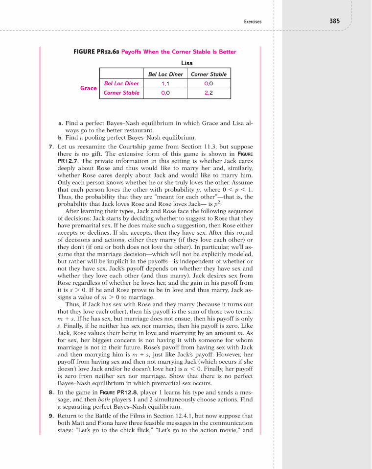
Exercises 385
a. Find a perfect Bayes–Nash equilibrium in which Grace and Lisa al-ways go to the better restaurant.
b. Find a pooling perfect Bayes–Nash equilibrium.
7. Let us reexamine the Courtship game from Section 11.3, but supposethere is no gift. The extensive form of this game is shown in FIGURE
PR12.7. The private information in this setting is whether Jack caresdeeply about Rose and thus would like to marry her and, similarly,whether Rose cares deeply about Jack and would like to marry him.Only each person knows whether he or she truly loves the other. Assumethat each person loves the other with probability p, where Thus, the probability that they are “meant for each other”—that is, theprobability that Jack loves Rose and Rose loves Jack— is
After learning their types, Jack and Rose face the following sequenceof decisions: Jack starts by deciding whether to suggest to Rose that theyhave premarital sex. If he does make such a suggestion, then Rose eitheraccepts or declines. If she accepts, then they have sex. After this roundof decisions and actions, either they marry (if they love each other) orthey don’t (if one or both does not love the other). In particular, we’ll as-sume that the marriage decision—which will not be explicitly modeled,but rather will be implicit in the payoffs—is independent of whether ornot they have sex. Jack’s payoff depends on whether they have sex andwhether they love each other (and thus marry). Jack desires sex fromRose regardless of whether he loves her, and the gain in his payoff fromit is If he and Rose prove to be in love and thus marry, Jack as-signs a value of to marriage.
Thus, if Jack has sex with Rose and they marry (because it turns outthat they love each other), then his payoff is the sum of those two terms:
If he has sex, but marriage does not ensue, then his payoff is onlys. Finally, if he neither has sex nor marries, then his payoff is zero. LikeJack, Rose values their being in love and marrying by an amount m. Asfor sex, her biggest concern is not having it with someone for whommarriage is not in their future. Rose’s payoff from having sex with Jackand then marrying him is just like Jack’s payoff. However, herpayoff from having sex and then not marrying Jack (which occurs if shedoesn’t love Jack and/or he doesn’t love her) is . Finally, her payoffis zero from neither sex nor marriage. Show that there is no perfectBayes–Nash equilibrium in which premarital sex occurs.
8. In the game in FIGURE PR12.8, player 1 learns his type and sends a mes-sage, and then both players 1 and 2 simultaneously choose actions. Finda separating perfect Bayes–Nash equilibrium.
9. Return to the Battle of the Films in Section 12.4.1, but now suppose thatboth Matt and Fiona have three feasible messages in the communicationstage: “Let’s go to the chick flick,” “Let’s go to the action movie,” and
u 6 0
m % s,
m % s.
m 7 0s 7 0.
p2.
0 6 p 6 1.
FIGURE PR12.6B Payoffs When the Corner Stable Is Better
1,1
0,0
0,0
2,2Grace
Lisa
Bel Loc Diner
Corner Stable
Bel Loc Diner Corner Stable

FIGURE PR12.7 The Courtship Game with Cheap Talk
Rose loves Jack Probability " p
Jack loves Rose Probability " p
Jack does notlove Rose Probability " 1 # p
Rose does not love Jack Probability " 1 # p
Nature
Nature
Accept
Suggests Does notsuggest
Suggests Does notsuggest
Suggests Does notsuggest
Suggests Does notsuggest
Decline
m
m
m
m
s
Rose
RoseJack
Jack
m % s
m % s u
Accept Decline
0
0
0
0
0
0
0
0
Rose loves Jack Probability " p
Rose does not love Jack Probability " 1 # p
Accept Decline
s
u
s
u
Accept Decline
0
0
0
0
386

Nature
y z
3
2
0
0
1
1
2
Player 2Player 1
y z
1
1
2
3
y z
3
2
0
0
y z
1
1
2
3
y z
0
0
1
1
y z
4
4
0
0
y z
0
0
1
1
y z
4
4
0
0
a b a b
w x w x w x w x
Type sProbability " 1
3
Type tProbability " 2
3
FIGURE PR12.8
387

388 CHAPTER 12: LIES AND THE LYING LIARS THAT TELL THEM: CHEAP TALK GAMES
“Party on.” Derive values for a, b, y, and z whereby the following strategyprofile is a subgame perfect Nash equilibrium:
■ Matt’s strategy:Text message “Let’s go to the chick flick” with probability a, “Let’s go tothe action movie” with probability b, and “Party on” with probability
Go to the chick flick if either (1) they both text messaged “Let’s go to thechick flick” or (2) one text messaged “Let’s go to the chick flick” and theother text messaged “Party on.”Go to the action movie if either (1) they both text messaged “Let’s go tothe action movie” or (2) one text messaged “Let’s go to the actionmovie” and the other text messaged “Party on.”For any other messages, go to the chick flick with probability
■ Fiona’s strategy:Text message “Let’s go to the chick flick” with probability y, “Let’s go tothe action movie” with probability z, and “Party On” with probability
Go to the chick flick if either (1) they both text messaged “Let’s go to thechick flick” or (2) one text messaged “Let’s go to the chick flick” and theother text messaged “Party on.”Go to the action movie if either (1) they both text messaged “Let’s go tothe action movie” or (2) one text messaged “Let’s go to the actionmovie” and the other text messaged “Party on.”For any other messages, go to the chick flick with probability
10. Return to the Battle of the Films in Section 12.4.1, but suppose now thatthere are two rounds of preplay communication rather than just one.Find a subgame perfect Nash equilibrium.
34.
1 " y " z.
13.
1 " a " b.
REFERENCES1. Thomas Chandler Haliburton, Sam Slick in England; or The Attaché (New
York: J. Winchester, 1843).
2. Paul F. Boller, Jr., Congressional Anecdotes (New York: Oxford UniversityPress, 1991), p. 104.
3. “McGwire admits nothing; Sosa and Palmeiro deny use,” ESPN.com newsservices, Mar. 18, 2005.
4. Call-Chronicle, Allentown, Pennsylvania, Feb. 3, 1963; cited in ErvingGoffman, Strategic Interaction (Philadelphia: University of PennsylvaniaPress, 1969), p. 16.
5. These findings are from David M. Studdert, et al., “Defensive MedicineAmong High-Risk Specialist Physicians in a Volatile MalpracticeEnvironment,” Journal of American Medical Association, 293 (2005),2609–17.
6. This model and its analysis are inspired by Kris De Jaegher and MarcJegers, “The Physician–Patient Relationship as a Game of StrategicInformation Transmission,” Health Economics, 10 (2001), 651–68.

References 389
7. This principle was first identified in Vince Crawford and Joel Sobel’s sem-inal paper on cheap talk games, “Strategic Information Transmission,”Econometrica, 50 (1982), 1431–51.
8. For a related analysis, see John Morgan and Phillip C. Stocken, “AnAnalysis of Stock Recommendations,” RAND Journal of Economics, 34(2003), 183–203.
9. William Power, “Analysts’ Terminology is Getting More Risky as “Strong-Hold” Rating Grows in Popularity,” Wall Street Journal, circa June 1993.
10. The ensuing analysis is based on Joseph Farrell, “Cheap Talk,Coordination, and Entry,” Rand Journal of Economics, 18 (1987), 34–39.
11. For a survey of this work, see Vince Crawford, “A Survey of Experimentson Communication via Cheap Talk,” Journal of Economic Theory, 78(1998), 286–98.

This page intentionally left blank

It is only those who have neither fired a shot nor heard the shrieks andgroans of the wounded who cry aloud for blood, more vengeance, moredesolation. War is hell. —GENERAL WILLIAM TECUMSEH SHERMAN
13.1 Trench Warfare in World War IWAR REMOVES THE MORAL RESTRAINTS that society puts on behavior. To kill an-other human is murder, but in a time of war, it is doing one’s duty. In terms ofthe amount of human carnage, World War I set the macabre standard bywhich all later wars are compared. Much of this killing took place from thetrenches constructed in France and other theaters of the war. The Allied andGerman sides would engage in sustained periods of combat as they regularlylaunched offensives from their dirt fortifications.
In the midst of this bloodletting, humanity did not entirely disappear. Peacewould occasionally flare up as the soldiers in opposing trenches would achievea truce. They would shoot at predictable intervals so that the other side couldtake cover, not shoot during meals, and not fire artillery at the enemy’s supplylines. But why listen to me when we can draw upon the authentic accounts ofthe soldiers in the trenches:1
In one section [of the camp] the hour of 8 to 9 A.M. was regarded as conse-crated to “private business,” and certain places indicated by a flag were re-garded as out of bounds by snipers on both sides.
So regular were [the Germans] in their choice of targets, times of shooting,and number of rounds fired, that, after being in the line one or two days,Colonel Jones had discovered their system, and knew to a minute where thenext shell would fall. His calculations were very accurate, and he was ableto take what seemed to uninitiated Staff Officers big risks, knowing that theshelling would stop before he reached the place being shelled.
I was having tea with A Company when we heard a lot of shouting and wentout to investigate. We found our men and the Germans standing on their re-spective parapets. Suddenly a salvo arrived but did no damage. Naturallyboth sides got down and our men started swearing at the Germans, when allat once a brave German got on to his parapet and shouted out “We are verysorry about that; we hope no one was hurt. It is not our fault, it is thatdamned Prussian artillery.”
At a time when killing was routine, these soldiers were able to reach an agree-ment not to kill each other. How was this cooperation achieved and sustained?As you might expect, game theory can shed some light on this puzzle. Toward
13
391
Playing Forever: Repeated Interactionwith Infinitely Lived Players

392 CHAPTER 13: PLAYING FOREVER: REPEATED INTERACTION WITH INFINITELY LIVED PLAYERS
that end, we’ll begin by constructing a strategic form game of the situationfaced by the soldiers in the trenches.
For simplicity, think of the war as having two players: Allied soldiers (as agroup) and German soldiers (as a group). Each player has two strategies.Soldiers can try to kill the enemy (shoot to kill) or not (shoot to miss). Ofcourse, it would be all too easy to generate the observed nonhostile behavior bysimply assuming that a soldier disliked killing the enemy. But that would be anassumption patently rejected by the many other instances in which soldiers didtry to kill. Rather, let us assume that each soldier values killing the enemy, butplaces a greater value on not getting killed. Specifically, a soldier’s payoff equals
4 % 2 ! (number of enemy soldiers killed) " 4 ! (number of own soldiers killed)
Soldiers in a Trench During World War I
HU
LTO
N A
RCH
IVES
/GET
TY IM
AG
ES
2,2
0,6
6,0
4,4Allied soldiers
German soldiers
Kill
Miss
Kill Miss
Note that a soldier’s payoff is higher when more of the enemy is killed, but islower when more of his own side are killed. Furthermore, an exchange of “onefor one” in terms of fatalities makes a soldier worse off, since, for each deathon his side, his payoff falls by four, and for each death on the other side, it risesby two, so that, on net, the payoff is decreased by two.
Next, assume that shooting to kill results in the death of oneenemy soldier and shooting to miss doesn’t kill anyone. Thisspecification results in the strategic form game depicted inFIGURE 13.1.
There is a unique Nash equilibrium in which both sides tryto kill each other. This solution is extremely compelling, be-cause it has kill as a dominant strategy. (In fact, this game isjust the Prisoners’ Dilemma.) Regardless of what the other sidedoes, a soldier is better off shooting to kill. Since he cannot in-fluence how many of his own side dies—that is determined by
FIGURE 13.1 Trench Warfare Game

13.2 Constructing a Repeated Game 393
what the enemy does—all he can affect is how many of the enemy perish. Sincethe more enemy soldiers that die, the better, kill is a dominant strategy.Nevertheless, both sides could make themselves better off if they could cooper-ate and agree not to try and kill each other; doing so would raise each player’spayoff from 2 to 4.
We have obviously failed in our mission to explain the periodic presence ofpeace in the trenches of World War I. Where did we go wrong? Did we mis-specify the preferences of the soldiers? Is the assumption of rationality off tar-get? To gain a clue, we might ask ourselves, Why was this peaceful behaviorobserved in the trenches of World War I and rarely in other theaters of this ormost any other war? A unique feature of trench warfare is that soldiers on thetwo sides repeatedly encounter each other. They weren’t just deciding once inthe heat of battle whether to shoot to kill, but rather made the same decisionday after day. Due to the entrenched nature of this style of warfare, soldiers re-peatedly faced each other over time.
Repetition of strategic interactions is the key to solving the puzzle of peace-ful behavior in the trenches of World War I, and it is what we’ll explore in thischapter. In many strategic settings—not just the trenches—repeated encoun-ters can sustain cooperation, which refers to players acting in a manner thatresults in everyone receiving a higher payoff than is achieved when the game isplayed just once. In Section 13.2, we formally construct a game with repeatedencounters. Then, in Sections 13.3 and 13.4, the Trench Warfare game is ana-lyzed, first when the number of encounters is finite (say, seven) and then whenit can go on forever. Section 13.5 offers some relevant experimental evidenceand shows that there is much about human behavior that we still do not un-derstand. Chapter 14 follows up with a variety of applications and draws someadditional insight into situations in which people repeatedly interact.
13.2 Constructing a Repeated GameA REPEATED GAME IS SIMPLY a situation in which players have the same en-counter—known as the stage game—over and over. The stage game is thebuilding block used to construct a repeated game and can be any game with afinite number of moves. For example, the game in Figure 13.1 is the stagegame that will ultimately result in a repeated-game version of trench warfare.In moving from the stage game to the repeated game, we need to redefinestrategy sets and payoff functions. Because a strategy is a fully specified deci-sion rule for a game, a feasible decision rule will look different if a player isexpected to have multiple encounters rather than just one. As for payoffs, it isnatural to assume that a player takes into account her well-being for all en-counters and not just the current one.
Suppose the Allied and German soldiers anticipate interacting T times inthe manner described in Figure 13.1. Think of their encounters occurring oncea day for T days. For the game in Figure 13.1, kill was a strategy, but a strat-egy is a more complex object in a repeated game. A strategy in the stage game,kill or miss, is now defined to be an action in the repeated game. The notionof a strategy in a repeated game is the same as for any extensive form game:A strategy for a player assigns an action to every information set. Thus, whata strategy looks like depends on what a player knows when he has to make adecision.

394 CHAPTER 13: PLAYING FOREVER: REPEATED INTERACTION WITH INFINITELY LIVED PLAYERS
Let’s consider two different information structures when so that thestage game is played just twice. This means that on day one the Allied andGerman soldiers simultaneously decide between kill and miss and then againmake simultaneous decisions on day two. FIGURE 13.2 is the extensive formgame when what happens on day one is not publicly known when playersmove again on day two. (At present, ignore the payoffs, which we’ll explainmomentarily.) Note that each player knows what he did on day one (other-wise, the game would not satisfy perfect recall), but doesn’t know what theother player did on day one, when he has to decide what to do on day two. TheAllied soldiers have three information sets: (I) the initial information set onday one, (II) the information set associated with having chosen kill on day one,and (III) the information set associated with having chosen miss on day one.A strategy is then a triple of actions, and a strategy set is composed of the eightways in which to assign kill and miss to the three information sets.
Contrast this game with the extensive form game shown in FIGURE 13.3. Thetree is exactly the same; what differs is the structure of the information sets. Nowit is assumed that what happened on day one is revealed to both players prior totheir deciding what to do on day two. Each player has five information sets: oneassociated with day one and four associated with day two. There are four for daytwo because there are four things that a player could know about what happenedon day one: (1) both sides could have chosen kill, (2) the Allied soldiers couldhave chosen kill and the German soldiers miss, (3) the Allied soldiers could havechosen miss and the German soldiers kill, and (4) both sides could have chosenmiss. A strategy for a player is then a quintuple of actions—one for each of thefive information sets—and there are feasible strategies.
This chapter will focus exclusively on the case when the history—that is, thepast choices of players—is common knowledge, as reflected in the game inFigure 13.3. For when the history is common knowledge and the stage game isplayed thrice, there are 21 information sets: the information set at the start ofday one, the 4 information sets associated with the start of day two, and the 16information sets associated with the start of day three. An information set forday three summarizes what happened over days one and two, which could be,for example, that both players chose miss on day one, and the Allied soldierschose kill on day two and the German soldiers chose miss on day two. There are16 histories for days one and two and thus 16 information sets for day three. Inthat case, a strategy for the three-period repeated game is a “21-tuple” of actions.
More generally, a strategy prescribes an action for each period, contingenton the history (and thus on what a player knows). For a general repeated gamewith T periods and for which each player has m actions in the stage game,there is one initial information set, information sets associated with period2, associated with period 3, . . . , and associated with period T.Thus, a strategy is a collection of actions. For aninfinitely repeated game (in which a strategy is an infinite number ofactions, since there is an infinite number of information sets. Although a strat-egy could be of mind-boggling complexity and size, that need not be the case.In fact, we’ll see that the resolution of the trench warfare puzzle can beachieved with very simple strategies.
The next ingredient in the construction of a repeated game is payoffs. Just asa strategy for the stage game is referred to as an action for the repeated game,a payoff for the stage game will be referred to as a single-period (or one-shot)
T # q),1 % m2 % m4 % p % m2(T"1)
m2(T"1)m4m2
25 # 32
T # 2,

Kill Miss Kill Miss
Kill Miss
Kill Miss
Kill Miss
Kill Miss
8
2
4
4
German
German
GermanAllied
Allied
Allied
II
I
6
6
2
8
Kill Miss Kill Miss
12
0
8
2
10
4
6
6
Kill Miss
Kill Miss Kill Miss
Kill Miss
6
6
2
8
III
4
10
0
12
Kill MissKill Miss Kill Miss
10
4
6
6
8
8
4
10
FIGURE 13.2 Two-Period Trench Warfare Game without Common Knowledge of the History
395

Kill Miss Kill Miss
Kill Miss
Kill Miss
Kill Miss
Kill Miss
8
2
4
4
German
German
GermanAllied
Allied
Allied
6
6
2
8
Kill Miss Kill Miss
12
0
8
2
10
4
6
6
Kill Miss
Kill Miss Kill Miss
Kill Miss
6
6
2
8
4
10
0
12
Kill MissKill Miss Kill Miss
10
4
6
6
8
8
4
10
FIGURE 13.3 Two-Period Trench Warfare Game with Common Knowledge of the History
396

13.2 Constructing a Repeated Game 397
payoff for the repeated game. The well-being of a player for the repeated gameis assumed to be influenced by the entire stream of single-period payoffs. For ex-ample, if and the history is
(miss,miss), (kill,miss), (miss,miss), (miss,kill), (kill,kill),
where the first action in each ordered pair is for the Allied side, then, from Figure13.1, the stream of single-period payoffs for the Allied soldiers is 4, 6, 4, 0, 2.
In selecting a strategy for a repeated game, the assumption is that a playerchooses the strategy that yields the best stream of payoffs. But what does itmean for one stream to be “better” than another stream? In comparing thestream 4, 6, 4, 0, 2 with the stream 6, 6, 6, 0, 2, it would seem quite compellingthat the latter is preferred, because it gives a higher single-period payoff in pe-riods 1 and 3 and the same values in the other periods. But suppose the alter-native stream is 6, 4, 4, 2, 6. Then, in a comparison with 4, 6, 4, 0, 2, it isn’tobvious which is better, because 6, 4, 4, 2, 6 is more attractive in periods 1, 4,and 5 and the other is better in period 2.
What we need is a criterion for comparing streams. A common device fordoing so is boiling a stream down to a single number—called a summary sta-tistic—and then assuming that a player chooses astrategy so as to maximize the summary statistic. Anatural candidate for the summary statistic is thesum of the single-period payoffs. Not only does ithave the appeal of simplicity, but also, the sum-mary statistic is higher whenever a single-periodpayoff is higher, which makes sense. For the threestreams examined in the previous paragraph, TABLE
13.1 reports this summary statistic. If that is whatwere used, the Allied soldiers would rank stream Cabove B and stream B above A. (Note that the sum of single-period payoffs isused in Figures 13.2 and 13.3.)
In some situations, using the sum of single-period payoffs is unsatisfactory, be-cause each period’s payoff is weighted the same. For example, if you sought tomaximize only the sum of your income from summer employment, then youwould be indifferent between being paid at the end of each week and being paidat the end of the summer. However, if you’re like most people, you strictly preferbeing paid each week. Even if you don’t intend to spend the money until the endof the summer, by receiving it earlier you can put it in the bank and earn inter-est. Generally, people prefer receiving money (or payoff) earlier rather than later.
With that idea in mind, an evaluation of a stream of payoffs may give moreweight to payoffs received earlier. Instead of the simple sum of single-periodpayoffs, let us consider a weighted sum, where the weight attached to a moredistant period is smaller. Letting denote the single-period payoff in periodt, we find that the summary statistic then takes the form
where
w1 7 w2 7 p 7 wT 7 0.
w1u1 % w2u2 % w3u3 % w4u4 % p % wT uT,
ut
T # 5
TABLE 13.1 SUM OF A STREAM OF PAYOFFS
Stream Summary Statistic
A 4, 6, 4, 0, 2 16
B 6, 6, 6, 0, 2 20
C 6, 4, 4, 2, 6 22

398 CHAPTER 13: PLAYING FOREVER: REPEATED INTERACTION WITH INFINITELY LIVED PLAYERS
Economists like to assign the following form to these weights:
In words, the weight assigned to period t equals the fraction (“delta”) multi-plied by itself times. Note that a number gets smaller when it is multi-plied by a fraction, so the weights are strictly declining (unless, of course, equals 0 or 1, in which case they are constant at 0 and 1, respectively). For ex-ample, if then the weights are
When the weights take this form, theweighted sum is referred to as the presentvalue of the stream of single-period payoffs,and it equals
is known as the discount factor, because it isthe factor used in discounting future payoffs.The present value of a stream is also referredto as the sum of discounted single-period pay-offs. The student who is not familiar with pres-ent value should read Appendix 13.1, whichdescribes some properties that will be usefulin later applications.
13.3 Trench Warfare: Finite HorizonIt is forbidden to kill; therefore all murderers are punished unless they kill inlarge numbers and to the sound of trumpets. —VOLTAIRE
WITH THE CONSTRUCTION OF a repeated game, we’re now ready to solve the puzzleof peace in the trenches of France. Let’s start by supposing that the Allied andGerman soldiers anticipate interacting twice and that each player acts tomaximize the simple sum of single-period payoffs The game is then as
shown in Figure 13.3. (Recall that, for the remainder of the chap-ter, we’ll be assuming that the history is common knowledge.)
This game is nothing more than an extensive form gamesimilar to those we solved in Chapter 8. Recall that our solu-tion concept of choice is subgame perfect Nash equilibriumand that these equilibria can be solved using backward induc-tion. Examining Figure 13.3, we see that there are five sub-games: the game itself and the four period 2 subgames. Themethod of backward induction has us solve each of the foursubgames for a Nash equilibrium.
Begin with the subgame associated with both sides havingchosen kill in the first period. The strategic form is shown inFIGURE 13.4, and it is easy to verify that it has the unique Nash
(d # 1).(T # 2)
d
u1 % du2 % d2u3 % d3u4 % p % dT"1uT.
w1 # 1, w2 # .6, w3 # .36, w4 # .216, . . . .
d # .6,
d
t " 1d
wt # dt"1, where 0 $ d $ 1.
Determine which of the three payoff streams shown in TABLE13.2 has the highest present value. Assume that d # .8.
13.1 CHECK YOUR UNDERSTANDING
TABLE 13.2 ALTERNATIVE PAYOFF STREAMS
Period Stream A Stream B Stream C
1 15 25 5
2 15 15 10
3 15 10 20
4 15 5 30
4,4
2,8
8,2
6,6Allied soldiers
German soldiers
Kill
Miss
Kill Miss
FIGURE 13.4 Period 2 Subgame ofthe Two-Period TrenchWarfare Game After(Kill, Kill) in Period 1

13.3 Trench Warfare: Finite Horizon 399
equilibrium (kill,kill). Thus, a subgame perfect Nash equilib-rium has both sides shooting to kill in period 2 if they bothshot to kill in period 1.
Now consider the subgame associated with the Allied sol-diers having shot to kill and the German soldiers having shotto miss in period 1. The strategic form is illustrated in FIGURE
13.5. Lo and behold, (kill,kill) is again the unique Nash equi-librium. I’ll leave it to you to verify that (kill,kill) is also theunique Nash equilibrium for the other two period 2 subgames.
As part of the procedure of backward induction, each ofthese four subgames is replaced with the associated Nash equi-librium payoffs. Performing that step leads to FIGURE 13.6. It isstraightforward to show that the game depicted inFigure 13.6 has a unique Nash equilibrium, whichis—surprise, surprise—both players shooting tokill. Pulling all this together, we find that the two-period Trench Warfare game in Figure 13.3 has aunique subgame perfect Nash equilibrium: Eachside’s strategy is to choose kill at each of its five in-formation sets. The resulting sequence of play isthat they shoot to kill in both of periods 1 and 2.
Well, that exercise was a big fat failure! We’re stillno closer to generating peaceful behavior as part ofan equilibrium. Allowing for a few more encounterswon’t help us either. Both sides trying to kill eachother is the only equilibrium behavior, whether it is10, 100, 1,000, or even 1 million periods.
Here’s why: Consider the last period of a gamewith T periods, and assume that the total payoff isthe sum of the single-period payoffs (although theargument applies even when a weighted sum isused). Letting and denote the sum ofsingle-period payoffs over the first periodsfor the Allied and German sides, respectively, wesee that the subgame faced in period T is as shown in FIGURE 13.7. Note that allwe’ve done is to take the game in Figure 13.1 and add to each of the Alliedsoldiers’ payoffs and to each of the German soldiers’ payoffs. Of course,if kill strictly dominates miss in the one-shot game, then that is still the case ifwe add a constant to every payoff. (Convince yourself.) In the final period, it is
GT"1AT"1
T " 1GT"1AT"1
8,2
6,6
12,0
10,4Allied soldiers
German soldiers
Kill
Miss
Kill Miss
FIGURE 13.5 Period 2 Subgame ofthe Two-Period TrenchWarfare Game After(Kill, Miss) in Period 1
Kill Miss Kill Miss
Kill Miss
8
2
4
4
German
GermanAllied
Allied
6
6
2
8
FIGURE 13.6 Period 1 of the Two-Period TrenchWarfare Game After BackwardInduction
AT#1 % 2,GT#1 % 2
AT#1,GT#1 % 6
AT#1 % 6,GT#1
AT#1 % 4,GT#1 % 4Allied soldiers
German soldiers
Kill
Miss
Kill Miss
FIGURE 13.7 Period T Subgame of the T-Period TrenchWarfare Game

400 CHAPTER 13: PLAYING FOREVER: REPEATED INTERACTION WITH INFINITELY LIVED PLAYERS
then clearly optimal for both sides to shoot to kill. Another way to see this re-sult is to note that the Allied side has already realized a payoff of over thefirst periods, and that is said and done. Come period T, it should just tryto maximize the payoff from that period by gunning down as many Germansoldiers as it can.
Now go back to period Regardless of what happens in bothsides will shoot to kill in the final period, as we just argued. Defining and
as the sum of the single-period payoffs over the first periods, weshow the game that the soldiers face in period in FIGURE 13.8. Again, weare just adding a constant to the payoffs in Figure 13.1, although it is now
or Hence, kill still strictly dominates miss, so both sideswill shoot to kill in the penultimate period as well.
GT"2 % 2.AT"2 % 2
T " 1T " 2GT"2
AT"2T " 1,T " 1.
T " 1AT"1
AT#2 % 4,GT# % 4
AT# % 2,GT# % 8
AT#1 % 8,GT# % 2
AT#1 % 6,GT# % 6Allied soldiers
German soldiers
Kill
Miss
Kill Miss
FIGURE 13.8 Period T # 1 Subgame of the T-Period TrenchWarfare Game
This argument can be used to show that both sides will shoot to kill inand all the way back to the very first period. Think about what
is going on here. In period T, the payoffs realized over the first periodsare fixed and cannot be affected by what a soldier does in period T. Optimalbehavior means choosing that action which maximizes the current period’spayoff; it’s just like the one-shot game in Figure 13.1, so kill is clearly best. Inperiod again the payoffs from past periods are fixed and cannot be af-fected by what happens in period while the future payoff (from periodT) is expected to be 2 regardless of what transpires in (since it is ex-pected that both sides will shoot to kill in the last period). Again, the period
situation is like a one-shot game: Period behavior influences onlythe period payoff. The argument works again if one goes back to period
what happened in the past cannot be changed, and what will happen inthe future cannot be influenced either, as both sides expect to try to kill eachother. So the period situation also is like a one-shot game. The logic canbe continually applied to each of the preceding periods to show that both sideswill shoot to kill in each and every period.
The news is even worse than it sounds, for this logic works not just for therepeated Trench Warfare game, but for any finitely repeated game for whichthe stage game has a unique Nash equilibrium. The significance of there beinga unique Nash equilibrium for the stage game is that it necessarily nails downhow players will behave in the last period. Thus, behavior in the penultimateperiod cannot influence what happens in the final period, and this logic worksiteratively all the way back to the initial period.*
T " 2
T " 2;T " 1
T " 1T " 1
T " 1T " 1,
T " 1,
T " 1T " 2, T " 3,
*Does this mean that cooperation can be sustained in a finitely repeated game if there are multiple Nashequilibria for the stage game? Yes, it can in fact occur if the conditions are right.

13.4 Trench Warfare: Infinite Horizon 401
If the stage game has a unique Nash equilib-rium, then, for a finitely repeated game, there is a uniquesubgame perfect Nash equilibrium path that is a repetitionof the stage-game Nash equilibrium. No cooperation issustainable.
13.4 Trench Warfare: Infinite HorizonWe are what we repeatedly do. —ARISTOTLE
AN IMPORTANT FEATURE OF the finitely repeated TrenchWarfare game is that players know exactly when their en-counters will end. Furthermore, that feature was pivotalto the analysis, for we argued that when players get tothat last period, they treat it as a one-shot game becausethey know that there is no future to their relationship.Although it may be reasonable to say that encounters arefinite in number—after all, we do not live forever—inmost contexts it is unreasonable to presume that playersknow exactly when those encounters will end.
A game that does not have that omniscient property is one with an indefi-nite horizon. An indefinite horizon means that there is always a chance thatthe game will continue. For example, suppose that in each period the proba-bility that players encounter each other again tomorrow is p, so the probabil-ity that the current encounter proves to be their last is What is impor-tant is that, at the moment that they are deciding how to behave, players areuncertain as to whether they’ll meet again tomorrow: There is always thechance that their relationship may continue. A game has an infinite horizonwhen so that their encounters continue for sure.
As explained in Appendix 13.1, the ensuing results hold whether the hori-zon is indefinite (i.e., or infinite We’ll assume that thehorizon is infinite, but you should always keep in mind that what is crucial isthat players never know for sure that the current period is the last time they’llinteract.
With an infinite horizon, it’ll be important to use the present-value criterionfor evaluating streams of single-period payoffs and to assume that the dis-count factor is less than 1. To see why, suppose instead that and con-sider a stream that delivers 5 in every period. The payoff is then
which adds up to a big whopping infinity. That’s a nasty num-ber to work with, and “work with it not will I,” as Yoda might say. If, instead,
then that same stream has a present value of
which can be shown to equal and that is a nice, well-behaved finitenumber. (The proof is in Appendix 13.1.) For example, if then the pay-off is
A strategy for an infinitely repeated game prescribes an action in each pe-riod for every history. Unfortunately, backward induction has no traction withan infinite horizon, because there is no final subgame to initiate the process.
20(# 5/(1 " .75)).d # .75,
5/(1 " d),
5 % d5 % d25 % d35 % p or aq
t#1dt"15,
0 6 d 6 1,
5 % 5 % 5 % p
d # 1,d
(p # 1).0 6 p 6 1)
p # 1,
1 " p.
Suppose players 1 and 2 play the stage gamein FIGURE 13.9 three times. Their payoff for thethree-period game is the sum of the single-period payoffs. What does subgame perfectNash equilibrium imply about the sequence ofactions?
13.2 CHECK YOUR UNDERSTANDING
2,2
1,6
3,3
6,1
5,5
1,2
3,3
2,1
0,0
Player 1
Player 2
Low
Medium
High
Low Medium High
FIGURE 13.9

402 CHAPTER 13: PLAYING FOREVER: REPEATED INTERACTION WITH INFINITELY LIVED PLAYERS
Still, although we lack a method for cranking out subgame perfect Nash equi-libria, it is possible to determine whether some candidate strategy profile is oris not such an equilibrium.
In Chapter 9, a strategy profile is defined to be a subgame perfect Nashequilibrium if, for every subgame, its substrategy profile is a Nash equilib-rium. Recall that a substrategy for a subgame is that part of a player’s strategywhich prescribes behavior only for information sets in that subgame. This def-inition can be refined for the context of a repeated game.
Subgame Perfect Nash Equilibrium for a Repeated Game: For a repeated game,a strategy profile is a subgame perfect Nash equilibrium if and only if, in eachperiod and for each history, the prescribed action is optimal for a player, giventhat (1) the other players act according to their strategies in the current periodand (2) all players (including the player under consideration) act according totheir strategies in all future periods. In other words, a strategy for a certainplayer prescribes an optimal action, given that other players act according totheir strategies and given the first player acts according to her strategy in thefuture.
The astute may be suspicious that I’m trying to pull a fast one here. Notethat we are requiring only that a player not want to deviate once from herstrategy, as it is presumed that she follows her strategy after any deviation. Butdon’t we also have to make sure that it is not optimal to engage in a series ofdeviations? Isn’t that necessary in order to show that this strategy is betterthan any other strategy? Absolutely, but in Appendix 13.2 we argue that if it isnot optimal to deviate once (in any period and for any history), then it is notoptimal to do so multiple times (even an infinite number of times).
Consider the following incredibly simple strategy: In any period and for anyhistory, choose kill. Although this strategy doesn’t have a player condition herchoice on the history, keep in mind that just because it is feasible for a playerto make her behavior contingent on history doesn’t mean that she has to doso. Let us prove that if both the Allied and German soldiers use this strategy,then it is a subgame perfect Nash equilibrium for the infinitely repeatedTrench Warfare game.
In this simple game, regardless of what period it is and what the history is,both players’ strategies prescribe the same thing: shoot to kill. By shooting tokill, a player expects a payoff of
[13.1]
The player also expects the other army to shoot to kill (as its strategy dictates)and expects both sides to shoot to kill in all future periods (as prescribed byboth strategies). Thus, a player expects to get 2 in the current period and 2 inall ensuing periods. In contrast, the player can shoot to miss, in which case thepayoff is
[13.2]
since the player will get only zero today (because the other army is expectedto shoot to kill) and 2 in all future periods (as, according to their strategies,
0 % d2 % d22 % d32 % p # d(2 % d2 % d22 % p) # d a 21 " d
b ,
2 % d2 % d22 % d32 % p #2
1 " d.

13.4 Trench Warfare: Infinite Horizon 403
both sides will be firing with reckless abandon). Clearly, the payoff is higherfrom kill, as
which holds because Another way to see why shooting to kill is preferredis that it delivers a higher payoff in the current period (2 versus 0) and the samepayoff in future periods.
We’ve just shown that both sides shooting to kill in every period is a subgameperfect Nash equilibrium when they interact forever. But what about an equilib-rium that generates the peaceful cooperation observed in some of the trenchesof World War I? Consider the following symmetric strategy pair:
■ In period 1, choose miss.■ In period t (where t ' 2).
choose miss if both armies chose miss in all past periods;choose kill for any other history.
If both sides use this strategy, then they’ll start out acting cooperatively byshooting to miss. As long as both sides have always behaved themselves (bychoosing miss), each will continue to shoot to miss. However, as soon as thereis a deviation from cooperative play (i.e., someone chose kill), both give up co-operating and shoot to kill thereafter. This is known as the grim-trigger strat-egy, because any deviation triggers a grim punishment in which both shoot tokill in all ensuing periods.
If both sides use the grim-trigger strategy, it will produce the desired outcomeof a truce in which they shoot to miss in every period. What we need to do is provethat that strategy is an equilibrium and, more specifically, that it prescribes an op-timal action in any period and any history. On the surface, this sounds really dif-ficult, since there is an infinite number of periods and histories. Nonetheless, inspite of its formidable appearance, there are only two cases to consider.
First, consider a period and history for which no one has ever chosen kill. Thiscould be either period 1 or some later period in which both sides chose miss in allprevious periods. An army’s strategy prescribes miss, and the anticipated payoff is
[13.3]
because it expects the other side to choose miss also, and it expects both sidesto choose miss in all future periods. To see that the latter claim is true, remem-ber that a player anticipates all players acting according to their strategies in allfuture periods. Since no one chose kill in any previous period, if both choosemiss in the current period, then, according to their strategies, they’ll choose missin the next period, and this reasoning applies as well to all subsequent periods.
Equilibrium requires that this payoff be at least as high as that of choosingany other action in the current period. The only alternative is to choose kill, andit delivers a payoff of
[13.4]6 % d2 % d22 % d32 % p # 6 % d a 21 " d
b .
4 % d4 % d24 % d34 % p #4
1 " d,
d 6 1.
21 " d
7 d a 21 " d
b ,

404 CHAPTER 13: PLAYING FOREVER: REPEATED INTERACTION WITH INFINITELY LIVED PLAYERS
So shooting to kill when the other side shoots to miss yields a nice, highcurrent-period payoff of 6. However, this strategy comes at the cost of retribu-tion: According to their strategies, both sides respond to someone shooting tokill by choosing kill in all ensuing periods, which delivers a low payoff of 2.
Equilibrium requires (13.3) to be at least as great as (13.4) so that each sideprefers to shoot to miss, as prescribed by its strategy:
[13.5]
Inequality (13.5) must hold for this strategy pair to be a subgame perfect Nashequilibrium.
Before you wipe your brow and head out to take a Red Bull break, we havea little more work to do. Recall that a strategy must prescribe optimal behav-ior for every period and every history. We just handled an infinity of them, butwe have another infinity to go! What’s left are all those histories in which, insome past period, someone shot to kill. According to its strategy, an armychooses kill for such a history and, given that the other army also chooses killand both will choose kill in all ensuing periods, the payoff is as in (13.1). Theonly alternative is to choose miss, which yields the payoff in (13.2).Equilibrium requires that (13.1) be at least as great as (13.2), which we’ve al-ready shown is true.
We thus have evaluated the optimality of this strategy pair for every periodand every history. Now, that didn’t take long, did it? Our conclusion is that thegrim-trigger strategy is a (symmetric) subgame perfect Nash equilibrium ifand only if (13.5) holds. Rearranging the terms in this condition will make ita bit more revealing, so let’s perform the following manipulations on (13.5):
Hence, if then the grim-trigger strategy is a symmetric equilibrium, andif then it is not. The puzzle of peace in the trenches of World War I hasbeen solved! Thank you for your patience.
Embedded in the condition is a general principle about what it takesto sustain cooperation. Suppose the two sides have thus far always cooperatedby shooting to miss. FIGURE 13.10 depicts the single-period payoff streams as-sociated with continuing to choose miss or instead switching to kill. As just de-rived, if a side chooses miss, it’ll receive a current-period payoff of 4 and a fu-ture stream of 4, since it expects continued cooperation. If, instead, that sideshoots to kill, then it receives 6 in the current period, but only 2 in future pe-riods, as both sides resort to bloody warfare. Thus, an army faces a trade-off.If it shoots to kill, it raises the current payoff from 4 to 6, which is depicted inFigure 13.10 as the shaded area entitled “current gain.” But this increasecomes at a cost: The future payoff stream is reduced from 4 to 2 as both sidesshift from a cease-fire to “fire at will.” This “future loss” is also depicted inFigure 13.10. To be an equilibrium, the future loss from “cheating” on thetruce must overwhelm the current gain. That will be true when a player’s
d ' 12
d 6 12,d ' 1
2,
4 ' (1 " d)6 % d21 4d ' 21 d '12
.
(1 " d) ! a 41 " d
b ' (1 " d) ! c6 % d a 21 " d
b d
41 " d
' 6 % d a 21 " d
b .

13.4 Trench Warfare: Infinite Horizon 405
future well-being is sufficiently important that the long-run loss exceeds theshort-run gain. Since a higher value of means that more weight is given tofuture payoffs, must be sufficiently high in order for cooperation to be opti-mal. Well, that is exactly what our condition is saying: must be at least asgreat as for the grim-trigger strategy to be an equilibrium.
At work here is nothing more than a reward-and-punishment scheme. If, onthe one hand, the Allied soldiers maintain the truce, they’ll be rewarded by theGermans not trying to kill them in the future. If, on the other hand, the Alliedsoldiers violate the truce by shooting to kill, then the Germans will punishthem by responding in kind in the future. And the same goes for the Germansoldiers if they maintain or violate the truce. Thus, peace is maintained not be-cause of pacifism or love for one’s fellow man, but rather through the pursuitof narrowly defined self-interest: Each side is peaceful in order to reduce thecarnage inflicted upon it in the future.
Although we have analyzed a particular game (Trench Warfare) and a par-ticular strategy (the grim trigger), the mechanism by which cooperation is sus-tained is universal because the trade-off shown in Figure 13.10 is generally ap-plicable. For consider any game in which the stage-game Nash equilibrium isnot collectively optimal in the sense that there is another array of actions forplayers such that all players are better off. For example, in the Trench Warfaregame, (kill,kill) is not collectively optimal because both players are better offat (miss,miss). Next, consider the infinitely repeated game and a strategy pro-file that has the players choose those collectively optimal actions. We knowthat such actions do not form a stage-game Nash equilibrium, which meansthat a player can increase her current-period payoff by doing something dif-ferent. That is, there is a short-run gain derived from cheating. Now, the onlyway in which to deter such cheating is to threaten the player with a lower fu-ture payoff. For that threat to work, however, the future loss must be bigenough, which requires that players attach sufficient weight to their future
12
d
d
d
Sing
le-p
erio
d pa
yoff
2
4
6
Timet t % 1 t % 2 t % 3 t % 4 …
Current gain
Future loss“Miss”
“Kill”
FIGURE 13.10 Comparing the Gains and Losses from a Deviation

406 CHAPTER 13: PLAYING FOREVER: REPEATED INTERACTION WITH INFINITELY LIVED PLAYERS
well-being; in other words, must be big enough. If, in-stead, then players care not about the future andare concerned only with the present; hence, they’ll cheatfor sure, so cooperation is unstable. This scenario leadsto the following general result.
In a repeated game with an indefinite or infinite horizon, so that there is always the prospect offuture encounters, if players care sufficiently about theirfuture well-being and if the likelihood of futureencounters is sufficiently great, then there is anequilibrium with cooperation.*
For cooperation to be stable, several conditions musthold. First, encounters must be repeated, and there mustalways be the prospect of future encounters. Second,how a player has behaved must be detectable. This con-dition was implicit in our analysis when we assumedthat the history of the game was common knowledge. Areward-and-punishment scheme will work only if devia-
tions can be observed and thereby punished. Finally, players must care suffi-ciently about what happens in the future.
13.5 Some Experimental Evidence for the Repeated Prisoners’ DilemmaGAME THEORY DELIVERS SOME fairly precise predictions when it comes to cooper-ation. Consider a game—such as the Prisoner’s Dilemma in FIGURE 13.12—which has a unique Nash equilibrium in which both players play mean. Thereis room for cooperation here, as both could increase their payoff from 2 to 3if they were to jointly play nice.
Summarizing the results of this chapter, game theory makes the followingpredictions:
Prediction 1: If the Prisoner’s Dilemma is played once, players will choosemean.
Prediction 2: If the Prisoner’s Dilemma is played a finite number oftimes, players will choose mean in every period.
Prediction 3: If the Prisoner’s Dilemma is played an indefi-nite or infinite number of times, players arelikely to choose nice some of the time.
Prediction 4: If the Prisoner’s Dilemma is played an indefi-nite (or infinite) number of times, players aremore likely to choose nice when the probabil-ity of continuation (or the discount factor) ishigher.
d # 0,d
*This Insight is not applicable to a constant-sum game, since it is a game of pure conflict and thus thereis no scope for cooperation.
For the infinitely repeated game based on thestage game in FIGURE 13.11, consider a sym-metric strategy profile in which a player initiallychooses x and continues to choose x as long asno player has ever chosen y; if y is ever chosen,then a player chooses z thereafter. Derive a con-dition on the discount factor for this strategy pro-file to be a subgame perfect Nash equilibrium.
13.3 CHECK YOUR UNDERSTANDING
5,5
7,2
3,1
2,7
1,0
3,3Player 1
Player 2
x
y
z
1,3
2,2
0,1
x y z
FIGURE 13.11
2,2
1,4
4,1
3,3Player 1
Player 2
Mean
Nice
Mean Nice
FIGURE 13.12 Prisoners’ Dilemma

13.5 Some Experimental Evidence for the Repeated Prisoner’s Dilemma 407
This is what theory says, but does it comport with human behavior?Legions of undergraduates throughout the world have played the game, andexperimentalists have closely monitored and recorded their behavior. Theevidence does not bode well for the theory, but neither is it entirely dis-heartening. Some of the predictions find some support, but others areroundly refuted. I guess that there is a lot about undergraduates that westill do not understand (including what they post on Facebook).
Representative of many studies is a recent set of experiments performed on390 UCLA undergraduates.2 These students were solicited to participate in eithera one-shot Prisoner’s Dilemma, a finitely repeated Prisoner’s Dilemma (for eithertwo or four periods), or a Prisoner’s Dilemma with an indefinite horizon. The in-definite horizon was operationalized by the roll of a die at the end of each roundto determine whether the game is terminated. In one treatment the probabilityof continuation (which we’ll denote p) was 50% (so the expected number ofrounds is two, though the game could, in principle, go on forever), and in theother treatment it was 75% (with an expected number of rounds of four). In eachcase, two students were randomly matched while maintaining anonymity. All in-formation about the game was known beforehand. At stake was real money;imagine that the payoffs in Figure 13.12 are in dollars. For about an hour’s work,students averaged almost $19, with a range of $12 to $22 across all the students.
The frequency with which students cooperated (played nice) is shown inTABLE 13.3. Contrary to Prediction 1, players chose nice 9% of the time in theone-shot scenarios. Still, 91% of the time people did act as predicted. Moreproblematic is Prediction 2. When students know that they’ll interact for justtwo rounds, they still choose nice 13% of the time in the first round, and whenthey know that they’ll interact for exactly four periods, a whopping 35% ofplay is cooperative in the first round.
TABLE 13.3 FREQUENCY OF COOPERATIVE PLAY BY ROUND
1 2 3 4 5 6 7 8 9 10 11 12
One-shot 9%
T " 2 13% 7%
T " 4 35% 22% 19% 11%
p " 31% 26% 20% 13% 13%
p " 46% 41% 39% 35% 33% 27% 25% 26% 29% 26% 32% 31%34
12
In spite of this disappointing evidence, there are some encouraging facts.First, in the last period of a finitely repeated game, behavior is approximatelythe same as the behavior that occurs when the players interact just once; com-pare 9% of play being cooperative in the one-shot game with 7% and 11% inthe last period of the two-period and four-period games, respectively. Thus,students seem to be treating the last round of a finitely repeated game thesame way they do a one-shot game. Second, the amount of cooperative playdeclines as players approach the end of the game. Although any cooperativeplay is a puzzle, there is less cooperative play when the future is shorter andthere is thus less opportunity to punish.

408 CHAPTER 13: PLAYING FOREVER: REPEATED INTERACTION WITH INFINITELY LIVED PLAYERS
Turning to when the horizon is indefinite (which, according to the theory,is equivalent to an infinite horizon), recall that the actual horizon is randomand will vary from experiment to experiment. It turns out that when thelongest an experiment went was five periods, while the maximal length was 12periods, for Consistent with Prediction 3, there is plenty of cooperativeplay. More interesting is a comparison of results for the finite and the indefi-nite horizon. Theory predicts that there should be more cooperation with anindefinite horizon, and that is indeed what was found. Note that, from the per-spective of the first period, the expected length of the horizon is the same for
and so one might expect the same punishment from choosingmean. Yet, players behaved cooperatively 31% of the time when the horizonwas indefinite and only 13% of the time when it was finite. Similar resultshold in a comparison of and Finally, consistent with Prediction 4,a higher probability of continuation results in more cooperation. When thereis a 75% chance that their encounters will continue, students choose nice any-where from 25% to 46% of the time. In contrast, when there is only a 50%chance of the game continuing, cooperative play occurs only 13% to 31% ofthe time.
Although students in an experiment often act cooperatively in the one-shotgame, does that happen in the real world? And does it happen when more thana few dollars are at stake? Indeed, it does.3 There is a game show called Friendor Foe? and part of it has contestants play a game similar to the Prisoner’sDilemma. Two people are matched and initially work together to answer triviaquestions. Answering a question correctly results in a contribution of $500 or$1,000 into a “trust fund.” In the second phase, they play a Prisoner’s Dilemma
in which the amount of money involved depends on the trustfund.
Letting denote the size of the trust fund, we depict the strate-gic situation they face in FIGURE 13.13 (where the entries are themonetary payments). Contestants simultaneously choose be-tween the strategies labeled Friend and Foe. If both chooseFriend, then they split the trust fund. If one chooses Friend andthe other chooses Foe, then the latter takes home the entire fund.If both choose Foe, then the two of them leave empty handed.Contrary to the Prisoner’s Dilemma, Foe weakly (rather thanstrictly) dominates Friend, but that’s close enough.
TABLE 13.4 reports the findings from 39 episodes of this show. The first row,labeled “Overall,” summarizes all of the data. The average size of the trustfund was $3,705—a lot more than a fistful of dollars! In spite of so muchmoney at stake, people chose Friend half of the time! If each person expectedeveryone else to choose Friend 50% of the time, then choosing Friend yields anexpected cash award of $926.25,* while choosing Foe would double the ex-pected award, to $1,852.50. Thus, choosing the weakly dominated strategycosts a person over $900!
A clue to why people cooperated in spite of the monetary cost might lie in howbehavior varied with personal traits. Table 13.4 reports that women cooperated
V
p # 34.T # 4
p # 12,T # 2
p # 34.
p # 12,
0,0
0,V
V,0Player 1
Player 2
Foe
Friend
Foe Friend
,V2
V2
FIGURE 13.13 Friend or Foe?
*The other player chooses Foe 50% of the time, so zero is received. The other 50% of the time, Friend ischosen, and by choosing Friend as well, a contestant gets half of $3,705. Thus, the expected payment is.5 ! 0 % .5 ! .5 ! 3,705 # 926.25.

13.5 Some Experimental Evidence for the Repeated Prisoner’s Dilemma 409
more than men, whites cooperated more than nonwhites, and older people coop-erated much more than younger people. What do you make of that?
But the intrigue doesn’t stop there, for a person’splay didn’t depend just on their own personal traits,but also on the traits of the person with whom theywere matched. Contrary to the experiments, a contest-ant saw her partner in Friend or Foe? TABLE 13.5 re-ports the frequency with which nice was chosen, de-pending on the traits of both people. The first entry ina cell is how often the row player chose nice. For ex-ample, when a man is matched with a woman, he co-operated 43% of the time, while she cooperated 55% ofthe time.
The gender of a woman’s partner had no effect onher play, as the difference between 55% (when thewoman was matched with a man) and 56% (when shewas matched with a woman) is insignificant. In con-trast, men cooperated less with women (43%) thanwith other men (48%). The age of one’s partner didn’tseem to matter. What is most striking concerns race:Cooperation is greater for interracial matches (thoughthe category “nonwhite” is quite diverse) than for intraracial matches. Whenmatched with a nonwhite person, a white person cooperated 58% of the time,while he cooperated with another white person only 51% of the time. And anonwhite person cooperated with a white person 44% of the time, but only25% with another nonwhite person. There are still many mysteries abouthuman behavior left to unravel!
Why do some people play cooperatively in the one-shotPrisoners’ Dilemma? In the finitely repeated Prisoners’ Dilemma? Do they “feelbad” about not playing nice? If so, why? Do they cooperate out of habit becausemost social encounters do hold out the possibility of future encounters? Whatis missing from our models?
TABLE 13.4 PERSONAL TRAITS AND COOPERATIVE PLAY IN FRIEND OR FOE?
Trivia Cooperation Take-HomeEarnings Rate Earnings
Overall $3,705 50% $1,455
Men $4,247 45% $1,834
Women $3,183 56% $1,088
White $3,957 53% $1,417
Nonwhite $2,825 42% $1,587
Young (# age 31) $3,603 41% $1,592
Mature ($ age 31) $3,839 63% $1,276
TABLE 13.5 PARTNER’S PERSONAL TRAITAND COOPERATIVE PLAY INFRIEND OR FOE?
Men Women
Men 48%, 48% 43%, 55%
Women 55%, 43% 56%, 56%
Young Mature
Young 40%, 40% 42%, 63%
Mature 63%, 42% 63%, 63%
White Nonwhite
White 51%, 51% 58%, 44%
Nonwhite 44%, 58% 25%, 25%

410 CHAPTER 13: PLAYING FOREVER: REPEATED INTERACTION WITH INFINITELY LIVED PLAYERS
SummaryThis chapter has explored the ability of people to achieve cooperation in thesense of sustaining collectively more attractive outcomes. The analysis beganwith a horrific strategic setting—the trenches of World War I—for which Nashequilibrium is not collectively optimal: Every soldier could be made better offif they would all stop trying to kill each other. Individually, each soldier isdoing the best he can by shooting at the enemy—for it is, of course, a Nashequilibrium—but jointly they are doing miserably and would be far better offwith a truce. The challenge is making a truce stable so that no one wants todeviate from it.
The crucial enrichment of this setting is to model it as a repeated game sothat the players—soldiers in the trenches—anticipate interacting in the future.What is key to sustaining cooperation is the ever-present prospect of future en-counters, either for certain (as with an infinite horizon) or with some proba-bility (as with an indefinite horizon). But even when a game is played repeat-edly, the collectively optimal outcome—such as a peaceful truce in thetrenches—creates a temptation for a player to deviate because she can raiseher payoff in the current encounter. This is necessarily the case because theoutcome does not form a Nash equilibrium for the stage game. Stable coop-eration requires that there be some force that counteracts the short-run incen-tive to deviate from cooperative play. This force is the anticipation that a de-viation will induce a shift in future behavior that serves to lower a player’s fu-ture payoff. With the grim-trigger strategy, the shift in behavior is to a stage-game Nash equilibrium for the remainder of the time. What repetition thencreates is the possibility of designing a reward-and-punishment scheme thatsustains cooperation. If all players behave cooperatively, then the reward iscontinued cooperative play and the high payoffs associated with it. If, how-ever, a player deviates and acts in such a way as to raise his current payoff tothe detriment of others, then a punishment ensues that lowers the payoff ofthe deviator. For the punishment considered in this chapter, all players suf-fer—because cooperation breaks down—but, as we’ll see in the next chapter,a punishment can focus on harming only the poorly behaved player.
All that has been said thus far concerns the possibility of sustaining coop-eration: that there exists a subgame perfect Nash equilibrium producing coop-erative play. At the same time, there are also equilibria lacking cooperation,such as one in which players just repeatedly behave according to a stage-gameNash equilibrium. If players are currently at an equilibrium that results in lowpayoffs, how is it that they are able to shift to a better equilibrium? More con-cretely, in the trenches of France, how can the soldiers in the field replace thenorm of trying to kill each other with a truce backed up by the threat of retal-iation if someone should break it? That is a difficult, but critical, question, andhow cooperation is actually achieved is not well understood. Game theory haslittle to say on the matter at present.
What game theory does have something to say about is when cooperationis feasible and when it is not. This mechanism for cooperation works onlyunder certain conditions. First, players must always have the prospect of fu-ture encounters. Cheating on the cooperative outcome can be deterred only ifthere is the threat of a future punishment, but a necessary condition for sucha threat to be credible is that there always be a future! (Of course, the experi-mental evidence says something a bit different which creates an intriguing

Exercises 411
puzzle.) Second, players must sufficiently value their future payoffs, as re-flected in a discount factor close to 1. If a player is myopic in caring exclu-sively about her payoff today, she will not be deterred by a punishment of lowfuture payoffs when she can do something to raise her current payoff. Thus,players must be patient and sufficiently value what they’ll receive in the future.If cooperation is to be stable, people must have the “patience of Job” and notlive by Horace’s famous dictum, “Carpe diem, quam minimum credula postero”(translating from the Latin, “Seize the day, put no trust in the morrow”).
1. There are three fishermen, and each day they individually decide howmany boats to send out to catch fish in the local lake. A fisherman cansend out one or two boats, and the daily cost of a boat is $15. The moreboats sent out, the more fish are caught. However, since there are onlyso many fish to be caught on a given day, the more boats another fisher-man sends out, the fewer fish the remaining fishermen can catch. Theaccompanying table reports the size of a fisherman’s catch, dependingon how many boats each fisherman sends out.
A fisherman’s current-period payoff is the value of his catch (assumethat each fish sells for a price of 1), less the cost of the boats. For exam-ple, if a fisherman sends out two boats and the other two fishermeneach send out one boat, then a fisherman’s payoff is Thestage game is symmetric, so the table is to be used to determine any fish-erman’s payoff. The fishermen play an infinitely repeated game wherethe stage game has them simultaneously choose how many boats to sendout. Each fisherman’s payoff is the present value of his payoff stream,where fisherman i’s discount factor is Find a collection of actions—one for each player—which results in a payoff higher than that achievedat the Nash equilibria for the stage game. Then construct a grim-triggerstrategy that results in those actions being implemented, and derive con-ditions for that strategy to be a symmetric subgame perfect Nash equi-librium.
di.
75 " 30 # 45.
EXERCISES
A FISHERMAN’S CATCH AND PAYOFF
No. of Boats Other Two
No. of Boats Fishermen Size of Cost ofof Sent Out Sent Out Catch Boats Payoff
1 2 40 15 25
1 3 35 15 20
1 4 30 15 15
2 2 75 30 45
2 3 65 30 35
2 4 50 30 20

412 CHAPTER 13: PLAYING FOREVER: REPEATED INTERACTION WITH INFINITELY LIVED PLAYERS
2. Consider the infinitely repeated version of the symmetric two-player stagegame in FIGURE PR13.2. The first number in a cell is player 1’s single-periodpayoff.
1,1
4,0
3,0
2,3
5,2
0,4
3,3
0,8
1,1
2,1
Player 1
Player 2
a
b
c
d
e
0,3
8,0
7,7
5,2
3,0
v w x
3,2
1,1
2,5
6,6
2,1
y
2,5
1,2
0,3
1,2
0,0
z
FIGURE PR13.2
Assume that past actions are common knowledge. Each player’s payoffis the present value of the stream of single-period payoffs, where the dis-count factor is a. Derive the conditions whereby the following strategy profile is a sub-
game perfect Nash equilibrium:
Player 1: In period 1, choose c. In period choose c if the out-come was (c, x) in period and choose d otherwise.
Player 2: In period 1, choose x. In period choose x if the out-come was (c, x) in period and choose y otherwise.
b. Derive the conditions whereby the following strategy profile is a sub-game perfect Nash equilibrium:
Player 1: In period 1, choose c. In period (1) choose c if theoutcome was (c, x) in periods (2) choose ifthe outcome was (c, x) in periods and, in pe-riod player 1 chose c and player 2 did not choose x;(3) choose if the outcome was (c, x) in periods and, in period player 1 did not choose c and player 2did choose x; and (4) choose b otherwise.
Player 2: In period 1, choose x. In period (1) choose x if theoutcome was (c, x) in periods (2) choose v ifthe outcome was (c, x) in periods and, in pe-riod player 1 chose c and player 2 did not choose x;(3) choose z if the outcome was (c, x) in periods
and, in period player 1 did not choose cand player 2 did choose x; and (4) choose w otherwise.
3. Suppose the stage game in Figure PR13.2 is repeated three times andeach player’s payoff is the sum of the single-period payoffs. Assume thatpast actions are common knowledge. Determine whether or not the fol-lowing strategy profile is a subgame perfect Nash equilibrium:
Player 1: In period 1, choose c. In period 2, choose c if the outcome inperiod 1 was and choose b otherwise. In period 3,choose d if the outcome in periods 1 and 2 was andchoose b otherwise.
Player 2: In period 1, choose x. In period 2, choose x if the outcome inperiod 1 was and choose w otherwise. In period 3,(c, x)
(c, x)(c, x)
t " 1,1, . . . , t " 2
t " 1,1, . . . , t " 2
1, . . . , t " 1;t(' 2),
t " 1,1, . . . , t " 2a
t " 1,1, . . . , t " 2
e1, . . . , t " 1;t(' 2),
t " 1t(' 2),
t " 1t(' 2),
d.

Exercises 413
choose y if the outcome in periods 1 and 2 was andchoose w otherwise.
4. Consider the infinitely repeated version of the symmetric two-player stagegame in FIGURE PR13.4. The first number in a cell is player 1’s single-periodpayoff.
(c, x)
Assume that past actions are common knowledge. Each player’s payoffis the present value of the stream of single-period payoffs, where the dis-count factor is for player i.a. Define a grim-trigger strategy profile.b. Derive conditions whereby the strategy profile in (a) is a subgame
perfect Nash equilibrium.
5. Consider the infinitely repeated version of the stage game in FIGURE
PR13.5. Assume that each player’s payoff is the present value of her pay-off stream and the discount factor is d.
di
a. Find a strategy profile that results in an outcome path in which bothplayers choose x in every period and the strategy profile is a subgameperfect Nash equilibrium.
b. Find a strategy profile that results in an outcome path in which bothplayers choose x in every odd period and y in every even period andthe strategy profile is a subgame perfect Nash equilibrium.
c. Find a strategy profile that results in an outcome path in which bothplayers choose x in periods 1 through 10 and choose z thereafter andthe strategy profile is a subgame perfect Nash equilibrium.
d. Assume that Find a strategy profile that results in an outcomepath in which both players choose y in every period and the strategyprofile is a subgame perfect Nash equilibrium.
d # 25.
2,7
1,1
3,2
4,0
Player 1
Player 2
a
b
c
d
1,4
2,2
4,3
3,1
w x
1,3
0,4
3,1
5,1
y
5,6
3,3
8,0
2,3
z
FIGURE PR13.4
4,4
3,5
2,6
1,1
Player 1
Player 2
w
x
y
z
5,3
6,6
10,7
7,2
w x
6,2
7,10
8,8
11,2
y
1,1
2,7
2,11
3,3
z
FIGURE PR13.5

414 CHAPTER 13: PLAYING FOREVER: REPEATED INTERACTION WITH INFINITELY LIVED PLAYERS
6. A well-known strategy for sustaining cooperation is Tit for Tat. A playerstarts off with cooperative play and then does whatever the other playerdid the previous period. Tit for Tat embodies the idea that “What goesaround comes around.” For the Trench Warfare game, it takes the fol-lowing form: In period 1, choose miss. In period choose miss ifthe other player chose miss during the previous period and choose kill ifthe other player chose kill during the previous period. For the infinitelyrepeated Trench Warfare game, derive conditions for Tit for Tat to be asubgame perfect Nash equilibrium.
7. A strategy for player 1 is a value for from the set Similarly, a strategyfor player 2 is a value for from the set Player 1’s payoff is
and player 2’s payoff is a. Assume that X is the interval of real numbers from 1 to 4 (including
1 and 4). (Note that this is much more than integers and includessuch numbers as 2.648 and 1.00037). Derive all Nash equilibria.
b. Now assume that the game is played infinitely often and a player’spayoff is the present value of his stream of single-period payoffs,where is the discount factor.(i) Assume that X is composed of only two values: 2 and 3; thus, a
player can choose 2 or 3, but no other value. Consider the follow-ing symmetric strategy profile: In period 1, a player chooses thevalue 2. In period a player chooses the value 2 if both play-ers chose 2 in all previous periods; otherwise, she chooses thevalue 3. Derive conditions which ensure that this is a subgameperfect Nash equilibrium.
(ii) Return to assuming that X is the interval of numbers from 1 to 4,so that any number between 1 and 4 (including 1 and 4) can beselected by a player. Consider the following symmetric strategyprofile: In period 1, a player chooses y. In period a playerchooses y if both players chose y in all previous periods; other-wise, he chooses z. y and z come from the set X, and furthermore,suppose Derive conditions on y, z, and wherebythis is a subgame perfect Nash equilibrium.
8. There are doctors who have created a partnership. In each period,each doctor decides how hard to work. Let denote the effort chosen bydoctor i in period t, and assume that can take 1 of 10 levels:
The partnership’s profit is higher when the doctors workharder. More specifically, total profit for the partnership equals twice theamount of total effort:
A doctor’s payoff is an equal share of the profits, less the personal costof effort, which is assumed to equal the amount of effort; thus,
This stage game is infinitely repeated, where each doctor’s payoff is thepresent value of the payoff stream and doctor i’s discount factor is di.
Doctor i’s payoff # a1nb ! 2 ! (et
1 % et2 % p % et
n) " eti.
Profit # 2 ! (et1 % et
2 % p % etn).
1, 2, . . . , 10.et
i
eti
n ' 3
d1 $ y 6 z $ 4.
t(' 2),
t(' 2),
d
V2(x1, x2) # 5 % x2 " 2x1.5 % x1 " 2x2
V1(x1, x2) #X.x2
X.x1
t(' 2),

Exercises 415
a. Assume that the history of the game is common knowledge. That is,in period t, the past choices of effort for all doctors over periods
is observed. Derive a subgame perfect Nash equilibriumin which each player chooses an effort
b. Assume that the history of the game is not common knowledge. In pe-riod t, only the total effort, in period is observedby all players (for all . (By the assumption of perfect recall,a player knows his own past effort, but you can ignore that informa-tion.) Find a subgame perfect Nash equilibrium in which each playerchooses an effort
9. The following quote is from a memo written by Prime Minister WinstonChurchill to one of his generals during the final year of World War II:
I want you to think very seriously over this question of poison gas. Itis absurd to consider morality on this topic when everybody used it inthe last war without a word of complaint from the moralists or theChurch. On the other hand, in the last war the bombing of open citieswas regarded as forbidden. Now everybody does it as a matter ofcourse. It is simply a question of fashion changing as she does be-tween long and short skirts for women. Why have the Germans notused it? Not certainly out of moral scruples or affection for us. Theyhave not used it because it does not pay them. . . . the only reason theyhave not used it against us is that they fear the retaliation. What is totheir detriment is to our advantage. I want the matter studied in coldblood by sensible people and not that particular set of psalm-singinguninformed defeatist which one runs across now here now there.
Let us consider the situation between Churchill and Adolf Hitler.Suppose that in each period they both decide how much poison gas touse. Let denote the amount used by Churchill in period t and theamount used by Hitler. Assume that in each period Churchill can usepoison gas in any amount ranging from zero up to a maximum of
Hitler has an upper bound on the amount of gas he canuse: The payoffs to Churchill and Hitler during period t are,respectively,
and
It is assumed that and Thus,Churchill’s payoff during period t increases with the amount of gas hismilitary uses (presumably because it increases the likelihood of victory)and decreases with the amount of gas used by German forces (for obvi-ous reasons). An analogous argument applies to Hitler. Assume that, ineach period, there is a probability p, where that the war willend. If the game ends, each player’s payoff is zero. Churchill’s payoff isthen
Vc(g1c, g1
h) % pVc(g2c, g2
h) % p2Vc(g3c, g3
h) % p or aq
t#1pt"1Vc(gt
c, g th).
0 6 p 6 1,
Gh 7 0.Gc 7 0,e 7 d 7 0,b 7 a 7 0,
Vh(gtc, gt
h) # dgth " egt
c.
Vc(gtc, gt
h) # agtc " bgt
h
0 $ gth $ Gh.
Gc : 0 $ gtc $ Gc.
gthgt
c
e* 7 1.
t $ t " 1)t(et1 % et2 % p % etn),
e* 7 1.1, . . . , t " 1

416 CHAPTER 13: PLAYING FOREVER: REPEATED INTERACTION WITH INFINITELY LIVED PLAYERS
Analogously, Hitler’s payoff is
In each period, the two players move simultaneously, knowing the entirehistory of past actions. In answering the following questions, be coldblooded and not one of those psalm-singing uninformed defeatists:a. Find a strategy profile and restrictions on parameters such that the
strategy profile is a subgame perfect Nash equilibrium and entailsneither country using poison gas; that is, the equilibrium outcomepath is and for all
b. Find a strategy profile and restrictions on parameters such that thestrategy profile is a subgame perfect Nash equilibrium and entailsboth countries using poison gas; that is, the equilibrium outcomepath is and for all
c. Find a strategy profile and restrictions on parameters such that thestrategy profile is a subgame perfect Nash equilibrium and entailsChurchill using gas but Hitler not using gas; that is, the equilibriumoutcome path is and for all t # 1, 2, 3, . . . .gt
h # 0gtc 7 0
t # 1, 2, 3, . . . .gth 7 0gt
c 7 0
t # 1, 2, 3, . . . .gth # 0gt
c # 0
Vh(g1c, g1
h) % pVh(g2c, g2
h) % p2Vh(g3c, g3
h) % p or aq
t#1pt"1Vh(gt
c, gth).
13.6 Appendix: Present Value of a Payoff StreamIMAGINE THAT YOUR RICH, eccentric uncle has passed away and you learn, to yoursurprise, that you’re mentioned in his will. Because he was a peculiar sort,what he’s left you is a choice. In the will are listed three series of paymentsover five years, referred to as options A, B, and C. (See TABLE 13.6.) Accordingto the will, you can pick one, but only one, payment plan.
TABLE 13.6 STREAMS OF PAYOFFS
Year Option A Option B Option C
1 100 40 30
2 80 50 40
3 70 60 50
4 40 100 80
5 30 120 100
After thinking about what a fun and wacky guy your uncle was, you go towork analyzing the options he gave you. It doesn’t take you long to determinethat you can eliminate option C: Since B gives a higher amount of money ineach of those five years, anyone who likes money will prefer B over C. Afterwondering “Geez, did my uncle think I was that stupid?” you scratch C off thelist. Unfortunately, the comparison between A and B is not so straightforward:Option A gives more money up front—in periods 1, 2, and 3—but option Bgives more money later on, in periods 4 and 5. What is needed is a method forranking A and B.

13.6 Appendix: Present Value of a Payoff Stream 417
A common approach to ranking a stream of money (or utilities or payoffs)is known as present value. Given a monetary stream, the idea is to find anamount of money such that if you were to receive it today (and nothing there-after) would make you indifferent between it and the stream of money. Inother words, what is the “present (or current) value” of that stream of money?
To figure out the present value, you need to ask yourself, “How much is $100received a year from now worth in terms of today’s money?” That is, if you wereto choose between receiving Y today and $100 a year from now, what is the valueof Y that would make you indifferent? In answering that question, imagine thatyour intent is not to spend the money until a year from now. In that case, if youreceived Y today, you could put it in the bank and earn an interest rate of r onit. For example, if the interest rate is 15%. Thus, if you received Y today,you would have tomorrow. To be indifferent, it must then be thecase that
Hence, you would be indifferent between receiving $87 today and $100 a yearfrom now.
Now suppose we asked you about receiving $100 two years from now. Ifyou received Z today, then you could put it in the bank for two years. At theend of the first year, you would have which you could then rein-vest for another year, resulting in or atthe end of two years. The present value of the stream of money is therefore
Consequently, you would be indifferent between receiving $76 today and $100two years from now.
More generally, you would be indifferent between receiving W today and $1t years from now, where W satisfies the relation
A dollar in t periods is thus valued the same as dollars today. Inthis formula, r is known as the discount rate, and (to save on notation)
is defined to be the discount factor.In calculating the present value of a stream, we want to convert all future
payments into their value in today’s money. We just showed that $1 in one pe-riod is worth today, so payments tomorrow should be weighted by Similarly, payments received in two periods should be weighted by and soforth. Given a stream of payments its present value is then
The present value is a weighted sum of the individual payments. Note that theweight is progressively smaller, since and every time is multipliedd0 6 d 6 1
u1 % du2 % d2u3 % d3u4 % p % dT"1uT.
u1, u2, u3, . . . , uT,d2,
d.$d
d # 1/(1 % r)
(1/(1 % r))t
(1 % r)t ! W # 11W #1
(1 % r)t # a 11 % r
bt.
1.152 ! Z # 1001 1.3225 ! Z # 1001 Z #100
1.3225# 76.
(1 % r)2 ! Z,(1 % r) ! (1 % r) ! Z,(1 % r) ! Z,
1.15 ! Y # 1001 Y #1001.15
# 87.
1.15 ! Yr # .15

418 CHAPTER 13: PLAYING FOREVER: REPEATED INTERACTION WITH INFINITELY LIVED PLAYERS
by itself, it shrinks. This idea captures the property that payments farther intothe future are valued less, which is a ubiquitous property of human behavior;people are impatient!
Let’s take this measure for a test run by calculating the present value of op-tions A and B when the discount rate is (which then implies thatd # .91):
r # .10
Option A:
Option B: 40 % (.91 ! 50) % (.912 ! 60) % (.913 ! 100) % (.914 ! 120) # 292.83.
# 100 % (.91 ! 80) % (.828 ! 70) % (.754 ! 40) % (.686 ! 30) # 281.50;100 % (.91 ! 80) % (.912 ! 70) % (.913 ! 40) % (.914 ! 30)
The present value of B then exceeds the present value of A, and thus, by thiscriterion, you would prefer B over A. However, if you discounted future pay-ments more—for example, suppose so that —then A is nowpreferred to B:
Since A gives more money up front, it is more attractive when you attachsmaller weights to later payments; that is, you are more impatient.
What if the stream of payments or payoffs is infinite? Then the present value is
[13.6]
Although this can be a tiring calculation with an infinite number of terms tosum up, it is actually quite simple when the stream of payments is constant.That is, if for all t, then
[13.7]
To get a simple expression for V, multiply both sides of (13.7) by
[13.8]
Now subtract (13.8) from (13.7):
On the right-hand side, a lot of terms cancel; appears in both expressionsin parentheses and cancels out, and so does and In fact, all terms can-cel except u. Thus, we have
It’s magic! We’ve converted an infinite sum into a nice, neat single number.
V " dV # u1 V(1 " d) # u1 V #u
1 " d.
d3u.d2udu
" (du % d2u % d3u % d4u % p).V " dV # (u % du % d2u % d3u % p)
dV # du % d2u % d3u % d4u % p.
d:
V # u % du % d2u % d3u % p.
ut # u
V # u1 % du2 % d2u3 % d3u4 % p # aq
t#1dt"1ut.
Option B: 40 % (.8 ! 50) % (.82 ! 60) % (.83 ! 100) % (.84 ! 120) # 218.75
# 100 % (.8 ! 80) % (.64 ! 70) % (.512 ! 40) % (.4096 ! 30) # 241. 57;Option A: 100 % (.8 ! 80) % (.82 ! 70) % (.83 ! 40) % (.84 ! 30)
d # .80r # .25,

13.6 Appendix: Present Value of a Payoff Stream 419
Now suppose your uncle with the sense of humor had offered you a fourthoption, denoted D, which pays 30 in every year (and suppose you live foreverto enjoy your good fortune). If then, by our preceding analysis, thepresent value of option D is , which is better than thepresent values of any of the other three options.
Let’s do some more present-value mathematics. Now suppose you receivedan infinite constant stream, doesn’t start until T periods today. Discounting this stream back to the current period, we find that itspresent value is
Once you get to period T , receiving a stream which has a present valueof at period T , resent value is worth only when it is discounted back to period 1.
The trick that allowed us to transform an infinite sum into a single num-ber can be done whenever the stream of payments is periodic—that is, when-ever it repeats itself. (Note that a constant stream repeats itself every pe-riod.) For example, suppose the sequence delivers x in odd periods and y ineven periods:
Rearrange this equation as follows:
[13.9]
Equation (13.9) can be thought of as a person’s receiving every otherperiod. Multiply both sides by (it’s and not because we’ve rearrangedthe equation so that something is being received every other period):
[13.10]
Now subtract (13.10) from (13.9):
For example, the present value of receiving 25 every other year and 35 everyother year (starting with 25) is
25 % .91 ! 35
1 " .912 # 330.72.
V(1 " d2) # x % dy1 V #x % dy
1 " d2.
" 3d2(x % dy) % d4(x % dy) % d6(x % dy) % p 4 ;V " d2V # 3x % dy % d2(x % dy) % d4(x % dy) % p 4d2V # d2(x % dy) % d4(x % dy) % d6(x % dy) % p.
d,d2,d2x % dy
V # x % dy % d2(x % dy) % d4(x % dy) % p.
V # x % dy % d2x % d3y % d4x % d5y % p.
dT(u/ (1 " d))u/ (1 " d)
# dT a u1 " d
b . # dT(u % du % d2u % p)0 % d ! 0 % p % dT"1 ! 0 % dTu % dT%1u % dT%2u % dT%3u % p
30/(1 " .91) # 333.33d # .91,

420 CHAPTER 13: PLAYING FOREVER: REPEATED INTERACTION WITH INFINITELY LIVED PLAYERS
Our last task is to analyze a random stream of payments. In the repeated-game context, such a stream corresponds to an indefinite horizon. The deal isthat if you’re still alive in period t, then you receive a payment of However,in each period, the probability that you survive until the next period is thus,at the end of each period, there is a probability of that you die. Let’s cal-culate the expected present value, where the presumption is that you attachvalue only to payments received while you are alive. For reasons to be madeclear in a moment, let us use d rather than to denote the discount factor.
The expected present value of the sequence isd
1 " pp;
ut.
Suppose an infinite stream provides 100 in period 1, 50 in period 2, and 25 in period 3and then repeats itself. The infinite sum is then
Derive a simple expression for this sum.
100 % d ! 50 % d2 ! 25 % d3 ! 100 % d4 ! 50 % d5 ! 25 % p.
13.4 CHECK YOUR UNDERSTANDING
[13.11]V # u1 % pdu2 % p2d2u3 % p3d3u4 % p # aq
t#1pt"1dt"1ut # a
q
t#1(pd)t"1ut.
In period 1, you receive for sure. With probability you survive to the sec-ond period and receive After discounting, the expected value for period 2is then (Of course, your payment is zero if you’re dead.) Withprobability you survive from period 2 to period 3, but, from the perspectiveof period 1, the probability that you survive until period 3 is or which is the compound probability of surviving from period 1 to period 2 andfrom period 2 to period 3. Thus, the expected payment in period 3 is
—and so forth.To see how an infinite horizon and an indefinite horizon are really the same
thing, substitute the term for in (13.11):
This equation is identical to equation (13.6). The discount factor can then bedetermined by both time preferences—how much a person discounts the fu-ture—and the likelihood of the game terminating.
13.7 Appendix: Dynamic ProgrammingIF A STRATEGY IS OPTIMAL in the sense of being part of a subgame perfect Nashequilibrium, then the strategy must maximize a player’s payoff for every infor-mation set, taking as given the other players’ strategies. In a repeated gamewhose history is known to all players, “every information set” is equivalent to“every period and history.”
d
V # aq
t#1(pd)t"1ut # a
q
t#1dt"1ut.
pdd
p2 ! d2 ! u3
p2,p ! p,p,
p ! d ! u2.u2.
p,u1

13.7 Appendix: Dynamic Programming 421
Optimal Strategy: A strategy is optimal (in the sense of subgame perfect Nashequilibrium) if it maximizes a player’s payoff for every period and history.
Let’s start with some strategy profile that is a candidate for being part of asubgame perfect Nash equilibrium. It is a fairly straightforward (though per-haps tedious) task to calculate each player’s payoff from using her candidatestrategy. To see how this is done, suppose it is period t and we let denote thelist of actions that were chosen in periods 1 through is the history asof period t. Each player’s candidate strategy assigns an action for the currentperiod, contingent on With that array of actions (one for each player),which we’ll call the payoff received in period t can be calculated by plug-ging the array into a player’s single-period payoff function. The history up toperiod is a composition of (what happened up to period t) and (whathappened in period t). Given each player’s candidate strategy prescribesan action for period With that array of actions, the payoffs for period
can be calculated. Iterating on this process, we can calculate the entirestream of payoffs for any candidate strategy profile, starting at any period andhistory.
Once we have derived the payoff for a candidate strategy, the determinationof its optimality requires comparing that payoff with the payoff from any al-ternative strategy for the player (while continuing to assume that the otherplayers use their candidate strategies). This task, however, sounds not only te-dious, but really difficult to carry out, because there are many—and I meanmany—alternative strategies. Remember that a strategy assigns an action toevery period and history, so if the game is an infinitely repeated game, then astrategy is composed of an infinite number of actions.
To help us out of the hole we’re in, more than half of a century ago themathematician Richard Bellman made a wonderful discovery known as dy-namic programming. The first step in this approach is to recognize that we re-ally don’t need to compare the candidate strategy’s payoff with the payoff fromevery alternative strategy, but rather only with that alternative strategy whichyields the highest payoff. For if the candidate strategy’s payoff is at least asgreat as the highest payoff from these alternative strategies, then it is betterthan any alternative strategy. With that thought in mind, we calculate the pay-off (i.e., the present value of the current and future single-period payoffs) foreach possible action in the current period, while assuming that the player actsoptimally in future periods. By making sure that the future payoff is maxi-mized, we’ll be calculating the maximal payoff associated with any action cho-sen in the current period.
All that is fine, but how do we find the maximal future payoff? Isn’t that justas hard to calculate? Actually, no, and the first step in doing it is to show thatthe candidate strategy is partially optimal.
Partially Optimal Strategy: A strategy is partially optimal (in the sense of subgameperfect Nash equilibrium) if, for every period and history, the action prescribed bythe strategy yields the highest payoff compared with choosing any other currentaction, while assuming that the player acts according to the strategy in all futureperiods.
A strategy is partially optimal when it is best compared with the alternativeof doing something different only in the current period. Thus, regardless of
t % 1t % 1.
ht%1,athtt % 1
at,ht.
htt " 1.ht

422 CHAPTER 13: PLAYING FOREVER: REPEATED INTERACTION WITH INFINITELY LIVED PLAYERS
what is chosen today, the player follows the candidate strategy in the future.(Keep in mind that the future sequence of actions can vary with the actionchosen today, because a different action today means a different history to-morrow and a strategy prescribes an action contingent on the history.) In thissense, we’ve shown that the candidate strategy is better than a limited set ofalternatives, and that is why we’ve called it partially optimal.
Suppose we’ve proven that the candidate strategy is partially optimal(which is not that difficult; we did it for the infinitely repeated Trench Warfaregame.) The player is now in period t, given a particular history. The candidatestrategy delivers the highest payoff compared with choosing some other ac-tion today and acting according to the candidate strategy in the future; inother words, it satisfies partial optimality. But is it in fact optimal to follow thecandidate strategy come period Well, by partial optimality, the candi-date strategy is indeed best compared with choosing some other action in
and acting according to the candidate strategy in the future. But is it op-timal to follow the candidate strategy come period By partial optimal-ity, the candidate strategy is indeed best compared with choosing some otheraction in and acting according to the candidate strategy in the future.But is it optimal. . . . ? I think you get the point. This argument works for everyfuture period and history because, by partial optimality, we’ve proven that, forevery period and history, the candidate strategy delivers the highest payoffcompared with choosing any other action and acting according to the candi-date strategy in the future.
With an amount of hand waving commensurate with Queen Elizabeth’s onher birthday, we’ve shown the following result.
Result: If a strategy is partially optimal, then it is optimal.
To prove the optimality of a strategy, we just need to show that a player cannever increase her payoff by deviating from that strategy just once and thenacting according to the strategy in the future. As long as we show that a playerdoesn’t want to deviate once and show that that is true regardless of the pe-riod and the history, we can draw the much stronger conclusion that the strat-egy is superior to any series of deviations. In other words, the strategy’s pay-off is at least as great as that from any other strategy.
REFERENCES1. These quotes are from Robert Axelrod, “The Live-and-Let-Live System in
Trench Warfare in World War I,” in The Evolution of Cooperation (NewYork: Basic Books, 1984), pp. 78, 84–5, 86.
2. These results are from Pedro Dal Bó, “Cooperation under the Shadow ofthe Future: Experimental Evidence from Infinitely Repeated Games,”American Economic Review, 95 (2005), 1591–1604.
3. The ensuing facts are from John A. List, “Friend or Foe? A NaturalExperiment of the Prisoner’s Dilemma,” NBER Working Paper No. 12097,March 2006.
t % 2
t % 2?t % 1
t % 1?

14.1 IntroductionIF COOPERATION CAN ARISE and sustain itself in the trenches of World War I, it isnot difficult to imagine that it can occur in many other situations. In thischapter, we entertain a menagerie of real-life episodes in which cooperationhas arisen. In doing so, variants in the structure of cooperation are consid-ered, as well as in the reward-and-punishment mechanism that sustains it.Recall from the previous chapter that, for cooperation to be stable, playersmust not yield to the temptation of earning a higher current payoff by cheat-ing. This temptation is squelched by a scheme of future rewards and punish-ments. If a player doesn’t cheat, then she is rewarded by her fellow players act-ing cooperatively in the future; if she cheats, then the consequence is retalia-tion in the future.
Because competition harms all companies by resulting in low prices, oneobserved form of cooperation occurs when companies collude and set highprices—this in spite of its illegality. We initially consider a recent episode inwhich the prestigious auction houses of Christie’s and Sotheby’s coordinatedthe commission rates they charged to their customers. In Chapter 13, the pun-ishment that enforced cooperation was the abandonment of all cooperation inthe future; in the current chapter, other forms of punishment will be dis-cussed. In the case of price-fixing between the aforesaid two auction houses,first we consider a temporary reversion to competition and its lower commis-sion rates and payoffs. Next, we consider a short, but intense, episode inwhich commission rates are below what companies would charge under nor-mal competition. Finally, a punishment designed to harm only the deviatingcompany is examined—a punishment that is more equitable.
In some cases, such as establishing a truce in the trenches of World War I,cooperation contemporaneously benefits all players. However, in other con-texts, cooperation involves one player helping out another player in need.Because such assistance is costly, it is done with the anticipation of some fu-ture compensation. This form of alternating cooperation—you help me nowand I’ll return the favor in the future—can be sustained as part of an equilib-rium. In Section 14.3, we show how it works in the U.S. Congress and in acolony of vampire bats.
The stability of a cooperative norm can also be understood through the lensof reputation. A player who cooperates builds a reputation for treating his fel-low players well, and they, in turn, act likewise, while a player who stiffs oth-ers develops a reputation for untrustworthiness and is treated accordingly. InSection 14.4, the role of reputation in sustaining cooperative play is exploredin the premodern historical context of local bankers lending to a king and in
14
423
Cooperation and Reputation:Applications of Repeated Interactionwith Infinitely Lived Players

424 CHAPTER 14: COOPERATION AND REPUTATION
understanding why Henry Ford more than doubled the wages of his employ-ees in the early part of the 20th century.
A critical element for cooperation to sustain itself is that any deviation besoundly punished. For that to occur, a deviation must be observed by the otherplayers, so that they know that they are to punish the deviator. Although it hasbeen assumed thus far that the history of the game is common knowledge—so that any player’s past actions are observed and thus a violation of coopera-tive play is duly noted—that is not always the case in reality. Section 14.5 con-siders a scenario involving countries trying to control military arms. Due tothe difficulty associated with monitoring a country from afar, a violation of atreaty could go unnoticed and thus unpunished. Our example will focus on anagreement between the United States and the former Soviet Union to limit thedeployment of defensive missile systems. It was arguably the most significanttreaty consummated during the Cold War.
14.2 A Menu of PunishmentsFor if we forgive, it will be a sign to those in the future that they can act with-out fear of punishment, and that the world has a moral escape valve labeledforgiveness that permits evil not only to survive but to thrive. . . . Forgivenessbecomes a weak virtue, one that Christians seem particularly prone to cham-pion, and one that always carries the possibility of condoning, rather thanconstricting, the spread of evil. —ROBERT MCAFEE BROWN
CRITICAL TO THE SUSTAINING of cooperation is not only that a punishment bethreatened if a player should misbehave, but also that the punishment be cred-ible. If the punishment is actually to deter socially inappropriate behavior,then players must believe that everyone will go through with it. Recall fromChapter 8 that the primary virtue of subgame perfect Nash equilibrium is thatit weeds out Nash equilibria predicated upon incredible threats. In Chapter 13,we showed that if, say, the Germans chose to shoot to kill, then it was indeedoptimal for the Allied side to retaliate by shooting to kill in all future periods.And it was optimal for the Allied side to implement such a punishment be-cause they expected the Germans to react the same way—shooting to kill—and the Allied side could do no better than to act in kind. The punishment isthen self-enforcing in that each player finds it optimal to go through with it,given what the other players are expected to do.
The punishment used to sustain a peaceful truce in the trenches of WorldWar I was rather severe: Even a single episode of cheating caused soldiers torevert irrevocably to the lower payoffs associated with a stage-game Nashequilibrium. In reality, cooperation isn’t always so fragile. In this section, we’llconsider less draconian punishments that are temporary and thus allow a re-turn to cooperation. But, since you may be a bit weary of the trenches, let’sstart by introducing a new application of repeated games: price competitionin the marketplace.
14.2.1 Price-FixingThe competitor is our friend and the customer is our enemy. —UNOFFICIAL
MOTTO OF ARCHER DANIELS MIDLAND WHILE PRICE-FIXING IN THE LYSINE MARKET.
Internationally, there are two premier auction houses for selling fine art:Christie’s and Sotheby’s.

Both founded in London in the mid-18th century, they have sold some of themost precious art, antiquities, wine, furniture, and other items of luxury. At itssimplest, these auction houses make money by charging the seller a commissionfor all items sold. If your Monet painting sells for $12,000,000 with a commis-sion rate of 5%, then the seller would pay the auction house $600,000. They mayalso charge a commission to the buyer.
Both auction houses were reaping high profits in the booming art market ofthe late 1980s, but then experienced a serious deterioration of their bottom linewhen the art market tanked. After earning profits in excess of $1 billion in 1989,Sotheby’s was barely profitable by 1992. The drop in profits was a combinationof less business and lower commission rates due to intensified competition be-tween Christie’s and Sotheby’s.
It was in the midst of that environment that the chairmen of these two houses,Sir Anthony Tennant of Christie’s and Alfred Taubman of Sotheby’s, decided itwas time to make a change. So they met in Mr. Taubman’s London apartment inthe spring of 1993, and Alfred said to Sir Anthony, “We’re getting killed on our bot-tom line. I feel it’s time to increase pricing.”1 This modest statement initiated whatwas to be a seven-year-long collusion that resulted in artificiallyhigh commission rates. After this illegal price-fixing was discov-ered by the authorities, Sotheby’s paid a fine of $45 million inthe United States and Mr. Taubman spent a year in jail, whileChristie’s got off because of its cooperation with the authorities.
A bit of game theory can explain how the collusion betweenthese two auction houses was able to persist for so long. Forsimplicity, suppose each house can set one of three commis-sion rates: 4%, 6%, and 8%. The stage game is depicted inFIGURE 14.1, and it has a unique Nash equilibrium in whichboth houses charge 6%.
14.2 A Menu of Punishments 425
Christie’s
TIM
OTH
Y A
. CLA
RY/A
FP/G
ETTY
IMA
GES
0,0 2,1
"1,4
1,2
1,7
4,4Christie's
Sotheby's
4%
6%
8%
4,"1
5,5
7,1
4% 6% 8%
FIGURE 14.1 Fine-Arts AuctionHouses Game

426 CHAPTER 14: COOPERATION AND REPUTATION
Now consider the infinitely repeated version in which they use the grim-trigger strategy to support high rates:
■ In period 1, charge 8%.■ In any other period,
charge 8% if both auction houses charged 8% in the previous period;charge 6% if one or both did not charge 8% in the previous period.
Notice that the punishment of 6% commission rates is contingent only onwhat happened in the previous period. This condition will sustain cooperationjust as effectively as making the punishment dependent on all past play (as wedid in supporting peace in the Trench Warfare game).
Suppose now that it is period 1 or some period in which both chose an 8%commission rate in the previous period. The strategy then prescribes that anauction house charge 8%, and equilibrium requires that it yield a payoff thatis at least as great as charging a lower rate. Hence,
[14.1]
[14.2]
The left-hand expression in these two inequalities is the payoff from charging8%. It is based upon the other house charging 8% in the current period—thusyielding a current payoff (or profit) of 5—and both houses charging 8% in allfuture periods (as dictated by their strategies). The present value of that pay-off stream is . The right-hand side expression in (14.1) is what ahouse gets if instead it sets a rate of 6%. A 6% rate delivers a current profit of7, but a profit of only 4 in the ensuing period, as this deviant behavior inducesboth houses to set 6% (as prescribed by their strategies). And if both set 6% inthe next period, then, according to their strategies, they’ll set 6% in the periodafter that, and so forth. Thus, not charging 8% today results in a profit of 4 inall future periods, and the present value of that profit is when itis discounted back to the current period.
Equilibrium requires that the payoff from an 8% rate be at least as great asthat from a 6% rate; that is, (14.1) holds. By a similar logic, 8% must be bet-ter than 4%, so (14.2) is true. Note that the only difference in the payoff fromcheating by dropping the rate to 4% and to 6% is in the current profit; the fu-ture profit stream is the same because the punishment—permanent reversionto a rate of 6%—is the same.
For equilibrium, we need both (14.1) and (14.2) to hold. Notice that theright-hand side of (14.2) is smaller than the right-hand side of (14.1), whichmeans that if the condition in (14.1) is true, then so is the one in (14.2). Inother words, if an auction house is going to deviate from the collusive agree-ment, then it should set a 6% rate. Therefore, we need only focus on ensuringthat (14.1) is satisfied. We solve (14.1) for d:
d(4/(1 " d))
5/(1 " d)
8% is better than 4% when 5
1 " d' 4 % d a 4
1 " db .
8% is better than 6% when 5
1 " d' 7 % d a 4
1 " db ;
(1 " d) ! a 51 " d
b ' (1 " d) ! c7 % d a 41 " d
bd 1 5 ' 7(1 " d) % d41 d '23
.
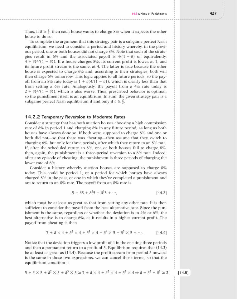
14.2 A Menu of Punishments 427
Thus, if then each house wants to charge 8% when it expects the otherhouse to do so.
To complete the argument that this strategy pair is a subgame perfect Nashequilibrium, we need to consider a period and history whereby, in the previ-ous period, one or both houses did not charge 8%. Note that each of the strate-gies result in 6% and the associated payoff is or, equivalently,
If a house charges 8%, its current profit is lower, at 1, andits future profit stream is the same, at 4. The latter is true because the otherhouse is expected to charge 6% and, according to their strategies, both willthen charge 6% tomorrow. This logic applies to all future periods, so the pay-off from an 8% rate today is which is clearly less than thatfrom setting a 6% rate. Analogously, the payoff from a 4% rate today is
which is also worse. Thus, prescribed behavior is optimal,so the punishment itself is an equilibrium. In sum, the given strategy pair is asubgame perfect Nash equilibrium if and only if
14.2.2 Temporary Reversion to Moderate RatesConsider a strategy that has both auction houses choosing a high commissionrate of 8% in period 1 and charging 8% in any future period, as long as bothhouses have always done so. If both were supposed to charge 8% and one orboth did not—so that there was cheating—then assume that they switch tocharging 6%, but only for three periods, after which they return to an 8% rate.If, after the scheduled return to 8%, one or both houses fail to charge 8%,then, again, the punishment is a three-period reversion to a 6% rate. Indeed,after any episode of cheating, the punishment is three periods of charging thelower rate of 6%.
Consider a history whereby auction houses are supposed to charge 8%today. This could be period 1, or a period for which houses have alwayscharged 8% in the past, or one in which they’ve completed a punishment andare to return to an 8% rate. The payoff from an 8% rate is
[14.3]
which must be at least as great as that from setting any other rate. It is thensufficient to consider the payoff from the best alternative rate. Since the pun-ishment is the same, regardless of whether the deviation is to 4% or 6%, thebest alternative is to charge 6%, as it results in a higher current profit. Thepayoff from cheating is then
[14.4]
Notice that the deviation triggers a low profit of 4 in the ensuing three periodsand then a permanent return to a profit of 5. Equilibrium requires that (14.3)be at least as great as (14.4). Because the profit stream from period 5 onwardis the same in those two expressions, we can cancel those terms, so that theequilibrium condition is
7 % d ! 4 % d2 ! 4 % d3 ! 4 % d4 ! 5 % d5 ! 5 % p.
5 % d5 % d25 % d35 % p,
d ' 23.
2 % d(4/(1 " d)),
1 % d(4/(1 " d)),
4 % d(4/(1 " d)).4/(1 " d)
d ' 23,
[14.5]5 % d ! 5 % d2 ! 5 % d3 ! 5 ' 7 % d ! 4 % d2 ! 4 % d3 ! 41 d % d2 % d3 ' 2.

428 CHAPTER 14: COOPERATION AND REPUTATION
Of course, we also need to check whether it is optimal to go along withthe punishment, but since the punishment consists of reverting to the stage-game Nash equilibrium for three periods, that is indeed the case. (As prac-tice, prove that it is optimal for each house to go through with the punish-ment.)
One can show that the condition in (14.5) is roughly equivalent to(Unless you get your kicks out of solving cubic equations, trust
me!) Note that the restriction on the discount factor is more stringent thanwhat we derived previously. When the punishment was permanent reversionto charging 6%, auction houses only had to be sufficiently patient, as reflectedin the discount factor being at least .67. Now, with only a three-period pun-ishment to deter each house from cutting its commission rate, the discountfactor has to be at least .81. By making the punishment weaker—an infrac-tion means a lower payoff of 4 only for three periods rather than forever—players have to value future payoffs more in order to squelch the temptationto cheat today.
In sustaining cooperation, there is a trade-off from a more severepunishment. A harsher punishment means a lower payoff if the punishment isinvoked, but the threat of a harsher punishment can do a better job ofsustaining cooperation.
14.2.3 Price Wars: Temporary Reversion to Low RatesIt is only those who have neither priced below cost nor heard the shrieks andgroans of shareholders who cry aloud for cutting prices, more vengeance,more desolation. Competition is hell. —WHAT GENERAL WILLIAM TECUMSEH
SHERMAN MIGHT HAVE SAID IF HE HAD RUN AN AIRLINE.
It’s been observed in some industries that when collusion breaks down, pricescan get really low, even lower than under normal competition. Indeed, pricescan even fall below cost, so that companies incur losses. Typically, such lowprices don’t persist, but the temporary reversion to aggressively low prices isknown as a price war.
Here is a strategy that encompasses the idea of a price war in that it in-volves a punishment more intense than simply reverting to a stage-game Nashequilibrium:
■ In period 1, charge 8%.■ In any other period,
charge 8% if either (1) both auction houses charged 8% in the previousperiod or (2) both charged 4% in the previous period;charge 4% for any other history.
First note that this strategy pair, if followed, will result in both houses set-ting an 8% rate. The punishment designed to deter any undercutting is forboth houses to set a low rate of 4% and then, if and only if both charged 4%,to return to a high rate of 8%.
To derive conditions whereby this symmetric strategy is a subgame perfectNash equilibrium, first consider either period 1 or a period whereby, in theprevious period, both houses either charged 8% or 4%. The prescribed behav-ior is to set 8%, and the resulting profit stream is 5 in all periods. This payoff
d ' 0.81.
14.2 A Menu of Punishments 429
must be at least as great as charging 4% or 6%. The better alternative of thetwo is a 6% rate, and it results in a payoff of
The deviating house earns a current profit of 7 and then zero in the next pe-riod, as both houses charge 4%. They then return to an 8% rate, and the profitis 5 thereafter. The equilibrium condition is
[14.6]
To complete the analysis, we need to ensure that the punishment is also anequilibrium—that is, that it is credible that the houses will go through withthe threatened punishment. So suppose the history is such that, in the previ-ous period, it was neither the case that both houses charged 8% nor that bothcharged 4%. Then the prescribed behavior is to set a 4% rate, and this yieldsa payoff of
[14.7]
Given that the other house also charges 4%, the profit is zero, but then jumpsto 5 as the two houses return to an 8% rate once the price war is over. Becausethe future payoff is the same whether the rate is 6% or 8%, the best alterna-tive to 4% is 6%, as that yields a higher current profit of 1 (as opposed to with an 8% rate). The resulting payoff from a 6% rate is
[14.8]
The company earns 1 in the current period, but then goes through the pricewar in the next period (as prescribed by its strategy), after which the commis-sion rate returns to 8%. When called upon to implement a price war, eachhouse goes along if (14.7) is at least as large as (14.8):
[14.9]
To sum up, this strategy pair is a subgame perfect Nash equilibrium whenboth (14.6) and (14.9) hold. Equation (14.6) ensures that an auction housewants to be cooperative (by charging 8% when the other company is expectedto do so) and (14.9) ensures that a house is willing to engage in a punishingprice war when needed. Both conditions hold when
There are two worthwhile points to make here. First, the punishment re-quires its own brand of cooperation. During a price war, a house can raise itscurrent profit by setting a rate of 6% rather than 4%. It is induced to go alongwith the “stick” of a price war by the lure of the “carrot” of a high commissionrate of 8% tomorrow. Only when the houses have set a low rate—and received
d ' 25.
1 d ! 5 ' 11 d '15
0 % d ! 5 % d2 ! 5 % d3 ! 5 % p ' 1 % d ! 0 % d2 ! 5 % d3 ! 5 % p
1 % d ! 0 % d2 ! 5 % d3 ! 5 % p.
"1
0 % d ! 5 % d2 ! 5 % d3 ! 5 % p.
1 5 % d ! 5 ' 71 d '25
.
5 % d ! 5 % d2 ! 5 % d3 ! 5 % p ' 7 % d ! 0 % d2 ! 5 % d3 ! 5 % p
7 % d ! 0 % d2 ! 5 % d3 ! 5 % p.
430 CHAPTER 14: COOPERATION AND REPUTATION
a low profit—do they return to setting a high rate andearning a high profit. It is then in the best interests of anauction house to “take its medicine” and hasten a returnto “good health.” Of course, companies have to value fu-ture profits sufficiently in order to get them to partici-pate in the price war, and that is what condition (14.9)guarantees.
The second point is that collusion is easier with thethreat of a one-period price war than with the threat of
reverting to regular competition forever. A price-war punishment made collu-sion stable when while permanently returning to a stage-game Nashequilibrium required that Collusion is then easier in the sense that thediscount factor doesn’t have to be quite so high; in other words, auctionhouses do not need to value future profits quite as much. A “short and nasty”punishment can then be more effective than a “long and mild” punishment.
14.2.4 A More Equitable PunishmentAn eye for an eye, and a tooth for a tooth. —THE BIBLE (EXODUS 21:23–27).
We’ve considered a variety of punishments—permanently reverting to compe-tition; temporarily reverting to competition; a short, intense price war—butthey are common in that they harm all parties, both the player who cheatedand the one who was victimized. A more equitable punishment would focusharm on the player who violated the cooperative norm. To such a punishmentwe now turn.
Again, the cooperative outcome is for both auction houses to charge 8% ineach period. If, however, say, Christie’s deviates by undercutting Sotheby’s rateof 8%, the punishment is that Sotheby’s gets to inflict the same harm onChristie’s. That is, in the next period, Christie’s charges 8%, while Sotheby’sundercuts it with a rate of 6%. If Christie’s does indeed follow through with an8% rate, then, in the ensuing periods, both houses return to charging 8%. Thedeviator is then required to set a high commission rate and allow the otherhouse to undercut it and take a big chunk of business. This occurs for one pe-riod, and then there is a return to the cooperative outcome. If there is anotherviolation in the future, then the same punishment ensues. Finally, if, bychance, the two houses simultaneously deviate, then the violations are ignoredand cooperative play continues.
Suppose both auction houses are to set the cooperative rate of 8%. It is op-timal to do so when
d ' 23.
d ' 25,
For the infinitely repeated game betweenChristie’s and Sotheby’s, now suppose the pun-ishment is a two-period price war in which bothauction houses set a commission rate of 4%.Derive the conditions for this strategy pair to bea subgame perfect Nash equilibrium.
14.1 CHECK YOUR UNDERSTANDING
The payoff from an 8% rate is a payoff stream of 5 forever. The highest payofffrom cheating is setting a 6% rate—earning a current profit of 7—and then in-curring the punishment payoff. The latter involves a profit of 1 next period—as the deviator sets an 8% rate and the other house charges 6%—and then areturn to both houses charging 8%.
Because punishment entails the deviator allowing its rival to undercut, it isessential to make sure that it is optimal to act in such a way. So suppose
5 % d ! 5 % d2 ! 5 % p ' 7 % d ! 1 % d2 ! 5 % p 1 5 % d ! 5 ' 7 % d1 d '12
.
14.3 Quid Pro Quo 431
Sotheby’s cheated in the previous period. Then it is now to set a rate of 8%while Christie’s charges 6%, a situation that yields a current profit of 1 forSotheby’s. Sotheby’s best alternative is to match Christie’s rate of 6%, but then,according to its strategy, to go through with the punishment in the ensuing pe-riod. Thus, Sotheby’s will optimally charge 8% and allow itself to be undercutby Christie’s if
1 % d ! 5 % d2 ! 5 % p ' 4 % d ! 1 % d2 ! 5 % p 1 1 % d ! 5 % '4 % d1 d '34
.
Note that the house which was cheated is happy to go along with the punish-ment. With the other house charging 8%, the former reaps a current profit of7 by charging 6%. Since the future payoff is the same regardless of what itdoes, it wants to maximize its current profit, and a rate of 6% does just that.
The punishment is one of responding in kind. If Sotheby’s cheats by under-cutting the agreed-upon rate of 8% and grabbing a lot of the business, then, ifcooperation is to be reestablished, Christie’s must have a chance to undercutSotheby’s. This is the ancient principle of retributive justice. But there is alsoa compensatory aspect, as the victimized auction house receives a profit thatis higher than it would be under cooperative play.
14.3 Quid Pro QuoTHE MAXIM “YOU SCRATCH my back and I’ll scratch yours” is followed not just byhumans, but by several other species in the animal kingdom. In Latin, it iscalled quid pro quo, meaning “something for something.” In some instances,this exchange may occur near contemporaneously—as when chimps taketurns grooming each other—but in other instances, the favor will be returnedat some distant and perhaps unspecified time. Indeed, it may occur only if aplayer is in need, something that may or may not arise.
This form of cooperation—exchanging favors over time—is explored herefor two bloodsucking species: vampire bats and politicians. The first exampleshows how the norm of quid pro quo can lead to an explosion of wastefulspending in the U.S. Congress. Senators support each others’ pet projects soas to aid their reelection efforts, with the taxpayers footing the bill. Similarly,vampire bats help each other out in a time of need, but the exchange is not invotes, but rather in regurgitated blood—messy and gross, but not as costly totaxpayers.
! SITUATION: U.S. CONGRESS AND PORK-BARREL SPENDING
At $286.4 billion, the highway bill just passed by Congress is the most ex-pensive public works legislation in U.S. history [and] it sets a new record forpork-barrel spending, earmarking $24 billion for a staggering 6,376 pet proj-ects, spread among virtually every congressional district in the land. . . . Itpassed 412 to 8 in the House, 91 to 4 in the Senate. —JEFF JACOBY (“THE
REPUBLICAN PORK BARREL,” BOSTON GLOBE, AUGUST 4, 2005)
Giving money and power to government is like giving whiskey and car keysto teenage boys. —P. J. O’ROURKE (PARLIAMENT OF WHORES, 1992)
432 CHAPTER 14: COOPERATION AND REPUTATION
In the 2005 Transportation Equity Act, the U.S. Congress was considering abill that, among other things, appropriated $223 million to build a bridge con-necting the town of Ketchikan, Alaska (with a population under 9,000), with itsairport on the Island of Gravina (population: 50). Although this project wouldsurely benefit a few thousand people in Alaska—both those who would use thebridge and those employed to build it—the cost involved struck most people asabsurd when placed in comparison to the number of people it would benefit.Dubbed the “Bridge to Nowhere,” it provoked a clamor once exposed.
The Bridge to Nowhere is a classic case of “pork-barrel spending.” A pork-barrel project is designed to benefit an elected official’s constituents—thus en-hancing his chances for reelection—but has little justification otherwise. Thestrategy is to draw resources from the broader population—in the case of thebridge in Ketchikan, all federal taxpayers would be footing the bill—and focusthe benefits on a narrow group of people—here, it was Senator Ted Stevens,who was trying to benefit the residents of his home state of Alaska.
Of course, one might ask, Why does Congress approve pork-barrel projects?At work is a version of quid pro quo among members of Congress. Each sen-ator or representative puts forth his own pork-barrel project with the under-standing that if others vote for it, then he’ll vote for their patronage projectwhen it comes to the floor. This form of cooperation benefits the members ofCongress—each brings money to his constituency—and the country as awhole pays the cost.
To explore the stability of the pork-barrel quid pro quo, suppose there arejust three members of the U.S. Senate: Senators Barrow, Byrd, and Stevens.*In each period, one of them has a pork-barrel project to propose. If the billpasses, its sponsor receives a payoff of 100, while the other two members havea payoff of Assume that the payoff is zero for all if the bill is not passed.Note that a member of Congress is worse off with another member’s pork,since her constituents do not benefit, but must pay for a part of it. Thoughcontrary to actual voting procedures, it’ll simplify our analysis if we assumethat all three votes are needed to pass a bill. Assume that pork-barrel projectsarise in an alternating fashion, with each senator proposing a project everythree periods. Senator Barrow proposes in periods 1, 4, 7, . . . , Senator Byrdin periods 2, 5, 8, . . . , and Senator Stevens in periods 3, 6, 9, . . .
In each period, there is a project on the agenda and each Senator has to de-cide whether to vote in favor of it. Consider a strategy profile in whichSenators start out voting for every project. If a Senator deviates by not votingfor someone else’s project, then the other two Senators vote against thatSenator’s next project. Once having done that, they return to supporting allprojects. This is a one-period asymmetric punishment akin to what was cov-ered in the previous section.
Suppose senators are currently in the cooperative phase in which all proj-ects are being supported and it is Senator Barrow’s turn to propose. It isclearly optimal for him to vote for his own project; the real issue is whetherSenators Byrd and Stevens should do so. If Senator Byrd supports the project,then his payoff is
"25.
[14.10]"25 % d ! 100 % d2 ! ("25) % d3 ! ("25) % d4 ! 100 % d5 ! ("25) % p.
*U.S. Senators Robert Byrd (Democrat from West Virginia) and Ted Stevens (Republican from Alaska) areconsidered masters of pork-barrel spending. A barrow is a castrated hog.

14.3 Quid Pro Quo 433
He gets by having Senator Barrow’s pork funded, but then receives 100 inthe next period (since his project is approved) and in the period after thatas Senator Stevens’s project is approved. The payoffs then cycle. Alternatively,Senator Byrd could vote against Senator Barrow’s project, in which caseSenator Byrd’s payoff is
"25"25
[14.11]0 % d ! 0 % d2 ! ("25) % d3 ! ("25) % d4 ! 100 % d5 ! ("25) % p.
He gets zero in the current period, since Senator Barrow’s project does notpass, and zero again in the following period as his project is voted down in re-taliation. After that, they all return to supporting pork.
Senator Byrd optimally votes for the project when (14.10) is at least as greatas (14.11). Notice that the payoff is the same from the third period onward.Canceling those common terms, we see that (14.10) is at least as great as(14.11) when
Continuing with the situation in which Senator Barrow’s project is on theagenda, now consider Senator Stevens. The difference between the situationfaced by Senators Byrd and Stevens is that the latter’s turn at the trough comesup in two periods rather than one. Senator Stevens optimally votes in favor when
"25 % d ! 100 ' 01 d ' .25.
Because the punishment is the same whether he votes against one or two bills,if Senator Stevens votes against Senator Barrow’s project, then he ought to voteagainst Senator Byrd’s project in the ensuing period as well. Thus, SenatorStevens receives a zero payoff in the first and second periods and, since his billis voted down in retaliation, a zero payoff in the third period. After that, thereis a return to the quid pro quo norm. Since the terms on both sides of (14.12)are identical from the fourth period onward, (14.12) is equivalent to
One can show that the analysis is analogous when it is Senator Byrd’s turnto propose a project. Senator Stevens then finds it optimal to vote in favorwhen and Senator Barrow finds it likewise when When it isSenator Stevens’s turn, Senator Barrow goes along if and Senator Byrddoes if Finally, if the history is such that there is a need for a punish-ment, it is clearly optimal to go through with voting against the project, giventhat everyone else does.
In sum, this norm of voting for one another’s patronage project is an equi-librium if (Note that this implies that holds as well.) If aSenator’s turn to propose is in the next period, then the discount factor mustbe at least as great as .25 in order for it to be optimal to vote in favor. However,if his turn doesn’t come for two periods, then he must be more patient, as re-flected in the discount factor having to be at least .64. Since the punishmentis in the more distant future, a senator must value the future more in order togo along with the proposed project.
d ' .25d ' .64.
d ' .64.d ' .25
d ' .64.d ' .25,
"25 " 25 ! d % 100 ! d2 ' 01 d ' .64.
[14.12]0 % d ! 0 % d2 ! 0 % d3 ! ("25) % d4 ! ("25) % d5 ! 100 % p."25 % d ! ("25) % d2 ! 100 % d3 ! ("25) % d4 ! ("25) % d5 ! 100 % p '

434 CHAPTER 14: COOPERATION AND REPUTATION
! SITUATION: VAMPIRE BATS AND RECIPROCAL ALTRUISM
Desmodus rotundus, or, as it is more commonly known, the vampire bat livesa harsh and precarious life. Feeding off of the blood of animals—cows andhorses more than homo sapiens—vampire bats need to eat 50–100% of theirbody weight each night. And they cannot survive for long without eating: Afterjust a few bloodless days, a vampire bat can lose as much as 25% of its bodyweight and its body temperature can fall dangerously low.2
With so much riding on regular consumption of blood, vampire bats havedeveloped a form of cooperation that evolutionary biologists refer to as recip-rocal altruism. A bat who has not fed recently and is in critical need receivesregurgitated blood from another bat who was successful in that night’s feed-ing. Interestingly, this practice of sharing exists only among female adults, al-though they also give blood to the young. Putting aside the question ofwhether the practice is the result of natural selection or social imitation, let ussee how game theory can show that it is a stable norm.*
For simplicity, suppose there are just two vampire bats in the colony. Eachnight, they fly out seeking the blood of the living. (Is game theory cool, orwhat?) At the end of the night, a bat can return with either a full or an emptystomach. Let denote the probability that a bat feeds itself on any given night.There are three possible outcomes. First, both bats succeeded in their hunt forblood, in which case there is no need to share. Second, both bats struck out sothere is no blood to share. The third outcome is that one bat fed and the other
did not, in which case the former decides whether to shareits nightly take with the latter.
TABLE 14.1 reports the payoffs to the bats, depending onwhether sharing occurs, when one fed that night and one didnot. If there is no sharing, then the bat that has fed has a pay-off of 10 and the hungry bat’s payoff is If they share, thefed bat’s payoff reduces to 8, since it consumes less blood,while the hungry bat’s payoff rises to 4.
As assumed throughout our analysis of repeated games,each bat maximizes the present value of its payoff stream.
Now, you may be a bit uncomfortable imagining nonhumans engaging in dis-counting, but experiments have shown that pigeons and rats do value currentpayoffs more than future ones (though, to my knowledge, these experimentshave not been conducted on bats). Recalling that the discount factor can alsobe interpreted as the probability of surviving to the next period, you can seethat it would not be surprising that natural selection results in an animal’s at-taching more importance to feeding today than feeding tomorrow, since itmay not be alive come tomorrow. But if you still feel uncomfortable withassuming that bats discount, then replace vampire bats with actual vam-pires—say, Anya and Spike from the television series Buffy the Vampire Slayer.
A strategy for a bat prescribes what a bat that has fed should do when theother bat is hungry, depending on the history of their interactions. Consider a
"1.
s
*Chapters 16 and 17 cover evolutionary game theory, which is a modification of game theory designed toapply more generally to the animal kingdom. While the example of sharing among vampire bats could justas well have fit in those chapters, I present it here to show the broad relevance of the theory of repeatedgames to explaining behavior.
TABLE 14.1 PAYOFFS OF VAMPIREBATS
Bat Sharing No Sharing
Fed bat 8 10
Hungry bat 4 #1

14.3 Quid Pro Quo 435
strategy in which the fed bat shares with the hungry bat as long as, in all pastsituations, a fed bat shared the contents of its stomach with a hungry one. If,in some past period, sharing in that situation did not occur, then neither batshares blood. This is just the grim-trigger strategy. Let us derive conditions forit to be a subgame perfect Nash equilibrium.
As an initial step in our analysis, we’ll derive the expected payoff from thisstrategy profile at the start of a night, before the bats learn about their successor failure with feeding. Letting V denote the expected payoff when bats are en-gaging in this sharing practice, we have
[14.13]V # s ! $s ! 10 % (1 " s) ! 8% % (1 " s) ! $s ! 4 % (1 " s) ! ("1)% % dV.
This equation requires a bit of explanation. With probability s, a bat feeds it-self that night, in which case its current-period expected payoff is
with probability s, the other bat has fed, so no sharingoccurs and both bats’ payoff is 10; while with probability the other batis hungry and sharing results in a current payoff of 8 for the first bat. Thisgives us the term in (14.13). The other possibility isthat a bat is unsuccessful in its feeding foray, which occurs with probability
It then receives a payoff of 4—when the other bat was successful andshares—and a payoff of —when the other bat is also hungry. This scenarioproduces the term The sum of the firsttwo terms in (14.13) is the expected current-period payoff for a bat. The thirdterm is which is the expected future payoff; a bat expects to get V comenext period and that is discounted by Now, let us solve for V and simplifythe resulting expression:
If there is a deviation, then the ensuing punishment has both bats no longersharing. The single-period expected payoff without sharing is
since a bat finds food with probability s, in which case its payoff is 10, anddoes not with probability in which case its payoff is Because thesepayoffs apply to every period, the present value of that payoff stream is
We can now turn to determining when a bat that has fed wants to share itsblood with a hungry bat. Suppose the two bats have always shared in that sit-uation in the past. Then the one that has fed finds it optimal to share when
[14.14]
By sharing, the bat’s current payoff is 8 and its future expected payoff is V,which is the payoff when bats anticipate sharing in the future. On the right-hand side is the expression denoting the payoff from not sharing. It yields a
8 % d a"3s2 % 14s " 11 " d
b ' 10 % d a11s " 11 " d
b .
(11s " 1)/(1 " d).
"1.1 " s,
s ! 10 % (1 " s) ! ("1) # 11s " 1,
1 V(1 " d) # "3s2 % 14s " 11 V #"3s2 % 14s " 1
1 " d.
V " dV # 10s2 % 8s(1 " s) % 4s(1 " s) " (1 " s)2
d.dV,
(1 " s) ! $s ! 4 % (1 " s) ! ("1)%."1
1 " s.
s ! $s ! 10 % (1 " s) ! 8%
1 " s,s ! 10 % (1 " s) ! 8;

436 CHAPTER 14: COOPERATION AND REPUTATION
higher current payoff of 10 and a future expected payoff of which now presumes that the bats do not share. If (14.14) holds, then it is op-timal to share when the sharing norm has never been violated.
If the history is such that there was a past violation from sharing, then thefed bat is not supposed to share, which is indeed optimal when
This condition always holds. Sharing lowers the current payoff and there is nocompensation with a higher future payoff, since it is regard-less of what happens. It is thus not optimal to reduce current food consump-tion if no reward of higher future consumption is anticipated.
The strategy profile with reciprocal altruism is then a subgame perfectNash equilibrium if (14.14) holds. After some manipulation, (14.14) can beshown to be equivalent to
For the remainder of the analysis, assume that so the preceding condi-tion becomes
Plotting in FIGURE 14.2, we see that the norm of reciprocal altruismis self-enforcing (i.e., it is an equilibrium) when the probability of success is
s(1 " s)s(1 " s) ' 1
6.d # .8,
s(1 " s) '2(1 " d)
3d.
(11s " 1)/(1 " d)
10 % da11s " 11 " d
b ' 8 % da11s " 11 " d
b .
(11s " 1)/(1 " d),
0 .2 .5 .8 1
s(1#s)
16
Cooperation occurs
s
FIGURE 14.2 Equilibrium Condition for There to be Reciprocal Altruism

14.4 Reputation 437
between .21 and .79; it can be neither too low nor toohigh. If the probability of success is too low, then thechances that the hungry bat will have blood to share inthe future are too small to induce the bat that has fed toshare its blood today. In other words, it is unlikely thatany favor will be returned in the future. If, instead, theprobability of success is too high, then the bat that hasfed is not that concerned about needing blood in the fu-ture and so assigns a high probability to being able tofeed itself. It is unlikely to need a favor in the future.Thus, it is when individual success in feeding is moder-ate that reciprocal altruism is stable.
Reciprocal altruism is sustainable when playerscare sufficiently about the future and the probability ofneeding help in the future is neither too likely nor toounlikely.
14.4 ReputationRegard your good name as the richest jewel you can pos-sibly be possessed of—for credit is like fire; when onceyou have kindled it you may easily preserve it, but if youonce extinguish it, you will find it an arduous task torekindle it again. —SOCRATES
A GOOD REPUTATION IS a valuable asset. A reputation for honesty (such as a highfeedback score on eBay) may make others inclined to trade with you. A repu-tation for hard work may land you a good job. A reputation for paying yourdebts may secure you a loan. At the same time, and as Socrates suggests, rep-utation can be fragile. A single lie can label you as a liar. A single day of cut-ting out of work early can label you a slacker. A single unpaid debt can labelyou a bad credit risk. The fragility of a reputation can be unfortunate, but alsonecessary to provide the right incentives so that people will behave properly.We’ll examine this assertion in the next two applications.
! SITUATION: LENDING TO KINGS
When faced with a short-run need for cash—such as cash required to financea war—kings in premodern Europe would borrow from private lenders. Creditwas particularly important, as taxation was not widespread. In some instances,a king reneged on his loans—such as in 1290, when King Edward I expelled hisJewish lenders (and Jews in general) from England—but in many cases he re-paid them. Now, a king is above the law, so why would he repay his debts?
Consider a situation with a king and a single lender. (You can think of thelender as a unified group of lenders, such as the banking community.) At thestart of any period, there is a probability b that the king needs to borrowfunds; for example, he may need to finance a war or purchase land. In thatevent, the lenders must decide whether to lend the king the money. Supposethe interest rate the lenders would charge is 10%. Then, with a loan of size
Consider the infinitely repeated game based onthe stage game in FIGURE 14.3. Player 1’sstrategy has him choose a in odd periods and cin even periods, as long as the outcome has al-ways been (a, z) in odd periods and (c, x) ineven periods. For any other history, player 1chooses b. Player 2’s strategy has her choose zin odd periods and x in even periods, as long asthe outcome has always been (a, z) in odd peri-ods and (c, x) in even periods. For any other his-tory, player 2 chooses y. Find the conditions forthis strategy pair to be a subgame perfect Nashequilibrium.
14.2 CHECK YOUR UNDERSTANDING
2,2 2,3
12,1
3,2
1,3
4,4Player 1
Player 2
a
b
c
1,12
1,1
3,1
x y z
FIGURE 14.3

438 CHAPTER 14: COOPERATION AND REPUTATION
100, the deal is that the king repays 110: the principal of 100, plus interest of10 (which is 10% of 100). At the end of the loan period, the king decideswhether to pay 110 or renege and pay nothing. Assume that the value of theloan to the king is 125. Thus, the king would prefer to take out the loan andrepay it than not to have a loan. Finally, assume that if the lenders didn’t lendthe money to the king, they would not earn any return on their money. Thus,the lenders would like to lend to the king if they think that he’ll repay the loan.
Consider a strategy in which the lender initially provides a loan whenneeded and continues to do so as long as the king has repaid past loans. If theking ever reneges, then the lender refuses to lend to him again. The king’sstrategy is to repay the initial loan and any future loan if he has always repaidit in the past. If he ever reneges, then he reneges on all future loans. Eachplayer is concerned with maximizing the expected present value of his mone-tary stream.
Consider the lender’s strategy. If the king is a good credit risk (i.e., he hasalways repaid his loans), then the lender does find it optimal to lend to himagain. Doing so yields a payoff of 10 on each loan (the 10% interest on the loanof 100). If, instead, the king has reneged on a past loan, then, according to theking’s strategy, he’ll renege on all future loans. In that case, the lender does notwant to lend to him. The lender’s strategy is then optimal.
The interesting analysis concerns the behavior of the king. If he has madehimself into a bad credit risk, then it is indeed optimal for him not to repay aloan, since, according to the lender’s strategy, he won’t get a future loan re-gardless of what he does. His payoff from repaying the loan is while itis zero from reneging. (Note that he has already reaped the 125 from gettingthe loan.)
Finally, consider the situation in which the king is a good credit risk andhas an outstanding loan. If the king repays the loan (and acts according to hisstrategy in the future), his payoff is
Repayment costs him 110 in the current period. With probability b, he needsa loan next period, and given that he has repaid his past loans, he’ll get it. Thisnew loan yields a payoff of 15, as the king values it at 125 and then we needto net out the repayment of 110. Similarly, there is a probability b that he’llneed a loan in each succeeding period. Alternatively, the king could renege onthe current loan, in which case his payoff is zero in the current period—sincehe foregoes no funds—and in all future periods—since the lender discontinueslending to him. It is then optimal for the king to repay the loan when
[14.15]
The king repays the loan not out of the goodness of his heart, but rather topreserve his reputation so that he can secure future loans. The lenders antici-pate that he has an incentive to maintain his reputation and thus lend moneyto him even though they know that the king is above the law and could refuseto make payment at any time.
"110 % d ab ! 151 " d
b ' 01 d '110
110 % 15b.
"110 % d ! b ! 15 % d2 ! b ! 15 % p # "110 % d ab ! 151 " d
b .
"110,

14.4 Reputation 439
It is worth exploring this equilibrium condition to gain some further in-sight. Suppose b is close to zero, so that the king doesn’t expect to need an-other loan. In that case, (14.15) is rather stringent, as the discount factor mustbe close to 1. If he doesn’t foresee there being much of a chance of needing afuture loan, the king is unlikely to repay the current one, and as a result, thelenders (anticipating that the king will renege) will not make the original loan.The only reason the king repays a loan is to preserve a reputation conduciveto securing more loans. If he expects the next loan to be the last one he’ll everneed, then he has no incentive to repay it. Ironically, the king is a bad creditrisk if the lenders never expect the king to need another loan.
Of even greater irony is the fact that the king is in a weaker position thanhis lowly subjects! Since the lenders can take anyone but the king to court anddemand repayment, it becomes credible that a person will repay a loan. Incontrast, credibility is problematic for the king because there is no court toforce him to make payment and he cannot commit himself to paying back aloan. He can only hope that the lenders think it’ll be in his best interests torepay a loan in order to preserve his reputation. That he is above the lawmakes it more, not less, difficult for him to borrow!
! SITUATION: HENRY FORD AND THE $5 WORKDAY
The Ford Motor Co., the greatest and most successful automobile manufac-turing company in the world, will, on Jan. 12, inaugurate the greatest revo-lution in the matter of rewards for its workers ever known in the industrialworld. —DETROIT JOURNAL, JANUARY 5, 1914.3
In 1914, Henry Ford offered the unheard-of wage of $5 a day for workers inhis factories. This was at a time when the typical daily wage in the automobileindustry was $2.25. Although we could conclude that Henry Ford was just gen-erous with his workers, such a strategy may actually have enhanced the profitof the Ford Motor Company. Let’s see how.
If a worker is employed by Henry Ford, he has to decide whether to workhard or shirk. Assume that the monetary cost to a worker is $1 from engagingin hard labor and zero from shirking. If the worker is paid a wage of w, hissingle-period payoff is then w if he shirks and if he works hard. Aworker’s payoff is the present value of his stream of single-period payoffs,where his discount factor is
Henry Ford’s payoff is the present value of the stream of profits (per worker),where (“beta”) is his discount factor. Suppose his company earns revenue of$4 per day from a worker who shirks and $7 from a worker who works hard.For example, if Henry Ford offers a wage of $5 and the worker shirks (wherebyshe is summarily fired), but the new worker works hard and does so in everyperiod thereafter, then Henry Ford’s payoff from that position is
Assume that there is an unlimited supply of workers who are willing towork for $5 a day. Similarly, there is an unlimited supply of jobs offered byother companies, so a worker who is fired can always find a position that pays
(4 " 5) % b(7 " 5) % b2(7 " 5) % p # "1 % b a 21 " b
b .
b
d.
w " 1

440 CHAPTER 14: COOPERATION AND REPUTATION
$3 and tolerates shirking. In this game, Henry Ford decides what wage to payand whether or not to fire a worker. If he fires a worker, then he automaticallyhires a new worker. A worker for Henry Ford decides whether to work hard.
Suppose Henry Ford offers the following contract to his workers (which ishis strategy): You’ll be paid a wage of $5 and continue to be employed as longyou work hard. If you shirk, then you’re labeled a slacker and fired. Theworker’s strategy is to work hard if he is paid a wage of at least $5. At anylower wage, he shirks.
In assessing whether Henry Ford’s strategy is optimal, first note that he is in-different between firing and retaining a worker, since workers are perfect sub-stitutes. Thus, firing a worker when he shirks and retaining him when he workshard is optimal for Henry Ford (i.e., there is no other firing-and-hiring strategythat yields a strictly higher payoff). The real issue is whether it is optimal tooffer a wage of $5. Suppose he offers a wage of w today. Then, given that heacts according to his strategy in the future (which means offering a wage of $5),and given that workers act according to their strategy, Henry Ford’s payoff is
If the wage is at least 5, then the worker works hard, so Henry Ford gets acurrent-period payoff of and, by acting according to his strategy in thefuture, receives a future payoff of as his per-period profit is 2from earning 7 and paying a wage of 5. If then the worker shirks,so Henry Ford’s current payoff is only with the same future payoff.Finally, if the wage is less than 3, then no worker is willing to work for HenryFord, since they can do better by working elsewhere at a wage of 3. Thismeans that Ford’s current payoff is zero, though his future payoff remains
Clearly, Henry Ford prefers to pay a wage of 5 to any higher wage; why paymore than is needed to induce hard work? Also, he prefers a wage of 3 to anywage above 3 and below 5, because a higher wage still fails to induce hardwork. Finally, he prefers to pay 3 to any wage below 3, since the former gen-erates revenue of 4 for a current profit of 1, while a wage below 3 is insuffi-cient to induce a worker to come work for him and thus produces zero profit.Therefore, the optimal wage is either 3 or 5. Henry Ford prefers to do as hisstrategy says and pay a wage of 5 if
In other words, he acts in accordance with his strategy if the additional rev-enue from having a worker work hard is at least as great as the wage premiumrequired to get the worker to work hard. Henry Ford’s strategy is optimal.
2 % b a 21 " b
b ' 1 % b a 21 " b
b 1 2 ' 1.
b(2/(1 " b)).
4 " w,3 $ w 6 5,
b(2/(1 " b)),7 " w
b a 21 " b
b if w 6 3.
(4 " w) % b a 21 " b
b if 3 $ w 6 5;
(7 " w) % b a 21 " b
b if 5 $ w;
14.5 Imperfect Monitoring and Antiballistic Missiles 441
Now consider a worker. Given Henry Ford’s strategy and given that theworker acts according to his own strategy in the future, he prefers workinghard (as his strategy prescribes) over shirking when
That is, as long as a worker’s discount factor is at least she would prefer towork hard at a wage of $5 rather than shirk and lose this high-paying job.
Key to this scheme is that Henry Ford values hard work more than it costshim to induce hard work. He gains additional revenue of $3 per day perworker from having them work hard, while workers need to be paid only $1to compensate them for not shirking. There is then a net gain of $2 per daywhen hard work occurs. The way to get workers to apply a high level of effortis to pay them a wage of $5—well above what others are paying—and firethem if they don’t perform. As long as workers value future wages sufficiently,a worker will keep his nose to the grindstone so as to maintain a reputationfor hard work. With this scheme, everyone is made better off. Henry Fordearns a higher profit per worker of $1 per day, and the worker is better off by$1 per day.
In closing, it is useful to remind ourselves that life is more complicatedthan our models, and indeed, that was the case with Henry Ford’s $5 wage. Itappears that he had more than profit or generosity in mind, for he wanted to“shape” the lives of his workers:
To be eligible for the $5.00 rate, the employee needed to demonstrate that hedid not drink alcohol or physically mistreat his family or have boarders inhis home, and that he regularly deposited money in a savings account,maintained a clean home, and had a good moral character.4
As a man of action, he didn’t just promulgate, but actually created, a “SociologicalDepartment” that would advise and monitor his workers—even at their homes!One wonders whether the $5 was worth it.
14.5 Imperfect Monitoring and Antiballistic MissilesThe United States of America and the Union of Soviet Socialist Republics,proceeding from the premise that nuclear war would have devastating con-sequences for all mankind, considering that effective measures to limit anti-ballistic missile systems would be a substantial factor in curbing the race instrategic offensive arms and would lead to a decrease in the risk of outbreakof war involving nuclear weapons, have agreed as follows: Each Party un-dertakes not to deploy ABM systems for a defense of the territory of its coun-try. For the purpose of providing compliance, each Party shall use nationaltechnical means of verification at its disposal in a manner consistent withgenerally recognized principles of international law. —[EXCERPTS FROM THE
“TREATY ON THE LIMITATION OF ANTI-BALLISTIC MISSILE SYSTEMS”]
BECAUSE THERE IS NO third party to enforce an agreement between two countries,international treaties work only when they are self-enforcing. Both sides mustbe willing to go along with the agreement at each moment in time. This situa-tion is to be contrasted with a buyer and a seller who have written a contract.
12,
5 " 11 " d
' 5 % d a 31 " d
b 1 d '12
.
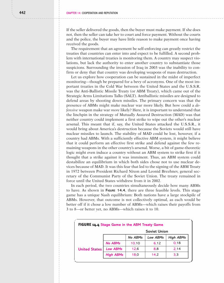
442 CHAPTER 14: COOPERATION AND REPUTATION
If the seller delivered the goods, then the buyer must make payment. If she doesnot, then the seller can take her to court and force payment. Without the courtsand the police, the buyer may have little reason to make payment once havingreceived the goods.
The requirement that an agreement be self-enforcing can greatly restrict thetreaties that countries can enter into and expect to be fulfilled. A second prob-lem with international treaties is monitoring them. A country may suspect vio-lations, but lack the authority to enter another country to substantiate thosesuspicions. Surrounding the invasion of Iraq in 2003 was the inability to con-firm or deny that that country was developing weapons of mass destruction.
Let us explore how cooperation can be sustained in the midst of imperfectmonitoring—though be prepared for a bevy of acronyms. One of the most im-portant treaties in the Cold War between the United States and the U.S.S.R.was the Anti-Ballistic Missile Treaty (or ABM Treaty), which came out of theStrategic Arms Limitations Talks (SALT). Antiballistic missiles are designed todefend areas by shooting down missiles. The primary concern was that thepresence of ABMs might make nuclear war more likely. But how could a de-fensive weapon make war more likely? Here, it is important to understand thatthe linchpin in the strategy of Mutually Assured Destruction (MAD) was thatneither country could implement a first strike to wipe out the other’s nucleararsenal. This meant that if, say, the United States attacked the U.S.S.R., itwould bring about America’s destruction because the Soviets would still havenuclear missiles to launch. The stability of MAD could be lost, however, if acountry had ABMs. With a sufficiently effective ABM system, it might believethat it could perform an effective first strike and defend against the few re-maining weapons in the other country’s arsenal. Worse, a bit of game-theoreticlogic might even induce a country without an ABM system to strike first if itthought that a strike against it was imminent. Thus, an ABM system coulddestabilize an equilibrium in which both sides chose not to use nuclear de-vices because of MAD. It was this fear that led to the signing of the ABM Treatyin 1972 between President Richard Nixon and Leonid Brezhnev, general sec-retary of the Communist Party of the Soviet Union. The treaty remained inforce until the United States withdrew from it in 2002.
In each period, the two countries simultaneously decide how many ABMsto have. As shown in FIGURE 14.4, there are three feasible levels. This stagegame has a unique Nash equilibrium: Both nations have a large stockpile ofABMs. However, that outcome is not collectively optimal, as each would bebetter off if it chose a low number of ABMs—which raises their payoffs from3 to 8—or better yet, no ABMs—which raises it to 10.
FIGURE 14.4 Stage Game in the ABM Treaty Game
10,10
18,0
12,6
6,12
14,2
8,8United States
Soviet Union
No ABMs
Low ABMs
High ABMs
0,18
3,3
2,14
No ABMs Low ABMs High ABMs

14.5 Imperfect Monitoring and Antiballistic Missiles 443
Suppose this strategic situation is infinitely repeated,but, contrary to the other applications in this and thepreceding chapter, the history of the game is not com-mon knowledge; that is, no country is assured of observ-ing the past choices of the other country. Thus, the de-termination of whether another country has ABMs isperformed imperfectly. The uncertainty in monitoring isreflected in TABLE 14.2. If a country has no ABMs, thenthe probability that the other country detects its ABMsis zero. If it chooses to a have a low number of ABMs,then there is a 10% chance that the missiles are ob-served, and there is a 50% chance that a high number of ABMs is detected.
In each period, the countries make a choice, and then, with the probabili-ties given in Table 14.2, a country observes that the other country has ABMs.If a country finds ABMs, then that fact is assumed to be common knowledgebetween the two countries. Each country seeks to maximize the expected pres-ent value of its payoff stream.
Consider a symmetric strategy pair that supports the outcome of prohibit-ing all ABMs:
■ In period 1, choose No ABMs.■ In any other period,
choose No ABMs if neither country has observed ABMs in the other coun-try in all past periods.choose High ABMs if either country has observed ABMs in the othercountry in some past period.
If there have been no observed violations, the payoff to not having ABMs isIf a country chooses instead to have a small number of ABMs, its
expected payoff is
[14.16]
With probability .1, this violation is detected, and both countries respond byinvesting heavily in ABMs thereafter. But there is also a 90% chance that theviolation is not detected. According to their strategies, both countries chooseNo ABMs.*
Rather than cheat with Low ABMs, either country could instead chooseHigh ABMs, which has an expected payoff of
[14.17]18 % d c .5 ! a 31 " d
b % .5 ! a 101 " d
b d .
12 % d c .1 ! a 31 " d
b % .9 ! a 101 " d
b d .10/(1 " d).
*We have glossed over a problematic issue regarding what a country’s payoff is if the country’s beliefs areinaccurate. For example, suppose the United States has no ABMs and it believes that the Soviet Union hasno ABMs as well, but, in fact, the Soviet Union has a low level of ABMs. Is the payoff 10 to the UnitedStates or 6? It would seem natural to suppose that the United States believes that it is 10 unless it discov-ers that the Soviet Union actually does have ABMs, in which case the U.S. payoff is 6. Regardless of howthis issue is settled, it does not affect the derivation of the equilibrium conditions, since they are basedupon a country’s having an accurate conjecture about what the other country is to do.
TABLE 14.2 MONITORING PROBABILITIESIN THE ABM TREATY GAME
Probability ofNumber of ABMs Detecting ABMs
None 0
Low .10
High .50

444 CHAPTER 14: COOPERATION AND REPUTATION
It is optimal to abide by the treaty when the payoff from doing so, is at least as great as (14.16) and (14.17). Hence, the following inequalitiesmust hold:
[14.18]
[14.19]
Thus, must be at least as large as .74. If thenboth a low number and a high number of ABMs arepreferred to none. If then a low numberof ABMs is preferred to complete prohibition. Onlywhen does each country find it optimal to abideby the ABM Treaty.
SummaryPeople acting in their own individual interests can leadto an outcome that is disappointing for everyone in thesense that if they could coordinate and do somethingdifferent, they would all be better off. As the various ex-amples in this chapter attest, such situations are farfrom rare and, in fact, permeate society. They can arisewith countries, kings, companies, politicians, factoryworkers, and even vampire bats. What the theory of re-peated games shows is how and when players can con-struct a mechanism that supports mutually beneficialactions.
The exact form of the mechanism may vary, but whatit always entails is players working together to both re-ward and punish each other. When everyone plays co-
operatively, players reward each other by continuing to play cooperatively.When someone deviates from cooperative play, the group punishes by engag-ing in aggressive play, such as setting low commission rates in the case of fine-arts auction houses. The punishment itself can take a variety of forms that dif-fer in terms of their severity, length, and who is punished. One form of pun-ishment is simply to stop cooperating and go to a stage-game Nash equilib-rium. This reversion to uncooperative play can occur for a specific length oftime—say, five periods—or forever. The longer the reversion, the more severeis the punishment and thus the more effective that threatened punishment willbe in deterring cheating. To pack more punch into a punishment, it can evenentail lower payoffs than occur at a stage-game Nash equilibrium. However,such an intense punishment cannot go on forever. In order to induce playersto participate in such a costly punishment, there must be the lure of returningto cooperative play in the future. This style of short, intense punishment hasbeen observed in the marketplace in the form of price wars, in which pricescan even fall below cost before rising back to profitable levels.
d ' .74
.70 6 d 6 .74,
d 6 .70,d
101 " d
' 18 % d c .5 ! a 31 " d
b % .5 ! a 101 " d
b d 1 d '8
11.5" .70
101 " d
' 12 % d c .1 ! a 31 " d
b % .9 ! a 101 " d
b d 1 d '2
2.7" .74
10/(1 " d),
Now suppose a technological advance improvesthe monitoring technology, so that the probabili-ties of detecting ABMs are as stated in TABLE14.3. Using the strategy profile just described,derive the equilibrium conditions. If you an-swered correctly, then you’ll find that the restric-tion on the discount factor is less stringent, indi-cating that better monitoring makes cooperationeasier.
14.3 CHECK YOUR UNDERSTANDING
TABLE 14.3 HIGHER MONITORINGPROBABILITIES IN THE ABM TREATY GAME
Probability ofNumber of ABMs Detecting ABMs
None 0
Low .30
High .75

Exercises 445
Another way to view how cooperation is sustained is that a player’s historyof play influences her reputation for how she’ll play in the future. If a playerdeviates from the norm of cooperative play, other players infer that she is an“uncooperative type” and expect similar behavior in the future. This expecta-tion causes them to change their own play—who wants to cooperate whensomeone is anticipated to take advantage of you?—and thus cooperationbreaks down. Repeated games can then shed light on what it takes to main-tain a reputation. We explored how, by repaying a loan, a king maintains hisreputation as a good credit risk and thereby induces lenders to offer him loansin the future, or how the decision of a factory employee to exert a high levelof effort can maintain a reputation for being a hard worker, whereas shirkingon the job can soil that reputation and lead to dismissal.
Our lives encompass an array of repeated games. We play them with ourparents, siblings, spouses, friends, neighbors, bosses, colleagues—the list goeson and on. In many of these situations, the mechanisms for supporting coop-eration reviewed in this and the previous chapter are subtly at work. Our re-lationships are constructed on understanding that we’ll treat each other fairly,and that if we don’t, then there are likely to be consequences. Although suchconsequences may be unpleasant, they perform a valuable function, for it isthe fear of those consequences that helps keep people acting in a socially con-structive way, and that makes everyone better off.
1. Consider an infinitely repeated game in which the stage game is thatshown in FIGURE PR14.1. Each player’s payoff is the present value of herpayoff stream, where the discount factor is a. Define a grim-trigger strategy that results in player 1’s choosing c and
player 2’s choosing y, and state conditions for that strategy’s resultingin a subgame perfect Nash equilibrium.
b. Consider the following strategy profile: In period 1, player 1 choosesc. In any other period, player 1 chooses c if, in the previous period,the outcome was either (c, y) or (d, z); otherwise he chooses d. In pe-riod 1, player 2 chooses y. In any other period, player 2 chooses y if,in the previous period, the outcome was either (c, y) or (d, z); other-wise she chooses z. Derive conditions for this profile to result in asubgame perfect Nash equilibrium.
d.
EXERCISES
2,2
1,3
0,2
"4,4
Player 1
Player 2
a
b
c
d
3,1
4,4
1,3
3,2
w x
2,0
3,1
7,7
9,3
y
4,"4
2,3
3,9
0,0
z
FIGURE PR14.1

446 CHAPTER 14: COOPERATION AND REPUTATION
c. Consider the following strategy profile: In period 1, player 1 choosesc. In any other period, player 1 chooses c if, in the previous period,the outcome was either (c, y), (d, w), or (a, z); he chooses d if, in theprevious period, player 2 chose y and player 1 did not choose c; hechooses a if, in the previous period, player 1 chose c and player 2 didnot choose y; otherwise he chooses b. In period 1, player 2 chooses y.In any other period, player 2 chooses y if, in the previous period, theoutcome was either (c, y), (d, w), or (a, z); she chooses w if, in the pre-vious period, player 2 chose y and player 1 did not choose c; shechooses z if, in the previous period, player 1 chose c and player 2 didnot choose y; otherwise she chooses x. Derive conditions for this pro-file to yield a subgame perfect Nash equilibrium.
2. As early as the 1820s, the custom of “pairing off” had developed inCongress. If a member of Congress was to miss a formal vote, he wouldarrange beforehand with a member on the opposing side of the issue forthe two not to vote. In modeling this situation, consider two members ofCongress—Representatives Smith and Jones—who, on a regular basis,would like to miss a House vote in order to take care of other business.Representative Smith would prefer to be away every three periods, start-ing with period 1 (hence periods 1, 4, 7, . . .), and receives a value of 3from being away. Representative Jones would prefer to be away everythree periods, starting with period 2 (hence, periods 2, 5, 8, . . .), andalso receives value of 3. Call these periods the representatives’ “travelingperiods.” In each such period, there is a House vote, and Smith receivesa value of 5 from being in attendance and voting and a value of ifJones is in attendance and votes. Analogously, Jones earns 5 from beingin attendance and voting and if Smith is in attendance and votes.Thus, if both are in attendance and vote, then Smith and Jones eachhave a payoff of During a traveling period, a representa-tive’s payoff is (1) 3 if he is not in attendance and the other representa-tive does not vote; (2) if he is not in attendance and theother representative votes; (3) 0 if both are in attendance and vote; and(4) 5 if he is in attendance and votes and the other does not vote. Duringa nontraveling period, a representative’s payoff is (1) 0 if he is not in at-tendance and the other representative does not vote; (2) if he is notin attendance and the other representative votes; (3) 0 if both are in at-tendance and vote; and (4) 5 if he is in attendance and votes and theother does not vote. In each period, the representatives simultaneouslydecide whether to be in attendance and vote. Each seeks to maximizethe present value of his single-period payoff stream, where the discountfactor is Find a subgame perfect Nash equilibrium in which each isnot in attendance during his traveling periods and during those periodsthey “pair off.”
3. Return to the Vampire Bats game in Section 14.3, but now suppose thetwo bats have different probabilities of success. For this purpose, let usname the bats Anya and Spike. The probability that Anya succeeds inher nightly feeding venture is a, and the probability of success for Spikeis s. Find the conditions for the strategy pair in Section 14.3 to yield asubgame perfect Nash equilibrium.
4. Three construction companies—A, B, and C—routinely bid on statehighway projects. In each period, the state offers a single contract andthe three companies simultaneously submit bids. A bid is how much
d.
"5
"2 (# 3 " 5)
0 # (5 " 5).
"5
"5

Exercises 447
money a company specifies that it must be paid in order to take on thejob. The company that submits the lowest bid wins the contract. Thestate specifies that bids must be in increments of 100 (feasible bids arethus 0, 100, 200, . . .) and that a contract will not be awarded if the low-est bid is in excess of 2,000. If two or more companies submit the low-est bid, then each of those companies has an equal chance of winning it.Assume that it would cost a company 1,000 to execute the contract.Hence, if a company wins the contract at a bid of b, its profit is
In this infinitely repeated game, a company’s payoff is thepresent value of its profit stream.a. Derive a symmetric Nash equilibrium for the stage game.b. Consider companies supporting collusion with a bid rotation scheme
using a grim-trigger strategy. In periods 1, 4, 7, . . . , company A bids2,000 while companies B and C bid above 2,000; in periods 2, 5, 8, . . . ,company B bids 2,000 while companies A and C bid above 2,000; andin periods 3, 6, 9, . . . , company C bids 2,000 while companies A andB bid above 2,000. Assume that any deviation from this behavior re-sults in companies permanently reverting to a symmetric stage-gameNash equilibrium. Derive conditions for this strategy profile to resultin a subgame perfect Nash equilibrium.
5. Sav-Mart is the lone store in town, and it is currently earning a profit of20. There is, however, a potential entrant—named Costless—that is con-sidering entering the market. Each period is composed of two stages:Stage 1 is an entry or exit stage and stage 2 is a pricing stage. If Costlessdid not previously enter, then in stage 1 of the current period it decideswhether to do so. Entry incurs a one-time cost of 16. If Costless does notenter, then Sav-Mart earns a current payoff of 20. If Costless enters, thenthe two stores compete in stage 2 by choosing from among a low, mod-erate, and high price policy, where the associated profits are shown inFIGURE PR14.5.
b " 1,000.
If Costless entered in a previous period then, in stage 1 of the currentperiod, it decides whether or not to exit. If it exits, then it recovers half(8) of its entry cost. If it does not exit, then the two stores play the gamein Figure PR14.1. There is an infinite number of periods, and each com-pany acts to maximize the present value of its profit stream. Assume thatCostless can enter and exit at most once. Also, the single-period payoffto Costless when it is not in the market is zero.a. Consider the following strategy pair: For Sav-Mart, if Costless is in
the market, then price low if this is Costless’ first period in the mar-ket or if Sav-Mart has priced low in all past periods for which Costlesswas in the market; otherwise price moderate. For Costless, consider
FIGURE PR14.5
3,3
4,5
2,8
5,4
7,7
4,12
8,2
12,4
10,10
Sav-Mart
Costless
Low
Moderate
High
Low Moderate High

448 CHAPTER 14: COOPERATION AND REPUTATION
first what it does in stage 1. In period 1, do not enter. In any other pe-riod, (1) if it did not previously enter, then do not enter; (2) if it didpreviously enter, then exit if Sav-Mart priced low in previous periods(in which Costless was in the market); otherwise do not exit. For stage2, if Costless entered in stage 1 of the current period, then price mod-erate. If it entered in a previous period (and has not exited), then pricemoderate. Note that this strategy pair deters Costless from entering,because Costless anticipates Sav-Mart pricing aggressively if Costlessdoes enter. Derive the conditions for the strategy pair to yield a sub-game perfect Nash equilibrium.
b. Find a strategy pair in which Costless enters, and derive the condi-tions for that strategy pair to result in a subgame perfect Nash equi-librium.
6. Return to the game in Section 14.4 concerning lending to a king. Assumethat in period 1 the king needs a loan of size M and would require a loanof only size 100 in future periods. Suppose the king and the lender usethe strategy profile described in Section 14.4.a. Find the conditions for that strategy profile to yield a subgame per-
fect Nash equilibrium.b. Show that equilibrium requires that the size of the initial loan not be
too much larger than the size of any anticipated future loan. Explainwhy this is true.
7. As Elizabeth Arden said, “Repetition makes reputation and reputationmakes customers.” Let’s see how that might work. In each period, amanufacturer can choose to produce a low-quality product at a cost of10 per unit or a high-quality product at a cost of 20 per unit. A consumeris willing to pay up to 15 for a low-quality product and up to 50 for ahigh-quality product. The problem is that a consumer cannot tell bylooking at the product whether it is of low or high quality. However, oncehaving purchased the product, a consumer learns its quality throughusage. There is one consumer each period, and a consumer buys as longas the net surplus from the product is nonnegative. The net surplus isthe expected value of the product (which is 15 if it is expected to be oflow quality and 50 if of high quality), minus the price paid. The manu-facturer’s payoff is the present value of its profit stream, where the profitin any period is zero if the consumer doesn’t buy and is the pricecharged, less the cost of making the good, if the consumer does buy. Themanufacturer’s discount factor is In each period, the manufacturer de-cides on the quality and price of the product. After observing the price(but not the quality), the consumer either buys or doesn’t buy. In eachperiod, all past actions, including all past prices, qualities, and purchas-ing decisions, are common knowledge. Find a strategy profile that re-sults in the manufacturer’s producing a high-quality product every pe-riod and charging a price of 50, and consumers buying the product.Derive conditions for this strategy profile to be a subgame perfect Nashequilibrium.
8. Let us modify Problem 7 by assuming that quality is imperfectly ob-served even after the product is purchased. Each period, the manufac-turer chooses the durability of the product. A product either works ordoesn’t, and its durability determines the likelihood that it works. Themanufacturer can produce a product with high durability at a cost of 20,
d.

Exercises 449
in which case the product has a 90% chance of working, or it can pro-duce a product with low durability at a cost of 15 with a 60% chance ofworking. The product that works is worth 30 to a consumer, and onethat doesn’t work is worth zero. As before, there is one consumer eachperiod, and that consumer decides whether or not to buy. A consumercannot observe a product’s durability when she buys, and after buying,she just observes whether or not the product works. A consumer’s pay-off is zero if she doesn’t buy and equals the expected value of the prod-uct less the price paid if she does buy. If the product is of high durabil-ity, then the expected value is and if it is of lowdurability, then the expected value is In each pe-riod, the manufacturer chooses the product’s durability and price so asto maximize the expected value of its profit stream. The current-periodprofit is zero if the consumer doesn’t buy and equals the price paid lessthe cost of producing the good if the consumer does buy. Consider thefollowing strategy pair: For the manufacturer, produce a product of highdurability in period 1 and price it at 27. In any other period, produce aproduct of high durability and price it at 27 if all past products have“worked”; otherwise, produce a product of low durability and price it at18. For the consumer, in period 1, buy if the price is no higher than 27.In any other period, (1) if all past products have worked, then buy if theprice is no higher than 27, and (2) if some past product did not work,then buy if the price is no higher than 18. Derive conditions for thisstrategy profile to be a subgame perfect Nash equilibrium.
9. Return to the infinitely repeated Trench Warfare game in Section 13.4,and consider the following strategy profile: Let and be the actionsof the Allied and German side, respectively, in period t. Define as thenumber of periods prior to period t for which ; thatis, the Allied side shot with malice and the Germans engaged in peace-ful behavior. Analogously, define as the number of periods prior toperiod t for which Next, define isa counter that keeps track of how many more times the Allied side vio-lated the truce than the Germans did, where a violation entails shootingto kill while the other side shoots to miss. Set (so that the counterstarts at zero), and consider the following symmetric strategy profile,which conditions behavior only on the counter: First, let us define theprofile for the Allied side. In period 1, choose miss. In period choose miss if for all and either or
In period choose kill if either (1) andfor all or (2) for some
Next, define the profile for the German side. In period 1, choose miss. Inperiod choose miss if for all and either
or In period choose kill if either (1) andfor all or (2) for some
This strategy pair has both players start off cooperating. Suppose thecounter has never strayed from the values 0, and 1, so that the dif-ference in the number of violations has never been too large. If —indicating that the numbers of violations in the past are equal for eachside-then both sides act cooperatively by choosing miss. If —indi-cating that the Allied side has engaged in one more violation than theGermans—then the Allied soldiers choose miss and the Germans sol-diers choose kill. Hence, the Germans get to take a crack at the Alliedside in order to even up the score; note that as a result. IfCt%1 # 0
Ct # 1
Ct # 0"1,
t $ t.Ct ! 5"1, 0, 16t $ t " 1;Ct ! 5"1, 0, 16, Ct # 1t(' 2),Ct # 1.Ct # 0t $ t " 1Ct ! 5"1, 0, 16t(' 2),
t $ t.Ct ' 5"1, 0, 16t $ t " 1;Ct ! 5"1, 0, 16, Ct # "1t(' 2),Ct # 1.Ct # 0t $ t " 1Ct ! 5"1, 0, 16 t(' 2),
C1 # 0
CtCt # CtA " Ct
G.(at,gt) # (miss,kill).Ct
G
(at,gt) # (kill,miss)Ct
A
gtat
.6 ! 30 % .4 ! 0 # 18..9 ! 30 % .1 ! 0 # 27,

450 CHAPTER 14: COOPERATION AND REPUTATION
REFERENCES1. Christopher Mason, The Art of the Steal (New York: Berkley Books, 2004),
p. 121.
2. For further information, see Gerald S. Wilkinson, “Food Sharing inVampire Bats,” Scientific American, February 1990, 76–82.
3. Cited in Steven Watts, The People’s Tycoon: Henry Ford and the AmericanCentury (New York: Alfred A. Knopf, 2005), p. 179.
4. Ibid., pp. 200–01.
—indicating that the Germans have engaged in one more viola-tion than the Allies—then the Allied soldiers choose kill and theGermans soldiers choose miss, and again follows. Finally, if thecounter is ever different from 0, or 1—so that the difference in thenumber of violations is two or more—then both sides choose kill in allensuing periods. In other words, if the history becomes too unbalancedin terms of violations, then both sides permanently give up on the truce.Derive conditions for this strategy profile to be a subgame perfect Nashequilibrium.
10. In each period, two players simultaneously choose between two actions:up and down. If both choose up, then each receives a payoff of 10 withprobability .8 and a payoff of 3 with probability .2. If both choose down,then they both receive a payoff of 5 for sure. If one chooses down andthe other chooses up, then the former receives a payoff of 10 for sure andthe latter receives a payoff of 10 with probability .6 and a payoff of 3with probability .4. When choosing an action, each player knows hispast choices and both players’ past payoffs, but neither knows what theother player actually chose in the past. This stage game is infinitely re-peated, where each player’s discount factor is Consider the followingsymmetric strategy pair: In period 1, both players choose up. In anyother period, choose up if both players received the same payoff (either3, 5, or 10) last period; otherwise choose down. Derive conditionswhereby this strategy pair is a subgame perfect Nash equilibrium.
d.
"1,Ct%1 # 0
Ct # "1

15.1 IntroductionIN THIS CHAPTER, COOPERATION will emerge in the most unlikely of places. As weknow from Chapters 13 and 14, cooperative play is erected on the prospect offuture encounters between players. The future holds out the possibility of pun-ishing someone for behaving poorly, and it is that threat which can induce goodbehavior today. As long as players are likely to run into each other again, coop-eration can be sustained if players care enough about their future payoffs.
Clearly, however, there are situations that do not appear to have the“shadow of the future” hanging over current encounters. Consider, for exam-ple, an employee who is about to retire. Because he does not anticipate inter-acting with his fellow employees in the future, is there no basis for coopera-tion between them? Or consider a common intergenerational scenario inwhich a person is asked to take care of her parents when they are old. Howcan her parents punish her if she fails to perform this familial duty? Of course,a child might fulfill this duty out of love or out of fear of being cut out of thewill. But if those forces are ruled out, does it mean that parents will be aban-doned when they are weak and have nothing to offer in return?
In Section 15.2, we consider settings in which people realize that their in-teractions with others will terminate at some point. In modeling these finitelifetimes, a key assumption is that the timing of lives do not perfectly coincide.In any period, some people will be in the early stage of their life, some in themiddle stage, and some in their twilight. Furthermore, when some people de-part—either by dying or by leaving an organization—new people enter.Although the person departs, the population is continually replenished, and inthis manner, the institution within which people interact lives forever. We’llsee that as long as the institution is infinitely lived, finitely lived players cansustain cooperation. There may not be cooperation throughout all of theirlives, but there’ll be enough to make things interesting.
Another class of situations that is problematic for the presence of coopera-tion is when strangers meet, because an encounter between those same twopeople is unlikely to repeat itself. We will refer to a population as “large” whentwo players who encounter each other do not expect to do so again in the fu-ture. Thus, cooperation cannot be sustained by James threatening to punishJessica when she doesn’t cooperate, because Jessica doesn’t expect to meetJames again. Still, although one person cannot then discipline another, soci-ety at large might be able to perform that function. For example, if informa-tion about past encounters is observed by other people who will interact withJessica in the future, they can punish her for acting improperly toward James.
15
451
Interaction in Infinitely Lived Institutions

452 CHAPTER 15: INTERACTION IN INFINITELY LIVED INSTITUTIONS
The preceding argument presumes that information about encounters ispublic, and that may not always be the case. However, we’ll see how a clearing-house for such information arises in practice and can be the basis for societypunishing those who misbehave. These issues are explored in Section 15.3,where we show that traders in the Middle Ages could trust each other—in spiteof not expecting to meet again—out of fear that poor behavior will be reportedto someone known as the Law Merchant. Although the Law Merchant had nopowers of enforcement, his edicts still had a substantive effect by influencingthe behavior of future traders with respect to the misbehaving trader. These is-sues remain pertinent to this day, popping up on eBay, as we shall see.
15.2 Cooperation with Overlapping GenerationsChildren are the only form of immortality that we can be sure of. —PETER USTINOV
PEOPLE COME AND GO, but societies persist because old members are replacedwith new ones. A corporation may see its older employees retire, but, at thesame time, it hires new employees to replace them. A corporation can then goon indefinitely even though its founders do not. A member of a legislature mayface a finite horizon because of term limits or simply not being reelected, butagain, her place will be taken by someone else. The politician perishes, but thelegislature lives. Indeed, this situation is descriptive of most collections of in-dividuals, whether they be extended families, college fraternities or sororities,sports teams, or tribal villages.
In this section, we explore cooperation in settings in which the members ofa group view their life span as being finite in length, while the group itself goeson forever, its membership continually replenished with fresh recruits. This re-plenishment does not occur all at once, but rather partially and continuallyover time. Each period, a few folks depart and are replaced, while those whowere already in the group get closer to the time at which they’ll depart. In otherwords, it’s just like a family, in which, at any moment, there are kids, parents,grandparents, and maybe great-grandparents. The kids grow up to become par-ents, the parents become grandparents, the grandparents—if they’re lucky—become great-grandparents, and the great-grandparents pass away.
This type of population structure, with different generations coexisting, isreferred to as overlapping generations. Since we’ll be working extensivelywith models of overlapping generations, it is worth being clear about theirstructure, so an example might be useful. Turning to FIGURE 15.1, we see thatthere are three people existing as of period 9: Jacob, Emily, and Michael. Jacob
FIGURE 15.1 A Community of Overlapping Generations
Jacob Michael Joshua Matthew Ethan Andrew
Emily Emma
7Period 8 9 10 11 12 13 14 15 16 17 18 19 20
Madison Abigail Olivia Isabella

15.2 Cooperation with Overlapping Generations 453
is in the third and last period of his life, Emily is going through a midlife cri-sis, and Michael is fresh out of the womb. Come period 10, Jacob has passedalong, Emily is now the senior citizen of the group, it’s Michael’s turn for amidlife crisis, and Emma has entered to take Jacob’s place. In each period,someone dies and someone is born, so there are always three people, each froma different generation.*
As we know from previous chapters, cooperation is difficult when playerscan expect to interact a specified number of times, whether it is 2, 10, or 20.One implication of that logic is that there’ll be no inducing someone to coop-erate in the last period of their lifetime (where “lifetime” refers to the person’stime as a member of a group). Nevertheless, the fact that a group with over-lapping generations lives on indefinitely can provide opportunities to inducecooperation. This section shows how cooperation can persist in infinitely livedsocieties even when their members are finitely lived.1
Our initial application concerns a tribal or village setting in which themembers are asked to sacrifice for the common good. Doing so is costly tothe individual, but if everyone does it, all of the tribe’s members are better off.The challenge is to avoid any member shirking his responsibility and takingadvantage of the sacrifices of others. The second example is a common inter-generational setting in which a person, when old, hopes her adult child willtake care of her. Assuming that there is no love between them, is it possible toinduce financial support of an elderly parent? The third and final examplecomes from the political realm and deals with the temptation of a lame-duckelected official to pursue his own personal interests while weakening thechances of his party retaining control of office.
! SITUATION: TRIBAL DEFENSE
A common feature of any group is that its members need to make sacrificesfor the good of the group. A member who works hard for the group benefitsall of its members, while the cost of working hard is incurred only by thatmember. On net, if everyone sacrifices, then the benefit realized by each mem-ber exceeds the personal cost. Thus, each member is better off if all work hardthan if all slack off. The challenge is to avoid free riding, which is when amember shirks his responsibility while enjoying the benefit of others’ hardwork. Of course, if enough members ride for free, then all may give up mak-ing sacrifices, in which case the group as a whole suffers.
One situation in which this scenario arises naturally is the case of defense.Whether it be a nation, a village, or a tribe, each member working to defend thegroup from its enemies benefits all members of the group. But that sacrifice—beit helping to construct physical defenses or risking one’s life in battle—is a per-sonal cost incurred for the benefit of all. Let us explore strategies that can inducetribal members to sacrifice and thus stave off the temptation to “shirk one’s duty.”2
To keep things simple, suppose a tribe has members and each mustdecide whether to sacrifice or shirk. The personal cost of sacrificing is 10,
N ' 2
*In case you’re wondering about the choice of names, these are the most popular American names forboys and girls for 2005, starting with Jacob and Emily. This information is from the Social SecurityAdministration website, which has an addictive search engine for combing Social Security records to un-cover the ranking of names for years going back to 1880. Did you know that Lisa was the reigning queenof names for girls from 1962 to 1969, but now drags in at 493rd!
454 CHAPTER 15: INTERACTION IN INFINITELY LIVED INSTITUTIONS
while the cost of shirking is zero. The benefit to each of the N members fromm members sacrificing is so each person that sacrifices raises the pay-off of everyone by 6. Let and be the payoff to amember of society when he chooses sacrifice and shirk, respectively, given thatm other members choose sacrifice:
First note that shirk is a dominant action. A member who sacrifices bene-fits himself (and each other member) by 6, but it costs him 10, so his payofffalls by 4. His sacrifice raises the group’s payoff by a total of 6N, which exceedsthe personal cost of 10 (since From an individual perspective, then, amember wants to shirk, but if everyone does so, then each gets a zero payoff.From a group perspective, it is best for everyone to sacrifice, since each per-son then receives a payoff of
If members interact infinitely often, we know from the previous chapterthat there is an easy solution. Consider a strategy in which each member sac-rifices and continues to do so as long as all members sacrificed in the past. Ifanyone ever shirks, the punishment is that everyone shirks for one period,after which they return to cooperative play. This is a subgame perfect Nashequilibrium as long as
6N " 10.
N ' 2).
V(action, m) # e6(m % 1) " 10 if action # sacrifice6m if action # shirk
V(shirk, m)V(sacrifice, m)6 ! m,
1 (6N " 10) % d ! (6N " 10) ' 6(N " 1) 1 d '4
6N " 10.
(6N " 10) % d ! (6N " 10) % d2 ! (6N " 10) % p ' 6(N " 1) % d ! 0 % d2 ! (6N " 10) % p
That would be too easy a solution, so we’ll assume instead that each memberperceives himself as being finitely lived, specifically for periods. At anymoment in time, there are members of each generation, where we assumethat N and T are such that N/T is an integer. For example, if and
then, in any period, there are four generations, each having 25 mem-bers: 25 people in the first period of their life (“children”), 25 in the second pe-riod (“teenagers”), 25 in the third period (“adults”), and 25 in their last period(“senior citizens”). Each player’s payoff is the sum single-perio
ayoffs over the T periods of his life. (In other words, Consider trying to sustain cooperative play in which everyone sacrifices.
One immediate problem is that there is no way to get the old folks to work.They are in the last period of their lives, which means that they will not bepunished if they shirk, since they have no future. We are then resigned to al-lowing people in the last period of their life to shirk.
But can we get the other folks to sacrifice? Consider a strategy in which aperson is supposed to sacrifice in the first periods of their lives and isallowed to shirk in the last period. If there is ever a deviation—in particular, ifsome person younger than age T does not sacrifice—then everyone shirks forone period and returns to sacrificing (except, of course, for those in the finalperiod of their life).
In establishing that this situation is an equilibrium, first note that the strat-egy is clearly optimal for someone in the last period of his life, since he is to
T " 1
d # 1.)
T # 4,N # 100
N/TT ' 2

15.2 Cooperation with Overlapping Generations 455
shirk. Next, consider a person who is in the penultimate period of her life. Herstrategy has her sacrifice, which is optimal when
[15.1]d '2
3(T " 1T )N
.c6 aT " 1Tb N " 10 d % d ! 6 aT " 1
Tb N ' 6 c aT " 1
Tb N " 1 d % d ! 01
This member anticipates all people younger than age T sacrificing, a groupthat, including herself, totals people. By sacrificing, this member canthen expect a current payoff of In her final period, she re-ceives a payoff of as, again, all members age and younger sac-rifice, while she, now someone in her final period, is expected to take it easy.The sum of these two payoffs gives us the left-hand side of (15.1). Turning tothe right-hand side, if this member instead shirks in the current period, sheraises her current payoff by 4, from to thetotal benefit declines by 6—because she is not sacrificing—but she avoids thepersonal cost of 10. The cost from shirking is that she induces everyone toshirk in the next period, yielding her a payoff of zero. If (15.1) holds, then thepayoff from sacrificing exceeds that from shirking for someone of age
Next, consider someone who is age The equilibrium condition is now
[15.2]
Shirking means a higher current payoff of 4, but the member loses out in thenext period as everyone shirks. This means foregoing in thenext period.
For anyone younger than age the condition is the same as in (15.2):Cheating raises the current payoff by 4, but lowers the next period payoff by
as all players shirk for one period. The payoff is the same inensuing periods as players return to sacrificing. Thus, all players younger than
find it optimal to sacrifice when (15.2) is satisfied.In sum, this strategy profile is a subgame perfect Nash
equilibrium if both (15.1) and (15.2) hold. Note that if(15.2) is satisfied, then so is (15.1). Intuitively, the temp-tation to cheat is weaker for someone in her penultimateperiod, because cheating would result in her forgoing thehigh payoff of which is the payoff receivedwhen all younger people sacrifice and that person is al-lowed to shirk. A person is treated very well in her lastperiod—she gets to relax while all younger folk workhard—but that “retirement benefit” is lost if she shirkedin her next-to-last period. The real challenge is inducingpeople to sacrifice when they are farther away from re-ceiving their retirement benefit.
6(T " 1T )N,
T " 1
6(T " 1T )N " 10,
T " 2,
6(T " 1T )N " 10
1 d '2
3(T " 1T )N " 5
.
' 6 c aT " 1Tb N " 1 d % d ! 0 % d2 ! 6 aT " 1
Tb N
c6 aT " 1Tb N " 10 d % d ! c6 aT " 1
Tb N " 10 d % d2 ! 6 aT " 1
Tb N
T " 2.T " 1.
6 3 (T " 1T )N " 1 4 ;6(T " 1
T )N " 10
T " 16(T " 1T )N,
6(T " 1T )N " 10.
(T " 1T )N
In the previous strategy profile, tribal defensewas supported by a punishment in which allmembers shirked for one period. Now, supposethe punishment lasts as long as the lifetime ofthe person who shirks. Thus, if a person shirksin period t of her life (when she was supposedto sacrifice), then everyone shirks for the next T " t periods. Derive the conditions which en-sure that all people sacrifice during the first T " 1 periods of their lives.
15.1 CHECK YOUR UNDERSTANDING

456 CHAPTER 15: INTERACTION IN INFINITELY LIVED INSTITUTIONS
Even when players are finitely lived, cooperation can be at leastpartially sustained if the population is continually replenished with newgenerations. A person can always be rewarded (for cooperating) and punished(for cheating) by the next generation.
! SITUATION: TAKING CARE OF YOUR ELDERLY PARENTS
When we were children, we used to think that when we were grown-up wewould no longer be vulnerable. But to grow up is to accept vulnerability. . . .To be alive is to be vulnerable. —MADELEINE L’ENGLE “WALKING ON WATER:REFLECTIONS ON FAITH AND ART,” 1980.
Always be nice to your children because they are the ones who will chooseyour rest home. —PHYLLIS DILLER
It is easy to explain why people take care of their elderly parents when they lovethem or when there is a large inheritance at stake. But suppose neither is true?Suppose a person is heartless, with no innate concern for her destitute elderlyparents. Can the person still be induced to do the right thing and support them?
To explore this question, assume that a person goes through two phases ofadulthood: adult and senior citizen. To make the discussion easier to follow,we’ll refer to the adult as a female and to the senior citizen as a male.Regardless of age, a person’s payoff in any period depends on how much he orshe consumes. The relationship between consumption and payoff is shown inFIGURE 15.2. Note that more consumption—more clothes, more meals at nicerestaurants, more downloads from iTunes—means a higher payoff. Thatsounds compelling. Note, however, that the incremental increase in payoff
FIGURE 15.2 The Relationship Between Consumption and Payoff
0
316
632
500
866
1,000
20 30 4010 50 60 70 80 90 100Consumption
Payo
ff

15.2 Cooperation with Overlapping Generations 457
from more consumption is less when the initial consumption level is higher.For example, the incremental gain in payoff from increasing one’s consump-tion from 10 to 25 is 184, while the gain in payoff from increasing one’s con-sumption from 25 to 40—the same rise of 15 in consumption—is only 132. Inother words, your first download from iTunes (say, “Born to Run”) is morevaluable than your 100th (“Born to Be Wild”), which is more valuable thanyour 1,000th (“Born to Hand Jive”).
As an adult, a person is productive in two ways: She generates income of100 and produces one child. Thus, in each period, there are three generations:youth, adult, and senior citizen. The current period’s youth will be next pe-riod’s adult, the adult will become a senior citizen, and, sadly, the senior citi-zen will pass on. Each person then lives for three periods. The dilemma hereis that an old person doesn’t produce income, and, to simplify matters, it’ll beassumed that there are no savings. A senior citizen is then reliant upon hischild—who is currently an income-producing adult—to support him.
The only decision maker at any point in time is the adult, who must decidehow much of her income to consume and how much to give to her parent. Forsimplicity, we’ll ignore the consumption of the youth.
Consider the intergenerational norm which holds that a person is supposedto take care of a parent if the parent is in compliance with that norm. To “takecare of your parent” means to provide consumption of at least 25. To be “incompliance with the norm,” a person must either (1) have taken care of herparent or (2) have a parent who was not in compliance. For example, a personis not in compliance if she did not take care of her parent when her parenttook care of his grandparent. If her parent did not take care of his parent (andhis parent was in compliance and thus should have been taken care of), thenthe person is in compliance even if she doesn’t take care of her parent. The ra-tionale is that she is punishing her parent for not taking care of his parent. Theessence of this intergenerational norm is that a person has an obligation totake care of a parent, unless that parent was negligent with respect to his orher parent, in which case neglect is the punishment.
The norm reflects intrafamilial expectations about behavior. We still needto specify an individual’s strategy, however. Suppose that a strategy prescribesproviding consumption of 25 to your parent if your parent is in compliancewith the norm and providing zero consumption if your parent is not in com-pliance. Note that if everyone uses this strategy, then if we start with the firstperson being in compliance, all ensuing generations will be in compliance.Thus, each adult child takes care of her elderly parent.
The next step is to derive conditions for this symmetric strategy profile to bea subgame perfect Nash equilibrium. Suppose the history is such that an adult isnot supposed to support her parent. Perhaps her parent did not support hergrandparent even though her grandparent supported her great-grandparent.Since this adult’s child will provide support of 25 to her regardless of how muchor little she supports her parent, she should choose the transfer that maximizesher current period’s payoff, which means giving nothing to her elderly parent.From Figure 15.2, her payoff is then as she gets a current pay-off of 1,000 from consuming 100 and a payoff of 500 next period from consum-ing 25 (given to her by her child), where her discount factor is Hence, the strat-egy is clearly optimal for that history. In other words, if the norm says that youdon’t need to support your elderly parent, then it is optimal to do exactly that.
d.
1,000 % d ! 500,

458 CHAPTER 15: INTERACTION IN INFINITELY LIVED INSTITUTIONS
The more challenging history is when an adult is supposed to support herparent. For example, suppose her parent supported her grandparent.According to the strategy, there should be a transfer of 25. There is no reasonto provide a bigger transfer, as doing that would only lower the current payoffwithout resulting in a higher future payoff. Thus, a transfer of 25 is clearlypreferable to a transfer exceeding 25. Since this implies a current consump-tion of 75 with a payoff of 866 (see Figure 15.2) and a future consumption of25 (because her child will support her when she is old) with a payoff of 500,the payoff from supporting her parent is Now consider insteadproviding support of less than 25 to her parent. Since this will induce her childnot to support her—and this is true whether the support is 0 or 24—sheprefers no support to any level between 0 and 25. The payoff from not support-ing her parent is then 1,000 as she consumes 100 today but receives nothingtomorrow, because her child punishes her for mistreating the child’s grand-parent. An adult then finds it optimal to support her parent when
The idea is simple enough: When a person’s parent is elderly and there is noinheritance to act as a lure, the elderly parent cannot punish her child for fail-ing to take care of him. Where the disciplining device lies is then not with theelderly parent, but rather with the elderly parent’s grandchild. If a persondoesn’t take care of her parent, then her child will take this as an excuse notto take care of her. Each generation acts socially responsibly by supportingtheir parents because the next generation’s support is contingent upon it.Thus, elderly parents are taken care of even by the selfish child.*
! SITUATION: POLITICAL PARTIES AND LAME-DUCK PRESIDENTS
Politicians are like diapers. They both need changing regularly and for thesame reason. —UNKNOWN
Political parties might moderate their platforms in order to get elected. Butwhat happens when an elected official is a lame duck? If he lacks any concernabout being reelected, will he indulge himself and pursue extreme policiesthat could harm his party’s reputation and thus its prospects for retaining con-trol of the office? Here we show that if the lame duck cares about policy atleast one period after leaving office, then concerns about party reputation caninduce him to avoid extremist policies.3
Suppose there are five distinct platforms or policies: liberal, moderately lib-eral, moderate, moderately conservative, and conservative. The ideology of theDemocratic party is liberal while that of the Republication party is conserva-tive. However, the most preferred policy of the general electorate is moderate.The situation is reflected in TABLE 15.1, which states the probability that theDemocrats win the election, given various platforms (with 1 minus that prob-ability being the probability that the Republicans win). The farther away a
866 % d ! 500 ' 1,0001 d '134500
# .268.
866 % d ! 500.
*my dad is away from his computer, probably fixing his comb-over. i have a warning for u about old daddy.he is a twisted lil man o yes very twisted, u should all b scared o yes soo scared. put the book down now.listen 2 what i say or u will b twisted 2 like him o yes a very twisted lil man u will b. he’s coming back,gotta go.

15.2 Cooperation with Overlapping Generations 459
party’s platform is from the voters’ ideal of a moderate policy, the lower is theprobability of winning the election. For example, if the Republican party takesa conservative stance, then the Democrats have a 50% chance to win if theyhave a liberal platform (liberal and conservative platforms are equidistantfrom a moderate position), while they have a 70% chance if they instead movecloser to the electorate’s moderate position with a moderately liberal platform.
Although it is natural to assume that candidates care about holding office,it’ll simplify matters to assume that they care only about the policy that is im-plemented. Their policy preferences are provided in TABLE 15.2. The more con-servative the policy implemented, the lower is a Democrat’s payoff. For exam-ple, Democrats receive a payoff of 4 from a moderately liberal policy, but apayoff of from a moderately conservative policy."3
TABLE 15.1 PROBABILITIES OF WINNING THE ELECTION
Democratic Republican Probability That the Platform Platform Democratic Candidate Wins
Liberal Moderate .1
Liberal Moderately conservative .3
Liberal Conservative .5
Moderately liberal Moderate .4
Moderately liberal Moderately conservative .5
Moderately liberal Conservative .7
Moderate Moderate .5
Moderate Moderately conservative .6
Moderate Conservative .9
TABLE 15.2 PAYOFFS FOR POLITICIANS
Policy Democrat’s Payoff Republican’s Payoff
Liberal 5 "5
Moderately liberal 4 "3
Moderate 0 0
Moderately conservative "3 4
Conservative "5 5
Assume that term limits restrict an elected official to holding office for onlya single term. Furthermore, a politician lives for only two periods, or, more tothe point, she cares only for two periods about which policy is implemented.You can imagine that she becomes apolitical after two periods, switching overfrom watching C-SPAN to viewing American Idol. From the perspective of apolitician who is in office in her first period, she receives a payoff dependingon the policy she implements and then, in the next period, a payoff from the

460 CHAPTER 15: INTERACTION IN INFINITELY LIVED INSTITUTIONS
policy pursued by her successor. The latter is weighted by where a condition that can be motivated by the usual time preference argument orby the argument that a politician values policy less when she is not in office.
The first step in our analysis is to show that a party wants to have a repu-tation for implementing policies more moderate than the party’s ideology.Suppose, for example, voters expect the Republicans to implement a moder-ately conservative policy. If voters expect the Democrats to implement a liberalpolicy, then, at the time of the election, the expected payoff for a Democrat is
Due to having a policy more extreme than the op-position, the Democrats will win only 30% of the time, although, in those in-stances, they’ll realize a high payoff of 5 from implementing a liberal policy.The Republicans win 70% of the time and implement a moderately conserva-tive policy, giving the Democrats a payoff of If, instead, the Democratscould convince voters that they aren’t quite that liberal—that they would im-plement a moderately liberal policy—their expected payoff would be higher, at
Even if the voters believed that the Republicanswould implement a conservative policy, it would still be better for theDemocrats to have a reputation of implementing a moderately liberal policyrather than a liberal policy, because
This argument works analogously for Republicans; they, too, would prefer tohave a reputation for being more moderate than their ideology.
Without the concern about being elected, a party would implement its ide-ology, so Democrats would implement a liberal policy and Republicans a con-servative policy. As just shown, election pressures make it attractive for a partyto moderate itself in the eyes of (moderate) voters because doing so enhancesthe chances of gaining control of office. The task, then, is for each party to de-velop a mechanism by which it is credible for a party to say that it’ll imple-ment relatively moderate policies.
In constructing an equilibrium in which both parties implement policiesmore moderate than their ideologies, consider the following simple strategy:The Democratic party starts with a reputation for implementing a moderatelyliberal policy and correspondingly implements a moderately liberal policy. Aslong as past Democratic politicians implemented moderately liberal policies,an elected official who is a Democrat also does so (and voters expect her to doso). However, if any Democratic politician deviates from a moderately liberalpolicy, then voters no longer trust the Democrats to be moderate, and theDemocratic party’s strategy has its politicians implement a liberal policy.Analogously, the strategy for Republicans is to begin by implementing a mod-erately conservative policy and to continue to do so as long as they have al-ways done so in the past (so voters continue to believe that a Republican willnot implement extreme policies). As soon as a Republican elected official de-parts from such a policy, Republicans implement a conservative policy, andthis turn about is anticipated by voters.
As described, this party strategy is very much in the spirit of the grim-triggerstrategy. What makes it tricky to implement is that the person who controlspolicy—the party’s member who is currently in office—cares only about theparty’s payoff for two periods. She’ll be around for one period after her time
.7 ! 4 % .3 ! ("5) 7 .5 ! 5 % .5 ! ("5)1 1.3 7 0.
.5 ! 4 % .5 ! ("3) # .5.
"3.
.3 ! 5 % .7 ! ("3) # ".6.
0 $ d $ 1,d,

15.2 Cooperation with Overlapping Generations 461
in office, and after that one period, she doesn’t care what policies are imple-mented and thus doesn’t care about the party’s reputation.
To show that this pair of party strategies is a subgame perfect Nash equilib-rium, we need to demonstrate that it prescribes optimal behavior for everyhistory. All histories can be partitioned into four sets for the purpose of ouranalysis. There are histories in which (1) neither party deviated from their rep-utation in the past (i.e., Democrats always implemented a moderately liberalpolicy and Republicans always implemented a moderately conservative pol-icy); (2) a Republican deviated from a moderately conservative policy in thepast, while no Democrat ever deviated from a moderately liberal policy; (3) aDemocrat deviated from a moderately liberal policy in the past, while noRepublican ever deviated from a moderately conservative policy; and (4) bothparties deviated from their reputation in the past. Since both the game and thestrategy profile are symmetric, it is sufficient to show the optimality of thestrategy for one of the parties, and we’ll make it the Democratic party.
In any period, the sole decision maker is the elected official, so suppose thatofficial is a Democrat. We’ll begin by considering a history from (1), so thatboth parties currently are expected to implement a policy more moderate thantheir ideology. The strategy prescribes a moderately liberal policy, whichwould yield a payoff of
[15.3]
for the elected official. Her current period payoff is 4. Come next period, votersexpect a Democrat to implement a moderately liberal policy—as the electedofficial’s behavior has not disrupted those expectations—and a Republican toimplement a moderately conservative policy. Given those voter expectations,each party has a 50% chance of winning the election, in which case next pe-riod’s policy is moderately liberal with probability .5—and the current electedofficial’s payoff is then 4—and moderately conservative with probability .5—and the current elected official’s payoff is
To determine whether it is indeed optimal to implement a moderately lib-eral policy, consider the alternative of implementing something else. If anyother policy is implemented, then, according to the Democratic party’s strat-egy, the party will implement a liberal policy thereafter. The rationale is thatvoters expect it to implement its ideology, since its reputation has been marredby having implemented something different from what voters expected.*Since the future payoff then is independent of the current policy, the electedofficial should choose a policy to maximize her current payoff, which meansimplementing a liberal policy. Her payoff in that case is
[15.4]
She gets 5 while in office and an expected payoff of in thenext period. Because voters now expect a Democrat to implement a liberal
.3 ! 5 % .7 ! ("3)
5 % d ! 3 .3 ! 5 % .7 ! ("3) 4 # 5 " .6d.
"3.
4 % d ! (.5 ! 4 % .5 ! "3) # 4 % .5d
*One might find it unreasonable that voters expect the Democrats to implement a liberal policy in the fu-ture if they deviated from a moderately liberal policy by, say, implementing a moderate policy. We couldadapt the strategy so that voters do not change their expectations of a moderately liberal policy in that case,and all of the ensuing analysis would still work.
462 CHAPTER 15: INTERACTION IN INFINITELY LIVED INSTITUTIONS
policy and continue to expect a Republican to implement a moderately con-servative policy, a Democrat has only a 30% chance of winning.
Given that neither party has deviated from its reputation in the past, it isoptimal for a Democratic elected official to implement a moderately liberalpolicy when (15.3) is at least as great as (15.4):
[15.5]4 % .5d ' 5 " .6d1 d '1
1.1" .91.
[15.6]4 % d ! 3 .7 ! 4 % .3 ! ("5) 4 ' 5 % d ! 3 .5 ! 5 % .5 ! ("5) 4 1 d '1
1.3" .77.
Next, we turn to a history in category (2), according to which a Republican de-viated from a moderately conservative policy in the past, while no Democrat everdeviated from a moderately liberal policy. Because Republicans have squanderedtheir reputation for moderation, voters’ expectations are that a Republican wouldimplement a conservative policy and a Democrat would implement a moderatelyliberal policy. A Democrat who is in office finds it optimal to implement a mod-erately liberal policy, as prescribed by her party’s strategy, when
Doing so yields a current payoff of 4 and serves to maintain voters’ expecta-tions, which means that there is a 70% chance that the Democrats will win inthe next period. By instead choosing a liberal policy (which is the best alter-native policy), she’ll squander the Democratic party’s reputation. Come nextperiod, voters will expect the Democrats to implement a liberal policy and theRepublicans a conservative policy, so each has a 50% chance of winning.
To complete the analysis, we need to consider histories in categories (3) and(4), which are both characterized by the Democrats having spoiled their rep-utation by veering from a moderately liberal policy in the past. Voters expectthem to implement a liberal policy, and that is independent of what aDemocratic politician does. Hence, a Democrat who is in office realizes thather next period’s expected payoff is the same regardless of what policy she im-plements. It’ll be for a history in category (3) and
for a history in category (4). The optimal policy for her isthen a policy that maximizes her current payoff; of course, that policy is a lib-eral policy. Since this is what is prescribed by the party’s strategy, the strategyis optimal for histories in categories (3) and (4).
To sum up, we’ve shown that the Democratic party’s strategy is optimal if(15.5) and (15.6) hold. By an analogous argument, we can show that theRepublican’s strategy is optimal under the same set of conditions. As long asa politician attaches sufficient weight to her payoff in the period after she isin office, it is an equilibrium for parties to implement policies more moderatethan their ideologies. By having a reputation for a relatively moderate policy,a party increases the chances of controlling the office. But it is important tokeep in mind that policy is actually controlled not by the party, but by theparty’s member who is in office, and that person unlike the party, is not infi-nitely lived. Nevertheless, a finitely lived selfish politician is willing to foregoimplementing her ideology in order to maintain the party’s reputation for im-plementing more moderate policies. By doing so, she increases the chances ofthe party maintaining control of the office during the next period, which willresult in a policy more to her taste.
.5 ! 5 % .5 ! ("5).3 ! 5 % .7 ! ("3)

15.3 Cooperation in a Large Population 463
15.3 Cooperation in a Large PopulationTHE ANALYSIS IN CHAPTERS 13 and 14 showed that cooperation can be sustainedwhen three conditions hold: First, players care sufficiently about the future;second, encounters between players are sufficiently frequent; third, past behav-ior is observed. Under those conditions, a player is disinclined to deviate fromthe cooperative norm, because other players—upon observing the deviation—will respond aggressively in their future encounters with the deviant.
In this section, we’ll test the resilience of cooperation by exploring whetherit’ll work in the less hospitable environment of a large population. What wemean by “large” is defined, not by the number of players per se—although inour examples there are thousands or even millions of players—but rather bytwo properties of strategic interactions. The first property is that encountersbetween the same two people are rare. For example, a buyer and a seller whocome together at eBay will not expect to interact again in the future. The sit-uation, then, is quite distinct from that of two employees who work side byside or siblings who battle for the bathroom daily. The second property is thatwhat happens in an encounter is private information to those who partici-pated. Thus, the buyer and seller in a bazaar will know how their transactionwent, but others in the bazaar are unlikely to witness what transpired.
Even if players are infinitely lived and value future payoffs significantly, itisn’t clear that cooperation can be sustained when the structure of encountersis as just described. If encounters between two people are rare, cooperationcannot be sustained through the usual mechanism: A threat of retaliating insome future interaction is not much of a threat if the time that interaction isanticipated is far in the future. Of course, punishment need not come from theperson who was victimized: In principle, the deviant could be punished byanyone with whom the deviant interacts in the future. There are two chal-lenges to such a disciplining device, however: First, someone who encountersthe deviant must find it in her best interests to punish him even though he didnot wrong her; second, she has to know that the person with whom she is cur-rently matched misbehaved in the past and thereby warrants punishment. Butif information about what happened in past encounters is not commonlyshared in the population, then a person may get away with behaving badly.
We explore these issues in the context of the marketplace. The first exampleis the virtual market that exists on eBay. With millions of buyers and sellers, thelikelihood is slim that two people who just engaged in a transaction will everdo so again. eBay was well aware of the possibility of fraudulent behavior—whether it be a seller peddling shoddy goods or a buyer who doesn’t make apayment—and designed a system whereby a trader can leave informationabout her experiences for the benefit of other traders. For our simple formula-tion of eBay, this feedback system will work like a charm to support coopera-tion. Of course, reality tends to be a bit more complicated than our models, andin fact, we’ll discuss some concerns about the veracity of feedback at eBay.
This last point raises the important issue of what incentives a person has toprovide truthful information to others. To analyze this problem, we remain in themarketplace, but travel back in time. Here, we consider the offline markets of13th-century Europe. In those markets, an amazing institution known as the LawMerchant provided traders with the incentive to report bad transactions—inspite of its being costly to report and the fact that the benefit from doing so wasrealized by other traders.

464 CHAPTER 15: INTERACTION IN INFINITELY LIVED INSTITUTIONS
Although the details of the marketplace may have changed over the lastseven centuries, the basic problem has not: How do you induce two traders toact honestly when, once they complete their transaction, they’ll never see eachother again?
! SITUATION: EBAY
excellent product, really fast shipping, Great eBay vendor AAAAA%
Awesome%%%% Great E-Bayer%%%FAST Shipment%%%Excellent Product
claimed they were authentic and they were fake. BUYER BEWARE!
One of the most popular settings in which people transact business is eBay.At any moment in time, millions of sellers are offering items for sale eitherby auction or with the “Buy It Now” option. On the other side of the market,millions of prospective buyers are combing eBay’s pages, looking for deals.This is a setting ripe for cheating. A seller may say that a product is new whenin fact it is used, or the winning bidder at an auction may never make a pay-ment to the seller. Because a particular buyer and seller are unlikely to inter-act again, there is little scope for punishing negligent or fraudulent behaviorand, therefore, weak incentives to act appropriately. eBay recognized this po-tential problem and constructed a feedback system to allow a buyer or sellerto share information with the population at large. This system sets the stagefor future traders to avoid making transactions with poorly behaving traders,thereby punishing them.
Let’s begin with a simple model of eBay and, after analyzing it, discusssome complications arising in practice. In each period, sellers and buyers arerandomly matched. One can think about a buyer selecting one of the manysellers who is selling what the buyer is looking to buy. In their interaction, theseller chooses the true quality of the item; it can be excellent, very good, orshoddy. The true quality is not observed by the buyer and is learned only aftermaking a purchase. As shown in TABLE 15.3, the cost to the seller increaseswith quality, as does the valuation that the buyer attaches to the good. A prod-uct of excellent quality costs the seller 13 and is worth 30 to the buyer; a verygood product costs the seller 8 and is valued 15 by the buyer; and a shoddyproduct costs only 2 to the seller, but is of no value to the buyer.
After choosing the true quality of the item, the seller posts a price on eBay.For simplicity, assume that there are just three prices: 5, 10, and 20. (Wecould also have had the seller report his quality—which may or may not betruthful—but that would have only complicated the analysis without adding
TABLE 15.3 COSTS AND VALUE OF PRODUCT QUALITY
True Quality Seller’s Cost Buyer’s Value
Excellent 13 30
Very good 8 15
Shoddy 2 0

15.3 Cooperation in a Large Population 465
anything of substance.) Before deciding whether or not to “Buy It Now,” thebuyer observes the price and the seller’s feedback score. The feedback scoreis composed of the number of positive and negative comments left by pastbuyers about this seller.
If the buyer chooses not to buy, then her payoff is zero. If she buys, then herpayoff is the true value attached to the good (which she learns only after buy-ing it), less the price paid. Assume that the seller incurs the cost of the prod-uct only if it is purchased; therefore, his payoff is zero if the product is notbought. TABLE 15.4 reports the payoffs for both sellers and buyers, dependingon quality and price. After the transaction is completed, the buyer leaves feed-back about the seller. Contrary to actual practice at eBay, we will not allow theseller to leave feedback about the buyer.
TABLE 15.4 EFFECT OF PRICE AND QUALITY ON PAYOFFS
True Quality Price Seller’s Cost Seller’s Payoff Buyer’s Value Buyer’s Payoff
Excellent 20 13 7 30 10
Excellent 10 13 "3 30 20
Excellent 5 13 "8 30 25
Very good 20 8 12 15 "5
Very good 10 8 2 15 5
Very good 5 8 "3 15 10
Shoddy 20 2 18 0 "20
Shoddy 10 2 8 0 "10
Shoddy 5 2 3 0 "5
There are an infinite number of periods, but a particular buyer and sellernever expect to meet again. The seller expects a different buyer each period.When a buyer shows up at a seller’s posting on eBay, all she knows about theseller’s history is what is reported in the feedback score. Assume that theseller’s payoff is the present value of his profit stream, and suppose that abuyer buys only once. Recall that a buyer’s payoff when she does not buy iszero, so she wants to buy only when she can get a positive payoff, whichmeans that the perceived value of the good exceeds its price.
Consider the following strategy pair:
■ Seller’s strategyIf the seller has no negative comments, then choose excellent quality andcharge a price of 20.If the seller has one negative comment, then choose very good quality andcharge a price of 10.If the seller has two or more negative comments, then choose shoddyquality and charge a price of 5.

466 CHAPTER 15: INTERACTION IN INFINITELY LIVED INSTITUTIONS
■ Buyer’s buying strategyIf the seller has no negative comments, then buy.If the seller has one negative comment, then buy if the price is 5 or 10,and do not buy if it is 20.If the seller has two or more negative comments, then do not buy.
■ Buyer’s feedback strategy (assuming that she has bought the product)Provide positive feedback if (1) the quality of the product was excellent or(2) the quality was very good and the price was 5 or 10.Provide negative feedback if (1) the quality of the product was very goodand the price was 20 or (2) the quality was shoddy.
Given the seller’s strategy, the buyer expects excellent quality from a sellerwith no negative feedback, very good quality from a seller with only one neg-ative comment, and shoddy quality from a seller with two or more negatives.For these beliefs, let us evaluate the optimality of the buyer’s strategy.
If the seller has no negative feedback, then the buyer should indeed buy, asprescribed by her strategy. Even if the price is 20, her payoff is expected to be10, as she anticipates excellent quality, which is valued at 30. Obviously, herpayoff is even higher for lower prices. If the seller has one negative comment,then the buyer should buy only if the price is 5 or 10. If the price is 20, thenher payoff is since she expects very good—not excellent—quality fromsuch a seller, and very good quality is valued only at 15. But if the price is 5(or 10), then the payoff is 10 (or 5), so the buyer prefers to buy. Finally, if theseller has two or more negatives, then the buyer expects shoddy quality, whichhas no value, so it is clearly optimal for the buyer not to buy even if the priceis 5. Hence, the buyer’s buying strategy is optimal.
As regards her feedback strategy, it is trivially optimal because we are as-suming that leaving feedback is costless and the buyer’s future payoff is inde-pendent of what feedback she leaves. Providing truthful feedback—which iswhat we’ve presumed—is then optimal. Of course, it is also optimal to leavefalse feedback—for example, saying that shipping was slow when in fact it ar-rived on time. However, our focus is on an equilibrium in which messages aretruthful. We’ll return to this point later when discussing actual practices ateBay.
Next, let us evaluate the seller’s strategy with regard to its optimality. Let’sstart with when the seller has two or more negative comments. In that case, itdoesn’t really matter what he does, because no buyer will buy from him, sincehe’s expected to deliver shoddy goods. His payoff is zero regardless of the qual-ity he chooses, in which case offering shoddy quality, as prescribed by hisstrategy, is as good as any other decision.
If the seller has one negative comment, then a buyer expects him to offervery good quality. The seller’s strategy has him provide very good quality at aprice of 10. This yields a current profit of 2—since the buyer buys—and resultsin positive feedback, according to the buyer’s strategy. Thus, the seller still hasonly one negative comment, which means that he can anticipate earning a fu-ture profit stream of 2. The payoff from offering very good quality at a priceof 10 is then By instead charging a price of 20, he guarantees thatthere will be no purchase today—as the buyer will not pay 20 for very goodquality—and thus the seller’s profit is zero. Since his future profit stream is
2/(1 " d).
"5,
15.3 Cooperation in a Large Population 467
still 2, charging 20 (and not making a sale) is inferior to charging 10 (and mak-ing a sale). A price of 10 is also preferable to a price of 5, as the lower priceserves merely to lower the current profit. The only interesting alternative tochoosing very good quality and charging a price of 10 is providing shoddyquality at a price of 10. (Convince yourself that he doesn’t want to provideshoddy quality and price at 5 or 20.) The current profit will then be 8, whichis higher than that from supplying very good quality. However, the buyer re-sponds with negative feedback once she discovers that the product is shoddy.Since the seller now has two negative comments, all buyers expect him to offershoddy products in the future and thus do not buy from him. His future profitstream is then zero. In sum, the provision of shoddy quality is inferior to of-fering very good quality when
[15.7]
Finally, consider the seller who has no negative feedback. His strategy hashim offer excellent quality at a price of 20. This delivers a current and futureprofit stream of 7 and thus a payoff of He could instead offer verygood quality. If he does so at a price of 10, then the current profit will be lower,at 2, while the future profit stream is the same (because the buyer gives himpositive feedback). So that’s no good. Or he could maintain a price of 20 andprovide lower quality. Since he’ll get a negative comment regardless ofwhether the quality is very good or shoddy, he ought to make it shoddy, sincehis current profit will then be higher. By offering shoddy quality at a price of20, his current profit is 18, while his future profit stream is only 2 due to hav-ing garnered one negative comment. Thus, a seller with no negative feedbackwill optimally provide excellent quality at a price of 20 when
[15.8]
In sum, this strategy profile is an equilibrium if (15.7) and (15.8) hold, or,equivalently,
What the feedback score does at eBay is allow the population of buyers tohave a collective memory so that any one of them can learn how a seller be-haved in past transactions. This creates the incentive for a seller to deliver asatisfying experience to buyers by providing high-quality merchandise; for ifhe does not, then a buyer can lay a negative comment on him for all the worldto see. The result would be that future buyers expect lower quality in the fu-ture, and the seller would then have less profitable transactions (if he wouldhave any transactions at all). Thus, the punishment to the seller for misbehav-ing is provided by future buyers, and it is the prospect of that punishment thatdeters a seller from cheating buyers.
In real life, the feedback system works reasonably well, though it does suf-fer from some ills. An important distinction between our model and reality isthat eBay allows both the buyer and the seller to provide feedback.Furthermore, comments are not made simultaneously. For example, a sellercan provide feedback on a buyer after learning what the buyer had to say abouthim. It turns out that this possibility creates an incentive for an eBayer to saynice things about another eBayer, even if he was just ripped off. The reason isas follows: By providing feedback, a person is delivering useful information to
d ' 34.
71 " d
' 18 % d a 21 " d
b1 d '1116
.
7/(1 " d).
21 " d
' 81 d '34
.

468 CHAPTER 15: INTERACTION IN INFINITELY LIVED INSTITUTIONS
other people; he is not helping himself. If a seller ripped off a buyer, that buyerknows not to deal with this seller anymore. By providing negative feedback, heis benefiting only other buyers who may be unaware of this disreputable seller.There is then no benefit to a person providing accurate feedback. In our model,there was no cost either, so it was perfectly optimal to provide truthful feed-back. But now suppose that the provision of negative feedback by the buyer in-duces the seller to retaliate by providing negative feedback about the buyer.This lowers the buyer’s feedback score, which can harm her in future transac-tions. There is then no benefit to a person in providing negative feedback, butthere is a cost. This asymmetry creates a bias for providing positive feedbackregardless of the quality of the transaction.
This bias is now well documented.4 As reported in TABLE 15.5, a recentstudy found that, of the comments left, 99% were positive.* While this highfraction of satisfied traders may simply reveal a wonderful world of transac-tions, a closer inspection reveals a more nefarious tale of retaliatory com-ments. When the buyer left positive feedback, the seller left positive feedback99.8% of the time. However, when the buyer left nonpositive feedback, theseller left positive feedback only 60.7% of the time. And if one examines theactual messages left—and not simply whether a message was recorded as pos-itive, neutral, or negative—the ugly vestiges of retaliation are quite clear. Forexample, consider this exchange regarding the purchase of an iPod:
Buyer: item did not work correctly. No reply from seller.
Seller: NOT an HONEST eBay Member. Very POOR communication.
AVOID this one.
TABLE 15.5 FEEDBACK ON EBAY (PERCENTAGE)
Type of Comment Buyer about Seller Seller about Buyer
Positive 51.2% 59.5%
Neutral 0.2% 0.2%
Negative 0.3% 1.0%
No comment 48.3% 39.4%
As this reality check reveals, some important issueswere skirted with our simple model of eBay. In the nextexample, we’ll tackle these issues head-on, though not incyberspace, but rather in the markets of 13th-centuryEurope. Instead of assuming that information is providedcostlessly, we will assume that it is costly to a trader, andin addition, we will not rely on him to be truthful. In thatmedieval setting, a market institution arose that inducedtraders to report fraudulent transactions, with the verac-ity of their claims decided upon by an impartial judge.
*From Table 15.5, positive comments were provided in 51.2% of transactions and comments of any typewere offered in 51.7% of transactions. Since , it follows that when a comment was left, it waspositive 99% of the time.
.99 # .512.517
Now suppose the seller provides shoddy quality(at a price of 5) as soon as he receives onenegative comment. As before, he chooses excel-lent quality at a price of 20 when he has nonegative comments. Assume that the buyer usesthe same feedback strategy as before. Find theoptimal buying strategy for the buyer, and derivethe condition which ensures that the seller’sstrategy is optimal.
15.2 CHECK YOUR UNDERSTANDING

15.3 Cooperation in a Large Population 469
Even if two people do not anticipate encountering themselves againin the future, cooperation can be sustained if knowledge of the outcome of theirencounter is disseminated to the remainder of the population.
! SITUATION: MEDIEVAL LAW MERCHANT
thou is the worthiest merchant who lyves A+++++
thanke you for the blisse thou hath given me +++
what sey yee o theef? i pray for your deeth.
It is 13th-century Europe, and a trader arrives in a village, selling goods.The buyer looks at the item and tries to assess its quality, while the seller sizesup the buyer as to whether he’ll pay in a timely manner. If both sides can trusteach other to hold up their end of the bargain, then an exchange takes place;otherwise, it does not.
If this particular buyer and seller anticipated any possible future transac-tions, each side would be wise to be fair in order to maintain a good reputation.But suppose encounters are rare and, in fact, this buyer and seller do not antic-ipate engaging in another exchange at anytime in the future. Is it necessarily thecase that they cannot trust each other? Will such transactions not occur?
To deal with these situations, an institution arose known as the Law Merchant,which governed many commercial transactions throughout Europe. The LawMerchant was a judge to which a wronged party could turn for retribution.
Medieval Market
HIS
TORI
CAL
PICT
URE
ARC
HIV
E/CO
RBIS

470 CHAPTER 15: INTERACTION IN INFINITELY LIVED INSTITUTIONS
Although the Law Merchant could pass judgment and award damages, it had noenforcement powers to ensure that damages would be paid. Without the power toensure that judgments would be implemented, what made the Law Merchant ef-fective in promoting honest trading?5
To address this question, consider the followinggame: Each trader is infinitely lived and, in each period,has the opportunity to engage in a transaction withsomeone else. If one or both traders decide not to partic-ipate in a transaction, then each receives a zero payoff.If they do decide to participate, then the transaction ismodeled as a Prisoners’ Dilemma. Traders simultane-ously decide whether to engage in honest or dishonestbehavior, as shown in FIGURE 15.3.
After they’ve made their decisions, each receives hispayoff and the two go their separate ways. Although each trader anticipates anunending stream of trading opportunities, he expects the identity of the traderwith whom he is matched never to be the same. Thus, in spite of traders trans-acting forever, each transaction is a one-shot situation. Assume that a trader’spayoff is the present value of his monetary stream, where his discount factor is
When two traders meet, each knows the history of his own transactions,but doesn’t know how the other trader behaved in the past. Thus, a traderwho cheats cannot be punished in the future, since his future partners will beunaware of how he has behaved in the past. There is then only one subgameperfect Nash equilibrium to this game, and it has both traders either nottransacting, or transacting dishonestly. Both situations deliver a zero payoff,while, if they could have engaged in an honest transaction, each would havereceived a 1.
Now we introduce the Law Merchant. In each period, there are six stagesto the game faced by two matched traders:
■ Stage 1 (Query): Each trader decides whether to query the LawMerchant so as to learn whether there are any unpaid judgments againstthe other trader. To do so, a trader must pay a price p. (The LawMerchant performs its services for profit, not for the benefit of society.)
■ Stage 2 (Transaction): Knowing whether the other trader checked withthe Law Merchant, the two traders then decide whether or not to carryout the transaction. If they both decide to do so, then they play the gamein Figure 15.3.
■ Stage 3 (Appeal): Given the outcome of the transaction, either tradermay go before the Law Merchant to ask for retribution if he feels that hewas cheated. The plaintiff—the person making the appeal—has to pay qto the Law Merchant for it to render a judgment.
■ Stage 4 (Judgment): If either trader appeals, then the Law Merchant isassumed to make a correct judgment. If one trader behaved dishonestlyand the other behaved honestly, then the Law Merchant states that theformer must pay damages of d to the latter. For any other outcome to thetransaction, no damages are awarded.
■ Stage 5 (Payment): If one of the traders was told to pay damages by theLaw Merchant, then he decides whether to do so.
d.
FIGURE 15.3 Exchange Game
1,1
2,"1
"1,2
0,0Trader 1
Trader 2
Honest
Dishonest
Honest Dishonest
15.3 Cooperation in a Large Population 471
■ Stage 6 (Recording): If damages were awarded and were not paid by theguilty party, then this unpaid judgment is recorded by the Law Merchantand becomes part of the Law Merchant’s permanent record. (As describedin stage 1, this record can be examined by anyone for a price p.)
Following strategy for all traders describes what to do at each stage inwhich a trader acts, depending on his personal history:
■ Stage 1 (Query): If a trader has no unpaid judgments, then he queriesthe Law Merchant about the other trader. If a trader has an unpaid judg-ment, then he does not query the Law Merchant.
■ Stage 2 (Transaction): If either trader failed to query the Law Merchant,or if a query establishes that at least one trader has an unpaid judgment,he does not transact. If both traders queried the Law Merchant and bothhave no unpaid judgments, he transacts and plays honestly.
■ Stage 3 (Appeal): If the traders transacted and one trader acted hon-estly and the other dishonestly, then the victim brings the case before theLaw Merchant. Otherwise, he does not bring the case.
■ Stage 5 (Payment): If a case is brought before the Law Merchant andthe Law Merchant finds the defendant guilty and assigns damages d,then the defendant pays damages to the victim if the defendant has nopreviously unpaid judgment. Otherwise, he does not pay damages.
Before determining the conditions under which this is a symmetric sub-game perfect Nash equilibrium, let us first describe what it implies about be-havior if all traders use the above strategy. Assume that traders start with nounpaid judgments; they have a clean record with the Law Merchant. Note thatthis needn’t mean that a trader has always engaged in honest transactions, butif he did act dishonestly, then he paid damages awarded by the Law Merchant.With a clean record, a trader will go to the Law Merchant to learn about theother trader, as stated by his strategy. Each will learn that the other has no un-paid judgments, which means that they’ll engage in honest transactions. If so,then neither brings a case before the Law Merchant. Thus, if traders enter theperiod with no unpaid judgments, then they’ll exit the period with no unpaidjudgments. Their payoff in the period is as they get 1 from an honesttransaction and they paid p to the Law Merchant to learn about the othertrader. Because a trader expects such an outcome in every period (though al-ways with a different partner), the present value of his monetary stream is
This is the payoff each trader gets from using this strategy,given that all other traders use it.
To establish that this strategy is optimal, we need to show that no otherstrategy delivers a higher payoff, for any personal history of the trader.Showing this requires considering prescribed behavior at each of the stagesduring which a trader has to make a decision.
When is it optimal to query the Law Merchant? First note that a trader’s futurepayoff is independent of whether or not he queries the Law Merchant. If he hasno unpaid judgments, then his strategy does not have him cheating the othertrader—regardless of whether he does or does not query the Law Merchant; thus,he’ll leave the period with a clean record. If he has an unpaid judgment, then hisrecord is permanently marred, in which case he doesn’t expect to engage in anyfuture transactions, regardless of whether or not he queries the Law Merchant.
(1 " p)/(1 " d).
1 " p,

472 CHAPTER 15: INTERACTION IN INFINITELY LIVED INSTITUTIONS
The optimal query decision is then determined by how it affects a trader’scurrent payoff. Suppose he has no unpaid judgments. If he queries the LawMerchant, then he expects to learn that the other trader has a clean record, inwhich case they’ll transact their business honestly and earn a current payoffof where we’ve netted out the cost of the query. If he doesn’t query theLaw Merchant, then, according to the strategy profile, there will not be atransaction, so his current payoff is zero. Hence, it is optimal to query when
or In other words, it is optimal to query the Law Merchantwhen the price of the query is not too large.
Now suppose he has an unpaid judgment. Then his current payoff from query-ing is since he pays for the query but then the other trader won’t transact withhim, as the other trader is expected to query the Law Merchant and will learn ofthe unpaid judgment. Not querying yields a payoff of zero. Hence, it is indeed op-timal not to bother with the Law Merchant if a trader has an unpaid judgment.
When is it optimal to transact business honestly? If one or both traders didnot query the Law Merchant, or if both queried and at least one trader has anunpaid judgment, then there is no transaction. Thus, suppose both queried theLaw Merchant and both have no unpaid judgments. In that situation, the pay-off from transacting honestly is
A trader gets a current payoff of 1 (the payment for the query is in the past andthus no longer relevant) and, by maintaining a clean record, has a future pay-off stream of By instead acting dishonestly (and following the strategythereafter), the trader has a payoff of
He receives a payoff of 2 from cheating the other trader, who, according to hisstrategy, will then appeal to the Law Merchant, who will award damages of d. Thedishonest trader’s strategy has him pay those damages, so his current period pay-off from acting dishonestly is Since his judgment is then paid, he can ex-pect a future payoff stream of It is then optimal to trade honestly when
Thus, damages must be sufficiently great to induce the trader to act honestly.When is it optimal for a victim to appeal? So suppose one trader cheated the
other. The latter’s strategy has him appeal to the Law Merchant. Doing so costshim q, but he can expect the Law Merchant to award damages, which theother trader will pay (as long as he has no other unpaid judgments, which ispresumed to be the case). Appealing is then optimal when —that is,when the damages to be received are at least as great as the price that the LawMerchant charges to hear the case.
When is it optimal to pay damages? This is the most intriguing case, as it dealswith whether the Law Merchant can induce someone to pay damages without
d " q ' 0
1 %d(1 " p)(1 " d)
' 2 " d %d(1 " p)(1 " d)
1 d ' 1.
1 " p.2 " d.
2 " d %d(1 " p)(1 " d)
.
1 " p.
1 %d(1 " p)(1 " d)
.
"p,
p $ 1.1 " p ' 0
1 " p,

Summary 473
the help of enforcement powers. If a judgment is made against a trader (whocurrently has no unpaid judgments), paying damages results in a payoff of
He has to pay d, but can then earn in future periods, since he’ll not haveany unpaid judgments. If, instead, he doesn’t pay damages, his current payoffis zero, and so is his future payoff, for he’ll have a dark mark on his record,which will prevent him from engaging in any future transactions. Thus, it isoptimal for the trader to pay damages when
Thus, damages cannot be too large.Pulling together the preceding analysis, we see that there are four condi-
tions that must be satisfied in order for this to be an equilibrium strategy:
■ It is optimal to query the Law Merchant when ■ It is optimal to engage in an honest transaction when ■ It is optimal to appeal to the Law Merchant when
■ It is optimal to pay damages when
The first condition is that the price of a query does not exceed the value of anhonest transaction. The second condition is that damages are sufficiently highthat a trader is deterred from cheating. The third condition is that the price ofusing the Law Merchant to gain a judgment is not so high that it is unprof-itable to do so when a trader has been victimized. The final condition is thatdamages are sufficiently low that a trader is willing to pay those damages inorder to maintain a good reputation through the Law Merchant. Damages,then, must be neither too high nor too low.
Although the Law Merchant has no enforcement powers, it played a vitalrole as a clearinghouse for information that then supported cooperative ex-change. Traders found it optimal to use the Law Merchant’s services—eventhough they were not free—and, by doing so, induced good behavior. Whengood behavior did not occur, the Law Merchant’s decisions informed othertraders of whom to avoid in the marketplace.
SummaryAlthough many strategic settings—sporting events, car dealerships, court-rooms, battlefields—are dominated by conflict, much of everyday life involvescooperation: people helping each other out and, in doing so, helping them-selves. Explaining cooperation doesn’t require assuming that people careabout other people: Selfish-minded people will cooperate if they know thatfailure to do so will disrupt future cooperative play, either temporarily or per-manently. As long as this future punishment casts a shadow on the present, itcan induce people to do what is good for everyone.
d $d(1 " p)(1 " d)
.
d ' q.
d ' 1.
p $ 1.
"d %d(1 " p)(1 " d)
' 01d(1 " p)(1 " d)
' d.
1 " p
"d %d(1 " p)(1 " d)
.

474 CHAPTER 15: INTERACTION IN INFINITELY LIVED INSTITUTIONS
1. In each period, the occupants of cubicles 101 and 102 play the gameshown in FIGURE PR15.1. Although the cubicles are infinitely lived, theiroccupants come and go, as a person lives for only two periods.Furthermore, when the occupant of cubicle 101 is in the first period ofhis time in that office, the occupant of 102 is in the second and final pe-riod of her time; and, analogously, when the occupant of 102 is in the
EXERCISES
In the current chapter, we have shown that this mechanism can work notonly between two people who anticipate interacting for the indefinite future, butalso for people who expect their interactions to stop in the near future. In thecase of a group with overlapping generations, each person anticipates beingaround only for a specified length of time. As she approaches the end of her timewith this group, the shadow of the future becomes fainter and fainter. In her lastperiod, there is no future and thus no way in which to induce good behavior inher. Nevertheless, cooperative play can be optimal for someone in all other pe-riods of their life. For consider the penultimate period of someone’s time withthe group in question. If the person misbehaves, everyone who is still aroundcan punish her tomorrow. And if she behaves, they can reward her tomorrow byacting cooperatively. What will induce her to act cooperatively tomorrow is thata future group—which may be composed of some different people—can punishher. Each generation is induced to act properly by the promise of a future gen-eration cooperating with them, and that future generation will cooperate by thepromise of the next generation cooperating with them, and so forth. Key to co-operative play being sustained is that the group never dies. With new arrivals re-placing departing members, there is always someone to ensure that sociallygood behavior is rewarded and socially bad behavior is punished.
A second class of situations in which encounters are limited is when a pop-ulation is large. In this case, although individuals may live forever, any en-counter between two particular people is unlikely to occur again. Thus, inter-actions are one-shot, and each person faces an endless stream of these one-shot situations. To make cooperation work, the punishment for bad behaviormust come from a person’s future encounters, since he does not expect to meetagain the person he wronged. What is critical is that society learns about mis-behavior, which then requires that people exchange information. Thus, soci-ety at large can enforce good behavior: If a person misbehaves, she’ll be pun-ished by whomever she meets in the future. We saw how the Law Merchant in13th-century Europe and the feedback system in 21st-century eBay served tospread information and promote cooperative play.
8,8 0,4
10,5
4,0
1,8
3,3Occupant of cubicle 101
Occupant of cubicle 102
a
b
c
5,10
0,0
8,1
x y z
FIGURE PR15.1 Cubicle Game

Exercises 475
first period of her life, the occupant of 101 is in the second period of hislife. There is an infinite number of periods, and each person’s payoff isthe sum of the single-period payoffs during his two-period lifetime.a. Find a subgame perfect Nash equilibrium that results in a sequence
of play that alternates between (c, x) and (a, z).b. Find a subgame perfect Nash equilibrium that results in (a, x) being
played every period.
2. Each member of a club with 20 members spends five periods in theclub. At any time, 4 of the members just entered, 4 entered one periodago, 4 entered two periods ago, 4 entered three periods ago, and 4 en-tered four periods ago (in which case the current period is their last pe-riod). The club has one officer, the president, and her job is a thanklessone that no one craves. The personal cost of being president is x, whilethe value to being a member of the club is v. Assume that A member who is not president then earns v, while a member who ispresident earns Each member’s payoff is the sum of his single-period payoffs (i.e., the discount factor equals 1). Since no one wantsto be president, the club’s procedure is to randomly assign the task tosomeone. A president holds the office for just one period, so this ran-dom selection takes place at the start of each period. In this game, theonly decision that a person is faced with is whether or not to be presi-dent if selected. If he or she declines being president after being se-lected, the club is dissolved, in which case everyone receives a zeropayoff.a. Assume that the random selection occurs from among those people
who have been in the club for two periods, so a person would becomepresident in her third period. Derive conditions for this game to be asubgame perfect Nash equilibrium for a person who has been se-lected to take on the job of president.
b. Suppose joining the club has a membership fee of p. Consider a strat-egy profile in which a person joins the club and, if, at the start of histhird period, he is selected to be president, he takes on the job. Deriveconditions for this strategy profile to be a subgame perfect Nash equi-librium.
3. Return to the Tribal Defense game in Section 15.2. Consider the samestrategy profile, except now assume that a punishment lasts for two pe-riods, rather than one. Derive the conditions for the strategy profile toyield a subgame perfect Nash equilibrium.
4. Consider a population of overlapping generations in which, at any time,there are three players, each of whom lives for three periods. In each pe-riod, they simultaneously decide among three actions: low, medium, andhigh. The game is symmetric and the payoffs are shown in the followingtable. For example, if one player chooses high, one chooses medium, andone chooses low, then their payoffs are, respectively, 0, 2, and 5. If no onechooses high and two players choose medium, then the players whochoose medium each earn 1 and the player choosing low earns 4.
Suppose cooperative play involves a player in the first period of his lifechoosing high, a player in his second period choosing medium, and aplayer in his last period choosing low. Consider the following strategy pro-file, designed to sustain such play: If the history has always involved co-operative play, then a player chooses high if he is in his first period,medium if he is in his second period, and low if he is in his last period. Forany other history, a player chooses low whether he is in his first, second,
v " x.
x 7 v 7 0.

476 CHAPTER 15: INTERACTION IN INFINITELY LIVED INSTITUTIONS
or last period. Derive conditions for this strategy profile to produce a sub-game perfect Nash equilibrium.
5. In the film Animal House, Chip Diller is pledging Omega house. The ini-tiation ritual has Chip strip down to his underwear, bend over, and clasphis ankles, while senior frat member Doug Neidermeyer viciouslysmacks Chip’s posterior with a wooden board, in response to which Chipis to reply, “Thank you sir. May I have another?” For the sake of ouranalysis, assume that students pledge a fraternity at the start of theirsecond year, and if they’re going with Omega house, they’ll have to sur-vive the spanking. Assume that the value of that spanking to the pledgeis m, where, for most people, (i.e., a pledge is worse off), but weneed not prejudge the like or dislike of a good spanking. The value ofbeing a member of Omega house is per year. As a senior, anOmega member is supposed to participate in the hazing exercise, whichis of value s. s could be positive—if you get your kicks out of smackinganother man’s bottom—or could be negative if that is not your cup of tea.Individual-year payoffs are discounted by For example, if Chip joinsOmega house and participates in the hazing both as a sophomore (whenhe is the recipient) and as a senior (when he is the deliverer of pain), hispayoff is Assume that a student getszero if he is not a member of Omega house. This game is an infinite-horizongame with overlapping generations. At any time, there are sophomores,juniors, and seniors; however, decisions are made only by sophomores andseniors. A sophomore has to decide whether to participate in the hazing ex-ercise and gain membership to Omega house. Failure to go through withthe hazing ritual means not being admitted. A senior has to decide whetherto participate in the hazing; failure to do so means being kicked out of thehouse for his senior year. Consider a symmetric strategy profile in which astudent participates both as a sophomore and as a senior.a. Derive conditions for this symmetric strategy profile to yield a sub-
game perfect Nash equilibrium.
(v % m) % d ! v % d2 ! (v % s).
d.
v 7 0
m 6 0
Number Number That Are That Are Choosing Choosing Payoff to a Player Choosing …
High Medium … High … Medium … Low
0 0 x x 0
0 1 x "1 2
0 2 x 1 4
0 3 x 3 x
1 0 "2 x 3
1 1 0 2 5
1 2 2 4 x
2 0 1 x 6
2 1 3 5 x
3 0 4 x x

Exercises 477
b. Assume that and Show that only sufficiently patientsadists join Omega house.
c. Assume that and Show that only sadomasochists joinOmega house.
6. There is a large population of players who are randomly matched ineach period to play the symmetric game shown in FIGURE PR15.6. No twoplayers ever expect to meet each other again. Each player’s payoff is thepresent value of the single-period payoffs, where the discount factor is
Assume that a player’s past actions are observed by the entire popu-lation. Find a subgame perfect Nash equilibrium in which the outcomeis (c, c) in every period.
d.
d # 0.v # 0
m 6 0.v # 0
7. Let us consider a variation of the eBay game presented in Section 15.3.Assume that eBay provides a narrow window of time for the buyer toprovide feedback on the seller: the time between the end of one period(or transaction) and the beginning of the next period (or transaction).Furthermore, a buyer may be unable to submit his or her feedback dur-ing that window because of technological problems. Hence, all buyersand sellers know that there is a probability r, where that abuyer is able to provide feedback. Consider the same strategy profile asin Section 5.3 (except that the buyer’s feedback strategy applies onlywhen she is technologically able to provide feedback, an event that oc-curs with probability r). Derive conditions for this strategy profile toyield a subgame perfect Nash equilibrium.
8. Consider a population of home renovation businesses and homeowners.In each period, a homeowner and a home renovation company arematched. The homeowner decides whether or not to use the company. Ifshe chooses to hire it, then the company decides whether to performhigh-quality or low-quality work. The associated payoffs are given in thetable below. A homeowner receives a payoff of 10 from not having workdone, while a home renovation company’s payoff is zero if its servicesare not used in the current period.
0 6 r 6 1,
1,1 0,2
0,7
2,0
1,4
3,3Player 1
Player 2
a
b
c
7,0
5,5
4,1
a b c
FIGURE PR 15.6
PAYOFFS IN HOME RENOVATION GAME
Quality of Work Home Renovation Company Homeowner
Low 30 5
High 20 25

478 CHAPTER 15: INTERACTION IN INFINITELY LIVED INSTITUTIONS
Home renovation companies live forever, and their payoff is the pres-ent value of the single-period payoffs, where the discount factor is Ahomeowner uses this service at most once.a. Suppose a homeowner learns of the experiences of all past customers of
a home renovation company. Find a subgame perfect Nash equilibriumin which the outcome has each homeowner use the company withwhich she is matched and the company provides high-quality work.
b. Suppose a homeowner learns only how many customers a companyhas had in the past, and if it has some past customers, she learns theexperience of one past customer selected by the company. Show thata subgame perfect Nash equilibrium must result in all homeownersnot using the services of any home renovation company.
d.
REFERENCES1. The seminal paper here is Jacques Cremer, “Cooperation in Ongoing
Organizations,” Quarterly Journal of Economics, 101 (1986), 33–50.
2. This analysis is based on Eric S. Dickson and Kenneth A. Shepsle, “Workingand Shirking: Equilibrium in Public-Goods Games with OverlappingGenerations of Players,” Journal of Law, Economics, and Organization, 17(2001), 285–318.
3. This analysis is based on Alberto Alesina and Stephen E. Spear, “AnOverlapping Generations Model of Electoral Competition,” Journal ofPublic Economics, 37 (1988), 359–79; and Joseph E. Harrington, Jr., “TheRole of Party Reputation in the Formation of Policy,” Journal of PublicEconomics, 49 (1992), 107–21.
4. The ensuing results are from Peter Resnick and Richard Zeckhauser, “TrustAmong Strangers in Internet Transactions: Empirical Analysis of eBay’sReputation System” (Ann Arbor, MI: University of Michigan, February2001).
5. This analysis is based on Paul R. Milgrom, Douglass C. North, and Barry R.Weingast, “The Role of Institutions in the Revival of Trade: The LawMerchant, Private Judges, and the Champagne Fairs,” Economics andPolitics, 2 (1990), 1–23.

The universe we observe has precisely the properties we should expectif there is, at bottom, no design, no purpose, no evil, no good, nothingbut blind, pitiless indifference. —CHARLES DARWIN
My theory of evolution is that Darwin was adopted. —STEVEN WRIGHT
16.1 Introducing Evolutionary Game TheoryIN THIS BOOK, WE’VE USED the methods of game theory to characterize humanbehavior in strategic contexts. The approach has been to identify a collectionof strategies with the property that each person has no way to improve herwell-being in light of the behavior of others. In this and the ensuing chapter,we want to adapt these methods to understand the behavior of other ani-mals—not only other primates, such as chimpanzees, but also birds, reptiles,fish, and even insects. In fact, we want methods that can be applied to under-standing any species on any planet (let’s be bold!)—methods that could explainmating rituals, competition for resources, cooperation, communication, andthe offspring sex ratio. The plan is to explore life-forms with levels of intellectfar below what is required to engage in the type of conscious reasoning pre-sumed in previous chapters. Surely, rationality is not common knowledgeamong ants!
If game theory is to work throughout the animal kingdom, the mechanismby which strategies are selected cannot then be cognitive. Just as much as thebiologist Charles Darwin borrowed ideas from the social scientist ThomasMalthus to develop The Origin of Species, we will now borrow back fromDarwin. The mechanism for choosing a strategy profile is natural selection, theunrelenting, unintentional process whereby more fit traits thrive in the popu-lation and less fit ones perish. Natural selection will lead to a stable collectionof strategies. The intelligence of the human brain is replaced with the “intelli-gence” of natural selection.
There are strong similarities between how we’ve analyzed human behaviorand how we will analyze the behavior of other animals. To make this point,let’s review the approach of the previous chapters, which I will now refer to asrational game theory. Using the strategic form, we start with a set of players,each endowed with preferences reflected in the payoffs they attach to thevarious outcomes of the game. A player is also endowed with a set of strate-gies, where a strategy is a decision rule for this game. A strategy profile—onefor each player—determines an outcome. In selecting a strategy, a player de-velops beliefs about the strategies selected by other players and, according torationality, chooses the strategy that maximizes his payoff, given those beliefs.
16
479
Evolutionary Game Theory and Biology:Evolutionarily Stable Strategies

480 CHAPTER 16: EVOLUTIONARY GAME THEORY AND BIOLOGY: EVOLUTIONARILY STABLE STRATEGIES
A stable strategy profile is characterized by a Nash equilibrium, which has theproperty that each player is doing the best she can, given what others aredoing. This characterization presumes accurate beliefs about the strategy se-lected by another player.
The approach to understanding the animal kingdom is referred to as evolu-tionary game theory.1 The starting point is again a strategic form game, butnow that game is embedded in a larger setting: a population of players, out ofwhich the set of players is selected. The strategic context may be a two-playerinteraction—such as two males battling for reproductive rights over afemale—and two members of the (male) population are randomly matched toplay the two-player game. However, they do not select a strategy, which is animportant departure from rational game theory. Rather, each member is en-dowed with a strategy. Thus, an animal is preprogrammed to play; there is nofree will as in rational game theory. The selection process for strategies occursinstead at the level of the population, not the individual. Strategies that per-form better—where performance is referred to as fitness rather than payoff—will, according to the mechanism of natural selection, displace less well per-forming strategies. Although an individual member cannot modify his behav-ior, the proportion of members who use a strategy can evolve: Those memberswho are more fit have more progeny, who inherit the strategy that made theirparents more fit. As with rational game theory, we’re looking for a stable out-come—more specifically, a population of strategies such that that populationpersists over time. In the evolutionary context, a population is stable when itis resilient to a mutation. TABLE 16.1 summarizes the parallels between ra-tional game theory and evolutionary game theory.
TABLE 16.1 PARALLEL CONCEPTS IN RATIONAL AND EVOLUTIONARY GAME THEORY
Rational Game Theory Evolutionary Game Theory
Set of players Population from which the set of players is drawn
Payoff: measure of well-being Fitness: measure of reproductive success
Strategy is chosen by a player Strategy is inherited by a player and “chosen” by naturalselection
Equilibrium: no player can do better Equilibrium: no small mutation in the population can survive
Although the methods of these two branches of game theory have somecommonality, it is crucial to emphasize that their perspectives are quite differ-ent. The basic unit of analysis in rational game theory is the player, and thegoal is to describe what that player does. In evolutionary game theory, thebasic unit is the strategy (or trait or gene), and we try to describe the mix ofstrategies in the population. An individual animal is just a vehicle for a strat-egy. That members of the population come and go is irrelevant; what is impor-tant is the mix of strategies in the population.
The primary objective of this chapter and the next is to figure out how tosolve for a stable population of strategies for a given strategic setting arisingin the animal kingdom. We’ll need to define what we mean by “stable” andthen learn how to solve for it. In this chapter, our attention is restricted to

16.2 Hawk–Dove Conflict 481
homogeneous populations, so that all members use the same strategy.Roughly speaking, a stable strategy for a population—what is known as anevolutionarily stable strategy (or ESS)—must satisfy the condition that it be re-sistant to the arrival of a small mutation deploying a different strategy. Interms of natural selection, the mutation is less fit than the ESS. In both moti-vating and defining an ESS, in Sections 16.2 and 16.3 we work with theHawk–Dove game, which models a common conflict in the animal kingdom.After solving for an ESS for both the Hawk–Dove game and an intriguing con-flict between dung flies (yup, dung, as in excrement; you’re going to love thisstuff), in Section 16.4 we discuss some properties of an ESS, including how itrelates to Nash equilibrium. The chapter concludes by considering two vari-ants on the basic structure. In Section 16.5, a multipopulation setting is intro-duced, as might arise when the strategic setting involves a male and a female.Then, in Section 16.6, an ESS is adapted to when the population size is small,and we show how evolution can produce the trait of spite. To understand themethods of this chapter, you will need to be comfortable in working withmixed strategies, a subject covered in Chapter 7.
The evolutionary approach is motivated by a dynamic story in which morefit strategies drive out less fit ones. While the definition of an ESS seeks toidentify the population that emerges from such a dynamic, the dynamicsthemselves are not explicitly modeled. An alternative approach within evolu-tionary game theory is to model those dynamics, and that we do in Chapter17. The model used is referred to as the replicator dynamic, and what it pro-duces in terms of stable populations is shown to have strong linkages with theconcept of ESS.
16.2 Hawk–Dove ConflictThe tendency to aggression is an innate, independent, instinctual disposi-tion in man [and] it constitutes the powerful obstacle to culture.—SIGMUND FREUD
DURING RUTTING SEASON, RED DEER stags often find themselves in conflict, and itcan get ugly. If they meet and a resource such as a doe or a territory is at stake,they go through a ritual to determine who acquires the resource. The ritualtypically begins with some roaring. Since health influences roaring capacity,the matter could be settled at this stage. If not, then the animals are likely toget physical by locking antlers and pushing against each other. This battle canlead to injury, but ultimately it will decide who is the winner.
Biologists model this situation with a game known as Hawk–Dove. In theHawk–Dove game, there are two possible strategies: hawk and dove (ooh, thatwas a surprise). If a stag has the strategy hawk, it is willing to fight in order tohave the resource. In contrast, a stag endowed with dove will posture (by roar-ing), but then back down if the other starts to fight. In terms of fitness, thevalue of the resource is V. Thus, if a stag using hawk faces a stag using dove,then hawk wins the resource, because dove retreats as soon as hawk starts tolock antlers. Hawk then receives fitness V, while dove receives zero fitness. Ifthe animals are both doves, then they engage in a prolonged posturing exer-cise until one decides to give up and wander away. Suppose each has a 50%chance of outlasting the other, so that the expected fitness when two dovesmeet is Finally, if two hawks meet, then there is a fight until one of them isV
2.

482 CHAPTER 16: EVOLUTIONARY GAME THEORY AND BIOLOGY: EVOLUTIONARILY STABLE STRATEGIES
injured. The fitness cost to being injured is C. The winner of the fight takescontrol of the resource, which produces fitness V, and the loser is injured andreceives fitness Assuming that the two hawks are evenly matched, eachhas an equal chance of winning the fight. Thus, the expected fitness of hawkwhen meeting another hawk is
These fitnesses give us the strategic form gameshown in FIGURE 16.1. Assume that sothat the fitness cost of the injury exceeds the fitnessbenefit of the territory. That is surely the case if theinjury is sufficiently life threatening.
Before analyzing this situation in nature, let’s de-scribe how the Hawk–Dove game can relate to hu-mans. Suppose two people meet randomly to bargainover some asset valued at V. A person can take thebargaining tactic of being bold (hawk), in which casehe is willing to hold out even if doing so is very costly,
or cautious (dove), in which case he avoids costly negotiation and is willing tosettle matters even if it means giving up a lot. If both people are cautious, theyensure that a trade occurs and split the gains, each getting If both are bold,they run the risk of losing the trade. Assume that the expected payoff for eachis something less than say, And if one is bold and the other is cau-tious, the latter gives in, knowing that the bold bargainer will risk losing thetrade in order to get a good deal. So the person who is bold gets V and the onewho is cautious gets zero.2
Now let’s return to the animal kingdom and bargainers that literally lockhorns. We begin with a population of all hawks. Two members of the popula-tion are randomly matched, and since both use hawk, each has a fitness of
Now, suppose there is a small mutation of doves in the population,so that a fraction are hawks and a fraction are doves, where (epsilon)is positive, but small. Then the expected fitness of a hawk is now
[16.1]
With probability it meets another hawk—with a resulting fitness of—and with probability it meets a dove—with fitness V. The ex-
pected fitness of one of these mutants—which are endowed with dove—is
[16.2]
This mutant meets a hawk with probability and has zero fitness, andmeets another dove with probability yielding a fitness of
For a population of only hawks to be stable, the hawk strategy must deliverstrictly higher fitness than the mutant strategy dove. If that were not the case,then the dove mutation would not be driven out. The requirement for the sta-bility of hawk is then that (16.1) exceed (16.2):
(1 " e) ! aV " C2b % e ! V 7 e !
V2
.
V2.e,
1 " e
(1 " e) ! 0 % e !V2
.
e,(V " C)/21 " e,
(1 " e) ! aV " C2b % e ! V.
ee1 " e(V " C)/2.
(V " C)/2.V2,
V2.
C 7 V 7 0,
(V " C)/2.
"C.
FIGURE 16. 1 Hawk–Dove Game
0,VRed deer stag 1
Red deer stag 2
Hawk
Dove
Hawk Dove
V,0
v2
, v2
v " c2
,v " c2
16.2 Hawk–Dove Conflict 483
We solve this expression for the size of the mutation:
[16.3]
Since (16.3) does not hold when the mutation is smaller than
What the analysis is telling us is that a sufficiently small mutated populationof doves can successfully invade a population of hawks. When there are nearlyall hawks, a hawk expects to face another hawk, so there is a 50% chance of in-curring an injury and a 50% chance of coming out unscathed with the re-source. These odds are not very attractive, since the value of the resource, V, isless than the cost of injury, C. A population of hawks fights too much. Now, be-cause the size of the mutated population is small, a dove can generally expectto face a hawk, in which case the dove backs down. Although it doesn’t get theresource, it doesn’t get injured either. A dove’s fitness of zero when facing ahawk is better than that of a hawk facing a hawk, which is Now,a hawk also has a chance of meeting a dove—for which the hawk’s fitness ishigh, at V—and a dove has a chance of meeting another dove—for which thedove’s fitness is less, at —but these occurrences are rare, since the fraction ofdoves in the population is small. (Remember, the mutation is presumed to betiny.) Hence, what drives a strategy’s fitness is how it performs when it is usedto face the ubiquitous hawk. In that case, a dove does better than a hawk.
A population of only hawks, then, is not stable, as it can be invaded by asmall mutation of doves. Now, what about a population of all doves? Is it re-silient against a mutation? Consider a small invasion of hawks that make up of the population. The expected fitness to a dove is
[16.4]
as it faces another dove with probability for which it earns a fitness ofand it faces a mutant hawk with probability for which its fitness earned
is zero. A mutant hawk’s expected fitness is
[16.5]
Most of the time, it meets a dove and does great with a fitness of V. Only a frac-tion of the time does it meet another (mutant) hawk and receives the low fit-ness of For a population of all doves to be immune to this invasionof hawks, (16.4) must exceed (16.5), so that the fitness of dove exceeds the fit-ness of hawk:
This condition can be rearranged to yield
[16.6]e 7 VC
.
(1 " e) ! aV2b 7 (1 " e) ! V % e ! aV " C
2b .
(V " C)/2.e
(1 " e) ! V % e ! aV " C2b .
e,V2,
1 " e,
(1 " e) ! aV2b % e ! 0,
e
V2
(V " C)/2 6 0.
(C " V)/C.e(C " V)/C 7 0,
e 7 C " VC
.
e

484 CHAPTER 16: EVOLUTIONARY GAME THEORY AND BIOLOGY: EVOLUTIONARILY STABLE STRATEGIES
Unfortunately, (16.6) is not true when the invasion is small (i.e., when is lessthan ).
If the population is made up of all doves and there is an invasion of a fewhawks, those hawks thrive. A hawk has a great time, as it generally meets adove and wins the resource without a fight. Only rarely does it meet anotherhawk and engage in a costly fight. Most of the time, a hawk is earning a fit-ness of V, while a dove earns zero. Thus, a population made up of only dovesis unstable.
To summarize, a population of all hawks is not stable because it can be suc-cessfully invaded by a small mutation of doves. Doves avoid the risk of injuryin the conflict-prone population of hawks. But it is also the case that a popu-lation of doves can be invaded by a small mutation of hawks. When everyonebacks down in the face of a fight, the aggressive hawks thrive, as simply beingwilling to fight gives them the resource. So is there a stable population ofstrategies in the Hawk–Dove game? To address that question better, we intro-duce a new concept that is central to evolutionary game theory.
16.3 Evolutionarily Stable StrategyTHUS FAR, WE HAVE SHOWN that neither a population of all hawks nor a popula-tion of all doves is stable. Since we are limiting ourselves to all members beingendowed with the same strategy, what is left? Well, recall from Chapter 7 thatthere are in fact many possibilities remaining, and they all involve randomiz-ing behavior. Let us then consider a strategy that has a stag take a hawk posi-tion in a fraction p of its encounters. If then sometimes it backsdown (like a dove), but other times it stands his ground, ready to fight (like ahawk). Let’s try to find a value for p whereby if every member of the popula-tion uses strategy p, then the population is immune to invasion.
Because a mutant can also randomize, consider what the expected fitnessof a mixed strategy is when it meets another mixed strategy. Letting denote the expected fitness earned by a member endowed with strategy when it meets another endowed with strategy F is defined by
[16.7]
To explain this expression, first note that both members choose hawk withprobability as the player with strategy chooses hawk with probabil-ity and the player with which it is matched chooses hawk with probability
Hence, with probability type (as well as type ) has a fitness of. This gives us the first of the four terms in (16.7). Further, with
probability type chooses hawk and type chooses dove, sothe former’s fitness is V; this gives us the second term. With probability
the roles are reversed, and type receives zero fitness. Finally,both choose dove with probability which yields a fitnessof
With that nasty equation (16.7) understood (it is understood, right?), con-sider next a population in which all members choose hawk with probability p.
V2.
(1 " p¿) ! (1 " p–),p¿(1 " p¿) ! p–,
p–p¿p¿ ! (1 " p–),(V " C)/2
p–p¿p¿ ! p–,p–.p¿
p¿p¿ ! p–,
% (1 " p¿) ! p– ! 0 % (1 " p¿) ! (1 " p–) ! aV2b.F( p¿, p–) # p¿ ! p– ! aV " C
2b % p¿ ! (1 " p–) ! V
p–,p¿
F( p¿, p–)
0 6 p 6 1,
VC
e

16.3 Evolutionarily Stable Strategy 485
With the arrival of a mutation (of size that chooses hawk with probabilityq, the expected fitness of strategy p is now
[16.8]
This deer meets its own type a fraction of the time, and it meets the mu-tant strategy q a fraction of the time. The expected fitness of strategy q is
[16.9]
For a population made up of only strategy p to be able to fend off this muta-tion, (16.8) must exceed (16.9) when is small:
[16.10]
Let’s see what happens to the condition in (16.10) as we shrink towardzero, so that the mutation becomes very tiny. Focusing on the left-hand expres-sion, we see that the term gets closer and closer to and the term gets closer and closer to zero. The same is true for theright-hand expressions. Thus, as gets closer and closer to zero, (16.10) getscloser and closer to looking like
[16.11]
If (16.11) holds, then so does (16.10) when is close enough to zero. Hence, ifthen p is safe against a small mutation of q. Now we’re
making progress! If, instead, then a population with strat-egy p can be successfully invaded by this mutation.
It might help to add some intuition to these mathematical expressions. Ifthen the ubiquitous strategy p has higher fitness against
itself than the mutant strategy q against strategy p. Since mutations aresmall in number, a strategy—p or q—is far more likely to meet strategy pthan the mutant strategy. Thus, if the ubiquitous strategy is better againstitself than the mutant strategy is against the ubiquitous strategy, then themutation fails. If the contrary is true—so that —then themutant thrives.
What about if so that strategy p and q are equally fitagainst strategy In that case, (16.10) becomes
Examining (16.10), we see that the first term on the left-hand side and the firstterm on the right-hand side cancel when Thus, if strategiesp and q are equally fit against strategy p, then, for strategy p to be immune toan invasion by strategy q, p must outperform q when it comes to facing themutant. Although such encounters are rare, they determine the relative fitnessof strategies p and q.
Summing up, we note that strategy p is stable against a mutation q if either(1) the fitness of p is higher than that of q when each faces p or (2) the fitnessof p is equal to the fitness of q when each faces p and is higher than the fitness
F( p, p) # F(q, p).
e ! F( p, q) 7 e ! F(q, q), or equivalently, F( p, q) 7 F(q, q).
p?F( p, p) # F(q, p),
F( p, p) 6 F(q, p)
F( p, p) 7 F(q, p),
F( p, p) 6 F(q, p),F( p, p) 7 F(q, p),
e
F( p, p) 7 F(q, p).
e
e ! F( p, q)F( p, p)(1 " e) ! F( p, p)
e
(1 " e) ! F( p, p) % e ! F( p, q) 7 (1 " e) ! F(q, p) % e ! F(q, q).
e
(1 " e) ! F(q, p) % e ! F(q, q).
e
1 " e
(1 " e) ! F( p, p) % e ! F( p, q).
e)

486 CHAPTER 16: EVOLUTIONARY GAME THEORY AND BIOLOGY: EVOLUTIONARILY STABLE STRATEGIES
of q when each faces q. A strategy that satisfies these conditions is known asan evolutionarily stable strategy.
✚ DEFINITION 16.1 p is an evolutionarily stable strategy (or ESS) if, forall q p, either F (p, p) ) F (q, p) (strong ESS), or F (p, p) # F (q, p) andF (p, q) ) F (q, q) (mild ESS).
If neither set of conditions (those for a strong ESS and those for a mild ESS)is satisfied, then the strategy is not an ESS. For example, if then the mutant q performs better against the ubiquitous type p and hence willgrow. Also, if and then, again, the mutantq will grow. Although q is equally fit against the ubiquitous type p, q outperformsp when each is matched with q. If and thenthe mutant is equally fit to that of the ubiquitous type, so there is no force caus-ing it either to grow or to shrink; it’ll continue to hang around.
Knowing what it takes for a strategy to be stable, let’s now find an ESS forthe Hawk–Dove game. Using the condition for a strong ESS, we need to deter-mine whether there is a value for p such that
With our explicit expressions for fitness, this condition takes the form
F( p, p) 7 F(q, p) for all q ( p.
F(p, q) # F(q, q),F( p, p) # F(q, p)
F( p, q) 6 F(q, q),F( p, p) # F(q, p)
F( p, p) 6 F(q, p),
(
for all To make this condition more “user friendly,” we perform a few manipulations
(which I need not bore you with), and we find that (16.12) is equivalent to
q ( p.
Now, suppose the term in brackets is positive. Then (16.13) doesn’t hold whenbecause in that case so the expression on the left-hand side
of the inequality is negative and thus not larger than zero. If the term in brack-ets is instead negative, then, by an analogous logic, (16.13) doesn’t hold if
It follows that this condition cannot hold for all We concludethat there is no value for p such that it is a strong ESS.
Let’s then consider the conditions for a mild ESS. First, we require that
From the analysis conducted around (16.13), when the left-hand expression in (16.13) equals zero for all a condition which re-quires that the bracketed term be zero:
[16.14]p ! aV " C2b % (1 " p) ! V " (1 " p) ! aV
2b # 0.
q ( p,F( p, p) # F(q, p)
F( p, p) # F(q, p) for all q ( p.
q ( p.p 7 q.
p " q 6 0,p 6 q,
[16.12]
p ! q ! aV " C2b % q ! (1 " p) ! V % (1 " q) ! p ! 0 % (1 " p) ! (1 " q) ! aV
2bp2 ! aV " C
2b % p ! (1 " p) ! V % (1 " p) ! p ! 0 % (1 " p)2 ! aV
2b 7
[16.13]( p " q) ! c p ! aV " C2b % (1 " p) ! V " (1 " p) ! aV
2b d 7 0 for all q ( p.

16.3 Evolutionarily Stable Strategy 487
Solving (16.14) for p, we find that But if this is so, then the fitness ofstrategy p against itself is the same as the fitness of any mutant q against strat-egy is then our candidate for an ESS, as it satisfies the first conditionfor a mild ESS. The second condition is
[16.15]
Substituting in the appropriate expressions, we see that (16.15) takes the form
F(p, q) 7 F(q, q) for all q ( p.
p # VCp.
p # VC.
for all Rearranging (16.16) and substituting for p, we getV
C
q ( p.
Working through a bit of algebra, we find that (16.17) is equivalent to
[16.18]
Since the square of a number—whether positive or negative—is always posi-tive, (16.18) holds. We conclude that strategy is a (mild) ESS.
What we’ve just shown is that while a mutant q does just as well againststrategy as does strategy , strategy does better against the mutant than amutant does against itself. Let’s delve into why this is so. If a mutant assigns ahigher probability than to choosing hawk, then it is better to choose hawk lessfrequently when faced with a mutant, as doing so means fewer injuries; hence,
does better than the more aggressive mutant. If a mutant assigns a lowerprobability to choosing hawk than does, then it is better to choose hawk morefrequently when faced with the more passive mutant, as that means grabbingmore resources; so does better than the mutant.
We finally reach our goal in solving for a stable population for theHawk–Dove game. If all members of the population choose hawk with proba-bility , then this population is immune to the arrival of a (small) mutation.Let’s add some flesh to this result by jumping from this mental exercise tosome actual Hawk–Dove confrontations that occur in the world of “red intooth and claw.”3
During the mating season, male Canadian musk oxen engage in aHawk–Dove situation, the result of which is that 5–10% incur lethal injuriesfrom fighting (i.e., by deploying the hawk strategy some of the time). Withmale fig wasps, as many as half have been found dead in a fig from male–malecombat. Finally, what goes on with the common toad is truly bizarre. Duringthe mating season, the male toads wait at a pond for females who appearready to spawn. Once having found a female, a male clings to her back as she
VC
VC
VC
VC
VC
VC
VC
VC
VC
a12b ! aV
C" qb2 7 0 for all q (
VC
.
[16.16]% (1 " q) ! q ! 0 % (1 " q)2 ! aV
2bq2 ! aV " C
2b % q ! (1 " q) ! V
% (1 " p) ! q ! 0 % (1 " p) ! (1 " q) ! aV2b 7p ! q ! aV " C
2b % p ! (1 " q) ! V
[16.17]aVC
" qb ! cq ! aV " C2b % (1 " q) ! V " (1 " q) ! aV
2b d 7 0 for all q (
VC
.

488 CHAPTER 16: EVOLUTIONARY GAME THEORY AND BIOLOGY: EVOLUTIONARILY STABLE STRATEGIES
travels around the spawning site. If anothermale spots her, he’ll climb on her back as welland struggle with the first male. In fact, morethan 20% of females end up carrying three tosix wrestling males on their back! In some
cases, this even leads to the death of the female by drowning.
! SITUATION: “STAYIN’ ALIVE” ON A COWPAT
It’s Friday night and a few guys head out to a disco. Checking out the action,they see that it’s rather thin in terms of women. Each has a drink and thinksabout whether to stay or try another place. To get biologists interested in thisscenario, we need to replace those 20-year-old Homo sapiens with dung fliesand substitute a cowpat for the disco. Because female dung flies like to puttheir fertilized eggs into a fresh cowpat, a male dung fly hovers around a cow-pat, waiting for females to arrive. But while he is waiting, the cowpat becomesstale and thus less attractive to a female. A male dung fly must then decide atwhat point to forsake the cowpat it has staked out and move on to fresher pas-tures. (The situation is analogous to finding the disco that is currently chic.)A second concern of a male dung fly is when it is one of multiple males hang-ing out at a cowpat. For then, if a female arrives, it’ll have to compete withthem to fertilize her eggs. If the other male dung flies intend to stubbornlystay, then it may be best to find another cowpat that is not so crowded.However, if the other males are impatient, then it would behoove the originaldung fly to wait, since it’ll soon be the only one there.
The strategic situation is then a war of attrition played by several maledung flies at a cowpat. Each decides whether to wait—hoping that others willleave—or move on. For simplicity, assume that there are only two male dung
flies on a cowpat and each can wait oneminute or two minutes. (Dung flies are as im-patient as two-year olds.) The fitness matrixfor this scenario is shown in FIGURE 16.2. If theother dung fly stays one minute, then a dungfly would prefer to stay longer and receive afitness of 5. By outlasting its rival, there is thechance that a female will show up when it isthe only male at that cowpat. If, instead, theother dung fly stays two minutes, then a dung
fly has a fitness of only 1 from also staying two minutes and would do betterby staying one minute and receiving a fitness of 2.
Consider a candidate strategy p. The fitness it earns against itself is
With probability p, a dung fly stays one minute and receives a fitness of 2 (re-gardless of how long the other male stays). With probability it stays twominutes. In that case, if the other dung fly stays only one minute, which oc-curs with probability p, the fitness of the first fly is 5; if the other fly stays twominutes as well, which occurs with probability the fitness of the first flyis only 1.
1 " p,
1 " p,
F( p, p) # p ! 2 % (1 " p) ! $p ! 5 % (1 " p) ! 1%.
Find an ESS for the Hawk–Dove game when V ) C.
16.1 CHECK YOUR UNDERSTANDING
FIGURE 16.2 Dung Fly Waiting at a Cowpat
2,2
5,2
2,5
1,1Dung fly 1
Dung fly 2
One minute
Two minutes
One minute Two minutes

16.3 Evolutionarily Stable Strategy 489
To be a strong ESS, strategy p has to do better against itself than does analternative strategy q:
Substituting the explicit expressions for fitness, we have
[16.19]
Clearly, this condition doesn’t hold for since both sides of (16.19) arethen zero. Now consider a value for p less than . In that case, andwe can divide both sides of (16.19) by so that the inequality becomes
Strategy p then satisfies the condition for a strong ESS only against amutant q less than p. Mutants that stay for one minute with higher probabil-ity than p actually have higher fitness. Hence, if then it is not a strongESS, as it can be successfully invaded by a less patient mutant. Next, considera value for p exceeding . Since we can divide both sides of (16.19)by so that the inequality becomes (Remember that dividingthrough by a negative number flips an inequality around.) Hence, if then the mutant has higher fitness. If then it is not a strong ESS, as itcan be successfully invaded by a more patient mutant. Summarizing thisanalysis, we note that the Dung Fly game does not have a strong ESS.
We next turn to considering whether the game has a mild ESS. The firstcondition for a mild ESS is that strategy p fare the same against itself as a mu-tant q does against p:
From the preceding analysis, this equation is equivalent to
This condition holds if and only if The second condition for a mild ESSis that, when matched with the mutant, strategy p earns a fitness that is higherthan when the mutant is matched with itself:
Using the explicit expressions, we have
[16.20]
Simplifying this expression and substituting for p, we find that (16.20) isequivalent to
[16.21]
Since (16.21) is indeed true, is a (mild) ESS.p # 14
a14b ! (1 " 4q)2 7 0 for all q (
14
.
14
! $q ! 5 % (1 " q) ! 1% for all q ( p.q ! 2 % (1 " q)
p ! 2 % (1 " p) ! $q ! 5 % (1 " q) ! 1% 7
F( p, q) 7 F(q, q) for all q ( p.
p # 14.
p(1 " 4p) # q(1 " 4p) for all q ( p.
F( p, p) # F(q, p) for all q ( p.
p 7 14,
p 7 q,p 6 q.1 " 4p,
1 " 4p 6 0,14
p 6 14,
p 7 q.1 " 4p,
1 " 4p 7 0,14
p # 14,
p ! (1 " 4p) 7 q ! (1 " 4p) for all q ( p.
F( p, p) 7 F(q, p) for all q ( p.

490 CHAPTER 16: EVOLUTIONARY GAME THEORY AND BIOLOGY: EVOLUTIONARILY STABLE STRATEGIES
The strategy of staying for one minute 25% of the time is an ESS becauseit does as well against itself as any mutant does and it does strictly betteragainst a mutant than the mutant does against itself. When the mutant is lesspatient than the latter does better because it is more likely to outlast themutant; and when the mutant is more patient than the latter still doesbetter because it tends to avoid a long of war of attrition.
I want to highlight a property of this ESS. The fitness that comes from stay-ing one minute is, of course, 2. Given that every other dung fly uses the strat-egy the fitness that comes from staying for two minutes is also 2, since
Given that the other dung flies stay for one minute 25% of the time, the fitnessfor any particular dung fly is the same whether it stays one or two minutes.This fact is not coincidental, and we’ll explain why in the next section. Rightnow, we want to determine whether, in practice, fitness is the same regardlessof how long you hang out at a disco—I mean a cowpat.
If male dung flies are using an ESS, then the expected fitness is predictedto be the same regardless of whether they stay a short time or a long time. Astudy estimated the relationship between mating success and length of stay ata cowpat. The results are plotted in FIGURE 16.3, where the horizontal axis isthe length of time at a cowpat and the vertical axis is a measure of mating suc-cess.4 The results are striking: Average fitness is pretty much constant with re-spect to stay time, exactly as is predicted by evolutionary game theory!
The next step in this research project is to go to discos with a stopwatch. Orbetter yet, maybe I’ll open up a disco called The Fresh Cowpat. I’m going tomake a fortune.
a14b ! 5 % a3
4b ! 1 # 2.
p # 14,
p # 14,
p # 14,
FIGURE 16.3 Stay Time and Mating Success for Male Dung Flies
0.006
0.003
D 300200100Stay time (min.)
Num
ber
of fe
mal
es p
er m
ale
per
min
ute

16.4 Properties of an ESS 491
16.4 Properties of an ESSWE’VE DEVELOPED THE CONCEPT of an ESS from the requirement that a popula-tion using a common strategy is stable if it is immune to invasion. As alludedto in the introduction of this chapter, there are links between nature’s “choos-ing” a strategy via the mechanism of natural selection—thereby yielding thehighest fitness—and a rational player’s choosing her most preferred strategy—thereby yielding the highest payoff. We can now draw a concrete implicationthat follows from the similarity between these two selection devices.
Since fitness in the evolutionary context is simply payoff in the social con-text, the condition for a strategy p to be a symmetric Nash equilibrium in atwo-player game is
In other words, given that the other player uses strategy p, a player can do nobetter than to also use p. We want to compare this condition with the condi-tions for a strategy p to be an ESS:
Thus, if p is an ESS, then either for all —in which casep is a Nash equilibrium—or for all —in which caseagain p is a Nash equilibrium. This conclusion leads us to the following result:
An ESS is a Nash equilibrium.
What about the converse? Is every Nash equilibrium an ESS? No, an ESSis more stringent; that is, it takes more for a strategy to be an ESS than to bea Nash equilibrium. In a sense, an ESS is a Nash equilibrium plus a stabilitycondition ensuring that a minor perturbation in what is being played does notupset the equilibrium.
To see more concretely that an ESS is a more demanding criterion, supposea strategy p satisfies the following two conditions:
(1)(2)
The first condition ensures that there is no strategy better than p; thus, a playerusing p has no incentive to change what she is doing. In other words, p is a Nashequilibrium. However, the second condition means that p is not an ESS, becausea mutant q outperforms p when q faces itself (and, by the first condition, q doesjust as well as p when each faces p). For example, a symmetric Nash equilibriumstrategy that is weakly dominated is not an ESS. For p to be an ESS, a minimumrequirement is that p yield a strictly higher fitness than any alternative q wheneach faces either p (in the case of a strong ESS) or q (in the case of a mild ESS),but if q weakly dominates p then p never outperforms q.
F( p, q) 6 F(q, q) for some q ( p.F( p, p) # F(q, p) for all q ( p;
q ( pF( p, p) # F(p, q)q ( pF( p, p) 7 F(q, p)
F( p, p) # F(q, p) for all q ( p and F( p, q) 7 F(q, q) for all q ( p.
or
F( p, p) 7 F(q, p) for all q ( p
F( p, p) ' F( p, q) for all q ( p.

492 CHAPTER 16: EVOLUTIONARY GAME THEORY AND BIOLOGY: EVOLUTIONARILY STABLE STRATEGIES
A Nash equilibrium need not be an ESS. In particular, a (symmetric)Nash equilibrium in which the equilibrium strategy is weakly dominated is notan ESS.
A strict Nash equilibrium is a Nash equilibrium in which each player’sstrategy is a unique best reply, so that any other strategy delivers a strictlylower payoff. The condition for a strong ESS is identical to the definition of a(symmetric) strict Nash equilibrium.
A symmetric strict Nash equilibrium is an ESS.
Now suppose we have an ESS that is a mixed strategy, as was the case in theHawk–Dove and Dung Fly games. Recall from Chapter 7 that if a player random-izes at a Nash equilibrium, then she must receive the same payoff from all thepure strategies over which she is randomizing; it can only be optimal to let a flipof a coin determine what you do if you’re indifferent among the options. In thecase of the Dung Fly game, it is a Nash equilibrium to stay for one minute withprobability because, given that the other dung fly stays for one minute withprobability , the expected payoff is the same between staying one minute andstaying two minutes. The expected payoff, then, is 2 for any randomization overthese two pure strategies. Now, since an ESS is a Nash equilibrium, if the ESS isa mixed strategy, then the fitness from that ESS is the same as the fitness earnedfrom using one of the pure strategies assigned a positive probability by the ESS.In the Dung Fly game, for example, if the other dung fly uses the fitness tostrategy is 2, which is the same as the fitness from any other strategy; that is,
But this then means that the ESS is not a strong ESS: When matched with it-self, a mixed-strategy ESS has the same fitness as a mutant that randomizesover the same pure strategies as the ESS.
If an ESS is not a pure strategy, then it is a mild ESS.
These insights can be useful in finding the set of evolutionarily stable strate-gies. Let’s see how it would have helped us with the Dung Fly game. Since everyESS is a symmetric Nash equilibrium, a strategy profile that is not a symmetric
Nash equilibrium is not an ESS. The first step, then, is tofind all of the symmetric Nash equilibria, since if there areany ESS’s, it will be among those equilibria. In the DungFly game, there are no symmetric pure-strategy Nashequilibria. A symmetric mixed-strategy Nash equilibriumis defined by a value for p such that if the other dung flystays for one minute with probability p, then a dung fly isindifferent between staying one and two minutes:
Solving this equation for p, we learn that Hence,there is a unique symmetric Nash equilibrium, and it is
p # 14.
2 # p ! 5 % (1 " p) ! 1.
F a14
,14b # F aq,
14b for any q.
14
p # 14,
14
14
For the game in FIGURE 16.4, find all ESS’s.
16.2 CHECK YOUR UNDERSTANDING
6,6 0,2
2,0 1,1Player 1
Player 2
Slow
Fast
Slow Fast
FIGURE 16.4

16.4 Properties of an ESS 493
This, then, is the lone candidate for an ESS. We know that it cannot bea strong ESS, so we just need to check whether it satisfies the conditions fora mild ESS.
! SITUATION: SIDE-BLOTCHED LIZARDS
To further explore the relationship between ESS and Nash equilibria, let’s returnto the game of Rock–Paper–Scissors from Section 4.2, which is reproduced inFIGURE 16.5. Because this game has been used to explain the colors of side-blotchedlizards, we have replaced Bart and Lisa with lizards and hand movements withcolors. (While Bart would probably find it cool to be turned into a lizard, I’m notsure Lisa would take kindly to it.) We’ll explain more about the biological settingin a moment. For now, let’s just view this as a game to be analyzed.
p # 14.
FIGURE 16.5 Side-Blotched Lizards
0,0
1,"1
"1,1
"1,1
0,0
1,"1
1,"1
"1,1
0,0
Lizard 1
Lizard 2
Blue
Orange
Yellow
Blue Orange Yellow
Using the methods from Chapter 7, we can show that there is a unique sym-metric Nash equilibrium, one in which each lizard chooses any color with prob-ability (Because it’s kind of messy, I’ve decided to leave out the derivation.)This, then, is the lone candidate for an ESS. We now want to show that this Nashequilibrium is not an ESS, which means that this game does not have an ESS.
Toward that end, consider a mutation in which the lizard randomizesamong blue and orange, assigning each probability (It should not be obvioushow I chose this mutant, but it will prove to be a mutant that survives, andthat’s sufficient for our purposes.) Let be the fitness earned bya lizard that uses mixed strategy (w, x)—choosing blue with probability w, or-ange with probability x, and yellow with probability —when theother lizard chooses mixed strategy (c, d) (which is analogously defined).
We want to show that can successfully invade a population in whichevery member uses in other words, is not an ESS. To do that, weevaluate the fitness of against itself and the fitness of against Here are the explicit expressions, in gory detail:
# a13b ! 0 % a1
3b ! 0 % a1
3b ! 0 # 0
% a13b ! c a1
3b ! ("1) % a1
3b ! 1 % a1
3b ! 0 d
% a13b ! c a1
3b ! 1 % a1
3b ! 0 % a1
3b ! ("1) d
F aa13
,13b, a1
3,
13bb # a1
3b ! c a1
3b ! 0 % a1
3b ! ("1) % a1
3b ! 1d
(13, 1
3).(12, 1
2)(13, 1
3)(1
3, 13)(1
3, 13);
(12, 1
2)
1 " w " x
F((w, x),(c, d))
12.
13.

494 CHAPTER 16: EVOLUTIONARY GAME THEORY AND BIOLOGY: EVOLUTIONARILY STABLE STRATEGIES
and
We then have
Hence, if is to be stable against the mutant it must perform betteragainst this mutant than the mutant does against itself; that is,
Once again evaluating these expressions, we obtain
and
# 0.
# a12b ! a"1
2b % a1
2b ! a1
2b
% a12b ! c a1
2b ! 1 % a1
2b ! 0 d
F aa12
,12b, a1
2,
12bb # a1
2b ! c a1
2b ! 0 % a1
2b ! ("1) d
# 0
# a13b ! a"1
2b % a1
3b ! a1
2b % a1
3b ! 0
% a13b ! c a1
2b ! ("1) % a1
2b ! 1d
% a13b ! c a1
2b ! 1 % a1
2b ! 0 d
Faa13
,13b, a1
2,
12bb # a1
3b ! c a1
2b ! 0 % a1
2b ! ("1) d
Faa13
,13b, a1
2,
12bb 7 Faa1
2,
12b, a1
2,
12bb .
(12, 1
2),(13, 1
3)
F aa13
,13b, a1
3,
13bb # 0 # F aa1
2,
12b, a1
3,
13bb .
# a12b ! 0 % a1
2b ! 0 # 0.
% a12b ! c a1
3b ! 1 % a1
3b ! 0 %% a1
3b ! ("1) d
F aa12
,12b, a1
3,
13bb # a1
2b ! c a1
3b ! 0 % a1
3b ! ("1) % a1
3b ! 1d

16.4 Properties of an ESS 495
Thus,
and the mutant has fitness equal to that of the strategy The candidate strategy and the mutant are equally fit when fac-
ing both and . Since the mutation would then not be drivenout of the population, is not an ESS.
Not every game has an ESS.
Without an ESS, the population mix will never settle on a single commonstrategy, because eventually a mutation will come along and persist. This typeof instability is easiest to see with pure strategies. For example, suppose allmembers of the population use the pure strategy rock. Then a mutation, all ofwhom use paper, will obviously thrive and come to dominate, but it can besupplanted by a mutation that uses scissors. If scissors takes over, then a mu-tation of rock can thrive, and so forth.
The lack of an ESS in Rock–Paper–Scissors is thought to explain the cyclingof colors in side-blotched lizards.5 Male side-blotched lizards differ in throatcolor, which is correlated with other traits pertinent to territorial defense andthus is of relevance to fitness. For example, lizards with an orange throat arehighly aggressive and willing to defend a large territory, while blue-throatedlizards are less aggressive and confine themselves to defending a smaller ter-ritory. Lizards with a yellow throat don’t have any territory; instead, they lurkaround the territories of other lizards.
Let’s now explain how this biological environment is like Rock–Paper–Scissors. First, note that a bigger territory means having access to more fe-males and thus spinning off more progeny. When the population is made uplargely of orange-throated lizards, the yellow-throated lizards do well, cluster-ing on the fringes of the territories. Once the yellow type dominates, the blue-throated lizards can come along and outperform the yellow-throated ones bydeveloping small territories. Because the territory of a blue type is smallerthan that of an orange type, the blue type can defend better against yellowtypes than can orange types. And since yellow types have no territories, blue-throated lizards have higher fitness. However, once there are plenty of bluetypes, orange-throated lizards can succeed, since they grab territory more ag-gressively. In sum, the expansionary strategy of the orange type is defeated bythe yellow type, which sneaks in at the territorial fringes. The yellow type is inturn defeated by the more effective mate-guarding strategy of the blue type,but then the orange type outperforms the blue type because it expands itsterritory (and there are initially few yellow types around to subvert thatstrategy).
Observing a population of side-blotched lizards over five years, biologistsdocumented a cycling of colors consistent with this description. The cyclebegan with a preponderance of blue-throated lizards, then the number oforange-throated lizards expanded, and finally, yellow-throated lizards grew innumber. The cycle was completed with the return of the dominance of blue-throated lizards. This series of events is consistent with the absence of an ESS,
(13, 1
3)(1
2, 12)(1
2, 12)(1
3, 13)
(12, 1
2)(13, 1
3)(1
3, 13).(1
2, 12)
Fa a13
,13b, a1
2,
12bb # 0 # Faa1
2,
12b, a1
2,
12bb ,

496 CHAPTER 16: EVOLUTIONARY GAME THEORY AND BIOLOGY: EVOLUTIONARILY STABLE STRATEGIES
so that the population never settles down, but endlessly cycles among differ-ent genetic strategies.
16.5 Multipopulation GamesIN THE SETTINGS EXAMINED thus far, all members of the population were in thesame strategic situation, whether it was a side-blotched lizard competing fora territory or a male dung fly deciding how patient to be at a cowpat.(Remember, in an evolutionary context, “deciding” is a metaphor for what ischosen by natural selection.) However, there are some biological settings inwhich members are endowed with different roles. For example, a male and afemale may be matched to decide on how much parental care to provide totheir young. Each member inherits not only a strategy or trait regarding theamount of parental care to give, but also a role in the situation, as defined byits gender.
To model situations with different roles, we assume that members are drawnfrom different populations—such as males and females—with one populationfor each role in the strategic setting. An evolutionary stable strategy profile(ESSP) is a strategy for each population such that any mutation is less fit.
To define an ESSP more carefully, suppose there are m populations, so thata strategic setting involves m members in total, one from each population. Inthe male–female case, Next, define a strategy profile whereby is the strategy used by the member of population i. The fitness toa member of population i is denoted Now suppose there is amutation in population i so that a small fraction of its members is endowedwith If is to be evolutionarily stable, the fitness of this mutantmust be less than that of
Furthermore, this must be true for each of the m populations.
✚ DEFINITION 16.2 Assume that there are m populations. Then (x *1, . . . ,x *m) is an evolutionarily stable strategy profile if
and for all
Note that this is exactly the definition of a strict Nash equilibrium: a strat-egy profile whereby each player’s strategy yields a strictly higher payoff thanany other strategy. That the definition of an ESSP in the multipopulation set-ting differs from that of an ESS in the single-population setting is because mu-tants do not meet themselves. If there is a mutation in, say, population 1, thefitness of that mutant depends only on the strategies deployed in the other
populations. To be more concrete, suppose the strategic scenario has amale matched up with a female. If some males mutate, then a mutant’s fitnessis based only on the strategy used by females; males do not meet up with othermales (not that there’s anything wrong with that). Hence, a mutant nevermeets another mutant.
m " 1
i # 1, 2, . . . , m.
Fi(x*1, . . . , x*
m) 7 Fi(x*1, . . . , x*
i"1, yi, x*i%1, . . . , x*
m) for all yi ( x*i
Fi(x1, . . . , xm) 7 Fi(x1, . . . , xi"1, yi, xi%1, . . . , xm).
xi:(x1, . . . , xm)yi.
Fi(x1, . . . , xm).xi
(x1, . . . , xm)m # 2.
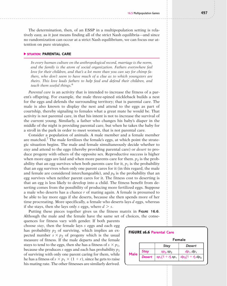
16.5 Multipopulation Games 497
The determination, then, of an ESSP in a multipopulation setting is rela-tively easy, as it just means finding all of the strict Nash equilibria—and sinceno randomization can occur at a strict Nash equilibrium, we can focus our at-tention on pure strategies.
! SITUATION: PARENTAL CARE
In every human culture on the anthropological record, marriage is the norm,and the family is the atom of social organization. Fathers everywhere feellove for their children, and that’s a lot more than you can say for chimp fa-thers, who don’t seem to have much of a clue as to which youngsters aretheirs. This love leads fathers to help feed and defend their children, andteach them useful things.6
Parental care is an activity that is intended to increase the fitness of a par-ent’s offspring. For example, the male three-spined stickleback builds a nestfor the eggs and defends the surrounding territory; that is parental care. Themale is also known to display the nest and attend to the eggs as part ofcourtship, thereby signaling to females what a great mate he would be. Thatactivity is not parental care, in that his intent is not to increase the survival ofthe current young. Similarly, a father who changes his baby’s diaper in themiddle of the night is providing parental care, but when he takes the baby fora stroll in the park in order to meet women, that is not parental care.
Consider a population of animals. A male member and a female memberare matched.7 The male fertilizes the female’s eggs, at which point the strate-gic situation begins. The male and female simultaneously decide whether tostay and attend to the eggs (thereby providing parental care) or desert to pro-duce progeny with others of the opposite sex. Reproductive success is higherwhen more eggs are laid and when more parents care for them. is the prob-ability that an egg survives when both parents care for it, is the probabilitythat an egg survives when only one parent cares for it (in this regard, the maleand female are considered interchangeable), and is the probability that anegg survives when neither parent cares for it. The fitness cost to deserting isthat an egg is less likely to develop into a child. The fitness benefit from de-serting comes from the possibility of producing more fertilized eggs. Supposea male who deserts has a chance r of mating again. A female is presumed tobe able to lay more eggs if she deserts, because she then spends more of hertime procreating. More specifically, a female who deserts lays d eggs, whereasif she stays, then she lays only s eggs, where
Putting these pieces together gives us the fitness matrix in FIGURE 16.6.Although the male and the female have the same set of choices, the conse-quences for fitness vary with gender. If both parentschoose stay, then the female lays s eggs and each egghas probability of surviving, which implies an ex-pected number of progeny which is the usualmeasure of fitness. If the male departs and the femalestays to tend to the eggs, then she has a fitness of because she produces s eggs and each has probability of surviving with only one parent caring for them, whilehe has a fitness of since he gets to raisehis mating rate. The other fitnesses are similarly derived.
s ! p1 ! (1 % r),
p1
s ! p1,
s ! p2
p2
d 7 s.
p0
p1
p2
FIGURE 16.6 Parental Care
sp2,sp2
sp1(1 % r),sp1Male
FemaleStay
dp1,dp1
dp0(1 % r),dp0
Desert
Stay
Desert

498 CHAPTER 16: EVOLUTIONARY GAME THEORY AND BIOLOGY: EVOLUTIONARILY STABLE STRATEGIES
An ESSP is a strict Nash equilibrium, and what constitutes a strict Nashequilibrium depends on the values of these six parameters: d, s, andr. Let us consider what it takes for each of the four possible strategy pairs tobe evolutionarily stable.
■ Both male and female desert. For no parental care to be an ESSP, wemust have
The first condition ensures that a male does better by deserting, whilethe second condition means that the female’s fitness is higher by desert-ing. The condition describing the female’s fitness can be rearranged to
This says that the gain in producing eggs by not staying—whichis measured by the size of d relative to s—must be large relative to thegain in egg survival from having some parental care—which is measuredby the size of relative to Examples of species that practice the “noparental care” strategy are sharks, skates, and rays. In addition, the careof eggs is uncommon among reptiles.
■ Female stays and male deserts. This strategy pair is an ESSP when
The first condition is for the male. Rearranging terms in it, we have
The left-hand side is the additional number of fertilized eggs that is ex-pected by deserting. Recall that r is the increase in the male’s mating ratethat occurs when the male does not hang around to help care for the eggs.The right-hand side is the cost to departing: The expected number ofsuccessful eggs would rise by that amount if the male stayed. If the benefitfrom deserting exceeds the cost of deserting, then the ESS for males is todeploy the “one-night stand” strategy. Of course, this calculus for the maleis predicated upon the female staying, which she will do if some parentalcare has a big enough impact relative to none, as reflected in the condition
This ESSP—the male cutting out while the female remains tocare for the young—is present in more than 95% of mammal species.
■ Female deserts and male stays. This is the other strategy pair that de-livers uniparental care, and it is an ESSP when
It will arise, for example, when the male isn’t able to procreate that muchmore by departing (i.e., r is low), while the female can produce a lotmore eggs by focusing on egg production rather than splitting her timebetween producing eggs and caring for them (i.e., d is large relative to s).Although this strategy pair is not frequently observed among us Homosapiens, it is quite common among fish. Most fish species are character-ized by uniparental care, and it is typically the male who performs thatfunction. For example, a male may protect the eggs by keeping them inhis mouth, an activity known as “mouth brooding.”
dp1 7 dp0(1 % r) and dp1 7 sp2.
sp1 7 dp0.
sp1r 7 s(p2 " p1).
sp1(1 % r) 7 sp2 and sp1 7 dp0.
p0.p1
ds 7
p1
p0.
dp0(1 % r) 7 dp1 and dp0 7 sp1.
p0, p1, p2,

16.6 Evolution of Spite 499
■ Both female and male stay. Dual parental care is an ESSP when
If having two parents around helps a lot with survival—and the cost interms of reducing mating is not large—then it is evolutionarily stablefor both parents to stay. About 90% of bird species practice dualparental care, with activities that usually include sharing the incuba-tion of eggs and the feeding of chicks. Both parents caring for theiryoung is rare among invertebrates, and though less than 5% of mam-mal species practice dual parental care, 30–40% of primates and carni-vores do.
16.6 Evolution of SpiteTHUS FAR, WE HAVE CONSIDERED populations with many members and in which amutation involves just a small fraction of them. In this section, it is assumedthat the population has only a few members, and a small mutation means asingle member adopting a new strategy. In this type of environment, some ofour earlier findings will change, and, most interestingly, evolution can pro-duce spite, which is the act of doing something to harm someone else eventhough it harms you as well.
Return to the setting of a single population, and now assume that it hasmembers. Define F(x, y) to be the fitness of a member that uses strategy
x when matched with someone using strategy y. For this setting, let us definewhat it takes for a strategy x to be an ESS. If the mutant strategy is y, the fit-ness of a member using the omnipresent strategy x is
[16.22]
With probability someone endowed with x meets anothermember endowed with x, a situation that results in a fitness of F(x, x); andwith probability it meets someone using the mutant strategy y andreceives a fitness of F(x, y).
For x to be an ESS, its fitness must exceed that of the mutant. Note thatsince there is just one mutant, the mutant is assured of meeting only thoseusing strategy x, so its fitness is simply F(y, x). This differs from the case weexamined earlier where multiple members used the mutant strategy. x is thenan ESS if and only if
[16.23]
The left-hand side in (16.23) is a weighted average of F(x, x) and F(x, y), andthis average must exceed the fitness that the mutant gets from meeting some-one using strategy x.
Now suppose
[16.24]F (x, x) 6 F (y, x),
an " 2n " 1
bF(x, x) % a 1n " 1
bF(x, y) 7 F (y, x) for all y ( x.
1/(n " 1),
(n " 2)/(n " 1),
an " 2n " 1
bF(x, x) % a 1n " 1
bF(x, y).
n ' 2
sp2 7 sp1(1 % r) and sp2 7 dp1.

500 CHAPTER 16: EVOLUTIONARY GAME THEORY AND BIOLOGY: EVOLUTIONARILY STABLE STRATEGIES
in which case y is a better reply against x than x is. If a player was rational andshe expected others to use x, she would then surely prefer y over x. However,if F(x, y) is big enough, then (16.23) can be satisfied even if (16.24) holds. Inother words, x can be an ESS even though it is not a best reply against itself!
An example may be useful here, and as a change ofpace, consider a situation taken from our own species.Suppose there are four companies and, in any given pe-riod, two of them are matched to compete for a cus-tomer. They compete through customer-specific market-ing, and each can choose modest or heavy marketing. Thelatter is more costly, but produces more sales. The fitness(or profit) matrix is shown in FIGURE 16.7.
In this game, a dominant strategy is to engage in mod-est marketing; implicitly, then, the cost of heavy market-
ing must be quite high. However, as we show next, the ESS is instead the dom-inated strategy of heavy marketing!
For modest to be an ESS, it must survive if one of the companies were tomutate to using heavy. One can think of a “mutation” as the random decisionto experiment with heavy marketing. Using the condition in (16.23), we seethat modest is not an ESS if and only if
or, from Figure 16.7,
The right-hand side is the fitness to the company using modest and is the par-ticular manifestation of (16.22). With three potential rivals, there is a proba-bility of that that company faces another company with modest marketing,in which case its profit is 9, and there is a probability of that it faces the com-pany using the mutant strategy of heavy marketing, in which case its profit is3. The left-hand side is the fitness to the mutant. Being the lone company de-ploying heavy marketing, it is assured of being matched with a company withmodest marketing, so its profit is 8. Because the profit of the company withheavy marketing is 8, and this exceeds the profit of those with modest market-ing, which is 7, the mutant is outperforming the latter companies. Hence,modest marketing is not an ESS.
Note that the company using the mutant strategy has seen its profit fall from9 to 8 by switching from modest to heavy marketing, given that all other com-panies use modest marketing. But—and this is crucial—the decline in profitfrom this mutation is even greater for the other companies, whose profit slidesfrom 9 to 3. In spite of the company that switched to heavy marketing beingworse off in absolute terms, it is now better off in relative terms—and with evo-lution, it is relative performance that matters. Thus, if a company were toswitch from modest to heavy marketing, one might find other companies imi-tating it because the company with heavy marketing is earning more than thosewhich employ modest marketing. (We just used imitation, rather than natural
13
23
8 ' a23b ! 9 % a1
3b ! 3(#7).
F(heavy, modest) ' a23b ! F(modest, modest) % a1
3b ! F(modest, heavy),
FIGURE 16.7 Marketing
1,1 8,3
3,8 9,9Company 1
Company 2
Heavy
Modest
Heavy Modest

Summary 501
selection, as the mechanism by which a more profitablestrategy may increase its presence in the population.)
This is an evolutionary argument for the personaltrait of spite—when you do something that lowers an-other person’s well-being or fitness even though it low-ers yours as well. Thus, evolution can favor a mutantthat detrimentally affects fitness, as long as it has an even greater detrimentaleffect on those members which do not use the mutant strategy.
SummaryWithin the framework of evolutionary game theory, this chapter has shownhow game theory can be modified to explore the behavior of many animals, notjust us big-brained humans. The selection device for a strategy is not rationality,but rather natural selection. This is the motivation for the concept of an evolu-tionarily stable strategy (ESS). Focusing on stable homogenous populations—so that an ESS is a single strategy—an ESS is a strategy for a population that isresilient to an invasion by a small mutation of an alternative strategy.
Though predicated on natural selection rather than rationality, ESS hasstrong connections to Nash equilibrium. An ESS is a symmetric Nash equilib-rium because, if a strategy is not a best reply to itself, then an invasion bysomething that is a best reply will have higher fitness and thus upset the cur-rent population. While not every Nash equilibrium is an ESS, every strict Nashequilibrium is an ESS. Hence, ESS is a more stringent solution concept thanNash equilibrium. Indeed, it can be so stringent that a game need not have anESS. Such was the case with side-blotched lizards who appear to be engagedin a competition akin to Rock–Paper–Scissors. Although that game has a Nashequilibrium, it does not have an ESS.
ESS was applied to a number of situations occurring in nature. In theHawk–Dove conflict, animals are drawn from a population to compete for a re-source. In the Dung Fly setting, each male is endowed with a strategy regard-ing how long to wait at a cowpat in anticipation of the arrival of a female.These are examples of a single population whose members are matched to in-teract. In some settings, there are instead multiple populations, such as whena male and a female interact. Males may have strategy sets that are differentfrom those of females, or the implication for fitness of a particular strategymay vary between a male and a female. For the multipopulation setting, anevolutionarily stable strategy profile (ESSP) is necessarily equivalent to astrict Nash equilibrium. This equivalence arises because a mutant never meetsitself in a multipopulation setting.
Although this chapter has mostly presumed that the population is large innumber and a mutation is a small fraction of that population, we also exploredthe case when the population has only a few members and a “small” mutationinvolves a single member. An implication is that a mutant does not meet itself,since there is only one mutant. In this special setting, an ESS need not be aNash equilibrium. In fact, a strategy can be strictly dominated and still be anESS! What this analysis highlights is how natural selection chooses high rela-tive performance, not high absolute performance. Thus, a mutant that lowers amember’s fitness can actually thrive if, at the same time, it lowers the fitness ofother members even more, for natural selection chooses the relatively fit.
For the game in Figure 16.7, show that heavyis an ESS.
16.3 CHECK YOUR UNDERSTANDING

502 CHAPTER 16: EVOLUTIONARY GAME THEORY AND BIOLOGY: EVOLUTIONARILY STABLE STRATEGIES
1. Consider the modified Hawk–Dove situation shown in FIGURE PR16.1.What differs from the original game is that there is now some chance(measured by the probability x) that a hawk injures a dove, where
Find all ESS’s. (Note that your answer will depend on thesize of x.)0 6 x 6 1.
EXERCISES
2. Consider the coordination game shown in FIGURE PR16.2. Find all ESS’s.
FIGURE PR16.1 Modified Hawk–Dove Game
"xC,V
V,"xCRed deer stag 1
Red deer stag 2
Hawk
Dove
Hawk Dove
v2
, v2
v " c2
,v " c2
FIGURE PR16.2
1,1 0,0
0,0 2,2Player 1
Player 2
a
b
a b
3. Consider the game depicted in FIGURE PR16.3. Find all ESS’s.
FIGURE PR16.3
4,4 2,5
5,2 1,1Player 1
Player 2
x
y
x y
4. Consider a two-player symmetric game with two pure strategies, and letF(x, y) be the expected fitness to a player using mixed strategy x whenmeeting another player using mixed strategy y.a. State in words what it means for b. State in words what it means for c. Suppose, for all and Is p
an ESS?
5. Consider the Battle of the Sexes game illustrated in FIGURE PR16.5. Findall ESS’s.
F( p, p) 7 F(q, q).F( p, p) # F(q, p)q ( p,F( p, p) 7 F(q, q) for all q ( p.F( p, p) 7 F(q, p) for all q ( p.

Exercises 503
6. Return to the Dung Fly setting in Figure 16.2. Now suppose that eachmale dung fly can stay for one, two, or three minutes. Assume that thecowpat is stale by the third minute, in which case there is no chance thata female dung fly will land on it. Assume also that the fitnesses whenboth male dung flies stay one or two minutes are the same as in Figure16.2. What are reasonable values to assign to the fitnesses denoted w, x,y, and z in FIGURE PR16.6?
FIGURE PR16.5 Battle of the Sexes
2,2 3,5
5,3 2,2Player 1
Player 2
Low
High
Low High
FIGURE PR16.6 Modified Dung Fly Game
2,2
5,2
x,2
2,5
1,1
y,w
2,x
w,y
z,z
Dung fly 1
Dung fly 2
One minute
Two minutes
Three minutes
One minute Two minutes Three minutes
7. Consider the game shown in FIGURE PR16.7. Find all ESS’s.
8. Consider the game depicted in FIGURE PR16.8. Find all ESS’s.
FIGURE PR16.7
3,3 2,5
2,2
5,2
0,0
1,1Player 1
Player 2
w
x
y
2,2
1,1
0,0
w x y
FIGURE PR16.8
2,2 1,4
6,4
4,1
2,5
2,2Player 1
Player 2
x
y
z
4,6
3,3
5,2
x y z

504 CHAPTER 16: EVOLUTIONARY GAME THEORY AND BIOLOGY: EVOLUTIONARILY STABLE STRATEGIES
9. Consider the game portrayed in FIGURE PR16.9. Find all ESS’s.
FIGURE PR16.9
1,1
4,3
0,0
3,2
Player 1
Player 2
w
x
y
z
3,4
5,5
4,2
0,3
w x
0,0
2,4
1,1
1,0
y
2,3
3,0
0,1
2,2
z
10. Consider the Hawk–Dove situation shown in FIGURE PR16.10.a. Show that an ESS uses hawk with probability .b. In this chapter, we’ve only allowed a mutation to be of a single strat-
egy. Departing from that assumption, consider a small mutation inwhich half of the mutants are hawks and half are doves (i.e., they useonly pure strategies). Determine whether the ESS in part (a) is im-mune to this mutation; that is, determine whether the ESS has higherfitness than that of each of these mutants.
23
0,4 2,2
4,0"1,"1Player 1
Player 2
Hawk
Dove
Hawk Dove
FIGURE PR16.10 Hawk–Dove Game Again
11. Consider the multipopulation game between males and females shownin FIGURE PR16.11. Find all ESS’s.
2,0
3,4
1,0
1,2
Male
Female
w
x
y
z
0,1
6,2
4,3
8,4
a b
3,1
3,3
2,1
4,5
c
4,2
2,1
2,3
1,3
d
FIGURE PR16.11
12. Consider the multipopulation game between males and females illus-trated in FIGURE PR16.12. Find all ESS’s.
3,3
0,2
2,2
1,2
Male
Female
w
x
y
z
1,2
4,1
6,3
3,3
a b
0,3
2,1
3,1
4,0
c
FIGURE PR16.12

References 505
REFERENCES1. An important reference for evolutionary game theory is John Maynard
Smith, Evolution and the Theory of Games (Cambridge, U.K.: CambridgeUniversity Press, 1982).
2. This interpretation is due to George J. Mailath, “Do People Play NashEquilibrium? Lessons from Evolutionary Game Theory,” Journal ofEconomic Literature, 36 (1998), 1347–74.
3. The ensuing facts are from J. R. Krebs and N. B. Davies, An Introduction toBehavioural Ecology (Oxford: Basil Blackwell, 1993), p. 157.
4. This is Figure 14 from G. A. Parker, “The Reproductive Behaviour and theNature of Sexual Selection in Scatophaga stercoraria L. (Diptera:Scatophagidae): II. The Fertilization Rate and the Spatial and TemporalRelationship of Each Sex Around the Site of Mating and Oviposition,”Journal of Animal Ecology, 39 (1970), 205–28.
5. B. Sinervo and C. M. Lively, “The Rock–Paper–Scissors Game and theEvolution of Alternative Male Strategies,” Nature, 380 (1996), 240–43.
6. Robert Wright, The Moral Animal (New York: Random Books, 1994), p. 57.
7. The ensuing discussion is based on John Maynard-Smith, “ParentalInvestment—A Prospective Analysis,” Animal Behaviour, 25 (1977), 1–9.Some of the examples come from T. H. Clutton-Brock, The Evolution ofParental Care (Princeton, NJ: Princeton University Press, 1991).

This page intentionally left blank

Named in honor of Charles Darwin, the father of evolution, the DarwinAwards commemorate those who improve our gene pool by removingthemselves from it.
Picture a college dorm room. Dirty laundry, sexy posters, foodwrappers, textbooks, and in the middle of it all, a student rocking out toloud music. A typical student, a typical day. But this particular student,bouncing on his bed as he rocked out on his air guitar, was about to“take things too far,” according to the coroner’s report. Li Xiao Meng, astudent at Singapore’s Hua Business School, bounced up and down onhis bed with such enthusiasm that he rocked himself right out of thethird-floor window.1
17.1 IntroductionALTHOUGH IT IS USEFUL to have read Chapter 16 prior to taking on this chapter,it is not necessary. What is essential reading, however, is Section 16.1, as itprovides an overview to evolutionary game theory. Once you’ve read that sec-tion, we can move on.
The most common approach of game theory—and the approach pursuedthus far in this book—is to impose conditions for a strategy profile to be a sta-ble configuration. This means that once players are using those strategies,there is no force of intellect or nature to disturb it. That is the tack taken withNash equilibrium and, in the previous chapter, with an evolutionarily stablestrategy. What is missing from this approach is a modeling of how players ac-tually get to that point: how they come to be acting according to the stableconfiguration. This chapter offers a dynamic model that is applicable tostrategic settings in nature. The model is predicated upon the mechanism ofnatural selection, whereby those strategies which are more fit survive, repro-duce at a higher rate, and thus make up a bigger share of the strategies usedby the next generation. (Having read Section 16.1, you’ll know that a memberof a population is endowed with a strategy, just as she may be endowed withblond hair and a talent for writing music.)
The particular way in which natural selection is modeled here is known asthe replicator dynamic. It specifies that the proportion of a population using astrategy increases when it produces fitness in excess of the average fitness of thepopulation, while the proportion decreases when it produces fitness that fallsshort of the average population fitness. In the context of a model of animal con-flict, the replicator dynamic is introduced in Section 17.2; a more formal andgeneral definition is offered in Section 17.3. Section 17.4 discusses how the strate-gies that do well under the replicator dynamic compare against evolutionarily
17
507
Evolutionary Game Theory and Biology:Replicator Dynamics

stable strategies, which is the concept used in Chapter 16. Section 17.4 shouldbe skipped if you haven’t read Chapter 16 (though you have read Section 16.1,right?). The remainder of the chapter applies the replicator dynamic to severalbiological and social settings. We use it to explore the phenomenon of commu-nal hunting in the context of the Stag Hunt game and then to investigate thehandedness of batters and pitchers in Major League Baseball over the last120 years. Finally, in the context of the repeated Prisoners’ Dilemma, we showhow cooperation can emerge and when it is stable. In other words, when is a so-ciety made up of scallywags and when is it made up of saints?
17.2 Replicator Dynamics and the Hawk–Dove GameMANY ANIMAL CONFLICTS IN NATURE involve competition for a resource, such as aterritory or reproduction with a female. To model such scenarios in a simpleway, biologists have developed the Hawk–Dove game. In this game, two ani-mals are matched and each is endowed with one of two possible strategies. Ananimal with the strategy hawk is willing to fight in order to control the re-source. In contrast, an animal endowed with dove postures as if he is willingto battle, but then backs down if the other animal starts to fight. In terms offitness, the value of the resource is V. Thus, if an animal using hawk facessomeone using dove, then hawk wins the resource—since dove retreats as soonas hawk starts to fight—which yields a fitness of V, while dove receives zero fit-ness. If the potential combatants are both doves, then they engage in a pro-longed posturing exercise until one decides to give up. If we let each have a50% chance of outlasting the other, the expected fitness when two doves meetis . Finally, if two hawks meet, then there is a fight until one of them is in-jured. The fitness to the loser is (where C is the cost of being injured),while the winner of the fight gains access to the resource, which produces fit-ness V. As two hawks are presumed to be evenly matched, each has an equalchance of winning the fight, so their expected fitness is
Assume that each animal receives a baselinefitness of Their fitness is then B, pluswhatever they get out of their encounter. Finally,suppose so that the fitness cost ofthe injury exceeds the fitness benefit of the ter-ritory, and suppose that B is big enough so thatall fitnesses are positive willsuffice). This scenario gives us the strategicform game shown in FIGURE 17.1.
The focus of evolutionary game theory is thepopulation, not the individual animal. The ob-jective is to characterize a stable population
mix of strategies. Toward that end, the primary unit of interest is the strategy,and in that light, animals are merely vehicles for strategies. The animals thatuse a strategy may come and go, but the mix of strategies in the populationcan persist.
The approach we’ll take to describing a stable population mix is rooted innatural selection: A strategy with higher fitness produces more progeny, andthis serves to increase that strategy’s share of the population in the next gen-eration. To model this mechanism, we need to write down the fitness of each
(B 7 (C " V)/2
C 7 V 7 0,
B 7 0.
(V " C)/2.
"C
V2
508 CHAPTER 17: EVOLUTIONARY GAME THEORY AND BIOLOGY: REPLICATOR DYNAMICS
Hawk
Dove B , B % V
B % V, BAnimal 1
Animal 2
Hawk Dove
B % B %V " C2
V " C2,
V2
V2B % B %,
FIGURE 17.1 Hawk–Dove Game with Baseline Fitness

17.2 Replicator Dynamics and the Hawk–Dove Game 509
strategy. Let denote the fitness attached to an animal endowed withstrategy x when matched with an animal endowed with strategy y (e.g.,
Consider those animals endowed with the strategy hawk. Each earns a fit-ness of when matched with another hawk and a fitness of when matched with a dove. Hence, the average fitness that an animal withhawk can expect to receive in this population depends on the mix of strategiesin the population. Let denote the fraction of the population endowed withhawk in generation t. Then the average fitness of the hawk strategy is
With frequency a hawk meets an animal that is similarly endowed and re-ceives a fitness of With frequency a hawk meets a dove,and the former receives fitness of Analogously, the fitness of dove ingeneration t is
The replicator dynamic specifies that the fraction of animals in the nextgeneration that use a strategy grows when that strategy’s fitness exceeds theaverage fitness in the population, and the fraction using a strategy shrinkswhen that strategy’s fitness falls short of the average population fitness. In theHawk–Dove game, the average population fitness in generation t is
A fraction of the population is endowed with the hawk trait and has an av-erage fitness of while a fraction has the dove trait and re-ceives an average fitness of
In the context of the Hawk–Dove game, the replicator dynamic is then
[17.1]
This equation says that the fraction of hawks in the population in generationdenoted equals the fraction in generation t, multiplied by a num-
ber that is the ratio of the hawk’s fitness to the average population fitness. Ifthe fitness of hawk exceeds the average population fitness then and, by (17.1), so the fraction of hawks is in-creasing. Furthermore, the more that hawk’s fitness exceeds the average pop-ulation fitness, the faster its share of the population grows. If, instead, hawk’sfitness is less than the average population fitness, then and,again by (17.1), The fraction of hawks is then decreasing.
As specified by the replicator dynamic, the population evolves in terms ofhow many are endowed with the hawk trait and how many with the dovetrait. Our next task is to describe this evolution. Suppose the current mix of
ht%1 6 ht.Ft(hawk)/Ft 6 1
ht%1 7 ht,Ft(hawk)/Ft 7 1(Ft(hawk) 7 Ft),
ht%1,t % 1,
ht%1 # ht ! aFt(hawk)
Ft b.Ft(dove).
1 " htFt(hawk),ht
Ft # ht ! Ft(hawk) % (1 " ht) ! Ft(dove).
Ft(dove) # ht ! B % (1 " ht) ! aB %V2b.
B % V.1 " ht,B % (V " C)/2.
ht,
Ft(hawk) # ht ! aB %V " C
2b % (1 " ht) ! (B % V).
ht
B % VB % (V " C)/2
F(hawk, dove) # B % V).
F(x, y)

510 CHAPTER 17: EVOLUTIONARY GAME THEORY AND BIOLOGY: REPLICATOR DYNAMICS
strategies in the population has the fitness of hawk exceeding that of thepopulation average:
Subtracting from both sides and rearranging terms, we have
Dividing each side by we get
Finally, point your wand at the page and say petrificus totalus. (If you’re not awizard, skip that last step.) The fitness of hawk then exceeds the average pop-ulation fitness if and only if it exceeds the fitness of dove. Since there are onlytwo strategies, if hawk is better than the average performing strategy, then itmust be better than dove.
By the replicator dynamic, the fraction of hawks grows when the fitness ofhawk exceeds that of dove, which is the case when
[17.2]
Cancelling B from both sides and then solving for we get
Thus, the fraction of hawks in the population grows when Recall thatwe have assumed that as the cost of an injury exceeds the value of theterritory. When the fraction of hawks is sufficiently low—specifically, —the fitness of hawk exceeds that of dove and, by the replicator dynamic, thefraction of hawks in the population increases.
If, instead, the fitness of dove exceeds the fitness of hawk, then the fitnessof hawk is less than the average population fitness and the fraction of hawksfalls. If we just flip around the inequality in (17.2) and again solve for wefind that the fraction of hawks is declining when If the population isheavy on hawks, doves then have the higher fitness and, by the replicator dy-namic, the fraction of doves rises.
Pulling all these specifications together, we have a description of how thepopulation evolves over time:
If ht 7 VC
, then ht%1 6 ht.
If ht = VC
, then ht%1 = ht.
If ht 6 VC
, then ht%1 7 ht.
ht 7 VC.
ht,
ht 6 VC
VC 6 1,
ht 6 VC.
ht 6 VC
.
ht,
ht ! aB %V " C
2b% (1 " ht) ! (B % V) 7 ht ! B % (1 " ht) ! aB %
V2b.
Ft(hawk) 7 Ft(dove).
1 " ht,
(1 " ht) ! Ft(hawk) 7 (1 " ht) ! Ft(dove).
ht ! Ft(hawk)
Ft(hawk) 7 ht ! Ft(hawk) % (1 " ht) ! Ft(dove).

17.2 Replicator Dynamics and the Hawk–Dove Game 511
This set of conditions is depicted graphicallyin FIGURE 17.2. When is increasingand moving closer to as is reflected inthe arrow pointing to the right, toward If
then is falling, and we see that thearrow is pointing to the left, again toward The replicator dynamic, then, moves the frac-tion of hawks in the direction of And when
then the fraction of hawks is frozen. Although you mightthink that this is due to our using the petrificus totalus charm, it’s actuallybecause the fitness of hawks is exactly the same as the fitness of doves andthus is the same as the average fitness of the population. Since hawk doesneither better nor worse than the population at large, it neither grows norshrinks.
A population mix in which hawks make up a fraction equal to is a restpoint. A rest point is a population mix of strategies that the replicator dynamicleaves undisturbed. Once the population is at a rest point, the replicator dy-namic keeps it there, generation after generation.*
✚ DEFINITION 17.1 A population mix s* is a rest point if, once the popu-lation mix is at s*, it stays there.
A population mix may be a rest point, but it isn’t necessarily the case thatthe replicator dynamic will lead the population to it. For that to occur, a restpoint must be locally stable. A locally stable rest point, or an attractor, is arest point such that if the population begins near the rest point, it eventuallyends up there. It is said to be locally stable because convergence to the restpoint is assured only if the population starts out “local” to the rest point.
✚ DEFINITION 17.2 A rest point s* is an attractor if, when the populationmix starts close to s*, then, eventually, the population mix goes to s*.
It is worth emphasizing that a rest point and an attractor are specific to thedynamic being specified. Change the dynamic, and those population mixeswhich are local attractors could change as well. In this chapter, we will be fo-cusing on rest points and attractors for the replicator dynamic.
To visualize the stability implicit in rest points and attractors, consider FIGURE
17.3. Imagine that a ball is moving along this one-dimensional surface, wherethe dynamic is now gravity, not natural selection. A rest point is a position onthat surface such that the ball is no longer moving. Position u is not a restpoint, because, if the ball is at u, it will roll downhill in the direction of po-sition v. Now suppose the ball is at v. There is no force causing it to leave v;once there, it stays there. The point v is then a rest point. Another rest point isposition x. Once the ball is nestled at the top of that hill, there the ball will re-main. However, while both v and x are rest points, v is an attractor and x is not.To see this, note that if we disturb the ball a little bit from position v—say, mov-ing it to position w—it’ll roll back downhill toward v and eventually settle there;hence, v is an attractor. In contrast, if we move the ball from position x to, say,
VC
ht%1 # ht;ht # VC,
VC.
VC.
htht 7 VC,
VC.
VC,
htht 6 VC,
*Trivially, a population of all doves is also a rest point by the replicator dynamic, since, if thenso In other words, if there are no hawks,
then hawks can’t reproduce. Similarly, a population of all hawks is a rest point, because, if thenht%1 # ht ! (Ft(hawk)/Ft) # 1 ! 1 # 1.
ht # 1,ht%1 # 0.ht%1 # ht ! (Ft(hawk)/Ft) # 0 ! (Ft(hawk)/Ft) # 0,
ht # 0,
0 1VC
ht
FIGURE 17.2 Replicator Dynamic in Hawk–Dove Game
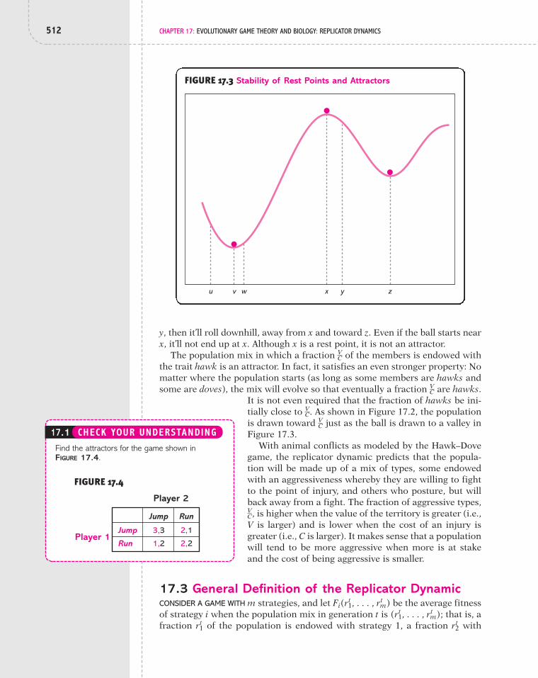
512 CHAPTER 17: EVOLUTIONARY GAME THEORY AND BIOLOGY: REPLICATOR DYNAMICS
y, then it’ll roll downhill, away from x and toward z. Even if the ball starts nearx, it’ll not end up at x. Although x is a rest point, it is not an attractor.
The population mix in which a fraction of the members is endowed withthe trait hawk is an attractor. In fact, it satisfies an even stronger property: Nomatter where the population starts (as long as some members are hawks andsome are doves), the mix will evolve so that eventually a fraction are hawks.
It is not even required that the fraction of hawks be ini-tially close to . As shown in Figure 17.2, the populationis drawn toward just as the ball is drawn to a valley inFigure 17.3.
With animal conflicts as modeled by the Hawk–Dovegame, the replicator dynamic predicts that the popula-tion will be made up of a mix of types, some endowedwith an aggressiveness whereby they are willing to fightto the point of injury, and others who posture, but willback away from a fight. The fraction of aggressive types,, is higher when the value of the territory is greater (i.e.,
V is larger) and is lower when the cost of an injury isgreater (i.e., C is larger). It makes sense that a populationwill tend to be more aggressive when more is at stakeand the cost of being aggressive is smaller.
17.3 General Definition of the Replicator DynamicCONSIDER A GAME WITH m strategies, and let be the average fitnessof strategy i when the population mix in generation t is that is, afraction of the population is endowed with strategy 1, a fraction withrt
2rt1
(rt1, . . . , rt
m);Fi(rt
1, . . . , rtm)
VC
VC
VC
VC
VC
u v w x y z
FIGURE 17.3 Stability of Rest Points and Attractors
Find the attractors for the game shown inFIGURE 17.4.
17.1 CHECK YOUR UNDERSTANDING
3,3
1,2
2,1
2,2Player 1
Player 2
Jump
Run
Jump Run
FIGURE 17.4

17.4 ESS and Attractors of the Replicator Dynamic 513
strategy 2, . . . , and a fraction with strategy m. Remember that the frac-tions sum to 1: Assume that fitness is always positive:
In any game, this can always be done by making the baseline fitness largeenough. Finally, define as the average fitness of the population, or
where
For example, in the Hawk–Dove game, if hawk is strategy 1 and dove is strat-egy 2, then
By the replicator dynamic, the fraction of strategy i in the next generation is
The proportion of a population that is endowed with a strategy grows when thefitness which that strategy delivers exceeds the average fitness of the population:
Analogously, the fraction using a strategy shrinks if its fitness is less than theaverage fitness of the population. And when the strategy’s fitness equals theaverage fitness of the population, the presence of that strategy in the popula-tion is unchanged.
17.4 ESS and Attractors of the Replicator DynamicIN CHAPTER 16, AN ALTERNATIVE approach to the replicator dynamic was putforth.* Rather than explicitly model the dynamic process jostling a populationmix, we defined an evolutionarily stable strategy (ESS). ESS is analogous toNash equilibrium in rational game theory. Just as a Nash equilibrium speci-fies conditions for a strategy profile to be stable (in the sense that no playerwants to change what she is doing), an ESS is a strategy such that, if all mem-bers of a population use it, then the population mix is stable in the sense thatany mutation is unsuccessful in invading the population. More specifically,that mutant has lower fitness than that of the currently ubiquitous strategy.
Fi(rt1, . . . , rt
m)
F(rt1, . . . , rt
m)7 1.
rt%1i # rt
i ! aFi(rt1, . . . , rt
m)
F(rt1, . . . , rt
m)b.
F1(rt1, rt
2) # r t1 ! aB %
V " C2b % rt
2 ! (B % V).
Fti # Fi(rt
1, . . . , rtm).
F(rt1, . . . , rt
m) # rt1 ! Ft
1 % rt2 ! Ft
2 % p % rtm ! Ft
m,
Ft
Fi(rt1, . . . , rt
m) 7 0 for all (rt1, . . . , rt
m).
rt1 % rt
2 % p % rtm # 1.rtm
*This section is intended for those who have read Chapter 16. Those who have not should skip to Section 17.5.

514 CHAPTER 17: EVOLUTIONARY GAME THEORY AND BIOLOGY: REPLICATOR DYNAMICS
The task of this section is to identify differences and similarities in thesetwo approaches to evolutionary game theory—ESS and the replicator dy-namic. Our use of ESS was limited to homogeneous populations—that is, pop-ulations in which all members use the same strategy. Although a mutationwould obviously deploy a different strategy, we assumed that all mutatedmembers adopted the same mutant strategy. Hence, while a population wascharacterized by one common strategy at an ESS, observed behavior couldstill be heterogeneous because we allowed for mixed strategies. For example,if choosing hawk with probability p is an ESS in the Hawk–Dove game, then,at any time, it would be observed that a fraction p of the population is exhibit-ing hawk-like behavior and a fraction of the population looks like doves.
Although the replicator dynamic can allow for mixed strategies, we willlimit our attention in this chapter to pure strategies. Counterbalancing this re-strictive assumption, a stable population mix is permitted to be heteroge-neous. Returning to the Hawk–Dove game, a stable population under thereplicator dynamic could entail a fraction p of the population being endowedwith the hawk strategy and a fraction with the dove strategy.
In a sense, the ESS approach and the replicator dynamic approach are equallyrich in terms of what behavior a population is permitted to exhibit. Taking theHawk–Dove game as an example, we can see that the following two situations areobservationally equivalent at the population level: (1) each member uses a mixedstrategy in which he plays hawk a fraction p of the time; and (2) a fraction p ofthe population is endowed with the pure-strategy hawk. Now, suppose one pop-ulation of animals—say, red deer—is described by situation 1 and another ani-mal population—say, fig wasps—is described by situation 2. If you’re a biologistrecording the behavior of these two populations, the records will look the same:in each population, hawk was chosen by a fraction p of animals. In this sense, thetwo situations—a homogeneous population using a mixed strategy and a hetero-geneous population using pure strategies—are indistinguishable.
This equivalence goes further in terms of what a stable population lookslike. In the previous section, it was shown that an attractor under the replica-tor dynamic is a fraction of the population endowed with hawk. In Section16.3, we showed that the unique ESS for the Hawk–Dove game is a mixedstrategy in which a member chooses hawk with probability . Both evolution-ary game-theoretic approaches deliver the same description: a fraction ofobserved play is hawkish. Although it is generated by different populations ofstrategies, the resulting behavior is the same.
This equivalence in outcomes in the Hawk–Dove game is not coincidental,for there are strong connections between an ESS and an attractor under thereplicator dynamic.
Every ESS is an attractor under the replicator dynamic.
The converse is not universally true, in that an attractor of the replicator dy-namic need not be an ESS. However, if we limit ourselves to games with twoplayers and two strategies—such as the Hawk–Dove game—then ESSes andreplicator dynamic attractors are equivalent.
In a game with two players, each of which has two strategies, everyESS is an attractor and every attractor is an ESS.
VC
VC
VC
1 " p
1 " p

17.5 ExamplesARMED WITH THE REPLICATOR dynamic, let’s wield this tool to investigate a varietyof settings. The Stag Hunt game explores the emergence of communal hunt-ing. Whereas the Hawk–Dove game had a single attractor, the Stag Hunt gamehas a pair of attractors. And now for something completely different: the evo-lution of handedness among batters and pitchers in Major League Baseball.Interestingly, our model will have no attractor and predicts a cycling of strate-gies. The final application is an old friend: the repeated Prisoners’ Dilemma.A population either evolves to having everyone play nice or having everyoneplay nasty.
! SITUATION: STAG HUNT
Many species work together to achieve a common goal. Lions (mostlyfemales) are much more effective when hunting as a group than going italone. In pursuing animals such as antelope, gazelle, and wildebeest, some ofthe lions will chase the prey in the direction of other lions who wait in am-bush, ready to pounce when the prey is near. The spotted hyena has been ob-served to hunt both singly and in groups whose size depends on the prey beinghunted. By working together, spotted hyenas can effectively hunt larger ani-mals, such as zebras.
The strategic situation just described can be modeled by a gameknown as the Stag Hunt, which is shown in FIGURE 17.5. In the StagHunt, two members of the population are matched to engage in in-dividual or communal hunting. As originally described by thephilosopher Jean-Jacques Rousseau in the eighteenth century, thetwo hunters can either work together to bring down large prey,such as a stag, or work separately to bring down small prey, suchas a hare. In terms of fitness, they do better by both choosingstag—receiving a fitness of 4—than by both choosing hare, with afitness of 3.
Suppose, in generation t, a fraction of the population is endowed with thestag strategy. Then the average fitness of a member using stag is
while the average fitness of a member using hare is
By the replicator dynamic, the fraction of stags is growing if and only if the fit-ness of those endowed with stag exceeds the average fitness of the population.Since there are only two strategies, an equivalent statement is that the fitnessof those endowed with stag exceeds the fitness of those endowed with hare. Inother words, if and only if
1 % 3st 7 3, or, equivalently, st 7 23
.
st%1 7 st
st ! 3 % (1 " st) ! 3 # 3.
st ! 4 % (1 " st) ! 1 # 1 % 3st,
st
17.5 Examples of Strategic Situations 515
4,4
3,1
1,3
3,3Player 1
Player 2
Stag
Hare
Stag Hare
FIGURE 17.5 Stag Hunt

516 CHAPTER 17: EVOLUTIONARY GAME THEORY AND BIOLOGY: REPLICATOR DYNAMICS
Alternatively, the fraction of members using stag is declining if and only if thefitness of those endowed with hare exceeds the fitness of those endowed withstag. That is, if and only if
These dynamics are depicted in FIGURE 17.6:when the fraction of stags is falling, andwhen the fraction of stags is rising. Bythe replicator dynamic, a population in whichall members use hare is an attractor. If the cur-rent fraction of the population with the stagstrategy is sufficiently low (that is, if then that fraction continues to decline, be-
cause the fitness of hare exceeds the fitness of stag; in Figure 17.6, the arrowpoints in the direction of all members using hare when If, instead,
then the fraction of stags is rising, and by the replicator dynamic, apopulation in which all members use stag is an attractor. In Figure 17.6, thearrow points in the direction of all members endowed with stag.
These results makes sense. It is worthwhile to hunt large game only if it issufficiently likely that your partner is willing to hunt large game as well, foronly then can you do so effectively. The replicator dynamic, then, results in anever-increasing fraction that uses stag as long as the initial fraction that usesstag is sufficiently great. However, if that fraction is initially low, then thepreferable strategy is to engage in individual hunting. Then, because moremembers are endowed with hare, it makes it yet more attractive to have thattrait, since few others are willing to hunt communally. With the Stag Huntgame, the locally stable population mix that emerges from the replicator dy-namic depends on the initial mix.
There is one final population mix that we have not analyzed: a populationthat starts out with exactly two-thirds of its members endowed with stag andone-third with hare. In this population, both the fitness of stag and the fitnessof hare is 3; therefore, each strategy has fitness equal to the average popula-tion fitness (which is, of course, 3). Since all strategies are equally fit, the repli-cator dynamic leaves this population mix undisturbed. A population with two-thirds of its members endowed with stag is then a rest point. However, it is notan attractor. To see this, suppose there is a slight perturbation in the popula-tion mix—for example, a lethal disease randomly inflicts animals, and by hap-penstance, the death rate is higher among those endowed with hare. Now thefraction endowed with stag is slightly higher than , and by Figure 17.6, thepopulation mix will steadily grow until all of its members are endowed withstag. Because the mix does not return to the rest point at which two-thirdshave the stag strategy, the original population, with two-thirds of its membersendowed with stag, is not an attractor.
For the Stag Hunt game, the replicator dynamic predicts that a stable pop-ulation has either all members endowed with stag or all endowed with hare,and which occurs depends on the initial population mix. The set of initial pop-ulation mixes that lead to a particular rest point is called the basin of attrac-tion for that rest point.
23
st 7 23,
st 6 23.
st 6 23),
st 7 23,
st 6 23,
3 7 1 % 3st, or, equivalently, st 6 23
.
st%1 6 st
0 123
st
FIGURE 17.6 Replicator Dynamic in Stag Hunt

17.5 Examples of Strategic Situations 517
✚ DEFINITION 17.3 The basin of attraction for a restpoint s* is the set of population mixes such that if thepopulation mix starts in the basin, then, eventually, thepopulation mix is at s*.
In Figure 17.6, the basin of attraction for the “allhare” attractor comprises population mixes in whichfewer than two-thirds of the members are endowed withstag, while the basin of attraction for the “all stag” at-tractor is made up of population mixes in which morethan two-thirds are endowed with stag. The basin of at-traction for the rest point at which two-thirds use stagand one-third uses hare is a single point: the populationmix in which two-thirds use stag and one-third useshare. Since its basin is trivially small, it is a rare event indeed that would re-sult in the heterogeneous rest point being reached.
! SITUATION: HANDEDNESS IN BASEBALL
Though motivated by biological settings, evolutionary game theory can also beused to shed light on human social behavior. So, let’s apply the replicator dy-namic to investigate historical patterns in the handedness of baseball players.As is well documented, right-handed batters perform better against left-handedpitchers, while left-handed batters perform better against right-handed pitch-ers. FIGURE 17.8 reports the fraction of right-handed batters and right-handedpitchers in major league baseball over 12 decades, from 1876 to 1985.2
The data reveal an intriguing historical trend. Initially, about 85–90% of bat-ters and pitchers were right handed, which is about the rate of right-handers inthe general population. Steadily, however, the fraction of right-handed battersand pitchers has fallen over time. It is also notable that the population mixes
For the game in FIGURE 17.7, find the attrac-tors under the replicator dynamic.
17.2 CHECK YOUR UNDERSTANDING
5,5
1,1
1,1
2,2Player 1
Player 2
Black
White
Black White
FIGURE 17.7
Perc
enta
ge
0.95
0.9
0.85
0.8
0.75
0.7
0.65
0.6
0.550.5
0 1 2 3 4 5 6 7 8 11109 12
Right-handed batter
Right-handed pitcher
Decades
FIGURE 17.8 Right-Handed Batters and Right-HandedPitchers, 1876–1985

518 CHAPTER 17: EVOLUTIONARY GAME THEORY AND BIOLOGY: REPLICATOR DYNAMICS
of both batters and pitchers appear to move together. The mix even-tually leveled off, so that today about 65–75% of batters and pitch-ers are right handed.
Let’s see whether evolutionary game theory can explain this trend.Contrary to the previous models in this chapter, assume that thereare two populations that coevolve according to the replicator dy-namic. One population is made up of batters, who can bat eitherright or left. The other population comprises pitchers, who can throweither right or left. The strategic situation faced by a batter and apitcher is shown in FIGURE 17.9. Note that a right-handed batter per-
forms better against a left-handed pitcher, while a left-handed batter hits betteragainst a right-handed pitcher, which is consistent with the facts. (See Table 2.2.)
Our objective is to understand the mix of batters who hit from the right orleft side of the plate and the mix of pitchers who throw right or are southpaws(so named because a left-hander’s throwing arm faces south when he is on themound). In doing so, the natural-selection metaphor is maintained. A pitcheror a batter does not choose his handedness; that is something with which he isendowed. What will happen, however, is that if, say, right-handed batters per-form better than left-handed batters, then managers will replace left-handedbatters with right-handed batters, so the fraction of right-handed batters rises.
Before cranking out the replicator dynamic equations, let’s apply a bit of in-tuition here. Examining Figure 17.9, we ought to expect there will be a mix ofhandedness types. If all pitchers were right handed, then left-handed batterswould outperform right handed batters, with a fitness of 36 (versus 30). But ifthis resulted in all batters being left handed, then we would expect managersto start cutting right-handed pitchers from their roster and replacing themwith left-handed pitchers, since the latter are performing better (compare 30and 21). Thus, neither all batters having the same handedness nor all pitchershaving the same handedness can be a rest point.
To assess the replicator dynamic in this setting, let denote the fraction ofright-handed batters and the fraction of right-handed pitchers, as of gener-ation t. Then the average fitness (or performance) of a right-handed batter is
A fraction of the time, a right-handed batter faces a right-handed pitcher,and his performance is 30; and a fraction of the time, the pitcher is left-handed, and a right-handed batter’s performance is significantly higher, at 44.The average fitness of a left-handed batter is
The replicator dynamic for batters is then
[17.3]
where the denominator is the average fitness among all batters. Since thereare only two strategies, right-handed batters perform better than the averagebatter when they perform better than left-handed batters:
bt%1 # bt ! a 44 " 14pt
bt ! (44 " 14pt) % (1 " bt) ! (30 % 6pt)b,
FtB(left) # pt ! 36 % (1 " pt) ! 30 # 30 % 6pt.
1 " ptpt
FtB(right) # pt ! 30 % (1 " pt) ! 44 # 44 " 14pt.
ptbt
30,30
36,21
44,24
30,30Batter
Pitcher
Right
Left
Right Left
FIGURE 17.9 Baseball

17.5 Examples of Strategic Situations 519
Solving this expression for the fraction of right-handed batters, we find thatIf less than 70 percent of pitchers are right handed, then right-handed
batters have higher performance than left-handed batters, and by the replicatordynamic, the fraction of right-handed batters is growing. In sum, the replicatordynamic tells us that the population of batters evolves in the following manner:
[17.4]
Next, we turn to the population of pitchers. The average performance of aright-handed pitcher equals
and for a left-handed pitcher, it is
The replicator dynamic then implies that
[17.5]
and from this equation, we get the following description of the evolution ofpitchers’ handedness:
[17.6]
If more than 60% of batters are right handed, then the fraction of right-handed pitchers increases.
The rest point for the replicator dynamic occurs where the performance of aright-handed batter is the same as that of a left-handed batter—which requiresthat —and the performance of a right-handed pitcher is the same as that ofa left-handed pitcher—which requires that Of course, this just says that ifthe population mix starts with 60% right-handed batters and 70% right-handedpitchers, it’ll stay there. But as we know from Figure 17.8, it didn’t start there; itstarted with 85–90% of batters and of pitchers being right handed. Starting at thatpoint, does the replicator dynamic push the population mix toward the rest point?
To explore that question, we’ll deploy the phase diagram shown in FIGURE
17.10.* On the horizontal axis are values for and on the vertical axis arebt,
bt # .6.pt # .7
If bt 6 .6, then pt%1 6 pt.
If bt = .6, then pt%1 = pt;
If bt 7 .6, then pt%1 7 pt;
pt%1 # pt ! a 21 % 9bt
pt ! (21 % 9bt) % (1 " pt) ! (30 " 6bt)b,
FtP(left) # bt ! 24 % (1 " bt) ! 30 # 30 " 6bt.
FtP(right) # bt ! 30 % (1 " bt) ! 21 # 21 % 9bt,
If pt 7 .7, then bt%1 6 bt.
If pt = .7, then bt%1 = bt;
If pt 6 .7, then bt%1 7 bt;
pt 6 .7.
44 " 14pt 7 30 % 6pt.
*Figures 17.2 and 17.6 are phase diagrams for their respective games.
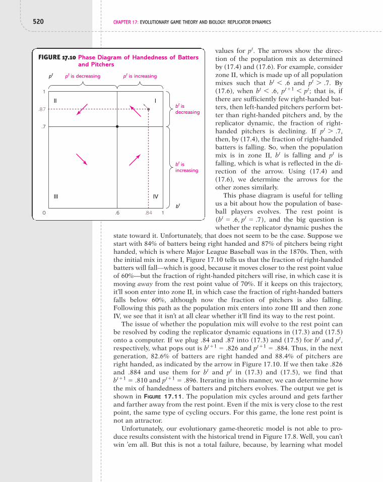
values for The arrows show the direc-tion of the population mix as determinedby (17.4) and (17.6). For example, considerzone II, which is made up of all populationmixes such that and By(17.6), when that is, ifthere are sufficiently few right-handed bat-ters, then left-handed pitchers perform bet-ter than right-handed pitchers and, by thereplicator dynamic, the fraction of right-handed pitchers is declining. If then, by (17.4), the fraction of right-handedbatters is falling. So, when the populationmix is in zone II, is falling and isfalling, which is what is reflected in the di-rection of the arrow. Using (17.4) and(17.6), we determine the arrows for theother zones similarly.
This phase diagram is useful for tellingus a bit about how the population of base-ball players evolves. The rest point is
and the big question iswhether the replicator dynamic pushes the
state toward it. Unfortunately, that does not seem to be the case. Suppose westart with 84% of batters being right handed and 87% of pitchers being righthanded, which is where Major League Baseball was in the 1870s. Then, withthe initial mix in zone I, Figure 17.10 tells us that the fraction of right-handedbatters will fall—which is good, because it moves closer to the rest point valueof 60%—but the fraction of right-handed pitchers will rise, in which case it ismoving away from the rest point value of 70%. If it keeps on this trajectory,it’ll soon enter into zone II, in which case the fraction of right-handed battersfalls below 60%, although now the fraction of pitchers is also falling.Following this path as the population mix enters into zone III and then zoneIV, we see that it isn’t at all clear whether it’ll find its way to the rest point.
The issue of whether the population mix will evolve to the rest point canbe resolved by coding the replicator dynamic equations in (17.3) and (17.5)onto a computer. If we plug .84 and .87 into (17.3) and (17.5) for and respectively, what pops out is and Thus, in the nextgeneration, 82.6% of batters are right handed and 88.4% of pitchers areright handed, as indicated by the arrow in Figure 17.10. If we then take .826and .884 and use them for and in (17.3) and (17.5), we find that
and Iterating in this manner, we can determine howthe mix of handedness of batters and pitchers evolves. The output we get isshown in FIGURE 17.11. The population mix cycles around and gets fartherand farther away from the rest point. Even if the mix is very close to the restpoint, the same type of cycling occurs. For this game, the lone rest point isnot an attractor.
Unfortunately, our evolutionary game-theoretic model is not able to pro-duce results consistent with the historical trend in Figure 17.8. Well, you can’twin ’em all. But this is not a total failure, because, by learning what model
pt%1 # .896.bt%1 # .810ptbt
pt%1 # .884.bt%1 # .826pt,bt
(bt # .6, pt # .7),
ptbt
pt 7 .7,
pt%1 6 pt;bt 6 .6,pt 7 .7.bt 6 .6
pt.
520 CHAPTER 17: EVOLUTIONARY GAME THEORY AND BIOLOGY: REPLICATOR DYNAMICS
.87
.7
0 .6 .84 1
1
II I
III IV
pt pt is decreasing pt is increasing
bt isincreasing
bt
bt isdecreasing
FIGURE 17.10 Phase Diagram of Handedness of Battersand Pitchers

does not explain handedness in baseball,we have narrowed our search for whatmodel does. Just as, when you’re lookingfor a lost item, it may be frustrating to havesearched your closet without success, atleast you know that you must search else-where. Here, we have eliminated onemodel, and now we can focus our energieson exploring other models.
! SITUATION: EVOLUTION OF COOPERATION
In the long history of humankind (and an-imal kind, too) those who learned to col-laborate and improvise most effectivelyhave prevailed. —CHARLES DARWIN
In spite of the image of natural selectionbeing driven by fierce competition, the ani-mal kingdom is in fact replete with exam-ples of cooperation.3 If you read Chapter 14, you’ll recall vampire bats worktogether by sharing food. A bat with a full stomach of cow’s blood regurgitatessome of it so that a hungry bat can eat. Grooming is a common form of coop-erative behavior. For example, impalas take turns performing an upwardsweep of the tongue along the neck in order to remove ticks. Another exampleis alarm calling. An animal sees a predator and, at the risk of drawing atten-tion to itself, lets out an alarm to other members of its group. This signalingis practiced by vervet monkeys, who are so advanced as to have distinct callsfor three different predators: eagles, leopards, and snakes—and it makes senseto have different calls, since the appropriate response depends on whether thepredator is in the air, on the ground, or in the trees. A major challenge in evo-lutionary biology has been to explain such cooperative behavior within theframework of natural selection. Research in this area has paid off handsomelyas biologists have discovered several ways in which cooperation can sit com-fortably with natural selection. Let us explore one of those ways here.
For analyzing the possibility of cooperation, the most common model is thePrisoner’s Dilemma, which is shown in FIGURE 17.12.4 Two members of the pop-ulation are matched, and each decides between defect and cooperate. In thecontext of grooming, to defect is not to groom another animal and to cooper-ate is to groom the animal. Although they realize higher fitness by both choos-ing cooperate, as opposed to both choosing defect, theproblem is that defect strictly dominates cooperate. Ifthis were actually the environment they faced, then it isclear that cooperation would not emerge.
In many of the settings in which cooperation hasbeen seen, a key feature is that animals interact repeat-edly. For example, impalas have many opportunities togroom each other. Accordingly, when two members ofthe population meet, we’ll assume that they play thePrisoners’ Dilemma not once, but 10 times. A strategy is
17.5 Examples of Strategic Situations 521
0.1 0.2 0.3 0.4 0.5b
p0.6 0.7 0.8 0.9 1.00
0.1
0.2
0.3
0.4
0.5
0.6
0.7
0.8
0.9
1.0
FIGURE 17.11 Path of Handedness in Baseball
3,3
1,8
8,1
5,5Player 1
Player 2
Defect
Cooperate
Defect Cooperate
FIGURE 17.12 Prisoners’ Dilemma

now a decision rule regarding how to act during that 10-period encounter. Itcould be a prescription to choose a sequence of actions, such as cooperate inthe first 7 periods and defect in the last 3. Or it could be a rule in which behav-ior is contingent on what the other player does. For example, cooperate ini-tially, but then defect permanently if the other player ever chooses defect(which, if you recall from Chapter 13, is the grim-trigger strategy).
There are many possible strategies for the 10-period repeated Prisoners’Dilemma. In order to keep the analysis simple, we’ll suppose there are onlythree strategies in the “gene” pool—that is, three strategies that a member ofthe population can be endowed with. One strategy is to always cooperate,which we’ll refer to as Cooperator. A second is to always defect, which we’ll callDefector. Those two strategies are rather simpleminded, in that a player’s be-havior is independent of what the other player does. The third strategy, knownas Tit for Tat, makes behavior contingent on what has previously transpired. Aplayer endowed with Tit for Tat chooses cooperate in the first period and then,in any future period, selects what the other player chose during the previousperiod. Since Tit for Tat responds in kind, it rewards someone who cooperatedand punishes someone who acted selfishly.
Do we think that some animals are programmed to play Tit for Tat? In fact,Tit for Tat has been observed in a variety of species, including even the three-spined stickleback. A stickleback is a small fish, and when there is a predatorsuch as a pike in its midst, it may approach the predator in order to assess thethreat. Since this is more safely done by two sticklebacks than one, coopera-tive behavior involves both sticklebacks approaching the predator, while de-fecting behavior has one stickleback lag behind the other as it approaches. Totest for Tit for Tat, an experiment was conducted with a single stickleback in atank, with mirrors used to simulate the behavior of the “other stickleback”(which was actually the reflection of the lone stickleback).5 One mirror madeit appear that the other stickleback was cooperating—moving forward withthe real stickleback—and the other mirror made it appear that it was defect-ing—lagging behind the real stickleback. Lo and behold, the reaction of thestickleback was consistent with Tit for Tat: Its response in the next encounterwith a predator was to cooperate when the cooperating mirror was previouslyused and to defect when the defecting mirror was used.
Endowed with one of three strategies—Defector, Cooperator, and Tit forTat—two members of the population are matched to engage in a 10-period en-counter. The strategic situation is then as described by the strategic form gamein FIGURE 17.13. If both members are endowed with Defector, then eachchooses defect in all 10 periods. With a fitness of 3 in each period, the fitness
for the entire encounter is 30. This cal-culation is how we get the fitnesses of
in the cell for when twoDefectors meet. Now, suppose a Defectormeets a Cooperator. Then in every period,the former chooses defect and the latterchooses cooperate, so the Defector has afitness of 80, while the Cooperator has afitness of only 10. The most interestingcases arise when at least one of themembers is endowed with Tit for Tat.
(30,30)
522 CHAPTER 17: EVOLUTIONARY GAME THEORY AND BIOLOGY: REPLICATOR DYNAMICS
30,30 80,10
10,80
28,35 50,50
50,50Player 1
Player 2
Defector
Cooperator
Tit for Tat
Defector Cooperator Tit for Tat
35,28
50,50
50,50
FIGURE 17.13 Repeated Prisoners’ Dilemma

17.5 Examples of Strategic Situations 523
Suppose a Tit for Tat meets a Cooperator. Both choose cooperate in the first pe-riod. In the second period, the Cooperator chooses cooperate—as that is all itknows how to do—and the Tit for Tat player chooses cooperate because it re-sponds in kind. This sequence of events repeats in all periods, so each playerhas a fitness of 50. The same outcome arises when a Tit for Tat meets anotherTit for Tat. Now, when a Tit for Tat meets a Defector, a very different story un-folds. In the first period, the Tit for Tat player chooses cooperate, while theDefector chooses defect. The Tit for Tat player retaliates with defect in period 2,and the Defector chooses defect again. Because the Defector always chooses de-fect, the Tit for Tat player always responds with defect. Thus, when a Tit for Tatmeets a Defector, the former has a fitness of 28 (earning a fitness of 1 in thefirst period and 3 in the remaining nine periods) and the latter has a fitness of35 (with 8 in the first period and 3 thereafter).
A comparison of these strategies reveals that none is strictly dominated. Ifthe other player uses Tit for Tat, then both Cooperator and Tit for Tat are bestreplies. The best reply to meeting a Defector is to be a Defector. However, notethat Tit for Tat weakly dominates Cooperator: They both yield the same fitnesswhen matched with either a Tit for Tat or a Cooperator (since cooperationarises in all periods), but when facing a Defector, Tit for Tat outperformsCooperator because Tit for Tat gets “ripped off” only once, while Cooperatorgets nailed 10 times by Defector.
We want to describe how the mix of strategies in the population evolvesover time. Can a population end up being dominated by Defectors so that play-ers are nasty to each other? Or can the trait Cooperator and Tit for Tat thriveso that society is cooperative?
To use the replicator dynamic to address these questions, we need to derivethe fitness for each of these three strategies. For generation t, let denote theproportion of Cooperators in the population, denote the proportion en-dowed with Tit for Tat, and denote the proportion that areDefectors. Then the average fitness for each strategy is as follows:
[17.7]
As an example, consider Tit for Tat. In a fraction of its encounters, a Tit forTat player meets a Cooperator and earns a fitness of 50; in a fraction of itsencounters, it meets another Tit for Tat player and also earns a fitness of 50;and in a fraction of its encounters, it meets a Defector and earns a fitnessof 28. Substituting for in (17.7) and simplifying, we have
[17.8]
Analyzing the replicator dynamic with three strategies can be rather challeng-ing. So, rather than write down the replicator dynamic equations—which arequite messy—we’ll work with a phase diagram. The first step in constructing a
Fitness of Defector: 30 % 50ptC % 5pt
T.
Fitness of Tit for Tat: 28 % 22ptC % 22pt
T;
Fitness of Cooperator: 10 % 40ptC % 40pt
T;
ptD1 " pt
C " ptT
ptD
ptT
ptC
Fitness of Defector: ptC ! 80 % pt
T ! 35 % ptD ! 30.
Fitness of Tit for Tat: ptC ! 50 % pt
T ! 50 % ptD ! 28;
Fitness of Cooperator: ptC ! 50 % pt
T ! 50 % ptD ! 10;
ptD(# 1 " pt
C " ptT)
ptT
ptC

524 CHAPTER 17: EVOLUTIONARY GAME THEORY AND BIOLOGY: REPLICATOR DYNAMICS
phase diagram is to evaluate the relative fitness of each strategy against everyother strategy. Beginning with Tit for Tat and Cooperator and using (17.8), we findthat the former is more fit if and only if
If there are at least some Defectors—so that —then Tit for Tat hasa higher fitness than Cooperator. However, if then Tit for Tat andCooperator are equally fit. Remember that these two strategies result in differ-ent outcomes only when they face a Defector.
Tit for Tat, then, has a higher fitness than Cooperator when andTit for Tat has a fitness equal to that of Cooperator when
Next, we compare the fitnesses of Tit for Tat and Defector. Tit for Tat is morefit when
If there are enough other Tit for Tats (i.e., if then Tit forTat outperforms Defector. When meeting another Tit for Tat, a Tit for Tat has along, rewarding spell of cooperation, while a Defector has only one period ofhigh fitness. For Tit for Tat to be a better performer than Defector, it is also nec-essary that there be not too many Cooperators, because, although Tit for Tat co-operates with a Cooperator, a Defector does even better against the naiveCooperator.
Tit for Tat has a higher (lower) fitness than Defector when
[17.9]
Let’s use this information to start to construct the phase diagram shown inFIGURE 17.14. A point in this diagram represents a particular population mix.For example, the point represents a population mix in which30% are endowed with Tit for Tat, 50% with Cooperator, and the remaining20% with Defector. Note that represents the situation whenthere are only Defectors in the population, and any point on the line runningfrom (1,0) to (0,1) has so there are no Defectors.
From (17.9), is the threshold value for that determineswhether Defector or Tit for Tat has the higher fitness. This threshold value is plot-ted in Figure 17.14 as the line denoted D-TFT. When and as increases, so does so D-TFT is upward sloping.Population mixes that lie to the left of D-TFT are ones in which Defector has ahigher fitness than Tit for Tat. Since we’ve also shown that Tit for Tat is alwaysmore fit than Cooperator, it follows that Defector is the most fit when the pop-ulation mix is to the left of D-TFT. If the population mix is in this area—whichis denoted zone I—then the proportion of Defectors is growing (becauseDefector has the highest fitness and thus must exceed the average populationfitness) and the proportion of Cooperators is declining (since Cooperator hasthe lowest fitness and thus must be less than the average population fitness).Because Defector is growing, the population mix will move in a “southerly”
(2 % 28ptC)/17,pt
C
(2 % 28ptC)/17 # 2
17,ptC # 0,
ptT(2 % 28pt
C)/17pt
T % ptC # 1,
(ptT, pt
C) # (0,0)
(ptT, pt
C) # (.3,.5)
ptT 7 (6 )
2 % 28ptC
17
ptT 7 (2 % 28pt
C)/17),
28 % 22ptC % 22pt
T 7 30 % 50ptC % 5pt
T, or, equivalently, ptT 7
2 % 28ptC
17.
ptC % pt
T # 1.pt
C % ptT 6 1,
ptC % pt
T # 1,pt
C % ptT 6 1
28 % 22ptC % 22pt
T 7 10 % 40ptC % 40pt
T, or, equivalently, ptC % pt
T 6 1.

17.5 Examples of Strategic Situations 525
pTt
pCt
0
I
II
D-TFT D-C
III
Tit for Tat is best.Defector is worst.
1
1
Tit for Tat is best. Cooperator is worst.
Defector is best. Cooperator is worst.
217
1035
FIGURE 17.14 Phase Diagram for Repeated Prisoners’ Dilemma
direction. It could be to the “southwest”—in which case both Tit for Tat andCooperator are declining—or in a “southeasterly” direction—in which caseCooperator is shrinking, but Tit for Tat is growing. Arrows have been placed inzone I to indicate the direction of the population mix.
When the population mix is to the right of D-TFT, Tit for Tat has higher fit-ness than Defector; thus, Tit for Tat is the most fit strategy, since it is alwaysmore fit than Cooperator. Hence, the proportion of members endowed with Titfor Tat is increasing when the mix is to the right of D-TFT. To assess what ishappening to Defectors and Cooperators, we need to compare their relative fit-ness. Cooperator is more fit than Defector when
Solving this equation for we have:ptT,
10 % 40ptC % 40pt
T 7 30 % 50ptC % 5pt
T.
[17.10]Cooperator has higher (lower) fitness than Defector when ptT 7 (6)
20 % 10ptC
35.
By (17.10), if sufficiently many members are endowed with Tit for Tat, thenCooperator has a higher fitness than Defector. Cooperator earns high fitness inbeing matched with Tit for Tat—as they cooperate extensively—while Defectordoesn’t do all that great, since it gets just one period of high fitness whenmatched with Tit for Tat. However, Defector is more fit than Cooperator when

526 CHAPTER 17: EVOLUTIONARY GAME THEORY AND BIOLOGY: REPLICATOR DYNAMICS
there is plenty of the latter strategy in the population. Although a Cooperatordoes nicely when it meets other Cooperators, a Defector does much better in apopulation loaded with members who only know how to play nice.
The critical threshold from (17.10) is plotted in Figure 17.14and labeled as the line D-C. For mixes to the left of D-C, Defector has a higherfitness than Cooperator, and the reverse is true when the mix is to the right.Thus, for population mixes in zone II, Tit for Tat is more fit than Defector andDefector is more fit than Cooperator. Hence, Tit for Tat is increasingly present inthe population, and the subpopulation of Cooperators is shrinking; the popula-tion mix moves in a “southeasterly” direction (note the arrow). Finally, if themix is in zone III, then it is to the right of both D-TFT and D-C, in which caseTit for Tat is more fit than Cooperator and Cooperator is more fit than Defector.Thus, in zone III, Tit for Tats are growing and Defectors are decreasing.
The next step is to use the phase diagram to assess in what direction the pop-ulation is evolving and what are the attractors. Suppose the initial populationhas few members endowed with Tit for Tat, as shown in FIGURE 17.15. ThenDefectors have the highest fitness, for the following reasons: If there are plentyof Cooperators, then, even though Tit for Tat is able to sustain cooperation withthem, a Defector does even better than a Tit for Tat against a Cooperator. If thereare few Cooperators, then there aren’t many players for Tit for Tat to cooperatewith, and again, Defectors have the higher fitness. The proportion of Defectorsincreases steadily, and Cooperator and Tit for Tat are both driven out. One at-tractor is to have all members endowed with the Defector strategy, in which
(20 % 10ptC)/35
0
I
II
pCt
III
1
1
pTt
FIGURE 17.15 Path When There Is a Low Fraction with Titfor Tat

17.5 Examples of Strategic Situations 527
case there is no cooperation in the population. This state of affairs occurs whenthe initial proportion of members endowed with Tit for Tat is low.
Now consider an initial population mix as shown in FIGURE 17.16, wheresufficiently many use Tit for Tat and sufficiently few use Cooperator. AlthoughDefector still has the highest fitness—so that it is growing—it is also the casethat the fraction endowed with Tit for Tat is increasing. Tit-for-Tat has plenty ofmembers to cooperate with, so it does reasonably well. However, the propor-tion of Cooperators is falling, since they are preyed upon by Defectors and thisoverwhelms the cooperative spells they have with Tit for Tats. As the fractionof Tit for Tats rises and the fraction of Cooperators falls, the environment be-comes more hospitable to Tit for Tat and less hospitable to Defector. When thepopulation mix enters into zone II, the fitness of Tit for Tat is at its highest, soit thrives while Cooperator continues to shrink. This situation leads the mixinto zone III, where Defector has the lowest fitness because there are so fewCooperators to prey upon. The subpopulation of Defectors then shrinks awayto nothing, while the presence of Tit for Tat and Cooperator rises. Although thepopulation ends up mostly endowed with Tit for Tat, there can be some whohave the Cooperator trait. Eventually, cooperative behavior is ubiquitous.
To those who are worried about the future of mankind, it may be a relief tolearn that cooperation is evolutionarily stable. If the initial population mix iswell endowed with members who have the Tit for Tat trait, then the trait willflourish, because Tit for Tat is able to sustain cooperation with all those mem-bers of the same type (and also with Cooperator). Although Defector outperforms
0
I
IIIII
1
1
pCt
pTt
FIGURE 17.16 Path When There Is a High Fraction with Titfor Tat

528 CHAPTER 17: EVOLUTIONARY GAME THEORY AND BIOLOGY: REPLICATOR DYNAMICS
Tit for Tat when they meet each other, this gain is less than what Tit for Tat earnsfrom the cooperation it enjoys when it meets another Tit for Tat.
Notice that if, instead, the population has a lot of Cooperators, so that it iswell into zone I, then cooperation is driven out, as the Defector strategy even-tually dominates. That cooperation emerges when there are many Tit for Tats,but not many Cooperators, is because Tit for Tat retaliates quickly againstDefector while Cooperator allows itself to be repeatedly taken advantage of byDefector. For cooperative behavior to persist, it is insufficient to be nice; play-ers must also be ready to punish cheaters, as only then will the nasty types bedriven out of the population.
Although cooperation can then emerge, there is an interesting source of in-stability that plagues a cooperative population. Suppose all members are en-dowed with Tit for Tat, and consider a mutation of Cooperators. There is noth-ing driving out the Cooperator strategy, because it earns the same fitness as theTit for Tat strategy. Thus, the population can persist with most being endowedwith Tit for Tat and some with Cooperator. If there were then further mutationsof this sort, the population mix would “drift” along the line, asshown in FIGURE 17.17. Let me emphasize, however, that there is nothing push-ing the mix in this direction. Rather, if it just so happens that some Tit for Tatsmutate into Cooperators, then the mix will move in that direction.
What could then happen is that the population mix drifts to having manyendowed with Cooperator, so that the mix is well into zone I, but on the bound-ary. Now suppose there is a mutation that introduces some Defectors and themix moves into the interior. At that point, Defectors flourish, as they feed off
ptT % pt
C # 1
0
I
IIIII
1
1
pTt
pCt
FIGURE 17.17 Instability of Cooperation

Summary 529
of all of the Cooperators. Eventually, the population is dominated by Defectors.In this manner, cooperation can be unstable.
There is an interesting story that can be told to motivate the dynamic pathjust described.6 Suppose the mechanism is not natural selection, but imita-tion: A strategy with a higher payoff (or fitness) grows because more peopleimitate it, since they see it performs relatively better. Now, if all members of apopulation currently use Tit for Tat, then the observed play is that everyone co-operates. The Tit for Tat strategy distinguishes itself from Cooperator only whenmatched with Defector, but because there are no Defectors in the population,the behavior of those using Tit for Tat and those using Cooperator are indistin-guishable. Hence, when a new cohort of people comes along, those individu-als may mistake Tit for Tat for Cooperator because all they see is cooperatealways being chosen. They fail to realize that one should stop playing cooper-ate if the other person starts choosing defect. A society can then forget whatmade cooperation stable (i.e., what drove out Defectors). If many come toadopt Cooperator, then, at that point, an innovation in the form of Defectorwould outperform Cooperator, and the next cohort would see that choosing de-fect yields a higher payoff than choosing cooperate and thus adopt Defector,not Cooperator. In this way, a norm of cooperation can be destabilized and asociety can drift from altruism to selfishness.
SummaryIn this chapter, we considered a population of animals—perhaps hyenas, orvervet monkeys, or baseball players—and a strategic setting modeled as astrategic form game. Members from that population are randomly matched toplay that game. Because these animals are not presumed to have the capacityto reason strategically in selecting a strategy, it is assumed that each memberis endowed with a strategy. Although a specific animal cannot choose how toplay, a population “chooses” the mix of strategies it has through the mecha-nism of natural selection. Those strategies which perform better—as mea-sured by fitness—make up a bigger share of the next generation’s population.
One model of the natural-selection mechanism that evolutionary game the-ory has developed is the replicator dynamic, which specifies that the propor-tion of a population that uses a strategy increases (decreases) when its fitnessis greater (less) than the average population fitness. Armed with the replicatordynamic, this chapter explored where that dynamic takes a population interms of the mix of strategies used by its members.
Natural candidates for the ultimate destination of the replicator dynamicare rest points. A rest point is a population mix such that, once the populationis there, the replicator dynamic keeps it there. A rest point is locally stable if,when the population mix is close to that rest point, the replicator dynamicdrives the population to the rest point. A locally stable rest point is referred toas an attractor. There can be multiple attractors, in which case where a pop-ulation ends up depends on where it starts. Those initial population mixes thatlead to a particular attractor constitute the attractor’s basin of attraction. Toexplore how a population evolves under the replicator dynamic, the conceptof a phase diagram was introduced, and since a picture is worth a thousandwords, I’ll refer you back to Figure 17.10 by way of a review. (Okay, I admitthat that’s lazy of me, but you try putting a phase diagram into words.)

1. Consider the game shown in FIGURE PR17.1, and let denote the fractionof the population endowed with strategy x in generation t.a. Describe how the population evolves according to the replicator
dynamic.b. Find the attractors and each attractor’s basin of attraction.
xt
EXERCISES
2. Consider the game illustrated in FIGURE PR17.2, and let denote the frac-tion of the population endowed with strategy x in generation t.a. Describe how the population evolves according to the replicator
dynamic.b. Find the attractors and each attractor’s basin of attraction.
xt
530 CHAPTER 17: EVOLUTIONARY GAME THEORY AND BIOLOGY: REPLICATOR DYNAMICS
Armed with these various concepts, we then explored when a populationwould evolve a practice of communal hunting or, instead, evolve to have mem-bers hunt on their own. We did this with the help of the Stag Hunt game,which was developed almost two centuries before the arrival of evolutionarygame theory. Looking at the issue of cooperation more broadly, we analyzedthe Repeated Prisoners’ Dilemma. There, we found that a population canevolve a cooperative norm—that is, cooperative play occurs at an attractor—when enough members are initially endowed with the strategy Tit for Tat. Thekey feature of Tit for Tat is that it responds in kind, so that if someone else co-operates, then it cooperates, while if someone else acts selfishly, then Tit forTat acts likewise. If a population is, by contrast, loaded with members whoalways cooperate, then, ironically, cooperation is driven out. The problemwith having lots of incessantly nice people is that a selfish strategy thrives insuch a population. For a society to sustain a norm of cooperation, everyonemust not only be nice, but be willing to be mean in retaliation to a threat. Thata population must have a proper balancing of conflict and cooperation is oneof the most significant lessons that game theory has to offer.
FIGURE PR17.1
4,4
2,9
9,2
10,10Player 1
Player 2
x
y
x y
FIGURE PR17.2
3,3
6,2
2,6
1,1Player 1
Player 2
x
y
x y

Exercises 531
3. Consider the game portrayed in FIGURE PR17.3. Let and denote theproportion in generation t endowed with strategies a and b, respectively.Thus, is the proportion endowed with strategy c.a. Write down the equations for the replicator dynamic.b. Draw the phase diagram, where the horizontal axis is and the ver-
tical axis is c. Find all rest points.
bt.at
1 " at " bt
btat
4. Consider the game shown in FIGURE PR17.4.a. Write down the equations for the replicator dynamic.b. Find the attractors and each attractor’s basin of attraction.
5. Return to the 10-period Repeated Prisoners’ Dilemma in Section 17.5.Now suppose there are just two strategies: Defector and Tit for Tat.a. Describe how the population evolves according to the replicator
dynamic.b. Find the attractors and each attractor’s basin of attraction.
6. Return again to the 10-period Repeated Prisoners’ Dilemma in Section17.5. Now suppose there are these three strategies: (1) Defector; (2) Titfor Tat; and (3) Sneaky Tit for Tat. The first two strategies are as previ-ously defined, while Sneaky Tit for Tat is exactly like Tit for Tat, exceptthat it always chooses defect in the 10th period, regardless of what itspartner chose in period 9. Let and denote the fraction of the pop-ulation in generation t that are endowed with Sneaky Tit for Tat and Titfor Tat, respectively.a. Derive the fitness matrix. (This is the analogue to Figure 17.13.)b. Compare the fitness of each pair of strategies.c. Is a population mix in which all are endowed with Tit for Tat an
attractor?d. Is a population mix in which all are endowed with Defector an
attractor?e. Is a population mix in which all are endowed with Sneaky Tit for Tat
an attractor?
ptTpt
S
FIGURE PR17.3
FIGURE PR17.4
4,4
2,1
4,2
2,4
3,1
2,2Player 1
Player 2
a
b
c
1,2
5,5
1,3
a b c
2,2 2,3
3,2
1,4 3,5
4,4Player 1
Player 2
Low
Medium
High
Low Medium High
4,1
4,4
5,3

532 CHAPTER 17: EVOLUTIONARY GAME THEORY AND BIOLOGY: REPLICATOR DYNAMICS
REFERENCES1. Darwin Awards, November 17, 2007 <www.darwinawards.com>.
2. This figure and the ensuing discussion is based on Stephen R. Goldsteinand Charlotte A. Young, “Evolutionary Stable Strategy of Handedness inMajor League Baseball,” Journal of Comparative Psychology, 110 (1996),164–69.
3. The ensuing examples are from Lee Alan Dugatkin, Cooperation AmongAnimals: An Evolutionary Perspective (New York: Oxford University Press,1997).
4. The interested reader may read Jonathan Bendor and Piotr Swistak, “TheEvolutionary Stability of Cooperation,” American Political Science Review,91 (1997), 290–307.
5. Manfred Milinski, “Tit for Tat in Sticklebacks and the Evolution ofCooperation,” Nature, 325 (January 1987), 433–35.
6. This discussion is based on Christopher S. Ruebeck, “Imitation Dynamicsin the Repeated Prisoners’ Dilemma: An Exploratory Example,” Journal ofEconomic Behavior and Organization, 40 (1999), 81–104.
7. Return to the Stag Hunt game in Figure 17.5. We showed that a popula-tion in which two-thirds are endowed with stag is a rest point, but is notan attractor. Now consider a homogeneous population in which allmembers use the mixed strategy in which stag is chosen with probabil-ity . Show that this strategy is not an ESS.2
3

A-1
ANSWERS TO CHECK YOUR UNDERSTANDING
CHAPTER 2
2.1
Mugger
3 5 2 6
Gun, Bullets, Show
Gun, No Bullets, Show
Gun, Bullets, Hide Gun,
No Bullets, Hide
No Gun
Simon
Resist Do not resist Resist Do not
resist
3 4
Resist Do not resist
gger 3 4
Resist Do not resist
2 6
Resist Do not resist
Father
Father
Daughter
4
1
1
5
7
2
2
7
Yes No Maybe
Daughter
8
3
5
9
Stay home
Go tothe mall
Stay home
Go tothe mall
Stay home
Go tothe mall
2.3 The strategy set for Vivica is the same as that derived for the extensive-formgame in Figure 2.1, as she still has only one information set. She has twostrategies: (1) If a kidnapping occurred, then pay ransom; and (2) if a kid-napping occurred, then do not pay ransom. In contrast, Guy’s strategy tem-plate has changed, since he now has only two information sets (instead ofthree):
At the initial node, _______ [fill in kidnap or do not kidnap]If a kidnapping occurred then _______ [fill in kill or release]
There are two possible actions at each of those two information sets, so Guyhas four feasible strategies: (1) At the initial node, kidnap, and if a kidnapping
2.2

A-2 ANSWERS TO CHECK YOUR UNDERSTANDING
occurred, then kill; (2) at the initial node, kidnap, and if a kidnappingoccurred, then release; (3) at the initial node, do not kidnap, and if a kid-napping occurred, then kill; and (4) at the initial node, do not kidnap, andif a kidnapping occurred, then release. Although the choices faced by Guyare unchanged, altering the structure of his information sets affects hisstrategy set.
2.4 The mugger has three strategies: gun and show; gun and hide; and no gun.Simon has two information sets, so a strategy for him is a pair of actions:what to do if the mugger shows a gun and what to do if he does not. Thereare then four strategies for Simon: R/R, R/DNR, DNR/R, and DNR/DNR(where R denotes resist, DNR denotes do not resist, and the first actionrefers to the information set in which the mugger shows a gun). The strate-gic form is as follows:
3,2 3,2 4,5
3,2 5,4 3,2
2,6 6,3 2,6
Simon
Mugger Gun & Hide
No gun
Gun & Show
R/DNRR/R DNR/R
4,5
5,4
6,3
DNR/DNR
CHAPTER 33.1 For player 1, strategy a strictly dominates c, and b weakly dominates d. For
player 2, y strictly dominates w and x, and w weakly dominates x.
3.2 For player 1, strategy a strictly dominates c; for player 2, y strictly domi-nates w and x. Because players are rational, those strategies can be elimi-nated. Since player 1 knows that player 2 is rational, it follows that player 1knows that player 2 will not use w and x. With those strategies for player 2eliminated, a strictly dominates b for player 1. Analogously, since player 2knows that player 1 is rational, it follows that player 2 knows that player 1will not use c. With that strategy for player 1 eliminated, z strictly domi-nates y for player 2. The answer is then strategies a and d for player 1 andstrategy z for player 2.
3.3 Because this is the same game used in CYU 3.2, we can continue on to step3. After step 2, strategies a and d remain for player 1 and strategy z forplayer 2. Strategy d then strictly dominates a. Accordingly, this game isdominance solvable, as there is a unique strategy pair that survives theIDSDS: Player 1 uses d and player 2 uses z.
CHAPTER 44.1 There are three Nash equilibria: (b, x), (a, z), and (d, z).
4.2 There are two Nash equilibria: (c, y, I) and (a, x, II).

ANSWERS TO CHECK YOUR UNDERSTANDING A-3
CHAPTER 55.1 Let (x, y, z) represent a strategy profile in which x sneetches have stars,
y have bars, and z have nothing. With seven sneetches, let’s start with(0,1,6). This is not an equilibrium, as the sneetch with nothing has apayoff of 0 (since the sneetch with a bar is in a smaller cliché), but itcould have a payoff of 1 by getting either a bar or a star. With (0,2,5), asneetch with nothing can improve by getting a star or a bar; in eithercase, it’ll be in the smallest group. With (0,3,4), a sneetch with nothingcan raise its payoff from 0 to 1 by getting a star. (Note, though, that get-ting a bar will not help.) (1,1,5) is a Nash equilibrium, as the sneetchwith a star and the sneetch with a bar each have a payoff of 1 and thuscannot do better, while a sneetch with nothing will still not be in thesmallest group even if it were to get a star or a bar. (1,3,3) is not a Nashequilibrium, as a sneetch with a bar can instead get a star and do better.Finally, (2,2,3) is a Nash equilibrium. We then conclude that it is a Nashequilibrium for there to be (1) one sneetch with a star and one with abar, and (2) two with stars and two with bars. There are other compara-ble equilibria with the labels just switched around. That is, in general,the Nash equilibria have (1) one sneetch with one strategy, one sneetchwith a second strategy, and the other sneetches with a third strategy; and(2) two sneetches with one strategy, two sneetches with a second strat-egy, and the other sneetches with a third strategy.
5.2 A Nash equilibrium has one airline choosing strategy 7 and the otherairlines choosing strategy 1. To begin, consider an airline that is
choosing Suppose it is airline 1. Then its payoff is. If then airline 1 could
do better by choosing strategy 7 and getting a payoff of 120. Hence, at aNash equilibrium, it must be that Now supposetwo or more airlines were choosing strategy 7. Then any one of themcould lower its strategy to 1 and raise its payoff from 120 to 180. Wethus conclude that there can only be a single airline that chooses a strat-egy of 7, and, as just argued, an airline that is not choosing 7 shouldchoose 1.
5.3 Any strategy profile in which three companies enter the market is aNash equilibrium, and any other strategy profile is not. From Table 5.6,note that when two other companies enter, entry by a third is profitable.Hence, it cannot be an equilibrium for only two companies to enter (or,quite obviously, for only one company to enter or for no company toenter). Note also that when three companies enter, it is unprofitable forany company to be the fourth to enter. Hence, it is not an equilibriumfor all four companies to enter. Putting all this together, if three compa-nies enter, then each entrant earns a nonnegative payoff—so its decisionto enter is optimal—and the remaining company that did not enterwould earn a negative payoff if it were to enter, so its decision not toenter is also optimal.
5.4 Recall that there are three Nash equilibria: (1) no one protests, (2) radi-cals and progressives protest, and (3) everyone protests. The associated
max5s1, . . . , sn6 # 7.
max5s1, . . . , sn6 6 7,50 % 10 ! max5s1, . . . , sn6max5s1, . . . , sn6.n " 1

A-4 ANSWERS TO CHECK YOUR UNDERSTANDING
From the table, equilibrium #3 yields a strictly higher payoff for each cit-izen than does equilibrium #1, or equilibrium #2. Thus, the unique payoff-dominant Nash equilibrium is equilibrium #3.
CHAPTER 66.1 Any strategy profile in which all three shops price at least as high as 10 and
at least two shops price at 10 is a Nash equilibrium. Any other strategyprofile is not. Suppose all three shops price above 10. If one of them is pric-ing higher than the other two, then it has zero demand and zero profit. Itcan do better by slightly undercutting the lowest priced shop, in which caseit has positive demand and, since it is pricing above cost, positive profit.From this argument, we can conclude that if all shops are pricing abovecost, then they must all set the same price. But that is not an equilibriumeither, as a shop can triple its demand (and almost triple its profit) byslightly undercutting the other two shops. We can then conclude that anequilibrium cannot have all three shops pricing above 10. Clearly, no shopwants to price below 10, so suppose that one shop prices at 10, in whichcase its profit is zero (though it sells to all consumers). But it could earn apositive profit by pricing slightly below the lowest price of the other twoshops. Now suppose two shops are pricing at 10. Each makes zero profit,but will have zero demand (and zero profit) if it prices above 10, becausethe other shop is pricing at 10. Now, the shop pricing above 10 has zero de-mand, unless it prices at 10, but then it still has zero profit. Thus, it is anequilibrium for all three shops to price at 10.
6.2 To derive Dell’s best reply, take the first derivative of its payoff functionwith respect to its own price and set it equal to zero:
Solving this equation for we see that Dell’s best reply function is
PDell #140 % PHP
4, or BRDell # 35 % .25PHP.
PDell,
# 140 " 4PDell % PHP # 0.
0VDell(PDell, PHP)
0PDell# 100 " 2PDell % PHP " 2PDell % 40 # 0
PAYOFFS FROM DIFFERENT NASH EQUILIBRIA
Citizen No one Radical and type protests progressives protest Everyone protests
Radicals 0 4,000 19,000
Progressives 0 2,000 17,000
Bourgeois 0 0 5,000
payoffs for each of the three types of citizens is shown in the followingtable:
s

ANSWERS TO CHECK YOUR UNDERSTANDING A-5
By symmetry, HP has the same best reply function:
A price pair is a Nash equilibrium when both computer man-ufacturers are simultaneously choosing best replies:
Substituting the second equation into the first, we get
Solving for Dell’s price, we obtain
where we have rounded off Dell’s price to the second decimal. Plugging thisvalue into HP’s best reply function, we get
There is, then, a unique Nash equilibrium, and it has both companies pric-ing at 46.67.
CHAPTER 77.1 Let p and q denote the probability of player 1’s choosing top and player 2’s
choosing left, respectively. Equating player 1’s expected payoff from choos-ing top and choosing bottom, we have
Solving for q, we obtain Equating player 2’s expected payoff fromchoosing left and choosing right, we have
Solving for p yields Thus, there is a unique Nash equilibrium withand
7.2 In applying the IDSDS, b strictly dominates a for player 1 and y strictlydominates z for player 2. In the second round, x strictly dominates w forplayer 2. This leaves player 1 with strategies b and c and player 2 withstrategies x and y. The reduced game is
q # 3/8.p # 1/2p # 1/2.
p ! 2 % (1 " p) ! 5 # p ! 6 % (1 " p) ! 1.
q # 3/8.
q ! 8 % (1 " q) ! 1 # q ! 3 % (1 " q) ! 4.
P̂HP # 46.67.
P̂HP # 35 % .25 ! 46.67,
P̂Dell # 46.67,
.9375 ! P̂Dell # 43.75,
P̂Dell # 35 % 8.75 % .0625 ! P̂Dell,
P̂Dell # 35 % .25 ! (35 % .25P̂Dell).
P̂HP # 35 % .25P̂Dell.
P̂Dell # 35 % .25P̂HP;
(P̂Dell, P̂HP)
BRHP # 35 % .25PDell.
2,6
4,1Player 1
Player 2
b
c 5,2
2,5
x y

A-6 ANSWERS TO CHECK YOUR UNDERSTANDING
This game has a unique mixed-strategy Nash equilibrium in which player 1chooses b with probability 1/2 and c with probability 1/2 and player 2chooses x with probability 3/5 and y with probability 2/5.
CHAPTER 88.1 At the decision node for player 2, her optimal choice is x, since it yields a
payoff of 4, versus a payoff of 1 from y. For player 3’s decision node, he’llchoose d. Now consider player 1’s decision node. By backward induction,player 1 anticipates a payoff of 1 from choosing a, because player 2 will re-spond by choosing x. If player 1 chooses b, the resulting payoff is 2, asplayer 3 will follow with d. Thus, player 1’s optimal choice is b. The uniquesubgame perfect Nash equilibrium, then, has player 1 choose b, player 2choose x, and player 3 choose d.
8.2 Consider the final decision node for player 1; her optimal choice is y. Next,consider the decision node for player 2 that comes from player 1’s havingchosen R. He can choose a and get a payoff of 1 or b and receive a payoffof 2 because player 1 will respond with y. Thus, player 2 chooses b. Atplayer 2’s other decision node, he’ll choose b. As for player 1’s initial deci-sion node, she can choose L and have a payoff of 3, M and have a payoff of1 (because player 2 will respond with b), or R and have a payoff of 4 (be-cause player 2 will respond with b and player 1 will follow up with y).Player 1’s optimal choice is then R, and it follows that the unique subgameperfect Nash equilibrium is for player 1 to choose R and y and for player 2to choose b at both of his decision nodes.
CHAPTER 99.1 There are seven subtrees, but only three regular subtrees: the subtree in-
duced by a and x having been played, the subtree induced by b and y hav-ing been played, and the tree itself.
9.2 Consider the final subgame associated with the mugger’s having a gun andhaving shown it to Simon. This is a one-player game that has a unique Nashequilibrium of do not resist. Replacing that subgame with the equilibriumpayoffs, we use backward induction, which results in the following game:
Resist Do not resist Resist Do not
resist
Mugger
Mugger
Simon
3
2
5
4
2
6
6
3
Gun &Show
Gun &Hide No gun
SimonMugger
Simon
4
5

ANSWERS TO CHECK YOUR UNDERSTANDING A-7
The only subgame of this game is the game itself. (Note that the part of thetree starting with the initial node and including only the branches gun &hide and no gun is not a subtree. This is because a subtree begins at a nodeand includes all nodes that follow it, whereas the part of the tree in questiondoes not include the terminal node associated with gun & show.) To find theNash equilibria for the game, we derive its strategic form, as follows:
4,5
3,2
2,6
Simon
Mugger Gun & Hide
No gun
Gun & Show
Do not resistResist
4,5
5,4
6,3
Note that Simon’s strategy refers to what he does in response to a gun notbeing displayed (as we’ve already derived what he does when it is dis-played). The game has a unique Nash equilibrium of (gun & show, resist).
To sum up, there is a unique subgame perfect Nash equilibrium, and ithas the mugger using a gun and showing it, while Simon does not resistwhen he sees a gun and resists when the mugger is not brandishing aweapon.
CHAPTER 10
10.1 Given that Earp is to draw, it is clear that (draw,draw) is best for thestranger. If he is a gunslinger, his payoff from drawing is 3, versus 1 fromwaiting; and if he is a cowpoke, then his payoff from drawing is 2, versus1 from waiting. Thus, the stranger’s strategy is optimal for each type ofplayer. Now, what about Earp’s strategy? Given the stranger’s strategy,Earp’s expected payoff from drawing is Withprobability .75, the stranger is a gunslinger and the payoff from Earpdrawing is 2. With probability .25, the stranger is a cowpoke and Earp’spayoff is 5 from drawing. (Recall that the cowpoke is drawing, since hisstrategy is (draw,draw).) If Earp waits instead, his expected payoff is
With probability .75, the stranger is a gun-slinger and Earp’s payoff is only 1 (compared with 2 if he drew his gun).If the stranger is instead a cowpoke, then Earp’s payoff is 6 from waiting(compared with 5 from drawing his gun on an unskilled shootist). Thus,it is optimal for Earp to draw his gun. Hence, strategy profile C is aBayes-Nash equilibrium.
10.2 For the same reason as in the text, a bid of 40 is optimal for a bidderwhen her valuation is 50. When a bidder has a high valuation, she does-n’t want to bid below 40, as that yields a zero payoff and, as we’ll see,there are bids that generate a positive payoff. Nor does she want to bidabove 80, since a bid of 80 means winning for sure; thus, there is no pointin bidding higher. We have then eliminated all bids except 40, 50, 60, 70,and 80. Their associated expected payoffs are as follows:
Expected payoff from a bid of 50 # .6 ! (100 " 50) # 30;
Expected payoff from a bid of 40 # .6 ! .5 ! (100 " 40) # 18;
.75 ! 1 % .25 ! 6 # 2.25.
.75 ! 2 % .25 ! 5 # 2.75.

A-8 ANSWERS TO CHECK YOUR UNDERSTANDING
Expected payoff from a bid of 80 # .6 ! (100 " 80) % .4 ! (100 " 80) # 20.
Expected payoff from a bid of 70 # .6 ! (100 " 70) % .4 ! .5 ! (100 " 70) # 24;
Expected payoff from a bid of 60 # .6 ! (100 " 60) # 24;
Thus, a bid of 50 is optimal. Hence, the given strategy pair is not a Bayes-Nash equilibrium.
CHAPTER 1111.1 Given the analysis in the text, we just need to make sure that it is optimal
for the manager not to hire the trainee when she works 60 hours. Now,the expected payoff from hiring her is so itmust be that
As long as the probability assigned to the trainee’s being lazy when sheworked 60 hours is at least 40/75, this strategy profile is a perfectBayes–Nash equilibrium.
11.2 Consider the trainee when she is the lazy type. By working 40 hours andnot being hired, her payoff is 20, whereas by working 60 hours and beinghired, her payoff is 55. Hence, she would prefer to work 60 hours, inwhich case the trainee’s strategy is not optimal.
11.3 Consider the following strategy profile and beliefs: The seller’s strategyhas her price the car at when it is of low quality and keep the car offof the market when it is of moderate or high quality. The buyer’s strategyhas him buy when the price is no higher than and not buy when theprice exceeds The buyer’s beliefs assign probability 1 to the car’s beingof low quality, for all prices. Clearly, the beliefs are consistent. The buyer’sstrategy is optimal if and only if in which case the price doesnot exceed the value of a low-quality car to the buyer. When she has alow-quality car, the seller’s strategy is optimal if and only if when she has a moderate-quality car, it is optimal to keep it off of themarket if and only if and when she has a high-quality car,it is optimal to keep it off of the market if and only if Pulling these conditions together, we find that it must be the case that
CHAPTER 12
12.1 One separating equilibrium has the sender (Tom) send the messagestop when he is of type nice and the message go when he is of typemean. The receiver (Jessica) chooses the action run in response to themessage stop and the action hide in response to the message go. Thereceiver assigns probability 1 to the sender’s type being nice when shesees the message stop and probability 1 to the sender’s type being meanwhen she sees the message go. There is a second separating equilib-rium which just has the messages reversed, so that Tom sends the mes-sage go when he is of type nice and the message stop when he is of typemean. Jessica chooses the action hide in response to the message stopand the action run in response to the message go. The receiver assigns
10,000 $ P¿ $ 12,000.
P¿ $ 20,000.P¿ $ 15,000;
P¿ ' 10,000;
P¿ $ 12,000,
P¿.P¿
P¿
60 ' p ! 25 % (1 " p) ! 100 or p ' 40/75.
p ! 25 % (1 " p) ! 100,

ANSWERS TO CHECK YOUR UNDERSTANDING A-9
probability 1 to the sender’s type being mean when she sees the mes-sage stop and probability 1 to the sender’s being nice when she seesthe message go. Turning to babbling equilibria, Jessica’s preferred ac-tion, given her prior beliefs (which will be her posterior beliefs at ababbling equilibrium), is run, as it delivers an expected payoff of
while the expected payoff from hide isOne babbling equilibrium has Tom send the
message stop for both types and Jessica responds with run for eithermessage. A second equilibrium has Tom send the message go for bothtypes and Jessica responds with run for either message.
12.2 Consistent beliefs have Gary assign probability to
Leslie’s being low and 2/3 to her being medium when the message isnow, and probability 1 to her being high when the message is later.With these beliefs, if Gary observes now, then his expected payofffrom up is and from down is
—and the former is preferred. When later is observed,Gary’s payoff from up is 1 and from down is 2, so down is preferred.Thus, Gary’s strategy satisfies sequential rationality. Now let us turnto Leslie’s strategy. Given Gary’s strategy, she knows that if shechooses message now, then he responds with up, and if she chooseslater, then he responds with down. Thus, if she is of type low, thennow delivers a payoff of 2 and later a payoff of 1; if she is of typemedium, then now delivers a payoff of 4 and later a payoff of 3; andif she is of type high, then now delivers a payoff of 2 and later a pay-off of 4. Thus, Leslie’s strategy prescribes an optimal message forevery type.
CHAPTER 13
13.1 If then the present value of a four-period stream that delivers apayoff in period t is Hence, thepresent value of stream A is 44.28, of stream B is 45.96, and of stream Cis 41.16. Thus, stream B is the best.
13.2 Although the stage game does not have a unique Nash equilibrium—both (high,low) and (low,high) are Nash equilibria—note that both resultin the same payoffs, namely, that each player gets a payoff of 3. Thismeans that regardless of what players do in period 2, they’ll each receivea payoff of 3 in the final period. Again, their period 2 encounter is effec-tively a one-shot, since the payoff received in period 1 cannot be changed(what is done, is done) and the period 3 payoff is 3 regardless of whathappens in period 2. Hence, subgame perfect Nash equilibrium play inperiod 2 must be a Nash equilibrium for the stage game. The same logicapplies to period 1. Thus, subgame perfect Nash equilibrium play for thethree-period game is any sequence of stage-game Nash equilibria—forexample, player 1 chooses low in period 1, high in period 2, and high inperiod 3; and player 2 chooses high in period 1, low in period 2, and lowin period 3.
u1 % .8 ! u2 % .64 ! u3 % .512 ! u4.ut
d # .8,
(2/3) ! 2 # 5/3(1/3) ! 1 %(1/3) ! 2 % (2/3) ! 3 # 8/3
1/3 #1/6
(1/6) % (1/3)
.4 ! 1 % .6 ! 2 # 1.6.
.4 ! 3 % .6 ! 1 # 1.8,

A-10 ANSWERS TO CHECK YOUR UNDERSTANDING
13.3 Consider either period 1 or some future period in which no player hasever chosen y. If a player chooses x, then she expects a payoff of 5 todayand into the future, the present value of which is If she choosesy, then her current payoff is 7, but she expects a future payoff stream of2, as both players choose z. The present value of that stream is
Finally, she can choose z today, which results in a cur-rent payoff of 3 and a future stream of 5. This last choice is clearly infe-rior to choosing x, since both alternatives yield the same future streamwhile x yields a higher current payoff. Thus, what is required for equilib-rium is that choosing x be at least as good as choosing y:
Now consider a history in which, at some time in the past, a player chosey. Players are expected to choose z from here on, and since that is a stage-game Nash equilibrium, it is clearly optimal. In sum, this strategy profileis a subgame perfect Nash equilibrium if and only if
13.4 Let
Multiply each side by
Now subtract the latter from the former and then solve for V:
CHAPTER 1414.1 Histories can be partitioned into three types. First, suppose the history is
such that both auction houses are to set a rate of 8%. Then the equilib-rium condition is
Now consider a history whereby there is to be a punishment starting inthe current period. Then the equilibrium condition is
Finally, if the auction houses are in the second period of the punishment,then the equilibrium condition is
14.2 Suppose either that it is period 1 or that in all past odd periods the out-come has been (a, z) and in all past even periods it has been (c, x). If it is
0 % d a 51 " d
b ' 1 % d ! 0 % d2 ! 0 % d3 a 51 " d
b.0 % d ! 0 % d2 a 5
1 " db ' 1 % d ! 0 % d2 ! 0 % d3 a 5
1 " db.
51 " d
' 7 % d ! 0 % d2 ! 0 % d3 a 51 " d
b.
V #100 % d ! 50 % d2 ! 25
1 " d3.
V " d3V # 100 % d ! 50 % d2 ! 25,
d3V # d3 ! 100 % d4 ! 50 % d5 ! 25 % d6 ! 100 % d7 ! 50 % d8 ! 25 % p.
d3:
V # 100 % d ! 50 % d2 ! 25 % d3 ! 100 % d4 ! 50 % d5 ! 25 % p.
d ' 2/5.
51 " d
' 7 % d a 21 " d
b or, after simplifying, d '25
.
7 % d(2/(1 " d)).
5/(1 " d).

ANSWERS TO CHECK YOUR UNDERSTANDING A-11
currently an odd period, then player 1 is to choose a. That action is opti-mal if and only if
15.2 The buyer’s optimal buying strategy is to buy if the seller has no negativecomments and not to buy when the seller has one or more negative com-ments. In considering the optimality of the seller’s strategy, the problem-atic case is when the seller has no negative comments. The prescribed ac-tion is to provide excellent quality at a price of 20, and the best alterna-tive choice is to offer shoddy quality at a price of 20 (by the same logic asthat in the chapter). The prescribed action is preferable when
71 " d
' 18 % d a 01 " d
b or d '1118
.
and, more generally, in period t it is
% dT"t ! 6 aT " 1Tb N ' 6 c aT " 1
Tb N " 1 d .
c6 aT " 1Tb N " 10 d % d ! c6 aT " 1
Tb N " 10 d % p % dT"t"1 ! c6 aT " 1
Tb N " 10 d
c6 aT " 1Tb N " 10 d % d ! c6 aT " 1
Tb N " 10 d % d2 ! 6 aT " 1
Tb N ' 6 c aT " 1
Tb N " 1 d ,
If it is currently an even period, player 1 is to choose c, and that is clearlyoptimal, since that action maximizes both her current payoff and her fu-ture payoff. For any other history, player 1 is supposed to choose b, and thatis clearly optimal, since player 2 is supposed to choose y in the current andall future periods. By symmetry, the same conditions apply to player 2.
14.3 No ABMs is preferred to low ABMs when
No ABMs is preferred to high ABMs when
This strategy pair is a subgame perfect Nash equilibrium when the dis-count factor is at least .6. With the weaker monitoring technology, the dis-count factor had to be at least .74.
CHAPTER 1515.1 In the penultimate period of a person’s life, she’ll find it optimal to coop-
erate if and only if
In period of her life, the equilibrium condition isT " 2
c6 aT " 1Tb N " 10 d % d ! 6 aT " 1
Tb N ' 6 c aT " 1
Tb N " 1 d .
101 " d
' 18 % d c .75 ! a 31 " d
b % .25 ! a 101 " d
b d 1 d '8
13.25" .60.
101 " d
' 12 % d c .3 ! a 31 " d
b % .7 ! a 101 " d
b d 1 d '2
4.1" .49.
1 % d ! 12 % d2 ! 1 % d3 ! 12 % p ' 3 % d a 41 " d
b or 1 % 12d
1 " d2' 3 % d a 4
1 " db.

A-12 ANSWERS TO CHECK YOUR UNDERSTANDING
Thus, this strategy profile is a subgame perfect Nash equilibrium if andonly if
CHAPTER 1616.1 The hawk strategy (i.e., so that hawk is chosen with probability 1) is
an ESS when The condition for a strong ESS is
or
for all
which is equivalent to
for all
This last condition is obviously true. That hawk is an ESS and is theunique ESS becomes clear when one inspects the payoff matrix in Figure16.1. Hawk strictly dominates dove, which means that hawk yields higherfitness than dove when it is matched with itself and also higher fitnessthan dove when it is matched with dove.
16.2 There are two strict Nash equilibria: and Both aresymmetric, so both are (strong) ESS’s. The only other possible ESS’s arein mixed strategies. Thus, let us find a Nash equilibrium in mixed strate-gies. If p is the probability of choosing slow, then p is a Nash equilibriumif and only if
is not a strong ESS, and for it to be a weak ESS, it must satisfythe following conditions:
(1) for all
(2) for all
Since
for all q
condition (1) is satisfied. Condition (2) is
aincluding q #15b,F aq,
15b #
65
q (15
.F a
15
,qb 7 F(q,q)
q (15
,F a
15
,15b # F aq,
15b
p # 1/5
p ! 6 % (1 " p) ! 0 # p ! 2 % (1 " p) ! 11 p #15
.
(fast,fast).(slow,slow)
0 $ q 6 1.1 7 q
0 $ q 6 1,aV " C2b 7 q ! aV " C
2b % (1 " q) ! 0
F(1, 1) 7 F(q, 1) for all 0 $ q 6 1,
V 7 C.p # 1,
d ' 11/18.
for all
which, after some manipulations, is equivalent to
10q % 45
7 1 % 5q2.
q (15
,7 q ! $q ! 6 % (1 " q) ! 0% % (1 " q) ! $q ! 2 % (1 " q) ! 1%
a15b ! $q ! 6 % (1 " q) ! 0% % a4
5b ! $q ! 2 % (1 " q) ! 1%

ANSWERS TO CHECK YOUR UNDERSTANDING A-13
This condition is not satisfied. For example, if then the previous
inequality is which is not true. Thus, there is no ESS in mixed
strategies. This game, then, has two ESS’s: Everyone uses slow andeveryone uses fast.
16.3 The condition for it to be an ESS is
or
or
which is satisfied.
CHAPTER 1717.1 Letting be the fraction of individuals in generation t that are endowed
with jump, we have
Thus, if and only if
which is the case as long as Hence, the attractor has all membersendowed with jump.
17.2 Let denote the proportion of members endowed with strategy black ingeneration t; hence, is the proportion of members endowed withstrategy white. The fitness earned by a member using black is
and that earned by a member using white is
By the replicator dynamic, the proportion using black grows if and only if
while the proportion using black shrinks if and only if
Summarizing, we have
If bt 7 15
, then bt%1 7 bt;
Ft(black) 6 Ft(white) or 1 % 4bt 6 2 " bt or bt 6 1/5.
Ft(black) 7 Ft(white) or 1 % 4bt 7 2 " bt or bt 7 1/5,
Ft(white) # bt ! 1 % (1 " bt) ! 2 # 2 " bt.
Ft(black) # bt ! 5 % (1 " bt) ! 1 # 1 % 4bt,
1 " btbt
pt 7 0.
2 % pt 7 2 " pt,
pt%1 7 pt
Fitness of run: pt ! 1 % (1 " pt) ! 2 # 2 " pt.
Fitness of jump: pt ! 3 % (1 " pt) ! 2 # 2 % pt;
pt
1037 3,
a23b ! 1 % a1
3b ! 8 7 3,
a23b ! F(heavy, heavy) % a1
3b ! F(heavy, modest) 7 F(modest, heavy),
1457 6
q # 1,

A-14 ANSWERS TO CHECK YOUR UNDERSTANDING
There are, then, two attractors. Every member using black is locally sta-ble; as long as the current proportion endowed with black exceeds 1/5, it’llconverge to that rest point. Every member using white is also locally sta-ble; as long as the current proportion endowed with black is less than 1/5,it’ll converge to the rest point with all white. It is also a rest point for 20%of the population to use black, but that state of affairs is not locally sta-ble. If the proportion using black is less than 20%, the population mixevolves to having none endowed with black (instead of having 20% en-dowed with black), while if the proportion is more than 20%, the popula-tion mix evolves to having all endowed with black.
If bt 6 15
, then bt%1 6 bt.
If bt #15
, then bt%1 # bt;

G-1
Action: In an extensive form game, the choice of a playerat a decision node.
Attractor: A rest point with the property that once thepopulation mix is close to that rest point, then eventuallyit is at that rest point.
Babbling equilibrium: A pooling equilibrium in a cheap-talk game.
Backward induction: A method for solving an extensiveform game for subgame perfect Nash equilibria. Thefinal subgames are solved for a Nash equilibrium, andthose subgames are replaced with the payoffs associatedwith equilibrium play. The process is repeated until theentire game is solved.
Backward suction: The process by which a student for-gets how he or she solved a game. The solution is “back-ward sucked” out of the student. Solving a game whileplugged into your iPod is a common cause of backwardsuction.
Basin of attraction: For an attractor, the set of popula-tion mixes of strategies such that if the population startsat one of them, then eventually it ends up at the attractor.
Bayesian game: A modification of a standard game inwhich Nature initially moves by endowing players withprivate information.
Bayes–Nash (Bayesian) equilibrium: A solution con-cept for a Bayesian game. A Bayes–Nash (or Bayesian)equilibrium is a strategy profile that prescribes optimalbehavior for each and every type of a player, given theother players’ strategies and given beliefs about otherplayers’ types.
Bayes’s rule: A method for modifying beliefs in light ofnew information. Let be a random variable, and let
represent the probability distribution on forexample, is the probability that . New in-formation is received in the form of the realization of an-other random variable Let denote the jointprobability of and The new beliefs on conditionalon having observed that are denoted .By Bayes’s rule, these conditional beliefs are given by theformula
Bayes rules: Often shouted at a convention of probabil-ity theorists. It so totally rocks.
Prob(x # y¿) #Prob(x,y¿)Prob(y¿)
.
Prob(x # y¿)y # y¿,x,y.x
Prob(x,y)y.
x # x¿Prob(x¿)x;Prob(x)
x
Best reply: A strategy that maximizes a player’s payoff,given his or her beliefs as to the other players’ strategies.
Branch: The part of an extensive form game that repre-sents an action for a player.
Cardinal payoffs: Payoffs that describe a player’s inten-sity of preferences and not only how various alternativesare ranked.
Cheap talk game: A signaling game in which thesender’s actions are costless in the sense that they do notdirectly affect players’ payoffs.
Commitment: The act of a player binding himself orherself to some future course of action. A player cancommit himself or herself by limiting his or her futureoptions or altering his or her future payoffs so that he’llor she’ll be disposed to act in a particular manner.
Common knowledge: A property about what playersbelieve. For example, the event that it rained yesterday iscommon knowledge to Jack and Jill if (1) both Jack andJill know that it rained yesterday; (2) Jack knows that Jillknows that it rained yesterday, and Jill knows that Jackknows that it rained yesterday; (3) Jack knows thatJill knows that Jack knows that it rained yesterday, andJill knows that Jack knows that Jill knows that it rainedyesterday; and so forth.
Common prior assumption: A property of a Bayesiangame whereby, prior to the determination of players’types, each player has the same beliefs about all players’types and those beliefs are common knowledge among theplayers.
Common value: In an auction setting, the situation inwhich all players assign the same value to the item beingauctioned, although they may be uncertain as to whatthat value is.
Complete preferences: Preferences are complete if aperson can compare any two options and say which oneis preferred or whether they are equally liked.
Conflict: A property of a game whereby, when compar-ing strategy profiles, if one player is made better off,then one or more other players are made worse off.
Congestion: A property of a payoff function whereby therelative attractiveness of using a strategy is less whenmore players use it.
Consistent beliefs: Consistency is a requirement placedon beliefs about a player’s type, conditional on thatplayer’s behavior. Consistency implements the idea that
Glossary

G-2 GLOSSARY
when a player updates beliefs about another player’stype, the updating should take account of the types ofplayers who would have behaved in such a manner. Thisrequires formulating a conjecture about the player’sstrategy and then determining the likelihood that eachtype of that player would choose the observed action.
Constant-sum game: A game in which the players’ pay-offs sum to the same number for all strategy profiles.These are games of pure conflict.
Continuous strategy set: A strategy set that is made upof intervals of real numbers.
Cooperation: In a repeated game, an equilibrium ex-hibits cooperation when players choose actions that re-sult in all players receiving higher average payoffs thancan be achieved at a Nash equilibrium for the stage game.
Coordination game: A game in which payoffs are max-imized when all players choose the same strategy.
Decision node: A point in an extensive form game atwhich one of the players is to choose an action.
Decision tree: A graphical representation of the se-quence with which players move and what actions theyhave available.
Discount factor: The weighting factor used to discounta stream of payoffs in deriving its present value. A lowerdiscount factor means that a player attaches less weightto future payoffs.
Discount rate: If the discount factor is then the dis-count rate is that value for which satisfies In some contexts, the discount rate corresponds to theinterest rate.
Dominance solvable: A game with the property that, foreach player, there is a unique strategy that survives theiterative deletion of strictly dominated strategies.
Dominant strategy: A strategy that strictly dominatesall other strategies.
Duh: The proof of a trivial claim. Synonym: dur.
El Stúpido: A player who uses a strictly dominatedstrategy. Other recommended terms are idiot, fool,damfool, and imbecile, though perhaps the most endear-ing expression is from a 1676 play by the English play-wright William Wycherley: “Thou senseless, impertinent,quibbling, drivelling, feeble, paralytic, impotent, fum-bling, frigid nincompoop.”
Equilibrium payoff dominance: A property of a Nashequilibrium whereby there is no other Nash equilibriumin which each player has a strictly higher payoff.
Equilibrium play: For an extensive form game, the se-quence of actions induced by players using their equilib-rium strategies.
d # 1/(1 % r).rd,
Evolutionarily Stable Strategy (ESS): For a single-population setting, a strategy whereby if all members ofa population use it, then, in response to a small muta-tion, the strategy has a higher fitness than that mutation.
Evolutionarily Stable Strategy Profile (ESSP): For amultipopulation setting, a strategy profile for whicheach population uses a strategy whereby, in response toa small mutation, the strategy has a higher fitness thanthat mutation.
Evolutionary game theory: The modification and ap-plication of game theory to biological contexts. The solu-tion concept of evolutionary game theory is predicatedupon natural selection rather than rationality.
Exhaustive search: A method for finding solutions (e.g.,Nash equilibria) that involves checking whether each andevery strategy profile satisfies the conditions required tobe a solution (e.g., the Nash equilibrium conditions).
Expectation: The average value of an event based on re-peating the situation many times.
Expected payoff: The average payoff based on repeat-ing the situation many times. The weighted average of aplayer’s payoffs, where the weight assigned to a payoff isthe probability of that payoff’s being received.
Expected value: See expectation.
Experiential learning: Learning through experience. Inthe context of determining how someone else will be-have, experiential learning means “forming beliefs basedon past behavior.”
Extensive form game: A graphical description of astrategic situation that depicts the sequence with whichplayers decide, the actions available to a player when heor she is to decide, what a player knows when he or sheis to decide, and the payoffs that players assign to a par-ticular outcome of the game.
Finite horizon: Situation that exists when the numberof encounters between players is finite.
Finitely repeated game: A repeated game with a finitehorizon.
First-price auction: An auction format in which all bid-ders simultaneously submit a bid and the item is won bythe bidder who submits the highest bid and he or shepays a price equal to his or her bid.
Focal point: A strategy profile that has prominence orconspicuousness.
Free riding: An individual’s benefiting from the effortsof others while not exerting a similar effort that wouldbenefit the group.
Game of complete information: A game that is com-mon knowledge to the players.

GLOSSARY G-3
Game of incomplete information: A game that is notcommon knowledge to the players—for example, thepayoffs of a player are known only to that player.
Game theory: Another term for the theory of games.
Game theory weary: A state of mind achieved afterstudying for a game theory final exam.
Grim-trigger strategy: A strategy in which any devia-tion from cooperative play results in permanent rever-sion to a stage-game Nash equilibrium.
Handwaving: The activity of glossing over the finer de-tails of an argument when one lacks the time, patience,or understanding to fully explain why something is true.It makes you want to ask for your tuition back.
History: The accumulation of past play. The history inperiod is made up of all choices by players over periods
Imperfect information: An extensive form game inwhich one or more information sets are not singletons.This means that, for at least one player, there is a pointat which the player must make a decision, although heor she does not know exactly what has thus far tran-spired in the game.
Imperfect recall: A property of an extensive form gamewhereby a player loses some information over the courseof the game. For example, a game has imperfect recall ifa player does not recall an action he or she previouslychose or if a player is able to distinguish between two de-cision nodes but, at a later information set, is unable todistinguish between them.
Incomplete information: A property of a gamewhereby the game is not common knowledge.
Incredible threat: An action proposed for a particularcontingency (or information set) such that the actionwould not be in a player’s best interests to perform if thatcontingency arose.
Indefinite horizon: Situation that exists when the num-ber of encounters between players is random and, inaddition, at no time do players believe that the currentencounter is their last one. With an indefinite horizon,players are always uncertain as to whether they will en-counter each other in the future.
Indefinitely repeated game: A repeated game with anindefinite horizon.
Independence: A property of random events wherebythe outcome of one event has no bearing on the likeli-hood of the outcome of the other event.
Independent private value: In an auction setting, thesituation in which the valuation that a player attaches to
1,2, . . . , t " 1.t
an item is unrelated to the valuation that other playershave for that item.
Infinite horizon: Situation that exists when the numberof encounters between players is infinite.
Infinite recess: A kid’s dream.
Infinite regress: Situation in which the solution to aproblem depends on solving an infinite sequence ofproblems, each of which depends on solving the previ-ous problem in the sequence. In other words, the solu-tion to a problem depends on the solution to a secondproblem, and the solution to the second problem de-pends on the solution to a third problem, and so forth.
Infinitely repeated game: A repeated game with an in-finite horizon.
Information set: In a game, a collection of decisionnodes that a player is incapable of distinguishing among.
Informational cascade (Informational herding): Asituation in which people act sequentially and the infor-mation revealed by the behavior of the first few peopleoverrides the individual signal that subsequent peoplehave, so that their behavior is independent of their ownprivate information.
Initial node: In an extensive form game, the decisionnode at which the first choice is made.
Iterative deletion of strictly dominated strategies(IDSDS): A procedure whereby all strictly dominatedstrategies are eliminated and then, for the game re-maining, all strictly dominated strategies are elimi-nated; this step is repeatedly applied until no morestrategies can be eliminated. The strategies that remainat the end of this procedure are said to be the strategiesthat “survive the iterative deletion of strictly dominatedstrategies.”
Locally stable rest point: See attractor.
Lying: To make an untrue statement with intent to de-ceive. Those who engage in this practice often find theirlower torso garment subject to a pyrotechnic display.
Maximin solution: A strategy profile in which eachplayer is using his or her maximin strategy.
Maximin strategy: A strategy for a player that maximizeshis or her expected payoff, given that the other playerschoose strategies to minimize that player’s expected pay-off in light of that player’s strategy. A maximin strategythen maximizes a player’s minimum expected payoff.
Message: A costless action by a player that has the po-tential to convey information or intentions.
Mixed strategy: A probability distribution over aplayer’s set of pure strategies.

G-4 GLOSSARY
Mutation: In the context of evolutionary game theory,a random change in the strategy of a member of apopulation.
Mutual interest: A property of a game whereby, whencomparing strategy profiles, if one player is made betteroff, then so are the other players.
Nash equilibrium: A strategy profile such that eachplayer’s payoff is maximized, given the strategy choicesof the other players.
Nash pit: Akin to a mosh pit, but instead where gametheorists slam bodies while solving games.
Nature: A player in a game whose behavior is speci-fied exogenously. Nature is typically assumed to actrandomly—its behavior is summarized by probabili-ties over various actions—and is intended to repre-sent players’ beliefs about random forces in their en-vironment.
Network effect: The property of a payoff functionwhereby the value of some choice is higher when moreplayers act similarly.
Non-constant-sum game: A game in which the players’payoffs do not sum to the same number for all strategyprofiles. Such a game may provide a basis for mutual in-terest, although can still retain some conflict.
Normal-form game: Another term for a strategic formgame. When the strategic form game is misspecified, itis referred to as an “abby-normal-form game.” (ViewYoung Frankenstein.)
n-tuple: A collection of n objects; for example, a strategyprofile for an n-player game is an n-tuple of strategies,one for each of the n players.
Optimal strategy: A strategy for a player that maxi-mizes his or her payoff.
Ordinal payoffs: Payoffs that describe only how aplayer ranks the various alternatives.
Outguessing game: A game in which a player’s bestreply is to act differently from what would make theother players’ strategies optimal for them. In otherwords, a player should choose a strategy that is unantic-ipated by the other players.
Overlapping generations: In a population, people fromdistinct generations. At any moment, the population iscomposed of people who entered the group at differentpoints in time in the past and will depart the group atdifferent points in time in the future.
Partially optimal strategy: In a repeated game, a strat-egy is partially optimal (in the sense of subgame perfect
Nash equilibrium) if, for every period and history, the ac-tion prescribed by the strategy yields the highest payoffcompared to choosing any other current action, whileassuming that in all future periods the player acts ac-cording to the strategy.
Payoff: A measurement of a player’s well-being associ-ated with a particular outcome of a game.
Payoff dominance: A property of a strategy profilewhereby there is no other strategy profile in which eachplayer has a strictly higher payoff.
Payoff-dominant Nash equilibrium: A Nash equilib-rium which gives a higher payoff to every player thanany other Nash equilibrium.
Payoff-dominated Nash equilibrium: A Nash equilib-rium in which there is another Nash equilibrium thatgives a higher payoff to every player.
Payoff function: For a player, an assignment of a payoffto each strategy profile.
Perfect Bayes–Nash equilibrium: A strategy profileand posterior beliefs whereby each player’s strategy isoptimal for each information set in light of that player’sbeliefs about other players’ types and those posterior be-liefs are consistent with players’ strategies and Bayes’srule whenever possible.
Perfect information: An extensive form game in whichall information sets are singletons. That is, a player al-ways knows what has transpired thus far in the gamewhen a decision is to be made.
Perfect recall: A property of an extensive form gamewhereby players never lose any information they gain.(For further elaboration, see the entry on “imperfect re-call,” which describes games that do not have perfectrecall.)
Phase diagram: A pictorial depiction of how a popula-tion mix of strategies evolves over time.
Pooling equilibrium: In a game of incomplete informa-tion, an equilibrium in which each player with privateinformation chooses the same action for every type.
Pooling strategy: A strategy in which a player choosesthe same action for every type.
Posterior beliefs: A player’s beliefs after updating themin response to receiving new information. Posterior be-liefs are derived with the use of Bayes’s rule.
Posterior relief: What you desire after sitting through atwo-hour lecture.
Preemption game: A game in which each player is de-ciding when to take a particular action and a player’spayoff is higher when (1) he or she takes this action be-fore others; and (2) he or she waits longer before takingthat action.

GLOSSARY G-5
Preplay communication: The initial part of an exten-sive form game for which players choose (costless) mes-sages prior to choosing (costly) actions.
Present value: The present value of a stream of payoffsis the current payoff that makes a player indifferent be-tween it and that stream. If the stream of single-periodpayoffs over periods is then the present value of that stream is
where is the discount factor. The present value of astream is also known as the sum of discounted single-period payoffs.
Prior beliefs: A player’s initial beliefs about somethingunknown.
Prisoners’ Dilemma: Where does the apostrophe go? Isit Prisoner’s Dilemma or Prisoners’ Dilemma? The de-bate among game theorists rages on. (Yeah, I know, geta life.)
Probability: The relative frequency with which an eventoccurs when the situation is repeated infinitely often.A probability lies between 0 and 1, inclusive.
Probability distribution: A collection of probabilitiesfor some random event—one probability for each of thepossible realizations of that event. The sum of theseprobabilities equals 1.
Projection: The projection of a strategy profile on a sub-game is that part of the strategy profile prescribing be-havior for the information sets in that subgame. Alsoknown as a substrategy profile.
Proper subgame: A subgame that is not the game itself.
Pure strategy: A strategy for a player that does not in-volve randomization.
Quid pro quo: The situation in which a person offerssomething for something else in exchange. Latin for“something for something” and malapropised by AustinPowers as “squid pro row.”
Random: Unpredictable.
Random event: An event that is unpredictable.
Random variable: A quantity whose (numerical) valuesare unpredictable.
Randomized version of a game: A game in whichplayer’s (pure) strategy set is replaced with the set ofmixed strategies, which are probability distributionsover the set of pure strategies for the original game. Inevaluating a mixed-strategy profile, a player’s payoff isreplaced with the expected payoff.
d
u1 % du2 % d2u3 % d3u4 % p % dT"1uT,
u1,u2,u3, . . . , uT,1,2, . . . , T
Rational: Acting to maximize one’s payoff given one’sbeliefs about the environment and about what otherplayers will do.
Rationality is common knowledge: An infinite hierar-chy of beliefs whereby players are rational, players knowthat players are rational, players know that players knowthat players are rational, and so forth.
Rationalizable: A strategy is rationalizable if it is con-sistent with rationality being common knowledge, whichmeans that the strategy is optimal for a player given be-liefs which are themselves consistent with rationalitybeing common knowledge.
Rationalizable strategy: A strategy that is optimal fora player, given beliefs over other players’ strategiesthat are consistent with rationality being commonknowledge.
Reciprocal altruism: The situation in which a person(or some other organism) engages in a costly activitythat benefits someone else in anticipation that the favorwill be returned in the future.
Regular subtree: A subtree that contains all informa-tion sets with at least one node in the subtree.
Repeated game: The repetition of a stage game.
Replicator dynamic: Principle which specifies that theproportion of a population that uses a strategy is relatedto the strategy’s fitness relative to the average fitness of allstrategies in the population. More specifically, a strategy’sproportion is increasing (decreasing) when its fitness isgreater (less) than the average fitness of the population.
Rest point: A population mix of strategies whereby oncethe population is at that mix, it stays there.
Schmargy: A term originated by my two daughters thatmeans “disgusting, but cute.” (They paid me $5 to in-clude it here. Did I sell out too cheaply?)
Second price auction: An auction format in which allbidders simultaneously submit a bid and the item is wonby the bidder who submits the highest bid and he or shepays a price equal to the second highest bid.
Self-awareness: The property of intelligent life wherebyit is aware of its own existence.
Self-enforcing agreement: An agreement among play-ers whereby it is in each player’s interest to go throughwith the agreement. An agreement is self-enforcing if itis a Nash equilibrium.
Semipooling equilibrium: An equilibrium in which aplayer with private information uses a semipoolingstrategy.
Semipooling strategy: In a Bayesian game, a strategythat is neither pooling nor separating. With such a strategy,

G-6 GLOSSARY
a player’s action reveals at least some information abouthis or her type and, in some instances, may reveal full in-formation. Also called a semiseparating strategy.
Semiseparating equilibrium: An equilibrium in whicha player with private information uses a semipoolingstrategy.
Semiseparating strategy: See semipooling strategy.
Separating strategy: A strategy in which a playerchooses a distinct action for each type.
Separating equilibrium: In a Bayesian game, an equi-librium in which each player with private informationchooses a distinct action for each type.
Sequential rationality: The requirement that, at eachpoint in a game, a player’s strategy prescribes an optimalaction, given his or her beliefs about what other playerswill do.
Set of players: The individuals in a game who are mak-ing decisions.
Signaling game: A two-player game of incomplete infor-mation in which, after one player (known as the sender)learns his or her type, he or she chooses an action that isthen observed by the second player (known as the re-ceiver), who then chooses an action.
Simulated introspection: The process by which the be-havior of another person is predicted by simulating thereasoning process that person uses to reach a decision.
Simultaneous-move game: An extensive form game inwhich all players choose an action without knowledge ofthe actions selected by other players.
Sneetch: A fictional character created by Dr. Seusswhose primary concern in life is deciding whether tohave a star on its belly.
Social norm: A standard of conduct that is enforced bysociety.
Sociological Department: Originally created in 1914 bythe Ford Motor Company, its role was to advise andmonitor the behavior of its employees to ensure “cooper-ative play.” It was a blend of Mr. Rogers and Big Brother.
Stage game: The subgame of a repeated game that is re-peated. Any game that is the building block of a repeatedgame. Also called a one-shot game.
Stage-game Nash equilibrium: A Nash equilibrium forthe stage game.
Strategic form game: A description of a strategic situa-tion defined by (1) the set of players, (2) each player’sstrategy set, and (3) each player’s payoff function.
Strategic interdependence: A property of an encounterbetween two or more people in which what is best forsomeone to do depends on what other people are plan-ning to do.
Strategy: A fully specified decision rule for how to playa game. In an extensive form game, a strategy for aplayer assigns an action to each of his information sets.
Strategy profile: A collection of strategies, one for eachplayer.
Strategy set: The set of feasible strategies for a player.
Strict Nash equilibrium: A Nash equilibrium in whicheach player’s strategy is the unique best reply. That is,any other strategy delivers a strictly lower payoff.
Strictly dominated strategy: A strategy with the prop-erty that there is another strategy that delivers a higherpayoff for every configuration of strategies for the otherplayers.
Stump: With terms like “branch” and “tree” to describean extensive form game, you would think that “stump”would refer to some feature of a game; well, it doesn’t.
Subgame: A regular subtree with the associated payoffs.
Subgame perfect Nash equilibrium: A strategy profileis a subgame perfect Nash equilibrium if, for every sub-game, its substrategy profile (or projection) is a Nashequilibrium.
Substrategy (substrategy profile): For a subgame, thatpart of a strategy which prescribes behavior for those in-formation sets in that subgame. A substrategy profile isalso referred to as a projection.
Subtree: A nonterminal node and all ensuing nodes of atree.
Summary statistic: A single number that summarizes acollection of numbers. For a stream of payoffs, an exampleof a summary statistic is the present value of that stream.
Symmetric game: A game for which (1) all players havethe same strategy sets; (2) players get the same payoffwhen they choose the same strategy; and (3) if you switchtwo players’ strategies, then their payoffs switch as well.
Terminal node: A final node in an extensive form game.Associated with a particular sequence of actions in thegame.
Terminator: The player to make the last move in agame, thereby reaching a terminal node. This is not areal game-theoretic term, but it ought to be.
Theory of games: Another term for “game theory.” Doyou really think I’m going to provide a concise descrip-tion of what it is we’re doing that would allow you toavoid having to read the remainder of this book?
Theory-of-mind mechanism (ToMM): The ability tounderstand that others have beliefs and preferences dif-ferent from one’s own.
Tipping: A property of a payoff function whereby therelative attractiveness of using a strategy is greater when

GLOSSARY G-7
more players use it. This is not to be confused with “cowtipping,” which is what inebriated college students do tounsuspecting bovine, or with “student tipping,” which iswhat instructors do to students who fall asleep in class.You’ve been warned.
Tit for tat: A strategy in which a player begins by actingcooperatively and then, in any period, does what the otherplayer did in the previous period. This strategy embodiesthe maxim “Do unto others as they have done to you.” Thismaxim should be distinguished from the more charitable“Do unto others as you would have them do unto you.”
Tragedy of the commons: With respect to the use of aresource, a situation in which there is a conflict of inter-est between an individual and the group of which that in-dividual is a member. With all individuals acting in theirown personal best interest, the resource is overexploited.
Transitive preferences: Preferences are transitive if,whenever option A is preferred to option B and option Bis preferred to option C, it follows that option A is pre-ferred to option C.
Trawling: Searching randomly for an equilibrium. Afterincorrectly answering the question “What is a Nash equi-librium for this game?” a student trawls for a solution byrandomly guessing, while casting the appearance that heor she knows what he or she is doing. It never works.
Type: In a Bayesian game, a player’s type is his or herprivate information endowed by Nature. For example, aplayer’s payoffs may be private information, in whichcase payoffs are a player’s type.
Type space: The collection of feasible types for a playerin a Bayesian game.
Undominated Nash equilibrium: A Nash equilibriumin which no player is using a weakly dominated strategy.
Utility: A number assigned to an item and intended torepresent a measure of the well-being that the item be-stows upon a person.
Utility function: A list of all feasible items and the utilityassigned to each of them.
War of attrition: A game in which each player is decid-ing when to take a particular action and a player’s payoffis higher when (1) others take that action before theaforesaid player does and (2) the aforesaid player takesthis action earlier.
Weakly dominant strategy: A strategy that weaklydominates all other strategies.
Weakly dominated strategy: A strategy with the prop-erty that there is another strategy which, for every con-figuration of strategies for the other players, delivers atleast as high a payoff and, for at least one configurationof strategies for the other players, delivers a strictlyhigher payoff.
Will Will will Will Will?: This is a legitimate sentence ofmy own invention. Will my grandfather Will bequest hisdog Will to his son Will? How about “Can Can can-can?”Can is a Turkish first name and can-can is a dance.Finally, “Yo, yo’ yo-yo Yo-Yo.” In other words, “Heythere, you forgot your yo-yo, Yo-Yo Ma.”
Winner’s curse: A winner’s curse is present when the actof winning at an auction can be bad news. It arises whenwinning reveals that the winning bidder excessively val-ued the item and thus may have paid too much.
Zero-sum game: A game in which the players’ payoffssum to zero for all strategy profiles. Alternatively, aconstant-sum game in which that constant sum iszero.
Zero-sum Society: The title of a famous book by econ-omist Lester Thurow. The rumor is that, although thebook had little to do with zero-sum games, the pub-lisher chose the title because it sounded sexy. Tothink of a game-theoretic term as “sexy” is downrightpathetic.

This page intentionally left blank

I-1
Index
AA Beautiful Mind, 90Abstention, strategic, 307–309Accurate beliefs, 90Action in repeated games, 393Affine transformation, 187Agenda control in Senate, 268–270Airline Security game, 122–125Altruism, reciprocal, 434–437American Idol Fandom game,
101–102Analyst-Investor game, 367–374Antiballistic Missile Treaty game,
441–444Asymmetric games, 117, 130–137Attractors, 511, 513–514Attrition, 235–239Auctions, 64–67, 301–307
first-price, sealed-bid, 301,319–323
shading your bid and, 302–304winner’s curse and, 306–307
Auto Dealership Haggling game,24–26, 41–42
Avranches gap strategy (WWII),193–197
BBabbling equilibrium, 365Backward induction, 221–235
experimental evidence and,239–241
logical paradox with, 242–243Baseball, handedness in, 517–521Baseball Strategy game, 21, 39–40Basin of attraction, 516–517Basketball game, 239–241Battle of the Films game, 379Battle of the Sexes game, 380–381Bayes, Thomas, 328Bayes–Nash equilibrium, 297–323.
See also Perfect Bayes–Nashequilibrium
Bayesian games, 296–312Bayes’s rule, 354–357Beliefs, 11–12Bertrand, Joseph, 150Bertrand price game, 150Best reply, 93, 99–100, 160–164
Boxed-Pigs game, 71–73Branches, decision tree, 18Brinkmanship game, 343–346British Intelligence game, 260–263Bystander effect, 204Bystander game, 204–207
CCalculus
solving for Nash equilibria with,157–174
solving for Nash equilibria with-out, 148–157
Cardinal payoffs, 186–187Cascade, informational, 312Cautious behavior games, 207–211Centipede game, 240–241Charitable giving, matching grants
and, 169–174Cheap Talk games, 359–382
communication in game-theoreticworld, 360–363
preplay communication and,374–381
signaling information and,363–374
signaling intentions and, 374–381Chicken game, 89–92Christie’s auction house, 424–427,
430–431Cigarette Advertising game, 60–64Civil unrest, 134–137Collective rationality, 139Collusion. See Price FixingCommitment value, 270–280
deterrence to entry and, 270–277managerial contracts and
competition, 277–280Committees, voting on, 307–312Common knowledge, 43–45, 127Common language, 361Common values, 301, 304–307,
321–323Communication
in game-theoretic world, 360–363nature of, 361preplay, 374–381
Competition for Elected Officegame, 38
Complete preferences, 8Concentration game, 5–8Conflict games, 99Congestion, 117–118Consistent beliefs, 327Consumption, relationship with
payoff, 456–457Continuous games, 147–175Continuous strategy set, 148Cooperation
defined, 393evolution of, 521–529
Cooperative playin large populations, 463–473with overlapping generations,
452–462personal traits and, 408–409punishments and, 424–431quid pro quo and, 431–437repeated interaction and, 423–445
Cooperator strategy, in Prisoners’Dilemma, 522–529
Coordination failure, 134Coordination game, 95Courtship game, 338–343Cuban missile crisis, 225–227
DDarwin, Charles, 479, 507Darwin Awards, 507Deception, 361–362Decision making under uncertainty,
182–187Decision nodes
definition of, 18initial node, 20terminal nodes, 20–21
Decision trees, 18Defector strategy, in Prisoners’
Dilemma, 521–529Devious voting, 104Differentiated products, price
competition with, 160–164Dirty tricks, 106–109Discount factor, 398, 417Discount rate, 417Discrete n-player games, 117–141Doctor-Patient game, 363–367Dominance solvable games, 76

I-2 INDEX
Dominant strategy, 56–64Doping game, 4–5, 73–75Dr. Strangelove or: How I Learned to
Stop Worrying and Love theBomb, 276–277
Driving Conventions game, 95Drug Trade game, 181–182, 187–193Dung Fly game, 488–490, 492Dynamic programming, 420–422
EeBay, 66–67, 464–468Enron and prosecution prerogative,
227–229Entry Deterrence game, 130–134,
197–198, 270–277Equilibrium
babbling, 365payoff dominance, 139–140
Equitable punishment, 430–431Evolution of cooperation,
521–529Evolutionary game theory,
479–501evolution of spite, 499–501evolutionary stable strategy, 481,
484–490introduction to, 479–481multipopulation games, 496–499properties of, 491–496replicator dynamics and, 507–530
Evolutionary stable strategy (ESS),481, 484–496, 513–514
Evolutionary stable strategy profile(ESSP), 496–499
Exchange game, 469–473Exhaustive search, 93Existence-of-God game, 70–71Expectation, probability and,
182–185Expected payoff, 185–186Expected values, 184Experiential learning, 12Experimental evidence, backward
induction and, 239–241Extensive form games
imperfect information and, 27–33
moving from strategic form to,42–43
moving to strategic form, 39–42perfect information and, 18–26subgame perfect Nash equilib-
rium and, 257Extinction of the Wooly Mammoth
game, 5, 164–169
FFine-Art Auction Houses game
equitable punishment and, 430–431price fixing and, 424–427temporary reversion to moderate
prices and, 427–428Finite games
finite horizon, 398–400Nash equilibrium in, 191–192
First-price, sealed-bid auctions, 64–66common value and, 304–307,
321–323continuum of types and, 319–323independent private values and,
301–304, 319–321Focal point concept, 140Ford and the $5-a-day wage, 4,
439–441Free riding, 453Frequency, 183Friday the 13th game, 201–204Friend or Foe?, 408–409
GGalileo and the Inquisition, 4,
22–23, 40–41Game of incomplete information,
291–296Game-theoretic world, communica-
tion in, 360–363Gender Pronoun game, 13–14Given beliefs, 327Global climate change, 169Grim-trigger strategy, 403Gunfight game, 298–300Gut feelings, 13
HHaggling game, 24–26, 41–42Hardin, Garrett, 169Harsanyi, John, 291Hawk-Dove game, 481–484,
486–488, 508–512Helping a stranger, 4Herding, informational, 312Housing Market game, 59–60
IImperfect information
extensive form games and, 27–33sequential games and, 255–281
Imperfect monitoring, 441–444Imperfect recall, 46Incomplete information games,
291–296
Incredible threat, 221Independent events, probability
and, 184Independent private values
auctions and, 301, 319–321shading your bid and, 302–304
Infinite horizon, repeated gamesand, 401–406
Infinite regress, 2–3Infinitely lived institutions, interac-
tion with, 451–474Information
nature of, 361–362sets, 27, 219signaling, 363–374
Informational cascade, 312Informational herding, 312Initial nodes, 20Intellect range, 13Intentions, signaling, 374–381Interests, coincident, 367Internship game, 128–130Intransitive preferences, 9Introspection, simulated, 12Iraq war and weapons of mass
destruction, 32–33Irrational numbers, defined, 148Iterative deletion of strictly
dominated strategies (IDSDS),76–78, 85, 87, 93, 109–110
JJoint probability, 184Juries, voting on, 4, 307–312
KKidnapping game
backward induction and, 222–225imperfect information and, 27–29,
255–256Nash equilibrium and, 220–221perfect information and, 18–21strategic form of, 55–56strategy and, 34–36subtrees in, 258–259
LLarge populations, cooperation in,
463–473Learning, experiential, 12Leibniz, Gottfried Wilhelm, 159Lemons game, 333–337Lending to Kings game, 437–439Lies, 362Literal models, 17

INDEX I-3
Locally stable rest point, 511Logical paradox, backward induction
and, 242–243
MMac operating systems, 125–128Malthus, Thomas, 479Management Trainee game, 329–333Managerial contracts and
competition, 277–280Market demand curve, 149–152Maximin property, 210Maximin strategy, 208–211Medieval Law Merchant game,
469–473Memento, 45–46Messages
definition of, 359nature of, 361–362
Metaphorical models, 17Mixed strategy Nash equilibria,
187–206, 215–216Monitoring, imperfect, 441–444Morgenstern, Oskar, 2, 211Mugging game, 29–30Multiplicity of Nash equilibria,
137–140Multipopulation games, evolution-
ary game theory and, 496–499Munich Agreement game, 291–296,
301Mutual interest games, 99
Nn-tuple, 36Nash, John, 90, 191Nash equilibrium, 89–112, 116
asymmetric games and, 130–137best-reply method and, 99–100classic two-player games and,
92–99defining, 89–92in discrete n-player games, 117–141evolutionary game theory and,
491–496evolutionary stable strategy pro-
files and, 498focal point and, 140foundations of, 109–111mixed strategies and, 187–206,
215–216payoff dominance and, 139–140relationship to rationality is com-
mon knowledge, 109–110repeated games and, 399–400,
402–403
selecting among equilibria,137–140
solving for without calculus,148–157
solving with calculus, 157–174strategy in context of, 110–111strict, 492subgame perfect, 221–235,
257–270symmetric games and, 118–130three-player games and, 101–109undominated equilibria and, 139
Natural selection, 479, 507Nature, games of incomplete infor-
mation and, 294–296Network effects, 125Neumann, John von, 2, 210–211New markets, cost of entry into,
197–198Newton, Sir Isaac, 159Nuclear standoff, 4
OOperating Systems game, 125–128Optimal strategy, 421Ordinal payoffs, 186–187OS/2 game, 264–268Outguessing games, 97–98, 182. See
also Randomized strategiesOverlapping generations, cooperation
with, 452–462
PParental Care game, 456–457,
497–499Pareto criterion, 139–140Partially optimal strategy, 421–422Pascal, Blaise, 70Payoff dominance, 139–140Payoff-dominant Nash equilibrium,
139–140Payoff stream, present value of,
416–420Payoffs
definition of, 19–20ordinal vs. cardinal, 186–187relationship with consumption,
456–457strategic form games and, 36
Penalty Kick game, 198–201Perfect Bayes–Nash equilibrium,
326–329, 331–333, 340–343Perfect information
extensive form games and, 18–26sequential games and, 219–244
Perfect recall, 46
Persistent behavior, 91Personal traits, cooperative play
and, 408–409Phase diagrams, 519–520, 525Player rationality, 55–79. See also
Solving gamesassumption other players know,
68–73backward induction and, 242–243collective, 139iterative deletion of strictly
dominated strategies, 76–78Nash equilibrium and, 90rationalizability, 84–87strict dominance and, 56–64, 84weak dominance and, 64, 84when rationality is common
knowledge, 73–78Policy convergence, 157Political campaigns, determining
winners of, 154–157Political parties, lame-duck presi-
dents and, 458–462Pooling strategy, 328Pork-barrel spending, 431–433Posterior beliefs, 327Preemption games, 235–238Preferences
over uncertain options, 185–186player, 8–11
Preplay communicationin practice, 379–381in theory, 374–379
Present valuepayoff stream and, 416–420weighted sums and, 398
Price competitionwith differentiated products,
160–164with identical products, 149–152neutralizing with price-matching
guarantees, 152–154Price fixing, 424–427Price-matching guarantees, 3–4,
152–154Price wars, 428–430Prior beliefs, 327Prisoners’ Dilemma, 93–94,
406–409, 521–529Private information games, 291–313
auctions, 301–307Bayesian games, 296–301voting on committees and juries,
307–312Probability and expectation,
182–185Probability distribution, 183–184

I-4 INDEX
Product quality, costs and value of,464–465
Promotion game, 106–109Proxy bid paradox, 66–67Psychological profile, player, 8–13
beliefs and, 11–12player differences and, 12–13preferences and, 8–11utility and, 10–11
Punishments, cooperative play and,424–431
Pure conflict games, 99, 207–211Pure strategies, 187
QQuid pro quo, 431–437Quinn, Kenneth, 122
RRacial discrimination and sports,
229–235Random events, 183Random variables, 184Randomized strategies, 181–211
decision making underuncertainty, 182–187
games of pure conflict andcautious behavior, 207–211
mixed strategies and Nashequilibrium, 187–191
ordinal vs. cardinal payoffs,186–187
preferences over uncertainoptions, 185–186
probability and expectation,182–185
Randomized version of the game,188
Range of intellect, 13Ransom, 46–47Rational game theory, 479–480Rational numbers, defined,
147–148Rationality, player. See Player
rationalityRationalizability, 56, 84–87Real numbers, defined, 148Recall, 46Reciprocal altruism, 434–437Regular subtrees, 258Relative frequency, 183Repeated games
construction of, 393–398with infinitely lived players,
391–411
Replicator dynamics, 481, 507–530evolutionary stable strategy and,
513–514general definition of, 512–513strategic situation examples and,
515–529Reputation, 437–441Rest point, 511Reward-and-punishment scheme,
405Rock-Paper-Scissors game, 97–99Roulette wheels, probability and,
183–185Rousseau, Jean-Jacques, 515
SSabotage, 106–109Schelling, Thomas, 140Science 84 game, 38Second-price auction, 65–66Self-awareness, 12Self-enforcing agreements, 140Semipooling strategy, 328Semiseperating strategy, 328Separating strategy, 328Sequential games
attrition and, 235–236, 238–239backward induction and, 221–235commitment and, 270–280with imperfect information,
255–281with perfect information,
219–244preemption and, 235–238subgame perfect Nash equilibrium
and, 221–235Sequential rationality, 326–327Sequential voting, 309–312Set of players, strategic form games
and, 36Shading your bid, 302–304Side-Blotched Lizards game,
493–496Signaling games, 325–348Signaling information, 363–374Signaling intentions, 374–381Simulated introspection, 12Sincere voting, 103Skill, 13Sobel, Joel, 138Solving games
when other players know thatplayers are rational, 68–73
when players are rational, 56–67when rationality is common
knowledge, 73–78
Sotheby’s auction house, 424–427,430–431
Spite, evolution of, 499–501Sports, racial bias and, 229–235Stable play, 117–141, 147–175Stag Hunt game, 101, 380–381,
515–517Stage game, 393–394Strategic abstention, 307–309Strategic form games, 36–39
moving from extensive form to,39–42
moving to extensive form, 42–43Strategic interdependence, 2Strategic situation modeling, 17–54
common knowledge and, 43–45definition of strategy and, 34–36extensive form games and
complete information, 18–26incomplete information and,
27–33game factuality and, 47–48literal models and, 17metaphorical models and, 17moving from extensive to strategic
form, 39–42moving from strategic to extensive
form, 42–43perfect and imperfect recall and,
45–46strategic form games and, 36–39
Strategic situations, sampling of,3–5
Strategy, definition of, 34–36Strategy of Conflict, 140Strategy profile, strategic form
games and, 36Strategy sets, 35–36Strict dominance, 56–64, 84Strict Nash equilibrium, 492Strictly concave functions, 160Subgame perfect Nash equilibrium
cooperation and punishment and,427–430
cooperation with overlapping gen-erations and, 455, 457–458, 461
imperfect information and,257–270
perfect information and, 221–235Subgames
defined, 258–259substrategy for, 259
Subtrees, 257–259Summary statistics, 397Sun Tzu, 34Symmetric games, 94, 117, 118–130Symmetric strategy pairs, 151

INDEX I-5
TTeam-Project game, 68–70Telephone game, 95–96Terminal nodes, 20–21The Final Solution, 207–210The Origin of Species, 479“The Sneetches” game, 119–121Theory of Games and Economic
Behavior, 2, 211Theory-of-mind mechanisms
(ToMM), 12Three-player games, 101–109Tipping, 117Tit for Tat strategy, in Prisoners’
Dilemma, 521–529Tosca game
extensive form games and, 43payoffs and, 186strategic form games and, 37–38strict dominance and, 56–58weak dominance and, 64
Tragedy of the commons, 169Transformation, affine, 187
Transitive preferences, 9Trench Warfare game, 4, 391–393
finite horizon and, 398–400infinite horizon and, 401–406two-period game with common
knowledge, 396two-period game without
common knowledge, 395Tribal Defense game, 453–455Two-player games, classic, 92–99Type, players, 296–297Type space, 297
UUncertain options, preferences over,
185–186Undominated Nash equilibria, 139Updating beliefs, 354–357U.S. Court of Appeals game,
30–32Utility, 10–11, 20Utility function, 11
VValues, expected, 184Vampire Bats game, 434–437Variables, random, 184Vickrey, William, 65Voting game, 102–106Voting on committees and juries,
307–312sequential voting in jury room,
309–312strategic abstention and, 307–309
WWaiting game, 4, 236–238War of Attrition game, 236Weak dominance, 64, 84Weakest Link Coordination game,
122–125Williams, J. D., 34Wilson, Robert, 191Windows operating systems, 125–128Winner’s curse, 306–307