Astronomy & Astrophysics manuscript no. output ©ESO 2022June 7, 2022

Gaia Data Release 3: Analysis of RVS spectra using the GeneralStellar Parametriser from spectroscopy

Alejandra Recio-Blanco1⋆ , P. de Laverny1 , P. A. Palicio 1, G. Kordopatis 1, M. A. Álvarez 2,M. Schultheis 1, G. Contursi 1, H. Zhao 1, G. Torralba Elipe2, C. Ordenovic1, M. Manteiga 3, C. Dafonte 2,

I. Oreshina-Slezak1, A. Bijaoui1, Y. Frémat 4, G. Seabroke5, F. Pailler 6, E. Spitoni 1, E. Poggio 1,O.L. Creevey 1, A. Abreu Aramburu7, S. Accart6, R. Andrae 8, C.A.L. Bailer-Jones8, I. Bellas-Velidis9,N. Brouillet 10, E. Brugaletta 11, A. Burlacu12, R. Carballo 13, L. Casamiquela 10, 14, A. Chiavassa 1,

W.J. Cooper 15, 16, A. Dapergolas9, L. Delchambre 17, T.E. Dharmawardena 8, R. Drimmel 16, B. Edvardsson18,M. Fouesneau 8, D. Garabato 2, P. García-Lario 19, M. García-Torres 20, A. Gavel 18, A. Gomez 2,

I. González-Santamaría 2, D. Hatzidimitriou 21, 9, U. Heiter 18, A. Jean-Antoine Piccolo 6, M. Kontizas 21,A.J. Korn 18, A.C. Lanzafame 11, 22, Y. Lebreton 23, 24, Y. Le Fustec12, E.L. Licata 16, H.E.P. Lindstrøm16, 25, 26,E. Livanou 21, A. Lobel 4, A. Lorca27, A. Magdaleno Romeo12, F. Marocco 28, D.J. Marshall 29, N. Mary30,

C. Nicolas6, L. Pallas-Quintela 2, C. Panem6, B. Pichon 1, F. Riclet6, C. Robin30, J. Rybizki 8, R. Santoveña 2,A. Silvelo 2, R.L. Smart 16, L.M. Sarro 31, R. Sordo 32, C. Soubiran 10, M. Süveges 33, A. Ulla 34,

A. Vallenari 32, J. Zorec35, E. Utrilla27, and J. Bakker7

(Affiliations can be found after the references)

Received March ??, 2022; accepted May, 17, 2022

ABSTRACT

Context. The chemo-physical parametrisation of stellar spectra is essential for understanding the nature and evolution of stars and of Galacticstellar populations. A worldwide observational effort from the ground has provided, in one century, an extremely heterogeneous collection ofchemical abundances for about two million stars in total, with fragmentary sky coverage.Aims. This situation is revolutionised by the Gaia third data release (DR3), which contains the parametrisation of Radial Velocity Spectrometer(RVS) data performed by the General Stellar Parametriser-spectroscopy, GSP-Spec, module. Here we describe the parametrisation of the first 34months of Gaia RVS observations.Methods. GSP-Spec estimates the chemo-physical parameters from combined RVS spectra of single stars, without additional inputs from astro-metric, photometric, or spectro-photometric BP/RP data. The main analysis workflow described here, MatisseGauguin, is based on projection andoptimisation methods and provides the stellar atmospheric parameters; the individual chemical abundances of N, Mg, Si, S, Ca, Ti, Cr, Fe i, Fe ii,Ni, Zr, Ce and Nd; the differential equivalent width of a cyanogen line; and the parameters of a diffuse interstellar band (DIB) feature. Anotherworkflow, based on an artificial neural network (ANN) and referred to with the same acronym, provides a second set of atmospheric parametersthat are useful for classification control. For both workflows, we implement a detailed quality flag chain considering different error sources.Results. With about 5.6 million stars, the Gaia DR3 GSP-Spec all-sky catalogue is the largest compilation of stellar chemo-physical parametersever published and the first one from space data. Internal and external biases have been studied taking into account the implemented flags. Insome cases, simple calibrations with low degree polynomials are suggested. The homogeneity and quality of the estimated parameters enableschemo-dynamical studies of Galactic stellar populations, interstellar extinction studies from individual spectra, and clear constraints on stellarevolution models. We highly recommend that users adopt the provided quality flags for scientific exploitation.Conclusions. The Gaia DR3 GSP-Spec catalogue is a major step in the scientific exploration of Milky Way stellar populations. It will be followedby increasingly large and higher quality catalogues in future data releases, confirming the Gaia promise of a new Galactic vision.

Key words. Stars: fundamental parameters; Stars: abundances; ISM: lines and bands; Galaxy: stellar content; Galaxy: abundances; Methods:data analysis

1. Introduction

The chemo-physical characterisation of stars is at the core ofstellar physics and Galactic studies, but also, through the anal-ysis of unresolved stellar populations, of extragalactic physics.Stellar spectra encode a wealth of information that we have nowlearned to decrypt. The light emitted by a star is absorbed by theatoms and molecules present in its own atmosphere. This createsspectral absorption lines whose profiles depend on the physicalproperties of the star and the abundances of the different absorb-

⋆ Corresponding author: Alejandra.Recio-Blanco@oca.eu

ing chemical species. Our understanding of stellar spectra, usedto decode the enclosed information on the nature of stars, re-lies on a complex and extensive theoretical framework, includ-ing (among others) nuclear, atomic, and molecular physics, stel-lar atmosphere physics, element nucleosynthesis, and radiativetransfer theory.

Before development of the necessary background theoreti-cal knowledge, stellar spectra motivated the definition of stellartypes and luminosity classes. These were the fruit of a classi-fication effort categorising stars based on the identification andstrength of their spectral features. Therefore, the chemo-physical

Article number, page 1 of 48

Article published by EDP Sciences, to be cited as https://doi.org/10.1051/0004-6361/202243750

A&A proofs: manuscript no. output

parametrisation of stellar spectra has its roots in the large ob-servational campaigns of the beginning of the 20th century (cf.Cannon & Pickering 1918) and the seminal works leading to theMorgan-Keenan classification (cf. Morgan et al. 1943).

The development of CCD detectors and, more recently, ofmultiobject facilities has resulted in the ability of even small tele-scopes to acquire large numbers of stellar spectra. Pioneeringprojects such as the Geneva Copenhaguen Survey (Nordströmet al. 2004), RAVE (Steinmetz et al. 2006), and SEGUE (Yannyet al. 2009), followed by archival parametrisation projects likeAMBRE (de Laverny et al. 2012) and a worldwide obser-vational effort illustrated by the Gaia-ESO Survey (Gilmoreet al. 2012), LAMOST (Zhao et al. 2012), APOGEE (Majew-ski et al. 2017), and GALAH (Martell et al. 2017) characteriseera of Galactic spectroscopic surveys. In parallel to the above-mentioned ground-based efforts, the design and preparation ofthe Gaia space mission, including the Radial Velocity Spectrom-eter (RVS; for a historical overview see Katz et al. 2004; Cropperet al. 2018, and references therein), opened new horizons in theobservation of Milky Way stellar populations, and delivered onthe promise of an unprecedentedly extensive spectroscopic sur-vey (Wilkinson et al. 2005).

This rapid evolution of observational capabilities brought tothe fore the need for automated parametrisation tools, enablingfast and homogeneous processing of extensive data sets. Onceagain, pioneering efforts followed the trail of the first spectro-scopic surveys (e.g. Allende Prieto et al. 2006, among others)and the Gaia space project (Recio-Blanco et al. 2006). A va-riety of mathematical approaches have been developed and ap-plied since then. These include different optimisation, projec-tion, and classification methods used as part of model-drivenor data-driven approaches (see e.g. Recio-Blanco 2014; AllendePrieto 2016; Jofré et al. 2019, and references therein).

Gaia observations started on 25 July 2014. The wavelengthrange covered by the RVS is [846− 870] nm, and its medium re-solving power is R = λ/∆λ ∼ 11 500 (Cropper et al. 2018). Thepresent work describes the parametrisation of the first 34 monthsof Gaia RVS observations by the General Stellar Parametriserfrom spectroscopy (GSP-Spec) module of the Astrophysical pa-rameters inference system (Apsis, Creevey et al. 2022). Ap-sis is the heritage of the previously described scientific path-way and the outcome of a long-term effort: from the develop-ment of innovative methodologies (Recio-Blanco et al. 2006;Bijaoui et al. 2010, 2012; Kordopatis et al. 2011a) to their in-tegration into the Gaia Data Processing and Analysis Consor-tium (DPAC) framework (Bailer-Jones et al. 2013), their tailor-ing to Gaia/RVS prelaunch characteristics (Recio-Blanco et al.2016; Dafonte et al. 2016) and their first publication as part ofthe Gaia Data Release 3 (DR3; Gaia Collaboration, Vallenariet al. 2022). This effort results in the largest catalogue of stellarchemo-physical parameters ever published, which is simultane-ously the first of its kind from a space spectroscopic survey andwith all-sky coverage.

Section 2 presents the GSP-Spec goals and output parame-ters. This is followed by a description of the input Gaia RVSdata (Sect. 3) and reference synthetic spectra grids (Sect. 4). Thespectral line selection used for individual abundance analysis isexplained in Sect. 5. The two GSP-Spec analysis workflows, Ma-tisseGauguin and artificial neural network (ANN), are describedin detail in Sects. 6 and 7, respectively. Section 8 presents theperformed validation of GSP-Spec outputs as part of Gaia DR3operations, and defines the implemented quality flags. Section 9is devoted to the comparison of GSP-Spec results to literature

data and suggested calibrations. Finally, in Sects. 10 and 11 wepresent the GSP-Spec catalogue and our conclusions.

2. Goals and outputs of GSP-Spec

The GSP-Spec module implements a purely spectroscopic treat-ment. It estimates the stellar chemo-physical parameters fromcombined RVS spectra of single stars. No additional informa-tion is considered from astrometric, photometric, or spectro-photometric BP/RP data.1

In particular, GSP-Spec estimates (i) the stellar effectivetemperature Teff , reported as teff_gspspec; (ii) the stellarsurface gravity expressed in logarithm log(g)2, reported aslogg_gspspec; (iii) the stellar mean metallicity [M/H]3 de-fined as the solar-scaled abundances of all elements heav-ier than He and reported as mh_gspspec; (iv) the enrich-ment of α-elements4 with respect to iron ([α/Fe]), reportedas alphafe_gspspec; (v) the individual abundances of 13chemical species ([N/Fe], [Mg/Fe], [Si/Fe], [S/Fe], [Ca/Fe],[Ti/Fe], [Cr/Fe], [Fe i/M], [Fe ii/M]5, [Ni/Fe], [Zr/Fe], [Ce/Fe],[Nd/Fe], (reported as Xfe_gspspec or Xm_gspspec, with X be-ing the chemical species), including the number of used spec-tral lines (Xfe_gspspec_nlines) and the line-to-line scatter (Xfe_gspspec_linescatter); (vi) a CN differential abundanceproxy reported as cnew_gspspec; (vii) the equivalent width(EW) and fitting parameters of the diffuse interstellar band (DIB)at 862 nm, reported as dibew_gspspec dibp1_gspspec anddibp2_gspspec; (viii) a goodness-of-fit (go f ) over the entirespectral range reported as logchisq_gspspec; and (ix) a qual-ity flag chain (the use of which is highly recommended) consid-ering different error sources affecting the output parameters andreported as flags_gspspec.

Two different procedures, MatisseGauguin and ANN, de-scribed in Recio-Blanco et al. (2016), are applied to estimate thestellar atmospheric parameters (Teff , log(g), [M/H], and [α/Fe]).Individual chemical abundances and DIB parameters are esti-mated by the GAUGUIN algorithm (Recio-Blanco et al. 2016)and Gaussian fitting methods (Zhao et al. 2021), respectively,and are only produced by the MatisseGauguin analysis work-flow6. The goodness-of-fit and the quality flag chain are pro-vided for both the MatisseGauguin and ANN parametrisation. Itis worth noting that, for each star, parameter uncertainties are es-timated from 50 Monte-Carlo realisations7 of its RVS spectrum,considering flux uncertainties. For each realisation, a new com-

1 A separate Apsis module, the GSP from photometry is in charge ofthe stellar parametrisation from BP/RP data, using constraints from as-trometric and stellar isochrones (Andrae et al. 2022).2 g being in cm.s−2

3 In the following, we adopt the standard abundance notation for agiven element X: [X/H] = log (X/H)⋆ − log (X/H)⊙, where (X/H) isthe abundance by number, and log ϵ(X) ≡ log (X/H) + 12.4 O, Ne, Mg, Si, S, Ar, Ca, and Ti are considered as α-elements andvary in lockstep.5 Fe i and Fe iiabundance enhancements with respect to the meanmetallicity are estimated and respectively called fem_gspspec andfeIIm_gspspec in the AstrophysicalParameters table.6 It is worth mentioning that MatisseGauguin algorithms have beenconceived assuming a white Gaussian noise framework7 This number of realisations has been optimised through simulationsto ensure a good sampling of the associated parameter distributions,and taking into account the computation time allocated to GSP-Spec.We note that this Monte-Carlo procedure does not take into account un-certainties in the radial velocity correction, which have been consideredthrough analysis flags (c.f. 8.2).

Article number, page 2 of 48

Alejandra Recio-Blanco et al.: GSP-Spec RVS analysis in Gaia DR3

Fig. 1. Global all-sky spatial density distribution of all the GSP-Specparametrised stars. This HEALPix map in Galactic coordinates has aspatial resolution of 0.46◦ and at least 100 stars are contained in eachresolution element.

Fig. 2. Gaia-magnitude distribution of all the GSP-Spec parametrisedstars. The APOGEE, GALAH, and GES magnitude distributions areshown for comparison in red, green, and blue, respectively.

plete analysis is implemented, including atmospheric parame-ters, individual chemical abundances, and CN and DIB parame-ters. From this analysis, upper and lower confidence values arerespectively provided from the 84th and 16th quantiles of the re-sulting parameter and abundance distributions and reported withthe suffix _upper and _lower, respectively (cf. Sect. 6.7).

The DR3 GSP-Spec analysis is available through two archivetables: the MatisseGauguin workflow provides 101 fields for5 594 205 stars in the AstrophysicalParameters table, and theANN workflow provides 13 fields for 5 524 387 stars in the As-trophysicalParametersSupp table with an added _ann suffix inthe parameter names. Figure 1 shows the spatial distributionin (l, b) Galactic coordinates of all the GSP-Spec parametrisedstars. One can see that most stars are located close to the Galac-tic plane, as expected, although larger latitudes are still verywell sampled with at least 100 stars per resolution element. Thesmall-scale structures close to the Galactic plane are caused byinterstellar absorption. Figure 2 illustrates the magnitude distri-bution of all the GSP-Spec parametrised stars in the G-band. Theparametrised stars can be seen to cover a large range of magni-tudes, starting from the brightest objects (about 4 000 of themhave G<6, i.e. about two-thirds of the sky visible to the nakedeye) to the faintest ones up to G ∼16 (more than half a mil-lion and ∼100 000 have G>13 and G>13.5, respectively). Thisvery high number statistics can also be appreciated for the mag-nitude bins with the highest number of stars. For instance, the

bin 12.4≤ G-mag<12.6 contains as many stars as published bythe large ground-based spectroscopic survey GALAH. For com-parison, Fig. 2 also shows the magnitude distributions of thelargest ground-based spectroscopic surveys whose spectral reso-lution is larger than the RVS one: APOGEE-DR17 (Abdurro’ufet al. 2021), GALAH-DR3 (Buder et al. 2021), and the Gaia-ESO Survey (GES) (Gilmore et al. 2022; Randich et al. 2022).The highest number statistics of the Gaia GSP-Spec catalogueis achieved for G<13.6 mag. For magnitudes fainter than aboutG∼14.0, APOGEE dominates with about 100 000 stars. GESalso complements Gaia DR3 data at such fainter magnitudeswith several tens of thousands, while GALAH has only a fewthousand stars fainter than this data release of GSP-Spec. Wenote that the number of stars parametrised by GSP-Spec willstrongly increase with the next Gaia data releases, being about afactor ten larger in DR4 as a result of the spectra signal-to-noiseratio (S/N) increase with repeated observations (and hence withobserving time).

The GSP-Spec analysis module is coded in Java followingDPAC requirements, and is executed at the Data Processing Cen-tre C hosted by the Centre National d’Etudes Spatiales (CNES)in Toulouse, France. During DR3 operations, about 6.9 millionspectra were processed by the module in ∼110 000 hours, spreadover ∼2 100 cores (execution time of around 130 h, all the coresnot being fully dedicated to GSP-Spec). The necessary RAM torun GSP-Spec is 25-30 GB. Therefore, the total execution timeto derive the two sets (MatisseGauguin and ANN) of four at-mospheric parameters, the 13 individual chemical abundances,the CN differencial abundance proxy, the DIB fitting parame-ters, and all the associated uncertainties and goodness of fit isabout one second per spectrum for one Monte-Carlo realisationof the noise.

An illustration of the GSP-Spec parameterisation was pub-lished as a Gaia Image of the Week8. GSP-Spec parametersare also used in the Gaia DR3 chemical cartography analysis(Gaia Collaboration, Recio-Blanco et al. 2022; Gaia Collabo-ration, Schultheis et al. 2022). GSP-Spec is the main spectro-scopic parametriser module of the Gaia Apsis pipeline, inde-pendent of other modules, and feeds some of them executed af-terwards in the module chain. The GSP-Spec methodology waslargely tested on ground-based spectroscopic observations re-sulting from different projects, such as RAVE (Steinmetz et al.2006), GES (Recio-Blanco et al. 2014), and AMBRE (de Lav-erny et al. 2013), among others.

3. Input Gaia RVS data

As input, GSP-Spec uses combined RVS spectra (averaged overmultiple transits) and their flux uncertainties per wavelengthpixel (wlp) over the 846-870 nm spectral domain. Prior to theGSP-Spec module operations, the stellar radial velocity (VRad,Katz et al. 2022) is used to Doppler shift RVS CCD spectra tothe rest frame before combining them into a mean RVS spec-trum (Seabroke et al. 2022). The actual RVS wavelength rangeextends into the filter wings (845-872 nm, see Cropper et al.2018, Fig. 16), and the cut to 846-870 nm minimises border ef-fects. In addition, the spectra are normalised at the local pseudo-continuum and are resampled to a wavelength bin width of0.01 nm (2400 wavelength points, wlp hereafter) by the DPAC/-Coordination Unit6 (CU6) pipelines.

It is important to note that GSP-Spec reassesses the con-tinuum placement during the parameterisation procedure (see

8 https://www.cosmos.esa.int/web/gaia/iow_20210709

Article number, page 3 of 48

A&A proofs: manuscript no. output

Sect. 6.3). Moreover, the spectra are rebinned from 2400 to 800wlp, sampled every 0.03 nm (without reducing the spectral res-olution thanks to the RVS oversampling), which increases theirS/N. The RVS spectra analysed by GSP-Spec during DR3 opera-tions were selected to have S/N>20 before resampling. The con-sidered S/N corresponds to the rv_expected_sig_to_noisevalue provided by the CU6 analysis (Seabroke et al. 2022).

It is worth mentioning that, although the mean RVS spec-tra serve as an input to GSP-Spec, subsequent filtering of VRadwas not propagated to GSP-Spec outputs for DR3. This meansthat there are a very small number of stars with GSP-Spec pa-rameters, but not VRad (Appendix A). A subset of RVS meanspectra (999 995, all having VRad) are published for the first timein DR3 (Seabroke et al. 2022). These articles detail the overlapof the published mean RVS spectra with GSP-Spec parameters(and other Gaia parameters).

4. Input and training synthetic spectra grids

GSP-Spec performs a model-driven parametrization for whichstellar flux dependencies on atmospheric parameters and surfacechemical abundances are interpreted through the comparison ofthe observed spectra with theoretical (synthetic) ones. For thispurpose, we have computed large grids of synthetic RVS spec-tra with different combinations of stellar atmospheric parameters(Teff , log(g), [M/H] and [α/Fe]) and individual chemical abun-dances ([X/Fe], with X being the considered element, with theexception of Fe i and Fe ii for which [X/M] is used). They spanthe entire parameter space of Galactic stellar populations with adetailed coverage that allows to reach the required parametriza-tion precision. The use of these grids is three-fold: i) trainingthe GSP-Spec MATISSE (cf. Sect. 6.1) and ANN (cf. Sect. 7)algorithms before their application; ii) acting as reference mod-els for the algorithm performing on-the-fly regressions (GAU-GUIN), and iii) anchoring the normalization and DIB analysisprocedures to reference flux values.

As a consequence, a 4-dimensional grid of spectra in Teff ,log(g), [M/H] and [α/Fe] (cf. Sect. 4.2) and 5-dimensional gridsfor twelve chemical elements with the fifth dimension being[X/Fe] (cf. Sect. 4.3) are provided as input for GSP-Spec to-gether with the learning functions of the parametrisation algo-rithms. These synthetic spectra are calculated through a proce-dure previously implemented for the AMBRE Project (de Lav-erny et al. 2012). We refer to a detailed description of the AM-BRE grid to de Laverny et al. (2013). In the following, we par-ticularly focus on several improvements considered for the GSP-Spec module.

4.1. Set of MARCS atmosphere models

The reference spectra are computed using MARCS atmospheremodels (Gustafsson et al. 2008). We first selected 13,848 modelsthat covered the following parameter space: 2600 to 8000 K forTeff in steps of 200 or 250 K (below or above 4000 K, respec-tively), -0.5 to 5.5 for log(g) (step of 0.5 dex), and -5.0 to 1.0 dexfor the mean metallicity (step of 0.25 dex for [M/H]>-2.0 dexand 0.5 dex for lower [M/H] values). For each metallicity, allthe available [α/Fe]-enrichments were considered. In practice,this corresponds to models with [α/Fe]-values varying betweenat most -0.4 dex and +0.8 dex, around the classical relation ob-served for Galactic populations: [α/Fe]= 0.0 dex for [M/H]≥0.0 dex, [α/Fe]= +0.4 dex for [M/H]≤ -1.0 dex and [α/Fe]= -0.4 × [M/H] for -1.0 ≤ [M/H]≤ 0.0 dex. We point out, however,that not all values of [α/Fe] were always available for a given set

of Teff , log(g), and [M/H]. Moreover, we only selected modelsfor dwarfs (defined as log(g)>3.5) with plane-parallel geome-try and a microturbulent-velocity parameter of 1.0 km/s whereasspherical geometry with a mass of 1 M⊙ and Vmicro=2 km/s wereconsidered for giants (log(g)≤3.5). Then, in order to improvethe covering of the parameter space (particularly in the [α/Fe]dimension for which we adopted a step of 0.1 dex), we filledthis first selection of MARCS models by models interpolated lin-early, using the tool developed by T. Masseron and available onthe MARCS website9. The resulting grid of MARCS atmospheremodels adopted in the present work contains 35,803 models.

4.2. The 4-D spectra grid in Teff , log(g), [M/H] and [α/Fe]

For each adopted MARCS atmosphere model, a synthetic spec-trum has been computed with the TURBOSPECTRUM code(version 19.1.2, Plez 2012) between 842.0 nm and 874.0 nm(i.e. a wider spectral domain than the one covered by the RVSspectra, in order not to be affected by border effects when sim-ulating the RVS-like spectra) and adopting an initial wavelengthstep of 0.001 nm (i.e. corresponding to a spectral resolutionlarger than ∼300,000). We considered the Solar abundances ofGrevesse et al. (2007), and specific atomic and molecular linelists. These line lists contain millions of lines and have beenchecked (and, when necessary, some atomic lines were cali-brated) with observed spectra of benchmark reference stars (seeContursi et al. 2021, for more details). For dwarfs (defined asabove for the MARCS models by log(g)>3.5), the spectra werecomputed assuming one-dimensional plane-parallel atmosphericmodel while for giants (log(g)≤3.5) a spherical geometry isconsidered. Both cases assume hydrostatic and local thermo-dynamic equilibria. Similar stellar masses as in the MARCSmodels were adopted for the computation. Moreover, consistent[α/Fe]-enrichments were considered in the model atmosphereand the synthetic spectrum calculation. Finally, we used an em-pirical law for the microturbulence parameter. This parametrizedrelation is a function of Teff , log(g) and [M/H] and has beenderived from Vmicro literature values for the Gaia-ESO Survey(Bergemann et al., in preparation). The spectra were computedin the air and then converted into vacuum wavelengths thanks tothe relation of Birch & Downs (1994). It is worth noting that nostellar rotation or macro-turbulence broadening were includedin these spectra. The impact of this assumption in the derivedstellar parameters has been estimated from simulations and ac-counted through quality flags (Sect. C.1). These flags are a func-tion of the vbroad parameter value of each star (available in thegaia_source table) but also of Teff , log(g) and [M/H].

The high-resolution spectra were then convolved and resam-pled in order to mimic real observed RVS spectra. For that pur-pose, we adopted a broadening instrumental profile correspond-ing to the RVS spectral resolution, keeping only the 846-870 nmdomain and adopting the sampling of 0.03 nm chosen for theparametrisation within GSP-Spec (800 wlp, see Sect. 3). In prac-tice, this convolution was performed thanks to tools developedfor the DR3 version of the CU6 pipeline (Sartoretti et al. 2018). Itassumes a Gaussian ALong-scan line spread function and adoptsthe median resolving power value known at the beginning ofCU8’s DR3 processing phase (R=11,500, Cropper et al. 2018).

Finally, for the stellar atmospheric parameters estimation(see Sect. 6 & 7), this original grid of RVS-like synthetic spectrahas been filled adopting a cubic Catmull-Rom (Catmull & Rom1974), a quadratic or linear 1-D interpolation, depending on the

9 https://marcs.astro.uu.se/

Article number, page 4 of 48

Alejandra Recio-Blanco et al.: GSP-Spec RVS analysis in Gaia DR3

300040005000600070008000

Teff (K)

−1

0

1

2

3

4

5

6

log(

g)

0

50

100

150

200

250

Cou

nts

300040005000600070008000

Teff (K)

−5

−4

−3

−2

−1

0

1

[M/H

](d

ex)

0

50

100

150

200

250

Cou

nts

−5 −4 −3 −2 −1 0 1

[M/H] (dex)

−1

0

1

2

3

4

5

6

log(

g)

0

50

100

150

200

250

Cou

nts

−5 −4 −3 −2 −1 0 1

[M/H] (dex)

−0.4

−0.2

0.0

0.2

0.4

0.6

0.8[α

/Fe]

(dex

)

0

50

100

150

200

250

Cou

nts

Fig. 3. Distribution in the 4-D parameter spaceof the GSP-Spec reference grid, that containsthe 51,373 synthetic spectra adopted for thestellar parametrisation. The colour-code refersto the number of available spectra in each 2-Dprojection. For the derivation of the chemicalabundance of a given chemical element X withthe GAUGUIN method, 21 spectra are com-puted for most combinations of the four atmo-spheric parameters by varying the individualabundance of X (12 different species were con-sidered: N, Mg, Si, S, Ca, Ti, Cr, Fe, Ni, Zr, Ce,Nd).

number of neighbour models available. The final 4-D grid con-tains 51,373 spectra with a constant step of 250 K, 0.5, 0.25 dexand 0.1 dex in Teff , log(g), [M/H] and [α/Fe], respectively. Fig-ure 3 illustrates the covered parameter space.

4.3. 5-D spectra grids for individual chemical abundanceestimations

For the derivation of individual chemical abundances with theGAUGUIN method (Sect. 6.4), we have computed sets of 5-Dgrids for which the first four dimensions are the ones of the 4-D grid described above while the fifth dimension correspondsto the abundance values of a specific chemical species [X/Fe](with the exception of Fe i and Fe ii for which [X/M] is used).The considered chemical elements, X, are N, Mg, Si, S, Ca, Ti,Cr, Fe, Ni, Zr, Ce, Nd. These species have been chosen due tothe availability of at least one of their atomic lines in the RVSspectral domain, following a careful line quality selection (seeSec. 5).

For these 5-D grids, we considered a subsample of theMARCS models selected in Sect. 4.1: Teff>3500 K, [M/H]>-3.0 dex and any values of log(g) and [α/Fe], except for Ca,Fe and Ti. Some atomic lines of these three atoms can in-deed be detected at the very metal-poor regime and we there-fore computed their 5-D grids for any [M/H] values, i.e. downto [M/H]=−5.0 dex. The adopted variations in the chemicalelement dimension are from -2.0 to +2.0 dex around ϵ(X) =ϵ(X)⊙+[M/H]+Kα, with a step of 0.2 dex (i.e. 21 different abun-dance values). Kα is assumed to be equal to zero for all elementsexcept the α-species for which it follows a similar variation withthe metallicity as [α/Fe]: Kα=0.0 for [M/H]≥ 0.0 dex, Kα=+0.4for [M/H]≤ -1.0 dex and Kα=-0.4 × [M/H] for -1.0 ≤ [M/H]≤0.0 dex.

In total, we have computed twelve 5-D grids of ∼478,400spectra each, except for Ca, Fe and Ti whose grids contain

∼590,750 spectra since they cover the entire metallicity regimeof the atmosphere model grids.

5. Line and wavelength interval selection forindividual abundance analysis

As mentioned above, the reference synthetic spectra grids con-tain all the atomic and molecular lines collected by Contursiet al. (2021). Most of these lines are too weak and/or blended andcan therefore not easily be used to derive reliable chemical diag-nostics. To choose the adequate spectral intervals for individualabundance estimation, we implemented a careful line selectionprocedure and a thorough definition of the wavelength intervalsfor abundance estimation and local normalisation described be-low.

Selection of unblended lines

First, we looked for unblended lines through visual inspectionof synthetic spectra at high-resolution (R ∼100 000) and at theresolution of RVS (R ∼11 500). The atmospheric parametersof four well-known reference stars were adopted: two cool gi-ants (Arcturus and µ Leo), one cool dwarf (the Sun), and onehot dwarf (Procyon)10. In particular, we looked at (i) the fluxcontribution of each chemical species (including the 12 atomicelements and the most abundant molecules) by computing spe-cific spectra with highly enhanced abundances, and (ii) the exist-ing blends assuming super-solar metallicities and high enhance-ments in α-elements. This led to an initial selection of about 130isolated atomic lines belonging to a dozen different atoms andfive CN lines11 that could be useful for chemical diagnostics.

10 The adopted parameters for these stars can be found in Contursi et al.(2021).11 In our tests, CN was the sole identified molecule with rather un-blended lines but this work has to be extended towards cooler stars(Teff< 4,000 K) for future Gaia releases.

Article number, page 5 of 48

A&A proofs: manuscript no. output

In particular, we identified interesting lines of some heavy el-ements (Zr, Ce, and Nd) and one line of singly ionised iron atλ = 858.794 nm, as suggested by Contursi et al. (2021), to com-plement iron abundance based on Fe i lines (see Sect.8.7.2). Thecorrect simulation of these lines was verified through the com-parison of synthetic spectra to high-resolution observed spectrafor the four mentioned benchmarks.

Second, the previous selection was confirmed by examiningthe observed RVS spectra of a few stars with atmospheric pa-rameters close to those of the reference ones. By visual inspec-tion, we kept only the lines showing the highest sensitivity toabundance variations in at least one of the inspected spectra, ex-cluding those for which blends were still suspected from lines ofdifferent chemical elements within ∼0.3 nm.

Selection of abundance and local normalization windows.To further optimise the line selection and the chemical anal-ysis procedure, we carefully defined two wavelength windowsaround the selected lines used in the abundance estimation andthe local normalisation, respectively. These were defined aftervisual inspection of the Arcturus, solar, and Procyon spectra atthe RVS resolution, maximising the wavelength domains (andtherefore the information on the abundance and the continuumplacement) and avoiding nearby lines. To ensure the reliabil-ity of the finally selected windows, chemical abundances werederived using GAUGUIN for a set of about 10 000 RVS spec-tra and slight variations of the window interval. This allowed usto exclude window definitions producing very discrepant results(≳ 0.5 dex) with respect to other lines of the same element andtheir average value.

For line doublets and triplets, the merger of each line within asingle abundance determination and normalisation window wasadopted whenever possible. These are referred to as mergedmultiplets hereafter. In the particular case of the Ca ii IR triplet,to minimise NLTE effects, two abundance windows were definedat the line wings, avoiding the cores (i.e. up to six independentabundance estimates can be provided for the three Ca ii lines).

Line selection based on line-to-line abundance scatterFinally, from the above set of unblended lines, we performedan additional selection to optimise the line-to-line scatter. Forsome species (N, Si, S, Ca, Ti, Cr, Fe i), the final element abun-dance was computed by combining the results of the differentsingle line (or merged multiplets) abundances of the same ele-ment (cf. Sect. 6.8)12. For that purpose, we computed 50 Monte-Carlo flux realisations of the above-mentioned set of RVS spec-tra, considering their corresponding flux covariances. For eachspectral line, the median and the inter-quartile range (IQR) wereestimated from the derived abundance distribution. We then ex-plored all the possible line combinations to evaluate the contri-bution of each line to the mean abundance, as well as its effect onthe total number of estimates. A mean abundance is derived foreach line combination, weighted by the inverse of the individualline abundance IQR. These weights were set to zero if they hadIQR>0.5 dex to avoid low-quality estimations. For each chemi-cal element, the combination of lines minimising the line-to-linescatter and maximising the correlation13 of the mean abundancewith [M/H] (for iron-peak elements) or [α/Fe] (for α-elements)was selected.12 Other derived abundances (Mg, Ni, Fe ii, Zr, Ce, Nd) rely on only asingle line or a single abundance determination in the case of mergedmultiplets.13 We first performed a linear fit and then obtained the slope, the inter-cept, the median, and the MAD of the distance |data-fit|.

The final list of 33 lines (some being merged multiplets) se-lected for the individual abundance analysis is provided in Ap-pendix B and Table B.1, together with their associated windowsfor chemical analysis and normalisation. We refer also to thetwo figures of Sect. 6 for some examples of observed and modelspectra that help to identify most of these lines. We note thatZr, Ce, and Nd lines passed all the above tests and are there-fore adopted for abundance estimation. Similarly, the Fe ii line isalso conserved. As a consequence, the GSP-Spec module is ableto estimate abundances of neutral and singly ionised iron (seeSect.8.7.2).

6. GSP-Spec MatisseGauguin analysis workflow

This section describes the MatisseGauguin analysis workflow insequential order. We reiterate that MatisseGauguin produces theGSP-Spec fields published in the AstrophysicalParameters ta-ble, including stellar atmospheric parameters, individual chemi-cal abundances, and DIB parameters.

The complete workflow of MatisseGauguin is summarised inFig. 4. In addition, to illustrate the MatisseGauguin parametrisa-tion performance, the challenging automated fit of two observedhigh-S/N spectra14 is presented in Figs. 5 and 6. The presentedsynthetic spectra are computed using the atmospheric parame-ters and chemical abundances estimated by GSP-Spec for thosetwo stars. The identification of several spectral lines is includedin the figures. It is worth noting that the combination of the auto-mated MatisseGauguin parametrisation with our reference spec-tra is able to find an excellent match with the observations thatconfirms the quality and the high precision of the observed RVSspectra and the input reference spectra grids.

6.1. MATISSE stellar atmospheric parameters

To initialise the whole MatisseGauguin procedure, a first guessof Teff , log(g), [M/H], and [α/Fe] is derived using the DEGASdecision-tree method (Bijaoui et al. 2010), which considers theentire parameter space of the 4D grid (see also Kordopatis et al.2011b, 2013, for first applications to observed spectra).

Subsequently, the MATISSE algorithm (Recio-Blanco et al.2006) is applied following an iterative procedure in the parame-ter estimation. This allows the user to overcome problems causedby a non-linear variation of the spectral flux with the stellar pa-rameters. MATISSE is a local multi-linear regression method,resulting from the projection of the full input spectrum onto aset of vectors (called BF functions in Fig. 4). These vectors (andthe associated coefficients) account for the sensitivity, at eachwavelength, of the stellar flux to variations of a given parame-ter (∆Teff , ∆log(g), ∆[M/H] or ∆[α/Fe]); they are derived dur-ing a training phase based on the noise-free 4D reference grids,and correspond to regions of the entire parameter space, span-ning ±500 K in Teff , ±0.5 dex in log(g), ±0.25 dex in [M/H], and±0.20 dex in [α/Fe]. The noise optimisation is taken into accountby employing a Landweber algorithm during the covariance ma-trix inversion and which is adapted to each scientific application(see Recio-Blanco et al. 2006, for more details). The MATISSEprojection is first applied at the DEGAS solution in a local en-vironment of ±500 K in Teff , ±0.5 dex in log(g), ±0.25 dex in[M/H], and ±0.20 dex in [α/Fe] (corresponding to the parameterspace region of each training function). This produces a secondsolution around which MATISSE is applied again. This iterative

14 These two spectra are not part of the set of RVS spectra published inthe Gaia DR3.

Article number, page 6 of 48

Alejandra Recio-Blanco et al.: GSP-Spec RVS analysis in Gaia DR3

Fig. 4. Complete MatisseGauguin workflow that estimated stellar atmo-spheric parameters (Teff , log(g), [M/H], and [α/Fe]), individual chemi-cal abundances of 12 species, CN, and DIB parameters (see Sect.6 fordetailed description).

procedure is repeated until convergence (i.e. the solution stayswithin the local environment), within a maximum of ten itera-tions.

6.2. GAUGUIN refinement of the atmospheric parameters

The GAUGUIN algorithm is then applied around the final MA-TISSE solution of the previous step, considering a local environ-ment of ±250 K in Teff , ±0.5 dex in log(g), ±0.25 dex in [M/H],and ±0.20 dex in [α/Fe]. GAUGUIN (Bijaoui et al. 2012; Recio-Blanco et al. 2016) is a classical, local optimisation method im-plementing a Gauss-Newton algorithm. It is based on a local lin-earisation around a given set of parameters that are associatedwith a reference synthetic spectrum (via linear interpolation ofthe derivatives). It is designed to find the direction in the param-eter space that has the highest negative gradient as a functionof distance (defined as the flux difference between the observedand synthetic spectra). Once this direction is found, the methodproceeds in an iterative way, by modifying the initial guess of

the studied parameter and re-calculating the gradient again, un-til convergence of the parameter solution. A few iterations arecarried out through linearisation around the new solution un-til the algorithm converges towards the minimum distance. Inpractice, and to avoid trapping into secondary minima, we recallthat GAUGUIN is initialised by parameters independently deter-mined by MATISSE. At the end of this process, the final Matis-seGauguin solution in Teff , log(g), [M/H], and [α/Fe] is providedas input to the spectrum normalisation procedure.

6.3. Spectra re-normalisation and iterations on atmosphericparameters

The parameter solution of the previous step is used to re-estimatethe continuum placement. This step is particularly important inthe case of cool stars, which have pseudo-continuum flux val-ues that can be much lower than one. The continuum placementand normalisation procedure is described in detail in Santos-Peral et al. (2020). In this step, the spectrum flux is normalisedover the entire RVS wavelength domain. For this purpose, theobserved spectrum (O) is compared to an interpolated syntheticone from the 4D reference grid (S ) with the same atmosphericparameters. First, the most appropriate wavelength points of theresiduals (Res = S/O) are selected using an iterative procedureimplementing a linear fit to Res followed by a σ−clipping. Theresidual trend is then fitted with a third-degree polynomial. Fi-nally, the refined normalised spectrum is obtained after dividingthe observed spectrum by a linear function resulting from the fitof the residuals.

This renormalised spectrum is then fed back to the first stepdescribed in Sect. 6.1 to re-estimate the atmospheric parametersusing the new spectra normalisation. This loop is performed fivetimes (a sufficient number to reach convergence), iterating on theparameters and the continuum placement.

The parameters of the converged solution in Teff , log(g),[M/H], and [α/Fe] is then saved, as well as the final normalisedspectrum. A goodness-of-fit (go f ) between the observed anda synthetic spectrum interpolated to the atmospheric param-eters is computed. The logarithm of this go f is reported inthe AstrophysicalParameters table under the logchisq_gspspecfield. The provided go f value reports the goodness of fit with re-spect to the observed spectrum, not including Monte-Carlo vari-ations of the flux (see Sect. 6.7).

6.4. GAUGUIN chemical abundances per spectral line

Considering the final atmospheric parameters solution and nor-malised spectrum, each of the 33 selected atomic lines (see Ta-ble B.1) is then analysed with GAUGUIN to estimate the chem-ical abundance of the related chemical element causing the lineabsorption.

First, for each line l associated with the chemical element X,a specific 1D grid in the [X/Fe] abundance space is generated.To this purpose, the corresponding 5D grid presented in Sect. 4.3is interpolated at the stellar Teff , log(g), [M/H], and [α/Fe] val-ues of the adopted MatisseGauguin solution (cf. Sect. 6.3). This1D reference spectra grid covers the entire normalisation wave-length range. It includes a large range of abundance variations inϵ(X). Second, a local normalisation around the line is performed(Santos-Peral et al. 2020). A minimum quadratic distance is thencalculated between the reference grid and the observed spec-trum, providing a first guess of the abundance estimate [X/Fe]l

0.This initial guess is then optimised using the GAUGUIN algo-

Article number, page 7 of 48

A&A proofs: manuscript no. output

Fig. 5. Observed (blue histogram) and synthetic (orange line) spectra of the Cepheid variable star Gaia DR3 5855468247702904704. The ob-served spectrum has a very high S/N (equal to 884) and its histogram bin size corresponds to the wavelength sampling adopted for the anal-ysis (0.03 nm, 800 wlp). The synthetic spectrum was computed from the GSP-Spec MatisseGauguin atmospheric parameters (Teff=5477 K,log(g)=1.44, [M/H]=0.07 dex, [α/Fe]=0.11 dex) and individual chemical abundances, was then convolved by a rotational profile to reproducethe CU6 estimated broadening velocity (15.6 km.s−1) and, finally, was degraded to the RVS spectral resolution and sampling. The atomic linesidentified in blue belong to the chemical species whose abundances were derived by the GAUGUIN method (the local normalisation performed forthe chemical analysis of these selected lines was not considered in the figure for clarity reasons). The lines in red were not analysed in the shownspectrum because of suspected blends in the present case. The feature around 868.3 nm is a blend of Si+Fei+Sii plus probably other potentialunidentified lines. The NonId feature at ∼858.8 nm is a blend of the Fe ii line described in Sect. 8.7.2 (seen in orange) and of unidentified linesthat cannot be reproduced with the present line list.

rithm, which iterates through linearisation around the successivenew solutions. The algorithm stops when the relative differencebetween two consecutive iterations is less than a given value(one-hundredth of the grid abundance step) and provides the fi-nal abundance estimation of each line ([X/Fe]l).

6.5. Diffuse interstellar band parameters

Once the atmospheric parameters and the individual abundanceshave been derived, the next step of the MatisseGauguin work-flow is to evaluate the presence of any DIB signature around∼862 nm. For each RVS spectrum, we first perform a local renor-malisation on the spectrum around the DIB feature (over 35 Åaround 862 nm). We then pass a preliminary detection of the DIBprofile by fitting a Gaussian profile to produce initial guesses forthe fitting and eliminate cases where noise is at the same level asor exceeds the depth of the possible detection of the DIB. Onlydetections above the 3σ-level are considered as true detections.In order to perform the main fitting process of the DIB, we then

separate our sample into cool (3 500<Teff≤ 7 000 K) and hot starsamples (Teff≥ 7 000 K). For cool stars, the observed spectrum isdivided by a synthetic spectrum whose atmospheric parametersare provided by MatisseGauguin. The residual, assumed to cor-respond to the DIB profile, is then renormalised and fitted by aGaussian function (see Fig. 7). For hot stars for which no linesare found close to the DIB feature, a Gaussian process similar toKos (2017) is applied where the DIB profile is fitted by a Gaus-sian process regression (Gershman & Blei 2012).

For each detected DIB feature, we determine its equivalentwidth (EW), the central wavelength of the fitted Gaussian (p1),its depth (p0), the width of the Gaussian profile (p2), and theiruncertainties which are estimated based on Monte-Carlo MarkovChain realisations (see Sect. 6.7). We remind the reader that, fora Gaussian, p2 = FWHM/(2*sqrt(2*ln 2)) with FWHM beingthe full width at half maximum. The EW is computed assuminga Gaussian profile: EW =

√2π × |p0| × p2/C where C is the

continuum level.

Article number, page 8 of 48

Alejandra Recio-Blanco et al.: GSP-Spec RVS analysis in Gaia DR3

Fig. 6. Same as Fig. 5 but for the hot dwarf Gaia DR3 6192650599479269632 whose MatisseGauguin atmospheric parameters are Teff=6754 K,log(g)=4.38, [M/H]=-0.03 dex, and [α/Fe]=0.15 dex (S/N=408). No rotational profile was applied as no broadening velocity was estimated(suspected low-rotating star).

Fig. 7. Similar to Fig. 5 but for the metal-poor hot subgiant Gaia DR34378933739135936000 around its DIB feature. The insert is a zoomonto the flux residual between observed and model spectra around theDIB. It has been renormalised and the DIB characteristics are mea-sured thanks to the Gaussian fit shown in red (EW=0.0244 nm andcentral wavelength p1=862.309 nm). The MatisseGauguin atmosphericparameters of this star are Teff=6414 K, log(g)=3.75, [M/H]=-0.61 dex,and [α/Fe]=+0.42 dex (S/N=293 and CU6 broadening velocity equal to17.1 km.s−1).

Finally, two quality flags (DIBq and QF) for the DIB param-eters were implemented in order to allow a selection of the bestdeterminations, depending on the science application (see e.g.Gaia Collaboration, Schultheis et al. 2022). The first quality flagDIBq is included in the GSP-Spec quality flag string chain andits value varies from zero (highest quality) to five (lowest qual-ity) and is equal to nine when no DIBs are measured; we refer toSect. 8.9 for its definition. The second flag QF is defined duringthe preliminary detection of the DIB profile and provides the rea-son why DIBq has been fixed to nine for a given spectrum. If thedepth of the fitted profile is smaller than 3-σ the noise level, wedo not consider this case to be a true detection and assign it QF=-1. Finally, stars with effective temperatures cooler than 3500 Kare automatically disregarded because their spectrum is crowdedby molecular lines, leading to undetectable DIB (QF=-2).

6.6. Cyanogen differential abundance proxy

In the spectra of cool stars, a couple of cyanogen lines can beseen (their wavelength identification can be found in Fig. 5, al-though the lines are weaker in the illustrated spectrum with re-spect to cooler stars). Five interesting CN lines were initiallyidentified when building the line list. The tests performed in theline-selection process presented in Sect. 5 selected one of these

Article number, page 9 of 48

A&A proofs: manuscript no. output

CN lines as a reliable CN over- or underabundance proxy in thespectra of cool stars.

This CN line is centred at 862.884 nm and a window of0.15 nm has been selected around it for its analysis. As for theDIB feature of cool stars, the observed spectrum is divided bythe corresponding synthetic spectrum, interpolated to the atmo-spheric parameters of the star derived by MatisseGauguin. Thissynthetic spectrum assumes the solar-scaled values of carbonand nitrogen abundances [C/Fe]=[N/Fe]=0.0 dex. We then es-timated the EW of the residual by adopting the same Gaussianfitting procedure as for the DIB parameters of cool stars. ThisCN proxy is therefore an indicator of the strength of the linewith respect to the standard value, and reveals a CN underabun-dance or overabundance (positive or negative EW, respectively).In addition, the central wavelength and the width of the residualfeature are also derived from the above-mentioned Gaussian fit,as already implemented for the DIB.

6.7. Propagation of flux uncertainties

The estimation of a star’s atmospheric parameters, chemicalabundances from individual lines, DIB, and CN-index param-eters described above is performed from the input RVS spec-trum, without considering the associated flux uncertainties perwlp. To estimate parameter uncertainties induced by the spec-tral noise, the complete MatisseGauguin workflow is rerun 50times to analyse the same number of different Monte-Carlo real-isations of the stellar spectrum. Upon each realisation, the inputstellar flux per wlp Fi is modified according to the correspondingflux uncertainty of that wlp, σFi. In particular, each realisation iscomputed by adding or subtracting a ∆Fi at each wlp i, randomlysampling a Gaussian distribution of standard deviation equal toσFi and centred at zero.

The complete Monte-Carlo implementation produces a to-tal set of 50 values for each estimated parameter (Teff , log(g),[M/H], [α/Fe], individual line abundances [X/Fe]l, DIB, and CNindexes). For each of the corresponding parameter distributions,we compute the median and the lower and upper confidence val-ues, from the 50th, 16th, and 84th quantiles, respectively. Themedian value of each parameter is saved as the adopted param-eter estimation in the GSP-Spec catalogue. Both the lower andupper confidence levels are also published. In summary, this pro-cedure allows parameter uncertainties to be properly estimatedfor each star, and for them to be tailored to the quality of the as-sociated spectrum, but also to its stellar type and chemical abun-dance pattern. It is important to note that, in this way, the un-certainties on individual line abundances [X/Fe]l propagate theatmospheric parameters ones, as new [X/Fe]l values are com-puted upon each realisation for the new Teff , log(g), [M/H], and[α/Fe] estimations. In addition, asymmetric uncertainties aroundthe finally considered median value are provided thanks to thelower and upper confidence levels. This Monte Carlo treatmentis made possible thanks to the extremely fast application of theGSP-Spec analysis (cf. Sect. 2).

6.8. Individual element chemical abundances

As explained in Sect.6.4, GAUGUIN provides chemical abun-dances for each of the 33 atomic lines of Table B.1, called[X/Fe]l. The final chemical abundances per element [X/Fe]are derived by combining the independent abundance estimates[X/Fe]l of all the available lines of the same species. To this pur-pose, a mean abundance per element is calculated, weighted by

Fig. 8. ANN workflow that provides the second set of the main stellaratmospheric parameters (Teff , log(g), [M/H] and [α/Fe]).

the inverse of the [X/Fe]l uncertainty of each line (defined asthe upper minus lower confidence values of the [X/Fe]l abun-dance distribution provided by the 50 Monte-Carlo realisations).The published abundances are [N/Fe], [Mg/Fe], [Si/Fe], [S/Fe],[Ca/Fe], [Ti/Fe], [Cr/Fe], [Fe i/M], [Fe ii/M]15, [Ni/Fe], [Zr/Fe],[Ce/Fe], and [Nd/Fe]. Their associated lower and upper con-fidence values are also published and were calculated as theweighted mean of the [X/Fe]l ones.

7. The GSP-Spec ANN workflow

The ANN algorithm is based on supervised learning and pro-vides a different parameterisation of the RVS spectra, indepen-dent from the MatisseGauguin workflow. ANN projects the RVSspectra onto the label space of the astrophysical parameters. Wetrained the network on the same grid of reference synthetic spec-tra as MatisseGauguin (see Sect. 4), in this case adding noise ac-cording to the different S/N scales in the observed spectra (Man-teiga et al. 2010).

The ANN architecture is feed-forward with three fully con-nected neuron layers. The input layer has as many neurons aswlp in the spectrum (800) whereas the output layer has four neu-rons corresponding to the number of estimated parameters. Thenumber of neurons in the hidden layer was empirically deter-mined between 50 and 100 for nets trained with low- to high-S/N spectra, respectively. In the same way, we determined thelearning rate in the range [0.001, 0.2]. The activation functionselected for input and output layers is linear, whereas the logis-tic function was selected for the hidden layer.

The training procedure is performed with the backpropaga-tion function, which can be interpreted as a problem of minimi-sation of the error existing between the obtained and desired out-

15 We provide iron abundances with respect to the mean metallicity fol-lowing the implementation of the reference grids. The classical [Fe/H]can be easily obtained by adding [M/H] to [Fe i/M] or [Fe ii/M].

Article number, page 10 of 48

Alejandra Recio-Blanco et al.: GSP-Spec RVS analysis in Gaia DR3

Table 1. Equivalent S/Ns between ANN networks and RVS spectra.

ANN 25 30 35 40 50RVS [20, 24] (24, 40] (40, 68] (68, 108] (108,∞]

puts. In order to avoid overtraining, and to select the ANN thatleads to the best generalisation, the early stopping procedure wasused, finalising the training process when the performance startsto degrade, and obtaining the net that minimises the error.

The effectiveness of the ANN depends on the input ordering.For that reason, we perform ten trainings with different ordering,selecting the one with minimum error. For each train, weightsinitialise in the range [-0.2,0.2], and we established a limit of1000 iterations because we observed that beyond that number,the training process does not improve but the computational costincreases.

The ANN parameterisation procedure that estimates the sec-ond set of GSP-Spec atmospheric parameters (Teff , log(g), [M/H]and [α/Fe]) is published in the AstrophysicalParametersSupp ta-ble and is summarised in Fig. 8. Specifically, the present ANNversion included in GSP-Spec proceeds as follows:

ANN selection: ANN behaves well in the presence ofnoise (Manteiga et al. 2010), confirming that it is a robustmethod when estimating astrophysical parameters for relativelylow-S/N spectra. As there is no noise model for the Gaia RVSspectra, we empirically determined the relation between thenoise given by CU6 and the Gaussian noise that we need to useto train the nets. The corresponding values are shown in Table 1.For each RVS input spectrum, we then used its S/N value, pro-vided by CU6, to select which net performs the parameter esti-mation.

Check boundaries: Some RVS spectra have zero flux val-ues at the beginning or at the end of their spectral range. Theseare often caused by radial velocity corrections and could lead tolarge flux variations in the borders and cause ANN malfunctions.To avoid this behaviour, we truncated these zero flux values andadopted the mean of the flux spectrum for these wlp.

Normalisation: A minimum–maximum scaling procedure isapplied to the RVS spectra, equalising it to avoid geometric bi-ases during the training stage in order to guarantee that all theinputs are in a comparable range.

Parameter estimation: Once the net has been selected, it isfed with the normalised spectrum to estimate Teff , log(g), [M/H]and [α/Fe]. The net returns these estimations normalised, and soa denormalisation procedure is applied to return the values in theexpected range.

Monte-Carlo iterations using flux uncertainties: The sameprocedure as for MatisseGauguin (see Sect. 6.7) is also appliedfor ANN to estimate the parameter uncertainties caused by fluxerrors. We therefore obtain the median and the lower and upperconfidence values of each AP again.

8. Validation and flags_gspspec quality flag chain

The GSP-Spec output after operations has been carefullychecked and validated, considering different potential errorsources. Following this validation procedure, a quality flag chain(flags_gspspec) is implemented (cf. Table 2)16. In this chain, avalue of 0 is the best, and 9 is the worst, generally implying

16 We note that the flags associated with the ANN results correspond tothe first 12 flags of this table.

the parameter masking. This allows the user to publish all kindsof quality results, satisfying the more or less restrictive needsof different science applications. Nevertheless, this implies thatconsidering these quality flags is mandatory for correct use ofthe GSP-Spec parameters and abundances. If not applied, resultsof low quality for a given application could be unconsciouslyincluded in the analysis, severely affecting its conclusions.

The following subsections review the different reasons forfailure, potential bias, and the uncertainty sources considered inthe GSP-Spec validation, and following the characters orderingin the quality flag chain. Several associated figures and tablescan be found in Appendix C.

8.1. Parameterisation biases induced by rotational andmacroturbulence line broadening (vbroad flags)

GSP-Spec is trained with reference spectra assuming no rota-tion (see Sect. 4). At the RVS spectral resolution, the parameter-isation tolerance to broadened spectra through rotational (Vsini)and/or macroturbulence broadening has to be flagged accordingto tests with synthetic data.

Potential biases in Teff , log(g), and [M/H] induced by stel-lar rotation were therefore modelled using a dedicated set ofsynthetic RVS spectra, which were broadened with differentVsini values from 0 to 70 km.s−1. For simplicity, we assumedin what follows that the line broadening factor produced by CU6(vbroad) is well reproduced by only mimicking a stellar rota-tion. The estimated biases (∆Teff , ∆log(g), ∆[M/H]) induced byrotational broadening are a function of Teff and log(g). Metallic-ity dependencies are also observed, with metal-poor objects be-ing more affected than metal-rich ones (a consequence of theirsmaller number of lines that can be used for the parametrisation).

First, using this data set, we identified the limiting Vsini val-ues inducing a bias larger than ∆Teff=2 000 K. We then modelledthe parameter dependence of the Vsini values leading to thatmaximum admitted bias by fitting a third-order polynomial withvariable Teff , log(g), and [M/H], as shown in Fig. C.1. To avoidextrapolation issues, upper and lower limits were imposed on thethird-order interpolation polynomial during the post-processing.This function was finally adopted during post-processing tomask the corresponding GSP-Spec results (Flag vbroadT=9 inTable 2). Similarly, we applied this procedure to define threeother values for this quality flag, depending on the amplitudeof the predicted induced bias in Teff : Flag vbroadT=0, 1, or 2 forstars with a possible bias ∆Teff≤250 K, 250<∆Teff≤500 K, and500<∆Teff<2 000 K, respectively.

Exactly the same procedure was adopted for defining theflags associated with a bias in log(g) and [M/H] induced by therotational and macroturbulence line broadening. Their detaileddefinition is given in Table C.1.

8.2. Parameterisation biases induced by radial velocityuncertainty (vrad flags)

In a very similar way, we investigated the possible bias in-duced by radial velocity uncertainties, because the GSP-Specparametrisation is performed whilst assuming that the observedspectra are perfectly at rest-frame. The examination of GSP-Spec unfiltered results reveals that large VRad errors (providedby CU6) are preferentially found in specific regions of the out-put atmospheric parameter space (combinations of Teff , log(g),and [M/H] where no stars are expected, or at extremely high

Article number, page 11 of 48

A&A proofs: manuscript no. output

Table 2. Definition of each character in the GSP-Spec quality flag string chain (flags_gspspec), including the possible values (col.3) and the relatedsubsection and tables providing further information (col.4). Flag names are split into three categories: Parameter flags (green), individual abundanceflags (blue), and EW flags (orange). All flags concern the MatisseGauguin parameters, while only the parameter flags except KMgiantPar areapplied to ANN results.

Chain character Considered Possible Relatednumber - name quality aspect adopted values subsection and table1 vbroadT vbroad induced bias in Teff 0,1,2,9 8.1 & C.12 vbroadG vbroad induced bias in log(g) 0,1,2,9 8.1 & C.13 vbroadM vbroad induced bias in [M/H] 0,1,2,9 8.1 & C.14 vradT VRad induced bias in Teff 0,1,2,9 8.2 & C.25 vradG VRad induced bias in log(g) 0,1,2,9 8.2 & C.26 vradM VRad induced bias in [M/H] 0,1,2,9 8.2 & C.27 fluxNoise Flux noise induced uncertainties 0,1,2,3,4,5,9 8.3 & C.3, C.48 extrapol Extrapolation level of the parametrisation 0,1,2,3,4,9 8.4 & C.5, C.69 negFlux Negative flux wlp 0,1,9 8.5 & C.710 nanFlux NaN flux wlp 0,9 8.5 & C.711 emission Emission line detected by CU6 0,9 8.5 & C.712 nullFluxErr Null uncertainties wlp 0,9 8.5 & C.713 KMgiantPar KM-type giant stars 0,1,2 8.6 & C.814 NUpLim Nitrogen abundance upper limit 0,1,2,9 8.7 & C.915 NUncer Nitrogen abundance uncertainty quality 0,1,2,9 8.7 & C.1016 MgUpLim Magnesium abundance upper limit 0,1,2,9 8.7 & C.917 MgUncer Magnesium abundance uncertainty quality 0,1,2,9 8.7 & C.1018 SiUpLim Silicon abundance upper limit 0,1,2,9 8.7 & C.919 SiUncer Silicon abundance uncertainty quality 0,1,2,9 8.7 & C.1020 SUpLim Sulphur abundance upper limit 0,1,2,9 8.7 & C.921 SUncer Sulphur abundance uncertainty quality 0,1,2,9 8.7 & C.1022 CaUpLim Calcium abundance upper limit 0,1,2,9 8.7 & C.923 CaUncer Calcium abundance uncertainty quality 0,1,2,9 8.7 & C.1024 TiUpLim Titanium abundance upper limit 0,1,2,9 8.7 & C.925 TiUncer Titanium abundance uncertainty quality 0,1,2,9 8.7 & C.1026 CrUpLim Chromium abundance upper limit 0,1,2,9 8.7 & C.927 CrUncer Chromium abundance uncertainty quality 0,1,2,9 8.7 & C.1028 FeUpLim Neutral iron abundance upper limit 0,1,2,9 8.7 & C.929 FeUncer Neutral iron abundance uncertainty quality 0,1,2,9 8.7 & C.1030 FeIIUpLim Ionised iron abundance upper limit 0,1,2,9 8.7 & C.931 FeIIUncer Ionised iron abundance uncertainty quality 0,1,2,9 8.7 & C.1032 NiUpLim Nickel abundance upper limit 0,1,2,9 8.7 & C.933 NiUncer Nickel abundance uncertainty quality 0,1,2,9 8.7 & C.1034 ZrUpLim Zirconium abundance upper limit 0,1,2,9 8.7 & C.935 ZrUncer Zirconium abundance uncertainty quality 0,1,2,9 8.7 & C.1036 CeUpLim Cerium abundance upper limit 0,1,2,9 8.7 & C.937 CeUncer Cerium abundance uncertainty quality 0,1,2,9 8.7 & C.1038 NdUpLim Neodymium abundance upper limit 0,1,2,9 8.7 & C.939 NdUncer Neodymium abundance uncertainty quality 0,1,2,9 8.7 & C.1040 DeltaCNq Cyanogen differential equivalent width quality 0,9 8.8 & C.1241 DIBq DIB quality flag 0,1,2,3,4,5,9 8.9 & C.13

or low [α/Fe]). This is an important illustration of the expectedparametrisation sensitivity to VRad uncertainties.

We therefore investigated the amplitude of possible biasesin Teff , log(g), and [M/H] caused by VRad errors varying be-tween 0 and 10 km.s−1 using specific synthetic spectra. Again,metal-poor stars (with a lower number of lines available for theparametrisation) were found to be more affected than metal-richones. As described above for the vbroad flags, specific third-order polynomials with variable Teff , log(g), and [M/H] werethen fitted to define the values associated with three vrad flags.Their precise definition is given in Table C.2.

8.3. Parameter uncertainties due to flux noise ( f luxNoiseflag)

The parametrisation is affected by uncertainties in the observedfluxes, that is, the noise at each wavelength leading to a meanS/N over the entire wavelength domain. To quantify this effectand as already explained in Sect.6.7, flux uncertainties are takeninto account by GSP-Spec through 50 Monte-Carlo realisationsof the spectral flux for each star. The GSP-Spec parameterisa-tion is then performed for those 50 spectrum realisations andparameter uncertainties (noted σ, hereafter) are defined from the16th and 84th quantiles of the obtained distributions. To enable

Article number, page 12 of 48

Alejandra Recio-Blanco et al.: GSP-Spec RVS analysis in Gaia DR3

a rapid selection of results in the GSP-Spec catalogue from theestimated parameter uncertainties, we defined a specific qualityflag ( f luxNoise). This flag simultaneously considers uncertain-ties in Teff , log(g), [M/H], and [α/Fe], labelling results of pro-gressively higher precision from f luxNoise=5 to f luxNoise=0.The exact conditions imposed during the post-processing forthe noise uncertainty quality flags are indicated in Tables C.3and C.4 for MatisseGauguin and ANN, respectively. It is worthnoting that stars with extremely poor quality parameters, suchas, for instance, those without any distinction between giantsand dwarfs (σlog(g)>2 dex) or between F, G, and K stellartypes (σTeff>2 000 K) are filtered out during the post-processing( f luxNoise=9) and do not appear in the finally published cata-logue.

8.4. Extrapolation level (extrapol flag)

Due to extrapolation, the GSP-Spec parameter solution couldbe located outside the parameter space of the training grid (cf.Fig. 3) for either one or several parameters. In addition, censoredtraining occurs near the grid borders. In order to flag those ex-trapolated results for which the parametrisation is less reliable,we have implemented a specific flag (extrapol) that is indicativeof the extrapolation level.

The definition of this flag is reported in Tables C.5 and C.6for MatisseGauguin and ANN, respectively, depending on theavailability (or not) of a go f and the distance between the pa-rameter solutions and the grid borders. The flag value dependson the level of extrapolation: from results near the grid limits(extrapol=4) to no extrapolation at all (and therefore a morereliable solution, extrapol=0). Again, sources without a go fand with Teff values outside the 2 500 to 9 000 K interval orlog(g) values outside the -1 to 6 dex range were filtered out(extrapol=9) during the post-processing and do not appear inthe final catalogue.

8.5. RVS flux issues or emission line flags

MATISSE and GAUGUIN being model-driven methods that es-sentially aim to maximise the goodness of fit between an obser-vation and a set of templates, any significant and/or systematicdifference between the RVS spectra and the reference grid canintroduce biases in the results. These differences can be associ-ated with the RVS spectra processing, or be inherent to the stellarphysics assumptions adopted when computing the reference grid(stellar activity being one example). When such issues randomlyaffect a wlp, then it can be very difficult (if not impossible) toproperly take them into account during the analysis. We haveimplemented four specific flags to identify such cases. Their def-inition is presented below and is summarised in Table C.7.

RVS spectral anomalies can manifest as wlp that have anegative flux (flag negFlux), or a flux (or associated variance)that is not a number (nanFlux and nullFluxErr flags, respec-tively). Whereas such caveats do not necessarily alter the RV de-termination, they can hamper parameterisation estimates relyingspecifically on the affected wlp. For instance, some tens of starshave a couple of wlp with negative flux. They are predominantlyfound in the cores of the strongest Ca ii lines and result froman oversubtraction of the straylight during the spectrum produc-tion. This leads to a modified line profile and could indeed af-fect the parametrisation. Similarly, NaN flux values can appearin the spectra. As explained in Seabroke et al. (2022), wlp aremasked in the CCD sample. When these are averaged, a chance

alignment of these masks when there are few CCD spectra pix-els contributing to a particular wavelength bin in the combinedspectrum could lead to a NaN flux value, which happens moreoften near the edges. The GSP-Spec treatment partly overcomesthis problem thanks to the rebinning (from 2400 to 800 wlp) ofthe oversampled input spectra. For this rebinning, a median fluxis computed every three wlp, excluding NaN values. As a conse-quence, NaN flux values in the rebinned spectra only remain ifthe three averaged wlp are equal to NaN. To filter out those rarecases, we have implemented the specific nanFlux flag. Finally,if no flux variance is associated with a wlp, then the derived pa-rameter uncertainty is unreliable or impossible to estimate. Thisis reported by the nullFluxErr flag.

As presented in Table C.5 , while the nanFlux and thenullFluxErr flags lead to a systematic exclusion of the sourcefrom the final catalogue (only values equal to 9 have been imple-mented), the negFlux flag can also be equal to 1 (one or two wlpwith negative flux values) or 0 (no negative wlp at all). However,for the reasons described above, we recommend preferentiallyselecting stars with negFlux=0.

On the other hand, emission lines due to stellar activity areinherent to the stellar properties and carry important informa-tion about the observed star. However, the physical conditionsthat lead to the emission lines are not considered in our grid ofsynthetic spectra. Therefore, if a star shows signs of activity, itsGSP-Spec parameters should also be discarded and consideredunreliable. We used the CU6_is_emission flag provided by theCU6 to detect such stars, and forced them to have a GSP-Specflag emission=9 to reject them.

8.6. Parametrisation quality of K and M type giants

The parametrisation of cool stars with effective temperatures be-low 4 000 K is known to be complex due to their crowded spec-tra, which results from the increasing presence of atomic and,especially, molecular lines. This aggravates normalisation issuesand parameter degeneracies, in particular for metal-rich stars.During the GSP-Spec validation process, a correlation was foundbetween the minimum flux value (Fmin) of the spectra of giantstars with Teff<∼4 000 K and their estimated log(g). In particu-lar, in this cool temperature regime, objects with higher log(g)values present larger Fmin values than expected when comparedto those of slightly hotter giants with similar log(g) and S/Nvalues. This reveals a parametrisation problem, as the pseudo-continuum should present lower values for cooler stars for whichthe line-crowding increases, and not vice versa. We have there-fore implemented a specific flag (KM-typestars) that takes thisissue into account. This flag depends on the Fmin value and thego f in order to take account of the influence of the S/N on Fmin.As reported in Table C.8, stars with KM-typestars equal to 1and 2 have corrected Teff and log(g) with uncertainties reflectingthe GSP-Spec parameterisation problems encountered for thesestars: Teff=4250±500 K and log(g)=1.5 ±1.

8.7. Quality of individual chemical abundances

We checked the reliability of all the abundance estimates, in-cluding their uncertainties across the Kiel diagram (log(g) vs.Teff plot) and taking into account the S/N. As a result of this pro-cess, we defined two flags for each individual abundance. Theirdefinitions are given in Table C.9 and C.10 (with associated co-efficients in Table C.11).

Article number, page 13 of 48

A&A proofs: manuscript no. output

On one hand, as expected, the estimation quality depends onthe strength of the spectral lines of the studied element, whichvaries with Teff , log(g), [M/H], and the abundance of the el-ement itself. To help the user to deal with this effect, we im-plemented the individual abundance upper limit flag (XU pLim),which is an indicator of the line depth with respect to the noiselevel. This flag is based on an estimate of the detectability limit(upper-limit) that depends on the line atomic data, the stellar pa-rameters, the line broadening, and the S/N. We note that, for thedefinition of this XU pLim flag, we adopted a GSP-Spec inter-nal estimate of the S/N that could slightly differ from the pub-lished rv_expected_sig_to_noise. The closer is the derivedabundance to this upper limit, the higher the flag value and theabundances should therefore be used more cautiously.

On the other hand, for low-S/N spectra (with a limiting S/Ndepending on the analysed lines), the reliability of the associ-ated abundance uncertainties can be underestimated. This is dueto the fact that the maximum allowed abundance value in thereference grids is [X/Fe]=2.0 dex, preventing higher values inthe abundance distribution associated with the flux noise Monte-Carlo realisations. This effect depends on the line detectabilityand the S/N. As a consequence, we defined a second individualabundance flag (XUncer) labelling the reliability of the associ-ated abundance uncertainty taking into account its dependenceon the stellar type (Teff , log(g), and [M/H]), the S/N estimate,and/or the go f . Moreover, it is worth noting that the distancebetween the [X/Fe] upper confidence level and the grid upperborder is also a good indicator of the estimate reliability.

8.7.1. Validation of heavy element abundances

An important illustration of the quality of the GSP-Spec abun-dance analysis with GAUGUIN is provided by the deriva-tion of heavy element abundances, the estimation of whichseemed too challenging for the RVS resolution. As an ex-ample, Fig. 9 shows the RVS spectrum of a red giantbranch (RGB) star around its cerium line. The Ce abundance([Ce/Fe]=0.26 dex with lower and upper confidence levels be-ing 0.18 and 0.38 dex, respectively) was derived from the Ma-tisseGauguin parameters: Teff=4157 K, log(g)=1.09, [M/H]=-0.4 dex, and [α/Fe]=0.12 dex. The GSP-Spec abundance flagsare CeU pLim=CeUncer=0. This star was previously anal-ysed by Forsberg et al. (2019) who derived a very consistent[Ce/Fe]=0.22 dex, adopting very similar atmospheric parame-ters. It is important to note that GSP-Spec cerium abundancesare on the same scale as those found by Forsberg et al. (2019)with a null median difference for the overlapping sample. Thisconfirms the high quality of the GSP-Spec chemical analysis andof the Gaia/RVS spectra.

8.7.2. Validation of the singly ionised iron abundance

The specific case of Fe ii abundances merits discussion. Whenbuilding the GSP-Spec line list, Contursi et al. (2021) identifiedan unknown line at 858.79 nm (in the vacuum) and proposed thatit is actually an Fe ii feature. Because of its unblended nature inthe RVS spectra of hot stars (see Fig. 6), it has been includedin the line list used by GAUGUIN for the individual abundanceanalysis (Table B.1).

In Fig. 10, Fe ii abundances are compared to Fe i ones in theatmospheric parameters regime where both estimates are possi-ble at the same time. Both iron abundances were calibrated assuggested in Sect. 9. We selected stars with all 13 atmospheric

Fig. 9. Fit of the RVS spectrum (blue histogram) of the RGB star GaiaDR3 1434412634690504192 around its cerium line. The model in greencorresponds to the GAUGUIN solution [Ce/Fe]=0.26 dex (in excel-lent agreement with the literature value) whereas those in orange have[Ce/Fe]=-2.0 dex (almost no cerium) and ±0.2 dex around the GAU-GUIN abundance, respectively. The S/N is 907 and the broadening ve-locity is equal to 10.4 km.s−1. See text for more details.

Fig. 10. Comparison between iron abundances measured from the pro-posed Fe ii line at 858.79 nm and from all the other Fe i lines. TheSpearman correlation coefficient is equal to 0.82. See text for more de-tails.

parameter flags equal to zero together with a rather strict qual-ity selection using the two abundance flags: XU pLim ≤1 andXUncer=0. We also selected only stars in which the Fe ii lineis easily detected (6 000<Teff<7 200 K). The agreement betweenboth iron abundances is excellent. The Spearman correlation co-efficient is equal to 0.82 and increases up to 0.89 when selectingthe ∼2 500 stars with S/N>300.

We can therefore safely conclude that this 858.79 nm line isindeed a very good metallicity proxy and probably correspondsto an absorption produced by an iron-peak element, Fe ii beingthe best candidate as suggested by Contursi et al. (2021).

Article number, page 14 of 48

Alejandra Recio-Blanco et al.: GSP-Spec RVS analysis in Gaia DR3

8.8. Quality of cyanogen differential equivalent width(DeltaCNq)

To validate CN parameters, literature data were used to identifycool RGB and AGB stars for which CN lines are expected to bepresent. The flag associated with the EW of this CN abundanceproxy (DeltaCNq) is defined in Table C.12; it depends on thethree line-broadening flags (vbroad), the S/N, the go f , and themeasured line position (p1).

8.9. DIB quality flag (DIBq)

To quantify the quality of the DIB analysis, we defined a spe-cific flag, ranging from DIBq=0 (highest quality) to 5 (lowestquality). When no DIB is measured (DIBq=9), another flag QF,not included in the flag chain, details the reasons as to why nomeasurements were performed (see Sect. 6.5). Its definition de-pends on the p0 and p2 parameters but also on the global noiselevel (Ra) defined by the standard deviation of the (data – model)residual between 860.5 and 864 nm as well as on the local noiselevel Rb, that is, the (data–model) residual within the DIB pro-file. Table C.13 explains the definition of the DIBq flag andFig. C.2 shows its flow chart. As discussed in Gaia Collabora-tion, Schultheis et al. (2022), we recommend the adoption of themost reliable DIB parameters (DIBq=0,1,2) as well as (i) a goodcentral wavelength measurement 862.0 < p1 < 862.6 nm, (ii) arather small uncertainty on the EW measurement (err(EW)/EW< 0.35), and (iii) a good stellar parametrisation (first 13 GSP-Spec flag being smaller than 2).

9. Known parameter and abundance biases

After the previous evaluation of the parameter quality through aflagging system, internal and external biases were studied, tak-ing into account the implemented flags. The result of this analy-sis is presented in this section for MatisseGauguin atmosphericparameters and abundances (Sect. 9.1 includes a summary of theproposed solutions at the end) and for ANN atmospheric param-eters (Sect. 9.2). Several figures and tables associated with thissection can be found in Appendix E. In some cases, simple cali-brations with low-degree polynomials are suggested. It is worthnoting that published DR3 GSP-Spec data are deliberately un-calibrated, and so users are able to (i) use the raw data that comefrom the GSP-Spec processing, (ii) apply, whenever suggested,the calibrations presented in this paper, and (iii) perform a newcalibration tailored to their scientific analysis.

On one hand, although specific work has been done on theoptimisation of the reference synthetic spectra grids, the ob-served biases can be partially due to mismatches between obser-vations and reference synthetic spectra if some physical aspectsnot considered in the modelling (e.g. stellar rotation, macrotur-bulence, departures from local thermodynamic and hydrostaticequilibria) become non-negligible for some parameters of cer-tain types of stars. This has been partially taken into accountwith parameter flags (e.g. vbroadT , vbroadG, vbroadM flags).We recall that the parametrisation of cool stars is often challeng-ing (see e.g. Sect. 8.6 and Soubiran et al. 2021), and even higherresolution surveys in the literature can exhibit biases.

On the other hand, it is worth noting that the observed bi-ases with respect to the literature can also have their origin inmethodological and theoretical assumption differences with re-spect to those adopted in this work, such as different atmospheremodels, atomic data, or reference solar abundances. In addition,several ground-based spectroscopic surveys have applied adhoc

Table 3. Polynomial coefficients for the calibration of the MatisseGau-guin gravities and metallicities.

Parameter p0 p1 p2 p3 p4log(g) 0.4496 -0.0036 -0.0224[M/H] 0.274 -0.1373 -0.0050 0.0048[M/H]OC -0.7541 1.8108 -1.1779 0.2809 -0.0222

offset corrections as a result of their calibration procedures. Fi-nally, the presented global biases with respect to the literaturedepend on the relative proportion of stars in the various referencecatalogues as a function of the S/N and the analysed parameterspace.

Finally, it is important to mention that reference catalogueshave their own biases. Although literature references are gener-ally calibrated (while Gaia archive data are not), this does notremove all the existent trends, as shown by some recent works(e.g. Soubiran et al. 2021). As a consequence, it cannot be ex-cluded that the observed trends in the comparison with externalcatalogues are partly due to biases that are still present in theliterature data.

As a consequence of all the above mentioned points, the re-sults of the bias analysis presented in the following have to becautiously and thoroughly considered. We recommend that theuser adapt any bias correction to the targeted scientific goal andselected sample.

9.1. GSP-Spec MatisseGauguin biases

The MatisseGauguin workflow produces both atmospheric pa-rameters and individual chemical abundances. Estimation biaseshave been evaluated for each case and are presented in the twofollowing subsections. We have chosen to present the [α/Fe] bi-ases together with those of individual abundances, as the under-lying spectral indicators are dominated by the Ca ii IR tripletlines and, as a consequence, the behaviour of [α/Fe] is verysimilar to that of the [Ca/Fe] abundance. Subsection 9.1.3 sum-marises the observed biases and the proposed solutions.

9.1.1. Analysis of Teff , log(g), and [M/H]

In this section, we compare the GSP-Spec MatisseGauguin Teff ,log(g), and [M/H] with the latest data releases of three majorground-based spectroscopic surveys, namely APOGEE-DR17(Abdurro’uf et al. 2021), GALAH-DR3 (Buder et al. 2021), andRAVE-DR6 (Steinmetz et al. 2020). We filtered the literaturesamples based on both the associated uncertainties of the pub-lished parameters (≤ 500 K, 0.5, 0.3 dex, for Teff , log(g) andmetallicity/iron abundance, respectively) and the reliability flags(following the suggestions of each of the respective surveys).In total, a sample of ∼ 8 · 105 stars (among which ∼ 7.5 · 105

unique targets) were selected in such a way. The three panelsin Figure 11 show how the main atmospheric parameters com-pare when all of the first 13 GSP-Spec flags are equal to zero(best quality sample, ∼ 1.7 · 105 stars plotted in green) and whenwe allow them to be smaller than or equal to one, except forthe KMgiantPar, which we insist must be equal to zero and thef luxnoise flag that we relax to smaller than or equal to three(medium quality sample, plotted in grey, ∼ 3.7 · 105 stars).

For our best quality sample, we find a median offset for Teff ,log(g), [M/H] of −17 K, −0.3 dex and 0.0 dex, respectively, anda robust standard deviation (i.e. ∼1.48 times the median abso-lute deviation) of 90 K, 0.19 dex, and 0.13 dex. These trends are

Article number, page 15 of 48

A&A proofs: manuscript no. output

Table 4. Polynomial coefficients, recommended parameter intervals, and extrapol flag values for Matisse-Gauguin [α/Fe] and individual abundancecalibrations (Eq. 3). The uncertainties associated with these coefficients are provided in Table E.1.

Element p0 p1 p2 p3 p4 Recommended interval extrapol flagAs a function of log(g) Min log(g) Max log(g)

[α/Fe] -0.5809 0.7018 -0.2402 0.0239 0.0000 1.01 4.85 0[Ca/Fe] -0.6250 0.7558 -0.2581 0.0256 0.0000 1.01 4.85 0[Mg/Fe] -0.7244 0.3779 -0.0421 -0.0038 0.0000 1.30 4.38 0[S/Fe] -17.6080 12.3239 -2.8595 0.2192 0.0000 3.38 4.81 0[Si/Fe] -0.3491 0.3757 -0.1051 0.0092 0.0000 1.28 4.85 0[Ti/Fe] -0.2656 0.4551 -0.1901 0.0209 0.0000 1.01 4.39 0[Cr/Fe] -0.0769 -0.1299 0.1009 -0.0200 0.0000 1.01 4.45 0[Fe i/H] 0.3699 -0.0680 0.0028 -0.0004 0.0000 1.01 4.85 0[Fe ii/H] 35.5994 -27.9179 7.1822 -0.6086 0.0000 3.53 4.82 0[Ni/Fe] -0.2902 0.4066 -0.1313 0.0105 0.0000 1.41 4.81 0[N/Fe] 0.0975 -0.0293 0.0238 -0.0071 0.0000 1.21 4.79 0[α/Fe] -0.2838 0.3713 -0.1236 0.0106 0.0002 0.84 4.44 ≤ 1[Ca/Fe] -0.3128 0.3587 -0.0816 -0.0066 0.0020 0.84 4.98 ≤ 1

As a function of t =Teff /5750 Min Teff Max Teff[α/Fe] -6.6960 20.8770 -21.0976 6.8313 0.0000 4000 6830 ≤ 1[Ca/Fe] -7.4577 23.2759 -23.6621 7.7657 0.0000 4000 6830 ≤ 1[S/Fe] 0.1930 -0.2234 0.0000 0.0000 0.0000 5700 6800 ≤ 1

globally similar when taking into account each reference cata-logue separately (see Appendix D).

Whereas Teff and [M/H] are globally well recovered (how-ever, see next paragraph), log(g) determination is slightly bi-ased. GSP-Spec MatisseGauguin finds consistently lower gravi-ties, the offset being larger for giants than for dwarfs. Based onthese findings, we suggest the following calibration for log(g):

log(g)calibrated = log(g) +2∑

i=0

pi · log(g)i. (1)

The pi coefficients were obtained by fitting the trends with re-spect to the above-mentioned literature compilation, and are re-ported in the first row of Table 3.

Furthermore, we note that despite finding, overall, a zero off-set in metallicity, a further investigation of the trends comparedto the literature shows that giants (log(g)≲ 1.5) have slightlyunderestimated metallicities, whereas dwarfs (log(g)≳ 4) haveslightly overestimated values (see top plot of Fig. 12). Thesetrends can be corrected by fitting a low-order polynomial to theresiduals as a function of uncalibrated log(g), and correcting theraw metallicities by this polynomial. The correction takes theform of:

[M/H]calibrated = [M/H] +deg∑i=0

pi · log(g)i. (2)

The pi coefficients are provided in Table 3. Two different cor-rections are proposed. The first one, a third-order polynomial,was obtained by fitting the trends with respect to the above-mentioned literature compilation. The result of this calibrationis illustrated in the bottom plot of Fig. 12. The second pro-posed correction, a fourth-order polynomial, is based on a setof open cluster stars with known metallicity from the literatureand high membership probability (Cantat-Gaudin et al. 2020;Castro-Ginard et al. 2021; Tarricq et al. 2021). The advantageof open cluster data is that they ensure a constant metallicity atall log(g) values for the same object. However, as open clustersare thin-disc objects, the considered [M/H] range is restricted tothe metal-rich regime. This alternative correction is illustrated inFig. 13 and reported in the last row of Table 3.

9.1.2. Analysis of [α/Fe] and individual chemical abundances

To evaluate, calibrate, and remove possible gravity dependencieson the measured [α/Fe], [Fe i/H], [Fe ii/H], and [X/Fe] abun-dance values (with X being an arbitrary element), we follow thestrategy described below. It assumes that the abundance distri-bution (expressed relative to the solar values) should be close tozero in the solar neighbourhood for stars with metallicities closeto solar and velocities close to the Local Standard of Rest (toavoid stars with large eccentricities). This strategy furthermorehas the advantage of avoiding any calibration based on externalcatalogues. The procedure that we carry out is the following.

We first select only stars that have their first 13 quality flags(see Table 2) less or equal to one, except for their KMgiantParflag and extrapol flag which we set to be equal to zero. In ad-dition, we also impose that the abundance flag associated withthe upper limit (XU pLim) is equal to zero, whereas the one as-sociated with the uncertainties (XUncer) is set to less than orequal to one. Finally, we set an upper limit for their uncertainty(defined as the difference between the upper value and the lowervalue divided by two) and the line scatter to be less than 0.2 dexfor both.

Amongst the selected stars, we further select the ones thatare located within 0.25 kpc of the Sun; have a global metallicity[M/H]= 0.0 ± 0.25 dex (to avoid possible effects due to metal-licty zero-point offsets); and have an azimuthal velocity Vϕ closeto the Local Standard of Rest (VLSR ± 25 km s−1).17 By choos-ing such a sample, we ensure that we select stars with a highprobability of having, on average, similar chemical properties tothe Sun. Therefore, their [X1/X2] abundance distributions (withX1 and X2 associated with two different elements or families ofelements) are expected to be centred on zero.

We then compute the running mean of [X1/X2] as a func-tion of log(g), in bins of δlog(g)= 0.2 dex (red full line on thefirst row of plots in Figs. 14, E.1, and E.2). This trend, for anunbiased abundance estimation, should be centred on zero, re-gardless of the dispersion of the underlying distribution (which17 Velocities are computed as in Gaia Collaboration, Recio-Blanco etal. (2022).

Article number, page 16 of 48

Alejandra Recio-Blanco et al.: GSP-Spec RVS analysis in Gaia DR3

Fig. 11. Density plots comparing GSP-Spec MatisseGauguin parame-ters with literature data (APOGEE-DR17, GALAH-DR3, RAVE-DR6).Green and grey show the best- and medium-quality subsamples, respec-tively (see text for details about these samples). The histograms insideeach plot show the difference between the literature and the GSP-Specparameters. Mean (µ), standard deviation (σ), median, robust standarddeviation (derived from the MAD), and the number of stars (N) of theoffsets for the best-quality subset are annotated inside each box.

is a manifestation of either a true Galactic dispersion, or of theprecision of GSP-Spec, or both).

Finally, we fit the trend defined by the running mean witha third- or fourth-order polynomial (choosing the correct com-promise, depending on the data behaviour, to avoid overfittings),where each point has a weight inversely proportional to the dis-persion of [X1/X2] within the considered log(g)-bin. This fit de-fines the correction that could be applied to our data (red dashedline on the leftmost panels in Figs. 14, E.1, and E.2). The correc-

Fig. 12. Comparison of GSP-Spec and literature metallicities. Top: 2Dhistogram of the differences between the GSP-Spec metallicities and theliterature values as a function of uncalibrated log(g) for our best-qualitysample. The red full line is the running mean of the difference, and thedashed line is the fit to the running mean, defining the correction to ap-ply. Bottom: Medium-quality sample showing the differences betweenthe calibrated metallicities and the literature values.

tion takes the form of:

[X1/X2]calibrated = [X1/X2] +deg∑i=0

pi · log(g)i, (3)

where deg=3 or 4 and X2 is either Fe or H, depending on thechemical species (see Table 4).

We also define the log(g) range over which the calibrationis expected to be valid (vertical orange lines in the figures). Thelatter is evaluated by estimating the difference between the run-ning mean and the fit, ∆fit, and excluding the points at log(g)±0.4from the boundaries for which ∆fit is larger than 0.05 dex (chosenarbitrarily). We note that the application of the calibration out-side this log(g) confidence range should be used with caution, ifnot avoided. To increase the validity log(g) range for the abun-dances with high number statistics ([α/Fe] and [Ca/Fe]), we pro-pose another calibration by relaxing the GSP-Spec quality flagassociated to the extrapolation (≤ 1). This leads to an alterna-tive fourth-order polynomial fitting (second and third last rowsof Table. 4) and allows a qualitative view of how the correctionbehaves outside the log(g)-confidence range of the third-orderpolynomial.

Article number, page 17 of 48

A&A proofs: manuscript no. output

Fig. 13. Metallicity bias with respect to the literature as a function of log(g) for the open cluster stars, excluding dwarfs with S/N lower than 50.The colour code used for each cluster is indicated in the legend. The solid blue line corresponds to the general metallicity correction while theblack line refers to that specifically obtained from the open clusters.

Fig. 14. Correction of [α/Fe] trends as a function of log(g). The left panel shows the 2D histogram of the stars with 3750 K≤Teff<5750 K,log(g)< 4.9 in green, with all of their quality flags equal to zero, located at the solar neighbourhood, with velocities close to the LSR andmetallicities close to solar values in the raw (i.e. uncalibrated) [α/Fe]-log(g) space, colour-coded by log(N). The running mean is plotted as a fullred line, and its fit is the red dashed line. The dashed black line is included as a visual reference for the y-axis. Vertical orange lines indicate thelog(g) range over which the calibration is assumed to be reliable (differences between the fit and the running mean smaller than 0.05 dex). Thesecond panel is similar to the left one, but the calibration has now been applied. The third panel shows the difference between the calibrated [α/Fe]and the calcium values from APOGEE DR17 as a function of MatisseGauguin log(g), where we have relaxed the extrapol flag to be less than orequal to one. Finally, the right panel shows the histograms of the differences compared to the literature data before (in grey) and after (in red) thecalibration. Quantifications of the mean, median, standard deviation, and robust standard deviation (1.4826·MAD) are shown in the top left cornerfor the uncalibrated values (in grey) and in the bottom right corner for the calibrated values (in red).

We then verify on the same sample that the correction im-proves the trends (second column of plots of Figs. 14, E.1, andE.2).

Finally, we use literature data, which contain a wider varietyof metallicities, to verify that the calibration is indeed improv-ing the offsets (third and fourth columns of Figs. 14, E.1, andE.2). The literature data we use in this case are composed ofAPOGEE-DR17 and GALAH-DR3 for all of the elements ex-cept sulphur, and AMBRE for this latter abundance (Perdigonet al. 2021). In the case of [α/Fe], the comparison is made withrespect to literature [Ca/Fe] values, as in the RVS domain the[α/Fe] indicators are dominated by the CaT lines. We note that,for these abundance comparisons, no agreement was requiredbetween GSP-Spec and the literature in the related stellar atmo-spheric parameters or the assumed solar abundances.

It can be seen from Fig. 14, Fig. E.1, and Fig. E.2 that theprovided calibrations for the [α/Fe] and individual chemicalabundance offsets significantly decrease their gravity depen-dence (and even remove it completely for several species),

and that they set them close to the solar values. Moreover,the comparison with literature data is also improved, reducingthe offset and/or the dispersion. The values of the polynomialcoefficients of Eq. 3 (pi) together with their domain of validityin log(g), to avoid extrapolations, are listed in Table 4. We alsoprovide the uncertainties on the polynomial coefficients (derivedfrom the fit) in Table E.1, as a possible criterion to evaluate therobustness of the calibration. We note that, for some elements, alower order polynomial might be sufficient to fit the data, but theverification made on the datasets suggests that we neverthelesscorrect without overfitting with a third-order polynomial.

Interestingly, the methodology described above does notallow calibration of the Zr and Nd abundances, as as insuffi-cient number of stars are selected with the criteria previouslydescribed. Furthermore, we note that the distribution of theliterature [Nd/Fe] values (GALAH-DR3, Buder et al. 2021)found for our solar neighborhood sample does not peak at 0 dex;therefore, an offset correction of [Nd/Fe] would be meaningless.

Article number, page 18 of 48

Alejandra Recio-Blanco et al.: GSP-Spec RVS analysis in Gaia DR3

Fig. 15. Same as Fig. 14 but using the effective temperature as a reference parameter, instead of log(g). The associated polynomial coefficients andapplicability intervals are provided in Table 3

.

For the same reason, we do not apply any correction to theGSP-Spec [Ce/Fe] abundances since our cross-match with liter-ature (Hinkel et al. 2014; Abdurro’uf et al. 2021; Forsberg et al.2019; Buder et al. 2021) reveals a similar offset in the ceriumdistribution with respect to the solar value. It is also importantto note that the log(g) domain covered by the abundances ofthese three heavy elements is not very large, minimising gravitytrends in the results.

Finally, it could be convenient for some scientific purposesto calibrate the abundance trends as a function of the effectivetemperature instead of the gravity. This is particularly the casewhen hot dwarf stars are included in the used sample. For thisreason, we provide an example of this alternative calibration ap-plied to [α/Fe] and illustrated in Fig.15. The derived third-orderpolynomial is provided at the end of Table 4. In those cases, thelog(g) variable in Eq. 3 should be replaced by the effective tem-perature. The use of similar calibrations as a function of Teff forother chemical abundances or to correct gravity trends has to beevaluated by the user, depending on the target sample and scien-tific goals. Such calibrations are not provided here for clarity.

9.1.3. Summary of GSP-Spec MatisseGauguin biases andproposed solutions

In this section, we summarise the observed MatisseGauguin pa-rameter and abundance biases, as well as the recommended so-lutions.Effective temperature:

No significant biases are observed in Teff . For hot stars, rota-tional mismatches could nevertheless affect the results.

Proposed solution: The vbroadT flag (or the vbroad value)has to be checked and/or used to clean the samples.

Surface gravity:A bias in log(g) is present. The median value is 0.3 dex on the

entire parameter space. It shows a slight trend with Teff , gettingworse as Teff decreases. This could be related to the progressivedominance of the CaT lines as log(g) indicators (they becomestronger along the giant branch as Teff decreases), and to the ab-sence of Paschen lines for Teff<∼5500 K. No clear relation withline broadening mismatches seems to exist.

Proposed solution: A global correction is proposed based onliterature data. For dwarf stars, a correction based on Teff could

offer more precise corrections, as the Teff range is higher thanthe log(g) one. We generally advise to optimise the correction tothe parameter space of the user.

Global metallicity:The observed log(g) bias seems to be associated with a

slight [M/H] bias, presenting a similar behaviour with Teff forTeff<∼5500 K (not related to line broadening mismatches). Forhotter stars, rotational mismatches could also cause a bias.

Proposed solution: Global corrections are proposed basedon literature data of (i) field stars and (ii) open clusters. Thesecorrections are only significant for giant stars in the low-log(g)regime. For hot stars, the vbroadM flag (or the vbroad value) hasto be checked and/or used to clean the sample.

[α/Fe] and individual abundances:Atmospheric parameter biases are linked to abundance bi-

ases. In the GSP-SpecMatisseGauguin case, the main sourcesseem to be the log(g) bias and the rotational mismatch. On thecontrary, the impact of the observed slight metallicity biases isprobably reduced thanks to the fact that most abundances are de-rived with respect to iron. In the regime Teff<∼5500 K, [α/Fe]and individual abundance biases are of small amplitude andshow a very weak trend with Teff and/or log(g). In the regimeTeff>∼5500 K, abundance biases seem dominated by rotationalmissmatches.

Proposed solution: Global corrections are proposed as afunction of log(g), based on a zero-point calibration to the LocalStandard of Rest at solar metallicity. Alternatively, global cor-rections as a function of Teff can be implemented (as in thatproposed for [α/Fe]), with very similar results in the regime ofTeff<∼5500 K. For samples with a short Teff and log(g) coverage, aconstant shift to the solar value at [M/H]=0 can be implementedif the user prefers to work with raw parameters (although the pro-posed calibrations are still valid). For dwarf stars, when includ-ing the hot temperature regime, a correction as a function of Teffshould be implemented. Alternatively, the sample can be cleanedusing the vbroadT, vbroadG, and vbroadM (or the vbroad value).We generally advise optimisation of the correction to the param-eter space of the user.

9.2. GSP-Spec ANN biases

The ANN workflow produces an alternative estimation of thestellar atmospheric parameters (Teff , log(g), [M/H], and [α/Fe])

Article number, page 19 of 48

A&A proofs: manuscript no. output

Fig. 16. Same as Fig.11 but for GSP-Spec-ANN, published in the com-plementary table AstrophysicalParametersSupp. The reference high-quality subsample used for the comparison statistics is different fromthat shown in Fig. 11 (for GSP-Spec-MatisseGauguin), as imposed bythe ANN quality flags.

that can be found in the AstrophysicalParametersSupp table. Inthe following, the observed ANN biases with respect to the liter-ature are presented, proceeding in a similar way to that describedfor MatisseGauguin results (cf. Section 9.1.1).

Figure 16 shows the comparison with the literature for twoANN subsamples: the best quality, in green, and the mediumquality, in grey. For our best-quality sample, we selected all thesources with the first eight flags equal to zero, excluding thosewith broadening and radial velocity issues, higher noise uncer-tainties, or extrapolations. The median offsets for the 274 592stars of the best-quality sample are −114 K, −0.12 dex, and−0.24 dex for Teff , log(g), and [M/H], respectively, and the cor-

Table 5. Polynomial coefficients for the calibration of ANN parameters(at S/NANN ∼50 for Teff , see Appendix F for other S/NANN values).

Parameter p0 p1 p2 p3Teff 12816 -8.1 1.65E-3 -1.07E-7

log(g) -0.006 0.023[M/H] 0.092 -0.446 -0.07[α/Fe] -0.038 0.099 -0.052 0.006

responding mean absolute deviations are 142 K, 0.28 dex, and0.14 dex.

Compared to the literature, ANN results present a larger biasthan MatisseGauguin in Teff and [M/H], and a slightly lower biasin log(g). Nevertheless, these differences come partially from thefact that the ANN quality flags select a different reference sub-sample for the comparison statistics than the one used for GSP-Spec-MatisseGauguin. In particular, cooler giants are outside theANN high-quality selection. Finally, the dispersion for the ANNparameterisation is also higher than for MatisseGauguin, partic-ularly for Teff and log(g).

We propose simple polynomial calibrations for Teff , log(g),and [M/H] based on the above comparison with the literatureusing the best-quality sample. It is important to note that the Teffcalibration of ANN is S/N dependent (c.f. F) because the ANNalgorithm was trained with synthetic spectra in five S/N levels(cf. Section 7).

We focus in the following on the high-S/N regime(S/NANN >50 corresponding to S/N>108, c.f. Table 1). For lowerS/N values, we refer the reader to Sect.F, where the correct S/Noptimisation of the algorithm is validated. We also highlight that,as the number of stars with Teff > 6000 K in the literature issmall, the proposed corrections should not be applied beyondthis temperature limit. The resulting calibrations take the formof:

Xcalibrated = X +deg∑i=0

pi · Xi, (4)

where pi coefficients for each parameter calibration can be foundin Table 5. Moreover, similarly to MatisseGauguin results, wealso suggest a calibration for [α/Fe], independent of literaturedata:

[α/Fe]calibrated = [α/Fe] +3∑

i=0

pi · log(g)i. (5)

In summary, although ANN parameters present slightlyhigher biases and uncertainties than MatisseGauguin ones (andthey are therefore published in the complementary table As-trophysicalParametersSupp), their overall quality provides amethodologically different parametrisation, which could be use-ful, in particular, to test the MatisseGauguin classification in thelow-S/N regime.

10. Illustration of GSP-Spec results

Illustrating all DR3 GSP-Spec results is obviously out of thescope of this paper. Two performance demonstration articles ex-clusively based on GSP-Spec MatisseGauguin parameters showtheir detailed application to Galactic chemo-dynamical studiesof the disc and halo populations (Gaia Collaboration, Recio-Blanco et al. 2022), and interstellar medium studies throughthe RVS diffuse interstellar band carrier (Gaia Collaboration,

Article number, page 20 of 48

Alejandra Recio-Blanco et al.: GSP-Spec RVS analysis in Gaia DR3

Fig. 17. Number of stars whose atmospheric parameters have been derived by MatisseGauguin and ANN (left and right panels, respectively). Thedark green histograms refer to the whole sample whereas the light-green ones show only the very best parametrised stars with all their parameterquality flags equal to zero.

Fig. 18. Same as Fig. 17 but for the individual abundances derived by GAUGUIN plus the CN-abundance proxy and the DIB. The light-bluehistogram (left bars) refers to the whole sample. The two other sets of bars (central and right bars) show only the very best stars with all theirparameter flags and their abundance uncertainty quality equal to zero. The abundance upper limit flag is lower than or equal to one and equal tozero for the medium-blue and dark-blue bars, respectively.

Schultheis et al. 2022). The homogeneous GSP-Spec treatmentof the exhaustive all-sky RVS survey enables a chemo-physicalparametrisation quality comparable to that of ground-based sur-veys of higher spectral resolution and wavelength coverage. Ex-amples of this are the precision in the estimated individual chem-ical abundances (including heavy elements) allowing chemo-dynamical studies of Galactic stellar populations, DIB parameterestimation from individual spectra, and the precision in the at-mospheric parameters providing clear constraints on stellar evo-lution models (see below).

In the following, we provide a few more examples of GSP-Spec results, focusing on (i) the number of parametrised starsin different quality regimes, (ii) the colour–effective temperaturerelation, (iii) an illustration of the Teff spatial distribution, (iv) theatmospheric parameters of high-S/N spectra and associated con-straints on stellar evolution models, and (v) the parametrisationof very metal-poor stars.

10.1. Number of parametrised stars in different qualityregimes

As explained throughout this article, GSP-Spec has producedtwo sets of parameters (one from the MatisseGauguin work-flow on the AstrophysicalParameters table, and another from theANN workflow on the AstrophysicalParametersSupp table) for

about 5.6 million stars from their RVS spectra. The total num-ber of derived atmospheric parameters by both workflows andthe number of GAUGUIN chemical abundances are illustrated inFig. 17 (left panel for MatisseGauguin and right panel for ANN)and Fig. 18, respectively. In both figures, the total number ofpublished parameters is shown together with the correspondingnumber for the best parametrised stars (from a high-quality se-lection, where all parameter flags are set to zero, including theabundance flags from MatisseGauguin). It is important to notethat imposing that the full flag chain be equal to zero correspondsto very demanding requirements, including very low associateduncertainties. This selects about two million stars for the atmo-spheric parameters, whereas, for the chemical abundances (cf.Fig. 18), the number of estimates varies over several orders ofmagnitude from one element to another, as expected. In partic-ular, calcium and iron (Fe i) are the most often derived specieswith estimates for around two millions stars, thanks to the Caprominent lines and the numerous available iron lines. Abun-dances of heavy elements are derived for up to 104-105 stars,although these numbers strongly decrease when all the flags areused to filter (Ce being the heavy element with the highest num-ber of estimates). However, we point out that this very strict qual-ity filtering can be relaxed to increase number statistics, depend-ing on the scientific goals of the user.

Article number, page 21 of 48

A&A proofs: manuscript no. output

Fig. 19. Trend of (BP-RP) colour with GSP-Spec effective temperature produced by the MatisseGauguin workflow for dwarfs (left panel) andgiants (right panel). The colour code indicates the estimated DIB EW, which increases with interstellar absorption (the DIB flag has been imposedto be equal to zero). Blue circles show the median values of the distribution for the stars with a DIB EW lower than 0.05 Å. Green circles arethe median values for stars whose DIB EW is equal to the median value of the distribution (0.07 Å for dwarf stars on the left panel, and 0.12Å for giants on the right panel), plus a dispersion of ±0.01 Å. Black dots (and white circles) are the values (and their median) predicted by theCasagrande et al. (2021) relation, assuming no extinction.

Fig. 20. Same as Fig.19 but using the estimated stellar metallicity [M/H] as colour code. The selected stars have the first 13 quality flags in thegspspec flagging chain equal to zero. Two extremely metal-poor stars, discussed in Sect.10.5, are indicated by star symbols. The number of starsis indicated in each panel.

10.2. Colour–temperature relation

A classical way of validating effective temperature estimates isto verify their expected correlation with stellar colour. Figure 19shows the trend between the (BP-RP) colour and the GSP-SpecTeff estimates from MatisseGauguin. To consider the effect ofextinction on the (BP-RP) colour, the points are colour codedaccording to the EW of the DIB derived for the same stars byGSP-Spec (only stars with the DIB flag equal to zero have beenselected). First, it is observed that the lower envelope of the dis-tribution corresponds to the lower DIB EW values, as expectedfrom the correlation between DIB absorption and extinction. Toquantify this observation, the median values of the distributionfor the stars with a DIB EW lower than 0.05 Å (blue circles)can be compared to those whose DIB EW is equal to the median

value of the distribution (0.07 Å for dwarf stars in the left panel,and 0.12 Å for giants in the right panel), plus a dispersion of±0.01 Å. Second, the observed relation is compared to a Teff de-rived from the Casagrande et al. (2021) prescription (black dots)based on an implementation of Gaia and 2MASS photometryin the InfraRed Flux Method. No extinction has been consid-ered in this case and the corresponding median values are shownas white circles. The Casagrande et al. (2021) predictions arein very good agreement with the low-extinction envelope of theGSP-Spec distribution (blue circles), validating the global be-haviour of the estimated temperatures.

To complement this analysis, Fig. 20 presents the metallictycorrelations of the colour–temperature relation for targets withall the parameter flags equal to zero. Again, the expected metal-licty trend is observed in the low-extinction envelope. Interest-

Article number, page 22 of 48

Alejandra Recio-Blanco et al.: GSP-Spec RVS analysis in Gaia DR3

Fig. 21. Milky Way as revealed by the GSP-Spec effective temperature estimated by MatisseGauguin (left) and ANN (right). These HEALPixmaps in Galactic coordinates have a spatial resolution of 0.46◦. The colour code corresponds to the median of Teff in each pixel.

Fig. 22. Kiel diagrams for the MatisseGauguin output parameters (stored in the main DR3 astrophysical parameters table) for high-quality spectra(S/N>150) and excluding high-rotating stars (vbroadT = vbroadG = vbroadM = 0) and possibly misclassified very cool giants (KMtypestars=0).The colour codes of the different panels show the stellar density (left panel) and the median of [M/H] and [α/Fe] per point (central and right panels,respectively). The proposed log(g) and [α/Fe] calibrations are applied.

Fig. 23. Zoom onto the MatisseGauguin Kiel diagram for stars in avery restricted metallicity domain, -0.05<[M/H]<0.00 dex, and withhigh-quality spectra. The RGB and AGB sequences appear as two re-solved parallel tracks. The very close-by RGB bump and HB clumpare also isolated. A sequence of young stars (with ages of less than∼1 Gyr) can be identified in the hotter side, with an overdensity ataround Teff∼5000 K.

ingly, the higher extinction region above the lower envelope ofthe distribution is mainly occupied by metal-rich stars. This isexpected from the fact that metal-rich stars are preferentiallyplaced near the Galactic plane, where the interstellar extinctionis higher.

10.3. Sky distribution of effective temperature estimates

Figure 21 presents the global all-sky spatial distribution inGalactic coordinates of the stars parametrised by GSP-Spec,colour-coded with their MatisseGauguin effective temperature(5 576 282 stars, left panel) and their ANN effective tempera-ture (5 524 387 stars, right panel). Both figures show the giantstar population dominating the Galactic disc and bulge regions.The in-plane interstellar extinction pattern can also be noticed byits effect on the underlying parameterised populations: in higherextinction regions, cool giant stars observable at large distancesbecome too faint in the RVS wavelength domain, and the medianof the temperature distribution becomes hotter. Finally, nearbyfainter dwarf stars in the foreground dominate the regions aboveand below the Galactic plane, increasing the median Teff values.It can be observed that ANN provides lower temperatures forthese stars. For more details on the GSP-Spec selection function,we refer to Gaia Collaboration, Recio-Blanco et al. (2022) (seetheir Sect. 3).

Article number, page 23 of 48

A&A proofs: manuscript no. output

Fig. 24. Same as Fig. 22 but for the ANN output parameters (stored in the supplementary DR3 astrophysical parameters table). In this case, weimposed that the first eight quality flags in Table 8 be equal to zero. The calibrations proposed in Sect. 9.2 were applied. Although a larger dispersionis observed with respect to MatisseGauguin, a general agreement exists, supporting the coherence of the two methodologically independentanalysis.

10.4. Atmospheric parameters of high-S/N spectra

To illustrate the GSP-Spec atmospheric parameter estimatesin the high-S/N regime, we selected all the stars withS/N>150, excluding high-rotating stars and potentially mis-classified cool giants (imposing vbroadT=vbroadG=vbroadM=0and KMtypestars=0, respectively). This selects a sample ofnearly 202 000 stars.

Figure 22 presents the MatisseGauguin parametrisation ofthe selected objects in different Kiel diagrams colour coded ac-cording to stellar density (left panel), [M/H] (middle panel),and [α/Fe] (right panel). We applied the log(g) calibration pro-posed in Sect. 9 and the [α/Fe] calibration reported in Table 4(fourth-order polynomial, without applying the suggested cutsin log(g) in order to show a complete Kiel diagram). The pa-rameters precision can be assessed from the well-defined evo-lutionary sequences. For instance, the clearly distinguishablered clump presents a metallicity dependence that is indepen-dent from that of the red giant branch, as expected. Additionally,younger, more massive stars populate the hotter metal-rich se-quence with logg<∼3. These stars are located in the Milky Wayspiral arms (cf. Gaia Collaboration, Recio-Blanco et al. 2022).It is worth noting that, in the high-S/N regime, the algorithmshows overfitting patterns (overdensity features at the referencegrid points). This can be observed in the left panel of Fig. 22 forthe Teff . The log(g) values are not affected in this figure becausethey have been calibrated.

The precision of the Matisse-Gauguin atmospheric param-eters (without any use of astrometric inputs) can also be ap-preciated from Fig. 23, which shows a zoom into the Kieldiagram of the stars in a very restricted metallicity domain,-0.05<[M/H]<0.00 dex (defined using the upper and lowerconfidence values in the form mh_gspspec_upper<0.00 dexand mh_gspspec_lower>-0.05 dex). In addition, only starswith Teff>3750 K, KMgiantPar=0 and logchisq_gspspec<-3.75 were selected so as to avoid classification problems atthe very cool end of the giant branch. It can be appreciatedthat the RGB bump18 is resolved as an overdensity feature at

18 The RGB bump corresponds to the arrival of the narrow burning H-shell to the sharp chemical discontinuity in the H-distribution profilecaused by the penetration of the convective envelope.

Teff∼4600 K and log(g)∼2.5. The very high parameter precisionallows us to separate this RGB feature from the nearby horizon-tal branch clump visible as a narrow elongated feature between4500<Teff<4800 K and 2.20<log(g)<2.50. Moreover, Fig. 23shows the capability of these very high-quality GSP-Spec param-eters to disentangle the extremely close-by red giant branch andasymptotic giant branch sequences, which appear as two paralleltracks for log(g)<2.25. Finally, the overdensity located aroundTeff∼5000 K and 2.50<log(g)<2.80 corresponds, as mentionedabove, to the evolutionary sequence of young stars of about lessthan 1 Gyr (cf. Gaia Collaboration, Recio-Blanco et al. (2022)for a more detailed analysis of these stars tracing the disc spi-ral arms). This will put important constraints on stellar evolutionmodels, and specifically on the mass and metallicity dependen-cies of the red clump, the RGB bump, and the RGB and AGBbehaviours.

Figure 24 shows the ANN results for the same stars, after im-posing that the first eight quality flags in Table 8 be equal to zeroand the four parameter calibrations proposed in Sect. 9.2. Onone hand, a general agreement is observed with respect to Matis-seGauguin. In particular, a well-defined Red Clump and a com-parable metallicity trend for giant stars are observed, althoughwith a higher dispersion and an underabundance of metal-poorstars in ANN results ([M/H]≤-1.0 dex, partly explainable by thetemperature cut in the cool regime due to calibration bound-aries). On the other hand, the metallicity and [α/Fe] distributionsdiffer from the MatisseGauguin one for dwarf stars, presentingan unexpected trend with gravity. Despite the higher dispersionof ANN parameters, its overall agreement with MatisseGauguinbrings support to the coherence of the two methodologically in-dependent analyses.

Additionally, Fig. 25 shows the [α/Fe] versus [M/H] distri-bution from the MatisseGauguin analysis for the selected high-S/N spectra, applying the suggested cuts in log(g) for the [α/Fe]calibration and imposing Teff≤6000 K and vbroad ≤10 km.s−1.These last two filters help to control the quality of the [α/Fe] byreducing second-order temperature trends and refining the filter-ing performed by the vbroadT , vbroadG, and vbroadM flags.The halo and disc sequences can be observed, with the thick discsequence joining the thin disc one at a metallicity of around -0.4 dex. It is also worth noting that, as expected from chemical

Article number, page 24 of 48

Alejandra Recio-Blanco et al.: GSP-Spec RVS analysis in Gaia DR3

Fig. 25. [α/Fe] versus [M/H] for the same MatisseGauguin stars as inFig.22 but applying the recommended gravity interval for the calibration(Table 4) and imposing Teff≤6000 K and vbroad ≤10 km.s−1.

Fig. 26. Metallicity distributions for the MatisseGauguin parametrisedstars. The light-blue histogram refers to the whole sample without anyfiltering. The medium-blue histogram presents a very strict filtering se-lecting stars with the best derived metallicities (see associated text formore details).

evolution models, the thin disc sequence continues to decrease atsupersolar metallicities. As shown in Gaia Collaboration, Recio-Blanco et al. (2022), the [α/Fe] clearly correlates with the kine-matical properties of stellar populations. Moreover, the Gaia -Enceladus sequence of accreted stars (Helmi et al. 2018) is alsodistinguishable (lower [α/Fe] values than those for typical thickdiscs and halos in the metal-poor regime). Finally, a group oflow-[α/Fe] stars at a metallicity of about [M/H]∼-0.4 dex is alsovisible. This corresponds to young massive stars in the spiralarms (for a discussion about the chemical properties of thesestars see, Gaia Collaboration, Recio-Blanco et al. 2022). It isworth noting that, as mentioned in Sect. 9, GSP-Spec [α/Fe] esti-mates are dominated by the [Ca/Fe] abundance. We refer to GaiaCollaboration, Recio-Blanco et al. (2022) for a detailed illustra-tion of individual α-element abundances, including Mg, Ca, Si,S, and Ti, as well as other chemical species including N, iron-peak elements, and heavy elements.

10.5. Parametrisation of extremely metal-poor stars

Metal-poor stars are relics of the most ancient formation epochsof the Milky Way, and in particular, they are crucial for disentan-gling the sequence of satellite mergers contributing to the Galaxybuild-up (e.g. Helmi 2020). For this reason, they are the priv-iledged targets of several spectroscopic surveys from the groundlike Pristine (Starkenburg et al. 2017). However, the lack of spec-tral signatures in metal-poor spectra reduces the information onthe stellar parameters, increasing the uncertainties and makingtheir parametrisation challenging. In the following, we illustratethe GSP-Spec capabilities to parametrise not only metal-poor,but also ultra-metal-poor ([M/H]<-3.0 dex) stars, providing sug-gestions on the necessary filters to apply.

Figure 26 shows the GSP-Spec MatisseGauguin metallic-ity distribution in a logarithmic scale. The light-blue histogramrefers to the complete sample without any quality filtering. Inthis distribution, which is useful for a rough stellar selection,there are about 66 000 stars with [M/H]≤-2.0 dex. It is neverthe-less observed that the profile of the histogram is unexpectedlyflat in the ultra-metal-poor regime. This is due to the Teff lim-itations of the GSP-Spec reference spectra grid (Teff≤8000 K)inducing a Teff–[M/H] degeneracy. This problem can be satis-factorily resolved, as shown by the medium-blue histogram, by(i) disregarding the [M/H] values for stars with the first six char-acters of the GSP-Spec flagging chain ≥2, which limits the pa-rameterisation biases, (ii) filtering out the metallicities of starswith extrapol flag (eighth character of the flagging chain) ≥3,which limits the extrapolation issues, (iii) eliminating the ultra-metal-poor stars hotter than 6000 K, which conservatively filtersout metallicities with unreliable uncertainties due to border ef-fects (in Teff and [M/H]), and (iv) filtering out possible remain-ing GSP-Spec misclassifications of very hot stars with stellartypes O and B as estimated by the Extended Stellar Parame-teriser of Hot Stars (ESP-HS) and reported in the Astrophysical-Parameters table as spectraltype_esphs. To complete the previ-ous filters, which are optimised for the very metal-poor regime,the medium-blue histogram of Fig.26 filters out the metallici-ties of stars with Teff<3500 or log(g)> 4.9 or KMgiantPar>0.The filtering implemeted by the KMgiantPar flag, which con-trols the quality of the parameterisation of very cool giants, canbe slightly extended, as reported in Gaia Collaboration, Recio-Blanco et al. (2022), disregarding the metallicity of stars withTeff<4150 K and 2.4<log(g)<3.8. Thanks to these different qual-ity filters, the medium-blue histogram presented in Fig. 26 re-covers the expected decrease in the number of stars in the verymetal-poor regime, reporting only very reliable results within thecorresponding uncertainties. Among these, there are about 300with [M/H]<-2.5 dex and about 40 stars with [M/H]<-3.0 dex.

To confirm that GSP-Spec is indeed able to correctly estimatethe parameters of very metal-poor and ultra-metal-poor stars, weshow the RVS spectrum of two of them, which were randomlychosen among the highest S/N spectra (Figs. 27 and 28). Thevery few lines present in these spectra are extremely weak (ex-cept those of Ca ii) and, as a consequence, no individual abun-dances were derived for both stars. [M/H] is therefore estimatedonly from very few available weak calcium or iron lines. Thecareful visual inspection of the synthetic spectra fit of the cor-responding RVS spectra corroborates the very metal-poor natureof both stars.

We first validated the atmospheric parameters of Gaia DR36268770373590148224 (Fig. 27, [M/H]=-3.19 dex) by com-puting several synthetic spectra with parameters found withinthe upper and lower MatisseGauguin uncertainties, i.e. between

Article number, page 25 of 48

A&A proofs: manuscript no. output

Fig. 27. RVS spectrum (blue histogram) of the very metal-poor star Gaia DR3 6268770373590148224 whose MatisseGauguin atmosphericparameters are Teff=5 331 K, log(g)=2.54, [M/H]=-3.19 dex, and [α/Fe]=0.56 dex (S/N=419). The model spectra correspond to the lower andupper [M/H] values (-3.60 and -2.71 dex in orange and green, respectively). No rotational profile was applied (suspected low-rotating star). Seetext for more details.

5 097 and 5 456 dex for Teff and [2.38, 2.76] for log(g). The pa-rameter values are confirmed within the uncertainties. The globalfit is excellent and [M/H] is indeed found between the publishedrange [-3.6, -2.7]. We note again that this rather large range of[M/H] is caused by the quasi absence of lines in its RVS spec-trum. We also checked the literature for this star and found it tobe known as the peculiar star HD 140283, already studied in sev-eral articles, the first one going back about 70 years (Chamber-lain & Aller 1951). Its most recent published parameters seem toconverge towards a slightly hotter star with the majority of pub-lished [M/H] being found around -2.5 dex, in agreement with ourestimates taking into account the literature error bars. Its [α/Fe]value of 0.56 dex and its kinematical parameters (a Galactic az-imuthal velocity of ∼29 km.s−1, as taken from Gaia Collabo-ration, Recio-Blanco et al. 2022) make this star a typical halorepresentative.

The second example, Gaia DR3 6477295296414847232, isshown in Fig. 28. This star has [M/H]=-3.52 dex (and confidencevalues between -3.94 dex and -3.17 dex), a Teff of 4994 K (withconfidence values between 4781 K and 5071 K) and a log(g) of2.13 (with confidence values between 1.5 and 2.26). Again, thisparameterisation is confirmed by visual inspection of the spec-trum fit in Fig. 28. Additionally, to exclude [M/H] values higherthan the reported upper confidence level ([M/H]=-3.07 dex),Fig. 28 includes a synthetic spectrum (in orange) correspond-ing to [M/H]=-2.5 dex, which clearly overestimates the CaII andFe lines depth and width and confirms that a lower metallicityis required, as in the one estimated by GSP-Spec. Finally, theliterature inspection of this object, identified as the peculiar starHD 2000654, leads to 23 different metallicity estimates with amedian value of -2.9 dex±0.25 dex, in agreement with our re-

sults. It is interesting to note that Roederer et al. (2014) andHansen et al. (2018) classify this star has an r-process enhancedobject of r-I type, with a metallicity of -3.13 dex and -2.91 dex,respectively. In addition, based on high-resolution spectra, Roed-erer et al. (2014) reports a [Ca/Fe]=0.47 dex±0.17 in agreementwith our calibrated [α/Fe]=0.62 dex, a carbon abundance of[C/Fe]=0.31 dex, and a nitrogen abundance of [N/Fe]=-0.4 dex.More recently, Placco et al. (2018), using medium-resolutionspectra, classify this star as a CEMP-II object, with a carbon en-hancement of [C/Fe]=0.71 dex. It is important to remark that nosign of carbon enhancement, perturbing the metallicity estimate,is present in the RVS spectra due to the absence of CH molecularlines. In summary, the literature results again validate the GSP-Spec parameterisation of this ultra-metal-poor star, including its[α/Fe] estimates.

11. Summary and conclusions

Here, we summarise the stellar parametrisation of Gaia RVSspectra performed by the GSP-Spec module and published aspart of Gaia DR3. The goals, the input data, the used method-ologies, and the validation are presented in detail. The result-ing catalogues are published in the AstrophysicalParameters ta-ble (for the GSP-Spec MatisseGauguin workflow, including stel-lar atmospheric parameters, individual chemical abundances, acyanogen differential EW, and DIB feature parameters), and inthe AstrophysicalParametersSupp (for the ANN workflow pro-viding atmospheric parameters). The GSP-Spec catalogue flagsare also carefully defined and guidance for their use is illustratedwith examples. We highly recommend future users of the GSP-

Article number, page 26 of 48

Alejandra Recio-Blanco et al.: GSP-Spec RVS analysis in Gaia DR3

Fig. 28. RVS spectrum (blue histogram) of the ultra-metal-poor star Gaia DR3 6477295296414847232 whose MatisseGauguin atmosphericparameters are Teff=4 994 K log(g)=2.13, [M/H]=-3.52 dex, and [α/Fe]=0.68 dex (S/N=236). The model spectra correspond to the lower and upper[M/H] values (-3.52 and -3.07 dex in black and orange, respectively). A spectrum with [M/H]=-2.5 dex is also shown (red line) to definitivelyexclude such higher metallicities. No rotational profiles were considered.

Spec parameters to adopt these flags for their specific sciencecases.

With about 5.6 million stars, the Gaia DR3 GSP-Spec all-skycatalogue is the largest compilation of stellar chemo-physicalparameters ever published and the first of its kind based ondata acquired in space. The extreme homogeneity of the anal-ysis combined with continuous data collection for almost threeyears enable a careful spectroscopic data reduction, a detailedmodelling of systematic errors, and consequently, higher num-ber statistics and a parametrisation quality that is comparable tothat of ground-based surveys of higher spectral resolution andwavelength coverage.

GSP-Spec parameters open new horizons in stellar, Galac-tic, and insterstellar medium studies. In addition to the scientificperformance analysis of GSP-Spec data published in Gaia Col-laboration, Recio-Blanco et al. (2022) and Gaia Collaboration,Schultheis et al. (2022), we illustrate the precision of the param-eters here with (i) the colour–temperature relation, (ii) the Kieldiagrams and the [α/Fe] vs. [M/H] distribution in the high-S/Nregime (S/N>150, more than 2 million stars), (iii) our ability todisentangle different evolutionary stages of giant stars that areextremely close-by in the parameter space (RGB/AGB, bump/-clump), and finally, (iv) a demonstration of the capability ofGSP-Spec in the challenging parametrisation of metal-poor andextremely metal-poor stars.

Finally, it is worth noting that, as GSP-Spec is one of theparametrisation modules activated at the end of the DPAC anal-ysis chain, this Gaia third data release is actually the first GSP-Spec data release. The acquired experience will benefit futurereleases, for which the number of parametrised stars will be afactor of ten larger (∼50 million stars) as a result of the spec-

tra S/N increase with observing time. It is important to notethat the present data set is already at least a factor 8 largerthan previous individual ground-based catalogues and a factor3 larger than their very heterogeneous joint compilation. GSP-Spec is therefore exploring Galactic regions that we had pre-viously only hypothesised from models (based on low numberstatistics). Thanks to the Gaia RVS GSP-Spec chemo-physicalparametrisation, we now have a privileged view of the sky frombeyond Earth.

Acknowledgements. This work presents results from the European SpaceAgency (ESA) space mission Gaia (https://www.cosmos.esa.int/gaia). Gaia dataare processed by the Gaia Data Processing and Analysis Consortium (DPAC).Funding for the DPAC is provided by national institutions, in particular the in-stitutions participating in the Gaia MultiLateral Agreement (MLA). The Gaiaarchive website is https://archives.esac.esa.int/gaia. Acknowledg-ments from the financial institutions are given in Appendix H.We sincerely thank the stellar atmosphere group in Uppsala for providing theMARCS model atmospheres, B. Plez for having developped and maintainingthe TURBOSPECTRUM package and, M. Bergemann for providing before pub-lication the adopted relation between microturbulent velocity and atmosphericparameters. We also thank A. Bragaglia for her comments on the manuscript andthe anonymous referee for very useful comments and suggestions.Finally, part of the calculations have been performed with the high-performancecomputing facility SIGAMM, hosted by the Observatoire de la Côte d’Azur.We acknowledge financial supports from the french space agency (CNES),Agence National de la Recherche (ANR 14-CE33-014-01) and Programmes Na-tionaux de Physique Stellaire & Cosmologie et Galaxies (PNPS & PNCG) ofCNRS/INSU. ES, ARB, PdL, GK and MS acknowledge funding from the Eu-ropean Union’s Horizon 2020 research and innovation program under SPACE-H2020 grant agreement number 101004214 (EXPLORE project).

ReferencesAbdurro’uf, Accetta, K., Aerts, C., et al. 2021, arXiv e-prints, arXiv:2112.02026

Article number, page 27 of 48

A&A proofs: manuscript no. output

Allende Prieto, C. 2016, Astronomische Nachrichten, 337, 837Allende Prieto, C., Beers, T. C., Wilhelm, R., et al. 2006, ApJ, 636, 804Andrae, R., Second, A., Third, A., & Fourth, A. 2022, A&ABailer-Jones, C. A. L., Andrae, R., Arcay, B., et al. 2013, A&A, 559, A74Bijaoui, A., Recio-Blanco, A., de Laverny, P., & Ordenovic, C. 2010, in ADA 6

- Sixth Conference on Astronomical Data Analysis, ed. J. L. Starck, M. SaberNaceur, & R. Murtagh, 9

Bijaoui, A., Recio-Blanco, A., de Laverny, P., & Ordenovic, C. 2012, StatisticalMethodology - Elsevier, 9, 55

Birch, K. P. & Downs, M. J. 1994, Metrologia, 31, 315Buder, S., Sharma, S., Kos, J., et al. 2021, MNRAS, 506, 150Cannon, A. J. & Pickering, E. C. 1918, Annals of Harvard College Observatory,

91, 1Cantat-Gaudin, T., Anders, F., Castro-Ginard, A., et al. 2020, A&A, 640, A1Casagrande, L., Lin, J., Rains, A. D., et al. 2021, MNRAS, 507, 2684Castro-Ginard, A., Jordi, C., Luri, X., et al. 2021, arXiv e-prints,

arXiv:2111.01819Catmull, E. & Rom, R. 1974, in Computer Aided Geometric Design, ed. R. E.

BARNHILL & R. F. RIESENFELD (Academic Press), 317–326Chamberlain, J. W. & Aller, L. H. 1951, ApJ, 114, 52Contursi, G., de Laverny, P., Recio-Blanco, A., & Palicio, P. A. 2021, A&A, 654,

A130Creevey et al. 2022, A&A submittedCropper, M., Katz, D., Sartoretti, P., et al. 2018, A&A, 616, A5Dafonte, C., Fustes, D., Manteiga, M., et al. 2016, A&A, 594, A68de Laverny, P., Recio-Blanco, A., Worley, C. C., et al. 2013, The Messenger,

153, 18de Laverny, P., Recio-Blanco, A., Worley, C. C., & Plez, B. 2012, A&A, 544,

A126Forsberg, R., Jönsson, H., Ryde, N., & Matteucci, F. 2019, A&A, 631, A113Gaia Collaboration, Recio-Blanco et al. 2022, A&A submittedGaia Collaboration, Schultheis et al. 2022, A&A submittedGaia Collaboration, Vallenari, A., others, & et al. 2022, A&AGershman, S. J. & Blei, D. M. 2012, Journal of Mathematical Psychology, 56, 1Gilmore, G., Randich, S., Asplund, M., et al. 2012, The Messenger, 147, 25Gilmore, G., Randich, S., Worley, C., & al. 2022Grevesse, N., Asplund, M., & Sauval, A. J. 2007, Space Sci. Rev., 130, 105Gustafsson, B., Edvardsson, B., Eriksson, K., et al. 2008, A&A, 486, 951Hansen, T. T., Holmbeck, E. M., Beers, T. C., et al. 2018, ApJ, 858, 92Helmi, A. 2020, ARA&A, 58, 205Helmi, A., Babusiaux, C., Koppelman, H. H., et al. 2018, Nature, 563, 85Hinkel, N. R., Timmes, F. X., Young, P. A., Pagano, M. D., & Turnbull, M. C.

2014, AJ, 148, 54Jofré, P., Heiter, U., & Soubiran, C. 2019, ARA&A, 57, 571Katz, D., Munari, U., Cropper, M., et al. 2004, MNRAS, 354, 1223Katz, D., Second, A., Third, A., & Fourth, A. 2022, A&AKordopatis, G., Hill, V., Irwin, M., et al. 2013, A&A, 555, A12Kordopatis, G., Recio-Blanco, A., de Laverny, P., et al. 2011a, A&A, 535, A106Kordopatis, G., Recio-Blanco, A., de Laverny, P., et al. 2011b, A&A, 535, A106Kos, J. 2017, MNRAS, 468, 4255Majewski, S. R., Schiavon, R. P., Frinchaboy, P. M., et al. 2017, AJ, 154, 94Manteiga, M., Ordóñez, D., Dafonte, C., & Arcay, B. 2010, Publications of the

Astronomical Society of the Pacific, 122, 608Martell, S. L., Sharma, S., Buder, S., et al. 2017, MNRAS, 465, 3203Morgan, W. W., Keenan, P. C., & Kellman, E. 1943, An atlas of stellar spectra,

with an outline of spectral classificationNordström, B., Mayor, M., Andersen, J., et al. 2004, A&A, 418, 989Perdigon, J., de Laverny, P., Recio-Blanco, A., et al. 2021, A&A, 647, A162Placco, V. M., Beers, T. C., Santucci, R. M., et al. 2018, AJ, 155, 256Plez, B. 2012, Turbospectrum: Code for spectral synthesis, Astrophysics Source

Code LibraryRandich, S., Gilmore, G., Magrini, L., & al. 2022Recio-Blanco, A. 2014, in Setting the scene for Gaia and LAMOST, ed. S. Feltz-

ing, G. Zhao, N. A. Walton, & P. Whitelock, Vol. 298, 366–374Recio-Blanco, A., Bijaoui, A., & de Laverny, P. 2006, MNRAS, 370, 141Recio-Blanco, A., de Laverny, P., Allende Prieto, C., et al. 2016, A&A, 585, A93Recio-Blanco, A., de Laverny, P., Kordopatis, G., et al. 2014, A&A, 567, A5Roederer, I. U., Preston, G. W., Thompson, I. B., et al. 2014, AJ, 147, 136Santos-Peral, P., Recio-Blanco, A., de Laverny, P., Fernández-Alvar, E., & Or-

denovic, C. 2020, A&A, 639, A140Sartoretti, P., Katz, D., Cropper, M., et al. 2018, A&A, 616, A6Seabroke, G., Second, A., Third, A., & Fourth, A. 2022, A&ASoubiran, C., Brouillet, N., & Casamiquela, L. 2021, arXiv e-prints,

arXiv:2112.07545Starkenburg, E., Martin, N., Youakim, K., et al. 2017, MNRAS, 471, 2587Steinmetz, M., Guiglion, G., McMillan, P. J., et al. 2020, AJ, 160, 83Steinmetz, M., Zwitter, T., Siebert, A., et al. 2006, AJ, 132, 1645Tarricq, Y., Soubiran, C., Casamiquela, L., et al. 2021, A&A, 647, A19Wilkinson, M. I., Vallenari, A., Turon, C., et al. 2005, MNRAS, 359, 1306Yanny, B., Rockosi, C., Newberg, H. J., et al. 2009, AJ, 137, 4377

Zhao, G., Zhao, Y.-H., Chu, Y.-Q., Jing, Y.-P., & Deng, L.-C. 2012, Research inAstronomy and Astrophysics, 12, 723

Zhao, H., Schultheis, M., Recio-Blanco, A., et al. 2021, A&A, 645, A14

1 Université Côte d’Azur, Observatoire de la Côte d’Azur, CNRS,Laboratoire Lagrange, Nice, France.

2 CIGUS CITIC - Department of Computer Science and InformationTechnologies, University of A Coruña, Campus de Elviña s/n, ACoruña, 15071, Spain

3 CIGUS CITIC, Department of Nautical Sciences and Marine En-gineering, University of A Coruña, Paseo de Ronda 51, 15071, ACoruña, Spain

4 Royal Observatory of Belgium, 3 avenue circulaire, 1180 Brussels,Belgium

5 Mullard Space Science Laboratory, University College London,Holmbury St Mary, Dorking, Surrey, RH5 6NT, United Kingdom

6 CNES Centre Spatial de Toulouse, 18 avenue Edouard Belin, 31401Toulouse Cedex 9, France

7 ATG Europe for European Space Agency (ESA), Camino bajo delCastillo, s/n, Urbanizacion Villafranca del Castillo, Villanueva de laCañada, 28692 Madrid, Spain

8 Max Planck Institute for Astronomy, Königstuhl 17, 69117 Heidel-berg, Germany

9 National Observatory of Athens, I. Metaxa and Vas. Pavlou, PalaiaPenteli, 15236 Athens, Greece

10 Laboratoire d’astrophysique de Bordeaux, Univ. Bordeaux, CNRS,B18N, allée Geoffroy Saint-Hilaire, 33615 Pessac, France

11 INAF - Osservatorio Astrofisico di Catania, via S. Sofia 78, 95123Catania, Italy

12 Telespazio for CNES Centre Spatial de Toulouse, 18 avenueEdouard Belin, 31401 Toulouse Cedex 9, France

13 Dpto. de Matemática Aplicada y Ciencias de la Computación, Univ.de Cantabria, ETS Ingenieros de Caminos, Canales y Puertos, Avda.de los Castros s/n, 39005 Santander, Spain

14 GEPI, Observatoire de Paris, Université PSL, CNRS, 5 Place JulesJanssen, 92190 Meudon, France

15 Centre for Astrophysics Research, University of Hertfordshire, Col-lege Lane, AL10 9AB, Hatfield, United Kingdom

16 INAF - Osservatorio Astrofisico di Torino, via Osservatorio 20,10025 Pino Torinese (TO), Italy

17 Institut d’Astrophysique et de Géophysique, Université de Liège,19c, Allée du 6 Août, B-4000 Liège, Belgium

18 Theoretical Astrophysics, Division of Astronomy and SpacePhysics, Department of Physics and Astronomy, Uppsala Univer-sity, Box 516, 751 20 Uppsala, Sweden

19 European Space Agency (ESA), European Space Astronomy Centre(ESAC), Camino bajo del Castillo, s/n, Urbanizacion Villafranca delCastillo, Villanueva de la Cañada, 28692 Madrid, Spain

20 Data Science and Big Data Lab, Pablo de Olavide University, 41013,Seville, Spain

21 Department of Astrophysics, Astronomy and Mechanics, Nationaland Kapodistrian University of Athens, Panepistimiopolis, Zo-grafos, 15783 Athens, Greece

22 Dipartimento di Fisica e Astronomia ""Ettore Majorana"", Univer-sità di Catania, Via S. Sofia 64, 95123 Catania, Italy

23 LESIA, Observatoire de Paris, Université PSL, CNRS, SorbonneUniversité, Université de Paris, 5 Place Jules Janssen, 92190Meudon, France

24 Université Rennes, CNRS, IPR (Institut de Physique de Rennes) -UMR 6251, 35000 Rennes, France

25 Niels Bohr Institute, University of Copenhagen, Juliane Maries Vej30, 2100 Copenhagen Ø, Denmark

26 DXC Technology, Retortvej 8, 2500 Valby, Denmark27 Aurora Technology for European Space Agency (ESA), Camino

bajo del Castillo, s/n, Urbanizacion Villafranca del Castillo, Vil-lanueva de la Cañada, 28692 Madrid, Spain

28 IPAC, Mail Code 100-22, California Institute of Technology, 1200E. California Blvd., Pasadena, CA 91125, USA

Article number, page 28 of 48

Alejandra Recio-Blanco et al.: GSP-Spec RVS analysis in Gaia DR3

29 IRAP, Université de Toulouse, CNRS, UPS, CNES, 9 Av. colonelRoche, BP 44346, 31028 Toulouse Cedex 4, France

30 Thales Services for CNES Centre Spatial de Toulouse, 18 avenueEdouard Belin, 31401 Toulouse Cedex 9, France

31 Dpto. de Inteligencia Artificial, UNED, c/ Juan del Rosal 16, 28040Madrid, Spain

32 INAF - Osservatorio astronomico di Padova, Vicolo Osservatorio 5,35122 Padova, Italy

33 Institute of Global Health, University of Geneva

34 Applied Physics Department, Universidade de Vigo, 36310 Vigo,Spain

35 Sorbonne Université, CNRS, UMR7095, Institut d’Astrophysiquede Paris, 98bis bd. Arago, 75014 Paris, France

Article number, page 29 of 48

A&A proofs: manuscript no. output

Appendix A: GSP-Spec and radial velocities

The number of stars missing radial velocities (VRad) for differentGSP-Spec parameters are provided in Table A.1. Parameters notlisted are not missing any VRad.

Table A.1. GSP-Spec and radial velocity statistics.

GSP-Spec parameter # stars missing VRadteff_gspspec 95logg_gspspec 95mh_gspspec 84alphafe_gspspec 83fem_gspspec 9sife_gspspec 6cafe_gspspec 6mgfe_gspspec 2feiim_gspspec 2sfe_gspspec 6

Appendix B: Atomic lines selected for the chemicalanalysis

This Appendix introduces the list of selected lines used in the de-termination of the chemical abundances. In Table B.1, we sum-marise the reference wavelength value of each atomic line, aswell as the wavelength ranges considered for its abundance de-termination and second normalisation windows. We note that thereference wavelength (col. 2) can differ from the vacuum wave-length of the analysed atomic line in case of multiplets or broadlines. For instance, for the Ca ii IR triplet transitions at 850.036,854.444, and 866.452 nm, two Ca abundances have been derivedfrom the wings of each line to avoid the line core that could notbe well modelled. In those cases, col. 2 refers to one of the Ca iiwings.

The following lines (denoted by an asterisk in Table B.1)have multiple lines within the same abundance determina-tion window: (855.913, 855.916) for Si i; (867.082, 867.258,867.297, 867.366) and (869.632, 869.701) for S i; (852.037,852.069) for Ti i; (848.283, 848.296, 848.431), (851.641,851.745, 851.751), (852.738, 852.901, 853.020) and (868.916,869.101) for Fe i19; (851.368, 851.381, 851.375) for Ce ii. Forthe Fe ii line measured in hot star spectra (see Sect. 8.7.2), someblends of weak Fe i transitions may be present in cooler starspectra.

19 Only the strongest transitions are provided for iron.

Table B.1. List of the atomic lines adopted for the determination ofindividual chemical abundances by GSP-Spec. Col. 2 refers to the ref-erence wavelength of the analysed lines (see text for details). The abun-dance determination window corresponds to the interval [λ−ab, λ

+ab] (third

and fourth column, respectively) while the refined normalisation win-dow includes the wavelength range [λ−norm, λ

+norm] (fifth and sixth col-

umn, respectively). All the wavelengths are in nanometres and in thevacuum.

Elt λ λ−ab λ+ab λ−norm λ+normN i 863.161 863.071 863.281 862.891 863.371N i 868.579 868.489 868.699 868.309 868.939

Mg i 847.602 847.512 847.692 847.212 847.812Si i 853.851 853.731 853.941 853.371 854.961∗Si i 855.916 855.856 856.036 855.376 856.156Si i 868.872 868.782 868.992 868.602 869.232∗S i 867.258 866.988 867.378 866.898 867.998∗S i 869.701 869.551 869.821 869.281 869.971Ca i 863.631 863.511 863.691 863.361 863.931Ca ii 849.856 849.706 849.976 849.586 850.276Ca ii 850.216 850.156 850.276 849.886 850.306Ca ii 854.264 854.114 854.384 853.544 854.864Ca ii 854.624 854.564 854.744 854.294 854.804Ca ii 866.272 866.152 866.332 866.002 866.572Ca ii 866.632 866.512 866.692 866.302 866.782∗Ti i 852.069 851.979 852.129 851.799 852.249Ti i 857.209 857.119 857.269 856.999 857.359Ti i 869.472 869.382 869.562 869.292 869.832Cr i 855.118 855.058 855.208 854.878 855.478Cr i 864.567 864.447 864.627 864.207 864.867∗Fe i 848.296 848.206 848.446 847.666 848.896∗Fe i 851.641 851.551 851.851 851.281 852.001∗Fe i 852.901 852.691 853.081 852.481 853.321Fe i 857.416 857.296 857.506 856.876 858.166Fe i 858.462 858.312 858.612 858.132 858.762Fe i 862.397 862.277 862.517 862.127 862.697Fe i 867.713 867.593 867.863 867.443 868.013∗Fe i 869.101 868.891 869.191 868.441 869.821Fe ii 858.794 858.764 858.824 858.254 859.274Ni i 863.937 863.847 864.027 863.697 864.147Zr ii 852.748 852.658 852.838 852.388 853.018∗Ce ii 851.375 851.285 851.465 851.015 851.555Nd ii 859.389 859.299 859.479 859.209 859.689

Article number, page 30 of 48

Alejandra Recio-Blanco et al.: GSP-Spec RVS analysis in Gaia DR3

Appendix C: Definition of the GSP-Spec flags

The following tables include the detailed definition of the indi-vidual characters in the GSP-Spec quality flag chain presentedin Table 2. In addition, Fig. C.1 illustrates the implementedmodelling of parameter biases induced by rotational broaden-ing, leading to the definition of vbroadT, vbroadG and vbroadMquality flags (cf. Sec. 8.1 and Table C.1). The particular caseof effective temperature biases is illustrated. Finally, Fig. C.2presents the validation flow chart associated with the definitionof quality flags for the DIB parametrisation (cf. Sect. 8.9 andTable C.13).

Table C.1. Definition of the parameter flags considering potential biasesdue to rotational velocity and/or macroturbulence. These flags are partof the flags_gspspec string chain defined in Table 2.

Flag Condition Flag valuename

vbroadT

∆Teff>2000 K Filtered all

500<∆Teff≤2000 K Flag 2250<∆Teff≤500 K Flag 1∆Teff≤250 K Flag 0

vbroadG

∆logg>2 dexFilter all except Teff& DIB if Teff>7000 K

Flag 91<∆logg≤2 dex Flag 2

0.5<∆logg≤1 dex Flag 1∆logg≤0.5 dex Flag 0

vbroadM

∆[M/H]>2 dex Filter [M/H] & [X/Fe]Flag 9

0.5<∆[M/H]≤2 dex Flag 20.25<∆[M/H]≤0.5 dex Flag 1∆[M/H]≤0.25 dex Flag 0

Table C.2. Same as Table C.1 but for the potential biases due to uncer-tainties in the radial velocity shift correction (see also Table 2).

Flag Condition Flag valuename

vradT∆Teff>2000 K Filter all

500<∆Teff≤2000 K Flag 2250<∆Teff≤500 K Flag 1∆Teff≤250 K Flag 0

vradG

∆logg>2 dexFilter all except Teff& DIB if Teff>7000 K

Flag 91<∆logg≤2 dex Flag 2

0.5<∆logg≤1 dex Flag 1∆logg≤0.5 dex Flag 0

vradM

∆[M/H]>2 dex Filter [M/H] & [X/Fe]Flag 9

0.5<∆[M/H]≤2 dex Flag 20.25<∆[M/H]≤0.5 dex Flag 1∆[M/H]≤0.25 dex Flag 0

Table C.3. Definition of the parameter flags considering potential biasesdue to uncertainties in the RVS flux (MatisseGauguin parametrisation;see also Table 2).

Flag Condition Flag valuename

fluxNoise

σTeff>2000 K or Filter allσlogg>2 dex Flag 9

σTeff≤2000 K and Filter [M/H]σlogg≤2 dex and & [X/Fe]σ[M/H]>2 dex Flag 5σTeff≤2000 K and Filter [α/Fe]σlogg≤2 dex and & [X/Fe]σ[M/H]≤2 dex and Flag 4σ[α/Fe]>0.8 dex

500<σTeff≤2000 K and

Flag 31<σlogg≤2 dex and0.5<σ[M/H]≤2 dex and0.2<σ[α/Fe]≤0.8 dex

250<σTeff≤500 K and

Flag 20.5<σlogg≤1 dex and0.25<σ[M/H]≤0.5 dex and

0.1<σ[α/Fe]≤0.2 dex100<σTeff≤250 K and

Flag 10.2<σlogg≤0.5 dex and0.1<σ[M/H]≤0.25 dex and

0.05<σ[α/Fe]≤0.1 dexσTeff≤100 K and

Flag 0σlogg≤0.2 dex andσ[M/H]≤0.1 dex andσ[α/Fe]≤0.05 dex

Table C.4. Same as Table C.3 but for the ANN parametrisation.

ANN fluxNoiseCondition Value

σTeff> 525 K or σlog(g)>0.9 orσ[M/H]>0.5 or σ[α/Fe]< 0.16 dex Flag 9

225<σTeff≤525 K and0.4<σlog(g)≤0.9 or0.19<σ[M/H]≤0.5 dex or0.09<σ[α/Fe]≤0.16 dex

Flag 3

140<σTeff≤225 K and0.3<σlog(g)≤0.4 or0.12<σ[M/H]≤0.19 dex or0.06<σ[α/Fe]≤0.09 dex

Flag 2

100<σTeff≤140 K and0.24<σlog(g)≤0.3 or0.09<σ[M/H]≤0.12 dex or0.05<σ[α/Fe]≤0.06 dex

Flag 1

σTeff≤100 K and σlog(g)≤0.24 andσ[M/H]≤0.09 dex and σ[α/Fe]≤0.05 dex Flag 0

Article number, page 31 of 48

A&A proofs: manuscript no. output

Fig. C.1. Limiting Vsini values (colour code) leading to a bias of 250<∆Teff≤500 K in the GSP-Spec parametrisation. This has been used toestimate the third-order polynomial with Teff , log(g), and [M/H] as variables used to define the vbroadT flag (equal to 1 in this example). The[M/H] values for each panel are indicated in their upper right corner.

EXIT(QF=5)

QF=0(b)(d)(i)

QF=1(b)(c)(e)(i)

QF=2(b)(d)(f)(j)

QF=3(b)(c)(e)(f)(j)

QF=4(b)(c)(g)(j)

YES

8614.3 < λc < 8625.7 Å& D < 0.15 Å ?

(a)

(b)

(c)

(d) (e)

(f)

(g)

(h)

(i) (j)

D > max{RA, RB} ? D > RB ?

YES

YES

YES

YES

NO

NONO

NO

NO

1.2 ⩽ σ ⩽ 3.2 Å ? 0.6 ⩽ σ < 1.2 Å ?

Fig. C.2. Flow chart of the different values for the DIB quality flag. Seeassociated text in Sect. 8.9.

Article number, page 32 of 48

Alejandra Recio-Blanco et al.: GSP-Spec RVS analysis in Gaia DR3

Table C.5. Definition of parameter flags considering potential biasesdue to extrapolated parameters (MatisseGauguin parametrisation, seealso Table 2).

Flag Condition Flag valuename

extrapol

go f=NaN and Filter all(Teff>9000 K or except DIBTeff<2500 K or if Teff>7000 K

logg>6 or Flag 9logg<-1 )

go f=NaN and2500≤Teff≤9000 K and Filter

-1≤logg≤6 and [M/H],[X/Fe]([M/H]<-6 dex or Flag 4[M/H]>1.5 dex )go f=NaN and

2500≤Teff<9000 K and-1≤logg≤6 and Filter [X/Fe]

-6≤[M/H]≤1.5 dex and Flag 3[α/Fe] out from standard by ± 0.8

go f=NaN and

Flag 22500≤Teff≤9000 K and

-1≤logg≤6 dex and-6≤[M/H]≤1.5 and

[α/Fe] within ± 0.8 from standardgo f ,NaN and

Flag 1(Teff≥7625 or Teff≤3500 K or

logg≥4.75 or logg≤0.25 or[M/H]≤-3 or [M/H]≥0.75 dex or[α/Fe] out from standard by ± 0.35)

go f ,NaN and

Flag 03500<Teff<7625 K and

0.25<logg<4.75 and-3<[M/H]<0.75 dex and

[α/Fe] within ± 0.35 from standard

Table C.6. Same as Table C.5 but for the ANN parametrisation.

ANN extrapolCondition Value

Teff>8320 K or Teff<3680 K orlog(g)>6.0 or log(g)<-1.0 or[M/H]>1.3 dex or [M/H]<-5.3 dex or[α/Fe]>1.0 dex or [α/Fe]<-0.6 dex

Flag 9

7680<Teff≤8320 K or3680≤Teff<4320 K or4.9<log(g)≤6.0 or-1.0≤log(g)<0.06 or0.6<[M/H]≤1.4 dex or-5.3≤[M/H]<-4.6 dex or0.6<[α/Fe]≤1.0 dex or-0.5≤[α/Fe]<0.2 dex

Flag 1

4320≤Teff≤7680 K and0.06≤log(g)≤4.9 and-4.6≤[M/H]≤0.6 dex and-0.2≤[α/Fe]≤0.6 dex

Flag 0

Table C.7. Definition of parameter flags considering RVS flux issues oremission line probability (see also Table 2).

Flag Condition Flag valuename

nanFlux Flux=NaNFilter all

except DIB if Teff>7000 KFlag 9

emission CU6_is_emissionFilter all

except DIB if Teff>7000 KFlag 9

negFlux

> 2 wlp Filter all

with flux<0 except DIB if Teff>7000 KFlag 9

1 or 2 wlp Flag 1with flux<0flux>0 Flag 0

nullFluxErr

σTeff=0 K orσlogg=0 dex or Filter allσ[M/H]=0 dex or Flag 9σ[α/Fe]=0 dex

Table C.8. Definition of the parameter flag considering problems in theparamerisation of KM-type giants. Fmin is the minimum flux value inthe corresponding RVS spectrum (see also Table 2).

Flag Condition Flag valuename

KM-type

Teff<4000 K and log(g)<3.5 Flag 2

stars

and (go f>-3.0 and Fmin>0.22) Filter [α/Fe]Teff<4000 K and log(g)<3.5

and [ (-3.4<go f<-3.0) Flag 1or (go f>-3.0 and Fmin<0.22) Filter [α/Fe]

or (go f<-3.4 and Fmin>0.22) ][ Teff<4000 K and log(g)<3.5

Flag 0and (go f<-3.4 or Fmin<0.22) ]or Teff>4000 or log(g)>3.5

Article number, page 33 of 48

A&A proofs: manuscript no. output

Table C.9. Definition of individual abundance upper limit flags (see Table 2). Xfe_gspspec_upper is the upper confidence value of the abundance(corresponding to the 84th quantile of the Monte-Carlo distribution). σ[X/Fe] is the 84th-16th interquantile abundance uncertainty. XfeUpperLimitis the mean value of the abundance upper limit for the considered lines of the X-element in the spectrum (depending on the mean S/N in the linewlp and the stellar parameters). X_MAD_UpperLimit is the median absolute deviation of upper limit in the line wlp. Finally, the c-coefficients arereported in Table C.11.

Flag Condition Flag valuename

vbroadT≥2 or vbroadG≥2or vbroadM≥2 or σ[X/Fe] = 0

or (Xfe_gspspec_upper - Xfe_gspspec) = 0or Teff≤c1 or Teff≥c2 Flag 9or logg≤c3 or logg≥c4 Filter [X/Fe]

or ( (2 - XfeUpperLimit) / σ[X/Fe] )≤c5or (S/N≤c6 and gof≥c7)

XUpLim

or (Xfe_gspspec + [M/H])≤c8vbroadT<2 and vbroadG<2

and vbroadM<2 and σ[X/Fe] != 0and (Xfe_gspspec_upper - Xfe_gspspec) != 0

and c1<Teff<c2and c3<logg<c4 Flag 2

and ( (2 - XfeUpperLimit) / σ[X/Fe] )>c5and (S/N>c6 or gof<c7)

and (Xfe_gspspec + [M/H])<c8and ( (Xfe_gspspec - XfeUpperLimit) / (1.48·X_MAD_UpperLimit) )<1.5

vbroadT<2 and vbroadG<2and vbroadM<2 and σ[X/Fe] != 0

and ( Xfe_gspspec_upper- Xfe_gspspec) != 0and c1<Teff<c2and c3<logg<c4 Flag 1

and ( (2 - XfeUpperLimit) / σ[X/Fe] )>c5and (S/N>c6 or gof<c7)

and (Xfe_gspspec+[M/H])<c8and 1.5≤( (Xfe_gspspec - XfeUpperLimit) / (1.48·X_MAD_UpperLimit) )<2.5

vbroadT<2 and vbroadG<2and vbroadM<2 and σ[X/Fe] != 0

and (Xfe_gspspec_upper - Xfe_gspspec) != 0and c1<Teff<c2and c3<logg<c4 Flag 0

and ( (2 - XfeUpperLimit) / σ[X/Fe] )>c5and (S/N>c6 or gof<c7)

and ( Xfe_gspspec + [M/H])<c8and ( (Xfe_gspspec - XfeUpperLimit) / (1.48·X_MAD_UpperLimit) )≥2.5

Article number, page 34 of 48

Alejandra Recio-Blanco et al.: GSP-Spec RVS analysis in Gaia DR3

Table C.10. Definition of individual abundance uncertainty flags (see Table 2). Xfe_gspspec_upper is the upper confidence value of the abundance(corresponding to the 84th quantile of the Monte-Carlo distribution). σ[X/Fe] is the 84th-16th interquantile abundance uncertainty. XfeUpperLimitis the mean value of the abundance upper limit for the considered lines of the X-element in the spectrum (depending on the mean S/N in the linewlp and the stellar parameters). Finally, the c-coefficients are reported in Table C.11.

Flag Condition Flag valuename

vbroadT≥2 or vbroadG≥2or vbroadM≥2 or σ[X/Fe]=0

or (Xfe_gspspec_upper - Xfe_gspspec) = 0or Teff≤c1 or Teff≥c2 Flag 9or logg≤c3 or logg≥c4 Filter [X/Fe]

or ( (2-XfeUpperLimit) / σ[X/Fe] )≤c5or (S/N≤c6 and gof≥c7)

or (Xfe_gspspec + [M/H])≤c8vbroadT<2 and vbroadG<2

and vbroadM<2 and σ[X/Fe] != 0and (Xfe_gspspec_upper - Xfe_gspspec) != 0 Flag 2

and c1<Teff<c2 and c3<logg<c4and c5<( (2 - XfeUpperLimit) / σ[X/Fe] )<7

and (S/N>c6 or gof<c7)XUncer and (Xfe_gspspec + [M/H])<c8

vbroadT<2 and vbroadG<2and vbroadM<2 and σ[X/Fe] != 0

and (Xfe_gspspec_upper - Xfe_gspspec) != 0and c1<Teff<c2 and c3<logg<c4 Flag 1

and 7 ≤ ( (2 - XfeUpperLimit) / σ[X/Fe] ) < 10and (S/N>c6 or gof<c7)

and (Xfe_gspspec + [M/H])<c8vbroadT<2 and vbroadG<2

and vbroadM<2 and σ[X/Fe] != 0and (Xfe_gspspec_upper - Xfe_gspspec) != 0

and c1<Teff<c2 and c3<logg<c4 Flag 0and ( (2 - XfeUpperLimit) / σ[X/Fe] ) ≥ 10

and (S/N>c6 or gof<c7)and (Xfe_gspspec + [M/H])<c8

Table C.11. Coefficients for individual chemical abundance filtering (see [X/Fe] upperLimit flag and σ[X/Fe] quality flag in Table C.9 and C.10,respectively).

Chemical abundance c1 c2 c3 c4 c5 c6 c7 c8

[N/Fe] 4200 8000 0.0 5.5 4.5 100 -3.6 99[Mg/Fe] 3500 8000 -1.0 5.5 5.5 80 -3.5 99[Si/Fe] 4000 8000 -1.0 5.5 6.0 110 -3.8 99[S/Fe] 5500 8000 3.0 5.5 5.0 120 -3.7 99[Ca/Fe] 3500 8000 -1.0 5.5 10.0 60 -3.2 99[Ti/Fe] 4000 6500 -1.0 5.5 6.0 110 -3.65 99[Cr/Fe] 3500 6000 -1.0 5.5 6.0 1000 -3.65 1.5[Fe i/M] 3500 8000 -1.0 5.5 5.0 1000 -3.4 1.5[Fe ii/M] 5700 8000 3.5 5.5 5.0 70 -3.5 1.5[Ni/Fe] 4000 6500 -1.0 5.5 6.0 100 -3.6 1.5[Zr/Fe] 3500 8000 -1.0 5.5 1.0 100 -3.4 99[Ce/Fe] 3500 8000 -1.0 5.5 5.0 100 -3.5 99[Nd/Fe] 3500 5500 -1.0 5.5 2.0 100 -3.5 99

Article number, page 35 of 48

A&A proofs: manuscript no. output

Table C.12. Definition of the quality flag of the CN differential EWwith respect to the solar C and N abundances.

Flag Condition Flag valuename

DeltaCNq

vbroadT≥1 or vbroadG≥1or vbroadM≥1 or CN_EW_err = 0

or S/N ≤ 80 or go f≥-3.5 Flag 9or Teff≥4800 K or log(g)≥3.8 Filteror |CN_p1 - 849.037|≥0.05 CN

or CN_p2≥0.25vbroadT<1 and vbroadG<1

Flag 0

and vbroadM<1 and CN_EW_err != 0and S/N > 80 and go f<-3.5

and Teff<4800 K and log(g)<3.8and |CN_p1 - 849.037|<0.05

and CN_p2<0.25

Table C.13. Definition of the quality flag for the DIB parameterisation.See Sect. 8.9 for the definition of Ra and Rb.

Flag Condition Flag valuename

DIBq

S/N≤70 or Vrad_err > 5 km.s−1

or Teff<3 500 K or Teff>105 K Flag 9or Σi RVS_Fluxi < 0 Filter DIB

or p0 < 3/(S/N)p1 < 861.66 nm

Flag 5or p1 > 862.81 nmor p0 > 0.015 nm

861.66 nm < p1 < 862.81 nmFlag 4and p0 < Rb

and 0.6 < p2 < 1.2861.66 nm < p1 < 862.81 nm

Flag 3and p0 > Rband 0.6 < p2 < 1.2

861.66 nm < p1 < 862.81 nmFlag 2and p0 > max(Ra,Rb)

and 0.6 < p2 < 1.2861.66 nm < p1 < 862.81 nm

Flag 1and p0 > Rband 1.2 < p2 < 3.2

861.66 nm < p1 < 862.81 nmFlag 0and p0 > max(Ra,Rb)

and 1.2 < p2 < 3.2

Article number, page 36 of 48

Alejandra Recio-Blanco et al.: GSP-Spec RVS analysis in Gaia DR3

Appendix D: Bias comparisons per survey forMatisseGauguin parameters

Fig. D.1. Cumulative histogram of RVS S/N for the selected compari-son sample between GSP-Spec MatisseGauguin and three ground-basedsurveys: RAVE-DR6, GALAH-DR3, APOGEE-DR17. Table D.1 pro-vides the median values and standard deviation per survey.

Here, we perform a similar analysis to that shown inSect. 9.1.1, but we investigate how the individual surveys com-pare with GSP-Spec. First of all, Figure D.1 presents a cumula-tive histogram of the RVS spectra S/N for the selected compar-ison samples between GSP-Spec MatisseGauguin and RAVE-DR6, GALAH-DR3, and APOGEE-DR17. As expected fromthe selection functions of the different ground-based surveys,RAVE-DR6 targets have RVS spectra with higher S/N valuesthan GALAH-DR3 or APOGEE-DR17.

Figure D.2 is the equivalent to Fig. 11, showing only the99 and 66 percent contour lines for RAVE-DR6 (in black),GALAH-DR3 (in red), and APOGEE-DR17 in blue. Table D.1quantifies the comparisons, by showing the median offset (GSP-Spec– reference) as well as the robust sigma before and after thecalibration for each survey. One can see that trends are similarno matter the reference catalogue, and that the biases are signifi-cantly decreased when using the calibrated values. It is importantto note here that RVS-RAVE targets benefit from a higher S/Nwith respect to those of RVS-GALAH and RVS-APOGEE.

Finally, we investigated how GSP-Spec MatisseGauguin andthe literature uncertainties compare to the observed parameterdifferences. To this purpose, Figure D.3 shows, in blue, the his-tograms of the Teff (left column), log(g) (middle column), and[M/H] (right column) differences with respect to RAVE-DR6(upper row), GALAH-DR3 (middle row), and APOGEE-DR17(lower row). GSP-Spec MatisseGauguin log(g) and [M/H] valuesare calibrated. These parameter differences are normalised by thetotal uncertainty (defined as the quadratic sum of the GSP-Specand the survey’s uncertainties). The dotted histograms show thesame distributions inflating the reported uncertainties by a fac-tor of 4. Additionally, the red curves show a normal distribu-tion of unit dispersion and zero mean. An unbiased parameterestimation with correct uncertainties should follow this distribu-tion. Regarding the effective temperature, the reported uncertain-ties from both GSP-Spec and the literature seem to correspondto the observed differences (with some uncertainty overestima-tion for the RVS-GALAH sample). Regarding log(g), the situ-ation differs from one survey to another. While the agreement

between GSP-Spec MatisseGauguin and GALAH is good andthe reported uncertainties appear overestimated again, the com-parison with RAVE and APOGEE suggests that the reported un-certainties are underestimated by a factor of 2 or 3 (the factor 4is excluded by the normal distribution). Finally, the right columnhistograms show that [M/H] uncertainties are coherent with theobserved differences between GSP-Spec and RAVE. However,[M/H] uncertainties from GSP-Spec or the GALAH/APOGEEreference or both seem underestimated by about a factor of 4.While in these examples, we only illustrate the impact of artifi-cially inflating GSP-Spec uncertainties (through the dotted his-tograms), it cannot be excluded that the disagreement with re-spect to the normal distribution is caused by an underestimationof the uncertainties reported by the literature, as possibly sug-gested by the variety of situations that exist, for the same atmo-spheric parameter, when comparing to different surveys.

This analysis illustrates the complexity of comparingparametrisation results from different sources, each of them withits own uncertainty definitions, methodological and theoreticaltrends, and underlying selection functions. Once again, the im-portance of using a homogeneous catalogue for scientific pur-poses rather than a compilation of different sources (even afterre-calibrations) is highlighted.

Article number, page 37 of 48

A&A proofs: manuscript no. output

Table D.1. Median offsets and robust sigma between GSP-Spec and individual surveys

Teff log(g) [M/H] log(g)calibrated [M/H]calibrated RVS S/NRAVE-DR6 (-12; 93) (-0.28; 0.19) (-0.05; 0.11) (-0.003; 0.18) (-0.05; 0.09) (94; 64)

GALAH-DR3 (20;87) (-0.26; 0.21) (0.01; 0.10) (0.003; 0.18) (-0.001; 0.10) (68; 53)APOGEE-DR17 (-32; 86) (-0.32; 0.17) (0.04; 0.12) (-0.005; 0.15) (0.06; 0.12) (65; 80)

Article number, page 38 of 48

Alejandra Recio-Blanco et al.: GSP-Spec RVS analysis in Gaia DR3

Fig. D.2. Similar to Fig. 11 but showing only the contour lines of the99th and 66th percentiles for RAVE-DR6 (black), GALAH-DR3 (red),and APOGEE-DR17 (blue).

Article number, page 39 of 48

A&A proofs: manuscript no. output

−5 0 5

(GSPspec− ref)/√σ2

GSPspec + σ2ref

0.0

0.1

0.2

0.3

0.4

0.5 µ =-0.34

σ =1.18

RAVE-DR6

−5 0 5

(GSPspec− ref)/√σ2

GSPspec + σ2ref

0.0

0.1

0.2

0.3

0.4

0.5

0.6µ =-0.12

σ =1.78

RAVE-DR6

−5 0 5

(GSPspec− ref)/√σ2

GSPspec + σ2ref

0.0

0.1

0.2

0.3

0.4µ =0.51

σ =1.35

RAVE-DR6

−5 0 5

(GSPspec− ref)/√σ2

GSPspec + σ2ref

0.0

0.1

0.2

0.3

0.4

0.5

0.6 µ =0.23

σ =1.37

GALAH-DR3

−5 0 5

(GSPspec− ref)/√σ2

GSPspec + σ2ref

0.0

0.2

0.4

0.6

µ =0.01

σ =0.98

GALAH-DR3

−5 0 5

(GSPspec− ref)/√σ2

GSPspec + σ2ref

0.0

0.1

0.2

0.3

0.4µ =-0.0

σ =1.92

GALAH-DR3

−5 0 5

(GSPspec− ref)/√σ2

GSPspec + σ2ref

0.0

0.1

0.2

0.3

0.4

0.5µ =-0.08

σ =1.12

APOGEE-DR17

−5 0 5

(GSPspec− ref)/√σ2

GSPspec + σ2ref

0.0

0.1

0.2

0.3

0.4

0.5

0.6 µ =-0.03

σ =1.92

APOGEE-DR17

−5 0 5

(GSPspec− ref)/√σ2

GSPspec + σ2ref

0.0

0.1

0.2

0.3

0.4µ =-1.95

σ =3.94

APOGEE-DR17

Fig. D.3. Distributions of parameter differences, normalised with respect to the reported GSP-Spec and literature uncertainties. From left to right:Teff , log(g), and [M/H] differences. From up to bottom: Differences with respect to RAVE-DR6, GALAH-DR3, and APOGEE-DR17. Dottedhistograms correspond to the same distributions inflating the uncertainties (GSP-Spec and literature) by a factor of 4. The red curve shows anormal distribution of unit dispersion and zero mean. An unbiased parameter estimation with correct uncertainties should follow this distribution.

Article number, page 40 of 48

Alejandra Recio-Blanco et al.: GSP-Spec RVS analysis in Gaia DR3

Appendix E: Illustration of polynomial correctionsfor MatisseGauguin chemical abundances andquantification of uncertainties

Figures E.1 and E.2 illustrate the calibrations for individualchemical abundances and the comparison with literature datapresented in Sect. 9.1.2. In addition, the uncertainties in the poly-nomial coefficients p1, p2, p3, and p4 provided in Table 4 arepresented in Table E.1.

Article number, page 41 of 48

A&A proofs: manuscript no. output

Fig. E.1. Same as Fig. 14, but for individual α-elements.

Article number, page 42 of 48

Alejandra Recio-Blanco et al.: GSP-Spec RVS analysis in Gaia DR3

Table E.1. Uncertainties on the polynomial coefficients of Table 4.

Element δp0 δp1 δp2 δp3 δp4 extrapol flagAs a function of log(g)

[α/Fe] 0.0965 0.0960 0.0302 0.0031 0.0000 0[Ca/Fe] 0.0750 0.0747 0.0236 0.0024 0.0000 0[Mg/Fe] 0.2002 0.2252 0.0819 0.0095 0.0000 0[S/Fe] 6.5357 4.7804 1.1639 0.0943 0.0000 0[Si/Fe] 0.1491 0.1562 0.0522 0.0056 0.0000 0[Ti/Fe] 0.0729 0.0807 0.0286 0.0032 0.0000 0[Cr/Fe] 0.0951 0.1310 0.0571 0.0077 0.0000 0[Fe i/H] 0.1254 0.1260 0.0401 0.0041 0.0000 0[Fe ii/H] 13.9985 10.1731 2.4608 0.1981 0.0000 0[Ni/Fe] 0.1829 0.1979 0.0692 0.0078 0.0000 0[N/Fe] 0.0580 0.0716 0.0283 0.0035 0.0000 0[α/Fe] 0.0646 0.0971 0.0524 0.0119 0.0010 ≤1[Ca/Fe] 0.1000 0.1419 0.0726 0.0158 0.0012 ≤1

As a function of t=Teff /5750[α/Fe] 0.5852 1.8825 2.0028 0.7049 0.0000 ≤1[Ca/Fe] 0.7270 2.3284 2.4674 0.8655 0.0000 ≤1[S/Fe] 0.0323 0.0300 0.0000 0.0000 0.0000 ≤1

Article number, page 43 of 48

A&A proofs: manuscript no. output

Fig. E.2. Same as Fig. 14, but for individual iron-peak elements.

Article number, page 44 of 48

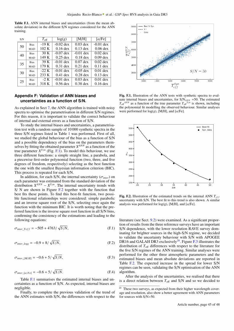
Alejandra Recio-Blanco et al.: GSP-Spec RVS analysis in Gaia DR3

Table F.1. ANN internal biases and uncertainties (from the mean ab-solute deviation) in the different S/N regimes considered for the ANNtraining.

S/N Teff log(g) [M/H] [α/Fe]

50 Bias

MAD

-19 K102 K

-0.02 dex0.16 dex

0.03 dex0.13 dex

-0.01 dex0.06 dex

40 Bias

MAD

30 K149 K

-0.07 dex0.25 dex

-0.01 dex0.18 dex

0.02 dex0.09 dex

35 Bias

MAD

39 K179 K

-0.01 dex0.31 dex

0.07 dex0.21 dex

0.02 dex0.11 dex

30 Bias

MAD

-22 K233 K

-0.01 dex0.41 dex

-0.05 dex0.28 dex

0.01 dex0.13 dex

25 Bias

MAD

-2 K318 K

-0.01 dex0.56 dex

0.03 dex0.38 dex

0.01 dex0.16 dex

Appendix F: Validation of ANN biases anduncertainties as a function of S/N.

As explained in Sect 7, the ANN algorithm is trained with noisyspectra to optimise the parametrisation in different S/N regimes.For this reason, it is important to validate the correct behaviourof internal and external errors as a function of S/N.

To study the internal biases and uncertainties, a parametrisa-tion test with a random sample of 10 000 synthetic spectra in thethree S/N regimes listed in Table 1 was performed. First of all,we studied the global behaviour of the bias as a function of S/Nand a possible dependency of the bias on the parameters them-selves by fitting the obtained parameter XANN as a function of thetrue parameter XS yn (Fig. F.1). To model this behaviour, we usethree different functions: a simple straight line, a parabola, anda piecewise first-order polynomial function (two, three, and fivedegrees of freedom, respectively) selecting as the best functionthe one with the smallest Bayesian information criterion (BIC).This process is repeated for each S/N.

In addition, for each S/N, the internal uncertainty (σinter) oneach parameter was estimated from the standard deviation of thedistribution XANN − XS yn. The internal uncertainty trends withS/ N are shown in Figure F.2 together with the function thatbest fits these points. To find this best-fit function, two possi-ble functional relationships were considered: simple parabolicand an inverse square root of the S/N, selecting once again thefunction with the minimum BIC. It is worth noting that the pre-ferred function is the inverse square root function in all S/N bins,confirming the consistency of the estimations and leading to thefollowing equations:

σinter_Te f f = −505 + 4763/√

S/N, (F.1)

σinter_logg = −0.9 + 8/√

S/N, (F.2)

σinter_[M/H] = −0.6 + 5/√

S/N, (F.3)

σinter_[α/Fe] = −0.6 + 5/√

S/N. (F.4)

Table F.1 summarises the estimated internal biases and un-certainties as a function of S/N. As expected, internal biases arenegligible.

Finally, to complete the previous validation of the trend ofthe ANN estimates with S/N, the differences with respect to the

Fig. F.1. Illustration of the ANN tests with synthetic spectra to eval-uate internal biases and uncertainties, for S/NANN =50. The estimatedTeff

ANN as a function of the true parameter TeffS yn is shown, including

the polynomial fit modelling the observed behaviour. Similar analyseswere performed for log(g), [M/H], and [α/Fe].

20 25 30 35 40 45 50S/N

150

200

250

300

350

400

450

500

550T e

ffBest fitSyn. data

Fig. F.2. Illustration of the estimated trends on the internal ANN Te f funcertainty with S/N. The best fit to this trend is also shown. A similaranalysis was performed for log(g), [M/H], and [α/Fe].

literature (see Sect. 9.2) were examined. As a significant propor-tion of results from the three reference surveys have an importantS/N dependence, with the lower resolution RAVE survey dom-inating for brighter sources in the high-S/N regime, we decidedto validate the uncertainty behaviour with S/N with APOGEEDR16 and GALAH DR3 exclusively20. Figure F.3 illustrates thedistribution of Teff differences with respect to the literature forthe five S/N regimes of the ANN training. Similar analyses wereperformed for the other three atmospheric parameters and theestimated biases and mean absolute deviations are reported inTable F.2. The expected increase in the spread for lower S/Nregimes can be seen, validating the S/N optimisation of the ANNalgorithm.

After the analysis of the uncertainties, we realised that thereis a direct relation between Teff and S/N and so we decided to

20 These two surveys, as expected from their higher wavelength cover-age and resolution, also show a better agreement with ANN parametersfor sources with S/N>50.

Article number, page 45 of 48

A&A proofs: manuscript no. output

Table F.2. ANN biases and mean absolute deviations with respect to theliterature, in the different S/N regimes considered for the ANN training.

S/N Teff log(g) [M/H] [α/Fe]

50 Bias

MAD

-162 K155 K

-0.13 dex0.21 dex

-0.29 dex0.15 dex

0.07 dex0.05 dex

40 Bias

MAD

-89 K139 K

-0.10 dex0.29 dex

-0.26 dex0.13 dex

0.10 dex0.07 dex

35 Bias

MAD

-38 K148 K

0.005 dex0.32 dex

-0.25 dex0.15 dex

0.12 dex0.08 dex

30 Bias

MAD

-6 K192 K

-0.04 dex0.42 dex

-0.32 dex0.19 dex

0.11 dex0.11 dex

25 Bias

MAD

-98 K253 K

-0.02 dex0.47 dex

-0.43 dex0.25 dex

0.09 dex0.12 dex

Table F.3. Polynomial coefficients for the Teff calibration at differentS/NANN values.

S/NANN p0 p1 p2 p3

Teff

30 -834 3.13E-1 -2.53E-535 -1344 4.95E-1 -4.26E-540 3182 -2.34 5.38E-4 -3.84E-850 12816 -8.1 1.65E-3 -1.07E-7

Fig. F.3. Error distributions for ANN estimations with respect to theliterature (Validation Source Table - VST).

propose different calibrations depending on the S/N ranges de-fined in Table 1. Furthermore, we observed that the number ofstars with Teff > 6000 K in the literature is statistically insignif-icant, and so the calibration beyond this limit should not be ap-plied. For log(g), [M/H], and [α/Fe], although there is an intrin-sic relation with S/N, the global calibration proved to be the bestsolution. We provide the calibration of Teff for S/NANN ∼50 inSection 9.2 and we give the polynomial coefficients for lowerS/N in Table F.3.

Appendix G: Query examples from the Gaia Archive

G.1. MatisseGauguin parameters from theAstrophysicalParameters table

SELECT source_idFROM user_dr3int6.astrophysical_parametersWHERE ((teff_gspspec>=3800) OR (logg_gspspec>=3.5))

AND ((teff_gspspec>=4150) OR (logg_gspspec>=3.6)OR (logg_gspspec<=2.4))

Listing 1. ADQL query example with simple cuts in the limitingparameters.

SELECT source_idFROM user_dr3int6.astrophysical_parametersWHERE (teff_gspspec>3500) AND (logg_gspspec>0) AND

(logg_gspspec<5) AND((teff_gspspec_upper-teff_gspspec_lower)<750)AND ((logg_gspspec_upper-logg_gspspec_lower)<1.)AND ((mh_gspspec_upper-mh_gspspec_lower)<.5) AND(teff_gspspec>=3800 OR logg_gspspec<=3.5) AND(teff_gspspec>=4150 OR logg_gspspec<=2.4 ORlogg_gspspec>=3.6 ) AND ((flags_gspspec LIKE"____________0%") OR (flags_gspspec LIKE"____________1%")) AND ((flags_gspspec LIKE"0%") OR (flags_gspspec LIKE "1%")) AND((flags_gspspec LIKE "_0%") OR (flags_gspspecLIKE "_1%")) AND ((flags_gspspec LIKE "__0%") OR(flags_gspspec LIKE "__1%")) AND ((flags_gspspecLIKE "___0%") OR (flags_gspspec LIKE "___1%"))AND ((flags_gspspec LIKE "____0%") OR(flags_gspspec LIKE "____1%")) AND((flags_gspspec LIKE "_____0%") OR(flags_gspspec LIKE "_____1%")) AND((flags_gspspec LIKE "______0%") OR(flags_gspspec LIKE "______1%") OR(flags_gspspec LIKE "______2%") OR(flags_gspspec LIKE "______3%")) AND((flags_gspspec LIKE "_______0%") OR(flags_gspspec LIKE "_______1%") OR(flags_gspspec LIKE "_______2%"))

Listing 2. ADQL query example including conditions on the parameterflags (c.f. Table 2)

G.2. ANN parameters from theAstrophysicalParametersSupp table

SELECT source_id, teff_gspspec_ann, logg_gspspec_ann,mh_gspspec_ann, alphafe_gspspec_ann,flags_gspspec_ann

FROM user_dr3int6.astrophysical_parameters_suppWHERE TO_BIGINT(flags_gspspec_ann) < 10000

Listing 3. Best quality sources, no S/N dependency (∼1.3 M sources)

SELECT ann.source_id, teff_gspspec_ann,logg_gspspec_ann, mh_gspspec_ann,alphafe_gspspec_ann, flags_gspspec_ann,rv_expected_sig_to_noise

FROM user_dr3int6.gaia_source as gaia RIGHT JOIN(

Article number, page 46 of 48

Alejandra Recio-Blanco et al.: GSP-Spec RVS analysis in Gaia DR3

SELECT source_id, teff_gspspec_ann,logg_gspspec_ann, mh_gspspec_ann,alphafe_gspspec_ann, flags_gspspec_ann

FROM user_dr3int6.astrophysical_parameters_suppWHERE TO_BIGINT(flags_gspspec_ann) < 10000) as ann USING(source_id)

WHERE rv_expected_sig_to_noise > 108

Listing 4. Best quality sources with S/N > 108 (S/NANN 50) (∼275 ksources)

Appendix H: Acknowledgements

(Funding) The Gaia mission and data processing have finan-cially been supported by, in alphabetical order by country:– the Algerian Centre de Recherche en Astronomie, Astro-physique et Géophysique of Bouzareah Observatory;– the Austrian Fonds zur Förderung der wissenschaftlichenForschung (FWF) Hertha Firnberg Programme through grantsT359, P20046, and P23737;– the BELgian federal Science Policy Office (BELSPO)through various PROgramme de Développement d’Expériencesscientifiques (PRODEX) grants, the Research FoundationFlanders (Fonds Wetenschappelijk Onderzoek) through grantVS.091.16N, the Fonds de la Recherche Scientifique (FNRS),and the Research Council of Katholieke Universiteit (KU)Leuven through grant C16/18/005 (Pushing AsteRoseismologyto the next level with TESS, GaiA, and the Sloan DIgital SkySurvEy – PARADISE);– the Brazil-France exchange programmes Fundação de Amparoà Pesquisa do Estado de São Paulo (FAPESP) and Coordenaçãode Aperfeicoamento de Pessoal de Nível Superior (CAPES) -Comité Français d’Evaluation de la Coopération Universitaireet Scientifique avec le Brésil (COFECUB);– the Chilean Agencia Nacional de Investigación y Desarrollo(ANID) through Fondo Nacional de Desarrollo Científico y Tec-nológico (FONDECYT) Regular Project 1210992 (L. Chemin);– the National Natural Science Foundation of China (NSFC)through grants 11573054, 11703065, and 12173069, theChina Scholarship Council through grant 201806040200, andthe Natural Science Foundation of Shanghai through grant21ZR1474100;– the Tenure Track Pilot Programme of the Croatian ScienceFoundation and the École Polytechnique Fédérale de Lausanneand the project TTP-2018-07-1171 ‘Mining the Variable Sky’,with the funds of the Croatian-Swiss Research Programme;– the Czech-Republic Ministry of Education, Youth, and Sportsthrough grant LG 15010 and INTER-EXCELLENCE grantLTAUSA18093, and the Czech Space Office through ESA PECScontract 98058;– the Danish Ministry of Science;– the Estonian Ministry of Education and Research throughgrant IUT40-1;– the European Commission’s Sixth Framework Programmethrough the European Leadership in Space Astrometry (ELSA)Marie Curie Research Training Network (MRTN-CT-2006-033481), through Marie Curie project PIOF-GA-2009-255267(Space AsteroSeismology & RR Lyrae stars, SAS-RRL), andthrough a Marie Curie Transfer-of-Knowledge (ToK) fellow-ship (MTKD-CT-2004-014188); the European Commission’sSeventh Framework Programme through grant FP7-606740(FP7-SPACE-2013-1) for the Gaia European Network forImproved data User Services (GENIUS) and through grant

264895 for the Gaia Research for European AstronomyTraining (GREAT-ITN) network;– the European Cooperation in Science and Technology (COST)through COST Action CA18104 ‘Revealing the Milky Waywith Gaia (MW-Gaia)’;– the European Research Council (ERC) through grants 320360,647208, and 834148 and through the European Union’s Horizon2020 research and innovation and excellent science programmesthrough Marie Skłodowska-Curie grant 745617 (Our Galaxy atfull HD – Gal-HD) and 895174 (The build-up and fate of self-gravitating systems in the Universe) as well as grants 687378(Small Bodies: Near and Far), 682115 (Using the MagellanicClouds to Understand the Interaction of Galaxies), 695099(A sub-percent distance scale from binaries and Cepheids –CepBin), 716155 (Structured ACCREtion Disks – SACCRED),951549 (Sub-percent calibration of the extragalactic distancescale in the era of big surveys – UniverScale), and 101004214(Innovative Scientific Data Exploration and Exploitation Appli-cations for Space Sciences – EXPLORE);– the European Science Foundation (ESF), in the framework ofthe Gaia Research for European Astronomy Training ResearchNetwork Programme (GREAT-ESF);– the European Space Agency (ESA) in the framework ofthe Gaia project, through the Plan for European Cooper-ating States (PECS) programme through contracts C98090and 4000106398/12/NL/KML for Hungary, through contract4000115263/15/NL/IB for Germany, and through PROgrammede Développement d’Expériences scientifiques (PRODEX)grant 4000127986 for Slovenia;– the Academy of Finland through grants 299543, 307157,325805, 328654, 336546, and 345115 and the Magnus Ehrn-rooth Foundation;– the French Centre National d’Études Spatiales (CNES),the Agence Nationale de la Recherche (ANR) through grantANR-10-IDEX-0001-02 for the ‘Investissements d’avenir’programme, through grant ANR-15-CE31-0007 for project‘Modelling the Milky Way in the Gaia era’ (MOD4Gaia),through grant ANR-14-CE33-0014-01 for project ‘The MilkyWay disc formation in the Gaia era’ (ARCHEOGAL),through grant ANR-15-CE31-0012-01 for project ‘Unlockingthe potential of Cepheids as primary distance calibrators’(UnlockCepheids), through grant ANR-19-CE31-0017 forproject ‘Secular evolution of galaxies’ (SEGAL), and throughgrant ANR-18-CE31-0006 for project ‘Galactic Dark Matter’(GaDaMa), the Centre National de la Recherche Scientifique(CNRS) and its SNO Gaia of the Institut des Sciences del’Univers (INSU), its Programmes Nationaux: Cosmologie etGalaxies (PNCG), Gravitation Références Astronomie Métrolo-gie (PNGRAM), Planétologie (PNP), Physique et Chimie duMilieu Interstellaire (PCMI), and Physique Stellaire (PNPS),the ‘Action Fédératrice Gaia ’ of the Observatoire de Paris, theRégion de Franche-Comté, the Institut National Polytechnique(INP) and the Institut National de Physique nucléaire et dePhysique des Particules (IN2P3) co-funded by CNES;– the German Aerospace Agency (Deutsches Zentrum fürLuft- und Raumfahrt e.V., DLR) through grants 50QG0501,50QG0601, 50QG0602, 50QG0701, 50QG0901, 50QG1001,50QG1101, 50QG1401, 50QG1402, 50QG1403, 50QG1404,50QG1904, 50QG2101, 50QG2102, and 50QG2202, andthe Centre for Information Services and High PerformanceComputing (ZIH) at the Technische Universität Dresden forgenerous allocations of computer time;– the Hungarian Academy of Sciences through the LendületProgramme grants LP2014-17 and LP2018-7 and the Hungarian

Article number, page 47 of 48

A&A proofs: manuscript no. output

National Research, Development, and Innovation Office (NK-FIH) through grant KKP-137523 (‘SeismoLab’);– the Science Foundation Ireland (SFI) through a Royal Society- SFI University Research Fellowship (M. Fraser);– the Israel Ministry of Science and Technology through grant3-18143 and the Tel Aviv University Center for ArtificialIntelligence and Data Science (TAD) through a grant;– the Agenzia Spaziale Italiana (ASI) through contractsI/037/08/0, I/058/10/0, 2014-025-R.0, 2014-025-R.1.2015, and2018-24-HH.0 to the Italian Istituto Nazionale di Astrofisica(INAF), contract 2014-049-R.0/1/2 to INAF for the Space Sci-ence Data Centre (SSDC, formerly known as the ASI ScienceData Center, ASDC), contracts I/008/10/0, 2013/030/I.0, 2013-030-I.0.1-2015, and 2016-17-I.0 to the Aerospace LogisticsTechnology Engineering Company (ALTEC S.p.A.), INAF, andthe Italian Ministry of Education, University, and Research(Ministero dell’Istruzione, dell’Università e della Ricerca)through the Premiale project ‘MIning The Cosmos Big Dataand Innovative Italian Technology for Frontier Astrophysics andCosmology’ (MITiC);– the Netherlands Organisation for Scientific Research (NWO)through grant NWO-M-614.061.414, through a VICI grant(A. Helmi), and through a Spinoza prize (A. Helmi), and theNetherlands Research School for Astronomy (NOVA);– the Polish National Science Centre through HAR-MONIA grant 2018/30/M/ST9/00311 and DAINA grant2017/27/L/ST9/03221 and the Ministry of Science and HigherEducation (MNiSW) through grant DIR/WK/2018/12;– the Portuguese Fundação para a Ciência e a Tecnologia(FCT) through national funds, grants SFRH/BD/128840/2017and PTDC/FIS-AST/30389/2017, and work contract DL57/2016/CP1364/CT0006, the Fundo Europeu de Desen-volvimento Regional (FEDER) through grant POCI-01-0145-FEDER-030389 and its Programa Operacional Competitividadee Internacionalização (COMPETE2020) through grantsUIDB/04434/2020 and UIDP/04434/2020, and the StrategicProgramme UIDB/00099/2020 for the Centro de Astrofísica eGravitação (CENTRA);– the Slovenian Research Agency through grant P1-0188;– the Spanish Ministry of Economy (MINECO/FEDER, UE),the Spanish Ministry of Science and Innovation (MICIN), theSpanish Ministry of Education, Culture, and Sports, and theSpanish Government through grants BES-2016-078499, BES-2017-083126, BES-C-2017-0085, ESP2016-80079-C2-1-R,ESP2016-80079-C2-2-R, FPU16/03827, PDC2021-121059-C22, RTI2018-095076-B-C22, and TIN2015-65316-P (‘Com-putación de Altas Prestaciones VII’), the Juan de la Cierva Incor-poración Programme (FJCI-2015-2671 and IJC2019-04862-I forF. Anders), the Severo Ochoa Centre of Excellence Programme(SEV2015-0493), and MICIN/AEI/10.13039/501100011033(and the European Union through European Regional De-velopment Fund ‘A way of making Europe’) through grantRTI2018-095076-B-C21, the Institute of Cosmos SciencesUniversity of Barcelona (ICCUB, Unidad de Excelencia ‘Maríade Maeztu’) through grant CEX2019-000918-M, the Universityof Barcelona’s official doctoral programme for the developmentof an R+D+i project through an Ajuts de Personal Investigadoren Formació (APIF) grant, the Spanish Virtual Observatorythrough project AyA2017-84089, the Galician Regional Gov-ernment, Xunta de Galicia, through grants ED431B-2021/36,ED481A-2019/155, and ED481A-2021/296, the Centro deInvestigación en Tecnologías de la Información y las Comu-nicaciones (CITIC), funded by the Xunta de Galicia and theEuropean Union (European Regional Development Fund – Gali-

cia 2014-2020 Programme), through grant ED431G-2019/01,the Red Española de Supercomputación (RES) computerresources at MareNostrum, the Barcelona SupercomputingCentre - Centro Nacional de Supercomputación (BSC-CNS)through activities AECT-2017-2-0002, AECT-2017-3-0006,AECT-2018-1-0017, AECT-2018-2-0013, AECT-2018-3-0011,AECT-2019-1-0010, AECT-2019-2-0014, AECT-2019-3-0003,AECT-2020-1-0004, and DATA-2020-1-0010, the Departa-ment d’Innovació, Universitats i Empresa de la Generalitat deCatalunya through grant 2014-SGR-1051 for project ‘Modelsde Programació i Entorns d’Execució Parallels’ (MPEXPAR),and Ramon y Cajal Fellowship RYC2018-025968-I fundedby MICIN/AEI/10.13039/501100011033 and the EuropeanScience Foundation (‘Investing in your future’);– the Swedish National Space Agency (SNSA/Rymdstyrelsen);– the Swiss State Secretariat for Education, Research, andInnovation through the Swiss Activités Nationales Complémen-taires and the Swiss National Science Foundation through anEccellenza Professorial Fellowship (award PCEFP2_194638 forR. Anderson);– the United Kingdom Particle Physics and Astronomy Re-search Council (PPARC), the United Kingdom Science andTechnology Facilities Council (STFC), and the United King-dom Space Agency (UKSA) through the following grantsto the University of Bristol, the University of Cambridge,the University of Edinburgh, the University of Leicester, theMullard Space Sciences Laboratory of University CollegeLondon, and the United Kingdom Rutherford Appleton Labo-ratory (RAL): PP/D006511/1, PP/D006546/1, PP/D006570/1,ST/I000852/1, ST/J005045/1, ST/K00056X/1, ST/K000209/1,ST/K000756/1, ST/L006561/1, ST/N000595/1, ST/N000641/1,ST/N000978/1, ST/N001117/1, ST/S000089/1, ST/S000976/1,ST/S000984/1, ST/S001123/1, ST/S001948/1, ST/S001980/1,ST/S002103/1, ST/V000969/1, ST/W002469/1, ST/W002493/1,ST/W002671/1, ST/W002809/1, and EP/V520342/1.

The GBOT programme uses observations collected at (i) theEuropean Organisation for Astronomical Research in the South-ern Hemisphere (ESO) with the VLT Survey Telescope (VST),under ESO programmes 092.B-0165, 093.B-0236, 094.B-0181,095.B-0046, 096.B-0162, 097.B-0304, 098.B-0030, 099.B-0034, 0100.B-0131, 0101.B-0156, 0102.B-0174, and 0103.B-0165; and (ii) the Liverpool Telescope, which is operated on theisland of La Palma by Liverpool John Moores University in theSpanish Observatorio del Roque de los Muchachos of the In-stituto de Astrofísica de Canarias with financial support fromthe United Kingdom Science and Technology Facilities Coun-cil, and (iii) telescopes of the Las Cumbres Observatory GlobalTelescope Network.

Article number, page 48 of 48