Functional zoning for Air Quality - CORE

Noname manuscript No.(will be inserted by the editor)

Functional zoning for Air Quality

Rosaria Ignaccolo · Stefania Ghigo ·Stefano Bande

Received: date / Accepted: date

Abstract This paper presents a land classification in zones featured by differ-ent criticality levels of atmospheric pollution, considering pollutant time seriesas functional data: we call this proposal “Functional Zoning”. We aim to meeta request of European laws that impose to distinguish zones needing furtheractions from those needing only maintenance according to air quality status.To carry out zoning for Piemonte (northern Italy), we consider the hourlyconcentration fields of the main pollutants produced by a deterministic airquality model, and we preprocess them by assimilating observations gatheredby monitoring networks. In order to consider administrative units which pol-icy makers refer to, we present three different alternatives to upscale data tomunicipality scale. Then, to aggregate by pollutant, we evaluate two strategies

Work partially supported by Regione Piemonte.

R. IgnaccoloDipartimento di Statistica e Matematica Applicata,Università di Torino,Corso Unione Sovietica, 218/bis, 10134 Torino (TO), ItalyTel.: +39-011-6705758Fax: +30-011-6705783E-mail: [email protected]. Ignaccolo is also affiliated to Statistics Initiative, Collegio Carlo Alberto, Italy

S. GhigoDipartimento di Statistica e Matematica Applicata,Università di Torino,Corso Unione Sovietica, 218/bis, 10134 Torino (TO), ItalyTel.: +39-011-6705758Fax: +30-011-6705783E-mail: [email protected]

S. BandeDipartimento Tematico Sistemi Previsionali, Qualità dell’aria,ARPA Piemonte,Via Pio VII 9, 10135 Torino (TO), Italyemail: [email protected]

2 Rosaria Ignaccolo et al.

to summarize time series: air quality index assessment, and use of the Mul-tivariate Functional Principal Component Analysis (MFPCA), respectively.Therefore, we partition municipalities clustering air quality time series andMPFCA scores, and finally we illustrate a comparison study of the differentstrategies’ results.

Keywords Functional Data · B-spline · Cluster Analysis · PAM (PartitioningAround Medoids) · Atmospheric Pollution

1 Introduction

European and Italian directives (Dir. 96/62/EC and D. Lgs. 351/99 art. 6) es-tablish that Italian regions have to identify different land zones in connectionto air quality status with the aim to plan suitable actions. In fact, in orderto improve or preserve air quality conditions, policy makers define recovery,action or maintenance plans for the different areas.To enforce these directives, it is necessary to find a classification strategy thattakes jointly into account several critical pollutants. Regional or provincialenvironmental agencies deal with this issue to provide support to policy mak-ers, and generally employ classical methodologies, as decision trees or clusteranalysis. Environmental agencies consider pollutant concentration statisticalsummaries, limit value exceedances, and variables featuring land and munici-palities to assign a municipality to a zone. Examples of such variables includepollutant emission density, inhabitant density, orography, and meteorologicalvariables.

In literature, to our knowledge, the land classification problem is not ap-proached in the air quality context, whereas it is discussed in several otherapplied sciences, sometimes with a different terminology. For instance, Hain-ing (2003) calls “regionalization” a particular classification where spatial unitsare aggregated according to spatial contiguity or adjacency constraints. Theseconstraints impose that the spatial units within a region must be geographi-cally connected. In this context, Duque et al (2007) make an interesting reviewof different techniques, grouping them with respect to the strategy applied forsatisfying the spatial contiguity constraints, directly or indirectly expressed.Also, Jacquez (2008) and Aldstadt (2010) describe different approaches forspatial clustering, whereas Guo (2008) and Duque et al (2010) employ themin geographical sciences for the 2004 US presidential election data and georef-erenced socio-demographic data in Accra, Ghana, respectively.In the agricultural framework, Wang et al (2010) carry out a regionalization ofcrop cultivation in China employing first a classical cluster analysis, and thenmodifying the resulting groups in order to preserve spatial contiguity, througha Geographical Information System (GIS) software.

Without considering spatial contiguity, Wang and Ni (2008) develop a Pro-jection Pursuit Dynamic Clustering applied on a multivariate dataset, in orderto classify China land according to water resources. Also, in the water quality

Functional zoning for Air Quality 3

context Robertson and Saad (2003), and Robertson et al (2005) present a re-gional classification scheme, meaning the partition of large areas into zoneswith similar environmental natural (not anthropic) factors affecting waterquality: they develop an approach called SPARTA (SPAtial Regression-TreeAnalysis) and its land-use-adjusted version. Note that this approach is similarto the strategies adopted by environmental local agencies to obtain zones in theair quality context. Analogously here, we do not take into account contiguityor adjacency in an explicit way, since our goal is not a spatial aggregation.

In this paper we propose a functional approach to partition a land in zonescharacterized by different criticality levels of atmospheric pollution, that wecall “Functional Zoning”. Specifically, we consider air pollutant time series pro-vided by a deterministic air quality model on a regular grid, and preprocessedby assimilating observations, as functional data (Ramsay and Silverman 2005).We then classify them by using functional clustering, where the PartitioningAround Medoids (PAM) algorithm is embedded (as in Ignaccolo et al 2008)in place of the k -means one, as proposed by Abraham et al (2003). Thus theallocation to a specific zone preserves information about pollution temporalpatterns and does not take into account any other information. By consideringair pollutant time series exclusively, we do not include any other informationabout covariates, while this is necessary in model-based approaches (e.g. Jamesand Sugar 2003, and Fruhwirth-Schnatter and Kaufmann 2008). Although ourapproach is proposed in the air quality context, it could be adopted wheneverthere are time series - that can be treated as functional data - observed in aspatial domain to be zoned.Our proposal can be applied to time series observed on grid points, but sincemunicipalities are the reference territorial administrative units for undertakingactions, we suggest three different algorithms to upscale data from a regulargrid to the municipality scale. On the other hand, to support policy decisors itis not sufficient to apply our proposal separately per pollutant. Therefore, inorder to have a multi-pollutant zoning, we propose at first a functional clus-tering of air quality index time series, calculated by aggregating by pollutant.Then we consider multivariate functional principal component analysis as analternative technique to summarize the main pollutant time series (PAM al-gorithm is employed to cluster functional principal component scores). Thedifferent analysis strategies (three upscaling algorithms times two pollutants’aggregations) are applied on air quality data of Piemonte (Northern Italy) in2005. Then, these strategies are compared by looking at differences betweencluster labels in the zoning outcomes in order to suggest a final choice.

The paper is organized as follows. A description of the available datasetand of the convenient preprocessing is provided in Section 2. Section 3 reviewsthe functional clustering approach and explains the two pollutant aggregationstrategies, while Section 4 presents the three different alternatives to upscaledata to a municipality scale. In Section 5, we illustrate the results of theproposed techniques concerning the main critical air pollutants in Piemonte,both separately per pollutant, and considering them jointly. Section 6 includescomparison among zoning outcomes and discussion.


2 Data description and preprocessing

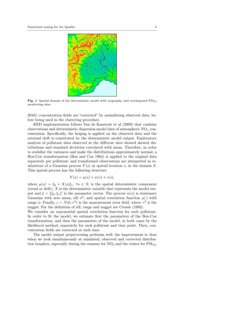
The information we are going to use consists of observed data gathered fromirregularly spaced sites of monitoring networks in Piemonte and the surround-ing area, and “simulated” data, given as output of a deterministic model ona regular thick grid. Note that the European law allows to use both observedand simulated data for the air quality assessment.The simulated time series are output of a three-dimensional deterministicmodeling system (C.T.M. F.A.R.M., Chemistry Transport Model Flexible AirQuality Regional Model) implemented by the environmental agency ARPAPiemonte (Bande et al 2007a). This model chain is capable to process meteo-rological observations and to simulate air pollutant transport, transformationand diffusion; moreover, it is effectively used in order to support the environ-mental department of Piemonte region in the annual evaluation of air qualitystatus. Concentration fields of the main atmospheric pollutants (such as CO,SO2, O3, PM10 and NO2), emission fields, principal meteorological and tur-bulence fields are produced on a hourly basis over a regular grid that has anhorizontal resolution of 4 km and covers Piemonte, neighbor Italian regionsand foreign countries (see Fig. 1). The total covered surface is 220×284 km2.In this paper, we analyze concentration values of CO, SO2, PM10 and NO2

in the year 2005 and we do not include O3 time series, even if O3 is one ofthe main critical pollutants during the summer (Cocchi and Trivisano 2002,Bodnar et al 2008). Indeed, ozone is a by-product arising from the reactionbetween nitrogen oxides and volatile organic compounds, and thus it seemsappropriate to consider in our analysis its precursors.The observed data are provided by the regional environmental agencies ofPiemonte and its neighbor regions. There are 26 PM10 monitoring sites (Fig. 1)that record daily data, while CO, SO2 and NO2 are monitored by respectively40, 12 and 61 instruments providing hourly data. Given the limited num-ber of monitoring sites and their absence in a few areas, a “standard” krig-ing would not be able to provide a good pollutant prediction on the wholePiemonte region. The kriging variance would be larger in the areas uncoveredby the monitoring network, and everywhere when the monitoring sites are only12. Therefore, we take advantage of the availability of the data simulated onPiemonte and its neighborhood.When comparing the output of the deterministic model with the observeddata, it turns out that pollutant concentration is sometimes underevaluatedor overevaluated (see Fig. 2 for an example). In fact, PM10 concentration levelsare clearly underevaluated in the winter semester (from October to March),especially for monitoring sites out of Torino metropolitan area. The NO2 out-put is characterized by underestimation of concentration peaks due to adverseweather conditions, while CO and SO2 concentrations are overestimated. How-ever, simulated levels of CO and SO2 are below the law thresholds, as well astheir observed levels. In order to improve pollutant model output, we prepro-cess the simulated data through Kriging with External Drift (KED, Wacker-nagel 2003), by employing the geoR package in R (Development Core Team


Fig. 1 Spatial domain of the deterministic model with orography, and overimposed PM10

monitoring sites

2010): concentration fields are “corrected” by assimilating observed data, be-fore being used in the clustering procedure.

KED implementation follows Van de Kassteele et al (2009) that combineobservations and deterministic dispersion model data of atmospheric NOx con-centration. Specifically, the kriging is applied on the observed data and theexternal drift is constituted by the deterministic model output. Exploratoryanalysis of pollutant data observed at the different sites showed skewed dis-tributions and standard deviation correlated with mean. Therefore, in orderto stabilize the variances and make the distributions approximately normal, aBox-Cox transformation (Box and Cox 1964) is applied to the original dataseparately per pollutant, and transformed observations are interpreted as re-alizations of a Gaussian process Y (s) at spatial location s, in the domain S.This spatial process has the following structure

Y (s) = µ(s) + w(s) + ε(s),

where µ(s) = ξ0 + X(s)ξ1, ∀s ∈ S, is the spatial deterministic component(trend or drift), X is the deterministic variable that represents the model out-put and ξ = {ξ0, ξ1}′ is the parameter vector. The process w(s) is stationaryGaussian with zero mean, sill σ2, and spatial correlation function ρ(·) withrange φ. Finally, ε ∼ N(0, τ2) is the measurement error field, where τ2 is thenugget. For the definition of sill, range and nugget see Cressie (1993).We consider an exponential spatial correlation function for each pollutant.In order to fit the model, we estimate first the parameters of the Box-Coxtransformation, and then the parameters of the model, in both cases by thelikelihood method, separately for each pollutant and time point. Then, con-centration fields are corrected at each time.

The model output preprocessing performs well: the improvement is clearwhen we look simultaneously at simulated, observed and corrected distribu-tion boxplots, especially during the summer for NO2 and the winter for PM10,


(a) NO2 in Orbassano (b) PM10 in Borgaro

Fig. 2 Boxplots by month of observed (red), simulated (blue) and corrected by KED (green)distributions for two monitoring sites of NO2 and PM10. The time scale is month, fromJanuary (1) to December (12)

for all the sites. Figure 2 shows two examples in two different monitoring sitesfor NO2 and PM10 distributions. Moreover, we carried out a cross-validationanalysis in order to evaluate the KED performance, and it shows that krig-ing results are satisfactory. The results of this analysis are not reported herebecause they are beyond the goal of this paper (for further details see Ghigo2009 - unpublished thesis).

3 Multi-pollutant functional zoning

Functional clustering methods (see Abraham et al 2003 and Ignaccolo et al2008) could be directly employed on each pollutant: indeed considering gridpoints’ pollutant time series as functional data and clustering estimated coeffi-cients, we obtain several zoning outcomes of the same land. However, decisorsneed to jointly consider different pollutants in order to get a multi-pollutantzoning: for this reason we propose two strategies for pollutant aggregation.We suggest to aggregate time series of different pollutants by using an air qual-ity index - called BC index - and, alternatively, to summarize them by means ofFunctional Principal Component Analysis (FPCA). While Functional ClusterAnalysis (FCA) is applied on air quality index time series, the PAM algorithmis employed to cluster functional principal component scores.In order to make pollutants comparable, we standardize and temporally ag-gregate them with respect to the aggregation functions reported in Table 1,provided by EU directives (1999/30/EC and 2000/69/EC).

3.1 Functional clustering on BC index

Through synthetic environmental indices it is possible to reduce multivariateinformation to an univariate one. It is well-known that local agencies use in-dices as summary values for measuring pollutant effect on human health and


Table 1 Information about analyzed pollutants provided by European directives (slp =standard limit value for the pollutant p)

Pollutant Temporal aggregation function slp Unit of measureCO Daily maximum of 8 hours moving average 10 mg/m3

NO2 Daily maximum 200 µg/m3

PM10 Daily mean 50 µg/m3

SO2 Daily mean 125 µg/m3

on natural environment.The family of air quality indices proposed by Bruno and Cocchi (2002) allowsto aggregate different pollutants in space and time, using the standard limitvalues (slp in Table 1) to standardize and make data dimensionless; we refer tothis family as BC indices. For our purposes, we aggregate in time and by typeof pollutant in order to obtain daily time series of the air quality index foreach site. Unlike classical air quality indices, the BC index is not featured byweights, since dividing each pollutant value by its standard limit we alreadytake into account its higher or smaller criticality.For a fixed site, let xpdh be the elementary measurement where p = 1, . . . , Pindexes the pollutants, d = 1, . . . , 365 the days and h = 1, . . . , 24 the hours.First, we temporally aggregate data according to the aggregation functions inTable 1, obtaining a daily value xpd = f(xpdh). Then, we choose to aggregateover pollutants by the maximum function, in order to keep information aboutcritical cases, obtaining a BC index time series for the fixed site. Therefore theindex is defined as

Id = maxp

(xpdslp

)d = 1, . . . , 365, (1)

where, as said before, slp represents the pollutant standard limit value.For all the sites, we consider these time series {Id}d=1,...,365 as observed

functional data and assume the existence of a continuous function underlyingthe data (Ramsay and Silverman 2005): each curve is summarized by a vectorof B-spline coefficients in Rg+K+1, where K is the knot number and g is thedegree of B-splines. Then, we cluster the spline coefficients and obtain groupsof sites, through a functional cluster analysis where PAM algorithm is embed-ded (Kaufman and Rousseeuw 2005). The choice falls on this non-hierarchicalalgorithm because it provides an object - the socalled “medoid” - representingthe cluster, which in this case is a fitted curve showing the temporal evolutionof the air quality index at a certain site. Moreover, this algorithm suggeststhe suitable clusters’ number to split the objects and provides useful clusterfeatures by the socalled “silhouette plot”. Indeed, the silhouette plot shows a“silhouette width” for each object that represents a belonging measure of theobject to a cluster and could have a negative value if misclassification hap-pens. Thus, by averaging silhouette widths over a cluster, we can compare thequality of different groups; similarly, by averaging silhouette widths over allobjects we have an index s̄k, changing with the number of groups k. PAM


suggests to choose k such that s̄k reaches the maximum (for further detailssee Kaufman and Rousseeuw 2005).

3.2 Clustering of Multivariate FPCA scores

In order to aggregate pollutants, as an alternative technique in the functionalcontext, we explore the Functional Principal Component Analysis in its multi-variate version (MFPCA, Ramsay and Silverman 2005, p. 167, and Henderson2006), that clearly takes into account pollutant interactions. We review heresome MFPCA theory and set the notation.

Let Gpi(t), p = 1, . . . , P and i = 1, . . . , n, be a functional object for thep-th pollutant and i-th site, assumed to be a smooth function underlying thepi-th time series, that is the datum ypij , j = 1, . . . ,m, is associated with thecurve value Gpi(tj) by the model

ypij = Gpi(tj) + εpij

where εpij are independent random errors.In the multivariate functional context, the weight functions subject to the

orthonormality constraints (||αr||2 =∫T αr(t)

2dt = 1 and∫T αr(t)αs(t)dt = 0

for r 6= s) that maximize the sample variance of the principal component scoresare P - dimensional vectors αr(t) = {α1

r(t), . . . , αPr (t)}, where r indicates the

r-th component. The functions αpr(t) are solutions of the eigenequation

P∑p∗=1

∫Tcpp∗(t, t?)αp

∗(t?)dt? = λαp(t) p = 1, . . . , P,

where cpp∗(t, t?) denotes the covariance function of Gpi(t) when p = p∗, whilecpp∗ is the cross-covariance function when p 6= p∗. Note that the eigenfunctioncomponents αpr(t) are defined over the same time range T of the functionaldata.Therefore, the r-th principal component scores are

zir =

P∑p=1

∫Tαpr(t)Gpi(t)dt, i = 1, . . . , n. (2)

MFPCA is employed on standardized (divided by slp) time series of the an-alyzed pollutants and its implementation takes place estimating Gpi by meansof B-splines using the fda package in R environment (pca.fd with centeredcurves). After we have obtained the principal component scores, we choosethe suitable number of functional principal components (FPCs). Sites are thengrouped by clustering the first few FPC scores by PAM algorithm. Note thatnow the medoids are not functions since the temporal component is integratedout in Eq. (2).

The choice of B-splines is classic for nonperiodic data, but recently Kayanoand Konishi (2009) have proposed to use Gaussian basis expansion instead of


B-splines since they deal with unbalanced data (time series observed at pos-sibly different time points). Our pollutant data are already balanced because,as we said before, through the aggregation functions (provided by air qualityEU directives) we obtain daily values.

4 Upscaling

In order to enforce air quality legislation and therefore perform actions toimprove air quality, policy makers have to refer to administrative units, thatare municipalities. So, it is necessary to upscale the “corrected” air quality timeseries from the grid point scale to the municipality one and, for this purpose,we consider three alternative procedures.

The aggregation at municipality scale could be realized solving the so-called “Change Of Support Problem” (COSP), that is “concerned with infer-ence about the values of the variable at points or blocks different from those atwhich it has been observed” (Gelfand 2010, chap. 29, p. 522). With this mean-ing, a solution of COSP presumes to fit a model or, at least, to implement anuniversal block kriging. Moreover, with a more complex model it is possible tocombine data at different scales provided by numerical models and monitoringnetworks, realizing a data fusion and solving COSP at the same time. How-ever, the goal of this paper is land classification and we propose solutions tocarry out data fusion and upscaling at a very reasonable computational costand at a moderate complexity such that practitioners could be encouraged toimplement them.

To retrieve a block value we can consider the integral over the area thatprovides a block average (BA), that is

Z(B) =1

|B|

∫B

Z(s)ds, (3)

where B ⊆ S ⊆ R2, Z is a spatial stochastic process defined by a randomvariable family {Z(s) : s ∈ S} and s a generic spatial location in the domainS. Since our spatial domain is discretized through grid points, after we haveidentified the ci points belonging to a municipality, Equation (3) becomes

Cci =

ci∑l=1

γilzil,

where Cci represents the mean pollutant concentration in a municipality, zilis the value of the stochastic process and γil is the weight for the l-th pointof the i-th municipality (it will be referred to as Municipality Block Averageor Munic. BA). More specifically, weights are calculated as the ratio betweenmunicipality area belonging to the l-th cell (a point in the grid represents acell) and the total municipality area.Moreover, as alternative weights, we propose to consider the built-up surfacepercentages (referred to as Built BA). Indeed, the built-up surface percentage


is an important indicator of the anthropic activity which could be associatedwith more pollution in a municipality, whereas a wide country area could notcontribute at all. Now, weights are the ratio between municipality built-uparea belonging to the l-th cell and the total municipality built-up area.Further, we propose to upscale taking the 90-th percentile (referred to as 90thperc.) of the values observed in the set of cells belonging to the consideredmunicipality. This is a measure of extreme cases in a municipality, and it istaken in a precautionary perspective. Although from this point of view themaximum could seem the natural statistic to consider, it could be an outlier,either too extreme or too rare. Therefore, the choice of the 90-th percentileguarantees a better robustness.

5 Piemonte zoning

We employ the methodologies introduced above on Piemonte preprocessedpollutants’ datasets (1763 grid point time series per pollutant), and then onupscaled datasets (1206 municipality time series per pollutant). In the follow-ing, results for the main critical pollutants are presented, first separately andthen jointly. In order to better highlight the criticality of the resulting zones,all the maps are characterized by a color gradation (as traffic lights) changingwith cluster mean values (green, orange, red and purple) that provides a sortof group ranking.For land classification we analyze NO2, PM10, CO and SO2. Since previousexploratory analysis show that NO2 and PM10 are more critical than CO andSO2, in Subsection 5.1 only NO2 and PM10 results are discussed. A first anal-ysis on single pollutants is illustrated in Bande et al (2007b), even if in thisprevious work simulated data are not preprocessed and we classify all the gridpoints of the model output (the whole rectangular region of Figure 1). The fol-lowing subsections show results of multi-pollutant zoning carried out throughthe proposed strategies: while Subsection 5.2 introduces the results on regulargrid time series, Subsection 5.3 presents findings on the municipality ones.

5.1 Zoning for single pollutants

In order to provide a land classification featured by each pollutant concentra-tion, we carry out a Functional Cluster Analysis on single pollutant time series.This step of our analysis is important for two reasons: on one hand decisorsare interested in the critical pollutants and consequently in zoning outcomesbased on them (despite the need to base decisions on global air quality status);on the other hand, the resulting maps for single pollutants can be helpful inthe interpretation of the following multi-pollutant zoning outcomes, lookingat possible similarities between single- and multi-pollutant maps.

First, we produce a land classification on 1763 Piemonte grid points forsingle pollutants and then we refer to municipalities using the three upscaling


approaches described in Section 4. Moreover, to select the “best” number kof clusters to partition all the curves, we look at the average silhouette widthover all objects s̄k and generally we choose the k that yields the highest s̄k;sometimes we make an exception, opportunely described when necessary.

Table 2 Average silhouette width over the cluster (s̄c), number of grid points or municipal-ities (nc) and color featuring each cluster in the grid point and municipality classifications(in the three upscaling cases)

NO2 PM10

cluster C1 C2 C3 C4 C1 C2 C3

color green orange red purple green orange redGrid points

s̄c 0.61 0.14 0.26 0.10 0.54 0.24 0.08nc 635 347 537 244 805 460 498

Munic. BAs̄c 0.52 0.21 0.17 0.12 0.45 0.24 0.13nc 387 325 321 173 328 365 513

Built BAs̄c 0.53 0.11 0.18 0.14 0.44 0.24 0.12nc 333 428 300 145 342 355 509

90th perc.s̄c 0.47 0.18 0.20 0.05 0.49 0.26 0.07nc 377 304 309 216 311 393 502

In Table 2 we show results for each classification obtained for NO2 andPM10, while Figure 3 focuses on the upscaling case 90th perc..NO2 cluster structure is quite similar when zoning results concern the gridpoints and when they are related to the municipality time series obtainedafter the three upscaling techniques. Indeed, these outcomes are character-ized by four clusters stretching in according to roadway networks and maincities (see Fig. 3(a)). Even if k = 4 corresponds to the third s̄k suggested byPAM, our choice falls upon it because it makes easier to distinguish emissionsources. These are concentrated in biggest conurbations and industrial areas ofPiemonte (Torino, Alessandria, Novara and their suburbs) that belong to thecluster 4 (C4). C3 includes zones around highways, main connection roads andnorthern plain and piedmont areas, while the cluster 2 is formed by remainingplain and piedmont areas. Mountains belong to C1. The medoids in Figure 3(a)highlight the big variation that exists, especially in the winter months, amongsites belonging to different groups: it reaches 30 µg/m3 for some time points.

As for PM10, k = 3 gives the best s̄k for the grid points case, and this kis also kept for the other cases because it corresponds to the three directiveplans (recovery, action, and maintenance) and it makes easier to compare allthe resulting PM10 maps. Figure 3(b) shows the three clusters in the 90th perc.upscaling case, but the other zoning outcomes are very similar. Indeed theyreflect morphology: the flat country belongs to C3, piedmont areas to C2 andmountains to C1.

Values of s̄c (that represent the average silhouette widths of objects be-longing to a cluster) in Table 2 highlight that grid points and municipalities


(a) NO2 (b) PM10

Fig. 3 Medoids (top) and municipality zoning outcome maps (bottom) for NO2 and PM10

in the 90th perc. case. The background layers show the regional boundaries, the highwaynetwork and the municipality built-up area

of the NO2 cluster 1, C1,NO2, - and also C1,PM10

- lie well within their clusteralthough some of them are spatially very far away. C4,NO2

and C3,PM10have a

low s̄c instead: since they group cities having similar features of industrializa-tion and morphology but not comparable for road conditions and population,low s̄c values look proper. Moreover, Table 2 provides the numerousness nc ofeach cluster. Looking at nc in the three different upscaling cases, we can ob-serve that some units “migrate” from one group to another one, even if clusterstructures are quite similar.

5.2 Multi-pollutant zoning on grid points

As we already mentioned, to look at the regional air quality status and to pro-vide one zoning outcome for all pollutants, two time series summary methodsare proposed, through BC air quality index and MFPCA (Section 3). First ofall, we implement these two strategies on 1763 grid point time series in orderto have a benchmark to evaluate the persistence of the resulting clusters whenwe move at municipality scale (in Section 5.3).


During the PAM step we choose the second best value, that is k = 3for both the strategies: the “best” is obtained with k = 2 that provides ameaningless partition from the policy point of view, because it splits Torinoand the metropolitan area from the rest of Piemonte, in a too simplistic way.

(a) PM10 (b) BC index (c) MFPCA

Fig. 4 PM10, BC and MFPCA zoning outcome maps (bottom) and corresponding medoids(top) of Piemonte grid points. The background layers show the regional boundaries, thehighway network and the municipality built-up area

As illustrated in Section 3.1, we classify functional BC indices by using thePAM algorithm. This multi-pollutant zoning outcome is characterized by s̄3

equal to 0.33. Figure 4(b) shows that the metropolitan area and almost thewhole Po valley belong to C3, piedmont regions to C2 and mountains to C1

again. Moreover Table 3 provides average silhouette width and numerousnessfor every cluster. Note that these values are very similar to those obtainedwhen we zone PM10 grid points (Tab. 2): the same number of grid pointsbelongs to cluster 3 in both the classifications, and a few grid points movefrom C1,BC to C2,PM10

, keeping about the same s̄c. Also PM10 and BC indexmaps and medoids are very similar, as it can be seen in Figure 4. Therefore,we can gather that the PM10 drives the construction of BC index defined inEq. (1).

When we summarize pollutant time series through MFPCA(see Section 3.2)we cluster the functional principal component scores by PAM. Figure 4(c) dis-plays the zoning outcome and the right side of Table 3 shows numerousnessand average silhouette width for every cluster, whereas the overall averagesilhouette width s̄3 is 0.46. In this analysis we take into account the firsttwo principal components that explain 90.89% of the total variability. The


Table 3 Average silhouette width over the cluster (s̄c), number of grid points (nc) andcolor featuring each cluster

BC index MFPCA scorescluster C1 C2 C3 C1 C2 C3

color green orange red green orange reds̄c 0.55 0.23 0.09 0.29 0.69 0.32nc 784 481 498 473 710 580

most critical cluster C3 includes main connection roads and industrial areas,grouping the biggest towns. C2 is characterized by piedmont areas, and C1 bymountains. Since

∑Pp=1 ||αpr ||2 = 1 by construction, ||αpr ||2 provides the pro-

portion of the variability in the r-th component ascribable to variation in thep-th pollutant curves. For the first principal component, 91.97% of variation isattributable to PM10 curves, that is ||αPM10

1 ||2 = 0.9197; 7.69% is associatedwith NO2 while the other pollutants play no substantial role (SO2: 0.11%, CO:0.23%). Also in the second principal component, the higher variability propor-tion concerns PM10 (||αPM10

2 ||2 = 0.9808); the other contributions are 0.59%,1.12% and 0.21% for NO2, SO2 and CO, respectively. Then, it is possible tosay that fine particulate matter explains almost all the variability of the firsttwo principal components, or rather they are essentially affected by PM10.When comparing the two outcomes, Table 3 highlights that C2,MFPCA is fea-tured by nc and s̄c bigger than C2,BC ones, whereas conversely nc and s̄c ofC1,MFPCA are smaller than those of C1,BC , as displayed by the different or-ange and green zones in Fig. 4(b) and (c). As for C3, the value of s̄C3,MFPCA

isbigger than s̄C3,BC

meaning that C3,MFPCA is more homogeneous than C3,BC .

5.3 Multi-pollutant zoning on municipalities

The three upscaling techniques illustrated in Section 4 are now implementedto refer to municipalities. We decided to keep k = 3 that makes easier tocompare new zoning results with the previous ones, and corresponds to thenumber of plans that currently policy makers have to define. The resultingmaps are shown in Figure 5. Generally, the most critical group C3 lengthensover the main road network, including main conurbations (Torino, Alessandriaand Novara) and their industrialized suburbs. The intermediate C2 is formedby piedmont municipalities. Mountain municipalities are grouped in the lesscritical C1 that is featured by the highest average silhouette width for everyobtained classification (Table 4). Overall, the municipalities’ partition resem-bles the grid points’ one (see Fig. 4(b)-(c) and Fig. 5), meaning that the threeupscaling techniques do not shuffle the zoning outcomes. Moreover, at firstglance, it seems that in all the municipalities’ maps PM10 overbears the otherpollutants as it can be seen by comparing Figure 5(a)-(f) with Figure 3(b).

Specifically, with regard to BC index zoning on municipalities, we have toemphasize that Figure 6(a) is associated with Figure 5(b) and it is a helpfulinstrument to look at the temporal evolution of the BC index in the three


(a) BC Munic. BA (b) BC Built BA (c) BC 90th perc.

(d) MFPCA Munic. BA (e) MFPCA Built BA (f) MFPCA 90th perc.

Fig. 5 BC index (top) and MFPCA (bottom) multi-pollutant zoning outcome maps in thethree upscaling cases. The background layers show the regional boundaries, the highwaynetwork and the municipality built-up area

zones. The left side of Table 4 shows that a small number of municipalities mi-grates from a group to another one when we change the upscaling algorithm,supporting the fact that maps are quite similar. Also the overall average silhou-ette widths (s̄3 = 0.252; 0.245; 0.241 for Munic. BA, Built BA and 90th perc.respectively) and the medoids are comparable (the interested reader can seeFig. 3.15 in Ghigo 2009 - unpublished thesis). Moreover, 90th perc. map (seeFig. 5(c)) seems to better reflect Piemonte land use: for instance the orangezone in southern Piemonte adheres to main road connections, while the redone in the south-east is due to the closeness to Genova metropolis. Munic. BAoutcome seems to present some misclassifications instead, for instance mostsouthern mountain municipalities belong to C2 instead of C1.To understand which pollutants have a part in the BC index construction, welook at the medoid time series composition, as we are used in the classicalPCA. Thus in Figure 6(b) for the Built BA case, medoid values at each timeinstant are drawn with a different shape depending on which pollutant gives


(a) Smoothed medoids (b) Medoids time series

Fig. 6 Medoids and their time series for BC index zoning in Built BA case. The point shapein time series changes with the pollutant giving the maximum in Eq. (1)

Table 4 Average silhouette width over the cluster (s̄c), number of municipalities (nc) andcolor featuring each cluster in the three upscaling cases

BC index MFPCA scorescluster C1 C2 C3 C1 C2 C3

color green orange red green orange redMunic. BA

s̄c 0.48 0.23 0.13 0.55 0.32 0.20nc 297 389 520 336 355 515

Built BAs̄c 0.45 0.23 0.13 0.50 0.34 0.18nc 317 361 528 378 331 497

90th perc.s̄c 0.50 0.25 0.07 0.59 0.29 0.24nc 309 403 494 303 447 456

the maximum in Eq. (1). We can observe that the predominant shape is thePM10 one, although SO2 prevails on a few summer days. So, as we supposedbefore, PM10 seems to be the driving pollutant. For the Munic. BA case theanalogous plot looks very similar to Figure 6(b), whereas in the 90th perc. onethe SO2 shape never appears.

When clustering MFPCA scores, we take into account the first three func-tional principal components: indeed the percentages of explained variabilityare 91.5%, 91.3% and 92.5%, as Table 5 shows. The summary values obtainedby applying the PAM on the MPCA scores are reported in the right side ofTable 4, and the overall average silhouette widths are s̄3 = 0.331; 0.328; 0.344for Munic. BA, Built BA and 90th perc., respectively. Even if the maps inFig. 5(d)-(f) seem quite similar to the BC index ones, there are maybe somemisclassifications. For instance, Built BA and 90th perc. place Cuneo (the redisolated unit in the south-west) in the red zone, while a preliminary data anal-ysis suggests that it is not so critical; indeed the negative silhouette widthswarn about a possible misclassification. Moreover, based on knowledge of landuse we would expect that some municipalities were in the critical C3. Instead,as for Munic. BA and Built BA, some municipalities in the north-west (nearValle D’Aosta, see Fig. 5(d) and (e)) featured by well-travelled connectionroads belong to C2 instead of C3. Analogously, for 90th perc. in Figure 5(f),


there are some municipalities close to the industrialized Genova in the south-east belonging to C2.

Table 5 Explained variabilities and variability percentages (||αpr ||2) for each pollutant of

the first three FPCs, in the three upscaling cases

Explained ||αpr ||

2

Variability PM10 NO2 SO2 COMunic. BA

65.6 1st FPC 0.9095 0.0503 0.0381 0.002120.5 2nd FPC 0.5740 0.0119 0.4134 0.00075.4 3rd FPC 0.8813 0.0686 0.0491 0.001091.5 Total

Built BA66.4 1st FPC 0.9127 0.0532 0.0320 0.002119.5 2nd FPC 0.5968 0.0111 0.3913 0.00085.4 3rd FPC 0.8738 0.0789 0.0463 0.001091.3 Total

90th perc.75.8 1st FPC 0.9116 0.0821 0.0030 0.003312 2nd FPC 0.9690 0.0012 0.0280 0.00184.7 3rd FPC 0.7616 0.2363 0.0006 0.001592.5 Total

Now, we can look at the proportion of variability of the components at-tributable to each pollutant curves (remember that

∑Pp=1 ||αr||2 = 1). Table 5

shows that FPCs are composed almost completely by PM10. Only for the sec-ond FPC of the two BA upscaling cases, some variability is explained by SO2

(||αSO22 || = 41.34% and 39.13% respectively), while in the third FPC of the

90th perc. case 23.63% of variability is associated to NO2. Thus, PM10 lookslike the driving pollutant of the functional principal components, as well as ofthe BC index.

6 Discussion

In order to support policy makers in enforcing European laws, environmentallocal agencies have to provide a land classification in relationship with air qual-ity status. In this paper, we propose a functional approach to zone, applied oncorrected air pollutant time series that are provided by a deterministic model.The preprocessing of simulated data through a KED procedure is carried outseparately for each pollutant.There are two convenient “constraints” to consider. First: recovery, action ormaintenance plans have to be determined on the basis of the air quality status,implying the need for an aggregation of critical pollutants. Second: plans haveto be applied to administrative units where responsibilities are well defined,so that any proposal is feasible in practice if zoning results concern municipal-ities. To satisfy the first need, we suggest an aggregation of several pollutantsin the BC air quality index (that is the input of the functional clustering) and,alternatively, a summary of data by MFPCA (employing PAM algorithm on


(a) 90th perc. (7.96 %) (b) Munic. BA (13.93 %) (c) Built BA (15.84 %)

(d) 90th perc.–Munic. BA(10.45 %)

(e) 90th perc.–Built BA(11.28 %)

(f) Munic. BA–Built BA(6.13 %)

(g) 90th perc.–Munic. BA(21.23 %)

(h) 90th perc.–Built BA(23.38 %)

(i) Munic. BA–Built BA(7.30 %)

Fig. 7 Maps of the differences between cluster labels in zoning outcomes: BC versus MF-PCA (top), BC versus BC (center), MFPCA versus MFPCA (bottom) in the three upscalingcases. The municipality color reflects the belonging, or not, to the same cluster in the com-pared classifications: blue corresponds to “-1” in Table 6, white to “0”, magenta to “+1” andpurple to “+2”. The number in round brackets represents the percentage of municipalitieswith different cluster labels in the two compared outcomes


Table 6 Frequency distributions of the differences between cluster labels in two comparedzoning outcomes (changing pollutants’ aggregation and upscaling algorithm)

-1 0 1 -1 0 1 -1 0 1 2BC-MFPCA

90th perc. Munic. BA Built BA32 1110 64 62 1038 106 50 1015 140 1

BC–BC90th perc.–Munic. BA 90th perc.–Built BA Munic. BA–Built BA82 1080 44 81 1070 55 31 1132 43 0

MFPCA–MFPCA90th perc.–Munic. BA 90th perc.–Built BA Munic. BA–Built BA141 950 115 124 924 158 17 1118 65 6

functional principal component scores). Then, in order to refer to municipal-ities, we propose to upscale data from a regular grid to municipality scale bymeans of three different methods: i) averaging the field values weighted byareas over the cells belonging to a certain municipality; ii) averaging using asweight the built-up percentage for every cell; iii) taking the 90-th percentileover the cell values in a municipality.

Crossing the proposed two pollutant aggregations and three upscaling so-lutions, we obtain six classifications of municipalities in Piemonte for the year2005, as shown through six maps in Figure 5. Obviously, a choice is necessary.To compare the zoning outcomes and realize a sensitivity analysis, we map thedifferences between cluster labels (1, 2 and 3) in Figure 7(a)-(i) and we presenttheir frequency distributions in Table 6. The municipalities that belong to thesame group in the two compared outcomes - white in the maps of Figure 7- vary from 924 to 1132 (see the frequencies of “0”). The “migrating” munic-ipalities, from a cluster to another one, are colored: blue corresponds to “-1”,magenta to “+1” and purple to “+2”. Since the clusters are labeled from 1 to 3according to a criticality ranking (based on the average air quality index), wecan read a difference “-1” as a shift towards a more critical zone, and interpreta large frequency of “-1” as indication of a more preventive zoning outcome:when we compare two zoning outcomes a large number of “-1” suggests thatthe second zoning strategy is more preventive. Indeed, overall the strategies,the frequency of “-1” varies from 17 to 141. Instead a difference equal to “+1”indicates a shift of a municipality towards a less critical zone and the frequencyof “+1” changes from 43 to 158. Finally, there are some purple municipalities(7 in total) that move from cluster C3 in the first zoning outcome to C1 in thesecond one.

The colored municipalities in the difference maps in Figure 7 do not ap-pear randomly distributed, and a randomness test based on joint counts (Cliff1970) confirms that. If the colored municipalities were randomly distributedon the difference maps, the two compared zoning outcomes could be consid-ered the same. Instead, they are grouped and located between mountain andpiedmont zones, as well as piedmont and plain zones, that roughly coincidewith boundaries between two different clusters.


When comparing the two pollutant aggregation strategies (BC versus MF-PCA) with the same upscaling algorithm, through the difference maps in Fig-ure 7(a)-(c), we can see that 90th perc. outcomes are very similar (differencesare mostly focused in the south-east of the region). In fact, the percentageof municipalities with different cluster labels is only 7.96% (corresponding to96 out of 1206). This percentage is at most 15.84% in the case of Built BAupscaling.

In order to carry out a sensitivity analysis with respect to the upscalingprocedure, we plot the difference maps in Figure 7(d)-(f) for the BC index andin Figure 7(g)-(i) for the MFPCA. In both the cases, the smallest percentageof migrating municipalities is observed in the comparison of the two weightedblock average methods (6.13% for BC and 7.30% for MFPCA). Instead, thehighest percentages of migrating municipalities occur when we compare 90thperc. with a block average method in the case of MFPCA pollutant aggrega-tion: 21.23% and 23.38% in Figure 7(g) and (h). Therefore MFPCA approachturns out to be less robust than the BC index with respect to the upscalingmethod.

In addition to the above better robustness to the upscaling procedures, wehave other reasons to prefer FCA on BC index rather than PAM on MFPCAscores. First of all, the construction of the BC index time series makes themeasily interpretable for policy makers who can also look at the medoids tohave an idea of the temporal evolution of the BC index in the correspondingzone. Then, since the frequency of “-1” is smaller than the frequency of “+1”in the three upscaling cases at the first row of Table 6, the BC zoning outcomeappears more preventive than the MFPCA one. Finally, a further “merit” ofthe FCA on BC procedure is that it does not take into account either spatialcorrelation or spatial contiguity among municipalities (spatial correlation isimplicitly considered in MFPCA instead) so that it does not force neighborsto be in the same zone and provides a zoning outcome based exclusively onthe similarity of the air quality status.

As for the choice of an upscaling method, we can see from Table 6 thatzoning outcomes are more cautionary with the Munic. BA procedure: thefrequency of “-1” is greater than that of “+1” when we compare Munic. BAwith 90th perc., and vice versa in the comparison Munic. BA versus Built BAin both the pollutant aggregation methods (see the second and the third rowof Table 6). However, discussing the choice from an interpretive point of viewwith policy makers, it seems that BC 90th perc. approach has more consistentresults with their previous knowledge about Piemonte land and air qualitystatus (as already said for Fig. 5(c)).

Very recently Kayano et al (2010) have proposed a multivariate FCA thatallows to consider all pollutants without synthesizing them. Their proposal isan alternative to the use of FCA on the BC index that we could take intoaccount in the future. Nevertheless, first of all an assessment of the compu-tational cost of that methodology would be necessary, whereas we have a lowcost for the proposed FCA on BC index. Moreover we stress again that theuse of PAM provides information about the air quality temporal evolution in


the zones and warning about a possible misclassification of a municipality.Another issue that could be worthy of attention is the data assimilation andupscaling by means of fitting a hierarchical model, as suggested in Gelfand(2010, chap. 29, p. 536). However, the related computational costs are surelyhigher than those necessary to implement the KED preprocessing and an up-scaling algorithm.Therefore, our proposal provides environmental agencies and policy makerswith a useful and easy-to-read instrument to prepare recovery, action, andmaintenance plans for the different zones at a very reasonable computationalcost. Moreover, the outline of the comparison study could be interesting formore general purposes, for example to compare municipalities’ classificationsyear by year.

Acknowledgements The authors wish to thank Giorgio Arduino, Michela Cameletti, andLuigi Ippoliti for useful discussion and comments.

References

Abraham C, Cornillon PA, Matzner-Løber E, Molinari N (2003) Unsupervisedcurve clustering using B-splines. Scandinavian Journal of Statistics 30:581–595

Aldstadt J (2010) Spatial clustering. In: Fischer MM, A G (eds) Handbook ofapplied spatial analysis, Springer, pp 279–300

Bande S, Clemente M, De Maria R, Muraro M, Picollo ME, Arduino G, CaloriG, Finardi S, Radice P, Silibello C, Brusasca G (2007a) The modelling sys-tem supporting Piemonte region yearly air quality assessment. UAQ 2007,Cipro, March 2007

Bande S, Ghigo S, Ignaccolo R (2007b) Functional zoning with respect to airquality assessment. In: Proceedings ISI Conference 2007

Bodnar O, Cameletti M, Fassò A, Schmid W (2008) Comparing air qualityin Italy, Germany and Poland using BC indexes. Atmospheric Environment42:8412–8421

Box GEP, Cox DR (1964) An analysis of transformations. Journal of the RoyalStatistical Society: Series B 26:211–246

Bruno F, Cocchi D (2002) A unified strategy for building simple air qualityindexes. Environmetrics 13:243–261

Cliff AD (1970) Computing the spatial correspondence between geographicalpatterns. Transactions, Institute of British Geographers 50:143–154

Cocchi D, Trivisano C (2002) Ozone. In: El-Sharaawi A, Piegorsch W (eds)Encyclopedia of environmetrics, Wiley, New York, pp 1518–1523

Cressie N (1993) Statistics for Spatial Data. John Wiley and SonsDevelopment Core Team (2010) A language and environment for statisticalcomputing. R Foundation for Statistical Computing, Vienna, Austria

Duque JC, Ramos R, Suriñach J (2007) Supervised regionalization methods:a survey. International Regional Science Review 30 (3):195–220


Duque JC, Aldstadt J, Velasquez E, Franco JL, Betancourt A (2010) A compu-tationally efficient method for delineating irregularly shaped spatial clusters.Journal of Geographical Systems DOI 10.1007/s10109-010-0137-1

Fruhwirth-Schnatter S, Kaufmann S (2008) Model-based clustering of multipletime series. Journal of Business and Economic Statistics 26 (1):78–89

Gelfand AE (2010) Misaligned spatial data: The change of support problem.In: Gelfand AE, Diggle PJ, Fuentes M, Guttorp P (eds) Handbook of SpatialStatistics, Chapman & Hall/CRC, pp 517–539

Guo D (2008) Regionalization with dynamically constrained agglomerativeclustering and partitioning (REDCAP). International Journal of Geograph-ical Information Science 22 (7):801–823

Haining R (2003) Spatial Data Analysis - Theory and Practice. CambrigeUniversity Press

Henderson B (2006) Exploring between site differences in water quality trends:a functional data analysis approach. Environmetrics 17:65–80

Ignaccolo R, Ghigo S, Giovenali E (2008) Analysis of air quality monitoringnetworks by functional clustering. Environmetrics 19:672–686

Jacquez GM (2008) Spatial cluster analysis. In: Fotheringham S, Wilson J(eds) The Handbook of Geographic Information Science, Blackwell Publish-ing, pp 395–416

James GM, Sugar CA (2003) Clustering for sparsely sampled functional data.Journal of the American Statistical Association 98:397–408

Kaufman L, Rousseeuw PJ (2005) Finding Groups in Data. An introductionto cluster analysis. Wiley

Kayano M, Konishi S (2009) Functional principal component analysis via reg-ularized gaussian basis expansions and its application to unbalanced data.Journal of Statistical Planning and Inference 139:2388–2398

Kayano M, Dozono K, Konishi S (2010) Functional cluster analysis via or-thonormalized gaussian basis expansion and its application. Journal of Clas-sification 27:211–230

Ramsay JO, Silverman BW (2005) Functional data analysis. SpringerRobertson DM, Saad DA (2003) Environmental water-quality zones forstreams: A regional classification scheme. Environmental Management 31(5):581–602

Robertson DM, Saad DA, Heisey DM (2005) A regional classification schemefor estimating reference water quality in streams using land-use-adjustedspatial regression-tree analysis. Environmental Management 37 (2):209–229

Van de Kassteele J, Stein A, Dekkers ALM, Velders GJM (2009) Externaldrift kriging of NOx concentrations with dispersion model output in a re-duced air quality monitoring network. Environmental and Ecological Statis-tics 16(3):321–339

Wackernagel H (2003) Multivariate geostatistics: an introduction with appli-cations. Springer

Wang H, Zhang X, Li S, Song X (2010) Spatial clustering and outlier analysisfor the regionalization of maize cultivation in China. WSEAS Transactionson Information Sciences and Applications 7 (6):860–869


Wang SJ, Ni CJ (2008) Application of projection pursuit dynamic clustermodel in regional partition of water resources in China. Water ResourcesManage 22:1421–1429

Functional zoning for Air Quality - CORE

Documents

Transcript of Functional zoning for Air Quality - CORE