Copyright

by

Murat Ates

2009

Fuel Economy Modeling of Light-Duty and Heavy-Duty Vehicles, and

Coastdown Study

by

Murat Ates, B.S.

Thesis

Presented to the Faculty of the Graduate School of

The University of Texas at Austin

in Partial Fulfillment

of the Requirements

for the Degree of

Master of Science in Engineering

The University of Texas at Austin

May 2009

Fuel Economy Modeling of Light-Duty and Heavy-Duty Vehicles, and

Coastdown Study

Approved by Supervising Committee: Ronald D. Matthews

Matthew J. Hall

Dedication

To my mother Zeynep Ates, who put a lot of effort on me and dedicated her life for mine

getting well education and being a responsible human for the world and for my family, to

my father Abdullah Ates, who instilled in me the desire to learn and be perfect in my life

and having high standards and to my sister Zeliha Ates, who is next to me whenever I

need support in my life.

v

Acknowledgements

Without love and support of my family I would not have come to this far in my

education life and make a very important step for my professional career.

I would like to express my gratitude and respect for Dr. Ron Matthews who gave

a great support to me and who listened to me cautiously all the time.

Thanks to Don Lewis and Duncan Stewart of Texas Department of Transportation

for funding this project and their great personalities and support. Without your feedback

and ideas this project would not be developed this much in a short amount of time.

Gracious thanks to Robert Harrison and Lisa D. Loftus-Otway from Center for

Transportation Research. Without your continued assistance, the project would not get

detailed and the Fuel Economy Model software would not be that user-friendly without

your feedbacks.

And finally I would like to thank to my colleagues in Engine Research Group and

Dr. Matthew J. Hall for their great support and giving me a feeling of having a big library

to help me whenever I need.

May 2009

vi

Abstract

Fuel Economy Modeling of Light-Duty and Heavy-Duty Vehicles, and

Coastdown Study

Murat Ates, M.S.E.

The University of Texas at Austin, 2009

Supervisor: Ronald D. Matthews

Development of a fuel economy model for light-duty and heavy-duty vehicles is

part of the Texas Department of Transportation’s “Estimating Texas Motor Vehicle

Operating Costs” project. A literature review for models that could be used to predict the

fuel economy of light-duty and heavy-duty vehicles resulted in selection of coastdown

coefficients to simulate the combined effects of aerodynamic drag and tire rolling

resistance.

For light-duty vehicles, advantage can be taken of the modeling data provided by

the United States Environmental Protection Agency (EPA) for adjusting chassis

dynamometers to allow accurate determination of emissions and fuel economy so that

compliance with emissions standards and Corporate Average Fuel Economy (CAFE)

regulations can be assessed. Initially, EPA provided vehicle-specific data that were

vii

relevant to a physics-based model of the forces at the tire-road interface. Due to some

limitations of these model parameters, EPA now provides three vehicle-specific

coefficients obtained from vehicle coastdown data. These coefficients can be related

back to the original physics-based model of the forces at the tire-road interface, but not in

a manner that allows the original modeling parameters to be extracted from the

coastdown coefficients. Nevertheless, as long as the operation of a light-duty vehicle

does not involve extreme acceleration or deceleration transients, the coefficients available

from the EPA can be used to accurately predict fuel economy.

Manufacturers of heavy-duty vehicles are not required to meet any sort of CAFE

standards, and the engines used in heavy-duty vehicles, rather than the vehicles

themselves, are tested (using an engine dynamometer) to determine compliance with

emissions standards. Therefore, EPA provides no data that could be useful for predicting

the fuel economy of heavy-duty vehicles. Therefore, it is necessary to perform heavy-

duty coastdown tests in order to predict fuel economy, and use these tests to develop

vehicle-specific coefficients for the force at the tire-road interface. Given these

coefficients, the fuel economy of a heavy-duty vehicle can be calculated for any driving

schedule. The heavy-duty vehicle model developed for this project is limited to pre-2007

calendar year heavy-duty vehicles due to the adverse effects of emissions components

that were necessary to comply with emissions standards that went into effect January

2007.

viii

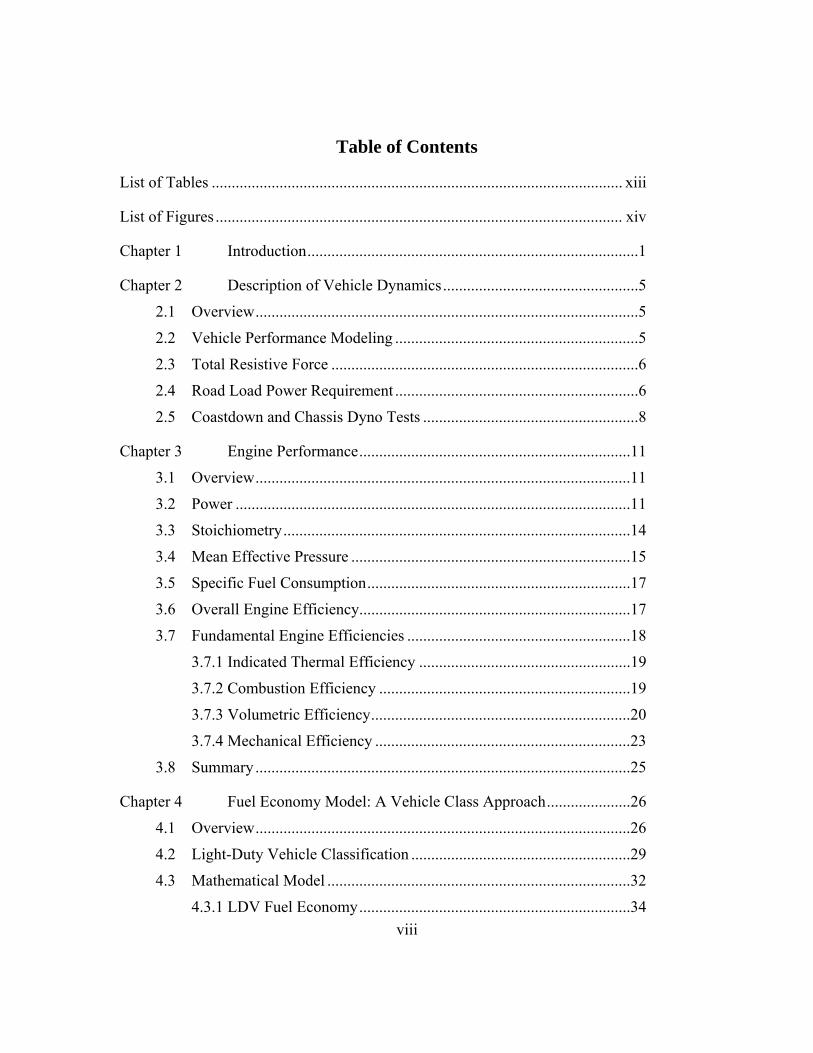
Table of Contents

List of Tables ....................................................................................................... xiii 

List of Figures ...................................................................................................... xiv 

Chapter 1  Introduction ...................................................................................1 

Chapter 2  Description of Vehicle Dynamics .................................................5 

2.1  Overview ................................................................................................5 

2.2  Vehicle Performance Modeling .............................................................5 

2.3  Total Resistive Force .............................................................................6 

2.4  Road Load Power Requirement .............................................................6 

2.5  Coastdown and Chassis Dyno Tests ......................................................8 

Chapter 3  Engine Performance ....................................................................11 

3.1  Overview ..............................................................................................11 

3.2  Power ...................................................................................................11 

3.3  Stoichiometry .......................................................................................14 

3.4  Mean Effective Pressure ......................................................................15 

3.5  Specific Fuel Consumption ..................................................................17 

3.6  Overall Engine Efficiency ....................................................................17 

3.7  Fundamental Engine Efficiencies ........................................................18 

3.7.1 Indicated Thermal Efficiency .....................................................19 

3.7.2 Combustion Efficiency ...............................................................19 

3.7.3 Volumetric Efficiency .................................................................20 

3.7.4 Mechanical Efficiency ................................................................23 

3.8  Summary ..............................................................................................25 

Chapter 4  Fuel Economy Model: A Vehicle Class Approach .....................26 

4.1  Overview ..............................................................................................26 

4.2  Light-Duty Vehicle Classification .......................................................29 

4.3  Mathematical Model ............................................................................32 

4.3.1 LDV Fuel Economy ....................................................................34 

ix

4.3.2 HDV Fuel Economy ...................................................................35 

4.4  EPA 2008 Fuel Economy Calculation Method ....................................35 

4.4.1 City FE Calculation.....................................................................35 

4.4.2 Highway FE Calculation .............................................................36 

4.5  Results ..................................................................................................37 

Chapter 5  Fuel Economy Model: A Vehicle Specific Approach ................69 

5.1  Overview ..............................................................................................69 

5.2  Road Load Force Model ......................................................................69 

5.3  Combustion Efficiency Model .............................................................69 

5.4  Mechanical Efficiency Model ..............................................................70 

5.5  Indicated Thermal Efficiency Model ...................................................72 

5.5.1 Air Equivalent SI Engine Model.................................................74 

5.5.2 AESI Indicated Thermal Efficiency Solution Procedure ............85 

5.5.3 Fuel Economy Model Graphical User Interface .........................91 

Chapter 6  SAE Coastdown Practice ............................................................99 

6.1  Overview ..............................................................................................99 

6.2  Technical Background .........................................................................99 

6.3  Road Load Measurement Using Coastdown Techniques ....................99 

6.3.1 Scope ...........................................................................................99 

6.3.2 Purpose ........................................................................................99 

6.4  Definitions............................................................................................99 

6.4.1 Test Weight .................................................................................99 

6.4.2 Test Mass ..................................................................................100 

6.4.3 Effective Mass ..........................................................................100 

6.4.4 Frontal Area ..............................................................................100 

6.5  Vehicle Road Load Measurement ......................................................100 

6.5.1 Instrumentation .........................................................................100 

6.5.2 Time and Speed.........................................................................100 

6.5.3 Temperature ..............................................................................101 

6.5.4 Atmospheric Pressure ...............................................................101 

x

6.5.5 Wind ..........................................................................................101 

6.5.6 Vehicle Weight .........................................................................101 

6.5.7 Tire Pressure .............................................................................101 

6.6  Test Conditions ..................................................................................101 

6.6.1 Ambient Temperature ...............................................................101 

6.6.2 Winds ........................................................................................101 

6.6.3 Road Conditions........................................................................102 

6.7  Vehicle Preparation ............................................................................102 

6.7.1 Break-In ....................................................................................102 

6.7.2 Vehicle Check-In ......................................................................102 

6.7.3 Instrumentation .........................................................................102 

6.7.4 Tire Pressure .............................................................................103 

6.7.5 Vehicle Frontal Area .................................................................103 

6.7.6 Vehicle Warm-Up .....................................................................103 

6.8  Coastdown Test ..................................................................................103 

6.8.1 Alternating Directions ...............................................................103 

6.8.2 Procedure ..................................................................................103 

6.8.3 Lane Changes ............................................................................104 

6.8.4 Data to be Recorded ..................................................................104 

6.8.5 Vehicle Test Weight .................................................................104 

Chapter 7  Analytical Basis of Coastdown Testing ..................................105 

7.1  Overview ............................................................................................105 

7.2  Analysis..............................................................................................106 

7.2.1 Aerodynamic Forces .................................................................107 

7.2.2 Tire and Chassis Drag ...............................................................111 

7.2.3 Mathematical Solution to Road Load Force .............................113 

7.2.4 Effective Vehicle Mass .............................................................117 

7.3  Data Acceptability Criteria ................................................................118 

7.3.1 Criteria 1 ...................................................................................119 

7.3.2 Criteria 2 ...................................................................................119 

xi

7.3.3 Result ........................................................................................119 

7.4  Data Correction ..................................................................................120 

7.4.1 Wind Correction to 0f ..............................................................120 

7.4.2 Temperature Correction to 0f ...................................................121 

7.4.3 Air Density Correction to 2f ....................................................121 

Chapter 8  Engine and Vehicle Simulation Software Programs .................122 

8.1  Overview ............................................................................................122 

8.2  AVL ADVISOR.................................................................................122 

8.3  AVL CRUISE ....................................................................................128 

8.4  AVL BOOST .....................................................................................128 

Chapter 9  Conclusions and Recommendations for Future Research ........130 

Appendix A:  Road Load Force Calculation MATLAB Code ........................133 

Appendix B:  Overall Drivetrain Efficiency Calculation MATLAB Code .....142 

B.1  City FE Calculation MATLAB Sub-Function (EPA 2008 Method) .147 

B.2  Highway FE Calculation MATLAB Sub-Function (EPA 2008 Method) ...................................................................................................147 

Appendix C:  Codes of Vehicle Specific Fuel Economy Model .....................148 

C.1  Main Function ....................................................................................148 

C.2  FE Calculation Function ....................................................................151 

C.3  Indicated Thermal Efficiency Calculation Function ..........................153 

C.4  Thermodynamic Properties Calculation of Ideal Gas Air ..................156 

C.5  Script Building MATLAB Codes into .NET Platform ......................158 

C.6  C# Graphical User Interface Codes ...................................................159 

Appendix D:  Vehicle Road Test Data Sheet ..................................................164 

Appendix E:  Coastdown Coefficient Calculation MATLAB Code ...............169 

E.1  Model Equation ..................................................................................171 

E.2  Data Acceptability Criteria 1 .............................................................171 

E.3  Data Acceptability Criteria 2a ...........................................................173 

xii

E.4  Data Acceptability Criteria 2b ...........................................................174 

E.5  Air Density Calculation .....................................................................175 

References ............................................................................................................178 

Vita .....................................................................................................................180 

xiii

List of Tables

Table 3-1  Part names in Figure 3.1 ............................................................12 

Table 4-1  Current and 5-Cycle Label Fuel Economies by Model Type ....27 

Table 4-2  Characteristics of the fuel economy and emissions tests of the 5-

cycle methodology ......................................................................28 

Table 4-3  Vehicle categories used in EPA Tier 2 standards ......................31 

Table 4-4  EPA Light-duty Vehicle Classification .....................................38 

Table 4-5  Representative Compact Class Vehicles ....................................45 

Table 4-6  Representative Midsize Class Vehicles .....................................45 

Table 4-7  2008 Compact Class City FE Overall Drivetrain Efficiency .....47 

Table 4-8  2008 Midsize Class City FE Overall Drivetrain Efficiency ......48 

Table 4-9  2008 Compact Class Highway FE Overall Drivetrain Efficiency .

.....................................................................................................49 

Table 4-10  2008 Midsize Class Highway FE Overall Drivetrain Efficiency 50 

Table 4-11  Overall Drivetrain Efficiency Summary of 2008 Model Year

Vehicles.......................................................................................67 

Table 5-1  Example Transmission Gear Efficiencies ..................................72 

Table 5-2  Gear Shifting Strategy ................................................................72 

xiv

List of Figures

Figure 2.1  Forces acting on a vehicle driving at steady speed. ......................6 

Figure 3.1  Engine connected to the dynamometer by coupling ...................12 

Figure 3.2  Schematic of principle of operation of dynamometer .................13 

Figure 4.1  New EPA Fuel Economy Label ..................................................29 

Figure 4.2  2008 Model Compact Class Road Load Force vs. Speed (Automatic

Transmission) ..............................................................................39 

Figure 4.3  2008 Model Compact Class Road Load Force vs. Speed (Manual

Transmission) ..............................................................................40 

Figure 4.4  2008 Model Midsize Class Road Load Force vs. Speed (Automatic

Transmission) ..............................................................................41 

Figure 4.5  2008 Model Midsize Class Road Load Force vs. Speed (Manual

Transmission) ..............................................................................42 

Figure 4.6  Excel Screen of 2008 City FE Calculation .................................43 

Figure 4.7  City FE Range of Vehicle Classes in Year 2008 ........................51 

Figure 4.8  Effects of Transmission on City FE on Vehicle Class (Part 1)...52 

Figure 4.9  Effects of Transmission on City FE on Vehicle Class (Part 2)...53 

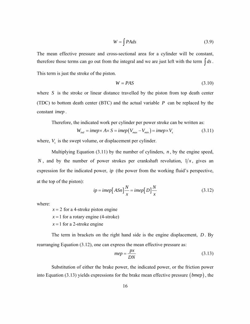
Figure 4.10  Coefficient of Variance of City FE .............................................54 

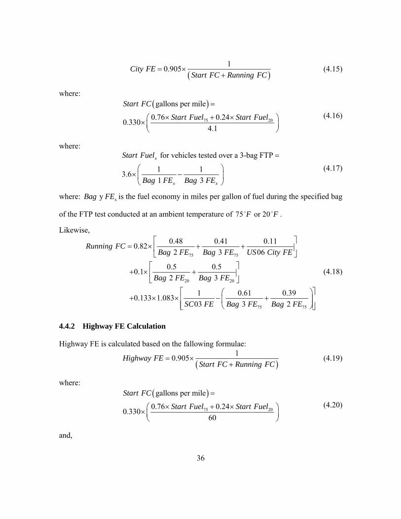
Figure 4.11  Highway FE Range of Vehicle Classes in Year 2008 ................55 

Figure 4.12  Effects of Transmission on Highway FE on Vehicle Class (Part 1)

.....................................................................................................56 

Figure 4.13  Effects of Transmission on Highway FE on Vehicle Class (Part 2)

.....................................................................................................57 

Figure 4.14  Coefficient of Variance of Highway FE .....................................58 

xv

Figure 4.15  Automatic Transmission City FE Comparison of Common Vehicles

on the Road .................................................................................59 

Figure 4.16  Automatic Transmission City FE % Error of Common Vehicles on

the Road ......................................................................................60 

Figure 4.17  Manual Transmission City FE Comparison of Common Vehicles on

the Road ......................................................................................61 

Figure 4.18  Manual Transmission City FE % Error of Common Vehicles on the

Road ............................................................................................62 

Figure 4.19  Automatic Transmission Highway FE Comparison of Common

Vehicles on the Road ..................................................................63 

Figure 4.20  Automatic Transmission Highway FE % Error of Common Vehicles

on the Road .................................................................................64 

Figure 4.21  Manual Transmission Highway FE Comparison of Common

Vehicles on the Road ..................................................................65 

Figure 4.22  Manual Transmission Highway FE % Error of Common Vehicles on

the Road ......................................................................................66 

Figure 5.1  Effect of Engine Speed on Indicated Thermal Efficiency ..........74 

Figure 5.2  Cross Section Showing One Cylinder of a Four-stroke Internal

Combustion Engine. ....................................................................76 

Figure 5.3  Four-stoke Schematic View of SI Engine (Ignition, Power Stroke &

Exhaust Stroke) ...........................................................................77 

Figure 5.4  Ideal P-V diagrams for the Air Equivalent SI Engine Model; a:

WOT, b: early intake, c: late intake, d: supercharged. ................78 

Figure 5.5  Control volume for analysis of intake process. ...........................80 

xvi

Figure 5.6  Ideal P V diagram for analysis of the exhaust process, including

State 4 ........................................................................................87 

Figure 5.7  Welcome screen of the Fuel Economy Model ............................92 

Figure 5.8  Default values of Ford F150 are loaded to Fuel Economy Model ..

.....................................................................................................93 

Figure 5.9  Result screen of the Fuel Economy Model .................................94 

Figure 5.10  Excel Spreadsheet of the Fuel Economy Model .........................95 

Figure 5.11  Welcome screen of the Fuel Economy Model installation. ........96 

Figure 5.12  Information screen about the software and the developers .........97 

Figure 5.13  GNU License Agreement screen of the Fuel Economy Model ..98 

Figure 7.1  Velocity vs. Time of Typical Coastdown Test .........................106 

Figure 7.2  Total airspeed is the vector sum of car speed and wind speed, both

relative to ground ......................................................................109 

Figure 7.3  Tire rolling resistance increases linearly with the square of speed.

...................................................................................................112 

Figure 8.1  Advisor Opening Snapshot .......................................................123 

Figure 8.2  Vehicle Input Screen .................................................................124 

Figure 8.3  Simulation Parameters Screen ..................................................126 

Figure 8.4  Results Screen ...........................................................................127 

1

Chapter 1 Introduction

Why is fuel economy important? In 2008, price of the crude oil went as high as

$145 a barrel in New York trading where regular gasoline pump price passed $4 per

gallon for the consumer in the US. Few industrial natural sources impact the world

economy directly like the oil prices. As oil prices rise, cost of the transportation

increases directly where it reflects to other products indirectly and finally it shows its

impact on the people’s lives as inflation.

Moreover, carbon dioxide emitted from the tailpipes of the vehicles contributes to

the global warming. According to EPA, 51% of the 2CO emissions in a typical household

are from vehicles owned in that household.1 Oil is a non-renewable source and hybrid

and electric vehicle technologies have not yet developed extensively to meet customers’

needs. Reducing the rate of the oil usage will allow time to scientists to create a better

world for our future.

The purpose of this thesis is to develop a computer based fuel economy model to

predict the fuel consumption of light-duty and heavy-duty vehicles. Two different

modeling approaches analyzed and two different models created for light-duty passenger

vehicles. First approach is a generalization of the vehicles to classes and modeling the

fuel economy for each class of the light-duty vehicles (LDV’s). EPA classifies light-duty

vehicles according to their Gross Vehicle Weight Ratings (GVWR) and the cargo

volume. A similar classification also exists for the heavy-duty vehicles (HDV’s);

however the classification is based on the GVWR and the number of axles.

1 http://www.fueleconomy.gov/feg/emissions/GHGemissions.htm

2

Second approach is a vehicle specific modeling of the fuel economy by using the

engine performance characteristics with the efficiency models of the engine and the

drivetrain. Total resistive forces on the light-duty vehicles can be calculated by the

coastdown coefficients released for every light-duty vehicle sold in the US by the EPA.

These resistive forces are related with engine power required to move vehicle forward

through efficiency models i.e. transmission efficiency, differential efficiency, and other

engine efficiency models like mechanical efficiency, indicated thermal efficiency, and

combustion efficiency. The engine power produced to move vehicle forward against the

resistive forces is extracted from the fuel combusted through a combustion process. The

fuel needed to produce engine power required in a specific vehicle ground speed gives

the fuel economy that is broadly known as the “ mpg ” which is the engineering units of

the fuel economy in miles per gallon mpg .

Chapter 2 of this thesis details the basics of the vehicle dynamics, including

aerodynamic drag forces, rolling resistance forces, and the forces imposed on the vehicle

due to grade. Comparison of the vehicles is of great importance in the automotive

industry in each vehicle class regarding fuel consumption. Thus, road load power

requirements of the vehicle are analyzed as a standard. Coastdown and chassis dyno tests

are discussed, along with the three coastdown coefficients and effective mass term.

Next chapter details the basics of the four-stroke internal combustion engines

widely used in the automotive industry. The author analyzes the engine power which is

the source to overcome the resistive forces explained in Chapter 2 and an introduction to

dynamometers also included to make a fundamental physical approach. In developing the

fuel economy model, stoichiometry of the air-fuel mixture is discussed which is

necessary to model combustion process accurately. Both of the fuel economy models are

directly related with engine efficiencies, thus; in addition to specific engine operating

3

efficiencies like indicated thermal efficiency, combustion efficiency, and mechanical

efficiency; an overall engine efficiency is described from point of classical

thermodynamics.

Chapter 4 discussed the vehicle class approach of the fuel economy modeling of

the LDV’s. Vehicle categories and vehicle class requirements are discussed in addition

to effects of the 2008 EPA fuel economy calculation method and new window stickers.

Mathematical model is analyzed using the physical equations derived in Chapter 2 and

the engine efficiency models discussed in Chapter 3. Moreover EPA’s fuel economy

calculation method is mathematically explained and related with the mathematical

expression derived at the beginning of the chapter with the overall drivetrain efficiencies.

Next, vehicle specific fuel economy model is discussed by modeling every

parameter of the engine and relating the power output of the engine through the

transmission end differential efficiency models to the road load power requirements of

the vehicle by using the coastdown coefficients. In developing the engine performance

model the Air Equivalent SI Engine Model is discussed in addition to intake,

compression, ignition, power, and exhaust strokes of the engine. Moreover, the fuel

economy mathematical model bundled to user-friendly software on the Microsoft’s .NET

platform which uses MATLAB codes in the background for capabilities of the

MATLAB. An installation setup is developed with Visual Studio 2008 for easy

distribution.

Chapter 6 discussed the SAE Recommended Coastdown Practice J1263 in details

starting from the instrument requirements, track specifications and the terms to the

procedure that needs to be followed during the coastdown tests. A Vehicle Data Sheet is

attached in Appendix D: for completeness of the procedure.

4

Next, analytical analysis of the coastdown tests are discussed in details. Korst’s

mathematical approach is mixed with Yasin’s approach and at the end equations are

altered in our needs for easy calculation of the coastdown coefficients. The criteria

explained in the SAE J1263 Coastdown Practice are detailed mathematically and finally

correction factors for the different environmental conditions applied to averaged

coastdown coefficients.

Chapter 8 discusses the software’s that can be used in fuel economy calculations

of the either light-duty or heavy-duty vehicles. AVL is the world’s largest privately

owned company for development of powertrains (combustion engines, hybrid systems,

electric drive) as well as simulation and test systems for light-duty vehicles, heavy-duty

vehicles and marine engines.2

Finally, a conclusion is drawn for the work presented in this thesis and

recommendations for future research is expressed.

2 http://www.avl.com/wo/webobsession.servlet.go?app=bcms&page=view&nodeid=400013015

5

Chapter 2 Description of Vehicle Dynamics

2.1 OVERVIEW

In this section, details of the vehicle dynamics necessary for modeling fuel

economy will be discussed. The scope of the study is for light-duty vehicles (LDVs) but

introductory information for heavy-duty vehicles (HDVs) will also be presented.

To predict the vehicle performance in both the light-duty and heavy-duty classes,

application of some fundamental principles of physics is required and this analysis is

illustrated in the following subsections.

2.2 VEHICLE PERFORMANCE MODELING

Figure 2.1 is an illustration of the forces resisting the movement of a vehicle

driving on a road at a steady speed. The total resistive force resF is the result of various

individual forces that are additive. These forces are the aerodynamic drag force DF the

rolling resistance RF and the force imposed by a grade GF :

res D R GF F F F (2.1)

6

Figure 2.1 Forces acting on a vehicle driving at steady speed.

The aerodynamic drag force is due to the air moving around the vehicle and is

experimentally measured in tests that are conducted in a wind tunnel. The rolling

resistance expresses the frictional force acting between the tires and the road while the

force imposed by a grade is the force of gravity acting on the vehicle while driving uphill

or downhill.

2.3 TOTAL RESISTIVE FORCE

The resistive force implies that a certain power is required to move the vehicle at

steady speed under given conditions of wind speed, vehicle speed, grade, etc. For driving

at steady speed with no wind on a level road, the resistive force is called the road load

force, as discussed in the following subsection.

2.4 ROAD LOAD POWER REQUIREMENT

One standard of vehicle performance is its behavior with no wind and no grade.

This condition is known as “road load” and the corresponding resistive force is called the

7

road load force RLF . In terms of the fundamental physical parameters, the road load

force is:

21

2 RL air D RR TF C AV C W (2.2)

where air is the ambient air density, DC is the drag coefficient of the vehicle, A

is the front cross-sectional area of the vehicle, V is the vehicle speed, RRC is the

coefficient of rolling resistance between the tires and the road surface, and TW is the total

weight of the vehicle. At one time, every manufacturer who sold light-duty vehicles in

the U.S. reported the values of DC and RRC to the EPA, who then published all of this

data (in hard copy, before the web). These values were essential for setting the

“absorption torque” on chassis dynamometers that were used to measure the fuel

economy and/or emissions from that specific vehicle. However, there were inaccuracies

in measuring the drag coefficient because, at the time, there were no “rolling road” wind

tunnels to accurately simulate the aerodynamics of the flow under the vehicle. Also, the

coefficient of rolling resistance is measured using a tire test machine in which a tire is

rotating by a moving belt, the surface of which was intended to simulate the average road

surface. The coefficient of rolling resistance is a function of the normal load on the tire

(the fraction of the total vehicle weight supported by each tire), so a weighted average

must be used to calculate RRC for use in Equation (2.2). Furthermore, RRC is a function

of vehicle speed, tire inflation pressure, tire temperature, tire construction, and tire

compound. Because the tests for DC and RRC were both expensive and involved

inaccuracies and uncertainties, the Society of Automotive Engineers (SAE) developed a

coastdown technique, as discussed in Subsection 2.5. Nevertheless, understanding the

underlying physics is important.

8

The power required to provide the road load force is called the road load power

RLP .

Road load power is useful for predicting “standard” vehicle performance under

steady driving conditions. Here, it is important to note that RLP is the power required at

the interface between the drive tires and the road, and is not the brake power required of

the engine to propel the vehicle at steady speed on a level road with no wind RLbp . The

relationship between RLP and RLbp is discussed in Chapter 4.

2.5 COASTDOWN AND CHASSIS DYNO TESTS

For chassis dyno testing, such as for emissions certification and fuel economy

tests, the resistive force is the force that must be absorbed by the dyno during prescribed

accelerations, decelerations, and steady state cruises. For such tests, there is no wind and

the vehicle speed is prescribed as a function of time, thus dictating the rate of change of

speed (acceleration or deceleration) each second.

SAE Recommended Practice J1263 shows how on-road coastdown tests can be

used to determine the road load coefficients. In practice, the coast-down data generally

yields a second order fit that includes a term that is linear in vehicle speed:

20 1 2res e

dVF M f f V f V

dt (2.3)

where 1f may be non-zero due to the characteristics of the tires. In fact, the tires

have a strong effect on the coast-down results. SAE Recommended Practice J2264

explains that such coast-down tests can also be used to determine the road load

coefficients using modern electric chassis dynamometers. In this case, the coefficients

from the on-road coast-down tests are used as “targets” for the initial chassis dyno coast-

down tests. The resulting chassis dyno coast-down data are fitted with a quadratic

equation that yields a term that is linear in vehicle speed:

9

2abs e

dVF M A BV CV

dt (2.4)

where coefficient B is required to compensate for internal friction in the dyno

and for the characteristics of the tires, and absF is the same as resF . If the coast-down

tests are done properly, Equation (2.4) is more accurate than Equation (2.2) due to

approximations in calculating the drag coefficient DC and the coefficient of rolling

resistance RRC from wind tunnel test data and tire test machine data, as discussed

previously. That is, due to approximations and assumptions in wind tunnel and tire

machine tests, coast-down data such as used for Equation (2.4) can be more accurate than

the more fundamental approach of Equation (2.2).

For emissions certification tests of light-duty vehicles, the EPA uses a test weight

that is the curb weight plus 2548 N (300 lb). SAE Recommended Practice J2264

explains that the effective mass appearing in Equation (2.4) depends upon the purpose of

the test. For determination of the road load coefficients A , B , and C , from coast-down

tests, the effective mass is called the highway inertia. For general testing, the actual road

load is desired - the rotational inertia of all four wheel assemblies must be accounted for.

In this case, the highway inertia includes the test mass plus the effective masses of both

the driven and non-driven wheel assemblies, and can be estimated as 1.03 times the

vehicle test mass for vehicles with only four tires. For certification purposes, the

highway inertia is dictated by regulations to be the effective test mass (an effective test

weight, ETW , is assigned for a vehicle to represent a class of vehicles) plus the effective

masses of only the driven wheel assemblies, and can be estimated as 1.015 times the

ETW g for vehicles with only two driven tires. When the chassis dyno is being used to

control the vehicle resistance, the effective mass in Equation (2.4) is called the inertia

mass and, again, there are two cases. For general testing it is recognized that only two

10

wheel assemblies are rotating during chassis dyno testing. In this case, the inertia mass

includes the test mass plus the effective masses of only the driven wheel assemblies, and

can be estimated as 1.015 times the vehicle test mass for vehicles with only two driven

tires. For tests that are dictated by regulations such as emissions certification and urban

and highway fuel economy, the effective mass equals the ETW g . To calculate the fuel

economy (or emissions) of a specific vehicle, as needed for this project, the effective

mass is the curb weight plus the payload weight (driver, cargo, etc.) plus the mass of all

of the wheel assemblies that rotate when the vehicle is driving down a road.

11

Chapter 3 Engine Performance

3.1 OVERVIEW

The fundamental equations governing vehicle dynamics were explained in

Chapter 2 and now it is time to examine the engine which is the power source to

overcome the resistive forces that nature imposes. The most widely used engine on the

roads nowadays is the gasoline engine, widely called the Spark Ignition (SI) engines.

Parameters defined in this chapter are applicable to diesel engines also but some

modifications to the equations may be required for such special cases.

By the advance of the technology, engine control strategies are changing by time

in addition to fuel injection systems and the materials used. However the fundamental

principle of the gasoline engine did not change much since Otto’s first engine. The

following subsections are going to provide some definitions and the governing equations

that are required by the fuel economy model. A full detailed parameter analysis can be

found at Matthews, 2007.

3.2 POWER

Torque and rotational speed (revolution per minute – rpm) can be measured by

using a machine called a dynamometer or dyno for short. The engine is placed on a test

bed and connected to the dyno by a coupling. Figure 3.1 shows the engine and dyno

setup.

Early dynamometers were called brakes since they used brake shoes to press

against the flywheel to apply the desired load (Obert, 1973). This explains the current

use of “brake power” and “brake torque” that refer to power and torque readings at the

engine output shaft as obtained from a dyno.

12

Figure 3.1 Engine connected to the dynamometer by coupling3

Table 3-1 summarizes the part names of the engine and dyno system shown in Figure 3.1.

Table 3-1 Part names in Figure 3.1

Part Number  Name 

1  Engine 

2  Coupling 

3  Tachometer 

4  Scales 

5  Torque Arm 

6  Stator (Housing) 

7  Rotor 

8  Bearings 

The rotor is coupled to the stator, as shown in Figure 3.2, by means of hydraulic,

electromagnetic or mechanical forces. In general the torque exerted on the stator by the 3 http://en.wikipedia.org/wiki/Dynamometer

13

rotating rotor is balanced with some means of restraining the rotation of the stator while

also measuring the restraining force.

Figure 3.2 Schematic of principle of operation of dynamometer4

The torque , produced by the engine can be calculated as force F times the

torque arm r as shown in Figure 3.2.

F r

(3.1)

The power p produced by the engine and absorbed by the dynamometer is the product of

torque and angular speed:

2p N (3.2)

where N is the engine crankshaft rotational speed.

4 J. B. Heywood, Figure 2-3

14

If the engine is running in steady state operation and the dynamometer is in the

absorption mode then the power described by Equation (3.2) is called the “brake power,

bp ”.

2bp N (3.3)

3.3 STOICHIOMETRY

During engine operation, both the fuel mass flow rate, fm ,and the air mass flow

rate, am ,are measured and these parameters control the power output of the engine. In

order to maintain stable combustion, homogenous charge SI engines must maintain an

almost constant, usually stoichiometric mixture.

The ratio of the fuel mass flow rate to the air mass flow rate defines the fuel/air

ratio FA and air/fuel ratio AF vice versa.

f

a

mFuel air ratio FA

m

(3.4)

a

f

mAir fuel ratio AF

m

(3.5)

In addition to the air/fuel ratio and fuel/air ratio, the automotive industry accepts

other ways of defining this ratio as standard depending upon preferences. The air/fuel

ratio is a number that sits between 12 and 18 for most of the SI engines while the fuel/air

ratio is just the inverse of the air/fuel ratio - that is, a number between 0.056 and 0.083.

The air/fuel ratio is widely used because of its meaningful range of numbers.

In addition to monitoring a state of the engine, it is also useful to compare that

state with a stoichiometric state. To achieve this, another parameter called the

equivalence ratio, , is introduced. The equivalence ratio of the engine is defined as the

ratio of fuel/air ratio to the stoichiometric fuel/air ratio. Mathematically,

s

s

AFFA

FA AF (3.6)

15

For stoichiometric combustion, 1.0 and the equivalence ratio is greater than 1.0 for

rich combustion and it is smaller than 1.0 for fuel lean combustion, respectively.

3.4 MEAN EFFECTIVE PRESSURE

The mean effective pressure is a parameter related to internal combustion

operation and is a measure of ability to do work and it is a benchmark parameter to

compare engines irrespective of their displacement, engine speed and whether the engine

is a four stokes or two strokes or even a Wankel engine. The mean effective pressure is

also a more fundamental metric for the load on an engine than is the power or torque.

While an engine is working, the pressure inside the combustion chamber is

continuously changing from atmospheric pressure (or less) to 30 times atmospheric

pressure or more depending upon the load and air entering the combustion chamber. The

“indicated” mean effective pressure imep may be thought of as the average pressure

over a cycle in the combustion chamber of the engine that produces the same work over

the same power stroke as the variable pressure over the whole engine cycle. The “brake”

mean effective pressure uses the same normalization but is from the perspective of the

engine output shaft.

Force can be written as pressure times the cross sectional area for a piston system

as well known from physics:

F P A (3.7)

Work can be defined as the amount of energy transferred by a force acting through a

distance and can be expressed as:

W Fds (3.8)

where F is the force vector and s is the position vector. By inserting Equation (3.7) into

Equation (3.8), one gets:

16

W PAds (3.9)

The mean effective pressure and cross-sectional area for a cylinder will be constant,

therefore those terms can go out from the integral and we are just left with the term ds .

This term is just the stroke of the piston.

W PAS (3.10)

where S is the stroke or linear distance travelled by the piston from top death center

(TDC) to bottom death center (BTC) and the actual variable P can be replaced by the

constant imep .

Therefore, the indicated work per cylinder per power stroke can be written as:

ind max min sW imep A S imep V V imep V (3.11)

where, sV is the swept volume, or displacement per cylinder.

Multiplying Equation (3.11) by the number of cylinders, n , by the engine speed,

N , and by the number of power strokes per crankshaft revolution, 1 x , gives an

expression for the indicated power, ip (the power from the working fluid’s perspective,

at the top of the piston):

N N

ip imep ASn imep Dx x

(3.12)

where: 2 for a 4-stroke piston engine

1 for a rotary engine (4-stroke)

1 for a 2-stroke engine

x

x

x

The term in brackets on the right hand side is the engine displacement, D . By

rearranging Equation (3.12), one can express the mean effective pressure as:

px

mepDN

(3.13)

Substitution of either the brake power, the indicated power, or the friction power

into Equation (3.13) yields expressions for the brake mean effective pressure bmep , the

17

indicated mean effective pressure imep , and the friction mean effective pressure

fmep respectively:

bp x

bmepD N

(3.14)

ip x

imepD N

(3.15)

fp x

fmepD N

(3.16)

3.5 SPECIFIC FUEL CONSUMPTION

Fuel consumption is measured as a flow rate but it is not directly comparable

among different engine sizes and load conditions. Another term called the specific fuel

consumption, sfc , allows the fuel efficiency of different internal combustions engines to

be directly compared. It measures how efficiently an engine is using the fuel supplied to

produce work:

fmsfc

p

(3.17)

Both the brake specific fuel consumption, bsfc , and the indicated specific fuel

consumption, isfc , can be defined through the appropriate substitutions into Equation

(3.17):

fmbsfc

bp

(3.18)

fmisfc

ip

(3.19)

3.6 OVERALL ENGINE EFFICIENCY

The ratio of the work produced per cycle to the amount of fuel energy supplied

per cycle with fuel during combustion can be used as a measure of the overall engine

efficiency. Thermodynamically, efficiency is a dimensionless performance measure and

is defined as the ratio of “what you get” to “what you pay for”. What we get in an

18

internal combustion engine is the power output of the engine, which is basically brake

power and what we pay for is the chemical energy in the fuel. The maximum rate of

energy released from the fuel in the combustion process can be calculated by multiplying

the mass flow rate of the fuel per cycle with the constant pressure Lower Heating Value

of the fuel, PLHV . Thus the overall engine efficiency is:

ef P

bp

m LHV

(3.20)

The maximum energy release in the combustion process can be attained with

complete combustion and constant pressure combustion in a flow calorimeter. The

Lower Heating Value is used rather than the Higher Heating Value for the practical

reason that condensation of water in the combustion chamber must be avoided.

By inserting Equation (3.18) into Equation (3.20), one can see the effect of

specific fuel consumption on the overall engine efficiency (sometimes called the brake

thermal efficiency):

1

ePbsfc LHV

(3.21)

Most transportation fuels are mixtures of many chemical species plus additives,

and their composition may be changed by time of the year and tank to tank. Therefore

there is a great variety among Heating Values and that makes comparison of overall

engine efficiencies difficult. However, as can be seen from Equation (3.21), lower

specific fuel consumption corresponds to higher overall engine efficiency, as expected.

3.7 FUNDAMENTAL ENGINE EFFICIENCIES

It is desirable to express the engine performance parameters discussed above in

terms of the engine design and operating conditions that control them. The mathematical

19

relationships developed in this section (Matthews, 1983) may be used to enhance

physical understanding of the factors that affect the engine’s performance.

3.7.1 Indicated Thermal Efficiency

The word “indicate” is described as “to point out or point to with more or less

exactness” in Webster’s Dictionary. If this definition is applied to the engine context,

one can use it for the terms which are results of the working fluid itself. Power is

produced by the working fluid (which is called the indicated power) but, due to frictional,

viscometric, and parasitic the losses between the working fluid space and the engine

output shaft (referred to as the friction power), one ends up with the brake power at the

engine output shaft.

In classical thermodynamics, a thermal efficiency is defined as the ratio of the

useful work (which is the net work done by the system, from the working fluid’s

perspective) to the thermal energy added to the working fluid. Beware that thermal

energy term is not “net”, because what we pay for is the chemical energy content of the

fuel. Mathematically one can write:

net nett

in in

W p

Q Q (3.22)

Equation (3.22) can be more precisely defined as the “indicated thermal efficiency” since

it is the efficiency - before the losses in the engine - from the working fluid’s perspective.

itin

ip

Q (3.23)

3.7.2 Combustion Efficiency

Combustion efficiency is defined as the ratio of the thermal energy (“heat”)

transferred to the working fluid after combustion to the maximum heat release from that

combustion. As explained in Section 3.6, the maximum heat release occurs for complete

20

combustion of a lean or stoichiometric mixture. Thus, the maximum heat release rate is

quantified as the fuel mass flow rate time the constant pressure Lower Heating Value,

PLHV , of the fuel (which is the chemical energy of fuel – what the consumer actually

pays for):

max f PQ m LHV (3.24)

Therefore, the combustion efficiency can be written as:

max

finc

mQ

Q

in

f

q

min

PP

q

LHVLHV (3.25)

where inq is the actual thermal energy transferred to the working fluid by combustion per

unit mass of fuel.

One can relate the indicated thermal efficiency with the combustion efficiency by

using the common term inQ in Equations (3.23) and (3.25).

maxin cit

ipQ Q

(3.26)

maxit cip Q (3.27)

By inserting Equation (3.24) for the maxQ term in Equation (3.27):

it c f Pip m LHV (3.28)

3.7.3 Volumetric Efficiency

The intake system of the engine includes parts like an air filter, throttle body,

intake manifold, intake ports, and intake valves that restrict the air to flow freely to the

combustion chamber. The volumetric efficiency is used to measure how efficiently an

engine can induct the air into the combustion chamber. The volumetric efficiency is

defined as the ratio of the air mass actually entered to the maximum theoretical air mass

that can be filled into the cylinders volume. This maximum mass of air is basically the

21

total engine cylinder volume or basically engine displacement times the density of the air

per engine revolution. Mathematically:

,

av

a theoeretical

m

m

(3.29)

,

air

a theoeretical

DNm

x (3.30)

where air is the air density at the inlet of the carburetor or throttle body, D is the engine

displacement, N is the engine rotational speed, and x is the number of crankshaft

revolutions per intake stroke.

a

vair

mDN

x

(3.31)

Note that the volumetric efficiency is not a real efficiency like the previous

efficiencies since it does not contain any power or heat transfer rate terms. Therefore,

one cannot expect it to stay between 0 and 1, indeed in many cases the volumetric

efficiency is over 1.

By using Equations (3.4) and (3.6), one can express the mass flow rate of the fuel

in terms of the air mass flow rate and equivalence ratio:

fs

a

mFA FA

m

(3.32)

f a sm m FA (3.33)

Substituting Equation (3.33) back into Equation (3.28) yields:

it c a s Pip m FA LHV (3.34)

By using Equation (3.31), substituting the air mass flow rate am in terms of the

volumetric efficiency and related engine parameters:

ait c v s P

DNip FA LHV

x

(3.35)

Rearranging terms yields:

22

it c v a s P

Nip D FA LHV

x

(3.36)

Similarly, the fuel mass flow rate can be written by combining Equations (3.31) and

(3.33):

af v s

DNm FA

x

(3.37)

Rearranging yields:

f v a s

Nm D FA

x

(3.38)

Equation (3.36) is a very useful equation since it relates three fundamental efficiencies of

the engine with the potential ability of an engine to do work. Further fundamental

relations can be retrieved by back inserting Equation (3.36) into Equation (3.15).

it c v a D

imep

N

x s PFA LHV x D N

(3.39)

it c v a s Pimep FA LHV (3.40)

Equation (3.40) shows that the indicated mean effective pressure is not a direct function

of engine displacement, engine speed, or whether the engine is a 4-stroke, a 2-stroke, or a

Wankel (via x , the number of revolutions per power stroke).

Another fundamental equation can be obtained via inserting Equations (3.36) and

(3.38) into Equation (3.19) for the indicated specific fuel consumption isfc :

v a s

f

ND FA

m xisfc

ip

it c v a s

ND FA

x

PLHV

(3.41)

1

it c P

isfcLHV

(3.42)

23

3.7.4 Mechanical Efficiency

In engine operation, there are power losses due to friction in bearings of the

crankshaft, friction between the pistons, and the cylinder walls, and other miscellaneous

mechanical losses, such as the power required to run the oil pump. All of these losses

combine to constitute the friction power, which is basically the difference between the

indicated power and the brake power.

ip bp fp (3.43)

The mechanical efficiency, m can be defined as the efficiency of converting the

net power available from the working fluid to available power at the output of the

crankshaft:

1m

bp fp

ip ip (3.44)

The mechanical efficiency can be written in terms of mean effective pressures by using

Equations (3.14), (3.15), and (3.16):

m

bmep D N

ximep D N

x

1

fmep D N

ximep D N

x

(3.45)

After cancelling the same terms:

1m

bmep fmep

imep imep (3.46)

Substituting Equation (3.44) into Equation (3.36) yields:

it c v a s Pm

bp ND FA LHV

x

(3.47)

Rearranging:

it c v m a s P

Nbp D FA LHV

x

(3.48)

24

Substitution of Equation (3.48) into Equation (3.14) and Equation (3.18) yields

fundamental relationships for the brake mean effective pressure and brake specific fuel

consumption:

it c v m a D

bmep

N

x s PFA LHV x D N

(3.49)

it c v m a s Pbmep FA LHV (3.50)

f

it c v m a s P

mbsfc

ND FA LHV

x

(3.51)

Inserting Equation (3.38) into Equation (3.51):

v

bsfc

a s

ND FA

x

it c v m a s

ND FA

x

PLHV

(3.52)

1

it c m P

bsfcLHV

(3.53)

The overall engine efficiency can be obtained in terms of other engine efficiencies by

inserting Equations (3.38) and (3.48) into Equation (3.20):

it c v

e

m a s P

ND FA LHV

x

v a s P

ND FA LHV

x

(3.54)

e it c m (3.55)

25

3.8 SUMMARY

This chapter was intended to familiarize reader with the engine parameters and

show a fundamental approach to derive governing equations in the engine operation. By

using the fundamental equations derived in this chapter, one can model the consumption

of fuel at different operating ranges as it will be shown in Chapter 4 and Chapter 5.

Moreover, these equations are useful for comparison of different types of the engines

performance characteristics wise or fuel economy point of view.

26

Chapter 4 Fuel Economy Model: A Vehicle Class Approach

4.1 OVERVIEW

The Environmental Protection Agency (EPA) fuel economy estimates have

appeared on the window stickers since the late 1970’s and well-recognized by the

customers5. The fuel economy estimates have two major uses: one is providing

consumers a benchmark to compare vehicles during the buying process and giving an

idea of how much fuel economy they would expect while using that specific vehicle.

EPA made some changes to the methods used to calculate fuel economy (FE)

estimates that are posted on window stickers of all new cars and light trucks sold in the

United States. The aim of this method is to estimate real world conditions i.e. aggressive

acceleration and deceleration, use of air conditioning, and operation in cold temperatures.

According to final rule posted on Federal Register (Vol.71, No. 248 / December 27,

2006), the city miles per gallon (mpg) estimates for the manufacturers of most vehicles

will drop by about 12 percent on average relative to today’s estimates, and city mpg

estimates for some vehicles will drop by as much as 30 percent. The highway mpg

estimates for most vehicles will drop on average by about 8 percent, with some estimates

dropping by as much as 25 percent relative to today’s estimates. Table 4-1 shows the

change in fuel economy in classes for new fuel economy calculation method compared to

old method.

5 EPA420-R-06-017

27

Table 4-1 Current and 5-Cycle Label Fuel Economies by Model Type6

Current City   5‐Cycle City   Current Highway   5‐Cycle Highway  

Conventional Vehicles     

Large car   15.7  13.8  21.9  19.7 

Midsize car   20.5  17.8  27.9  25.6 

Minivan   17.4  15.2  23.6  20.9 

Pickup   15.1  13.2  18.9  17.2 

Small car   20.7  18.1  27.3  25.3 

Station wagon   20.3  17.6  26.6  23.5 

SUV   16.8  14.6  21.6  19.5 

Van   12.5  10.9  16  14.3 

All conventional   18.6  16.2  24.6  22.4 

All hybrids   41.6  32  40.6  36.8 

Diesel (one midsize car)   26.2  22.7  35.3  31.4 

All vehicles   19.1  16.4  24.9  22.7 

The previous method was established in 1984 by adjusting the city test result

(Federal Test Procedure FTP) 10 percent downward and the highway test result

(Highway Fuel Economy Test HFET) 22 percent downward. In 2008 method of EPA,

additional tests are incorporated to represent today’s driving style which includes higher

speeds, aggressive acceleration and deceleration, air conditioner usage and cold air

conditions. Clearly FTP and HFET do not capture the real world driving conditions;

therefore FTP, HFET, US06, SC03 and Cold FTP combined. EPA refers to this test as

“5-cycle” method; however in our mechanistic model FTP and Cold FTP are same so

6 EPA420-R-06-017

28

basically in our method cold start conditions are not represented as it is intended by EPA.

The five test procedures are summarized in the following table:

Table 4-2 Characteristics of the fuel economy and emissions tests of the 5-cycle methodology7

With changes in calculation method in 2008, EPA also changed fuel economy

label design as it is shown in Figure 4.1.

The label shows the estimated city mpg at the top left, and highway mpg at the

top right and below these estimates there is another estimate depending upon driver

habits what kind of mpg values would consumer expect. The center of the label provides

estimated annual fuel costs based on a given number of miles and fuel price also listed on

the label. This information is very useful to understand the operating cost of that vehicle

and stands as a benchmark economy wise. The lower center of the label gives a

combined city/highway estimate for that vehicle, and shows where that value falls on a

bar scale that gives the highest and lowest fuel economy of all other vehicles in its class.

7 Federal Register, Vol. 71, No. 248, Table I-1

29

Figure 4.1 New EPA Fuel Economy Label8

4.2 LIGHT-DUTY VEHICLE CLASSIFICATION

Light-duty vehicle (LDV) regulations are divided into those applicable to

passenger cars and those applicable to light-duty trucks. Light-duty trucks are defined as

trucks of less than 8500 lbs Gross Vehicle Weight Rating (GVWR or GVW) after 1979,

except for those with more than 45 ft2 frontal area. Light-duty trucks were classified as

heavy-duty vehicles in the Clean Air Act but are treated as LDVs by the U.S.

Environmental Protection Agency (EPA) as far as test procedures are concerned.

Federally, light-duty trucks are divided into light light-duty trucks (LLDTs) and heavy

light-duty trucks (HLDTs) in four categories, with separate emissions standards for each

8 http://www.epa.gov/fueleconomy/420f06069.htm

30

category. The categories are based upon Loaded Vehicle Weight (LVW, curb weight +

300 lb), Gross Vehicle Weight Rating, and/or Adjusted Loaded Vehicle Weight ( )

2

LVW GVWRALVW

. LLDTs are divided into two categories: LDT1s and

LDT2s, both of which have GVWR < 6000 lb. HLDTs are also divided into two

categories: LDT3s and LDT4s both of which have 6000 < GVWR ≤ 8500 lb. Beginning

in 2004, a new federal vehicle category was introduced: the medium-duty passenger

vehicle (MDPV). This category was designed to bring large passenger vehicles (such as

large SUVs and passenger vans) over 8500 lbs GVWR into the “Tier 2” emissions

standard program. MDPVs are defined as any complete heavy-duty vehicle less than

10,000 lbs GVWR designed primarily for transportation of people.

U.S. Department of Transportation (DOT) ruled to integrate medium-duty

passenger vehicles (MDPV), including large SUVs and vans, into the Corporate Average

Fuel Economy (CAFE) program starting in 2011; EPA must now include these vehicles

in the fuel economy labeling program. Thus, EPA will be requiring fuel economy

labeling of certain passenger vehicles up to 10,000 lb gross vehicle weight rating

(GVWR). These vehicles used to be exempt because they weighed more than the

previous cut-off of 8,500 lb. Vehicle manufacturers will be required to post fuel economy

labels on MDPVs beginning with the 2011 model year.

31

Table 4-3 Vehicle categories used in EPA Tier 2 standards9

Vehicle Category Abbreviation Requirements

Light-Duty Vehicle LDV max. 8500 lb GVWR

Light-Duty Truck LDT max. 8500 lb GVWR, max. 6000 lb curb weight and max. 45 ft2 frontal area

Light light-duty truck LLDT GVWR < 6000 lb

Light-duty truck 1 LDT1 LVW1 < 3750 lb

Light-duty truck 2 LDT2 3751 lb < LVW1 < 5750 lb

Heavy light-duty truck HLDT 6000 lb < GVWR ≤ 8500 lb

Light-duty truck 3 LDT3 3751 lb < ALVW2 < 5750 lb

5751 lb < ALVW2 < 8550 lb

Light-duty truck 4 LDT4 min. 5750 lb ALVW2

Medium-Duty Passenger Vehicle MDPV 8500 lb < GVWR3 < 10000 lb 1 - LVW (loaded vehicle weight) = curb weight + 300 lb

2 - ALVW (adjusted loaded vehicle weight) = average of GVWR and curb weight

3 - Manufacturers may alternatively certify engines for diesel fueled MDPVs through the heavy-duty diesel engine regulations

9 http://www.dieselnet.com/standards/us/ld_t2.php

32

4.3 MATHEMATICAL MODEL

The steady state or when vehicle is not undergoing rapid changes in speed, fuel

economy of the vehicle migal is the ratio of the vehicle speed mi

hr to the volumetric rate

of fuel consumption galhr .

mihrmi

galgal

hrf

VFE

V

(4.1)

Equation (4.1) can also be written in terms of fuel density and fuel mass flow rate:

f

f

VFE

m

(4.2)

Furthermore it is already known from Equations (3.18) and (3.53) that:

1f

it c m P

mbsfc

bp LHV

(4.3)

Rearranging yields:

fit c m P

bpm bsfc bp

LHV (4.4)

Substituting back into Equation (4.2) yields:

f f

f

it c m P

V VFE

bpmLHV

(4.5)

Rearrange to get:

it c m P f

VFE LHV

bp

(4.6)

The engine supplies power to overcome resistive forces explained in Chapter 2.

Engine power available at the output of the crankshaft is called brake power, bp and this

power first passes through transmission and differential then become available at the tires

to push the vehicle forward and this available power at the tires is called the motive

power, motp . The motive power that is available at the drive tires is basically the engine

33

brake power minus the energy losses in the transmission and differential respectively. By

using the transmission and differential efficiencies, one can write:

mot t dp bp (4.7)

where bp is the brake power available at the crankshaft, t is the transmission

efficiency, and d is the differential efficiency.

Motive force motF can be also calculated from motive power since it is well known that

power is the time rate of work which indicates power is the force time speed:

mot motp F V (4.8)

The term in brackets in Equation (4.6) can be expressed by Equations (4.7) and (4.8) as:

mot t dF V bp (4.9)

t d

mot

V

bp F

(4.10)

Substituting back into Equation (4.6) yields:

t dit c m P f

mot

FE LHVF

(4.11)

Under steady state road load conditions, this becomes:

t dit c m P f

RL

FE LHVF

(4.12)

Equation (4.12) can be manipulated to yield:

e dt

f pRL

FE LHVF

(4.13)

where e is the overall engine efficiency, dt is overall drivetrain efficiency, f

is fuel

density, and pLHV is the energy density of the fuel.

Equation (4.13) is the base equation for both LDV’s and HDV’s. Fuel property

effects can be easily found from thermodynamic tables. Equation (2.4) estimates the road

34

load force where coefficients are EPA target values. Only left part is product of

efficiencies: e dt .

The product depends upon both engine speed and torque and will require

calibration against experimental data. Fortunately, this product can be back-calculated

from the “unadjusted” urban and highway fuel economy for a variety of vehicles from the

data in EPA’s Fuel Economy Guide (www.epa.gov/fueleconomy). The FTP (urban fuel

economy) and HFET (highway fuel economy) is available in excel spreadsheets. The

fuel economy will be calculated in each second, using a user-specified constant for

e dt .

After calculating the FE in each second, the distance travelled during that second

is calculated, and this is used to calculate the gallons of fuel used during that second. At

the end of the driving cycle, sum up the gallons of fuel consumed, and add together the

miles traveled, and calculate the ratio: the FE migal for this driving cycle. The value of

adjustable constant e dt that provides the best agreement with the data is the

calibrated value to be used for that class of vehicle.

4.3.1 LDV Fuel Economy

1) There is some imprecision for each category of LDV due to the necessity of using

average values for each class of vehicle. It is also necessary to “filter” EPA’s data.

2) Extrapolation to alternative fuels will be simple since density and lover heating

value can be easily inserted in the fuel economy calculation through Equation

(4.13).

3) Experimental data can be used to calculate coastdown coefficients as it is

explained in Chapter 6 and Chapter 7.

35

4.3.2 HDV Fuel Economy

HDV’s are not subjected to FE standards and there is no EPA data that will be

useful to this study from the HDV perspective.

Because truck manufacturers generally offer a choice of engines from 2 or more

manufacturers, and because a specific engine from an engine manufacturer may be used

in a variety of applications, the engines are subjected to emissions regulations and the

certification tests are done using an engine dyno instead of a chassis dyno.

However, Equation (4.13) is still valid and can be used for the HDV fuel economy

calculation with some difference from the LDV part. Instead of Equation (2.4) to

estimate road load force, fundamental approach can be used; which is Equation (2.1).

Equation (2.1) can be written in advanced form as:

21sin

2RL air D RR T TF C AV C W W (4.14)

Commercial software packages (AVL’s Advisor, Cruise, and Boost) can be used

to determine e and dt for HDV’s. A general info about software’s is given in Chapter 8.

4.4 EPA 2008 FUEL ECONOMY CALCULATION METHOD10

As it is stated in Section 4.1, EPA 2008 fuel economy calculation is altered

regarding cold start formulation in this study. Calculated fuel economy is lowered by

9.5% for both city and highway FE calculations due to non-dynamometer effects not

considered.

4.4.1 City FE Calculation

City FE is calculated based on the fallowing formulae:

10 Federal Register, Vol. 71, No. 248, Pg. 77884

36

1 0.905

City FE

Start FC Running FC

(4.15)

where:

75 20

gallons per mile

0.76 0.24 0.330

4.1

Start FC

Start Fuel Start Fuel

(4.16)

where:

for vehicles tested over a 3-bag FTP

1 13.6

1 3

x

x x

Start Fuel

Bag FE Bag FE

(4.17)

where: x y Bag FE is the fuel economy in miles per gallon of fuel during the specified bag

of the FTP test conducted at an ambient temperature of 75 or 20F F .

Likewise,

75 75

20 20

75 75

0.48 0.41 0.11 0.82

2 3 06

0.5 0.50.1

2 3

1 0.61 0.390.133 1.083

03 3 2

Running FCBag FE Bag FE US City FE

Bag FE Bag FE

SC FE Bag FE Bag FE

(4.18)

4.4.2 Highway FE Calculation

Highway FE is calculated based on the fallowing formulae:

1 0.905

Highway FE

Start FC Running FC

(4.19)

where:

75 20

gallons per mile

0.76 0.24 0.330

60

Start FC

Start Fuel Start Fuel

(4.20)

and,

37

75 75

0.79 0.21 1.007

06

1 0.61 0.390.133 0.377

03 3 2

Running FCUS Highway FE HFET FE

SC FE Bag FE Bag FE

(4.21)

4.5 RESULTS

Environmental Protection Agency (EPA) has a database of Annual Certification

Tests Results at (http://www.epa.gov/otaq/crttst.htm). The Annual Certification Tests

Results Report (often referred to as Federal Register Test Results Report) includes light-

duty vehicle and heavy-duty engine reports for model years 1979 through 1994 and light-

duty only data for later model years. The data includes target coastdown coefficients for

every vehicle sold in U.S.

Years starting from 2000 till 2008 are analyzed and vehicles are classified

according to the Table 4-4. After this classification, road load forces are calculated in

each class for every vehicle listed in Annual Certification Test Results Database for years

2000 till 2008 to see the trend of the class and select the representative vehicles for each

class.

38

Table 4-4 EPA Light-duty Vehicle Classification11

Class

Two-Seaters

Sedans

Minicompact

Subcompact

Compact

Mid-Size

Large

Small

Mid-Size

Large

Class

Pickup Trucks Through Model Year 2007 Beginning Model Year 2008

Small < 4,500 pounds < 6,000 pounds

Standard 4,500 - 8,500 pounds 6,000 - 8,500 pounds

Vans

Passenger

Cargo

Minivans

Sport Utility Vehicles (SUVs)

Special Purpose Vehicles

<130

CARS

Passenger & Cargo Volume (Cu. Ft.)

Any (cars designed to seat only two adults)

< 85

85 - 99

100 - 109

110 - 119

120 or more

Station Wagons

*Gross Vehicle Weight Rating (GVWR) = truck weight plus carrying capacity.

130 - 159

160 or more

TRUCKS

Gross Vehicle Weight Rating (GVWR)*

< 8,500 pounds

< 8,500 pounds

< 8,500 pounds

< 8,500 pounds

< 8,500 pounds

Figure 4.2 and Figure 4.3 shows the road load force RLF trends for 2008 year

model compact class automatic transmission and manual transmission respectively.

Maximum, minimum, and average road load forces showed on these figures to see the

11 http://www.fueleconomy.gov/FEG/info.shtml#sizeclasses

39

average trend in that class. If a vehicle is purely dominating the maximum road load

force or minimum road load force then it is also pointed out as it is shown in Figure 4.3.

A MATLAB code to generate these figures from the EPA Annual Certification Test

Results Data is given in Appendix A: Road Load Force Calculation MATLAB Code.

Figure 4.2 2008 Model Compact Class Road Load Force vs. Speed (Automatic Transmission)

0 10 20 30 40 50 6020

40

60

80

100

120

140

160

Speed [mph]

FR L (

Roa

d Lo

ad F

orce

) [lb

f]

Compact - 2008 (Automatic)

(FRL

) max

(FRL) min

(FRL

) avg

40

Figure 4.3 2008 Model Compact Class Road Load Force vs. Speed (Manual Transmission)

As a base calculation compact and midsize 2008 model vehicles were used,

therefore for completeness of road load force comparison among these classes and their

overall efficiencies following road load figures for midsize vehicles are also included.

0 10 20 30 40 50 6020

40

60

80

100

120

140

Speed [mph]

FR L (

Roa

d Lo

ad F

orce

) [lb

f]Compact - 2008 (Manual)

PONTIAC - G6

(FRL

) max

(FRL

) min

(FRL

) avg

41

Figure 4.4 2008 Model Midsize Class Road Load Force vs. Speed (Automatic Transmission)

Sometimes due to lack of detailing in classification of light-duty vehicles, one can

see extraordinary results as Ferrari 612 Scaglietti being considered as a midsize vehicle

although it is well accepted as a sport car but it is not able to satisfy two-seaters class

properties

0 10 20 30 40 50 6020

40

60

80

100

120

140

160

180

200

220

Speed [mph]

FR L (

Roa

d Lo

ad F

orce

) [lb

f]Midsize - 2008 (Automatic)

FERRARI - 612 SCAGLIETTI FERRARI - 612 SCAGLIETTI

(FRL

) max

(FRL

) min

(FRL

) avg

42

Figure 4.5 2008 Model Midsize Class Road Load Force vs. Speed (Manual Transmission)

After this analysis, class efficiencies calculated in excel sheets for selected

vehicles before a whole class analysis in MATLAB. Figure 4.6 shows the Excel

calculation screen of Audi A4 Quattro for city FE calculation.

0 10 20 30 40 50 6020

40

60

80

100

120

140

160

180

200

220

Speed [mph]

FR L (

Roa

d Lo

ad F

orce

) [lb

f]Midsize - 2008 (Manual)

FERRARI - 612 SCAGLIETTI

(FRL

) max

(FRL

) min

(FRL

) avg

43

Figure 4.6 Excel Screen of 2008 City FE Calculation

44

Ten vehicles from each of compact class and midsize class are selected; including

cars seen daily on roads and some sport models to increase the standard deviation of the

mpg calculation to increase the sensitivity of the model. Table 4-5 and Table 4-6 show

the list of the vehicles in compact and midsize classes respectively.

For each vehicle five FE test mpg ’s are calculated by the approach explained in

Section 4.3 and formulae explained in Section 4.4 are applied to calculate city and

highway FE. EPA’s fuel economy database for the vehicle mpg ’s is used to find the

overall efficiency of the vehicle which is the multiplication of engine and drivetrain

efficiencies.

A vehicle which runs on E85 fuel is also added to the representative vehicles, and

also manual vehicles included in addition to automatic ones. The efficiencies of manual

vehicles are in the range of the automatic transmission vehicles in compact and medium

classes. Therefore, transmission differentiation is not needed at least for these classes for

the time being but it is desirable to differentiate them. The model also proves that it can

handle different types of fuels. At this point density and lower heating values at constant

pressure is needed. Moreover, fuel economy calculations of hybrid vehicles are different

and a four bag FTP cycle is required for them.

45

Table 4-5 Representative Compact Class Vehicles

Manufacturer  Carline 

AUDI  A4 QUATTRO 

BMW  335XI 

CHEVROLET  AVEO 

FORD  FOCUS   FWD 

JAGUAR  X‐TYPE 

LEXUS  GS 450H 

MAZDA  MAZDA3 

MERCEDES‐BENZ  C300 (E85) 

MERCEDES‐BENZ  C300 (Premium) 

MITSUBISHI  LANCER 

Table 4-6 Representative Midsize Class Vehicles

Manufacturer  Carline 

ACURA  RL 

AUDI  S8 

BMW  M5 

BUICK  LACROSSE/ALLURE 

CHEVROLET  MALIBU 

DODGE  CALIBER 

FERRARI  612 

INFINITI  G35X 

JAGUAR  S‐TYPE R 

LEXUS  ES 350 

As it can be seen from the Table 4-7 and Table 4-8, calculated average

efficiencies are 20.3% and 19.4% for compact class and midsize city FE’s respectively.

Similarly, 35.8% and 36.4% efficiencies for compact and midsize class highway FE’s

respectively as it is detailed in Table 4-9 and Table 4-10.

46

As expected at highway, midsize vehicles are more efficient than compact class

where it is vice versa at city FE. 35% generic drivetrain efficiency is used to calculate

highway FE and 20% generic drivetrain efficiency to calculate city FE in our model.

These generic drivetrain efficiencies are applied to whole classes and results are

shown with the figures for city and highways FE’s preceding the following tables.

47

Table 4-7 2008 Compact Class City FE Overall Drivetrain Efficiency

Manufacturer  Carline  Disp.  Transmission  Fuel  eff  City '08 City Hwy '08 Hwy

% City Error 

% Hwy Error  % eff 

AUDI  A4 QUATTRO  1984 L6 LOCK‐UP/AUTOMATIC/6‐SPEED     0.205 19 19 15 27 0.00 45.91 0.80 

BMW  335XI  2979 S6 SEMI‐AUTOMATIC SIX SPEED     0.197 17 17 13 25 0.00 47.46 3.01 

CHEVROLET  AVEO  1598 M5 MANUAL FIVE‐SPEED     0.186 24 24 18 34 0.00 47.98 8.37 

FORD  FOCUS   FWD  2000 L4 LOCK‐UP/AUTOMATIC/4‐SPEED     0.202 24 24 18 33 0.00 45.71 0.56 

JAGUAR  X‐TYPE  2967 L5 LOCK‐UP/AUTOMATIC/5‐SPEED     0.163 16 16 14 22 0.00 36.99 19.85 

LEXUS  GS 450H  3456 AV AUTOMATIC VARIABLE GEAR RATIOS     0.268 22 22 17 25 0.00 30.56 31.57 

MAZDA  MAZDA3  1990 M5 MANUAL FIVE‐SPEED     0.201 24 24 18 32 0.00 43.50 1.10 

MERCEDES‐BENZ  C300  2996 L7 LOCK‐UP/AUTOMATIC/7‐SPEED  E85  0.206 13 13 10 19 0.00 45.75 1.47 

MERCEDES‐BENZ  C300  2996 L7 LOCK‐UP/AUTOMATIC/7‐SPEED  Premium  0.196 18 18 14 25 0.00 43.91 3.87 

MITSUBISHI  LANCER  2000 AV AUTOMATIC VARIABLE GEAR RATIOS     0.209 22 22 17 29 0.00 42.56 2.91 

avg  0.203 19.900 19.900 15.363 27.100 0.000 43.033 7.350 

* Efficiencies are for which make % City Error zero.  

48

Table 4-8 2008 Midsize Class City FE Overall Drivetrain Efficiency

Manufacturer  Carline  Disp.  Transmission  Fuel  eff  City '08 City Hwy '08 Hwy

% City Error 

% Hwy Error  % eff 

ACURA  RL  3500S5 SEMI‐AUTOMATIC FIVE SPEED  11 0.190  16 16 12 24 0.00 49.68 1.96

AUDI  S8  5204L6 LOCK‐UP/AUTOMATIC/6‐SPEED  11 0.210  16 16 13 23 0.00 44.02 8.27

BMW  M5  4999S7 SEMI‐AUTOMATIC SEVEN SPEED  11 0.127  11 11 9 17 0.00 49.79 34.26

BUICK  LACROSSE/ALLURE  3600L4 LOCK‐UP/AUTOMATIC/4‐SPEED  11 0.182  17 17 13 25 0.00 47.94 6.20

CHEVROLET  MALIBU  2400L4 LOCK‐UP/AUTOMATIC/4‐SPEED  11 0.223  22 22 17 30 0.00 44.78 14.99

DODGE  CALIBER  2400M6 MANUAL SIX SPEED  61 0.233  23 23 17 29 0.00 42.89 20.02

FERRARI  612  5748A6 AUTOMATIC 6‐SPD(NO LOCKUP)  21 0.124  9 9 7 16 0.00 59.33 36.26

INFINITI  G35X  3498S5 SEMI‐AUTOMATIC FIVE SPEED  11 0.279  17 17 13 23 0.00 42.63 43.68

JAGUAR  S‐TYPE R  4196L6 LOCK‐UP/AUTOMATIC/6‐SPEED  11 0.174  15 15 12 22 0.00 47.30 10.21

LEXUS  ES 350  3456L6 LOCK‐UP/AUTOMATIC/6‐SPEED  11 0.198  19 19 15 27 0.00 44.69 1.92

avg  0.194  16.500 16.500 12.586 23.600 0.000 47.306 17.778

* Efficiencies are for which make % City Error zero.  

49

Table 4-9 2008 Compact Class Highway FE Overall Drivetrain Efficiency

Manufacturer  Carline  Disp. Transmission  Fuel  eff  City '08 City Hwy '08 Hwy

% City Error 

% Hwy Error  % eff 

AUDI  A4 QUATTRO  1984 L6 LOCK‐UP/AUTOMATIC/6‐SPEED     0.379 35 19 27 27 84.88 0.00 5.91 

BMW  335XI  2979 S6 SEMI‐AUTOMATIC SIX SPEED     0.376 32 17 25 25 90.33 0.00 4.92 

CHEVROLET  AVEO  1598 M5 MANUAL FIVE‐SPEED     0.358 46 24 34 34 92.23 0.00 0.11 

FORD  FOCUS   FWD  2000 L4 LOCK‐UP/AUTOMATIC/4‐SPEED     0.373 44 24 33 33 84.21 0.00 4.11 

JAGUAR  X‐TYPE  2967 L5 LOCK‐UP/AUTOMATIC/5‐SPEED     0.259 25 16 22 22 58.71 0.00 27.71 

LEXUS  GS 450H  3456 AV AUTOMATIC VARIABLE GEAR RATIOS     0.386 32 22 25 25 44.00 0.00 7.68 

MAZDA  MAZDA3  1990 M5 MANUAL FIVE‐SPEED     0.356 42 24 32 32 77.00 0.00 0.51 

MERCEDES‐BENZ  C300  2996 L7 LOCK‐UP/AUTOMATIC/7‐SPEED  E85  0.381 24 13 19 19 84.32 0.00 6.29 

MERCEDES‐BENZ  C300  2996 L7 LOCK‐UP/AUTOMATIC/7‐SPEED  Premium  0.349 32 18 25 25 78.28 0.00 2.60 

MITSUBISHI  LANCER  2000 AV AUTOMATIC VARIABLE GEAR RATIOS     0.365 38 22 29 29 74.09 0.00 1.81 

avg  0.358 35.174 19.900 27.100 27.100 76.805 0.000 6.163 

* Efficiencies are for which make % Hway Error zero.  

50

Table 4-10 2008 Midsize Class Highway FE Overall Drivetrain Efficiency

Manufacturer  Carline  Disp.  Transmission  Fuel  eff  City '08 City Hwy '08 Hwy

% City Error 

% Hwy Error  % eff 

ACURA  RL  3500S5 SEMI‐AUTOMATIC FIVE SPEED  11 0.378  32 16 24 24 98.74 0.00 3.66

AUDI  S8  5204L6 LOCK‐UP/AUTOMATIC/6‐SPEED  11 0.375  29 16 23 23 78.62 0.00 2.89

BMW  M5  4999S7 SEMI‐AUTOMATIC SEVEN SPEED  11 0.254  22 11 17 17 99.15 0.00 30.35

BUICK  LACROSSE/ALLURE  3600L4 LOCK‐UP/AUTOMATIC/4‐SPEED  11 0.349  33 17 25 25 92.08 0.00 4.14

CHEVROLET  MALIBU  2400L4 LOCK‐UP/AUTOMATIC/4‐SPEED  11 0.404  40 22 30 30 81.10 0.00 10.79

DODGE  CALIBER  2400M6 MANUAL SIX SPEED  61 0.407  40 23 29 29 75.11 0.00 11.82

FERRARI  612  5748A6 AUTOMATIC 6‐SPD(NO LOCKUP)  21 0.304  22 9 16 16 145.87 0.00 16.63

INFINITI  G35X  3498S5 SEMI‐AUTOMATIC FIVE SPEED  11 0.485  30 17 23 23 74.31 0.00 33.25

JAGUAR  S‐TYPE R  4196L6 LOCK‐UP/AUTOMATIC/6‐SPEED  11 0.330  28 15 22 22 89.77 0.00 9.34

LEXUS  ES 350  3456L6 LOCK‐UP/AUTOMATIC/6‐SPEED  11 0.357  34 19 27 27 80.81 0.00 1.95

avg  0.364  30.964 16.500 23.600 23.600 91.558 0.000 12.481

* Efficiencies are for which make % Hway Error zero.  

51

Figure 4.7 City FE Range of Vehicle Classes in Year 2008

52

Figure 4.8 Effects of Transmission on City FE on Vehicle Class (Part 1)

53

Figure 4.9 Effects of Transmission on City FE on Vehicle Class (Part 2)

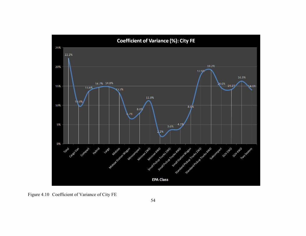
54

Figure 4.10 Coefficient of Variance of City FE

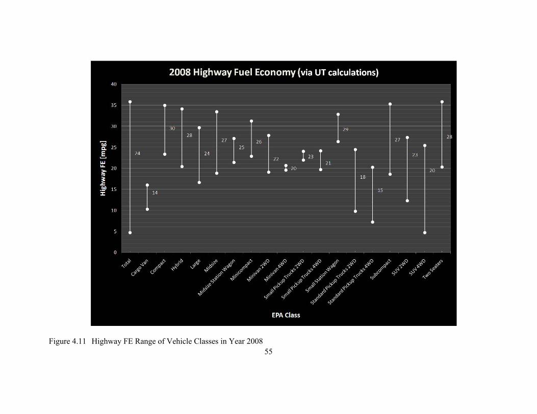
55

Figure 4.11 Highway FE Range of Vehicle Classes in Year 2008

56

Figure 4.12 Effects of Transmission on Highway FE on Vehicle Class (Part 1)

57

Figure 4.13 Effects of Transmission on Highway FE on Vehicle Class (Part 2)

58

Figure 4.14 Coefficient of Variance of Highway FE

59

Figure 4.15 Automatic Transmission City FE Comparison of Common Vehicles on the Road

60

Figure 4.16 Automatic Transmission City FE % Error of Common Vehicles on the Road

61

Figure 4.17 Manual Transmission City FE Comparison of Common Vehicles on the Road

62

Figure 4.18 Manual Transmission City FE % Error of Common Vehicles on the Road

63

Figure 4.19 Automatic Transmission Highway FE Comparison of Common Vehicles on the Road

64

Figure 4.20 Automatic Transmission Highway FE % Error of Common Vehicles on the Road

65

Figure 4.21 Manual Transmission Highway FE Comparison of Common Vehicles on the Road

66

Figure 4.22 Manual Transmission Highway FE % Error of Common Vehicles on the Road

67

Table 4-11 Overall Drivetrain Efficiency Summary of 2008 Model Year Vehicles

68

Table 4-11 summarizes the overall drivetrain efficiencies od e dt of the

vehicle classes of year 2008. 265 vehicles are included to calculate these generic

efficiencies. Initially it is stated that 19% generic overall drivetrain efficiency is decided

for compact and midsize vehicles’ city FE and 35% for highway FE. 18.8% in compact

class and 19.8% midsize vehicles for city FE is calculated which is in the range of 19%.

Similarly, 34.8% and 36.5% efficiencies are calculated for compact and midsize highway

FE’s respectively which is in the range of 35% generic overall drivetrain efficiency

selected.

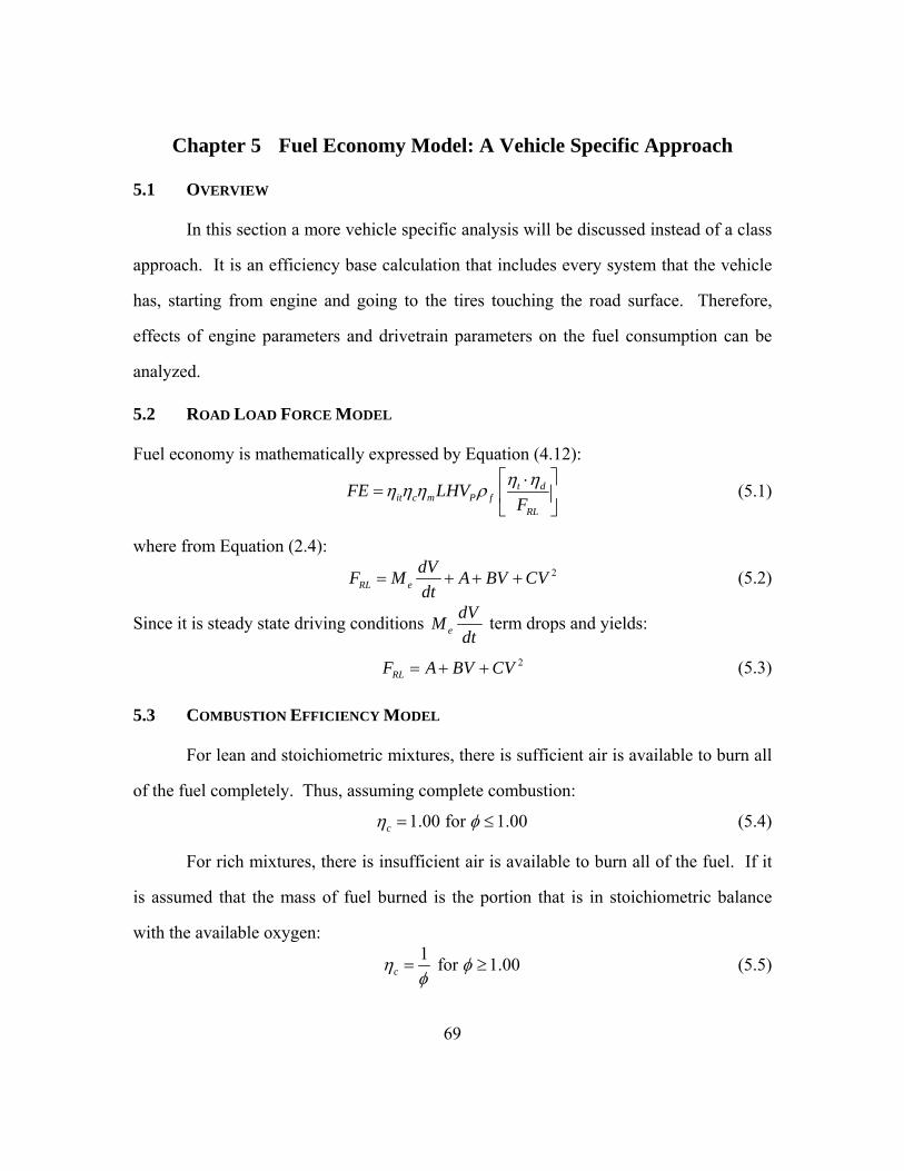
69

Chapter 5 Fuel Economy Model: A Vehicle Specific Approach

5.1 OVERVIEW

In this section a more vehicle specific analysis will be discussed instead of a class

approach. It is an efficiency base calculation that includes every system that the vehicle

has, starting from engine and going to the tires touching the road surface. Therefore,

effects of engine parameters and drivetrain parameters on the fuel consumption can be

analyzed.

5.2 ROAD LOAD FORCE MODEL

Fuel economy is mathematically expressed by Equation (4.12):

t dit c m P f

RL

FE LHVF

(5.1)

where from Equation (2.4):

2RL e

dVF M A BV CV

dt (5.2)

Since it is steady state driving conditions e

dVM

dt term drops and yields:

2RLF A BV CV (5.3)

5.3 COMBUSTION EFFICIENCY MODEL

For lean and stoichiometric mixtures, there is sufficient air is available to burn all

of the fuel completely. Thus, assuming complete combustion:

1.00 for 1.00c (5.4)

For rich mixtures, there is insufficient air is available to burn all of the fuel. If it

is assumed that the mass of fuel burned is the portion that is in stoichiometric balance

with the available oxygen:

1

for 1.00c

(5.5)

70

5.4 MECHANICAL EFFICIENCY MODEL

Mechanical efficiency m is zero when engine is idling and it increases linearly

up to 25% of load and becomes constant at 0.85.

0.25 0.85

0.850.25

0.25

m

m

LOAD

LOAD LOAD

(5.6)

where:

requiredbpLOAD

bp (5.7)

and, requiredbp is the brake power required at the tires and the bp is the brake power

supplied by the engine. It is known that engine rotational speed, N and the rotational

speed of drive wheels, dwN is not same. By using the transmission and differential gear

ratios one can write:

dwt d

NN

r r (5.8)

where tr is the gear ratio of the transmission and dr is the gear ratio of the differential.

Rotational speed of the wheels can be related with vehicle speed:

2dw tireV N R (5.9)

where tireR is the rolling radius of the tires.

2

2540tire

Section width Aspect ratioD inch Wheel diameter

(5.10)

By combining Equations (5.8) and (5.9):

2 tire t d

V N

R r r (5.11)

Rearrange:

2

t d t d

tire tire

Vr r Vr rN

R D (5.12)

71

Brake power that is available at the engine crankshaft can be calculated by

assuming a linear relationship between idle engine operating condition and wide open

throttle condition where maximum brake power of the engine is attained:

bp N slope constant (5.13)

where:

max idle

max idle

bp bp

bp bpslope

N N

(5.14)

and,

maxmax bpconstant bp slope N (5.15)

Idle brake power can be calculated by using Equation (3.48):

idleidle it v c m a s P

Nbp D FA LHV

x

(5.16)

Mechanical efficiency is assumed to be 0.85 in idle operation and only unknown

term is the multiplication of the indicated thermal efficiency and volumetric efficiency

and they assumed to be almost constant during operation of the engine and can be derived

from the wide open throttle position state:

max

maxit v

bpc m a s P

bpN

D FA LHVx

(5.17)

Therefore, brake power at any engine speed can be calculated at the Equation

(5.7) to calculate LOAD . Only portion left in that equation is the requiredbp . From

Equation (4.10) brake power can be written as:

RLrequired

t d

VFbp

(5.18)

Equation (5.18) completes the load calculation and therefore determination of the

mechanical efficiency.

72

It is well known that transmission efficiencies t for each gear ratio can be assumed to be

constant. An example of t for a four speed automatic transmission can be given as:

Table 5-1 Example Transmission Gear Efficiencies

Gear  t  

1  0.85 

2  0.87 

3  0.88 

4  0.90 

Differential efficiency d can be calculated by:

2

150

0.6652 0.003732 0.00001061

0.987

d

d

kmif V hr

V V

else

(5.19)

A speed changing strategy is needed for calculation of the engine speed and other

related parameters:

Table 5-2 Gear Shifting Strategy

Speed  Gear 

< 20  1 

< 40  2 

< 60  3 

≥ 60  4 

5.5 INDICATED THERMAL EFFICIENCY MODEL

The only parameter left is the indicated thermal efficiency it in the calculation of

fuel economy by Equation (5.1). it can be modeled in different ways starting from the

most basic method to the most advanced form it will be described in the following

paragraphs.

73

The well known Air Standard Otto cycle treats the combustion process as a heat

addition at constant volume and it can be expressed as:

1

11it k

cr (5.20)

where cr is the compression ratio and k is the ratio of the specific heats of the air. Since

Equation (5.20) overestimates the indicated thermal efficiency by factor of 2 it is

multiplied by 1 2 to get a better estimation.

1

1 11

2it kcr

(5.21)

Equation (5.21) models indicated thermal efficiency for maximum engine speed

but efficiency drops to around 40% of this maximum indicated thermal efficiency for idle

engine speed. Figure 5.1 shows a linear trend of indicated thermal efficiency changing

with engine speed. A better estimation can be a quadratic fit between maximum

indicated efficiency and 40% of that value. For a quadratic fit one needs another point

and that can be the 83% of the maximum indicated thermal efficiency at engine speed of

2idle maxN N

.

74

Figure 5.1 Effect of Engine Speed on Indicated Thermal Efficiency

5.5.1 Air Equivalent SI Engine Model

A better estimation for indicated thermal efficiency can be obtained via Air

Equivalent SI Engine Model (AESI). Homogenous charge 4-stroke SI engine is the most

commonly used engine in the world, and in fact this engine dominates the market by a

significant margin. Therefore analysis will focus on homogenous charge 4-stroke SI

engine exclusively.

75

Assumptions:12

1) Variable specific heat of air is assumed.

2) The intake and exhaust strokes are included in the cycle analysis.

3) It is assumed that exhaust stroke is reversible and isobaric.

4) It is assumed that no heat transfer occurs within the cylinder during the

intake and exhaust processes. It will be also assumed that the valves open

and close instantaneously at TDC and BDC and there are no pressure

losses associated with flow across the valves. Also it is assumed that there

is not any pressure losses associated with the flow through inlet manifold

and exhaust system.

5) The working fluid has the properties of air, but displacement of the air by

the fuel and residual gases is taken into account.

6) The compression, heat addition, expansion, and exhaust blowdown

processes are idealized.

Figure 5.2 shows a typical cross section of a SI engine cylinder. More

information will be given in the following paragraphs about SI strokes and the P v

diagrams of the AESI model.

12 R. D. Matthews, 2007

76

Figure 5.2 Cross Section Showing One Cylinder of a Four-stroke Internal Combustion Engine.13

Figure 5.3 shows the four-stroke of the SI engine schematically. Air and fuel

mixture enters the cylinder in the inlet stroke through the open inlet valves as the piston

travels downward and creating a sucking force. In the compression stroke inlet valve

closes and the piston travels upwards compressing the air fuel mixture and increasing its

temperature. By spark plug mixture of air and fuel is ignited and the mixture starts to

combust. The pressure increase forces the piston downwards providing power and this

stroke is called the power stroke. And finally, products of the combustion and any

13 Merriam-Webster

77

remaining unburned or partially burned fuel are pushed out of the open exhaust valves by

the moving piston upwards.

Starting position Intake Compression

Ignition Power Stroke Exhaust Stroke

Figure 5.3 Four-stoke Schematic View of SI Engine (Ignition, Power Stroke & Exhaust Stroke)14

14 http://en.wikipedia.org/wiki/Four_stroke

78

101

102

103

104

0 100 200 300 400 500 600

Pre

ssu

re [

kPa]

Volume [cm3]

1=5

2

3

4

6

TD

C

BD

C

WOT

101

102

103

104

0 100 200 300 400 500 600

Pre

ssu

re [

kP

a]

Volume [cm3]

5

2

3

4

6

TD

C

BD

C

IVO at TDCor

early IVO

16'

(a) (b)

101

102

103

104

0 100 200 300 400 500 600

Pre

ssu

re [

kPa]

Volume [cm3]

5

2

3

4

6

TD

C

BD

C

late IVO

16"

101

102

103

104

105

0 100 200 300 400 500 600

Pre

ssu

re [

kPa]

Volume [cm3]

5

2

3

4

6

TD

C

BD

C

supercharged

16"'

(c) (d)

Figure 5.4 Ideal P-V diagrams for the Air Equivalent SI Engine Model; a: WOT, b: early intake, c: late intake, d: supercharged.15

15 R. D. Matthews, Figure 4.8 (2007)

79

In AESI model sole working fluid is assumed to be air and that explains the “Air”

Equivalent SI Engine Model name. Figure 5.4 shows the P v diagrams of AESI for

different engine operating conditions.

Mathematical model will be described in details in the following paragraphs:

The intake process occurs between TDC and BDC and control volume is drawn

around the periphery of the combustion chamber for this uniform-state uniform-flow

process. First law of the thermodynamics can be applied as:

6 1Process :

6 6 6 6

6 1 1 1 1 1 6 1i i i i e e e e

m u ke pe

m h ke pe m h ke pe Q m u ke pe W

(5.22)

where state 6 is the exhaust residuals and state 1 is the state at the end of the intake

process therefore state 1 is the combination of trapped mass inside the cylinder and the

fresh air. In addition i refers the inlet and representing the charge entering the cylinder

and similarly e refers the exit and representing mass that exits from the cylinder however

in the intake process there is not any exiting mass therefore that term equals to zero.

Neglecting the kinetic and potential energy terms when compared to the thermal energy

terms their effect is insignificant and also assuming intake process is adiabatic one can

simplify Equation (5.22) as:

6 6 1 1 6 1i im u m h m u W (5.23)

Intake streams from multiple intake valves are combined into an equivalent single

intake stream. Work against a moving boundary can be calculated from:

2

1 2

1

W PdV (5.24)

Substituting Equation (5.24) back into Equation (5.23) yields:

1

6 6 1 1

6

i im u m h m u PdV (5.25)

80

Figure 5.5 Control volume for analysis of intake process.16

Conservation of mass principle can be applied over the control volume as shown

in Figure 5.5:

6 1im m m (5.26)

Exhaust gas residual fraction f can also be defined as:

6 6

1 6 i

m mf

m m m

(5.27)

A ratio between mass inducted and the total mass at the end of the intake process

can be described in terms of the exhaust gas residual fraction.

1 1

1

1

1

1

i

i

i

fm m m

m f m

mf

m

(5.28)

16 R. D. Matthews, Figure 4.9b (2007)

m6

expands into intake

at IVO but is drawn

back in along with

fresh charge

m1

is composed of residual

plus fresh charge

at BDC

TDC

BDC

State 6 to 1

81

Work term in Equation (5.25) is changing due to different operating conditions as

it is shown in Figure 5.4. The simplest case for the solution of the work done during the

intake stroke is the Wide Open Throttle (WOT) operation as can be seen from Figure 5.4

(a). The pressure from state 6 to state 1 is constant therefore integral term can be written

as:

1

6 1

6

1 1 6

1 1 1 6 6 6

W PdV

P V V

m Pv m P v

(5.29)

It should be noted that it is assumed there is not any pressure drop across valves

and it is also assumed that throttle butterfly is fully opened in WOT operation and there is

not any pressure drop associated with the throttle body. 1v is the specific volume of the

mixture at the end of the intake stroke and 6v is the specific volume of the mixture at the

end of the exhaust stroke.

For WOT operation one can insert Equation (5.29) back into Equation (5.25):

1 6

6 6 1 1 1 1 1 6 6 6

1 1 1 1 6 6 6 6

i i

i i

h h

m u m h m u m Pv m P v

m h m u Pv m u P v

(5.30)

1 1 6 6i im h m h m h (5.31)

Mass terms in Equation (5.31) can be represented in terms of exhaust gas residual

fraction f by using Equations (5.27) and (5.28):

1 1 1 1 6

1

1

1

if m h m h fm h

f m

1ih m

1 6

1 61 i

h fh

f h h fh

(5.32)

82

Rearranging and solving for the enthalpy of the mixture at the beginning of the

compression stroke yields:

1 61 ih f h fh (5.33)

Engine is not working all the time at WOT operating condition instead it works

dominantly on part throttle operation. The pressure in the intake manifold is less than the

pressure in the exhaust manifold because of the pressure drop across the throttle plate in

part throttle operation. As it is shown in Figure 5.5 part of the exhaust gasses expand into

the intake manifold but it is then sucked back into the cylinder due to pressure difference

as can be seen from Figure 5.4 (b). For early intake valve opening (IVO) operation

which is the usual case, a similar analysis for the work term can be:

6 1 6 6 6 1

6 1

6 6

1 1 6

1 1 1 6 1 6

0

W W W

PdV PdV

P V V

m Pv m Pv

(5.34)

For early IVO operation one can insert Equation (5.34) back into Equation (5.25):

1

6 6 1 1 1 1 1 6 1 6

6 6 1 6 1 1 1 1

6 6 1 6 1 1

i i

i i

h

i i

m u m h m u m Pv m Pv

m u Pv m h m u Pv

m u Pv m h m h

(5.35)

Mass terms in Equation (5.35) can be represented in terms of exhaust gas residual

fraction f by using Equations (5.27) and (5.28):

83

1f m 6 1 6 11u Pv f m 1ih m

1

6 1 6 1

1 6 1 6

1

1

i

i

h

f u Pv f h h

h f h f u Pv

(5.36)

Although late IVO and supercharged operations are not included in the study, for

completeness their enthalpy of the mixture at the beginning of the compression can be

expressed as follows for late IVO and supercharged operation respectively:

1 61 ih f h fh (5.37)

1 61 ih f h fh (5.38)

Equations (5.33), (5.36), (5.37), and (5.38) are all form of the first law of the

thermodynamics and requires the information about the enthalpy of the fresh air charge

ih . This term is expressed in Matthews, 2007 as follows17:

,, , ,

1

1 1 1 1

S a

a TP ai a IV e a f v f

Qh m FA

h h x hFA FA FA FA

(5.39)

where ,a IVh is the specific enthalpy of air entering the combustion chamber, FA is the

fuel air ratio, ,a TPh is the specific enthalpy of the air crossing the throttle plate, S aQ is the

rate of heat transfer from intake surfaces to air, am is the mass flow rate of air into the

engine, ,e a fx is the mass fraction of fuel evaporated due to heat transfer from only the

air, and ,v fh is the specific enthalpy of vaporization of the fuel at 298K .

The analysis above allows all of the states of the P v diagrams to be

determined. Therefore one can now define indicated thermal efficiency for the AESI

model. Thermodynamically indicated thermal efficiency it is defined as:

,

netit

a th

w

q (5.40)

17 R.D. Matthews, Equation 4.66c, 2007

84

where the net work per unit mass of air is found by summing the work terms around the

cycle:

1 2 2 3 3 4 4 5net pw w w w w w (5.41)

where pw is the pumping work per unit mass which is basically the net work required to

pump the working fluid into and out of the combustion chamber. Combustion and heat

extraction processes considered to be a constant volume processes as can be seen from

Figure 5.4, therefore; 2 3 4 5 and w w are both equal to zero.

The total pumping work pW is the area enclosed between States 5,6, and 1,

including the appropriate intermediate states 6 , 6 , or 6 . For the usual case of early

IVO specific pumping work can be mathematically expressed as:

5 6 6 6 6 1

6 2 1 1 1 2

1 6 1 2

0

pW W W W

P V V P V V

P P V V

(5.42)

By dividing the Equation (5.42) by the compressed mass 1m , one can get:

1 6 1 21

pp

Ww P P v v

m (5.43)

Remaining work terms in Equation (5.41) 1 2 3 4and w w can be determined from

the first law of the thermodynamics, thus following expression can be obtained for the

early IVO by inserting Equation (5.43) into Equation (5.41):

1 2 3 4 1 6 1 2netw u u u u P P v v (5.44)

For WOT operation 1 6 1 2P P v v term in Equation (5.44) drops since there is

not any pumping work is necessary in WOT operation.

85

Thermal energy per unit mass of trapped mixture can be obtained by the

following equation. A detailed analysis is available at Matthews, 200718.

, 11a th c P

FAq f LHV

FA

(5.45)

5.5.2 AESI Indicated Thermal Efficiency Solution Procedure

In this section an iterative algorithm will be presented to find an indicated thermal

efficiency for an operating condition of the SI engine.

1) Combustion efficiency can be determined by Section 5.3.

2) Two intensive properties needed to fix State 1 however, only pressure is known.

Therefore, make a guess for residual fraction f and the temperature of the

mixture trapped at the beginning of the compression stroke 1T .

3) Pressure of the State 1 is assumed to be equal to atmospheric pressure for WOT

operation since it is assumed that there are no flow losses at throttle and inlet

manifold. And for early IVO pressure can be modeled by means of the LOAD

since the throttle plate opening angle can be related with LOAD , when throttle

plate is fully closed it is assumed that the 1 33P kPa .

1

1

(WOT)

33 33 (early IVO)ex

ex

P P

P P LOAD

(5.46)

4) Specific volume of the State 1 can be found via ideal gas law for air:

11

1

aR Tv

P (5.47)

5) Since the compression process from State 1 to State 2 is isentropic and the only

working fluid is air thus relative specific volume rv relationship can be used.

18 R. D. Matthews, Equation 4.83d, 2007

86

,1 1

,2 2

rc

r

v vr

v v (5.48)

where, cr is the compression ratio. ,1rv can be found by using the air

thermodynamics table by assuming air as an ideal gas. A MATLAB code is

supplied in Appendix C.4 which is used to calculate air properties in the model.

,1,2

rr

c

vv

r (5.49)

By using Equation (5.49) one can calculate the relative specific volume of the

State 2, ,2rv , and thus the other state properties 2 2and T u can be read from the

thermodynamics table of ideal gas air.

6) It is known that from Figure 5.4 the volume is constant during combustion

process of 2-3. Thus,

3 2v v (5.50)

where:

12

c

vv

r (5.51)

1st Law of Thermodynamics:

2 , 3 2 3a thu q u w (5.52)

Work term is zero since the volume does not change. And heat addition term is

expressed by Equation (5.45). Therefore 3u can be calculated by Equation (5.52)

and this enables to find properties of the State 3, 3

03 ,3, , and r TT v s , through the

thermodynamics table of ideal gas air.

33

3

amax

R TP P

v (5.53)

7) Process 3-4 is isentropic expansion and relative specific volume of the State 4 can

be found by:

,4 ,3r r cv v r (5.54)

87

Therefore, temperature at the end of the expansion process, 4 EVOT T , can be read

from air tables.

8) It will be assumed that working fluid that remains inside the combustion chamber

after the combustion process, State 4, expands isentropically to the exhaust

manifold pressure during the exhaust blowdown, which is assumed to occur at

constant volume at BDC as it is shown in Figure 5.6.

101

102

103

104

0 200 400 600 800 1000

Pre

ssu

re [

kPa]

Volume [cm3]

5

2

3

4

6

TD

C

BD

C

16'

4'

Figure 5.6 Ideal P V diagram for analysis of the exhaust process, including State 4.19

Dashed lines from 4 to 4 to 5 indicate “imaginary” parts of the cycle. Dot-dash

lines indicate open portions of the cycle (mass loss or gain). State 4 represents

19 R. D. Matthews, Figure 4.10, 2007

88

the state of the working fluid that remains within the combustion chamber during

the exhaust blowdown process. As it can be seen from the Figure 5.6, pressure at

State 4 equals to pressure at State 5 and pressure at State 6 which is the exhaust

manifold pressure and assumed to be equal to atmospheric pressure.

4 5 6 extP P P P (5.55)

Since the process 3 4 is isentropic one can write following equation for change

of specific entropies of the ideal gases:

4 3

0 0 44 3

3

0 lnT T a

Ps s s s R

P

(5.56)

Rearrange to get:

4 3

0 0 4

3

lnT T a

Ps s R

P

(5.57)

4T can be found by using the thermodynamic tables since 4

0Ts

is known. It is also

known that there is not any heat transfer occurs between States 4 , 5, and 6. And

also during the exhaust stroke, the working fluid in State 4 undergoes an

isentropic process. If one writes Equation (5.56) between these states the pressure

term will be zero since all pressure terms are zero as stated in Equation (5.55).

Thus, standard state entropies for these states will be equal to each other, which

imply all thermodynamic properties of these states will be identical.

4 5 6

4 5 6

T T T

h h h

(5.58)

Specific volume of the State 4 can be calculated by:

44

4

aR Tv

P

(5.59)

Since temperatures and pressures in States 4 , 5, and 6 are same their specific

volumes should also be same:

89

4 5 6v v v (5.60)

9) Initial guesses of exhaust gas residual fraction f and temperature before

compression 1T needs to be checked to continue analysis.

It is known from Equation (5.27) that:

6

1

mf

m (5.61)

Exhaust gas residual fraction can be calculated with known properties of the

States 2 and 4 :

6 2 2 2

6 6 4 1 2 2

1 1 1 4 4 4new

V V V Vm v v m m v

fm m m v v v

(5.62)

New residual fraction should be in the 0.5% of the assumed residual fraction:

0.995 1.005newf f f (5.63)

Equations (5.33) and (5.36) can be used to calculate specific enthalpy of the

trapped mixture at the beginning of the compression process 1h for WOT and

early IVO operations respectively.

1 6

1 6 1 6

1 (NA @ WOT)

1 (early IVO)

i

i

h f h fh

h f h f u Pv

(5.64)

Enthalpy of fresh charge ih can be calculated from Equation (5.39).

@298

,, , ,

0.15 303.60

1

1 1 1 1

KS a

a TP ai a IV e a f v f

kJkg

Qh m FA

h h x hFA FA FA FA

(5.65)

Specific enthalpy of the air is calculated at 298K and it is assumed there is not a

heat transfer from intake surfaces to air. Moreover evaporation rate for the

gasoline is typically 15% and for a generic gasoline heat of vaporization ,v fh is

303.6kJkg .

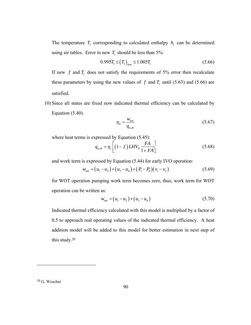
90

The temperature 1T corresponding to calculated enthalpy 1h can be determined

using air tables. Error in new 1T should be less than 5%:

1 1 10.995 1.005new

T T T (5.66)

If new 1 and f T does not satisfy the requirements of 5% error then recalculate

these parameters by using the new values of 1and f T until (5.63) and (5.66) are

satisfied.

10) Since all states are fixed now indicated thermal efficiency can be calculated by

Equation (5.40).

,

netit

a th

w

q (5.67)

where heat terms is expressed by Equation (5.45):

, 11a th c P

FAq f LHV

FA

(5.68)

and work term is expressed by Equation (5.44) for early IVO operation:

1 2 3 4 1 6 1 2netw u u u u P P v v (5.69)

for WOT operation pumping work term becomes zero, thus; work term for WOT

operation can be written as:

1 2 3 4netw u u u u (5.70)

Indicated thermal efficiency calculated with this model is multiplied by a factor of

0.5 to approach real operating values of the indicated thermal efficiency. A heat

addition model will be added to this model for better estimation in next step of

this study.20

20 G. Woschni

91

5.5.3 Fuel Economy Model Graphical User Interface

The physical model explained in this chapter is coded with MATLAB for broader

engine operating conditions and faster computation purposes. Thus, MATLAB codes are

wrapped with a C# Graphical User Interface (GUI) on the .NET platform of Windows to

deliver the computational capability to users who does not have MATLAB installed on

their computers with full power of the MATLAB.

Following figure shows the welcome screen of the Fuel Economy Model GUI.

Program expects user to enter some engine design parameters, tires specifications in

addition to drivetrain gear ratios.

92

Figure 5.7 Welcome screen of the Fuel Economy Model

Figure 5.8 shows the default values entered by pressing the “Load Defaults”

button for the Ford F-150 full size 4WD pickup.

93

Figure 5.8 Default values of Ford F150 are loaded to Fuel Economy Model

Figure 5.9 shows the Fuel Economy versus Speed graph for the default values of

the Fuel Economy Model. It is a MATLAB figure screen and having full power of the

MATLAB inside which makes this software very different. First Excel spreadsheet

model of the Fuel Economy Model is shown in Figure 5.10 also. MATLAB and C#

codes can be found in Appendix C: Codes of Vehicle Specific Fuel Economy Model.

94

Figure 5.9 Result screen of the Fuel Economy Model

95

Figure 5.10 Excel Spreadsheet of the Fuel Economy Model

96

A setup file also created for easy distribution of the software. Following figure

shows the welcome screen of the Fuel Economy Model GUI.

Figure 5.11 Welcome screen of the Fuel Economy Model installation.

97

Figure 5.12 Information screen about the software and the developers

Figure 5.12 shows the information screen of the Fuel Economy Model, version

number of the model and institution info who holds the copyright is given in addition to

names of the engineers who developed the software.

GNU General Public License is used for free distribution of the software as

shown in Figure 5.13.

98

Figure 5.13 GNU License Agreement screen of the Fuel Economy Model

99

Chapter 6 SAE Coastdown Practice21

6.1 OVERVIEW

This procedure is adopted from SAE Recommended Practice J1263. Definitions,

procedures regarding coastdown tests will be explained in this chapter.

6.2 TECHNICAL BACKGROUND

Physical equations governing coastdown tests are explained in Chapter 2 and

detailed analysis is given in Chapter 7.

6.3 ROAD LOAD MEASUREMENT USING COASTDOWN TECHNIQUES

6.3.1 Scope

This procedure covers measurement of vehicle road load on a straight, level road

at speeds less than 70 mph.

6.3.2 Purpose

The purpose is to provide a uniform testing procedure for measuring the road load

force and determining coastdown coefficients , , and A B C on a vehicle through vehicle

speed versus time data.

6.4 DEFINITIONS

6.4.1 Test Weight

Test weight is the weight of the vehicle as tested; including driver, operator (if

necessary), and all instrumentation.

21 SAE J1263

100

6.4.2 Test Mass

Test mass is the mass of the vehicle as tested; including driver, operator (if

necessary), and all instrumentation.

6.4.3 Effective Mass

Effective mass is equal to the sum of the test mass and the effective inertias of the

driven and non-driven axles.

6.4.4 Frontal Area

Frontal area is the area of the orthogonal projection of the vehicle including tires

and suspension components onto a plane perpendicular to the longitudinal axis of the

vehicle.

6.5 VEHICLE ROAD LOAD MEASUREMENT

6.5.1 Instrumentation

All instrumentation must be calibrated for each vehicle.

6.5.2 Time and Speed

An instrument to measure vehicle speed as a function of elapsed time is used in

this procedure. The device must meet the following specifications:

a) Time:

i. Accuracy 0.1% of total coastdown time interval

ii. Resolution 0.1 s

b) Speed:

i. Accuracy 0.25 mph

ii. Resolution 0.1 mph

101

6.5.3 Temperature

The temperature indicating devices must have a resolution of 02 F and an

accuracy of 02 F . The sensing element must be shielded from radiant heat sources.

6.5.4 Atmospheric Pressure

A barometer with an accuracy of 0.7 kPa or 0.2 in Hg is necessary.

6.5.5 Wind

Wind speed and direction during the test should be continuously monitored.

Wind measurements should permit the determination of average longitudinal and

crosswind components within 1 mph .

6.5.6 Vehicle Weight

Vehicle weight should be measured to an accuracy of 10 lb per axle.

6.5.7 Tire Pressure

Tire pressure should be measured to an accuracy of 0.5 psi .

6.6 TEST CONDITIONS

6.6.1 Ambient Temperature

Tests may be conducted at ambient temperatures between 030 F and 090 F .

The recommended temperature range is from 041 F to 090 F . Data obtained at

temperatures outside this range cannot be reliably adjusted to standard conditions by

Section 7.4.

6.6.2 Winds

Tests may not be conducted when wind speeds average more than 10 mph (or

when peak wind speeds are more than 12.3 mph ). The average of the component of the

wind velocity perpendicular to the test road may not exceed 5 mph .

102

6.6.3 Road Conditions

Roads must be dry, clean, smooth, and must not exceed 0.5% grade. In addition,

the grade should be constant and the road should be straight since variations in grade or

straightness can significantly affect results. The road surface should be concrete or rolled

asphalt (or equivalent) in good condition since rough roads can significantly affect rolling

resistance. In addition, tests may not be run during foggy or rainy conditions: roads must

be dry.

6.7 VEHICLE PREPARATION

6.7.1 Break-In

The test vehicle should have accumulated a minimum of 300 miles prior to

testing. The tires should have accumulated a minimum of 100 miles and should have at

least 75% of the original tread depth remaining.

6.7.2 Vehicle Check-In

The following items should be compared to manufacturer’s recommendation and

recorded on the Appendix D: Vehicle Road Test D prior to test:

a) Tire type, size, and cold inflation pressure (see Section 6.7.4)

b) Wheel size, conditions, and presence of wheel covers

c) Brake adjustment

d) Lubricants in the drivetrain and in the non-driving wheel bearings

e) Vehicle suspension heights

6.7.3 Instrumentation

The speed-time measuring device and other necessary equipment must be

installed so that they do not hinder vehicle operation or alter the operating characteristics

of the vehicle.

103

6.7.4 Tire Pressure

Inflate the tires of the test vehicle to the manufacturer’s recommended cold

inflation pressure, corrected for the temperature difference (if any) between the vehicle

tires and the test area. The tire pressure should be increased 1 psi for each 013 F that

the vehicle preparation area temperature the test is above the test temperature. Record

the actual inflation pressure and preparation area temperature on the Appendix D:

Vehicle Road Test D.

6.7.5 Vehicle Frontal Area

The vehicle frontal area must be known, measured, or estimated and the value

recorded on the Appendix D: Vehicle Road Test D. The frontal area will be estimated by

taking a front picture of the vehicle with a reference area in that picture. Frontal area

than will be calculated through pixel comparison with known area.

6.7.6 Vehicle Warm-Up

The vehicle must be driven a minimum of 30 min at an average speed of 50 mph

immediately prior to the test.

6.8 COASTDOWN TEST

6.8.1 Alternating Directions

A minimum of 10 runs are made in alternating directions. The runs must be

paired for the data reduction process in order to reduce error.

6.8.2 Procedure

The vehicle windows must be closed. At the start of each run, accelerate the

vehicle to 65 mph , start the recording equipment, and shift into neutral and let the engine

104

idle. The vehicle clutch must be engaged. When the vehicle stops, stop the recording

equipment, engage the transmission, and prepare for the next run.

6.8.3 Lane Changes

While coasting, lane changes should be avoided if at all possible. If necessary,

they should be done as slowly as possible and over a distance of at least a quarter mile. If

such a gradual change cannot be made, abort the run.

6.8.4 Data to be Recorded

Record the direction and number of each run (including aborted runs) in such a

way that the speed time data can be separated by run number. Record the ambient

temperature and atmospheric pressure after warm-up and after the test. Average the two

values to determine the value to be used in the data reduction.

The total wind and either the wind direction or the crosswind component of the

total wind must be recorded. The wind quantities should be recorded, screened for gusts

exceeding the ambient conditions limit in Section 6.6.2, and averaged. Record the results

on the Appendix D: Vehicle Road Test D.

6.8.5 Vehicle Test Weight

After the coastdown run, weight the vehicle to determine the vehicle test weight

or mass. Include the weight of the spare wheel, driver, and all instrumentation used.

Record the weight on the Appendix D: Vehicle Road Test D.

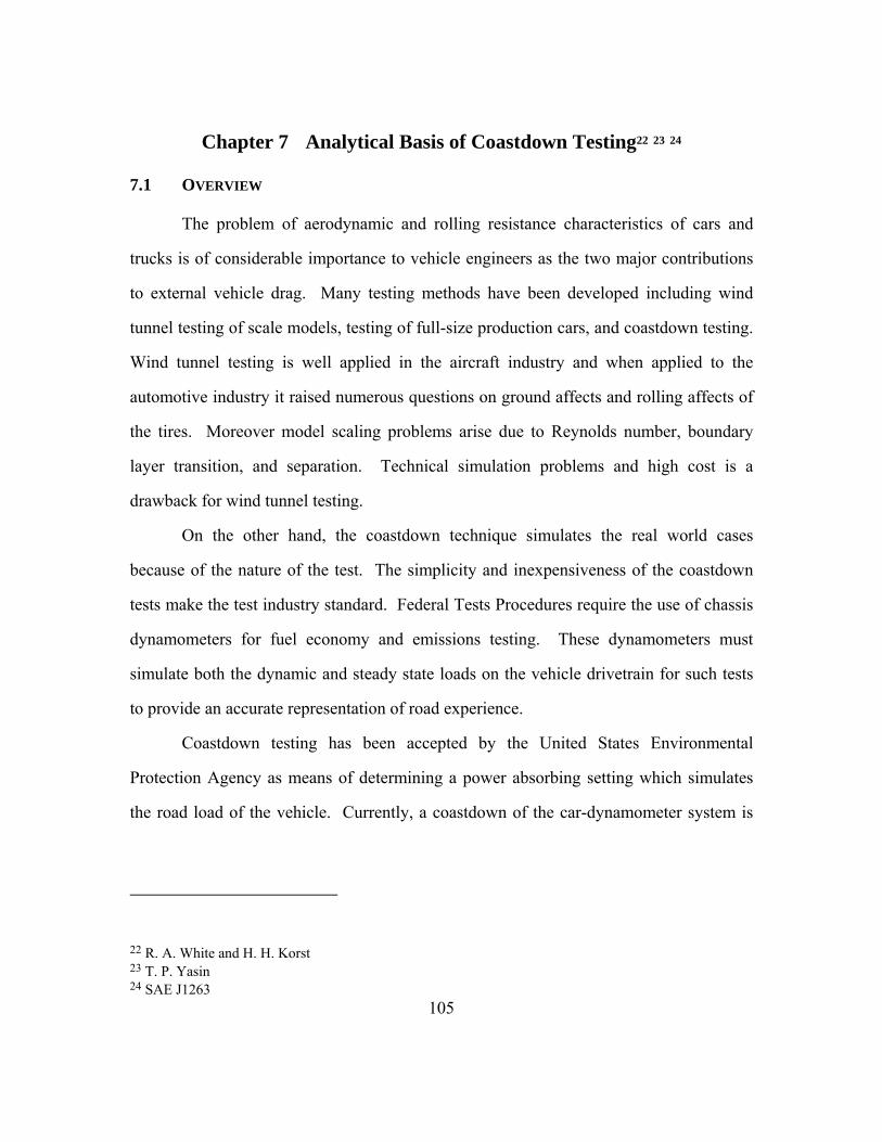
105

Chapter 7 Analytical Basis of Coastdown Testing22 23 24

7.1 OVERVIEW

The problem of aerodynamic and rolling resistance characteristics of cars and

trucks is of considerable importance to vehicle engineers as the two major contributions

to external vehicle drag. Many testing methods have been developed including wind

tunnel testing of scale models, testing of full-size production cars, and coastdown testing.

Wind tunnel testing is well applied in the aircraft industry and when applied to the

automotive industry it raised numerous questions on ground affects and rolling affects of

the tires. Moreover model scaling problems arise due to Reynolds number, boundary

layer transition, and separation. Technical simulation problems and high cost is a

drawback for wind tunnel testing.

On the other hand, the coastdown technique simulates the real world cases

because of the nature of the test. The simplicity and inexpensiveness of the coastdown

tests make the test industry standard. Federal Tests Procedures require the use of chassis

dynamometers for fuel economy and emissions testing. These dynamometers must

simulate both the dynamic and steady state loads on the vehicle drivetrain for such tests

to provide an accurate representation of road experience.

Coastdown testing has been accepted by the United States Environmental

Protection Agency as means of determining a power absorbing setting which simulates

the road load of the vehicle. Currently, a coastdown of the car-dynamometer system is

22 R. A. White and H. H. Korst 23 T. P. Yasin 24 SAE J1263

106

used to match the load on the drive line at fifty miles per hour to that determined from the

road tests.

7.2 ANALYSIS

Typical coastdown test data can be presented in the form of velocity versus time

curves similar to Figure 7.1.

Figure 7.1 Velocity vs. Time of Typical Coastdown Test25

25 R. A. White and H. H. Korst

107

The following analysis is intended to define the form of the major forces acting on

a vehicle as a function of speed. It is assumed that:

Road grade is zero

Wind speed is less than vehicle speed

Wind speed is steady

There is not any major gust

Aerodynamic yaw angles remain small

In Chapter 2 forces resisting the vehicle’s movement described and formulated

with Equation (2.1). Road grade is assumed to be zero, therefore 0GF and Equation

(2.1) can be written as sum of aerodynamic and tire and chassis drag forces:

RL D RF F F (7.1)

Resistive force is identified as road load force due to absence of wind and grade

as it is explained in Section 2.4.

Ambient conditions affect these force components differently, so that each must

be analyzed separately.

7.2.1 Aerodynamic Forces

Three mutually perpendicular forces: drag, lift, and side act on the vehicle. The

forces take the form:

XX C Aq (7.2)

where: : is any one of the three aerodynamic forces

: is the coefficient of the force X

: is the reference (frontal) area

: is the dynamic pressure of the airstream

X

X

C

A

q

108

By definition,

2

2av

q

(7.3)

where: : is air density and

: is the total relative airspeedav

Ideal gas law can be written as:

P RT (7.4)

where: : is gas constant and

: is absolute temperature

R

T

Air density varies with absolute temperature and barometric pressure by:

0

0 0

TP

P T

(7.5)

where 0 0 0, , and P T are respectively density, pressure, and absolute temperature

of a reference condition. The total effect of humidity on air density is less than 1% at

normal test temperatures and can be neglected.

In the presence of a wind of speed v , having components and x ySv v parallel and

perpendicular to the vehicle’s path respectively and S is 1 depending on vehicle

coastdown direction; av will be related to vehicle ground speed V as shown in Figure 7.2

by:

2 2a x yv V Sv v (7.6)

Thus, Equation (7.3) becomes:

2 2

2

x yV Sv vq

(7.7)

109

Figure 7.2 Total airspeed is the vector sum of car speed and wind speed, both relative to ground

The drag coefficient DC is the sum of the drag coefficient at zero yaw DC and

a coefficient k times the square of the sine of the yaw angle, for a typical passenger

car.

2sinD DC C k (7.8)

where:

2 2

sin y

x y

v

V Sv v

(7.9)

Therefore Equation (7.8) becomes:

2

2 2

yD D

x y

vC C k

V Sv v

(7.10)

Aerodynamic drag force can be written by inserting Equations (7.7) and (7.10)

into Equation (7.2).

2 22

2 2 2

X

x yyD D

x y

C q

V Sv vvF C k A

V Sv v

(7.11)

Equation (7.11) can be simplified as it is shown below:

110

2 22 22

2 22 2

x y x yyD D

x y

V Sv v V Sv vvF C A k A

V Sv v

(7.12)

2 2

2

2 2

2

x y

D D

y

x y

V Sv vF C A

vk

V Sv v

2 2x yV Sv v

A

2

(7.13)

2 2

2

2 2

x y

D D y

V Sv vF C A kv A

(7.14)

2 2 21 1

2 2D D x y yF C A V Sv v kAv (7.15)

Further simplification can be done to Equation (7.15) by factoring and

unwrapping the first square term on the right hand side.

2 2

22

2

1 1

2 2x x

D D y D x

V VSv v

F C k Av C A V Sv

(7.16)

The term linear in V is ignored. The error introduced by ignoring this term (and

the road grade) is minimized by the averaging process subsequently applied because

these terms change sign for each change in coastdown direction.

Collecting terms, Equation (7.16) can be rewritten as:

2 2 21 1

2 2D D x D yF C A V v C k Av (7.17)

A similar analysis can be applied to formulate lift and side forces, however the

change in altitude is small and road that coastdown test is held is straight, and the effect

of lift and side forces will be neglected.

111

7.2.2 Tire and Chassis Drag

A detailed analysis of all the forces, torques, and inertias on a vehicle chassis is

beyond the scope of this study. However, the total force can be expected to vary as a

function of air temperature, road temperature, ground speed, normal load, and lateral

load.

In the absence of slip angles, tire rolling resistance, RF can be expected to

increase with speed. Although this increase is often considered to be linear at normal

speeds, a second degree function will fit well in the speed range of a coastdown test, as

seen in Figure 7.3.

112

Figure 7.3 Tire rolling resistance increases linearly with the square of speed.26

Tire rolling resistance is defined as coefficient of rolling resistance, , times

vehicle test weight W .

RF W (7.18)

where:

20 1 V (7.19)

Equation (7.19) describes the relationship, with 0 designating the extrapolation

of rolling resistance to zero speed, and describing the rate of change of rolling

26 T. P. Yasin

113

resistance with the square of vehicle ground speed. In other words, 0 is the velocity

independent coefficient of rolling resistance and is the velocity coefficient of rolling

resistance.

Hence, tire rolling resistance can be written in the absence of aerodynamic lift

forces and lateral force effects as:

20 1RF V W (7.20)

7.2.3 Mathematical Solution to Road Load Force

Road load force can be formulated by inserting Equations (7.17) and (7.20) into

Equation (7.1):

2 2 2 20

1 11

2 2 RL D x D yF C A V v C k Av V W (7.21)

Road load force can be expressed as rate of change of vehicle speed times

effective mass of the vehicle:

RL e

dVF M

dt (7.22)

Therefore:

2 2 2 20

1 11

2 2 e D x D y

dVM C A V v C k Av V W

dt (7.23)

Collecting terms, Equation (7.23) can be rewritten as:

20 2e

dVM f f V

dt (7.24)

where:

2 20 0 2 0

1

2x DY yf W f W v C Av (7.25)

2 0

1

2 Df W C A (7.26)

The crosswind aerodynamic drag coefficient DYC is a measure of the response of

the vehicle to the crosswind component of the wind at small yaw angles. It may be

calculated by:

114

DY DC C k (7.27)

Equation (7.24) will be resembled to following integral to apply its solution to road load

force equation:

1

2

tanbx

adx

a bx a b

(7.28)

where Equation (7.24) can be written as:

20 2

e e

a b

dVdt

f fV

M M

(7.29)

Integrating both sides will give the right hand solution of the Equation (7.28). Similarly,

one can write:

2

1

0

0 2

tan e

e

e e

fV

M

fM

t constantf f

M M

(7.30)

Effective mass terms at nominator can be cancelled and denominator effective mass term

can be factored out as follows:

2

1tane

f

M

0

e

V

f

M

0 2

e

t constantf f

M

(7.31)

One can get the following expression to apply boundary conditions and determine

constant .

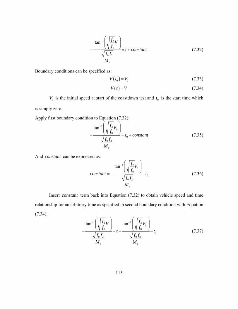
115

1 2

0

0 2

tan

e

fV

ft constant

f f

M

(7.32)

Boundary conditions can be specified as:

0 0V t V (7.33)

V t V (7.34)

0V is the initial speed at start of the coastdown test and 0t is the start time which

is simply zero.

Apply first boundary condition to Equation (7.32):

1 20

00

0 2

tan

e

fV

ft constant

f f

M

(7.35)

And constant can be expressed as:

1 20

00

0 2

tan

e

fV

fconstant t

f f

M

(7.36)

Insert constant term back into Equation (7.32) to obtain vehicle speed and time

relationship for an arbitrary time as specified in second boundary condition with Equation

(7.34).

1 12 20

0 00

0 2 0 2

tan tan

e e

f fV V

f ft t

f f f f

M M

(7.37)

116

Arrange terms to get:

1 12 20

0 00

0 2 0 2

tan tan

e e

f fV V

f ft t

f f f f

M M

(7.38)

By factoring terms, one gets:

1 12 20 0

0 00 2

tan taneM f ft t V V

f ff f

(7.39)

This is the equation which, after correction of the coefficients determined by the

White and Korst technique or equivalent, is used to calculate the coastdown time interval.

The units for 0 2 0, , , , and eM f f V V must be chosen so that the argument of the inverse

tangent function is dimensionless and the resultant coastdown time is in seconds. The

individual terms and their corrections are described in the 7.4 Data Correction.

After this point, one can nondimensionalize Equation (7.39) and follow White and

Korst technique or keep the equation with these parameters and write it as speed as a

function of time instead of time as a function of speed as it is in Equation (7.39).

Result wise there is not any difference between nondimensionalizing and keeping

dimensional parameters. Only difference comes when writing program codes for the

solution. Nondimensionalize solution requires changing input from vehicle speed versus

time to nondimensionalized vehicle speed and time. On the other hand in dimensional

approach, vehicle speed versus time data is supplied as they are obtained from coastdown

tests. For simplicity parametric approach is followed in this study and following steps

taken to get vehicle speed as a function of time from Equation (7.39).

0 2 1 12 20 0

0 0

tan tane

f f f ft t V V

M f f

(7.40)

117

0 21 12 20 0

0 0

tan tane

f ff fV V t t

f f M

(7.41)

Take tangents of both sides:

0 212 20 0

0 0

tan tane

f ff fV V t t

f f M

(7.42)

0 210 20 0

2 0

tan tane

f ff fV V t t

f f M

(7.43)

Applying the method of least squares to Equation (7.43) for determining optimal

values of 0f and 2f requires that

2

0 20

, , 0i iV V f f tf

(7.44)

2

0 22

, , 0i iV V f f tf

(7.45)

Mathematical solution to these equalities is carried out via MATLAB and written

code is represented at Appendix E: Coastdown Coefficient Calculation MATLAB Code.

7.2.4 Effective Vehicle Mass

The effective vehicle mass eM is the sum of the final vehicle test mass

WM g and the effective mass of the rotating components. The effective mass of the

drivetrain components other than the wheels, tires, and brakes may be ignored. For each

tire, wheel, and brake rotor or drum, the effective mass, em is:

2e

Im

r (7.46)

where:

r is the rolling radius of the tire and I is the polar moment of inertia of the

assembly. The polar moment of inertia may be measured or may be estimated

circular disk expression:

118

2

2wW r

Ig

(7.47)

where:

wW is the weight of the tire, wheel, and brake rotor or drum. If no measurements

are available, the effective inertia of all the rotating components may be estimated

3.0% of the vehicle test mass.

1.03 1.03e

WM M

g (7.48)

Or, one can insert Equation (7.47) to Equation (7.46) and obtain:

2w

e

W rg

m 2

2

r (7.49)

2

we

Wm

g (7.50)

Therefore one can find effective vehicle mass, eM by adding effective masses of tire,

wheel, and brake rotor or drum, em to vehicle mass M .

e eM M m (7.51)

By inserting Equation (7.50) following effective vehicle mass is obtained to use in

Equation (7.43) while solving for 0f , and 2f .

2

we

WM M

g (7.52)

7.3 DATA ACCEPTABILITY CRITERIA

Experience has shown that the criteria of this section are necessary and sufficient

to provide accurate and precise test results. Data which exceed these criteria generally

arise from wind gusts or driver inputs, which violate the assumption that the forces on

vehicle are depicted by the following equation:

20 2e

dVM f f V

dt (7.53)

119

7.3.1 Criteria 1

a) Analyze each individual coastdown V t in the set of paired runs by White &

Korst method to obtain the coefficients 0f and 2f .

b) Compare each individual V t trace and its analytical counterpart 0 2, ,V f f t by

using:

1 12 20 0

0 00 2

tan taneM f ft t V V

f ff f

(7.54)

If the root mean square deviation (RMSD) exceeds 0.25 mph on any

individual run, discard that run and the paired run in the opposite

direction.

If less than three pairs comply with this criterion, the test run is invalid.

7.3.2 Criteria 2

Of the paired runs meeting the first criteria, those which fail to satisfy the

following criteria regarding 0f and 2f must also be discarded.

a) The standard deviation of the 0f ’s must be less than 2.5 lb or 5% of the

mean. If this value is exceeded, discard the run and its pair with 0f

farthest from mean and recompute the standard deviation until compliance

is obtained or until the remaining pairs number less than three.

b) The standard deviation of the 2f ’s must be less than 20.001 lb mph or

3% of the mean. If this value is exceeded, discard the run and its pair with

2f farthest from the mean and recompute the standard deviation until

compliance is obtained or until the remaining pairs number less than three.

7.3.3 Result

If less than three pairs remain, the test run is invalid.

Average 0f ’s and 2f ’s of all remaining runs to determine a 0f and 2f .

120

7.4 DATA CORRECTION

The average 0f and 2f values must now be corrected to a standard set of ambient

conditions. The standard conditions are:

Temperature 068 F

Atmospheric pressure 29.00 in Hg

Zero wind

The effect of humidity on air density may be ignored

7.4.1 Wind Correction to 0f

2 20 0 2 0

1

2x DY yf W f W v C Av (7.55)

Separate the rolling resistance from wind effects as follows:

2 20 2

0 2

12

1

x DY y

x

f f v C AvW

v

(7.56)

where:

Mass density of ambient air

Velocity coefficient of rolling resistance

DYC Crosswind aerodynamic drag coefficient

xv Component of wind parallel to track

yv Component of wind perpendicular to the track

Unless specific information about the test vehicle is available, use the following

values for the coefficients:

2

2

2

6 150 10

3.4ft

s

mph

DY mphC

(7.57)

121

7.4.2 Temperature Correction to 0f

The temperature dependence of rolling resistance shall be corrected by:

0 0 01 tf W k T T (7.58)

Unless specific information about the test vehicle is available, use:

3 14.8 10 t Fk (7.59)

Significant changes in sun load may affect rolling resistance and, consequently,

contribute to test variations.

7.4.3 Air Density Correction to 2f

Adjust the coefficient of the 2V term to standard ambient conditions

30.002266 air slugs ft by the equation:

02 2 0 0

0

PTf f W f

PT

(7.60)

Where:

P Barometric pressure

0P 29.00 in Hg

T Absolute temperature of the ambient air 0or K R

0T 293.16 K (527.69 0R )

122

Chapter 8 Engine and Vehicle Simulation Software Programs

8.1 OVERVIEW

In this chapter of the thesis software programs: AVL ADVISOR, CRUISE, and

BOOST which will be used in future analysis of the heavy-duty vehicles are discussed.

AVL ("Anstalt für Verbrennungskraftmaschinen" - Institute for Internal Combustion

Engines) is the world's largest privately owned company for development of powertrains

(combustion engines, hybrid systems, and electric drive) as well as simulation and test

systems for passenger cars, trucks and marine engines.27

AVL ADVISOR and CRUISE are the vehicle simulation software programs, and

BOOST is specialized in the engine simulation. While CRUISE is broader and much

advanced vehicle simulation software, ADVISOR is much smaller and easy to use

software compared to CRUISE however it runs on the MATLAB platform which means

user needs to have MATLAB installed in his computer to use ADVISOR. However,

CRUISE and BOOST are standalone applications and they can connect to each other for

a co-simulation like CRUISE using a BOOST engine.

8.2 AVL ADVISOR28

A trial version of the AVL ADVISOR was tested to understand its capabilities

and user options. Advisor is a MATLAB based vehicle simulation program and it is

integrated into the MATLAB with special blocks and a user interface as shown in Figure

1 to control and communicate with the SIMULINK models. As can be seen from the

27 http://www.avl.com/wo/webobsession.servlet.go?app=bcms&page=view&nodeid=400013015 28 AVL ADVISOR User Guide

123

Figure 8.1, ADVISOR is capable of doing calculations in both metric and US unit

system.

Figure 8.1 Advisor Opening Snapshot

Start button takes you to the input screen as seen below in Figure 8.2. Standard

vehicle and corresponding default values can be seen in the figure.

Previously saved vehicle models can be loaded or vehicle models can be

generated by using input screen. Drivetrain configuration can be set and by changing that

Vehicle Input picture is changing. Vehicle Input picture is a dynamic picture which you

can change the part properties by clicking on them. Moreover you have access to

individual drivetrain m-file which can be manipulated through a pop-up window. These

m-files generally contain the energy loss characteristics of that drivetrain unit i.e. torque-

efficiency map.

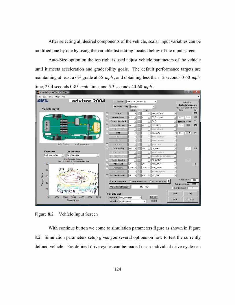
124

After selecting all desired components of the vehicle, scalar input variables can be

modified one by one by using the variable list editing located below of the input screen.

Auto-Size option on the top right is used adjust vehicle parameters of the vehicle

until it meets acceleration and gradeability goals. The default performance targets are

maintaining at least a 6% grade at 55 mph , and obtaining less than 12 seconds 0-60 mph

time, 23.4 seconds 0-85 mph time, and 5.3 seconds 40-60 mph .

Figure 8.2 Vehicle Input Screen

With continue button we come to simulation parameters figure as shown in Figure

8.2. Simulation parameters setup gives you several options on how to test the currently

defined vehicle. Pre-defined drive cycles can be loaded or an individual drive cycle can

125

be built by trip builder. Time steps and the number of cycles that is going to be repeated

can be set in this part also.

In addition to standard tests, acceleration and grade tests can also be applied

independently. Moreover by multiple cycles up to eight drive cycles can be tested

simultaneously. Standard test procedures i.e. SAE J1711, Real World, City Highway,

TEST FTP and TEST FTP HYBRID, can be applied to the vehicle if this option is

selected.

Auxiliary electric loads can be taken into account by activating them through the

checkbox located at the bottom of the parameter page. On-off times and characteristic

power usages of these units can be set through the opened auxiliary load page.

To see the effect that up to three variables have on the vehicle, select a parametric

study. The low and high values may be set, as well as the number of points desired for

that variable. A parametric study runs a set of simulations to cover the matrix of input

points, such that if 3 variables are selected with 3 points each, 27 simulations will run. If

the Save Runs checkbox is selected, each of the individual runs will be saved with a

naming convention of Prefix_Factor1Level#_Factor2Level#_Factor3Level#.mat. The

saved results can be analyzed by loading them into the results figure or the compare

simulation window.

When Run DOE under Options menu is selected, a new window will appear to

guide the user through the process of running a statistical design of experiments. The

DOE feature allows the user to specify as many factors and levels as desired which is an

expansion of the parametric study feature.

126

Figure 8.3 Simulation Parameters Screen

The results figure presents some summary results (fuel economy, emissions, total

distance, etc.) and allows the user to plot up to four time series plots by selecting a

variable from the popup menu. If the acceleration and gradeability checkboxes were

picked in the simulation setup screen, appropriate results will also be displayed. An

emission test results will be presented as a standard also but extensive analysis options

are not available in the program.

By clicking the Energy Use Figure button, a new figure is opened showing how

energy was used and transferred for the vehicle during the simulation. The Output Check

127

Plots button pulls up plots that show the vehicle's performance, some of which are not

available under the time series plots.

Figure 8.4 Results Screen

Apart from this portion of the program there is the MATLAB portion of the

ADVISOR. To make an extensive analysis and to explore the capabilities of the

ADVISOR this portion will be analyzed also.

128

8.3 AVL CRUISE29

CRUISE is a software for simulating driving performance, fuel consumption and

emissions. Its modular concept enables free modeling of all possible vehicle

configurations while sophisticated solvers guarantee short calculation times.

CRUISE is typically used in drive train and engine development to calculate and

optimize the following:

Fuel Consumption and Emissions

Driving Performance (acceleration, elasticity)

Transmission Ratios

Braking Performance

and for the determination of:

Collective Loads for Stress Calculations

Drivetrain Vibrations

The modular structure of CRUISE permits modeling of all existing and future

vehicle concepts for both single and double track vehicles (motorcycles, passenger cars,

trucks, etc.).

8.4 AVL BOOST30

BOOST simulates a wide variety of engines, 4-stroke or 2-stroke, spark or auto-

ignited. Applications range from small capacity engines for motorcycles or industrial

purposes up to large engines for marine propulsion. BOOST can also be used to simulate

the characteristics of pneumatic systems.

29 AVL CRUISE User Guide 30 AVL BOOST User Guide

129

The BOOST program package consists of an interactive pre-processor which

assists with the preparation of the input data for the main calculation program. Results

analysis is supported by an interactive post-processor.

The pre-processing tool of the AVL Workspace Graphical User Interface features

a model editor and a guided input of the required data. The calculation model of the

engine is designed by selecting the required elements from a displayed element tree by

mouse-click and connecting them by pipe elements. In this manner even very complex

engine configurations can be modeled easily, as a large variety of elements is available.

The main program provides optimized simulation algorithms for all available

elements. The flow in the pipes is treated as one-dimensional. This means that the

pressures, temperatures and flow velocities obtained from the solution of the gas dynamic

equations represent mean values over the cross-section of the pipes. Flow losses due to

three-dimensional effects, at particular locations in the engine, are considered by

appropriate flow coefficients. In cases where three-dimensional effects need to be

considered in more detail, a link to AVL's three-dimensional flow simulation code FIRE

is available. This means that a multi-dimensional simulation of the flow in critical engine

parts can be combined with a fast one-dimensional simulation elsewhere. This feature

could be of particular interest for the simulation of the charge motion in the cylinder, the

scavenging process of a two-stroke engine or for the simulation of the flow in

complicated muffler elements.

130

Chapter 9 Conclusions and Recommendations for Future Research

“Fuel Economy Modeling of Light-Duty and Heavy-Duty Vehicles and

Coastdown Study” thesis is product of the one and a half year research for the Texas

Department of Transportation’s (TxDOT’s) “Estimating Texas Vehicle Operating Costs”

project. The goal of the TxDOT project is to estimate vehicle operating costs for the

fleets of the vehicles including broad range of vehicles class i.e. light- to heavy-duty

vehicles. Vehicle operating costs (Vcost) play an important role in several TxDOT

policy making areas ranging from the economic evaluation of highway construction,

maintenance, and rehabilitation strategies to lane rental, liquidated damages and

construction bonus calculations. Vcost relationships have not been studied in Texas for

over two decades and these now risk obsolescence in the face of new design

technologies, engine changes – both hybrid and improved gasoline/diesel – better tire

performance.31

Fuel cost is the dominant cost in vehicle operating costs with 35%. With the

increasing oil prices and carbon dioxide emissions of the automobiles fuel economy’s

importance is high in recent years with increase in awareness of the consumers.

Fuel estimation took an experimental format until the mid 1980s when alternative

modeling offered more flexible ways of estimating consumption. Mechanistic models

incorporates changes in engine design, body style and tire technology developments

which results in a dynamic fuel economy model and it is independent of region.

Moreover, different types of fuels can be easily adapted to the model and their effects on

the fuel consumption can be analyzed.

31 TxDOT Project No. 0-5974 Proposal

131

Fuel economy model for class of vehicles aim is to calculate a fleet fuel economy

for different compositions of the fleets. This is very useful for big enterprises who own

wide range of vehicles from light- to heavy-duty vehicles. Effect of setting a speed limit

of 65 mph instead of 64 mph can be analyzed easily and effect of increasing speed in

delivery times and its effect on company profit can be analyzed. While putting this

model together EPA’s data is used to get enough vehicles in each class for years 2000 till

2008. A database needs to be created for the software for adding every coming year and

the software should be able to convert the data according to its needs.

Road load force analysis that was done on the EPA’s Annual Certification Data

revealed that classes of the vehicles specified by the EPA has some uncertainty as it was

shown with Ferrari 612 Scaglietti as medium class vehicle. It is also noticed that the

world does not have a single standard about vehicle classes in LDV’s.

On the other hand, vehicle specific approach uses the equations derived by

Matthews, 2007. This model is purely mechanistic and its base is the power flow through

vehicle systems and analysis of the losses on these systems. The road load force

requirements again calculated by use of the coastdown coefficients derived from EPA’s

website and for heavy-duty vehicles these coefficients will be derived from the

coastdown tests that were done at SH45 SE toll-road of Austin, TX before the road was

opened to the public on May 1, 2009. The software developed for the vehicle specific

approach needs to be developed more by a better indicated thermal efficiency model.

Effects of engine efficiencies on fuel economy are analyzed and it is observed that

indicated thermal efficiency plays an important role in gear changes. Indicated thermal

132

efficiency model will be updated by Woschni’s32 heat transfer model for the internal

combustion engines. A user’s manual needs to be written for the software updates for the

future researchers who wants to update the model. Effects of tires on the fuel

consumption need to be analyzed for better fuel economy model. It is known that

Bridgestone has a computer model to analyze the effects of the different tires including

other brands. Some effort is put to get access to this software however it was not

successful. A broader literature search needs to be done for this subject.

Hybrid vehicles analyzed only in the class based approach of the fuel economy in

Chapter 4 however, vehicle specific approach is not capable of analyzing the hybrid

vehicles. The number of the hybrid vehicles on the roads is increasing in the US

extensively with the rise of gasoline pump prices, thus more attention should be given to

hybrids. Newly, hybrid heavy-duty vehicles are also available in the market. AVL

Advisor software is capable of analyzing the hybrid vehicles including serial and parallel

hybrid configurations, therefore; AVL Advisor can be a benchmark and a starting point

for future analysis.

An AVL Cruise and Boost co-simulation will be used for heavy-duty vehicle fuel

economy model.33 This model will be very important for the future studies related with

the fuel economy since it needs close analysis of the each vehicle component. Thus

effect of the components on the fuel consumption will be analyzed more accurately.

32 G. Woschni 33 Regner, G., E. Loibner, J. Krammer, L. Walter, and R. Truemner

133

Appendix A: Road Load Force Calculation MATLAB Code

clear clc fprintf ('Input year: \n'); year = input('Specify year from 2000 to 2008 \n'); [num, txt] = xlsread('2008-2000 all data.xlsx', num2str(year)); mkdir(['LDV Figures\',num2str(year)]) % Make A,B,C zero to handle empty cell problem. A = zeros(length(num),1); B = zeros(length(num),1); C = zeros(length(num),1); A = num(:,17); B = num(:,18); C = num(:,19); class = txt(:,1); trans = txt(:,3); division = txt(:,10); carline = txt(:,12); j = 1; for i=2:(length(A)-1) if strcmp(class(i), class(i+1)) ~= 1 N(j) = i-1; j = j + 1; end end x = length (N); N(x+1) = length (A); S=0:60; i = 1; j = 1; m = 1; k = 1;

134

r = 1; t = 1; for m=1 :length (N) % Empty cells which are holding data in while loop M = zeros (1,1); Auto = zeros(1,1); Manual = zeros(1,1); Name = cellstr(''); AutoName = cellstr(''); ManualName = cellstr(''); checkAuto = 0; checkManual = 0; z = 1; r = 1; t = 1; while (i <= N(j)) for k=1 : length(S) M(z,k)=A(i)+B(i)*S(k)+C(i)*S(k)^2; % Automatic and manual transmission differentiation if strcmp(trans(i+1), 'A') == 1 Auto(r,k) = M(z,k); checkAuto = 1; else Manual(t,k) = M(z,k); checkManual = 1; end end Name(z) = cellstr([char(division(i+1)), ' - ', char(carline(i+1))]); if strcmp(trans(i+1), 'A') == 1 AutoName(r) = cellstr([char(division(i+1)), ' - ', char(carline(i+1))]); r = r+1; else ManualName(t) = cellstr([char(division(i+1)), ' - ', char(carline(i+1))]); t = t+1; end i = i+1;

135

z = z+1; end % ************************************************************************ % ************************************************************************ % ************************************************************************ % ************************************************************************ % % % FIGURE OF CLASS (AUTO & MANUAL) % % figure(3*m-2); [row,col] = size(M); if row == col plot(S, M', 'DisplayName', Name, 'XDataSource', 'S', 'YDataSource','M'); figure(gcf); else plot(S, M, 'DisplayName', Name, 'XDataSource', 'S', 'YDataSource','M'); figure(gcf); end hold on; xlabel('Speed [mph]'); ylabel('F_R _L (Road Load Force) [lbf]'); title([char(class(i)), ' - ', num2str(year)]); grid on; if row ~= 1 M_max = max (M); M_min = min (M); M_avg = mean (M);

136

h(1) = plot(S, M_max, '-.or', 'DisplayName', '(F_R_L) _m_a_x', 'XDataSource', 'S', 'YDataSource', 'M_max'); figure(gcf); h(2) = plot(S, M_min, '-.ob', 'DisplayName', '(F_R_L) _m_i_n', 'XDataSource', 'S', 'YDataSource', 'M_min'); figure(gcf); h(3) = plot(S, M_avg, '-.vk', 'DisplayName', '(F_R_L) _a_v_g', 'XDataSource', 'S', 'YDataSource', 'M_avg'); figure(gcf); legend(h, 'Location', 'NorthWest'); end for d = 1 : (z-1) if M(d,:) == M_max text('String',[char(Name(d)), ' \rightarrow '],... 'Position',[S(50),M(d,50)],... 'HorizontalAlignment','right', 'FontWeight', 'bold'); end if M(d,:) == M_min text('String',[' \leftarrow ', char(Name(d))],... 'Position',[S(27),M(d,25)],... 'HorizontalAlignment','left', 'FontWeight', 'bold'); end end hold off; % ***************************************************************** % Printing % ***************************************************************** orient landscape; % print -P\\ENGR-Print1\ENGR-SC2-Laser-1; % print -PTFS; % ***************************************************************** % Saving % *****************************************************************

137

saveas(gcf,['LDV Figures\', num2str(year), '\', char(class(i)), ' - ', num2str(year)],'fig') set(gcf, 'Visible', 'off'); % ************************************************************************ % ************************************************************************ % ************************************************************************ % ************************************************************************ % % % FIGURE OF AUTOMATIC TRANSMISSION CLASS % % if checkAuto figure(3*m-1); [row,col] = size(Auto); if row == col plot(S, Auto', 'DisplayName', AutoName, 'XDataSource', 'S', 'YDataSource','Auto'); figure(gcf); else plot(S, Auto, 'DisplayName', AutoName, 'XDataSource', 'S', 'YDataSource','Auto'); figure(gcf); end hold on; xlabel('Speed [mph]'); ylabel('F_R _L (Road Load Force) [lbf]'); title([char(class(i)), ' - ', num2str(year), ' (Automatic)']); grid on; if row ~= 1 Auto_max = max (Auto); Auto_min = min (Auto);

138

Auto_avg = mean (Auto); h(1) = plot(S, Auto_max, '-.or', 'DisplayName', '(F_R_L) _m_a_x', 'XDataSource', 'S', 'YDataSource', 'Auto_max'); figure(gcf); h(2) = plot(S, Auto_min, '-.ob', 'DisplayName', '(F_R_L) _m_i_n', 'XDataSource', 'S', 'YDataSource', 'Auto_min'); figure(gcf); h(3) = plot(S, Auto_avg, '-.vk', 'DisplayName', '(F_R_L) _a_v_g', 'XDataSource', 'S', 'YDataSource', 'Auto_avg'); figure(gcf); legend(h, 'Location', 'NorthWest'); end for d = 1 : (r-1) if Auto(d,:) == Auto_max text('String',[char(AutoName(d)), ' \rightarrow '],... 'Position',[S(50),Auto(d,50)],... 'HorizontalAlignment','right', 'FontWeight', 'bold'); end if Auto(d,:) == Auto_min text('String',[' \leftarrow ', char(AutoName(d))],... 'Position',[S(27),Auto(d,25)],... 'HorizontalAlignment','left', 'FontWeight', 'bold'); end end hold off; % ***************************************************************** % Printing % ***************************************************************** orient landscape; % print -P\\ENGR-Print1\ENGR-SC2-Laser-1; % print -PTFS; % ***************************************************************** % Saving

139

% ***************************************************************** saveas(gcf,['LDV Figures\', num2str(year), '\', char(class(i)), ' - ', num2str(year), ' (Automatic)'],'fig') set(gcf, 'Visible', 'off'); end % ************************************************************************ % ************************************************************************ % ************************************************************************ % ************************************************************************ % % % FIGURE OF MANUAL TRANSMISSION CLASS % % if checkManual figure(3*m); [row,col] = size(Manual); if row == col plot(S, Manual', 'DisplayName', ManualName, 'XDataSource', 'S', 'YDataSource','Manual'); figure(gcf); else plot(S, Manual, 'DisplayName', ManualName, 'XDataSource', 'S', 'YDataSource','Manual'); figure(gcf); end hold on; xlabel('Speed [mph]'); ylabel('F_R _L (Road Load Force) [lbf]'); title([char(class(i)), ' - ', num2str(year), ' (Manual)']); grid on; if row ~= 1

140

Manual_max = max (Manual); Manual_min = min (Manual); Manual_avg = mean (Manual); h(1) = plot(S, Manual_max, '-.or', 'DisplayName', '(F_R_L) _m_a_x', 'XDataSource', 'S', 'YDataSource', 'Manual_max'); figure(gcf); h(2) = plot(S, Manual_min, '-.ob', 'DisplayName', '(F_R_L) _m_i_n', 'XDataSource', 'S', 'YDataSource', 'Manual_min'); figure(gcf); h(3) = plot(S, Manual_avg, '-.vk', 'DisplayName', '(F_R_L) _a_v_g', 'XDataSource', 'S', 'YDataSource', 'Manual_avg'); figure(gcf); legend(h, 'Location', 'NorthWest'); end for d = 1 : (t-1) if Manual(d,:) == Manual_max text('String',[char(ManualName(d)), ' \rightarrow '],... 'Position',[S(50),Manual(d,50)],... 'HorizontalAlignment','right', 'FontWeight', 'bold'); end if Manual(d,:) == Manual_min text('String',[' \leftarrow ', char(ManualName(d))],... 'Position',[S(27),Manual(d,25)],... 'HorizontalAlignment','left', 'FontWeight', 'bold'); end end hold off; % ***************************************************************** % Printing % ***************************************************************** orient landscape; % print -P\\ENGR-Print1\ENGR-SC2-Laser-1; % print -PTFS;

141

% ***************************************************************** % Saving % ***************************************************************** saveas(gcf,['LDV Figures\', num2str(year), '\', char(class(i)), ' - ', num2str(year), ' (Manual)'],'fig') set(gcf, 'Visible', 'off'); end i = N(j) + 1; j = j + 1; end

142

Appendix B: Overall Drivetrain Efficiency Calculation MATLAB Code

clear clc fprintf ('Input year: \n'); year = input('Specify year from 2000 to 2008 \n'); % READ VEHICLE DATA [num, txt] = xlsread('Data v1.xlsx', num2str(year)); % Make A,B,C zero to handle empty cell problem. A = zeros(length(num),1); B = zeros(length(num),1); C = zeros(length(num),1); ETW = zeros(length(num),1); displ = num(:,15); ETW = num(:,17); A = num(:,20); B = num(:,21); C = num(:,22); fuel = num(:,28); class = txt(:,1); division = txt(:,11); carline = txt(:,13); trans = txt(:,17); % READ EPA'S FUEL ECONOMY DATABASE % Fuel Economy Database 1.xlsx : For year 2007 and before 2007 % Fuel Economy Database 2.xlsx : For year 2008 % Fuel Economy Database 3.xlsx : For TxDOT's data if year == 2008 [num, txt] = xlsread('Fuel Economy Database 2.xlsx', num2str(year)); else [num, txt] = xlsread('Fuel Economy Database 1.xlsx', num2str(year)); end

143

division2 = txt(:,2); carline2 = txt(:,3); trans2 = txt(:,6); fuel2 = txt(:,14); displ2 = num(:,1); FE_City = num(:,8); FE_Hway = num(:,9); % READ COMPARISON DATABASE % Manufacturer [num, txt] = xlsread('Comparison Database.xlsx', 'Manufacturer'); division0 = txt(:,1); division1 = txt(:,2); % Carline [num, txt] = xlsread('Comparison Database.xlsx', 'Carline'); carline0 = txt(:,2); carline1 = txt(:,3); carline_ = txt(:,4); % Carline 1'in degisik versiyonu olursa % Transmission [num, txt] = xlsread('Comparison Database.xlsx', 'Transmission'); trans0 = txt(:,1); trans1 = txt(:,2); % Displacement [num, txt] = xlsread('Comparison Database.xlsx', 'Displacement'); displ0 = num(:,1); displ1 = num(:,2); % Fuel Type [num, txt] = xlsread('Comparison Database.xlsx', 'Fuel Type'); fuel0 = num(:,1); fuel1 = txt(:,2); % DENSITY & LHV density_array = num(:,4); % [kg/m^3] LHV_array = num(:,5); % [MJ/kg] % READ FTP DATA [num, txt] = xlsread('DDS.xlsx', 'FTP'); T_FTP = num(:,1); % TIME (s) S_FTP = num(:,2); % SPEED (mph)

144

X_FTP = sum(S_FTP)/3600; if year == 2008 % Split FTP into Bags T_Bag1 = num(1:506,1); T_Bag2 = num(506:1370,1); T_Bag3 = num(1370:1875,1); S_Bag1 = num(1:506,2); S_Bag2 = num(506:1370,2); S_Bag3 = num(1370:1875,2); X_Bag1 = sum(S_Bag1)/3600; X_Bag2 = sum(S_Bag2)/3600; X_Bag3 = sum(S_Bag3)/3600; % READ SC03 DATA [num, txt] = xlsread('DDS.xlsx', 'SC03'); T_SC03 = num(:,1); % TIME (s) S_SC03 = num(:,2); % SPEED (mph) X_SC03 = sum(S_SC03)/3600; % READ US06 DATA [num, txt] = xlsread('DDS.xlsx', 'US06'); T_US06 = num(:,1); % TIME (s) S_US06 = num(:,2); % SPEED (mph) X_US06 = sum(S_US06)/3600; end % READ HWFET DATA [num, txt] = xlsread('DDS.xlsx', 'HWFET'); T_HWFET = num(:,1); % TIME (s) S_HWFET = num(:,2); % SPEED (mph) X_HWFET = sum(S_HWFET)/3600; for i=1 :length (A) Manufacturer = Match(division(i+1), division0, division1, 1); [answer1, answer2] = Carline_Match(carline(i+1), carline0, carline1, carline_); Transmission = Match(trans(i+1), trans0, trans1, 1);

145

Displacement = Match(displ(i), displ0, displ1, 1); Fuel = Match(fuel(i), fuel0, fuel1, 0); [density, LHV] = Fuel_properties(fuel(i), fuel0, density_array, LHV_array); for j=1 :length(FE_City) error = 0; if ( strcmp(answer1, carline2(j+1)) || strcmp(answer2, carline2(j+1)) ) if strcmp(Transmission, trans2(j+1)) if Displacement == displ2(j) if strcmp(Fuel, fuel2(j+1)) if strcmp(Manufacturer, division2(j+1)) x1(i,1) = FE_City(j); % Find the corresponding City FE x2(i,1) = FE_Hway(j); % Find the corresponding Highway FE if year == 2008 Bag1 = FuelUsed2(ETW(i), A(i), B(i), C(i), density, LHV, T_Bag1, S_Bag1, X_Bag1); Bag2 = FuelUsed2(ETW(i), A(i), B(i), C(i), density, LHV, T_Bag2, S_Bag2, X_Bag2); Bag3 = FuelUsed2(ETW(i), A(i), B(i), C(i), density, LHV, T_Bag3, S_Bag3, X_Bag3); SC03 = FuelUsed2(ETW(i), A(i), B(i), C(i), density, LHV, T_SC03, S_SC03, X_SC03); US06 = FuelUsed2(ETW(i), A(i), B(i), C(i), density, LHV, T_US06, S_US06, X_US06); HWFET = FuelUsed2(ETW(i), A(i), B(i), C(i), density, LHV, T_HWFET, S_HWFET, X_HWFET); dummy_FE_City(i,1) = City_FE(Bag1, Bag2, Bag3, SC03, US06); City_eff(i,1) = x1(i,1) / dummy_FE_City(i,1); dummy_FE_Hway(i,1) = Hway_FE(Bag1, Bag2, Bag3, SC03, US06, HWFET); Hway_eff(i,1) = x2(i,1) / dummy_FE_Hway(i,1); else

146

City_eff(i,1) = Efficiency(ETW(i), A(i), B(i), C(i), x1(i,1), density, LHV, T_FTP, S_FTP, X_FTP); Hway_eff(i,1) = Efficiency(ETW(i), A(i), B(i), C(i), x2(i,1), density, LHV, T_HWFET, S_HWFET, X_HWFET); end break else error = 1; end else error =1; end else error =1; end else error =1; end else error =1; end end if error City_eff(i,1) = 0; Hway_eff(i,1) = 0; x1(i,1) = 0; x2(i,1) = 0; end end xlswrite('Data v1.xlsx', {'% City eff'}, num2str(year), 'AN1'); xlswrite('Data v1.xlsx', City_eff, num2str(year), 'AN2'); xlswrite('Data v1.xlsx', {'% Highway eff'}, num2str(year), 'AO1'); xlswrite('Data v1.xlsx', Hway_eff, num2str(year), 'AO2'); xlswrite('Data v1.xlsx', {'UNRND CITY (EPA)'}, num2str(year), 'AP1'); xlswrite('Data v1.xlsx', x1, num2str(year), 'AP2'); xlswrite('Data v1.xlsx', {'UNRND HWY (EPA)'}, num2str(year), 'AQ1'); xlswrite('Data v1.xlsx', x2, num2str(year), 'AQ2');

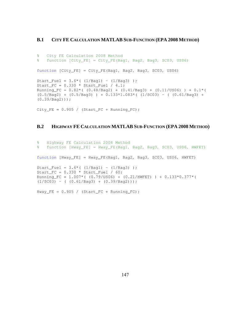
147

B.1 CITY FE CALCULATION MATLAB SUB-FUNCTION (EPA 2008 METHOD)

% City FE Calculation 2008 Method % function [City_FE] = City_FE(Bag1, Bag2, Bag3, SC03, US06) function [City_FE] = City_FE(Bag1, Bag2, Bag3, SC03, US06) Start_Fuel = 3.6*( (1/Bag1) - (1/Bag3) ); Start_FC = 0.330 * Start_Fuel / 4.1; Running_FC = 0.82*( (0.48/Bag2) + (0.41/Bag3) + (0.11/US06) ) + 0.1*( (0.5/Bag2) + (0.5/Bag3) ) + 0.133*1.083*( (1/SC03) - ( (0.61/Bag3) + (0.39/Bag2))); City_FE = 0.905 / (Start_FC + Running_FC);

B.2 HIGHWAY FE CALCULATION MATLAB SUB-FUNCTION (EPA 2008 METHOD)

% Highway FE Calculation 2008 Method % function [Hway_FE] = Hway_FE(Bag1, Bag2, Bag3, SC03, US06, HWFET) function [Hway_FE] = Hway_FE(Bag1, Bag2, Bag3, SC03, US06, HWFET) Start_Fuel = 3.6*( (1/Bag1) - (1/Bag3) ); Start_FC = 0.330 * Start_Fuel / 60; Running_FC = 1.007*( (0.79/US06) + (0.21/HWFET) ) + 0.133*0.377*( (1/SC03) - ( (0.61/Bag3) + (0.39/Bag2))); Hway_FE = 0.905 / (Start_FC + Running_FC);

148

Appendix C: Codes of Vehicle Specific Fuel Economy Model

C.1 MAIN FUNCTION

This function takes the input values from the C# GUI that user is specifying the

input parameters. Main Function than sends these parameters in desired forms to the main

calculation functions.

function outdata = mpgCalculate(indata) %"MPG Calculate" Calculation of mpg through physical approach % % Input parameters: % in.disp - Engine displacement (L) % in.cr - Compression ratio % in.maxPower - Maximum engine power (hp) % in.maxRPM - Engine speed @ maximum power (rpm) % in.first - 1st gear ratio % in.second - 2nd gear ratio % in.third - 3rd gear ratio % in.fourth - 4th gear ratio % in.axle - Axle ratio % in.overdrive - Overdrive ratio % in.transfer - Transfer case ratio % in.section - Section width of the tire (mm) % in.aspect - Aspect ratio of the tire (%) % in.rim - Rim diameter (in) % in.A - Coastdown coefficient A % in.B - Coastdown coefficient B % in.C - Coastdown coefficient C % % Output parameters: % % out.speed - Speed (mph) % out.mpg - Fuel economy (mpg) % % Murat Ates % (c) The University of Texas at Austin 2008 % Load the data from a structure into individual variable names global first second third fourth axle overdrive transfer coefA coefB coefC; global roFuel LHV CV2 combustEff idleRPM; global dTire slope constant;

149

global equivalenceRatio compRatio disp fuelAirRatio; disp = indata.disp; compRatio = indata.cr; maxPower = indata.maxPower; maxRPM = indata.maxRPM; first = indata.first; second = indata.second; third = indata.third; fourth = indata.fourth; axle = indata.axle; overdrive = indata.overdrive; transfer = indata.transfer; section = indata.section; aspect = indata.aspect; rim = indata.rim; coefA = indata.A; coefB = indata.B; coefC = indata.C; %% Set general properties roAir = 101.21/0.287/293.15; % Air density (kg/m^3) roFuel = 744.255; % Fuel density (kg/m^3) LHV = 44.6; % Lower heating value (MJ/kg) CV2 = 1609.344*4.448221615*264.1720524/10^6/3600; equivalenceRatio = 1; % Equivalence ratio AFs = 14.6; % Standard air-fuel ratio FAs = 1/AFs; % Standard fuel-air ratio if equivalenceRatio>1 combustEff = 1/equivalenceRatio; % Combustion efficiency elseif equivalenceRatio <= 1 combustEff = 1.00; % Combustion efficiency end fuelAirRatio = equivalenceRatio/AFs; % Standard fuel air ratio x = 2; idleRPM = 800; % Idle rpm

150

% %% Indicated thermal efficiency coeefficient calculation % % eta_ti = a*N*N + b*N + c where N is rpm % % Determine a, b, c coefficients % % dummy_rpm(1,1) = idleRPM; % Idle rpm % dummy_rpm(2,1) = 0.5*maxRPM; % dummy_rpm(3,1) = maxRPM; % % eta_ti_MAX = 0.5*(1-(1/compRatio)^0.4); % % eta_ti(1,1) = 0.4*eta_ti_MAX; % eta_ti(2,1) = 0.83*eta_ti_MAX; % eta_ti(3,1) = eta_ti_MAX; % % % The better your initial condition guess are, the faster % % the lsqcurvefit command will converge onto a solution % initialGuess = [-0.00000001, 0.0001, 0.0223]; % a, b, c coefficients % % % eta_tiCoeffs is an array containing the optimal values that will % % generate a curve that will best fit (rpm vs. indicated thermal efficiency) data % % Error is the sum of the error squared. The lower this number is, the better. % % [eta_tiCoeffs] = lsqcurvefit(@indicatedEff, initialGuess, dummy_rpm, eta_ti); %% Tire diameter calculation dTire = (2*section*aspect/2540) + rim; % Tire diameter (in) %% Calculate (indicated thermal efficiency * volumetric efficiency) eta_ind_eta_vol = maxPower*60 / (combustEff*0.85*roAir*disp*maxRPM*LHV*fuelAirRatio*1.34102209/x); %% Calculate idle brake power (hp) bp_idle = eta_ind_eta_vol*0.85*roAir*disp*idleRPM*LHV*fuelAirRatio*1.34102209/120; %% Calculate slope and constant of bp curve slope = (maxPower-bp_idle) / (maxRPM-idleRPM); constant = maxPower - slope*maxRPM;

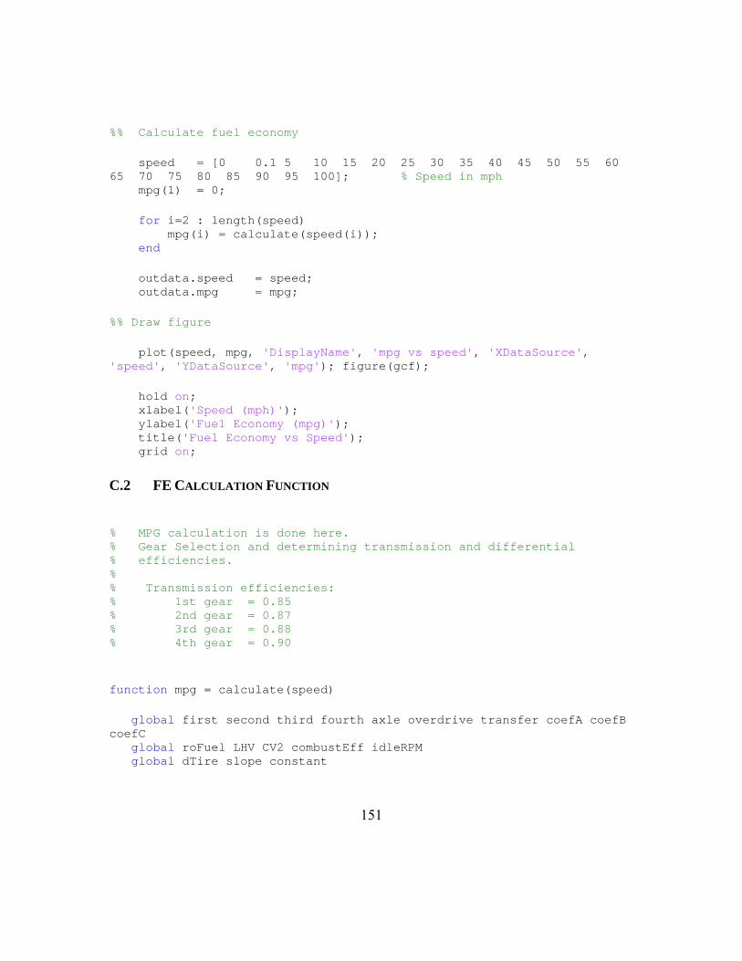
151

%% Calculate fuel economy speed = [0 0.1 5 10 15 20 25 30 35 40 45 50 55 60 65 70 75 80 85 90 95 100]; % Speed in mph mpg(1) = 0; for i=2 : length(speed) mpg(i) = calculate(speed(i)); end outdata.speed = speed; outdata.mpg = mpg; %% Draw figure plot(speed, mpg, 'DisplayName', 'mpg vs speed', 'XDataSource', 'speed', 'YDataSource', 'mpg'); figure(gcf); hold on; xlabel('Speed (mph)'); ylabel('Fuel Economy (mpg)'); title('Fuel Economy vs Speed'); grid on;

C.2 FE CALCULATION FUNCTION

% MPG calculation is done here. % Gear Selection and determining transmission and differential % efficiencies. % % Transmission efficiencies: % 1st gear = 0.85 % 2nd gear = 0.87 % 3rd gear = 0.88 % 4th gear = 0.90 function mpg = calculate(speed) global first second third fourth axle overdrive transfer coefA coefB coefC global roFuel LHV CV2 combustEff idleRPM global dTire slope constant

152

%% Gear selection setting transmission efficiencies based on speed(mph) if speed >= 60 gear = fourth; transEff = 0.90; else if speed >= 40 gear = third; transEff = 0.88; else if speed >= 20 gear = second; transEff = 0.87; else gear = first; transEff = 0.85; end end end %% Differential Efficiency Calculation if speed < 150*0.6213711922 diffEff = 0.6652 + 0.003732*speed*1.609344 - 0.00001061*(speed*1.609344)^2; else diffEff = 0.987; end %% Engine RPM calculation rpm = speed*gear*axle*overdrive*transfer*63360 / (pi*dTire*60); %% If engine speed is less than idle speed of 800 rpm, make it equal to idle engine speed if rpm < idleRPM rpm = idleRPM; end %% LOAD Calculation bp = rpm*slope + constant; % Brake power produced by engine (hp) forceRL = coefA + coefB*speed + coefC*speed^2; % Road load force required to move the vehicle in that speed (lbf) bp_required = forceRL*4.448221615*speed*0.44704*0.00134102209/transEff/diffEff; % Required brake power to move vehicle in that speed (hp) load = bp_required / bp; %% Mechanical Efficiency Calculation

153

if load >= 0.25 mechanicalEff = 0.85; else mechanicalEff = (0.85/0.25)*load; end indicatedThermalEff = 0.5*indicatedEff(load); mpg = mechanicalEff*combustEff*indicatedThermalEff*transEff*diffEff*roFuel*LHV / (3600*CV2*forceRL);

C.3 INDICATED THERMAL EFFICIENCY CALCULATION FUNCTION

function indicated = indicatedEff(load) % % Indicated Thermal Efficiency Function % % Air Equivalent Spark Ignition (AESI) Model % %% % % Murat Ates % (c)2009 The University of Texas at Austin % % % v1: 5-February-2009 % %% Global variables global compRatio LHV fuelAirRatio combustEff % compRatio = 9.8; % LHV = 43.6; % fuelAirRatio = 1/14.6; % combustEff = 1; %% Determine Friction Power

154

% fp = 1.975*10^-5 * sqrt(compRatio) *Stroke*disp*(rpm/100)^2; % Eqn 4.18a %% Make a guess for f & T1 f = 0.0285; T1 = 300; %% Constant values P_ex = 99; R_air = 0.287; if load == 1 P1 = P_ex; else P1 = (P_ex-33)*load + 33; end h_a_TP = airProp(298,'T','h'); h_v_f = 303.6; x_e_af = 0.15; %% Set Errors to enter WHILE LOOP at least once error_f = 1; errorT = 1; while (error_f >= 0.5) && (errorT >= 0.5) % While loop is to optimize temperature and residual fraction %% STATE 1 v1 = R_air*T1/P1; [u1, vr1] = airProp(T1,'T',{'u' 'vr'}); %% STATE 2 v2 = v1/compRatio; vr2 = vr1/compRatio; [T2, u2] = airProp(vr2,'vr',{'T' 'u'}); v3 = v2; %% Calculate head added

155

q_a_th = combustEff*(1-f)*LHV*1000*fuelAirRatio/(1+fuelAirRatio); %% STATE 3 u3 = u2+q_a_th; [T3, vr3, sT3] = airProp(u3,'u',{'T' 'vr' 'sT'}); P3 = R_air*T3/v3; %% STATE 4 vr4 = vr3*compRatio; [T4, u4] = airProp(vr4,'vr',{'T' 'u'}); %% STATE 4' P4p = P_ex; P5 = P_ex; P6 = P_ex; sT4p = sT3 + R_air*log(P4p/P3); [T4p, h4p] = airProp(sT4p,'sT',{'T' 'h'}); v4p = R_air*T4p/P4p; %% STATE 5&6 T5 = T4p; T6 = T4p; h5 = h4p; h6 = h4p; v5 = v4p; v6 = v4p; u6 = airProp(T6,'T','u'); %% Check initial conditions f_new = v2/v4p; h_i = (h_a_TP/(1+fuelAirRatio)) + 0 - x_e_af*(fuelAirRatio/(1+fuelAirRatio))*h_v_f; % Eqn. 4.66c if load == 1 h1 = (1-f)*h_i + f*h6; % Eqn. 4.60 (NA SI at WOT) else h1 = (1-f)*h_i + f*(u6+P1*v6); % Eqn. 4.62 (early IVO) end T1new = airProp(h1,'h','T'); error_f = abs(f - f_new)*100/f; errorT = abs(T1 - T1new)*100/T1;

156

% If new(f & T1) is out of bounds then recalculate by using new values of % f & T1. f = f_new; T1 = T1new; end %% Indicated Thermal Efficiency w_net = (u1-u2) + (u3-u4) + (P1-P6)*(v1-v2); % Eqn. 4.82 (early IVO) indicated = w_net/q_a_th;

C.4 THERMODYNAMIC PROPERTIES CALCULATION OF IDEAL GAS AIR

function varargout=airProp(inputValue,inputName, prop) %% % Interpolates thermodynamic properties of AIR as an Ideal Gas % Temperature range: 250 - 3500 K % % Reference: % Ronald D. Matthews % Internal Combustion Engines and Automotive Engineering, % Appendix A1 % % Values are in SI-units: % % col-# prop. units % ------------------------ % 1 T K % 2 u kJ/kg % 3 h kJ/kg % 4 sT kJ/(kgK) % 5 Pr - % 6 vr - % % inputValue : This is the value that is going to be used to find other properties. % inputName : This is the name of the supplied inputValue % prop : prop contains the properties that are requested % % % Example 1: out=airProp(1000,'h','T') % Example 2: [T,u,h,sT,Pr]=airProp(15,'vr',{'T' 'u' 'h' 'sT' 'Pr'})

157

% Example 3: [T,u,h,sT,Pr]=airProp([15 20],'vr',{'T' 'u' 'h' 'sT' 'Pr'}) % %% % % Murat Ates % (c)2009 The University of Texas at Austin % % % v1: 5-February-2009 % %% % check # of input arguments if ~isequal(nargin,3) error('airProp requires 3 input arguments!') return end % get table load propTabAir % find input's column number inputColumn=find(strcmp(propInfo,inputName)); % if multi property request if iscell(prop) % scan along cells for idx=1:length(prop) % identify property column col=find(strcmp(propInfo,prop(idx))); if isempty(col) disp(['Property "' char(prop(idx)) '" not recognized!']) else % create output varargout{idx}=interp1(airTab(:,inputColumn),airTab(:,col),inputValue); end end % single property request else % identify property column col=find(strcmp(propInfo,prop)); if isempty(col) disp(['Property "' prop '" not recognized!']) else % create output varargout{1} =interp1(airTab(:,inputColumn),airTab(:,col),inputValue);

158

end end

C.5 SCRIPT BUILDING MATLAB CODES INTO .NET PLATFORM

%% Build Script % This script will build the mcode for the TxDOT Vehicle Operating Costs Project. % % This build_mcode makes .NET deployment of MATLAB using Builder for .NET. % % % Murat Ates % Copyright 2008 The University of Texas at Austin %% Determine path names workdir = pwd(); basedir = fileparts(workdir); outdir = fullfile(basedir, 'Output'); dnetdir = fullfile(workdir, 'mpgCalculate_dotnet'); %% Determine file names mfile_mpgCalculate = fullfile(workdir, 'mpgCalculate.m'); dnetdll = fullfile(dnetdir, 'mpgCalculate_dotnet.dll'); dnetctf = fullfile(dnetdir, 'mpgCalculate_dotnet.ctf'); %% Verify mfile can be found if (exist(mfile_mpgCalculate, 'file') ~= 2) error('Unable to find mfile mpgCalculate.m'); end %% Create directories if needed if (exist(outdir, 'dir') ~= 7) mkdir(outdir); end if (exist(dnetdir, 'dir') ~= 7) mkdir(dnetdir); end %% Build .NET Assembly disp('Compiling .NET Assembly...');

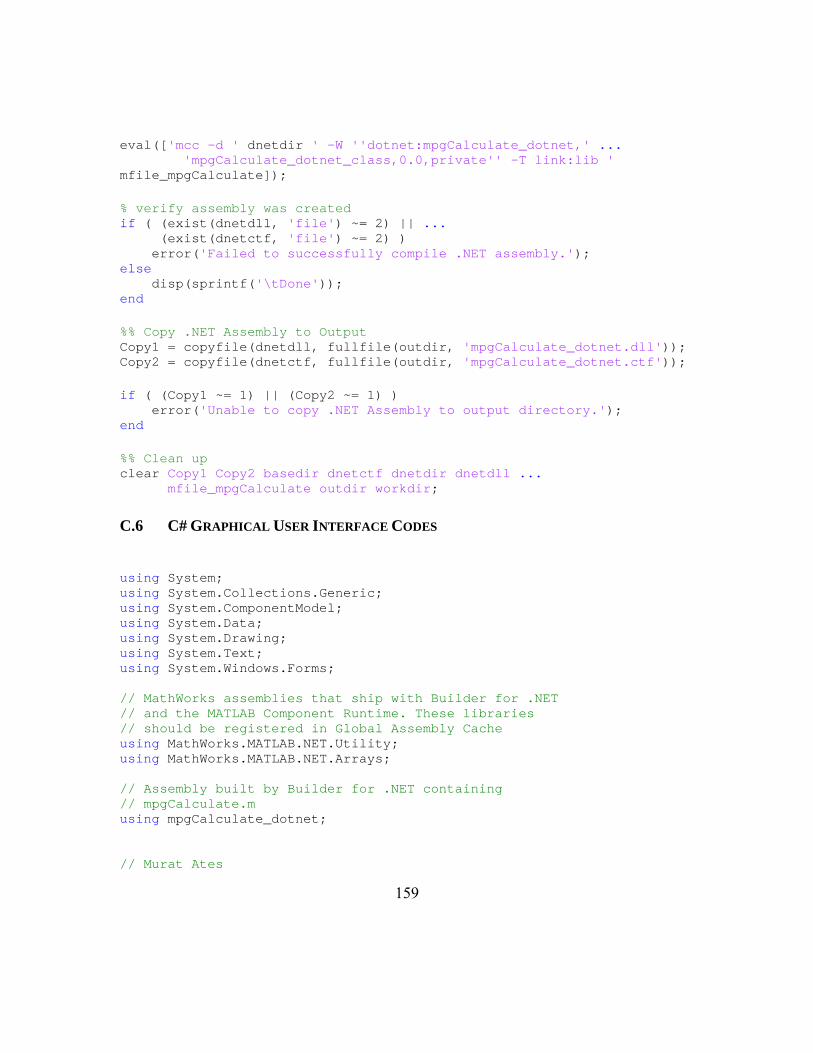
159

eval(['mcc -d ' dnetdir ' -W ''dotnet:mpgCalculate_dotnet,' ... 'mpgCalculate_dotnet_class,0.0,private'' -T link:lib ' mfile_mpgCalculate]); % verify assembly was created if ( (exist(dnetdll, 'file') ~= 2) || ... (exist(dnetctf, 'file') ~= 2) ) error('Failed to successfully compile .NET assembly.'); else disp(sprintf('\tDone')); end %% Copy .NET Assembly to Output Copy1 = copyfile(dnetdll, fullfile(outdir, 'mpgCalculate_dotnet.dll')); Copy2 = copyfile(dnetctf, fullfile(outdir, 'mpgCalculate_dotnet.ctf')); if ( (Copy1 ~= 1) || (Copy2 ~= 1) ) error('Unable to copy .NET Assembly to output directory.'); end %% Clean up clear Copy1 Copy2 basedir dnetctf dnetdir dnetdll ... mfile_mpgCalculate outdir workdir;

C.6 C# GRAPHICAL USER INTERFACE CODES

using System; using System.Collections.Generic; using System.ComponentModel; using System.Data; using System.Drawing; using System.Text; using System.Windows.Forms; // MathWorks assemblies that ship with Builder for .NET // and the MATLAB Component Runtime. These libraries // should be registered in Global Assembly Cache using MathWorks.MATLAB.NET.Utility; using MathWorks.MATLAB.NET.Arrays; // Assembly built by Builder for .NET containing // mpgCalculate.m using mpgCalculate_dotnet; // Murat Ates

160

// Copyright 2008 The University of Texas at Austin // Texas Vehicle Operating Costs Project namespace VCost { public partial class MainForm : Form { public MainForm() { InitializeComponent(); //buttonStart.Image = VCost.Properties.Resources.start_button_75pxl; //buttonStart.BackColor = Color.Transparent; } private void buttonDefaults_Click(object sender, EventArgs e) { // load default values to input fields textBox_disp.Text = "5.4" ; textBox_cr.Text = "9.8" ; textBox_maxPower.Text = "300" ; textBox_maxRPM.Text = "5000" ; textBox_first.Text = "2.84" ; textBox_second.Text = "1.55" ; textBox_third.Text = "1.00" ; textBox_fourth.Text = "0.70" ; textBox_axle.Text = "4.1" ; textBox_overdrive.Text = "1.0" ; textBox_transfer.Text = "1.0" ; textBox_section.Text = "235" ; textBox_aspect.Text = "70" ; textBox_rim.Text = "17" ; } private void buttonStart_Click(object sender, EventArgs e) { // check inputs if (!checkInputs()) { // Write a warning message and return MessageBox.Show("Input Error!" + "\nCheck your inputs!", "VCost Input Error", MessageBoxButtons.OK, MessageBoxIcon.Error); return; }

161

// Set coastdown coefficients here explicitly // for the time being. They are going to be changed later. string coastdownA, coastdownB, coastdownC; coastdownA = "47.7"; coastdownB = "1.0532"; coastdownC = "0.03339"; /* * This function calls the mpgCalculate method from * inside a .NET assembly created with MATLAB * using Builder for .NET */ // Instantiate our .NET class from the MATLAB the MATLAB created component mpgCalculate_dotnet_class FuelEconomyMATLABClass = new mpgCalculate_dotnet_class(); // package input into MW Structure Array // // in this case we are allowing implicit conversion // of the system.double into an MWArray which is // then used to set the values in field named for the // entire MWStructArray. Since we only have one element // in our array this is very straightforward. String[] InputStructFields = { "disp", "cr", "maxPower", "maxRPM", "first", "second", "third", "fourth", "axle", "overdrive", "transfer", "section", "aspect", "rim", "A", "B", "C" }; MWStructArray Input = new MWStructArray(1, 1, InputStructFields); Input.SetField("disp", Double.Parse(textBox_disp.Text)); Input.SetField("cr", Double.Parse(textBox_cr.Text)); Input.SetField("maxPower", Double.Parse(textBox_maxPower.Text)); Input.SetField("maxRPM", Double.Parse(textBox_maxRPM.Text)); Input.SetField("first", Double.Parse(textBox_first.Text)); Input.SetField("second", Double.Parse(textBox_second.Text)); Input.SetField("third", Double.Parse(textBox_third.Text)); Input.SetField("fourth", Double.Parse(textBox_fourth.Text));

162

Input.SetField("axle", Double.Parse(textBox_axle.Text)); Input.SetField("overdrive", Double.Parse(textBox_overdrive.Text)); Input.SetField("transfer", Double.Parse(textBox_transfer.Text)); Input.SetField("section", Double.Parse(textBox_section.Text)); Input.SetField("aspect", Double.Parse(textBox_aspect.Text)); Input.SetField("rim", Double.Parse(textBox_rim.Text)); Input.SetField("A", Double.Parse(coastdownA)); Input.SetField("B", Double.Parse(coastdownB)); Input.SetField("C", Double.Parse(coastdownC)); // call mpgCalculate from Assembly specifying the number // of return arguments expected and passing in Input MWArray[] Output = FuelEconomyMATLABClass.mpgCalculate(1, Input); // unpack the output string speed, mpg; speed = ((MWStructArray)Output[0]).GetField("speed").ToString(); mpg = ((MWStructArray)Output[0]).GetField("mpg").ToString(); /*MessageBox.Show("Speed:" + "\n" + speed, "Speed (mph)", MessageBoxButtons.OK, MessageBoxIcon.Information); MessageBox.Show("Fuel Economy:" + "\n" + mpg, "Fuel Economy (mpg)", MessageBoxButtons.OK, MessageBoxIcon.Information); */ //MessageBox.Show("Fuel economy calculation is finished!", "Result", MessageBoxButtons.OK, MessageBoxIcon.Asterisk); } // end Start Button Click private bool checkInputs() { return ( (textBox_disp.TextLength > 0) && (textBox_cr.TextLength > 0) && (textBox_maxPower.TextLength > 0) && (textBox_maxRPM.TextLength > 0) &&

163

(textBox_first.TextLength > 0) && (textBox_second.TextLength > 0) && (textBox_third.TextLength > 0) && (textBox_fourth.TextLength > 0) && (textBox_axle.TextLength > 0) && (textBox_overdrive.TextLength > 0) && (textBox_transfer.TextLength > 0) && (textBox_section.TextLength > 0) && (textBox_aspect.TextLength > 0) && (textBox_rim.TextLength > 0) ); } } // end class MainForm } // end NameSpace VCost

164

Appendix D: Vehicle Road Test Data Sheet

165

166

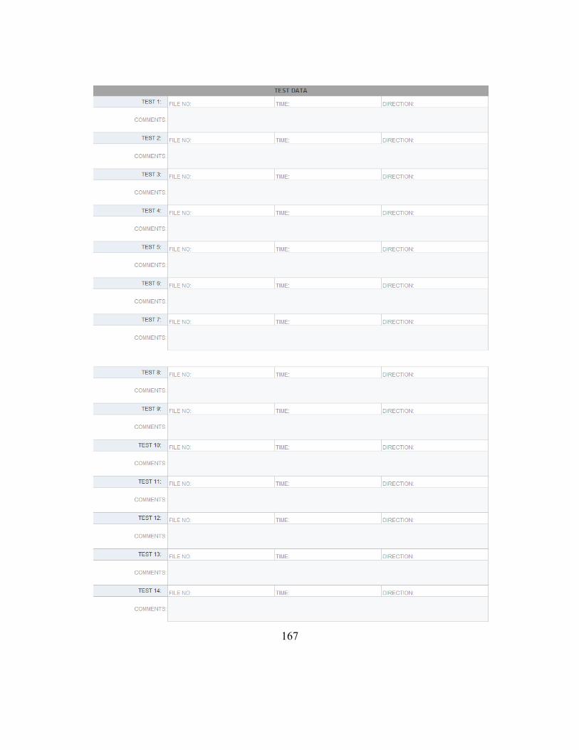
167

168

169

Appendix E: Coastdown Coefficient Calculation MATLAB Code

clear; clc; % Read coastdown data [num, txt] = xlsread('Coastdown Data.xlsx', 'Main'); effectiveMassPounds = num(1,1); % [lb] avgWindSpeed = num(2,1); % [mph] windDirection = num(3,1); % [deg] frontalArea = num(4,1); % [ft^2] avgPressure = num(5,1); % [in.Hg] avgTemperature = num(6,1); % [F] relativeHumidity = num(7,1); % [%] theta = windDirection*pi/180; % Convert degree to radians wind_X = avgWindSpeed*sin(theta); % Component of wind parallel to track [mph] wind_Y = avgWindSpeed*cos(theta); % Component of wind perpendicular to the track [mph] T0 = 68; % Standard ambient temperature [deg.F] P0 = 29; % Standard ambient pressure [in.Hg] [num, txt] = xlsread('Coastdown Data.xlsx', 'Data'); %[num] includes all Time [seconds] vs. Speed [mph] data [row, col] = size(num); for i=1 : (col/2) indice = find(isfinite(num(:,2*i-1)), 1, 'last' ); % Correction to compensate different row sizes. At num matrice MATLAB puts NaN for shorter columns. [f0(i,1), f2(i,1), RMSE(i,1)]= curveFitting (num(1:indice,2*i-1), num(1:indice,2*i), effectiveMassPounds); testName(i,1) = txt(1, 2*i-1); end % Data Acceptability Criteria #1 [testName_1, f0_1, f2_1, RMSE_1, checkResult]= criteria1 (testName, f0, f2, RMSE); if (checkResult == 0) msgbox('INVALID TEST: Criteria #1','Error','error')

170

return end % Data Acceptability Criteria 2a [testName_2a, f0_2a, f2_2a, RMSE_2a, checkResult]= criteria2a (testName_1, f0_1, f2_1, RMSE_1); if (checkResult == 0) msgbox('INVALID TEST: Criteria #2a','Error','error') return end % Data Acceptability Criteria 2b [testName_2b, f0_2b, f2_2b, RMSE_2b, checkResult]= criteria2a (testName_2a, f0_2a, f2_2a, RMSE_2a); if (checkResult == 0) msgbox('INVALID TEST: Criteria #2b','Error','error') return end % Average f0's and f2's of all remaining runs to determine an fo and f2. f0Accepted = mean(f0_2b); f2Accepted = mean(f2_2b); % Data Correction % The average f0 and f2 values must now be corrected to a standard set of % ambient constions. The standard constions are: % a. Temperature - 20 deg.C (68 deg.F) % b. Atmospheric pressure - 736.6 mm Hg (29.00 in.Hg) % c. Zero wind % d. The effect of humidity on air density may be ignored % AIR_DENSITY calculates density of air % Usage :[ro] = air_density(t,hr,p) % Inputs: t = ambient temperature (ºC) % hr = relative humidity [%] % p = ambient pressure [Pa] (1000 mb = 1e5 Pa) % Output: ro = air density [kg/m3] airDensity = air_density((avgTemperature-32)/1.8, relativeHumidity, avgPressure*3386.388158); % [kg/m^3] % SAE J1263 Equation 12

171

% Wind correction to f0 muPrime = 50*10^-6; % Velocity coefficient of rolling resistance [1/mph^2] C_DY = 3.4; % Crosswind aerodynamic drag coefficient [(ft/s)^2/mph^2] rollingResistance = (f0Accepted - f2Accepted*wind_X^2 - (0.5*airDensity*C_DY*frontalArea*wind_Y^2)*(1.94*10^-3)) / (1 - muPrime*wind_X^2); % SAE J1263 Equation 14 % Temperature correction to f0 k_t = 4.8*10^-3; % Temperature coefficient of rolling ressitance [1/deg.F] f0Prime = rollingResistance*(1 + k_t*(avgTemperature - T0)); % SAE J1263 Equation 16 % Air density correction to f2 f2Prime = (P0*(avgTemperature + 459.67)/avgPressure/(T0 + 459.67)) * (f2Accepted - muPrime*rollingResistance) + muPrime*f0Prime;

E.1 MODEL EQUATION

function speed = modelEquation (initialGuess, time) f0 = initialGuess(1); f2 = initialGuess(2); conversionFactor = 0.682; % time [seconds], effectiveMass [slugs] global initialSpeed effectiveMass % Equation 7 which is our model to represent the data from SAE J1263 speed = sqrt(f0/f2) * tan( atan( sqrt(f2/f0)*initialSpeed ) - sqrt(f0*f2)*time*conversionFactor/effectiveMass );

E.2 DATA ACCEPTABILITY CRITERIA 1

% Data Acceptability Criteria #1 % % % If the Root Mean Square Error (RMSE) exceeds 0.25 mph on any individual

172

% run, discard that run and the paired run in the opposite direction. If % less than three pairs comply with this criterion, the test run is % invalid. function [testName, f0, f2, RMSE, checkResult]= criteria1 (testName, f0, f2, RMSE) locator = find(RMSE>5); % Changed from 0.25 to 5 [row, col] = size(RMSE); for i=1 : row Result(i,1) = cellstr('OK'); end if isempty(locator) checkResult = 1; return else [row,col] = size(locator); for i=1 : row if mod(locator(i),2) % When it is an odd number delete that row and the consequitive one Result(locator(i),1) = cellstr('delete'); Result(locator(i)+1,1) = cellstr('delete'); else Result(locator(i),1) = cellstr('delete'); Result(locator(i)-1,1) = cellstr('delete'); end end for i=1 : (2*length(locator)) for j=1 : length(RMSE) if strcmp(Result(j) ,'delete') == 1 RMSE(j) = []; f0(j) = []; f2(j) = []; testName(j) = []; Result(j) = []; break end end if length(RMSE) < 6 checkResult = 0; return end end

173

end [row, col] = size(RMSE); if (row >= 6) checkResult = 1; % If less than 3 pairs comply with this criteria then [checkResult = 0], otherwise [checkResult = 1] else checkResult = 0; end

E.3 DATA ACCEPTABILITY CRITERIA 2A

function [testName, f0, f2, RMSE, checkResult]= criteria2a (testName, f0, f2, RMSE) if ( std(f0) < 2.5 || std(f0) < mean(f0)*0.5 ) % Changed from 0.05 to 0.5 checkResult = 1; return else while ( std(f0) >= 2.5 && std(f0) >= mean(f0)*0.2 ) % Changed from 0.05 to 0.2 [maxValue, row] = max(abs(f0-mean(f0))); if mod(row,2) RMSE(row) = []; RMSE(row) = []; f0(row) = []; f0(row) = []; f2(row) = []; f2(row) = []; testName(row) = []; testName(row) = []; else RMSE(row) = []; RMSE(row-1) = []; f0(row) = []; f0(row-1) = []; f2(row) = [];

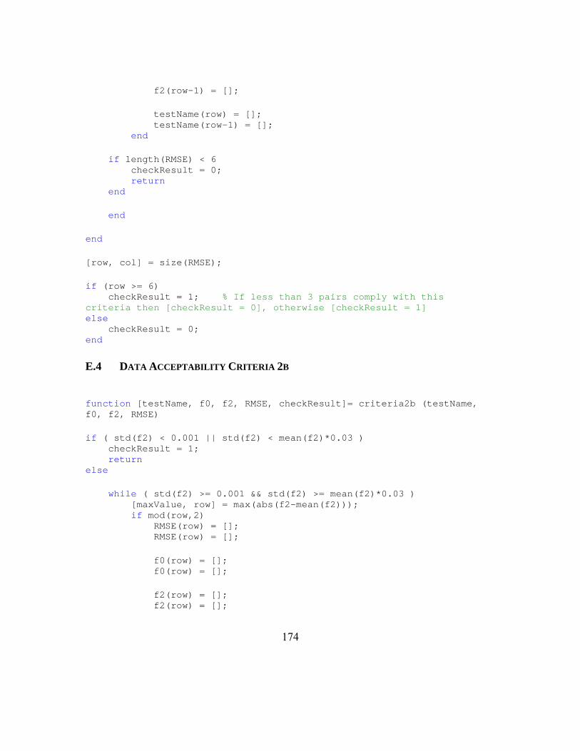
174

f2(row-1) = []; testName(row) = []; testName(row-1) = []; end if length(RMSE) < 6 checkResult = 0; return end end end [row, col] = size(RMSE); if (row >= 6) checkResult = 1; % If less than 3 pairs comply with this criteria then [checkResult = 0], otherwise [checkResult = 1] else checkResult = 0; end

E.4 DATA ACCEPTABILITY CRITERIA 2B

function [testName, f0, f2, RMSE, checkResult]= criteria2b (testName, f0, f2, RMSE) if ( std(f2) < 0.001 || std(f2) < mean(f2)*0.03 ) checkResult = 1; return else while ( std(f2) >= 0.001 && std(f2) >= mean(f2)*0.03 ) [maxValue, row] = max(abs(f2-mean(f2))); if mod(row,2) RMSE(row) = []; RMSE(row) = []; f0(row) = []; f0(row) = []; f2(row) = []; f2(row) = [];

175

testName(row) = []; testName(row) = []; else RMSE(row) = []; RMSE(row-1) = []; f0(row) = []; f0(row-1) = []; f2(row) = []; f2(row-1) = []; testName(row) = []; testName(row-1) = []; end if length(RMSE) < 6 checkResult = 0; return end end end [row, col] = size(RMSE); if (row >= 6) checkResult = 1; % If less than 3 pairs comply with this criteria then [checkResult = 0], otherwise [checkResult = 1] else checkResult = 0; end

E.5 AIR DENSITY CALCULATION

function [ro] = air_density(t,hr,p) % AIR_DENSITY calculates density of air % Usage :[ro] = air_density(t,hr,p) % Inputs: t = ambient temperature (ºC) % hr = relative humidity [%] % p = ambient pressure [Pa] (1000 mb = 1e5 Pa) % Output: ro = air density [kg/m3] % % Refs:

176

% 1)'Equation for the Determination of the Density of Moist Air' P. Giacomo Metrologia 18, 33-40 (1982) % 2)'Equation for the Determination of the Density of Moist Air' R. S. Davis Metrologia 29, 67-70 (1992) % % ver 1.0 06/10/2006 Jose Luis Prego Borges (Sensor & System Group, Universitat Politecnica de Catalunya) % ver 1.1 05-Feb-2007 Richard Signell (rsignell@usgs.gov) Vectorized %------------------------------------------------------------------------- T0 = 273.16; % Triple point of water (aprox. 0ºC) T = T0 + t; % Ambient temperature in ºKelvin %------------------------------------------------------------------------- %------------------------------------------------------------------------- % 1) Coefficients values R = 8.314510; % Molar ideal gas constant [J/(mol.ºK)] Mv = 18.015*10^-3; % Molar mass of water vapour [kg/mol] Ma = 28.9635*10^-3; % Molar mass of dry air [kg/mol] A = 1.2378847*10^-5; % [ºK^-2] B = -1.9121316*10^-2; % [ºK^-1] C = 33.93711047; % D = -6.3431645*10^3; % [ºK] a0 = 1.58123*10^-6; % [ºK/Pa] a1 = -2.9331*10^-8; % [1/Pa] a2 = 1.1043*10^-10; % [1/(ºK.Pa)] b0 = 5.707*10^-6; % [ºK/Pa] b1 = -2.051*10^-8; % [1/Pa] c0 = 1.9898*10^-4; % [ºK/Pa] c1 = -2.376*10^-6; % [1/Pa] d = 1.83*10^-11; % [ºK^2/Pa^2] e = -0.765*10^-8; % [ºK^2/Pa^2] %------------------------------------------------------------------------- % 2) Calculation of the saturation vapour pressure at ambient temperature, in [Pa] psv = exp(A.*(T.^2) + B.*T + C + D./T); % [Pa] %-------------------------------------------------------------------------

177

% 3) Calculation of the enhancement factor at ambient temperature and pressure fpt = 1.00062 + (3.14*10^-8)*p + (5.6*10^-7)*(t.^2); %------------------------------------------------------------------------- % 4) Calculation of the mole fraction of water vapour xv = hr.*fpt.*psv.*(1./p)*(10^-2); %------------------------------------------------------------------------- % 5) Calculation of the compressibility factor of air Z = 1 - ((p./T).*(a0 + a1*t + a2*(t.^2) + (b0+b1*t).*xv + (c0+c1*t).*(xv.^2))) + ((p.^2/T.^2).*(d + e.*(xv.^2))); %------------------------------------------------------------------------- % 6) Final calculation of the air density in [kg/m^3] ro = (p.*Ma./(Z.*R.*T)).*(1 - xv.*(1-Mv./Ma));

178

References

Matthews, R. D. (2007), “Internal Combustion Engines and Automotive Engineering”, Spring ed. Austin: The University of Texas at Austin Co-op Press.

Heywood, J. B. (1988), “Internal Combustion Engine Fundamentals”, International ed. Singapore: McGraw Hill.

Obert, E. F. (1973), “Internal Combustion Engines and Air Pollution”, New York: Harper & Row.

http://www.fueleconomy.gov/feg/emissions/GHGemissions.htm.

http://en.wikipedia.org/wiki/Dynamometer.

Environmental Protection Agency December 2006. Fuel Economy Labeling of Motor Vehicles: Revision to Improve Calculation of Fuel Economy Estimates. (http://www.epa.gov/fueleconomy/420r06017.pdf): EPA420-R-06-017.

Environmental Protection Agency December 27, 2006. 40 CFR Parts 86 and 600 Fuel Economy Labeling of Motor Vehicles: Revision to Improve Calculation of Fuel Economy Estimates; Final Rule. (http://www.epa.gov/fedrgstr/EPA-AIR/2006/December/Day-27/a9749.pdf): Federal Register / Vol. 71, No. 248 / Wednesday, December 27, 2006 / Rules and Regulations.

http://www.epa.gov/fueleconomy/420f06069.htm.

http://www.dieselnet.com/standards/us/ld_t2.php.

http://www.fueleconomy.gov/FEG/info.shtml#sizeclasses.

http://www.epa.gov/otaq/crttst.htm.

Sierra Research, Inc. 2000. I/M Lookup Table Update. Report No. SR00-10-01 prepared for: U.S. Environmental Protection Agency Transportation and Regional Programs, October 3, 2000.

G. & C. Merriam Company (1971), “Webster’s Seventh New Collegiate Dictionary”, Springfield, Massachusetts: The Lakeside Press

http://www.answers.com/topic/internal-combustion-engine.

http://en.wikipedia.org/wiki/Four_stroke.

SAE J1263: Surface Vehicle Recommended Practice “Road Load Measurement and Dynamometer Simulation Using Coastdown Techniques”; 1996.

179

White, R.A., and H.H. Korst (1972), “The Determination of Vehicle Drag Contributions from Coast-Down Tests”, SAE Technical Paper 720099.

Yasin, T.P. (1978), “Analytical Basis of Automobile Coastdown Testing”, SAE Technical Paper 780334.

Regner, G., E. Loibner, J. Krammer, L. Walter, and R. Truemner (2002), “Analysis of Transient Drive Cycles using CRUISE-BOOST Co-Simulation Technique”, SAE Technical Paper 2002-01-0627.

LaClair, T.J., and R. Truemner (2005), “Modeling of Fuel Consumption for Heavy-Duty Trucks and the Impact of Tire Rolling Resistance”, SAE Technical Paper 2005-01-3550.

Korst, H.H., R.A. White, and D. Metz (2007), “Road Evaluation of the Aerodynamic Characteristics of Heavy Trucks”, SAE Technical Paper 2007-01-4297.

Woschni G. (1967), “A Universally Applicable Equation for the Instantaneous Heat Transfer Coefficient in the Internal Combustion Engine”, SAE Technical Paper 670931.

http://www.avl.com/wo/webobsession.servlet.go?app=bcms&page=view&nodeid=400013015.

AVL ADVISOR User Guide.

AVL CRUISE User Guide.

AVL BOOST User Guide.

Texas Department of Transportation (2008), “Estimating Texas Motor Vehicle Operating Costs – Exhibit B”, Project No. 0-5974.

180

Vita

Murat Ates was born in Antalya, Turkey on February 15, 1982, the son of

Abdullah and Zeynep Ates. After the primary school he got through the Anatolian High

School Exam and entered to Metin-Nuran Cakallikli Anatolian High School where

education language is English. In 2001 he entered to Middle East Technical University

(METU), Mechanical Engineering Department by being in top 1% in the Turkish

University Entrance Exam. He graduated with honor roll from METU in 2006 by

receiving his Bachelor of Science degree and in the same year he was admitted to the

University of Texas at Austin, Mechanical Engineering Department as a Master’s

student.

He received a five years scholarship from one of Turkey’s biggest company

Sabanci Holding during his undergraduate studies. Moreover he completed internships at

Fiat-GM Powertrain and Procter & Gamble, which gave him opportunity to work in a

global diverse environment.

He is admitted to the University of Texas at Austin, Mechanical Engineering

Department as a PhD candidate. He is looking forward to get his doctoral degree by

2012.

Permanent address: Yuksekalan M. 489. S. Sofular A. N:1 D:10

07040 Antalya / TURKEY

This thesis was typed by Murat Ates.