Ibero-Amerika Institut für Wirtschaftsforschung Instituto Ibero-Americano de Investigaciones Económicas

Ibero-America Institute for Economic Research (IAI)

Georg-August-Universität Göttingen

(founded in 1737)

Nr. 201

Freight Rates and the Margins of Intra-Latin American Maritime Trade

Inmaculada Martínez-Zarzoso, Gordon Wilmsmeier

January 2010

Diskussionsbeiträge · Documentos de Trabajo · Discussion Papers

Platz der Göttinger Sieben 3 ⋅ 37073 Goettingen ⋅ Germany ⋅ Phone: +49-(0)551-398172 ⋅ Fax: +49-(0)551-398173

e-mail: uwia@gwdg.de ⋅ http://www.iai.wiwi.uni-goettingen.de

1

FREIGHT RATES AND THE MARGINS OF INTRA-LATIN AMERICAN

MARITIME TRADE

Inmaculada MARTÍNEZ ZARZOSO*

Universidad Jaume I, Spain and Georg-August Universitaet

Platz Der Goettinger Sieben 3, Goettingen, Germany

martinei@eco.uji.es

Gordon WILMSMEIER

Transport Research Institute

Edinburgh Napier University, Edinburgh, UK

G.Wilmsmeier@napier.ac.uk>

*We would like to thank two anonymous referees and the participants in the IAME conference and the 4th Kuhmo-Nectar, both held in Copenhagen, for the very helpful comments and suggestions received. Financial support from both the Spanish Ministry of Public Works and the Spanish Ministry of Science and Technology is gratefully acknowledged (P21/08 and SEJ 2007-67548).

2

FREIGHT RATES AND THE MARGINS OF INTRA-LATIN AMERICAN

MARITIME TRADE

ABSTRACT

This paper focuses on the analysis of the relationship between maritime trade and transport cost in Latin

America. The data available are disaggregated (SITC 5 digit level) maritime trade flows on trade routes

within Latin America over the period 1999-2004. The contribution to the literature is to disentangle the

effects that transport costs have on the extensive margin (number of products imported) and the intensive

margin (quantity imported of each product) of international trade in order to test some of the predictions of

the trade theories that introduce firm heterogeneity in productivity, as well as fixed costs of exporting.

Recent investigations show that spatial frictions (distance) reduce trade mainly by reducing the number of

shipments and that most firms ship only to geographically proximate customers, instead of shipping to

many destinations in quantities that decrease in distance. Our findings confirm this result for intra-LA trade

and show that the opposite pattern is observed for ad-valorem freight rates that reduce aggregate trade

values mainly by reducing the quantity imported (intensive margin).

KEYWORDS: Transport costs; Maritime trade; Latin America; Sectoral data;

Competitiveness

JEL CODES: F10

1. INTRODUCTION

How does trade cost affect countries’ ability to participate in the global economy

and what impact do changes in the cost of trade have on a country’s trade and real

income? This paper is devoted to partially answer these questions. While the gains from

trade are widely accepted, less is known about the magnitude of the penalty faced by

countries for which trade is costly. Reducing trade costs has direct and indirect benefits; it

promotes trade and also leads to industrial restructuration in the economy; higher

specialisation, and changes in factor prices and real income. How do these effects operate,

and how large might they be?

The relationship between international trade and transport costs is usually

estimated as part of a gravity model of trade, which relates bilateral trade flows to the

3

income and population of trading partners and the geographical distance between them.

Recent research has been concerned with the use of more accurate proxies for transport

costs, like freight rates, infrastructure or customs procedures. In this line, Limao and

Venables (2001) analyse empirically the dependency of trade and transport costs on

geographical and infrastructural variables and estimate an elasticity of trade with respect

to transport costs in the range 2-5. More recently, Martínez-Zarzoso and Suárez-Burguet

(2005) and Martínez-Zarzoso et al. (2007) found similar results using disaggregated data.

The theoretical models used to generate the gravity equation usually assume

homogeneous firms within a country and consumer love of variety. These two

assumptions imply that all products are traded to all destinations. However, empirical

observation indicates that few firms export and exporting firms commonly sell in a

limited number of countries. This empirical fact has led to the development of the so-

called new-new trade theories based on firm heterogeneity in productivity and fixed cost

of exporting (Melitz, 2003). These new theories predict the existence of a productivity

threshold for each country that firms have to exceed in order to become exporters. As a

result two margins of trade emerge: The number of unique shipments (extensive margin)

and the average value of shipments (intensive margin).

In marked contrast with previous studies for maritime trade, we decompose total

trade into extensive margin and intensive margin in order to shed light on why trade costs

matter for trade, isolating which component of trade they most affect. We find that the

number of unique shipments between origin and destination pairs does co-vary with

distance. It is also worth noting that once freight rates are added as an explanatory

variable of each trade margin, distance still explains both of them. This result confirms

that the distance variable captures other barriers to bilateral trade different from transport

costs such as information costs, business networks and cultural barriers.

4

Some recent studies have found that distance is imperfectly correlated with

transport costs. In light of these findings, a number of investigations have underlined the

importance of obtaining better data on transport costs. Clark (2007) and Martinez-

Zarzoso and Nowak-Lehmann (2007) find that distance is a poor proxy for transport

costs. Distance may be a proxy for other types of trade costs and has the advantage of

being truly exogenous of the volume of trade in goods.

Evidence that suggests that transport costs are only vaguely related to distance

should not be confused with the finding that distance is correlated with trade flows.

Hilberry and Hummels (2008) note that roughly a quarter of world trade takes place

between countries sharing a common border and half of world trade occurs between

partners less than 3000 kilometres apart. It is not clear however whether the effect of

distance on trade volumes can be ascribed to transport costs or to other trade determinants

such as historical ties, cultural proximity or business networks.

We use import values and volumes and freight rates from the International

Transport Database (BTI) from UNECLAC1. Our dataset compiles information on import

and export of countries2 in Latin America and the Caribbean, representing a total of 277

maritime trade routes over a period of six years (1999-2004). Since the data represent

individual shipments and contains precisely defined origin-destination detail for those

shipments, we are able to decompose bilateral trade values into extensive and intensive

margin and to investigate how well the variability of each margin is explained by freight

rates. We can also observe the evolution over time of the number of commodities shipped

and the number of origins from which the commodities are imported. Whereas the

number of commodities shipped increase over time, the number of origins from which

products are shipped is relatively stable over the years.

1 United Nations Economic Commission for Latin America and the Caribbean. 2 Importers: Argentina, Bolivia, Brazil, Chile, Colombia, Ecuador, Peru, Uruguay and Venezuela. Exporters: Anguila, Antigua and Barbuda, Argentina, Aruba, Bahamas, Barbados, Belize, Bermuda, Bolivia, Brazil, Chile, Colombia, Costa Rica, Cuba, Dominica, Dominican Republic, Ecuador, El Salvador, French Guiana, Grenada,Guatemala, Guyana, Honduras, Jamaica, Mexico, Nicaragua, Panama, Paraguay, Peru, Puerto Rico, Suriname, Trinidad and Tobago, Uruguay and Venezuela.

5

This paper contributes to the existent literature in several respects. Unlike previous

work, we decompose intra-Latin American maritime trade flows into multiple

components in an effort to study what margins of trade freight rates act upon. Also, we

are able to compare the effect of distance with the effect of freights and to show that

spatial frictions are not as relevant in explaining maritime trade in comparison to total

trade.

Section 2 presents the methodology to decompose shipments into several

components and the main hypotheses to be tested. Section 3 describes the data and

Section 4 shows the main results. Finally, Section 5 concludes.

2. DECOMPOSING MARITIME TRADE AND MAIN HYPOTESIS

In the related literature, the effect transport costs on trade has been commonly

analysed using a gravity model of trade, with the dependent variable being the aggregate/

disaggregate value of trade between two countries. Some recent studies for aggregated

trade are Sánchez, Hoffmann, Micco, Pizzolitto, Sgut and Wilmsmeier (2003), Martinez-

Zarzoso and Suarez-Burguet (2005) and Limao and Venables (2001) and for

disaggregated trade Martínez-Zarzoso, García-Menendez and Suárez-Burguet (2003) and

Martinez-Zarzoso (2009). This approach relies on a model that assumes iceberg trade

costs3 and symmetric firms. In this setting, aggregated trade values react to trade cost in

exactly the same way as firm-level quantities and consumers buy positive quantities of all

varieties.

In this context we can express the quantity of a variety from origin country i to

destination country j (qij) as

3 Iceberg trade costs mean that for each good that is exported a certain fraction melts away during the trip as if an iceberg were shipped across the ocean.

6

( )⎟⎟⎠

⎞⎜⎜⎝

⎛=

−

j

ijijij P

tpEq ~

σ

(1)

where Ej denotes country j’s total expenditure on the differentiated product, (pitij)

is the price of product i at destination j, this prices varies across destinations due to

positive iceberg transport costs, tij. ( )∑ −=i

ijij tpP )1(~ σ is a price index and σ is the

elasticity of substitution, which is constant across varieties4 (CES)5.

Since the quantity traded of each variety is in most cases not observable, adding

two assumptions: All varieties in the origin are symmetric and the destinations will

consume all the varieties in equal quantity, will allow us to multiply quantity per variety

(qij) by prices (pi) and by the number of varieties (ni ) to obtain total trade values. The

outcome is

( )⎟⎟⎠

⎞⎜⎜⎝

⎛==

−

j

ijiiijijiiij P

tppnEqpnT ~

σ

(2)

In equation (2) quantity per variety is the only component of Tij that has bilateral

variation. As in Hillberry and Hummels (2008), with our dataset we are able to examine

each of the components of total trade values in a more flexible way since not only

quantities, but also prices and the number of varieties vary across origin and destinations.

This could be the case when some of the assumptions above are relaxed. Prices may vary

across destinations if the elasticity of substitution is not constant or if transport costs are

not iceberg (Hummels and Skiba, 2004). Therefore for a given year t:

4 Varieties refer to different products that are substitutes in consumption. 5 The constant elasticity of substitution (CES) assumption is made in order to obtain a simple model that is easily derived and with testable implications.

7

ijijijij qpnT = (3)

At least three reasons have been suggested in the literature to explain why the

number of traded varieties might vary with trade cost. First, goods produced in different

locations (origin and destination) could be homogeneous. In this case, if production costs

in origin and destination are very similar or the trade costs are sufficiently large, these

goods will not be traded. Also, the higher freight costs are, the more likely products are to

be non-traded goods. Second, if goods are differentiated by country of origin, each

country producing a different variety has to incur in a fixed cost to sell the product in each

destination country. Therefore, not all the varieties will be shipped to each destination and

the number of varieties traded will depend negatively on the size of this fixed trade costs.

Finally, the reason could be that not all varieties are consumer goods. Intermediated

inputs that are used in the production of final goods would only be exporter to destination

j if country j produces the final good. Due to “just on time” production processes

intermediates are usually traded along short distances.

The methodology we use to decompose aggregate value of trade into its various

components is based on Hillberry and Hummels (2008). Unique shipments are indexed by

s and the total value of shipments from country i to country j is given by

∑=

=ijN

s

sij

sijij QPT

1 (4)

where Nij is the number of unique shipments (extensive margin of trade) and ijPQ

is the average value per shipment (the intensive margin). Hence, total trade value is

decomposed first into extensive and intensive margin

8

ijijij QPNT = (5)

where ( )

ij

sij

N

ss

ijij N

QPQP

ij∑ == 1

Since there can be multiple unique shipments within an origin-destination country

pair, the number of shipments can be further decomposed into the number of distinct

SITC goods shipped, Nijk, and the number of average shipments between a country of

origin and a destination country, NijF. Nij

F>1 means that we observe more than 1 unique

shipment per commodity travelling from country i to country j.

Fij

kij NNN

ij= (6)

The average value per shipment can also be further decomposed into average price

and average quantity per shipment

( ) ( )ijij

ij

N

s ijN

s ij

N

ssij

sij

ij QPN

Q

Q

QPQP

ij

ij

ij

== ∑∑∑ =

=

= 1

1

1 (7)

By substituting equations (6) and (7) into (5) we can decompose total trade

between two countries into four different components

ijijFij

kij QPNNT

ij= (8)

The units to measure quantities are tons for all commodities. Using a common unit

allow us to aggregate over different products and compare prices (import unit values)

across all commodities.

9

We now have two decomposition levels, the first given by equation (5)

decomposes total trade value into number of products traded and average value per

product and the second, given by equation (8) decompose further these two components

into another two each: the number of distinct SITC goods shipped, the number of average

shipments between a country of origin and a destination country, average price and

average quantity. Taking logs for the first and second level decompositions and adding

the time dimension, t:

ijtijtijt QPNT lnlnln += (9)

ijtijtFijt

kijt QPNNT

ijtlnlnlnlnln +++= (10)

Next we began to analyze how each of the components of equation (10) co-varies

with distance and with other trade-related costs. Before we specify the empirical model,

we state a number of hypotheses that are based on recent theories of international trade

under imperfect competition and heterogeneous firms. One of the starting points of these

theories was Melitz (2003) who introduced firm heterogeneity and fixed costs in a general

equilibrium model of international trade. Chaney (2008) extended Melitz’s model to

multiple countries with asymmetric trade barriers and derives three predictions for

aggregated trade:

First, for aggregated bilateral trade flows the model predicts that the elasticity of

exports with respect to trade barriers is larger than in the absence of firm heterogeneity

and larger than the elasticity for each individual firm. A reduction on variable cost has

two effects: it increases the size of exports of each exporter and it also allows some new

10

firms to enter the market. Therefore, the extensive margin amplifies the impact of variable

costs.

Second, in more homogeneous sectors aggregated exports are very sensitive to

changes in transportation costs because many firms enter and exit when variable costs

changes.

Third, the elasticity of exports with respect to variable costs does not depend on

the elasticity of substitution between goods, whereas the elasticity of exports with respect

to fixed costs is negatively related to the elasticity of substitution, in contrast with models

with representative firms, according to which the elasticity of exports with respect to

transport costs equals the elasticity of substitution minus one.

Finally, with respect to the two margins of trade, Chaney (2008) shows that in the

presence of firm heterogeneity, the extensive margin and the intensive margin are affected

in different directions by the elasticity of substitution. The impact of trade barriers is

strong in the intensive margin for high elasticities of substitution, whereas the impact is

mild on the extensive margin. The author proves that the dampening effect of the

extensive margin dominates the magnifying effect of the intensive margin.

We are interested to know if these predictions hold for maritime trade flows in

Latin America. In order to test some of the abovementioned predictions, the estimating

equation takes the following form:

ijkttkijjtitjtitjiijkt DPOPPOPGPDGDPM ελγαααααβα +++++++++= lnlnlnlnlnln 54321

(11)

were γk and λt are industry and year fixed effects and αi and βj are importer and

exporter fixed effects. εijkt is an error term and ln(Mijkt) is in turn the log of total imports

and each of its components: the log of average value per shipment (intensive margin), and

the log of the number of shipments (extensive margin), as described in equation (9). Since

11

OLS is linear, the coefficient on total imports will be equal to the sum of the coefficients

on the two margins. A further decomposition can be done, using as dependent variable in

equation (11) each of the components of equation (10). Some summary statistics of our

data are presented in Table 1.

3. DATA DESCRIPTION

The main data source we use is the raw data files from the BTI (International

Transport Database) dataset from UNECLAC that gives information on the actual freight

rates per ton paid for the export of a certain good between countries i and j excluding

loading costs.

The international transport database covers annual trade and transport statistics of

eleven Latin American countries - Argentina, Bolivia, Brazil, Chile, Colombia, Ecuador,

Mexico, Paraguay, Peru, Uruguay, and Venezuela. The BTI is maintained by ECLAC's

Transport Unit. It covers annual trade and transport statistics of each country and contains

detailed information about the value and volume of imports and exports. It also includes

information about the use of different transport modes, the costs of international freight

and insurance, and the traded commodities. Data is for the years 1999-2004, and grouped

by the Standard International Trade Classification (SITC) codes. Country data are

processed by national customs services and due to the large quantity of data, it is possible

to formulate detailed queries, combining the different fields of information covered by the

database. Income and population data are from the World Development Indicators

Database 2008 and distance is from CEPII6.

Table 1 in the Appendix shows the split between pure freight rates and insurance

costs by importer. Insurance cost in ad-valorem terms is the highest for Argentina, it

6 http://www.cepii.fr/anglaisgraph/bdd/distances.htm.

12

represents a 13 percent of total cif-fob costs (freight + insurance) and Venezuela (8.6

percent) and it is the lowest for Brazil (0.55 percent).

4. MAIN RESULTS

First we present some results for the decomposition of trade flows in Table 2.

Argentina, followed by Brazil, shows the highest total import value. We observe the

highest average number of shipments for Colombia and the lowest for Bolivia, whereas in

terms of average value shipped Mexico shows the highest value and Bolivia, once more,

the lowest.

Table 3 presents the results of testing model (1) using distance as a proxy for

transport costs and Table 4 adds freight rates as an additional explanatory variable.

The dependent variable in the first column in Table 3 is total imported value,

whereas in the following columns each of the components of equation (10) is used as

dependent variable. The coefficients of the gravity equation have the expected sign. GDP

has a significant positive effect on both, the volume exported by firms and the number of

exporters. Distance has a negative estimate for most of the components. Only the average

price shows a positive distance coefficient. Increases in shipment distance correspond to

increases in average price per ton. A similar result was obtained by Hillberry and

Hummels (2008).

The decomposition of the influence of distance on trade shows a greater effect on

the extensive margin (column 2 of Table 3), for all products and for our sample. About

71% of the distance effect on trade works through the extensive margin (i.e.

0.399/(0.399+0.163)); 29% of the increase in aggregate trade flows comes from larger

average shipments. Previous research finds similar results, with the extensive margin

being more important than the intensive margin (Hillberry and Hummels, 2008; Mayer

and Ottaviano, 2008). Our results are closer to Mayer and Ottaviano (2008), who analyze

13

French and Belgian individual export flows and show that 75% of the distance effect on

trade comes from the extensive margin.

Turning to the second level decomposition of equation (11), on the one hand we

see that the decline in number of shipments over space come entirely from the second

component (Nijf), proximate geographic countries see a larger number of unique

shipments per commodity, whereas the number of commodities shipped between

countries (Nijk in column 4 of Table 3) does not seem to vary with distance. On the other

hand, the components of average value per shipment (columns 6 and 7 in Table 3) change

with distance in opposite direction. Increases in shipment distance correspond to increases

in average prices per ton and decreases in average quantities shipped. The more plausible

explanation is related to trade composition: goods with low value to weight are imported

from closer locations than goods with high value to weight ratios.

Table 4 shows the decomposition of the influence of ad-valorem transport costs on

maritime trade. The effect is lower on the extensive margin (column 2), for all products

and for our sample. Around 29% of the trade cost effect on trade works through the

extensive margin, whereas 71% of the variation in aggregate trade works through the

intensive margin (column 3). Hence, shipping costs seems to affect to a higher extent the

intensive margin, which is in accordance with the theoretical prediction that states that

changes in variable costs mainly affect the intensive margin of trade (Chaney, 2008). It is

widely recognized that shipping costs decrease with higher values traded and hence can

be considered as variable costs of trade.

To our knowledge, this is the first paper that evaluates the effect of maritime

transport costs on the two margins of trade. Previous research finds similar results for the

effect on total import values. Our results are close to those found in a recent study done

by Korinek (2009). The results in her study indicate that, for a broad sample of countries,

14

a 10% increase in shipping costs is associated with a 3% drop in trade. In our sample a

10% increase in shipping costs is associated with a 2.4% drop in trade.

Turning to the second level decomposition of equation (11), on the one hand we

see that the decline in number of unique shipments due to higher shipping costs come

entirely from the first component (Nijk). Model 4 (Table 3) shows that the number of

commodities shipped between countries decreases when shipping costs are higher,

whereas the number of unique shipments per commodity (Nijf) plays no role (Column 5).

On the other hand, results in Models 6 and 7 show that the components of average value

per shipment change with shipping costs in the same direction. Increases in shipment

costs are associated to decreases in average quantities shipped and in average prices per

ton. 87% of the variation in average imported value works trough changes in average

prices per ton, whereas only 13% works trough changes in average quantities shipped.

With respect to the previous results found in Table 3 for spatial frictions, the main

pattern remains unchanged, the only difference is that adding shipping costs slightly

reduces the estimated coefficient for distance and that the percentage of variation in

distance explained through the extensive margin of maritime trade increases from 71

percent to 77 percent.

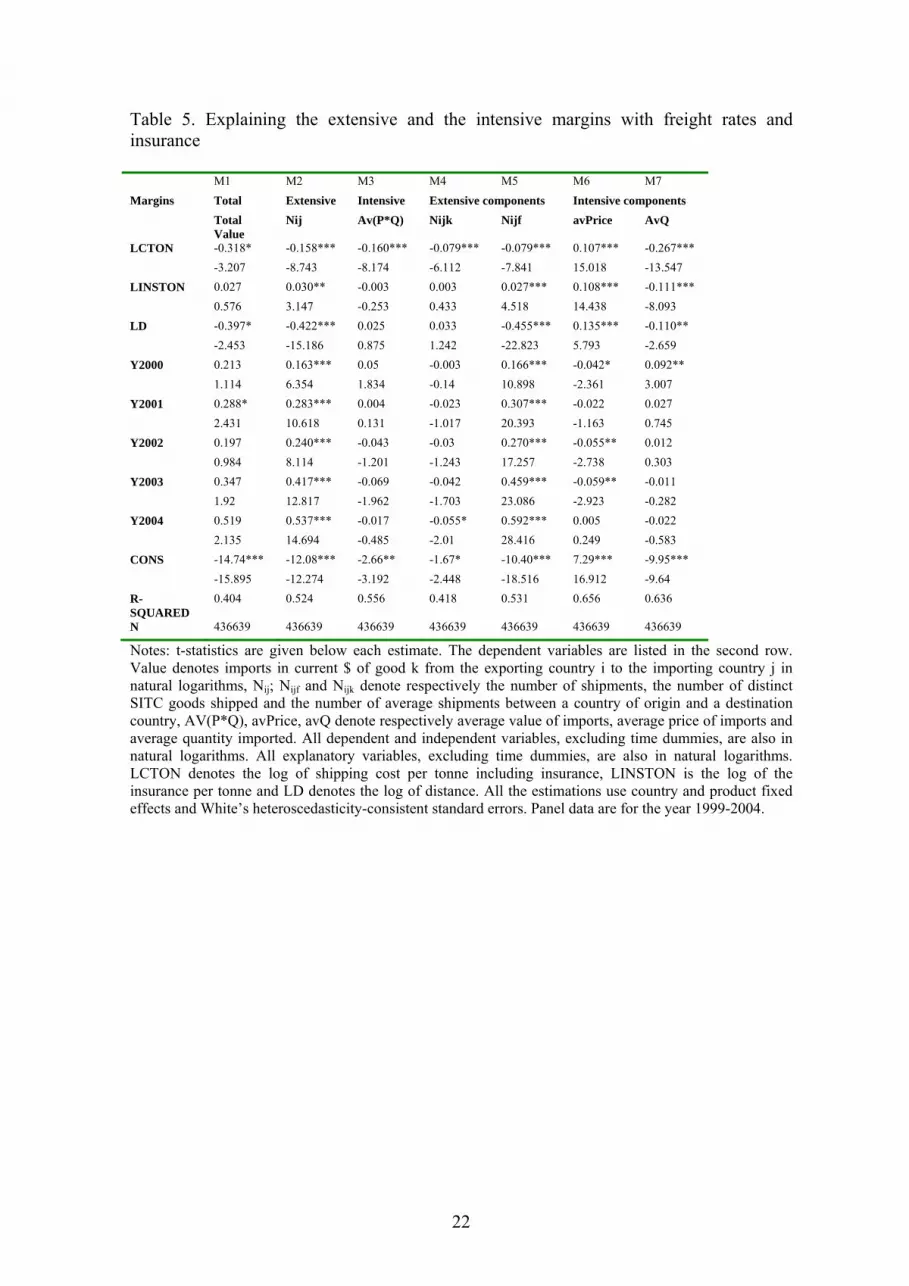
Shipping costs can also be decomposed into insurance and pure freight and we use

this decomposition to test some of the predictions outlined before with respect to fix and

variable trade costs. The results are presented in Table 5. In this case we are using

transport cost per tonne and insurance paid per tonne shipped. In this specification the

effect of transport costs on the two margins of trade is more evenly distributed (50% of

the variation of total imports is explained through the extensive margin and 50% through

the intensive margin) and the effect of distance works completely through the extensive

margin and does not affect the intensive margin. With respect to insurance, the effect on

15

each margin goes in opposite direction: a higher insurance per tonne increases the number

of unique shipments and slightly reduces the average value of the shipments.

Turning to the second level decomposition of equation (11), on the one hand we

see that the increase in number of shipments due to a higher insurance cost come entirely

from the second component (Nijf), higher insurance costs is associated to a larger number

of unique shipments per commodity, whereas the number of commodities shipped

between countries does not seem to vary with insurance cost. On the other hand, the

components of average value per shipment change with shipping costs in opposite

directions and they almost compensate each other. Increases in insurance cost are

associated to decreases in average quantities shipped and to increases in average prices

per ton. 50% of the absolute variation in average imported value works trough each

channel. The explanation could be related, once again, to trade composition: goods with

low value to weight pay a lower insurance than goods with high value to weight ratios.

Finally, Table 6 present separated results by three product categories: Agriculture,

raw materials and manufactures. Whereas the results for manufactures are very similar to

those found for all products (Table and 4), interesting differences are found for

agriculture and raw materials.

First, when the sample is restricted to agriculture and raw materials the total value

of imports does not depend on distance, whereas shipping cost presents a higher estimated

coefficient that for raw materials is almost double than the one found for manufactures.

Turning to the second level decomposition of equation (11), on the one hand we

see that the decline in number of shipments over space come entirely from the second

component (Nijf) only for manufactures, proximate geographic countries see a larger

number of unique shipments per commodity, whereas for agricultural products and raw

materials the number of commodities shipped between countries does seem to increase

with distance. On the other hand, the components of average value per shipment change

16

with distance in opposite direction only for manufactures. Increases in shipment distance

correspond to increases in average prices per ton and decreases in average quantities

shipped. However, for raw materials and agriculture only the average price increases with

distance, whereas the average quantity does not co-vary with spatial frictions.

With respect to shipping costs, we also observe a different pattern for agriculture

and raw materials as compared with manufactures. The effect of a reduction in shipping

costs on trade comes through both margins for the former, whereas for the latter it mainly

works through the intensive margin.

As a robustness check, and in line with some previous findings (Martínez-Zarzoso

and Nowak-Lehman, 2007), we consider a non-linear relationship between distance and

the trade margins. The results are presented in Appendix 2. While for total value exported

the coefficient of squared distance is not statistically significant from zero, we find an

inverted U-shaped relationship between distance and the number of shipments, between

distance and the average value shipped and between distance and the average quantity

shipped. Therefore, the number of goods shipped increase with distance for shorter

distances and then decreases. The turning point corresponds to a distance of 563

kilometres (the minimum distance in our sample is between Argentina and Uruguay, 215

km and the maximum 2854 km). The average quantity shipped increase only for distances

lower than 702 km, whereas the average value imported increases with distances lower

than 1252 km and then decreases. Further research is needed to explain these findings, a

possible explanation can be found by considering the type of products shipped.

5. CONCLUSIONS

This paper focuses on the analysis of the relationship between maritime trade and

transport costs in Latin America. According to new theories of international trade with

imperfect competition and heterogeneous firms, lower trade costs increases bilateral trade

17

through an increase of both margins of trade: The number of exporting firms (extensive

margin) and the average value of imports (intensive margin). We use highly

disaggregated trade data to decompose intra-LA imports into these two components to

shed some light on why trade costs matter for trade. Several new findings are derived.

First, about 77 percent of the distance effect on trade works through the extensive margin,

indicating that the number of shipments sharply decreases with distance. Spatial frictions

are less relevant for the intensive margin, with only 23 percent of the distance effect

working through this margin. Second, the opposite pattern is observed for ad-valorem

freight rates: only 29 percent of its effect on trade works through the extensive margin,

whereas 71 percent is attributable to the intensive margin.

Finally, the main results hold for manufactures, but change for agriculture and raw

materials, especially with respect to spatial frictions, that are much less relevant for these

categories of goods.

18

Table 1. Summary statistics VARIABLE Obs Mean Std. Dev. Min Max LTCIF 897652 13.735 2.230 0.000 19.328 LNIJ 897652 4.004 1.509 0.000 7.301 LNIJF 897652 4.367 1.156 0.000 6.309 LNIJK 897652 -0.363 0.980 -6.309 1.453 LAVCIF 897652 9.731 1.737 0.000 17.488 LAVP 897652 7.957 1.076 -1.955 19.058 LAVQ 897652 1.774 2.058 -6.908 11.541 LCIFOB 689121 -2.911 1.062 -14.202 9.079 LD 896980 7.700 0.769 5.371 8.971 LIGDP 897652 8.115 0.327 6.918 8.897 LEGDP 860986 8.389 0.330 6.109 9.521 LIPOPU 897652 17.381 0.888 15.058 19.043 LEPOPU 860986 16.861 1.664 11.184 19.043

Note: where L denote natural logs, TCIF denote the value of bilateral imports ($), NIJ; NIJF AND NIJK denote respectively the number of shipments, the number of distinct SITC goods shipped and the number of average shipments between a country of origin and a destination country, AVCIF, AVP, AVQ denote respectively average value of imports, average price of imports and average quantity imported. CIFOB refers to the ad-valorem transport cost, IGDP and EGDP are GDP of the importer and the exporter country respectively and IPOPU and EPOPU refer to populations in origin and destination.

19

Table 2. The extensive and the intensive margins of Latin American maritime trade flows

Var. Means Value Nij Average Value Argentina 9705055 106.701 117584.3 Bolivia 41808.58 10.307 6510.563 Brazil 6152345 104.636 102297.9 Chile 2186648 35.161 86494.24 Colombia 3625897 255.318 41095.26 Ecuador 3685330 126.920 35877.6 Mexico 5241092 18.884 278440.5 Peru 2447187 35.246 102030.2 Uruguay 206142.1 13.263 29462.56 Venezuela 3993809 146.725 51066.9

20

Table 3. Explaining the extensive and the intensive margins with distance M1 M2 M3 M4 M5 M6 M7 Margins Total Extensive Intensive Extensive components Intensive components Value Nij Av(P*Q) Nijf Nijk avPrice AvQ LD -0.562** -0.399*** -0.163*** -0.410*** 0.011 0.175*** -0.338*** -4.128 -16.746 -4.978 -26.845 0.451 8.54 -7.937 IGDPLN 2.294*** 0.532*** 1.762*** 0.594*** -0.063 0.637*** 1.125*** 34.059 10.457 27.081 24.923 -1.498 14.075 13.539 EGDPLN 0.485*** 0.348*** 0.137* 0.388*** -0.04 0.033 0.105 5.582 6.915 2.442 9.184 -0.972 1.086 1.552 IPOPULN 1.336*** 0.792*** 0.545*** 0.787*** 0.004 -0.066*** 0.611*** 14.167 26.717 15.334 42.343 0.199 -3.504 14.94 EPOPULN 0.424** 0.015 0.408*** -0.028 0.043 0.052** 0.357*** 4.68 0.448 15.117 -1.962 1.78 2.945 11.709 Y2000 0.297* 0.268*** 0.029 0.256*** 0.012 -0.132*** 0.160*** 2.346 14.801 1.393 28.763 0.809 -8.864 6.486 Y2001 0.302* 0.151*** 0.151*** 0.142*** 0.009 -0.110*** 0.261*** 3.008 9.612 5.594 20.105 0.672 -6.186 7.557 Y2002 0.173 0.135*** 0.038 0.128*** 0.006 -0.167*** 0.205*** 0.995 7.217 1.465 17.636 0.386 -8.458 6.095 Y2003 0.134 0.306*** -0.172*** 0.312*** -0.006 -0.233*** 0.061 0.665 12.958 -5.737 34.024 -0.336 -10.109 1.794 Y2004 0.302 0.375*** -0.073* 0.383*** -0.008 -0.136*** 0.063 1.526 13.668 -2.264 40.718 -0.36 -6.011 1.606 CONSTANT -38.44*** -17.70*** -20.74*** -15.04*** -2.659** 1.971** -22.71*** -23.661 -18.29 -22.415 -31.095 -3.301 3.01 -18.474 R-SQUARED 0.33 0.485 0.518 0.476 0.401 0.571 0.563 N 860986 860986 860986 860986 860986 860986 860986 LL -1721049 -1283085 -1376281 -1061089 -973961 -892378 -1474909 RMSE 1.786261 1.074062 1.196847 0.829949 0.750071 0.682261 1.34211 AIC 3442116 2566204 2752595 2122212 1947957 1784791 2949851 BIC 3442221 2566402 2752794 2122411 1948155 1784989 2950050

Notes: t-statistics are given below each estimate. The dependent variables are listed in the second row. Value denotes imports in current $ of good k from the exporting country i to the importing country j in natural logarithms, Nij; Nijf and Nijk denote respectively the number of shipments, the number of distinct SITC goods shipped and the number of average shipments between a country of origin and a destination country, AV(P*Q), avPrice, avQ denote respectively average value of imports, average price of imports and average quantity imported. All dependent and independent variables, excluding time dummies, are also in natural logarithms. LD denotes the log of distance, EGDPLN and IGDPLN denote Gross Domestic Product of the exporter and the importer country respectively and EPOPULN and IPOPULN denote the respective populations. All the estimations use country and product fixed effects and White’s heteroscedasticity-consistent standard errors. Panel data are for the year 1999-2004.

21

Table 4. Explaining the extensive and the intensive margins with freight rates M1 M2 M3 M4 M5 M6 M7 Margins Total Extensive Intensive Extensive components Intensive components Value Nij Av(P*Q) Nijk Nijf avPrice AvQ LCIFOB -0.240* -0.050*** -0.190*** -0.049*** -0.001 -0.166*** -0.024 -3.041 -4.37 -14.06 -5.858 -0.116 -14.23 -1.685 LD -0.538** -0.414*** -0.123*** 0.02 -0.434*** 0.236*** -0.359*** -3.906 -16.143 -3.808 0.865 -27.589 10.772 -8.063 IGDPLN 2.187*** 0.510*** 1.677*** -0.092* 0.602*** 0.582*** 1.095*** 28.376 10.283 25.222 -2.165 25.448 12.84 13.49 EGDPLN 0.382** 0.346*** 0.037 -0.053 0.399*** -0.017 0.053 3.661 6.35 0.613 -1.246 9.904 -0.554 0.721 IPOPULN 1.239*** 0.746*** 0.493*** -0.015 0.761*** -0.081*** 0.575*** 12.88 25.105 13.639 -0.71 38.694 -4.458 13.677 EPOPULN 0.435** 0.037 0.398*** 0.042 -0.005 0.031 0.366*** 4.172 1.093 15.36 1.697 -0.341 1.907 12.529 Y2000 0.277 0.213*** 0.065** 0.035 0.178*** -0.087*** 0.151*** 1.801 9.848 2.619 1.748 21.213 -5.074 4.756 Y2001 0.378* 0.292*** 0.086** 0.01 0.282*** -0.060*** 0.146*** 3.064 15.064 2.711 0.552 36.057 -3.566 3.757 Y2002 0.304 0.252*** 0.052 0.008 0.244*** -0.126*** 0.178*** 1.688 10.415 1.544 0.395 26.241 -6.458 4.143 Y2003 0.316 0.451*** -0.135*** 0.004 0.447*** -0.193*** 0.058 2.055 14.505 -4.009 0.156 38.985 -9.369 1.398 Y2004 0.468* 0.545*** -0.077* 0.005 0.539*** -0.110*** 0.034 2.76 15.361 -2.155 0.181 45.431 -5.513 0.76 CONS -35.954*** -17.013*** -

18.942*** -1.959* -15.054*** 2.623*** -21.565***

-47.244 -17.393 -20.001 -2.391 -31.89 4.144 -17.343 R-SQUARED 0.386 0.512 0.557 0.399 0.532 0.614 0.585 N 665383 665383 665383 665383 665383 665383 665383 LL -1294469 -967913 -1041602 -752022 -775480 -670847 -1135914 RMSE 1.693311 1.036559 1.157952 0.749345 0.776235 0.663284 1.334282 AIC 2588955 1935860 2083238 1504077 1550994 1341729 2271861 BIC 2589046 1936054 2083432 1504271 1551188 1341923 2272055

Notes: t-statistics are given below each estimate. The dependent variables are listed in the second row. Value denotes imports in current $ of good k from the exporting country i to the importing country j in natural logarithms, Nij; Nijf and Nijk denote respectively the number of shipments, the number of distinct SITC goods shipped and the number of average shipments between a country of origin and a destination country, AV(P*Q), avPrice, avQ denote respectively average value of imports, average price of imports and average quantity imported. All dependent and independent variables, excluding time dummies, are also in natural logarithms. LCIFOB denotes ad-valorem shipping costs, including freight and insurance, LD denotes the log of distance, EGDPLN and IGDPLN denote Gross Domestic Product of the exporter and the importer country respectively and EPOPULN and IPOPULN denote the respective populations. All the estimations use country and product fixed effects and White’s heteroscedasticity-consistent standard errors. Panel data are for the year 1999-2004.

22

Table 5. Explaining the extensive and the intensive margins with freight rates and insurance M1 M2 M3 M4 M5 M6 M7 Margins Total Extensive Intensive Extensive components Intensive components Total

Value Nij Av(P*Q) Nijk Nijf avPrice AvQ

LCTON -0.318* -0.158*** -0.160*** -0.079*** -0.079*** 0.107*** -0.267*** -3.207 -8.743 -8.174 -6.112 -7.841 15.018 -13.547 LINSTON 0.027 0.030** -0.003 0.003 0.027*** 0.108*** -0.111*** 0.576 3.147 -0.253 0.433 4.518 14.438 -8.093 LD -0.397* -0.422*** 0.025 0.033 -0.455*** 0.135*** -0.110** -2.453 -15.186 0.875 1.242 -22.823 5.793 -2.659 Y2000 0.213 0.163*** 0.05 -0.003 0.166*** -0.042* 0.092** 1.114 6.354 1.834 -0.14 10.898 -2.361 3.007 Y2001 0.288* 0.283*** 0.004 -0.023 0.307*** -0.022 0.027 2.431 10.618 0.131 -1.017 20.393 -1.163 0.745 Y2002 0.197 0.240*** -0.043 -0.03 0.270*** -0.055** 0.012 0.984 8.114 -1.201 -1.243 17.257 -2.738 0.303 Y2003 0.347 0.417*** -0.069 -0.042 0.459*** -0.059** -0.011 1.92 12.817 -1.962 -1.703 23.086 -2.923 -0.282 Y2004 0.519 0.537*** -0.017 -0.055* 0.592*** 0.005 -0.022 2.135 14.694 -0.485 -2.01 28.416 0.249 -0.583 CONS -14.74*** -12.08*** -2.66** -1.67* -10.40*** 7.29*** -9.95*** -15.895 -12.274 -3.192 -2.448 -18.516 16.912 -9.64 R-SQUARED

0.404 0.524 0.556 0.418 0.531 0.656 0.636

N 436639 436639 436639 436639 436639 436639 436639

Notes: t-statistics are given below each estimate. The dependent variables are listed in the second row. Value denotes imports in current $ of good k from the exporting country i to the importing country j in natural logarithms, Nij; Nijf and Nijk denote respectively the number of shipments, the number of distinct SITC goods shipped and the number of average shipments between a country of origin and a destination country, AV(P*Q), avPrice, avQ denote respectively average value of imports, average price of imports and average quantity imported. All dependent and independent variables, excluding time dummies, are also in natural logarithms. All explanatory variables, excluding time dummies, are also in natural logarithms. LCTON denotes the log of shipping cost per tonne including insurance, LINSTON is the log of the insurance per tonne and LD denotes the log of distance. All the estimations use country and product fixed effects and White’s heteroscedasticity-consistent standard errors. Panel data are for the year 1999-2004.

23

Table 6. Results by product category M1 M2 M3 M4 M5 M6 M7 Margins Total Extensive Intensive Extensive components Intensive components

MANUFACTURES VALUE Nij Av(P*Q) Nijk Nijf avPrice AvQ LCIFOB -0.231* -0.045*** -0.186*** -0.042*** -0.003 -0.164*** -0.022 -2.892 -3.799 -13.42 -5.02 -0.299 -13.592 -1.503 LD -0.595** -0.432*** -0.163*** -0.012 -0.420*** 0.235*** -0.399*** -3.843 -16.252 -5.114 -0.523 -25.139 10.388 -8.801 R-SQUARED 0.391 0.494 0.553 0.401 0.53 0.607 0.565 N 621981 621981 621981 621981 621981 621981 621981

AGRICULTURAL PRODUCTS VALUE Nij Av(P*Q) Nijk Nijf avPrice AvQ LCIFOB -0.328* -0.144** -0.185* -0.134*** -0.009 -0.146*** -0.038 -3.322 -3.62 -2.089 -3.974 -0.562 -6.55 -0.384 LD 0.322 0.135 0.187 0.459*** -0.324*** 0.088 0.099 1.207 1.75 1.132 4.54 -5.729 1.93 0.509 R-SQUARED 0.403 0.484 0.335 0.383 0.444 0.461 0.333 N 29646 29646 29646 29646 29646 29646 29646

RAW MATERIALS VALUE Nij Av(P*Q) Nijk Nijf avPrice AvQ LCIFOB -0.444*** -0.152** -0.293** -0.096 -0.056 -0.283*** -0.01 -6.143 -3.517 -3.767 -1.475 -1.219 -5.507 -0.141 LD 0.229 0.028 0.202 0.495*** -0.467*** 0.148** 0.054 0.54 0.36 1.796 4.736 -6.313 3.788 0.455 R-SQUARED 0.349 0.432 0.42 0.364 0.531 0.537 0.453 N 9348 9348 9348 9348 9348 9348 9348

Notes: t-statistics are given below each estimate. The dependent variables are listed in the second row. Value denotes imports in current $ of good k from the exporting country i to the importing country j in natural logarithms, Nij; Nijf and Nijk denote respectively the number of shipments, the number of distinct SITC goods shipped and the number of average shipments between a country of origin and a destination country, AV(P*Q), avPrice, avQ denote respectively average value of imports, average price of imports and average quantity imported. All dependent and independent variables, excluding time dummies, are also in natural logarithms. LCIFOB denotes ad-valorem shipping costs, including freight and insurance and LD denotes the log of distance. All the estimations use country and product fixed effects and White’s heteroscedasticity-consistent standard errors. Panel data are for the year 1999-2004.

24

REFERENCES

Anderson, J. E. and van Wincoop, E. (2004), Trade Costs, Journal of Economic

Literature 42 (3): 691-751.

Chaney, T. (2008), Distorted Gravity: The Intensive and Extensive Margins of

International Trade, American Economic Review 98:4, 1707-1721.

Clark, D. P. (2007), Distance, Production and Trade, Journal of International Trade and

Economic Development 16 (3): 359-371.

Hillberry, R. and Hummels, D. (2008), Trade Responses to Geographical Frictions: A

Decomposition Using Micro-Data, European Economic Review 52, 527–550.

Hummels, D. and Skiba, A. (2004) Shipping the Good Apples Out? An Empirical

Confirmation of the Alchian-Allen Conjecture, Journal of Political Economy,

112(6), 1384-1402.

Korinek, J. (2009), “Maritime Transport Costs and their Impacts on Trade”, Organization

for Economic Co-operation and Development TAD/TC/WP (2009)7.

Limao, N. and Venables, A. J. (2001), Infrastructure, Geographical Disadvantage,

Transport Costs and Trade, World Bank Economic Review 15 (3), 451-479.

Martínez-Zarzoso, I., García-Menendez, L. and Suárez-Burguet, C. (2003), The Impact of

Transport Cost on International Trade: The Case of Spanish Ceramic Exports,

Maritime Economics & Logistics 5 (2), 179-198.

Martinez-Zarzoso, I. and Nowak-Lehmann D., F. (2007), Is Distance a Good Proxy for

Transport Costs? The Case of Competing Transport Modes, Journal of

International Trade and Economic Development 16 (3): 411-434.

Martinez-Zarzoso, I. (2009), On Transport Costs and Sectoral Trade: Further Evidence

for Latin-American Imports from the European Union, forthcoming in Grabriele

25

Tondl (ed.) European Community Studies Association of Austria Publication

Series.

Mayer, T. and Ottaviano, G. I. P. (2007), The Happy Few: New Facts on the

Internationalisation of European Firms, Bruegel-CEPR EFIM 2007 Report,

Bruegel Blueprint Series.

Sánchez, R. J., Hoffmann, J., Micco, A., Pizzolitto, C.V., Sgut, M. and Wilmsmeier, G.

(2003), Port Efficiency and International Trade: Port Efficiency as a Determinant

of Maritime Transport Costs, Maritime Economics & Logistics 5, 199-218.

World Bank (2008), World Development Indicators Database, Washington, US.

26

Appendix 1. Split between pure freight rates and insurance costs by importer

Importer Fleadv Segadv Cifob Flekg Segkg Cifobkg Argentina 0.0490459 0.0073304 0.0563763 0.3271372 0.6548943 0.9820315 Bolivia 0.4041397 0 0.4041397 0.6919587 0 0.6919587 Brazil 0.3278932 0.0018188 0.329712 0.4661918 0.1758087 0.6420005 Chile 0.1790524 0.0092822 0.1883346 4.010412 0.3088272 4.3192392 Colombia 0.1197173 0.001803 0.1215203 0.25325 0.0422111 0.2954611 Ecuador 1.495182 0.0333283 1.5285103 0.2729071 0.1759368 0.4488439 Mexico 0 0 0 0 0 0 Peru 0.1834594 0.0117477 0.1952071 0.3292462 0.4173018 0.746548 Uruguay 0.0855957 0.0062402 0.0918359 0.5498556 0.1598914 0.709747 Venezuela 0.0007182 0.0000677 0.0007859 0.0017304 0.0032216 0.004952 Total 0.3798533 0.0089007 0.388754 0.4404921 0.1779462 0.6184383 In percent: Importer Fleadv Segadv Cifob Flekg Segkg Cifobkg Argentina 87.00% 13.00% 100% 33.31% 66.69% 100% Bolivia 100.00% 0.00% 100% 100.00% 0.00% 100% Brazil 99.45% 0.55% 100% 72.62% 27.38% 100% Chile 95.07% 4.93% 100% 92.85% 7.15% 100% Colombia 98.52% 1.48% 100% 85.71% 14.29% 100% Ecuador 97.82% 2.18% 100% 60.80% 39.20% 100% Mexico Peru 93.98% 6.02% 100% 44.10% 55.90% 100% Uruguay 93.21% 6.79% 100% 77.47% 22.53% 100% Venezuela 91.39% 8.61% 100% 34.94% 65.06% 100% Total 97.71% 2.29% 100% 71.23% 28.77% 100% Note: Fleadv denote ad-valorem pure freight rates (as a % of fob values), Segadv denote ad-valorem insurance, Cifob denotes the sum of Fletacv and Segadv , Flekg denotes pure freight in $ per kilogram, Segkg denote insurance in $ per kilogram and Cifobkg denotes the sum of Flekg and Segkg. For Mexico there are no data for pure freights and insurance costs and for Bolivia there are no data available for insurance cost.

27

Appendix 2. Non linear relationship between distance and trade margins M1 M2 M3 M4 M5 M6 M7 Margins Total Extensive Intensive Extensive components Intensive components

Value Nij Av(P*Q) Nijk Nijf avPrice AvQ LD 4.842 1.989*** 2.853*** 0.425 1.564*** 0.677* 2.176*** 1.349 5.957 6.56 1.261 6.793 2.022 3.862 LD2 -0.356 -0.157*** -0.199*** -0.027 -0.130*** -0.033 -0.166*** -1.48 -7.023 -6.82 -1.215 -8.751 -1.528 -4.43 IGDPLN 2.524*** 0.634*** 1.891*** -0.045 0.679*** 0.659*** 1.232*** 12.656 11.943 27.051 -1.024 27.78 14.312 14.013 EGDPLN 0.592** 0.395*** 0.197*** -0.032 0.427*** 0.043 0.155* 4.773 7.704 3.388 -0.773 10.021 1.353 2.171 IPOPULN 1.232*** 0.746*** 0.487*** -0.004 0.749*** -0.076*** 0.563*** 9.378 27.229 13.381 -0.181 40.89 -3.468 12.898 EPOPULN 0.417*** 0.012 0.405*** 0.042 -0.030* 0.051** 0.354*** 5.729 0.363 14.864 1.76 -2.122 2.934 11.515 Y2000 0.317* 0.277*** 0.04 0.014 0.263*** -0.130*** 0.170*** 2.323 15.137 1.915 0.913 29.06 -8.77 6.802 Y2001 0.310* 0.154*** 0.156*** 0.01 0.145*** -0.109*** 0.264*** 3.056 9.766 5.722 0.714 20.421 -6.161 7.636 Y2002 0.178 0.137*** 0.041 0.007 0.130*** -0.166*** 0.207*** 1.016 7.245 1.561 0.407 17.484 -8.455 6.128 Y2003 0.143 0.310*** -0.167*** -0.006 0.316*** -0.232*** 0.066 0.711 13.038 -5.509 -0.297 33.59 -10.109 1.898 Y2004 0.309 0.378*** -0.069* -0.008 0.386*** -0.136*** 0.066 1.602 13.623 -2.108 -0.336 39.302 -6.003 1.667 CONS -59.500** -27.006*** -32.494*** -4.273** -22.733*** 0.016 -32.510*** -3.933 -17.759 -17.428 -2.779 -26.247 0.011 -13.195 TURNING POINT - 563.628 1252.003 - 409.683 28497.620 702.199 R-SQUARED

0.337 0.488 0.521 0.401 0.48 0.572 0.564

N 860986 860986 860986 860986 860986 860986 860986 LL -1716142 -1280442 -1372883 -973799 -1058063 -892090 -1473034 RMSE 1.776111 1.07077 1.192133 0.74993 0.827038 0.682033 1.339192 AIC 3432305 2560919 2745801 1947633 2116163 1784216 2946104 BIC 3432421 2561129 1947843 2116373 1784426 2946314 Notes: t-statistics are given below each estimate. The dependent variables are listed in the second row. Value denotes imports in current $ of good k from the exporting country i to the importing country j in natural logarithms, Nij; Nijf and Nijk denote respectively the number of shipments, the number of distinct SITC goods shipped and the number of average shipments between a country of origin and a destination country, AV(P*Q), avPrice, avQ denote respectively average value of imports, average price of imports and average quantity imported. All dependent and independent variables, excluding time dummies, are also in natural logarithms. LCIFOB denotes ad-valorem shipping costs, including freight and insurance, LD denotes the log of distance, LD2 denotes the log of distance squared, EGDPLN and IGDPLN denote Gross Domestic Product of the exporter and the importer country respectively and EPOPULN and IPOPULN denote the respective populations. All the estimations use country and product fixed effects and White’s heteroscedasticity-consistent standard errors. Panel data are for the year 1999-2004.