Frame Synchronization for Satellite-based Internet of Things ...
119
Technische Universit¨ at M¨ unchen Lehrstuhl f¨ ur Nachrichtentechnik Prof. Dr. sc. techn. Gerhard Kramer Master’s Thesis Frame Synchronization for Satellite-based Internet of Things (IoT) Applications Vorgelegt von: Marco Liess M¨ unchen, Dezember 2021 Betreut von: Dr. Francisco L´ azaro (DLR), Dr. Andrea Munari (DLR)
-
Upload
khangminh22 -
Category
Documents
-
view
1 -
download
0
Transcript of Frame Synchronization for Satellite-based Internet of Things ...

Technische Universitat Munchen
Lehrstuhl fur Nachrichtentechnik
Prof. Dr. sc. techn. Gerhard Kramer
Master’s Thesis
Frame Synchronization for
Satellite-based Internet of Things (IoT)
Applications
Vorgelegt von:
Marco Liess
Munchen, Dezember 2021
Betreut von:
Dr. Francisco Lazaro (DLR), Dr. Andrea Munari (DLR)

Master’s Thesis am
Lehrstuhl fur Nachrichtentechnik (LNT)
der Technischen Universitat Munchen (TUM)
Titel : Frame Synchronization for Satellite-based Internet of Things (IoT) Applications
Autor : Marco Liess
Marco Liess

Ich versichere hiermit wahrheitsgemaß, die Arbeit bis auf die dem Aufgabensteller bereits
bekannte Hilfe selbstandig angefertigt, alle benutzten Hilfsmittel vollstandig und genau
angegeben und alles kenntlich gemacht zu haben, was aus Arbeiten anderer unverandert
oder mit Abanderung entnommen wurde.
Munchen, 22.12.2021. . . . . . . . . . . . . . . . . . . . . . . . . . . . . . . . . . . . . . . . . . . . . . . . . . . . . . . . . . . . . . . . . . . . . . . . . . . . . . . . . . . . . . .
Ort, Datum (Marco Liess)


Abstract
This thesis aims at exploring the task of frame synchronization in the presence of a large,
unknown Doppler shift. The effect of the Doppler shift is twofold. First, it impairs the
performance of traditional correlation-based frame synchronization schemes. Second, it
introduces intersymbol interference (ISI) due to imperfect receive filtering. The former is
first analyzed in an isolated baseband discussion and later complemented by the effects of
ISI. Several frame synchronization algorithms robust to frequency offsets are compared in
different scenarios. As a reference, we also consider an algorithm employing an optimal
metric. It is shown that an approximation of the optimal metric is tight for a high
signal-to-noise ratio (SNR), but loses performance in satellite typical low SNR scenarios.
Other algorithms, namely the bank of correlators and the swiveled correlator, reach close
to optimal performance. In the presence of ISI, the bank of correlators performs the
best out of the studied algorithms, but has a high complexity, whereas the swiveled
correlator performs worse, but has a very low complexity. Analytic models for the latter
two algorithms are presented, which can tightly estimate the performance of the schemes.
The models are extended to account for ISI.
i


Contents
1. Introduction 1
2. Background and System Model 5
2.1. System Model and Architecture . . . . . . . . . . . . . . . . . . . . . . . . 5
2.2. Background on Frame Synchronization . . . . . . . . . . . . . . . . . . . . 7
2.2.1. Maximum Likelihood Detection . . . . . . . . . . . . . . . . . . . . 8
2.2.2. Hypothesis Testing . . . . . . . . . . . . . . . . . . . . . . . . . . . 9
2.2.3. Related Work . . . . . . . . . . . . . . . . . . . . . . . . . . . . . . 11
I. Analysis in a Baseband Environment 13
3. Optimal Frame Synchronization for Bursty Transmissions 15
3.1. Setting Description . . . . . . . . . . . . . . . . . . . . . . . . . . . . . . . 15
3.2. Optimal Likelihood Ratio Test . . . . . . . . . . . . . . . . . . . . . . . . 16
4. Comparison of relevant Synchronization Algorithms 21
4.1. Simple Correlator . . . . . . . . . . . . . . . . . . . . . . . . . . . . . . . . 21
4.2. Bank of Correlators . . . . . . . . . . . . . . . . . . . . . . . . . . . . . . 24
4.3. Swiveled Correlator . . . . . . . . . . . . . . . . . . . . . . . . . . . . . . . 26
4.3.1. Description . . . . . . . . . . . . . . . . . . . . . . . . . . . . . . . 26
4.3.2. Zero-Padding . . . . . . . . . . . . . . . . . . . . . . . . . . . . . . 31
4.4. Second-order Approximation of the Optimal Detector . . . . . . . . . . . 33
4.5. Choi-Lee Detector . . . . . . . . . . . . . . . . . . . . . . . . . . . . . . . 34
4.6. Comparison and Simulation Results . . . . . . . . . . . . . . . . . . . . . 35
4.6.1. Means of Comparison . . . . . . . . . . . . . . . . . . . . . . . . . 35
4.6.2. Discussion . . . . . . . . . . . . . . . . . . . . . . . . . . . . . . . . 36
4.7. Summary . . . . . . . . . . . . . . . . . . . . . . . . . . . . . . . . . . . . 42
5. Analytic Modeling of Correlation-based Algorithms 45
5.1. Simple Correlator . . . . . . . . . . . . . . . . . . . . . . . . . . . . . . . . 45
5.2. Bank of Correlators . . . . . . . . . . . . . . . . . . . . . . . . . . . . . . 47
iii

Contents
5.3. Swiveled Correlator . . . . . . . . . . . . . . . . . . . . . . . . . . . . . . . 50
5.4. Numerical Results . . . . . . . . . . . . . . . . . . . . . . . . . . . . . . . 52
II. Discussion of Realistic Effects on Frame Synchronization 57
6. Passband Signal Processing with Frequency Offset 59
6.1. Setting Description . . . . . . . . . . . . . . . . . . . . . . . . . . . . . . . 59
6.2. Effect of Frequency Offset on Receive Filtering . . . . . . . . . . . . . . . 60
7. Effect of ISI on Frame Synchronization 65
7.1. Analytic Modeling . . . . . . . . . . . . . . . . . . . . . . . . . . . . . . . 65
7.1.1. Simple Correlator . . . . . . . . . . . . . . . . . . . . . . . . . . . 65
7.1.2. Bank of Correlators . . . . . . . . . . . . . . . . . . . . . . . . . . 67
7.1.3. Swiveled Correlator . . . . . . . . . . . . . . . . . . . . . . . . . . 68
7.1.4. Numerical Results . . . . . . . . . . . . . . . . . . . . . . . . . . . 69
7.2. Comparison and Discussion . . . . . . . . . . . . . . . . . . . . . . . . . . 71
7.3. Complexity . . . . . . . . . . . . . . . . . . . . . . . . . . . . . . . . . . . 76
7.4. Summary . . . . . . . . . . . . . . . . . . . . . . . . . . . . . . . . . . . . 78
8. Simulations of Realistic Satellite Link 79
9. Conclusion 81
A. Derivations and Proofs I
A.1. Derivation of the Optimal LRT . . . . . . . . . . . . . . . . . . . . . . . . I
A.2. Approximation of the Optimal LRT . . . . . . . . . . . . . . . . . . . . . IV
A.3. Simplification of R0 . . . . . . . . . . . . . . . . . . . . . . . . . . . . . . VI
A.4. Derivation of In . . . . . . . . . . . . . . . . . . . . . . . . . . . . . . . . VI
A.5. Simplification of In . . . . . . . . . . . . . . . . . . . . . . . . . . . . . . . VIII
A.6. Derivation of Doppler Distribution in Satellite Beam . . . . . . . . . . . . XI
B. Reduction of ISI by Modification of the Receive Filter XV
Bibliography XIX
iv

Acronyms
ACF auto-correlation function. 1, 16, 40
AWGN additive white Gaussian noise. 1, 11, 15, 17, 60
CDF cumulative density function. 1, 46
CoC center of coverage. XI, 1, 79
EoC edge of coverage. 1, 79
FFT fast Fourier transform. 1, 27, 29–31, 37, 50, 51, 69, 76
FIR finite impulse response. XVI, 1, 69, 71
i.i.d. independent and identically distributed. 1, 17, 46, 49, 52, 54, 67
IoT Internet of Things. vii, 1–3, 5, 6, 8, 11, 16, 38
ISI intersymbol interference. i, viii, VIII, XV, 1, 3, 11, 12, 26, 45, 59–63, 65–76, 78, 79,
81, 82
LEO low earth orbit. viii, ix, 1, 2, 79, 80
LRT likelihood-ratio test. IV, 1, 17–19, 21, 33, 35–39, 41–43, 81, 82
MAC medium access control. 1, 5
ML maximum likelihood. vii, 1, 8–11, 34
NB narrowband. 1
NP Neyman-Pearson. 1, 16
NTN non-terrestrial network. 1
PDF probability density function. 1, 16–18, 46, 47, 50, 51
v

Acronyms
PSD power spectral density. 1, 15, 60
PSK phase-shift keying. XVI, 1, 15, 22, 27, 46
RF radio frequency. 1, 60
ROC receiver operating characteristic. vii, viii, XVI, XVII, 1, 35, 38–42, 52, 53, 55, 56,
70, 72–74, 80
RV random variable. 1, 16–18, 45–52, 66, 67, 69
SINR signal-to-noise-and-interference ratio. viii, XVI, XVII, 1
SNR signal-to-noise ratio. i, vii, viii, 1, 3, 11, 12, 16, 23, 26, 36–43, 52, 55, 69, 71–76,
78–82
SRRC square-root raised cosine. vii, viii, VIII, IX, XV–XVII, 1, 59, 60, 62, 63
TDM time-division multiplexing. 1, 5
vi

List of Figures
2.1. Network architecture in an IoT via satellite scenario . . . . . . . . . . . . 6
2.2. Exemplary timeline of packet traffic . . . . . . . . . . . . . . . . . . . . . 6
2.3. Visualization of frame synchronization as a 2D-search problem . . . . . . 7
2.4. Comparison of the workflow and output of the ML detector and hypothesis
testing . . . . . . . . . . . . . . . . . . . . . . . . . . . . . . . . . . . . . . 10
4.1. Block diagram of the simple correlator . . . . . . . . . . . . . . . . . . . . 21
4.2. R0(fd) as a function of the normalized Doppler shift . . . . . . . . . . . . 23
4.3. Block diagram of the bank of correlators in baseband . . . . . . . . . . . . 25
4.4. Block diagram of the swiveled correlator . . . . . . . . . . . . . . . . . . . 28
4.5. Expected output of the swiveled correlator . . . . . . . . . . . . . . . . . . 30
4.6. Expected output of the swiveled correlator with zero-padding . . . . . . . 32
4.7. Scalloping loss for different amounts of zero-padding . . . . . . . . . . . . 33
4.8. Detection performance across the frequency shift . . . . . . . . . . . . . . 37
4.9. Simulated ROC at high SNR . . . . . . . . . . . . . . . . . . . . . . . . . 38
4.10. Simulated ROC at low SNR with short preambles . . . . . . . . . . . . . . 39
4.11. Simulated ROC at low SNR . . . . . . . . . . . . . . . . . . . . . . . . . . 40
4.12. Visualization of signal stream for simulation . . . . . . . . . . . . . . . . . 40
4.13. Simulated ROC at high SNR considering partially contained preambles . 41
4.14. Simulated ROC at low SNR considering partially contained preambles . . 42
5.1. LC analytic and simulated ROC . . . . . . . . . . . . . . . . . . . . . . . 53
5.2. LB analytic and simulated Pfa . . . . . . . . . . . . . . . . . . . . . . . . . 53
5.3. LB analytic and simulated Pd . . . . . . . . . . . . . . . . . . . . . . . . . 54
5.4. LB analytic and simulated ROC . . . . . . . . . . . . . . . . . . . . . . . 55
5.5. LS analytic and simulated ROC . . . . . . . . . . . . . . . . . . . . . . . . 56
6.1. Schematic representation of the communication system . . . . . . . . . . . 59
6.2. Visualization of In . . . . . . . . . . . . . . . . . . . . . . . . . . . . . . . 62
6.3. Frequency analysis of a SRRC filter pair . . . . . . . . . . . . . . . . . . . 63
6.4. In(fd) as a function of the normalized Doppler shift . . . . . . . . . . . . 63
vii

List of Figures
7.1. Block diagram of the bank of correlators with receive filter . . . . . . . . . 68
7.2. LC analytic and simulated ROC considering ISI . . . . . . . . . . . . . . . 70
7.3. LS analytic and simulated ROC considering ISI . . . . . . . . . . . . . . . 70
7.4. Comparison of the detection performance across the frequency offset . . . 72
7.5. Simulated ROC at high SNR considering ISI . . . . . . . . . . . . . . . . 72
7.6. Simulated ROC at low SNR considering ISI . . . . . . . . . . . . . . . . . 73
7.7. Simulated ROC at high SNR considering ISI and partially contained pream-
bles . . . . . . . . . . . . . . . . . . . . . . . . . . . . . . . . . . . . . . . 74
7.8. Simulated ROC at low SNR considering ISI and partially contained pream-
bles . . . . . . . . . . . . . . . . . . . . . . . . . . . . . . . . . . . . . . . 74
7.9. Comparison of software execution time . . . . . . . . . . . . . . . . . . . . 77
8.1. Simulated ROC for a realistic LEO satellite link . . . . . . . . . . . . . . 80
A.1. Geometry of a satellite link . . . . . . . . . . . . . . . . . . . . . . . . . . XII
B.1. SINR for different SRRC roll-off factors . . . . . . . . . . . . . . . . . . . XVI
B.2. Simulated ROC for different SRRC roll-off factors . . . . . . . . . . . . . XVI
viii

List of Tables
7.1. Computational complexity . . . . . . . . . . . . . . . . . . . . . . . . . . . 77
8.1. Parameters of LEO satellite link . . . . . . . . . . . . . . . . . . . . . . . 79
ix


1. Introduction
In the past years the Internet of Things (IoT) has become more and more ubiquitous and
is a driving technology for many emerging applications. At a high level of abstraction,
the IoT aims at interconnecting all kinds of electronic devices and integrating them into
the Internet in order to interact with them or enable them to publish data. Typical
applications include smart homes or smart factories in the context of Industrial IoT,
where devices with sensors and actuators are interconnected to monitor, supervise and
control specific tasks. A core requirement that all IoT devices have in common is the need
for a network connection. Since the location of a device may not be known in advance
or may change during its life cycle, the devices are typically connected wirelessly to a
gateway in relatively close proximity. Many communication protocols were developed
specifically for such use cases, like Sigfox [Sig21] or LoRa [LoR21], which aim to service
certain application areas ranging from very low-power devices with a short communication
range to long range scenarios with a very poor signal quality.
As the popularity and the quality of IoT solutions increase and its usefulness becomes
apparent, more applications are found to benefit from its usage, but still pose challenges
to be solved. Such applications include scenarios for which an integration into terrestrial
networks is not feasible or which do not offer the possibility of connecting to a near
gateway. An example could be maritime buoys containing sensors to measure the chemical
composition of the ocean at different locations of the earth. Although the coverage of
terrestrial mobile communication systems is good on densely populated continental areas,
providing enough gateways and base stations for extremely remote devices located in the
middle of an ocean or a desert would be very complex and expensive. Hence, a solution
with a much larger coverage area is required. Especially considering that a massive
amount of devices have to be serviced, it seems appealing to use a non-terrestrial network
(NTN), such as a constellation of satellites. This is also emphasized by recent 3GPP
releases, e.g. [3GP21], about the standardization of narrowband (NB)-IoT for NTN,
including satellite connectivity. When designing such systems it has to be considered that
IoT devices are usually battery operated and have a finite energy budget, which limits
the available transmit power and therefore also the maximum distance of the wireless
link. It is therefore desirable to choose a satellite constellation in low earth orbit (LEO).
1

1. Introduction
Although this provides a promising solution from an architectural point of view, with the
large coverage area enabling the integration of a large number of devices, the nature of
a direct LEO satellite link poses new challenges to the communication in the context of
the IoT.
Due to the variety of tasks the IoT devices are used for and the need to minimize the
power consumption, most devices are in sleep mode for most of the time and sporadi-
cally wake up to gather data, interact with their surroundings and transmit or receive
information. This does not have to happen in a periodic fashion, since many monitoring
tasks only require updating information in the case of a spontaneous change of events.
Periodic updates are typical for applications using sensing devices for data collection
purposes, while other applications require spontaneous information transmission, such
as early warning systems for natural disaster management. Additionally, the amount
of data transmitted will be rather small in most occasions. For these reasons, the data
will be transmitted in small packets, rather than as a continuous stream.Therefore, we
consider a scenario where the devices are uncoordinated and unsynchronized, and spo-
radically transmit packets, which is described as a bursty transmission. In this scenario,
the receiver, i.e., the satellite, has to detect the incoming packets to be able to start
a decoding process. This task is essentially known as frame synchronization for bursty
transmissions. The problem of detecting the start of a frame has been studied for a long
time (see e.g. [Mas72]), however, the nature of a direct LEO satellite link introduces some
additional challenges, mainly a large Doppler shift negatively affecting the performance
of traditional detection algorithms.
In this setting, the large Doppler shift originates from a large relative speed between
the ground terminal and the satellite, induced by the orbital mechanics of the satellite.
Hereby, the lower the orbit of the satellite, the larger will be the range of Doppler shifts.
Since the maximum slant range of the wireless link is limited by the transmit power of the
terminal, increasing the altitude of the satellite to reduce the Doppler shift is not possible.
A common strategy to counteract the Doppler shift when directly communicating with a
LEO satellite is precompensation. Hereby, the terminal needs accurate knowledge of its
own location and the satellite orbit, as well as a stable time reference, which enables it to
calculate the satellite’s trajectory and position, the expected relative speed and therefore
finally the expected Doppler shift. The carrier frequency is then adjusted accordingly in
order to ensure the signal arrives at the satellite roughly at the correct frequency. This
is also the approach envisioned by the 3GPP [3GP21]. However, IoT devices may not be
stationary and may not always have access to their accurate locations. Additionally, the
calculation of the Doppler shift requires some computational effort, and very low-power
IoT devices often lack the computational resources or the necessary power budget to
2

perform the calculation of the expected Doppler shift. Therefore, in many scenarios IoT
devices will not be able to precompensate for the Doppler shift and the correction has to
be performed at the satellite.
Thus, a frequency correction requires an estimation of the Doppler shift from the received
signal at the satellite, but before that, it is necessary to detect that there is an incoming
packet at all. As mentioned above, this becomes significantly more difficult in the presence
of a large Doppler shift and is the main focus of this thesis. For this purpose we will
thoroughly study the problem of frame synchronization and the effects of a large, unknown
Doppler shift on the problem. We consider several algorithms aiming to solve the problem.
Hereby, the analysis will be split into two parts: Part I analyzes the impact of a Doppler
shift on the baseband version of the incoming signal and the detection algorithms. Part
II features an in-depth analysis of the effect of the Doppler shift on the passband signal
reception and processing, especially the receive filtering, and the impact of the resulting
ISI on the detection process. Therefore, the main contributions of the thesis can be listed
as:
• A comprehensive comparison of several relevant detection algorithms is provided for
different scenarios. As a reference, we consider an algorithm employing an optimal
metric. As a result, it will be shown that a considered approximation of the optimal
metric does not perform well in low SNR scenarios, which is the regime in which
satellite-based IoT applications are expected to operate.
• We furthermore contribute a detailed discussion of the effects of a large frequency
offset on the processing of a passband signal and the impact of the resulting ISI
on the presented detectors. Hereby, additionally to a comparison of the presented
schemes in different scenarios, we provide an analytic approximation for the algo-
rithms of the simple correlator, the bank of correlators and the swiveled correlator,
which accurately estimate their performance, also including the effects of ISI.
3


2. Background and System Model
This chapter will help clarify the system model considered in this thesis. It also provides
some fundamentals and prior work on frame synchronization.
2.1. System Model and Architecture
IoT systems present certain challenges and requirements on the network. Certainly chal-
lenging is the servicing of massive amounts of devices. Although the large coverage area
of a satellite allows the connection of a virtually infinite amount of devices, the load and
traffic management can pose difficulties. An overview of the considered architecture is
given in Figure 2.1. The most important aspect is that heaps of devices will be accessing
the network over the same channel, which requires the selection of an appropriate medium
access control (MAC) protocol.
For this, the protocol needs to suit the characteristics and requirements of the IoT. The
devices are unsynchronized and transmit their data in packets, and, depending on the
application, often at sporadic points in time. This results in the traffic being bursty
and spontaneous. Such scenarios are typically well suited for random access protocols,
which aim at sharing the resources between the users, in contrast to e.g. time-division
multiplexing (TDM), where users are assigned different timeslots to transmit, thereby
avoiding interference. A random access protocol particularly suitable to a large number
of devices with low activity is ALOHA.
Pure ALOHA [Abr70] was the first random access protocol ever developed and uses a
blind access approach. This means that any terminal can transmit at any time without
considering further information about the channel. This is very applicable for satellite
transmission scenarios, as the terminals are usually not in the coverage of each other and
can therefore not use any carrier sensing methods. Such an approach will eventually be
subject to interference of packets and potentially experience unsuccessful recovery at the
satellite. In IoT, this problem is of limited severity since most devices carry out tasks that
involve sensing and data gathering, which are typically either not time-critical and able
to retransmit data without further consequences, or can tolerate packet losses altogether.
A key task of the receiver is to detect incoming packets. To illustrate the task and the
5

2. Background and System Model
Common Channel
IoT Devices
Satellite Footprint
Figure 2.1.: Assumed network architecture in an IoT via satellite scenario. The terminalsin the satellites footprint share a common channel.
t
P ID 1 P ID 2
P ID 3
P ID 1
P ID 4
P ID 5
Figure 2.2.: Exemplary timeline for packet traffic. A packet consists of data (white)and a known synchronization sequence (shaded). The origin of the packetis denoted by an identification number. The timeline illustrates differentscenarios of interference concerning frame synchronization.
problems that can occur and prevent correct detection Figure 2.2 shows an example input
packet traffic to the satellite. Hereby, the origin of the packet is denoted by an identifi-
cation number. A packet consists of the transmitted data (white) and a known preamble
(shaded), whose purpose will be clarified later. For now it is sufficient to know that the
preamble is required to successfully detect the packet. The first packet of the bunch does
not interfere with other packets and therefore represents the easiest scenario for detec-
tion. The second packet’s preamble is not overlapping with other packets and therefore
also matches the scenario of easy detection. The data of the second packet is interfering
with the third packet, which can cause problems and hinder a successful reception. The
preamble of the third packet is interfered by the second packet and therefore will be more
difficult detect. The preambles of packets four and five are overlapping, which increases
the difficulty to detect both packets and may lead to failed detection. Of course, more
than two packets may overlap and further prevent correct detection and reception.
6

2.2. Background on Frame Synchronization
t
f
∆t
∆f
0
fmax
−fmax
Figure 2.3.: Visualization of frame synchronization with large frequency offsets as a 2D-search problem. The start of a packet is located in one of the grid cells. It isthe task of the receiver to identify the correct cell.
Additionally to the problems arising from interference, in the case of a direct satellite
link the received signal can be affected by a large Doppler shift. This creates a second
unknown, which makes frame synchronization similar to a two-dimensional search prob-
lem. This is visualized in Figure 2.3. The search space is a two-dimensional grid that
spans infinitely in time with a resolution of ∆t and spans frequencies up to the maximum
expected Doppler shift fmax in both positive and negative direction around the carrier
frequency fc. The time resolution ∆t depends on the symbol time and the oversampling
factor and the frequency resolution ∆f is to be chosen as a trade-off between accuracy
and complexity, which will be addressed later in this thesis. The start of a packet is
located in one of the grid cells and it is the task of the receiver to locate the packet in
the two-dimensional grid.
2.2. Background on Frame Synchronization
The problem of detecting the start of a frame has been studied for a long time and solved
in a variety of ways. A core concept used by almost all synchronization schemes is the
usage of a likelihood function L(µ), which is a measure for the likelihood that the start
of the frame is located at time µ. The design of the likelihood function is a key success
criterion that has a large influence on the performance of the detector and depends on the
setting and on the available information and resources. The embodiments range from the
simple energy detector, which aims to pick up an increase in the energy of the received
signal when a frame starts, to the better performing and widely used preamble-based
detectors. Here a fixed sequence of symbols, referred to as synchronization sequence or
preamble, is known to the transmitter and the receiver and prepended to every packet,
as indicated in Figure 2.2. The receiver can then make use of the known sequence to
7

2. Background and System Model
improve the quality of the output of the likelihood function. Several of such algorithms
will be presented in Chapter 4.
The output of the likelihood function then has to be evaluated and interpreted, to deter-
mine the presence of packets. Hereby, four outcomes are possible, which are known as
correct rejection, successful detection, false alarm and missed detection in literature:
Correct rejection. The preamble is absent and the receiver correctly does not detect a
packet. This is the desired decision for absent preambles.
Successful detection. The preamble is present and the correct sample is identified as
the start of the packet. This is the desired decision for present preambles.
False alarm. The receiver claims detection based on the output of the likelihood func-
tion, although the preamble is absent. From a receiver perspective, this is undesired
and leads to the further processing and decoding of the received signal although
there is no packet. This results in a waste of resources and may lead to congestions.
Missed detection. The preamble is present in the incoming signal, but the detector
fails to identify the sequence, which leads to the loss of the packet. The severity of
a packet loss depends on the criticality of the application. Some applications, e.g.
periodic sensor updates, may tolerate a certain amount of missed detections, while
lost packets may have severe consequences in critical applications, such as disaster
warning systems.
Mainly two methods can be used to evaluate the output of the likelihood function, which
are maximum likelihood (ML) detection and hypothesis testing. Both will be presented
and evaluated concerning their applicability in the IoT setting in the following.
2.2.1. Maximum Likelihood Detection
The essence of the ML detector is to examine a window of P symbols, where P is typically
equal to the length of one frame, and select the time position µ, which maximizes the
likelihood function. This point in time will then be assumed as the start of the frame.
This approach is very promising for scenarios with a fixed frame length and certainty
of the presence of a frame start, as is common for continuous transmissions of periodic
frames. In bursty settings, several challenges arise using the ML detector, which will now
be highlighted.
Let us assume an ML frame detector is employed in a random access scenario, with a
timeline similar to the one presented in Figure 2.2. The preamble length is set to K
symbols and the length of a packet is not fixed and unknown. The likelihood function
8

2.2. Background on Frame Synchronization
evaluates K consecutive received samples and, therefore, produces a metric for every
possible position of the preamble. An exemplary evolution of the metric is depicted in
Figure 2.4a. The positions of incoming packets are marked with an arrow. The ML
detector now examines batches of P symbols, indicated in the figure by the dashed,
vertical lines, and selects the sample corresponding to the largest metric as the start of
the packet. In the figure, successful detections are marked with green, solid circles, false
alarms are marked with blue, dotted circles and missed packets are marked with red,
dashed circles.
It can be seen that in the first window, one packet is present and it is successfully detected,
as the likelihood function produced the largest output for the corresponding sample. A
characteristic of random access transmissions is that there may be a longer period of time
without an incoming packet, followed by multiple packets arriving in a short time period.
This is shown in the batches two and three, where two packets arrive in window two
and no packet arrives in the third window. The ML detector always selects the highest
output of one window as the start of a packet, for which reason in window two it will only
successfully detect one packet and miss the other, and in window three it will produce a
false alarm.
2.2.2. Hypothesis Testing
Hypothesis testing in general is a method to decide between two (or more) statistical
hypotheses. Hereby, the considered hypotheses represent different realizations of random
variables. In a binary case, the test shall then be used to decide whether some observed
data is more likely to be generated by random variables corresponding to the first hy-
pothesis, typically known as null hypothesis, or by the alternative hypothesis. Applied
to frame synchronization, the observed data are the samples of the incoming signal, the
null hypothesis is that the preamble is absent and the alternative hypothesis is that the
preamble is present. Therefore, based on the samples of the incoming signal, the hypoth-
esis test decides if the analyzed output was more likely to be generated by noise, which
represents the null hypothesis or by the presence of a preamble, corresponding to the
alternative hypothesis.
In literature, the application of hypothesis testing to the frame synchronization problem is
also known as sequential frame synchronization [CM06]. As the name suggests, the output
of the likelihood function is evaluated sequentially for every time step µ and compared
with a threshold λ. If the output surpasses the threshold, a detection is assumed. If the
output is smaller than the threshold, the next time step is examined.
To analyze the workflow of a detector based on hypothesis testing in a random access
9

2. Background and System Model
Batch Length
µ
LikelihoodfunctionL
(a) Exemplary ML Detection Output
threshold
µ
LikelihoodfunctionL
(b) Exemplary Hypothesis Testing Detection Output
Figure 2.4.: Comparison of the workflow and output of the ML detector and hypothesistesting. The likelihood function evaluates K consecutive symbols, where K isthe preamble length, and produces an output for every possible position µ ofthe preamble. Successful detections are indicated by green, solid circles, falsealarms by blue, dotted circles and missed detections by red, dashed circles.
scenario, we will carry out a similar example as for ML detection. The same setting as
previously described is assumed. The same likelihood function is employed, so that the
exemplary output stream given in Figure 2.4b is equivalent to the one passed to the ML
detector in the previous section. In contrast to the ML detector, the detector based on
hypothesis testing decides about the presence of a packet for each sample individually, and
assumes a detection was made if the threshold is surpassed. In the figure, the threshold
level is indicated by the dashed, horizontal line. For the first incoming packet, the output
of the likelihood function surpasses the threshold, and the detection is successful. A
10

2.2. Background on Frame Synchronization
few samples later, a false alarm occurs, as the threshold was surpassed although no
preamble was present. This may happen if incoming noise causes a large output of the
likelihood function, which is otherwise only achieved by the presence of a preamble. In
sequential detection, the threshold can be optimized to allow a tradeoff between false
alarms and correct detections. This can be useful when dealing with different traffic
loads to adaptively control the ability to correctly detect more packets at the expense of
more false alarms.
2.2.3. Related Work
In a pioneering work on frame synchronization, [Mas72], Massey proved that the ML
detector in combination with a certain derived likelihood function is optimal, considering
a continuous transmission of frames with periodically embedded preambles in an additive
white Gaussian noise (AWGN) channel. He explicitly states that the solution does not
apply to the synchronization of bursty transmissions. Robertson extended the analysis
of the ML detector to other channel models and modulation schemes in [Rob95]. A
discussion of a setting with aperiodically inserted preambles and therefore unknown frame
lengths in a continuous transmission was performed by Chiani in [CM06], which derived
an optimal hypothesis testing framework for the given setting. It is notable that the
metric derived for the case of unknown frame lengths was equivalent to the metric found
for the case of periodically embedded preambles in [Mas72]. A true bursty transmission
scenario was regarded in [SCW08].
In a later work, [Chi10], Chiani extended the discussion to consider imperfectly synchro-
nized channels with phase offsets and very small frequency uncertainty in the recovered
baseband symbols. This introduced optimal metrics for both ML and hypothesis testing
frameworks in the regarded setting. The work in [CL02] considered imperfect synchro-
nization and larger frequency offsets for an ML detection framework. A more recent
approach, presented in [WRKH18], featured a discussion of an optimal hypothesis test-
ing framework for large frequency offsets and a possible, lower complexity realization,
which we will analyze in depth. The analysis in [CPV06] and [PVVC+10] included an
approximation of the effects of ISI due to imperfect receive filtering for very small fre-
quency shifts.
Considering the problem of frame synchronization in the application of IoT via satellite,
several aspects have not been sufficiently explored. A major challenge is the correct packet
detection under large Doppler shifts, which has been considered in [CL02] and [WRKH18].
The latter provided an optimal metric and a possible, low complexity approximation.
However, the discussion was limited to high SNR scenarios, which may not be given in
11

2. Background and System Model
the setting considered in this thesis. Furthermore, in a realistic communications system,
the unknown frequency offset makes it impossible to apply a (perfectly) matched receive
filter, which results in the introduction of ISI. This has only been approximated for very
small frequency offsets in [CPV06] and [PVVC+10], whereas a detailed discussion for
larger offsets is missing.
It seems that, in literature, the usage of hypothesis testing frameworks is more common
for bursty transmission scenarios. Additionally, due to the strong unpredictability of
random access scenarios, it seems more natural to employ a synchronization algorithm
that sequentially makes a decision for every sample, as is the case for hypothesis testing.
In the first part of the thesis we will present a discussion of an optimal hypothesis testing
framework and a comparison of several practical detection schemes for a simplified setting
in baseband. Hereby, different SNR scenarios will be considered. The second part will
feature an analysis of the ISI arising from imperfect receive filtering for large frequency
offsets and the resulting effects on the frame detection algorithms.
12

Part I.
Analysis in a Baseband
Environment
13


3. Optimal Frame Synchronization for
Bursty Transmissions
For the first part of this thesis, we will analyze the problem of frame synchronization
with a potentially large frequency shift under some simplifying assumptions, which are
often considered in literature and which will be described in detail in the first part of this
chapter. This allows us to derive an optimal metric for a detection strategy based on
hypothesis testing. Furthermore, we are able to derive an approximation to this optimal
metric and compare it with other relevant detection schemes. We can also accurately
model and predict the performance of some of the presented schemes.
3.1. Setting Description
As mentioned in Chapter 2, we assume that a packet consists of a fixed-length, known
preamble and data of unspecified length. The preamble c[k] is an M -ary phase-shift
keying (PSK) modulated symbol sequence of length K. In this simplified setting we
assume that the signal is transmitted over an AWGN channel and that it may be affected
by a Doppler shift Fd and an initial phase offset ϕ due to unsynchronized oscillators in
the devices. In this case, the received signal is given by
r[k] = c[k] ej(2πkFdTS+ϕ) + n[k], k ∈ {0,K − 1}. (3.1)
Hereby, TS is the symbol period, n[k] is zero-mean complex white Gaussian noise with a
variance of σ2n = N0
2 in each dimension, where N0 is the one-sided power spectral density
(PSD) of the noise, and k is the time index.
For the remainder of the thesis we will characterize the Doppler effect by the normalized
frequency shift fd = FdTS , or its representation in radianssample as θ = 2πFdTS , therefore we
have
r[k] = c[k] ej(2πkfd+ϕ) + n[k] = c[k] ej(θk+ϕ) + n[k]. (3.2)
This enables us to present our discussion independent of the symbol rate of the system.
15

3. Optimal Frame Synchronization for Bursty Transmissions
Both the Doppler shift θ and the phase offset ϕ can be viewed as realizations of their
random variables (RVs) Θ and Φ. For the analytic discussion of the thesis, they will
be assumed to be uniformly distributed, i.e., Θ ∼ U(−2πfmax, 2πfmax),Φ ∼ U(−π, π).
Therefore, we can define the probability density functions (PDFs) of these RVs as:
fΘ(θ) =
14πfmax
θ ∈ [−2πfmax, 2πfmax]
0 otherwise,fΦ(ϕ) =
12π ϕ ∈ [−π, π]
0 otherwise.(3.3)
Unless otherwise specified, the maximum Doppler shift will be assumed to be fmax = 0.5,
therefore Θ ∼ U(−π, π). A more realistic approach than assuming a uniform Doppler
shift will be considered in Chapter 8.
3.2. Optimal Likelihood Ratio Test
Recalling the background on hypothesis testing given in Chapter 2 and taking into account
the setting we defined above, we can now formulate the two hypotheses regarding frame
detection:
H0 : r[k] = n[k], k ∈ {0,K − 1}H1 : r[k] = c[k] ej(θk+ϕ) + n[k], k ∈ {0,K − 1}.
(3.4)
Hereby, the null hypothesis H0 describes the case in which the incoming signal does not
contain the preamble and is only defined by noise. The alternative hypothesisH1 accounts
for the cases in which the signal contains the Doppler affected preamble and therefore
stands for the location of the start of the packet. In a practical setting, there are actually
more than these two possibilities, since only a fraction of the preamble may be contained
in the input signal, or it may overlap with signals from other terminals. However, we
disregard these cases for the sake of simplicity. In general, this will be a valid assumption
when considering low SNR scenarios, as are typical for satellite-based IoT applications,
and a properly chosen preamble with very good autocorrelation properties. This means
that the auto-correlation function (ACF) of the preamble yields a large output for the
central sample and very small output for the side lobes. Therefore, the correlation output
of a partially contained preamble is expected to be very low, hereby being dominated by
the noise and subsumed by the H0 hypothesis.1
The decisions for either of the two hypothesis are indicated by D0 and D1, respectively.
To make this decision, the Neyman-Pearson (NP) lemma [NP33] demonstrates that the
1For continuous transmissions it was empirically confirmed in [CM06], that partially contained preamblesgenerally cause for a lower amount of false alarms and therefore less disturbance than random data.
16
3.2. Optimal Likelihood Ratio Test
most powerful test, i.e., the optimal decision rule, is given by a likelihood-ratio test (LRT),
where the ratio of the PDFs of the two hypothesis are compared to a threshold λ. If the
ratio stays below the threshold the null-hypothesis H0 will be accepted, whereas it will
be rejected if the threshold is exceeded. The likelihood function corresponding to the
optimal LRT can be formulated as
LO(µ) =fR(r|H1)
fR(r|H0)
H1
⋛H0
λ, (3.5)
where r = (r[µ + 0], r[µ + 1], ..., r[µ +K − 1]) is the vector of incoming samples, which
represent realizations of the RVs R = (R[µ + 0], R[µ + 1], ..., R[µ + K − 1]), where the
randomness originates from the noise.
Following the approach given by [WRKH18], in this idealized environment it is possible
to find expressions for these PDFs and also find a closed form expression for the optimal
LRT. A brief overview of the methods used to obtain a solution will be presented here,
while a detailed derivation can be found in Appendix A.1.
To obtain an expression for the PDF of the null hypothesis fR(r|H0) we can use the
properties of AWGN, since the samples only contain noise. Therefore, the RVs in R
are independent and identically distributed (i.i.d.) and each of them follows a complex
Gaussian distribution:
fR[µ+k](r[µ+ k]|H0) =1
πσ2n
e− 1
σ2n|r[µ+k]|2
. (3.6)
Using the independence, their joint PDF is given as
fR(r|H0) =1
(πσ2n)
Ke− 1
σ2n
K−1∑k=0
|r[µ+k]|2. (3.7)
Regarding the PDF of the alternative hypothesis fR(r|H1), we know that the received
signal r contains the Doppler and phase shifted preamble and noise. As the Doppler shift
and phase offset are also RVs and their distributions are known, integrating over their
distributions renders them given. Therefore, we can express the PDF of H1 in terms of
the conditional PDF of R given Φ and Θ, and the PDFs of Φ and Θ as
fR(r|H1) =
2πfmax∫
−2πfmax
π∫
−π
fR|Φ,Θ(r|H1, ϕ, θ) fΦ(ϕ) fΘ(θ) dϕ dθ. (3.8)
We can now follow the same approach as for the PDF of H0, except that the argument
is now not only characterized by r, but also by the preamble c = (c[0], c[1], ..., c[K − 1]),
17

3. Optimal Frame Synchronization for Bursty Transmissions
the phase offset ϕ and the Doppler shift θ. The only remaining RV is the noise, for which
an expression can be found by solving Equation (3.4) for n[k]. The resulting PDF then
corresponds to a nonzero mean complex Gaussian distribution:
fR|Φ,Θ(r|H1, ϕ, θ) =1
(πσ2n)
Ke− 1
σ2n
K−1∑k=0
|r[µ+k]−c[k]ej(θk+ϕ)|2. (3.9)
Inserting the found expressions (3.7), (3.8), (3.9) and the PDFs of Φ and Θ given in
Equation (3.3) into the optimal LRT yields
LO(µ) =
π∫
−π
2πfmax∫
−2πfmax
fR|Φ,Θ(r|H1, ϕ, θ) fΦ(ϕ) dϕ fΘ(θ) dθ
fR(r|H0)
H1
⋛H0
λ
=
18π2fmax
π∫
−π
2πfmax∫
−2πfmax
1(πσ2
n)K e
− 1
σ2n
K−1∑k=0
|r[µ+k]−c[k]ej(θk+ϕ)|2dϕ dθ
1(πσ2
n)K e
− 1
σ2n
K−1∑k=0
|r[µ+k]|2
H1
⋛H0
λ.
(3.10)
This expression can be simplified (see Appendix A.2 for details), to finally describe the
optimal LRT as
LO(µ) =1
4πfmax
2πfmax∫
−2πfmax
I0
(2
σ2n
∣∣∣∣∣K−1∑
k=0
r[µ+ k] c∗[k] e−jθk
∣∣∣∣∣
)dθ
H1
⋛H0
λ, (3.11)
where I0(x) is the modified Bessel function of the first kind and zeroth order. This is
defined in [Wat95] as
I0(x) =1
2π
∫ π
−πex cos(ϕ) dϕ. (3.12)
The argument of the Bessel function in Equation (3.11) corresponds to the absolute
value of the correlation of the received signal and a variably frequency shifted preamble2. The complete expression can, however, not be easily implemented, as it involves the
evaluation of the Bessel function, which is very complex for the given argument. This
is shown in Appendix A.2 by using the series representation of the Bessel function. A
2Integrating over all possible frequencies can be viewed as correlating the incoming signal with infinitelymany, differently frequency shifted preambles and summing the results. This therefore definitelyincludes the correlation of the Doppler shifted preamble in the received signal with the equally shiftedlocal preamble, which corresponds to the autocorrelation and gives a large output.
18

3.2. Optimal Likelihood Ratio Test
possible approach is to approximate the expression by only regarding the first few terms
of the infinite series. This approach was also taken in [WRKH18] and will be further
analyzed later in the thesis. It will also be compared to the optimal LRT and several
other detection schemes presented in the next chapter.
19


4. Comparison of relevant
Synchronization Algorithms
In this chapter we will present several relevant synchronization algorithms, which, in
contrast to the optimal LRT presented in the previous chapter, are more easily imple-
mentable. Hereby, we will stick to the approach of describing the algorithms with a
likelihood function, which is then compared to a threshold λ to decide whether the frame
start was found or not.
4.1. Simple Correlator
The simple correlator is a widely used detector in practice and one of the simplest
preamble-based schemes. As introduced in Section 2.2, we assume that a preamble is
prepended to a packet that can then be used by the receiver to correctly identify the
start of a frame. In the case of the simple correlator, in order to locate the preamble the
receiver correlates the incoming sample stream with the known preamble and then takes
the absolute value of the result. The corresponding block diagram is shown in Figure 4.1.
The likelihood function can therefore be expressed as
LC(µ) =
∣∣∣∣∣K−1∑
k=0
r[µ+ k] c∗[k]
∣∣∣∣∣ . (4.1)
Since the received signal has an unknown phase and frequency shift, this is also referred
to as noncoherent correlation in literature and may also be referred to as such in the
thesis.
⋆ | · |r[µ+ k] w[µ]
c[k]
LC(µ)
Figure 4.1.: Block diagram of the simple correlator.
21

4. Comparison of relevant Synchronization Algorithms
As mentioned in Section 3.1, we assume that the preamble has very good correlation
properties. This means that the correlation of the input stream with the preamble will
result in a very high output if the preamble is present and aligned, while the correlation
with any other sequence or a misaligned preamble will produce a very small output.
However, due to this property and the dependency of the correlation on the phase, a large
Doppler shift can severely decrease the output of the correlation for aligned preambles
and therefore affect the performance. The effect of a Doppler shift on the output of the
simple correlator in the case of aligned preambles will now be mathematically analyzed.
At the correct sample, which we will denote with µ = 0, the incoming signal r contains
the frequency shifted preamble superimposed to noise, as described in Equation (3.1), and
is correlated with the known preamble c. The correlation output for fully overlapping
preambles is given as
w[0] =K−1∑
k=0
r[k] c∗[k](3.1)=
K−1∑
k=0
(ej(2πfdk+ϕ)c[k] + n[k]) c∗[k]
=
K−1∑
k=0
ej(2πfdk+ϕ) c[k] c∗[k] +K−1∑
k=0
n[k] c∗[k].
(4.2)
It can be seen that due to the additive property of the noise the result can be split into the
correlation of the preamble with a Doppler shifted version of itself and the correlation
of the preamble with the noise. The first term has a very characteristic influence on
the output, which will shortly be presented, and it will also play a role in the further
discussion of the other correlation-based synchronization schemes. For these reasons, we
will define it as an auxiliary function:
R0(fd) =
K−1∑
k=0
ej(2πkfd+ϕ) c[k] c∗[k]. (4.3)
We can further simplify this expression using the property z∗z = |z|2 for complex num-
bers and the property |c[k]|2 = ES for PSK symbols, where ES is the symbol energy.
Furthermore, without loss of generality, we assume that symbols have unit energy, i.e.,
ES = 1. From here it can already be established that R0 does not depend on the specific
preamble, but only on its length and the frequency and phase shift. Using some further
modifications presented in Appendix A.3, R0 can be simplified to
R0(fd) =
K−1∑
k=0
ej(2πkfd+ϕ) =sin(Kπfd)
sin(πfd)ej((K−1)πfd+ϕ). (4.4)
22

4.1. Simple Correlator
0 0.1 0.2 0.3 0.4 0.50
5
10
15
20
Normalized Doppler shift fd
CorrelationOutput|R
0(f
d)|
L = 10
L = 20
Figure 4.2.: Magnitude of R0(fd) for different preamble lengths K = 10 and K = 20.Restricted to positive frequencies as function is symmetric.
It becomes apparent that the absolute value of R0 only depends on the preamble length
K and the Doppler shift fd. We are now interested in the effect of the Doppler shift on
the output of the simple correlator. In a noiseless scenario, i.e., n[k] = 0, for all k, the
output simplifies to the absolute value of R0. Therefore, |R0| can give us an idea of how
the simple correlator behaves in different Doppler shifts. It is plotted across the range of
possible Doppler shifts and for different preamble lengths K in Figure 4.2.
Mainly two characteristics can be identified when comparing the correlation output for
the different preamble lengths. For a normalized Doppler shift of fd = 0, it can be seen
that the amplitude of the output corresponds to the preamble length. Therefore, longer
preambles induce a larger correlation output, which in turn leads to an improved per-
formance against noise and interference. The second characteristic involves the behavior
of the output across the range of frequency shifts, which shows that the amplitude of
the output decreases rapidly with growing Doppler shifts. Furthermore, this effect is
increased for longer preambles. We can identify that the correlation output is zero for
fd = 1K , for which a detection is definitely impossible. A reliable detection is therefore
only possible for Doppler shifts well below 1K , for which the output of the correlation is
still large. In this sense, we define the bandwidth of a correlator to be the maximum
Doppler shift for which a reliable detection is still possible. This depends on the scenario,
i.e., the SNR, and the requirements of the applications, but it is definitely far less than1K .
Summarizing, we can identify a tradeoff concerning the preamble length, where longer
23

4. Comparison of relevant Synchronization Algorithms
preambles lead to an increased robustness against noise, but in turn reduce the bandwidth
against frequency shifts. However, also with short preambles the simple correlator is not
able to reliably detect packets for large Doppler shifts. It is therefore necessary to consider
other synchronization schemes, which are more robust against frequency shifts, as will be
done in the next sections.
4.2. Bank of Correlators
The most straightforward approach to cover a greater range of Doppler shifts is by simply
operating several simple correlators at different center frequencies. This algorithm is
known as bank of correlators and the idea is to evenly space N simple correlators in the
expected Doppler range ([−fmax, fmax]) and hereby ensure that one of the correlators
operates inside its bandwidth. As the output of the simple correlator decreases very
quickly with growing frequency shifts, a larger number of parallel correlators, also known
as branches, will lead to better performance. This can be expressed by the resolution of
the bank of correlators, which is the frequency difference between two adjacent branches:
∆f = 2fmax
N − 11. (4.5)
The likelihood function of the bank of correlators can therefore be expressed as
LB(µ) = maxi
(∣∣∣∣∣K−1∑
k=0
e−j2πk(fmax−(i−1)∆f) r[µ+ k] c∗[k]
∣∣∣∣∣
), i ∈ {1, N}. (4.6)
The corresponding block diagram is shown in Figure 4.3. The algorithm takes the incom-
ing signal r as an input and passes it to N branches. The first step is to apply a different
frequency shift to the incoming signal for every branch. The frequency shifted signals are
then supplied to a simple correlator in each branch, which was analyzed in the previous
section. At least one of those correlators will operate on a frequency shifted preamble
which is inside its bandwidth and, depending on the noise, will therefore likely produce a
reliable output. The output of the bank of correlators will then be the maximum of the
outputs of each branch. It is notable that the algorithm also outputs an estimate of the
Doppler shift f [µ], which can be derived from the index of the branch that caused the
largest output. This can then be used for the correction and further processing of the
data part of the detected packet.
1In the special case of fmax = 0.5, the two outermost branches will be shifted by e−jπk and ejπk
respectively, which is equivalent. Thus, one of the branches is redundant. It is therefore desirable toredistribute the branches between [−fmax, fmax(1− 1
N)]. The resolution is then given as ∆f = 2 fmax
N.
24

4.2. Bank of Correlators
...
× × ... ×
SimpleCorrelator
SimpleCorrelator
... SimpleCorrelator
Maximum Selector
r[µ+ k]
e−j2πkfmax e−j2πk(fmax−∆f) ej2πkfmax
r1[µ+ k] r2[µ+ k] rN [µ+ k]
∣∣w1[µ]∣∣ ∣∣w2[µ]
∣∣ ∣∣wN [µ]∣∣
LB(µ) f [µ]
Figure 4.3.: Block diagram of the bank of correlators in baseband.
Regarding the analysis of the output, by applying different frequency shifts to every
branch, the branch with the frequency shift closest to the actual Doppler shift experienced
by the signal will have a maximum residual frequency offset of fr = 12∆f . The actual
residual frequency offset fr will always be smaller than this, i.e., |fr| ≤ fr. However, due
to noise, this does not mean that this branch will also give the highest output. But it can
be used to get more information on the expected output of the algorithm for different
Doppler shifts, similar to the analysis for the simple correlator. For this, we again consider
the correct sample µ = 0, where the Doppler affected preamble is fully contained in the
incoming signal. For the branch with the frequency shift closest to the actual Doppler
shift, let us assume this is the i-th branch, a lot of the initial frequency offset is corrected
and only a residual offset remains. This gives
|wi[0]| =∣∣∣∣∣K−1∑
k=0
ej(±2πkfr+ϕ) c[k] c∗[k] +K−1∑
k=0
n[k] c∗[k]
∣∣∣∣∣
=
∣∣∣∣∣R0(fr) +K−1∑
k=0
n[k] c∗[k]
∣∣∣∣∣ .(4.7)
In a noiseless scenario, this branch will give the highest output and therefore the complete
output of the bank of correlators can also be characterized by R0, but in contrast to the
simple correlator the frequency argument fr has a much smaller range. The maximum
25

4. Comparison of relevant Synchronization Algorithms
residual frequency was already presented earlier, hence, the range of fr can be given as
fr ∈ [−fr, fr] = [−∆f
2,∆f
2]. (4.8)
By adjusting the number of branchesN , the range of residual frequencies can be controlled
and, recalling the shape of R0, the output of the closest branch can be kept in an operating
window that allows a reliable detection. Virtually, this means that increasing the number
of branches leads to an increase in performance. In fact, we can see that if we were to use
an infinite number of correlators, i.e., N = ∞, the maximum residual frequency offset
would go to zero. This would lead to a scenario of a fully compensated Doppler shift.
Although increasing the number of branches reduces the residual frequency offset and
therefore significantly improves the performance, it also results in a complexity increase,
as every added branch implies an additional simple correlator that needs to be operated.
Although this tradeoff also has its advantages in certain scenarios, it fails to provide a good
solution in very low SNR scenarios, where it is necessary to employ very long preambles
in order to increase the correlation output with respect to the noise. As discussed for the
simple correlator, longer preambles lead to a shorter bandwidth of the simple correlator,
which has to be counteracted in the bank of correlators by employing more branches
and increasing the complexity. Due to this large complexity in low SNR, the bank of
correlators may not be feasible to be executed on a satellite.
4.3. Swiveled Correlator
4.3.1. Description
While the previous two correlators rely on the output of the correlation of the incoming
signal and the preamble to be detectable against the noise, the idea of the swiveled
correlator is to detect the Doppler shift in the incoming preamble. The algorithm was
first presented in [SKMB90] and is used in the S-MIM system [DGdRHG14]. Since then
it has been referenced and analyzed in [SSS+00, WRKH17], however we will extend the
discussion by deriving an analytic model for the considered setting, also including the
effects of ISI in Part II of the thesis.
The principle workflow of the algorithm is to firstly split the local preamble into N parts
of length M = KN . These preamble fragments can be denoted as
cn = (c[(n− 1)M ], c[(n− 1)M + 1], ..., c[nM − 1]), (4.9)
where n ∈ {1, N} is the index of the respective branch. The incoming signal r will then
26

4.3. Swiveled Correlator
be correlated with the respective preamble fragment in each branch. The outputs will be
aligned in time by means of a delay. The idea of the swiveled correlator is then to combine
the partial correlation outputs by applying several phase shifts, so that the signals add up
constructively. This can be efficiently implemented using a fast Fourier transform (FFT).
The corresponding block diagram is depicted in Figure 4.4.
For a better understanding of the algorithm, we can analyze the effect for each processing
step. First, the subsequences of the incoming signal are noncoherently correlated with
the partial preamble corresponding to each branch. Formally, we have
wn[µ] =
nM−1∑
k=(n−1)M
r[µ+ k] c∗[k]. (4.10)
If the input signal only contains noise, then the output of all branches will have a random
phase. If the input signal contains the full preamble, the idea of the partial correlation
in each branch is to eliminate the phase of the PSK-modulated symbols, so that only
the Doppler shift fd, the constant initial phase offset ϕ and the phase of the disturbing
noise remains in the input signal. Therefore, disregarding the distortion by the noise,
the phase difference between the outputs of two adjacent branches is equivalent to the
Doppler shift experienced over the length of the subsequence, i.e., fdM . This Doppler
induced phase shift shall be detected by a subsequent FFT, taken over the aligned outputs
of the branches, i.e., over the dimension n (and not k, which is the temporal dimension).
A general expression for the output of the i-th FFT bin can be given as
vi[µ] =
N∑
n=1
wn[µ] e−j2π n
Ni. (4.11)
Combining Equations (4.10) and (4.11), as well as selecting the bin with the highest abso-
lute value, yields the full expression of the likelihood function of the swiveled correlator:
LS(µ) = maxi
∣∣∣∣∣∣
N∑
n=1
nM−1∑
k=(n−1)M
r[µ+ k] c∗[k] e−j2π nNi
∣∣∣∣∣∣
, i ∈ {1, N}. (4.12)
Similar to the previous algorithms, in order to obtain information on the behavior of the
swiveled correlator across different Doppler shifts, we will analyze the found expressions
in case of a fully contained preamble. Therefore, assuming µ = 0 and starting from
Equation (4.10), the output of the partial correlations in case of a present preamble can
27
4. Comparison of relevant Synchronization Algorithms
...
⋆ ⋆ ... ⋆
z−M(N−1) z−M(N−2) ...
|FFT|
Maximum Selector
r[µ+ k]
r r rc1 c2 cN
w1[µ] w2[µ]
wN [µ]
|v[µ]|
LS(µ) f [µ]
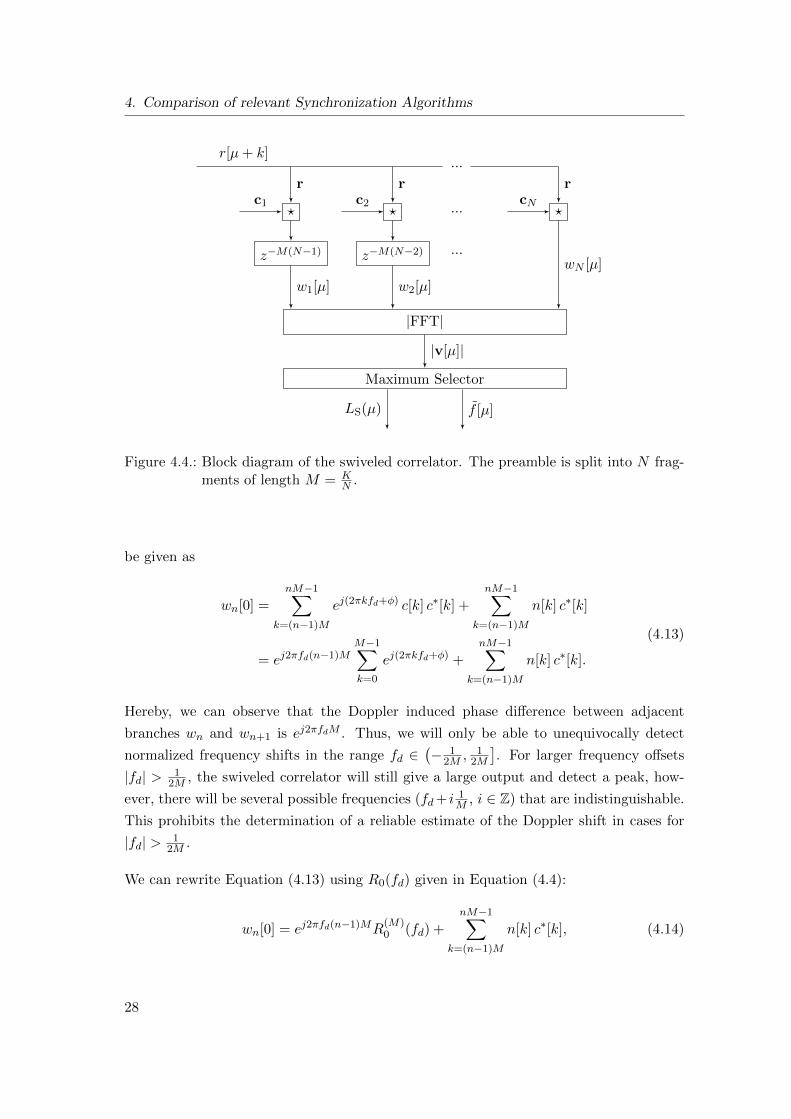
Figure 4.4.: Block diagram of the swiveled correlator. The preamble is split into N frag-ments of length M = K
N .
be given as
wn[0] =nM−1∑
k=(n−1)M
ej(2πkfd+ϕ) c[k] c∗[k] +nM−1∑
k=(n−1)M
n[k] c∗[k]
= ej2πfd(n−1)MM−1∑
k=0
ej(2πkfd+ϕ) +nM−1∑
k=(n−1)M
n[k] c∗[k].
(4.13)
Hereby, we can observe that the Doppler induced phase difference between adjacent
branches wn and wn+1 is ej2πfdM . Thus, we will only be able to unequivocally detect
normalized frequency shifts in the range fd ∈(− 1
2M , 12M
]. For larger frequency offsets
|fd| > 12M , the swiveled correlator will still give a large output and detect a peak, how-
ever, there will be several possible frequencies (fd+ i 1M , i ∈ Z) that are indistinguishable.
This prohibits the determination of a reliable estimate of the Doppler shift in cases for
|fd| > 12M .
We can rewrite Equation (4.13) using R0(fd) given in Equation (4.4):
wn[0] = ej2πfd(n−1)MR(M)0 (fd) +
nM−1∑
k=(n−1)M
n[k] c∗[k], (4.14)
28

4.3. Swiveled Correlator
where R0 is adjusted to the length of the partial correlation:
R(M)0 (fd) =
sin(Mπfd)
sin(πfd)ej((M−1)πfd+ϕ). (4.15)
This indicates that the outputs of the partial correlations suffer from the same noncoher-
ent correlation loss experienced by the simple correlator. A more detailed interpretation
follows shortly. The next step is the FFT, which, given the output of the branches in
Equation (4.14), can be computed as
vi[0] = R(M)0 (fd)
N∑
n=1
ej2πfd(n−1)Me−j2π nNi +
N∑
n=1
nM−1∑
k=(n−1)M
n[k] c∗[k] e−j2π nNi. (4.16)
The summation in the first term is very similar to the summation in R0, and it also has a
very characteristic influence on the expected output of the swiveled correlator, for which
reason we will also define it as an auxiliary function:
K0,i(fd) =N∑
n=1
ej2πfd(n−1)Me−j2π nNi. (4.17)
Since the expression is very similar to R0, we can follow the same methods presented in
Appendix A.3 to simplify the expression to
K0,i(fd) =sin(π(fdK − i))
sin( πN (fdK − i))
ejπ((N−1)(fdM−N+1N
i). (4.18)
In a noiseless case, the output of the swiveled correlator is then finally given by
|K0(fd)R(M)0 (fd)|, (4.19)
where
K0(fd) = maxi
(|K0,i(fd)|) . (4.20)
Figure 4.5 shows a plot of the expected output of the swiveled correlator for different
subsequence lengths. It is important to note the shape of the curves only depends on M ,
i.e., the ratio of K to N , and varying K only affects the scale of the curves. The effect
of the noncoherent correlation loss R0 is shown by the envelopes, which are given in the
figure by the dashed curves. Hereby, it can be seen that noncoherently combining longer
subsequences leads to a greater loss for smaller frequency shifts, as was also emphasized
for the simple correlator. It is notable that M = 1 corresponds to the case where sub-
sequences of length 1 are correlated, i.e., each symbol of the preamble is processed in a
29

4. Comparison of relevant Synchronization Algorithms
0 0.1 0.2 0.3 0.4 0.50
5
10
15
20
Normalized Doppler shift fd
|K(f
d)R
(M)
0(f
d)|
M = 4
M = 2
M = 1
Figure 4.5.: Comparison of the swiveled correlator output for different subsequencelengths. A preamble length of K = 20 symbols was used. The dashedcurves represent the envelope of the plots and correspond to the influence of
R(M)0 (fd).
separate branch. Therefore, this configuration does not suffer from noncoherent corre-
lation loss, which is indicated in the figure by a corresponding constant envelope. The
decay of R0 is fairly moderate for small frequency shifts, which indicates that in scenar-
ios with small maximum frequency shifts, the subsequences can be chosen to be longer.
This corresponds to a smaller number of branches N and therefore lower complexity.
However, in this thesis the focus is on large frequency shifts, for which reason only the
case of N = K will be practical. A similar conclusion about the maximum length of the
subsequence to reduce correlation losses is found in [CPV06], where a design rule for the
maximum subsequence length depending on the frequency offset is derived. Although
this rule is only valid for small Doppler shifts, it supports the idea of operating with very
short subsequences for large Doppler shifts.
Additionally to the noncoherent correlation loss, it can be seen that the output dips quite
significantly in between two adjacent bins. This is the effect of K0(fd) and is due to the
discreteness of the FFT and the finite number of input samples. If the Doppler shift
of the input sequence does not coincide exactly with the center frequency of a bin of
the FFT, then some of the energy will be contained in other bins. The effect is most
prominent in the middle of two adjacent frequencies, where the energy is equally shared
between the two bins. In literature, the difference between the maximum output and
the minimum output is also referred to as the scalloping loss. A common method to
30

4.3. Swiveled Correlator
counteract scalloping loss and increase the minimum output of the FFT is zero-padding,
which will now be more closely discussed.
4.3.2. Zero-Padding
Zero-padding can help to improve the performance of the FFT by interpolating between
the FFT bins and therefore effectively adding more bins in the same frequency range.
To analyze the benefit of zero-padding we perform the same discussion for the output of
the swiveled correlator again, this time assuming that the N branch outputs will be fed
into the FFT together with a padding of Z zeros. A characteristic of the FFT is that it
produces as many output bins as it is given input bins, in this case it will be N +Z, and
therefore i ∈ {1, N + Z}. The output of the i-th bin can now be computed with
vi[µ] =N+Z∑
n=1
wn[µ] e−j2π n
N+Zi. (4.21)
Given that wn[µ] = 0, for all n > N , we can adjust the limit of the sum to
vi[µ] =
N∑
n=1
wn[µ] e−j2π n
N+Zi. (4.22)
Therefore, the likelihood function of the swiveled correlator can be generalized to
LS(µ) = maxi
∣∣∣∣∣∣
N∑
n=1
nM−1∑
k=(n−1)M
r[µ+ k] c∗[k] e−j2π nN+Z
i
∣∣∣∣∣∣
, i ∈ {1, N + Z}. (4.23)
Considering a fully contained preamble and following a similar evaluation as for the
discussion without zero-padding, we can express the expected output of the zero-padded
swiveled correlator in a noiseless scenario by
|KZ(fd)R(M)0 (fd)| = |R(M)
0 (fd)| maxi
(|KZ,i(fd)|)
= |R(M)0 (fd)| max
i
(∣∣∣∣∣sin(πN(fdM − i
N+Z ))
sin(π(fdM − iN+Z ))
∣∣∣∣∣
).
(4.24)
In order to show the benefit of zero-padding, we compare the two approaches in Figure 4.6.
The dashed curves show the expected output for different subsequent lengths without
zero-padding. Here, the scalloping loss is very dominant. The effect of zero-padding can
be seen by comparing the dashed curves to the solid curves, which employ a zero-padding
ratio ZN = 2. It can clearly be seen that the dips between adjacent peaks are much less
31

4. Comparison of relevant Synchronization Algorithms
0 0.1 0.2 0.3 0.4 0.50
5
10
15
20
Normalized Doppler shift fd
|KZ(f
d)R
(M)
0(f
d)|
M = 1, Z = 2N
M = 2, Z = 2N
M = 1, Z = 0
M = 2, Z = 0
Figure 4.6.: Comparison of the effect of zero-padding on the swiveled correlator output.The assumed preamble length is K = 20. A comparison is performed for twodifferent number of branches, N = 20 and N = 10.
severe and that therefore the scalloping loss is much smaller. To establish how many
zeros should be added as a tradeoff between performance and complexity, an expression
of the normalized scalloping loss depending on the amount of zeros can be found:
SL(Z) = max(KZ)−min(KZ) = 1− 1
N
sin( Nπ2(N+Z))
sin( π2(N+Z))
. (4.25)
As it is not immediately visible from the equation how the scalloping loss behaves for
different amounts of zero-padding, we can try to find a polynomial approximation using
the Taylor expansion of the sine-function. The first order approximation evaluates to
zero, for which reason a meaningful estimate is given by the second order approximation:
S(2)L (Z) = π2 1−N2
π2 − 24(N + Z)2. (4.26)
Assuming a fixed number of branches N , it can be seen that the second order approxi-
mation is reciprocal with respect to Z. Therefore, it can be stated that the initial gain
of adding several zeros has a large effect, however, by further increasing Z the benefit
becomes smaller and smaller. The effect is depicted in Figure 4.7, which shows the exact
expression of the scalloping loss and the second order taylor expansion.
It can be seen that there is still a slight gap between the exact expression and the second
order approximation for small amounts of zero-padding, whereas it becomes closer for
32

4.4. Second-order Approximation of the Optimal Detector
0 0.5 1.0 1.5 2.0 2.5 3.00
0.25
0.50
Zero-padding ratio ZN
ScallopingLoss
SL
SL
S(2)L
Figure 4.7.: Behavior of scalloping loss for different amounts of zero-padding.
higher zero-padding ratios ZN . Given the reciprocal shape, it becomes clear that the
scalloping loss cannot be eliminated, as was possible for the noncoherent correlation loss
by choosing M = 1, but it can be reduced very effectively. As zero-padding can be
implemented very efficiently [AML05] and therefore does not cause a large increase in
complexity, for the remainder of the thesis we assume a zero-padding factor ZN = 3. The
scalloping loss then resolves to less then 3% of the amplitude of the output of the swiveled
correlator and even larger zero-padding ratios only provide minor improvement.
4.4. Second-order Approximation of the Optimal Detector
Another different approach was already mentioned in Chapter 3 and involves the approx-
imation of the optimal LRT to make it implementable. In contrast to the previously
presented schemes, this approach is not initially based on a correlation of the incoming
signal with a preamble, but it is derived from the optimal decision rule. This idea was
presented in [WRKH18] and showed a close to optimal performance in the analyzed set-
ting, i.e., the performance loss to the optimal LRT was very small. It was found that the
improvement of approximations higher than the second order is very little and therefore
the second order approximation is a good tradeoff between performance and complexity.
In this section we will therefore present this second order approximation and extend the
expression to account for arbitrary maximum Doppler shifts fmax. We will then also
extend the analysis made in [WRKH18] to other scenarios later in this chapter.
Similar to the derivation of the optimal LRT, the derivation of a simplified, closed-form
33

4. Comparison of relevant Synchronization Algorithms
expression of the second order approximation is quite elaborate and therefore presented
in Appendix A.2. For a general maximum Doppler shift fmax we have
LA(µ) =K−1∑
k1=0
K−1∑
l1=0
K−1∑
k2=0
K−1∑
l2=0
r[µ+ k1] r∗[µ+ l1] c
∗[k1] c[l1]
· r[µ+ k2] r∗[µ+ l2] c
∗[k2] c[l2] sinc (2fmax (k1 − l1 + k2 − l2)) . (4.27)
When the maximum Doppler shift is fixed to fmax = 0.5, a much simpler expression can
be found, since the sinc-function simplifies to the Dirac-delta function for integers k:
sinc(k) = δ[k], for all k ∈ Z. (4.28)
Since this only has nonzero contribution for k = 0, several terms drop out and [WRKH18]
shows that LA(µ) can be simplified to
LA(µ) =K−1∑
m=1
∣∣∣∣∣K−1∑
k=m
r∗[µ+ k] c[k] r[µ+ k −m] c∗[k −m]
∣∣∣∣∣
2
. (4.29)
Hereby, the inner sum is also referred to as the double correlation of lag m in literature.
Therefore, LA(µ) corresponds to the sum of the absolute square of all possible double
correlations with lag m. For simplicity, we will also refer to this detection scheme as the
double correlator.
4.5. Choi-Lee Detector
A very similar detection scheme was presented in [CL02]. It was shown that the derived
metric performs well in scenarios with moderate frequency offsets and phase uncertainty.
Although the detector was derived in an ML framework, the metric was shown to also
perform well when used for hypothesis testing [WRKH18]. It has since been widely used
as a reference in literature [Chi10],[WRKH17],[PVVC+10]. The metric is given as:
LCL(µ) =
K−1∑
m=1
∣∣∣∣∣K−1∑
k=m
r∗[µ+ k] c[k] r[µ+ k −m] c∗[k −m]
∣∣∣∣∣
2
−K−1∑
k=m
|r[µ+ k]|2|r[µ+ k −m]|2}. (4.30)
34
4.6. Comparison and Simulation Results
The first part hereby corresponds to LA(µ) and therefore the double correlation, and
the second part is an energy, or data, correction term. This detector was derived for a
continuous transmission of periodic frames, so the data correction term is supposed to
reduce the influence of random data or partially contained preambles on the false alarm
rate. Although we disregarded these cases for the derivation of the optimal LRT, we will
later simulate the approaches considering partially contained preambles to review the
validity of our assumption.
4.6. Comparison and Simulation Results
4.6.1. Means of Comparison
In order to compare the presented algorithms, we want to emphasize the employed metrics
and methods. In the given setting, the most prominent metrics are the probability of
false alarm Pfa and the probability of correct detection Pd or missed detection Pm. In the
hypothesis testing framework, these depend on the employed threshold λ and therefore
offer a tradeoff, where increasing the threshold leads to an increase in Pfa and Pd, and
vice versa. Pfa is defined as the probability that hypothesis H1 was chosen although H0
was true, i.e.,
Pfa = Pr[D1|H0
]. (4.31)
As discussed, when employing hypothesis testing the hypothesisH1 is chosen if the output
of the likelihood function L(µ) surpasses the threshold λ. Therefore, the equation can be
rewritten as
Pfa = Pr[L(µ) > λ|H0
]. (4.32)
Likewise, the probability of missed detection Pm corresponds to choosing hypothesis H0
when H1 is true, where H0 is chosen if the threshold is not exceeded:
Pm = Pr[D0|H1
]= Pr
[L(µ) < λ|H1
]. (4.33)
As a correct detection is the complementary event to a missed detection, the probability
of correct detection can be defined as
Pd = 1− Pm = Pr[D1|H1
]= Pr
[L(µ) > λ|H1
]. (4.34)
It corresponds to making the correct decision of choosing H1 when H1 holds true.
A very meaningful figure of merit to compare the algorithms in the hypothesis testing
framework is the receiver operating characteristic (ROC) curve, which is widely used
35

4. Comparison of relevant Synchronization Algorithms
in literature [Chi10]. Hereby, the algorithms are evaluated with different thresholds λ,
which lead to different combinations of Pfa and Pd or Pm. These can then be plotted to
obtain a curve, which shows all operating points of the algorithm in the given scenario.
Depending on the required Pd and on the available resources, a certain threshold matching
the requirements can then be chosen.
4.6.2. Discussion
To compare the algorithms, we carried out several simulations in different scenarios. The
interesting factors include the behavior of the different detectors in high and low SNR
and the performance in differently strong Doppler shifts. Furthermore, we want to verify
the validity of the assumption made in the beginning of Chapter 3 to only consider fully
contained preambles and treat incoming signals with partially contained preambles the
same way as pure noise.
Simulation notes
In general, the two hypotheses and therefore Pfa and Pd can be simulated separately. For
H0, a stream of noise was supplied to the detection schemes and averaged over a sufficient
amount of iterations. For H1, uniformly random Doppler shifts and noise were applied to
the preamble, before being passed to the detectors and averaged. Hereby, only the central
sample of the correlation output will be analyzed, since we disregard cases with partially
contained preambles. However, we will later provide simulations taking also such cases
into account, which will give insight on the validity of this assumption.
For the simulation of the optimal LRT, we used Monte Carlo integration to integrate
the output of the Bessel function over the frequency. For both the bank of correlators
and the swiveled correlator, we want to use their ability to also estimate the experienced
Doppler shift and only accept a correct detection if both the sample and the frequency
were identified correctly. Because frequency shifts that lie towards the middle of two
branches/bins will cause a similarly large output in both, we choose to soften the rule of
correct detection to also accept directly adjacent branches/bins 2. Therefore, the estima-
tion of the Doppler shift in this setup has a maximum error of 3∆f . Using this frequency
estimation slightly decreases the performance of the two algorithms and therefore a com-
parison to other detectors that do not perform Doppler estimation might not be entirely
fair. However, producing a reliable Doppler estimation can be very helpful, as will be
further clarified in the second part of the thesis.
2In practice, depending on the frequency resolution of the algorithms and the requirements of theapplication, even more than one adjacent branch/bin will often be accepted, as this increases theperformance of detection and still provides a good enough Doppler estimation.
36

4.6. Comparison and Simulation Results
−0.5 −0.375 −0.25 −0.125 0 0.125 0.25 0.375 0.50.70
0.75
0.80
0.85
0.90
0.95
1.00
Normalized Doppler shift fd
Proab
ilityof
detection
Pd
LC
LA
LCL
LS : N = K,Z = 0
LB : N = K
Figure 4.8.: Comparison of the detection performance across the normalized frequencyoffset in a high SNR scenario. ES
N0= 1dB, K = 10, Pfa = 10−1 ± 10−3.
Performance across Doppler range
To confirm the expected behavior of the different algorithms in varying Doppler shifts
with simulations, Figure 4.8 plots the detection performance against the frequency offset
for an SNR of ESN0
= 1dB, a preamble length of K = 10 symbols and a probability of
false alarm of Pfa = 10−1 ± 10−3. The parameters were chosen in a way to effectively
visualize the behavior of the detection schemes. It shows the expected degradation of the
simple correlator LC with larger frequencies, resembling the shape of R0(fd). The bank
of correlators LB uses several branches with this behavior at different frequencies and by
choosing the one with the highest output, the performance shows a characteristic sine-
shape. The same behavior can be seen for the swiveled correlator LS, where the behavior
comes from the scalloping loss of the FFT . Hereby, the length of the subsequence was
chosen to M = 1. For longer subsequences, the swiveled correlator would show a stronger
degradation towards larger frequencies, similar to the behavior in Figure 4.5. It is also
notable that the performance of the bank of correlators and the swiveled correlator would
greatly improve when using more resources, i.e., a larger number of branches for the bank
of correlators or zero-padding for the swiveled correlator. We refrain from doing so for
this figure in order to present the sinusoidal behavior. Finally, it can be seen that the
approximation LA of the optimal LRT and the Choi-Lee detector LCL show a constant
performance across all frequency shifts.
37

4. Comparison of relevant Synchronization Algorithms
0 0.0125 0.025 0.0375 0.050.90
0.92
0.94
0.96
0.98
1.00
Probability of false alarm Pfa
Proab
ilityof
detection
Pd
LO
LA
LCL
LS : N = K,Z = 3N
LB : N = 2K
Figure 4.9.: Simulated ROC at high SNR. ESN0
= 0dB, K = 15, fmax = 0.5.
High SNR
For a first comparison of the different algorithms concerning their performance, we choose
a high SNR environment, where short preambles can be used. The result of the simulation
can be found in Figure 4.9, which shows the ROC curves of the detectors. It can be
seen that the optimal LRT LO, derived in Section 3.2, gives an upper bound on the
performance of the other detection schemes, which confirms that it corresponds to the
optimal decision rule. The second order approximation LA, derived in Section 4.4, is
very tight in this scenario and comes very close to the performance of the optimal test.
Similarly the bank of correlators and the swiveled correlator with the given specifications
show the same performance. The Choi-Lee detector LCL performs slightly worse, which
can be attributed to the energy correction term. This is subtracted from the double
correlation and therefore reduces the output, which slightly decreases the performance in
this scenario.
Low SNR
Concerning an application in IoT via satellite, a low SNR scenario may be more fitting as
a basis for comparison, since satellite links are typically characterized by a low SNR. The
effect of a lower SNR while employing a preamble of the same length as in the high SNR
case is shown by the simulated ROC curves in Figure 4.10. Hereby, the performance of
38

4.6. Comparison and Simulation Results
0 0.25 0.5 0.75 10
0.25
0.50
0.75
1.00
Probability of false alarm Pfa
Proab
ilityof
detection
Pd
LO
LA
LCL
LS : N = K,Z = 3N
LB : N = 2K
Figure 4.10.: Simulated ROC at low SNR with short preambles. ESN0
= −9 dB, K = 15,fmax = 0.5.
all detectors drastically decreases, because the correlation output of the short preamble
cannot be detected over the larger amount of noise. This emphasizes the argument
discussed in Section 4.1, that in lower SNR environments, longer preambles have to
be used, which leads to a shorter bandwidth of the correlation. At first glance, it is
counterintuitive that the bank of correlators and the swiveled correlator do not reach a
detection probability of 100% for a false alarm probability of 100%, but this is inflicted
by additionally requiring a correct frequency estimation. Therefore, even if the threshold
is set very low and all output branches would exceed the threshold, it is very unlikely
that the correct branch has the highest output, which only then would be accepted as a
correct detection.
Therefore, to account for the lower SNR, the preamble length needs to be increased if
one wishes to detect the preamble with high probability. Figure 4.11 includes the ROC
curves of the analyzed detectors in a low SNR scenario with a longer preamble. The
optimal LRT again provides the best possible performance. However, its approximation
LA shows a large degradation compared to the high SNR scenario. While at high SNR
the performance of LA was very close to the optimal LRT and on a par with both the
bank of correlators and the swiveled correlator, it performs even worse than the Choi-Lee
correlator at low SNR. Also the performance disparity between the Choi-Lee correlator
and the optimal LRT increases, while the bank of correlators and the swiveled correlator
39

4. Comparison of relevant Synchronization Algorithms
0 0.0125 0.025 0.0375 0.050.88
0.90
0.92
0.94
0.96
0.98
Probability of false alarm Pfa
Proab
ilityof
detection
Pd
LO
LA
LCL
LS : N = K,Z = 3N
LB : N = 2K
Figure 4.11.: Simulated ROC at low SNR. ESN0
= −9 dB, K = 150, fmax = 0.5.
P P P
µ3K
Figure 4.12.: Visualization of signal stream for the simulations considering partially con-tained preambles. A preamble was inserted every 3K symbols.
remain very close. We believe that the bad performance of the LA detector can be
attributed to the approximation of the Bessel function. As this has not been observed
before in literature, it deserves further attention and a precise explanation is subject to
further investigation.
Considering partially contained preambles
In a further simulation we want to examine the effect of including cases with partially
contained preambles. Throughout the discussion of the detectors in this Chapter, we
assumed that the ACF of the preamble was very good and therefore incoming signals with
partially contained preambles were treated the same way as pure noise. The simulation
now reveals whether this assumption was justified. For this, the probability of false alarm
and probability of detection are simulated together, by creating a stream of noise and
embedding preambles every 3K symbols, as illustrated in Figure 4.12. The stream is then
40

4.6. Comparison and Simulation Results
0 0.025 0.05 0.075 0.10.86
0.88
0.90
0.92
0.94
0.96
Probability of false alarm Pfa
Proab
ilityof
detection
Pd
LO
LA
LCL
LS : N = K,Z = 3N
LB : N = 2K
Figure 4.13.: Simulated ROC at high SNR considering partially contained preambles.ESN0
= 0dB, K = 15, fmax = 0.5.
passed through the detectors and correct detections and false alarms are averaged. The
result is presented in Figure 4.13.
It is essential to point out that cases with partially contained preambles were disregarded
in the derivation of the optimal LRT, for which reason the LO metric will not be optimal
in this setting, and therefore may not be viewed as an upper bound. For this reason
the curve is shown dashed. Nonetheless, we include it in the plot to see the effect of
partially contained preambles and the assumption of disregarding them. Looking at the
curves, it becomes apparent that all of the schemes lose in performance, indicating that
partially contained preambles induce a higher probability of false alarm. It therefore may
be worthwhile to consider partially contained preambles in the derivation of a modified
optimal LRT for the given scenario in the future, at least for high SNR. It is notable
that the performance of the Choi-Lee correlator suffers the least degradation. This is
due to the energy correcting second term in the metric given in Equation (4.30). The
increased probability of false alarm for the other schemes, comes from an increase in the
energy of the incoming signal, due to the partially contained preamble. This increase in
energy is countered by the energy correcting term of the Choi-Lee correlator, enhancing
its performance with respect to the other detectors.
The simulation in a low SNR environment is given in Figure 4.14. The biggest difference
to the high SNR case can be seen for the Choi-Lee correlator, which significantly drops
41

4. Comparison of relevant Synchronization Algorithms
0 0.0125 0.025 0.0375 0.050.86
0.88
0.90
0.92
0.94
0.96
Probability of false alarm Pfa
Proab
ilityof
detection
Pd
LO
LA
LCL
LS : N = K,Z = 3N
LB : N = 2K
Figure 4.14.: Simulated ROC at low SNR considering partially contained preambles.ESN0
= −9 dB, K = 150, fmax = 0.5.
in performance compared to the other schemes. The good performance at high SNR was
due to the compensation of the signal energy. As the SNR is defined as the signal energy
with respect to the noise energy, this compensation has a much smaller effect when the
incoming signal is dominated by the noise. This is also emphasized by the correlation
output, which, according to R0, increases with growing preamble length and therefore
causes for a much larger contribution than the signal energy on its own. This also explains
why the performance loss of the other detectors, including the optimal LRT, is much
smaller when comparing the low SNR scenarios with and without considering partially
contained preambles to the high SNR equivalents. This suggests that the assumption of
H0 subsuming cases with partially contained preambles is much more accurate for low
SNR scenarios and therefore validates the assumption in the given satellite setting.
4.7. Summary
The considered detectors all showed close to optimal performance in a high SNR scenario,
when disregarding partially contained preambles. It was shown that the bank of corre-
lators and the swiveled correlator come very close to the optimal LRT in all scenarios,
i.e., both high and low SNR and both with and without considering partially contained
preambles, and therefore represent promising solutions. The approximation LA of the op-
42

4.7. Summary
timal LRT significantly drops in performance when considering low SNR scenarios. The
Choi-Lee correlator shows better results in a scenario with high SNR and considering
partially contained preambles due to the energy correcting term, however, this benefit
disappears for long preambles and low SNRs. Therefore, in the given satellite setting,
which is characterized by low SNRs and long preambles, our experimental results show
that the bank of correlators and the swiveled correlator outperform the other detectors,
approaching the performance the optimal LRT.
43


5. Analytic Modeling of
Correlation-based Algorithms
Additionally to the analysis of the output of the simple correlator, the bank of correlators
and the swiveled correlator presented in Chapter 4, it is useful to derive models for the
probability of false alarm, Pfa, and the probability of correct detection, Pd, in order to
estimate and predict the performance of the mentioned algorithms in different scenarios.
For this, the deterministic analysis of the expected output has to be complemented by
a statistical discussion of the noise throughout the processing steps. For the simplified
baseband representation assumed in the first part of this thesis, this discussion is known
in literature, e.g. for the swiveled correlator in [SSS+00]. Nonetheless, we present it as a
basis for the later extension of the models accounting for ISI, which is novel.
5.1. Simple Correlator
Probability of false alarm Pfa
As mentioned in the previous chapter, we characterize a false alarm as the selection of
hypothesis H1 although H0 was true. In the binary hypothesis testing framework, this
means that the probability of false alarm is solely characterized by the noise:
r[µ+ k] = n[µ+ k]. (5.1)
Recall that n[µ+k] is a circularly symmetric complex Gaussian RV, where each component
has zero mean and a variance of σ2n. Hence, we have
Re (n[µ+ k]) ∼ N (0, σ2n), Im (n[µ+ k]) ∼ N (0, σ2
n). (5.2)
The output of the correlation is given as
w[µ] =K−1∑
k=0
n[µ+ k] c∗[k]. (5.3)
45

5. Analytic Modeling of Correlation-based Algorithms
Since we assume unit energy PSK symbols, i.e., |c[k]|2 = 1, the correlation corresponds
to the sum of K complex Gaussian RVs. We can then use the linearity of expectation,
which always holds, and the linearity of variance, which holds for uncorrelated RVs. For
two RVs Xi and Xj , this is formally described by
E[∑
i
Xi
]=∑
i
E[Xi]
and Var[∑
i
Xi
]=∑
i
Var[Xi] + 2∑
i,ji<j
Cov[Xi, Xj ],
where Cov[Xi, Xj ] = 0, if Xi and Xj are uncorrelated.
(5.4)
We know that the RVs of n[µ+ k] are i.i.d., and therefore, using the property that inde-
pendent RVs are also uncorrelated, we have that w[µ] is a circularly symmetric Gaussian
RV with per component variance Kσ2n. The final processing step of the simple correlator
is to then take the absolute value of the correlation output, i.e., |w[µ]|. The absolute valueof a circularly symmetric Gaussian random variable with zero mean and per component
variance of σ2 follows a Rayleigh distribution with scale parameter σ [PP02]. Hence, we
have
|w[µ]| ∼ Rayleigh(√Kσ2
n). (5.5)
For a Rayleigh distributed RV x, its PDF is given by
fX(x) =x
Kσ2n
e− x2
2Kσ2n . (5.6)
The corresponding cumulative density function (CDF) is
FX(x) = 1− e− x2
2Kσ2n . (5.7)
An expression for the probability of false alarm can now be computed as the probability
that the Rayleigh distributed output is larger than the previously defined threshold λ:
Pfa(λ) = Pr[|w[µ]| > λ
]= 1− Pr
[|w[µ]| ≤ λ
]= 1− FRayleigh(λ) = e
− λ2
2Kσ2n . (5.8)
46

5.2. Bank of Correlators
Probability of correct detection Pd
For the probability of correct detection, we analyze the hypothesis H1. In this case, we
know from Equation (4.2) that the output is given as
w[0] = R0(fd) +
K−1∑
k=0
n[k] c∗[k]. (5.9)
Hereby, we have already established above that the second term is a circularly symmetric
Gaussian RV with zero mean and a per component variance of Kσ2n. The first term is
deterministic, i.e., it has zero variance. Using the rules given in (5.4), we get that w[0]
is a circularly symmetric Gaussian RV with mean E[w[0]] = R0(fd) and per component
variance ofKσ2n. We know that the absolute value of such a RV follows a Rice distribution
[JBS06]:
|w[0]| ∼ Rice(s,√
Kσ2n), where s(fd) = |R0(fd)|. (5.10)
The PDF of such a Rice distributed RV x is given by
fX(x) =x
Kσ2n
e−x2+s2(fd)
2Kσ2n I0
(xs(fd)
Kσ2n
). (5.11)
The probability of correct detection can then be obtained by the probability that the
Rice distributed output exceeds the threshold λ:
Pd(λ) = Pr[|w[0]| > λ
]=
∞∫
λ
x
Kσ2n
e−x2+s2(fd)
2Kσ2n I0
(xs(fd)
Kσ2n
)dx. (5.12)
5.2. Bank of Correlators
Probability of false alarm Pfa
The bank of correlators employs N parallel branches with simple correlators operating
at different center frequencies. From Section 5.1 we know that the outputs |wi[µ]| ofeach branch are Rayleigh distributed with scale parameter
√Kσ2
n. The algorithm then
selects the maximum of those branches. The probability of false alarm is then given as
the probability that the maximum of N Rayleigh distributed RVs exceeds the threshold:
Pfa(λ) = Pr[max
i(|wi[µ]|) > λ
]= Pr
[|w1[µ]| > λ, |w2[µ]| > λ, ..., |wN [µ]| > λ
]
= 1− Pr[|w1[µ]| ≤ λ, |w2[µ]| ≤ λ, ..., |wN [µ]| ≤ λ
].
(5.13)
47

5. Analytic Modeling of Correlation-based Algorithms
As a simplifying assumption, we can treat the different RVs as independent. This is
generally not the case, since the outputs of the branches are all characterized by the
same input noise realization and only differ in the applied frequency shift. Intuitively, the
smaller this frequency shift becomes, the more dependent are the outputs of the adjacent
branches. In the case of infinitely many branches and therefore infinitely small frequency
differences, adjacent branches will be the same. The tightness of the approximation for a
moderate amount of branches will be numerically analyzed later. Assuming the RVs are
independent, the probability that no RV exceeds the threshold is equal to the product of
the probabilities that each RV does not exceed the threshold. Additionally, the RVs are
identically distributed, which lets us simplify the expression to
Pfa(λ) ≈ 1−N∏
i=1
Pr[|wi[µ]| < λ
]= 1− (FRayleigh(λ))
N (5.7)= 1−
(1− e
− λ2
2Kσ2n
)N
. (5.14)
Probability of correct detection Pd
Regarding the probability of correct detection, we again have to consider the signal con-
tent and noise. In contrast to the simple correlator, the bank of correlators can provide
an estimate of the Doppler shift fd, which can be used for the correction and further
processing of the packet. Since this is very useful, we want to ensure a reliable Doppler
estimation and therefore assume that a detection is only made correctly, if both the cor-
rect (time) sample and the correct (frequency) branch exceeded the threshold. Following
the analysis of the simple correlator, it is intuitive that the correlation is likely to be
highest in the branch with the frequency shift closest to the Doppler shift, however the
effects of noise could lead to a wrongly estimated frequency. We can again use the results
from Section 5.1 and establish that the output |wi[0]| of each branch is Rice distributed
with parameters s(fd − i∆f) and√Kσ2
n. Hereby, the Rice parameter is modified by the
center frequency of the branch.
A correct detection is made if the following two properties hold:
1) The output of the correct branch exceeds the threshold λ to trigger the detection.
2) The output of the correct branch is larger than the output of all otherN−1 branches
to give a correct frequency estimation.
The second statement is equivalent to the correct branch being larger than the maximum
of the other branches. Let us now assume that the i-th branch is the correct one, i.e.,
the one whose center frequency is closest to fd, and denote its output with x. Recall that
we defined the residual frequency offset in this branch as fr in Section 4.2. Therefore,
48

5.2. Bank of Correlators
we have that x is Rice distributed with parameters s(fr) and√Kσ2
n. Furthermore, we
denote the maximum output of the incorrect branches with y, which gives
x = |wi[0]|, y = maxj =i
(|wj [0]|). (5.15)
We can now formally describe the probability of correct detection as
Pd(λ) = Pr[x > λ, x > y
]=
∞∫
λ
x∫
0
fX,Y (x, y) dy dx, (5.16)
where fX,Y is the joint probability distribution of X and Y . However, this is not available
to us and we will therefore make some assumptions to derive an approximation. Due to the
fast decay of the correlation output R0(fd) (contained in the Rice factor), we can assume
that the incorrect branches experience a very small correlation output. Therefore, we will
approximate them as (N − 1) i.i.d. Rayleigh distributed RVs, which yields
FY (y) = Pr[Y < y
]=
(1− e
− y2
2Kσ2n
)N−1
. (5.17)
We will further approximate that x and y are independent, so that the joint probability
distributions corresponds to the product of the distributions of each RV. The follow-
ing then gives the formal derivation of an approximation of the probability of correct
detection:
Pd(λ) ≈∞∫
λ
x∫
0
fY (y)dy fX(x)dx =
∞∫
λ
FY (x)fX(x)dx
=
∞∫
λ
(1− e
− x2
2Kσ2n
)N−1x
Kσ2n
e−x2+s2(fr)
2Kσ2n I0
(xs(fr)
Kσ2n
)dx.
(5.18)
It is notable that this approximation only holds for a moderate amount of branches for
two reasons:
1) With this approximation only the correct branch is allowed to operate inside its
specified bandwidth, as otherwise approximating incorrect branches as Rayleigh
RVs is faulty. In other words, if the frequency difference between adjacent branches
becomes very small, multiple simple correlators may operate inside their bandwidth
and give a large correlation output. These branches can then not be characterized
as Rayleigh RVs anymore and would also have to be considered as Rice distributed.
49

5. Analytic Modeling of Correlation-based Algorithms
2) Furthermore, as mentioned earlier, the smaller the resolution of the bank of corre-
lators, i.e., the frequency difference between two adjacent branches, the larger will
be the error of approximating the branches as independent.
5.3. Swiveled Correlator
Probability of false alarm Pfa
For the swiveled correlator, the output of the correlation between the incoming noise and
the preamble fragments is given by
wn[µ] =nM−1∑
k=(n−1)M
n[µ+ k] c∗[k], n ∈ {1, N}, (5.19)
where M = KN . Similarly to the analysis for the bank of correlators, we can establish that
every wn[µ] corresponds to the sum of M circularly symmetric Gaussian RVs. Therefore,
each wn[µ] is also a circularly symmetric Gaussian RV with zero mean and per component
variance of Mσ2n. These are then fed as input to an FFT together with a padding of Z
zeros, for which Equation (4.22) gives the output of each bin as
vi[µ] =N∑
n=1
wn[µ] e−j2π n
N+Zi, i ∈ {1, N + Z}. (5.20)
As the complex exponential has unit magnitude, i.e., |ejφ| = 1, vi[µ] corresponds to
the sum of N circularly symmetric Gaussian RVs with zero mean and per component
variance of Mσ2n. Thus, vi[µ] is a circularly symmetric Gaussian RV with zero mean and
per component variance of NMσ2n = Kσ2
n. The next step is to then take the absolute
value of each bin. Hence, |vi[µ]| is Rayleigh distributed with scale parameter√
Kσ2n. The
PDF for each of the RVs is given by Equation (5.6). Similar to the bank of correlators,
the probability of false alarm is given as the probability that the maximum of (N + Z)
Rayleigh distributed RVs exceeds the threshold λ:
Pfa(λ) = Pr[max
i(|vi[µ]|) > λ
]= 1− Pr
[|v1[µ]| ≤ λ, |v2[µ]| ≤ λ, ..., |vN+Z [µ]| ≤ λ
].
(5.21)
We will rely on approximating this by assuming that the (N +Z) Rayleigh RVs are inde-
pendent. Equivalently to the reasoning for the bank of correlators, this can be formally
50

5.3. Swiveled Correlator
expressed as
Pfa(λ) ≈ 1−N+Z∏
i=1
Pr[|vi[µ]| < λ
]= 1− FN+Z
Rayleigh(λ)(5.7)= 1−
(1− e
− λ2
2Kσ2n
)N+Z
. (5.22)
Probability of correct detection Pd
According to Equations (4.14),(4.22) and (4.24), the output of each FFT bin for a fully
contained preamble in the incoming signal is given by
vi[0] = R(M)0 (fd)KZ,i(fd) +
N∑
n=1
nM−1∑
k=(n−1)M
n[k] c∗[k] e−j2π nN+Z
i, i ∈ {1, N + Z}. (5.23)
Hereby, we can see that the first term is deterministic for a given Doppler shift. We also
know from the derivation of Pfa above, that the second term is a circularly symmetric
Gaussian RV. Therefore, the output of each bin, vi[0], is a circularly symmetric Gaussian
RV with mean R(M)0 (fd)KZ,i(fd) and per component variance of Kσ2
n. The absolute value
of such a RV is Rice distributed:
|vi[0]| ∼ Rice(s′, σ), where s′(fd, i) = |R(M)0 (fd)KZ,i(fd)| and σ =
√Kσ2
n. (5.24)
In contrast to the bank of correlators, the Rice factor now depends on the Doppler shift
fd and not on the difference between fd and the center frequency of the respective branch.
Again, we will assume that a correct detection occurs if 1) the output of the correct bin
exceeds the threshold and 2) the output of the correct bin is larger than the outputs of
all other bins. Let us now assume that the i-th bin is the correct one and we will denote
its output with x. Furthermore, we will denote the maximum output of the incorrect
bins with y, hence we have
x = |vi[0]|, y = maxj =i
(|vj [0]|). (5.25)
We can now formally describe the probability of correct detection as
Pd(λ) = Pr[x > λ, x > y
]=
∞∫
λ
x∫
0
fX,Y (x, y) dy dx. (5.26)
As was the case for the bank of correlators, the joint PDF is unknown, and we will make
some assumptions to obtain an approximation for Pd. Equivalent to the assumptions
made for the approximation of the bank of correlators, we assume that the incorrect
51

5. Analytic Modeling of Correlation-based Algorithms
bins are i.i.d. Rayleigh distributed. This yields a similar result as the one presented in
Equation (5.17):
FY (y) = Pr[Y < y
]=
(1− e
− y2
2Kσ2n
)N+Z−1
, (5.27)
with the difference of having (N+Z−1) Rayleigh RVs. We will also further approximate
that the correct bin is independent from the incorrect bins, i.e., x is independent of y.
The approximation of the probability of correct detection for the swiveled correlator can
then be found equivalently to the approximation for the bank of correlators given in
Equation (5.18):
Pd(λ) ≈∞∫
λ
(1− e
− x2
2Kσ2n
)N+Z−1x
Kσ2n
e−x2+s′2(fd)
2Kσ2n I0
(xs′(fd)Kσ2
n
)dx, (5.28)
where s′(fd) = |R(M)0 (fd)KZ(fd)|.
For the same reasons as given for the bank of correlators, we expect the considered
approximation to be tight for a moderate amount of zero-padding.
5.4. Numerical Results
We will now validate the tightness of the presented analytic models for the three detection
schemes by comparing them to simulations. Hereby, we expect that the model for the
simple correlator is exact, since we do not make any approximations. For the bank
of correlators and the swiveled correlator, we expect the approximations to be tight in
configurations with a moderate amount of branches/bins.
Figure 5.1 shows the analytic and simulated ROC curve for the simple correlator, in a
high SNR scenario. Hereby, a maximum Doppler shift of fmax = 0.05 was assumed,
as the performance of the simple correlator decreases for larger Doppler shifts. It can
be seen that the two curves coincide, which suggests that the model is indeed exact.
Furthermore, this also holds for low SNR scenarios, but a similar performance can then
only be achieved by increasing the preamble length and reducing the maximum Doppler
shift.
To verify the tightness of the approximations made for the bank of correlators and the
swiveled correlator, we can analyze Pfa and Pd separately. Figure 5.2 compares the
probability of false alarm Pfa of the analytic model and the simulation for the bank
of correlators. It can be seen that the model is very tight for a moderate number of
branches N = K. Increasing the number of branches to N = 4K, and therefore reducing
52

5.4. Numerical Results
0 0.025 0.05 0.075 0.1
10−1
100
Probability of false alarm Pfa
1-Pd
Simulation
Analytic
Figure 5.1.: ROC curve comparison of the analytic model and simulation for the simplecorrelator. ES
N0= 0dB,K = 15, fmax = 0.05.
60 70 80 90 100 110 1200
0.25
0.5
0.75
1
Threshold λ
Probab
ilityof
falsealarm
Pfa
Sim. - N = K
Ana. - N = K
Sim. - N = 4K
Ana. - N = 4K
Figure 5.2.: Pfa comparison of th analytic model and simulation for the bank of correla-tors. ES
N0= −9 dB,K = 150, fmax = 0.5.
53

5. Analytic Modeling of Correlation-based Algorithms
80 100 120 140 160 180 2000
0.25
0.5
0.75
1
Threshold λ
Probab
ilityof
detection
Pd
Sim. - N = K
Ana. - N = K
Sim. - N = 4K
Ana. - N = 4K
80 100 120 140 160 180 2000
0.25
0.5
0.75
1
Threshold λ
Probabilityof
detection
Pd
Sim. - N = K
Ana. - N = K
Sim. - N = 4K
Ana. - N = 4KFigure 5.3.: Pd comparison of th analytic model and simulation for the bank of correlators.ESN0
= −9 dB,K = 150, fmax = 0.5.
the frequency difference in adjacent branches, leads to a reduction in tightness. This is in
line with the expectations, that the assumption of the branch outputs being independent
becomes loose for a large number of branches. A very similar behavior was observed for
the swiveled correlator.
Figure 5.3 plots the probability of detection Pd of the bank of correlators across the
threshold range. It can be seen that the analytic model is not exact, but still tight.
Hereby, the analytic model considers the correct branch to be Rice distributed and the
other branches to be i.i.d. Rayleigh. Therefore, we would also expect to see here, that
the approximation is tighter for a moderate number of branches. Comparing the curves
in the figure, it can be observed that this is true for low probability of detections of up
to around 75%, whereas for high probabilities the analytic model for a large number of
branches becomes tighter. This is highlighted by the magnified part of the figure. This
effect comes from also accepting Doppler estimates in adjacent branches of the correct
branch. As mentioned earlier, since Doppler shifts in between two center frequencies
cause an equally large output in the corresponding branches, we also consider Doppler
estimates from one adjacent branch as a correct detection. This slightly increases the
probability of detection with respect to the analytic model. The effect is reduced for a
larger amount of branches, since the ratio of accepted frequency estimates to unaccepted
frequency estimates becomes smaller. Also this effect could be observed for the swiveled
54

5.4. Numerical Results
0 0.025 0.05 0.075 0.110−2
10−1
100
Probability of false alarm Pfa
1-Pd
Sim. - N = K
Ana. - N = K
Sim. - N = 4K
Ana. - N = 4K
Figure 5.4.: ROC curve comparison of the analytic model and simulation for the bank ofcorrelators. ES
N0= −9 dB,K = 150, fmax = 0.5.
correlator, which was expected considering we made the same approximating assumptions
for both schemes.
The combination of Pfa and Pd for the bank of correlators is shown as the ROC curve in
Figure 5.4. Hereby, the analytic model is compared to a simulation in a low SNR scenario.
It can be seen that both the models for a moderate amount of branches N = K and the
model for a larger number of branches N = 4K are reasonably accurate. Hereby, the
inaccuracy of the model with a moderate amount of branches comes from Pd and therefore
from accepting frequency estimates of adjacent branches, while for the model with a
large number of branches the inaccuracy comes from Pfa and therefore the assumption
of independent branch outputs. The same behavior can be seen in Figure 5.5 for the
swiveled correlator. It can also be noted that, in general, due to accepting multiple
branches/bins, the analytic model underestimates the performance of the detector and a
slightly better performance is observed in the simulations.
55

5. Analytic Modeling of Correlation-based Algorithms
0 0.025 0.05 0.075 0.110−2
10−1
100
Probability of false alarm Pfa
1-Pd
Sim. - N = K,Z = 0
Ana. - N = K,Z = 0
Sim. - N = K,Z = 3N
Ana. - N = K,Z = 3N
Figure 5.5.: ROC curve comparison of the analytic model and simulation for the swiveledcorrelator. ES
N0= −9 dB,K = 150, fmax = 0.5.
56
Part II.
Discussion of Realistic Effects on
Frame Synchronization
57


6. Passband Signal Processing with
Frequency Offset
The second part of this thesis will contain a more realistic discussion of the problem of
frame synchronization in the presence of a large Doppler shift. We will hereby deviate
from the simplified environment that was assumed in the first part of the thesis, and in
most related works in literature, and present a discussion of the impact of a frequency
offset on the processing of a passband signal and the effect of the resulting ISI on the
frame detection algorithms. We will start by shortly presenting the setting for the second
part of thesis, focusing on differences to the first part and what effects they have.
6.1. Setting Description
A schematic representation of the processing chain in a practical communication system
is given in Figure 6.1. Several processing steps irrelevant to the considered problem, such
as coding, are omitted for simplicity. The incoming data bits b[m] ∈ {0, 1} are firstly
mapped to symbols a[n] of the employed modulation scheme. The major difference to
the setting in the first part of the thesis, is that in a practical transmission the resulting
complex symbol stream has to undergo pulse shaping in order to create a waveform x[k],
which can actually be transmitted by an antenna. The pulse shaping filter employed in
the course of the discussion is the square-root raised cosine (SRRC) pulse, which together
SourceSymbolMapping
PulseShaping
RFFrontend
Channel
RFFrontend
ReceiveFiltering
De-tection
De-mapping
Sink
b[m] a[n] x[k] xBP(t)
rBP(t)r(t)z[k]d[n]s[m]
Figure 6.1.: Block diagram of the processing steps a communication system.
59
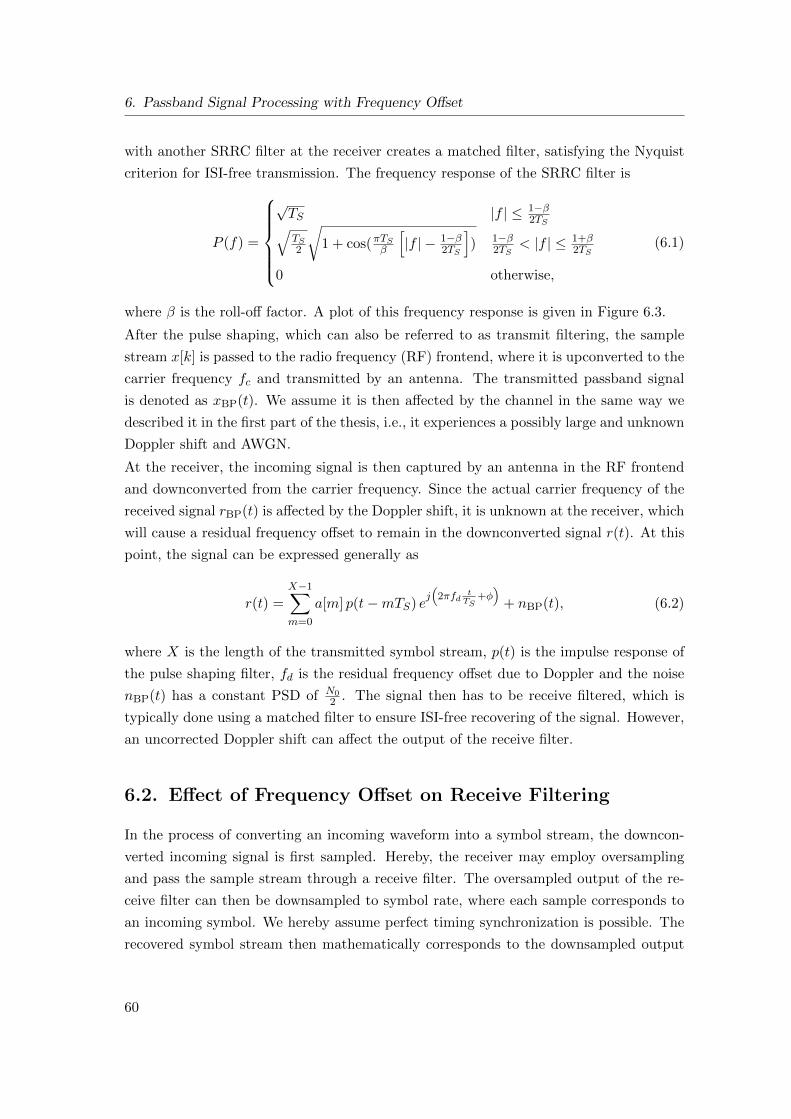
6. Passband Signal Processing with Frequency Offset
with another SRRC filter at the receiver creates a matched filter, satisfying the Nyquist
criterion for ISI-free transmission. The frequency response of the SRRC filter is
P (f) =
√TS |f | ≤ 1−β
2TS√TS2
√1 + cos(πTS
β
[|f | − 1−β
2TS
]) 1−β
2TS< |f | ≤ 1+β
2TS
0 otherwise,
(6.1)
where β is the roll-off factor. A plot of this frequency response is given in Figure 6.3.
After the pulse shaping, which can also be referred to as transmit filtering, the sample
stream x[k] is passed to the radio frequency (RF) frontend, where it is upconverted to the
carrier frequency fc and transmitted by an antenna. The transmitted passband signal
is denoted as xBP(t). We assume it is then affected by the channel in the same way we
described it in the first part of the thesis, i.e., it experiences a possibly large and unknown
Doppler shift and AWGN.
At the receiver, the incoming signal is then captured by an antenna in the RF frontend
and downconverted from the carrier frequency. Since the actual carrier frequency of the
received signal rBP(t) is affected by the Doppler shift, it is unknown at the receiver, which
will cause a residual frequency offset to remain in the downconverted signal r(t). At this
point, the signal can be expressed generally as
r(t) =X−1∑
m=0
a[m] p(t−mTS) ej(2πfd
tTS
+ϕ)+ nBP(t), (6.2)
where X is the length of the transmitted symbol stream, p(t) is the impulse response of
the pulse shaping filter, fd is the residual frequency offset due to Doppler and the noise
nBP(t) has a constant PSD of N02 . The signal then has to be receive filtered, which is
typically done using a matched filter to ensure ISI-free recovering of the signal. However,
an uncorrected Doppler shift can affect the output of the receive filter.
6.2. Effect of Frequency Offset on Receive Filtering
In the process of converting an incoming waveform into a symbol stream, the downcon-
verted incoming signal is first sampled. Hereby, the receiver may employ oversampling
and pass the sample stream through a receive filter. The oversampled output of the re-
ceive filter can then be downsampled to symbol rate, where each sample corresponds to
an incoming symbol. We hereby assume perfect timing synchronization is possible. The
recovered symbol stream then mathematically corresponds to the downsampled output
60

6.2. Effect of Frequency Offset on Receive Filtering
of the convolution of the sample stream with the impulse response of the filter:
z[k] = (r ∗ g)[k]
=
X−1∑
m=0
a[m]
∞∫
−∞
g(t) p((k −m)TS − t
)e−j2πfd
tTS dt
ej(2πkfd+ϕ) + n[k],
(6.3)
where
n[k] =
∞∫
−∞
g(t)nBP(kTS − t)dt
is the sampled and filtered noise, which now has a per component variance of σ2n = N0
2 ,
g(t) is the impulse response of the receive filter and g(t) = p∗(−t) holds in the case of a
matched filter.
The work in [PM96] presents the idea of splitting this representation of the filter output
into several components:
z[k] =
a[k]I0(fd) +
X−1∑
m=0m =k
a[m]Ik−m(fd)
ej(2πkfd+ϕ) + n[k], (6.4)
where
In(fd) =∞∫
−∞
g(t) p(nTS − t) e−j2πfd
tTS dt =
∞∫
−∞
G(f +fdTS
)P (f) ej2πfnTSdf. (6.5)
Hereby, G(f + fdTS
= G(f + Fd) is the frequency response of the receive filter, shifted in
frequency by Fd. The set of functions In(fd) describe the effect of the loss in symbol
quality due to the Doppler shift. I0(fd) is an expression for the amplitude of the target
symbol, which is attenuated in comparison to the Doppler free case, while In(fd) for
n = 0 gives the amplitude of the n-th adjacent symbol, hereby describing the impact of
ISI. The detailed derivation of Equations (6.3), (6.4) and (6.5) is given in Appendix A.4.
A visualization of the effect of a frequency offset on the absolute value of the impulse
response of the matched filter pair is shown in Figure 6.2. It is indicated how the values
of In help to interpret the loss in signal quality. It also shows the twofold effect of, firstly,
the attenuation of the amplitude of the target symbol, and additionally, the increase in
amplitude of adjacent symbols at the time of the target symbol, t = 0.
It is possible to find an analytical, closed form solution for In(fd) by using the frequency
response of the transmit filter P (f) and the shifted frequency response of the receive filter
61

6. Passband Signal Processing with Frequency Offset
2T −T T 2T
1
(1− |I0|)
|I1||I2|
fd = 0
fd = 0.4
t
Figure 6.2.: Visualization of the ISI effects In on the absolute value of the impulse re-sponse of a combined SRRC matched filter pair.
G(f+Fd). This is intuitive, since, due to the Doppler shift, the transmit and receive filter
virtually operate at different frequencies. For the case of using a SRRC pulse shaping
filter with frequency response given in (6.1), and a corresponding matched filter at the
receiver with frequency response G(f) = P (f), the shifted frequency response of the
SRRC receive filter is
G(f + Fd) =
√TS |f + Fd| ≤ 1−β
2TS√TS2
√1 + cos(πTS
β
[|f + Fd| − 1−β
2TS
]) 1−β
2TS< |f + Fd| ≤ 1+β
2TS
0 otherwise.
(6.6)
Both frequency responses are defined as piecewise functions, for which reason the product
of the two is also a piecewise function. Therefore, the solution for In(fd) can be computed
by integrating the sub-functions over the corresponding intervals. The boundaries of the
intervals correspond to the locations where one of the frequency responses changes its
behavior. This is visualized in Figure 6.3. It has to be considered that these sections are
only valid for |fd| < β.
The piecewise integrals can be solved analytically to derive a closed form expression of
the attenuation of the target symbol and the additional ISI components dependent on
the Doppler shift. The detailed construction and solution of the integral is presented in
Appendix A.5. For n = 0 the solution of the integral simplifies to
|I0(fd)| = 1− β − |fd|+4β
πsin
(∣∣∣∣πfd2β
∣∣∣∣)+ (β − |fd|) cos(
πfd2β
). (6.7)
62

6.2. Effect of Frequency Offset on Receive Filtering
−1+
β2T
S
−1−
β2T
S−F d
−1−
β2T
S
1−β
2TS−F d 1−β
2TS
1+β
2TS−F d
0.5
1
P (f)G(f + Fd)
−Fd
f
Figure 6.3.: Frequency analysis of a SRRC filter pair. P (f) is the transmit filter andG(f + Fd) is the receive filter, virtually operating at a shifted frequency.
0 0.1 0.2 0.3 0.4 0.50
0.25
0.5
0.75
1
Normalized Doppler shift fd
Normalized
Amplitude
|I0||I1||I2||I3|
Figure 6.4.: I0(fd) up to I3(fd) as a function of the normalized Doppler shift, for a SRRCmatched filter pair with roll-off β = 0.5.
The functions I0(fd) to I3(fd) are plotted in Figure 6.4 for a matched filter pair of
SRRC pulses with a roll-off factor of β = 0.5. It can be seen that both the attenuation
of the target symbol and the ISI from adjacent symbols are rather moderate for very
small Doppler shifts, but become worse for Doppler shifts in the order of tenths of the
bandwidth. Additionally, it can be noted that the amplitude of the ISI decreases signif-
icantly with growing distance between the observed symbol and the interfering symbol,
suggesting that the immediate neighbors have the largest impact. In the remainder of
the thesis, we will now refer to both the effects of attenuation and ISI simply as ISI.
63


7. Effect of ISI on Frame
Synchronization
Let us know analyze the effect of ISI and the thereby distorted incoming symbols on
the problem of frame synchronization. We will derive analytic models for the simple
correlator, the bank of correlators and the swiveled correlator. Furthermore, we will also
compare the detection schemes presented in Chapter 4 considering their performance and
complexity.
7.1. Analytic Modeling
We will now conduct a similar analysis to the one presented in Chapter 5, only this
time considering the effects of ISI. The discussion of the probability of false alarm Pfa
follows the lines of what was presented in Chapter 5, since the noise is not affected by
ISI. Therefore, the analytic models for Pfa can be found in Equations (5.8) for the simple
correlator, (5.14) for the bank of correlators and (5.22) for the swiveled correlator. The
discussion of the probability of correct detection Pd will be presented for each of the
algorithms.
7.1.1. Simple Correlator
We now consider an ISI affected incoming symbol stream containing the preamble, which
we get from Equation (6.4) by substituting the general symbols with the preamble:
z[k] =
c[k]I0(fd) +
K−1∑
m=0m =k
c[m]Ik−m(fd)
ej(2πkfd+ϕ) + n[k]. (7.1)
65
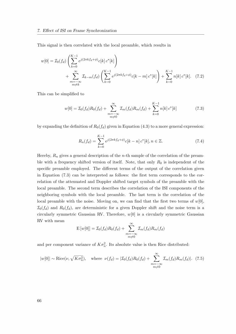
7. Effect of ISI on Frame Synchronization
This signal is then correlated with the local preamble, which results in
w[0] = I0(fd)(
K−1∑
k=0
ej(2πkfd+ϕ)c[k] c∗[k]
)
+∞∑
m=−∞m=k
Ik−m(fd)
(K−1∑
k=0
ej(2πkfd+ϕ)c[k −m] c∗[k]
)+
K−1∑
k=0
n[k] c∗[k]. (7.2)
This can be simplified to
w[0] = I0(fd)R0(fd) +
∞∑
m=−∞m =0
Im(fd)Rm(fd) +
K−1∑
k=0
n[k] c∗[k] (7.3)
by expanding the definition of R0(fd) given in Equation (4.3) to a more general expression:
Rn(fd) =K−1∑
k=0
ej(2πkfd+ϕ)c[k − n] c∗[k], n ∈ Z. (7.4)
Hereby, Rn gives a general description of the n-th sample of the correlation of the pream-
ble with a frequency shifted version of itself. Note, that only R0 is independent of the
specific preamble employed. The different terms of the output of the correlation given
in Equation (7.3) can be interpreted as follows: the first term corresponds to the cor-
relation of the attenuated and Doppler shifted target symbols of the preamble with the
local preamble. The second term describes the correlation of the ISI components of the
neighboring symbols with the local preamble. The last term is the correlation of the
local preamble with the noise. Moving on, we can find that the first two terms of w[0],
I0(fd) and R0(fd), are deterministic for a given Doppler shift and the noise term is a
circularly symmetric Gaussian RV. Therefore, w[0] is a circularly symmetric Gaussian
RV with mean
E [w[0]] = I0(fd)R0(fd) +∞∑
m=−∞m=0
Im(fd)Rm(fd)
and per component variance of Kσ2n. Its absolute value is then Rice distributed:
|w[0]| ∼ Rice(ν,√Kσ2
n), where ν(fd) = |I0(fd)R0(fd) +∞∑
m=−∞m =0
Im(fd)Rm(fd)|. (7.5)
66

7.1. Analytic Modeling
The probability of correct detection again corresponds to the probability that this Rice
distributed RV exceeds the threshold λ:
Pd(λ) = Pr[|w[0]| > λ
]=
∞∫
λ
x
Kσ2n
e−x2+ν2(fd)
2Kσ2n I0
(xs(fd)
Kσ2n
)dx. (7.6)
Since the Rice factor ν(fd) depends on Rn(fd) and this is generally not independent
of the specific preamble, the above expression also depends on the specific preamble.
Furthermore, computing expressions for In(fd) and Rn(fd) becomes cumbersome for long
preambles, for which reason we approximate the Rice factor as
ν(fd) = |I0(fd)R0(fd)|. (7.7)
We expect this approximation to be tight. We can therefore give a general approximation
of the probability of correct detection that is independent of the preamble:
Pd(λ) ≈∞∫
λ
x
Kσ2n
e−x2+ν2(fd)
2Kσ2n I0
(xν(fd)
Kσ2n
)dx. (7.8)
7.1.2. Bank of Correlators
For the bank of correlators we will again consider N parallel branches. However, the bank
of correlators has the distinct advantage that it is easily possible to shift the frequency
for each branch before the receive filter. The corresponding block diagram is depicted
in Figure 7.1. Although this increases the complexity, as also N receive filters have to
operated, it significantly reduces the effects of ISI and therefore increases the performance
for large Doppler shifts, which will be emphasized using simulations in the next section.
Instead of the receive filter dealing with Doppler shifts between [−fmax, fmax], the receive
filter of the correct branch only has a maximum frequency offset of fr = fmax
N−1 . This
significantly reduces ISI in the correct branch.
We know from our previous discussion that the output |wi[0]| of each branch (combination
of receive filter and simple correlator) is Rice distributed with parameters ν(fd−(i−1)∆f)
(or ν for an approximation of the Rice factor) and√Kσ2
n. For the correct branch, the
Rice factor will be ν(fr) (or ν(fr)), while we will again approximate the other branches
with i.i.d. Rayleigh RVs with scale parameter√Kσ2
n. The rest of the discussion is
equivalent to the one presented for Pd of the bank of correlators in Chapter 5, which
67

7. Effect of ISI on Frame Synchronization
...
× × ... ×
Rx Filter Rx Filter ... Rx Filter
SimpleCorrelator
SimpleCorrelator
... SimpleCorrelator
Maximum Selector
r(t)
e−j2πfmaxt e−j2π(fmax−∆f)t ej2πfmaxt
r1(t) r2(t) rN (t)
z1[µ+ k] z2[µ+ k] zN [µ+ k]
∣∣w1[µ]∣∣ ∣∣w2[µ]
∣∣ ∣∣wN [µ]∣∣
LB(µ) f [µ]
Figure 7.1.: Block diagram of the bank of correlators including the receive filters in everybranch.
ultimately leads to an approximation of the probability of detection as
Pd(λ) =
∞∫
λ
(1− e
− x2
2Kσ2n
)N−1x
Kσ2n
e−x2+ν2(fr)
2Kσ2n I0
(xν(fr)
Kσ2n
)dx. (7.9)
7.1.3. Swiveled Correlator
For the swiveled correlator the discussion will become significantly more complex, due
to the partial correlation with preamble fragments. For the sake of simplicity, we will
approximate the incoming symbol stream by neglecting the actual ISI effects and only
considering the attenuation of the target symbol, i.e.,
z[k] = c[k]I0(fd)ej(2πkfd+ϕ) + n[k]. (7.10)
This is equivalent to the approximation made for the Rice factor in Section 7.1.1. The
outputs of the partial correlations are then given by
wn[0] = I0(fd)R(M)0 (fd)e
j2πfd(n−1)M +
nM−1∑
k=(n−1)M
n[k] c∗[k], n ∈ {1, N} (7.11)
68
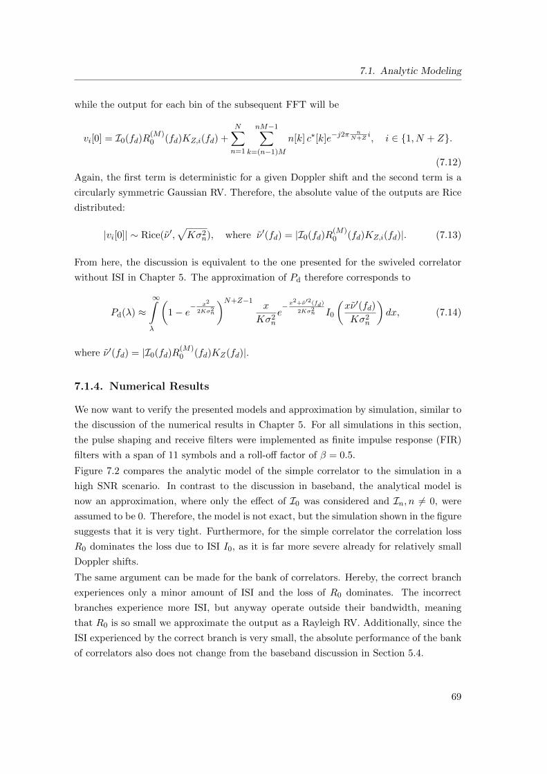
7.1. Analytic Modeling
while the output for each bin of the subsequent FFT will be
vi[0] = I0(fd)R(M)0 (fd)KZ,i(fd) +
N∑
n=1
nM−1∑
k=(n−1)M
n[k] c∗[k]e−j2π nN+Z
i, i ∈ {1, N + Z}.
(7.12)
Again, the first term is deterministic for a given Doppler shift and the second term is a
circularly symmetric Gaussian RV. Therefore, the absolute value of the outputs are Rice
distributed:
|vi[0]| ∼ Rice(ν ′,√
Kσ2n), where ν ′(fd) = |I0(fd)R(M)
0 (fd)KZ,i(fd)|. (7.13)
From here, the discussion is equivalent to the one presented for the swiveled correlator
without ISI in Chapter 5. The approximation of Pd therefore corresponds to
Pd(λ) ≈∞∫
λ
(1− e
− x2
2Kσ2n
)N+Z−1x
Kσ2n
e−x2+ν′2(fd)
2Kσ2n I0
(xν ′(fd)Kσ2
n
)dx, (7.14)
where ν ′(fd) = |I0(fd)R(M)0 (fd)KZ(fd)|.
7.1.4. Numerical Results
We now want to verify the presented models and approximation by simulation, similar to
the discussion of the numerical results in Chapter 5. For all simulations in this section,
the pulse shaping and receive filters were implemented as finite impulse response (FIR)
filters with a span of 11 symbols and a roll-off factor of β = 0.5.
Figure 7.2 compares the analytic model of the simple correlator to the simulation in a
high SNR scenario. In contrast to the discussion in baseband, the analytical model is
now an approximation, where only the effect of I0 was considered and In, n = 0, were
assumed to be 0. Therefore, the model is not exact, but the simulation shown in the figure
suggests that it is very tight. Furthermore, for the simple correlator the correlation loss
R0 dominates the loss due to ISI I0, as it is far more severe already for relatively small
Doppler shifts.
The same argument can be made for the bank of correlators. Hereby, the correct branch
experiences only a minor amount of ISI and the loss of R0 dominates. The incorrect
branches experience more ISI, but anyway operate outside their bandwidth, meaning
that R0 is so small we approximate the output as a Rayleigh RV. Additionally, since the
ISI experienced by the correct branch is very small, the absolute performance of the bank
of correlators also does not change from the baseband discussion in Section 5.4.
69

7. Effect of ISI on Frame Synchronization
0 0.025 0.05 0.075 0.1
10−1
100
Probability of false alarm Pfa
1-Pd
Simulation
Analytic
Figure 7.2.: ROC curve comparison of the analytic model and simulation for the simplecorrelator considering ISI. ES
N0= 0dB,K = 15, fmax = 0.05.
0 0.025 0.05 0.075 0.110−2
10−1
100
Probability of false alarm Pfa
1-Pd
Sim. - ESN0
= −9 dB,K = 300
Ana. - ESN0
= −9 dB,K = 300
Sim. - ESN0
= −5 dB,K = 100
Ana. - ESN0
= −5 dB,K = 100
Sim. - ESN0
= 0dB,K = 20
Ana. - ESN0
= 0dB,K = 20
Figure 7.3.: ROC curve comparison of the analytic model and simulation for the swiveledcorrelator considering ISI. The swiveled correlator was configured with N =K branches, therefore, M = 1, and a padding of Z = N zeros. The maximumDoppler shift was fmax = 0.5.
70

7.2. Comparison and Discussion
Finally, for the swiveled correlator the ISI losses actually dominate over R0 for subse-
quence lengths of M = 1. Therefore, by approximating the Rice factor with the effects of
I0 and R0 and disregarding the interference from adjacent symbols, the modeled output
of the correct bin will be (slightly) larger. However, during the discussion in the base-
band setting in Section 5.4 we established that the analytic model gives a conservative
approximation, meaning that the actual performance was observed to be slightly better
than the model estimated. Therefore, the effects discussed in the baseband setting and
the approximation of the Rice factor counteract eachother and the resulting model con-
sidering ISI is even slightly more tight than in the baseband setting. The comparison of
the analytic model and the simulation is shown in Figure 7.3 for different scenarios. The
experimental results show the tightness of the analytic model in several SNR scenarios.
7.2. Comparison and Discussion
To compare the different detection schemes in an ISI affected setting, we performed
simulations in a similar manner as described in Section 4.6. The employed pulse shaping
and receive filters were implemented as FIR filters with a span of 11 symbols and a roll-off
factor of β = 0.22.
Performance across Doppler range
Similar to the comparison in the first part of thesis, we want to examine the detection
performance across the range of frequency offsets. This is plotted in Figure 7.4. The
simple correlator LC behaves very similarly to the baseband discussion without ISI. This
can be attributed to the dominance of the correlation loss R0(fd) over the loss due to
ISI. The effect of ISI becomes apparent when considering the swiveled correlator LS, the
double correlator LA or the Choi-Lee detector LCL, which show a significant degradation
in detection performance for larger frequency offsets. Also, the advantage of the bank
of correlators LB in the ISI affected setting becomes apparent: due to the frequency
adjustment before the receive filter operation, the effect of ISI is limited on the frequency
range of one branch. In other words, the receive filter of the correct branch operates with
a small residual frequency offset, whereas the receive filter in the other detection schemes
has to deal with the full range of Doppler shifts. Apart from the loss in between the
branches due to the small bandwidth of the correlation, the detection performance of the
bank of correlators is constant over the full Doppler range. The severity of the loss in
between branches, and likely the scalloping loss of the swiveled correlator, can again be
reduced by using more resources.
71

7. Effect of ISI on Frame Synchronization
−0.5 −0.375 −0.25 −0.125 0 0.125 0.25 0.375 0.50
0.25
0.5
0.75
1
Normalized Doppler shift fd
Proab
ilityof
detection
Pd
LC
LA
LCL
LS : N = K,Z = 0
LB : N = K
Figure 7.4.: Comparison of the detection performance across the normalized frequencyoffset in a high SNR scenario. ES
N0= 2dB, K = 10, Pfa = 10−1 ± 10−3.
0 0.025 0.05 0.075 0.10.90
0.93
0.95
0.98
1.00
Probability of false alarm Pfa
Proabilityofdetection
Pd
LA
LCL
LS : N = K,Z = 3N
LB : N = 2K
Figure 7.5.: Simulated ROC at high SNR considering ISI. ESN0
= 0dB, K = 30, fmax = 0.5.
72

7.2. Comparison and Discussion
0 0.025 0.05 0.075 0.10.80
0.85
0.90
0.95
1.00
Probability of false alarm Pfa
Proab
ilityof
detection
Pd
LA
LCL
LS : N = K,Z = 3N
LB : N = 2K
Figure 7.6.: Simulated ROC at low SNR considering ISI. ESN0
= −9 dB, K = 250,fmax = 0.5.
High SNR
Figure 7.5 shows the simulation results for a high SNR scenario of a passband trans-
mission. It can be seen that the bank of correlators with a number of branches of 2K
significantly outperforms the other detection schemes. This can be attributed to the use
of a bank of receive filters, which greatly reduces the effects of ISI in the correct branch,
so that again the correlation loss R0(fd) dominates. The cost of reducing ISI is a much
higher complexity. Regarding the other detection schemes, the double correlator performs
better than the swiveled correlator and the Choi-Lee detector in this high SNR scenario.
Low SNR
Again considering a low SNR scenario, which is more typical for a satellite link, Figure 7.6
shows that the double correlator LA strongly loses in performance. This is in line with
the findings of the baseband discussion in Part I, which showed that the LA detector did
not perform well in low SNR scenarios.
Considering partially contained preambles
Similarly to the discussion in Part I, we can examine the effect of partially contained
preambles. The simulation setup is hereby chosen equivalently, embedding a preamble
73

7. Effect of ISI on Frame Synchronization
0 0.025 0.05 0.075 0.10.80
0.85
0.90
0.95
1.00
Probability of false alarm Pfa
Proab
ilityof
detection
Pd
LA
LCL
LS : N = K,Z = 3N
LB : N = 2K
Figure 7.7.: Simulated ROC at high SNR considering ISI and partially contained pream-bles. ES
N0= 0dB, K = 30, fmax = 0.5.
0 0.025 0.05 0.075 0.10.80
0.85
0.90
0.95
1.00
Probability of false alarm Pfa
Proabilityofdetection
Pd
LA
LCL
LS : N = K,Z = 3N
LB : N = 2K
Figure 7.8.: Simulated ROC at low SNR considering ISI and partially contained pream-bles. ES
N0= −9 dB, K = 250, fmax = 0.5.
74

7.2. Comparison and Discussion
every 3K symbols, as previously shown in Figure 4.12. This symbol stream will then be
pulse shaped, impaired by Doppler shift and noise, received filtered, and then supplied to
the detectors. The Simulated a high SNR environment shows that also in the ISI affected
setting, the Choi-Lee detector suffers the smallest performance loss, actually performing
similarly well as without partially contained preambles. This can again be attributed to
the energy correction term.
Accordingly, the Simulated a low SNR environment, shown in Figure 7.8, reveals that the
benefit of this energy correction term becomes smaller in low SNR environments, where
the signal energy is anyway dominated by the noise. When comparing Figures 7.6 and 7.8,
it becomes apparent that the performance of the swiveled correlator barely changes when
considering partially contained preambles. This further validates the assumption of dis-
regarding partially contained preambles in a low SNR satellite setting for the analytic
modeling of the detection schemes presented in Section 7.1.
Different tradeoffs between performance and complexity
The presented simulations confirmed that the bank of correlators corresponds to a de-
tector design that achieves very good performance, but has a high complexity. On the
other hand, the swiveled correlator performs significantly worse, but has a very low com-
plexity. A possible method to find a tradeoff in between these two, i.e., a design with
good performance and moderate complexity, could be to use a hybrid approach, which
may be called bank of swiveled correlators. Hereby, the idea is to operate several receive
filters and swiveled correlators at different center frequencies to reduce the effects of ISI
in the correct branch and identify the correct branch with a maximum selector. This
corresponds to exchanging the simple correlators in the branches of the bank of correla-
tors with swiveled correlators. However, a much smaller amount of branches can be used,
which will be elaborated in the following.
Essentially, the bank of correlators was presented in Chapter 4 as a method to mitigate the
correlation loss R0(fd). As discussed, the swiveled correlator already solves this problem
in a different way. However, the performance of the swiveled correlator is significantly
decreased by the effects of ISI, In(fd), due to imperfect receive filtering. The losses
due to ISI can be reduced by employing a bank of receive filters, as is done for the
bank of correlators. However, the losses due to ISI, In(fd), are much less severe than
the correlation loss R0(fd), especially for small frequency shifts. Additionally, they are
independent of the preamble length and therefore do not become more severe for longer
preambles used in low SNR scenarios, as is the case for the correlation loss. Therefore,
already a small amount of receive filters, e.g. four or eight, could substantially reduce
75

7. Effect of ISI on Frame Synchronization
the losses due to ISI. For the standard bank of correlators, a configuration with such
a small amount of branches would be impractical, since the residual frequency offset in
each branch would still cause unacceptably large correlation losses. However, since the
swiveled correlator is not subject to such large correlation losses, the reduced ISI by
employing a a bank of swiveled correlators with a few branches with receive filters at
different frequency shifts can significantly improve the performance, while still achieving
a much lower complexity than the bank of correlators.
A comparison of different configurations corresponding to different tradeoffs between
performance and complexity is left for further study. A more detailed analysis of this
detection scheme is expected to be a relatively straightforward extension of the discussion
in Section 7.1.
7.3. Complexity
An important aspect of the previous sections is that the bank of correlators can success-
fully reduce the effect of ISI by performing the receive filtering after the frequency shift
in each branch. However, this significantly increases the computational complexity of the
algorithm. Since the resources of a satellite are limited, the problem of frame detection
is subject to constraints in the computational effort. It is generally desirable to find a
tradeoff with good performance and low complexity. It is therefore important to also
compare the regarded schemes considering their computational complexity. Hereby, it
is necessary to consider different preamble lengths, since the preamble length has to be
adjusted to the SNR in order to reach high detection probabilities.
A well-suited and commonly used figure of merit for such a comparison is the Big O
notation of the number of operations with respect to the preamble length. Table 7.1
gives the computational complexity of each detector. The simple correlator, naturally,
has the lowest complexity, corresponding to the length of the correlation, i.e., O(K). The
bank of correlators employs N parallel branches with simple correlators (and also receive
filters) and is therefore N times as complex. The number of branches N is O(K), since
the number of branches has to be increased for longer preambles in order to obtain a
high detection probability. Therefore, the bank of correlators requires O(K2) operations.
Similarly, the double correlator and the Choi-Lee detector compute the sum of all possible
double correlations, which also corresponds to O(K2) operations. The swiveled correlator
uses N branches, in each of which a correlation of length M is performed. This results
in a complexity of O(K) operations for the correlation, which is succeeded by an FFT.
The complexity of an FFT is O(K logK) and therefore dominates over the correlation.
The Big O notation provides us a first insight into the complexity of the different schemes
76

7.3. Complexity
Detector Operations
Simple correlator LC O(K)
Bank of correlators LB O(K2)
Swiveled correlator LS O(K logK)
Double correlator LA O(K2)
Choi-Lee detector LCL O(K2)
Table 7.1.: Computational complexity of the considered detection schemes
50 100 150 200 250 300
10−4
10−3
10−2
Preamble length K
Execution
timeper
sample
[s]
LC
LA
LCL
LS : N = K,Z = N
LB : N = K
Figure 7.9.: Comparison of the execution time of software implementations of the detec-tion schemes.
in the asymptotic regime where K tends to infinity, i.e., for very large preamble lengths.
However, in practical systems we can expect the preamble length to be at most in the order
of a few thousands, more commonly a few hundred symbols. In this regime, we cannot
expect asymptotic considerations to hold tightly, thus it is important to look at other,
non-asymptotic measures for the complexity. For this reason, we simulated the expected
execution time of the MATLAB software implementations of the detectors. Figure 7.9
plots the execution time per output sample across the preamble length. This shows,
that for small preambles, the bank of correlators is already much more computationally
expensive. This is mainly due to the bank of receive filters. It can also be seen that
the Choi-Lee detector is slightly more complex than the double correlator, which comes
77

7. Effect of ISI on Frame Synchronization
from the additional computation of the data correction term. It becomes clear that the
swiveled correlator has by far the lowest complexity of the detection schemes that can
deal with large Doppler shifts.
It may be added that in a practical implementation other criteria, such as the possibility
to parallelize the processing, might play an important role. A more detailed complexity
analysis is left for further study.
7.4. Summary
When comparing the detection schemes in an ISI affected setting, it becomes clear that
due the employment of a bank of receive filters, the bank of correlators outperforms the
other schemes by far. The cost for the better performance is a significantly increased
complexity. The comparison also reveals that the swiveled correlator is the least complex
detector and, additionally, shows a better performance than the double correlator and the
Choi-Lee detector in satellite characteristic low SNR scenarios. Furthermore, the benefit
of simultaneously performing frame synchronization and obtaining an estimate for the
Doppler shift (as can be done for the bank of correlators and the swiveled correlator)
becomes clear: if a preamble is correctly detected, the Doppler estimate can be used to
adjust the center frequency of the receive filter for the subsequent processing of the rest
of the packet. This significantly reduces the effect of ISI and increases the probability of
correctly decoding the data.
78

8. Simulations of Realistic Satellite Link
For the previous analysis and simulations we assumed a very controlled scenario, with
constant SNR and a uniform Doppler shift between fd ∈ [−fmax, fmax], where usually
fmax = 0.5. Such a large Doppler shift can be considered extreme and not particularly
realistic in practical satellite transmission scenarios. Additionally, although we consid-
ered low SNR scenarios in the previous simulations and we tried to indicate towards the
characteristics of a satellite transmission, we will now present some simulations for a re-
alistic LEO satellite link. The parameters characterizing the link are listed in Table 8.1.
To simulate the transmission from any terminal in the coverage of the satellite, we uni-
formly sample a point in the coverage area. We then compute the Doppler shift (see
Appendix A.6 for details) and the SNR for this point. It is notable that the distribution
of the Doppler shift is not anymore uniform. We then average over a significant amount
of such transmissions to obtain the average performance of the detection schemes in the
satellites coverage area. The results of the simulation are shown in Figure 8.1.
It can be seen that the bank of correlators with 2K parallel branches performs significantly
better than all other detectors. This is again attributed to the mitigation of ISI losses by
employing a bank of receive filters. A configuration using less resources, i.e., K parallel
branches, shows a significant decrease in performance due to stronger correlation losses.
Hereby, the correlation loss R0 still dominates the additional loss due to ISI. In this
configuration it performs similarly well as the swiveled correlator with a subsequence
length of M = 1 and a zero-padding ratio of ZN = 3. While the Choi-Lee correlator
Description Symbol Value
Carrier frequency fc 2GHz
Symbol rate 1TS
250 kHz
Satellite altitude h 575 km
Maximum slant range dmax 1300 km
SNR at CoC EsN0
∣∣CoC
−6 dB
SNR at EoC EsN0
∣∣EoC
−13 dB
Table 8.1.: Parameters of the considered LEO satellite link.
79

8. Simulations of Realistic Satellite Link
0 0.025 0.05 0.075 0.110−3
10−2
10−1
100
Probability of false alarm Pfa
1-Pd
LA
LCL
LS : N = K,Z = 3N
LB : N = K
LB : N = 2K
Figure 8.1.: Simulated ROC for a realistic LEO satellite link. The employed preamblelength was K = 350 symbols. Other parameters are given in Table 8.1.
performs slightly worse than those two, the double correlator has a substantially lower
detection probability. This emphasizes that the double correlator does not perform well
in low SNR scenarios. However, it is interesting that the Choi-Lee detector performs
significantly better than the the double correlator, considering it also uses the double
correlation and subtracts a data correction term. Although this is intended to reduce
the influence of random data surrounding the preamble, it seems like it also improves the
performance in low SNR scenarios. The root cause of this could not be established in the
narrow time frame of this thesis and therefore remains subject to further investigation.
80

9. Conclusion
The research presented in this thesis explored the problem of frame synchronization in a
satellite setting, in which a large, possibly unknown Doppler shift cannot be precompen-
sated and therefore decreases the performance of traditional synchronization algorithms.
Additionally, the process of receive filtering is affected by the Doppler induced frequency
offset and ISI occurs. Due to the highly dynamic nature of a random access setting,
sequential frame detection techniques based on hypothesis testing were considered.
In the first part of the thesis, a simplified discussion of the problem considering a baseband
representation of the incoming signal was performed. Hereby, in Chapter 3, the derivation
of an optimal LRT in the considered setting was presented.
Chapter 4 introduced several relevant detection algorithms, including an approximation
of the optimal LRT. It was also shown that a frequency offset in the incoming preamble
leads to a substantial decrease of the correlation output, making detection less reliable
in the presence of noise. The presented detectors aim to resolve this problem and were
compared in different scenarios. It was shown that the approximation of the optimal
LRT, which corresponds to a double correlation, significantly loses performance in low
SNR environments. The swiveled correlator and the bank of correlators show close to
optimal performance in all considered scenarios, where the swiveled correlator achieves a
much lower complexity.
In Chapter 6 we conducted an in-depth study of the effects of ISI due to receive filtering
when a frequency offset is present. While we identified in Chapter 7 that using a bank
of matched filters for the bank of correlators solves the problem in a performant way, the
complexity of the algorithm becomes unacceptably high. The swiveled correlator shows
a good tradeoff between performance and complexity.
In Chapters 5 and 7, analytic models were derived for the simple correlator, the bank of
correlators and the swiveled correlator for both cases with and without ISI. The devel-
oped approximations can quickly estimate and predict the performance of the algorithms.
This can help to explore the parameter space and determine an approximate configura-
tion of preamble length, number of branches and amount of zero-padding fitting to the
requirements of the application. Making these design choices with an analytical model
rather than elaborate simulations can speed up the development process.
81

9. Conclusion
Finally, the simulations of a realistic satellite link presented in Chapter 8 confirm that the
findings established in a simplified scenario also apply to the characteristics of a realistic
link.
Future Work
The discussion of the frame synchronization problem in the given satellite setting is
still somewhat incomplete and needs to be extended with further research. Given the
findings we made in the thesis, we may indicate interesting issues to consider in the
future. Additionally, some smaller peculiarities were identified in the course of the thesis,
but remain unsolved.
In Chapter 4, it was identified that the approximation of the optimal LRT is not tight
in low SNR scenarios. The origin of this loss may be the approximation of the Bessel
function with a second order polynomial, which may only be tight in certain scenarios.
However, this was not sufficiently investigated and deserves further attention. It could
also be interesting to explore other low-complexity approximations for the Bessel function.
It became clear in Chapter 8, that the double correlator performs substantially worse
than the Choi-Lee detector, although the two differ only in a data correction term. It
is unclear why the data correction term, which is intended to reduce the influence of
random data surrounding the preamble, increases the performance and deserves further
research.
The comparison of the discussed detection schemes considering ISI conducted in Chapter 7
showed that the bank of correlators significantly outperforms the other methods. This can
be attributed to the employment of a bank of matched filters, which reduces ISI effectively,
but significantly increases the complexity. It could be worthwhile to investigate low-
complexity alternatives to this problem. A first starting point could be the modification
of the receive filter, e.g. increasing the bandwidth to capture more of the incoming signal.
A very brief introduction to this is given in Appendix B.
The problem of frame synchronization in the considered random access satellite setting
was discussed in a simplified manor by analyzing an isolated preamble. Therefore, further
research has to be conducted considering also the data part of the packet. In the absence
of multi-user interference, the data part could be used in addition to the preamble to
detect the packet. In the simplest form, an additional energy detector would confirm the
presence of the packet using the data part. However, it is unclear how effective this is in
low SNR scenarios, given that the noise energy is dominating, and if other methods can
be found to favorably use the data part of the packet for detection.
Furthermore, a very important aspect of frame synchronization in a random access setting
82

is the influence of interference from other users. It is generally desirable to operate a
system at a high load, so all resources are optimally used. However, this leads to the
collision and interference of packets. The effect of incoming preambles interfering with
random data or other preambles with possibly different frequency shifts is therefore an
important subject of further research.
83


A. Derivations and Proofs
A.1. Derivation of the Optimal LRT
Starting from Equation (3.10),
L(µ) =
18π2fmax
π∫
−π
2πfmax∫
−2πfmax
1(πσ2
n)K · e
− 1
σ2n
K−1∑k=0
|r[µ+k]−c[k]ej(θk+ϕ)|2dϕ dθ
1(πσ2
n)K · e
− 1
σ2n
K−1∑k=0
|r[µ+k]|2
H1
⋛H0
λ, (A.1)
we can use the independence of r[µ+ k] on θ and ϕ to move the denominator inside the
integral and reduce the constant factor to give
L(µ) =1
8π2fmax
π∫
−π
2πfmax∫
−2πfmax
e− 1
σ2n
K−1∑k=0
|r[µ+k]−c[k]ej(θk+ϕ)|2· e
1
σ2n
K−1∑k=0
|r[µ+k]|2dϕ dθ. (A.2)
In the next step the integrals can be combined:
L(µ) =1
8π2fmax
π∫
−π
2πfmax∫
−2πfmax
e
1
σ2n
(K−1∑k=0
|r[µ+k]|2−K−1∑k=0
|r[µ+k]−c[k]ej(θk+ϕ)|2)dϕ dθ. (A.3)
We can define z1 = r[µ+ k] and z2 = c[k]ej(θk+ϕ) and use the following rules of complex
numbers:
|z1 − z2|2 = (z1 − z2)(z1− z2)∗ = (z1 − z2)(z∗1 − z∗2)
= z1z∗1 − z1z
∗2 − z2z
∗1 + z2z
∗2
= |z1|2 + |z2|2 − 2Re (z1z∗2)
I

A. Derivations and Proofs
to give
∣∣∣r[µ+ k]− c[k]ej(θk+ϕ)∣∣∣2= |r[µ+ k]|2 +
∣∣∣c[k]ej(θk+ϕ)∣∣∣2− 2Re
(r[µ+ k]
(c[k]ej(θk+ϕ)
)∗)
= |r[µ+ k]|2 +∣∣∣c[k]ej(θk+ϕ)
∣∣∣2− 2Re
(r[µ+ k]c∗[k]e−j(θk+ϕ)
).
(A.4)
Equation (A.4) can then be input into equation (A.3) to result in
L(µ) =1
8π2fmax
π∫
−π
2πfmax∫
−2πfmax
e
1
σ2n
(K−1∑k=0
|r[µ+k]|2−K−1∑k=0
(|r[µ+k]|2+|c[k]ej(θk+ϕ)|2−2Re(r[µ+k]c∗[k]e−j(θk+ϕ))
))dϕ dθ
(A.5)
=1
8π2fmax
π∫
−π
2πfmax∫
−2πfmax
e
1
σ2n
(K−1∑k=0
2Re(r[µ+k]c∗[k]e−j(θk+ϕ))−K−1∑k=0
|c[k]ej(θk+ϕ)|2)dϕ dθ
(A.6)
=1
8π2fmax
π∫
−π
2πfmax∫
−2πfmax
e2
σ2n
K−1∑k=0
Re(r[µ+k]c∗[k]e−j(θk+ϕ))e− 1
σ2n
K−1∑k=0
|c[k]|2dϕ dθ (A.7)
=1
8π2fmaxC(c, σ2
n)
π∫
−π
2πfmax∫
−2πfmax
e2
σ2n
K−1∑k=0
Re(r[µ+k]c∗[k]e−j(θk+ϕ))dϕ dθ, (A.8)
where C(c, σ2n) = e
− 1
σ2n
∑K−1k=0 |c[k]|2
. From equation (A.5) to (A.6) we use the associativity
of the sum and simplify the resulting expression. Furthermore, in (A.6) it can be exploited
that a complex exponential has unit magnitude:
∣∣∣c[k] · ej(θk+ϕ)∣∣∣2= |c[k]|2 ·
∣∣∣ej(θk+ϕ)∣∣∣2= |c[k]|2. (A.9)
Therefore, the result of (A.9) can be split into a separate exponential as given in (A.7).
As this term is independent of θ and ϕ it can be moved outside the integral and was
named C(c, σ2n). Equation (A.8) corresponds to Equation (6) in [WRKH18], where some
typing errors where corrected.
We can further simplify the expression by using the following rule of sums of complex
II

A.1. Derivation of the Optimal LRT
numbers:
Re (z) + Re (w) = Re (z + w) . (A.10)
The argument of the exponential in A.8 can then be transformed:
2
σ2n
K−1∑
k=0
Re(r[µ+ k]c∗[k]e−j(θk+ϕ)
)= Re
(2
σ2n
K−1∑
k=0
r[µ+ k]c∗[k]e−j(θk+ϕ)
). (A.11)
This can also be expressed in terms of the magnitude and phase of the complex number:
Re
(2
σ2n
K−1∑
k=0
r[µ+ k]c∗[k]e−j(θk+ϕ)
)= ρ · cos(ϕ′), (A.12)
with ρ =2
σ2n
∣∣∣∣∣K−1∑
k=0
r[µ+ k]c∗[k]e−j(θk+ϕ)
∣∣∣∣∣
and ϕ′ = arg
(2
σ2n
K−1∑
k=0
r[µ+ k]c∗[k]e−j(θk+ϕ)
)= η + ϕ,
where η contains the phase of the transmitted symbols, which for M-PSK follows a discrete
uniform distribution depending on the modulation order, the phase due to the frequency
shift θk and the phase of the random noise. Since we integrate over ϕ, it can take an
arbitrary value and therefore also absorb η, so that integrating over ϕ and ϕ′ is equivalent.
We can therefore integrate over ϕ′ instead of ϕ, which results in
L(µ) =1
8π2fmaxC(c, σ2
n)
π∫
−π
2πfmax∫
−2πfmax
eρ·cos(ϕ′) dϕ′ dθ
H1
⋛H0
λ. (A.13)
We can now solve the integral over ϕ′ using the zeroth order modified Bessel function,
given in [Wat95] as
I0(ρ) =1
π
∫ π
0eρ·cos(ϕ
′) dϕ′ =1
2π
∫ π
−πeρ·cos(ϕ
′) dϕ′. (A.14)
We can also remove the random phase offset ϕ from ρ, since it does not depend on the
III

A. Derivations and Proofs
index of the sum and has unit magnitude:
r =2
σ2n
∣∣∣∣∣K−1∑
k=0
r[µ+ k]c∗[k]e−j(θk+ϕ)
∣∣∣∣∣ =2
σ2n
∣∣∣∣∣K−1∑
k=0
r[µ+ k]c∗[k]e−jθke−jϕ
∣∣∣∣∣
=2
σ2n
∣∣∣∣∣e−jϕ
K−1∑
k=0
r[µ+ k]c∗[k]e−jθk
∣∣∣∣∣ =2
σ2n
· 1 ·∣∣∣∣∣K−1∑
k=0
r[µ+ k]c∗[k]e−jθk
∣∣∣∣∣
=2
σ2n
∣∣∣∣∣K−1∑
k=0
r[µ+ k]c∗[k]e−jθk
∣∣∣∣∣ .
(A.15)
Finally moving C(c, σ2n) to the threshold and applying the modified Bessel function leads
us to the ultimate representation of the LRT
L(µ) =1
4πfmax
2πfmax∫
−2πfmax
I0
(2
σ2n
∣∣∣∣∣K−1∑
k=0
r[µ+ k]c∗[k]e−jθk
∣∣∣∣∣
)dθ
H1
⋛H0
λ. (A.16)
A.2. Approximation of the Optimal LRT
The optimal LRT and therefore the starting point for finding an approximation is given
by
L(µ) =1
4πfmax
2πfmax∫
−2πfmax
I0
(2
σ2n
∣∣∣∣∣K−1∑
k=0
r[µ+ k]c∗[k]e−jθk
∣∣∣∣∣
)dθ. (A.17)
The first step is to expand the Bessel function using its series representation:
I0(x) =
∞∑
i=0
(14x
2)i
(i!)2, (A.18)
which yields
L(µ) =1
4πfmax
2πfmax∫
−2πfmax
1 +
∞∑
i=1
(1
σ2n
)2i 1
(i!)2
K−1∑
k1=0
K−1∑
l1=0
...
K−1∑
ki=0
K−1∑
li=0
r[µ+ k1]r∗[µ+ l1]
· c∗[k1]c[l1]r[µ+ ki]r∗[µ+ li]c
∗[ki]c[li] · ejθ[(k1−l1)+...+(ki−li)] dθ. (A.19)
IV

A.2. Approximation of the Optimal LRT
After applying the sum rule of integrals we can once again exploit the independence of r
and c on θ and move the terms outside the integral:
L(µ) =1
4πfmax
2πfmax∫
−2πfmax
1 dθ +∞∑
i=1
(1
σ2n
)2i 1
(i!)2
K−1∑
k1=0
K−1∑
l1=0
...K−1∑
ki=0
K−1∑
li=0
r[µ+ k1]r∗[µ+ l1]
·c∗[k1]c[l1]r[µ+ ki]r∗[µ+ li]c
∗[ki]c[li]
2πfmax∫
−2πfmax
ejθ
i∑q=1
(kq−lq)
dθ
. (A.20)
The next step is to solve the integral over the complex exponential. We can hereby use
the general rules of solving integrals and the Euler’s formula to find that
1
4πfmax
2πfmax∫
−2πfmax
ejθkdθ =1
4πfmax
[1
jkejθk
]2πfmax
−2πfmax
=1
4πfmax
(ej2πfmaxk − e−j2πfmaxk
)
=1
j4πfmax
(cos(2πfmaxk) + j sin(2πfmaxk)
− cos(2πfmaxk) + j sin(2πfmaxk))
=sin(2πfmaxk)
2πfmaxk= sinc(2fmaxk).
(A.21)
Applying Equation (A.21) to (A.20) yields
L(µ) = 1 +∞∑
i=1
(1
σ2n
)2i 1
(i!)2
K−1∑
k1=0
K−1∑
l1=0
...K−1∑
ki=0
K−1∑
li=0
r[µ+ k1]r∗[µ+ l1]c
∗[k1]c[l1] ...
r[µ+ ki]r∗[µ+ li]c
∗[ki]c[li] · sinc
2fmax
i∑
q=1
(kq − lq)
. (A.22)
Since we compare the likelihood function to a threshold λ, the constant 1 can be absorbed
by this threshold. We then follow the same approach as [WRKH18] and only consider
the term i = 2. Thus, we have
LA(µ) =
K−1∑
k1=0
K−1∑
l1=0
K−1∑
k2=0
K−1∑
l2=0
r[µ+ k1] r∗[µ+ l1] c
∗[k1] c[l1]
· r[µ+ k2] r∗[µ+ l2] c
∗[k2] c[l2] sinc (2fmax (k1 − l1 + k2 − l2)) . (A.23)
V
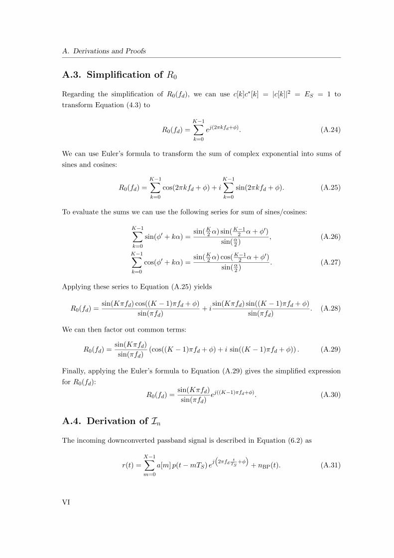
A. Derivations and Proofs
A.3. Simplification of R0
Regarding the simplification of R0(fd), we can use c[k]c∗[k] = |c[k]|2 = ES = 1 to
transform Equation (4.3) to
R0(fd) =K−1∑
k=0
ej(2πkfd+ϕ). (A.24)
We can use Euler’s formula to transform the sum of complex exponential into sums of
sines and cosines:
R0(fd) =K−1∑
k=0
cos(2πkfd + ϕ) + iK−1∑
k=0
sin(2πkfd + ϕ). (A.25)
To evaluate the sums we can use the following series for sum of sines/cosines:
K−1∑
k=0
sin(ϕ′ + kα) =sin(K2 α) sin(
K−12 α+ ϕ′)
sin(α2 ), (A.26)
K−1∑
k=0
cos(ϕ′ + kα) =sin(K2 α) cos(
K−12 α+ ϕ′)
sin(α2 ). (A.27)
Applying these series to Equation (A.25) yields
R0(fd) =sin(Kπfd) cos((K − 1)πfd + ϕ)
sin(πfd)+ i
sin(Kπfd) sin((K − 1)πfd + ϕ)
sin(πfd). (A.28)
We can then factor out common terms:
R0(fd) =sin(Kπfd)
sin(πfd)(cos((K − 1)πfd + ϕ) + i sin((K − 1)πfd + ϕ)) . (A.29)
Finally, applying the Euler’s formula to Equation (A.29) gives the simplified expression
for R0(fd):
R0(fd) =sin(Kπfd)
sin(πfd)ej((K−1)πfd+ϕ). (A.30)
A.4. Derivation of InThe incoming downconverted passband signal is described in Equation (6.2) as
r(t) =X−1∑
m=0
a[m] p(t−mTS) ej(2πfd
tTS
+ϕ)+ nBP(t). (A.31)
VI

A.4. Derivation of In
This signal is then filtered using a receive filter with impulse response g(t). This mathe-
matically corresponds to the convolution, for which we can use its distributivity and its
associativity with scalar multiplication:
z′(t) = (r ∗ g) =X−1∑
m=0
a[m]
(ej(2πfd
tTS
+ϕ)p(t−mTS) ∗ g(t)
)+ nBP(t) ∗ g(t). (A.32)
Expanding the convolution yields
z′(t) =X−1∑
m=0
a[m]
∞∫
−∞
g(τ)p(t− τ −mTS)ej(2π
fdTS
(t−τ)+ϕ)dτ +
∞∫
−∞
g(τ)nBP(t− τ)
= ej(2πfd
tTS
+ϕ) X−1∑
m=0
a[m]
∞∫
−∞
g(τ)p(t− τ −mTS)e−j2π
fdTS
τdτ+
∞∫
−∞
g(τ)nBP(t− τ) dτ.
(A.33)
The filtered signal is then downsampled to symbol rate, so each sample corresponds to
a symbol of the transmitted signal. Hereby, perfect timing synchronization is assumed.
Thus, by sampling at t = kTS we obtain
z[k] = ej(2πkfd+ϕ)X−1∑
m=0
a[m]
∞∫
−∞
g(τ)p((k −m)TS − τ)e−j2π
fdTS
τdτ+
∞∫
−∞
g(τ)nBP(kTS − τ) dτ.
(A.34)
Now, exchanging τ with t yields
z[k] = ej(2πkfd+ϕ)X−1∑
m=0
a[m]
∞∫
−∞
g(t)p((k −m)TS − t)e−j2π
fdTS
tdt+
∞∫
−∞
g(t)nBP(kTS − t) dt.
(A.35)
This proves Equation 6.3.
As mentioned in Chapter 6, we now follow the approach of [PM96] by rephrasing this
equation to
z[k] =
a[k]I0(fd) +
X−1∑
m=0m =k
a[m]Ik−m(fd)
ej(2πkfd+ϕ) + n[k], (A.36)
where
In(FdTS) =
∞∫
−∞
g(t)p(kT − t)e−j2πFdt dt. (A.37)
VII
A. Derivations and Proofs
Since the impulse responses of SRRC filters are infinite and the frequency responses are
finite, to evaluate the integral it is desirable to transform the expression into the frequency
domain. For this, let
u1(t) = g(t)ej2π(−Fd)t u∗2(t) = p(kTS − t). (A.38)
We can then reformulate Equation (A.37) to
In(FdTS) =
∞∫
−∞
g(t)p(kTS − t)e−j2πFdt dt =
∞∫
−∞
u1(t)u∗2(t) dt. (A.39)
The frequency domain representation can be obtained by applying Parseval’s theorem:
In(FdTS) =
∞∫
−∞
u1(t)u∗2(t) dt =
∞∫
−∞
U1(f)U∗2 (f) df. (A.40)
U1(f) and U∗2 (f) can then be found by the Fourier transform of u1(t) and u∗2(t) respec-
tively. Regarding the Fourier transform of u1(t), we can use the translation property of
the Fourier transform:
F (u1(t)) = F(g(t)ej2π(−Fd)t
)= G(f + Fd). (A.41)
For the Fourier transform of u∗2(t) the modulation property can be used:
F (u2(t)) = F (p(kTS − t)) = P (−f)ej2πfkTS . (A.42)
We can now exploit the symmetry of the frequency response of the SRRC filter, i.e.,
P (−f) = P (f). Using this and applying Equations (A.41) and (A.42) to Equation
(A.40), we obtain an expression for the ISI components in the frequency domain:
In(FdTS) =
∞∫
−∞
G(f + Fd)P (f)ej2πfkTS df. (A.43)
A.5. Simplification of InThe different ISI components In(fd) can be computed with
In(fd) =∞∫
−∞
g(t) p(kTS − t) e−j2πfd
tTS dt =
∞∫
−∞
G(f +fdTS
)P (f) ej2πfkTSdf. (A.44)
VIII

A.5. Simplification of In
From the frequency responses of the SRRC pulse shaping filter P (f) given in Equation
(6.1) and the frequency shifted receive filter G(f + fdTS
) = G(f + Fd) given in Equation
(6.6) we can identify seven sections for the case of |FdTS | < β:
S1 = [−∞,−1 + β
2TS], S2 = [−1 + β
2TS,−1− β
2TS− Fd], S3 = [−1− β
2TS− Fd,
1− β
2TS],
S4 = [−1− β
2TS,1− β
2TS− Fd], S5 = [
1− β
2TS− Fd,
1− β
2TS], S6 = [
1− β
2TS,1 + β
2TS− Fd],
S7 = [1 + β
2TS− Fd,∞].
This is visualized in Figure 6.3. The integral in Equation (A.44) can then be split into
several integrals over the given sections:
In(fd) =∫
S1
0 df +
∫
S4
TS ej2πfkTSdf +
∫ ∞
S7
0 df
+
∫
S2
TS
2
√1 + cos
(πTS
β
[−(f + Fd)−
1− β
2TS
])
·√
1 + cos
(πTS
β
[−f − 1− β
2TS
])ej2πfkTSdf
+
∫
S3
TS√2
√1 + cos
(πTS
β
[−f − 1− β
2TS
])ej2πfkTSdf
+
∫
S5
TS√2
√1 + cos
(πTS
β
[f + Fd −
1− β
2TS
])ej2πfkTSdf
+
∫
S6
TS
2
√1 + cos
(πTS
β
[f + Fd −
1− β
2TS
])
·√1 + cos
(πTS
β
[f − 1− β
2TS
])ej2πfkTSdf.
(A.45)
The evaluation of the integrals is generally rather elaborate due to the complex exponen-
tial. For the case of n = 0 however, the complex exponential disappears. We will therefore
exemplify the evaluation of the integrals for I0(fd). We will denote each integral with Si,
where i corresponds to the section. The evaluation of S1, S7 and S4 is trivial:
S1 = S7 =
∫
S7
0 df = 0, (A.46)
IX

A. Derivations and Proofs
S4 =
1−β2
−Fd∫
− 1−β2TS
TS df = 1− β − FdTS . (A.47)
For the evaluation of S2, let x1 and x2 denote the arguments of the cosines:
x1 =πTS
β
[−(f + Fd)−
1− β
2TS
], x2 =
πTS
β
[−f − 1− β
2TS
]. (A.48)
The following identity can be used to eliminate the square roots:
√1 + cos(x) =
√2 cos
(x2
). (A.49)
This yields
S2 =
∫
S2
TS cos(x12
)cos(x22
)df. (A.50)
We can then use the product-to-sum identities of trigonometry to obtain
S2 =
∫
S2
TS
2cos(x12
− x22
)+
TS
2cos(x12
+x22
). (A.51)
Resubstituting x1 and x2 gives
S2 =
− 1−β2TS
−Fd∫
− 1+β2TS
TS
2cos
(πFdTS
2β
)+
TS
2cos
(πTS
β
[−f − 1− β
2TS
]− πFdTS
2β
)df. (A.52)
Finally, we can solve the integral to obtain
S2 =1
2cos
(πFdTS
2β
)(β − FdTS). (A.53)
Regarding the evaluation of section S3, we can also use the identity given in Equation
(A.49) to eliminate the square root. The resulting integral can be easily solved:
S3 =
− 1−β2TS∫
− 1−β2TS
−Fd
TS cos
(πTS
2β
[−f − 1− β
2TS
])df =
2β
πsin
(πFdTS
2β
). (A.54)
The solutions to S5 and S6 can be obtained equivalently to S3 and S2, respectively. The
result is intuitive, since the areas between P (f) and G(f + Fd) are equal for sections
X

A.6. Derivation of Doppler Distribution in Satellite Beam
S3, S5 and S2, S6 respectively. Therefore, we have
S6 = S2 =1
2cos
(πFdTS
2β
)(β − FdTS), (A.55)
S5 = S3 =2β
πsin
(πFdTS
2β
). (A.56)
It can be noted that the results of all integrals always contain the combination of FdTS ,
which corresponds to the normalized Doppler shift fd and can therefore be substituted.
Finally, according to Equation (A.45), the results of the integrals of the different sections
can be added to yield an expression for I0(fd):
I0(fd) = S1 + S2 + S3 + S4 + S5 + S6 + S7
= 1− β − fd +4β
πsin
(πfd2β
)+ (β − fd) cos
(πfd2β
).
(A.57)
A.6. Derivation of Doppler Distribution in Satellite Beam
In this section we want to derive the Doppler shift at any location in the satellite footprint.
In general the Doppler shift depends on the relative velocity of transmitter and receiver,
i.e., terminal and satellite, the carrier frequency Fc and the speed of light c. It can be
computed as
Fd =Fcvrelc
. (A.58)
The relative velocity vrel depends on the location of the terminal with respect to the
satellite. The terminal may be located in a random location in the coverage area. In
order to obtain an expression for the relative velocity of a randomly located terminal,
the geometry of the satellite link has to be analyzed. A depiction of this is given in
Figure A.1. We define the z-axis as the line connecting the center of the Earth and the
satellite, which also passes through the center of coverage (CoC) on the Earth’s surface.
Hereby, we assume that the satellite’s antenna is pointed towards the Earth along the
z-axis, i.e., the satellite is not tilted. Furthermore, we define the x- and y-axis so that the
speed vector vs of the satellite only has one non-zero component, in our case we choose
y. Therefore, the speed vector is given as
vs =
0
vs
0
, (A.59)
where vs is the satellites orbital velocity. This depends solely on constants and the
XI

A. Derivations and Proofs
x
y
r
RE
RE
vs
0
z
d
β
ϕ
Figure A.1.: Geometry of a satellite link.
satellites altitude h, therefore, it can be calculated as
vs =
√GM
RE + h, (A.60)
whereG = 6.667·10−11 m3
kg s2is the gravitational constant,M = 5.972·1024 kg is the Earth’s
mass and RE = 6378 km is the Earth’s radius. We assume that the communication system
has a maximum distance at which the link can be closed. This is known as the maximum
slant range dmax. With this we can define the coverage of the satellite as a spherical cap
with a maximum slant range of dmax. Essentially, this corresponds to a circle around the
z-axis with radius rmax, which can be geometrically found to be
rmax = RE
√1−
((RE + h)2 +R2
E − d2max
2RE(RE + h)
)2
. (A.61)
Once the coverage area is established, a general expression for the location of the terminal
shall be found in order to compute the relative velocity. A point in the coverage area
XII

A.6. Derivation of Doppler Distribution in Satellite Beam
can be well defined in cylindrical coordinates, with the satellite being the center of the
coordinate system. A point is then given by the distance from the center axis r, a phase
ϕ and a height z. A restriction on the z-coordinate is that it must lay on the surface
of the Earth. The Pythagoras theorem can be used to find z = −RE +√R2
E − r2 − h.
Therefore, every point d in the coverage area of the satellite is characterized by
d =
r sin(ϕ)
r cos(ϕ)
−RE +√R2
E − r2 − h
, where r ∈ [0, rmax], ϕ ∈ [0, 2π]. (A.62)
The relative velocity between terminal and satellite is the component of vs, which acts
in direction of d. This can be found using trigonometry:
vrel = vs cos(β), (A.63)
where β is the angle between the speed vector of the satellite and the vector from satellite
to terminal. As both of these are known, we can calculate cos(β) as
cos(β) =vs · d
||vs|| ||d||. (A.64)
Hereby, ||d|| corresponds to the slant range of the link and be computed from either
equation (A.62) or (A.61) as
d(r) = ||d|| =√
(RE + h)2 +R2E − 2(RE + h)
√R2
E − r2. (A.65)
We can finally put together equations (A.65), (A.64), (A.63) and (A.58) to calculate the
Doppler shift as
Fd =Fcvrelc
=Fcvsr cos(ϕ)
c d(r). (A.66)
XIII


B. Reduction of ISI by Modification of
the Receive Filter
Conventional communication systems ensure an ISI free transmission by employing a
combination of pulse shaping and receive filter that satisfies the Nyquist criterion. Usu-
ally, this is achieved with SRRC filters at the transmitter and the receiver. However, in
the given satellite scenario, the Doppler shift is unknown and therefore it is not possible
to apply a (perfectly) matched filter at the receiver. As shown in Chapter 6, this has a
twofold effect: an energy loss due to the frequency components which are filtered out,
and the introduction of ISI. The discussion in the thesis has shown that the former ef-
fect dominated the performance for the problem of frame synchronization. It would be
desirable to modify the filtering process to reduce the energy loss and ISI caused by the
frequency offset. This short appendix introduces the strategy of using a different, broader
receive filter, which yields better performance by mitigating the energy loss.
To reduce the energy loss, a larger amount of the spectral components of the incoming
signal have to be contained by the filter. An intuitive approach to achieve this is to
increase the bandwidth of the receive filter by the maximum expected Doppler shift
fmax, such that independently of the actual Doppler shift the received signal will always
be completely contained by the filter. This would increase the captured signal energy,
but would also increase the energy of the filtered noise, due to the larger bandwidth
of the receive filter. Furthermore, increasing the bandwidth could also lead to inter-
carrier interference from adjacent channels. However, given sufficiently large guard bands
this may be neglected. A detailed study may provide more insight on the tradeoff of a
reduction of ISI and the increase of the noise energy for larger bandwidth filters.
A possible strategy to increase the captured frequency components without increasing
the energy of the filtered noise is to increase the roll-off factor of the SRRC receive filter.
This widens the frequency response of the filter, i.e., it increases its spectral range, such
that more frequency components are picked up, although with a small amplification. The
energy of the Gaussian noise filtered with a SRRC receive filter does not depend on its
roll-off factor [JBS06] and therefore does not increase for larger roll-offs. Thus, since
a broader spectral range is considered, the energy loss of the signal is reduced, while
XV

B. Reduction of ISI by Modification of the Receive Filter
0 0.1 0.2 0.3 0.4 0.5−12
−9
−6
−3
0
Normalized Doppler shift fd
SN+I[dB]
RRC: βrx = 0.22
RRC: βrx = 0.99
Figure B.1.: SINR for different SRRC roll-off factors. The roll-off of the transmitted pulseis βtx = 0.22. A filter span of 11 symbols and binary PSK was considered.ESN0
= 0dB.
0 0.025 0.05 0.075 0.10.90
0.93
0.95
0.98
1.00
Probability of false alarm Pfa
Proabilityofdetection
Pd
βrx = 0.22
βrx = 0.99
Figure B.2.: Simulated ROC using the swiveled correlator LS with different SRRC roll-off factors for the receive filter. The roll-off of the transmitted pulse isβtx = 0.22. The filters were implemented as FIR filters with a span of 11symbols. ES
N0= −7 dB,K = 150, fmax = 0.5.
XVI

the energy of the filtered noise stays the same. A powerful measure to compare the
performance of different filtering strategies is the signal-to-noise-and-interference ratio
(SINR), which gives an insight on how large the useful signal energy is compared to the
energy of the noise and interfering symbols. The SINR for SRRC filters with different
roll-off factors is plotted in Figure B.1.
For a Doppler shift of fd = 0, the modified roll-off negatively affects the SINR, since the
combined pulse shaping and receive filter does not satisfy the Nyquist criterion. However,
for larger Doppler shifts the effect reverses and the reduced energy loss due to the larger
spectral range becomes apparent. Regarding the problem of frame synchronization, Fig-
ure B.2 shows the effect this has on the simulated ROC curve of the swiveled correlator.
It becomes clear that increasing the roll-off factor has a beneficial effect on the detection
performance when considering a large range of Doppler shifts. This study is far from
complete and should only provide an initial insight on the possible benefit of modifying
the receive filtering process.
XVII


Bibliography
[3GP21] 3GPP, “Study on narrow-band Internet of things (NB-IoT) /enhanced
machine type communication (eMTC) support for non-terrestrial
networks (NTN),” 3rd Generation Partnership Project (3GPP), Technical
Report (TR) 36.763, 06 2021, version 17.0.0. [Online]. Available:
https://www.3gpp.org/ftp/Specs/archive/36 series/36.763/
[Abr70] N. Abramson, “The ALOHA system: Another alternative for computer
communications,” in Proceedings of the November 17-19, 1970, Fall Joint
Computer Conference, ser. AFIPS ’70 (Fall). New York, NY, USA:
Association for Computing Machinery, 1970, p. 281–285. [Online].
Available: https://doi.org/10.1145/1478462.1478502
[AML05] K. Aamir, M. Maud, and A. Loan, “On Cooley-Tukey FFT method for
zero padded signals,” in Proceedings of the IEEE Symposium on Emerging
Technologies, 2005., 2005, pp. 41–45.
[Chi10] M. Chiani, “Noncoherent frame synchronization,” IEEE Transactions on
Communications, vol. 58, no. 5, pp. 1536–1545, 2010.
[CL02] Z. Y. Choi and Y. Lee, “Frame synchronization in the presence of frequency
offset,” IEEE Transactions on Communications, vol. 50, no. 7, pp. 1062–
1065, 2002.
[CM06] M. Chiani and M. Martini, “On sequential frame synchronization in
AWGN channels,” IEEE Transactions on Communications, vol. 54, no. 2,
pp. 339–348, 2006.
[CPV06] G. Corazza, R. Pedone, and M. Villanti, “Frame acquisition for continuous
and discontinuous transmission in the forward link of satellite systems,” In-
ternational Journal of Satellite Communications and Networking, vol. 24,
pp. 185 – 201, 03 2006.
[DGdRHG14] R. De Gaudenzi, O. del Rio Herrero, and G. Gallinaro, “Enhanced
spread ALOHA physical layer design and performance,” International
XIX

Bibliography
Journal of Satellite Communications and Networking, vol. 32, no. 6, pp.
457–473, 2014. [Online]. Available: https://onlinelibrary.wiley.com/doi/
abs/10.1002/sat.1078
[JBS06] M. C. Jeruchim, P. Balaban, and K. S. Shanmugan, Simulation of commu-
nication systems: modeling, methodology and techniques. Springer Science
& Business Media, 2006.
[LoR21] LoRa Alliance, “The LoRa alliance wide area networks for Internet
of Things,” Accessed Dec. 6, 2021. [Online]. Available: https:
//www.lora-alliance.org
[Mas72] J. Massey, “Optimum frame synchronization,” IEEE Transactions on
Communications, vol. 20, no. 2, pp. 115–119, 1972.
[NP33] J. Neyman and E. S. Pearson, “On the problem of the most efficient tests
of statistical hypotheses,” Philosophical Transactions of the Royal Society
A, vol. 231, pp. 289–337, 1933.
[PM96] T. Pollet and M. Moeneclaey, “The effect of carrier frequency offset on
the performance of band limited single carrier and OFDM signals,” in
Proceedings of GLOBECOM’96. 1996 IEEE Global Telecommunications
Conference, vol. 1, 1996, pp. 719–723 vol.1.
[PP02] A. Papoulis and S. Pillai, Probability, Random Variables, and Stochastic
Processes, ser. McGraw-Hill series in electrical engineering: Communica-
tions and signal processing. McGraw-Hill, 2002.
[PVVC+10] R. Pedone, M. Villanti, A. Vanelli-Coralli, G. E. Corazza, and P. T. Math-
iopoulos, “Frame synchronization in frequency uncertainty,” IEEE Trans-
actions on Communications, vol. 58, no. 4, pp. 1235–1246, 2010.
[Rob95] P. Robertson, “Optimal frame synchronization for continuous and packet
data transmission,” Ph.D. dissertation, UniBw Muenchen, Munich, April
1995. [Online]. Available: https://elib.dlr.de/58752/
[SCW08] W. Suwansantisuk, M. Chiani, and M. Z. Win, “Frame synchronization
for variable-length packets,” IEEE Journal on Selected Areas in Commu-
nications, vol. 26, no. 1, pp. 52–69, 2008.
[Sig21] Sigfox, “SIGFOX: The global communications service provider for
the Internet of Things,” Accessed Dec. 6, 2021. [Online]. Available:
https://www.sigfox.com
XX

Bibliography
[SKMB90] M. Sust, R. Kaufmann, F. Molitor, and G. Bjornstrom, “Rapid acquisi-
tion concept for voice activated CDMA communication,” in [Proceedings]
GLOBECOM ’90: IEEE Global Telecommunications Conference and Ex-
hibition, 1990, pp. 1820–1826 vol.3.
[SSS+00] S. Spangenberg, I. Scott, M. Stephen, G. Povey, D. Cruickshank, and
P. Grant, “An FFT-based approach for fast acquisition in spread spectrum
communication systems,” Wireless Personal Communications, vol. 13, pp.
27–55, 01 2000.
[Wat95] G. N. Watson, A treatise on the theory of Bessel functions. Cambridge
university press, 1995.
[WRKH17] R. Wuerll, J. Robert, G. Kilian, and A. Heuberger, “A comparison of meth-
ods for detecting preambles with frequency offset at low SNR,” in 2017 2nd
International Conference on Computer and Communication Systems (IC-
CCS), 2017, pp. 96–100.
[WRKH18] R. Wuerll, J. Robert, G. Kilian, and G. Heuberger, “Optimal one-shot
detection of preambles with frequency offset,” in 2018 IEEE Interna-
tional Conference on Advanced Networks and Telecommunications Systems
(ANTS), 2018, pp. 1–4.
XXI