185

AAS 14-214

FORMATION FLYING AND RELATIVE DYNAMICS UNDER THE

CIRCULAR RESTRICTED THREE-BODY PROBLEM

FORMULATION

Fabio Ferrari* and Michèle Lavagna†

Formation Flying can greatly answer some very complex mission goals at thecost of a quite challenging trajectory design and station keeping problem solv-ing. For this reason formation flying is now one of the most frequently em-ployed architecture for space missions and relative position and velocity re-quirements are becoming very important in the design process. The dynamicalproperties of a low-acceleration environment such as the vicinity of librationpoints associated to the Circular Restricted Three-Body Problem (CR3BP), canbe effectively exploited to design spacecraft configurations able of satisfy rela-tive position and velocity requirements. This work analyzes the effects of thethree-body dynamics on a free uncontrolled formation of spacecraft. Thethree-body dynamical environment is then analyzed when some constraints areimposed to the relative dynamics of two co-operating spacecraft with the per-spective of providing a useful and powerful tool to support refined missionanalysis for future challenging missions to be designed.

INTRODUCTION

The problem of Formation Flying has been extensively studied within the case of the Two-Body

Problem, while only recently formation flying has been studied within the Three-Body Problem

environment. The majority of studies which consider formations of spacecraft in the Three-Body

Problem, analyses suitable control strategies, but very few of them treats the topic of free uncon-

trolled formations. Barden and Howell1 exploited the natural motion on the center manifold near

periodic orbits to reproduce tori of quasi-periodic trajectories which can be useful for the design of

naturally bounded formations of satellites. Few years later, Gomez et al.2 derived regions around

periodic orbits with zero relative velocity and radial acceleration, which ideally keep unchanged the

relative distances between the spacecraft in the formation. Finally, Heritier and Howell3 extended

the analysis done by Gomez et al. and derived low drift regions (low relative velocity and accel-

eration) around periodic orbits, as quadric surfaces. Both studies performed by Gomez et al. and

Heritier and Howell, focus on the linearized dynamics and consider small formations of satellites.

The aim of the present work is to deepen the understanding of the relative dynamics related to

a highly unstable and non-linear environment such as the one provoked by multiple gravitational

sources. The research can be divided into two main parts. The free dynamics of a formation fly-

ing under CR3BP modeling is firstly discussed: a three spacecraft triangularly-shaped formation

is assumed as a representative geometry to be investigated. As a further step, constraints on the

∗Ph.D. Candidate, Department of Aerospace Science and Technology, Politecnico di Milano, Milan, Italy, 20156.†Associate Professor, Department of Aerospace Science and Technology, Politecnico di Milano, Milan, Italy, 20156.

186

formation dynamics have been imposed and regions which satisfy the constraining set, still under a

CR3BP formulation have been identified.

As far as the first study branch is concerned, it is here clarified that initial configurations and

their performance in terms of formation keeping, have been investigated and key parameters, which

mainly control the formation dynamics under a CR3BP formulation, have been identified. The ana-

lysis has been performed under four degrees of freedom to define the geometry and the orientation

of the equilateral triangle in the CR3BP rotating frame: one parameter defines the size of the tri-

angle and three angles describe the orientation with respect to the rotating frame. In general the

triangle can be representative not only of a formation of spacecraft but also of a single spacecraft,

shaped as a planar triangle. From this point of view, the change in shape and size of the triangle can

be seen as stresses in the structure of the single spacecraft and then, as deformations, considering a

real deformable body: the more the triangle is able of maintaining its initial shape and size, the less

the structure is subject to stresses and deformations.

The second part of the present research considers a two spacecraft formation flying as a case of

reference and regions compliant with specific dynamical constraints (i.e. zero relative acceleration

and velocity) are identified. Similar analyses have been recently performed2, 3 but since they both

consider the linearized CR3BP dynamical system, they are valid within the linear approximation,

i.e. when the deputy is located very close to the chief spacecraft (close enough to let linear ap-

proximation be valid). The present work analyzes the problem without the assumption of linearity,

considering the full non-linear problem. Therefore solutions from current literature are extended to

non-linear scenarios. Both planar and three-dimensional problems have been studied, and the results

are here proposed. The results obtained in this section represent new and powerful tools to support

refined mission analysis for future missions to be designed, when two co-operating spacecraft are

considered.

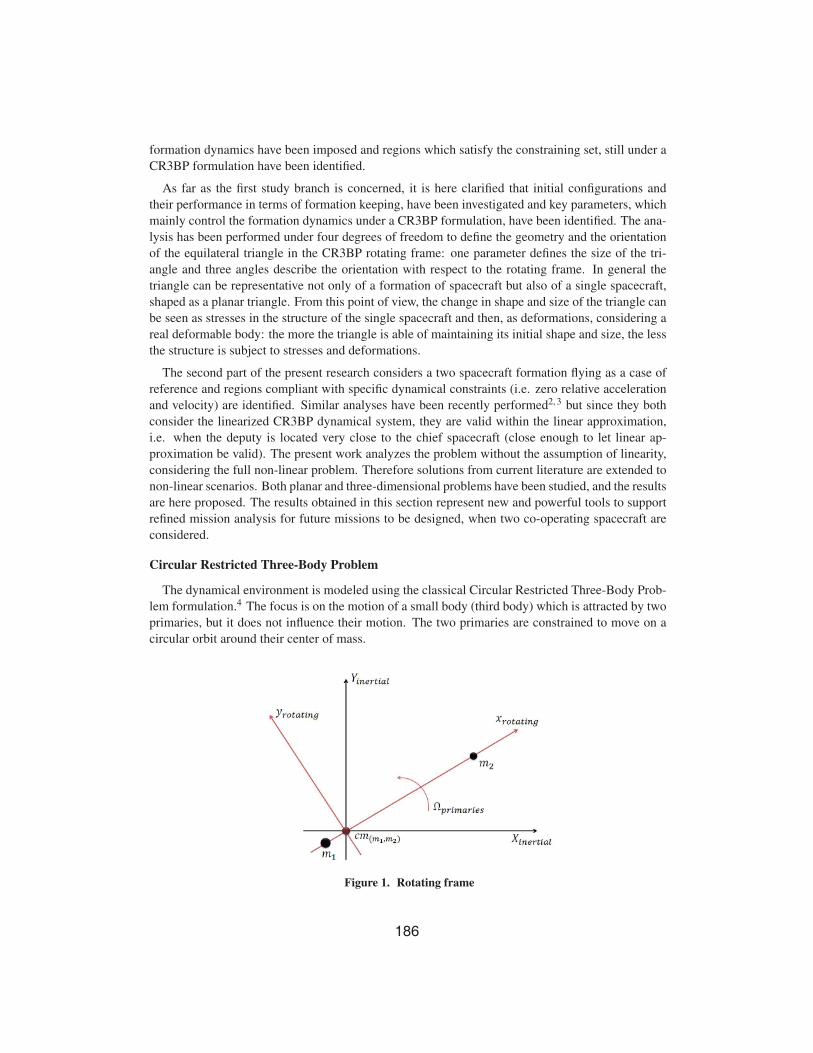
Circular Restricted Three-Body Problem

The dynamical environment is modeled using the classical Circular Restricted Three-Body Prob-

lem formulation.4 The focus is on the motion of a small body (third body) which is attracted by two

primaries, but it does not influence their motion. The two primaries are constrained to move on a

circular orbit around their center of mass.

Figure 1. Rotating frame

187

Equations of motion. It is useful to express the equations of motion of the third body in a refer-

ence frame which is centered in the center of mass of the two primaries and rotates together with

them, with the same angular velocity (Figure 1). The equations of motion can be conveniently

written in a nondimensional form, using the potential function associated to the problem

U =1

2(x2 + y2) +

1− μ

r1+

μ

r2(1)

with

r1 =√

(x+ μ)2 + y2 + z2 (2a)

r2 =√

(x− (1− μ))2 + y2 + z2 (2b)

the parameter μ is called mass ratio and it is defined as follows

μ =m2

m1 +m2(3)

The equations of motion are then ⎧⎨⎩x− 2y = Ux

y + 2x = Uy

z = Uz

(4)

where the notation U(·) means partial derivative of the potential with respect to the variable (·).

FREE TRIANGULAR FORMATION

It is useful to study and understand how a formation of satellites interacts with the surrounding

environment: this analysis is aimed to explore the CR3BP dynamical environment and its effects on

a simple unconstrained formation. In particular, the analysis deals with a triangular formation and

explores initial configuration which provide good performance in terms of formation keeping. Only

free motion is analyzed and no control is considered for formation keeping.

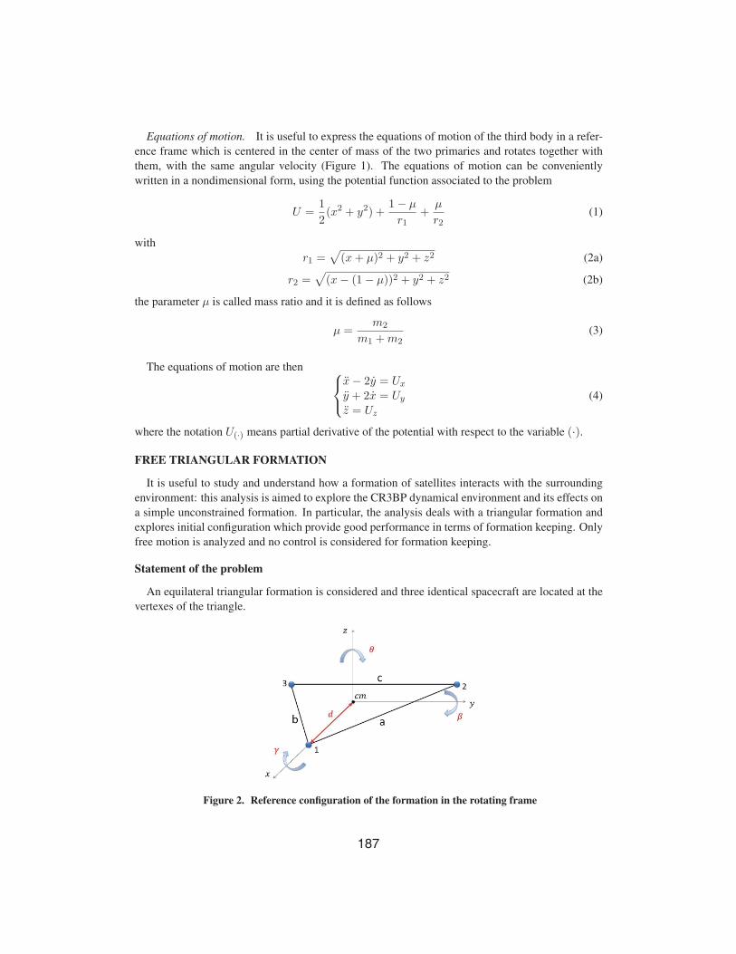
Statement of the problem

An equilateral triangular formation is considered and three identical spacecraft are located at the

vertexes of the triangle.

Figure 2. Reference configuration of the formation in the rotating frame

188

Figure 2 shows the reference configuration of the formation and its four degrees of freedom,

which define the geometry and the orientation of the triangle in the rotating frame: γ, β, θ describe

the orientation in the space with respect to the CR3BP rotating frame, being respectively the rotation

angle around x, y and z rotating frame axes, while d defines the size of the formation, being it the

distance between each spacecraft and the barycenter of the triangle. Angles are considered to be

zero as the formation is in its reference configuration: in this case the triangle lies on the (x, y)plane (Figure 2). The barycenter of the triangular formation is placed on a reference periodic orbit

in the CR3BP. The equations of motion are integrated for each of the three spacecraft as they evolve

near the reference trajectory and the evolution of the formation is analyzed. The aim of the analysis

is to find good initial configurations in terms of its four degrees of freedom (γ, β, θ, d), looking at

different reference orbits (size and type of orbit).

The analysis has been performed for the case of Earth-Moon system, hence the results are shown

for this particular system. Even so, a brief analysis shows that the meaning of the results is not

changing if other systems are considered, therefore the following analysis and its results can be

considered valid for any generic μ value.

Definition of performance factors

The ideal formation keeping condition can be synthesized as no change in shape and size of the

initial triangular configuration. This condition is of course impossible to obtain if the formation

is free and uncontrolled, in an extremely chaotic and non-linear environment such as the CR3BP,

but it is possible to seek preferred initial configurations which lead to small changes in shape and

size of the formation during its evolution on the orbit, and then to cheaper formation keeping needs.

In order to evaluate how characteristics of the formation are maintained, it is important to analyze

how the shape and the size of the triangular formation change during the evolution of the three

spacecraft along the orbit. In particular it is useful to define a way to measure formation keeping

performance, trying to quantify both shape and size changes, in order then to be able of seeking

good initial configurations which allow good formation keeping maintenance. To this purpose, two

performance factors have been built: the Shape Factor (SF), which takes into account for the change

in the shape of the triangle, and the Size or Dimension Factor (DF), which takes into account for the

change in size of the triangular formation.

Shape Factor

To evaluate and quantify the change in shape of the triangular formation during its evolution on

the reference orbit, the Shape Factor has been defined and a convenient mathematical expression

has been found to express it. The mathematical expression shall fulfill some needs that shall be

accomplished by the Shape Factor function. First of all, a nondimensional factor should be consid-

ered, in order to allow comparisons between different systems and different analyses and to keep

the expression as general as possible. Also, the variables of the function, shall be meaningfully

allowing the monitoring of the shape changes. A good choice is to select the ratios of the sides of

the triangle, referring to Figure 2:

ε1 =a

bε2 =

a

cε3 =

b

c(5)

These three parameters, provide a good choice in terms of monitoring of the shape changes: it can

be easily seen that the shape is unchanged if and only if

ε1 = ε2 = ε3 = 1 (6)

189

and therefore they can provide a good way of determine where the shape is unchanged. Note that

only two of these parameters are independent: it is possible to choose then, for example, ε1 and ε2as variables for the Shape Factor

SF = f(ε1, ε2) (7)

Then, once the variables have been selected, the mathematical expression of the Shape Factor

function shall be built. To proceed, it is convenient to introduce some constraints in order to shape

the mathematical function in a convenient way. For example, it can be convenient to consider a

mathematical expression which is equal to one if and only if the shape of the triangle is unchanged.

It can be also useful to set this mathematical function such as it can range from 0 to 1 in a mono-

tonic way, so that the lower is its value, the worse is the condition in terms of shape maintenance.

Considering then the selected variables, both ε1 and ε2 are always greater than zero, being the ratios

of two positive numbers. For this reason, it is better to consider a function whose variables’ domain

is always greater than zero. Moreover, as the choice of the ratios (5) is arbitrary, it is convenient to

have a function which is symmetric with respect to ε and 1ε , having this way an expression which is

not dependent on the definition of the ratios. For example, considering two sides of the triangle:

a = 1 unit

b = 5 units

the Shape Factor shall give the same result if the ratio has been defined both

ε =a

b=

1

5or ε =

b

a= 5

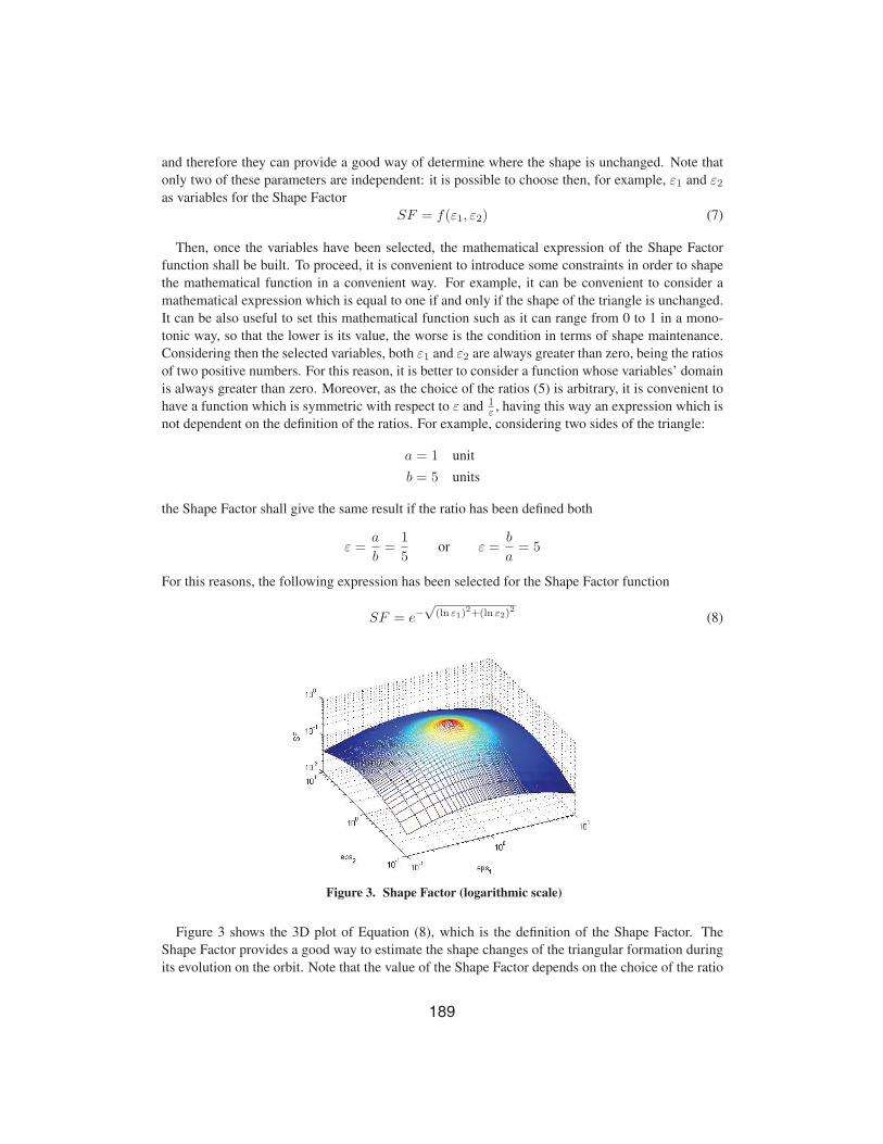
For this reasons, the following expression has been selected for the Shape Factor function

SF = e−√

(ln ε1)2+(ln ε2)

2

(8)

Figure 3. Shape Factor (logarithmic scale)

Figure 3 shows the 3D plot of Equation (8), which is the definition of the Shape Factor. The

Shape Factor provides a good way to estimate the shape changes of the triangular formation during

its evolution on the orbit. Note that the value of the Shape Factor depends on the choice of the ratio

190

to use: for example, the choice (ε1, ε2) will provide different numerical results form the choice

(ε1, ε3) or (ε2, ε3). It is possible to make the Shape Factor independent also from that choice by

computing SF for all three possible choices and then taking the average value. However, without

any loss of generality, the analysis performed in this work relates to Equation (8), and not to the

averaged SF.

Dimension Factor

To evaluate formation keeping performance, the other important aspect to be monitored during

the evolution of the formation on its orbit is the size of the triangle formed by the spacecraft. It

can happen that the distance between the spacecraft grows very fast without changes (or with little

changes) in the shape of the formation: this situation is not detectable with the Shape Factor moni-

toring, hence another factor (Size or Dimension Factor) is required. Similarly to what done for the

Shape Factor, a nondimensional factor is considered. Also in this case side ratios are considered as

variables, but this time the ratio is computed with respect to the initial length of the side. Referring

to Figure 2

η1 =a

a0η2 =

b

b0η3 =

c

c0(9)

where the subscript 0 denotes the initial length of the sides (initial configuration). To find the

mathematical expression, the only condition to be verified is that the Dimension Factor equals one

at the initial condition and if the average size of the formation is maintained. Then, it shall be also

considered that, once again, the variables represent ratios of positive numbers. A very simple form

for the Dimension Factor can be adopted, averaging the three ratios η1, η2 and η3

DF =η1 + η2 + η3

3(10)

Equation (10) let then understand if the three spacecraft are getting farther or closer to each other.

Differently from the Shape Factor, it needs information on the initial state of the formation and

provides a measure of the size of the formation at a certain time after initial time. Roughly speaking,

DF=10 at t = t1 (with t1 > t0) means that the triangle is, on average, 10 times bigger than its initial

size at t = t0.

Results

As specified in the previous section, the goal of the analysis is to seek initial configurations which

provide good performance in terms of formation keeping. To this aim, several initial configurations

have been considered, for different choice of initial orientation angles γ, β, θ, different choice of

initial distance between the spacecraft and the barycenter of the triangular formation d and consid-

ering different types and size of orbits in the CR3BP. In particular, the following initial conditions

have been explored:

γ, β, θ ranging from 0 to 2π

d 1, 10, 100 km

191

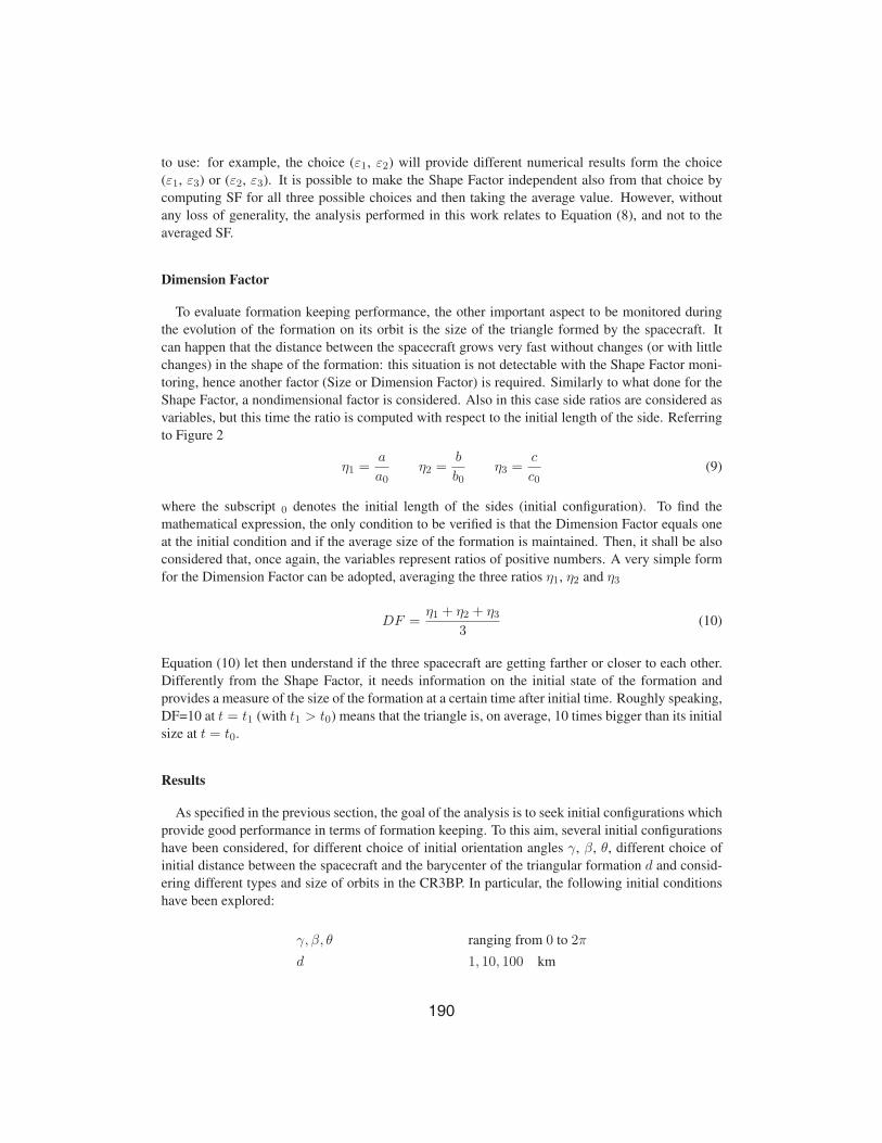
Figure 4. SF(t) and DF(t) for different β with d = 10 km, L1(1)

In this analysis, the value of the performance factors after half period of the reference orbit has

been used as comparison variable: the analysis performed in the next paragraphs considers SF and

DF evaluated after half orbit (functions in Figure 4 evaluated at t = 0.5 Torb) for any different initial

orientation angle, d and reference orbit.

Shape Factor Analysis. It is interesting to look at how the Shape Factor behaves for different

initial configuration angles, after half orbit. The initial configuration of the triangular formation

(Figure 2 shows the reference condition, with γ, β, θ = 0), is then placed on its reference orbit and

the value of the Shape Factor is evaluated after half orbit.

For what concerns reference orbits, the analysis has been performed considering only planar orbits.

In particular, the following Lyapunov orbits about L1, L2 and L3 have been employed:

L1 Ax = 2194, 9497.6, 18723.1 km

L2 Ax = 2611, 35224, 56434 km

L3 Ax = 3437, 50582, 179230 km

In the followings, the orbits will be referenced as L1(1), L1(2), L1(3), L2(1), L2(2),. . . where the

numbers in the brackets indicates which orbit, from the smallest (1) to the largest (3), is being

referenced. For example, L3(2) refers to the orbit about L3 with Ax = 50582 km.

The barycenter of the formation is placed on the reference orbit and the evolution in time of

the triangle is monitored for half period of the reference orbit. To find good initial configurations

in terms of formation keeping the behavior of performance factors has been analyzed to find the

closest conditions to the ideal situation, which is represented by

SF = 1 DF = 1 (11)

Figure 4 shows an example of how the performance factors behaves in time during the evolution

of the formation on the reference orbit: in this case the smallest L1 orbit have been chosen and

the spacecraft are initially 10 km distant from the barycenter of the formation, the performance

factors have been evaluated for β = 0◦, 30◦, 60◦, 90◦. The time coordinate is on the abscissa: it is

represented in nondimensional coordinates, referring to the period of the orbit (in this case the time

span goes from 0 to 0.5 Torb).

192

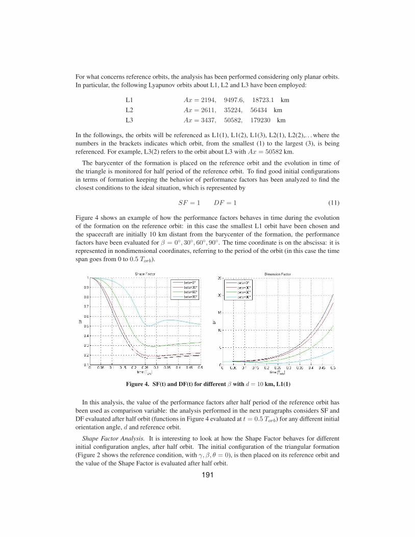
For example, looking at the evolution of the formation for γ ranging from 0 to 2π and β, θ = 0 for

a given choice of d and reference orbit, the SF after one orbit can be plotted as function of γ. Figure 5

shows the values of SF after half orbit with respect to its initial orientation (for γ ranging from 0 to

2π and considering always β, θ = 0), for a formation placed on the small reference orbit about L1,

with initial distance between each spacecraft and the barycenter of the formation d = 1. Looking

at this plot, it is easy to find the best condition and the corresponding initial orientation (γ) with all

the other conditions fixed: the ideal formation keeping case is SF = 1 and so the best condition (the

one that gets closer to the ideal formation keeping case) is the maximum of the function SF(γ). In

this case the maximum is achieved for an initial γ of 180◦. However, the maximum value of the

Shape Factor is quite low (SF = 0.244), hence it is not a good initial condition in terms of formation

keeping. To look for better conditions, the other parameters (angles, d and reference orbit) shall be

changed.

Figure 5. SF vs γ with d = 1 km, L1(1)

The behavior of the Shape Factor is analyzed separately with respect to γ, β and θ, looking, for

each case, at how the parameter d and the choice of the reference orbit affect the results. Properties

of functions SF(γ) (with β, θ = 0), SF(β) (with γ, θ = 0) and SF(θ) (with γ, β = 0) are then

investigated.

The analysis shows that the major influence on the Shape Factor is due to the initial orientation

of the formation and to the choice of the reference orbit, while the parameter d plays a minor role.

The functions SF(γ), SF(β) and SF(θ) show an oscillating behavior and a periodicity of period πor 2π. In any case, the shape of the function is little dependent on the choice of the orbit and on the

parameter d. Performance is always quite good in the case of SF(θ) (SF � 0.534), while the results

are bad if a rotation about the x axis is considered (SFmax = 0.390). The best case is obtained for

the function SF(β), considering the orbit L3(1) with β = 90◦ (SF = 0.911). The choice of the

reference orbit is also important and in general, with few exceptions, the best results are obtained

for small orbits about L3.

Dimension Factor Analysis. Similarly to what done for the Shape Factor, the behavior of the

Dimension Factor has been characterized with respect to initial orientation angle, d and reference

orbit, to find the best initial configuration, trying to be as close as possible to the ideal formation

keeping condition (DF = 1).

193

of period π/3, 23π or π. This time the performance is quite poor for any case (DF � 10) except

for the DF(β): the best condition is again achievable for L3(1) with β = 90◦ (DF = 1.054). As

for the Shape Factor, the parameter d shows no influence on the results and the best performance is

achieved for small orbits about L3.

Results Summary. The results of the study highlight the importance of the initial orientation of

the triangular formation for formation keeping. Analyzing the effect of the other parameters in-

volved (size of the triangular formation and reference orbit), it is clear that the size of the formation

has practically no influence on its formation keeping performance, while the orbit can have relevant

effects. For these reasons, when considering the design of a mission which employs a triangular

formation placed on a periodic orbit in the CR3BP, to lower formation keeping needs in terms of

Δv to be provided to the three spacecraft, the initial (or reference) orientation and the reference

orbit must be chosen carefully.

Both Shape and Dimension Factor analyses show that a formation initially rotated around the xaxis (γ �= 0) with respect to its reference configuration (Figure 2) produces bad performance in

terms of formation keeping: indeed, the three spacecraft triangular formation loses its shape and

grows in size very quickly. Overall, the best performance is achieved when the formation is initially

rotated around y axis (β �= 0), while the rotation around z axis (θ �= 0) gives good results only

for what concerns the shape maintenance but not in terms of size keeping. For what concerns the

reference orbits, the best place to locate the formation is near L3. It can be also useful to notice that

SF functions are periodic of period 2π (SF(γ), SF(β)) or π (SF(θ)), while DF functions are periodic

of period π (DF(γ), DF(β)) and π/3 or 2/3π in the case of DF(θ), meaning that more than one best

condition can be present in the [0− 2π] domain.

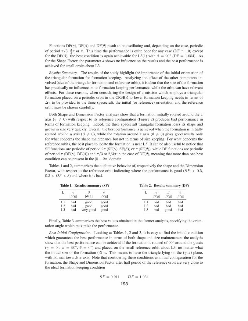
Tables 1 and 2, summarizes the qualitative behavior of, respectively the shape and the Dimension

Factor, with respect to the reference orbit indicating where the performance is good (SF > 0.5,

0.3 < DF < 3) and where it is bad.

Table 1. Results summary (SF)

L γ β θ[deg] [deg] [deg]

L1 bad good goodL2 bad good goodL3 bad very good good

Table 2. Results summary (DF)

L γ β θ[deg] [deg] [deg]

L1 bad bad badL2 bad bad badL3 bad good bad

Finally, Table 3 summarizes the best values obtained in the former analysis, specifying the orien-

tation angle which maximize the performance.

Best Initial Configuration. Looking at Tables 1, 2 and 3, it is easy to find the initial condition

which guarantees the best performance in terms of both shape and size maintenance: the analysis

show that the best performance can be achieved if the formation is rotated of 90◦ around the y axis

(γ = 0◦, β = 90◦, θ = 0◦) and placed on the small reference orbit about L3, no matter what

the initial size of the formation (d) is. This means to have the triangle lying on the (y, z) plane,

with normal towards x axis. Note that considering these conditions as initial configuration for the

formation, the Shape and Dimension Factor after half period of the reference orbit are very close to

the ideal formation keeping condition

SF = 0.911 DF = 1.054

Functions DF(γ), DF(β) and DF(θ) result to be oscillating and, depending on the case, periodic

194

Figure 6. SF(left) and DF(right) time behavior during one orbit with γ = 0◦, β = 90◦,θ = 0◦, d = 10 km, L3(1)

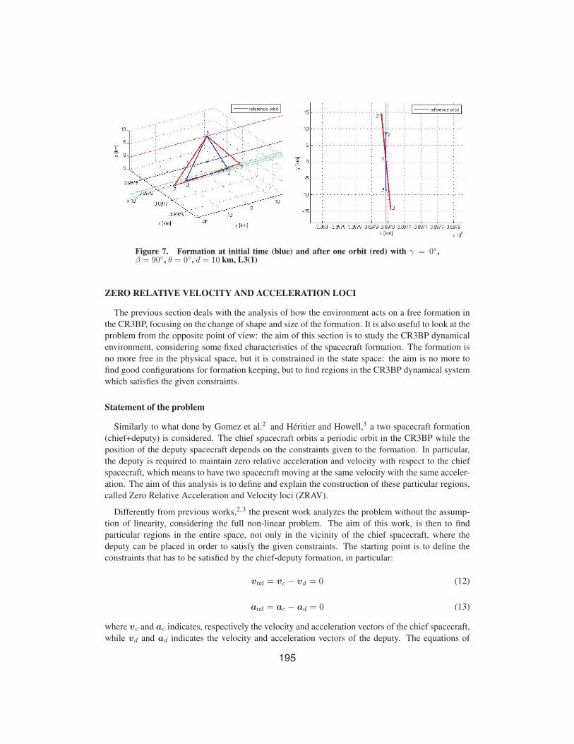
Figure 7 shows the comparison between the triangular formation at time t = 0 (blue triangle) and

the formation after a complete orbit (red triangle). Note that spacecraft 1 return exactly on its initial

position, so its orbit has exactly the same period of the reference one and, indeed, it turns out to be

a very similar orbit but rotated of a small angle around y axis. Also the orbit followed by spacecraft

2 and 3 (they are practically on the same orbit but with a different initial position) is rotated around

the y axis, but this time the period is not the same, as a small offset in the position of the spacecraft

after one complete orbital period is present. The right part of Figure 7 shows that the projection

of the triangle on the (x, y) plane has slightly changed its orientation by adding a small rotation

around z axis. Overall, the performance after one orbit, starting from the optimal condition found

as a result of the previous analysis, is still good: the size of the formation is only slightly bigger

(DF=1.353) and its shape is still very similar (SF=0.722) being now an isosceles triangle instead of

an equilateral one.

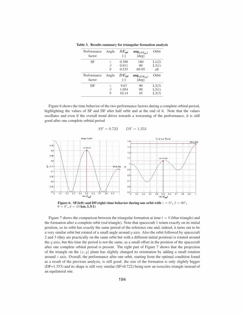
Table 3. Results summary for triangular formation analysis

Performance Angle SFopt ang(SFopt)Orbit

factor [-] [deg]

SF γ 0.390 180 L1(2)β 0.911 90 L3(1)θ 0.535 69-95 all

Performance Angle DFopt ang(DFopt)Orbit

factor [-] [deg]

DF γ 9.67 90 L3(3)β 1.054 90 L3(1)θ 10.14 45 L3(3)

Figure 6 shows the time behavior of the two performance factors during a complete orbital period,

highlighting the values of SF and DF after half orbit and at the end of it. Note that the values

oscillates and even if the overall trend drives towards a worsening of the performance, it is still

good after one complete orbital period

SF = 0.722 DF = 1.353

195

Figure 7. Formation at initial time (blue) and after one orbit (red) with γ = 0◦,β = 90◦, θ = 0◦, d = 10 km, L3(1)

ZERO RELATIVE VELOCITY AND ACCELERATION LOCI

The previous section deals with the analysis of how the environment acts on a free formation in

the CR3BP, focusing on the change of shape and size of the formation. It is also useful to look at the

problem from the opposite point of view: the aim of this section is to study the CR3BP dynamical

environment, considering some fixed characteristics of the spacecraft formation. The formation is

no more free in the physical space, but it is constrained in the state space: the aim is no more to

find good configurations for formation keeping, but to find regions in the CR3BP dynamical system

which satisfies the given constraints.

Statement of the problem

Similarly to what done by Gomez et al.2 and Heritier and Howell,3 a two spacecraft formation

(chief+deputy) is considered. The chief spacecraft orbits a periodic orbit in the CR3BP while the

position of the deputy spacecraft depends on the constraints given to the formation. In particular,

the deputy is required to maintain zero relative acceleration and velocity with respect to the chief

spacecraft, which means to have two spacecraft moving at the same velocity with the same acceler-

ation. The aim of this analysis is to define and explain the construction of these particular regions,

called Zero Relative Acceleration and Velocity loci (ZRAV).

Differently from previous works,2, 3 the present work analyzes the problem without the assump-

tion of linearity, considering the full non-linear problem. The aim of this work, is then to find

particular regions in the entire space, not only in the vicinity of the chief spacecraft, where the

deputy can be placed in order to satisfy the given constraints. The starting point is to define the

constraints that has to be satisfied by the chief-deputy formation, in particular:

vrel = vc − vd = 0 (12)

arel = ac − ad = 0 (13)

where vc and ac indicates, respectively the velocity and acceleration vectors of the chief spacecraft,

while vd and ad indicates the velocity and acceleration vectors of the deputy. The equations of

196

motion for the chief read as follows⎧⎪⎪⎪⎨⎪⎪⎪⎩

xc = xc + 2yc − 1−μr31c

(xc + μ)− μr32c

(xc − (1− μ))

yc = yc − 2xc − yc

(1−μr31c

+ μr32c

)

zc = −zc(1−μr31c

+ μr32c

) (14)

with

r1c =√

(xc + μ)2 + y2c + z2c

r2c =√

(xc − (1− μ))2 + y2c + z2c

the same set of equations (Eq. (14)) is of course valid also for the deputy (with subscript d instead

of c). The first step is then to evaluate the relative acceleration (Eq. (13)) and to equate it to zero

⎧⎨⎩xc − xd = 0yc − yd = 0zc − zd = 0

(16)

which is equivalent to

⎧⎪⎪⎪⎪⎪⎪⎨⎪⎪⎪⎪⎪⎪⎩

xc + 2yc − 1−μr31c

(xc + μ)− μr32c

(xc − (1− μ)) =

= xd + 2yd − 1−μr31d

(xd + μ)− μr32d

(xd − (1− μ))

yc − 2xc − yc

(1−μr31c

+ μr32c

)= yd − 2xd − yd

(1−μr31d

+ μr32d

)

−zc(1−μr31c

+ μr32c

)= −zd

(1−μr31d

+ μr32d

)(17)

then, the other constraint (Eq. (12)) can be written as

⎧⎨⎩xc − xd = 0yc − yd = 0zc − zd = 0

(18)

substituting it into (17), the system becomes

⎧⎪⎪⎪⎪⎪⎪⎨⎪⎪⎪⎪⎪⎪⎩

xc − 1−μr31c

(xc + μ)− μr32c

(xc − (1− μ)) =

= xd − 1−μr31d

(xd + μ)− μr32d

(xd − (1− μ))

yc − yc

(1−μr31c

+ μr32c

)= yd − yd

(1−μr31d

+ μr32d

)

−zc(1−μr31c

+ μr32c

)= −zd

(1−μr31d

+ μr32d

)(19)

Note that the resulting system is not a system of differential equations any more, but it is a non-linear

algebraic system.

The whole problem can be better handled exploiting the state representation of the dynamics of

the spacecraft. Equations (14) for the chief and the deputy can be written, in an extremely compact

form, as

Xc = f(Xc) (20)

Xd = f(Xd) (21)

197

where X represents the six dimensional state of the spacecraft

Xc =

⎧⎪⎪⎪⎪⎪⎪⎨⎪⎪⎪⎪⎪⎪⎩

xcyczcxcyczc

⎫⎪⎪⎪⎪⎪⎪⎬⎪⎪⎪⎪⎪⎪⎭

Xd =

⎧⎪⎪⎪⎪⎪⎪⎨⎪⎪⎪⎪⎪⎪⎩

xdydzdxdydzd

⎫⎪⎪⎪⎪⎪⎪⎬⎪⎪⎪⎪⎪⎪⎭

Then, the constraint (Equations (12) and (13)), can be written as

Xc − Xd = 0 (22)

Finally, applying the constraints, the results is equivalent to the one obtained before

f(rc) = f(rd) (23)

which represent the non-linear algebraic system (19).

As specified at the beginning of this section, the chief spacecraft is considered to be orbiting a

periodic orbit in the CR3BP, hence, its position vector rc is known. The system (19) (or equiva-

lently (23)) is then composed by three non-linear algebraic equations and it has three unknowns

represented by the three components of the position vector of the deputy rd. The problem is then

reduced to the solution of the non-linear algebraic system (19), whose solutions represent the points

in the space where the deputy has the same acceleration and velocity of the chief spacecraft.

Results

The analysis has been performed considering the Earth-Moon system and the results for this

particular system are shown here. However, as for the free triangular formation, a brief analysis

showed that the qualitative results are the same, if the system is changing. For that reason, the results

and the main analysis can be considered valid for any general μ value. The following reference

orbits for the chief spacecraft have been considered:

2D case (Lyapunov) L1: Ax = 14879 km T = 14.4 days

L2: Ax = 35223 km T = 16.1 days

L3: Ax = 272296 km T = 27.1 days

3D case (Halo) L1: Ay = 48494 km, Az = 53308 km T = 12 days

L2: Ay = 48861 km, Az = 27616 km T = 14.1 days

L3: Ay = 466575 km, Az = 186281 km T = 27.1 days

Planar case

Before considering the general three-dimensional system, to have a better understanding of the

problem it can be useful to simplify it: to this aim, the planar case (x, y plane) is initially considered.

The acceleration constraint (13) can be written then in the two dimensional case as

arel = ac − ad =

{acx − adxacy − ady

}=

{arelx

arely

}= 0 (24)

198

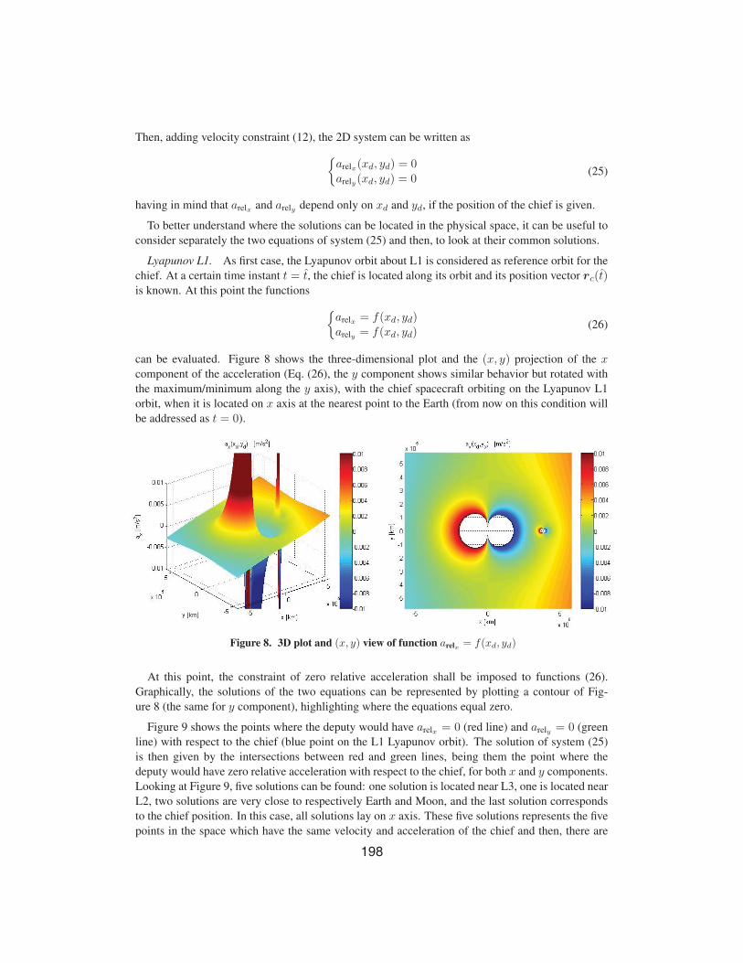
Figure 8. 3D plot and (x, y) view of function arelx = f(xd, yd)

At this point, the constraint of zero relative acceleration shall be imposed to functions (26).

Graphically, the solutions of the two equations can be represented by plotting a contour of Fig-

ure 8 (the same for y component), highlighting where the equations equal zero.

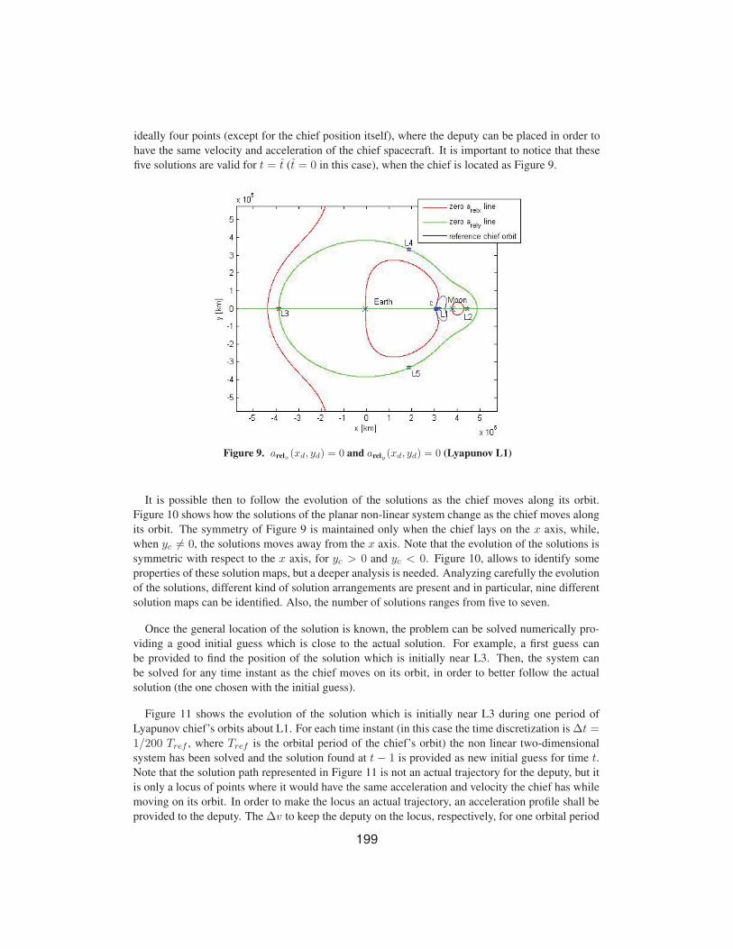
Figure 9 shows the points where the deputy would have arelx = 0 (red line) and arely = 0 (green

line) with respect to the chief (blue point on the L1 Lyapunov orbit). The solution of system (25)

is then given by the intersections between red and green lines, being them the point where the

deputy would have zero relative acceleration with respect to the chief, for both x and y components.

Looking at Figure 9, five solutions can be found: one solution is located near L3, one is located near

L2, two solutions are very close to respectively Earth and Moon, and the last solution corresponds

to the chief position. In this case, all solutions lay on x axis. These five solutions represents the five

points in the space which have the same velocity and acceleration of the chief and then, there are

Then, adding velocity constraint (12), the 2D system can be written as

{arelx(xd, yd) = 0arely(xd, yd) = 0

(25)

having in mind that arelx and arely depend only on xd and yd, if the position of the chief is given.

To better understand where the solutions can be located in the physical space, it can be useful to

consider separately the two equations of system (25) and then, to look at their common solutions.

Lyapunov L1. As first case, the Lyapunov orbit about L1 is considered as reference orbit for the

chief. At a certain time instant t = t, the chief is located along its orbit and its position vector rc(t)is known. At this point the functions

{arelx = f(xd, yd)arely = f(xd, yd)

(26)

can be evaluated. Figure 8 shows the three-dimensional plot and the (x, y) projection of the xcomponent of the acceleration (Eq. (26), the y component shows similar behavior but rotated with

the maximum/minimum along the y axis), with the chief spacecraft orbiting on the Lyapunov L1

orbit, when it is located on x axis at the nearest point to the Earth (from now on this condition will

be addressed as t = 0).

199

Figure 9. arelx(xd, yd) = 0 and arely (xd, yd) = 0 (Lyapunov L1)

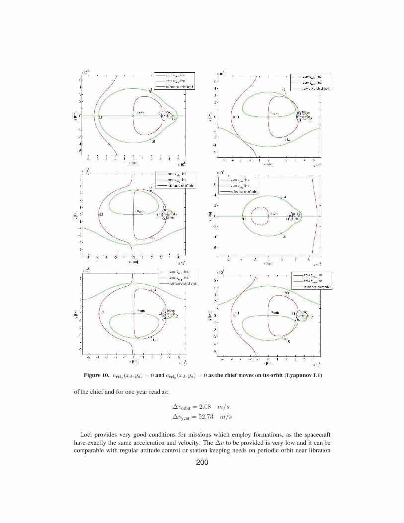
It is possible then to follow the evolution of the solutions as the chief moves along its orbit.

Figure 10 shows how the solutions of the planar non-linear system change as the chief moves along

its orbit. The symmetry of Figure 9 is maintained only when the chief lays on the x axis, while,

when yc �= 0, the solutions moves away from the x axis. Note that the evolution of the solutions is

symmetric with respect to the x axis, for yc > 0 and yc < 0. Figure 10, allows to identify some

properties of these solution maps, but a deeper analysis is needed. Analyzing carefully the evolution

of the solutions, different kind of solution arrangements are present and in particular, nine different

solution maps can be identified. Also, the number of solutions ranges from five to seven.

Once the general location of the solution is known, the problem can be solved numerically pro-

viding a good initial guess which is close to the actual solution. For example, a first guess can

be provided to find the position of the solution which is initially near L3. Then, the system can

be solved for any time instant as the chief moves on its orbit, in order to better follow the actual

solution (the one chosen with the initial guess).

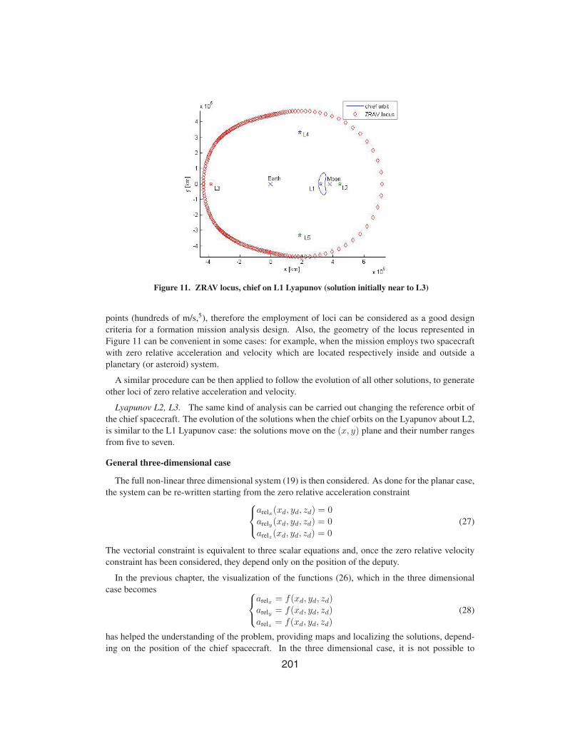
Figure 11 shows the evolution of the solution which is initially near L3 during one period of

Lyapunov chief’s orbits about L1. For each time instant (in this case the time discretization is Δt =1/200 Tref , where Tref is the orbital period of the chief’s orbit) the non linear two-dimensional

system has been solved and the solution found at t − 1 is provided as new initial guess for time t.Note that the solution path represented in Figure 11 is not an actual trajectory for the deputy, but it

is only a locus of points where it would have the same acceleration and velocity the chief has while

moving on its orbit. In order to make the locus an actual trajectory, an acceleration profile shall be

provided to the deputy. The Δv to keep the deputy on the locus, respectively, for one orbital period

ideally four points (except for the chief position itself), where the deputy can be placed in order to

have the same velocity and acceleration of the chief spacecraft. It is important to notice that these

five solutions are valid for t = t (t = 0 in this case), when the chief is located as Figure 9.

200

of the chief and for one year read as:

Δvorbit = 2.08 m/s

Δvyear = 52.73 m/s

Loci provides very good conditions for missions which employ formations, as the spacecraft

have exactly the same acceleration and velocity. The Δv to be provided is very low and it can be

comparable with regular attitude control or station keeping needs on periodic orbit near libration

Figure 10. arelx(xd, yd) = 0 and arely (xd, yd) = 0 as the chief moves on its orbit (Lyapunov L1)

201

Figure 11. ZRAV locus, chief on L1 Lyapunov (solution initially near to L3)

points (hundreds of m/s,5), therefore the employment of loci can be considered as a good design

criteria for a formation mission analysis design. Also, the geometry of the locus represented in

Figure 11 can be convenient in some cases: for example, when the mission employs two spacecraft

with zero relative acceleration and velocity which are located respectively inside and outside a

planetary (or asteroid) system.

A similar procedure can be then applied to follow the evolution of all other solutions, to generate

other loci of zero relative acceleration and velocity.

Lyapunov L2, L3. The same kind of analysis can be carried out changing the reference orbit of

the chief spacecraft. The evolution of the solutions when the chief orbits on the Lyapunov about L2,

is similar to the L1 Lyapunov case: the solutions move on the (x, y) plane and their number ranges

from five to seven.

General three-dimensional case

The full non-linear three dimensional system (19) is then considered. As done for the planar case,

the system can be re-written starting from the zero relative acceleration constraint⎧⎨⎩arelx(xd, yd, zd) = 0arely(xd, yd, zd) = 0

arelz(xd, yd, zd) = 0

(27)

The vectorial constraint is equivalent to three scalar equations and, once the zero relative velocity

constraint has been considered, they depend only on the position of the deputy.

In the previous chapter, the visualization of the functions (26), which in the three dimensional

case becomes ⎧⎨⎩arelx = f(xd, yd, zd)arely = f(xd, yd, zd)

arelz = f(xd, yd, zd)

(28)

has helped the understanding of the problem, providing maps and localizing the solutions, depend-

ing on the position of the chief spacecraft. In the three dimensional case, it is not possible to

202

visualize functions (28) and to perform the same analysis as for the planar case. However, the under-

standing of the problem provided by the two-dimensional analysis can be successfully applied in the

general three-dimensional case because of the same nature of the problem. Some results, in terms of

zero relative acceleration and velocity loci, are shown here, considering the full three-dimensional

case. The chief is placed on the Halo orbits about L1, L2 and L3 defined at the beginning of the

Earth-Moon analysis. In order to solve the non-linear system and to find the loci, initial guesses

from the two-dimensional analysis have been considered respectively for L1, L2 and L3.

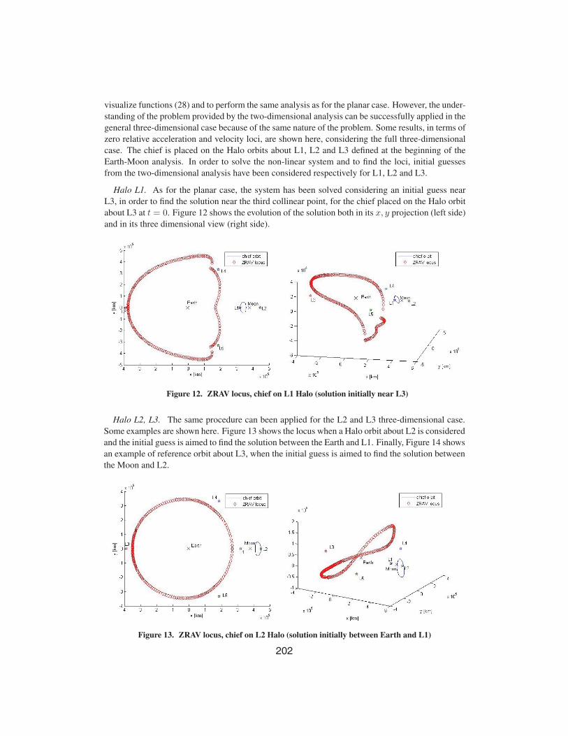
Halo L1. As for the planar case, the system has been solved considering an initial guess near

L3, in order to find the solution near the third collinear point, for the chief placed on the Halo orbit

about L3 at t = 0. Figure 12 shows the evolution of the solution both in its x, y projection (left side)

and in its three dimensional view (right side).

Figure 12. ZRAV locus, chief on L1 Halo (solution initially near L3)

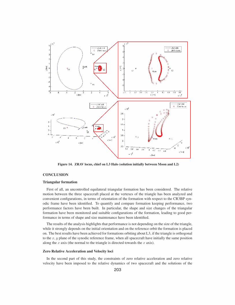
Halo L2, L3. The same procedure can been applied for the L2 and L3 three-dimensional case.

Some examples are shown here. Figure 13 shows the locus when a Halo orbit about L2 is considered

and the initial guess is aimed to find the solution between the Earth and L1. Finally, Figure 14 shows

an example of reference orbit about L3, when the initial guess is aimed to find the solution between

the Moon and L2.

Figure 13. ZRAV locus, chief on L2 Halo (solution initially between Earth and L1)

203

CONCLUSION

Triangular formation

First of all, an uncontrolled equilateral triangular formation has been considered. The relative

motion between the three spacecraft placed at the vertexes of the triangle has been analyzed and

convenient configurations, in terms of orientation of the formation with respect to the CR3BP syn-

odic frame have been identified. To quantify and compare formation keeping performance, two

performance factors have been built. In particular, the shape and size changes of the triangular

formation have been monitored and suitable configurations of the formation, leading to good per-

formance in terms of shape and size maintenance have been identified.

The results of the analysis highlights that performance is not depending on the size of the triangle,

while it strongly depends on the initial orientation and on the reference orbit the formation is placed

on. The best results have been achieved for formations orbiting about L3, if the triangle is orthogonal

to the x, y plane of the synodic reference frame, when all spacecraft have initially the same position

along the x axis (the normal to the triangle is directed towards the x axis).

Zero Relative Acceleration and Velocity loci

In the second part of this study, the constraints of zero relative acceleration and zero relative

velocity have been imposed to the relative dynamics of two spacecraft and the solutions of the

Figure 14. ZRAV locus, chief on L3 Halo (solution initially between Moon and L2)

204

constrained problem have been investigated. The study of the planar case has been useful for the

understanding of the problem through the possibility of visualizing the solutions of the resulting

nonlinear algebraic system. The full three-dimensional problem has been investigated and three-

dimensional solutions have been identified.

The results obtained in this section represent new and convenient tools for mission and trajectory

design, when two co-operating spacecraft are considered. In particular, considering a chief and a

deputy spacecraft, trajectories which allow the deputy to have zero relative acceleration and velocity

with respect to the chief have been identified in the CR3BP dynamical environment. These particular

trajectories have been called Zero Relative Acceleration and Velocity loci (ZRAV). As the spacecraft

are located in a low-acceleration environment such as the one provided by CR3BP dynamics, the

amount of acceleration to be provided to the spacecraft in order to maintain its position on the ZRAV

locus turns out to be very low: in terms of Δv, the cost is of the same order of magnitude of station

keeping cost to maintain the spacecraft on a periodic orbit within the CR3BP.

REFERENCES[1] B. T. Barden and H. K. C, “Formation Flying in the Vicinity of Libration Point Orbits,” 1998.

[2] G. Gomez, M. Marcote, J. J. Masdemont, and J. M. Mondelo, “Natural Configurations and ControlledMotions Suitable for Formation Flying,” AAS 05-347, 2005.

[3] A. Heritier and K. C. Howell, “Regions Near the Libration Points Suitable to Maintain Multiple Space-craft,” 2012.

[4] V. Szebehely, Theory of Orbits: The Restricted Problem of Three Bodies. New York and London:Academic Press, 1967.

[5] W. S. Koon, M. W. Lo, J. E. Marsden, and S. D. Ross, Dynamical Systems, the Three Body Problemand Space Mission Design. 2006.

[6] H. Schaub and J. L. Junkins, Analytical Mechanics of Aerospace Systems. American Institute Of Aero-nautics Astronautics, 2002.

[7] K. C. Howell, “Families of Orbits in the Vicinity of the Collinear Libration Points,” The Journal of theAstronautical Sciences, Vol. 49, 2001, pp. 107–125.

[8] A. Jorba and J. Masdemont, “Dynamics in the Centre Manifold of the Collinear Points of the RestrictedThree Body Problem,” 1997.

[9] K. C. Howell, “Three-Dimensional Periodic ’Halo’ Orbits,” 1983.

[10] K. C. Howell and J. V. Breakwell, “Almost Rectilinear Halo Orbits,” Celestial Mechanics, Vol. 32,1984, pp. 29–52.

[11] J. J. C. M. Bik, P. N. A. M. Visser, and O. Jenrich, “Stabilization of the triangular LISA satelliteformation,”

[12] A. Heritier, “Exploration of the Region Near the Sun-Earth Collinear Libration Points for the Controlof Large Formations,” PhD Thesis, Purdue University, 2012.

[13] B. T. Barden and K. C. Howell, “Dynamical Issues Associated with Relative Configurations of MultipleSpacecraft Near the Sun-Earth/Moon L1 Point,” AAS/AIAA Astrodynamics Specialist Conference, 1999.

[14] B. G. Marchand, “Spacecraft Formation Keeping Near the Libration Points of the Sun-Earth/MoonSystem,” PhD Thesis, Purdue University, 2004.

[15] K. C. Howell and B. T. Barden, “Trajectory Design and Stationkeeping for Multiple Spacecraft inFormation Near the Sub-earth L1 Point,” IAF, 1999.

[16] K. C. Howell and B. G. Marchand, “Design and Control of Formations Near Libration Points of theSun-Earth/Moon Ephemeris System,”

[17] M. Bando and A. Ichikawa, “Periodic Orbits and Formation Flying Near the Libration Points,”

[18] S. Gong, J. Li, H. Baoyin, and Y. Gao, “Formation Reconfiguration in Restricted Three-Body Problem,”Acta Mech Sin, No. 23, 2007, pp. 321–328.

[19] P. Gurfil, M. Idan, and N. J. Kasdin, “Adaptive Neural Control of Deep-Space Formation Flying,”Journal of Guidance, Control and Dynamics, Vol. 26, No. 3, 2003.

[20] P. Gurfil and N. J. Kasdin, “Stability and Control of Spacecraft Formation Flying in Trajectories of theRestricted Three-Body Problem,” Acta Astronautica, No. 54, 2004, pp. 433–453.