A semantic touch interface for flying camera photography
107
A SEMANTIC TOUCH INTERFACE FOR FLYING CAMERA PHOTOGRAPHY by LAN ZIQUAN B.Comp. (Computer Science, NUS) 2013 B.Sci. (Applied Mathematics, NUS) 2013 A THESIS SUBMITTED FOR THE DEGREE OF DOCTOR OF PHILOSOPHY in COMPUTER SCIENCE in the DEPARTMENT OF NUS GRADUATE SCHOOL FOR INTEGRATIVE SCIENCES AND ENGINEERING of the NATIONAL UNIVERSITY OF SINGAPORE 2019 Supervisor: Professor David HSU Examiners: Associate Professor Marcelo Jr. H. ANG Assistant Professor Brian Y. LIM Associate Professor Ping TAN, Simon Fraser University
-
Upload
khangminh22 -
Category
Documents
-
view
4 -
download
0
Transcript of A semantic touch interface for flying camera photography
A SEMANTIC TOUCH INTERFACEFOR FLYING CAMERA PHOTOGRAPHY
by
LAN ZIQUAN
B.Comp. (Computer Science, NUS) 2013B.Sci. (Applied Mathematics, NUS) 2013
A THESIS SUBMITTED FOR THE DEGREE OF
DOCTOR OF PHILOSOPHY
in
COMPUTER SCIENCE
in the
DEPARTMENT OF NUS GRADUATE SCHOOLFOR INTEGRATIVE SCIENCES AND ENGINEERING
of the
NATIONAL UNIVERSITY OF SINGAPORE
2019
Supervisor:Professor David HSU
Examiners:Associate Professor Marcelo Jr. H. ANG
Assistant Professor Brian Y. LIMAssociate Professor Ping TAN, Simon Fraser University
Declaration
I hereby declare that this thesis is my original work and it has been written by me
in its entirety. I have duly acknowledged all the sources of information which have
been used in the thesis.
This thesis has also not been submitted for any degree in any university previ-
ously.
Ziquan Lan
31 Dec 2018
Acknowledgements
First and foremost, I would like to express my heartfelt gratitude to my thesis
advisor David Hsu for the guidance and support. His insights in Robotics have been
continuously guiding me even before my PhD study. David is also a life mentor who
is always supportive during my ups and downs. I am truly grateful.
Next, I would like to thank Shengdong Zhao and Gim Hee Lee for sharing with
me their insights in Human Computer Interaction and Computer Vision during the
project discussions. Their suggestions across different research fields enable me to
complete this interdisciplinary thesis. In addition, my special thanks goes to Wee
Sun Lee for his constructive feedback during the group meetings.
I also thank Marcelo Jr. H. Ang, Brian Y. Lim and Ping Tan for providing
constructive feedback to improve the quality of my thesis.
The members in our AdaComp Lab are a group of wonderful people. Mohit
Shridhar is my project partner. I will always remember the experiences when we
worked together towards those demo and paper deadlines. Also, I received tremendous
help from my labmates, Haoyu Bai, Andras Kupcsik, Nan Ye, Zhan Wei Lim, Kegui
Wu, Shaojun Cai, Min Chen, Juekun Li, Neha Garg, Yuanfu Luo, Wei Gao, Peter
Karkus, Xiao Ma, Panpan Cai, Devesh Yamparala, etc.
In addition, I have been also working among people from other research labs as
well. Experiences and ideas from different perspectives inspired me along the way. I
would like to thank the seniors, Nuo Xu, Ruofei Ouyang, Jinqiang Cui, Zhen Zhang
and my old friend Yuchen Li. I learnt a lot from them.
I would like to thank NUS Graduate School of Integrative of Science and Engi-
neering for providing me the scholarship, and NUS UAV group for the experimental
facilities.
i
I have a happy family since I was born. I am greatly indebted to my parents,
Zhiliang Lan and Meiling Yang, for their unconditional love. I also very grateful
to other family members for their support in general. Last but not least, to my
beloved wife, Yuwei Jin, who is always nourishing my life with her understanding and
encouragement.
ii
Abstract
Compared with handheld cameras widely used today, a camera mounted on a
flying drone affords the user much greater freedom in finding the point of view (POV)
for a perfect photo shot. In the future, many people may take along compact flying
cameras, and use their touchscreen mobile devices as viewfinders to take photos. To
make this dream come true, the interface for photo-taking using flying cameras has
to provide a satisfactory user experience.
In this thesis, we aim to develop a touch-based interactive system for photo-taking
using flying cameras, which investigates both the user interaction design and system
implementation issues. For interaction design, we propose a novel two-stage explore-
and-compose paradigm. In the first stage, the user explores the photo space to take
exploratory photos through autonomous drone flying. In the second stage, the user
restores a selected POV with the help of a gallery preview and uses intuitive touch
gestures to refine the POV and compose a final photo. For system implementation,
we study two technical problems and integrate them into the system development:
(1) the underlying POV search problem for photo composition using intuitive touch
gestures; and (2) the obstacle perception problem for collision avoidance using a
monocular camera.
The proposed system has been successfully deployed in indoor, semi-outdoor and
limited outdoor environments for photo-taking. We show that our interface enables
fast, easy and safe photo-taking experience using a flying camera.
iii
Contents
List of Figures vii
List of Tables ix
1 Introduction 1
1.1 User Interfaces for Photo-taking . . . . . . . . . . . . . . . . . . . . . 1
1.2 Flying Camera Photography . . . . . . . . . . . . . . . . . . . . . . . 3
1.3 User Interactions for POV Navigation . . . . . . . . . . . . . . . . . . 6
1.3.1 Device-centric Techniques . . . . . . . . . . . . . . . . . . . . 7
1.3.2 View-centric Techniques . . . . . . . . . . . . . . . . . . . . . 9
1.4 Outline . . . . . . . . . . . . . . . . . . . . . . . . . . . . . . . . . . . 11
2 System Design 13
2.1 User Interaction . . . . . . . . . . . . . . . . . . . . . . . . . . . . . . 14
2.1.1 Interview Study . . . . . . . . . . . . . . . . . . . . . . . . . . 14
2.1.2 Explore-and-Compose . . . . . . . . . . . . . . . . . . . . . . 17
2.2 System Functions . . . . . . . . . . . . . . . . . . . . . . . . . . . . . 21
2.2.1 Object of Interest Selection . . . . . . . . . . . . . . . . . . . 22
2.2.2 POV Sampling . . . . . . . . . . . . . . . . . . . . . . . . . . 22
2.2.3 POV Restore . . . . . . . . . . . . . . . . . . . . . . . . . . . 23
iv
2.2.4 Direct View Manipulation . . . . . . . . . . . . . . . . . . . . 23
2.3 Discussion . . . . . . . . . . . . . . . . . . . . . . . . . . . . . . . . . 23
2.3.1 Problem in Camera Localization . . . . . . . . . . . . . . . . . 23
2.3.2 Problem in Object Tracking . . . . . . . . . . . . . . . . . . . 24
2.3.3 Problem in Photo Composition . . . . . . . . . . . . . . . . . 25
2.3.4 Problem in Collision Avoidance . . . . . . . . . . . . . . . . . 25
3 POV Selection for Photo Composition 26
3.1 Two Objects Composition . . . . . . . . . . . . . . . . . . . . . . . . 28
3.1.1 Related Work . . . . . . . . . . . . . . . . . . . . . . . . . . . 29
3.1.2 Problem Formulation . . . . . . . . . . . . . . . . . . . . . . . 30
3.1.3 P2P Solution in Closed Form . . . . . . . . . . . . . . . . . . 32
3.1.4 Evaluation . . . . . . . . . . . . . . . . . . . . . . . . . . . . . 44
3.1.5 Discussion . . . . . . . . . . . . . . . . . . . . . . . . . . . . . 49
3.2 Three or More Objects Composition . . . . . . . . . . . . . . . . . . 51
3.3 Summary . . . . . . . . . . . . . . . . . . . . . . . . . . . . . . . . . 52
4 Depth Perception for Collision Avoidance 53
4.1 Depth Map Construction . . . . . . . . . . . . . . . . . . . . . . . . . 55
4.1.1 Related Work . . . . . . . . . . . . . . . . . . . . . . . . . . . 55
4.1.2 Problem Formulation . . . . . . . . . . . . . . . . . . . . . . . 59
4.1.3 Depth Map Construction Pipeline . . . . . . . . . . . . . . . . 59
4.1.4 Evaluation . . . . . . . . . . . . . . . . . . . . . . . . . . . . . 62
4.1.5 Discussion . . . . . . . . . . . . . . . . . . . . . . . . . . . . . 63
4.2 Summary . . . . . . . . . . . . . . . . . . . . . . . . . . . . . . . . . 65
5 System Implementation 66
5.1 System Hardware and Software Setup . . . . . . . . . . . . . . . . . . 66
v
5.1.1 Hardware . . . . . . . . . . . . . . . . . . . . . . . . . . . . . 66
5.1.2 Software . . . . . . . . . . . . . . . . . . . . . . . . . . . . . . 66
5.2 System Components . . . . . . . . . . . . . . . . . . . . . . . . . . . 67
5.2.1 Gesture Recognition . . . . . . . . . . . . . . . . . . . . . . . 67
5.2.2 Camera Localization . . . . . . . . . . . . . . . . . . . . . . . 68
5.2.3 Object Tracking . . . . . . . . . . . . . . . . . . . . . . . . . . 68
5.2.4 Photo Composition . . . . . . . . . . . . . . . . . . . . . . . . 70
5.2.5 Trajectory Planning . . . . . . . . . . . . . . . . . . . . . . . 70
5.2.6 Collision Avoidance . . . . . . . . . . . . . . . . . . . . . . . . 72
5.2.7 Drone Control . . . . . . . . . . . . . . . . . . . . . . . . . . . 75
6 System Evaluation 77
6.1 Experimental Setup . . . . . . . . . . . . . . . . . . . . . . . . . . . . 77
6.2 Interaction Design Evaluation . . . . . . . . . . . . . . . . . . . . . . 78
6.2.1 Evaluation of POV Exploration . . . . . . . . . . . . . . . . . 78
6.2.2 Evaluation of Visual Composition . . . . . . . . . . . . . . . . 79
6.2.3 Experimental Design . . . . . . . . . . . . . . . . . . . . . . . 79
6.2.4 Results . . . . . . . . . . . . . . . . . . . . . . . . . . . . . . . 80
6.3 System Performance Evaluation . . . . . . . . . . . . . . . . . . . . . 81
6.3.1 Evaluation of Photo-taking - Single Object of Interest . . . . . 82
6.3.2 Evaluation of Photo-taking - Multiple Objects of Interest . . . 83
6.3.3 Experimental Design . . . . . . . . . . . . . . . . . . . . . . . 84
6.3.4 Results . . . . . . . . . . . . . . . . . . . . . . . . . . . . . . . 84
6.4 Discussion . . . . . . . . . . . . . . . . . . . . . . . . . . . . . . . . . 86
7 Conclusion 87
Bibliography 89
vi
List of Figures
1.1 Cameras from the past to the future . . . . . . . . . . . . . . . . . . 2
1.2 Compare a common joystick interface and XPose . . . . . . . . . . . 4
1.3 An envisioned use case of XPose . . . . . . . . . . . . . . . . . . . . . 5
1.4 POV navigation technique classification . . . . . . . . . . . . . . . . . 7
2.1 User intents for direct view manipulation . . . . . . . . . . . . . . . . 19
2.2 Exploration modes . . . . . . . . . . . . . . . . . . . . . . . . . . . . 20
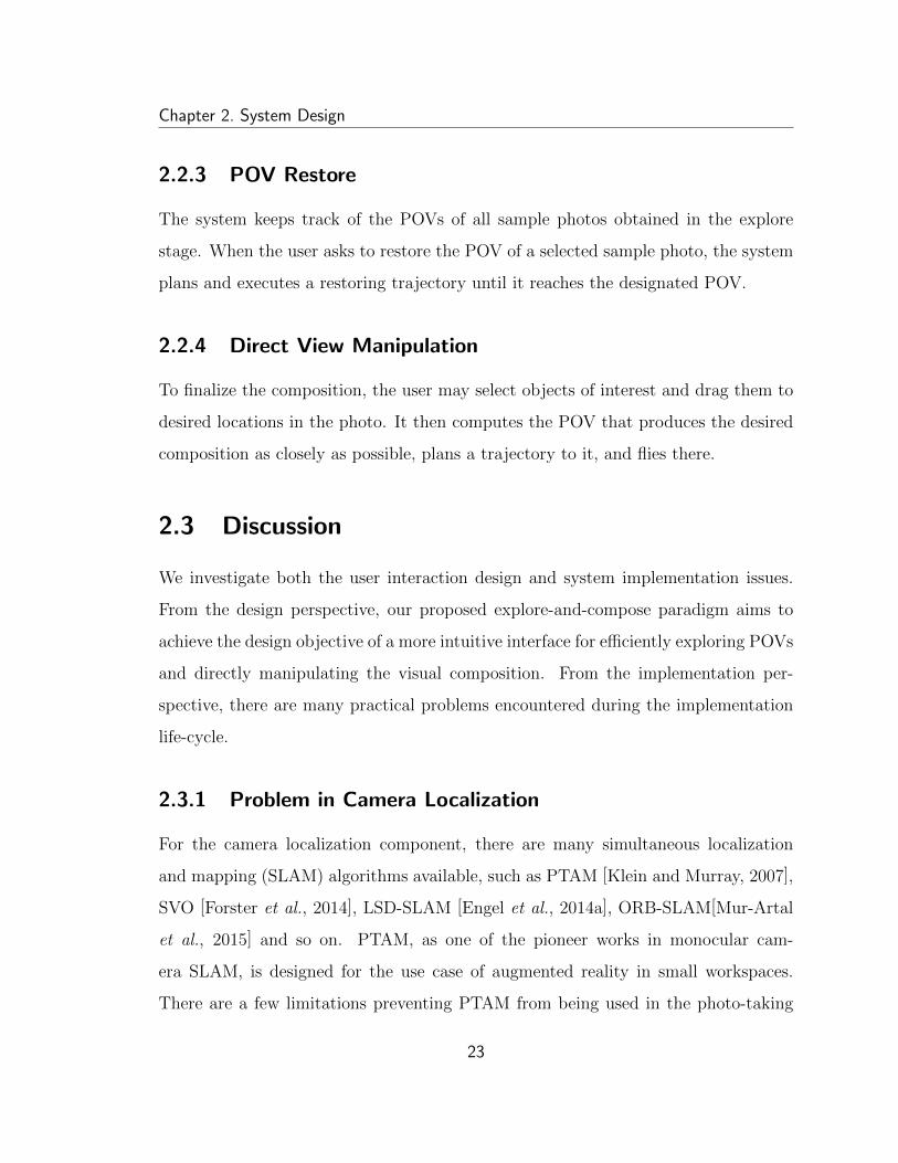
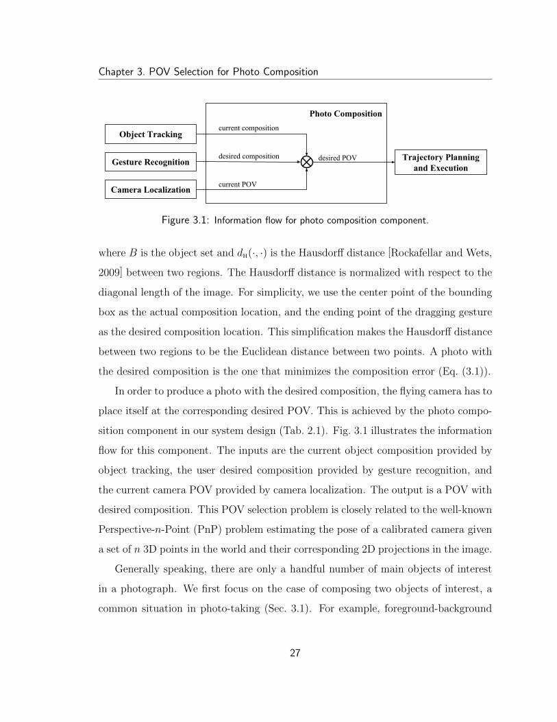
3.1 Information flow for photo composition component . . . . . . . . . . 27
3.2 Photos with two main objects of interest . . . . . . . . . . . . . . . . 28
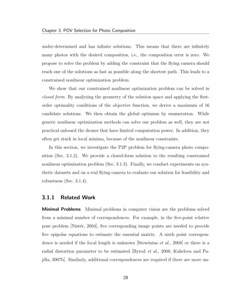
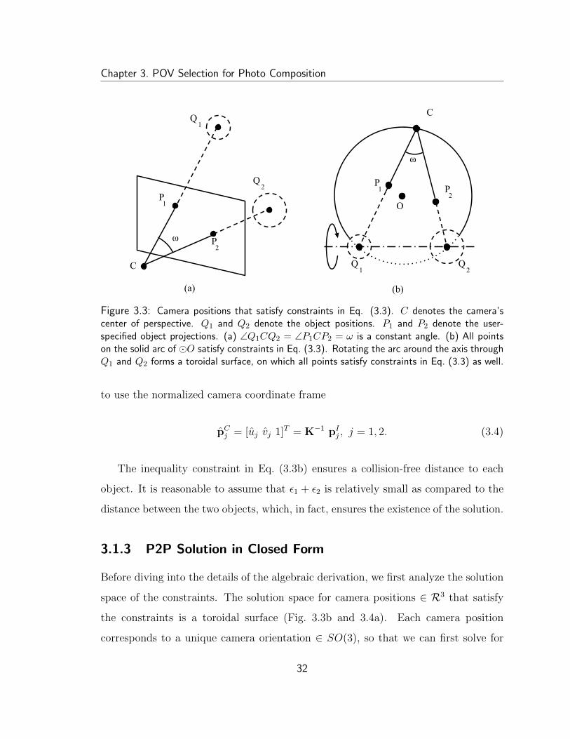
3.3 Camera positions that satisfy constraints in Eq. (3.3) . . . . . . . . . 32
3.4 The auxiliary frame FA . . . . . . . . . . . . . . . . . . . . . . . . . . 33
3.5 Parameterization of c1CA using θ . . . . . . . . . . . . . . . . . . . . . 36
3.6 Optimal camera position candidates . . . . . . . . . . . . . . . . . . . 40
3.7 Results from synthetic datasets . . . . . . . . . . . . . . . . . . . . . 45
3.8 Results from real robot experiments . . . . . . . . . . . . . . . . . . . 48
3.9 The viewpoint changing process . . . . . . . . . . . . . . . . . . . . . 50
4.1 Portable flying cameras . . . . . . . . . . . . . . . . . . . . . . . . . . 53
4.2 Information flow for collision avoidance component . . . . . . . . . . 54
4.3 Monocular depth perception . . . . . . . . . . . . . . . . . . . . . . . 57
vii
4.4 Monocular dense depth map construction . . . . . . . . . . . . . . . . 61
4.5 Nearby vertices that enclose a pixel . . . . . . . . . . . . . . . . . . . 61
5.1 Overview of the system architecture . . . . . . . . . . . . . . . . . . . 67
5.2 Information flow for gesture recognition component . . . . . . . . . . 68
5.3 Information flow for object tracking component . . . . . . . . . . . . 69
5.4 Information flow for trajectory planning component . . . . . . . . . . 70
5.5 Local depth map as a 3D point cloud . . . . . . . . . . . . . . . . . . 73
5.6 Aggregated occupancy grid map . . . . . . . . . . . . . . . . . . . . . 74
5.7 Local trajectory planning . . . . . . . . . . . . . . . . . . . . . . . . . 74
5.8 Information flow for drone control component . . . . . . . . . . . . . 75
6.1 Interaction design evaluation setup . . . . . . . . . . . . . . . . . . . 78
6.2 Performance comparison between the joystick interface and XPose in
interaction design evaluation . . . . . . . . . . . . . . . . . . . . . . . 80
6.3 System performance evaluation setup for photo-taking of one object of
interest . . . . . . . . . . . . . . . . . . . . . . . . . . . . . . . . . . . 82
6.4 System performance evaluation setup for photo taking of multiple ob-
jects of interest . . . . . . . . . . . . . . . . . . . . . . . . . . . . . . 83
6.5 Performance comparison between the joystick interface and XPose in
overall system performance evaluation . . . . . . . . . . . . . . . . . 84
viii

List of Tables
2.1 Main functions and system components . . . . . . . . . . . . . . . . . 22
4.1 Results on Make3D dataset . . . . . . . . . . . . . . . . . . . . . . . 64
4.2 Results on KITTI dataset . . . . . . . . . . . . . . . . . . . . . . . . 64
ix
Chapter 1
Introduction
1.1 User Interfaces for Photo-taking
User interfaces for photo-taking evolve together with the new characteristics of camera
devices, making photo-taking much easier and quicker. This evolution starts since two
centuries ago. In 1826, the first permanent photograph in the history of mankind was
taken by Joseph Nicphore Nipce [Gernsheim and Gernsheim, 1969]. The photo was
made using an 8-hour exposure on pewter coated with bitumen. Later, in 1839, the
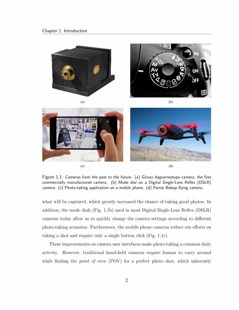
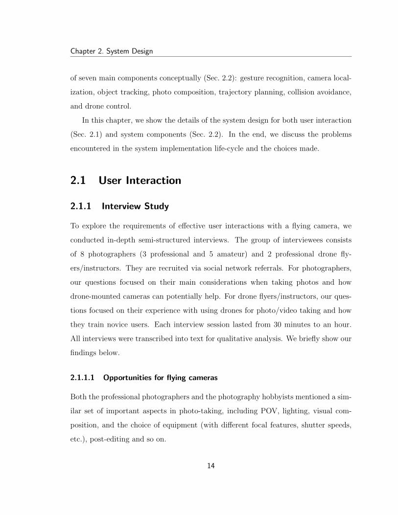
Giroux daguerreotype camera (Fig. 1.1a) became the first commercially manufactured
camera. It was a double-box design, with a lens fitted to the outer box, and a holder
for a focusing screen on the inner box. To take a photo, the user needs to perform
many steps. First, slide the inner box to adjust the focusing screen for imagery
sharpness. Then, replace the screen with a sensitized plate. Next, release the shutter
made by a brass plate in the front of the lens. Finally, wait for 5 to 30 minutes of
exposure time. As time goes by, cameras evolve from cumbersome to portable, manual
to automated, analog to digital. For instance, the Single-Lens Reflex (SLR) camera
mechanisms were invented to enable us to view through the lens and see exactly
1
Chapter 1. Introduction
(d)(c)
(b)(a)
Figure 1.1: Cameras from the past to the future. (a) Giroux daguerreotype camera, the firstcommercially manufactured camera. (b) Mode dial on a Digital Single-Lens Reflex (DSLR)camera. (c) Photo-taking application on a mobile phone. (d) Parrot Bebop flying camera.
what will be captured, which greatly increased the chance of taking good photos. In
addition, the mode dials (Fig. 1.1b) used in most Digital Single-Lens Reflex (DSLR)
cameras today allow us to quickly change the camera settings according to different
photo-taking scenarios. Furthermore, the mobile phone cameras reduce our efforts on
taking a shot and require only a single button click (Fig. 1.1c).
These improvements on camera user interfaces make photo-taking a common daily
activity. However, traditional hand-held cameras require human to carry around
while finding the point of view (POV) for a perfect photo shot, which inherently
2
Chapter 1. Introduction
limits the cameras’ physical reachability and viewpoint coverage. This limitation
can be overcome using a flying camera, i.e., a camera mounted on a flying platform
(Fig. 1.1d). In this thesis, we aim to further elevate the usability of cameras with the
new flying capability.
1.2 Flying Camera Photography
Taking photos with a flying device is not a new concept. As early as the 1860s, bal-
loons, kites and trained pigeons were used to carry cameras for airborne photography.
Later, in the early 1900s, airplanes and dirigibles were invented and used. Today, with
the advances of miniaturized flying drones, flying cameras are no longer exclusive to
the professional users. In the future, many people may take along compact flying
cameras, and use their touchscreen mobile devices as viewfinders to compose favor-
able shots. Although many drone related accessories and gadgets are available in the
commercial market, such as combining a joystick with a virtual reality headset to
support a firstperson shooter experience, we envision that using a flying camera shall
be as easy and natural as using a mobile phone camera today. This thesis proposes a
touch-based prototype flying camera interface based on a Parrot Bebop quadcopter
(Fig. 1.1d).
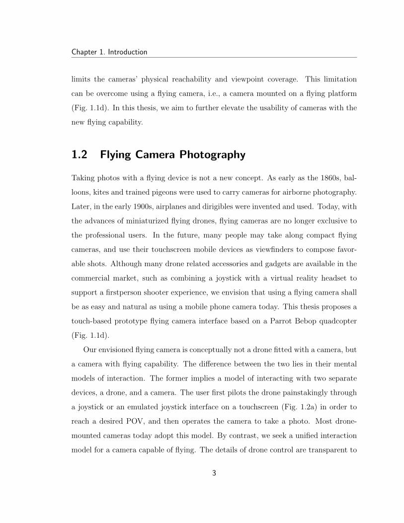
Our envisioned flying camera is conceptually not a drone fitted with a camera, but
a camera with flying capability. The difference between the two lies in their mental
models of interaction. The former implies a model of interacting with two separate
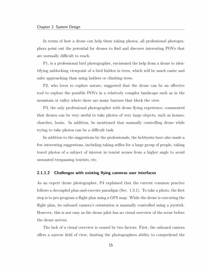
devices, a drone, and a camera. The user first pilots the drone painstakingly through
a joystick or an emulated joystick interface on a touchscreen (Fig. 1.2a) in order to
reach a desired POV, and then operates the camera to take a photo. Most drone-
mounted cameras today adopt this model. By contrast, we seek a unified interaction
model for a camera capable of flying. The details of drone control are transparent to
3
Chapter 1. Introduction
(a) (b)
Figure 1.2: Compare a common joystick interface and XPose. (a) The left joystick controls thedrone’s heading direction and altitude. The right joystick controls its translational movementalong or orthogonal to the heading direction. (b) With XPose, the user interacts directly withthe image contents, such as selecting an object of interest by drawing a circle.
the user, making the flying camera more intuitive and easier to use. To realize such a
unified interaction model for photo-taking, we introduce the concept of photo space. It
is defined as the collection of all possible photographs taken for a target scene. Photo-
taking becomes a searching problem that looks for a small set of camera views in the
entire photo space. In this thesis, we assume the scene is static or almost static, which
covers many genres of photography, such as architectural, still life, portrait scenic,
etc. Furthermore, we assume each POV produces a unique photo. In other words,
each photo is determined only by the camera’s extrinsic parameters that define the
camera’s poses. It is not critical to consider the intrinsic parameters or the internal
settings, such as focal length, camera distortion, frame shape and filter style, since
those effects can be achieved easily during the post-production process using an image
editing software, such as Photoshop.
The development of an interactive system is challenging. The challenges lie in
the interplay between interaction design and system implementation. From the in-
teraction design perspective, efficiently searching the infinite photo space is a hard
problem in itself. From the system implementation perspective, a light-weight drone
4
Chapter 1. Introduction
(a) (b) (c)
(d) (e) (f)
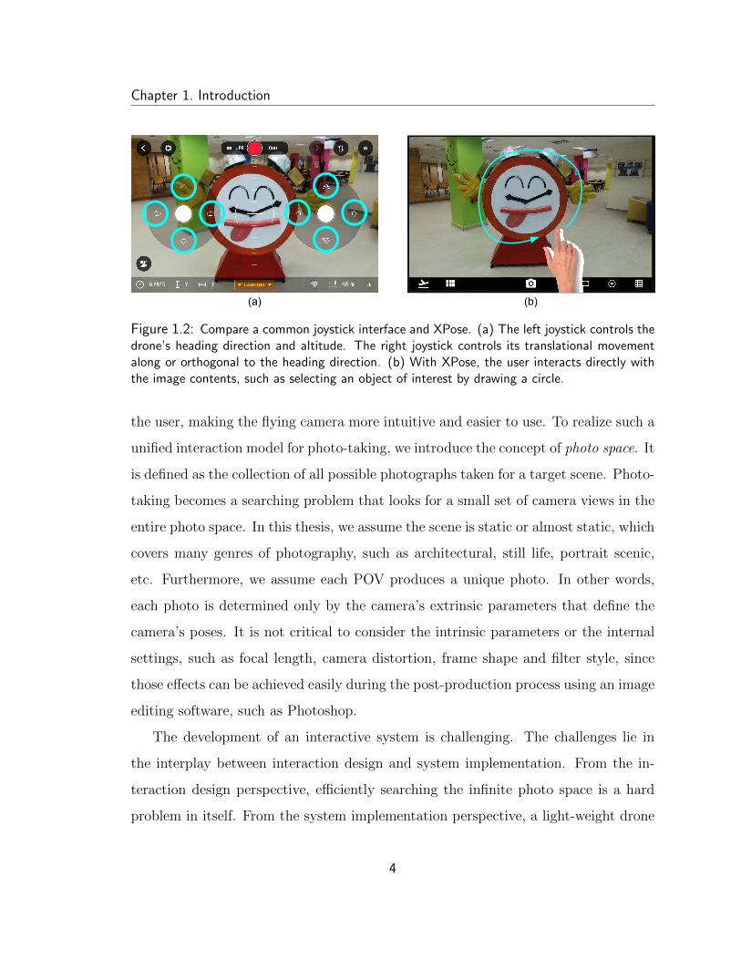
(g) (h) (i)
Figure 1.3: An envisioned use case of XPose. (a) Select an object of interest with the encirclegesture. (b) Activate the Orbit exploration mode. (c) The drone-mounted camera takes samplephotos while orbiting the object of interest autonomously. (d) Enter the gallery preview. (e)Browse sample photos in the gallery. (f) Restore a POV associated with a selected samplephoto. (g) Compose a final shot by dragging selected objects of interest to desired locations inthe photo. (h) Take the final shot. (i) The final photo.
such as the Parrot Bebop has a severe restriction on the payload and carries only a
single forward-facing main camera with a very limited field of view. With a single
monocular camera, the system needs to localize the camera with respect to objects
of interest, track objects reliably, and avoid collision with obstacles.
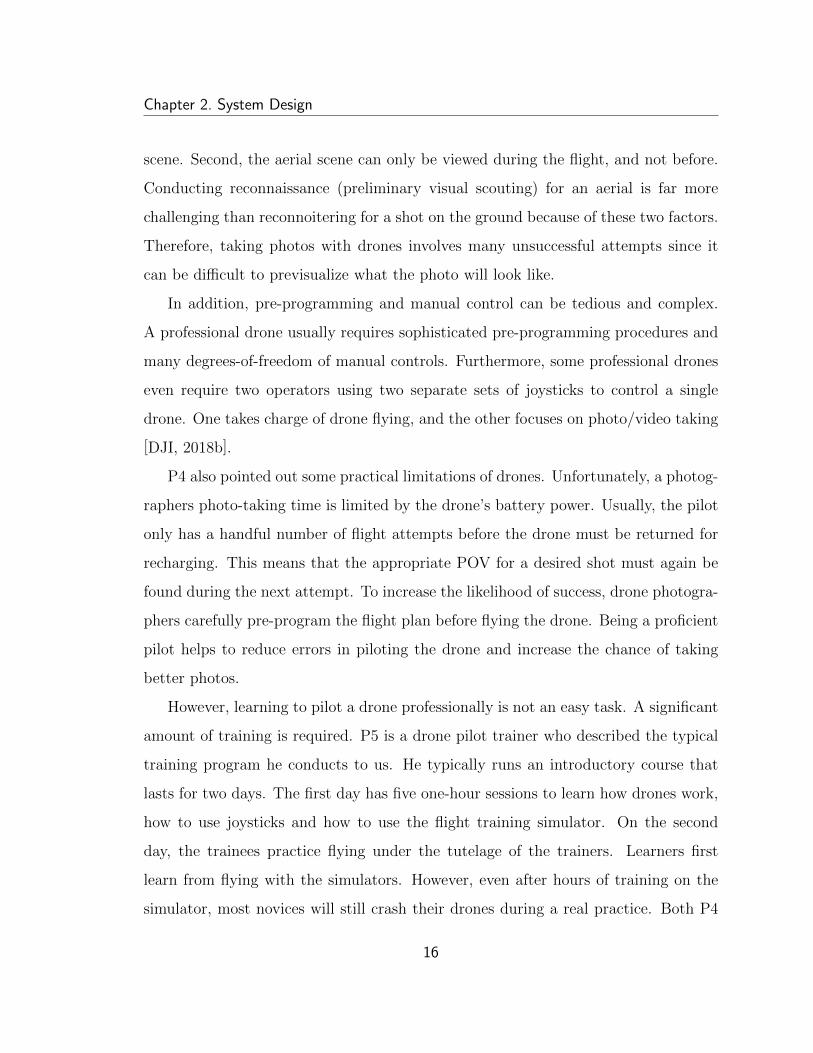
We present a touch-based interactive system, named XPose, which investigates
both the user interaction design and system implementation issues. For interaction
design, XPose proposes a novel two-stage eXplore-and-comPose paradigm for efficient
and intuitive photo-taking. In the explore stage, the user first selects objects of inter-
5
Chapter 1. Introduction
est (Fig. 1.3a) and the interaction mode (Orbit, Pano, and Zigzag) on a touchscreen
interface (Fig. 1.3b). The camera then flies autonomously along predefined trajecto-
ries and visits many POVs to take exploratory photos (Fig. 1.3c). The sample photos
are presented as a gallery preview (Fig. 1.3d,e). The user taps on a potentially in-
teresting preview photo and directs the drone to revisit the associated POV in order
to finalize it (Fig. 1.3f). In the compose stage, the user composes the final photo
on the touchscreen, using familiar dragging gestures (Fig. 1.3g). The camera flies
autonomously to a desired POV (Fig. 1.3h), instead of relying on the user to pilot
manually.
Based on the design requirements in the explore-and-compose paradigm, we iden-
tify seven main system components for system implementation: gesture recognition,
camera localization, object tracking, photo composition, trajectory planning, colli-
sion avoidance, and drone control. In the context of flying camera photography, the
problems of photo composition and collision avoidance are crucial. In this thesis,
we further investigate these two system components. More specifically, we study the
underlying POV selection problem for photo composition using intuitive touch ges-
tures, and the obstacle perception problem for collision avoidance using a monocular
camera.
In summary, we integrate interaction design and flying camera autonomy to pro-
vide an intuitive touch interface so that the user interacts with photos directly and
focuses on photo-taking instead of drone piloting.
1.3 User Interactions for POV Navigation
POV navigation can be achieved by manipulating the camera pose and/or interacting
with the camera view.Based on the modalities, we categorize different user interac-
tions into device-centric techniques and view-centric techniques (Fig. 1.4). Device-
6
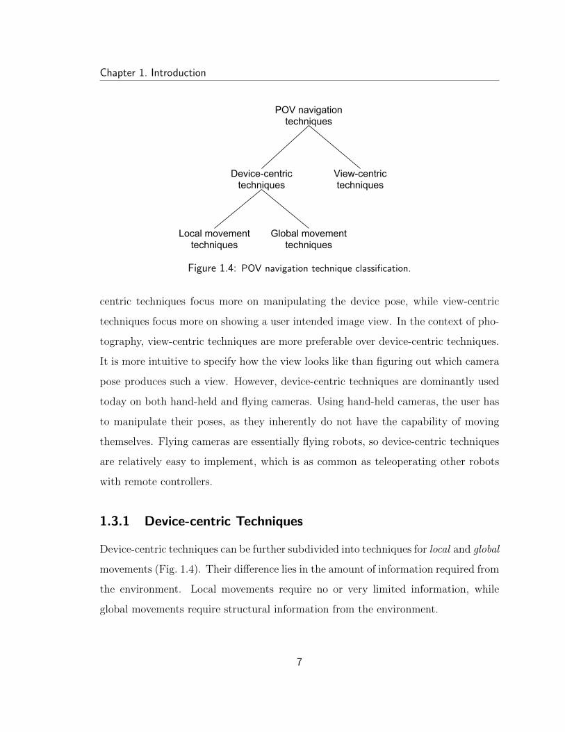
Chapter 1. Introduction
POV navigationtechniques
Device-centrictechniques
View-centrictechniques
Local movementtechniques
Global movementtechniques
Figure 1.4: POV navigation technique classification.
centric techniques focus more on manipulating the device pose, while view-centric
techniques focus more on showing a user intended image view. In the context of pho-
tography, view-centric techniques are more preferable over device-centric techniques.
It is more intuitive to specify how the view looks like than figuring out which camera
pose produces such a view. However, device-centric techniques are dominantly used
today on both hand-held and flying cameras. Using hand-held cameras, the user has
to manipulate their poses, as they inherently do not have the capability of moving
themselves. Flying cameras are essentially flying robots, so device-centric techniques
are relatively easy to implement, which is as common as teleoperating other robots
with remote controllers.
1.3.1 Device-centric Techniques
Device-centric techniques can be further subdivided into techniques for local and global
movements (Fig. 1.4). Their difference lies in the amount of information required from
the environment. Local movements require no or very limited information, while
global movements require structural information from the environment.
7
Chapter 1. Introduction
Local Movement Techniques Local movements usually refer to pan, tilt, dolly,
truck and pedestal camera motions. Photographers with hand-held cameras practice
these local movements unintentionally. These camera motions have been transferred
into the virtual environment to navigate a POV via walking/driving/flying metaphors
[Ware and Osborne, 1990; Bowman et al., 1997]. For consumer drones fitted with
cameras, the most common interface for POV navigation is probably a touchscreen
with emulated joysticks (Fig. 1.2a). The user watches a live video feed from the
drone-mounted camera and commands the drone to perform local movements through
the joysticks. This approach, which combines joysticks and live video feedback, is
also common for teleoperation of remote vehicles [Ballou, 2001; Hainsworth, 2001].
Experiences there suggest that manual control through the joysticks faces several
difficulties. The low-level motion control afforded by the joysticks is tedious. Further,
operating the drone through only the video feed often results in loss of situational
awareness, inaccurate attitude judgment, and failure to detect obstacles [McGovern,
1991].
Another commonly used local movement is rotate (also referred to as orbit, tum-
ble or sweep), which is a standard technique for inspecting a target in the virtual
environment, such as Autodesk’s 3DS MAX and Maya. The rotate movement only
requires the target position to determine the center of rotation and remain a constant
distance to it. This is easily obtained in the virtual environment. Similarly, GPS
tracking devices [Lily-Next-Gen, 2017] are widely used to enable the flying camera’s
orbiting movement. However, the GPS may be unavailable or unreliable in indoor
environments and urban canyons. Further, GPS maps do not supply the visual in-
formation required by the user to identify attractive POVs for photo composition.
Besides GPS, image-based tracking algorithms [Skydio-R1, 2018] are used as well.
However, existing image-based tracking algorithms are not robust against large view-
ing angle changes in the process of orbiting around [Kalal et al., 2012].
8
Chapter 1. Introduction
Global Movement Techniques Global movements specify camera poses using struc-
tural information of the environment. Commonly used structural information is a
coordinate system or a map. In virtual environments, the user can specify a precise
camera pose in the global coordinate. Similarly, GPS satellite map is used to guide
drones to fly to particular GPS locations [DJI, 2018a; Bebop, 2018].
Another way to use structural information is to guide the camera movement by
constraining its motion. For example, virtual tours have been created in virtual
environments. The camera moves along a predefined trajectory automatically while
allowing users to deviate locally form the tour [Galyean, 1995; Elmqvist et al., 2008].
Such a tour is conceptually a 1-dimensional constraint. A 2-dimensional constraint
is called a “guide manifold” [Hanson and Wernert, 1997; Burtnyk et al., 2002; Khan
et al., 2005] that constrains the camera movement along some specially designed 2-
dimensional subspace. Constraining the motion of a flying camera has been realized
through a decoupled plan-and-execute paradigm [Joubert et al., 2015; Gebhardt et
al., 2016]. POV trajectory planning occurs offline and relies on a given 3D virtual
model of the real-world environment. Then, the drone carries the camera to execute
the planned trajectory. This decoupled plan-and-execute paradigm implies a slow
interaction cycle and is not quite suitable for photo-taking in real-time. Moreover,
the acquisition of accurate 3D models is also a major challenge in itself and remains
an active area of research [Fuentes-Pacheco et al., 2012; Marder-Eppstein, 2016].
1.3.2 View-centric Techniques
As aforementioned, photo-taking using view-centric techniques is more intuitive than
using device-centric techniques. Unfortunately, view-centric techniques for photogra-
phy have not been drawn much attention. Nevertheless, many view-centric techniques
have been studied and applied to the virtual camera that is similar to the flying
9
Chapter 1. Introduction
camera in many aspects. They both can hover in the space and move agilely and
autonomously. It is worthy to notice that many device-centric techniques have been
applied to both the virtual camera and the flying camera due to their similarities.
View-centric techniques move a POV autonomously based on user intent. A com-
mon approach is to communicate user intent with respect to a point of interest (POI).
Estimating a user intended POV with respect to a POI was firstly proposed in the
Point of Interest Logarithmic Flight technique [Mackinlay et al., 1990] that moves the
virtual camera towards and face the POI. Instead of directly facing the POI, UniCam
[Zeleznik and Forsberg, 1999] proposes to estimate the camera orientation according
to the proximity of the edges of some objects. Rather than estimating a user intended
POV, Navidget [Hachet et al., 2008] provides direct and real-time visual feedback us-
ing a 3D widget coupled with a preview window so that the user can select a POV
while moving a cursor on the 3D widget.
Another view-centric technique is to manipulate the screen-space projection of a
scene in the camera view directly, i.e., direct manipulation. Direct manipulation in
screen-space [Gleicher and Witkin, 1992; Reisman et al., 2009; Walther-Franks et al.,
2011] allows the user to specify desired object positions on the screen. The virtual
camera is autonomously controlled so that the selected objects on the screen always
stick to the corresponding device pointers, for example, fingertips. A different but
related application of direct view manipulation is video browsing [Satou et al., 1999;
Dragicevic et al., 2008; Karrer et al., 2008]. Since a video can be seen as a sequence
of camera views produced by a fixed trajectory of camera poses, a desired camera
view can be found by directly dragging the objects in the video content.
View-centric techniques developed for virtual cameras cannot be directly applied
to physical flying cameras. Their fundamental difference lies in their moving speeds,
which greatly affects their feedback cycles. In the virtual environment, the user
interface is able to respond to rapid user inputs. In particular, the 3D widget of
10
Chapter 1. Introduction
Navidget corresponds to a collection of all possible views with respect to the target.
When the mouse cursor moves on the virtual widget, the corresponding camera view is
rendered in the preview window in real-time. By contrast, the physical flying camera
cannot afford to provide real-time visual feedback with such a rapid rate, because the
camera has to physically fly from one POV to another with limited traveling speed.
In this thesis, we propose the explore-and-compose paradigm, a view-centric POV
navigation technique for flying camera photography. Furthermore, we investigate the
complete interactive system that aids the user for real-time photo-taking without a
3D model given a priori.
1.4 Outline
The rest of the thesis is organized as follows.
Chapter 2 presents the system design. First, we start with an interview study
with photographers and drone flyers to understand the design objective and introduce
the two-stage explore-and-compose paradigm in detail. Then, we analyze the main
system functions in the interactive paradigm and identify the required main system
components to implement each function.
Among the main system components, photo composition (Chap. 3) and collision
avoidance (Chap. 4) are crucial in the context of flying camera photo-taking. We
further investigate them respectively. In Chapter 3, we investigate the underlying
POV search problem for photo composition using intuitive touch gestures. We focus
on a common situation in photo-taking, i.e., composing a photo with two objects
of interest. We model it as a Perspective-2-Point problem, formulate a constrained
nonlinear optimization problem, and solve it in closed form. Experiments on both
synthetic datasets and the Parrot Bebop flying camera are reported. In addition, we
propose a sample-based POV search method for composing a photo with three or
11
Chapter 1. Introduction
more objects of interest. Next, in Chapter 4, we investigate the obstacle perception
problem for collision avoidance using monocular cameras. To perceive obstacles, we
propose an algorithm to estimate a dense and accurate depth map for each image
frame, which combines the strengths of both the geometry-based approach and the
data-driven approach to depth estimation. Our depth map estimation algorithm
is evaluated with datasets of real images, and implemented for collision-free path
planning with the Parrot Bebop flying camera.
Chapter 5 and Chapter 6 present the system implementation and evaluation re-
spectively. Chapter 5 shows the implementation details of the main system compo-
nents. Chapter 6 reports the evaluation results for both interaction design and system
performance on photo-taking tasks.
Finally, in Chapter 7, we summarize the main results and point out directions for
future research.
12
Chapter 2
System Design
Flying cameras have produced extraordinary photos, with POVs rarely reachable
otherwise [Dronestagram, 2017], and endeared themselves to amateur and professional
photographers alike. While today flying cameras remain the toys of hobbyists, in the
future many people may carry compact drones in pockets [AirSelfie, 2018] or even wear
them on the wrists [Flynixie, 2018]. They release the drones into the sky for photo-
taking and use their touchscreen mobile phones as viewfinders. This chapter presents
the overall design of the flying camera we dreamed of, with the goal of investigating
the underlying user interaction design and system implementation issues.
To explore the interaction design requirements, we started with an interview study
with photographers and drone flyers (Sec. 2.1.1), and identified the main objective of
helping the user to explore POVs efficiently while avoiding the perception of latency
when the camera transitions between POVs. We propose the novel two-stage explore-
and-compose paradigm that was briefly introduced in Sec. 1.2, which is described with
more details later, in Sec. 2.1.
Further, to realize the proposed explore-and-compose design paradigm, XPose is
implemented based on the Parrot Bebop quadcopter. The interactive system consists
13
Chapter 2. System Design
of seven main components conceptually (Sec. 2.2): gesture recognition, camera local-
ization, object tracking, photo composition, trajectory planning, collision avoidance,
and drone control.
In this chapter, we show the details of the system design for both user interaction
(Sec. 2.1) and system components (Sec. 2.2). In the end, we discuss the problems
encountered in the system implementation life-cycle and the choices made.
2.1 User Interaction
2.1.1 Interview Study
To explore the requirements of effective user interactions with a flying camera, we
conducted in-depth semi-structured interviews. The group of interviewees consists
of 8 photographers (3 professional and 5 amateur) and 2 professional drone fly-
ers/instructors. They are recruited via social network referrals. For photographers,
our questions focused on their main considerations when taking photos and how
drone-mounted cameras can potentially help. For drone flyers/instructors, our ques-
tions focused on their experience with using drones for photo/video taking and how
they train novice users. Each interview session lasted from 30 minutes to an hour.
All interviews were transcribed into text for qualitative analysis. We briefly show our
findings below.
2.1.1.1 Opportunities for flying cameras
Both the professional photographers and the photography hobbyists mentioned a sim-
ilar set of important aspects in photo-taking, including POV, lighting, visual com-
position, and the choice of equipment (with different focal features, shutter speeds,
etc.), post-editing and so on.
14
Chapter 2. System Design
In terms of how a drone can help them taking photos, all professional photogra-
phers point out the potential for drones to find and discover interesting POVs that
are normally difficult to reach.
P1, is a professional bird photographer, envisioned the help from a drone to iden-
tifying unblocking viewpoint of a bird hidden in trees, which will be much easier and
safer approaching than using ladders or climbing trees.
P2, who loves to explore nature, suggested that the drone can be an effective
tool to explore the possible POVs in a relatively complex landscape such as in the
mountain or valley where there are many barriers that block the view.
P3, the only professional photographer with drone flying experience, commented
that drones can be very useful to take photos of very large objects, such as houses,
churches, boats. In addition, he mentioned that manually controlling drone while
trying to take photos can be a difficult task.
In addition to the suggestions by the professionals, the hobbyists have also made a
few interesting suggestions, including taking selfies for a large group of people, taking
travel photos of a subject of interest in tourist scenes from a higher angle to avoid
unwanted trespassing tourists, etc.
2.1.1.2 Challenges with existing flying cameras user interfaces
As an expert drone photographer, P4 explained that the current common practice
follows a decoupled plan-and-execute paradigm (Sec. 1.3.1). To take a photo, the first
step is to pre-program a flight plan using a GPS map. While the drone is executing the
flight plan, its onboard camera’s orientation is manually controlled using a joystick.
However, this is not easy as the drone pilot has no visual overview of the scene before
the drone arrives.
The lack of a visual overview is caused by two factors. First, the onboard camera
offers a narrow field of view, limiting the photographers ability to comprehend the
15
Chapter 2. System Design
scene. Second, the aerial scene can only be viewed during the flight, and not before.
Conducting reconnaissance (preliminary visual scouting) for an aerial is far more
challenging than reconnoitering for a shot on the ground because of these two factors.
Therefore, taking photos with drones involves many unsuccessful attempts since it
can be difficult to previsualize what the photo will look like.
In addition, pre-programming and manual control can be tedious and complex.
A professional drone usually requires sophisticated pre-programming procedures and
many degrees-of-freedom of manual controls. Furthermore, some professional drones
even require two operators using two separate sets of joysticks to control a single
drone. One takes charge of drone flying, and the other focuses on photo/video taking
[DJI, 2018b].
P4 also pointed out some practical limitations of drones. Unfortunately, a photog-
raphers photo-taking time is limited by the drone’s battery power. Usually, the pilot
only has a handful number of flight attempts before the drone must be returned for
recharging. This means that the appropriate POV for a desired shot must again be
found during the next attempt. To increase the likelihood of success, drone photogra-
phers carefully pre-program the flight plan before flying the drone. Being a proficient
pilot helps to reduce errors in piloting the drone and increase the chance of taking
better photos.
However, learning to pilot a drone professionally is not an easy task. A significant
amount of training is required. P5 is a drone pilot trainer who described the typical
training program he conducts to us. He typically runs an introductory course that
lasts for two days. The first day has five one-hour sessions to learn how drones work,
how to use joysticks and how to use the flight training simulator. On the second
day, the trainees practice flying under the tutelage of the trainers. Learners first
learn from flying with the simulators. However, even after hours of training on the
simulator, most novices will still crash their drones during a real practice. Both P4
16
Chapter 2. System Design
and P5 mentioned that it took them about one year of frequent practice to achieve
their current proficiency levels.
2.1.1.3 Summary
In summary, the photographers’ responses suggest a set of well-established considera-
tions for photo-taking: POVs, visual composition, lighting conditions, shutter speed,
depth of field, etc. They also point to the potential for drone-mounted cameras to
discover novel POVs. The drone flyers/instructors’ responses include lengthy prepara-
tions for drone photo/video taking sessions and extensive training required for novice
users. These led to our design objective of a simple, intuitive interface for efficiently
exploring many POVs and directly manipulating the visual composition.
2.1.2 Explore-and-Compose
With traditional hand-held cameras, the user explores POVs by moving around and
looking through the viewfinder. Limited by the user’s physical movements, the ex-
ploration of POVs is local, but the visual feedback is almost instantaneous. The
joystick touchscreen interface tries to reproduce this experience for flying cameras:
the joysticks control the camera’s local movements, and the touchscreen provides vi-
sual feedback. However, this approach does not account for the difference in device
characteristics between hand-held cameras and flying cameras. The camera’s ability
to fly offers the opportunity of exploring POVs more globally. At the same time, it
is more difficult for a flying camera to achieve an intended POV precisely, due to air
disturbance and other factors. Further, visual feedback is not instantaneous, because
of the communication delay between the flying camera and the user’s mobile device.
We introduce a two-stage explore-and-compose paradigm, which enables the user
to explore a wide range of POVs efficiently in a hierarchical manner. In the explore
17
Chapter 2. System Design
stage, the user samples many POVs globally at a coarse level, through autonomous
drone flying. In the compose stage, the user chooses a sampled POV for further
refinement and composes the final photo on the touchscreen by interacting directly
with objects of interest in the image.
We now illustrate our approach in detail with a concrete scenario (Fig. 1.3). Our
main character, Terry, walks along a river on a sunny day and stops at a white statue.
She wishes to take a photo of the statue, but can hardly get a close-up shot with a
hand-held camera, as the statue is almost 15 feet in height. Terry launches XPose
using the associated app on her mobile device. The home view of the app contains a
viewfinder, which displays the live video feed from the drone-mounted camera.
2.1.2.1 Explore
Terry is initially unsure about the best viewing angle for the shot and decides to
explore the POVs around the statue. She selects the statue as the object of interest
and uses XPose’s exploration modes to sample the POVs.
Object of Interest Selection First, Terry performs pan and zoom gestures (Fig. 2.1)
on the touchscreen to get the statue into the viewfinder. Then she draws a circle
around the statue in the viewfinder (Fig. 1.3a). A rectangular bounding box appears
to confirm that the statue has been selected and is being tracked.
POV Sampling While the statue is being tracked in the viewfinder, Terry activates
the Orbit exploration mode (Fig. 1.3b). The flying camera then takes sample shots
while orbiting around the statue autonomously (Fig. 1.3c).
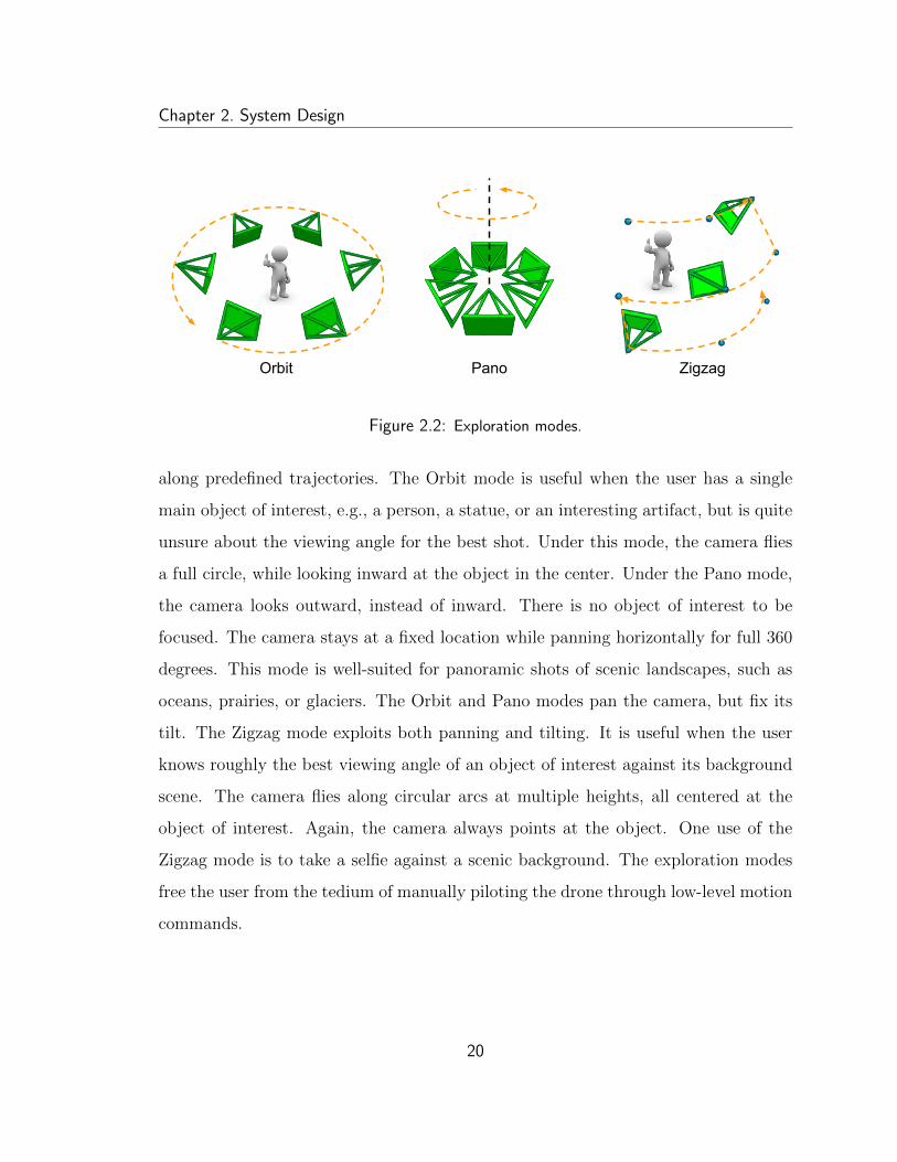
XPose currently provides three explorations modes: Orbit, Pano, and Zigzag
(Fig. 2.2). They leverage the autonomous flying capability of a drone-mounted cam-
era and systematically explore the POVs by taking sample shots evenly distributed
18

Chapter 2. System Design
Eyeball Panning
Gestures
Camera Motion
Use Case
Pan and tilt
Translational Panning
Gestures
Camera Motion
Use Case
Move in the image plane
Zooming
Gestures
Camera Motion
Use Case
Zoom in and out
Figure 2.1: User intents for direct view manipulation. User intents of eyeball panning andtranslation panning are expressed via swiping gestures with four and two fingers respectively.The zooming intents are expressed via pinch and stretch gestures. In addition, single-fingergestures are already reserved for object selection by encircling (Fig. 1.3a) and object compositionby dragging (Fig. 1.3g).
19
Chapter 2. System Design
Orbit Pano Zigzag
Figure 2.2: Exploration modes.
along predefined trajectories. The Orbit mode is useful when the user has a single
main object of interest, e.g., a person, a statue, or an interesting artifact, but is quite
unsure about the viewing angle for the best shot. Under this mode, the camera flies
a full circle, while looking inward at the object in the center. Under the Pano mode,
the camera looks outward, instead of inward. There is no object of interest to be
focused. The camera stays at a fixed location while panning horizontally for full 360
degrees. This mode is well-suited for panoramic shots of scenic landscapes, such as
oceans, prairies, or glaciers. The Orbit and Pano modes pan the camera, but fix its
tilt. The Zigzag mode exploits both panning and tilting. It is useful when the user
knows roughly the best viewing angle of an object of interest against its background
scene. The camera flies along circular arcs at multiple heights, all centered at the
object of interest. Again, the camera always points at the object. One use of the
Zigzag mode is to take a selfie against a scenic background. The exploration modes
free the user from the tedium of manually piloting the drone through low-level motion
commands.
20
Chapter 2. System Design
2.1.2.2 Compose
After getting many sample shots through the Orbit mode, Terry is ready to finalize
the photo.
POV Restore Terry switches to the gallery view in the app (Fig. 1.3d) and browses
the sample shots displayed there (Fig. 1.3e). All sample photos have the statue in
the center, but different backgrounds. To take a closer look, Terry taps on a photo to
see it in the full-screen photo view (Fig. 1.3e,f). One photo with many tall buildings
in the background looks promising, but the composition is not ideal. The accidental
alignment of the statue’s head and a tall building is distracting. To refine it, Terry
taps a button and commands the flying camera to restore the POV associated with
the selected sample photo (Fig. 1.3f).
Direct View Manipulation From the restored POV, Terry selects two buildings in
the viewfinder as additional objects of interest and drags them, one at a time, to
the left and right side of the statue respectively, so that the statue’s head appears
in the gap between the two buildings (Fig. 1.3g). XPose flies to a new POV that
produces the desired composition as closely as possible and displays the photos in the
viewfinder. Quite satisfied, Terry takes the final shot (Fig. 1.3h,i).
2.2 System Functions
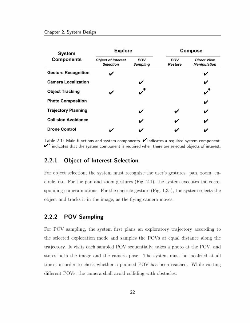
System functions introduced in the explore-and-compose paradigm are supported by
seven system components: gesture recognition, camera localization, object track-
ing, photo composition, trajectory planning, collision avoidance, and drone control.
This subsection shows how the system functions depend on the system components.
Tab. 2.1 is an overview.
21
Chapter 2. System Design
SystemComponents
Explore Compose
Object of Interest Selection
POVSampling
POVRestore
Direct View Manipulation
✔ ✔
✔
✔ ✔✔
Camera Localization ✔
Object Tracking *✔
*✔✔
Gesture Recognition
Photo Composition
Trajectory Planning
✔
✔✔ ✔
✔ ✔✔✔
Collision Avoidance
Drone Control
Table 2.1: Main functions and system components. "indicates a required system component."* indicates that the system component is required when there are selected objects of interest.
2.2.1 Object of Interest Selection
For object selection, the system must recognize the user’s gestures: pan, zoom, en-
circle, etc. For the pan and zoom gestures (Fig. 2.1), the system executes the corre-
sponding camera motions. For the encircle gesture (Fig. 1.3a), the system selects the
object and tracks it in the image, as the flying camera moves.
2.2.2 POV Sampling
For POV sampling, the system first plans an exploratory trajectory according to
the selected exploration mode and samples the POVs at equal distance along the
trajectory. It visits each sampled POV sequentially, takes a photo at the POV, and
stores both the image and the camera pose. The system must be localized at all
times, in order to check whether a planned POV has been reached. While visiting
different POVs, the camera shall avoid colliding with obstacles.
22
Chapter 2. System Design
2.2.3 POV Restore
The system keeps track of the POVs of all sample photos obtained in the explore
stage. When the user asks to restore the POV of a selected sample photo, the system
plans and executes a restoring trajectory until it reaches the designated POV.
2.2.4 Direct View Manipulation
To finalize the composition, the user may select objects of interest and drag them to
desired locations in the photo. It then computes the POV that produces the desired
composition as closely as possible, plans a trajectory to it, and flies there.
2.3 Discussion
We investigate both the user interaction design and system implementation issues.
From the design perspective, our proposed explore-and-compose paradigm aims to
achieve the design objective of a more intuitive interface for efficiently exploring POVs
and directly manipulating the visual composition. From the implementation per-
spective, there are many practical problems encountered during the implementation
life-cycle.
2.3.1 Problem in Camera Localization
For the camera localization component, there are many simultaneous localization
and mapping (SLAM) algorithms available, such as PTAM [Klein and Murray, 2007],
SVO [Forster et al., 2014], LSD-SLAM [Engel et al., 2014a], ORB-SLAM[Mur-Artal
et al., 2015] and so on. PTAM, as one of the pioneer works in monocular cam-
era SLAM, is designed for the use case of augmented reality in small workspaces.
There are a few limitations preventing PTAM from being used in the photo-taking
23
Chapter 2. System Design
setting. In particular, PTAM can hardly localize the camera while building a large
map during exploration, because PTAM runs a full bundle adjustment which limits
its scale to small workspaces [Strasdat et al., 2011]. SVO, the first version [Forster
et al., 2014], assumes an almost planar environment. It works well for a downward-
looking camera, but is not the ideal choice for localizing a forward-facing camera
on the Parrot Bebop drone. SVO2 [Forster et al., 2017] removes this assumption.
LSD-SLAM localizes the camera by comparing the entire images to each other to
reference them to each other, which is not robust against outliers. Unfortunately, the
drone-mounted camera suffers from poor image quality and frequent frame dropping
due to limited onboard processing power and unstable wireless connection, so that
LSD-SLAM is not a reliable choice. Finally, ORB-SLAM became our choice in the
prototype implementation. It employs the concept of covisibility [Mei et al., 2010;
Strasdat et al., 2011] to enable exploration in large environment. Moreover, ORB-
SLAM localizes the camera by exacting corner features from each frame, which makes
it robust against many practical issues common to drone-mounted cameras, such as
temporary frame drops, occlusions, camera exposure changes, etc.
2.3.2 Problem in Object Tracking
For the object tracking component, an image-based tracking algorithm [Kalal et al.,
2012; Nebehay and Pflugfelder, 2015] seems to be a natural choice. However, existing
image-based tracking algorithms are not robust against large viewing angle changes
(e.g., in the Orbit mode) or large viewing distance changes (e.g., while zooming in
and out). We present our approach to robust object tracking in Sec. 5.2.3.
24
Chapter 2. System Design
2.3.3 Problem in Photo Composition
Composition is one of the utmost important aspects of photo-taking. In our design,
the system needs to compute the POV that produces the user desired composition.
Chapter 3 is dedicated to investigating the underlying POV search problem for com-
posing multiple objects of interest in the scene.
2.3.4 Problem in Collision Avoidance
Last but not least, collision avoidance is a standard but important problem to be
addressed for flying drones. Due to the interactive nature of the system design, the
system needs to avoid collisions while achieving user intended POVs. In Chapter 4,
we present a method that estimates a dense depth map based on monocular camera
image input that is then used to reach user intended POVs while avoiding obstacles.
25

Chapter 3
POV Selection for Photo Composition
Composition in photography refers to the arrangement of visual elements within an
image frame. It is critical for a photograph. A well-composed photo conveys a clear
message from the photographer to the viewer. Usually, the photographer interprets
a group of visual elements as an object of interest in the scene, such as a statue, a
crowd of people, a row of buildings in the background, etc. With XPose, the user
performs intuitive gestures to directly compose multiple objects of interest on the
image plane (Fig. 1.3g,h). This chapter is dedicated to investigating the underlying
POV selection problem for composing multiple objects of interest in the scene.
While composing a photo, the photographer decides where each object of interest
is located in the viewfinder. We define the composition of a photo as the compositions
of all objects of interest. Formally speaking, the composition of each object β is the
region it occupies on the image, denoted by Rβ, and its desired composition is another
region R∗β on the image. We define composition error εc as the difference between
the actual composition and the desired composition:
εc =∑β∈B
dH(Rβ,R∗β) (3.1)
26
Chapter 3. POV Selection for Photo Composition
Photo Composition
Trajectory Planningand Execution
Gesture Recognitiondesired composition
current POVCamera Localization
desired POV
current compositionObject Tracking
Figure 3.1: Information flow for photo composition component.
where B is the object set and dH(·, ·) is the Hausdorff distance [Rockafellar and Wets,
2009] between two regions. The Hausdorff distance is normalized with respect to the
diagonal length of the image. For simplicity, we use the center point of the bounding
box as the actual composition location, and the ending point of the dragging gesture
as the desired composition location. This simplification makes the Hausdorff distance
between two regions to be the Euclidean distance between two points. A photo with
the desired composition is the one that minimizes the composition error (Eq. (3.1)).
In order to produce a photo with the desired composition, the flying camera has to
place itself at the corresponding desired POV. This is achieved by the photo compo-
sition component in our system design (Tab. 2.1). Fig. 3.1 illustrates the information
flow for this component. The inputs are the current object composition provided by
object tracking, the user desired composition provided by gesture recognition, and
the current camera POV provided by camera localization. The output is a POV with
desired composition. This POV selection problem is closely related to the well-known
Perspective-n-Point (PnP) problem estimating the pose of a calibrated camera given
a set of n 3D points in the world and their corresponding 2D projections in the image.
Generally speaking, there are only a handful number of main objects of interest
in a photograph. We first focus on the case of composing two objects of interest, a
common situation in photo-taking (Sec. 3.1). For example, foreground-background
27

Chapter 3. POV Selection for Photo Composition
(a) (b) (c)
(d) (e) (f)
Figure 3.2: Photos with two main objects of interest.
composition and side-by-side composition are good practices in both hand-held cam-
era photography (Fig. 3.2a,b,c) and flying camera photography (Fig. 3.2d,e,f). To
compose more objects of interest, we propose a sampled-based method in Sec. 3.2.
3.1 Two Objects Composition
Assume that the positions of two objects of interest are known and their correspond-
ing projections on the image plane are specified by the user. Determining the 6
DoFs camera pose that satisfies the composition constraints corresponds to the PnP
problem with n = 2. P2P is related to the family of minimal problems in computer
vision, and our solution approach shares a similar line of thought. Many minimal
problems in computer vision attempt to solve for the unique solution of the unknown
camera parameters with a minimum number of correspondences. In particular, P3P
is the minimal problem in the family of PnP problems, which requires n = 3 point
correspondences. Having only n = 2 point correspondences, the P2P problem is
28
Chapter 3. POV Selection for Photo Composition
under-determined and has infinite solutions. This means that there are infinitely
many photos with the desired composition, i.e., the composition error is zero. We
propose to solve the problem by adding the constraint that the flying camera should
reach one of the solutions as fast as possible along the shortest path. This leads to a
constrained nonlinear optimization problem.
We show that our constrained nonlinear optimization problem can be solved in
closed form. By analyzing the geometry of the solution space and applying the first-
order optimality conditions of the objective function, we derive a maximum of 16
candidate solutions. We then obtain the global optimum by enumeration. While
generic nonlinear optimization methods can solve our problem as well, they are not
practical onboard the drones that have limited computation power. In addition, they
often get stuck in local minima, because of the nonlinear constraints.
In this section, we investigate the P2P problem for flying-camera photo compo-
sition (Sec. 3.1.2). We provide a closed-form solution to the resulting constrained
nonlinear optimization problem (Sec. 3.1.3). Finally, we conduct experiments on syn-
thetic datasets and on a real flying camera to evaluate our solution for feasibility and
robustness (Sec. 3.1.4).
3.1.1 Related Work
Minimal Problems Minimal problems in computer vision are the problems solved
from a minimal number of correspondences. For example, in the five-point relative
pose problem [Nister, 2004], five corresponding image points are needed to provide
five epipolar equations to estimate the essential matrix. A sixth point correspon-
dence is needed if the focal length is unknown [Stewenius et al., 2008] or there is a
radial distortion parameter to be estimated [Byrod et al., 2008; Kukelova and Pa-
jdla, 2007b]. Similarly, additional correspondences are required if there are more un-
29
Chapter 3. POV Selection for Photo Composition
known camera parameters, such as the eight-point problem for estimating fundamen-
tal matrix and single radial distortion parameter for uncalibrated cameras [Kukelova
and Pajdla, 2007a], and the nine-point problem for estimating fundamental matrix
and two different distortion parameters for uncalibrated cameras [Byrod et al., 2008;
Kukelova and Pajdla, 2007b]. By contrast, we solve for a camera pose with six un-
known parameters, but it only has four equations derived from two correspondences.
Perspective-n-Point PnP problems estimate the rotation and translation of a cal-
ibrated perspective camera by using n known 3D reference points and their corre-
sponding 2D image projections. Since each correspondence provides two equality
constraints, the minimal case is having three correspondences [Gao et al., 2003]. Four
and more correspondences have been also investigated to improve the robustness of
the solution [Triggs, 1999; Lepetit et al., 2009; Li et al., 2012; Zheng et al., 2013;
Urban et al., 2016].
This section solves a P2P problem. Early studies on P2P make additional as-
sumptions, such as planar motion constraints [Booij et al., 2009; Choi and Park,
2015], known camera orientation [Merckel and Nishida, 2008; Bansal and Daniilidis,
2014], known viewing direction and triangulation constraint of the 3D points [Cam-
poseco et al., 2017]. We make no such assumptions. Instead, we form an optimization
problem to find the solution with the minimal flying distance to reach.
3.1.2 Problem Formulation
We represent each object as a ball BWj , j = 1, 2, in a world coordinate frame FW
1.
The ball center qWj = [xWj , yWj , z
Wj ]T represents the estimated object centroid position,
and the radius εj denotes a collision-free distance estimated based on the object size
1In this chapter, the superscripts, W , I and C, denote the world, image and camera coordinateframes, respectively.
30
Chapter 3. POV Selection for Photo Composition
during selection. Compared with other object representations with more details, a
ball representation is not only easy for human to interact with, but also efficient in
computation [Gleicher and Witkin, 1992; Kyung et al., 1996; Reisman et al., 2009;
Lino and Christie, 2015]. For each object, its corresponding user-specified projections
on the image plane are represented as pIj = [uIj , vIj , 1]T in the homogeneous image
coordinate frame FI . It is worth to notice that the correspondences between pIj and
qWj form a P2P problem that is known to have infinitely many solutions.
Among the solutions, we are interested in one camera pose in the world coordinate
frame FW that could be represented as a rotation matrix RWC and a translation vector
tWC from the camera coordinate frame FC to FW . This particular camera pose should
be the nearest one to a given starting camera position tW0 = [xW0 , yW0 , z
W0 ]T in FW .
Moreover, it should not collide with the two objects of interest. Hence, we formulate
an optimization problem as follows.
argminRW
C ,tWC
‖tWC − tW0 ‖2, (3.2)
subject to
λjpIj = K (RC
W qWj + tCW ), (3.3a)
‖tWC − qWj ‖ ≥ εj, (3.3b)
in which j = 1, 2. λj denotes the depth factor of the j-th object. K is the calibrated
intrinsic parameter matrix for the perspective camera with the pinhole imaging model.
RCW and tCW denote the rotation matrix and translation vector from FW to FC , re-
spectively.
The equality constraint in Eq. (3.3a) corresponds to the projective imaging equa-
tions derived from the two point correspondences. Since K is known, it is convenient
31
Chapter 3. POV Selection for Photo Composition
(a) (b)
O
ω
Q2
C
Q1
P1
P2
Q2
Q1
P1 P
2
C
ω
Figure 3.3: Camera positions that satisfy constraints in Eq. (3.3). C denotes the camera’scenter of perspective. Q1 and Q2 denote the object positions. P1 and P2 denote the user-specified object projections. (a) ∠Q1CQ2 = ∠P1CP2 = ω is a constant angle. (b) All pointson the solid arc of �O satisfy constraints in Eq. (3.3). Rotating the arc around the axis throughQ1 and Q2 forms a toroidal surface, on which all points satisfy constraints in Eq. (3.3) as well.
to use the normalized camera coordinate frame
pCj = [uj vj 1]T = K−1 pIj , j = 1, 2. (3.4)
The inequality constraint in Eq. (3.3b) ensures a collision-free distance to each
object. It is reasonable to assume that ε1 + ε2 is relatively small as compared to the
distance between the two objects, which, in fact, ensures the existence of the solution.
3.1.3 P2P Solution in Closed Form
Before diving into the details of the algebraic derivation, we first analyze the solution
space of the constraints. The solution space for camera positions ∈ R3 that satisfy
the constraints is a toroidal surface (Fig. 3.3b and 3.4a). Each camera position
corresponds to a unique camera orientation ∈ SO(3), so that we can first solve for
32
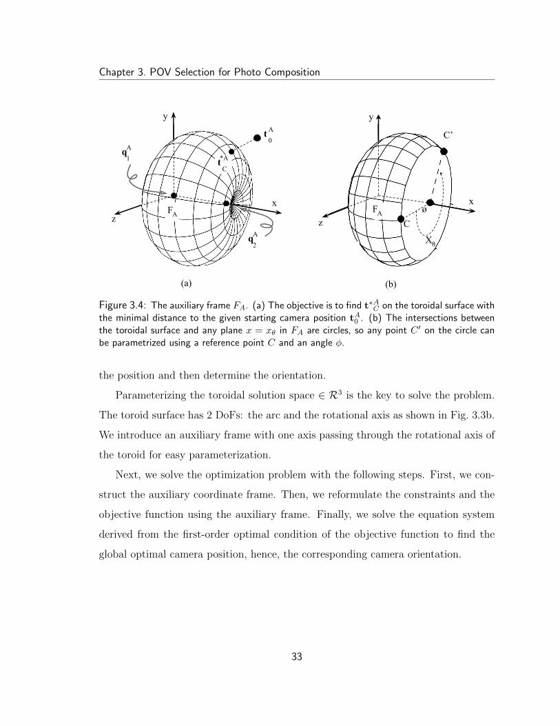
Chapter 3. POV Selection for Photo Composition
(a) (b)
q2A
z
y
x
t0A
x
y
zø
q1A
C’
C
Xθ
tC
*A
FAFA
Figure 3.4: The auxiliary frame FA. (a) The objective is to find t∗AC on the toroidal surface withthe minimal distance to the given starting camera position tA0 . (b) The intersections betweenthe toroidal surface and any plane x = xθ in FA are circles, so any point C ′ on the circle canbe parametrized using a reference point C and an angle φ.
the position and then determine the orientation.
Parameterizing the toroidal solution space ∈ R3 is the key to solve the problem.
The toroid surface has 2 DoFs: the arc and the rotational axis as shown in Fig. 3.3b.
We introduce an auxiliary frame with one axis passing through the rotational axis of
the toroid for easy parameterization.
Next, we solve the optimization problem with the following steps. First, we con-
struct the auxiliary coordinate frame. Then, we reformulate the constraints and the
objective function using the auxiliary frame. Finally, we solve the equation system
derived from the first-order optimal condition of the objective function to find the
global optimal camera position, hence, the corresponding camera orientation.
33
Chapter 3. POV Selection for Photo Composition
3.1.3.1 Constructing the Auxiliary Frame
We construct the auxiliary frame FA with one axis be the axis of rotation passing
through qW1 and qW2 as shown in Fig. 3.3. More specifically, qW1 coincides with the
origin of FA and qW2 sits on the positive x-axis of FA (Fig. 3.4a), i.e.,
qA1 =
0
0
0
, qA2 =
ξlen
0
0
, ξlen = ‖qW1 − qW2 ‖. (3.5)
Using the auxiliary frame, we manage to reformulate and solve the original prob-
lem in a simpler form, as shown later from Sec. 3.1.3.2 to Sec. 3.1.3.7.
Let RWA and tWA be the rotation matrix and translation vector from FA to FW ,
respectively. Then, tWA = qW1 , and the first column of RWA , c1
WA = (qW2 − qW1 )/ξlen.
The second and the third columns of RWA could be chosen as an arbitrary pair of
orthonormal vectors that span the null space of c1WA . In the case when RW
A is an
improper rotation matrix, i.e., det(RWA ) = −1, we swap the second and the third
columns of RWA .
3.1.3.2 Reformulating Equality Constraints
Now, we use the auxiliary frame FA to reformulate the equality constraints in Eq. (3.3a),
λjpCj = RC
A qAj + tCA, j = 1, 2, (3.6)
in which RCA and tCA are the unknown rotation matrix and translation vector from FA
to FC ,
RCA =
r11 r12 r13
r21 r22 r23
r31 r32 r33
, tCA =
t1
t2
t3
. (3.7)
34
Chapter 3. POV Selection for Photo Composition
Next, it is desirable to eliminate the depth factors as follows,
[pCj ]× (RCA qAj + tCA) = 03×1, j = 1, 2, (3.8)
where [pCj ]× is the skew-symmetric matrix for vector pCj . Eq. (3.8) produces six
equality constraints, and two of them are redundant. We transform the remaining
four equality constraints into a matrix form,
A w = 04×1, (3.9)
where
A =
0 0 0 0 −1 v1
0 0 0 1 0 −u10 −1 v2 0 −1/ξlen v2/ξlen
1 0 −u2 1/ξlen 0 −u2/ξlen
, w =
r11
r21
r31
t1
t2
t3
, (3.10)
in which r11, r21, r31, t1, t2 and t3 are the entries in RCA and tCA defined above. Note
that there is a constraint imposed on the first three entries, r11, r21 and r31, in w, as
they form the first column c1CA of RC
A, which means ‖c1CA‖ = 1.
The benefit of constructing FA shows up. Since qA1 and qA2 are constructed to have
only one non-zero entry, w is much simplified so that it does not contain the entries
in the second column c2CA and the third column c3
CA of RC
A. Otherwise, without FA,
w would contain all the 9 entries in a rotation matrix with more constraints imposed.
Next, we parameterize w. The vector w of unknowns belongs to the null space of
A. Since nullity(A) = 2 as rank(A) = 4 according to Eq. (3.10), w can be expressed
35
Chapter 3. POV Selection for Photo Composition
ρ1
ρ2
c1CA
||ρ ||1
ρ1
θ
ρ x ρ1 2
Figure 3.5: Parameterization of c1CA using θ.
as the following linear combination form,
w =[e1 e2
]α1
α2
, e1 =
u2
v2
1
0
0
0
, e2 =
u2 − u1v2 − v1
0
u1ξlen
v1ξlen
ξlen
, (3.11)
where α1 and α2 are two coefficients, e1 and e2 are the two eigenvectors of A corre-
sponding to the two null eigenvalues of A, which could be easily verified. Hence, c1CA
and tCA can be expressed as linear combinations as well,
c1CA =
[ρ1 ρ2
]α1
α2
, tCA =[τ 1 τ 2
]α1
α2
, (3.12)
in which ρ1 = pC2 , ρ2 = pC2 − pC1 , τ 1 = 03×1 and τ 2 = pC1 ξlen.
Now, c1CA and tCA are parameterized with two parameters, α1 and α2. Next, we
use the constraint, ‖c1CA‖ = 1, to reduce to a form using only one parameter. The
idea is depicted in Fig. 3.5. We observe that c1CA is a unit vector in the 2D plane
spanned by ρ1 and ρ2. Hence, it can be parameterized using a rotation angle θ. We
36
Chapter 3. POV Selection for Photo Composition
denote the matrix for a rotation by an angle of θ around ρ1 × ρ2 as Rθ. Hence,
c1CA = Rθρ1/‖ρ1‖, which contains θ as the only parameter. More explicitly,
c1CA = sin(θ)
ξ1
ξ2
ξ3
+ cos(θ)
ξ4
ξ5
ξ6
, (3.13)
in which ξk’s are constant, k = 1, 2, 3, 4, 5, 6, i.e.,
ξ1 =−u1 + u2 + u2v1v2 − u1v22
‖ρ1‖‖ρ1 × ρ2‖, ξ4 =
u2‖ρ1‖
,
ξ2 =−v1 + v2 + v2u1u2 − v1u22
‖ρ1‖‖ρ1 × ρ2‖, ξ5 =
v2‖ρ1‖
,
ξ3 =u1u2 + v1v2 − u22 − v22‖ρ1‖‖ρ1 × ρ2‖
, ξ6 =1
‖ρ1‖.
(3.14)
Since c1CA is a linear combination of ρ1 and ρ2 (Eq. (3.12)), we have
α1
α2
= S+ c1CA, (3.15)
in which S+ is the Moore-Penrose matrix inverse of [ρ1 ρ2]. Plugging Eq. (3.15) back
into Eq. (3.12), we parameterize tCA with θ as
tCA = sin(θ)‖ρ1‖
‖ρ1 × ρ2‖τ2. (3.16)
3.1.3.3 Reformulating Inequality Constraints
Similarly, we also reformulate the inequality constraints in Eq. (3.3b) using FA as
‖tAC − qAj ‖ ≥ εj, j = 1, 2, (3.17)
37
Chapter 3. POV Selection for Photo Composition
where tAC is the unknown translation vector from FC to FA,
tAC =
x
y
z
= −
(c1
CA)T
(c2CA)T
(c3CA)T
tCA, (3.18)
in which c1CA, c2
CA and c3
CA are respectively the first, second and third columns of RC
A
defined previously.
To obtain the boundary points that satisfy both the equality and inequality con-
straints, we use the parameterizations in Sec. 3.1.3.2 to parameterize x, y and z in
tAC respectively, as follows.
First, we can parameterize x with θ using the parameterizations of c1CA and tCA in
Eq. (3.13) and Eq. (3.16),
x = ξlen sin(θ)[sin(θ)− pC1 · pC2‖pC1 × pC2 ‖
cos(θ)], (3.19)
in which · and × denote the inner product and the cross product of two vectors
respectively. Let ω denote the angle between the two known vectors pC1 and pC2 ,
which corresponds to ∠P1CP2 as shown in Fig. 3.3. Since pC1 · pC2 = ‖pC1 ‖‖pC2 ‖ cos(ω)
and ‖pC1 × pC2 ‖ = ‖pC1 ‖‖pC2 ‖ sin(ω), we can simplify x as
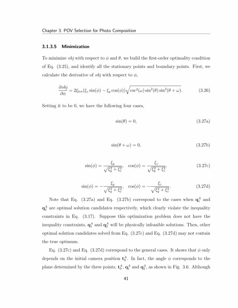
x = ξlen sin(θ)[sin(θ)− cot(ω) cos(θ)] = −ξlen csc(ω) sin(θ) cos(θ + ω). (3.20)
Next, we parameterize y and z. Since ‖tAC‖ = ‖tCA‖, we have
y2 + z2 = ‖tCA‖2 − x2 = ξ2len csc2(ω) sin2(θ) sin2(ω + θ). (3.21)
The benefit of constructing FA shows up, again. Eq. (3.20) and Eq. (3.21) show
38
Chapter 3. POV Selection for Photo Composition
that both x and y2 + z2 are functions of θ. In other words, a fixed θ determines a
plane in FA with a fixed x value, and the points on that plane forms a circle with
a fixed radius√y2 + z2, which is depicted in Fig. 3.4b. Hence, we introduce a new
parameter φ for the angle of rotation around the x-axis of FA, so that
y = sin(φ)ξlen
√csc2(ω) sin2(θ) sin2(ω + θ),
z = cos(φ)ξlen
√csc2(ω) sin2(θ) sin2(ω + θ).
(3.22)
Finally, plugging Eq. (3.20) and Eq. (3.22) back into Eq. (3.17), we obtain two
equations for the boundary
sin(θ) = ± sin(ω)ε1/ξlen, (3.23a)
sin(θ + ω) = ± sin(ω)ε2/ξlen, (3.23b)
from which we can solve for eight possible pairs of sin(θ) and cos(θ) corresponding to
eight solutions of θ.
In fact, the parameterization of y2 + z2 in Eq. (3.21) suffices our need to parame-
terize the boundary points. Nevertheless, the individual parameterization of y and z
is useful below in Sec. 3.1.3.4.
3.1.3.4 Reformulating the Objective Function
At last, we reformulate the objective function in Eq. (3.2) using FA as well,
argminRW
C ,tWC
‖tAC − tA0 ‖2
(3.24)
39
Chapter 3. POV Selection for Photo Composition
C12
q1A
t0A
q2Az
y
xø
C11
C21
C22
C’11
C’21
C’12
C’22
FA
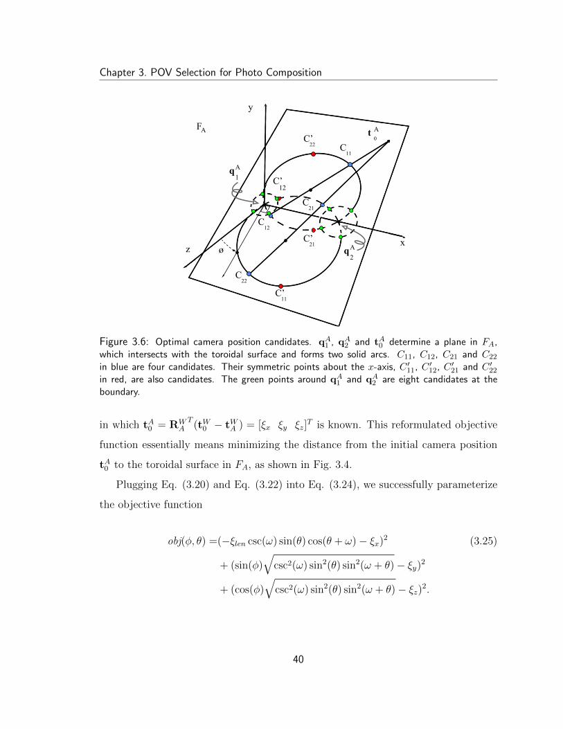
Figure 3.6: Optimal camera position candidates. qA1 , qA2 and tA0 determine a plane in FA,which intersects with the toroidal surface and forms two solid arcs. C11, C12, C21 and C22
in blue are four candidates. Their symmetric points about the x-axis, C ′11, C ′12, C ′21 and C ′22in red, are also candidates. The green points around qA1 and qA2 are eight candidates at theboundary.
in which tA0 = RWAT
(tW0 − tWA ) = [ξx ξy ξz]T is known. This reformulated objective
function essentially means minimizing the distance from the initial camera position
tA0 to the toroidal surface in FA, as shown in Fig. 3.4.
Plugging Eq. (3.20) and Eq. (3.22) into Eq. (3.24), we successfully parameterize
the objective function
obj(φ, θ) =(−ξlen csc(ω) sin(θ) cos(θ + ω)− ξx)2 (3.25)
+ (sin(φ)√
csc2(ω) sin2(θ) sin2(ω + θ)− ξy)2
+ (cos(φ)√
csc2(ω) sin2(θ) sin2(ω + θ)− ξz)2.
40
Chapter 3. POV Selection for Photo Composition
3.1.3.5 Minimization
To minimize obj with respect to φ and θ, we build the first-order optimality condition
of Eq. (3.25), and identify all the stationary points and boundary points. First, we
calculate the derivative of obj with respect to φ,
∂obj
∂φ= 2ξlen(ξz sin(φ)− ξy cos(φ))
√csc2(ω) sin2(θ) sin2(θ + ω). (3.26)
Setting it to be 0, we have the following four cases,
sin(θ) = 0, (3.27a)
sin(θ + ω) = 0, (3.27b)
sin(φ) =ξy√ξ2y + ξ2z
, cos(φ) =ξz√ξ2y + ξ2z
. (3.27c)
sin(φ) = − ξy√ξ2y + ξ2z
, cos(φ) = − ξz√ξ2y + ξ2z
. (3.27d)
Note that Eq. (3.27a) and Eq. (3.27b) correspond to the cases when qA1 and
qA2 are optimal solution candidates respectively, which clearly violate the inequality
constraints in Eq. (3.17). Suppose this optimization problem does not have the
inequality constraints, qA1 and qA2 will be physically infeasible solutions. Then, other
optimal solution candidates solved from Eq. (3.27c) and Eq. (3.27d) may not contain
the true optimum.
Eq. (3.27c) and Eq. (3.27d) correspond to the general cases. It shows that φ only
depends on the initial camera position tA0 . In fact, the angle φ corresponds to the
plane determined by the three points, tA0 , qA1 and qA2 , as shown in Fig. 3.6. Although
41
Chapter 3. POV Selection for Photo Composition
two solutions of φ can be solved from Eq. (3.27c) and Eq. (3.27d), they differ from
each other by π, which essentially correspond to the same plane. Therefore, the
optimal camera position sits on the plane determined by tA0 , qA1 and qA2 .
Next, we substitute the two solutions of φ from Eq. (3.27c) and Eq. (3.27d) into
the derivative of obj with respect to θ, and obtain the following two cases.
∂obj
∂θ=ξlen csc2(ω)
2E1
(E1E2 + E3E4), (3.28a)
∂obj
∂θ=ξlen csc2(ω)
2E1
(E1E2 − E3E4), (3.28b)
where
E1 =√
csc2(ω) sin2(θ) sin2(θ + ω),
E2 = 2ξx sin(2θ + 2ω) + 2(ξlen − ξx) sin(2θ),
E3 =√ξ2y + ξ2z ,
E4 = sin(4θ + 2ω)− sin(2θ + 2ω)− sin(2θ).
(3.29)
E1 can be further simplified by removing the square root with two cases,
E1 = ± csc(ω) sin(θ) sin(θ + ω). (3.30)
Setting Eq. (3.28a) and Eq. (3.28b) to be 0, we obtain four equations, among
which two are duplicates, therefore, redundant. The remaining two cases can be
further simplified to
sin(2θ)ξ7 + cos(2θ)ξ8 = 0, (3.31a)
sin(2θ)ξ9 + cos(2θ)ξ10 = 0, (3.31b)
42
Chapter 3. POV Selection for Photo Composition
where ξk’s are constant, k = 7, 8, 9, 10, i.e.,
ξ7 = cos(2ω)ξx − sin(2ω)√ξ2y + ξ2z − ξx + ξlen,
ξ8 = sin(2ω)ξx + cos(2ω)√ξ2y + ξ2z −
√ξ2y + ξ2z ,
ξ9 = cos(2ω)ξx + sin(2ω)√ξ2y + ξ2z − ξx + ξlen,
ξ10 = sin(2ω)ξx − cos(2ω)√ξ2y + ξ2z +
√ξ2y + ξ2z .
(3.32)
Using Eq. (3.31), we can easily solve for eight possible pairs of sin(θ) and cos(θ)
corresponding to eight general solutions of θ. Fig. 3.6 depicts the geometric meanings
of the eight general solutions.
3.1.3.6 Identifying the Best Camera Position
Plugging sin(φ), cos(φ), sin(θ) and cos(θ) solved from Eq. (3.27c), Eq. (3.27d), Eq.
(3.23) and Eq. (3.31) back into Eq. (3.20) and Eq. (3.22), we can get eight solutions
at the boundary and eight general solutions of tAC as illustrated in Fig. 3.6. We apply
three steps to identify the best camera position in FW . First, we use the property of
∠pA1 tACp
A2 = ω (Fig. 3.3) and the inequality constraints to eliminate the infeasible
solutions. Second, among the feasible solutions, we pick t∗AC , the one with the shortest
distance to tA0 . Finally, we compute the best camera position t∗WC in FW , using RWA
and tWA constructed in Sec. 3.1.3.1.
3.1.3.7 Determining the Camera Orientation
The optimal orientation is uniquely determined. In Fig. 3.3, the lengths of the line
segments CP1 and CP2 are both fixed, so the optimal camera position t∗WC determines
two more points in FW . It is then easy and standard to retrieve the optimal camera
orientation R∗WC using these three known points [Umeyama, 1991].
43
Chapter 3. POV Selection for Photo Composition
3.1.3.8 Analyzing the Closed-Form Solution
At the end of this subsection, we briefly discuss the issues related to multiple optimal
solutions and the change in the flying distance caused by noisy inputs.
There are three special cases with multiple optima. First, when the two object
projections coincide with each other, i.e., ω = 0, csc(ω) in Eq. (3.20) is undefined.
Then, x can be any arbitrary value and y = z = 0. This corresponds to the cases
that the optimal camera positions are aligned with the two objects. Second, when
the initial camera position is aligned with the two objects, i.e., ξy = ξz = 0, sin(φ)
and cos(φ) in Eq. (3.27c) and Eq. (3.27d) are undefined. Then, φ can be any
arbitrary value. The optimal camera positions form a circle. Third, when the initial
camera position coincides with some point like O in Fig. 3.3, i.e., ξx = ξlen/2 and
‖tCA‖ = csc(ω)ξlen/2. Then, solving Eq. (3.31) may yield infinitely many solutions of
θ, which correspond to all the points on the solid arc in Fig. 3.3.
Using Fig. 3.6, we can intuitively see how the flying distance is affected after
perturbing the inputs. There are three cases. First, if tA0 stays outside the toroid be-
fore and after perturbing the inputs, the toroid’s shape and size are not substantially
changed, so that the flying distance does not change much either. Second, if tA0 stays
inside the toroid before and after perturbing, the flying distance is upper bounded
by the toroid size, so that the flying distance is also stable. Third, if tA0 crosses the
toroid surface because of the perturbation, the flying distance is small hence stable.
The next section presents the empirical results of using noisy inputs.
3.1.4 Evaluation
Though the closed-form solution is optimal, we are interested in its applicability and
robustness in real photo-taking scenarios, which contain both inaccurate human in-
puts caused by e.g., fat-finger errors [Siek et al., 2005] and imperfect robot executions.
44
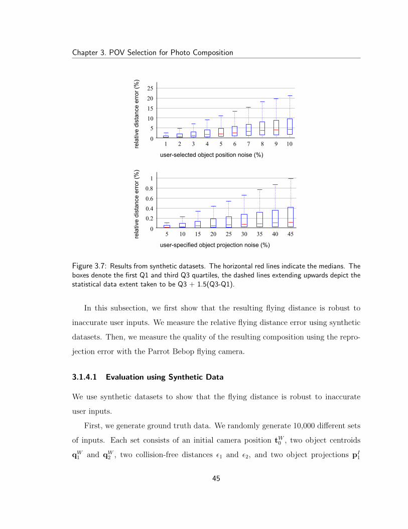
Chapter 3. POV Selection for Photo Composition
25
20
15
105
0re
lativ
e di
stan
ce e
rror
(%)
1 2 3 4 5 6 7 8 9
user-selected object position noise (%)
10
1
0.8
0.6
0.40.2
05 10 15 20 25 30 35 40 45
user-specified object projection noise (%)
rela
tive
dist
ance
err
or (%
)
Figure 3.7: Results from synthetic datasets. The horizontal red lines indicate the medians. Theboxes denote the first Q1 and third Q3 quartiles, the dashed lines extending upwards depict thestatistical data extent taken to be Q3 + 1.5(Q3-Q1).
In this subsection, we first show that the resulting flying distance is robust to
inaccurate user inputs. We measure the relative flying distance error using synthetic
datasets. Then, we measure the quality of the resulting composition using the repro-
jection error with the Parrot Bebop flying camera.
3.1.4.1 Evaluation using Synthetic Data
We use synthetic datasets to show that the flying distance is robust to inaccurate
user inputs.
First, we generate ground truth data. We randomly generate 10,000 different sets
of inputs. Each set consists of an initial camera position tW0 , two object centroids
qW1 and qW2 , two collision-free distances ε1 and ε2, and two object projections pI1
45
Chapter 3. POV Selection for Photo Composition
and pI2 on the image plane. The image size is 1920 × 1080. tW0 , qW1 and qW2 are
uniformly drawn from a unit cube [0, 1]3. ε1 and ε2 are uniformly generated so that
ε1 + ε2 ≤ ‖qW1 − qW2 ‖. pI1 and pI2 are uniformly drawn within the image size.
Then, we consider two types of noise introduced by inaccurate user inputs.
Noisy User-Selected Object Positions During object selection, the object positions
may be inaccurately estimated. We corrupt qW1 and qW2 with noise that follows a
uniform distribution around the original object centroids. The noise ranges from 1%
to 10% of their original relative distances in 3D.
Noisy User-Specified Object Projections During direct manipulation, the object
projections may not be specified accurately as in one’s mind. We corrupt pI1 and pI2
with noise that follows a uniform distribution around the original object projections.
The noise ranges from 5% to 45% of their original relative distances on the image to
ensure non-overlapping sampling regions.
Measurement We measure the relative flying distance error denoted as
Errordist(%) =|dnoisefree − dnoisy|‖qW1 − qW2 ‖
, (3.33)
in which dnoisefree = ‖tW0 − tnoisefreeWC ‖ is the distance from the initial camera position
tW0 to the optimized final position tnoisefreeWC based on noise-free user inputs, dnoisy =
‖tW0 − tnoisyWC ‖ is the distance from tW0 to the optimized position tnoisy
WC based on
corrupted user inputs, and ‖qW1 − qW2 ‖ indicates the scale of the environment.
Fig. 3.7 shows that the flying distance solved using our method is robust to very
noisy user inputs in both cases.
46
Chapter 3. POV Selection for Photo Composition
3.1.4.2 Evaluation with Parrot Bebop
To show our closed-form solution is applicable in real flying camera photography, we
evaluate it on the Parrot Bebop drone whose camera resolution is 1280 × 720. Please
refer to Sec. 5.1 for a detailed system hardware and software setup.
Robot Trajectory Execution Here, we highlight the necessary system components
to reach the computed POV with the Parrot Bebop drone.
The 6 DoFs camera pose is estimated using ORB-SLAM [Mur-Artal et al., 2015]
without other external sensors. However, the drone driver [AutonomyLab, 2018] only
supports 5 DoFs camera control. We enable the 6th DoF by rotating the image plane,
so that the effective image area becomes a circular area at the center of the image,
as in Fig. 3.9. Due to the hardware constraint, the pan-tilt range is also limited, so
that some viewpoints are not achievable.
The camera flying trajectory is modeled as a straight line connecting the initial
camera position to the goal position, by assuming the environment to be free of major
obstruction for flying. The camera orientation is computed based on its position at
that moment, in order to minimize the composition error Eq. (3.1) at all times.
To execute the flying trajectory, each DoF of the camera is controlled by an
independent PID controller. The control gains are fine-tuned by assuming that the
SLAM map is in the metric unit. To resolve the scale ambiguity of the SLAM map, we
adopt a scale estimation method using the onboard ultrasonic altitude measurement
[Engel et al., 2014b].
In practice, the goal camera viewpoint can never be achieved. A viewpoint is
considered as successful, if it satisfies all the following conditions. The camera position
error is below 0.5 meter. The orientation error is below 1 degree. All control signals
at that moment are below certain thresholds as well.
47

Chapter 3. POV Selection for Photo Composition
25
20
15
10
5
0
frequ
ency
(%)
reprojection error (%)0 0.5 1.0 1.5 2.0 2.5 3.0 3.5 4.0 4.5 5.0 5.5 6.0
Figure 3.8: Results from real robot experiments.
Data Collection The experiments are conducted in an indoor environment of size
8m× 6m× 2.5m. We use two distinctive colored balls of diameter 10cm to represent
two objects of interest. We place the two balls at fixed locations in the center area of
the room. Their distance is 1.5 meter from each other.
We collect data from 50 trials. After building a SLAM map, we place the camera
at the locations of the two balls to record their positions qW1 and qW2 in the SLAM
map. Since the objects in real photo-taking scenarios have various shapes, we are
not interested in the accuracy of object centroid estimation. We set the collision-free
distances ε1 and ε2 to be 0.5m and 0.8m respectively.
For each trial, we randomly generate tW0 within the environment. We also ran-
domly generate pI1 and pI2 that are uniformly drawn from the circular area of diameter
700 pixels at the center of the image. We collect 30 frames at the successful view-
points from each trial. We reject the unreachable viewpoints that are outside the
environment or beyond the camera pan-tilt range limits.
Measurement We measure the composition error using the reprojection error on
each collected frame. For each frame, we exact the centroid pixel pexactedIj for each
ball j, and measure the distance to its corresponding desired composition, ej =
‖pexactedIj − pIj‖. Hence, the reprojection error of a frame with respect to the im-
48
Chapter 3. POV Selection for Photo Composition
age size is Errorreproj(%) = (e1 + e2)/(2× 720).
The histogram in Fig. 3.8 shows the distribution of reprojection errors. Over-
all, the reprojection errors are relatively small, under very challenging conditions,
including imperfect controls, SLAM system errors, etc.
3.1.4.3 Viewpoint Changing Process
We illustrate the viewpoint changing process while composing two objects using a
concrete scenario. As shown in Fig. 3.9, the scenario starts from a high-angle view-
point. The two main parts of the sculpture are selected as the objects of interest.
We build the SLAM map, and record the estimated object positions. We manually
specify the desired compositions for the objects in order to emulate the end points of
direct manipulation gestures.
The viewpoint changes in two steps. First, it quickly changes the orientation to
compose one object, since changing orientation is much faster than flying. Gradually,
the other object converges to the desired composition while the camera is moving
towards the goal. This phenomenon is caused by the fact that the orientation is
recomputed based on the camera position at that time in order to minimize the
reprojection error.
3.1.5 Discussion
The evaluation results show that our closed-form solution to the formulated opti-
mization problem is applicable to real flying robot systems. Our problem focuses
on a subset of aspects that are important to flying camera photography, including
minimizing the flying distance, and avoiding collisions with objects of interest. We
believe the formation could be generalized to include other aspects as well, such as
stabilizing the frame by removing one DoF from rotation, or collision-free flying by
49
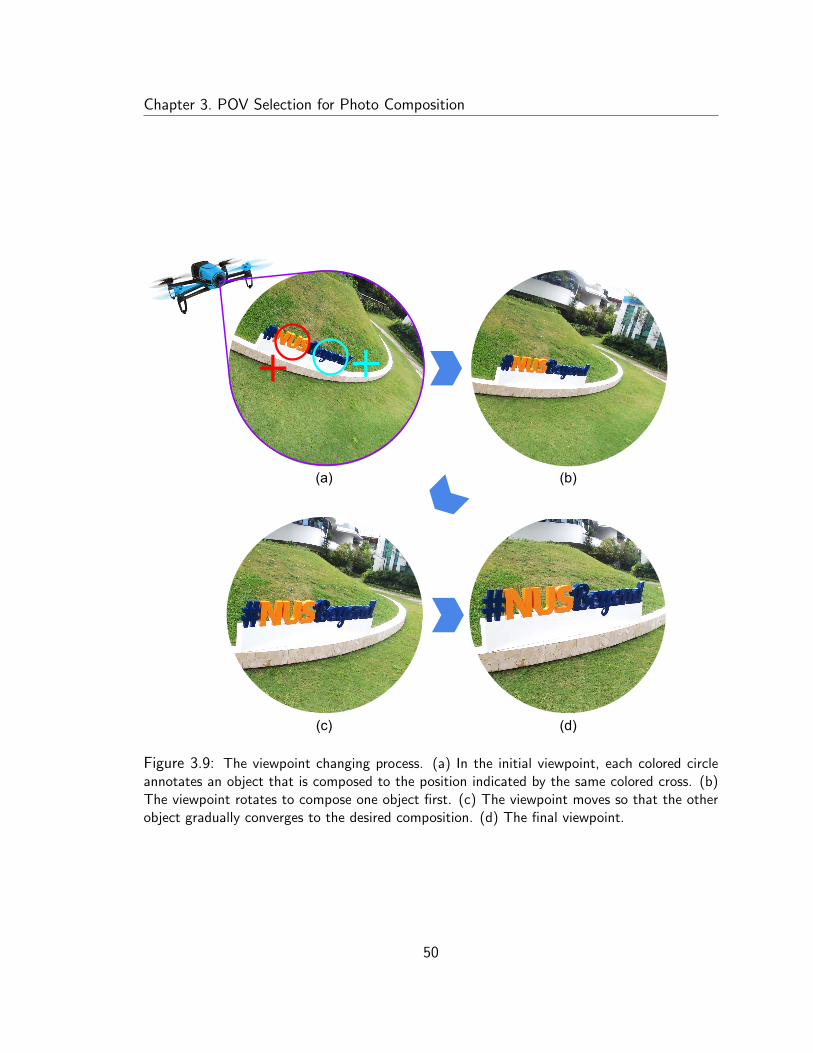
Chapter 3. POV Selection for Photo Composition
(a) (b)
(c) (d)
Figure 3.9: The viewpoint changing process. (a) In the initial viewpoint, each colored circleannotates an object that is composed to the position indicated by the same colored cross. (b)The viewpoint rotates to compose one object first. (c) The viewpoint moves so that the otherobject gradually converges to the desired composition. (d) The final viewpoint.
50
Chapter 3. POV Selection for Photo Composition
adding constraints for obstacles in the environments.
In addition to the two objects composition problem studied in this section, we
describe a method for three or more objects in the next section.
3.2 Three or More Objects Composition
To compose multiple objects, we propose a sample-based method that solves the
problem with an approximate POV, which is easy to implement, and can be applied
to solve two objects composition problem as well.
The idea is to sample multiple candidate POVs and pick the best one. How-
ever, the space of POVs is very large. To achieve real-time performance, we reduce
the sampling space by decoupling the camera position and the camera orientation.
We only sample camera positions, and at each sampled camera position we find an
approximately optimal orientation. The details are described below.
First, the method samples many camera positions as candidates around the cur-
rent POV. Those camera positions are sampled unevenly: it is denser near the current
POV and sparser further away (with an upper bound). This sampling strategy is to
increase the chance of finding good nearby POVs in order to minimize the potential
flying distance. Second, the candidate orientation at each candidate position is es-
timated by averaging multiple orientations. Each is the optimal orientation at that
candidate position for one object. At last, the candidate POV with the minimum
composition error is returned.
The POV found by this sampled-based method is an approximate solution that
may not be globally optimal. However, since the dragging gestures are imprecise touch
inputs after all, it is unnecessary to over-interpret those gestures very accurately.
51
Chapter 3. POV Selection for Photo Composition
3.3 Summary
We investigated the underlying POV search problem for composing multiple objects
of interest. Sec. 3.1 solved the P2P problem for composing two objects of interest.
To the best of our knowledge, it is the first study that determines the camera param-
eters given an under-constrained system. By incorporating the user’s composition
requirements and minimizing the camera’s flying distance, we formed a constrained
nonlinear optimization problem, solved it in closed form, and evaluated the applica-
bility in real flying camera systems. Sec. 3.2 proposed a general sample-based method
to solve the multiple objects composition problem. In system evaluation (Chap. 6),
we implement this method to evaluate the explore-and-compose paradigm proposed
in Sec. 2.1.2.
In this chapter, the proposed methods assume that the intended POV can be
achieved safely without colliding with obstacles. Next, we study the depth perception
problem for collision avoidance with a monocular camera in the following chapter.
52
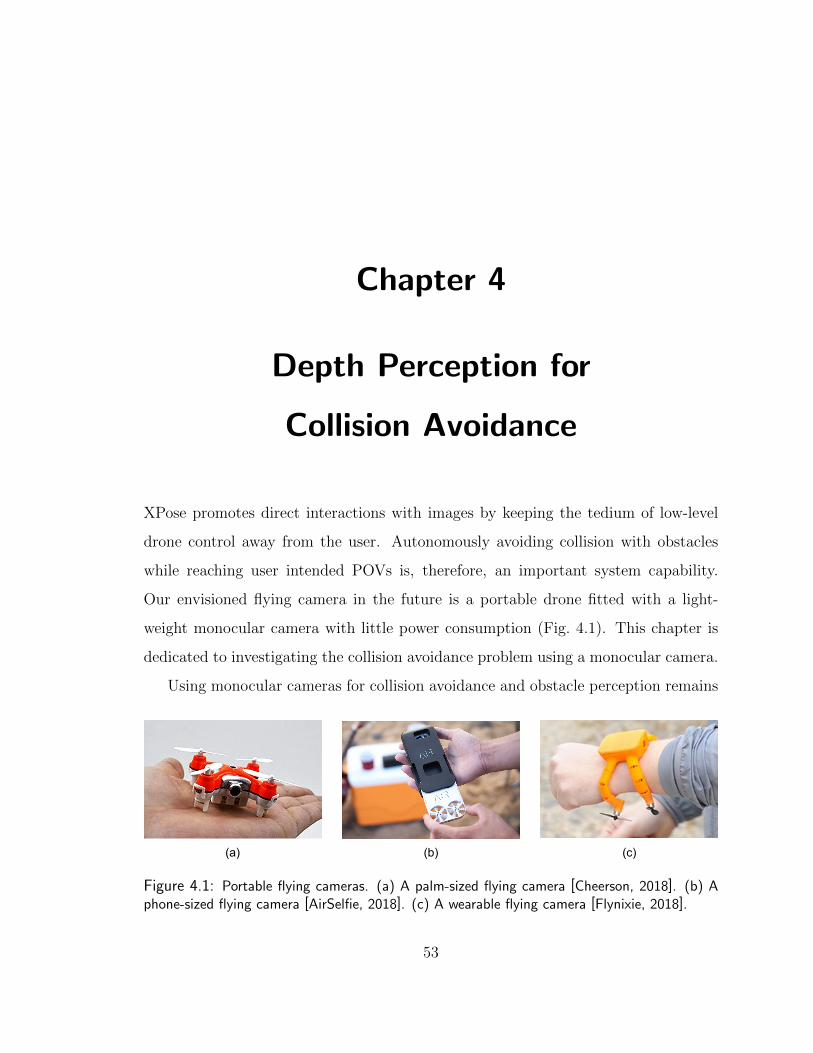
Chapter 4
Depth Perception for
Collision Avoidance
XPose promotes direct interactions with images by keeping the tedium of low-level
drone control away from the user. Autonomously avoiding collision with obstacles
while reaching user intended POVs is, therefore, an important system capability.
Our envisioned flying camera in the future is a portable drone fitted with a light-
weight monocular camera with little power consumption (Fig. 4.1). This chapter is
dedicated to investigating the collision avoidance problem using a monocular camera.
Using monocular cameras for collision avoidance and obstacle perception remains
(a) (b) (c)
Figure 4.1: Portable flying cameras. (a) A palm-sized flying camera [Cheerson, 2018]. (b) Aphone-sized flying camera [AirSelfie, 2018]. (c) A wearable flying camera [Flynixie, 2018].
53
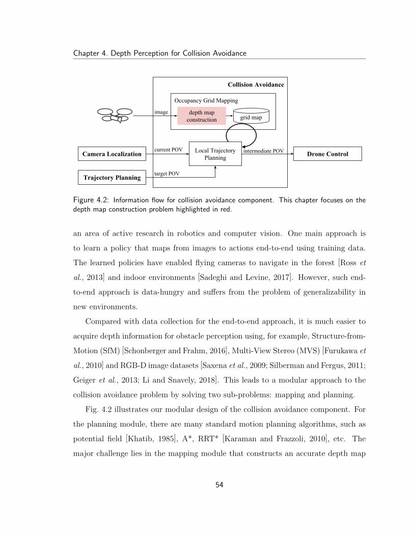
Chapter 4. Depth Perception for Collision Avoidance
Collision Avoidance
Drone ControlCamera Localizationcurrent POV
image
Trajectory Planning
intermediate POV
target POV
Local Trajectory Planning
Occupancy Grid Mapping
grid mapdepth map
construction
Figure 4.2: Information flow for collision avoidance component. This chapter focuses on thedepth map construction problem highlighted in red.
an area of active research in robotics and computer vision. One main approach is
to learn a policy that maps from images to actions end-to-end using training data.
The learned policies have enabled flying cameras to navigate in the forest [Ross et
al., 2013] and indoor environments [Sadeghi and Levine, 2017]. However, such end-
to-end approach is data-hungry and suffers from the problem of generalizability in
new environments.
Compared with data collection for the end-to-end approach, it is much easier to
acquire depth information for obstacle perception using, for example, Structure-from-
Motion (SfM) [Schonberger and Frahm, 2016], Multi-View Stereo (MVS) [Furukawa et
al., 2010] and RGB-D image datasets [Saxena et al., 2009; Silberman and Fergus, 2011;
Geiger et al., 2013; Li and Snavely, 2018]. This leads to a modular approach to the
collision avoidance problem by solving two sub-problems: mapping and planning.
Fig. 4.2 illustrates our modular design of the collision avoidance component. For
the planning module, there are many standard motion planning algorithms, such as
potential field [Khatib, 1985], A*, RRT* [Karaman and Frazzoli, 2010], etc. The
major challenge lies in the mapping module that constructs an accurate depth map
54
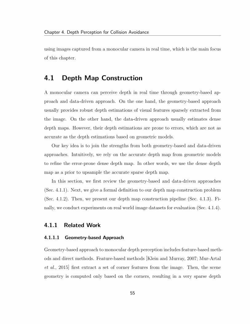
Chapter 4. Depth Perception for Collision Avoidance
using images captured from a monocular camera in real time, which is the main focus
of this chapter.
4.1 Depth Map Construction
A monocular camera can perceive depth in real time through geometry-based ap-
proach and data-driven approach. On the one hand, the geometry-based approach
usually provides robust depth estimations of visual features sparsely extracted from
the image. On the other hand, the data-driven approach usually estimates dense
depth maps. However, their depth estimations are prone to errors, which are not as
accurate as the depth estimations based on geometric models.
Our key idea is to join the strengths from both geometry-based and data-driven
approaches. Intuitively, we rely on the accurate depth map from geometric models
to refine the error-prone dense depth map. In other words, we use the dense depth
map as a prior to upsample the accurate sparse depth map.
In this section, we first review the geometry-based and data-driven approaches
(Sec. 4.1.1). Next, we give a formal definition to our depth map construction problem
(Sec. 4.1.2). Then, we present our depth map construction pipeline (Sec. 4.1.3). Fi-
nally, we conduct experiments on real world image datasets for evaluation (Sec. 4.1.4).
4.1.1 Related Work
4.1.1.1 Geometry-based Approach
Geometry-based approach to monocular depth perception includes feature-based meth-
ods and direct methods. Feature-based methods [Klein and Murray, 2007; Mur-Artal
et al., 2015] first extract a set of corner features from the image. Then, the scene
geometry is computed only based on the corners, resulting in a very sparse depth
55
Chapter 4. Depth Perception for Collision Avoidance
map. By contrast, direct methods do not extract features. They optimize the scene
geometry based on the image intensity changes over consecutive frames. In addition
to corners, edges from the image may also have robust depth estimations, resulting
a semi-dense depth map [Forster et al., 2014; Engel et al., 2014a]. Dense mapping
with direct methods has also been studied [Newcombe et al., 2011], but in small-scale
environments.
A recent method, FLaME [Nicholas Greene and Roy, 2017], combines feature-
based and direct methods to construct dense 3D depth maps for flying robot navi-
gation. The idea is to extract point features uniformly from the image and estimate
their depths using direct search along the epipolar lines. Finally, the sparse depth
map is densified by smoothly propagating the sparse information out using a De-
launay triangulation on the image plane. This method was implemented on a flying
drone for collision avoidance. However, the method relies on very accurate camera
poses and high-quality image streams, which cannot be reliably acquired for low-cost
commercial drones, such as Parrot Bebop drones. In our system implementation, we
use ORB-SLAM [Mur-Artal et al., 2015] to construct a sparse depth map due to its
robustness in practice. Inspired by FLaME, we perform Delaunay triangulation to
propagate the sparse information.
4.1.1.2 Data-driven Approach
Monocular depth estimation can also be data-driven, i.e., learned from training data.
There is a large body of work that focuses on supervised learning methods [Liu et
al., 2014; Eigen and Fergus, 2015; Li et al., 2015; Liu et al., 2015; Laina et al., 2016;
Xu et al., 2017], which learns a mapping from monocular images to their depth maps.
By contrast, unsupervised learning methods do not need ground truth depth images
[Godard et al., 2017; Zhou et al., 2017]. Instead, stereo images are used. Deep neural
networks are trained to synthesis disparity maps for reconstructing stereo images.
56
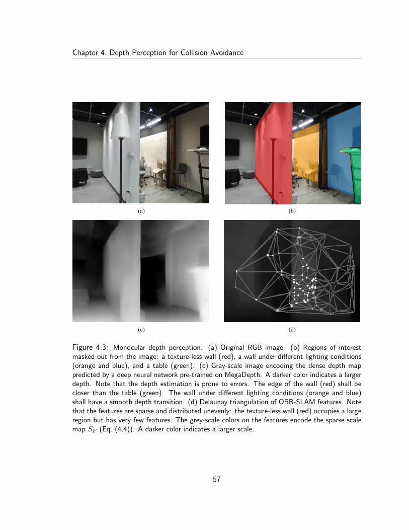
Chapter 4. Depth Perception for Collision Avoidance
(d)(c)
(b)(a)
Figure 4.3: Monocular depth perception. (a) Original RGB image. (b) Regions of interestmasked out from the image: a texture-less wall (red), a wall under different lighting conditions(orange and blue), and a table (green). (c) Gray-scale image encoding the dense depth mappredicted by a deep neural network pre-trained on MegaDepth. A darker color indicates a largerdepth. Note that the depth estimation is prone to errors. The edge of the wall (red) shall becloser than the table (green). The wall under different lighting conditions (orange and blue)shall have a smooth depth transition. (d) Delaunay triangulation of ORB-SLAM features. Notethat the features are sparse and distributed unevenly: the texture-less wall (red) occupies a largeregion but has very few features. The grey-scale colors on the features encode the sparse scalemap SF (Eq. (4.4)). A darker color indicates a larger scale.
57
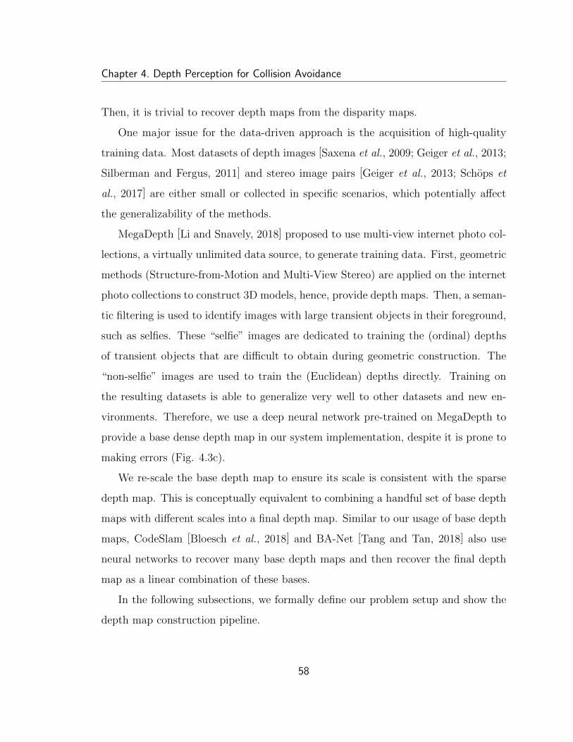
Chapter 4. Depth Perception for Collision Avoidance
Then, it is trivial to recover depth maps from the disparity maps.
One major issue for the data-driven approach is the acquisition of high-quality
training data. Most datasets of depth images [Saxena et al., 2009; Geiger et al., 2013;
Silberman and Fergus, 2011] and stereo image pairs [Geiger et al., 2013; Schops et
al., 2017] are either small or collected in specific scenarios, which potentially affect
the generalizability of the methods.
MegaDepth [Li and Snavely, 2018] proposed to use multi-view internet photo col-
lections, a virtually unlimited data source, to generate training data. First, geometric
methods (Structure-from-Motion and Multi-View Stereo) are applied on the internet
photo collections to construct 3D models, hence, provide depth maps. Then, a seman-
tic filtering is used to identify images with large transient objects in their foreground,
such as selfies. These “selfie” images are dedicated to training the (ordinal) depths
of transient objects that are difficult to obtain during geometric construction. The
“non-selfie” images are used to train the (Euclidean) depths directly. Training on
the resulting datasets is able to generalize very well to other datasets and new en-
vironments. Therefore, we use a deep neural network pre-trained on MegaDepth to
provide a base dense depth map in our system implementation, despite it is prone to
making errors (Fig. 4.3c).
We re-scale the base depth map to ensure its scale is consistent with the sparse
depth map. This is conceptually equivalent to combining a handful set of base depth
maps with different scales into a final depth map. Similar to our usage of base depth
maps, CodeSlam [Bloesch et al., 2018] and BA-Net [Tang and Tan, 2018] also use
neural networks to recover many base depth maps and then recover the final depth
map as a linear combination of these bases.
In the following subsections, we formally define our problem setup and show the
depth map construction pipeline.
58
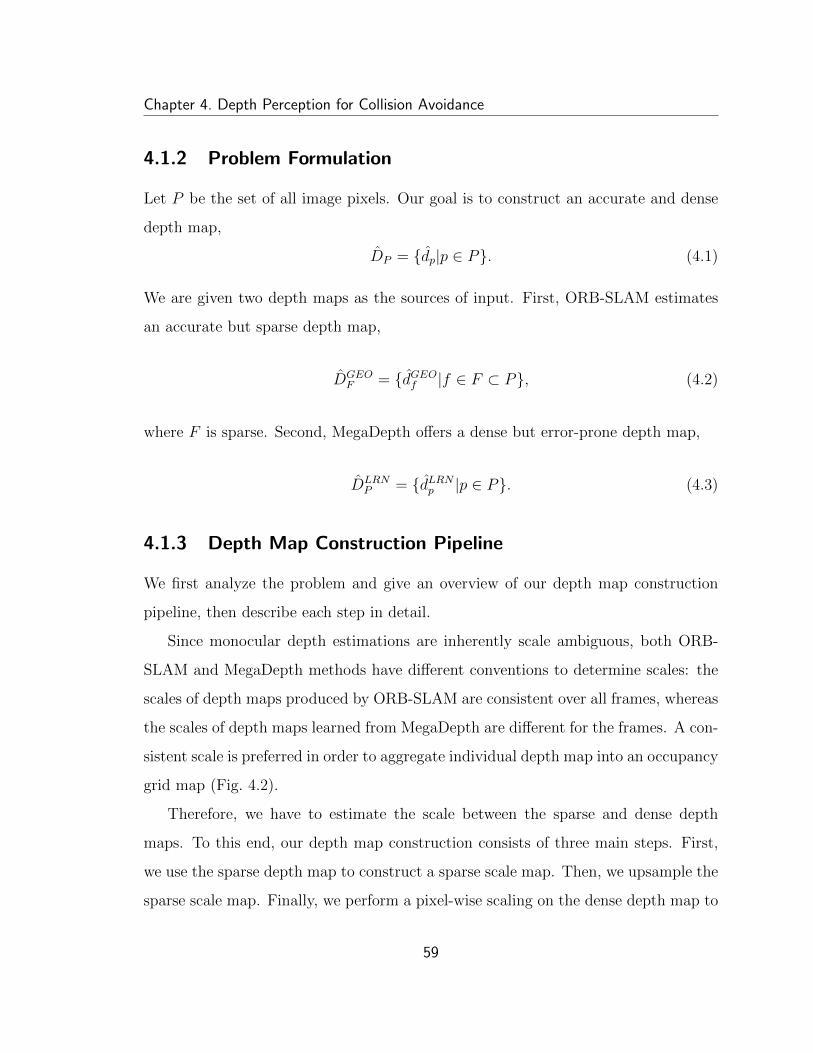
Chapter 4. Depth Perception for Collision Avoidance
4.1.2 Problem Formulation
Let P be the set of all image pixels. Our goal is to construct an accurate and dense
depth map,
DP = {dp|p ∈ P}. (4.1)
We are given two depth maps as the sources of input. First, ORB-SLAM estimates
an accurate but sparse depth map,
DGEOF = {dGEOf |f ∈ F ⊂ P}, (4.2)
where F is sparse. Second, MegaDepth offers a dense but error-prone depth map,
DLRNP = {dLRNp |p ∈ P}. (4.3)
4.1.3 Depth Map Construction Pipeline
We first analyze the problem and give an overview of our depth map construction
pipeline, then describe each step in detail.
Since monocular depth estimations are inherently scale ambiguous, both ORB-
SLAM and MegaDepth methods have different conventions to determine scales: the
scales of depth maps produced by ORB-SLAM are consistent over all frames, whereas
the scales of depth maps learned from MegaDepth are different for the frames. A con-
sistent scale is preferred in order to aggregate individual depth map into an occupancy
grid map (Fig. 4.2).
Therefore, we have to estimate the scale between the sparse and dense depth
maps. To this end, our depth map construction consists of three main steps. First,
we use the sparse depth map to construct a sparse scale map. Then, we upsample the
sparse scale map. Finally, we perform a pixel-wise scaling on the dense depth map to
59
Chapter 4. Depth Perception for Collision Avoidance
obtain our desired dense depth map.
4.1.3.1 Sparse Scale Map Construction
With a sparse depth map DGEOF and a dense depth map DLRN
F , we first compute a
sparse scale map SF ,
SF = {sf =dGEOf
dLRNf
|f ∈ F ⊂ P}. (4.4)
In practice, DGEOF contains outliers, so that SF is contaminated with outliers as
well. In the ideal case, however, all sf ’s shall be the same. This is a useful prior
to prune those outliers. It is convenient to use the interquartile range (IQR) rule to
identify outliers that are far away from the median.
However, since the sparse set of features is not uniformly distributed in general
(Fig. 4.3d), features in the dense region dominate the overall distribution. Hence,
instead of applying the IQR rule globally on the whole set of SF , we apply it on a
local neighborhood set Neighbors(f) of each feature f .
There are two popular choices of neighborhood sets: features within some fixed
distance and k-nearest-neighbors. However, they are also not suitable when the fea-
tures are not uniformly distributed: neighbors from the dense region dominate again.
We define a neighborhood set based on the Delaunay triangulation of F . More
specifically, Neighbors(f) is defined as the set of vertices such that they belong to the
distance-1 or distance-2 neighborhood of vertex f on the triangulation. Our definition
of neighborhood ensures the neighbors are distributed around vertex f . Fig. 4.3d is
an example of the sparse scale map after outliers removed.
4.1.3.2 Dense Scale Map Construction
For each image pixel p ∈ P\F , we find a set of nearby vertices {pi} that enclose p in
the triangulation as shown in Fig. 4.5. Its estimated scale sp is a weighted sum of
60
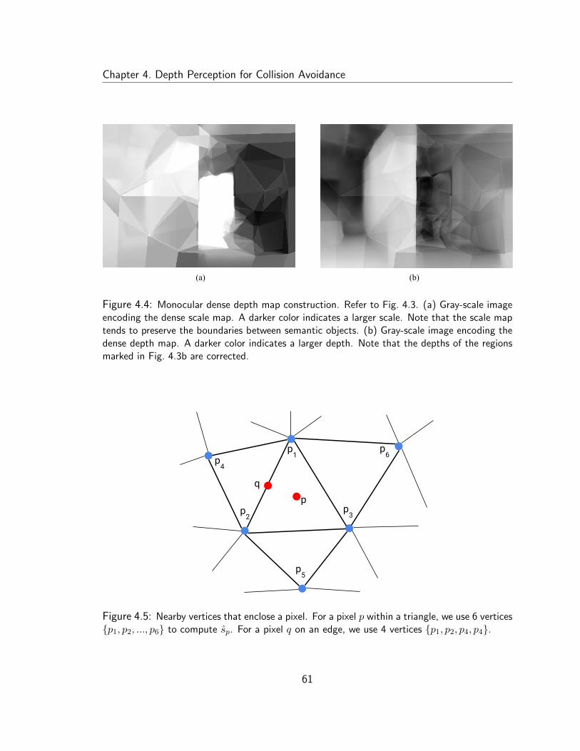
Chapter 4. Depth Perception for Collision Avoidance
(b)(a)
Figure 4.4: Monocular dense depth map construction. Refer to Fig. 4.3. (a) Gray-scale imageencoding the dense scale map. A darker color indicates a larger scale. Note that the scale maptends to preserve the boundaries between semantic objects. (b) Gray-scale image encoding thedense depth map. A darker color indicates a larger depth. Note that the depths of the regionsmarked in Fig. 4.3b are corrected.
p
p1
p2
p3
p4
p6
p5
q
Figure 4.5: Nearby vertices that enclose a pixel. For a pixel p within a triangle, we use 6 vertices{p1, p2, ..., p6} to compute sp. For a pixel q on an edge, we use 4 vertices {p1, p2, p4, p4}.
61
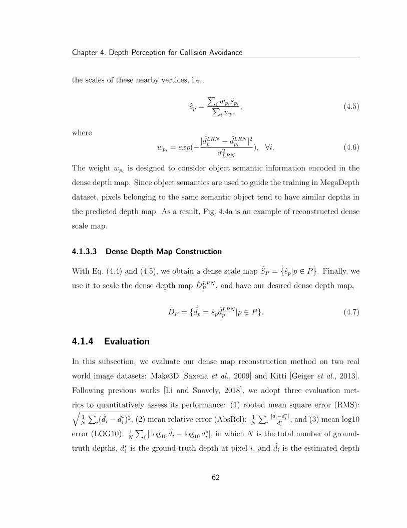
Chapter 4. Depth Perception for Collision Avoidance
the scales of these nearby vertices, i.e.,
sp =
∑iwpi spi∑iwpi
, (4.5)
where
wpi = exp(−|dLRNp − dLRNpi
|2
σ2LRN
), ∀i. (4.6)
The weight wpi is designed to consider object semantic information encoded in the
dense depth map. Since object semantics are used to guide the training in MegaDepth
dataset, pixels belonging to the same semantic object tend to have similar depths in
the predicted depth map. As a result, Fig. 4.4a is an example of reconstructed dense
scale map.
4.1.3.3 Dense Depth Map Construction
With Eq. (4.4) and (4.5), we obtain a dense scale map SP = {sp|p ∈ P}. Finally, we
use it to scale the dense depth map DLRNP , and have our desired dense depth map,
DP = {dp = spdLRNp |p ∈ P}. (4.7)
4.1.4 Evaluation
In this subsection, we evaluate our dense map reconstruction method on two real
world image datasets: Make3D [Saxena et al., 2009] and Kitti [Geiger et al., 2013].
Following previous works [Li and Snavely, 2018], we adopt three evaluation met-
rics to quantitatively assess its performance: (1) rooted mean square error (RMS):√1N
∑i(di − d∗i )2, (2) mean relative error (AbsRel): 1
N
∑i|di−d∗i |d∗i
, and (3) mean log10
error (LOG10): 1N
∑i | log10 di − log10 d
∗i |, in which N is the total number of ground-
truth depths, d∗i is the ground-truth depth at pixel i, and di is the estimated depth
62

Chapter 4. Depth Perception for Collision Avoidance
using our method.
To test on the datasets, we use the neural network, trained on MegaDepth only,
to produce the input dense depth maps. In addition, we synthesis the input sparse
depth maps as follows. We randomly sample κ% of ground truth depths to form
sparse depth maps, κ = 1, 2, 3, 4, 5. To emulate outliers, we randomly sample 1%
from the sparsely sampled depths, and multiply them by a random number between
3 to 10. For the rest 99% samples, we corrupted them with noise, to emulate noisy
measurements.
Make3D To test on Make3D, we follow the protocol of prior work [Liu et al., 2015]
to remove ground truth depths larger than 70m (since Make3D data is unreliable at
large distances). Table 4.1 summarizes the results. Results from other algorithms are
reported in [Li and Snavely, 2018]. The bottom block of Table 4.1 shows that our
method outperforms prior state-of-the-art results. As expected, all errors decrease
monotonically when we increase κ.
KITTI Next, we evaluate our method on the KITTI test set based on the split
of [Eigen et al., 2014]. Table 4.2 summarizes the results. Similar to the case in
Make3D, our method achieves the state-of-the-art accuracy, and all errors decrease
monotonically when we increase κ.
4.1.5 Discussion
The evaluation results show that our method is able to reconstruct dense and accu-
rate depth map for obstacle perception. Not surprisingly, increasing the number of
accurate input depths improves the overall accuracy.
While our method for depth perception is shown to be effective, it is not ready
to be used in an overall system evaluation for photo-taking in the current stage, due
63
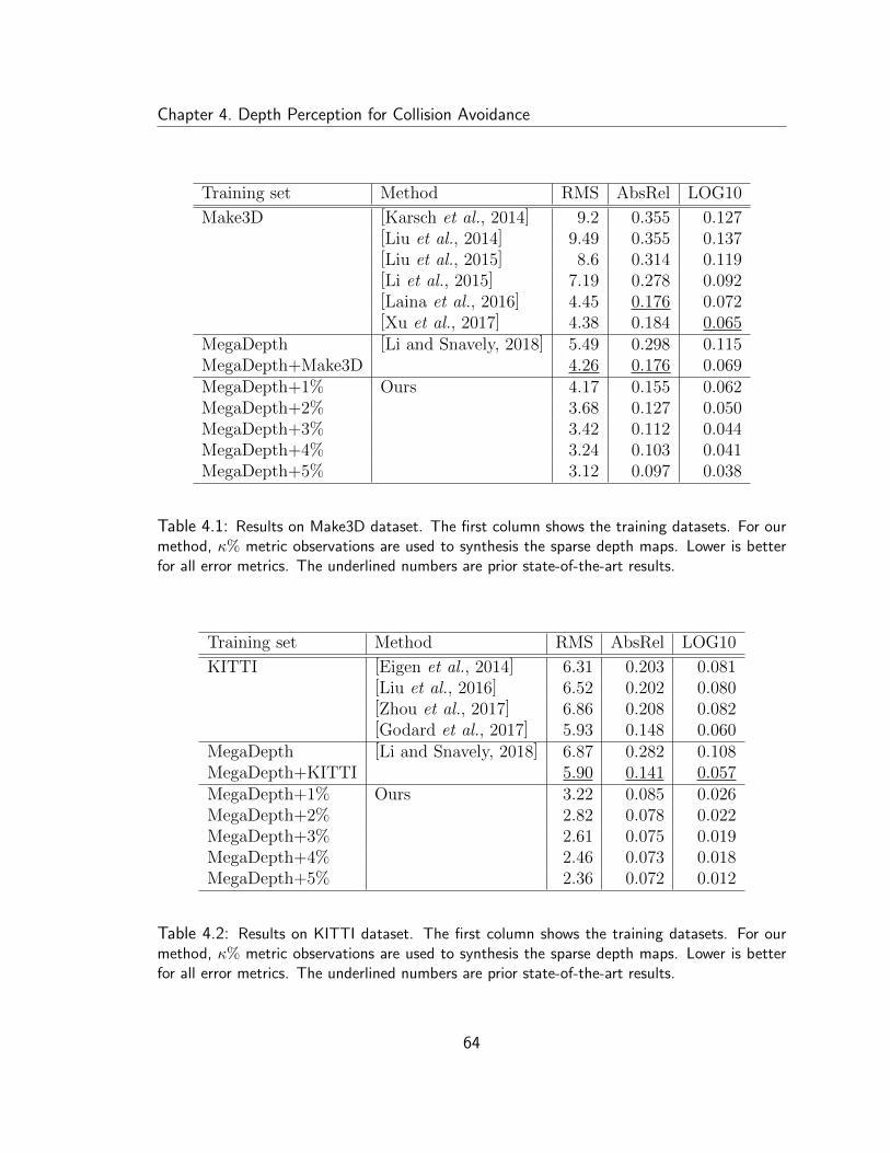
Chapter 4. Depth Perception for Collision Avoidance
Training set Method RMS AbsRel LOG10
Make3D [Karsch et al., 2014] 9.2 0.355 0.127[Liu et al., 2014] 9.49 0.355 0.137[Liu et al., 2015] 8.6 0.314 0.119[Li et al., 2015] 7.19 0.278 0.092[Laina et al., 2016] 4.45 0.176 0.072[Xu et al., 2017] 4.38 0.184 0.065
MegaDepth [Li and Snavely, 2018] 5.49 0.298 0.115MegaDepth+Make3D 4.26 0.176 0.069MegaDepth+1% Ours 4.17 0.155 0.062MegaDepth+2% 3.68 0.127 0.050MegaDepth+3% 3.42 0.112 0.044MegaDepth+4% 3.24 0.103 0.041MegaDepth+5% 3.12 0.097 0.038
Table 4.1: Results on Make3D dataset. The first column shows the training datasets. For ourmethod, κ% metric observations are used to synthesis the sparse depth maps. Lower is betterfor all error metrics. The underlined numbers are prior state-of-the-art results.
Training set Method RMS AbsRel LOG10
KITTI [Eigen et al., 2014] 6.31 0.203 0.081[Liu et al., 2016] 6.52 0.202 0.080[Zhou et al., 2017] 6.86 0.208 0.082[Godard et al., 2017] 5.93 0.148 0.060
MegaDepth [Li and Snavely, 2018] 6.87 0.282 0.108MegaDepth+KITTI 5.90 0.141 0.057MegaDepth+1% Ours 3.22 0.085 0.026MegaDepth+2% 2.82 0.078 0.022MegaDepth+3% 2.61 0.075 0.019MegaDepth+4% 2.46 0.073 0.018MegaDepth+5% 2.36 0.072 0.012
Table 4.2: Results on KITTI dataset. The first column shows the training datasets. For ourmethod, κ% metric observations are used to synthesis the sparse depth maps. Lower is betterfor all error metrics. The underlined numbers are prior state-of-the-art results.
64
Chapter 4. Depth Perception for Collision Avoidance
to a major hardware constraint: the Parrot Bebop’s forward-facing camera has a
very limited viewing angle. The flying camera has to fly around slowly to build the
occupancy grid map before the system plans for a collision-free path, which adversely
affects the seamless photo-taking experience. This limitation can be overcome by
using a wide angle camera, such as an omnidirectional camera. Existing SLAM
systems for omnidirectional cameras [Caruso et al., 2015] can be used to estimate
the sparse depth maps. In addition, the MegaDepth dataset requires modification to
train a neural network for the omnidirectional cameras as well.
4.2 Summary
We are pursuing a modular approach to the collision avoidance problem. In this
chapter, we focused on the mapping module that constructs an accurate depth map.
To realize the collision avoidance capability, we integrate our depth map construction
pipeline into the collision avoidance component as shown in Fig. 4.2. The integration
details are described in the next system implementation chapter.
65
Chapter 5
System Implementation
We show the system implementation details in this chapter. First, we provide system
hardware and software setup (Sec. 5.1). Then, we describe the system components
(Sec. 5.2) implementing the system functions for our explore-and-compose paradigm
(Sec. 2.2).
5.1 System Hardware and Software Setup
5.1.1 Hardware
Our system uses a Parrot Bebop drone with a built-in forward-facing camera. The
user’s mobile device is an ASUS Google Nexus 7 (2012) tablet with a 7.0” multi-touch
display, running Android version 5.1. Both the drone and the tablet are connected
via Wi-Fi to a laptop PC with an Intel Core i7 processor and a GTX 1060 GPU.
5.1.2 Software
We use an open-source drone driver, Bebop Autonomy [AutonomyLab, 2018], to com-
municate with the Bebop at 30 Hz. The Bebop runs low-level controllers onboard.
66
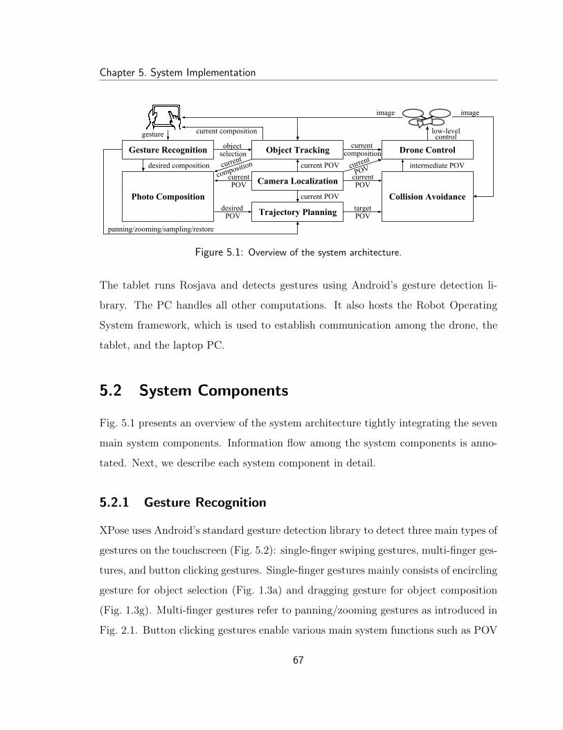
Chapter 5. System Implementation
intermediate POVdesired composition
Gesture Recognition
Camera Localization
Object Tracking
Trajectory Planning
Drone Control
image
controlgesture current composition low-level
Photo Composition Collision Avoidance
image
panning/zooming/sampling/restore
POVcurrent
POVtarget
POVdesired
compositioncurrentcomposition
current
current POV
current POV
POVcurrent POVcurrent
selectionobject
Figure 5.1: Overview of the system architecture.
The tablet runs Rosjava and detects gestures using Android’s gesture detection li-
brary. The PC handles all other computations. It also hosts the Robot Operating
System framework, which is used to establish communication among the drone, the
tablet, and the laptop PC.
5.2 System Components
Fig. 5.1 presents an overview of the system architecture tightly integrating the seven
main system components. Information flow among the system components is anno-
tated. Next, we describe each system component in detail.
5.2.1 Gesture Recognition
XPose uses Android’s standard gesture detection library to detect three main types of
gestures on the touchscreen (Fig. 5.2): single-finger swiping gestures, multi-finger ges-
tures, and button clicking gestures. Single-finger gestures mainly consists of encircling
gesture for object selection (Fig. 1.3a) and dragging gesture for object composition
(Fig. 1.3g). Multi-finger gestures refer to panning/zooming gestures as introduced in
Fig. 2.1. Button clicking gestures enable various main system functions such as POV
67
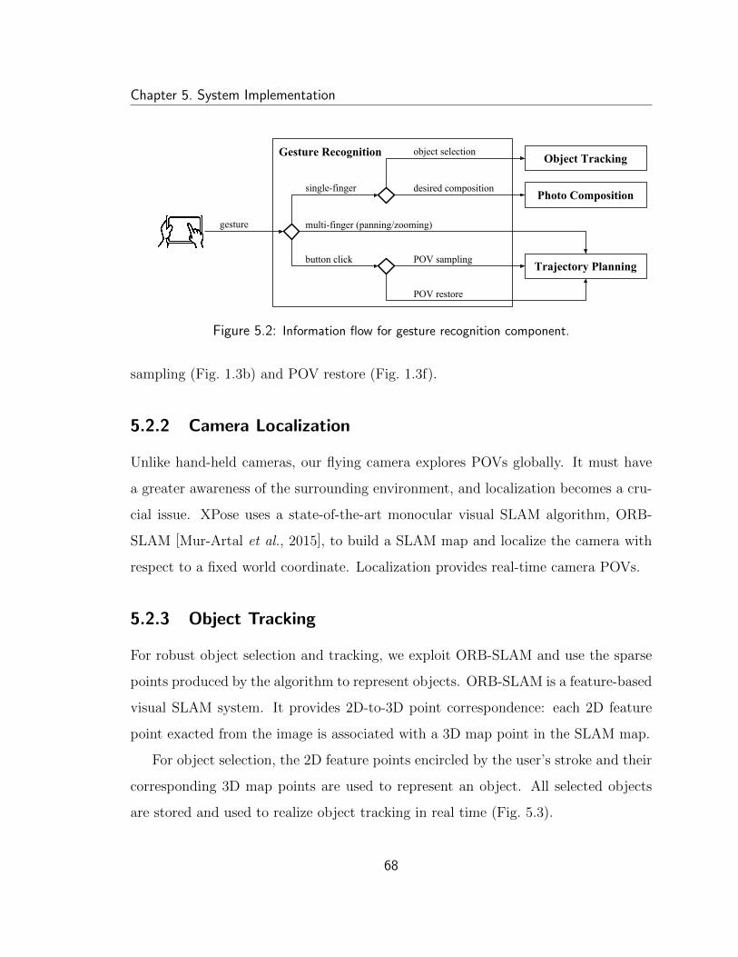
Chapter 5. System Implementation
Gesture Recognition Object Tracking
Trajectory Planning
gesture
object selection
Photo Compositiondesired compositionsingle-finger
multi-finger (panning/zooming)
button click POV sampling
POV restore
Figure 5.2: Information flow for gesture recognition component.
sampling (Fig. 1.3b) and POV restore (Fig. 1.3f).
5.2.2 Camera Localization
Unlike hand-held cameras, our flying camera explores POVs globally. It must have
a greater awareness of the surrounding environment, and localization becomes a cru-
cial issue. XPose uses a state-of-the-art monocular visual SLAM algorithm, ORB-
SLAM [Mur-Artal et al., 2015], to build a SLAM map and localize the camera with
respect to a fixed world coordinate. Localization provides real-time camera POVs.
5.2.3 Object Tracking
For robust object selection and tracking, we exploit ORB-SLAM and use the sparse
points produced by the algorithm to represent objects. ORB-SLAM is a feature-based
visual SLAM system. It provides 2D-to-3D point correspondence: each 2D feature
point exacted from the image is associated with a 3D map point in the SLAM map.
For object selection, the 2D feature points encircled by the user’s stroke and their
corresponding 3D map points are used to represent an object. All selected objects
are stored and used to realize object tracking in real time (Fig. 5.3).
68
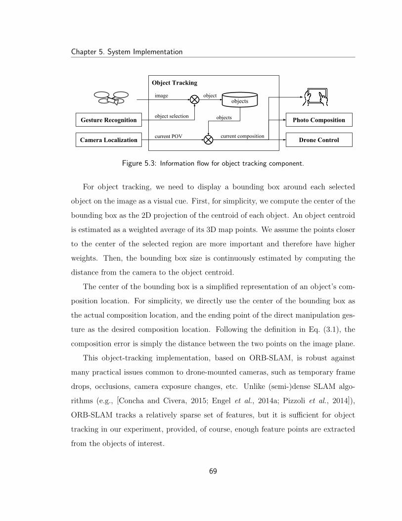
Chapter 5. System Implementation
Object Tracking
Drone Control
Photo CompositionGesture Recognition
Camera Localization
image
object selection
objectsobject
current POV current composition
objects
Figure 5.3: Information flow for object tracking component.
For object tracking, we need to display a bounding box around each selected
object on the image as a visual cue. First, for simplicity, we compute the center of the
bounding box as the 2D projection of the centroid of each object. An object centroid
is estimated as a weighted average of its 3D map points. We assume the points closer
to the center of the selected region are more important and therefore have higher
weights. Then, the bounding box size is continuously estimated by computing the
distance from the camera to the object centroid.
The center of the bounding box is a simplified representation of an object’s com-
position location. For simplicity, we directly use the center of the bounding box as
the actual composition location, and the ending point of the direct manipulation ges-
ture as the desired composition location. Following the definition in Eq. (3.1), the
composition error is simply the distance between the two points on the image plane.
This object-tracking implementation, based on ORB-SLAM, is robust against
many practical issues common to drone-mounted cameras, such as temporary frame
drops, occlusions, camera exposure changes, etc. Unlike (semi-)dense SLAM algo-
rithms (e.g., [Concha and Civera, 2015; Engel et al., 2014a; Pizzoli et al., 2014]),
ORB-SLAM tracks a relatively sparse set of features, but it is sufficient for object
tracking in our experiment, provided, of course, enough feature points are extracted
from the objects of interest.
69
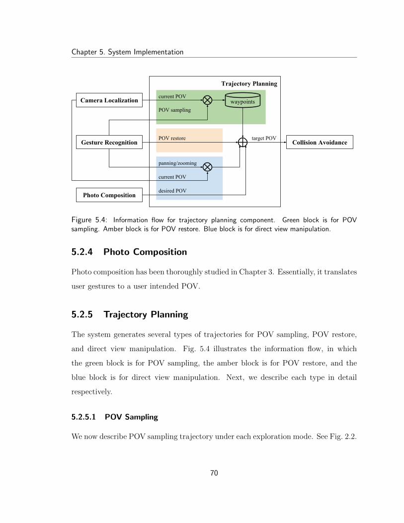
Chapter 5. System Implementation
Trajectory Planning
Collision AvoidanceGesture Recognition
Camera Localization
POV restore
POV sampling
panning/zooming
Photo Composition
waypoints
target POV
current POV
current POV
desired POV
Figure 5.4: Information flow for trajectory planning component. Green block is for POVsampling. Amber block is for POV restore. Blue block is for direct view manipulation.
5.2.4 Photo Composition
Photo composition has been thoroughly studied in Chapter 3. Essentially, it translates
user gestures to a user intended POV.
5.2.5 Trajectory Planning
The system generates several types of trajectories for POV sampling, POV restore,
and direct view manipulation. Fig. 5.4 illustrates the information flow, in which
the green block is for POV sampling, the amber block is for POV restore, and the
blue block is for direct view manipulation. Next, we describe each type in detail
respectively.
5.2.5.1 POV Sampling
We now describe POV sampling trajectory under each exploration mode. See Fig. 2.2.
70
Chapter 5. System Implementation
Orbit To start the Orbit mode, XPose requires a main object of interest to be
selected. The Orbit mode generates a full circular trajectory of POVs looking inward
at the object. Formally speaking, the circle is essentially a line of latitude on a sphere,
of which the center is the object centroid in the map, and the radius of the sphere is
the distance from the object centroid to the camera position where the Orbit mode
starts. For each camera position along the circle, a camera orientation is computed
to maintain the object composition on the image plane.
The sample shots are planned to be taken evenly along the circle. However, since
a drone can hardly reach a planned POV exactly, the sampling condition is relaxed
from reaching an exact POV to entering a region of satisfied POVs. The region is
bounded by various factors: the composition error, the distance difference to the
object centroid, the latitude and longitude angle differences of the sphere centered at
the object.
Pano The Pano mode does not require an object of interest to be selected. It
generates a trajectory of POVs by spinning around at a fixed point. In other words,
the POVs have the same camera position and tilt angle, but different camera pan
angles.
The sample shots are taken at evenly distributed pan angles. Again, a region
of satisfied POVs is used, which is bounded by the position displacement and the
orientation difference.
Zigzag The trajectory generation and execution of the Zigzag mode are very similar
to that of the Orbit mode. The Zigzag mode also requires a main object of interest
to be selected. The major difference is the sampling pattern. Considering the sphere
centered at the object, the Zigzag mode samples POVs on a patch of the sphere by
deviating locally from the camera position where the Zigzag mode starts. The patch
71
Chapter 5. System Implementation
is discretized as multiple circular arcs along different latitudes of the sphere. During
execution, the drone moves along each arc one by one.
5.2.5.2 POV Restore
For POV restore, the trajectory is simply a line segment connecting the current POV
and the target POV to be restored. Potential collisions are handled in the next
collision avoidance component.
The end of a POV restoring trajectory is a region of POVs around the target
POV, which is bounded by the position displacement and the orientation difference.
5.2.5.3 Direct View Manipulation
For direct view manipulation, the trajectory is also a line segment, but connecting
from the current POV to the user desired POV according to different gestures.
The target POV for a panning/zooming gesture (Fig. 2.1) is computed based on
the current POV and the corresponding intended camera motion. For example, the
target POV for a zooming-in gesture is a POV in front of the current image plane
along the camera’s principal axis.
The target POV for direct object composition is simply the desired POV computed
from the photo composition component.
5.2.6 Collision Avoidance
As illustrated in Fig. 4.2, we pursue a modular approach to collision avoidance. The
collision avoidance component consists of two main parts: mapping and planning. For
mapping, we aggregate individual depth maps to construct a metric-scaled occupancy
grid map (Sec. 5.2.6.1). Then, we use the standard potential field algorithm to plan
a collision-free path (Sec. 5.2.6.2).
72
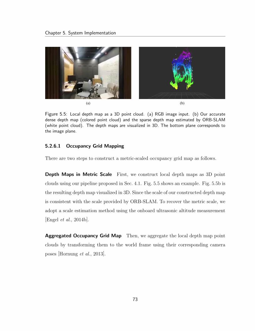
Chapter 5. System Implementation
(d)(c)
(b)(a)
Figure 5.5: Local depth map as a 3D point cloud. (a) RGB image input. (b) Our accuratedense depth map (colored point cloud) and the sparse depth map estimated by ORB-SLAM(white point cloud). The depth maps are visualized in 3D. The bottom plane corresponds tothe image plane.
5.2.6.1 Occupancy Grid Mapping
There are two steps to construct a metric-scaled occupancy grid map as follows.
Depth Maps in Metric Scale First, we construct local depth maps as 3D point
clouds using our pipeline proposed in Sec. 4.1. Fig. 5.5 shows an example. Fig. 5.5b is
the resulting depth map visualized in 3D. Since the scale of our constructed depth map
is consistent with the scale provided by ORB-SLAM. To recover the metric scale, we
adopt a scale estimation method using the onboard ultrasonic altitude measurement
[Engel et al., 2014b].
Aggregated Occupancy Grid Map Then, we aggregate the local depth map point
clouds by transforming them to the world frame using their corresponding camera
poses [Hornung et al., 2013].
73
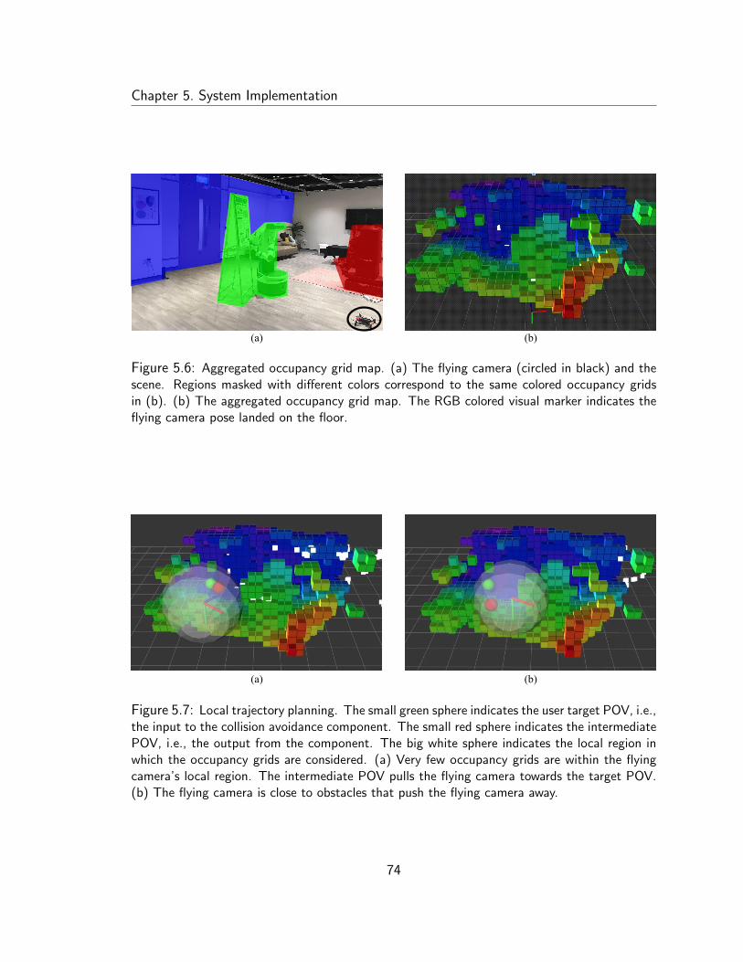
Chapter 5. System Implementation
(b)(a)
Figure 5.6: Aggregated occupancy grid map. (a) The flying camera (circled in black) and thescene. Regions masked with different colors correspond to the same colored occupancy gridsin (b). (b) The aggregated occupancy grid map. The RGB colored visual marker indicates theflying camera pose landed on the floor.
(b)(a)
Figure 5.7: Local trajectory planning. The small green sphere indicates the user target POV, i.e.,the input to the collision avoidance component. The small red sphere indicates the intermediatePOV, i.e., the output from the component. The big white sphere indicates the local region inwhich the occupancy grids are considered. (a) Very few occupancy grids are within the flyingcamera’s local region. The intermediate POV pulls the flying camera towards the target POV.(b) The flying camera is close to obstacles that push the flying camera away.
74
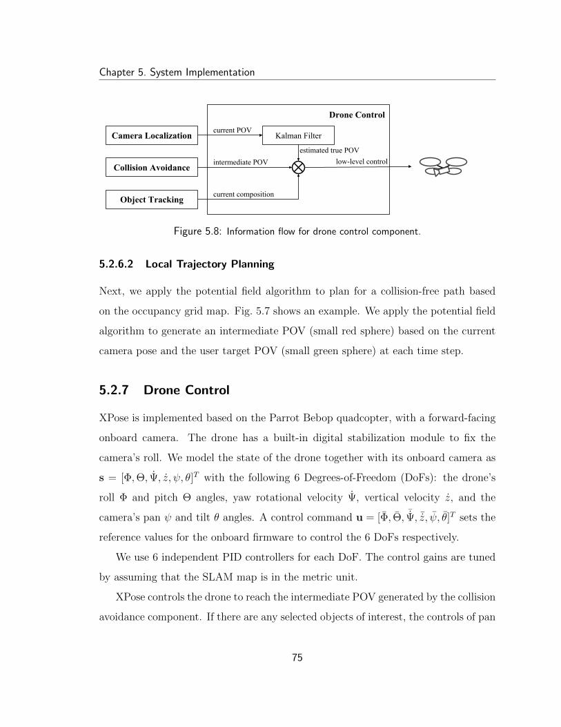
Chapter 5. System Implementation
Drone Control
Collision Avoidance
current composition
current POV
Object Tracking
intermediate POV
Camera Localization
low-level control
Kalman Filter
estimated true POV
Figure 5.8: Information flow for drone control component.
5.2.6.2 Local Trajectory Planning
Next, we apply the potential field algorithm to plan for a collision-free path based
on the occupancy grid map. Fig. 5.7 shows an example. We apply the potential field
algorithm to generate an intermediate POV (small red sphere) based on the current
camera pose and the user target POV (small green sphere) at each time step.
5.2.7 Drone Control
XPose is implemented based on the Parrot Bebop quadcopter, with a forward-facing
onboard camera. The drone has a built-in digital stabilization module to fix the
camera’s roll. We model the state of the drone together with its onboard camera as
s = [Φ,Θ, Ψ, z, ψ, θ]T with the following 6 Degrees-of-Freedom (DoFs): the drone’s
roll Φ and pitch Θ angles, yaw rotational velocity Ψ, vertical velocity z, and the
camera’s pan ψ and tilt θ angles. A control command u = [Φ, Θ, ¯Ψ, ¯z, ψ, θ]T sets the
reference values for the onboard firmware to control the 6 DoFs respectively.
We use 6 independent PID controllers for each DoF. The control gains are tuned
by assuming that the SLAM map is in the metric unit.
XPose controls the drone to reach the intermediate POV generated by the collision
avoidance component. If there are any selected objects of interest, the controls of pan
75
Chapter 5. System Implementation
and tilt angles are overwritten in order to directly minimize the composition error.
We define FW as the world coordinate frame. We further denote the intermedi-
ate POV as pW = [xW, yW, zW, ψW, θW]T , which consists of 3-DoF camera position
[xW, yW, zW]T and 2-DoF orientation (pan ψW and tilt θW).
During trajectory execution, the POV estimated by ORB-SLAM cannot be di-
rectly used, due to the delay caused by video transmission (∼200ms) and processing
(∼20ms). A delayed estimation of POV may cause oscillating behaviors while con-
trolling the system at a high update rate. To compensate the delay, a Kalman Filter
is used to estimate the true POV with a constant-velocity model. This estimated
POV at time t, denoted as pWt = [xWt , y
Wt , z
Wt , ψ
Wt , θ
Wt ]T , is then used to compute
the low-level control commands. While our method serves the purpose of system
evaluation (Chap. 6), there are more sophisticated methods [Engel et al., 2014b] if
needed.
Finally, the 3-DoF camera position [xW, yW, zW]T is achieved by controlling the
drone’s roll Φ and pitch Θ angles, and vertical velocity z. The tilt angle θW is achieved
by controlling the camera’s tilt θ. The pan angle ψW is jointly controlled by the yaw
rotational velocity Ψ and the camera’s pan ψ.
76
Chapter 6
System Evaluation
We conducted a user study to compare XPose and a joystick interface, in order to
examine the feasibility of XPose and quantify the performance differences between
the two.
6.1 Experimental Setup
The study consists of two sets of experiments. The first set focuses on interaction
design. It evaluates XPose’s design of POV exploration and of visual composition
separately. To avoid confounding factors resulting from the system implementation,
it places the flying camera in a motion capture studio, which provides highly accurate
camera localization and object tracking at 50 Hz. The second set of experiments focus
on the overall system performance in more realistic settings, without the help of a
motion capture system.
We compare XPose with one of the Parrot Bebop’s native interfaces, the Joypad
mode in the FreeFlight Pro app. Joypad emulates a joystick interface on a touchscreen
and provides the user low-level manual control of the drone (Fig. 1.2a). We use it as
the baseline for comparison, as joysticks and emulated joystick interfaces are widely
77
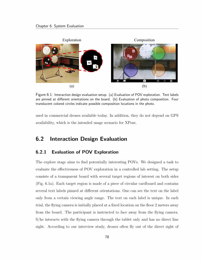
Chapter 6. System Evaluation
Exploration Composition
(a) (b)
Figure 6.1: Interaction design evaluation setup. (a) Evaluation of POV exploration. Text labelsare pinned at different orientations on the board. (b) Evaluation of photo composition. Fourtranslucent colored circles indicate possible composition locations in the photo.
used in commercial drones available today. In addition, they do not depend on GPS
availability, which is the intended usage scenario for XPose.
6.2 Interaction Design Evaluation
6.2.1 Evaluation of POV Exploration
The explore stage aims to find potentially interesting POVs. We designed a task to
evaluate the effectiveness of POV exploration in a controlled lab setting. The setup
consists of a transparent board with several target regions of interest on both sides
(Fig. 6.1a). Each target region is made of a piece of circular cardboard and contains
several text labels pinned at different orientations. One can see the text on the label
only from a certain viewing angle range. The text on each label is unique. In each
trial, the flying camera is initially placed at a fixed location on the floor 2 meters away
from the board. The participant is instructed to face away from the flying camera.
S/he interacts with the flying camera through the tablet only and has no direct line
sight. According to our interview study, drones often fly out of the direct sight of
78
Chapter 6. System Evaluation
operators. The participant is asked to read out all the text labels on the board as fast
as possible. The trial terminates when the participant believes that s/he has finished
reading all the text labels and lands the flying camera. The trial pauses, if the flying
camera crashes. The drone is placed on the floor at the crash site. The trial resumes
after the participant relaunches the drone and continues with the task.
We measured the completion time for each trial and the coverage, i.e., the per-
centage of correctly reported text labels.
6.2.2 Evaluation of Visual Composition
Once a potential POV is identified, the compose stage aims to place objects of interest
at desired locations in the photo by refining the POV. We designed another evaluation
task for composition, with a similar setup. In each trial, the participant sees in the
viewfinder four circles of different colors, placed in the photo frame according to the
rule of thirds (Fig. 6.1b). S/he is asked to put a specified target region at the location
of a randomly assigned circle so that they match as well as possible.
Again, we measured the completion time for each trial as well as the composition
error (Eq. (3.1)), which provides one measure of composition quality.
6.2.3 Experimental Design
Participants 8 volunteers (2 female, 6 male, aged 23–30) were recruited from the
university community and the IT industry. All participants had prior experience
taking photos, and 3 had experience flying drones.
Within-Participants Design Each participant used each interface to perform each
of the two evaluation tasks three times. The order of trying the two interfaces was
counterbalanced. The two tasks were ordered sequentially, as we were not interested
79
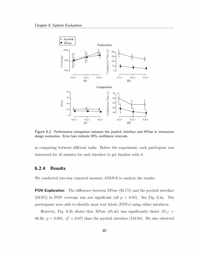
Chapter 6. System Evaluation
2%
150
70
30
(a) (b)
(c) (d)
Exploration
Composition
Erro
r
Photo-taking
(e)
Trial 1 Trial 2 Trial 3Trial 1 Trial 2 Trial 3
Trial 1 Trial 2 Trial 3Trial 1 Trial 2 Trial 3
Easy Hard
Com
plet
ion
Tim
e (s
)C
ompl
etio
n Ti
me
(s)
Cov
erag
e
Com
plet
ion
Tim
e (s
)
JoystickXPose
100%
80%
90%
200
0
100
50
4%
0
1%
3%
50
40
60
150
50
100
0
Figure 6.2: Performance comparison between the joystick interface and XPose in interactiondesign evaluation. Error bars indicate 95% confidence intervals.
in comparing between different tasks. Before the experiment, each participant was
instructed for 10 minutes for each interface to get familiar with it.
6.2.4 Results
We conducted two-way repeated measure ANOVA to analyze the results.
POV Exploration The difference between XPose (93.1%) and the joystick interface
(93.6%) in POV coverage was not significant (all p > 0.05). See Fig. 6.2a. The
participants were able to identify most text labels (POVs) using either interfaces.
However, Fig. 6.2b shows that XPose (85.4s) was significantly faster (F1,7 =
46.36, p < 0.001, η2 = 0.87) than the joystick interface (153.9s). We also observed
80
Chapter 6. System Evaluation
a significant trend (F2,14 = 14.72, p < 0.001, η2 = 0.68) on completion time over
the trials, indicating a learning effect for participants for both interfaces. Since most
participants were not familiar with drone flying, this effect was expected. However,
there was no significant interaction between the effect of interface and that of a trial
on the completion time (p > 0.05), suggesting that the learning curves of the two
interfaces are similar.
Visual Composition The composition error using XPose (0.86%) was smaller than
that of the joystick interface(1.28%). See Fig. 6.2c. While the difference was statis-
tically significant (F1,7 = 21.336, p = 0.002, η2 = 0.75), both errors were about 1%
and unlikely to make much difference in most photos. We did not observe any other
main effects or interaction effects (all p > 0.05).
Again, Fig. 6.2d shows that XPose (34.2s) was significantly faster (F1,7 = 24.36, p =
0.002, η2 = 0.78) than the joystick interface (47.8s). The participants also became
significantly faster over trials (F2,14 = 7.65, p = 0.006, η2 = 0.52), and there was no
significant interaction between the effect of interface and that of trial on the comple-
tion time (p > 0.05).
Overall, XPose was significantly faster than the joystick interface in both POV
exploration and photo composition, while achieving a comparable level of task per-
formance measured in POV coverage or composition error. Although the number
of participants in the study is relatively small, the confidence intervals are clearly
separated (Fig. 6.2b,d).
6.3 System Performance Evaluation
We conducted the second set of experiments to evaluate the system performance using
more realistic photo-taking settings, by removing the motion capture system. We use
81
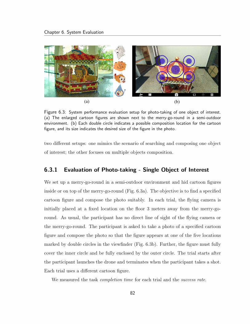
Chapter 6. System Evaluation
Exploration Composition
(a) (b)
Figure 6.3: System performance evaluation setup for photo-taking of one object of interest.(a) The enlarged cartoon figures are shown next to the merry-go-round in a semi-outdoorenvironment. (b) Each double circle indicates a possible composition location for the cartoonfigure, and its size indicates the desired size of the figure in the photo.
two different setups: one mimics the scenario of searching and composing one object
of interest; the other focuses on multiple objects composition.
6.3.1 Evaluation of Photo-taking - Single Object of Interest
We set up a merry-go-round in a semi-outdoor environment and hid cartoon figures
inside or on top of the merry-go-round (Fig. 6.3a). The objective is to find a specified
cartoon figure and compose the photo suitably. In each trial, the flying camera is
initially placed at a fixed location on the floor 3 meters away from the merry-go-
round. As usual, the participant has no direct line of sight of the flying camera or
the merry-go-round. The participant is asked to take a photo of a specified cartoon
figure and compose the photo so that the figure appears at one of the five locations
marked by double circles in the viewfinder (Fig. 6.3b). Further, the figure must fully
cover the inner circle and be fully enclosed by the outer circle. The trial starts after
the participant launches the drone and terminates when the participant takes a shot.
Each trial uses a different cartoon figure.
We measured the task completion time for each trial and the success rate.
82
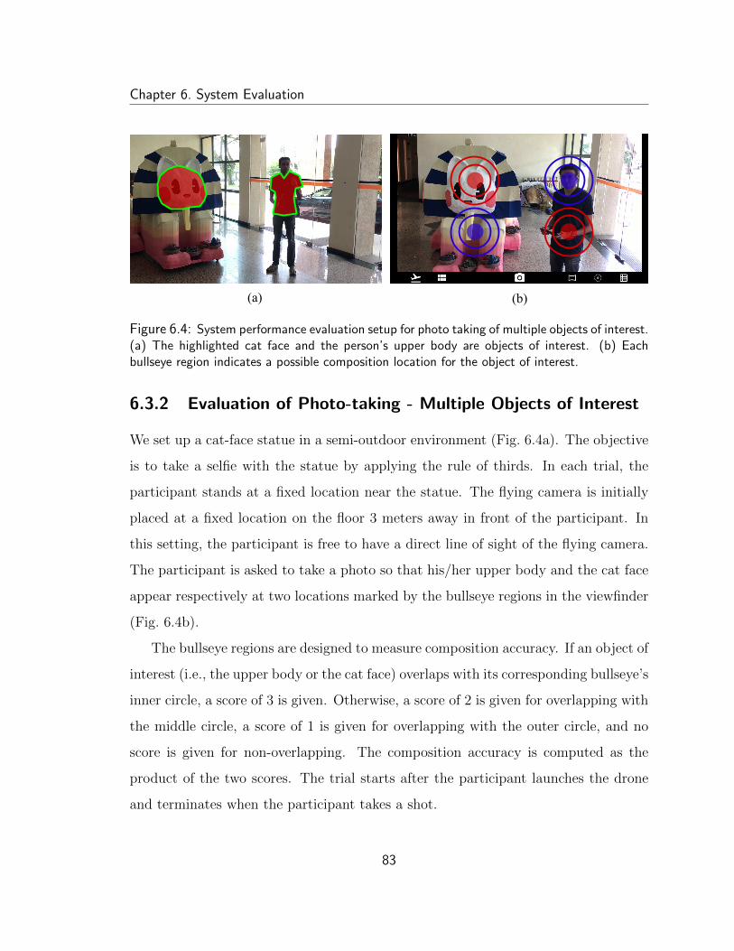
Chapter 6. System Evaluation
Exploration Composition
(a) (b)
Figure 6.4: System performance evaluation setup for photo taking of multiple objects of interest.(a) The highlighted cat face and the person’s upper body are objects of interest. (b) Eachbullseye region indicates a possible composition location for the object of interest.
6.3.2 Evaluation of Photo-taking - Multiple Objects of Interest
We set up a cat-face statue in a semi-outdoor environment (Fig. 6.4a). The objective
is to take a selfie with the statue by applying the rule of thirds. In each trial, the
participant stands at a fixed location near the statue. The flying camera is initially
placed at a fixed location on the floor 3 meters away in front of the participant. In
this setting, the participant is free to have a direct line of sight of the flying camera.
The participant is asked to take a photo so that his/her upper body and the cat face
appear respectively at two locations marked by the bullseye regions in the viewfinder
(Fig. 6.4b).
The bullseye regions are designed to measure composition accuracy. If an object of
interest (i.e., the upper body or the cat face) overlaps with its corresponding bullseye’s
inner circle, a score of 3 is given. Otherwise, a score of 2 is given for overlapping with
the middle circle, a score of 1 is given for overlapping with the outer circle, and no
score is given for non-overlapping. The composition accuracy is computed as the
product of the two scores. The trial starts after the participant launches the drone
and terminates when the participant takes a shot.
83

Chapter 6. System Evaluation
(a) (b)
Single Object of Interest
Easy Hard
Com
plet
ion
Tim
e (s
)
JoystickXPose
150
50
100
0
Side-by-side Diagonal
Com
plet
ion
Tim
e (s
) 80
0
40
(c)Side-by-side Diagonal
Accu
racy
(sco
re) 9
4
Multiple Objects of Interest
Figure 6.5: Performance comparison between the joystick interface and XPose in overall systemperformance evaluation. Error bars indicate 95% confidence intervals.
We measured the task completion time for each trial and the composition accuracy.
6.3.3 Experimental Design
Participants For each evaluation setup, 8 new volunteers were recruited from the
university community. None participated in the earlier experiments. All participants
had experience taking photos, and none of them are experienced drone pilots.
Within-Participants Design For the evaluation using a single object of interest,
each participant used each interface to perform the task with two difficulty levels,
one having an easy-to-find figure and one having a harder-to-find figure. The order
of trying the interfaces was counterbalanced.
For the evaluation using multiple objects of interest, each participant used each
interface to perform the task with two types of compositions: side-by-side composition
and diagonal composition. A side-by-side composition refers to using the two top (or
the two bottom) bullseye regions. A diagonal composition refers to using one top and
one bottom bullseye regions. The order of trying the interfaces was counterbalanced.
6.3.4 Results
We conducted two-way repeated measure ANOVA to analyze the results.
84
Chapter 6. System Evaluation
Single Object of Interest The success rate was 100%, as all specified cartoon figures
were found and composed as required. We analyzed the completion time (Fig. 6.5a).
XPose (57.1s) was significantly faster (F1,7 = 19.12, p = 0.003, η2 = 0.73) than
the joystick interface (85.3s). The effect size value (η2 = .73) again, suggests a high
practical difference between the two interfaces. As expected, completing the easy task
was significantly faster (F1,7 = 52.79, p < 0.001, η2 = 0.88) than completing the hard
task. Interestingly, there was significant interaction (F1,7 = 6.10, p = 0.043, η2 =
0.47) between the effect of interface and that of difficulty on the completion time.
Increased difficulty caused a large increase in the completion time for the joystick
interface, but it caused a smaller increase for XPose. We propose the following reason.
In the more difficult task, the cartoon figure was partially occluded. XPose provided
a gallery preview so that participants could examine each sample shot closely and
find the partially occluded figure faster.
Multiple Objects of Interest We analyzed both the completion time (Fig. 6.5b)
and the composition accuracy (Fig. 6.5c). XPose was not only significantly faster
(F1,7 = 71.13, p < 0.001, η2 = 0.91) but also significantly more accurate (F1,7 =
10.34, p = 0.015, η2 = 0.60) than the joystick interface. The effect size values
(η2 = .91 and 0.60) both suggest a high practical difference between the two inter-
faces. Interestingly, composing a side-by-side photo is both significantly faster (F1,7 =
35.88, p < 0.001, η2 = 0.84) and more accurate (F1,7 = 6.33, p = 0.04, η2 = 0.48)
than composing a diagonal one. A potential reason is that the height of the statue
is about the same as the height of a person. It is relatively easy for participants to
compose side-by-side shots.
Similar to the case in composing single object of interest, there was significant
interaction (F1,7 = 12.22, p = 0.01, η2 = 0.63) between the effect of interface and
that of composition type on the completion time. Again, increased difficulty caused a
85
Chapter 6. System Evaluation
large increase in the completion time for the joystick interface, but it caused a smaller
increase for XPose. In this setup, a diagonal composition requires to fly a longer
distance as compared with a side-by-side composition. XPose freed the participants
from tedious control through autonomy.
6.4 Discussion
The evaluation results show that XPose outperforms the joystick interface in POV
exploration, in visual composition, and in photo-taking. The joystick interface forces
the user to pilot the drone manually through low-level motion commands. Doing so
while searching for a good POV at the same time is difficult and tedious. Further,
the communication delay between the flying camera and the touchscreen mobile de-
vice often causes the camera to overshoot the desired pose. Our explore-and-compose
approach demonstrates great potentials for photo-taking with flying cameras. While
our experiments tested only a small range of representative tasks, we are pleased to
see that our interaction design enabled more efficient POV exploration with prede-
fined exploration modes and easier photo composition with direct manipulation of
objects of interest. POV exploration and photo composition are essential sub-tasks
for photo taking. Creating more efficient and user-friendly approaches to these tasks
contribute significantly to better photo taking. Participants expressed that XPose is
more natural and intuitive to use: “Yours (XPose) is easier to use as I can focus on
the task instead of flying the drone.” More encouragingly, the two stages, explore and
compose, worked well together for more realistic photo-taking tasks in a GPS-denied
semi-outdoor environment. Together, the results of our user study suggest that XPose
clearly represents a step forward towards a practically useful system.
86
Chapter 7
Conclusion
We presented XPose, a touch-based interactive system for flying camera photo-taking.
XPose introduces the explore-and-compose paradigm to photo-taking and provides a
unified interaction model for flying cameras. It enables a low-cost quadcopter to fly
in a GPS-denied environment and provides intuitive and effective interactions that
aid the user for photo-taking in real time. As a result, the user focuses on taking
photos, instead of piloting the drone.
Our experience highlights the importance of integrating interaction design (Chap. 2)
and system implementation (Chap. 5). Good interaction design must be rooted in
realistic assumptions of system capabilities, and new system implementation tech-
nologies open up opportunities for innovative interaction design.
From the interaction design perspective, the explore-and-compose paradigm cur-
rently focuses on photo-taking in static scenes. We believe that the underlying design
idea is useful for dynamic scenes as well, but the interaction design and the sys-
tem implementation become more challenging. In addition, the explore-and-compose
paradigm could also be adopted in other modalities, such as mouse-based interfaces.
From the system implementation perspective, our current prototype works suc-
87
Chapter 7. Conclusion
cessfully in indoor, semi-outdoor, and limited outdoor settings, with two main limi-
tations. First, we rely on a laptop computer for most of the required computation,
because the Parrot Bebop drone has a very limited onboard processing power. Sec-
ond, due to the limited viewing angle of the forward-facing camera on the Parrot
Bebop, the collision-free path planning cannot be seamlessly integrated. With rapid
advances in hardware technology and decreasing cost, we expect to overcome these
limitations in the near future.
While our prototype implementation still has several limitations, it is a first step
towards the ultimate vision of a flying camera for everyday use.
88
Bibliography
[AirSelfie, 2018] AirSelfie. The only portable flying camera integrated in your photocover. http://www.airselfiecamera.com/, 2018.
[AutonomyLab, 2018] AutonomyLab. Bebop autonomy. https://github.com/
autonomylab/bebop_autonomy, 2018.
[Ballou, 2001] P Ballou. Improving pilot dexterity with a telepresent rov. In Proc.the Vehicle Teleoperation Interfaces Workshop, ICRA, 2001.
[Bansal and Daniilidis, 2014] Mayank Bansal and Kostas Daniilidis. Geometric urbangeo-localization. In CVPR, 2014.
[Bebop, 2018] Bebop. Parrot bebop drone. http://global.parrot.com/au/
products/bebop-drone, 2018.
[Bloesch et al., 2018] Michael Bloesch, Jan Czarnowski, Ronald Clark, StefanLeutenegger, and Andrew J Davison. Codeslamlearning a compact, optimisablerepresentation for dense visual slam. In CVPR, 2018.
[Booij et al., 2009] Olaf Booij, Zoran Zivkovic, et al. The planar two point algorithm.IAS technical report, University of Amsterdam, 2009.
[Bowman et al., 1997] Doug A Bowman, David Koller, and Larry F Hodges. Travelin immersive virtual environments: An evaluation of viewpoint motion controltechniques. In Virtual Reality Annual International Symposium, 1997.
[Burtnyk et al., 2002] Nicholas Burtnyk, Azam Khan, George Fitzmaurice, RavinBalakrishnan, and Gordon Kurtenbach. StyleCam: interactive stylized 3D nav-igation using integrated spatial & temporal controls. In UIST, 2002.
[Byrod et al., 2008] Martin Byrod, Zuzana Kukelova, Klas Josephson, Tomas Pajdla,and Kalle Astrom. Fast and robust numerical solutions to minimal problems forcameras with radial distortion. In CVPR, 2008.
89
BIBLIOGRAPHY
[Camposeco et al., 2017] Federico Camposeco, Torsten Sattler, Andrea Cohen, An-dreas Geiger, and Marc Pollefeys. Toroidal constraints for two-point localizationunder high outlier ratios. In CVPR, 2017.
[Caruso et al., 2015] David Caruso, Jakob Engel, and Daniel Cremers. Large-scaledirect slam for omnidirectional cameras. In IROS, 2015.
[Cheerson, 2018] Cheerson. Experience the flying dream. http://www.
cheersonhobby.com/en-US/, 2018.
[Choi and Park, 2015] Sung-In Choi and Soon-Yong Park. A new 2-point absolutepose estimation algorithm under planar motion. Advanced Robotics, 2015.
[Concha and Civera, 2015] Alejo Concha and Javier Civera. DPPTAM: Dense piece-wise planar tracking and mapping from a monocular sequence. In IROS, 2015.
[DJI, 2018a] DJI. DJI Drones. http://www.dji.com/products/drones, 2018.
[DJI, 2018b] DJI. Inspire 1 pro-dual remote controllers mode. http://wiki.dji.
com/en/index.php/Inspire_1_Pro-Dual_Remote_Controllers_Mode, 2018.
[Dragicevic et al., 2008] Pierre Dragicevic, Gonzalo Ramos, Jacobo Bibliowitcz,Derek Nowrouzezahrai, Ravin Balakrishnan, and Karan Singh. Video browsingby direct manipulation. In ACM SIGCHI, 2008.
[Dronestagram, 2017] Dronestagram. International dronephotography contest. http://www.dronestagr.am/
2017-international-drone-photography-contest, 2017.
[Eigen and Fergus, 2015] David Eigen and Rob Fergus. Predicting depth, surfacenormals and semantic labels with a common multi-scale convolutional architecture.In ICCV, 2015.
[Eigen et al., 2014] David Eigen, Christian Puhrsch, and Rob Fergus. Depth mapprediction from a single image using a multi-scale deep network. In NIPS, 2014.
[Elmqvist et al., 2008] Niklas Elmqvist, Mihail Eduard Tudoreanu, and PhilippasTsigas. Evaluating motion constraints for 3d wayfinding in immersive and desktopvirtual environments. In ACM SIGCHI, 2008.
[Engel et al., 2014a] Jakob Engel, Thomas Schops, and Daniel Cremers. LSD-SLAM:Large-scale direct monocular slam. In ECCV, 2014.
[Engel et al., 2014b] Jakob Engel, Jurgen Sturm, and Daniel Cremers. Scale-awarenavigation of a low-cost quadrocopter with a monocular camera. RAS, 2014.
90
BIBLIOGRAPHY
[Flynixie, 2018] Flynixie. The first wearable camera that can fly — flynixie. http:
//flynixie.com, 2018.
[Forster et al., 2014] Christian Forster, Matia Pizzoli, and Davide Scaramuzza. Svo:Fast semi-direct monocular visual odometry. In ICRA, 2014.
[Forster et al., 2017] Christian Forster, Zichao Zhang, Michael Gassner, ManuelWerlberger, and Davide Scaramuzza. Svo: Semidirect visual odometry for monoc-ular and multicamera systems. IEEE Transactions on Robotics, 2017.
[Fuentes-Pacheco et al., 2012] Jorge Fuentes-Pacheco, Jose Ruız Ascencio, andJuan M. Rendon-Mancha. Visual simultaneous localization and mapping: a survey.Artificial Intelligence Review, 2012.
[Furukawa et al., 2010] Yasutaka Furukawa, Brian Curless, Steven M Seitz, andRichard Szeliski. Towards internet-scale multi-view stereo. In CVPR, 2010.
[Galyean, 1995] Tinsley A Galyean. Guided navigation of virtual environments. InI3D, 1995.
[Gao et al., 2003] Xiao-Shan Gao, Xiao-Rong Hou, Jianliang Tang, and Hang-FeiCheng. Complete solution classification for the perspective-three-point problem.TPAMI, 2003.
[Gebhardt et al., 2016] Christoph Gebhardt, Benjamin Hepp, Tobias Nageli, StefanStevsic, and Otmar Hilliges. Airways: Optimization-based planning of quadrotortrajectories according to high-level user goals. In ACM SIGCHI, 2016.
[Geiger et al., 2013] Andreas Geiger, Philip Lenz, Christoph Stiller, and Raquel Ur-tasun. Vision meets robotics: The kitti dataset. IJRR, 2013.
[Gernsheim and Gernsheim, 1969] Helmut Gernsheim and Alison Gernsheim. Thehistory of photography: from the camera obscura to the beginning of the modernera. New York: McGraw-Hill, 1969.
[Gleicher and Witkin, 1992] Michael Gleicher and Andrew Witkin. Through-the-lenscamera control. In ACM SIGGRAPH, 1992.
[Godard et al., 2017] Clement Godard, Oisin Mac Aodha, and Gabriel J Brostow.Unsupervised monocular depth estimation with left-right consistency. In CVPR,2017.
[Hachet et al., 2008] Martin Hachet, Fabrice Decle, Sebastian Knodel, and PascalGuitton. Navidget for easy 3D camera positioning from 2D inputs. 3DUI, 2008.
91
BIBLIOGRAPHY
[Hainsworth, 2001] David W Hainsworth. Teleoperation user interfaces for miningrobotics. Autonomous Robots, 2001.
[Hanson and Wernert, 1997] Andrew J Hanson and Eric A Wernert. Constrained 3Dnavigation with 2D controllers. In Visualization, 1997.
[Hornung et al., 2013] Armin Hornung, Kai M Wurm, Maren Bennewitz, CyrillStachniss, and Wolfram Burgard. Octomap: An efficient probabilistic 3d map-ping framework based on octrees. Autonomous robots, 2013.
[Joubert et al., 2015] Niels Joubert, Mike Roberts, Anh Truong, FloraineBerthouzoz, and Pat Hanrahan. An interactive tool for designing quadrotor camerashots. ACM TOG, 2015.
[Kalal et al., 2012] Zdenek Kalal, Krystian Mikolajczyk, Jiri Matas, et al. Tracking-learning-detection. TPAMI, 2012.
[Karaman and Frazzoli, 2010] Sertac Karaman and Emilio Frazzoli. Incrementalsampling-based algorithms for optimal motion planning. RSS, 2010.
[Karrer et al., 2008] Thorsten Karrer, Malte Weiss, Eric Lee, and Jan Borchers.Dragon: a direct manipulation interface for frame-accurate in-scene video navi-gation. In ACM SIGCHI, 2008.
[Karsch et al., 2014] Kevin Karsch, Ce Liu, and Sing Bing Kang. Depth transfer:Depth extraction from video using non-parametric sampling. TPAMI, 2014.
[Khan et al., 2005] Azam Khan, Ben Komalo, Jos Stam, George Fitzmaurice, andGordon Kurtenbach. Hovercam: interactive 3d navigation for proximal objectinspection. In I3D, 2005.
[Khatib, 1985] Oussama Khatib. Real-time obstacle avoidance for manipulators andmobile robots. In ICRA, 1985.
[Klein and Murray, 2007] Georg Klein and David Murray. Parallel tracking and map-ping for small ar workspaces. In ISMAR, 2007.
[Kukelova and Pajdla, 2007a] Zuzana Kukelova and Tomas Pajdla. A minimal solu-tion to the autocalibration of radial distortion. In CVPR, 2007.
[Kukelova and Pajdla, 2007b] Zuzana Kukelova and Tomas Pajdla. Two minimalproblems for cameras with radial distortion. In ICCV, 2007.
[Kyung et al., 1996] Min-Ho Kyung, Myung-Soo Kim, and Sung Je Hong. A newapproach to through-the-lens camera control. GMIP, 1996.
92
BIBLIOGRAPHY
[Laina et al., 2016] Iro Laina, Christian Rupprecht, Vasileios Belagiannis, FedericoTombari, and Nassir Navab. Deeper depth prediction with fully convolutionalresidual networks. In 3D Vision, 2016.
[Lepetit et al., 2009] Vincent Lepetit, Francesc Moreno-Noguer, and Pascal Fua.EPnP: an accurate O(n) solution to the PnP problem. IJCV, 2009.
[Li and Snavely, 2018] Zhengqi Li and Noah Snavely. Megadepth: Learning single-view depth prediction from internet photos. In CVPR, 2018.
[Li et al., 2012] Shiqi Li, Chi Xu, and Ming Xie. A robust O(n) solution to theperspective-n-point problem. TPAMI, 2012.
[Li et al., 2015] Bo Li, Chunhua Shen, Yuchao Dai, Anton Van Den Hengel, andMingyi He. Depth and surface normal estimation from monocular images usingregression on deep features and hierarchical crfs. In CVPR, 2015.
[Lily-Next-Gen, 2017] Lily-Next-Gen. Flying robots get your lily robot. http://
www.lily.camera/, 2017.
[Lino and Christie, 2015] Christophe Lino and Marc Christie. Intuitive and efficientcamera control with the toric space. ACM TOG, 2015.
[Liu et al., 2014] Miaomiao Liu, Mathieu Salzmann, and Xuming He. Discrete-continuous depth estimation from a single image. In CVPR, 2014.
[Liu et al., 2015] Fayao Liu, Chunhua Shen, and Guosheng Lin. Deep convolutionalneural fields for depth estimation from a single image. In CVPR, 2015.
[Liu et al., 2016] Fayao Liu, Chunhua Shen, Guosheng Lin, and Ian Reid. Learningdepth from single monocular images using deep convolutional neural fields. TPAMI,2016.
[Mackinlay et al., 1990] Jock D Mackinlay, Stuart K Card, and George G Robertson.Rapid controlled movement through a virtual 3d workspace. In ACM SIGGRAPH,1990.
[Marder-Eppstein, 2016] Eitan Marder-Eppstein. Project tango. In ACM SIG-GRAPH Real-Time Live!, 2016.
[McGovern, 1991] Douglas E McGovern. Experience and results in teleoperation ofland vehicles. In Pictorial Communication in Virtual and Real Environments, 1991.
[Mei et al., 2010] Christopher Mei, Gabe Sibley, and Paul Newman. Closing loopswithout places. In IROS, 2010.
93

BIBLIOGRAPHY
[Merckel and Nishida, 2008] Loic Merckel and Toyoaki Nishida. Evaluation of amethod to solve the perspective-two-point problem using a three-axis orientationsensor. In CIT, 2008.
[Mur-Artal et al., 2015] Raul Mur-Artal, Jose Maria Martinez Montiel, and Juan DTardos. ORB-SLAM: a versatile and accurate monocular slam system. T-RO,2015.
[Nebehay and Pflugfelder, 2015] Georg Nebehay and Roman Pflugfelder. Clusteringof static-adaptive correspondences for deformable object tracking. In CVPR, 2015.
[Newcombe et al., 2011] Richard A Newcombe, Steven J Lovegrove, and Andrew JDavison. Dtam: Dense tracking and mapping in real-time. In ICCV, 2011.
[Nicholas Greene and Roy, 2017] W Nicholas Greene and Nicholas Roy. FLaME: FastLightweight Mesh Estimation Using Variational Smoothing on Delaunay Graphs.In ICCV, 2017.
[Nister, 2004] David Nister. An efficient solution to the five-point relative pose prob-lem. TPAMI, 2004.
[Pizzoli et al., 2014] Matia Pizzoli, Christian Forster, and Davide Scaramuzza. RE-MODE: Probabilistic, monocular dense reconstruction in real time. In ICRA, 2014.
[Reisman et al., 2009] Jason L Reisman, Philip L Davidson, and Jefferson Y Han. Ascreen-space formulation for 2d and 3d direct manipulation. In UIST, 2009.
[Rockafellar and Wets, 2009] R Tyrrell Rockafellar and Roger J-B Wets. Variationalanalysis, volume 317. Springer Science & Business Media, 2009.
[Ross et al., 2013] Stephane Ross, Narek Melik-Barkhudarov, Kumar ShauryaShankar, Andreas Wendel, Debadeepta Dey, J Andrew Bagnell, and MartialHebert. Learning monocular reactive uav control in cluttered natural environ-ments. In ICRA, 2013.
[Sadeghi and Levine, 2017] Fereshteh Sadeghi and Sergey Levine. (CAD)2RL: Realsingle-image flight without a single real image. In RSS, 2017.
[Satou et al., 1999] Takashi Satou, Haruhiko Kojima, Akihito Akutsu, and Yoshi-nobu Tonomura. Cybercoaster: Polygonal line shaped slider interface to spatio-temporal media. In ACM Multimedia, 1999.
[Saxena et al., 2009] Ashutosh Saxena, Min Sun, and Andrew Y Ng. Make3d: Learn-ing 3d scene structure from a single still image. TPAMI, 2009.
94
BIBLIOGRAPHY
[Schonberger and Frahm, 2016] Johannes L Schonberger and Jan-Michael Frahm.Structure-from-motion revisited. In CVPR, 2016.
[Schops et al., 2017] Thomas Schops, Johannes L. Schonberger, Silvano Galliani,Torsten Sattler, Konrad Schindler, Marc Pollefeys, and Andreas Geiger. A multi-view stereo benchmark with high-resolution images and multi-camera videos. InCVPR, 2017.
[Siek et al., 2005] Katie A Siek, Yvonne Rogers, and Kay H Connelly. Fat finger wor-ries: how older and younger users physically interact with PDAs. In INTERACT,2005.
[Silberman and Fergus, 2011] Nathan Silberman and Rob Fergus. Indoor scene seg-mentation using a structured light sensor. In Computer Vision Workshops (ICCVWorkshops), 2011.
[Skydio-R1, 2018] Skydio-R1. Skydio the self-flying camera has arrived. https:
//www.skydio.com/, 2018.
[Stewenius et al., 2008] Henrik Stewenius, David Nister, Fredrik Kahl, and FrederikSchaffalitzky. A minimal solution for relative pose with unknown focal length.Image and Vision Computing, 2008.
[Strasdat et al., 2011] Hauke Strasdat, Andrew J Davison, JM Martınez Montiel, andKurt Konolige. Double window optimisation for constant time visual slam. InICCV, 2011.
[Tang and Tan, 2018] Chengzhou Tang and Ping Tan. Ba-net: Dense bundle adjust-ment network. arXiv preprint arXiv:1806.04807, 2018.
[Triggs, 1999] Bill Triggs. Camera pose and calibration from 4 or 5 known 3d points.In ICCV, 1999.
[Umeyama, 1991] Shinji Umeyama. Least-squares estimation of transformation pa-rameters between two point patterns. TPAMI, 1991.
[Urban et al., 2016] Steffen Urban, Jens Leitloff, and Stefan Hinz. MLPnP-a real-time maximum likelihood solution to the perspective-n-point Problem. ISPRSjournal of photogrammetry and remote sensing, 2016.
[Walther-Franks et al., 2011] Benjamin Walther-Franks, Marc Herrlich, and RainerMalaka. A multi-touch system for 3D modelling and animation. In InternationalSymposium on Smart Graphics, 2011.
95
BIBLIOGRAPHY
[Ware and Osborne, 1990] Colin Ware and Steven Osborne. Exploration and virtualcamera control in virtual three dimensional environments. ACM SIGGRAPH, 1990.
[Xu et al., 2017] Dan Xu, Elisa Ricci, Wanli Ouyang, Xiaogang Wang, and NicuSebe. Multi-scale continuous crfs as sequential deep networks for monocular depthestimation. In CVPR, 2017.
[Zeleznik and Forsberg, 1999] Robert Zeleznik and Andrew Forsberg. UniCam2Dgestural camera controls for 3D environments. In I3D, 1999.
[Zheng et al., 2013] Yinqiang Zheng, Yubin Kuang, Shigeki Sugimoto, Kalle Astrom,and Masatoshi Okutomi. Revisiting the pnp problem: a fast, general and optimalsolution. In ICCV, 2013.
[Zhou et al., 2017] Tinghui Zhou, Matthew Brown, Noah Snavely, and David G Lowe.Unsupervised learning of depth and ego-motion from video. In CVPR, 2017.
96