Forest Research Papers, Vol. 74 (1), 2013

ORIGINAL RESEARCH ARTICLE

DOI: 10.2478/frp-2013-0001 Forest Research PapersMarch 2013, Vol. 74 (1): 5–11.

Received 25 July 2012, accepted after revision 22 October 2012© 2013, Forest Research Institute

Characteristic and diagnostic features of the most frequently occurring species of the Thripidae family (Insecta, Thysanoptera) in crown canopies of Central European forests

Halina Kucharczyk1*, Marek Kucharczyk2

1 Maria Curie-Sklodowska University, Department of Zoology, 19 Akademicka, 20-033 Lublin, Poland;2 Maria Curie-Sklodowska University, Department of Nature Conservation, 19 Akademicka, 20-033 Lublin, Poland.

* Tel. +48 81 537 50 19; e-mail: [email protected]

Abstract. The paper presents characteristic and morphological diagnostic features of females and second larval instar of six terebrantian species: Oxythrips ajugae Uzel 1895, O. bicolor (O. M. Reuter 1879), Taeniothrips inconsequens (Uzel 1895), Thrips calcaratus Uzel 1895, T. minutissimus Linnaeus 1758 and T. pini (Uzel 1895). The species are the most numerously and frequently caught in traps in the canopy layer of various Central European forests. Both adults and larvae of Oxythrips spp. may be easily recognized by features present at the end of their abdomen: the former by length of the abdominal segment X; the latter by differences in the length and position of spines. Adults of other the species mentioned above differ in the following features: number of antennal segments, number of setae in the distal part of their first pair of wings, presence or absence of additional setae on abdominal sternites and pleurites, presence or absence of a tooth on the tarsus of the first pair of legs. The main features differentiating larvae of these species (besides T. pini larva which have been hitherto undescribed) are body sclerotisation and length, and shape of the comb surrounding the IXth abdominal segment.

Key words: Thysanoptera, Terebrantia, morphology, second larval instar, canopy layer

1. Introduction

The thrips order divides into two suborders: Terebrantia, which includes smaller insects (measur-ing 1-3 mm), mainly connected with green plants, and Tubulifera converging slightly bigger species (3-15 mm), both herbivorous and mycetophagous. In both suborders, predatory species are poorly represent-ed. Apomorphic feature which differentiates thrips from other insects is the asymmetric structure of piercing-sucking mouthparts which has no right mandible. Left mandible with jaws is used for puncturing tissues. The maxillary stylets create a tunnel, through which the sali-vary secretion runs down and is also used for sucking food. Two larval instars and adults present the highest alimentary activity. The propupa and pupa stages (in Tubulifera there are two pupa stages) are usually inac-tive and do not nourish themselves (Moritz 1997). The thrips, both in direct and indirect way, contribute to

the damage of plants and sometimes even to plant decay which causes economic loss. Due to sucking mesophyll cells by herbivorous species, discoloration occurs on leaves or flowers which subsequently leads to deforma-tion, languishment, and early fall. Some of the species from Terebrantia suborder have the ability to convey plant viruses which are collected from the infected plants only by larval stages. Therefore, only imago stage is a virus vector for thrips (Whitfield et al. 2005).

In the age of global trade, it is easier for extrane-ous species to extend on new territories; not having natural enemies, they can become the invasive species. The ability for parthenogenetic reproduction facilitates thrips with the process of colonization and migration on new areas. An example is Thrips calcaratus (Uzel 1985), which were dragged to North America and now have become a major pest in forests, causing basswood tree defoliation (Tilia americana L.) (Raffa, Hall 1988; Raffa 1991).

H. Kucharczyk et M. Kucharczyk / Forest Research Papers, 2013, Vol. 74 (1); 5–11.6

In Poland, 226 species of thrips were found hith-erto – 152 belong to Terebrantia and 74 to Tubulifera (Kucharczyk 2007; Plesz 2010 and verbal inf.). Among them 51 are connected alimentarily with trees and bushes. In this group, 23 species prey on leaves and on flowers in crown canopies and on bushes: 18 be-long to the Thripidae family (Terebrantia) and 5 to Phlaeothripidae (Tubulifera). The remaining 28 species from Phlaeothripidae family are mycetophagous that live on decaying wood.

Despite numerous presence of thrips, it is because of their small sizes and often a hidden lifestyle that they are usually omitted in faunal and ecological research. Sometimes they are being treated as a group, without proper identification to species rank or at least a sub-order, regardless of the fact that differences between representatives of both suborders are clear and vis-ible when using a stereoscopic microscope with a low magnification (Schliephake, Klimt 1979; Moritz 1994, 2006; Mound, Kibby 1998). Usually adult specimens are identified from collected thrips, without the notifi-cation of larvae which are often much more numerous than imago and easier to collect due to their appearance on host plants. They also occur numerously in traps (Vierbergen et al. 2010).

The purpose of this research is to show distinctive morphological features of females and second lar-val instar of six, related with trees, terebrantian spe-cies from the Thripidae family: Oxythrips ajugae Uzel 1895, O.bicolor (O.M. Reuter 1879), Taeniothrips in-consequens (Uzel 1895), Thrips calcaratus Uzel 1895, T. minutissimus Linnaeus 1758 and T. pini (Uzel 1895). Selected features will allow (without making micro-scope slides) us to recognize species most numer-ously and frequently caught in traps and collected dur-ing shaking trees and bushes leafy branches in forest communities. Due to the fact that larvae of T.pini were hitherto undescribed in this research, only the features of imago were presented.

2. Material and methods

The thrips being the subject of this research were collected by the authors during long-term research in forest communities of south-eastern Poland (Lublin Upland, Roztocze, Sandomierz Forest, The Beskid Low Mts., Bieszczady Mts.) and preserved in AGA fluid (70% of ethyl alcohol, acetic acid analytically pure and gliceryne in proportions 9:1:1). Part of materials gathered in traps in Białowieża Forest, coming from Forestry Research Institute collections, was donated by Ph. D J. Gutowski. The microscope slides were made from all specimens before their identification by inun-dating them into Berlese’s liquid or in Canadian balm (Mound, Kibby 1998). The specimens were identified to species rank with the use of a microscope (Olympus BX 61), using keys of zur Strassen (2003), Schliephake and Klimt (1979), and Vierbergen et al. (2010). The measurements were taken with the use of program for analysis called cellSens Dimension ver. 2010, and pictures were taken with Olympus DP 72. The evidence materials are placed in the Department of Zoology of Biology and Biochemistry Institute of Maria Curie-Skłodowska University in Lublin.

3. Characteristics of dendrophilous species from Thripidae family

The thrips from Thripidae family are herbivorous insects connected with herbaceous plants both mono- and dicotyledonous. Among 18 dendrophilous taxons occurring in Poland, Thrips juniperinus Linnaeus 1758, as is Ankothrips niezabitowskii (Schille 1910) from the Melanthripidae family, is an anthophilous species that feeds on Juniper Common pollen (Juniperus com-munis L.); its larvae and adults therefore can be seen only for a short period (May, June) on host plant, after-wards their growth runs in soil. In Poland only a few stations of the above mentioned species were found: in Roztocze, Lublin Upland, Wołyń Upland, and in Karpaty Mts. (Kucharczyk 2006; Kucharczyk, Kucharczyk 2008; Kucharczyk et al. 2008; Kucharczyk, Stanisławek 2010). Species from Mycterothrips Trybom genus occur in humid places, mainly on leaves and in willow inflorescences (Salix sp.). To less often and less frequently captured species, belong the species from Dendrothrips Uzel and Drepanothrips Uzel gen-era. The representatives of the first genus prey on ash tree (Fraxinus sp.), alder (Alnus sp.), lime (Tilia sp.), and privet (Ligustrum sp.); the second genus preys on a birch (Betula sp.), hazel (Corylus sp.), and oak (Quercus sp.). In western and southern Europe, Drepanothrips

H. Kucharczyk et M. Kucharczyk / Forest Research Papers, 2013, Vol. 74 (1); 5–11. 7

reuteri Uzel 1895 is also considered to be a grapevine pest (Vitis vinifera) (Marullo 2003; Strassen zur 2003; Jenser et al. 2010).

Dendrophilous foliivores from Thripidae family most frequently occurring in forests of Central Europe are: Oxythrips ajugae and O. bicolor, Taeniothrips in-consequens, Thrips calcaratus, T. minutissimus, and T. pini (syn. Taeniothrips laricivorus; Kratochvil 1941). Their adult specimens and larvae are most frequently caught in May and June with Moericke’s traps and screen traps placed in crown canopies or in bush coat-ing, also with photoeclectors placed on tree trunks and in soil cover, with enthomological net during larval migra-tion to soil and soil cover, where they undergo a further growth (Lewis 1973; Kucharczyk, Sęczkowska 1990; Kucharczyk 2004; Dubovský et al. 2010; Kucharczyk, Kucharczyk 2011). It is not yet known whether, during migration, larvae prey on herbaceous plants (Vierbergen et al. 2010).

The discussed species have only one generation a year; they winter in a pupa or imago stage. At the end of April and May, adult insects leave the wintering place, prey on the developing leaf buds and lay eggs within the easy reach of main veins on the underside of young leaves. Larvae incubate after approximately 2 weeks, intensively prey, and in June they migrate to soil and soil cover underneath a tree base. Propupas and pupas most frequently pass their growth on the depth of 5-20 cm; however they were also found below 50 cm (Skinner, Parker 1991). Adult specimen T. minutissimus and T. pini leave the place of metamorphosis and at the beginning of August, complete the prey and on autumn return for wintering to soil.

With conifers the European conifer thrips T.pini is connected, whose preying causes needle deforma-tion of pine (Pinus sp.), spruce (Picea sp.), and larch

(Larix sp.) in addition to shoot’s decay. At mass appear-ance it can cause major damage, especially in forest nurseries; and as other thrips, it facilitates penetration of fungus and bacteria to damaged cells. Also O.bicolor is more often found in coniferous forests (Kucharczyk 1994, 2004). The remaining discussed taxa, prey on deciduous trees. European species T. calcaratus and T. inconsequens were dragged on the beginning of XXth century to Canada and United States, where they have become serious pests of American linden (Tilia americana L.) and sugar maple (Acer saccharum Marshall) (Raffa, Hall 1988; Raffa 1991; Schultz 1991). In European conditions T. inconsequens can cause a sig-nificant damage in fruit tree cultivation and in ornamen-tal plants from Rosaceae family, while in forest’s edges it preys on maples, hawthorn, and blackthorn. The dam-ages are mainly made by numerously occurring larvae which prey on trees and flower buds as well as on young leaves, causing their decay (Zawirska 1994).

4. Diagnostic features of the thrips of crown canopies

Thrips from Oxythrips genus are characterized by bright color (from yellow to light brown), antennae compound of 8 segments, and the presence of only one pair of very long setae at the hind edge of pronotum. Back edge of abdominal tergite VIII is deprived of row of bristles (without comb). O. ajugae and O. bicolor can be easily distinguished by the shape of abdominal segment X which in latter species is highly elongated (fig. 1A-D). Males of both species are smaller than fe-males, have two pairs of short spines on IXth abdominal tergite and are more difficult to differentiate.

Figure 1. Body shape and characteristics of Oxythrips sp. adults: A – O. bicolor,

B – antenna of O. ajugae; end of abdomen: C – O. ajugae, D – O. bicolor.


Figure 2. Characteristics of adults: A – ctenidium on tergite VI of T. minutissimus; antennae: B – Taeniothrips inconsequens, C – Thrips minutissimus, D – T. pini; tooth on foretarsus: E – T. calcaratus, F – Taeniothrips inconsequens; G – distal part of forewing of T. pini, H – additional setae on sternites and pleurites of T. minutissimus; I – forewing of T. minutissimus.

Figure 3. Body shape – A, and characteristics of second larval instar of Thrips minutissimus: B – pro-, meso-, and metanotum sclerotization, C – spinula on meso- and metasternite.

Figure 4. Characteristics of second larval instar. End of abdomen: A – Oxythrips ajugae, B – O. bicolor, C – Taeniothrips inconsequens, dorsal side, D – T. inconsequens, ventral side, E – Thrips calcaratus,

dorso-lateral side, F – T. calcaratus, ventral side, G – T. minutissimus, dorsal side; antennal segments IV–VII:

H – T. minutissimus, I – Taeniothrips inconsequens (features a–d explained in tab. 1).


In thrips from Thrips genus, there is a pair of lateral ctenidia on sides of V-VIII tergites (fig. 2A) which is not present in Taeniothrips species (Mound 2003). Taking into consideration the antennae structure, the discussed thrips can be divided into 2 groups: adult specimens of T. pini and T. inconsequens have 8-segmented an-tennae (on this basis the former was earlier assigned to Taeniothrips genus), and T. calcaratus and T. minutis-simus 7-segmented antennae (figs. 2B-D).

T. pini is characterized by the presence of additional setae on abdominal sternites which T. inconsequens lacks. The latter species has a visible tooth on tarsus of foreleg (fig. 2F) and its forewings are pale at the base and darker in the distal section. At the end of first vein of this wing in T. inconsequens there are 4-6 setae, while in T. pini on uniformly dark wing are only 3 setae (fig. 2G).

In second species group, a visible tooth on tarsus of first leg pair can be found in T. calcaratus (fig. 2E), while it is missing in T. minutissimus. The latter spe-cies is characterized by the presence of numerous setae both on abdominal sternites and pleurites and 7-11 setae in row at the end of forewings primary vein (fig. 2H, I).

In T. calcaratus (fig. 2E), additional setae are present only on sternites, and the distal part of wing vein is equipped with only 3 setae.

Wingless thrips larvae from the Terebrantia sub-order are usually creamy white or yellowish, older before pupation adopt a light-brown tone. Their an-tennae are 7-segmented and number and location of setae on body are permanent for all Terebrantia; dif-ferences in chaetotaxy are expressed mainly in setae length and the shape of their apex. Essential features that will allow larvae identification are cuticle sculp-ture and the sclerotization degree on particular parts of the body, presence or absence of spines on IXth and Xth abdominal segment, and shape and length of teeth forming comb at the end of IXth abdominal segment (Kucharczyk 2010, Vierbergen et al. 2010). At second larval instar from Oxythrips genus there is no stronger sclerotization, and the sculpture of cuticle is indistinct. Both above mentioned species can be recognized by their characteristic features, e.g., spines present on IXth and Xth abdominal segment, and they differenti-ate by their length and mutual location (tab.1, fig. 4A, B) (Kobro 2002; Vierbergen et al. 2010).

Table 1. Distinguishable characteristics of the second larval instar of Oxythrips ajugae and O. bicolor (letters a-d marked on figures 4A, B)

Feature Oxythrips ajugae Oxythrips bicolor

Length of spines on tergite IX (a) 10–12,5 μm ~ 7,5 μm

Basal width of spines (b) ≥ 5 μm 3–4 μm

Distance between spines at the end of segment X (c) ~ 10 μm spines close together

Sclerotization between spines (d) absent present

Table 2. Distinguishable characteristics of second larval instar of T. inconsequens, T. calcaratus and T. minutissimus

Feature T. inconsequens T. calcaratus T. minutissimus

Range of comb teeth on segment IX terga and pleura terga, pleura and part of sterna

terga

Number of teeth in the comb 8 17–18 ~ 15

Length of comb teeth the longest lateral ones≥30 µm

the longest lateral ones~ 30 µm

all in similar length ~10 µm

Length/width ratio of antennal segment VII

≥3 ~ 2 ~ 2


Larva of second instar of T. minutissimus is char-acterized by very strong head, thorax, and abdominal end sclerotization (fig. 3A-C, 4G), which is missing in T. inconsequens and T. calcaratus (fig. 4C-F) (larva of T. pini is hitherto undescribed). The remaining features of IXth abdominal segment differentiating the described species are listed in table 2 and illustrated in figure 4 (tab. 2, figs. 4C-I) (Kucharczyk 2010; Vierbergen et al. 2010).

5. Summary

Dendrophilous thrips from Thripidae family oc-cur most frequently in spring and early summer dur-ing leaf and flower development. Most often they are representatives of six species: Oxythrips ajugae, O. bicolor, Taeniothrips inconsequens, Thrips calcaratus, T. minutissimus, and T. pini. Besides adult specimen, their larvae occur numerously both in crown canopies and in shrub layer on host plants. They are often found in traps of different kind, where they are caught after being passively precipitated by wind or during migration for further metamorphosis to soil or soil cover. Larvae of described species can be distinguished by their charac-teristic features, which are: strongly developed abdomi-nal spines (Oxythips spp.) or teeth surrounding the IXth segment of abdomen (other species). Those elements can perform defensive functions against predatory mites and insects during preying on leaves and soil where thrips spend majority of their lives and where their develop-ment from larvae to propupa and pupa to imago takes place. In Central Europe two of the described species – T. inconseques and T. pini – are considered to be tree and bush pests. Remaining species, despite mass occurrence during spring in their natural range, do not cause direct loss; however, they facilitate phytopathogens penetra-tion into tissues which were damaged during the prey. Understanding the characteristics of most frequently oc-curring imago and larvae of thrips in forests, will allow the identification of species and potential vermin recog-nition.

References

Dubovský M., Fedor P., Kucharczyk H., Masarovič M., Balkovič J. 2010. Zgrupowania wciornastków (Thysanoptera) pni drzew w różnowiekowych lasach dębowych Słowacji. Sylwan, 154(10): 659–668.

Jenser G., Szita E., Szénási A., Vörös G., Tóth M. 2010. Monitoring the population of vine thrips (Drepanothrips reuteri Uzel) (Thysanoptera: Thripidae) by using fluo-

rescent yellow sticky traps. Acta Phytopathologica et Entomologica Hungarica, 45(2): 329–335.

Kobro S. 2002. Distinguishing the second-stage larvae of two Oxythrips species (Thysanoptera). Norwegian Journal of Entomology, 49: 19–22.

Kucharczyk H. 1994. Przylżeńce (Thysanoptera) Roztocza. Fragmenta Faunistica, 37(6): 167–180.

Kucharczyk H. 2004. Wciornastki (Insecta: Thysanoptera) jako element monitoringu ekologicznego w Puszczy Białowieskiej. Leśne Prace Badawcze, 3: 85–94

Kucharczyk H. 2006. Ankothrips niezabitowskii (Schille 1910) – rzadki gatunek wciornastka (Insecta: Thysanoptera) w Polsce. Wiadomości Entomologiczne, 25, Supl. 2: 113–116.

Kucharczyk H. 2007. Wciornastki (Thysanoptera), in: Bogdanowicz W., Chudzicka E., Pilipiuk I., Skibińska E. (ed.). Fauna Polski. Charakterystyka i wykaz gatunków. II. Warszawa, MiIZ PAN: 391–398

Kucharczyk H. 2010. Comparative morphology of the second larval instar of the Thrips genus species (Thysanoptera: Thripidae) occurring in Poland. Olsztyn, Wydawnictwo Mantis, 152 pp. ISBN 978-83-929997-7-5.

Kucharczyk H., Kucharczyk M. 2008. The Red List of Threatened Thrips Species (Thysanoptera, Insecta) of Middle-Eastern Poland. Acta Phytopathologica et Entomologica Hungarica, 43(2): 297–305.

Kucharczyk H., Kucharczyk M. 2011. Wciornastki (Thysanoptera) lasów bukowych południowo-wschodniej Polski. Leśne Prace Badawcze, 72(4): 329–337.

Kucharczyk H., Sęczkowska K. 1990. Przylżeńce (Thysanoptera) zespołu grądowego (Tilio-Carpinetum) w rezerwacie Bachus (Wyżyna Lubelska). Fragmenta Faunistica, 33 (20): 349–360.

Kucharczyk H., Stanisławek K. 2010. Wciornastki (Thysanoptera) obszarów górskich Polski. Wiadomości Entomologiczne, 29 Supl.: 53–64.

Kucharczyk H., Zawirska I., Malczewska E. 2008. Thrips (Thysanoptera, Insecta) of Babia Góra Massif (Western Carpathians, Poland). Acta Phytopathologica et Entomologica Hungarica, 43 (1): 307–315.

Lewis T. 1973. Thrips. Their biology, ecology and economic importance. London – New York, Academic Press, 349 pp. ISBN 0-12-447160-9.

Marullo R. 2003. Host relationships at plant family lev-el in Dendrothrips Uzel (Thysanoptera: Thripidae: Dendrothripinae) with a new Australian species. Australian Journal of Entomology, 42: 46–50.

Moritz G. 1994. Pictorial key to the economically impor-tant species of Thysanoptera in Central Europe. Bulletin OEPP/EPPO Bulletin, 24: 181–208.

Moritz G. 1997. Structure, Growth and Development, in: Lewis T. (ed.): Thrips as Crop Pests. Wallingford, CAB International, 15–64.

Moritz G. 2006. Thripse. Fransenflügler, Thysanoptera. Die Neue Brehm-Bücherei Bd. 663. Westarp Wissenschaften. Hohenwarsleben, 384 pp. ISBN-10:3-89432-891-6.

Mound L., A., Kibby G. 1998. Thysanoptera: an Identification Guide. CAB International: 70 pp. ISBN 0-85199-211-0.

Mound L.A. 2003. The Thrips and Frankliniella genus-groups: the phylogenetic significance of ctenidia. in: Mound L.A.,


Marullo R. (ed.) Thrips and Tospoviruses: Proceedings of the 7th International Symposium of Thysanoptera: 379–386.

Plesz J. E. 2010. Wciornastki (Thysanoptera, Insecta) występujące na granicy rezerwatu ścisłego i lasów gospo-darczych Puszczy Białowieskiej. Manuskrypt w Zakładzie Zoologii UMCS, 50 pp.

Raffa K., F. 1991. Biology and impact of Thrips calcaratus Uzel in the Great Lakes region, in: Parker B.L., Skinner M., Lewis T. (ed.). Towards Understanding Thysanoptera. General Technical Report, NE-147, USDA, Forest Service, Radnor, Pensylvania: 333–339.

Raffa K.F., Hall D.J. 1988. Thrips calcaratus Uzel (Thysanoptera: Thripidae), a new pest of basswood trees in the Great Lakes region. Canadian Journal of Forest Research, 19: 1661–1662.

Schliephake G., Klimt K. 1979. Thysanoptera, Fransenflügler. Die Tierwelt Deutschlands, 66. Jena, VEB Gustav Fischer Verlag, 477 pp.

Schultz J.C. 1991. Potential causes of the pear thrips outbreak in sugar maple, in: Parker B.L., Skinner M., Lewis T. (ed.) Towards Understanding Thysanoptera. General Technical

Report, NE-147, USDA, Forest Service, Radnor, Pensylvania: 113–125.

Skinner M., Parker B., L. 1991. Bioecology of pear thrips: dis-tribution in forest soils, in: Parker B.L., Skinner M., Lewis T. (ed.) Towards Understanding Thysanoptera. General Technical Report, NE-147, USDA, Forest Service, Radnor, Pensylvania: 193–208.

Strassen zur R. 2003. Die Terebranten Europas und des Mittelmeer-Gebietes. in: Dahl F. (ed.). Die Tierwelt Deutschlands. Goecke & Evers, Keltern, 74: 277 pp. ISBN 3-931374-58-0.

Whitfield A.E., Ullman D.E., German T.L. 2005. Tospovirus-Thrips Interactions. Annual Review Phytopathology, 43: 459–489.

Vierbergen G., Kucharczyk H., Kirk W.D.J. 2010. A key to the second instar larvae of the Thripidae of the Western Palearctic region. Tijdschrift voor Entomologie, 153 (1): 99–160.

Zawirska I. 1994. Wciornastki (Thysanoptera), in: Boczek J. (ed.). Diagnostyka szkodników roślin i ich wrogów nat-uralnych. Warszawa, Wyd. SGGW: 145–174.




Electrophysiological characteristics of undergrowth shrubs in the forest-steppe zone of western Ukraine

Taras V. Bondarenko*

Ukrainian National Forestry University 79057 Lviv, 103 Gen. Chuprynka str.

* Tel. +38 0322352269; e-mail: [email protected]

Abstract. The article reviews the electrophysiological characteristics of pre-cambial phloem material in undergrowth shrubs. The electrophysiological properties of hazel (Corylus avellana L.), elder (Sambucus nigra L.) and other un-dergrowth shrubs are compared, as well as how these characteristics change depending on stand density indices. Differences in electrophysiological characteristics reveal the crucial role of light for the growth, development, and persistence of undergrowth shrubs. I suggest that a quantitative assessment of electrophysiological characteristics should be undertaken when managing forest stands for the creation of desirable undergrowth.

Key words: electrophysiological characteristics, dielectric parameters, understorey, impedance, polarization capacity, shrubs, stand density.

1. Introduction

An understorey is an important element of the forest ecosystem (Morozov 1926; Ivanitsky 1939; Vysockyj 1983; Gil 2010). While biological characteristics of un-dergrowth shrubs have been a subject of the accurate research, their electrophysiological characteristics such as bioelectrical potential (impedance and polarization capacity) have been less studied. In environmental re-search such characteristics are commonly used regard-ing trees (Mac Dougall 1988; Krynic’kyj 1992; Zaika 2004; Lavnyj, Krynic’kyj 2011) as integral indices of the intensity and specific character of day’s, seasonal and ontogenetic physiological and biochemical proc-esses. These characteristics are also used to characterize general plants’ condition.

The pre-cambial group of tree and shrub tissues con-sists of cambium, phloem, and sapwood. These tissues are characterized by high physiological activity. They are susceptible to plants’ condition changes and are easily detected by measurement instrument’s sensors.

Their electrical characteristics differ significantly from the characteristics of other tissues. The obtained results of Mac Dougall’s (1988), Krynicki’s (1992), Zaika’s (2004), and Lavnyja and Krynicki’s (2011) research have indicated that impedance and polarization capacity correlate either moderately or closely with intensity of the tree growth in various growth stages of the stand, with the phytomass growth, plants’ location, and with the extent of tree damages caused by insects. Impedance of pre-cambial tissues of trees in the predominant layer is lower than that of trees in other layers. Moreover, there is a distinct relation between polarization capac-ity, growth, and biomass of the assimilation apparatus. Electrophysiological characteristics of the understorey have not been studied yet, either in the forest-steppe zone of western Ukraine or in the rest of the natural zone of the region. The aim of this study was to compare the electrophysiological characteristics (impedance and po-larization capacity) of shrub tissues in the understorey of the Carpinetum betuli in the forest-steppe zone of western Ukraine.

T.V. Bondarenko / Forest Research Papers, 2013, Vol. 74 (1); 13–16.14

2. Research subject

Research was conducted in Tarnopol region, in the “Medobory” reservoir (Wiknianskie forest district) and in Tarnopolskie forest inspectorate (Mykulyneckie for-est district). This is a composition of the “Medobory” reservoir (Wiknianskie forest district), where the hazel understorey was found: 10Db (10 Oak) and admixture of species such as hornbeam, lime, and northern red oak. Stand density index was 0.7, and age 60 years. Research of the black elder understorey was conduct-ed in Wiknianskie forestry district, quarter 18, Gostra Mountain, in the middle age Carpinetum betuli 3Db7Gb (3 Oak 7 Hardwood). Studies of electrophysiologi-cal characteristics of shrub species were conducted in two places in Wiknianskie forest district: 1) in the first age class thicket after early cleaning, 2) in full-grown broad-leaved stand. There were 12 shrub species in the greenwood without a forest canopy: common hazel (Corylus avellana L.), European spindle (Euonymus europaea L.) and Euonymus verrucosus Scorp., black elder (Sambucus nigra L.), common dogwood (Cornus sanguinea L.), alder buckthorn (Frangula alnus Mill.), common buckthorn (Rhamnus cathartica L.), black-

thorn (Prunus spinosa L.), dog rose (Rosa canina L.), water elder (Viburnum opulus L.), Spiraea L., and com-mon hawthorn (Crataegus monogyna Jacq.).

The broad-leaved stand, where a number of shrub species were found under the forest canopy (common hazel, common spindle, Euonymus verrucosus Scorp., black elder, common dogwood, and common haw-thorn), was characterized as the Carpinetum betuli in the fresh deciduous site type of the locally variable species composition: English oak – 20-30%, European ash – 10-20%, Norway maple – 10-20%, hornbeam – 30-60%. The stand was the first age class – ‘growing-full-grown’. There was 0.7-0.8 hedge of the stand.

3. Methodology

Dielectric parameters of pre-cambial plant tissues (impedance and polarization capacity) were measured by the measuring instrument RLC-F4320. Measurements were conducted at frequency 1 kHz. Electrodes were placed into the plants’ phloems at height 0.20 m at the land level. Distance between the electrodes was 2 cm (Krynicki 1992).

Table 1. Dielectric parameters of undergrowth shrubs in stands with different stand density index

Stand density indexImpedance Polarization capacity

М±m, kΩm % tf V, % М±m, nF % tf V, %

Hazel, Mykulyneckie forest, compartment 20,4 (9.07.2010)

stand edge – control) 22,9±1,7 100,0 0,00 48,2 1,49±0,12 100,0 0,00 51,6

0,4 20,6±1,3 90,0 1,07 39,2 2,08±0,13 139,6 3,33 37,9

0,8 41,2±4,6 179,9 3,73 45,7 1,16±0,18 77,9 1,53 64,2

Elder, Wiknianskie forest, compartment 29,9 (8.07.2010)

stand edge – control) 5,6±0,2 100,0 0,00 11,1 3,59±0,13 100,0 0,00 13,0

0,5 11,6±0,9 207,1 6,51 40,2 2,39±0,28 42,7 9,33 59,9

0,6 11,1±0,6 198,2 8,70 27,9 1,87±0,12 66,6 3,89 32,0

0,7 13,8±1,0 246,4 8,04 28,8 1,65±0,10 46,0 11,83 25,2

0,8 16,3±1,6 291,1 6,64 31,5 1,50±0,11 41,8 12,27 22,7

0,9 17,8±0,7 317,9 16,76 19,8 1,44±0,05 40,1 15,44 15,3

M – mean valuem – mean value error tf – TF value V – Coefficient of variationConfidence interval at α=0,05 is 2,00-2,20

T.V. Bondarenko / Forest Research Papers, 2013, Vol. 74 (1); 13–16. 15

In regard to the most common species in the re-gion – common hazel (Corylus avellana L.) and black elder (Sambucus nigra L.) – their persistence was de-fined depending on the hedge. There were 20 repetitions on average. Student’s t-test was used for the statistical analysis.

4. Results and discussion

Research results of dielectric parameters of the common hazel and black elder, depending on a hedge of the stand, are presented in table 1. Measurement re-sults (tab.1) indicate that dielectric parameters of the common hazel and black elder change significantly depending on hedges. In regard to common hazel,

impedance parameters fluctuate within the scope of 22.9-41.2 kΩm, and polarization capacity within 1.16-2.08 nF. There is considerably lower impedance (circa 10%) observed and significantly higher polariza-tion capacity (circa 39,6%) in the stand of 0.4 hedge than in the control environment (the stand edge). Growing conditions and hazel’s persistence get worse in conjunc-tion with the higher hedge. When there is 0.8 hedge, im-pedance indicator of the hazel goes up to 79.9%, and po-larization capacity indicator is reduced to 22.1%. When a hedge is small, the growing conditions are the best for common hazel. A variability coefficient of impedance is lowest when there is 0.4 hedge (39.2%). Though, it is higher both in the stand edge (48.2%) and when there is 0.8 hedge (45.7%). A variability coefficient of polari-zation capacity changes from 37.9% to 64.2%.

Table 2. Dielectric parameters of undergrowth shrubs in forest with stand density index 0,7–0,8 (in denominator)and in the open-space (in numerator), in forest district Wilkniańskie, compartment 18, Gostra Mountain; 27.06.2011)

Stand density indexImpedance Polarization capacity

М±m, kΩm % tf V, % М±m, nF % tf V, %

Corylus avellana L. 34,4±1,0 100,0 0,00 14,9 1,05±0,06 100,0 0,00 27,048,0±6,6 139,5 2,04 36,5 0,56±0,08 53,3 4,90 38,2

Euonymus europaea L. 8,5±0,4 100,0 0,00 24,4 3,14±0,24 100,0 0,00 38,935,6±4,0 418,8 6,74 33,8 1,26±0,16 40,1 6,52 38,8

Euonymus verrucosus Scop. 23,4±1,5 100,0 0,00 31,0 1,55±0,12 100,0 0,00 38,836,5±2,6 156,0 4,36 35,9 0,69±0,06 44,5 6,41 41,9

Sambucus nigra L. 9,6±1,1 100,0 0,00 19,3 2,55±0,26 100,0 0,00 17,431,5±4,6 328,1 4,63 25,5 1,25±0,09 49,0 4,72 12,0

Cornus sanguinea L. 13,4±1,1 100,0 0,00 42,5 2,51±0,13 100,0 0,00 25,526,5±1,4 197,8 7,36 22,2 0,67±0,05 26,7 13,21 28,2

Frangula alnus Mill. 19,1±2,4 100,0 0,00 28,0 1,36±0,25 100,0 0,00 41,428,8±2,9 150,8 2,58 20,1 0,95±0,27 69,9 1,11 56,8

Rhamnus cathartica L. 11,1±1,9– –

42,7 3,37±0,65– –

47,2– – – –

Prunus spinosa L. 17,1±0,9– –

23,6 2,46±0,16– –

29,1– – – –

Rosa canina L. 19,4±1,4– –

34,8 1,69±0,12– –

34,6– – – –

Viburnum opulus L. 12,7±1,4– –

24,3 2,50±0,28– –

25,5– – – –

Crataegus monogyna Jack. 22,6±2,0– –

36,1 1,20±0,14– –

45,6– – – –

Spirea sp. 51,1±1,7– –

16,4 0,54±0,03– –

25,0– – – –

For symbols see Table 1Confidence interval at α=0,05 is 2,00–2,18

T.V. Bondarenko / Forest Research Papers, 2013, Vol. 74 (1); 13–16.16

Dielectric parameters of the black elder were stud-ied in the stand edge (control) and when there was 0.5-0.9 hedge (tab.1). An increase of impedance and a reduction of polarization capacity of elder tissues are observed as the hedge increases. Therefore, impedance of the black elder in the stand edge is 5.6 kΩm, and under the forest canopy of the various hedges it is 2.0-3.2 fold higher. Polarization capacity indices of the black elder under the forest canopy are significantly lower – circa 33.4-59.9% – than in the control.

The most favorable growing conditions for black elder are in the stand edge. Under the forest canopy, elder’s condition get worse as the hedge increases.

Dielectric parameters variability coefficients of the black elder in the control and in researched alternatives vary between 11.1 and 59.9%. The lowest coefficients are in the control and in the stand of 0.9 hedge.

In order to determine the influence of phytocenosis coefficients on undergrowth species and their persist-ence, research on dielectric parameters in the open-space and under the forest canopy of 0.7-0.8 hedge was conducted. The results are presented in table 2.

The results presented in table 2 show that impedance parameters of shrubs in the open-space and under the forest canopy differ statistically significantly. The low-est values of impedance and high values of polarization capacity are observed regarding all shrub species in the open-space. Impedance indices of hazel growing under the forest canopy are 39.5% higher, Euonymus verru-cosus Scop. – 56% higher, alder buckthorn – 50.8%, European spindle – 4 fold higher, black elder – over 3 fold higher, and common dogwood – almost twice fold higher. Polarization capacity indices of hazel growing under the forest canopy were 26.7-69.9% lower than in the control (the open-space). The obtained results indi-cate lower intensity of shrub metabolic processes under the forest canopy of 0.7-0 hedge than in the open-space. The results show that shrub impedance varies between 11.1 and 51.1 kΩm in the open-space, and polarization capacity between 0.54 and 3.37% (tab. 2). Variability of shrub dielectric parameters varies between 14.9 and 47.2% in the open-space.

5. Conclusion

In the open-space we observed differences in the shrub growth conditioned genetically which indicates influence on electrophysiological characteristics pre-sented in the article. European spindle, black elder, and common buckthorn are characterized by low impedance and high polarization capacity. Spiraea and common hazel are characterized by high impedance and low po-larization capacity. High variability of impedance pa-rameters and polarization capacity is characteristic for common buckthorn, common dogwood, and common hawthorn. Spiraea and common hazel are character-ized by low variability of impedance and polarization capacity. The observed differences in electrophysiologi-cal characteristics reveal the crucial role of light for the growth, development, and persistence of undergrowth shrubs. I suggest that a quantitative assessment of the electrophysiological characteristics should be undertak-en when managing forest stands cultivation and while creating shrub layer.

References

Gil W. 2010. Krzewy w gospodarce leśnej / krzewy polskich lasów. Warszawa, Państwowe Wydawnictwo Rolnicze i Leśne. ISBN 9788309990260.

Ivanyckyj R., Zaika V., Krynyc’kyj G. 2009. Do pytannia pryrodnogo lisovidnovlennia i formuvannia nasadżen na pokynutyh staroornyh zemlah Pivniczno-Zahidnogo Podillia. Naukovyj visnyk NLTU Ukrainy, 19.15: 285-291.

Ivanyckyj B. 1939. Lisy i lisove gospodarstvo na Ukraini. Praci ukrains’kogo naukovogo instytutu, t.1. Varshava.

Krynyc’kyj G. 1992. Pro metodyku vykorystannia elektrofizio-logicznyh pokaznykiv dla vyznaczennia żyttezdatnosti derevnyh roslyn. Lisove gospodarstwo, lisova, paperova i derevoobrobna promyslovist, 23: 3-10.

Lavnyj V., Krynyc’kyj G. 2011. Elektrofiziologiczni poka-znyky pidrostu derevnyh porid. Naukovyj visnyk NLTU Ukrainy, 21.17: 86-90.

Morozov G. 1926. Uczenie o lese. Leningrad, Gosudarstvennoe izd-vo.

Mac Dougall R., Maclen D., Thomson R. 1988. The use of electrical capacitance to determine growth and vigor of spruce and fir trees and stands in New Brunswick. Canadian Journal of Forest Research, 5: 587-594.

Vysockij G. 1983. Zaszczitnoe lesorazvedenie. Kiev, Naukova dumka.



Received 20 June 2012, accepted after revision 3 October 2012© 2013, Forest Research Institute

A comparison of two growing stock assessments by stratified sampling– how does accuracy of inventory affect our interpretation of the results

Marek JabłońskiForest Research Institute, Department of Forest Management,

Braci Leśnej 3, Sękocin Stary, 05-090 Raszyn, Poland

* Tel. +48 22 715 06 60; e-mail: [email protected]

Abstract. Since 1967, when the Polish State Forests were first inventoried, a continuous increase in the volume of growing stock has been recorded. This increase in timber resources is mainly the result of sustainable forest manage-ment. However, during this time period inventory methods have been changed a few times and this may have affected the estimates of of wood resources.

Since 2011 new instructions have been in place for forest management plans in the Polish State Forests. Despite this, the method of taking forest inventories remained consistent with the previous guidelines. This should allow us to consider changes in the volume of growing stock in relation to inventory methods and their accuracy.

In this paper, the results of growing stock estimations based on two assessments made using stratified random sampling are compared. After five years of inventories made for forest management plans, 422 sample plots in two forest districts were measured within 15 strata. Predicted age classes structure at the beginning of successive manage-ment plans was used to determine new strata. Data from two inventories were compared on the basis of age class. In addition, data from the State Forests Information System i.e. updated stand level inventory data (on felling and tree growth) were analyzed.

Comparing data from the two inventories, in three of seven age classes there was a decrease in the volume of growing stock after a five year period. We found no rational explanation for this. The extent of felling in the analyzed stand was very low, as confirmed by data from State Forests database. However, the largest decrease in volume was 1.5%, whereas the accuracy of growing stock assessment of discussed age class was estimated at some 9% in 2006 and 8% in 2011. Hence, from statistical viewpoint there was no differences between the results of both inventories.

However, the differences between volume of growing stock of examined age classes, updated in the Information System of the State Forests and results of assessments by stratified sampling are less than 95% confidence intervals for means of samples. Because of that, updated information could be used in the long term management planning. The results clearly suggest that changes of growing stock, estimated as a difference between two assessments, should be interpreted in conjunction with the accuracy of these inventories. The accuracy of sampling should be also taken into account when creating management plans.

Key words: changes of growing stock, stratified sampling, accuracy of inventory

1. Introduction

Since the end of the sixties of the 20th century, a steady increase in the volume of timber resources has been recorded in the State Forests National Forest Holding

(PGLLP). This increase is primarily a result of forest man-agement in accordance with the principle of sustainability of forests. It should be noted, however, that the use of more accurate inventory methods is also mentioned as one of the reasons for the increase of resources (Raport 2011).

SzmitP

Textbox

.

M. Jabłoński / Forest Research Papers, 2013, Vol. 74 (1); 17–25.18

Inventory of growing stock in the State Forests runs in a 10-year cycle, in the preparation of management plans for the forest districts. Forest inventory results are then updated each year. In the last few decades inven-tory methods underwent significant changes.

Within the so-called definite management planning, the volume of forest stand was estimated on the basis of selective sample plots (Instrukcja 1957). Consecutive Forest Management Plan (FMP thereinafter) Manual (1970), as a complementary method of inventory, intro-duced variable-radius sample plots (angle count sam-pling) also established at representative area in stands. In the next revision of the forest management planning, the basic inventory system was formed by randomly chosen variable-radius sample plots or alternatively circle plots (Instrukcja 1980). Subsequent method as-sumed random sample plots in different stands or strati-fied sampling, depending on the variant of the method adopted (Instrukcja 1994). Both the Manual of 1994, as well as the two previous ones, assumed that in the stands below the age of 40 years no random sampling was ex-pected and the volume of growing stock was estimated instead, using the appropriate tables or selective plots.

The stratified random sampling method of measur-ing the growing stock of a forest division, introduced in the FMP Manual in 2003, finally draws the line at the tree stand as the basic unit of inventory. Based on the age and dominant species of the stands there are created layers, in which random circle plots are estab-lished. Only tree stands over the age of 20 years and with a height of dominant species over 7 m, or those which meet the relevant site index criteria, qualify for measuring (Instrukcja 2003). The process of prepar-ing a forest management plan (early signing contracts) makes the new instructions come into practice usually with a delay. Less than half of the districts having forest management plans as of January 1, 2005 were surveyed using the stratified random sampling. In most districts, in accordance with the agreements previously signed, inventories were performed using the earlier method.

In 2011 the new FMP Manual was introduced for use in PGLLP (Instrukcja 2012). What is particularly im-portant, determining the growing stock of the forest di-vision according to the mentioned Manual is to be done using the same method of survey. Only the algorithm for determining the number of sample plots for the division has changed. Therefore, for the forest districts managed according to the Manual of 2003 and 2012, the changes of timber resources in the subsequent cycles of forest management planning will not be affected by the differ-ences in the inventory methods used.

As noted by Bruchwald (2004), between the vol-ume of the forest unit at the beginning and at the end of

the period there may be one of the following relation-ships: the volume of the end of the period is equal to, greater than or less than the volume at the beginning of the period, which means that the volume increment is respectively equal to, greater than or less than the loss in trees (in current management). For these, relationships should be noted on the inventory data accuracy issue. In the case of a stratified random sampling method it can be expected that the estimation error of the forest divi-sions growing stock does not exceed 4-5% at the 95% confidence interval for the mean from the sample, while for the age class usually is at the level of 5-10%, and in rare cases can exceed 20% (Jabłoński 2011). The differ-ence in the volumes of divisions in subsequent cycles of forest management planning (at the beginning and end of the 10-year period) will largely depend on the repre-sentativeness of the sample.

The purpose of this study is to present the changes in the volume of growing stock in subsequent cycles of forest management planning when a stratified random sampling with temporary plots is used.

2. Study areas and methods

Since none of the districts used a stratified random sampling method of inventory twice so far, it is assumed that a comparison of data from inventory in selected units with the results of remeasurements performed at these units five years later will provide the information about the changes of timber resources.

Inventory measurements were conducted in selected age classes in Szczytno Division of Szczytno Forest District on August and September 2009. This district has an FMP dated January 1, 2005 (forest inventory was done in 2004). The measurements made in 2009 characterize the state of timber resources dated January 1, 2010. Szczytno Division was chosen as an object of research due to, among others, the fact of having forest management inventory data (in the form of the Taksator programme) obtained for the earlier studies. What is important, the sample size for Szczytno Division was determined during forest management works based on new forest survey specification (stand description). Therefore, in this forest unit there was no problem with the reallocation of the sample and its consequent mis-match with the species and age structure of the division in contrast to a situation where updated information from previous FMP are used for stratification (Jabłoński 2010).

Additional inventory of growing stock was conduct-ed in August and November 2010 in three age classes of Jedlnia Division, Radom Forest District. This district

M. Jabłoński / Forest Research Papers, 2013, Vol. 74 (1); 17–25. 19

has a forest management plan dated January 1, 2006 (forest inventory was done in 2005). Measurements made in 2010 characterize the state of timber resources of analyzed age classes dated January 1, 2011.

To determine the sample size for each layer to be measured in inventory, procedures of Taksator applica-tion, version 5.2.3 were used. Age layers were based on the age of stands predicted in a consecutive forest management plan (on January 1, 2015 for Szczytno Forest District and January 1, 2016 for Radom Forest District). Adoption of real age of stands (dated January 1, 2010 and 2011) and creating the table of age classes (subclasses) on this basis would mean that each age class after 5 years would consist of different stands than at the time of the development of a forest manage-ment plan, which would undoubtedly affect the results obtained and the possibility of their interpretation. The applied solution in turn allows us to compare the same groups of stands and reflects the actual shift to higher age subclasses in the following revision of forest man-agement. Therefore, the age of the species listed in the composition of forest stands (in the table f_storey_species of Taksator application database) of analyzed forest divisions has been increased by 10 years. For mature stands, in addition, the changes in structure re-sulting from felling had to be taken into consideration. Because in the last five years of forest management plans being performed, felling was conducted only in a part of the stands, for the purpose of determining the number of sample plots for the division and their allo-cation to the various layers during the re-inventory, an assumption was taken that felling would be performed in all stands provided for in the plan. Modification of forest survey specification for mature stands is impor-tant, because their total area determines the number of sample plots planned also in other layers of inventory. The modification of above-mentioned specification in Taksator application databases included the following changes:

– in the table f_storey_species the age was changed to 5 years for the stands planned to be clear-cut;

– in the table f_subarea the area of forest subcom-partments was reduced by the area of stands planned to be partly clear-cut (on manipulation plots);

– in the table f_subarea the description of the struc-ture of forest stands was changed from even-aged to un-even-aged for the stands, which were scheduled to start more complex fellings;

– in the table f_subarea the description of stand structure was changed from uneven-aged to even-aged and in the table f_storey the age was changed to 10 years (providing exact age is not necessary) for the stands where overstorey removal was planned;

– in the table f_subarea two fields describing forest subcompartments and their area were created in the case of stands, where more complex felling was planned on manipulation plots; in one of the subcompartments the stand structure was changed from even-aged to uneven-aged.

The structure of selected age-species strata within Szczytno Division, both as on January 1, 2005 and the one forecasted in the next revision of forest management are shown in table 1. Inventory measurements covered stands representing IIb, IIIa, Va, and VI age classes ac-cording to age layers forecasted for 2015. Limiting the scope of research to four age classes resulted from the high workload of field work. In these layers, 300 circu-lar sample plots were established.

The characteristics of the layers within the in-ventory of Jedlnia Division are contained in table 2. Measurements included stands that belonged to IIb, IIIa, and Vb age classes, where a total of 122 sample plots were set up.

Location of sample plots in the stands was also per-formed using the procedure in Taksator application, i.e. using geometric data of districts (subcompartments unit layers). Then the offset (azimuth and distance) between sample plot and the datum points – rendered on the map – was determined. As reference points were recognized: the intersections of compartment lines, roads, power lines, etc. Offset to the center of the plot was derived using a measuring tape and compass. The idea of us-ing GPS receivers instead was intentionally discarded because of its accuracy, and therefore high probability of subjective choice of the plot center.

Measurements were performed following the meth-odology adopted in the FMP Manual in 2003.


Table 1. Characteristics of analyzed age-species strata in the Szczytno forest division

After forest management plan in 2005 Forecast of forest management plan in 2015

age class* dominant species**

area [ha]

number of sample plots age class dominant

speciesarea [ha]

number of sample plots

… … … …

IIa Św 39,57 4 IIb Św 39,57 4

IIa So 283,93 14 IIb So 283,93 18

IIa Brz 67,89 5 IIb Brz 67,89 6

IIb So 614,66 38 IIIa So 614,66 46

IIb Ol 34,32 4 IIIa Ol 34,32 4

IIb Brz 54,04 5 IIIa Brz 54,04 6

… … … … … … … …

IVb So 441,39 56 Va So 429,16 60

… … … … … … … …

VI So 609,79 115 VI So 789,30 140

Vb Db 42,46 6

VI Db 55,34 12 VI Db 82,24 16

Forest division 6829,44 778 Forest

division 6613,32 789

* Age classes of stands are: IIa – 21-30 years, IIb – 31-40, IIIa – 41-50, IIIb – 51-60, IVb – 71-80, Va – 81-90, Vb – 91-100, VI – 101-120.** Św – Norway spruce, So – Scots pine, Brz – birch, Ol – black alder, Db – oak

Table 2. Characteristics of analyzed age-species strata in the Jedlnia forest division

After forest management plan in 2005 Forecast of forest management plan in 2016

age class* dominant species**

area [ha]

number of sample plots age class dominant

speciesarea [ha]


… … … …

IIa Ol 60,23 6 IIb Ol 60,23 7

IIa So 184,41 15 IIb So 191,06 19

IIb Jd 34,86 7 IIIa Jd 46,78 7

IIb Ol 51,69 6 IIIa Ol 51,69 8

IIb So 218,07 18 IIIa So 218,07 27

… … … … … … … …

Va So 223,61 49 Vb So 218,77 54

… … … … … … … …

Forest division 4271,07 778 Forest

division 4260,63 858

* As in Table 1** Ol – black alder, So – Scots pine, Jd – silver fir


By deploying the Taksator application the data from sample plots were introduced to the database and then the growing stock volume of the trees on the plots as well as of inventory layers were calculated. The next step was to determine the accuracy of the estimation, with a 95% confidence interval, of the growing stock of each age-species layer [ph- formula 1] and the whole age classes [pkl.w. - formula 2]:

[1]

where:kh – the critical value of za/2 - a normal distribution for the layers of

at least 30 samples, or ta/2 (Student’s distribution) in layers of less than 30 samples,

vh – the coefficient of variation of the growing stock volume of plots in h-layer,

nh – the number of sample plots in h-layer.

[2]

where:Wh – the share area of the selected species-age layer within the total

area of the age class.

Furthermore the accuracy of the growing stock esti-mation for all analyzed layers of the divisions was fixed together. Parameter Wh in this case was defined as a ratio between the area of selected age-species layer and the total area of all measured layers.

Since only the standard error is estimated during the FMP, the formulas [1] and [2] were used to determine the accuracy of growing stock estimation of the age lay-ers analyzed within the forest management works.

Changes in the growing stock of the layers analyzed in inventory, defined as the difference between meas-urements made in 2009-2010 and forest inventory data,

were also compared with the changes resulting from the growing stock updating in the Information System of the State Forest (thereinafter SILP). SILP data for Szczytno District dated January 1, 2010, and for Radom District dated January 1, 2011 was obtained in the form of se-lected tables (f_arodes, f_arod_storey, f_storey_species, f_subarea). Because within this study the inventory was carried out in age classes accordant with the state at the end of the period of validity of forest management plans (January 1, 2015 or January 2, 2016), the age of the trees in the table f_storey_species was increased by 5 years. Taking into consideration that the area of analyzed age classes, according to the assumptions made in the study, may differ from SILP data, when comparing the results the average volume of growing stock was used for ana-lyzed age classes.

3. Results

Average growing stock per hectare of analyzed age classes in Szczytno Division, resulting from growing stock inventory via stratified random sampling method taken in two points in time, and the volume of growing stock updated in SILP, are shown in figure 1.

Average growing stock per hectare of re-inventory was higher than the results of measurements of 2005 only for class IIb, while in the case of IIIa, Va, and VI age classes it was found that after 5 years of inventory the average growing stock volume of these classes was lower by 2-3 m3/ha. It should be noted, however, that these differences fit into the confidence interval evalu-ated for the mean from the samples. For example, the er-ror of growing stock estimation for Va age class in 2005 was ± 30 m3/ha and in 2010 ± 27 m3/ha, hence ten times more than the difference in average growing stock per hectare between the measurements (tab. 3). The great-est error of the growing stock estimation, which was af-

0IIb IIIa Va VI

100

150

50

200

Vol

ume

[m3 /h

a]

age classes

250

300

350

400

450

147 188 202 213 226 211 372 384 369 419 420 417

inventory 2005updating by SILP for 2010inventory 2010

Figure 1. The average volume of growing stock and confidence intervals for the mean of analyzed age classes in the Szczytno forest division: updating for 2010 was made using the Information System of the State Forests.


fected by establishing only 23 sample plots in 2005 and 28 in 2010, was found for age class IIb.

In the case of IIIa, Va, and VI age classes the volume of growing stock of forest stands in 2010, determined on the basis of inventory measurements, was lower than the growing stock updated for stands by SILP made on January 1, 2010. According to the SILP the grow-ing stock per hectare of IIIa age class dated January 1, 2010 was 226 m3/ha, while the average growing stock per hectare of this age class estimated on the basis of the measurements was 211 m3/ha. Similar pattern was ob-served in the case of Va age class. Its value of growing stock volume according to SILP updates amounted to 384 m3/ha, while the average of 60 sample plots estab-lished in the framework of the audit works was 369 m3/ha (15 m3/ha less), (fig. 1). These differences, however, fit the confidence intervals specified for the samples.

With respect to stands of VI age class, it should be noted that the obtained results were affected by the as-sumption that they were planned to undergo the felling. In 2010, the stands of VI age class, in fact, occupied a much larger area than it was forecasted for the end of the forest management plan. The volume of growing stock updated in SILP for the same stands of VI age

class, which were included in the inventory measure-ments, averaged 415 m3/ha, was therefore 2 m3/ha less than the result of inventory measurement in 2010.

The increase in the growing stock per hectare ob-tained in the update process in SILP clearly indicates that the extent of felling in the stands of analyzed age classes was lower than the increase in growing stock (by tables). Therefore the possibly high level of felling cannot be considered responsible for the decrease in the volume of growing stock in IIIa and Va age classes be-tween 2005 and 2010.

The results of measurements carried out in Jedlnia Division are shown in figure 2 and table 4. The growing stock per hectare of stands of IIb age class, determined from measurements on 26 plots dated 01.01.2011, amounted to 182 m3/ha and was by 17% (27 m3/ha) high-er than the results of the SILP updates. In the case of IIIa age class the difference between the measurements and the updated data amounted to about 7% (14 m3/ha).

When it comes to the stands of Vb age class, it was found that their volume of growing stock dated 01.01.2011, determined from measurements of 54 sam-ple plots, was 15 m3/ha less than the one resulting from the updates in SILP. The growing stock per hectare de-

Table 3. The accuracy of growing stock estimation of analyzed age classes in the Szczytno forest division (with 95% confidence interval)

Age class

01.01.2005 01.01.2010


error number of sample plots

error

% m3/ha % m3/ha

IIb 23 ± 28,4 ±42 28 ± 19,0 ±38

IIIa 47 ± 9,3 ±20 56 ± 9,2 ±20

Va 56 ± 8,2 ±30 60 ± 7,4 ±27

VI 133 ± 5,1 ±21 156 ± 5,2 ±22

Total ± 6,3 ±19 ± 4,7 ±15

Table 4. The accuracy of growing stock estimation of analyzed age classes in the Jedlnia forest division (with 95% confidence interval)

Age class

1.01.2006 1.01.2011


error number of sample plots

error

% m3/ha % m3/ha

Iib 21 ± 25,8 ± 32 26 ± 21,2 ± 39

IIIa 31 ± 15,0 ± 26 42 ± 14,2 ± 29

Vb 49 ± 9,1 ± 30 54 ± 8,1 ± 26

Total ±10,2 ± 20 ± 8,9 ± 21


termined for 2011 is at once lower by 5 m3/ha than the results of the inventory in 2006. The volume of growing stock for stands of this particular age class, among all analyzed age classes in Jedlnia Division, was estimated with the greatest accuracy. The percentage error deter-mined by formulas [1] and [2] equals 4.2% for the in-ventory in 2011, which corresponds to 26 m3/ha.

4. Discussion

The use of a random distribution of sample plots not only excludes an element of subjectivity, but also allows us to determine the theoretical accuracy of the parameter estimates (Rosa 1972). Evolution of the growing stock inventory methods applied in forests meant that the is-sue of the accuracy of the results of the inventory was given no special attention. Applying the same method of inventory in two successive management plans per-mits, or even forces, us to take into account the element of accuracy in the analysis of changes in the volume of timber resources of districts. The results of research presented here show in a meaningful way the need for interpretation of data from forest inventories in the light of the statistical assumptions of the method used, i.e. treating them as a random variable (Zasępa 1972).

The projection of the results from the sample plots on the general population (e.g., forest division) requires giving an error of such a generalization. Repeat sam-pling and measurement of the same number of sample plots (at the same time) each time will provide a slightly different result, but fitting with a certain probability the confidence interval specified for the mean from the sam-ple (Banaś 2005).

In the face of presented results identifying the meas-urements on the sample plots as the actual growing stock of a stand would mean that after five years it reduced, for example, in stands of Vb age class in Jedlnia Division from 325 m3/ha in 2006 to 320 m3/ha in 2011. The only reason for such a change could be the felling after ac-cessing the rate of stock growth of these stands, which was not confirmed by the results of the growing stock updates in SILP. The difference of 1.5% between the growing stock of the age class mentioned in 2011 and 2006 is invalid in the situation when the results of both measurements were characterized by 8-9% estimation error. Until the confidence intervals for the mean from the sample are part of a joint, you cannot talk about the differences from a statistical point of view. Establishing 49 sample plots in the age class Vb in Jedlnia Division allows us to conclude that the actual growing stock of this age layer in 2006, with a 95% probability, is some-where between 295 and 355 m3/ha. We could speak of a statistically lower value of growing stock in the situa-tion of obtaining the result of 270 m3/ha (assuming 8% error of estimate) in the second measurement (2011).

The study adopted the assumptions regarding the number of sample plots from the Forest Management Guideline of 2003. The algorithm to determine the number of sample plots for the division proposed in the current Guideline (Instrukcja 2012), makes it more de-pendent on the division area. According to the current instructions about 20% less sample plots should be set within Jedlnia Division, which means that the accuracy of the growing stock estimation for the division and for the individual layers would have additionally declined.

Due to the highly labor-consuming inventory works this research deals only with a few selected age classes.

0

50

100

150

200

250

300

350

400

IIb IIIa Vb

inventory 2006updating by SILP for 2011inventory 2011

123 155 182 172 193 207 325 335 320

Vol

ume

[m3 /h

a]

age classes

Figure 2. The average volume of growing stock and confidence intervals for the mean from the sample of analyzed age classes in the Szczytno forest division: updating for 2010 was made using the Information System of the State Forests


At the division or higher forest unit level, the results are expected to average. It is as much likely a possibility that in the other age classes after ten years the average growing stock per hectare will be far too high accord-ing to the knowledge about increase of timber resources in stands. It is important, however, to understand the limitations of the method applied whenever a situation like in IIIa and Va age classes in Szczytno Division or in Vb age class in Jedlnia Division occurs.

The use of temporary sample plots is an effective way of assessing the forest at any given moment in time. Comparison of the survey results of the two moments in time also allows us to determine the changes in the volume of wood resources (Scott 1998). This method, however, is not effective (Schreuder et al. 1993). It is not possible to determine the components of the growth, and its variance is equal to the sum of the variances of the growing stock volume of the two measurements.

Obtaining reliable information about changes in timber resources, including the relationship between the processes of tree growth, loss and increment, is possible through the use of permanent sample plots (continuous forest inventory). The solution is propagated in Poland since the late 70s of the last century (Rutkowski et al. 1972; Banaś 2005). As a result of the occurrence of a positive covariance between the results of the meas-urements on permanent plots, the increase is determined with a smaller error than in the case of independent tem-porary sample plots (Scott 1998).

In situations where the subject of the research is both the size of the resources at any given time as well as their changes, it is reasonable to also apply the method using both space and time constants (sampling with par-tial replacement), (Scott 1984). This system is especial-ly reasonable in the case of stratified random sampling and if there are changes in the structure of the layers be-tween the measurements (Scott, Köhl 1994; Saborowski et al. 2010). As noticed by Köhl et al. (1995), where the measurements are carried out in more than two points in time, due to the simplicity, the method of permanent sample plots is more appropriate for the assessment of the changes in wood resources

5. Conclusions

The study results tend to formulate the following conclusions:

(1) Assessment of the growing stock volume of age classes in the successive revisions of forest management without information on the accuracy of estimating this volume, but only from the point of view of the mean from the sample, may lead to inappropriate generalizations.

(2) Possibly lower average volume of growing stock of the inventory layer or age class in the consecutive revision of forest management doesn’t denote the de-crease in volume, and may be the result of a random sample.

(3) Average annual changes in the volume of grow-ing stock of the age layer between consecutive cycles of forest management at the level of 2-3 m3/ha can arise solely from the method used in survey.

(4) When considering forest divisions it can be ex-pected that the errors of the growing stock estimation of the individual inventory layers and age classes will average, as demonstrated by both the results of this pa-per and the literature data. In order to avoid bias, do not question the results indicating decrease of growing stock volume of stands even if it looks unreasonable in the light of the knowledge about tree growth.

(5) The results obtained in this work indicate that it is necessary to take into account the element of statisti-cal accuracy of the stratified random sampling method (especially at the age classes level) in the course of ana-lytical works performed in accordance with § 76-77 of forest management guideline (Instrukcja 2012), namely:

– the analysis of forest management for the duration of the current FMP and the formulation of proposals for the future,

– the analysis of timber resources and determining the desired level of stocks at the end of the planned eco-nomic period.

6. Acknowledgments

The paper presents the results of studies carried out in the framework of the project “Integrated methodol-ogy of growing stock assessment for the purposes of forest management,” funded by the Directorate General of State Forests.


References

Banaś J. 2005. Drzewostanowa metoda inwentaryzacji i kon-troli lasów różnowiekowych. Sylwan, 11: 18-24.

Bruchwald A. 2004. Relacje między użytkowaniem głównym i przyrostem miąższości. Sylwan, 5: 3-12.

Instrukcja urządzania lasu. 1957. PWRiL. Warszawa. pp. 182.Instrukcja urządzania lasu. 1970. PWRiL. Warszawa. pp. 148.Instrukcja urządzania lasu. Tom 1. 1980. PWRiL. Warszawa.

pp. 301.Instrukcja urządzania lasu. Część ogólna. 1994. IBL.

Warszawa. pp. 140.Instrukcja urządzania lasu. Część 1. Instrukcja sporządza-

nia planu urządzenia lasu dla nadleśnictwa. 2003. CILP. Warszawa. pp. 177.

Instrukcja urządzania lasu. Część 1. Instrukcja sporządza-nia planu urządzenia lasu dla nadleśnictwa. 2012. CILP. Warszawa. pp. 287

Jabłoński M. 2010. Warstwowanie drzewostanów w staty-stycznej metodzie reprezentacyjnej pomiaru miąższości obrębu leśnego – praktyczna realizacja założeń. Sylwan, 154(6): 397-404.

Jabłoński M. 2011. Teoretyczna dokładność statystycznej me-tody reprezentacyjnej pomiaru miąższości obrębu leśne-go. Leśne Prace Badawcze, 72(2): 131–143.

Köhl M., Scott C.T., Zingg A. 1995. Evaluation of perma-nent sample surveys for growth and yield studies: a Swiss example. Forest Ecology and Management, 71: 187-194.

Raport o stanie lasów w Polsce 2010. 2011. CILP. Warszawa. pp. 84

Rosa W. 1972. Z badań nad dokładnością określania powierzchni przekroju drzewostanu na podstawie po-wierzchni próbnych. Sylwan, 6: 35-43.

Rutkowski B., Poznański R., Przybylska K. 1972. Wstępne wyniki zastosowania statystyczno-matematycznego kon-trolnego sposobu inwentaryzacji w rezerwacie Turbacz im. Wł. Orkana w Gorcach. Zeszyty Naukowe Akademii Rolniczej w Krakowie, Leśnictwo, 7: 45-69.

Saborowski J., Marx A., Nagle J., Böckmann T. 2010. Double sampling for stratification in periodic inventories—Infinite population approach. Forest Ecology and Management, 260: 1886–1895

Schreuder H. T., Gregoire T.G., Wood G.B. 1993. Sampling methods for multiresource forest inventory. John Wiley and Sons, New York

Scott C.T. 1984. A new look at sampling with partial replace-ment. Forest Science, 30(1): 157-166.

Scott C.T. 1998. Sampling methods for estimating change in forest resources. Ecological Applications, 2: 228-233.

Scott C.T., Köhl M. 1994. Sampling with partial replacement and stratification. Forest Science, 40(1): 30-46.

Zasępa R. 1972. Metoda reprezentacyjna. Państwowe Wydawnictwo Ekonomiczne. Warszawa. pp. 366.



Received 7 May 2012, accepted after revision 24 October 2012© 2013, Forest Research Institute

Stand damage when harvesting timber using a tractor for extraction

Zbigniew Karaszewski*, Dieter F. Giefing2, Piotr S. Mederski2, Mariusz Bembenek2, Anita Dobek3, Anastasia Stergiadou4

1 Wood Technology Institute, Wood Science and Application Department, Winiarska 1, 60-654 Poznań, Poland; 2 Poznań University of Life Sciences, Department of Forest Utilisation, Wojska Polskiego 71a, 60 - 625 Poznań, Poland; 3 Poznań

University of Life Sciences, Department of Mathematical and Statistical Methods, Wojska Polskiego 28, 60-637 Poznań, Poland; 4 Aristotle University of Thessaloniki, Institute of Mechanical Science and Topography, 54124, Thessaloniki, Greece.

* Tel. +48 61 849 24 12; email [email protected]

Abstract. Damage to the remaining stand is an unavoidable consequence of thinning operations. The different ma-chines used for timber extraction differ in the level of damage of trees they cause, mainly through wounds to the bark and cambium which can make a substantial impact on the remaining trees. Three different methods of timber harvest-ing with a chainsaw were analyzed: the short wood system (SWS), the long wood system (LWS) and the full tree system (FTS) in which an agricultural tractor is used for timber extracting. All systems were analyzed in stands con-taining three different age classes: 2nd (21–40 years), 3rd (41-60 years) and 4th (61–80 years). The level of damage to the remaining stand was assessed considering the percentage of trees exhibiting wounds (scratched bark and/or damage to the cambium) to calculate an index of stand damage (WDI) which incorporated the volume of harvested timber per hectare. The SWS produced the lowest damage to trees in stands of all age classes: average 5%, with the less damage in the oldest stand. After using the LWS, 9% of trees were wounded; in this method there was no statistical difference in frequency of wounding across all the analyzed stands. The highest level of damage was incurred after the FTS, causing 11% of trees to be injured. In stands of the 2nd age class, the method of timber harvesting had no statistically significant effect on the amount of wounding endured. The WDI was lowest in SWS: 0.08, higher in LWS: 0.15 and the highest, 0.23, when FTS was applied.

Key words: tree damage, Scots pine stands, forest operations, timber harvesting methods, extraction by tractor

1. Introduction

Modern timber harvesting technologies are based on the use of multifunctional harvesting machines, with a number of advantages in the fields of ergonom-ics, economics and environmental protection of the forest. Various authors estimate that there are no more than 200 such machines currently operating in Poland (Skarżynski and Brzózko 2010), harvesting no more than about 4 million m3 of wood. There has been a sig-nificant increase in the number of forwarding machines (forwarders with trailers attached to agricultural trac-tors) being used. In the process of machine harvesting,

chainsaws continue to be used (midfield method), help-ing to increase efficiency and reduce costs (Mederski 2006). In terms of pine tree harvesting in the country, the agricultural tractor is most commonly used, adapt-ed to forestry work by aggregating various processors (Athanassiadis 1997; Stańczykiewicz et al. 2011) or self-loading trailers for extraction. In this study, the ag-ricultural tractor was used to perform both skidding for processes based on the long wood system and full tree system, as well as for forwarding in the short wood sys-tem with a trailer attached to the tractor.

The hypothesis proposed is that the size of the har-vested timber when thinning stands significantly affect

Z. Karaszewski / Forest Research Papers, 2013, Vol. 74 (1); 27–34.28

the amount of damage to the remaining trees – the longer and wider the assortments, the greater the probability of damage. This is especially true when the logged wood has to be transported by performing a large number of turns in dense tree stands.

2. Research subject

The study was conducted in the Toruń Regional Directorate of the State Forests National Forest Holding, the Zamrzenica Forest District and Lnianek Forest in pine stands of 2nd, 3rd and 4th age classes while perform-ing early (II age class) and late (III and IV age classes) thinning.

Logging was carried out in all study plots using manual-machine technology with tractor extraction us-ing the following three methods:

1) short wood system: phase: chainsaw tree felling, stump debarking, de-

limbing with an axe, or a chainsaw in older age classes, bucking stems at the stump with a chainsaw,

phase: forwarding with an Ursus C-360 agricultural tractor and trailer, stacking log piles at road side;

2) long wood system:phase: chainsaw tree felling, stump debarking, de-

limbing with a chainsaw,phase: whole log hauling using the Ursus C-360 ag-

ricultural tractor - hauling, bucking, stacking log piles at road side;

3) full tree system:phase: chainsaw tree felling, stump debarking,phase: skidding the trees using an agricultural trac-

tor,phase: delimbing and bucking with a chainsaw,

stacking at road side.During the development of methods to assess dam-

age to trees and soil, the experiences of researchers in the Department of Forest Utilisation of Poznań University of Life Sciences were used, as well as the American concepts of conducting research in this field (Meyeretal., 1966). Sample plots of 50 × 50 m (0.25 ha) were estab-lished. Logging was carried out in plots slightly larger than the study area, surrounded by a buffer zone of sev-eral meters to prevent the distortion of study results from the logging methods used in adjacent sites. Four meter wide skidding trails were located at 30-35 m intervals. They were laid out through the middle of the plots and between them. The stand was assessed before and after logging. The number of damaged and destroyed trees was specified, indicating the location of the damage and depth of the wounds (bark scratches, cambium damage and damage to wood fibers). The damage was catego-

rized according to the respective classes (tab. 1), which allowed the percentage of damaged trees and a weighted coefficient of tree damage (W) to be calculated,

W= ,I × R

N

9

R=1

where I is the number of damaged trees in the study plot, R the tree damage class, and N the total number of trees in the study plot after thinning.

When more than one damage class was identified on one tree, the more serious damage was recorded. In or-der to take into account the volume of harvested wood the weighted stand damage index (WDI) was calculated – as proposed by Meyeretal (1966), and popularized in Poland by Sosnowski (1999),

WDI = × 1000,I × R

N × C

9

R=1

where I is the number of trees with damage in a giv-en damage class in 0.25 hectares of the remaining tree stand, R is the numerical value of the damage class number, N is the number of remaining trees in 0.25 hec-tares, and C is the number of harvested wood from 0.25 ha area.

The standard deviation was calculated for each log-ging method for the weighted coefficient of tree damage and the weighted index of damage to the remaining trees in the stand.

Using the Chi-square test, the frequency of dam-age observed among the different logging methods was compared. The same test was used to compare the dif-ferences in the frequency of damaged wood using the same logging method in stands of different age classes.

3. Results

Damaged trees were observed for all logging meth-ods and in all age classes. Damage occurred on all parts of the trees. During the study, damage was observed in the tree crowns, on trunks, and the roots of the remain-ing trees (fig. 1). Broken limbs and smaller branches were damaged in tree crowns. One tree in IV age class was damaged due to having been significantly bent.

Tree trunks were found to be frequently damaged. As many as 58.6% of all the damage was due to bark scratches on the trunk. A relatively frequent type of

Z. Karaszewski / Forest Research Papers, 2013, Vol. 74 (1); 27–34. 29

damage, with 24.3% of occurrences, was the open cam-bium on tree trunks. Roots were also observed to be damaged, with wounds of varying depths, which were also noted on the stem surface.

The depth of a wound is critical for predicting the prognosis of the damaged trees because the extensive exposure of wood fiber contributes to a high risk of in-fection by pathogenic fungi. In this study, the wood fib-ers of tree trunks were damaged 33 times, representing 12.5% of all observations.

Although the most intensive thinning occurred in III age class stands, most tree damage was observed in the youngest age class stands studied. As the number of trees growing in a test plot decreases, so does the number of damaged trees (tab. 2). In II age class plots, with 621 trees remaining in the test sites, trees were damaged on average 53 times for all three studied harvesting sys-tems. Significantly fewer trees were damaged in III class age stands, where with 370 trees remaining, dam-age was sustained approx. 26 times. The least amount of

Table 1. Tree damage classes

Damage class Damaged part of tree Damage type

1 bark Trunk or root neck bark scratch

2 bark roots bark scratch

3 cambium Trunk or root neck scratched bark, opened or damaged cambium

4 cambium roots scratched bark, opened or damaged cambium

5 wood Trunk or root neck wood fibers wounded

6 wood roots wood fibers wounded

7 tree bent slightly bent tree with opportunity for further growth

8 tree bent significantly tree bent significantly with little chance of good development

9 tree damaged broken or pulled-off

154

7

64

4

331

bark scratch – trunk

bark scratch – roots

opened cambium – trunk

wood �bers wounded – trunk

tree bent slightly

opened cambium – roots

Figure 1. Number of trees with damage in all analyzed stands


Table 2. Tree damage in the analyzed forest operations

Age class of stand Damage characteristics

Method of timber harvestingp (χ2)

SWS LWS FTS mean

II Number of trees with damage 40 61 59 53,3 0,119

Number of remaining trees (including trees with damage) 602 636 626 621,3 -

Ratio of trees with damage to number of remaining trees (%)

6,6 9,6 9,4 8,6 -

III Number of trees with damage 14 29 34 25,7 0

Number of remaining trees (including trees with damage) 472 373 265 370 -


3,0 7,8 12,8 7,9 -

IV Number of trees with damage 2 6 18 8,7 0

Number of remaining trees (including trees with damage) 108 103 97 102,7 -


1,9 5,8 18,6 8,7 -

p (χ2) 0,001 0,322 0,004 -

All stands

Number of trees with damage 56 96 111 87,7

All remaining trees 1182 1112 988 1094


4,7 8,6 11,2 8,2

Table 3. Weighted stand damage coefficient W and weighted stand damage index WDI values after using different methods of timber harvesting

CoefficientMethod of timber harvesting

SWS LWS FTS

W ± std deviation 0,08±0,06 0,15±0,08 0,23±0,03

WDI ± std deviation 8,91±4,82 22,28±1,64 41,41±37,22


damage noted after harvesting was in the oldest studied age class, with an average of less than 9 times with 103 trees remaining in the study plots.

The percentage of damaged trees by harvesting sys-tem was assessed in relation to the number of trees re-maining in the study plots after harvesting and extract-ing. The smallest proportion of damage occurred with the short wood system. The share of damage with the long wood system was 8.6% and, therefore, was similar to the average of 8.2% for all three methods. The full tree system caused the greatest damage, with as many as 11.2% of all remaining trees sustaining damage.

The probability of causing damage presented in ta-ble 2 indicates a highly significant difference between the values obtained for III and IV age classes (p<0.01). There were no differences found between the frequen-cies of damage for II age class (p = 0.119). The values obtained with regard to the probability of damage oc-curring while using the same harvesting system but in different age class stands indicates a highly significant difference in the case of using the short wood system and full tree system: p = 0.001 and p = 0.004, respec-tively. However, no significant difference was found in the frequency of tree damage among different age class-es when using the long wood system (p = 0.322).

The effect of the harvesting systems tested while us-ing an agricultural tractor for skidding was expressed by a weighted coefficient of tree damage W. The higher the value of W, the stronger the negative effect of the sys-tem. The lowest coefficient values W were for the short wood system (W = 0.08), medium values for the long wood system (W = 0.15), and the highest (W = 0.23) for the full tree system (tab. 3).

Similar results were found in the case of the index of tree damage to the remaining trees in the stand (WDI), where the harvesting system and intensity of mainte-nance activities - early and late thinning - can be verified because the formula takes the harvested volume into ac-count (tab. 3). Even though tree stands may be of equal age and form one division, they often differ in terms of stand density and tending needs. For this reason, more intensive cutting may be needed in some parts of the stand than in others.

WDI values vary depending on the logging methods used. In all three tree stand age classes, the short wood system had the smallest negative effect on the remaining trees. The long wood system resulted in tree stand dam-age at a WDI level of 22.28. The full tree method caused the most damage in terms of wounds and the amount of wood obtained. The WDI index in this case was 41.41, differing significantly from the values obtained with the remaining harvesting systems.

4. Diuscussion

Comparing the results of tree damage presents some methodological difficulties (Giefing 1995, 1999; Sowa et al. 2008). The existing systems of classifying tree dam-age differ both in terms of registering damage on differ-ent areas of the tree (root, neck and trunk, and crown), as well as due to their cumbersome use and applied co-efficients (Giefing 1997; Suwała 2000; Gil 1999, 2000; Karaszewski 2004, Stańczykiewicz 2011). The least dif-ficult is to compare the percentage of damaged trees in the remaining stand. In Zastocki (2003 a, b), in uncut stands where the assortment system (using short wood) of logging takes place, the share of damaged trees was on average 11.8%, whereas the long wood system dam-aged an average of 13.5% of trees. These figures are significantly higher than those obtained by the authors of this study (4.7% for the short wood system and 8.6% for the long wood system). However, Giefing (1994), in examining II age class tree stand damage after skid-ding with an agricultural tractor, found that only 2.2% of the remaining trees were damaged. The reasons for these differences may depend on such factors as em-ployers’ skills, the season of the timber harvest, as well as the skidding equipment used. In their summary of 10 years of studies at different research centers, Sowa and Stańczykiewicz (2007) present a wide variety of results obtained on the extent of tree stand damage and dam-aged saplings. These authors report levels of tree dam-age varying from 0.8% to more than 85.0%.

The available research results show that an impor-tant factor influencing the degree of tree damage is the length of the harvested assortment. According to Erler (2005), the average ratio of damage for harvesting short wood, logs (up to 2.5 m) and the entire trunk is respec-tively 1: 2: 5. This means that it is better for the stands to process the wood on site and in the shortest possible assortments (Erler 2005). This study also showed the least damage (4.7%) occurring with the short wood sys-tem. Assuming this level of damage at 1, the long wood system achieved 2 (8.6%), and the full tree system 2.5 (11.2%). In Stańczykiewicz’s study (2003), damage to trees using the assortment method (short wood) is also smaller than with the long wood system.

These results are consistent with the views of most scientists. Paschal (1999) assesses the long wood system as practically non-recommendable because of issues re-lated to protection of the forest environment, whereas the assortment system offers the greatest protection to forest ecosystems. Suwała (1996) postulated the gradual elimination of dragging and skidding by tractors. The research of Grodecki and Stempski (2005) confirmed that most of the trees are damaged with the use of a trac-


tor for hauling, especially when an agricultural tractor is used in tree stands with no access to the network of logging roads.

The full tree method proved to contribute to the greatest amount of disturbance to the remaining stand. This method is the most disadvantageous not only be-cause of environmental protection requirements, but also due to the cost of harvesting (Porter, 1998). This is consistent with the position of Barzdajna et al. (1997), who state that the less valuable wood and tree remains should be left in the forest according to forest protection requirements. A similar opinion on the full tree system was voiced by Pilarek and others (2005).

The statistical analysis of the research presented here produced interesting results:

No differences were obtained in the incidence of damage to II age class stands regardless of the logging system used.

No significant differences were found in the fre-quency of tree stand damage using the long wood sys-tem among the different age classes of stands.

In the first case, the tree density of II age class stands was so high that numerous collisions occurred between the harvested and extracted assortments and remaining trees, regardless of the logging system used. Additionally, the tree stand was still in the early stages of development, so that the harvested trees were much smaller in size than in the older age classes (classes III and IV), therefore the differences in the lengths of short and long assortments were smaller. Regardless of the logging system used, a similar level of damage was ob-served (8.6%) in the youngest age class stands.

In the latter case, tree density was also the decisive factor for the remaining trees in the stand. It should be noted that this phenomenon (lack of difference in the frequency of damage in stands of different age classes) occurred regardless of the fact that long assortments in IV age class tree stands were approx. two times longer than the long assortments in II age class stands. Using the long wood system in stands of different age classes caused damage at a similar level (8.6%).

In the remaining cases, statistically significant dif-ferences were found in the frequency of damage. The short wood system achieved the best results in the oldest IV age class (contributing to the smallest number of de-fects). Meanwhile, the full tree system caused progres-sively more damage with the increasing stand age. This is indicated by the ratio of the number of damaged trees to the number of remaining trees (tab. 2).

Using various factors to assess the impact of a given harvesting system on the forest environment has both positive and negative consequences. Using the W co-efficient and WDI index allows us to assess the stud-

ied harvesting technologies also in terms of the dam-age resulting to trees, and to take other factors into account, such as the volume of wood obtained from the harvested stands. The literature, however, presents yet other factors for tree, tree stand, and sapling dam-age (Stańczykiewicz 2003, 2006, 2011). The different methodologies make it difficult to compare research re-sults, often only allowing for the observation of trends exhibited by the different technological processes. We agree with the constative statement expressed by Sowa and Stańczykiewicz (2007), of the necessity to develop a universal methodology to assess the damage resulting from logging in the forest environment.

5. Conclusion

The smallest damage to tree stands in all age classes were observed when using the short wood system. At the same time, this method resulted in the lowest fre-quency of damage in the oldest age class studied.

The lowest level of damage occurred with the use of the short wood system, which is exhibited by the per-centage of damaged trees (5%), the value of W = 0.08 and the WDI value= 8.91.

Applying the long wood system caused a similar level of damage (9%) in all age class stands analyzed. The W coefficient with the long wood system was high-er than the short wood system, resulting in a value of 0.15 and a WDI value of 22.28.

The full tree logging system caused the highest inci-dence of damage to the remaining trees: 11%. The value of the W coefficient, also the highest in the full tree sys-tem at 0.23, indicates a higher level of damage to trees than the rate expressed as a percentage. The WDI value for this method was 41.41.

The statistical analysis showed no effect of the har-vesting system on the level of damage to trees in II age class, but the systems used had an impact on III and IV age class stands.

There were no statistically significant differences in the level of damage to trees in the age classes analyzed using the long wood system.


References

Athanassiadis D. 1997. Residual stand damage following cut-to-length harvesting operations with a farm tractor in two conifer stands. Silva Fennica, 31(4): 461-67.

Barzdajn W., Ceitel J., Zientarski J. 1997. Wyróżniki leśnictwa wykorzystującego i chroniącego przyrodę. Sylwan, 4: 119-127.

Erler J. 2005. Was kostet die Rückegasse. AFZ-der Wald, 6: 297-301.

Giefing D.F. 1990. Wpływ technologii pozyskiwania i trans-portu drewna w cięciach przedrębnych na szkody i jakość techniczną pozostających drzewostanów sosnowych, w: Reakcja ekosystemów leśnych i ich elementów składowych na antropopresję. Centralny Program Badań Podstawowych 04.10 Podprogram CPBP 04.10.07. Synteza II, 24: 77-85.

Giefing D. F. 1994. Ciągniki rolnicze w procesie pozyskiwania drewna. Przegląd Techniki Rolniczej i Leśnej, 10: 22-23.

Giefing D. F. 1995. Wpływ pozyskiwania drewna w czyszcze-niach późnych drzewostanów sosnowych na środowisko. Część 1. Uszkodzenia drzew. Sylwan, 6: 55-62.

Giefing D. F. 1997: Untersuchungen von technologischen-Prozessen der Holzgewinnung im Pflegehieben (DiemethodologischenFragen der Untersuchungen), in: Technológiaspracovaniadreva a využitiedreva v kom-plexnominteriéri, (red. D. Horský). Technická Univer-zitavo Zvolene, Zvolen: 213-218.

Giefing D. F. 1999. Kryteria oceny i doboru procesów techno-logicznych w leśnictwie, in: Tendencje i problemy mecha-nizacji prac leśnych w warunkach leśnictwa wielofunk-cyjnego (red. H. Różański). Poznań, Prodruk: 17-24.

Gil W. 1999. Problem wyboru środków do operacji pozyskaniowo-zrywkowych. Sylwan, 6: 47-60.

Gil W. 2000. Naziemna zrywka drewna skiderami w ujęciu kodeksu praktyk pozyskaniowych. Sylwan, 1: 59-74.

Grodecki J., Stempski W. 2005. Wpływ technologii na pozi-om uszkodzeń środowiska leśnego podczas pozyskiwan-ia drewna z cięć trzebieżowych, in: Użytkowanie lasu a trwały i zrównoważony rozwój leśnictwa (red. D.F. Giefing, M. Bembenek). Poznań, Akademia Rolnicza: 132–136.

Karaszewski Z. 2004. Optymalizacja procesów technolog-icznych pozyskiwania sosny w cięciach przedrębnych pod kątem ochrony środowiska leśnego. Maszynopis. KatedraUżytkowaniaLasu AR, Poznań.

Mederski P.S. 2006. A comparison of harvesting productiv-ity and costs in thinning operations with and without mid-field. Forest Ecology and Management, 224: 286-296.

Meyer G., Ohman J.H., Oettel, R. 1966. Skidding hardwoods. Articulated rubber-tyred skidders vs. crawler tractors. Journal of Forestry, 64: 194-196.

Paschalis P. 1999. Wpływ technologii użytkowania lasu (trzebieży i cięć rębnych) na różnorodność biologiczną lasów produkcyjnych w Polsce, w: Ocena wpływu praktyki leśnej na różnorodność biologiczną w lasach w Europie Środkowej (red. K. Rykowski, G. Matuszewski,

E. Lenart). Studium w zakresie polskiej Ustawy o la-sach i innych przepisów prawnych. Warszawa, Instytut Badawczy Leśnictwa: 137-155.

Pilarek Z., Gornowicz R., Gałązka S. 2005. Badania nad sposobami utylizacji pozostałości pozrębowych w drze-wostanach sosnowych, in: Użytkowanie lasu a trwały i zrównoważony rozwój leśnictwa (red. D.F Giefing, M. Bembenek). Poznań, Akademia Rolnicza,: 84-85.

Porter B. 1998. Pozyskanie i zrywka drewna wobec zrównoważonej, wielofunkcyjnej gospodarki leśnej, in: Użytkowanie lasu i problemy regulacji użytkowania lasu w Polsce (red. P. Paschalis). Warszawa, Fundacja „Rozwój SGGW”: 64-67.

Skarżyński, J., Brzózko, J. 2010. Harwestery do pozyski-wania drewna stosowane w polskich lasach. Cz. 1. Charakterystyka ogólna – nośniki. Technika Rolnicza Ogrodnicza Leśna, 6. http://www.pimr.poznan.pl/trol6_2010/JSJB6_2010.pdf [23.05.2012].

Sosnowski J. 1999. Problem oceny szkód wyrządzanych przy zrywce drewna. Sylwan, 7: 33-43.

Sowa J.M., Stańczykiewicz A. 2007. Uszkodzenia drzew i odnowienia przy pozyskaniu i zrywce drewna ciągnikami rolniczymi, in: Technika i technologia w leśnictwie pol-skim (red. W. Zychowicz, M. Aniszewska, K. Wójcik). Warszawa, Wydawnictwo SGGW. Warszawa: 89-94.

Sowa J.M., Kulak D., Leszczyński K., Stańczykiewicz A., Szewczyk G. 2008. The level of environmental damage from timber harvesting depending on skidding methods, in: 41st International Symposium on Forestry Mechanization. Formec 2008 (ed. KWF). Schmallenberg: 101-110.

Stańczykiewicz A. 2003. Wpływ wybranych technologii pozyskiwania drewna na rodzaj i wielkość szkód w drzewostanie. Maszynopis. Katedra Użytkowania Lasu i Drewna AR, Kraków.

Stańczykiewicz A. 2006. Poziom uszkodzeń odnowienia w wyniku stosowania ręczno-maszynowych technologii pozyskiwania drewna. Acta Agraria et Silvestria. Series Silvestria, 44: 91-116.

Stańczykiewicz A., Sowa J.M., Szewczyk G. 2011. Uszkodzenia drzew i odnowienia w wyniku ręczno-maszynowego pozyskiwania drewna z wykorzystaniem urządzeń agregowanych z ciągnikami rolniczymi. Sylwan, 2: 129-137.

Suwała M. 1996. Pozyskiwanie drewna metodą sortymentową. Prace Instytutu Badawczego Lesnictwa, Seria B, 30: 63-76.

Suwała M. 2000. Próba syntetycznej oceny uszkodzeń drzew i gleby przy pozyskiwaniu drewna na przykładzie późnych trzebieży drzewostanów sosnowych. Sylwan, 10: 29-38.

Zastocki D. 2003a. Wpływ zastosowanych technologii pozyskiwania drewna przez Zakłady Usług Leśnych na obecną i przyszłą jakość techniczną drzewostanów przedrębnych. Sylwan,3: 28-34.

Zastocki D. 2003b. Wpływ stosowanych przez Zakłady Usług Leśnych środków zrywkowych na uszkodzenia gleby i pozostających drzew w sosnowych drzewostanach przedrębnych. Sylwan, 4: 53-58.

SzmitP

Rectangle

SzmitP

Rectangle

SzmitP

Textbox

(ed.

SzmitP

Rectangle

SzmitP

Textbox

(ed.

SzmitP

Rectangle

SzmitP

Textbox

(ed.

SzmitP

Rectangle

SzmitP

Textbox

(ed.

SzmitP

Rectangle

SzmitP

Textbox

(ed.

SzmitP

Rectangle

SzmitP

Textbox

(ed.

SzmitP

Textbox

in:



Received 7 February 2012, accepted after revision 24 October 2012© 2013, Forest Research Institute

Seasonal changes in the understorey biomass of an oak-hornbeam forest Galio sylvatici-Carpinetum betuli

Andrzej M. Jagodziński1, 2*, Katarzyna Pietrusiak2, Mateusz Rawlik2, Sławomir Janyszek3

1 Institute of Dendrology, Polish Academy of Sciences, Parkowa 5, 62–035 Kórnik, Poland; 2 Poznań University of Life Sciences, Department of Game Management and Forest Protection, Wojska Polskiego 71c, 60–625 Poznań, Poland;

3 Poznań University of Life Sciences, Department of Botany, Wojska Polskiego 71c, 60–625 Poznań, Poland.

* Tel. +48 61 817 00 33, fax: +48 61 817 00 33, e-mail: [email protected]

Abstract. We studied seasonal changes in the understorey biomass of an oak-hornbeam forest association Galio sylvatici-Carpinetum betuli. Samples were collected weekly during the most dynamic period of herbaceous layer de-velopment (April–May 2010), and every two weeks for the remainder of the growing season (June-October). Samples were collected from 10 randomly selected localities of 0.36 m2 within the plant community. The plants harvested were separated by species, then oven-dried and weighed. There were statistically significant differences in aboveground understorey biomass during the time between harvests. For example, the lowest plant biomass (produced in 2010 and previous years) was found on April 3rd (37.2 kg/ha), whereas the two highest were on May 1st (308.1 kg/ha) and June 12th (337.6 kg/ha). The lowest biomass of plants produced in 2010 was on April 3rd (13.0 kg/ha) and the highest was on May 1st (259.8 kg/ha). When biomass of particular herbaceous plant species were analyzed, there was no one clearly dominant species. For example, from March 20th to May 22nd the biomass of Ficaria verna was the highest at ca. 36% of the total herbaceous layer plant biomass (range: 14.5–51.0%). During the next harvesting period (June–October), there were a few dominant herbaceous plant species, e.g. Geranium robertianum, Stachys sylvatica, Impatiens parvi-flora, Dryopteris dilatata, Dryopteris carthusiana, Dryopteris filix-mas, and Maianthemum bifolium.

Key words: plant biomass, herbaceous layer, oak-hornbeam forest association, geophytes, seasonal changes.

1. Introduction

The aim of research on productivity and quantitative changes in plant biomass during the growing season is, in addition to the assessment of the amount of organic matter produced in a given time by plants, monitoring the flow of matter and energy flow in the ecosystem. An important aspect of the carried out research is to obtain information on the potential productivity of plant communities (Kaźmierczakowa 1971; Parzych, Sobisz 2010). According to many researchers, the production of understorey biomass is a good indicator of soil fertility (Chapin 1980; Gilliam 1988; Gilliam, Roberts 2003).

The studies on forest productivity rarely provide a detailed analysis of the potential productivity of herbaceous layer. The research results so far have

shown that the share of understorey biomass in relation to the total aboveground biomass of the forest ecosystem is small (about 1–2%), but the importance of it in the context of macro- and micronutrient cycle is disproportionately higher (Yari 1980; Muller 2003; Gilliam 2007). For example Kaźmierczakowa (1971) showed that the annual biomass production in an oak-hornbeam forest association Tilio-Carpinetum stachyetosum amounts to approximately 11.3 t/ha, of which the production of understorey biomass is about 20%, despite the fact that during the period of the most intensive growth of herbs its biomass is only 0.7% of the maximum total biomass of the community. Today, this type of research is becoming particularly important in the context of validation of mathematical models, which generally ignore the “contribution” of undergrowth

Unauthenticated | 81.210.116.235Download Date | 3/27/13 2:01 PMUnauthenticated | 81.210.116.235Download Date | 4/2/13 3:11 PM

SzmitP

Rectangle

SzmitP

Textbox

rd

A. M. Jagodziński et al. / Forest Research Papers, 2013, Vol. 74 (1); 35–47.36

plant in the fixation of CO2 from the atmosphere (Dixon et al. 1994; Widén 2002).

In temperate climate, the standing biomass and production of understorey biomass depend on the growing season. This is particularly evident in deciduous and mixed forest stands. In spring, when trees are still leafless, ample light reaches the forest floor. This enables the rampant development of geophytes (Rothstein, Zak 2001; Small, McCarthy 2002; Rawlik et al. 2012). The substances accumulated in the geophytes underground storage organs enable their dynamic growth in early spring, before the development of tree leaves and other competing plants (Dafni et al. 1981). The emergence of foliage in woody plants limits the access of light to the lower layers of the forest, affecting the conditions in the ground vegetation. This limitation results in inhibition of geophytes growth, followed by their gradual decay. Then, their place is taken by summer plants, which have a less dynamic development (Barbier et al. 2008).

The aim of this study was to investigate the seasonal variability of aboveground biomass of undergrowth plants in oak-hornbeam forest association Galio sylvatici-Carpinetum betuli.

2. Materials and Methods

Study area

The study area has been located in the Syców Forest District (RDSF in Poznań), Forestry Wioska (latitude and longitude coordinates for the center of the plot: 51°17’56’’ N, 17°44’4’’ E). According to the forest regionalization, the study area is in the Land of Silesia, Wroclaw District and Mezoregion of Oleśnicka Plain (Trampler et al. 1990).

According to the data contained in the forest stand and soil report (BULiGL 2000), the area of the Syców Forest District is located in the transition zone between the lowlands and the highlands belt. In the warmest month – July – the average temperature is 19°C, and in January – the coldest month – 1.5°C. A characteristic feature of this area is a rapid drop in temperature, occurring mainly in May. Average annual temperature ranges from 8.0°C to 8.5°C. Total annual precipitation ranges from 500 to 600 mm, with 65% of it due to summer rainfall. Around the Ostrzeszowskie Hills, characteristics of continental climate can be observed and the length of the growing season in this area lasts 210 days (BULiGL 2000).

Plant material was collected in compartments 82c and 82g, which are part of the forest complex acting as

a protective forest, located near the city park in Syców. By placing the study plot in a managed forest on the outskirts of the park, it was relatively little exposed to penetration by humans.

The range of the designated study area did not cover the whole area of compartments 82c and 82g, but only parts of them (2.24 ha). In the compartment 82c there is a 65-year-old stand of Fraxinus excelsior (share – 60%, average diameter at breast height – 33 cm, average height – 26 m), the additional species are Quercus robur (share – 30%, average diameter at breast height – 31 cm, average height – 25 m) and Acer pseudoplatanus (share – 10%, the average diameter at breast height – 32 cm, average height – 25 m), and there also occur single trees of Tilia platyphyllos, T. cordata, Betula pendula, and Carpinus betulus. 70% of the study area is covered by undergrowth, which is composed of C. betulus, Corylus avellana, A. pseudoplatanus, Sorbus aucuparia, Sambucus nigra, and Padus avium. In compartment 82g, the dominant species is Q. robur at the age of 140 years, with an average diameter at breast height of 53 cm and an average height of 29 m and 50% share in the species composition. Less abundant tree species within the site are T. cordata, Fagus sylvatica, and C. betulus. Understorey covers about 70% of the area and is composed of the same species as in compartment 82g. According to the data contained in the forest management plan (BULiGL 2010) forest stand type in surveyed areas is identified as fresh forest (strongly fresh variant), developed on acid brown soils. Ground cover is defined as herbaceous. The ground vegetation in the growing season is very rampant mostly due to the spring plants. The study area is crossed by 1 m wide ditch, which is partially drained during the summer. The presence of this stream generates a specific microclimate in a narrow strip along its banks, enabling the development of plants with higher moisture requirements.

Phytosociological classification of community

In June 2010, 10 phytosociological relevés were made, documenting all physiognomically distinguishable variants of the studied forest stand, using the classic Braun-Blanquet method. Phytosociological abundance scale according to Barkman et al. (1964) was applied. Relevés are summarized in the phytosociological table (tab. 1). Syntaxonomic classification was adopted after Matuszkiewicz W. (2007), while the subassociation classification was based on the paper of Matuszkiewicz J.M. (2001). We followed the plant nomenclature adopted by Rutkowski (2006).


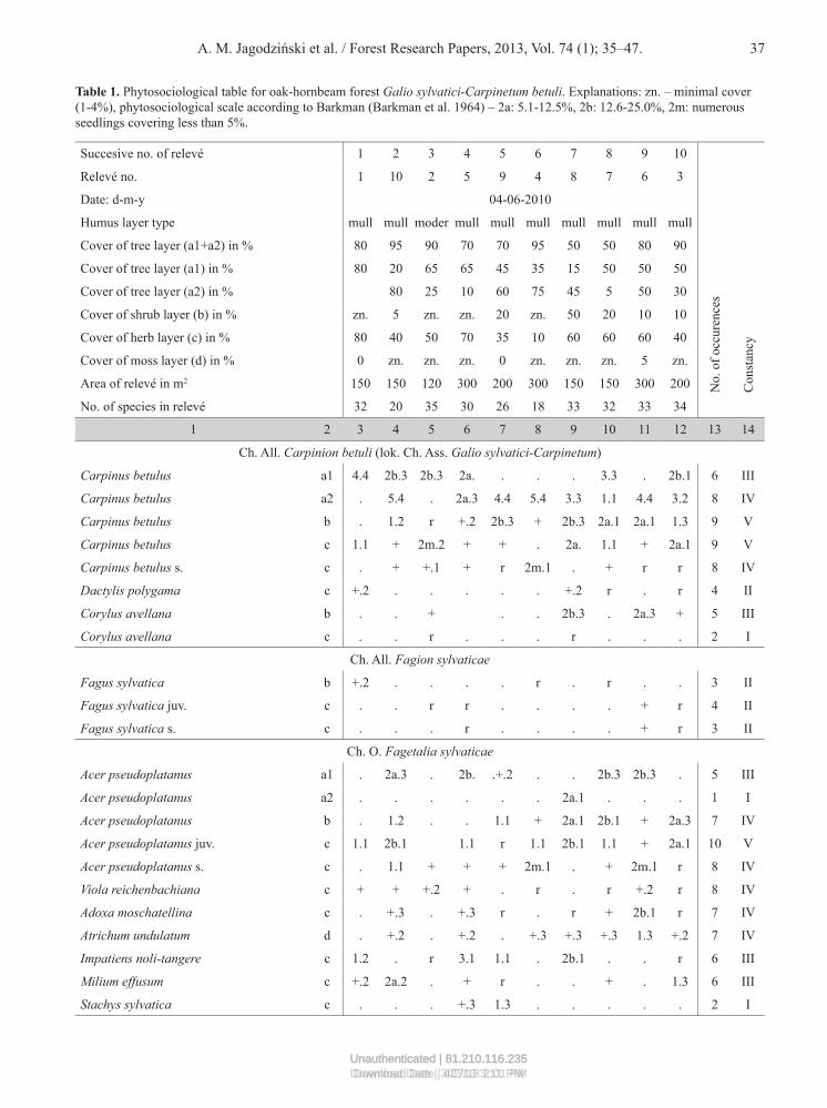
A. M. Jagodziński et al. / Forest Research Papers, 2013, Vol. 74 (1); 35–47. 37

Table 1. Phytosociological table for oak-hornbeam forest Galio sylvatici-Carpinetum betuli. Explanations: zn. – minimal cover (1-4%), phytosociological scale according to Barkman (Barkman et al. 1964) – 2a: 5.1-12.5%, 2b: 12.6-25.0%, 2m: numerous seedlings covering less than 5%.

Succesive no. of relevé 1 2 3 4 5 6 7 8 9 10

No.

of o

ccur

ence

s

Con

stan

cy

Relevé no. 1 10 2 5 9 4 8 7 6 3

Date: d-m-y 04-06-2010

Humus layer type mull mull moder mull mull mull mull mull mull mull

Cover of tree layer (a1+a2) in % 80 95 90 70 70 95 50 50 80 90

Cover of tree layer (a1) in % 80 20 65 65 45 35 15 50 50 50

Cover of tree layer (a2) in % 80 25 10 60 75 45 5 50 30

Cover of shrub layer (b) in % zn. 5 zn. zn. 20 zn. 50 20 10 10

Cover of herb layer (c) in % 80 40 50 70 35 10 60 60 60 40

Cover of moss layer (d) in % 0 zn. zn. zn. 0 zn. zn. zn. 5 zn.

Area of relevé in m2 150 150 120 300 200 300 150 150 300 200

No. of species in relevé 32 20 35 30 26 18 33 32 33 34

1 2 3 4 5 6 7 8 9 10 11 12 13 14

Ch. All. Carpinion betuli (lok. Ch. Ass. Galio sylvatici-Carpinetum)

Carpinus betulus a1 4.4 2b.3 2b.3 2a. . . . 3.3 . 2b.1 6 III

Carpinus betulus a2 . 5.4 . 2a.3 4.4 5.4 3.3 1.1 4.4 3.2 8 IV

Carpinus betulus b . 1.2 r +.2 2b.3 + 2b.3 2a.1 2a.1 1.3 9 V

Carpinus betulus c 1.1 + 2m.2 + + . 2a. 1.1 + 2a.1 9 V

Carpinus betulus s. c . + +.1 + r 2m.1 . + r r 8 IV

Dactylis polygama c +.2 . . . . . +.2 r . r 4 II

Corylus avellana b . . + . . 2b.3 . 2a.3 + 5 III

Corylus avellana c . . r . . . r . . . 2 I

Ch. All. Fagion sylvaticae

Fagus sylvatica b +.2 . . . . r . r . . 3 II

Fagus sylvatica juv. c . . r r . . . . + r 4 II

Fagus sylvatica s. c . . . r . . . . + r 3 II

Ch. O. Fagetalia sylvaticae

Acer pseudoplatanus a1 . 2a.3 . 2b. .+.2 . . 2b.3 2b.3 . 5 III

Acer pseudoplatanus a2 . . . . . . 2a.1 . . . 1 I

Acer pseudoplatanus b . 1.2 . . 1.1 + 2a.1 2b.1 + 2a.3 7 IV

Acer pseudoplatanus juv. c 1.1 2b.1 1.1 r 1.1 2b.1 1.1 + 2a.1 10 V

Acer pseudoplatanus s. c . 1.1 + + + 2m.1 . + 2m.1 r 8 IV

Viola reichenbachiana c + + +.2 + . r . r +.2 r 8 IV

Adoxa moschatellina c . +.3 . +.3 r . r + 2b.1 r 7 IV

Atrichum undulatum d . +.2 . +.2 . +.3 +.3 +.3 1.3 +.2 7 IV

Impatiens noli-tangere c 1.2 . r 3.1 1.1 . 2b.1 . . r 6 III

Milium effusum c +.2 2a.2 . + r . . + . 1.3 6 III

Stachys sylvatica c . . . +.3 1.3 . . . . . 2 I



1 2 3 4 5 6 7 8 9 10 11 12 13 14Ch. Cl. Querco-Fagetea

Fraxinus excelsior a1 . . . 2a. 1.2 2a. 2a.3 1.3 3.1 2b.1 7 IVFraxinus excelsior b . . . . . . . r . . 1 IFraxinus excelsior s. c +.2 r + + + 2m.1 . r . . 7 IVFraxinus excelsior juv. c + + r r 1.1 r + + 1.1 r 10 VAcer platanoides a1 . . 3.3 . . 1.1 . . . 2b.1 3 IIAcer platanoides a2 . . . . 1.1 . 2b.1 . . . 2 IAcer platanoides b 1.2 . . . + . r r + . 5 IIIAcer platanoides juv. c + + + + r + r + + r 10 VAcer platanoides s. c . . + + . 2m.1 . r r + 6 IIIPoa nemoralis c +.2 1.2 +.2 1.2 . . + + r + 8 IVAegopodium podagraria c 1.3 . . . 1.2 . . . . . 2 IEuonymus europaeus c . r . . r . + r r . 5 III

Ch. Cl. Artemisietea vulgaris Galium aparine c 1.2 r r 1.1 . r +.2 + 1.3 r 9 VAllaria petiolata c r r +.2 +.2 . + +.2 + . 8 IVImpatiens parviflora c 4.4 2a.1 2b.1 . 1.1 1.1 . 2b.1 2b.1 2a.1 8 IVGeranium robertianum c 3.4 r 1 . + . 1.1 +.2 + . 7 IVChaerophyllum temulum c +.1 . r . . . r r . . 4 IIChelidonium majus c +.2 . r . r . . . . 4 IIGlechoma hederacea c . . . . . . +.2 + 1.3 4 IIGaleopsis pubescens c . . . 1.3 . . . +.2 +.2 . 3 IIGeum urbanum c +.1 . . r . . +.2 . . . 3 IIUrtica dioica c +.2 . . . . . +.2 . . . 2 IRubus idaeus c . . . . +.2 . 2b.3 . . . 2 I

Accompanying speciesQuercus robur a1 . . 5.3 1.1 3.4 2a.2 2a.3 . . . 5 IIIQuercus robur c . .r r r . r r r . . 6 IIIAesculus hippocastanum a1 2b.3 . . . . . . . . . 1 IAesculus hippocastanum a2 . . 2b.3 . . . . . . . 1 IAesculus hippocastanum juv. c . . r . r . . . . . 2 IAesculus hippocastanum s. c r . . . . . . . . 2 IRobinia pseudoacacia a2 . . + . . . . . . 2 IRobinia pseudoacacia juv. c . . r . . . . r . 3 IITilia platyphyllos juv. c .+ . + . r + r r . . 6 IIIRubus fruticosus (sp. coll.) c . r +.2 1.2 r r . + r + 8 IVDryopteris carthusiana c r . + r . + +.2 r +.2 1.1 8 IVOxalis acetosella c +.2 . +.2 +.3 . +.3 . 1.3 . + 6 IIIMoehringia trinervia c r . r + . + . + +.2 + 7 IVMaianthemum bifolium c +.2 + 2b.3 . +.2 . . . r r 6 IIIPadus avium b . . . . . . . + . . 1 IPadus avium c . . r r + . r + . 6 IIIPrunus serotina c r . . r . . . . r r 4 IIAthyrium filix-femina c + . + . . . . . . + 3 IISambucus nigra b . . . . . . + . + r 3 IISambucus nigra c . r . r + . . . + . 4 IITilia sp. s. c . + . r . r . . r . 4 IIBrachythecium rutabulum d . . r r . . r . . 4 IIRubus caesius c . . +.2 . . +.2 . . . 3 IIUlmus laevis c . . . . r . r . . r 3 IICrataegus monogyna c . . . r . r . . . r 3 II



Plant collection and lab works

Understorey biomass was determined by the plant material collected from the study plots from March 20 to October 2, 2010 (in 18 terms). From March 20 to May 29 the plants were harvested every 7 days, and then every 14 days. The frequency of material collection was initially greater in order to register the dynamic changes taking place in the undergrowth in the spring. This is particularly important in the case of associations in which geophytes can be observed.

At each time, the material was collected from 10 randomly placed frames (repetitions), under relatively uniform topographic conditions, marking sample points on a simplified map and avoiding their overlapping in the following harvest dates. A single sample consisted of a collection of plants from the area limited by a square metal frame with dimensions of 0.6 × 0.6 m (0.36 m2). While choosing locations of sample plots, trodden paths, dense clumps of natural regeneration, piles of woody debris, and places of wild boar rooting were avoided. All plants (including woody plants of height up to 0.5 m) that grew within the frame were collected by cutting them flush with the surface of the ground using scissors and shears. Individuals growing outside of the frame, but having some parts inside, were not taken into account. However, those plants which grew within the frame, i.e. in the area of the sample, were cut and whole of it was treated as a part of the collection sample. It has been assumed that inside the frame the parts of plants growing outside it balance the sticking out fragments of individuals growing in the sample area. The plants were separated by identifying the species. The collected material was placed into the separated appropriately identified envelopes. During fieldwork, the biomass of woody plants and herbaceous perennials produced

in 2010 was separated from that produced in previous years. In order to assess changes in herbaceous biomass produced during the growing season of 2010, both biomass of woody plants (seedlings) and herbaceous biomass produced before 2010 were excluded from the collected biomass. Due to the fact that in some places the collection of plant material was composed solely of woody plants, the number of samples included in the analysis ranged from 7 to 10.

The collected material was transported to the Institute of Dendrology of the Polish Academy of Sciences in Kórnik, where it was dried at 65ºC to constant weight (at least 7 days) in forced-air dryers (ULE 600, Memmert GmbH + Co.KG, Germany), and then weighed. The total mass from each of the collected samples was determined for each species separately with accuracy of 0.001 g using weights BP 210 S and Mettler Toledo PG 1003-S.

Statistical analysis

Statistical differences between the weights of plants in the analyzed harvest dates were determined using one-way analysis of variance (ANOVA), and the mean values were compared using the Tukey’s test. Hereinafter we use abbreviations SE and CV for standard error and coefficient of variation, respectively. The weight of plants of each species was related to the whole collection period, even if the species did not appear in all of the collected samples. Regardless of the number of samples in which the species occurred, the average weight was calculated as though it was present in each collected sample. For statistical analyzes the JMP software was used (SAS Institute, Cary, NC, USA).

Sporadic species Ch. All. Carpinion betuli (lok. Ch. Ass. Galio sylvatici-Carpinetum): Tilia cordata b 1 (r), 8 (r), T. cordata c 8 (r);Ch. Cl. Querco-Fagetea (incl. Ch. O. Fagetalia sylvaticae, Ch. All. Fagion sylvaticae, Ch. All. Alno-Ulmion): Ulmus minor b 1 (r), U. minor c 5 (r), Plagiomnium undulatum d 9 (1), Acer campestre c 3 (r), Populus tremula c 3 (r), Dryopteris filix-mas 3 (+), 10 (r), Ribes spicatum b 6 (r), R. spicatum c 7 (r), 9 (+), Scrophularia nodosa 7 (r), 8 (r), Carex digitata 9 (+), Anemone nemorosa 9 (r), Carex sylvatica 10 (r), Crataegus laevigata 7 (r);Ch. Cl. Artemisietea vulgaris: Lamium maculatum 1 (2a).Accompanying species: Stellaria media 10 (r), Sorbus aucuparia b 1 (+), 10 (r), S. aucuparia c 3 (r), Tilia platyphyllos b 6 (r), 9 (+), Ajuga reptans 1 (+), 7 (1), Dryopteris carthusiana 3 (1), 7 (r), Geum rivale 6 (r), 10 (r), 4 (r), Lysimachia vulgaris 5 (r), 7 (+), Poa trivialis 1 (r), 9 (r), Scleropodium purum d 3 (r), 10 (r), Dicranella heteromalla d 4 (r), 8 (r), Fraxinus pennsylvanica a1 10 (2), Picea abies a1 3 (2a), Quercus rubra 9 (r), Robinia pseudoacacia s., Mycelis muralis 8 (+), Viola canina 7 (+), Betula pendula a1 9 (+), B. pendula a2 3 (+), Polytrichum formosum d 10 (r).



3. Results

Phytosociological relations

Based on phytosociological relevés made on the experimental plot, the presence of oak-hornbeam forest in two subassociations was diagnosed: Galio sylvatici-Carpinetum typicum and Galio sylvatici-Carpinetum corydaletosum, All. Carpinion betuli, O. Fagetalia sylvaticae, Cl. Querco- Fagetea (tab. 1).

On the study area, plant species diversity is faint and plant community exhibits features of severe impoverishment. There are no characteristic species in the strict sense for Galio sylvatici-Carpinetum; therefore, assigning the studied area to this community is determined mainly by a significant quantitative share of Carpinus betulus and the presence of Dactylis polygama, recognized as a characteristic species of the Carpinion betuli association. Another species attributed to this plant association is Corylus avellana, but its connections with the oak-hornbeam forests in the Greater Poland region are hardly visible; this species is common here in the ash and alder riparian forests. Additional feature which contributes to recognition of the studied plant community as oak-hornbeam forest, is a very small proportion of species characteristic for other types of mesotrophic forests: riparian (All. Alno-Ulmion) and beech (All. Fagion) forests.

It is problematic to assign the studied plant patches to plant subassociation. Due to the topographical and hydrological situation (located in the valley of a few streams and high water table) it should be expected that the studied patches represent the most humid variant of an oak-hornbeam forest - G.s.-C. corydaletosum; however, in the studied patches very few geophytes occurred, and their range was limited to the closest vicinity of the stream. The described area also lacked distinctive species of other subassociations of oak-hornbeam forest, such as poor acid oak-hornbeam forest G.s.-C polytrichetosum and dry oak-hornbeam forest G.s.-C. lathyretosum. Thus, on the basis of a floral composition, these patches need to be assigned to a typical subassociation Galio sylvatici-Carpinetum typicum. It should be noted that it is impossible to determine whether such phytocoenosis formation is only the result of habitat, or the lack of distinctive species is due to observable floristic impoverishment, which may be the result of anthropopression (periodically strong thinning, grazing and even eradication of plants due to collection for decorative purposes). Such interactions are very likely in the woods adjacent to the park complex located near urban areas. The anthropopression supposition is

also supported by the fact that in the undergrowth the geophytes, which are not associated with humid habitats and which are generally abundant in typical variant of hornbeam forest, such as Anemone nemorosa, Adoxa moschatellina, and even Hepatica nobilis, which also occurs frequently in dry oak habitats, are very poorly represented. These floristically poor forms of oak-hornbeam forests, probably of anthropogenic origin, are known from the whole Polish lowland, and the most striking example in spring geophytes is the poor Grabina oak-hornbeam forest reserve in the Wielkopolska (Greater Poland) National Park (Balcerkiewicz et al. 1992).

Apart from a clear depletion of flora, the studied forest community bears no visible signs of other forms of degeneration of plant communities. The only clear anthropogenic trace is the presence of a few individuals of an alien tree species on the periphery of the tree stand – Aesculus hippocastanum – and a single occurrence of two other invasive species: Padus serotina and Impatiens parviflora. The last two of these species in the study area are relatively sparse.

Dynamics of understorey biomass

The material collected throughout the growing season includes 57 species of both herbaceous (33 species) and tree (24 species) plants. Additionally, among the collected plant material four species of mosses have been found: Atrichum undulatum, Brachythecium rutabulum, Polytrichum formosum, Pseudoscleropodium purum.

Average mass of plants (produced in 2010 and earlier) differ significantly between terms of collection (p=0.0006, tab. 2). The smallest biomass was recorded on April 3 (37.2 kg/ha), while the highest one on June 12 (337.6 kg/ha), May 1 (308.1 kg/ha), May 15 (280.0 kg/ha) and May 8 (279.5 kg/ha).

By analyzing changes in solely herbaceous biomass produced during the growing season of 2010, a statistically significant difference between them could be observed at different times of collection (p=0.0007, tab. 2). The smallest mass of herbs was observed on April 3 (13.0 kg/ha), while the largest on May 1 (259.8 kg/ha), June 12 (246.5 kg/ha) and May 15 (245.4 kg/ha).

The most commonly reported species in the growing season were: Oxalis acetosella (in 18 collections), Moehringia trinervia (17), Geranium robertianum (16), Impatiens parviflora (14), Maianthemum bifolium (13), and Viola reichenbachiana (13). Although these species were found in many of the analyzed periods, their share in the total biomass of herbaceous plants was not high. For example, the average share of Oxalis acetosella was 2%, of Moehringia trinervia – 3%, Geranium robertianum



and Impatiens parviflora – both 6%, Maianthemum bifolium – 8%, and Viola reichenbachiana – 4% (tab. 3).

In the analyzed periods, different numbers of herbaceous species within the samples (from 9 to 22, tab. 3) were reported. Analysis of the share of each species in the understorey biomass indicated the dominance of just a few of them, but their dominance has been changing in the course of growing season. For example, biomass of Ficaria verna predominated in 8 of 18 collection periods (from March 20 to May 22, with the exception of May 1, when it was a co-dominant species), and its presence was recorded nine times in total. Average weight of F. verna from all terms in which it was recorded, amounted to 48.2 kg/ha and ranged from 5.5 kg/ha to 88.4 kg/ha. The average share of biomass for this species was 36.0% and oscillated between 14.5 and 51.0% during the growing season (tab. 3). Distinctive group of plants, i.e., ferns Athyrium filix-femina, Dryopteris filix-mas, Dryopteris carthusiana, were reported only in 1-4 terms; nevertheless, the share of their biomass in the total weight of herbaceous plants collected in a given term was very high. For example, the average share of the mass of Athyrium filix-femina (recorded only on September 4)

was 52.2%, the average share of biomass of Dryopteris filix-mas (recorded on three dates: May 8, August 7, and September 18) was 33.4%, while that of Dryopteris carthusiana (recorded four times: March 20, April 17, July 10, and October 2) was 25.9%.

The obtained results allow us to trace the changes in biomass of individual species in the growing season (tab. 3). For example, the biomass of Oxalis acetosella, a species present in all harvest dates, reached its maximum value on May 15 (8.4 kg/ha), accounting for 3.4% of the total mass of plants collected on that date. The greatest share of this species (7.6%) in total herbaceous biomass was recorded on March 20. The average weight of Moehringia trinervia was 3.2 kg/ha (range from 0.01 to 16.6 kg/ha). The average share of biomass of this species was 3.0% and ranged from 0.02% (on August 7) to 14.7% (on March 20). Slightly less frequently recorded species was Impatiens parviflora. Its biomass ranged from 0.7 kg/ha (on September 18) to 39.8 kg/ha (on June 12) and averaged 9.7 kg/ha. The share of Impatiens parviflora with respect to the total biomass ranged from 0.5% (September 18) to 16.2% (June 12).

Table 2. Mean biomass of all plants (herbaceous and woody species, produced in the year 2010 and previous years) and herbaceous plants (produced in the year 2010).

Date of biomass

harvesting

Day of year

Plant biomass (kg/ha) Biomass of herbaceous plants (kg/ha)

min. max. mean SE CV (%) min max. mean SE CV

(%)20.03. 79 19,2 469,1 105,4 ab 42,2 126,7 1,8 108,7 33,1 ab 11,2 101,803.04. 93 2,9 87,9 37,2 b 8,6 73,0 0,0 34,5 13,0 b 3,7 91,110.04. 100 81,0 792,3 214,9 ab 8,6 108,7 26,8 436,5 110,5 ab 37,9 108,417.04. 107 91,5 505,1 219,1 ab 42,3 61,0 4,5 351,4 169,7 ab 34,5 64,324.04. 114 18,9 573,0 210,5 ab 59,6 89,5 1,8 549,7 173,3 ab 61,2 111,701.05. 121 28,7 449,4 308,1 a 44,3 45,4 89,8 384,1 259,8 a 37,0 42,708.05. 128 28,7 695,6 279,5 ab 61,0 69,1 16,1 569,3 226,0 ab 54,5 76,215.05. 135 22,6 731,1 280,0 ab 67,4 76,1 83,8 662,0 245,4 a 63,3 77,422.05. 142 30,8 654,7 182,4 ab 61,2 106,1 1,1 572,9 129,1 ab 55,1 134,812.06. 163 30,5 821,6 337,6 a 76,3 71,5 0,1 794,8 246,5 a 76,8 98,626.06. 177 83,1 482,6 253,3 ab 41,7 52,0 51,6 362,2 147,9 ab 29,5 63,010.07. 191 72,4 381,4 188,4 ab 38,7 65,0 15,6 377,4 130,1 ab 41,4 100,724.07. 205 41,0 363,8 219,0 ab 41,8 60,3 4,1 358,4 128,2 ab 39,3 96,807.08. 219 31,7 230,6 124,4 ab 21,8 55,5 2,4 230,6 79,5 ab 27,8 105,021.08. 233 22,3 220,7 121,6 ab 26,3 68,5 0,4 218,0 64,3 ab 29,5 121,404.09. 247 10,9 454,3 123,6 ab 45,9 117,5 1,1 344,9 64,8 ab 42,0 183,218.09. 261 13,7 644,1 119,9 ab 63,5 167,4 7,3 600,1 146,0 ab 83,9 151,902.10. 275 10,0 254,2 97,0 ab 24,1 78,6 3,8 216,1 42,6 ab 25,2 167,7

ANOVA F P F PP>F 2,7129 0,0006 2,6858 0,0007


A. M. Jagodziński et al. / Forest Research Papers, 2013, Vol. 74 (1); 35–47.Ta

ble

3. M

ean

plan

t bio

mas

s (kg

/ha)

of t

he p

artic

ular

her

bace

ous s

peci

es a

nd p

erce

nt b

iom

ass o

f ind

ivid

ual p

lant

spec

ies b

y ha

rves

t per

iod

in re

latio

n to

the

tota

l her

bace

ous

plan

t bio

mas

s har

vest

ed o

n a

give

n da

te (%

).

Spec

ies

Plan

t bio

mas

s (kg

/ha)

and

bio

mas

s sha

re in

tota

l und

erst

orey

bio

mas

s (%

)20

.03.

03.0

4.10

.04.

17.0

4.24

.04.

01.0

5.08

.05.

15.0

5.22

.05.

12.0

6.26

.06.

10.0

7.24

.07.

07.0

8.21

.08.

04.0

9.18

.09.

02.1

0.

Adox

a m

osch

atel

lina

0,46

(3,5

8)15

,14

(13,

70)

18,9

7(1

1,17

)3,

03(1

,75)

48,1

4(1

8,53

)9,

73(4

,31)

27,3

2(1

1,14

)11

,98

(9,2

8)3,

42(1

,39)

4,32

(2,9

2)0,

32(0

,25)

Aego

podi

um p

odag

rari

a1,

60(1

,44)

1,86

(1,0

7)6,

33(4

,90)

1,11

(0,4

5)2,

21(1

,49)

8,46

(6,5

0)6,

59(5

,14)

5,06

(6,3

7)0,

16(0

,24)

9,38

(6,4

2)

Ajug

a re

ptan

s2,

40(7

,24)

11,1

9(4

,31)

34,6

6(1

5,34

)28

,98

(11,

81)

10,5

0(8

,13)

1,20

(0,4

9)11

,42

(7,7

2)2,

52(1

,94)

3,37

(2,6

3)1,

65(2

,54)

Allia

ria

petio

lata

1,15

(3,4

6)0,

71(0

,64)

0,72

(0,4

2)5,

49(2

,11)

2,57

(1,1

4)0,

35(0

,14)

1,79

(1,3

9)0,

06(0

,02)

1,42

(1,0

9)0,

41(0

,32)

0,32

(0,2

2)

Anem

one

nem

oros

a2,

32(1

7,89

)5,

16(4

,67)

16,5

6(9

,76)

4,26

(2,4

6)37

,14

(14,

30)

9,09

(4,0

2)2,

81(2

,18)

Athy

rium

filix

-fem

ina

36,4

4(5

6,20

)

Cha

erop

hyllu

m te

mul

um1,

65(0

,95)

27,5

4(1

1,17

)7,

09(4

,80)

0,01

(0,0

2)

Che

lidon

ium

maj

us1,

43(1

,29)

4,83

(1,8

6)0,

29(0

,68)

Dac

tylis

pol

ygam

a5,

89(2

,39)

7,10

(8,9

2)

Dry

opte

ris c

arth

usia

na2,

15(6

,49)

7,77

(4,5

8)37

,74

(29,

00)

27,0

1(6

3,46

)

Dry

opte

ris d

ilata

ta5,

13(2

,09)

11,1

1(4

,51)

35,4

7(2

3,97

)35

,80

(27,

92)

10,1

0(1

2,70

)7,

59(1

1,80

)1,

49(3

,51)

Dry

opte

ris fi

lix-m

as21

,07

(9,3

2)25

,62

(32,

23)

85,7

3(5

8,70

)

Fica

ria

vern

a15

,92

(48,

05)

5,51

(42,

44)

55,5

6(5

0,28

)79

,49

(46,

83)

88,4

1(5

1,03

)37

,74

(14,

53)

55,7

3(2

4,66

)76

,16

(31,

04)

18,9

5(1

4,68

)

Gal

eops

is p

ubes

cens

0,08

(0,0

3)0,

63(0

,48)

1,50

(1,8

9)1,

81(2

,82)

0,52

(0,8

1)5,

05(3

,46)

5,72

(13,

45)

Gal

ium

apa

rine

3,64

(3,3

0)0,

97(0

,57)

1,60

(0,9

3)7,

13(2

,75)

0,54

(0,2

4)0,

34(0

,14)

2,34

(1,8

1)0,

40(0

,16)

0,10

(0,0

7)

Ger

aniu

m ro

bert

ianu

m0,

45(0

,41)

0,92

(0,5

4)9,

74(5

,62)

4,20

(1,6

2)8,

47(3

,74)

26,5

8(1

0,83

)7,

16(5

,55)

50,8

3(2

0,62

)16

,78

(11,

34)

5,95

(4,5

7)7,

33(5

,72)

2,72

(3,4

2)6,

07(9

,43)

1,21

(1,8

7)0,

24(0

,16)

2,21

(5,2

0)


43A. M. Jagodziński et al. / Forest Research Papers, 2013, Vol. 74 (1); 35–47.

Geu

m u

rban

um0,

64(1

,94)

0,06

(0,0

3)1,

31(0

,58)

0,58

(0,2

4)12

,05

(9,3

3)7,

88(3

,20)

3,40

(4,2

8)14

,63

(22,

74)

4,25

(6,5

5)

Gle

chom

a he

dera

cea

13,7

6(6

,09)

4,65

(1,9

0)0,

04(0

,03)

16,0

4(6

,51)

3,02

(2,3

2)1,

69(1

,32)

0,02

()0,

02

Impa

tiens

nol

i-tan

gere

0,11

(0,0

7)0,

02(0

,01)

1,34

(0,5

9)0,

07(0

,03)

2,14

(0,8

7)1,

50(1

,02)

Impa

tiens

par

viflo

ra1,

12(0

,66)

6,96

(4,0

2)7,

57(2

,91)

12,5

4(5

,55)

11,9

7(4

,88)

10,2

2(7

,91)

39,8

1(1

6,15

)10

,69

(7,2

3)17

,42

(13,

38)

8,60

(6,7

1)2,

81(3

,53)

3,17

(4,9

4)1,

55(2

,38)

0,72

(0,4

9)

Lam

ium

mac

ulat

um28

,23

(16,

63)

32,1

9(1

8,58

)3,

51(1

,42)

17,5

3(1

3,67

)30

,67

(21,

00)

Lysi

mac

hia

num

mul

aria

18,9

3(2

3,80

)

Mai

anth

emum

bifo

lium

1,61

(12,

43)

9,61

(5,6

6)15

,18

(8,7

6)29

,19

(11,

24)

5,78

(2,5

6)9,

31(3

,80)

18,4

3(1

4,27

)16

,14

(6,5

5)15

,31

(10,

35)

14,6

2(1

1,23

)16

,15

(12,

59)

1,49

(2,3

0)1,

32(0

,90)

Mili

um e

ffusu

m20

,92

(8,0

5)18

,27

(8,0

9)35

,86

(14,

61)

23,3

4(1

5,78

)16

,48

(12,

67)

5,53

(4,3

1)22

,67

(35,

24)

2,56

(3,9

4)4,

58(3

,14)

3,52

(8,2

8)

Moe

hrin

gia

trin

ervi

a4,

88(1

4,73

)1,

43(1

1,02

)2,

01(1

,82)

1,77

(1,0

4)1,

02(0

,59)

16,6

2(6

,40)

4,75

(2,1

0)7,

21(2

,94)

7,87

(6,1

0)2,

16(0

,88)

1,57

(1,0

6)1,

73(1

,33)

0,23

(0,1

8)0,

01(0

,02)

0,04

(0,0

6)0,

23(0

,16)

0,33

(0,7

7)

Myc

elis

mur

alis

0,09

(0,6

8)0,

10(0

,06)

2,31

(0,9

4)

Oxa

lis a

ceto

sella

2,51

(7,5

6)0,

04(0

,28)

5,48

(4,9

6)1,

32(0

,78)

5,16

(2,9

8)1,

60(0

,62)

1,56

(0,6

9)8,

43(3

,44)

1,18

(0,9

1)2,

17(0

,88)

4,31

(2,9

1)0,

11(0

,09)

0,18

(0,1

4)2,

22(2

,79)

1,60

(2,4

9)0,

42(0

,65)

0,08

(0,0

5)1,

90(4

,45)

Poa

nem

oral

is2,

36(7

,14)

12,6

7(1

1,47

)1,

23(0

, 71)

22,6

8(8

,73)

21,3

0(9

,42)

6,11

(4,7

3)15

,69

(12,

24)

Poa

triv

ialis

0,06

(0,0

2)0,

12(0

,08)

Stac

hys s

ylva

tica

50,3

8(2

0,44

)8,

31(5

,62)

18,6

0(1

4,30

)9,

12(7

,11)

Urt

ica

dioi

ca1,

44(1

1,11

)11

,37

(8,8

0)1,

28(1

,99)

Viol

a ca

nina

5,30

(2,0

4)0,

67(1

,03)

Viol

a re

iche

nbac

hian

a1,

12(3

,39)

0,07

(0,5

6)6,

64(6

,01)

3,00

(1,7

7)3,

54(1

,57)

2,41

(0,9

8)2,

27(0

,92)

5,53

(3,7

3)1,

10(0

,84)

5,50

(8,5

6)13

,89

(21,

43)

7,62

(5,2

1)0,

09(0

,20)

Day

of y

ear

7993

100

107

114

121

128

135

142

163

177

191

205

219

233

247

261

275

Num

ber o

f spe

cies

99

1212

1716

1816

1622

1515

1413

913

139


44 A. M. Jagodziński et al. / Forest Research Papers, 2013, Vol. 74 (1); 35–47.

4. Discussion

The study results showed statistically significant differences in the understorey biomass between the periods of material collection. Among the published studies on seasonal changes in understorey biomass in forest communities there are some which have shown a strong correlation between the date of harvest and the amount of biomass produced (e.g. Kaźmierczakowa 1971; Rawlik et al. 2012), as well as those which have demonstrated the lack of such a relationship (e.g. Tremblay, Larocque 2001). The amounts of understorey biomass may vary significantly in different plant communities at the same time. This is confirmed, for example, by the work of Kubiček and Jurko (1975), who determined the understorey biomass in August 1973 in Little Carpathians in Slovakia in five different forest communities varying in terms of trophic and moisture conditions. In Luzulo-Fagetum association, herbaceous biomass amounted to 41 kg/ha (excluding mosses), in Dentario-Fagetum – 364 kg/ha, in Aceri-Carpinetum – 476 kg/ha, in Carici pilosae-Carpinetum – 691 kg/ha, while in Stellario-Alnetum – 1364 kg/ha. On the other hand, in plant communities formed mainly by shrubs and mosses, standing biomass can take much greater value. For example, research of Sobisz and Parzych (2010) carried out in the Słowiński National Park shows that the understorey biomass in plant community of Vaccinio uliginosi-Betuletum pubescentis is 4745 kg/ha (of which 24% is the biomass of mosses), while in other plant community such as Empetro nigri-Pinetum it is 3393 kg/ha (of which 29% is the biomass of mosses).

The course of changes in understorey biomass (total and produced in 2010) in the growing season in the studied patches of Galio sylvatici-Carpinetum betuli is similar. Undergrowth biomass increases rapidly in early spring, reaches its maximum values in May and mid-June, and then decreases markedly. Maximum total biomass (including woody plants) is approximately 300 kg/ha, while the maximum herbaceous biomass produced during the analyzed growing season stands at around 250 kg/ha.

Comparison with the literature data shows that the states of understorey biomass in oak-hornbeam communities can be very diverse. For example, in oak-hornbeam forest of Tilio-Carpinetum stachyetosum, Kaźmierczakowa (1971) observed the highest values of undergrowth biomass in early July (in 1965 – 660 kg/ha, and in 1967 – 270 kg/ha). A significant difference in amounts of biomass between the investigated years was most likely caused by pathogenic fungi in the second turn of research. In the oak-hornbeam forest investigated by us, the highest weight of all plants was

recorded on June 12 and it amounted to 337.6 kg/ha, while the highest herbaceous biomass was produced on May 1, 2010 (259.8 kg/ha). Differences in the periods of maximum biomass occurrence may result from the species composition of ground vegetation, especially from the characteristics of growth and development of the dominant species. It is well illustrated by the oak-hornbeam forest described by Kaźmierczakowa (1971), in which the dominant species in terms of weight were Aegopodium podagraria, Stellaria holostea, Galium odoratum, and Ranunculus lanuginosus, i.e. species that grow rapidly after the end of flowering of the spring geophytes and that contribute to the easily observable effect of late-spring “greening” of the forest floor, which is very characteristic for the oak-hornbeam and riparian forests. In the oak-hornbeam forest in the Syców Forest District, however, there was no single species that would dominate throughout the whole growing season. The periodically largest share in the total weight of the plants has been observed in Ficaria verna and Impatiens parviflora. The first species is an early spring geophyte, the only representative of this typical for oak-hornbeam forests group of species that was observed constantly in the study area. The second one is an invasive annual plant species, beginning its growth relatively late and reaching a maximum density in June and early July (Piskorz, Klimko 2002; Piskorz 2005). This species is probably responsible for the observed maximum of the biomass in this study plot in the middle of June (compare with fig. 1). We also recorded the occurrence of Aegopodium podagraria in the investigated area, but its share in the total biomass was significantly lower than the one observed by Kaźmierczakowa (1971).

Understorey biomass production rate during the growing season and dates when biomass reaches the maximum value in the given plant community may vary in successive years. For example, Banasik (1978) found the highest values of understorey biomass in the medium moist oak-hornbeam forest Tilio-Carpinetum typicum on July 14, 1967 (433.4 kg/ha) and on June 4, 1968 (445.5 kg/ha), and of standing biomass very close to the maximum were reported on May 26, 1967 (374.2 kg/ha) and May 3, 1968 (312.2 kg/ha). These values are much higher than those obtained by us in the plant community of Galio sylvatici-Carpinetum betuli, although the states of maximum biomass were observed later. In turn, in the moist oak-hornbeam forest Tilio-Carpinetum stachyetosum, with a much smaller coverage of ground vegetation, the highest state of biomass was noted already on April 23, 1968 (243.0 kg/ha) (Banasik 1978). Both the term and amount of biomass are similar to the results obtained in plant community of Galio sylvatici-Carpinetum betuli in the



Syców Forest District. Research carried out by Traczyk and Traczyk (1967) shows that in forest communities with a significant share of geophytes the maximum values of understorey biomass are recorded in June-July. These authors noted undergrowth biomass in the community of Tilio-Carpinetum at two dates: April 28 (121.6 kg/ha) and July 8 (338.2 kg/ha).

Comparison of the results presented in this paper with data of Rawlik et al. (2012) from the area of the Różańsko Forest District indicates that the maximum biomass of understorey in Galio sylvatici-Carpinetum betuli takes place at the same time as in the community of Stellario holosteae-Carpinetum betuli (end of April to mid-May, fig. 1). Both total understorey biomass, i.e. including

woody (seedlings) and herbaceous plants (produced in 2010 and earlier, fig. 1A), as well as herbaceous biomass produced in 2010 (fig. 1B), were significantly higher in patches of Stellario holosteae-Carpinetum betuli studied by Rawlik et al. (2012) than in patches of Galio sylvatici-Carpinetum betuli in Syców during the period of maximum plant biomass in both communities. It is worth noting the fact that in the second decade of May the state of biomass in the oak-hornbeam forest Galio sylvatici-Carpinetum betuli is still higher than the one recorded at the same time in the community of Stellario holosteae-Carpinetum betuli (until the end of July). The maximum herbaceous biomass produced in 2010 was recorded in the community of Galio sylvatici-Carpinetum betuli on May 1 (259.8 kg/ha), while in the community of Stellario holosteae-Carpinetum betuli it was on May 15 (378.4 kg/ha) (Rawlik et al. 2012). It can be assumed that the differences observed in Syców are caused by a high share in the undergrowth of an annual neophyte Impatiens parviflora, which reaches its maximum development in late spring and summer (Piskorz, Klimko 2002; Piskorz 2005). The presence of this species can also cause the reduction in biomass of other oak-hornbeam forest species, including the taxa determining the maximum biomass in spring in typical oak-hornbeam forests (Balcerkiewicz et al. 1996).

Floristic characteristics indicate differences in the herbaceous species composition of both communities. In the ground vegetation of oak-hornbeam in Syców there are quite numerous plant species of the class Artemisietea vulgaris, which are not typical for decidu-ous forests, and their presence may be due to the lo-cation of research area in the vicinity of the city park, and thus increased anthropopression. The undergrowth of oak-hornbeam forest in Różańsko species in class-es other than Querco-Fagetea have not been found (Rawlik et al. 2012). The ground flora in Różańsko is rather dominated by one species of geophytes, i.e. Anemone nemorosa, which reached the highest share in total plant biomass on April 10 (85% biomass), and the highest value of biomass on May 1 (258.23 kg/ha, 75.4% of the total biomass). In the plant community of Galio sylvatici-Carpinetum betuli the dominant species in spring was Ficaria verna; however, the prevalence of this species is not as clear as in the community of Stellario holosteae-Carpinetum betuli. The maximum weight of this species in patches of Galio sylvatici-Carpinetum betuli was reached on April 24 and was 88.4 kg/ha, which accounted for 51% of the total mass of plants in this period of collection. A similar, though slightly lower, share of Ficaria verna in the total mass was recorded on March 20. Therefore both communi-ties are marked by early spring geophytes domination,

0

100

200

300

400

500

50 100 150 200 250 300

Stellario holosteae – Carpinetum betuli (Rawlik et al. 2012)Galio sylvatici – Carpinetum betuli (this study)

A)

0

100

200

300

400

500

50 100 150 200 250 300Day of year

B)

Plan

t bio

mas

s (k

g/ha

)Pl

ant b

iom

ass

(kg/

ha)

Stellario holosteae – Carpinetum betuli (Rawlik et al. 2012)Galio sylvatici – Carpinetum betuli (this study)

Figure 1. Changes in mean plant biomass of A) woody and herbaceous species produced in 2010 and previous years and B) herbaceous species produced in 2010 in two plant com-munities: Stellario holosteae-Carpinetum betuli and Galio sylvatici-Carpinetum betuli over the growing season.



but the species are different and have different habitat requirements. In the ground vegetation of an oak-horn-beam forest Stellario holosteae-Carpinetum betuli after the period of geophytes dominance, the plant weight reduces significantly. After the withering of geophytes, the summer species start to dominate: Galeobdolon lu-teum and Galium odoratum. In this period in the ground vegetation of oak-hornbeam forest Galio sylvatici-Car-pinetum betuli the species noticed without any marked dominance were more.

The development of ground flora is significantly influenced by tree species composition, especially the share of deciduous trees, which determines the changing light conditions in the studied phytocoenosis. In early spring, when the trees have not yet developed leaves, the forest floor gets more light, of which spring plants take advantage. In the investigated oak-hornbeam forest the highest average biomass of herbaceous plants was recorded on May 1, when the undergrowth was dominated by geophytes. In communities where geophytes are not so numerous, the highest state of biomass is generally observed in June and July in the case of dicots, while in the case of monocots – in mid-September (Kaźmierczakowa 1971).

5. Summary

The study results showed statistically significant differences in the state of understorey biomass during the growing season. The smallest total biomass of an understorey layer (including woody plants) was recorded on April 3 (37.2 kg/ha), while the highest on June 12 (337.6 kg/ha), May 1 (308.1 kg/ha), May 15 (280.0 kg/ha) and May 8 (279.5 kg/ha). Taking into consideration only herbaceous biomass produced during the analyzed growing seasosn, the lowest biomass was found on April 3 (13.0 kg/ha), while the highest on May 1 (259.8 kg/ha), June 12 (246.5 kg/ha) and May 15 (245.4 kg/ha). The data indicate that although the share of herbaceous biomass expressed as a percentage of total aboveground biomass of the forest community is small, the rate of biomass production is important in the macro- and micronutrient cycle in the ecosystem. The greatest amounts of biomass and the rate of its production in oak-hornbeam forest Galio sylvatici-Carpinetum betuli were found in early spring, when the access of light to the forest floor is not limited by the developed leaves of the trees. Geophytes play an important role in the increased biomass production in spring, as they produce large amounts of biomass in a relatively short period of time.

Acknowledgment

We would like to thank the reviewers for insightful and valuable comments, which were used in the final version of the article.

References

Balcerkiewicz S., Brzeg A., Kasprowicz M. 1992. Roślinność rezerwatów ścisłych Wielkopolskiego Parku Narodowego, in: Przyroda Wielkopolskiego Parku Narodowego. (ed. L. Kaczmarek, B. Walna). Materiały z konferencji nauko-wej. Uniwersytet im. Adama Mickiewicza w Poznaniu, Stacja Ekologiczna w Jeziorach, pp. 91–96.

Balcerkiewicz S., Brzeg A., Kasprowicz M. 1996. Roślinność rezerwatu “Pod Dziadem” w Wielkopolskim Parku Narodowym. Badania Fizjograficzne nad Polską Zachodnią – seria B, 45: 79–120.

Banasik J. 1978. Sezonowy rozwój i produkcja netto runa w dwóch płatach lasu grądowego Puszczy Niepołomickiej. Studia Naturae – seria A, 14: 67–134.

Barbier S., Gosselin F., Balandier P. 2008. Influence of tree species on understorey vegetation diversity and mechani-sms involved – A critical review for temperate and boreal forests. Forest Ecology and Management, 254(1): 1–15.

Barkman J.J., Doing H., Segal S. 1964. Kritische Bemerkungen und Vorschläge zur quantitativen Vegetationsanalyse. Acta Botanica Neerlandica, 13: 394–419.

BULiGL 2000. Operat siedliskowo-glebowy dla Nadleśnictwa Syców wg stanu na 01.01.2000 na okres obowiązywania od 01.01.2000 do 31.12.2009. Biuro Urządzania Lasu i Geodezji Leśnej w Brzegu. Maszynopis w Nadleśnictwie Syców.

BULiGL 2010. Plan Urządzenia Lasu dla Nadleśnictwa Syców wg stanu na 01.01.2010 na okres obowiązywa-nia od 01.01.2010 do 31.12.2019. Biuro Urządzania Lasu i Gospodarki Leśnej w Brzegu. Maszynopis w Nadleśnictwie Syców.

Chapin F.S. 1980. The mineral nutrition of wild plants. Annual Review of Ecology and Systematics, 11: 233–260.

Dafni A., Cohen D., Noy-Mier I. 1981. Life-cycle variation in geophytes. Annals of the Missouri Botanical Garden, 68(4): 652–660.

Dixon R.K., Brown S., Houghton R.A., Solomon A.M., Trexler M.C., Wisniewski J. 1994. Carbon pools and flux of global forest ecosystems. Science, 263: 185–190.

Gilliam F.S. 1988. Interactions of fire with nutrients in the herbaceous layer of a nutrient-poor Coastal Plain forest. Bulletin of the Torrey Botanical Club, 115(4): 265–271.

Gilliam F.S. 2007. The ecological significance of the herbace-ous layer in temperate forest ecosystems. Bioscience, 57: 845–858.

Gilliam F.S., Roberts M.R. 2003. The herbaceous layer in forests of eastern North America. New York. Oxford University Press. ISBN: 0-19-514088-5.

Kaźmierczakowa R. 1971. Ekologia i produkcja runa świetli-stej dąbrowy i grądu w rezerwatach Kwiatkówka i Lipny Dół na Wyżynie Małopolskiej. Studia Naturae, 15: 1–107.



Kubiček F., Jurko A. 1975. Estimation of the above-ground biomass of the herb layer in forest communities. Folia Geobotanica et Phytotaxonomica, 10: 113–129.

Matuszkiewicz J.M. 2001. Zespoły leśne Polski. Warszawa. WN PWN. ISBN: 83-01-13401-1

Matuszkiewicz W. 2007. Przewodnik do oznaczania zbioro-wisk roślinnych Polski. Warszawa. PWN. ISBN: 978-83-01-14439-5.

Muller R.N. 2003. Nutrient relations of the herbaceous layer in deciduous forest ecosystems, w: The herbaceous lay-er in forests of eastern North America. (red. F.S. Gilliam, M.R. Roberts). New York. Oxford University Press, pp. 15–37. ISBN: 0-19-514088-5.

Parzych A., Sobisz Z. 2010. Biomasa i produkcja pierwot-na netto roślin runa w wybranych zespołach leśnych Słowińskiego Parku Narodowego. Ochrona Środowiskai Zasobów Naturalnych, 42: 72–83.

Piskorz R. 2005. The effect of oak-hornbeam diversity on flo-wering and fruiting of Impatiens parviflora DC. Roczniki Akademii Rolniczej w Poznaniu – Botanica Steciana, 373(9): 187–196.

Piskorz R., Klimko M. 2002. Fenologia Impatiens parviflora DC. w silnie prześwietlonym gradzie środkowoeuropej-skim na lokalnym stanowisku w Wielkopolskim Parku Narodowym. Roczniki Akademii Rolniczej w Poznaniu – Botanika, 347(5): 135–144.

Rawlik M., Jagodziński A.M., Janyszek S. 2012. Sezonowe zmiany stanu biomasy w runie lasu grądowego Stellario holosteae-Carpinetum betuli. Leśne Prace Badawcze, 73(3): 221–235.

Rothstein D.E., Zak D.R. 2001. Photosynthetic adaptation and acclimation to exploit seasonal periods of direct irradian-ce in three temperate, deciduous-forest herbs. Functional Ecology, 15: 722–731.

Rutkowski L. 2006. Klucz do oznaczania roślin naczynio-wych Polski niżowej. Warszawa. PWN. ISBN: 978-83-01-14342-8.

Small C.J., McCarthy B.C. 2002. Spatial and temporal varia-bility of herbaceous vegetation in an eastern deciduous forest. Plant Ecology, 164: 37–48.

Traczyk H., Traczyk T. 1967. Tentative estimation of the pro-duction of herb layer. Ekologia Polska, 15(46): 823–835.

Trampler T., Kliczkowska A., Dmyterko E., Sierpińska A. 1990. Regionalizacja przyrodniczo-leśna na podstawach ekologiczno-fizjograficznych. Warszawa. PWRiL. ISBN: 83-913320-6-3.

Tremblay N.O., Larocque G.R. 2001. Seasonal dynamics of understorey vegetation in four eastern Canadian forest types. International Journal of Plant Sciences, 162(2): 271–286.

Widén B. 2002. Seasonal variation in forest-floor CO2 exchan-ge in a Swedish coniferous forest. Agricultural and Forest Meteorology, 111: 283–297.

Yarie J. 1980. The role of understorey vegetation in the nu-trient cycle of forested ecosystems in the mountain hem-lock biogeoclimatic zone. Ecology, 61: 1498–1514.


SzmitP

Rectangle

SzmitP

Textbox

in



Received 17 July 2012, accepted after revision 6 November 2012© 2013, Forest Research Institute

Slow Sand Filters as a part of integrated protection of seedlings against disease in forest nurseries

Tomasz Oszako1*, Katarzyna Anna Kubiak1, Marta Siebyła2, Justyna Anna Nowakowska3

1 Forest Research Institute, Department of Forest Protection, Braci Leśnej 3, Sękocin Stary, 05-090 Raszyn, Poland;2 Warsaw University of Life Sciences, Faculty of Agriculture and Biology, Nowoursynowska 159, 02-776 Warsaw, Poland;

3 Forest Research Institute, Department of Silviculture and Genetics, Braci Leśnej 3, Sękocin Stary, 05-090 Raszyn, Poland.

* Tel. + 48 22 715 38 23, fax. +48 22 715 05 57, e-mail: [email protected]

Abstract. Slow Sand Filters (SSF) are a biological method used to protect nursery plants, from pathogen infections which can cause serious diseases in many forest tree species. Thanks to SSF application the number of phytopathogens in nurseries can be significantly reduced, as demonstrated by many field and greenhouse experiments (e.g. in Polish nurseries, and for horticultural crops in Germany and The Netherlands).

In this study, the effect of pollution from fertilizers and fungicides used in agriculture (e.g. PCNB) on the efficiency of SSFs was assessed. A quantitative analysis was performed of the copiotrophic and oligotrophic bacterial composition colonizing SSF biofilms. The efficiency with which selected Oomycete strains belonging to the genus Phytophthora (P. alni, P. cactorum, P. plurivora) were removed from water was determined based on genetic material (DNA of the organisms) found in the SSF filtrate. Specific primers and TaqMan probes (qPCR) appeared to be the most sensitive molecular methods. Moreover, the microbiological analysis of SSF biofilm performed with selective media allowed the growth of copiothrophic and oligothrophic bacteria to be estimated. The influence of fungicide (PCNB) and N-fertilizer on the number of bacteria in each biofilm was also evaluated.

The pollution of water with fertilizer (being used for plant irrigation) was demonstrated to reduce the efficiency of filtration more than fungicide addition (the amount of DNA from those investigated pathogens in the water decreased with time). The amount of bacteria in SSF biofilm readily increased after application of N-fertilizer in contrast to fungicide (PCNB) addition.

Key words: Phytopathogen, biofilm, SSF, PCNB, mineral fertilizer

1. Introduction

Taking up water from natural surface water intakes (waterways) and its use for watering plants in nurseries, is risky because of spreading phytopathogens and the development of many plant diseases (Runia 1995; Wohanka 1995; Ehret et al., 2001). Water from nearby lakes and ponds is most often used for irrigation of nurseries. Frequently, these shots are located in the catchment area of the land used for agriculture, and that is why they are mostly contaminated with phytopathogens and products originating from agricultural sources (fertilizers, pesticides). Improper or excessive use of

chemical plant protection products involves numerous risks, including contamination of the environment (residue of plant protection products), reduction of biodiversity and occurrence of resistant organisms, harmful to plants.

Slow sand filters with biological membrane (biofilm) are designed to eliminate pathogens from water (Kubiak, Oszako 2011), among others, oomycetes belonging to the genus Phytophthora, which affect plants for plantings. Phytopathogens removal efficiency through filters depends on their types and activity of microbial processes occurring in their biofilters (Davey and O’toole 2000), which are also affected by anthropogenic pollution (e.g., caused by agricultural activities).

T. Oszako et al. / Forest Research Papers, 2013, Vol. 74 (1); 49–56.50

The aim of the study was to assess the impact of fertilizer (N) and fungicide (PCNB) on the effectiveness of working of slow sand filters (SSF) in the removal of phytopathogens from water used for plants watering. The analysis of the impact of water pollution (e.g., fertilizer), for quantitative composition of bacteria colonizing the biofilms of filters being used for watering plants in nurseries, was carried out too.

2. Materials and Methods

Analysis of the effectiveness of the elimination of phytopathogens by biofilters (SSF)

Was prepared in three variants. A) Biofilter 1 – control (natural); B) biofilter 2 – enriched with mineral fertilizer (in the amount of 55 ml/40 l of water with the composition as follows: total nitrogen – 3%, nitrate nitrogen – 1%, urea nitrogen – 2%, phosphorus pentoxide – 5%, potassium oxide – 7%, boron – 0.02%, copper – 0.008, iron – 0.03%, manganese – 0.015%, molybdate – 0.002%, zinc – 0.015%); C) biofilter 3 – containing additive of 1 g fungicide (PCNB) dissolved in 50 ml of 96% ethanol (fig. 1). Pure cultures of Phytophthora alni, P. plurivora, and P. cactorum were added to the container where 120 l of tap water was accumulated. Isolates that originated from the collection of Forest Research Institute (IBL) were incubated for 4 weeks in the dark at room temperature, growing on the liquid vegetable medium (V8). The day before the filtration had started, the above cultures were transferred for 24 hours to the temperature

of 4°C (to initiate spores production), and then were homogenized and mixed together in equal volumes. After adding the mixture of oomycetes to tap water, the filtration system worked for two days without any break. The water was pumped out in parallel to the three filters (SSF) having different biofilm variants: filter 1 (F1) – biofilm control, filter 2 (F2) – a biofilm with a mineral fertilizer, and filter 3 (F3) – biofilm with PCNB. Samples of water were collected prior to and during the filtration at specified intervals (3, 6, 9, 12, 24, and 48 hours after the filtration had started). Water samples were collected into sterile flasks (1 l of volume) from water storage tank (to determine the amount of pathogen DNA prior to filtration), and directly from filtrates (to compare the amount of pathogen DNA after filtration). The isolation of genomic DNA, and quantitative analysis of selected oomycetes species by qPCR (real-time PCR) allowed us to evaluate the presence of pathogen DNA in both unfiltered water and filtrates.

Preparation of water samples for analysis of molecular qPCR

Water samples were filtered twice with a vacuum pump by a Millipore membrane filter (47 mm Ø) (Millipore ®) with the pore diameter of 11 microns; the filtrate was further filtered through a membrane filter with a pore diameter of 5 mm in order to retain the spores and mycelia fragments of oomycetes. Then, the membrane filter with the sludge was placed in Eppendorf tubes to which 2 ml of sterile and distilled water was added, and the water was shaken for 60 min at room temperature at a speed of 1400 rpm. The suspension thus obtained was centrifuged for 15 min at 13 000 rpm; the filter was removed and the precipitate was collected at the bottom and treated as a starting material. DNA isolation was performed using a set of GenElute PLANT GENOMIC DNA Miniprep Kit from Sigma Aldrich according to the manufacturer’s instructions with some modifications. Namely, during the cell lysis, 20 ml of glass beads was added to Eppendorf tubes containing the precipitate of water and shaken with lysis buffer for 15 min at 65°C (1400 rpm), and then for 15 min at room temperature under manual MoBio vortexing at maximum speed; the action was repeated twice. Isolated genomic DNA was purified by Clean Up kit A & A Biotechnology and separated by electrophoresis in 1% agarose gel.

Quantitative analysis – qPCR

In order to determine the presence and to estimate the DNA quantity of selected oomycetes species (before and after filtration), both molecular primers and TaqMan probes were used (tab. 1). Each sample was analyzed

Photo 1. Prototypes of Slow Send Filters installed in Forest Research Institute greenhouse

SzmitP

Rectangle

SzmitP

Textbox

µl

T. Oszako et al. / Forest Research Papers, 2013, Vol. 74 (1); 49–56. 51

three times, and therefore the result is the average of these three replicates. The composition of the qPCR reaction mixture to a volume of 20 ml was as follows: 10 ml of mixture of Lumino Ct, 2 ml primer mixture (10 mM each), 2 ml probe (P. alni – 5 mM, P. cactorum – 10 mM, P . plurivora – 1 mM), 2 ml of DNA (approximately 20 ng), 4 ml of MilliQ-water. Quantitative PCR reaction consisted of the following cycles: denaturation initial – 94°C for 3 min, amplification – 40 cycles, denaturation – 94°C for 30 s, primer attachment of – 55°C for 30 s, elongation of the primer – 72°C for 30 s. The obtained quantitative results were statistically analyzed. The differences between the mean values of respondents reduction of pathogens in all variants of biofilms in filters F1, F2, and F3 were tested using multivariate ANOVA in STATISTICA v.8.0, assuming α = 0.05.

Analysis of the quantitative composition of the biofilm colonizing bacteria SSF

In order to assess the presence of oligotrophic and copiotrofic bacteria in the biofilm, the microbial analysis was performed by dilution and culture on solid media. 1 g of biofilm from each variant of SSF biofilter was taken and transferred to 9 ml of sterile 0.85% saline, and then the whole product was shaken for 15 min in a bath. In the succeeding stage, a further series of dilution of the parent sample in the tubes containing 9 ml of sterile saline solution was done, transferring 1 ml of the previous dilution to the next one. Then, inoculation by bacteria was done using 0.1 ml of the suspension on nutrient agar (for copiotrofic bacteria) or nutrient agar diluted 1000-fold (for oligotrophic bacteria) from a dilution series (10-2, 10-3, 10-4, 10-5) in triplicates. After the incubation process, which was done at room temperature for 3 days (copiotrofs) and 7 days

(oligotrofs) the number of grown colonies was counted. Statistical differences between mean values for copiotrofic bacteria (copio) and oligotrophic (oligo) in all variants of biofilms (in filters F1, F2, and F3) were tested using univariate ANOVA in STATISTICA v.8.0.

3. Results

Quantitative results obtained using qPCR with TaqMan probes provided data on the basis of which the degree of elimination of pathogens was expressed as reduced content of their DNA in the filtered water. DNA reduction of P. alni in the control biofilter and biofilter with PCBN proceeded smoothly and efficiently, namely the quantity of DNA was decreasing with increasing time of filtration, and reached the high level of DNA reduction (99.9% and 99.1% respectively) after 48 hour of filtration. However, in the biofilter with fertilizer, the elimination P. alni was significantly affected. Till 6th hour of continuous filtration, the DNA reduction of P. alni was recorded at the level of 72.5%, and subsequent measurements after 9 and 12 hours showed changes in the effectiveness of the reduction to only 43.5%, then after 24 and 48 hours the filtration efficiency again increased by almost half, and reached after 48 hours, the level of 83.7% (fig. 1).

Table 1. Sequences of molecular primers and probes TaqMan types complementary to the DNA of selected phytopathogens used in quantitative analysis – qPCR

Species Sequences of starters Probe of TaqMan type

Phytophtora alni CTGTCGATGTCAAAGTTGATGGGTTTAAAAGATAAGGG [HEX]ACCCAAACGCTCGCCATGATA[HBQ1]

Phytophtora cactorum:

ACGTGAACCGTTTCAAACCAGCCGCCAACAATAAAG [TET]CAGCCGCCACCAGACAAGAC[HBQ1]

Phytophtora plurivora

CCGTATCAACCCTTTTAGGCAGTATAATCAGTATTGTAGA [6FAM]CCCAGACCGAAGTCCAAACAT[HBQ1]

SzmitP

Rectangle

SzmitP

Rectangle

SzmitP

Textbox

µl

SzmitP

Rectangle

SzmitP

Rectangle

SzmitP

Rectangle

SzmitP

Rectangle

SzmitP

Textbox

µl

SzmitP

Textbox

µl

SzmitP

Textbox

µl

SzmitP

Textbox

µl

SzmitP

Rectangle

SzmitP

Textbox

µl


Reducing the amount of P. cactorum DNA in the control biofilter proceeded efficiently and evenly and reached the level of 99.1% reduction of pathogen DNA after 48 hours of filtration. The biofilter with PCBN after two days of filtration, to reduce the level of DNA, was also high at 99%. However, after 6 and 24 hours, there was a slight decrease in filtration efficiency for the level of 69.4% and 86.9%, respectively. In the biofilter with fertilizer, the elimination of P. cactorum was high (at 89.7%) until the expiry of six hours, and then showed

%

of D

NA

redu

ctio

n

% o

f DN

A re

duct

ion

%

of D

NA

redu

ctio

n

Figure 1. Reducing the amount of DNA of P. alni (in%) in three variants of SSF biofilter during 48 hours of water filtration inoculated with phytopathogens

Figure 2. Reduction of P. cactorum DNA (in %) in three variants of SSF biofilters during 48 hours of water filtration inoculated with phytopathogens

%

of D

NA

redu

ctio

n

% o

f DN

A re

duct

ion

%

of D

NA

redu

ctio

n

Figure 3. Reducing the amount of P. plurivora DNA (in%) in 3 variants of SSF biofilters during 48 hours of water filtration inoculated with phytopathogens

%

of D

NA

redu

ctio

n

% o

f DN

A re

duct

ion

%

of D

NA

redu

ctio

n

% o

f DN

A re

duct

ion

average

average ± std error

average ± std dev.

F1 F2 F320

30

40

50

60

70

80

90

100

110Phytophthora alni

F1 F2 F30

10

20

30

40

50

60

70

80

90

100

110Phytophthora cactorum

% o

f DN

A re

duct

ion

average


average ± std dev.

F1 F2 F355

60

65

70

75

80

85

90

95

100

Phytophthora plurivora

% o

f DN

A re

duct

ion

average


average ± std dev.

Figure 4. The reduction of pathogen P. alni (Pa) by the application of three variants of filters: F1 (control), F2 (phosphite), and F3 (PCNB). Differences between the reduction of P. alni and the type of filter are statistically significant (p = 0.00000).

% o

f DN

A re

duct

ion

average


average ± std dev.

F1 F2 F320

30

40

50

60

70

80

90

100


F1 F2 F30

10

20

30

40

50

60

70

80

90

100


% o

f DN

A re

duct

ion

average


average ± std dev.

F1 F2 F355

60

65

70

75

80

85

90

95

100


% o

f DN

A re

duct

ion

average


average ± std dev.

Figure 5. The reduction of pathogen P. cactorum (Pc) in three variants of filters: F1 (control), F2 (phosphite), and F3 (PCNB). Differences between the reduction of P. cactorum and the type of filter are statistically significant (p = 0.00000).

a tendency to decrease, reaching the value only 6% after 48 hours (fig. 2).

Reducing the amount of P. plurivora DNA in the control biofilter proceeded efficiently and evenly

reaching the level of 99% reduction of pathogen DNA after 48 hours of filtration. During filtration (in the biofilter with PCBN) a low decrease of filtration efficiency was observed after 3 and 12 hours (the levels of 93.9% and 82.8%, respectively) and after 48 hours the performance of pathogen elimination from contaminated water was high again, 86.5%. In the biofilter with mineral fertilizer, the filtration efficiency was interfered after 3, 9, and 24 hours, when the reduction of P. plurivora DNA amounted to 52.9%,


71.4%, and 67.7%, respectively; but after 48 hours of filtration it rose again to 72.3% (fig. 3).

Based on the results of the statistical analysis it was found that the effectiveness of the biofilm in the filter depends on the measurement time and the type of filter contamination of agricultural origin. After the addition of a mineral fertilizer (F2), a statistically

significant reduction in the filtration efficiency of the tested species was shown, regardless of the pathogen (P. alni, P. cactorum or P. plurivora), for α = 0.05 (fig. 4, 5, and 6). When PCNB was added to the filter (F3), there was no statistically significant difference with the control filter (F1), calculated using the Tuckey test for heterogeneous samples, α = 0.05. The effectiveness of the elimination of 3 studied pathogenic species from contaminated water stabilized and reached its maximum after 48 hours (fig. 7).

Quantitative analysis of the biofilm collected from the control filter No. 1 showed that the number of oligotrophic and copiotrophic bacteria was similar and amounted to 23 × 106 and 21 × 106 JTK / 1 g of biofilm (colony forming units in 1 g of biofilm). The biofilm samples collected from filter No. 2 after application of fertilizer revealed 77% more copiotrophs and 33% oligotrophs (compared to control); their number was: 40.8 × 106 and 28 × 106. In biofilm samples after application of PCNB, 18% less copiotrophs and 17% less oligotrophs were noted (compared to control); their number was: 18.9 × 106 and 17.6 × 106 JFK /1 g of biofilm (fig. 8, 9).Statistical analysis showed that the differences between the average amounts of copiotrophic bacteria and a kind of filter were statistically significant (p = 0.00001 for α = 0.05) (fig. 10), and that differences between the average

% o

f DN

A re

duct

ion

average


average ± std dev.

F1 F2 F320

30

40

50

60

70

80

90

100


F1 F2 F30

10

20

30

40

50

60

70

80

90

100


% o

f DN

A re

duct

ion

average


average ± std dev.

F1 F2 F355

60

65

70

75

80

85

90

95

100


% o

f DN

A re

duct

ion

average


average ± std dev.

Figure 6. The reduction of pathogen P. plurivora (Pp) in three variants of filters: F1 (control), F2 (phosphite), and F3 (PCNB). Differences between the reduction of P. plurivora and the kind of filter are statistically significant (p = 0.00000).

P.a P.c

P.p

3 6 9

-20

0

20

12 24 48 3 6 9 12 24 48

40

60

80

100

120

F1 F2 F3

Mea

sure

men

t (h)

:

Mea

sure

men

t (h)

: 3 6 9 12 24 48

Mea

sure

men

t (h)

:

Figure 7. The reduction of pathogens P. alni (Pa), P. cactorum (Pc) and P. plurivora (Pp) at the time of from 3 to 48 hours for three of the filters F1 (control) F2 (phosphite) and F3 (PCNB).


amounts of oligotrophic bacteria and the type of filter were statistically significant (p = 0.04867 for α = 0.05) (fig. 11). In the case of oligotrophic bacteria p-values are on the border of significance (at p = 0.05).

4. Summary and Discussion

Literature focuses on the construction, operation, and effectiveness of the SSF type of sand filters in removing phytopathogens from the contaminated water. Not much research describes modifications of biofilms by the addition to filtered water substances such as fungicides or fertilizers. In our experiments, pollution of filtered water originated from agriculture reduced the performance of SSF biofilters, interfering their efficiency of the elimination of phytopathogens. Both the mineral fertilizer as well as PCNB influenced the SSF biofilm microbial balance. The quantitative composition and species of bacteria and microscopic fungi was changed, which is also confirmed in the literature (Macedo et al. 2007; Barragán-Huerta et al. 2007; Davey, O’toole 2000). It was observed that the presence of a mineral fertilizer in the filtered water decreased the elimination of phytopathogens more than the performance of SSF filtration of water containing fungicide, PCNB. Biofilm’s efficiency depends on the spatial structure and species’ composition of the microbial communities that inhabit them (Davey, O’toole 2000). Both of these items, unless they are violated, ensure the proper functioning of the alive and dead elements of biofilm as a whole, which is consistent with the results of other authors (Lewandowski et al. 1993; Moller et al. 1996). In water and soil environment under the influence of mineral –

Figure 8. The number of copiotrophic bacteria in biofilm samples taken from three variants of SSF filters working in parallel in the IBL greenhouse (n = 3)

8

9

N

umbe

r of J

TK ×

106

0

10

20

30

40

50

Filter No 2 – bio�lm with mineral fertilizer

Filter No 3 – bio�lm with PCNB

Filter No 1 – natural bio�lm

N

umbe

r of J

TK ×

106

0

10

20

30

40

50




Figure 9. The number of oligotrophic bacteria in biofilm samples taken from the three variants of SSF filters working in parallel in the Forest Research Institute (IBL) greenhouse (n = 3)

8

9

N

umbe

r of J

TK ×

106

0

10

20

30

40

50




N

umbe

r of J

TK ×

106

0

10

20

30

40

50




Figure 10. Measurement of the average number of copiotrofic bacteria (copio) +/- in three variants of filters: F1 (control), F2 (phosphite), and F3 (PCNB).

10

11F1 F2 F31,2E7

1,4E7

1,6E7

1,8E7

2E7

2,2E7

2,4E7

2,6E7

2,8E7

3E7

3,2E7

3,4E7

F1 F2 F31,5E7

2E7

2,5E7

3E7

3,5E7

4E7

4,5E7

Figure 11. Measurement of the amount of oligotrophic (oligo) bacteria +/- in three variants of filters: F1 (control), F2 (phosphite), and F3 (PCNB).

10

11F1 F2 F31,2E7

1,4E7

1,6E7

1,8E7

2E7

2,2E7

2,4E7

2,6E7

2,8E7

3E7

3,2E7

3,4E7

F1 F2 F31,5E7

2E7

2,5E7

3E7

3,5E7

4E7

4,5E7

SzmitP

Rectangle


nutrients – fertilizers both the quantity and species of microorganisms are in the realignment form that mainly starts growing microorganisms with high nutritional requirements, which are widespread in the environment (Koch 2001). They are biologically less active than microorganisms with medium or very poor nutritional requirements (Kuznetsov et al. 1979; Alabouvette 1986). It was found that the presence of fungicide (PCNB) in filtered water probably slowed down the development of microscopic fungi normally inhabiting the SSF biofilter. Microscopic fungi in the community of microbial biofilms play a dual role, because they produce exogenous active substances (enzymes) and due to the complex structure of the mycelia are additional mechanical barrier for pollutants carried with water flowing through the biofilter (Wohanka 1995). Integrated protection of nurseries has been validated legally by orders of the European Commission (EU) (Directive No. 2009/128/EC of 21.10.2009 and Regulation No 546/2011 of 10.06.2011 on the integrated protection of plants against pests). This idea is based on the complementary use of several (or all) of the possible methods for plant protection. Legislatives were established to protect the environment in order to reduce the proportion of chemicals (pesticides), which residues are found in drinking water (Aslan 2005). Accordingly, the Ministry of Agriculture and Rural Development elaborated a project of the national action plan to reduce the risks associated with the use of plant protection products during 2013-2017. The tests performed have shown the ability to remove fertilizer from water using SSF at the expense of losing efficiency in eliminating filter phytopathogens. This phenomenon was not observed (not statistically significant) in the presence of fungicide, PCNB, probably because it does not affect so strongly the bacteria present in the biofilm than the fertilizer added to the filtered water. In the presence of water pollution of agricultural origin one must take into account the deterioration of the filtering properties of biofilms. Common presence of phytopathogens in surface waters is crucial for the health of seedlings, if water is used for watering the plants for plantings. Without filtering, pathogens will be easily distributed in nurseries. It should be noted that the increased number of sand filters (working under pressure) are not as effective as biological filters (SSF) due to too rapid flow of water through a bed of sand. They can only capture the weed seeds. The offered new technologies like the use of membrane filters or application of UV radiation are effective but very expensive. In contrast, the use of such chemicals like sodium hypochlorite is cheaper but contrary to the principles of environmental protection

(Wohanka 1995). Water resources in Poland per capita amounts to one-third of the European average, so in the future, the water drawn from deep wells will be a privilege (taxed accordingly), or developing international environmental legislation generally will prohibit its use for this purpose, hence the need to increase the use of natural water surface, although they contain a lot of human and plant pathogens (pathogenic bacteria). Nurseries with appropriate filter systems for this task will be better prepared and will be more competitive on the market of the nursery plants production. Sand filters of SSF type will become particularly important in the nursery, arising in the future nursery farm with a closed water circulation, perhaps with a set of filters in sequence to remove residues of pesticides and fertilizers, and phytopathogens. Closed water circuits installed in nurseries contribute significantly to water economy. Perhaps, the Polish State Forests will follow German nurseries soon and will build the first full-size type SSF filter in one of the nurseries in Poland. Interested forest districts could then benefit from its experience and become convinced about the efficacy of water treatment as a part of integrated plant protection in nursery practice. This will limit the use of pesticides to a minimum and thus minimize the pressures on the environment and will have a beneficial effect on the conservation of forest biodiversity.

5. Conclusions

1. Natural slow sand filters are effective in removing pathogens of the genus Phytophthora, only when water is contaminant-free from agricultural sources (fertilizers, except fungicide PCNB).

2. It is not recommended to add the nitrogen-containing fertilizer and phosphites to tanks storing water for watering plants in nurseries, as it reduces the effectiveness of the biofilm.

3. If adding of fertilizer to the water reservoir for irrigation is necessary, then water intended for watering the plants should be filtered for at least 48 hours.

4. Addition of a mineral fertilizer (containing nitrogen and phosphites) and fungicide (PCNB) causes changes in the size and the composition of bacteria colonizing the biofilm, which affects the efficiency of the elimination of pathogens by the SSF.

5. Adding of fertilizer increases over double the number of bacteria in the biofilm, both copiotrophic and oligotrophic, as compared to the control.

6. Addition of PCNB reduces the number of bacteria, both copiotrophic and oligotrophic by nearly one-fifth compared to the control.


The study was carried out in the framework of a research project funded by the National Research and Development Centre entitled “The impact of selected environmental factors on phytopathogens removal from water”, contract No. 7124/B/P01/2011/40.

References

Alaboouvette C. 1986. Fusarium-wilt suppressive soils from the Châteaurenard region: review of a 10-year study. Agronomie, 3: 273–284.

Aslan S. 2005. Combined removal of pesticides and nitrates in drinking waters using biodenitrification and sand filter system. Process Biochemistry, 40(1): 417–424.

Barragán-Huerta B. E., Costa-Pérez C., Peralta-Cruz J., Barrera-Corte J., Esparza-García F., Rodríguez-Vázquez R. 2007. Biodegradation of organochlorine pesticides by bacteria grown in microniches of the porous structure of green bean coffee. International Biodeterioration & Biodegradation, 59: 239–244.

Davey M. E., O’Toole G. A. 2000. Microbial biofilms: from ecology to molecular genetics. Microbiology and Molecular Biology Reviews, 64(4): 847–867.

Ehret D., Alsanius B., Wohanka W., Menzies J., G., Utkhede R. 2001. Disinfestation of recirculating nutrient solutions in greenhouse horticulture. Agronomie, 21: 323–339.

Koch A. L. 2001. Oligotrophs versus copiotrophs. BioEssays, 23: 657–661.

Kubiak K., Oszako T. 2011. Filtry biologiczne jako metoda ochrony siewek przed patogenami w szkółkach leśnych. Sylwan, 155(4): 228−235.

Kuznetsov S. I., Dubinia G.A., Lapteva N.A. 1979. Biology of oligotrophic bacteria. Annual Review of Microbiology, 33: 377–387.

Lewandowski Z., Altobelli S.A., Fukushima E. 1993. NMR and microelectrode studieren of hydrodynamic and kinetics in biofilms. Biotechnology Progress, 9: 40–45.

Macedo A.J., Timmis K.N., Abraham W.R. 2007. Widespread capacity to metabolize polychlorinated biphenyls by diverse microbial communities in soils with no significant exposure to PCB contamination. Environmental Microbiology, 9(8): 1890–1897.

Möller S., Pederson A.R., Ponulsen L.K., Arvin E., Molin S. 1996. Activity and three-dimensional distribution of toluene-degrading Pseudomonas putida in a multispecies biofilm assessed by quantitative in situ hybrydization and scanning confocal laser microscopy. Applied & Environmental Microbiology, 62: 4632–4640.

Runia W.T.H. 1995. A review of possibilities for disinfection of recirculation water from soilless cultures. Acta Horticulturae, 382: 221–229.

Wohanka W. 1995. Disinfection of recirculating nutrient solutions by slow sand filtration. Acta Horticulturae, 382: 246–255.

Source materials:

Dyrektywa Parlamentu Europejskiego i Rady 2009/128/WE z dnia 21 października 2009 r. ustanawiająca ramy wspólnotowego działania na rzecz zrównoważonego stosowania pestycydów.

Rozporządzenie Komisji (UE) NR 546/2011 z dnia 10 czerwca 2011 r. wykonujące rozporządzenie (WE) nr 1107/2009 Parlamentu Europejskiego i Rady w odniesieniu do jednolitych zasad oceny i udzielania zezwolenia na środki ochrony roślin.




The recreational functions of Warsaw’s urban and suburban forests

Piotr GołosForest Research Institute, Department of Forest Management, Braci Leśnej 3, Sękocin Stary, 05-090 Raszyn, Poland.

Tel. +48 22 715 06 74 ; e-mail: [email protected]

Abstract. To research attitudes to urban and suburban forests, a questionnaire was given to the random sample of 500 Warsaw residents. The most important factors identified by respondents included unlimited accessibility of urban forests as well as their proximity to urban areas.

The main forest recreational activities expected by Warsaw residents were longer walks, natural silence and calm, also the absence of litter. A few respondents were receptive to the idea of managed forests as well as natural forests, if improving the quality of recreation is not taken into account.

Respondents were willing to be taxed at 52 PLN/person/year in order to receive the desired level of non-timber forest functions in urban forests. Like residents of other regions of Poland, the respondents specified that the protection of air quality and protection of the natural environment are the most important non-timber forest functions. Among the most frequently visited forests located within the borders of Warsaw city are forests close to Choszczówka, Bielański forest and the forest in Koło, which receive respectively 251, 204 and 162 visitors/ha/day. The management of recreational resources in urban forests is expected to be diverse and adapted to the preferences of visitors.

Key words: preferences and social research, cities, recreation.

1. Introduction

Forest areas, irrespectively of their location, natu-ral characteristics and functions, are an important geographic element, which has special significance for the development of recreation and tourism, while importance of forests differ for the residents of rural and urban areas (Burlita 2006)1.

In case of urban residents, such factors as life style, higher income level, higher value of free time, increased mobility (number of private vehicles2) as well as acces-sibility of forests (well developed road network3) make recreation in forests a more common form of spending

the free time. This raises the intensity of recreational use in such areas.

For the resident of largely modified anthropogenic environment, such as cities, forests create a possibility to satisfy the primary necessity to have a contact with natural environment. Moreover, it has a positive effect on human mentality, helps to cure or to mitigate many illnesses, as well as to find calmness and relaxation (Jaszczak 2008). Those are the main reasons causing the rapid increase in demand for places of rest and recreation in quickly ex-tending and densely populated urban areas (Kaliszewski 2006). In response to growth in such demand, respective-ly prepared forest areas are being searched for.

1 The difference in acceptance of forests as a special place for recreation for urban and rural residents comes from the difference in their treatment of free time, which is related to the urban life style (non-agricultural economic activity), and corresponds to ceremonial arrangement of farm activities and ritual-religious activities in countryside.

2 In 2005, in Poland there were more than 12,3 million private cars, and in 2009 – 16,5 million vehicles. The number of cars in 2009 in Mazo- wieckie province was 480 per 1000 residents, while in 2005 this number was 370 cars per 1000 residents (Transport drogowy w Polsce 2010).

3 On average in 2009, there were 122 km of roads per 100 km2 of land area. In Mazowieckie province this number was 141 km, and in Śląski Region it was the highest and equal to more than 200 km (Transport drogowy w Polsce 2010).

P. Gołos / Forest Research Papers, 2013, Vol. 74 (1); 57–70.58

The study of public opinion should be used as guid-ance during planning and implementation of economic activities related to recreational forest functions and forest areas with intense recreational use while serving the protection of forest environment and improvement of economic efficiency. Such studies help to meet the needs and expectations of urban population and at the same time to gain its affection for the projects related not only to recreational and tourist use of forest areas, but also for the daily economic activities, which are of-ten poorly accepted by local residents.

The goal of current study is to learn the views of the Warsaw residents (Warsaw being the largest agglomera-tion in Poland) on the topic of urban forests, needs for rest and recreation, and also readiness to bear necessary costs covering such needs.

2. Subject and scope of research

According to the National Census of Population of 2011, the population of Polish cities is 23.1 million peo-ple (60% of Polish residents). The average population density in cities is 1074 persons/km2, while the national average is 123 persons/km2 and 53 persons/km2 in rural areas (Cities in numbers 2010).

Mean monthly expenditures on recreation and cul-ture of urban residents in 2010 (in cities with more than 500 thousand residents) were 167 PLN, in smaller towns (20-99 thousand residents) it was 80 PLN, while in vil-lages it was 49 PLN (Budgets of home economies in 2010). It could also be surprising that residents of large cities work shorter hours than rural residents. The peo-ple who work 50 hours and more weekly were 10.6% in cities in the 4th quarter of 2009, and 14.2% in the coun-tryside. It is important to mention that shortening the work hours is becoming a tendency worldwide and also in Poland. The standard annual time of work (regulated by the Labor Code) decreased from 2156 hours in 2000 to 2016 hours in 2012 (Rocznik 2010).

Forest areas used for rest and recreation by urban residents gain a particular significance if area of urban forest is taken into account. About 900 thousand hec-tares of forests4 (with an average of 0.06 ha/person) are located within 86 cities with more than 50 thousand res-idents and population of 14200 thousand people at the distance of 10 km from their borders, including:

– 654 thous. ha of forests managed by the PGLLP (Leśnictwo 2010)

– 84 thous. ha county forests,– 22 thous. ha of hiking and recreational parks, and– almost 10 thous. ha of greens (Mienie 2009).In Warsaw, the area of forests is about 8 thous. ha

(15% of its area), including 4.6 thous. ha of public forests from which 1.4 thous. ha of forests is man-aged by PGLLP and 0.4 thous. ha are within county forests. Private forests occupy an area of 3 thous. ha (ObszarMetropolitalnyWarszawy 2011). Forests with the area of 3,6 thous. ha belong to the city of Warsaw. They are divided into 15 forest complexes in 4 forest zones: Bielany – Młociny (838 ha), Bemowo – Koło (556 ha), Kabaty (903 ha), Forest of Sobieski (1353 ha) (Janeczko, Woźnicka 2009).

Eight thousand hectares of forests located within the Warsaw city boundaries are complemented by the forests of 4 forest districts - Chojnów, Celestynów, Drewnica and Jabłonna, which circle the capital with the forest area of 48 thous. ha5. The area of four more forest districts - Garwolin, Pułtusk, Mińsk Mazowiecki and Wyszków – is about 68 thous. ha. They create a pro-tective belt for the Forest Promotional Complex (LKP) “Warsaw Forests”.

National forests managed by the PGLLP, which in-clude 8 forest districts located within 40-50 km from the center of Warsaw and have the area of about 120 thous. ha, are complemented by 82 thous. ha of private forests supervised by forest districts. In addition, there is the Kampinos National Park with an area of about 30 thous. ha.

The area of forests in the close proximity to Warsaw city is about 230 thous. ha (30% of forests in the Mazowieckie province of Poland).

There is about 0.005 ha of forest (around 50 m2) per one Warsaw resident6, while there is 0.13 ha of forest per the resident of Warsaw agglomeration (Warsaw and nearby counties), whereas Polish average is 0.23 ha of forests. It is one of the main arguments, which leads many authors to the conclusion that major changes in natural environment are occurring within the metro-politan area of Warsaw (Furman, 2001), which cov-ers the area as far as 30-40 km from Warsaw center (Chmielewski, 1996).

That is the reason due to which Warsaw area is con-sidered one of two most problematic areas of forest

4 The data of the Central Statistical Office (GUS) does not include the total area of private forests in cities. It could be estimated that approximately such area is not less than 150 thous. ha.

5 Forest Promotional Complex “Warsaw Forests” was created within the borders of forests districts on April 1, 2005.6 By the end of 2008, the number of Warsaw residents was 1 709 thousand people (Ludność … 2009).

P. Gołos / Forest Research Papers, 2013, Vol. 74 (1); 57–70. 59

management (the second one is industrial Górnośląski region) (Łonkiewicz 1993).

The following goals were set during the question-naire research conducted among the 500 random sam-ples of Warsaw residents:

1) to research the views and opinion of Warsaw resi-dents on the topic of non-timber forest function, includ-ing recreational management of forests,

2) to identify forest complexes located in Warsaw and its surrounding, which are visited by Warsaw resi-dents for the purposes of rest and recreation,

3) to establish maximum distance, which Warsaw residents are ready to cover in order to spend free time in forests,

4) to estimate the readiness to co-finance non-timber forest functions using the method of CVM – Contingent Valuation Method7. This method includes the question allowing us to identify the value of hypothetical mon-etary sum, which Warsaw residents are ready to allo-cate on co-financing of recreational forest management of forests situated in their direct surrounding (amount described as WTP – Willingness To Pay).

3. Methodology

The research using the questionnaire was conducted from July 26 to August 7, 2008. The survey covered a random representative sample of 500 Warsaw residents older than 18 years. The questionnaire comprised of 15 questions. Three of them had an open format, while the rest of them were multiple-choice questions or cafete-ria-style checklist8. The survey also included questions about the social-economic position of the respondent. The structure of the questionnaire, understanding of questions, comprehensiveness and correctness in choice of cafeteria questions was tested during the pilot study.

The following factors were established from the pre-sented views of Warsaw residents in order to fulfill the first goal of the research:

1) frequency of forest visits for recreational pur-poses,

2) motives, which lead to a forest visit,3) factors affecting the convenience of recreation,

4) dangers related to forest visits,5) ranking of selected forest functions,6) elements affecting recreational attractiveness of

forest areas,7) the most important elements of recreational for-

est management, which are lacking in Warsaw and sur-rounding forests,

8) preferred type of forest stands and forests using pictures (Gołos 2010).

Other research goals were fulfilled through estab-lishment of names of visited forest complexes, by evalu-ation of distances accepted by respondents for traveling to forest sites where they prefer to rest, or by estimation of economic values of public forest functions using the CVM and WTP methods.

The discussion of research results is presented be-low. It includes among others, the analysis of the pro-portional structure of replies and in some cases the at-tempt to generalize the results of random sample to the population of Warsaw city.

4. Results

All the questions of the questionnaire were cov-ered by 431 respondents (86.2% of total number of questioned respondents), who during the period of 12 months (July 2007 – July 2008) visited (with varying frequency) the forests of Warsaw city and its surround-ings. The largest group of respondents indicated that they visit forests at least once per month (41% of re-spondents), while daily forest visits were declared by 7% of respondents (tab. 1).

Warsaw residents more commonly visit nearby for-ests during weekends – 58% of respondents (tab. 2). If we assume that such forest visit covers only one day of the weekend, then every weekend day could expect the visitation of about 350 thousand people or 1.5 per-son/ha/day of each weekend day (for the forest area of 230 thousand ha). Recalculating this to the forest area of 50 thousand ha, which includes forests within Warsaw city borders and four nearby forest districts, brings the intensity level to 7 person/ha/day. If assuming that resi-dents spend every weekend day only in forests within

7 The Contingent Valuation Method (CVM) is the technique used for valuation of goods which do not have market price (public goods or external effects). This technique is survey-based and establishes hypothetical amounts, which respondents are ready to spend in exchange for given in the survey actions, in our case related to forest environment. The valuation can include the estimation of particular amount or Willingness To Pay (WTP) in order to preserve high quality of forest environment or improvement of its quality. It could also estimate the monetary value, which is expected by respondents in order to cover damages caused by the low quality of the environment when such state could not be improved or in case of decreasing environmental quality – Willingness To Accept (WTA) (Garrod G.D., Willis K.G. 1997; Loomis J.B, Gonzales-Caban A. 1998)

8 Cafeteria-style checklist is a set of proposed replies in the closed question of survey. While answering to such question, the respondent selects the answer, to which he agrees, or which is close to his views, opinion.


city limits (8 thous. ha), the intensity level comes to 50 person/ha/day. The small group of respondents – about 5% or 50 thousand people – showed that they can find time for forest visits also during weekdays.

The most commonly visited forest areas were Kampinos Forest (28% of respondents) and Kabacki Forest (11% of Warsaw residents). Significance of the Kabacki Forest for recreation comes mainly from its location near to the largest residential areas of Warsaw – Ursynów and Kabaty – as well as its proximity to transportation lines (metro station). The open format of the question related to the names of forests visited by Warsaw residents generated inaccuracy in methodol-ogy. The respondents often mentioned instead of forest names the names of places where forests are located. Due to this reason, it was difficult to associate such an-swers as “around Zegrze,” legionowski or wyszkowski forests to specific forest complexes. The large number

of respondents did mention other forest areas largely lo-cated further away from Warsaw. Among them should be mentioned Kozienicka Forest, vicinity of Radom, forests along Pilica, vicinity of Minsk Mazowiecki, or forests in Mazury.

Besides the question on the most commonly visited forest areas, there was a question on forest areas as the fa-vorite place for recreation. To this question the respond-ents more often indicated Kampinoski Forest (23% of respondents – 260 thous. people) and Kabacki Forest (20% of respondents – 225 thous. people) (tab. 3). If we assume that replies to the above questions reflect the intensity of recreational use, then every weekend day Kampinoski and Kabacki Forests can expect visitation of 160 and 140 thousand people or 5 and 75 person/ha, respectively. A higher intensity was shown for Belanski Forest, forest on Koło and forest of Bródno: 204, 162 and 157 person/ha/day (tab. 4).

Table 1. Visit frequency in forests of the Warsaw residents

Visit frequency in forests % of responses

Estimated number of Warsaw residents visiting forests (thousands)

Maximum statistical error

1 2 3 4

Daily 7 102 2,2

Several times per week 5 58 1,9

Once per week 12 154 2,8

1-2 times per month 21 279 3,5

Less than once per month 41 564 4,3

Never visiting forests 14 181 3,0

Total 100 – –

Table 2. Visiting schedule in forests for Warsaw residents

Day of the week % of responses

Estimated number of Warsaw residents visiting forests (thousands)

Maximum statistical error

1 2 3 4

On weekends 58% 697 4,5

On weekends and weekdays 30% 350 4,0

On weekdays 5% 50 1,9

Hard to say 7% 50 2,0

Total 100 – –


The hierarchy of factors attracting people to forest recreation demonstrated that the most important role have aspects related to respondents’ habit to rest in forest environment – 70% of respondents selected the definition “in such place it is possible to rest” (tab. 5). Moreover, forest is associated with the place having sig-nificantly better air quality – the category “like to breathe fresh air” was selected by 41% of respondents. Another important factor is the possibility to collect forest mush-rooms and berries, which was mentioned by almost every forth respondent visiting the forest. Traveling cost and time were shown to be essential for the selection of recreational forest area by a large number of respond-ents. Twenty percent of respondents selected the term “forest is near to my home.” A similar response (20%) was given to the question related to the “low cost of recreation.” Furthermore, the group of questions defined as “family motives” should also be highlighted among the motives contributing to visitation in forests. It was

selected by 33% of respondents, including such motives as having a dog – 18%, or children and grandchildren – 15% of respondents. The motives showing the forest as a habitat for wildlife also play an important role, as 21% of respondents showed that in forests they “like to observe the nature”.

Among seven factors of questionnaire, which have an effect on recreational attractiveness of forests sur-rounding the Warsaw city, the largest group of respond-ents selected silence and calm (more than 31% of re-spondents – table 6). Such choice corresponds to replies to the question on reasons for forest recreation. Seventy percent of respondents recognized that they like forest as a place for recreation (tab. 5). Significantly smaller group of respondents – 17% – valued natural qualities of forests, including the look of forest stands. The location of forests also has a very large influence on the attrac-tiveness of forests as was shown in the reply “proximity of forests to someone’s home” selected by 15% of re-

Table 3. Forest complexes indicated by the Warsaw residents as their favorite recreational areas

Forest complexes % of responses

Estimated number of Warsaw residents visiting forest complexes on weekends (thousands)

1 3 4

Kampinos forest 23% 161 000

Kabacki forest 20% 140 000

Bielański forest 9% 63 000

Mazowiecki Landscape Park 8% 56 000

Chojnowski Landscape Park 7% 49 000

Choszczówka and its vicinity 5% 35 000

Forests near Zegrze 5% 35 000

Forest in Bródno (and vicinity) 4% 28 000

Wyszkowski forest (and its vicinity) 4% 28 000

Rembertowski forest 3% 21 000

Legionowskie forests 3% 21 000

Forest in Koło 2% 14 000

Bemowo 2% 14 000

Młociny 2% 14 000

Nadarzyn and Podkowa Leśna 2% 14 000

Forests near Magdalenka and Sękocin 2% 14 000

Other 13% 91 000

Hard to say 5% 35 000


Table 4. Intensity of recreational activities in selected forests of Warsaw and its vicinities (person/ha/day)

Forest complexes Forest area (ha) Intensity of recreational activities (person/ha/day)

1 2 3

Choszczówka and its vicinity 139 251

Bielański forest 152 204

Forest in Koło 43 162

Forest in Bródno (and vicinity) 89 157

Forestsnear Zegrze 332 105

Kabacki forest 925 75

Młociny 102 68

Rembertowski forest 933 22

Bemowo 509 14

Forests near Magdalenka and Sękocin 1 073 13

Nadarzyn and Podkowa Leśna 2 166 6

Legionowskie forests 3 821 5

Chojnowski Landscape Park 6 800 3

Kampinos forest 38 000 2

Wyszkowski forest (and its vicinity) 21 000 1

Mazowiecki Landscape Park 22 000 1

Other – –

Table 5. Motive for the recreation in forests as indicated by the Warsaw residents

Motives % of responces*

1 2

I like forest as a good place to get some rest 70%

I like to breathe fresh air 41%

I like to pick mushrooms, berries, etc. 27%

I like to observe the nature, birds, insects 21%

The forest is near to my home 20%

I select such type of recreation due to its low costs 20%

I have a dog, which likes and has to run 18%

I have children, grandchildren who like to walk in the forest 15%

I don’t have another possibility to get rest outside my home (for example garden plot, family in the village) 11%

I like biking in the forest 9%

Other reasons 7%

Hard to say 1%

* The sum is not equal to 100, because of the possibility to give maximum three answers.


spondents. On smaller scale, recreational attractiveness of forests is decided by such elements as landscape, presence of riparian areas, or recreational infrastructure.

Rest facilities (benches, tables, shade structures, etc.) were commonly named by almost half of the respond-ents as the most lacking element of recreational infra-structure (tab. 7). Partial explanation of such response could be the dominant way of spending time in forests

(hiking) or social-economic characteristic of majority of forest visitors (older people – 46% of respondents were 50 years and older, among whom 27% were above 60 years of age). The respondents also indicated the lack of forest trails – bike trails (38% of respondents) and hiking trails (30% of respondents). Some people point-ed to missing “thematic” trails: health and sport trails – 20% of respondents, and educational trails – 19%

Table 6. Factors listed by the Warsaw residents as being crucial for recreational attractiveness of forests surrounding the city

Factors Average numer of points

1 2

Silence and calm 31,4

Appearance of tree stands 16,7

Proximity of forests to someone’s home 14,7

Landscape 12,6

Presence of riparian areas 10,6

Developed recreational infrastructure 8,5

Cultural, historical and traditional heritage of the given site 5,5

Other reasons 0,3

Total 100

Table 7. Elements of recreational infrastructure, which are listed by the Warsaw residents as lacking from the forests surrounding the city

Elements % of responses*

1 2

Rest facilities (benches, tables, shade structures, etc.) 46%

Bike trails 38%

Hiking trails 30%

Tourist information (road signs, information boards, trail markers) 25%

Health (sport) trails 20%

Educational trails 19%

Car parking lots 10%

Grill areas 9%

Playgrounds 9%

Camping fire areas 7%

Horse-riding trails 5%

Other 2%

Hard to say 10%

* The sum is not equal to 100, because of the possibility to give more than one answer.


Table 8. Factors lowering the quality of recreation in forests surrounding Warsaw as indicated by its residents

Factors % of responses*

1 2

Garbage disposal 76%

Contamination of water reservoirs, streams, rivers 38%

Mosquitos, tics, ants 29%

Stray, wandering dogs 22%

Theft, robbery 21%

Fire danger 18%

Danger from bike riders 10%

Lack of monitored parking lots 7%

Other 1%

Hard to say 9%


Table 9. The part of the forest, where Warsaw residents prefer to spend time

Part of the forest % of responses*

1 2

Deep in the forest 43%

Close to forest edges 25%

On forest roads and trails 21%

Close to residential areas 5%

Other 0%

Hard to say 6%

Total 100


Table 10. Forest areas which are preferred by the Warsaw residents

Forest areas % of responses*

1 2

Near to riparian areas 40%

Within managed areas 23%

In the wild and inaccessible places 20%

Not far from their car, parking lot 8%

Other 1%

Hard to say 8%

Total 100



of respondents. The results confirm high importance of tourist information (road signs and information boards or the elements) which helps them to easily orient them-selves in the forest, thereby feeling more secure. The lack of such elements was noted by every forth forest visitor. Interestingly enough, relatively small number of people indicated the lack of parking places – only 10% of re-spondents, and the lack of places allowing them to spend time with children more interestingly (playgrounds) – 9% of respondents.

Among the factors lowering the quality of recreation, the respondents more frequently named garbage disposal – 76% of respondents, contamination of water reservoirs, streams and rivers – 38% of respondents (tab. 8). They

also underlined the significance of biotic elements of forest environment, such as mosquitoes, tics and ants, in lowering the quality of the most popular form of forest recreation, i.e. hiking. For the survey participants, it was also important to feel safe in forests. 20% of respondents selected such negative factors as stray, wandering dogs and theft or robbery.

The most commonly selected part of forest for spend-ing time was deep in the forest – 43% of respondents (tab. 9) – and on forest roads and trails – 25 and 21% of respondents. The largest number of respondents would be willing to rest near to riparian areas – 40% of respond-ents. Similar number of people selected managed areas – 23%; and wild and inaccessible places – 20% of respond-

Table 11. Factors which are disturbing forest recreation as indicated by the Warsaw residents

Factors % of responses*

1 2

Garbage and mess in the forest 78%

Broken benches, shade structures, garbage cans 45%

Untidy looking tree stands, broken tree stems, branches 28%

Large number of people 25%

Forest maintenance, timber harvesting, thinning 11%

Absence of stores and restaurants providing food products 10%

Lack of parking lots 8%

Other reasons 3%

Hard to say 5%


Table 12. Rating of selected forest functions as stated by the Warsaw residents

Forest functions Average number of points

1 2

Protection of air purity 22,2

Forest as habitat of plants and animals 19,9

Forest as recreational site 14,1

Forest as element affecting climate (weather) 13,7

Protection of water resources 12,9

Soil protection 12,3

Production of timber 4,7

Other 0,1

Total 100


ents. Forest visitors like to be near to places, where they left their cars, or near to developed areas. Only 8% and 5% of respondents had other opinion.

The answers clearly indicate that abiotic factors domi-nate among factors, which are disturbing forest recreation, including garbage and mess in the forest (78% of respond-ents), broken benches, shade structures or garbage cans

(45% of respondents). Even the large number of forest visitors was not as disturbing (25% of respondents) as dirty and ruined rest sites (tab. 11). Less significant were the factors related to forest management – only 28% of respondents noted untidy looking tree stands, broken tree stems and branches, while only 10% indicated that forest maintenance, timber harvesting or thinning were disturb-ing. The respondents preferred to rest in tall tree stands, stands with green mossy forest floor, old and open stands, with mixed species structure dominated by broadleaf trees.

Protection of air purity (22 points) and forest as a habitat for plants and animals (20 points) were selected as the most important forest functions (tab. 12). Similar number of points was given to two functions: forest as a place for recreation and forest as an element affecting climate (weather) (14 points). Water and soil protection were equally important to respondents. The water protec-tion function was assigned almost 13 points, while soil protection function received slightly above 12 points. Timber production function was least important to re-spondents, its average score was around 5 points.

The equipment essential for cleanliness and tidiness of forest sites was stated as most significant for improv-ing the quality and attractiveness of forest recreation, with garbage cans mentioned by 72% of respondents9

Table 13. Significance of equipment improving quality and attractiveness of forest stay and recreation as stated by the Warsaw residents

Equipment % of responses*

1 2

Garbage cans 72%

Information boards 36%

Toilets 35%

Drinking water sources 28%

Places for sitting, benches, tables 26%

Shade structures 21%

Camp-fire sites 12%

Play equipment 6%

Parking lots 5%

Fitness equipment 2%

Other 1%

Hard to say 8%


Table 14. Structure of the declared by the Warsaw residents hypothetical sums of money: hypothetical value of selected non-timber forest functions (WTP)

WTP, PLN % of responses

1 2

10 41

20 21

50 19

100 14

200 1

500 1

Another amount 3

9 In this question, the respondents could select maximum three among ten types of equipment, which improves quality of recreation in forests.


and toilets by 35% of respondents (tab. 13). Survey par-ticipants also noted elements improving safeness, such as information boards – 36% of respondents. Smaller significance was assigned to the level of development of tourist and recreational facilities, including drinking water sources (28% of respondents), places for sitting, benches, tables (26% of respondents), and shade struc-tures (21% of respondents).

Survey participants were also asked if they could assign specific sum annually on co-financing of non-timber forest functions (such as air and water protec-tion, recreation or protection of plants and animals) of forests surrounding their home. The readiness to assign some amount for such purpose WTP>0 PLN was shown by 53% of respondents. Among those people, 41% declared the amount of 10 PLN, twice less or 21% of respondents declared 20 PLN/year/person. Only 16% among 264 survey participants declared sum equal or higher than 100 PLN (tab. 14). The average sum WTP/year/person was 52 PLN, but if negative replies are

also taken into account, this average sum decreases to 27 PLN. People, who denied declaring a specific sum, motivated their answer by their economic situation. Almost 30% of those people accepted that they cannot afford supporting non-timber forest functions (tab. 15).

The attractiveness of forests for rest and recreation could above all be expressed through intensity of rec-reational attendance. If factor of accessibility of forest complexes is excluded, it could be assumed that the per-son traveling to specific forest will first of all be driven by forest attractiveness and familiarity, as well as pres-ence of free time he could spend on traveling to the for-est and back and also on being in the forest. In such a situation, the factor which holds ground for selection of forest area is the distance from someone’s home, and within the Warsaw agglomeration it would be the time of traveling to the forest. The distance which could be considered as midpoint is about 30 km. People, who are ready to travel (maximum 29 km) for recreational pur-poses consisted 44% of respondents, and those, who are ready to travel more than 30 km – 51% (tab. 16).

The choice of pictures presented to respondents (Gołos 2010) indicated that Warsaw residents more readily select broadleaf forest as the place for recreation. Largely over-grown forest floor is not considered as obstacle. There was a difference in expectations toward forest appear-ance and visited forest types. The respondents more often pointed to the picture of beech forest with low amount of light reaching forest floor (26% of respondents) and the picture showing coniferous forest with well-devel-oped ground cover (21% of respondents). Interestingly enough, small number of respondents also reported their willingness to rest in young pine forest (10% respond-ents) or on forest plantation (6% of respondents).

Table 15. Reasons due to which some Warsaw residents stopped participating in co-financing of non-timber forest functions

Reasons % of responses

1 2

I am not able to pay 29

Other organizations should be responsible for such payments (state, government, country, etc.) 13

Because I pay taxes 9

I don’t see the need for that 4

Other 6

Hard to say 39

Total 100

Table 16. Distances, which Warsaw residents are ready to travel in order to come to their favorite forest

Distance (km) %

1 2

≤ 14 23

15-29 21

30-44 18

45-99 17

≥ 100 16


5. Discussion

The analysis of presented results of social studies against the background of studies conducted in different objects among local residents and tourists should take into account not only the existing differences in char-acteristics of the research objects or plots, but also the differences in survey structure and content (number and type of categories for selection in closed questions) as well as method of asking the question. When detailed survey analysis can not be implemented, the results presented in the discussion should be treated as general comparison of received results.

The results of the given study of the random rep-resentative sample of Warsaw residents (Zając, Gołos 2008) largely differ from the similar study conducted in 2008 using a sample of 521 Warsaw residents (Janeczko, Woźnicka 2009). Our results show significantly small-er number of people who visit forest daily or once per week – 7 and 12% of respondents respectively, com-pared to the study of Janeczko and Woźnicka (2009) where visitation was estimated to be 17 and 44% respec-tively. Preferred places of rest in the forest also differed. Our study showed that 43% of respondents would like to rest deep in the forest. In the study of Janeczko and Woźnicka (2009) such people accounted to only 12%. Forest edges were selected as the preferred place of rest by almost 25% of respondents in the current study, whereas their share was 57% in the study of Janeczko and Woźnicka (2009). Forest interior was more favored by the residents of Śląsk (38% of respondents) (Gołos et al. 2002), and of Podlasie (44% of respondents) (Zając et al. 2002).

The share of respondents indicating the lack of bike and hiking trails in the current study comprised 38 and 30% of the respondents from Warsaw10, which is similar to the study of Janeczko and Woźnicka (2009) where 22% of respondents pointed to the lack of hiking trails and 14% of respondents to the lack of bike trails. The large significance of hiking trails was also confirmed by the studies in the Podlaski (Zając et al. 2002) and Śląski (Gołosi 2002) regions of Poland. In the first study more than 44% of respondents and in the second study more than 58% of respondents identified hiking trails as an important element of the recreational forest manage-ment. The significance of linear elements of recreational management is confirmed by the answers of respondents from the Tucholskie forests, where more desired were the bike trails (20%) and hiking trails (10%) (Kikulski 2009).

There were differences in reasons deciding the at-tractiveness of urban Warsaw forests for people in the current study and the study of JaneczkoiWoźnicka (2009). The respondents in our study mostly selected the need to contact with nature (31% of respondents). Among the seven factors crucial for recreational at-tractiveness of forests surrounding Warsaw, most of the respondents selected “silence and calm” (more than 31%). Silence and calm (60% of respondents) as well as healthy air (53% of respondents) were main reasons for visiting forests to the residents of Rogów (Sławska, Sławski 2009).

Garbage in the forest (31% of respondents), ruined recreational equipment, such as broken benches, turned around garbage cans, etc. (19%), noise (17%) and high numbers of other people (15%) were the most common factors selected while questioning on the elements dis-turbing forest recreation in urban Warsaw forests ac-cording to the study by JaneczkoiWoźniacka (2009). In the study by Sławska and Sławski (2009), the respond-ents of the Rogów town were also coherent in their opin-ion that the biggest problem in forests is garbage. Such response was given by as much as 68% of respondents. Our study showed similar results. Main factors disturb-ing forest recreation were garbage and mess in the forest (78% of respondents), broken benches, shade structures, and garbage cans (45% of respondents). Even the large number of forest visitors was not as disturbing (25% of respondents) as dirty and destroyed places of recreation (Zając, Gołos 2008).

In two studies similar number of respondents ex-pressed their will to rest in managed forests: 26% of respondents in the study of Janeczko and Woźniacka (2009) and 23% in the study of Zając and Gołos (2008). Besides that the large number of respondents selected for recreation unmanaged forests (20% of respondents). This agrees with the data from Rogów town where 21% of respondents preferred forests without recreational in-frastructure (Sławska and Sławski 2009). The share of such people in Tucholskie forests was 34% (Kikulski 2009).

The results of the study and characteristics of the forest areas located within city limits and their direct surroundings indicate the necessity to establish spe-cially designed methods of forest management specifi-cally related to recreational management, which differ from the methods in forest areas located further from large cities. It is even more justified due to reduction of various functions of forests to social function only (Paschalis 2009). Implementing in practice special for-

10 The respondents could select maximum three among eleven elements, which are missing from the forest sites around Warsaw.


est management methods designed for productive urban and suburban forests could strengthen the existing opin-ion in public consciousness that the main goal of urban forests (independently of their ownership) is to manage them according to the recreational needs of residents and not to maximize the timber production (Ważyński 2007). Creation and further enhancement of the positive perception of forest management in public conscious-ness could have a special significance for the work of the State Forests National Forest Holding (PGLLP). It could become an efficient method for generating posi-tive response of the essential economic activities in forests, which are currently viewed as damaging and destructive work of foresters.

The methods “devoted” to urban forests should not only use the environmental and technical achievements of forest practice, but also take into account directions and methods of forest management expected by the local community. It could be the way of solving potential and existing social conflicts related to forest economy. The principal goal of such activities should be protection of forests through methods preventing anthropogenic haz-ards. Detailed guidelines and principles of management in urban forests should apply to all types of ownership; however, they should take into account the limitations related to the differences in ownership rights.

6. Summary and conclusions

The outcomes of the survey conducted on the ran-dom representative sample of 500 Warsaw residents al-low us to evaluate their recreational activity and learn their opinion and preference as well as expectations to-ward the methods and directions of recreational forest management. The collected information confirms the crucial role of forests located within the limits of large cities and their vicinities as an important element of rec-reational space, which allows daily and weekend recrea-tion of its residents. Attractiveness of these areas comes from their unlimited accessibility and direct proximity to residential areas. In author’s opinion, featured results can serve as guidelines for forest practices as well as the source of knowledge on the topic of social perception of the role and significance of forests.

The results of the study allow us to formulate the following conclusions:

1. Preferences of Warsaw residents indicate that forest interior has special significance for recreation. Elements which facilitate and improve the attractive-ness of hiking – the dominant form of forest recreation – should be located there. Such information is significant for the planning of various types of roads, so that their

direction would not be limited to forest edges, but also lead to forest interior.

2. While taking care of quality of forest recreation, it would be important to provide silence and calm and also to pay special attention to cleanliness and tidiness of forest sites doing this in agreement with autonomous authorities. The first factor listed above is decisive for attractiveness of forest areas as recreational sites, while the second one is the factor which decreases the qual-ity of recreation the most. In order to take care of for-est neatness, it is crucial to provide sufficient number of garbage cans and to look after their good technical condition.

3. While preparing plans for recreational forest man-agement, it is necessary to meet the expectations of the group which prefers to have developed recreational in-frastructure as well as those, who like natural forest ap-pearance without recreational facilities (similar number of responses – 23 and 20% of respondents). Based on the collected data, it could be assumed that in many cases it would be sufficient to prepare convenient ac-cess to forests (parking lots) resigning from the special equipment.

4. The residents of Warsaw (53% of respondents) expressed their readiness to co-finance non-timber for-est functions and management declaring the hypotheti-cal sum of 52 PLN/person/year (Contingent Valuation Method). Such result indicates that in the future it would be possible to get at least partial financing of selected forms of recreational activities of Warsaw residents.

5. The collected amount of evidence confirms the rooted social consciousness order of the most important non-timber forest functions and management. Similar to other studies (Gołos 2010), the most important function specified by respondents was protection of air purity (22 points) and forest place as a habitat for plants and ani-mals (20 points).

Frequency of forest visitations showed significant activity of Warsaw residents related to spending part of their free time in forests located close to their homes. Estimates of recreational intensity of selected forest areas in Warsaw indicated special need in taking care of forests in vicinity of Choszczówka, Bielański Forest and forest on Koło.


References

Burlita A. 2006. Zachowania konsumentów w czasie wol-nym i ich uwarunkowania na przykładzie konsumentów klasy średniej regionu zachodniopomorskiego. Rozprawy i Studia T. (DCCXIV) 640. Szczecin, Wydawnictwo Naukowe Uniwersytetu Szczecińskiego. 327 pp.

Budżety gospodarstw domowych w 2011 r. Warszawa, GUS. 276 pp.

Chmielewski J.M. 1996. Studium rozwoju obszaru met-ropolitalnego Warszawy – możliwości powstania Wielkiej Warszawy, Towarzystwo Urbanistów Polskich, Komunikaty 1, Warszawa.

Furman S. 2001. Metropolia warszawska, in: J. Kołodziejski, T. Parteka (ed.), Kształtowanie ładu przestrzennego pol-skich metropolii w procesie transformacji ustrojowej III RP, Biuletyn KPZK PAN 193: 219–264.

Garrod G.D., Willis K.G. 1997. The non-use benefits of en-hancing forest biodiversity: A contingent ranking study. Ecological Economics, 21: 45-61.

Gołos P. 2010. Społeczne znaczenie publicznych funkcji lasu – pożądany dla rekreacji i wypoczynku model drzewost-anu i lasu. Leśne Prace Badawcze, 71(2): 149-164.

Janeczko E., Woźnicka M. 2009. Zagospodarowanie rekrea-cyjne lasów Warszawy w kontekście potrzeb i oczekiwań mieszkańców stolicy. Studia i Materiały Centrum Edukacji Przyrodniczo-Leśnej, 11, 4(23): 131-139.

Jaszczak R. 2008. Las i gospodarka leśna w zasięgu oddziaływania miast w Polsce. Studia i Materiały Centrum Edukacji Przyrodniczo-Leśnej, 10, 3(19): 152-171

Kaliszewski A. 2006. Lasy miejskie – przegląd wybranych zagadnień na podstawie literatury. Leśne Prace Badawcze, 1: 103–118.

Kikulski J. 2009. Model rekreacyjnego zagospodarowania lasów na terenach pojezierzy. Studia i Materiały Centrum Edukacji Przyrodniczo-Leśnej, 11, 4(23): 165-171.

Leśnictwo 2010. Rocznik Głównego Urzędu Statystycznego, Warszawa.

Łonkiewicz B. 1993. Założenia delimitacji obszarów leśnych w gospodarce przestrzennej kraju. PraceInstytutuBadawczegoLeśnictwa, 747–751: 33–62.

Loomis J.B, Gonzales-Cabana. 1998. A willingness-to-pay function for protecting acres of spotted owl habitat from fire. Ecological Economics, 25: 315-322.

Ludność i powierzchnia Warszawy w latach, GUS. Warszawa: 1–19.

Miasta w liczbach 2007-2008. 2010. Warszawa, GUS, Urząd Statystyczny w Poznaniu.

Mienie gmin i powiatów w latach 2006-2008. 2009 Warszawa. GUS, Urząd Statystyczny we Wrocławiu.

Obszar Metropolitalny Warszawy w 2009 r. 2011. Warszawa, Urząd Statystyczny w Warszawie.

Paschalis-Jakubowicz P. 2009. Leśnictwo a leśna tury-styka i rekreacja. Studia i Materiały Centrum Edukacji Przyrodniczo-Leśnej, 11, 4(23): 29-35.

Rocznik Statystyczny Pracy 2010. Warszawa, GUS. 379 pp.Sławski M., Sławska M. 2009. Las jako miejsce wypoczynku i

rekreacji – analiza oczekiwań społecznych na przykładzie gminy Rogów. Studia i Materiały Centrum Edukacji Przyrodniczo-Leśnej, 11, 4(23): 140-150.

Transport drogowy w Polsce w latach 2005-2009. 2011, Warszawa, GUS. 235 pp.

Ważyński B. 2007. Zasady prowadzenia gospodarki leśnej wokół aglomeracji miejskich. Biblioteczka Leśniczego 253. Warszawa, Wyd. Świat.

Zając S., Gołos P. 2008. Opracowanie metod delimitacji funkcji lasu oraz zasad wielofunkcyjnej i zrównoważonej gospodarki leśnej na przykładzie LKP Lasy Warszawskie. Dokumentacja naukowa IBL, etap II, pp. 149.



Received 11 October 2012, accepted after revision 30 November 2012© 2013, Forest Research Institute

Beetles (Coleoptera) occurring in decaying birch (Betula spp.) wood in the Kampinos National Park

Michał SawoniewiczBialystok University of Technology, Faculty of Forestry in Hajnówka, Piłsudskiego 8, 17-200 Hajnówka, Poland

Tel. +48 85 682 95 08, e-mail: [email protected]

Abstract. The composition and structure of beetle clusters living in rotting birch wood in Kampinos National Park was investigated. Photoeclectors were used to remove beetles from collected wood samples. Ten different research plots, each corresponding to a different forest type, were sampled every month over a 1-year period. A collection of 3256 beetles from 37 families comprising 206 species was amassed during the study. The collected beetles were di-vided into trophic families, species rareness, and constancy and site fidelity classes. At the more fertile sites, species only able to live on highly-decayed wood were collected (F3), also species facultatively able to live on either dying trees or decaying wood (F1), species that do not live on decayed wood (F0) and other rare species. Trophic group of carnivores (Z) provided most species on more fertile sites. At coniferous forest sites, as well as mixed deciduous for-est sites, most individuals collected belonged to mycophagous and myxomycophagous trophic groups. At the other sites, the largest group of collected individuals was zoophagous. The number of rare species was positively related to site fertility. The average number of species increased in accordance with increasing site fertility, however this trend was only statistically significant when applied to moist coniferous forest (Bw) and moist mixed broadleaved forest (LMw) sites. The study revealed differences in the composition and structure of beetle clusters from different forest types. These differences were probably not directly related to site type, but more likely to the form of nature conserva-tion imposed on a particular area and the potential number of decayed deciduous tree trunks. Two different clusters of saproxylic Coleoptera related to birch rot were distinguished: the first includes strictly protected deciduous forest types, the second contains the remaining forest types.

Key words: forest type, Coleoptera, saproxylic insects, Betula, Kampinos National Park

1. Introduction

Many articles about lifeless trees and associated organisms were published in recent years. Many re-searchers pointed out the importance of decaying wood in ecosystem and began studies on this impor-tant issue. One of the largest ecological groups living in this environment is of saproxylic beetles. Beetles associated to decaying wood, in Poland, belong to over 70 families and about 1300 species (Gutowski 2006). According to Ammer (1991), about 700 species can be found on lifeless birches. Largest fauna of saproxy-lic beetles can be found in forests similar to natural forests, with a large number of lifeless trees forming diversified rotten wood areas. Such forests can still be found in national parks and nature preservation ar-

eas under strict protection, where no harvesting takes place (Gutowski 2006).

Kampinos National Park (KNP) is one of the most valuable yet less known (in the entomological way) national parks in Poland (Banaszak et al. 2004). Chudzicka and others (2003) reported that 656 spe-cies of beetles can be found in the area of KNP and its buffer zone. Following are the pieces of research that were conducted on beetles in Kampinos National Park: Kaczmarek 1963, Plewka 1981, Byk and others 1998, Kubisz and others 2000, Jędryczkowski 2006, Owieśny and Grzywacz 2007, Marczak 2010. Lots of scrappy data on KNP beetles can be found in catalogs, mono-graphs, and systematic revisions on fauna. Perliński and Sawoniewicz (2011) have published an article that is fully dedicated to saproxylic beetles in this area. Data of

M. Sawoniewicz / Forest Research Papers, 2013, Vol. 74 (1); 71–85.72

saproxylic coleopterofauna related to birches in Poland can be found in the following studies: Starzyk (1995), Byk (2001a, 2001b, 2007), Rutkiewicz (2001, 2007), Byk and Byk (2004), Kuś and Kuś (2004), Gawroński and Oleksy (2006), Staniec (2006), Byk and Mokrzycki (2007), Mokrzycki (2007, 2011), and Perliński (2007).

The aim of this study was investigation on composi-tion and structure of saproxylic beetle clusters associ-ated to birch that can be found on different forest site types in the Kampinos National Park area.

2. Research area

Research was conducted in the area of Protective Zone Laski in Kampinos National Park. Ten different sample plots were chosen where each corresponded to the following forest site types: fresh coniferous forest (Bśw), wet coniferous forest (Bw), fresh mixed conifer-ous forest (BMśw), wet mixed coniferous forest (BMw), fresh mixed deciduous forest (LMśw), wet mixed decid-uous forest (LMw), fresh deciduous forest (Lśw), wet deciduous forest (Lw), alder forest (Ol), and alder-ash wet forest (OLJ). Four of these plots (Lśw, Lw, Ol, and OlJ) were located in Strict Protected Area of Sieraków. A detailed description of sample plots can be found in the work of Perliński and Sawoniewicz (2011).

3. Methodology

Beetles’ collection came from rot samples collected from rotten wood areas in the last three phases of de-cay. Research had been conducted for 12 consecutive months, since April 2008 to March 2009. At the second half of each month, three 2-liter samples of birch rot were collected from each sample plot. A total of 360 samples were collected, 36 from each sample plot (720 liters of rot). During material harvesting, whole research plots were penetrated in order to select the most diverse rotten wood areas. Only one, two liters of big sample, were collected from each rotten wood area. Detailed description of particular features of rotten wood area, where samples were collected, can be found in the work of Perliński and Sawoniewicz (2011).

Rot collected at research plots was placed in labeled folic bags and transported to a laboratory. The process of scaring out the insects in photoeclector, using 25-Watt bulb, lasted 10 days. After that time insects were prepared and determined. Individuals only in imago sta-dium were considered in this research.

Collected species were classified in one of the fol-lowing classes of fidelity:

F3 – species obligatorily associated with decayed wood; F2 – species less associated with the state of de-composition of wood, but prefer the fructifications of wood fungi, the subcortical environment, tree hollows, etc.; F1 – species facultatively associated with decaying wood or weakened trees; and F0 – species not associ-ated with occupying wood.

Particular species were also divided into trophic groups as follows: F – phytophagous, K – xylopha-gous, M – mycophagous, Mx – myxomycophagous, N – necrophagous, S – saprophagous, Z – zoophagous. Some species were classified in more than one trophic group; however in statistical calculation only one, most important trophic form of particular species, was taken (in tab.1 trophic form named as first).

Rare species (R) were also selected, occurring on isolated, single plots and/or relics of primeval forests which require natural environment with large number of diverse rotten wood areas.

Determination index (D) was calculated to deter-mine part of individuals from particular species relative to total number of individuals from particular system-atic (Szujecki 1980):

D = 100Ss

(%)

where:D – determination index,s – number of individuals of particular species,S – total number of insects collected at particular research area.

Based on determination index value, six classes were determined (Kasprzak, Niedbała 1981): superdominants ≥ 30,01%, eudominants 10,01 – 30,00%, dominants 5,01 – 10,00%, subdominants 2,01 – 5,00%, recedents 1,01 – 2,00%, subrecedents ≤ 1,00%.

Constancy index (C) was calculated; it shows per-centage of samples, where particular species was found (Szujecki 1980):

C = Qq

100 (%)

where:C – constancy index,Q – total number of samples,q – number of samples, where particular species was found.

Based on constancy index values, 4 different classes were divided (Kasprzak, Niedbała 1981) and following ranges were established: eukonstants ≥ 50,01%, kon-stants 20,01–50,00%, accessory species 5,01– 20,00%, akcydenty ≤ 5,00%.

Collected beetles were mostly marked by the au-thor of this study. Species belonging to subfamilies:

M. Sawoniewicz / Forest Research Papers, 2013, Vol. 74 (1); 71–85. 73

Aleocharinae, Oxytelinae, Paederinae, Phloeocharinae, Staphylininae, and Steninae within family Staphylinidae were marked by prof. A. Szujecki and the mark of most individuals from subfamilies Euaesthetinae, Habrocerinae, Omaliinae, and Tachyporinae (Staphylinidae) was also verified.

The evidence is placed in author’s private collec-tion, in collection of Department of Forest Protection and Ecology SGGW in Warsaw and in private col-lection of prof. A. Szujecki. Species nomenclature and systematic design were taken after “Catalogue of Palaearctic Coleoptera” (Löbl, Smetana 2003-2008) and “A new checklist of the weevils of Poland, Coleoptera: Curculionoidea” (Wanat, Mokrzycki 2005).

Due to lack of normality distribution of variables, the impact of forest site type on number of collected individuals and saproxylic Coleoptera species was ana-lyzed using the Kruskal-Wallis test. Calculations were done using Statistica.

4. Results

3256 beetles (individuals in imago stadium) belong-ing to 206 species and 37 families (tab. 1) were collect-ed during the research. The largest family in terms of number of species were Staphylinidae (47,68%), subse-quently Ptiliidae (15,76%), Ciidae (8,36%), Cerylonidae (5,56%), Scydmaenidae (4,92%) and Carabidae (4,27%). Smaller share in families’ structure were of: Leiodidae (2,18%), Latridiidae (2,06%), Elateridae (1,54%), and Tenebrionidae (1,04%). All remaining families’ share was less than 1%. Pteryx suturalis turned out to be eu-dominant species, its share came to 10,29%. Scaphisoma agaricinum (8,17%), Euplectus nanus (6,11%), Gabrius splendidulus (5,38%), Cerylon histeroides (5,10%), and Sepedophilus testaceus (5,07%) can be considered as dominant species.

Subdominants were Microscydmus minimus (3,78%), Ptinella aptera (3,78%), Gyrophaena minima, (3,13%), Bibloporus bicolor (2,40%), Cis fagi (2,18%), and Ennearthron cornutum (2,06%). Smaller role in species’ structure had recedents like Dinaraea angus-tula (1,69%), Cis castaneus (1,66%), Euplectus karste-nii (1,63%), Cis micans (1,38%), Bibloplectus tenebro-sus (1,35%), Dyschirius globosus (1,17%), Corticaria longicollis (1,14%), Micridium halidaii (1,14%), Oxypselaphus obscurus (1,14%), and Saulcyella schmidtii (1,14%). The remaining subrecedent species share came out to be less than 1%.

Beetles belonging to rare fauna and relics of prime-val forests (R) composed 13,59% of species and 9,62% of individuals. Fidelity class grouping by insects obliga-

torily associated to the decayed wood (F3)consisted of 18,93% of species and 38,28% of individuals. Insects associated with the state of decomposition of wood, but preferring the fructifications of wood fungi, the sub-cortical environment, and tree hollows (F2) presented 33,01% of species and 47,28% of individuals. Beetles facultatively associated with decaying wood or weak-ened trees (F1) composed 16,99% of species and 6,97% of individuals. Fidelity class formed by insects not as-sociated with occupying wood (F0) included 31,07% of species and 7,47% of individuals.

The largest trophic group were predatory beetles; they composed 40,52% of all collected individuals and 44,66% species. Next in terms of number were beetles feeding on fungi and myxomycetes; their share was 37,76% of individuals and 23,79% of species. Beetles feeding on dead organic matter composed 18,13% of individuals and 14,56% of species. Least numerous groups were beetles, their main diet components are liv-ing plant components (0,71% of individuals and 5,34% of species), wood (0,40% of individuals and 2,43% of species), and dead animals (0,09% and 0,97% of spe-cies). For remaining 2,40% of individuals and 8,25% of species we do not know food preferences as they were not identified adequately.

Most individuals were collected in wet mixed decid-uous forest while least in wet mixed coniferous forest. The richest in terms of species was alder forest while the poorest was wet coniferous forest (tab. 1).

Number of rare species or relics of primeval forests (R) was the largest on four most fertile forest site types (Ol, Lśw, Lw, and OlJ). Species from this group were the least frequently collected on weaker forest site types (Bśw, BMw, and Bw). Species obligatorily associated to decoyed wood (F3) were most frequent at fresh decidu-ous forest site and alder-ash wet forest site. The F3 class was less frequent in species at weaker site types (Bśw, Bw, and BMśw). At almost all site types (except LMśw, Lśw, and Ol) most frequent collected species were less associated to the state of decomposition of wood, but prefer the fructifications of wood fungi, the subcortical environment, and tree hollows (F2). The number of spe-cies from this class was the largest at less fertile forest site types (BMśw, LMw, Bw, and Bśw). Species from fi-delity class F1 were mostly collected at four most fertile sites (Ol, Lw, Lśw, and OlJ). They were barely found at fresh coniferous forest, wet coniferous forest, and wet mixed coniferous forest sites. Species representing F0 class were the most frequent at 5 most fertile forest site types (Ol, LMw, Lśw, Lw, and OlJ). To recap, on fertile sites more species from classes F3, F1, and F0; and rare (R) were collected. Number of species from class F2 was larger on less fertile sites (fig. 1).


Table 1. Beetles collected in birch mould in the Kampinos National Park (KPN) in particular forest habitats

Taxon F R T

Number of specimens

Bśw

Bw

BM

św

BM

w

LMśw

LMw

Lśw

Lw Ol

OlJ

1 2 3 4 6 7 8 9 10 11 12 13 14 15Carabidae Agonum micans (Nicolai, 1822) F1 Z 6 6 1Agonum muelleri (Herbst, 1784) F1 Z 1 Agonum viduum (Panzer, 1796) F1 Z 1 2 9Amara brunnea (Gyllenhal, 1810) F0 ZF 1 Amara pulpani Kult, 1949 F0 ZF 1 1 Badister unipustulatus Bonelli, 1813 F1 Z 1 Bembidion doris (Panzer, 1796) F0 Z 1 Bembidion properans (Stephens, 1828) F0 Z 1 Calathus micropterus (Duftschmid, 1812) F1 Z 2 Carabus arcensis Herbst, 1784 F0 Z 1 2 Carabus granulatus Linnaeus, 1758 F1 Z 1 4 2Dyschirius globosus (Herbst, 1784) F1 Z 1 2 5 22 8Loricera pilicornis (Fabricius, 1775) F1 Z 1 1 Microlestes minutulus (Goeze, 1777) F0 Z 4 1 Oxypselaphus obscurus (Herbst, 1784) F1 Z 19 8 10 Pterostichus anthracinus (Illiger, 1798) F1 Z 1 2 2Pterostichus oblongopunctatus (Fabricius, 1787) F1 Z 1 1 1 2 Tachyta nana (Gyllenhal, 1810) F2 Z 2 1 Hydrophilidae Cercyon lateralis (Marsham, 1802) F0 ? 1 1 2 Histeridae Eblisia minor (Rossi, 1790) F2 Z 1 Paromalus flavicornis (Herbst, 1792) F2 Z 1 Plegaderus caesus (Herbst, 1792) F3 Z 3 1 1 6 5 13 1Ptiliidae Acrotrichis atomaria (De Geer, 1774) F0 S 1 2 5Micridium halidaii (Matthews, 1868) F3 R S 1 5 5 3 2 4 17Millidium minutissimum (Ljungh, 1804) F0 R S 1 Ptenidium pusillum (Gyllenhal, 1808) F1 S 2 7Pteryx suturalis (Heer, 1841) F3 S 54 37 34 3 69 4 36 72 26Ptinella aptera (Guérin-Ménéville, 1839) F3 S 1 4 72 12 7 8 3 9 7Leiodidae Agathidium atrum (Paykull, 1798) F2 Mx 1 Agathidium rotundatum (Gyllenhal, 1827) F2 R Mx 4 Agathidium seminulum (Linnaeus, 1758) F2 Mx 1 2 3 6 5 5 2 2Anisotoma castanea (Herbst, 1792) F3 Mx 2 Anisotoma glabra (Fabricius, 1787) F3 R Mx 4 1 2 1 2Anisotoma humeralis (Fabricius, 1792) F3 Mx 1 3 7 1Liodopria serricornis (Gyllenhal, 1813) F3 R M 14 2 Scydmaenidae Euconnus maklinii (Mannerheim, 1844) F2 Z 1 Euconnus pubicollis (Müller et Kunze, 1822) F2 Z 1 1 1 3 3 3


Taxon F R T

Number of specimens

Bśw

Bw

BM

św

BM

w

LMśw

LMw

Lśw

Lw Ol

OlJ

1 2 3 4 6 7 8 9 10 11 12 13 14 15Eutheia linearis (Mulsant et Rey, 1861) F2 R Z 2 Microscydmus minimus (Chaudoir, 1845) F3 Z 3 26 11 19 13 2 25 8 11 5Neuraphes elongatulus (Müller et Kunze, 1822) F1 Z 4 5 2Stenichnus godarti (Latreille, 1806) F3 Z 1 2 3 4 1Silphidae Phosphuga atrata (Linnaeus, 1758) F0 ZN 1 8 4 7 7 2 1 2Staphylinidae Acrotona fungi (Gravenhorst, 1806) F0 ZM 1 Anomognathus cuspidatus (Erichson, 1839) F2 ? 1 1 4 2 Anotylus rugosus (Fabricius, 1775) F0 ? 1 Anthobium atrocephalum (Gyllenhal, 1827) F0 SN 1 1 5 10 Atheta benickiella Brundin, 1948 F0 R ZS 1 Atheta boletophila (Thomson, 1856) F2 R ZM 1 Atheta crassicornis (Fabricius, 1793) F1 ZS 3 1Atheta cribrata (Kraatz, 1856) F1 R ZS 1 Atheta euryptera (Stephens, 1832) F2 ZS 1 Atheta fungivora (Thomson, 1867) F2 R ZM 1 1Atheta gagatina (Baudi di Selve, 1848) F0 ZS 2 12 1 Atheta sp. 1 Batrisodes adnexus (Hampe, 1863) F2 Z 2 1Bibloplectus tenebrosus (Reitter, 1880) F2 Z 3 25 14 2Bibloporus bicolor (Denny, 1825) F2 Z 3 26 7 7 12 9 5 1 8Bolitochara obliqua Erichson, 1837 F3 Z 1Bryaxis bulbifer (Reichenbach, 1816) F1 Z 5 Bryaxis puncticollis (Denny, 1825) F2 Z 1 3 4Carpelimus gracilis (Mannerheim, 1830) F0 ? 1 7Cypha longicornis (Paykull, 1800) F1 ? 1 Dexiogyia corticina Thomson, 1858 F2 ? 2 1 5 1 8 2 Dinaraea aequata (Erichson, 1837) F3 Z 1 3 1 3 1 1 9Dinaraea angustula (Gyllenhal, 1810) F2 Z 10 24 1 8 2 2 1 7Dinaraea linearis (Gravenhorst, 1802) F2 Z 3Euaesthetus bipunctatus (Ljungh, 1804) F0 S 3 1 Euaesthetus ruficapillus (Lacordaire, 1835) F0 S 3 Euplectus karstenii (Reichenbach, 1816) F2 Z 4 14 5 1 5 6 6 2 2 8Euplectus nanus (Reichenbach, 1816) F3 Z 17 22 39 7 12 33 37 20 1 11Euplectus punctatus Mulsant et Rey, 1861 F2 Z 2 4 2 1 1 1 2 5Euryusa castanoptera Kraatz, 1856 F3 R ? 1 Gabrius splendidulus (Gravenhorst, 1802) F3 Z 36 8 20 7 30 41 2 23 4 4Gabrius trossulus (Nordmann, 1837) F0 Z 1 1 Geostiba circellaris (Gravenhorst, 1806) F1 Z 7 2 3 3 3 Gyrophaena lucidula Erichson, 1837 F2 M 1 Gyrophaena minima Erichson, 1837 F2 R M 1 100 1 Habrocerus capillaricornis (Gravenhorst, 1806) F0 S 1 1 1 1 2 1Ischnosoma splendidum (Gravenhorst, 1806) F0 S 3 2 Lathrobium fovulum Stephens, 1833 F0 R ZS 2 1 Lathrobium geminum Kraatz, 1857 F0 ZS 1 2Lathrobium impressum Heer, 1841 F0 ZS 1


Taxon F R T

Number of specimens

Bśw

Bw

BM

św

BM

w

LMśw

LMw

Lśw

Lw Ol

OlJ

1 2 3 4 6 7 8 9 10 11 12 13 14 15Lathrobium longulum Gravenhorst, 1802 F0 ZS 4 3 2 8Leptacinus formicetorum Märkel, 1841 F1 Z 1 Leptusa pulchella (Mannerheim, 1830) F3 ZS 2 8 Lordithon lunulatus (Linnaeus, 1760) F1 MS 1 Mycetoporus baudueri Mulsant & Rey, 1875 F0 S 1 Mycetoporus lepidus (Gravenhorst, 1806) F0 S 1 Mycetoporus rufescens (Stephens, 1832) F0 S 2 1Myllaena intermedia Erichson, 1837 F0 ? 1 Ocypus picipennis (Fabricius, 1793) F0 ? 1 Ocyusa maura (Erichson, 1837) F0 R ? 1 Othius subuliformis Stephens, 1833 F0 ? 1 2 6 1 Oxypoda mutata Sharp, 1871 F0 ZS 2 Oxypoda procerula Mannerheim, 1830 F0 ZS 1 1 Oxypoda recondita Kraatz, 1856 F0 R ZS 1 Parabolitobius formosus (Gravenhorst, 1806) F0 S 1 Philonthus fumarius (Gravenhorst, 1806) F0 S 1 3 Phloeocharis subtilissima Mannerheim, 1830 F2 Z 6 5 1 6 Phloeonomus punctipennis Thomson, 1867 F2 ZS 1 16 Phloeopora nitidiventris Fauvel, 1900 F2 R Z 1 Phloeopora scribae (Eppelsheim, 1884) F2 Z 1 Phloeopora teres (Gravenhorst, 1802) F2 Z 13 4 1Placusa tachyporoides (Waltl, 1838) F2 Z 5 Pselaphus heisei Herbst, 1792 F1 Z 1 Quedius scitus (Gravenhorst, 1806) F3 R Z 1 1 2 1 1Rugilus rufipes Germar, 1836 F0 S 1 1 Rybaxis longicornis (Leach, 1817) F1 Z 1 Saulcyella schmidtii (Märkel, 1845) F3 R Z 2 3 2 20 6 4 Scaphidium quadrimaculatum Olivier, 1790 F2 M 1 1 9 1 1 1 Scaphisoma agaricinum (Linnaeus, 1758) F2 M 32 18 94 6 32 82 1 1Sepedophilus bipunctatus (Gravenhorst, 1802) F3 R Z 6 1 3 Sepedophilus immaculatus (Stephens, 1832) F2 Z 1 1 Sepedophilus marshami (Stephens, 1832) F2 Z 1 Sepedophilus testaceus (Fabricius, 1793) F2 M 15 48 8 14 20 25 7 17 2 9Staphylinus erythropterus Linnaeus, 1758 F0 Z 1 2 Stenus atratulus Erichson, 1839 F0 Z 1 Stenus humilis Erichson, 1839 F0 Z 5 4 4 2 1 Tachyporus chrysomelinus (Linnaeus, 1758) F1 S 1 Tachyporus hypnorum (Fabricius, 1775) F0 S 1 1Tachyporus transversalis Gravenhorst, 1806 F1 R S 1 Trimium brevicorne (Reichenbach, 1816) F3 Z 1 1 1 1 2 2Tyrus mucronatus (Panzer, 1805) F2 ? 1 Xantholinus linearis (Olivier, 1795) F0 SN 2 Xantholinus longiventris Heer, 1839 F0 S 1 1 1 Xantholinus tricolor (Fabricius, 1787) F0 S 1 Scirtidae Cyphon ochraceus Stephens, 1830 F0 ? 1 3 1 Microcara testacea (Linnaeus, 1767) F0 ? 1 1


Taxon F R T

Number of specimens

Bśw

Bw

BM

św

BM

w

LMśw

LMw

Lśw

Lw Ol

OlJ

1 2 3 4 6 7 8 9 10 11 12 13 14 15Byrrhidae Cytilus sericeus (Forster, 1771) F0 ? 1Eucnemidae Xylophilus testaceus (Herbst, 1806) F3 R K 6Throscidae Trixagus dermestoides (Linnaeus, 1767) F1 ? 3 1 2 2 1 1 2Elateridae Ampedus balteatus (Linnaeus, 1758) F3 Z 1 2 1 Ampedus elegantulus (Schönherr, 1817) F3 R Z 2 2Ampedus nigrinus (Herbst, 1784) F3 Z 3 Ampedus nigroflavus (Goeze, 1777) F3 Z 2 1 Ampedus pomonae (Stephens, 1830) F3 Z 5 1Ampedus pomorum (Herbst, 1784) F3 Z 1 1 1 1 10 1 6 1Athous subfuscus (Müller, 1764) F1 S 1 Cardiophorus ruficollis (Linnaeus, 1758) F1 Z 1 Dalopius marginatus (Linnaeus, 1758) F1 S 1 2 Melanotus villosus (Geoffroy, 1785) F3 Z 3 Cantharidae Malthodes crassicornis (Maeklin, 1846) F3 Z 4 1Dermestidae Anthrenus museorum (Linnaeus, 1761) F1 N 2 Globicornis emarginata (Gyllenhal, 1808) F3 R N 1 Ptinidae Ptinus raptor Sturm, 1837 F1 S 1 Dasytidae Dasytes plumbeus (Müller, 1776) F3 Z 3 Sphindidae Aspidiphorus orbiculatus (Gyllenhal, 1808) F2 Mx 2 2 Sphindus dubius (Gyllenhal, 1808) F3 Mx 2 2 Nitidulidae Cyllodes ater (Herbst, 1792) F2 S 1 Epuraea biguttata (Thunberg, 1784) F1 S 1 Epuraea variegata (Herbst, 1793) F2 MS 1Monotomidae Monotoma conicicollis Chevrolat, 1837 F2 SZ 3 Rhizophagus bipustulatus (Fabricius, 1792) F2 SZ 3 1 2 1 2 Silvanidae Uleiota planata (Linnaeus, 1761) F2 MZ 3 1 Cryptophagidae Atomaria elongatula Erichson, 1846 F2 M 8 1 1 Cryptophagus badius Sturm, 1845 F1 M 1 4 1 1Erotylidae Dacne bipustulata (Thunberg, 1781) F2 M 1


Taxon F R T

Number of specimens

Bśw

Bw

BM

św

BM

w

LMśw

LMw

Lśw

Lw Ol

OlJ

1 2 3 4 6 7 8 9 10 11 12 13 14 15Cerylonidae Cerylon ferrugineum Stephens, 1830 F2 Mx 2 2 3 4 1 2Cerylon histeroides (Fabricius, 1792) F2 Mx 16 8 22 6 62 28 8 14 2 Cerylon impressum Erichson, 1845 F2 Mx 1 Endomychidae Endomychus coccineus (Linnaeus, 1758) F2 M 1 Leiestes seminiger (Gyllenhal, 1808) F2 R M 7 Coccinellidae Adalia decempunctata (Linnaeus, 1758) F0 Z 1 Coccidula rufa (Herbst, 1783) F0 Z 2 Coccinella septempunctata Linnaeus, 1758 F0 Z 1 Psyllobora vigintiduopunctata (Linnaeus, 1758) F0 Z 1 Corylophidae Orthoperus corticalis (Redtenbacher, 1845) F3 M 2 Sericoderus lateralis (Gyllenhal, 1827) F1 M 1 Latridiidae Corticaria lapponica (Zetterstedt, 1838) F2 R M 1 Corticaria longicollis (Zetterstedt, 1838) F2 M 20 2 15 Cortinicara gibbosa (Herbst, 1793) F1 M 1 3 1 2 4 2 3 1 1Enicmus fungicola (Thomson, 1868) F2 Mx 1 Enicmus rugosus (Herbst, 1793) F2 Mx 1 1 3 1 2 2 Mycetophagidae Litargus connexus (Fourcroy, 1785) F2 MZ 2 Mycetophagus fulvicollis Fabricius, 1792 F2 R MZ 1 Mycetophagus quadriguttatus Müller, 1821 F2 MZ 3 Ciidae Cis boleti (Scopoli, 1763) F2 M 1 1 2 8 Cis castaneus (Herbst, 1793) F2 R M 3 9 3 2 3 1 21 7 5Cis fagi Waltl, 1839 F2 M 1 40 3 1 3 22 1Cis micans (Fabricius, 1792) F2 M 2 15 24 4 Ennearthron cornutum (Gyllenhal, 1827) F2 M 1 14 1 21 17 3 3 1 6Octotemnus glabriculus (Gyllenhal, 1827) F2 M 19 Rhopalodontus perforatus (Gyllenhal, 1813) F2 R M 1 1Sulcacis affinis (Gyllenhal, 1827) F2 M 1 1 Melandryidae Orchesia micans (Panzer, 1792) F2 M 4 Zopheridae Bitoma crenata (Fabricius, 1775) F2 MZ 2 2 Tenebrionidae Bolitophagus reticulatus (Linnaeus, 1767) F2 M 6 2 2 13 Diaperis boleti (Linnaeus, 1758) F2 M 4 Mycetochara flavipes (Fabricius, 1792) F3 R K 1 Myrmechixenus subterraneus Chevrolat, 1835 F1 R ? 2 Neomidia haemorrhoidalis (Fabricius, 1787) F2 R M 2 1 Uloma rufa (Piller et Mitterpacher, 1783) F3 KM 1


Taxon F R T

Number of specimens

Bśw

Bw

BM

św

BM

w

LMśw

LMw

Lśw

Lw Ol

OlJ

1 2 3 4 6 7 8 9 10 11 12 13 14 15Pyrochroidae Schizotus pectinicornis (Linnaeus, 1758) F3 ZS 1 1 1 1 Scraptiidae Anaspis flava (Linnaeus, 1758) F3 K 3 Anaspis rufilabris (Gyllenhal, 1827) F3 K 1 1 Chrysomelidae Chaetocnema concinna (Marsham, 1802) F0 F 1 Chaetocnema confusa (Boheman, 1851) F0 F 1 Cryptocephalus parvulus Müller, 1776 F0 F 1 Oulema melanopus (Linnaeus, 1758) F0 F 1 1 Phyllotreta exclamationis (Thunberg, 1784) F0 F 1 1 2Phyllotreta nemorum (Linnaeus, 1758) F0 F 1 2 1 Prasocuris marginella (Linnaeus, 1758) F0 F 1 Curculionidae Anthonomus pomorum (Linnaeus, 1758) F0 F 1 Ceutorhynchus ignitus Germar, 1824 F0 F 1Sirocalodes depressicollis (Gyllenhal, 1813) F0 F 1 1Strophosoma capitatum (DeGeer, 1775) F0 F 1 4 Trypodendron signatum (Fabricius, 1792) F1 MK 1 2Total number of specimens 261 335 417 210 336 495 341 314 306 241Total number of species 48 43 51 50 49 68 61 58 77 64

Sites: Bśw – fresh coniferous forest, Bw – wet coniferous forest, BMśw – fresh mixed coniferous forest, BMw – wet mixed coniferous forest, LMśw –fresh mixed deciduous forest, LMw – wet mixed deciduous forest, Lśw – fresh deciduous forest, Lw – wet deciduous forest, Ol – alder forest, OLJ – alder-ash wet forestF – Class of fidelity in relation to highly decomposed wood: F3 – species obligatorily associated with decayed wood, F2 – species less associated

with the state of decomposition of wood, but prefer the fructifications of wood fungi, the subcortical environment, tree hollows, etc., F1 – species facultatively associated with decaying wood or weakened trees, F0 – species not associated with occupying wood

R – species representing faunal rarities and /or relics of primeval forestsT – trophic group: F – phytophagous, K – xylophagous, M – mycophagous, Mx – myxomycophagous, N – necrophagous, S – saprophagous,

Z – zoophagous


The greatest number of individuals belonging to rare species or relics of primeval forests (R) was collected on four most fertile sites (Lśw, Lw, OlJ, and Ol). Smaller disproportion between number of individuals from par-ticular classes collected on more fertile forest site types can be observed (fig. 2).

The most of collected species belonged to trophic group of zoophagous. This group was especially formed by species on more fertile sites (fig. 3). At coniferous for-est sites as well as mixed deciduous forest sites, the most collected individuals belong to trophic groups of myco-phagous and myxomycophagous. At the other sites, the largest group of collected individuals was of zoophagous (fig. 4).

Together with growth of site fertility grew number of accessory species (fig. 5). The least species belonging to constants were characteristic for four most fertile forest site types (OlJ, Lśw, Lw, and Ol).

We will now make an analysis of similarities between particular forest site types, conducted on the basis of pres-ence or lack of species in the community; let us distin-guish two separate beetle communities (fig. 6). The first

one includes beetles collected from most fertile forest site types (Lw, Lśw, Ol, OLJ). Dominating species in this community are Bibloplectus tenebrosus, Cis castaneus, Cis fagi, Dyschirius globosus, Euplectus nanus, Gabrius splendidulus, Gyrophaena minima, Micridium halidaii, Microscydmus minimus, Pteryx suturalis, Saulcyella schmidtii, and Sepedophilus testaceus. Second commu-nity is made of beetles from less fertile sites (Bśw, Bw, BMśw, BMw, LMśw, LMw). Dominating species in this community are Atheta gagatina, Bibloporus bicolor, Cerylon histeroides, Cis fagi, Corticaria longicollis, Dinaraea angustula, Ennearthron cornutum, Euplectus nanus, Gabrius splendidulus, Microscydmus minimus, Pteryx suturalis, Ptinella aptera, Scaphisoma agarici-num, and Sepedophilus testaceus. Both communities differ in number of species and individuals collected on average at particular forest site types. In case of commu-nity from less fertile sites, there were on average 342,17 of individuals and 51,5 species collected, while in com-munity from more fertile sites – respectively 300,5 of in-dividuals and 65 species. Average number of individuals from classes of fidelity F3 and F2 collected in particular

02468

1012141618202224262830

N

N

N

45

N250

200

150

100

50

0

40

35

30

25

20

15

10

5

0

Forest habitat

Forest habitat

Forest habitat

Bśw Bw BMśw BMw LMśw LMw Lśw Lw Ol OlJ

R F3 F2 F1 F0

020406080

100120140160180200220240


R F3 F2 F1 F0


Forest habitat


N

Forest habitat


45

40

35

30

25

20

15

10

5

0

02468

1012141618202224262830

N

N

N

45

N250

200

150

100

50

0

40

35

30

25

20

15

10

5

0

Forest habitat

Forest habitat

Forest habitat


R F3 F2 F1 F0

020406080

100120140160180200220240


R F3 F2 F1 F0


Forest habitat


N

Forest habitat


45

40

35

30

25

20

15

10

5

0

Figure 1. Number of species belonging to different classes of fidelity and rarely caught in particular forest habitats

Figure 2. Number of specimens belonging to different classes of fidelity and rarely caught in particular forest habitats


forest site types was larger than in community of less fertile sites. Average number of species and individu-als belonging to classes of fidelity F1 and F0 collected in particular forest site types was bigger in community of more fertile sites. Average number of species and individuals belonging to rare fauna and relics of pri-meval forests collected on particular forest site types

was bigger in community of more fertile sites. Average number of individuals belonging to the trophic groups of saprophagous and zoophagous collected on particular forest site types was bigger in community of more fer-tile sites. The average number of individuals belonging to mycophagous and myxomycophagous was bigger in the community of less fertile sites.

02468

1012141618202224262830

N

N

N

45

N250

200

150

100

50

0

40

35

30

25

20

15

10

5

0

Forest habitat

Forest habitat

Forest habitat


R F3 F2 F1 F0

020406080

100120140160180200220240


R F3 F2 F1 F0


Forest habitat


N

Forest habitat


45

40

35

30

25

20

15

10

5

0

02468

1012141618202224262830

N

N

N

45

N250

200

150

100

50

0

40

35

30

25

20

15

10

5

0

Forest habitat

Forest habitat

Forest habitat


R F3 F2 F1 F0

020406080

100120140160180200220240


R F3 F2 F1 F0


Forest habitat


N

Forest habitat


45

40

35

30

25

20

15

10

5

0

02468

1012141618202224262830

N

N

N

45

N250

200

150

100

50

0

40

35

30

25

20

15

10

5

0

Forest habitat

Forest habitat

Forest habitat


R F3 F2 F1 F0

020406080

100120140160180200220240


R F3 F2 F1 F0


Forest habitat


N

Forest habitat


45

40

35

30

25

20

15

10

5

0

Figure 3. Number of species belonging to a group of trophic consisting of mycophagous (M), myxomycophagous (Mx), saprophagous (S), and zoophagous (Z) caught in particular forest habitatscaught in particular forest habitats

Figure 4. Number of specimens belonging to a group of trophic consisting of mycophagous (M), myxomycophagous (Mx), saprophagous (S), and zoophagous (Z) caught in particular forest habitats

Figure 5. Number of species belonging to different classes of constancy caught in particular forest habitats: 1 – absolute species having constancy of 50,01–100%, 2 – konstant species having constancy of 20,01–50,00%, 3 – accessory species having constancy of 5,01–20,00%, 4 – accidental species having constancy lower than 5,00%


Figure 6. Dendrogram of similarity between communities of beetles collected in particularforest sites (Ward’s method) – on the basis of presence or absence of particular species(Bśw – fresh coniferous forest, Bw – wet coniferous forest, BMśw – fresh mixed coniferous forest, BMw – wet mixed coniferous forest, LMśw – fresh mixed deciduous forest, LMw – wet mixed deciduous forest, Lśw – fresh deciduous forest, Lw – wet deciduous forest, Ol – alder forest, OLJ – alder-ash wet forest)

Figure 7. Median number of species caught in particular forest habitats (same letters indicate lack of statistical differences, α=0,05)

Figure 8. Median number of specimens caught in particular forest habitats (same letters indicate lack of statistical differences, α=0,05)

5Ol Lw OlJ Lśw LMw BMśw BMw LMśw Bw Bśw

6

7

8

9

10

11

12

Forest site type

0Bśw

ab

a ab

ab

ab

Median25%-75%Min-Max

b

abab

ab

ab

Bw BMśw BMw LMśwForest site type

Num

ber o

f spe

cies

LMw Lśw Lw Ol OlJ

2

4

6

8

10

12

14

16

0Bśw

Median25%-75%Min-Max

Bw BMśw BMw LMśwForest site type

Num

ber o

f spe

cim

ens

LMw Lśw Lw Ol OlJ

20

40

60

80

P>0,05100


Numerous data analyses pointed differences in number of saproxylic beetle species collected on particu-lar forest site types (p=0,0291; H=18,58; df=9; N=360), but these differences were only between wet mixed deciduous forest and wet coniferous forest (p=0,0142) (fig. 7). Significant differences between number of col-lected individuals (p=0,0553; H=16,60; df=9; N=360) (fig. 8) were not found.

5. Discussion

According to Szujecki (1980) every forest site type, according to specific conditions such as floristic compo-sition, soil conditions, microclimate, vegetation levels, and history of its forming, creates specific living con-ditions for insects. Saproxylic beetles, in general, have wider environment toleration ranges than plants based on forest site types were determined. This fact creates the problem in defining potential relationship between particular species and forest site type. The most abun-dant species were found in all or in almost all forest site types, while rare species were collected only in some of them. It seems likely, that continuation of research would let us collect them also in other forest site types.

Number of beetle species associated to environ-ment of lifeless birches in KNP demonstrates slightly upward trend according to growing fertility of sites. Byk (2001a) noticed similar regularity during studies in Hajnówka Forest District. Beetles settled in lifeless, standing trees and hollows were mostly collected at al-der forest sites while less species at coniferous forest sites and deciduous forest sites were found. Other stud-ies from this author, conducted in Białowieża National Park (Byk 2001a, 2001b), Hajnówka Forest District (Byk 2001b) and Holly Cross Mountains (Byk 2007) do not corroborate this dependence.

The increase of average number of rare species (R), collected from birch rot, with increasing site’s fertility could be caused by other factors than forest site type. Probably the most important fact is that most of strict protection areas in KNP are at wet and fertile sites. Ambiguous results of studies conducted by Byk (2001a, 2001b) in Białowieża National Park and Hajnówka Forest District also do not affirm existence of close dependence between the rare species occurrence and forest site type. Analogous situation can be observed at average number of beetles from F3 class associated to lifeless birches environment. Increase in the number of species from this class of fidelity was probably re-lated to specific character of research area; strict pro-tection areas were mostly localized at deciduous forest site types. Variability of results obtained by Byk (2001a,

2001b) also show lack of dependence between number of species F3 and site type. Large number of rare bee-tles, individuals (R) collected in birch rot on fresh de-ciduous forest site, should also be pointed. It was due to the collection of rare species such as Gyrophaena mini-ma, which tends to occur in communities rather than the direct influence of forest site type.

Comparing results of this study with literature data, it is difficult to draw unequivocal conclusions on impact of forest fertility and humidity on species composition and structure of communities of saproxylic beetles associated to birch rot. It should be noted that four most fertile forest site types were areas of strict preservation (see chapter 2: Research area). At this point the question that arises is: Which factor, forest site type, or preservation form has stronger influence at natural value of entomoceonosis as-sociated to birch rotten wood? It seems that the preserva-tion form connected with number of rotten wood is of great importance. However site’s fertility and wetness, which have impact on share of deciduous trees in a stand, influence only indirectly on entomofauna’s abundance. Comparing number of rare species (R) and those belong-ing to F3 class with percentage share of deciduous trees in a stand on particular sites (Perliński, Sawoniewicz 2011), a dependence on these elements can be noticed. It is hard to notice strong dependence between number of rare spe-cies (R) and from F3 class and percentage share of birch in a stand. It indicates lack of strong connection between communities of saproxylic beetles and tree genus or spe-cies. The basic condition for these species (Coleoptera) to occur is the existence of lifeless deciduous trees. Decaying birch wood occurring on all studied sites seems to be appropriate microclimate for them (Byk et Byk 2004).With the increase of site’s fertility and partial wet-ness as well as preservation level, potential quantity of deciduous rot increases. The main factor determining the composition and abundance of beetle communities is the number and diversity of rotten wood areas available to insects, not only the forest site type.

According to Økland and others (1996) relation-ships between the number of rotten wood areas and abundance of beetle species can be noticed only in the objects of bigger scale (100–400 ha). Research plots at Strict Preservation, Sieraków, experienced collection of the largest number of rare species. This shows that pas-sive preservation at big areas has a positive influence. The fauna of saproxylic Coleoptera, sensitive to influ-ence of anthropogenic impact, on such an area can find refugium free from intensive forest management, which is a big threat for them (Kaila et al. 1997; Niemelä 1997). Although many species can survive in harvested forests, communities from these environments differ drastically from natural forests (Väisänen et al. 1993).


Analyzing number of saproxylic beetle species as-sociated to birch in different classes of constancy in re-lation to particular forest site types, some regularity can be noticed (fig. 5). Number of accessory species (lower constancy of occurring) was positively related to site’s fertility. Species from class of konstants were the least numerous at the four most fertile forest site types, all in strict preservation areas. These data show that species from less fertile sites have a wide range of ecological tolerance and create bigger communities. By settling on impermanent, often quite far from each other, e.g., microclimates, they also have quite high disposition to dispersion (Jonsson et al. 2005). On the other hand, on more fertile sites, more species can be found, but less numerous and characterized by narrow range of ecolog-ical tolerance. This fact points out greater naturalness and balance of these ecosystems. At strict preservation areas accumulation of lifeless trees is higher, so sten-otopic species can choose rotten wood area optimal for their development. At less fertile sites lack of diversi-fied rotten wood areas is a factor significantly reducing number of specialized species.

Acknowledgments

The author would like to thank Prof. Andrzej Szujecki for determining most beetles from Staphylinidae family and for providing valuable information on this group; and all the employees of the Department of Forest Protection and Ecology of SGGW, Warsaw, that con-tributed to the writing of this paper.

References

Ammer U. 1991. Konsequenzen aus den Ergebnissen der Totholzforschung für die forstliche Praxis. Forstwissenschaftliches Centralblatt, 110: 149–157.

Banaszak J., Buszko J., Czachorowski S., Czechowska W., Hebda G., Liana A. et al.2004. Przegląd badań inwenta-ryzacyjnych nad owadami w parkach narodowych Polski. Wiadomości Entomologiczne, 23, Supl. 2: 5–56.

Byk A. 2001a. Próba waloryzacji drzewostanów starszych klas wieku Puszczy Białowieskiej na podstawie struk-tury zgrupowań chrząszczy (Coleoptera) związanych z rozkładającym się drewnem pni martwych drzew sto-jących i dziupli, in: Próba szacunkowej waloryzacji la-sów Puszczy Białowieskiej metodą zooindykacyjną, A. Szujecki (ed.), Warszawa, Wydawnictwo SGGW: 333–367.

Byk A. 2001b. Próba waloryzacji drzewostanów starszych klas wieku Puszczy Białowieskiej na podstawie struktury zgrupowań chrząszczy (Coleoptera) związanych z rozkła-dającym się drewnem leżących pni i pniaków, in: Próba

szacunkowej waloryzacji lasów Puszczy Białowieskiej metodą zooindykacyjną, A. Szujecki (ed.), Warszawa, Wydawnictwo SGGW: 369–393.

Byk A. 2007. Waloryzacja lasów Gór Świętokrzyskich na podstawie struktury zgrupowań chrząszczy saproksy-licznych, in: Waloryzacja ekosystemów leśnych Gór Świętokrzyskich metodą zooindykacyjną, J. Borowski, S. Mazur (ed.),Warszawa, Wydawnictwo SGGW: 57–118.

Byk A., Byk S. 2004. Chrząszcze saproksylofilne próchno-wisk rezerwatu „Dęby w Krukach Pasłęckich”. Parki Narodowe i Rezerwaty Przyrody, 23(4): 555–580.

Byk A., Mazur S., Smoleński M. 1998. Chrząszcze (Coleoptera) odłowione w ptasich budkach lęgowych w Kampinoskim Parku Narodowym. Wiadomości Entomologiczne, 17(1): 59–60.

Byk A., Mokrzycki T. 2007. Chrząszcze saproksyliczne jako wskaźnik antropogenicznych odkształceń Puszczy Białowieskiej. Studia i Materiały Centrum Edukacji Przyrodniczo-Leśnej, 2/3(16): 475–509.

Chudzicka E., Skibińska E., Pilipiuk I. 2003. Stopień po-znania fauny Puszczy Kampinoskiej, w: Kampinoski Park Narodowy. Tom I, Przyroda Kampinoskiego Parku Narodowego, R. Andrzejewski (ed.), Izabelin, pp. 483–498.

Gawroński R., Oleksa A. 2006. Wstępna waloryzacja alei śród-polnych Parku Krajobrazowego Pojezierza Iławskiego na podstawie chrząszczy saproksylicznych. Parki Narodowe i Rezerwaty Przyrody, 25(1): 85–107.

Gutowski J. M. 2006. Saproksyliczne chrząszcze. Kosmos, 1(270): 53–73.

Jędryczkowski W. 2006. Różnorodność gatunkowa chrząsz-czy (Coleoptera: Elateridae, Coccinellidae) środowisk antropogenicznych Kampinoskiego Parku Narodowego. Wiadomości Entomologiczne, 25, Supl. 2: 95–98.

Jonsson B. G., Kruys N., Ranius T. 2005. Ecology of species living on dead wood – lessons for dead wood manage-ment. Silva Fennica, 39(2): 289–309.

Kaczmarek W. 1963. An analysis of interspecific competition in communities of the soil macrofauna of some habitats in the Kampinos National Park. Ekologia Polska, A, 11(17): 421–482.

Kaila L., Martikainen P., Punttila P. 1997. Dead trees left in clear-cuts benefit saproxylic Coleoptera adapted to natural disturbances in boreal forest. Biodiversity and Conservation, 6: 1–18.

Kasprzak K., Niedbała W. 1981. Wskaźniki biocenotyczne stosowane przy porządkowaniu i analizie danych w bada-niach ilościowych, in: Metody stosowane w zoologii gle-by. M. Górny, L. Grüm (ed.) Warszawa, PWN: 397–416.

Kubisz D., Hilszczański J., Garbaliński P. 2000. Chrząszcze (Coleoptera) rezerwatów Czerwińskie Góry I i II i ich otuliny w Puszczy Kampinoskiej. Parki Narodowe i Rezerwaty Przyrody, 19(4): 83–89.

Kuś J., Kuś D. 2004. Entomofauna rozkładającego się drewna świerka, buka i brzozy na terenie Karkonoskiego Parku Narodowego, in: J. Štursa, K. Mazurski R., A. Palucki, J.Potocka (ed.). Geoekologické problémy Krkonoš. Sborn. Mez. Věd. Konf., Listopad 2003, Szklarska Poręba, Opera Corcontica, 41: 269–280.


Löbl I., Smetana A. (ed.) 2003. Catalogue of Palaearctic Coleoptera. Volume 1. Archostemata – Myxophaga – Adephaga, Stenstrup, Apollo Books.

Löbl I., Smetana A. 2004. Catalogue of Palaearctic Coleoptera. Volume 2. Hydrophiloidea – Histeroidea – Staphylinoidea, Stenstrup, Apollo Books.

Löbl I., Smetana A. 2006. Catalogue of Palaearctic Coleoptera. Volume 3. Scarabaeoidea – Scirtoidea – Dascilloidea – Buprestoidea – Byrrhoidea, Stenstrup, Apollo Books.

Löbl I., Smetana A. 2007. Catalogue of Palaearctic Colcoptera. Volume 4. Elateroidea – Derodontoidea – Bostrichoidea – Lymexyloidea – Cleroidea – Cucujoidea, Stenstrup, Apollo Books.

Löbl I., Smetana A., 2008. Catalogue of Palaearctic Coleoptera. Volume 5. Tenebrionoidea, Stenstrup, Apollo Books.

Marczak D. 2010. Rzadkie gatunki chrząszczy (Insecta: Coleoptera) Kampinoskiego Parku Narodowego. Parki Narodowe i Rezerwaty Przyrody, 29(2): 81–91.

Mokrzycki M. 2007. Waloryzacja ekosystemów leśnych Gór Świętokrzyskich na podstawie struktury zgrupo-wań chrząszczy związanych z pniakami, in: Waloryzacja ekosystemów leśnych Gór Świętokrzyskich metodą zoo-indykacyjną J. Borowski, S. Mazur (ed.), Warszawa. Wydawnictwo SGGW: 148–193.

Mokrzycki M. 2011. Zgrupowania saproksylicznych chrząsz-czy (Coleoptera) w pniakach wybranych gatunków drzew – studium porównawcze. Warszawa, Wydawnictwo SGGW, pp. 148.

Niemelä J. 1997. Invertebrates and Boreal Forest Management. Conservation Biology. 11(3): 601–610.

Økland B., Bakke A., Hågvar S., Kvamme T. 1996. What fac-tors influence the diversity of saproxylic beetles? A mul-tiscaled study from a spruce forest in southern Norway. Biodiversity and Conservation, 5: 75–100.

Owieśny M., Grzywacz A. 2007. Występowanie Carabidae (Col.) i Lepidoptera w odnowieniach naturalnych i sztucznych terenów porolnych Kampinoskiego Parku Narodowego. Przegląd Przyrodniczy, 1–2: 193–202.

Perliński S. 2007. Waloryzacja ekosystemów leśnych Gór Świętokrzyskich na podstawie leśnych chrząszczy

z rodziny sprężykowatych (Coleoptera, Elateridae), in: Waloryzacja ekosystemów leśnych Gór Świętokrzyskich metodą zooindykacyjną. J. Borowski, S. Mazur (ed.), Warszawa, Wydawnictwo SGGW: 217–231.

Perliński S., Sawoniewicz M. 2011. Larwy sprężykowatych (Elateridae) występujące w próchnie brzóz (Betula spp.) na terenie Kampinoskiego Parku Narodowego. Leśne Prace Badawcze, 72(4): 381–388.

Plewka T. 1981. Niektóre interesujące gatunki owadów fau-ny Kampinoskiego Parku Narodowego, in: Entomologia a gospodarka narodowa, H.Sandner (ed.), Warszawa–Wrocław, PWN: 91–93.

Rutkiewicz A. 2001. Próba waloryzacji lasów Puszczy Białowieskiej metodą zooindykacyjną na przykładzie niefitofagicznych chrząszczy podkorowych (Coleoptera), in: Próba szacunkowej waloryzacji lasów Puszczy Białowieskiej metodą zooindykacyjną. A. Szujecki (ed.), Warszawa, Wydawnictwo SGGW: 319–332.

Rutkiewicz A. 2007. Waloryzacja lasów Gór Świętokrzyskich na podstawie struktury zgrupowań chrząszczy saproksy-licznych powierzchni pni drzew, in: Waloryzacja ekosyste-mów leśnych Gór Świętokrzyskich metodą zooindykacyj-ną. J. Borowski, S. Mazur, (ed.) Warszawa, Wydawnictwo SGGW: 20–56.

Staniec B. 2006. Kusakowate (Coleoptera: Staphylinidae) zasiedlające próchnowiska w południowo-wschodniej Polsce. Wiadomości Entomologiczne, 25(3): 165–174.

Starzyk J. R. 1995. Owady kambio- i ksylofagiczne rozwija-jące się w pniakach, in: Szkodniki wtórne, ich rola oraz znaczenie w lesie. Poznań, „Acarus”: 93–102.

Szujecki A. 1980. Ekologia owadów leśnych. Warszawa, PWN, pp. 604.

Väisänen R., Biström O., Heliövaara K. 1993. Sub-cortical Coleoptera in dead pines and spruces: is primeval species composition maintained in managed forests? Biodiversity and Conservation,2: 95–113.

Wanat M., Mokrzycki T. 2005. A new checklist of the weevils of Poland (Coleoptera: Curculionoidea). Genus, 16(1): 69–117.

Forest Research Papers, Vol. 74 (1), 2013

Documents

Transcript of Forest Research Papers, Vol. 74 (1), 2013