International Journal of Forecasting 16 (2000) 207–227www.elsevier.com/ locate / ijforecast

Forecasting OECD industrial turning points using unobservedcomponents models with business survey data

*´Antonio Garcıa-Ferrer , Marcos Bujosa-Brun´ ´ ´Departamento de Analisis Economico, Economıa Cuantitativa, Ciudad Universitaria de Cantoblanco,

´Universidad Autonoma de Madrid, 28049 Madrid, Spain

Abstract

The approach followed in this paper stresses the importance of timing in signalling turning points. This is done in twostages; first a signal that a turning point is likely to occur, and later a statement of when it will occur. We use Young’s trendderivative method, adding leading qualitative survey data. We find high coherence between its low frequency component andthat of the corresponding economic variable. We study industrial production in six OECD countries with special emphasis onFrance and Spain. Inclusion of survey data improves forecast accuracy. 2000 International Institute of Forecasters.Published by Elsevier Science B.V. All rights reserved.

Keywords: Turning point forecasting, Unobserved components and qualitative survey data

1. Introduction no simple reliable forecasting procedures, Gar-´cıa-Ferrer and Queralt (1998b). Third, turning

There is a long tradition in business cycle point forecasting is often based on the use offorecasting to focus on turning points. Gross leading indicators requiring special types ofNational Product and Industrial Production are models, data and methodology, as well as anthe most frequently used reference series. Ear- explicit definition of the turning point notion,lier studies show that these series are not Zellner et al. (1991).periodic but recurring. Neither are the sizes of It is also well known that quantitative fore-the fluctuations stable over time, Westlund cast evaluation becomes harder when we focus(1993). Second, given the difficulties in de- on the model’s ability to forecast turning points.veloping one simple theory that encompasses all This is a crucial issue, because business peoplethe basic features of business cycles, there are and policy-makers are often less interested in

GNP growth rates forecasts than in answers tosimple questions like ‘‘Is consumption going to

*Corresponding author. Tel.: 134-91-3974811; fax:take off next quarter?’’ or, ‘‘Will present infla-134-91-3974091.tion rates remain low next year?’’´E-mail address: antonio.garcia@uam.es (A. Garcıa-

Ferrer) To address such questions a growing litera-

0169-2070/00/$ – see front matter 2000 International Institute of Forecasters. Published by Elsevier Science B.V. All rights reserved.PI I : S0169-2070( 99 )00049-7

´208 A. Garcıa-Ferrer, M. Bujosa-Brun / International Journal of Forecasting 16 (2000) 207 –227

ture has developed to estimate the probability This paper is organized as follows: the nextthat a turning point will occur at some future section describes the theoretical framework.unspecified date. We follow an alternative that Section 3 proposes a turning point characteriza-stresses the importance of timing when forecast- tion, using monthly industrial production for sixing turning points. A turning point signal is OECD countries. Section 4 analyses the be-considered as a two-stage decision process: a havior and forecasting performance of thestatement that a turning point is likely to occur model when the BTS-variable Industrial New(anticipation of the recession), and a statement Orders (INO) is used as a leading indicator forof when it will occur (confirmation of the manufacturing in France and Spain. Finally,recession). To address this strategy we start Section 5 discusses the implications of the

´ ´from Garcıa-Ferrer et al. (1994) and Garcıa- results for existing and future empirical work.Ferrer and Queralt (1998a) that use univariateunobserved components models with time vary-ing parameters, developed by Young (1994) and 2. The theoretical frameworkYoung et al. (1999). In particular, the first of

It is reasonable to assume that economic timethese references uses the derivative of theseries are particularly appropriate for a timeunobserved trend component as a device forvarying parameters modeling approach. Sincequalitative anticipation of peaks and troughs, asover a long period of time, the economic systemwell as to provide alternative definitions ofmay be nonlinear, it seems logical to allow forexpansions and recessions in the economy.variation in model parameters. Following Young´More recently, Garcıa-Ferrer and Queralt(1994) we can write the unobserved compo-(1998a) suggest a simple method for improvingnents model of a seasonal time series Y asquantitative point forecasts for a large set of t

seasonal monthly time series of the SpanishY 5 T 1 S 1 e (1)t t t teconomy. This paper shares the same methodo-

logical approach, but generalizes the results by where T is a low frequency trend component, St t2introducing qualitative survey data. Business is a seasonal component; and e is i.i.d. (0,s ).t eTendency Surveys (BTS) in many countries are Eq. (1) may be appropriate for dealing with

becoming increasingly popular as leading in- economic data, exhibiting pronounced trend anddicators (LI), given their prompt availability seasonality, as is the case with the monthlyand lack of systematic revisions. If, additionally, variables used in this paper. It is assumed thatwe can find a high coherence between the LI the trend can be represented by a local linearlow frequency component and the reference Integrated Random Walk (IRW) of the form,variable, we may be able to use this relationshipto obtain improved forecasts of turning points. T 5 T 1 Dt t21 t21 (2)That question has been studied by many re- D 5 D 1 jt t21 tsearchers over the years and the results arerelatively mixed. While Hanssens and Vanden where D denotes the local slope or derivative oft

2Abeele (1987) claim that BTS are not useful for the trend, and j is i.i.d. (0,s ). and e and jt j t t

this purpose, more recent studies by Madsen are mutually independent. The IRW trend model¨¨(1993); Kauppi and Terasvirta (1996); Oller and is an interesting alternative to modeling low

¨Tallbom (1996) and Rahiala and Terasvirta frequency components with a minimum number(1993) found predictive survey information of unknown parameters. In Eq. (2) only j ist

useful in short-term forecasting. Our results unknown and it can be defined by the Noiseconfirm the latter finding. Variance Ratio (NVR):

´A. Garcıa-Ferrer, M. Bujosa-Brun / International Journal of Forecasting 16 (2000) 207 –227 209

2 3. Turning point characterization withs j]NVR 5 (3) monthly seasonal data2s e

The problem of defining what constitutes aIt is also assumed that the seasonal com-turning point has attracted considerable atten-ponent can be adequately represented by ation in the literature, because of its closeDynamic Harmonic Regression (DHR),relationship with business cycle dating. With the

F exception of annual data, where turning pointsS 5O a cos 2pf t 1 b sin 2pf t (4)h s d s d jt jt j jt j are easily defined, the remaining data frequen-

j51cies often present many situations where precise

where f , j 5 1,2, . . . ,F are the frequencies in definitions of recessions and contractions arej

cycles per units of time, and the regression case dependent, cf. Hess and Iwata (1997).coefficients a , b , j 5 1,2, . . . ,F are time Even for seasonally-adjusted quarterly data,jt jt

variable parameters that can handle nonstation- using the NBER rule for defining a recession asary seasonality. It is assumed that parameter the first of at least two successive quarters ofvariation in a and b can be expressed as decline in seasonal differences of GNP, has hadj j

random-walks serious flaws in characterizing business cyclefacts (McNees (1991)). Further modifications ofa a mjt jt21 jt

5 1 , (5) ´ ´this criterion (e.g. Garcıa-Ferrer and SebastianF G F G F Gb b hjt jt21 jt(1996)) also indicate that no simple rule is

where again m and h are i.i.d. with expected sufficient to translate quarterly GNP changesjt jt2 2values zero and variances s and s , respec- into official cyclical turning points. Somehow,m h

tively. Furthermore, m and h should be mutual- there seems to be a need for ad hoc rules thatly independent. work with certain types of data and also may

This assumption is useful for time series with hold for future turning points in a large numbergrowing amplitude seasonality, as is commonly of cases.found in many economic time series data. When using seasonally unadjusted data theseYoung (1994) has shown that the DHR model is ad hoc criteria abound. In the case of Swedish

¨an extension of classical Fourier analysis, with quarterly data, Oller and Tallbom (1996) definethe number of frequencies (2pf ) limited by the a turning point where the seasonal logarithmicnumber of observations. In the DHR model, the difference, = y changes sign, and keeps it for at4 t

number of frequencies is constrained by the least four quarters. However, direct translationrequirement of spectral separation of the model of this rule when using monthly data leads to ancomponents. Also, parameter variation should excessive number of turning points making itbe chosen such that the components take on useless. An alternative solution is to propose awell defined shapes (Young et al. (1999)). Both new set of definitions of recessions and expan-the trend and the seasonal models can be sions which, in our case, are directly linked toformulated in state-space form and it is straight- the IRW trend derivative, outlined in the previ-forward to assemble both structures into an ous section. The IRW trend model seems toaggregate state-space model (Ng and Young have some advantages over other procedures.(1990)). On the other hand, expressions for the Although most of the alternatives may track thepower spectra of the IRW/DHR models are long term behavior in any time series equally

´derived in Garcıa-Ferrer and Queralt (1998a) well, when we look at their associated firstand Young et al. (1999) that also provide the difference transformations the picture changesdetails of the Quasi-Fisher estimation algorithm. dramatically. In some cases, estimated trends

´210 A. Garcıa-Ferrer, M. Bujosa-Brun / International Journal of Forecasting 16 (2000) 207 –227

actually contain some higher frequency com- time-series were too short. In all countries in theponents related to the annual cycle, which are sample, IPIs are high quality indicators of thethen amplified by the differencing operation, (cf. country’s industrial activity. Because of accen-

´Morales and Rojo (1992); Garcıa-Ferrer and tuated seasonals, we use IRW/DHR models. InQueralt (1998a)). Therefore, using the IRW this case, the trend’s NVR is updated duringtrend derivative, our goal is simply to formalize estimation, and the NVR values associated withand make transparent an alternative definition of the main seasonal frequency (and its harmonics)turning points when using monthly seasonal are also estimated recursively. The AR spectraldata. estimates have peaks at 12, 6, 4, 3, 2.4 and 2

(6th harmonic) months, so the annual frequen-cies used in the subsequent analysis will be 0,3.1. Definitions1/12, 1 /6, 1 /4, 1 /3, 5 /12 and 1/2.

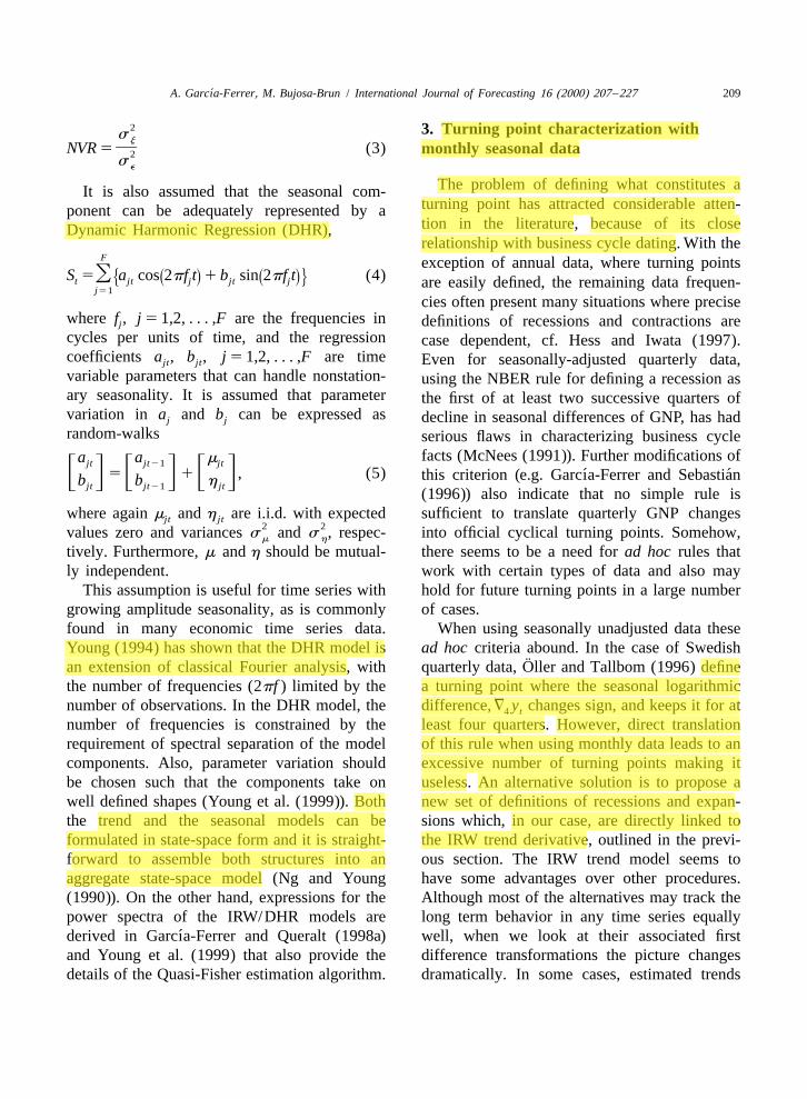
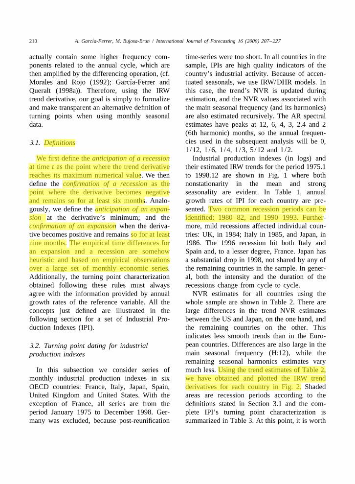
We first define the anticipation of a recession Industrial production indexes (in logs) andat time t as the point where the trend derivative their estimated IRW trends for the period 1975.1reaches its maximum numerical value. We then to 1998.12 are shown in Fig. 1 where bothdefine the confirmation of a recession as the nonstationarity in the mean and strongpoint where the derivative becomes negative seasonality are evident. In Table 1, annualand remains so for at least six months. Analo- growth rates of IPI for each country are pre-gously, we define the anticipation of an expan- sented. Two common recession periods can besion at the derivative’s minimum; and the identified: 1980–82, and 1990–1993. Further-confirmation of an expansion when the deriva- more, mild recessions affected individual coun-tive becomes positive and remains so for at least tries: UK, in 1984; Italy in 1985, and Japan, innine months. The empirical time differences for 1986. The 1996 recession hit both Italy andan expansion and a recession are somehow Spain and, to a lesser degree, France. Japan hasheuristic and based on empirical observations a substantial drop in 1998, not shared by any ofover a large set of monthly economic series. the remaining countries in the sample. In gener-Additionally, the turning point characterization al, both the intensity and the duration of theobtained following these rules must always recessions change from cycle to cycle.agree with the information provided by annual NVR estimates for all countries using thegrowth rates of the reference variable. All the whole sample are shown in Table 2. There areconcepts just defined are illustrated in the large differences in the trend NVR estimatesfollowing section for a set of Industrial Pro- between the US and Japan, on the one hand, andduction Indexes (IPI). the remaining countries on the other. This

indicates less smooth trends than in the Euro-pean countries. Differences are also large in the3.2. Turning point dating for industrialmain seasonal frequency (H:12), while theproduction indexesremaining seasonal harmonics estimates vary

In this subsection we consider series of much less. Using the trend estimates of Table 2,monthly industrial production indexes in six we have obtained and plotted the IRW trendOECD countries: France, Italy, Japan, Spain, derivatives for each country in Fig. 2. ShadedUnited Kingdom and United States. With the areas are recession periods according to theexception of France, all series are from the definitions stated in Section 3.1 and the com-period January 1975 to December 1998. Ger- plete IPI’s turning point characterization ismany was excluded, because post-reunification summarized in Table 3. At this point, it is worth

´A. Garcıa-Ferrer, M. Bujosa-Brun / International Journal of Forecasting 16 (2000) 207 –227 211

Fig. 1. OECD countries’ industrial production (in logs) and estimated IRW trends, 1975.1–1998.12.

´212 A. Garcıa-Ferrer, M. Bujosa-Brun / International Journal of Forecasting 16 (2000) 207 –227

Table 1Annual growth rates: 1976–1998

Year France Italy Japan Spain UK US

1976 9.03 11.7 10.5 4.94 3.26 8.801977 1.79 1.19 4.13 5.04 5.09 7.861978 2.20 1.85 6.11 2.31 2.91 5.691979 4.49 6.46 7.09 0.78 3.69 3.311980 21.00 4.80 4.62 1.00 26.83 22.82

1981 21.06 22.98 0.98 21.11 23.09 1.631982 20.88 23.06 0.34 21.17 1.94 25.521983 0.14 22.08 3.13 2.77 3.56 3.601984 1.77 3.58 8.92 1.02 20.03 8.641985 1.49 20.23 3.63 1.81 5.45 1.63

1986 0.56 3.86 20.18 2.83 1.45 1.171987 1.23 2.48 3.31 4.51 4.02 4.511988 4.57 7.11 9.97 3.12 5.06 4.451989 3.66 3.97 4.71 4.45 2.12 1.791990 1.57 6.11 4.12 20.02 0.03 20.22

1991 21.19 20.66 1.92 20.66 23.32 22.021992 21.25 21.58 25.95 22.89 0.40 3.101993 23.89 21.97 24.51 24.67 2.07 3.401994 3.93 6.43 1.23 7.19 5.29 5.261995 2.06 6.19 3.24 4.53 1.80 4.82

1996 0.25 23.19 2.34 20.70 1.04 4.351997 3.04 2.80 3.48 6.61 0.79 5.851998 4.60 1.30 26.68 5.50 0.90 3.64

checking whether the length and timing of the duration of contractions (in months) and ‘‘aster-recessions are in agreement with the results isks’’ (*) denote periods where estimated reces-shown by the annual growth rates in Table 1. sions do not seem agree with annual growthThe fourth column in Table 3 indicates the rates. This happens twice for France and Japan,

Table 2Dynamic harmonic regression estimation results for IPI

aCountry Noise variance ratiosb 2Trend H:12 H:6 H:4 H:3 H:2.4. H:2 s

cFrance 7.22 6.50 3.50 2.04 2.29 6.89 3.80 0.0142Italy 6.97 20.7 7.66 9.56 8.28 4.74 5.46 0.0208Japan 21.9 3.08 2.80 3.00 12.6 5.91 1.62 0.0112Spain 3.23 6.90 4.13 7.78 19.5 8.15 4.45 0.0209UK 5.53 31.5 4.69 4.74 23.4 5.59 2.46 0.0158US 87.9 49.8 4.05 2.59 1.19 1.95 0.50 0.0053

a 3All NVR estimated coefficients are multiplied by 10 .b H:X stands for harmonic and X is the annual frequency.c Estimation period: 1976.1–1998.11.

´A. Garcıa-Ferrer, M. Bujosa-Brun / International Journal of Forecasting 16 (2000) 207 –227 213

Fig. 2. Estimated trend derivatives of IPI and recession periods.

´214 A. Garcıa-Ferrer, M. Bujosa-Brun / International Journal of Forecasting 16 (2000) 207 –227

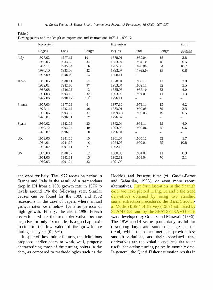
Table 3Turning points and the length of expansions and contractions 1975.1–1998.12

Recession Expansion Ratio

Expansion]]Begins Ends Length Begins Ends Length Recession

Italy 1977.02 1977.12 10* 1978.01 1980.04 28 2.81980.05 1983.03 34 1983.04 1984.10 18 0.51984.11 1985.04 6 1985.05 1990.09 64 10.71990.10 1993.06 32 1993.07 11995.08 25 0.81995.09 1996.10 13 1996.11 – – –

Japan 1980.05 1980.11 6* 1978.01 1980.12 12 2.01982.01 1982.10 9* 1983.04 1982.11 32 3.51985.08 1986.09 13 1985.05 1986.10 52 4.01991.03 1993.12 32 1993.07 1994.01 41 1.3

? ?1997.06 1998.12 18 1996.11 – – –

France 1977.03 1977.09 6* 1977.10 1979.11 25 4.21979.11 1982.12 36 1983.01 1990.05 89 2.51990.06 1993.07 37 11993.08 1995.03 19 0.51995.04 1996.01 7* 1996.02 – – –

Spain 1980.02 1982.03 25 1982.04 1989.11 99 4.01989.12 1993.04 40 1993.05 1995.06 25 0.61995.07 1996.03 8 1996.04 – – –

UK 1979.08 1981.03 19 1981.04 1983.12 32 1.71984.01 1984.07 6 1984.08 1990.01 65 10.81990.02 1991.11 21 1992.12 – – –

US 1979.08 1980.07 12 1980.08 1981.07 11 0.91981.08 1982.11 15 1982.12 1989.04 76 5.11989.05 1991.04 23 1991.05 – – –

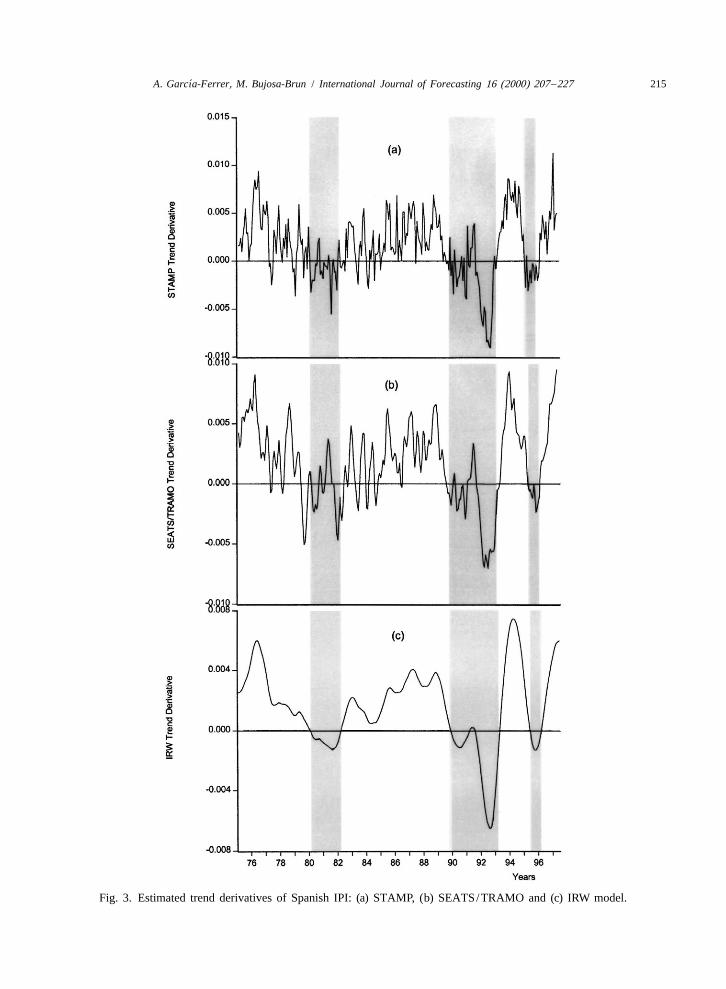
´and once for Italy. The 1977 recession period in Hodrick and Prescott filter (cf. Garcıa-Ferrer´France and Italy is the result of a tremendous and Sebastian, 1996), or even more recent

drop in IPI from a 10% growth rate in 1976 to alternatives. Just for illustration in the Spanishlevels around 1% the following year. Similar case, we have plotted in Fig. 3a and b the trendcauses can be found for the 1980 and 1982 derivatives obtained by using two standardrecessions in the case of Japan, where annual signal extraction procedures: the Basic Structur-growth rates were below 1% after periods of al Model (BSM) of Harvey (1989) estimated byhigh growth. Finally, the short 1996 French STAMP 5.0, and by the SEATS/TRAMO soft-recession, where the trend derivative became ware developed by Gomez and Maravall (1996).negative for only six months, is a good approxi- The IRW model seems particularly useful formation of the low value of the growth rate describing large and smooth changes in theduring that year (0.25%). trend, while the other methods provide less

In spite of these minor failures, the definitions smooth variations, and their associated trendproposed earlier seem to work well, properly derivatives are too volatile and irregular to becharacterizing most of the turning points in the useful for dating turning points in monthly data.data, as compared to methodologies such as the In general, the Quasi-Fisher estimation results in

´A. Garcıa-Ferrer, M. Bujosa-Brun / International Journal of Forecasting 16 (2000) 207 –227 215

Fig. 3. Estimated trend derivatives of Spanish IPI: (a) STAMP, (b) SEATS/TRAMO and (c) IRW model.

´216 A. Garcıa-Ferrer, M. Bujosa-Brun / International Journal of Forecasting 16 (2000) 207 –227

Table 4aNoise variance ratio estimates for different subperiods

2ˆEstimation Trend H:12 H:6 H:4 H:3 H:2.4 H:2 s

period

France1976.01–1990.07 3.16 21.5 6.70 6.40 11.4 7.03 3.18 0.01421975.01–1993.12 3.88 24.1 5.22 5.36 15.6 7.32 2.34 0.01361975.01–1995.07 4.39 23.2 4.71 5.87 14.0 6.94 1.37 0.0138

Spain1975.01–1989.12 0.71 13.5 3.98 12.2 20.6 11.0 6.36 0.01951975.01–1993.10 1.81 12.9 2.34 10.9 17.8 10.0 5.97 0.02021975.01–1995.09 2.71 7.3 2.82 8.46 17.7 8.65 6.16 0.02071975.01–1996.10 2.46 9.3 2.19 7.91 20.5 8.09 5.37 0.0208

a 3All NVR estimated coefficients are multiplied by 10 .

smooth changes in all the component’s am- 4. Forecasting turning points using surveyplitude and the smoothly varying trend. This dataseems to be a typical feature of this method

So far, we have shown that the univariaterepeating itself in a large number of data sets,decomposition and forecasting method is easye.g. Pedregal (1995). The maximum likelihoodto apply on any manufacturing time series. IPIestimator applied by Harvey and Gomez andof six countries has been included to show this.Maravall appears to produce higher NVR valuesThis section also shows that you can take oneexplaining the higher volatility in the compo-further step and include leading information, butnents. In the case of Spain, the estimated trend

NVR in Table 2 is 0.00323 which implies that requires a lot of work and knowledge of theretaining trend cycles longer than 27 months. economy proper. Hence only two countries areThe other trend alternatives seem to allow for presented as examples of how much forecast

1shorter cycles. For the spectral properties of the accuracy improvement can be achieved byIRW filter, see Young (1988); Pedregal (1995). doing so. Therefore, we have split the French

and Spanish data into subsamples in order togenerate forecasts for the last two turning pointsof our data, the first turning points are too closeto the beginning of the series and therefore1These contrasting results are directly related to the keydropped from the comparison.issue of smoothness and, the ability of alternative detrend-

Table 4 presents estimates of the univariateing methods to broadly replicate asymmetric businesscycles. Although a detailed treatment of this issue is IRW/DHR model for alternative sample periodsoutside the scope of this paper, a consensus is emerging in both countries. The estimated NVR for thethat the choice of the signal extraction method should trend has large changes after 1990, reflectingdepend both on the purpose of the research (Wickens

different industrial growth rates over the estima-(1995)) and on initial judgements on either the length oftion period. As in Table 3, the main seasonalthe cycle or the required degree of smoothness of the trend

(Canova (1994)). frequency (H:12) indicates variation in the

´A. Garcıa-Ferrer, M. Bujosa-Brun / International Journal of Forecasting 16 (2000) 207 –227 217

seasonal weights, while the remaining seasonal 4.1. Industrial new orders (INO)harmonics are less variable.

This survey variable, both for France andIn assessing the ability of the IRW/DHRSpain, offers several advantages over its com-model in anticipating trend reversals, we willpetitors. Apart from its prompt availability andcompare its turning point forecasts to that oflack of systematic revisions, the INO is basedtwo univariate methods: (Box and Jenkinson realized industrial orders rather than on(1970)) multiplicative seasonal ARIMA, andexpectations. However, as usually happens with(Harvey (1989)) BSM model which had ansurvey data, the main problem with INO is theexcellent forecasting record for the 111 seasonal

time series in Andrews (1994). Accuracy in scale of measurement. Questions on recentturning point forecasting is presented in Tables economic performance and on a firm’s short-5–7 and discussed in Section 4.2. term plans are designed to be easily answered,

Table 5RMSE of turning points (h-steps ahead)

Estimation period Forecast period ARIMA BSM IRW/DHR LI

France1976.1–1990.7 1990.8–1991.12 0.049 0.041 0.039 0.0181976.1–1993.12 1994.1–1994.12 0.053 0.056 0.051 0.0291976.1–1995.7 1995.8–1996.12 0.035 0.33 0.034 0.024

Spain1975.1–1989.12 1990.1–1990.12 0.041 0.047 0.044 0.0211975.1–1993.10 1993.11–1994.12 0.110 0.120 0.119 0.0551975.1–1995.9 1995.10–1996.12 0.050 0.059 0.052 0.0311975.1–1996.10 1996.11–1997.12 0.055 0.056 0.059 0.041

Table 6Observed and forecasted annual growth rates for IPI

Year Observed G.R. ARIMA BSM IRW/DHR LIaFrance

1991 21.19 3.76 2.15 2.05 20.031994 3.03 20.67 20.98 20.92 1.591996 0.25 2.65 1.79 2.73 0.81

aSpain1990 20.01 2.8 3.8 3.1 1.11994 7.2 23.1 24.7 23.3 2.01996 20.7 3.6 4.3 3.9 1.21997 6.8 3.2 2.7 2.0 5.1

a Forecasted growth rates for alternative models.

´218 A. Garcıa-Ferrer, M. Bujosa-Brun / International Journal of Forecasting 16 (2000) 207 –227

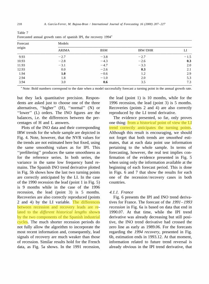
Table 7aForecasted annual growth rates of spanish IPI, the recovery 1994

Forecast Modelsorigin

ARIMA BSM IRW/DHR LI

9.93 22.7 23.8 22.7 21.510.93 22.8 24.3 22.6 0.311.93 23.1 24.7 23.3 2.012.93 0.0 22.6 0.3 2.11.94 1.0 20.6 1.2 2.92.94 1.8 21.0 2.0 5.33.94 3.0 0.6 3.5 7.3

a Note: Bold numbers correspond to the date when a model successfully forecast a turning point in the annual growth rate.

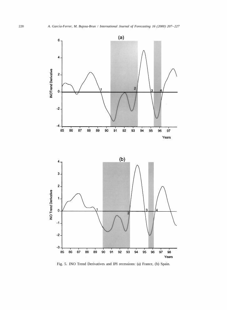
but they lack quantitative precision. Respon- the lead (point 1) is 10 months, while for thedents are asked just to choose one of the three 1996 recession, the lead (point 3) is 5 months.alternatives, ‘‘higher’’ (H), ‘‘normal’’ (N) or Recoveries (points 2 and 4) are also correctly‘‘lower’’ (L) orders. The INO figures are the reproduced by the LI trend derivative.balances, i.e. the differences between the per- The evidence presented, so far, only provescentages of H and L answers. one thing: from a historical point of view the LI

Plots of the INO data and their corresponding trend correctly anticipates the turning points.IRW trends for the whole sample are depicted in Although this result is encouraging, we shouldFig. 4. Note, however, that the NVR values for not forget that both trends are smoothed esti-the trends are not estimated here but fixed, using mates, that at each data point use informationthe same smoothing values as for IPI. This pertaining to the whole sample. In terms of‘‘prefiltering’’ produces the same smoothness as forecasting, however, the real test implies con-for the reference series. In both series, the firmation of the evidence presented in Fig. 5variance in the same low frequency band re- when using only the information available at themains. The Spanish INO trend derivative plotted beginning of each forecast period. This is donein Fig. 5b shows how the last two turning points in Figs. 6 and 7 that show the results for eachare correctly anticipated by the LI. In the case one of the recession / recovery cases in bothof the 1990 recession the lead (point 1 in Fig. 5) countries.is 9 months while in the case of the 1996recession, the lead (point 3) is 5 months. 4.1.1. FranceRecoveries are also correctly reproduced (points Fig. 6 presents the IPI and INO trend deriva-2 and 4) by the LI variable. The differences tives for France. The forecast of the 1991 –1993between recession and recovery leads are re- recession in Fig. 6a is based on data that end inlated to the different historical lengths shown 1990.07. At that time, while the IPI trendby the two components of the Spanish industrial derivative was already decreasing but still posi-cycles. The much shorter recession periods do tive, the INO trend derivative had crossed thenot fully allow the algorithm to incorporate the zero line as early as 1989.06. For the forecastsmost recent information and, consequently, lead regarding the 1994 recovery, presented in Fig.signals of recovery are much weaker than those 6b, estimation ends in 1993.12. At that moment,of recession. Similar results hold for the French information related to future trend reversal isdata, as Fig. 5a shows. In the 1991 recession, already obvious in the IPI trend derivative, that

´A. Garcıa-Ferrer, M. Bujosa-Brun / International Journal of Forecasting 16 (2000) 207 –227 219

Fig. 4. Industrial New Orders (INO) and estimated IRW Trend: (a) France, (b) Spain.

´220 A. Garcıa-Ferrer, M. Bujosa-Brun / International Journal of Forecasting 16 (2000) 207 –227

Fig. 5. INO Trend Derivatives and IPI recessions: (a) France, (b) Spain.

´A

.G

arcıa-Ferrer,

M.

Bujosa-B

run/

InternationalJournal

ofF

orecasting16

(2000)207

–227221

Fig. 6. (a) Estimated Trend Derivatives for IPI and INO for the start of the 1991–93 recession. (b) Estimated Trend Derivatives for IPI and INO for therecovery from the 1991–93 recession. (c) Estimated Trend Derivatives for IPI and INO for the start of the 1996 recession.

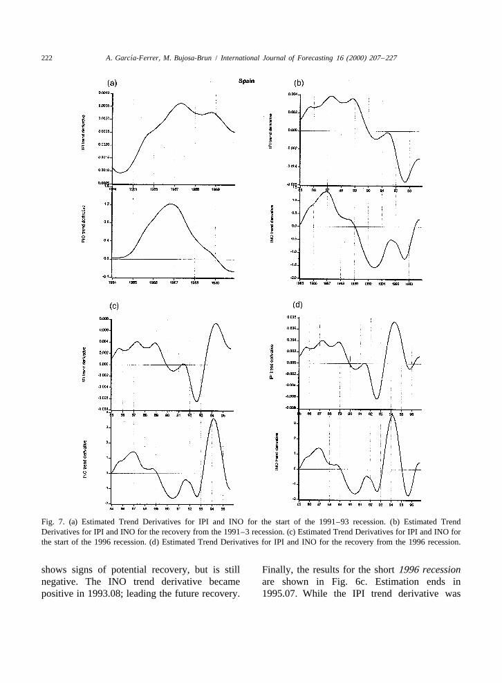
´222 A. Garcıa-Ferrer, M. Bujosa-Brun / International Journal of Forecasting 16 (2000) 207 –227

Fig. 7. (a) Estimated Trend Derivatives for IPI and INO for the start of the 1991–93 recession. (b) Estimated TrendDerivatives for IPI and INO for the recovery from the 1991–3 recession. (c) Estimated Trend Derivatives for IPI and INO forthe start of the 1996 recession. (d) Estimated Trend Derivatives for IPI and INO for the recovery from the 1996 recession.

shows signs of potential recovery, but is still Finally, the results for the short 1996 recessionnegative. The INO trend derivative became are shown in Fig. 6c. Estimation ends inpositive in 1993.08; leading the future recovery. 1995.07. While the IPI trend derivative was

´A. Garcıa-Ferrer, M. Bujosa-Brun / International Journal of Forecasting 16 (2000) 207 –227 223

already slowing down, it is still positive, while for all the trend characterizations proposed inthe INO trend derivative is signalling the in- the unobserved components model literature,coming recession in 1995.05. and hence, for their reduced form, ARIMA. As

an example, take the IRW trend of the IRW/DHR model. The prediction is a straight line4.1.2. Spainwith constant slope equal to the last value of theFig. 7a presents estimates of the IPI and INOderivative. This is a rather restrictive and con-trend derivatives (NVR 5 0.00071). In order toservative assumption, given the evolution of theforecast the long 1990 –1993 recession, wederivative in the vicinity of turning points, asended estimation at 1989.12. At that time, while

2Figs. 6 and 7 have shown.the IPI trend was not showing any sign of trendSpecification and estimation of the transferreversal, the INO trend had already started to

function LI model are associated with someturn down nine months earlier. On the otherdifficulties. One is the asymmetry of recessionshand, while the IPI trend derivative was alreadyand expansions. In a truly ex-ante forecastslowing down, but still positive, the INO trendexperiment, the lead is unknown and has to bederivative had crossed the zero line (confirma-estimated. In the Spanish case, INO leads varytion of a recession) by 1989.03.considerably between recessions and expansionsAs regards the 1994 recovery, results arefrom a maximum of six (in the 1990 recession)presented in Fig. 7b. In this case, estimationto a minimum of one month (in the case of theends at 1993.10. At that time, information1997 recovery). Since our goal is longer fore-regarding a future trend reversal is alreadycast horizons we have to rely on univariateevident in the IPI trend derivative, but the INOforecasts of the input (cf. Ashley, 1983). Doingtrend derivative became positive in 1993.06,that we found only minor forecasting gains inleading the subsequent industrial recovery.the short-term (and none in the long-term) inSimilar results hold for the short 1996 reces-comparison with the approach developed bysion and the post-1997 recovery. For the first

´Garcıa-Ferrer and Queralt (1998a) where the IPIcase, results are shown in Fig. 7c, wheretrend derivatives were forecasted directly fromestimation ends at 1995.9. As before, while thetheir univariate ARIMA representations. In allIPI trend shows a healthy growth at the end ofcases, the resulting AR(3) models indicate thethe sample, the one corresponding to INO hadpresence of one real and two complex rootsalready turned negative in 1995.6. Similarly, theoutside, but close to the unit circle.INO trend derivative signals the incoming re-

To construct the forecasts of our LI model wecession as early as 1995.4. In the second caseproceed as follows:(Fig. 7d) both derivatives confirm the end of the

short and mild 1996 recession although, in thiscase, the lead is very short.

2Proposals of different (more flexible) trend characteriza-4.2. Comparing model forecast accuracy at tions that adequately represent long term variations in the

trend derivative already exist in the unobserved com-turning pointsponents literature. A promising alternative is the SmoothedRandom Walk trend, proposed by Young (1994), whereLI model forecasts will now be comparedsmoothing constants can be included in the optimizationwith those of the alternative univariate modelsprocess. Another one is the Double Integrated Autorregre-

mentioned earlier. A well known shortcoming ´sive model developed by Garcıa-Ferrer et al. (1996) forof univariate models is their limited ability to estimation of locally smooth trends in annual economicanticipate turning points. This seems to be true data.

´224 A. Garcıa-Ferrer, M. Bujosa-Brun / International Journal of Forecasting 16 (2000) 207 –227

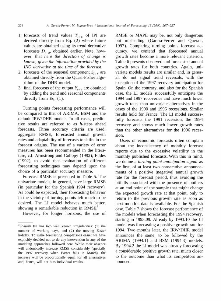
1. forecasts of trend values T of IPI are RMSE or MAPE may be, not only dangeroust1h

´derived directly from Eq. (2) where future but misleading (Garcıa-Ferrer and Queralt,values are obtained using its trend derivative 1997). Comparing turning points forecast ac-forecasts D , obtained earlier. Note, how- curacy, we contend that forecasted annualt1h

ever, that here the direction of change is growth rates become a more relevant criterion.known, given the information provided by the Table 6 presents observed and forecasted annualINO derivative at the time of the forecast. growth rates for both countries. Again, uni-

2. forecasts of the seasonal component S are variate models results are similar and, in gener-t1h

obtained directly from the Quasi-Fisher algo- al, do not signal trend reversals, with therithm of the DHR model. exception of the 1997 recovery anticipation for

3. final forecasts of the output Y are obtained Spain. On the contrary, and also for the Spanisht1h

by adding the trend and seasonal components case, the LI models successfully anticipate thedirectly from Eq. (1). 1994 and 1997 recoveries and have much lower

growth rates than univariate alternatives in theTurning points forecasting performance will cases of the 1990 and 1996 recessions. Similar

be compared to that of ARIMA, BSM and the results hold for France. The LI model success-default IRW/DHR models. In all cases, predic- fully forecasts the 1991 recession, the 1994tive results are referred to as h-steps ahead recovery and shows much lower growth ratesforecasts. Three accuracy criteria are used: than the other alternatives for the 1996 reces-aggregate RMSE, forecasted annual growth sion.rates and adaptability of forecasts to shifts in the Users of economic forecasts often complainforecast origins. The use of a variety of error about the inconsistency of monthly forecastmeasures has been recommended in the litera- reports due to the excessive volatility in theture, c.f. Armstrong and Collopy (1992); Fildes monthly published forecasts. With this in mind,(1992), to avoid that evaluation of different we define a turning point anticipation signal asforecasting techniques may depend upon the the first, of at least two consecutive announce-choice of a particular accuracy measure. ments of a positive (negative) annual growth

Forecast RMSE is presented in Table 5. The rate for the forecast period, thus avoiding theunivariate models, in general, have large RMSE pitfalls associated with the presence of outliers(in particular for the Spanish 1994 recovery). at an end point of the sample that might changeAs could be expected, their forecasting behavior the expected growth rate at that point, only toin the vicinity of turning points left much to be return to the previous growth rate as soon asdesired. The LI model behaves much better, next month’s data is available. For the Spanish

3showing a remarkable reduction in RMSE. case, Table 7 shows the forecast performance ofHowever, for longer horizons, the use of the models when forecasting the 1994 recovery,

starting in 1993.09. Already by 1993.10 the LI3 model was forecasting a positive growth rate forSpanish IPI has two well known irregularities: (1) the

1994. Two months later, the IRW/DHR modelnumber of working days, and (2) the moving Easterholiday. To make forecasting comparisons easier we have announces the same, to be followed by theexplicitly decided not to do any intervention in any of the ARIMA (1994.1) and BSM (1994.3) models.modeling approaches followed here. While their absence By 1994.2 the LI model was already forecastingwill undoubtedly increase RMSE considerably (specially

a considerable positive growth rate, much closerthe 1997 recovery when Easter falls in March), theto the outcome than what its competitors an-increase will be proportionally equal for all alternatives

and, hence, will not bias individual results. nounced.

´A. Garcıa-Ferrer, M. Bujosa-Brun / International Journal of Forecasting 16 (2000) 207 –227 225

5. Conclusions lack systematic revisions, should become animportant area for future research. Also, the

We propose an alternative approach to an- similarities between some of the national cyclesticipating and confirming turning points in suggest alternative multivariate approaches, e.g.monthly time series. A turning point signal is dynamic factor models, where common trendsconsidered as a two-stage decision process: a and common cycles could be fully exploited.statement that a turning point is likely to occur(anticipation), and a statement of when it will

Acknowledgementsoccur (confirmation). The starting point is aunivariate unobserved components model using We are grateful to Alfonso Novales, Pilartime variable parameters developed by Young Poncela and Gerald Sweeney whose suggestions(1994). The derivative of the estimated trend have led to significant improvements. We alsocomponent is used as a device for qualitative thank Jan G. de Gooijer and an Associate Editoranticipation of peaks and troughs, as well as for for helpful comments and corrections. Anyproviding alternative definitions of expansions errors are entirely ours. An early version of thisand recessions. A complete turning point paper was presented at the 17th Internationalcharacterization, providing information about all Symposium on Forecasting in Edinburgh, Scot-the industrial business cycle features, is ob- land. The preparation of this paper and thetained for six OECD countries. With minor research that it describes have been supportedfailures, the length and timing of the recessions ´by the Comision Interministerial de Ciencia yare consistent with annual growth rates. Our ´Tecnologıa, programs P94-0180 and PB98-approach, also contrasts with other, less smooth, 0075.alternatives that seem to contain shorter cyclesthan the ones implied by the IRW trend model.

Appendix. Data definitions and sourcesFor both France and Spain, ex-ante turningpoint forecasts are improved by introducing

All IPI data are in seasonally unadjusted formsurvey data. In particular, Industrial New Ordersand are obtained from the OECD database, with(INO) is systematically leading IPI. The re-the exception of the Spanish data that have beensulting leading indicator (LI) model is com-obtained from the Instituto Nacional de Estad-pared to well known modeling strategies inıstica. In all cases, the base year is 19905100.order to asses how accurately it forecasts theThe INO data for the France also comes fromlast seven turning points in the sample. Usingthe OECD data base, while the Spanish datadifferent forecasting accuracy measures, LIhave been obtained from the Ministerio decompares favorably with the competing alter-

´Industria y Energıa database.natives.While the empirical results presented here

only concern industrial production, similar re- Referencessults have been found for a large number of

Andrews, R. L. (1994). Forecasting performance of struc-seasonal economic time series in several coun-tural time series models. Journal of Business andtries. However, while the univariate modelingEconomic Statistics 12, 129–133.results are already well established, the leading

Armstrong, J., & Collopy, F. (1992). Error measures forindicator approach requires an input series that generalizing about forecasting methods: empirical com-systematically leads the output. Business ten- parisons. International Journal of Forecasting 8, 69–dency surveys, that are promptly available and 90.

´226 A. Garcıa-Ferrer, M. Bujosa-Brun / International Journal of Forecasting 16 (2000) 207 –227

¨Ashley, R. (1983). On the usefulnes of macroeconomic Kauppi, E. J. L., & Terasvirta, T. (1996). Short-termforecasts as inputs to forecasting models. Journal of forecasting of industrial production with business surveyForecasting 2, 211–223. data: experience from Finland’s great depression 1990–

Box, G. E. P., & Jenkins, G. M. (1970). Time Series 1993. International Journal of Forecasting 12, 373–Analysis: Forecasting and Control, Holden Day, San 381.Francisco. Oller, L., & Tallbom, C. (1996). Smooth and timely

Canova, F. (1994). Detrending and turning points. Euro- business cycle indicators for noisy Swedish data. Inter-pean Economic Review 38, 614–623. national Journal of Forecasting 3, 389–402.

Fildes, R. (1992). The evaluation of extrapolative forecast- Madsen, J. B. (1993). The predictive value of productioning methods. International Journal of Forecasting 8, expectations in manufacturing industry. Journal of81–98. Forecasting 12, 273–289.

´ ´Garcıa-Ferrer, A., del Hoyo, J., Novales, A., & Sebastian,McNees, S. (1991). Forecasting cyclical turning points:C. (1994). The use of economic indicators to forecast

The record in past three recessions. In: Lahiri, K., &the Spanish economy: preliminary results from theMoore, G. H. (Eds.), Leading Economic Indicators:ERISTE project, Tech. Rep. WP 9412, U.A.M. Dept. DeNew Approach and Forecasting Records, Cambridge´ ´Analisis Economico.University Press, Cambridge, pp. 149–168.´Garcıa-Ferrer, A., del Hoyo, J., Novales, A., & Young, P.

Morales, E. E. A., & Rojo, M. L. (1992). UnivariateC. (1996). Recursive identification estimation and fore-methods for the analysis of the industrial sector incasting of nonstationary time series with applications to

´Spain. Investigaciones Economicas 16(1), 127–149.GNP international data. In: Berry, D. A., Chaloner, K.Ng, C. N., & Young, P. C. (1990). Recursive estimationM., & Geweke, J. K. (Eds.), Bayesian Analysis in

and forecasting of nonstationary time series. Journal ofStatistics and Econometrics: Essays in Honor of ArnoldForecasting 9, 173–204.Zellnerm, John Wiley, New York, pp. 15–27.

´Garcıa-Ferrer, A., & Queralt, R. (1997). A note on ´ ´Pedregal, D. (1995). Comparacion teorica estructural yforecasting international tourist demand in Spain. Inter- predictiva de modelos de componentes no observables ynational Journal of Forecasting 13, 539–549. extensiones del modelo de Young, Ph.D. thesis, Facultad

´Garcıa-Ferrer, A., & Queralt, R. (1998a). Can univariate ´de C.C. Economicas y Empresariales, Universidadmodels forecast turning points in seasonal economic ´Autonoma de Madrid.time series? International Journal of Forecasting 14, ¨Rahiala, M., & Terasvirta, T. (1993). Business survey data433–446. in forecasting the output of Swedish and Finnish metal

´Garcıa-Ferrer, A., & Queralt, R. (1998b). Using long-, and engineering industries: a Kalman filter approach.medium-, and short-term trends to forecast turning International Journal of Forecasting 2, 191–200.points in the business cycle: Some international evi- Westlund, A. H. (1993). Busines Cycle Forecasting. Jour-dence. Studies in Nonlinear Dynamics and Economet- nal of Forecasting 12(3 and 4), 187–196.rics 3(2), 79–105.

Wickens, M. (1995). Trend extraction: A practitioner’s´ ´Garcıa-Ferrer, A., & Sebastian, C. (1996). A businessguide. In: Technical report, Government Economiccycle characterization of the Spanish economy: 1970–Service.1994, Tech. Rep. WP 9606, ICAE, Universidad Com-

Young, P. C. (1988). Recursive extrapolation interpolationplutense de Madrid.and smoothing of non-stationary time series. In: Identifi-Gomez, V., & Maravall, A. (1996). Programas TRAMOcation and System Parameter Estimation, Pergamonand SEATS instructions for the user (BETA Version:Press, Oxford, pp. 33–44.Sept. 1996), Tech. Rep. WP 9628, Bank of Spain,

Young, P. C. (1994). Time variable parameters and trendMadrid.estimation in non-stationary economic time series. Jour-Hanssens, D. M., & Vanden Abeele, P. M. (1987). A timenal of Forecasting 13, 179–210.series study of the formation and predictive performance

Young, P. C., Pedregal, D., & Tych, W. (1999). Dynamicof EEC production survey expectations. Journal ofHarmonic Regression. Journal of Forecasting 18, 369–Business and Economic Statistics 5, 507–519.394.Harvey, A. (1989). Forecasting Structural Time Series

Models and the Kalman Filter, Cambridge University Zellner, A., Hong, C., & Min, C. (1991). ForecastingPress, Cambridge. turning points in international output growth rates using

Hess, G. D., & Iwata, S. (1997). Measuring and comparing Bayesian exponentially weighted autoregression timebusiness-cycle features. Journal of Business and Econ- varying parameters and pooling techniques. Journal ofomic Statistics 15, 432–444. Econometrics 49, 275–304.

´A. Garcıa-Ferrer, M. Bujosa-Brun / International Journal of Forecasting 16 (2000) 207 –227 227

´Biographies: Antonio GARCIA-FERRER is Professor of published in various journals and edited the special Issue´ ´Econometrics in the Departamento de Analisis Economico: on Time Series Advances in Economic Forecasting (Jour-

´ ´Economıa Cuantitativa, Universidad Autonoma de Madrid. nal of Forecasting 13 (2) 1994).From 1977 to 1980 he was Assistant Professor at the

´Universidad de Alcala de Henares and Fulbright VisitingProfessor at the Graduate School of Business of the Marcos BUJOSA-BRUN is a PhD student at Departamento

´ ´ ´University of Chicago in 1984–85. He obtained his PhD in de Analisis Economico: Economıa Cuantitativa, Univer-´Economics at UC Berkeley in 1977, and is Associate sidad Autonoma de Madrid, and an economist at Facultad

´Editor of the International Journal of Forecasting. His de C.C. Economicas y Empresariales, Universidad Au-´research interests include modelling and forecasting tonoma de Madrid. He is currently involved in developing

seasonal economic time series. On this topic, he has optimization algorithms in the frequency domain.