Flight patterns of birds at offshore gas platform K14

Flight intensity, flight altitudes and species

composition in comparison to OWEZ

R.C. FijnA. GyimesiM.P. CollierD. BeukerS. DirksenK.L. Krijgsveld

Consultants for environment & ecology

Flight patterns of birds at offshore gas platform K14 Flight intensity, flight altitudes and species composition in comparison to OWEZ R.C. Fijn A. Gyimesi M.P. Collier D. Beuker S. Dirksen K.L. Krijgsveld

commissioned by: NoordzeeWind with support of We@Sea 23 May 2012 NoordzeeWind report nr OWEZ_R_232_T1_20120523_fluxes_far_offshore Bureau Waardenburg report nr 11-112

3

Status: final report

Report nr.: 11-112

Date of publication: 23 May 2012

Title: Flight patterns of birds at offshore gas platform K14

Subtitle: Flight intensity, flight altitudes and species composition in comparison to OWEZ

Authors: R.C. Fijn, MSc. dr. A. Gyimesi M.P. Collier, MSc. D. Beuker drs. S. Dirksen drs. K.L. Krijgsveld

Number of pages incl. appendices: 94

Project nr: 07-336

Project manager: drs. S. Dirksen / drs. K.L. Krijgsveld

Name & address client: Noordzeewind, ing. H.J. Kouwenhoven 2de Havenstraat 5B 1976 CE IJmuiden

Reference client:

Signed for publication: Director Bureau Waardenburg bv drs. A.J.M. Meijer

Initials:

Bureau Waardenburg bv is not liable for any resulting damage, nor for damage which results from applying results of work or other data obtained from Bureau Waardenburg bv; client indemnifies Bureau Waardenburg bv against third-party liability in relation to these applications.

© Bureau Waardenburg bv / NoordzeeWind / We@Sea

This report is produced at the request of the client mentioned above and is his property. All rights reserved. No part of this publication may be reproduced, stored in a retrieval system, transmitted and/or publicized in any form or by any means, electronic, electrical, chemical, mechanical, optical, photocopying, recording or otherwise, without prior written permission of the client mentioned above and Bureau Waardenburg bv, nor may it without such a permission be used for any other purpose than for which it has been produced.

The Quality Management System of Bureau Waardenburg bv has been certified by CERTIKED according to ISO 9001:2000.

4

5

Preface

In order to compare flight patterns at the Offshore Wind farm Egmond aan Zee (OWEZ) with flight patterns further offshore, densities, flight altitudes and species composition of flying birds far offshore were quantified. This was done by means of both visual and radar observations that were carried out from the NAM offshore gas platform K14 during one year. In this report the results of this study are presented. The study was jointly commissioned by NoordzeeWind and We@Sea. The Offshore Wind farm Egmond aan Zee has a subsidy from the Ministry of Economic Affairs under the CO2 reduction Scheme of the Netherlands. The project was carried out by a project team from Bureau Waardenburg. Field work was carried out by Daniël Beuker, Mark Collier, Sjoerd Dirksen, Ruben Fijn en Karen Krijgsveld. Visual data were analysed and reported by Mark Collier. Radar data were analysed and reported by Abel Gyimesi, Ruben Fijn and Karen Krijgsveld.

6

7

Table of contents Preface...............................................................................................................................................5 Summary ...........................................................................................................................................9 1 Introduction...............................................................................................................................11

1.1 Background.................................................................................................................11 1.2 Aim of the study ...........................................................................................................12 1.3 Means ...........................................................................................................................12 1.4 This report.....................................................................................................................13

2 Materials and methods............................................................................................................15 2.1 Study area ....................................................................................................................15 2.2 Study period .................................................................................................................18 2.3 Visual observation methods......................................................................................19

2.3.1 Panorama scans...........................................................................................19 2.3.2 Additional observations................................................................................22

2.4 Radar observation methods.......................................................................................23 2.4.1 Technical specifications radar and Merlin..................................................23 2.4.2 Data filtering ..................................................................................................31 2.4.3 Attraction of birds and insects to the illuminated K14 platform................37

3 Visual observations of flying birds: species composition and flight altitude ......................41 3.1 Species composition ...................................................................................................41 3.2 Species abundance.....................................................................................................46 3.3 Species-specific flight altitudes ..................................................................................51 3.4 Comparison of visual observations with OWEZ.......................................................52

4 Radar observations of bird movements: flight intensity and altitude.................................57 4.1 Overall numbers and fluxes.......................................................................................57

4.1.1 Monthly variation in flight intensity ............................................................57 4.1.2 Seasonal variation in flight intensity...........................................................60 4.1.3 Diurnal variation in flight intensity..............................................................61 4.1.4 Statistical analysis of flight intensities at K14 and OWEZ......................66

4.2 Flight altitude as determined with radar ...................................................................68 4.2.1 Seasonal variation in flight height .............................................................70 4.2.2 Diurnal variation in flight height .................................................................72 4.2.3 Statistical analysis of flight heights at K14 and OWEZ ..........................74

8

4.3 Bird groups at risk altitude ..........................................................................................76 4.3.1 Diurnal variation in flight intensity at risk height.......................................78 4.3.2 Statistical analysis of birds flying at risk height........................................81

5 Discussion...............................................................................................................................83 6 Acknowledgements.................................................................................................................89 7 Literature...................................................................................................................................91 Appendix 1.......................................................................................................................................93

9

Summary

This study aimed to assess the flux (number of birds passing per vertical surface per time) of flying birds, differentiated to flight altitude, season, time of day/night and species (group) at K14, a gas production platform situated approximately 80 km west-north-west from the Dutch coast in the North Sea. In particular, this project aimed to compare the flux and flight altitude of birds at K14 with the metmast in OWEZ, a windfarm situated 10-18 km from the Dutch coast. Observations were made between March 2010 and March 2011, using both visual and radar observation techniques. During a total of 11 field visits, we carried out visual observations to obtain information on species composition, as well as species-specific fluxes and flight altitudes of birds flying at lower altitudes. The observations consisted of panorama scans, visual counts of all birds flying within sight of the observation platform, carried out once every hour during daylight. In addition, also line scans were conducted, when one certain area was observed using either binoculars or telescope. All species entering the field of view were recorded and the distance, direction and activity, i.e. flight, were noted. In addition, with a 25 kW Merlin marine surveillance radar developed by Detect.Inc, operating in vertical position and set to a range of 0.75 NM, we continuously monitored flight activity, thus providing detailed insight in fluxes and flight altitudes in the area of K14. In order to obtain comparable data from OWEZ, a similar radar set-up was simultenously operating there as well. As objects other than birds were also detected by the radar, several processing steps (such as filtering out clutter, rain and insects) were carried out on the collected data before analysis. Based on the visual observations, most species occurring at K14 were species commonly found in the marine environment, such as northern gannet, northern fulmar, great black-backed gulls, kittiwake and auks. Coastal species, such as lesser black-backed gull, herring gull, terns and great cormorant, were less abundant at K14 than at OWEZ. However, the proportions of pelagic species, such as gannets (20%) and alcids (5.4%) were markedly greater at K14 compared to around OWEZ (2 and 0.8%, respectively). The number of birds recorded at K14 by the radar was lower (i.e. 344,215 bird groups/km after correction for radar interruptions) in comparison with OWEZ (652,291 bird groups/km). The yearly mean traffic rate (MTR: number of bird groups/km/hour) at K14 was 45 bird groups/km/h, ranging from 14 bird groups/km/h in May to 107 bird groups/km/h in March 2010. At OWEZ, the highest MTR was observed in September. Although no such an autumn migration peak occurred at K14, MTRs were on average the highest in autumn. Otherwise, the general patterns of bird fluxes resembled each other at the two locations: high values in March followed by a reduction in April – May and a subsequent increase in the summer months. Fluxes were clearly the lowest in the winter months.

10

Considering the whole study period, an almost equal number of birds passed both locations during daylight and in darkness. However, there was a strong in-between month variation in diurnal flight intensity. During the migration months of March and April, as well as October and November, the percentage of birds recorded during darkness was on average 68% at K14. On the contrary, from May to September the mean proportion of night flights was only 25% at K14. Except for the winter, the daily pattern in flight altitudes largely followed the daily pattern of MTRs. In other words, increasing MTRs occurred parallel with increasing flight heights, meaning also that the large number of birds passing during the nights of the migration periods generally flew higher. On the contrary, altogether 49% of the birds flew in the lowest altitude band of 0–69 m at K14, most of which (i.e. 57%) during daylight. Although these values were reasonably comparable between the two locations, a statistical analysis revealed a significantly higher mean flight altitude at OWEZ, probably caused by the relatively larger fluxes during the migration periods.

11

1 Introduction

1.1 Background

Offshore wind energy in Dutch offshore waters is steadily growing. Since the first offshore wind farm in Dutch waters, OWEZ, has come operational in early 2007, a second wind farm has been completed and permits for more wind farms have been issued. From several sides, strategic research was undertaken and stimulated, and in the project on which this report provides results, two of these came together. In 2006 the Offshore Wind farm Egmond aan Zee (OWEZ) was built. OWEZ is a wind farm of 36 turbines (10-18 km from the coast) and owned by NoordzeeWind (Nuon and Shell Wind Energy). To evaluate the economical, technical, ecological and social effects of offshore wind farms in general, a Monitoring and Evaluation Program (NSW-MEP) in OWEZ was developed. Carrying out this MEP serves ‘learning goals’ for future wind farms further offshore as well as ‘effect assessment goals’ for the near-shore wind farm itself. The knowledge gained by this project will be made available to all parties involved in the realisation of large-scale offshore wind farms. Bureau Waardenburg has executed the study on effects on flight paths, flight altitudes and flux of migratory and non-migratory birds of this wind farm. The final report of this study will be published in the autumn of 2011 (Krijgsveld et al. 2011). Part of NSW-MEP was to carry out a comparable study on flight altitudes and flux of migratory and non-migratory birds at a location much further offshore. We@Sea is a combined effort of public and private interests towards realizing the desired transition to new offshore wind energy business. Research was financed from a grant from government (BSIK programme) and co-financed by the partners in the We@Sea program. The central objective of the knowledge programme is to develop a structural basis for long-term business development in the Netherlands, for the purpose of preparing, designing, constructing, operating, maintaining and, in due course, dismantling offshore wind power plants. The programme should comprise the entire chain of technological, economical and ecological activities and be internationally leading in its field. The application of knowledge and experience acquired remains a continuing process, in which We@Sea plays an active role. In the NSW-MEP, a learning goal was included on comparing the situation relatively close to the coast (Meetpost Noordwijk and metmast OWEZ) with a location much further offshore. This is very relevant for new offshore wind farms, which will mainly be planned (much) further from the coast than the two now existing. The Nederlandse Aardolie Maatschappij (NAM) kindly offered the possibility to do this research on their K14 FA-1 platform (or K14C, hereafter K14). Although being further west and north than was initially aimed for, this was not only the only site available, but has proven to be a good site bearing in mind recent developments in planning round 2 and 3 offshore wind farms.

12

1.2 Aim of the study

This task deals with the following research question from MEP: Assessing the flux (number of birds passing per vertical surface per time) of flying birds, differentiating to season, time of day/night, distance to coast, species (group), as basis for assessing collision risks. As stated, an essential aim of the monitoring programme was to collect information on bird densities along a gradient perpendicular to the Dutch the coast. So far, studies have been done from land (IJmuiden), Meetpost Noordwijk (9 km from the coast) and at the metmast in OWEZ (10-18 km from the Dutch coast). To collect information on bird densities further offshore, we measured in the study reported here, flight patterns at K14, a site further offshore, 80 km from the Dutch coast. In the light of the potential effects of wind farms on birds, three aspects of flight patterns of birds are important: 1) flight paths, 2) fluxes, 3) flight altitudes. In the absence of wind turbines at the K14 study site, flight paths were not relevant and were not studied.

1.3 Means

In order to investigate the densities and flight altitudes of flying birds far offshore, observations were made between March 2010 and March 2011 from the offshore platform K14. This is a gas production platform in the Dutch North Sea, owned by the NAM. The K14 platform is situated approximately 80 km west-north-west from the Dutch coast and 140 km from the coast of England. To study the flight patterns, we used both radar and visual observation techniques. With the radar we continuously monitored flight activity, thus providing detailed insight in fluxes and flight altitudes in the area. For this purpose a 25 kW vertical Merlin radar was used, developed and installed by DeTect Inc. With the visual observations we obtained information on species composition, as well as in species-specific fluxes and flight altitudes of birds flying at lower altitudes. In addition, the visual observations serve to calibrate and interpret results obtained by radar.

13

1.4 This report

In this report, we present the results of both the visual and the radar observations. Chapters are divided as follows: Chapter 2: Information on the study area, on observation techniques used and on how

radar data were processed. Chapter 3: Results from visual observations on species composition and species-

specific flight patterns Chapter 4: Results from radar observation on fluxes and flight altitudes Chapter 5: Discussion of the results and conclusion

14

15

2 Materials and methods

2.1 Study area

The K14 gas production platform is located just over 80 km west-north-west of Den Helder and 140 km east – south-east of the English coast in the Dutch North Sea at 53o16’08”N 3o37’44”W (fig. 2.1). The platform is owned and operated by NAM. The location was expected to lie on the migration route of birds flying to and from Scandinavia and England, as well as to and from southern Europe and Africa.

Figure 2.1 Location of NAM gas platform K14 in the North Sea. For reference, the

offshore wind farms Offshore Wind Egmond aan Zee (OWEZ) and Prinses Amalia are shown as well.

16

The platform consists of three main structures: a production platform, a compression platform and an accommodation platform (figs. 2.2 - 2.4). These platforms are joined by a gangway and an open deck. In addition, a vent stack extends horizontally for approximately 100m from the northern corner of the compression platform (fig. 2.2). The K14 platform was reached by helicopter departing from Den Helder airport .

Figure 2.2 K14 gas platform of the NAM, as seen looking southwards from the vent

stack. Left is the production platform and right the compression platform with the accommodation platform behind it. Photo: Karen Krijgsveld

17

Figure 2.3 The production platform at K14 as seen from the south. Photo: Karen

Krijgsveld.

Figure 2.4 The accommodation platform at K14 as seen from the east. Photo: Sjoerd

Dirksen.

18

2.2 Study period

Radar The radar was installed on 11 March 2010 and from that moment on data on flux and flight altitude of birds around the K14 platform were continuously collected 24 hours a day, 7 days a week. Simultaneously, an earlier installed radar was operating at OWEZ. For this report, data were collected until 23 March 2011 at both locations. The radar was not running continuously, due to either strong winds or software or hardware failures (e.g., software issue in August 2010) (table 2.1). In total, data on flux and flight altitude were collected on 293 out of 378 days at K14 (78%). Because a comparison is made between results from K14 and OWEZ, the radar effort of the latter location is included in table 2.1 (336 out of 378 days (89%)). Table 2.1 Overview of the number of days per month on which data were collected

with the vertical radar (fluxes and altitudes). An overview of visual observation days is given in table 2.2.

year season month K14 OWEZ 2010 spring March 21 21 April 30 28 May 30 30 summer June 30 30 July 23 31 August 2 29 autumn September 23 28 October 30 29 November 22 28 winter December 9 21 2011 January 26 22 February 25 16 spring March 22 23 overall 293 336 % of number of days available prior to data filtering 78 89 Visual observations Between April 2010 and March 2011, a total of 11 field visits was undertaken. The number of visits per season was determined based on the expected flight activity, with more visits during periods with more expected flight activity (table 2.2). Due to both safety reasons and observation protocols, two observers were present during each of the fieldwork periods. Incidental records of bird species were also recorded during additional visits to the platform relating to the radar installation. These were during December 2009 and March 2010.

19

Table 2.2 Dates of visits to K14. Start and end dates indicate the days during which panorama scans were carried out. During these periods, the number of days spent on the platform may have been longer due to arrival or departure days or due to other activities such as radar maintenance.

period start date end date activity

1 15-12-2009 15-12-2009 installation

2 9-3-2010 11-3-2010 installation

3 14-4-2010 17-4-2010 observations

4 4-5-2010 6-5-2010 observations

5 25-5-2010 27-5-2010 observations

6 14-6-2010 16-6-2010 observations

7 31-8-2010 2-9-2010 observations

8 21-9-2010 21-9-2010 observations

9 5-10-2010 7-10-2010 observations

10 26-10-2010 27-10-2010 observations

11 16-11-2010 17-11-2010 observations

12 22-2-2011 24-2-2011 observations

13 21-3-2011 23-3-2011 observations

2.3 Visual observation methods

Birds were observed visually by means of standardised observation protocols by experienced field workers who also worked on the OWEZ project. Mutual calibration between observers of estimated distances was done regularly. The main protocol was the panorama scan. In addition, all species observed during visits to the platform were recorded, including both incidental records and during searches (see §2.3.2).

2.3.1 Panorama scans

During observations, panorama scans were carried out once every hour during daylight. A panorama scan is a visual count of all birds flying within sight of the observation platform (Lensink et al. 2000). Birds sitting on the surface of the water are recorded as well. It provides additional data and enhances the interpretation of the radar counts, and provides information on species composition, density, flight altitude and flight direction of birds around the platform. The technique has been extensively calibrated (Lensink et al. 1998; Poot et al. 2000), and was similar to panorama scans carried out at OWEZ. A panorama scan involved scanning the air and water in a 360° area around the platform, using a high-quality pair of 10*42 binoculars fixed on a tripod. The 360° area was divided into 8 sectors (fig. 2.5), to be able to register where the bird was flying (e.g., NW or SE). The eight sectors were observed from a total of four different observation points on the decks of the accommodation and compression platforms. Four different observations points were needed to allow unobstructed viewing (fig.

20

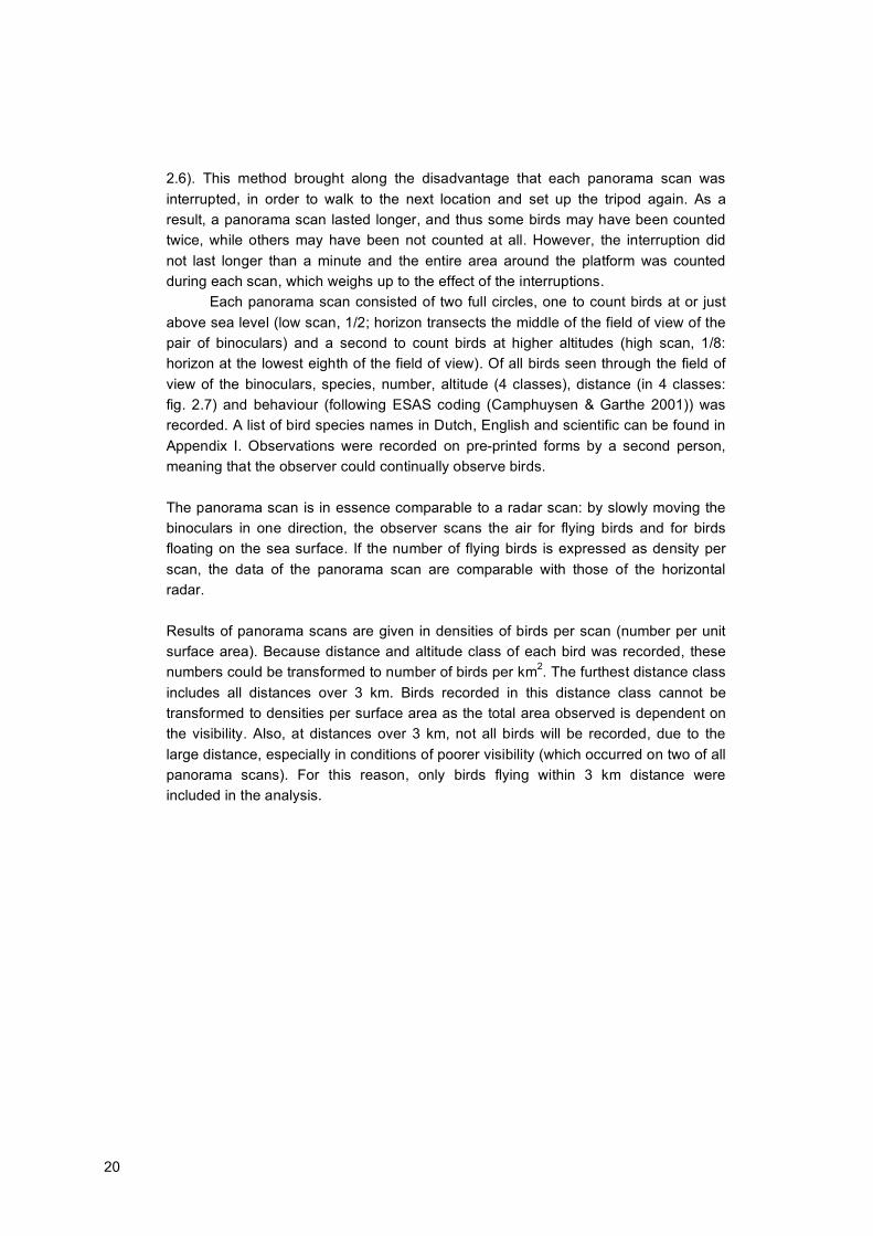
2.6). This method brought along the disadvantage that each panorama scan was interrupted, in order to walk to the next location and set up the tripod again. As a result, a panorama scan lasted longer, and thus some birds may have been counted twice, while others may have been not counted at all. However, the interruption did not last longer than a minute and the entire area around the platform was counted during each scan, which weighs up to the effect of the interruptions.

Each panorama scan consisted of two full circles, one to count birds at or just above sea level (low scan, 1/2; horizon transects the middle of the field of view of the pair of binoculars) and a second to count birds at higher altitudes (high scan, 1/8: horizon at the lowest eighth of the field of view). Of all birds seen through the field of view of the binoculars, species, number, altitude (4 classes), distance (in 4 classes: fig. 2.7) and behaviour (following ESAS coding (Camphuysen & Garthe 2001)) was recorded. A list of bird species names in Dutch, English and scientific can be found in Appendix I. Observations were recorded on pre-printed forms by a second person, meaning that the observer could continually observe birds. The panorama scan is in essence comparable to a radar scan: by slowly moving the binoculars in one direction, the observer scans the air for flying birds and for birds floating on the sea surface. If the number of flying birds is expressed as density per scan, the data of the panorama scan are comparable with those of the horizontal radar. Results of panorama scans are given in densities of birds per scan (number per unit surface area). Because distance and altitude class of each bird was recorded, these numbers could be transformed to number of birds per km2. The furthest distance class includes all distances over 3 km. Birds recorded in this distance class cannot be transformed to densities per surface area as the total area observed is dependent on the visibility. Also, at distances over 3 km, not all birds will be recorded, due to the large distance, especially in conditions of poorer visibility (which occurred on two of all panorama scans). For this reason, only birds flying within 3 km distance were included in the analysis.

21

Figure 2.5 Schematic view of the eight sectors surveyed with the panorama scans

and the three distance classes. The platform, as observation platform, is situated in the centre. North is the boundary between sectors 1 and 8. Surface areas are: distance 0-0.5 km = 0.79 km2, 0.5-1.5 km = 6.28 km2, 1.5–3 km = 21.21 km2.

Figure 2.6 The four locations used to carry out the panorama scans: above left,

sectors 3 and 4; above right, sectors 5 and 6; below left, sector 7; below right, sectors 8, 1 and 2. Photos: Mark Collier and Sjoerd Dirksen.

22

Figure 2.7 Schematic view of the volume of air covered with panorama scans. Scans

were performed at two altitudes: a low scan with the horizon halfway in the binocular view and a high scan with the horizon at 1/8 in the lower part of the binocular view. With the sea surface visible in the bottom part of the view, maximum altitude at which birds are scanned is 172 m at 1500 m distance. Data from distance class 4 were not included in the density analysis, because no bird densities could be defined for this area.

2.3.2 Additional observations

All species that were observed while at the platform were recorded. This included species recorded between panorama scans or outside of the panorama scan search area, such as by the second observer as well as during periods of additional observations and line scans. Line scans are periods of time in which a fixed area along an imaginary line was observed using either binoculars or telescope. All species entering the field of view were observed and the distance, direction and activity, i.e. flight, were recorded. These line scans observations typically took place between panorama scans or in periods when time was too limited to carry out a panorama scan and afforded information on additional species present in the area.

23

Birds were occasionally recorded on the platform itself, both in the manned areas and on the structures of the platform, i.e. platform legs or towers. On occasions the platform decks were searched in order to find birds resting or sheltering on the platform. Dead birds were also collected and identified. Inaccessible areas, such as legs, towers and cranes were checked using binoculars or telescope.

2.4 Radar observation methods

2.4.1 Technical specifications radar and Merlin

Information on flight patterns for an extended and continuous period of time, and on diurnal as well as nocturnal flight movements, requires more than visual observations only. Therefore, bird tracking by marine surveillance radars was used to obtain the objected information. Radars have been widely accepted as tools to study flight patterns of birds (Eastwood 1967; Poot et al. 2000, van Belle et al. 2002; Petersen et al. 2006). One of the main aims of this project was to compare the flux and flight altitude of birds at the metmast in OWEZ (Krijgsveld et al. 2011) with those of birds at K14. To be able to do so, a similar radar set-up was chosen with an X-band marine surveillance radar (25 kW) which was tilted 90º to rotate vertically, and thus scan the air vertically rather than horizontally (fig. 2.8). The radar was set to a range of 0.75 NM, which is 1389 m up in the air, chosen to detect bird movements in the altitude range including wind turbines and well above it, while at the same time avoiding serious detection loss.

Figure 2.8 Schematic view of the vertical radar. Radar bundle is shaded in the image.

The radars scanned in a northwest to southeast direction, perpendicular to the expected flight direction of migratory birds. This maximizes the chance of recording each passing bird group as one track. In addition, the calculation of bird fluxes at a certain location relies on the main assumption that the radar scans perpendicular to the mean flight direction. If this assumption is not fulfilled, the surface area of the

24

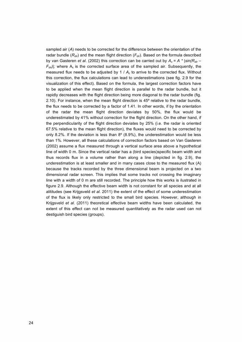
sampled air (A) needs to be corrected for the difference between the orientation of the radar bundle (Rdir) and the mean flight direction (Fdir). Based on the formula described by van Gasteren et al. (2002) this correction can be carried out by Ac = A * |sin(Rdir – Fdir)|; where Ac is the corrected surface area of the sampled air. Subsequently, the measured flux needs to be adjusted by 1 / Ac to arrive to the corrected flux. Without this correction, the flux calculations can lead to underestimations (see fig. 2.9 for the visualization of this effect). Based on the formula, the largest correction factors have to be applied when the mean flight direction is parallel to the radar bundle, but it rapidly decreases with the flight direction being more diagonal to the radar bundle (fig. 2.10). For instance, when the mean flight direction is 45º relative to the radar bundle, the flux needs to be corrected by a factor of 1.41. In other words, if by the orientation of the radar the mean flight direction deviates by 50%, the flux would be underestimated by 41% without correction for the flight direction. On the other hand, if the perpendicularity of the flight direction deviates by 25% (i.e. the radar is oriented 67.5% relative to the mean flight direction), the fluxes would need to be corrected by only 8.2%. If the deviation is less than 8º (8.9%), the underestimation would be less than 1%. However, all these calculations of correction factors based on Van Gasteren (2002) assume a flux measured through a vertical surface area above a hypothetical line of width 0 m. Since the vertical radar has a (bird species)specific beam width and thus records flux in a volume rather than along a line (depicted in fig. 2.9), the underestimation is at least smaller and in many cases close to the measured flux (A) because the tracks recorded by the three dimensional beam is projected on a two dimensional radar screen. This implies that some tracks not crossing the imaginary line with a width of 0 m are still recorded. The principle how this works is ilustrated in figure 2.9. Although the effective beam width is not constant for all species and at all alititudes (see Krijgsveld et al. 2011) the extent of the effect of some underestimation of the flux is likely only restricted to the small bird species. However, although in Krijgsveld et al. (2011) theoretical effective beam widths have been calculated, the extent of this effect can not be measured quantitatively as the radar used can not destiguish bird species (groups).

25

Figure 2.9 Schematic example of birds passing through (arrows) the radar bundle

(square oriented to 0º) by a 90º (left image) and diagonal (right image) flight direction relative to the bundle. The distance in-between the arrows is the same, meaning that the flux is the same, only the direction of the bird flight is different. In the right image the dashed arrows symbolize the underestimated number of birds because of the non-perpendicular flight direction, however, only when a assuming a beam width of 0 m, in this case the left line of the box. In case of much wider beam, e.g. like the depicted box in the picture, still all tracks of birds will be recorded as they all will be projected as tracks on the two dimensional surface of the radar screen. In this example no correction should be needed at all, but in reality the width of the box is species- and radar specific and not one to one applicable to all cases.

Figure 2.10 The required correction factor for flux calculations dependent on the

flight direction relative to the orientation of the radar bundle. When flight direction is perpendicular to the radar bundle, the correction factor is 1. The cyclus repeats itself every 90 degrees. In the inset the correction factors for flight directions between 30 and 90 degrees are more interpretable.

26

In conclusion, comparison of fluxes at different locations is only possible if flight directions are similar. In order to post-control the perpendicular position of the radars to the main flight route, and to test whether the flight directions differed at OWEZ and K14, the lengths of recorded echo tracks were compared between the two locations (fig. 2.11). In case of a lot of birds fly parallel to the radar beam, long tracklengths are expected. The more the mean flight direction approaches 90º relative to the radar beam, the shorter track lengths are expected. Generally, the tracklengths were short at both locations, suggesting that most birds flew perpendicular through the radar beam. Taking all the observations into account the median tracklength was 34 pixels at K14 and 32 at OWEZ, out of the maximally possible 1024 pixels determined by the width of the radar screen (i.e. 3.3% and 3.1% of the total possible length). A statistical comparison between the medians of the tracklengths measured per month (n = 13) at the two locations was carried out by a paired t-test. Based on the test results (t12 = 0.96, p > 0.3), the median tracklengths (and thus flight directions) can not be considered different at the two locations. In certain months some deviations occurred between the locations, but still negligible on the scale of 1024 pixels.

Figure 2.11 Median tracklength of the recorded echoes (given in pixels) as measured

by the vertical radars at K14 (dark bars) and OWEZ (light bars). Error bars

indicate standard deviations. The possible maximum length is 1024 pixels

determined by the radar screen.

Fluxes in this report are given as the number of tracks (bird groups) per kilometre per hour. In order to be able to calculate this flux a standardized method was used by selecting two rectangular areas of the scanned half circle (fig. 2.8) with a width of 500 m halfway the radar-range (from 278 m to 778 horizontal m measured from the radar). In these columns the number of bird tracks was determined per hour for flux measurements. This area is called the ‘Two Column Analysis Area’ in this report (grey

27

in fig. 2.12). For a detailed description of this method see Krijgsveld et al. 2011. The two columns were equally divided into 10 altitude bands with the same height (139 m). The lowest altitude band was then split into half (0 – 69 m and 70 – 139 m) to allow more small-scale analysis at the lowest altitude (fig. 2.12). By doing so, flight altitude and fluxes migrating through different altitude bands could be studied in more detail.

Figure 2.12 Schematic view of the two columns (grey area) in which all tracks were

selected for analysis of flux and flight altitude. Columns are each 500m wide and divided in eleven altitude bands.

Restricting the analysis to two columns has several advantages. For instance, effects of beam-shape close to the radar were minimized as the columns were sampled in the area where beam width is more or less constant. As a result, fluxes were good representations of the actual MTRs in the area. However, some disadvantages occurred, which may potentially have consequences for the calculated MTRs: • In most studies MTR is the number of birds per hour that crosses an imaginary line

of 1 km on the ground. Due to beam shape of the radar the columns are 3D columns instead of 2D planes. This means that birds could be recorded in the column but did not physically cross the 1-km line. Comparing radar studies with visual migration counts should therefore be done with some care. This is not so much a consequence of selecting only two columns for analysis, but of using radar to quantify fluxes. The impact of this issue is limited however, because the radar was placed perpendicularly to the main migratory directions.

• Two columns on either side means that potentially birds could fly through both columns when flying parallel to the radar beam and get recorded twice. From visual observations of the radar screen we know that chances of this phenomenon were small and were of minor effect.

• At altitude bands 9 and 10 (see fig. 2.18) parts of the column were outside the range of the radar. Only a minor part of altitude band 9 was not analysed and half of band 10. The numbers of birds in the sampled volume at altitude 10 were corrected during the analysis.

28

Using a radar in the relatively short X-band frequencies allows high-resolution target identification and information. In this way, bird flux could be quantified by counting the number of birds that crossed the radar beam during a fixed amount of time, and flight altitude of birds could be measured by recording the vertical distance of the bird to the sea surface. The radar was positioned on the vent-stack at the north-eastern side of the platform (fig. 2.13 and photo below that). The beam was oriented in the direction south-east to north-west. It scanned the area sideways and upwards of the radar, up to a distance / altitude of 1390 m (0.75 NM) into the air. It automatically recorded echoes continuously throughout the year, every day, both day and night, and thus recorded all bird movements within the area. Figure 2.13 View from above of platform K14 with the vent stack in the north-east

where the radar was situated (C = compression part of platform, P =

production part, A = accomodation part).

Vent Stack with radar and schematic representation of the radar beam in grey shading. Radar and beam not to scale.

C

P A

North

North

29

The radar on the vent stack of K14.

The vertical radar was an integrated part of a system called Merlin, developed by DeTect Inc., Panama City, Florida, USA. This system entails the radars, the computer-radar interfaces and the tracking-software. In brief, the Merlin system functions as follows. A moving object (a bird or group of birds, but also rain, helicopters, ships or clutter) is detected by the Furuno radar (the ‘black box’ in fig. 2.14). This signal is digitised in computer 1 (signal processor) and sent to a second computer (data processor). Both computers were located in the control room of K14. In the second computer the signal is processed with Merlin tracking software to identify signals as belonging to birds or not, and simultaneously to get rid of as many false echoes (clutter) as possible. All tracks classified as birds are then stored in a database in the second computer. Subsequent echoes identified as belonging to a single object (the echo track or trail) are given the same trackID in the database. This enables analysis of the flight path of that specific object. With each recorded echo, the Merlin system records a large number of parameters that define the characteristics of each signal. These characteristics can be used to separate between actual birds and erroneously recorded objects other than birds (clutter). On the one hand, these parameters represent the shape and intensity of the echoes, such as area, reflectivity, elongation, perimeter, radius, etc. On the other hand there are a number of derived parameters that represent position and movement of the echo, such as latitude and longitude, X- and Y-position relative to the radar, speed, heading, bearing, as well as length of the entire track.

30

Figure 2.14 Schematic overview of the radar equipment used at K14.

Between 1 and 30 MS-Access-files (depending on bird activity, weather and sea state) were stored on a daily basis from the vertical radar. Each file was 75 MB in size, corresponding to roughly 130,000 records. By end of the reported period (12 months, the entire K14 database consisted of 972 files or ca. 73 GB. Table 2.2 gives a complete list of all technical specifications of the radar and Merlin used for this research. Specifications and settings of the radars at the metmast in OWEZ are given as well (from Krijgsveld et al. 2011). The same radar and settings were used on K14 except for a different altitude above sea level. Table 2.2 Specifications of the vertical radars used in this study.

vertical radar K14 vertical radar metmast

Brand FR1525 MK3 FR1525 MK3 Used range 0.75 NM i.e. 1389 m 0.75 NM i.e. 1389 m Wavelength freq X-band X-band Power 25 KW 25 KW Antenna length 2.50 m 2.50 m Beam width 20o 20o Rotation speed, avg 25 rpm 25 rpm Orientation NW – SE NW – SE Altitude axis ca. 34 m above sea level ca. 13 a.s.l. Merlin software version 4.1.19 version 4.0.6

31

2.4.2 Data filtering

The radar used in this study was equipped with Merlin software. This system however, was not perfect and not all birds were detected and recorded in the database. Moreover, objects other than birds were also detected and recorded in the database. Therefore, collected data required several processing steps before data analysis could start. In this paragraph we present data that were collected specifically to monitor, validate and evaluate the performance of the vertical radar system. Radar performance The vertical radar used was an X-band radar, a type of radar more sensitive to receive echoes from objects such as waves and rain. Therefore besides birds also waves, rain, helicopters and insects were recorded in the database. Several analysis steps were designed to delete these false data form the Merlin database. Detection was good throughout the range although detection loss of smaller passerines (e.g., robins, phylloscopes, goldcrests, pipits) is expected at altitudes above 930 m (for more detailed information see §7.1 in Krijgsveld et al. 2011). At lower altitudes some detection loss might occur when seabirds fly in the troughs between waves where they use the local winds to fly energetically efficient. Seabirds such as tubenoses, gannets, sea ducks and alcids are prone to show this flight behaviour and total numbers of these species could potentially be underestimated. The consequences from these two phenomena were discussed in Krijgsveld et al. (2011) and were not found to be of major influence on the annual or monthly fluxes found, because the results corresponded well with results from visual observations and with general migration patterns known from the literature. Birds flying head-on into the radar beam, slightly toward the radar itself, have a higher chance of being detected by the radar than birds that are hit by the radarbeam at the tail side (Poot et al. 2006). Due to these different detection probabilities in relation to heading of the bird, overall differences in detection probability might have occurred between both sides of the radar beam. Mean traffic rates (MTRs) were calculated separately for data from the north-western and the south-eastern sides of the radar to test whether, despite the perpendicular orientation of the radar, more birds were detected at one side of the radar than at the other. Throughout the year slightly more birds were found on average on the northwestern side of the radar (fig. 2.15). Only in August more birds flew on the southeastern side but in this month the sample size was small with only very little numbers of tracks recorded due to software failure (see table 2.1). If the visible difference would be related to heading aspects, one would expect the ratio to change in relation to season: in spring a pattern opposite to that in autumn should emerge. No such pattern was found, so heading effects are unlikely to have caused the difference. A band of interference of unknown origin occurred regulary on the southeastern side of the Merlin screen, at low altitude just above and to the side of the platform. Here, substantial amounts of clutter were generated and may have resulted in a reduced detection of bird tracks in this area. This clutter seemed to be related to the platform, possibly caused by condensation of warm air

32

above the platform. Possibly this causes the skew in tracks at the two sides of the platform. However, the exact origin of the skew is unknown.

Figure 2.15 Throughout the study period a higher proportion of bird tracks was found

on the northwestern side of the radar compared to the south-eastern side.

Merlin performance Merlin performance was overall in line with findings in Krijgsveld et al. (2011). Merlin showed clear tracks of birds under dry circumstances. However, Merlin collected numerous tracks of rain, and also insects were in certain periods tracked in higher densities than at OWEZ. Removal of these tracks is discussed below (radar post-processing and §2.4.3). Radar data pre-processing One year of data was collected in this study. Merlin generated MS-Access database files with echo characteristics that needed to be processed before analysis could start. Data were moved from MS-Access to SPSS databases (SPSS 18.0). Additional variables, like track length, track quality, turnangle, angular deviation, distance ratio and screen speed of echoes, were calculated to obtain more information about individual tracks. After these calculations several steps were taken to filter out false tracks based on position. All tracks with a range (distance radar – target) beyond 0.75 NM (1389 m) were removed from the database as they are situated outside the limit to which detection range of the vertical radar was set. As some clutter was generated on the edge of the radar range, the limit of detection was set to 1370 m instead of 1389 m. Also, all records at or below sea level reflected sea clutter and were removed from the data set (altitude < 0 m). As there is still some clutter left in the database after these steps it was important to be able to distinguish these clutter-echoes from

33

those of actual birds, to clean up the database. So, additional filter steps needed to be explored (see below and in Krijgsveld et al. 2011). Radar data processing To establish the characteristics of various bird and non-bird radar echoes and differentiate between them, a ‘flagfile’ of objects detected with vertical radar was built. On the Merlin screen, tracks differed clearly between bird and non-bird objects. Birds are visible as sequences of echoes in a more or less straight line (depending on flight behaviour, route and direction through the radar beam) whereas interference and clutter was visible as random spikes on the Furuno screen. However, sometimes these random spikes were joined as a track in random directions as well, without an apparent echo trail. A human observer was able to ‘flag’ different tracks and mark these as being either from a bird, a ship, a helicopter, from clutter or any other known origin. Echoes were flagged on the vertical radar on fieldwork days throughout the entire study period, resulting in a total of 337 flags, on 13 different days (table 2.3). Table 2.3 Number of flagged echoes for vertical Merlin data.

group nr of flagged tracks bird 211 clutter 126 total 337 The data set (flagfile) consisted of bird and non-bird tracks and to be able to distinguish between these different groups, the characteristics of echoes recorded by Merlin needed to vary between the groups (most importantly birds versus non-birds). Preferably, the groups did not overlap at all, since this would make it easy to classify the echoes. However, in practice characteristics did overlap, making it more difficult to assess whether a certain value of a characteristic represented a bird or clutter. Based on the observed differences, ‘threshold values’ of various characteristics were determined with a Classification And Regression Tree analysis (CART), performed in R with the package RPart. A CART analysis (see Krijgsveld et al. 2011) was done to separate birds and clutter in the database. Generally bird tracks consisted of three echoes or more based on flight speed (max. of 100 km/hr for ducks with tailwind), radar rotation time (2.5 sec), range (1389 m) and radar beam width (min. of 290 m). Echo characteristics that were likely to differ between bird and clutter data (given the ‘behaviour’ of bird- and clutter tracks) were chosen as input for the regression tree analysis. These included measures quantifying variation of the heading (clutter has more irregular direction than birds), speed (clutter differs more in speed between echoes than birds), flight altitude (birds have a more or less constant flight altitude), and track length. The CART analysis provided a set of filtering rules to remove clutter from the database. The CP-tree used to determine the cut-off level is shown in figure 2.16. The chosen cut-off point had as CP value of 0.15 resulting in the tree shown in figure 2.17. Any additional branches resulted in more false classifications and a more complicated model did not add to a further classification of birds and clutter.

34

Figure 2.16 CP-tree of flagged data from vertical radar. Cut-off point selected at

0.015.

Figure 2.17 Regression tree based on flagged bird and clutter data from vertical radar,

used to define threshold values between clutter and bird data.

Filtering clutter from the vertical Merlin database was done based on the following characteristics for which CART analysis provided threshold values in different filtering paths: DELTA_AGL_m_mean - mean altitude change of individual hits per track and H_Ang_Dev - circular measure of the variation in heading within a track. The thresholds of these characteristics were set to such a level that the minimal number of bird records would be removed. This is important as the vertical radar is used to determine fluxes (numbers of bird groups/km/hr). Losing birds would imply smaller and thus incorrect fluxes. Some clutter still remained in the data after filtering, but in a much smaller number than before.

35

Evaluation of clutter filter Originally 337 tracks were manually flagged. The distribution of the assigned flags to these tracks was 211 birds and 126 clutter. • 95% of flagged records manually identified as bird, fell within bird-criteria (Correct) • 5% of flagged records manually identified as bird, fell outside bird-criteria (Wrong*) • 94% of flagged records manually identified as non-bird, fell outside bird-criteria

(Correct) • 6% of flagged records manually identified as non-bird, fell within bird-criteria

(Wrong**) * records were erroneously classified as clutter and removed from the data set. ** records were erroneously classified as bird and stayed in the data set.

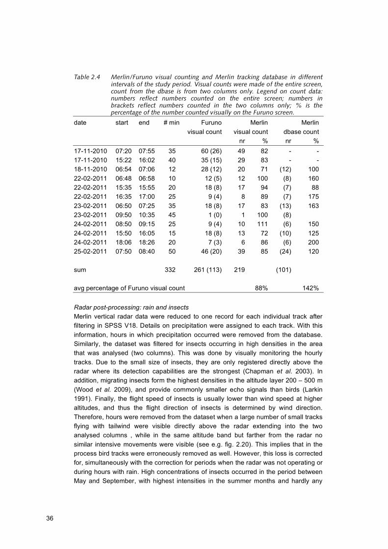
Comparison of tracks visible on the Merlin screen and on the Furuno screen The most direct test of the performance of the Merlin bird detection system was a comparison of the numbers of tracks visible on the Furuno screen (raw radar) and the numbers of tracks tracked on the Merlin screen within the same time span. Therefore, simultaneous recording of flight movements observed on the Merlin screen and on the Furuno screen (both in the K14 Control Room), gives detection chances of Merlin compared to visual detection from ‘raw’ radar. A total of 261 tracks were recorded, of which 84% was correctly detected by Merlin (table 2.4). Comparison of tracks recorded by Merlin and visually seen on the Furuno screen Analysis of the flagfile resulted in a clutter filter that was applied to all generated Merlin data collected at K14. The question was if this clutter filter based on the flagfile could be applied to the actual Merlin data as well or if the flagfile was aspecific for the actual Merlin data. The most direct test to evaluate the applied clutter filter was a comparison of the numbers of tracks visually observed on the screen (raw radar) and the numbers of tracks recorded in the Merlin database within the same time span (in line with procedures described in Krijgsveld et al. 2011). In general two to three times as many tracks were counted visually on the Furuno screen compared to the number recorded in the Merlin database, although large variation existed (261 versus 101; table 2.4). This is not a fair comparison however, because visual counts were done in the whole radar screen whereas in the Merlin database only two columns were selected (fig. 2.9). To make a fair comparison, some corrections need to be made. The two columns represent a total of roughly 1,350,000 m2 of the sampled surface. The total sampled surface is (0,5 screen * pi *(0,75 NM)2) = 3,013,140 m2. This means that a rough correction factor of 0.44 should be applied to the total number of tracks found. This results in 101*0.44 = 113 tracks (on average). After this correction, more tracks were recorded in the database than were seen visually on the Furuno screen (146%). Sample size is low however, so this figure only gives a rough indication. The difference is probably due to tracks of birds being separated into more tracks, and due to some clutter remaining in the database.

36

Table 2.4 Merlin/Furuno visual counting and Merlin tracking database in different

intervals of the study period. Visual counts were made of the entire screen,

count from the dbase is from two columns only. Legend on count data:

numbers reflect numbers counted on the entire screen; numbers in

brackets reflect numbers counted in the two columns only; % is the

percentage of the number counted visually on the Furuno screen.

date start end # min Furuno Merlin Merlin visual count visual count dbase count nr % nr % 17-11-2010 07:20 07:55 35 60 (26) 49 82 - - 17-11-2010 15:22 16:02 40 35 (15) 29 83 - - 18-11-2010 06:54 07:06 12 28 (12) 20 71 (12) 100 22-02-2011 06:48 06:58 10 12 (5) 12 100 (8) 160 22-02-2011 15:35 15:55 20 18 (8) 17 94 (7) 88 22-02-2011 16:35 17:00 25 9 (4) 8 89 (7) 175 23-02-2011 06:50 07:25 35 18 (8) 17 83 (13) 163 23-02-2011 09:50 10:35 45 1 (0) 1 100 (8) 24-02-2011 08:50 09:15 25 9 (4) 10 111 (6) 150 24-02-2011 15:50 16:05 15 18 (8) 13 72 (10) 125 24-02-2011 18:06 18:26 20 7 (3) 6 86 (6) 200 25-02-2011 07:50 08:40 50 46 (20) 39 85 (24) 120 sum 332 261 (113) 219 (101) avg percentage of Furuno visual count 88% 142% Radar post-processing: rain and insects Merlin vertical radar data were reduced to one record for each individual track after filtering in SPSS V18. Details on precipitation were assigned to each track. With this information, hours in which precipitation occurred were removed from the database. Similarly, the dataset was filtered for insects occurring in high densities in the area that was analysed (two columns). This was done by visually monitoring the hourly tracks. Due to the small size of insects, they are only registered directly above the radar where its detection capabilities are the strongest (Chapman et al. 2003). In addition, migrating insects form the highest densities in the altitude layer 200 – 500 m (Wood et al. 2009), and provide commonly smaller echo signals than birds (Larkin 1991). Finally, the flight speed of insects is usually lower than wind speed at higher altitudes, and thus the flight direction of insects is determined by wind direction. Therefore, hours were removed from the dataset when a large number of small tracks flying with tailwind were visible directly above the radar extending into the two analysed columns , while in the same altitude band but farther from the radar no similar intensive movements were visible (see e.g. fig. 2.20). This implies that in the process bird tracks were erroneously removed as well. However, this loss is corrected for, simultaneously with the correction for periods when the radar was not operating or during hours with rain. High concentrations of insects occurred in the period between May and September, with highest intensities in the summer months and hardly any

37

during the spring and autumn bird migration (tabel 2.5). Beyond this period, insects were occasionally observed, but in low concentrations outside the two columns that were analysed. During this filtering process, in total 197 hours with 17,901 tracks were removed. Table 2.5 Number of hours removed per month due to high concentrations of insects

in the analysed columns.

month nr of removed hours March 2 April 2 May 14 June 73 July 97 August 1 September 8

Radar analysis Fluxes (i.e. Mean Traffic Rate; MTR) in this report are given as the number of tracks (bird groups) per kilometre per hour. These fluxes were determined by using the ‘Two Column Analysis Area’ (fig. 2.12). These two columns were equally divided into 10 altitude bands with the same height (139 m). The lowest altitude band was then split into half (0 – 69 m and 70 – 139 m) to allow more small-scale analysis at the lowest altitude. Statistical analysis of radar data In order to determine whether MTRs were statistically different among months, hours or diurnal periods at K14, general linear models (GLMs) were applied to the dataset. Therefore, MTRs were determined per hour and log-transformed in order to counteract that the dataset was highly skewed. Subsequently, data were tested on the main effect of month, hour and light (i.e. diurnal period), as well as on the interaction between month and hour, and between month and light. Seasonal differences were not statistically tested, as seasons in fact provide a summary of monthly effects. A similar test was carried out to investigate differences in mean flight altitudes, which values were also log-transformed before analysis. Finally, mean proportions of all birds flying at risk altitude (25 – 139 m) were compared between K14 and OWEZ. Therefore, mean values were calculated per month, arcsine transformed and used as replicates in a paired t-test.

2.4.3 Attraction of birds and insects to the illuminated K14 platform

Birds In contrast to the metmast at OWEZ, K14 is a lighted platform. This means that birds can be attracted to the lights on the platform. As a result, measurements of fluxes can be elevated when the radar is tracking birds approaching the platform and flying around it in circles. To investigate to what extent this effect occurred, we analysed hourly trackplots of nights during migration periods.

38

In some instances, attraction around the platform was indeed observed. A rough estimate based on trackplot images, indicates that attraction may possibly have occurred on 5-10% of the nights at maximum in spring and autumn. Birds circling around the platform were however confined to an area that fell outside the two columns that were analysed. Therefore, any tracks of birds circling around the platform, were not included in the flux presented in this report. Attraction of birds from higher altitudes down to the platform was not observed in the data (see fig. 2.18).

Figure 2.18 Two examples of bird migration at night, without indication of attraction to

the platform. Trackplots of echoes recorded by Merlin during one hour, on 10 Oct 2010 1:00-2:00 h (top) and on 17 Oct 2010 3:00-4:00h (bottom). Trackplots based on unfiltered data, including clutter. Colours: green - reflects birds flying to the right of the screen; purple - birds flying to the left; gray - background image of the radar screen, showing the sea surface at the bottom of the screen, and bands of interference closely around the radar (§2.4.2). Lower panel: birds were migrating in a diagonal angle to the radar, which explains the curved tracks in what appear to be both directions.

39

Insects Merlin also recorded tracks of insects. These tracks were mostly found in summer and straight above the radar. In contrast to OWEZ, where tracks of insects were restricted to a narrow band just above the radar (fig. 2.19), higher concentrations of insects were observed above K14 (fig. 2.20. Apparently, insects were also attracted to the illuminated platform at night, because numbers occasionally increased dramatically during hours of darkness. While at OWEZ the vast majority of insects was removed from the data because they fell outside the two columns that were analysed (see §2.4.1 ‘Two Column Analysis’), this was not the case at K14. However, data with high concentrations of insects were removed from the database (see above, under ‘radar post-processing’).

Figure 2.19 Examples of insects (and some birds) tracked by Merlin above the

metmast at OWEZ. Top: 17 June 2007 19:00-20:00h. Bottom: 8 July 2007 20:00-21:00h. Trackplot legend see fig. 2.15.

40

Figure 2.20 Examples of high densities of insects tracked during dark above K14.

Top: 8 June 2010 2:00-3:00 h. Bottom: 2 June 2010 23:00-00:00h. Trackplot legend see fig. 2.15.

41

3 Visual observations of flying birds: species composition and flight altitude

3.1 Species composition

Between 14 April 2010 and 23 March 2011, a total of 146 panorama scans was carried out over 29 days. Birds were recorded during all but six panorama scans. In line with the aim of the study, most panorama scans were made in spring and autumn (the main migratory periods), with fewer during summer and winter (fig. 3.1).

Figure 3.1 Numbers of observation days and panorama scans undertaken during

each season. A total of 87 species was recorded during observations from K14, plus an additional 19 species groups that could not be identified to the species level, such as swan species, tern species and songbird species (table 3.1). During the panorama scans a total of 40 species and 14 species groups was recorded. Species recorded at K14 included typical seabird species as well as terrestrial species that were on migration. Seabirds recorded abundantly included species such as northern fulmar, northern gannet, great-black-backed gull, kittiwake and guillemot, all of which were recorded in most months. Scarcer species included a single Balearic shearwater in September, a long-tailed skua in October, a Sabine’s gull in September and little auk in October and November. Terrestrial species were recorded both in flight and on the platform itself; these were species that were migrating. Consequently, most records of these were made during spring and autumn. One notable exception to this is the records of six wader species (oystercatcher, lapwing, golden plover, woodcock, snipe and curlew) that were noted in February and were

42

possibly undertaking migration in response to weather conditions. Some scarcer species recorded include a Pallas’ warbler in November, an ortolan bunting in May. Other interesting records included short-eared owls in September, October and November, a wood lark in November and a grasshopper warbler, marsh warbler and snow bunting, all in October. Table 3.1 Species recorded during observations from K14. Species groups are

indicated in italics. ‘X’ indicates that the species was recorded during the

panorama scans between 14 April 2010 and 23 March 2011, ‘o’ indicates

the species was only recorded during additional observations. No

observations were carried out during January and July (-), and no

panorama scans in December.

Jan Feb Mar Apr May Jun Jul Aug Sep Oct Nov Dec divers red-throated diver - X - X black-throated diver - X - X great northern diver - o - diver spec. - o X X - X X tubenoses northern fulmar - o X X X - o X X X tubenose spec. - - X shearwaters Balearic shearwater - - o gannets northern gannet - o o X X X - X X X X cormorants great cormorant - X - o X European shag - o X - o o cormorant spec. - - X X geese & swans white-fronted goose - o - X dark-bellied brent goose - X - X swan spec. - - X goose spec. - - o other ducks common shelduck - - o Eurasian wigeon - o - o teal - o - red-breasted merganser - X - sea ducks eider - o - common scoter - X X - X X duck spec. - o o - rails - rail spec. - - o waders oystercatcher - o o - lapwing - o - X woodcock - o - o snipe - o - curlew - o - common sandpiper - - o dunlin - - o Continued on next page.

43

Table 3.1 Continued.

Jan Feb Mar Apr May Jun Jul Aug Sep Oct Nov Dec skuas great skua - - X o pomarine skua - X - X X Arctic skua - - o X long-tailed skua - - X gulls common gull - X X X - o X X great black-backed gull - X X X X - o X X X o glaucous gull - o - herring gull - X X o - o X X o lesser black-backed gull - o X X X X - X X o o black-headed gull - o X X X - o o X little gull - o X X X - o X Sabine's gull - - o kittiwake - X X X X X - X X X X o black-backed gull spec. - o X X X X - X X X X large gull - X X X X X - X X X small gull - X X X X - X gull spec. - X X - X X terns Arctic tern - - X common tern - X - Sandwich tern - X X - o X o common/arctic tern - X - tern spec. - X - alcids little auk - - X X guillemot - X X X X o - X X X razorbill - X X X X - o X Atlantic puffin - X X o - razorbill/guillemot - X X X X X - o X X X raptors & owls hen harrier - - o sparrowhawk - X - X o kestrel - - o merlin - - o short-eared owl - X - o o o other land birds larger landbirds stock dove - o - wood pigeon - o o - collared dove - o o o - jackdaw - - o rook - o - medium-sized passerines blackbird - o - o X o fieldfare - - o o redwing - - X o song thrush - - o o X Continued on next page.

44

Table 3.1 Continued.

Jan Feb Mar Apr May Jun Jul Aug Sep Oct Nov Dec small passerines skylark - - X wood lark - - o swallow - o - house martin - o - meadow pipit - o - X X water pipit - o o o - o o rock pipit - - o o yellow wagtail - - o white wagtail - X - pied wagtail - o - goldcrest - o - grasshopper warbler - - o marsh warbler - - o willow warbler - o - chiffchaff - o X - o o o willow warbler/chiffchaff - o - Pallas' warbler - - o blackcap - - o o garden warbler - - o whitethroat - o - spotted flycatcher - o - pied flycatcher - - o robin - o o o - o o redstart - - o o northern wheatear - o - o starling - o X X o - X X chaffinch - o - o o brambling - - o siskin - - o ortolan bunting - o - snow bunting - - X pipit spec. - - o thrush spec. - - X X finch spec. - - X small songbird spec. - X X 0 - 0 X

45

Figure 3.2 Birds recorded at K14 during the observation periods, clockwise from top left European shags, kittiwakes, kestrel (above door), snipe, blackbird, collared doves, lapwing and lesser black-backed gulls (including the colour-ringed bird J49N, as read with the aid of a telescope) and great black-backed gull. Photos: Daniël Beuker, Karen Krijgsveld and Mark Collier.

46

During the observations a number of colour-ringed gulls were seen on K14 (fig. 3.2 second on left). The colour-rings of two lesser black-backed gulls and four great black-backed gulls were traced as all being marked in Norway (table 3.2). For one additional observation a discrepancy between the recorded species and the species ringed with that specific colour-ring meant that the ringing details for this bird could not be confirmed. It concerned a lesser black-backed gull ringed as pullus in Denmark.

Table 3.2 Colour-ringed gulls read at K14. All gulls were ringed as pulli in colonies in Norway. Ringing data courtesy of Morten Helberg (www.ringmerking.no/cr).

Species Ring Date ringed Location Dates on K14

Lesser black-backed gull J49N 15-7-2007 Rauna, Norway 15-4-2010 16-4-2010

Lesser black-backed gull J7ZZ 8-7-2006 Rauna, Norway 15-4-2010

Great black-backed gull J16Z 22-6-2007 Ronekilen, Norway 27-10-2010

Great black-backed gull JA125 27-6-2008 Kamferhof, Norway 1-9-2010 21-9-2010

Great black-backed gull JH074 20-6-2010 Indre Teistholmen, Norway 1-9-2010 2-9-2010

Great black-backed gull JH333 8-7-2010 Kjellingen, Norway 2-9-2010

3.2 Species abundance

Bird densities A total of 47 species or species groups was recorded in flight during the panorama scans; the abundance of these species is given in table 3.3. The total density of all flying birds combined was 0.47 birds/km2. The densities of 13 species were 0.01 birds/km2 or higher. The most abundant species were northern gannet (0.10 birds/km2), starling (0.10 birds/km2), kittiwake (0.07 birds/km2), great black-backed gull (0.06 birds/km2) and lesser black-backed gull (0.04 birds/km2). Seasonal variation Of the 47 species or species groups that were recorded in flight during the panorama scans, 38 of these were recorded during autumn. The fewest species (five) were recorded in summer. Similarly, the abundance of flying birds was highest in autumn (1.21 birds/km2) and was over twice that of the other seasons combined. Densities above 0.1 birds/km2 were recorded for eight species; these were northern gannet (autumn), common scoter (spring), great black-backed gull (autumn), lesser black-backed gull (spring), common gull (winter), kittiwake (autumn), guillemot (autumn) and starling (autumn). For the majority of species, the highest densities of flying birds were recorded during autumn. Exceptions were common scoter and lesser black-backed gull, which peaked in spring, and common gull, which peaked in winter.

47

The densities of most species groups were highest in November (fig. 3.3). Exceptions were other ducks, which peaked in February, sea ducks, which peaked in March and terns, which peaked in September. Terns were also present during spring and early summer, coinciding with the main migration periods for these species. Gulls were recorded in all months during which panorama scans were carried out. Densities of gulls were highest in early spring, late summer and autumn. Following the peak recorded in early spring, numbers declined during the breeding season.

48

Table 3.3 Density of flying birds observed at K14 per season (birds/scan//km2). Maximum densities are shown in bold. Only birds recorded within 3 km of the platform are considered. No value indicates that the species was not recorded during the season. Colour indicates maximum density: dark blue >0.1; mid-blue 0.01-01; light blue 0.005-0.01. n indicates the number of panorama scans carried out. No panorama scans were carried out during January, December (both winter) or July (summer).

mean density (birds/scan/km2) at K14 spring summer autumn winter total group species (n=72) (n=20) (n=39) (n=15) (n=146) divers black-throated diver <0,005 <0,005 diver spec. <0,005 <0,005 <0,005 red-throated diver <0,005 <0,005 <0,005 tubenoses northern fulmar <0,005 0,01 <0,005 tubenose spec. <0,005 <0,005 gannets northern gannet <0,005 0,02 0,32 0,10 cormorant spec. <0,005 <0,005 great cormorant <0,005 <0,005 geese & swans white-fronted goose 0,01 <0,005 sea ducks common scoter 0,02 <0,005 0,01 other ducks red-breasted merganser <0,005 <0,005 waders lapwing 0,01 <0,005 skuas arctic skua <0,005 <0,005 pomarine skua <0,005 <0,005 gulls black-backed gull spec. 0,01 <0,005 0,01 0,01 great black-backed gull 0,02 0,17 0,01 0,06 herring gull <0,005 <0,005 <0,005 <0,005 large gull 0,02 0,04 0,01 0,02 lesser black-backed gull 0,07 0,02 <0,005 0,04 black-headed gull <0,005 <0,005 <0,005 common gull <0,005 0,01 0,17 0,02 kittiwake 0,02 0,03 0,20 0,07 small gull 0,01 0,01 0,03 0,01 little gull <0,005 <0,005 <0,005 gull spec. 0,01 0,01 terns common tern <0,005 <0,005 common/arctic tern <0,005 <0,005 Sandwich tern <0,005 <0,005 <0,005 alcids Atlantic puffin <0,005 <0,005 guillemot <0,005 0,02 <0,005 0,01 little auk 0,01 <0,005 razorbill <0,005 0,01 <0,005 <0,005 razorbill/guillemot 0,01 0,03 <0,005 0,01 raptors & owls sparrowhawk <0,005 <0,005 short-eared owl <0,005 <0,005 songbirds redwing <0,005 <0,005 (small&medium) song thrush <0,005 <0,005 starling 0,01 0,31 0,10 thrush spec. 0,01 <0,005 chiffchaff <0,005 <0,005 finch spec. <0,005 <0,005 meadow pipit <0,005 <0,005 white wagtail <0,005 <0,005 skylark <0,005 <0,005 snow bunting <0,005 <0,005 songbird spec. <0,005 0,01 <0,005 bird unidentified bird spec. <0,005 <0,005 all birds 0,22 0,08 1,21 0,23 1,74

49

Figure 3.3 Variation in density of flying birds throughout the year for various species

groups. Only birds within 3 km of the platform are considered and no counts were carried out in July, December or January.

divers

landbirds (excl. raptors and owls)

geese & swans

terns gulls

other ducks sea ducks

cormorants gannets

alcids

Month

Bird

den

sity

(bird

s/km

2 )

50

Species composition Gulls were the most abundant species group, making up half (49%) of all birds recorded (fig. 3.4). Gannets (northern gannet) and land birds each constituted around 20% of all flying birds recorded. During autumn the relative abundance of each of these groups was 26% and 27% respectively. Land birds were recorded in very low numbers during the rest of the year and even in spring only represented 1% of all birds recorded. Over 5% of the flying birds recorded were alcids.

Figure 3.4 Relative abundance of species groups recorded in flight during panorama

scans. The axis of the lower figure has been limited to 5% to enable comparison of species groups representing a low percentage of the total birds recorded.

51

3.3 Species-specific flight altitudes

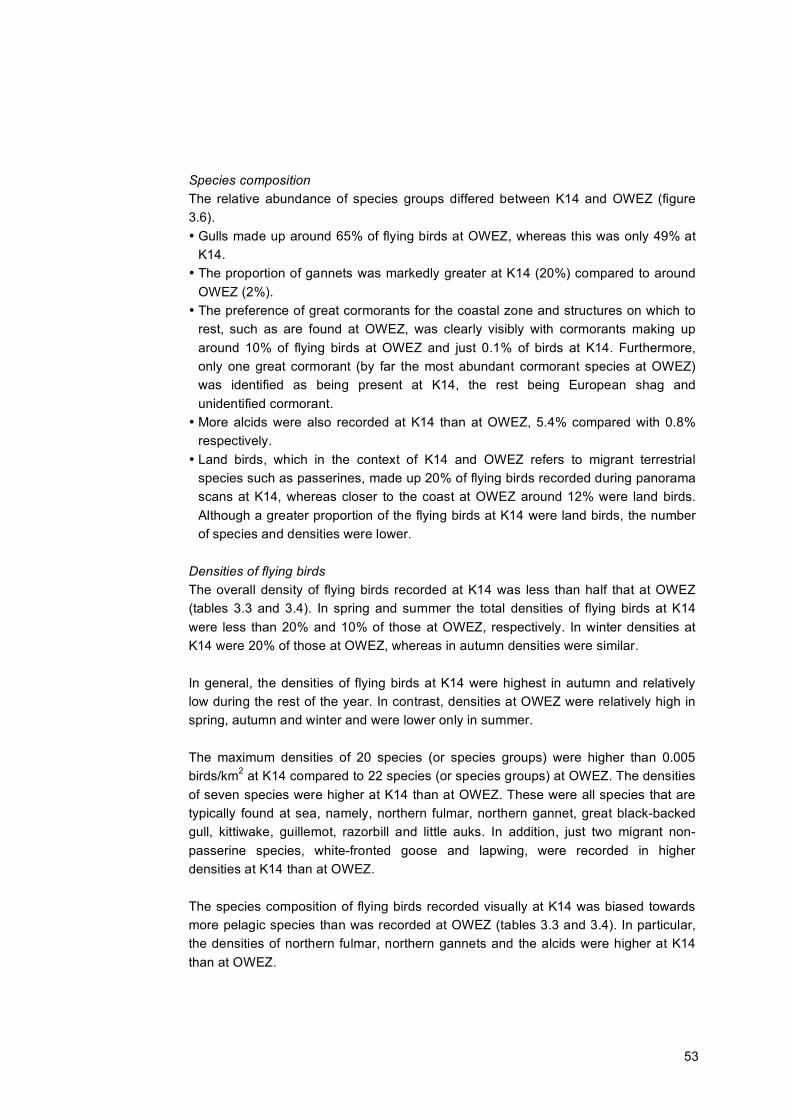
The average flight altitudes of flying bird groups as recorded during the panorama scans are given in figure 3.5. Average flight heights varied between less than 1 m to over 60 m. The actual flight heights of some birds were often greater than shown here as the heights presented are averaged for the distance and height category in which the bird was recorded. The average flight height of divers was around 20 m, although most were under this height with an occasional high-flying bird (c.50 to 100 m) recorded. The tubenoses (northern fulmar) were generally recorded below 20 m, as were sea ducks, other ducks, waders, terns and alcids. Gannets (northern gannet) and cormorants were recorded at a range of heights, from under 10 m to over 60 m. The same was true for the gulls, which were recorded across the widest range of altitudes (<5 to >80 m). Geese and swans were recorded at heights of between 45 m and 80 m. Raptors and owls also showed a tendency to higher altitudes, being recorded between 50 m and 75 m. The average flight height of land birds was around 30 m, although birds were recorded across a wide range of altitudes.

Figure 3.5 Average flight altitudes and standard deviations of species groups

recorded in flight during panorama scans. In Krijgsveld et al. (2011), birds flying between 25 and 139 m were assumed to be at a risk altitude for collisions with wind turbines in OWEZ.

52

3.4 Comparison of visual observations with OWEZ

In order to allow a comparison to the results from similar observations carried out at OWEZ results from Krijgsveld et al. (2011) have been reproduced here. For full interpretation of the results from OWEZ refer to Krijgsveld et al. (2011).

Figure 3.6 Relative abundance of species groups recorded in flight during panorama

scans at K14 (black bars) and OWEZ (grey bars). The axis of the right hand figure has been limited to 5% to enable comparison of species groups representing a low percentage of the total birds recorded. Data from OWEZ adapted from Krijgsveld et al. (2011). Data for K14 taken from figure 3.4.

53

Species composition The relative abundance of species groups differed between K14 and OWEZ (figure 3.6). • Gulls made up around 65% of flying birds at OWEZ, whereas this was only 49% at

K14. • The proportion of gannets was markedly greater at K14 (20%) compared to around

OWEZ (2%). • The preference of great cormorants for the coastal zone and structures on which to

rest, such as are found at OWEZ, was clearly visibly with cormorants making up around 10% of flying birds at OWEZ and just 0.1% of birds at K14. Furthermore, only one great cormorant (by far the most abundant cormorant species at OWEZ) was identified as being present at K14, the rest being European shag and unidentified cormorant.

• More alcids were also recorded at K14 than at OWEZ, 5.4% compared with 0.8% respectively.

• Land birds, which in the context of K14 and OWEZ refers to migrant terrestrial species such as passerines, made up 20% of flying birds recorded during panorama scans at K14, whereas closer to the coast at OWEZ around 12% were land birds. Although a greater proportion of the flying birds at K14 were land birds, the number of species and densities were lower.

Densities of flying birds The overall density of flying birds recorded at K14 was less than half that at OWEZ (tables 3.3 and 3.4). In spring and summer the total densities of flying birds at K14 were less than 20% and 10% of those at OWEZ, respectively. In winter densities at K14 were 20% of those at OWEZ, whereas in autumn densities were similar. In general, the densities of flying birds at K14 were highest in autumn and relatively low during the rest of the year. In contrast, densities at OWEZ were relatively high in spring, autumn and winter and were lower only in summer. The maximum densities of 20 species (or species groups) were higher than 0.005 birds/km2 at K14 compared to 22 species (or species groups) at OWEZ. The densities of seven species were higher at K14 than at OWEZ. These were all species that are typically found at sea, namely, northern fulmar, northern gannet, great black-backed gull, kittiwake, guillemot, razorbill and little auks. In addition, just two migrant non-passerine species, white-fronted goose and lapwing, were recorded in higher densities at K14 than at OWEZ. The species composition of flying birds recorded visually at K14 was biased towards more pelagic species than was recorded at OWEZ (tables 3.3 and 3.4). In particular, the densities of northern fulmar, northern gannets and the alcids were higher at K14 than at OWEZ.

54

Table 3.4 Density of flying birds at OWEZ observed per season (birds/scan//km2). Maximum densities shown in bold. Only birds recorded within 3 km from metmast at OWEZ are considered. No value indicates that the species was not recorded during the season. Colour indicates maximum density: dark blue >0,1; mid-blue 0,01-01; light blue 0,005-0,01. n indicates the number of panorama scans carried out. From Krijgsveld et al. (2011).

spring summer autumn winter totalgroup subgroup species (n=140) (n=71) (n=121) (n=73) (n=405)divers black-throated diver <0,005 <0,005

red-throated diver <0,005 0,01 <0,005diver spec. <0,005 <0,005 <0,005

grebes great crested grebe <0,005 <0,005tubenoses northern fulmar <0,005 <0,005 <0,005 <0,005gannets northern gannet 0,03 <0,005 0,05 0,02 0,03cormorants European shag <0,005 <0,005

great cormorant 0,06 0,18 0,08 0,07 0,09geese & swans anser geese greylag goose <0,005 <0,005

branta geese dark-bellied brent goose 0,01 0,01 0,04 0,01unidentified geese goose spec. <0,005 <0,005

sea ducks common scoter 0,03 <0,005 <0,005 <0,005 0,01eider <0,005 <0,005 <0,005velvet scoter <0,005 <0,005

other ducks diving ducks scaup <0,005 <0,005 <0,005mergansers goosander <0,005 <0,005

red-breasted merganser <0,005 <0,005 <0,005swimming ducks Eurasian wigeon <0,005 <0,005 <0,005

northern pintail 0,01 <0,005teal <0,005 <0,005

unidentified ducks duck spec. <0,005 <0,005 <0,005waders Eurasian curlew <0,005 <0,005

grey plover <0,005 <0,005calidris spec. <0,005 <0,005dunlin 0,01 <0,005Eurasian golden plover <0,005 <0,005lapwing <0,005 <0,005oystercatcher <0,005 <0,005wader spec. <0,005 <0,005

skuas arctic skua <0,005 <0,005gulls large gulls black-backed gull spec. 0,02 0,01 0,01 0,01 0,01

lesser black-backed gull 0,23 0,20 0,06 <0,005 0,13great black-backed gull 0,03 <0,005 0,05 0,11 0,05herring gull 0,19 0,06 0,02 0,10 0,10common/herring gull <0,005 <0,005large gull spec. 0,21 0,13 0,09 0,10 0,14

small gulls black-headed gull 0,05 0,05 0,01 0,03 0,03common gull 0,06 <0,005 0,03 0,31 0,09kittiwake <0,005 0,14 0,23 0,08Sabine's gull <0,005 <0,005little gull 0,12 0,01 0,04small gull spec. 0,02 0,01 0,06 0,02

unidentified gulls gull spec. 0,01 0,02 0,01 0,01terns arctic tern <0,005 <0,005

common tern <0,005 <0,005 <0,005common/arctic tern <0,005 <0,005 <0,005 <0,005black tern <0,005 <0,005sandwich tern 0,01 0,06 0,01 0,02tern spec. <0,005 <0,005 <0,005

alcids guillemot <0,005 <0,005 <0,005razorbill <0,005 <0,005 <0,005 <0,005razorbill/guillemot <0,005 0,01 <0,005

raptors & owls raptors goshawk <0,005 <0,005kestrel <0,005 <0,005marsh harrier <0,005 <0,005merlin <0,005 <0,005peregrine <0,005 <0,005

landbirds other large birds grey heron <0,005 <0,005wood pigeon <0,005 <0,005homing pigeon <0,005 <0,005 <0,005pigeon spec. <0,005 <0,005carrion crow <0,005 <0,005jackdaw <0,005 <0,005

small passerines redpoll <0,005 <0,005skylark <0,005 <0,005swallow <0,005 <0,005swift <0,005 <0,005yellow wagtail <0,005 <0,005songbird spec. <0,005 <0,005 <0,005

medium-sized pass. blackbird <0,005 <0,005 <0,005redwing <0,005 <0,005song thrush <0,005 <0,005thrush spec. 0,02 0,01starling 0,17 <0,005 0,63 0,01 0,25

small passerines chaffinch <0,005 <0,005 <0,005house martin <0,005 <0,005meadow pipit <0,005 <0,005pied wagtail <0,005 <0,005pipit spec. <0,005 <0,005

all birds 1,28 0,71 1,26 1,15 1,15

mean density (birds/km2/scan)

55

Although gulls were the most abundant species group recorded at both K14 and OWEZ, the proportions of each species recorded differed between the two locations. The main gulls species recorded at K14 were kittiwake and great black-backed gull, whereas at OWEZ, lesser black-backed gulls, herring gulls and common gulls were most abundant. Flight altitudes The average flight altitudes of birds as recorded during the panorama scans at K14 and OWEZ are given in figure 3.7. Due to the fact that differences in flight heights were seen between birds inside and outside the OWEZ wind farm, the data presented here for OWEZ only includes observations of birds outside of the boundary of the OWEZ wind farm. The actual flight heights of some birds were often greater than shown here as the heights presented are averaged for the distance and height category in which the bird was recorded. The following general patterns can be seen:

• The average flight altitudes of most species groups were largely similar at both K14 and OWEZ. For some species-groups differences may be due to a small number of observations, for example, geese & swans, other ducks, waders and raptors & owls.

• Tubenoses (northern fulmar), sea ducks and alcids flew at low altitudes (<20 m).

• Gulls flew at a range of altitudes, although on average around 50 m. • Gannets (northern gannet) and cormorants were recorded at slightly higher

altitudes at K14 than at OWEZ. • Terns flew higher at OWEZ than around K14. • Land birds (mainly migrant passerines) flew at an average height of below 40

m and all were observed below 100 m. This, however, is most likely due to limited detection of small birds, which is generally much lower at distances greater than 100m.

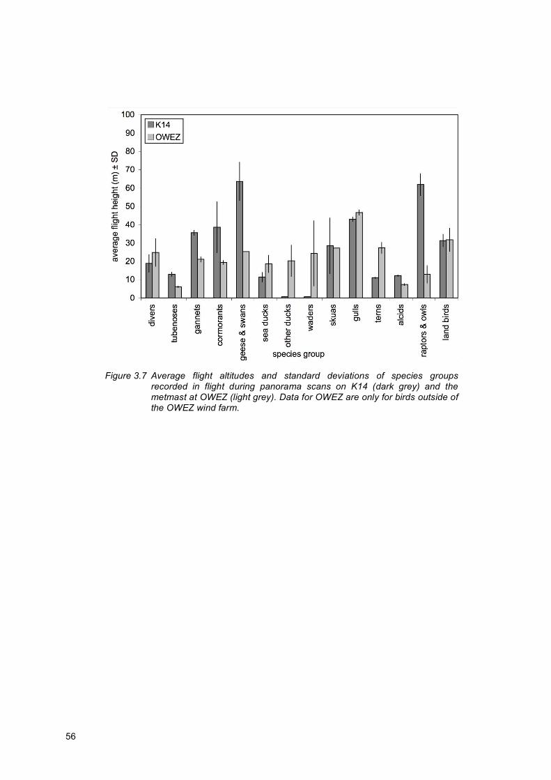
56

Figure 3.7 Average flight altitudes and standard deviations of species groups

recorded in flight during panorama scans on K14 (dark grey) and the metmast at OWEZ (light grey). Data for OWEZ are only for birds outside of the OWEZ wind farm.

57

4 Radar observations of bird movements: flight intensity and altitude

In this chapter we present the results of the radar observations at K14 in comparison with OWEZ. It focuses on the temporal numbers, fluxes and flight altitudes of bird groups throughout the period March 2010 – March 2011. It separately presents also the number of bird groups measured during daylight and in darkness, as well as flight altitudes categorized in risk classes in relation to wind turbine heights.

4.1 Overall numbers and fluxes

4.1.1 Monthly variation in flight intensity

Overall number of bird groups Between March 2010 and March 2011, the radar registered a total of 212,987 bird groups at K14 in a stretch of 1 km up to 1,400 m altitude. However, due to technical failures and strong winds (i.e. wind speed above 7 Bft) the radar was not functioning continuously, and hence summed numbers had to be corrected for the periods that the radar was not operating. The proportion of radar interruptions varied between 97% (August 2010) to 2% (April 2010), with an average of 33%. Assuming a homogeneous distribution of bird numbers within a month, the total number of bird groups per month was estimated by extrapolating the actually registered numbers. This resulted in a corrected total of 344,215 bird groups/km for the whole study period.

Figure 4.1 Number of bird groups per month in a 1-km stretch, as measured with

vertical radar (dark bars) and corrected for radar interruptions (white bars).

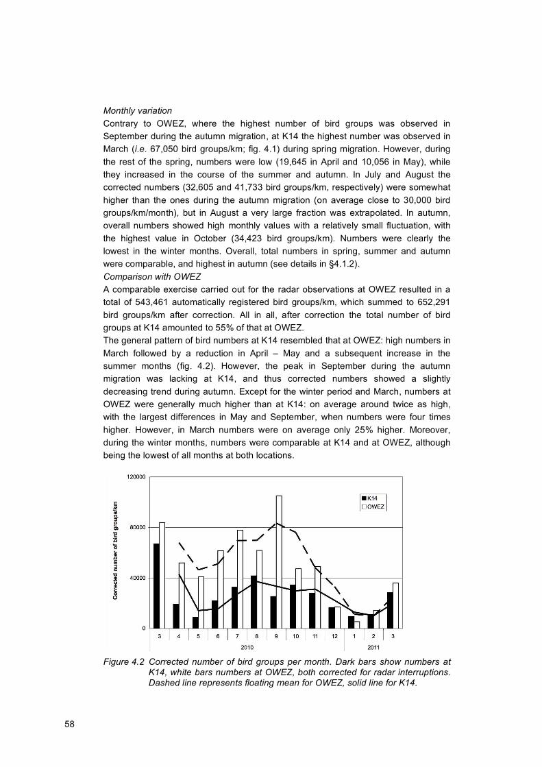
58

Monthly variation Contrary to OWEZ, where the highest number of bird groups was observed in September during the autumn migration, at K14 the highest number was observed in March (i.e. 67,050 bird groups/km; fig. 4.1) during spring migration. However, during the rest of the spring, numbers were low (19,645 in April and 10,056 in May), while they increased in the course of the summer and autumn. In July and August the corrected numbers (32,605 and 41,733 bird groups/km, respectively) were somewhat higher than the ones during the autumn migration (on average close to 30,000 bird groups/km/month), but in August a very large fraction was extrapolated. In autumn, overall numbers showed high monthly values with a relatively small fluctuation, with the highest value in October (34,423 bird groups/km). Numbers were clearly the lowest in the winter months. Overall, total numbers in spring, summer and autumn were comparable, and highest in autumn (see details in §4.1.2). Comparison with OWEZ A comparable exercise carried out for the radar observations at OWEZ resulted in a total of 543,461 automatically registered bird groups/km, which summed to 652,291 bird groups/km after correction. All in all, after correction the total number of bird groups at K14 amounted to 55% of that at OWEZ. The general pattern of bird numbers at K14 resembled that at OWEZ: high numbers in March followed by a reduction in April – May and a subsequent increase in the summer months (fig. 4.2). However, the peak in September during the autumn migration was lacking at K14, and thus corrected numbers showed a slightly decreasing trend during autumn. Except for the winter period and March, numbers at OWEZ were generally much higher than at K14: on average around twice as high, with the largest differences in May and September, when numbers were four times higher. However, in March numbers were on average only 25% higher. Moreover, during the winter months, numbers were comparable at K14 and at OWEZ, although being the lowest of all months at both locations.

Figure 4.2 Corrected number of bird groups per month. Dark bars show numbers at

K14, white bars numbers at OWEZ, both corrected for radar interruptions. Dashed line represents floating mean for OWEZ, solid line for K14.

59

Mean traffic rates Logically, expressing the overall numbers as mean traffic rate (MTR: number of bird groups/km/hour), resulted in a similar picture as the overall numbers (fig. 4.3). The overall numbers presented here above are a result of summing all detected bird groups, and thus are directly affected by large within day and between day fluctuations. MTRs represent hourly averages, and therefore the effect of large fluctuations dissolves in the means. The yearly mean MTR at K14 was 45 bird groups/km/h, ranging from 14 bird groups/km/h in May to 107 bird groups/km/h in March 2010. In the period July – September, the measured MTR was nearly constant, with a mean of 51 bird groups/km/h, with the smallest variation (depicted by the SD bars in fig. 4.3). Although the total numbers during the autumn migration in October – November were lower (see above), MTRs slightly increased to a mean of 64 bird groups/km/h, due to occasional highly concentrated migration influxes alternated by periods with less intense movements. During summer, the smaller SD values in combination with relatively high MTRs, reflect a steadier bird flux leading to higher overall numbers.

Corresponding MTR figures for OWEZ were a yearly mean of 73 bird groups/km/h, with a minimum of 10 bird groups/km/h in January and a maximum of 160 bird groups/km/h in September. Similarly to the overall numbers, MTRs measured at K14 and OWEZ were comparable in March and in the winter months. The largest variation in MTRs was recorded in March and October at K14, and March and September at OWEZ.

Figure 4.3 Mean traffic rate (number of bird groups/km/hour) per month registered at

K14 (black bars) and OWEZ (white bars), as measured by vertical radar. Lines above bars represent standard deviations of the means.

60

4.1.2 Seasonal variation in flight intensity

Seasonal variation in overall numbers As the species community and their abundance is coupled to a regular annual cycle, with mainly local birds expected in summer (breeding birds) and winter (wintering birds) and a higher proportion of migrants in the migration periods of spring and autumn, the flight intensities were also categorized per season. Summing the numbers this way depicted a fairly constant number of bird groups from spring to autumn both at K14 and at OWEZ. At K14 these numbers stayed below 100,000 bird groups/km/season, whereas at OWEZ at around 200,000 bird groups/km/season, thus more than twice as high as at K14. At both locations, numbers were clearly lower during winter, and nearly identical to each other: 36,893 and 36,153 bird groups/km at K14 and at OWEZ, respectively. At K14, this seasonal pattern resulted from on the one hand an average in the spring of very high numbers in March (fig. 4.4) and low numbers in April and May, and on the other hand a relatively high number with less in-between month variation from July until November. Interestingly, no clear peak comparable to March in the spring migration was observed during the autumn migration. At OWEZ, except for the winter, numbers were fluctuating more per month, and hence the fairly constant numbers are more a result of a monthly peak (i.e. March, July and September) combined with lower numbers in the rest of the season. Seasonal variation in mean traffic rates The seasonal pattern of MTRs showed a similar picture (fig. 4.5): a clearly lower value in the winter (23 bird groups/km/hour) and relatively low in-between season variation from spring to autumn (mean of 51 bird groups/km/hour), with the lowest mean MTR value in summer (46 bird groups/km/hour) and the highest in autumn (60 bird groups/km/hour).

Figure 4.4 Trackplot image of bird flight movements recorded by the vertical radar

(set at a range of 0.75 NM) on 16 March 2010, a day with heavy migration in all height altitudes to easterly directions (purple tracks). K14 is positioned in the middle at the bottom of the image.

61

Figure 4.5 Mean traffic rate (number of bird groups/km/hour) per season registered at

K14 (black bars) and OWEZ (white bars) by the vertical radar. Lines above bars represent standard deviations.

At OWEZ MTRs were commonly higher and varied slightly more from spring to autumn (between 78 bird groups/km/hour in spring to 106 bird groups/km/hour in autumn), but was the same during winter (20 bird groups/km/hour). The standard deviation (SD) was the lowest in winter at both locations, indicating a rather constant bid flux throughout the season. In the other seasons SDs were higher, but except for spring even more at OWEZ. In other words, except for spring, bird fluxes at K14 were less fluctuating compared with OWEZ. The largest fluctuations at K14 were recorded in spring and autumn, indicating the influx of large groups of migrating birds with lower fluxes in between.

4.1.3 Diurnal variation in flight intensity

Diurnal variation in overall numbers Considering the whole study period, an almost equal number of bird groups passed K14 during daylight and in darkness: 48% against 52%, respectively (fig. 4.6). At OWEZ similar proportions were observed, but with an opposite tendency: 53% of all bird groups were recorded during daylight against 47% during darkness.

However, a further specification of the records revealed a strong variance in diurnal flight intensity among months, both at K14 and OWEZ (fig. 4.7). At K14, during March and April, as well as during October and November, the percentage of bird groups recorded during darkness was above 50%: on average 68% in these months, with the maximum of 84% registered in March 2010. In the rest of the year, the proportion of night activity was generally lower at K14. From May to September the mean proportion of night flights was only 25%, with the three summer months being below this value. During winter the proportions were

62

higher (on average 43%), increasing throughout the season, but remained below the values of the migration periods. The values observed at OWEZ were comparable in summer and winter to that at K14. Interestingly, however, during the spring months relatively more night activity was registered at K14 compared with OWEZ, whereas the opposite was observed during the autumn months.

Figure 4.6 Number of bird groups passing K14 (left) and OWEZ (right) during daylight

(white) and in darkness (black) in a 1-km stretch, as measured with vertical radar.

Figure 4.7 Percentage of bird groups passing K14 (black bars) and OWEZ (white

bars) during darkness in a certain month, as measured with vertical radar.

63

Periods with highest nocturnal flight activity In order to highlight the periods when the highest number of birds is potentially at risk of collisions, an analysis was conducted to visualize which months’ night periods contributed the most to the overall recorded bird numbers in a year. Therefore, the numbers recorded in the different diurnal periods in a certain month are depicted as a relative proportion to the overall numbers in figure 4.8. This categorization revealed that 23% of all movements occurred in the dark periods of March 2010 and 2011 together, and another 12% during the nights of October and November (fig. 4.8). In other words, more than third of all registered movements of the whole study period occurred in the nights of March, October and November. In the rest of the year, the contribution of the night movements in a certain month to the total number of bird groups passing at K14 was much lower compared with the proportion that flew during daytime. For instance, in the period July – September, when still a reasonable amount of bird groups were registered (see fig. 4.2), most movements occurred during daylight. As a result, 21% of the yearly total number of movements occurred during daylight hours of these months.

Figure 4.8 Proportion of bird groups passing K14 during darkness (black) and daylight

(white) in a peculiar month, relative to all registered bird groups throughout the study period, as measured with vertical radar.

Interestingly, March (both in 2010 and 2011) was the only month when the contribution of night movements to the overall numbers in the study period was much higher at K14 than at OWEZ (fig. 4.9). In September the opposite was observed (e.g. the relative contribution of night movements in September was more than four times higher at OWEZ), whereas the rest of the year was comparable.

64

Figure 4.9 Proportion of bird groups passing K14 (black bars) and OWEZ (white bars)

during darkness in a certain month relative to all registered bird groups throughout the study period, as measured with vertical radar.

Diurnal variation in mean traffic rates Considering the whole year, the mean MTR at K14 was 36 bird groups/km/h during daytime, and higher during darkness with on average 58 bird groups/km/h (i.e. 159% of daylight MTR). A smaller diurnal difference was observed at OWEZ: 78 bird groups/km/h during daylight and 95 bird groups/km/h during darkness (i.e. 122% of the daylight MTR). The within-day variation in MTR was largely different among seasons (fig. 4.10). The largest fluctuation within the day was observed in spring: after a fairly constant MTR around a mean of 16 bird groups/km/h during daytime, the flight intensity rapidly increased after sunset to reach a maximum MTR 107 bird groups/km/h at 23:00. After that the flight intensity steadily decreased until the hours after sunrise.

65

Figure 4.10 Diurnal variation of mean traffic rate (number of bird groups/km/hour) at

K14 (solid line) and OWEZ (dashed line) averaged per hour in the four seasons. Shaded areas represent periods with darkness within a day in local time.

Such large differences between day and night MTRs were not observed in the other three seasons. Commonly, the sunrise brought about a peak in flight intensity, which steadily decreased to reach a minimum halfway the afternoon. In autumn, the MTR sharply increased around sunset, remained elevated for a few hours, and then decreased until shortly before sunrise.

In summer, the opposite pattern occurred: measured intensity dropped to a daily minimum around sunset, but increased again during the night. In winter the flight intensity was the lowest of all seasons with the lowest within-day variation: the only small peak occurred around sunrise. The daily pattern of flight intensities was the most comparable between K14 and OWEZ during spring and winter. In this latter season, not only the patterns, but also the actual values were similar. In autumn, the hourly MTR values showed a similar pattern during the day but the peak in flight intensity around sunset was much more prominent at OWEZ, and remained higher until shortly before sunrise. Another interesting phenomenon, a second peak in flight intensity during the night at OWEZ in summer and autumn caused by black-headed gulls coming from the Wadden Sea to sleep at open sea, was lacking at K14, as expected due to the farther situation of K14.

66

4.1.4 Statistical analysis of flight intensities at K14 and OWEZ

Considering MTRs measured at K14, a significant difference was detected between months, hours and light conditions (table 4.1, main effects month, light and hour). Moreover, the effect of hour was also significant in interaction with month, meaning that the hourly differences in MTRs were large, but in another way in the different months. On the other hand, despite the mean MTRs measured in daylight and in darkness being generally different (main effect light), the difference was comparable among months (interaction term month*light not significant). In conclusion, when considering MTRs measured at K14, care should be taken that mean MTRs measured in different months, hours and light conditions are not comparable. Table 4.1 Summary of the analysis of variance on the effects of month, hour and light

and their interactions on MTRs at K14. The symbol * indicates interactions between effects. Sig. show p-values (interpreted as significant below 0.05).

Source Type III Sum of Squares df Mean Square F Sig.

Corrected Model 575 296 1.9 9.0 <0.001 Intercept 2157 1 2156.7 10023.7 <0.001 Month 184 11 16.7 77.8 <0.001 Hour 37 23 1.6 7.5 <0.001 light 2 1 1.9 8.8 <0.01 Month * Hour 121 250 0.5 2.2 <0.001 Month * light 3 11 0.3 1.3 0.2 Error 1078 5010 0.2 Total 9741 5307 Corrected Total 1653 5306

In a further analysis, the MTRs between K14 and OWEZ, in combination with the effect of month, hour and light conditions were compared. Here the main effect of location and its interactions with month, hour and light were important. The test revealed that except for the interaction term light*location, all other tested effects were highly significant (table 4.2). In general, MTRs were significantly higher at OWEZ (main effect location), but the effect was dependent on months and hours. For instance, MTRs were comparable in October, November and all winter months. Comparably, the difference in MTRs was less in certain hours than in others. On the other hand, the non-significant interaction term between location and light revealed that although light had an effect on MTRs (see also above only for K14 in table 4.1), the difference was similar at K14 as at OWEZ.

67

Table 4.2 Summary of the analysis of variance on the effects of location and its interaction with month, hour and light on mean traffic rates (MTRs). Sig. indicates p-values.

Source Type III Sum of Squares df Mean Square F Sig.

Corrected Model 1804 596 3.0 14.8 <0.001 Intercept 7689 1 7689.1 37622.5 <0.001 Month 395 11 35.9 175.6 <0.001 Hour 47 23 2.0 9.9 <0.001 light 5 1 4.7 23.2 <0.001 location 50 1 49.8 243.5 <0.001 Month * location 103 11 9.4 45.9 <0.001 Hour * location 23 23 1.0 4.8 <0.001 light * location 0.03 1 0.03 0.2 0.7 Month * Hour * location 312 503 0.6 3.0 <0.001 Month * light * location 21 22 1.0 4.7 <0.001 Error 2432 11900 0.2 Total 29449 12497 Corrected Total 4236 12496

68

4.2 Flight altitude as determined with radar

Considering the whole study period, the most bird groups were detected in the lowest altitude band (0 – 69 m) both at K14 (more than 100,000) and at OWEZ (more than 230,000), which translates to 49% of the total flux at K14 and a slightly lower 43% at OWEZ (fig. 4.11).

Figure 4.11 Number of bird groups/km registered by vertical radar at OWEZ (white

bars) and at K14 (black bars) divided in 11 altitude bands. Above overall numbers are presented, below the observed numbers depicted as percentages of the total. Note that the two lowest altitude bands are half the height of the other classes. Flight altitudes at K14 were highly comparable to those at OWEZ.

69

Above the lowest altitude band the number of detected bird groups gradually decreased until the highest altitude at K14, whereas at OWEZ the altitude band 139 – 277 m had slightly more bird movements than registered at 69 – 139 m. However, summing these lowest three altitude bands revealed that proportions were similar between the two locations: 76% of all registered bird movements occurred below 277 m at K14 and 70% at OWEZ. Also the proportions at higher altitude classes from 277 m to 1247 m were highly comparable between K14 and OWEZ. The measured MTRs showed a similar distribution per altitude band to the overall numbers. The mean MTR at K14 in the lowest band was 19 bird groups/km/h over the whole study period, whereas 33 bird groups/km/h at OWEZ. Above this band, bird fluxes were substantially lower at K14: 9, 8, 6 bird groups/km/h in a sequential order, followed by a more or less constant flux around 5 groups/km/h from 416 m until 1247 m and a lower mean value of 2 groups/km/h in the highest band. Obviously, the MTRs at OWEZ were higher, but above the lowest altitude band the figures of OWEZ and K14 were gradually approaching each other. However, in the highest two altitude bands, again much higher MTRs were recorded at OWEZ.

Figure 4.12 Trackplot image of bird flight movements at K14 recorded by the

vertical radar on 23 April 2010. The image shows heavy migration to easterly directions (purple tracks) at all altitudes, but clearly the most tracks are in the lower altitude bands. Radar is positioned in the middle at the bottom of the image and was operating at a range of 0.75 NM.

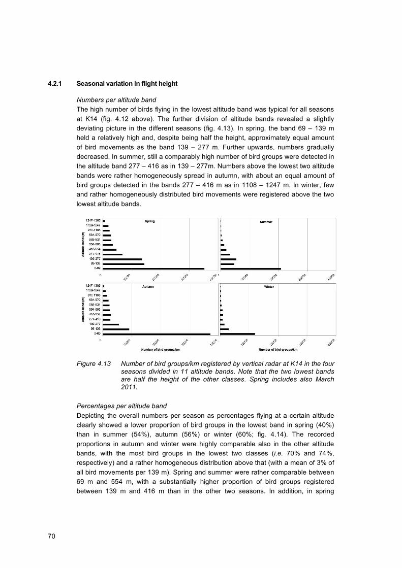
70

4.2.1 Seasonal variation in flight height

Numbers per altitude band The high number of birds flying in the lowest altitude band was typical for all seasons at K14 (fig. 4.12 above). The further division of altitude bands revealed a slightly deviating picture in the different seasons (fig. 4.13). In spring, the band 69 – 139 m held a relatively high and, despite being half the height, approximately equal amount of bird movements as the band 139 – 277 m. Further upwards, numbers gradually decreased. In summer, still a comparably high number of bird groups were detected in the altitude band 277 – 416 as in 139 – 277m. Numbers above the lowest two altitude bands were rather homogeneously spread in autumn, with about an equal amount of bird groups detected in the bands 277 – 416 m as in 1108 – 1247 m. In winter, few and rather homogeneously distributed bird movements were registered above the two lowest altitude bands.

Figure 4.13 Number of bird groups/km registered by vertical radar at K14 in the four

seasons divided in 11 altitude bands. Note that the two lowest bands are half the height of the other classes. Spring includes also March 2011.

Percentages per altitude band Depicting the overall numbers per season as percentages flying at a certain altitude clearly showed a lower proportion of bird groups in the lowest band in spring (40%) than in summer (54%), autumn (56%) or winter (60%; fig. 4.14). The recorded proportions in autumn and winter were highly comparable also in the other altitude bands, with the most bird groups in the lowest two classes (i.e. 70% and 74%, respectively) and a rather homogeneous distribution above that (with a mean of 3% of all bird movements per 139 m). Spring and summer were rather comparable between 69 m and 554 m, with a substantially higher proportion of bird groups registered between 139 m and 416 m than in the other two seasons. In addition, in spring

71

relatively more bird groups were flying in the higher altitude classes (approximately from 550 m and above) than in summer, 16% compared with only 6%.

Figure 4.14 Percentage of bird groups passing K14 in different altitude bands in the

spring (green bars), summer (red bars), autumn (grey bars) and winter (black bars), as measured with vertical radar. Note that the two lowest bands are half the height of the other classes.

Mean flight altitudes per season Due to the highly skewed distribution of flight altitudes to the lower altitude bands (see above figures), mean flight altitudes should not be interpreted as the height where an average bird would most commonly fly. However, temporal and spatial differences in mean flight altitude do provide the possibility to compare periods and locations with each other. For instance, the pattern of mean flight altitudes per hour measured at K14 was largely comparable among seasons (fig. 4.15). Mean flight altitudes were highest in spring, with values below 150 m only occurring around midday. Furthermore, mean altitudes were in all seasons lower during daylight hours, normally between 50 m and 150 m. Typically, the daily peak in flight altitudes was recorded around sunset, at around 400 m in spring and autumn, and lower in summer (approximately 210 m) and winter (336 m). Except for the summer, altitudes gradually decreased in the night hours until sunrise, to stabilize during daytime. In summer, the mean flight altitude remained relatively constant at the peak level during the whole night, and gradually decreased during daytime to reach a minimum at the end of the afternoon just above 100 m. On the contrary, the daily minimum flight altitude in winter was measured by sunrise at around 65 m. Afterwards, the measured mean altitude increased until sunset, and then started to decrease again. Except for the winter, the daily pattern in flight altitudes largely followed the daily pattern of MTRs (see fig. 4.10). In other words, a higher number of bird movements was accompanied by higher measured flight altitudes. This was especially obvious in spring when increasing flux during sunset occurred parallel with increasing flight heights and a decreasing flux during the night with decreasing heights. In summer, the slightly decreasing flight heights during daytime were

72

comparable with the decrease in flux but around sunset fluxes decreased while the heights increased. In autumn the matching peaks in flight intensity and flight height around sunset were again clearly visible.

Figure 4.15 Variation in mean flight altitude (m) at K14 (solid line) and OWEZ

(dashed line) averaged per hour in the four seasons. Shaded areas represent periods with darkness within a day in local time.

The mean flight altitude per hour registered by the radar in the different seasons revealed a similarity daily pattern between K14 and OWEZ. Patterns generally followed each other closely, sometimes with highly comparable values. In spring and summer, only the daily maximums around sunset were different between the two locations, the rest of the day was highly comparable. These could be caused by a relatively higher proportion of migrants at K14 in spring compared with OWEZ and the opposite in summer. On the contrary, in autumn the peaks around sunset closely resembled each other, also in values, but during daytime mean flight altitudes were lower at K14, indicating comparable migration intensity around sunset but not during daytime. Finally, in winter, values fluctuated the most at both locations (likely caused by the low number of birds present), but the general patterns resembled each other: highest flight altitude around sunset, which gradually decreased to a minimum in the morning hours, and gradually increased again afterwards.

4.2.2 Diurnal variation in flight height

Comparing the number of bird groups recorded at a certain altitude band during daylight hours and in darkness revealed that in the lowest altitude class more bird

73

groups were flying during daytime than during darkness (57% vs. 43%; fig. 4.16). In all other altitude bands more bird movements were registered during darkness than during daytime.

Figure 4.16 Number of bird groups/km registered by vertical radar at K14 during

daylight hours (white bars) and in darkness (black bars) divided in 11 altitude bands. Above overall numbers are presented, below the observed numbers depicted as percentages of the total. Note that the two lowest altitude bands are half the height of the other classes.

However, the seasonal height distribution of bird movements between night and day showed remarkable differences (fig. 4.17). In spring, in all altitude classes more movements occurred during the night, with the lowest proportion of 59% at the lowest altitude class and an average of 83% at higher altitudes (see also fig. 4.8 for general percentages during day and night). In summer the opposite pattern appeared: in the lowest altitude only 14% of the movements occurred during the night, and at higher altitudes an average of 33%. Autumn resembled the general pattern the most, with more bird groups in the lowest altitude band during daytime (55% of the movements at this altitude) and in all other bands a homogeneously higher activity (with a mean of

74

71%) during the night. During winter, the proportion of daytime activity was gradually decreasing from around 64% in the lowest altitude band to around 29% at altitudes 300 – 500 m, to increase again and remain stable at around 20% from 830 m and above.

Figure 4.17 Number of bird groups registered by vertical radar during daylight

hours (white bars) and in darkness (black bars) at K14 in a certain altitude band. Note that the two lowest altitude bands are half the height of the other classes.

4.2.3 Statistical analysis of flight heights at K14 and OWEZ

Due to the highly skewed distribution of flight altitudes to the lower altitude bands (see above figures), mean flight altitudes should not be interpreted as the height where an average bird would most commonly fly. However, temporal and spatial differences in mean flight altitudes do provide the possibility to compare periods and locations with each other. In this sense, considering the mean flight altitudes measured at K14, a significant difference was detected between months and hours, but not between different light conditions (main effect month, hour, light; table 4.3). However, this latter was significant in interaction with month. In other words, flight altitudes were not generally different in daylight and in darkness, but in certain months such differences did occur. Furthermore, the effect of hour was significant, also in interaction with month, meaning that the hourly differences in flight altitudes were large, but in another direction in the different months. Therefore, when considering flight altitudes of birds at K14, at least the general monthly and hourly differences should be accounted for. In a further analysis, the mean flight altitudes between K14 and OWEZ, in combination with the effect of month, hour and light conditions were compared. Here the main effect of location and its interactions with month, hour and light were important. The test revealed that all tested effects were highly significant (table 4.4). In general, mean flight altitudes were significantly higher at OWEZ (main effect

75

location), but the effect was dependent on months, hours and light conditions. For instance, flight altitudes were comparable in February but were much higher at OWEZ during the autumn migration. Comparably, the difference in flight altitudes between the two locations was larger during the second half of the night and in the morning than in other hours. Finally, mean flight altitudes were largely different during the night and less during daytime (caused by the larger difference within the OWEZ data), resulting in the significant interaction term of location with light. Table 4.3 Summary of the analysis of variance on the effects of month, hour and light

and their interactions on mean flight altitudes at K14. The symbol * indicates interactions between effects. Sig. show p-values (interpreted as significant below 0.05).

Source Type III Sum of Squares df Mean Square F Sig.

Corrected Model 13692 296 46.3 152.2 <0.001 Intercept 68859 1 68858.5 226564.2 <0.001 Month 1597 11 145.2 477.6 <0.001 light 0.6 1 0.6 2.1 0.15 Hour 135 23 5.9 19.3 <0.001 Month * Hour 3473 250 13.9 45.7 <0.001 Month * light 20 11 1.8 5.9 <0.001 Error 64642 212690 0.3 Total 870206 212987 Corrected Total 78334 212986

Table 4.4 Summary of the analysis of variance on the effects of location and its

interaction with month, hour and light on mean flight altitudes at K14 and OWEZ. The symbol * indicates interactions between effects. Sig. show p-values (interpreted as significant below 0.05).

Source Type III Sum of Squares df Mean Square F Sig.

Corrected Model 47575 596 79.8 231.9 <0.001 Intercept 242018 1 242018.3 703180.1 <0.001 location 768 1 767.8 2230.7 <0.001 Month 3368 11 306.2 889.6 <0.001 light 8 1 7.6 22.0 <0.001 location * Month 743 11 67.5 196.2 <0.001 location * light 16 1 16.1 46.7 <0.001 location * Month * light 227 22 10.3 29.9 <0.001 Hour 298 23 13.0 37.7 <0.001 location * Hour 91 23 4.0 11.5 <0.001 location * Month * Hour 8105 503 16.1 46.8 <0.001 Error 257020 746767 0.3 Total 3245478 747364 Corrected Total 304595 747363

76

4.3 Bird groups at risk altitude

For the OWEZ wind farm, we estimated the percentage of bird groups that flew at rotor height at OWEZ, and that were therefore at risk of collision. To compare the flight heights at OWEZ with those at K14, we made a similar analysis of the distribution of flight heights at K14. Obviously, most birds are capable of avoiding collision with obstacles, but below we give an idea of the number of bird groups normally flying at risk altitude. Based on the measured mean altitude recorded by the radar, bird tracks were categorized in three groups and related to the rotor height of wind turbines. Bird groups flying below rotor height (0 – 25m), at rotor height (25 – 139 m) and above turbines (> 139 m) were summed at K14 and OWEZ separately. Although the overall number of bird groups was much higher at OWEZ, the distribution in the three risk classes was comparable (fig. 4.18). Less bird groups passed by below rotor height at OWEZ (19%) compared with K14 (23%). At K14, 41% of the bird groups passed by at rotor height, whereas 37% at OWEZ. Finally, another 36% flew above rotor height at K14 and somewhat more at OWEZ (44%). According to the radar measurements, more than 87,000 bird groups/km flew at rotor height per year at K14, which amounts to 131,358 bird groups/km/year considering a mean radar interruption period of 33% in a year (see §4.1.1).

Figure 4.18 Number of bird groups/km registered by vertical radar (not corrected for

interruptions) at K14 (left) and at OWEZ (right) divided in three risk categories based on measured track altitude. The category 25–139 m represents the highest risk class for collisions with wind turbines. Left absolute numbers, right proportions of the total per risk class.

The seasonal distribution of bird movements at risk height varied only slightly (fig. 4.19). At K14, summer showed the lowest proportion of bird movements (i.e. 35%; around 33,000 bird groups) at risk height and the highest in autumn with 47% (i.e. 41,000 bird groups). The other two seasons were in between, with 39% in spring and 43% in winter. At OWEZ, a minimum of 34% was measured in autumn. Here, spring

77

and summer were similar with 39% and 37%, respectively. The highest percentage was here measured in winter with 48%.

Figure 4.19 Percentage of bird groups passing K14 (black bars) and OWEZ (white

bars) at risk height (25–139 m) in a certain season, as measured with vertical radar. Actual numbers were two times higher at OWEZ from spring to autumn.

In order to highlight the periods with the highest number of birds potentially at risk to collisions, an analysis was conducted to determine in which months’ night periods the majority of bird groups flew by at risk height, relative to the overall recorded bird numbers in a year. The results are depicted in figure 4.20. This analysis revealed that 20% of all movements (more than 25,000 bird groups) at K14 at risk height occurred in March 2010. The contribution to the overall numbers was lower in the rest of the spring, in June and in winter (around 5% or less). In the months from July to November, a mean of 10% of all bird groups passing at this height were registered monthly. At OWEZ, the highest contribution was measured in September, followed by two comparable peaks in March and July, and hence showing another pattern of monthly contributions.

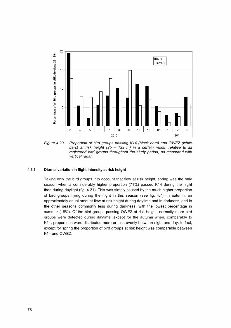
78

Figure 4.20 Proportion of bird groups passing K14 (black bars) and OWEZ (white

bars) at risk height (25 – 139 m) in a certain month relative to all registered bird groups throughout the study period, as measured with vertical radar.

4.3.1 Diurnal variation in flight intensity at risk height

Taking only the bird groups into account that flew at risk height, spring was the only season when a considerably higher proportion (71%) passed K14 during the night than during daylight (fig. 4.21). This was simply caused by the much higher proportion of bird groups flying during the night in this season (see fig. 4.7). In autumn, an approximately equal amount flew at risk height during daytime and in darkness, and in the other seasons commonly less during darkness, with the lowest percentage in summer (18%). Of the bird groups passing OWEZ at risk height, normally more bird groups were detected during daytime, except for the autumn when, comparably to K14, proportions were distributed more or less evenly between night and day. In fact, except for spring the proportion of bird groups at risk height was comparable between K14 and OWEZ.

79

Figure 4.21 Percentage of bird groups at risk altitude (25 – 139 m) passing K14

(black bars) and OWEZ (white bars) during darkness, as measured with vertical radar. Actual numbers at OWEZ were on average two times higher from spring to autumn.

Taking all bird groups into account that were registered in an hour, the four seasons showed different patterns in the fraction of bird groups flying at risk altitude (fig. 4.22). At K14, the proportion of bird groups flying at risk altitude was maximally around 50%, with the lowest, but relatively constant hourly means in summer (between 30 and 40%). Proportions were also lower during the winter nights, with values fluctuating largely between 30 - 45%. However, the highest values were also measured in winter during daytime, with a peak of 60% in the morning hours, which decreased during daytime to a minimum of 30% just after sunset. The proportions at risk height observed in the second half of the nights of spring and autumn were comparable, with values fluctuating around 45%. Moreover, in autumn the measured proportions were varying around this value during the whole day. On the contrary, in spring this was only true for the first half of the day, whereas in the afternoon the values decreased to a minimum of 25% around sunset, and gradually increased afterwards (fig. 4.23).

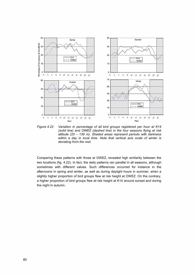
80

Figure 4.22 Variation in percentage of all bird groups registered per hour at K14

(solid line) and OWEZ (dashed line) in the four seasons flying at risk altitude (25 – 139 m). Shaded areas represent periods with darkness within a day in local time. Note that vertical axis scale of winter is deviating from the rest.

Comparing these patterns with those at OWEZ, revealed high similarity between the two locations (fig. 4.22). In fact, the daily patterns ran parallel in all seasons, although sometimes with different values. Such differences occurred for instance in the afternoons in spring and winter, as well as during daylight hours in summer, when a slightly higher proportion of bird groups flew at risk height at OWEZ. On the contrary, a higher proportion of bird groups flew at risk height at K14 around sunset and during the night in autumn.

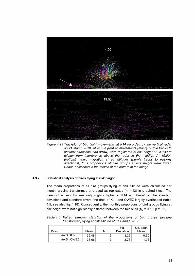
81

Figure 4.23 Trackplot of bird flight movements at K14 recorded by the vertical radar

on 21 March 2010. At 4:00 h (top) all movements (mostly purple tracks to easterly directions, see arrow) were registered at risk height of 25-139 m (clutter from interference above the radar in the middle). At 19:00h (bottom) heavy migration at all altitudes (purple tracks to easterly directions), thus proportions of bird groups at risk height were lower. Radar positioned in the middle at the bottom of the image.

4.3.2 Statistical analysis of birds flying at risk height

The mean proportions of all bird groups flying at risk altitude were calculated per month, arcsine transformed and used as replicates (n = 13) in a paired t-test. The mean of all months was only slightly higher at K14 and based on the standard deviations and standard errors, the data of K14 and OWEZ largely overlapped (table 4.5; see also fig. 4.18). Consequently, the monthly proportions of bird groups flying at risk height were not significantly different between the two sites (t12 = 0.58; p = 0.6). Table 4.5 Paired samples statistics of the proportions of bird groups (arcsine

transformed) flying at risk altitude at K14 and OWEZ.

Pairs Mean N Std.

Deviation Std. Error

Mean ArcSinK14 39.48 13 3.26 0.90 ArcSinOWEZ 38.66 13 3.78 1.05

4:00

19:00

82

83

5 Discussion

The visual and radar observations of bird movements carried out at K14 have provided data on the species, numbers, fluxes and flight heights of birds at an offshore site in the Dutch North Sea. By simultaneously measuring fluxes and flight heights at Offshore Wind Farm Egmond aan Zee, closer to the coast, using the same radar equipment and settings, we obtained a unique dataset of parallel measurements on flying birds at two locations in the Dutch North Sea. Species Most species seen at K14 during the visual observations were species commonly found in the marine environment, such as seabirds, gulls and terns. In particular, species that are most associated with offshore habitats, such as northern gannet, northern fulmar, great black-backed gulls, kittiwake and auks, were most abundant. In addition, migrant species were also recorded that are not able to use marine habitats, including land birds, raptors and owls, most likely moving between continental Europe and the UK. These species were observed in the highest numbers in autumn, during their post-breeding migration, but likely the high fluxes recorded by the radar in March were also caused by migratory birds. Based on the time of year and the mainly easterly orientation of the movements, these fluxes could have been caused by migrating birds leaving Great Britain, and heading towards their breeding grounds in Scandinavia or northern Russia. This group includes, for instance, swans, several duck and wader species, as well as some songbirds. In comparison with OWEZ, pelagic species of seabirds, such as northern gannet, kittiwake and the alcids, were more abundant at K14 than at OWEZ. Similarly, coastal species, such as lesser black-backed gull, herring gull, terns and great cormorant, were more abundant at OWEZ. Number of birds The number of bird groups recorded at K14 were generally lower in comparison with OWEZ. The echo tracklengths registered by the radar (i.e., an indication of the flight direction) were not significantly different at the two locations. In addition, based on the visual observations, the group size of birds was similar at the two locations. Therefore, detection capabilities of the radars can be considered comparable. Consequently, differences between the two locations are more likely a the result of K14 being farther from the coast of the Netherlands. The visual observations revealed that there were fewer coastal birds present at K14,. Gannets and alcids formed a large proportion of the birds at K14. These species often fly so low that they might not be detected by the radar among the waves. In addition, there might be a difference in wave height at OWEZ and K14. This could lead to discrepancies in the proportion of detected bird groups between the two study sites. Nevertheless, at OWEZ 300,000 more bird groups were registered in one year. This difference cannot be accounted for

84

by the higher number (by maximum 70,000 birds) of gannets and alcids at K14 that fly low above the waves.

Moreover, in addition to local birds, passage rates as recorded with the radar were also higher at OWEZ during migration (except for the first half of the nights in spring).,. Due to the closer distance to the shoreline, at OWEZ also migrating birds that follow the coast can pass, whereas this is not the case at K14. K14 lies on the expected migration route of birds flying to and from Scandinavia and England and to and from southern Europe and Africa. A part of the birds that migrate from Scandinavia above open water in the middle of the North Sea can also cross the coastal zone back to land, bringing the cumulative numbers there, and thus also at OWEZ, higher. The tracklengths measured by the radars at the two locations showed some moderate differences in certain months, indicating that flight directions might be slightly different in certain periods (i.e., more parallel to the radar bundle). This could occur, for instance, due to a higher proportion of birds flying to and from England at a certain location than at the other in a certain period. Although this could cause an underestimation of the number of bird groups at a certain site compared to the other, the differences were relatively small (maximally 17 pixels in medians, on the scale of 1024 pixels). Moreover, the differences were statistically not significant.

Interestingly, MTRs were especially higher at OWEZ during the nights of the autumn migration and less in spring. In this latter period, birds are heading towards their breeding grounds, and commonly travel faster than in autumn (Newton, 2010). This can be due to the limited time available for breeding, or due to the scarcity of nesting sites birds trying to be the first to occupy a site. Therefore, during spring, the same bird species may follow a different migration strategy, and thus migration route, than in autumn, by taking the shortest way, even if this means crossing larger distances above open water. On the contrary, during autumn migration birds are less urged and move slower. Therefore, one may speculate that in autumn birds may follow the landscape features more and cross seas at the narrowest corridors above open water (Bourne, 1980). Alternatively, the dominating westerly winds in the area may shape the changes in migration patterns. In autumn, when most bird movements were registered to the west, and thus against the prevailing westerly wind, birds may prefer to fly shorter distances above open water (Alerstam & Lindstrom, 1990, Lensink et al., 2002). Conversely, during spring birds may be able to travel faster due to tailwinds, and hence choose to follow a direct easterly route.

In addition, as the fluxes in autumn were mainly higher during daytime at OWEZ compared with K14, the difference between the two locations can largely be attributed to the number of daylight migrants. An important aspect why birds are thought to prefer nocturnal migration above the open sea is to minimize predation risk (Alerstam & Lindstrom, 1990). In autumn continuing migration is less urgent, and thus the same bird species may be less motivated to cross the sea during daytime at larger distances above open water where they are more vulnerable to predators (Bourne, 1980), whereas the intensity of migration in the safety of darkness seems to be less affected.

85

Seasonal variation Based on the visual observations, numbers were highest and comparably high between K14 and OWEZ during autumn. However, the radar observations revealed that also in autumn numbers were much higher at OWEZ, with a high proportion of bird groups passing during the night. The daily peak in MTRs around or just after sunset both in autumn and spring indicated the influx of a large number of migratory land birds that accumulated during daytime in the coastal region waiting to depart in the darkness (Lack 1963). Also the higher mean flight altitudes and higher variation in MTRs (see SD bars in fig. 4.5) point towards migration fluxes, instead of constantly present local birds. In some species, migration continued during daytime as well, based on the many land birds, mainly starlings, recorded by the visual observations at K14 in autumn. The finding that numbers of migrant land birds (particularly starlings) observed during the autumn migration period by visual observations at K14 was half that at OWEZ might be indicative that migration rates have a comparable ratio also during the night, and thus total numbers as well. Although the fluxes recorded with radar at K14 were lower than at OWEZ, it is likely that the observed numbers per km reflect broad front migration of bird species flying across a large area of the Dutch North Sea. The cumulative number of birds crossing a larger part of the North Sea at latitudes between the Netherlands and Britain may approximate the numbers measured at OWEZ, where migration is concentrated in a narrower corridor along the coast. Based on the radar observations, the highest number of bird groups passed K14 in March 2010, during the spring migration, and not during one of the autumn months as at OWEZ (see also Krijgsveld et al. 2011 for comparable results in the period 2007-2009). On the other hand, the total number of bird groups recorded at K14 in spring and autumn were comparable, with even higher MTRs in autumn. These resulted from very high fluxes in March and considerably lower in the rest of the spring, while in autumn fluxes were relatively high and constant throughout several months. Nevertheless, numbers at K14 were considerably lower in March 2011 than in March 2010, indicating the occurrence of annual variation within one site (see also Krijgsveld et al. 2011).

Although not many landbirds were seen in March during the visual observations, the radar recorded the highest activity during the night, and thus out of scope of the visual observations. This elevated night activity, together with elevated flight altitudes during the night, also indicated intensive migration in March. In addition, the proportion of night activity was higher in the spring months compared with OWEZ, which indicates that the total numbers registered in this period were formed by relatively more migrants at K14. All in all, it seemed that the contribution of spring migration to the overall numbers is relatively higher at K14 compared with OWEZ. In fact, at K14 fluxes of more than 100 bird groups/km/h were only reached in spring during the first half of the nights, which were comparable levels to those measured at OWEZ. Interestingly, relatively fewer bird groups were recorded during the rest of the spring at K14 than at OWEZ. This may be caused by the high numbers of migrating lesser black-backed gulls and little gulls observed at OWEZ during this

86

period, which compared with the lower numbers at K14 may reflect the more coastal occurrence of these species. In summer and especially in winter, at both locations lower proportions of nocturnal flights were recorded than in the migratory seasons of spring and autumn. This may reflect that in summer and winter mainly local seabirds were present being active during the day, without large fluxes of night migrants passing by. The total number of bird groups in summer was comparable to those of spring and autumn, but this was mainly caused by relatively constant and high numbers of bird groups flying during daytime. Consequently, the hourly MTRs were not much lower in summer than in autumn. This was especially due to high numbers of bird groups in July and August. Of these months, the August values relied on the extrapolation of only two days of actual measurements, and thus could have been caused by extrapolating two days with intensive movements by chance, and therefore should be considered with caution. However, in July the number of recorded bird movements were as high as in September and November, during the autumn migration. The higher proportion of night activity and the higher mean flight height during the night in autumn indicates that a larger part of the recorded bird movements were migrating bird groups, while in summer mostly local seabirds were recorded during daytime without elevated flight altitudes during the night.

On the other hand, the mean flight altitudes increased after sunset to a daily peak also in summer and winter (comparable to the other seasons), probably indicating an influx of migrant birds in these periods as well. Because from July onwards several species already start their post-breeding migration (e.g. lapwings, black-headed gulls, starlings, swallows and swifts; Lack, 1963, Lensink 1 2002), this may reflect mainly local foraging birds in the beginning of summer, replaced by migrants towards the end of the summer, also indicated by the gradually increasing mean flight altitudes during the night. Additionally, birds flying to night roosts in the evening, for example gulls, might have caused the elevated flight height around sunset followed by a drop in MTR, which was observed in winter. Similarly, birds arriving from night roosts might clarify the elevated fluxes around sunrise in summer and winter. Finally, the numbers in winter were clearly the lowest of all seasons, implying a lower number of wintering birds at sea compared with the other seasons.

87

Flight heights During the visual observations, the observed species such as divers, tubenoses (northern fulmar), sea ducks, terns and auks were recorded to fly at low altitudes, and gannets (northern gannet), skuas and gulls across a range of altitudes, but mostly below 100m. Land birds on migration, such as starlings, were visually also recorded mainly below 60 m. However, it is important to remember that visual observations, due to the methods and locations involved, are always conducted during daylight and are limited to the lower latitudes, especially in the case of small birds. The radar observations revealed that although most birds flew in the lowest altitude band (i.e. 0–69 m), a considerable amount flew higher, especially during migration periods. At both ends numbers might be somewhat underestimated, due to the limited detection probability of small songbirds at high altitudes (i.e. > 1000 m) and of birds flying very low over the water surface (< 5 m) to be distinguished from sea clutter. Therefore, the overall distribution of proportions and mean flight altitudes should not be considerably influenced. Altogether 49% of bird groups flew in the lowest altitude band of 0–69 m at K14, most of which (i.e. 57%) during daylight. At all other heights more birds flew during the night, resulting in a nearly equal number of bird groups passing K14 during daylight and in darkness. However, the higher flight altitudes during the night also mean that relatively fewer bird groups flew at risk height in the dark when birds might be more prone to collide with obstacles. On the other hand, comparing the recorded flight heights of bird groups based on the radar observations at K14 and OWEZ, revealed a lower mean flight altitude closer to the coast at OWEZ. This could be caused by the relatively higher proportion of migrants recorded at OWEZ, which generally fly higher than local birds. Implications regarding effects of wind farms Based on the findings from visual and radar observations undertaken at K14, the density of flying birds in the Dutch North Sea was lower farther offshore (80 km from the coast) compared to 10-18 km from the coast at OWEZ. The proportion of bird groups flying at rotor height in the altitude band of 25–139 m, forming the highest risk altitude for birds to collide with a wind turbine, was similar between the two locations, but the mean flight altitude was higher at OWEZ. The flight heights at K14 were recorded in absence of wind turbines, and birds may choose to fly higher or lower in response to the presence of a wind farm. Nevertheless,, in terms of offshore wind farms, mainly due to the lower fluxes at K14, fewer potential collision victims are expected far offshore, where fluxes of migrating landbirds are lower. However, avoidance rates of structures such as wind turbines, which have a large influence on the actual numbers of birds at risk of collision, may be species- and location-specific. Theoretically, this could mean that although the total number of flying birds far offshore is lower, the species involved may have a different avoidance rate. The species that were more abundant at K14 far offshore than at 10-18 km offshore at OWEZ are especially pelagic seabirds such as northern gannets and

88

auks/guillemots, and these are known to show higher avoidance of the OWEZ wind farm. Nevertheless, in order to fully assess the potential collision risk to species at wind farms far offshore, species- and location-specific studies will be needed, specifically addressing the responses to wind turbines in areas far offshore and under the conditions that prevail there.

89

6 Acknowledgements

We kindly thank the employees of Nederlandse Aardolie Maatschappij for their cooperation and supportive attitude towards this project. Their help has been instrumental in both the starting and the practical phase of this project. We thank Andreas Smith and his colleagues from DeTect Inc. for their cooperation and support in installing and maintaining the Merlin radars and software. Finally we thank Henk Kouwenhoven of NoordzeeWind for his involvement in and positive contribution to this project.

90

91

7 Literature

Alerstam, T. & A. Lindstrom 1990. Optimal bird migration: the relative importance of time, energy and safety. In, E. Gwinner (Ed.): Bird migration: physiology and ecophysiology, pp. 331-351. Springer-Verlag.

van Belle, J., L.S. Buurma & H. van Gasteren, 2002. Kwantificering van vogelbewegingen langs de kust bij IJmuiden: een radarstudie. Koninklijke Luchtmacht, Den Haag.

Bourne, W.R.P. 1980. The midnight descent, dawn ascent and re-orientation of land birds migrating across the North Sea in autumn. Ibis, 122: 536-540.

Camphuysen, C.J. & S. Garthe, 2001. Recording foraging seabirds at sea: standardised recording and coding of foraging behaviour and multi-species foraging associations. NIOZ internal report, Texel, Netherlands.

Chapman, J.W., D.R. Reynolds & A.D. Smith, 2003. Vertical-looking radar: a new tool for monitoring high-altitude insect migration. BioScience, 53: 503-511.

Eastwood, E., 1967. Radar Ornithology. Richard Clay, The Chaucer Press, Bungay, Suffolk.

van Gasteren, H., J. van Belle & L.S. Buurma, 2002. Kwantificering van vogelbewegingen langs de kust bij IJmuiden: een radarstudie. Koninklijke Luchtmacht, Den Haag.

Krijgsveld, K.L., R.C. Fijn, M. Japink, P.W. van Horssen, C. Heunks, M.P. Collier, M.J.M. Poot, D. Beuker & S. Dirksen, 2011. Effect studies Offshore Wind Egmond aan Zee: Final report on fluxes, flight altitudes and behaviour of flying birds. Report 10-219 / OWEZ_R_231_T1_20111111. Bureau Waardenburg bv, Culemborg.

Lack, D. 1963. Migration across the southern North Sea studied by radar. Part 4. Autumn. Ibis, 105: 1-54.

Larkin, R.P. 1991. Flight speeds observed with radar, a correction: slow "birds" are insects. Behavioral Ecology and Sociobiology, 29: 221-224.

Lensink, R., M.J.M. Poot, S. Dirksen & J. van der Winden, 1998. Kwantificering van vogelbewegingen op en rond vliegveld Eindhoven; ontwikkeling van methodieken en waarneemprotocollen. Rapport 98.32. Bureau Waardenburg bv, Culemborg.

Lensink, R., M.J.M. Poot, I. Tulp, A. de Hoon & S. Dirksen, 2000. Vliegende vogels op en rond vliegveld Eindhoven. Een studie naar aantallen en dichtheden in de onderste luchtlaag. Rapport 00-005. Bureau Waardenburg bv, Culemborg.

Lensink, R., H. van Gasteren, F. Hustings, L.S. Buurma, G. van Duin, L. Linnartz, F. Vogelzang & C. Witkamp, 2002. Vogeltrek over Nederland 1976-1993. Schuyt & Co. Haarlem.

Newton, I. 2010. Bird Migration. Harper Collins Publishers. London, UK. Petersen, I.K., T.K. Christensen, J. Kahlert, M. Desholm & A.D. Fox, 2006a. Final

results of bird studies at the offshore wind farms at Nysted and Horns Rev, Denmark. NERI Report Commissioned by DONG energy and Vattenfall A/S. National Environmental Research Institute, Ministry of the Environment, Rønde, Denmark.

Poot, M.J.M., R. Lensink, J. van Belle & H. van Gasteren, 2000. Validatie visuele waarneemmethoden met behulp van radar op de Pier van IJmuiden 1999 en vogeldichtheden boven de Pier van IJmuiden, in het kader van ONL -

92

Vliegveiligheid en vogels. Rapport 00-083. Bureau Waardenburg bv, Culemborg.

Poot, M.J.M., J. van Belle, K. Krijgsveld, H. van Gasteren & S. Dirksen, 2006. Correcting detection loss in observations on bird migration with vertical marine surveillance radar. Poster at the XXIV International Ornithological Congress, Hamburg, Germany.

Wood, C.R., D.R. Reynolds, P.M. Wells, J.F. Barlow, I.P. Woiwod, & J.W. Chapman, 2009. Flight periodicity and the vertical distribution of high-altitude moth migration over southern Britain. Bulletin of entomological research, 99: 525-535.

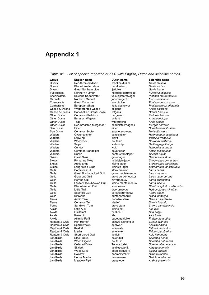
93

Appendix 1

Table A1 List of species recorded at K14, with English, Dutch and scientific names. Group English name Dutch name Scientific name Divers Red-throated diver roodkeelduiker Gavia stellata Divers Black-throated diver parelduiker Gavia arctica Divers Great Northern diver ijsduiker Gavia immer Tubenoses Northern Fulmar noordse stormvogel Fulmarus glacialis Shearwaters Balearic Shearwater vale pijlstormvogel Puffinus mauretanicus Gannets Northern Gannet jan-van-gent Morus bassanus Cormorants Great Cormorant aalscholver Phalacrocorax carbo Cormorants European Shag kuifaalscholver Phalacrocorax aristotelis Geese & Swans White-fronted Goose kolgans Anser albifrons Geese & Swans Dark-bellied Brent Goose rotgans Branta bernicla Other Ducks Common Shelduck bergeend Tadorna tadorna Other Ducks Eurasian Wigeon smient Anas penelope Other Ducks Teal wintertaling Anas crecca Other Ducks Red-breasted Merganser middelste zaagbek Mergus serrator Sea Ducks Eider eider Somateria mollissima Sea Ducks Common Scoter zwarte zee-eend Melanitta nigra Waders Oystercatcher scholekster Haematopus ostralegus Waders Lapwing kievit Vanellus vanellus Waders Woodcock houtsnip Scolopax rusticola Waders Snipe watersnip Gallinago gallinago Waders Curlew wulp Numenius arquata Waders Common Sandpiper oeverloper Actitis hypoleucos Waders Dunlin bonte strandloper Calidris alpina Skuas Great Skua grote jager Stercorarius skua Skuas Pomarine Skua middelste jager Stercorarius pomarinus Skuas Arctic Skua kleine jager Stercorarius parasiticus Skuas Long-tailed Skua kleinste jager Stercorarius longicaudus Gulls Common Gull stormmeeuw Larus canus Gulls Great Black-backed Gull grote mantelmeeuw Larus marinus Gulls Glaucous Gull grote burgemeester Larus hyperboreus Gulls Herring Gull zilvermeeuw Larus argentatus Gulls Lesser Black-backed Gull kleine mantelmeeuw Larus fuscus Gulls Black-headed Gull kokmeeuw Chroicocephalus ridibundus Gulls Little Gull dwergmeeuw Hydrocoloeus minutus Gulls Sabine's Gull vorkstaartmeeuw Xema sabini Gulls Kittiwake drieteenmeeuw Rissa tridactyla Terns Arctic Tern noordse stern Sterna paradisaea Terns Common Tern visdief Sterna hirundo Terns Sandwich Tern grote stern Sterna sandvicensis Alcids Little Auk kleine alk Alle alle Alcids Guillemot zeekoet Uria aalge Alcids Razorbill alk Alca torda Alcids Atlantic Puffin papegaaiduiker Fratercula arctica Raptors & Owls Hen Harrier blauwe kiekendief Circus cyaneus Raptors & Owls Sparrowhawk sperwer Accipiter nisus Raptors & Owls Kestrel torenvalk Falco tinnunculus Raptors & Owls Merlin smelleken Falco columbarius Raptors & Owls Short-eared Owl velduil Asio flammeus Landbirds Stock Dove holenduif Columba oenas Landbirds Wood Pigeon houtduif Columba palumbus Landbirds Collared Dove Turkse tortel Streptopelia decaocto Landbirds Skylark veldleeuwerik Alauda arvensis Landbirds Wood Lark boomleeuwerik Lullula arborea Landbirds Swallow boerenzwaluw Hirundo rustica Landbirds House Martin huiszwaluw Delichon urbicum Landbirds Meadow Pipit graspieper Anthus pratensis

94

Group English name Dutch name Scientific name Landbirds Water Pipit waterpieper Anthus spinoletta Landbirds Rock Pipit oeverpieper Anthus petrosus Landbirds Yellow Wagtail Engelse kwikstaart Motacilla flavissima Landbirds White Wagtail witte kwikstaart Motacilla alba Landbirds Pied Wagtail rouwkwikstaart Motacilla alba Landbirds Blackbird merel Turdus merula Landbirds Fieldfare kramsvogel Turdus pilaris Landbirds Redwing koperwiek Turdus iliacus Landbirds Song Thrush zanglijster Turdus philomelos Landbirds Goldcrest goudhaantje Regulus regulus Landbirds Grasshopper Warbler sprinkhaanzanger Locustella naevia Landbirds Marsh Warbler bosrietzanger Acrocephalus palustris Landbirds Willow Warbler fitis Phylloscopus trochilus Landbirds Chiffchaff tjiftjaf Phylloscopus collybita Landbirds Pallas' Warbler Pallas' boszanger Phylloscopus proregulus Landbirds Blackcap zwartkop Sylvia atricapilla Landbirds Garden Warbler tuinfluiter Sylvia borin Landbirds Whitethroat grasmus Sylvia communis Landbirds Spotted Flycatcher grauwe vliegenvanger Muscicapa striata Landbirds Pied Flycatcher bonte vliegenvanger Ficedula hypoleuca Landbirds Robin roodborst Erithacus rubecula Landbirds Redstart gekraagde roodstaart Phoenicurus phoenicurus Landbirds Northern Wheatear tapuit Oenanthe oenanthe Landbirds Jackdaw kauw Corvus monedula Landbirds Rook roek Corvus frugilegus Landbirds Starling spreeuw Sturnus vulgaris Landbirds Chaffinch vink Fringilla coelebs Landbirds Brambling keep Fringilla montifringilla Landbirds Siskin sijs Carduelis spinus Landbirds Ortolan ortolaan Emberiza hortulana Landbirds Snow Bunting sneeuwgors Plectrophenax nivalis

Consultants for environment & ecology

P.O. Box 3654100 AJ Culemborg The NetherlandsTel +31 345 512 710 Fax + 31 345 519 849E-mail: info@buwa.nl Website: www.buwa.nl