Fixed Budgets as a Cost Containment

Measure for Pharmaceuticals

David Granlund, Niklas Rudholmand and Magnus Wikström

Department of Economics

Umeå University

SE-901 87 Umeå

Sweden

June 2005 version. The �nal version is published in:The European Journal of Health Economics 7, 37-45, 2006

(available at www.springerlink.com).

Abstract

In the county of Västerbotten, Sweden, there are two health cen-

tres which (contrary to all other health centres in the region) have a

strict responsibility over their pharmaceutical budget. The purpose

of this paper is to examine if the prices and quantities of pharma-

ceuticals prescribed by physicians working at these health centres dif-

fer signi�cantly from those prescribed by physicians at health centres

with open-ended budgets. Estimation results using matching meth-

ods, which allows us to compare similar patients at the di¤erent health

centres, show that the introduction of �xed pharmaceutical budgets

did not a¤ect physicians�prescription behaviour.

Key words: Fixed budgets, pharmaceuticals, cost containment, propen-sity score matching.

JEL classi�cation: I11, I18

1

1 Introduction

In Sweden, there is an ongoing debate concerning the high cost for drugs.

In the last twenty-�ve years, the expenditures on drugs have risen with on

average 10 per cent per year and in 2002 the cost reached 31.7 billions SEK.

Prescription pharmaceuticals accounted for 24.5 billion, while hospital and

over-the-counter drugs accounted for 2.7 and 4.5 billion SEK, respectively.

The Swedish development parallels that of many other European countries,

which has spurred an interest in di¤erent methods to contain pharmaceu-

tical costs (see e.g. Dukes, 1993, Chapter 7 and Mossialos and Le Grand,

1999). Within the market for pharmaceuticals, cost containing measures

operate both on the pharmaceutical industry, e.g. price controls, and refer-

ence prices, and on the demand side, e.g. payment systems for physicians

and pharmacists, positive or negative lists suggesting which pharmaceuti-

cals physicians should prescribe, generic substitution requirements, and/or

patient co-payment plans.

During the period under study in this paper, the most widely used form

of cost containment in Sweden was patient co-payments. In Sweden, the

pharmaceutical insurance system is non-linear, making patient co-payments

decrease as total expenditure for pharmaceuticals increase. All costs for the

patient exceeding 1800 SEK per year are �nanced through the Swedish phar-

maceuticals insurance system. Another well known cost containment mea-

sure is the so called reference price system which was introduced in Sweden in

1993. The reference price system stated that all costs above a predetermined

reference price had to be borne by the patient. Similar systems have also

been introduced in the Netherlands, Finland, Norway and Germany, among

other countries. The Swedish system speci�ed that any costs exceeding the

price of the least expensive generic substitute by more than 10 per cent had

to be borne by the patient. On October 1, 2002, the reference price system in

Sweden was abolished. Instead a law (SFS 2002:160) was introduced, requir-

ing pharmacists to substitute the prescribed pharmaceutical to the cheapest

equivalent pharmaceutical product available at the local pharmacy.

2

Exclusions of pharmaceuticals from the pharmaceutical reimbursement

plan have on occasion been used in Sweden. In the dataset used in this study,

approximately 2.2 per cent of all prescriptions relates to pharmaceuticals ex-

cluded from the reimbursement plan. Another possible cost containment

measure is to restrict the number of diagnoses for which a pharmaceutical

product can be prescribed. This has, however, been seen by policy makers as

to much of a restriction on physician autonomy, a concept central in medi-

cine (Dukes 1993, p. 138). Note also that under the Swedish pharmaceutical

insurance system there are usually no formal restrictions on physician pre-

scription behavior or pecuniary incentives for the physician to internalize a

proportion of the insurers utility.

Since 1998, the Swedish county councils are responsible for the costs of

prescription pharmaceuticals which is not paid by the patient. It is thus in

the interest of the county council to contain drug costs. In spite of this, health

centers located in Västerbotten, which are the main source of pharmaceutical

prescriptions made in the region, usually work with open-ended budgets for

pharmaceutical expenditure, meaning that the prescribing agency has little

incentive to contain costs.

The purpose of the present paper is to study the e¤ects of an attempt

by the local county council to introduce �hard�budget constraints in phar-

maceutical budgets in two of the health centers in Västerbotten, Sweden. In

2001, these two health centers were given �xed budgets for pharmaceutical

expenditures, giving them an incentive to decrease expenditures as they were

allowed to keep any surplus (and being forced to repay any de�cit) generated

during the year.

Whether or not introducing �xed budgets will help contain costs in public

agencies is, however, an open question. On the one hand, �xed budget con-

straints are often considered a necessary condition for the budgetary process

to be e¤ective. On the other hand, �xed budget constraints are seldom seen

as su¢ cient cost containing measures in public agencies. One problem is that

�xed budgets must be credible. The principal may be tempted to adjust bud-

3

gets according to history, creating an incentive to overspend in order not to

get future budget cuts, the so called ratchet e¤ect (see Kornai et al 2003

for a discussion of soft budget constraints). Another problem is that lack of

information may render the principal to introduce more or less fuzzy con-

tracts, making incentives unclear (see e.g. Prendergast, 1999, for a lengthier

discussion of problems associated with optimal incentive contracts). Thus,

the e¢ cacy of introducing hard budget constraints on cost containment is an

empirical question.

This paper contributes to the literature on cost containment in health

care by comparing pharmaceutical expenditure at health centers with �xed

pharmaceutical budgets to those with open-ended budgets. Changes in the

expenditures on pharmaceuticals are decomposed into three parts; the num-

ber of prescriptions, the size of prescriptions (the number of de�ned daily

doses per prescription), and the price of the pharmaceutical. Prescriptions

are matched according to a large number of background variables, includ-

ing age and diagnosis, using the method of propensity score matching. This

makes it possible to study if physicians respond to the budgetary rules by

prescribing cheaper medicine or fewer doses of medicine per prescription. Fi-

nally, the number of prescriptions in health centers with �xed budgets are

compared to those with open-ended budgets.

The results show that the number of prescriptions in the two health cen-

ters with �xed budgets declined relative to the control group after the in-

troduction of the �xed budgets. However, there is no systematic di¤erence

regarding either price or quantity per prescription between the two types of

health centers. A possible explanation is that the prescribing physicians do

not believe the �xed budgets to be credible.

The rest of the paper is organized as follows: section 2 presents the main

hypotheses to be explored in this paper. Section 3 presents the empirical

analysis. The data to be used are presented in subsection 3.1. Subsection

3.2 describes the matching method to be used, while subsections 3.3 and

3.4 contain the results from the propensity score estimations and from the

4

matching, respectively. Finally, section 4 concludes the paper.

2 Background and hypotheses to be explored

As mentioned, the purpose of this paper is to study if di¤erences in budgetary

rules among health centers in Sweden a¤ect physicians�prescription behavior.

From 1998, the county councils in Sweden are responsible for the costs of

prescription pharmaceuticals which are not paid by the patient. For the

county council in Västerbotten, these costs are approximately 500 million

SEK per year. The county councils are to some extent reimbursed by the

central government through the Swedish National Insurance Board (SNIB).

An agreement between the local county council in Västerbotten and the

SNIB states that during the years 2000 to 2004, the SNIB will pay a total of

1.5 billion SEK for pharmaceutical insurance costs in Västerbotten, Sweden.

This means that approximately 375 million SEK per year is paid by the

SNIB, while all additional costs for pharmaceutical insurance is paid by the

local county council in Västerbotten.

In the county of Västerbotten, health centers have since 2001 budgetary

responsibility for pharmaceutical costs. The county council works with target

budgets for the health centers, which are decided partly upon on the basis

of population characteristics, primary age and gender, within each health

center�s reception area and partly upon each health center�s result in 2001.

However, budgets are not �xed in the sense that surpluses or de�cits are car-

ried over to the next year�s budget. This means that the economic incentives

to reduce drug costs are limited.

Starting in 2001, two health centers located in Västerbotten (Burträsk

and Moröbacke health centers) obtained �xed budgets as a part of an agree-

ment intended to increase the centers�self-autonomy. A �xed budget is here

de�ned as a budget that is determined on the basis of characteristics which

are exogenous to the decisions made by the health center, and where sur-

pluses and de�cits carry over to the next year�s budget.

5

There are several ways by which an introduction of �xed budgets may

a¤ect prescription behavior in health centers. First, the amount of prescrip-

tions made out can be decreased. Having a �xed budget reasonably means

that physicians will be more reluctant of writing prescriptions at given prices

and quantities. Second, since marginal co-payment decreases with the total

purchase of medicine during a full year, physicians can �choose�to change the

mix of patients who obtain prescription drugs. In order to engage in patient

substitution, a physician must have information regarding the position of the

patient in the price schedule. Such information has not been available during

the period of our study.

Third, the price of medicine for a given treatment can be decreased by,

for example, an increased use of generic drugs. Availability of information

regarding the price of di¤erent pharmaceuticals has increased during the

period under study. Finally, prescriptions can be made to reduce the number

of de�ned daily doses (DDD:s) per prescription. A well known problem with

prescription pharmaceuticals is that large amounts of the pharmaceuticals are

wasted, indicating that a major problem is overprescribing. However, note

also that if the number of doses is reduced, there is an increased likelihood

that the patient returns to the health center for a new prescription, which

may increase costs. In the present paper, we address the two last channels, i.e.

if the introduction of a �xed budget decreases prices for drugs within speci�c

ATC-groups, and if the number of doses per prescription is a¤ected. We

also include some tentative information on the total number of prescriptions

made out at the di¤erent health centers.

In order to study the price and quantity e¤ects, a comparison is made

between the two health centers with �xed budgets (the treatment group) to

a group of health centers which have target budgets (the comparison group).

Since prescription behavior can di¤er before the introduction of �xed budgets,

a time dimension is also included. A di¤erence-in-di¤erence method is used

to study price and quantity e¤ects. If �xed budgets have the intended e¤ects,

we expect the prices and/or number of DDD:s to drop in the treatment group

6

relative to the comparison group.

Finally, on October 1, 2002, the so called substitution reform was intro-

duced, requiring pharmacists to substitute the prescribed pharmaceutical to

the cheapest equivalent pharmaceutical product available at the local phar-

macy. This reform has had a large e¤ect on drug costs, in particular prices,

in health centers (Socialstyrelsen 2003, p. 15). The substitution reform of-

fers another possibility to test our hypotheses. Since the introduction of

�xed budgets was made in 2001, prices and quantities should already have

dropped in the health centers with �xed budgets before the introduction of

the substitution reform. Therefore, making a similar comparison before and

after the introduction of the substitution reform, we would expect a price

decrease in the comparison group relative to the group of �treated�health

centers.

To summarize, our main hypotheses are as follows: (i) comparing the

period January to September 2002, when �xed budgets are newly introduced,

with the pre-reform period, we expect prices and quantities in treated health

centers to fall relative to the comparisons; and (ii) for the period after the

introduction of the substitution reform, we expect the relative price di¤erence

to be positive. A potential problem with the data is that the year 2001,

which forms the basis for our �rst comparison, is an adjustment period for

the health centers where �xed budgets are to be introduced. This means

that the treated health centers may have acted so as to increase their future

budgets. In order to at least shed some light on whether such behavior might

have in�uenced our data, we also compare post and pre-reform periods in the

year 2001.

7

3 The empirical analysis

3.1 Data

The data used in this study has been provided by the county council of

Västerbotten, Sweden. It contains a total of 6.2 million observation, covering

all pharmaceuticals sold in the county of Västerbotten or sold in other parts

of Sweden to residents of Västerbotten between January 2001 and June 2003.

From this population a random sample of twenty-�ve per cent is drawn.

The county of Västerbotten (population 255 122, June 2003) consists of

�fteen administrative areas. The two health centres Burträsk andMoröbacke,

which both are located in the administrative area of Skellefteå, received �xed

budgets for prescription pharmaceuticals on May 1, 2001, and November 1,

2001, respectively. Since these are the two health centres of interest in this

paper and since we want to avoid potential di¤erences between the areas to

in�uence the results, all observations not originating from physicians work-

ing at health centres in Skellefteå are excluded. In this step, we also exclude

nearly six per cent of the observations lacking information about the physi-

cian�s workplace. In addition, nearly six per cent of the observations are

dropped since the cost per DDD can not be calculated or because they indi-

cate resell of the pharmaceutical product to the pharmacy. The �nal sample

to be used in the empirical analysis consists of 292 419 observations.

The dataset includes information regarding the patients age, gender and

area of residency. Patients are however not traceable over time. The infor-

mation about the prescription contains the month in which it is sold, the

pharmaceuticals ATC-code and an indicator if the pharmaceutical is packed

in patient-doses rather than their ordinary packages. Patients who have rel-

atively stable medication and can be expected to have some problem keeping

track of how big doses they should take, often receives their prescriptions in

patient-doses. In addition, the dataset includes information about the cost

of the prescription as well as the patient�s co-payment for the prescription.

Using these variables and information about the di¤erent phases in the re-

8

imbursement system, we have calculated the co-payment bracket in which

the patient was prior to paying for the current prescription. The calculations

have been left out in order to save space, but are available from the authors

upon request. The dummy variables Copay100, Copay50, Copay25, Copay10

and Copay0 are de�ned so as to correspond to marginal rates of co-payment

of 100, 50, 25, 10 and 0 per cent, respectively. Some prescriptions are always

free of charge for the patient and others are excluded from the reimbursement

plan (for example cough medicine), irrespective of the patient�s co-payment

bracket. For these observations the patients�co-payment rates bear no in-

formation of previous cost for prescription pharmaceuticals. The dummy

variables Free and Unsub indicate that a prescription is free of charge and

unsubsidized, respectively.

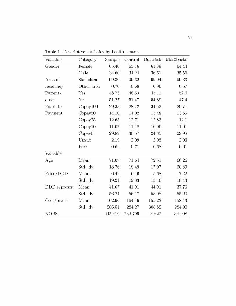
Descriptive statistics by health centres are presented in Table 1. For the

di¤erent indicator variables the percentage of the material which belongs

to each category are presented. For continuous variables the means and

standard deviations are presented instead.

Table 1 about here.

The data contains 146 four-digit ATC-groups. Of these groups 52 have

less than 100 observations, 39 have between 100 and 1 000 observations,

55 have more than 1 000 observations. The observations are quite evenly

distributed between the thirty months included in the study, with fewest

pharmaceuticals (7 830) sold in June 2002 and most pharmaceuticals (11

178) sold in October 2002.

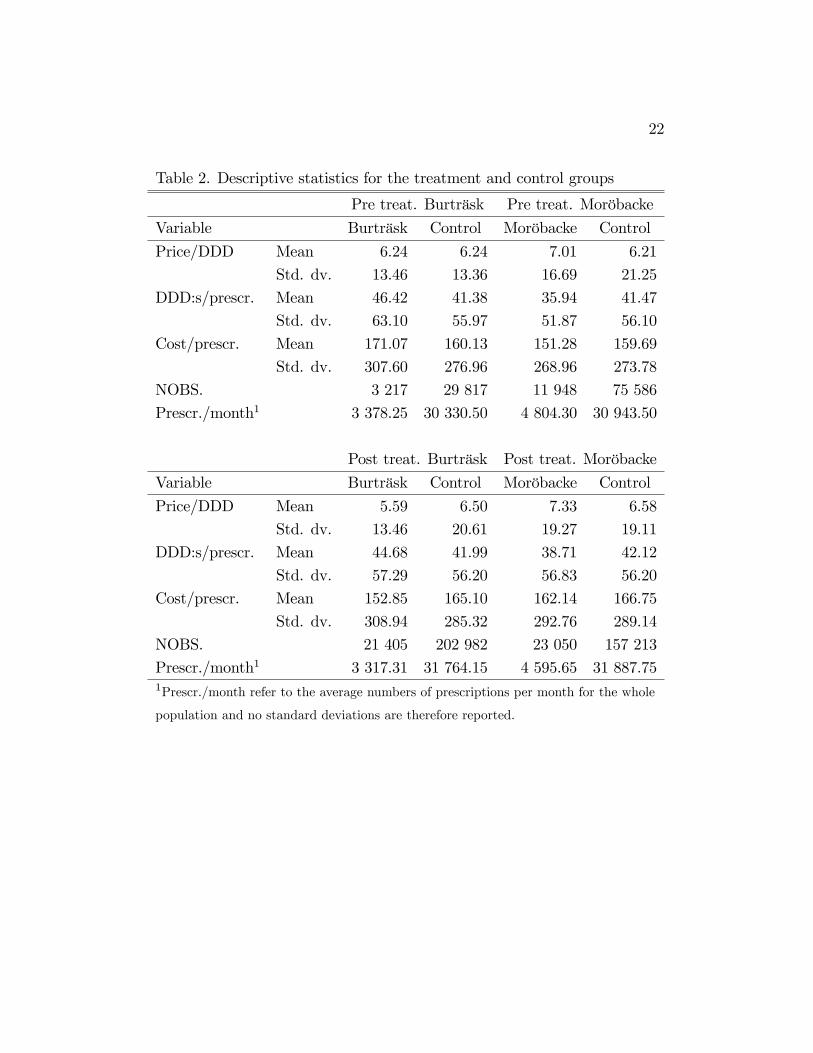
Descriptive statistics of the key-variables of interest both prior to and

after the introduction of �xed budget constraints are presented in Table 2 be-

low. Table 2 show that the Price/DDD and the number of DDD:s/prescription

have been reduced for Burträsk after �xed budgets were introduced. The op-

posite is true for Moröbacke, but the number of prescriptions per month have

decreased for Moröbacke. For the entire sample the average cost per DDD is

6.5 SEK, the average number of DDD:s per prescription equals 41.7 and the

9

average cost per prescription is 163 SEK.

Table 2 about here.

3.2 Econometric Method

To test whether the average price per DDD and the average number of DDD:s

per prescription are a¤ected by the introduction of �xed budgets, we would

like to estimate the average treatment e¤ect on the treated for these two

outcome variables. Treated in this case means that the prescription is written

by a physician working at a health center with �xed pharmaceutical budget.

When evaluating the average treatment e¤ect on the treated, we can view

the problem as if there for every observation, at every time, are two possible

outcomes, labelled Y1 if the observation is treated, and Y0 if the observation

is untreated. We can only observe one outcome for each observation at each

time. The average treatment e¤ect on the treated could be expressed as

E(Y1 � Y0jD = 1) = E(Y1jD = 1)� E(Y0jD = 1),

where D is a dummy which takes the value 1 if the observation actually

is treated and the term E(Y0jD = 1) is unobservable. That is, we cannot

observe what the outcome would have been for the treated, if they had not

been treated. Rosenbaum and Rubin (1983) showed that if this term is

estimated with the outcome for the untreated we get a bias which can be

written as

Bias = E(Y0jD = 1)� E(Y0jD = 0).

Both the OLS and the matching method deal with this bias problem by

adjusting for a set of observable variables, X, which are di¤erently distributed

in the groups and can in�uence the outcome. One advantage of the matching

method is that it is semiparametric and therefore avoids the functional form

restrictions of the OLS equation.

10

In this study, a variant of propensity score matching will be used, in which

untreated observations are determined to be suitable matches for treated

observations if they have similar probability of being treated. Rosenbaum

and Rubin (1983) prove that if the following three conditions are satis�ed,

when the outcome is independent of treatment assignment conditioned on

the propensity score, Pr(D = 1jX); and the bias is zero. The �rst conditionis that all relevant di¤erences between the groups have to be captured by

their observables X. The second condition states that the matching must be

done over a region where the probability of being treated conditioned on X

is between zero and one, that is:

0 < Pr(D = 1jX) < 1.

As shown by Smith and Todd (2003a) the condition 0 < Pr(D = 1jX) isnot required when the parameter of interest is the average treatment e¤ect

on the treated, since it only guarantees good matches for each untreated

observation. The �nal condition is that the observables must be independent

of treatment assignment conditioned on the propensity score.

By using both pre- and post-treatment data we avoid having to ful�ll

the �rst condition. We do this by using a di¤erence-in-di¤erence extension

of propensity score matching which can take account of time-invariant un-

observable heterogeneity. This method makes it possible to get a unbiased

estimate of the treatment e¤ect on the treated even if unobservable di¤erences

exists between Burträsk and Moröbacke and other health centers, as long as

these di¤erences are time-invariant. We estimate the di¤erences between the

treated-control outcome di¤erences after treatment and the treated-control

outcome di¤erences before treatment, that is:

�DIDD=1 = [E(Y1jD = 1)� E(Y0jD = 1)]� [E(Y 01 jD0 = 1)� E(Y 00 jD0 = 1)],

where 0 indicates the period before treatment and D0 is a dummy which takesthe value one for observations originating from Burträsk or Moröbacke before

11

they received �xed budgets for prescription pharmaceutical. The e¤ect will

be estimated separately for Burträsk and Moröbacke since they received �xed

pharmaceutical budgets at di¤erent times.

Matching methods di¤er by placing di¤erent weights on the control ob-

servations. Nearest neighbor matching, which will be used in this paper, puts

all weight on the observation in the non-treated group which has the most

similar propensity score. This reduces bias since only the best matches are

used, but could lead to increased variance compared to the other matching

methods which uses more observations from the control group. We impose

a common support condition by specifying that the maximum allowed dis-

tance between the propensity score of the treated and the control is 0.01.

Treated observations for which no matches can be found within this caliper

are excluded from the analysis.

3.3 Estimation of propensity score

The �rst step in estimating the di¤erence in di¤erence is to estimate the

propensity scores before and after treatment. To be able to get robust esti-

mates we want to use variables which a¤ect treatment, as well as variables

which a¤ect the outcome, when estimating the propensity score. We include

gender, using an indicator variable equaling one if the individual is a female,

and age by using indicator variables for each �ve-year group. We also include

a dummy variable, denoted Area, which takes the value one if the patient�s

area of residency is some other than Skellefteå, and include indicator variables

for the month in which the pharmaceutical is sold.

As can be seen in Table 1, the share of the prescriptions made out in

patient-doses di¤ers between health centres. Coscelli (2000) has shown that

patients exhibit strong state dependence, that is, they prefer the drug they

have been prescribed before. This gives the usually more expensive brand-

name drug a �rst mover advantage. The state dependence is probably more

important among the patients receiving their prescriptions in patient-doses,

since these patients usually have relatively stable medication. We therefore

12

include a dummy variable, referred to as Doses below, which takes the value

one if the prescription is made out in patient doses.

Previous studies have shown that the patient�s co-payment is likely to

a¤ect the prescription being made (see e.g. Lundin, 2002, and Rudholm,

2004). We include the dummy variables Copay, Unsub and Free to take

account of this e¤ect. We use the patient�s co-payment bracket prior to

receiving the prescription in question, to avoid the endogenity problem of co-

payment being a¤ected by the price and volume of the drug being prescribed.

Another variable which is important to include is the four digit ATC-

groups of the pharmaceuticals. The ATC-group a¤ects treatment as the

health centers have physicians with di¤erent specialities, and a¤ects out-

come since average price per DDD and number of DDD:s per prescription

vary considerable between ATC-groups. We view ATC-group as a predeter-

mined health indicator which is a function of the patient�s health status and

therefore exogenous of treatment. The same argument goes for Doses, Unsub

and Free.

Among a general set of models, all including the variables discussed above

but including di¤erent interaction terms, the �nal speci�cations are chosen

to maximize the within-sample correct prediction rates using the hit-or-miss

method (e.g. Heckman, Ichimura, and Todd, 1997). This method ascribes

observations a �1�if the estimated propensity score is larger than the portion

of the sample which is treated and a �0�otherwise. The propensity scores

have been calculated using logit estimations of versions of the following equa-

tion;

13

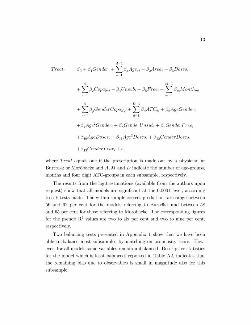
Treati = �0 + �1Genderi +A�1Xa=1

�aAgeai + �2Areai + �3Dosesi

+

4Xc=1

�cCopayci + �4Unsubi + �5Freei +M�1Xm=1

�mMonthmi

+

4Xg=1

�gGenderCopaygi +D�1Xd=1

�dATCdi + �6AgeGenderi

+�7Age2Genderi + �8GenderUnsubi + �9GenderFreei

+�10AgeDosesi + �11Age2Dosesi + �12GenderDosesi

+�13GenderY eari + "i,

where Treat equals one if the prescription is made out by a physician at

Burträsk or Moröbacke and A;M and D indicate the number of age-groups,

months and four digit ATC-groups in each subsample, respectively.

The results from the logit estimations (available from the authors upon

request) show that all models are signi�cant at the 0.0001 level, according

to a F-tests made. The within-sample correct prediction rate range between

56 and 62 per cent for the models referring to Burträsk and between 58

and 65 per cent for those referring to Moröbacke. The corresponding �gures

for the pseudo R2 values are two to six per cent and two to nine per cent,

respectively.

Two balancing tests presented in Appendix 1 show that we have been

able to balance most subsamples by matching on propensity score. How-

ever, for all models some variables remain unbalanced. Descriptive statistics

for the model which is least balanced, reported in Table A2, indicates that

the remaining bias due to observables is small in magnitude also for this

subsample.

14

3.4 Matching Results

As discussed in section 2, we expect the di¤erence-in-di¤erence estimates to

be non constant over time. We will therefore divide the data into sub peri-

ods in order to test the hypotheses that prices and quantities are a¤ected by

the introduction of �xed budgets. Three post-treatment periods are identi-

�ed. First, for the period 2002 and after, the treated health centers had an

incentive to decrease prices and quantities. However, on October 1, 2002,

the substitution reform was introduced, which may have had a large impact

on health centers which prescribed relatively expensive medicine. If �xed

budgets had an impact on prices and quantities, we would most likely �nd

a di¤erence in prices and quantities for the period up to the substitution re-

form. Therefore, the �rst comparison is made between the period January to

September 2002 and the period 2001 prior to the introduction of �xed bud-

gets. Second, after October 1, 2002, when the substitution reform is enforced,

we expect the prices in the comparison group to be a¤ected more strongly

than those in the treated health centers, since, if �xed budgets had the hy-

pothesized e¤ects, prices should already have adjusted in the treated health

centers. Third, the �xed pharmaceutical budgets are in part determined

by outcomes in 2001, which gives the treated health centers an incentive to

overspend in 2001 in order to increase their future budgets. We therefore

compare the period 2001 after the formal introduction of the new rules with

the period 2001 prior to the introduction of �xed budgets (January to April

for Burträsk and January to October for Moröbacke) in order to study if this

incentive led to changes in prescription behavior.

Of the prescriptions made out by physicians at Burträsk and Moröbacke,

2.7 and 4.9 per cent respectively, are made out to patients not listed at the re-

spective health centres, which means that they do not have to bear the costs

for these prescription. Neither are the health centers budgets charged for

the 0.6 per cent of the observations which refers to special pharmaceuticals.

The results to be presented are not a¤ected when dropping these observa-

tions and the observations which refer to unsubsidized pharmaceuticals. The

15

results are also robust against small changes in the speci�cation of the se-

lection models. In order to investigate if the introduction of �xed budgets

and/or the substitution reform had di¤erent e¤ects on di¤erent pharmaceu-

tical treatments, we also distinguish between ATC-groups. The three groups

chosen are A, C and N, which refer to drugs related to digestive organs and

metabolism, heart and circulation, and the nervous system, respectively. The

groups constitute approximately 12, 24 and 28 per cent of the prescriptions,

respectively.

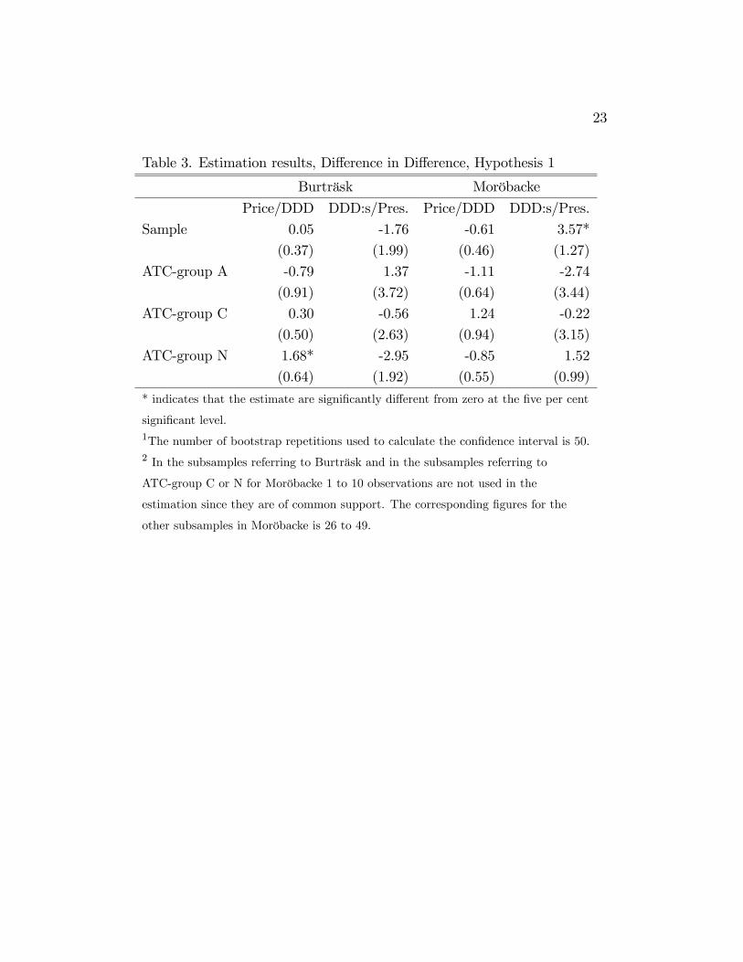
Let us start by comparing the period January to September 2002 with

the period prior to treatment. The average treatment e¤ects on the treated

of introducing �xed budgets for this period are presented in Table 3. As

mentioned in our �rst hypotheses in section 2, we expect both prices and

quantities to decrease relative to the comparison group. However, the es-

timated quantity di¤erence for Moröbacke is positive and signi�cant when

comparing all ATC-groups, and there is a large variation in the estimated

quantity di¤erences between ATC-groups. For Burträsk, one can note that

the price di¤erence is positive and signi�cant in ATC-group N, the other

estimated di¤erences vary in size as well as sign.

Table 3 about here.

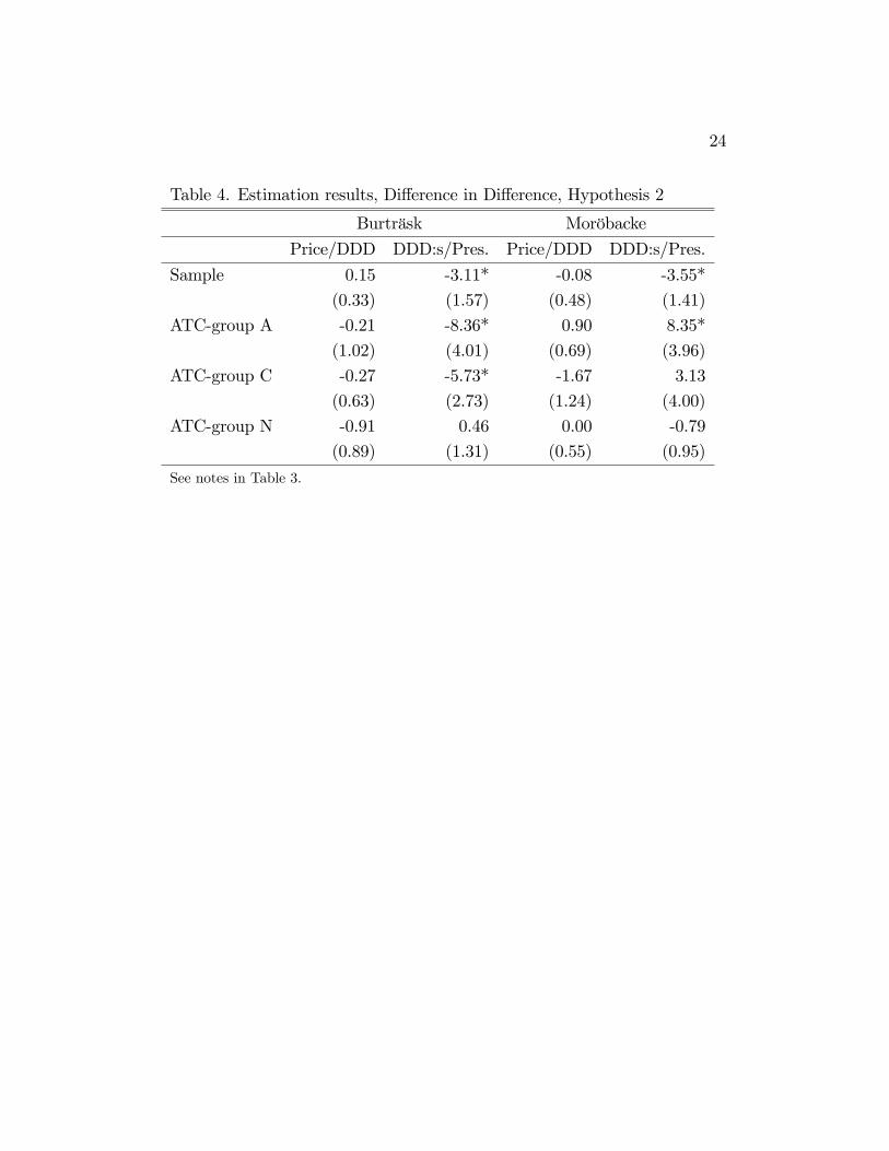
In order to test our second hypotheses, we take the di¤erences between

the period September 2002 and after, and January to September 2002. These

results are presented in Table 4. Burträsk and Moröbacke has lowered the

number of DDD:s/prescription after the substitution reform relative to the

control group, but prices per DDD are largely una¤ected. This is surprising

since the reform is aimed to a¤ect price per DDD but not the number of

DDD:s.

Table 4 about here.

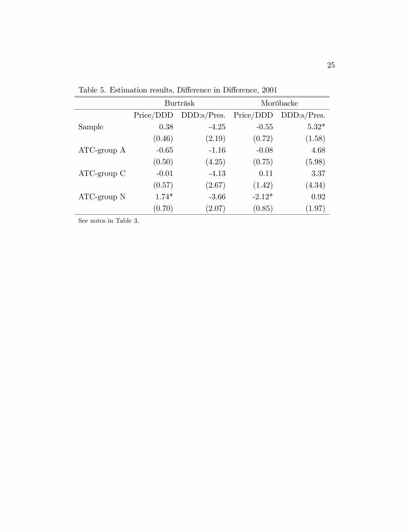
As discussed previously, a potential problem when testing our �rst hy-

potheses is that the price and quantities in the year 2001 could be a¤ected

16

by an attempt of the treated health centres to increase their future budgets.

An increase in price and quantities relative to the comparison group, when

comparing the post and pre-reform periods in the year 2001, would indicate

that such behavior might have in�uenced our data. The results presented in

Table 5 show that quantities are signi�cantly increased in Moröbacke when

comparing over all the ATC-groups, and there is a general tendency of pos-

itive e¤ects also within ATC-groups. For Burträsk, quantity di¤erences are

generally negative, although insigni�cant. There is no systematic di¤erences

in prices between the groups. Again, signi�cant results are found within

ATC-group N. Even though the results for quantities in Moröbacke have the

expected sign, no systematic di¤erence in prescription behavior can be ob-

served when comparing the post and pre-reform periods in the year 2001.

This is however a weak test of strategic behavior since such behavior could

have started before the formal introduction of the new rules. If the results

for the �rst hypotheses are a¤ected by strategic behavior, this would lead to

an overestimation of potential reductions in price and quantities due to the

introduction of �xed pharmaceutical budgets. To conclude, independent of

comparison, only a few of the estimated e¤ects turns out in favour of our

hypotheses. Most of the estimates are not signi�cantly di¤erent from zero.

Often, signi�cant estimates are contrary to expectations. Thus, the data

display no support for the hypothesis that �xed budgets a¤ect physician

prescription behavior.

Table 5 about here.

4 Discussion

Tentative results from this paper show that when health centers in Väster-

botten were given a �xed budget, the number of prescriptions of pharmaceu-

tical products declined. This can be seen as an indication that the prescrib-

ing physicians adopted to the new budgetary rules by reducing the number

17

of prescriptions, as compared with the previous situation when they were

given open-ended budgets. Other possible explanations for this result in-

clude changes in the health status of the population using these two health

centers, or demographic factors in the community were the health centers are

located. However, the short time period under study makes such explana-

tions less probable, since health status and demographic factors are, in most

cases, relatively constant over short periods of time.

The results also show that there are no systematic di¤erences regarding

either price or quantity per prescription between health centers using �xed

and open-ended budgets for pharmaceutical products, after controlling for

several confounding factors. One possible explanation is that the prescribing

physicians do not believe the �xed budgets to be credible, in the sense that

they expect the county council to cover de�cits or to cut future budgets in

the case of surplus. Another possible explanation is that the new incentive

structure is not clear to the prescribing physicians, or that physicians believe

that any surplus generated could be used in ways that they dislike.

A potential problem is that introducing the new budgetary system with

�xed budgets was voluntary for both the health centers and the local county

council. As such, the health centers which entered an agreement with the

county council to have �xed pharmaceuticals budgets might be centers which

had low initial pharmaceutical expenditures. In addition, both of the health

centers which were given �xed budgets are located in Skellefteå, a region

were several other cost containment measures, as for example recommended

lists, have been used. Such recommended lists often include not only which

pharmaceutical product to use, but also recommendations regarding the op-

timal package size to prescribe in order to avoid overprescribing. This could

mean that decreasing the pharmaceutical costs per prescription further, for

example by introducing �xed budgets, might be di¢ cult. As such, the only

way to reduce pharmaceutical costs is to reduce the number of prescriptions

made, as observed in the two health centers which were given �xed budgets.

18

5 References

Coscelli, A., 2000. The Importance of Doctors�and Patients�Preferences in

Prescription Drug Markets, Journal of Industrial Economics, 48 (3),

349-369.

Dukes, M.N.D., (ed.), 1993. Drug Utilization Studies. World Health Orga-

nization, Copenhagen.

Heckman, J., Ichimura, H., Todd, P., 1997. Matching as an Econometric

Evaluation Estimator: Evidence from Evaluating a Job Training Pro-

gram, Review of Economic Studies, 64, 605-654.

Kornai, J., Maskin, E.,Roland, G., 2003. Understanding the Soft Budget

Constraint, Journal of Economic Literature, 41(4), 1095- 1136.

Lundin, D., 2000. Moral Hazard in Physician Prescription Behavior, Journal

of Health Economics, 19, 639-662.

Mossialos, E., Le Grand, J., 1999. Cost Containment in the EU: An Overview,

in: Mossialos, E., and J. Le Grand (eds.), Health Care and Cost Con-

tainment in the European Union, Ashgate.

Prendergast, C., 1999. The Provision of Incentives in Firms, Journal of

Economic Literature 37(1), 7-64.

Rosenbaum, P., Rubin, D., 1983. The Central Role of the Propensity Score

in Observational Studies for Causal E¤ects, Biometrica, 70, 41-55.

Rudholm, N., 2004. Pharmaceutical Insurance and the Demand for Prescrip-

tion Pharmaceuticals in Västerbotten, Sweden, mimeo, Umeå Univer-

sity. Forthcoming in Scandinavian Journal of Public Health.

SFS 2002:160 Lag om läkemedelsförmåner.

Socialstyrelsen 2003. Läkemedelsförsäljningen I Sverige - en analys, Skill-

nader mellan landsting, 2003:1.

Smith, J., Todd, P., 2003a. Does Matching Overcome Lalonde�s Critique

of Nonexperimental Estimators?, mimeo, University of Maryland, Uni-

versity of Pennsylvania.

Smith, J., Todd, P., 2003b. Rejoinder, mimeo, University of Maryland, Uni-

versity of Pennsylvania.

19

Appendix 1. Balancing tests

As mentioned above, to guarantee that propensity score matching will elimi-

nate all the bias which the observables can account for, the observables must

be independent of the treatment assignment conditioned on the propensity

score. Several di¤erent test of this condition are proposed in the literature.

The tests have di¤erent limitations and little is known about their statistic

properties.

In this paper we employ two balancing tests. The �rst is a Hotelling

T 2 test of the joint null hypothesis of equal means between the treatment

groups and their control groups. This test can, however, fail to reject the

null hypothesis even if X is dependent of treatment assignment, conditioned

on the propensity score. One example of this could be if some variables

have higher values in the treated group, compared to the matched group,

for high values of the propensity score but lower values for low values of the

propensity score.

The second balancing test we conduct is a regression based test described

in Smith and Todd (2003b). For each variable used in estimating the propen-

sity score we estimate the following regression:

Xk = �0 + �1P̂ (X) + �2P̂ (X)2 + �3P̂ (X)

3 + �4P̂ (X)4

+�5D + �6DP̂ (X) + �7DP̂ (X)2 + �8DP̂ (X)

3 + �9DP̂ (X)4 + ",

where D is an indicator variable which takes the value one if the observation

is treated. In an attempt to test whether D provides additional information

about Xk conditioned on P (X) we test the joint null hypothesis that all the

coe¢ cients of the terms involving D equal zero. A shortcoming to this test

is that the choice of the order of the polynomial may a¤ect the result.

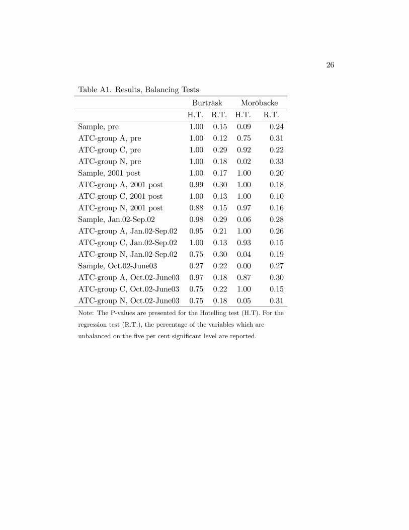
Table A1 about here.

20

The results from the tests appear in Table A1. The Hotelling test reject

balance for three of the subsamples for Moröbacke. The results from the re-

gression based test show that between 10 and 33 per cent of the independent

variables remain unbalanced conditioned on the propensity score in all mod-

els. Descriptive statistics, available from the authors upon request, indicate

that the remaining bias is small in magnitude.

21

Table 1. Descriptive statistics by health centres

Variable Category Sample Control Burträsk Moröbacke

Gender Female 65.40 65.76 63.39 64.44

Male 34.60 34.24 36.61 35.56

Area of Skellefteå 99.30 99.32 99.04 99.33

residency Other area 0.70 0.68 0.96 0.67

Patient- Yes 48.73 48.53 45.11 52.6

doses No 51.27 51.47 54.89 47.4

Patient�s Copay100 29.33 28.72 34.53 29.71

Payment Copay50 14.10 14.02 15.48 13.65

Copay25 12.65 12.71 12.83 12.1

Copay10 11.07 11.18 10.06 11.01

Copay0 29.89 30.57 24.35 29.98

Unsub 2.19 2.09 2.08 2.93

Free 0.69 0.71 0.68 0.61

Variable

Age Mean 71.07 71.64 72.51 66.26

Std. dv. 18.76 18.49 17.07 20.89

Price/DDD Mean 6.49 6.46 5.68 7.22

Std. dv. 19.21 19.83 13.46 18.43

DDD:s/prescr. Mean 41.67 41.91 44.91 37.76

Std. dv. 56.24 56.17 58.08 55.20

Cost/prescr. Mean 162.96 164.46 155.23 158.43

Std. dv. 286.51 284.27 308.82 284.90

NOBS. 292 419 232 799 24 622 34 998

22

Table 2. Descriptive statistics for the treatment and control groups

Pre treat. Burträsk Pre treat. Moröbacke

Variable Burträsk Control Moröbacke Control

Price/DDD Mean 6.24 6.24 7.01 6.21

Std. dv. 13.46 13.36 16.69 21.25

DDD:s/prescr. Mean 46.42 41.38 35.94 41.47

Std. dv. 63.10 55.97 51.87 56.10

Cost/prescr. Mean 171.07 160.13 151.28 159.69

Std. dv. 307.60 276.96 268.96 273.78

NOBS. 3 217 29 817 11 948 75 586

Prescr./month1 3 378.25 30 330.50 4 804.30 30 943.50

Post treat. Burträsk Post treat. Moröbacke

Variable Burträsk Control Moröbacke Control

Price/DDD Mean 5.59 6.50 7.33 6.58

Std. dv. 13.46 20.61 19.27 19.11

DDD:s/prescr. Mean 44.68 41.99 38.71 42.12

Std. dv. 57.29 56.20 56.83 56.20

Cost/prescr. Mean 152.85 165.10 162.14 166.75

Std. dv. 308.94 285.32 292.76 289.14

NOBS. 21 405 202 982 23 050 157 213

Prescr./month1 3 317.31 31 764.15 4 595.65 31 887.751Prescr./month refer to the average numbers of prescriptions per month for the whole

population and no standard deviations are therefore reported.

23

Table 3. Estimation results, Di¤erence in Di¤erence, Hypothesis 1

Burträsk Moröbacke

Price/DDD DDD:s/Pres. Price/DDD DDD:s/Pres.

Sample 0.05 -1.76 -0.61 3.57*

(0.37) (1.99) (0.46) (1.27)

ATC-group A -0.79 1.37 -1.11 -2.74

(0.91) (3.72) (0.64) (3.44)

ATC-group C 0.30 -0.56 1.24 -0.22

(0.50) (2.63) (0.94) (3.15)

ATC-group N 1.68* -2.95 -0.85 1.52

(0.64) (1.92) (0.55) (0.99)

* indicates that the estimate are signi�cantly di¤erent from zero at the �ve per cent

signi�cant level.1The number of bootstrap repetitions used to calculate the con�dence interval is 50.2 In the subsamples referring to Burträsk and in the subsamples referring to

ATC-group C or N for Moröbacke 1 to 10 observations are not used in the

estimation since they are of common support. The corresponding �gures for the

other subsamples in Moröbacke is 26 to 49.

24

Table 4. Estimation results, Di¤erence in Di¤erence, Hypothesis 2

Burträsk Moröbacke

Price/DDD DDD:s/Pres. Price/DDD DDD:s/Pres.

Sample 0.15 -3.11* -0.08 -3.55*

(0.33) (1.57) (0.48) (1.41)

ATC-group A -0.21 -8.36* 0.90 8.35*

(1.02) (4.01) (0.69) (3.96)

ATC-group C -0.27 -5.73* -1.67 3.13

(0.63) (2.73) (1.24) (4.00)

ATC-group N -0.91 0.46 0.00 -0.79

(0.89) (1.31) (0.55) (0.95)

See notes in Table 3.

25

Table 5. Estimation results, Di¤erence in Di¤erence, 2001

Burträsk Moröbacke

Price/DDD DDD:s/Pres. Price/DDD DDD:s/Pres.

Sample 0.38 -4.25 -0.55 5.32*

(0.46) (2.19) (0.72) (1.58)

ATC-group A -0.65 -1.16 -0.08 4.68

(0.50) (4.25) (0.75) (5.98)

ATC-group C -0.01 -4.13 0.11 3.37

(0.57) (2.67) (1.42) (4.34)

ATC-group N 1.74* -3.66 -2.12* 0.92

(0.70) (2.07) (0.85) (1.97)

See notes in Table 3.

26

Table A1. Results, Balancing Tests

Burträsk Moröbacke

H.T. R.T. H.T. R.T.

Sample, pre 1.00 0.15 0.09 0.24

ATC-group A, pre 1.00 0.12 0.75 0.31

ATC-group C, pre 1.00 0.29 0.92 0.22

ATC-group N, pre 1.00 0.18 0.02 0.33

Sample, 2001 post 1.00 0.17 1.00 0.20

ATC-group A, 2001 post 0.99 0.30 1.00 0.18

ATC-group C, 2001 post 1.00 0.13 1.00 0.10

ATC-group N, 2001 post 0.88 0.15 0.97 0.16

Sample, Jan.02-Sep.02 0.98 0.29 0.06 0.28

ATC-group A, Jan.02-Sep.02 0.95 0.21 1.00 0.26

ATC-group C, Jan.02-Sep.02 1.00 0.13 0.93 0.15

ATC-group N, Jan.02-Sep.02 0.75 0.30 0.04 0.19

Sample, Oct.02-June03 0.27 0.22 0.00 0.27

ATC-group A, Oct.02-June03 0.97 0.18 0.87 0.30

ATC-group C, Oct.02-June03 0.75 0.22 1.00 0.15

ATC-group N, Oct.02-June03 0.75 0.18 0.05 0.31

Note: The P-values are presented for the Hotelling test (H.T). For the

regression test (R.T.), the percentage of the variables which are

unbalanced on the �ve per cent signi�cant level are reported.