Chemical Engineering Science 101 (2013) 99–108

Contents lists available at SciVerse ScienceDirect

Chemical Engineering Science

0009-25http://d

n CorrE-m

journal homepage: www.elsevier.com/locate/ces

Fisher information matrix based time-series segmentationof process data

László Dobos, János Abonyi n

Department of Process Engineering, University of Pannonia, P.O. Box 158, H-8201 Veszprém, Hungary

H I G H L I G H T S

� Parameter estimation depends on information content of process data segments.

� Selection of highly informative data needs multivariate time-series segmentation tool.� Fisher information based time-series segmentation framework is developed.� Segments with parameter-set specific information content can be segregated.� Tools of Optimal Experiment Design is applied to measure the information content.

a r t i c l e i n f o

Article history:Received 21 August 2012Received in revised form27 March 2013Accepted 7 June 2013

Keywords:Process modelTime-series segmentationOptimal experimental design (OED)Fisher information matrixParameter identification

09/$ - see front matter Crown Copyright & 20x.doi.org/10.1016/j.ces.2013.06.030

esponding author. Tel.: +36 88 622793.ail address: janos@abonyilab.com (J. Abonyi).

a b s t r a c t

Advanced chemical process engineering tools, like model predictive control or soft sensor solutionsrequire proper process models. Parameter identification of these models needs input–output data withhigh information content. When model based optimal experimental design techniqes cannot be applied,the extraction of informative segements from historical data can also support system identification. Wedeveloped a goal-oriented Fisher information based time-series segmentation algorithm, aimed atselecting informative segments from historical process data. The utilized standard bottom-up algorithmis widely used in off-line analysis of process data. Different segments can support the identification ofparameter sets. Hence, instead of using either D- or E-optimality as the criterion for comparing theinformation content of two input sequences (neigbouring segments), we propose the use of Krzanowski'ssimilarity coefficient between the eigenvectors of the Fisher information matrices obtained from thesequences. The efficiency of the proposed methodology is demonstrated by two application examples.The algorithm is capable to extract segments with parameter-set specific information content fromhistorical process data.

Crown Copyright & 2013 Published by Elsevier Ltd. All rights reserved.

1. Introduction

Most of advanced chemical process monitoring, control, andoptimization algorithms rely on process model. Often some para-meters of these models are not known a priori, so t hey must beestimated from experimental or historical process data. Theaccuracy of these parameters largely depends on the informationcontent of data selected to parameter identification (Bernaertset al., 2002). There are two ways to get informative data foridentification: the first is the classical, iterative design of experi-ments, while the second is to extract the most informativesegments form the already available data. Currently there is no

13 Published by Elsevier Ltd. All r

available algorithm that can support information content based onthis selection of segments of process data.

The selection of appropriate data sequences can be consideredas a time-series segmentation. Time-series segmentation is oftenused to extract internally homogeneous segments from a giventime series e.g. to locate stable periods of time, to identify changepoints (Fu, 2011). A suitable segmentation algorithm has beenpresented in Keogh et al. (2001) to extract homogeneous segmentsfrom historical or streaming data. We developed a fuzzy clusteringalgorithm to detect changes in the correlation structure of multi-variate time-series in Abonyi et al. (2005). Historical process dataalone may not be sufficient for the monitoring of complexprocesses. We incorporated the first-principle model of theprocess into the segmentation algorithm in Feil et al. (2005) touse a model-based non-linear state-estimation algorithm to detectthe changes in the correlation among the state-variables. For off-line purposes the bottom-up approach is widely followed, while

ights reserved.

L. Dobos, J. Abonyi / Chemical Engineering Science 101 (2013) 99–108100

for on-line application the so-called sliding window segmentationtechnique is applied. By combining and integrating recursive anddynamic principal component analysis (PCA) into time seriessegmentation techniques efficient multivariate segmentationmethod is obtained to detect homogenous operation ranges basedon process data (Dobos and Abonyi, 2012).

These applications are mostly applicable in process monitoringsince they can detect changes in the correlation structure ofprocess data. However, now we are interested in extractinginformative segments applicable for the identification of set ofparameters of a well defined process model. This novel modelbased segmentation task is practically important, since it is wellknown that “data themselves cannot produce information; theycan only produce information in the light of a particular model”(Box and Hunter, 1965).

Extraction of time-series segments from historical process datawith high information content requires novel, goal-oriented time-series segmentation algorithm. Our key idea is to utilize the tools ofOptimal Experimental Design (OED). An overview and criticalanalysis of experimental design techniques can be found inFranceschini and Macchietto (2008). Tools of OED are applicableto measure the information content of datasets (Asprey andMacchietto, 2002). Usually OED is an iterative procedure that canmaximize the information content of experimental data throughoptimization of input profiles (Rojas et al., 2007). OED is based onFisher information matrix constructed from partial derivatives ofmodel outputs with respect to changes of selected model para-meters. Based on the Fisher information matrix the informationcontent of the considered input data can be measured by utilizing A,E or D criteria (Asprey and Macchietto, 2002; Bernaerts et al., 2005).

When several rival mathematical models are available for thesame process, model discrimination may become more efficient andeffective if uncertainty is reduced first. This can be achieved byperforming experiments designed to increase the accuracy of theparameter estimates and, thus, the model predictions. However,performing such an additional experiment for each rival modelmay undermine the overall goal of optimal experimental design,which is to minimize the experimental effort. Donckels et al. (2010)deals with the design of a so-called compromise experiment, whichis an experiment that is not optimal for each of the rival models, butsufficiently informative to improve the overall accuracy of theparameters of all rival models. A new design criterion for discrimina-tion of rival models has been presented in Alberton et al. (2012). Thisapplication also illustrates that OED is a continuously developingfield of chemical engineering with wide range of applications.

In this paper a OED is utilized to extract informative segmentsfrom a given time-series, where different segments can be used toidentify different models or parameters. The segmentation algorithmis designed to detect changes in the correlation structure of para-meter sensitivities. Fisher information matrix is a perfect tool torepresent this correlation. Based on the Fisher information matricesthe information content of the data sets can be compared directly.Since Fisher matrix can possess surplus information (not only just thequantity of the information but also its direction in the consideredinformation space), the similarity of these matrices can be used tofind the time series segments with similar information content. Withthe help of the Krzanowski distance measure, (Krzanowski, 1979), itis possible to determine the similarity of the Fisher matrices. Whencalculating the Fisher information matrix the eigenvectors areordered regarding to the descending order of the eigenvalues. In apreliminary examination the eigenvectors with zero eigenvalues areexcluded and the remaining eigenvectors are used in the segmenta-tion algorithm. It is assumed that eigenvectors with zero eigenvalueshave no information contribution in the considered parameter space.The proposed novel and intuitive segmentation algorithm makespossible to identify parameter sets from the most appropriate time

frame of experimental data. With the help of this method it ispossible to reduce the cost and time consumption of parameterestimation. The applicability of the proposed methodology is pre-sented throughout a simple example with a linear model and asynthetic data set of a polymerization process.

The rest of the paper is organized as follows. In Section 2 thetools of the developed algorithms are presented in details liketools of OED, the calculation ways of sensitivities, finally thedeveloped algorithms are described in details. In Section 3 theapplicability of the proposed time-series segmentation method ispresented through demonstrative examples.

2. Optimal experimental design based time seriessegmentation

We apply time-series segmentation to extract data sequenceswith high information content. Since extracted data is used forparameter identification its information content is measured basedon Fisher information matrix constructed from the sensitivities of themodel output with respect to the parameters. Various ways ofcalculating sensitivities are presented. At the end of the section theresulted time-series segmentation algorithm is described.

2.1. Background of model based optimal experimental design

The Fisher information matrix (F) is based on the sensitivity ofthe model output (yðuðtÞ) respect to the parameters (p), calculatedas follows:

F¼ 1tend

Z tend

t ¼ 0

∂y∂p

���Tp ¼ p0

ðtÞ � ∂y∂p

���p ¼ p0

ðtÞ dt ð1Þ

The calculation of the derivatives require a process model

dxðtÞdt

¼ f ðxðtÞ;uðtÞ;pÞ ð2Þ

yðtÞ ¼ gðxðtÞÞ ð3Þwhere u¼ ½u1…unu� (nu is the number of inputs) is the vector ofthe manipulated inputs, y¼ ½y1…yny� (ny is the number of outputs)is the vector of the outputs, x¼ ½x1…xnx� (nx is the number ofstates) represents the states, and p¼ ½p1…pnp� (np is the number ofinputs) denotes the model parameters.

The p parameters are unknown and should be estimated usingthe data taken from experiments. The estimation of these para-meters is based on the minimization of the square error betweenthe output of the system and the output of the model

minp

JmseðuðtÞ;pÞ ¼1tend

Z tend

t ¼ 0eðtÞT �Q ðtÞ � eðtÞ dt ð4Þ

eðtÞ ¼ ~yðuðtÞÞ−yðuðtÞ;pÞ ð5Þwhere ~yðuðtÞÞ is the output of the system for a certain u½t : tend�input profile, and yðuðtÞÞ is the output of the model for the sameu½t : tend� input profile with p parameters. Q ðtÞ is a user suppliedsquare weighting matrix.

The optimal design criterion aims the minimization of a scalarfunction of the F matrix. Several criterion exist

�

D-optimal experimental design maximizes the determinant ofthe Fisher matrix (Eq. (1)), and thus maximizes the volume ofthe joint confidence region.

JD ¼ maxu½t:tend �

ðdetðFÞÞ ð6Þ

�

E-optimal experimental design is based on the ratio of themaximal and minimal eigenvalues of the Fisher matrix (Eq. (1)).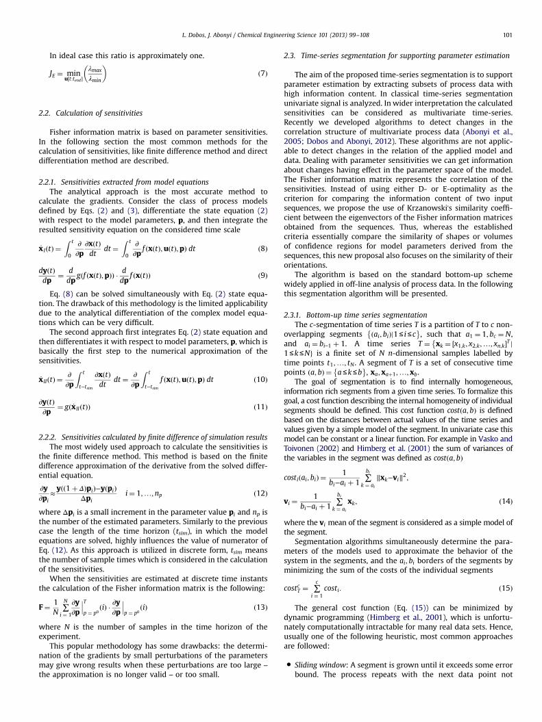

L. Dobos, J. Abonyi / Chemical Engineering Science 101 (2013) 99–108 101

In ideal case this ratio is approximately one.

JE ¼ minu½t:tend �

λmax

λmin

� �ð7Þ

2.2. Calculation of sensitivities

Fisher information matrix is based on parameter sensitivities.In the following section the most common methods for thecalculation of sensitivities, like finite difference method and directdifferentiation method are described.

2.2.1. Sensitivities extracted from model equationsThe analytical approach is the most accurate method to

calculate the gradients. Consider the class of process modelsdefined by Eqs. (2) and (3), differentiate the state equation (2)with respect to the model parameters, p, and then integrate theresulted sensitivity equation on the considered time scale

_x IðtÞ ¼Z t

0

∂∂p

∂xðtÞdt

dt ¼Z t

0

∂∂p

f ðxðtÞ;uðtÞ;pÞ dt ð8Þ

dyðtÞdp

¼ ddp

gðf ðxðtÞ;pÞÞ � ddp

f ðxðtÞÞ ð9Þ

Eq. (8) can be solved simultaneously with Eq. (2) state equa-tion. The drawback of this methodology is the limited applicabilitydue to the analytical differentiation of the complex model equa-tions which can be very difficult.

The second approach first integrates Eq. (2) state equation andthen differentiates it with respect to model parameters, p, which isbasically the first step to the numerical approximation of thesensitivities.

_x IIðtÞ ¼∂∂p

Z t

t−tsim

∂xðtÞdt

dt ¼ ∂∂p

Z t

t−tsimf ðxðtÞ;uðtÞ;pÞ dt ð10Þ

∂yðtÞ∂p

¼ gð _x IIðtÞÞ ð11Þ

2.2.2. Sensitivities calculated by finite difference of simulation resultsThe most widely used approach to calculate the sensitivities is

the finite difference method. This method is based on the finitedifference approximation of the derivative from the solved differ-ential equation.

∂y∂pi

≈yðð1þ ΔÞpiÞ−yðpiÞ

Δpii¼ 1;…;np ð12Þ

where Δpi is a small increment in the parameter value pi and np isthe number of the estimated parameters. Similarly to the previouscase the length of the time horizon (tsim), in which the modelequations are solved, highly influences the value of numerator ofEq. (12). As this approach is utilized in discrete form, tsim meansthe number of sample times which is considered in the calculationof the sensitivities.

When the sensitivities are estimated at discrete time instantsthe calculation of the Fisher information matrix is the following:

F¼ 1N

∑N

i ¼ 1

∂y∂p

���Tp ¼ p0

ðiÞ � ∂y∂p

���p ¼ p0

ðiÞ ð13Þ

where N is the number of samples in the time horizon of theexperiment.

This popular methodology has some drawbacks: the determi-nation of the gradients by small perturbations of the parametersmay give wrong results when these perturbations are too large –

the approximation is no longer valid – or too small.

2.3. Time-series segmentation for supporting parameter estimation

The aim of the proposed time-series segmentation is to supportparameter estimation by extracting subsets of process data withhigh information content. In classical time-series segmentationunivariate signal is analyzed. In wider interpretation the calculatedsensitivities can be considered as multivariate time-series.Recently we developed algorithms to detect changes in thecorrelation structure of multivariate process data (Abonyi et al.,2005; Dobos and Abonyi, 2012). These algorithms are not applic-able to detect changes in the relation of the applied model anddata. Dealing with parameter sensitivities we can get informationabout changes having effect in the parameter space of the model.The Fisher information matrix represents the correlation of thesensitivities. Instead of using either D- or E-optimality as thecriterion for comparing the information content of two inputsequences, we propose the use of Krzanowski's similarity coeffi-cient between the eigenvectors of the Fisher information matricesobtained from the sequences. Thus, whereas the establishedcriteria essentially compare the similarity of shapes or volumesof confidence regions for model parameters derived from thesequences, this new proposal also focuses on the similarity of theirorientations.

The algorithm is based on the standard bottom-up schemewidely applied in off-line analysis of process data. In the followingthis segmentation algorithm will be presented.

2.3.1. Bottom-up time series segmentationThe c-segmentation of time series T is a partition of T to c non-

overlapping segments ðai; biÞj1≤ i≤c� �

, such that a1 ¼ 1; bc ¼N,and ai ¼ bi−1 þ 1. A time series T ¼ xk ¼ ½x1;k; x2;k;…; xn;k�T j

�1≤k≤Ng is a finite set of N n-dimensional samples labelled bytime points t1;…; tN . A segment of T is a set of consecutive timepoints ða; bÞ ¼ a≤k≤b

� �, xa; xaþ1;…; xb.

The goal of segmentation is to find internally homogeneous,information rich segments from a given time series. To formalize thisgoal, a cost function describing the internal homogeneity of individualsegments should be defined. This cost function costða;bÞ is definedbased on the distances between actual values of the time series andvalues given by a simple model of the segment. In univariate case thismodel can be constant or a linear function. For example in Vasko andToivonen (2002) and Himberg et al. (2001) the sum of variances ofthe variables in the segment was defined as costða;bÞ

costiðai; biÞ ¼1

bi−ai þ 1∑bi

k ¼ ai

∥xk−vi∥2;

vi ¼1

bi−ai þ 1∑bi

k ¼ ai

xk; ð14Þ

where the vi mean of the segment is considered as a simple model ofthe segment.

Segmentation algorithms simultaneously determine the para-meters of the models used to approximate the behavior of thesystem in the segments, and the ai; bi borders of the segments byminimizing the sum of the costs of the individual segments

costcT ¼ ∑c

i ¼ 1costi: ð15Þ

The general cost function (Eq. (15)) can be minimized bydynamic programming (Himberg et al., 2001), which is unfortu-nately computationally intractable for many real data sets. Hence,usually one of the following heuristic, most common approachesare followed:

�

Sliding window: A segment is grown until it exceeds some errorbound. The process repeats with the next data point not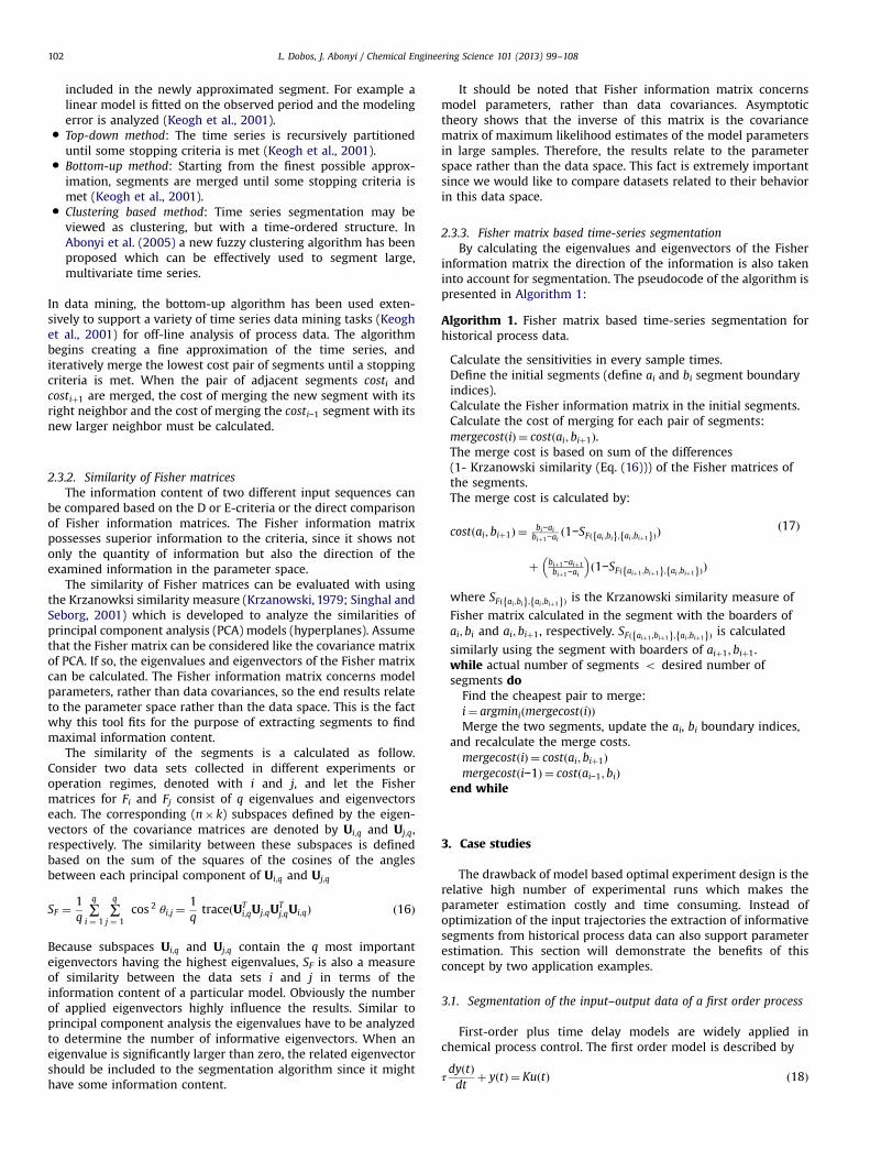

L. Dobos, J. Abonyi / Chemical Engineering Science 101 (2013) 99–108102

included in the newly approximated segment. For example alinear model is fitted on the observed period and the modelingerror is analyzed (Keogh et al., 2001).

�

Top-down method: The time series is recursively partitioneduntil some stopping criteria is met (Keogh et al., 2001).

�

Bottom-up method: Starting from the finest possible approx-imation, segments are merged until some stopping criteria ismet (Keogh et al., 2001).

�

Clustering based method: Time series segmentation may beviewed as clustering, but with a time-ordered structure. InAbonyi et al. (2005) a new fuzzy clustering algorithm has beenproposed which can be effectively used to segment large,multivariate time series.

In data mining, the bottom-up algorithm has been used exten-sively to support a variety of time series data mining tasks (Keoghet al., 2001) for off-line analysis of process data. The algorithmbegins creating a fine approximation of the time series, anditeratively merge the lowest cost pair of segments until a stoppingcriteria is met. When the pair of adjacent segments costi andcostiþ1 are merged, the cost of merging the new segment with itsright neighbor and the cost of merging the costi−1 segment with itsnew larger neighbor must be calculated.

2.3.2. Similarity of Fisher matricesThe information content of two different input sequences can

be compared based on the D or E-criteria or the direct comparisonof Fisher information matrices. The Fisher information matrixpossesses superior information to the criteria, since it shows notonly the quantity of information but also the direction of theexamined information in the parameter space.

The similarity of Fisher matrices can be evaluated with usingthe Krzanowksi similarity measure (Krzanowski, 1979; Singhal andSeborg, 2001) which is developed to analyze the similarities ofprincipal component analysis (PCA) models (hyperplanes). Assumethat the Fisher matrix can be considered like the covariance matrixof PCA. If so, the eigenvalues and eigenvectors of the Fisher matrixcan be calculated. The Fisher information matrix concerns modelparameters, rather than data covariances, so the end results relateto the parameter space rather than the data space. This is the factwhy this tool fits for the purpose of extracting segments to findmaximal information content.

The similarity of the segments is a calculated as follow.Consider two data sets collected in different experiments oroperation regimes, denoted with i and j, and let the Fishermatrices for Fi and Fj consist of q eigenvalues and eigenvectorseach. The corresponding (n� k) subspaces defined by the eigen-vectors of the covariance matrices are denoted by Ui;q and Uj;q,respectively. The similarity between these subspaces is definedbased on the sum of the squares of the cosines of the anglesbetween each principal component of Ui;q and Uj;q

SF ¼1q

∑q

i ¼ 1∑q

j ¼ 1cos 2 θi;j ¼

1qtraceðUT

i;qUj;qUTj;qUi;qÞ ð16Þ

Because subspaces Ui;q and Uj;q contain the q most importanteigenvectors having the highest eigenvalues, SF is also a measureof similarity between the data sets i and j in terms of theinformation content of a particular model. Obviously the numberof applied eigenvectors highly influence the results. Similar toprincipal component analysis the eigenvalues have to be analyzedto determine the number of informative eigenvectors. When aneigenvalue is significantly larger than zero, the related eigenvectorshould be included to the segmentation algorithm since it mighthave some information content.

It should be noted that Fisher information matrix concernsmodel parameters, rather than data covariances. Asymptotictheory shows that the inverse of this matrix is the covariancematrix of maximum likelihood estimates of the model parametersin large samples. Therefore, the results relate to the parameterspace rather than the data space. This fact is extremely importantsince we would like to compare datasets related to their behaviorin this data space.

2.3.3. Fisher matrix based time-series segmentationBy calculating the eigenvalues and eigenvectors of the Fisher

information matrix the direction of the information is also takeninto account for segmentation. The pseudocode of the algorithm ispresented in Algorithm 1:

Algorithm 1. Fisher matrix based time-series segmentation forhistorical process data.

Calculate the sensitivities in every sample times.Define the initial segments (define ai and bi segment boundaryindices).Calculate the Fisher information matrix in the initial segments.Calculate the cost of merging for each pair of segments:mergecostðiÞ ¼ costðai; biþ1Þ.The merge cost is based on sum of the differences(1- Krzanowski similarity (Eq. (16))) of the Fisher matrices ofthe segments.The merge cost is calculated by:

costðai; biþ1Þ ¼ bi−aibiþ1−ai

ð1−SFð ai ;bif g; ai ;biþ1f gÞÞð17Þ

þ biþ1−aiþ1biþ1−ai

� �ð1−SFð aiþ1 ;biþ1f g; ai ;biþ1f gÞÞ

where SFð ai ;bif g; ai ;biþ1f gÞ is the Krzanowski similarity measure of

Fisher matrix calculated in the segment with the boarders ofai; bi and ai; biþ1, respectively. SFð aiþ1 ;biþ1f g; ai ;biþ1f gÞ is calculated

similarly using the segment with boarders of aiþ1; biþ1.while actual number of segments o desired number ofsegments doFind the cheapest pair to merge:i¼ argminiðmergecostðiÞÞMerge the two segments, update the ai, bi boundary indices,

and recalculate the merge costs.mergecostðiÞ ¼ costðai; biþ1Þmergecostði−1Þ ¼ costðai−1; biÞ

end while

3. Case studies

The drawback of model based optimal experiment design is therelative high number of experimental runs which makes theparameter estimation costly and time consuming. Instead ofoptimization of the input trajectories the extraction of informativesegments from historical process data can also support parameterestimation. This section will demonstrate the benefits of thisconcept by two application examples.

3.1. Segmentation of the input–output data of a first order process

First-order plus time delay models are widely applied inchemical process control. The first order model is described by

τdyðtÞdt

þ yðtÞ ¼ KuðtÞ ð18Þ

1000 2000 3000 4000 5000 6000 7000 8000 9000 100000.5

1

1.5

Samples

Value of dy/dK

1000 2000 3000 4000 5000 6000 7000 8000 9000 100000.02

0.01

0

0.01

0.02

Samples

Value of dy/d

Fig. 2. Sensitivities of the first order process. Comparison of thee calculationmethods. Full line – analytical sensitivity using I. approach, dotted line – analyticalsensitivity using II. approach, dashed line – finite difference method.

1 2 3 4 5 6 7 8 9 10

0.51

0.5105

0.511

Periodic time (sec)

E c

riter

ia

1 2 3 4 5 6 7 8 9 105.65

5.66

5.67

5.68

Periodic time (sec)

D c

riter

ia

Fig. 3. Information content of binary signals with different periodic times.

L. Dobos, J. Abonyi / Chemical Engineering Science 101 (2013) 99–108 103

In this study the nominal parameters of the model are K¼1, τ¼ 10and the sample time is 0.1 s.

The aim of this example is to demonstrate the effects of theparameters of the proposed time-series segmentation algorithm,like the differences in the calculation ways of sensitivities, thegeneration of Fisher matrices and the result of time seriessegmentation. We investigated the dataset depicted on Fig. 1.

3.1.1. Calculation of sensitivitiesThe analytical sensitivities can be calculated by differentiating

Eq. (18) first and then solving the partial differential equationsimultaneously with the state equations (I. approach):

ddt

dydK

ðtÞ ¼ 1τuðtÞ−1

τ

dyðtÞdt

ð19Þ

ddt

dydτ

ðtÞ ¼−1τ2

uðtÞ þ 1τ2

yðtÞ−1τ

dyðtÞdt

ð20Þ

The second approach presented in Section 2.2 is based on thesolution of the state equation (Eq. (18)):

yðtÞ ¼ Kτ

R t0 e

t=τuðtÞ dt þ cet=τ

ð21Þ

The direct differentiation of Eq. (21) provides the third way tocalculate the sensitivities (II. approach)

∂yðtÞ∂K

¼ 1τ

R t0 e

t=τuðtÞ dt þ cet=τ

ð22Þ

∂yðtÞ∂τ

¼−Kτ2

R t0 e

t=τuðtÞ dt þ cet=τ

þ Kτ3

te−tτ

Z t

0et=τuðtÞ dt−e−t

τ

Z t

0tet=τuðtÞ dt

� �ð23Þ

The differences in the proposed methods are shown in Fig. 2.The numerical approximation of the sensitivities are not

exactly identical to the analytical sensitivities (Fig. 2). In thisparticular case of finite difference method the simulation time is250. Since at the calculation of Fisher matrices normalized valuesof sensitivities are applied, the constant shift in the values ofsensitivities does not affect the information content (see Eq. (1)).

3.1.2. Time-series segmentation scenariosWe determined the optimal input signal of the process to

provide a good background of comparison. Several studies dealwith optimal design of identification experiments (Goodwin, 1971;Mehra, 1974; Yuan and Ljung, 1984; Morari and Leeb, 1999;

1000 2000 3000 4000 5000 6000 7000 8000 9000 10000

0.8

1

1.2

Out

put

Samples

1000 2000 3000 4000 5000 6000 7000 8000 9000 10000

0.5

1

1.5

2

Inpu

t

Samples

Fig. 1. Input–output process data of the first order process.

Bernaerts et al., 2002; Hildebrand and Gevers, 2002). In this studybinary signal is chosen to determine the optimal input signal formodel parameter identification. OED tools are highly suitable forcomputing the optimal value of periodic time of the input signal.Fig. 3 shows the information content of an input signal withdifferent periodic times measure by the introduced E and Dmetrics. As it is depicted the highest information content is theinput signal with periodic time of four which is basically almostthe third of the time constant of the considered transfer function.

Based on the calculated sensitivities the proposed bottom-uptime-series segmentation algorithm (Algorithm 1) is applied onthe proposed data set in Fig. 1. In the Fisher information basedtime-series segmentation methodology the most important eigen-vectors of the Fisher information matrices are compared directlyusing the Krzanowski similarity measure (Eq. (16)). The eigenvec-tors with zero eigenvalues are excluded from the calculation. Theminimal resolution was 2000 samples. The number of segmentswas set to 10. The dataset with low frequency constitutes an entiresegment and segregated from the data set segments with highfrequency, as it could be expected. Without any additional knowl-edge a segment where the frequency of the input variable is 33% of

1000 2000 3000 4000 5000 6000 7000 8000 9000 100000.5

1

1.5

E criteria based time−series segmentation

Out

put

Time (s)

1000 2000 3000 4000 5000 6000 7000 8000 9000 100000

1

2

Inpu

t

Time (s)

L. Dobos, J. Abonyi / Chemical Engineering Science 101 (2013) 99–108104

the time constant is also automatically detected. As it can beexpected this segment has the highest information content (Fig. 4).

The D or E criteria measure directly the information content ofthe data regarding to a certain parameter or set of parameters. Forcomparison these criteria based univariate bottom-up time-seriessegmentation has also been applied. As can be seen in Figs. 5 and 6none of these segmentation results provided as good segmentationsas the Fisher matrix based algorithm. We also applied classicallinear model based segmentations, but these techniques were notable to accurately detect changes related to the information contentof the data.

1000 2000 3000 4000 5000 6000 7000 8000 9000 10000

234

Time (s)

E c

riter

ia o

f the

segm

ents

3.1.3. Identification scenarios based on the results of time-series

scenarioTo be able to prove the benefit of Fisher matrix based

time-series segmentation method, three different identificationscenarios are considered:

Fig. 6. Results of the E criteria based segmentation.

�

Figcrit

identification using optimal input signal sequence with theperiodic time of 4.

�

identification scenario based on the result of performed time-series segmentation using the segment with the highest Ecriteria value. It is for representing the segment with the lowestinformation content. In this example, it is the first segment.

1000 2000 3000 4000 5000 6000 7000 8000 9000 100000.5

1

1.5

Fisher matrix based time series segmentation

Out

put

Time (s)

1000 2000 3000 4000 5000 6000 7000 8000 9000 100000

1

2

Inpu

t

Time (s)

1000 2000 3000 4000 5000 6000 7000 8000 9000 10000

345

Time (s)

E c

riter

ia o

f the

seg

men

ts

. 4. Result of Fisher matrix based time-series segmentation and the value of Eeria in the segments are also shown.

1000 2000 3000 4000 5000 6000 7000 8000 9000 100000.5

1

1.5

D criteria based time−series segmentation

Out

put

Time (s)

1000 2000 3000 4000 5000 6000 7000 8000 9000 100000

1

2

Inpu

t

Time (s)

1000 2000 3000 4000 5000 6000 7000 8000 9000 10000

1

2

3

Time (s)

D c

riter

ia o

f the

seg

men

ts

Fig. 5. Result of the D criteria based segmentation.

Fig. 7. Process data used in the polymerization reactor example.

�

identification scenario based on the result of performed time-series segmentation using the segment with the lowest E criteriavalue. It is for representing the segment with the highestinformation content. In this example, it is the second segment.

The identification scenarios are performed using MATLAB andits fmincon function. The initial condition for K¼1.5, time con-stant¼14. The parameters of the transfer function could bedetermined in all scenarios, only the number of function evalua-tions of the parameter optimization was different. The less numberof function evaluations was needed to the optimized identificationdata thanks to its higher information content (43 iterations). Thesegment with high information content can provide almost thecomputational demand (44 iterations). As it can be expected thefirst segment with the less conditioned information matrixrequired the largest number of iterations.

3.2. Example with synthetic data of a polymerization process

The identification of highly nonlinear process models is morecomplex task than the previously presented illustrative example.

L. Dobos, J. Abonyi / Chemical Engineering Science 101 (2013) 99–108 105

Due to the complex nonlinear effect of the parameters it is reallynecessary to support the parameter estimation procedure byinformation rich data regarding to the estimated parameters.Polymerization processes and their first principle models arehighly suitable for representing the characteristics of nonlinearmodels. The task is to automatically determine information richsegments that are applicable to the identify the parameters of thefirst principle model described in the following subsection.

3 3.5 4 4.5 5 5.5 63.15

3.2

3.25

3.3

3.35x 104

Time (h)

NA

MW

(kg/

kmol

)

3 3.5 4 4.5 5 5.5 6340

342

344

346

348

Time (h)

Tem

pera

ture

(K)

Fig. 9. Results of identification scenarios (full line – original data, dashed line – theworst scenario, and dashdot line – the best scenario).

Table 1Result of identification scenarios of determining all kinetic parameters.

Scenario Segment Cost1000 samples

Type of parameter r¼p

Original - – kr 1.77�1Er 1.8283�

Best Fifth 7.71�107 kr 2.13�1Er 2.07�1

Worst First 3.38�108 kr 2.85�1Er 2.18�1

100 200 300 400 500 600 700

2.5

3

3.5

x 104 Fisher matrix based time series segmentation

Out

put

Time (h)

100 200 300 400 500 600 700

34

36

38

40

Time (h)

log(

E) c

riter

ia o

f the

seg

men

ts

21 43 5 6

Fig. 8. Result of segmentation for supporting to the identification of all kineticparameters.

3.2.1. Description of the processA continuously stirred tank reactor (CSTR) in which a free

radical polymerization reaction of methyl-metacrylate using azo-bisisobutironitil (AIBN) as initiator and toulene as solvent isconsidered. The number-average molecular weight (NAMW) isused for qualifying the product and process state. The polymeriza-tion process can be described by the following model equations(Silva-Beard and Flores-Tlacuahuac, 1999):

dCm

dt¼−ðkp þ kfmÞCmP0 þ

FðCmin−CmÞV

ð24Þ

dCI

dt¼ −kICI þ

FICIin−FCIÞV

ð25Þ

dTdt

¼ ð−ΔHÞkpCm

ρCpP0−

UAρCpV

ðT−TjÞ þFðTin−TÞ

Vð26Þ

dD0

dt¼ ð0:5ktc þ ktdÞP2

0 þ kfmCmP0−FD0

Vð27Þ

dD1

dt¼Mmðkp þ kfmÞCmP0−

FD1

Vð28Þ

dTj

dt¼ FcwðTw0−TjÞ

V0þ UA

ρwCpwVðT−TjÞ ð29Þ

where

P0 ¼ffiffiffiffiffiffiffiffiffiffiffiffiffiffiffiffiffiffi2f nCIkIktd þ ktc

sð30Þ

kr ¼ Are−Er=RT ; r¼ p; fm; I; td; tc ð31Þ

r¼ fm r¼ I r¼tc r¼td

09 1.0067�1015 3.792�1018 3.8223�1010 3.1457�1011

104 7.4478�104 1.2877�105 2.9442�103 2.9442�103

09 1.75�1015 2.33�1018 2.53�1010 1.57�1011

04 8.16�104 1.25�105 3.95�103 2.33�103

09 9.09�1014 7.58�1018 4.42�1010 2.77�1011

04 7.97�104 1.29�105 2.11�103 2.36�103

100 200 300 400 500 600 700

2.5

3

3.5

x 104 Fisher matrix based time series segmentation

Out

put

Time (h)

100 200 300 400 500 600 700

13

14

15

16

17

Time (h)

log(

E) c

riter

ia o

f the

segm

ents

1 2 3 4 5 6

Fig. 10. Result of segmentation for supporting the identification of exponentialparameters.

3 3.5 4 4.5 5 5.5 63.2

3.4

3.6

3.8x 104

Time (h)

NA

MW

(kg/

kmol

)

3 3.5 4 4.5 5 5.5 6344

345

346

347

Time (h)

Tem

pera

ture

(K)

Fig. 11. Result of identification of the exponential parameters (full line – originaldata, dotted line – best case, and dashed line – worst case).

100 200 300 400 500 600 700

2.5

3

3.5

x 104 Fisher matrix based time series segmentation

Out

put

Time (h)

44

1 2 3 4 5 6

L. Dobos, J. Abonyi / Chemical Engineering Science 101 (2013) 99–108106

The mathematical model of the simple input simple outputprocess consists of four states (Cm, CI, D0, D1) and four nonlineardifferential equations, where the manipulated input is the inletflowrate of the initiator and the output is the NAMW defined bythe ratio of D1=D0.

The mathematical model of the multiple-input multiple-outputprocess consists of six states (Cm, CI, T, D0, D1, Tj) and six nonlineardifferential equations. By assuming an isotherm operation modethe process model could be reduced to four differential equationsby neglecting Eqs. (26) and (29), which yields also a highlynonlinear process but an easier way to investigate the proposedmethodology.

3.2.2. Time-series segmentation scenarios and resultsThe process data that shall be segmented is depicted in Fig. 7.First all kinetic parameters of the model defined in Eq. (31) are

considered unknown and involved in the segmentation (identifi-cation) procedure.

As the state equations are built up as complex combinations ofmodel parameters the estimation of the model parameters arequite difficult. Also due to this complexity the derivation ofsensitivities from state equation is quite complicated, so the finitedifference method is chosen to generate the sensitivities. Thesample time in this case is 0.03 h, the simulation time is chosen tobe 100 time samples, which is longer than the dominant timeconstant of the process (which is almost 1 h).

The first step of the segmentation procedure is the selection ofthe minimal resolution. In this particular case initial segmentsconsist of 1000 samples. Using the bottom-up segmentationalgorithm six segments were determined. The results of thetime-series segmentation is summarized in Fig. 8.

The first segment has the lowest information content and thefifth is the richest in this aspect. An identification procedure isperformed using the data of worst and the best segments toconfirm this difference. In the identification process the followingcost function is minimized

minAr ;Er

∑N

i ¼ 1ð100 � ð ~yi;T−yi;T Þ2 þ ð ~yi;NAMW−yi;NAMW Þ2Þ ð32Þ

where ~yi;T ; yi;T are output and calculated temperature values in ithsample time, ~yi;NAMW ; yi;NAMW mean the same in terms of NAMW.

Fig. 9 shows informative results, the model identified from thebest segment gives much better performance than model identi-fied based on the worst segment. In this example all parameterswere taken into account. Two further examples were designed tocheck the selectivity of the method respect to the parameter-set

42

a of

the

nts

1.

TabRes

S

BW

40

iteri

me

just the Er parameters from Eq. (31) are considered as unknownand involved in the identification procedure.

38

) cr

seg

2.

100 200 300 400 500 600 700

34

36

Time (h)

log(

E

Fig. 12. Result of segmentation for supporting the identification of preexponentialparameters.

just the Ar parameters from Eq. (31) are involved in theidentification procedure.

First just the determination of values of exponential para-meters (Er) is examined when the previously determined preex-ponential (kr) parameters are fixed. The segments with differentinformation content are differentiated regarded to the exponential

le 2ult of identification scenarios of determining exponential parameters.

cenario Segment Cost1000 samples

Type of parameter r¼p

est Fifth 4.0538�103 Er 1.8626�orst Second 1.9573�106 Er 1.9978�

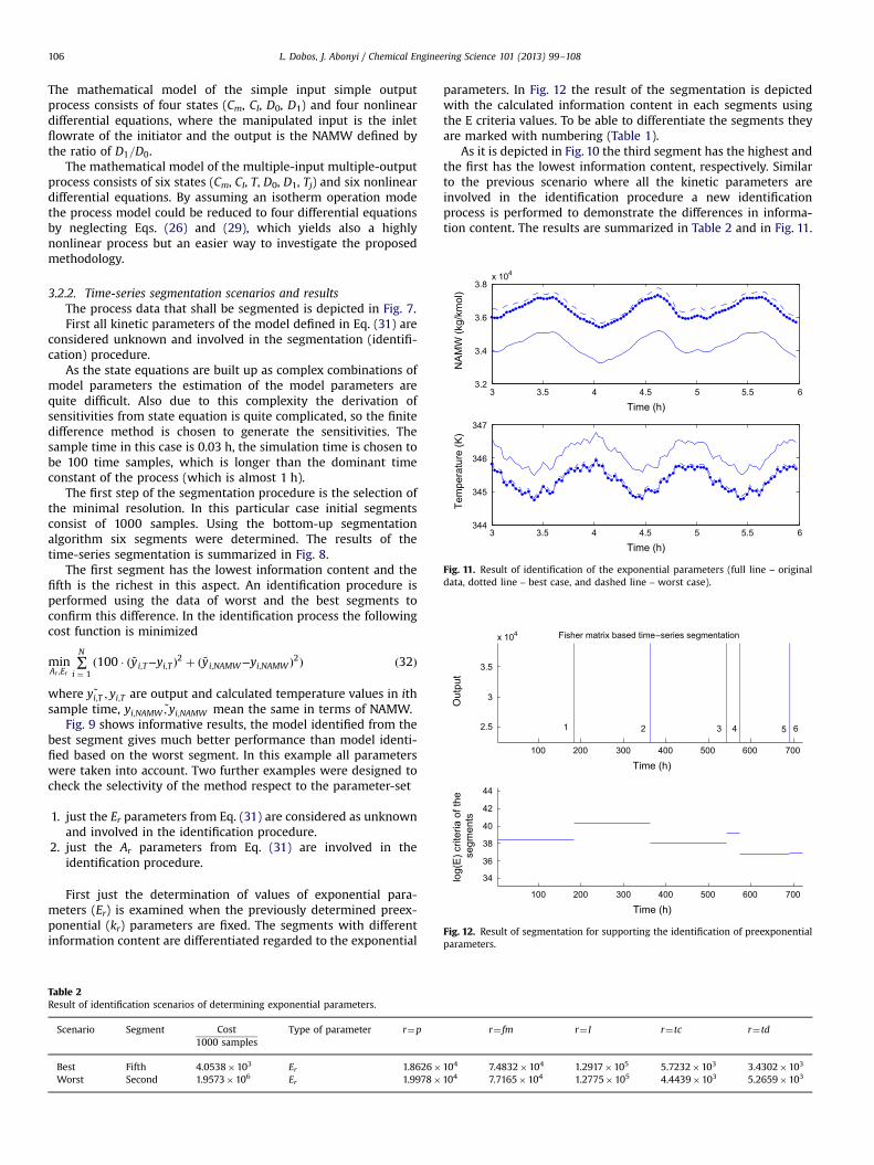
parameters. In Fig. 12 the result of the segmentation is depictedwith the calculated information content in each segments usingthe E criteria values. To be able to differentiate the segments theyare marked with numbering (Table 1).

As it is depicted in Fig. 10 the third segment has the highest andthe first has the lowest information content, respectively. Similarto the previous scenario where all the kinetic parameters areinvolved in the identification procedure a new identificationprocess is performed to demonstrate the differences in informa-tion content. The results are summarized in Table 2 and in Fig. 11.

r¼ fm r¼ I r¼tc r¼td

104 7.4832�104 1.2917�105 5.7232�103 3.4302�103

104 7.7165�104 1.2775�105 4.4439�103 5.2659�103

Table 3Result of identification scenarios of determining preexponential parameters.

Scenario Segment Cost1000 samples

Type of parameter r¼p r¼ fm r¼ I r¼tc r¼td

Best Fifth 165 kr 1.6281�109 9.2605�1014 4.3787�1018 6.6971�1010 2.4946�1011

Worst Second 1.6794�107 kr 2.1630�109 1.6956�1015 2.3419�1018 2.6473�1010 1.5729�1011

3 3.5 4 4.5 5 5.5 63.1

3.2

3.3

3.4

3.5x 104

Time (h)

NA

MW

(kg/

kmol

)

3 3.5 4 4.5 5 5.5 6345

346

347

348

Time (h)

Tem

pera

ture

(K)

Fig. 13. Identification result focusing to preexponential parameters (full line –

original data, dotted line – best case, and dashed line – worst case).

L. Dobos, J. Abonyi / Chemical Engineering Science 101 (2013) 99–108 107

The value of the cost function is significantly reduced compar-ing the best case of this scenario and the previous case. This provesthat some historical data segments have higher informationcontent than the other ones.

The identification of the preexponential parameters (kr) isexamined to further improve prediction performance in the nextscenario. In this case the exponential parameters are fixed in thevalue of the best case of the previous scenario. In Fig. 12 the resultof the segmentation is depicted with the information content ineach segments using the E criteria.

Figs. 10 and 12 show that the result of the two scenarios are thesame, but the information content of the segments are different asthe identification point of view is changed. As this figure showsdifferent segments of historical data are suitable for identificationof different model parameters. Similar to the scenarios above, anidentification procedure is performed in this case too. The richestsegment in information (related to the identification of thepreexponential parameter) is fifth and the poorest is the secondas it is depicted in Fig. 10. The results of this identification scenariois summarized in Table 3 and Fig. 13.

As Fig. 13 shows the best case of the recent scenario approachesthe original data quite well, since the difference is minimal (as it isshown in Table 3).

4. Conclusion

The drawback of model based experimental design is therelative high number of experimental runs which makes theparameter estimation costly and time consuming. The extractionof informative segments from historical process data also cansupport parameter estimation instead of optimization of inputtrajectories. A novel time-series segmentation algorithm has beenintroduced to extract segments from process data that are infor-mation rich for the identification of a given set of parameters. The

methodology is based on the Fisher information matrix, whichrepresents not only the quantity of the information but also it candistinguish the type of information in the parameter space.Krzanowksi similarity measure is utilized to evaluate the simila-rities of Fisher matrices of different segments. A useful tool isresulted by integrating Fisher information matrix and Krzanowksisimilarity measure into a bottom-up time-series segmentationalgorithm.

The applicability of the methodology is successfully presentedby a first order linear process and a more complex multivariatepolymerization example. The results illustrate that with the helpof the proposed algorithm we are able to extract segments ofhistorical data that are more suitable for identification of certainset of parameters thanks to their specific information content.

The related MATLAB programs are downloadable from thewebsite of the author: www.abonyilab.com.

Acknowledgments

This publication/research has been supported by the EuropeanUnion and the Hungarian Republic through the projectsTMOP-4.2.2.A-11/1/KONV-2012-0071 and TMOP-4.2.2.C-11/1/KONV-2012-0004 – National Research Center for Developmentand Market Introduction of Advanced Information and Commu-nication Technologies.

References

Abonyi, J., Feil, B., Nemeth, S., Arva, P., 2005. Modified Gath-Geva clustering forfuzzy segmentation of multivariate time-series. Fuzzy Set Syst. 149 (1), 39–56.

Alberton, A.L., Schwaab, M., Lobao, M.W.N., Pinto, J.C., 2012. Design of experimentsfor discrimination of rival models based on the expected number of eliminatedmodels. Chem. Eng. Sci. 75, 120–131.

Asprey, S., Macchietto, S., 2002. Designing robust optimal dynamic experiments. J.Process Control 12, 545–556.

Bernaerts, K., Servaes, R.D., Kooyman, S., Versyck, K.J., Van Impe, J.F., 2002. Optimaltemperature design for estimation of the square root model parameters:parameter accuracy and model validity restrictions. Int. J. Food Microbiol. 73,147–157.

Bernaerts, K., Gysemans, K.P.M., Minh, T.N., van Impe, J.F., 2005. Optimal experi-ment design for cardinal values estimation: guidelines for data collection. Int. J.Food Microbiol. 100, 153–165.

Box, G.P., Hunter, W.G., 1965. The experimental study of physical mechanisms.Technometrics 7 (1), 23–42.

Dobos, L., Abonyi, J., 2012. On-line detection of homogeneous operation ranges bydynamic principal component analysis based time-series segmentation. Chem.Eng. Sci. 75, 96–105.

Donckels, B.M., Pauw, D.J.D., Vanrolleghem, P.A., Baets, B.D., 2010. An ideal pointmethod for the design of compromise experiments to simultaneously estimatethe parameters of rival mathematical models. Chem. Eng. Sci. 65, 1705–1719.

Feil, B., Abonyi, J., Nemeth, S., Arva, P., 2005. Monitoring process transitions bykalman filtering and time-series segmentation. Comput. Chem. Eng. 29 (6),1423–1431.

Franceschini, G., Macchietto, S., 2008. Model-based design of experiments forparameter precision: state of the art. Chem. Eng. Sci. 63, 4846–4872.

Fu, T.C., 2011. A review on time series data mining. Eng. Appl. Artif. Intell. 24,164–181.

Goodwin, G., 1971. Optimal input signals for nonlinear-system identification. Proc.Inst. Electr. Eng. 118, 922–926.

Hildebrand, R., Gevers, M., 2002. Identification for control: optimal input designwith respect to a worst-case ν�gap cost function. SIAM J. Control Optim. 41 (5),1586–1608.

L. Dobos, J. Abonyi / Chemical Engineering Science 101 (2013) 99–108108

Himberg, J., Korpiaho, K., Mannila, H., Tikanmaki, J., Toivonen, H., 2001. Time-seriessegmentation for context recognition in mobile devices. In: IEEE InternationalConference on Data Mining (ICDM 01), San Jose, California, pp. 466–473.

Keogh, E., Chu, S., Hart, D., Pazzani, H., 2001. An online algorithm for segmentingtime series. In: IEEE International Conference on Data Mining. URL: ⟨http://citeseer.nj.nec.com/keogh01online.html⟩.

Krzanowski, W., 1979. Between group comparison of principal components. J. Am.Stat. Assoc., 703–707.

Mehra, R., 1974. Optimal input signals for parameter estimation in dynamic systems– survey and new results. IEEE Trans. Autom. Control 19, 753–768.

Morari, M., Leeb, J.H., 1999. Model predictive control: past, present and future.Comput. Chem. Eng. 23, 667–682.

Rojas, C.R., Welsh, S.J., Goodwin, G.C., Feuer, A., 2007. Robust optimal experimentdesign for system identification. Automatica 43, 993–1008.

Silva-Beard, A., Flores-Tlacuahuac, A., 1999. Effect of process design/operation onsteady-state operability of a methyl-metacrylate polymerization reactor. Ind.Eng. Chem. Res. 38, 4790–4804.

Singhal, A., Seborg, D., 2001. Matching patterns from historical data using PCA anddistance similarity factors. In: Proceedings of the American Control Conference,pp. 1759–1764.

Vasko, K., Toivonen, H., 2002. Estimating the number of segments in time seriesdata using permutation tests. IEEE International Conference on Data Mining,pp. 466–473.

Yuan, Z.D., Ljung, L., 1984. Black-box identification of multivariable transferfunctions-asymptotic properties and optimal input design. Int. J. Control 40,233–256.