Math GeosciDOI 10.1007/s11004-011-9359-0

Dependence of Bayesian Model Selection Criteriaand Fisher Information Matrix on Sample Size

Dan Lu · Ming Ye · Shlomo P. Neuman

Received: 11 June 2010 / Accepted: 26 August 2011© International Association for Mathematical Geosciences 2011

Abstract Geostatistical analyses require an estimation of the covariance structure ofa random field and its parameters jointly from noisy data. Whereas in some cases (asin that of a Matérn variogram) a range of structural models can be captured with oneor a few parameters, in many other cases it is necessary to consider a discrete set ofstructural model alternatives, such as drifts and variograms. Ranking these alterna-tives and identifying the best among them has traditionally been done with the aid ofinformation theoretic or Bayesian model selection criteria. There is an ongoing debatein the literature about the relative merits of these various criteria. We contribute to thisdiscussion by using synthetic data to compare the abilities of two common Bayesiancriteria, BIC and KIC, to discriminate between alternative models of drift as a func-tion of sample size when drift and variogram parameters are unknown. Adopting theresults of Markov Chain Monte Carlo simulations as reference we confirm that KICreduces asymptotically to BIC and provides consistently more reliable indications ofmodel quality than does BIC for samples of all sizes. Practical considerations oftencause analysts to replace the observed Fisher information matrix entering into KICwith its expected value. Our results show that this causes the performance of KIC todeteriorate with diminishing sample size. These results are equally valid for one andmultiple realizations of uncertain data entering into our analysis. Bayesian theory in-dicates that, in the case of statistically independent and identically distributed data,posterior model probabilities become asymptotically insensitive to prior probabili-ties as sample size increases. We do not find this to be the case when working withsamples taken from an autocorrelated random field.

D. Lu · M. Ye (�)Department of Scientific Computing, Florida State University, Tallahassee, FL 32306, USAe-mail: mye@fsu.edu

S.P. NeumanDepartment of Hydrology and Water Resources, University of Arizona, Tucson, AZ 85721, USA

Math Geosci

Keywords Model uncertainty · Model selection · Variogram models · Drift models ·Prior model probability · Asymptotic analysis

1 Introduction

Geostatistical analyses require estimating the covariance structure of a random fieldand its parameters jointly from noisy data. Whereas in some cases (as in that ofa Matérn variogram; Matérn 1986; Marchant and Lark 2007) a range of structuralmodels can be captured with one or a few parameters, in many other cases onemust consider a discrete set of structural (such as drift and variogram) model al-ternatives (Hoeksema and Kitanidis 1985; McBratney and Webster 1986; Samperand Neuman 1989a, 1989b; Ye et al. 2004, 2005; Marchant and Lark 2004, 2007;Riva and Willmann 2009; Nowak et al. 2010; Nowak 2010; Singh et al. 2010;Riva et al. 2011). Ranking these alternatives and identifying the best among themhas traditionally been done with the aid of information theoretic model selec-tion (discrimination, information) criteria such as Akaike Information Criterion(AIC, Akaike 1974) and Corrected Akaike Information Criterion (AICc, Hurvichand Tsai 1989) or Bayesian criteria, most commonly Bayesian Information Cri-terion (BIC, Schwarz 1978; Rissanen 1978) and Kashyap Information Criterion(KIC, Kashyap 1982). There is an ongoing debate in the literature about the rela-tive merits and demerits of these and related criteria (Poeter and Anderson 2005;Tsai and Li 2008a, 2008b, 2010; Ye et al. 2008a, 2010a, 2010b; Riva et al. 2011).We contribute to this discussion by using synthetic data coupled with Markov ChainMonte Carlo (MCMC) simulations to compare the abilities of BIC and KIC to dis-criminate between alternative models of drift as a function of sample size when driftand variogram parameters are unknown. As our comparison is based on Bayesianstatistics, it does not apply directly to AIC and AICc, since these are derived based onother principles.

Consider a set of K alternative (drift and/or variogram) models Mk of an autocor-related random function Y with Nk unknown parameters θk (bold letters designatingvectors), k = 1, . . . ,K . We wish to compare and rank these models after each hasbeen calibrated by maximum likelihood (ML) against a common sample D of N

measured Y values at various points in space and/or time. One way to do so is toassociate the following criteria with each model

AICk = −2 ln[L(θk|D)

] + 2Nk, (1)

AICck = −2 ln[L(θk|D)

] + 2Nk + 2Nk(Nk + 1)

N − Nk − 1, (2)

BICk = −2 ln[L(θk|D)

] + Nk lnN, (3)

KICk = −2 ln[L(θk|D)

] − 2 lnp(θk) + Nk ln(N/2π) + ln |Fk| (4)

where θk is the ML estimate of θk;− ln[L(θk|D)] is the negative log-likelihood(NLL) function − ln[L(θk|D)] evaluated at θk;p(θk) is the prior probability of θk

evaluated at θk ; and Fk = Fk/N is the normalized (by N ) observed (implicitly con-

Math Geosci

ditioned on D and evaluated at θk) Fisher information matrix (FIM), Fk , having ele-ments (Kashyap 1982)

Fk,ij = 1

NFk,ij = − 1

N

∂2 ln[L(θk|D)]∂θki∂θkj

∣∣∣∣θk=θk

. (5)

This allows rewriting KICk in (4) as

KICk = −2 ln[L(θk|D)

] − 2 lnp(θk) − Nk ln(2π) + ln |Fk|, (6)

a form known in Bayesian statistics as the Laplace approximation (Kass andVaidyanathan 1992; Kass and Raftery 1995), the origin of which can be traced back toJeffreys (1961) and Mosteller and Wallace (1964). The four criteria embody the prin-ciple of parsimony, penalizing (to various degrees) models having a relatively largenumber of parameters if this does not bring about a corresponding improvement inmodel fit. A comparative discussion of the four criteria, their underlying principlesand ways to compute them can be found in Ye et al. (2008a).

Rather than selecting the highest ranking model, it may sometimes be advanta-geous to retain several dominant models and average their results. Here we consideran maximum likelihood (ML) version of Bayesian model averaging (MLBMA) pro-posed by Neuman (2003) and employed by Ye et al. (2004, 2005, 2008a). If � is thequantity one wants to predict, then Bayesian Model Averaging (BMA) consists ofexpressing the posterior probability of � as (Hoeting et al. 1999)

p(�|D) =K∑

k=1

p(�|Mk,D)p(Mk|D) (7)

where p(�|Mk,D) is the posterior probability of � under model Mk having posteriorprobability p(Mk|D). Bayes’ theorem implies that the latter is given by

p(Mk|D) = p(D|Mk)p(Mk)∑K

l=1 p(D|Ml)p(Ml)(8)

where p(Mk) is the prior probability of model Mk and

p(D|Mk) =∫

p(D|θk,Mk)p(θk|Mk)dθk (9)

is its integrated likelihood, p(θk|Mk) being the prior probability density of θk undermodel Mk and p(D|θk,Mk) the joint likelihood of Mk and θk . The integrated like-lihood can be evaluated using various Monte Carlo (MC) simulation methods (Kassand Raftery 1995), most notably the Markov Chain Monte Carlo (MCMC) technique(Lewis and Raftery 1997; Draper 2007). Though we employ MCMC in this paper, wenote that MC methods are computationally demanding and require specifying a priorprobability distribution for each set of model parameters. When prior informationabout parameters is unavailable, vague or diffuse one can resort to MLBMA (Neuman2003) according to which (Ye et al. 2004)

p(D|Mk) ≈ exp

(−1

2KICk

). (10)

Math Geosci

Theory shows (Draper 1995; Raftery 1995; Ye et al. 2008a) that as the sample size N

increases relative to Nk,KIC tends asymptotically to BIC and so

p(D|Mk) ≈ exp

(−1

2BICk

). (11)

Substituting (10) or (11) into (8) yields

p(Mk|D) = exp(− 12�ICk)p(Mk)

∑Kl=1 exp(− 1

2�ICl )p(Ml)(12)

where �ICk = ICk − ICmin and ICmin = mink{ICk}, IC being either KIC or BIC.Equation (12) does not apply formally to AIC and AICc as these are based on in-

formation theory, not on Bayesian statistics. The information theoretic equivalent ofMLBMA has been to average model outputs using so-called Akaike weights com-puted via (Burnham and Anderson 2002, 2004; Poeter and Anderson 2005)

wk = exp(− 12�AICk)

∑Kl=1 exp(− 1

2�AICl)or wk = exp(− 1

2�AICck)∑K

l=1 exp(− 12�AICcl )

. (13)

Interpreting (13) within a Bayesian context would be equivalent to assigning an equalprior probability p(Mk) = 1/K to each model. Another ad hoc option discussed byBurnham and Anderson (2002, 2004) and adopted by Poeter and Hill (2007) is to use(12) regardless of whether IC is information theoretic or Bayesian.

There is general consensus in the literature that AICc is more accurate than AICwhen N/Nk < 40, converging rapidly to AIC as N/Nk increases beyond 40 (Burn-ham and Anderson 2002; Poeter and Anderson 2005). There is less consensus aboutthe relative merits of BIC and KIC (Tsai and Li 2008a, 2010; Ye et al. 2008a, 2010a,2010b) even though KIC is known to converge toward BIC as N/Nk goes up (Draper1995; Raftery 1995; Kass and Raftery 1995; Ye et al. 2008a). Whereas Kass andRaftery (1995) found BIC to yield unsatisfactory approximations of integrated likeli-hood even for very large N/Nk , Tsai and Li (2008a) considered KIC to have yielded“unreasonable” posterior model probabilities. In light of contrary findings by Ye etal. (2008a) and several references therein, there appears to be a need to clarify theissue further, as we do below.

In this paper we use samples from a synthetic random field to compare the abil-ities of BIC and KIC to discriminate between alternative models of drift as a func-tion of sample size when drift and variogram parameters are unknown. Our studyfocuses on model probabilities, not on predictive performance. It contributes theo-retically and numerically to our understanding of roles played in model selection byobserved and expected versions of the Fisher information matrix (Ye et al. 2010b).The study extends to one as well as multiple realizations of uncertain data employedin model calibration. To our knowledge, we are the first to compare the performanceof model discrimination criteria against Markov Chain Monte Carlo simulations ofvarious size replicate data sampled from a spatially correlated random field in morethan one dimension. For reasons noted earlier, we exclude AIC and AICc from furtherconsideration in this paper.

Math Geosci

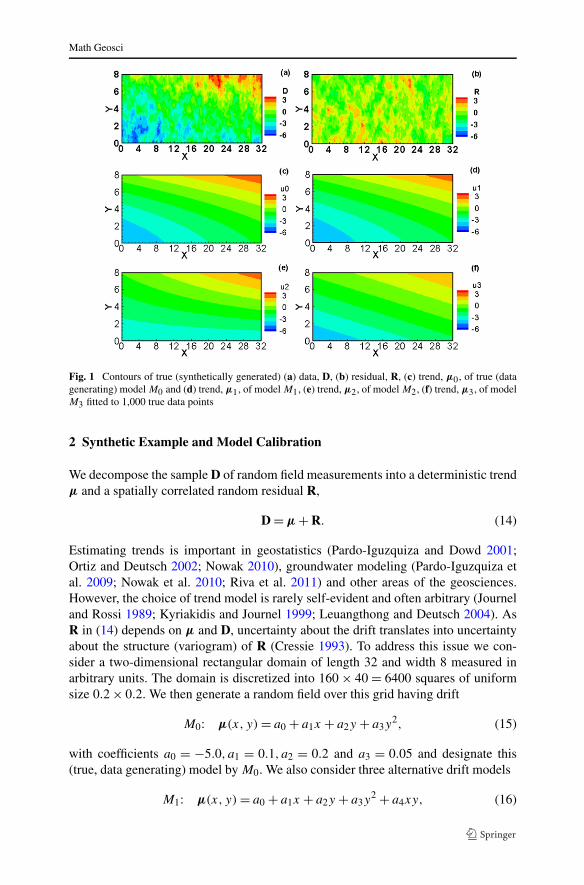
Fig. 1 Contours of true (synthetically generated) (a) data, D, (b) residual, R, (c) trend, μ0, of true (datagenerating) model M0 and (d) trend, μ1, of model M1, (e) trend, μ2, of model M2, (f) trend, μ3, of modelM3 fitted to 1,000 true data points

2 Synthetic Example and Model Calibration

We decompose the sample D of random field measurements into a deterministic trendμ and a spatially correlated random residual R,

D = μ + R. (14)

Estimating trends is important in geostatistics (Pardo-Iguzquiza and Dowd 2001;Ortiz and Deutsch 2002; Nowak 2010), groundwater modeling (Pardo-Iguzquiza etal. 2009; Nowak et al. 2010; Riva et al. 2011) and other areas of the geosciences.However, the choice of trend model is rarely self-evident and often arbitrary (Journeland Rossi 1989; Kyriakidis and Journel 1999; Leuangthong and Deutsch 2004). AsR in (14) depends on μ and D, uncertainty about the drift translates into uncertaintyabout the structure (variogram) of R (Cressie 1993). To address this issue we con-sider a two-dimensional rectangular domain of length 32 and width 8 measured inarbitrary units. The domain is discretized into 160 × 40 = 6400 squares of uniformsize 0.2 × 0.2. We then generate a random field over this grid having drift

M0: μ(x, y) = a0 + a1x + a2y + a3y2, (15)

with coefficients a0 = −5.0, a1 = 0.1, a2 = 0.2 and a3 = 0.05 and designate this(true, data generating) model by M0. We also consider three alternative drift models

M1: μ(x, y) = a0 + a1x + a2y + a3y2 + a4xy, (16)

Math Geosci

M2: μ(x, y) = a0 + a2y + a3y2 + a4xy, (17)

M3: μ(x, y) = a0 + a1x + a2y. (18)

In comparison to M0, model M1 is over-parameterized, model M3 is under-parameterized and model M2 has elements of both. We then use sequential Gaus-sian simulation (SGSIM; Deutsch and Journel 1998) to generate stationary, zero-mean random residuals R about μ having unit variance and an exponential vari-ogram, γ (h) = s[1 − exp(−h/λ)], with sill (variance) s = 1 and integral scale λ = 1where h is separation distance or lag. The corresponding covariance function of R isQ(h) = s exp(−h/λ). To keep the problem manageable we consider neither alterna-tive variogram models nor measurement noise in this example. The generated (true)field of D, residual, R, and drift, μ (from model M0) are illustrated in Figs. 1(a)–1(c), respectively. Figures 1(d)–1(f) depict drifts generated after fitting (via ML, asdescribed later) the drift models corresponding to models M1,M2 and M3 to 1,000true data points. Visual inspection suggests that drift model M1 is closest and M2farthest from the true drift model M0 in Fig. 1(c).

Let θ = {a,β} where a is a vector of drift parameters and β a vector of variogramparameters. If D is multivariate Gaussian with mean μ(a) = E[D] and covariancematrix Q(β) = E[(D − μ)(D − μ)T ], the negative logarithm of the joint likelihoodfunction (NLL) for any given model takes the form (after dropping the subscript k)

NLL = −2 ln[L(θ |D)

] = −2 ln[L(a,β|D)

] = 2 lnp(D|a,β)

= N ln 2π + ln∣∣Q(β)

∣∣ + (D − μ(a)

)T Q−1(β)(D − μ(a)

). (19)

Minimizing NLL simultaneously with respect to a and β would yield biased esti-mates of β (Cressie 1993). To avoid this, we follow Ye et al. (2004) by first usingadjoint state ML cross validation (ASMLCV, Samper and Neuman 1989a) in con-junction with universal kriging to obtain an ML estimate β of β , then obtaining anML estimate a of a by minimizing

−2 ln[L(a, β|D)

] = N ln 2π + ln∣∣Q(β)

∣∣ + (D − μ(a)

)T Q−1(β)(D − μ(a)

)(20)

with the aid of generalized least squares. The NLL component constituting the firstterm of each model selection criterion in (1)–(6) is thus given by

−2 ln[L(θ |D)

] = −2 ln[L(a, β|D)

]

= N ln 2π + ln∣∣Q(β)

∣∣ + (D − μ(a))T Q−1(β)(D − μ(a)

). (21)

We start by drawing a sample D of 50 randomly situated data from the 6,400synthetic random field values in Fig. 1(a), and then increase the sample size to 100.Subsequently, the sample size is gradually increased in 12 increments of 100–200additional randomly selected data till the total reaches 1,700. We then use each ofthese 14 samples D to calibrate the variogram and all alternative drift models in themanner just described. Corresponding estimates of sill s and integral scale λ associ-ated with each model are plotted in Fig. 2. The estimates of both parameters are seen

Math Geosci

Fig. 2 Estimates of variogramparameters (a) sill and (b)integral scale for four alternativedrift models and fourteensample sizes

to improve (or approach their true values) with sample size regardless of which driftmodel one uses, the best estimates being associated with the true model M0 and theworst with the under-parameterized model M3, as one would expect.

Fluctuations in parameter estimates and their statistics reflect randomness of thegenerated field and of samples drawn from it. We explore this effect below for se-lected sample sizes (50, 100, 300, 500, 800 and 1,000) by extracting 100 replicatesamples of each size and calibrating the models against each replicate in the mannerdescribed earlier. The results of one and replicate samples are equally important. Theone-sample situation mimics what could happen in an actual situation; the replicatesindicate the average properties of different diagnostics. When results obtained fromone sample are ambiguous or conflict with expectation, one may wish to collect moredata and/or supplement them with subjective expert judgment (Ye et al. 2005, 2008b).

Equation (19) is the negative logarithm of a corresponding likelihood functionp(D|θ ,M). The latter is associated with an observed Fisher information matrix (FIM)given analytically by (Kitanidis and Lane 1985)

Fij = −∂2 lnp(D|θ ,M)

∂θi∂θj

= −1

2Tr

(Q−1 ∂Q

∂θi

Q−1 ∂Q∂θj

)+ 1

2Tr

(Q−1 ∂2Q

∂θi∂θj

)

+ ∂μT

∂θi

Q−1 ∂Q∂θj

Q−1(D − μ) + (D − μ)T Q−1 ∂Q∂θi

Q−1 ∂Q∂θj

Q−1(D − μ)

Math Geosci

− 1

2(D − μ)T Q−1 ∂2Q

∂θi∂θj

Q−1(D − μ)

+ ∂μT

∂θi

Q−1 ∂μ

∂θj

+ (D − μ)T Q−1 ∂Q∂θi

Q−1 ∂μ

∂θj

− (D − μ)T Q−1 ∂2μ

∂θi∂θj

. (22)

To avoid computing second-order derivatives of μ and Q one often approximates theobserved FIM by the more popular expected FIM (Kitanidis and Lane 1985)

〈Fij 〉 = 1

2Tr

(Q−1 ∂Q

∂θ i

Q−1 ∂Q∂θ j

)+ ∂μT

∂θ i

Q−1 ∂μ

∂θ j

. (23)

Equations (22) and (23) yield two different values of KIC which we designate below,respectively, by KICobs and KICexp.

To set a standard against which the accuracies of BIC and KIC are measured weevaluate the integrated likelihood in (9) by Markov Chain Monte Carlo (MCMC)simulations. Treating the prior distribution of each parameter, p(θk|Mk), as if itwas uniform and independent between specified lower and upper bounds, the con-ventional Metropolis-Hastings algorithm (Hastings 1970) is used to implement theMCMC process. Our implementation of the algorithm is similar to that of Rojas etal. (2008, 2010a, 2010b, 2010c); more advanced MCMC techniques are discussed byChib (1995) and Marshall et al. (2004, 2005). The ranges of the uniform distributionsare initially set to 50% and 150% of the ML parameter estimates and modified bytrial-and-error during the sampling process to obtain an acceptance rate of 20–40%.Three chains are launched and their convergence of MCMC is evaluated using the R

statistics of Gelman et al. (1995). A total of 50,000 samples are generated from eachchain; the first 1,000 samples are discarded (burn-in) after R is 1.0002 for all the pa-rameters. Random parameter samples from MCMC allow calculating a joint negativelog-likelihood function according to (19), which in turn is used to approximate theintegrated likelihood function (9) numerically via

p(D|Mk) = 1

l

l∑

i=1

p(D|θ (i)

k ,Mk

)(24)

where l is the number of parameter samples, p(D|θ (i)k ,Mk) being the joint likelihood

function of the ith parameter sample, θ(i)k . We then adopt the MCMC results as refer-

ence against which the accuracies of BIC and KIC are judged. Note that we could notdo so for AIC and AICc because these are not associated with integrated likelihoodfunctions.

3 Results and Discussion

In this section we compare values of BIC and KIC computed for each of the fouralternative drift models and fourteen sample sizes. We also compare values of KICcomputed using observed and expected FIM, integrated likelihood functions com-puted by BIC, KIC and MCMC, and posterior model probabilities obtained using the

Math Geosci

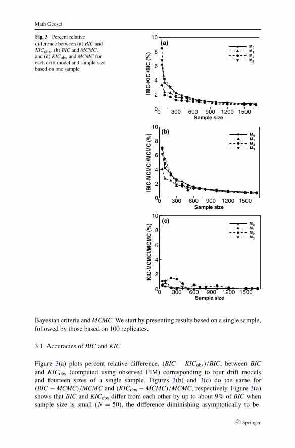
Fig. 3 Percent relativedifference between (a) BIC andKICobs, (b) BIC and MCMC,and (c) KICobs and MCMC foreach drift model and sample sizebased on one sample

Bayesian criteria and MCMC. We start by presenting results based on a single sample,followed by those based on 100 replicates.

3.1 Accuracies of BIC and KIC

Figure 3(a) plots percent relative difference, (BIC − KICobs)/BIC, between BICand KICobs (computed using observed FIM) corresponding to four drift modelsand fourteen sizes of a single sample. Figures 3(b) and 3(c) do the same for(BIC − MCMC)/MCMC and (KICobs − MCMC)/MCMC, respectively. Figure 3(a)shows that BIC and KICobs differ from each other by up to about 9% of BIC whensample size is small (N = 50), the difference diminishing asymptotically to be-

Math Geosci

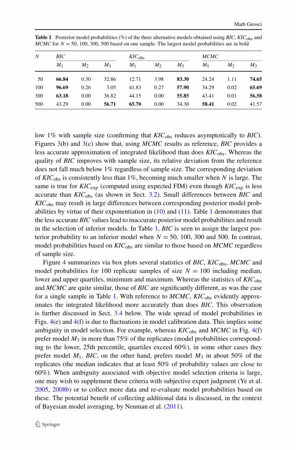
Table 1 Posterior model probabilities (%) of the three alternative models obtained using BIC, KICobs andMCMC for N = 50, 100, 300, 500 based on one sample. The largest model probabilities are in bold

N BIC KICobs MCMC

M1 M2 M3 M1 M2 M3 M1 M2 M3

50 66.84 0.30 32.86 12.71 3.98 83.30 24.24 1.11 74.65

100 96.69 0.26 3.05 41.83 0.27 57.90 34.29 0.02 65.69

300 63.18 0.00 36.82 44.15 0.00 55.85 43.41 0.01 56.58

500 43.29 0.00 56.71 65.70 0.00 34.30 58.41 0.02 41.57

low 1% with sample size (confirming that KICobs reduces asymptotically to BIC).Figures 3(b) and 3(c) show that, using MCMC results as reference, BIC provides aless accurate approximation of integrated likelihood than does KICobs. Whereas thequality of BIC improves with sample size, its relative deviation from the referencedoes not fall much below 1% regardless of sample size. The corresponding deviationof KICobs is consistently less than 1%, becoming much smaller when N is large. Thesame is true for KICexp (computed using expected FIM) even though KICexp is lessaccurate than KICobs (as shown in Sect. 3.2). Small differences between BIC andKICobs may result in large differences between corresponding posterior model prob-abilities by virtue of their exponentiation in (10) and (11). Table 1 demonstrates thatthe less accurate BIC values lead to inaccurate posterior model probabilities and resultin the selection of inferior models. In Table 1, BIC is seen to assign the largest pos-terior probability to an inferior model when N = 50, 100, 300 and 500. In contrast,model probabilities based on KICobs are similar to those based on MCMC regardlessof sample size.

Figure 4 summarizes via box plots several statistics of BIC, KICobs, MCMC andmodel probabilities for 100 replicate samples of size N = 100 including median,lower and upper quartiles, minimum and maximum. Whereas the statistics of KICobs

and MCMC are quite similar, those of BIC are significantly different, as was the casefor a single sample in Table 1. With reference to MCMC, KICobs evidently approx-imates the integrated likelihood more accurately than does BIC. This observationis further discussed in Sect. 3.4 below. The wide spread of model probabilities inFigs. 4(e) and 4(f) is due to fluctuations in model calibration data. This implies someambiguity in model selection. For example, whereas KICobs and MCMC in Fig. 4(f)prefer model M3 in more than 75% of the replicates (model probabilities correspond-ing to the lower, 25th percentile, quartiles exceed 60%), in some other cases theyprefer model M1. BIC, on the other hand, prefers model M3 in about 50% of thereplicates (the median indicates that at least 50% of probability values are close to60%). When ambiguity associated with objective model selection criteria is large,one may wish to supplement these criteria with subjective expert judgment (Ye et al.2005, 2008b) or to collect more data and re-evaluate model probabilities based onthese. The potential benefit of collecting additional data is discussed, in the contextof Bayesian model averaging, by Neuman et al. (2011).

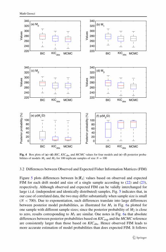
Math Geosci

Fig. 4 Box plots of (a)–(d) BIC, KICobs and MCMC values for four models and (e)–(f) posterior proba-bilities of models M1 and M3 for 100 replicate samples of size N = 100

3.2 Differences between Observed and Expected Fisher Information Matrices (FIM)

Figure 5 plots differences between ln |Fk| values based on observed and expectedFIM for each drift model and size of a single sample according to (22) and (23),respectively. Although observed and expected FIM can be validly interchanged forlarge i.i.d. (independent and identically distributed) samples, Fig. 5 indicates that, inour case of correlated data, the two may differ substantially when sample size is small(N < 700). Due to exponentiation, such differences translate into large differencesbetween posterior model probabilities, as illustrated for M1 in Fig. 6a plotted forone sample with different sample sizes; since the posterior probability of M2 is closeto zero, results corresponding to M3 are similar. One notes in Fig. 6a that absolutedifferences between posterior probabilities based on KICexp and the MCMC referenceare consistently larger than those based on KICobs. Hence observed FIM leads tomore accurate estimation of model probabilities than does expected FIM. It follows

Math Geosci

Fig. 5 Differences betweenln |Fk | values based on expectedand observed Fisher informationmatrices (FIM) for each driftmodel and size of a singlesample

Fig. 6 Absolute differencesbetween posterior probabilitiesof M1 based on KICobs andKICexp relative to MCMC for(a) each size of a single sampleand (b) 100 replicate samples ofsize N = 100. As posteriorprobability of M2 is almostzero, absolute differencescorresponding to M3 are similar

that KICobs and KICexp may, in some cases, prefer different models as observed inthe numerical experiments when N = 500 and 1200. The poor performance of KICexp

relative to KICobs stems from the following assumption behind (23) (Kitanidis andLane 1985),

E[D − μ] = 0

E[(D − μ)(D − μ)T

] = Q(25)

Math Geosci

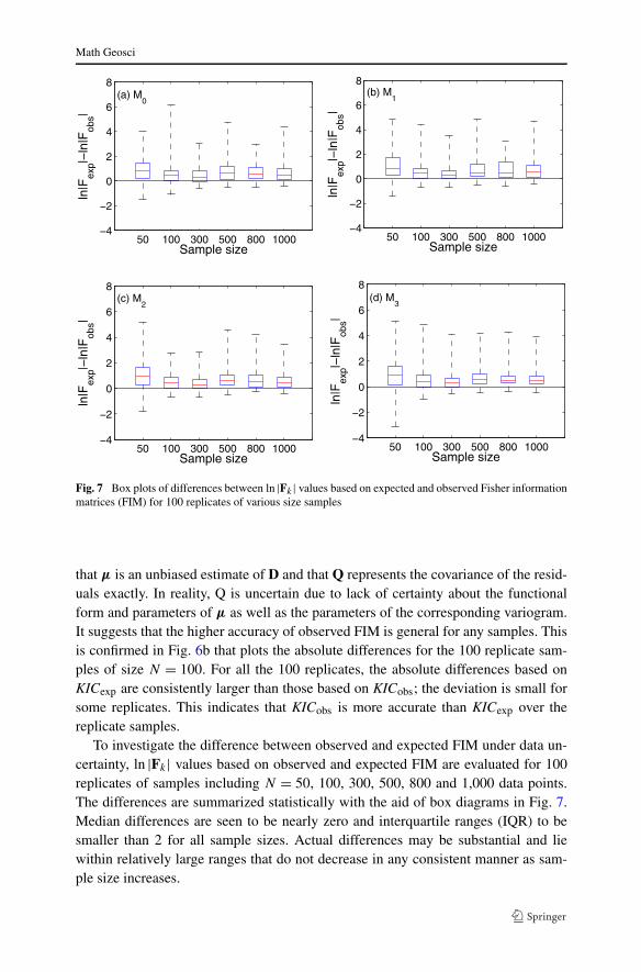
Fig. 7 Box plots of differences between ln |Fk | values based on expected and observed Fisher informationmatrices (FIM) for 100 replicates of various size samples

that μ is an unbiased estimate of D and that Q represents the covariance of the resid-uals exactly. In reality, Q is uncertain due to lack of certainty about the functionalform and parameters of μ as well as the parameters of the corresponding variogram.It suggests that the higher accuracy of observed FIM is general for any samples. Thisis confirmed in Fig. 6b that plots the absolute differences for the 100 replicate sam-ples of size N = 100. For all the 100 replicates, the absolute differences based onKICexp are consistently larger than those based on KICobs; the deviation is small forsome replicates. This indicates that KICobs is more accurate than KICexp over thereplicate samples.

To investigate the difference between observed and expected FIM under data un-certainty, ln |Fk| values based on observed and expected FIM are evaluated for 100replicates of samples including N = 50, 100, 300, 500, 800 and 1,000 data points.The differences are summarized statistically with the aid of box diagrams in Fig. 7.Median differences are seen to be nearly zero and interquartile ranges (IQR) to besmaller than 2 for all sample sizes. Actual differences may be substantial and liewithin relatively large ranges that do not decrease in any consistent manner as sam-ple size increases.

Math Geosci

3.3 Randomness of Observed and Expected Fisher Information Matrices (FIM)

The large ranges depicted in Fig. 7 between observed and expected FIM stem fromthe random natures of calibration data and associated parameter estimates. The ob-served FIM is evidently random due to its dependence on random calibration data D.The expected FIM is theoretically nonrandom but its approximation, obtained by cal-ibrating each model against each random sample and then applying (23), remainsrandom due to limited sample size and estimation errors associated with correspond-ing parameter estimates. To our knowledge, the effect of randomness in observed andexpected FIM has not been previously analyzed in the manner we do here.

Effects of data and parameter estimation uncertainty are illustrated in Figs. 8(a)–8(d) where ln |Fk| associated with expected and observed FIM based on a singlesample are plotted against sample size. Fluctuation in Fig. 8(a) reflects uncertaintyin ln |Fk| as computed on the basis of (23). This uncertainty is removed for the truemodel in Fig. 8(b) (the curve becoming smooth) by computing ln |Fk| using true driftand variogram parameters. Figures 8(c) and 8(d) are similar to Figs. 8(a) and 8(b) butcorrespond to observed FIM. Even though ln |Fk| in Fig. 8(d) is computed using truedrift model with true drift and variogram parameters, it nevertheless fluctuates. Thisis due to data uncertainty which does not impact Fig. 8(b). Averaging out data uncer-tainty as described below leads to a smooth result in Fig. 8(d). Comparing Figs. 8(a)and 8(c) with Figs. 8(b) and 8(d), respectively, shows that effects of data and param-eter estimation uncertainty on the estimation of FIM is large. In addition, the effectof data uncertainty is larger than that of parameter estimation uncertainty. When fluc-tuations in model calibration data cause ambiguity in model selection, one may wishto rely on expert judgment or collect additional data as discussed in Sect. 3.1. Fig-ures 8(e) and 8(f) depict ln |Fk| based on expected and observed FIM averaged over100 replicate samples for various sample sizes. Comparing the two figures with theircounterparts in Figs. 8(a) and 8(c) confirms that averaging reduces randomness indata and parameter estimates. More importantly, the averaged ln |Fk| in Figs. 8(e)and 8(f) are almost identical. This does not conflict with the implication of Fig. 7that KICobs is more accurate than KICexp for one sample. Instead, it suggests thataveraging over many replicates reduces differences between observed and expectedKIC.

3.4 Role of FIM in Model Selection

Figure 8 shows that ln |F1| > ln |F2| > ln |F0| > ln |F3| regardless of sample size.This consistent order reflects a tendency of ln |Fk|, and hence KIC, to impose in-creasing penalty on models having greater complexity (number of parameters). Al-though model M1 contains more information per datum (as measured by ln |Fk|) thandoes model M3, its goodness-of-fit measure (see next section) is only slightly better.Ye et al. (2010b) pointed out that “all else being equal, if increasing the expectedinformation content of a model fails to improve its performance relative to anothermodel, then selecting a model with greater expected information content would, ac-cording to KIC, be unjustified”. This is supported by the fact that KIC favor M3 in

Math Geosci

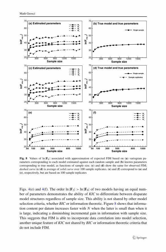
Fig. 8 Values of ln |Fk | associated with approximation of expected FIM based on (a) variogram pa-rameters corresponding to each model estimated against each random sample and (b) known parameterscorresponding to true model, as functions of sample size. (c) and (d) show the same for observed FIM;dashed curve in (d) is average of solid curve over 100 sample replicates. (e) and (f) correspond to (a) and(c), respectively, but are based on 100 sample replicates

Figs. 4(e) and 4(f). The order ln |F2| > ln |F0| of two models having an equal num-ber of parameters demonstrates the ability of KIC to differentiate between disparatemodel structures regardless of sample size. This ability is not shared by other modelselection criteria, whether BIC or information theoretic. Figure 8 shows that informa-tion content per datum increases faster with N when the latter is small than when itis large, indicating a diminishing incremental gain in information with sample size.This suggests that FIM is able to incorporate data correlation into model selection,another unique feature of KIC not shared by BIC or information theoretic criteria thatdo not include FIM.

Math Geosci

3.5 Consistency and Asymptotic Behavior of BIC and KIC

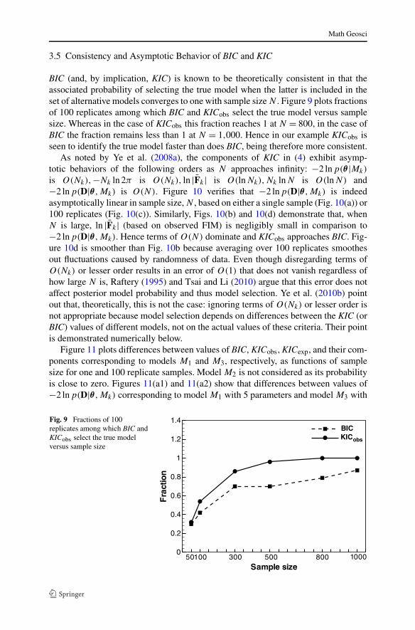
BIC (and, by implication, KIC) is known to be theoretically consistent in that theassociated probability of selecting the true model when the latter is included in theset of alternative models converges to one with sample size N . Figure 9 plots fractionsof 100 replicates among which BIC and KICobs select the true model versus samplesize. Whereas in the case of KICobs this fraction reaches 1 at N = 800, in the case ofBIC the fraction remains less than 1 at N = 1,000. Hence in our example KICobs isseen to identify the true model faster than does BIC, being therefore more consistent.

As noted by Ye et al. (2008a), the components of KIC in (4) exhibit asymp-totic behaviors of the following orders as N approaches infinity: −2 lnp(θ |Mk)

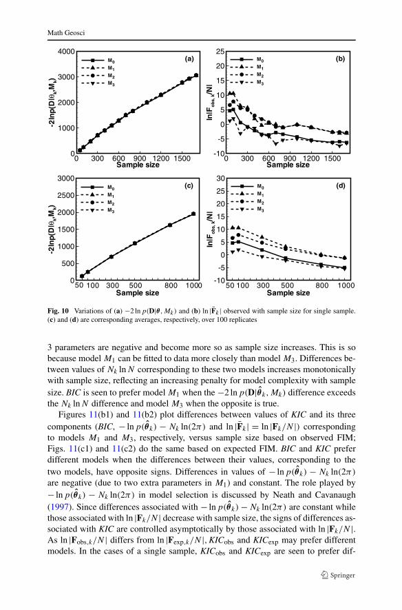
is O(Nk),−Nk ln 2π is O(Nk), ln |Fk| is O(lnNk),Nk lnN is O(lnN) and−2 lnp(D|θ ,Mk) is O(N). Figure 10 verifies that −2 lnp(D|θ ,Mk) is indeedasymptotically linear in sample size, N , based on either a single sample (Fig. 10(a)) or100 replicates (Fig. 10(c)). Similarly, Figs. 10(b) and 10(d) demonstrate that, whenN is large, ln |Fk| (based on observed FIM) is negligibly small in comparison to−2 lnp(D|θ ,Mk). Hence terms of O(N) dominate and KICobs approaches BIC. Fig-ure 10d is smoother than Fig. 10b because averaging over 100 replicates smoothesout fluctuations caused by randomness of data. Even though disregarding terms ofO(Nk) or lesser order results in an error of O(1) that does not vanish regardless ofhow large N is, Raftery (1995) and Tsai and Li (2010) argue that this error does notaffect posterior model probability and thus model selection. Ye et al. (2010b) pointout that, theoretically, this is not the case: ignoring terms of O(Nk) or lesser order isnot appropriate because model selection depends on differences between the KIC (orBIC) values of different models, not on the actual values of these criteria. Their pointis demonstrated numerically below.

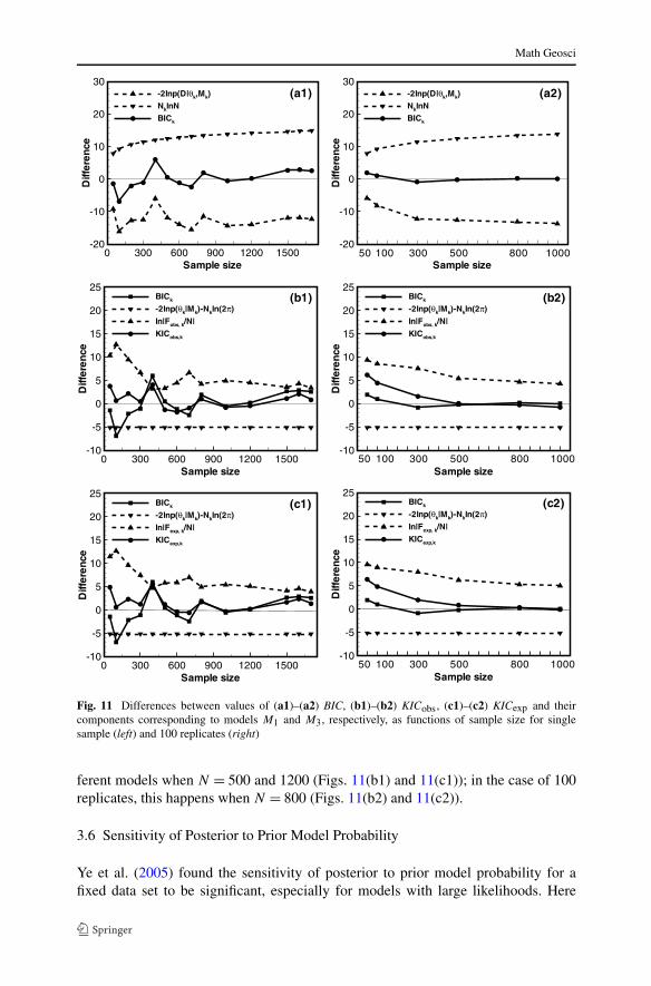
Figure 11 plots differences between values of BIC, KICobs,KICexp, and their com-ponents corresponding to models M1 and M3, respectively, as functions of samplesize for one and 100 replicate samples. Model M2 is not considered as its probabilityis close to zero. Figures 11(a1) and 11(a2) show that differences between values of−2 lnp(D|θ ,Mk) corresponding to model M1 with 5 parameters and model M3 with

Fig. 9 Fractions of 100replicates among which BIC andKICobs select the true modelversus sample size

Math Geosci

Fig. 10 Variations of (a) −2 lnp(D|θ ,Mk) and (b) ln |Fk | observed with sample size for single sample.(c) and (d) are corresponding averages, respectively, over 100 replicates

3 parameters are negative and become more so as sample size increases. This is sobecause model M1 can be fitted to data more closely than model M3. Differences be-tween values of Nk lnN corresponding to these two models increases monotonicallywith sample size, reflecting an increasing penalty for model complexity with samplesize. BIC is seen to prefer model M1 when the −2 lnp(D|θk,Mk) difference exceedsthe Nk lnN difference and model M3 when the opposite is true.

Figures 11(b1) and 11(b2) plot differences between values of KIC and its threecomponents (BIC, − lnp(θk) − Nk ln(2π) and ln |Fk| = ln |Fk/N |) correspondingto models M1 and M3, respectively, versus sample size based on observed FIM;Figs. 11(c1) and 11(c2) do the same based on expected FIM. BIC and KIC preferdifferent models when the differences between their values, corresponding to thetwo models, have opposite signs. Differences in values of − lnp(θk) − Nk ln(2π)

are negative (due to two extra parameters in M1) and constant. The role played by− lnp(θk) − Nk ln(2π) in model selection is discussed by Neath and Cavanaugh(1997). Since differences associated with − lnp(θk) − Nk ln(2π) are constant whilethose associated with ln |Fk/N | decrease with sample size, the signs of differences as-sociated with KIC are controlled asymptotically by those associated with ln |Fk/N |.As ln |Fobs,k/N | differs from ln |Fexp,k/N |,KICobs and KICexp may prefer differentmodels. In the cases of a single sample, KICobs and KICexp are seen to prefer dif-

Math Geosci

Fig. 11 Differences between values of (a1)–(a2) BIC, (b1)–(b2) KICobs, (c1)–(c2) KICexp and theircomponents corresponding to models M1 and M3, respectively, as functions of sample size for singlesample (left) and 100 replicates (right)

ferent models when N = 500 and 1200 (Figs. 11(b1) and 11(c1)); in the case of 100replicates, this happens when N = 800 (Figs. 11(b2) and 11(c2)).

3.6 Sensitivity of Posterior to Prior Model Probability

Ye et al. (2005) found the sensitivity of posterior to prior model probability for afixed data set to be significant, especially for models with large likelihoods. Here

Math Geosci

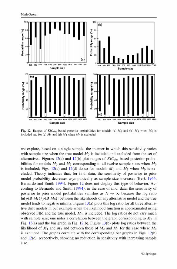
Fig. 12 Ranges of KICobs-based posterior probabilities for models (a) M0 and (b) M3 when M0 isincluded and for (c) M1 and (d) M3 when M0 is excluded

we explore, based on a single sample, the manner in which this sensitivity varieswith sample size when the true model M0 is included and excluded from the set ofalternatives. Figures 12(a) and 12(b) plot ranges of KICobs-based posterior proba-bilities for models M0 and M3 corresponding to all twelve sample sizes when M0

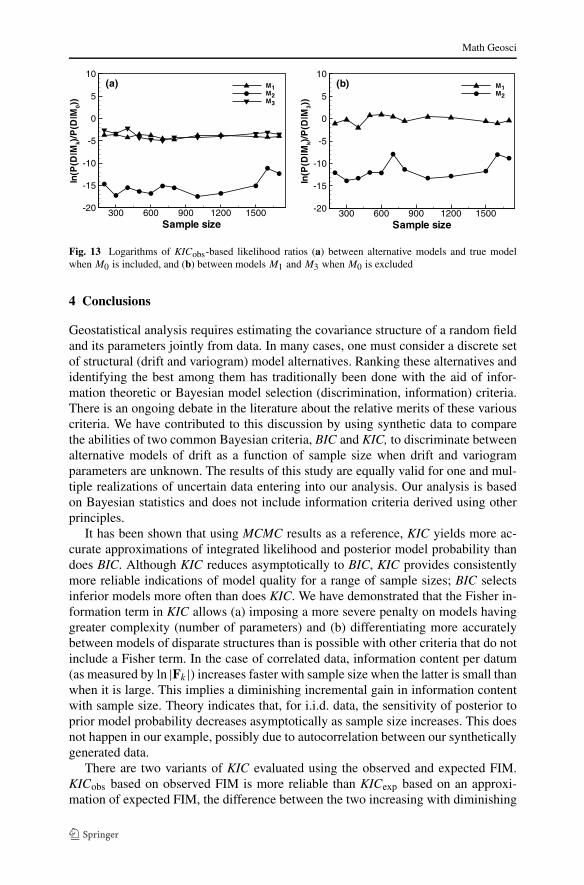
is included; Figs. 12(c) and 12(d) do so for models M1 and M3 when M0 is ex-cluded. Theory indicates that, for i.i.d. data, the sensitivity of posterior to priormodel probability decreases asymptotically as sample size increases (Berk 1966;Bernardo and Smith 1994). Figure 12 does not display this type of behavior. Ac-cording to Bernardo and Smith (1994), in the case of i.i.d. data, the sensitivity ofposterior to prior model probabilities vanishes as N → ∞ because the log ratioln[p(D|Mk)/p(D|M0)] between the likelihoods of any alternative model and the truemodel tends to negative infinity. Figure 13(a) plots this log ratio for all three alterna-tive drift models in our example when the likelihood function is approximated usingobserved FIM and the true model, M0, is included. The log ratios do not vary muchwith sample size; one notes a correlation between the graph corresponding to M3 inFig. 13(a) and the bar graph in Fig. 12(b). Figure 13(b) plots log ratios between thelikelihood of M1 and M3 and between those of M2 and M3 for the case where M0

is excluded. The graphs correlate with the corresponding bar graphs in Figs. 12(b)and 12(c), respectively, showing no reduction in sensitivity with increasing samplesize.

Math Geosci

Fig. 13 Logarithms of KICobs-based likelihood ratios (a) between alternative models and true modelwhen M0 is included, and (b) between models M1 and M3 when M0 is excluded

4 Conclusions

Geostatistical analysis requires estimating the covariance structure of a random fieldand its parameters jointly from data. In many cases, one must consider a discrete setof structural (drift and variogram) model alternatives. Ranking these alternatives andidentifying the best among them has traditionally been done with the aid of infor-mation theoretic or Bayesian model selection (discrimination, information) criteria.There is an ongoing debate in the literature about the relative merits of these variouscriteria. We have contributed to this discussion by using synthetic data to comparethe abilities of two common Bayesian criteria, BIC and KIC, to discriminate betweenalternative models of drift as a function of sample size when drift and variogramparameters are unknown. The results of this study are equally valid for one and mul-tiple realizations of uncertain data entering into our analysis. Our analysis is basedon Bayesian statistics and does not include information criteria derived using otherprinciples.

It has been shown that using MCMC results as a reference, KIC yields more ac-curate approximations of integrated likelihood and posterior model probability thandoes BIC. Although KIC reduces asymptotically to BIC, KIC provides consistentlymore reliable indications of model quality for a range of sample sizes; BIC selectsinferior models more often than does KIC. We have demonstrated that the Fisher in-formation term in KIC allows (a) imposing a more severe penalty on models havinggreater complexity (number of parameters) and (b) differentiating more accuratelybetween models of disparate structures than is possible with other criteria that do notinclude a Fisher term. In the case of correlated data, information content per datum(as measured by ln |Fk|) increases faster with sample size when the latter is small thanwhen it is large. This implies a diminishing incremental gain in information contentwith sample size. Theory indicates that, for i.i.d. data, the sensitivity of posterior toprior model probability decreases asymptotically as sample size increases. This doesnot happen in our example, possibly due to autocorrelation between our syntheticallygenerated data.

There are two variants of KIC evaluated using the observed and expected FIM.KICobs based on observed FIM is more reliable than KICexp based on an approxi-mation of expected FIM, the difference between the two increasing with diminishing

Math Geosci

sample size. Computing these using multiple replicate samples reduces the differ-ence between KICobs and KICexp. Difference in KICobs and KICexp causes the differ-ence in their corresponding model probabilities. KICobs-based estimates of integratedmodel likelihood and model probability are close to but not identical with correspond-ing MCMC-based estimates. However, MCMC simulation may require a much largercomputational effort.

Acknowledgements The authors thank David Draper and Bruno Mendes for their helpful commentsand advices. The first two authors were supported in part by NSF-EAR grant 0911074 and DOE-SBRgrant DE-SC0002687. The third author was supported in part by the US Department of Energy througha contract between Vanderbilt University and the University of Arizona under the Consortium for RiskEvaluation with Stakeholder Participation (CRESP) III.

References

Akaike H (1974) New look at statistical model identification. IEEE Trans Autom Control AC-19:716–722Berk R (1966) Limiting behavior of posterior distributions when the model is incorrect. Ann Math Stat

37:51–58Bernardo JM, Smith AFM (1994) Bayesian theory. Wiley, ChichesterBurnham KP, Anderson DR (2002) Model selection and multiple model inference: a practical information-

theoretical approach, 2nd edn. Springer, New YorkBurnham KP, Anderson DR (2004) Multimodel inference—understanding AIC and BIC in model selec-

tion. Sociol Methods Res 33(2):261–304 conditions: 3. Application to synthetic and field data. WaterResour Res 22(2):228–242

Chib S (1995) Marginal likelihood from the Gibbs output. J Am Stat Assoc 90:1313–1321Cressie N (1993) Statistics of spatial data. Wiley, New YorkDeutsch CV, Journel AG (1998) GSLIB: Geostatistical software library and user’s guide, 2nd edn. Oxford

Univ Press, New YorkDraper D (1995) Assessment and propagation of model uncertainty. J R Stat Soc B 57(1):45–97Draper D (2007) Bayesian multilevel analysis and MCMC. In: de Leeuw J (ed) Handbook of Quantitative

Multilevel Analysis. Springer, New York, Chapter 3Gelman A, Carlin JB, Stern HS, Rubin DB (1995) Bayesian data analysis, 1st edn. Chapman & Hall, USAHastings W (1970) Monte Carlo sampling methods using Markov chains and their applications. Biometrika

57(1):97–109Hoeksema RJ, Kitanidis PK (1985) Analysis of the spatial structure of properties of selected aquifers.

Water Resour Res 21(4):563–572Hoeting JA, Madigan D, Raftery AE, Volinsky CT (1999) Bayesian model averaging: A tutorial. Stat Sci

14(4):382–417Hurvich CM, Tsai CL (1989) Regression and time series model selection in small sample. Biometrika

76(2):99–104Jeffreys H (1961) Theory of probability, 3rd edn. Oxford University Press, OxfordJournel AG, Rossi ME (1989) When do we need a trend model in kriging? Math Geol 21(7):715–739Kashyap RL (1982) Optimal choice of AR and MA parts in autoregressive moving average models. IEEE

Trans Pattern Anal Mach Intell 4(2):99–104Kass RE, Vaidyanathan SK (1992) Approximate Bayes factors and orthogonal parameters, with application

to testing equality of two binomial proportions. J R Stat Soc, Ser B, Stat Methodol 54(1):129–144Kass RE, Raftery AE (1995) Bayesian factor. J Am Stat Assoc 90:773–795Kitanidis PK, Lane RW (1985) Maximum likelihood parameter estimation of hydrologic spatial processes

by the Gaussian-Newton method. J Hydrodyn 79:53–71Kyriakidis PC, Journel AG (1999) Geostatistical space–time models: a review. Math Geol 31(6):651–684Lewis SM, Raftery AE (1997) Estimating Bayes factor via posterior simulation with the Laplace–

Metropolis estimator. J Am Stat Assoc 92(438):648–655Leuangthong O, Deutsch CV (2004) Transformation of residuals to avoid artifacts in geostatistical model-

ing with a trend. Math Geol 36(3):287–305Marchant BP, Lark RM (2004) Estimating variogram uncertainty. Math Geol 36(8):867–898

Math Geosci

Marchant BP, Lark RM (2007) The Matern variogram model: implications for uncertainty propagation andsampling in geostatistical surveys. Geoderma 140:337–345

Marshall L, Nott D, Sharma A (2004) A comparative study of Markov chain Monte Carlo methods forconceptual rainfall-runoff modeling. Water Resour Res 40:W02501. doi:10.1029/2003WR002378

Marshall L, Nott D, Sharma A (2005) Hydrological model selection: A Bayesian alternative. Water ResourRes 41:W10422. doi:10.1029/2004WR003719

Matérn B (1986) Spatial variation. Springer, BerlinMcBratney AB, Webster R (1986) Choosing functions for semi-variogram of soil properties and fitting

them to sampling estimates. J Soil Sci 37:617–639Mosteller F, Wallace DL (1964) Inference and disputed authorship: the federalist. Addison-Wesley, Read-

ingNeath AA, Cavanaugh JE (1997) Regression and time series model selection using variants of the Schwarz

information criterion. Commun Stat, Theory Methods 26:559–580Neuman SP (2003) Maximum likelihood Bayesian averaging of alternative conceptual-mathematical mod-

els. Stoch Environ Res Risk Assess 17(5):291–305Neuman SP, Xue L, Ye M, Lu D (2011) Bayesian analysis of data-worth considering model and parameter

uncertainties. Adv Water Resour doi:10.1016/j.advwaters.2011.02007Nowak W (2010) Measures of parameter uncertainty in geostatistical estimation and geostatistical optimal

design. Math Geosci 42(2):199–221Nowak W, de Barros FPJ, Rubin Y (2010) Bayesian geostatistical design: task—driven optimal

site investigation when the geostatistical model is uncertain. Water Resour Res 46:W03535.doi:10.1029/2009WR008312

Ortiz CJ, Deutsch CV (2002) Calculation of uncertainty in the variogram. Math Geol 34(2):169–183Pardo-Iguzquiza E, Dowd P (2001) Variance-covariance matrix of the experimental variogram: assessing

variogram uncertainty. Math Geol 33(4):397–419Pardo-Iguzquiza E, Chico-Olmo M, Garcia-Soldado MJ, Luque-Espinar JA (2009) Using semivariogram

parameter uncertainty in hydrogeological applications. Ground Water 47(1):25–34Poeter EP, Anderson DA (2005) Multimodel ranking and inference in ground water modeling. Ground

Water 43(4):597–605Poeter EP, Hill MC (2007) MMA, A computer code for multi-model analysis. US Geological Survey

Techniques and Methods TM6-E3Raftery AE (1995) Bayesian model selection in social research. Sociol Method 25:111–163Riva M, Willmann M (2009) Impact of log-transmissivity variogram structure on groundwater flow and

transport predictions. Adv Water Resour 32:1311–1322Riva M, Panzeri M, Guadagnini A, Neuman SP (2011) Role of model selection criteria in geostatis-

tical inverse estimation of statistical data- and model-parameters. Water Resour Res 47:W07502.doi:10.1029/2011WR010480

Rissanen J (1978) Modeling by shortest data description. Automatica 14:465–471Rojas R, Feyen L, Dassargues A (2008) Conceptual model uncertainty in groundwater modeling: Combin-

ing generalized likelihood uncertainty estimation and Bayesian model averaging. Water Resour Res44:W12418. doi:10.1029/2008WR006908

Rojas R, Batelaan O, Feyen L, Dassargues A (2010a) Assessment of conceptual model uncertainty for theregional aquifer Pampa del Tamarugal–North Chile. Hydrol Earth Syst Sci 14(2):171–192

Rojas R, Kahunde S, Peeters L, Batelaan O, Feyen L, Dassargues A (2010b) Application of a multimodelapproach to account for conceptual model and scenario uncertainties in groundwater modelling. JHydrol 394(3–4):416–435

Rojas R, Feyen L, Batelaan O, Dassargues A (2010c) On the value of conditioning data to re-duce conceptual model uncertainty in groundwater modeling. Water Resour Res 46:W08520.doi:10.1029/2009WR008822

Samper FJ, Neuman SP (1989a) Estimation of spatial covariance structures by adjoint state maximumlikelihood cross-validation: 1. Theory. Water Resour Res 25(3):351–362

Samper FJ, Neuman SP (1989b) Estimation of spatial covariance structures by adjoint state maximumlikelihood cross-validation: 2. Synthetic experiments. Water Resour Res 25(3):363–371

Singh A, Walker DD, Minsker BS, Valocchi AJ (2010) Incorporating subjective and stochastic uncertaintyin an interactive multi-objective groundwater calibration framework. Stoch Environ Res Risk Assess.doi:10.1007/s00477-010-0384-1

Schwarz G (1978) Estimating the dimension of a model. Ann Stat 6(2):461–464

Math Geosci

Tsai FTC, Li X (2010) Reply to comment by Ming Ye et al. on “Inverse groundwater modeling for hy-draulic conductivity estimation using Bayesian model averaging and variance window”. Water Re-sour Res 46:W02802. doi:10.1029/2009WR008591

Tsai FTC, Li X (2008a) Inverse groundwater modeling for hydraulic conductivity estimationusing Bayesian model averaging and variance window. Water Resour Res 44:W09434.doi:10.1029/2007WR006576

Tsai FTC, Li X (2008b) Multiple parameterization for hydraulic conductivity identification. Ground Water46(6):851–864

Ye M, Neuman SP, Meyer PD (2004) Maximum Likelihood Bayesian averaging of spatial variability mod-els in unsaturated fractured tuff. Water Resour Res 40:W05113. doi:10.1029/2003WR002557

Ye M, Neuman SP, Meyer PD, Pohlmann KF (2005) Sensitivity analysis and assessment of priormodel probabilities in MLBMA with application to unsaturated fractured tuff. Water Resour Res41:W12429. doi:10.1029/2005WR004260

Ye M, Meyer PD, Neuman SP (2008a) On model selection criteria in multimodel analysis. Water ResourRes 44:W03428. doi:10.1029/2008WR006803

Ye M, Pohlmann KF, Chapman JB (2008b) Expert elicitation of recharge model probabilities for the DeathValley regional flow system. J Hydrol 354:102–115. doi:10.1016/j.jhydrol.2008.03.001

Ye M, Pohlmann KF, Chapman JB, Pohll GM, Reeves DM (2010a) A model-averaging method for as-sessing groundwater conceptual model uncertainty. Ground Water. doi:10.1111/j.1745-6584.2009.00633.x

Ye M, Lu D, Neuman SP, Meyer PD (2010b) Comment on “Inverse groundwater modeling for hydraulicconductivity estimation using Bayesian model averaging and variance window” by Frank T.-C. Tsaiand Xiaobao Li. Water Resour Res 46:W02801. doi:10.1029/2009WR008501