FISH ASSEMBLAGES OF CARIBBEAN CORAL REEFS:

EFFECTS OF OVERFISHING ON CORAL COMMUNITIES UNDER CLIMATE

CHANGE

Abel Valdivia-Acosta

A Dissertation Submitted to the Faculty of University of North Carolina at Chapel Hill

In Partial Fulfillment of the Requirements for the Degree of

Doctor of Philosophy in Biological Sciences

in the Department of Biology, College of Art and Sciences.

Chapel Hill

2014

Approved by:

John Bruno

Charles Peterson

Allen Hurlbert

Julia Baum

Craig Layman

ii

© 2014

Abel Valdivia-Acosta

ALL RIGHTS RESERVED

iii

ABSTRACT

Abel Valdivia-Acosta: Fish assemblages of Caribbean coral reefs:

Effects of overfishing on coral communities under climate change

(Under the direction of John Bruno)

Coral reefs are threatened worldwide due to local stressors such as overfishing, pollution,

and diseases outbreaks, as well as global impacts such as ocean warming. The persistence of this

ecosystem will depend, in part, on addressing local impacts since humanity is failing to control

climate change. However, we need a better understanding of how protection from local stressors

decreases the susceptibility of reef corals to the effects of climate change across large-spatial

scales. My dissertation research evaluates the effects of overfishing on coral reefs under local

and global impacts to determine changes in ecological processes across geographical scales.

First, as large predatory reef fishes have drastically declined due to fishing, I reconstructed

natural baselines of predatory reef fish biomass in the absence of human activities accounting for

environmental variability across Caribbean reefs. I found that baselines were variable and site

specific; but that contemporary predatory fish biomass was 80-95% lower than the potential

carrying capacity of most reef areas, even within marine reserves. Second, I examined the effect

of current native predatory reef fishes on controlling the invasion of Pacific lionfish across the

Caribbean. Native predators and lionfish abundance were not related, even when predatory

capacity was relatively high within certain marine reserves. Third, as herbivorous fishes may

facilitate coral recovery after warming events by controlling competitive macroalgae, I evaluated

whether major benthic groups, such as hard corals, crustose coralline algae, and macroalgae,

were associated with these fish assemblages across Caribbean and Pacific reefs. Although,

iv

macroalgae abundance was negatively related to herbivorous fishes across geographical regions,

contemporary coral cover showed no association with herbivores abundance after a recent

history of thermal stress. Finally, I analyzed the relationship between ~30 years of thermal stress

anomalies and coral assemblages in the Caribbean and suggest that recent warming has partially

promoted a shift in coral-community composition across the region that compromise reef

functionality. My dissertation research highlights the complex interactions among functional

groups in coral reefs, local stressors, and environmental variability across geographical scales,

and provides novel insights to reevaluate conservation strategies for this ecosystem in a rapidly

changing world.

v

To my wife and love of my life, I couldn’t have done this without you.

Thank you for all your support during this journey.

vi

ACKNOWLEDGEMENTS

First, thanks to my advisor, John Bruno, for all the support, mentorship, knowledge,

enthusiasm, discussions, travels, and childish passion for Science that has inspired me and

pushed me to grow as a young scientist over the years. Second, to my committee members, I

have greatly benefited from your help, support, and constructive criticism over the years. Craig

Layman, for always being willing and able to help me with logistics in the field, surveys, editing

manuscripts, productive discussions, and providing thorough reviews. Pete Peterson, for

providing words of wisdom during meetings and enlighten me with alternative approaches to

tackle research questions. Julia Baum, for your honest and thorough reviews; you have inspired

me to question conventional wisdom on predatory reef fish ecology. Allen Hurlbert, for assisting

me with stats and help me to think about the macroecological perspective of my research

questions.

Funding for this project has come from a variety of sources. I am particularly grateful to

the UNC Institute of Studies of Americas (ISA), especially Beatriz Riefkhol Muniz and Shelley

Clark for facilitating financial support through ISA travel grants, a Tinker pre-dissertation grant

and a Mellon Dissertation Fellowship that allowed me to fund several research trips to Cuba and

the Bahamas over the years. Thanks to UNC Graduate School for travel grants and the Henry

Van Peter Wilson Memorial Fund for Marine Biology. I am immensely thankful for the

generosity of Dr. Edward and Carol Smithwick for endowing my Royster Society of Fellows

Dissertation Completion Fellowship. The support of this fellowship enabled me to focus on my

vii

research and writing during the last year of my PhD. This fellowship has also provided me with

professional development skills crucial in my future career.

This work would not have been possible without the continued support of the exceptional

graduate students and friends in the Bruno Lab that started with me five years ago. In particular,

a special thanks to Courtney Cox, Lindsey Car, and Rachel Gittman for sharing unforgettable

moments in the lab, in the field, lab retreats, and at conferences, for your team support and

friendship during all this time. Thanks also to Serena Hackerott, Katie Dubois, Karl Castillo,

Ivana Vu, Emily Darling, and Clare Fieseler for your help during field seasons in the Bahamas,

Belize, and Cuba, for making the journey more than fun, and for discussions about my research

questions that have promoted continuing collaborations.

Over the last five years, my research has taken me to several countries across the

Caribbean. Without the help of colleagues from these places I would not have been able to

collect data, obtain research permits, or figure out logistics. Thanks to my colleagues from Cuba,

Daylin Muñoz, Maickel Armenteros, Fabian Pina, Tamara Figueredo, Javier Rodriguez, Noel

Lopez, the crew of the R/V Itajara, and Patricia Gonzalez, for providing logistic support and help

me with field surveys. Special thanks to the crew of the Mexico expedition to the Yucatán

Peninsula, Joseph Pawlik, Tse Lynn, Micah Martin, Lindsey Denigan, John Hammer, and Jan

Vincent for inviting me to a great adventure across the Mesoamerican barrier. Thanks also to the

team in Abaco, Bahamas, including Craig Layman’s students, Betsy Stone, Lauren Yeaguer,

Sean Giery, Serina Sebillan, and Joey Peters for allow me to share a house, boats, and food with

you. The work in Abaco was also supported by Kristin Williams, from Friends of the

Environment and David Knowles from the Bahamas National Trust. Special thanks to Nancee

Kumpfmiller, Carolina Stahala, and Rikka Puntilla for your help in Abaco.

viii

Most importantly, this thesis is dedicated to my wife and love of my life, Elizabeth

Valdivia. Thank you very much for all the support, help, patience, sacrifices, and unconditional

love you have given me over the past years. I couldn’t have done it without you and I am very

lucky to share this long journey with you. This degree goes to both. I am also very thankful of

my parents, Juana Acosta and Abel Valdivia (father) and my super brother Alain Valdivia for

being there all my life, for supporting me in all my decisions, for their love, and for believing in

me all the way. I want to express a huge gratitude to my Wisconsin family, Barbara and Tim

Poser, Sadie and Justin Poser, and Kristin and Maickel Poser, for their understanding and

wonderful times during holiday seasons that took me away every semester during grad school.

Finally, thank you to my almost family, Daylin Munoz and Nancee Kumpfmiller for their

friendship and love over the years.

ix

TABLE OF CONTENTS

LIST OF TABLES ......................................................................................................................... xi

LIST OF FIGURES ...................................................................................................................... xii

CHAPTER 1: Reconstructing baselines for Caribbean predatory reef fishes ................................ 1

Abstract ................................................................................................................................1

Introduction ..........................................................................................................................2

Materials and Methods .........................................................................................................6

Results ................................................................................................................................12

Discussion ..........................................................................................................................17

Conclusion and implications ..............................................................................................22

References ..........................................................................................................................30

CHAPTER 2: Re-examining the relationship between invasive lionfish and

native grouper in the Caribbean ........................................................................................ 35

Abstract ..............................................................................................................................35

Introduction ........................................................................................................................36

Materials and Methods .......................................................................................................38

Results and Discussion ......................................................................................................42

References ..........................................................................................................................51

CHAPTER 3: Reef fish assemblages and resilience of coral reefs to ocean

warming across two distinct geographical regions ........................................................... 57

Abstract ..............................................................................................................................57

Introduction ........................................................................................................................58

Materials and Methods .......................................................................................................62

Results ................................................................................................................................69

x

Discussion ..........................................................................................................................75

References ..........................................................................................................................87

CHAPTER 4: Ocean warming shifts coral community composition ........................................... 95

Abstract ..............................................................................................................................95

Introduction ........................................................................................................................96

Materials and Methods .....................................................................................................100

Results ..............................................................................................................................104

Discussion ........................................................................................................................106

References ........................................................................................................................113

APPENDIX 1: Supplementary material for Chapter 1 ............................................................... 127

Appendix 1.1 Detailed description of covariates .............................................................132

Appendix 1.2 Analysis and R code to predict total predator biomass in the

absence of humans ...........................................................................................................141

Appendix 1.3 Detailed description of reef fish biomass variability ................................148

Appendix 1.4 Detailed discussion of the relationships between predatory

fish biomass and cofactors and their potential underlying mechanisms ..........................151

Appendix 1.5 References .................................................................................................155

APPENDIX 2: Supplementary material for Chapter 2 ............................................................... 159

APPENDIX 3: Supplementary material for Chapter 3 ............................................................... 165

Appendix 3.1 Description of anthropogenic and environmental covariates

used in the models ............................................................................................................165

Appendix 3.2 References .................................................................................................180

APPENDIX 4: Supplementary material for Chapter 4 ............................................................... 182

Appendix 4.1 Description of variables used as predictors in the generalized

linear mixed effect models. ..............................................................................................182

Appendix 4.2 Mechanisms of acquisition of thermal tolerance ......................................193

Appendix 4.3 References .................................................................................................196

xi

LIST OF TABLES

Table 1.1 Summary of generalized linear mixed effect model comparisons

using Akaike’s information criterion corrected for small sample sizes

(AICc)for apex predators, piscivore-invertivores, and total predators. ............................ 23

Table 4.1 Description of variables used as predictors in the generalized linear

mixed-effect models (GLMMs). ..................................................................................... 125

Table 4.2 Relative importance of explanatory variables from the top GLMMs ......................... 126

Table S1.1 Study sites, site codes, regions and, protection level ................................................ 127

Table S1.2 Fish trophic guilds, species taxonomic information, and allometric

parameters used to calculate biomass. ............................................................................ 128

Table S1.3 Summary of preliminary, anthropogenic, physical, biotic, and

management-related predictors used in the analysis. ...................................................... 131

Table S1.4 Spearman’s rank (rs) order correlation matrix for response and

explanatory variables. ..................................................................................................... 138

Table S1.5 Covariate selection procedure for closely related variables for

each predator group based on AICc ................................................................................ 140

Table S1.6 Estimates of current and potential average biomass (± standard error, se)

of predatory reef fishes in the absence of humans (i.e. coastal development)

while categorizing every site as a no-take zone (i.e. no fishing). ................................... 154

Table S2.1 Reef site detailed information................................................................................... 161

Table S2.2 Summary of the glmmADMB results. ...................................................................... 164

Table S3.1 Survey locations, regions, and protection level for reef sites in the Caribbean ....... 170

Table S3.2 Survey locations, regions, and status for US Pacific islands used in this study ....... 171

Table S3.3 Top generalized linear mixed-effect models (GLMMs) for percent

cover of corals, CCA, and macroalgae across 38 Caribbean reefs and

36 US Pacific islands ...................................................................................................... 174

Table S4.1 General descriptive information of surveyed sites ................................................... 186

Table S4.2 Classification of Caribbean scleractinian coral species in three

life history strategies ....................................................................................................... 187

Table S4.3 Summary of the linear regression models parameters of the trend

of thermal stress anomalies on years for each study sites ............................................... 188

xii

LIST OF FIGURES

Figure 1.1 Distribution of survey locations .................................................................................. 25

Figure 1.2 Mean biomass of trophic guilds per reef site +1 standard error

for total fish biomass ......................................................................................................... 26

Figure 1.3 Mean coefficient estimates (± 95% confidence interval) of top

models (∆AICc < 2 where Σ wAICc > 0.95) for apex predators,

piscivore-invertivores, and total predators. ....................................................................... 27

Figure 1.4 Relations between total predator and apex predator biomass and

six individual covariates ................................................................................................... 28

Figure 1.5 Boxplot of the observed (orange) and predicted (light blue)

median (50% and 99% quartiles) of predatory reef fish biomass

across survey sites (ordered from lowest to highest biomass). ......................................... 29

Figure 2.1 Coefficient estimates (± 95% confident intervals) showing the

effect of different variables on lionfish abundance ........................................................... 48

Figure 2.2 Relationship between mean grouper and lionfish biomass ......................................... 49

Figure 2.3 Histograms of grouper class size (total length in cm) by categories ........................... 50

Figure 3.1 Location of reef sites across the Western and Central Caribbean (a),

and US Pacific islands (b) analyzed in this study ............................................................. 81

Figure 3.2 Model-averaged coefficients from the top generalized linear

mixed-effect models (GLMMs; Δ AICc < 2; Table S3.2) of variables

associated with percentage cover of coral, crustose coralline algae (CCA),

and macroalgae across 38 fore-reefs in the Caribbean (a) and 36 Pacific islands (b). ..... 83

Figure 3.3 Relationship among contemporary percentage of coral cover,

TSA frequency, and the biomass of piscivorous and herbivorous fishes

across 38 fore reefs in the Caribbean and 36 US Pacific islands ...................................... 85

Figure 3.4 Relationship between the average of macroalgae cover (%) and

total herbivorous fish biomass (gm-2) across 38 fore reefs in the

Caribbean and 36 US Pacific islands ................................................................................ 86

Figure 4.1 Long-term mean and standard deviation of frequency of thermal

stress-anomalies for the Western and Central Caribbean ............................................... 120

Figure 4.2 Model-averaged coefficients from the top generalized mixed-effect

models of current coral cover ......................................................................................... 122

Figure 4.3 Relationship between current coral cover of life-history strategies

and average frequency of annual thermal stress anomalies ............................................ 123

xiii

Figure 4.4 Non-metric multidimensional scaling ordination of coral species

abundance on the frequency of thermal stress anomalies ............................................... 124

Figure S1.1 Plots of residuals vs. fitted values (left panels) and normal scores

of standardized residual deviance (right panels) for the final

models (Set A and B) of total predator biomass ............................................................. 143

Figure S1.2 Plots of the spline correlogram function against distance. ...................................... 144

Figure S1.3 Boxplot of total fish (a) and predator biomass (b) by country

and protection level ......................................................................................................... 145

Figure S1.4 Scatterplots of the mean proportion of trophic guilds per site and survey year ...... 146

Figure S1.5 Scatterplots of the mean biomass of predators (apex predator +

piscivores-invertivore) and lower trophic guilds across sites ......................................... 147

Figure S1.6 Relationship between reef structural complexity and fish trophic guilds ............... 150

Figure S2.1 Location of survey sites........................................................................................... 159

Figure S2.2 Moran’s I similarity spline correlograms for lionfish and grouper raw data .......... 160

Figure S3.1 Spearman rank correlations (lower panel) and scatterplot matrix

(upper panel) of covariates used in the GLMMs for the Caribbean (a) and Pacific (b) . 172

Figure S4.1 Spearman’s rank correlation matrix of absolute values and pairs

plot for explanatory variables used in the GLMMs ........................................................ 189

Figure S4.2 Frequency of thermal stress anomalies for each surveyed site

from 1982 to 2010 ........................................................................................................... 190

Figure S4.3 Notched boxplot of average TSA frequency over 29 years for

each sub-region (country) ............................................................................................... 191

Figure S4.4 Scatterplot of means (± standard deviation) of current coral

cover on TSA frequency over 29 years (1982-2010) ...................................................... 192

___________________________

1 A version of this chapter is in review in ECOLOGY as Valdivia, A., C.E. Cox., J.F. Bruno.

Reconstructing baselines for Caribbean predatory reef fishes

1

CHAPTER 1

Reconstructing baselines for Caribbean predatory reef fishes1

Abstract

The natural, pre-human, abundance of most large predators is unknown due to the lack of

historical data and the poor understanding of the natural factors that control their populations.

We assessed the relationship between the biomass of predatory reef fishes and several

anthropogenic and environmental variables to (1) attribute among site variability in predator

abundance to both human impacts and natural factors, and (2) estimate historical baselines of

fish predator biomass in the absence of humans. We hypothesized that predatory fish abundance

declines with human influence but is also strongly influenced by natural environmental

variability. We assessed the biomass structure of reef fishes at 39 sites over three years across the

greater Caribbean. Using generalized linear mixed effect models, we examined the relationships

between the biomass of predatory reef fishes and a comprehensive set of 29 anthropogenic,

physical, spatial, biotic, and management-related covariates. We used the best explanatory

models to predict the biomass of fish predators in the absence of humans. Predatory reef fish

biomass was higher in marine reserves but strongly negatively related to human impacts,

especially coastal development. Over 50% of the variability in predator biomass, however, was

also explained by non-human factors including reef complexity, ocean productivity, and prey

2

abundance. Comparing site-specific predicted values to field observations suggests predatory

reef fish biomass has declined by 80-95% in most sites, even within most marine reserves.

Bottom-up forces are critical (yet often overlooked) drivers of reef fish predators across strong

gradients of human exploitation. This suggests that we could underestimate historical biomass at

sites that provide ideal conditions for predators or greatly overestimate that of seemingly

predator-depleted sites that may have never supported large predator populations due to

suboptimal environmental conditions. We highlight areas that are natural “hot spots” of predator

biomass that can be targeted for strategic protection and restoration.

Keywords: baselines, predatory reef fish, fish biomass, human impacts, coastal development,

marine reserves, overfishing, habitat complexity, trophic levels

Introduction

Overharvesting and habitat degradation have caused the loss of countless large predator

species from most of the world’s biomes (Jackson et al. 2001, Estes et al. 2011). For example,

population levels of grey wolves in North America (Ripple et al. 2001), tigers in India’s forests

(Jhala et al. 2008), and sharks in the Northwest Atlantic (Myers et al. 2007) have declined to

<20% of their historical values. Their widespread depletion has indirectly modified (or

eliminated) species interactions, redistributed the flow of energy, altered ecosystem functioning

and services (Terborgh and Estes 2010, Estes et al. 2011), and even caused trophic cascades

resulting in the loss of entire fisheries (Myers et al. 2007). Historical analysis suggest that

extensive reduction of predators often preceded their population evaluations, making it difficult

to establish natural baselines (Jackson et al. 2001, Pandolfi et al. 2003, Lotze and Worm 2009)

3

Restoring predator populations and communities requires, at minimum, ending

overharvesting and the restoration of their habitats (Myers and Worm 2005). Additionally,

knowledge of the natural state of predator assemblages – the baseline – gives managers

reasonable science-based restoration goals to evaluate the efficacy of management. Baselines,

however, vary with environmental context (Bruno et al 2013). Therefore, to assess the degree to

which human activities have altered communities and to estimate local and regional baselines,

we need a better understanding of the factors that control the structure and composition of

unexploited communities. We know surprising little about the natural abundance and distribution

of predator assemblages across landscapes and regions (Worm et al. 2005, Sinclair et al. 2010,

Terborgh and Estes 2010, Estes et al. 2011). We tend to assume that predators used to be

ubiquitous – present at all locations – (Jackson et al. 2001, Lotze and Worm 2009) but

knowledge of natural spatial-temporal distribution and abundance is limited. Given their

dependence on the presence of prey species (Sims et al. 2008, Sinclair et al. 2010) and disparate

response to environmental variability (Friedlander et al. 2003, Richards et al. 2012, Nadon et al.

2012), natural predator populations were likely patchy in space and time.

Natural predator assemblages in heterogeneous environments are influenced by resource

distribution and limitation (i.e., bottom-up regulation) (Terborgh and Estes 2010). For example,

in the Serengeti ecosystem of East Africa, predator (e.g., canid and felid) abundance and

composition respond positively to the biomass, accessibility, diversity and body size of their

ungulate prey (Sinclair et al. 2010). Foraging patterns of several marine predators (e.g., sharks,

tuna, and turtles) also respond to their prey accessibility and density distribution (Sims et al.

2008). Predator responses can also be influenced by other predators, competitors, temperature,

4

and habitat structural complexity (Worm et al. 2005, Hunsicker et al. 2011). Yet in exploited

ecosystems, bottom-up forcing can be difficult to detect because predators are affected by

pronounced geographic and temporal variations in top-down regulation by humans (i.e., hunting

or fishing) that obscures any response of the community to environmental variability (Worm et

al. 2005, Frank et al. 2007, Terborgh and Estes 2010).

Fishing alone has reduced the biomass of predatory fishes in pelagic ecosystems by as

much as 90% (Myers and Worm 2003, Lotze and Worm 2009). Although overfishing is severe in

many regions, quantifying its extent has proven challenging because we generally lack

quantitative spatially replicated baseline data on the pre-exploited state of fish assemblages

(Jackson et al. 2001). Furthermore, most regional to global scale evidence of extensive predatory

fish depletion is based on fisheries-dependent data (i.e., derived from commercial catch or effort

data) (e.g., Baum et al. 2003, Myers and Worm 2003, Baum and Myers 2004, Worm et al. 2005).

But these data are biased towards commercial species and can be prone to misreporting, gear

related changes, and differential effort distribution (Hampton et al. 2005). In contrast,

assessments through fisheries-independent data (i.e., scientific surveys) provides standardized

abundance, size, and life history information of target and non-target species (Ferretti et al. 2008,

Lotze and Worm 2009, Stallings 2009, Ward-Paige et al. 2010). However, both type of data have

collected decades to centuries after exploitation began and thus likely underestimates the real

impacts of fishing (Lotze and Worm 2009). Historical records such as photographs, catch

records, and logbooks hint at severe predator losses even before official records started in the

mid-20th century (Jackson et al. 2001, McClenachan 2009, Lotze and Worm 2009). Yet, such

information does little to help establish quantitative targets for modern fisheries management as

5

they generally cannot be translated into a metric such as biomass per unit area to estimate natural

spatial variability in predator assemblages.

An alternative approach is to study spatial gradients of human impacts, using “quasi-

pristine” areas with minimal disturbance, to evaluate exploitation effects on more disturbed areas

(DeMartini et al. 2008, Sandin et al. 2008, Williams et al. 2011). These rare undisturbed sites

should reflect pre-exploitation levels that can approximate historical baselines (Lotze and Worm

2009). Gradients of human disturbance, however, are imbedded in other physical-oceanographic

gradients that may influence predator abundance. For example, in coral reefs of the central

Pacific, sea surface temperature and primary productivity cause differences in reef shark

abundances within regions under the same human impact levels (Nadon et al. 2012). In the

western Pacific, fishing pressure can explain ~26-60% of the variability in diversity and biomass

of large-bodied reef fish, while ~19-53% can be explained by factors including atoll position,

temperature, depth, wave energy, distance to deep water, and topography complexity (Mellin et

al. 2008, Richards et al. 2012). Thus, the assumption that all sites and regions have the potential,

in the absence of fishing, to sustain fish communities similar to “quasi pristine” baseline sites

(Sandin et al. 2008) may be unfounded. Instead, variation at local, landscape, and regional scales

of the site characteristics and resource availability can be at least as influential as fishing. To

gain insights into the original state of predatory fish populations we need to understand species

responses to both anthropogenic stressors and environmental patterns that are often overlooked at

regional scales.

The primary purpose of this study was to quantify how human impacts (e.g., fishing and

other related activities) have altered predatory reef fish biomass by reconstructing site-specific

6

potential baselines at 39 reefs across the central-western Caribbean. First, we quantified reef fish

community structure at each site over a three years period. Second, we determined the

relationship between the biomass of predatory reef fishes (e.g., sharks, groupers, and snappers)

and 29 anthropogenic, physical, biotic, and management-related variables known to influence

fish abundance. We used generalized linear mixed effect models to identify the factors that best

explained the variability of fish predator assemblages among sites. Third, we used these models

to predict natural predatory reef fish biomass at each reef in the absence of humans (i.e., the

estimated baseline). Finally, we compared the site-specific predicted baselines to observed

values to calculate the degree of predator losses locally and regionally. Our results not only

indicate severe depletion of predatory fish biomass on Caribbean reefs, but also suggest that

natural predator abundance varies greatly among sites due to the influence of resource

availability and abiotic factors like habitat heterogeneity. These findings have implications for

reef management and expectations for predatory reef fish restoration.

Materials and Methods

Study sites

Surveys were performed on slope and spur-and-groove fore-reefs 10-15m deep, usually

dominated by the corals Montastraea and Orbicella, across 39 sites in The Bahamas, Cuba,

Florida (USA), Mexico, and Belize (Fig. 1.1, Table S1.1). We selected sites to maximize the

range of total fish biomass in each sub-region by including reefs inside and outside marine

reserves (i.e., no-take zones where fishing is prohibited), except at Dry Tortugas where only a

reserve site was surveyed. Four sites in Gardens of the Queen marine reserve in Cuba (Fig. 1.1,

7

Table S1.1) were chosen a priori because there were reputed to have relatively high predator

biomass with fairly intact fish communities (Newman et al. 2006). To minimize seasonal

variability, we conducted all surveys during the summer months of May to July, 2010-2012

(Table S1.1).

Fish Abundance

Underwater visual censuses, with methods modified from Lang et al. (2010), were used

to characterize the fish assemblages. At each site we randomly placed six to eight belt transect

sets parallel to the spur-and-groove habitat or along the reef-slope formation following constant

isobaths. In each transect, we recorded fish species, number, and estimated body size. Fish total

length (TL) was binned by 10 cm size intervals, except for individuals <10 cm TL, for which two

5 cm intervals were used. As a transect tape was positioned, a diver counted fish of medium size

(5-40 cm TL) in a 30 x 2 m belt area, followed by a 15 x 1 m belt to estimate small fish <5 cm

TL. A second diver counted fish > 40 cm TL within a 50 x 10 m belt to account for more mobile

and large-bodied fish (e.g., sharks) (McCauley et al. 2012a). The two smaller transects were

contained within the largest transect to create a transect set. Each transect set was surveyed in

~15 minutes, covered the entire visible water column, and were at least 10 m apart.

Biomass was calculated through the allometric length-weight conversion formula, W =

aTLb, where W is body mass in grams, TL is the total length of each fish in cm (mid-point of the

5 or 10 cm interval estimates), and the parameters a and b are species-specific selected from

geographic areas close to our study region (Froese and Pauly 2013). When these parameters were

unavailable, we used estimates for congeneric species of similar morphology and size (Table

8

S1.2). For all the analysis, we used fish biomass because it is often used as a comprehensive

indicator of fish assemblages status across disturbance gradients (Newman et al. 2006).

Fish species were assigned to a functional group based on six trophic guilds: apex

predators, piscivore-invertivores, invertivores, planktivores, omnivores, and herbivores following

reported dietary information (Froese and Pauly 2013). For the purpose of this study, we

considered “fish predators” apex predators and/or piscivore-invertivores because both feed on

fish. That is, apex predators consume mostly fish and piscivore-invertivores feed on fish and

invertebrates; invertivores only feed on invertebrates; omnivores consume marine plants and

invertebrates; and herbivores only feed on marine plants (Table S1.2).

Covariates

For each reef site, we gathered a data set of 29 anthropogenic, physical, biotic, and

management-related variables that are known to explain variability of predatory fish abundance

(for detailed justification see Table S1.3 & Appendix 1.1). The best explanatory variables were

then used to predict baselines in the absence of humans (see data analysis section). Direct and

accurate measures of anthropogenic impacts are scarce for the study sites. For example, fishing

pressure could not be accurately estimated for each site because of the lack of information on

fishing activities. Therefore, we assumed that several human population parameters were

adequate indicators of anthropogenic impacts (e.g., harvesting intensity, pollution,

sedimentation) as the number of people are positively correlated with fishing pressure (Newton

et al. 2007, Stallings 2009, Ward-Paige et al. 2010, Williams et al. 2011, Nadon et al. 2012). As

such, the actual mechanisms related to anthropogenic impacts will remain open to discussion.

9

Anthropogenic variables included: coastal development (electrical power), number of

humans, and area of cultivated land (proxy of terrestrial runoff or pollution) and were measured

within 50 km of each site. This radius of influence has been adequate in detecting human effects

in the region (Mora 2008). Additionally, we measured number of humans and distance to the

nearest population settlement per site (as a proxy for fish demand and distance traveled to

markets) (Table S1.3, Appendix 1.1). Physical and spatial covariates included: average and

minimum average of sea surface temperature (2002-2011), average oceanic net primary

productivity (2002-2012), wave exposure, depth, reef structural complexity, reef area (within 5

and 10 km), distance to deep water, distance to reef breaks, and distance to mangrove (Table

S1.3, Appendix 1.1). Biotic factors were mangrove perimeter (within 5 km and 10 km), coral

cover, algae cover, gorgonian abundance, and biomass of lower trophic fish groups. Reef area

and mangrove perimeter were calculated at multiple scales to determine the influence of

landscape extend on fish predators (Table S1.3, Appendix 1.1). Management related variables

included protection level (none; marine protected areas or MPAs; and no-take zones or NTZs),

reserve size and age, and poaching levels (low or high) inside reserves (Table S1.3, Appendix

1.1). For detailed descriptions and measurements of each covariate refer to Appendix 1.1.

Data Analysis

To explore the variability of fish predator biomass in relation to strict protection (e.g.,

reserve and non-reserve) and country, we used a linear mixed-effect model in which fish biomass

was predicted by those two factors, and grouped by sites. We analyzed differences between

factors using Bonferroni-corrected pairwise comparisons. To analyze the covariates that

10

influence predatory fish biomass, we first evaluated collinearity among all explanatory variables

using a Spearman’s rank (rs) correlation matrix for all sites and for sites within marine reserve

(Table S1.4). Several covariates were sufficiently correlated (-0.5 > rs > +0.5) to compromise

interpretation when modeled together (Graham 2003). For example, reef area (rs = 0.83) and

mangrove perimeter (rs = 0.93) were highly correlated within 5 and 10 km, as were the log

values among most of the human-related variables (rs > 0.5) (see Table S1.4 for other

correlations). Thus, we first ran generalized linear models with related covariates (e.g., human

related) to examine the best supporting covariates using the weights of Akaike’s Information

Criterion corrected for small samples (AICc) (Table S1.5). Improvement in fit was evaluated

with analysis of deviance among models (Zuur et al. 2009).

We evaluated the effect of the selected set of variables on the biomass of predatory reef

fish (apex predators, piscivore-invertivores, and total predators) with generalized linear mixed

effect models (GLMMs, Zuur et al. 2009) fitted by maximum likelihood (Laplace

approximation), in which reef sites, region, and year of survey were nested and coded as random

effects, and the explanatory variables as fixed effects. The biomass of total predators and

piscivore-invertivores was modeled with a Gaussian distribution, while apex predators with an

inverse Gaussian error structure, both models with log link. All fish groups were log (x+1)

transformed to improve homogeneity of variance and model fit. Numerical covariates were

standardized and centered (mean of zero and standard deviation of one) to aid in model

comparisons. Meaningful interactions and quadratic terms were included in exploratory models.

We modeled separately those covariates that were correlated (Table S1.4), eliminating

factors that did not improve model fit. We created two sets of global models: A) for all reef sites

11

considering protection level and B) for the subset of sites within marine reserves (Table 1.1). To

verify the lack of multi-collinearity among covariates, we calculated the variance inflation

factors (VIF) after fitting the models. We sequentially removed and modeled separately each

covariate for which the VIF value was above 2 (Graham 2003).

The variables included in the best models were selected through a multi-model inference

approach and model averaging based on AICc weights (ΔAICc < 2 where ΣAICc weights > 0.95)

(Burnham and Anderson 2002) (Table 1.1). For final models, a coefficient of determination

(pseudo adjusted-R2) based on likelihood-ratio test was calculated, which represented the

“variance explained” by fixed factors. Finally, using the best explanatory models for total

predatory fish, we predicted the expected biomass range in the absence of humans by setting

human-related variables to zero and categorizing all sites as no-take zones (i.e., no fishing).

Predicted means and 95% confidence intervals per site were obtained by bootstrapping

(Appendix 1.2).

Homogeneous and normal distribution errors of final models were confirmed in the plot

of residuals against fitted values and by using the normal scores of standardized residuals

deviance, respectively (Zuur et al. 2009) (Fig. S1.1). Spline spatial correlograms were plotted to

corroborate that the final model residuals were independent and not spatially autocorrelated

(Zuur et al. 2009) (Fig. S1.2). All analyses were performed in R v.3.03 (R Core Team 2013)

using the package lme4 v.0.99-2 for GLMMs and MuMIn v.1.9.13 for model averaging.

12

Results

Predatory fish biomass variability

Among the 39 fore reef sites studied, the average total fish biomass per site (mean ±

standard error) ranged from ~58 ± 8 g m-2

at Mexico Rocks (MR) in Belize to ~527 ± 148 g m-2

at Cueva Pulpo (CF) inside the Gardens of the Queen marine reserve in Cuba (Fig. 1.2). Mean

total fish biomass was less than 200 g m-2

on ~80% of unprotected reefs compared with over 300

g m-2

on selected marine reserves (Fig. 1.2; Fig. S1.3). The mean biomass of apex predators and

piscivore-invertivores combined (hereafter “predators”) ranged from ~4 ± 1 g m-2

at Ebano (EB)

to ~441 ± 139 g m-2

at Cueva Pulpo (CF), both sites in Cuba (Fig. 1.2). Although there was high

variability among reefs within countries and protection levels, total fish and predator biomass

was higher within the marine reserves of Abaco, Cuba, and Mexico than in reserves of Belize

(Fig. 1.2; Fig. S1.3). The proportion of trophic guilds varied across sites (Fig. 1.2; Fig. S1.4), but

the biomass of all lower trophic levels, were slightly and positively correlated with predator

biomass (rs ~ 0.20-0.35, p=0.000, Fig. S1.5). For detailed description of fish biomass variability

see Appendix 1.4.

Predatory fish biomass models

All the human-related variables, except “distance to population centers”, explained some

of the variability of predatory fish biomass in the single variable models (Table S1.5). The “log

of coastal development within 50 km” (hereafter “coastal development”) yielded better goodness

of fit (i.e., lowest AICc and highest weights) when considering all sites. For the subset of sites

within marine reserves, however, the “log of humans within 50 km” (hereafter “human

13

population”) showed higher weights for total predators and piscivore-invertivore biomass, while

the “log of cultivated land within 50 km” (hereafter “cultivated land”) had the highest weights

for apex predators. We selected “minimum monthly sea surface temperature” (hereafter

“temperature”), “reef area within 5 km” (hereafter “reef area”), and “mangrove perimeter within

5 km” (hereafter “mangrove”) because they had highest AICc weights (Table S1.5). We

discarded “wave exposure”, “depth”, “distance to deeper water”, “minimum distance to

mangrove”, “distance to reef breaks”, and “macroalgae cover”, because they did not contribute to

model fit in exploratory models. Different combinations of non-correlated variables were

considered candidate predictors for predatory fish biomass.

The combination of top models (ΔAICc < 2 where Σ wAICc > 0.95) in set A (all sites)

included “coastal development” as the predictor with the strongest negative effect among the

human-related variables for all predator groups (Table 1.1, Fig. 1.3). This was in concordance

with the results of the single covariate models (Table S1.5). “Human population” was not

selected on the top models, although improved goodness-of-fit in exploratory models (Table

1.1). For apex predators, “cultivated land” was also selected in the top models (Table 1.1) and

had a negative effect (Fig. 1.3). Among the physical cofactors (Table 1.1), “ocean productivity”

had a small positive effect on apex predator, while the quadratic term of “temperature”

temperature improved model fit and had a slightly positive effect on piscivore-invertivores (Fig.

1.3). In contrast, “reef complexity” had a positive effect on the biomass of both apex predators

and piscivore-invertivores that was reflected on total predators (Table 1.1, Fig. 1.3).

Most biotic variables improved model fit and had a positive effect on predators (Table

1.1, Fig. 1.3). “Mangrove perimeter”, however, had a slight positive effect only on apex

14

predators. Unexpectedly, “coral cover” and “gorgonian abundance” had a slight negative effect

on the biomass of apex predators and piscivore-invertivore, respectively (Fig. 1.3). Lower

trophic fish groups (except planktivores) were important in predicting the biomass of piscivore-

invertivores from which invertivores and omnivores had the strongest positive effects (Table 1.1,

Fig. 1.3). Yet, only piscivore-invertivores were good predictors for apex predators (Table 1.1,

Fig. 1.3). Therefore, only omnivores and invertivores had a positive effect on total predators

(Fig. 1.3).

The effect of protection level (e.g., none, MPA, and NTZ) was different for both fish

predator groups. NTZs (i.e., no fishing) had only a positive effect on apex predator biomass (Fig.

1.3). In contrast, MPAs (i.e., some fishing is allowed) had no effect on apex predators, but

showed strong negative effect on piscivore-invertivores biomass thus total predators (Fig. 1.3).

No-protection was used to set the comparisons for the NTZ and MPA categories. Overall, these

models (set A) “explained” ~50%, ~57%, and ~61% of the variability in the biomass of apex

predators, piscivores-invertivores and total predators, respectively (Table 1.1).

Within marine reserves (model set B), the top models (∆AICc < 2 where Σ wAICc > 0.95)

included “coastal development” and “human population” for both predator groups, and

“cultivated land” for apex predators (Table 1.1). These variables had the strongest negative effect

of all predictors (Fig. 1.3). Among the physical cofactors, “ocean productivity” was only selected

for apex predators (Table 1.1) with a positive effect on their biomass (Fig. 1. 3). In contrast to all

sites, “temperature” did not improve model fit for any group within marine reserves (Table 1.1,

Fig. 1.3). “Reef complexity” was also selected in the top models for all predators (Table 1.1)

showing a positive effect on their biomass (Fig. 1.3). Among the biotic predictors, “mangrove”

15

had a positive effect on the biomass of apex predators, showed no effect on piscivore-

invertivores, and did not improve model fit for total predators within marine reserves (Table 1.1,

Fig. 1.3). “Coral cover” improved models fit (Table 1.1) but showed no effect on predator

biomass (Fig. 1.3). “Gorgonian” abundance was only selected for apex predators (Table 1.1) but

showed no effect on their biomass (Fig. 1.3). Piscivore-invertivores had a positive effect on apex

predator biomass (Table 1.1, Fig. 1.3). In contrast, “invertivores” and “omnivores” were the only

fish groups selected in the top models for piscivore-invertivores and showed a positive effect on

their biomass within marine reserves (Table 1.1, Fig. 1.3). Finally, higher “poaching levels”

within marine reserves contributed to model fit for all predator groups (Table 1.1) with a slightly

negative effect on apex predator biomass (Fig. 1.3). Surprisingly, reserve age and size were not

important for any predator group in our study (Table 1.1). Within marine reserves, all these

covariates explained ~ 43% of the variability of apex predators, ~56 % for piscivore-invertivores,

and ~58 % for total predators (Table 1.1).

To visualize some of these relationships across all sites and survey years we plotted the

mean total predator biomass per site versus “coastal development”, “ocean temperature”, “reef

complexity”, and “invertivores” as the trend was similar for apex predators and piscivore-

invertivores (Fig. 1.4a-d). We also plotted the mean apex predator biomass per site versus

“productivity” and “mangrove” (Fig. 1.4e-f). Additionally, we overlaid the expected predatory

fish biomass as a function of the plotted predictor by holding other covariates at a representative

value for each site (Fig. 1.4). The predicted total predator biomass followed a steeply declining

power function because a small increase in coastal development (based on light pixels) was

associated with a drastic 75-95% decline in predator biomass (Fig. 1.4a). Temperature predicted

piscivore-invertivore biomass with high variability at lower values, peaking at ~23ºC and

16

declining towards 27ºC (Fig. 1.4b). Most survey sites, however, exhibited minimum average

temperatures over 24ºC and the scarce number of sites with temperature below this value hinders

a meaningful interpretation of our patterns. In contrast, reef structural complexity increased 10

fold the predicted values for total predator biomass from the lowest to the highest score (Fig.

1.4c). This landscape-scale index of reef complexity had stronger positive effect on apex

predators and piscivore-invertivores than on the rest of the trophic guilds (Fig. S1.6). Among the

lower trophic levels with positive effects on total predator biomass, for example, an increase in

invertivore biomass (~145 gm-2

) was associated with a similar increase (~140 gm-2

) in the

predicted total predator biomass (Fig. 1.4d). However, an increase of 200 gm-2

of piscivore-

invertivores was only associated with a 20 gm-2

increase in the biomass of apex predators.

Finally, an increase of ~1400 mg C m-2

day-1

in productivity and over 150 km of mangrove

perimeter was associated with a ~ 5 g m-2 increase in apex predator biomass (Figs. 1.4e-f).

Reconstructing baseline biomass for reef fish predators

Considering the effect of all these variables in the absence of humans, our analysis

suggests that three out of four reefs (30 out of 39 sites), even within marine reserves, have lost

between 80-96% of predatory fish biomass due to human activities associated with coastal

development (Fig. 1.5, see Table S1.6 for values). Populations of apex predators such as sharks,

jacks, barracudas, tarpon, and large-bodied groupers have declined severely by over 98% in

median biomass (94 ± 4 %, mean ± 95% CI). We estimated that piscivore-invertivore of

medium-bodied size such as jacks, snappers, and groupers, have lost ~88% in median biomass

across sites (mean 82 ± 4 %). Few sites, mostly within reserves, showed less loss (Fig. 1.5, Table

S1.6). For example, in the Gardens of the Queen reserve in Cuba, Cueva Pulpo (CF) and Pipin

17

(PP) have lost in average ~7% and ~39% of the total predator fish biomass, respectively. Other

reserves such as Dry Tortugas (LG) in Florida and Hol Chan (HC) in Belize may have lost ~53%

and 62%, respectively (Fig. 1.5, Table S1.6). On average, sites within NTZs showed ~ a 66%

decline in predatory fish biomass, while loss was ~88% at sites with no protection and within

MPAs.

Discussion

Predatory reef fishes have been overexploited and depleted globally in a general sense,

but we know little about their historical baselines and how they varied in space (Nadon et al.

2012). The evidence for widespread predatory fish loss in coral reefs are based on historical data

(Jackson et al. 2001, McClenachan 2009), analysis of presence/absence from citizen science data

(Stallings 2009, Ward-Paige et al. 2010), indirect measures of fish gradients and size-spectra as

proxy of fishing pressure (Graham et al. 2005, Newman et al. 2006) or by considering responses

to gradient of human impacts (Hawkins and Roberts 2004, Newton et al. 2007, DeMartini et al.

2008, Sandin et al. 2008, Williams et al. 2011, Richards et al. 2012). We built on these

approaches by modeling current predatory fish abundances across gradients of both exploitation

and environmental variability to reconstruct local-specific and regional baselines across the

Caribbean.

Overall, human-related variables had the strongest negative influence on predatory fish

biomass while habitat structural “complexity”, prey availability, and protection from fishing

(e.g., marine reserves) had the strongest positive effects. Other physical and biotic variables such

as ocean “productivity”, “temperature”, “mangrove”, “coral cover”, and “gorgonian abundance”

18

had weak or undetectable effects but contributed to model fit. Understanding how these natural

and anthropogenic covariates simultaneously affect predatory fish biomass was crucial to

reconstructing the potential baselines for local assemblages. We estimated that the magnitude of

predatory reef fish biomass losses is 80-96% across most of our sites, which is concordant with

similar patterns in other coastal and oceanic systems (Baum et al. 2003, Myers and Worm 2003,

2005, Ferretti et al. 2008, Lotze and Worm 2009, Nadon et al. 2012). Our simulations also

support the hypothesis that the baseline for reef fish predators is highly variable and context

specific.

Response of predatory fish biomass to human impacts and environmental factors

The estimated total fish biomass in our study varied by approximately nine fold (over 460

g m-2

), a finding consistent with other large spatial-scale reef studies across gradients of human

impact. Our range (58-527 g m-2

) fell within the wider range (15-596 g m-2

) observed in similar

areas of the Caribbean (Newman et al. 2006) and elsewhere. In the Western-Central Pacific, for

instance, fish biomass gradually increased from 13 g m-2

on reefs of the heavily populated island

of Guam to 348 g m-2

on the isolated Kure atoll (Williams et al. 2011), and up to 527 g m-2

on

the remote Kingman atoll (Sandin et al. 2008). This generalized gradient of fish biomass across

large spatial-scales is assumed to have been caused largely or entirely by spatial variation in

fishing intensity due to proximity to human settlements (Sandin et al. 2008, Williams et al.

2011).

Predatory fishes represented a substantial portion (over 40%) of the total fish biomass at

relatively isolated reefs and inside well-enforced marine reserves (Fig. 1.2). In these areas, reef

fish assemblages resembled the trophic structure of remote and less human-populated Pacific

19

islands (DeMartini et al. 2008, Sandin et al. 2008, Williams et al. 2011). Large predators could

dominate the biomass structure of the fish assemblage inside well-enforced, larger and older

reserves (Babcock et al. 2010). This is because fishing pressure differentially affects species with

dissimilar life-history traits (DeMartini et al. 2008), leading to disparate recovery rates of

different trophic guilds in response to protection (Russ and Alcala 2003, Babcock et al. 2010).

As large predators recover more slowly than species of lower trophic levels (due to slow growth

and low fecundity rates) they can reach larger sizes over time (Graham et al. 2011). In response,

the proportions of less intensely targeted lower trophic groups tend to decrease or stabilize over

time. Thus, the differences in the proportion of trophic guild biomass at each reef site may be in

part associated with the removal of large predators as documented in other regions (DeMartini et

al. 2008).

Human-related activities associated with coastal development and population density had

strong negative effect on reef fish predators, as seen in other large-scale studies (Stallings 2009,

Ward-Paige et al. 2010, Nadon et al. 2012). Most protected reefs had higher total fish and

predator biomass (Fig. 1.2), and the abundance of apex predators, such as sharks, groupers,

snappers, and jacks, sharply declined across a gradient of human impact (Fig. 1.4a). In fact, most

of these predators were entirely absent from unprotected sites (Fig. 1.2), a finding concordant

with presence/absence surveys performed by citizen scientists (Stallings 2009). Large reef

predators are rare throughout the Caribbean and occupy only a small fraction of sites due to

selective targeting by fisherman (Stallings 2009, Ward-Paige et al. 2010). Although we could not

directly assess the relative role of fishing and other human impacts, we suspect fishing was the

main proximate cause of predator depletion. The ultimate causes include coastal development,

increased human populations, and economic growth.

20

Few site-specific characteristics strongly modulated the variability of reef fish predator

abundance and must be considered to explain observed patterns and predict baselines (Mellin et

al. 2008, Richards et al. 2012, Nadon et al. 2012). For example, reef complexity was one of the

most important predictors of predatory fish biomass. Although a positive relationship between

landscape reef complexity and density of large-bodied reef fish (Richards et al. 2012) or reef

sharks (Nadon et al. 2012) is not always evident (Hixon and Beets 1993), sites with higher

structural complexity may attract relative large resident and transient predators that take

advantage of greater prey availability (McCauley et al. 2012b). In fact, lower trophic levels were

also strong predictors of total predator biomass especially for piscivore-invertivores. The higher

the biomass of lower trophic levels, the greater the biomass of predators tended to be. Predator

dependence on prey is common within large terrestrial reserves (Sinclair et al. 2010) and positive

associations among reef fish trophic guilds may increase with protection (Newman et al. 2006,

Babcock et al. 2010). Thus, in our study, the variability of predicted predator populations in the

absence of humans greatly respond to resource availability (i.e., habitat complexity and prey

abundance) and other environmental variables such as productivity, temperature, and

connectivity with other systems, played a less important role. For a full discussion of the

relationships between predatory fish biomass and cofactors and their potential underlying

mechanisms refer to Appendix 1.5.

Our models explained more than 50% of the variability observed in predator biomass due

to human impacts and environmental variability which are crucial to assess differences across

space and predict historical baselines. We caution that there are likely additional variables we did

not consider. For example, larval supply (Caley et al. 1996), intra-guild competition and

predation (Hixon and Beets 1993, Hixon and Carr 1997), and habitat connectivity (Mumby et al.

21

2004, McCauley et al. 2012b) may also regulate predatory fish populations. These variables,

however, are species-specific and could be considered for species-specific predictions.

Reconstructing predatory reef fish biomass baselines

Simulated predatory reef fish biomass in the absence of humans suggests severe losses

(80-96%). Although other studies have suggested similar declines for reef fish assemblages

(Lotze and Worm 2009), the relative magnitude of these losses across space has not been

thoroughly investigated (but see Nadon et al. 2012). The predicted baseline for predators does

not necessarily translate into higher number of individuals but may also be related to body size

increments in the absence of fishing (Shackell et al. 2010). These striking declines (Fig 1.5,

Table S1.6), not previously reported for the entire assemblage of Caribbean predatory reef fishes,

coincides with other large spatial and temporal scale studies that show losses of over 90% of the

original baselines in coastal and oceanic waters across the globe, primarily due to overfishing

(Baum et al. 2003, Myers and Worm 2003, 2005, Myers et al. 2007, Nadon et al. 2012). Unlike

most of those studies, however, our analysis was based on fisheries-independent that accounts

for environmental variability.

Based on our models, some reef sites are potential hotspots for predatory fish biomass

with predicted values over ~800-1500 gm-2

if human-related activities are eliminated and fishing

regulations are better enforced. For example, Columbia Reef (CR) within the marine reserve of

Cozumel, Mexico, could support ten times the current levels of predator biomass (~891 gm-2

in

average) (Fig. 1.5, Table S1.6). The central and north sites of Banco Chinchorro in Mexico could

hold average predator fish biomass of ~ 1067-1562 gm-2

. Currently these sites showed ~10% of

predicted values (Fig. 1.5, Table S1.6). Surprisingly, non-protected sites such as Bacunayagua

22

(BA) in the northern site of Cuba and Rocky Point (RP) in the south tip of Abaco, Bahamas,

could potentially reach ten and five times higher biomass that current levels, respectively (Fig.

1.5, Table S1.6). This information can be used by local managers to better tailor conservation

efforts for strategic protection and restoration.

Conclusion and implications

The analysis of broad spatial gradients of exploitation and environmental variability

provides insight into the magnitude of anthropogenic stressors and the natural factors that

regulate predator assemblages at regional scales. Current predatory reef fish abundances are

partially driven by these two opposing forces. Without taking this in consideration we could

underestimate historical exploitation levels in areas that provide ideal conditions for predators, or

greatly overestimate that of seemingly predator-depleted sites as some areas may have never

supported large predator populations due to suboptimal physical and biological conditions. This

in turn makes it difficult to determine appropriate baselines and restoration targets to evaluate the

extent and consequences of predator depletion at local and regional scale. The baseline for

predatory fish biomass, therefore, should be variable and site-specific, and proposed global

baselines derived from remote sites with unique oceanographic features (e.g., Sandin et al. 2008)

are unlikely to provide an accurate representation of historical conditions in most locations.

Restoring predatory fish biomass would require an intensive ecosystem-level effort tailored at

reducing exploitation of these species and their prey, strengthening enforcement in marine

reserves, and identifying and protecting additional hotspots that could potentially support higher

biomass.

23

Table 1.1 Summary of generalized linear mixed effect model comparisons using Akaike’s

information criterion corrected for small sample sizes (AICc) for apex predators, piscivore-

invertivores, and total predators. Only the null model, an exploratory model that outperformed

the null model, and final models (∆AICc < 2 where Σ wAICc > 0.95) are shown. Model sets A

and B include all sites and sites within reserves, respectively. Parameters are model maximum

log-likelihood (LL), degrees of freedom (df ), change in AICc (∆AICc), AICc weights (wAICc),

and the pseudo adjusted coefficient of determination based on likelihood ratio test (R2). Models

are ordered by increasing wAICc. Table footnote shows variable codes.

Models LL df ΔAICc wAICc R2

Set A Apex predators

Null -234.6 5 10.27 0.00 0.00

Cd + Tp2 + Ma + Co + Go + Pi + Pr -221.3 13 0.52 0.21 0.51

Cd + Tp2 + Ru + Ma + Co + Go + Pi -222.2 12 0.18 0.25 0.50

Cl + Tp2 + Ma + Co + Pi + Pr -222.2 12 0.17 0.25 0.50

Cl + Pp + Tp2 + Ru + Ma + Co + Pi -222.1 12 0.00 0.28 0.50

Set B

Null -115.4 5 8.40 0.00 0.00

Cd + Ru + Ma + Co + Go + Pi + In + Om + Ag -104.6 14 8.21 0.00 0.44

Cl + Ma + Co + Go + Pi + Po -105.9 11 1.26 0.14 0.43

Ru + Ma + Co + Pi + Po -105.9 10 0.88 0.17 0.43

Cd + Ru + Co + Go + Pi -105.8 10 0.62 0.19 0.43

Hu + Co + Go + Pi -106.7 9 0.14 0.24 0.42

Pp + Ru + Co + Pi + Po -105.5 10 0.00 0.26 0.42

Set A Piscivore - Invertivore

24

Null -249.0 5 63.29 0.00 0.00

Cd + Pp + Tp2 + We + Ru + Ma + Co + Al + Go + In + Om +

Pl + He + Pr -204.5 20 6.50 0.04 0.58

Cd + Tp2 + Ru + Co + Go + In + Om + Pl + He + Pr -205.7 16 0.00 0.96 0.57

Set B

Null -83.84 5 17.30 0.00 0.00

Cd + Tp2 + We + Ru + Co + Go + In + Om + Pl + He + Po -64.10 17 8.39 0.01 0.59

Hu + Ru + Ma + Co + In + Om + Po -66.54 12 0.12 0.48 0.55

Cd + Ru + Co + In + Om + Po -67.72 11 0.00 0.51 0.56

Set A Total Predators

Null -250.0 5 46.37 0.00 0.00

Cd + Pp + Tp2 + We + De + Ru + Db + Dm + Ma + Co + Al

+ Go + In + Om + Pl + He + Pr -218.6 21 18.00 0.00 0.60

Cd + Tp2 + Ru + Co + Go + In + Om + Pl + He + Pr -215.2 16 0.00 1.00 0.61

Set B

Null -88.41 5 24.21 0.00 0.00

Cd + Ru + Ma + Co + Go + In + Om + Pl + He + Si + Ag +

Po -73.66 17 13.28 0.00 0.59

Hu + Ru + Co + In + Om + Po -75.54 11 1.58 0.31 0.57

Cd + Ru + Co + In + Om + Po -74.75 11 0.00 0.69 0.58

Model covariates include: Cd, Coastal development within 50 km; Pp, net primary production; Tp2, quadratic term

of minimum monthly mean sea surface temperature; We, Wave exposure; De, Depth; Ru, reef complexity; Db,

Distance to reef break; Dm, Distance to mangrove; Ma, mangrove perimeter within 5km; Co, Corals; Al, Algae;

Go, Gorgonians; Pi, piscivore-invertivores; In, invertivores; Pl, planktivores; Om, omnivores; He, herbivores; Ra,

reef area within 5km; Pr, Protection level; Si, reserve size; Ag, reserve age; Po, poaching level within reserve. See

Table S1.3 for units.

25

Figure 1.1 Distribution of survey locations. For site abbreviations, survey dates, coordinates,

and protection level refer to Table S1.1. MBR, Mesoamerican Barrier Reef. No-take zones and

minimum fished marine protected areas are represented with solid symbols.

26

Figure 1.2 Mean biomass of trophic guilds per reef site +1 standard error for total fish

biomass. Sites are organized from low to high total fish biomass. Trophic categories were based

on dietary information (Froese and Pauly 2013). For site abbreviations see Table S1.1. For

species list in each group see Tables S1.2. No-take zones and minimum fished marine protected

areas are noted as reserves (*), but for detailed protection level information is in Table S1.1.

27

Figure 1.3 Mean coefficient estimates (± 95% confidence interval) of top models (∆AICc < 2

where Σ wAICc > 0.95) for apex predators, piscivore-invertivores, and total predators.

Black and blue circles include all study sites and sites within marine reserves, respectively. NTZ,

no-take zones; MPA, marine protected areas; poaching high, high level of poaching. Only

estimates that improved model fit are shown. Grey horizontal lines divide variables by

anthropogenic, physical, biotic, and management categories. Longer confidence intervals are

truncated for improved visualization.

28

Figure 1.4 Relations between total predator and apex predator biomass and six individual

covariates: (a) coastal development within 50 km in light pixels; (b) minimum monthly mean

sea surface temperature; (c) reef structural complexity; (d) invertivore biomass; (e) ocean

productivity, and (f) mangrove perimeter within 5 km. Black dots are means per site. Black line

is the mean (± 95% confidence interval) of the predicted predator biomass as a function of a

given covariate, calculated by holding other covariates at a representative value for each reef.

29

Figure 1.5 Boxplot of the observed (orange) and predicted (light blue) median (50% and

99% quartiles) of predatory reef fish biomass across survey sites (ordered from lowest to

highest biomass). Predicted biomass was based on the best explanatory model given no coastal

development within 50 km (i.e., in the absence of humans) and every site considered as no-take

zone (i.e., no fishing). Based on the predictive models three out four reefs have lost 80-95% of

the potential predatory fish biomass. No-takes zones and marine protected areas with minimum

fishing are noted as marine reserves (*). For better representation Y axis is in log scale. For site

codes see Table S1.1.

30

References

Babcock, R. C., N. T. Shears, A. C. Alcala, N. S. Barrett, G. J. Edgar, K. D. Lafferty, T. R.

McClanahan, and G. R. Russ. 2010. Decadal trends in marine reserves reveal differential

rates of change in direct and indirect effects. Proceedings of the National Academy of

Sciences 107:18256 –18261.

Baum, J. K., and R. A. Myers. 2004. Shifting baselines and the decline of pelagic sharks in the

Gulf of Mexico. Ecology Letters 7:135–145.

Baum, J. K., R. A. Myers, D. G. Kehler, B. Worm, S. J. Harley, and P. A. Doherty. 2003.

Collapse and conservation of shark populations in the Northwest Atlantic. Science

299:389–392.

Burnham, K. P., and D. R. Anderson. 2002. Model selection and multi-model inference: a

practical information-theoretic approach. 2nd edition. Springer New York.

Caley, M. J., M. H. Carr, M. A. Hixon, T. P. Hughes, G. P. Jones, and B. A. Menge. 1996.

Recruitment and the local dynamics of open marine populations. Annual Review of

Ecology and Systematics 27:477–500.

DeMartini, E. E., A. M. Friedlander, S. A. Sandin, and E. Sala. 2008. Differences in fish-

assemblage structure between fished and unfished atolls in the northern Line Islands,

central Pacific. Marine Ecology Progress Series 365:199–215.

Estes, J. A., J. Terborgh, J. S. Brashares, M. E. Power, J. Berger, W. J. Bond, S. R. Carpenter, T.

E. Essington, R. D. Holt, J. B. C. Jackson, R. J. Marquis, L. Oksanen, T. Oksanen, R. T.

Paine, E. K. Pikitch, W. J. Ripple, S. A. Sandin, M. Scheffer, T. W. Schoener, J. B.

Shurin, A. R. E. Sinclair, M. E. Soulé, R. Virtanen, and D. A. Wardle. 2011. Trophic

downgrading of planet Earth. Science 333:301 –306.

Ferretti, F., R. A. Myers, F. Serena, and H. K. Lotze. 2008. Loss of Large Predatory Sharks from

the Mediterranean Sea. Conservation Biology 22:952–964.

Frank, K. T., B. Petrie, and N. L. Shackell. 2007. The ups and downs of trophic control in

continental shelf ecosystems. Trends in Ecology & Evolution 22:236–242.

Friedlander, A. M., E. K. Brown, P. L. Jokiel, W. R. Smith, and K. S. Rodgers. 2003. Effects of

habitat, wave exposure, and marine protected area status on coral reef fish assemblages in

the Hawaiian archipelago. Coral Reefs 22:291–305.

Froese, R., and D. Pauly. 2013. FishBase. http://www.fishbase.org.

Graham, M. H. 2003. Confronting multicollinearity in ecological multiple regression. Ecology

84:2809–2815.

31

Graham, N. A. J., P. Chabanet, R. D. Evans, S. Jennings, Y. Letourneur, M. Aaron MacNeil, T.

R. McClanahan, M. C. Öhman, N. V. C. Polunin, and S. K. Wilson. 2011. Extinction

vulnerability of coral reef fishes. Ecology Letters 14:341–348.

Graham, N., N. Dulvy, S. Jennings, and N. Polunin. 2005. Size-spectra as indicators of the

effects of fishing on coral reef fish assemblages. Coral Reefs 24:118–124.

Hampton, J., J. R. Sibert, P. Kleiber, M. N. Maunder, and S. J. Harley. 2005. Fisheries: Decline

of Pacific tuna populations exaggerated? Nature 434:E1–E2.

Hawkins, J. P., and C. M. Roberts. 2004. Effects of artisanal fishing on Caribbean coral reefs.

Conservation Biology 18:215–226.

Hixon, M. A., and J. P. Beets. 1993. Predation, prey refuges, and the structure of coral-reef fish

assemblages. Ecological Monographs 63:77–101.

Hixon, M. A., and M. H. Carr. 1997. Synergistic predation, density dependence, and population

regulation in marine fish. Science 277:946 –949.

Hunsicker, M. E., L. Ciannelli, K. M. Bailey, J. A. Buckel, J. Wilson White, J. S. Link, T. E.

Essington, S. Gaichas, T. W. Anderson, and R. D. Brodeur. 2011. Functional responses

and scaling in predator–prey interactions of marine fishes: contemporary issues and

emerging concepts. Ecology letters 14:1288–1299.

Jackson, J. B. C., M. X. Kirby, W. H. Berger, K. A. Bjorndal, L. W. Botsford, B. J. Bourque, R.

H. Bradbury, R. Cooke, Jon Erlandson, J. A. Estes, T. P. Hughes, S. Kidwell, C. B.

Lange, H. S. Lenihan, J. M. Pandolfi, C. H. Peterson, R. S. Steneck, M. J. Tegner, and R.

R. Warner. 2001. Historical overfishing and the recent collapse of coastal ecosystems.

Science 293:629–638.

Jhala, Y. V., R. Gopal, and Q. Qureshi. 2008. Status of tigers, co-predators and prey in India.

National Tiger Conservation Authority, Govt., of India, New Delhi and Wildlife Institute

of India, Dehradun. TR 2011/003.

Lang, J. C., K. W. Marks, P. A. Kramer, P. Richards Kramer, and R. N. Ginsburg. 2010.

AGRRA Protocols version 5.4 Atlantic and Gulf Rapid Reef Assessment Program.

University of Miami, Florida.

Lotze, H. K., and B. Worm. 2009. Historical baselines for large marine animals. Trends in

Ecology & Evolution 24:254–262.

McCauley, D. J., K. A. McLean, J. Bauer, H. S. Young, and F. Micheli. 2012a. Evaluating the

performance of methods for estimating the abundance of rapidly declining coastal shark

populations. Ecological Applications 22:385–392.

32

McCauley, D. J., H. S. Young, R. B. Dunbar, J. A. Estes, B. X. Semmens, and F. Micheli. 2012b.

Assessing the effects of large mobile predators on ecosystem connectivity. Ecological

Applications 22:1711–1717.

McClenachan, L. 2009. Documenting loss of large trophy fish from the Florida Keys with

historical photographs. Conservation Biology 23:636–643.

Mellin, C., J. Ferraris, R. Galzin, M. Harmelin-Vivien, M. Kulbicki, and T. L. de Loma. 2008.

Natural and anthropogenic influences on the diversity structure of reef fish communities

in the Tuamotu Archipelago (French Polynesia). Ecological Modelling 218:182–187.

Mora, C. 2008. A clear human footprint in the coral reefs of the Caribbean. Proceedings of the

Royal Society B: Biological Sciences 275:767–773.

Mumby, P. J., A. J. Edwards, J. E. Arias-González, K. C. Lindeman, P. G. Blackwell, A. Gall,

M. I. Gorczynska, A. R. Harborne, C. L. Pescod, H. Renken, C. C. C. Wabnitz, and G.

Llewellyn. 2004. Mangroves enhance the biomass of coral reef fish communities in the

Caribbean. Nature 427:533–536.

Myers, R. A., J. K. Baum, T. D. Shepherd, S. P. Powers, and C. H. Peterson. 2007. Cascading

effects of the loss of apex predatory sharks from a coastal ocean. Science 315:1846–

1850.

Myers, R. A., and B. Worm. 2003. Rapid worldwide depletion of predatory fish communities.

Nature 423:280–283.

Myers, R. A., and B. Worm. 2005. Extinction, survival or recovery of large predatory fishes.

Philosophical Transactions of the Royal Society B: Biological Sciences 360:13 –20.

Nadon, M. O., J. K. Baum, I. D. Williams, J. M. Mcpherson, B. J. Zgliczynski, B. L. Richards,

R. E. Schroeder, and R. E. Brainard. 2012. Re‐creating missing population baselines for

Pacific reef sharks. Conservation Biology 26:493–503.

Newman, M. J. H., G. A. Paredes, E. Sala, and J. B. C. Jackson. 2006. Structure of Caribbean

coral reef communities across a large gradient of fish biomass. Ecology Letters 9:1216–

1227.

Newton, K., I. M. Côté, G. M. Pilling, S. Jennings, and N. K. Dulvy. 2007. Current and future

sustainability of island coral reef fisheries. Current Biology 17:655–658.

Pandolfi, J. M., R. H. Bradbury, E. Sala, T. P. Hughes, K. A. Bjorndal, R. G. Cooke, D.

McArdle, L. McClenachan, M. J. H. Newman, G. Paredes, R. R. Warner, and J. B. C.

Jackson. 2003. Global Trajectories of the Long-Term Decline of Coral Reef Ecosystems.

Science 301:955–958.

R Core Team. 2013. R: A Language and Environment for Statistical Computing, Vienna,

Austria. V. 3.03. http://www.R-project.org.

33

Richards, B. L., I. D. Williams, O. J. Vetter, and G. J. Williams. 2012. Environmental factors

affecting large-bodied coral reef fish assemblages in the mariana archipelago. PLoS ONE

7:e31374.

Ripple, W. J., E. J. Larsen, R. A. Renkin, and D. W. Smith. 2001. Trophic cascades among

wolves, elk and aspen on Yellowstone National Park’s northern range. Biological

Conservation 102:227–234.

Russ, G. R., and A. C. Alcala. 2003. Marine reserves: rates and patterns of recovery and decline

of predatory fish, 1983-2000. Ecological Applications 13:1553–1565.

Sandin, S. A., J. E. Smith, E. E. DeMartini, E. A. Dinsdale, S. D. Donner, A. M. Friedlander, T.

Konotchick, M. Malay, J. E. Maragos, D. Obura, O. Pantos, G. Paulay, M. Richie, F.

Rohwer, R. E. Schroeder, S. Walsh, J. B. C. Jackson, N. Knowlton, and E. Sala. 2008.

Baselines and degradation of coral reefs in the Northern Line Islands. PLoS ONE

3:e1548.

Shackell, N. L., K. T. Frank, J. A. D. Fisher, B. Petrie, and W. C. Leggett. 2010. Decline in top

predator body size and changing climate alter trophic structure in an oceanic ecosystem.

Proceedings of the Royal Society B: Biological Sciences 277:1353–1360.

Sims, D. W., E. J. Southall, N. E. Humphries, G. C. Hays, C. J. A. Bradshaw, J. W. Pitchford, A.

James, M. Z. Ahmed, A. S. Brierley, M. A. Hindell, D. Morritt, M. K. Musyl, D.

Righton, E. L. C. Shepard, V. J. Wearmouth, R. P. Wilson, M. J. Witt, and J. D. Metcalfe.

2008. Scaling laws of marine predator search behaviour. Nature 451:1098–1102.

Sinclair, A. R. E., K. Metzger, J. S. Brashares, A. Nkwabi, G. Sharam, J. M. Fryxell, J. Terborgh,

and J. A. Estes. 2010. Trophic cascades in African savanna: Serengeti as a case study.

Trophic cascades: predators, prey and the changing dynamics of nature, Island Press,

Washington, DC, USA:255–274.

Stallings, C. D. 2009. Fishery-independent data reveal negative effect of human population

density on Caribbean predatory fish communities. PLoS ONE 4:e5333.

Terborgh, J., and J. A. Estes. 2010. Trophic cascades : predators, prey, and the changing

dynamics of nature. Island Press, Washington DC.

Ward-Paige, C. A., C. Mora, H. K. Lotze, C. Pattengill-Semmens, L. McClenachan, E. Arias-

Castro, and R. A. Myers. 2010. Large-scale absence of sharks on reefs in the Greater-

Caribbean: a footprint of human pressures. PLoS ONE 5:e11968.

Williams, I. D., B. L. Richards, S. A. Sandin, J. K. Baum, R. E. Schroeder, M. O. Nadon, B.

Zgliczynski, P. Craig, J. L. McIlwain, and R. E. Brainard. 2011. Differences in reef fish

assemblages between populated and remote reefs spanning multiple archipelagos across

the central and western pacific. Journal of Marine Biology 2011, 14 pages.

34

Worm, B., M. Sandow, A. Oschlies, H. K. Lotze, and R. A. Myers. 2005. Global patterns of

predator diversity in the open oceans. Science 309:1365–1369.

Zuur, A., E. N. Ieno, N. Walker, A. A. Saveliev, and G. M. Smith. 2009. Mixed effects models

and extensions in ecology with R. Springer.

__________________________

1 A version of this chapter is published as: Valdivia, A., J.F. Bruno, C.E. Cox,

S. Hackerott, S.J.

Green (2014) Re-examining the relationship between invasive lionfish and native grouper in the

Caribbean. PeerJ 2:e348; DOI 10.7717/peerj.348

35

CHAPTER 2

Re-examining the relationship between invasive lionfish and native grouper in the

Caribbean1

Abstract

Biotic resistance is the idea that native species negatively affect the invasion success of

introduced species, but whether this can occur at large spatial scales is poorly understood. Here

we re-evaluated the hypothesis that native large-bodied grouper and other predators are

controlling the abundance of exotic lionfish (Pterois volitans/miles) on Caribbean coral reefs.

We assessed the relationship between the biomass of lionfish and native predators at 71 reefs in

three biogeographic regions while taking into consideration several cofactors that may affect fish

abundance, including among others, proxies for fishing pressure and habitat structural

complexity. Our results indicate that the abundance of lionfish, large-bodied grouper and other

predators were not negatively related. Lionfish abundance was instead controlled by several

physical site characteristics, and possibly by culling. Taken together, our results suggest that

managers cannot rely on current native grouper populations to control the lionfish invasion.

Key words: biotic resistance, coral reef, invasive species, lionfish, grouper, Caribbean

36

Introduction

Biotic resistance describes the capacity of native or resident species in a community to

constrain the success of invasive species (Elton, 1958). While there are several examples of

native species controlling invasive populations, especially invasive plants (Reusch & Williams,

1999; Mazia et al., 2001; Magoulick & Lewis, 2002; Levine et al., 2004; Mitchell et al., 2006),

less clear are the ecological mechanisms that allow heterogeneous communities to resist invasion

(Lockwood et al., 2005; Melbourne et al., 2007), and whether these processes are strong enough

to compromise invasion success on a large scale (Byers & Noonburg, 2003; Davies et al., 2005).

Especially elusive is whether native predators or competitors can constrain the expansion of

exotic predator species at large spatial scales (but see, deRivera et al., 2005). Although biotic

resistance substantially reduces the establishment of invaders, there is little evidence that species

interactions such as predation completely prevent invasion (Levine et al., 2004; Bruno et al.,

2005)

The invasion of Pacific lionfishes (Pterois volitans and Pterois miles) into the Caribbean

basin (Schofield, 2009) over the past ten years provides an example of biotic interactions within

a system that have been unable to reduce exotic invasion at a regional scale (Hackerott et al.,

2013). Lionfish have spread to every shallow and deep habitat of the Western North Atlantic and

the Caribbean (Whitfield et al., 2007; Betancur-R et al., 2011) including fore reef and patch reef

environments (Green & Côté, 2009; Albins & Hixon, 2011), seagrass meadows (Claydon et al.,

2012), mangrove root forests (Barbour et al., 2010), estuarine habitats (Jud et al., 2011), and

even depths of ~90 meters (Green, pers. obs.). Lionfish dissemination in the region has added

additional stress (Albins & Hixon, 2011; Lesser & Slattery, 2011; Côté et al., 2013) to an already

disturbed coral reef ecosystem (Paddack et al., 2009; Schutte et al., 2010). Their voracious

37

appetite threatens small reef fish and juveniles of depleted fish populations including

commercially important species such as groupers and snappers, and keystone grazers such as

parrotfishes (Albins & Hixon, 2008; Green et al., 2012). The failure of the system to constrain

invasion success may be associated in part to the lack of native predatory capacity due to

overfishing (Carlsson et al., 2009; Mumby et al., 2011), or weak biotic resistance by the native

predators and competitors (Levine et al., 2004).

The first study to investigate the potential for biotic control of lionfish by native predators

found an inverse relationship between the biomass of native groupers and lionfish on reefs at the

Exuma Cays Land and Sea Park (ECLSP) in the Bahamas (Mumby et al., 2011). Specifically,

Mumby et al. (2011) found that grouper biomass could explain ~56% of the variability in

lionfish biomass, and concluded that large-bodied groupers can constrain lionfish abundance if a

series of cofactors at the site level are kept constant (i.e., reef complexity, larval supply, habitat

characteristics). To examine whether this relationship holds true at a scale that reflects the

heterogeneity of Caribbean reefs, Hackerott et al. (2013) gathered data on lionfish and grouper

abundance from 71 sites across multiple regions in the Caribbean. When accounting for several

site-specific covariates, Hackerott et al. (2013) did not find a relationship between the abundance

of lionfish and native predators/competitors at a broad spatial scale in the Caribbean.

Aside from the suite of variables considered by Hackerott et al. (2013), several other

covariates that are known to affect fish community structure, but vary across the region, could

mask the effect native predators have on lionfish abundance. Accounting for spatial scale and

potential cofactors is essential when evaluating the importance of any single variable in a spatial

comparative study (MacNeil et al., 2009). In particular, fishing mortality, larval dispersal, habitat

quality, connectivity, reef structural complexity, depth, ecological interactions, and a myriad of

38

other factors control the population dynamics of reef fish species (Sale, 2002). Here we re-

evaluated the relationship between large-bodied grouper and other predators and lionfish

abundance, accounting for a broader set of covariates than those included by Hackerott et al.

(2013) that may mediate the interaction between predators and the invader (Mumby et al.,

2013).We also evaluated the grouper bio-control hypothesis proposed by Mumby et al. (2011)

and provide new insights into how such biotic resistance is unlikely at the scale of the Caribbean

reef system. The issue still remains how to best manage and/or reduce numbers of lionfish where

they are currently found, and the only effective solution to date is direct removal by fisherman

and divers (Barbour et al., 2011; Frazer et al., 2012; Green et al., 2013 in press).

Materials and Methods

Sites and fish surveys

Survey methods are explained in detail in Hackerott et al., (2013). In summary, we

surveyed 71 coral reefs (3-15 m deep) across three distinct reef habitats (spur-and-grove, slope,

and patch reef) in three regions of the Caribbean: The Bahamas, Cuba, and the Mesoamerican

Barrier Reef (Belize and Mexico) from 2009 to 2012 (Fig. S2.1, Table S2.1). All these habitats

were once dominated by the coral complex Montastraea/Orbicella (Edmunds & Elahi, 2007).

Reef sites were selected to cover a wide range of reef fish abundance. To survey fish abundance,

we conducted underwater visual censuses at each site using belt transects (for spur-and-grove

and slopes) or roving survey dives (for patch reef) (see details in Hackerott et al., 2013). Fish

biomass was calculated through the allometric length-weight conversion formula (Froese &

Pauly, 2013) and scaling parameters for lionfish were obtained elsewhere (Green et al., 2011).

39

Grouper was defined as the combined biomass of relatively large-bodied species such as Nassau

(Epinephelus striatus), tiger (Mycteroperca tigris), black (Mycteroperca bonaci), and yellowfin

grouper (Epinephelus intersticialis) as defined also by Mumby et al., (2011). These species could

potentially prey on lionfish (Maljković et al., 2008; Mumby et al., 2011) and are relatively more

abundant than other potential predators in the region (Hackerott et al., 2013). Other predators

considered in this study included any species that could potentially prey on lionfish (see Table

S2 in Hackerott et al., 2013). To directly compare our study with the generality of the results by

Mumby et al. (2011), we overlaid their values of fish biomass on our main biomass plot and

added boxplots that described the distribution of both data sets.

Covariates

The site-specific parameters included as covariates in our statistical model were wind

exposure, habitat type, protection status, depth, and time since invasion which are described in

detail in Hackerott et al. (2013). We added two new variables to the models that are hypothesized

to strongly modulate lionfish abundance (Mumby et al., 2013): human population density/reef

area (humans/reef) which is a proxy for fishing effects (Newton et al., 2007; Mora, 2008), and is

predicted to be negatively correlated with lionfish density; and reef complexity, which is a proxy

for habitat heterogeneity within sites, predicted to have a positive effect on lionfish density

(Green et al., 2012). Human population density was calculated as the number of humans within

50 km (maximum number of people living within 50 km radius of each site). We chose 50 km

because it is a reasonable range of human influence on Caribbean reefs (Mora, 2008). Estimates

of human population counts for the year 2010 were obtained from the Gridded Population of the

40

World V.3 at 0.25 degree resolution (SEDAC, 2010). Reef area was calculated within 10 km

radius of each site, well below the average home range for certain predators species (Farmer &

Ault, 2011). Reef area was calculated from the Global Distribution of Coral Reefs (2010)

database as available at the Ocean Data Viewer (http://data.unep-wcmc.org/datasets/13). This

database represents the global distribution of warm-water coral reefs compiled mostly from the

Millennium Coral Reef Mapping Project (UNEP-WCMC et al., 2010). All spatial calculations

were done in ArcGIS v10.0. Humans/Reef Area (humans/km2 of reef) was defined as:

Number of humans within 50 km / Reef area within 10 km / (π102) (km

2)

To estimate reef complexity we used a rugosity index (0-5) estimated at the transect

level, where “0” was a flat substrate with no vertical relief and “5” was an exceptionally complex

substrate with numerous caves and overhangs (Polunin & Roberts, 1993). Relief complexity for

Eleuthera and New Providence sub-regions was estimated by averaging measurements of reef

height (i.e., the vertical distance between the lowest and highest point of the reef structure in

cm), taken at five haphazard points within the survey area (either transect or rover diver area)

(Wilson et al., 2007). To make reef complexity estimates homogenous for all sites, we

transformed the relief complexity estimates taken in Eleuthera and New Providence to the

rugosity index, described by Polunin & Roberts (1993), by assigning a gradient of 0 cm to “0”

and over 300 cm to “5”. This resulted in a continuous rugosity index for these two sub-regions

that was comparable with the rest of the sites.

41

Data analysis

Before applying the statistical model, we explored the data and determined that a

negative binomial or Poisson were the most plausible distributions for lionfish counts.

Additionally, we checked for collinearity among covariates. We ran a logistic regression model

with all the covariates and examined the variance inflation factor (VIF) for each variable. We

used a VIF > 2 as a threshold to determine collinearity (Graham, 2003). Depth was correlated

with reef habitat type as shallower sites tended to be dominated by patch reefs. Thus we modeled

these two factors separately. However, we found that keeping depth in the full model, together

with habitat type, did not compromise fitting or the magnitude of the effects.

We ran a generalized linear mixed-effect model using the Automatic Differentiation

Model Builder (glmmADMB) package (Skaug et al., 2013) in R 3.0.2 (R Core Team, 2013). As

the lionfish data were over-dispersed and with excess of zeroes (Hackerott et al., 2013), a

glmmADMB which accommodates zero inflation was the most adequate model structure (Bolker

et al., 2012). We modeled lionfish counts with a negative binomial type 1 distribution and log

link because this model performed better than a Poisson distribution based on the Akaike

Information Criterion (AIC). Since a negative binomial is a discrete distribution we included an

offset in the model to account for survey area (sampling unit level), thus we could effectively

analyze the relationship between the density of lionfish and grouper biomass, i.e.:

Log (LF Density) = Log (LF Counts) - Log (Survey Area)

Because lionfish density and biomass were highly correlated (Pearson’s product moment

correlation ~0.96, p<0.0001), the results of the model should be applicable to biomass as well.

The rest of the covariates were considered fixed. We standardized and centered the numerical

42

covariates to aid in comparison of the coefficient estimates. To account for spatial

autocorrelation we nested sites within sub-regions and used them as random effects (see Table

S2.1 for sub-regions). To validate the model we corroborated that no patterns were found on the

plot of the model residuals versus fitted values.

Moran’s I similarity spline correlograms constructed from the residuals of the

glmmADMB model (Zuur et al., 2009) graphically indicated that our mixed-effect modeling

framework successfully accommodated the spatial autocorrelation observed in the raw data (Fig

S2). Additionally, we used Mantel tests (Mantel, 1967) to confirm the lack of spatial

autocorrelation between the Pearson residuals of the model and the lag distance (in km) between

sites (i.e., whether sites that are closer together were more similar), and found that the overall

correlation coefficient for the model was low (r = 0.073, p = 0.0001). We performed the

autocorrelation analyses using the spatial nonparametric covariance function (ncf) package

version 1.1-5 (BjØrnstad, 2013). All analyses were performed in R version 3.0.2 (R Core Team,

2013). We provide the entire workflow R code (https://peerj.com/articles/348/#supp-5 ) and the

master data summary by site level (FigShare, http://dx.doi.org/10.6084/m9.figshare.899210).

Results and Discussion

Even when including proxies for fishing and habitat structure in our statistical model, we

found no support for an effect of large-bodied grouper or other predator biomass on lionfish

abundance (Fig. 2.1, Table S2.2). As in Hackerott et al. (2013), the effects of other covariates in

our analysis (namely wind exposure, habitat type, and protection status) (Fig. 2.1) remained the

principal factors that appear to influence lionfish abundance. Our analyses suggest that variation

43

in lionfish density across the region is driven by environmental processes and human activity and

not by biotic resistance from native predators.

The absence of a relationship between lionfish and native grouper biomass across a large

scale suggests that the results of Mumby et al. (2011), which found a negative association across

12 sites – 5 inside and 7 adjacent to a no-take reserve (ECLSP) – represented a subset of a much

broader and complicated relationship driven by other factors (Fig. 2.1 and 2.2). The average

biomass of large-bodied grouper in our study of the Caribbean region (7.6 ± 0.8 gm-2

, mean ±

standard error) was slightly lower (Wilcoxon test, W = 1197, p = 0.002) than that found by

Mumby et al. (2011) at Exuma (10.0 ± 2.6 gm-2

) (Fig. 2.2). In contrast, the average biomass of

lionfish in our study (7.8 ± 0.5 gm-2

) was ~20 times higher (or ~2 times higher excluding patch

reefs, i.e., 0.7 ± 0.1 gm-2

) than those found at Exuma (0.4 ± 0.1 gm-2

) by Mumby et al. (2011)

(Fig. 2.2). In that study, relatively low lionfish biomass (~0.3 gm-2

) was associated with

relatively high grouper biomass (~ 25 gm-2

). However, across 71 sites in our study, lionfish

biomass ranged widely (0-50 gm-2

) at sites with equivalent grouper abundance (Fig. 2.2). Thus,

while predators may negatively impact lionfish under a particular set of local conditions (Mumby

et al., 2011), the underlying relationship between lionfish and predator biomass was undetectable

on a wide range of heterogeneous sites across the Caribbean region.

In this study, we assume that high predator biomass is indicative of high predatory

capacity resulting from a high frequency of large individuals (Fig. 2.3a). Grouper at protected

sites were, on average, larger (48.6 ± 1.5 cm TL, mean ± standard error total length) than those at

unprotected sites (34.7 ± 1.1 cm) (t = -7.68, p<0.001, Fig. 2.3a). It is unlikely that sites with

relatively high grouper biomass have low predatory capacity as a result of more abundant, but

smaller, individual fishes. Indeed, the exact opposite pattern is well documented in a wide range

44

of habitat types for several fish species (Gust et al., 2001; Friedlander & DeMartini, 2002;

McClanahan et al., 2007). This seems to also be the case for groupers in our study (Fig. 2.3b). At

sites with grouper biomass of at least 10 gm-2

, which was the minimum biomass per site in the

ECLSP (Mumby et al., 2011), there were relatively high frequencies of medium/large individuals

(Fig. 2.3b). Medium/large groupers ( >30cm TL) have been classified as having potentially high

predatory capacity (Mumby et al., 2011). We found relatively lower frequencies (<50%) of small

individuals (<30 cm TL) across all protected sites. Therefore, it is unlikely that a lack of

predatory capacity at sites with the highest grouper biomass (Fig. 2.2 and Fig. 2.3b) explains the

absence of a relationship between lionfish and grouper in our results.

While we did not find evidence for an effect of native predators on invasion status,

lionfish biomass varied significantly between the reef types we examined. All of our fore-reef

sites (slope and spur-and-groove) constituted high-profile habitats and we also included a set of

patch reefs, a reef habitat common in the region. In particular, slope and spur-and-groove habitat

had a negative effect on lionfish abundance (Fig. 2.1, Table S2.2) with higher average lionfish

abundance in patch reef habitats (27.5 ± 2.1 gm-2

vs. 0.7 ± 0.1 gm-2

). However, both lionfish and

large-bodied grouper and predators were frequently observed in each of these habitats (Fig.

2.3c). The class size distribution for groupers among reef habitats were similar (Fig. 2.3c).

Almost 90% of the patch reef sites had groupers in the 21-40 cm class size range, while ~60 % of

slope and spur-and-groove sites had groupers within 31-50 cm total length (Fig. 2.3c). Although,

the size distribution of our study sites indicates that grouper >30cm TL (deemed 'large-bodied’

by Mumby et al. 2011) were frequently (over 50%) observed in patch reef habitats (Figure 2.3c),

we caution that other patch reefs across the Caribbean must be surveyed in order to make

meaningful extrapolations of the observed patterns in this habitat.

45

Other variables may also partly explain the variability of lionfish abundance in the

region. Wind exposure, specifically whether sites were located on the windward side, had a weak

negative effect on lionfish abundance (Fig. 2.1). However, the mechanism behind this

association is not well understood and a premature explanation may be misleading. Larval

supply, which we did not measure, may contribute to the lack of biotic resistance. As with other

reef fish species (James et al., 2002; Cowen & Sponaugle, 2009), differential larval supply could

influence site-specific lionfish recruitment (Ahrenholz & Morris, 2010). However, such data is

not available for our sites. While measuring larval supply would have been interesting, it was

outside the scope of our study due to the large number of sites included and the regional scale of

the analysis. Additionally, though larval supply can be predicted by biophysical models that

describe oceanographic features such as wind direction, surface temperature, or tidal amplitude,

these relationships are often taxon-dependent (Wilson & Meekan, 2001; Vallès et al., 2009).

The question from a management point of view is whether native predators can actually

constrain lionfish abundance across the Caribbean, given the heterogeneity of the systems and

the factors that seemingly affect lionfish abundance. While we found no evidence that large-

bodied grouper or any other large-bodied predators influence lionfish invasion success across the

region, this finding is expected based on other systems and examples of invasive predators. For

example, there is weak support in the literature for the biotic resistance hypothesis of native

species constraining exotic predators in natural ecosystems, and rarely can resident predators

constrain the distribution expansion of the invader (Harding, 2003; deRivera et al., 2005). In fact,

the exact opposite is typical in systems where native predators are abundant. For example, the

successful invasion of the Burmese python (Python molurus bivittatus) in the Everglades of

South Florida has not been constrained by potential and abundant predators such as alligators

46

(Alligator mississippiensis) (Willson et al., 2011). Moreover, it is common that invasive

predators feed on the juveniles of the resident predators and competitors (Snyder & Evans, 2006;

MacDonald et al., 2007; Doody et al., 2009; Kestrup et al., 2011; Willson et al., 2011; Côté et al.,

2013), further weakening the potential resistance capacity of the system. Ecological interactions,

such as predation and competition, seldom enable communities to resist invasion, but instead

constrain the abundance of invasive species once they have successfully established (Levine et

al., 2004). However, the abundance of lionfish across the region does not appear to be

constrained by ecological interactions (Hackerott et al., 2013). In the one published record of

grouper eating lionfish (Maljkovic et al., 2008), it could not be determined whether the lionfish

were dead or alive when consumed. It is common for divers and tour operators to feed speared

lionfish to native predators, including sharks (Busiello, 2011). However, there is no evidence that

this practice has changed the natural predatory instincts of resident predators towards the invader

and feeding speared lionfish to native predators is now being discouraged due to safety concerns

for divers (Whittaker, 2013).

Our results indicate that protection status (i.e., whether sites were located within a marine

reserve or not) also had a negative effect on lionfish abundance (Fig. 2.1). This is most likely due

to targeted culling in protected areas. Morris and Whitfield (2009) suggested that lionfish

removals should be focused on ecologically important areas, including marine protected areas

and reserves. Lionfish removals have since occurred in many marine reserves through organized

citizen programs (Biggs & Olden, 2011; López-Gómez et al., 2013) and by reef managers

(author pers. comm. with Belize Audubon Society). This effort is paying off and has the potential

to greatly reduce lionfish abundance, at least temporarily (Barbour et al., 2011; Frazer et al.,

2012; Côté et al., 2013). In our dataset, of the six sites with grouper biomass over 20 gm-2

, five

47

were in protected areas where culling is very likely occurring (Fig. 2.2). This pattern supports the

results of our statistical analysis that lionfish abundance is reduced in marine protected areas due

to some factor other than predator abundance. The negative effect of protection status on lionfish

abundance and lack of effect of grouper or other predator biomass on lionfish abundance indicate

that culling within protected areas most likely explains the observed pattern.

This analysis expands our original statistical model of the relationship between invasive

lionfish and native grouper species (Hackerott et al., 2013) to include two additional covariates

hypothesized to moderate the relationship between these species (Mumby et al. (2013). After

accounting for these additional processes, we find that: (a) the biomasses of lionfish and large-

bodied grouper (or other predators) are not negatively related, and (b) lionfish biomass is

controlled by a number of physical site characteristics, as well as by culling within marine

reserves. Our study was motivated by the desire to explore whether the findings and solutions

from local case studies will be effective elsewhere, which is key to informed management

decisions about the invasion. We conclude that removals are most likely the only feasible

mechanism for controlling lionfish at a Caribbean-wide scale.

48

Figure 2.1 Coefficient estimates (± 95% confident intervals) showing the effect of different

variables on lionfish abundance. Lionfish counts were modeled with a generalized linear

mixed effect model using the automatic differentiation model builder (glmmADMB) based on a

negative binomial distribution type 1 and log link. Abundance values were obtained by adding

the log of survey area as offset in the model. Numerical variables (top axis, circles) and

categorical variables (bottom axis, squares) are on different scale for easy visual representation

as the magnitude effects of the former are relatively smaller. For full summary of the model see

Table S2.3.

49

Figure 2.2 Relationship between mean grouper and lionfish biomass. In this study, 71 fore

reefs (black dots protected sites, grey dots non-protected sites) were surveyed and analyzed

across the Caribbean. For comparison, we included 12 sites (red squares) surveyed at Exuma

Cays Land and Sea Park by Mumby et al., (2011). Red fitted line is for the linear regression

model by Mumby et al., (2011) that explain 56 % of the variability of lionfish biomass due to

grouper abundance. Note that red squares represent ~16 % of all sites. Boxplots are median

(vertical or horizontal line), 50 and 90 percentiles for lionfish biomass (right) and grouper

biomass (top). Boxplots with black dots (general mean) correspond to our study and boxplots

with red squares (general mean) to Mumby et al., (2011). Empty circle are outliers. Axes are in

log scale.

50

Figure 2.3 Histograms of grouper class size (total length in cm) by categories. A) Class size

distribution for protected and non-protected sites, B) for sites with over and under 10 gm-2

of

grouper biomass, and C) for reef habitat types. Note that over 90% of protected sites and sites

with >10 gm-2

of grouper biomass have individuals >30 cm in total length. Only every other

class size has a label for clarity.

51

References

Ahrenholz DW, Morris JA. 2010. Larval duration of the lionfish, Pterois volitans along the

Bahamian Archipelago. Environmental Biology of Fishes. 88(4):305–309.

Albins M, Hixon M. 2011. Worst case scenario: potential long-term effects of invasive predatory

lionfish (Pterois volitans) on Atlantic and Caribbean coral-reef communities.

Environmental Biology of Fishes. 1–7.

Albins MA, Hixon MA. 2008. Invasive Indo-Pacific lionfish Pterois volitans reduce recruitment

of Atlantic coral-reef fishes. Marine Ecology Progress Series. 367:233–238.

Barbour AB, Allen MS, Frazer TK, Sherman KD. 2011. Evaluating the Potential Efficacy of

Invasive Lionfish (Pterois volitans) Removals. PLoS ONE. 6(5):e19666.

Barbour AB, Montgomery ML, Adamson AA, Díaz-Ferguson E, Silliman BR. 2010. Mangrove

use by the invasive lionfish Pterois volitans. Mar Ecol Prog Ser. 401:291–294.

Betancur-R R, Hines A, Acero P. A, Ortí G, Wilbur AE, Freshwater DW. 2011. Reconstructing

the lionfish invasion: insights into Greater Caribbean biogeography. Journal of

Biogeography. 38(7):1281–1293.

Biggs CR, Olden JD. 2011. Multi-scale habitat occupancy of invasive lionfish (Pterois volitans)

in coral reef environments of Roatan, Honduras. Aquatic Invasions. 6(3):447–453.

BjØrnstad ON. 2013. ncf: Spatial nonparametric covariance functions. R package version 1.1-5.

Bolker B, Skaug H, Magnusson A, Nielsen A. 2012. Getting started with the glmmADMB

package.

Bruno J, Fridley J, Bromberg K, Bertness M. 2005. Insights into biotic interactions from studies

of species invasions. Species invasions: insights into ecology, evolution and

biogeography. 13–40.

Busiello A. 2011. Pictures: Sharks Taught to Hunt Alien Lionfish. National Geographic.

Byers JE, Noonburg EG. 2003. Scale dependent effects of biotic resistance to biological

invasion. Ecology. 84(6):1428–1433.

Carlsson NO, Sarnelle O, Strayer DL. 2009. Native predators and exotic prey –an acquired taste?

Frontiers in Ecology and the Environment. 7(10):525–532.

Claydon JAB, Calosso MC, Traiger SB. 2012. Progression of invasive lionfish in seagrass,

mangrove and reef habitats. Marine Ecology Progress Series. 448:119–129.

Côté IM, Green SJ, Hixon MA. 2013. Predatory fish invaders: Insights from Indo-Pacific

lionfish in the western Atlantic and Caribbean. Biological Conservation. 164:50–61.

52

Cowen RK, Sponaugle S. 2009. Larval Dispersal and Marine Population Connectivity. Annual

Review of Marine Science. 1(1):443–466.

Davies KF, Chesson P, Harrison S, Inouye BD, Melbourne BA, Rice KJ. 2005. Spatial

heterogeneity explains the scale dependence of the native–exotic diversity relationship.

Ecology. 86(6):1602–1610.

deRivera CE, Ruiz GM, Hines AH, Jivoff P. 2005. Biotic resistance to invasion: native predator

limits abundance and distribution of an introduced crab. Ecology. 86(12):3364–3376.

Doody JS, Green B, Rhind D, Castellano CM, Sims R, Robinson T. 2009. Population-level

declines in Australian predators caused by an invasive species. Animal Conservation.

12(1):46–53.

Edmunds PJ, Elahi R. 2007. The demographics of a 15-year decline in cover of the Caribbean

reef coral Montastraea annularis. Ecological Monographs. 77(1):3–18.

Elton CS. 1958. The ecology of invasions by plants and animals. Methuen, London. 18.

Farmer NA, Ault JS. 2011. Grouper and snapper movements and habitat use in Dry Tortugas,

Florida. Marine Ecology Progress Series. 433:169–184.

Frazer TK, Jacoby CA, Edwards MA, Barry SC, Manfrino CM. 2012. Coping with the Lionfish

Invasion: Can Targeted Removals Yield Beneficial Effects? Reviews in Fisheries

Science. 20(4):185–191.

Friedlander AM, DeMartini EE. 2002. Contrasts in density, size, and biomass of reef fishes

between the northwestern and the main Hawaiian islands: the effects of fishing down

apex predators. Marine Ecology Progress Series. 230:253–264.

Froese R, Pauly D. 2013. FishBase. World Wide Web electronic publication (version 10/2013).

Graham MH. 2003. Confronting multicollinearity in ecological multiple regression. Ecology.

84(11):2809–2815.

Green S, Côté I. 2009. Record densities of Indo-Pacific lionfish on Bahamian coral reefs. Coral

Reefs. 28(1):107–107.

Green SJ, Akins JL, Ct IM. 2011. Foraging behaviour and prey consumption in the Indo-Pacific

lionfish on Bahamian coral reefs. Marine Ecology Progress Series. 433:159–167.

Green SJ, Akins JL, Maljković A, Côté IM. 2012. Invasive Lionfish Drive Atlantic Coral Reef

Fish Declines. PLoS ONE. 7(3):e32596.

Green SJ, Dulvy NK, Brooks ALM, Akins JL, Cooper AB, Miller S, Côté IM. 2013. Linking

removal targets to the ecological effects of invaders: a predictive model and field test.

Ecological Applications.

53

Green SJ, Tamburello N, Miller SE, Akins JL, Côté IM. 2012. Habitat complexity and fish size

affect the detection of Indo-Pacific lionfish on invaded coral reefs. Coral Reefs.

Gust N, Choat J, McCormick M. 2001. Spatial variability in reef fish distribution, abundance,

size and biomass: a multi-scale analysis. Marine Ecology Progress Series. 214:237–251.

Hackerott S, Valdivia A, Green SJ, Côté IM, Cox CE, Akins L, Layman CA, Precht WF, Bruno

JF. 2013. Native Predators Do Not Influence Invasion Success of Pacific Lionfish on

Caribbean Reefs. (F. Guichard, Ed.)PLoS ONE. 8(7):e68259.

Harding JM. 2003. Predation by blue crabs, Callinectes sapidus, on rapa whelks, Rapana venosa:

possible natural controls for an invasive species? Journal of Experimental Marine

Biology and Ecology. 297(2):161–177.

James MK, Armsworth PR, Mason LB, Bode L. 2002. The structure of reef fish

metapopulations: modelling larval dispersal and retention patterns. Proceedings of the

Royal Society of London. Series B: Biological Sciences. 269(1505):2079–2086.

Jud ZR, Layman CA, Lee JA, Arrington DA. 2011. NOTE Recent invasion of a Florida (USA)

estuarine system by lionfish Pterois volitans / P. miles. Aquatic Biology. 13(1):21–26.

Kestrup ÅM, Dick JTA, Ricciardi A. 2011. Interactions between invasive and native crustaceans:

differential functional responses of intraguild predators towards juvenile hetero-specifics.

Biological Invasions. 13(3):731–737.

Lesser MP, Slattery M. 2011. Phase shift to algal dominated communities at mesophotic depths

associated with lionfish (Pterois volitans) invasion on a Bahamian coral reef. Biological

Invasions. 13(8):1855–1868.

Levine JM, Adler PB, Yelenik SG. 2004. A meta-analysis of biotic resistance to exotic plant

invasions. Ecology Letters. 7(10):975–989.

Lockwood JL, Cassey P, Blackburn T. 2005. The role of propagule pressure in explaining

species invasions. Special issue: Invasions, guest edited by Michael E. Hochberg and

Nicholas J. Gotelli. 20(5):223–228.

López-Gómez MJ, Aguilar-Perera A, Perera-Chan L. 2013. Mayan diver-fishers as citizen

scientists: detection and monitoring of the invasive red lionfish in the Parque Nacional

Arrecife Alacranes, southern Gulf of Mexico. Biological Invasions. 1–7.

MacDonald JA, Roudez R, Glover T, Weis JS. 2007. The invasive green crab and Japanese shore

crab: behavioral interactions with a native crab species, the blue crab. Biological

Invasions. 9(7):837–848.

MacNeil MA, Graham NAJ, Polunin NVC, Kulbicki M, Galzin R, Harmelin-Vivien M, Rushton

SP. 2009. Hierarchical drivers of reef-fish metacommunity structure. Ecology.

90(1):252–264.

54

Magoulick DD, Lewis LC. 2002. Predation on exotic zebra mussels by native fishes: effects on

predator and prey. Freshwater Biology. 47(10):1908–1918.

Maljković A, Leeuwen TEV, Cove SN. 2008. Predation on the invasive red lionfish, Pterois

volitans (Pisces: Scorpaenidae), by native groupers in the Bahamas. Coral Reefs.

27(3):501–501.

Maljkovic A, van Leeuwen TE, Cove SN. 2008. Predation on the invasive red lionfish, Pterois

volitans (Pisces : Scorpaenidae), by native groupers in the Bahamas. Coral Reefs.

27:501–501.

Mantel N. 1967. The Detection of Disease Clustering and a Generalized Regression Approach.

Cancer Research. 27(2 Part 1):209 –220.

Mazia NC, Chaneton EJ, Ghersa CM, León RJ. 2001. Limits to tree species invasion in pampean

grassland and forest plant communities. Oecologia. 128(4):594–602.

McClanahan TR, Graham NAJ, Calnan JM, MacNeil MA. 2007. Toward pristine biomass: reef

fish recovery in coral reef marine protected areas in kenya. Ecological Applications.

17(4):1055–1067.

Melbourne BA, Cornell HV, Davies KF, Dugaw CJ, Elmendorf S, Freestone AL, Hall RJ,

Harrison S, Hastings A, Holland M, Holyoak M, Lambrinos J, Moore K, Yokomizo H.

2007. Invasion in a heterogeneous world: resistance, coexistence or hostile takeover?

Ecology Letters. 10(1):77–94.

Mitchell CE, Agrawal AA, Bever JD, Gilbert GS, Hufbauer RA, Klironomos JN, Maron JL,

Morris WF, Parker IM, Power AG, Seabloom EW, Torchin ME, Vázquez DP. 2006.

Biotic interactions and plant invasions. Ecology Letters. 9(6):726–740.

Mora C. 2008. A clear human footprint in the coral reefs of the Caribbean. Proceedings of the

Royal Society B: Biological Sciences . 275 (1636 ):767–773.

Morris JA, Akins JL. 2009. Feeding ecology of invasive lionfish (Pterois volitans) in the

Bahamian archipelago. Environmental Biology of Fishes. 86(3):389–398.

Mumby PJ, Brumbaugh DR, Harborne AR, Roff G. 2013. On the relationship between native

grouper and invasive lionfish in the Caribbean. PeerJ PrePrints.

Mumby PJ, Harborne AR, Brumbaugh DR. 2011. Grouper as a natural biocontrol of invasive

lionfish. PLoS ONE. 6(6):e21510.

Newton K, Côté IM, Pilling GM, Jennings S, Dulvy NK. 2007. Current and Future Sustainability

of Island Coral Reef Fisheries. Current Biology. 17(7):655–658.

Paddack MJ, Reynolds JD, Aguilar C, Appeldoorn RS, Beets J, Burkett EW, Chittaro PM,

Clarke K, Esteves R, Fonseca AC, Forrester GE, Friedlander AM, García-Sais J,

González-Sansón G, Jordan LKB, McClellan DB, Miller MW, Molloy PP, Mumby PJ,

55

Nagelkerken I, Nemeth M, Navas-Camacho R, Pitt J, Polunin NVC, Reyes-Nivia MC,

Robertson DR, Rodríguez-Ramírez A, Salas E, Smith SR, Spieler RE, Steele MA,

Williams ID, Wormald CL, Watkinson AR, Côté IM. 2009. Recent region-wide declines

in Caribbean reef fish abundance. Current biology : CB. 19(7):590–595.

Polunin NVC, Roberts CM. 1993. Greater biomass and value of target coral-reef fishes in two

small Caribbean marine reserves. Marine Ecology-Progress Series. 100:167.

R Core Team. 2013. R: A Language and Environment for Statistical Computing, Vienna,

Austria.

Reusch TB, Williams SL. 1999. Macrophyte canopy structure and the success of an invasive

marine bivalve. Oikos. 398–416.

Sale PF. 2002. Coral Reef Fishes: Dynamics and Diversity in a Complex Ecosystem. Academic

Press.

Schofield P. 2009. Geographic extent and chronology of the invasion of non-native lionfish

(Pterois volitans [Linnaeus 1758] and P. miles [Bennett 1828]) in the Western North

Atlantic and Caribbean Sea. Aquatic Invasions. 4(3):473–479.

Schutte VGW, Selig ER, Bruno JF. 2010. Regional spatio-temporal trends in Caribbean coral

reef benthic communities. Mar Ecol Prog Ser. 402:115–122.

SEDAC (Socioeconomic Data and Applications Center). 2010. Global rural-urban mapping

project – settlement points. Columbia University, New York.

Skaug H, Fournier D, Nielsen A, Magnusson A, Bolker B. 2013. glmmADMB: Generalized

linear mixed models using AD model builder. R package version 0.7.7. 4.

Snyder WE, Evans EW. 2006. Ecological Effects of Invasive Arthropod Generalist Predators.

Annual Review of Ecology, Evolution, and Systematics. 37:95–122.

UNEP-WCMC, WorldFish Centre, WRI, TNC. 2010. Global distribution of warm-water coral

reefs, compiled from multiple sources, including the Millennium Coral Reef Mapping

Project. UNEP World Conservation Monitoring Centre. Cambridge (UK).

Vallès H, Hunte W, Kramer DL. 2009. Variable temporal relationships between environment and

recruitment in coral reef fishes. Mar Ecol Prog Ser. 379:225–240.

Whitfield P, Hare J, David A, Harter S, Muñoz R, Addison C. 2007. Abundance estimates of the

Indo-Pacific lionfish Pterois volitans-miles complex in the Western North Atlantic.

Biological Invasions. 9(1):53–64.

Whittaker J. 2013. Hunters warned not to feed lionfish to predators. CayCompass.

56

Willson JD, Dorcas ME, Snow RW. 2011. Identifying plausible scenarios for the establishment

of invasive Burmese pythons (Python molurus) in Southern Florida. Biological Invasions.

13(7):1493–1504.

Wilson DT, Meekan MG. 2001. Environmental influences on patterns of larval replenishment in

coral reef fishes. Marine Ecology Progress Series. 222:197–207.

Wilson S, Graham N, Polunin N. 2007. Appraisal of visual assessments of habitat complexity

and benthic composition on coral reefs. Marine Biology. 151(3):1069–1076.

Zuur AF, Ieno EN, Walker NJ, Saveliev AA, Smith GM. 2009. Violation of Independence – Part

II. In: Mixed effects models and extensions in ecology with R. Springer New York, 161–

191.

57

CHAPTER 3

Reef fish assemblages and resilience of coral reefs to ocean warming across two distinct

geographical regions

Abstract

The persistence of coral reef ecosystems in the near future will greatly depend on the

capacity of the system to resist and recover from global-scale stressors such as ocean warming

and acidification. Reducing localized stressors such overfishing may increase the resilience of

the system to tolerate climate-related disturbances. Particularly, increasing the abundance and

functional diversity of key herbivores that shift the balance between macroalgae and corals may

facilitate coral recovery after warming events. However, the direct link between fish, algae and

coral under different thermal stress regimes has never been analyzed across large spatial scales.

Here we asked whether reefs with higher abundance of reef fishes were associated with higher

contemporary coral cover (as an approximated measured of coral resilience), across two

geographically distinct regions, such that those communities may have lost relatively less coral

cover after a recent history of thermal anomalies. We found that spatial patterns of coral cover at

geographical scales were associated with a myriad of factors, and the relationship of herbivores-

algae-cover was complex. Reefs that experienced higher frequency of thermal stress anomalies

showed higher coral cover. However, herbivorous fishes were not more abundant in those reefs,

although they showed strong negative correlation with macroalgae cover. Our results do not

support the hypothesis that current fish biomass, especially herbivorous fishes, has a cascading

effect on contemporary coral cover across geographical scales.

58

Keywords: climate change, fish biomass, coral reefs, resilience, Caribbean, Pacific

Introduction

Global climate change such as ocean warming combined with local stressors such as

overfishing and pollution have been major drivers of considerable marine ecosystem degradation

during the past decades (Gardner et al. 2003, Hughes et al. 2003, Pandolfi et al. 2003, Bellwood

et al. 2004, Bruno and Selig 2007, Hoegh-Guldberg et al. 2007). Restoring degraded marine

ecosystems will depend on addressing local chronic stressors to increase ecosystem resilience to

global effects (Hughes et al. 2003, 2007, McClanahan et al. 2008, Knowlton and Jackson 2008,

McLeod et al. 2009) since humanity is failing to control climate change (Victor 2008, Dutt and

Gonzalez 2012, IPCC 2013). This approach is based on the premise that reducing local stressors

can increase the capacity of an ecosystem to resist and recover from future climate disturbances

(Hughes et al. 2003, 2007, Mumby et al. 2014). However, evidence that support such statement

is equivocal (Côté and Darling 2010).

No-take marine reserves are currently the best management tool to ameliorate the effects

of local-scale stressors (Halpern and Warner 2002, Lubchenco et al. 2003, Edgar et al. 2014).

Although they have been mostly effective in restoring fish biomass, increasing biodiversity of a

variety of taxa, and protecting critical habitats (Côté et al. 2001, Halpern and Warner 2002,

Lester et al. 2009, Gaines et al. 2010), marine reserves are incapable of shielding ecosystems

from the effects of climate change (Keller et al. 2009). In coral reefs for example, reserve’s

boundaries cannot protect reef-building corals from acute thermal stress anomalies that cause

widespread bleaching and mortality (Hughes et al. 2003, Graham et al. 2008, Selig et al. 2012),

or from ocean acidification that constrains coral calcification (Hoegh-Guldberg et al. 2007, Dove

59

et al. 2013, Billé et al. 2013). But protection could promote the control of local land-based

threats such as sedimentation and pollution, potentially reducing coral’s susceptibly to diseases

(Bruno et al. 2003) and bleaching (Wiedenmann et al. 2013). Individual marine reserves can also

restore fish assemblages that may indirectly promote coral recovery (Mumby et al. 2007a,

Mumby and Harborne 2010). Thus, the elimination of these localized stressors are hypothesized

to increase the capacity of corals to resist and recover from climate-driven stress anomalies

(Hughes et al. 2007, McLeod et al. 2009, Keller et al. 2009, Rau et al. 2012, Graham et al. 2013).

In reality, current conservation efforts in coral reefs rely mostly or entirely on fisheries

regulations (Lester et al. 2009, Gaines et al. 2010), because the reduction of local stressors such

as pollution or sedimentation is in most cases impractical (McLeod et al. 2009, Keller et al. 2009,

Rau et al. 2012). Thus, the restoration of reef fish assemblages within reserves may be the most

realistic solution to promote coral resilience under climate change scenarios. But marine reserves

can reach disparate levels of fish abundance (Harborne et al. 2008, Babcock et al. 2010,

Karnauskas et al. 2011) depending on their oceanographic conditions, placement, configuration,

past history, age, size, and enforcement level (Gaines et al. 2010, Edgar et al. 2014). In this

context, the actual currency to measure the potential effects of marine reserves on coral

resilience must be the abundance and composition of their fish assemblages. A fundamental

question remains as whether increasing fish abundance and functional diversity will confer

benefits to reef building organisms in the face of climate change, such that coral communities

within areas of higher fish abundance will fare better than in areas with less fish.

Reef fish assemblages could increase coral resilience to thermal disturbance through at

least two indirect mechanisms. First, through top-down grazing by herbivorous fishes that shift

the balance between macroalgae and corals, facilitating coral recovery (McCook et al. 2001,

60

Mumby et al. 2007a, Hughes et al. 2007). In principle, increasing the abundance and diversity of

a whole set of key herbivorous fishes increases grazing pressure on different functional groups of

algae (Williams and Polunin 2001, Bellwood et al. 2006, Cheal et al. 2010) that inhibited coral

settlement, recruitment, or that smoother juveniles and adult corals (McCook et al. 2001, Kuffner

et al. 2006, Birrell et al. 2008, Diaz-Pulido et al. 2010, Rasher and Hay 2010). Greater grazing

intensity may also promote higher coverture of crustose coralline algae (CCA) that facilitate

coral settlement (Bak 1976, O’Leary et al. 2012). Second, fish communities may provide coral

resilience through bottom-up effects by supplying consumer-mediated nutrients of adequate N:P

ratios necessary to maintain healthy coral-endosymbionts relationships (Allgeier et al. 2014).

This last mechanism is however, a hypothesis that has yet to be tested at appropriated scales.

Thus, more resilient coral reefs may exhibit relatively higher abundance of both calcifying

functional groups, corals, and CCA (Vroom 2011) and less macroalgae along a gradient of fish

abundance and functional diversity. In theory, both of these top-down or bottom-up controls may

promote resilience of coral communities to thermal stress at large spatial scales.

Regardless of the mechanism, there is little evidence that across broad geographical

scales increasing fish abundance within marine reserves can benefit corals to counteract the

effects of acute thermal disturbance (Keller et al. 2009, Darling et al. 2010, Selig et al. 2012).

This lack of clear effects could be explained if protection is insufficient to restore fish to

adequate levels to reverse degradation of coral reefs to less degraded states (Côté and Darling

2010, Graham et al. 2013) or because numerous variables affect the mechanisms through which

fish can benefit corals. Although most marine reserves have no positive effect on coral

communities (Huntington et al. 2011, Toth et al. 2014), some individuals reserves show higher

coral species diversity (McClanahan 2008), may prevent coral loss (Selig and Bruno 2010), and

61

may facilitate coral recruitment and rates of coral recovery by ultimately declining algae

abundance (Mumby et al. 2007a, Mumby and Harborne 2010). However, even when marine

reserves may promote limited coral recovery, it is not clear whether this pattern can be detected

across broad spatial scales because frequent thermal-stress events can outweigh any benefit

provided by local protection from fishing (Hoegh-Guldberg et al. 2007, Darling et al. 2013).

Here, we assess the relationship between major functional groups of benthic and reef fish

assemblages across broad spatial scales within two biogeographically distinct regions of the

world, the Caribbean and US Pacific Islands. These reef regions greatly differ in species

diversity, functional redundancy, oceanographic conditions, and ecosystem resilience (Roff and

Mumby 2012). Our main objective was to determine whether general and spatial patterns of

contemporary coral communities, that have resisted and partially recovered from recent thermal

stress anomalies over the past three decades, are associated with current abundance of reef fish

functional groups. While several studies have analyzed the relationship between fish and benthic

assemblages across space (e.g., Newman et al. 2006, Sandin et al. 2008, Sala et al. 2012), or

evaluate the effects of coral loss on fish assemblages and fisheries productivity (Jones et al.

2004, Rogers et al. 2014, Graham 2014), a direct link between reef fishes facilitating coral

recovery from thermal stress anomalies has never been established across geographical regions.

Thus, we hypothesize that across large spatial scales and independent of geographical regions,

higher abundance of reef fishes may be associated with higher resilience of coral assemblages

such that those communities may have lost relatively less coral cover due to thermal disturbance

(Hughes et al. 2007, Côté and Darling 2010, Mumby et al. 2014). These coral reefs may exhibit

relatively higher percentage of coral cover, higher cover of crustose coralline algae, and lower

macroalgae abundance. However, whether these patterns can be detected across large

62

geographical scales is unclear due to a myriad of factors that affect the cascading effects of fish

assemblages on benthic communities. Thus, we examined the contemporary response of these

benthic coral reef communities across a gradient of fish abundance, thermal stress anomalies,

human impact, and environmental variability that may compromise any effect of fish on coral

recovery.

Materials and Methods

Caribbean study regions

Surveys of benthic and fish assemblages were performed on slope and spur-and-groove

fore-reefs 10-15m deep, usually dominated by the corals Orbicella spp. (formerly named

Monstastrea spp.), across 38 sites in The Bahamas, Cuba, Florida (USA), Mexico, and Belize

(Fig. 3.1a, Table S3.1). We selected sites to maximize the range of total fish biomass in each

sub-region by including reefs inside and outside marine reserves (i.e. no-take zones where

fishing was prohibited). To minimize seasonal variability, we conducted all surveys during the

summer months of May to July, 2010-2012 (Table S3.1).

Pacific study regions and data acquisition

We used data on coral reef fish and benthic assemblages gathered by the NOAA’s Pacific

Reef Assessment and Monitoring Program (Pacific RAMP) that survey coral reefs at US flag

islands across the Pacific. Surveys were conducted by the NOAA Pacific Islands Fisheries

Science Center’s Coral Reef Ecosystem Division (CRED) in four major regions, the Hawaiian

and Mariana Archipelagos, American Samoa islands, and the Pacific Remote Island Areas

(PRIAs). Except for the unpopulated PRIAs, several islands within each region sustain dense

63

human populations that directly affect their coral reefs through fishing (Williams et al. 2011,

Nadon et al. 2012). Islands such as Oahu (Hawaii), Guam (Mariana Archipelago), and Tutuila

(American Samoa) are among the most populated in the tropical Pacific (Williams et al. 2011).

In contrast, remote islands far from human settlements are mostly free of direct human influence.

We selected data from 36 islands and atolls (hereafter “islands”) surveyed between 2006

and 2010 where both fish and benthic assemblages have been studied in detail (Table S3.2). Reef

sites comprised fore reef environments <30 m deep. We exclude from the analysis islands with

very different oceanographic conditions (e.g., upwelling episodes, no storms events, high

frequency of thermal stress anomalies) (Gove et al. 2013). The extent of differences across these

36 islands for reef fish assemblages and shark populations are quantified in detail in Williams et

al. (2011) and Nadon et al. (2012), respectively. Major benthic groups such as corals,

macroalgae, and crustose coralline algae are also characterized in Vroom (2011) and Schils et al.

(2013).

Fish assemblage surveys

Underwater visual censuses (UVC) were used to characterize the fish assemblages.

Survey design and methodology was characterized in detail in Chapter 1 for the Caribbean, and

in Williams et al. (2011) for the Pacific.

For the Caribbean, at each reef site we randomly placed six to eight belt transect sets

along the fore reef’s spur-and-groove or slope formations and recorded, identified, and estimated

body size of all reef fish species. Each set consisted in a 50 x 10 m transect area to estimate fish

> = 40 cm in total length (TL) (McCauley et al. 2012) and a nested 30 x 2 transect area to

estimate fish <40 cm TL (Lang et al. 2010). Fish size was estimated to the nearest 10 cm, except

64

for fish <10 cm where a 5 cm interval was used. Each transect belt set was surveyed in ~15

minutes, covered the entire visible water column, and were at least ~10 m apart.

For the Pacific, fish data was extracted from Williams et al., (2011) from which two UVC

survey methods were used. In the Mariana Archipelago, American Samoa, and PRIA, surveys

were performed using stationary point counts (SPCs) as in Ault et al. (2006), while belt transects

and SPCs were used in the Hawaiian Archipelago. Both methods give similar estimates of total

fish and planktivore biomass (<5% mean difference), but relative to SPCs, belt transects tend to

over-represent herbivore (by 19%) and secondary consumer (by 34%) while under-represent

piscivores biomass (by 23%) (Williams et al. 2011). Each SPC consisted in a 15 m diameter plot

where fish species were identified, counted, and sizes were estimated (total length, TL, to the

nearest cm). Detailed description of the SPCs protocol is elsewhere (Ault et al. 2006). For belt

transect surveys, fish species were identified, counted and sized (TL to the nearest cm) in two

swimming passes along a 25 m long belt transect. Fish >= 20 cm TL were recorded on 4 m-wide

belts during the first pass, while fish < 20 cm TL were recorded on 2 m-wide belts at the return

pass (Williams et al. 2011). At each site, two SPC or belt transects were surveyed and both

covered the entire visible vertical water column. The number of surveyed sites per island varied

and fish biomass was averaged at the island level for analysis.

Fish biomass per unit area (hereafter “biomass”) was used as the currency to analyze fish

abundance. Biomass was calculated using the allometric conversion relationship W= aLb (Froese

and Pauly 2013) where W is the weight of each fish in grams, L is the total length (TL) or fork

length (FL) in cm, and the parameters a and b are species specific. Length-length conversion

parameters were used to convert TL to FL for those species that L was based on FL. When the

65

allometric parameters (a and b) were not available we used those values from congeneric species

of similar size and shape and of similar geographical range (Froese and Pauly 2013).

Fish species were grouped into four major trophic groups, “primary consumers”

(herbivores and detritivores); “secondary consumers” (omnivores and benthic invertivores);

“planktivores”; and “piscivores” (e.g., species mostly feed on fish but can also feed on

invertebrates) based on dietary information (Froese and Pauly 2013). For fish species

classification see Chapter 1, Table S1.2 for the Caribbean and Sandin and Williams (2010) for

the Pacific.

Benthic assemblage surveys

For the Caribbean, current cover data of benthic communities by categories (i.e. coral by

species, algae by genus or functional groups, gorgonians, sponges, and other) were measured at

each site using point intercepts in 6-8 transect lines (10 m long) (Lang et al. 2010) and/or in 6-8

video transects (50 m long) (Carleton and Done 1995). Point intercept transects (PITs) were used

at the Belize sites, while both PITs and video transects were used at the rest of the sites. Both

methods provided similar accuracy and results in estimating benthic cover categories in our

study. Each benthic transect corresponded to a fish transect set. To estimate percent cover, 100

points per transect was used in PITs (Lang et al. 2010), while ~600 points were extracted from

each video transect (Carleton and Done 1995).

Benthic percent cover data for the US Pacific islands were extracted from Vroom et al.

(2011). These data was collected via CRED towed-diver surveys (Kenyon et al. 2006) from 2004

through 2009 RAMP research expeditions. The towed-diver survey method characterizes benthic

communities at a coarse taxonomic resolution across large spatial scales. As such, benthic

66

assemblages were divided in several major functional groups (e.g. hard coral, crustose coralline

algae, macroalgae, soft coral, sand, rubble, other). For the purpose of our study, however, we

only used the average among years for the benthic cover data correspondent to hard corals,

crustose coralline algae, and macroalgae as in Vroom et al. (2011). We used five years of data

because we were interested on the overall effects of fish communities on the benthic

assemblages. For detail description of tower-diver methodology see Kenyon et al. (2006).

Covariates

For each Caribbean site and Pacific islands we created a data set of anthropogenic,

oceanographic, physical, and biotic parameters (see supporting information). These variables

may directly and indirectly affect the coverture of calcifying organisms (i.e. hard corals and

CCA) and macroalgae abundance and therefore may modulate the cascading effect of fish

assemblages on benthic communities. Anthropogenic-related parameters included number of

humans within 50 km radius of each site for the Caribbean and human population density per

island for the Pacific. Oceanographic variables included mean frequency of thermals stress

anomalies (TSA), oceanic primary productivity (for the Caribbean) and Chlorophyll-a

concentration (proxy for oceanic primary productivity for the Pacific), and average wave

exposure. Physical parameters included landscape reef complexity measured on a six-level scale

(Polunin and Roberts 1993), reef area around each Pacific island, and maximum island elevation.

Biotic parameters included the biomass of aforementioned trophic fish groups. For detail

description, measurements and reasoning for using each variable refer to Appendix 3.1.

67

Data analysis

Effect of fish biomass and temperature anomalies on corals and CCA cover

Our study was based on the premise that increasing fish abundance, especially

piscivorous and herbivorous fishes, may have increased the resilience of major calcifying

organisms (e.g., corals and CCA) to tolerate warming anomalies, such that the relative

contemporary benthic cover of these groups would be higher. Therefore, in our models we

assume that fish assemblages affect benthic communities by top down control (Mumby et al.

2007a) and resources supply (Allgeier et al. 2014). In this context, the interactive effects of fish

abundance with thermal stress anomalies on benthic communities should be significant. We did

not include protection level in the models as MPAs are not a good predictor of coral change

(Selig and Bruno 2010, Selig et al. 2012). As such, we avoid problems associated with the

effectiveness of MPAs in protecting fish assemblages. Thus, we assumed that a gradient of fish

biomass (especially piscivorous and herbivorous fish) may better explain a potential effect on

benthic communities.

We evaluated multi-collinearity among all explanatory predictors using a Spearman’s

rank (rs) correlation matrix and pairs plot based on the mean values for Caribbean sites and

Pacific islands (Fig S3.1). Several covariates were sufficiently correlated (-0.5 > rs > +0.5) to

compromise the interpretation of coefficient estimates when modeled together (Graham 2003).

For example, in the Caribbean, the biomass of herbivorous fishes was negative correlated with

macroalgae cover (rs = -0.62), as it was the biomass of piscivorous fishes and reef complexity (rs

= 0.60), and macroalgae and turf cover (rs = -0.62) (Fig. S3.1a). In the Pacific, high correlations

occurred among several biotic and environmental variables that could not be modeled together

(Fig. S3.1b). For the rest of the correlation values among predictors see Fig. S3.1. To avoid

68

multi-collinearity problems we grouped uncorrelated variables (e.g., -0.5 < rs < +0.5) and created

three model sets for the Caribbean and four model sets for the Pacific (Table S3.3). With this

approach we model all potential covariates; however, we cannot differentiate between unique

and shared variance contributions of each strongly correlated covariate on the response variable.

Model selection and multi-model averaging

We used generalized linear mixed-effects models (GLMMs, Bolker et al. 2009) to assess

the interaction effect of fish abundance and thermal stress anomalies on benthic assemblages. We

created several sets of global models for each response variable (i.e., coral, CCA, and

macroalgae cover) at each geographical region. To account for potential spatial autocorrelation

we used random intercept models where sites (or islands) where allowed to vary within country

and region respectively. A logistic (logit) transformation was applied to the percent cover data

and treated the logit as normally distributed (Lessafre et al. 2007). We transformed (log (x+1))

the biomass values of each fish functional group used as predictors in the models.

For each response variable, we run models fitted by maximum likelihood (Adaptive

Gauss-Hermite Quadrature, nAGO = 0) with all possible combinations of predictors and

hypothesized interactions within the model sets. To compare relative effect sizes of predictors,

we standardized our data by centering and dividing by two standard deviations (Zuur et al.

2009). We evaluated the relative importance of each predictor using AICc (for small sample

sizes) model selection and incorporated model uncertainty using model averaging for those with

ΔAICc < 2 using the ‘natural average’ method (Burnham and Anderson 2002, Grueber et al.

2011). Average parameter estimates were calculated for each predictor from its weights in the set

of top models.

69

Model validation to assess heterogeneity was performed by examining the error

distribution of top models in the plot of normalized residuals against fitted and explanatory

values. For normality validation we used the normal scores of standardized residuals deviance

(Zuur et al. 2009). Additionally, spline spatial correlograms were plotted to corroborate that the

top model residuals were independent and not spatially autocorrelated (Zuur et al. 2009). All

analyses were performed in the statistical software R v.3.03 (R Core Team 2013) using the

function glmer() from package lme4 v.0.99-2 for GLMMs and MuMIn v.1.9.13 for model

averaging.

Results

Spatial variation of benthic and fish functional groups in the Caribbean and Pacific

The average coral cover across the 38 fore reefs in the Caribbean was 15.6 ± 1.2 % (mean

± SE) ranging from 1.5 % at Loggerhead (LG, Florida), to 29.5 % at Pampion (PO, Belize).

Reefs within and outside protected areas had similar coral cover with 15.5 ± 1.6 % and 15.7 ±

2.0 %, respectively. Across the 36 US Pacific islands, mean coral cover was 16.7 ± 1.3 % and

similar to the Caribbean (Welch test, df = 71.5, p = 0.5336) with the lowest value (2.5 %) at

Midway atoll (MID, Hawaiian archipelago), and the highest (36.9 %) at Swains islands (SWA,

American Samoa). Overall, populated islands in the Pacific had lower mean coral cover (13.9 ±

1.6 %) than remote islands (18.7 ± 1.8 %), however, this apparent difference was not statistically

significant (F = 3.6, df = 34, p = 0.0675).

The mean cover of crustose coralline algae (CCA) across the Caribbean was 7.2 ± 1.2 %

while across the Pacific islands was significantly higher with 12.2 ± 1.5 % (Welch test, df = 67.1,

p = 0.01). In the Caribbean, CCA cover ranged from 0.7% at Rocky Point (RP) to 36.5% at

70

Fowls Cay (FC), both sites in the Bahamas. Protected reefs in the Caribbean had slightly higher

mean CCA cover (9.0 ± 2.4%) than reefs outside marine reserves (5.9 ± 1.2 %), but these values

were statistically similar (F = 1.69, df = 36, p = 0.2015). Across the Pacific islands, CCA cover

was the lowest at Lanai islands (LAN, Hawaiian archipelago) with 2.5% and the highest at Ofu

and Olosega islands (OFU, American Samoa) with ~41.0%. Remote and populated islands had

similar average of CCA cover with 12.4 ± 1.8% and 12.0 ± 2.7%, respectively.

Macroalgae cover was twofold higher across the Caribbean than in the Pacific islands.

Mean macroalgae cover across the Caribbean was 39.1 ± 2.1 % while in the Pacific islands was

significantly lower with 20.2 ± 1.6 % (Welch test, df = 68.3, p <0.00001). The Caribbean site

with the lowest mean macroalgae cover was Paraiso Bajo (PB, Mexico) with 6.2 %, while the

site with the highest cover was South Water (SW, Belize) with 56.5 %. Protected reefs in the

Caribbean had lower average of macroalgae cover (31.9 ± 3.3 %) than reefs outside marine

reserves (43.8 ± 2.3 %) (F = 9.5, df = 36, p = 0.003). Across the Pacific islands, Farallón de

Pájaros (FDP) had the lowest average of macroalgae cover with 2.6% while Tinian (TIN)

showed the highest values with 42.7 %, both islands are within the Mariana archipelago.

Although remote Pacific islands had apparently lower macroalgae cover (17.9 ± 1.6 %) than

populated islands (23.4 ± 2.9 %), this difference was not significant (F = 3.1, df = 34, p = 0.089).

Overall, the patterns of benthic cover of major functional groups across protection status

in the Caribbean and remote/populated islands in the Pacific were variable and indicated that

protection or remoteness was not a good predictor of relative abundance across spatial scales.

71

Model description for corals

Contemporary coral cover, showed both similar and disparate response to several

anthropogenic and environmental variables across Caribbean sites and Pacific islands (Fig. 3.2).

The density of humans per reef area (a proxy of anthropogenic impact) showed no effect on the

average coral cover across both geographical regions (Fig. 3.2). Coral cover declined along a

gradient of wave exposure across the Caribbean but showed not trend across the Pacific islands

(Fig. 3.2). In contrast, it showed no association with Chlorophyll-a concentration (a proxy of

ocean productivity) across Caribbean sites, but both variables were positively associated across

the Pacific islands (Fig. 3.2). Coral cover was also positively correlated with reef complexity

across both geographical regions (Fig. 3.2), and this variable had high relative importance in all

top models (Table S3.3). In both regions, reef complexity was estimated at the seascape level and

does not necessarily accounts for current percentage of coral cover. Across Pacific islands, reef

area and island elevation had not relationship with coral cover (Fig. 3.2). Finally, coral cover was

positively associated with the average frequency of thermal stress anomalies (TSA) over ~28

years (1982-2010) in both geographical regions (Figs. 3.2 and 3.3). However, TSA had greater

relative importance and had a stronger effect (greater coefficient estimates) in the Caribbean than

across Pacific islands (Table S3.3, Figs. 3.2 and 3.3). In fact, the coefficient estimate for TSA

was only significant in one out of two model sets for the Pacific (Fig. 3.2b).

We found no evidence of positive interaction between TSA frequency and the biomass of

herbivorous fishes on coral cover across Caribbean sites (Figs. 3.2a and 3.3a), or between TSA

and piscivores biomass across Pacific islands. This last interaction term was not selected in the

top models for the Pacific and we excluded it from the summary table (Table S3.3, Fig. 3.3).

Because the negative correlation between piscivores and TSA (rs = - 0.55) across the Caribbean,

72

and between herbivores and TSA (rs = - 0.59) across the Pacific, we could not model these

variables together in the GLMMs. However, by plotting the relationships between coral cover on

TSA frequency and herbivore and piscivores biomass, we found no support for the hypothesis

that the response of contemporary coral cover to recent thermal stress has been modulated by

contemporary fish abundance (herbivorous and piscivorous fish biomass) across geographical

regions (Fig. 3.3). Nonetheless, current coral cover was positively associated with the biomass of

piscivorous fishes in the Caribbean (Figs. 3.2a and 3.3a). Piscivores biomass, however, increased

with reef complexity (rs = 0.60) (Fig. S3.2) and may be driving the association with corals. In

contrast, coral cover showed no relationship with piscivorous fishes across Pacific islands (Figs

3.2b and 3.3b) or with the biomass of herbivorous fishes across both geographical regions (Figs.

3.2 and 3.3). In fact, herbivorous fishes had zero relative importance on coral cover across

Pacific islands and did not make the top models (Table S3.3; Figs 3.2b and 3.3b). Finally, coral

cover was also unrelated to the biomass of fish secondary consumers (i.e., invertivores and

omnivores) and planktivores across both geographical regions (Fig. 3.2).

We found no relationship between contemporary coral and macroalgae cover across both

geographical regions (Fig. 3.2). However, the cover of crustose coralline algae (CCA) was

positively related to coral cover across Caribbean sites, but showed no association across the

Pacific islands (Fig. 3.2). Turf cover was negatively related to coral cover across Caribbean sites.

But we considered this association to be non-significant because the relative importance of this

variable in the model set was 0.76 (Table S3.3) and the significance (p-value = 0.0488) from the

GLMMs model averaging was too close to 0.05. Although we found no direct link between fish

biomass (especially herbivorous fishes) and coral cover, we evaluated next well-established

73

hypotheses of functional and ecological relationship between herbivorous fishes and CCA and

macroalgae cover across geographical regions.

Models description for CCA

CCA cover was negatively related to humans/reef across the Caribbean (Fig. 3.2a),

however we found no association across Pacific islands where this covariate did not make the top

models (Table S3.3, Fig. 3.2b). Among the environmental variables, wave exposure had not

effect on CCA cover in either region (Fig. 3.2). CCA cover was negatively related to

Chlorophyll-a concentration in two out of three model sets across the Caribbean (Table S3.3.

Fig. 3.2a), but we found a weak non-significant positive association across the Pacific islands

(Fig. 3.2b). Overall, reef complexity showed no effect on CCA cover across both geographical

regions (Fig. 3.2), but one of two models sets across the Caribbean showed a positive association

(Table S3.3, Fig. 3.2a). Finally, TSA frequency showed no effect on CCA cover across both

geographical regions (Fig. 3.2). Although one of two model sets showed a weak negative

association between CCA and TSA in the Pacific (Fig. 3.2b), this predictor had also low relative

importance (0.54) (Table S3.3). Across the Pacific islands, CCA cover was not related to

available reef area but decreased with island elevation (Fig. 3.2b).

The interaction between herbivore biomass and TSA frequency was negatively associated

with CCA cover across Caribbean sites (Fig. 3.2a) but this relationship was not significant across

Pacific islands (Fig. 3.2b). However, CCA cover was not directly related to herbivorous fish

biomass across the Caribbean (Fig. 3.2a) but both were positively correlated across the Pacific

islands (Fig. 3.2b). The relationship of other fish functional groups and CCA cover was variable.

Piscivores did not make the top models across the Caribbean (Tables S3, Fig. 3.2a) but showed a

74

slight positive association with CCA cover across Pacific islands (Fig. 3.2a). Secondary

consumers showed a negative relationship with CCA cover across the Caribbean (Fig. 3.2a)

which was not strong across the Pacific (Fig. 3.2b). Planktivores showed no relationship with

CCA cover in both regions (Fig. 3.2). Both turf algae and macroalgae cover had a negative effect

on CCA cover across the Caribbean (Fig. 3.2a), but macroalgae was no related to CCA across

the Pacific and turf was not analyzed in this last region (Fig. 3.2b).

Model descriptions for macroalgae

Macroalgae cover decreased as reef complexity, piscivore, and herbivore biomass

increased, and was also negatively correlated with turf algae cover across the Caribbean (Fig.

3.2a). As turf algae was positively associated with herbivorous fish biomass (rs = 0.52) (Fig.

S3.2a), these two covariates were modeled separately (Table S3.3). In contrast, macroalgae cover

only increased with ocean productivity and slightly with wave exposure across the Caribbean

(Fig. 3.2a). Finally, macroalgae cover showed no response to humans/reef and was not

associated to the biomass of fish secondary consumers or planktivores across the region (Fig.

3.2a). Across the Pacific islands, macroalgae cover decreased with ocean productivity, reef

complexity and island elevation (Fig. 3.2b). But in contrast to the Caribbean, it showed a positive

association with the density of humans per reef area and with TSA frequency (Fig. 3.2b).

Macroalgae cover showed no relationship with wave exposure, reef area or with the biomass of

any fish functional groups, including herbivores across Pacific islands (Fig. 3.2b).

To further analyze the relationship between macroalgae cover and herbivorous fish

biomass we run general linear regression models accounting for protection and remote vs.

populated status across the Caribbean and Pacific islands, respectively (Fig. 3.4). We found that

75

macroalgae cover decreased as herbivorous fish biomass increased within protected areas (F =

5.79, df = 13, p = 0.0318, R2 = 0.31) as well as outside marine reserves (F = 17.78, df = 21, p =

0.00038, R2 = 0.46) across the Caribbean (Fig. 3.4). In contrast, macroalgae cover was not

related to herbivore biomass within remote islands (F = 4.507, df = 19, p = 0.0471, R2 = 0.19)

but decreased as herbivore biomass increased within populated islands (F = 8.126, df = 13, p =

0.0136, R2 = 0.38) across the Pacific (Fig. 3.4).

Discussion

Coral reefs of the Caribbean and the Pacific not only differ greatly in species

composition, functional diversity and redundancy, grazing pressure, and ecological resilience

(Roff and Mumby 2012), but also in environmental conditions (Chollett et al. 2012, Gove et al.

2013). However, by analyzing major functional groups, similar patterns that are based on

ecological processes emerge despite the disparity between these biogeographical regions.

Coral cover was positively associated with the average frequency of thermal stress

anomalies across both geographical regions. This is not because temperature anomalies are

positively affecting reef corals. There is unequivocal and extensive evidence that coral cover

have drastically declined globally and regionally over the past decades due in part to warming

events and other stressors (Bruno and Selig 2007, Hoegh-Guldberg et al. 2007, Eakin et al. 2010,

Selig et al. 2012). Contemporary coral cover is now relatively low with regional averages of ~

15-25% (Bruno and Selig 2007, Schutte et al. 2010, De’ath et al. 2012). However, frequent

thermal disturbance may have already eliminated sensitive individuals, promoting other species

that are more resistant to additional disturbance (see Chapter 4). At large-scales, reefs that

recently (~30 years) experienced higher frequency of thermal stress anomalies may have lost

76

significantly less total coral cover or have recovered faster than reefs where thermal anomalies

are sporadic (Thompson and Woesik 2009, Guest et al. 2012). This may respond to adaptation or

acclimatization to repeated thermal anomalies by increasing the thermal tolerance threshold of

some dominant coral species that drive community responses (Maynard et al. 2008); or to

increased relative abundance of few weedy coral species that can successfully colonize new

available substrate due to fast reproduction, high turnover, and high tolerance to disturbances

(see Chapter 4).

Our results do not support the hypothesis that current fish biomass, especially

herbivorous fishes, have a cascading effect on contemporary coral cover across geographical

scales, such that reefs with greater fish abundance may have lost less coral cover over the years

after thermal stress events. Thus, reefs with higher coral cover that have experienced and are

probably more resistant to thermal stress anomalies were not associated with more herbivorous

fish abundance. The evidence that increasing grazing pressure by herbivores facilitate coral

resilience after bleaching events is based on exclusion experiments (Hughes et al. 2007) or on

small-scale field studies that showed higher coral recovery and recruitment within a marine

reserve (Mumby et al. 2007a, Mumby and Harborne 2010). However, several studies have

shown that coral recovery after thermal disturbances can take many years to develop even within

marine reserves (Selig and Bruno 2010), and that post disturbance protected and fished sites may

reach very similar coral cover (Darling et al. 2010). For example, Stockwell et al. (2009) found

no evidence of coral recovery after macroalgae decline followed an increase of total herbivores

in Philippine’s not-take marine reserves after 12 years of protection. Similarly, Kenya’s marine

protected areas (i.e., unfished reefs) showed no better or faster coral recovery when compared

with fished sites after 20 years of the 1998 massive bleaching event (Darling et al. 2013).

77

Our results highlight that increasing herbivorous fish biomass does not necessarily

promote coral resilience after warming events across broad geographical scales. However,

herbivorous fishes play a crucial role in promoting coral recovery in the long term (Mumby et al.

2007a, Hughes et al. 2007). But the temporal scales of this recovery may be reef specific,

depends on initial coral cover (Selig et al. 2012), and on several factors unrelated with grazing

pressure (Graham et al. 2011). There is strong evidence that increasing grazing intensity,

although beneficial to control macroalgae and increase CCA cover that facilitate coral

recruitment (Hughes et al. 2007, Mumby and Harborne 2010), may not be sufficient to promote

coral recovery after thermal stress, especially on reefs where coral cover is relatively low

(Huntington et al. 2011, Toth et al. 2014). The complexities of coral community dynamics and

greater generation times of corals compared with fish and algae probably mask any influence of

grazing by herbivorous fishes on coral cover across large spatial scales (Newman et al. 2006,

Mumby et al. 2007a). Coral recovery may directly depend on the capacity of the remaining coral

assemblage to reproduce, successfully recruit and growth (Connell 1997, Graham et al. 2011),

and may not respond quickly to a decline of reef macroalgae. Indeed, coral and macroalgae cover

were not related across broad geographical scales in the Caribbean or Pacific islands which is

supported by other studies (Roff and Mumby 2012). This also supports previous results from

global meta-analysis that found little evidence of phase shifts from coral to macroalgal

dominance on coral reefs (Bruno et al. 2009). Other factors such as rates of recruitment, nutrient

loading, sedimentation, and diseases history, are important variables that affect coral survival

and recovery (Hughes et al. 2003, Pandolfi et al. 2003, Graham et al. 2013, Mumby et al. 2014)

and should be considered in studies across large geographical scales

78

Herbivorous fishes were differentially associated with CCA and macroalgae cover across

both geographical regions. For example, as herbivorous fishes increased across the Caribbean,

macroalgae cover decreased and turf algae and CCA increased. At the same time, CCA cover

was negatively affected by macroalgae and turf algae. However, across Pacific islands, increased

herbivores was associated with higher CCA cover but macroalgae cover only decreased across

populated islands. Our results support the well-established ecological relationships that

increasing herbivorous fish biomass suppresses macroalgae abundance across large geographical

scales in both the Caribbean (Williams and Polunin 2001, Newman et al. 2006, Jackson et al.

2014) and the Pacific (Sandin et al. 2008). This pattern emerges regardless of several

confounding factors, (e.g., protection status, human impacts, reef complexity, etc) and the

disparity in the resilience of coral reefs between these two geographical regions (Roff and

Mumby 2012). These results also support previous small scales empirical and modelling studies

that demonstrate that changes in herbivorous fish biomass influence benthic communities via

reduction of fleshy macroalgae (Mumby et al. 2006), increasing turf cover and promoting CCA

growth (Mumby et al. 2007b). Our study highlights that these relationship can be detected when

analyzing all functional groups of herbivorous fishes combined (e.g., parrotfish, surgeonfish,

chubs) across regional scales (Williams and Polunin 2001, Roff and Mumby 2012, Jackson et al.

2014).

Although in our study total herbivore biomass values (14-80 gm-2

) were similar as those

found across Pacific islands (Fig S3.3). Previous and more than a decade old study across the

Caribbean (Williams and Polunin 2001) showed much lower total herbivorous fish biomass (~3-

17 gm-2

). But these discrepancies may be simply related to different surveyed sites or methods.

Nonetheless, the average macroalgae cover across the Caribbean (~39%) was two-time higher

79

than across the Pacific (~20%). There are several non-exclusive hypotheses that may explain

these differences. First, higher diversity and greater functional redundancy of herbivorous fishes

may keep algae abundance at lower levels in the Pacific in comparison with the Caribbean

(Bellwood et al. 2003, Burkepile and Hay 2008, Roff and Mumby 2012). Second, the functional

loss of the dominant sea urchin (Diadema antillarum) in the Caribbean may have kept algae

biomass relatively high in the region (Mumby et al. 2007b). Finally, analysis of several exclusion

experiments across both regions indicate faster rates of macroalgae growth and higher rates of

algae recruitment in the Caribbean than in the Pacific (Roff and Mumby 2012).

Reef complexity was an important variable positively associated with coral cover across

both geographical regions, and may play a crucial role in the long term recovery of corals.

Because contemporary coral cover was relatively low across both geographical areas (mean of

~15-16%) ranging from ~2% to 37%, it is likely that current reef complexity respond to

architectural structure from the past (Alvarez-Filip et al. 2009). That is, remnant coral cover was

higher at reefs with greater tridimensional structure which may have supported higher coral

abundance decades ago. For example, higher reef structural complexity was related to large dead

stand colonies of reef-builder corals such as Orbicella spp. and Acropora palmata in the

Caribbean (Alvarez-Filip et al. 2011), but contemporary coral cover of these species are

relatively low across the region (Chapter 4). Additionally, higher reef complexity support a more

functional diverse and abundant reef fish assemblage (Bellwood et al. 2003, Rogers et al. 2014)

by modifying predator-prey interactions (Hixon and Beets 1993) and providing refuge and

habitat (Graham 2014) . Thus, reef complexity may facilitate greater grazing pressure by

herbivores that affect macroalgae abundance. In fact, we found that macroalgae cover was

negatively related to reef structural complexity.

80

In conclusions, we found no support for the hypothesis that higher fish abundance,

especially herbivorous fish biomass, was associated with higher coral cover across geographical

regions. Although reef areas with higher frequency of thermal stress anomalies showed higher

coral cover, we found no evidence that herbivorous fishes have facilitated this relationship or

provided more resilience to corals. Spatial patterns of coral cover at geographical scales were

associated with a myriad of factors, and the relationship of herbivores-algae-cover was complex.

Herbivorous fish biomass, however, was negatively associated with macroalgae cover and

positively associated with crustose coralline cover across large spatial scale. Thus, herbivores

play a crucial role in controlling algae abundance and provide adequate conditions for coral

recovery (Hughes et al. 2007). But coral recovery may ultimately depend on the remnant coral

community to successfully reproduce and growth which can take many years to achieve (Selig et

al. 2012).

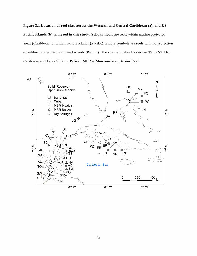
81

Figure 3.1 Location of reef sites across the Western and Central Caribbean (a), and US

Pacific islands (b) analyzed in this study. Solid symbols are reefs within marine protected

areas (Caribbean) or within remote islands (Pacific). Empty symbols are reefs with no protection

(Caribbean) or within populated islands (Pacific). For sites and island codes see Table S3.1 for

Caribbean and Table S3.2 for Paficic. MBR is Mesoamerican Barrier Reef.

a)

82

b)

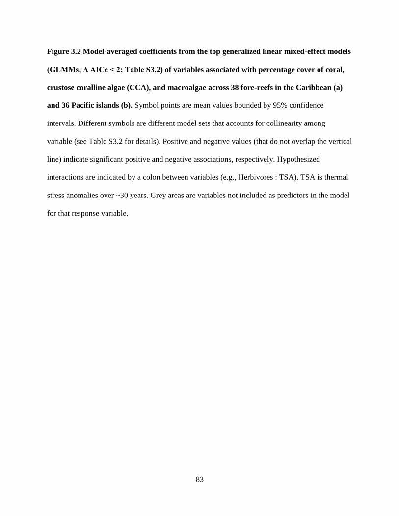
83

Figure 3.2 Model-averaged coefficients from the top generalized linear mixed-effect models

(GLMMs; Δ AICc < 2; Table S3.2) of variables associated with percentage cover of coral,

crustose coralline algae (CCA), and macroalgae across 38 fore-reefs in the Caribbean (a)

and 36 Pacific islands (b). Symbol points are mean values bounded by 95% confidence

intervals. Different symbols are different model sets that accounts for collinearity among

variable (see Table S3.2 for details). Positive and negative values (that do not overlap the vertical

line) indicate significant positive and negative associations, respectively. Hypothesized

interactions are indicated by a colon between variables (e.g., Herbivores : TSA). TSA is thermal

stress anomalies over ~30 years. Grey areas are variables not included as predictors in the model

for that response variable.

84

85

Figure 3.3 Relationship among contemporary percentage of coral cover, TSA frequency,

and the biomass of piscivorous and herbivorous fishes across 38 fore reefs in the Caribbean

and 36 US Pacific islands. Bubble size is proportional to the average fish biomass (g m-2

) per

site or island. Black line (bounded by 95% confidence interval) is the fitting prediction from the

GLMMs model-averaging of percentage coral cover on TSA frequency accounting for all

covariates in the models (Table S3.3). Note that average values were calculated at the site level

in the Caribbean, while at island level in the Pacific.

86

Figure 3.4 Relationship between the average of macroalgae cover (%) and total

herbivorous fish biomass (gm-2) across 38 fore reefs in the Caribbean and 36 US Pacific

islands. Lines (bounded by 95% confidence interval) are fitting predictions of macroalgae cover

on herbivores biomass accounting for several variables in the GLMMs. Black like is the fitting

for all sites, grey line for protected/remote sites, and white lines are for non-protected/populated

sites. Note that the slope is significant for protected, non-protected and all sites in the Caribbean,

while in the US Pacific island the relationship is only significant within populated islands.

87

References

Allgeier, J. E., C. A. Layman, P. J. Mumby, and A. D. Rosemond. 2014. Consistent nutrient

storage and supply mediated by diverse fish communities in coral reef ecosystems.

Global Change Biology:n/a–n/a.

Alvarez-Filip, L., N. K. Dulvy, I. M. Côté, A. R. Watkinson, and J. A. Gill. 2011. Coral identity

underpins architectural complexity on Caribbean reefs. Ecological Applications 21:2223–

2231.

Alvarez-Filip, L., N. K. Dulvy, J. A. Gill, I. M. Côté, and A. R. Watkinson. 2009. Flattening of

Caribbean coral reefs: region-wide declines in architectural complexity. Proceedings of

the Royal Society B: Biological Sciences 276:3019–3025.

Ault, J. S., S. G. Smith, J. A. Bohnsack, J. Luo, D. E. Harper, and D. B. McClellan. 2006.

Building sustainable fisheries in Florida’s coral reef ecosystem: positive signs in the Dry

Tortugas. Bulletin of Marine Science 78:633–654.

Babcock, R. C., N. T. Shears, A. C. Alcala, N. S. Barrett, G. J. Edgar, K. D. Lafferty, T. R.

McClanahan, and G. R. Russ. 2010. Decadal trends in marine reserves reveal differential

rates of change in direct and indirect effects. Proceedings of the National Academy of

Sciences 107:18256 –18261.

Bak, R. 1976. The growth of coral colonies and the importance of crustose coralline algae and

burrowing sponges in relation with carbonate accumulation. Netherlands Journal of Sea

Research 10:285–337.

Bellwood, D. R., A. S. Hoey, and J. H. Choat. 2003. Limited functional redundancy in high

diversity systems: resilience and ecosystem function on coral reefs. Ecology Letters

6:281–285.

Bellwood, D. R., T. P. Hughes, C. Folke, and M. Nyström. 2004. Confronting the coral reef

crisis. Nature 429:827–833.

Bellwood, D. R., T. P. Hughes, and A. S. Hoey. 2006. Sleeping Functional Group Drives Coral-

Reef Recovery. Current Biology 16:2434–2439.

Billé, R., R. Kelly, A. Biastoch, E. Harrould-Kolieb, D. Herr, F. Joos, K. Kroeker, D. Laffoley,

A. Oschlies, and J.-P. Gattuso. 2013. Taking Action Against Ocean Acidification: A

Review of Management and Policy Options. Environmental Management 52:761–779.

Birrell, C. L., L. McCook, B. L. Willis, and G. Diaz-Pulido. 2008. Effects of benthic algae on the

replenishment of corals and the implications for the resilience of coral reefs. Pages 25–63

Oceanography and Marine Biology: An Annual Review. R.N. Gibson, R.J.A Atkinson,

J.D.M. Gordon, Taylor & Francis, London, U.K.

88

Bolker, B. M., M. E. Brooks, C. J. Clark, S. W. Geange, J. R. Poulsen, M. H. H. Stevens, and J.

S. S. White. 2009. Generalized linear mixed models: a practical guide for ecology and

evolution. Trends in Ecology & Evolution 24:127–135.

Bruno, J. F., L. E. Petes, C. Drew Harvell, and A. Hettinger. 2003. Nutrient enrichment can

increase the severity of coral diseases. Ecology Letters 6:1056–1061.

Bruno, J. F., W. F. Precht, P. S. Vroom, and R. B. Aronson. 2014. Coral reef baselines: How

much macroalgae is natural? Marine Pollution Bulletin.

Bruno, J. F., and E. R. Selig. 2007. Regional decline of coral cover in the Indo-Pacific: timing,

extent, and subregional comparisons. PLoS ONE 2:e711.

Bruno, J. F., H. Sweatman, W. F. Precht, E. R. Selig, and V. G. W. Schutte. 2009. Assessing

evidence of phase shifts from coral to macroalgal dominance on coral reefs. Ecology

90:1478–1484.

Burkepile, D. E., and M. E. Hay. 2008. Herbivore species richness and feeding complementarity

affect community structure and function on a coral reef. Proceedings of the National

Academy of Sciences 105:16201–16206.

Burnham, K. P., and D. R. Anderson. 2002. Model selection and multi-model inference: a

practical information-theoretic approach. 2nd edition. Springer New York.

Carleton, J. H., and T. J. Done. 1995. Quantitative video sampling of coral reef benthos: large-

scale application. Coral Reefs 14:35–46.

Cheal, A. J., M. A. MacNeil, E. Cripps, M. J. Emslie, M. Jonker, B. Schaffelke, and H.

Sweatman. 2010. Coral–macroalgal phase shifts or reef resilience: links with diversity

and functional roles of herbivorous fishes on the Great Barrier Reef. Coral Reefs

29:1005–1015.

Chollett, I., P. J. Mumby, F. E. Müller-Karger, and C. Hu. 2012. Physical environments of the

Caribbean Sea. Limnology and Oceanography 57:1233–1244.

Connell, J. H. 1997. Disturbance and recovery of coral assemblages. Coral Reefs 16:S101–S113.

Côté, I. M., and E. S. Darling. 2010. Rethinking Ecosystem Resilience in the Face of Climate

Change. PLoS Biology 8:e1000438.

Côté, I. M., I. Mosqueira, and J. D. Reynolds. 2001. Effects of marine reserve characteristics on

the protection of fish populations: a meta-analysis. Journal of Fish Biology 59:178–189.

Darling, E. S., T. R. McClanahan, and I. M. Côté. 2010. Combined effects of two stressors on

Kenyan coral reefs are additive or antagonistic, not synergistic. Conservation Letters

3:122–130.

89

Darling, E. S., T. R. McClanahan, and I. M. Côté. 2013. Life histories predict coral community

disassembly under multiple stressors. Global Change Biology 19:1930–1940.

De’ath, G., K. E. Fabricius, H. Sweatman, and M. Puotinen. 2012. The 27-year decline of coral

cover on the Great Barrier Reef and its causes. Proceedings of the National Academy of

Sciences 109:17995–17999.

Diaz-Pulido, G., S. Harii, L. McCook, and O. Hoegh-Guldberg. 2010. The impact of benthic

algae on the settlement of a reef-building coral. Coral Reefs 29:203–208.

Dove, S. G., D. I. Kline, O. Pantos, F. E. Angly, G. W. Tyson, and O. Hoegh-Guldberg. 2013.

Future reef decalcification under a business-as-usual CO2 emission scenario. Proceedings

of the National Academy of Sciences 110:15342–15347.

Dutt, V., and C. Gonzalez. 2012. Human control of climate change. Climatic Change 111:497–

518.

Edgar, G. J., R. D. Stuart-Smith, T. J. Willis, S. Kininmonth, S. C. Baker, S. Banks, N. S.

Barrett, M. A. Becerro, A. T. F. Bernard, J. Berkhout, C. D. Buxton, S. J. Campbell, A.

T. Cooper, M. Davey, S. C. Edgar, G. Försterra, D. E. Galván, A. J. Irigoyen, D. J.

Kushner, R. Moura, P. E. Parnell, N. T. Shears, G. Soler, E. M. A. Strain, and R. J.

Thomson. 2014. Global conservation outcomes depend on marine protected areas with

five key features. Nature.

Froese, R., and D. Pauly. 2013. FishBase. http://www.fishbase.org.

Gaines, S. D., C. White, M. H. Carr, and S. R. Palumbi. 2010. Designing marine reserve

networks for both conservation and fisheries management. Proceedings of the National

Academy of Sciences 107:18286–18293.

Gardner, T. A., I. M. Côté, J. A. Gill, A. Grant, and A. R. Watkinson. 2003. Long-term region-

wide declines in Caribbean corals. Science 301:958–960.

Gove, J. M., G. J. Williams, M. A. McManus, S. F. Heron, S. A. Sandin, O. J. Vetter, and D. G.

Foley. 2013. Quantifying climatological ranges and anomalies for Pacific coral reef

ecosystems. PloS one 8:e61974.

Graham, M. H. 2003. Confronting multicollinearity in ecological multiple regression. Ecology

84:2809–2815.

Graham, N. A., D. R. Bellwood, J. E. Cinner, T. P. Hughes, A. V. Norström, and M. Nyström.

2013. Managing resilience to reverse phase shifts in coral reefs. Frontiers in Ecology and

the Environment 11:541–548.

Graham, N. A. J. 2014. Habitat Complexity: Coral Structural Loss Leads to Fisheries Declines.

Current Biology 24:R359–R361.

90

Graham, N. A. J., T. R. McClanahan, M. A. MacNeil, S. K. Wilson, N. V. C. Polunin, S.

Jennings, P. Chabanet, S. Clark, M. D. Spalding, Y. Letourneur, L. Bigot, R. Galzin, M.

C. Öhman, K. C. Garpe, A. J. Edwards, and C. R. C. Sheppard. 2008. Climate Warming,

Marine Protected Areas and the Ocean-Scale Integrity of Coral Reef Ecosystems. PLoS

ONE 3:e3039.

Graham, N. a. J., K. L. Nash, and J. T. Kool. 2011. Coral reef recovery dynamics in a changing

world. Coral Reefs 30:283–294.

Grueber, C. E., S. Nakagawa, R. J. Laws, and I. G. Jamieson. 2011. Multimodel inference in

ecology and evolution: challenges and solutions. Journal of Evolutionary Biology

24:699–711.

Guest, J. R., A. H. Baird, J. A. Maynard, E. Muttaqin, A. J. Edwards, S. J. Campbell, K.

Yewdall, Y. A. Affendi, and L. M. Chou. 2012. Contrasting patterns of coral bleaching

susceptibility in 2010 suggest an adaptive response to thermal stress. PLoS ONE

7:e33353.

Halpern, B. S., and R. R. Warner. 2002. Marine reserves have rapid and lasting effects. Ecology

Letters 5:361–366.

Harborne, A. R., P. J. Mumby, C. V. Kappel, C. P. Dahlgren, F. Micheli, K. E. Holmes, J. N.

Sanchirico, K. Broad, I. A. Elliott, and D. R. Brumbaugh. 2008. Reserve effects and

natural variation in coral reef communities. Journal of Applied Ecology 45:1010–1018.

Hixon, M. A., and J. P. Beets. 1993. Predation, prey refuges, and the structure of coral-reef fish

assemblages. Ecological Monographs 63:77–101.

Hoegh-Guldberg, O., P. J. Mumby, A. J. Hooten, R. S. Steneck, P. Greenfield, E. Gomez, C. D.

Harvell, P. F. Sale, A. J. Edwards, K. Caldeira, N. Knowlton, C. M. Eakin, R. Iglesias-

Prieto, N. Muthiga, R. H. Bradbury, A. Dubi, and M. E. Hatziolos. 2007. Coral reefs

under rapid climate change and ocean acidification. Science 318:1737–1742.

Hughes, T. P., A. H. Baird, D. R. Bellwood, M. Card, S. R. Connolly, C. Folke, R. Grosberg, O.

Hoegh-Guldberg, J. B. C. Jackson, J. Kleypas, J. M. Lough, P. Marshall, M. Nyström, S.

R. Palumbi, J. M. Pandolfi, B. Rosen, and J. Roughgarden. 2003. Climate change, human

impacts, and the resilience of coral reefs. Science 301:929–933.

Hughes, T. P., M. J. Rodrigues, D. R. Bellwood, D. Ceccarelli, O. Hoegh-Guldberg, L. McCook,

N. Moltschaniwskyj, M. S. Pratchett, R. S. Steneck, and B. Willis. 2007. Phase Shifts,

Herbivory, and the Resilience of Coral Reefs to Climate Change. Current Biology

17:360–365.

Huntington, B. E., M. Karnauskas, and D. Lirman. 2011. Corals fail to recover at a Caribbean

marine reserve despite ten years of reserve designation. Coral Reefs 30:1077–1085.

IPCC. 2013. Climate Change 2013: The Physical Science Basis. Contribution of Working Group

I to the Fifth Assessment Report of the Intergovernmental Panel on Climate Change.

91

Stocker, T.F., D. Qin, G.-K. Plattner, M. Tignor, S.K. Allen, J. Boschung, A. Nauels, Y.

Xia, V. Bex and P.M. Midgley. Cambridge University Press, Cambridge, United

Kingdom and New York, NY, USA.

Jackson, J. B. C., M. K. Donovan, K. L. Cramer, and Lam. 2014. Status and Trends of Caribbean

Coral Reefs: 1970-2012. Global Coral Reef Monitoring Network, IUCN, Gland,

Switzerland.

Jones, G. P., M. I. McCormick, M. Srinivasan, and J. V. Eagle. 2004. Coral decline threatens fish

biodiversity in marine reserves. Proceedings of the National Academy of Sciences of the

United States of America 101:8251 –8253.

Karnauskas, M., B. E. Huntington, E. A. Babcock, and D. Lirman. 2011. Pre-existing spatial

patterns in fish abundances influence species-specific responses in a Caribbean marine

reserve. Marine Ecology Progress Series 432:235–246.

Keller, B. D., D. F. Gleason, E. McLeod, C. M. Woodley, S. Airamé, B. D. Causey, A. M.

Friedlander, R. Grober-Dunsmore, J. E. Johnson, S. L. Miller, and R. S. Steneck. 2009.

Climate Change, Coral Reef Ecosystems, and Management Options for Marine Protected

Areas. Environmental Management 44:1069–1088.

Kenyon, J. C., R. E. Brainard, R. K. Hoeke, F. A. Parrish, and C. B. Wilkinson. 2006. Towed-

diver surveys, a method for mesoscale spatial assessment of benthic reef habitat: a case

study at Midway Atoll in the Hawaiian Archipelago. Coastal Management 34:339–349.

Knowlton, N., and J. B. C. Jackson. 2008. Shifting Baselines, Local Impacts, and Global Change

on Coral Reefs. PLoS Biol 6:e54.

Kuffner, I. B., L. J. Walters, M. A. Becerro, V. J. Paul, R. Ritson-Williams, and K. S. Beach.

2006. Inhibition of coral recruitment by macroalgae and cyanobacteria. Marine Ecology

Progress Series 323:107–117.

Lang, J. C., K. W. Marks, P. A. Kramer, P. Richards Kramer, and R. N. Ginsburg. 2010.

AGRRA Protocols version 5.4 Atlantic and Gulf Rapid Reef Assessment Program.

University of Miami, Florida.

Lessafre, E., D. Rizopoulos, and R. Tsonaka. 2007. The logistic-transform for bounded outcome

scores. Biostatistics 8:72–85.

Lester, S., B. Halpern, K. Grorud-Colvert, J. Lubchenco, B. Ruttenberg, S. Gaines, S. Airamé,

and R. Warner. 2009. Biological effects within no-take marine reserves: a global

synthesis. Marine Ecology Progress Series 384:33–46.

Lubchenco, J., S. R. Palumbi, S. D. Gaines, and S. Andelman. 2003. Plugging a hole in the

ocean: the emerging science of marine reserves 1. Ecological applications 13:3–7.

Maynard, J., K. Anthony, P. Marshall, and I. Masiri. 2008. Major bleaching events can lead to

increased thermal tolerance in corals. Marine Biology 155:173–182.

92

McCauley, D. J., K. A. McLean, J. Bauer, H. S. Young, and F. Micheli. 2012. Evaluating the

performance of methods for estimating the abundance of rapidly declining coastal shark

populations. Ecological Applications 22:385–392.

McClanahan, T. R. 2008. Response of the coral reef benthos and herbivory to fishery closure

management and the 1998 ENSO disturbance. Oecologia 155:169–177.

McClanahan, T. R., J. E. Cinner, J. Maina, N. A. J. Graham, T. M. Daw, S. M. Stead, A.

Wamukota, K. Brown, M. Ateweberhan, V. Venus, and N. V. C. Polunin. 2008.

Conservation action in a changing climate. Conservation Letters 1:53–59.

McCook, Jompa, and Diaz-Pulido. 2001. Competition between corals and algae on coral reefs: a

review of evidence and mechanisms. Coral Reefs 19:400–417–417.

McCune, B., J. B. Grace, and D. L. Urban. 2002. Analysis of Ecological Communities. MjM

Software Design, Gleneden Beach, Oregon, USA.

McLeod, E., R. Salm, A. Green, and J. Almany. 2009. Designing marine protected area networks

to address the impacts of climate change. Frontiers in Ecology and the Environment

7:362–370.

Mumby, P. J., C. P. Dahlgren, A. R. Harborne, C. V. Kappel, F. Micheli, D. R. Brumbaugh, K.

E. Holmes, J. M. Mendes, K. Broad, J. N. Sanchirico, K. Buch, S. Box, R. W. Stoffle,

and A. B. Gill. 2006. Fishing, trophic cascades, and the process of grazing on coral reefs.

Science 311:98–101.

Mumby, P. J., and A. R. Harborne. 2010. Marine Reserves Enhance the Recovery of Corals on

Caribbean Reefs. PLoS ONE 5:e8657.

Mumby, P. J., A. R. Harborne, J. Williams, C. V. Kappel, D. R. Brumbaugh, F. Micheli, K. E.

Holmes, C. P. Dahlgren, C. B. Paris, and P. G. Blackwell. 2007a. Trophic cascade

facilitates coral recruitment in a marine reserve. Proceedings of the National Academy of

Sciences 104:8362–8367.

Mumby, P. J., A. Hastings, and H. J. Edwards. 2007b. Thresholds and the resilience of

Caribbean coral reefs. Nature 450:98–101.

Mumby, P. J., N. H. Wolff, Y.-M. Bozec, I. Chollett, and P. Halloran. 2014. Operationalizing the

Resilience of Coral Reefs in an Era of Climate Change. Conservation Letters 7:176–187.

Nadon, M. O., J. K. Baum, I. D. Williams, J. M. Mcpherson, B. J. Zgliczynski, B. L. Richards,

R. E. Schroeder, and R. E. Brainard. 2012. Re‐creating missing population baselines for

Pacific reef sharks. Conservation Biology 26:493–503.

Newman, M. J. H., G. A. Paredes, E. Sala, and J. B. C. Jackson. 2006. Structure of Caribbean

coral reef communities across a large gradient of fish biomass. Ecology Letters 9:1216–

1227.

93

Oksanen, J., F. G. Blanchet, R. Kindt, M. J. Oksanen, and M. Suggests. 2013. Package “vegan.”

Community ecology package Version 2:0–0.

O’Leary, J. K., D. C. Potts, J. C. Braga, and T. R. McClanahan. 2012. Indirect consequences of

fishing: reduction of coralline algae suppresses juvenile coral abundance. Coral Reefs

31:547–559.

Pandolfi, J. M., R. H. Bradbury, E. Sala, T. P. Hughes, K. A. Bjorndal, R. G. Cooke, D.

McArdle, L. McClenachan, M. J. H. Newman, G. Paredes, R. R. Warner, and J. B. C.

Jackson. 2003. Global trajectories of the long-term decline of coral reef ecosystems.

Science 301:955–958.

Polunin, N. V. C., and C. M. Roberts. 1993. Greater biomass and value of target coral-reef fishes

in two small Caribbean marine reserves. Marine Ecology Progress Series 100:177–183.

Rasher, D. B., and M. E. Hay. 2010. Chemically rich seaweeds poison corals when not

controlled by herbivores. Proceedings of the National Academy of Sciences 107:9683–

9688.

Rau, G. H., E. L. McLeod, and O. Hoegh-Guldberg. 2012. The need for new ocean conservation

strategies in a high-carbon dioxide world. Nature Climate Change 2:720–724.

R Core Team. 2013. R: A Language and Environment for Statistical Computing, Vienna,

Austria. V. 3.03. http://www.R-project.org.

Roff, G., and P. J. Mumby. 2012. Global disparity in the resilience of coral reefs. Trends in

Ecology & Evolution 27:404–413.

Rogers, A., J. L. Blanchard, and P. J. Mumby. 2014. Vulnerability of Coral Reef Fisheries to a

Loss of Structural Complexity. Current Biology.

Sala, E., E. Ballesteros, P. Dendrinos, A. Di Franco, F. Ferretti, D. Foley, S. Fraschetti, A.

Friedlander, J. Garrabou, H. Güçlüsoy, P. Guidetti, B. S. Halpern, B. Hereu, A. A.

Karamanlidis, Z. Kizilkaya, E. Macpherson, L. Mangialajo, S. Mariani, F. Micheli, A.

Pais, K. Riser, A. A. Rosenberg, M. Sales, K. A. Selkoe, R. Starr, F. Tomas, and M.

Zabala. 2012. The structure of mediterranean rocky reef ecosystems across environmental

and human gradients, and conservation implications. PLoS ONE 7:e32742.

Sandin, S. A., J. E. Smith, E. E. DeMartini, E. A. Dinsdale, S. D. Donner, A. M. Friedlander, T.

Konotchick, M. Malay, J. E. Maragos, D. Obura, O. Pantos, G. Paulay, M. Richie, F.

Rohwer, R. E. Schroeder, S. Walsh, J. B. C. Jackson, N. Knowlton, and E. Sala. 2008.

Baselines and degradation of coral reefs in the Northern Line Islands. PLoS ONE

3:e1548.

Sandin, S. A., and I. Williams. 2010. Trophic Classifications of Reef Fishes from the Tropical

US Pacific (Version 1.0). Technical Report.

94

Schils, T., P. S. Vroom, and A. D. Tribollet. 2013. Geographical partitioning of marine

macrophyte assemblages in the tropical Pacific: a result of local and regional diversity

processes. Journal of Biogeography 40:1266–1277.

Schutte, V. G. W., E. R. Selig, and J. F. Bruno. 2010. Regional spatio-temporal trends in

Caribbean coral reef benthic communities. Mar Ecol Prog Ser 402:115–122.

Selig, E. R., and J. F. Bruno. 2010. A Global Analysis of the Effectiveness of Marine Protected

Areas in Preventing Coral Loss. PLoS ONE 5:e9278.

Selig, E. R., K. S. Casey, and J. F. Bruno. 2012. Temperature-driven coral decline: the role of

marine protected areas. Global Change Biology 18:1561–1570.

Stockwell, B., C. R. L. Jadloc, R. A. Abesamis, A. C. Alcala, and G. R. Russ. 2009. Trophic and

benthic responses to no-take marine reserve protection in the Philippines. Marine

Ecology, Progress Series 389:1–15.

Thompson, D. M., and R. van Woesik. 2009. Corals escape bleaching in regions that recently

and historically experienced frequent thermal stress. Proceedings of the Royal Society B:

Biological Sciences 276:2893–2901.

Toth, L. T., R. van Woesik, T. J. T. Murdoch, S. R. Smith, J. C. Ogden, W. F. Precht, and R. B.

Aronson. 2014. Do no-take reserves benefit Florida’s corals? 14 years of change and

stasis in the Florida Keys National Marine Sanctuary. Coral Reefs:1–13.

Victor, D. G. 2008. The collapse of the Kyoto Protocol and the struggle to slow global warming.

Princeton University Press.

Vroom, P. S. 2011. Coral Dominance: A Dangerous Ecosystem Misnomer? Journal of Marine

Biology 2011.

Wiedenmann, J., C. D’Angelo, E. G. Smith, A. N. Hunt, F.-E. Legiret, A. D. Postle, and E. P.

Achterberg. 2013. Nutrient enrichment can increase the susceptibility of reef corals to

bleaching. Nature Climate Change 3:160–164.

Williams, I. D., B. L. Richards, S. A. Sandin, J. K. Baum, R. E. Schroeder, M. O. Nadon, B.

Zgliczynski, P. Craig, J. L. McIlwain, and R. E. Brainard. 2011. Differences in reef fish

assemblages between populated and remote reefs spanning multiple archipelagos across

the central and western pacific. Journal of Marine Biology 2011.

Williams, and Polunin. 2001. Large-scale associations between macroalgal cover and grazer

biomass on mid-depth reefs in the Caribbean. Coral Reefs 19:358–366–366.

Zuur, A., E. N. Ieno, N. Walker, A. A. Saveliev, and G. M. Smith. 2009. Mixed effects models

and extensions in ecology with R. Springer.

_________________________

1A version of this Chapter is in preparation for publication in Nature Climate Change as:

Valdivia, A., Cox, C.E., Darling, E.R., Bruno, J. Ocean warming shifts coral community

composition

95

CHAPTER 4

Ocean warming shifts coral community composition1

Abstract

Rising ocean temperatures threaten coral reef ecosystems with more frequent and severe

bleaching events that can cause widespread mortality and decline of reef-building corals.

However, the response of coral communities to warming seems to vary spatially across multiple

scales depending on the thermal history of reef areas. Here we investigate whether ~30 years of

thermal history can partially explain patterns in current coral community composition throughout

the Caribbean. We found that contemporary coral cover was positively related to the frequency

of recent thermal stress anomalies due to a shift in coral community composition towards

smaller, stress-tolerant and weedy species. Our findings suggest that coral communities that have

experienced more frequent thermal anomalies may be composed of more disturbance-tolerant

species or genotypes. While the re-assortment of coral taxa due to environmental filtering in

response to warming may result in communities that can cope with thermal stress, these

communities likely have less structural complexity and coral diversity that may compromise

ecosystem functioning. Our study reinforces the role of climate change in causing changes in

composition and function rather than outright ecosystem loss.

96

Keywords: Coral reefs, ecological strategies, thermal stress anomalies, selection pressure,

bleaching, global warming, thermal tolerance

Introduction

Greenhouse gas emissions are warming the atmosphere and oceans, causing disruptions

to ecosystems and the services they provide to humanity (Hoegh-Guldberg et al. 2007, Hoegh-

Guldberg and Bruno 2010, Burrows et al. 2011, IPCC 2013). The ecological responses of climate

change are well documented and include changes in the phenology and physiology of organisms,

altered species interactions, and shifts in range distributions (Walther et al. 2002, Hoegh-

Guldberg and Bruno 2010, Burrows et al. 2011, Graham et al. 2014a). There is also growing

evidence that climate change is leading to shifts in composition, structure, and functioning of

natural systems as opposed to ecosystem collapse (Walther et al. 2002, Precht and Aronson

2004, Hobbs et al. 2009, Burrows et al. 2011, Graham et al. 2014a, Dornelas et al. 2014).

However, the reorganization of species assemblages by global warming into novel or emerging

ecosystems, and the goods or services that altered ecosystems can continue to support, remains

poorly understood (Williams and Jackson 2007, Hobbs et al. 2009, Burrows et al. 2011, Graham

et al. 2014a).

Several mechanisms can underlie changes in community composition in response to rapid

warming. Some populations may be able to cope with increasing temperatures by dispersing to

new more hospitable areas, introducing new species to existing communities, i.e., species range

shifts (Greenstein and Pandolfi 2008, Burrows et al. 2011, 2014). Other populations, with slower

dispersion rates, may have to acclimatize to new environmental conditions in their home range or

97

adapt by natural selection through the survival of resilient individuals or genotypes (Walther et

al. 2002, Williams and Jackson 2007, Edmunds and Gates 2008). Still other populations will be

locally extirpated as the climate changes too quickly for adaptation or acclimatization to keep

pace (Edmunds and Gates 2008, Burrows et al. 2011, Hoegh-Guldberg 2012). Thus, new

ecological communities can emerge from hybrids of former ones or completely novel

assemblages through species immigration and/or extinctions driven by changes in local and

regional environmental conditions (Burrows et al. 2014). For example, rapid warming in the

Southern Ocean can allow shell-braking crabs and fishes to return to the Antarctic Peninsula,

strengthening the top-down control in a region that has been free of predators since the Eocene

~41 million years ago (Aronson et al. 2009).

Global warming will be the dominant driver of change in the world’s oceans over the

coming decades (Hoegh-Guldberg et al. 2011, Graham et al. 2014a, McClanahan et al. 2014).

Coral reef ecosystems are especially vulnerable, in part due to the narrow thermal range of their

foundational species, Scleractinian corals (Hoegh-Guldberg 1999, Hoegh-Guldberg and Bruno

2010). Sensitive to elevated sea temperatures, corals can exhibit extensive bleaching (i.e., the

loss of their endosymbiotic algae and/or their photosynthetic pigment) with consequent partial or

whole-colony mortality (Glynn 1993, Hoegh-Guldberg et al. 2007). Mass bleaching events,

combined with chronic exposure to local stressors such as overfishing, pollution, and diseases,

have contributed to the regional and global decline of hard corals over the past decades (Hoegh-

Guldberg 1999, Gardner et al. 2003, Pandolfi et al. 2003, Bruno and Selig 2007).

Counterintuitively, long-term exposure to these stressors can also remove less resistant and

resilient genotypes and increase the ability of the system to cope with new stresses (Côté and

Darling 2010, Graham et al. 2014a, McClanahan et al. 2014). For example, widespread mortality

98

due to bleaching not only results in coral decline (Hoegh-Guldberg 1999, Bruno and Selig 2007),

but may promote differential mortality that changes coral genotypic and species composition

(Loya et al. 2001, Carpenter et al. 2008, Van Woesik et al. 2011) by selecting for ‘winning’

genotypes and species that are tolerant to thermal stress (Maynard et al. 2008, Thompson and

Woesik 2009, Van Woesik et al. 2011, Graham et al. 2014a, Palumbi et al. 2014). Thus, while

coral assemblages have experienced substantial functional losses with thermal disturbance, post-

stress communities may be better suited to survive future environmental conditions (Graham et

al. 2014a, McClanahan et al. 2014).

Thermal stress anomalies vary spatially in intensity and frequency resulting in regional

variability in the exposure of coral reefs to ocean warming (Thompson and Woesik 2009, Selig

et al. 2010, Guest et al. 2012). Certain geographic regions experience thermal anomalies more

often than others (Selig et al. 2010). For example, reefs of Central America, the Persian Gulf,

and the Central Pacific display higher average frequency and magnitude of thermal stress

anomalies than reefs of the Florida Keys, the Bahamas, or the Hawaiian Islands (Selig et al.

2010). Regional differences in bleaching responses by corals are likely related to the thermal

history of each reef, which may result in different communities of thermally-tolerant species or

genotypes across oceanographic regions (Maynard et al. 2008, Thompson and Woesik 2009,

Guest et al. 2012). Evidence suggests that some reefs with historically dominant branching and

plating competitive corals have been replaced by more resistant and opportunistic species

(Aronson et al. 2004, Green et al. 2008, Van Woesik et al. 2011, Darling et al. 2013). For

example, 20-years of coral community disassembly on Kenyan coral reefs identified the loss of

the competitive life history and the replacement with an altered assemblage of stress-tolerant and

weedy ‘survivor’ life histories (Darling et al. 2013). In the Caribbean, a decline in total coral

99

cover over the last 30 years has led to an increase in the relative dominance of fast-growing

opportunistic “weedy” species, e.g., Porites spp. and Agaricia spp., with small-size colonies and

high turnover rates (Aronson et al. 2004, Green et al. 2008, Alvarez-Filip et al. 2011). These

shifts in coral assemblage composition have resulted in rapid losses of reef calcification and

rugosity that threaten continued architectural complexity and ecosystem functionality(Alvarez-

Filip et al. 2013, Bozec et al. 2014). These critical community shifts are associated with

differential mortality due to bleaching events, disease outbreaks, and other local-scale stressors

(Aronson et al. 2004, Green et al. 2008). While most studies have focused on documenting and

forecasting coral reef deterioration (Gardner et al. 2003, Pandolfi et al. 2003, Bruno and Selig

2007, Carpenter et al. 2008, Hoegh-Guldberg et al. 2011), the potential role of ocean warming in

shifting coral community composition towards more disturbance-tolerant species have been

predicted (Loya et al. 2001, Maynard et al. 2008, Thompson and Woesik 2009, Van Woesik et

al. 2011, Darling et al. 2012) but seldom tested across broad regional spatial scales (Precht and

Aronson 2004, Greenstein and Pandolfi 2008, Graham et al. 2014b).

Here, we test the hypothesis that contemporary coral community structure (i.e., coral

cover patterns and relative composition of major coral taxa) has been influenced by recent

thermal history. We examine: (i) the degree to which local thermal stress anomalies are related to

changes in contemporary coral cover (and presumably loss), and (ii) whether coral assemblages

have shifted towards species potentially more tolerant to temperature anomalies. That is, we

asked whether reef areas that experience high-frequency of thermal anomalies act as

environmental filters, selecting for traits that results in compositional shifts towards thermally

resistant coral species or genotypes (Thompson and Woesik 2009, Darling et al. 2012) and away

from the historical composition and structure of Caribbean reefs (Aronson et al. 2004).

100

Materials and Methods

Study sites and coral surveys

Surveys were performed at 39 sites in five countries throughout the Western and Central

Caribbean in slope and spur-and-groove fore-reef habitats ~10-15m deep and formerly

dominated by Orbicella corals (Table S4.1). Percent cover data of benthic communities (i.e.,

coral by species and algae by functional groups) were measured at each site using point

intercepts in 6-8 transect lines (10 m long) (Lang et al. 2010) and/or in 6-8 video transects (50 m

long) (Carleton and Done 1995) along the slope or spur-and-groove habitats. Point intercept

transects (PITs) were used at the Belize sites, while both PITs and video transects were used at

the rest of the sites. To estimate percentage cover, 100 points per transect were used in PITs

(Lang et al. 2010), while ~600 points were extracted from each video transect (Carleton and

Done 1995). Both methods provided similar accuracy and results in estimating benthic cover

categories in our study (Supplementary Methods). To minimize seasonal variability in algal

composition we conducted all surveys during the summer months of May to July 2010-2012.

Thermal stress anomalies and other covariates

We created a 29-year dataset (1982-2010) of annual frequency of weekly Thermal Stress

Anomalies (Selig et al. 2006) (TSA) for each surveyed reefs using the National Oceanic and

Atmospheric Administration’s (NOAA) National Oceanographic Data Center (NODC) Coral

Reef Temperature Anomaly Database (CoRTAD) Version 4.0 (Casey et al. 2010, Selig et al.

2010) (Fig. 4.1). Temperature anomalies for this database were calculated from the Pathfinder

Version 5.2 data temperature with a spatial resolution of ~4 km grid cells (Casey et al. 2010,

101

Selig et al. 2010) and with a quality flag of four or better (Kilpatrick et al. 2001). TSAs area

defined as deviations of one-week where sea surface temperature (SST) was 1ºC or greater than

the mean maximum climatological week or the long term average warmest week from 1982 to

2010 (Selig et al. 2010). This threshold is generally accepted for environmental conditions that

may cause bleaching and coral mortality (Glynn 1993). We calculated the long-term (29 years)

average and standard deviation of annual-frequency TSA (weeks/year) for the grid cell that

corresponded to each study site to be used as fixed predictor in linear mixed effect models (Fig.

4.1).

Additionally, we measured a set of anthropogenic, physical, and biotic parameters that

are known to affect coral assemblages and could modulate their response to temperature (Table

4.1). Anthropogenic-related parameters included number of humans per squared kilometer of

reef and area of cultivated land within 50 km of each reef. Physical variables were mean oceanic

primary productivity, wave exposure, and landscape reef complexity. Biotic variables included

percentage cover of benthic macroalgae, crustose coralline algae (CCA) and turf algae, and the

biomass of two functional fish groups; herbivores and piscivores. For a detailed description,

measurement, and justification of each variable refer to Table 4.1 and supplementary methods.

Data analysis

We used percent coral cover as response variable because is an important metric of coral

reef health that respond directly to temperature stress through bleaching and mortality (Glynn

1993). To analyze spatial differences in coral community structure, species of scleractinian

corals were grouped in three life-history strategy categories (Darling et al. 2013) (e.g.,

competitive, stress-tolerant, and weedy, Table S4.2) as defined by Darling et al. (Darling et al.

102

2012) and based on a global analysis of species traits. Two Caribbean coral species (Orbicella

faveolata and Orbicella franksi), that were originally classified as generalists (Darling et al.

2012), were reclassified as stress-tolerant which is consistent with the classification of their

congeneric species Orbicella annularis (Bégin et al. 2014).

We used generalized linear mixed effect models (GLMMs) and applied a logistic (logit)

transformation to the percent coral cover data (total corals and by life-history-strategy groups)

where the logit was treated as normally distributed (Lessafre et al. 2007). Competitive corals

(e.g., Acropora sp. and Dendrogyra cylindrus, Table S4.2) were analyzed with a binomial

distribution (0-absence and 1-presence) as percentage cover of these species in our study sites

was relatively low, and included an excess of zeroes and over-dispersed distribution (0.4 ±1.9 %,

mean ± standard deviation, out of 39 study sites). To account for potential spatial autocorrelation

we used a random intercept model where transect where allowed to vary within sites and survey

year. Thus, coral cover (Y) at transect k of site i and year j was described as the proportional

cover (πijk) out of the number of points surveyed in each transect in that site and year (nijk). The

logistic GLMM that describes Yijk was as follows,

Yijk ~ B (nijk, πijk),

with mean E (Yijk ) and variance var ( Yijk ) where,

E (Yijk ) = πijk × nijk and var ( Yijk ) = nijk × πijk × (1- πijk).

The logit transformation of percentage coral cover was predicted by,

logit (πijk) = β0 + β1 × TSAijk + β2 × Human/km2Reefijk + β3 × CultivatedLandijk

+ β4 × ReefComplexityijk + β5 × Productivityijk + β6 × WaveExposureijk

+ β7 × Herbivoreijk + β8 × Piscivoreijk + β9 × Macroalgaeijk + β10 × CCAijk + β11 × Turfijk + aij

aij ~ N (0, σ2

a),

103

where β0 is the intercept, β1…11 are coefficient estimates of the linear regression for each of the

explanatory variables, and aij is the random intercept (sites nested in survey years), assumed to

be normally distributed with mean zero and variance σ2

a . Fish were comprised of herbivore and

piscivore biomass and algae cover was divided in three functional groups (macroalgae, CCA and

turf). Collinearity among explanatory variables was assessed using a Spearman rank correlation

matrix and scatterplots with loess smoothing curves of span 0.5 (Fig. S4.1).

We modeled all potential combinations of explanatory variables to explain total coral

cover and the three coral life histories, including interactions among fish biomass, humans per

reef, and reef complexity. We used a model averaging approach for model selection based on

Akaike’s Information criterion corrected for small samples (AICc, where ΔAICc < 3) (Burnham

and Anderson 2002). Two explanatory variables, turf and area of cultivated land, were

sufficiently correlated (|rs| > 0.5) with macroalgae and human population / reef, respectively, to

compromise model results(Graham 2003), thus we eliminated them from all models. To assess

the extent of any remaining collinearity in the final models we calculated the variance inflation

factors (VIFs) of the variables and eliminate those cofactors which values were >2 (Graham

2003).

Model validation to assess heterogeneity and normality of the residuals was performed by

examining the error distribution of top models (ΔAICc < 3) in the plot of normalized residuals

against fitted and explanatory values, and used the normal scores of standardized residuals

deviance, respectively (Zuur et al. 2009). Additionally, spline spatial correlograms were plotted

to corroborate that the final model residuals were independent and not spatially autocorrelated

(Zuur et al. 2009). Finally, we run a non-metric multi-dimensional scaling (NMDS) ordination

analysis to explore patterns of coral community composition across reef sites. We fitted a smooth

104

surface using penalize splines of TSA values on the ordination results to analyze the relationship

with coral species. All analyses were performed in R v.3.03 (R Core Team 2013) using the

packages lme4 v.0.99-2 for GLMMs, MuMIn v.1.9.13 for model averaging, ncf v.1.1-5 for

spatial autocorrelation, and vegan v.2.0-1.0 for the ordination analysis.

Results

Annual thermal-stress anomalies (TSA) increased at 22 out of 39 sites (~56%) over a 29-

year period (1982-2010) across the Central and Western Caribbean (Fig. 4.1; Table S4.3 and Fig.

S4.2). The long-term average (± standard deviation) of TSA frequency across all sites over this

period was 1.34 ± 0.71 anomaly weeks/year. The annual TSA frequency increased significantly

at most reefs of the Mesoamerican barrier in Belize and Mexico while this trend was less

pronounced for reef sites in Cuba, the Bahamas, and the Florida keys (Fig. 4.1; Fig. S4.2). Mean

annual TSA frequency also varied significantly among sub-regions (F = 280.7, df = 4, p < 2.2e-

16) (Fig. 4.1; Fig. S4.3). The lowest long-term anomalies were found in Dry Tortugas, FL (0.28

± 0.00 weeks/year) and Abaco, Bahamas (0.42 ± 0.20 weeks/year) and the highest values were

found in Belize (1.94 ± 0.94 weeks/year) (Fig S4.3).

Current coral cover was positively and significantly associated with long-term TSA

frequency across the study sites (Fig. S4.4). A simple exploratory linear regression model

showed that annual average TSA frequency alone explained ~ 25 % of the variability in average

of current coral cover across 39 reef sites (F=12.069, df = 38, R2 = 0.246, p = 0.0013; Fig. S4.4).

Coral cover ranged from 1.5 ± 1.2 % (mean ± standard deviation) at Dry Tortugas, FL (site: LG)

to 29.5 ± 13.2 % at Pompion, Belize (site: PO) (Fig. S4.4). The site with the lowest TSA

105

frequency was Little Harbor in Abaco, Bahamas (0.21 ± 0.55 weeks/year; LH) and the reef with

the highest frequency was Ranguana, Belize (2.36 ± 2.59 weeks/year; RA) (Fig 4.1; Fig. S4.4).

The possible combinations of all explanatory variables for all response variables

produced 6 to 28 models of 4 to 10 parameters (including fixed and random effects) with model

weights between 0.02 and 0.33 for all coral groups considering ΔAIC < 3 (Table 4.2). TSA

frequency was identified as the most important variable (i.e., wi = 1.00) for all corals response

variables, except the competitive life history (wi = 0.11). Macroalgae cover was important in

models of stress-tolerant, weedy, and all corals (wi = 1.00), but was less important for

competitive life histories (wi = 0.05, Table 4.2). Reef landscape complexity showed higher

relative importance (wi > 0.71) in all top models, while wave exposure had the highest

importance for total coral cover (wi = 0.68) (Table 4.2). Piscivore and herbivore fish biomass had

relative high importance (wi = 0.77 and wi = 1.00) for competitive and weedy corals,

respectively. The rest of the explanatory variables had lower (wi < 0.56) relative importance for

any other coral group (Table 4.2).

Competitive coral species were only slightly and positively associated with reef

landscape complexity among all explanatory factors (Fig. 4.2). Reef complexity was also good

predictor of weedy and total coral cover but had no strong effect on stress-tolerant corals (Fig.

4.2). Algae cover was negatively associated with weedy and stress-tolerant coral species which

was reflected in total coral cover, but had no effect on competitive corals (Fig. 4.2). Piscivore

and herbivore biomass, CCA cover, ocean productivity, wave exposure, and humans/reef had no

measurable effect on most coral life-history strategies (Fig. 4.2). However, herbivore biomass

was weakly negatively related to the cover of weedy coral species (Fig. 4.2).

106

Long term TSA frequency had the strongest and most positive effect on coral cover

among all explanatory variables (Figs. 4.2 and 4.3). Weedy species (e.g., Porites spp., Agaricia

spp.) showed a positive and strong response to TSA, followed by stress-tolerant (e.g.,

Siderastrea siderea, Orbicella spp.) (Figs. 4.2 and 4.3). Competitive corals (e.g., Acropora spp.

and Dendrogyra cylindrus) displayed no trend with respect to long term average TSA frequency

(Figs. 4.2 and 4.3). Percent cover of these competitive species was extremely low and patchy

across the study sites (mean ± standard deviation, 0.32 ± 1.28 %). In fact, the averaged

coefficient estimates for every explanatory variable that explain competitive corals showed wider

confidence intervals than the rest of the coral groups (Fig. 4.2).

The ordination analysis supported the results of the predictive models (Fig. 4.4). After

fitting the TSA data onto the ordination, this factor explained 39% of the variability observed in

coral community composition across sites (r2

= 0.390, p = 0.0007 based on 1000 permutations)

(Fig. 4.4). Higher cover percentage of certain species were associated with higher TSA values

(Fig. 4.4) that drove the relationship at life-history levels (Fig. 4.3). Weedy corals such as

Agaricia agaricites, Porites astreoides, Porites porites and Agaricia tenuifolia, and stress-

tolerant species such as Siderastrea siderea, Orbicella spp. complex and Montastrea annularis

were more abundant on sites with higher TSA frequencies (Fig. 4.4).

Discussion

We took advantage of variation among regions and sites in the thermal stress regime to

infer effects of warming on coral cover and species composition across the Caribbean.

Contemporary coral cover was positively associated with the frequency of thermal-stress

anomalies across the region (Figs. 4.2 and 4.3). This is not because ocean warming

107

(operationally measured as temperature anomalies) is not affecting reef corals. There is extensive

evidence at global, regional, and local scales that temperature anomalies promote coral mortality

and reduce coral cover (Glynn 1993, Bruno et al. 2001, Hughes et al. 2003, Hoegh-Guldberg et

al. 2007, Baker et al. 2008, Selig et al. 2012) especially in the Caribbean (Williams and Bunkley-

Williams 1988, Lang et al. 1992, Winter et al. 1998, Wilkinson and Souter 2008, Eakin et al.

2010). However, warming and other stressors have been affecting reefs for decades and coral

cover is now relatively low (generally regional averages range from 15-25% (Bruno and Selig

2007, Bruno et al. 2009, Schutte et al. 2010, De’ath et al. 2012), but see (Ateweberhan et al.

2011)) that additional disturbance and environmental stress is having smaller and increasingly

undetectable effects on total coral cover. In other words, there is much less coral to loose now

than in the 1980s. Selig et al. (2012) found a positive association between TSA frequency and

annual coral cover loss globally, however, this effect was dependent on initial coral cover. Reefs

with relative high coral cover are generally dominated by competitive taxa that are very sensitive

to anomalously high temperatures (Bruno et al. 2001) and many other stressors (Bruno et al.

2007, Darling et al. 2013). Thus, coral communities that are often disturbed and that have lost

sensitive species are more resistant to future disturbance, and change in total coral cover would

no longer be a useful metric to assess the general impact of a disturbance like a temperature

anomaly. In contrast, reef areas with lower anomaly frequencies may be more vulnerable when

they experience an acute thermal stress event (Côté and Darling 2010).

Our results suggest that ocean warming is selecting for weedy and stress-tolerant species

that can survive short-term temperature anomalies or are able to rapidly colonize disturbed reefs

after mass bleaching events. The cover of weedy species (e.g., Porites spp., Agaricia spp.) was

most strongly positively related to the frequency of high temperature anomalies, followed by

108

stress-tolerant species (e.g., Orbicella spp., Siderastrea siderea). The extremely low cover (<1%

across sites) of once dominant competitive corals (e.g., Acropora spp.) was not related to

temperature anomalies (Figs. 4.2 and 4.3). This is not surprising because the primary cause of the

decline of Caribbean acroporids was the regional white band epizootic that largely preceded

temperature anomalies related to greenhouse gas emissions (Aronson and Precht 2001, 2006,

Barton and Casey 2005, Schutte et al. 2010, Williams and Miller 2012). Similar shifts towards

weedy and stress-tolerant life histories (although not in response to ocean warming per se) have

been documented in other areas of the Caribbean (Aronson et al. 2004, Green et al. 2008,

Alvarez-Filip et al. 2013), Kenya (Darling et al. 2013), and Australia’s Great Barrier Reef

(Graham et al. 2014b).

There are at least two non-mutually exclusive explanations for the observed dominance

of weedy and stress-tolerant coral taxa in highly disturbed environments, such as those with

more frequent TSAs. First, they could be less sensitive to thermal stress. Temperature anomalies

can increase thermal tolerance in coral species or genotypes (Loya et al. 2001, Edmunds and

Gates 2008, Thompson and Woesik 2009, Van Woesik et al. 2011, Oliver and Palumbi 2011).

Increased thermal tolerance is assumed to occur through a variety of mechanisms including

phenotypic plasticity (i.e., acclimatization) or adaptation of the coral host or their endosymbionts

(Baker et al. 2004, Edmunds and Gates 2008, Hoegh-Guldberg 2012, Palumbi et al. 2014).

Second, various life history traits could enable them to recover from acute disturbances. For

example, weedy species can rapidly recolonize unoccupied substrate after disturbances such as

temperature anomalies (Darling et al. 2013) and diseases outbreaks (Aronson et al. 2004). This

ability is after all what defines a weedy life history (Grime 1977). Most weedy coral species

(e.g., Agaricia spp. and Porites spp.) are brooders (i.e., internal fertilization with production of

109

few larvae) that reach maturity early at smaller colony size and reproduce year around via sexual

and asexual reproduction (Darling et al. 2012). Even at low colony densities, brooders can still

produce larvae that can settle on available space after mortality of their benthic competitors

(Green et al. 2008). Thus, weedy corals could benefit from ocean warming despite their

physiological sensitivity to thermal stress because they can rapidly colonize disturbed

environments. This is made possible by the patchy nature of temperature anomalies across the

region (Fig. 4.1)(Selig et al. 2010).

Most stress-tolerant corals have massive, submassive, or encrusting growth forms with

thick tissue that are proposed to have higher colony mass-transfer efficiencies under thermal

stress and bleaching (Loya et al. 2001). Slower growth rates, larger colony size, and larger

corallites may also allow stress-tolerant corals to persevere frequent stressful events of bleaching

and recover from partial colony mortality (Darling et al. 2012, 2013). Although most stress-

tolerant species are broadcast spawners (i.e., external fertilization with high fecundity), they are

vulnerable to reproductive failure at low colony densities (Edmunds and Elahi 2007). A

combination of traits that are tolerant to environmental disturbances may allow these corals to

survive acute bleaching events and persevere over the long term.

The shift towards smaller opportunistic weedy coral species (Fig. 4.4) due to warming

and other disturbances can reduce structural complexity, reef accretion, and thus functional

integrity of the reef (Alvarez-Filip et al. 2013). Interestingly, we found a positive relationship

between landscape-scale structural complexity and coral cover, especially for competitive and

weedy coral species (Fig. 4.2). While competitive branching corals can increase structural

complexity (Alvarez-Filip et al. 2011) we speculate that weedy corals may not contribute

positively to reef structure (Alvarez-Filip et al. 2013). Much of this structural complexity was

110

created by dead stands of large Acropora palmata (competitive) and Orbicella faveolata (stress-

tolerant), even though live cover of these species was as low as 0.12% and 1.74 %, respectively.

It is likely that reefs with higher structural complexity, historically had higher live coral, thus

current complexity values are to a large degree a remnant of past composition and cover

(Alvarez-Filip et al. 2011). Additionally, greater reef complexity created by the skeletons of dead

corals may provide more settlement habitat for coral recruits, particularly for opportunistic

weedy species with little competition from formerly dominant coral taxa (Green et al. 2008,

Alvarez-Filip et al. 2013). However, this relic feature of reefs of the past is ephemeral as

biological and physical processes may eventually (in a matter of decades) erode these skeletons,

flatten the reef surface, and remove any remaining structure of provided by long-dead corals.

Relative or absolute increase of weedy coral species does not ensure persistence of reef

functionality since community calcification and reef accretion will decrease or cease (Alvarez-

Filip et al. 2013). Because they grow more slowly and form smaller colonies with greater

turnover rates, weedy coral taxa contribute far less to reef accretion and habitat complexity than

large stress-tolerant and competitive corals (Alvarez-Filip et al. 2013, Bozec et al. 2014). As the

current cover of large-colonies of reef-building corals such as Acropora spp. and Orbicella spp.

continue to decline due to diseases, bleaching, and reproductive failure (Edmunds and Elahi

2007, Williams and Miller 2012), non-reef building weedy species such as Porites spp. and

Agaricia spp. are increasing proportionally in abundance (Aronson et al. 2004, Green et al. 2008,

Alvarez-Filip et al. 2013). These new assemblages will provide less structural complexity

(Alvarez-Filip et al. 2013, McClanahan et al. 2014), the framework that coral reefs are built on,

and that provide critical habitat to support a diverse and productive ecosystem for fishes and

other reef inhabitants. Similarly, the loss of foundation species, as a result of climate change and

111

anthropogenic disturbance, are being observed in other ecosystems like tropical forests with

profound consequences for fluxes of energy and nutrient, food webs, and biodiversity (Ellison et

al. 2005).

The magnitude and frequency of warm temperature anomalies will continue to increase

with business as usual carbon emissions scenarios (IPCC 2013). This could potentially

strengthen shifts in coral species composition and ecosystem functioning (Thompson and

Woesik 2009, Van Woesik et al. 2011). Our results suggest that coral communities that

experience greater thermal stress will become dominated by smaller weedy species with high

population turnover (Aronson et al. 2004, Green et al. 2008, Graham et al. 2014a) and stress-

tolerant species of massive or encrusting growth forms with slower rates of calcification (Hoegh-

Guldberg et al. 2007, Graham et al. 2014a, McClanahan et al. 2014). These communities will

likely contribute less to carbonate accretion and architectural complexity, which compromise

overall ecosystem structure and functioning (Alvarez-Filip et al. 2013, Graham et al. 2014b).

While strong environmental filtering from thermal anomalies may favor a coral assemblage

dominated by few more thermally resistant individuals (Maynard et al. 2008, Thompson and

Woesik 2009, Van Woesik et al. 2011), even the most thermally tolerant taxa may reach

physiological limits (Hoegh-Guldberg et al. 2007, Graham et al. 2014a) with projected 4ºC

increases of planetary warming (IPCC 2013). Over the short-term, bleaching events on reefs with

stressful thermal histories may become less severe and frequent if coral assemblages are able to

tolerate new environmental conditions (Thompson and Woesik 2009, Guest et al. 2012, Graham

et al. 2014a). However, it is unclear when future limits of thermal tolerance will be reached

(Hoegh-Guldberg et al. 2007, Pandolfi et al. 2011). We document growing evidence of high

variability in species responses to climate change and that responses of dominant species will

112

likely drive community patterns (Aronson et al. 2004, Darling et al. 2013, Alvarez-Filip et al.

2013). Instead of ecosystem collapse, a rapidly changing environment may slowly erode

ecosystem composition and function. Efforts to identify climate refugia and global actions to

control greenhouse gas emissions are our best hope to support functioning coral reefs into the

future.

113

References

Alvarez-Filip, L., J. P. Carricart-Ganivet, G. Horta-Puga, and R. Iglesias-Prieto. 2013. Shifts in

coral-assemblage composition do not ensure persistence of reef functionality. Scientific

Reports 3.

Alvarez-Filip, L., N. K. Dulvy, I. M. Côté, A. R. Watkinson, and J. A. Gill. 2011. Coral identity

underpins architectural complexity on Caribbean reefs. Ecological Applications 21:2223–

2231.

Aronson, R. B., I. G. Macintyre, C. M. Wapnick, and M. W. O’Neill. 2004. Phase shifts,

alternative states, and the unprecedented convergence of two reef systems. Ecology

85:1876–1891.

Aronson, R. B., R. M. Moody, L. C. Ivany, D. B. Blake, J. E. Werner, and A. Glass. 2009.

Climate change and trophic response of the antarctic bottom fauna. PLoS ONE 4:e4385.

Aronson, R. B., and W. F. Precht. 2001. White-band disease and the changing face of Caribbean

coral reefs. Pages 25–38 in J. W. Porter, editor. The ecology and etiology of newly

emerging marine diseases. Springer Netherlands.

Aronson, R. B., and W. F. Precht. 2006. Conservation, precaution, and Caribbean reefs. Coral

Reefs 25:441–450.

Ateweberhan, M., T. R. McClanahan, N. A. J. Graham, and C. R. C. Sheppard. 2011. Episodic

heterogeneous decline and recovery of coral cover in the Indian Ocean. Coral Reefs

30:739–752.

Baker, A. C., P. W. Glynn, and B. Riegl. 2008. Climate change and coral reef bleaching: An

ecological assessment of long-term impacts, recovery trends and future outlook.

Estuarine, Coastal and Shelf Science 80:435–471.

Baker, A. C., C. J. Starger, T. R. McClanahan, and P. W. Glynn. 2004. Coral reefs: Corals’

adaptive response to climate change. Nature 430:741–741.

Barton, A. D., and K. S. Casey. 2005. Climatological context for large-scale coral bleaching.

Coral Reefs 24:536–554.

Bégin, C., E. S. Darling, T. A. Oliver, and I. M. Côté. 2014. Impacts of multiple stressors on

Caribbean coral reefs: Community shifts and coral species vulnerability. Coral Reefs in

review.

Bozec, Y.-M., L. Alvarez-Filip, and P. J. Mumby. 2014. The dynamics of architectural

complexity on coral reefs under climate change. Global Change Biology:n/a–n/a.

Bruno, J. F., and E. R. Selig. 2007. Regional decline of coral cover in the Indo-Pacific: timing,

extent, and subregional comparisons. PLoS ONE 2:e711.

114

Bruno, J. F., E. R. Selig, K. S. Casey, C. A. Page, B. L. Willis, C. D. Harvell, H. Sweatman, and

A. M. Melendy. 2007. Thermal stress and coral cover as drivers of coral disease

outbreaks. PLoS Biology 5:e124.

Bruno, J. F., C. E. Siddon, J. D. Witman, P. L. Colin, and M. A. Toscano. 2001. El Niño related

coral bleaching in Palau, Western Caroline Islands. Coral Reefs 20:127–136.

Bruno, J. F., H. Sweatman, W. F. Precht, E. R. Selig, and V. G. W. Schutte. 2009. Assessing

evidence of phase shifts from coral to macroalgal dominance on coral reefs. Ecology

90:1478–1484.

Burnham, K. P., and D. R. Anderson. 2002. Model selection and multi-model inference: a

practical information-theoretic approach. 2nd edition. Springer New York.

Burrows, M. T., D. S. Schoeman, L. B. Buckley, P. Moore, E. S. Poloczanska, K. M. Brander, C.

Brown, J. F. Bruno, C. M. Duarte, B. S. Halpern, J. Holding, C. V. Kappel, W. Kiessling,

M. I. O’Connor, J. M. Pandolfi, C. Parmesan, F. B. Schwing, W. J. Sydeman, and A. J.

Richardson. 2011. The pace of shifting climate in marine and terrestrial ecosystems.

Science 334:652–655.

Burrows, M. T., D. S. Schoeman, A. J. Richardson, J. G. Molinos, A. Hoffmann, L. B. Buckley,

P. J. Moore, C. J. Brown, J. F. Bruno, C. M. Duarte, B. S. Halpern, O. Hoegh-Guldberg,

C. V. Kappel, W. Kiessling, M. I. O’Connor, J. M. Pandolfi, C. Parmesan, W. J.

Sydeman, S. Ferrier, K. J. Williams, and E. S. Poloczanska. 2014. Geographical limits to

species-range shifts are suggested by climate velocity. Nature 507:492–495.

Carleton, J. H., and T. J. Done. 1995. Quantitative video sampling of coral reef benthos: large-

scale application. Coral Reefs 14:35–46.

Carpenter, K. E., M. Abrar, G. Aeby, R. B. Aronson, S. Banks, A. Bruckner, A. Chiriboga, J.

Cortés, J. C. Delbeek, L. DeVantier, G. J. Edgar, A. J. Edwards, D. Fenner, H. M.

Guzmán, B. W. Hoeksema, G. Hodgson, O. Johan, W. Y. Licuanan, S. R. Livingstone, E.

R. Lovell, J. A. Moore, D. O. Obura, D. Ochavillo, B. A. Polidoro, W. F. Precht, M. C.

Quibilan, C. Reboton, Z. T. Richards, A. D. Rogers, J. Sanciangco, A. Sheppard, C.

Sheppard, J. Smith, S. Stuart, E. Turak, J. E. N. Veron, C. Wallace, E. Weil, and E.

Wood. 2008. One-third of reef-building corals face elevated extinction risk from climate

change and local impacts. Science 321:560–563.

Casey, K. S., T. B. Brandon, P. Cornillon, and R. Evans. 2010. The past, present, and future of

the AVHRR pathfinder SST program. Pages 273–287 in V. Barale, J. F. R. Gower, and

L. Alberotanza, editors. Oceanography from Space. Springer Netherlands, Dordrecht.

Chollett, I., P. J. Mumby, F. E. Müller-Karger, and C. Hu. 2012. Physical environments of the

Caribbean Sea. Limnology and Oceanography 57:1233–1244.

Côté, I. M., and E. S. Darling. 2010. Rethinking Ecosystem Resilience in the Face of Climate

Change. PLoS Biology 8:e1000438.

115

Darling, E. S., L. Alvarez-Filip, T. A. Oliver, T. R. McClanahan, and I. M. Côté. 2012.

Evaluating life-history strategies of reef corals from species traits. Ecology Letters

15:1378–1386.

Darling, E. S., T. R. McClanahan, and I. M. Côté. 2013. Life histories predict coral community

disassembly under multiple stressors. Global Change Biology 19:1930–1940.

De’ath, G., K. E. Fabricius, H. Sweatman, and M. Puotinen. 2012. From the Cover: The 27-year

decline of coral cover on the Great Barrier Reef and its causes. Proceedings of the

National Academy of Sciences 109:17995–17999.

Dornelas, M., N. J. Gotelli, B. McGill, H. Shimadzu, F. Moyes, C. Sievers, and A. E. Magurran.

2014. Assemblage time series reveal biodiversity change but not systematic loss. Science

344:296–299.

Eakin, C. M., J. A. Morgan, S. F. Heron, T. B. Smith, G. Liu, L. Alvarez-Filip, B. Baca, E.

Bartels, C. Bastidas, C. Bouchon, M. Brandt, A. W. Bruckner, L. Bunkley-Williams, A.

Cameron, B. D. Causey, M. Chiappone, T. R. L. Christensen, M. J. C. Crabbe, O. Day, E.

de la Guardia, G. Díaz-Pulido, D. DiResta, D. L. Gil-Agudelo, D. S. Gilliam, R. N.

Ginsburg, S. Gore, H. M. Guzmán, J. C. Hendee, E. A. Hernández-Delgado, E. Husain,

C. F. G. Jeffrey, R. J. Jones, E. Jordán-Dahlgren, L. S. Kaufman, D. I. Kline, P. A.

Kramer, J. C. Lang, D. Lirman, J. Mallela, C. Manfrino, J.-P. Maréchal, K. Marks, J.

Mihaly, W. J. Miller, E. M. Mueller, E. M. Muller, C. A. Orozco Toro, H. A. Oxenford,

D. Ponce-Taylor, N. Quinn, K. B. Ritchie, S. Rodríguez, A. R. Ramírez, S. Romano, J. F.

Samhouri, J. A. Sánchez, G. P. Schmahl, B. V. Shank, W. J. Skirving, S. C. C. Steiner, E.

Villamizar, S. M. Walsh, C. Walter, E. Weil, E. H. Williams, K. W. Roberson, and Y.

Yusuf. 2010. Caribbean Corals in Crisis: Record Thermal Stress, Bleaching, and

Mortality in 2005. PLoS ONE 5:e13969.

Edmunds, P. J., and R. Elahi. 2007. The demographics of a 15-year decline in cover of the

Caribbean reef coral Montastraea annularis. Ecological Monographs 77:3–18.

Edmunds, P. J., and R. D. Gates. 2008. Acclimatization in tropical reef corals. Marine Ecology

Progress Series 361:307–310.

Ellison, A. M., M. S. Bank, B. D. Clinton, E. A. Colburn, K. Elliott, C. R. Ford, D. R. Foster, B.

D. Kloeppel, J. D. Knoepp, G. M. Lovett, J. Mohan, D. A. Orwig, N. L. Rodenhouse, W.

V. Sobczak, K. A. Stinson, J. K. Stone, C. M. Swan, J. Thompson, B. Von Holle, and J.

R. Webster. 2005. Loss of foundation species: consequences for the structure and

dynamics of forested ecosystems. Frontiers in Ecology and the Environment 3:479–486.

Gardner, T. A., I. M. Côté, J. A. Gill, A. Grant, and A. R. Watkinson. 2003. Long-term region-

wide declines in Caribbean corals. Science 301:958–960.

Glynn, P. W. 1993. Coral reef bleaching: ecological perspectives. Coral Reefs 12:1–17.

116

Graham, M. H. 2003. Confronting multicollinearity in ecological multiple regression. Ecology

84:2809–2815.

Graham, N. A., J. E. Cinner, A. V. Norström, and M. Nyström. 2014a. Coral reefs as novel

ecosystems: embracing new futures. Current Opinion in Environmental Sustainability

7:9–14.

Graham, N. A. J., K. M. Chong-Seng, C. Huchery, F. A. Januchowski-Hartley, and K. L. Nash.

2014b. Coral Reef Community Composition in the Context of Disturbance History on the

Great Barrier Reef, Australia. PLoS ONE 9:e101204.

Green, D., P. Edmunds, and R. Carpenter. 2008. Increasing relative abundance of Porites

astreoides on Caribbean reefs mediated by an overall decline in coral cover. Marine

Ecology Progress Series 359:1–10.

Greenstein, B. J., and J. M. Pandolfi. 2008. Escaping the heat: range shifts of reef coral taxa in

coastal Western Australia. Global Change Biology 14:513–528.

Grime, J. 1977. Evidence for the existence of three primary strategies in plants and its relevance

to ecological and evolutionary theory. American Naturalist 111:1169–1194.

Guest, J. R., A. H. Baird, J. A. Maynard, E. Muttaqin, A. J. Edwards, S. J. Campbell, K.

Yewdall, Y. A. Affendi, and L. M. Chou. 2012. Contrasting Patterns of Coral Bleaching

Susceptibility in 2010 Suggest an Adaptive Response to Thermal Stress. PLoS ONE

7:e33353.

Hobbs, R. J., E. Higgs, and J. A. Harris. 2009. Novel ecosystems: implications for conservation

and restoration. Trends in Ecology & Evolution 24:599–605.

Hoegh-Guldberg, O. 1999. Climate change, coral bleaching and the future of the world’s coral

reefs. Marine and Freshwater Research 50:839–866.

Hoegh-Guldberg, O. 2012. The adaptation of coral reefs to climate change: Is the Red Queen

being outpaced? Scientia Marina 76:403–408.

Hoegh-Guldberg, O., and J. F. Bruno. 2010. The impact of climate change on the world’s marine

ecosystems. Science 328:1523–1528.

Hoegh-Guldberg, O., P. J. Mumby, A. J. Hooten, R. S. Steneck, P. Greenfield, E. Gomez, C. D.

Harvell, P. F. Sale, A. J. Edwards, K. Caldeira, N. Knowlton, C. M. Eakin, R. Iglesias-

Prieto, N. Muthiga, R. H. Bradbury, A. Dubi, and M. E. Hatziolos. 2007. Coral reefs

under rapid climate change and ocean acidification. Science 318:1737–1742.

Hoegh-Guldberg, O., J. C. Ortiz, and S. Dove. 2011. The future of coral reefs. Science

334:1494–1495.

Hughes, T. P., A. H. Baird, D. R. Bellwood, M. Card, S. R. Connolly, C. Folke, R. Grosberg, O.

Hoegh-Guldberg, J. B. C. Jackson, J. Kleypas, J. M. Lough, P. Marshall, M. Nystrom, S.

117

R. Palumbi, J. M. Pandolfi, B. Rosen, and J. Roughgarden. 2003. Climate change, human

impacts, and the resilience of coral reefs. Science 301:929–933.

IPCC. 2013. Climate Change 2013: The Physical Science Basis. Contribution of Working Group

I to the Fifth Assessment Report of the Intergovernmental Panel on Climate Change.

Stocker, T.F., D. Qin, G.-K. Plattner, M. Tignor, S.K. Allen, J. Boschung, A. Nauels, Y.

Xia, V. Bex and P.M. Midgley. Cambridge University Press, Cambridge, United

Kingdom and New York, NY, USA.

Kilpatrick, K. A., G. P. Podestá, and R. Evans. 2001. Overview of the NOAA/NASA advanced

very high resolution radiometer Pathfinder algorithm for sea surface temperature and

associated matchup database. Journal of Geophysical Research: Oceans 106:9179–9197.

Lang, J. C., H. R. Lasker, E. H. Gladfelter, P. Hallock, W. C. Japp, F. J. Losada, and R. G.

Muller. 1992. Spatial and temporal variability during periods of “recovery” after mass

bleaching on Western Atlantic coral reefs. American Zoologist 32:696–706.

Lang, J. C., K. W. Marks, P. A. Kramer, P. Richards Kramer, and R. N. Ginsburg. 2010.

AGRRA Protocols version 5.4 Atlantic and Gulf Rapid Reef Assessment Program.

University of Miami, Florida.

Lessafre, E., D. Rizopoulos, and R. Tsonaka. 2007. The logistic-transform for bounded outcome

scores. Biostatistics 8:72–85.

Loya, Sakai, Yamazato, Nakano, Sambali, and Van Woesik. 2001. Coral bleaching: the winners

and the losers. Ecology Letters 4:122–131.

Maynard, J., K. Anthony, P. Marshall, and I. Masiri. 2008. Major bleaching events can lead to

increased thermal tolerance in corals. Marine Biology 155:173–182.

McClanahan, T. R., N. A. Graham, and E. S. Darling. 2014. Coral reefs in a crystal ball:

predicting the future from the vulnerability of corals and reef fishes to multiple stressors.

Current Opinion in Environmental Sustainability 7:59–64.

Oliver, T. A., and S. R. Palumbi. 2011. Many corals host thermally resistant symbionts in high-

temperature habitat. Coral Reefs 30:241–250.

Palumbi, S. R., D. J. Barshis, N. Traylor-Knowles, and R. A. Bay. 2014. Mechanisms of reef

coral resistance to future climate change. Science:1251336.

Pandolfi, J. M., R. H. Bradbury, E. Sala, T. P. Hughes, K. A. Bjorndal, R. G. Cooke, D.

McArdle, L. McClenachan, M. J. H. Newman, G. Paredes, R. R. Warner, and J. B. C.

Jackson. 2003. Global trajectories of the long-term decline of coral reef ecosystems.

Science 301:955–958.

Pandolfi, J. M., S. R. Connolly, D. J. Marshall, and A. L. Cohen. 2011. Projecting coral reef

futures under global warming and ocean acidification. Science 333:418–422.

118

Precht, W. F., and R. B. Aronson. 2004. Climate flickers and range shifts of reef corals. Frontiers

in Ecology and the Environment 2:307–314.

R Core Team. 2013. R: A Language and Environment for Statistical Computing, Vienna,

Austria. V. 3.03. http://www.R-project.org.

Schutte, V. G. W., E. R. Selig, and J. F. Bruno. 2010. Regional spatio-temporal trends in

Caribbean coral reef benthic communities. Mar Ecol Prog Ser 402:115–122.

Selig, E. R., K. S. Casey, and J. F. Bruno. 2010. New insights into global patterns of ocean

temperature anomalies: implications for coral reef health and management: Global

variability in temperature anomalies on coral reefs. Global Ecology and Biogeography

19:397–411.

Selig, E. R., K. S. Casey, and J. F. Bruno. 2012. Temperature-driven coral decline: the role of

marine protected areas. Global Change Biology 18:1561–1570.

Selig, E. R., C. Drew Harvell, J. F. Bruno, B. L. Willis, C. A. Page, K. S. Casey, and H.

Sweatman. 2006. Analyzing the Relationship Between Ocean Temperature Anomalies

and Coral Disease Outbreaks at Broad Spatial Scales. Pages 111–128 Coral Reefs and

Climate Change: Science and Management. American Geophysical Union.

Thompson, D. M., and R. van Woesik. 2009. Corals escape bleaching in regions that recently

and historically experienced frequent thermal stress. Proceedings of the Royal Society B:

Biological Sciences 276:2893–2901.

Walther, G.-R., E. Post, P. Convey, A. Menzel, C. Parmesan, T. J. C. Beebee, J.-M. Fromentin,

O. Hoegh-Guldberg, and F. Bairlein. 2002. Ecological responses to recent climate

change. Nature 416:389–395.

Wilkinson, C., and D. Souter. 2008. Status of Caribbean coral reefs after bleaching and

hurricanes in 2005. Global Coral Reef Monitoring Network, and Reef and Rainforest

Research Centre.

Williams, D. E., and M. W. Miller. 2012. Attributing mortality among drivers of population

decline in Acropora palmata in the Florida Keys (USA). Coral Reefs 31:369–382.

Williams, E. H., and L. Bunkley-Williams. 1988. Bleaching of Caribbean reef symbionts in

1987-1988. Pages 313–318 Proceedings of the 6th International Coral Reef Symposium.

Australia.

Williams, J. W., and S. T. Jackson. 2007. Novel climates, no-analog communities, and

ecological surprises. Frontiers in Ecology and the Environment 5:475–482.

Winter, A., R. S. Appledoorn, A. Bruckner, E. H. J. Williams, and C. Goenaga. 1998. Sea

surface temperatures and coral reef bleaching off La Parguera, Puerto Rico (northeastern

Caribbean Sea). Coral Reefs 17:377–382.

119

Van Woesik, R., K. Sakai, A. Ganase, and Y. Loya. 2011. Revisiting the winners and the losers a

decade after coral bleaching. Mar Ecol Prog Ser 434:67–76.

Zuur, A., E. N. Ieno, N. Walker, A. A. Saveliev, and G. M. Smith. 2009. Mixed effects models

and extensions in ecology with R. Springer.

120

Figure 4.1 Long-term mean and standard deviation of frequency of thermal stress-

anomalies for the Western and Central Caribbean. Long-term mean frequency of TSA (a)

and standard deviation (b) over 29 years (1982-2010) for the Western and Central Caribbean.

Red dots are surveyed reefs where coral cover was measured. For sites coordinates refer to

Supplementary Table S4.1.

121

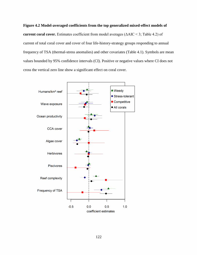
122

Figure 4.2 Model-averaged coefficients from the top generalized mixed-effect models of

current coral cover. Estimates coefficient from model averages (ΔAIC < 3; Table 4.2) of

current of total coral cover and cover of four life-history-strategy groups responding to annual

frequency of TSA (thermal-stress anomalies) and other covariates (Table 4.1). Symbols are mean

values bounded by 95% confidence intervals (CI). Positive or negative values where CI does not

cross the vertical zero line show a significant effect on coral cover.

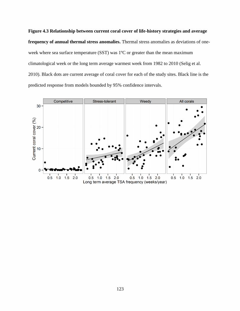
123

Figure 4.3 Relationship between current coral cover of life-history strategies and average

frequency of annual thermal stress anomalies. Thermal stress anomalies as deviations of one-

week where sea surface temperature (SST) was 1ºC or greater than the mean maximum

climatological week or the long term average warmest week from 1982 to 2010 (Selig et al.

2010). Black dots are current average of coral cover for each of the study sites. Black line is the

predicted response from models bounded by 95% confidence intervals.

124

Figure 4.4 Non-metric multidimensional scaling ordination of coral species abundance on

the frequency of thermal stress anomalies. Scleractinian coral species are divided in three life-

history strategies separated from hydrocorals. Circle size is proportional to the average of

absolute cover of each species across sites. Average frequency of thermal stress anomalies (TSA)

are isolines with numbers (weeks/year). Only the most abundant species are labeled. For species

codes refer to Table S4.2.

125

Table 4.1 Description of variables used as predictors in the generalized linear mixed-effect

models (GLMMs). Each variable is known to potentially influence current coral cover across

the study sites. *See supplementary methods for a detailed description of each variable and

reasoning for usage.

Variable name Range Units Source

Anthropogenic

Humans per reef area 0.4 4314.1 #/km2 reef World Gridded Population*

Cultivated land within 50 km 0 3917 km2 Global Land Cover 2010*

Physical

Thermals stress anomalies (TSA) 0.2 2.4 frequency CorTAD v.4*

Net primary productivity 203 1610 mg C m-2

day-1

Aqua MODIS*

Wave exposure (log) 3.9 7.9 J m-3

Caribbean wave exposure*

Reef structural complexity 1.5 5 # In situ estimations*

Biotic

Macroalgae cover 6.2 71.2 % In situ measurements/video

Crustose coralline algae cover 0 17.2 % In situ measurements/video

Turf algae cover 1.3 55.7 % In situ measurements/video

Herbivore fish biomass 14.1 210.1 g m-2

In situ measurements*

Piscivore fish biomass 3.6 441.0 g m-2

In situ measurements*

126

Table 4.2 Relative importance of explanatory variables from the top GLMMs of logit

transformed percentage cover from competitive, stress-tolerant, weedy, and all corals

species. Relative importance is the sum of the weights of all models that contain that particular

variable. Top models were chosen for ΔAICc < 3, where ΔAIC c is the difference in AICc values

between model i and the best model considered. Weights is the probability of model i being the

best of the set. Range of the model summary parameters (df, logLik, AICc) are shown for each

coral group.

Competitive Stress-

tolerant Weedy All corals

Frequency of TSA 0.11 1.00 1.00 1.00

Algae cover 0.05 1.00 1.00 1.00

Reef complexity 1.00 0.72 1.00 0.91

Wave exposure 0.13 0.19 0.14 0.68

Piscivore biomass 0.77 0.13 0.12 0.67

Herbivore biomass 0.05 0.10 1.00 0.23

Humans/km2

reef 0.29 0.41 0.14 0.16

Ocean productivity 0.13 0.55 0.15 0.13

CCA cover 0.16 0.16 0.12 0.08

Degree of freedom 4-7 5-9 7-8 6-10

logLik (-125.6,

-127.7)

(-1021.8,

-1025.7)

(-1218.3,

-1218.5)

(-1344.7,

-1348.7)

AICc (262.4-

265.4)

(2059.9,

2062.7)

(2451.4,

2453.1)

(2707.1,

2709.9)

ΔAIC c (ΔAIC < 3) 0.0-2.99 0.0-2.89 0.0-2.04 0.0-2.92

Weights 0.03-0.15 0.02-0.08 0.12-0.33 0.03-0.13

Number of top models 17 28 6 19

127

APPENDIX 1: SUPPLEMENTARY MATERIAL FOR CHAPTER 1

Table S1.1 Study sites, site codes, regions and, protection level. Habitat type, S&G: Spur and

Grove; Protection level, NTZ: No-take zone, MPA: marine protected area. Date of survey is

month and year(s).

Site name Site

code

Habitat

type

Depth

(m)

Date of

survey

Latitude Longitude Protection

level

MR

year

Mesoamerican Barrier, Mexico

Cancún GH S & G 12 Jul 12 21.02544 -86.7713 none

Cozumel North PB S & G 10 Jul 12 20.47188 -86.9815 NTZ 1996

Akumal XA S & G 15 Jul 12 20.42689 -87.2860 none

Cozumel South CR S & G 15 Jul 12 20.31961 -87.0266 NTZ 1996

Chinchorro North BCN S & G 15 Jul 12 18.74867 -87.3476 MPA 1996

Chinchorro Central BCC S & G 15 Jul 12 18.57457 -87.4198 MPA 1996

Chinchorro South BCS S & G 15 Jul 12 18.41008 -87.4169 MPA 1966

Mesoamerican Barrier, Belize

Bacalar Chico BC S & G 12-15 May 10/12 18.16282 -87.82222 NTZ 1996

Mexico Rocks MR S & G 12-15 May 10/12 17.98782 -87.90382 none

Tackle Box TB S & G 12-15 May 10/12 17.91056 -87.95083 none

Hol Chan HC S & G 12-15 May 10/12 17.86343 -87.97238 NTZ 1987

Gallows GA S & G 12-15 May 10/12 17.49592 -88.04255 none

Calabash Caye CA S & G 12-15 May 10/12 17.26147 -87.81970 none

Half Moon Caye HM S & G 12-15 May 10/12 17.20560 -87.54679 NTZ 1982

Alligator Caye AL S & G 12-15 May 10/12 17.19660 -88.05115 none

Tobacco Caye TO S & G 12-15 May 10/12 16.91911 -88.04757 none

South Water Caye SW S & G 12-15 May 10/12 16.81346 -88.07756 MPA 1996

Middle Caye MC S & G 12-15 May 10/12 16.73703 -87.80536 MPA 1993

South Middle Caye SM S & G 12-15 May 10/12 16.72875 -87.82867 MPA 1993

Pampion Caye PO S & G 12-15 May 10/12 16.37310 -88.08913 none

Ranguana Caye RA S & G 12-15 May 10/12 16.28501 -88.15031 none

Southwest Caye ST S & G 12-15 May 10/12 16.11247 -88.27107 none

Nicholas Caye NI S & G 12-15 May 10/12 16.11230 -88.25586 MPA 2003

Dry Tortugas, USA LG S & G 12 Jun 12 24.68508 -82.91050 NTZ 1992

Bay of Pigs, Cuba

Cueva Peces CP Slope 10-12 Jun 10/12 22.16627 -81.13827 none

Punta Perdiz PZ Slope 10-12 Jun 10/12 22.11003 -81.11626 none

Ebano EB Slope 10-12 Jun 10 22.07914 -81.07599 none

Brinco BR Slope 10-12 Jun 12 22.06939 -81.05588 none

Bacunayagua, Cuba BC Slope 10-12 Jun 12 23.14653 -81.66664 none

Jardines de la Reina, Cuba

El Peruano EP Slope 10-12 Jun 11 20.84411 -79.02166 NTZ 1996

Pipin PP S & G 12-15 Jun 11 20.82586 -78.98026 NTZ 1996

Anclita AN Slope 10-12 Jun 11 20.78697 -78.94317 NTZ 1996

Cueva Pulpo CF Slope 10-12 Jun 11 20.75266 -78.83634 NTZ 1996

Abaco, Bahamas

Guana Cay GC S & G 10-12 Jul 11/12 26.70967 -77.15408 none

Fowls Cay FC Slope 10 Jul 11/12 26.63717 -77.03848 NTZ 2009

Man o’ War MW S & G 10-12 Jul 11/12 26.62122 -77.00550 none

Pelican Cay PC Slope 10 Jul 11/12 26.39783 -76.98850 NTZ 1972

Little Harbor LH S & G 10-12 Jul 11/12 26.32390 -76.99160 none

Rocky Point RP Slope 10-12 Jul 11/12 25.99661 -77.40092 Remote

128

Table S1.2 Fish trophic guilds, species taxonomic information, and allometric parameters

used to calculate biomass.

Trophic Group Family Common Name Species Name a b

Apex predator Carangidae Greater Amberjack Seriola dumerili 0.0325 2.870

Apex predator Carangidae Almaco Jack Seriola rivoliana 0.0122 2.957

Apex predator Carcharhinidae Silky Shark Carcharhinus falsiformis 0.0101 3.060

Apex predator Carcharhinidae Blacktip Shark Carcharhinus limbatus 0.0061 3.010

Apex predator Carcharhinidae Reef Shark Carcharhinus perezi 0.0271 3.000

Apex predator Carcharhinidae Lemon shark Negaprion brevirostris 0.0053 3.160

Apex predator Elopidae Tarpon Megalops atlanticus 0.0120 2.984

Apex predator Lutjanidae Cubera Snapper Lutjanus cyanopterus 0.0152 3.060

Apex predator Muraenidae Green Moray Gymnothorax funebris 0.0041 2.856

Apex predator Rhincodontidae Nurse Shark Ginglymostoma cirratum 0.0105 2.892

Apex predator Scombridae Cero Scomberomorus regalis 0.0202 2.800

Apex predator Serranidae Black Grouper Mycteroperca bonaci 0.0082 3.140

Apex predator Serranidae Yellowmouth Grouper Mycteroperca interstitialis 0.0141 3.000

Apex predator Serranidae Tiger Grouper Mycteroperca tigris 0.0094 3.120

Apex predator Serranidae Yellowfin Grouper Mycteroperca venenosa 0.0122 3.000

Apex predator Sphyraenidade Great Barracuda Sphyraena barracuda 0.0070 2.972

Pisc/Invertivore Aulostomidae Trumpetfish Aulostomus maculatus 0.0040 2.866

Pisc/Invertivore Belonidae Houndfish Tylosurus crocodilus 0.0008 3.205

Pisc/Invertivore Bothidae Peacock Flounder Bothus lunatus 0.0098 3.189

Pisc/Invertivore Carangidae Bar Jack Carangoides ruber 0.0180 2.990

Pisc/Invertivore Carangidae Blue Runner Caranx crysos 0.0318 2.949

Pisc/Invertivore Carangidae Crevalle Jack Caranx hippos 0.0329 2.855

Pisc/Invertivore Carangidae Horse Eye Jack Caranx latus 0.0186 2.856

Pisc/Invertivore Carangidae Palometa Trachinotus goodei 0.0204 3.000

Pisc/Invertivore Carangidae Yellow Jack Caranx bartholomaei 0.0259 2.908

Pisc/Invertivore Centropomidae Common Snook Centropomus undecimalis 0.0104 2.910

Pisc/Invertivore Dasyatidae Southern Stingray Dasyatis americana 0.0739 2.810

Pisc/Invertivore Haemulidae Sailors Choice Haemulon parra 0.0199 2.993

Pisc/Invertivore Haemulidae White Grunt Haemulon plumieri 0.0259 3.000

Pisc/Invertivore Lutjanidae Mutton Snapper Lutjanus analis 0.0146 3.034

Pisc/Invertivore Lutjanidae Schoolmaster Lutjanus apodus 0.0189 3.000

Pisc/Invertivore Lutjanidae Gray Snapper Lutjanus griseus 0.0240 2.910

Pisc/Invertivore Lutjanidae Dog Snapper Lutjanus jocu 0.0198 2.960

Pisc/Invertivore Lutjanidae Mahogany Snapper Lutjanus mahogoni 0.0428 2.719

Pisc/Invertivore Lutjanidae Lane Snapper Lutjanus synagris 0.0216 2.917

Pisc/Invertivore Lutjanidae Yellowtail Snapper Ocyurus chrysurus 0.0314 2.793

Pisc/Invertivore Scombridae King Mackerel Scomberomorus caballa 0.0091 2.960

Pisc/Invertivore Scorpinadae Lionfish Pterois volitans 0.0050 3.291

Pisc/Invertivore Serranidae Graysby Cephalopholis cruentata 0.0121 3.082

Pisc/Invertivore Serranidae Coney Cephalopholis fulva 0.0188 2.973

Pisc/Invertivore Serranidae Rock Hind Epinephelus adscensionis 0.0125 3.224

Pisc/Invertivore Serranidae Red Hind Epinephelus guttatus 0.0084 3.100

Pisc/Invertivore Serranidae Jewfish Epinephelus itajara 0.0131 3.056

Pisc/Invertivore Serranidae Red Grouper Epinephelus morio 0.0162 2.990

Pisc/Invertivore Serranidae Nassau Grouper Epinephelus striatus 0.0065 3.229

Pisc/Invertivore Serranidae Greater Soapfish Rypticus saponaceus 0.0010 1.000

Pisc/Invertivore Serranidae Shy Hamlet Hypoplectrus guttavarius 0.0090 3.040

Pisc/Invertivore Serranidae Indigo Hamlet Hypoplectrus indigo 0.0110 3.182

129

Pisc/Invertivore Serranidae Black Hamlet Hypoplectrus nigricans 0.0110 3.182

Pisc/Invertivore Serranidae Barred Hamlet Hypoplectrus puella 0.0090 3.040

Pisc/Invertivore Serranidae Butter Hamlet Hypoplectrus unicolor 0.0090 3.040

Pisc/Invertivore Sphyraenidade Southern Sennet Sphyraena picudilla 0.0067 2.942

Macroinvertivore Balistadae Queen Triggerfish Balistes vetula 0.0354 2.900

Macroinvertivore Balistadae Ocean Triggerfish Canthidermis sufflamen 0.0217 3.000

Macroinvertivore Carangidae Permit Trachinotus falcatus 0.0301 2.958

Macroinvertivore Echeneidae Sharksucker Echeneis naucrates 0.0010 3.290

Macroinvertivore Ephippidae Atlantic Spadefish Chaetodipterus faber 0.0530 2.952

Macroinvertivore Gerreidae Yellowfin Mojarra Gerres cinereus 0.0184 3.084

Macroinvertivore Haemulidae Black Margate Anisotremus surinamensis 0.0233 3.010

Macroinvertivore Haemulidae Porkfish Anisotremus virginicus 0.0148 3.167

Macroinvertivore Haemulidae White Margate Haemulon album 0.0144 3.070

Macroinvertivore Haemulidae Tomtate Haemulon aurolineatum 0.0120 3.100

Macroinvertivore Haemulidae Caesar Grunt Haemulon carbonarium 0.0147 3.056

Macroinvertivore Haemulidae Smallmouth Grunt Haemulon chrysargyreum 0.0106 3.047

Macroinvertivore Haemulidae French Grunt Haemulon flavolineatum 0.0232 3.000

Macroinvertivore Haemulidae Spanish Grunt Haemulon macrostomum 0.0176 3.060

Macroinvertivore Haemulidae Cottonwick Haemulon melanurum 0.0226 2.953

Macroinvertivore Haemulidae Bluestriped Grunt Haemulon sciurus 0.0194 2.999

Macroinvertivore Haemulidae Striped Grunt Haemulon striatum 0.0175 3.099

Macroinvertivore Holocentridae Squirrelfish Holocentrus adscensionis 0.0216 3.000

Macroinvertivore Holocentridae Longspine Squirrelfish Holocentrus rufus 0.0170 3.000

Macroinvertivore Holocentridae Blackbar Soldierfish Myripristis jacobus 0.1110 2.720

Macroinvertivore Holocentridae Longjaw Squirrelfish Neoniphon marianus 0.0215 3.000

Macroinvertivore Labridae Spanish Hogfish Bodianus rufus 0.0145 3.053

Macroinvertivore Labridae Slippery Dick Halichoeres bivittatus 0.0105 3.093

Macroinvertivore Labridae Yellowhead Wrasse Halichoeres garnoti 0.0052 3.375

Macroinvertivore Labridae Clown Wrasse Halichoeres maculipinna 0.0028 3.693

Macroinvertivore Labridae Rainbow Wrasse Halichoeres pictus 0.0052 3.375

Macroinvertivore Labridae Puddingwife Halichoeres radiatus 0.0131 3.038

Macroinvertivore Labridae Hogfish Lachnolaimus maximus 0.0237 2.950

Macroinvertivore Labridae Bluehead Thalassoma bifasciatum 0.0101 3.040

Macroinvertivore Malacanthidae Sand Tilefish Malacanthus plumieri 0.0001 2.680

Macroinvertivore Myliobatidae Spotted Eagle Ray Aetobatus narinari 0.0059 3.130

Macroinvertivore Ostracidae Honeycomb Cowfish Acanthostracion polygonius 0.0178 3.083

Macroinvertivore Pomacanthidae Blue Angelfish Holacanthus bermudensis 0.0319 2.899

Macroinvertivore Pomacanthidae Queen Angelfish Holacanthus ciliaris 0.0337 2.900

Macroinvertivore Priacanthidae Glasseye Snapper Heteropriacanthus cruentatus 0.0188 3.000

Macroinvertivore Serranidae Harlequin Bass Serranus tigrinus 0.0145 3.048

Macroinvertivore Sparidae Saucereye Porgy Calamus calamus 0.0125 3.180

Macroinvertivore Sparidae Sheepshead Porgy Calamus penna 0.0764 2.666

Macroinvertivore Tetraodontidae Bandtail Puffer Sphoeroides spengleri 0.0235 3.050

Microinvertivore Chaetodontidae Foureye Butterflyfish Chaetodon capistratus 0.0220 3.190

Microinvertivore Chaetodontidae Spotfin Butterflyfish Chaetodon ocellatus 0.0318 2.984

Microinvertivore Chaetodontidae Banded Butterflyfish Chaetodon striatus 0.0220 3.140

Microinvertivore Gobiidae Neon Goby Elacatinus oceanops 0.0080 3.137

Microinvertivore Grammatidae Fairy Basslet Gramma loreto 0.0001 1.111

Microinvertivore Grammatidae Blackcap Basslet Gramma melacara 0.0001 1.111

Microinvertivore Monacanthidae Whitespotted Filefish Cantherhines macrocerus 0.0561 2.653

Microinvertivore Mullidae Yellow Goatfish Mulloidichthys martinicus 0.0110 3.092

Microinvertivore Mullidae Spotted Goatfish Pseudupeneus maculatus 0.0150 3.157

Microinvertivore Sciaenidae Jackknife Fish Equetus lanceolatus 0.0011 3.844

Microinvertivore Sciaenidae Spotted Drum Equetus punctatus 0.0153 3.062

Planktivore Labridae Creole Wrasse Clepticus parrae 0.0145 3.053

130

Planktivore Pomacentridae Blue Chromis Chromis cyanea 0.0188 3.000

Planktivore Pomacentridae Brown Chromis Chromis multilineata 0.0262 2.753

Large Omnivore Balistadae Black Durgon Melichthys niger 0.0217 3.000

Large Omnivore Pomacanthidae Rock Beauty Holacanthus tricolor 0.0203 3.126

Large Omnivore Pomacanthidae Gray Angelfish Pomacanthus arcuatus 0.0203 3.126

Large Omnivore Pomacanthidae French Angelfish Pomacanthus paru 0.0203 3.126

Small Omnivore Monacanthidae Scrawled Filefish Aluterus scriptus 0.0022 3.000

Small Omnivore Monacanthidae Orangespotted Filefish Cantherhines pullus 0.0684 2.563

Small Omnivore Pomacentridae Sergeant Major Abudefduf saxatilis 0.0227 3.142

Small Omnivore Pomacentridae Dusky Damselfish Stegastes adustus 0.0384 3.010

Small Omnivore Pomacentridae Beaugregory Stegastes leucostictus 0.0303 2.887

Small Omnivore Pomacentridae Threespot Damselfish Stegastes planifrons 0.0379 2.857

Small Omnivore Pomacentridae Cocoa Damselfish Stegastes variabilis 0.0324 2.836

Small Omnivore Tetraodontidae Sharpnose Puffer Canthigaster rostrata 0.0323 2.953

Herbivore Acanthuridae Ocean Surgeonfish Acanthurus bahianus 0.0236 2.975

Herbivore Acanthuridae Doctorfish Acanthurus chirurgus 0.0225 3.000

Herbivore Acanthuridae Blue Tang Acanthurus coeruleus 0.0305 3.000

Herbivore Blennidae Redlip Blenny Ophioblennius atlanticus 0.0324 2.379

Herbivore Kyphosidae Bermuda Chub Kyphosus saltatrix 0.0174 3.080

Herbivore Pomacentridae Yellowtail Damselfish Microspathodon chrysurus 0.0239 3.082

Herbivore Pomacentridae Longfin Damselfish Stegastes diencaeus 0.0353 2.896

Herbivore Pomacentridae Bicolor Damselfish Stegastes partitus 0.0182 3.152

Herbivore Scaridae Midnight Parrotfish Scarus coelestinus 0.0153 3.062

Herbivore Scaridae Blue Parrotfish Scarus coeruleus 0.0124 3.111

Herbivore Scaridae Rainbow Parrotfish Scarus guacamaia 0.0155 3.063

Herbivore Scaridae Striped Parrotfish Scarus iserti 0.0158 3.052

Herbivore Scaridae Princess Parrotfish Scarus taeniopterus 0.0177 3.000

Herbivore Scaridae Queen parrotfish Scarus vetula 0.0158 3.052

Herbivore Scaridae Greenblotch Parrotfish Sparisoma atomarium 0.0122 3.028

Herbivore Scaridae Redband Parrotfish Sparisoma aurofrenatum 0.0129 3.110

Herbivore Scaridae Redtail Parrotfish Sparisoma chrysopterum 0.0135 3.100

Herbivore Scaridae Bucktooth Parrotfish Sparisoma radians 0.0179 3.035

Herbivore Scaridae Redfin Parrotfish Sparisoma rubripinne 0.0194 3.000

Herbivore Scaridae Stoplight Parrotfish Sparisoma viride 0.0250 2.921

131

Table S1.3 Summary of preliminary, anthropogenic, physical, biotic, and management-

related predictors used in the analysis. For a detailed description of each variable see

Appendix 1.1.

Variable name Range Units Source

Anthropogenic

Coastal Development in 50km 0-26470 light pixels Suomi NPP satellite a

Humans within 50 km 54-67140 # World Gridded Population b

Humans of closest town 0-628300 # Country census

Distance to population centers 1.6-115.8 km Calculated in ArcGIS 10

Cultivated land within 50 km 0-3917 km2 Global Land Cover 2000

c

Physical

Net primary productivity 203-1610 mg C m-2

day-1

Aqua MODIS

Sea surface temperature (SST) 26.0-29.3 ºC AHVRR Pathfinder v5.2

Minimum SST 20.8-26.5 ºC AHVRR Pathfinder v5.2

Wave exposure (log) 3.9-7.9 J m-3

(Chollett et al. 2012)

Depth 10-16 meters In situ measurements

Reef structural complexity 1.5-5 # In situ estimations

Distance to deep water 0.03-32.9 km NOAA bathymetry charts

Distance to tide channels 0.4-6.0 km Calculated in ArcGIS 10

Distance to mangrove 0.34-31.9 km Calculated in ArcGIS 10

Reef area within 5 km 0.1-25.9 km2 Global Coral Reef 2010

d

Reef area within 10 km 0.4-43.1 km2 Global Coral Reef 2010

Biotic

Mangrove perimeter in 5 km 0-175.6 km Global Mangrove 2011e

Mangrove perimeter in 10 km 0-406.10 km Global Mangrove 2011

Live coral cover 1.5-31.6 % In situ measurements/video

Macroalgae cover 6.2-71.2 % In situ measurements/video

Gorgonian cover 0-17.2 % In situ measurements/video

Fish biomass (lower trophic) 3.5-441.0 g m-2

In situ measurements

Management regime

Protection level None, MPA, NTZ categorical Reef Base

Reserve size 7.8-2170 km2 Reef Base

Reserve age 3-40 years Reef Base

Poaching level low, high categorical Reef Base, Interviews

a Suomi NPP satellite global at 750 m resolution available at NASA Earth Observatory (Black Marble)

b Gridded Population of the World V.3 at 0.25 degree resolution estimated for 2010

c Global Land Cover 2000 database

d Global Distribution of Coral Reef 2010 database from Ocean Data Viewer UNEP-WCMC

e Global Distribution of Mangroves USGS 2011 database from the Ocean Data Viewer UNEP-WCMC

132

Appendix 1.1 Detailed descriptions of covariates

Human population density

We considered three measures of human effects based on population size: 1) humans

within 50 km (maximum number of people that occurred within 50-km radius of each site); 2)

number of humans in the nearest population center (indicator of spatially immediate human

pressure); and 3) distance to nearest population centers (indicator of long-distance effects,

calculated from each site to the center of nearest population settlements). We chose 50 km as

radius for the first measured variable because it is a reasonable range of anthropogenic influence

on Caribbean reefs (Mora, 2008). Projection estimates of human population counts for the year

2010 were obtained from the Gridded Population of the World V.3 at 0.25 degree resolution

(SEDAC, 2010) and calculated in ArcGIS v10.0.

Coastal Development

This variable quantified the use of electrical power measured as the intensity of the

Earth’s city lights at night within 50 km radius of each site. Power infrastructure can be used as a

proxy of coastal development which is a good surrogate for fishing pressure (Sanderson et al.

2002). Light intensity was calculated as the sum of pixel values that corresponded to city and

town lights within the interest area. We used the high resolution (750 m) composite map of the

world assembled from data acquired by the Suomi NPP satellite global available at NASA Earth

Observatory (http://earthobservatory.nasa.gov/Features/NightLights/page3.php). All calculations

were performed in ArcGIS v10.0.

133

Cultivated land

We quantified the area of cultivated land that occurred within a 50 km radius of each reef

site. The raster data for this variable was obtained from the Global Land Cover 2000 database

(GLC 2003). Specifically, we used the regional dataset (North and Central America) that depicts

the spatial distribution of 29 different land attributes for the year 2000 as calculated from satellite

images at 1 km resolution. Cultivated land could be a surrogate of terrestrial run-offs with

potential effects on macroalgae cover when herbivory is reduced (McCook 1999). Additionally

sediment derived from agriculture may alter predator-prey interactions in coral reef fish and

compromise planktivores feeding efficiency (Wenger et al. 2013). Spatial analyses were

performed in ArcGIS v10.

Marine Reserve size, age, and poaching level

In this study we only considered marine reserves where fishing was not allowed, at least

in theory (i.e. no-take areas). We assessed three variables that together describe some degree of

protection effectiveness for reef sites inside marine reserves (Mora et al. 2006). These variables

were reserve size, years since the establishment (reserve age) and poaching level. Reserve size

and age can positively influence fish communities, as in general, older and larger reserves tend to

accumulate relative more fish biomass than younger and smaller reserves (Côté et al. 2001,

Halpern 2003, Claudet et al. 2008, Babcock et al. 2010). In contrast, poaching can directly affect

fish abundance and undermine the protection efforts particularly when reserves are small (Kritzer

2004). Poaching levels inside the reserve was classified as “low” or “high” based on interviews

with park managers and regular users such as dive shops (method modified from Mora et al.

134

2006). We assumed that poaching inevitable exist in each reserve, thus a range of low to high

was established based on a 5 point scale for which 1-2 was low while 3-5 was high.

Reef Area

Reef areas within 5 km and 10 km radius of each site was calculated from the Global

Distribution of Coral Reefs (2010) database as available at the Ocean Data Viewer United

Nations Environment Program's World Conservation Monitoring Centre (UNEP-WCMC)

(http://data.unep-wcmc.org/datasets/13). This database represents the global distribution of warm

water coral reefs compiled mostly from the Millennium Coral Reef Mapping Project validated

and un-validated maps as well as other sources acquired by UNEP-WCMC. Reef areas within

the interest region were calculated in ArcGIS v10.0.

Reef structural complexity

For each transect set we visually estimated structural reef complexity on a scale of 0-5,

where 0 was given to reefs with no vertical relief; 1, low and sparse relief; 2, low but widespread

relief; 3, moderately complex relief; 4, very complex relief with numerous caves and fissures;

and 5, reefs with exceptionally complex habitats, with numerous caves and overhangs (Polunin

and Roberts 1993). This topographic measure provided an assessment of reef complexity at the

seascape level which is relevant to large and medium-sized fish (Polunin and Roberts 1993,

Wilson et al. 2007). To minimize estimation subjectivity among observers, at least two divers

estimated reef structural complexity for each transect set and the average was calculated to be

used in the models. We evaluated the accuracy of the estimations among observers by comparing

135

the standard deviations (SD) among transects per site and found that SDs were 0-0.7 in all cases,

meaning that average estimation differences were never over 1 unit.

Mangrove Perimeter

Mangrove abundance was quantified as the perimeter covered by mangrove within 5 km

and 10 km radius of each site. Estimates of Caribbean mangrove distribution were obtained from

the Global Distribution of Mangroves USGS (2011) database as available at the Ocean Data

Viewer UNEP-WCMC (http://data.unep-wcmc.org/datasets/21). This database depicts the

distributions of global mangroves based on Global Land Survey data and Landsat images.

Landsat images (30 m resolution) were interpreted using unsupervised and supervised digital

image classification techniques. Each image was atmospherically corrected, ground truth and

validated with existing maps and databases.

Net primary productivity

We calculated mean oceanic net primary productivity (mg C m-2

day-1

) for each site

between 2002 and 2012 using remote-sensing. This was obtained from Aqua MODIS satellite

monthly data combined in the vertical generalized production model (Behrenfeld and Falkowski

1997) at a spatial resolution of 0.0833º (Oregon State University 2013). We used the mean of the

last ten years period because primary productivity is inherently variable in time and established

predatory communities may respond better to long term trends in primary productivity than to

survey year or monthly mean values. Calculations were performed in ArcGIS 10.0.

136

Sea surface temperature

We used AHVRR Pathfinder Version 5.2 (PFV5.2) satellite data obtained from the US

National Oceanographic Data Center and GHRSST (NOAA 2013). The PFV5.2 data are an

updated version of the Pathfinder Version 5.0 and 5.1 collections described in Casey et al.

(2010). We calculated average monthly sea surface temperature (SST, 2002-2011) for each

source 4 km2 grid cell that corresponded to each reef site. We also calculated mean minimum

monthly SST by selecting the lowest monthly average temperature per year to compute an

average across years. Mean minimum monthly SST could be a better predictor of physiological

constrains of some fish predator species (Jennings et al. 2008, Nadon et al. 2012). We used mean

temperature of nine years because it may represent better the temperature regimen these top

consumers experience overtime. All calculations were performed in ArcGIS 10.0.

Wave exposure

The log of wind driven wave exposure (J m-3

) was extracted in ArchGIS 10.0 from the

wave stress map for the Caribbean basin built by Chollett et al. (2012) and available at

(http://www.marinespatialecologylab.org/wp-content/uploads/2010/11/PECS1.png). This index

does not include the influence of tides or swells, which are not generated by local wind, and it is

an approximation of wave patterns in shallow areas (Chollett et al. 2012). Wave exposure has

been a good predictor of spatial variation in reef building corals such as Orbicella sp. (former

Montastrea sp.) (Chollett and Mumby 2012) and can partially explain beta diversity patterns of

benthic communities (Harborne et al. 2011). Wave exposure may also directly affect the biomass

and diversity of tropical reef fish (Friedlander et al. 2003) and the distribution and abundance of

temperate reef fish by compromising swimming abilities (Fulton and Bellwood 2004).

137

Alternatively, by modifying the distribution of foundation species like corals, wave exposure

could affect fish species that depend on them. The detailed description of the wave exposure

calculations and assumptions can be found in Chollett & Mumby (2012).

Benthic cover

Percent cover data of benthic communities by categories (i.e. coral by species, algae by

genus or functional groups, gorgonians, sponges, and other) were measured at each site using

point intercepts in 6-8 transect lines (10 m long) (Lang et al. 2010) and/or in 6-8 video transects

(50 m long) (Carleton and Done 1995). Point intercept transects (PITs) were used at the Belize

sites, while both PITs and video transects were used at the rest of the sites. Both methods

provided similar accuracy and results in estimating benthic cover categories in our study. Each

benthic transect corresponded to a fish transect set. To estimate percent cover, 100 points per

transect was used in PITs (Lang et al. 2010), while ~600 points were extracted from each video

transect (Carleton and Done 1995). As model predictors we only used live coral, fleshy algae,

and gorgonian cover as they provide physical structure that may affect small and medium size

fish predators (Alvarez-Filip et al. 2011).

References

See references in Appendix 1.5

138

Table S1.4 Spearman’s rank (rs) order correlation matrix for response and explanatory

variables. Bold values are correlations rs > 0.50. Upper matrix panel are correlations within

marine reserves. Lower matrix corresponds to values for all sites. Number codes are: apex

predator (1), piscivore-invertivore (2), herbivore (3), omnivore (4), invertivore (5), planktivore

(6), mangrove within 5 km (7), mangrove within 10 km (8), coral cover (9), algae cover (10),

gorgonian cover (11), net primary productivity (12), sea surface temperature (13), minimum sea

surface temperature (14), wave exposure (15), depth (16), reef structural complexity (17),

distance to deep water (18), distance to channels (19), distance to mangrove (20), reef area

within 5 km (21), reef area within 10 km (22), coastal development within 50 km (23), number

of humans within 50 km (24), number of humans in the closest town (25), minimum distance to

closest town (26), area of cultivate land within 50 km (27), reserve age (28), reserve size (29).

Note that reserve age and size are only applicable to sites within reserves.

139

Table S1.4

1 2 3 4 5 6 7 8 9 10 11 12 13 14 15 16 17 18 19 20 21 22 23 24 25 26 27 28 29

1

0.38 0.02 0.10 0.10 0.05 0.29 0.25 0.07 0.12 0.16 0.29 0.11 -0.12 -0.16 -0.04 0.26 -0.08 0.12 -0.33 -0.04 0.03 -0.40 -0.39 -0.36 0.39 -0.49 0.08 0.32

2 0.35

0.26 0.31 0.42 0.18 0.03 -0.03 -0.02 -0.06 0.07 0.10 -0.04 -0.06 -0.35 0.08 0.21 -0.27 0.28 -0.12 0.10 0.14 -0.24 -0.30 -0.28 0.32 -0.19 0.16 0.46

3 0.16 0.36

0.02 0.22 0.08 -0.16 -0.20 0.00 -0.46 0.07 -0.19 -0.50 -0.36 -0.09 -0.39 0.31 0.15 0.28 0.05 -0.40 -0.24 -0.06 -0.25 0.04 -0.12 -0.15 0.20 -0.23

4 0.07 0.24 0.18

0.29 0.33 0.06 0.00 0.06 -0.14 -0.17 -0.18 0.14 0.34 -0.41 0.35 -0.01 -0.54 0.29 -0.14 0.00 -0.10 0.22 0.17 0.11 -0.03 0.15 0.07 0.34

5 0.18 0.37 0.35 0.25

0.31 -0.16 -0.21 0.03 -0.24 0.04 -0.15 -0.14 0.18 -0.37 0.10 0.07 -0.30 0.33 0.00 0.14 0.12 -0.02 -0.08 -0.19 0.14 -0.03 -0.08 0.26

6 0.06 0.25 0.16 0.28 0.22

-0.01 -0.03 0.24 -0.07 -0.05 -0.21 0.07 0.23 -0.13 0.19 0.21 -0.30 0.15 -0.10 -0.04 -0.05 0.10 0.11 0.02 -0.08 0.11 0.01 -0.03

7 0.21 0.05 -0.03 -0.02 -0.05 -0.11

0.97 0.52 0.38 0.14 0.46 0.61 -0.27 -0.21 0.04 0.02 0.08 -0.30 -0.89 -0.32 -0.38 -0.44 -0.30 0.00 0.24 -0.32 -0.04 0.28

8 0.15 0.04 -0.01 -0.05 -0.10 -0.08 0.93

0.53 0.43 0.13 0.47 0.67 -0.28 -0.14 -0.01 -0.07 0.19 -0.47 -0.79 -0.35 -0.39 -0.42 -0.27 0.01 0.15 -0.27 -0.13 0.19

9 -0.09 -0.07 -0.15 0.03 -0.04 0.05 0.21 0.26

-0.02 -0.08 0.00 0.38 0.04 -0.24 0.06 0.28 -0.07 -0.25 -0.58 -0.18 -0.21 -0.31 -0.01 -0.12 0.08 -0.22 -0.30 -0.01

10 -0.13 -0.20 -0.29 -0.03 -0.16 -0.19 0.19 0.06 -0.10

-0.06 0.50 0.59 0.12 0.21 0.22 -0.12 0.03 -0.50 -0.27 0.16 0.17 -0.17 -0.10 -0.09 0.16 0.05 0.07 0.17

11 0.14 0.05 0.07 -0.02 0.08 0.04 0.08 0.00 -0.20 0.02

0.48 -0.17 -0.44 0.00 -0.22 -0.26 0.38 0.18 -0.04 0.05 0.17 -0.53 -0.67 -0.40 0.47 -0.43 0.05 0.29

12 0.04 -0.04 -0.22 0.05 -0.02 -0.07 0.04 -0.02 0.17 0.31 0.14

0.43 -0.25 0.27 0.06 -0.25 0.24 -0.17 -0.28 0.24 0.41 -0.64 -0.71 -0.46 0.66 -0.38 0.42 0.55

13 -0.26 -0.32 -0.37 0.04 -0.23 -0.08 -0.10 0.00 0.31 0.17 -0.23 0.29

0.38 0.06 0.44 -0.17 -0.30 -0.45 -0.47 0.17 0.08 -0.13 0.10 -0.08 0.17 0.05 -0.02 0.38

14 -0.28 -0.27 -0.35 0.11 -0.10 0.00 -0.17 -0.13 0.27 0.14 -0.26 0.18 0.61

-0.01 0.71 0.08 -0.79 0.08 0.07 0.50 0.36 0.39 0.59 -0.07 -0.03 0.30 -0.08 0.20

15 0.00 -0.10 0.01 -0.20 -0.10 -0.23 0.00 -0.15 -0.29 0.24 0.25 -0.17 -0.28 -0.26

-0.20 -0.26 0.36 -0.13 0.40 0.08 0.21 0.03 0.08 0.00 -0.05 0.00 0.22 -0.38

16 -0.12 -0.17 -0.35 0.15 -0.05 0.04 0.00 -0.15 0.10 0.27 -0.06 0.14 0.32 0.48 0.00

0.05 -0.65 -0.03 -0.11 0.52 0.39 0.21 0.28 -0.02 0.15 0.38 0.11 0.45

17 0.28 0.37 0.25 -0.02 0.11 0.29 0.13 0.15 0.22 -0.33 0.00 -0.19 -0.21 -0.27 -0.20 -0.15

-0.34 0.12 -0.34 -0.05 0.03 -0.22 -0.05 -0.25 0.15 -0.31 0.09 -0.10

18 0.11 -0.02 0.14 -0.18 -0.08 -0.28 0.28 0.21 -0.10 0.15 0.27 -0.02 -0.33 -0.50 0.49 -0.18 -0.07

-0.41 0.19 -0.38 -0.25 -0.22 -0.35 0.13 -0.18 -0.10 -0.16 -0.48

19 0.06 0.06 0.14 0.00 0.04 -0.17 0.07 0.04 -0.18 -0.02 0.16 -0.29 0.03 0.06 0.14 -0.20 -0.11 0.14

0.12 0.07 0.08 0.06 -0.14 -0.14 0.26 -0.27 0.37 0.29

20 -0.08 0.12 0.06 -0.04 0.01 0.18 -0.41 -0.35 -0.17 -0.17 -0.06 -0.28 -0.26 -0.17 0.07 -0.08 0.10 -0.28 -0.10

0.22 0.29 0.48 0.25 0.16 -0.33 0.41 0.07 -0.33

21 -0.14 -0.22 -0.37 0.00 -0.01 -0.08 -0.09 -0.26 0.08 0.33 0.10 0.42 0.28 0.48 0.05 0.56 -0.19 -0.14 -0.04 -0.20

0.91 -0.14 0.03 -0.52 0.57 0.06 0.01 0.46

22 -0.08 -0.09 -0.23 -0.06 0.01 -0.03 -0.11 -0.24 0.09 0.23 0.12 0.26 0.05 0.31 0.13 0.32 0.00 -0.12 0.15 -0.04 0.83

-0.33 -0.23 -0.68 0.66 -0.08 0.18 0.45

23 -0.23 -0.16 0.10 0.08 -0.01 0.08 -0.29 -0.20 -0.21 -0.10 -0.14 -0.24 -0.04 -0.07 -0.09 0.13 -0.18 0.06 -0.15 0.05 -0.11 -0.25

0.79 0.81 -0.81 0.76 0.04 -0.42

24 -0.23 -0.17 -0.09 0.07 0.00 0.08 -0.30 -0.17 0.07 -0.11 -0.39 -0.10 0.26 0.19 -0.24 0.01 -0.06 -0.41 -0.46 0.11 -0.13 -0.27 0.47

0.57 -0.65 0.61 -0.32 -0.42

25 -0.28 -0.25 -0.01 -0.01 -0.15 0.01 -0.04 0.09 -0.01 -0.05 -0.27 -0.17 0.16 -0.06 -0.13 0.02 -0.14 -0.02 -0.37 -0.09 -0.24 -0.41 0.76 0.72

-0.86 0.70 0.10 -0.49

26 0.05 -0.05 -0.20 0.08 0.03 0.01 -0.08 -0.18 0.13 0.08 0.28 0.45 0.43 0.39 -0.15 0.33 -0.01 -0.17 0.21 -0.40 0.68 0.51 -0.28 -0.28 -0.39

-0.65 0.17 0.72

27 -0.34 -0.13 -0.06 0.05 -0.01 0.11 -0.30 -0.11 0.07 -0.05 -0.36 -0.01 0.16 0.19 -0.35 0.08 -0.16 -0.35 -0.50 0.22 -0.19 -0.29 0.52 0.62 0.63 -0.43

0.05 -0.24

28

0.29

139

140

Table S1.5 Covariate selection procedure for closely related variables for each predator

group based on AICc (AIC corrected for small samples). wAICc, AICc weigths; Pr(>|z|)

significance level from the generalized linear models; CoastDev50km, coastal development

within 50 km; PopDen50km, number of humans within 50 km; PopDenclstowns, number of

humans in the closest population center; CultLand50km, area of cultivated land within 50 km;

DistPop, minimum distance to nearest population center; SSTmin, average monthly minimum

sea surface temperature; SST, average sea surface temperature; ReefArea5km(10km), reef area

within 5 and 10 km; MangrvPer5km(10km), mangrove perimeter within 5 and 10 km.

All Sites Predators Apex predators Pisc-Invertivores

Covariate AICc wAICc Pr(>|z|) AICc wAICc Pr(>|z|) AICc wAICc Pr(>|z|)

CoastDev50km 670.4 1 *** 767.6 1 *** 634.5 0.97 ***

PopDen50km 684.3 0 *** 791.1 0 *** 641.4 0.03 ***

PopDenclstowns 710.7 0 *** 819.5 0 *** 661.8 0 **

CulLand50km 711.1 0 *** 798.9 0 *** 666.0 0 *

DistPop 725.2 0 ns 842.1 0 ns 669.3 0 ns

SSTmin 686.8 0.96 *** 812.2 0.93 *** 641.0 0.68 ***

SST 693.4 0.04 *** 817.4 0.07 *** 642.0 0.38 ***

ReefArea5km 713.7 0.96 *** 835.8 0.62 * 658.9 0.98 ***

ReefArea10km 720.3 0.04 * 836.7 0.38 * 666.2 0.02 .

MangrvPer5km 719.6 0.79 * 817.3 1 *** 668.4 0.60 ns

MangrvPer10km 722.3 0.21 . 829.1 0 *** 669.3 0.40 ns

Reserves (NTZ) Predators Apex predators Pisc-Invertivores

Covariate AICc wAICc Pr(>|z|) AICc wAICc Pr(>|z|) AICc wAICc Pr(>|z|)

CoastDev50km 218.7 0.22 *** 276.6 0.26 *** 206.3 0.16 ***

PopDen50km 216.2 0.75 *** 280.3 0.04 *** 203.2 0.74 ***

CulLand50km 223.4 0.02 *** 274.6 0.69 *** 212.0 0.01 ***

DistPop 225.2 0.01 *** 291.1 0 *** 207.5 0.09 *

PopDenclstowns 230.3 0 ** 294.7 0 *** 212.5 0.01 *

SSTmin 239.7 0.51 ns 306.4 0.20 ns 218.1 0.53 ns

SST 239.8 0.49 ns 303.6 0.80 . 218.3 0.38 ns

ReefArea5km 239.2 0.39 ns 306.4 0.49 ns 218.0 0.30 ns

ReefArea10km 240.1 0.61 ns 306.3 0.51 ns 216.3 0.70 ns

MangrvPer5km 239.5 0.60 ns 297.5 0.77 ** 218.5 0.34 ns

MangrvPer10km 240.3 0.40 ns 299.9 0.23 * 217.2 0.66 ns

Significance codes: 0 ‘***’ , 0.001 ‘**’ , 0.01 ‘*’ , 0.05 ‘.’, non-significant ‘ns’

141

Appendix 1.2 Analysis and R code to predict total predator biomass in the absence of

humans considering all sites as no fishing areas based on the best explanatory model from Table

1.1. Note that all numerical predictors were standardized and centered before model run. Some

predictors were log transformed to improve model fit.

# Top model for total predatory fish biomass

modelPR.final <- glmer(log(Predators+1) ~ log(CoastDev50km) + I(SSTmin^2) + Rugosity + Coral + Gorgonian + log(Invertivore) + log(Omnivore) + log(Planktivore) + log(Herbivore) + Protection.level + (1|Year/Region/Site.Code), na.action=na.omit, Data = fishcoral, family= Gaussian ("log"), nAGQ=1L) summary (modelPR.final)

Generalized linear mixed model fit by maximum likelihood (Laplace Approximation) [glmerMod] Family: gaussian ( log ) Formula: Predators.log ~ log(CoastDev50km) + I(SSTmin.s^2) + Rugosity.s + Coral.s + Gorgonian.s + scale(Invert.log) + scale(Herbivore.log) + scale(Omniv.log) + scale(Planktivore.log) + (1 | Year/Region/Site.Code) + Protection.Level Data: fishcoral AIC BIC logLik deviance df.resid 462.3 525.1 -215.2 430.3 358 Scaled residuals: Min 1Q Median 3Q Max -2.7773 -0.5935 -0.0186 0.5598 4.0192 Random effects: Groups Name Variance Std.Dev. Site.Code:(Region:Year) (Intercept) 4.769e-03 0.0690604 Region:Year (Intercept) 8.772e-07 0.0009366 Year (Intercept) 7.373e-04 0.0271531 Residual 1.757e-01 0.4191577 Number of obs: 374, groups: Site.Code:(Region:Year), 62; Region:Year, 14; Year, 3 Fixed effects: Estimate Std. Error t value Pr(>|z|) (Intercept) 0.847396 0.040077 21.144 < 2e-16 *** CoastDev50km.s -0.073770 0.019775 -3.730 0.000191 *** I(SSTmin.s^2) 0.019078 0.012005 1.589 0.112022 Rugosity.s 0.047850 0.016361 2.925 0.003448 ** Coral.s -0.026879 0.012604 -2.133 0.032963 * Gorgonian.s -0.024912 0.012930 -1.927 0.054013 . scale(Invert.log) 0.039759 0.010812 3.677 0.000236 *** scale(Herbivore.log) 0.021963 0.011721 1.874 0.060962 . scale(Omniv.log) 0.033216 0.010522 3.157 0.001595 ** scale(Planktivore.log) 0.011406 0.011098 1.028 0.304087 Protection.LevelMPA -0.163262 0.053497 -3.052 0.002275 ** Protection.LevelNTZ 0.004572 0.042879 0.107 0.915090 --- Signif. codes: 0 ‘***’ 0.001 ‘**’ 0.01 ‘*’ 0.05 ‘.’ 0.1 ‘ ’ 1

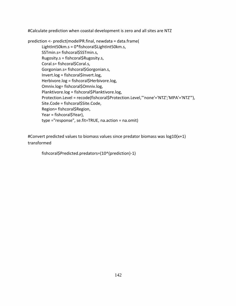
142

#Calculate prediction when coastal development is zero and all sites are NTZ

prediction <- predict(modelPR.final, newdata = data.frame( LightInt50km.s = 0*fishcoral$LightInt50km.s, SSTmin.s= fishcoral$SSTmin.s, Rugosity.s = fishcoral$Rugosity.s, Coral.s= fishcoral$Coral.s, Gorgonian.s= fishcoral$Gorgonian.s, Invert.log = fishcoral$Invert.log, Herbivore.log = fishcoral$Herbivore.log, Omniv.log= fishcoral$Omniv.log, Planktivore.log = fishcoral$Planktivore.log, Protection.Level = recode(fishcoral$Protection.Level,"'none'='NTZ';'MPA'='NTZ'"), Site.Code = fishcoral$Site.Code, Region= fishcoral$Region, Year = fishcoral$Year), type ="response", se.fit=TRUE, na.action = na.omit)

#Convert predicted values to biomass values since predator biomass was log10(x+1)

transformed

fishcoral$Predicted.predators=(10^(prediction)-1)

143

Figure S1.1 Plots of residuals vs. fitted values (left panels) and normal scores of

standardized residual deviance (right panels) for the final models (Set A and B) of total

predator biomass. The plots for apex predators and piscivore-invertivores are not shown

because the patterns are similar to total predators. See Table 1.1 for model details.

144

Figure S1.2 Plots of the spline correlogram function against distance. The spline correlogram

is based on the residuals of the final models for total predators in all sites (a) and for two selected

models within marine reserves (b and c). See Table 1.1 for models. The plots for apex predators

and piscivore-invertivores show similar patterns and are not shown. A 95% pointwise confidence

envelope is superimposed.

145

Figure S1.3 Boxplot of total fish (a) and predator biomass (b) by country and protection

level. White boxes are non-reserve whereas grey boxes are reserves. Black points represent the

pooled means by site and year of survey for each country. Dry Tortugas is excluded because

does not have a non-reserve site.

146

Figure S1.4 Scatterplots of the mean proportion of trophic guilds per site and survey year.

Red line is the best fit from a linear model. Note that higher total fish biomass is driven by higher

proportion of apex predators and piscivore-invertivores, while lower total fish biomass is

comprise mostly (> 0.55) of herbivores.

147

Figure S1.5 Scatterplots of the mean biomass of predators (apex predator + piscivores-

invertivore) and lower trophic guilds across sites. The Spearman’s rank correlation coefficient

(rho) and the significance probability (p) are shown. Red lines are loess smoothing curve with a

span width of 3 in each panel to aid visual interpretation. Axes are in log scale.

148

Appendix 1.3 Detailed description of reef fish biomass variability

The combined average of total fish biomass in the marine reserves of Abaco, Cuba and

Mexico (337 ± 25 g m-2

) was 1.6 times higher than in the unprotected reefs of these sub-regions

(215 ± 20 g m-2

, p<0.001). Similarly, the combined predator biomass in reserves of Abaco, Cuba

and Mexico (154 ± 22 g m-2

) was 2.4 times greater than the combined value of their unprotected

sites (65 ± 10 g m-2

, p<0.001). We found no significant difference in the combined total fish or

predator biomass inside and outside marine reserves of Abaco (p = 0.44, p = 0.68, respectively),

or in Belize (p = 0.78, p = 0.94, respectively). However, reef sites inside the marine reserves of

Hol Chan (HC) and Half Moon Caye (HM) had the highest fish and predator biomass within

Belize (Fig. 1.2). Yet the highest total fish biomass found in Belize at HM (212 ± 14 g m-2

) was

comparable with the combined average of the unprotected sites in the rest of the sub-regions

(~215 ± 20 g m-2

). The combined total fish biomass for Belize (118 ± 8 g m-2

) was 1.8 times

lower than in the unprotected sites of Abaco, Cuba and Mexico (p<0.01, Fig. 1.2, Fig. S1.3).

Finally, most sites in the marine reserves of Abaco, Cuba and Mexico had average total fish

biomass >200 g m-2

and predator biomass >100 g m-2

(Fig. 1.2, Fig. S1.3).

The proportion trend of trophic groups within the fish assemblages varied across reef

sites (Fig. 1.2, Fig. S1.4). The proportion of apex predators and piscivore-invertivores increased

with increased total fish biomass from 0% to ~22% (rs = 0.67, p < 0.001) and from ~15% to

~35% (rs = 0.58, p < 0.001), respectively (Fig. S1.4). In combination, the proportion of predators

increased from ~13% to ~55% (rs = 0.76, p < 0.001) with increased total fish biomass.

Invertivores, planktivores and omnivores did not follow a clear pattern with increased total fish

biomass and each group represented less than 20% of the total biomass at most sites. In contrast,

149

the proportional trend of herbivores decreased from ~55% to ~20% (rs = -0.58, p < 0.001) with

increased total fish biomass (Fig. S1.4).

The biomass of invertivores, omnivores, planktivores, and herbivores were slightly but

significantly and positively correlated with total predator biomass (Fig. S1.5). This relationship

was relatively stronger and less variable for invertivores and herbivores (rs = 0.35, p = 0.000),

but weaker and more variable for planktivores and herbivores (rs = 0.20-0.23, p~0.000) (Fig.

S1.5).

150

Figure S1.6 Relationship between reef structural complexity and fish trophic guilds. Red

lines are loess smoothing curve with a span width of 3 in each panel to aid visual interpretation.

Y axis is in log scale. Reef complexity is described in Appendix 1.1.

151

Appendix 1.4 Detailed discussion of the relationships between predatory fish biomass and

cofactors and their potential underlying mechanisms

Ocean productivity had a small positive effect on apex predator biomass. Large predators

have been related with quantity and quality of primary production in terrestrial ecosystems (e.g.,

Serengeti in Africa, Hopcraft et al. 2010). In marine ecosystems, the positive indirect effect of

ocean productivity on teleost biomass has been tested theoretically (Jennings et al. 2008) and

empirically (Chassot et al. 2010) at global scales, and is probably driven by bottom-up increases

of prey populations (Frank et al. 2007). The observed weak connection of apex predators with

ocean productivity may not be through increasing reef fish prey, as they did not respond to

primary productivity (Fig. 3.3). Instead, mobile apex predators, such as reef sharks and jacks,

may also be feeding upon prey directly linked with ocean productivity via plankton in adjacent

oceanic waters (McCauley et al. 2012).

Reef complexity was one of the most important predictors of fish predator biomass. This

variable has a strong positive influence on the relative abundance, species richness, and local

distribution of small and medium-sized fishes (e.g., 10-30 cm TL) (Wilson et al. 2007, Graham

and Nash 2013). As reef complexity increases, refuges become more available to avoid predation

and competition (Hixon and Beets 1993). In contrast, less clear is the relationship between

landscape reef complexity and the density of large-bodied reef fish (Richards et al. 2012) or reef

sharks (Nadon et al. 2012). Large transient predators that actively chase their prey may avoid

highly complex environments that reduce hunting efficiency (Hixon and Beets 1993).

Conversely, sites with higher structural complexity may attract relative large resident and

transient predators that take advantage of greater prey availability (McCauley et al. 2012). Reef

tridimensional structure complexity is nonetheless crucial to enhance predatory fish biomass and

152

may be further compromised by the Caribbean-wide reduction of architectural complexity

(Alvarez-Filip et al. 2009).

Several physical and biotic cofactors, such as “ocean temperature”, “coral cover”,

“gorgonian abundance”, and herbivore and planktivore biomass did not have a significant effect

on predator biomass; however, they improved model fit and may be important to support

predator biomass within regions. Ocean temperature, for example, showed a weak “unimodal”

response on the biomass of piscivore-invertivores. Non-linear relationship between the diversity

of pelagic fish predators and temperature has been observed at a global scale (Worm et al. 2005).

However, a clear response to temperature by an entire trophic level may be difficult to detect as

the response to temperature gradients is species-specific through physiological constraints that

affect individual biomass (Jennings et al. 2008, Munday et al. 2008).

Mangrove was a predictor of apex predator biomass, but unexpectedly not of piscivore-

invertivores. Reefs associated with mangrove habitats have been reported to support more

species, and higher density and biomass of reef fishes, including greater prey biomass for

piscivore predators (Nagelkerken et al. 2002, Mumby et al. 2004). Mangroves also provide

protection and high-quality nursery grounds for juveniles of top predator teleosts (e.g.,

Sphyraena barracuda, Nagelkerken et al. 2002) and sharks (e.g., Negaprion brevirostris,

Chapman et al. 2009) that later may migrate as adults to adjacent reef habitats (Mumby et al.

2004). Piscivore-invertivores in our study included several species with strong mangrove

association (e.g., most Lutjanus spp., see Mumby et al. 2004), but other species with a weak

connection with mangroves (e.g., Lutjanus mahogoni, see Nagelkerken et al. 2002) may dilute

the average response of the trophic guild. Further research will be needed to identify those

153

species with tight connections with mangrove across our sites, but such endeavor was not

objective in this paper.

Lower trophic levels were good predictors of total predator biomass, especially for

piscivore-invertivores (Table 1.1, Fig. 1.3). We found no evidence of top-down regulation at a

regional scale. In fact, the higher the biomass of lower trophic levels, the greater the biomass of

predators tended to be. Predator dependence on prey, for example, is common within large

reserves of terrestrial savannas and woodland ecosystems (Jhala et al. 2008, Sinclair et al. 2010).

Positive associations among reef fish trophic guilds also increase as fishing pressure decreases

with protection (Newman et al. 2006, Babcock et al. 2010). Since reef predators are often

generalists with opportunistic feeding habits, preying upon several trophic levels including their

own, predation pressure may be distributed across levels (Russ and Alcala 2003). Alternatively,

subsistence fishing in the Caribbean has simultaneously targeted and depleted all trophic levels

potentially overriding predator-prey interactions at regional scale (Hawkins and Roberts 2004,

Paddack et al. 2009).

154

Table S1.6 Estimates of current and potential average biomass (± standard error, se) of

predatory reef fishes in the absence of humans (i.e. coastal development) while categorizing

every site as a no-take zone (i.e. no fishing). The potential percent lost is shown. Sites with

exceptionally high predicted predator biomass are highlighted. Site order follows Fig. 5. For site

codes refer to Table S1.1.

Protection Current biomass Predicted biomass Sites level mean se mean se % lost EB None 3.5 1.3 81.8 8.7 95.8 NI MPA 9.5 3.0 205.2 26.8 95.4 XA None 9.1 4.7 147.0 16.4 93.8 SM MPA 23.2 16.0 185.7 21.6 87.5 SW MPA 8.5 2.0 194.0 14.1 95.6 CA None 16.4 7.9 145.0 20.0 88.7 MR None 10.7 4.1 119.7 10.1 91.1 BC NTZ 10.1 3.0 124.7 5.7 91.9 MC MPA 15.0 5.2 177.3 17.4 91.5 GH None 14.4 2.9 229.2 33.3 93.7 RA None 27.8 8.1 196.9 22.9 85.9 AL None 15.9 2.9 199.1 21.8 92.0 ST None 16.6 2.8 201.1 17.9 91.7 GA None 32.8 11.4 287.7 37.1 88.6 HC NTZ 85.4 67.7 222.5 53.8 61.6 PC NTZ 88.2 38.4 502.0 76.9 82.4 TO None 19.8 3.6 199.6 20.8 90.1 CP None 28.3 7.3 214.9 20.9 86.8 PO None 41.9 12.7 238.0 30.3 82.4

BCS MPA 50.9 28.4 299.2 25.0 83.0 PZ None 35.3 10.8 290.9 41.0 87.9 TB None 71.9 39.5 295.1 86.6 75.6

MW None 34.2 8.7 310.3 28.2 89.0 FC NTZ 125.9 57.2 736.0 182.3 82.9 HM NTZ 89.7 41.8 408.2 63.0 78.0 PB NTZ 59.2 18.3 667.3 131.8 91.1 BR None 67.2 28.4 480.4 38.1 86.0 LH None 63.2 10.5 520.8 51.2 87.9 GC None 47.7 7.7 471.3 58.9 89.9 CR NTZ 83.0 35.8 890.9 116.8 90.7 BA None 72.3 21.7 826.7 150.1 91.3 LG NTZ 129.0 52.2 273.6 35.3 52.8 AN NTZ 90.8 16.2 273.1 49.6 66.7

BCN MPA 109.3 16.3 1067.4 169.3 89.8 RP None 268.6 73.4 1157.8 200.8 76.8 EP NTZ 263.6 77.5 505.8 103.2 47.9

BCC MPA 174.1 35.4 1562.0 308.5 88.9 PP NTZ 244.5 58.3 402.2 60.7 39.2 CF NTZ 441.0 139.4 474.3 92.1 7.0

155

Appendix 1.5 References

Alvarez-Filip, L., N. K. Dulvy, J. A. Gill, I. M. Côté, and A. R. Watkinson. 2009. Flattening of

Caribbean coral reefs: region-wide declines in architectural complexity. Proceedings of

the Royal Society B: Biological Sciences 276:3019–3025.

Alvarez-Filip, L., J. A. Gill, and N. K. Dulvy. 2011. Complex reef architecture supports more

small-bodied fishes and longer food chains on Caribbean reefs. Ecosphere 2:art118.

Babcock, R. C., N. T. Shears, A. C. Alcala, N. S. Barrett, G. J. Edgar, K. D. Lafferty, T. R.

McClanahan, and G. R. Russ. 2010. Decadal trends in marine reserves reveal differential

rates of change in direct and indirect effects. Proceedings of the National Academy of

Sciences 107:18256 –18261.

Behrenfeld, M. J., and P. G. Falkowski. 1997. Photosynthetic rates derived from satellite-based

chlorophyll concentration. Limnology and oceanography:1–20.

Carleton, J. H., and T. J. Done. 1995. Quantitative video sampling of coral reef benthos: large-

scale application. Coral Reefs 14:35–46.

Casey, K. S., T. B. Brandon, P. Cornillon, and R. Evans. 2010. The past, present, and future of

the AVHRR pathfinder SST program. Pages 273–287 in V. Barale, J. F. R. Gower, and

L. Alberotanza, editors. Oceanography from Space. Springer Netherlands, Dordrecht.

Chapman, D., E. A. Babcock, S. H. Gruber, J. Dibattista, B. Franks, S. Kessel, T. Guttridge, E.

K. Pikitch, and K. A. Feldheim. 2009. Long-term natal site-fidelity by immature lemon

sharks (Negaprion brevirostris) at a subtropical island. Molecular Ecology 18:3500–

3507.

Chassot, E., S. Bonhommeau, N. K. Dulvy, F. Mélin, R. Watson, D. Gascuel, and O. Le Pape.

2010. Global marine primary production constrains fisheries catches. Ecology Letters

13:495–505.

Chollett, I., and P. J. Mumby. 2012. Predicting the distribution of Montastraea reefs using wave

exposure. Coral Reefs 31:493–503.

Chollett, I., P. J. Mumby, F. E. Müller-Karger, and C. Hu. 2012. Physical environments of the

Caribbean Sea. Limnology and Oceanography 57:1233–1244.

Claudet, J., C. W. Osenberg, L. Benedetti-Cecchi, P. Domenici, J.-A. García-Charton, Á. Pérez-

Ruzafa, F. Badalamenti, J. Bayle-Sempere, A. Brito, F. Bulleri, J.-M. Culioli, M.

Dimech, J. M. Falcón, I. Guala, M. Milazzo, J. Sánchez-Meca, P. J. Somerfield, B.

Stobart, F. Vandeperre, C. Valle, and S. Planes. 2008. Marine reserves: size and age do

matter. Ecology Letters 11:481–489.

156

Côté, I. M., I. Mosqueira, and J. D. Reynolds. 2001. Effects of marine reserve characteristics on

the protection of fish populations: a meta-analysis. Journal of Fish Biology 59:178–189.

Frank, K. T., B. Petrie, and N. L. Shackell. 2007. The ups and downs of trophic control in

continental shelf ecosystems. Trends in Ecology & Evolution 22:236–242.

Friedlander, A. M., E. K. Brown, P. L. Jokiel, W. R. Smith, and K. S. Rodgers. 2003. Effects of

habitat, wave exposure, and marine protected area status on coral reef fish assemblages in

the Hawaiian archipelago. Coral Reefs 22:291–305.

Fulton, C. J., and D. R. Bellwood. 2004. Wave exposure, swimming performance, and the

structure of tropical and temperate reef fish assemblages. Marine Biology 144:429–437.

GLC. 2003. Global Land Cover 2000 Project.

http://bioval.jrc.ec.europa.eu/products/glc2000/products.php.

Global Distribution of Mangrove USGS. 2011. Global distribution of mangrove USGS.

http://data.unep-wcmc.org/datasets/21.

Graham, N. A. J., and K. L. Nash. 2013. The importance of structural complexity in coral reef

ecosystems. Coral Reefs 32:315–326.

Halpern, B. S. 2003. The impact of marine reserves: do reserves work and does reserve size

matter? Ecological Applications 13:117–137.

Harborne, A. R., P. J. Mumby, K. Zychaluk, J. D. Hedley, and P. G. Blackwell. 2011. Modeling

the beta diversity of coral reefs. Ecology 87:2871–2881.

Hawkins, J. P., and C. M. Roberts. 2004. Effects of artisanal fishing on Caribbean coral reefs.

Conservation Biology 18:215–226.

Hixon, M. A., and J. P. Beets. 1993. Predation, prey refuges, and the structure of coral-reef fish

assemblages. Ecological Monographs 63:77–101.

Hopcraft, J. G. C., H. Olff, and A. R. E. Sinclair. 2010. Herbivores, resources and risks:

alternating regulation along primary environmental gradients in savannas. Trends in

Ecology & Evolution 25:119–128.

Jennings, S., F. Mélin, J. L. Blanchard, R. M. Forster, N. K. Dulvy, and R. W. Wilson. 2008.

Global-scale predictions of community and ecosystem properties from simple ecological

theory. Proceedings of the Royal Society B: Biological Sciences 275:1375–1383.

Jhala, Y. V., R. Gopal, and Q. Qureshi. 2008. Status of tigers, co-predators and prey in India.

National Tiger Conservation Authority, Govt., of India, New Delhi and Wildlife Institute

of India, Dehradun. TR 2011/003.

157

Kritzer, J. P. 2004. Effects of noncompliance on the success of alternative designs of marine

protected-area networks for conservation and fisheries management. Conservation

Biology 18:1021–1031.

Lang, J. C., K. W. Marks, P. A. Kramer, P. Richards Kramer, and R. N. Ginsburg. 2010.

AGRRA Protocols version 5.4 Atlantic and Gulf Rapid Reef Assessment Program.

University of Miami, Florida.

McCauley, D. J., H. S. Young, R. B. Dunbar, J. A. Estes, B. X. Semmens, and F. Micheli. 2012.

Assessing the effects of large mobile predators on ecosystem connectivity. Ecological

Applications 22:1711–1717.

McCook, L. J. 1999. Macroalgae, nutrients and phase shifts on coral reefs: scientific issues and

management consequences for the Great Barrier Reef. Coral Reefs 18:357–367.

Mora, C., S. Andrèfouët, M. J. Costello, C. Kranenburg, A. Rollo, J. Veron, K. J. Gaston, and R.

A. Myers. 2006. Coral reefs and the global network of marine protected areas. Science

312:1750–1751.

Mumby, P. J., A. J. Edwards, J. E. Arias-González, K. C. Lindeman, P. G. Blackwell, A. Gall,

M. I. Gorczynska, A. R. Harborne, C. L. Pescod, H. Renken, C. C. C. Wabnitz, and G.

Llewellyn. 2004. Mangroves enhance the biomass of coral reef fish communities in the

Caribbean. Nature 427:533–536.

Munday, P. L., G. P. Jones, M. S. Pratchett, and A. J. Williams. 2008. Climate change and the

future for coral reef fishes. Fish and Fisheries 9:261–285.

Nadon, M. O., J. K. Baum, I. D. Williams, J. M. Mcpherson, B. J. Zgliczynski, B. L. Richards,

R. E. Schroeder, and R. E. Brainard. 2012. Re‐creating missing population baselines for

Pacific reef sharks. Conservation Biology 26:493–503.

Nagelkerken, I., C. M. Roberts, G. van der Velde, M. Dorenbosch, M. C. van Riel, E. C. de la

Morinire, and P. H. Nienhuis. 2002. How important are mangroves and seagrass beds for

coral-reef fish? The nursery hypothesis tested on an island scale. Marine Ecology

Progress Series 244:299–305.

Newman, M. J. H., G. A. Paredes, E. Sala, and J. B. C. Jackson. 2006. Structure of Caribbean

coral reef communities across a large gradient of fish biomass. Ecology Letters 9:1216–

1227.

NOAA, (National Oceanic and Atmospheric Administration). 2013. The AVHRR Pathfinder

Version 5.2 dataset. http://www.nodc.noaa.gov/SatelliteData/pathfinder4km/.

Oregon State University. 2013. Ocean Productivity: Online VGPM Data.

http://orca.science.oregonstate.edu/1080.by.2160.monthly.hdf.vgpm.m.chl.m.sst4.php.

158

Paddack, M. J., J. D. Reynolds, C. Aguilar, R. S. Appeldoorn, J. Beets, E. W. Burkett, P. M.

Chittaro, K. Clarke, R. Esteves, A. C. Fonseca, G. E. Forrester, A. M. Friedlander, J.

García-Sais, G. González-Sansón, L. K. B. Jordan, D. B. McClellan, M. W. Miller, P. P.

Molloy, P. J. Mumby, I. Nagelkerken, M. Nemeth, R. Navas-Camacho, J. Pitt, N. V. C.

Polunin, M. C. Reyes-Nivia, D. R. Robertson, A. Rodríguez-Ramírez, E. Salas, S. R.

Smith, R. E. Spieler, M. A. Steele, I. D. Williams, C. L. Wormald, A. R. Watkinson, and

I. M. Côté. 2009. Recent region-wide declines in Caribbean reef fish abundance. Current

Biology 19:590–595.

Polunin, N. V. C., and C. M. Roberts. 1993. Greater biomass and value of target coral-reef fishes

in two small Caribbean marine reserves. Marine Ecology Progress Series 100:177–183.

Richards, B. L., I. D. Williams, O. J. Vetter, and G. J. Williams. 2012. Environmental factors

affecting large-bodied coral reef fish assemblages in the mariana archipelago. PLoS ONE

7:e31374.

Russ, G. R., and A. C. Alcala. 2003. Marine reserves: rates and patterns of recovery and decline

of predatory fish, 1983-2000. Ecological Applications 13:1553–1565.

Sanderson, E., W., M. Jaitteh, M. Levy A., K. Redford H., A. Wannebo V., and G. Woolmer.

2002. The human footprint and the last of the Wild. BioScience 52:891–904.

Sinclair, A. R. E., K. Metzger, J. S. Brashares, A. Nkwabi, G. Sharam, J. M. Fryxell, J. Terborgh,

and J. A. Estes. 2010. Trophic cascades in African savanna: Serengeti as a case study.

Trophic cascades: predators, prey and the changing dynamics of nature, Island Press,

Washington, DC, USA:255–274.

UNEP-WCMC, WorldFish Centre, WRI, and TNC. 2010. Global distribution of warm-water

coral reefs, compiled from multiple sources, including the Millennium Coral Reef

Mapping Project. UNEP World Conservation Monitoring Centre. Cambridge (UK).

http://data.unep-wcmc.org/datasets/13.

Wenger, A. S., M. I. McCormick, I. M. McLeod, and G. P. Jones. 2013. Suspended sediment

alters predator–prey interactions between two coral reef fishes. Coral Reefs 32:369–374.

Wilson, S., N. Graham, and N. Polunin. 2007. Appraisal of visual assessments of habitat

complexity and benthic composition on coral reefs. Marine Biology 151:1069–1076.

Worm, B., M. Sandow, A. Oschlies, H. K. Lotze, and R. A. Myers. 2005. Global patterns of

predator diversity in the open oceans. Science 309:1365–1369.

159

APPENDIX 2: SUPPLEMENTARY MATERIAL FOR CHAPTER 2

Figure S2.1 Location of survey sites. For site abbreviations, surveys dates and coordinates refer

to Table S2.1

160

Figure S2.2 Moran’s I similarity spline correlograms for lionfish and grouper raw data

across all sites (top two panels) and for the glmmADMB model residuals (bottom panel).

Note the strong spatial autocorrelation of the raw data (i.e., swirling lines around zero) and how

the hierarchical structure of the random effects (sites nested in regions) of the full glmmADMB

model eliminated this correlation in the model residuals. A Mantel test of the model Pearson

residuals (r = 0.073) corroborates the lack of spatial correlation of the residuals. Lines are the

mean ± 95% confidence interval.

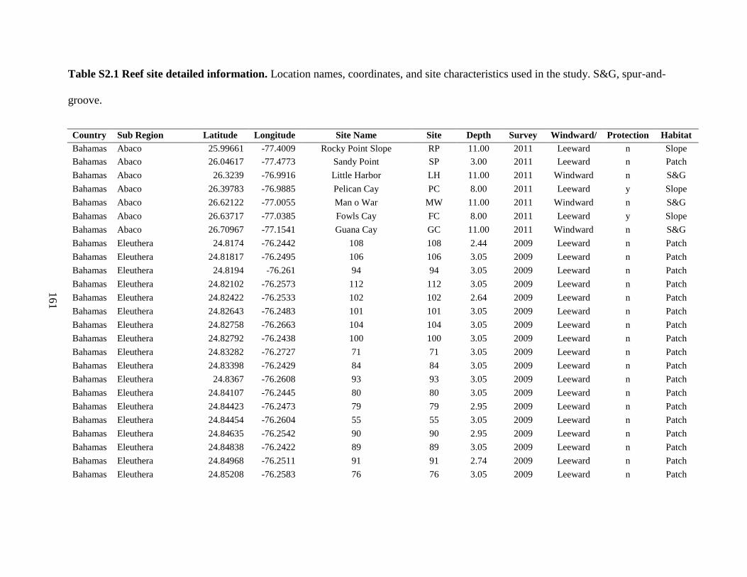
161

Table S2.1 Reef site detailed information. Location names, coordinates, and site characteristics used in the study. S&G, spur-and-

groove.

Country Sub Region Latitude Longitude Site Name Site

Code

Depth

(m)

Survey

Year

Windward/

Leeward

Protection

(y/n)

Habitat

type Bahamas Abaco 25.99661 -77.4009 Rocky Point Slope RP 11.00 2011 Leeward n Slope

Bahamas Abaco 26.04617 -77.4773 Sandy Point SP 3.00 2011 Leeward n Patch

Bahamas Abaco 26.3239 -76.9916 Little Harbor LH 11.00 2011 Windward n S&G

Bahamas Abaco 26.39783 -76.9885 Pelican Cay PC 8.00 2011 Leeward y Slope

Bahamas Abaco 26.62122 -77.0055 Man o War MW 11.00 2011 Windward n S&G

Bahamas Abaco 26.63717 -77.0385 Fowls Cay FC 8.00 2011 Leeward y Slope

Bahamas Abaco 26.70967 -77.1541 Guana Cay GC 11.00 2011 Windward n S&G

Bahamas Eleuthera 24.8174 -76.2442 108 108 2.44 2009 Leeward n Patch

Bahamas Eleuthera 24.81817 -76.2495 106 106 3.05 2009 Leeward n Patch

Bahamas Eleuthera 24.8194 -76.261 94 94 3.05 2009 Leeward n Patch

Bahamas Eleuthera 24.82102 -76.2573 112 112 3.05 2009 Leeward n Patch

Bahamas Eleuthera 24.82422 -76.2533 102 102 2.64 2009 Leeward n Patch

Bahamas Eleuthera 24.82643 -76.2483 101 101 3.05 2009 Leeward n Patch

Bahamas Eleuthera 24.82758 -76.2663 104 104 3.05 2009 Leeward n Patch

Bahamas Eleuthera 24.82792 -76.2438 100 100 3.05 2009 Leeward n Patch

Bahamas Eleuthera 24.83282 -76.2727 71 71 3.05 2009 Leeward n Patch

Bahamas Eleuthera 24.83398 -76.2429 84 84 3.05 2009 Leeward n Patch

Bahamas Eleuthera 24.8367 -76.2608 93 93 3.05 2009 Leeward n Patch

Bahamas Eleuthera 24.84107 -76.2445 80 80 3.05 2009 Leeward n Patch

Bahamas Eleuthera 24.84423 -76.2473 79 79 2.95 2009 Leeward n Patch

Bahamas Eleuthera 24.84454 -76.2604 55 55 3.05 2009 Leeward n Patch

Bahamas Eleuthera 24.84635 -76.2542 90 90 2.95 2009 Leeward n Patch

Bahamas Eleuthera 24.84838 -76.2422 89 89 3.05 2009 Leeward n Patch

Bahamas Eleuthera 24.84968 -76.2511 91 91 2.74 2009 Leeward n Patch

Bahamas Eleuthera 24.85208 -76.2583 76 76 3.05 2009 Leeward n Patch

161

162

Bahamas Eleuthera 24.85253 -76.2551 75 75 3.05 2009 Leeward n Patch

Bahamas Eleuthera 24.85275 -76.2471 78 78 3.35 2009 Leeward n Patch

Bahamas Eleuthera 24.85302 -76.2492 77 77 3.25 2009 Leeward n Patch

Bahamas Eleuthera 24.85712 -76.2574 74 74 3.15 2009 Leeward n Patch

Bahamas Eleuthera 24.85883 -76.2543 73 73 2.74 2009 Leeward n Patch

Bahamas Eleuthera 24.86077 -76.2594 72 72 3.35 2009 Leeward n Patch

Bahamas Eleuthera 24.95058 -76.2871 70 70 3.05 2009 Leeward n Patch

Bahamas New Providence 24.91062 -77.5263 RSP Group RS 15.40 2010 Leeward n S&G

Bahamas New Providence 24.97067 -77.5342 Mike's Reef MK 13.00 2010 Leeward n S&G

Bahamas New Providence 24.97443 -77.5352 Pumpkin Patch PK 11.50 2010 Leeward n S&G

Bahamas New Providence 25.0013 -77.5416 Power Plant PW 7.00 2010 Leeward n S&G

Bahamas New Providence 25.0045 -77.5538 DC3 Wall DW 13.75 2010 Leeward n S&G

Bahamas New Providence 25.00617 -77.552 David Tucker DT 14.50 2010 Leeward n S&G

Bahamas New Providence 25.0085 -77.5572 Bond Wrecks BW 11.50 2010 Leeward n S&G

Bahamas New Providence 25.01535 -77.5698 Willaurie WI 15.00 2010 Leeward n S&G

Belize Meso American 16.1123 -88.2559 Nicholas NI 13.00 2012 Windward y S&G

Belize Meso American 16.11247 -88.2711 Southwest ST 13.00 2012 Windward n S&G

Belize Meso American 16.28501 -88.1503 Ranguana RA 13.00 2012 Windward n S&G

Belize Meso American 16.3731 -88.0891 Pampion PO 13.00 2012 Windward n S&G

Belize Meso American 16.72875 -87.8287 South Middle Cay SM 13.00 2012 Windward y S&G

Belize Meso American 16.73703 -87.8054 Middle Cay MC 13.00 2012 Windward y S&G

Belize Meso American 16.81346 -88.0776 South Water SW 13.00 2012 Windward y S&G

Belize Meso American 16.91911 -88.0476 Tobacco TO 13.00 2012 Windward n S&G

Belize Meso American 17.1966 -88.0512 Alligator AL 13.00 2012 Windward n S&G

Belize Meso American 17.2056 -87.5468 Half Moon HM 13.00 2012 Leeward y S&G

Belize Meso American 17.26147 -87.8197 Calabash CA 13.00 2012 Windward n S&G

Belize Meso American 17.49592 -88.0426 Gallows GA 13.00 2012 Windward n S&G

Belize Meso American 17.86343 -87.9724 Hol Chan HC 13.00 2012 Windward y S&G

Belize Meso American 17.91056 -87.9508 Tackle Box TB 13.00 2012 Windward n S&G

Belize Meso American 17.98782 -87.9038 Mexico Rocks MR 13.00 2012 Windward n S&G

Belize Meso American 18.16282 -87.8222 Bacalar Chico BC 13.00 2012 Windward n S&G

162

163

Cuba Bay of Pigs 22.07914 -81.076 Ebano EB 11.00 2010 Windward n Slope

Cuba Bay of Pigs 22.11003 -81.1163 Punta Perdiz PZ 9.00 2010 Leeward n Slope

Cuba Bay of Pigs 22.16627 -81.1383 Cueva Peces CP 9.00 2010 Leeward n Slope

Cuba Jardines de la Reina 20.76177 -78.8522 Five Sea CF 11.00 2011 Leeward y Slope

Cuba Jardines de la Reina 20.78697 -78.9432 Anclita AN 11.00 2011 Leeward y Slope

Cuba Jardines de la Reina 20.82586 -78.9803 Pipin PP 16.00 2011 Leeward y S&G

Cuba Jardines de la Reina 20.84411 -79.0217 El Peruano EP 11.00 2011 Leeward y Slope

Cuba North Coast 23.14654 -81.6666 Bacunayaua BA 10.00 2012 Windward n Slope

Mexico Akumal 20.42689 -87.286 Xaak XA 15.00 2012 Windward n S&G

Mexico Banco Chinchorro 18.41008 -87.4169 Banco Chinchorro South BCS 15.00 2012 Leeward y S&G

Mexico Banco Chinchorro 18.57457 -87.4198 Banco Chinchorro Central BCC 15.00 2012 Leeward y S&G

Mexico Banco Chinchorro 18.74867 -87.3476 Banco Chinchorro North BCN 15.00 2012 Leeward y S&G

Mexico Cancun 21.02544 -86.7713 Gardener of Hope GH 12.00 2012 Windward n S&G

Mexico Cozumel 20.31961 -87.0266 Columbia Reef CR 15.00 2012 Leeward y S&G

Mexico Cozumel 20.47188 -86.9815 Paraiso Bajo PB 10.00 2012 Leeward y S&G

163

164

Table S2.2 Summary of the glmmADMB results. Lionfish abundance (ind. 100 m-2

) on

grouper biomass (g 100 m-2

), predators, and other co-factors.

Coefficients Estimate Std. Error z value Pr(>|z|)

(Intercept) 3.19012 1.18970 2.68 0.0073 **

Habitat (Spur & Groove) -3.34259 1.44490 -2.31 0.0207 *

Habitat (Slope) -2.75324 1.33400 -2.06 0.0390 *

Windward -1.27082 0.63682 -2.00 0.0460 *

Protection (yes) -1.32074 0.48898 -2.70 0.0069 **

Depth 0.25256 0.30394 0.83 0.4060

Time since invasion 0.32035 0.34958 0.92 0.3595

Reef complexity -0.00503 0.07948 -0.06 0.9496

Humans/Reef 0.09210 0.08807 1.05 0.2957

Predator biomass -0.08192 0.09066 -0.90 0.3662

log(Grouper biomass) -0.00709 0.04494 -0.16 0.8747

Significance codes: 0 ‘***’ 0.001 ‘**’ 0.01 ‘*’ 0.05 ‘.’ 0.1 ‘ ’ 1

Number of observations: total=363, Region=11, Region: Site.Code=71

Random effect variance(s):

Group=Region

Variance StdDev

(Intercept) 1.179 1.086

Group=Region/Site.Code

Variance StdDev

(Intercept) 0.3861 0.6214

Negative binomial dispersion parameter: 1.568 (std. err.: 0.16423)

Zero-inflation: 0.0083623 (std. err.: 0.0096232 )

Log-likelihood: -618.889 AIC: 1267.8

165

APPENDIX 3: SUPPLEMENTARY MATERIAL FOR CHAPTER 3

Appendix 3.1 Description of anthropogenic and environmental covariates used in the

models

Human population density

We estimated the number of humans within 50 km of each Caribbean site (maximum

number of people that occurred within 50-km radius of each site).We chose 50 km as radius

because is a reasonable range of anthropogenic influence on Caribbean reefs (Mora 2008).

Projection estimates of human population counts for the year 2010 were obtained from the

Gridded Population of the World V.3 at 0.25 degree resolution (SEDAC 2010) and calculated in

ArcGIS v10.0. For the Pacific island we extracted the population density for every inhabited

island from Williams et al. (2011).

Cultivated land

We quantified the area of cultivated land that occurred within a 50 km radius of each

Caribbean reef site, and on those Pacific islands with measurable agricultural activities. Data for

this variable was obtained from the Global Land Cover Share database (Latham et al. 2014) at

(http://www.glcn.org/databases/lc_glcshare_en.jsp). This global database provides a set of major

thematic land cover layers combining the best available high resolution national, regional and

subregional land cover databases and it is calculated from satellite images at 1 km resolution.

Cultivated land could be a surrogate of terrestrial run-offs with potential effects on macroalgae

cover when herbivory is reduced (McCook 1999). Spatial analyses were performed in ArcGIS

v10.

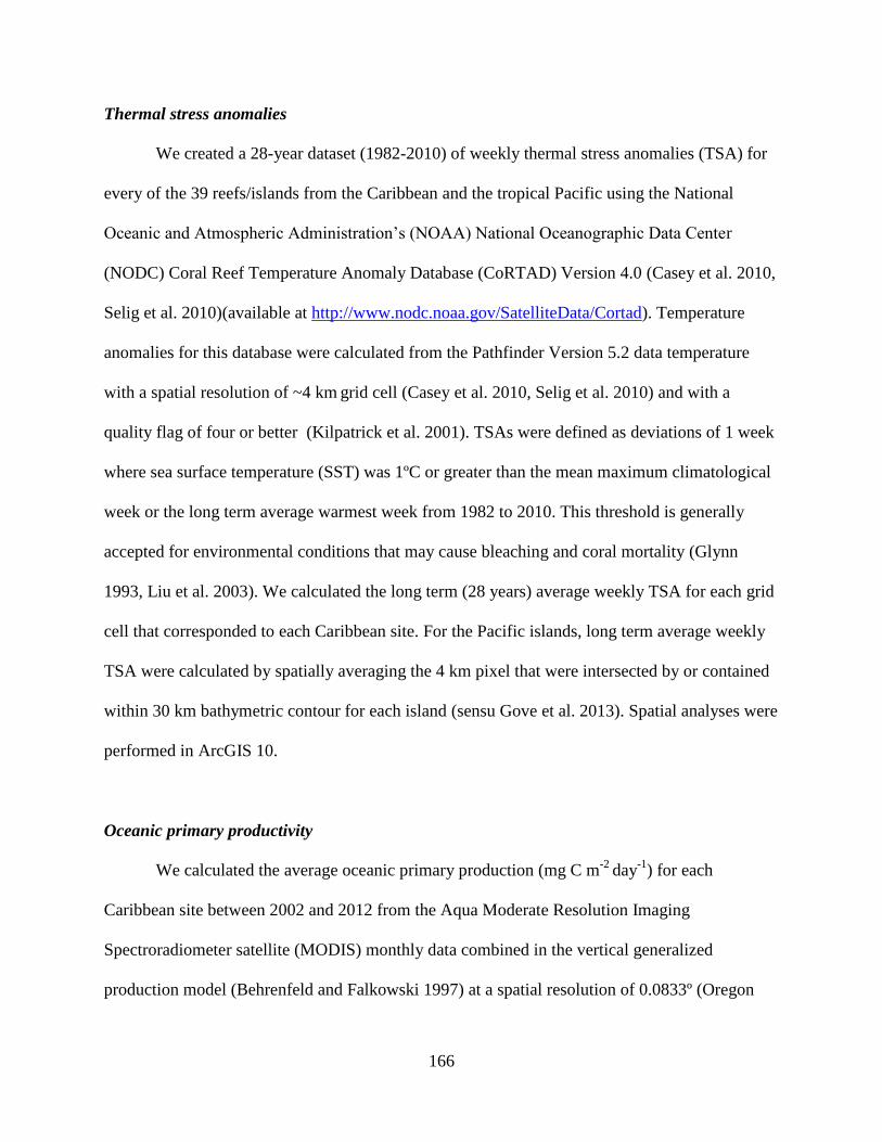
166

Thermal stress anomalies

We created a 28-year dataset (1982-2010) of weekly thermal stress anomalies (TSA) for

every of the 39 reefs/islands from the Caribbean and the tropical Pacific using the National

Oceanic and Atmospheric Administration’s (NOAA) National Oceanographic Data Center

(NODC) Coral Reef Temperature Anomaly Database (CoRTAD) Version 4.0 (Casey et al. 2010,

Selig et al. 2010)(available at http://www.nodc.noaa.gov/SatelliteData/Cortad). Temperature

anomalies for this database were calculated from the Pathfinder Version 5.2 data temperature

with a spatial resolution of ~4 km grid cell (Casey et al. 2010, Selig et al. 2010) and with a

quality flag of four or better (Kilpatrick et al. 2001). TSAs were defined as deviations of 1 week

where sea surface temperature (SST) was 1ºC or greater than the mean maximum climatological

week or the long term average warmest week from 1982 to 2010. This threshold is generally

accepted for environmental conditions that may cause bleaching and coral mortality (Glynn

1993, Liu et al. 2003). We calculated the long term (28 years) average weekly TSA for each grid

cell that corresponded to each Caribbean site. For the Pacific islands, long term average weekly

TSA were calculated by spatially averaging the 4 km pixel that were intersected by or contained

within 30 km bathymetric contour for each island (sensu Gove et al. 2013). Spatial analyses were

performed in ArcGIS 10.

Oceanic primary productivity

We calculated the average oceanic primary production (mg C m-2

day-1

) for each

Caribbean site between 2002 and 2012 from the Aqua Moderate Resolution Imaging

Spectroradiometer satellite (MODIS) monthly data combined in the vertical generalized

production model (Behrenfeld and Falkowski 1997) at a spatial resolution of 0.0833º (Oregon

167

State University 2013). We calculated the climatological mean of the last ten years period

because primary production is inherently variable in time and we were interested on long term

effects instead of specific variability. Calculations were performed in ArcGIS 10.0.

For the Pacific islands, Chlorophyll-a concentration (mg m-3

) was used as proxy for

ocean productivity. Eight-days, 0.0417º-resolution (~4 km) time series of Chlorophyll-a

concentration was obtained from the Aqua MODIS satellite (http://modis.gsfc.nasa.gov/) for the

July 2002 – May 2011 period. Land and shallow water areas (<30 m) were removed to avoid

unreliable data associated with bottom reflectance that is not related with Chlorophyll-a signal

(Boss and Zaneveld 2003). The zone most proximate to the islands (~3.3-6.5 km from the 30 m

contour) was used to calculate chlorophyll-a values as it captures the most representative signal

(Gove et al. 2013). As in the Caribbean, we used the long term climatological mean as predictors

in the models. Average per island was extracted from Gove et al. (2013).

Reef complexity

For the Caribbean sites, we visually estimated structural reef complexity at each transect

set on a scale of 0-5, where 0 was given to reefs with no vertical relief; 1, low and sparse relief;

2, low but widespread relief; 3, moderately complex relief; 4, very complex relief with numerous

caves and fissures; and 5, reefs with exceptionally complex habitats, with numerous caves and

overhangs (Polunin and Roberts 1993). This topographic measure provided an assessment of

reef complexity at the seascape level which is relevant to large and medium-sized fish (Polunin

and Roberts 1993, Wilson et al. 2007). For the Pacific islands, the same complexity index was

estimated in each tow-diver survey and island mean was calculated for statistical analysis.

168

Reef area

Reef areas within 5 km and 10 km radius of each Caribbean site was calculated from the

Global Distribution of Coral Reefs (2010) database as available at the Ocean Data Viewer United

Nations Environment Program's World Conservation Monitoring Centre (UNEP-WCMC)

(http://data.unep-wcmc.org/datasets/13) in ArcGIS v10.0. This database represents the global

distribution of warm water coral reefs compiled mostly from the Millennium Coral Reef

Mapping Project validated and un-validated maps as well as other sources acquired by UNEP-

WCMC. For each Pacific islands, reef areas was calculated from the shoreline to 10 fathom line

or ~18 m isobaths and obtained from Rohmann et al. (2005).

Maximum island elevation

Maximum land elevation for each Pacific island was obtained from CRED’s

Data/Information Products Team (http://www.pifsc.noaa.gov/cred/). We included island

elevation because may have a positive effect on macroalgae richness probably due to more

available space (Schils et al. 2013)

Wave exposure

Wave exposure for the Caribbean sites, given as the log of wind driven wave exposure (J

m-3

), was extracted in ArchGIS 10.0 from the wave stress map for the Caribbean basin built by

Chollett et al. (2012) and available at (http://www.marinespatialecologylab.org/wp-

content/uploads/2010/11/PECS1.png). This index does not include the influence of tides or

swells, which are not generated by local wind, and it is an approximation of wave patterns in

shallow areas over time (Chollett et al. 2012). Wave exposure in a given location is a function of

169

the basin shape (i.e. fetch), wind speed and direction and it is calculated using the method

described by Ekeborn et al. (2003). Wind speed and direction were obtained from QuickSCAT

satellite scatterometer data (1999-2008) available at (http://www.ssmi.com/qscat). The detailed

description of the wave exposure calculations and assumptions can be found in Chollett &

Mumby (2012).

For the Pacific, average wave exposure or energy (kW m-1

) for each island was extracted

from Gove et al. (2013). This variable was quantified using the global full spectral wave model

Wave Watch III (http://polar.ncep.noaha.gov/waves). It was calculated at one-degree spatial

resolution incorporating the 3-hour output of mean significant wave height, peak period, and

direction from 1997 to 2010. Wave data were extracted from the one-degree grid cell in which

each island was located. For detailed calculations of wave energy flux for each Pacific island

refer to Gove et al. (2013).

Wave energy and exposure (given the dependence on wave period and height) are more

realistic estimates of wave forcing and thus, more ecologically relevant variable to quantify wave

impact on benthic communities (Friedlander et al. 2003, Storlazzi et al. 2005, Chollett and

Mumby 2012). Wave exposure has been a good predictor of spatial variation in reef building

corals such as Orbicella sp. (former Montastrea sp.) (Chollett and Mumby 2012) and can

partially explain beta diversity patterns of benthic communities (Harborne et al. 2011). Wave

exposure may also directly affect the biomass and diversity of tropical reef fish (Friedlander et

al. 2003) and the distribution and abundance of temperate reef fish by compromising swimming

abilities (Fulton and Bellwood 2004).

170

Table S3.1 Survey locations, regions, and protection level for reef sites in the Caribbean.

Date of survey is month and year(s). Protection level, NTZ: No-take zone, MPA: marine

protected area. P code is protection level divided in two categories: N (none, MPA) and P (NTZ).

Site name Site

code

Depth

(m)

Date of

survey

Latitude Longitude Protection

level

P

code

Mesoamerican Barrier, Mexico

Cancún GH 12 Jul 12 21.02544 -86.7713 none N

Cozumel North PB 10 Jul 12 20.47188 -86.9815 NTZ P

Akumal XA 15 Jul 12 20.42689 -87.2860 none N

Cozumel South CR 15 Jul 12 20.31961 -87.0266 NTZ P

Chinchorro North BCN 15 Jul 12 18.74867 -87.3476 MPA N

Chinchorro Central BCC 15 Jul 12 18.57457 -87.4198 MPA N

Chinchorro South BCS 15 Jul 12 18.41008 -87.4169 MPA N

Mesoamerican Barrier, Belize

Bacalar Chico BC 12-15 May 10/12 18.16282 -87.82222 NTZ P

Mexico Rocks MR 12-15 May 10/12 17.98782 -87.90382 none N

Tackle Box TB 12-15 May 10/12 17.91056 -87.95083 none N

Hol Chan HC 12-15 May 10/12 17.86343 -87.97238 NTZ P

Gallows GA 12-15 May 10/12 17.49592 -88.04255 none N

Calabash Caye CA 12-15 May 10/12 17.26147 -87.81970 none N

Half Moon Caye HM 12-15 May 10/12 17.20560 -87.54679 NTZ P

Alligator Caye AL 12-15 May 10/12 17.19660 -88.05115 none N

Tobacco Caye TO 12-15 May 10/12 16.91911 -88.04757 none N

South Water Caye SW 12-15 May 10/12 16.81346 -88.07756 MPA N

Middle Caye MC 12-15 May 10/12 16.73703 -87.80536 MPA N

South Middle Caye SM 12-15 May 10/12 16.72875 -87.82867 MPA N

Pampion Caye PO 12-15 May 10/12 16.37310 -88.08913 none N

Ranguana Caye RA 12-15 May 10/12 16.28501 -88.15031 none N

Southwest Caye ST 12-15 May 10/12 16.11247 -88.27107 none N

Nicholas Caye NI 12-15 May 10/12 16.11230 -88.25586 MPA N

Dry Tortugas, USA LG 12 Jun 12 24.68508 -82.91050 NTZ P

Cuba

Cueva Peces CP 10-12 Jun 10/12 22.16627 -81.13827 none N

Punta Perdiz PZ 10-12 Jun 10/12 22.11003 -81.11626 none N

Ebano EB 10-12 Jun 10 22.07914 -81.07599 none N

Brinco BR 10-12 Jun 12 22.06939 -81.05588 none N

Bacunayagua, Cuba BC 10-12 Jun 12 23.14653 -81.66664 none N

El Peruano EP 10-12 Jun 11 20.84411 -79.02166 NTZ P

Pipin PP 12-15 Jun 11 20.82586 -78.98026 NTZ P

Anclita AN 10-12 Jun 11 20.78697 -78.94317 NTZ P

Cueva Pulpo CF 10-12 Jun 11 20.75266 -78.83634 NTZ P

Abaco, Bahamas

Guana Cay GC 10-12 Jul 11/12 26.70967 -77.15408 none N

Fowls Cay FC 10 Jul 11/12 26.63717 -77.03848 NTZ P

Man o’ War MW 10-12 Jul 11/12 26.62122 -77.00550 none N

Pelican Cay PC 10 Jul 11/12 26.39783 -76.98850 NTZ P

Little Harbor LH 10-12 Jul 11/12 26.32390 -76.99160 none N

Rocky Point RP 10-12 Jul 11/12 25.99661 -77.40092 none N

171

Table S3.2 Survey locations, regions, and status for US Pacific islands used in this study.

P/R, populated versus remote islands.

Island Island code Latitude Longitude P/R

Hawaiian archipelago

Kaui KAU 22.09119 -159.570 P Niihau NII 21.89792 -160.151 P

Oahu OAH 21.48649 -158.003 P

Molokai MOL 21.14063 -157.091 P

Lanai LAN 20.82110 -156.918 P

Maui MAI 20.81507 -156.400 P

Hawaii HAW 19.52631 -155.416 P

Kure KUR 28.42340 -178.331 R Midway MID 28.22690 -177.380 R

Pearl and Hermes PHR 27.85629 -175.847 R

Lisianski LIS 26.00917 -173.950 R

Laysan LAY 25.77585 -171.732 R

Maro MAR 25.41415 -170.579 R

French Frigate FFS 23.79099 -166.213 R

Mariana archipelago

Saipan SAI 15.18538 145.7533 P Tinian TIN 14.99162 145.6324 P

Aguijan AGU 14.85228 145.5548 P

Rota ROT 14.16038 145.2103 P

Guam GUA 13.46281 144.7875 P

Farallon de Pajaros FDP 20.54689 144.8934 R Maug MAU 20.02211 145.2219 R

Asuncion ASC 19.69406 145.4011 R

Agrihan AGR 18.76091 145.6564 R

Pagan PAG 18.11034 145.7565 R

Alamagan ALA 17.60291 145.8253 R

Guguan GUG 17.30801 145.8373 R

Sarigan SAR 16.70606 145.7757 R

Pacific remote islands

areas

Wake WAK 19.30113 166.6156 R Johnston JOH 16.74147 -169.516 R

Kingman KIN 6.39852 -162.379 R

Palmyra PAL 5.54049 -162.104 R

Howland HOW 0.80441 -176.621 R

Baker BAK 0.19631 -176.479 R

Jarvis JAR -0.37374 -159.997 R

American Samoa

Ofu-Olesoga OFU -14.1736 -169.649 P Tau TAU -14.2390 -169.469 P

Tutuila TUT -14.2972 -170.695 P

Rose ROS -14.5460 -168.156 R Swains SWA -11.0562 -171.082 R

172

Figure S3.1 Spearman rank correlations (lower panel) and scatterplot matrix (upper panel)

of covariates used in the GLMMs for the Caribbean (a) and Pacific (b). Red lines in the

upper panel are smooth lowess curves with span of 2/3. Sizes of numbers in lower panel are

proportional to the correlation. Covariates with correlation > 0.50 were not included in the same

global model.

173

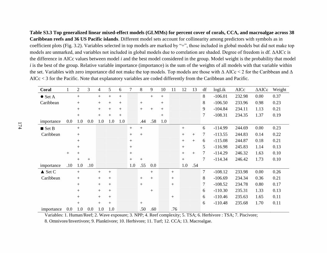
Table S3.3 Top generalized linear mixed-effect models (GLMMs) for percent cover of corals, CCA, and macroalgae across 38

Caribbean reefs and 36 US Pacific islands. Different model sets account for collinearity among predictors with symbols as in

coefficient plots (Fig. 3.2). Variables selected in top models are marked by “+”, those included in global models but did not make top

models are unmarked, and variables not included in global models due to correlation are shaded. Degree of freedom is df. ΔAICc is

the difference in AICc values between model i and the best model considered in the group. Model weight is the probability that model

i is the best of the group. Relative variable importance (importance) is the sum of the weights of all models with that variable within

the set. Variables with zero importance did not make the top models. Top models are those with Δ AICc < 2 for the Caribbean and Δ

AICc < 3 for the Pacific. Note that explanatory variables are coded differently from the Caribbean and Pacific.

Coral 1 2 3 4 5 6 7 8 9 10 11 12 13 df logLik AICc ΔAICc Weight

● Set A + + + + + + 8 -106.01 232.98 0.00 0.37

Caribbean + + + + + + 8 -106.50 233.96 0.98 0.23

+ + + + + + + 9 -104.84 234.11 1.13 0.21

+ + + + + 7 -108.31 234.35 1.37 0.19

importance 0.0 1.0 0.0 1.0 1.0 1.0 .44 .58 1.0

■ Set B + + + + 6 -114.99 244.69 0.00 0.23

Caribbean + + + + + 7 -113.55 244.83 0.14 0.22

+ + + + 6 -115.08 244.87 0.18 0.21

+ + + 5 -116.98 245.83 1.14 0.13

+ + + + + 7 -114.29 246.32 1.63 0.10

+ + + + + 7 -114.34 246.42 1.73 0.10

importance .10 1.0 .10 1.0 .55 0.0 1.0 .54

▲ Set C + + + + + 7 -108.12 233.98 0.00 0.26

Caribbean + + + + + + 8 -106.69 234.34 0.36 0.21

+ + + + + 7 -108.52 234.78 0.80 0.17

+ + + + 6 -110.30 235.31 1.33 0.13

+ + + + 6 -110.46 235.63 1.65 0.11

+ + + + 6 -110.48 235.68 1.70 0.11

importance 0.0 1.0 0.0 1.0 1.0 .50 .60 .76

Variables: 1. Human/Reef; 2. Wave exposure; 3. NPP; 4. Reef complexity; 5. TSA; 6. Herbivore : TSA; 7. Piscivore;

8. Omnivore/Invertivore; 9. Planktivore; 10. Herbivore; 11. Turf; 12. CCA; 13. Macroalgae.

174

CCA 1 2 3 4 5 6 7 8 9 10 11 12 13 df logLik AICc ΔAICc Weight

● Set A + + + + + + 8 -94.49 209.94 0.00 0.31

Caribbean + + + + + + + 9 -93.26 210.95 1.01 0.19

+ + + + + 7 -96.95 211.64 1.70 0.13

+ + + + + + 8 -95.36 211.68 1.74 0.13

+ + + + + + + 9 -93.73 211.88 1.95 0.12

+ + + + + 7 -97.08 211.90 1.96 0.12

importance .88 0.0 .62 .12 1.0 1.0 1.0 .44 1.0

■ Set B + + + + + 7 -103.08 223.90 0.00 0.27

Caribbean + + + + 6 -104.86 224.44 0.54 0.21

+ + + + 6 -105.00 224.70 0.81 0.18

+ + + + + + 8 -102.15 225.27 1.37 0.14

+ + + 5 -106.95 225.78 1.89 0.11

+ + + + + 7 -104.04 225.82 1.93 0.10

importance 1.0 .24 .61 0.0 1.0 .69 1.0

▲ Set C + + + + 6 -104.14 222.99 0.00 0.73

Caribbean + + + + + 7 -103.60 224.93 1.94 0.27

importance 0.0 .27 1.0 1.0 0.0 1.0 0.0 1.0

Variables: 1. Human/Reef; 2. Wave exposure; 3. NPP; 4. Reef complexity; 5. TSA; 6. Herbivore : TSA; 7. Piscivore;

8. Omnivore/Invertivore; 9. Planktivore; 10. Herbivore; 11. Turf; 12. CCA; 13. Macroalgae.

175

Macroalgae 1 2 3 4 5 6 7 8 9 10 11 12 13 df logLik AICc ΔAICc Weight

● Set A + + + + 6 -155.83 326.38 0.00 0.14

Caribbean + + + + + 7 -154.37 326.47 0.09 0.13

+ + + 5 -157.59 327.06 0.68 0.10

+ + + + 6 -156.27 327.25 0.87 0.09

+ + + + + + 8 -153.25 327.46 1.08 0.08

+ + + + + 7 -154.87 327.48 1.10 0.08

+ + + + + + 8 -153.29 327.55 1.18 0.08

+ + + + 6 -156.59 327.90 1.52 0.06

+ + + + + 7 -155.09 327.92 1.54 0.06

+ + + + + + + 9 -151.77 327.96 1.58 0.06

+ + + + + + 8 -153.52 328.00 1.62 0.06

+ + + 5 -158.17 328.22 1.85 0.05

importance .54 .63 .80 1.0 .49 .28 1.0

■ Set B + + + + 6 -156.49 327.68 0.00 0.43

Caribbean + + + + + 7 -155.68 329.10 1.42 0.21

+ + + 5 -158.75 329.38 1.70 0.18

+ + + + + 7 -155.85 329.43 1.75 0.18

importance .18 1.0 1.0 .82 .21 0.0 1.0

Variables: 1. Human/Reef; 2. Wave exposure; 3. NPP; 4. Reef complexity; 5. TSA; 6. Herbivore : TSA; 7. Piscivore;

8. Omnivore/Invertivore; 9. Planktivore; 10. Herbivore; 11. Turf; 12. CCA; 13. Macroalgae.

176

Coral 1 2 3 4 5 6 7 8 9 10 11 12 13 df logLik AICc ΔAICc Weight

● Set A + + 4 -122.47 254.24 0.00 0.65

Pacific + + + 5 -121.73 255.46 1.22 0.35

importance 1.0 1.0 .35 0.0 0.0 0.0

■ Set B + 3 -146.83 300.42 0.00 0.19

Pacific + + 4 -145.63 300.55 0.13 0.18

+ 3 -147.34 301.43 1.01 0.11

+ + 4 -146.09 301.47 1.06 0.11

+ + + 5 -144.77 301.53 1.11 0.11

+ + + 5 -144.92 301.85 1.43 0.09

+ + 4 -146.47 302.24 1.82 0.08

+ + 4 -146.54 302.38 1.96 0.07

+ + 4 -146.55 302.38 1.96 0.07

importance .63 .25 0.0 .28 .74

▲ Set C + + 4 -116.52 242.33 0.00 0.26

Pacific + + + 5 -115.18 242.37 0.03 0.26

+ + + 5 -115.28 242.55 0.22 0.24

+ + + + 6 -114.48 243.85 1.51 0.12

+ + + + 6 -114.58 244.05 1.71 0.11

importance 1.0 1.0 .21 .45 .35 0.0 0.0

▼ Set D + 3 -124.78 256.31 0.00 0.47

Pacific + + 4 -123.83 256.94 1.64 0.34

+ + 4 -124.45 258.20 1.89 0.18

importance .34 1.0 0.0 .18

Variables: 1. Human/Reef; 2. Wave exposure; 3. NPP; 4. Reef complexity; 5. Reef area; 6. Island elevation; 7. TSA; 8. Piscivore;

9. Omnivore/Invertivore; 10. Planktivore; 11. Herbivore; 12. CCA; 13. Macroalgae.

177

CCA 1 2 3 4 5 6 7 8 9 10 11 12 13 df logLik AICc ΔAICc Weight

● Set A + + 4 -110.90 231.10 0.00 0.33

Pacific + + + 5 -109.73 231.45 0.36 0.28

+ + + 5 -109.88 231.76 0.67 0.24

+ 3 -112.97 232.69 1.59 0.15

importance 0.0 .28 1.0 .85 .24

■ Set B + + 4 -110.15 229.58 0.00 0.45

Pacific + 3 -111.84 230.42 0.84 0.30

+ + + 5 -109.39 230.79 1.20 0.25

importance 0.0 0.0 .70 1.0 .25

▲ Set C + + 4 -111.06 231.42 0.00 0.28

Pacific + + 4 -111.10 231.49 0.07 0.27

+ + + 5 -110.13 232.26 0.84 0.18

+ + + 5 -110.31 232.61 1.20 0.15

+ + + 5 -110.64 233.27 1.86 0.11

importance .72 .15 .46 .54 0.0 .58

▼ Set D + + 4 -112.10 233.49 0.00 0.39

Pacific + 3 -113.44 233.64 0.15 0.36

+ + 4 -112.50 234.30 0.81 0.26

importance 1.0 .26 .39

Variables: 1. Human/Reef; 2. Wave exposure; 3. NPP; 4. Reef complexity; 5. Reef area; 6. Island elevation; 7. TSA; 8. Piscivore;

9. Omnivore/Invertivore; 10. Planktivore; 11. Herbivore; 12. CCA; 13. Macroalgae.

178

Macroalgae 1 2 3 4 5 6 7 8 9 10 11 12 13 df logLik AICc ΔAICc Weight

● Set A + + 4 -152.87 315.03 0.00 0.41

Pacific + + + 5 -151.86 315.72 0.69 0.29

+ + + 5 -152.25 316.49 1.47 0.20

+ + + + 6 -151.45 317.80 2.77 0.10

importance 1.0 1.0 .30 .39

■ Set B + 3 -177.17 361.10 0.00 0.43

Pacific + + 4 -176.72 362.74 1.64 0.19

+ + 4 -177.01 363.31 2.21 0.14

+ 3 -178.48 363.71 2.62 0.12

+ + 4 -177.21 363.71 2.62 0.12

importance .77 .26 .42

▲ Set C + + + + 6 -132.97 280.84 0.00 0.79

Pacific + + + + + 7 -132.74 283.49 2.65 0.21

importance 1.0 1.0 1.0 1.0 .21

▼ Set D + 3 -160.98 328.72 0.00 0.59

Pacific + + 4 -160.06 329.42 0.70 0.41

importance .41 1.0

Variables: 1. Human/Reef; 2. Wave exposure; 3. NPP; 4. Reef complexity; 5. Reef area; 6. Island elevation; 7. TSA; 8. Piscivore;

9. Omnivore/Invertivore; 10. Planktivore; 11. Herbivore; 12. CCA; 13. Macroalgae.

179

180

Appendix 3.2 References

Behrenfeld, M. J., and P. G. Falkowski. 1997. Photosynthetic rates derived from satellite-based

chlorophyll concentration. Limnology and oceanography:1–20.

Boss, E., and J. R. Zaneveld. 2003. The effect of bottom substrate on inherent optical properties:

Evidence of biogeochemical processes.

Casey, K. S., T. B. Brandon, P. Cornillon, and R. Evans. 2010. The past, present, and future of

the AVHRR pathfinder SST program. Pages 273–287 in V. Barale, J. F. R. Gower, and

L. Alberotanza, editors. Oceanography from Space. Springer Netherlands, Dordrecht.

Chollett, I., and P. J. Mumby. 2012. Predicting the distribution of Montastraea reefs using wave

exposure. Coral Reefs 31:493–503.

Chollett, I., P. J. Mumby, F. E. Müller-Karger, and C. Hu. 2012. Physical environments of the

Caribbean Sea. Limnology and Oceanography 57:1233–1244.

Ekebom, J., P. Laihonen, and T. Suominen. 2003. A GIS-based step-wise procedure for

assessing physical exposure in fragmented archipelagos. Estuarine, Coastal and Shelf

Science 57:887–898.

Friedlander, A. M., E. K. Brown, P. L. Jokiel, W. R. Smith, and K. S. Rodgers. 2003. Effects of

habitat, wave exposure, and marine protected area status on coral reef fish assemblages in

the Hawaiian archipelago. Coral Reefs 22:291–305.

Fulton, C. J., and D. R. Bellwood. 2004. Wave exposure, swimming performance, and the

structure of tropical and temperate reef fish assemblages. Marine Biology 144:429–437.

Glynn, P. W. 1993. Coral reef bleaching: ecological perspectives. Coral Reefs 12:1–17.

Gove, J. M., G. J. Williams, M. A. McManus, S. F. Heron, S. A. Sandin, O. J. Vetter, and D. G.

Foley. 2013. Quantifying climatological ranges and anomalies for Pacific coral reef

ecosystems. PloS one 8:e61974.

Harborne, A. R., P. J. Mumby, K. Zychaluk, J. D. Hedley, and P. G. Blackwell. 2011. Modeling

the beta diversity of coral reefs. Ecology 87:2871–2881.

Kilpatrick, K. A., G. P. Podestá, and R. Evans. 2001. Overview of the NOAA/NASA advanced

very high resolution radiometer Pathfinder algorithm for sea surface temperature and

associated matchup database. Journal of Geophysical Research: Oceans 106:9179–9197.

Latham, J., R. Cumani, I. Rosati, and M. Bloise. 2014. FAO Global Land Cover SHARE (GLC-

SHARE) database Beta-Release Version 1.0-2014. FAO.

181

Liu, G., A. E. Strong, and W. Skirving. 2003. Remote sensing of sea surface temperatures during

2002 Barrier Reef coral bleaching. Eos, Transactions American Geophysical Union

84:137–141.

McCook, L. J. 1999. Macroalgae, nutrients and phase shifts on coral reefs: scientific issues and

management consequences for the Great Barrier Reef. Coral Reefs 18:357–367.

Mora, C. 2008. A clear human footprint in the coral reefs of the Caribbean. Proceedings of the

Royal Society B: Biological Sciences 275:767–773.

Oregon State University. 2013. Ocean Productivity: Online VGPM Data.

http://orca.science.oregonstate.edu/1080.by.2160.monthly.hdf.vgpm.m.chl.m.sst4.php.

Polunin, N. V. C., and C. M. Roberts. 1993. Greater biomass and value of target coral-reef fishes

in two small Caribbean marine reserves. Marine Ecology Progress Series 100:177–183.

Rohmann, S. O., J. J. Hayes, R. C. Newhall, M. E. Monaco, and R. W. Grigg. 2005. The area of

potential shallow-water tropical and subtropical coral ecosystems in the United States.

Coral Reefs 24:370–383.

Schils, T., P. S. Vroom, and A. D. Tribollet. 2013. Geographical partitioning of marine

macrophyte assemblages in the tropical Pacific: a result of local and regional diversity

processes. Journal of Biogeography 40:1266–1277.

SEDAC, (Socioeconomic Data and Applications Center). 2010. Global rural-urban mapping

project – settlement points. Columbia University, New York.

http://sedac.ciesin.columbia.edu/data/set/gpw-v3-population-density/data-download.

Selig, E. R., K. S. Casey, and J. F. Bruno. 2010. New insights into global patterns of ocean

temperature anomalies: implications for coral reef health and management. Global

Ecology and Biogeography 19:397–411.

Storlazzi, C. D., E. K. Brown, M. E. Field, K. Rodgers, and P. L. Jokiel. 2005. A model for wave

control on coral breakage and species distribution in the Hawaiian Islands. Coral Reefs

24:43–55.

UNEP-WCMC, WorldFish Centre, WRI, and TNC. 2010. Global distribution of warm-water

coral reefs, compiled from multiple sources, including the Millennium Coral Reef

Mapping Project. UNEP World Conservation Monitoring Centre. Cambridge (UK).

http://data.unep-wcmc.org/datasets/13.

Williams, I. D., B. L. Richards, S. A. Sandin, J. K. Baum, R. E. Schroeder, M. O. Nadon, B.

Zgliczynski, P. Craig, J. L. McIlwain, and R. E. Brainard. 2011. Differences in reef fish

assemblages between populated and remote reefs spanning multiple archipelagos across

the central and western pacific. Journal of Marine Biology 2011.

Wilson, S., N. Graham, and N. Polunin. 2007. Appraisal of visual assessments of habitat

complexity and benthic composition on coral reefs. Marine Biology 151:1069–1076.

182

APPENDIX 4: SUPPLEMENTARY MATERIAL FOR CHAPTER 4

Appendix 4.1 Description of variables used as predictors in the generalized linear mixed

effect models.

Humans per reef area

Humans per reef area were used as a proxy of anthropogenic disturbance because human

activities have a direct and indirect negative effect on coral assemblages (Hughes et al. 2003,

Mora 2008, Bellwood et al. 2011, Barott et al. 2012). Human population size was estimated as

the maximum number of people that occurred within 50-km radius of each site. We chose 50 km

as radius because is a reasonable range of anthropogenic influence on Caribbean reefs (Mora

2008). Projection estimates of human population counts for the year 2010 were obtained from

the Gridded Population of the World V.3 at 0.25 degree resolution (SEDAC 2010). Reef areas

within 10 km radius of each site was calculated from the Global Distribution of Coral Reefs

(2010) database as available at the Ocean Data Viewer United Nations Environment Program's

World Conservation Monitoring Centre (UNEP-WCMC) (http://data.unep-

wcmc.org/datasets/13). All spatial calculations were performed in ArcGIS v10.0. Humans/ Reef

Area (humans/km2 reef) was calculated as: number of humans within 50km/Reef area within

10km/ (π 102) (km

2)

Cultivated land

Cultivated land could be a surrogate of terrestrial run-offs with potential effects on coral

and macroalgae cover when herbivory is reduced (McCook 1999, Mora 2008). We quantified the

area of cultivated land that occurred within a 50 km radius of each reef site. The raster data for

this variable was obtained from the Global Land Cover Share 2013 database (Latham et al.

183

2014). Specifically, we used the regional dataset (North and Central America) that depicts the

spatial distribution of 29 different land attributes for the year 2010 as calculated from satellite

images at 1 km resolution. Spatial analyses were performed in ArcGIS v10.

Reef structural complexity

Reef structural complexity was estimated at the seascape level. This topographic measure

provided an assessment of overall complexity accounting for living benthic organisms and reef

structure that have built over time (Polunin and Roberts 1993, Wilson et al. 2007). For each

transect set at each site we visually estimated structural reef complexity on a scale of 0-5, where

0 was given to reefs with no vertical relief; 1, low and sparse relief; 2, low but widespread relief;

3, moderately complex relief; 4, very complex relief with numerous caves and fissures; and 5,

reefs with exceptionally complex habitats, with numerous caves and overhangs (Polunin and

Roberts 1993). To minimize estimation subjectivity among observers, at least two divers

estimated reef structural complexity for each transect set and the average was calculated to be

used in the models. We evaluated the accuracy of the estimations among observers by comparing

the standard deviations (SD) among transects per site and found that SDs were 0-0.7 in all cases,

meaning that average estimation differences were never over 1 unit.

Ocean productivity

Mean oceanic net primary productivity (mg C m-2

day-1

) was estimated for each site

between 2002 and 2012 using remote-sensing. This was obtained from Aqua MODIS satellite

monthly data combined in the vertical generalized production model (Behrenfeld and Falkowski

1997) at a spatial resolution of 0.0833º (Oregon State University 2013). We used the mean of the

last ten years period because primary productivity is inherently variable in time and established

184

benthic communities may respond better to long term trends in primary productivity than to

survey year or monthly mean values. Calculations were performed in ArcGIS 10.0.

Wave exposure

Wave exposure is a good predictor of spatial variation in reef-building corals such as

Orbicella spp. (former Montastrea spp.) (Chollett and Mumby 2012) and can partially explain

beta diversity patterns of benthic communities (Harborne et al. 2011). The log of wind driven

wave exposure (J m-3

) was extracted in ArcGIS 10.0 from the wave stress map for the Caribbean

basin built by Chollett et al. (2012) and available at

(http://www.marinespatialecologylab.org/wp-content/uploads/2010/11/PECS1.png). The detailed

description of the wave exposure calculations and assumptions can be found in Chollett &

Mumby (2012).

Fish biomass

Piscivore and herbivorous fishes can indirectly affect coral assemblages through

cascading effects(Dulvy et al. 2004, Mumby et al. 2006, 2007). Underwater visual censuses

(UVC) were used to characterize the fish assemblages. At each reef site we randomly placed six

to eight belt transect sets along the fore reef’s spur-and-groove or slope formations and recorded,

identified, and estimated body size of all reef fish species. Each set consisted in a 50 x 10 m

transect area to estimate fish > = 40 cm in total length (TL) (McCauley et al. 2012) and a nested

30 x 2 transect area to estimate fish <40 cm TL (Lang et al. 2010). Fish size was estimated to the

nearest 10 cm, except for fish <10 cm where a 5 cm interval was used. Each transect belt set was

surveyed in ~15 minutes, covered the entire visible water column, and were at least ~10 m apart.

185

Fish biomass biomass was calculated using the allometric conversion relationship W=

aLb (Froese and Pauly 2013) where W is the weight of each fish in grams, L is the total length

(TL) or fork length (FL) in cm, and the parameters a and b are species specific. Length-length

conversion parameters were used to convert TL to FL for those species that L was based on FL.

When the allometric parameters (a and b) were not available we used those values from

congeneric species of similar size and shape and of similar geographical range (Froese and Pauly

2013).

186

Table S4.1 General descriptive information of surveyed sites. S&G means spur-and-groove.

Country Site name Site

code

Latitude Longitude Habitat

type

Depth

(m)

Date of

survey

Mexico Cancún GH 21.02544 -86.7713 S & G 12 Jul 12

Cozumel North PB 20.47188 -86.9815 S & G 10 Jul 12

Akumal XA 20.42689 -87.2860 S & G 15 Jul 12

Cozumel South CR 20.31961 -87.0266 S & G 15 Jul 12

Chinchorro North BCN 18.74867 -87.3476 S & G 15 Jul 12

Chinchorro Central BCC 18.57457 -87.4198 S & G 15 Jul 12

Chinchorro South BCS 18.41008 -87.4169 S & G 15 Jul 12

Belize Bacalar Chico BC 18.16282 -87.82222 S & G 12-15 May 10/12

Mexico Rocks MR 17.98782 -87.90382 S & G 12-15 May 10/12

Tackle Box TB 17.91056 -87.95083 S & G 12-15 May 10/12

Hol Chan HC 17.86343 -87.97238 S & G 12-15 May 10/12

Gallows GA 17.49592 -88.04255 S & G 12-15 May 10/12

Calabash Caye CA 17.26147 -87.81970 S & G 12-15 May 10/12

Half Moon Caye HM 17.20560 -87.54679 S & G 12-15 May 10/12

Alligator Caye AL 17.19660 -88.05115 S & G 12-15 May 10/12

Tobacco Caye TO 16.91911 -88.04757 S & G 12-15 May 10/12

South Water Caye SW 16.81346 -88.07756 S & G 12-15 May 10/12

Middle Caye MC 16.73703 -87.80536 S & G 12-15 May 10/12

South Middle Caye SM 16.72875 -87.82867 S & G 12-15 May 10/12

Pampion Caye PO 16.37310 -88.08913 S & G 12-15 May 10/12

Ranguana Caye RA 16.28501 -88.15031 S & G 12-15 May 10/12

Southwest Caye ST 16.11247 -88.27107 S & G 12-15 May 10/12

Nicholas Caye NI 16.11230 -88.25586 S & G 12-15 May 10/12

USA Dry Tortugas, USA LG 24.68508 -82.91050 S & G 12 Jun 12

Cuba Cueva Peces CP 22.16627 -81.13827 Slope 10-12 Jun 10/12

Punta Perdiz PZ 22.11003 -81.11626 Slope 10-12 Jun 10/12

Ebano EB 22.07914 -81.07599 Slope 10-12 Jun 10

Brinco BR 22.06939 -81.05588 Slope 10-12 Jun 12

Bacunayagua, Cuba BC 23.14653 -81.66664 Slope 10-12 Jun 12

El Peruano EP 20.84411 -79.02166 Slope 10-12 Jun 11

Pipin PP 20.82586 -78.98026 S & G 12-15 Jun 11

Anclita AN 20.78697 -78.94317 Slope 10-12 Jun 11

Cueva Pulpo CF 20.75266 -78.83634 Slope 10-12 Jun 11

Bahamas Guana Cay GC 26.70967 -77.15408 S & G 10-12 Jul 11/12

Fowls Cay FC 26.63717 -77.03848 Slope 10 Jul 11/12

Man o’ War MW 26.62122 -77.00550 S & G 10-12 Jul 11/12

Pelican Cay PC 26.39783 -76.98850 Slope 10 Jul 11/12

Little Harbor LH 26.32390 -76.99160 S & G 10-12 Jul 11/12

Rocky Point RP 25.99661 -77.40092 Slope 10-12 Jul 11/12

187

Table S4.2 Classification of Caribbean scleractinian coral species in three life history

strategies after Darling et al. (2012) These species were identified during our surveys.

Family Species Code Life history

Acroporidae Acropora cervicornis Acrcer Competitive

Acroporidae Acropora palmata Acrpal Competitive

Agaricidae Agaricia agaricites Agaaga Weedy

Agaricidae Agaricia fragilis Agafra Weedy

Agaricidae Agaricia grahamae Agagra Weedy

Agaricidae Agaricia humilis Agahum Weedy

Agaricidae Agaricia lamarcki Agalam Weedy

Agaricidae Agaricia tenuifolia Agaten Weedy

Mussidae Colpophyllia natans Colnat Stress-tolerant

Meandrinidae Dendrogyra cylindrus Dencyl Competitive

Meandrinidae Dichocoenia stokesi Dicsto Stress-tolerant

Mussidae Diploria labyrinthiformis Diplab Stress-tolerant

Caryophyllidae Eusmilia fastigiata Eusfas Stress-tolerant

Faviidae Favia fragum Favfra Stress-tolerant

Mussidae Isophyllia sinuosa Isosin Stress-tolerant

Agaricidae Leptoseris cucullata Lepcuc Weedy 1

Pocilloporidae Madracis decactis Maddec Weedy

Pocilloporidae Madracis mirabilis Madmir Weedy 2

Mussidae Manicina areolata Manare Weedy

Meandrinidae Meandrina meandrites Meamea Stress-tolerant

Milleporidae Millepora alcicornis Milalc Hydrocoral

Milleporidae Millepora complanata Milcom Hydrocoral

Montastreidae Montastraea cavernosa Moncav Stress-tolerant

Mussidae Mussa angulosa Musang Weedy 1

Mussidae Mycetophyllia aliciae Mycali Weedy

Mussidae Mycetophyllia danae Mycdan Weedy

Mussidae Mycetophyllia ferox Mycfer Weedy

Mussidae Mycetophyllia lamarckiana Myclam Weedy

Merulinidae Orbicella annularis Orbann Stress-tolerant

Merulinidae Orbicella faveolata Orbfav Stress-tolerant

Merulinidae Orbicella franksi Orbfra Stress-tolerant

Poritidae Porites astreoides Porast Weedy

Poritidae Porites divaricata Pordiv Weedy

Poritidae Porites furcata Porfur Weedy

Poritidae Porites porites Porpor Weedy

Mussidae Pseudodiploria clivosa Psecli Stress-tolerant

Mussidae Pseudodiploria strigosa Psestr Stress-tolerant

Siderastreidae Siderastrea radians Sidrad Weedy

Siderastreidae Siderastrea siderea Sidsid Stress-tolerant

Mussidae Scolymia lacera Scolac Weedy1

incertae sedis 3 Solenastrea buornoni Solbuo Stress-tolerant

Astrocoeniidae Stephanocoenia intersepta Steint Stress-tolerant 1Life history assigned from species in family

2Life history assigned from congeneric species

3Classification still dubious (Budd et al. 2012)

188

Table S4.3 Summary of the linear regression models parameters of the trend of thermal

stress anomalies on years for each study sites. For site codes refer to Table S1. Significance

codes are: 0 ‘***’ 0.001 ‘**’ 0.01 ‘*’ 0.05 ‘.’

Country Site Estimate Std. Error t-value F-statistic Pr(>|t|) R2

Bahamas FC 0.01122 0.04019 0.279 0.079 0.7823 0.002

Bahamas GC 0.05473 0.03611 1.516 2.297 0.1417 0.081

Bahamas LH 0.01505 0.02165 0.695 0.483 0.4931 0.018

Bahamas MW 0.03777 0.02043 1.849 3.418 0.0759. 0.116

Bahamas PC 0.00931 0.02458 0.379 0.143 0.7081 0.005

Bahamas RP 0.00438 0.02199 0.199 0.039 0.8437 0.002

Belize AL 0.11549 0.02695 4.286 18.37 0.0002*** 0.414

Belize BC 0.09031 0.04229 2.136 4.560 0.0423* 0.149

Belize CA 0.16530 0.05483 3.015 9.089 0.0057** 0.259

Belize GA 0.14614 0.04044 3.164 13.06 0.0012** 0.334

Belize HC 0.12397 0.02872 4.317 18.64 0.0002*** 0.418

Belize HM 0.09606 0.03086 3.112 9.687 0.0044** 0.271

Belize MC 0.16284 0.04218 3.860 14.90 0.0007*** 0.364

Belize MR 0.06513 0.04723 1.379 1.902 0.1800 0.065

Belize NI 0.14231 0.06065 2.347 5.506 0.0269* 0.175

Belize PO 0.10208 0.04964 2.056 4.228 0.0499* 0.139

Belize RA 0.13547 0.05678 2.386 5.692 0.0246* 0.179

Belize SM 0.16010 0.04300 3.723 13.86 0.0009*** 0.348

Belize ST 0.16845 0.04147 4.062 16.50 0.0004*** 0.388

Belize SW 0.09797 0.04459 2.197 4.827 0.0371* 0.157

Belize TB 0.09743 0.04164 2.340 5.474 0.0273* 0.174

Belize TO 0.17950 0.04630 3.878 15.04 0.0006*** 0.366

Cuba AN 0.05911 0.02809 2.105 4.430 0.0451* 0.146

Cuba BA -0.01286 0.05436 -0.237 0.056 0.8148 0.002

Cuba BR 0.04735 0.02248 2.106 4.434 0.0450* 0.146

Cuba CF 0.05446 0.04329 1.258 1.583 0.2200 0.057

Cuba CP 0.07553 0.04768 1.584 2.509 0.1253 0.088

Cuba EB 0.04351 0.01668 2.608 6.804 0.0149* 0.207

Cuba EP 0.08046 0.04001 2.011 4.045 0.0548. 0.135

Cuba PP 0.07526 0.04312 1.745 3.046 0.0928. 0.105

Cuba PZ 0.02600 0.02514 1.034 1.070 0.3105 0.039

USA LG 0.01423 0.02777 0.512 0.263 0.6126 0.010

Mexico BCC 0.10317 0.02622 3.935 15.48 0.0006*** 0.373

Mexico BCN 0.12014 0.03605 3.333 11.11 0.0026** 0.299

Mexico BCS 0.09661 0.02793 3.459 11.96 0.0019** 0.315

Mexico CR 0.06541 0.03073 2.128 4.530 0.0429* 0.148

Mexico GH 0.05200 0.02711 1.918 3.678 0.0662. 0.124

Mexico PB 0.03311 0.02600 1.274 1.623 0.2140 0.059

Mexico XA 0.05966 0.03440 1.734 3.008 0.0947 0.104

189

Figure S4.1 Spearman’s rank correlation matrix of absolute values and pairs plot for

explanatory variables used in the GLMMs. The size of the correlation numbers is proportional

to the amount of correlation. Turf algae and Cultivated land were dropped from the models

because they were correlated (rs > 0.50) with Algae cover and Humans/reef, respectively.

190

Figure S4.2 Frequency of thermal stress anomalies for each surveyed site from 1982 to

2010. Blue line is the predicted simple linear model regression bounded by 95% confidence

interval. Most sites in Belize and Mexico have increased the frequency of TSA over ~30 year.

For site labels refer to Supplementary Table S4.1. For the results of the linear model see Table

S4.3.

191

Figure S4.3 Notched boxplot of average TSA frequency over 29 years for each sub-region

(country). Non-overlapping notches indicate statistically significant differences between

medians (horizontal black line). Black dot is the mean value for each sub-region.

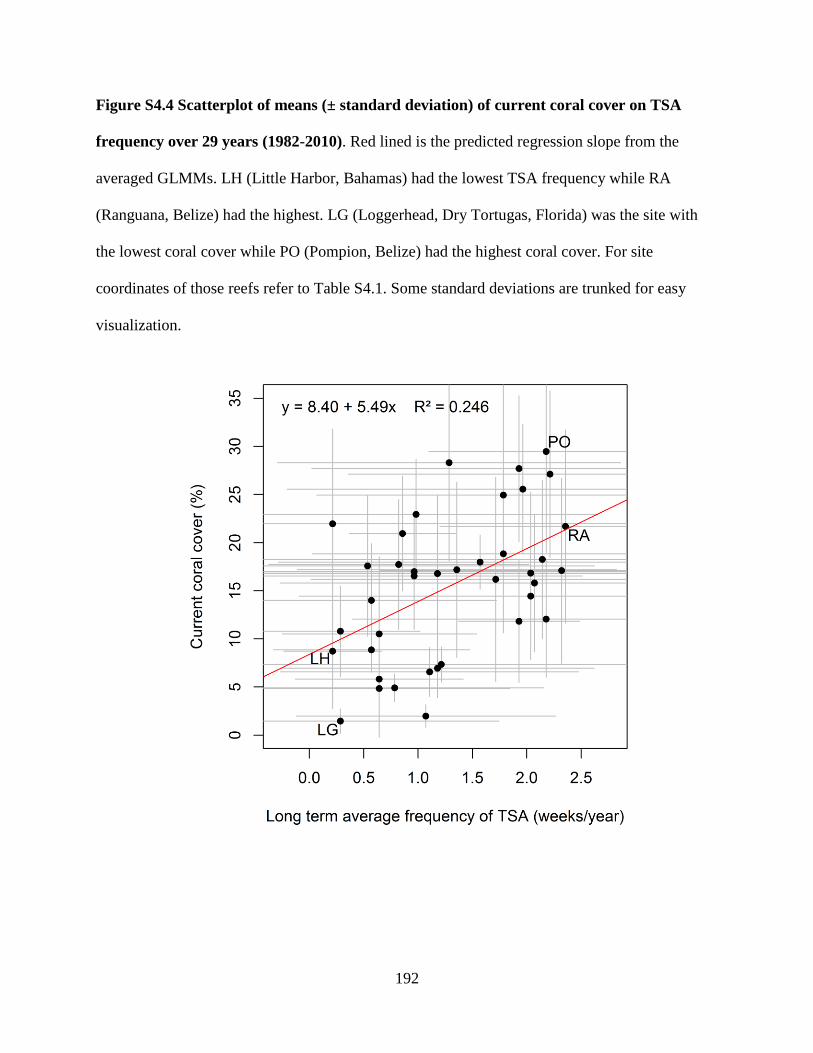
192

Figure S4.4 Scatterplot of means (± standard deviation) of current coral cover on TSA

frequency over 29 years (1982-2010). Red lined is the predicted regression slope from the

averaged GLMMs. LH (Little Harbor, Bahamas) had the lowest TSA frequency while RA

(Ranguana, Belize) had the highest. LG (Loggerhead, Dry Tortugas, Florida) was the site with

the lowest coral cover while PO (Pompion, Belize) had the highest coral cover. For site

coordinates of those reefs refer to Table S4.1. Some standard deviations are trunked for easy

visualization.

193

Appendix 4.2 Mechanisms of acquisition of thermal tolerance

Thermal tolerance of different coral species can occur via genetic adaptation or

physiological acclimatization (i.e., phenotypic plasticity), two mechanisms that have been widely

studied for coral species and genotypes over the past decade (Edmunds and Gates 2008,

Bellantuono et al. 2012, Hoegh-Guldberg 2012, Palumbi et al. 2014). Adaptation occurs through

natural selection of heat-tolerant lineages of algal symbionts and/or coral host (Baker et al. 2004,

Guest et al. 2012, Hoegh-Guldberg 2012). Micro-evolutionary adaptation to rapid warming may

take decades (Hoegh-Guldberg 2012), especially for major reef building broadcasting corals

(e.g., Acropora spp., Siderastrea spp., and Orbicella spp. in the Caribbean) that reproduce

annually or biannually and that reach maturity after several years (Darling et al. 2012).

Physiological acclimatization of either or both host and symbiont in response to frequent thermal

anomalies (Edmunds and Gates 2008, Bellantuono et al. 2012, Palumbi et al. 2014) can occur

much faster than genetic adaptation in slow-growing organisms (like corals) and may bolster

resistance to future temperature stress (Edmunds and Gates 2008, Palumbi et al. 2014),

especially for weedy and brooder corals (e.g., Porites spp. and Agaricia spp.) that reproduce

often (Green et al. 2008).

Acclimatization may work through at least two major pathways that promote thermal

tolerance of corals, first by hosting, shifting or acquiring stress-tolerant algal symbionts (Baker et

al. 2004, Berkelmans and Oppen 2006, Oliver and Palumbi 2011) and second by physiological

changes of coral host and/or endosymbionts (Baird et al. 2009, Barshis et al. 2010, LaJeunesse et

al. 2010, Bellantuono et al. 2012). Many corals can host, exchange or shift algal symbiont

composition to thermally resistant clades which may confer them distinct thermal tolerance in

high-temperature habitats (Berkelmans and Oppen 2006, Oliver and Palumbi 2011). For

194

example, during warming events in the Pacific, corals that host specific members of

Symbiodinium clade D, and to lesser extent C1 subtype, suffered less bleaching and mortality

than those harboring different clades (Baker et al. 2004, Berkelmans and Oppen 2006, Oliver and

Palumbi 2011) . Previous studies have suggested that members of stress-tolerant clade D may

showed in higher proportions in hotter, higher-stress environments, and during different seasons

(Jones et al. 2008, LaJeunesse et al. 2010, Oliver and Palumbi 2011, Barshis et al. 2013, Palumbi

et al. 2014). Additionally, some scleractinian coral species may host multiple algal symbiont

clades with the potential to shift towards thermal-stress tolerant ones when necessary(Oliver and

Palumbi 2011). In fact, after natural bleaching events, some corals (e.g., Acropora spp. in the

Pacific) can increase the density of thermal tolerant symbiont clades (Jones et al. 2008,

LaJeunesse et al. 2010, Oliver and Palumbi 2011). However, not all coral species that resist

thermal stress change symbiont composition with environmental conditions (LaJeunesse et al.

2010, Bellantuono et al. 2012). For example, hydrocorals such as Millepora divaricata are

common in higher-temperature habitats in the Pacific but harbor a single symbiont type (Oliver

and Palumbi 2011). This implies that although changes in symbiont composition may be

important for certain coral species, other species can successfully acclimate to local high-

frequency of thermal stress anomalies without changing algal symbiont identity(Bellantuono et

al. 2012, Palumbi et al. 2014).

Acclimatization can be also achieved through physiological plasticity of the host and/or

symbiotic algae in response to temperature anomalies (Bellantuono et al. 2012). Increasing the

expression of certain genes that promote high protein turnover has been associated with thermal

tolerance in the host by providing protection from bleaching without altering Symbiodinium

dynamics (Palumbi et al. 2014). For example, acquire tolerance of preconditioned Acropora

195

millepora corals to thermal stress was not associated to changes in endosymbionts or bacterial

community in experimental studies (Bellantuono et al. 2012). In fact, the aposymbiotic larvae of

A. millepora show pronounce gene expression that leads to production of heat-shock proteins in

response to thermal stress (Rodriguez-Lanetty et al. 2009). Similarly, exposure of Orbicella

franksi to elevated temperature result in the upregulation of heat-shock HSP70 proteins (i.e.,

which are involved in protein folding processes) after 6 and 48 hours of heat stress (Edmunds

and Gates 2008). Other experiments have shown that host genotypes of Pocillopora damicornis

originating from non-upwelling thermal-stressed areas showed greater thermal tolerance than

genotypes originating from upwelling areas that exhibit lower thermal stress regime (D’Croz and

Maté 2004). Reciprocal transplant experiments of genetically distinct populations of Porites

lobata between back-reef and forereef environments also demonstrate host physiological

acclimatization to stress driven by colony genotype (Barshis et al. 2010). In this species, thermal

tolerance of back-reef individuals was associated with higher levels of ubiquiting-conjugate

proteins in response to highly fluctuating back reef environment (Barshis et al. 2010). On the

other hand, differences in photo-acclimation of algae symbionts, by reductions of Chlorophyll-a

or by dissipating excess excitation energy through non-photochemical pathways in response to

elevated irradiance, may partially explain why fore-reef generalist corals such as Orbicella

annularis are less thermally tolerant than back-reef weedy species such as Siderastrea radians

(Warner et al. 1996) in the Caribbean.

196

Appendix 4.3 References

Baird, A. H., R. Bhagooli, P. J. Ralph, and S. Takahashi. 2009. Coral bleaching: the role of the

host. Trends in Ecology & Evolution 24:16–20.

Baker, A. C., C. J. Starger, T. R. McClanahan, and P. W. Glynn. 2004. Coral reefs: Corals’

adaptive response to climate change. Nature 430:741–741.

Barott, K. L., G. J. Williams, M. J. A. Vermeij, J. Harris, J. E. Smith, F. L. Rohwer, and S. A.

Sandin. 2012. Natural history of coral−algae competition across a gradient of human

activity in the Line Islands. Marine Ecology Progress Series 460:1–12.

Barshis, D. J., J. T. Ladner, T. A. Oliver, F. O. Seneca, N. Traylor-Knowles, and S. R. Palumbi.

2013. Genomic basis for coral resilience to climate change. Proceedings of the National

Academy of Sciences.

Barshis, D. J., J. H. Stillman, R. D. Gates, R. J. Toonen, L. W. Smith, and C. Birkeland. 2010.

Protein expression and genetic structure of the coral Porites lobata in an environmentally

extreme Samoan back reef: does host genotype limit phenotypic plasticity? Molecular

Ecology 19:1705–1720.

Behrenfeld, M. J., and P. G. Falkowski. 1997. Photosynthetic rates derived from satellite-based

chlorophyll concentration. Limnology and oceanography:1–20.

Bellantuono, A. J., O. Hoegh-Guldberg, and M. Rodriguez-Lanetty. 2012. Resistance to thermal

stress in corals without changes in symbiont composition. Proceedings of the Royal

Society B: Biological Sciences 279:1100–1107.

Bellwood, D. R., A. S. Hoey, and T. P. Hughes. 2011. Human activity selectively impacts the

ecosystem roles of parrotfishes on coral reefs. Proceedings of the Royal Society B:

Biological Sciences.

Berkelmans, R., and M. J. H. van Oppen. 2006. The role of zooxanthellae in the thermal

tolerance of corals: a “nugget of hope” for coral reefs in an era of climate change.

Proceedings of the Royal Society B: Biological Sciences 273:2305–2312.

Budd, A. F., H. Fukami, N. D. Smith, and N. Knowlton. 2012. Taxonomic classification of the

reef coral family Mussidae (Cnidaria: Anthozoa: Scleractinia). Zoological Journal of the

Linnean Society 166:465–529.

Chollett, I., and P. J. Mumby. 2012. Predicting the distribution of Montastraea reefs using wave

exposure. Coral Reefs 31:493–503.

Chollett, I., P. J. Mumby, F. E. Müller-Karger, and C. Hu. 2012. Physical environments of the

Caribbean Sea. Limnology and Oceanography 57:1233–1244.

197

Darling, E. S., L. Alvarez-Filip, T. A. Oliver, T. R. McClanahan, and I. M. Côté. 2012.

Evaluating life-history strategies of reef corals from species traits. Ecology Letters

15:1378–1386.

D’Croz, L., and J. L. Maté. 2004. Experimental responses to elevated water temperature in

genotypes of the reef coral Pocillopora damicornis from upwelling and non-upwelling

environments in Panama. Coral Reefs 23:473–483.

Dulvy, N. K., R. P. Freckleton, and N. V. C. Polunin. 2004. Coral reef cascades and the indirect

effects of predator removal by exploitation. Ecology Letters 7:410–416.

Edmunds, P. J., and R. D. Gates. 2008. Acclimatization in tropical reef corals. Marine Ecology

Progress Series 361:307–310.

Froese, R., and D. Pauly. 2013. FishBase. http://www.fishbase.org.

Green, D., P. Edmunds, and R. Carpenter. 2008. Increasing relative abundance of Porites

astreoides on Caribbean reefs mediated by an overall decline in coral cover. Marine

Ecology Progress Series 359:1–10.

Guest, J. R., A. H. Baird, J. A. Maynard, E. Muttaqin, A. J. Edwards, S. J. Campbell, K.

Yewdall, Y. A. Affendi, and L. M. Chou. 2012. Contrasting Patterns of Coral Bleaching

Susceptibility in 2010 Suggest an Adaptive Response to Thermal Stress. PLoS ONE

7:e33353.

Harborne, A. R., P. J. Mumby, K. Zychaluk, J. D. Hedley, and P. G. Blackwell. 2011. Modeling

the beta diversity of coral reefs. Ecology 87:2871–2881.

Hoegh-Guldberg, O. 2012. The adaptation of coral reefs to climate change: Is the Red Queen

being outpaced? Scientia Marina 76:403–408.

Hughes, T. P., A. H. Baird, D. R. Bellwood, M. Card, S. R. Connolly, C. Folke, R. Grosberg, O.

Hoegh-Guldberg, J. B. C. Jackson, J. Kleypas, J. M. Lough, P. Marshall, M. Nyström, S.

R. Palumbi, J. M. Pandolfi, B. Rosen, and J. Roughgarden. 2003. Climate change, human

impacts, and the resilience of coral reefs. Science 301:929–933.

Jones, A. M., R. Berkelmans, M. J. H. van Oppen, J. C. Mieog, and W. Sinclair. 2008. A

community change in the algal endosymbionts of a scleractinian coral following a natural

bleaching event: field evidence of acclimatization. Proceedings of the Royal Society B:

Biological Sciences 275:1359–1365.

LaJeunesse, T. C., R. Smith, M. Walther, J. Pinzón, D. T. Pettay, M. McGinley, M.

Aschaffenburg, P. Medina-Rosas, A. L. Cupul-Magaña, A. L. Pérez, H. Reyes-Bonilla,

and M. E. Warner. 2010. Host–symbiont recombination versus natural selection in the

response of coral–dinoflagellate symbioses to environmental disturbance. Proceedings of

the Royal Society B: Biological Sciences:rspb20100385.

198

Lang, J. C., K. W. Marks, P. A. Kramer, P. Richards Kramer, and R. N. Ginsburg. 2010.

AGRRA Protocols version 5.4 Atlantic and Gulf Rapid Reef Assessment Program.

University of Miami, Florida.

Latham, J., R. Cumani, I. Rosati, and M. Bloise. 2014. FAO Global Land Cover SHARE (GLC-

SHARE) database Beta-Release Version 1.0-2014. FAO.

McCauley, D. J., K. A. McLean, J. Bauer, H. S. Young, and F. Micheli. 2012. Evaluating the

performance of methods for estimating the abundance of rapidly declining coastal shark

populations. Ecological Applications 22:385–392.

McCook, L. J. 1999. Macroalgae, nutrients and phase shifts on coral reefs: scientific issues and

management consequences for the Great Barrier Reef. Coral Reefs 18:357–367.

Mora, C. 2008. A clear human footprint in the coral reefs of the Caribbean. Proceedings of the

Royal Society B: Biological Sciences 275:767–773.

Mumby, P. J., C. P. Dahlgren, A. R. Harborne, C. V. Kappel, F. Micheli, D. R. Brumbaugh, K.

E. Holmes, J. M. Mendes, K. Broad, J. N. Sanchirico, K. Buch, S. Box, R. W. Stoffle,

and A. B. Gill. 2006. Fishing, trophic cascades, and the process of grazing on coral reefs.

Science 311:98–101.

Mumby, P. J., A. R. Harborne, J. Williams, C. V. Kappel, D. R. Brumbaugh, F. Micheli, K. E.

Holmes, C. P. Dahlgren, C. B. Paris, and P. G. Blackwell. 2007. Trophic cascade

facilitates coral recruitment in a marine reserve. Proceedings of the National Academy of

Sciences 104:8362–8367.

Oliver, T. A., and S. R. Palumbi. 2011. Many corals host thermally resistant symbionts in high-

temperature habitat. Coral Reefs 30:241–250.

Oregon State University. 2013. Ocean Productivity: Online VGPM Data.

http://orca.science.oregonstate.edu/1080.by.2160.monthly.hdf.vgpm.m.chl.m.sst4.php.

Palumbi, S. R., D. J. Barshis, N. Traylor-Knowles, and R. A. Bay. 2014. Mechanisms of reef

coral resistance to future climate change. Science:1251336.

Polunin, N. V. C., and C. M. Roberts. 1993. Greater biomass and value of target coral-reef fishes

in two small Caribbean marine reserves. Marine Ecology Progress Series 100:177–183.

Rodriguez-Lanetty, M., S. Harii, and O. Hoegh-Guldberg. 2009. Early molecular responses of

coral larvae to hyperthermal stress. Molecular Ecology 18:5101–5114.

SEDAC, (Socioeconomic Data and Applications Center). 2010. Global rural-urban mapping

project – settlement points. Columbia University, New York.

http://sedac.ciesin.columbia.edu/data/set/gpw-v3-population-density/data-download.

UNEP-WCMC, WorldFish Centre, WRI, and TNC. 2010. Global distribution of warm-water

coral reefs, compiled from multiple sources, including the Millennium Coral Reef

199

Mapping Project. UNEP World Conservation Monitoring Centre. Cambridge (UK).

http://data.unep-wcmc.org/datasets/13.

Warner, M. E., W. K. Fitt, and G. W. Schmitt. 1996. The effects of elevated temperature on the

photosynthetic efficiency of zooxanthellae in hospite from four different species of reef

coral: a novel approach. Plant, Cell & Environment 19:291–299.

Wilson, S., N. Graham, and N. Polunin. 2007. Appraisal of visual assessments of habitat

complexity and benthic composition on coral reefs. Marine Biology 151:1069–1076.