First-Best Equilibrium in Insurance Markets with Transaction ...

First-Best Equilibrium in Insurance Markets with Transaction Costs and HeterogeneityAuthor(s): Jerry W. Liu and Mark J. BrowneSource: The Journal of Risk and Insurance, Vol. 74, No. 4 (Dec., 2007), pp. 739-760Published by: American Risk and Insurance AssociationStable URL: http://www.jstor.org/stable/25145245 .

Accessed: 06/07/2014 19:40

Your use of the JSTOR archive indicates your acceptance of the Terms & Conditions of Use, available at .http://www.jstor.org/page/info/about/policies/terms.jsp

.JSTOR is a not-for-profit service that helps scholars, researchers, and students discover, use, and build upon a wide range ofcontent in a trusted digital archive. We use information technology and tools to increase productivity and facilitate new formsof scholarship. For more information about JSTOR, please contact [email protected].

.

American Risk and Insurance Association is collaborating with JSTOR to digitize, preserve and extend accessto The Journal of Risk and Insurance.

http://www.jstor.org

This content downloaded from 131.252.96.28 on Sun, 6 Jul 2014 19:40:19 PMAll use subject to JSTOR Terms and Conditions

http://www.jstor.org/action/showPublisher?publisherCode=ari

http://www.jstor.org/stable/25145245?origin=JSTOR-pdf

http://www.jstor.org/page/info/about/policies/terms.jsp


? The Journal of Risk and Insurance, 2007, Vol. 74, No. 4,739-760

First-Best Equilibrium in Insurance Markets With Transaction Costs and Heterogeneity

Jerry W. Liu

Mark J. Browne

Abstract

We investigate extensions of the classic Rothschild and Stiglitz (1976) (RS) model of adverse selection under asymmetric information. In RS, low-risk

customers are worse off owing to an externality created by high-risk buyers

in the market. We find critical changes in insurance buyers' behavior un

der the joint assumptions of transaction costs and buyer heterogeneity with

respect to either risk aversion or wealth. Combining transaction costs and

heterogeneity, we find a separating equilibrium in which neither high-risk nor low-risk individuals are penalized due to information asymmetry.

Introduction

The impact of asymmetric information on markets is an important issue in the eco

nomics literature. In 2001, Joseph Stiglitz, George Akerlof, and Michael Spence were

awarded the Nobel Prize in Economics for their analyses of markets under asymmet ric information. In their seminal paper, Rothschild and Stiglitz (1976) (RS) provide a

framework for analyzing the problem of adverse selection in insurance markets. Their central finding is that information asymmetry causes markets to deteriorate. When a separating equilibrium exists, "The high-risk (low ability, etc.) individuals [exert] a

dissipative externality on the low-risk (high ability) individuals/'1 so that the low-risk customers are worse off due to the presence of high-risk customers. Furthermore, RS find that competitive insurance markets may have no equilibrium.

In spite of the pessimistic conclusions of RS, we observe that many markets func tion well under asymmetric information: labor markets, credit markets, and security

Jerry W. Liu is at the Krannert School of Management, Purdue University. Mark J. Browne is at the School of Business, University of Wisconsin-Madison. The authors can be contacted

via e-mail: [email protected] and [email protected]. We thank Thomas Cosimano,

Suzanne Bellezza, Georges Dionne, Edward Frees, Thomas Gresik, Donald Hausch, Szilvia

Papai, Pierre Picard, Robert Puelz, Cheng-zhong Qin, Larry Samuelson, Virginia Young, and

seminar participants at the 2003 Risk Theory Society meeting, University of Wisconsin-Madison for helpful comments. The suggestions of two anonymous referees were

especially helpful in

improving the article. All errors are strictly ours. 1 Rothschild and Stiglitz (1976, p. 468).

739



740 The Journal of Risk and Insurance

markets are obvious examples. Moreover, the results of empirical studies are not

always consistent with the RS predictions. For example, in RS, high-risk insurance

customers always buy more insurance than low-risk customers. However, Chiappori and Salanie (2000) find no statistical evidence that customers with higher accident

probabilities purchase contracts with more comprehensive coverage. In this article, we modify several of RS's assumptions and offer new insights into why the RS results are not always consistent with empirical findings.

The most important contribution of this article is that we show conditions under which

markets with asymmetric information remain efficient. Whereas RS assume that there are no transaction costs in the insurance markets and that customers are identical

except for loss probability, we evaluate equilibrium when there are transaction costs

and when customers differ with respect to risk aversion or endowment, in addition

to loss probability. In the RS framework, all customers prefer full coverage. In our

setting, when there are proportional costs, all buyers prefer partial coverage. Our

assumptions of heterogeneity with respect to risk aversion or wealth indicate that

relevant factors other than loss probability play a part in the insurance decision. We

find that if customers are different enough in these new dimensions, and if there are transaction costs, a separating equilibrium exists in which there are no negative externalities.

This article contributes to two areas of the literature that have evolved from RS. First, it extends previous work on the effect of transaction costs in insurance markets. Many

papers investigate optimal choice when the premium contains a fixed-percent pre mium loading. Arrow (1971) uses calculus of variations to show the optimality of a

deductible, whereas Mossin (1968) proposes a theorem stating that partial insurance

is optimal. In another important study, Dionne, Gourieroux, and Vanasse (1998) make

an attempt to show that the RS result remains unchanged when different risk types have the same proportional cost structure. We integrate transaction costs into the RS

framework by systematically evaluating two cost structures: constant costs and pro

portional costs. We argue that high-risk individuals suffer more from proportional costs than low-risk individuals, and the RS externality result persists.

Second, our study extends the literature on heterogeneity among insurance customers.

The RS model assumes that people are homogeneous in risk aversion, endowment

wealth, and loss severity. These assumptions may not be realistic, and we offer an

alternative setting that yields new insights.2

Heterogeneous risk aversion has been previously evaluated by De Meza and Webb

(2001). They assume that risk-averse people tend to buy more insurance coverage, whereas reckless people put less value on insurance protection. In their setting, it is

possible to reach a partial pooling equilibrium, in which some, but not all, low-risk

individuals are worse off. In our model, heterogeneous risk aversion has a different

2 Our article is closely related to Doherty and Jung (1993). They modify the RS model by considering severity differences in addition to probability and their conclusion is that first

best solutions are feasible. Although Doherty and Jung concentrate on a single assumption, we focus on the externality conclusion of the RS model by revising multiple assumptions.



First-Best Equilibrium in Insurance Markets 741

effect: we find that the market may reach a new separating equilibrium and the infor

mation problem becomes irrelevant. This result, however, relies on the simultaneous

presence of proportional costs and heterogeneous risk aversion.

In our framework with proportional costs, we analyze two scenarios: Scenario A, in which high-risk customers are more risk averse (less wealthy) than low-risk cus

tomers, and Scenario B, in which low-risk customers are more risk averse (wealthier) than high-risk customers. In Scenario A, when the difference in risk aversion (wealth)

between high- and low-risk customers is great enough, the optimal contracts of the

high- and low-risk customers will diverge, creating a separating equilibrium. In the new separating equilibrium, neither risk group imposes a negative externality on the

other group. Henceforth, we call this an NE (no externality) equilibrium. In Scenario B, an NE equilibrium exists when the difference in risk aversion (wealth) is large and the

difference in loss probabilities is small. Moreover, if consumers differ in wealth, rather

than in risk aversion, the same no-externality result occurs (high wealth is equivalent to low-risk aversion).

It appears that the RS negative externality conclusion depends on the assumption that

high- and low-risk customers are identical on all dimensions other than loss probabil ity; customers are so similar that the risk groups prefer the same policy. They do not

have other reasons for preferring policies that are different. Our results suggest that

the interaction between transaction costs and consumer heterogeneity may explain, at least in part, why we observe markets thriving under asymmetric information and

why empirical results do not always confirm the RS predictions.

The remainder of this article is organized as follows: first is an overview of the RS

model, followed by an analysis of the effect of transaction costs in the next section.

The case of heterogeneous risk aversion and the NE equilibrium are presented next, and then the effect of heterogeneous wealth is investigated. Finally, conclusions are

presented.

The Model

Because our analysis is based on the RS model, we begin with a brief review of their model and its assumptions. There are two types of insurance customers in the market,

low-risk and high-risk. They have different accident probabilities, pH > pL. Customers know their accident probabilities, but the insurance company does not. RS also make the following four simplifying assumptions:

1. There are no transaction costs and the insurer makes zero expected profit.

2. Both types of customers have the same level of risk aversion.

3. Every client has an identical endowment W.

4. If there is an accident, both risk groups have the identical loss amount d.

In this article, we modify the first three assumptions, thus making the two groups more

dissimilar than they are in the original model. We adopt the following assumptions from the RS model.




The insurance company writes a contract a = (ct\, 012), where a\ is the premium

amount and a2 the net indemnity amount (premium is deducted). If an accident

occurs, the individual will receive a total indemnity of ot\ +a2. The price of in surance is q(a)

= a\/a2. Since neither the insurance premium nor the indemnity should be negative, we call an insurance contract (pt\, aj) admissible if and only if

a\ > 0 and a2 > 0.3 The individual agent's wealth in the two states of nature (accident or no accident) is represented by a vector (YI\, W2). If there is no accident, the agent's wealth is the

endowment minus the premium paid to the insurer,

W1 = W-a1. (1)

If an accident occurs, he suffers a loss d and receives a reimbursement a\ -f a2,

W2 = W-d+a2. (2)

Insurers behave as if they are risk neutral. RS argue that insurance company share

holders hold well-diversified portfolios. The equilibrium is defined as a set of contracts such that, when customers choose

contracts to maximize expected utility: (1) no contract in the equilibrium set makes

negative expected profits, and (2) there is no contract outside the equilibrium set

that, if offered, will make a nonnegative profit.4 All insurance customers have absolute risk aversion,

U"(x)

'"-m- <3)

where r (x) may be a constant, a decreasing or an increasing function of wealth x. In

this article, when studying the role of risk aversion, r(x) is assumed to be constant

in order to control for wealth effects. We postulate that r(x) decreases with wealth

while discussing the effect of heterogeneous wealth.

The expected utility of a risk-type t individual (t = H, L), who purchases contract

a (ai, a2) is

V*(ai,a2) = (!

- Pl)U(W

- e*i) + pfU(W -d+ a2). (4)

From (4), the marginal rate of substitution for type t is

MRS' dW2 Q-WM) (5)

3 This restriction is necessary since without it the optimal premium could become negative

when transaction costs are extremely high.

4 The main result of this article, no externality equilibrium, relies on

envy-free allocations; any

such allocation is an equilibrium whatever the concept (among standard ones). In this respect,

most of the article is robust to alternative equilibrium concepts.




It is clear to see that ^?^~

> 1~? ) the low-risk indifference curve is everywhere

steeper than the high-risk indifference curve.

Transaction Costs

In the RS model, there are no transaction costs and insurance firms make zero expected

profits. Consequently, for each insurance policy, the expected claim, p(a\ + oti), is equal to the premium a\. The insurer's expected profit can be expressed as

n = a\ -

p(?i + a2) = 0. (6)

In reality, insurance contracts cost more than the expected value of their claims. Allard,

Cresta, and Rochet (1997) modify the RS model by introducing a distribution cost, which corresponds to the cost of designing and marketing an insurance contract.

The key feature of their model is that the total cost is assumed to be a constant, and

therefore the per-customer cost decreases when more customers buy the contract. This

economy of scale provides a counterforce to adverse selection, and it leads to their most important conclusion: "Pooling equilibria always exist when the set-up cost is

large enough."

In this article, the cost structure has both a constant term and terms that are propor tional to their premium or reimbursement:

cost = a + boi\ + cp(pt\ + a?). (7)

The cost function can be added to the right side of the budget Equation (6). Below, we

discuss the constant and proportional components of the general cost function, and

analyze their respective impacts on insurance buyers' behavior.

Constant Cost

Insurance companies have many fixed costs, such as rent, technical hardware and

maintenance, and utilities. Let us first look at the effect of having a constant cost

alone,

cost = a. (8)

With a fixed cost, the individual's optimization problem is (hereafter Problem I)5

Max : E(U) =

(1 -

p)U(W- c*i) + pU(W-d+a2)

5 In Problem I, the first condition is the budget constraint and the second condition states that people need to see an improvement in their welfare before they pay for any amount of insurance. The final condition guarantees the insurance premium will not become negative.

The detailed solution to Problem I is available from the authors on request.




Subject to : a\(l ?

p) ?

a2p = a

(1 -

p)U(W -

ax) + pU(W - d + a2) > (1

- p)U(W) + pU(W

- d)

on > 0, a2> 0.

Previous studies have shown that full coverage is optimal when costs are constant.

As long as the fixed cost is not too high, people will pay a premium of pd + a and

will have wealth W ? pd

? a regardless of whether an accident occurs. Without any costs, customers' optimal wealth level is W ?

pd, and when there is a fixed cost a, the

amount is reduced to W ? pd

? a. We can view the constant load as a reduction in

endowment; all insurance buyers start with reduced assets and make the same choice as in a perfect market without transaction costs.

People will not buy any insurance if the fixed cost is too high. An interesting case

emerges when the fixed cost is such that the low risks are forced out of the market but

the high risks still stay. If this happens, the high risks get their first best contract and

the low-risk contract in the second best is the same as in the first best. The high risks

do not bring any negative effects to the low risks and the market reaches a special

separating equilibrium.

Proportional Cost

Insurance companies also have variable costs, such as commissions, premium taxes,

claim adjustment expenses, and litigation expenses, so we can assume that costs also

include a variable component. An example of these costs is premium taxes, which

vary from 2 to 4 percent of the premium, depending on state regulations. Expenses associated with claim settlements are closely correlated with the total claim amount

Consequently, our cost function includes two proportional components:

Cost = ba\ + pc(ot\ + a2), (9)

where b and c are constants. The insurance buyer seeks to maximize his expected

utility (Problem II):

Max: E(U) = (1 -

p)U(W- on) + pU(W-d+a2)

Subject to: a\(l ?

p) ?

a2p = bot\ + po.(a\ + a2)

ot\ > 0, a2 > 0.

Previous studies, such as Smith (1968), conclude that partial insurance is optimal if

there are proportional loadings in the premium. In the context of Problem II, partial insurance means that individuals have more wealth in the non-loss state than in the

loss state, Wl>W^. The proof is omitted in the interest of brevity. Figure 1 illustrates

why partial insurance becomes optimal. The customer's wealth in the no-accident

state is on the x-axis and his wealth in the accident state is on the y-axis. The 45-degree line represents full coverage: the buyer's wealth is the same in both states of nature.




Figure 1

Optimal Choice Under Proportional Costs

W2

Accident /

No Cost /

A . /

With Cost . XV

B ^ yy \^

I s N% * \

/ "'X..\

/ B

|/^45_

No Accident

The customer's endowment is E. The lines AE and BE are budget, or market odds

lines. Their slope is the dollar coverage per premium dollar. Proportional transaction

costs reduce the coverage per premium dollar, causing the budget lines to flatten out.

High-risk customers face a shallow slope; they get less coverage per premium dollar

than do low-risk customers. When there is no cost, the customer buys full coverage, a*. When there is a proportional cost, the customer's utility curve is tangent to the

more shallow budget line at a point P*, below the full coverage line; the customer buys

only partial coverage. Without full coverage, the customer is worse off if an accident occurs.

Externality Under Proportional Costs

Let us first recall the situation in the RS model without transaction costs. In the absence

of asymmetric information, both risk types take full insurance aH and aL, as shown




Figure 2

Separating Equilibrium in the Original RS Framework

Accident /

/ a* rv^F-? / / \ A v*

No Accident

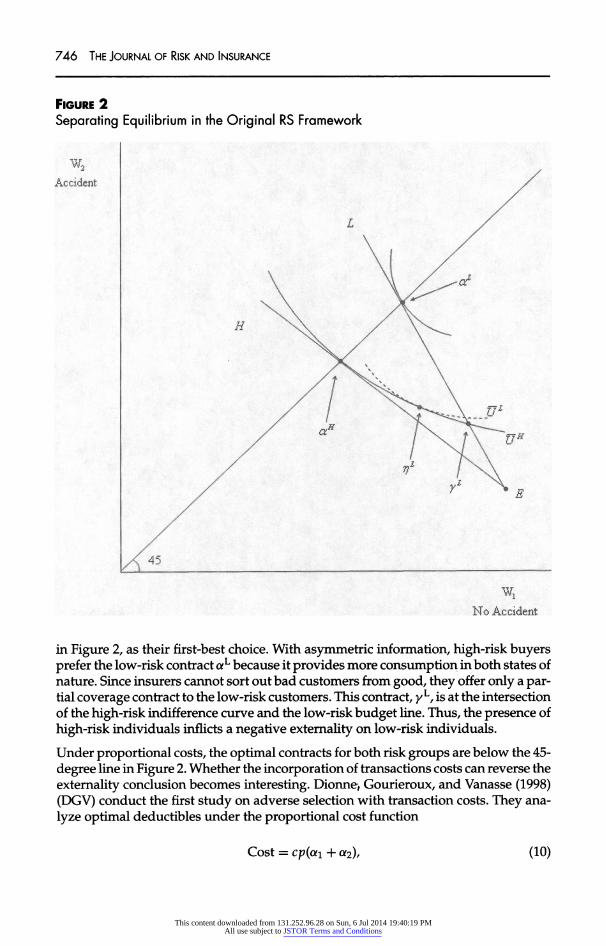
in Figure 2, as their first-best choice. With asymmetric information, high-risk buyers

prefer the low-risk contract aL because it provides more consumption in both states of

nature. Since insurers cannot sort out bad customers from good, they offer only a par tial coverage contract to the low-risk customers. This contract, yL, is at the intersection

of the high-risk indifference curve and the low-risk budget line. Thus, the presence of

high-risk individuals inflicts a negative externality on low-risk individuals.

Under proportional costs, the optimal contracts for both risk groups are below the 45

degree line in Figure 2. Whether the incorporation of transactions costs can reverse the

externality conclusion becomes interesting. Dionne, Gourieroux, and Vanasse (1998)

(DGV) conduct the first study on adverse selection with transaction costs. They ana

lyze optimal deductibles under the proportional cost function

Cost = CJ)((X\ + ot2), (10)




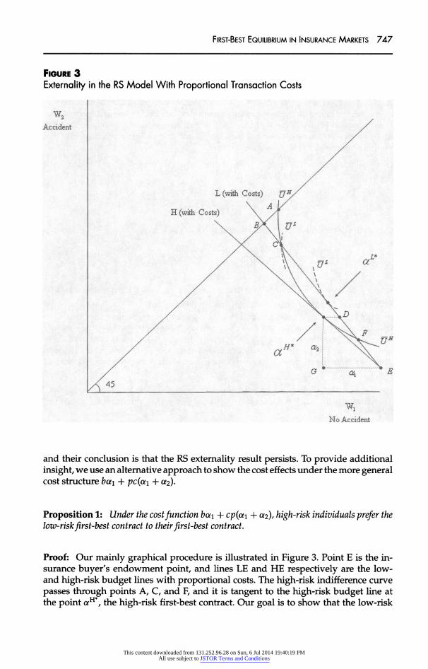
Figure 3

Externality in the RS Model With Proportional Transaction Costs

w* ! Accident j /

L (with Costs) TJH/ \ A / H (with Costs) \ /

\ P\ 1 U*

/ \v\\ff' a

/ a"* ^| ^^ / O *.4.^ ?

^45_

No Accident

and their conclusion is that the RS externality result persists. To provide additional

insight, we use an alternative approach to show the cost effects under the more general cost structure bct\ + pc(ot\ + o^).

Proposition 1: Under the cost function bot\ + cp{ct\ + ct2), high-risk individuals prefer the

low-risk first-best contract to their first-best contract.

Proof: Our mainly graphical procedure is illustrated in Figure 3. Point E is the in surance buyer's endowment point, and lines LE and HE respectively are the low and high-risk budget lines with proportional costs. The high-risk indifference curve

passes through points A, C, and F, and it is tangent to the high-risk budget line at

the point aH*, the high-risk first-best contract. Our goal is to show that the low-risk




first-best contract aL* must fall between C and F.6 Therefore, the high-risk customers

prefer aL* to aH*.

As a first step, we show that aL* will fall to the southeast of point C. It is obvious that, at point C, the high-risk indifference curve is steeper than LE, the low-risk budget line.

From equation (5) we know that the low-risk indifference curve is steeper than the

high-risk one. The tangent point of the low-risk indifference curve and the low-risk

budget line ctL* must fall to the southeast of C.

Our goal in the second step is to prove that aL* will be above point F. We start from

the first-order condition in Problem II:

U'(W-ai(p)) = l-b-p(l+c) U'(W-d+a2(p)) (l+c)(l-p)

' ( '

Taking the derivative of both sides with respect to p, we have

d*i = g[U'(W2) -

IT'(WQ] -

(1 -

p)(ai + a2)U?(Vh) (m dp g2W{]N2) + p{l-p)U'\]N1)

' K }

whereg =

1~b~^1 +

c). Since W > 0 (increasingutility), U" < 0 (decreasing marginal

utility), and W\ > W2 (partial coverage), it is trivial to show that -^

< 0, which means

that the low-risk first-best contract offers a larger net reimbursement than the high risk contract. In Figure 3, point D is the point on the low-risk budget line with the

same net reimbursement a2 as aH*. Obviously the low-risk first-best contract aL* is

above D. Since D is positioned to the northwest of F, the optimal contract aL* is above

point F, the intersection of the high-risk indifference curve and the low-risk budget line.

We have proved that aL* must fall between C and F on the low-risk budget line.

Therefore, the high-risk consumers' utility is higher if they purchase a?L* instead of

aH*.

Transaction costs are much like taxes imposed on insurance buyers. All else equal,

high-risk individuals pay higher premiums (receive less net reimbursement), ot\ (a2), than do low-risk individuals. Under the cost structure bot\ + cp{ot\ + a2), high-risk individuals suffer more from the proportional cost, and their coverage is reduced to

a greater extent than low-risk individuals' coverage. Therefore, the low-risk contract

is more attractive to the high-risk individuals. Moreover, it is trivial to show the RS

externality result holds under other conventional transaction cost structures, such as

ba\ and cp(a\ + ot2)7

6 It is also possible that point C, the intersection of the high-risk indifference curve and the

low-risk budget line, falls above point A, the intersection of the high-risk indifference curve

and the 45-degree line. In that case, the graph is different and it is obvious that aL* would be to

the southeast of point C, the intersection of the high-risk indifference curve and the 45-degree line.

7 We would like to point out that the RS externality result can be reversed under certain cost

schemes. For example, if cost = ca2, the low risks will be affected more than the high risks.




Risk Aversion

Insurance buyers might have different levels of risk aversion. This possibility has been

evaluated in an information asymmetry setting by several previous researchers. RS

point out that it is possible that low-risk individuals are less risk averse. RS discuss

the possibility that high-risk people are more risk averse than low-risk individuals

and conclude that a pooling equilibrium cannot exist. De Meza and Webb (2001) find

that low-risk, highly risk-averse individuals tend to buy more coverage than high risk, less risk-averse individuals. In their setting, a pooling equilibrium is possible. Smart (2000) and Villeneuve (2003) add heterogeneous risk aversion to the RS model. In Smart's model, there are four customer groups: high risks with high risk aversion

(hh), high risks with low risk aversion (hi), low risks with high risk aversion (lh), and low risks with low risk aversion (11). His major conclusion is that the indifference curves of the hi and lh types may cross twice and different risk types may be pooled in one contract. Villeneuve assumes that one risk class is more risk averse than the

other risk class in the market. He reaches the conclusion that positive profits are

sustainable for the low-risk contract and that random insurance contracts may also

exist. Our article differs from Smart and Villeneuve in two critical ways: First, we

incorporate transaction costs, in addition to heterogeneous risk aversion, into the RS

model. Second and most important, we contest the externality conclusion of the RS model.

In this section, we extend the basic RS model with a new set of assumptions:

1. There are proportional transaction costs:

Cost = boti + pc(ai + a2). (13)

2. Insurance customers' utility functions depend on risk aversion. The respective utility functions of the high-risk and low-risk customers are UH(x) and UL(x), and their respective risk aversion coefficients are rH(x) and rL(x). We examine the two possible scenarios: In Scenario A, high-risk individuals are more risk averse

than low-risk individuals, r(x)H > r(x)L, whereas in Scenario B the relation is reversed.

3. It is usually assumed that absolute risk aversion depends on wealth level. We neutralize the wealth effect by assuming that customers have constant absolute risk aversion (CARA). This assumption is not critical; our result could be eas

ily generalized to other cases. According to Pratt (1964), constant risk aversion

generates a negative exponential utility function,

U*(x) = -e~rt\ t = H,L. (14)

We find numerical examples in which the high risks are no longer interested in the low-risk contract.




Are These Scenario Assumptions Realistic?

Both Scenario A and Scenario B are reasonable in different circumstances. Customers

with a history of serious, extended illnesses in their families often have a relatively high likelihood of contracting these illnesses. It is sensible to think that customers with such

family histories would also be more risk averse than others in making their health

insurance decisions. This gives us a realistic situation of Scenario A. In alternative

circumstances, we can find real-world situations for Scenario B. For example, reckless

(high-risk) drivers might be less risk averse, and may tend to buy only minimum

coverage, since both recklessness and low coverage are consistent with disregard for

risk. Likewise, cautious (low-risk) drivers might also be more risk averse and buy more coverage, since both behaviors are consistent with risk aversion.

Indifference Curves

Following RS, our procedure is mainly graphical. The slope of the indifference curve

is represented by the marginal rate of substitution,

Under CARA, MRS is [(1 -

pt)/pt]e"''^-w^. Therefore, the ratio of high-risk MRS

and low-risk MRS is

MRSH = (Izrl llz?\e-frM)xw^ (i6) MRSL V PH I PL J

We wish to determine whether this ratio is greater than one; this will tell us whether

the high- or low-risk-aversion customers have a greater MRS. Clearly, the first factor

on the right side of the equation, l~S /?/?-, is positive and less than one. Is the

second factor, e~(r ~r

)x(Wi-w2)^ ajso jess faan one? Locking at the exponent of this

factor, we know that customers should not have more wealth in the loss state than in

the no-loss state, W2 < Wi, so the last factor in the exponent is positive. Thus, whether

the risk aversion factor in the exponent is greater than or less than one depends on

the relative levels of risk aversion of the two risk groups.

Scenario A - High-risk individuals are more risk averse than low-risk individuals.

In this case, rH > rL. So e^rH-rL^w'-w^ is less than one and MRSH < MRSL. The

high-risk indifference curve is always flatter than the low-risk indifference curve.

Scenario B - High-risk individuals are less risk averse than low-risk individuals.

In this case, rH < rL and e~(r -rL)x(Wi-w2) js greater than one. It is unclear whether

the product of the two factors in (16) is greater than or less than one, and therefore,

which indifference curve is flatter. If we hold pH and pL fixed, then e~(r ~r )x(wi-w2)

increases with the difference between rH and rL, and with the difference between Wi




and W2. When these differences are sufficiently large, ^-(rH-rL)x(wi-w2) dominates the

first factor and T^|tr

> 1. In this case, the high-risk-indifference curve is steeper than

the low-risk-indifference curve. On the other hand, when the differences between rH

and rL and between ]N\ and W2 are small, the low-risk indifference curve is steeper.

If the indifference curve of one risk type is always flatter, as in Scenario A, the two

indifference curves will cross only once. However, if the indifference curves of each

risk type are flatter in some circumstances and steeper in others, as in Scenario B, the

indifference curves may cross twice.

Market Equilibrium Under Heterogeneous Risk Aversion and No Transaction Costs

Under these assumptions, we find that, in most circumstances, there cannot be a

pooling equilibrium, which is consistent with RS. RS note that at any possible pooling

point the two indifference curves have different slopes. Any new contract that lies

between the two indifference curves will attract the low-risk type away from the

pooling point, making the potential pooling equilibrium unstable. In our Scenario

A, the slope of the low-risk indifference curve is steeper than the high-risk slope. In

Scenario B, it is possible that the low-risk indifference curve is flatter than the high-risk indifference curve. In this case, we can find a destabilizing contract that lies to the west

of the point of intersection, above the low-risk indifference curve and below the high risk indifference curve, as shown in Figure 2 of the original RS paper. This contract

will attract the low-risk individuals away from the potential pooling point, making a

pooling equilibrium impossible to sustain. In Figure 2, rjL stands for a possible low

risk equilibrium contract if the low-risk indifference curve is flatter than that of the

high-risks', which scenario is discussed later in the article.

A special pooling equilibrium can emerge, however, when the two indifference curves are tangent to each other. This case can only be found in Scenario B and it requires that the high-risk indifference curve lies below the low-risk indifference curve. More

over, it is also necessary that the tangent point falls on the aggregate budget line, which makes zero profit when both high- and low-risk individuals buy one con

tract. Any contract that lies between the two indifference curves will attract only the

high-risk individuals, and it will lead to a negative profit. As noted by Wambach

(2000), this type of pooling equilibrium is rare since it calls for special parameter values.

When it comes to the separating equilibrium, the introduction of heterogeneous risk aversion alone does not change the RS argument. The main reason for this is that both risk types take full insurance as their first-best choice. Thus, as in the cases discussed in the "Transaction Costs" section, the presence of high-risk individuals inflicts a

negative externality on low-risk individuals.8

8 Villeneuve (2003) suggests that, in Scenario B, the low-risk-indifference curve might be flatter than that of the high-risk group at yL, as in Figure 2. In this case, the low-risk group will prefer another point nL, the tangent point of the two indifference curves. The contract ?yLis profitable to the insurer since it is located below the low-risk budget line.




Separating Equilibrium With Heterogeneous Risk Aversion and Proportional Costs

Overall, the new separating equilibrium under proportional costs and heterogeneous risk aversion differs from the RS equilibrium in two ways. First, both risk groups pre fer to have less than full coverage; their optimal contracts are below the 45-degree line.

This is due to the presence of proportional costs. Second, we know from Schlesinger (2000) that with proportional costs, whichever group has low risk aversion prefers less insurance; their optional contract is closer to the endowment on the budget line.

The consumer's optimizing decision is as follows. For a type t individual (t = H, L) the optimal contract ar(ai, a2) is defined as the solution to the following problem (Problem III):

Max: E(U) = (1

- pf)lW

- ?i) + p'tfiW

- d + a2)

Subject to: ?i(l -

pl) -

a2pf = ba\ + pc(pt\ + a2)

ct\ > 0, and a2 > 0.

The expected utility of a type s (s = H, L) individual from a type t 's optimal contract

is expressed as Vs (a**). For example, a high-risk individual's expected utility from

the low-risk optimal contract is

VH[aL*] = (1 -

pH)U[W -

al(pL)] + pHU[W -d+ a2*(pL)].

Definition 1: A separating equilibrium in which neither group imposes a negative external

ity to the other group, which we call an NE (no externality) equilibrium, satisfies the following conditions:

VH[aH*] > VH[aL*] and (17)

VL[aL*] > VL[aH*l (18)

Definition 1 says that an NE equilibrium exists if each risk type prefers the contract de

signed for their type. The insurance market reaches a separating equilibrium because

of self-selection by risk type, and neither risk group imposes a negative externality on the others.

Lemma 1: VL[aL*] > VL[aH*] always holds in the presence of a linear cost function.

Proof: See the Appendix.

Lemma 1 indicates that if there are proportional costs, low-risk individuals will always

prefer the contract designed for their risk group, and thus condition (18) is always true. Therefore, to show that a separating equilibrium exists, it is only necessary to

show that high-risk customers prefer their contract, condition (17).




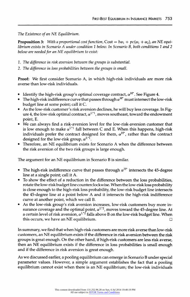
The Existence of an NE Equilibrium.

Proposition 3: With a proportional cost function, Cost = ba\ + pc{a\ + ot2), an NE equi librium exists in Scenario A under condition 1 below. In Scenario B, both conditions 1 and 2

below are needed for an NE equilibrium to exist:

1. The difference in risk aversion between the groups is substantial.

2. The difference in loss probabilities between the groups is small.

Proof: We first consider Scenario A, in which high-risk individuals are more risk averse than low-risk individuals.

Identify the high-risk group's optimal coverage contract, aH*. See Figure 4.

The high-risk indifference curve that passes through aH* must intersect the low-risk

budget line at some point; call it C.

As the low-risk customer's risk aversion declines, he will buy less coverage. In Fig ure 4, the low-risk optimal contract, aLn, moves southeast, toward the endowment

point, E.

We can always find a risk-aversion level for the low-risk-aversion customer that

is low enough to make aLn fall between C and E. When this happens, high-risk individuals prefer the contract designed for them, arH*, rather than the contract

designed for the low-risk group, aul.

Therefore, an NE equilibrium exists for Scenario A when the difference between

the risk aversion of the two risk groups is large enough.

The argument for an NE equilibrium in Scenario B is similar.

The high-risk indifference curve that passes through aH* intersects the 45-degree line at a single point; call it A.

To show the effect of a reduction in the difference between the loss probabilities, rotate the low-risk budget line counterclockwise. When the low-risk loss probability is close enough to the high-risk loss probability, the low-risk budget line intersects the 45-degree line at a point below A and it intersects the high-risk indifference curve at another point, which we call B.

As the low-risk group's risk aversion increases, low-risk customers buy more in surance coverage and the optimal point, aL*2, moves toward the 45-degree line. At a certain level of risk aversion, aL*2 falls above B on the low-risk budget line. When this occurs, we have an NE equilibrium.

In summary, we find that when high-risk customers are more risk averse than low-risk

customers, an NE equilibrium exists if the difference in risk aversion between the risk

groups is great enough. On the other hand, if high-risk customers are less risk averse, then an NE equilibrium exists if the difference in loss probabilities is small enough and if the difference in risk aversion is great enough.

As we discussed earlier, a pooling equilibrium can emerge in Scenario B under special parameter values. However, a simple argument establishes the fact that a pooling equilibrium cannot exist when there is an NE equilibrium; the low-risk individuals




Figure 4 NE Equilibrium With Proportional Costs and Heterogeneous Risk Aversion

Accident /

\/\A5_*

No Accident

prefers the contract ah*2, as in Figure 4, to any other contract since it is the first

best contract under the low-risk budget constraint. Any potential pooling contract is

unstable; the low-risk individuals prefer aL*2 to the pooling contract and will choose to

leave. The contract aL*2 has no appeal to the high-risk individuals since, to a high-risk customer, aH* is better than aL*2 when an NE equilibrium exists.

In the insurance markets, risk categorization, in which insurers use observable traits

that are related to risk for separating customers into risk groups, is often used to

mitigate adverse selection. When the loss probabilities are close, as discussed in the NE

equilibrium in Scenario B, risk classification is probably of limited practical value; not

only are the risk levels too close to distinguish but the risk categorization variables are

not particularly sensitive to other variables, such as risk aversion. Risk categorization is most important when consumers do not differ much on dimensions other than risk.9

9 We thank an anonymous referee for suggesting this point.




Will an NE equilibrium exist within a normal range of risk-aversion parameters?

Empirical studies of the magnitude of relative risk aversion indicate that the level

of risk aversion varies substantially from person to person. In a study of investment

behavior, Hansen and Singleton (1993) find that estimates of relative risk aversion

range from 0.359 to 58.25. Barsky et al. (1997) find, in an experimental study, that

estimates of relative risk aversion range from 0.7 to 15.8. The following example demonstrates that an NE equilibrium may exist within this range of risk-aversion

parameters.

Examples of NE Equilibria Let every customer in the insurance market have initial wealth W = 1. By definition,

relative risk aversion is R(W) = ? W

jp^ and absolute risk aversion is r(W)

= ?jp^

Since wealth is set to one, absolute risk aversion has the same range as relative risk

aversion. We assume that when an accident occurs, the individual suffers a loss d =

0.5, and that both the low- and high-risk customers have negative exponential utility U(x)

= -e~rx.

First, consider Scenario A: high-risk customers are more risk averse than low-risk

customers. Let low-risk individuals have a loss probability pL = 0.1 and high-risk

individuals a probability pH = 0.15. Let the absolute risk aversion of the high-risk,

high-risk-aversion individuals be rH = 2, and let rL = 0.5 for the low-risk, low-risk

aversion individuals.

If insurance companies provide actuarially fair policies (cost =

0), both low- and high risk individuals prefer full coverage, and in a transparent market, they are willing to

pay premiums of 0.05 and 0.075, respectively. When a loss of 0.5 occurs, customers are

fully reimbursed. However, with asymmetric information, the high-risk individuals

prefer the low-risk policy. They will gain 0.0077 in expected utility if they buy the low

risk policy. Thus, insurance companies are forced to offer a partial coverage policy to

the low-risk customers. The low-risk customers are worse off due to the presence of

high-risk customers.

Now, consider the case in which the premium includes a proportional transaction cost bai + pc(a\ + a2). Let both b and c be 10 percent. No one will buy full insurance because the premium is not actuarially fair. The high-risk customers pay a premium a

J1 = 0.07, compared to 0.075 in the zero-cost case. If a loss d = 0.5 occurs, they will receive a reimbursement of 0.38. Low-risk customers will scale back their premium payment

a\ from 0.05 to 0.0059, and in case of a loss, they will recover only 0.049, about 10

percent of the loss amount. Because the low-risk best coverage is much lower than the

high-risk best coverage, high-risk individuals receive greater expected utility10 from their own policy VH[aH*]

= -0.162 compared to the low-risk policy cut, VH[aL*] =

?0.167. Low-risk customers also prefer their own policy V^a^*] = ?0.624 to the

high-risk policy (VL[aH*] = -0.631). Thus, self-selection leads to an NE equilibrium.

10 The expected utility level is negative because U(x)

= -e~rx. If the reader prefers positive

expected utility, it is always permissible to add a fixed positive number. The utility function

U(x) is equivalent to the utility function U(x) = AU(x) + B, with A > 0.




Similarly, under Scenario B, in which low-risk customers are more risk averse, there

may also be an NE equilibrium. Let high-risk customers have an absolute risk-aversion coefficient rH = 0.5, and let low-risk customers have a coefficient rL = 2. Assume that

high-risk customers have a loss probability pH = 0.105, and that low-risk customers

have a loss probability that is close to the low-risk probability, pL = 0.1. In this case,

high-risk customers are willing to spend 0.0059 on a premium, whereas low-risk customers will pay a premium of 0.047. In case of a loss, d = 0.5, high-risk customers

will only receive a payment of 0.046, whereas low-risk customers will recover 0.39.

Again, low-risk customers prefer their own policy, V^a11*] ?

VL[o?H*] = 0.0047, and

high-risk customers prefer a high-risk policy, VH[arH*] ?

V,H[aL*] = 0.0002, and an NE

equilibrium exists.

Wealth

RS assume that all agents have the same endowment, but it is possible that one risk

class is wealthier than the other. For example, when use of age is prohibited in health

insurance underwriting, young individuals are in general both lower risk and less

affluent than middle-aged individuals. Alternatively, disabled individuals maybe, on

average, both less wealthy and less healthy than the general population. In states such as New Jersey, New York, and Vermont, where use of disability status is prohibited, this gives a perfect example of negative association between risk and wealth level.

When both proportional costs and heterogeneous wealth are added to the RS model, an NE equilibrium may occur. Insurance buyers' absolute risk aversion should vary

with wealth and we assume decreasing absolute risk aversion (DARA).11 In this situa

tion, wealth influences agents' behavior through risk aversion; under DARA, greater wealth is equivalent to lower risk aversion, and vice versa. The analyses under hetero

geneous wealth are identical to those under heterogeneous risk aversion, and are not

repeated in the interest of brevity.

It might be argued that since wealth is probably observable, risk classification could be

utilized to control for the divergence in endowment. However, there are two reasons

that risk classification may not be relevant in this case. First, we find that a self

selecting NE equilibrium often exists, and risk classification is irrelevant when this occurs. Second, classification is becoming problematic in the United States. Various state laws and regulations prohibit insurers from using certain characteristics, such as a person's sex, age, and physical or mental impairment, to discriminate among individuals applying for insurance.

Conclusion

In this article, we investigate several extensions of the RS model of adverse selection

in insurance markets. RS assume that markets are without transaction costs and that

agents are homogenous except in loss probability. They conclude that at the least,

negative externalities harm consumers in one risk category, and at the worst, the

market may not be able to reach an equilibrium. We analyze the same problem under

11 DARA is a

commonly accepted assumption in the literature. An alternative assumption is

increasing absolute risk aversion (IARA). Individual's behavior would be a mirror image of

what we see under DARA, with the roles of the two risk types reversed. Since our result relies

on the difference between the two types, the NE equilibrium may also exist under IARA.




the joint assumption that transaction costs are present and that the risk types differ on

another dimension (risk aversion or wealth) in addition to risk level. We summarize our study as follows:

1. Transaction Costs. Contrary to the assumptions of RS, transaction costs do ex

ist. When proportional transaction costs are present, individuals choose partial coverage.

2. Adverse Selection. Inclusion of transaction costs leads to fundamental changes in

the dynamic of the RS model. Analysis of informational problems more closely resembles actual market dynamics when transaction costs are considered.

3. Heterogeneity. First, insurance buyers may differ in risk aversion depending on

their risk types. Practical examples are found in medical insurance and automobile

insurance. Moreover, one risk type may also be more wealthy than another risk

type. Finally, risk types might have heterogeneous loss severity. This case has

been studied by Doherty and Jung (1993), and their conclusion is consistent with ours.

4. NE Equilibrium. The interaction of transaction costs and consumer heterogeneity may lead consumers to self-selection by risk type, and in this separating equilib rium there may be no negative externalities.

5. Risk Categorization. Our study suggests that risk classification is likely to be most

useful when customers do not differ significantly on relevant dimensions other than risk. When they do differ in other ways, then an NE equilibrium may occur,

making risk assessment irrelevant.

It has been long noted that RS negative externality and market equilibrium results are not consistent with many observable phenomena and empirical results. Many

markets, such as labor and financial markets, function well in the presence of infor mation asymmetry, in contrast to the pessimistic RS prediction. Chiappori and Salani?

(2000) find that customers who have higher accident probabilities show no evidence of choosing contracts with more comprehensive coverage. Our results provide some

insight into the forces within markets that may partially explain these phenomena. The role of interactions between market characteristics and consumer heterogeneity on multiple dimensions may provide a fruitful avenue for future empirical work in

markets characterized by information asymmetry.

Appendix

Proof of Lemma 1: We are comparing the value of function VL[a] at two points, aL*[ai(pL),a2(pL)] andaH*[ai(pH),a2(pH)].

The low-risk individual's optimal solution, aL*, is the solution to the following problem:

Max: E(U) =

(1 -

pL)U(W -

c*i) + pLU(W - d + a2)

Subject to: a?i(l ?

pL) ?

a2pL =

ba\ -hex pL(a\ + u\)

a\ > 0, ct\

> 0.




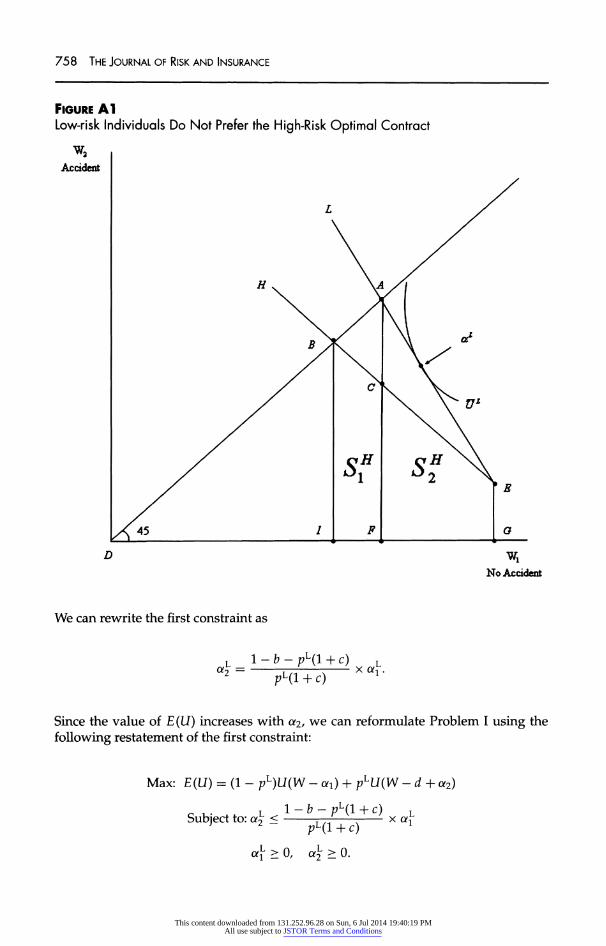
Figure Al Low-risk Individuals Do Not Prefer the High-Risk Optimal Contract

Accident

/\\ \ / V Vs.

/ ̂ \ \ Ul

/ r?jy ctH \\

/ I B

X45 if a ' \ i 4 9

D Wx No Accident

We can rewrite the first constraint as

l-fr_pL(1+c) a2

= -T7T-^- x al 2

pL(l + c) l

Since the value of E(U) increases with a2/ we can reformulate Problem I using the

following restatement of the first constraint:

Max: E(U) = (1 -

pL)U(W -

ax) + pLU(W - d + a2)

l l-b-p\l + c) L Subject to: ak <-. ,/ \- x ot\ } 2 "

pL(l + c) 1

ot\ > 0, a\

> 0.




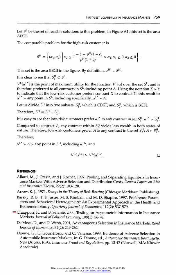
Let SL be the set of feasible solutions to this problem. In Figure Al, this set is the area

AEGF.

The comparable problem for the high-risk customer is

f l-b-vH(l+c) 1 SH =

(c*i,cx2) a2 < -hm+c)--

x a1/ttl > 0,a2 > 0 .

This set is the area BEGI in the figure. By definition, aH* e SH.

It is clear to see that Sf c SL.

VL[aL*] is the point of maximum utility for the function VL[a] over the set SL, and is

therefore preferred to all contracts in SL, including point A. Using the notation X > Y to indicate that the low-risk customer prefers contract X to contract Y, this result is:

aL* > any point in SL, including specifically: aL* >- A.

Let us divide SH into two subsets: Sf, which is CEGF, and S^1, which is BCFL

Therefore, SH = S2H U Sf.

It is easy to see that low-risk customers prefer aL* to any contract in set S^: aL* > S^.

Compared to contract A, any contract within S|* yields less wealth in both states of nature. Therefore, low-risk customers prefer A to any contract in the set S^: A >

S^.

Therefore,

aL* >- A > any point in SH, including aH*, and

VL[aL*] >

yL[aH*].

References

Allard, M., J. Cresta, and J. Rochet, 1997, Pooling and Separating Equilibria in Insur ance Markets With Adverse Selection and Distribution Costs, Geneva Papers on Risk and Insurance Theory, 22(2): 103-120.

Arrow, K. J., 1971, Essays in the Theory of Risk-Bearing (Chicago: Markham Publishing).

Barsky, R. B., T. F. Juster, M. S. Kimball, and M. D. Shapiro, 1997, Preference Param eters and Behavioral Heterogeneity: An Experimental Approach in the Health and Retirement Study, Quarterly Journal of Economics, 112(2): 537-579.

Chiappori, P., and B. Salanie, 2000, Testing for Asymmetric Information in Insurance

Markets, Journal of Political Economy, 108(1): 56-78.

De Meza, D., and D. Webb, 2001, Advantageous Selection in Insurance Markets, Rand

Journal of Economics, 32(2): 249-262.

Dionne, G., C. Gourieroux, and C. Vanasse, 1998, Evidence of Adverse Selection in Automobile Insurance Markets, in: G. Dionne, ed., Automobile Insurance: Road Safety, New Drivers, Risks, Insurance Fraud and Regulation, pp. 13-47 (Norwell, MA: Kluwer

Academic).




Doherty, N. A., and H. J. Jung, 1993, Adverse Selection When Loss Severities Differ:

First-Best and Costly Equilibria, Geneva Papers Risk and Insurance Theory, 18(2): 173

182.

Hansen, L. P., and K. J. Singleton, 1983, Stochastic Consumption, Risk Aversion, and

the Temporal Behaviors of Asset Returns, Journal of Political Economy, 91(2): 249-265.

Mossin, J., 1968, Aspects of Rational Insurance Purchasing, Journal of Political Economy, 76(4): 553-568.

Pratt, J. W., 1964, Risk Aversion in the Small and in the Large, Econometrica, 32(1/2): 83-98.

Rothschild, M., and J. E. Stiglitz, 1976, Equilibrium in Competitive Insurance Markets:

An Essay on the Economics of Imperfect Information, Quarterly Journal of Economics,

90(4): 629-649.

Schlesinger, H., 2000, The Theory of Insurance Demand, Handbook of Insurance (Nor well, MA: Kluwer Academic).

Smart, M., 2000, Competitive Insurance Markets With Two Unobservables, Interna

tional Economic Review, 41(1): 153-169.

Villeneuve, B., 2003, Concurrence et Antiselection Multidimensionnelle en Assurance, Annates d'Economie et Statistique, 69:119-142.

Wambach, A., 2000, Introducing Heterogeneity in the Rothschild-Stiglitz Model, Jour nal of Risk and Insurance, 67(4): 579-592.



First-Best Equilibrium in Insurance Markets with Transaction ...

Documents

Transcript of First-Best Equilibrium in Insurance Markets with Transaction ...