Financial Risk Management in Social and Pension Insurance ...

Financial Risk Management inSocial and Pension Insurance

Chapter I: Introduction

ETH Zurich, Fall Semester, 2020

Peter Blum

Suva, The Swiss National Accident Insurance Fund, Lucerne

September 13, 2020

Peter Blum (Suva) I Introduction September 13, 2020 1 / 44

Table of Contents

1. Administrative matters

2. Properties of social insurance

3. About this course

4. Assuring future pensions: the danger of taking no risk


1. Administrative matters


About the lecturer: Peter BlumEducational background:

I Professional degree in electronics and software engineering.

I Diploma in mathematics from ETH Zurich.

I PhD in financial and insurance mathematics from ETH Zurich [3].

I Chartered Financial Analyst (CFA), CFA Institute.

I Fully qualified actuary (Aktuar SAV) of the Swiss Actuarial Society

Professional experience:

I Industrial software engineering at Landis & Gyr and Siemens.

I Asset / Liability Management, research and financial engineering at Zurich Re,then Converium (now Scor).

I With Suva - The Swiss National Accident Insurance Fund since 2005, initiallyas an analyst, then heading teams in asset allocation, treasury and research.

I Deputy head of portfolio management during the Great Financial Crisis.

I Chief Risk Officer and Chief of Staff of the Finance Department since 2011,with responsibilities both on the asset and on the liability side.

I Also heavily involved in the strategic management of the Suva Pension Fund.


Institutional background

Suva - The Swiss National Accident Insurance Fund (figures as of 2019)

I Provider of compulsory accident insurance for the secondary and public sectorsin Switzerland since 1918.

I 2.067 million insured persons in 130’000 insured companies and institutions.

I 479’746 cases of accident and professional disease processed.

I Benefits of CHF 4.5 billion paid, including medical costs, daily indemnities and83’709 disability and survivors’ pensions totaling CHF 1’648 million.

I Assets under management of CHF 53.8 billion.

Suva Pension Fund (figures as of 2019)

I Pension fund according to Swiss law (2nd Pillar) for the employees of Suva, inoperation since 1985.

I 3’958 active and 2’121 retired members.

I Contributions of CHF 115 million, benefits of CHF 111 million.

I Assets under management of CHF 3.3 billion.


Course schedule

Lectures every Wednesday afternoon from 16:15 to 18:00

I Lectures will take place online via Zoom.

I Lectures will be recorded, and recordings will be available to students.

I Changes in course schedule will be announced by e-mail.

Lecturer available for questions after the lectures and during the break.

Otherwise: [email protected]

Course language: English.


Documentation

Slide presentations as made available on the ETH web platform plus whiteboardnotes made in the lectures.

Slides are made such that they can be printed black-and-white and 2-up withoutloss of information.

Not all presentations have been published yet. Publication of further chapters orrevised versions of already-published chapters will be announced by e-mail.

If you find mistakes in the presentations, please tell the lecturer.

Excel sheets and R code made available on the web platform are for illustrationonly.

References given, unless otherwise stated, are for information only.


Exams

Oral exam of 30 minutes.

During the ordinary exam session (next one: January 25 to February 19, 2021).

Examination language: English (German may be available upon demand).

Further information and instructions in the last lecture.


2. Properties of social insurance


Risks covered by social insurance

The most common forms of social insurance include

I Old-age provision, i.e. pension insurance. In its capital-based variant the mostimportant type of social insurance covered in this course.

I Health insurance, at least the basic, compulsory part of it.

I Accident insurance, if it is separate from health insurance. May be further sub-divided into insurance against occupational accidents and diseases (Workers’Compensation) and insurance against spare-time accidents.

I Disability insurance, to the extent that it is not yet covered by other types ofinsurance providers.

I Unemployment insurance.

I Etc. (In Switzerland, for instance, building / fire insurance is essentially alsoa type of social insurance.)

Organization, benefits and financing of the social insurance system vary greatlyfrom country to country.


Properties of social insurance

Social insurance is usually mutually compulsory, i.e. clients must take out theinsurance, and insurers must accept the clients:

I There is a defined market; growth corresponds to the growth of the client baseas specified by law.

I No risk selection; in particular, no adverse selection. Insurers can and mustinsure both ”good” and ”bad” risks.

I On the other hand, there is an assured client base for the insurer over a longtime, which is beneficial for long-term planning.

Defined insurance benefits for defined insured risks:

I Little to no room for product design.

I No growth opportunities through product innovation.

Generally high regulation density; usually regulation through special laws and spe-cial regulatory bodies differing from the ones for private insurance. This may includespecial accounting standards.


Social insurance institutions are often not publicly listed companies. Many socialinsurance institutions have a special legal status:

I Swiss pension funds are usually foundations, legally and financially separatedfrom their sponsoring institutions. There is also a legal obligation to keep thefoundation funded. This is an extremely effective means of risk management.

I Many social insurance institutions are outright governed by special law, e.g.also Suva.

I But, in some cases, also normal publicly listed companies or private mutualsocieties may be carriers of social insurance.

I However, in general, analytic approaches based on the economic theory of thefirm (see e.g. [6]) are not applicable in a social and pension insurance contextand will not be discussed any further in this course.

Social insurance is usually not-for-profit, but financial stability and financial sus-tainability are of utmost importance:

I Therefore, social insurance is still insurance - even under particularly demandingconditions - and thus a valid field for actuarial reasoning.

I We do not consider social benefits that are paid from the general public budgetand, hence, are not insurance in our sense.

I Limited profit-taking may be allowed if private companies provide social insur-ance services, in order to compensate them for their cost of capital.


The most important feature of social and pension insurance, however, is the oftenvery long time horizon:

I Think of pension insurance: The saving process starts e.g. at age 25, whereaslife expectancy is above 80 (and increasing), with a substantial chance forpeople to make it well into their nineties.

I Taking into account disability and long-term care, the time horizons in accidentinsurance are by no means shorter.

I Or think of asbestos-related diseases: a malignant mesothelioma may breakout 20 or 40 or even more years after the actual exposure.


Illustration: life expectancy

Pension insurance and also other forms of social insurance must remain availableover the entire life span of their clients.


Basic financing modes

For pension insurance, there are two basic financing modes:

Pay-as-you-go:

I Current benefits are paid from current contributions.

I Current contributors acquire the right to receive benefits in the future.

I No (or no substantial amount of) money is accumulated. Hence, there areno (substantial) investment proceeds that contribute to the financing, and norisks either from investing the money.

Capital-based insurance:

I Contributions of each contributor are accumulated and then used to pay old-age benefits for that person when they are due.

I While being accumulated, the money is invested. This generates investmentproceeds that are a source of funding.

I Substantial financial risk may arise from the investment of the accumulatedcontributions.


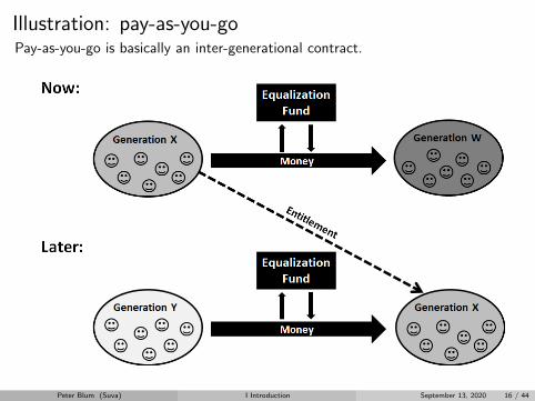
Illustration: pay-as-you-goPay-as-you-go is basically an inter-generational contract.


Illustration: capital-based insuranceIn capital-based insurance, each generation (in principle) cares for itself.


Illustration: capital-based old-age insurance processOur big question: How much can we expect from the investment proceeds? Andwhat investment risk do we take in turn?


3. About this course


Focus and goal of this course

Since substantial financial risk only arises in the capital-based setup, we will focuson the latter and we will not treat pay-as-you-go any further.

Given the properties of social and pension insurance as outlined before, we will haveto work in a long-term, multi-period framework. This represents a big challenge:

I Financial risk in short-term, single-period and asset-only setups is very wellunderstood; see [5].

I Financial risk in a long-term, multi-period setup and in the presence of liabilitiesis less well-understood, and some original reasoning will be necessary.

We will take a micro perspective, i.e. the point of view of a single social insuranceinstitution or pension fund. This is the situation that actuaries will most likely befaced with in practice.

Macro considerations aimed at designing entire pension systems are undoubtedlyalso interesting, but beyond the scope of this course. See [2] for more on this.


About stochastic simulationIn practice, settings are usually too complicated for comprehensive analytical tractabil-ity. Therefore, stochastic simulation is usually applied as a tool of analysis.

Hence, a solid understanding of the methods and numerics of stochastic simulationis indispensable for an analyst wanting to solve practical problems related to financialrisk in social and pension insurance. A good textbook is e.g. [1].

I The usefulness of many studies is hampered or even negated by technical mis-takes such as too few simulation runs, lack of care for variance and dependence,lack of care for the tails, etc.

Numerical quality is necessary, but not sufficient. Most importantly, models mustbe well-designed, i.e.

I They must be parsimonious and focus on the really important influence factorsand distinguish them from the less relevant ones.

I They must treat the relevant influence factors properly.

I In particular, they must give due care to the dependencies and the interplaybetween the influence factors.

In brief, good models must be simple, focused on the relevant factors and riskmeasures, and modular. This is where this course attempts to add value.


Call from practice:

If you have to present important results in front of a board of directors or trustees(which usually mainly consists of non-quantitative people) you must:

I perfectly understand what you are talking about, and

I be able to explain everything in simple, understandable and conclusive words.

If you are able to do this, people will likely accept your proposals, and they willlikely trust the scientific models underneath the conclusions, even if they cannotunderstand them in detail.

Two voices on this topic:

I ”Make things as simple as possible, but not simpler.” (Attributed to Einstein)

I ”Whereof one cannot speak, thereof one must remain silent.” (Wittgenstein,Tractatus logico-philosophicus)


Concept of this courseOur focus will be on Asset / Liability Management (ALM), i.e. the interface be-tween assets and liabilities, throughout the course. For assets and liabilities on astandalone basis, there are other courses.

We will develop a relatively simple modeling framework that focuses on the top-level influence factors, policy variables and risk measure as well as on their interplay.This modeling framework abstracts, but comprises many subordinated details.

Under some assumptions, we will obtain an analytically tractable model that pro-vides closed-form solutions for a number of important questions. In this analyticmodel, we will be able to develop a solid understanding of the most relevant ALMfactors and their interplay:

I required return / liability growth rateI expected returnI risk-taking capabilityI short-term (investment) riskI long-term (financial) risk

The most interesting and most intriguing aspect will be the relationship betweenshort-term and long-term risk. We will see that reducing short-term risk will notnecessarily reduce long-term risk.


On good risk management

Good risk management is not simply the avoidance or reduction of risk. Goodrisk management actually means considerate risk-taking with long-term financialstability as the goal.

The tools developed and the insights gained in the analytical framework are alsouseful in more general settings where stochastic simulation must be used:

I They allow to build well-focused and well-structured models.

I They provide useful analytics to assess the financial condition of an institution.

I They allow to better understand and appraise the outcomes of studies of allkinds and to draw valid conclusions.

Very fundamentally, it is not the goal of this course to provide cookbook-typerecipes. This is rather about enabling people to think independently and in a well-structured manner about problems related to financial risk in a social and pensioninsurance context and to develop valid and sensible tailor-made solutions for theseproblems.


Mathematical prerequisites

While this course aims at being as self-contained as possible, some mathematicalknowledge is nevertheless taken for granted:

I Knowledge of basic concepts of probability theory and statistics on the level ofan undergraduate course.

I Knowledge of calculus and linear algebra on the level of undergraduate courses.

I Other concepts will be introduced in due course.

We will see that even fairly simple mathematical reasoning - when applied rigorouslyand focused on the relevant factors - can provide very deep and useful insights.

This is very useful nowadays when plentiful computing power allows to create sim-ulation models that overwhelm the analyst with a plethora of more or less usefulinformation. Staying focused on the relevant factors and issues is really crucial.

It would be possible to formalize the problems treated in this course in much moresophisticated manners (e.g. in continuous time with diffusion processes and anincomplete-markets setup); this is, however, still work in progress.


4. Assuring future pensions: the danger of taking no risk


Introduction

The following presentation is intended to motivate the most important problems,notions and concepts that will be treated throughout this course.

It is from a talk given on Risk Day 2017 at ETH Zurich.

It specifically shows the situation of Swiss pensions funds. But it is representativefor many other capital-based social insurance institutions worldwide.


The Task: Financing Future Pensions

Let t denote time in years. We have some stream of future promised cashflowsC = (C1, . . . , CT )

′ ∈ RT , assumed to be deterministic here, e.g.:

At time t = 0 (i.e. now), we must put up an amount A0 of assets in such a way thatthe payment of all future cashflows Ct is assured. These assets can be invested,and the returns from doing so must be taken into account.


First Approach: Immunization

Let P (0, s) denote the value at time t = 0 of a zero-coupon bond (ZCB) maturingat time t = s, with P (s, s) = 1.

Now, we replicate the cashflow stream C = (C1, . . . , CT )′ ∈ RT by using ZCBs:

At time t = 0 and for each time t > 0, we buy Ct units of the ZCB maturing at t,at a price of P (0, t) per unit. The total cost of this is

A0 = PVZCB0 (C) =

T∑t=1

P (0, t)Ct

In the absence of credit risk, the payment of all future promised cashflows Ct isthus assured. That is, we have managed to create an immunized position at timet = 0, and all subsequent financial risk is eliminated.

Therefore, the immunized value PVZCB0 (C) is a viable valuation of the cashflow

stream C.

Note: There is no ZCB market in CHF, but an essentially equivalent portfolio canbe constructed from coupon bonds, interest rate swaps and bond futures - at leastfor time horizons not exceeding 30 years.


The Cost of ImmunizationWe use the ZCB curve for the CHF as mandated by the Finma for the SST 2017:

Based on this curve, we obtain the following immunized value for our examplecashflow stream:

PVZCB0 (C) =

T∑t=1

P (0, t)Ct = 20’726 MCHF

This corresponds to 95% of the sum of undiscounted cashflows of 21’730 MCHF.That is, we must put up almost the entire amount up front; there is only a verysmall contribution of interest rates to the financing.


The Statutory Setup of Swiss Pension FundsIn reality, Swiss pension funds do not use market-derived ZCB curves for the valu-ation of their liabilities. Rather, they use a constant discount rate λ:

L0 = PV0(C, λ) =

T∑t=1

Ct(1 + λ)t

This discount rate λ, called technical interest rate, is fixed by the board of trusteesof each pension fund.

In order to make this comparable to the immunized approach, we can specify theequivalent immunized discount rate

λZCB := IRR(

PVZCB0 (C), C

)which equates the two valuations, i.e.

PV0

(C, λZCB

)= PVZCB

0 (C)

In our specific example, we have λZCB = 0.35%, and this would also be the orderof magnitude for other Swiss pension funds.


Technical Interest Rate: Development & Current Situation

From Swisscanto, Schweizer Pensionskassenstudie 2020 [7] (520 institutions withtotal AuM of CHF 772 bln. and 3.8 mln. insured persons).

Technical interest rates λ were reduced considerably over the past ten years. Butwith values well above 2%, they are far away from values in the immunized case,which would be below 0.5%.


The Effective Situation of Swiss Pension FundsSwiss pension funds are far away from immunized positions. Achieving this wouldhave a strong impact on the valuation of their liabilities; in our example:

Achieving immunized positions would thus require drastic measures:

I Either the injection of large sums of additional financing.

I Or severe reductions of benefits: At λ = 0.35%, conversion rates (UWS)would be below 4%, whereas at λ = 2%, they are between 4.5% and 5%.

Thus, rather than immunizing their liabilities, Swiss pension funds try to financetheir higher discount rates by running mixed investment strategies with considerableshares of risky assets such as equities or real estate.

This then creates financial risk, i.e. the possibility that some of the promisedpayments may not be made due to investment losses. How can this situation bedealt with?


The Essential Asset / Liability Management Setup

With A0 and L0 given, we consider the following generic Asset / Liability model:

At = At−1(1 +Rt) + CtLt = Lt−1(1 + λ) + Ct

for t ∈ 1, . . . , T

At = value of assets at time t

Lt = value of liabilities at time t

Ct = net cashflow from insurance, i.e. contributions - paid benefits - costs

λ = intrinsic growth rate of liabilities; here equal to the technical interest rate

Rt = investment returns: Rt ∼ iid with E [Rt] ≡ µ and Var [Rt] ≡ σ2 <∞

That is, the liabilities develop deterministically, whereas the assets follow a randomwalk. The quantity of interest for further investigations is the funding ratio, i.e.

FRt =AtLt

This is then also a random walk. We would like to have FRt ≥ 1, i.e. the assets attime t cover the liabilities from time t on.


Long-term Financial Risk

Long-term financial risk consists of the possibility that some of the promised cash-flows may not be paid due to adverse investment returns Rt over one or severalperiods. Quantification of long-term financial risk is, therefore, associated with thestate of underfunding, i.e. FRτ < 1 for some fixed time horizon 1 ≤ τ ≤ T .

The most widespread risk measure used is the probability of underfunding, i.e.

ψτ := P [FRτ ≤ 1|FR0]

As usual in quantitative risk management [5], we would like to have a risk measurethat also incorporates the extent of the underfunding. To this end, we define theExpected Funding Shortfall, i.e.

EFSα,τ = 1−E [FRτ |FRτ ≤ qα(FRτ )]

Here, qα(FRτ ) is the left α-quantile of the distribution of FRτ given FR0. Weconsider the difference to 1 because this is the funding shortfall that must be filledup in order to re-attain fully-funded status.


A Simple Analytical Model for Long-term Financial RiskIf the fund is in equilibrium, i.e. Ct ≡ 0, and if we assume (somewhat dangerously)that Rt ∼ iid N (µ, σ2), then FRτ given FR0 is log-normally distributed, and wehave for the probability of underfunding:

ψτ (FR0, λ, µ, σ2) = Φ

(− log FR0 + (µ− λ)τ

σ√τ

)and for the Expected Funding Shortfall [4]:

EFSα,τ (FR0, λ, µ, σ2) = 1− 1

α FR0 exp(µ− λ+ 1

2σ2)τ

Φ(Φ−1(α)− σ

√τ)

These formula allow to get a good intuition of the interplay between the variousvariables, in particular:

∂ EFSα,τ∂ λ > 0 ⇒ required return

∂ EFSα,τ∂ µ < 0 ⇒ expected return

∂ EFSα,τ∂ FR0

< 0 ⇒ risk-taking capability

∂ EFSα,τ∂ σ > 0 under realistic conditions ⇒ short-term investment risk


The Task of Asset / Liability Management

If we cannot avoid long-term financial risk altogether by immunizing, we should atleast set up our fund in such a way that long-term financial risk is minimized.

I The main policy variable is the technical interest rate λ that can be fixed bythe board of trustees.

I Moreover, the investment strategy can be designed so as to attain a certainexpected return µ. For a sustainable funding, we must have µ ≥ λ , and wespecify here that µ = λ.

However, given the choices of λ and µ = λ, the other variables cannot be chosenfreely anymore:

I Since initial assets A0 are given, the initial funding ratio FR0 depends on thetechnical interest rate λ, i.e. FR0 = FR0(λ). This is the liability profile, andits properties are determined by the liabilities of the pension fund.

I A certain level of return µ = λ entails a certain level of short-term invest-ment risk σ, i.e. σ = σ(µ) = σ(λ). This is the risk / return profile, and itsproperties are determined by the financial markets and by applicable invest-ment constraints.

We must, therefore, optimize long-term financial risk under these contingencies.


The Liability Profile and the Risk / Return ProfileIn realistic settings, the liability profile and the risk-return profile are both convex:

Liability profile: Risk / return profile:

In principle, these developments are compatible with one another:

I Higher technical interest rate λ ⇒ higher required return µ ⇒ higher short-term investment risk σ, but also higher risk-taking capability FR0.

I And vice versa.

The question now is which one of the two profiles dominates, and whether thereis an optimum in terms of long-term financial risk somewhere within the range offeasible policies.


The Full Picture in the Analytical Model

Letting µ = λ, and plugging the liability profile FR0 = FR0(λ) and the risk / returnprofile σ = σ(λ) into the formula for the Expected Funding Shortfall, we obtain:

EFSα,τ (λ) = 1− 1α FR0(λ) exp

12 (σ(λ))

2τ

Φ(Φ−1(α)− σ(λ)

√τ)

Thus, the Expected Funding Shortfall simply becomes a function of the technicalinterest rate λ. This can be evaluated easily over a range of realistic values for λ.

The optimal technical interest rate λ∗ is then simply the one that minimizes theExpected Funding Shortfall, i.e.

λ∗ = arg minλ∈[µmin, µmax]

EFSα,τ (λ)

In more complex settings, evaluations along the exact same logic can be done byusing stochastic simulation.

The essential point is not the formula, but the logic with the liability profile (insti-tutional side) and the risk / return profile (financial markets side).


Minimizing Long-term Financial Risk

For our example and plugging in a risk / return profile that reflects current conditionsin the financial markets, we obtain the following result:

That is, it makes sense to fix a moderately elevated technical interest rate λ∗ andto assume the associated short-term investment risk σ(λ∗) in order to minimizelong-term financial risk.


Conclusions

Since the cost of immunization is currently too high, Swiss pensions fund are heavilyexposed to financial risk.

In the interest of their fiduciary duty, they should set themselves up in such a mannerthat long-term financial risk is minimized.

This is, however, not necessarily achieved by choosing the lowest possible technicalinterest rates and by assuming the lowest possible amounts of investment risk.

Fixing a higher technical interest rate and assuming more investment risk in theshort term may, at least to some extent, reduce financial risk in the long term.

Good strategic risk management is, thus, not necessarily myopic risk avoidance, butrather considerate risk-taking with long-term financial stability in mind.

Bear in mind that the optimum always depends on the specific characteristic of theinstitutions under investigation. Do only what you thoroughly understand based onserious qualitative and quantitative analysis.


Structure of the course

Chapter I Introduction

Chapter II Preliminaries

Chapter III Financing Liabilities

Chapter IV The Asset / Liability Framework

Chapter V The Lognormal Model

Chapter VI ALM Study 1 - Dealing with the Risk / Return Profile

Chapter VII ALM Study 2 - Incorporating Required Return

Chapter VIII ALM Study 3 - Valuation and Risk Management

Chapter IX Portfolio Construction and the Risk / Return Profile

Chapter X Synopsis, Wrap-up and Conclusions


Bibliography I

[1] Assmussen, S., and Glynn, P.Stochastic Simulation: Algorithms and Analysis.Springer, Berlin, 2007.

[2] Blake, D.Pension Economics.John Wiley & Sons, Chichester, 2006.

[3] Blum, P.On some mathematical aspects of dynamic financial analysis.Doctoral thesis, ETH, Zurich, 2005.

[4] Blum, P.Financial Risk Management in Social and Pension Insurance.Lecture notes, ETH Zurich, Zurich, 2016.

[5] McNeil, A., Frey, R., and Embrechts, P.Quantitative Risk Management, revised ed.Princeton University Press, Princeton, 2015.


Bibliography II

[6] Scherer, B.Liability Hedging and Portfolio Choice.Risk Books, London, 2005.

[7] Swisscanto.Schweizer Pensionskassenstudie 2020.Survey, Swisscanto, Zurich, 2020.



Chapter II: Preliminaries


Peter Blum


September 16, 2020

Peter Blum (Suva) II Preliminaries September 16, 2020 1 / 37

Table of contents

1. Cashflows and their properties

2. Bonds and yield curves


1. Cashflows and their properties


Time scale conventions

A discrete time scale will be used throughout the course.Let t denote time in years: t ∈ 0, 1, . . . , T ⊆ N0 with final time T <∞.

Time t = 0 denotes the present, at which valuations usually take place; values t > 0denote the future.

If t denotes a time interval, then this is to be interpreted as (t − 1, t]. Usually, itsuffices to identify t with the end of the respective year.

Note: All considerations in this course could easily be made also on quarterly,monthly or even continuous time scales. For the ease of presentation, however,only the yearly time scale will be used hereinafter.


Cashflows

Let Ct ∈ R denote some promised cashflow that occurs at time t, e.g.

I one installment of an old-age or disability pension,

I a reimbursement of a medical treatment,

I a reimbursement for long-term care,

I an unemployment benefit.

By convention, the cashflow Ct always takes place at the end of year t.

Let C = (C1, . . . , CT )′ ∈ RT denote a stream of cashflows taking place over timest ∈ 1, . . . , T.

Special case: If Ct = c for all t, then C is called an annuity.

Attention: There is no universal convention regarding signs. When only liabilitiesare considered, a positive sign may mean a cash outflow from the institution. Inother instances, a positive sign may denote an inflow, whereas a negative sign maydenote an outflow.


Mean Time to Payment

Definition 1 (Mean Time to Payment (MTP))

Let C = (C1, . . . , CT )′ ∈ RT denote a stream of cashflows with Ct ≥ 0 for all t.The Mean Time to Payment is defined as:

MTP(C) =

T∑t=1

t Ct∑Ts=1 Cs

MTP is a weighted time to payment where each time t is weighted by the relativecontribution of the cashflow Ct to the total payment

∑Ts=1 Cs.

MTP is a useful summary statistic which is independent of any discount rates. Itmeasures the average time horizon of the cashflow stream.

If C is an annuity, then we have MTP(C) = T+12 . This is due to the fact that∑T

t=1 t = T (T+1)2 .


Time value of moneyWe stand at t = 0 and we must finance some cashflow Ct taking place at somefuture time t > 0. Hence, we must incorporate the time value of money:

Let there be an account in which we can deposit money and which grants an interestof δ, i.e. if we invest an amount M at t = 0, we have at t = 1:

M + δM = M(1 + δ)

And over several time periods, due to the compounding of interest, we have

M(1 + δ)(1 + δ) · · · (1 + δ) = M(1 + δ)t

If there is some set amount Ct at time t, we can equate

M(1 + δ)t = Ct

Solving for M , we obtain

M =Ct

(1 + δ)t

M is the present value as of time t = 0 and with discount rate δ of the futurecashflow Ct. I.e. if we can set aside M at time t = 0 and if the interest rate δ isguaranteed, then we end up with Ct at time t.


Note: This whole course is basically about

1. selecting a sensible value for the discount rate δ, and

2. making sure that δ will actually be earned.

Note: In life insurance mathematics, one usually considers the so-called discountfactor v = (1 + δ)−1, and one considers this factor as deterministic and given; seee.g. [4].

Note: In the past, one used to assume that δ > 0, and one used to make consid-erable efforts to build interest rate models that avoid negative rates, see e.g. [1].Nowadays, we must relax this assumption and also allow for negative interest ratesand discount rates.


Present Value of a stream of cashflows

Definition 2 (Present Value)

Let C = (C1, . . . , CT )′ ∈ RT be a stream of cashflows, and let δ be a discountrate. The Present Value of C as of time 0 is defined as

PV0(C, δ) =

T∑t=1

Ct(1 + δ)t

That is, each single cashflow is discounted back to time t = 0, and these discountedvalues are summed up. Hence, if the discount rate δ is guaranteed, we can set asidethe amount PV0(C, δ) at time t = 0, and this suffices to finance all committedcashflows Ct of C with certainty.

This formula can easily be generalized to some general valuation date s > 0:

PVs(C, δ) =

T∑t=s+1

Ct(1 + δ)t−s


For general cashflows streams, the present value must be computed numerically;see example spreadsheets. For regular cashflows, in particular for annuities, we canobtain explicit formulae:

Proposition 1 (Present value of an annuity)

Let CT be a T -year annuity, i.e. CT = (c, . . . , c)′ ∈ RT , and let δ be the dis-count rate with δ ∈ (−1,∞) \ 0. Then we have:

PV0(CT , δ) =c

δ

(1− 1

(1 + δ)T

)

Proof: Using the definition of the present value, we have:

PV0(C, δ) = c

T∑t=1

1

(1 + δ)t=: c

T∑t=1

vt for v =1

1 + δ

Here, the vt form a geometric sequence (at)t with a1 = v and at+1/at = v.


Proof: (cont’d) Therefore, we have for the T -th partial sum, see [2]:

T∑t=1

vt = v1− vT

1− v

Re-inserting v = 11+δ and rearranging, we obtain the claim.

This formula and proof also work for negative discount rates, provided that theyare greater than -100% (which amounts to a full confiscation).

There are other such standardized cashflow streams in life insurance mathematics;see [4] for more details.


Internal Rate of Return

Definition 3 (Internal Rate of Return (IRR))

Let C = (C1, . . . , CT )′ ∈ RT be a stream of cashflows, and assume that itspresent value is known to be PV ∗0 . Assume that there exists some discount rateδ∗ such that PV0(C, δ∗) = PV ∗0 . Then, δ∗ is called the Internal Rate of Return,formally IRR(C,PV ∗0 ).

The IRR is simply the discount rate that equates the present value of some givencashflow stream to some given value:

PV0(C, IRR(C,PV∗0)) = PV∗0

When it comes to bonds, the IRR is also called yield to maturity, see next section.

When some promised cashflow stream C is specified, and when a certain amountM of money is given to finance it, then IRR(C,M) is the discount rate that mustbe guaranteed so that M suffices to pay C.

In general, the IRR must be determined numerically; when cashflows have opposingsigns, this can cause problems.


Dependence of present value on discount rateFor a stream of cashflows C = (C1, . . . , CT )′ ∈ RT , the present value is given by

PV0(C, δ) =∑T

t=1

Ct(1 + δ)t

If Ct > 0 for all t, then PV0 decreases as δ increases, and vice versa.

Example: Consider an annuity with T = 20 and Ct = c = 1′000:

If we are able to sustain a discount rate of 5%, we have to put up 12’462 at timezero to finance the annuity. If we are only able to sustain 2%, we have to put up16’351, i.e. 31% more. These differences are dramatic. Therefore, it is cruciallyimportant to choose the discount rate δ carefully.


For a given cashflow stream C, the relationship δ 7→ PV0(C, δ) can be computedexplicitly. For the annuity example above, this looks as follows:

As one would expect from the formula, the relationship is non-linear.

In order to express the relationship between δ and PV0(C, δ) more concisely, thereexist the notions of duration and convexity.


Duration of a stream of cashflows

Definition 4 (Duration)

Let C = (C1, . . . , CT )′ ∈ RT be a stream of cashflows with Ct > 0 for all t.The Duration of C is then defined as

D(C, δ) = − ∂

∂δPV0(C, δ)

/PV0(C, δ)

The duration is the relative change in value of C in response to an infinitesimalchange in the discount rate δ.

In the finance literature, this form of duration is called Modified Duration. If the Ctdo not depend on δ, it also equals the Effective Duration. It does, however, differslightly from the often-cited Macaulay Duration which equals (1 + δ)D(C, δ).

If useful, we can use the relationship D(C, δ) = − ∂∂δ log PV0(C, δ).

The term − ∂∂δPV0(C, δ) is the absolute change in value and often referred to as

the Dollar (or whatever currency you like) Duration.


Proposition 2 (Duration of a stream of cashflows)

Under the assumptions of Definition 4, we have

D(C, δ) =1

1 + δ

T∑t=1

t Ct(1 + δ)t

/T∑t=1

Ct(1 + δ)t

Proof: Take first derivatives and rearrange terms.

D(C, δ) can thus be interpreted as a specially weighted mean time to payment,hence the name duration. One should, however, be careful with this interpretation.

If Ct > 0 tor all t, then D(C, δ) > 0 and ∂∂δPV0(C, δ) < 0. I.e. PV0 decreases

whenever δ increases, and vice versa.

Attention: Care must be taken with the sign whenever using the duration.


Convexity of a stream of cashflows

Definition 5 (Convexity)

Let C = (C1, . . . , CT )′ ∈ RT be a stream of cashflows with Ct > 0 for all t.The Convexity of C is then defined as

K(C, δ) =∂2

∂δ2PV0(C, δ)

/PV0(C, δ)

This is just the second order term, the change in the change of value.

Proposition 3 (Convexity of a stream of cashflows)

Under the assumptions of Definition 5, we have

K(C, δ) =1

(1 + δ)2

T∑t=1

t (t+ 1)Ct(1 + δ)t

/T∑t=1

Ct(1 + δ)t

Proof: Take second derivatives and rearrange terms.

If the cashflows Ct are positive and and fixed, the convexity is always positive.Peter Blum (Suva) II Preliminaries September 16, 2020 17 / 37

Approximation formula

We can now use duration and convexity in the classical manner to make first orsecond order Taylor approximations for the change of PV0(C, δ). Let δ0 denote thestarting point, and let ∆δ denote the change in discount rate. Then:

First order:

PV0(C, δ0 + ∆δ)− PV0(C, δ0)

PV0(C, δ0)= −D(C, δ0)∆δ + o((∆δ)2)

Second order:

PV0(C, δ0 + ∆δ)− PV0(C, δ0)

PV0(C, δ0)= −D(C, δ0)∆δ + 1

2 K(C, δ0)(∆δ)2 + o((∆δ)3)


How good is this approximation in practice?

In the presence of significant non-linearity, the first-order approximation does ratherpoorly for larger changes of the discount rate.


Call from practice

Actual cashflow streams from social and pension insurance often exhibit signifi-cant convexity. Hence, using duration alone as a measure for sensitivity againstchanges of interest rate / discount rate may be misleading and dangerous. There-fore, in practice:

1. Use explicit calculation of true present value if possible.

2. Or use at least the second order approximation.

Particularly, if larger changes of discount rates have to be dealt with.


2. Bonds and yield curves


Bond basicsBonds are the most basic and most frequent type of security in which capital-basedsocial and pension insurance institutions invest the money that they hold in orderto cover their liabilities. For a comprehensive reference, see [3].

A (bullet) bond is a security by which an issuer (e.g. the Swiss Confederation)takes on some amount of money P , called the Principal and promises to pay a fixedCoupon c each year for a specified number of years N as well as to pay back theprincipal at the time of Maturity, i.e. when the N years have expired.

Basically, the owner of the bond, e.g. a pension fund, extends a loan of P to theissuer, e.g. the Swiss Confederation, and is indemnified for doing so by receivingthe regular coupon payments c. The loan is to be paid back in full at maturity.

The lifetime N of a bond is fixed at issuance. We are, however, more interested inits residual lifetime at the time when we do the valuation. i.e. usually at t = 0.We call this the Time to Maturity M .

I A 10-year bond (N = 10) issued 5 years ago (at t = −5) is now (at t = 0) abond with 5 years time to maturity (M = 5).

I The same holds for a 30-year bond issued 25 years ago.


Hence, a bond is basically a standardized stream of cashflows:

In the terminology introduced before, we can, therefore, express the bond as follows:

C = (C1 = c, . . . , CM−1 = c, CM = c+ P )′ ∈ RM (1)

Thus, we can apply all the cashflow concepts introduced above also to bonds.

Outlook: One intuitive idea would be to match the cashflows of some bonds withthe promised cashflows from the insurance side in order to obtain an immunizedposition. This will be looked at in the following chapter.


For the time being, we make the following simplifying assumptions:

I There is no credit risk, i.e. we can be reasonably sure that all the paymentswill actually be made.

I There is only one coupon payment per year.

I All payments take place at the end of the respective year.

Convention: We will always quote the principal P as 100. Thus, everything elsecorresponds to a percentage of the principal. This corresponds to standard practicein the bond markets. If we need a position of more than 100, we simply use severalunits of the bond.


Market price and Yield to maturity

A bond is a standardized security that can, in principle, be bought and sold in anorganized market at any time during its lifespan.

Let B0 denote the market price of a bond with cashflows C as in Formula 1 prevailingat the valuation time t = 0. We can now determine the discount rate δ∗ that equatesthe present value of the bond to its market price:

PV0(C, δ∗)!= B0 ⇔ δ∗ = IRR(C, B0)

In the bond world, this internal rate of return δ∗ is called Yield to Maturity andabbreviated by R(0,M).

The yield to maturity is, in principle, the annual rate of return that can be achievedif one buys the bond at price B0 at t = 0 and holds it up until maturity at timet = M .

This is based on the assumption that the coupon payments c can be reinvested atthe interest rate R(0,M) between time t when they are made and maturity M .This is not always realistic, as interest rates change over time.


The traded price B0 of a bond is not necessarily equal to the par value P , and theyield to maturity R(0,M) is not necessarily equal to the coupon rate c/P . BothB0 and R(0,M) depend on supply and demand as they prevail in the market, e.g.:

For a bond with P = 100, the following nomenclature is common:

I A bond with a market price B0 < 100 is said to trade at a discount.

I A bond with a market price B0 > 100 is said to trade at a premium.

I A bond with a market price B0 ≈ 100 is said to trade at par.


The yield curveIn the market, there are usually comparable bonds for a range of different maturitiesM1 < M2 < . . . < Mn, each one with its traded price B0(Mi) and its yield tomaturity R(0,Mi). The graph (Mi, R(0,Mi)) : i = 1, . . . , n is called theYield Curve.

Example: Yield curve for bonds of the US Treasury as of August 2018:


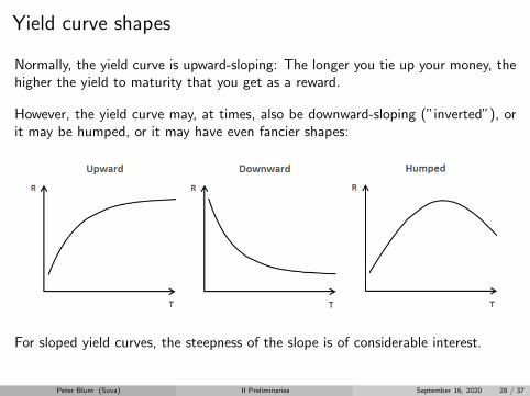
Yield curve shapes

Normally, the yield curve is upward-sloping: The longer you tie up your money, thehigher the yield to maturity that you get as a reward.

However, the yield curve may, at times, also be downward-sloping (”inverted”), orit may be humped, or it may have even fancier shapes:

For sloped yield curves, the steepness of the slope is of considerable interest.


Yield curve historyOver the past decades, yields have decreased dramatically over the entire range ofmaturities; here e.g. the Swiss case:

This is a major problem for capital-based social and pension insurance institutions,as we will see in the next chapters.


Zero-coupon bondsCoupon bonds as introduced are rather cumbersome due to the intermediate couponcashflows. A simpler alternative:

A Zero-Coupon Bond (ZCB) with maturity M pays the amount of 1 at maturityM , and no coupons in between t = 0 and t = M . Let P (0,M) be the market priceof a ZCB at time t = 0. Applying the usual valuation method, we then must havefor some discount rate δ∗:

PV0

(ZM , δ∗

)= P (0,M) =

1

(1 + δ∗)Mor δ∗ =

1

P (0,M)1/M− 1

The resulting discount rate δ∗ =: Z(0,M) is called Zero-Coupon Yield or alsoSpot Rate. It has no underlying issues with reinvestment.

Convention: Zero coupon bonds are always quoted with a final value of 1.

Therefore, the price of a zero coupon bond can be directly used as an alternativediscount factor for a cashflow CT occurring at time T :

PV0(CT , Z(0, T )) := P (0, T )CT


Based on this, we can express a coupon bond as a portfolio of zero-coupon bonds:

I For each time t ∈ 1, . . . , M, we hold c units of a ZCB with maturity t.

I For t = M , we hold an additional P units of a ZCB with maturity M .

This ZCB portfolio produces exactly the same pattern of cashflows as a couponbond. Therefore, if the market is arbitrage-free, the traded price B0 of the couponbond must be equal to the price of the ZCB portfolio:

B0!=

M∑t=1

c P (0, t) + P (0,M)P (2)

In most markets, zero coupon bonds do not actually exist. Formula 2, appliedto a number of different maturities can, however, be used to compute artificialequivalent ZCB rates from the prices of actually traded coupon bonds by means ofa procedure called bootstrapping.

We will not treat this further here. ZCB curves are readily available from differentsources, e.g. from Bloomberg or also from supervisory authorities for statutorypurposes.


Example: Zero-coupon rate curves computed by FINMA for use in the Swiss Sol-vency Test 2020:


Valuation based on ZCB curves

The valuation logic based on ZCB prices and rates as shown above can also beapplied to general cashflow streams, i.e. instead of computing

PV0(C, δ) =

T∑t=1

Ct(1 + δ)t

for a single discount rate δ, one can also compute

PV0(C) =T∑t=1

Ct P (0, t) =T∑t=1

Ct(1 + Z(0, t))t

This amounts to applying a specific discount rate for each time t. If we start withthe latter approach, we can link this to the former one by letting

δ∗ = IRR(C, PV0) such that PV0(C, δ∗) = PV0(C)

δ∗ is then the equivalent single discount rate.


Duration and convexity of bonds

Since bonds are simply streams of cashflows, we can apply the concepts of durationand convexity directly to them.

For a coupon bond, we have C = (c, . . . , c, c + P )′ ∈ RM ; letting δ = R(0,M)and using Propositions 2 and 3, we obtain:

D(C, δ) =1

1 + δ

[M∑t=1

c t

(1 + δ)t+

MP

(1 + δ)M

]/[M∑t=1

c

(1 + δ)t+

P

(1 + δ)M

]

K(C, δ) =1

(1 + δ)2

[M∑t=1

c(t+ 1)t

(1 + δ)t+M(M + 1)P

(1 + δ)M

]/[M∑t=1

c

(1 + δ)t+

P

(1 + δ)M

]

For a zero coupon bond, the cashflow stream is C = (0, . . . , 0, 1)′ ∈ RM , and,letting δ = Z(0, T ), the formulae simplify to:

D(C, δ) =M

1 + δ≈M and K(C, δ) =

M (M + 1)

(1 + δ)2


Also with bonds, convexity is an issue, and second-order approximation should bepreferred over first-order approximation.


Duration and convexity of a portfolio of bonds

Proposition 4 (Portfolio duration and convexity)

Assume that we hold n1 units of a bond C1 valued at PV 10 per unit, and n2 units

of a bond C2 priced at PV 20 per unit. Then we have for the combined position:

D(n1C1 + n2C2, δ) = w1D(C1, δ) + w2D(C2, δ)

K(n1C1 + n2C2, δ) = w1K(C1, δ) + w2K(C2, δ)

where wi =niPV i

0

n1PV 10 + n2PV 2

0

for i ∈ 1, 2.

Proof: Use ∂∂δ

[n1PV 1

0 + n2PV 20

]= n1

∂∂δ PV 1

0 + n2∂∂δ PV 2

0 , then divide by the

portfolio value n1PV 10 + n2PV 2

0 and rearrange.

Same procedure with second derivatives for convexity.

This naturally generalizes to portfolios with n bonds. The relation only holds exactlyif all bonds have the same yield δ. Otherwise it is a (usually good) approximation.


Bibliography I

[1] Blum, P.On some mathematical aspects of dynamic financial analysis.Doctoral thesis, ETH, Zurich, 2005.

[2] Bronstein, I., Semendjajew, K., Musiol, G., and Muhlig, H.Taschenbuch der Mathematik.Verlag Harri Deutsch, Thun, 1995.

[3] Fabozzi, F.Fixed Income Analysis, second ed.John Wiley & Sons, Chichester, 2007.

[4] Gerber, H.Life Insurance Mathematics, third ed.Springer, Berlin, 1997.



Chapter III: Financing Liabilities


Peter Blum


September 16, 2020

Peter Blum (Suva) III Financing Liabilities September 16, 2020 1 / 45

Table of Contents

1. Introduction and overwiew

2. Cashflow matching and immunized value

3. Simplification: duration matching

4. Alternative: loose coupling


1. Introduction and overwiew


The task

Let t ∈ 0, 1, . . . , T for T <∞ denote time in years.

Assume that we have a stream C = (C1, . . . , CT )′ ∈ RT of promised cashflows

with Ct ≥ 0 for all t. This can be e.g. a portfolio of old-age or disability pensions.Assume, for the time being, that these cashflows are deterministic and known.

We stand at time t = 0 and must put up a portfolio of assets A0 such that thepayment of all cashflows Ct for all times t ∈ 1, . . . , T is assured (at least withhigh probability).

How can this be achieved?


Example: cashflow stream

A typical cashflow stream in social and pensions insurance (albeit with an unusuallyshort time horizon, for simplicity’s sake):


Naıve approach: bank account

Assume that there is a bank account which pays an annual interest rate δ. Thenwe can put up the amount

A0 =

T∑t=1

Ct

(1 + δ)t(= PV0(C, δ))

and all future payments are assured; c.f. Section 1 of Chapter II.

Does this work? If the earning of the interest rate δ is guaranteed for the entiretime span t = 0, 1, . . . , T : YES.

Is the interest rate guaranteed? NO! It can actually vary quite considerably overtime. If this is the case, payment of all liabilities is no longer assured.

I in the 1980-ies: δ ≈ 4%

I around 2000: δ ≈ 2%

I now: δ ≈ 0%

This does not work. FORGET IT!


Alternative: bonds

Recall from Section 2 of Chapter II that a bond is basically a standardized streamof cashflows:

B = (c, . . . , c, c+ P )′ ∈ RM

where c is the (annual) coupon, P is the principal and M is the number of yearsto maturity, i.e. the redemption of the principal. We shall follow the convention ofChapter II and always let P = 100.

By paying the market price B0 prevailing at t = 0, we can acquire the bond, i.e.the right to receive exactly this stream of cashflows.

I Important: After the purchase, there is no more uncertainty about the cash-flows ...

I ... under the tacit assumption that the issuer of the bond does not go bankruptuntil the maturity of the bond.

Ansatz: At time t = 0, we buy a portfolio of different bonds, composed in such away that their cashflows are equal to the liability cashflows to be financed.


2. Cashflow matching and immunized value


Bond portfolio

Assume that we have a bond market with N different bonds Bi, i ∈ 1, . . . , N.Each bond has its specific coupon ci and its specific maturity M i. We assume thatM i ≤ T for all i. Following the usual convention, we also assume that the principalP i of each bond equals 100. That is, we have a number of standardized streamsof cashflows

Bi =(ci, . . . ci, 100 + ci

)′ ∈ RMi

We assume that all these bonds are (reasonably) free of credit risk, which is thecase e.g. for bonds of the Swiss confederation.

We stand at t = 0 as usual. All bonds are assumed to be traded in the market, withcurrent market prices Bi

0 for i ∈ 1, . . . , N. This also means that each bond hasits yield to maturity

R(0,M i) = IRR(Bi, Bi

0

)i.e. the discount rate that equates the present value of the cashflow pattern to theprice paid in the market.


Cashflow matrix

Assume w.l.o.g. that 1 = M1 ≤ M2 ≤ · · · ≤ MN = T . Then, we can expressthe cashflows in matrix form: B ∈ RT×N such that Bt,i expresses the cashflow ofbond i at time t:

B =

100 + c1 c2 · · · ci · · · cN

0 100 + c2...

...... 0

......

......

......

... ci...

...... 100 + ci

......

... 0...

......

... cN

0 0 · · · 0 · · · 100 + cN


Example: bond market data

Market data from the Swiss bond market as of Summer 2018:


Example: yield curve

Yield curve resulting from the bond market data:

This does not look like in the textbooks. But it is the reality that Swiss institutionalinvestors have to cope with nowadays.


Example: cashflow matrix

Cashflow matrix resulting from the bonds indicated above:


Immunization: idea

At time t = 0, from each bond Bi, we can buy ni units at the market price Bi0.

This results in a portfolio

n := (n1, . . . , nN )′ ∈ RN

Given the cashflow matrix B, this portfolio will produce a cashflow stream Bn ∈ RT

over time. If we manage to fix n in such a way that

Bn = C or (Bn)t = Ct for all t ∈ 1, . . . , T

where Ct is the given liability cashflow at time t, then we have achieved the stateof immunization, i.e.

I We buy the portfolio n at time t = 0 for the price∑N

i=1 niBi0.

I At each time t ∈ 1, . . . , T, this portfolio gives us an income of (Bn)t.

I And this income is then used (and sufficient) to pay the cashflow Ct owed.

That is, by purchasing the portfolio n at time t = 0, we have covered all ourobligations for t ∈ 1, . . . , T.


Simple immunizationLet C = (C1, . . . , CT )

′ ∈ RT denote the liability cashflow stream.

Assume that we have exactly N = T different bonds Bi, i ∈ 1, . . . , N = T,and each of these bonds matures in a different year. That is, for each single yeart ∈ 1, . . . , T, we we have one bond with i = t and cashflow pattern

Bt =(ct, . . . , ct, 100 + ct

)′ ∈ Rt

This yields a cashflow matrix that is quadratic, i.e. B ∈ RT×T and that hasupper triangular form. If the coupon rates are non-degenerate, then B also has fullrank. With the portfolio vector n = (n1, . . . , nT )

′ ∈ RT , we obtain the followingcondition for immunization:

Bn = C

and this has the (under these circumstances unique) solution

n = B−1C

The problem with this simple solution is that certain elements of this solution maybe negative, i.e. ni < 0 for some i ∈ 1, . . . , T.


This amounts to a short position in bond Bi. Such a short position can, in principle,be implemented. But in the context of social and pension insurance, short positionsare often forbidden by law or regulation. And even if they are not forbidden, theyare not desirable for reasons related to operations and risk management.

Anyway, in realistic settings with longer time horizons than 10 years, it is usuallydifficult or impossible to set up a cashflow matrix that is exactly upper triangular.

Therefore, we need a more general formulation of the immunization problem. Itmust accommodate the constraint that n ≥ 0 (to be understood as ni ≥ 0 forall components i), and it should also be able to deal with more general cashflowmatrices where N 6= T .

Note: A setting where each (reasonably measurable) cashflow can be perfectlyreplicated by securities available in the market is called a complete market.


General immunization problem

Let C = (C1, . . . , CT )′ ∈ RT with Ct ≥ 0 for all t ∈ 1, . . . , T be a given

stream of liability cashflows.

Assume that we have N bonds Bi with coupons ci and with maturities such that1 = M1 ≤ · · · ≤ MN = T , each one with its market price Bi

0 and its yield tomaturity Ri(0,M i) = IRR(Bi, Bi

0) at time t = 0.

The resulting cashflow matrix is B = (Bt,i)t∈1, ... , T, i∈1, ... , N , where Bt,i de-

notes the cashflow from bond i at time t.

Let n = (n1, . . . , nN )′ ∈ RN denote the portfolio, i.e. ni is the number of units

of bond i that we purchase at time t = 0. We always impose n ≥ 0.

If we hold some bond portfolio n, then for each time t ∈ 1, . . . , T, we have atotal cash inflow (Bn)t and a cash outflow of Ct from the liabilities, resulting in adiscrepancy (C − Bn)t. In the simplest case, we would simply minimize the sumof these discrepancies, i.e.

minn

1′ (C−Bn) s.t. n ≥ 0

This is a simple linear programming problem as proposed e.g. in [1].


The solution may, however, not be satisfactory. We might have the situation wherea large positive discrepancy at some time t1 may be compensated by a large negativediscrepancy at some other time t2. This is contrary to our intention of matchingcashflows from the bond holdings with cashflows for the liabilities as best as wecan. To the latter end, we should rather optimize absolute deviations, i.e.

minn

T∑t=1

((Bn)t − Ct)2 s.t. n ≥ 0 (1)

The square makes sure that larger discrepancies (in whatever direction) are morepenalized than smaller ones. Using matrix notation, this problem is equivalent to

minn

12 n′(B′B)n− (C′B)n s.t. n ≥ 0 (2)

This is a standard quadratic programming problem that can be solved by any stan-dard software package. If necessary, we can also impose further equality or inequalityconstraints.


Proof: (Equivalence of equations 1 and 2)

We have (Bn)t =∑N

i=1 Bt,i ni. Therefore:

((Bn)t − Ct)2 =

(∑N

i=1Bt,i ni − Ct

)2

=

(∑N

i=1Bt,i ni

)2

− 2Ct

∑N

i=1Bt,i ni + C2

t

The term C2t does not depend on n and needs not be considered any further. For the second

term, we can sum over t to obtain:∑T

t=1Ct

∑N

i=1Bt,i ni =

∑T

t=1

∑N

i=1Ct Bt,i ni

=∑N

i=1

(∑T

t=1Ct Bt,i

)ni = (C′B)n

For the first term, we have(∑N

i=1Bt,i ni

)2

= ((Bn)t)2 =

(n′B′)

t(Bn)t

and therefore ∑T

t=1

(n′B′)

t(Bn)t = n′(B′B)n

Putting everything together and multiplying by 12

, we obtain

12n′(B′B)n− (C′B)n


Immunizing portfolio

Let n∗ denote the solution of Optimization Problem 2, i.e. the bond portfolio thatbest matches the given liability cashflows C. What does this mean?

I At time t = 0, we buy ni units of Bond Bi at market price Bi0 for each

i ∈ 1, . . . , N. This results in a total purchase price of∑N

i=1 n∗iB

i0.

I We then hold this portfolio unaltered over time, without buying or selling.Thus, at each time t ∈ 1, . . . , T we receive a cashflow of (Bn∗)t.

I We then use this cashflow in order to pay the liability cashflow Ct.

Generally, there will be no exact match between (Bn∗)t and Ct. But if the discrep-ancies are small relative to the value of the bond portfolio, i.e.√∑T

t=1((Bn∗)t − Ct)

2 N∑i=1

n∗iBi0

this is a viable approximation. We simply need to hold a relatively small amount ofadditional cash D∗ to make sure that the discrepancies will be covered.


Example: resultsComposition of portfolio, purchase price and residual:


Immunized value

By following the procedure above, for some given stream of liability cashflows, wehave the following situation:

I By buying the bond portfolio n∗ at time t = 0 for the price∑N

i=1 n∗iB

i0, and

by putting up additional cash D∗,

I we can make sure that all subsequent liability cashflows at all future timest ∈ 1, . . . , T can be paid with certainty.

This situation is completely independent of the subsequent development of thebond prices. By paying Bi

0 at t = 0, we have assured the receipt of the cashflows(ci, . . . , ci, 100 + ci), irrespective of what the price for doing this would be in thefuture.

That is, we have effectively created an immunized position, and the price for doingso is the immunized value of the cashflow stream C:

IV0(C) :=

N∑i=1

n∗iBi0 +D∗ ≈

N∑i=1

n∗iBi0


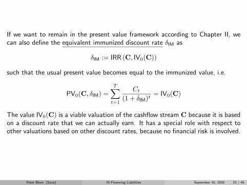
If we want to remain in the present value framework according to Chapter II, wecan also define the equivalent immunized discount rate δIM as

δIM := IRR (C, IV0(C))

such that the usual present value becomes equal to the immunized value, i.e.

PV0(C, δIM) =

T∑t=1

Ct

(1 + δIM)t= IV0(C)

The value IV0(C) is a viable valuation of the cashflow stream C because it is basedon a discount rate that we can actually earn. It has a special role with respect toother valuations based on other discount rates, because no financial risk is involved.


Example: immunized value

For our example, we obtain the following results:

I Immunized value: IV0(C) = 658′718 + 0.02 = 658′718

I Equivalent immunized discount rate: δIM = −0.35%

I Undiscounted sum of liability cashflows: 648′841

Since the equivalent immunizing discount rate is negative, the purchase price of theimmunizing portfolio is higher than the undiscounted sum of cashflows.

That is, in order to achieve an immunized position under the current market condi-tions, we must put up more money at the beginning than we will pay out over thecourse of time. We have managed to eliminate financial risk, but the price for thisis a negative contribution from financial returns.


Immunization with zero-coupon bondsAnother drawback of the immunization approach as presented is that the handlingof the coupon bonds is relatively cumbersome.

The situation would be less complicated if we had zero-coupon bonds. Recall fromsection 2 of Chapter II that a zero-coupon bond is a security that pays the amountof 1 at maturity M > 0 and nothing in-between times 0 and M . One unit of thezero coupon bond can be purchased at the price P (0,M) at time t = 0.

Assume that for each time t ∈ 1, . . . , T, we have a zero-coupon bond availablewith purchase price P (0, t) at time 0.

Let C = (C1, . . . , CT )′ ∈ RT be a given stream of liability cashflows with Ct ≥ 0for all t. Then, at time t = 0 and for each future time t ∈ 1, . . . , T, we cansimply buy Ct units of the zero-coupon bond maturing at time t. In this case,we are completely immunized, even without an approximation error. The cost ofachieving this immunization is

PV0(C) =T∑

t=1

P (0, t)Ct

where PV0(C) is the alternative present value as in Section 2 of Chapter II.Peter Blum (Suva) III Financing Liabilities September 16, 2020 25 / 45

Here again, we can compute the equivalent immunized discount rate:

δIMZ := IRR(C, PV0(C)

)such that the immunized value matches the usual present value, i.e.

PV0(C, δIMZ) =

T∑t=1

Ct

(1 + δIMZ)t= PV0(C)

In most markets except the US, zero-coupon bond do not exist as traded securities.

Hence, PV0(C) is, in principle, not a viable valuation.

However, as described in Section 2 of Chapter II, one can compute notional zero-

coupon bond prices and rates. And the value PV0(C) obtained from these notionalprices is a - typically fairly good - approximation of the actual immunized value.


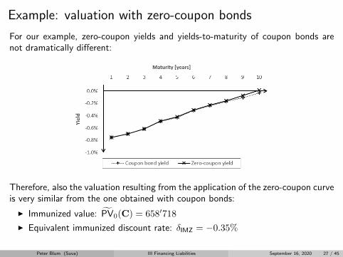
Example: valuation with zero-coupon bonds

For our example, zero-coupon yields and yields-to-maturity of coupon bonds arenot dramatically different:

Therefore, also the valuation resulting from the application of the zero-coupon curveis very similar from the one obtained with coupon bonds:

I Immunized value: PV0(C) = 658′718

I Equivalent immunized discount rate: δIMZ = −0.35%


Immunization: conclusions

The concept of immunization is very appealing: By purchasing a portfolio of securi-ties at time t = 0, we can - in principle - ensure the payment of all future promisedcashflows without any financial risk remaining.

Therefore, the immunized value of a stream of liability cashflows is an importantreference value: It denotes the amount of money that must be put up if one wantsto ensure the payment of the liabilities without financial risk interfering. This isrelated to the economic concept of the certainty equivalent.

The immunized value has, however, also a number of drawbacks, notably:

I For longer-dated liabilities (e.g. t 20 years), there may not exist enoughbonds with corresponding maturities.

I One could still compute the immunized value by using extrapolated bond pricesand yields (in particular for zero-coupon bonds).

I But these immunized values are only meaningful to a limited extent, becausethe immunizing position cannot actually be implemented. That is, in this case,there is financial risk remaining.


In the current situation, however, the main drawback is that the immunized valueis very expensive. With current bond prices and yields (c.f. the example), theequivalent discount rates are around or even below zero, and one must put up veryhigh amounts of money to assure payment of the liabilities without financial risk.

In our example, δIM = −0.35% for IV0(C, δIM) = 658′718. Compare this to thevalues obtained with other discount rates.

δ PV0(C, δ)0% 648′8411% 621′9902% 596′8553% 573′2984% 551′194

The rest of this course will be basically about judging whether it makes sense toincur some financial risk in order to sustain a somewhat higher discount rate andachieve a lower valuation of the liabilities.


3. Simplification: duration matching


IntroductionThe task here is the same as in the case of cashflow matching: We are given astream of cashflows C = (C1, . . . , CT )

′ ∈ RT with Ct ≥ 0 for all t, and we wantto set up a bond portfolio at time t = 0 in such a manner that the payment of Cis assured without financial risk at t > 0.

If the assets held are only bonds, then financial risk arises from changes in interestrates. If interest rates change, then the value of the bonds held changes. But -at least in principle - one should also adapt the discount rate of liabilities, whichcauses a change in the value of liabilities.

If we set up the bond portfolio in such a way that its change in value is equal to thechange in value of the liabilities, then we are - at least in principle - immunized:

I If interest rates rise, the value of the bonds diminishes. But so does thevalue of the liabilities if the discount rate is adapted accordingly.

I If interest rates fall, the discount rate of liabilities should be reduced. Thiscauses the value of liabilities to rise. But so does the value of the bonds.

The approach is now to make sure that the movement on the asset side and on theliability side are (approximately) equal.


Interest rate sensitivity

Recall Chapter II: The measures of interest rate sensitivity for any stream of dis-counted cashflows - liabilities and bonds alike - are the duration (1st order) and theconvexity (2nd order):

Duration: D(C, δ) = − ∂

∂δPV0(C, δ)

/PV0(C, δ)

Convexity: K(C, δ) =∂2

∂δ2PV0(C, δ)

/PV0(C, δ)

For a bond, the discount rate δ equals its yield to maturity R(0,M). For a port-folio of bonds, the overall duration and convexity can be calculated or at leastapproximated by using Proposition 4 of Chapter II.


Duration matching

Let C = (C1, . . . , CT )′ ∈ RT with Ct ≥ 0 for all t be a stream of liability

cashflows, and let δ denote its discount rate.

Let B1 . . . , BN denote a set of bonds, each one with its yield to maturityRi(0,M i)and market price Bi

0 as of t = 0. Let n = (n1 . . . , nN )′ ∈ RN with ni ≥ 0 for all

i denote the number of units of bond i that we hold in our portfolio.

To achieve duration (and convexity) matching, we must select n at t = 0 such that

D

(∑N

i=1ni B

i, δn

)= D(C, δ)

K

(∑N

i=1ni B

i, δn

)= K(C, δ)

δn ≥ δn ≥ 0

The additional convexity condition should normally be included in social and pensioninsurance settings. It may, however, be omitted in certain situations.


δn denotes the overall yield to maturity of the bond portfolio , i.e.

δn = IRR

(∑N

i=1ni B

i,∑N

i=1niB

i0

)We will see in the next chapter that the condition δn ≥ δ is important.

If the set of available bonds is sufficiently rich, this problem will not have a uniquesolution, and we may be able to impose additional constraints or targets, e.g.

I maximize yield δn or minimize purchase price∑N

i=1 niBi0

I impose cashflow matching for the first few years

Note that, in general, there is absolutely no guarantee that the cashflows will match.


Immunization by duration matchingAssume that the yield in the bond market changes by ∆δ for all maturities. Thisalso means that δn changes by ∆δ. Because of the condition δn ≥ δ, this alsomeans that we should change the discount rate δ by ∆δ.

Relative effect on the asset side:

∆ PV(∑N

i=1 ni Bi, δn + ∆δ

)PV(∑N

i=1 ni Bi, δn

) = −D(∑N

i=1ni B

i, δn

)(∆δ)

+1

2K

(∑N

i=1ni B

i, δn

)(∆δ)

2+ o

((∆δ)

3)

Relative effect on the liability side:

∆ PV (C, δ + ∆δ)

PV (C, δ)= −D (C, δ) (∆δ) +

1

2K (C, δ) (∆δ)

2+ o

((∆δ)

3)

Due to the matching conditions, these relative changes will be equal. That is, ifliabilities increase, then so will the assets used to cover them. And vice versa.To the extent that duration and convexity are a good measure for interest ratesensitivity, we have at least in principle an immunized position.


Example: duration-matched portfolios

Two possible duration-matched portfolios and the cashflow-matched portfolio forcomparison:


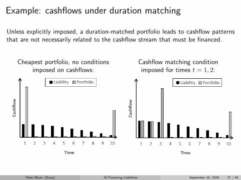
Example: cashflows under duration matching

Unless explicitly imposed, a duration-matched portfolio leads to cashflow patternsthat are not necessarily related to the cashflow stream that must be financed.

Cheapest portfolio, no conditionsimposed on cashflows:

Cashflow matching conditionimposed for times t = 1, 2:


Duration matching: conclusions

By applying duration (and convexity) matching, one can create an (approximately)immunized position of assets and liabilities with less restrictive conditions than forcashflow matching.

One can also combine duration matching (for longer time horizons) and cashflowmatching (for shorter time horizons).

Due to the restriction δ ≤ δn, also duration matching will only allow for very lowdiscount rates under current market conditions, leading to very high liability valuessimilar to the ones attained under cashflow matching.

Basic duration matching as shown here only works for parallel shifts of the yieldcurve where rates for all maturities move by the same amount ∆δ, which is notrealistic in many situations. To circumvent this, there exist more sophisticatedmethods based e.g. on so-called key rate durations; see [1].

Duration and convexity can only be determined accurately for fixed income se-curities. If an institution also holds other asset classes like equities, real estate oralternative investments, then one can - in principle - estimate the durations of theseassets, but these estimates lack accuracy. This is particularly the case nowadayswhen interest rates are mainly determined politically.


4. Alternative: loose coupling


Situation with immunization

With the immunizing approaches (to the extent that they are implementable), oneis in a position where one can set up a portfolio of securities at time t = 0 in sucha way that the payment of all subsequent cashflows Ct for all subsequent timest ∈ 1, . . . , T ist assured (at least with a very high probability). This is a verycomfortable position.

An immunizing portfolio can only be created by using (high-grade) bonds or -in practice - similar fixed income securities such as high-grade loans or privateplacements or derivatives such as bond futures or swaps.

The discount rate cannot be higher than the overall yield of the immunizing port-folio. Therefore, applicable discount rates tend to be very low, particularly in thecurrent low-interest environment.

This leads to high valuations for some given stream of liability cashflows, and to alow contribution of investment returns to the overall financing of the liability.


Challenges and requirements

In many situations (e.g. in Swiss compulsory accident insurance), the discount ratefor the liabilities is exogenously given, and the given level may be well above whatis attainable with an immunizing approach.

Or there may be the desire or the requirement of the institution to have a higherinvestment income than just bond yields. Motivations for this may be:

I Higher benefits for the same level of premium or contributions.

I Lower premium or contribution for the same benefits.

I Financing cost increases, particularly due to longevity.

Or the institution may simply have an in-force portfolio that contains substantialamounts of non-fixed income securities like equities, real estate or alternative in-vestments.

In all these situations, a less restrictive coupling between the assets and the liabilitiesis necessary.


Loose coupling setupWe have a stream of liability cashflows C = (C1, . . . , CT )

′ ∈ RT with givendiscount rate δ, such that the initial value of the liabilities is L0 = PV0(C, δ). Forcovering the liabilities, we hold assets valued A0. For financing the liabilities, wesubdivide the institution into two functions:

I The insurance function services the liabilities. For doing so, it receives afixed interest δ from the investment function.

I The investment function invests the assets and generates investment pro-ceeds IPt. It uses these investment proceeds to finance the fixed interestpayments δ.

This subdivision into an insurance and an investment function is related to theprinciple of funds transfer pricing, see e.g. [2].

Now, assets and liabilities are only coupled by the discount rate δ and by their totalvalues A0 and L0. Hence the name loose coupling.


Investment risk and the role of surplusIn an immunized setup, one need not care about changes in the value of the invest-ment (bond) portfolio over time, since assets and liabilities are immunized.

In the loose coupling approach, investment proceeds are generally variable, andthey may or may not be sufficient to fund the fixed rate δ in any given year. Tocompensate this uncertainty, the institution must hold a capital buffer, called surplus(or equity, in the corporate world).


In an immunized setup,the discount rate is low, and thus the valuation of theliabilities is high. But there is little to no risk from investing the assets due to theimmunized position. Therefore, one needs to hold little or no surplus as a bufferagainst investment risk.

In a loosely coupled setup, one may set a higher discount rate, leading to lowervaluations of the liabilities. But, in order to finance this discount rate, one has toincur a non-negligible investment risk. As a buffer against this, one needs, in turn,a higher surplus. Hence, the choice of discount rate has consequences in the formof investment risk and necessary surplus to compensate it.

Where is the optimum in this dynamic and circular relationship? What is theinterplay between discount rate, investment risk and necessary surplus? What isfeasible, and what is not feasible?

These questions are of high relevance, since many social and pension insurance in-stitutions work according to the loose coupling principle, in particular Swiss pensionfunds and compulsory accident insurance.

In the subsequent chapters, we will suitably formalize the problem sketched here,and we will build a thorough understanding.


Bibliography I

[1] Scherer, B.Liability Hedging and Portfolio Choice.Risk Books, London, 2005.

[2] Wilson, T.Value and Capital Management.John Wiley & Sons, Chichester, 2015.



Chapter IV: The Asset / Liability Framework


Peter Blum


September 17, 2020

Peter Blum (Suva) IV Asset / Liability Framework September 17, 2020 1 / 48

Table of Contents

1. Working principle of capital-based insurance

2. Model framework for social insurance

3. Liabilities and required return

4. Elements of the financial account

5. General random walk model and net profit condition


1. Working principle of capital-based insurance


Promised benefits and liabilities

The institution receives premium income or contributions from its clients or fromthird parties.

In return, the institution promises - and thus owes - to its clients certain well-specified future benefits, e.g.

I old-age or disability pensions

I reimbursement of medical costs from injury or illness

I indemnities for foregone salaries

I subsidies for long-term care

I unemployment benefits

These benefits can be expressed as (estimated) future cashflows.

The present value of these future cashflows, possibly augmented by certain rein-forcements, is the liability of the institution.


Accident insurance: short-term benefitsFuture payments for medical treatment and income substitution related to accidentsalready happened.

”Short-term” is relative: After 5 years, 20% of ultimate payments are still open.And after 20 years, 5% of ultimate payments are still open. Some payments occurup to 75 years after the accident.


Accident insurance: long-term benefits

Future pension payments for disabled and next-of-kin from accidents already hap-pened. Average age at beginning of pension is around 42 years.


Accident insurance: liabilities

Excerpt from the balance sheet of the Swiss National Accident Insurance Fund(see suva.ch):


Assets and investment proceedsIn order to cover the liabilities, the social insurance institution must hold an appro-priate amount of assets.

These assets can be invested, e.g. in bonds, equities, real estate or alternativeinvestments and thus generate investment proceeds.

The investment proceeds are an important part of the funding of the institution.Higher investment proceeds result in lower premia or higher benefits.

In order to facilitate planning and tariffication, a target (required return) is imposedfor the investment proceeds.

By investing its assets (e.g. in equities), the institution incurs investment risk, i.e.the investment proceeds may be higher or lower than the target.

The institution must, hence, take appropriate precautions in order to deal withdeviations of actual investment proceeds from required ones.

The extent to which the institution can absorb such deviations of actual investmentproceeds from required ones is called the risk-taking capability.


Example: assets

Excerpt from the Suva balance sheet:

Substantial portions of the assets are invested in risky asset classes such as equitiesor alternative investments.


Example: investment proceedsHistory of investment returns of Suva:

Due to the relatively high percentage of equity holdings, performance fluctuatedconsiderably from year to year.

On average over several years, however, the performance was sufficient to cover thefinancing needs.


Asset / Liability Management

The big picture obtained comprises the following elements:

Institution Financial markets

Required return Realized investment proceeds

Risk-taking capability Investment risk incurred

Asset / Liability Management (ALM) is the task of reconciling these different andoften conflicting aspects such that the promised payouts can be made with highprobability.


2. Model framework for social insurance


Balance sheetThe balance sheet describes the state of the institution at some point t in time:

Let t denote time in years; t ∈ 0, . . . T for some final time T <∞. Time t = 0is the present, t > 0 denotes the future.

Let At denote the total value of assets at time t. Specifically, At is the market valueof the assets at the end of year t.

The total assets can be subdivided into n asset classes Ai,t, i.e.

At =

n∑i=1

Ai,t with Ai,t ≥ 0 for all t ∈ 0, . . . T and i ∈ 1, . . . n


Ai,t can denote e.g. equities, bonds, real estate or alternative investments.

By wi,t := Ai,t/At we denote the portfolio weight of asset class i at time t.

The entire portfolio is specified by wt = (w1,t, . . . wn,t)′ ∈ Rn. and we have

wi,t ≥ 0 and∑ni=1 wi,t = 1.

By Lt we denote the value of the liabilities at time t, i.e. the present value of futurecashflows plus necessary reinforcements; see next section for more details.


Surplus and Funding Ratio

Definition 1 (Surplus)

The surplus is the difference between assets and liabilities: St = At − Lt

Surplus is expressed in monetary units and bears limited information; e.g.

I 1 MCHF of surplus against 5 MCHF of liabilities (solid)

I 1 MCHF of surplus against 100 MCHF of liabilities (shaky)

This deficit is overcome by the funding ratio which relates surplus to liabilities:

Definition 2 (Funding Ratio)

The funding ratio is the ratio of assets and liabilities:

FRt =AtLt

= 1 +StLt

If FRt ≥ 1, i.e. At ≥ Lt or St ≥ 0, the institution is fully funded or overfunded.Otherwise, the institution is underfunded. The probability or the expected depth ofan underfunding are important risk measures in the ALM context.


Example: Funding ratio of Swiss pension funds according to the Swisscanto pensionfund studies (see www.swisscanto.ch):

Notice the considerable fluctuations. This development is owed to the financialcrises of 2001 and 2008 and to the general downward trend in interest rates. Fi-nancial risk management is a serious issue. And it is a long-term issue.


Income statementThe income statement describes the change in the financial position of the institu-tion in the t-th year, i.e. in (t− 1, t]:

Income Expense

Premium / Contribution Insurance benefitsPt Bt

Investment proceeds Revaluation of liabilitiesIPt RLt

Pt is the income from premia or contributions; this is an actual cash inflow.

IPt denotes the proceeds from the investment of the assets in monetary units. Thiscan be an actual cash inflow (e.g. dividends) or a non-cash change in value (positiveor negative).

Bt is the expense from paying promised insurance benefits; this is an actual cashoutflow.


RLt is the non-cash expense for the intrinsic revaluation of liabilities; see next sectionfor an in-depth treatment. It can be positive or negative.

We define Ct := Pt −Bt as the net cashflow from insurance operations.

We could also define NRt = Pt+ IPt−Bt−RLt as the net result. This is, however,less important in social insurance. The main interest is focused on the balancesheet, in particular on the surplus St and the funding ratio FRt.


Transition equation for assets

The change in the value of assets in year t depends on the investment proceedsobtained in the financial markets and on the net cashflow from insurance operations;the latter is assumed to take place at year-end:

At = At−1 + IPt + Ct

Let Rt denote the rate of return from investing the assets, i.e.

Rt =IPtAt−1

=At − CtAt−1

− 1 =At−

At−1− 1

The return Rt only depends on the conditions in the financial markets and onhow At−1 is distributed on the different asset classes, but it does not depend oncashflows from insurance operations.

Example: Assume that At−1 = 100, Rt = 5.8% and Ct = 7.5. Then we haveAt− = 100 · (1 + 5.8%) = 105.8 and At = At− + Ct = 105.8 + 7.5 = 113.3.


The transition equation can thus be restated as follows:

At = At−1 +RtAt−1 + Ct = (1 +Rt)At−1 + Ct

We can also introduce returns on the level of single asset classes, i.e.

Ri,t =Ai,t−

Ai,t−1− 1 and Rt = (R1,t, . . . , Rn,t)

′ ∈ Rn

The return on the full asset portfolio is then given by the weighted sum of assetclass returns, i.e.

Rt =

n∑i=1

wi,t−1Ri,t = w′t−1Rt

The question of how to construct a suitable portfolio wt from the different assetclasses will be dealt with in the second part of the course. In the meantime, we willmainly consider the aggregate returns Rt.


Transition equation for liabilities

The change in the value of liabilities can be expressed in the same way as the changein the value of assets:

Lt = Lt−1 + RLt + Ct

There is a change due to net cashflows from insurance operations, and there is achange due to the intrinsic revaluation. For the latter, we can define

λt =RLtLt−1

=Lt − CtLt−1

− 1 =Lt−

Lt−1− 1

We call λt the liability return or the rate of intrinsic change of the liabilities. Fordetails and examples, see the next section The transition equation then becomes

Lt = Lt−1 + λtLt−1 + Ct = (1 + λt)Lt−1 + Ct


Transition equation for surplus

For the assets and the liabilities, we have:

At −At−1 = RtAt−1 + Ct

Lt − Lt−1 = λtLt−1 + Ct

Since St = At − Lt, this leads to

St − St−1 = (RtAt−1 + Ct)− (λtLt−1 + Ct)

= RtAt−1 − λtLt−1= IPt − RLt

That is, if surplus is to remain at least constant, the investment proceeds must beat least equal to the intrinsic revaluation of liabilities. For the return Rt, this means

RtAt−1 − λtLt−1 ≥ 0 or Rt ≥ λtLt−1At−1

=λt

FRt−1

Hence, the higher the funding ratio, the lower the required return. In practice, forthe reasons stated above, the funding ratio is more important than the surplus.


Transition equation for funding ratioInserting the transition equations for assets and liabilities into the funding ratio, weobtain

FRt =AtLt

=(1 +Rt)At−1 + Ct(1 + λt)Lt−1 + Ct

If Ct = 0, i.e. if contributions and benefits are in balance, this boils down to

FRt = FRt−1(1 +Rt)

(1 + λt)

That is, to keep the funding ratio at least constant, Rt must be at least equal toλt. In this case, λt specifies the required return.

For Ct 6= 0, this simple relation is distorted; consider

1!=

FRtFRt−1

=AtLt· Lt−1At−1

=At−1(1 +Rt) + CtLt−1(1 + λt) + Ct

· Lt−1At−1

By rearranging, we obtain

At−1Lt−1(1 +Rt) + CtLt−1 = At−1Lt−1(1 + λt) + CtAt−1


Dividing by At−1Lt−1 and rearranging, we obtain

Rt = λt +CtLt−1

− CtAt−1

Using At−1 = FRt−1Lt−1, we finally obtain

Rt = λt +

(1− 1

FRt−1

)CtLt−1

That is, the required return depends not only on λt, but also on the current fundingratio and on the net cashflow in relation to the existing liabilities.

Using Lt−1 = At−1

FRt−1, we obtain the alternative representation

Rt = λt + (FRt−1 − 1)CtAt−1

That is, if FRt−1 > 1 and Ct > 0, this dilutes the surplus, and we must earn anextra return to compensate this dilution.


In general, this yields the following situation:

underfunded overfundedFRt−1 < 1 FRt−1 > 1

net cash outflowRt

!> λt Rt

!< λtCt < 0

net cash inflowRt

!< λt Rt

!> λtCt > 0

The extent of the difference must be evaluated case by case.


3. Liabilities and required return


Overview

In the general model, the liabilities are assumed to behave according to the generictransition equation

Lt = Lt−1 + λtLt−1 + Ct = (1 + λt)Lt−1 + Ct

In the sequel, we explore what this means specifically for different forms of liabilities,in particular with respect to the intrinsic rate of change λt.

The most typical form of liabilities is when Lt is the present value of some streamof future cashflows. But there also exist other forms of liabilities that will beconsidered.


Liability is the present value of a cashflow streamAssume that the liability is the present value of some stream of promised benefitsB = (B1, . . . , BT )′ ∈ RT , i.e. for a fixed and given discount rate δ, we have

Lt = PVt(B, δ) =

T∑s=t+1

Bs(1 + δ)s−t

How does the value of the liability change between t− 1 and t?

Lt − Lt−1 =

T∑s=t+1

Bs(1 + δ)s−t

−T∑s=t

Bs(1 + δ)s−t+1

=

T∑s=t+1

Bs(1 + δ)s−t

−T∑

s=t+1

Bs(1 + δ)s−t+1

− Bt1 + δ

=

T∑s=t+1

Bs(1 + δ)s−t

− 1

1 + δ

T∑s=t+1

Bs(1 + δ)s−t

− Bt1 + δ

= Lt

(1− 1

1 + δ

)− Bt

1 + δ


Solving this equation for the value of the liability Lt yields

Lt = (1 + δ)Lt−1 −Bt

That is, we have

I λt = δ, i.e. the intrinsic rate of change equals the discount rate.

I Ct = −Bt, i.e. the cash outflow equals the liability payment.

Recalling the considerations from the previous section, this means that the discountrate δ is the main determinant of the required return. If the cash outflow is relativelysmall w.r.t. the total liability, and if the funding ratio is not too far away from 1,the required return is approximately equal to the discount rate δ.

Attention: This is based on the tacit assumption that the estimates for the cashflowsare unbiased. If the estimates have to be revised from year to year, the intrinsicrate of change can be significantly different from δ.


Liability is a savings account

In a typical Swiss pension fund, the accumulation process of the active membersbefore retirement works as follows:

I Each year t, the employees and the employer make a contribution totaling Ptthat is credited to the fund.

I Each year t, an interest ρt is granted on the money in the fund.

In particular, all past contributions and all past interest credits are guaranteed andthus a liability with the following transition equation:

Lt = Lt−1 + Lt−1ρt + Pt = Lt−1(1 + ρt) + Pt

That is, we have:

I λt = ρt, the credited interest rate,

I Ct = Pt, the contributions.

In a general setup, further cashflows would have to be added (benefits of freepassage, retirements).

Attention: This is called ”Beitragsprimat”, but it is not equal to a defined contri-bution plan in Anglo-American terminology, but rather to a cash balance plan.


Other liabilities

Besides the above-mentioned elements, the balance sheet of a social insuranceinstitution may also contain other liability elements, e.g.

I Actuarial reserves against fluctuations in the liability cashflows, e.g. due tomortality.

I Reserves for financing future adjustments of the liability parameters, e.g. tocater for longevity.

Most of these liabilities can be modeled in the form

Lt = (1 + λt)Lt−1 + Ct

for some suitable choices of λt and Ct.


Portfolio of liabilities

Assume that the total liabilities consist of several positions, i.e.

Lt =

m∑i=1

Li,t with Li,t = (1 + λi,t)Li,t−1 + Ci,t for all i

Then, the consolidated rate of intrinsic change λt is a weighted sum of the singlerates, i.e.

λt =

m∑i=1

Li,t−1Lt−1

λi,t

The cashflows simply add up: Ct =∑mi=1 Ci,t.

Hence, the generic model is quite broadly applicable.


4. Elements of the financial account


Recapitulation of generic model

We have developed the following generic model:

At = At−1(1 +Rt) + Ct

Lt = Lt−1(1 + λt) + Ct

With given value A0 for initial assets and L0 for initial liabilities, and suitableassumptions for the intrinsic growth rate λt and for the investment return Rt, themodel can always be evaluated by straightforward stochastic simulation. Note:

I In many practical situations, the intrinsic growth rate λt of the liabilities canbe modeled as deterministic. This is particularly the case if Lt already containssuitable reserve components to deal with fluctuations of actuarial risk.

I Unless we have a full immunization (see previous chapter), the investmentreturns Rt must be considered as a random variable.


Actuarial risk and required return

If λ were stochastic, Var[λt] or some other suitable risk measure like VaRα[λt] orESα[λt] could be used to denote actuarial risk. However, in the sequel, λt willmostly be considered as deterministic.

The required return is the minimum value that the return Rt must attain such thatFRt ≥ FRt−1, i.e. remains at least constant. As seen before, we have:

Rt!≥ λt +

(1− 1

FRt−1

)CtLt−1

= λt + (FRt−1 − 1)CtAt−1

If the net cashflow Ct = 0, this boils down to Rt ≥ λt.


Expected return and investment risk

For all t ∈ 1, . . . , T, we consider Rt as a random variable on a probability space(Ω,F ,P), i.e. Rt ∼ Ft with µt := E [Rt] <∞ and σ2

t := Var [Rt] <∞.

I The assumption σ2t <∞ (finite second moments) is fairly realistic for annual

investment returns. If it comes to higher moments, they may not always beassumed to exist.

I We do not impose any other assumptions at this point, neither Normal distri-bution nor absence of serial correlation.

We call µt := E [Rt] the expected return.

The short-term investment risk may be denoted by σ2t = Var [Rt] or by any other

suitable risk measure such as VaRα[Rt] or ESα[Rt]

I The notion ”short term” is important. This only describes risk for one outof many periods. This is a necessary ingredient, but not sufficient in order tocope with the long-term nature of social and pension insurance.


Risk-taking capability

For the time being, we take the initial funding ratio FR0 as a measure for therisk-taking capability. Intuitively, we have:

I The higher FR0, the thicker is the cushion for absorbing insufficient invest-ment proceeds without falling into underfunding.

I The lower FR0, the thinner is the cushion for absorbing insufficient invest-ment proceeds without falling into underfunding.

This is an approximation. Effectively, one would also have to to consider the pos-sibilities that the institution has to increase income or reduce obligations when itfalls into underfunding.


Example: High vs. low initial funding ratio.

High initial funding ratio Low initial funding ratio

The lines represent the 1%- and 99%-quantiles of the funding ratio; the gray areabelow FR = 1 represents the state of underfunding.


Asset / Liability Management: overview

From the above, we obtain the following overall view:

Institution Financial marketsRequired return Expected return

λt + (FRt−1 − 1) Ct

At−1← → µt

l lRisk-taking capability ← → Investment risk

FR0 σ2t

The challenge is that these quantities are intricately related:

I higher expected return comes at the price of higher investment risk

I lower required return usually also entails a lower risk-taking capability

Asset / Liability Management is the task of reconciling these often-conflicting di-mensions such that the payment of the promised insurance benefits is assured withhigh probability. This task must often be accomplished under additional constraints.


Financial risk

The goal of social an pension insurance is to assure with high probability that allpromised payments C = (C1, . . . , CT )′ over the full time period t = 1, . . . , Tcan be made.

The proceeds from investing the assets are a source of funding for these promisedpayments. Financial risk consists of the danger that promised payments cannot bemade at any time during the time span t = 1, . . . , T due to insufficient investmentreturns Rt.

There is no generally accepted way of quantifying financial risk; possible measuresthat will be explored subsequently include

I probability of underfunding ψt = P [FRt < 1]

I Expected Funding Shortfall EFSα,t or Funding Ratio at Risk FRaRα,t

for one or several time horizons t.


5. General random walk model and net profit condition


General random walk setup

We start from the standard model, i.e. from

FRt =At−1(1 +Rt) + CtLt−1(1 + λt) + Ct

We make the following assumptions:

I Contributions equal benefits: Ct = 0 for all t.

I Constant intrinsic liability growth rate: λt = λ for all t.

I Investment returns follow a random walk: Rt = µ + εt where εt ∼ iid withE [εt] = 0 and Var [εt] <∞.

This leads toFRt

FRt−1=

1 + µ+ εt1 + λ

Letting LFRt = log FRt and taking logarithms, we obtain

LFRt − LFRt−1 = log

(1 + µ+ εt

1 + λ

)


For small-enough values, we have log(1 + Rt) ≈ Rt and log(1 + λ) ≈ λ, and wecan use the approximation

LFRt = LFR0 +

t∑s=1

Xs where Xs := µ− λ+ εs

or, equivalently

Zt := LFRt − LFR0 =

t∑s=1

Xs

That is, we have managed to represent the evolution of the funding ratio as arandom walk. The condition FRt > 1 translates into LFRt > 0.

The assumption that the investment returns Rt form a random walk is not toounrealistic, at least for the annual returns that we consider here.

This allows us to apply a classic result from the theory of stochastic processes.


Proposition 1 (Random Walk Theorem)

Let Xs ∼ iid with P [Xs = 0] < 1 and E [|Xs|] < ∞. Then, the random walk(Zt)t∈N0

with Zt =∑ts=1Xs has one of the three following behaviors:

I if E [Xs] > 0 then limt→∞ Zt = +∞ P-a.s.

I if E [Xs] < 0 then limt→∞ Zt = −∞ P-a.s.

I if E [Xs] = 0 then lim inft→∞ Zt = −∞ and lim supt→∞ Zt = +∞ P-a.s.

Proof: See e.g. the classical book by Resnick [1].

If E [Xs] < 0, this may well mean that Zt dwells in the positive range for quite sometime. But sooner or later it will invariably become and remain negative. Hence, inorder to assure a sustainable funding, we must have E [Xs] > 0, i.e. µ > λ.

Under our assumptions here, λ represents the required return, and µ the expectedreturn. The theorem basically tells us that, irrespective of the initial value, thefunding ratio will invariably go below 1 if the expected return is lower than therequired return.


Fundamental principle

In order to ensure a sustainable long-term funding of the institution, it is necessarythat the expected return be higher than the required return.

If this turns out to be unrealistic, the setup must be adapted such that the requiredreturn becomes lower.


General random walk: Lundberg bound

If the log-funding ratio follows a random walk, then we have for the infinite-timeruin probability

ψ(LFR0) ≤ e−R · FR0

where the Lundberg coefficient B is such that MXs(R) = 1 with M( · ) being the

moment-generating function of the innovations Xs; see e.g. [2].

This only yields an upper bound, and this bound is only valid for the infinite timehorizon.

Moreover, this only works for thin-tailed distributions where the moment-generatingfunction actually exists. In our context, this would almost invariably be the Normalone. But for this one, we have a much more powerful framework that we will explorein the sequel.

Therefore, we will not pursue this any further.


General random walk: Spitzer’s formula

We define negative ladder heights Yk as the difference between one local minimumand the next one. It can be shown that the ladder heights are iid with somedistribution function H( · ); see e.g. [2]. Spitzer’s formula the states that

ψ(LFR0) = (1− ψ(0))∑k∈N

ψ(0)k(1−H∗k(LFR0)

)This time, we have an equality, but still only for the infinite time horizon. And then-fold convolutions are rather cumbersome as well.

We see once more why one has to revert to stochastic simulation in most practicalsetups.

In order to maintain some analytical tractability, we must revert to a different, morerestrictive model based on the normal distribution.


Bibliography I

[1] Resnick, S.Adventures in Stochastic Processes.Birkhauser, Basel, 1992.

[2] Wuthrich, M.Non-life insurance mathematics and statistics.Lecture notes, ETH Zurich, Zurich, 2015.



Chapter V: The Lognormal Model


Peter Blum


September 17, 2020

Peter Blum (Suva) V Lognormal Model September 17, 2020 1 / 54

Table of Contents

1. Concept and model

2. Moment generating functions

3. Lognormal distribution

4. Probability of underfunding

5. Alternative risk measures


1. Concept and model


Generic model

In the sequel, we follow the loose coupling approach, i.e. we allow for a generalinvestment strategy and for investment risk and financial risk. That is, there maybe a mismatch between required return and realized return.

Recall the generic model:

At = At−1(1 +Rt) + Ct

Lt = Lt−1(1 + λt) + Ct

for t ∈ 1, . . . , T

with the following generic elements:

I the initial value of assets (A0) and liabilities (L0)

I the stream of net cashflows Ct from insurance for t ∈ 1, . . . , TI the intrinsic rate of change λt of the liabilities for t ∈ 1, . . . , TI the investment returns Rt ∼ Ft for t ∈ 1, . . . , T on some (Ω,F ,P)

We assume that A0 and L0 are given. The cashflows Ct and the intrinsic rate ofchange of the liabilities λt may be deterministic (usually) or stochastic, wheras theinvestment returns Rt are always stochastic.


The generic model is fairly flexible. It can cover a wide range of situations andinstitutions, and it can also be adapted and extended if necessary.

In general, the model can only be evaluated by stochastic simulation. In practice,this is the usual and predominant procedure.

In order to obtain an analytically tractable model, we must make a number ofrestricting assumptions.

However, this analytically tractable model allows us to define a number of sensiblerisk measures and to explore their properties and the general interplay betweenassets and liabilities in an understandable and intuitive manner.

The concepts developed and the insights gained within the analytic framework canthen be generalized to the stochastic simulation setup.

Thus, while not necessarily applicable directly, the analytical framework is a veryimportant help for developing better simulation models and for better interpretingthe outcomes of simulation models.


The specific model

We assume that the initial values of assets A0 and liabilities L0 are given.

Let us assume that the intrinsic growth rate of liabilities λt is deterministic andconstant over time, i.e. λt = λ for all t ∈ 1, . . . , T and some given λ.

We assume that the institution is in equilibrium, i.e. contributions received andbenefits paid cancel out such that Ct = 0 for all t ∈ 1, . . . , T.We assume that the investment returns follow a Normal random walk, that isRt = µ+ εt for all t ∈ 1, . . . , T with εt ∼ iid N (0, σ2) for fixed values of µ andσ2 <∞. Equivalently Rt ∼ N (µ, σ2).

Under these assumptions, we have

AtLt

=At−1(1 + µ+ εt)

Lt−1(1 + λ)or, equivalently FRt = FRt−1

1 + µ+ εt1 + λ

For small values of µ, λ and εt, we can use the approximation

1 + µ+ εt1 + λ

≈ 1 + µ− λ+ εt


This gives rise to the a modified model

FRt = FRt−1 (1 + µ− λ+ εt)

Letting ∆FRt = FRt − FRt−1, this is also equivalent to

∆FRtFRt−1

= µ− λ+ εt

And if we went into continuous time, this would translate into

dFRtFRt

= (µ− λ)dt+ σdWt

for a standard Brownian Motion (Wt)t∈R+0

. That is, the funding ratio in continuous

time follow a geometric Brownian Motion, and we could apply Ito’s lemma to obtain

FRt = FR0 exp(µ− λ− 1

2σ2)t+ σWt

This means that, given FR0, FRt is Lognormally distributed, i.e. FRt ∼ LN(µ, σ2)with µ = (µ− λ− 1

2σ2)t+ log FR0 and σ2 = σ2t.


Models based on the geometric Brownian Motion, i.e. basically models of the Black-Scholes type, are extensively used in life insurance mathematics for the valuationof unit-linked life insurance contracts; see e.g. [3].

However, we want to remain in discrete time and follow a different avenue. If weconsider directly

FRt = FRt−11 +Rt1 + λ

this leads to nothing analytically tractable. Product distributions are highly cum-bersome, even in the simplest settings. Therefore, as in the general random walksetup in Section 5 of Chapter IV, we take logarithms to obtain

log FRt − log FRt−1 = log(1 +Rt)− log(1 + λ)

Applying again the approximations log(1+Rt) ≈ Rt and log(1+λ) ≈ λ, we obtainthe the following model, which will turn out to be Lognormal.


The Lognormal model

Definition 1 (Lognormal model)

We assume that the logarithm of the funding ratio follows a Normal randomwalk, i.e. for a given FR0 we have

log FRt − log FRt−1 = µ− λ+ εt

for all t ∈ 1, . . . , T and for given values µ, λ ∈ R, with εt ∼ iid N (0, σ2) forsome given σ2 with 0 < σ2 <∞.

By iterating the definition, we obtain

log FRt = log FRt−1 + (µ− λ) + εt

= log FRt−2 + (µ− λ) + εt−1 + (µ− λ) + εt

= . . .

= log FR0 + (µ− λ)t+∑t

s=1εs


Since the sum of independent Normal random variables is again normally distributed,we have: log FRt ∼ N (µ, σ2) with µ = log FR0 + (µ − λ)t and σ2 = σ2t. Thisalso means that FRt is Lognormally distributed:

Proposition 1 (Lognormal model)

Under the model set forth in Definitionn 1, the funding ratio has a Lognormaldistribution, i.e. FRt ∼ LN(µ, σ2) with

I µ = log FR0 + (µ− λ)t

I σ2 = σ2t

Before exploring the consequences of this, we study a few essential properties ofthe Lognormal distribution and of moment generating functions.


2. Moment generating functions


Definition 2 (Moment Generating Function (MGF))

Let X ∼ F be a random variable on a probability space (Ω,F ,P) taking values inR. Let r ∈ R. The Moment Generating Function (MGF) is given by

MX(r) = E [exp rX] =

∫R

exp rx dF (x)

If X is absolutely continuous with density function f(x), then we also have

MX(r) =

∫R

exp rx f(x)dx

The MGF is closely related to the Laplace transform of a function.

The MGF is a versatile and useful tool for many situations in probability theory andits applications.


Proposition 2

Assume that there exists some r0 > 0 such that we have MX(r) < ∞ for allr ∈ (−r0,+r0). Then we have

MX(r) =

∞∑k=0

rk

k!E[Xk]

Proof: Just a sketch; the basic line of argumentation is

MX(r) = E [exp rX] = E

[ ∞∑k=0

(rX)k

k!

]=

∞∑k=0

rk

k!E[Xk]

The last equality is not trivial and takes some additional reasoning [4].

Taking derivatives and remembering that 0! = 1, it immediately follows that

dk

drkMX(r)

∣∣∣∣r=0

= E[Xk]<∞

Hence the name moment generating function.


Proposition 3

Let X ∼ FX and assume that there exists some r0 > 0 such that MX(r) < ∞for all r ∈ (−r0,+r0). Then, F is completely determined by MX .

That is, if we have X and Y with MX = MY , then FX = FY .

Proof: See e.g. [1].

This is the first main use of the MGF: It allows us to show that two random variablesactually have the same probability law.


Proposition 4

Let X1, . . . , Xn be independent random random variables. Then we have

M∑ni=1Xi

(r) =

n∏i=1

MXi(r)

Proof: By using the properties of exponential functions and independence, we obtain

M∑ni=1Xi

(r) = E[exp

r∑n

i=1Xi

]= E

[∏n

i=1exp rXi

]=∏n

i=1E [exp rXi]

=∏n

i=1MXi(r)

This is the second main use of MGF, i.e. obtaining the law of sums of independentrandom variables. For more on MGF and their uses, see e.g. [2] or [4].


3. Lognormal distribution


Normal distributionThe Normal distribution and its properties are assumed to be known; otherwiserefer e.g. to [2]. This is just for completeness.

Definition 3 (Normal distribution)

Let µ ∈ R and σ2 ∈ R+ with µ, σ2 < ∞. A random variable X has a Normaldistribution with parameters µ and σ2, i.e. X ∼ N (µ, σ2) if, for all x ∈ R:

P [X ≤ x] = Φ

(x− µσ

)where

Φ(x) =

∫ x

−∞ϕ(ξ) dξ and ϕ(x) =

1√2π

exp

−1

2x2

A random variable with X ∼ N (0, 1) is said to have a standard Normal distribution.The function Φ(x) is the cumulative distribution function of the standard Normaldistribution, and ϕ(x) is its density. We will use these two functions frequently inthe sequel.


Note and remember that ϕ(x) = Φ′(x) > 0 for all x ∈ R.

The density of a general Normal random variable X ∼ N (µ, σ2) is then

f(x) =1√2πσ

exp

−1

2

(x− µ)2

σ2

Proposition 5 (Moments of the Normal distribution)

Let X ∼ N (µ, σ2). Then we have:

I Expectation: E [X] = µ

I Variance: Var [X] = σ2

I Moment-generating function: MX(r) := E[erX

]= exp

rµ+ 1

2r2σ2


Proof: First, we derive the moment-generating function of a Normal random variable:

MX(r) =

∫ +∞

−∞erx

1√2πσ

exp

−(x− µ)2

2σ2

dx

=

∫ +∞

−∞

1√2πσ

exp

−x2 − 2

(µ+ rσ2

)x+ µ2

2σ2

dx

=

∫ +∞

−∞

1√2πσ

exp

−x2 − 2

(µ+ rσ2

)x+

(µ2 + 2µrσ2 + r2σ4

)− 2µrσ2 − r2σ4

2σ2

dx

=

∫ +∞

−∞

1√2πσ

exp

−(x−

(µ+ rσ2

))22σ2

dx exp

2µrσ2 + r2σ4

2σ2

= exprµ+ 1

2r2σ2

Then, we use the moment-generating function to derive the moments:

d

drMX(r)

∣∣∣∣r=0

= exprµ+ 1

2r2σ2

(µ+ rσ2

)∣∣r=0

= µ

= E [X]


Proof: (continued)

d2

dr2MX(r)

∣∣∣∣r=0

= exprµ+ 1

2r2σ2

(µ+ rσ2

)2+ exp

rµ+ 1

2r2σ2

σ2∣∣∣r=0

= µ2 + σ2

Var [X] = E[X2]−E [X]2

= σ2


Proposition 6 (Sum of Normal random variables)

Let X1, . . . , Xn ∼ iid N (µ, σ2). Then∑ni=1Xi ∼ N (nµ, nσ2).

Proof: Using the properties of the moment-generating function:

M∑ni=1Xi

(r) =

n∏i=1

MXi(r)

=

n∏i=1

exprµ+ 1

2r2σ2

= expr(nµ) + 1

2r2(nσ2)

The latter is the moment-generating function of a Normal random variable withparameters nµ and nσ2, and only of this one.


Lognormal distributionA Lognormal random variable is a random variable the logarithm of which has aNormal distribution; see also [4].

Definition 4 (Lognormal distribution)

Let X ∼ N (µ, σ2). Then the random variable Y := eX has a Lognormal distribu-tion; formally Y ∼ LN(µ, σ2).

Proposition 7 (Cumulative distribution function and density)

Let Y ∼ LN(µ, σ2). Then we have for y > 0:

I Cumulative distribution function: G(Y ) = P [Y ≤ y] = Φ(

log y−µσ

)I Density: g(y) = 1√

2πσ1y exp

− 1

2(log y−µ)2

σ2

Proof: If Y ∼ LN(µ, σ2), then Y = eX with X ∼ N (µ, σ2). But then, we have:

P [Y ≤ y] = P[eX ≤ y

]= P [X ≤ log y] = Φ

(log y−µ

σ

). The density is obtained

by taking the first derivative. Peter Blum (Suva) V Lognormal Model September 17, 2020 22 / 54

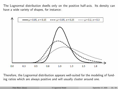
The Lognormal distribution dwells only on the positive half-axis. Its density canhave a wide variety of shapes, for instance:

Therefore, the Lognormal distribution appears well-suited for the modeling of fund-ing ratios which are always positive and will usually cluster around one.


Proposition 8 (Scaling property)

Let Y ∼ LN(µ, σ2) and ρ > 0. Then ρY ∼ LN(µ+ log ρ, σ2).

Proof: P [ρY ≤ y] = P[Y ≤ y

ρ

]= Φ

(log yρ−µ

σ

)= Φ

(log y−(µ+log ρ)

σ

)

Proposition 9 (Moments)

Let Y ∼ LN(µ, σ2). Then we have

I Expectation: E [Y ] = expµ+ 1

2 σ2

I Variance: Var [Y ] = exp

2µ+ σ2 (

expσ2− 1)

Proof: Since Y = eX with X ∼ N (µ, σ2):

E [Y ] = E[eX]

= MX(1) = expµ+ 1

2 σ2

Similarly E[Y 2]

= MX(2) = exp

2µ+ 2σ2

,

then Var [Y ] =E[Y 2]−E [Y ]

2


Proposition 10 (Loss size index)

Let Y ∼ LN(µ, σ2) and y > 0. Then we have:

I(y) :=E[1Y≤yY

]E [Y ]

= Φ

(log y − (µ+ σ2)

σ

)Proof: Using the expressions for the density and the expectation:

I(y) =

∫ y

0

x g(x) dx/

expµ+ 1

2 σ2

=

∫ y

0

1√2πσ

explog x exp

− (log x− µ)2

2σ2

exp

−µ− σ2

2

1

xdx

=

∫ y

0

1√2πσ

exp

− (log x)2 − 2(µ+ σ2) log x+ (µ2 + 2µσ2 + σ4)

2σ2

1

xdx

=

∫ y

0

1√2πσ

exp

− (log x− (µ+ σ2))2

2σ2

1

xdx

= Φ

(log y − (µ+ σ2)

σ

)


4. Probability of underfunding


Funding ratio: distribution and moments

Under the model as set forth in Definition 1, and according to Proposition 1, givenFR0 and for t > 0, we have for the funding ratio:

FRt ∼ LN(µ, σ2) with µ = log FR0 + (µ− λ)t and σ2 = σ2t

By applying Proposition 9, we obtain:

E [FRt|FR0] = FR0 exp

(µ− λ+ 12σ

2)t

(1)

Var [FRt|FR0] = (FR0)2 exp

2(µ− λ+ 12σ

2)t (

expσ2t− 1)

(2)

We note that the expected value of the funding ratio actually increases as the(short-term) investment risk σ2 increases. This should, however, be consideredwith caution and in the context of the probability of underfunding hereafter. Notein particular that also the variance of the funding ratio increases as σ2 increases.


Underfunding

Recall that an institution is underfunded when its assets At are insufficient to coverits liabilities Lt, i.e. At < Lt, or equivalently FRt = At/Lt < 1.

In the corporate world, this corresponds to an insolvency. However, for a socialinsurance institution, this does not necessarily mean bankruptcy and liquidation.

Often, the existence of the institutions is guaranteed by law. This does not implya financial guarantee, but just the guarantee that the institution will have a clientbase and premium or contribution revenue over an unlimited period of time.

Therefore, social insurance institutions are often - at least under certain circum-stances - allowed to be temporarily underfunded. This may represent an importantadvantage.

Nevertheless, underfunding is an undesirable state, and the probability of this hap-pening is an important long-term risk measure.


Funding ratio distribution

The graphic shows the evolution of the funding ratio distribution over time, asexpressed by some quantiles:

Note the asymmetry in the distribution of the funding ratio.


Probability of underfunding

Definition 5 (Probability of underfunding)

Let t > 0. Then the probability of underfunding at time t is defined as

ψt := P [FRt ≤ 1|FR0]

For technical reasons, we use ”≤” rather that ”<”. In the Lognormal model, weimmediately obtain the following result:

Proposition 11 (Probability of underfunding in the Lognormal model)

Let the Lognormal model according to Definition 1 hold. Then, the probability ofunderfunding is given by

ψt = ψt(FR0, λ, µ, σ2) = Φ

(− log FR0 + (µ− λ)t

σ√t

)

Proof: Recall that the Lognormal CDF is Φ(

log y−µσ

)and use y = 1.


Sensitivities

Sensitivity is an important concept in risk management. It consists of exploringhow a risk measure reacts to changes in one of the input parameters. Specifically,we consider the probability of underfunding:

ψt = ψt(FR0, λ, µ, σ2) = Φ


σ√t

)and we take partial derivatives w.r.t. the input parameters:

I FR0: initial funding ratio

I λ: intrinsic rate of growth of the liabilities (= required return)

I µ: expected investment return

I σ2: (short-term) investment risk

These sensitivities are to be understood ”ceteris paribus”, i.e. all else remainingequal. In practice, input factors will not change independently from one another.For instance, a higher expected return will come along with a higher investmentrisk. This will be investigated in the subsequent chapters.


Sensitivity to initial funding ratio

Under the Lognormal model, we have:

∂ψt∂FR0

=∂

∂FR0Φ


σ√t

)= − 1

σ√tϕ


σ√t

)1

FR0< 0

Since ϕ( · ) is the density of the standard Normal distribution, it is always positive;the same holds for FR0 and σ. Therefore, the sensitivity ∂ψt

∂FR0is always negative.

That is, a higher initial funding ratio leads to a lower probability of underfunding,and vice versa.


Sensitivity to intrinsic growth rate of liabilities


∂ψt∂λ

=∂

∂λΦ


σ√t

)=

√t

σϕ


σ√t

)> 0

For the same reasons as above, this sensitivity is always positive.

That is, the higher the intrinsic growth rate of liabilities (and hence the requiredreturn), the higher becomes the probability of underfunding, and vice versa.


Sensitivity to expected return


∂ψt∂µ

=∂

∂µΦ


σ√t

)= −√t

σϕ


σ√t

)< 0

For the same reasons as above, this sensitivity is always negative.

That is, the higher the expected return, the lower becomes the probability of un-derfunding, and vice versa.


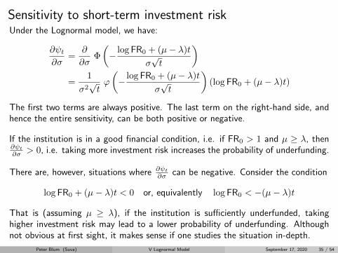
Sensitivity to short-term investment riskUnder the Lognormal model, we have:

∂ψt∂σ

=∂

∂σΦ


σ√t

)=

1

σ2√tϕ


σ√t

)(log FR0 + (µ− λ)t)

The first two terms are always positive. The last term on the right-hand side, andhence the entire sensitivity, can be both positive or negative.

If the institution is in a good financial condition, i.e. if FR0 > 1 and µ ≥ λ, then∂ψt∂σ > 0, i.e. taking more investment risk increases the probability of underfunding.

There are, however, situations where ∂ψt∂σ can be negative. Consider the condition

log FR0 + (µ− λ)t < 0 or, equivalently log FR0 < −(µ− λ)t

That is (assuming µ ≥ λ), if the institution is sufficiently underfunded, takinghigher investment risk may lead to a lower probability of underfunding. Althoughnot obvious at first sight, it makes sense if one studies the situation in-depth.


Probability of underfunding: assessment

The probability of underfunding is a good risk measure, and one often used inpractice, for a number of reasons:

I It is sensible in that it addresses a serious danger.

I It takes a long-term view that is adapted to the nature of social and pensioninsurance.

I It can be easily calculated in analytical models, and it can be easily estimatedby stochastic simulation.

I It lends itself to intuitive interpretation, and it is easy to explain also to non-quantitative audiences.

An important disadvantage is that it only indicates the probability of an underfund-ing to occur. We would, however, also like to know something about the extent ofthe underfunding. To this end, we explore a few alternative risk measures in thenext section.


5. Alternative risk measures


ConceptConsider the distribution of the funding ratio, here under the Lognormal model:

Contrary to normal practice in insurance risk management, we are not interested inthe right tail. The danger consists of funding ratios below one, i.e. lies in the lefttail. We consider the following measures for the funding ratio:

1. The left α-quantile: qα(FRt)

2. The left expected shortfall: E [FRt|FRt ≤ qα(FRt)]

3. The conditional expectation: E [FRt|FRt ≤ 1]


In all three cases, we are ultimately interested in the difference between these threevalues and 1 (provided this difference is positive), i.e.

max (1−Measure 1, 2 or 3, 0)

because this is the funding deficit that must actually be financed in the event ofan underfunding. In this way, we obtain the desired measures that also containinformation on the extent of an eventual underfunding.

We derive these quantities in the Lognormal framework and explore their proper-ties. Note, however, that they all can be easily estimated also by using stochasticsimulation (with some care to be taken such that the tail is sufficiently populatedwith data points).

For simplicity, we start with a generic Lognormal random variable Y ∼ LN(µ, σ2)and insert the specific values for the Lognormal funding ratio model afterwards.


Left quantile

Proposition 12 (Left quantile)

Let Y ∼ LN(µ, σ2) and α ∈ (0, 1). Then we have:

qα(Y ) = expµ+ Φ−1(α) σ

Proof: We are looking for y0 such that P [Y ≤ y0] = α, i.e.

Φ

(log y0 − µ

σ

)= α

log y0 − µσ

= Φ−1(α)

y0 = expµ+ Φ−1(α) σ

Typical values of α are e.g. 1% or 5%.


Conditional expectation

Proposition 13 (Conditional expectation)

Let Y ∼ LN(µ, σ2). Then we have:

E [Y |Y ≤ 1] = expµ+ 1

2 σ2

Φ

(− µ+ σ2

σ

)/Φ

(− µσ

)Proof: On the one hand, we have according to Proposition 10

E[1Y≤1Y

]= E [Y ] Φ

(log 1− (µ+ σ2)

σ

)= exp

µ+ 1

2 σ2

Φ

(− µ+ σ2

σ

)On the other hand, we have

P [Y ≤ 1] = Φ

(− µσ

)Then E [Y |Y ≤ 1] = E

[1Y≤1Y

]/P [Y ≤ 1].


Expected shortfall

Proposition 14 (Expected shortfall)

Let Y ∼ LN(µ, σ2) and α ∈ (0, 1). Then we have:

E [Y |Y ≤ qα(Y )] = 1α exp

µ+ 1

2 σ2

Φ(Φ−1(α)− σ

)Proof: Using Propositions 10 and 12 we have

E[1Y≤qα(Y )Y

]= exp

µ+ 1

2 σ2

Φ

(log qα(Y )− (µ+ σ2)

σ

)= exp

µ+ 1

2 σ2

Φ

(µ+ Φ−1(α)σ − (µ+ σ2)

σ

)= exp

µ+ 1

2 σ2

Φ

(Φ−1(α)σ − σ2

σ

)= exp

µ+ 1

2 σ2

Φ(Φ−1(α)− σ

)Moreover, we have P [Y ≤ qα(Y )] = α.


Back to the Lognormal model

Recall that in the Lognormal model according to Definition 1, we have accordingto Proposition 1

µ = log FR0 + (µ− λ)t and σ2 = σ2t

Inserting this into the results of Propositions 12, 13 and 14 yields:

1.) For the quantile:

qα(FRt) = expµ+ Φ−1(α) σ

= exp

log FR0 + (µ− λ)t+ Φ−1(α)σ

√t

= FR0 exp

(µ− λ)t+ Φ−1(α)σ√t


2.) For the conditional expectation:

E [FRt|FRt ≤ 1] = expµ+ 1

2 σ2

Φ

(− µ+ σ2

σ

)/Φ

(− µσ

)= exp

log FR0 + (µ− λ)t+ 1

2σ2t×

Φ

(− log FR0 + (µ− λ)t+ σ2t

σ√t

)/Φ


σ√t

)= FR0 exp

(µ− λ)t+ 1

2σ2t×

Φ


σ√t

)/Φ


σ√t

)= E [FRt]×

Φ


σ√t

)/Φ


σ√t

)


3.) For the expected shortfall:

E [FRt|FRt ≤ qα(FRt)] = 1α exp

µ+ 1

2 σ2

Φ(Φ−1(α)− σ

)= 1

α exp

log FR0 + (µ− λ)t+ 12σ

2t

Φ(

Φ−1(α)− σ√t)

= 1α FR0 exp

(µ− λ+ 1

2σ2)t

Φ(

Φ−1(α)− σ√t)

= 1α E [FRt] Φ

(Φ−1(α)− σ

√t)


Expected Funding ShortfallWe introduce a new risk measure that takes into account the extent of an eventualunderfunding as desired:

Definition 6 (Expected Funding Shortfall)

Let α ∈ (0, 1) and t > 0. The Expected Funding Shortfall is defined as

EFSα,t := 1−E [FRt|FRt ≤ qα(FRt)]

Proposition 15 (EFS in the Lognormal model)

Under the Lognormal model according to Definition 1, the Expected FundingShortfall is given by

EFSα,t = 1− 1α FR0 exp

(µ− λ+ 1

2σ2)t

Φ(

Φ−1(α)− σ√t)

= 1− 1α E [FRt] Φ

(Φ−1(α)− σ

√t)

Proof: See calculations above.


Illustration: FRaR and EFS

Graphically, the various measures can be interpreted as follows:

We might as well work directly with the quantile qα or the Expected Shortfall ESα.But in practice, one is more interested in the deficit that might have to be madeup in order to reach fully-funded status (i.e. FRt = 1) again. Therefore, it ispreferrable to work with the difference to 1.


This is the expected difference to the funding ratio of 1 (i.e. the expected fundingshortfall) that is present if the α-event materializes. It is a measure for the amountof money that must be put up in order to bring the institution to fully funded status.

Note that EFSα,t is here expressed in terms of funding ratio. It can, however, beeasily translated into monetary terms.

When doing stochastic simulation, this measure is easy to calculate either in mon-etary terms or in terms of funding ratio.

For the levels of EFSα,t, we have:

I High value: BAD

I Low value: GOOD

For the changes of EFSα,t, we have:

I Increase: BAD

I Decrease: GOOD


Also with EFSα,t, we explore the sensitivities:

∂ EFSα,t∂ FR0

= − 1α exp

(µ− λ+ 1

2σ2)t

Φ(

Φ−1(α)− σ√t)< 0

∂ EFSα,t∂ µ

= − tα FR0 exp

(µ− λ+ 1

2σ2)t

Φ(

Φ−1(α)− σ√t)< 0

∂ EFSα,t∂ λ

= tα FR0 exp

(µ− λ+ 1

2σ2)t

Φ(

Φ−1(α)− σ√t)> 0

∂ EFSα,t∂ σ

= 1α FR0 exp

(µ− λ+ 1

2σ2)t×[√

t ϕ(

Φ−1(α)− σ√t)− t σΦ

(Φ−1(α)− σ

√t)]

The first three sensitivities are as one would expect. For the fourth expression, theterm in the square brackets will be positive, unless

ϕ(Φ−1(α)− σ

√t)

Φ(Φ−1(α)− σ

√t) < σ

√t

which is difficult to attain for realistic values of α. This is different from theprobability of underfunding, where we can have a negative sensitivity to σ underfairly realistic conditions. That is, EFSα,t is more conservative in this respect.


Normal density and CDF

Typical values for α are e.g. 1%, 5% or 10%. In these cases Φ−1(α) is at -2.3, -1.6and -1.3, respectively. Typical values for σ are (well) below 10%.


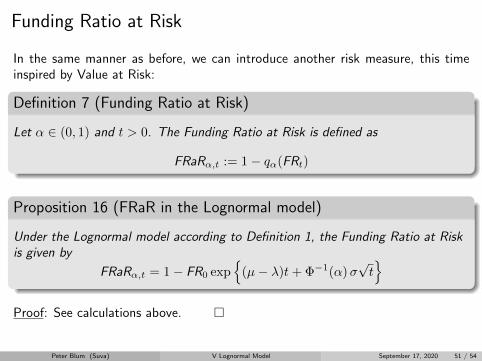
Funding Ratio at Risk

In the same manner as before, we can introduce another risk measure, this timeinspired by Value at Risk:

Definition 7 (Funding Ratio at Risk)

Let α ∈ (0, 1) and t > 0. The Funding Ratio at Risk is defined as

FRaRα,t := 1− qα(FRt)

Proposition 16 (FRaR in the Lognormal model)

Under the Lognormal model according to Definition 1, the Funding Ratio at Riskis given by

FRaRα,t = 1− FR0 exp

(µ− λ)t+ Φ−1(α)σ√t

Proof: See calculations above.


For the sensitivities, we obtain:

∂

∂FR0FRaRα,t = − exp

(µ− λ)t+ Φ−1(α)σ

√t< 0

∂

∂µFRaRα,t = −tFR0 exp

(µ− λ)t+ Φ−1(α)σ

√t< 0

∂

∂λFRaRα,t = tFR0 exp

(µ− λ)t+ Φ−1(α)σ

√t> 0

∂

∂σFRaRα,t = −Φ−1(α)

√t FR0 exp

(µ− λ)t+ Φ−1(α)σ

√t> 0 if α < 0.5

This is as one would expect. Given that we are in the left tail, sensible values for αare e.g. 1%, 5% or 10%, certainly not more. Also here, there is no realistic situationwhere the sensitivity to σ is negative, even if the institution is underfunded.


Concluding remarks

In practice, the probability of underfunding ψt is the predominant risk measure,and there is no fundamental objection against this. However, ψt does only providelimited information:

I ψt just gives the probability of something undesirable, i.e. an underfunding,happening,

I but it bears no information on the extent of the underfunding.

The alternative risk measures EFSα,t and FRaRα,t also bear information on theextent of the underfunding. In the case of a turnaround, they can be used as aproxy for the turnaround costs.

This is very useful when weighting the cost of measures for risk reduction againsttheir effect. See the subsequent chapters with the ALM studies for more on this.

Moreover, at least at first sight, EFSα,t and FRaRα,t seem to be more conservativewhen it comes to the treatment of (short-term) investment risk. We will also explorethis further in the subsequent chapters.


Bibliography I

[1] Billingsley, P.Probability and Measure, third ed.John Wiley & Sons, Chchester, 1995.

[2] Grimmett, G., and Stirzaker, D.Probability and Random Processes, second ed.Clarendon Press, Oxford, 1992.

[3] Koller, M.Stochastic models in life insurance.Lecture notes, ETH, Zurich, 2015.




Chapter VI: ALM Study 1Dealing with the risk / return profile


Peter Blum


September 17, 2020

Peter Blum (Suva) VI ALM Study 1 September 17, 2020 1 / 33

Table of Contents

1. Problem statement

2. Risk / return profile

3. Optimizing the probability of underfunding

4. Optimizing alternative risk measures


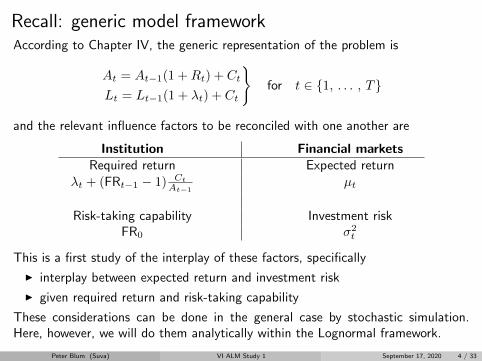
Recall: generic model frameworkAccording to Chapter IV, the generic representation of the problem is

At = At−1(1 +Rt) + Ct

Lt = Lt−1(1 + λt) + Ct

for t ∈ 1, . . . , T

and the relevant influence factors to be reconciled with one another are


λt + (FRt−1 − 1) Ct

At−1µt

Risk-taking capability Investment riskFR0 σ2

t

This is a first study of the interplay of these factors, specifically

I interplay between expected return and investment risk

I given required return and risk-taking capability

These considerations can be done in the general case by stochastic simulation.Here, however, we will do them analytically within the Lognormal framework.


Recall: Lognormal modelAs in Definition 1 and Proposition 1 of Chapter V, we assume that the institutionis in equilibrium (i.e. Ct ≡ 0), and we let

log FRt − log FRt−1 = µ− λ+ εt where εt ∼ iid N(0, σ2

)For given FR0, this means that FRt ∼ LN

(log FR0 + (µ− λ)t, σ2t

). This gives

rise to the long-term risk measures:

Probability of underfunding (Chapter V, Proposition 8):

ψt (FR0, λ, µ, σ) = Φ


σ√t

)Expected Funding Shortfall (Chapter V, Proposition 12):

EFSα,t (FR0, λ, µ, σ) = 1− 1α FR0 exp

(µ− λ+ 1

2σ2)t

Φ(

Φ−1(α)− σ√t)

Funding Ratio at Risk (Chapter V, Proposition 13):

FRaRα,t (FR0, λ, µ, σ) = 1− FR0 exp

(µ− λ)t+ Φ−1(α)σ√t

The goal is to optimize the values of these long-term risk measures under certainassumptions.


Assumptions

We assume throughout this chapter that the required return λ and the risk-takingcapability FR0 are given.

I This corresponds to a situation where the discount rate δ is fixed and givenand cannot be changed by the institution.

I Then, also FR0 directly results from this.

The variables are thus the expected return µ and the short-term investment riskσ2. In principle, long-term risk is optimized by selecting a high µ and a low σ2; c.f.the sensitivity analysis in Chapter V.

The problem is that expected return and investment risk are related, i.e. if we selecta higher expected return, then we will invariably incur more investment risk.

Therefore, we assume that there is a functional relationship between expected returnµ and investment risk σ2, or σ for the purpose: σ = σ(µ).

This relationship σ = σ(µ) is called Risk / Return Profile.


Call from practice

In practice, one considers the standard deviation σ of the investment returns ratherthan the variance σ2. This is because the standard deviation is on the same scale asthe returns themselves and their expectation. Therefore, it lends itself to an easierinterpretation, e.g.

I A standard deviation of 5% means that the average absolute deviation of thereturns from their expectation is 5%.

I The resulting variance of 0.0025 has no intuitive interpretation.


2. Risk / return profile


Fundamental situation

It is a fundamental matter of fact that a higher expected return µ comes along witha higher investment risk σ:

I This is theoretically well underpinned, e.g. by the Capital Asset Pricing Model(CAPM); see [1].

I And it is also empirically confirmed; see the subsequent considerations in thiscourse or e.g. [2].

Note that we use σ for the risk, and not σ2.


We are mainly interested in the points (risk / return combinations) on the line:

I Points below the line are suboptimal, i.e. less return for the same risk or morerisk for the same return.

I Points above the line are not feasible.

As risk becomes higher, the extra return obtained becomes lower. This reflects theeconomic principle of decreasing marginal utility, and it also makes sense empirically.

We can safely assume that the function µ(σ) is twice continuously differentiable,so that we can state

µ′(σ) > 0 (increasing return)

µ′′(σ) ≤ 0 (decreasing marginal return)

For the moment, these facts should be taken as given. We will see in subsequentchapters, when we look at the construction of investment portfolios, why they arewell justified.


Risk / return profiles in practiceRisk / return profiles feasible for typical Swiss pension funds; as it used to be around2005 and as it is nowadays:

Parallel to the decrease in interest rates (see Chapter II), there was a dramaticdecline in return expectations over the past ten years. That is:

I (Much) more risk for the same return as before (if feasible at all).

I (Much) less return for the same risk as before.


Formalization of risk / return profileIn practice, our policy variable is the expected return µ:

I Required returns are clearly defined, and we must set µ accordingly; e.g. inthe Lognormal model this means µ ≥ λ.

I The requirements for the investment risk σ are generally less clearly defined.This is more of a consequence.

Therefore, we work with a risk / return profile of the form σ = σ(µ), which createsthe following situation:


We have µ ∈ [µmin, µmax] for some minimum attainable return µmin and somemaximum attainable return µmax > µmin. Nowadays, we must admit the situationwhere µmin < 0.

Consequently, there is a minimum risk σmin = σ (µmin) and a maximum risk σmax =σ (µmax) such that σ ∈ [σmin, σmax]. Note that still nowadays σ ≥ 0.

Hence, we let σ(µ) be a twice continuously differentiable function with

σ(µ) ≥ 0σ′(µ) > 0σ′′(µ) > 0

for all µ ∈ [µmin, µmax]

That is, σ(µ) is a convex function on a compact support.

Example: Let σ(µ) = α (µ− µmin)2 for µ ≥ µmin and α > 0. Then, we have

σ(µ) ≥ 0

σ′(µ) = 2α (µ− µmin) > 0 for µ > µmin

σ′′(µ) = 2α > 0


Setup

Let the Lognormal model according to Definition 1 of Chapter V hold.

Assume that we have a risk / return profile σ(µ) defined on µ ∈ [µmin, µmax] asintroduced above.

Assume that FR0 and λ are given and fixed. Assume moreover that λ ∈ (µmin, µmax),i.e. it is actually possible to attain the required return. (The situation where λ needsto be adapted will be considered in the next chapter.)

Note that we assume the net profit condition to be respected, i.e. µ ≥ λ. Ingeneral, this is indispensable for assuring a sustainable funding.

The question is now: Does it make sense to increase µ beyond λ, i.e. take morerisk than absolutely necessary in order to achieve a higher expected return than theminimum. The criterion is long-term risk, e.g. the probability of underfunding. Ifthe latter decreases as we increase µ, then it is worthwhile.

In other words: Can an increase in short-term risk (i.e. σ) lead to a decrease inlong-term risk (e.g. ψt)? And if so, under what circumstances?


Graphical exploration

Given λ and FR0 as parameters and some fixed t, ψt becomes a mapping

ψt,λ,FR0: R× R+ → R+

(µ, σ) 7→ Φ


σ√t

)We can simply calculate this for each pair (µ, σ) ∈ R × R+, whether feasible ornot, and we can plot the results as a risk map in µ/σ-space, e.g. as a line plot.

In a line plot, the lines connect all those combinations (µ, σ) that lead to the samevalue of ψt. That is, the lines in the plot are iso-ψt-lines similar to height curves ina topographic map or to isobars in weather chart.


Example: map of ψt given FR0 = 110%, λ = 2% and t = 10 in µ/σ-space:

ψt becomes lower for higher µ and for lower σ as one would expect from thesensitivities computed in Chapter V.


Call from practice

The good thing about this representation is that in more complicated settings,where there is no analytical tractability, one can always obtain this risk map bystochastic simulation. It requires some computing power, since the simulation ofthe probability of underfunding must be repeated for a large number of combinationsof µ and σ. Moreover, it also requires some brain power from the analyst to getthe numerics under control. But it works universally.


Now, we can simply superimpose our risk / return profile of feasible combinationsof µ and σ. There are two basic situations:

σ(µ) grows slowly w.r.t. ψt, such thatwe obtain a lower ψt by increasing µbeyond λ.

σ(µ) grows too quickly w.r.t. ψt, suchthat we obtain a higher ψt by increas-ing µ beyond λ.


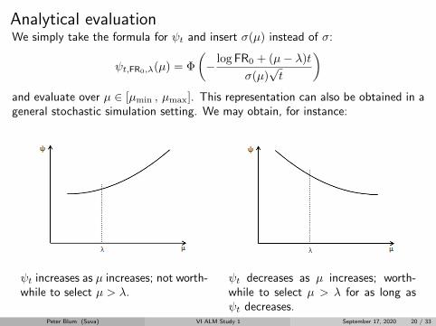
Analytical evaluationWe simply take the formula for ψt and insert σ(µ) instead of σ:

ψt,FR0,λ(µ) = Φ


σ(µ)√t

)and evaluate over µ ∈ [µmin , µmax]. This representation can also be obtained in ageneral stochastic simulation setting. We may obtain, for instance:

ψt increases as µ increases; not worth-while to select µ > λ.

ψt decreases as µ increases; worth-while to select µ > λ for as long asψt decreases.


Let us now study the derivative ddµ ψt,FR0,λ(µ); we have:

d

dµψt,FR0,λ(µ) = ϕ


σ(µ)√t

)(−f ′(µ))

where

f(µ) =log FR0 + (µ− λ)t

σ(µ)√t

Applying the quotient rule to f(µ) and rearranging, we obtain

d

dµψt,FR0,λ(µ) = ϕ

(− log FR0 + (µ− λ) t

σ(µ)√t

)×

1

σ2(µ)√t

[(log FR0 + (µ− λ) t

)σ′(µ)− σ(µ) t

]

We are interested in the situation where ddµ ψt,FR0,λ(µ) < 0. Since both ϕ( · ) and

σ(µ) > 0, this occurs if and only if the term in square brackets is negative, i.e. if

(log FR0 + (µ− λ) t)σ′(µ) < σ(µ) t


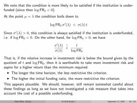
We note that the condition is more likely to be satisfied if the institution is under-funded (since then log FR0 < 0).

At the point µ = λ the condition boils down to

log FR0 σ′(λ) < σ(λ) t

Since σ′(λ) > 0, this condition is always satisfied if the institution is underfunded,i.e. if log FR0 < 0. On the other hand, for log FR0 > 0, we have

σ′(λ)

σ(λ)

!<

t

log FR0

That is, if the relative increase in investment risk is below the bound given by thequotient of t and log FR0, then it is worthwhile to take more investment risk andaspire for a higher return than the minimum required.

I The longer the time horizon, the less restrictive the criterion.

I The higher the initial funding ratio, the more restrictive the criterion.

This appears plausible. We should, however, still remain somewhat careful aboutthese findings as long as we have not investigated a risk measure that takes intoaccount the cost of a possible underfunding.


Overview

The same risk / return consideration as in the previous section can also be donebased on the Expected Funding Shortfall and on the Funding Ratio at Risk.

As before, let λ and FR0 be given, and let σ = σ(µ) denote the risk / return profile.Then, we have according to Proposition 12 and 13 of Chapter V:

EFSα,t(µ) = 1− 1α FR0 exp

(µ− λ+ 1

2σ2(µ)

)t

Φ(

Φ−1(α)− σ(µ)√t)

FRaRα,t(µ) = 1− FR0 exp

(µ− λ)t+ Φ−1(α)σ(µ)√t

The added value of these evaluations is that they also take into account the extentof a possible underfunding, not just the probability of it happening.


Graphical evaluationThe graphical evaluations can be done in the same manner as for the probability ofunderfunding. Numbers are in % of funding ratio.

Expected Funding Shortfall Funding Ratio at Risk

All else being equal, the Funding Ratio at Risk is less conservative than the ExpectedFunding Shortfall. Otherwise, the basic pattern is not fundamentally different fromthe probability of underfunding. To explore differences, we have to revert to ana-lytical evaluations.


Analytical evaluationBased on the equation for EFSα,t with σ = σ(µ) as above, i.e.

EFSα,t(µ) = 1− 1α FR0 exp

(µ− λ+ 1

2σ2(µ)

)t

Φ(

Φ−1(α)− σ(µ)√t)

we obtaind

dµEFSα,t(µ) = − 1

αFR0

(d

dµg(µ)h(µ)

)where we have

g(µ) = exp(µ− λ+ 1

2σ2(µ)

)t

h(µ) = Φ(

Φ−1(α)− σ(µ)√t)

Observing that

g′(µ) = exp(µ− λ+ 1

2σ2(µ)

)t(t+ σ(µ)σ′(µ) t

)h′(µ) = −σ′(µ)

√t ϕ

(Φ−1(α)− σ(µ)

√t)

and ... ./.Peter Blum (Suva) VI ALM Study 1 September 17, 2020 26 / 33

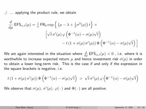
./. ... applying the product rule, we obtain

d

dµEFSα,t(µ) = 1

α FR0 exp(µ− λ+ 1

2σ2(µ)

)t×[√

t σ′(µ)ϕ(

Φ−1(α)− σ(µ)√t)

− t (1 + σ(µ)σ′(µ)) Φ(

Φ−1(α)− σ(µ)√t) ]

We are again interested in the situation where ddµ EFSα,t(µ) < 0 , i.e. where it is

worthwhile to increase expected return µ and hence investment risk σ(µ) in orderto obtain a lower long-term risk. This is the case if and only if the expression inthe square brackets is negative, i.e.

t (1 + σ(µ)σ′(µ)) Φ(

Φ−1(α)− σ(µ)√t)>√t σ′(µ)ϕ

(Φ−1(α)− σ(µ)

√t)

We observe that σ(µ), σ′(µ), ϕ( · ) and Φ( · ) are all positive.


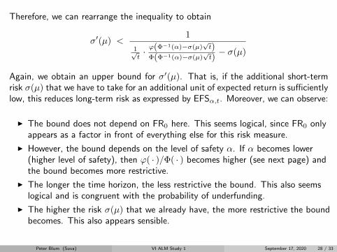
Therefore, we can rearrange the inequality to obtain

σ′(µ) <1

1√t· ϕ(Φ−1(α)−σ(µ)

√t)

Φ(Φ−1(α)−σ(µ)√t)− σ(µ)

Again, we obtain an upper bound for σ′(µ). That is, if the additional short-termrisk σ(µ) that we have to take for an additional unit of expected return is sufficientlylow, this reduces long-term risk as expressed by EFSα,t. Moreover, we can observe:

I The bound does not depend on FR0 here. This seems logical, since FR0 onlyappears as a factor in front of everything else for this risk measure.

I However, the bound depends on the level of safety α. If α becomes lower(higher level of safety), then ϕ( · )/Φ( · ) becomes higher (see next page) andthe bound becomes more restrictive.

I The longer the time horizon, the less restrictive the bound. This also seemslogical and is congruent with the probability of underfunding.

I The higher the risk σ(µ) that we already have, the more restrictive the boundbecomes. This also appears sensible.


Normal density vs. CDF



Based on the equation for FRaRα,t and with σ = σ(µ) as above, we have

FRaRα,t(µ) = 1− FR0 exp

(µ− λ)t+ Φ−1(α)σ(µ)√t

For the first derivative w.r.t. µ, we obtain

d

dµFRaRα,t(µ) = −FR0 exp

(µ− λ)t+ Φ−1(α)σ(µ)

√t(

t+ Φ−1(α)σ′(µ)√t)

For this to be negative, we must have

t+ Φ−1(α)σ′(µ)√t > 0

For reasonable values of α, i.e. α 0.5, we have Φ−1(α) < 0, and therefore

σ′(µ) < −√t

Φ−1(α)

That is, we again have an upper bound for the marginal investment risk σ′(µ).


As with the Expected Funding Shortfall, we have the following properties:

I The bound does not depend on FR0.

I It depends, however, on the level of safety α. The higher the level of safety,i.e. the lower α, the more restrictive the bound becomes.

I The longer the time horizon, the less restrictive the bound becomes.

Contrary to the Expected Funding Shortfall, we have:

I The bound does not depend on the absolute level of investment risk σ(µ)already in force.

Although the expression for the Funding Ratio at Risk is very handy, the ExpectedFunding Shortfall may be the more comprehensive and also the more prudent deci-sion criterion.


Concluding remarks

In this chapter, we have basically studied the interplay between short-term risk andlong-term risk:

I Short-term: single-period investment risk as expressed by σ(µ).

I Long-term: multi-period risk to assets and liabilities as expressed by the mea-sures ψt, EFSα,t or FRaRα,t.

We have seen that, in certain situations, the short-term risk and the long-term riskmay be conflicting dimensions, i.e.

I It may make sense to increase short-term investment risk in order to decreasethe long-term risk of underfunding.

The condition for this to be the case is generally when the marginal short-term riskis below certain bounds that depend on initial funding ratio, time horizon or desiredlevel of safety.


Bibliography I

[1] Brealy, R., and Myers, S.Priciples of Corporate Finance, sixth ed.Irwin McGraw–Hill, Boston, 2000.

[2] Campbell, J., Lo, A., and MacKinlay, A.The Econometrics of Financial Markets.Princeton University Press, Princeton, 1997.



Chapter VII: ALM Study 2Incorporating required return


Peter Blum


September 17, 2020

Peter Blum (Suva) VII ALM Study 2 September 17, 2020 1 / 45

Table of Contents


2. Liability profile



5. Example


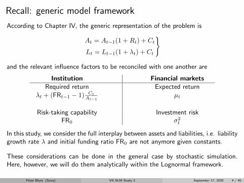
Recall: generic model framework

According to Chapter IV, the generic representation of the problem is

At = At−1(1 +Rt) + Ct

Lt = Lt−1(1 + λt) + Ct

and the relevant influence factors to be reconciled with one another are


λt + (FRt−1 − 1) Ct

At−1µt

Risk-taking capability Investment riskFR0 σ2

t

In this study, we consider the full interplay between assets and liabilities, i.e. liabilitygrowth rate λ and initial funding ratio FR0 are not anymore given constants.

These considerations can be done in the general case by stochastic simulation.Here, however, we will do them analytically within the Lognormal framework.


Recall: Lognormal modelAs in Definition 1 of Chapter V, we assume that the institution is in equilibrium(i.e. Ct = 0), and we let

log FRt − log FRt−1 = µ− λ+ εt where εt ∼ iid N(0, σ2

)For given FR0, this means that FRt ∼ LN

(log FR0 + (µ− λ)t, σ2t

). This gives

rise to the long-term risk measures:

Probability of underfunding:

ψt = Φ


σ√t

)Expected Funding Shortfall:


(µ− λ+ 1

2σ2)t

Φ(

Φ−1(α)− σ√t)

Funding Ratio at Risk:


(µ− λ)t+ Φ−1(α)σ√t

The goal is to optimize the values of these long-term risk measures under certainassumptions as given below.


Recall: risk / return profileIn the first ALM study in Chapter VI, we have introduced the relationship betweenthe expected return µ and the short-term investment risk σ, i.e. σ = σ(µ):

Specifically, we assumed that σ(µ) is twice continuously differentiable with

σ(µ) > 0σ′(µ) > 0σ′′(µ) > 0


We will maintain this assumption throughout this second study.


The problem

In the previous study, we have assumed that λ ∈ (µmin, µmax), i.e. the requiredreturn is within the range of feasible returns.

We have also (tacitly) assumed that the short-term risk σ as well as the long-termrisk as expressed by ψt, EFSα,t or FRaRα,t are acceptable for the institution.

Now, we assume that this is not the case anymore:

I Either λ is simply unfeasible, i.e. λ > µmax.

I Or, at least, the long-term risk caused by letting µ = λ is deemed unacceptablyhigh for the institution.

That is, we must now adapt λ in such a manner that a feasible and acceptablesolution becomes possible.


Relevance of the problemAt the beginning of this century, it was commonplace for Swiss pension funds tohave discount rates δ ≥ 4% for their liabilities, giving rise to required returnsλ ≥ 4%. With the then-prevailing risk / return profiles, this was fairly reasonable.

However, since then, risk / return profiles have deteriorated dramatically. Formerlyfeasible and acceptable required returns are not sensible anymore.

Therefore, reducing discount rates has become a standard task for Swiss (and manyother) pension funds.


The consequences

Think of the liabilities as the present value of future promised cashflows, c.f. Chap-ters II and III:

L0(δ) = PV0(C, δ) =

T∑t=1

Ct(1 + δ)t

Now, if we reduce δ (and hence λ), this also means that the present value L0

increases. For instance, using the approximation introduced earlier, we have

L0(δ + ∆δ)− L0(δ) ≈ −DLL0(δ)(∆δ) + 12 K

LL0(δ)(∆δ)2

Given that the funding ratio is defined as FRt = At/Lt this also means that theinitial funding ratio FR0, and hence the risk-taking capability decrease.

That is, reducing the discount rate δ reduces the required return λ and the short-term investment risk σ that must be taken. But it also reduces the risk-takingcapability so that the long-term risk may eventually increase. We somehow mustfind an optimal balance in this situation.


The optimization taskIf we put these influences together, we have two different developments:

Institutional side:

If the liability growth rate λ is re-duced, then also FR0, i.e. the risk-taking capability, becomes lower, andvice versa.

Financial markets side:

If the required return λ is reduced,then also the investment risk σ(λ) isreduced, and vice versa.

In principle, these developments are compatible with one another, but we mustexplore which one dominates under what conditions.


2. Liability profile


Liability values

We take a closer look at the relationship between the initial value of the liabilitiesL0 and the intrinsic growth rate of liabilities λ. This consideration builds on Section1 of Chapter II. Assume for the moment that L0 can be expressed as the presentvalue of a stream of cashflows:

L0(λ) =

T∑t=1

Ct(1 + λ)t

Here, we have inserted the intrinsic growth rate λ instead of the discount rate δ.This is justified by the equality of the two, λ = δ, as it was shown in Section 3of Chapter III. And, according to Propositions 2 and 3 of Chapter II, we have fornon-negative cashflows Ct:

L′0(λ) =∂

∂λPV0(C, λ) < 0

L′′0(λ) =∂2

∂λ2PV0(C, λ) > 0

That is, the value of the liabilities decreases as λ increases, and vice versa.


Illustration: Relationship between initial value of liabilities and intrinsic liabilitygrowth rate (= discount rate):


Economic interpretation

Now that we know the relationship between the liability growth rate λ and therequired value for the expected investment return, we can also give an economicinterpretation to the relationship with the value of the liabilities. For some givenstream of promised cashflows, we have:

I If we choose a high value for λ (i.e. a high discount rate δ), then the initialvalue of the liability L0 is low. I.e. we have to put up less money at thebeginning, but we have to earn a higher investment return µ over time, andwe must bear a higher investment risk σ(µ) for doing so.

I If we choose a low value for λ (i.e. a low discount rate δ), we only have toearn a lower investment return µ, and we incur a lower investment risk σ(µ)for doing so. But the initial value L0 is higher, i.e. we have to put up a higheramount of money at the beginning.

In principle, it is desirable to maximize λ, and hence the contribution from invest-ment returns. But this must be done without compromising long-term security asexpressed by ψt (or EFSα.t or FRaRα.t).

This study is basically about finding a suitable balance.


Duration and Convexity

We have already introduced the concepts of Duration and Convexity in Section 1of Chapter II, and we can apply them here.

Let λ0 denote the liability growth rate currently in force, i.e. our starting point.Then we have for the Duration DL and for the Convexity KL of the liabilities:

DL = −L′0(λ0)

L0(λ0)> 0 and KL =

L′′0(λ0)

L0(λ0)> 0

In principle, we can usually calculate L0(λ) directly for any value of λ. However, ifnecessary, we can use the second-order Taylor approximation

L0(λ) ≈ L0(λ0)−DLL0(λ0)(λ− λ0) + 12K

LL0(λ0)(λ− λ0)2

Up until now, we have motivated these relationships for a situation where L0(λ)is the present value of a stream of cashflows C. In the sequel, we also assumethat they hold when the liabilities contain other elements. For typical social insur-ance liabilities, this is usually the case. However, in the context of unit-linked lifeinsurance products, these assumptions may no longer hold; see e.g. [1]. This isparticularly the case if Ct = Ct(λ) which we exclude here.


Initial funding ratioThe initial funding ratio is defined as FR0 = A0/L0. In our setup, where λ isdeliberately set by the institution, the asset value A0, i.e. the market value, isindependent of λ, so that we have:

FR0(λ) =A0

L0(λ)

Note: In an immunized setup (c.f. Sections 2 and 3 of Chapter IV), both A0 andL0 would move with λ which, in turn, is determined by bond yields, and thesemovements would cancel out if the immunization is good.

In the setup prevailing here, however, we have

FR′0(λ) =d

dλFR0(λ) = − A0

(L0(λ))2L′0(λ) = −FR0(λ)

L′0(λ)

L0(λ)> 0

The expression is positive since we have L′0(λ) < 0. Specifically for λ = λ0, sinceDL = −L′0(λ0)/L0(λ0), we have

FR′0(λ0) = DL A0

L0(λ0)= DL FR0(λ0)


For the second derivative, we obtain (by applying the quotient rule):

FR′′0(λ) =d

dλ(−A0)

L′0(λ)

(L0(λ))2

= (−A0)

[L′′0(λ) (L0(λ))

2 − L′0(λ) 2L0(λ)L′0(λ)

(L0(λ))4

]

= (−A0)

[L′′0(λ)

(L0(λ))2 − 2

(L′0(λ))2

(L0(λ))3

]

=A0

L0(λ)

[2

(L′0(λ)

L0(λ)

)2

− L′′0(λ)

L0(λ)

]

= FR0(λ)

[2

(L′0(λ)

L0(λ)

)2

− L′′0(λ)

L0(λ)

]


Specifically for λ = λ0, the latter expression is equivalent to

FR′′0(λ0) = FR0(λ0)[2(DL)2 −KL

]The second derivative FR′′0(λ) may thus be positive or negative, depending on thesign of the expression in the square brackets. Specifically, we have FR′′0(λ) > 0 if

L′′0(λ)

L0(λ)< 2

(L′0(λ)

L0(λ)

)2

or, at λ = λ0: KL < 2(DL)2

That is, the convexity of the liabilities should be bounded with respect to theirduration. We refrain from evaluating this condition analytically, but we observe:

I For realistic cashflow patterns, we will usually have FR′′0(λ) > 0.

I FR′′0(λ) < 0 is mainly achieved by degenerate cashflow patterns, e.g. with highcashflows at the beginning and at the end, with nothing in-between.


That is, in most practical settings, the second derivative FR′′0(λ) will usually benon-negative. Therefore, the funding ratio as a function of the liability growth ratehas the following generic (convex) shape:

That is, if we increase the value of λ, then also FR0, and thus also the risk-takingcapability, increases (and even the marginal risk-taking capability increases). Thisis, in principle, compatible with the fact that we have to take more investment riskin order to finance a higher λ.


Finally, we take a brief look at the log-funding ratio. On the one hand, we have

log FR0(λ) = logA0 − logL0(λ)

and hence

d

dλlog FR0(λ) = −L

′0(λ)

L0(λ)

(= DL > 0 if λ = λ0

)And on the other side, we have

d

dλlog FR0(λ) =

FR′0(λ)

FR0(λ)

This may prove to be useful.


Setup

The liability profile is the relationship λ 7→ FR0(λ) as introduced above. We alsohave the risk / return profile µ 7→ σ(µ) as introduced in the last chapter. Moreover,we equate liability growth rate and expected return, i.e. µ = λ. Putting all thistogether, we obtain for the probability of underfunding

ψt(λ) = Φ

(− log FR0(λ)

σ(λ)√t

)We want to find the value λ ∈ [µmin, µmax] that minimizes the probability ofunderfunding. If necessary, λ0 denotes the current value of λ, which may not bethe optimum.

Notice the difference in the setup: In the previous chapter, the institutional side,i.e. λ and FR0, was given, and only the position on the risk / return profile was upfor optimization. Here, also the institutional side is under review.

In practice, we would simply compute ψt(λ) over the full range λ ∈ [µmin, µmax]and look up the optimum. This also works well in a general setup where stochasticsimulation must be applied. Here, however, we make a few analytical considerations.


General situationWe take the first derivative

d

dλψt(λ) =

d

dλΦ

(− log FR0(λ)

σ(λ)√t

)

= −ϕ(− log FR0(λ)

σ(λ)√t

)(g(λ)

h(λ)

)′where g(λ) = log FR0(λ) and h(λ) = σ(λ)

√t. We then have

g′(λ) =FR′0(λ)

FR0(λ)

(and, in particular: g′(λ0) = DL

)h′(λ) = σ′(λ)

√t

This yields then

(g(λ)

h(λ)

)′=

FR′0(λ)FR0(λ)

σ(λ)√t− log FR0(λ)σ′(λ)

√t

(σ(λ))2t


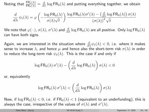
Noting thatFR′0(λ)FR0(λ)

= ddλ log FR0(λ) and putting everything together, we obtain

d

dλψt(λ) = ϕ

(− log FR0(λ)

σ(λ)√t

)log FR0(λ)σ′(λ)−

(ddλ log FR0(λ)

)σ(λ)

(σ(λ))2√

t

We note that ϕ( · ), σ(λ), σ′(λ) and ddλ log FR0(λ) are all positive. Only log FR0(λ)

can have both signs.

Again, we are interested in the situation where ddλψt(λ) < 0, i.e. where it makes

sense to increase λ, and hence µ and hence also the short-term risk σ(λ) in orderto reduce the long-term risk ψt(λ). This is the case if and only if

log FR0(λ)σ′(λ)−(d

dλlog FR0(λ)

)σ(λ) < 0

or, equivalently

log FR0(λ)σ′(λ) <

(d

dλlog FR0(λ)

)σ(λ)

Now, if log FR0(λ) < 0, i.e. if FR0(λ) < 1 (equivalent to an underfunding), this isalways the case, irrespective of the values of σ(λ) and σ′(λ).


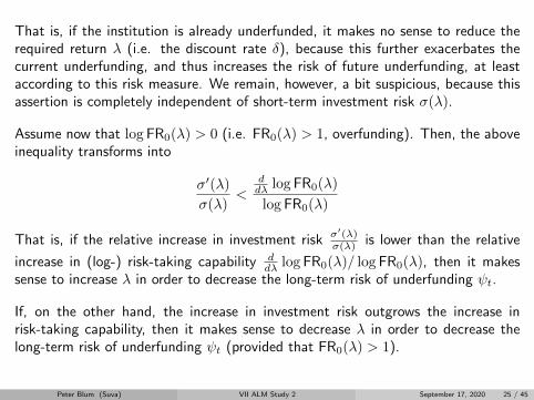
That is, if the institution is already underfunded, it makes no sense to reduce therequired return λ (i.e. the discount rate δ), because this further exacerbates thecurrent underfunding, and thus increases the risk of future underfunding, at leastaccording to this risk measure. We remain, however, a bit suspicious, because thisassertion is completely independent of short-term investment risk σ(λ).

Assume now that log FR0(λ) > 0 (i.e. FR0(λ) > 1, overfunding). Then, the aboveinequality transforms into

σ′(λ)

σ(λ)<

ddλ log FR0(λ)

log FR0(λ)

That is, if the relative increase in investment risk σ′(λ)σ(λ) is lower than the relative

increase in (log-) risk-taking capability ddλ log FR0(λ)/ log FR0(λ), then it makes

sense to increase λ in order to decrease the long-term risk of underfunding ψt.

If, on the other hand, the increase in investment risk outgrows the increase inrisk-taking capability, then it makes sense to decrease λ in order to decrease thelong-term risk of underfunding ψt (provided that FR0(λ) > 1).


This criterion appears entirely plausible and is easy to evaluate. In the situationwhere λ = λ0, it boils further down to

σ′(λ)

σ(λ)<

DL

log FR0(λ0)

That is, if this criterion is satisfied, it makes sense to set λ > λ0. If the contrary istrue, it makes sense to set λ < λ0.


Global considerations

As we have seen, we can choose λ ∈ [µmin, µmax]. The global optimization taskconsists of choosing λ∗ such that the risk of underfunding is minimized, i.e.

λ∗ = arg minλ∈[µmin, µmax]

ψt(λ)

Given that we have functional representations for log FR0(λ) and σ(λ), we caneasily calculate

ψt(λ) = Φ

(− log FR0(λ)

σ(λ)√t

)for λ ∈ [µmin, µmax]

and look up the optimum λ∗. In order to further characterize λ∗ analytically, we

would have to take the second derivative d2

dλ2ψt(λ). This is, of course, possible, butthe expression is rather unwieldy and does not lead to any intuitive criteria.

Given the easy direct consideration of ψt(λ), we need not be unhappy about this.


Expected Funding ShortfallWe do the same reasoning as before for the Expected Funding Shortfall accordingto Definition 5 and Proposition 12 in Chapter V:


(µ− λ+ 1

2σ2)t

Φ(

Φ−1(α)− σ√t)

Letting µ = λ, FR0 = FR0(λ) and σ = σ(λ), we have

EFSα,t(λ) = 1− 1α FR0(λ) exp

12 (σ(λ))

2t

Φ(

Φ−1(α)− σ(λ)√t)

The first derivative is given by

d

dλEFSα,t(λ) = − 1

α

d

dλ(f(λ)g(λ)h(λ))

with component functions

f(λ) = FR0(λ)

g(λ) = exp

12 (σ(λ))

2t

h(λ) = Φ(

Φ−1(α)− σ(λ)√t)


The derivatives of these components are

f ′(λ) = FR′0(λ) > 0

g′(λ) = exp

12 (σ(λ))

2tσ(λ)σ′(λ) t > 0

h′(λ) = −ϕ(

Φ−1(α)− σ(λ)√t)σ′(λ)

√t < 0

Applying the three-factor version of the product rule, i.e.

(fgh)′ = (fg)′h+ (fg)h′

= (f ′g + fg′)h+ (fg)h′

= f ′gh+ fg′h+ fgh′

and taking account of the minus signs, we obtain:

d

dλEFSα,t(λ) = 1

α exp

12 (σ(λ))

2t×[

FR0(λ)ϕ(

Φ−1(α)− σ(λ)√t)σ′(λ)

√t

− FR′0(λ) Φ(

Φ−1(α)− σ(λ)√t)

− FR0(λ) Φ(

Φ−1(α)− σ(λ)√t)σ(λ)σ′(λ) t

]Peter Blum (Suva) VII ALM Study 2 September 17, 2020 30 / 45

We note that all single terms within the square brackets are positive. Hence, forddλ EFSα,t(λ) to be negative, we must have

FR0(λ) ϕ(

Φ−1(α)− σ(λ)√t)σ′(λ)

√t

< Φ(

Φ−1(α)− σ(λ)√t) [

FR′0(λ) + FR0(λ)σ(λ)σ′(λ) t]

which is equivalent to

ϕ(Φ−1(α)− σ(λ)

√t)

Φ(Φ−1(α)− σ(λ)

√t) <

FR′0(λ) + FR0(λ)σ(λ)σ′(λ) t

FR0(λ)σ′(λ)√t

which is also equivalent to

ϕ(Φ−1(α)− σ(λ)

√t)

Φ(Φ−1(α)− σ(λ)

√t) <

FR′0(λ)

FR0(λ)σ′(λ)√t

+ σ(λ)√t

That is, a situation with ddλ EFSα,t(λ) < 0 can, in principle, arise, depending on

the specific parametrizations of σ(λ) and FR0(λ).


The criterion depends on the chosen level of safety α. The higher the level ofsafety, i.e. the lower α (e.g. 1%), the more restrictive the criterion becomes; seethe graphic on the next page.

The right-hand side depends on the relative growth of the risk-taking capability, i.e.FR′0(λ)/FR0(λ) as opposed to the growth and level of investment risk, i.e. σ′(λ)and σ(λ), although the relationship is less handy than the one for ψt.

In any case, a high growth of investment risk, i.e. a high value of σ′(λ), reducesthe term on the right-hand side and makes the criterion less likely to be satisfied,which is plausible.

Here again, the global optimum λ∗ = arg minλ∈[µmin, µmax] EFSα,t(λ) is best ob-tained by evaluating the function EFSα,t(λ) over all feasible values λ ∈ [µmin, µmax]and looking up λ∗.


Standard Normal density and CDF and their ratio



According to Definition 6 and Proposition 13 in Chapter V, we have


(µ− λ)t+ Φ−1(α)σ√t

For µ = λ, FR0 = FR0(λ) and σ = σ(λ), this becomes

FRaRα,t(λ) = 1− FR0(λ) exp

Φ−1(α)σ(λ)√t

Taking the first derivative is straightforward:

d

dλFRaRα,t(λ) = − exp

Φ−1(α)σ(λ)

√t×[

FR′0(λ) + FR0(λ) Φ−1(α)σ′(λ)√t]

We note that Φ−1(α) < 0 for all sensible values, i.e. α 0.5. Therefore, also inthis case, there can be situations where d

dλ FRaRα,t(λ) is negative, i.e. where itmakes sense to increase λ, and hence σ(λ) in order to decrease long-term risk asexpressed by FRaRα,t.


For the derivative to be negative, we must thus have:

FR′0(λ) + FR0(λ) Φ−1(α)σ′(λ)√t > 0

This is equivalent to

FR′0(λ) > −FR0(λ) Φ−1(α)σ′(λ)√t

which, in turn, is equivalent to

FR′0(λ)

FR0(λ)> −Φ−1(α)σ′(λ)

√t

That ist, the relative growth of the risk-taking capability, i.e. FR′0(λ)/FR0(λ) mustbe greater than the growth of the investment risk, i.e. σ′(λ), weighted by thechosen level of safety α.

The higher the level of safety, i.e. the lower α (e.g. 1%), the more restrictive thecriterion becomes. We also note that a lower initial funding ratio FR0(λ) increasesthe left-hand side, so that the criterion is more easily satisfied.


ConclusionsRecall that the liability growth rate λ is a policy variable that the institution canchoose. If the liabilities only consist of the present value of some promised cashflows,then λ is mainly determined by the discount rate δ. This is also predominantly thecase in more general situations.

The consequence of the choice of λ is, however, that one must attain a correspond-ing expected investment return µ. In the Lognormal model, we specifically haveµ = λ. In particular, one must also incur the related investment risk σ(λ). In amyopic setup, one would simply set λ as low as possible in order to incur the lowestpossible investment risk.

This may, however, not be optimal in the long term. Choosing a higher liabilitygrowth rate and thus incurring a higher short-term investment risk may actuallylead to a lower risk of underfunding in the long run, relative to all considered riskmeasures ψt, EFSα,t and FRaRα,t.

Whether or not this is the case, depends on the specific liability profile (λ 7→ FR0(λ))and risk / return profile (µ 7→ σ(µ)). In the simple Lognormal framework used here,the interplay between these profiles can be studied and optimized analytically. Inmore general settings, the same logic can still be applied directly, based on stochasticsimulation models structured accordingly.


5. Example


Situation and task

We consider an institution that might e.g. be a Swiss Pension fund. We assumethat the institution is in equilibrium, i.e. cash inflows and outflows from insuranceoperations cancel out, so that we can directly apply the Lognormal model.

The current discount rate / liability growth rate / required return λ0 equals 3.0%.At this rate, the liabilities have a value L0 of 1’695 MCHF; their duration DL equals12.2. The institution holds assets A0 of 2’035 MCHF, so that the funding ratioFR0 at λ0 equals 120%.

We assume that the risk / return profile of nowadays, as shown in Chapter VI,is applied for the institution. Under this risk / return profile, an expected returnµ = λ0 of 3.0% is feasible. However, it comes at a high volatility σ(λ0) of 8.33%.

Question: Is λ0 still optimal in terms of long-term risk, or would a different λ∗ leadto a lower long-term risk. We consider all risk measures ψt, EFSα,t and FRaRα,twith a time horizon of t = 10 years and a safety level of α = 5%.


Liability valuations

Valuations of the liabilities L0 resulting from the application of different possiblediscount rates / liability growth rates λ:

Depending of the value of λ chosen, the valuation of the liabilities can vary quiteconsiderably. Note that cashflows are up to 40 years in the future, and the durationof the liabilities is around 12.


Liability profile

The initial value of the assets is unaffected by the choice of λ. Therefore, thefollowing liability profile results from the liability values according to the last page:

As expected, higher values of λ lead to higher values of FR0 and thus to a higherrisk-taking capability. Does this relation keep pace with the risk / return profile?


Risk / return profile

The risk / return profile in the representation adapted to our needs, i.e. with µ = λas the independent policy variable and σ(λ) as the dependent variable:

As required return λ is increased, the incurred investment risk σ(λ) increases over-proportionally. Does this increase outpace the increase in risk-taking capability?


Probability of underfunding

Probability of underfunding ψt (for t = 10 years) resulting from the liability profileand risk / return profile given above for different feasible values of λ:

For values λ < 2.5%, ψt increases dramatically. Therefore, based on the consider-ation of ψt alone, it is advisable not to decrease λ below 2.5%. Even the currentvalue λ0 = 3.0% could be considered as optimal.


Alternative risk measures

EFSα,t and FRaRα,t (for t = 10 years and α = 5%) resulting from the liabilityprofile and risk / return profile given above for different feasible values of λ:

Taking into account also the extent of an eventual underfunding, it appears advis-able to select λ∗ ≈ 2%, significantly lower than what is suggested by ψt. Valuesconsiderably higher or lower than 2% lead to significantly higher long-term risk.


Observations

As we have conjectured from the analytical considerations, the alternative risk mea-sures that take into account the extent of an eventual underfunding lead to moreconservative conclusions than the mere probability of an underfunding.

In real-world situations, it is, indeed, advisable to take into account the extent ofan eventual underfunding. This extent represents the potential turnaround costsfor the underfunding if the latter turns out to be intolerable.

Form among the alternative risk measures, Expected Funding Shortfall turns out tobe consistently more conservative than Funding Ratio at Risk, as one would expectfrom the analytical construction of the two measures.

The conclusions drawn from these evaluations are fairly robust against variations inthe time horizon t and the safety level α. The actual values of the risk measuresdiffer considerably, but the derived optimal values λ∗ are fairly similar.

In any real-world decision making, one should rely on some risk measure that takesinto account the extent of an underfunding and its financial consequences, not justof the probability of it happening.


Bibliography I

[1] Koller, M.Stochastic models in life insurance.Lecture notes, ETH, Zurich, 2015.



Chapter VIII: Portfolio Constructionand the Risk / Return Profile


Peter Blum


November 14, 2020

Peter Blum (Suva) VIII Portfolio Construction November 14, 2020 1 / 56

Table of Contents

1. Introduction

2. Investment strategy

3. Portfolio optimization in the mean / variance case

4. Conclusions and observations


1. Introduction


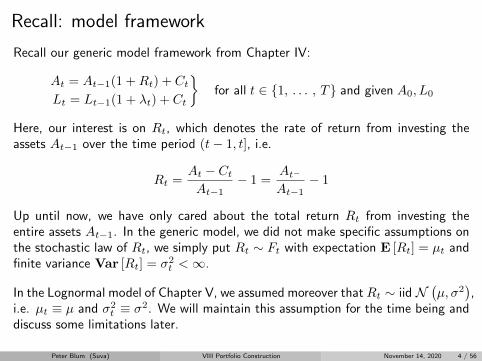
Recall: model framework

Recall our generic model framework from Chapter IV:

At = At−1(1 +Rt) + Ct

Lt = Lt−1(1 + λt) + Ct

for all t ∈ 1, . . . , T and given A0, L0

Here, our interest is on Rt, which denotes the rate of return from investing theassets At−1 over the time period (t− 1, t], i.e.

Rt =At − CtAt−1

− 1 =At−

At−1− 1

Up until now, we have only cared about the total return Rt from investing theentire assets At−1. In the generic model, we did not make specific assumptions onthe stochastic law of Rt, we simply put Rt ∼ Ft with expectation E [Rt] = µt andfinite variance Var [Rt] = σ2

t <∞.

In the Lognormal model of Chapter V, we assumed moreover thatRt ∼ iid N(µ, σ2

),

i.e. µt ≡ µ and σ2t ≡ σ2. We will maintain this assumption for the time being and

discuss some limitations later.


Recall: risk / return profile

In Chapter VI, we assumed that by investing the assets At in different manners, wecan attain different levels of expected returns µ ∈ [µmin, µmax]. And by doing so,we will incur an investment risk σ that depends on the level of expected return, i.e.σ = σ(µ) with

σ(µ) > 0

σ′(µ) > 0

σ′′(µ) ≥ 0


That is, if we want a higher level of return, we must invariably incur a higher levelof investment risk.

We called the relationship µ 7→ σ(µ) the risk / return profile and took it as given.

In this chapter, we will look at how the assets At can be invested into differentasset classes and how the risk / return profile can be derived from doing so. Inparticular, we will see that the postulated properties of the risk / return profile areactually sensible.


Terminology: asset classes

We assume that there are n different asset classes i ∈ 1, . . . , n. Asset classescan be e.g. foreign bonds, domestic equities, real estate or hedge funds. In practice,this set of available asset classes is often called the investment universe. We denoteby Ai,t the amount of money that is invested in asset class i, so that we have

At =

n∑i=1

Ai,t where Ai,t ≥ 0 for all i and t

Note that we could also allow for Ai,t < 0. This corresponds to a so-called shortposition. However, in a social and pension insurance context, such short positionsare usually neither allowed nor desirable.

The portfolio weights wt ∈ Rn denote the relative share that each asset class ihold of the total portfolio, i.e.

wt = (w1,t, . . . , wn,t)′ ∈ Rn with wi,t =

Ai,tAt


Under the assumptions above, we have

wt ≥ 0 and 1′wt = 1

The first expression is to be understood component-wise, and in the second expres-sion 1 = (1, , . . . , 1)′ ∈ Rn such that 1′wt =

∑ni=1 wi,t.

Note that wt is a policy variable, i.e. in principle we can set wt to values accordingto our needs and wishes at any time t by buying and selling assets of the differentasset classes. In practice, market liquidity or other constraints may limit this abilityto some extent.


Example: asset classes

Distribution of the investment assets of The Swiss National Accident InsuranceFund (Suva) onto various asset classes:

The investment universe of Suva is fairly vast.


Asset class returns

As for the total portfolio return Rt, each asset class has its return Ri,t, i.e.

Ri,t :=Ai,t − Ci,tAi,t−1

− 1 =Ai,t−

Ai,t−1− 1

with µi,t = E [Ri,t] and σ2i,t = Var [Ri,t] < ∞. The return vector is defined as

Rt = (R1,t, . . . , Rn,t)′ ∈ Rn. For the time being, we assume that returns are iid

multivariate Normal, i.e.Rt ∼ iid Nn (µ,Σ)

with expectation µ = (µ1, . . . , µn)′

= E [Rt] ∈ Rn and with covariance ma-trix Cov [Rt] ∈ Rn×n. The covariance matrix is symmetric and positive (semi-)definite. Its elements can be represented as

Σij = ρijσiσj for all i, j ∈ 1, . . . , n

where σ2i = Var [Ri,t], σ

2j = Var [Rj,t] and ρij = Corr [Ri,t, Rj,t], i.e. the

correlation which describes the dependence between asset classes i and j.


We always have ρii = 1, and in the case of the multivariate Normal distribution,we also have ρij ∈ [−1,+1]. Note that for other multivariate distributions, ρijmay only take values in a subset of [−1,+1], and the correlation may not be ameaningful measure of dependence; see [4].

By R = (ρij)i,j∈1, ... , n ∈ Rn×n, we denote the correlation matrix.

In asset management, it is fairly commonplace to consider the correlation matrixR and the standard deviations σi (called volatilities) separately, because this lendsitself to a more intuitive interpretation than the covariance matrix.

If we have Rt ∼ Nn(µ,Σ), and if the portfolio weights at the beginning of theperiod are wt−1, then we have

E [Rt] = E[w′t−1Rt

]= w′t−1 µ

Var [Rt] = Var[w′t−1Rt

]= w′t−1Σwt−1

This is a general property of multivariate distributions; see e.g. [1].


Example: investment universe

For our subsequent considerations, we will use the following, somewhat simplifiedinvestment universe:

Note that the expected returns had to be revised dramatically over time althoughthey were meant to be long-term... (c.f. Chapters II, VI and VII). The volatilitiesand correlations, however, turned out to be fairly stable.


2. Investment strategy


SetupWe assume that we have n asset classes with returns Rt = (R1,t, . . . , Rn,t)

′ ∈ Rnfor all t ∈ 1, . . . , T. Specifically, we assume

Rt ∼ iid Nn(µ,Σ) for all t ∈ 1, . . . , T

That is, investment returns on asset class level have an iid multivariate Normaldistribution with

I Expected return vector µ = E [Rt] ∈ Rn,

I Covariance matrix Σ = Cov [Rt] ∈ Rn×n.

We specifically assume that Σ is positive definite instead of just semi-definite, andwe also assume that µ is linearly independent of 1, i.e. not all asset classes havethe same expected return.

Moreover, we assume constant portfolio weights over time, i.e.

wt ≡ w for all t ∈ 1, . . . , T

This is a so-called rebalancing strategy, i.e. at each time t > 0, the portfolio isrebalanced to its original weights w by buying and selling assets.


Illustration: rebalancing

Two asset classes: i ∈ 1, 2 (think of bonds and equities; total assets A0 = 100).

At t = 0: w1,0 = 60% and w2,0 = 40%, corresponding to A1,0 = 60 and A2,0 = 40.

Between t = 0 and t = 1: R1,1 = −2% and R2,1 = +10%

This leads to A1,1− = 58.8 and A2,1− = 44.0 for A1− = 102.8.

We have R1 = A1−/A0 − 1 = 2.8% = (60%, 40%)′(−2%,+10%).

Before rebalancing we have portfolio weights w1,1− = 58.8/102.8 = 57.2% andw2,1− = 44.0/102.8 = 42.8%

Rebalancing: Sell 2.9 of Asset 2 and buy 2.9 of Asset 1 to obtain A1,1 = 61.7 andA2,1 = 41.1, corresponding to w1,1 = 60% and w2,1 = 40%.

Basically, we sell the winners and buy the losers. This works well in a cyclicalmarket.


More on rebalancingA rebalancing strategy corresponds to an anti-cyclical behavior, i.e. assets with highreturns in the previous period are sold, and those with low returns in the previousperiod are bought. If investment returns are mean-reverting, this is a reasonablestrategy. Moreover, it keeps the risk profile of the portfolio constant.

Rebalancing strategies maintained over several years are fairly commonplace forlong-term institutional investors.

I There may be different disciplines for rebalancing, e.g. calendar-based (eachyear / quarter / month), or threshold-based, i.e. when actual weights are toofar away from required ones.

I There may or may not be some active overlay that allows for limited oppor-tunistic deviations from the strategic portfolio weights w.

There exist more sophisticated, dynamic approaches to investment strategy design.They basically take into account the specific path of the returns and adjust weightsin an adaptive manner.

I A simple example is portfolio insurance. This approach tends not to work whenone needs it most.

Treatment of more sophisticated dynamic strategies requires stochastic optimizationmethodology that is beyond the scope of this course.


Illustration: value of rebalancingCumulative performance of Pictet BVG 25 Plus Index (strictly rebalancing) vs.Credit Suisse Pension Fund Index (containing procyclical behavior).

Rebalancing strategy outperforms sustainably. Outperformance is particularly highafter losses sustained in financial crises.


ConstraintsForm now on, let w = (w1, . . . , wn)′ ∈ Rn denote the static portfolio weightsthat are valid for all times under consideration (not necessarily up to time T ).

As already mentioned, we need to have∑n

i=1wi = 1 or 1′w = 1

That is, we require that all assets are fully invested in the asset classes 1, . . . , n.

Moreover, we require that wi ≥ 0 for all i ∈ 1, . . . , n, abbreviated w ≥ 0. Thatis, no short positions are allowed. This makes sense for a pension fund, and it isoften (e.g. in Switzerland) also mandated by law.

Moreover, there may be other constraints in place, either given by law or regulation,or self-imposed by the institution, or simply by necessity for practical reasons. Theseconstraints may have two generic forms:

I Equality constraints: f(w) = 0

I Inequality constraints: f(w) ≤ 0


Depending on how well-behaved the functions f and g are, these constraints may bemore or less easily incorporated into an optimization problem. It is most convenientif constraints are linear, i.e.

I Equality constraints: Aw = b (or Aw − b = 0)

I Inequality constraints: Aw ≤ b (or Aw − b ≤ 0)

for some A ∈ Rk×n and b ∈ Rk.


Example: constraints

Swiss pension fund regulation (BVV 2, SR 831.441.1) specifically imposes the fol-lowing constraints:

I No short positions.

I Max. 50% in mortgages or mortgage-backed securities incl. Pfandbriefe.

I Max. 50% in equities.

I Max. 30% in real estate, incl. max. 10% in foreign real estate.

I Max. 15% in alternative investments.

I Max. 30% in unhedged foreign-currency investments of all kinds.

All these constraints can be represented as linear inequality constraints.


The optimization taskIn an asset / liability setup, we are always given some required return. And we musthave an expected return µ = µ′w = E[Rt] that is at least equal to this requiredreturn in order to assure a sustainable funding, provided that this is feasible; c.f.Chapter VI and VII. In the general model, this amounts to

µ ≥ λt + (FRt−1 − 1)CtAt−1

In the simplified Lognormal model, we simply have µ ≥ λ.

In the sequel, we consider µ as the given target return. We must find portfolioweights w such that µ′w ≥ µ. There is no unique solution to this problem.

From among all possible solutions, it makes sense to choose the one that pro-duces the minimal short-term investment risk σ2 = w′Σw. Including our otherconstraints, this amounts to

minw

w′Σw s.t. 1′w = 1

µ′w ≥ µw ≥ 0


A portfolio w∗ that is the solution of this optimization problem is then calledmean / variance - efficient, because from all portfolios that satisfy the constraints,it is the one with the lowest variance, i.e. the lowest risk.

Optimization problems of this kind are called quadratic convex optimization prob-lems (because the objective function is both quadratic and convex, and the con-straints are convex).

There exist many numerical optimizers to solve such optimization problems effi-ciently. This is also the case if further constraints are added, provided that they aresufficiently well-behaved. For more information on mathematical optimization andits applications, see e.g. [3].

We will, however, follow a different path hereafter, i.e. we will try to explore someproperties of mean / variance - efficient portfolios analytically so as to gain a deeperunderstanding.


3. Portfolio optimization in the mean / variance case


Task: properties of efficient portfolios

We use the setup just introduced, and we assume the following elements to begiven:

I Expected return vector µ ∈ Rn, linearly independent of 1.

I Covariance matrix Σ ∈ Rn×n, positive definite.

I Target return µ ∈ R.

The mean / variance efficient portfolio w∗ is then the solution of the problem

minw

12 w′Σw s.t. 1′w = 1

µ′w ≥ µw ≥ 0

Note that we have added the factor 1

2 for mathematical convenience. While µand Σ are given by the financial markets, µ is a policy variable that we can set todifferent values.


For the different values of µ, different optimal portfolios w∗(µ) will result,withdifferent optimal portfolio variances σ2(µ) = w∗(µ)′Σw∗(µ). That is, we have afunctional relationship σ = σ(µ), determined by µ and Σ and the constraints. Thisis actually the risk / return profile that we already used.

We are now going to explore the properties of this risk / return profile in order tojustify the assumptions that we simply made in the previous chapters.

I We do this first in the most basic setup with just the constraint 1′w = 1.

I Then we add further constraint and look at their influence.


Prerequisite: Lagrange multipliersThis should be known from an undergraduate calculus course; otherwise see someappropriate textbook, e.g. [2].

Let X be an open subset of Rn, and let

f : X → R and g = (g1, . . . , gm)′ : X → Rm

be continuously differentiable; m ≤ n. Let f have a local extremum in ξ ∈ X thatsatisfies the constraint g(ξ) = 0. Assume moreover that the matrix

g′(ξ) =

(∂gi(ξ)

∂xj

)i∈1, ... ,m, j∈1, ... ,n

has full rank. Then, there exist m numbers λ1, . . . , λm (the Lagrange multipliers)such that we have

f ′(ξ) +

m∑i=1

λi g′i(ξ) = 0

Important: This only holds for equality constraints gi(ξ) = 0. For inequality con-straints, the similar but more complicated Karush-Kuhn-Tucker conditions must beapplied and evaluated; see [3].


In practice, this means that, if we want to solve the problem

minxf(x) s.t. g1(x) = 0, . . . gm(x) = 0

we first establish the Lagrange function or Lagrangian

L(x, λ1, . . . , λm) = f(x) +

m∑i=1

λi gi(x)

Then, we take derivatives with respect to x and λ1, . . . , λm, set them all to zeroand solve the resulting system of equations

∂L∂x

= 0 ;∂L∂λ1

= 0 , . . . ,∂L∂λm

= 0

If f is twice continuously differentiable, and if the Hessian Matrix

(Hf)(ξ) =

(∂2f

∂xi∂xj(ξ)

)i,j∈1, ... ,n

is positive definite in ξ, then ξ is actually a minimum. For our typical target functionf(x) = 1

2x′Σx, we have (Hf)(x) = Σ, which is positive definite by assumption.


Global minimum variance portfolio

To begin with, we drop the short constraint (w ≥ 0) as well as the return require-ment (µ′w ≥ µ) and consider the simplified problem

minw

12 w′Σw s.t. 1′w = 1 (⇔ 1′w − 1 = 0)

The resulting optimal portfolio wmin is called global minimum variance portfolio. Itis the least risky portfolio given that one must be fully invested.

The Lagrangian is L(w, λ) = 12 w′Σw + λ(1′w − 1).

We must solve the following system

∂L∂w

= Σw + λ1 = 0

∂L∂λ

= 1′w − 1 = 0

The first equation yieldsw = −λΣ−11


Inserting this into the second equation yields

−λ1′Σ−11 = 1 ⇒ −λ =1

1′Σ−11

Thus, the global minimum variance portfolio wmin is given by

wmin =Σ−11

1′Σ−11

For its return µmin and its variance σ2min, we obtain

µmin = µ′wmin =µ′Σ−11

1′Σ−11

σ2min = w′minΣwmin

=1

(1′Σ−11)21′Σ−1ΣΣ−11

=1

1′Σ−11


Example: simple investment universe

For the simple investment universe as introduced in Section 1, the global minimumvariance portfolio and its properties look as follows:


Portfolios with defined returnsLet us assume that µ ≥ µmin. And, given this, let us change the requirementµ′w ≥ µ into µ′w = µ. (One could show that this must be the case anyway foroptimal portfolios.) This leads to the optimization problem (see also [6]):

minw

12 w′Σw s.t. 1′w − 1 = 0

µ′w − µ = 0

The Lagrangian for this optimization problem is

L(w, λ1, λ2) = 12 w′Σw + λ1(1′w − 1) + λ2(µ′w − µ)

This leads to the optimality conditions

∂L∂w

= Σw + λ11 + λ2µ = 0 (1)

∂L∂λ1

= 1′w − 1 = 0 (2)

∂L∂λ2

= µ′w − µ = 0 (3)


From condition (1) we obtain

w = −λ1Σ−11− λ2Σ−1µ

Provided that 1′Σ−1µ 6= 0, we can rewrite this as

w = −λ1(1′Σ−11

) Σ−11

1′Σ−11− λ2

(1′Σ−1µ

) Σ−1µ

1′Σ−1µ

From condition (2), we obtain moreover

1′w = −λ1 1′Σ−11− λ2 1′Σ−1µ = 1

This is equivalent to

−λ2 1′Σ−1µ = 1− (−λ1 1′Σ−11)

Letting ν := −λ1 1′Σ−11, we then have 1− ν = −λ2 1′Σ−1µ.


That is, we can represent the optimal portfolio w as

w = νwmin + (1− ν)wrisk

where we have

wmin =Σ−11

1′Σ−11and wrisk =

Σ−1µ

1′Σ−1µ

We note that wmin is actually the minimum risk portfolio that we have introducedbefore. That is, the optimal portfolio w is a convex combination of the minimumrisk portfolio wmin and some risky portfolio wrisk. For the latter, we have

µrisk = µ′wrisk =µ′Σ−1µ

1′Σ−1µ

σ2risk = w′riskΣwrisk

=1

(1′Σ−1µ)2(Σ−1µ)′Σ(Σ−1µ)

=µ′Σ−1µ

(1′Σ−1µ)2



For the simple investment universe as introduced in Section 1, the risky portfolioand its properties look as follows:



Using wmin and wrisk from the simple investment universe (version 2015), for dif-ferent values of ν, we obtain the following risk / return profile:

One might think that this is a hyperbola.


Relation to expected return µ

We now must further investigate ν. To this end, we evaluate constraint (3), i.e.µ′w = µ by inserting the expression for w:

µ = µ′ (νwmin + (1− ν)wrisk)

= ν (µ′wmin) + µ′wrisk − ν (µ′wrisk)

= ν µmin + µrisk − ν µrisk

This can be solved to yield

ν =µrisk − µµrisk − µmin

That is, if µ = µrisk, then ν = 0. And if µ = µmin, then ν = 1. We also have:

1− ν =µ− µmin

µrisk − µmin


Shape of the risk / return profileWe want to establish a functional relationship between σ2 and µ. To this end, weexplore

σ2 = w′Σw

= (νwmin + (1− ν)wrisk)′Σ (νwmin + (1− ν)wrisk)

= ν2 w′minΣwmin + 2ν(1− ν)w′minΣwrisk + (1− ν)2 w′riskΣwrisk

Recall that w′minΣwmin = σ2min > 0 and w′riskΣwrisk = σ2

risk > 0. We also haveσ2risk > σ2

min. Moreover, we have

w′minΣwrisk =1

(1′Σ−11)(1′Σ−1µ)(1Σ−1)′Σ(Σ−1µ)

=1

1′Σ−11= σ2

min

That is, we can rewrite the expression for σ2 as

σ2 = ν2σ2min +

(2ν − 2ν2

)σ2min +

(1− 2ν + ν2

)σ2risk

= ν2(σ2risk − σ2

min

)− 2ν

(σ2risk − σ2

min

)+ σ2

risk


This, in turn, can be rewritten as (noting that σ2risk − σ2

min > 0)

σ2

σ2risk − σ2

min

= ν2 − 2ν +σ2risk

σ2risk − σ2

min

= (ν − 1)2 +σ2risk

σ2risk − σ2

min

− 1

= (ν − 1)2 +σ2min

σ2risk − σ2

min

This is, indeed, the equation of a hyperbola in ν. And since

ν =µrisk − µµrisk − µmin

i.e. ν is just an affine coordinate transform of µ, this also describes a north - southopening hyperbola in µ− σ - space:

σ2

σ2risk − σ2

min

=(µ− µmin)

2

(µrisk − µmin)2 +

σ2min

σ2risk − σ2

min


Illustration: risk / return profile

The risk / return profile resulting from the optimization problem on p.20 (portfoliowith defined returns) is a hyperbola in µ− σ - space.

Note that the hyperbola asymptotically tends towards a straight line.


Properties of the risk / return profileSince the risk / return profile (under the given constraints in this optimization) isa hyperbola in µ− σ - space, it has the following generic representation:

σ2

a2− (µ− c)2

b2= 1

For the positive branch with a > 0, this means

σ(µ) = a

√1 +

(µ− c)2b2

for a2 = 1; b2 =σ2min

σ2risk − σ2

min

(µrisk − µmin)2

; c = µmin

Therefore, we have

I σ(µ) > 0 for all µ ≥ µmin

I σ′(µ) > 0 for all µ > µmin (with σ′(µmin) = 0)

I σ′′(µ) > 0 for all µ ≥ µmin (with limµ→∞ σ′′(µ) = 0)

as we have postulated in the previous chapters.Peter Blum (Suva) VIII Portfolio Construction November 14, 2020 39 / 56

Digression: adding a risk-free assetAssume we have an additional, risk-free asset 0 with deterministic return µ0. Letµ = (µ0,µ)′ ∈ Rn+1 and w = (w0,w)′ ∈ Rn+1. We solve the modified problem

minw

12 w′Σw s.t. 1′w = 1

µ′w = 1

Then, provided that 1 and µ are linearly independent, one can show (see e.g. [6])that optimal portfolios are still of the form

w = ν w1 + (1− ν) w2

but this time with

w1 = (1, 0, . . . , 0)′ ∈ Rn+1 and w2 = (0, w1, . . . , wn)′ ∈ Rn+1

That is, each optimal portfolio is a combination of the risk-free asset and somefixed risky reference portfolio w2. One can also show that in this case, the risk /return profile σ = σ(µ) boils down to a straight line, i.e. we should have σ′(µ) > 0and σ′′(µ) = 0.

This is, in principle, more favorable than the situation with only risky assets. How-ever, is is not realistic for all cases where w is at some distance from w2, since itis not possible to hold a large portion of the portfolio in cash.


Where do we stand?

Recall that in the optimization problem that we have just solved analytically, wehave made two omissions:

I We made the constraint µ′w = µ instead of µ′w ≥ µ. For any µ ≥ µmin thisis not important.

I We have not required w ≥ 0, i.e. we still allow for short positions. This,however, is an important omission.

The optimizations problem including the additional inequality constraint w ≥ 0can be solved numerically without any problem; c.f. also the risk / return profileexamples already shown.

However, it is not tractable analytically. Thus, in order to gain some qualitativeinsights, we have to follow a different path.


Reformulation of the optimization problem

The generic optimization problem can be formulated as follows:

minw

f(w) s.t. gi(w) = 0, i = 1, . . . , m

gj(w) ≤ 0, j = m+ 1, . . . , r

Let us now consider the set Ar ⊆ Rn containing all points w ∈ Rn that satisfy allr constraints, i.e.

Ar := w ∈ Rn | gi(w) = 0 ∀ i = 1, . . . , m; gj(w) ≤ 0 ∀ j = m+ 1, . . . , r

The original optimization problem is thus equivalent to

minw∈Ar

f(w)

Let wr ∈ Ar denote the optimal solution.


Adding further constraints

Now, we can add a further constraint, irrespective of whether this is an equality orinequality constraint:

minw

f(w) s.t. gi(w) = 0, i = 1, . . . , m

gj(w) ≤ 0, j = m+ 1, . . . , r

gr+1(w) ≤ 0

This can again be formulated in set notation, i.e.

Ar+1 := w ∈ Rn | gi(w) = 0 ∀ i = 1, . . . , m; . . .

. . . gj(w) ≤ 0 ∀ j = m+ 1, . . . , r; gr+1(w) ≤ 0

The only difference between Ar and Ar+1 is the additional constraint. This alsomeans that

Ar+1 ⊆ ArThat is, the additional constraint leads to an equal or smaller set of admissiblepoints.


Now, there can be exactly two situations:

I wr ∈ Ar+1, i.e. the solution of the original problem also satisfies the additionalconstraint. Then we have wr+1 = wr, and also f(wr+1) = f(wr).

I wr ∈ Ar \ Ar+1, i.e. the solution of the original problem does not satisfy theadditional constraint. Then we have wr+1 6= wr. And, due to the optimalityof wr on all of Ar, we also have f(wr+1) > f(wr)

Translated back to our portfolio optimization problem, this means:

I For the same level of expected return µ, adding a further constraint leads toat least as much or more risk than without the additional constraint.

I That is, the hyperbola that we have obtained before is a minorant for all therisk / return profiles where more constraints apply.

I In particular, the hyperbola is a minorant for the risk / return profile of theoriginal optimization problem that also incorporates the non-negativity con-straint.



We use the simple investment universe as introduced in Section 1. Relative tothe setup already explored analytically, we investigate (numerically) also the twofollowing setups featuring additional constraints:

I Add only the non-negativity constraint w ≥ 0.

I Add also the additional constraints imposed by Swiss pension fund legislationand supervision (c.f. p. 19).


Example: influence of constraintsRisk / return profiles under various sets of constraints:

Under full constraints, returns above 3.5% are not feasible.


4. Conclusions and observations


Conclusions on the risk / return profile

The properties of the risk / return profile σ = σ(µ), i.e.

σ(µ) > 0

σ′(µ) > 0

σ(µ) ≥ 0

for all µ ∈ (µmin, µmax)

are confirmed to be sensible.

The more constraints one adds, the more risk one has to take in order to achievethe same expected return.

Therefore, investment constraints should only be imposed where they are reallynecessary and sensible. Freedom has a value and regulation has a cost.


Relation between return and short-term investment riskSo-called risk-adjusted performance measures put expected return in relation with

the risk that must be incurred to earn the return. Let µw = µ′w and σ2w = w′Σw

denote the expected value and the variance of the portfolio with weights w.

The best-known example is the Sharpe Ratio which assumes the presence of a risk-free asset with deterministic return µ0. Then we have:

SRw =µw − µ0

σw

In our context, where the availability of a risk-free asset is limited, it makes senseto consider the risk-adjusted return above the minima given by the global minimumvariance portfolio (c.f. p.27):

RARw =µw − µmin

σw − σmin

The Information Ratio considers unadjusted risk and return. Its application is,however, more suitable in the context of active asset management:

IRw =µw

σw


Contributions to risk and return

We have µw = µ′w =∑ni=1 wiµi. Therefore, we can easily identify the absolute

and relative contribution of some asset class i to the overall return:

ACReturni = wi µi resp. RCReturn

i =wi µiµw

For the risk, such an easy additive decomposition is less straightforward. First, wehave to take σ2

w rather than σw. Then, we can state:

σ2w = w′Σw =

∑n

i=1wi

(∑n

j=1σij wj

)The term in the parentheses contains both the risk from the variance of the assetclass itself (σiiwi) as well as the risk from the covariance with the other asset classes(σijwj , j 6= i). Thus, we can state

ACRiski =

∑n

j=1σijwj and RCRisk

i =1

σ2w

∑n

j=1σijwj


Marginal contributions to risk and return

Here, we consider the effect that a marginal change in the portfolio weight of assetclass i has on overall risk and return.

For the return:d

dwkµw = µk

For the risk:

d

dwkσ2w =

d

dwk

n∑i=1

n∑j=1

σij wi wj = 2

(wk σkk +

n∑i=1

wiσik

)

It is worthwhile to increase the weight of an asset class if it has a favorable relation-ship between high marginal contribution to return and low marginal contribution torisk.


Limitations of the mean / variance optimizationMean / variance optimization is an excellent and simple tool for studying the in-terplay between risk, return and constraints in investment portfolios. However, inreal-world settings, it has a number of limitations.

In particular, asset class returns are assumed to follow a multivariate Normal distri-bution. This may be relaxed somewhat to general elliptical distributions, but thisis still a restrictive assumption.

I It is well-known that many financial time series exhibit significantly non-Normalbehavior; see [4]. The higher the frequency, the more so.

I Moreover, dependence structures tend to be non-linear. In particular, there maybe correlation breakdowns in times of financial crises. That is, diversificationmay not work when it is needed most urgently; see also [4].

I This may be less of an issue with yearly data, but care must still be taken!

In any case, the underlying markets must be analyzed carefully. If Normality cannotbe assumed to hold, either different models should be used, or the Normal modelshould be complemented with suitable stress tests.

The portfolios obtained from mean / variance optimization tend to be rather sen-sitive to changes in estimates for expected returns µ and covariances Σ. Given thehigh estimation uncertainty, particularly for µ, this is an issue.


Example: sensitivities

Simple investment universe as on p.11. Slight changes in return estimates lead torather sizable changes in optimal portfolio weights.

The same effects would be obtained with changes in volatility or correlation as-sumptions.

The risk / return profile, i.e. σ = σ(µ) is less sensitive against such changes, whichis an advantage in the present context.


Alternatives for portfolio construction

For portfolio optimization, there exist many alternatives to the simple mean / vari-ance optimization introduced here; see e.g. [5]:

I Portfolio bootstrapping, which does not rely on any parametric model for theasset returns.

I Use of different risk measures, e.g. mean / expected shortfall optimization.

I Bayesian approaches that explicitly incorporate the estimation uncertainty forµ in the Black / Litterman framework.

In practice, the construction of the strategic portfolio w of an institutional investorwill involve both qualitative and quantitative steps. Operational restrictions alsoplay an important role.

If it simply comes to determining the risk / return profile σ = σ(µ), the solutionobtained from mean / variance optimization is always a reference: actual risk σ(µ)for some give level of return µ will likely not be lower that what is suggested by themean / variance optimization.

Irrespective of the optimization method: The generic characteristics of the risk /return profile, i.e. σ(µ) > 0, σ′(µ) > 0 and σ′′(µ) ≥ 0 are certainly plausible.


Bibliography I


[2] Heuser, H.Lehrbuch der Analysis.Teubner, Stuttgart, 1993.

[3] Luptacik, M.Mathematical Optimization and Economic Analysis.Springer, Berlin, 2010.


[5] Meucci, A.Risk and Asset Allocation.Springer, Berlin, 2005.


Bibliography II

[6] Muller, H.Modern portfolio theory: Some main results.ASTIN Bulletin 18, 2 (1988), 127–145.



Chapter IX: Empirical Considerations


Peter Blum


November 14, 2020

Peter Blum (Suva) Empirical November 14, 2020 1 / 13

Problem statement

In the Lognormal model, we assume that investment returns follow a Normal distri-bution N (µ, σ2). And in mean / variance portfolio optimization, we assume thatthe asset class returns follow a multivariate Normal distribution Nn(µ,Σ).

Also with any other model or method, we make certain (implicit or explicit) as-sumptions on the stochastic law of the investment returns and other stochasticvariables. It is extremely important to verify whether the underlying markets satisfythese assumtions. Otherwise, the model is invalid.

Therefore, empirical data analysis is an indispensable part of the modelling process.One must understand the relevant empirical properties of the data in order to makevalid models and draw valid conclusions: Let the data tell us their story!

The first step is always a descriptive analysis by preparing graphical evaluations andby computing summary statistics. This is assumed to be known and not treatedany further here.

Then, inferential analysis can be made; see e.g. [1] or [4]. We will limits ourselveshere to some evaluations in order to check Normality.


Descriptive statistics

Everyone according to his or her own needs and preferences...

(Data and chart: Bloomberg)


Multivariate Normal distributionA random vector X ∈ Rn is said to have a multivariate Normal distribution, writtenX ∼ Nn(µ,Σ), if its probability density function is given by

fX(x) =1√

(2π)n|Σ|exp

−1

2(x− µ)

′Σ−1 (x− µ)

for some vector µ ∈ Rn and some symmetric and positive definite matrix Σ ∈ Rn×n.We then have (refer e.g. to [2] for all this):

E [X] = µ and Cov [X] = Σ

Moreover, for some w ∈ Rn (think of portfolio weights), we have

E [w′X] = w′µ and Var [w′X] = w′Σw

If X ∼ Nn(µ,Σ), then Xi ∼ N (µi,Σii) for all i ∈ 1, . . . , n. That is, themarginal distributions are univariate Normal.

On the other hand, if Xi ∼ N (µi, σi) for i ∈ 1, . . . , n, this does not necessarilymean that X = (X1, . . . Xn)

′ ∈ Rn is multivariate Normal. There must also be avery specific linear dependence structure; see [3].


Quantile-Quantile plot (QQ plot)Let x1, . . . , xK be K independent observations from some random variable X,and let x(1), . . . , x(K) be the respective order statistics. x(k) corresponds to the

empirical kK - quantile.

For X ∼ F (e.g. F = N (µ, σ2)), we can also compute the theoretical quantiles

F−1(

k− 12

K

). The correction k − 1

2 is in order to avoid F−1(1).

If x1, . . . , xK do actually come from X ∼ F , then the scatter plot of empiricalagainst theoretical quantiles should form approximately a straight line.


QQ plots for monthly returnsClear deviations from normality in some cases. (Data: Bloomberg)


QQ plots for quarterly returnsPredominantly normal, but with exceptions and outliers. (Data: Bloomberg)


QQ plots for yearly returnsUsually normal, but occasional outliers occur. (Data: Bloomberg)


Kolmogorov-Smirnov testLet x1, . . . , xK be K independent observations from some random variable X.The empirical cumulative distribution function is then given by

F (x) =1

K

K∑k=1

1xk≤x

If actually X ∼ F , then the empirical distribution function F (x) should not be toodifferent from the theoretical one. The difference can be expressed as

Dn := ‖F − F‖∞ = supx|F (x)− F (x)|

Under the null hypothesis X ∼ F against a two-sided alternative, we must have

√nDn

D→ K (n→∞) where K(x) = 1− 2

∞∑j=1

(−1)j+1 exp−2j2x2

K is called Kolmogorov-Smirnov distribution (see e.g. [5]). The null hypothesis is

rejected on significance level α ∈ (0, 1) if Dn >1√nK←(1− α).


Illustration: cumulative distribution functions

Empirical (jagged, blue) and theoretical (smooth, red) cumulative distribution func-tions for two data series:

The Kolmogorov-Smirnov test is based on the greatest (vertical) difference betweentheoretical and empirical distribution function.


Kolmogorov-Smirnov test: results


Concluding remarks

For financial times series with frequencies of monthly and higher, non-normal returndistributions are the rule rather than the exception (see [3]), and the use of modelsbased on the Normal distribution is problematic in such cases.

For yearly investment returns, however, the hypothesis of a Normal distributionof the returns cannot be rejected in many cases. Models based on the Normaldistribution may thus be viable in these instances.

We should, however, notice that even in the most well-behaved yearly time se-ries, there are occasional outliers that cannot be reconciled with the hypothesis ofnormality.

When using Normal models, they should, therefore, always be complemented withsome stress scenarios (historical ones or constructed ones).


Bibliography I

[1] Campbell, J., Lo, A., and MacKinlay, A.The Econometrics of Financial Markets.Princeton University Press, Princeton, 1997.



[4] Stahel, W.Statistische Datenanalyse, third ed.Vieweg, Braunschweig, 2000.



Financial Risk Management in Social and Pension Insurance ...

Documents

Transcript of Financial Risk Management in Social and Pension Insurance ...