Final-Year Project (TN10) Internship Report

Controlling processing consistency, quality and efficiency by predictive modeling of meat

by-products transformation

INRA Centre of Theix (Auvergne, France) AgResearch Centre of Lincoln (Canterbury, New Zealand)

LEPERS Valentin Process Engineering Student

February 16th 2015 – July 31st 2015

UTC Supervisor : Pr Khalil SHAKOURZADEH BOLOURI INRA Supervisor : Dr Alain KONDJOYAN

AgResearch Supervisor : Dr Stefan CLERENS

2

Résumé technique

En Nouvelle-Zélande, Taranaki Bio Extracts (TBE), filiale du groupe ANZCO a mis au point un procédé

d'extraction de protéines depuis les co-produits de l'industrie de la viande. Ainsi, des carcasses de boeuf

sont amenées à haute température dans un milieu aqueux sous pression afin d'en extraire les protéines

structurelles (principalement du collagène de type I). Afin de mieux comprendre les phénomènes

intervenant au cours du procédé, un contrat a été établi entre TBE et AgResearch, le principal institut de

recherche néo-zélandais. Le centre INRA de Theix (région Auvergne) a rejoint le projet en raison des

compétences en modélisation dont il disposait.

Des expériences en laboratoire ont été réalisées à AgResearch (cuisson sous pression et à différentes

températures d'os de bœuf et de viande grasse présente sur les carcasses) afin de déterminer les

cinétiques d'extraction protéique au cours du procédé, l'évolution colorimétrique du bouillon (paramètre

critique du produit final) et, dans une moindre mesure, la composition des produits obtenus à l'échelle

moléculaire. Les résultats ont été interprétés et exploités à l'INRA.

Mots-clés : Recherche, International, Agro-industrie, Procédé, Laboratoire, Viande, Os, Biologie, Biochimie,

Protéines

3

Acknowledgements

Before starting the actual report of my 24 weeks spent between Auvergne in France and

Canterbury in New Zealand, I would sincerely like to thank all the people that helped me at some point

during this project :

My two supervisors : Dr Alain Kondjoyan at INRA and Dr Stefan Clerens at AgResearch for their

trust, their receptiveness, their sympathy and their benevolence. Having the opportunity to

discover Research and to travel to New Zealand at the same time was truly special.

Dr Santanu Deb-Choudhury, one of my coworkers at AgResearch, for his receptiveness, his

patience, and his daily good mood and sense of humor.

Mike North, the plant manager of TBE III, for his nice welcome and for having taken the time to

walk us through his process when Dr Deb-Choudhury and I visited him in Hawera.

4

Table of Contents

Résumé technique .............................................................................................................................................. 2

Acknowledgements ............................................................................................................................................ 3

Table of illustrations ........................................................................................................................................... 6

Tables ............................................................................................................................................................. 6

Figures ............................................................................................................................................................ 6

Introduction ........................................................................................................................................................ 8

I/ Internship context ........................................................................................................................................... 9

I ; 1/ Presentation of INRA .............................................................................................................................. 9

I ; 2/ Presentation of AgResearch ................................................................................................................. 10

I ; 3/ Presentation of Taranaki Bio Extracts .................................................................................................. 11

II/ Project problematization ............................................................................................................................. 12

II ; 1/ Raw material composition .................................................................................................................. 12

II ; 2/ Process description ............................................................................................................................. 14

II ; 3/ Involved phenomena .......................................................................................................................... 17

III/ Material and methods ................................................................................................................................ 19

III ; 1/ Experimental design ........................................................................................................................... 19

III ; 1 ; 1/ Preliminary reflection ................................................................................................................ 19

III ; 1 ; 2/ Building the definitive experimental design ............................................................................. 20

III ; 2/ Analysis methods ............................................................................................................................... 22

III ; 3/ Experimental raw material preparation ............................................................................................ 26

III ; 4/ Design and working of the lab scale pressure cooker ....................................................................... 27

IV/ Results, analysis and discussion.................................................................................................................. 32

IV ; 1/ Modification of the experimental set-up .......................................................................................... 32

IV ; 1 ; 1/ Beef meat and scraps early results : first two runs in AgResearch’s pressure cooker ............. 32

IV ; 1 ; 2/ Beef mixed bones early results : highlighting a mixing defect ................................................. 35

IV ; 1 ; 3/ Improving the pressure cooker ................................................................................................. 37

IV ; 2/ Measurement uncertainties .............................................................................................................. 39

IV ; 2 ; 1/ Colour measurement ................................................................................................................ 39

IV ; 2 ; 2/ Protein concentration measurement ....................................................................................... 40

IV ; 3/ Final experimental results ................................................................................................................. 42

IV ; 3 ; 1/ Colour measurements ............................................................................................................... 43

IV ; 3 ; 2/ Protein concentration measurements ...................................................................................... 47

5

IV ; 3 ; 3/ Amino acid analysis ................................................................................................................... 54

IV ; 3 ; 4/ Mass spectrometry results........................................................................................................ 56

IV ; 4/ Modeling and analysis ....................................................................................................................... 59

IV ; 4 ; 1/ Heat transfer modeling ............................................................................................................. 59

IV ; 4 ; 2/ Proteins extraction kinetics modeling ...................................................................................... 62

IV ; 5/ Prospects for TBE ............................................................................................................................... 67

Conclusion ........................................................................................................................................................ 69

References ........................................................................................................................................................ 70

Annex ................................................................................................................................................................ 72

Annex 1 : Colour evolution of stocks ............................................................................................................ 72

Beef scraps ............................................................................................................................................... 72

Leg bones (130°C) ................................................................................................................................... 73

Mixed bones ............................................................................................................................................. 73

Annex 2 : Cooked material pictures ............................................................................................................. 74

Beef scraps ............................................................................................................................................... 74

Leg bones (130°C) ..................................................................................................................................... 74

Mixed bones ............................................................................................................................................. 75

6

Table of illustrations

Tables

Table 1 : Bone material composition (Composition de la matière osseuse) ...................................................................... 13

Table 2 : Beef scraps composition (Composition des déchets) .......................................................................................... 13

Table 3 : Raw material composition (Composition de la matière première) ..................................................................... 13

Table 4 : Experimental raw material composition (Composition de la matière première utilisée en laboratoire) ........... 26

Table 5 : 90°C uncertainty measurement (Mesure des incertitudes à 90°C) ..................................................................... 41

Table 6 : 110°C/130°C uncertainty measurement (Mesure des incertitudes à 110°C/130°C) ........................................... 42

Table 7 : Final runs working conditions (Conditions de fonctionnement des runs finaux) ................................................ 43

Table 8 : Beef scraps cooking : T-P evolution (Cuisson de déchets : évolution de T et P) .................................................. 49

Table 9 : Beef scraps cooking : achieved extraction yelds (final results) (Cuisson de déchets : rendements d’extraction

obtenus, résultats finaux) .................................................................................................................................................. 50

Table 10 : Beef leg bones cooking at 130°C : T-P evolution (Cuisson d’os de pattes de bœuf à 130°C : évolution de T et P)

.......................................................................................................................................................................................... 51

Table 11 : Beef leg bones cooking at 130°C : achieved extraction yields (final results) (Cuisson d’os de pattes de bœuf à

130°C : rendements d’extraction obtenus, résultats finaux) ............................................................................................. 51

Table 12 : Beef mixed bones cooking : T-P evolution (Cuisson d’os de bœuf mélangés : évolution de T et P) .................. 53

Table 13 : Beef mixed bones cooking : achieved extraction yields (final results) (Cuisson d’os de bœuf mélangés :

rendements d’extraction obtenus, résultats finaux) ......................................................................................................... 53

Table 14 : Amino acid analysis results (Résultats des analyses en acides aminés) ........................................................... 55

Table 15 : List of amino acid targets used for modification searches (Liste des acides amines ciblés par les recherches de

modifications) ................................................................................................................................................................... 57

Table 16 : Heat transfer modeling : input parameters (Modélisation du transfert de chaleur : paramètres d’entrée) .... 61

Table 17 : Protein extraction tendencies, depending on cooking temperature and kind of raw material (Tendances de

l’extraction protéique en fonction de la température du cuiseur et de la matière première) ........................................... 63

Table 18 : Building the model : optimized parameters (Construction du modèle : paramètres optimisés) ...................... 64

Table 19 : Input values for the calculation of kinetics constants (Paramètres d’entrée pour le calcul des constantes de

cinétique)........................................................................................................................................................................... 66

Figures

Fig. 1 : Beef bone protein extraction process flow diagram (Flow chart du procédé d’extraction protéique sur des os de

bœuf) __________________________________________________________________________________________ 16

Fig. 2 : First order kinetics curve (focusing on product) (Courbe typique de la cinétique de premier ordre) __________ 20

Fig. 3 : Meat and mixed bones cooking in an 85°C water bath : protein concentration (Cuisson de viande maigre et d’os

mélangés dans un bain-marie à 85°C : concentration en protéines) _________________________________________ 21

Fig. 4 : CIE L*a*b* colour space (Représentation spatiale du modèle CIE L*a*b*) ______________________________ 23

Fig. 5 : Direct Detect spectrometer (Spectromètre Direct Detect) ___________________________________________ 24

Fig. 6 : AgResearch’s bone crushing equipment (Matériel utilisé par AgResearch pour le broyage des os) __________ 27

Fig. 7 : Assembled cooker, front view (Cuiseur assemblé, vue de face) _______________________________________ 28

Fig. 8 : Experimental cooker parameters control (Contrôle des paramètres du cuiseur expérimental) ______________ 29

Fig. 9 : Empty cooker, top view (Cuiseur vide, vue de dessus) ______________________________________________ 30

Fig. 10 : Cooker with basket, top view (Cuiseur avec panier, vue de dessus) __________________________________ 30

Fig. 11 : Cooking basket, side view (Panier de cuisson, vue de côté) _________________________________________ 30

Fig. 12 : Cooking basket, bottom view (Panier de cuisson, vue de dessous) ___________________________________ 30

7

Fig. 13 : Cooking basket, looking up inner tube. Arrows indicate rows of 5 mm diameter holes (Panier de cuisson,

intérieur du tube) _________________________________________________________________________________ 31

Fig. 14 : Cooking basket, looking along inner tube (Panier de cuisson, extérieur du tube) ________________________ 31

Fig. 15 : Beef meat cooking at 132°C : colour evolution (early results) (Cuisson de viande de bœuf maigre à 132°C :

évolution de la couleur, résultats préliminaires)_________________________________________________________ 33

Fig. 16 : Beef scraps cooking at 132°C : colour evolution (early results) (Cuisson de déchets à 132°C : évolution de la

couleur, résultats préliminaires) _____________________________________________________________________ 33

Fig. 17 : Beef meat cooking at 132°C : protein concentration evolution (early results) (Cuisson de viande de bœuf

maigre à 132°C : évolution de la concentration en protéines, résultats préliminaires) __________________________ 34

Fig. 18 : Beef scraps cooking at 132°C : protein concentration evolution (early results) (Cuisson de déchets à 132°C :

évolution de la concentration en protéines, résultats préliminaires)_________________________________________ 34

Fig. 19 : Beef mixed bones cooking at 132°C : colour evolution (early results) (Cuisson d’os de bœuf mélangés à 132°C :

évolution de la couleur, résultats préliminaires)_________________________________________________________ 35

Fig. 20 : Beef mixed bones cooking at 132°C : protein concentration evolution (early results) (Cuisson d’os de bœuf

mélangés à 132°C : évolution de la concentration en protéines, résultats préliminaires) ________________________ 36

Fig. 21 : From left to right : scraps stock, lean meat stock and mixed bones stock after cooling, 8h mixed bones gel

(early runs) (De gauche à droite : bouillons obtenus à partir de déchets, de viande maigre, et d’os mélangés après

refroidissement, gel obtenu à partir d’os mélangés après 8h de cuisson (runs préliminaires) _____________________ 37

Fig. 22 : Pressure cooker with new motor, front view (Cuiseur avec moteur de remplacement, vue de face) _________ 38

Fig. 23 : Beef scraps cooking : colour evolution (final results) (Cuisson de déchets : évolution de la couleur, résultats

finaux) _________________________________________________________________________________________ 44

Fig. 24 : Beef leg bones cooking at 130°C : colour evolution (final results) (Cuisson d’os de pattes de bœuf à 130°C :

évolution de la couleur, résultats finaux) ______________________________________________________________ 45

Fig. 25 : Beef mixed bones cooking : colour evolution (final results) (Cuisson d’os de bœuf mélangés : évolution de la

couleur, résultats finaux) ___________________________________________________________________________ 46

Fig. 26 : Beef scraps cooking : protein concentration evolution (final results) (Cuisson de déchets : évolution de la

concentration en protéines, résultats finaux) ___________________________________________________________ 48

Fig. 27 : Beef leg bones cooking at 130°C : protein concentration evolution (final results) (Cuisson d’os de pattes de

bœuf à 130°C : évolution de la concentration en protéines, résultats finaux) _________________________________ 50

Fig. 28 : Beef mixed bones cooking : protein concentration evolution (final results) (Cuisson d’os de bœuf mélangés :

évolution de la concentration en protéines, résultats finaux) ______________________________________________ 52

Fig. 29 : Beef mixed bones cooking at 110°C and 130°C : oxidative modification scores (Cuisson d’os de bœuf mélangés

à 110°C et 130°C : indices d’oxydation) _______________________________________________________________ 57

Fig. 30 : Beef mixed bones cooking at 110°C and 130°C : other modifications scores (Cuisson d’os de bœuf mélangés à

110°C et 130°C : autres indices de dégâts) _____________________________________________________________ 58

Fig. 31 : Lab scale heat transfer (central point) (Transfert de chaleur à l’échelle expérimentale, point central) _______ 61

Fig. 32 : Process scale heat transfer (central point) (Transfert de chaleur à l’échelle industrielle, point central) ______ 61

Fig. 33 : Process scale cooker temperature profile : t = 8h, y' = 0 (Profil de température du cuiseur industriel : t = 8h, y’ =

0) _____________________________________________________________________________________________ 62

Fig. 34 : Beef mixed bones cooking : protein extraction modeling (Cuisson d’os de bœuf mélangés : modélisation de

l’extraction protéique) _____________________________________________________________________________ 64

Fig. 35 : Beef scraps cooking : protein extraction modeling (Cuisson de déchets : modélisation de l’extraction protéique)

_______________________________________________________________________________________________ 65

Fig. 36 : Beef leg bones cooking : protein extraction modeling (Cuisson d’os de pattes de bœuf : modélisation de

l’extraction protéique) _____________________________________________________________________________ 65

8

Introduction

Beef meat is nowadays an ordinary consumer product in most civilizations around the World and

the current emergence of new economical powers results in a constantly higher demand for it. However,

customers are only interested in precise parts of the animal (i.e. lean meat), while the rest (bones,

connective tissues, residual meat… that represent 30% of the carcass mass) is at best considered as by-

products and at worst as waste that needs to be removed from food products fabrication processes. When

they are not destroyed, by-products can be sold, for example as an ingredient for broth or as pets food.

Bones can also be used at industrial scale for gelatin or animal meal fabrication, among other things.

However, the proportion of bones recovered through these processes is rather low.

If bones are used in this manner, this is because they display interesting nutritive properties as they

are constituted by 65% of minerals and 35% of proteins (most of which is type I collagen, from which

gelatin is a derived product). Bones as such represent about 50% of meat by-products, the rest being fat,

residual meat, tendons and other connective tissues. Therefore, even with meat taken off, carcasses are a

non-negligible source of proteins that need to be used, their destroying (via combustion) and burying being

a potential cause of pollution and health risks. The process of animal meal seemed to provide a viable

solution to this issue, but their use has been strictly regulated (if not forbidden) since the epidemic of

bovine spongiform encephalitis (mad cow disease) that struck Europe during the 1990’s, making developing

new carcass-based processes a necessity. Indeed, the worldwide demand for gelatin is far from being

sufficient to absorb all bone waste, gelatin production processes moreover being time-consuming and

providing low yields (in the 15-20 % range).

In New Zealand, Taranaki Bio Extracts (TBE), a 50:50 joint venture company between Taranaki By

Products Ltd and ANZCO Foods Ltd, has developed a protein extraction process based on the hydrolysis of

beef bones under high temperature and pressure, resulting in a protein-rich concentrated stock (bone

extract). In 2014, TBE contacted AgResearch (the main New Zealand research institute) to establish a

contract as they wanted a better understanding of the underlying phenomena that occurred during their

process. AgResearch, on the other hand, contacted INRA in order to make the project international and to

have available skills regarding modeling. A lab scale experimental set-up was built in AgResearch’s lab in

Lincoln. During my final-year student project in Process Engineering (Université de Technologie de

Compiègne, 16/02/2015 – 31/07/2015), I performed experiments in Lincoln before exploiting the results in

Theix (INRA centre of Clermont-Ferrand). During this study, we focused on proteins extraction kinetics,

stock colour evolution (colour being a critical property of the final product), and to a lesser extent, on the

product composition at molecular scale. From these results, hypotheses were built regarding the extraction

mechanisms (some of which were modeled) and proposals were made regarding process improvement.

The results of this study are now being used for the writing of a scientific publication.

9

I/ Internship context

I ; 1/ Presentation of INRA

INRA (National Institute for Agricultural Research) is a French public research institute dedicated to

scientific studies concerning agriculture. It was founded in 1946 and is a Public Scientific and Technical

Research Establishment (EPST) under the joint authorities of Ministries of Research and Agriculture. Since

April of 2012, the Institute has been presided by François Houllier. INRA leads projects of research for a

sustainable agriculture, a safeguarded environment and a healthy and high quality food. Based on the

number of publications in agricultural, crops and animal sciences, INRA is the first institute for agricultural

research in Europe, and the second in the world. It belongs to the top 1% most cited research institutes and

its main tasks are :

To gather and disseminate knowledge ;

To build know-how and innovation for the society ;

To provide expertise to public institutions and private companies ;

To participate in science-society debates ;

To train in research.

The institute employs roughly 1800 researchers, 2400 research engineers, 4200 lab workers/field

workers/administrative staff. It also welcomes 1700 PhD students and 1000 interns/foreign researchers

every year. INRA is composed of 13 scientific departments :

Environment and Agronomy ;

Biology and crop breeding ;

Plant health and environment ;

Ecology of forest, meadows and aquatic environment ;

Animal genetics ;

Animal physiology and animal production systems ;

Animal health ;

Characterization and processing of agricultural products ;

Microbiology and food processing ;

Human nutrition ;

Sciences for action and development ;

Social sciences, agriculture and food, territories and environment ;

Applied mathematics and computer science.

Nowadays, INRA has 17 regional centres in France, on more than 150 sites and it develops partnerships

with Universities and French top-schools in agricultural/veterinary sciences, French research institutes of

fundamental and targeted research (CNRS, INSERM), French research institues of agricultural applied

research and the main agricultural research institutes in the world, nearly half of its publications being co-

authored by non-French scientists. [1]

When I was working in France during my internship (16/02/2015 - 24/03/2015 ; 03/06/2015 -

31/07/2015), I was based at the centre of Clermont-Theix-Lyon, which employs research teams in Auvergne

10

and Rhône-Alpes regions as well as in Limoges. It is the third largest INRA research centre and it involves 8

% of the Institutes’ total staff, with almost all the previously listed scientific departments being represented

there. The research team I was working in was part of the CEPIA department (Characterization and

Processing of Agricultural Products), which studies the processing of animal/vegetal raw materials and

waste (by-products, industrial and urban waste). The research led in this department is targeted on

processing these raw materials into food products, materials (plastic…), energy or molecules for chemical

and pharmaceutical industry. It employs 500 people, distributed among 23 laboratories on the French

territory.

Each research department is divided into units and subunits. My team was part of the QuaPA

(Quality of Animal Products) unit, led by Dr Alain Kondjoyan. The unit employs 36 people full-time,

welcomes PhD and post-doc students on a regular basis and its purpose is to improve the safety and

nutritional quality of animal products, while preserving their technological and sensory qualities. Lastly, I

was working for the IT (Imaging and Transfer) team, whose purpose is to characterize the structural and

chemical evolution of food products during their processing, but also during their digestion. Modeling is a

major part of this team’s work.

I ; 2/ Presentation of AgResearch

AgResearch is New Zealand’s largest Crown Research Institute (CRI) and partners with the pastoral

sector to identify and deliver the innovation that is needed to create value for the country. It employs

approximately 850 staff spread across four campuses and farms in the Waikato, Manawatu, Canterbury and

Otago regions. Agriculture is New Zealand’s largest export income earner, and AgResearch plays a key role

in delivering new knowledge and technologies which underpin the pastoral, agri-food and agri-technology

value chains. The institute is a leader in the following areas :

Pasture-based animal production systems ;

New pasture plant varieties ;

Agriculture-derived greenhouse gas mitigation and pastoral climate change adaptation ;

Agri-food and bio-based products and agri-technologies ;

Integrated social and biophysical research to support pastoral, agri-food and agri-technology sector

development.

AgResearch’s science capability is divided into six groups :

Animal Productivity : the group encompasses a wide range of disciplines, with the purpose of

developing advanced technology options for animal reproduction and enhancement of animal

performance.

Food & Bio-based Products : its role is to create the knowledge and tools to develop high value

foods, ingredients and products from pastoral-based agriculture. The group researches, develops

and produces a diverse range of consumer materials from meat and dairy foods, woolen carpet and

fabric, health and beauty products to the tools and machinery to support these industries.

Forage Improvements : the group develops new tools and technologies to improve on-farm

productivity, enhance the performance of New Zealand’s pastoral, agricultural and biotechnology

industries and build on New Zealand’s position at the forefront of these sectors.

11

Innovative Farm Systems : the group is committed to creating more profitable and sustainable

farms and agribusinesses.

Land and Environment : the group looks at land use and land management in relation to

environmental impacts and climate change. Their goals are to improve dairy farming, beef, lamb

and deer production systems by producing innovative research on soil and water management,

pasture fertilization and farm nutrient management, while reducing negative impacts on the quality

of soil, water and atmosphere and ecosystems.

Knowledge and Analytics : the group works very closely with researchers in meeting their

knowledge and information resources needs. It also collaborates with internal and external

scientists in providing data analysis solutions. [2] [3]

When I was working in New Zealand during my internship (30/03/2015 - 27/05/2015), I was based at

the Lincoln centre, 15 km West of Christchurch (Canterbury region). The research led in this centre focuses

on biocontrol and biosecurity, plant breeding and seed technology, wool and skin biology and animal fibers

and textiles. I was working for the “Proteins and biomaterials” team, led by Dr Stefan Clerens and which is

part of the “Food and Bio-based products” science group.

I ; 3/ Presentation of Taranaki Bio Extracts

Taranaki Bio Extracts (TBE) produces and supplies ingredients and products made from New

Zealand beef and beef bone for the food manufacture and food service industries in New Zealand and

internationally. It was established in 2002 and it is based just outside the town of Hawera (Taranaki region)

on the North Island of New Zealand. Taranaki Bio Extracts is a 50:50 joint venture company between

Taranaki By Products Ltd (part of the SBT Group) and ANZCO Foods Ltd. The SBT Group is a family-owned

business employing more than 150 staff. [4] ANZCO Foods is one of New Zealand’s largest exporters with

sales of NZD 1.3bn and over 3 000 staff worldwide. The company owns 8 offshore offices, 7 NZ

slaughter/boning facilities, 3 food manufacturing sites and 1 innovation centre. ANZCO processes beef and

lamb-based food products and ships them to more than 80 countries around the world. [5]

Among other products, TBE manufactures beef bone extract on the plant of TBE III, thanks to a hot-

pressure hydrolysis process. Mike North, the plant manager, contacted AgResearch in 2014 as he wanted to

have a better understanding of his process and of the underlying phenomena that occur during protein

extraction and hydrolysis. AgResearch, on the other hand, contacted the INRA centre of Theix in order to

make the project international and to have available skills regarding modeling. A lab scale experimental set-

up was built in Lincoln and, its use being very time-consuming, Dr Stefan Clerens (AgResearch) and Dr Alain

Kondjoyan (INRA), who were in charge of the project, decided to hire a student who would be able to work

full-time on the project.

12

II/ Project problematization

II ; 1/ Raw material composition

Between the moment when cows and oxen get slaughtered and the one when the best meat parts

for human consumption are sold in supermarkets and butcher shops, the animals are bled dry and

deboned. Bones come in a variety of shapes and sizes and have a complex internal and external structure.

They are lightweight yet strong and hard, and serve multiple functions. Bone is an active tissue composed

of different cells : osteoblasts are involved in the creation and mineralization of bone, whereas osteocytes

and osteoclasts are involved in the reabsorption of bone tissue. The mineralized matrix of bone tissue has

an organic component mainly of collagen and an inorganic component of bone mineral made up of various

salts. [6]

Beef carcasses obtained after deboning can be broken down to three main kinds of material :

Leg bones are long, very thick, white, hard and dry. Their water content is about 20 % and little

meat is attached to them, as their long shape and smooth surface makes them relatively easy

to clean. Bones of this kind are the ones that contain the higher proportion of yellow marrow

(which mainly consists of lipids) with about 18 % of it. The remaining 62 % of solid material

consists in 65% of minerals and 35 % of proteins, among which 90 % of type I collagen and 10%

of other structural and non-structural proteins (osteocalcin, osteonectin, fibronectin…), whose

role can for example be to help fixing minerals (calcium carbonate…) on bones. [7]

The remaining parts of the carcass (vertebrae, ribs…) will be called “mixed bones” throughout

this report. Mixed bones are different from leg bones in that among them we can either find

hard dark little bones, cartilage, white bones which are easy to cut through (unlike leg bones),

and a non-negligible amount of red, cancellous bones. Bones are indeed the place where blood

production occurs when an animal is alive and thus mixed bones still contain a relatively high

proportion of blood. This contributes to make the water proportion of mixed bones (about 50

%) much higher than that of leg bones. A large amount of meat is still attached to them, and

yellow marrow is not present in as high a proportion as seen before (the fat quantity drops

down to about 2 %). The remaining 48 % of solid material has the same composition than that

of leg bones.

The meat material remaining on bones (more often referred to as “beef scraps” in this report)

contains a high amount of fat (28 %, against about 2 % for regular lean meat), along with

muscle and connective tissues. The overall water amount is 55%, and the remaining 17 % are

mainly proteins (16.5 %) along with ashes (0.5 %). Among these proteins we can find muscle

fibers proteins (sarcoplasmic proteins and myofibrillar proteins such as myosin or actin),

connective tissues proteins (collagen, elastin…) and other smaller peptides or free amino-acids.

Leg bones contain about 90 % of actual bone material (including marrow) and 10 % of meat,

whereas mixed bones contain half of each.

The following tables display the composition of leg bones, mixed bones and beef scraps. Blood

proteins (due to blood in mixed bones) such as hemoglobin, myoglobin or serum albumin are missing from

13

the bone material composition, as we are unable to give their accurate proportion. It is important,

however, to keep in mind that their presence in mixed bones is not negligible. The water content of mixed

bones was measured in the lab (data not shown) by drying scraped bones in a 105°C oven overnight. The

yellow marrow proportion in leg bones, along with the scraps ratio (for both mixed bones and leg bones)

were also measured in the lab, by weighing each component (bones, scraps and marrow) after a manual

separation of the raw material (see part III ; 3, table 4). In the tables, all the data that were measured in the

lab are written in green, the ones that were found online [8] [9] are written in blue and the ones that were

calculated are written in black.

Table 1 : Bone material composition (Composition de la matière osseuse)

Table 2 : Beef scraps composition (Composition des déchets)

Table 3 : Raw material composition (Composition de la matière première)

Looking at these tables, we can see that type I collagen is the main protein in the system, whether

we are dealing with mixed bones (49.5 % of total protein content) or leg bones (83.7 % of total protein

content). A type I collagen molecule is a group of three polypeptide chains (each about 1300-1700 amino

Mixed bones Leg bones

50,00% 20,00%

48,00% 62,00%

65,00% 31,20% 40,30%

35,00% 16,80% 21,70%

Collagen 90,00% 31,50% 15,12% 19,53%

Others 10,00% 3,50% 1,68% 2,17%

2,00% 18,00%Yellow marrow

Bone type

Water

Solid material

Minerals

Proteins

55,00%

16,50%

Sarcoplasma fibres proteins 33,33% 5,50%

Myosin 27,78% 4,58%

Actin 11,11% 1,83%

Contraction regulation proteins 11,11% 1,83%

Collagen 8,33% 1,38%

Elastin 0,56% 0,09%

Hemoglobin 0,56% 0,09%

Free Aas, peptids… 8,33% 1,38%

28,00%

0,50%

Water

Proteins

Scraps

Lipids

Others (glucids, minerals, ashes)

Mixed bones Leg bones

46,00% 88,00%

54,00% 12,00%

52,70% 24,20%

14,35% 35,46%

16,04% 19,20%

16,64% 21,08%

Collagen 7,70% 17,35%

Others 8,94% 3,72%

Proteins

Raw material type

Bone material

Scraps

Water

Minerals

Lipids

14

acid long) intertwined into the so-called collagen triple-helix. Each chain has a repeating amino acid triplet :

G-X-Y where G is glycine, and X and Y are, in most cases, proline and hydroxyproline. This structure is

stabilized by hydrogen bonds, many of which are associated with hydroxyproline. The collagen molecules

are arranged in fibers which are stabilized by intra and inter-molecular crosslinks, many involving lysine or

hydroxylysine. Type I collagen is identified as the major fibrillar collagen in almost all vertebrates

connective tissues. [10] [11]

II ; 2/ Process description

The extraction process takes place in Okaiawa (New Zealand North island, Taranaki region) on the

plant of TBE III. Two kinds of products are manufactured there : beef leg bones extract (BLB) and beef

mixed bones extract (BMB), which can both be used, among other things, for soups, sauces and fillings. For

example, BLB is mostly produced for the Korean market as a basis for a traditional Korean soup.

The carcasses processed by TBE all come from animals bred and slaughtered in New Zealand. When

TBE receive their raw material, mixed bones and leg bones are already separated. Mixed bones come into

the plant at approximately 10°C and are usually treated quickly upon arrival (approximately 24h), whereas

leg bones are supplied frozen and kept that way until enough material is gathered for a batch. Before being

processed, bones go through back pressure rollers to be roughly crushed. They are then soaked for

approximately 2h in water in order to remove as much blood as possible, as blood is believed to be

responsible for extract coloration, which is not always desirable especially for BLB. However, as it is now,

the cleaning step is not as efficient as expected.

Once bones have been crushed and cleaned, they are loaded into the cooking baskets. Two cookers

sit in TBE III, and each of them is large enough to contain two baskets (basket #2 sitting on top of basket

#1). The cookers have a volume of 10 m3, with a diameter of about 2m. For a BLB batch, each basket is

loaded with approximately 1.75 t of raw bones (3.5 t/cooker). Beef mixed bones being less dense than leg

bones, only 1.5 t of raw material is loaded in each basket for a BMB batch (3 t/cooker). After loading the

crushed bones in the basket, water is introduced into the pressure cooking vessels at 80°C for sanitary

reasons, using a water to bone ratio of 2:1 w/w. The system temperature usually drops to around 50°C

before it goes back up to the set extraction temperature thanks to a heat exchange where the heating fluid

is superheated steam flowing around the cooker. No steam hits the product at any stage during the

process, though, except of course for the steam resulting from water evaporation inside the cooker

(liquid/vapor equilibrium). It takes about 2h for the set temperature to be reached, after what it is

maintained at 131°C ± 2°C for an additional 2h for BMB and at 127°C ± 2°C for an additional 6h for BLB.

The inside temperature of the cooker (measured at its bottom) is controlled as follows : once the

set temperature is reached, the heating steam flow stops until the temperature drops more than 2°C apart

from it (i.e. below 125°C for BLB and 129°C for BMB). Only at this point will steam start flowing around the

cooker again until the temperature is brought up to its set value. Moreover, each time steam circulation is

on, a recirculating pump starts in order to homogenize the system. This pump brings the stock from the

bottom of the cooking vessel to its top, and it also starts intermittently throughout the process,

independently of temperature. The pressure inside the cooker (measured at its top) is around 2.5-3 bars

(differential pressure) but it slightly rises each time stock is reheated until a maximum of 4 bars is reached

and pressure is partly released. Working temperatures were determined empirically and the reason why

15

BLB is produced at a lower temperature is because higher working temperatures result in a darker colour of

the extract, which is unwanted for this product.

The extraction procedure produces two phases : an aqueous phase (stock) with a viscosity of 5-8

Brix that is protein rich, and an oil phase (melted fat) which sits on top of the aqueous phase. After

extraction, the liquid is removed from the bottom of the cooking vessels and transferred to a holding tank.

During this process the liquor passes through two heat exchangers and its temperature drops from 130°C

to 85°C. Moreover, during transfer, the liquid passes through an Ecofilter to remove all particulate matter

(dark, overcooked small pieces of meat, present in larger quantities for BMB than for BLB). Due to their

small size, these particles go through the basket perforations and can be found in the stock later on, hence

the need of the filtration step.

The conductivity of the liquid is monitored continuously to check for the oil phase. Once oil is

detected, the remaining liquid is diverted to an oil holding tank, which provides a preliminary oil

separation. The stock then passes through two disc centrifuges for remaining oil to be removed before

being collected in two holding tanks. As for the oil, it is filtered and concentrated under vacuum (82°C) to

remove moisture (from 2 % to about 0.1 % moisture). Oil will be used later on, either to be added back in

the product at the end of the process or to be sold separately. At this stage, the stock has a consistency of

5-8 Brix (5-10 % protein) and it goes through a double effect evaporator (vacuum, 75°C) to be concentrated

to 55 Brix (45-50 % protein). This is the highest achievable concentration, as above 55 Brix the liquor

becomes too viscous and blocks the evaporator plates. In some cases, especially for BLB (which has to be

lighter in colour), oil is reintroduced and mixed with the stock using a homogenizer under 65-70°C.

The stock is either packed as a frozen perishable product, or crystallized sea salt is added (12 % of

the final product) to reduce water activity and make it shelf stable. In this case, it is packed as a salt-added

product. However, before being packed, the product is pasteurized as follows :

Salt added products are exposed to heat (80°C) for 10 min, before being cooled down to 60-

65°C and hot filled in 20 kg bag-in-box.

Perishable products are exposed to heat (80°C) for 10 min, before being cooled down to 20-

22°C in the storage tank, cool packed in plastic pails and chilled below 4°C.

The total time necessary to run a full batch, from loading the crushed bones into the cooking basket

to packaging the final product, is 18h. At the end of a batch, the leftover bones (which look solid but can

actually be easily crushed by hand) are sent to the rendering plant. This procedure of protein extraction

provides 10x value addition to the raw material, and one run in the plant is roughly costed at 7000 NZD

(about 5000 USD) A diagram summarizing the whole process is displayed on next page :

16

Fig. 1 : Beef bone protein extraction process flow diagram (Flow chart du procédé d’extraction protéique sur des os de bœuf)

17

II ; 3/ Involved phenomena

TBE’s process consists in performing a high temperature hydrolysis on beef bones. The working

temperatures lie in the 125°C – 135°C range and therefore, the cooking step takes place under pressure.

Bone hydrolysis at an industrial scale is usually performed in order to produce gelatin (collagen gel) but in

this case, the working temperature would be much lower (in the 60°C -80°C range), as a high temperature

is a hindrance to gel stability and strength. Moreover, for gelatin production, raw material is usually pre-

treated (acid, alkali or enzymatic pre-treatment) and cooking often takes place in acidic conditions, as a

simple hydrolysis with a non-pretreated raw material in this temperature range yields very poor results.

TBE, on the other hand does not aim to produce gelatin but beef bone stock, which is liquid and protein-

rich. Very little information could be found in the literature regarding the behavior of bone material and

proteins at such a high temperature (130°C). Among all the publications I found, only one article, published

by Dong et al in 2014 was reporting results obtained in conditions similar to those of TBE. In this article,

called Development of a novel method for hot-pressure extraction of protein from chicken bone and the

effect of enzymatic hydrolysis on the extract, the researchers report to have cooked chicken bones in water

at 130°C for 2h and according to them, 80 % of initial bone proteins were recovered thanks to this method.

This is a much better yield than what had been observed before, as previous studies reported that

depending on the method of extraction, only 6.7-17.6% of total proteins from chicken bones could be

recovered. [12]

Given the knowledge we had of TBE’s process and the information we gathered in the literature, we

knew that the following phenomena were to be expected during high-temperature beef bone hydrolysis :

Heat transfer : For bones and bone proteins to undergo heat-induced modifications, they

obviously need to be exposed to high temperatures. At the industrial scale, raw material is

cooked in a large-dimension cooking basket of cylindrical shape. Each basket is about 1.4m

large in diameter and therefore, we can reasonably expect heat transfer to display inertia, i.e.

that time will be necessary for the central part of the cooker to be exposed to heat mainly

coming from its sides. Heat transfer will occur via conduction through fluid and cooked material

and via convection, as bones are immerged in circulating fluid. Moreover, depending on how

densely it is packed inside the cooker, water and/or steam (resulting from the high

temperature) will also circulate through the porous media (resulting from crushed bone pieces

and scraps), thus increasing heat transfer.

Heat induced aggregation/gelation : According to Zhang et al (2009), “the thermal gelation

process of globular proteins generally consists of three steps : thermal denaturation of

proteins, followed by soluble aggregate formation from denatured or unfolded proteins,

further association of the aggregates to form gel networks (if the protein concentration

exceeds a given critical threshold concentration, and the environmental conditions other than

protein concentration are specific). This process is affected by a considerable number of

parameters, including pH, ionic strength, protein concentration, and heating conditions.” [13]

This summary applies to globular proteins (such as hemoglobin or immunoglobins, for

example), but we believe it also describes collagen behavior well enough. After proteins have

been extracted from the raw material, their unfolding (due to heat exposure) exposes their

hydrophobic parts, resulting in aggregation. We also have reasons to believe that when

18

exposed to high temperatures for a long time, proteins will tend to precipitate. Little

information is available in the literature regarding the exact mechanisms of protein

denaturation in our temperature and pH ranges, studies usually focusing on lower

temperatures and non-neutral pH, whereas we worked under neutral/slightly acidic conditions

and with high temperatures. Only very little gel formation was noticed at high temperatures.

Proteins modifications : Due to a long exposure to water and heat, a number of structural

modifications are prone to appear on the extracted proteins, such as oxidation or deamidation,

for example. Among those possible modifications, the occurring of Maillard reaction is of

particular interest to us, given the fact that stock browning is noticed during the cooking step,

and that it seems to be a critical parameter. Maillard reaction is a form of non-enzymatic

browning, involving amino acids and reducing sugars. It is responsible for many colors and

flavors in food, such as the browning of various meats when grilled, the darkened crust of

bread, or malted barley (found in malt whisky or beer). The first step of Maillard reaction is a

reaction between the sugar’s carbonyl group and the amino group of the amino acid, producing

a Schiff base, a N-substituted glycosylamine and water. Depending on the nature of the

reducing sugar, the N-glycosylamine will be rearranged, resulting in the formation of an

Amadori intermediate or of a Heyns intermediate. After then, depending on pH, temperature

and water activity, the reaction can go on in a large number of different manners, always

resulting in the end in browning and in the formation of flavor compounds.

Proteins migration : Once proteins have been extracted from the initial solid material and are

either dissolved or suspended in water, they start migrating for a homogeneous protein

concentration to be reached in the system, according to Fick’s first law (Adolf Fick, 1855) :

𝐽 = −𝐷.𝜕𝐶

𝜕𝑥 where J is the diffusion flux (kg.m-2.s-1), D is the diffusivity (m².s-1), C is the

concentration (kg.m-3) and x is the position (m). This equation tells us that, if a concentration

gradient exists with regards to a particular species in a solution, then the considered species

will migrate from high-concentration areas, to low-concentration areas, until equilibrium is

reached. This obviously causes concentration to change along time, which is described by Fick’s

second law : 𝜕𝐶

𝜕𝑡= 𝐷.

𝜕2𝐶

𝜕𝑥2. In our case, proteins migration will be both diffusive (Fick’s law), but

also forced, due to fluid (liquid water and steam) circulation inside the cooker.

19

III/ Material and methods

III ; 1/ Experimental design

III ; 1 ; 1/ Preliminary reflection

At the beginning of my internship in February 2015, before I came to work in Lincoln, AgResearch

performed a number of runs in their cooker and sent INRA a first batch of results for us to analyze. The raw

material that AgResearch used for their runs was mixed bones (46 % bone material, 54 % scraps), that were

cooked at 122°C, 127°C and 132°C for eight hours in their lab scale pressure cooker, with three replicates

for each temperature. For each of these runs, AgResearch took a 2 mL sample after 2h, 4h, 6h and 8h of

cooking and performed mass spectrometry analysis on it. Mass spectrometry analysis provides data

regarding the kind of damage inflicted to the proteins (oxidation, Maillard reaction, deamidation…), along

with semi-quantitative data regarding the protein composition of the sample. However, even though we

were able to determine which proteins were majority in the system (collagen, fibronectin, serum albumine,

hemoglobin, myoglobin, myosin, actin, elastin, DNA, RNA, histone) the data regarding protein damage

seemed to be a blur, as no clear tendency could be observed, whether we were looking at the influence of

temperature or of cooking time. Moreover, the data were strongly divergent from one replicate to the

other, so there was nothing we could be really sure of and there was no way we could start building a

model from these results at INRA.

At this point, the main information we had about the process was that proteins were extracted

from beef bones during a high temperature hydrolysis, usually around 130°C. We also knew that browning

was observed during cooking, which we quickly related to the occurring of Maillard reaction, and that

collagen was likely to be the main protein in the system. However, we immediately understood that the

presence of bones, meat, fat and connective tissues all together in the raw material could be a hindrance to

a clear interpretation of the data. In this regard, it was decided that during my stay in Lincoln, I would have

to perform new runs in the pressure cooker after having separated bones from scraps in the raw material,

even though this separation step does not exist in the process. The general idea was to try to understand

the impact of each component of the system regarding :

Quantity of extracted proteins and extraction kinetics ;

Occurring of non-enzymatic browning (Maillard reaction) ;

Kind of extracted proteins ;

Undergone damage.

Regarding proteins extraction, we knew from past experience that when a process is complex, with

various phenomena occurring simultaneously, apparent first order kinetics are to be expected in most

cases. These are usually governed by an equation of the following kind :

𝑑𝐶(𝑡)

𝑑𝑡= −𝑘. 𝐶(𝑡) where C(t) is the concentration of the observed reactant and k is a kinetic constant

However, in our case, we will focus on a product (extracted proteins) whose concentration will be rising

along time, most likely tending towards a maximal value Cmax, Cmax being higher than C(t) at all times :

20

𝑑𝐶(𝑡)

𝑑𝑡= 𝑘. (𝐶𝑚𝑎𝑥 − 𝐶(𝑡))

∫1

𝐶(𝑡)−𝐶𝑚𝑎𝑥

𝐶(𝑡)

𝐶0. 𝑑𝐶(𝑡) = −𝑘. ∫ 𝑑𝑡

𝑡

0

𝑙𝑛 [𝐶(𝑡)−𝐶𝑚𝑎𝑥

𝐶0−𝐶𝑚𝑎𝑥] = −𝑘. 𝑡

𝐶(𝑡) = 𝐶𝑚𝑎𝑥 − (𝐶𝑚𝑎𝑥 − 𝐶0). 𝑒−𝑘.𝑡

If C0 = 0 g/L, then we have 𝐶(𝑡) = 𝐶𝑚𝑎𝑥. (1 − 𝑒−𝑘.𝑡) and the higher k is, the faster Cmax will be reached.

Since we didn’t have any information regarding the extraction kinetics, we thought it would be pertinent to

start sampling before 2h of cooking, as there was a possibility that not much was left to observe after then.

The kind of equation described earlier indeed results in curves of the following type :

Fig. 2 : First order kinetics curve (focusing on product) (Courbe typique de la cinétique de premier ordre)

It also seemed to us that the working temperatures chosen by AgResearch were too close from one

another for us to be able to see obvious differences. Thus, instead of working with only 5°C intervals, we

decided to keep three working temperatures, but to choose them 20°C apart from one another. The

working temperatures we selected were 130°C, 110°C and 90°C.

III ; 1 ; 2/ Building the definitive experimental design

The original experimental design as we had planned it for my two months in Lincoln was as follows :

Cooking meat and bones in test tubes in a 90°C water bath in order to exhibit the main

tendencies regarding colour evolution and protein extraction ;

Conducting preliminary runs in the pressure cooker at 130°C while analyzing colour evolution

and protein extraction kinetics to select the optimal set of sampling points ;

X(t)

Time

C(t) = Cmax.(1-exp(-k.t))

k3 = 4*k1

k2 = 2*k1

k1

21

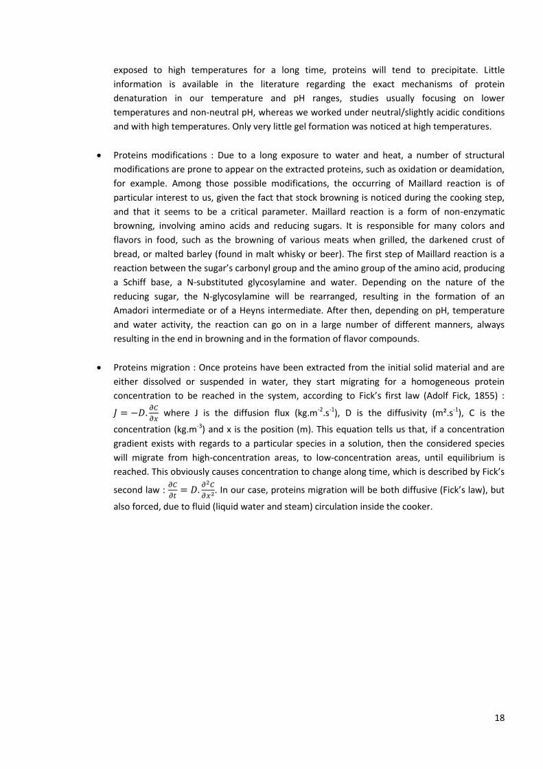
Cooking scraped mixed bones and meat scraps in the pressure cooker at 130°C, 110°C and 90°C

with at least two replicates for each temperature, and measuring colour and protein

concentration for each sample. The results obtained from these final runs would help us build a

model at INRA during my last two months in Clermont-Ferrand. The obtained samples would be

kept at AgResearch for further analysis to be conducted after my departure.

The first two runs that I conducted respectively consisted in meat (rump steak) and mixed bones

(100 % bone material) cooked in test tubes (4g of raw material and 8g of water) plunged in an 85°C water

bath (technical restrictions made it impossible to reach 90°C in a water bath). For each measurement point,

three test tubes were taken out of the water bath and plunged in ice in order to stop any ongoing

reactions. The purpose of these experiments was to be able to witness the colour evolution of the stock at

all time (which would be impossible in the cooker) and to highlight a tendency in the extraction kinetics,

while getting used to the concentration measurement method, which needs training to master. The

obtained results showed that there was almost no extraction occurring when cooking meat at this

temperature, but that 85°C was enough to extract proteins from bones. However, the extraction was slow

and even if we suspect that a maximal concentration was reached at some point between 6h end 23h, we

could not be absolutely sure of it, since we lacked measurement points between these two times as it can

be seen on the chart below :

Fig. 3 : Meat and mixed bones cooking in an 85°C water bath : protein concentration (Cuisson de viande maigre et d’os mélangés dans un bain-marie à 85°C : concentration en protéines)

Regarding colour evolution, no browning was observed at this temperature for either kind of raw material.

At this point, we concluded that the amount of extractible proteins was higher in bone material than in

meat, but the cause of Maillard reaction was still unknown to us, even though our first assumption was that

0

2

4

6

8

10

12

14

16

0 200 400 600 800 1000 1200 1400 1600

Protein concentration (g/L)

Cooking time (min)

Meat and mixed bones cooking in an 85°C water bath

Meat

Mixed bones

22

meat was responsible for it. Indeed, sugars are necessary for Maillard reaction to occur and, bones

containing very little of it (mainly in glycoproteins and proteoglycans, whose proportions are very low), we

did not think bone sugar by itself could be the main cause of Maillard reaction.

Following theses preliminary experiments, three runs were performed at 130°C in the pressure

cooker (respectively beef rump steak, scraps, and scraped mixed bones). The chosen sampling times were 5

min, 15 min, 30 min, 1h, 2h, 4h, 6h and 8h. However, at this point a mixing defect in the pressure cooker

was noticed (see Part IV ; 1) and it took us one week to fix it. Consequently, I was running out of time and I

was not able to carry out all the runs that we had originally planned, especially given the fact that the

results that I got from the first three runs in the cooker were mostly useless due to the bad mixing.

Therefore, I was able to collect results from runs performed on scraped mixed bones and scraps at

130°C, 110°C and 90°C, as planned, but I did not have enough time for any more replicates. Indeed, as each

run takes a full working day worth of time to perform, and cleaning the cooker to have it ready for the next

run is also time consuming, we lost approximately two weeks at this point, which would normally have

been enough time to repeat every run. I did have enough time to perform one last run, though, using

scraped leg bones at 130°C to check the behavior difference between the two types of bone material. For

these final seven runs, the chosen sampling times were 5 min, 30 min, 1h, 1h30, 2h, 2h30, 3h, 4h, 5h, 6h,

8h and 10h.

III ; 2/ Analysis methods

The analysis methods we used to collect our results will be described in this part of the report. During

my stay in Lincoln, I personally performed analysis regarding colour and protein concentration

measurement. Mass spectrometry and amino acid analysis were performed by AgResearch’s researchers

after my departure.

Colour measurement

Colour measurement was performed thanks to a UV spectrophotometer (Thermo Scientific

Evolution 220). For each measurement, 1 mL of solution was collected with an Eppendorf 0.5 mL pipette

and put in a cuvette. The solution was scanned with the following parameters being applied :

Wavelength range : 250 nm – 700 nm

Integration time : 0.2 s

Wavelength step : 2 nm

Scanning speed : 600 nm/min

Bandwidth : 2 nm

Once the scan was over, a transmittance spectrum was obtained. The spectrum was imported in VisionLite

ColorCalc (colour measurement software) for CIELAB (D65/2) values to be calculated. CIELAB is a color

space specified by the International Commission on Illumination (in French, Commission Internationale de

l'Eclairage, hence its CIE initialism). It describes all the colors visible to the human eye and was created to

serve as a device-independent model to be used as a reference. The three coordinates of CIELAB represent

the lightness of the color (L* = 0 yields black and L* = 100 indicates diffuse white), its position between

red/magenta and green (a* varies between -128 and +127, negative values indicate green while positive

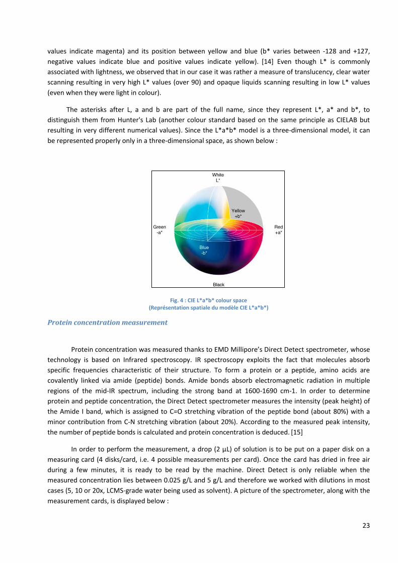
23

values indicate magenta) and its position between yellow and blue (b* varies between -128 and +127,

negative values indicate blue and positive values indicate yellow). [14] Even though L* is commonly

associated with lightness, we observed that in our case it was rather a measure of translucency, clear water

scanning resulting in very high L* values (over 90) and opaque liquids scanning resulting in low L* values

(even when they were light in colour).

The asterisks after L, a and b are part of the full name, since they represent L*, a* and b*, to

distinguish them from Hunter's Lab (another colour standard based on the same principle as CIELAB but

resulting in very different numerical values). Since the L*a*b* model is a three-dimensional model, it can

be represented properly only in a three-dimensional space, as shown below :

Fig. 4 : CIE L*a*b* colour space (Représentation spatiale du modèle CIE L*a*b*)

Protein concentration measurement

Protein concentration was measured thanks to EMD Millipore’s Direct Detect spectrometer, whose

technology is based on Infrared spectroscopy. IR spectroscopy exploits the fact that molecules absorb

specific frequencies characteristic of their structure. To form a protein or a peptide, amino acids are

covalently linked via amide (peptide) bonds. Amide bonds absorb electromagnetic radiation in multiple

regions of the mid-IR spectrum, including the strong band at 1600-1690 cm-1. In order to determine

protein and peptide concentration, the Direct Detect spectrometer measures the intensity (peak height) of

the Amide I band, which is assigned to C=O stretching vibration of the peptide bond (about 80%) with a

minor contribution from C-N stretching vibration (about 20%). According to the measured peak intensity,

the number of peptide bonds is calculated and protein concentration is deduced. [15]

In order to perform the measurement, a drop (2 µL) of solution is to be put on a paper disk on a

measuring card (4 disks/card, i.e. 4 possible measurements per card). Once the card has dried in free air

during a few minutes, it is ready to be read by the machine. Direct Detect is only reliable when the

measured concentration lies between 0.025 g/L and 5 g/L and therefore we worked with dilutions in most

cases (5, 10 or 20x, LCMS-grade water being used as solvent). A picture of the spectrometer, along with the

measurement cards, is displayed below :

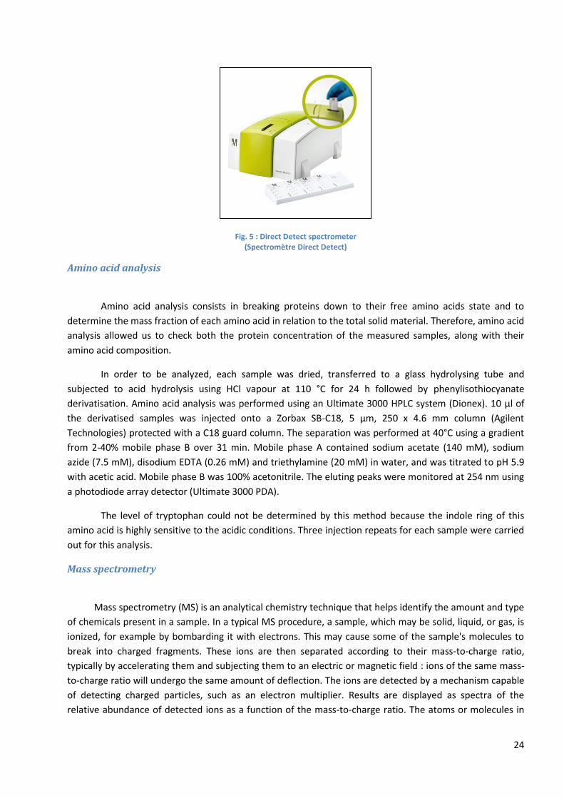
24

Fig. 5 : Direct Detect spectrometer (Spectromètre Direct Detect)

Amino acid analysis

Amino acid analysis consists in breaking proteins down to their free amino acids state and to

determine the mass fraction of each amino acid in relation to the total solid material. Therefore, amino acid

analysis allowed us to check both the protein concentration of the measured samples, along with their

amino acid composition.

In order to be analyzed, each sample was dried, transferred to a glass hydrolysing tube and

subjected to acid hydrolysis using HCl vapour at 110 °C for 24 h followed by phenylisothiocyanate

derivatisation. Amino acid analysis was performed using an Ultimate 3000 HPLC system (Dionex). 10 µl of

the derivatised samples was injected onto a Zorbax SB-C18, 5 μm, 250 x 4.6 mm column (Agilent

Technologies) protected with a C18 guard column. The separation was performed at 40°C using a gradient

from 2-40% mobile phase B over 31 min. Mobile phase A contained sodium acetate (140 mM), sodium

azide (7.5 mM), disodium EDTA (0.26 mM) and triethylamine (20 mM) in water, and was titrated to pH 5.9

with acetic acid. Mobile phase B was 100% acetonitrile. The eluting peaks were monitored at 254 nm using

a photodiode array detector (Ultimate 3000 PDA).

The level of tryptophan could not be determined by this method because the indole ring of this

amino acid is highly sensitive to the acidic conditions. Three injection repeats for each sample were carried

out for this analysis.

Mass spectrometry

Mass spectrometry (MS) is an analytical chemistry technique that helps identify the amount and type

of chemicals present in a sample. In a typical MS procedure, a sample, which may be solid, liquid, or gas, is

ionized, for example by bombarding it with electrons. This may cause some of the sample's molecules to

break into charged fragments. These ions are then separated according to their mass-to-charge ratio,

typically by accelerating them and subjecting them to an electric or magnetic field : ions of the same mass-

to-charge ratio will undergo the same amount of deflection. The ions are detected by a mechanism capable

of detecting charged particles, such as an electron multiplier. Results are displayed as spectra of the

relative abundance of detected ions as a function of the mass-to-charge ratio. The atoms or molecules in

25

the sample can be identified by correlating known masses to the identified masses or through a

characteristic fragmentation pattern. [16]

In our case, preliminary trypsin digestion was necessary for samples to be analyzed. Trypsin mostly

cuts proteins at lysine and arginine, resulting in 5-30 AA long peptides. Each peptide which is taken into

consideration by the measure is then related to its “mother protein” and modification scores can also be

calculated. In our case, we looked for amino-acid modifications regarding oxidation, nitration,

kynurenine/hydroxykynurenine, deamidation, dehydroalanine, dehydration and Maillard products. Each

modification can only affect certain amino acids and each score is actually a percentage representing the

number of amino acids bearing a modification in relation to the number of amino acids which could have

born it. For example, only asparagine and glutamine are concerned by deamidation and therefore,

deamidation score is calculated by dividing the number of deamidated Asn and Gln by the total number of

Asn and Gln.

Each sample was prepared as follows :

In order to precipitate the proteins, 100 µL of liquid sample was mixed with 400 µL of

methanol, 100 µL of chloroform and 300µL of water. The mix was then centrifuged for 1 min at

14000 rpm, resulting in the formation of 2 phases : an aqueous layer on top and an organic

layer at the bottom, proteins sitting between the two phases. After the aqueous layer was

removed, 400 µL of methanol was once again added, the mix was centrifuged at 14000 rpm for

2 min, methanol was removed and the sample was dried under a fume hood.

Proteins were resuspended via the addition of 100 µL of 50 mM Ammonium bicarbonate and

20 µL of 50 mM TCEP (tris(2-carboxyethyl)phosphine). The mix was incubated for 1h at room

temperature and alkylated with 20 µL of 150 mM iodoacetamide. Trypsin digestion was then

performed thanks to the addition of 10 µL of trypsin aliquots and 14 µL of CAN, before the

sample was incubated at 37°C for 18h and dried.

The dried protein digests were resuspended in 100 µl of 0.1% formic acid and diluted 3 times

prior to LC-MS/MS.

LC-MS/MS was performed on a nanoAdvance UPLC coupled to an amaZon speed ETD mass

spectrometer equipped with a CaptiveSpray source (Bruker Daltonik). 5 μL of sample was loaded on a

C18AQ nano trap (Bruker, 75 μm x 2 cm, C18AQ, 3 μm particles, 200 Å pore size). The trap column was then

switched in line with the analytical column (Bruker Magic C18AQ, 100 μm x 15 cm C18AQ, 3 μm particles,

200 Å pore size). The column oven temperature was 50 °C. Elution was with a gradient from 0-25% B in 65

min, to 35% B in 75 min, total 90 min at a flow rate of 800 nl/min. Solvent A was LCMS-grade water with

0.1% FA and 1% ACN; solvent B was LCMS-grade ACN with 0.1% FA and 1% water. Samples were measured

in auto MS/MS mode, with a mass range of m/z 350-1200. One MS was followed by 10 MS/MS of the most

intense ions.

Raw LC-MS/MS data files were processed using Bruker DataAnalysis 4.2 to produce peaklists. These

peaklists, after import into ProteinScape 3.1 (Bruker), were analysed using iterative proteomic search

strategies, involving protein identification and modification searching with the Mascot search engine

(Matrix Science). All searches used semitrypsin as the enzyme, allowing up to 1 missed cleavage (i.e.

accepting peptides that have up to one internal lysine or arginine, which would normally be broken under

100% digestion efficiency), with a monoisotopic peptide tolerance of 0.1 Da and an MS/MS tolerance of 0.3

Da. Instrument specificity was electrospray ion trap. The database was Uniprot, taxonomy Bos taurus.

26

Following iterative searching, proteins and peptides were compiled into master lists for each replicate, and

exported to Excel. An in-house developed collection of Visual Basic scripts was then used to further analyse

the occurrence and frequency of the different modifications in relation to the total observed occurrence of

each amino acid. The scores thus calculated allow simple comparison of samples.

III ; 3/ Experimental raw material preparation

Beef mixed bones and leg bones were bought at Lincoln supermarket and frozen at -25°C. While

frozen, they were roughly cut in cubes of about 3x3x3 cm3 and put back in the freezer until further use.

They were then unfrozen and kept in an ice box at low temperature while bone material and beef scraps

were separated, using a kitchen knife and a scalpel. Scraped bones were packed in plastic bags (about 500

g/bag) and scraps in others (500 g/bag as well). In the case of leg bones, yellow marrow was also removed

and put aside. This scraping step helped me to have a better understanding of the kind of raw material that

was used for the process. The data I obtained is displayed in the table below, and I used some of it to build

the tables that were given in part II ; 1 (tables 1 and 2 giving, the raw material composition).

Table 4 : Experimental raw material composition (Composition de la matière première utilisée en laboratoire)

Scraps were cut into thin slices with a kitchen knife and clean bones were crushed using

AgResearch workshop’s equipment, as shown below :

Bone material type Mixed bones Leg bones

Total treated mass (g) 7206 3132

Bone material mass (g) 3298 2257

Scraps mass (g) 3908 378

Yellow marrow mass (g) 0 497

Bone material % 45,8% 72,1%

Scraps % 54,2% 12,1%

Yellow marrow % 0,0% 15,9%

27

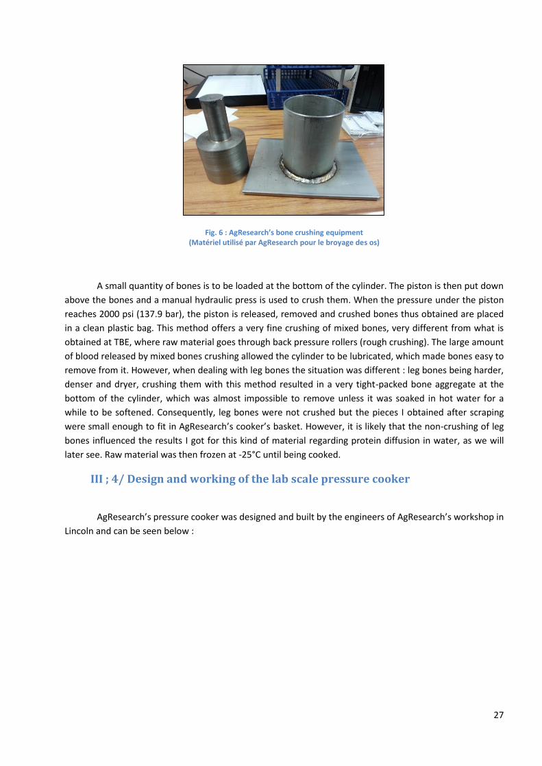
Fig. 6 : AgResearch’s bone crushing equipment (Matériel utilisé par AgResearch pour le broyage des os)

A small quantity of bones is to be loaded at the bottom of the cylinder. The piston is then put down

above the bones and a manual hydraulic press is used to crush them. When the pressure under the piston

reaches 2000 psi (137.9 bar), the piston is released, removed and crushed bones thus obtained are placed

in a clean plastic bag. This method offers a very fine crushing of mixed bones, very different from what is

obtained at TBE, where raw material goes through back pressure rollers (rough crushing). The large amount

of blood released by mixed bones crushing allowed the cylinder to be lubricated, which made bones easy to

remove from it. However, when dealing with leg bones the situation was different : leg bones being harder,

denser and dryer, crushing them with this method resulted in a very tight-packed bone aggregate at the

bottom of the cylinder, which was almost impossible to remove unless it was soaked in hot water for a

while to be softened. Consequently, leg bones were not crushed but the pieces I obtained after scraping

were small enough to fit in AgResearch’s cooker’s basket. However, it is likely that the non-crushing of leg

bones influenced the results I got for this kind of material regarding protein diffusion in water, as we will

later see. Raw material was then frozen at -25°C until being cooked.

III ; 4/ Design and working of the lab scale pressure cooker

AgResearch’s pressure cooker was designed and built by the engineers of AgResearch’s workshop in

Lincoln and can be seen below :

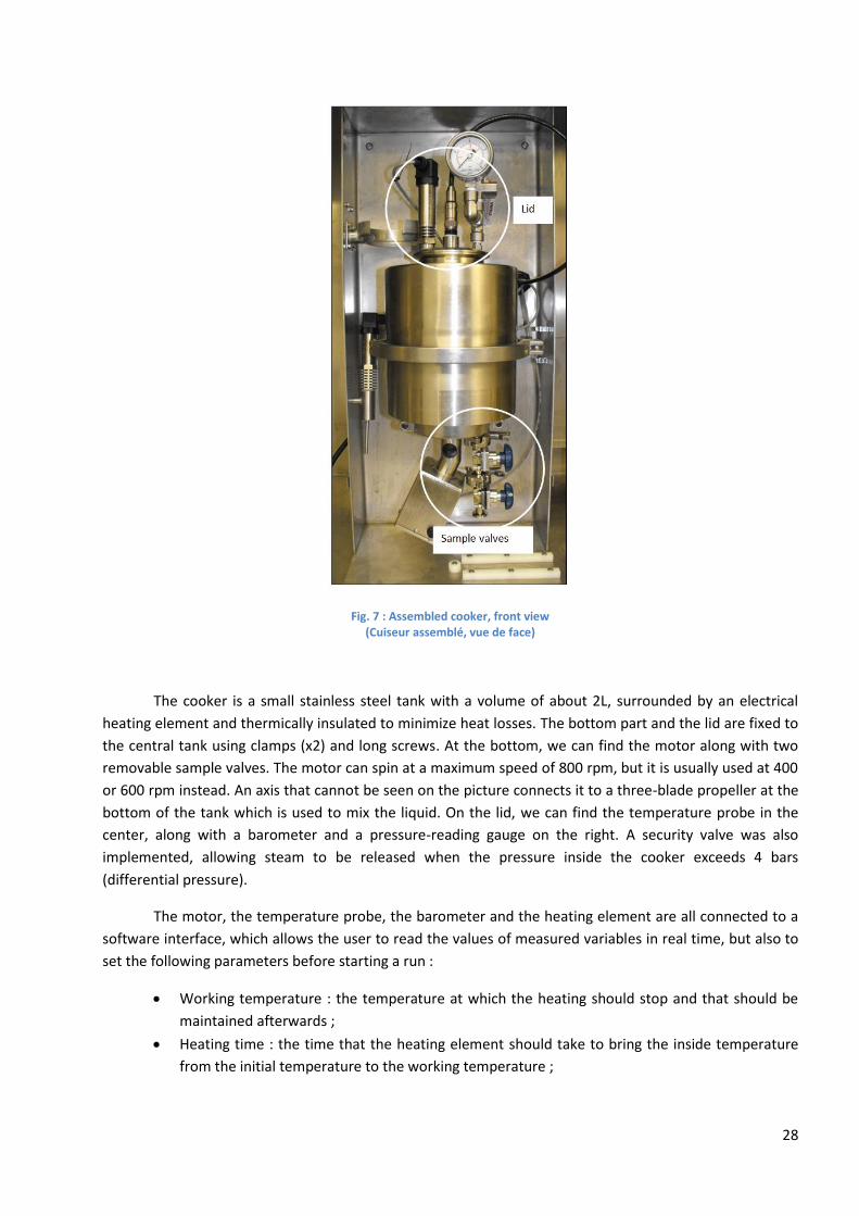
28

Fig. 7 : Assembled cooker, front view (Cuiseur assemblé, vue de face)

The cooker is a small stainless steel tank with a volume of about 2L, surrounded by an electrical

heating element and thermically insulated to minimize heat losses. The bottom part and the lid are fixed to

the central tank using clamps (x2) and long screws. At the bottom, we can find the motor along with two

removable sample valves. The motor can spin at a maximum speed of 800 rpm, but it is usually used at 400

or 600 rpm instead. An axis that cannot be seen on the picture connects it to a three-blade propeller at the

bottom of the tank which is used to mix the liquid. On the lid, we can find the temperature probe in the

center, along with a barometer and a pressure-reading gauge on the right. A security valve was also

implemented, allowing steam to be released when the pressure inside the cooker exceeds 4 bars

(differential pressure).

The motor, the temperature probe, the barometer and the heating element are all connected to a

software interface, which allows the user to read the values of measured variables in real time, but also to

set the following parameters before starting a run :

Working temperature : the temperature at which the heating should stop and that should be

maintained afterwards ;

Heating time : the time that the heating element should take to bring the inside temperature

from the initial temperature to the working temperature ;

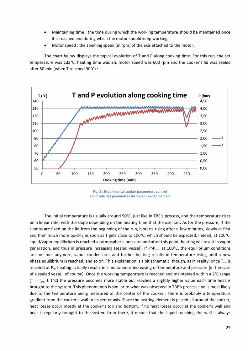
29

Maintaining time : the time during which the working temperature should be maintained once

it is reached and during which the motor should keep working ;

Motor speed : the spinning speed (in rpm) of the axis attached to the motor.

The chart below displays the typical evolution of T and P along cooking time. For this run, the set

temperature was 132°C, heating time was 2h, motor speed was 600 rpm and the cooker’s lid was sealed

after 50 min (when T reached 90°C) :

Fig. 8 : Experimental cooker parameters control (Contrôle des paramètres du cuiseur expérimental)

The initial temperature is usually around 50°C, just like in TBE’s process, and the temperature rises

on a linear rate, with the slope depending on the heating time that the user set. As for the pressure, if the

clamps are fixed on the lid from the beginning of the run, it starts rising after a few minutes, slowly at first

and then much more quickly as soon as T gets close to 100°C, which should be expected. Indeed, at 100°C,

liquid/vapor equilibrium is reached at atmospheric pressure and after this point, heating will result in vapor

generation, and thus in pressure increasing (sealed vessel). If P>Patm at 100°C, the equilibrium conditions

are not met anymore, vapor condensates and further heating results in temperature rising until a new

phase equilibrium is reached, and so on. This explanation is a bit schematic, though, as in reality, once Tsat is

reached at P0, heating actually results in simultaneous increasing of temperature and pressure (in the case

of a sealed vessel, of course). Once the working temperature is reached and maintained within a 2°C range

(T = Tset ± 1°C) the pressure becomes more stable but reaches a slightly higher value each time heat is

brought to the system. This phenomenon is similar to what was observed in TBE’s process and is most likely

due to the temperature being measured at the center of the cooker : there is probably a temperature

gradient from the cooker’s wall to its center axis. Since the heating element is placed all around the cooker,

heat losses occur mostly at the cooker’s top and bottom. If no heat losses occur at the cooker’s wall and

heat is regularly brought to the system from there, it means that the liquid touching the wall is always

0,00

0,50

1,00

1,50

2,00

2,50

3,00

3,50

4,00

4,50

50

60

70

80

90

100

110

120

130

140

0 50 100 150 200 250 300 350 400 450

P (bar) T (°C)

Cooking time (min)

T and P evolution along cooking time

T

P

30

boiling, resulting in vapor generation and pressure increasing, the barometer being moreover placed on the

external part of the lid (see fig. 7). The heat flux being lower during the maintaining step than during the

heating step, this could explain why the pressure rising rate decreases after 2h of cooking. This is also

corroborated by the fact that the pressure measured when Tset is reached is higher than what the vapor

pressure should be at this temperature and by the fact that the pressure starts rising before T reaches

100°C as explained earlier. Lastly, like in TBE’s process, if the pressure inside the cooker exceeds 4 bars, a

security valve opens and some of the pressure is released, as it can be seen on the chart (t = 430 min).

The following pictures display the visual aspect and the geometry of both the cooker’s tank and the

cooking basket.

Fig. 9 : Empty cooker, top view (Cuiseur vide, vue de dessus)

Fig. 10 : Cooker with basket, top view (Cuiseur avec panier, vue de dessus)

Fig. 11 : Cooking basket, side view (Panier de cuisson, vue de côté)

Fig. 12 : Cooking basket, bottom view (Panier de cuisson, vue de dessous)

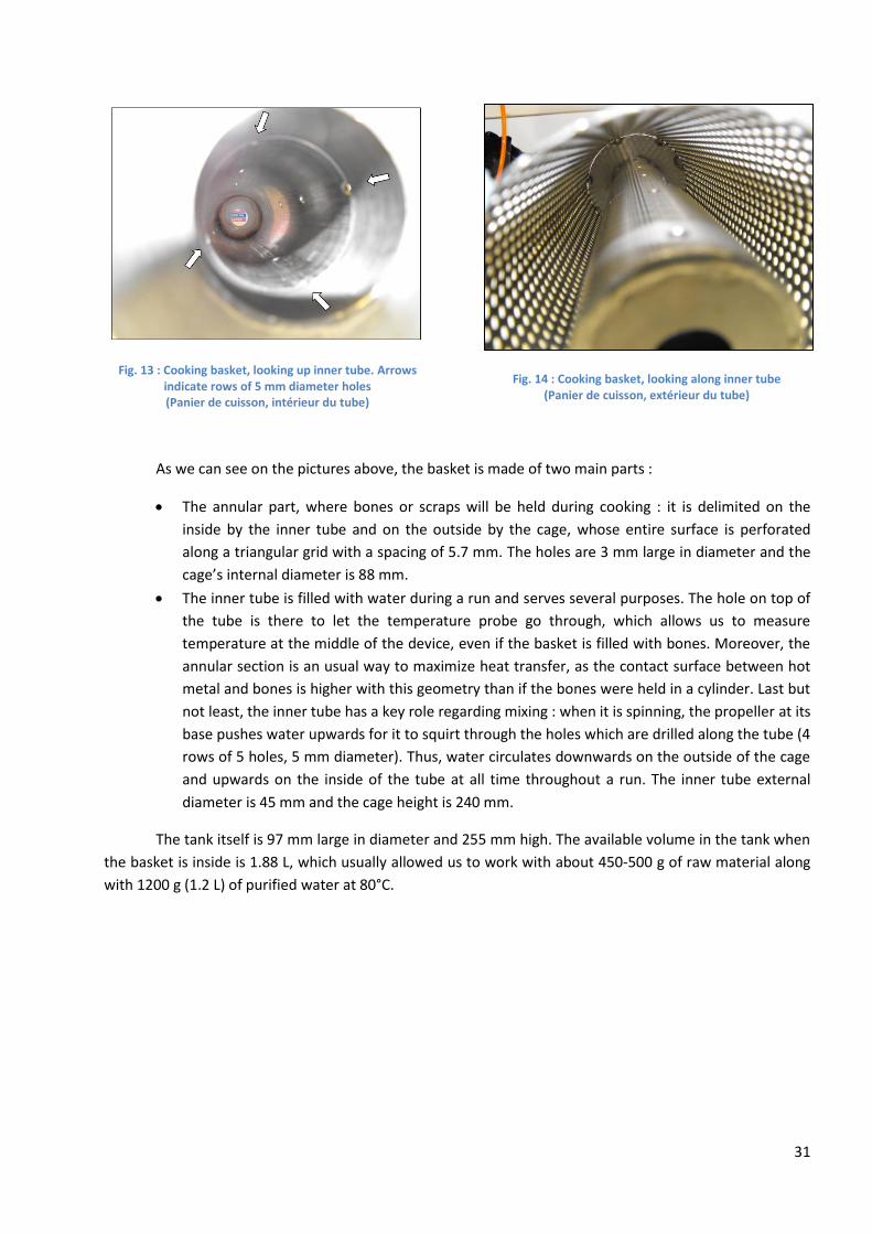
31

Fig. 13 : Cooking basket, looking up inner tube. Arrows indicate rows of 5 mm diameter holes (Panier de cuisson, intérieur du tube)

Fig. 14 : Cooking basket, looking along inner tube (Panier de cuisson, extérieur du tube)

As we can see on the pictures above, the basket is made of two main parts :

The annular part, where bones or scraps will be held during cooking : it is delimited on the

inside by the inner tube and on the outside by the cage, whose entire surface is perforated

along a triangular grid with a spacing of 5.7 mm. The holes are 3 mm large in diameter and the

cage’s internal diameter is 88 mm.

The inner tube is filled with water during a run and serves several purposes. The hole on top of

the tube is there to let the temperature probe go through, which allows us to measure

temperature at the middle of the device, even if the basket is filled with bones. Moreover, the

annular section is an usual way to maximize heat transfer, as the contact surface between hot

metal and bones is higher with this geometry than if the bones were held in a cylinder. Last but

not least, the inner tube has a key role regarding mixing : when it is spinning, the propeller at its

base pushes water upwards for it to squirt through the holes which are drilled along the tube (4

rows of 5 holes, 5 mm diameter). Thus, water circulates downwards on the outside of the cage

and upwards on the inside of the tube at all time throughout a run. The inner tube external

diameter is 45 mm and the cage height is 240 mm.

The tank itself is 97 mm large in diameter and 255 mm high. The available volume in the tank when

the basket is inside is 1.88 L, which usually allowed us to work with about 450-500 g of raw material along

with 1200 g (1.2 L) of purified water at 80°C.

32

IV/ Results, analysis and discussion

IV ; 1/ Modification of the experimental set-up

As it was mentioned in part III ; 1 ; 2, three first runs were performed in the pressure cooker once

the early trends regarding colour and protein concentration had been observed thanks to the experiments

in the water bath. These three runs consisted in :

508 g of beef meat (rump steak) cooked at 132°C in 1000 g of purified water.

501 g of scraps (meat, fat and connective tissues) cooked at 132°C in 1200 g of purified water.

455 g of crushed mixed bones (bone material only, with a non-negligible quantity of blood)

cooked at 132°C in 1210g of purified water.

For each of these runs, the initial temperature was about 50°C and the heating time (time needed to reach

the set temperature) was 1h. The motor was spinning at 400 rpm. During cooking, samples of 10-15 mL

were taken from the bottom of the cooker at the following time points : 5 min, 15 min, 30 min, 1h, 2h, 4h,

6h and 8h. All the collected samples were then analyzed regarding colour (L*a*b* standard) and protein

concentration.

IV ; 1 ; 1/ Beef meat and scraps early results : first two runs in AgResearch’s

pressure cooker

Colour evolution

The following charts display the results that were obtained regarding colour evolution (L*a*b*

standard) along cooking time for beef rump steak and mixed bones scraps cooked at 132°C :

0

20

40

60

80

100

0 100 200 300 400 500

L*

Cooking time (min)

Beef meat cooking at 132°C : L*

0

20

40

60

80

100

0 100 200 300 400 500

L*

Cooking time (min)

Scraps cooking at 132°C : L*

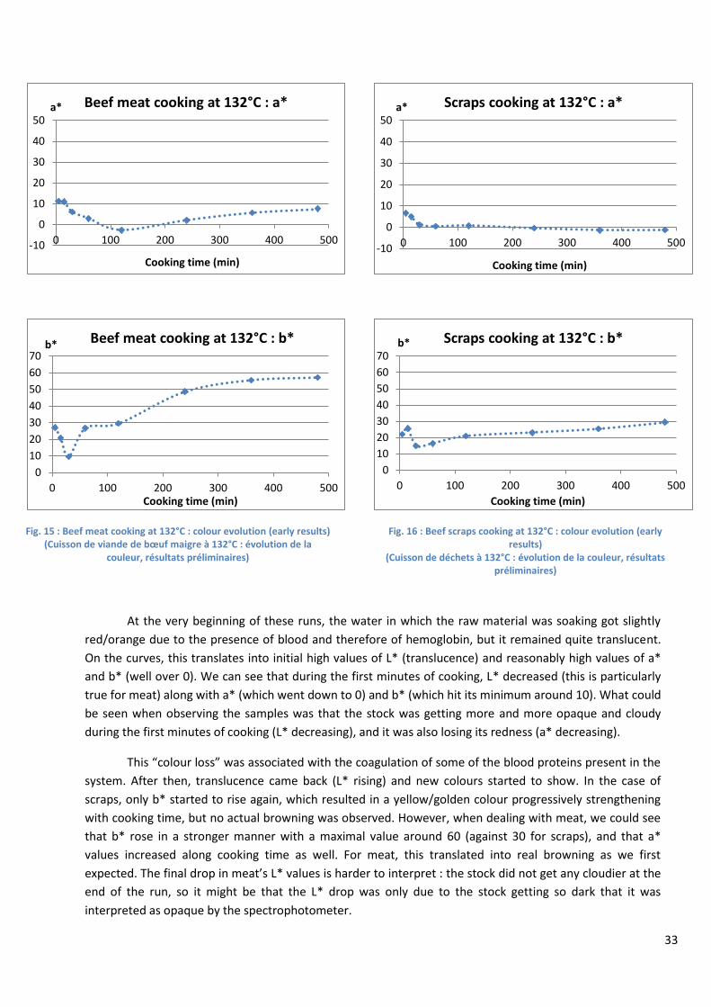
33

Fig. 15 : Beef meat cooking at 132°C : colour evolution (early results) (Cuisson de viande de bœuf maigre à 132°C : évolution de la

couleur, résultats préliminaires)

Fig. 16 : Beef scraps cooking at 132°C : colour evolution (early results)

(Cuisson de déchets à 132°C : évolution de la couleur, résultats préliminaires)

At the very beginning of these runs, the water in which the raw material was soaking got slightly

red/orange due to the presence of blood and therefore of hemoglobin, but it remained quite translucent.

On the curves, this translates into initial high values of L* (translucence) and reasonably high values of a*

and b* (well over 0). We can see that during the first minutes of cooking, L* decreased (this is particularly

true for meat) along with a* (which went down to 0) and b* (which hit its minimum around 10). What could

be seen when observing the samples was that the stock was getting more and more opaque and cloudy

during the first minutes of cooking (L* decreasing), and it was also losing its redness (a* decreasing).

This “colour loss” was associated with the coagulation of some of the blood proteins present in the

system. After then, translucence came back (L* rising) and new colours started to show. In the case of

scraps, only b* started to rise again, which resulted in a yellow/golden colour progressively strengthening

with cooking time, but no actual browning was observed. However, when dealing with meat, we could see

that b* rose in a stronger manner with a maximal value around 60 (against 30 for scraps), and that a*

values increased along cooking time as well. For meat, this translated into real browning as we first

expected. The final drop in meat’s L* values is harder to interpret : the stock did not get any cloudier at the

end of the run, so it might be that the L* drop was only due to the stock getting so dark that it was

interpreted as opaque by the spectrophotometer.

-10

0

10

20

30

40

50

0 100 200 300 400 500

a*

Cooking time (min)

Beef meat cooking at 132°C : a*

-10

0

10

20

30

40

50

0 100 200 300 400 500

a*

Cooking time (min)

Scraps cooking at 132°C : a*

0

10

20

30

40

50

60

70

0 100 200 300 400 500

b*

Cooking time (min)

Beef meat cooking at 132°C : b*

0

10

20

30

40

50

60

70

0 100 200 300 400 500

b*

Cooking time (min)

Scraps cooking at 132°C : b*

34

What can be deduced from these results is that, in our case, it is very likely that Maillard reaction is

occurring when these three trends are observed simultaneously :

a* increases,

b* increases,

L* first increases and then starts slowly decreasing after a while.

However, even if we saw Maillard browning occurring when cooking lean meat as we expected, we cannot

be sure that we witnessed any of it when dealing with scraps (see fig. 16 : no a rising, final colour closer to

yellow than to brown). This struck us as odd at first, as we knew that browning occurred during the actual

TBE process, which involves scraps and not lean meat. The only explanation to make sense was that bones

were actually the main cause of browning, which was unexpected, their sugar content being very low and

most likely insufficient.

Protein concentration evolution

The charts below display the results we obtained regarding protein concentration evolution along

cooking time for beef rump steak and mixed bones scraps cooked at 132 °C :

Fig. 17 : Beef meat cooking at 132°C : protein concentration evolution (early results)

(Cuisson de viande de bœuf maigre à 132°C : évolution de la concentration en protéines, résultats préliminaires)

Fig. 18 : Beef scraps cooking at 132°C : protein concentration evolution (early results)

(Cuisson de déchets à 132°C : évolution de la concentration en protéines, résultats préliminaires)

Like what was observed for colour evolution, we can see that the results obtained at 132°C strongly

diverged from those obtained at 85°C (see part III ; 1 ; 2). The extraction kinetics varied from one kind of

material to the other, as the maximal concentration (about 15-16 g/L) was reached after 4h of cooking for

beef scraps, whereas the curve obtained from meat cooking seems to keep on rising even after 8h, most

likely tending towards a value in the 20 g/L range. At first, it can seem surprising that the maximal values

should be so close, given the fact that scraps apparently contained a much lower proportion of muscle (and

thus of proteins) than lean meat. However, the figures given online by the United Nations [8] state that

beef lean meat contains 75 % of water, 22 % of proteins and 2 % of fat, whereas beef scraps contain only 55

% of water for 16.5 % of proteins and 28 % of fat. Thus, the protein content of lean meat and scraps are

0

5

10

15

20

25

0 100 200 300 400 500

Concentration (g/L)

Cooking time (min)

Beef meat cooking at 132°C

0

5

10

15

20

25

0 100 200 300 400 500

Concentration (g/L)

Cooking time (min)

Scraps cooking at 132°C

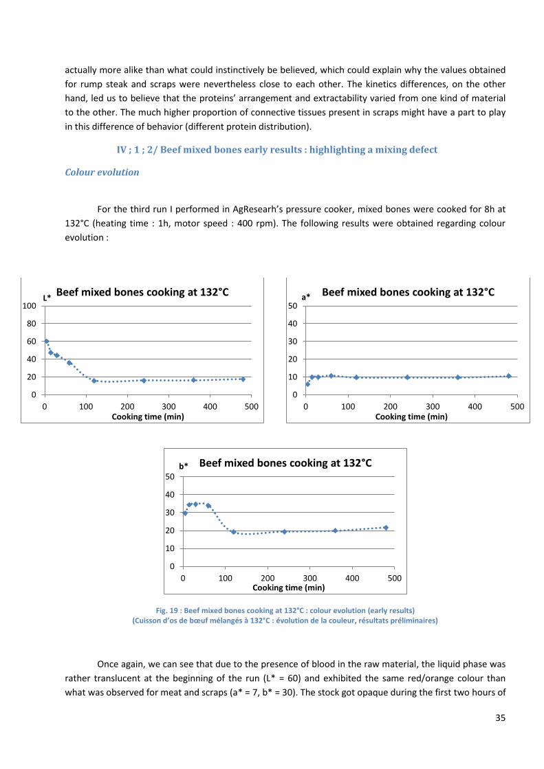
35

actually more alike than what could instinctively be believed, which could explain why the values obtained

for rump steak and scraps were nevertheless close to each other. The kinetics differences, on the other

hand, led us to believe that the proteins’ arrangement and extractability varied from one kind of material

to the other. The much higher proportion of connective tissues present in scraps might have a part to play

in this difference of behavior (different protein distribution).

IV ; 1 ; 2/ Beef mixed bones early results : highlighting a mixing defect

Colour evolution

For the third run I performed in AgResearh’s pressure cooker, mixed bones were cooked for 8h at

132°C (heating time : 1h, motor speed : 400 rpm). The following results were obtained regarding colour

evolution :

Fig. 19 : Beef mixed bones cooking at 132°C : colour evolution (early results) (Cuisson d’os de bœuf mélangés à 132°C : évolution de la couleur, résultats préliminaires)

Once again, we can see that due to the presence of blood in the raw material, the liquid phase was

rather translucent at the beginning of the run (L* = 60) and exhibited the same red/orange colour than

what was observed for meat and scraps (a* = 7, b* = 30). The stock got opaque during the first two hours of

0

20

40

60

80

100

0 100 200 300 400 500

L*

Cooking time (min)

Beef mixed bones cooking at 132°C

0

10

20

30

40

50

0 100 200 300 400 500

a*

Cooking time (min)

Beef mixed bones cooking at 132°C

0

10

20

30

40

50

0 100 200 300 400 500

b*

Cooking time (min)

Beef mixed bones cooking at 132°C

36

cooking, whereas a stabilized around 10 and b* dropped and stabilized around 20. Therefore, the stock was

cloudy, opaque and slightly yellow after 2h of cooking, after when samples’ colour did not evolve anymore.

Protein concentration evolution

The chart below displays the results we obtained regarding protein concentration evolution along

cooking time for beef mixed bones at 132 °C :

Fig. 20 : Beef mixed bones cooking at 132°C : protein concentration evolution (early results) (Cuisson d’os de bœuf mélangés à 132°C : évolution de la concentration en protéines, résultats préliminaires)

We can see that protein concentration rose slowly at first along a linear rate and then more quickly

along what looks like first-order kinetics. The maximal concentration (around 100 g/L) was reached after

about 4h of cooking. However, a simple calculation tells us that this results is most likely to be inconsistent :

𝑚𝑏,𝑖 = 455 𝑔, the initial mass of bones

𝑉 = 1.2 𝐿, the volume of stock

𝑚𝑝,𝑖 = 0.168 ∗ 𝑚𝑏,𝑖 = 76.44 𝑔, the estimated mass of proteins in the raw material (see Table 1)

𝑚𝑝,𝑒 = 𝐶𝑚𝑎𝑥. 𝑉 = 121 𝑔, the mass of extracted proteins, according to the results

Thus, the measured concentration tells us that there are more proteins in the solution at the end of the run

that what was available at first, which is simply impossible. Moreover, when I emptied the tank to clean it

on the day following this run, I realized that the stock inside it was a deep dark brown, completely different

from the cloudy and slightly yellow liquid I had seen when collecting samples. When all the stock was

removed from the tank, I also realized that a thin layer of gel was coating the bottom pat of the cooker,

0

20

40

60

80

100

120

0 50 100 150 200 250 300 350 400 450 500

Concentration (g/L)

Cooking time (min)

Beef mixed bones cooking at 132°C

37

which led us to believe that the cooker wasn’t mixing properly and that layering was occurring although we

should have had a homogeneous mix. Therefore, the gel was collected and added back to the stock,

everything was mixed together and a sample of this mix was taken and analyzed. The results of these last

measurements were very different from the 8h sample’s :

Variable\Sample 8h (taken from cooker’s bottom) Next day

L* 17.5 29.0

a* 10.5 23.5

b* 21.6 44.2

Protein concentration 103.8 g/L 53.8 g/L

The looks of the stock, along with the high values of a* and b*, led us to believe that Maillard

reaction occurred during the cooking step, even though we were not expecting it coming from bones. What

we deduced then is that the bones themselves were not responsible for it, but rather the blood that they

contained, which naturally contains the necessary sugar. The picture below displays the various stocks that

we had obtained so far :

Fig. 21 : From left to right : scraps stock, lean meat stock and mixed bones stock after cooling, 8h mixed bones gel (early runs) (De gauche à droite : bouillons obtenus à partir de déchets, de viande maigre, et d’os mélangés après refroidissement, gel

obtenu à partir d’os mélangés après 8h de cuisson (runs préliminaires)

IV ; 1 ; 3/ Improving the pressure cooker

We think that this mixing problem could especially occur when collagen was involved, which is why

we did not notice it during the first two runs. Indeed, when collagen is extracted from bones, what happens

at first is that a gel is formed (this is the principle of gelatin fabrication processes), and we think that it was

too heavy to circulate correctly in the cooker and that it was simply sitting at its bottom instead. This would

explain why the samples’ concentrations were so high and why we could not witness any colour change

along cooking time, as samples were taken from the bottom of the tank. The first idea we had to quickly

solve this issue was to create a new sampling point on the side of the tank to be able to sample actual

stock, but this would have required drilling through the heating element and furthermore this would not

really have solved the bad mixing problem.

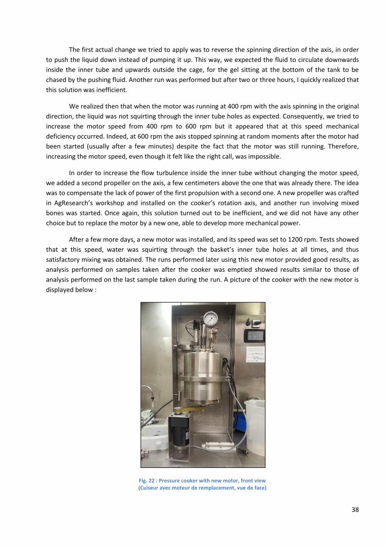
38

The first actual change we tried to apply was to reverse the spinning direction of the axis, in order

to push the liquid down instead of pumping it up. This way, we expected the fluid to circulate downwards

inside the inner tube and upwards outside the cage, for the gel sitting at the bottom of the tank to be

chased by the pushing fluid. Another run was performed but after two or three hours, I quickly realized that

this solution was inefficient.

We realized then that when the motor was running at 400 rpm with the axis spinning in the original

direction, the liquid was not squirting through the inner tube holes as expected. Consequently, we tried to

increase the motor speed from 400 rpm to 600 rpm but it appeared that at this speed mechanical

deficiency occurred. Indeed, at 600 rpm the axis stopped spinning at random moments after the motor had

been started (usually after a few minutes) despite the fact that the motor was still running. Therefore,

increasing the motor speed, even though it felt like the right call, was impossible.

In order to increase the flow turbulence inside the inner tube without changing the motor speed,

we added a second propeller on the axis, a few centimeters above the one that was already there. The idea

was to compensate the lack of power of the first propulsion with a second one. A new propeller was crafted

in AgResearch’s workshop and installed on the cooker’s rotation axis, and another run involving mixed

bones was started. Once again, this solution turned out to be inefficient, and we did not have any other

choice but to replace the motor by a new one, able to develop more mechanical power.

After a few more days, a new motor was installed, and its speed was set to 1200 rpm. Tests showed

that at this speed, water was squirting through the basket’s inner tube holes at all times, and thus

satisfactory mixing was obtained. The runs performed later using this new motor provided good results, as

analysis performed on samples taken after the cooker was emptied showed results similar to those of

analysis performed on the last sample taken during the run. A picture of the cooker with the new motor is

displayed below :

Fig. 22 : Pressure cooker with new motor, front view (Cuiseur avec moteur de remplacement, vue de face)

39

IV ; 2/ Measurement uncertainties

On top of the usual measurement uncertainties that are inherent in every measuring device

(regarding precision, number of significant digits…), there is a number of other potential causes of

measurement errors or limitations that need to be kept in mind when dealing with the results we obtained

during this project. This is what will be discussed in this part.

IV ; 2 ; 1/ Colour measurement

The colour measurement method that we used consisted in measuring the transmittance spectrum

of a 1.5 mL stock sample, before importing this spectrum in a software that calculated L*a*b* values from

it. Therefore, the uncertainties on the spectrum itself are mainly due to the device, but the way the

software calculates L*a*b* values is unknown to us. It is likely that some errors may occur at this point as

well.

Moreover, quantifying the aspect of a liquid sample is not an easy task, as colour itself is not the

only observable parameter : among others, we can mention translucence or shininess, for example. In our

case, we can only work with three variables which, if we take each of them separately, do not have a clear

meaning. Colour is a combination of these three values and different sets of L*a*b* can sometimes result

in similar colours, and conversely, similar L*a*b* values may be obtained from samples that have different

aspects. What is important to understand here is that the measured quantities regarding the evolution of

stock aspect are far from being exhaustive, and that the results we obtained must be interpreted with

caution : pictures are still the best way to give an idea of an object’s aspect, but they do not allow any

modeling. For that matter, we will see that even if the L*a*b* evolution of the stock makes sense when put

in relation with the actual samples’ colour, the curves sometimes had peculiar behaviors and for this

reason, colour evolution will not be included in the model. However, colour measurement allowed us to

highlight some tendencies, which is already good enough.

Last but not least, even though the curves’ main tendencies made sense, we realized that when

entering the obtained L*a*b* values in a colour calculator, the results were often different from what was

actually observed, which incites to even more caution. This is probably due to the fact that other

parameters interfered with the colour measurement. For example, in the L*a*b* standard L* is the value

commonly related to lightness (with 0 resulting in black and 100 resulting in white). However in our case,

we associated L* with translucence : the measure of a colourless liquid (pure water for example) resulted in

very high L* values (between 90 and 100) even though water is clearly not white. On the other hand, when

measuring very cloudy and opaque samples, we usually obtained low L* values (around 10-20) even when

the measured samples showed a light colour and were clearly nothing near black. Thus, relating L* to

translucence rather than to lightness is our interpretation of the measure, but when typing a low L* value

into a colour calculator, the result will always be a dark colour, which makes colour measurement even

harder to interpret.

In other words, we can say that the data about colour given in this report should be taken more as

semi-quantitative data : the trends make sense when interpreted correctly but the absolute values rarely fit

the classic L*a*b* standard, which is also why no modeling will be done regarding colour evolution.

40

IV ; 2 ; 2/ Protein concentration measurement

The Direct Detect machine counts the number of peptide bonds that are present in one drop of

solution (2 µL). This is an extremely small quantity of liquid and, therefore, the possibility of measuring a

“non-representative drop” exists, on top of the fact that the user has to be extremely precise when

applying the solution drop on the measuring card. This is corroborated by the fact that, from one drop to

the other of the same solution, the results could vary significantly : for this reason, some points required

about 8 or 10 measurements before an agreeable value was reached. Moreover, the machine we used only

gives reliable results when the sample concentration lies between 0.025 g/L and 5 g/L. Therefore, we

worked with dilutions for most samples (in most cases 10x or 20x dilutions). This means that the dilution

quality can also be a cause of uncertainty, and that the more diluted a sample is, the stronger the

uncertainty will be. Given the fact that the more critical points lie at the end of the curves (as we expect a

constant concentration to be reached) and that the last samples were the most protein-rich and thus the

ones we needed to dilute the most, it was sometimes quite hard to obtain consistent results. Lastly,

AgResearch’s researchers know from past experience that collagen is one of the most complicated proteins

to work with. When measuring concentrations thanks to the Direct Detect machine, it often happens that

the presence of collagen in the measured sample interferes with the results. Collagen being expected to be

one of the main proteins in the system, this might be another cause of uncertainty. Therefore, in order to

diminish these uncertainties, amino acid analysis were carried out on some of the obtained samples. This

kind of analysis gives a more precise and reliable result, but is extremely time-consuming. For this reason,

only a few samples were analyzed this way, in order to verify a number of critical values.

Direct Detect measurement uncertainties were calculated using results obtained from mixed bones

runs at 85/90°C and at 130/132°C. Significant behavior differences were noticed between the two sets of

results and, therefore, two typical uncertainties were calculated : we used the first one for the 90°C results

and the second one for the 110/130°C results.

In order to calculate the “low temperature” uncertainty, results from the following experiments

were taken into account :

Mixed bones cooked in a 85°C water bath (see part III ; 1 ; 2) ;

Mixed bones cooked at 90°C in the pressure cooker (two runs).

For the first 90°C run I performed in the pressure cooker, bones were cooked for 10h and samples were

collected on a regular basis. However, no final value appeared to be reached and consequently another run

was carried out with samples being taken after 10h, 20h and 24h of cooking. Similar protein concentration

values were obtained for these three time points and therefore, we deduced that 10h was the necessary

cooking time for the final protein concentration to be reached at 90°C : any value obtained after 10h of

cooking or more would be used for uncertainty measurement. For the second run at 90°C, crushed bones

had been preliminary washed and therefore no blood was present in the raw material for this run. The

values we obtained after 23h of cooking at 85°C varied in the same range than the ones obtained at 90°C,

and the average values were close (around 12 g/L), which led us to believe that variations in cooking

method/temperature had little influence on the results (in this temperature range). However, as we have

just mentioned it, concentration variations were observed among values obtained in the same working

conditions (between 8.2 g/L and 15.4 g/L). Therefore, we deduced that uncertainties were mainly due to

raw material preparation and sampling (initial composition, crushing, cutting…). The facts that the results

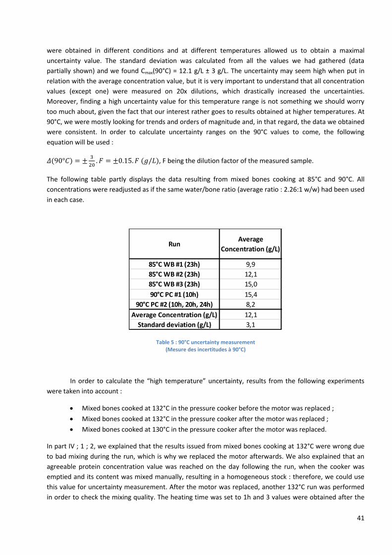
41

were obtained in different conditions and at different temperatures allowed us to obtain a maximal

uncertainty value. The standard deviation was calculated from all the values we had gathered (data

partially shown) and we found Cmax(90°C) = 12.1 g/L ± 3 g/L. The uncertainty may seem high when put in

relation with the average concentration value, but it is very important to understand that all concentration

values (except one) were measured on 20x dilutions, which drastically increased the uncertainties.

Moreover, finding a high uncertainty value for this temperature range is not something we should worry

too much about, given the fact that our interest rather goes to results obtained at higher temperatures. At

90°C, we were mostly looking for trends and orders of magnitude and, in that regard, the data we obtained

were consistent. In order to calculate uncertainty ranges on the 90°C values to come, the following

equation will be used :

𝛥(90°𝐶) = ±3

20. 𝐹 = ±0.15. 𝐹 (𝑔/𝐿), F being the dilution factor of the measured sample.

The following table partly displays the data resulting from mixed bones cooking at 85°C and 90°C. All

concentrations were readjusted as if the same water/bone ratio (average ratio : 2.26:1 w/w) had been used

in each case.

Table 5 : 90°C uncertainty measurement (Mesure des incertitudes à 90°C)

In order to calculate the “high temperature” uncertainty, results from the following experiments

were taken into account :

Mixed bones cooked at 132°C in the pressure cooker before the motor was replaced ;

Mixed bones cooked at 132°C in the pressure cooker after the motor was replaced ;

Mixed bones cooked at 130°C in the pressure cooker after the motor was replaced.

In part IV ; 1 ; 2, we explained that the results issued from mixed bones cooking at 132°C were wrong due

to bad mixing during the run, which is why we replaced the motor afterwards. We also explained that an

agreeable protein concentration value was reached on the day following the run, when the cooker was

emptied and its content was mixed manually, resulting in a homogeneous stock : therefore, we could use

this value for uncertainty measurement. After the motor was replaced, another 132°C run was performed

in order to check the mixing quality. The heating time was set to 1h and 3 values were obtained after the

RunAverage

Concentration (g/L)

85°C WB #1 (23h) 9,9

85°C WB #2 (23h) 12,1

85°C WB #3 (23h) 15,0

90°C PC #1 (10h) 15,4

90°C PC #2 (10h, 20h, 24h) 8,2

Average Concentration (g/L) 12,1

Standard deviation (g/L) 3,1

42

final concentration was reached (4h, 6h, 8h). Satisfactory mixing having been obtained, the final set of

experiments was carried out and mixed bones were cooked once again, this time at 130°C with heating

time set to 2h. 2 values were obtained after the final concentration was reached for this run (6h, 8h). Once

again, the temperature difference was too low to lead to significant variations and uncertainties seemed to

be mostly due to raw material preparation and sampling. The standard deviation was calculated from all

the values we had gathered (data partially shown) and we found Cmax(130°C) = 51.1 g/L ± 2 g/L. This time,

the absolute uncertainty represents less than 5 % of the average value, which is very satisfactory, especially

given the fact that, once again, we worked with 20x dilutions. In order to calculate uncertainty ranges for

the 110°C/130°C values to come, the following equation will be used :

𝛥(130°𝐶) = ±2

20. 𝐹 = ±0.1. 𝐹 (𝑔/𝐿), F being the dilution factor of the measured sample.

The following table partly displays the data resulting from mixed bones cooking at 130°C and 132°C. All

concentrations were readjusted as if the same water/bone ratio (average ratio : 2.67:1 w/w) had been used

in each case.

Table 6 : 110°C/130°C uncertainty measurement (Mesure des incertitudes à 110°C/130°C)

We can see that runs carried out at high temperatures were better mastered than those performed

at lower temperatures. This implies that the effects of the solid matter’s network structure and porosity

(due to the way it was crushed and then arranged in the cooker) shade off as cooking temperature

increases. The reasons for these behavior differences will be explained later.

IV ; 3/ Final experimental results

After the cooker was improved and satisfactory mixing was finally obtained, a total of 7 runs were

performed :

Crushed mixed bones (scraps removed) at 90°C, 110°C and 130°C,

Beef scraps from mixed bones at 90°C, 110°C and 130°C,

Uncrushed leg bones (scraps and marrow removed) at 130°C.

RunAverage

Concentration (g/L)

132°C PC #1 (next day) 53,5

132°C PC #2 (4h, 6h, 8h) 50,4

130°C PC #1 (6h, 8h) 49,4

Average Concentration (g/L) 51,1

Standard deviation (g/L) 2,1

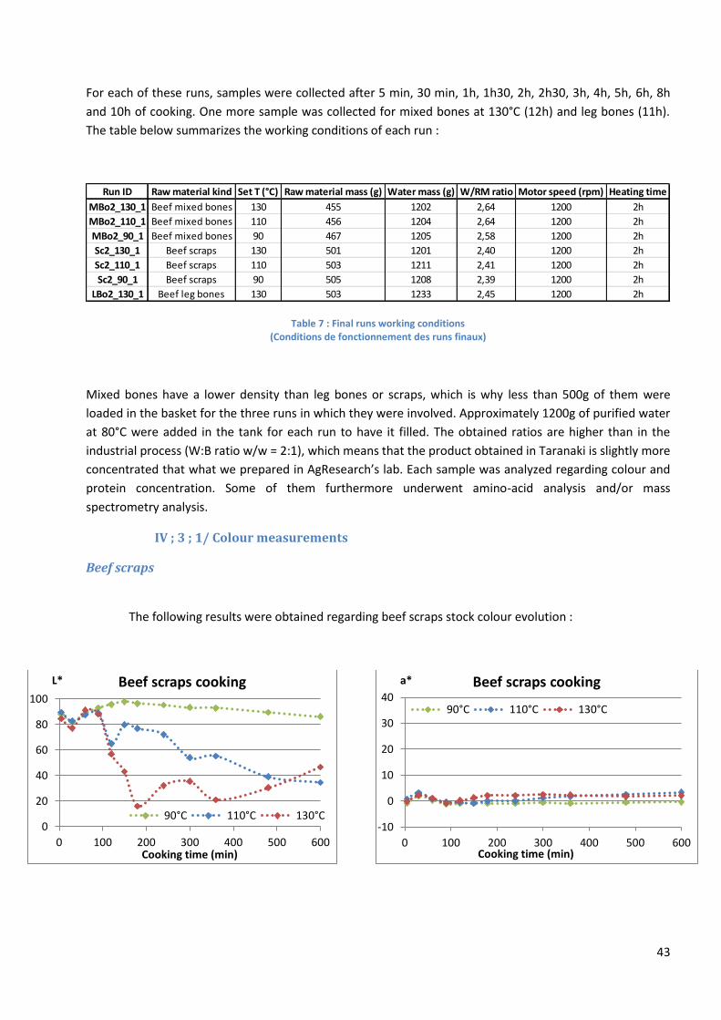
43

For each of these runs, samples were collected after 5 min, 30 min, 1h, 1h30, 2h, 2h30, 3h, 4h, 5h, 6h, 8h

and 10h of cooking. One more sample was collected for mixed bones at 130°C (12h) and leg bones (11h).

The table below summarizes the working conditions of each run :

Table 7 : Final runs working conditions (Conditions de fonctionnement des runs finaux)

Mixed bones have a lower density than leg bones or scraps, which is why less than 500g of them were

loaded in the basket for the three runs in which they were involved. Approximately 1200g of purified water

at 80°C were added in the tank for each run to have it filled. The obtained ratios are higher than in the

industrial process (W:B ratio w/w = 2:1), which means that the product obtained in Taranaki is slightly more

concentrated that what we prepared in AgResearch’s lab. Each sample was analyzed regarding colour and

protein concentration. Some of them furthermore underwent amino-acid analysis and/or mass

spectrometry analysis.

IV ; 3 ; 1/ Colour measurements

Beef scraps

The following results were obtained regarding beef scraps stock colour evolution :

Run ID Raw material kind Set T (°C) Raw material mass (g) Water mass (g) W/RM ratio Motor speed (rpm) Heating time

MBo2_130_1 Beef mixed bones 130 455 1202 2,64 1200 2h

MBo2_110_1 Beef mixed bones 110 456 1204 2,64 1200 2h

MBo2_90_1 Beef mixed bones 90 467 1205 2,58 1200 2h

Sc2_130_1 Beef scraps 130 501 1201 2,40 1200 2h

Sc2_110_1 Beef scraps 110 503 1211 2,41 1200 2h

Sc2_90_1 Beef scraps 90 505 1208 2,39 1200 2h

LBo2_130_1 Beef leg bones 130 503 1233 2,45 1200 2h

0

20

40

60

80

100

0 100 200 300 400 500 600

L*

Cooking time (min)

Beef scraps cooking

90°C 110°C 130°C-10

0

10

20

30

40

0 100 200 300 400 500 600

a*

Cooking time (min)

Beef scraps cooking

90°C 110°C 130°C

44

Fig. 23 : Beef scraps cooking : colour evolution (final results) (Cuisson de déchets : évolution de la couleur, résultats finaux)

Pictures of all stock samples can be seen in Annex 1. The data that we obtained for scraps did not

reveal clear tendencies especially at 130°C where oscillations can be noticed for L* and b*, making the data

harder to interpret. However, at this temperature, the main tendencies seem to be :

L* decreased from a very high value (84.5) to much lower values (two minima were hit after

180 min (16.1) and after 360 min (21.1)) before it started to rise again. The first step of cooking

resulted in stock getting cloudy and opaque before translucence came back during the last 4

hours.

Due to the presence of hemoglobin in meat, b* values were reasonably high at the beginning of

the run (19 after 5 min, 22.9 after 30.9) before dropping to hit a minimum (4.4) after 90 min.

After then, b* oscillated between 4.4 and 16.5 from 90 min to 360 min, before it started to rise

significantly. Hence, colour disappeared during the first steps of cooking, before it started

appearing again, hesitantly at first and then in a stronger manner.

a* values stayed close to 0 during the whole run, which means that no redness was noticed at

any moment.

If we combine these three tendencies, it appears that the very clear and slightly coloured stock we had at

first (5 min) lost its colour (90 min) before getting opaque (180 min) and slightly yellow (360 min). After

then, translucence came back, and yellowness became stronger, until we obtained a yellow/golden stock

after 10h of cooking. At 130°C, the final result was similar to what was obtained in one of our previous runs

(see fig. 21 in part IV ; 1 ; 2). Most likely, no Maillard reaction occurred here, even at the highest operating

temperature. The results are quite different to what was measured in part IV ; 1 ; 2, but it is important to

keep in mind that these were obtained under different working conditions.

At 110°C, the main tendency is a continuous decreasing of L* along with a decreasing of b* in the

first place (from 30 min to 120 min). After 2h, b* started increasing until it stabilized between 15 and 16

(360 min) for the end of the run, which is in the range of b* oscillations at 130°C (between 4.4 and 16.5).

Lastly, a* values stayed close to 0 during the whole run, like what was observed at 130°C. It looks like at

110°C, The colour evolution matched the first steps of the 130°C run (between 0 min and 3h). The stock

obtained at the end of the run was cloudy and slightly yellow.

0

10

20

30

40

0 100 200 300 400 500 600

b*

Cooking time (min)

Beef scraps cooking

90°C 110°C 130°C

45

Finally, regarding the 90°C run, L* values remained very high (between 80 and 100), while a* values

remained close to 0. On the other hand, b* values decreased until a minimum was reached (150 min, b* =

2.9) like at 130°C and 110°C, after which it started rising again until the end of the run. The final result was

a clear and slightly yellow solution. No browning was observed for any of the three temperatures, which

confirms what we deduced from previous experiments : stock browning in TBE process most likely comes

from bones and not from scraps.

Beef leg bones

Only one run at 130°C was performed and the following results were obtained regarding beef leg

bones stock colour evolution :

Fig. 24 : Beef leg bones cooking at 130°C : colour evolution (final results) (Cuisson d’os de pattes de bœuf à 130°C : évolution de la couleur, résultats finaux)

Pictures of all stock samples can be seen in Annex 1. Once again, the initial L* value was very high

(5 min, L* = 93.9). It first decreased until it hit a minimum (240 min, L* = 32.2) and then it started rising

again. Initial a* values were close to 0 and a slightly increased throughout the run (600 min, a* = 6.3). The

values of b* also increased throughout the run, with slight oscillations, until it reached 30.4 after 660 min

(11h) of cooking. Due to the complete absence of hemoglobin here, the stock was colourless and extremely

0

20

40

60

80

100

0 100 200 300 400 500 600 700

L*

Cooking time (min)

Beef leg bones cooking

-10

0

10

20

30

40

0 100 200 300 400 500 600 700

a*

Cooking time (min)

Beef leg bones cooking

0

10

20

30

40

50

0 100 200 300 400 500 600 700

b*

Cooking time (min)

Beef leg bones cooking

46

clear at first, before it started getting cloudier and more strongly coloured. Some translucence came back

during the second part of the run, but the final result was an opaque stock whose colour tended towards

orange. The final values are in the same range than what was observed with scraps cooked at 130°C.

Therefore, no browning occurred for leg bones either and if it does in mixed bones again, it will not be due

to bone material in itself.

Beef mixed bones

The following results were obtained regarding beef mixed bones stock colour evolution :

Fig. 25 : Beef mixed bones cooking : colour evolution (final results) (Cuisson d’os de bœuf mélangés : évolution de la couleur, résultats finaux)

Pictures of all stock samples can be seen in Annex 1. At the beginning of the 130°C run, the stock

was translucent (L* = 54.8) and displayed a red/orange colour (a* = 13.7, b* = 30.5). During the first hours

of cooking, the stock progressively became cloudy and opaque (1h) before losing its colour until it reached

a “colour minimum” after 2h30 (L* = 9.5, a* = 4.6, b* = 9.7), resulting in an opaque whitish stock similar to

the samples we took during the first mixed bones run, before the motor was replaced (see part IV ; 1 ; 2).

Once this minimum was reached, Maillard browning started to appear, as L* increased and then decreased

0

20

40

60

80

100

0 200 400 600 800

L*

Cooking time (min)

Beef mixed bones cooking

90°C 110°C 130°C

0

10

20

30

40

50

0 200 400 600 800

a*

Cooking time (min)

Beef mixed bones cooking

90°C 110°C 130°C

0

20

40

60

80

0 200 400 600 800

b*

Cooking time (min)

Beef mixed bones cooking

90°C 110°C 130°C

47

and a* and b* increased. It seems that b* reached a maximum value after 12h (b* = 72), whereas it looks

like a* could have risen even higher if we had kept on cooking (a* = 30.7 after 12h).

Regarding the 110°C run, the same initial tendency was noticed even if it took longer for colour to

reach its minimum (which should be expected, as a higher temperature usually results in higher kinetics). At

110°C, the colour minimum was reached after 5h (300 min, L* = 9.9, a* = 6.6, b* = 11.2). After then, colour

and translucence started to reappear as L* and b* rose. However, L* did not start decreasing like at 130°C

which means that the stock never got as dark as it did then. Moreover, a* kept decreasing : the observed

tendency was no browning, but rather a “yellowing”/”goldening”. It is likely that Maillard reaction only

barely occurred (if it did at all) at 110°C. Lastly, regarding the 90°C run, we never got past the “opaque light

brown” step. Once again, the initial loss of translucence and colour was assimilated to hemoglobin

denaturation (due to heating), most likely resulting in its coagulation and aggregation.

Thus, if stocks obtained after long cooking times at 130°C were to be ordered from darker to

lighter, the ranking would be :

Beef mixed bones stock

Beef lean meat stock (see part IV ; 1 ; 2)

Beef scraps stock

Beef leg bones stock

It appears that colour strengthening and browning are related both to the kind of raw material and to the

working temperature. A higher temperature no doubt results in a darker stock, and blood is most likely a

major cause of colouring. However, it is very clear that significant colouration may occur without any blood

being present in the raw material (cf leg bones). Even though it seems highly likely that Maillard browning

occurred for mixed bones and lean meat cooked at 130°C, we cannot be sure that this was (or was not) the

case for the other runs. The only way we can have more accurate information is through a mass

spectrometry analysis, as a Maillard index can be calculated from the data it provides.

IV ; 3 ; 2/ Protein concentration measurements

Beef scraps

The following results were obtained regarding beef scraps stock protein concentration evolution :

48

Fig. 26 : Beef scraps cooking : protein concentration evolution (final results) (Cuisson de déchets : évolution de la concentration en protéines, résultats finaux)

The protein concentration was usually slightly above 0 g/L straight from the beginning of the run

(about 1 g/L after 5 min), no matter what the set temperature was. This is simply because some proteins

such as hemoglobin mixed with water inside the tank before cooking even started and therefore it mustn’t

be mistaken with the occurring of bone protein extraction. It appears that no extraction occurred at the

beginning of the run for either temperature, as it only started after 1.5h at 130°C and after 2h at 110°C (i.e.

when the cooker’s temperature reached 110°C in both cases, heating time having been set to 2h). Given

the fact that extraction barely occurred at 90°C (600 min, C = 2.39 g/L), we can affirm that a high

temperature is necessary for proteins to be extracted from scraps. Moreover, at 110°C, the system was in a

state of liquid-vapor equilibrium with P>Patm, which was not the case at 90°C. Given the fact that there is a

significant behavior difference between 90°C and 110°C (110°C and 130°C behaviors being quite similar),

we can also say that the state change inside the cooker (from liquid water to liquid-vapor equilibrium,

occurring from 100°C) had a significant part to play in the extraction’s efficiency.

Regarding the curves’ trends, the 130°C extraction clearly followed first order kinetics after it

started, whereas the 110°C trend is less obvious. Proteins migration was less efficient at 110°C in the first

hours following the actual extraction start (quite remote to an exponential behavior). On the other hand,

we can see that it did not take much longer for maximal concentration to be reached at 110°C (8h) than at

130°C (6h, maximal concentration also being higher when dealing with a higher temperature). We have

reasons to believe that the kinetics differences between the two runs in the 2h-5h range were mainly due

to migration issues.

Scraps initially contained quite a lot of fat and after the 90°C run, it looked like it had stayed

inside the cooking basket the whole time. Even though in our case fat was taken in a structured collagen

network (making it harder to melt than fat contained in marrow for example, which is in a free state and

melts within a few minutes when exposed to 90°C), it should have melted anyway within 10h of cooking.

0

5

10

15

20

25

0 100 200 300 400 500 600 700

Protein concentration (g/L)

Cooking time (min)

Beef scraps cooking

90°C

110°C

130°C

49

Therefore we deduced that the fat that we could see at the end of the 90°C run had probably melted, but

did not migrate in water and went back to its solid form when temperature decreased. Once again, we can

witness the importance of the state change in diffusion, as the difference between 90°C and 110°C was

obvious. Finally, there was less fat remaining on the scraps cooked at 130°C than on those cooked at 110°C

: along with what could be seen on the curves (fig. 26), this shows the influence of temperature on

diffusion, both for lipids and proteins. Pictures of cooked scraps can be seen in Annex 2.

Finally, the following table partly displays the evolution of T and P* (P* = P – Patm) inside the cooker

during the 110°C and 130°C runs :

Table 8 : Beef scraps cooking : T-P evolution (Cuisson de déchets : évolution de T et P)

If we refer to fig. 8 (part III ; 4), we can see that, as soon as the cooker’s lid is sealed, pressure starts

increasing inside the cooker, slowly at first and then much more quickly as soon as T exceeds 100°C. In the

case of the 110°C scraps run, the lid was sealed after 90 min of cooking (T = 94.5°C), which explains why P

hadn’t started increasing after 60 min. However, in the case of fig. 8, the cooker’s lid was also sealed at T =

90°C, but P reached 3 bar at T = 130°C, which is very similar to what we found when cooking mixed bones

at 130°C, although the lid was sealed from the start of the run (see later). This leads us to believe that the

lid-sealing timing has no influence on the final pressure. What can be seen in this table is that P only

increased by 0.56 bar at 110°C, whereas it increased by 2.56 bar (including about 1.6 bar in the 100°C-130°C

range) at 130°C. Therefore, we also believe that a higher pressure had a positive influence on the

extraction’s efficiency and, more precisely, that the significant pressure variation that occurred during the

130° run, along with the high temperature, the cutting in small pieces (improving solid/fluid contact and

therefore improving heat and mass transfer) and the state change allowed the curve’s first-order kinetics

shape to appear.

The mass of extracted proteins can be calculated by multiplying concentration and stock volume :

𝑚𝑝,𝑒𝑥𝑡 = 𝐶 ∗ 𝑉 = 𝐶 ∗𝑚𝑤𝑎𝑡𝑒𝑟

𝜌𝑤𝑎𝑡𝑒𝑟 with ρwater = 1000 kg/m3. Dividing this result by the initial raw material mass

gives us a yield, that can be refined if it is once again divided by the raw material’s protein proportion :

𝜂 =𝑚𝑝,𝑒𝑥𝑡

𝑚𝑖 with mi being the initial raw material mass (mass yield)

𝜂𝑝 =𝜂

𝑤𝑝 with wp being the mass fraction of proteins in the raw material (protein yield)

Initial mass values (for both raw material and water) were given in table 7 at the beginning of part IV ; 3 and

the protein content of scraps (16.5 %) was given in table 1 (part II ; 1). Therefore we can build the following

table :

T(°C) P* (bar) T (°C) P* (bar)

0 47,3 0 50,5 0

60 78,4 0 90,7 0,56

120 110 0,56 130 2,5

110°C run 130°C runCooking t (min)

50

Table 9 : Beef scraps cooking : achieved extraction yelds (final results) (Cuisson de déchets : rendements d’extraction obtenus, résultats finaux)

Beef leg bones

The following results were obtained regarding beef leg bones stock protein concentration evolution

at 130°C :

Fig. 27 : Beef leg bones cooking at 130°C : protein concentration evolution (final results) (Cuisson d’os de pattes de bœuf à 130°C : évolution de la concentration en protéines, résultats finaux)

The extraction started after 2h and protein concentration stabilized around 50 g/L after 8h of

cooking (the drop at 10h is probably nothing more than a measurement error). The curve does not quite fit

the first order kinetics typical curve as we will later see. As it has been explained in part III ; 3, I could not

crush leg bones using the material available at AgResearch and therefore the raw material I used for this

run consisted in uncrushed pieces of leg bones, bone marrow having previously been removed and put

aside. The following table partly displays the evolution of T and P inside the cooker during the first two

hours of cooking :

Cooking T (°C) 90 110 130

Cmax (g/L) 2,39 17,23 22,06

Extracted proteins (g) 2,89 20,87 26,49

ηmax 0,57% 4,15% 5,29%

ηp,max 3,47% 25,14% 32,05%

0

10

20

30

40

50

60

0 100 200 300 400 500 600 700

Protein concentration (g/L)

Cooking time (min)

Beef leg bones cooking

51

Table 10 : Beef leg bones cooking at 130°C : T-P evolution (Cuisson d’os de pattes de bœuf à 130°C : évolution de T et P)

Therefore, when the extraction started (after 2h), the state change had already taken place (T > 100°C) and

T and P had reached their maximal value or were sufficiently close to it (P kept on slightly rising

afterwards). This confirms that a state change and high temperature and pressure are necessary for

extraction to occur. However, this also confirms that a good crushing (improving contact between solid

material and heated fluid, therefore improving heat and mass transfers) is necessary for first-order kinetic

to appear which is not the case here (even if we seem to be closer to it than when cooking scraps at 110°C).

At the end of the run, the remaining bone pieces looked solid (see Annex 2) but were actually really easy to

break, proving that structural proteins had been extracted. Moreover, it seems that a limit concentration

value was reached, indicating that no extractible proteins were left in the bone material. There is a

possibility that a higher final concentration would have been reached if we had used crushed bones, as

more proteins would have been immediately available for extraction. Obviously, this hypothesis would

have to be checked by another experiment.

Regarding the values we obtained, we can see that we reached a much higher final concentration

than when dealing with scraps, even though the initial raw material masses were very similar (see table 5).

The protein mass fraction of leg bones (marrow removed) has been estimated to 26.5% and the following

table gathers data regarding extraction yield :

Table 11 : Beef leg bones cooking at 130°C : achieved extraction yields (final results) (Cuisson d’os de pattes de bœuf à 130°C : rendements d’extraction obtenus, résultats finaux)

Beef mixed bones

The following results were obtained regarding beef mixed bones stock protein concentration

evolution :

T(°C) P* (bar)

0 60,9 0

60 96,5 0,72

120 130 3,67

Cooking t (min)130°C run

Cooking T (°C) 130

Cmax (g/L) 48,89

Extracted proteins (g) 60,28

ηmax 11,99%

ηp,max 45,24%

52

Fig. 28 : Beef mixed bones cooking : protein concentration evolution (final results) (Cuisson d’os de bœuf mélangés : évolution de la concentration en protéines, résultats finaux)

What can be observed for mixed bones is that protein concentration rose along a more or less

linear rate at first, before first order kinetics were witnessed, as expected (110°C and 130°C). At 90°C, the

exponential behavior did not appear. This is very different from what was observed for scraps and leg

bones, where no extraction was witnessed before state change had occurred and sufficiently high

temperature and pressure were reached. Moreover, at 130°C a concentration drop could be observed at

the end of the run (after 8h of cooking). The reason for this drop is probably a very strong denaturation of

proteins, perhaps resulting in precipitation or in the destruction of a large number of peptide bonds. Since

the Direct Detect machine calculates the protein concentration by using the number of peptide bonds as an

input, this may be an explanation. It is also possible that extracted proteins got involved in chemical

reactions where peptide bonds were eliminated.

Our first interpretation was that the linear step was due to the fact that during the first two hours

of cooking the system was in a transitional state, as temperature was rising from 50°C to 90/110/130°C.

Therefore, we thought that the kinetics constant k could be varying with temperature (and time), resulting

in an apparent linear extraction during the first steps of cooking. However, the facts that no linear step was

observed when dealing with scraps and leg bones, and that protein extraction kept following a linear trend

after 2h at 90°C and 110°C (even though temperature was kept constant past this point) led us to believe

that this was not the right explanation. It has been mentioned before (see part IV ; 2 ; 2) that when cooking

mixed bones at 90°C, the final concentration was reached after 10h, which means that even if the 90°C run

had lasted longer, the extraction curve would have flattened. Moreover, bone pieces were kept whole and

hard after 10h of cooking at 90°C. When cooking uncrushed leg bones at 130°C, bone pieces were still

whole at the end of the run as well, but they were really easy to break which was not the case here, as

bone pieces were still very hard : this tends to show that, at 90°C, only a few structural proteins had been

extracted (see Annex 2). A second run was performed at 90°C with crushed mixed bones that were

preliminarily washed (blood thus removed) and a final protein concentration of about 7.5 g/L was reached,

with amino acid analysis revealing that almost 100% of extracted proteins were collagen (bone proteins).

0

10

20

30

40

50

60

0 100 200 300 400 500 600 700 800

Concentration (g/L)

Cooking time (min)

Mixed bones cooking : protein concentration

90°C

110°C

130°C

53

Therefore, we can say that the linear step is partly due to blood proteins migration, but also to the crushing

quality that made migration possible from the beginning of the run, which was not the case with the other

kinds of raw material.

The following table partly displays the evolution of T and P inside the cooker during the 110°C and

130°C runs :

Table 12 : Beef mixed bones cooking : T-P evolution (Cuisson d’os de bœuf mélangés : évolution de T et P)

Regarding the 130°C run, extraction (notwithstanding the preliminary linear step) started after 2h, when T

and P reached sufficiently high values (130°C, i.e. T maximal value for this run and 3.06 bar, P having kept

continuously increasing until it reached 3.93 bar). Therefore, the 130°C dynamics are, in this regard, in

agreement with what was previously observed for leg bones. However, the 110°C behavior is more

peculiar, as 3h were necessary for extraction to begin even though nothing changed inside the cooker

(regarding fluid state, pressure or temperature) between 2h and 3h.

Lastly, at the end of the 110°C and 130°C runs, bones had been reduced from whole pieces of

crushed bones to what looked like wet powder (probably mostly minerals, along with remaining proteins),

as it can be seen in Annex 2. This shows that, due to high pressure/temperature and to a fine crushing, heat

and mass transfer were optimized between solid material and heating fluid, resulting in the disintegration

of the collagen network, making proteins migration in water even easier : this resulted in curves fitting first-

order kinetics very well for these two temperatures, although the reasons for the 110°C delay are still

unknown to us. Moreover, extraction was much faster at 130°C than what was observed for leg bones,

once again proving the importance of an efficient pre-crushing.

The protein mass fraction of mixed bones has been estimated to 16.8% and the following table

gathers data regarding extraction yield. In order to solely focus on bone proteins in the yield calculation, we

introduced a new variable called η’max, which we calculated by subtracting 1.6 % to the ηmax values (1.6 %

being the fraction that we believe was due to blood proteins at 90°C, calculation not shown). Therefore, we

have 𝜂′𝑝,𝑚𝑎𝑥 =𝜂′𝑚𝑎𝑥

𝑤𝑝.

Table 13 : Beef mixed bones cooking : achieved extraction yields (final results) (Cuisson d’os de bœuf mélangés : rendements d’extraction obtenus, résultats finaux)

T(°C) P* (bar) T (°C) P* (bar)

0 32,3 0 48 0

60 72,3 0,33 89,2 0,55

120 110 1,5 130 3,06

110°C run 130°C runCooking t (min)

Cooking T (°C) 90 110 130

Cmax (g/L) 13,48 43,23 50,26

Extracted proteins (g) 16,24 52,05 60,41

ηmax 3,48% 11,43% 13,28%

η'max 1,88% 9,83% 11,68%

η'p,max 11,20% 58,50% 69,51%

54

The obtained extraction yields were very satisfactory, especially given the fact that no acid or alkali

treatments were applied at any point during the experiments. The 130°C yield was close to 70%, which is

lower than the 80% that were obtained for chicken bones cooked under similar conditions by Dong et al

(2014). [12] This is to be expected, as chicken collagen is known to display less crosslinks than beef collagen

(this was for example noticed in chicken skin), making chicken proteins easier to denaturate.

Looking at the gathered data, the following statements can be made :

High working temperature and pressure are necessary for protein extraction to be fast and

efficient, along with a state change as results obtained after a 90°C run were quite poor

(especially regarding scraps) compared to those obtained at 110°C or 130°C. The only kind of

material for which protein migration/extraction was witnessed at 90°C was mixed bones, but

half of those proteins did not come from bones. Indeed, mixed bones contained a non-

negligible amount of blood that was released during the crushing step : hence, the raw material

was coated with blood, whose proteins must have migrated in water from the start of the run

thanks to the cooker’s water circulation.

The state change is necessary as boiling water and steam most likely offer a much better heat

transfer than subcooled water, steam allowing the system to be better homogenized, resulting

in a better matter transfer. In a way, this reminds us of extraction processes involving

supercritic fluids (CO2 and, more recently, water), which are often extremely efficient. Even if,

in our case, we were far from reaching supercritic conditions, this is evidence that a change of

state can be the key to a far better process efficiency.

Actual extraction started appearing after a reasonably long cooking time at 110°C and 130°C for

every kind of raw material. The results that fitted first order kinetics the best were observed

when the raw material was reduced to small particles by the end of the run (mixed bones at

110°C and 130°C, scraps at 130°C). Leg bones were cooked at 130°C without having been

crushed before and the resulting extraction curve did not quite match first order kinetics either,

even though the conditions regarding state change, temperature and pressure were met.

Moreover, they remained whole (even though very easily breakable by hand) whereas crushed

mixed bones were reduced to powder. This shows that an increased contact surface between

cooked material and hot fluid (favored by crushing, among other things) allows a more efficient

extraction as, with first order kinetics, one will get close to the limit concentration value in a

shorter time. The presence of big pieces of solid material, limiting the contact area between

proteins and working fluid, appear to be a hindrance to heat and matter transfers. Kinetics will

be compared in a more accurate manner in part IV ; 4 ; 2.

IV ; 3 ; 3/ Amino acid analysis

55

The amino acid analysis consists in breaking a sample’s proteins down to their free amino acids

state and to determine the mass fraction of each amino acid in relation to the total solid material. Two

samples were analyzed :

- Mixed bones stock, cooked at 110°C for 10h ;

- Mixed bones stock, cooked at 130°C for 8h.

For these two samples, the final concentration had been reached and we think that amino-acid analysis will

give us information about the exact composition of the final bone extract at both temperatures. The

following results were obtained :

Table 14 : Amino acid analysis results (Résultats des analyses en acides aminés)

Amino acids represented 68.37 % of the solid material in the 110°C sample and 76.84 % of the solid

material in the 130°C sample (the rest most likely being constituted of minerals and maybe lipids), which

confirms that protein extraction is more efficient at a higher temperature. Moreover, solid bone material

Amino acidMolar fraction

(AA content)

Mass fraction

(dry matter)

Molar fraction

(AA content)

Mass fraction

(dry matter)

Aspartic Acid 4,29% 3,50% 5,01% 4,56%

Glutamic Acid 8,83% 7,96% 9,94% 10,01%

Serine 3,47% 2,23% 3,71% 2,67%

Glycine 30,04% 13,81% 28,60% 14,69%

Histidine 0,60% 0,57% 0,70% 0,74%

Arginine 4,67% 4,98% 4,54% 5,41%

Threonine 2,14% 1,56% 2,11% 1,72%

Alanine 9,83% 5,36% 10,91% 6,65%

Proline 12,32% 8,68% 11,30% 8,90%

Tyrosine 0,56% 0,62% 0,58% 0,72%

Valine 2,07% 1,49% 2,22% 1,78%

Lanthionine 0,00% 0,00% 0,01% 0,02%

Methionine 0,91% 0,83% 0,89% 0,90%

Cysteine 0,25% 0,19% 0,17% 0,14%

Isoleucine 0,52% 0,42% 0,53% 0,47%

Leucine 3,03% 2,43% 3,13% 2,81%

Phenylalanine 1,54% 1,55% 1,46% 1,65%

Lysine 1,93% 1,73% 2,41% 2,41%

Lysinoalanine 0,00% 0,00% 0,00% 0,00%

Hydroxyprolin 13,01% 8,68% 11,81% 8,68%

Proteins 68,37% 76,84%

Collagen 64,30% 64,31%

Mixed bones, 110°C, 10h Mixed bones, 130°C, 8h

56

being constituted of 65% of minerals and 35 % of proteins (among which 90 % is type I collagen), it seems

that proteins are more likely to be extracted at high temperatures than minerals.

We can see that the two amino acid profiles are extremely similar, the main amino acids being

glycine, proline, hydroxyproline (the three main constituents of collagen), alanine and glutamic acid. In its

free state, glutamic acid is responsible for a characteristic umami flavor and is sometimes used as a flavor

enhancer (E620). It is the most common amino acid in human alimentation. When it is a constituent of

proteins, glutamic acid is flavorless. [17]

The dry matter proportions were as follows : 5.40 % for the 110°C sample and 6.14 % for the 130°C

sample. If we consider the solution’s density to be 1000 kg/m3, we can track the protein concentration back

from the data shown in the previous table by using the following equation :

𝐶 = 𝑤𝑝,𝑑 ∗ 𝑤𝑑 ∗ 𝜌 where wp,d is the mass fraction of proteins in dry matter and wd is the dry matter

proportion.

Therefore, the concentrations we calculated via amino acid analysis are 36.9 g/L for the 110°C sample (10h

of cooking) and 47.3 g/L for the 130°C sample (8h of cooking), which is quite close to the values we

obtained using the Direct Detect spectrometer (43.2 g/L at 110°C and 50.3 g/L at 130°C). The collagen

proportion can be calculated thanks to the hydroxyproline peak, as hydroxyproline is believed to represent

13.5 % of the collagen protein. Therefore, dividing the Hyp proportion by 0.135 yields the collagen

proportion in the sample’s dry matter :

𝑤𝑐𝑜𝑙𝑙,𝑑(110°𝐶) =0.0868

0.135= 64.3 %

𝑤𝑐𝑜𝑙𝑙,𝑑(130°𝐶) =0.0868

0.135= 64.3 %

Dividing this result by the protein proportion in dry matter yields the collagen proportion in proteins :

𝑤𝑐𝑜𝑙𝑙,𝑝(110°𝐶) =0.643

0.684= 94.1 %

𝑤𝑐𝑜𝑙𝑙,𝑝(130°𝐶) =0.643

0.768= 83.7 %

For both samples, we can see that the collagen proportion in proteins is over 80 %, which is in

appropriateness to the protein composition of bones that was found in the literature (90% of collagen). The

collagen proportion is lower at 130°C, which could mean that at this temperature it is easier to extract non-

collagenic proteins. Due to a lack of time, we could not analyze more samples before the end of my

internship, but further analysis is being done at the moment.

IV ; 3 ; 4/ Mass spectrometry results

For the evaluation of peptide modifications, bioinformatic searches were conducted using a

combination of up to four of the target modifications listed in table 15 as variable amino acid modifications

at any given time.

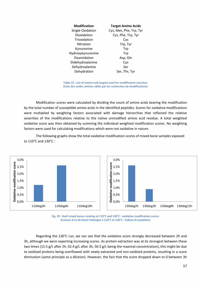
57

Modification Target Amino Acids Single Oxidation Cys, Met, Phe, Trp, Tyr

Dioxidation Cys, Phe, Trp, Tyr Trioxidation Cys

Nitration Trp, Tyr Kynurenine Trp

Hydroxykynurenine Trp Deamidation Asp, Gln

Didehydroalanine Cys Dehydroalanine Ser

Dehydration Ser, Thr, Tyr

Table 15 : List of amino acid targets used for modification searches (Liste des acides amines ciblés par les recherches de modifications)

Modification scores were calculated by dividing the count of amino acids bearing the modification

by the total number of susceptible amino acids in the identified peptides. Scores for oxidative modifications

were multiplied by weighting factors associated with damage hierarchies that reflected the relative

severities of the modifications relative to the native unmodified amino acid residue. A total weighted

oxidative score was then obtained by summing the individual weighted modification scores. No weighting

factors were used for calculating modifications which were not oxidative in nature.

The following graphs show the total oxidative modification scores of mixed bone samples exposed

to 110°C and 130°C :

Fig. 29 : Beef mixed bones cooking at 110°C and 130°C : oxidative modification scores (Cuisson d’os de bœuf mélangés à 110°C et 130°C : indices d’oxydation)

Regarding the 130°C run, we can see that the oxidative score strongly decreased between 2h and

3h, although we were expecting increasing scores. As protein extraction was at its strongest between these

two times (15.5 g/L after 2h, 42.4 g/L after 3h, 50.3 g/L being the maximal concentration), this might be due

to oxidized proteins being overflowed with newly extracted and non-oxidized proteins, resulting in a score

diminution (same principle as a dilution). However, the fact that the score dropped down to 0 between 3h

0,0%

0,5%

1,0%

1,5%

2,0%

2,5%

3,0%

110deg3h 110deg4h 110deg10h

Oxi

dat

ive

mo

dif

icat

ion

sco

re

0,0%

0,5%

1,0%

1,5%

2,0%

2,5%

3,0%

130deg2h 130deg3h 130deg8h 130deg12h

Oxi

dat

ive

mo

dif

icat

ion

sco

re

58

and 8h (idem at 110°C between 4h and 10h) seems odd to us. Several interpretations can be made : either

the fact that proteins were strongly denatured after a long heat exposure made it impossible for trypsin to

digest them (and therefore they do not appear in the final results), or the oxidative damage progressed to a

level too complex for our analysis to see. Morevoer, previous studies led at INRA on free meat amino acids

showed that tyrosine was extremely sensitive to oxidation, and that other amino acids were less likely to

get oxidized. [18] Tyrosine being present in only a minor proportion in each sample (0.6 %, see table 14),

this might also explain the low values of oxidative scores. The hypothesis of proteins precipitation (due to

strong denaturation) seems unlikely to us, as we witnessed a concentration drop after a long cooking time

only once, for mixed bones cooked at 130°C for more than 8h. However, score drops can also be noticed at

110°C, which does not relate to the results we obtained until now (see fig. 28).

The following results were obtained regarding the other modifications damage score for mixed

bones stock exposed to 110°C and 130°C :

Fig. 30 : Beef mixed bones cooking at 110°C and 130°C : other modifications scores (Cuisson d’os de bœuf mélangés à 110°C et 130°C : autres indices de dégâts)

The results regarding the other modifications scores seem more consistent, especially at 110°C,

where we can see that the score is rising throughout the run. This is also the case at 130°C, except at the

very end of the run (between 8h and 12h). Once again, this may be due to bad trypsin digestion or to

modifications getting too complex for the analysis to see. Either way, the modification kind we wanted to

have information about was the occurring of Maillard reaction but none of the usual Maillard-induced

modifications were picked up (data not shown). However, the modifications we looked for were related to

the very first steps of Maillard reaction (carboxymethyllysine, lactosylation of lysine and arginine) and there

is a possibility that after 2 or 3 hours of cooking, we had already gone past these modifications, making

them impossible to notice. Of course, this could also mean that we were wrong and that the browning we

observed was actually not due to Maillard reaction but this seems highly unlikely. Performing more

searches on samples taken after shorter times could be a way to check this.

All in all, we can say that, for now, the mass spectrometry results bring more questions than

answers. However, only a few samples were analyzed when this report was written, and we expect more

analysis to be done and more consistent results to be deduced from them in the future.

0,0%

1,0%

2,0%

3,0%

4,0%

5,0%

6,0%

7,0%

110deg3h 110deg4h 110deg10h

Oth

er

mo

dif

icat

ion

sco

re

0,0%

2,0%

4,0%

6,0%

8,0%

10,0%

12,0%

14,0%

130deg2h 130deg3h 130deg8h 130deg12h

Oth

er

mo

dif

icat

ion

sco

re

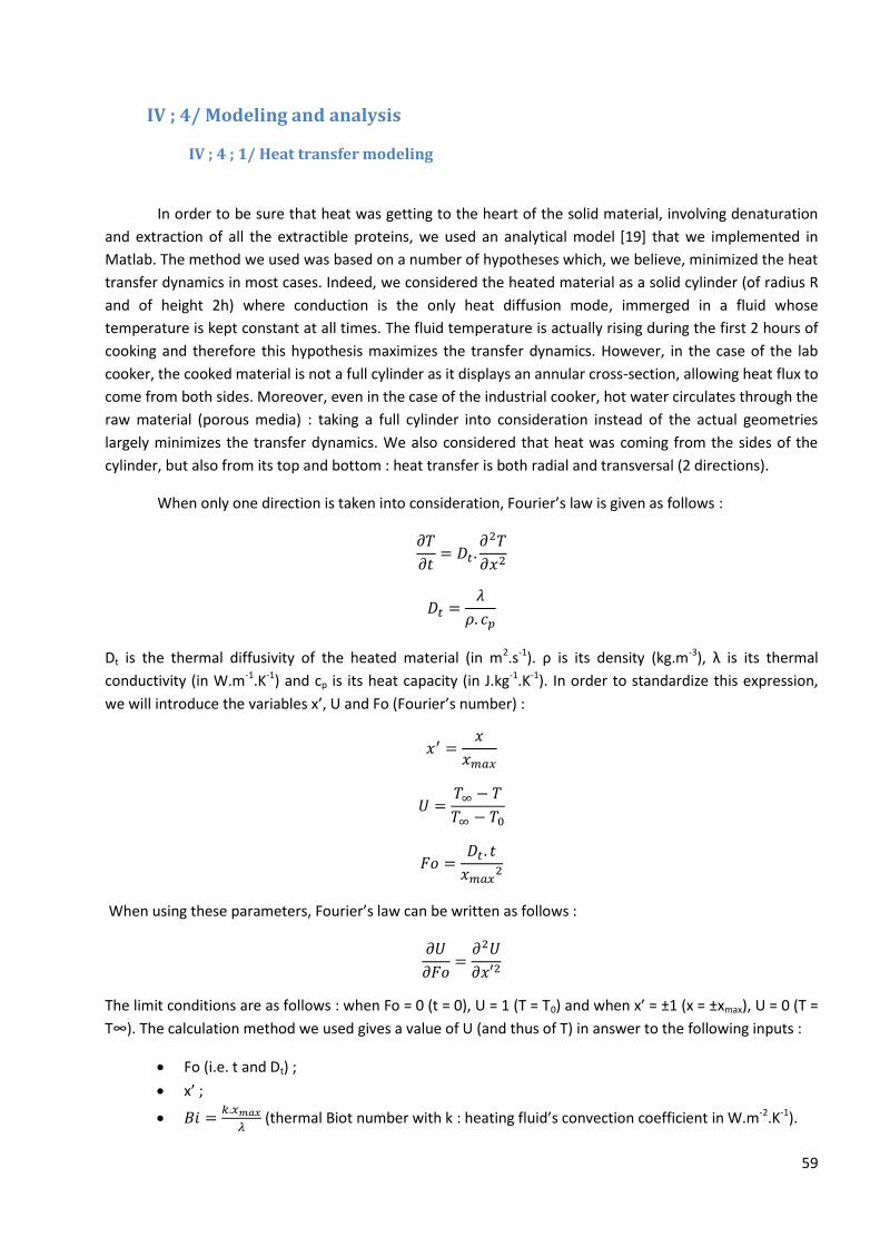
59

IV ; 4/ Modeling and analysis

IV ; 4 ; 1/ Heat transfer modeling

In order to be sure that heat was getting to the heart of the solid material, involving denaturation

and extraction of all the extractible proteins, we used an analytical model [19] that we implemented in

Matlab. The method we used was based on a number of hypotheses which, we believe, minimized the heat

transfer dynamics in most cases. Indeed, we considered the heated material as a solid cylinder (of radius R

and of height 2h) where conduction is the only heat diffusion mode, immerged in a fluid whose

temperature is kept constant at all times. The fluid temperature is actually rising during the first 2 hours of

cooking and therefore this hypothesis maximizes the transfer dynamics. However, in the case of the lab

cooker, the cooked material is not a full cylinder as it displays an annular cross-section, allowing heat flux to

come from both sides. Moreover, even in the case of the industrial cooker, hot water circulates through the

raw material (porous media) : taking a full cylinder into consideration instead of the actual geometries

largely minimizes the transfer dynamics. We also considered that heat was coming from the sides of the

cylinder, but also from its top and bottom : heat transfer is both radial and transversal (2 directions).

When only one direction is taken into consideration, Fourier’s law is given as follows :

𝜕𝑇

𝜕𝑡= 𝐷𝑡.

𝜕2𝑇

𝜕𝑥2

𝐷𝑡 =𝜆

𝜌. 𝑐𝑝

Dt is the thermal diffusivity of the heated material (in m2.s-1). ρ is its density (kg.m-3), λ is its thermal

conductivity (in W.m-1.K-1) and cp is its heat capacity (in J.kg-1.K-1). In order to standardize this expression,

we will introduce the variables x’, U and Fo (Fourier’s number) :

𝑥′ =𝑥

𝑥𝑚𝑎𝑥

𝑈 =𝑇∞ − 𝑇

𝑇∞ − 𝑇0

𝐹𝑜 =𝐷𝑡 . 𝑡

𝑥𝑚𝑎𝑥2

When using these parameters, Fourier’s law can be written as follows :

𝜕𝑈

𝜕𝐹𝑜=

𝜕2𝑈

𝜕𝑥′2

The limit conditions are as follows : when Fo = 0 (t = 0), U = 1 (T = T0) and when x’ = ±1 (x = ±xmax), U = 0 (T =

T∞). The calculation method we used gives a value of U (and thus of T) in answer to the following inputs :

Fo (i.e. t and Dt) ;

x’ ;

𝐵𝑖 =𝑘.𝑥𝑚𝑎𝑥

𝜆 (thermal Biot number with k : heating fluid’s convection coefficient in W.m-2.K-1).

60

U values are calculated for each direction separately :

Ur is calculated in relation to heat transfer in the radial direction. The applied model is the

infinite cylinder (of radius R) ;

Uy is calculated in relation to heat transfer in the transversal direction. The applied model is the

infinite plate (of thickness 2h).

From these results, the three-dimensional U is calculated thanks to Newman’s expression :

𝑈 = 𝑈𝑟 . 𝑈𝑧

Ur can be calculated thanks to the following expression :

𝑈𝑟 = ∑2. 𝐽1(µ𝑛)

µ𝑛. [𝐽02(µ𝑛) + 𝐽1

2(µ𝑛)]. 𝐽0(µ𝑛. 𝑟′). 𝑒−µ𝑛

2.𝐹𝑜

∞

𝑛=1

= ∑ 𝑇𝑟,𝑛

∞

𝑛=1

In this expression, J0 and J1 are Bessel functions of the first kind, of orders 0 and 1, and µn is the nth solution

of the equation : 𝐽0(µ)

𝐽1(µ)=

µ

𝐵𝑖. When n increases, Tr,n tends towards 0 : for the model to be efficient, it is

necessary to calculate enough solutions for the sum to converge.

Uy can be calculated thanks to the following expression :

𝑈𝑦 = ∑2. sin µ𝑛

µ𝑛 + sin µ𝑛 . cos µ𝑛. cos(µ𝑛. 𝑥′) . 𝑒−µ𝑛

2.𝐹𝑜

∞

𝑛=1

= ∑ 𝑇𝑦,𝑛

∞

𝑛=1

In this expression, µn is the nth solution of the equation : cot µ =µ

𝐵𝑖. When n increases, Ty,n tends towards 0

: for the model to be efficient, it is necessary to calculate enough solutions for the sum to converge.

In order to know the temperature of a point of the system at a precise moment, the program works as

follows :

Inputs : Dt, λ, k, T0, T∞, R, h, r’, y’, t, Nsol,r, Nsol,y ;

Calculation of Biot and Fourier numbers along r and y ;

Calculation of the N first solutions of the previous equations ;

Calculation of Ur, Uy and U.

Thanks to the use of loops, it is of course possible to model the temperature rise of a specific point of the

system, or to draw the temperature profile of the cylinder at a precise moment and height. The following

values were used as inputs :

61

Table 16 : Heat transfer modeling : input parameters (Modélisation du transfert de chaleur : paramètres d’entrée)

The actual convection coefficient value was unknown to us and the value we used was chosen

arbitrary. However, we calculated that choosing a value higher than 2000 W.m-1.K-1 served no purpose, as

transfer by conduction became limiting above this value (calculation not shown). The following results were

obtained :

Fig. 31 : Lab scale heat transfer (central point) (Transfert de chaleur à l’échelle expérimentale, point central)

Fig. 32 : Process scale heat transfer (central point) (Transfert de chaleur à l’échelle industrielle, point central)

Applying the hypotheses that we explained earlier, we found that the temperature at the center of

the lab cooker’s basket was getting close to 130°C in a relatively short time (about 2h). Given the fact that

our hypotheses minimized the transfer, we can say that the transfer was very efficient in the lab scale

pressure cooker, and that all the raw material got exposed to the set temperature within a satisfactory

amount of time. However, it is also obvious that, using these hypotheses, the heat transfer would be

completely inefficient in a cooker as big as TBE’s, as the temperature at its center would never rise in the

first 10h of heating. In order to check the inefficiency of the transfer, we calculated the temperature profile

of the cooker at mid-height (y’=0) and after 8h (28800 s) of heating :

Lab scale Process scale

Dt (m2.s-1) 1,23E-07 1,23E-07

λ (W.m-1.K-1) 0,5 0,5

k (W.m-2.K-1) 2000 2000

T0 (°C) 50 50

T∞ (°C) 130 130

R (m) 0,044 0,7

h (m) 0,12 2,3

r' 0,756 0

y' 0 0

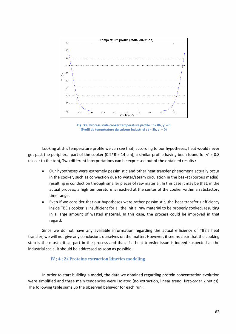
62

Fig. 33 : Process scale cooker temperature profile : t = 8h, y' = 0 (Profil de température du cuiseur industriel : t = 8h, y’ = 0)

Looking at this temperature profile we can see that, according to our hypotheses, heat would never

get past the peripheral part of the cooker (0.2*R = 14 cm), a similar profile having been found for y’ = 0.8

(closer to the top), Two different interpretations can be expressed out of the obtained results :

Our hypotheses were extremely pessimistic and other heat transfer phenomena actually occur

in the cooker, such as convection due to water/steam circulation in the basket (porous media),

resulting in conduction through smaller pieces of raw material. In this case it may be that, in the

actual process, a high temperature is reached at the center of the cooker within a satisfactory

time range.

Even if we consider that our hypotheses were rather pessimistic, the heat transfer’s efficiency

inside TBE’s cooker is insufficient for all the initial raw material to be properly cooked, resulting

in a large amount of wasted material. In this case, the process could be improved in that

regard.

Since we do not have any available information regarding the actual efficiency of TBE’s heat

transfer, we will not give any conclusions ourselves on the matter. However, it seems clear that the cooking

step is the most critical part in the process and that, if a heat transfer issue is indeed suspected at the

industrial scale, it should be addressed as soon as possible.

IV ; 4 ; 2/ Proteins extraction kinetics modeling

In order to start building a model, the data we obtained regarding protein concentration evolution

were simplified and three main tendencies were isolated (no extraction, linear trend, first-order kinetics).

The following table sums up the observed behavior for each run :

63

Table 17 : Protein extraction tendencies, depending on cooking temperature and kind of raw material (Tendances de l’extraction protéique en fonction de la température du cuiseur et de la matière première)

Each curve (except for mixed bones at 90°C) was divided into two main parts, the first one making

way for the second one at t = tr. The model was built using the following equations :

No extraction : 𝜂(𝑡) = 0 %

Linear trend : 𝜂(𝑡) = 𝑎. 𝑡 + 𝑏

First-order kinetics : 𝜂(𝑡) = 𝜂(𝑡𝑟) + (𝜂𝑚𝑎𝑥 − 𝜂(𝑡𝑟)). (1 − 𝑒−𝑘.(𝑡−𝑡𝑟))

We chose to use the yield (extracted mass divided by total initial mass) instead of the rough concentration

in this model, as the water/bone ratio varied from one run to the other : focusing on the yield allowed us to

bypass this variation. Therefore, the system is governed by 4 parameters (a, b, k and tr), all depending on

both cooking temperature and kind of raw material. For each case, tr was determined visually and the right

equation was applied to each point. The working parameters were optimized using a linear regression

method, which consists in minimizing the sum of square errors (difference between experimental values

and calculated values) :

𝐸 = ∑[𝜂𝑒𝑥𝑝(𝑡𝑖) − 𝜂𝑚𝑜𝑑(𝑡𝑖)]2

𝑛

𝑖=1

A numerical solver was used to determine the parameters allowing a minimal value of E, some of them

were manually adjusted, and the following results were obtained :

Mixed bones t<tr t>tr

130°C Linear First-order

110°C Linear First-order

90°C Linear /

Scraps t<tr t>tr

130°C No extraction First-order

110°C No extraction First-order

90°C No extraction Linear

Leg bones t<tr t>tr

130°C No extraction First-order

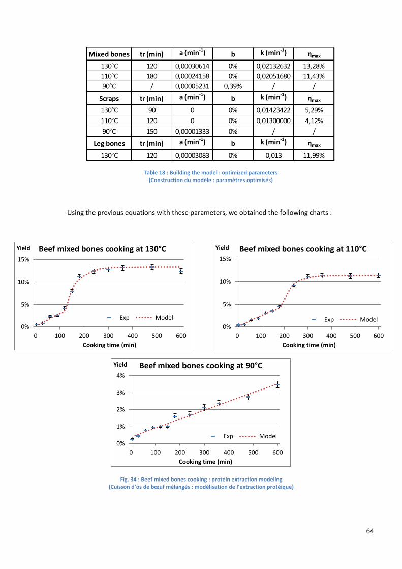
64

Table 18 : Building the model : optimized parameters (Construction du modèle : paramètres optimisés)

Using the previous equations with these parameters, we obtained the following charts :

Fig. 34 : Beef mixed bones cooking : protein extraction modeling (Cuisson d’os de bœuf mélangés : modélisation de l’extraction protéique)

Mixed bones tr (min) a (min-1) b k (min-1) ηmax

130°C 120 0,00030614 0% 0,02132632 13,28%

110°C 180 0,00024158 0% 0,02051680 11,43%

90°C / 0,00005231 0,39% / /

Scraps tr (min) a (min-1) b k (min-1) ηmax

130°C 90 0 0% 0,01423422 5,29%

110°C 120 0 0% 0,01300000 4,12%

90°C 150 0,00001333 0% / /

Leg bones tr (min) a (min-1) b k (min-1) ηmax

130°C 120 0,00003083 0% 0,013 11,99%

0%

5%

10%

15%

0 100 200 300 400 500 600

Yield

Cooking time (min)

Beef mixed bones cooking at 130°C

Exp Model

0%

5%

10%

15%

0 100 200 300 400 500 600

Yield

Cooking time (min)

Beef mixed bones cooking at 110°C

Exp Model

0%

1%

2%

3%

4%

0 100 200 300 400 500 600

Yield

Cooking time (min)

Beef mixed bones cooking at 90°C

Exp Model

65

Fig. 35 : Beef scraps cooking : protein extraction modeling (Cuisson de déchets : modélisation de l’extraction protéique)

Fig. 36 : Beef leg bones cooking : protein extraction modeling (Cuisson d’os de pattes de bœuf : modélisation de l’extraction protéique)

Just as we had previously sensed it (part IV ; 3 ; 2), some of the obtained curves fit first-order

kinetics really well (mixed bones at 130°C and 110°C, scraps at 130°C), whereas the similarity is, in some

other cases, less obvious (scraps at 110°C, leg bones) or even inexistent (90°C runs), hypotheses on the

reasons for these behavior variations having been given at the end of part IV ; 3 ; 2 . It is most likely that

0%

2%

4%

6%

0 100 200 300 400 500 600

Yield

Cooking time (min)

Beef scraps cooking at 130°C

Exp Model 0%

1%

2%

3%

4%

5%

0 100 200 300 400 500 600

Yield

Cooking time (min)

Beef scraps cooking at 110°C

Exp Model

0%

1%

2%

3%

4%

0 100 200 300 400 500 600

Yield Beef scraps cooking at 90°C

Exp Model

0%

5%

10%

15%

0 100 200 300 400 500 600

Yield

Cooking time (min)

Beef leg bones cooking at 130°C

Exp Model

66

90°C is too low a temperature for efficient extraction and first order kinetics to occur, and there is

probably a critical temperature point between 90°C and 110°C where protein extraction dynamics

drastically change, switching from a linear mode to an exponential one. The fact that some of the curves

should a priori follow first-order kinetics but actually do not is probably due (as explained previously) to

crushing and/or to the presence of diffusion-preventing solid material (pieces of non-melted fat in the

case of scraps). This would imply that the curves’ shapes are actually more a result of proteins diffusion in

the system than a result of extraction kinetics.

An Excel file was built from these results, allowing the user to observe how the stock’s protein

concentration evolution would react to changes of the following input parameters :

Working temperature (with 2h of heating time) ;

Scraps proportion ;

Water : bone ratio.

Due to the facts that there are such significant behavior differences between runs at 90°C and ones at

110°C, and that we do not have any data over 130°C, the obtained model is believed to be mainly reliable

in the 110°C-130°C temperature range. Output parameters a, tr and ηmax are calculated via linear

interpolation of the available data (110°C and 130°C), whereas k is calculated thanks to Arrhenius’ law :

𝑘(𝑇) = 𝑘0. 𝑒−𝐸𝑎𝑅𝑇

<=> ln[𝑘(𝑇)] =−𝐸𝑎

𝑅.1

𝑇+ ln (𝑘0)

In this equation, k0 is a pre-exponential factor, Ea is the activation energy (in J), R is the ideal gas constant

and T is to be converted in K. The linearized form of the equation allowed us to calculate Ea and k0, whose

values are used in the regular equation to calculate k for any temperature :

Table 19 : Input values for the calculation of kinetics constants (Paramètres d’entrée pour le calcul des constantes de cinétique)

During the previous paragraphs we widely discussed the fact that the crushing quality, (i.e. the

porosity of the cooked material), was a critical parameter of the extraction process. This parameter is not

taken into account in this model and therefore it could probably be largely improved. Indeed, in our case,

the extraction behavior is calculated by predicting the behavior of scraps and bones separately, before

calculating weighted average values (with coefficients depending on the scraps proportion). However, the

presence of scraps can for example be a hindrance to fluid circulation between crushed bones, resulting

in lower concentration values than what would have been calculated with a simple average value, along

with different extraction kinetics. Further experiments would need to be conducted in order to confirm

(or not) this hypothesis. Results obtained with our model have been compared to one of AgResearch’s

first runs (performed before my arrival, at 132°C with about 50% of scraps in the raw material) and the

Mixed bones Scraps

Ea (J) 2484,89 5823,96

k0 (min-1) 0,044757332 0,08090335

67

model matched the actual results quite well, but we cannot be sure that predictions would be efficient at

lower temperatures, as we witnessed that, for example, the concentration evolution of scraps stock at

110°C did not match first order kinetics.

In order to obtain a really effective model, we would need to determine the exact influence of

temperature and pressure on the extraction quality, along with the influence of porosity. The quality of

heat transfer is also a very important parameter, as proteins will not denaturate and migrate from solid

material to water without being exposed to heat, and further research would have to be led regarding the

way the fluid circulates in the cooker, both at lab scale and at industrial scale. Therefore, a good model

would also have to focus on the cooker’s geometry, on the evolution of temperature and pressure,

especially during the first two hours of cooking, as in this time range we find ourselves in a transitory

mode. Unfortunately, our time resources were insufficient for us to go further in that direction. The actual

model can nevertheless be used to obtain orders of magnitude.

IV ; 5/ Prospects for TBE

Regarding the results we obtained and discussed during this study, we can say that :

The bone-crushing step has a crucial part to play in the process, as a fine crushing will result in

a higher cooked material porosity, thus allowing a better fluid circulation, which is to say a

better heat/matter transfer.

High temperatures and high pressures are necessary to reach a satisfactory extraction. This is

to put in relation with the state change (vaporization) that occurs during cooking. The

presence of steam plays a critical part in heat transfer quality and in the system’s

homogenization.

Browning is apparently mainly due to the presence of blood in the raw material, as colour

results on lean meat and mixed bones showed. For other kinds of raw material (scraps and leg

bones), we cannot talk of actual browning but colour was significantly present at the end of

the run anyway.

A higher working temperature will result in a stronger colouration/browning. Therefore, if

colour is to be avoided, lowering the working temperature is a solution, but this will also

lower the extraction’s efficiency. Removing blood is probably the most efficient solution : a

soaking step already exists in the process but its efficiency is believed to be quite poor. It is

very likely that this is due to the fact that the crushing step is quite rough : blood does not exit

bones when these are crushed, thus making soaking inefficient. However, removing blood will

also result in a lower final protein concentration, as concentration results on mixed bones

suggested.

The quality of heat transfer also seems to be of significant importance. The calculations we

did gave terrible results in that regard, but the hypotheses we had chosen were extremely

pessimistic (no fluid circulation inside the cooked material was considered, for example). Our

position does not allow us to draw conclusions from these calculations at the industrial scale,

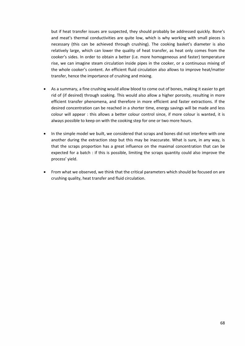
68

but if heat transfer issues are suspected, they should probably be addressed quickly. Bone’s

and meat’s thermal conductivities are quite low, which is why working with small pieces is

necessary (this can be achieved through crushing). The cooking basket’s diameter is also

relatively large, which can lower the quality of heat transfer, as heat only comes from the

cooker’s sides. In order to obtain a better (i.e. more homogeneous and faster) temperature

rise, we can imagine steam circulation inside pipes in the cooker, or a continuous mixing of

the whole cooker’s content. An efficient fluid circulation also allows to improve heat/matter

transfer, hence the importance of crushing and mixing.

As a summary, a fine crushing would allow blood to come out of bones, making it easier to get

rid of (if desired) through soaking. This would also allow a higher porosity, resulting in more

efficient transfer phenomena, and therefore in more efficient and faster extractions. If the

desired concentration can be reached in a shorter time, energy savings will be made and less

colour will appear : this allows a better colour control since, if more colour is wanted, it is

always possible to keep on with the cooking step for one or two more hours.

In the simple model we built, we considered that scraps and bones did not interfere with one

another during the extraction step but this may be inaccurate. What is sure, in any way, is

that the scraps proportion has a great influence on the maximal concentration that can be

expected for a batch : if this is possible, limiting the scraps quantity could also improve the

process’ yield.

From what we observed, we think that the critical parameters which should be focused on are

crushing quality, heat transfer and fluid circulation.

69

Conclusion

This study confirmed what had been previously observed by Dong et al. with chicken bones, i.e.

that when cooking bones in water, increasing the working temperature over 100°C (thus entailing a state

change from liquid water to vapor, and a higher working pressure) results in far better yields than what

the traditional protein extraction processes allow (at lower temperatures for gelatin production). [12] An

efficient crushing is also necessary for a better process control as it allows :

Better heat and matter transfer, and thus better extraction kinetics and a more efficient

extraction;

The possibility to wash blood away from bones prior to cooking ;

A better control on colour evolution.

The mixing quality also being determining in the efficiency of heat and matter transfer, we think that it

should be given special attention by TBE, along with the crushing step and the heating method.

From a more personal point of view, this internship was a very good experience. Even though the

field of study (food industry, biology, biochemistry) was quite remote from my University specialty (heat

and energy production and transfer phenomena), these six months spent at INRA and at AgResearch gave

me the opportunity to take part in a research project in an international context. As I would like to start

my career in the Research and Development domain, this internship was in line with my professional

project. All the results that were found during my internship, along with results obtained from later

analysis will furthermore be used in the months to come for the writing of a scientific publication, which is

very rewarding. The specialty divergence was the opportunity for me to obtain more transversal skills

than I would have if I had chosen a project more directly related to my specialty, which I believe is of high

necessity for a Process Engineer. This project allowed me to improve my skills in various domains,

including :

Scientific and technical knowledge, through the in-depth study of a very specific process ;

Project management through the building of an experimental design, the performing of various

experiments in a laboratory, and the analysis and interpretation of experimental results. This kind

of work requires rigour, organization and a good traceability, especially given the fact that I was

working on my own most of the time.

Communication and Language through the daily use of English in emails, Skype meetings and daily

life during my two-months stay in Lincoln. My stay there also gave me the opportunity to be a

part of a widely multicultural team, as New Zealand relies a lot on foreign workers. This was

particularly enriching, as I believe that the aptitude to work and communicate daily with people

having various cultural backgrounds is necessary for contemporary engineers.

For all these reasons, I consider this final-year project to be an excellent supplement to my previous

internship as an assistant engineer (Solvay Rare Earths Systems, La Rochelle, France), during which I was

part of a production team, with drastically different stakes and challenges. The combination of my two

internships provides me with experience in both Production and Research, factory and laboratory,

management and science, and therefore with a solid background for my first steps in the workforce after

graduation.

70

References

[1] “Institut National de la Recherche Agronomique,” [Online]. Available:

https://en.wikipedia.org/wiki/Institut_national_de_la_recherche_agronomique. [Accessed 11

August 2015].

[2] “AgResearch,” [Online]. Available: https://en.wikipedia.org/wiki/AgResearch. [Accessed 11 August

2015].

[3] “About AgResearch,” [Online]. Available: http://www.agresearch.co.nz/about/. [Accessed 12 August

2015].

[4] “About Taranaki Bio Extracts,” [Online]. Available: http://www.taranakibioextracts.co.nz/about/.

[Accessed 12 August 2015].

[5] “About ANZCO Foods,” [Online]. Available: http://www.anzcofoods.com/about-us/company-

overview. [Accessed 12 August 2015].

[6] “Bone,” [Online]. Available: https://en.wikipedia.org/wiki/Bone. [Accessed 11 August 2015].

[7] P. Orcel and T. Funck-Brentano, “Aspects physiopathologiques et cliniques du vieillisesement

osseux,” [Online]. Available:

http://www.chups.jussieu.fr/polys/capacites/capagerontodocs/fondementale2011/Aspectcliniqued

uvieillissementosseuxThomasFUNCKBRENTANOPhORCEL.pdf. [Accessed 11 August 2015].

[8] “Nutritional composition of meat and other food sources,” [Online]. Available:

http://www.fao.org/ag/ags/post-harvest-management/meat-meat-products/background-and-meat-

consumption/composition-of-meat/en/. [Accessed 11 August 2015].

[9] F. Danieau, “Les Viandes,” [Online]. Available:

http://fdanieau.free.fr/cours/bts/A2/stbi/chapitre10/Poly_Viandes.pdf. [Accessed 11 August 2015].

[10] D. Liu, X. Zhang, T. Li, H. Yang, H. Zhang, J. Regenstein and P. Zhou, “Extraction and characterization

of acid- and pepsin-soluble collagens from the scales, skins and swim bladders of grass carp

(Ctenopharyngodon idella),” Food Bioscience, no. 9, pp. 68-74, 2015.

[11] N. Wright and J. Humphrey, “Denaturation of collagen via heating : an irreversible rate process,”

Annual review of biomedical engineering, no. 4, pp. 109-128, 2002.

[12] X. Dong, C. Zhang, J. Wang, C. Tang, H. Sun, W. Jia, Y. Li and L. Chen, “Development of a novel

method for hot-pressure extraction of protein from chicken bone and the effect of enzymatic

hydrolysis on the extracs,” Food Chemistry, no. 157, pp. 339-346, 2014.

[13] Y. Zhang, C. Tang, Q. Wen, X. Yang, L. Li and W. Deng, “Thermal aggregation and gelation of kidney

bean (Phaseolus vulgaris L.) protein isolate at pH 2.0 : Influence of ionic strength,” Food

71

Hydrocolloids, no. 24, pp. 266-274, 2010.

[14] “Lab color space,” [Online]. Available: https://en.wikipedia.org/wiki/Lab_color_space. [Accessed 12

August 2015].

[15] “Direct Detect Spectrometer,” [Online]. Available: http://www.emdmillipore.com/CA/en/life-

science-research/protein-detection-quantification/direct-detect-

spectrometer/NWGb.qB.NtgAAAFBfBwRRkwm,nav?cid=BI-XX-BSP-P-GOOG-DIDE-B328-1005&bd=1.

[Accessed 12 August 2015].

[16] “Mass spectrometry,” [Online]. Available: https://en.wikipedia.org/wiki/Mass_spectrometry.

[Accessed 12 August 2015].

[17] «Glutamic acid,» [En ligne]. Available: https://en.wikipedia.org/wiki/Glutamic_acid. [Accès le 12

August 2015].

[18] P. Gatellier, A. Kondjoyan, S. Portanguen et V. Santé-Lhoutellier, «Effect of cooking on protein

oxidation in n-3 polyunsaturated fatty acids enriched beef : Implication on nutritional quality,» Meat

Science, n° %185, pp. 645-650, 2010.

[19] J.-J. Bimbenet and M. Loncin, Bases du génie des procédés alimentaires, Paris: Masson, 1995.

[20] “Collagen,” [Online]. Available: https://en.wikipedia.org/wiki/Collagen. [Accessed 11 August 20015].

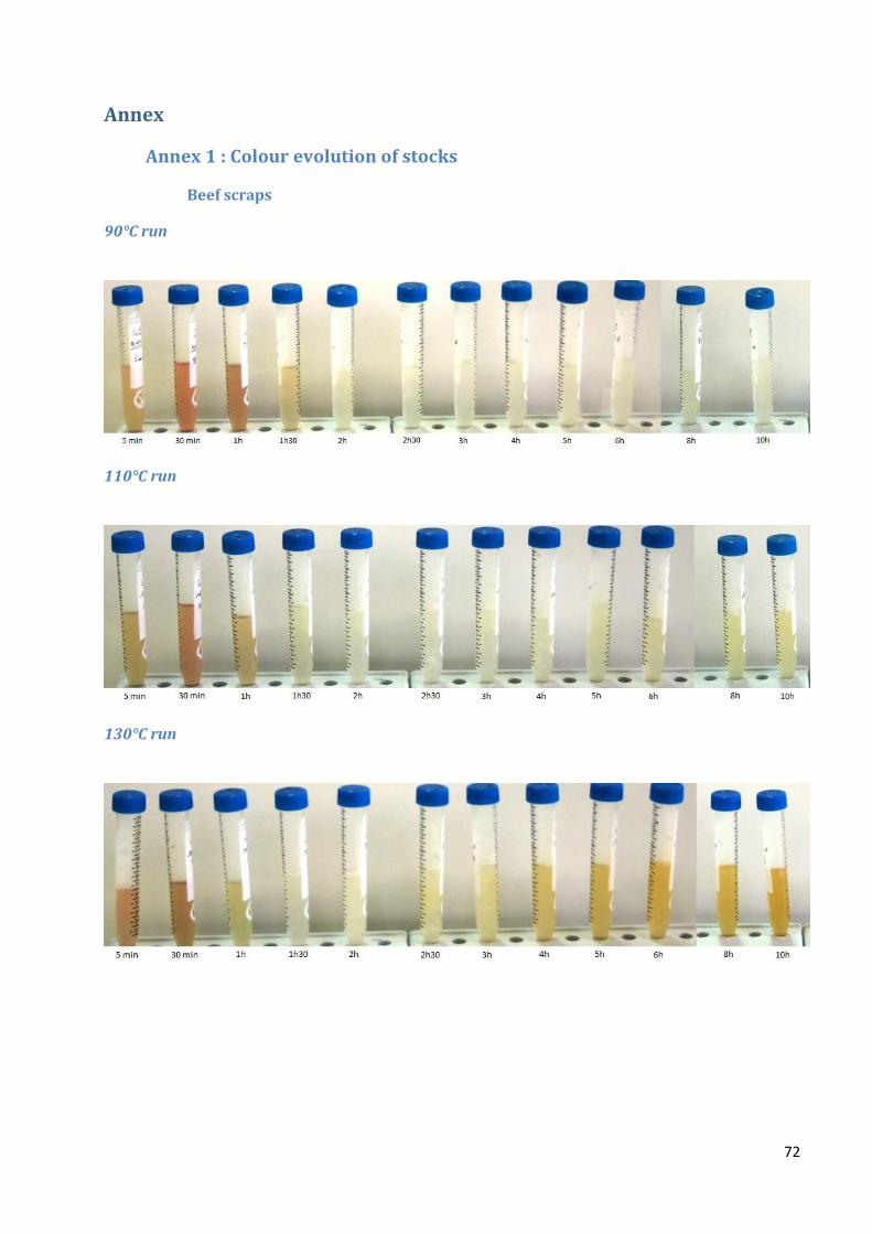
72

Annex

Annex 1 : Colour evolution of stocks

Beef scraps

90°C run

110°C run

130°C run

73

Leg bones (130°C)

Mixed bones

90°C run

110°C run

130°C run

74

Annex 2 : Cooked material pictures

Beef scraps

Beef scraps after 10h of cooking at 130°C

Beef scraps after 10h of cooking at 110°C

Beef scraps after 10h of cooking at 90°C

Leg bones (130°C)

Beef leg bones after 11h of cooking at 130°C

75

Mixed bones

Beef mixed bones after 12h of cooking at 130°C

Beef mixed bones after 12h of cooking at 130°C (dry matter sample

Beef mixed bones after 10h of cooking at 90°C