CSPC403 DATABASE MANAGEMENT SYSTEM L T P

3 0 0

UNIT – I Introduction

File System vs. DBMS – Views of data – Data Models – Database Languages – Database Management System Services

– Overall System Architecture – Data Dictionary – Entity – Relationship (E-R) – Enhanced Entity – Relationship Model.

File System vs. DBMS

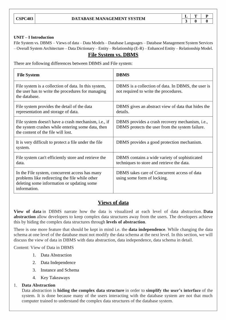
There are following differences between DBMS and File system:

File System DBMS

File system is a collection of data. In this system,

the user has to write the procedures for managing

the database.

DBMS is a collection of data. In DBMS, the user is

not required to write the procedures.

File system provides the detail of the data

representation and storage of data.

DBMS gives an abstract view of data that hides the

details.

File system doesn't have a crash mechanism, i.e., if

the system crashes while entering some data, then

the content of the file will lost.

DBMS provides a crash recovery mechanism, i.e.,

DBMS protects the user from the system failure.

It is very difficult to protect a file under the file

system.

DBMS provides a good protection mechanism.

File system can't efficiently store and retrieve the

data.

DBMS contains a wide variety of sophisticated

techniques to store and retrieve the data.

In the File system, concurrent access has many

problems like redirecting the file while other

deleting some information or updating some

information.

DBMS takes care of Concurrent access of data

using some form of locking.

Views of data

View of data in DBMS narrate how the data is visualized at each level of data abstraction. Data

abstraction allow developers to keep complex data structures away from the users. The developers achieve

this by hiding the complex data structures through levels of abstraction.

There is one more feature that should be kept in mind i.e. the data independence. While changing the data

schema at one level of the database must not modify the data schema at the next level. In this section, we will

discuss the view of data in DBMS with data abstraction, data independence, data schema in detail.

Content: View of Data in DBMS

1. Data Abstraction

2. Data Independence

3. Instance and Schema

4. Key Takeaways

1. Data Abstraction

Data abstraction is hiding the complex data structure in order to simplify the user’s interface of the

system. It is done because many of the users interacting with the database system are not that much

computer trained to understand the complex data structures of the database system.

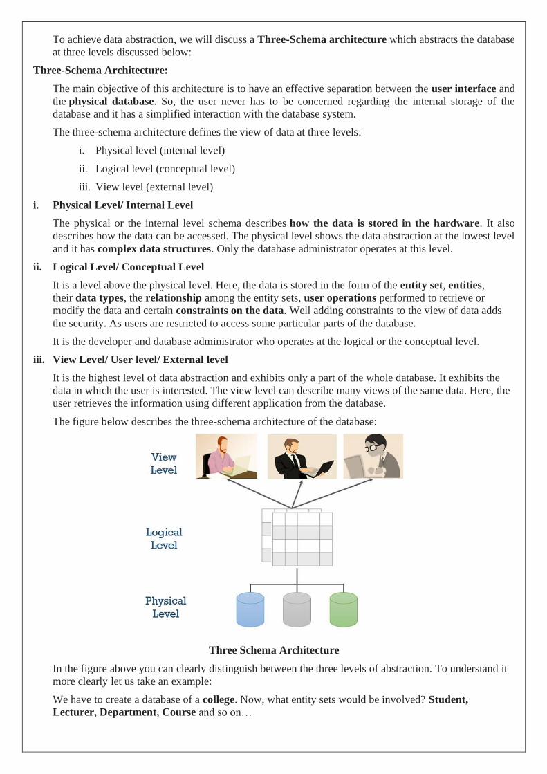
To achieve data abstraction, we will discuss a Three-Schema architecture which abstracts the database

at three levels discussed below:

Three-Schema Architecture:

The main objective of this architecture is to have an effective separation between the user interface and

the physical database. So, the user never has to be concerned regarding the internal storage of the

database and it has a simplified interaction with the database system.

The three-schema architecture defines the view of data at three levels:

i. Physical level (internal level)

ii. Logical level (conceptual level)

iii. View level (external level)

i. Physical Level/ Internal Level

The physical or the internal level schema describes how the data is stored in the hardware. It also

describes how the data can be accessed. The physical level shows the data abstraction at the lowest level

and it has complex data structures. Only the database administrator operates at this level.

ii. Logical Level/ Conceptual Level

It is a level above the physical level. Here, the data is stored in the form of the entity set, entities,

their data types, the relationship among the entity sets, user operations performed to retrieve or

modify the data and certain constraints on the data. Well adding constraints to the view of data adds

the security. As users are restricted to access some particular parts of the database.

It is the developer and database administrator who operates at the logical or the conceptual level.

iii. View Level/ User level/ External level

It is the highest level of data abstraction and exhibits only a part of the whole database. It exhibits the

data in which the user is interested. The view level can describe many views of the same data. Here, the

user retrieves the information using different application from the database.

The figure below describes the three-schema architecture of the database:

Three Schema Architecture

In the figure above you can clearly distinguish between the three levels of abstraction. To understand it

more clearly let us take an example:

We have to create a database of a college. Now, what entity sets would be involved? Student,

Lecturer, Department, Course and so on…

Now, the entity sets Student, Lecturer, Department, Course will be stored in the storage as

the consecutive blocks of the memory location. This is the physical or internal level and is hidden

from the programmers but the database administrator is it aware of it.

At the logical level, the programmers define the entity sets and relationship among these entity sets

using a programming language like SQL. So, the programmers work at the logical level and even the

database administrator also operates at this level.

At the view level, the users have the set of applications which they use to retrieve the data they are

interested in.

2. Data Independence

Data independence defines the extent to which the data schema can be changed at one level without modifying

the data schema at the next level. Data independence can be classified as shown below:

Logical Data Independence:

Logical data independence describes the degree up to which the logical or conceptual schema can be changed

without modifying the external schema. Now, a question arises what is the need to change the data schema at

a logical or conceptual level?

Well, the changes to data schema at the logical level are made either to enlarge or reduce the database by

adding or deleting more entities, entity sets, or changing the constraints on data.

Physical Data Independence:

Physical data independence defines the extent up to which the data schema can be changed at the physical or

internal level without modifying the data schema at logical and view level.

Well, the physical schema is changed if we add additional storage to the system or we reorganize some files

to enhance the retrieval speed of the records.

3. Instances and Schemas

What is an instance?

We can define an instance as the information stored in the database at a particular point of time. Let us

discuss it with the help of an example.

As we discussed above the database comprises of several entity sets and the relationship between them.

Now, the data in the database keeps on changing with time. As we keep inserting or deleting the data to and

from the database.

Now, at a particular time if we retrieve any information from the database then that corresponds to an

instance.

What is schema?

Whenever we talk about the database the developers have to deal with the definition of database and the data

in the database.

The definition of a database comprises of the description of what data it would contain what would be the

relationship between the data. This definition is the database schema.

4. Key Takeaways:

• View of data in DBMS describes the abstraction of data at three-level

i.e. physical level, logical level, view level.

• The physical level of abstraction defines how data is stored in the storage and also reveals its access

path.

• Abstraction at the logical level describes what data would be stored in the database? what would be

the relation between the data? and the constraints applied to the data.

• The view level or external level of abstraction describes the application which the users use to retrieve

the information from the database.

• Data independence explains the extent to which data at a certain level can be modified without

disturbing the data next higher levels.

• An instance is the retrieval of information from the database at a certain point of time. An instance in a

database keeps on changing with time.

• Schema is the overall design of the entire database. Schema of the database is not changed frequently.

So that’s all about the view of data in the database which help us to understand the database from users,

developers and database administrator aspects.

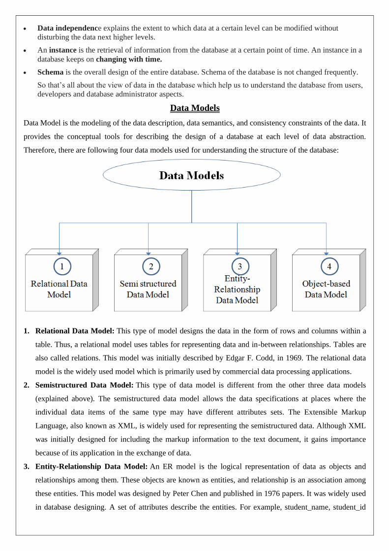
Data Models

Data Model is the modeling of the data description, data semantics, and consistency constraints of the data. It

provides the conceptual tools for describing the design of a database at each level of data abstraction.

Therefore, there are following four data models used for understanding the structure of the database:

1. Relational Data Model: This type of model designs the data in the form of rows and columns within a

table. Thus, a relational model uses tables for representing data and in-between relationships. Tables are

also called relations. This model was initially described by Edgar F. Codd, in 1969. The relational data

model is the widely used model which is primarily used by commercial data processing applications.

2. Semistructured Data Model: This type of data model is different from the other three data models

(explained above). The semistructured data model allows the data specifications at places where the

individual data items of the same type may have different attributes sets. The Extensible Markup

Language, also known as XML, is widely used for representing the semistructured data. Although XML

was initially designed for including the markup information to the text document, it gains importance

because of its application in the exchange of data.

3. Entity-Relationship Data Model: An ER model is the logical representation of data as objects and

relationships among them. These objects are known as entities, and relationship is an association among

these entities. This model was designed by Peter Chen and published in 1976 papers. It was widely used

in database designing. A set of attributes describe the entities. For example, student_name, student_id

describes the 'student' entity. A set of the same type of entities is known as an 'Entity set', and the set of

the same type of relationships is known as 'relationship set'.

4. Object-based Data Model: An extension of the ER model with notions of functions, encapsulation, and

object identity, as well. This model supports a rich type system that includes structured and collection

types. Thus, in 1980s, various database systems following the object-oriented approach were developed.

Here, the objects are nothing but the data carrying its properties.

Database Languages

• A DBMS has appropriate languages and interfaces to express database queries and updates.

• Database languages can be used to read, store and update the data in the database.

Types of Database Language

1. Data Definition Language

• DDL stands for Data Definition Language. It is used to define database structure or pattern.

• It is used to create schema, tables, indexes, constraints, etc. in the database.

• Using the DDL statements, you can create the skeleton of the database.

• Data definition language is used to store the information of metadata like the number of tables and

schemas, their names, indexes, columns in each table, constraints, etc.

Here are some tasks that come under DDL:

• Create: It is used to create objects in the database.

• Alter: It is used to alter the structure of the database.

• Drop: It is used to delete objects from the database.

• Truncate: It is used to remove all records from a table.

• Rename: It is used to rename an object.

• Comment: It is used to comment on the data dictionary.

These commands are used to update the database schema that's why they come under Data definition

language.

2. Data Manipulation Language

DML stands for Data Manipulation Language. It is used for accessing and manipulating data in a database.

It handles user requests.

Here are some tasks that come under DML:

• Select: It is used to retrieve data from a database.

• Insert: It is used to insert data into a table.

• Update: It is used to update existing data within a table.

• Delete: It is used to delete all records from a table.

• Merge: It performs UPSERT operation, i.e., insert or update operations.

• Call: It is used to call a structured query language or a Java subprogram.

• Explain Plan: It has the parameter of explaining data.

• Lock Table: It controls concurrency.

3. Data Control Language

• DCL stands for Data Control Language. It is used to retrieve the stored or saved data.

• The DCL execution is transactional. It also has rollback parameters.

(But in Oracle database, the execution of data control language does not have the feature of rolling

back.)

Here are some tasks that come under DCL:

• Grant: It is used to give user access privileges to a database.

• Revoke: It is used to take back permissions from the user.

There are the following operations which have the authorization of Revoke:

CONNECT, INSERT, USAGE, EXECUTE, DELETE, UPDATE and SELECT.

4. Transaction Control Language

TCL is used to run the changes made by the DML statement. TCL can be grouped into a logical transaction.

Here are some tasks that come under TCL:

• Commit: It is used to save the transaction on the database.

• Rollback: It is used to restore the database to original since the last Commit.

Database Management System Services

• The advancements in technology have opened the floodgates for endless volumes of data to flow into

the system. With this tremendous amount of data pouring in from diverse sources and in multiple

formats, it becomes a critical task for organizations to store, process and manage this data. And even

more so in today’s data driven world, where it has become the key to business success.

• A robust and efficient database management system resolves all your data worries, giving your business

the power to lead.

Choosing the right database

• In order to ensure a successful database management system, you need to carefully devise a strategy in

alignment with the data requirements and business roadmap of your organization. Today, with numerous

database options available in both open as well as closed source database categories, it is important to

choose a database solution as per the volume, variety.

• SMAC (social, mobile, analytics and cloud) has resulted into a data explosion which is overwhelming

for legacy DBMS. Every second, large amount of data is being generated through a widespread network

of data sources – images, graphs, hyper-text, documents, etc. Legacy systems prove to be insufficient to

address this magnanimity of data management, and that is when the more agile and updated non-

relational (NoSQL)databases find applicability. They are not only capable of handling complex data

management needs, but also provide numerous database options for diverse needs and data types.

NoSQL forms the bedrock for big data and analytics, which enables organizations to make highly-

informed strategic decisions.

Our comprehensive offerings of new age database management services

Overall System Architecture

The architecture of a database system is greatly influenced by the underlying computer system on which the

database is running:

i. Centralized.

ii. Client-server.

iii. Parallel (multi-processor).

iv. Distributed

Database Users:

Users are differentiated by the way they expect to interact with the system:

• Application programmers:

o Application programmers are computer professionals who write application programs.

Application programmers can choose from many tools to develop user interfaces.

o Rapid application development (RAD) tools are tools that enable an application programmer

to construct forms and reports without writing a program.

• Sophisticated users:

o Sophisticated users interact with the system without writing programs. Instead, they form their

requests in a database query language.

o They submit each such query to a query processor, whose function is to break down DML

statements into instructions that the storage manager understands.

• Specialized users :

o Specialized users are sophisticated users who write specialized database applications that do

not fit into the traditional data-processing framework.

o Among these applications are computer-aided design systems, knowledge base and expert

systems, systems that store data with complex data types (for example, graphics data and audio

data), and environment-modeling systems.

• Naive users :

o Naive users are unsophisticated users who interact with the system by invoking one of the

application programs that have been written previously.

o For example, a bank teller who needs to transfer $50 from account A to account B invokes a

program called transfer. This program asks the teller for the amount of money to be transferred,

the account from which the money is to be transferred, and the account to which the money is

to be transferred.

Database Administrator:

• Coordinates all the activities of the database system. The database administrator has a good

understanding of the enterprise’s information resources and needs.

• Database administrator's duties include:

o Schema definition: The DBA creates the original database schema by executing a set of data

definition statements in the DDL.

o Storage structure and access method definition.

o Schema and physical organization modification: The DBA carries out changes to the

schema and physical organization to reflect the changing needs of the organization, or to alter

the physical organization to improve performance.

o Granting user authority to access the database: By granting different types of

authorization, the database administrator can regulate which parts of the database various

users can access.

o Specifying integrity constraints.

o Monitoring performance and responding to changes in requirements.

Query Processor:

The query processor will accept query from user and solves it by accessing the database.

Parts of Query processor:

• DDL interpreter

This will interprets DDL statements and fetch the definitions in the data dictionary.

• DML compiler

a. This will translates DML statements in a query language into low level instructions that the query

evaluation engine understands.

b. A query can usually be translated into any of a number of alternative evaluation plans for same

query result DML compiler will select best plan for query optimization.

• Query evaluation engine

This engine will execute low-level instructions generated by the DML compiler on DBMS.

Storage Manager/Storage Management:

• A storage manager is a program module which acts like interface between the data stored in a

database and the application programs and queries submitted to the system.

• Thus, the storage manager is responsible for storing, retrieving and updating data in the database.

• The storage manager components include:

o Authorization and integrity manager: Checks for integrity constraints and authority of

users to access data.

o Transaction manager: Ensures that the database remains in a consistent state although there

are system failures.

o File manager: Manages the allocation of space on disk storage and the data structures used

to represent information stored on disk.

o Buffer manager: It is responsible for retrieving data from disk storage into main memory. It

enables the database to handle data sizes that are much larger than the size of main memory.

o Data structures implemented by storage manager.

o Data files: Stored in the database itself.

o Data dictionary: Stores metadata about the structure of the database.

o Indices: Provide fast access to data items.

Data Dictionary

Data Dictionary consists of database metadata. It has records about objects in the database.

Data Dictionary consists of the following information:

1. Name of the tables in the database

2. Constraints of a table i.e. keys, relationships, etc.

3. Columns of the tables that related to each other

4. Owner of the table

5. Last accessed information of the object

6. Last updated information of the object

An example of Data Dictionary can be personal details of a student:

Example

<StudentPersonalDetails>

Student_ID Student_Name Student_Address Student_City

The following is the data dictionary for the above fields:

Field Name Datatype Field Length Constraint Description

Student_ID Number 5 Primary Key Student id

Student_Name Varchar 20 Not Null Name of the student

Student_Address Varchar 30 Not Null Address of the student

Student_City Varchar 20 Not Null City of the Student

Types of Data Dictionary

Here are the two types of data dictionary:

Active Data Dictionary

The DBMS software manages the active data dictionary automatically. The modification is an automatic task

and most RDBMS has active data dictionary. It is also known as integrated data dictionary.

Passive Data Dictionary

Managed by the users and is modified manually when the database structure change. Also known as non-

integrated data dictionary.

The ER model defines the conceptual view of a database. It works around real-world entities and the

associations among them. At view level, the ER model is considered a good option for designing databases.

Entity

An entity can be a real-world object, either animate or inanimate, that can be easily identifiable. For example,

in a school database, students, teachers, classes, and courses offered can be considered as entities. All these

entities have some attributes or properties that give them their identity.

An entity set is a collection of similar types of entities. An entity set may contain entities with attribute sharing

similar values. For example, a Students set may contain all the students of a school; likewise a Teachers set

may contain all the teachers of a school from all faculties. Entity sets need not be disjoint.

A real-world thing either living or non-living that is easily recognizable and nonrecognizable. It is anything in

the enterprise that is to be represented in our database. It may be a physical thing or simply a fact about the

enterprise or an event that happens in the real world.

An entity can be place, person, object, event or a concept, which stores data in the database. The characteristics

of entities are must have an attribute, and a unique key. Every entity is made up of some 'attributes' which

represent that entity.

Examples of entities:

• Person: Employee, Student, Patient

• Place: Store, Building

• Object: Machine, product, and Car

• Event: Sale, Registration, Renewal

• Concept: Account, Course

An entity may be any object, class, person or place. In the ER diagram, an entity can be represented as

rectangles.

Consider an organization as an example- manager, product, employee, department etc. can be taken as

an entity.

a. Weak Entity

An entity that depends on another entity called a weak entity. The weak entity doesn't contain any key attribute

of its own. The weak entity is represented by a double rectangle.

Relationship (E-R)

A relationship is used to describe the relation between entities. Diamond or rhombus is used to represent the

relationship.

Types of relationship are as follows:

1. One-to-One Relationship

When only one instance of an entity is associated with the relationship, then it is known as one to one relationship.

For example, A female can marry to one male, and a male can marry to one female.

2. One-to-many relationship

When only one instance of the entity on the left, and more than one instance of an entity on the right

associates with the relationship then this is known as a one-to-many relationship.

For example, Scientist can invent many inventions, but the invention is done by the only specific

scientist.

3. Many-to-one relationship

When more than one instance of the entity on the left, and only one instance of an entity on the right

associates with the relationship then it is known as a many-to-one relationship.

For example, Student enrolls for only one course, but a course can have many students.

4. Many-to-many relationship

When more than one instance of the entity on the left, and more than one instance of an entity on the right

associates with the relationship then it is known as a many-to-many relationship.

For example, Employee can assign by many projects and project can have many employees.

Enhanced Entity – Relationship Model

The enhanced entity–relationship (EER) model (or extended entity–relationship model) in computer science

is a high-level or conceptual data model incorporating extensions to the original entity–relationship (ER)

model, used in the design of databases.

Prerequisite –

Generalization, Specialization and Aggregation in ER model are used for data abstraction in which abstraction

mechanism is used to hide details of a set of objects.

Generalization –

Generalization is the process of extracting common properties from a set of entities and create a generalized

entity from it. It is a bottom-up approach in which two or more entities can be generalized to a higher level

entity if they have some attributes in common. For Example, STUDENT and FACULTY can be generalized

to a higher level entity called PERSON as shown in Figure 1. In this case, common attributes like P_NAME,

P_ADD become part of higher entity (PERSON) and specialized attributes like S_FEE become part of

specialized entity (STUDENT).

Specialization –

In specialization, an entity is divided into sub-entities based on their characteristics. It is a top-down approach

where higher level entity is specialized into two or more lower level entities. For Example, EMPLOYEE entity

in an Employee management system can be specialized into DEVELOPER, TESTER etc. as shown in Figure

2. In this case, common attributes like E_NAME, E_SAL etc. become part of higher entity (EMPLOYEE) and

specialized attributes like TES_TYPE become part of specialized entity (TESTER).

Aggregation –

An ER diagram is not capable of representing relationship between an entity and a relationship which may be

required in some scenarios. In those cases, a relationship with its corresponding entities is aggregated into a

higher level entity. For Example, Employee working for a project may require some machinery. So, REQUIRE

relationship is needed between relationship WORKS_FOR and entity MACHINERY. Using aggregation,

WORKS_FOR relationship with its entities EMPLOYEE and PROJECT is aggregated into single entity and

relationship REQUIRE is created between aggregated entity and MACHINERY.

UNIT – II Relational Approach

Relational Model – Relational Data Structure – Relational Data Integrity – Domain Constraints – Entity Integrity –

Referential Integrity – Operational Constraints – Keys – Relational Algebra – Fundamental operations – Additional

Operations –Relational Calculus - Tuple Relational Calculus – Domain Relational Calculus - SQL – Basic Structure –

Set operations – Aggregate Functions – Null values – Nested Sub queries – Derived Relations – Views – Modification

of the database – Joined Relations – Data Definition Language – Triggers.

Relational Model

Relational model can represent as a table with columns and rows. Each row is known as a tuple. Each table of

the column has a name or attribute.

Domain: It contains a set of atomic values that an attribute can take.

Attribute: It contains the name of a column in a particular table. Each attribute Ai must have a domain,

dom(Ai)

Relational instance: In the relational database system, the relational instance is represented by a finite set of

tuples. Relation instances do not have duplicate tuples.

Relational schema: A relational schema contains the name of the relation and name of all columns or

attributes.

Relational key: In the relational key, each row has one or more attributes. It can identify the row in the relation

uniquely.

Example: STUDENT Relation

NAME ROLL_NO PHONE_NO ADDRESS AGE

Ram 14795 7305758992 Noida 24

Shyam 12839 9026288936 Delhi 35

Laxman 33289 8583287182 Gurugram 20

Mahesh 27857 7086819134 Ghaziabad 27

Ganesh 17282 9028 9i3988 Delhi 40

o In the given table, NAME, ROLL_NO, PHONE_NO, ADDRESS, and AGE are the attributes.

o The instance of schema STUDENT has 5 tuples.

o t3 = <Laxman, 33289, 8583287182, Gurugram, 20>

Properties of Relations

o Name of the relation is distinct from all other relations.

o Each relation cell contains exactly one atomic (single) value

o Each attribute contains a distinct name

o Attribute domain has no significance

o tuple has no duplicate value

o Order of tuple can have a different sequence

Relational Data Structure

The database and the database structure are defined in the installation process. The structure of the database

depends on whether the database is Oracle Database, IBM® DB2®, or Microsoft SQL Server. A database that

can be perceived as a set of tables and manipulated in accordance with the relational model of data. Each

database includes:

• a set of system catalog tables that describe the logical and physical structure of the data

• a configuration file containing the parameter values allocated for the database

• a recovery log with ongoing transactions and archivable transactions

Component Description

Data

dictionary

A repository of information about the application programs, databases, logical data models,

and authorizations for an organization.

When you change the data dictionary, the change process includes edit checks that can

prevent the data dictionary from being corrupted. The only way to recover a data dictionary

is to restore it from a backup.

Container A data storage location, for example, a file, directory, or device that is used to define a

database.

Storage

partition

A logical unit of storage in a database such as a collection of containers. Database storage

partitions are called table spaces in DB2 and Oracle, and called file groups in SQL Server.

Business

object

A tangible entity within an application that users create, access, and manipulates while

performing a use case. Business objects within a system are typically stateful, persistent,

and long-lived. Business objects contain business data and model the business behavior.

Database

object

An object that exists in an installation of a database system, such as an instance, a database,

a database partition group, a buffer pool, a table, or an index. A database object holds data

and has no behavior.

Table A database object that holds a collection of data for a specific topic. Tables consist of rows

and columns.

Column The vertical component of a database table. A column has a name and a particular data type

for example, character, decimal, or integer.

Row The horizontal component of a table, consisting of a sequence of values, one for each

column of the table.

View A logical table that is based on data stored in an underlying set of tables. The data returned

by a view is determined by a SELECT statement that is run on the underlying tables.

Index A set of pointers that is logically ordered by the values of a key. Indexes provide quick

access to data and can enforce uniqueness of the key values for the rows in the table.

Relationship A link between one or more objects that is created by specifying a join statement.

Join An SQL relational operation in which data can be retrieved from two tables, typically based

on a join condition specifying join columns.

Table 1. Database hierarchy

• Data dictionary tables

The structure of a relational database is stored in the data dictionary tables of the database.

• Integrity checker

The integrity checker is a database configuration utility that you can use to assesses the health of the base layer

data dictionary. The tool compares the data dictionary with the underlying physical database schema. If errors

are detected, the tool produces error messages detailing how to resolve the issues.

• Storage partitions

A database storage partition is the location where a database object is stored on a disk. Database storage

partitions are called table spaces in DB2 and Oracle, and called file groups in SQL Server.

• Business objects

A business object is an object that has a set of attributes and values, operations, and relationships to other

business objects. Business objects contain business data and model the business behaviour.

• User-defined objects

Objects can be created in two ways: you can create an object in the database or an object can be natively

defined in the database. User-defined objects are always created in the Database Configuration application.

• Configuration levels for objects

Levels describe the scope of objects and must be applied to objects. Depending on the level that you assign to

objects, you must create certain attributes. For users to access an object, an attribute value must exist at the

level to which they have authority. The level that you assign to an object sometimes depends on the level of

the record in the database.

• Database relationships

Database relationships are associations between tables that are created using join statements to retrieve data.

• Business object attributes

Attributes of business objects contain the data that is associated with a business object. A persistent attribute

represents a database table column or a database view column. A nonpersistent attribute exists in memory

only, because the data that is associated with the attribute is not stored in the database.

• Attribute data types

Each database record contains multiple attributes. Every attribute has an associated data type.

• Database views

A database view is a subset of a database and is based on a query that runs on one or more database tables.

Database views are saved in the database as named queries and can be used to save frequently used, complex

queries.

• Indexes

You can use indexes to optimize performance for fetching data. Indexes provide pointers to locations of

frequently accessed data. You can create an index on the columns in an object that you frequently query.

• Primary keys

When you assign a primary key to an attribute, the key uniquely identifies the object that is associated with

that attribute. The value in the primary column determines which attributes are used to create the primary key.

Structure of Relational Database

1. A relational database consists of a collection of tables, each having a unique name.

A row in a table represents a relationship among a set of values.

Thus a table represents a collection of relationships.

2. There is a direct correspondence between the concept of a table and the mathematical concept of a relation.

A substantial theory has been developed for relational databases.

Relational Data Integrity

It is evident that most of the relations have an attribute, which can uniquely identify each tuple in the relation.

In some cases there can be more than one attribute, which can uniquely identify each tuple in the relation. This

attribute is called the candidate key. In other words a candidate key is an attribute that can uniquely identify a

row in a table.

ELEMENT Table

In the above table, the attributes symbol, name and atomic number can uniquely identify each row, so any one

can be a candidate key, or the ELEMENT_TABLE has three candidate keys. Since the body of a relation is a

set and sets by definition do not contain duplicate elements, it follows that at any given time no two tuples (or

rows) of a relation can be duplicates of each other (or in other words no two rows can be the same). Let R be

the relation with attributes Al, A2 An. The set of attributes K=(Ai,Aj, An) of R is said to be a candidate key

of R if and only if the following two properties are satisfied:

• Uniqueness - At any given time, no two distinct tuples (rows) of R have the same value for Ai, the same

value for Aj and the same value for An.

• Minimality - No proper subset of the set (Ai, Aj, An) has the uniqueness property.

Every relation has at least one candidate key, because at least the combination of all its attributes has the

uniqueness property. In the case of base relations (relations of a base table), one candidate key is designated

as the primary key and the remaining candidate keys are called alternate keys. For example in the

ELEMENT_TABLE, the relation has three candidate keys. We can choose any one of them as the primary

key. So if we choose the symbol as the primary key, then the name and atomic number become alternate keys.

But there are no hard and fast rules on how to choose the primary key from the list of candidate keys; it is a

matter of preference and convenience of the database designer.

The terms candidate keys and primary keys should not be abbreviated to just 'keys'. The term 'key' has too

many meanings in the database world. In the relational model alone, there are candidate keys, primary keys,

alternate keys, foreign keys, search keys, parent keys, encryption keys, decryption keys, and so on. So it is

better to qualify the word 'key' with the appropriate title to avoid confusion. Consider the following two tables.

One is the ELEMENT_TABLE and the other the SHIPMENTJTABLE.

SHIPMENT Table

Let us take a look at the attribute 'Item' of relation SHIPMENTJTABLE. It is clear that a given value for that

attribute, say item 'Au' should be permitted to appear in the database only if the same value appears as a value

of the primary key 'Symbol' in the relation ELEMENT_TABLE. Such an attribute is called a foreign key. Or

in other words, a foreign key is an attribute or attribute combination of one relation (table) whose values are

required to match those of the primary key of some other relation (table). Also the foreign key and the primary

key should be defined on the same underlying domain.

Primary Key - Foreign Key relationship

From the above discussions we are now able to identify many integrity rules (or constraints) for the relational

model. Relational data model includes several types of constraints whose purpose is to maintain the accuracy

and integrity of the data in the database. The major types of integrity constraints are:

• Domain Constraints

• Entity Integrity

• Referential Integrity

• Operational Constraints

Domain Constraints

All the values that appear in a column of a relation (table) must be taken from the same domain. As we have seen

before, a domain is a set of values that may be assigned to an attribute. A domain definition usually consists of the

following components:

• Domain name

• Meaning

• Data Type

• Size or Length

• Allowable values or Allowable range (if applicable)

For example, in the ELEMENT table, the domain for the column Symbol is a character of length 2, and should be

from the list of the elements. In other, words, the domain of the column Symbol is a value whose maximum length

is 2 characters and the first letter is in uppercase and it should be a value from the periodic table of elements.

Similarly the domain of the column atomic number is an integer and so on.

Attributes have specific values in real-world scenario. For example, age can only be a positive integer. The

same constraints have been tried to employ on the attributes of a relation. Every attribute is bound to have a

specific range of values. For example, age cannot be less than zero and telephone numbers cannot contain a

digit outside 0-9.

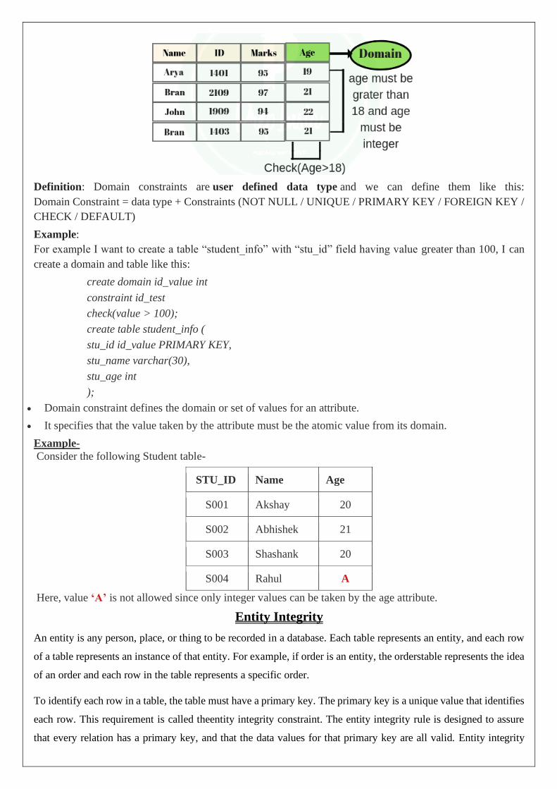
Definition: Domain constraints are user defined data type and we can define them like this:

Domain Constraint = data type + Constraints (NOT NULL / UNIQUE / PRIMARY KEY / FOREIGN KEY /

CHECK / DEFAULT)

Example:

For example I want to create a table “student_info” with “stu_id” field having value greater than 100, I can

create a domain and table like this:

create domain id_value int

constraint id_test

check(value > 100);

create table student_info (

stu_id id_value PRIMARY KEY,

stu_name varchar(30),

stu_age int

);

• Domain constraint defines the domain or set of values for an attribute.

• It specifies that the value taken by the attribute must be the atomic value from its domain.

Example-

Consider the following Student table-

STU_ID Name Age

S001 Akshay 20

S002 Abhishek 21

S003 Shashank 20

S004 Rahul A

Here, value ‘A’ is not allowed since only integer values can be taken by the age attribute.

Entity Integrity

An entity is any person, place, or thing to be recorded in a database. Each table represents an entity, and each row

of a table represents an instance of that entity. For example, if order is an entity, the orderstable represents the idea

of an order and each row in the table represents a specific order.

To identify each row in a table, the table must have a primary key. The primary key is a unique value that identifies

each row. This requirement is called theentity integrity constraint. The entity integrity rule is designed to assure

that every relation has a primary key, and that the data values for that primary key are all valid. Entity integrity

guarantees that every primary key attribute is non-null. No attribute participating in the primary key of a base

relation is allowed to contain nulls. Primary key performs the unique identification function in a relational model.

Thus a null primary key value within a base relation would be like saying that mere was some entity that had no

known identity. An entity that cannot be identified is a contradiction in terms, hence the name entity integrity. In

some cases, a particular attribute cannot be assigned a data value. There are two situations where this is likely to

occur:

• There is no applicable data value

• Applicable data value is not known when the values are assigned

For example, consider a situation where you are filling out your personal details. There is a column for fax number

and you don't have a fax number. You will leave the field blank. This is an example of no applicable data value. In

another case, suppose you are filling the ELEMENT table, you do not know the melting point for Nickel. You

know that Nickel has a melting point, but you do not know the exact value at that point in time. So you leave that

field blank since that information is not known at that point.

The relational model allows you to assign a null value to an attribute in the above-described situations. A null is a

value that is assigned to an attribute when no other value applies, or when the applicable value is unknown. In

reality, a null is not a value, but rather the absence of a value. For example, null is not the same as 0 (for numeric

fields) or blank (for character fields). The inclusion of nulls in the relational model is somewhat controversial, since

operations involving nulls sometimes leads to unpredictable results. On the other hand using null for missing values

is a good idea. But whatever the pros and cons of using null, it is imperative that the primary key values be non-

null.

• Entity integrity constraint specifies that no attribute of primary key must contain a null value in any

relation.

• This is because the presence of null value in the primary key violates the uniqueness property.

Example- Consider the following Student table-

STU_ID Name Age

S001 Akshay 20

S002 Abhishek 21

S003 Shashank 20

S004 Rahul 20

This relation does not satisfy the entity integrity constraint as here the primary key contains a NULL value.

Referential Integrity

Referential integrity refers to the relationship between tables. Because each table in a database must have a primary

key, this primary key can appear in other tables because of its relationship to data within those tables. When a

primary key from one table appears in another table, it is called aforeign key. Foreign keys join tables and establish

dependencies between tables. Tables can form a hierarchy of dependencies in such a way that if you change or

delete a row in one table, you destroy the meaning of rows in other tables.

In the relational data model, associations between tables are defined using foreign keys. For example, the

association between the ELEMENT and the SHIPMENT tables is defined by including the Symbol attribute as a

foreign key in the SHIPMENT table. This implies that before we insert a new row in the SHIPMENT table, the

element for that order must already exist in the ELEMENT table. If you examine the rows in the SHIPMENT table,

you will find that every item name in that table appears in the ELEMENT table.

A referential integrity constraint is a rule that maintains consistency among the rows of two tables (relations). The

rule states that if there is a foreign key in one relation, either each foreign key value must match a primary key

value in the other table or else the foreign key value must be null.

If base relation (table) includes a foreign key- PR matching the primary key PK of some other base relation, then

every value of FK in the first table must either be equal to the value of PK in some tuple (row) of the second table

or be wholly null (that is each attribute value participating in that FK value must be null). Or in other words, a

given foreign key value must have matching primary key value in some tuple of the referenced relation if that

foreign key value is non-null. Sometimes, it is necessary to permit foreign keys to accept nulls. Here it must be

noted that the null are of the variety 'value does not exist' rather than 'value unknown'.

• This constraint is enforced when a foreign key references the primary key of a relation.

• It specifies that all the values taken by the foreign key must either be available in the relation of the

primary key or be null.

Important Results-

The following two important results emerges out due to referential integrity constraint-

• We can not insert a record into a referencing relation if the corresponding record does not exist in the

referenced relation.

• We can not delete or update a record of the referenced relation if the corresponding record exists in the

referencing relation.

Example- Consider the following two relations- ‘Student’ and ‘Department’.

Here, relation ‘Student’ references the relation ‘Department’.

Student

STU_ID Name Dept_no

S001 Akshay D10

S002 Abhishek D10

S003 Shashank D11

S004 Rahul D14

Department

Dept_no Dept_name

D10 ASET

D11 ALS

D12 ASFL

D13 ASHS

Here,

• The relation ‘Student’ does not satisfy the referential integrity constraint.

• This is because in relation ‘Department’, no value of primary key specifies department no. 14.

• Thus, referential integrity constraint is violated.

Handling Violation of Referential Integrity Constraint-

To ensure the correctness of the database, it is important to handle the violation of referential integrity

constraint properly.

Operational Constraints

These are the constraints enforced in the database by the business rules or real world limitations. For example, if

the retirement age of the employees in an organization is 60, then the age column of the employee table can have

a constraint "Age should be less than or equal to 60." These kinds of constraints, enforced by the business and the

environment are called operational constraints.

Four basic update operations performed on relational database model are

Insert, update, delete and select.

• Insert is used to insert data into the relation

• Delete is used to delete tuples from the table.

• Modify allows you to change the values of some attributes in existing tuples.

• Select allows you to choose a specific range of data.

Whenever one of these operations are applied, integrity constraints specified on the relational database schema

must never be violated.

Insert Operation

The insert operation gives values of the attribute for a new tuple which should be inserted into a relation.

Update Operation

You can see that in the below-given relation table CustomerName= 'Apple' is updated from Inactive to Active.

Delete Operation

To specify deletion, a condition on the attributes of the relation selects the tuple to be deleted.

In the above-given example, CustomerName= "Apple" is deleted from the table.

The Delete operation could violate referential integrity if the tuple which is deleted is referenced by foreign

keys from other tuples in the same database.

Select Operation

In the above-given example, CustomerName="Amazon" is selected.

Keys • Keys play an important role in the relational database.

• It is used to uniquely identify any record or row of data from the table. It is also used to establish and

identify relationships between tables.

For example: In Student table, ID is used as a key because it is unique for each student. In PERSON table,

passport_number, license_number, SSN are keys since they are unique for each person.

Student Person

ID Name

Name DOB

Address Passport_Number

Course License_Number

SSN

Types of key:

1. Primary key

• It is the first key which is used to identify one and only one instance of an entity uniquely. An entity

can contain multiple keys as we saw in PERSON table. The key which is most suitable from those

lists become a primary key.

• In the EMPLOYEE table, ID can be primary key since it is unique for each employee. In the

EMPLOYEE table, we can even select License_Number and Passport_Number as primary key

since they are also unique.

• For each entity, selection of the primary key is based on requirement and developers.

2. Candidate key

o A candidate key is an attribute or set of an attribute which can uniquely identify a tuple.

o The remaining attributes except for primary key are considered as a candidate key. The candidate

keys are as strong as the primary key.

For example: In the EMPLOYEE table, id is best suited for the primary key. Rest of the attributes like SSN,

Passport_Number, and License_Number, etc. are considered as a candidate key.

3. Super Key

Super key is a set of an attribute which can uniquely identify a tuple. Super key is a superset of a candidate

key.

For example: In the above EMPLOYEE table, for(EMPLOEE_ID, EMPLOYEE_NAME) the name of two

employees can be the same, but their EMPLYEE_ID can't be the same. Hence, this combination can also be

a key.

The super key would be EMPLOYEE-ID, (EMPLOYEE_ID, EMPLOYEE-NAME), etc.

4. Foreign key

• Foreign keys are the column of the table which is used to point to the primary key of another table.

• In a company, every employee works in a specific department, and employee and department are two

different entities. So we can't store the information of the department in the employee table. That's

why we link these two tables through the primary key of one table.

• We add the primary key of the DEPARTMENT table, Department_Id as a new attribute in the

EMPLOYEE table.

• Now in the EMPLOYEE table, Department_Id is the foreign key, and both the tables are related.

Relational Algebra

Relational algebra is a procedural query language. It gives a step by step process to obtain the result of the

query. It uses operators to perform queries. Types of Relational operation shown below.

Fundamental operations

1. Select Operation:

• The select operation selects tuples that satisfy a given predicate.

• It is denoted by sigma (σ).

i. Notation: σ p(r)

Where:

σ is used for selection prediction

r is used for relation

p is used as a propositional logic formula which may use connectors like: AND OR and NOT. These

relational can use as relational operators like =, ≠, ≥, <, >, ≤.

For example: LOAN Relation

BRANCH_NAME LOAN_NO AMOUNT

Downtown L-17 1000

Redwood L-23 2000

Perryride L-15 1500

Downtown L-14 1500

Mianus L-13 500

Roundhill L-11 900

Perryride L-16 1300

Input:

i. σ BRANCH_NAME="perryride" (LOAN)

Output:

BRANCH_NAME LOAN_NO AMOUNT

Perryride L-15 1500

Perryride L-16 1300

2. Project Operation:

• This operation shows the list of those attributes that we wish to appear in the result. Rest of the

attributes are eliminated from the table.

• It is denoted by ∏.

i. Notation: ∏ A1, A2, An (r)

Where

A1, A2, A3 is used as an attribute name of relation r.

Example: CUSTOMER RELATION

NAME STREET CITY

Jones Main Harrison

Smith North Rye

Hays Main Harrison

Curry North Rye

Johnson Alma Brooklyn

Brooks Senator Brooklyn

Input:

i. ∏ NAME, CITY (CUSTOMER)

Output:

NAME CITY

Jones Harrison

Smith Rye

Hays Harrison

Curry Rye

Johnson Brooklyn

Brooks Brooklyn

3. Union Operation:

• Suppose there are two tuples R and S. The union operation contains all the tuples that are either in R

or S or both in R & S.

• It eliminates the duplicate tuples. It is denoted by ∪.

i. Notation: R ∪ S

A union operation must hold the following condition:

• R and S must have the attribute of the same number.

• Duplicate tuples are eliminated automatically.

Example:

DEPOSITOR RELATION

CUSTOMER_NAME ACCOUNT_NO

Johnson A-101

Smith A-121

Mayes A-321

Turner A-176

Johnson A-273

Jones A-472

Lindsay A-284

BORROW RELATION

CUSTOMER_NAME LOAN_NO

Jones L-17

Smith L-23

Hayes L-15

Jackson L-14

Curry L-93

Smith L-11

Williams L-17

Input:

i. ∏ CUSTOMER_NAME (BORROW) ∪ ∏ CUSTOMER_NAME (DEPOSITOR)

Output:

CUSTOMER_NAME

Johnson

Smith

Hayes

Turner

Jones

Lindsay

Jackson

Curry

Williams

Mayes

4. Set Intersection:

• Suppose there are two tuples R and S. The set intersection operation contains all tuples that are in

both R & S.

• It is denoted by intersection ∩.

i. Notation: R ∩ S

Example: Using the above DEPOSITOR table and BORROW table

Input:

i. ∏ CUSTOMER_NAME (BORROW) ∩ ∏ CUSTOMER_NAME (DEPOSITOR)

Output:

CUSTOMER_NAME

Smith

Jones

5. Set Difference:

• Suppose there are two tuples R and S. The set intersection operation contains all tuples that are in R

but not in S.

• It is denoted by intersection minus (-).

i. Notation: R - S

Example: Using the above DEPOSITOR table and BORROW table

Input:

i. ∏ CUSTOMER_NAME (BORROW) - ∏ CUSTOMER_NAME (DEPOSITOR)

Output:

CUSTOMER_NAME

Jackson

Hayes

Willians

Curry

6. Cartesian product

• The Cartesian product is used to combine each row in one table with each row in the other table. It is

also known as a cross product.

• It is denoted by X.

i. Notation: E X D

Example:

EMPLOYEE

EMP_ID EMP_NAME EMP_DEPT

1 Smith A

2 Harry C

3 John B

DEPARTMENT

DEPT_NO DEPT_NAME

A Marketing

B Sales

C Legal

Input:

i. EMPLOYEE X DEPARTMENT

Output:

EMP_ID EMP_NAME EMP_DEPT DEPT_NO DEPT_NAME

1 Smith A A Marketing

1 Smith A B Sales

1 Smith A C Legal

2 Harry C A Marketing

2 Harry C B Sales

2 Harry C C Legal

3 John B A Marketing

3 John B B Sales

3 John B C Legal

7. Rename Operation:

The rename operation is used to rename the output relation. It is denoted by rho (ρ).

Example: We can use the rename operator to rename STUDENT relation to STUDENT1.

i. ρ(STUDENT1, STUDENT)

Additional Operations

Additional operations are defined in terms of the fundamental operations. They do not add power to the

algebra, but are useful to simplify common queries.

1. The Set Intersection Operation

Set intersection is denoted by , and returns a relation that contains tuples that are in both of its argument

relations.

It does not add any power as

r s = r - (r - s)

To find all customers having both a loan and an account at the SFU branch, we write

ename(bname=SFU ⋈(Borrow)) ename(bname = SFU ⋈(deposit))

2. The Natural Join Operation

Often we want to simplify queries on a cartesian product.

For example, to find all customers having a loan at the bank and the cities in which they live, we

need borrow and customer relations:

borrow,ename,ecity(borrow.ename= customer. ename (borrow × customer))

Our selection predicate obtains only those tuples pertaining to only one cname.

This type of operation is very common, so we have the natural join, denoted by a ⋈ sign. Natural join

combines a cartesian product and a selection into one operation. It performs a selection forcing equality

on those attributes that appear in both relation schemes. Duplicates are removed as in all relation

operations.

To illustrate, we can rewrite the previous query as

ename,ecity(borrow ⋈ customer)

The resulting relation is shown below table.

ename ecity

Smith Burnaby

Hayes Burnaby

Jones Vancouver

Joining borrow and customer relations.

We can now make a more formal definition of natural join.

• Consider R and S to be sets of attributes.

• We denote attributes appearing in both relations by R S.

• We denote attributes in either or both relations by R S.

• Consider two relations r(R) and s(S).

• The natural join of r and s, denoted by r ⋈ s is a relation on scheme R S.

• It is a projection onto R S of a selection on r × s where the predicate requires r.Ʌ = s.Ʌ for each

attribute Ʌ in R S.

Formally,

r ⋈ s =RS (r.A1=s.A1Ʌ r.A3Ʌ......Ʌr.An=s.An(r × s))

where R S = {Ʌ1, Ʌ2,.....Ʌn}

To find the assets and names of all branches which have depositors living in Stamford, we

need customer, deposit and branch relations:

bname,assets(ecity = Stamford ⋈ (Customer ⋈ deposit ⋈ branch))

Note that ⋈ is associative.

To find all customers who have both an account and a loan at the SFU branch:

ename(bname=SFU ⋈(borrow ⋈ deposit))

This is equivalent to the set intersection version we wrote earlier. We see now that there can be several

ways to write a query in the relational algebra.

If two relations r(R) and s(S) have no attributes in common, then RS=, and r ⋈ s = r × s.

3. The Division Operation

Division, denoted ÷, is suited to queries that include the phrase ``for all''.

Suppose we want to find all the customers who have an account at all branches located in Brooklyn.

Strategy: think of it as three steps.

We can obtain the names of all branches located in Brooklyn by

r1 = bname(bcity=Brooklyn⋈(branch))

We can also find all cname, bname pairs for which the customer has an account by

r2 = ename,bname(deposit)

Now we need to find all customers who appear in r2 with every branch name in r1.

The divide operation provides exactly those customers:

ename,bname(deposit) ÷ bname(bcity=Brooklyn⋈(branch))

which is simply r2 ÷ r1.

Formally,

• Let r(R) and s(S) be relations.

• Let S R.

• The relation r ÷s is a relation on scheme R - S.

• A tuple t is in r ÷s if for every tuple ts in s there is a tuple tr in r satisfying both of the following:

tr[S] = ts[S]

tr[R – S] = t[R – S]

• These conditions say that the R – S portion of a tuple t is in r ÷s if and only if there are tuples with

the r – s portion and the S portion in r for every value of the S portion in relation S.

We will look at this explanation in class more closely.

The division operation can be defined in terms of the fundamental operations.

Read the text for a more detailed explanation.

4. The Assignment Operation

Sometimes it is useful to be able to write a relational algebra expression in parts using a temporary

relation variable (as we did with r1 and r2 in the division example).

The assignment operation, denoted , works like assignment in a programming language.

We could rewrite our division definition as

temp R – S (r)

temp – R – S ((temp × s) – r)

Relational Calculus

• Relational calculus is a non-procedural query language. In the non-procedural query language, the user is

concerned with the details of how to obtain the end results.

• The relational calculus tells what to do but never explains how to do.

Types of Relational calculus:

Tuple Relational Calculus (TRC)

• The tuple relational calculus is specified to select the tuples in a relation. In TRC, filtering variable

uses the tuples of a relation.

• The result of the relation can have one or more tuples.

Notation:

1. {T | P (T)} or {T | Condition (T)}

Where

T is the resulting tuples

P(T) is the condition used to fetch T.

For example:

i. { T.name | Author(T) AND T.article = 'database' }

OUTPUT: This query selects the tuples from the AUTHOR relation. It returns a tuple with 'name'

from Author who has written an article on 'database'.

TRC (tuple relation calculus) can be quantified. In TRC, we can use Existential (∃) and Universal

Quantifiers (∀).

For example:

i. { R| ∃T ∈ Authors(T.article='database' AND R.name=T.name)}

Output: This query will yield the same result as the previous one.

Domain Relational Calculus (DRC)

• The second form of relation is known as Domain relational calculus. In domain relational calculus,

filtering variable uses the domain of attributes.

• Domain relational calculus uses the same operators as tuple calculus. It uses logical connectives ∧

(and), ∨ (or) and ┓ (not).

• It uses Existential (∃) and Universal Quantifiers (∀) to bind the variable.

Notation:

1. { a1, a2, a3, ..., an | P (a1, a2, a3, ... ,an)}

Where

a1, a2 are attributes

P stands for formula built by inner attributes

For example:

i. {< article, page, subject > | ∈ java ∧ subject = 'database'}

Output: This query will yield the article, page, and subject from the relational java, where the subject is a

database.

SQL

• SQL stands for Structured Query Language. It is used for storing and managing data in relational

database management system (RDMS).

• It is a standard language for Relational Database System. It enables a user to create, read, update and

delete relational databases and tables.

• All the RDBMS like MySQL, Informix, Oracle, MS Access and SQL Server use SQL as their

standard database language.

• SQL allows users to query the database in a number of ways, using English-like statements.

Rules:

SQL follows the following rules:

• Structure query language is not case sensitive. Generally, keywords of SQL are written in uppercase.

• Statements of SQL are dependent on text lines. We can use a single SQL statement on one or

multiple text line.

• Using the SQL statements, you can perform most of the actions in a database.

• SQL depends on tuple relational calculus and relational algebra.

SQL process:

• When an SQL command is executing for any RDBMS, then the system figure out the best way to

carry out the request and the SQL engine determines that how to interpret the task.

• In the process, various components are included. These components can be optimization Engine,

Query engine, Query dispatcher, classic, etc.

• All the non-SQL queries are handled by the classic query engine, but SQL query engine won't handle

logical files.

Basic Structure

A relational database is a collection of tables. Each table has its own unique name.

The basic structure of an SQL expression consists of three clauses:

• The select clause which corresponds to the projection operation. It is the list of attributes that will

appear in the resulting table.

• The from clause which corresponds to the Cartesian-product operation. It is the list of tables that will

be joined in the resulting table.

• The where clause which corresponds to the selection operation. It is the expression that controls the

which rows appear in the resulting table.

A typical SQL query has the form of:

select A1, A2, ..., An

from r1, r2, ..., rn,

where P

The query is the equivalent to the relational algebra expression

A1, A2, ..., An ( P ( r1 r2 ... rn ) )

The select Clause

Formal query languages are based on the mathematical notion of a relation being a set. Duplicate tuples never

appear in relations. In practice, duplicate elimination is relatively time consuming. SQL allows duplicates in

relations as well as the results of SQL expressions.

In those cases where we want to force the elimination of duplicates, we insert the keyword distinct after select.

The default is to retain duplicates. This can be explicitly required with the keyword all.

The asterisk symbol "*" can be used in place of listing all the attributes.

The clause can also contain arithmetic expressions involving the operators +, -, *, and /.

A dot notation is used when explicitly identifying the table that the attribute comes from: borrower.loan-

number

The from Clause

The from clause defines a Cartesian product of the tables in the clause.

The where Clause

SQL uses and, or and not (not symbols) and the comparison operators <, <=, >, >=, = , and <>. Also

available is between:

where amount between 90000 and 100000

Additional, not between can be used.

The rename Operation

SQL uses the as clause:

old_name as new_name

You can do pattern matching on strings, using like and special characters:

• % which matching any substring>/li>

• _ which matches any single character

• escape which allows you override another character:

o like "ab\%cd%" escape "\" which matches any strong that starts with "ab\cd"

Ordering the Display of Tuples

SQL uses the order by clause to control the order of the display of rows, either ascending (asc) or

descending (desc):

order by amount desc

Sorting a large number of tuples may be costly and its use should be limited.

Set operations

The SQL Set operation is used to combine the two or more SQL SELECT statements.

Types of Set Operation

1. Union

2. UnionAll

3. Intersect

4. Minus

1. Union

• The SQL Union operation is used to combine the result of two or more SQL SELECT queries.

• In the union operation, all the number of datatype and columns must be same in both the tables on

which UNION operation is being applied.

• The union operation eliminates the duplicate rows from its resultset.

Syntax

i. SELECT column_name FROM table1

ii. UNION

iii. SELECT column_name FROM table2;

Example:

The First table

ID NAME

1 Jack

2 Harry

3 Jackson

The Second table

ID NAME

3 Jackson

4 Stephan

5 David

Union SQL query will be:

1. SELECT * FROM First

2. UNION

3. SELECT * FROM Second;

The resultset table will look like:

ID NAME

1 Jack

2 Harry

3 Jackson

4 Stephan

5 David

2. Union All

Union All operation is equal to the Union operation. It returns the set without removing duplication and

sorting the data.

Syntax:

i. SELECT column_name FROM table1

ii. UNION ALL

iii. SELECT column_name FROM table2;

Example: Using the above First and Second table.

Union All query will be like:

i. SELECT * FROM First

ii. UNION ALL

iii. SELECT * FROM Second;

The resultset table will look like:

ID NAME

1 Jack

2 Harry

3 Jackson

3 Jackson

4 Stephan

5 David

3. Intersect

• It is used to combine two SELECT statements. The Intersect operation returns the common rows

from both the SELECT statements.

• In the Intersect operation, the number of datatype and columns must be the same.

• It has no duplicates and it arranges the data in ascending order by default.

Syntax

i. SELECT column_name FROM table1

ii. INTERSECT

iii. SELECT column_name FROM table2;

Example:

Using the above First and Second table.

Intersect query will be:

i. SELECT * FROM First

ii. INTERSECT

iii. SELECT * FROM Second;

The resultset table will look like:

ID NAME

3 Jackson

4. Minus

• It combines the result of two SELECT statements. Minus operator is used to display the rows which

are present in the first query but absent in the second query.

• It has no duplicates and data arranged in ascending order by default.

Syntax:

i. SELECT column_name FROM table1

ii. MINUS

iii. SELECT column_name FROM table2;

Example

Using the above First and Second table.

Minus query will be:

i. SELECT * FROM First

ii. MINUS

iii. SELECT * FROM Second;

The resultset table will look like:

ID NAME

1 Jack

2 Harry

Aggregate Functions

• SQL aggregation function is used to perform the calculations on multiple rows of a single column of

a table. It returns a single value.

• It is also used to summarize the data.

Types of SQL Aggregation Function

1. COUNT FUNCTION

• COUNT function is used to Count the number of rows in a database table. It can work on both

numeric and non-numeric data types.

• COUNT function uses the COUNT(*) that returns the count of all the rows in a specified table.

COUNT(*) considers duplicate and Null.

Syntax

COUNT(*)

or

COUNT( [ALL|DISTINCT] expression )

Sample table:

PRODUCT_MAST

PRODUCT COMPANY QTY RATE COST

Item1 Com1 2 10 20

Item2 Com2 3 25 75

Item3 Com1 2 30 60

Item4 Com3 5 10 50

Item5 Com2 2 20 40

Item6 Cpm1 3 25 75

Item7 Com1 5 30 150

Item8 Com1 3 10 30

Item9 Com2 2 25 50

Item10 Com3 4 30 120

Example: COUNT()

SELECT COUNT(*)

FROM PRODUCT_MAST;

Output:

10

Example: COUNT with WHERE

SELECT COUNT(*)

FROM PRODUCT_MAST;

WHERE RATE>=20;

Output:

7

Example: COUNT() with DISTINCT

SELECT COUNT(DISTINCT COMPANY)

FROM PRODUCT_MAST;

Output:

3

Example: COUNT() with GROUP BY

SELECT COMPANY, COUNT(*)

FROM PRODUCT_MAST

GROUP BY COMPANY;

Output:

Com1 5

Com2 3

Com3 2

Example: COUNT() with HAVING

SELECT COMPANY, COUNT(*)

FROM PRODUCT_MAST

GROUP BY COMPANY

HAVING COUNT(*)>2;

Output:

Com1 5

Com2 3

2. SUM Function

Sum function is used to calculate the sum of all selected columns. It works on numeric fields only.

Syntax

SUM()

or

SUM( [ALL|DISTINCT] expression )

Example: SUM()

SELECT SUM(COST)

FROM PRODUCT_MAST;

Output:

670

Example: SUM() with WHERE

SELECT SUM(COST)

FROM PRODUCT_MAST

WHERE QTY>3;

Output:

320

Example: SUM() with GROUP BY

SELECT SUM(COST)

FROM PRODUCT_MAST

WHERE QTY>3

GROUP BY COMPANY;

Output:

Com1 150

Com2 170

Example: SUM() with HAVING

SELECT COMPANY, SUM(COST)

FROM PRODUCT_MAST

GROUP BY COMPANY

HAVING SUM(COST)>=170;

Output:

Com1 335

Com3 170

3. AVG function

The AVG function is used to calculate the average value of the numeric type. AVG function returns the

average of all non-Null values.

Syntax

AVG()

or

AVG( [ALL|DISTINCT] expression )

Example:

SELECT AVG(COST)

FROM PRODUCT_MAST;

Output:

67.00

4. MAX Function

MAX function is used to find the maximum value of a certain column. This function determines the

largest value of all selected values of a column.

Syntax

MAX()

or

MAX( [ALL|DISTINCT] expression )

Example:

SELECT MAX(RATE)

FROM PRODUCT_MAST;

Output:

30

5. MIN Function

MIN function is used to find the minimum value of a certain column. This function determines the

smallest value of all selected values of a column.

Syntax

MIN()

or

MIN( [ALL|DISTINCT] expression )

Example:

SELECT MIN(RATE)

FROM PRODUCT_MAST;

Output:

10

Null values

The SQL NULL is the term used to represent a missing value. A NULL value in a table is a value in a field

that appears to be blank.

A field with a NULL value is a field with no value. It is very important to understand that a NULL value is

different than a zero value or a field that contains spaces.

Syntax

The basic syntax of NULL while creating a table.

SQL> CREATE TABLE CUSTOMERS (

ID INT NOT NULL,

NAME VARCHAR (20) NOT NULL,

AGE INT NOT NULL,

ADDRESS CHAR (25) ,

SALARY DECIMAL (18, 2),

PRIMARY KEY (ID)

);

Here, NOT NULL signifies that column should always accept an explicit value of the given data type. There

are two columns where we did not use NOT NULL, which means these columns could be NULL.

A field with a NULL value is the one that has been left blank during the record creation.

Example

The NULL value can cause problems when selecting data. However, because when comparing an unknown

value to any other value, the result is always unknown and not included in the results. You must use the IS

NULL or IS NOT NULL operators to check for a NULL value.

Consider the following CUSTOMERS table having the records as shown below.

+----+----------+-----+-----------+----------+

| ID | NAME | AGE | ADDRESS | SALARY |

+----+----------+-----+-----------+----------+

| 1 | Ramesh | 32 | Ahmedabad | 2000.00 |

| 2 | Khilan | 25 | Delhi | 1500.00 |

| 3 | kaushik | 23 | Kota | 2000.00 |

| 4 | Chaitali | 25 | Mumbai | 6500.00 |

| 5 | Hardik | 27 | Bhopal | 8500.00 |

| 6 | Komal | 22 | MP | |

| 7 | Muffy | 24 | Indore | |

+----+----------+-----+-----------+----------+

Now, following is the usage of the IS NOT NULLoperator.

SQL> SELECT ID, NAME, AGE, ADDRESS, SALARY

FROM CUSTOMERS

WHERE SALARY IS NOT NULL;

This would produce the following result −

+----+----------+-----+-----------+----------+

| ID | NAME | AGE | ADDRESS | SALARY |

+----+----------+-----+-----------+----------+

| 1 | Ramesh | 32 | Ahmedabad | 2000.00 |

| 2 | Khilan | 25 | Delhi | 1500.00 |

| 3 | kaushik | 23 | Kota | 2000.00 |

| 4 | Chaitali | 25 | Mumbai | 6500.00 |

| 5 | Hardik | 27 | Bhopal | 8500.00 |

+----+----------+-----+-----------+----------+

Now, following is the usage of the IS NULL operator.

SQL> SELECT ID, NAME, AGE, ADDRESS, SALARY

FROM CUSTOMERS

WHERE SALARY IS NULL;

This would produce the following result −

+----+----------+-----+-----------+----------+

| ID | NAME | AGE | ADDRESS | SALARY |

+----+----------+-----+-----------+----------+

| 6 | Komal | 22 | MP | |

| 7 | Muffy | 24 | Indore | |

+----+----------+-----+-----------+----------+

Nested Sub queries

In nested queries, a query is written inside a query. The result of inner query is used in execution of outer

query. We will use STUDENT, COURSE, STUDENT_COURSE tables for understanding nested queries.

STUDENT

S_ID S_NAME S_ADDRESS S_PHONE S_AGE

S1 RAM DELHI 9455123451 18

S2 RAMESH GURGAON 9652431543 18

S3 SUJIT ROHTAK 9156253131 20

S4 SURESH DELHI 9156768971 18

COURSE

C_ID C_NAME

C1 DSA

C2 Programming

C3 DBMS

STUDENT_COURSE

S_ID C_ID

S1 C1

S1 C3

S2 C1

S3 C2

S4 C2

S4 C3

There are mainly two types of nested queries:

• Independent Nested Queries: In independent nested queries, query execution starts from innermost

query to outermost queries. The execution of inner query is independent of outer query, but the result of

inner query is used in execution of outer query. Various operators like IN, NOT IN, ANY, ALL etc are

used in writing independent nested queries.

IN: If we want to find out S_ID who are enrolled in C_NAME ‘DSA’ or ‘DBMS’, we can write it with the

help of independent nested query and IN operator. From COURSE table, we can find out C_ID for C_NAME

‘DSA’ or DBMS’ and we can use these C_IDs for finding S_IDs from STUDENT_COURSE TABLE.

STEP 1: Finding C_ID for C_NAME =’DSA’ or ‘DBMS’

Select C_ID from COURSE where C_NAME = ‘DSA’ or C_NAME = ‘DBMS’

STEP 2: Using C_ID of step 1 for finding S_ID

Select S_ID from STUDENT_COURSE where C_ID IN

(SELECT C_ID from COURSE where C_NAME = ‘DSA’ or C_NAME=’DBMS’);

The inner query will return a set with members C1 and C3 and outer query will return those S_IDs for which

C_ID is equal to any member of set (C1 and C3 in this case). So, it will return S1, S2 and S4.

• Note: If we want to find out names of STUDENTs who have either enrolled in ‘DSA’ or ‘DBMS’, it

can be done as:

Select S_NAME from STUDENT where S_ID IN

(Select S_ID from STUDENT_COURSE where C_ID IN

(SELECT C_ID from COURSE where C_NAME=’DSA’ or C_NAME=’DBMS’));

NOT IN: If we want to find out S_IDs of STUDENTs who have neither enrolled in ‘DSA’ nor in

‘DBMS’, it can be done as:

Select S_ID from STUDENT where S_ID NOT IN

(Select S_ID from STUDENT_COURSE where C_ID IN

(SELECT C_ID from COURSE where C_NAME=’DSA’ or C_NAME=’DBMS’));

The innermost query will return a set with members C1 and C3. Second inner query will return

those S_IDs for which C_ID is equal to any member of set (C1 and C3 in this case) which are S1, S2

and S4. The outermost query will return those S_IDs where S_ID is not a member of set (S1, S2 and

S4). So it will return S3.

• Co-related Nested Queries: In co-related nested queries, the output of inner query depends on the row

which is being currently executed in outer query. e.g.; If we want to find out S_NAME of STUDENTs

who are enrolled in C_ID ‘C1’, it can be done with the help of co-related nested query as:

Select S_NAME from STUDENT S where EXISTS

(select * from STUDENT_COURSE SC where S.S_ID=SC.S_ID and SC.C_ID=’C1’);

For each row of STUDENT S, it will find the rows from STUDENT_COURSE where S.S_ID =

SC.S_ID and SC.C_ID=’C1’. If for a S_ID from STUDENT S, atleast a row exists

in STUDENT_COURSE SC with C_ID=’C1’, then inner query will return true and

corresponding S_ID will be returned as output.

Derived Relations

A subquery expression to be used in the from clause.

If such an expression is used, the result relation must be given a name, and the attributes can be renamed.

Find the average account balance of those branches where the average account balance is greater than $1,000.

select bname, avg-balance

from (select bname, avg(balance)

from account

group by (bname)

as result(bname, avg-balance)

where avg-balance > 1000

Find the average account balance of those branches where the average account balance is greater than $1200.

select branch-name, avg-balance

from (select branch-name, avg (balance)

as avg-balance from account

group by branch-name)

where avg-balance > 1200

Note that we do not need to use the having clause, since we compute the temporary (view) relation in the

FROM clause, and the attributes of result can be used directly in the where clause.

Views

• Views in SQL are considered as a virtual table. A view also contains rows and columns.

• To create the view, we can select the fields from one or more tables present in the database.

• A view can either have specific rows based on certain condition or all the rows of a table.

Sample table:

Student_Detail

STU_ID NAME ADDRESS

1 Stephan Delhi

2 Kathrin Noida

3 David Ghaziabad

4 Alina Gurugram

Student_Marks

STU_ID NAME MARKS AGE

1 Stephan 97 19

2 Kathrin 86 21

3 David 74 18

4 Alina 90 20

5 John 96 18

1. Creating view

A view can be created using the CREATE VIEW statement. We can create a view from a single table or

multiple tables.

Syntax:

CREATE VIEW view_name AS

SELECT column1, column2.....

FROM table_name

WHERE condition;

2. Creating View from a single table

In this example, we create a View named DetailsView from the table Student_Detail.

Query:

CREATE VIEW DetailsView AS

SELECT NAME, ADDRESS

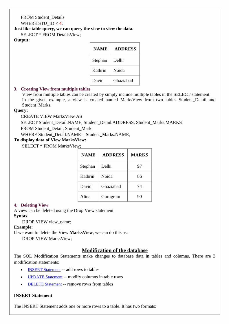
FROM Student_Details

WHERE STU_ID < 4;

Just like table query, we can query the view to view the data.

SELECT * FROM DetailsView;

Output:

NAME ADDRESS

Stephan Delhi

Kathrin Noida

David Ghaziabad

3. Creating View from multiple tables

View from multiple tables can be created by simply include multiple tables in the SELECT statement.

In the given example, a view is created named MarksView from two tables Student_Detail and

Student_Marks.

Query:

CREATE VIEW MarksView AS

SELECT Student_Detail.NAME, Student_Detail.ADDRESS, Student_Marks.MARKS

FROM Student_Detail, Student_Mark

WHERE Student_Detail.NAME = Student_Marks.NAME;

To display data of View MarksView:

SELECT * FROM MarksView;

NAME ADDRESS MARKS

Stephan Delhi 97

Kathrin Noida 86

David Ghaziabad 74

Alina Gurugram 90

4. Deleting View

A view can be deleted using the Drop View statement.

Syntax

DROP VIEW view_name;

Example:

If we want to delete the View MarksView, we can do this as:

DROP VIEW MarksView;

Modification of the database The SQL Modification Statements make changes to database data in tables and columns. There are 3

modification statements:

• INSERT Statement -- add rows to tables

• UPDATE Statement -- modify columns in table rows

• DELETE Statement -- remove rows from tables

INSERT Statement

The INSERT Statement adds one or more rows to a table. It has two formats:

INSERT INTO table-1 [(column-list)] VALUES (value-list)

and,

INSERT INTO table-1 [(column-list)] (query-specification)

The first form inserts a single row into table-1 and explicitly specifies the column values for the row. The

second form uses the result of query-specification to insert one or more rows into table-1. The result rows

from the query are the rows added to the insert table. Note: the query cannot reference table-1.

Both forms have an optional column-list specification. Only the columns listed will be assigned values.

Unlisted columns are set to null, so unlisted columns must allow nulls. The values from the VALUES

Clause (first form) or the columns from the query-specification rows (second form) are assigned to the

corresponding column in column-list in order.

If the optional column-list is missing, the default column list is substituted. The default column list contains

all columns in table-1 in the order they were declared in CREATE TABLE, or CREATE VIEW.

VALUES Clause

The VALUES Clause in the INSERT Statement provides a set of values to place in the columns of a new row.

It has the following general format:

VALUES ( value-1 [, value-2] ... )

value-1 and value-2 are Literal Values or Scalar Expressions involving literals. They can also specify NULL.

The values list in the VALUES clause must match the explicit or implicit column list for INSERT in degree

(number of items). They must also match the data type of corresponding column or be convertible to that data

type.

INSERT Examples

INSERT INTO p (pno, color) VALUES ('P4', 'Brown')

Before After

Pno descr color

P1 Widget Blue

P2 Widget Red

P3 Dongle Green

➔

pno descr Color

P1 Widget Blue

P2 Widget Red

P3 Dongle Green

P4 NULL Brown

INSERT INTO sp

SELECT s.sno, p.pno, 500

FROM s, p

WHERE p.color='Green' AND s.city='London'

Before After

sno pno qty

S1 P1 NULL

S2 P1 200

S3 P1 1000

S3 P2 200

➔

sno pno qty

S1 P1 NULL

S2 P1 200

S3 P1 1000

S3 P2 200

S2 P3 500

UPDATE Statement

The UPDATE statement modifies columns in selected table rows. It has the following general format:

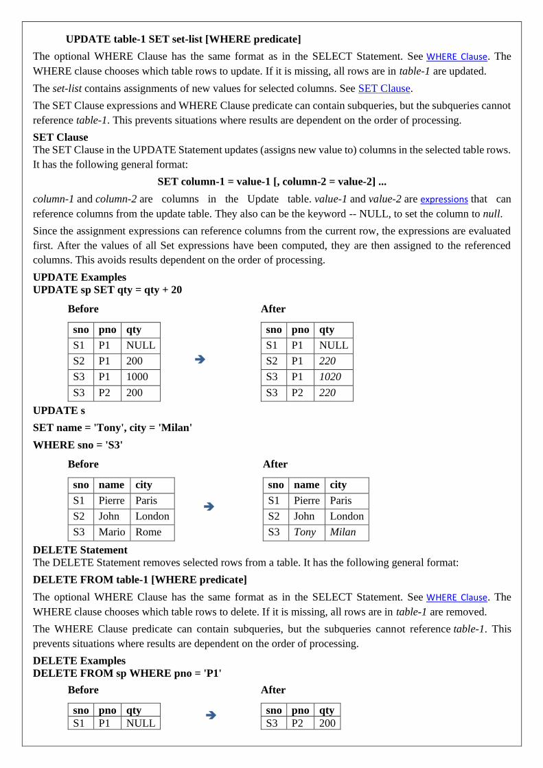
UPDATE table-1 SET set-list [WHERE predicate]

The optional WHERE Clause has the same format as in the SELECT Statement. See WHERE Clause. The

WHERE clause chooses which table rows to update. If it is missing, all rows are in table-1 are updated.

The set-list contains assignments of new values for selected columns. See SET Clause.

The SET Clause expressions and WHERE Clause predicate can contain subqueries, but the subqueries cannot

reference table-1. This prevents situations where results are dependent on the order of processing.

SET Clause

The SET Clause in the UPDATE Statement updates (assigns new value to) columns in the selected table rows.

It has the following general format:

SET column-1 = value-1 [, column-2 = value-2] ...

column-1 and column-2 are columns in the Update table. value-1 and value-2 are expressions that can

reference columns from the update table. They also can be the keyword -- NULL, to set the column to null.

Since the assignment expressions can reference columns from the current row, the expressions are evaluated

first. After the values of all Set expressions have been computed, they are then assigned to the referenced

columns. This avoids results dependent on the order of processing.

UPDATE Examples

UPDATE sp SET qty = qty + 20

Before After

sno pno qty

S1 P1 NULL

S2 P1 200

S3 P1 1000

S3 P2 200

➔

sno pno qty

S1 P1 NULL

S2 P1 220

S3 P1 1020

S3 P2 220

UPDATE s

SET name = 'Tony', city = 'Milan'

WHERE sno = 'S3'

Before After

sno name city

S1 Pierre Paris

S2 John London

S3 Mario Rome

➔

sno name city

S1 Pierre Paris

S2 John London

S3 Tony Milan

DELETE Statement

The DELETE Statement removes selected rows from a table. It has the following general format:

DELETE FROM table-1 [WHERE predicate]

The optional WHERE Clause has the same format as in the SELECT Statement. See WHERE Clause. The

WHERE clause chooses which table rows to delete. If it is missing, all rows are in table-1 are removed.

The WHERE Clause predicate can contain subqueries, but the subqueries cannot reference table-1. This

prevents situations where results are dependent on the order of processing.

DELETE Examples

DELETE FROM sp WHERE pno = 'P1'

Before After

sno pno qty

S1 P1 NULL ➔

sno pno qty

S3 P2 200

S2 P1 200

S3 P1 1000

S3 P2 200

DELETE FROM p WHERE pno NOT IN (SELECT pno FROM sp)

Before After

pno descr color

P1 Widget Blue

P2 Widget Red

P3 Dongle Green

➔

pno descr color

P1 Widget Blue

P2 Widget Red

SQL JOIN

As the name shows, JOIN means to combine something. In case of SQL, JOIN means "to combine two or

more tables".

In SQL, JOIN clause is used to combine the records from two or more tables in a database.

Types of SQL JOIN

1. INNER JOIN

2. LEFT JOIN

3. RIGHT JOIN

4. FULL JOIN

Sample Table

EMPLOYEE

EMP_ID EMP_NAME CITY SALARY AGE

1 Angelina Chicago 200000 30

2 Robert Austin 300000 26

3 Christian Denver 100000 42

4 Kristen Washington 500000 29

5 Russell Los angels 200000 36

6 Marry Canada 600000 48

PROJECT

PROJECT_NO EMP_ID DEPARTMENT

101 1 Testing

102 2 Development

103 3 Designing

104 4 Development

1. INNER JOIN

In SQL, INNER JOIN selects records that have matching values in both tables as long as the condition is

satisfied. It returns the combination of all rows from both the tables where the condition satisfies.

Syntax

SELECT table1.column1, table1.column2, table2.column1,....

FROM table1

INNER JOIN table2

ON table1.matching_column = table2.matching_column;

Query

SELECT EMPLOYEE.EMP_NAME, PROJECT.DEPARTMENT

FROM EMPLOYEE

INNER JOIN PROJECT

ON PROJECT.EMP_ID = EMPLOYEE.EMP_ID;

Output

EMP_NAME DEPARTMENT

Angelina Testing

Robert Development

Christian Designing

Kristen Development

2. LEFT JOIN

The SQL left join returns all the values from left table and the matching values from the right table. If

there is no matching join value, it will return NULL.

Syntax

SELECT table1.column1, table1.column2, table2.column1,....

FROM table1

LEFT JOIN table2

ON table1.matching_column = table2.matching_column;

Query

SELECT EMPLOYEE.EMP_NAME, PROJECT.DEPARTMENT

FROM EMPLOYEE

LEFT JOIN PROJECT

ON PROJECT.EMP_ID = EMPLOYEE.EMP_ID;

Output

EMP_NAME DEPARTMENT

Angelina Testing

Robert Development

Christian Designing

Kristen Development

Russell NULL

Marry NULL

3. RIGHT JOIN

In SQL, RIGHT JOIN returns all the values from the values from the rows of right table and the matched

values from the left table. If there is no matching in both tables, it will return NULL.

Syntax

SELECT table1.column1, table1.column2, table2.column1,....

FROM table1

RIGHT JOIN table2

ON table1.matching_column = table2.matching_column;

Query

SELECT EMPLOYEE.EMP_NAME, PROJECT.DEPARTMENT

FROM EMPLOYEE

RIGHT JOIN PROJECT

ON PROJECT.EMP_ID = EMPLOYEE.EMP_ID;

Output

EMP_NAME DEPARTMENT

Angelina Testing

Robert Development

Christian Designing

Kristen Development

4. FULL JOIN

In SQL, FULL JOIN is the result of a combination of both left and right outer join. Join tables have all

the records from both tables. It puts NULL on the place of matches not found.

Syntax

SELECT table1.column1, table1.column2, table2.column1,....

FROM table1

FULL JOIN table2

ON table1.matching_column = table2.matching_column;

Query

SELECT EMPLOYEE.EMP_NAME, PROJECT.DEPARTMENT

FROM EMPLOYEE

FULL JOIN PROJECT

ON PROJECT.EMP_ID = EMPLOYEE.EMP_ID;

Output

EMP_NAME DEPARTMENT

Angelina Testing

Robert Development

Christian Designing

Kristen Development

Russell NULL

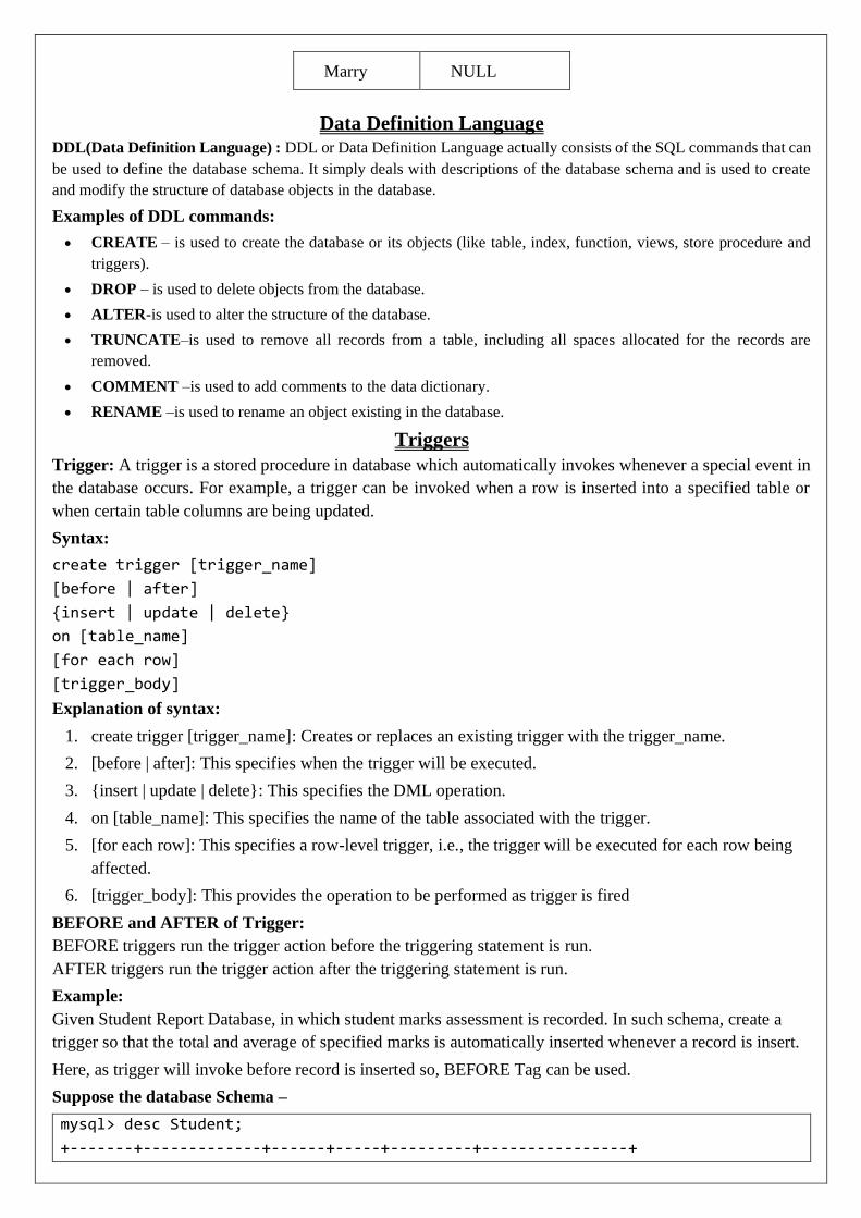
Marry NULL

Data Definition Language

DDL(Data Definition Language) : DDL or Data Definition Language actually consists of the SQL commands that can

be used to define the database schema. It simply deals with descriptions of the database schema and is used to create

and modify the structure of database objects in the database.

Examples of DDL commands:

• CREATE – is used to create the database or its objects (like table, index, function, views, store procedure and

triggers).

• DROP – is used to delete objects from the database.

• ALTER-is used to alter the structure of the database.

• TRUNCATE–is used to remove all records from a table, including all spaces allocated for the records are

removed.

• COMMENT –is used to add comments to the data dictionary.

• RENAME –is used to rename an object existing in the database.

Triggers

Trigger: A trigger is a stored procedure in database which automatically invokes whenever a special event in

the database occurs. For example, a trigger can be invoked when a row is inserted into a specified table or

when certain table columns are being updated.

Syntax:

create trigger [trigger_name]

[before | after]

{insert | update | delete}

on [table_name]

[for each row]

[trigger_body]

Explanation of syntax:

1. create trigger [trigger_name]: Creates or replaces an existing trigger with the trigger_name.

2. [before | after]: This specifies when the trigger will be executed.

3. {insert | update | delete}: This specifies the DML operation.

4. on [table_name]: This specifies the name of the table associated with the trigger.

5. [for each row]: This specifies a row-level trigger, i.e., the trigger will be executed for each row being

affected.

6. [trigger_body]: This provides the operation to be performed as trigger is fired

BEFORE and AFTER of Trigger:

BEFORE triggers run the trigger action before the triggering statement is run.

AFTER triggers run the trigger action after the triggering statement is run.

Example:

Given Student Report Database, in which student marks assessment is recorded. In such schema, create a

trigger so that the total and average of specified marks is automatically inserted whenever a record is insert.

Here, as trigger will invoke before record is inserted so, BEFORE Tag can be used.

Suppose the database Schema –

mysql> desc Student;

+-------+-------------+------+-----+---------+----------------+

| Field | Type | Null | Key | Default | Extra |

+-------+-------------+------+-----+---------+----------------+

| tid | int(4) | NO | PRI | NULL | auto_increment |

| name | varchar(30) | YES | | NULL | |

| subj1 | int(2) | YES | | NULL | |

| subj2 | int(2) | YES | | NULL | |

| subj3 | int(2) | YES | | NULL | |

| total | int(3) | YES | | NULL | |

| per | int(3) | YES | | NULL | |

+-------+-------------+------+-----+---------+----------------+

7 rows in set (0.00 sec)

SQL Trigger to problem statement.

create trigger stud_marks

before INSERT

on

Student

for each row

set Student.total = Student.subj1 + Student.subj2 + Student.subj3, Student.per = Student.total * 60 / 100;

Above SQL statement will create a trigger in the student database in which whenever subjects marks are

entered, before inserting this data into the database, trigger will compute those two values and insert with the

entered values. i.e.,

mysql> insert into Student values(0, "ABCDE", 20, 20, 20, 0, 0);

Query OK, 1 row affected (0.09 sec)

mysql> select * from Student; +-----+-------+-------+-------+-------+-------+------+ | tid | name | subj1 | subj2 | subj3 | total | per | +-----+-------+-------+-------+-------+-------+------+ | 100 | ABCDE | 20 | 20 | 20 | 60 | 36 | +-----+-------+-------+-------+-------+-------+------+ 1 row in set (0.00 sec)

In this way trigger can be creates and executed in the databases.

UNIT – III Database Design

Functional Dependencies – Pitfalls in Relational Database Design – Decomposition – Normalization using

Functional Dependencies – Normalization using Multi-valued Dependencies – Normalization using Join

Dependencies – Domain - Key Normal form.

A functional dependency A->B in a relation holds if two tuples having same value of attribute A also have

same value for attribute B. For Example, in relation STUDENT shown in table 1, Functional Dependencies

Functional Dependencies

Functional Dependency (FD) determines the relation of one attribute to another attribute in a database

management system (DBMS) system. Functional dependency helps you to maintain the quality of data in the

database. A functional dependency is denoted by an arrow →. The functional dependency of X on Y is

represented by X → Y. Functional Dependency plays a vital role to find the difference between good and bad

database design.

Example:

Employee number Employee Name Salary City

1 Dana 50000 San Francisco

2 Francis 38000 London

3 Andrew 25000 Tokyo

In this example, if we know the value of Employee number, we can obtain Employee Name, city, salary, etc.

By this, we can say that the city, Employee Name, and salary are functionally depended on Employee number.

Key terms

Key Terms Description

Axiom Axioms is a set of inference rules used to infer all the functional dependencies on a

relational database.

Decomposition It is a rule that suggests if you have a table that appears to contain two entities which are

determined by the same primary key then you should consider breaking them up into two

different tables.

Dependent It is displayed on the right side of the functional dependency diagram.

Determinant It is displayed on the left side of the functional dependency Diagram.

Union It suggests that if two tables are separate, and the PK is the same, you should consider

putting them. together

Rules of Functional Dependencies

Below given are the Three most important rules for Functional Dependency:

• Reflexive rule –. If X is a set of attributes and Y is_subset_of X, then X holds a value of Y.

• Augmentation rule: When x -> y holds, and c is attribute set, then ac -> bc also holds. That is adding

attributes which do not change the basic dependencies.

• Transitivity rule: This rule is very much similar to the transitive rule in algebra if x -> y holds and y -

> z holds, then x -> z also holds. X -> y is called as functionally that determines y.

Types of Functional Dependencies

• Multivalued dependency:

• Trivial functional dependency:

• Non-trivial functional dependency:

• Transitive dependency:

Multivalued dependency in DBMS

Multivalued dependency occurs in the situation where there are multiple independent multivalued

attributes in a single table. A multivalued dependency is a complete constraint between two sets of attributes

in a relation. It requires that certain tuples be present in a relation.

Example:

Car_model Maf_year Color

H001 2017 Metallic

H001 2017 Green

H005 2018 Metallic

H005 2018 Blue

H010 2015 Metallic

H033 2012 Gray

In this example, maf_year and color are independent of each other but dependent on car_model. In this

example, these two columns are said to be multivalue dependent on car_model.

This dependence can be represented like this:

car_model -> maf_year

car_model-> colour

Trivial Functional dependency:

The Trivial dependency is a set of attributes which are called a trivial if the set of attributes are included in

that attribute.

So, X -> Y is a trivial functional dependency if Y is a subset of X.

For example:

Emp_id Emp_name

AS555 Harry

AS811 George

AS999 Kevin

Consider this table with two columns Emp_id and Emp_name.

{Emp_id, Emp_name} -> Emp_id is a trivial functional dependency as Emp_id is a subset of

{Emp_id,Emp_name}.

Non trivial functional dependency in DBMS

Functional dependency which also known as a nontrivial dependency occurs when A->B holds true where B

is not a subset of A. In a relationship, if attribute B is not a subset of attribute A, then it is considered as a non-

trivial dependency.

Company CEO Age

Microsoft Satya Nadella 51

Google Sundar Pichai 46

Apple Tim Cook 57

Example:

(Company} -> {CEO} (if we know the Company, we knows the CEO name)

But CEO is not a subset of Company, and hence it's non-trivial functional dependency.

Transitive dependency:

A transitive is a type of functional dependency which happens when t is indirectly formed by two functional

dependencies.

Example:

Company CEO Age

Microsoft Satya Nadella 51

Google Sundar Pichai 46

Alibaba Jack Ma 54

{Company} -> {CEO} (if we know the compay, we know its CEO's name)

{CEO} -> {Age} If we know the CEO, we know the Age

Therefore according to the rule of rule of transitive dependency:

{Company} -> {Age} should hold, that makes sense because if we know the company name, we can know

his age.

Note: You need to remember that transitive dependency can only occur in a relation of three or more attributes.

Pitfalls in Relational Database Design

• Relational database design requires that we find a “good” collection of relation schemas. A bad design

may lead to

• Repetition of Information.

• Inability to represent certain information.

• Design Goals:

• Avoid redundant data

• Ensure that relationships among attributes are represented

• Facilitate the checking of updates for violation of database integrity constraints.

Example

Consider the relation schema:

Lending-schema = (branch-name, branch-city, assets, customer-name, loan-number, amount)

Problems:

• Redundancy:

• Data for branch-name, branch-city, assets are repeated for each loan that a branch makes

• Wastes space

• Complicates updating, introducing possibility of inconsistency of assets value

• Null values

• Cannot store information about a branch if no loans exist

• Can use null values, but they are difficult to handle.

Decomposition

• When a relation in the relational model is not in appropriate normal form then the decomposition of a

relation is required.

• In a database, it breaks the table into multiple tables.

• If the relation has no proper decomposition, then it may lead to problems like loss of information.

• Decomposition is used to eliminate some of the problems of bad design like anomalies,

inconsistencies, and redundancy.

Types of Decomposition

Lossless Decomposition

• If the information is not lost from the relation that is decomposed, then the decomposition will be

lossless.

• The lossless decomposition guarantees that the join of relations will result in the same relation as it

was decomposed.

• The relation is said to be lossless decomposition if natural joins of all the decomposition give the

original relation.

Example:

EMPLOYEE_DEPARTMENT table:

EMP_ID EMP_NAME EMP_AGE EMP_CITY DEPT_ID DEPT_NAME

22 Denim 28 Mumbai 827 Sales

33 Alina 25 Delhi 438 Marketing

46 Stephan 30 Bangalore 869 Finance

52 Katherine 36 Mumbai 575 Production

60 Jack 40 Noida 678 Testing

The above relation is decomposed into two relations EMPLOYEE and DEPARTMENT

EMPLOYEE table:

EMP_ID EMP_NAME EMP_AGE EMP_CITY

22 Denim 28 Mumbai

33 Alina 25 Delhi

46 Stephan 30 Bangalore

52 Katherine 36 Mumbai

60 Jack 40 Noida

DEPARTMENT table

DEPT_ID EMP_ID DEPT_NAME

827 22 Sales

438 33 Marketing

869 46 Finance

575 52 Production

678 60 Testing

Now, when these two relations are joined on the common column "EMP_ID", then the resultant relation will

look like:

Employee ⋈ Department

EMP_ID EMP_NAME EMP_AGE EMP_CITY DEPT_ID DEPT_NAME

22 Denim 28 Mumbai 827 Sales

33 Alina 25 Delhi 438 Marketing

46 Stephan 30 Bangalore 869 Finance

52 Katherine 36 Mumbai 575 Production

60 Jack 40 Noida 678 Testing

Hence, the decomposition is Lossless join decomposition.

Dependency Preserving

• It is an important constraint of the database.

• In the dependency preservation, at least one decomposed table must satisfy every dependency.

• If a relation R is decomposed into relation R1 and R2, then the dependencies of R either must be a part

of R1 or R2 or must be derivable from the combination of functional dependencies of R1 and R2.

• For example, suppose there is a relation R (A, B, C, D) with functional dependency set (A->BC). The

relational R is decomposed into R1(ABC) and R2(AD) which is dependency preserving because FD

A->BC is a part of relation R1(ABC).

Normalization using Functional Dependencies

The functional dependency is a relationship that exists between two attributes. It typically exists between the

primary key and non-key attribute within a table.

X → Y

The left side of FD is known as a determinant, the right side of the production is known as a dependent.

For example:

Assume we have an employee table with attributes: Emp_Id, Emp_Name, Emp_Address.

Here Emp_Id attribute can uniquely identify the Emp_Name attribute of employee table because if we know

the Emp_Id, we can tell that employee name associated with it.

Functional dependency can be written as:

Emp_Id → Emp_Name

We can say that Emp_Name is functionally dependent on Emp_Id.

Types of Functional dependency

1. Trivial functional dependency

• A → B has trivial functional dependency if B is a subset of A.

• The following dependencies are also trivial like: A → A, B → B

Example:

Consider a table with two columns Employee_Id and Employee_Name.

{Employee_id, Employee_Name} → Employee_Id is a trivial functional dependency as

Employee_Id is a subset of {Employee_Id, Employee_Name}.

Also, Employee_Id → Employee_Id and Employee_Name → Employee_Name are trivial dependenci

es too.

2. Non-trivial functional dependency

• A → B has a non-trivial functional dependency if B is not a subset of A.

• When A intersection B is NULL, then A → B is called as complete non-trivial.

Example:

ID → Name,

Name → DOB

Normalization

• Normalization is the process of organizing the data in the database.

• Normalization is used to minimize the redundancy from a relation or set of relations. It is also used to

eliminate the undesirable characteristics like Insertion, Update and Deletion Anomalies.

• Normalization divides the larger table into the smaller table and links them using relationship.

• The normal form is used to reduce redundancy from the database table.

Types of Normal Forms

There are the four types of normal forms:

Normal Form Description

1NF A relation is in 1NF if it contains an atomic value.

2NF A relation will be in 2NF if it is in 1NF and all non-key attributes are fully

functional dependent on the primary key.

3NF A relation will be in 3NF if it is in 2NF and no transition dependency exists.

4NF A relation will be in 4NF if it is in Boyce Codd normal form and has no multi-

valued dependency.

5NF A relation is in 5NF if it is in 4NF and not contains any join dependency and joining

should be lossless.

First Normal Form (1NF)

• A relation will be 1NF if it contains an atomic value.

• It states that an attribute of a table cannot hold multiple values. It must hold only single-valued attribute.

• First normal form disallows the multi-valued attribute, composite attribute, and their combinations.

Example: Relation EMPLOYEE is not in 1NF because of multi-valued attribute EMP_PHONE.

EMPLOYEE table:

EMP_ID EMP_NAME EMP_PHONE EMP_STATE

14 John 7272826385,

9064738238

UP

20 Harry 8574783832 Bihar

12 Sam 7390372389,

8589830302

Punjab

The decomposition of the EMPLOYEE table into 1NF has been shown below:

EMP_ID EMP_NAME EMP_PHONE EMP_STATE

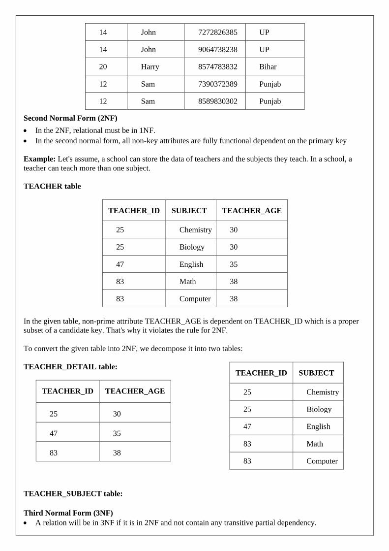
14 John 7272826385 UP

14 John 9064738238 UP

20 Harry 8574783832 Bihar

12 Sam 7390372389 Punjab

12 Sam 8589830302 Punjab

Second Normal Form (2NF)

• In the 2NF, relational must be in 1NF.

• In the second normal form, all non-key attributes are fully functional dependent on the primary key

Example: Let's assume, a school can store the data of teachers and the subjects they teach. In a school, a

teacher can teach more than one subject.

TEACHER table

TEACHER_ID SUBJECT TEACHER_AGE

25 Chemistry 30

25 Biology 30

47 English 35

83 Math 38

83 Computer 38

In the given table, non-prime attribute TEACHER_AGE is dependent on TEACHER_ID which is a proper

subset of a candidate key. That's why it violates the rule for 2NF.

To convert the given table into 2NF, we decompose it into two tables:

TEACHER_DETAIL table:

TEACHER_ID TEACHER_AGE

25 30

47 35

83 38

TEACHER_SUBJECT table:

TEACHER_ID SUBJECT

25 Chemistry

25 Biology

47 English

83 Math

83 Computer

Third Normal Form (3NF)

• A relation will be in 3NF if it is in 2NF and not contain any transitive partial dependency.

• 3NF is used to reduce the data duplication. It is also used to achieve the data integrity.

• If there is no transitive dependency for non-prime attributes, then the relation must be in third normal form.

A relation is in third normal form if it holds atleast one of the following conditions for every non-trivial

function dependency X → Y.

1. X is a super key.

2. Y is a prime attribute, i.e., each element of Y is part of some candidate key.

Example:

EMPLOYEE_DETAIL table:

EMP_ID EMP_NAME EMP_ZIP EMP_STATE EMP_CITY

222 Harry 201010 UP Noida

333 Stephan 02228 US Boston

444 Lan 60007 US Chicago

555 Katharine 06389 UK Norwich

666 John 462007 MP Bhopal

Super key in the table above:

{EMP_ID}, {EMP_ID, EMP_NAME}, {EMP_ID, EMP_NAME, EMP_ZIP}....so on

Candidate key: {EMP_ID}

Non-prime attributes: In the given table, all attributes except EMP_ID are non-prime.

Here, EMP_STATE & EMP_CITY dependent on EMP_ZIP and EMP_ZIP dependent on EMP_ID. The non-

prime attributes (EMP_STATE, EMP_CITY) transitively dependent on super key(EMP_ID). It violates the

rule of third normal form.

That's why we need to move the EMP_CITY and EMP_STATE to the new <EMPLOYEE_ZIP> table, with

EMP_ZIP as a Primary key.

EMPLOYEE table:

EMP_ID EMP_NAME EMP_ZIP

222 Harry 201010

333 Stephan 02228

444 Lan 60007

555 Katharine 06389

666 John 462007

EMPLOYEE_ZIP table:

EMP_ZIP EMP_STATE EMP_CITY

201010 UP Noida

02228 US Boston

60007 US Chicago

06389 UK Norwich

462007 MP Bhopal

Boyce Codd normal form (BCNF)

• BCNF is the advance version of 3NF. It is stricter than 3NF.

• A table is in BCNF if every functional dependency X → Y, X is the super key of the table.

• For BCNF, the table should be in 3NF, and for every FD, LHS is super key.

Example: Let's assume there is a company where employees work in more than one department.

EMPLOYEE table:

EMP_ID EMP_COUNTRY EMP_DEPT DEPT_TYPE EMP_DEPT_NO

264 India Designing D394 283

264 India Testing D394 300

364 UK Stores D283 232

364 UK Developing D283 549

In the above table Functional dependencies are as follows:

EMP_ID → EMP_COUNTRY

EMP_DEPT → {DEPT_TYPE, EMP_DEPT_NO}

Candidate key: {EMP-ID, EMP-DEPT}

The table is not in BCNF because neither EMP_DEPT nor EMP_ID alone are keys.

To convert the given table into BCNF, we decompose it into three tables:

EMP_COUNTRY table:

EMP_ID EMP_COUNTRY

264 India

264 India

EMP_DEPT table:

EMP_DEPT DEPT_TYPE EMP_DEPT_NO

Designing D394 283

Testing D394 300

Stores D283 232

Developing D283 549

EMP_DEPT_MAPPING table:

EMP_ID EMP_DEPT

D394 283

D394 300

D283 232

D283 549

Functional dependencies:

EMP_ID → EMP_COUNTRY

EMP_DEPT → {DEPT_TYPE, EMP_DEPT_NO}

Candidate keys:

For the first table: EMP_ID

For the second table: EMP_DEPT

For the third table: {EMP_ID, EMP_DEPT}

Now, this is in BCNF because left side part of both the functional dependencies is a key.

Fourth normal form (4NF)

• A relation will be in 4NF if it is in Boyce Codd normal form and has no multi-valued dependency.

• For a dependency A → B, if for a single value of A, multiple values of B exists, then the relation will be

a multi-valued dependency.

Example

STUDENT

STU_ID COURSE HOBBY

21 Computer Dancing

21 Math Singing

34 Chemistry Dancing

74 Biology Cricket

59 Physics Hockey

The given STUDENT table is in 3NF, but the COURSE and HOBBY are two independent entity. Hence,

there is no relationship between COURSE and HOBBY.

In the STUDENT relation, a student with STU_ID, 21 contains two courses, Computer and Math and two

hobbies, Dancing and Singing. So there is a Multi-valued dependency on STU_ID, which leads to

unnecessary repetition of data.

So to make the above table into 4NF, we can decompose it into two tables:

STUDENT_COURSE

STU_ID COURSE

21 Computer

21 Math

34 Chemistry

74 Biology

59 Physics

STUDENT_HOBBY

STU_ID HOBBY

21 Dancing

21 Singing

34 Dancing

74 Cricket

59 Hockey

Fifth normal form (5NF)

• A relation is in 5NF if it is in 4NF and not contains any join dependency and joining should be lossless.

• 5NF is satisfied when all the tables are broken into as many tables as possible in order to avoid

redundancy.

• 5NF is also known as Project-join normal form (PJ/NF).

Example

SUBJECT LECTURER SEMESTER

Computer Anshika Semester 1

Computer John Semester 1

Math John Semester 1

Math Akash Semester 2

Chemistry Praveen Semester 1

In the above table, John takes both Computer and Math class for Semester 1 but he doesn't take Math class for

Semester 2. In this case, combination of all these fields required to identify a valid data.

Suppose we add a new Semester as Semester 3 but do not know about the subject and who will be taking that

subject so we leave Lecturer and Subject as NULL. But all three columns together acts as a primary key, so

we can't leave other two columns blank.

So to make the above table into 5NF, we can decompose it into three relations P1, P2 & P3:

P1

SEMESTER SUBJECT

Semester 1 Computer

Semester 1 Math

Semester 1 Chemistry

Semester 2 Math

P2

SUBJECT LECTURER

Computer Anshika

Computer John

Math John

Math Akash

Chemistry Praveen

P3

SEMSTER LECTURER

Semester 1 Anshika

Semester 1 John

Semester 1 John

Semester 2 Akash

Semester 1 Praveen

Normalization using Multi-valued Dependencies

Multivalued Dependency

• Multivalued dependency occurs when two attributes in a table are independent of each other but, both

depend on a third attribute.

• A multivalued dependency consists of at least two attributes that are dependent on a third attribute

that's why it always requires at least three attributes.

Example: Suppose there is a bike manufacturer company which produces two colors(white and black) of each

model every year.

BIKE_MODEL MANUF_YEAR COLOR

M2011 2008 White

M2001 2008 Black

M3001 2013 White

M3001 2013 Black

M4006 2017 White

M4006 2017 Black

Here columns COLOR and MANUF_YEAR are dependent on BIKE_MODEL and independent of each other.

In this case, these two columns can be called as multivalued dependent on BIKE_MODEL. The representation

of these dependencies is shown below:

BIKE_MODEL → → MANUF_YEAR

BIKE_MODEL → → COLOR

This can be read as "BIKE_MODEL multidetermined MANUF_YEAR" and "BIKE_MODEL

multidetermined COLOR".

Normalization using Join Dependencies

Join Dependency

• Join decomposition is a further generalization of Multivalued dependencies.

• If the join of R1 and R2 over C is equal to relation R, then we can say that a join dependency (JD) exists.

• Where R1 and R2 are the decompositions R1(A, B, C) and R2(C, D) of a given relations R (A, B, C, D).

• Alternatively, R1 and R2 are a lossless decomposition of R.

• A JD ⋈ {R1, R2,..., Rn} is said to hold over a relation R if R1, R2,....., Rn is a lossless-join decomposition.

• The *(A, B, C, D), (C, D) will be a JD of R if the join of join's attribute is equal to the relation R.

• Here, *(R1, R2, R3) is used to indicate that relation R1, R2, R3 and so on are a JD of R.

Domain - Key Normal form

• DKNF stands for Domain Key Normal Form requires the database that contains no constraints other than

domain constraints and key constraints.

• In DKNF, it is easy to build a database.

• It avoids general constraints in the database which are not clear domain or key constraints.

• The 3NF, 4NF, 5NF and BCNF are special cases of the DKNF.

• It is achieved when every constraint on the relation is a logical consequence of the definition.

Domain key normal form (DKNF)

There is no Hard and fast rule to define normal form up to 5NF. Historically the process of normalization and

the process of discovering undesirable dependencies were carried through 5NF, but it has been possible to

define the stricter normal form that takes into account additional type of dependencies and constraints.

The basic idea behind the DKNF is to specify the normal form that takes into account all the possible

dependencies and constraints.

In simple words, we can say that DKNF is a normal form used in database normalization which requires that

the database contains no constraints other than domain constraints and key constraints.

In other words, a relation schema is said to be in DKNF only if all the constraints and dependencies that

should hold on the valid relation state can be enforced simply by enforcing the domain constraints and the

key constraints on the relation. For a relation in DKNF, it becomes very straight forward to enforce all the

database constraints by simply checking that each attribute value is a tuple is of the appropriate domain and

that every key constraint is enforced.

Reason to use DKNF are as follows:

1. To avoid general constraints in the database that are not clear key constraints.

2. Most database can easily test or check key constraints on attributes.

However, because of the difficulty of including complex constraints in a DKNF relation its practical

utility is limited means that they are not in practical use, since it may be quite difficult to specify general

integrity constraints.

Let’s understand this by taking an example:

Example –

Consider relations CAR (MAKE, vin#) and MANUFACTURE (vin#, country),

Where vin# represents the vehicle identification number ‘country’ represents the name of the country

where it is manufactured.

A general constraint may be of the following form:

If the MAKE is either ‘HONDA’ or ‘MARUTI’ then the first character of the vin# is a ‘B’ If the country

of manufacture is ‘INDIA’

If the MAKE is ‘FORD’ or ‘ACCURA’, the second character of the vin# is a ‘B” if the country of

manufacture is ‘INDIA’.

There is no simplified way to represent such constraints short of writing a procedure or general assertion

to test them. Hence such a procedure needs to enforce an appropriate integrity constraint. However,

transforming a higher normal form into domain/key normal form is not always a dependency-preserving

transformation and these are not possible always.

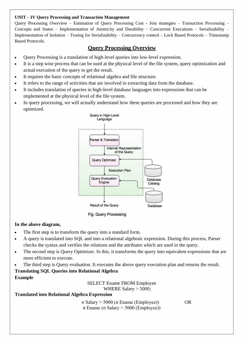
UNIT – IV Query Processing and Transaction Management

Query Processing Overview – Estimation of Query Processing Cost - Join strategies – Transaction Processing –

Concepts and States – Implementation of Atomicity and Durability – Concurrent Executions – Serializability –

Implementation of Isolation – Testing for Serializability – Concurrency control – Lock Based Protocols – Timestamp

Based Protocols.

Query Processing Overview

• Query Processing is a translation of high-level queries into low-level expression.

• It is a step wise process that can be used at the physical level of the file system, query optimization and

actual execution of the query to get the result.

• It requires the basic concepts of relational algebra and file structure.

• It refers to the range of activities that are involved in extracting data from the database.

• It includes translation of queries in high-level database languages into expressions that can be

implemented at the physical level of the file system.

• In query processing, we will actually understand how these queries are processed and how they are

optimized.

In the above diagram,

• The first step is to transform the query into a standard form.

• A query is translated into SQL and into a relational algebraic expression. During this process, Parser

checks the syntax and verifies the relations and the attributes which are used in the query.

• The second step is Query Optimizer. In this, it transforms the query into equivalent expressions that are

more efficient to execute.

• The third step is Query evaluation. It executes the above query execution plan and returns the result.

Translating SQL Queries into Relational Algebra

Example

SELECT Ename FROM Employee

WHERE Salary > 5000;

Translated into Relational Algebra Expression

σ Salary > 5000 (π Ename (Employee)) OR

π Ename (σ Salary > 5000 (Employee))

• A sequence of primitive operations that can be used to evaluate a query is a Query Execution Plan or

Query Evaluation Plan.

• The above diagram indicates that the query execution engine takes a query execution plan and returns

the answers to the query.

• Query Execution Plan minimizes the cost of query evaluation.

Estimation of Query Processing Cost

1. To choose a strategy based on reliable information, the database system may store statistics for each

relation r:

• nr - the number of tuples in r.

• sr - the size in bytes of a tuple of r (for fixed-length records).

• V(A, r) - the number of distinct values that appear in relation r for attribute A.

2. The first two quantities allow us to estimate accurately the size of a Cartesian product.

• The Cartesian product r × s contains nrns tuples.

• Each tuple of r × s occupies sr + ss bytes.

• The third statistic is used to estimate how many tuples satisfy a selection predicate of the

form

<attribute-name> = <value>

• We need to know how often each value appears in a column.

• If we assume each value appears with equal probability, then

𝐴 = 𝑎(𝑟)

is estimated to have

𝑛𝑟

𝑉(Ʌ, 𝑟)

tuples.

• This may not be the case, but it is a good approximation of reality in many relations.

• We assume such a uniform distribution for the rest of this chapter.

• Estimation of the size of a natural join is more difficult.

• Let r1(R1) and r2(R2) be relations on schemes R1 and R2 .

• If R1 R2 = (no common attributes), then r1 ⋈ r2 is the same as r1 × r2 and we can

estimate the size of this accurately.

• If R1 R2 is a key for R1 , then we know that a tuple of r2 will join with exactly one tuple

of r1.

• Thus the number of tuples in r1 ⋈ r2 will be no greater than nr2 .

• If R1 R2 is not a key for R1 or R2 , things are more difficult.

• We use the third statistic and the assumption of uniform distribution.

• Assume R1 R2 = {Ʌ}.

• We assume there are

𝑛𝑟2

𝑉(Ʌ, 𝑟2)

tuples in r2 with an A value of t[A] for tuple t in r1 .

• So tuple t of r1 produces

𝑛𝑟2

𝑉(Ʌ, 𝑟2)

tuples in r1 ⋈ r2.

Join strategies

Generally, the order in which two or more joined tables are written in the FROM clause of a SELECT

statement doesn’t influence the decision made by the SQL Server optimizer in relation to their processing

order.

Many different factors influence the decision of the optimizer regarding which table will be accessed first. On

the other hand, you can influence the join order selection by using the FORCE ORDER hint.

Join processing techniques

The join operation is the most time-consuming operation in query processing. The Database Engine supports

the following three different join processing techniques, so the optimizer can choose one of them depending

on the statistics for both tables:

• Nested loop

• Merge join

• Hash join

The following subsections describe these techniques.

Nested loop

Nested loop is the processing technique that works by “brute force.” In other words, for each row of the outer

table, each row from the inner table is retrieved and compared. The pseudo-code in Algorithm 1 demonstrates

the nested loop processing technique for two tables.

ALGORITHM 1

In Algorithm 1, every row selected from the outer table (table A) causes the access of all rows of the inner

table (table B). After that, the comparison of the values in the join columns is performed and the row is added

to the result set if the values in both columns are equal.

The nested loop technique is very slow if there is no index for the join column of the inner table. Without such

an index, the Database Engine would have to scan the outer table once and the inner table n times, where n is

the number of rows of the outer table. Therefore, the query optimizer usually chooses this method if the join

column of the inner table is indexed, so the inner table does not have to be scanned for each row in the outer

table.

Merge join

The merge join technique provides a cost-effective alternative to constructing an index for nested loop. The

rows of the joined tables must be physically sorted using the values of the join column. Both tables are then

scanned in order of the join columns, matching the rows with the same value for the join columns. The pseudo-

code in Algorithm 2 demonstrates the merge join processing technique for two tables.

ALGORITHM 2

The merge join processing technique has a high overhead if the rows from both tables are unsorted. However,

this method is preferable when the values of both join columns are sorted in advance. (This is always the case

when both join columns are primary keys of corresponding tables, because the Database Engine creates by

default the clustered index for the primary key of a table.)

Hash join

The hash join technique is usually used when there are no indices for join columns. In the case of the hash join

technique, both tables that have to be joined are considered as two inputs: the build input and the probe input.

(The smaller table usually represents the build input.) The process works as follows:

1. The value of the join column of a row from the build input is stored in a hash bucket depending on the

number returned by the hashing algorithm.

2. Once all rows from the build input are processed, the processing of the rows from the probe input

starts.

3. Each value of the join column of a row from the probe input is processed using the same hashing

algorithm.

4. The corresponding rows in each bucket are retrieved and used to build the result set.

NOTE

The hash join technique requires no index. Therefore, this method is highly applicable for ad hoc queries,

where indices cannot be expected. Also, if the optimizer uses this processing technique, it could be a hint that

you should create additional indices for one or both join columns.

Transaction Processing

• The transaction is a set of logically related operation. It contains a group of tasks.

• A transaction is an action or series of actions. It is performed by a single user to perform operations for

accessing the contents of the database.

Example: Suppose an employee of bank transfers Rs 800 from X's account to Y's account. This small

transaction contains several low-level tasks:

X's Account

Open_Account(X)

Old_Balance = X.balance

New_Balance = Old_Balance - 800

X.balance = New_Balance

Close_Account(X)

Y's Account

Open_Account(Y)

Old_Balance = Y.balance

New_Balance = Old_Balance + 800

Y.balance = New_Balance

Close_Account(Y)

Operations of Transaction:

Following are the main operations of transaction:

Read(X): Read operation is used to read the value of X from the database and stores it in a buffer in main

memory.

Write(X): Write operation is used to write the value back to the database from the buffer.

Let's take an example to debit transaction from an account which consists of following operations:

R(X);

X = X - 500;

W(X);

Let's assume the value of X before starting of the transaction is 4000.

• The first operation reads X's value from database and stores it in a buffer.

• The second operation will decrease the value of X by 500. So buffer will contain 3500.

• The third operation will write the buffer's value to the database. So X's final value will be 3500.

But it may be possible that because of the failure of hardware, software or power, etc. that transaction may

fail before finished all the operations in the set.

For example: If in the above transaction, the debit transaction fails after executing operation 2 then X's

value will remain 4000 in the database which is not acceptable by the bank.

To solve this problem, we have two important operations:

Commit: It is used to save the work done permanently.

Rollback: It is used to undo the work done.

States of Transaction In a database, the transaction can be in one of the following states -

Active state

• The active state is the first state of every transaction. In this state, the transaction is being executed.

• For example: Insertion or deletion or updating a record is done here. But all the records are still not

saved to the database.

Partially committed

• In the partially committed state, a transaction executes its final operation, but the data is still not

saved to the database.

• In the total mark calculation example, a final display of the total marks step is executed in this state.

Committed

A transaction is said to be in a committed state if it executes all its operations successfully. In this state, all

the effects are now permanently saved on the database system.

Failed state

• If any of the checks made by the database recovery system fails, then the transaction is said to be in

the failed state.

• In the example of total mark calculation, if the database is not able to fire a query to fetch the marks,

then the transaction will fail to execute.

Aborted

• If any of the checks fail and the transaction has reached a failed state then the database recovery

system will make sure that the database is in its previous consistent state. If not then it will abort or

roll back the transaction to bring the database into a consistent state.

• If the transaction fails in the middle of the transaction then before executing the transaction, all the

executed transactions are rolled back to its consistent state.

• After aborting the transaction, the database recovery module will select one of the two operations:

1. Re-start the transaction

2. Kill the transaction

Implementation of Atomicity and Durability

The recovery-management component of a database system can support atomicity and durability by a variety

of schemes. We first consider a simple, but extremely in- efficient, scheme called the shadow copy scheme.

This scheme, which is based on making copies of the database, called shadow copies, assumes that only one

transaction is active at a time. The scheme also assumes that the database is simply a file on disk. A pointer

called db-pointer is maintained on disk; it points to the current copy of the database.

In the shadow-copy scheme, a transaction that wants to update the database first creates a complete copy of

the database. All updates are done on the new database copy, leaving the original copy, the shadow copy,

untouched. If at any point the transaction has to be aborted, the system merely deletes the new copy. The old

copy of the database has not been affected.

If the transaction completes, it is committed as follows. First, the operating system is asked to make sure that

all pages of the new copy of the database have been written out to disk. (Unix systems use the flush command

for this purpose.) After the operating system has written all the pages to disk, the database system updates the

pointer db-pointer to point to the new copy of the database; the new copy then becomes the current copy of

the database. The old copy of the database is then deleted. The below Figure depicts the scheme, showing the

database state before and after the update.

The transaction is said to have been committed at the point where the updated db- pointer is written to disk.

We now consider how the technique handles transaction and system failures. First, consider transaction failure.

If the transaction fails at any time before db-pointer is updated, the old contents of the database are not affected.

We can abort the trans- action by just deleting the new copy of the database. Once the transaction has been

committed, all the updates that it performed are in the database pointed to by db- pointer. Thus, either all

updates of the transaction are reflected, or none of the effects are reflected, regardless of transaction failure.

Now consider the issue of system failure. Suppose that the system fails at any time before the updated db-

pointer is written to disk. Then, when the system restarts, it will read db-pointer and will thus see the original

contents of the database, and none of the effects of the transaction will be visible on the database. Next,

suppose that the system fails after db-pointer has been updated on disk. Before the pointer is updated, all

updated pages of the new copy of the database were written to disk. Again, we assume that, once a file is

written to disk, its contents will not be damaged even if there is a system failure. Therefore, when the system

restarts, it will read db-pointer and will thus see the contents of the database after all the updates performed

by the transaction.

The implementation actually depends on the write to db-pointer being atomic; that is, either all its bytes are

written or none of its bytes are written. If some of the bytes of the pointer were updated by the write, but others

were not, the pointer is meaningless, and neither old nor new versions of the database may be found when the

system restarts. Luckily, disk systems provide atomic updates to entire blocks, or at least to a disk sector. In

other words, the disk system guarantees that it will update db-pointer atomically, as long as we make sure that

db-pointer lies entirely in a single sector, which we can ensure by storing db-pointer at the beginning of a

block.

Thus, the atomicity and durability properties of transactions are ensured by the shadow-copy implementation

of the recovery-management component.

As a simple example of a transaction outside the database domain, consider a text- editing session. An entire

editing session can be modelled as a transaction. The actions executed by the transaction are reading and

updating the file. Saving the file at the end of editing corresponds to a commit of the editing transaction;

quitting the editing session without saving the file corresponds to an abort of the editing transaction.

Many text editors use essentially the implementation just described, to ensure that an editing session is

transactional. A new file is used to store the updated file. At the end of the editing session, if the updated file

is to be saved, the text editor uses a file rename command to rename the new file to have the actual file name.

The rename, assumed to be implemented as an atomic operation by the underlying file system, deletes the old

file as well.

Unfortunately, this implementation is extremely inefficient in the context of large databases, since executing

a single transaction requires copying the entire database.

Furthermore, the implementation does not allow transactions to execute concurrently with one another.

There are practical ways of implementing atomicity and durability that are much less expensive and more

powerful.

ACID Properties

A transaction is a very small unit of a program and it may contain several lowlevel tasks. A transaction in a

database system must maintain Atomicity, Consistency, Isolation, and Durability − commonly known as

ACID properties − in order to ensure accuracy, completeness, and data integrity.

• Atomicity − This property states that a transaction must be treated as an atomic unit, that is, either all

of its operations are executed or none. There must be no state in a database where a transaction is left

partially completed. States should be defined either before the execution of the transaction or after the

execution/abortion/failure of the transaction.

• Consistency − The database must remain in a consistent state after any transaction. No transaction

should have any adverse effect on the data residing in the database. If the database was in a consistent

state before the execution of a transaction, it must remain consistent after the execution of the

transaction as well.

• Durability − The database should be durable enough to hold all its latest updates even if the system

fails or restarts. If a transaction updates a chunk of data in a database and commits, then the database

will hold the modified data. If a transaction commits but the system fails before the data could be

written on to the disk, then that data will be updated once the system springs back into action.

Isolation − In a database system where more than one transaction are being executed simultaneously and in

parallel, the property of isolation states that all the transactions will be carried out and executed as if it is the

only transaction in the system. No transaction will affect the existence of any other transaction.

Concurrent Executions

Transaction-processing systems usually allow multiple transactions to run concurrently. Allowing multiple

transactions to update data concurrently causes several complications with consistency of the data.

Ensuring consistency in spite of concurrent execution of transactions requires extra work; it is far easier to

insist that transactions run serially—that is, one at a time, each starting only after the previous one has

completed.

However, there are two good reasons for allowing concurrency:

Improved throughput and resource utilization:

• A transaction consists of many steps. Some involve I/O activity; others involve CPU activity. The CPU

and the disks in a computer system can operate in parallel. Therefore, I/O activity can be done in parallel

with processing at the CPU.

• The parallelism of the CPU and the I/O system can therefore be exploited to run multiple transactions in

parallel.

• While a read or write on behalf of one transaction is in progress on one disk, another transaction can be

running in the CPU, while another disk may be executing a read or write on behalf of a third transaction.

• All of this increases the throughput of the system—that is, the number of transactions executed in a given

amount of time.

• Correspondingly, the processor and disk utilization also increase; in other words, the processor and disk

spend less time idle, or not performing any useful work.

Reduced waiting time:

• There may be a mix of transactions running on a system, some short and some long.

• If transactions run serially, a short transaction may have to wait for a preceding long transaction to

complete, which can lead to unpredictable delays in running a transaction.

• If the transactions are operating on different parts of the database, it is better to let them run concurrently,

sharing the CPU cycles and disk accesses among them.

• Concurrent execution reduces the unpredictable delays in running transactions.

• Moreover, it also reduces the average response time: the average time for a transaction to be completed

after it has been submitted.

The idea behind using concurrent execution in a database is essentially the same as the idea behind using

multi programming in an operating system.

The database system must control the interaction among the concurrent transactions to prevent them from

destroying the consistency of the database. It is achieved using concurrency-control schemes.

Serializability

Serializability is the classical concurrency scheme. It ensures that a schedule for executing concurrent

transactions is equivalent to one that executes the transactions serially in some order. It assumes that all

accesses to the database are done using read and write operations. A schedule is called ``correct'' if we can

find a serial schedule that is ``equivalent'' to it. Given a set of transactions T1...Tn, two schedules S1 and S2

of these transactions are equivalent if the following conditions are satisfied:

Read-Write Synchronization: If a transaction reads a value written by another transaction in one schedule, then

it also does so in the other schedule.

Write-Write Synchronization: If a transaction overwrites the value of another transaction in one schedule, it

also does so in the other schedule.

When multiple transactions are being executed by the operating system in a multiprogramming environment,

there are possibilities that instructions of one transactions are interleaved with some other transaction.

• Schedule − A chronological execution sequence of a transaction is called a schedule. A schedule can

have many transactions in it, each comprising of a number of instructions/tasks.

• Serial Schedule − It is a schedule in which transactions are aligned in such a way that one transaction

is executed first. When the first transaction completes its cycle, then the next transaction is executed.

Transactions are ordered one after the other. This type of schedule is called a serial schedule, as

transactions are executed in a serial manner.

In a multi-transaction environment, serial schedules are considered as a benchmark. The execution sequence

of an instruction in a transaction cannot be changed, but two transactions can have their instructions executed

in a random fashion. This execution does no harm if two transactions are mutually independent and working

on different segments of data; but in case these two transactions are working on the same data, then the results

may vary. This ever-varying result may bring the database to an inconsistent state.

To resolve this problem, we allow parallel execution of a transaction schedule, if its transactions are either

serializable or have some equivalence relation among them.

Equivalence Schedules

An equivalence schedule can be of the following types −

Result Equivalence

If two schedules produce the same result after execution, they are said to be result equivalent. They may yield

the same result for some value and different results for another set of values. That's why this equivalence is

not generally considered significant.

View Equivalence

Two schedules would be view equivalence if the transactions in both the schedules perform similar actions

in a similar manner.

For example −

• If T reads the initial data in S1, then it also reads the initial data in S2.

• If T reads the value written by J in S1, then it also reads the value written by J in S2.

• If T performs the final write on the data value in S1, then it also performs the final write on the data

value in S2.

Conflict Equivalence

Two schedules would be conflicting if they have the following properties −

• Both belong to separate transactions.

• Both accesses the same data item.

• At least one of them is "write" operation.

Two schedules having multiple transactions with conflicting operations are said to be conflict equivalent if

and only if −

• Both the schedules contain the same set of Transactions.

• The order of conflicting pairs of operation is maintained in both the schedules.

Note − View equivalent schedules are view serializable and conflict equivalent schedules are conflict

serializable. All conflict serializable schedules are view serializable too.

Implementation of Isolation

In order to maintain consistency in a database, it follows ACID properties. Among these four properties

(Atomicity, Consistency, Isolation and Durability) Isolation determines how transaction integrity is visible to

other users and systems. It means that a transaction should take place in a system in such a way that it is the

only transaction that is accessing the resources in a database system.

Isolation levels define the degree to which a transaction must be isolated from the data modifications made by

any other transaction in the database system. A transaction isolation level is defined by the following

phenomena –

• Dirty Read – A Dirty read is the situation when a transaction reads a data that has not yet been

committed. For example, Let’s say transaction 1 updates a row and leaves it uncommitted, meanwhile,

Transaction 2 reads the updated row. If transaction 1 rolls back the change, transaction 2 will have read

data that is considered never to have existed.

• Non Repeatable read – Non Repeatable read occurs when a transaction reads same row twice, and get

a different value each time. For example, suppose transaction T1 reads data. Due to concurrency, another

transaction T2 updates the same data and commit, Now if transaction T1 rereads the same data, it will

retrieve a different value.

• Phantom Read – Phantom Read occurs when two same queries are executed, but the rows retrieved by

the two, are different. For example, suppose transaction T1 retrieves a set of rows that satisfy some

search criteria. Now, Transaction T2 generates some new rows that match the search criteria for

transaction T1. If transaction T1 re-executes the statement that reads the rows, it gets a different set of

rows this time.

Based on these phenomena, The SQL standard defines four isolation levels :

1. Read Uncommitted – Read Uncommitted is the lowest isolation level. In this level, one transaction

may read not yet committed changes made by other transaction, thereby allowing dirty reads. In

this level, transactions are not isolated from each other.

2. Read Committed – This isolation level guarantees that any data read is committed at the moment

it is read. Thus it does not allows dirty read. The transaction holds a read or write lock on the

current row, and thus prevent other transactions from reading, updating or deleting it.

3. Repeatable Read – This is the most restrictive isolation level. The transaction holds read locks on

all rows it references and writes locks on all rows it inserts, updates, or deletes. Since other

transaction cannot read, update or delete these rows, consequently it avoids non-repeatable read.

4. Serializable – This is the Highest isolation level. A serializable execution is guaranteed to be

serializable. Serializable execution is defined to be an execution of operations in which

concurrently executing transactions appears to be serially executing.

The Table is given below clearly depicts the relationship between isolation levels, read phenomena and locks:

Isolation level Dirty reads Non-repeatable reads Phantoms

Read Uncommitted May Occur May Occur May Occur

Read Committed Don’t Occur May Occur May Occur

Repeatable Read Don’t Occur Don’t Occur May Occur

Serialized Don’t Occur Don’t Occur Don’t Occur

Anomaly Serializable is not the same as Serializable. That is, it is necessary, but not sufficient that a

Serializable schedule should be free of all three phenomena types.

Testing of Serializability

Serialization Graph is used to test the Serializability of a schedule.

Assume a schedule S. For S, we construct a graph known as precedence graph. This graph has a pair G = (V,

E), where V consists a set of vertices, and E consists a set of edges. The set of vertices is used to contain all

the transactions participating in the schedule. The set of edges is used to contain all edges Ti ->Tj for which

one of the three conditions holds:

1. Create a node Ti → Tj if Ti executes write (Q) before Tj executes read (Q).

2. Create a node Ti → Tj if Ti executes read (Q) before Tj executes write (Q).

3. Create a node Ti → Tj if Ti executes write (Q) before Tj executes write (Q).

Serialization Graph is used to test the Serializability of a schedule.

Assume a schedule S. For S, we construct a graph known as precedence graph. This graph has a pair G = (V,

E), where V consists a set of vertices, and E consists a set of edges. The set of vertices is used to contain all

the transactions participating in the schedule. The set of edges is used to contain all edges Ti ->Tj for which

one of the three conditions holds:

1. Create a node Ti → Tj if Ti executes write (Q) before Tj executes read (Q).

2. Create a node Ti → Tj if Ti executes read (Q) before Tj executes write (Q).

3. Create a node Ti → Tj if Ti executes write (Q) before Tj executes write (Q).

• If a precedence graph contains a single edge Ti → Tj, then all the instructions of Ti are executed before

the first instruction of Tj is executed.

• If a precedence graph for schedule S contains a cycle, then S is non-serializable. If the precedence

graph has no cycle, then S is known as serializable.

Explanation:

Read(A): In T1, no subsequent writes to A, so no new edges.

Read(B): In T2, no subsequent writes to B, so no new edges

Read(C): In T3, no subsequent writes to C, so no new edges

Write(B): B is subsequently read by T3, so add edge T2 → T3

Write(C): C is subsequently read by T1, so add edge T3 → T1

Write(A): A is subsequently read by T2, so add edge T1 → T2

Write(A): In T2, no subsequent reads to A, so no new edges

Write(C): In T1, no subsequent reads to C, so no new edges

Write(B): In T3, no subsequent reads to B, so no new edges

Precedence graph for schedule S1:

The precedence graph for schedule S1 contains a cycle that's why Schedule S1 is non-serializable.

Explanation:

Read(A): In T4,no subsequent writes to A, so no new edges

Read(C): In T4, no subsequent writes to C, so no new edges

Write(A): A is subsequently read by T5, so add edge T4 → T5

Read(B): In T5,no subsequent writes to B, so no new edges

Write(C): C is subsequently read by T6, so add edge T4 → T6

Write(B): A is subsequently read by T6, so add edge T5 → T6

Write(C): In T6, no subsequent reads to C, so no new edges

Write(A): In T5, no subsequent reads to A, so no new edges

Write(B): In T6, no subsequent reads to B, so no new edges

Precedence graph for schedule S2:

The precedence graph for schedule S2 contains no cycle that's why ScheduleS2 is serializable.

Concurrency control

• In the concurrency control, the multiple transactions can be executed simultaneously.

• It may affect the transaction result. It is highly important to maintain the order of execution of those

transactions.

Problems of concurrency control

Several problems can occur when concurrent transactions are executed in an uncontrolled manner. Following

are the three problems in concurrency control.

1. Lost updates

2. Dirty read

3. Unrepeatable read

1. Lost update problem

When two transactions that access the same database items contain their operations in a way that makes the

value of some database item incorrect, then the lost update problem occurs.

If two transactions T1 and T2 read a record and then update it, then the effect of updating of the first record

will be overwritten by the second update.

Example:

Transaction-X Time Transaction-Y

- t1 -

Read A t2 -

- t3 Read A

Update A t4 -

- t5 Update A

- t6 -

Here,

• At time t2, transaction-X reads A's value.

• At time t3, Transaction-Y reads A's value.

• At time t4, Transactions-X writes A's value on the basis of the value seen at time t2.

• At time t5, Transactions-Y writes A's value on the basis of the value seen at time t3.

• So at time T5, the update of Transaction-X is lost because Transaction y overwrites it without looking at

its current value.

• Such type of problem is known as Lost Update Problem as update made by one transaction is lost here.

2. Dirty Read

• The dirty read occurs in the case when one transaction updates an item of the database, and then the

transaction fails for some reason. The updated database item is accessed by another transaction before it

is changed back to the original value.

• A transaction T1 updates a record which is read by T2. If T1 aborts then T2 now has values which have

never formed part of the stable database.

Example:

Transaction-X Time Transaction-Y

- t1 -

- t2 Update A

Read A t3 -

- t4 Rollback

- t5 -

• At time t2, transaction-Y writes A's value.

• At time t3, Transaction-X reads A's value.

• At time t4, Transactions-Y rollbacks. So, it changes A's value back to that of prior to t1.

• So, Transaction-X now contains a value which has never become part of the stable database.

• Such type of problem is known as Dirty Read Problem, as one transaction reads a dirty value which has

not been committed.

3. Inconsistent Retrievals Problem

• Inconsistent Retrievals Problem is also known as unrepeatable read. When a transaction calculates some

summary function over a set of data while the other transactions are updating the data, then the

Inconsistent Retrievals Problem occurs.

• A transaction T1 reads a record and then does some other processing during which the transaction T2

updates the record. Now when the transaction T1 reads the record, then the new value will be

inconsistent with the previous value.

Example:

Suppose two transactions operate on three accounts.

Account – 1 Account – 2 Account – 3

Balance = 200 Balance = 250 Balance =150

• Transaction-X is doing the sum of all balance while transaction-Y is transferring an amount 50 from

Account-1 to Account-3.

• Here, transaction-X produces the result of 550 which is incorrect. If we write this produced result in the

database, the database will become an inconsistent state because the actual sum is 600.

• Here, transaction-X has seen an inconsistent state of the database.

Concurrency Control Protocol

Concurrency control protocols ensure atomicity, isolation, and serializability of concurrent transactions. The

concurrency control protocol can be divided into three categories:

1. Lock based protocol

2. Time-stamp protocol

3. Validation based protocol

Lock Based Protocols

Database systems equipped with lock-based protocols use a mechanism by which any transaction cannot read

or write data until it acquires an appropriate lock on it. Locks are of two kinds −

• Binary Locks − A lock on a data item can be in two states; it is either locked or unlocked.

• Shared/exclusive − This type of locking mechanism differentiates the locks based on their uses. If a

lock is acquired on a data item to perform a write operation, it is an exclusive lock. Allowing more

than one transaction to write on the same data item would lead the database into an inconsistent state.

Read locks are shared because no data value is being changed.

There are four types of lock protocols available −

Simplistic Lock Protocol

Simplistic lock-based protocols allow transactions to obtain a lock on every object before a 'write' operation

is performed. Transactions may unlock the data item after completing the ‘write’ operation.

Pre-claiming Lock Protocol

Pre-claiming protocols evaluate their operations and create a list of data items on which they need locks.

Before initiating an execution, the transaction requests the system for all the locks it needs beforehand. If all

the locks are granted, the transaction executes and releases all the locks when all its operations are over. If

all the locks are not granted, the transaction rolls back and waits until all the locks are granted.

Two-Phase Locking 2PL

This locking protocol divides the execution phase of a transaction into three parts. In the first part, when the

transaction starts executing, it seeks permission for the locks it requires. The second part is where the

transaction acquires all the locks. As soon as the transaction releases its first lock, the third phase starts. In

this phase, the transaction cannot demand any new locks; it only releases the acquired locks.

Two-phase locking has two phases, one is growing, where all the locks are being acquired by the transaction;

and the second phase is shrinking, where the locks held by the transaction are being released.

To claim an exclusive (write) lock, a transaction must first acquire a shared (read) lock and then upgrade it

to an exclusive lock.

Strict Two-Phase Locking

The first phase of Strict-2PL is same as 2PL. After acquiring all the locks in the first phase, the transaction

continues to execute normally. But in contrast to 2PL, Strict-2PL does not release a lock after using it. Strict-

2PL holds all the locks until the commit point and releases all the locks at a time.

Strict-2PL does not have cascading abort as 2PL does.

Timestamp-based Protocols

The most commonly used concurrency protocol is the timestamp based protocol. This protocol uses either

system time or logical counter as a timestamp.

Lock-based protocols manage the order between the conflicting pairs among transactions at the time of

execution, whereas timestamp-based protocols start working as soon as a transaction is created.

Every transaction has a timestamp associated with it, and the ordering is determined by the age of the

transaction. A transaction created at 0002 clock time would be older than all other transactions that come

after it. For example, any transaction 'y' entering the system at 0004 is two seconds younger and the priority

would be given to the older one.

In addition, every data item is given the latest read and write-timestamp. This lets the system know when the

last ‘read and write’ operation was performed on the data item.

Timestamp Ordering Protocol

The timestamp-ordering protocol ensures serializability among transactions in their conflicting read and write

operations. This is the responsibility of the protocol system that the conflicting pair of tasks should be

executed according to the timestamp values of the transactions.

• The timestamp of transaction Ti is denoted as TS(Ti).

• Read time-stamp of data-item X is denoted by R-timestamp(X).

• Write time-stamp of data-item X is denoted by W-timestamp(X).

Timestamp ordering protocol works as follows −

• If a transaction Ti issues a read(X) operation −

o If TS(Ti) < W-timestamp(X)

▪ Operation rejected.

o If TS(Ti) >= W-timestamp(X)

▪ Operation executed.

o All data-item timestamps updated.

• If a transaction Ti issues a write(X) operation −

o If TS(Ti) < R-timestamp(X)

▪ Operation rejected.

o If TS(Ti) < W-timestamp(X)

▪ Operation rejected and Ti rolled back.

o Otherwise, operation executed.

UNIT – V Trends in Data Base Technologies

Distributed Databases - Homogeneous and Heterogeneous Databases - Distributed Data Storage - Distributed

Transactions - Commit Protocols - Concurrency Control in Distributed Databases - Availability - Distributed Query

Processing - Heterogeneous Distributed Databases- Cloud-Based Databases - Directory Systems.

TRENDS IN DATA BASE TECHNOLOGIES: DISTRIBUTED DATABASES

In a distributed database, there are a number of databases that may be geographically distributed all over the

world. A distributed DBMS manages the distributed database in a manner so that it appears as one single

database to users. In the later part of the chapter, we go on to study the factors that lead to distributed

databases, its advantages and disadvantages.

A distributed database is a collection of multiple interconnected databases, which are spread physically

across various locations that communicate via a computer network.

Features

• Databases in the collection are logically interrelated with each other. Often they represent a single

logical database.

• Data is physically stored across multiple sites. Data in each site can be managed by a DBMS

independent of the other sites.

• The processors in the sites are connected via a network. They do not have any multiprocessor

configuration.

• A distributed database is not a loosely connected file system.

• A distributed database incorporates transaction processing, but it is not synonymous with a transaction

processing system.

Distributed Database Management System

A distributed database management system (DDBMS) is a centralized software system that manages a

distributed database in a manner as if it were all stored in a single location.

Features

• It is used to create, retrieve, update and delete distributed databases.

• It synchronizes the database periodically and provides access mechanisms by the virtue of which the

distribution becomes transparent to the users.

• It ensures that the data modified at any site is universally updated.

• It is used in application areas where large volumes of data are processed and accessed by numerous

users simultaneously.

• It is designed for heterogeneous database platforms.

• It maintains confidentiality and data integrity of the databases.

Factors Encouraging DDBMS

The following factors encourage moving over to DDBMS −

• Distributed Nature of Organizational Units − Most organizations in the current times are

subdivided into multiple units that are physically distributed over the globe. Each unit requires its

own set of local data. Thus, the overall database of the organization becomes distributed.

• Need for Sharing of Data − The multiple organizational units often need to communicate with each

other and share their data and resources. This demands common databases or replicated databases that

should be used in a synchronized manner.

• Support for Both OLTP and OLAP − Online Transaction Processing (OLTP) and Online Analytical

Processing (OLAP) work upon diversified systems which may have common data. Distributed

database systems aid both these processing by providing synchronized data.

• Database Recovery − One of the common techniques used in DDBMS is replication of data across

different sites. Replication of data automatically helps in data recovery if database in any site is

damaged. Users can access data from other sites while the damaged site is being reconstructed. Thus,

database failure may become almost inconspicuous to users.

• Support for Multiple Application Software − Most organizations use a variety of application

software each with its specific database support. DDBMS provides a uniform functionality for using

the same data among different platforms.

Advantages of Distributed Databases

Following are the advantages of distributed databases over centralized databases.

Modular Development − If the system needs to be expanded to new locations or new units, in centralized

database systems, the action requires substantial efforts and disruption in the existing functioning. However,

in distributed databases, the work simply requires adding new computers and local data to the new site and

finally connecting them to the distributed system, with no interruption in current functions.

More Reliable − In case of database failures, the total system of centralized databases comes to a halt.

However, in distributed systems, when a component fails, the functioning of the system continues may be at

a reduced performance. Hence DDBMS is more reliable.

Better Response − If data is distributed in an efficient manner, then user requests can be met from local data

itself, thus providing faster response. On the other hand, in centralized systems, all queries have to pass

through the central computer for processing, which increases the response time.

Lower Communication Cost − In distributed database systems, if data is located locally where it is mostly

used, then the communication costs for data manipulation can be minimized. This is not feasible in centralized

systems.

Adversities of Distributed Databases

Following are some of the adversities associated with distributed databases.

• Need for complex and expensive software − DDBMS demands complex and often expensive

software to provide data transparency and co-ordination across the several sites.

• Processing overhead − Even simple operations may require a large number of communications and

additional calculations to provide uniformity in data across the sites.

• Data integrity − The need for updating data in multiple sites pose problems of data integrity.

• Overheads for improper data distribution − Responsiveness of queries is largely dependent upon

proper data distribution. Improper data distribution often leads to very slow response to user requests.

Homogeneous and Heterogeneous Databases

Distributed databases can be broadly classified into homogeneous and heterogeneous distributed database

environments, each with further sub-divisions, as shown in the following illustration.

Homogeneous Distributed Databases

In a homogeneous distributed database, all the sites use identical DBMS and operating systems. Its properties

are −

• The sites use very similar software.

• The sites use identical DBMS or DBMS from the same vendor.

• Each site is aware of all other sites and cooperates with other sites to process user requests.

• The database is accessed through a single interface as if it is a single database.

Types of Homogeneous Distributed Database

There are two types of homogeneous distributed database −

• Autonomous − Each database is independent that functions on its own. They are integrated by a

controlling application and use message passing to share data updates.

• Non-autonomous − Data is distributed across the homogeneous nodes and a central or master DBMS

co-ordinates data updates across the sites.

Heterogeneous Distributed Databases

In a heterogeneous distributed database, different sites have different operating systems, DBMS products and

data models. Its properties are −

• Different sites use dissimilar schemas and software.

• The system may be composed of a variety of DBMSs like relational, network, hierarchical or object

oriented.

• Query processing is complex due to dissimilar schemas.

• Transaction processing is complex due to dissimilar software.

• A site may not be aware of other sites and so there is limited co-operation in processing user requests.

Types of Heterogeneous Distributed Databases

• Federated − The heterogeneous database systems are independent in nature and integrated together

so that they function as a single database system.

• Un-federated − The database systems employ a central coordinating module through which the

databases are accessed.

Distributed Data Storage

There are 2 ways in which data can be stored on different sites. These are:

1. Replication

In this approach, the entire relation is stored redundantly at 2 or more sites. If the entire database is

available at all sites, it is a fully redundant database. Hence, in replication, systems maintain copies of

data. This is advantageous as it increases the availability of data at different sites. Also, now query requests

can be processed in parallel. However, it has certain disadvantages as well. Data needs to be constantly

updated. Any change made at one site needs to be recorded at every site that relation is stored or else it

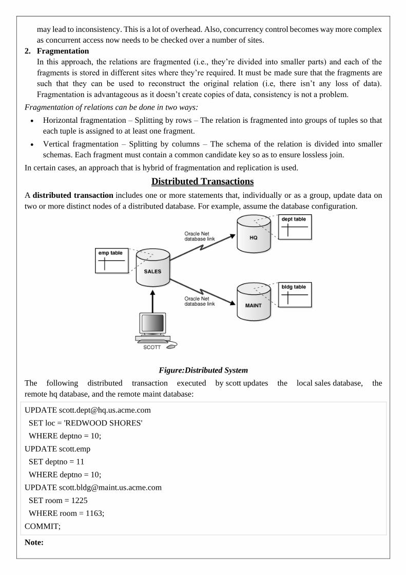
may lead to inconsistency. This is a lot of overhead. Also, concurrency control becomes way more complex

as concurrent access now needs to be checked over a number of sites.

2. Fragmentation

In this approach, the relations are fragmented (i.e., they’re divided into smaller parts) and each of the

fragments is stored in different sites where they’re required. It must be made sure that the fragments are

such that they can be used to reconstruct the original relation (i.e, there isn’t any loss of data).

Fragmentation is advantageous as it doesn’t create copies of data, consistency is not a problem.

Fragmentation of relations can be done in two ways:

• Horizontal fragmentation – Splitting by rows – The relation is fragmented into groups of tuples so that

each tuple is assigned to at least one fragment.

• Vertical fragmentation – Splitting by columns – The schema of the relation is divided into smaller

schemas. Each fragment must contain a common candidate key so as to ensure lossless join.

In certain cases, an approach that is hybrid of fragmentation and replication is used.

Distributed Transactions

A distributed transaction includes one or more statements that, individually or as a group, update data on

two or more distinct nodes of a distributed database. For example, assume the database configuration.

Figure:Distributed System

The following distributed transaction executed by scott updates the local sales database, the

remote hq database, and the remote maint database:

UPDATE scott.dept@hq.us.acme.com

SET loc = 'REDWOOD SHORES'

WHERE deptno = 10;

UPDATE scott.emp

SET deptno = 11

WHERE deptno = 10;

UPDATE scott.bldg@maint.us.acme.com

SET room = 1225

WHERE room = 1163;

COMMIT;

Note:

If all statements of a transaction reference only a single remote node, then the transaction is remote, not

distributed.

There are two types of permissible operations in distributed transactions:

• DML and DDL Transactions

• Transaction Control Statements

DML and DDL Transactions

The following are the DML and DDL operations supported in a distributed transaction:

• CREATE TABLE AS SELECT

• DELETE

• INSERT (default and direct load)

• LOCK TABLE

• SELECT

• SELECT FOR UPDATE

You can execute DML and DDL statements in parallel, and INSERT direct load statements serially, but note

the following restrictions:

• All remote operations must be SELECT statements.

• These statements must not be clauses in another distributed transaction.

• If the table referenced in the table_expression_clause of an INSERT, UPDATE,

or DELETE statement is remote, then execution is serial rather than parallel.

• You cannot perform remote operations after issuing parallel DML/DDL or direct load INSERT.

• If the transaction begins using XA or OCI, it executes serially.

• No loopback operations can be performed on the transaction originating the parallel operation. For

example, you cannot reference a remote object that is actually a synonym for a local object.

• If you perform a distributed operation other than a SELECT in the transaction, no DML is parallelized.

Transaction Control Statements

The following are the supported transaction control statements:

• COMMIT

• ROLLBACK

• SAVEPOINT

COMMIT − to save the changes.

ROLLBACK − to roll back the changes.

SAVEPOINT − creates points within the groups of transactions in which to ROLLBACK.

Commit Protocols

In a local database system, for committing a transaction, the transaction manager has to only convey the

decision to commit to the recovery manager. However, in a distributed system, the transaction manager

should convey the decision to commit to all the servers in the various sites where the transaction is being

executed and uniformly enforce the decision. When processing is complete at each site, it reaches the partially

committed transaction state and waits for all other transactions to reach their partially committed states. When

it receives the message that all the sites are ready to commit, it starts to commit. In a distributed system, either

all sites commit or none of them does.

The different distributed commit protocols are −

• One-phase commit

• Two-phase commit

• Three-phase commit

Distributed One-phase Commit

Distributed one-phase commit is the simplest commit protocol. Let us consider that there is a controlling site

and a number of slave sites where the transaction is being executed. The steps in distributed commit are

• After each slave has locally completed its transaction, it sends a “DONE” message to the controlling

site.

• The slaves wait for “Commit” or “Abort” message from the controlling site. This waiting time is

called window of vulnerability.

• When the controlling site receives “DONE” message from each slave, it makes a decision to commit

or abort. This is called the commit point. Then, it sends this message to all the slaves.

• On receiving this message, a slave either commits or aborts and then sends an acknowledgement

message to the controlling site.

Distributed Two-phase Commit

Distributed two-phase commit reduces the vulnerability of one-phase commit protocols. The steps performed

in the two phases are as follows −

Phase 1: Prepare Phase

• After each slave has locally completed its transaction, it sends a “DONE” message to the controlling

site. When the controlling site has received “DONE” message from all slaves, it sends a “Prepare”

message to the slaves.

• The slaves vote on whether they still want to commit or not. If a slave wants to commit, it sends a

“Ready” message.

• A slave that does not want to commit sends a “Not Ready” message. This may happen when the slave

has conflicting concurrent transactions or there is a timeout.

Phase 2: Commit/Abort Phase

• After the controlling site has received “Ready” message from all the slaves −

o The controlling site sends a “Global Commit” message to the slaves.

o The slaves apply the transaction and send a “Commit ACK” message to the controlling site.

o When the controlling site receives “Commit ACK” message from all the slaves, it considers

the transaction as committed.

• After the controlling site has received the first “Not Ready” message from any slave −

o The controlling site sends a “Global Abort” message to the slaves.

o The slaves abort the transaction and send a “Abort ACK” message to the controlling site.

o When the controlling site receives “Abort ACK” message from all the slaves, it considers the

transaction as aborted.

Distributed Three-phase Commit

The steps in distributed three-phase commit are as follows −

Phase 1: Prepare Phase

The steps are same as in distributed two-phase commit.

Phase 2: Prepare to Commit Phase

• The controlling site issues an “Enter Prepared State” broadcast message.

• The slave sites vote “OK” in response.

Phase 3: Commit / Abort Phase

The steps are same as two-phase commit except that “Commit ACK”/”Abort ACK” message is not required.

Concurrency Control in Distributed Databases

Concurrency controlling techniques ensure that multiple transactions are executed simultaneously while

maintaining the ACID properties of the transactions and serializability in the schedules.

In this chapter, we will study the various approaches for concurrency control.

Locking Based Concurrency Control Protocols

Locking-based concurrency control protocols use the concept of locking data items. A lock is a variable

associated with a data item that determines whether read/write operations can be performed on that data item.

Generally, a lock compatibility matrix is used which states whether a data item can be locked by two

transactions at the same time.

Locking-based concurrency control systems can use either one-phase or two-phase locking protocols.

One-phase Locking Protocol

In this method, each transaction locks an item before use and releases the lock as soon as it has finished using

it. This locking method provides for maximum concurrency but does not always enforce serializability.

Two-phase Locking Protocol

In this method, all locking operations precede the first lock-release or unlock operation. The transaction

comprise of two phases. In the first phase, a transaction only acquires all the locks it needs and do not release

any lock. This is called the expanding or the growing phase. In the second phase, the transaction releases the

locks and cannot request any new locks. This is called the shrinking phase.

Every transaction that follows two-phase locking protocol is guaranteed to be serializable. However, this

approach provides low parallelism between two conflicting transactions.

Timestamp Concurrency Control Algorithms

Timestamp-based concurrency control algorithms use a transaction’s timestamp to coordinate concurrent

access to a data item to ensure serializability. A timestamp is a unique identifier given by DBMS to a

transaction that represents the transaction’s start time.

These algorithms ensure that transactions commit in the order dictated by their timestamps. An older

transaction should commit before a younger transaction, since the older transaction enters the system before

the younger one.

Timestamp-based concurrency control techniques generate serializable schedules such that the equivalent

serial schedule is arranged in order of the age of the participating transactions.

Some of timestamp based concurrency control algorithms are −

• Basic timestamp ordering algorithm.

• Conservative timestamp ordering algorithm.

• Multiversion algorithm based upon timestamp ordering.

Timestamp based ordering follow three rules to enforce serializability −

• Access Rule − When two transactions try to access the same data item simultaneously, for conflicting

operations, priority is given to the older transaction. This causes the younger transaction to wait for

the older transaction to commit first.

• Late Transaction Rule − If a younger transaction has written a data item, then an older transaction is

not allowed to read or write that data item. This rule prevents the older transaction from committing

after the younger transaction has already committed.

• Younger Transaction Rule − A younger transaction can read or write a data item that has already

been written by an older transaction.

Optimistic Concurrency Control Algorithm

In systems with low conflict rates, the task of validating every transaction for serializability may lower

performance. In these cases, the test for serializability is postponed to just before commit. Since the conflict

rate is low, the probability of aborting transactions which are not serializable is also low. This approach is

called optimistic concurrency control technique.

In this approach, a transaction’s life cycle is divided into the following three phases −

• Execution Phase − A transaction fetches data items to memory and performs operations upon them.

• Validation Phase − A transaction performs checks to ensure that committing its changes to the

database passes serializability test.

• Commit Phase − A transaction writes back modified data item in memory to the disk.

This algorithm uses three rules to enforce serializability in validation phase −

Rule 1 − Given two transactions Ti and Tj, if Ti is reading the data item which Tj is writing, then Ti’s

execution phase cannot overlap with Tj’s commit phase. Tj can commit only after Ti has finished execution.

Rule 2 − Given two transactions Ti and Tj, if Ti is writing the data item that Tj is reading, then Ti’s commit

phase cannot overlap with Tj’s execution phase. Tj can start executing only after Ti has already committed.

Rule 3 − Given two transactions Ti and Tj, if Ti is writing the data item which Tj is also writing, then Ti’s

commit phase cannot overlap with Tj’s commit phase. Tj can start to commit only after Ti has already

committed.

Availability

The importance of data and database availability, it is necessary to first have a good definition of availability.

After all, we should know what we are talking about. Simply stated, availability is the condition wherein a

given resource can be accessed by its consumers. So in terms of databases, availability means that if a database

is available, the users of its data—that is, applications, customers, and business users—can access it. Any

condition that renders the resource inaccessible causes the opposite of availability: unavailability.

Another perspective on defining availability is the percentage of time that a system can be used for productive

work. The required availability of an application will vary from organization to organization, within an

organization from system to system, and even from user to user.

Database availability and database performance are terms that are often confused with one another, and

indeed, there are similarities between the two. The major difference lies in the user’s ability to access the

database. It is possible to access a database suffering from poor performance, but it is not possible to access a

database that is unavailable. So, when does poor performance turn into unavailability? If performance suffers

to such a great degree that the users of the database cannot perform their job, the database has become, for all

intents and purposes, unavailable. Nonetheless, keep in mind that availability and performance are different

and must be treated by the DBA as separate issues—even though a severe performance problem is a potential

availability problem.

Availability comprises four distinct components, which, in combination, assure that systems are running and

business can be conducted:

▪ Manageability—the ability to create and maintain an effective environment that delivers service to users

▪ Recoverability—the ability to reestablish service in the event of an error or component failure

▪ Reliability—the ability to deliver service at specified levels for a stated period

▪ Serviceability—the ability to determine the existence of problems, diagnose their cause(s), and repair the

problems.

All four of these “abilities” impact the overall availability of a system, database, or application.

Distributed Query Processing

Distributed Query Processing Architecture

In a distributed database system, processing a query comprises of optimization at both the global and the

local level. The query enters the database system at the client or controlling site. Here, the user is validated,

the query is checked, translated, and optimized at a global level.

The architecture can be represented as −

Mapping Global Queries into Local Queries

The process of mapping global queries to local ones can be realized as follows −

• The tables required in a global query have fragments distributed across multiple sites. The local

databases have information only about local data. The controlling site uses the global data dictionary

to gather information about the distribution and reconstructs the global view from the fragments.

• If there is no replication, the global optimizer runs local queries at the sites where the fragments are

stored. If there is replication, the global optimizer selects the site based upon communication cost,

workload, and server speed.

• The global optimizer generates a distributed execution plan so that least amount of data transfer occurs

across the sites. The plan states the location of the fragments, order in which query steps needs to be

executed and the processes involved in transferring intermediate results.

• The local queries are optimized by the local database servers. Finally, the local query results are

merged together through union operation in case of horizontal fragments and join operation for

vertical fragments.

For example, let us consider that the following Project schema is horizontally fragmented according to City,

the cities being New Delhi, Kolkata and Hyderabad.

PROJECT

PId City Department Status

Suppose there is a query to retrieve details of all projects whose status is “Ongoing”.

The global query will be &inus;

$$\sigma_{status} = {\small "ongoing"}^{(PROJECT)}$$

Query in New Delhi’s server will be −

$$\sigma_{status} = {\small "ongoing"}^{({NewD}_-{PROJECT})}$$

Query in Kolkata’s server will be −

$$\sigma_{status} = {\small "ongoing"}^{({Kol}_-{PROJECT})}$$

Query in Hyderabad’s server will be −

$$\sigma_{status} = {\small "ongoing"}^{({Hyd}_-{PROJECT})}$$

In order to get the overall result, we need to union the results of the three queries as follows

$\sigma_{status} = {\small "ongoing"}^{({NewD}_-{PROJECT})} \cup \sigma_{status} = {\small

"ongoing"}^{({kol}_-{PROJECT})} \cup \sigma_{status} = {\small "ongoing"}^{({Hyd}_-

{PROJECT})}$

Distributed Query Optimization

Distributed query optimization requires evaluation of a large number of query trees each of which produce

the required results of a query. This is primarily due to the presence of large amount of replicated and

fragmented data. Hence, the target is to find an optimal solution instead of the best solution.

The main issues for distributed query optimization are −

• Optimal utilization of resources in the distributed system.

• Query trading.

• Reduction of solution space of the query.

Optimal Utilization of Resources in the Distributed System

A distributed system has a number of database servers in the various sites to perform the operations pertaining

to a query. Following are the approaches for optimal resource utilization −

Operation Shipping − In operation shipping, the operation is run at the site where the data is stored and not

at the client site. The results are then transferred to the client site. This is appropriate for operations where

the operands are available at the same site. Example: Select and Project operations.

Data Shipping − In data shipping, the data fragments are transferred to the database server, where the

operations are executed. This is used in operations where the operands are distributed at different sites. This

is also appropriate in systems where the communication costs are low, and local processors are much slower

than the client server.

Hybrid Shipping − This is a combination of data and operation shipping. Here, data fragments are

transferred to the high-speed processors, where the operation runs. The results are then sent to the client site.

Query Trading

In query trading algorithm for distributed database systems, the controlling/client site for a distributed query

is called the buyer and the sites where the local queries execute are called sellers. The buyer formulates a

number of alternatives for choosing sellers and for reconstructing the global results. The target of the buyer

is to achieve the optimal cost.

The algorithm starts with the buyer assigning sub-queries to the seller sites. The optimal plan is created from

local optimized query plans proposed by the sellers combined with the communication cost for reconstructing

the final result. Once the global optimal plan is formulated, the query is executed.

Reduction of Solution Space of the Query

Optimal solution generally involves reduction of solution space so that the cost of query and data transfer is

reduced. This can be achieved through a set of heuristic rules, just as heuristics in centralized systems.

Following are some of the rules −

• Perform selection and projection operations as early as possible. This reduces the data flow over

communication network.

• Simplify operations on horizontal fragments by eliminating selection conditions which are not relevant

to a particular site.

• In case of join and union operations comprising of fragments located in multiple sites, transfer

fragmented data to the site where most of the data is present and perform operation there.

• Use semi-join operation to qualify tuples that are to be joined. This reduces the amount of data transfer

which in turn reduces communication cost.

• Merge the common leaves and sub-trees in a distributed query tree.

Heterogeneous Distributed Databases

In a heterogeneous distributed database, different sites have different operating systems, DBMS products and

data models. Its properties are −

• Different sites use dissimilar schemas and software.

• The system may be composed of a variety of DBMSs like relational, network, hierarchical or object

oriented.

• Query processing is complex due to dissimilar schemas.

• Transaction processing is complex due to dissimilar software.

• A site may not be aware of other sites and so there is limited co-operation in processing user requests.

Types of Heterogeneous Distributed Databases

• Federated − The heterogeneous database systems are independent in nature and integrated together

so that they function as a single database system.

• Un-federated − The database systems employ a central coordinating module through which the

databases are accessed.

Distributed DBMS Architectures

DDBMS architectures are generally developed depending on three parameters −

• Distribution − It states the physical distribution of data across the different sites.

• Autonomy − It indicates the distribution of control of the database system and the degree to which

each constituent DBMS can operate independently.

• Heterogeneity − It refers to the uniformity or dissimilarity of the data models, system components

and databases.

Cloud-Based Databases

Traditional databases require companies to provision all of the underlying infrastructure and resources

necessary to manage their databases on-premises with cloud-based technology. This makes them familiar

territory for customers with on-premises operations. However, companies that are moving to the cloud may

want to look into other options, such as Database as a Service (DBaaS).

Database as a Service (DBaaS)

A DBaaS is a database cloud service that takes over the management of the underlying infrastructure and

resources cloud databases require and allow companies to take advantage of services in the cloud. This can

free up personnel to focus on other tasks, or allow smaller organizations to get started quickly without the

need for several specialists. In many cases with a DBaaS you can quickly set up a database with a few clicks.

Running a cloud-based database makes it easy to grow your databases as your needs grow, in addition to

scaling up or down on-demand to accommodate those peak-workload periods. You can also have peace of

mind for any security and availability concerns as the cloud enables database replication across multiple

geographical locations, in addition to several backup and recovery options.

And while there are many cloud providers that offer DBaaS, the market leaders are currently Amazon Web

Services (AWS), Microsoft Azure, and Google Cloud Platform. Each offers DBaaS in a variety of flavors

(MySQL cloud database, Microsoft SQL Server, PostgreSQL, Oracle, and NoSQL databases such as Hadoop

or MongoDB, etc.) such as the database as a service AWS offerings Amazon RDS and Amazon Aurora, Azure

database as a services Azure Database for MySQL, Azure Database for PostgreSQL, Azure SQL Database,

and GCP’s Cloud SQL. The cloud service providers also have database migration services to help you migrate

your data to the cloud.

A cloud database is a database that typically runs on a cloud computing platform, and access to the database

is provided as-a-service.

Database services take care of scalability and high availability of the database. Database services make the

underlying software-stack transparent to the user. There are two primary methods to run a database in a cloud:

Virtual machine

Cloud platforms allow users to purchase virtual-machine instances for a limited time, and one can run

a database on such virtual machines. Users can either upload their own machine image with a database

installed on it, or use ready-made machine images that already include an optimized installation of a

database.

Database-as-a-service (DBaaS)

With a database as a service model, application owners do not have to install and maintain the database

themselves. Instead, the database service provider takes responsibility for installing and maintaining

the database, and application owners are charged according to their usage of the service. This is a type

of Saas - Software as a Service.

Architecture and common characteristics

• Most database services offer web-based consoles, which the end user can use to provision and

configure database instances.

• Database services consist of a database-manager component, which controls the underlying

database instances using a service API. The service API is exposed to the end user, and permits

users to perform maintenance and scaling operations on their database instances.

• Underlying software-stack stack typically includes the operating system, the database and third-

party software used to manage the database. The service provider is responsible for installing,

patching and updating the underlying software stack and ensuring the overall health and

performance of the database.

• Scalability features differ between vendors – some offer auto-scaling, others enable the user to

scale up using an API, but do not scale automatically.

• There is typically a commitment for a certain level of high availability (e.g. 99.9% or 99.99%).

This is achieved by replicating data and failing instances over to other database instances..

Data model

The design and development of typical systems utilize data management and relational databases as

their key building blocks. Advanced queries expressed in SQL work well with the strict relationships

that are imposed on information by relational databases. However, relational database technology was

not initially designed or developed for use over distributed systems. This issue has been addressed

with the addition of clustering enhancements to the relational databases, although some basic tasks

require complex and expensive protocols, such as with data synchronization.

Modern relational databases have shown poor performance on data-intensive systems, therefore, the

idea of NoSQL has been utilized within database management systems for cloud based

systems. Within NoSQL implemented storage, there are no requirements for fixed table schemas, and

the use of join operations is avoided. "The NoSQL databases have proven to provide efficient

horizontal scalability, good performance, and ease of assembly into cloud applications." Data models

relying on simplified relay algorithms have also been employed in data-intensive cloud mapping

applications unique to virtual frameworks.

It is also important to differentiate between cloud databases which are relational as opposed to non-

relational or NoSQL:

SQL databases

are one type of database which can run in the cloud, either in a virtual machine or as a service,

depending on the vendor. While SQL databases are easily vertically scalable, horizontal scalability

poses a challenge, that cloud database services based on SQL have started to address.

NoSQL databases

NoSQL databases are another type of database which can run in the cloud. NoSQL databases are built

to service heavy read/write loads and can scale up and down easily, and therefore they are more natively

suited to running in the cloud. However, most contemporary applications are built around an SQL data

model, so working with NoSQL databases often requires a complete rewrite of application code.

Some SQL databases have developed NoSQL capabilities including JSON, binary JSON

(e.g. BSON or similar variants), and key-value store data types.

A multi-model database with relational and non-relational capabilities provides a standard SQL

interface to users and applications and thus facilitates the usage of such databases for contemporary

applications built around an SQL data model. Native multi-model databases support multiple data

models with one core and a unified query language to access all data models.

Directory Systems

Typical kinds of directory information

• Employee information such as name, id, email, phone, office addr, ..

• Even personal information to be accessed from multiple places

o e.g. Web browser bookmarks „ White pages

• Entries organized by name or identifier

o Meant for forward lookup to find more about an entry „ Yellow pages

• Entries organized by properties

• For reverse lookup to find entries matching specific requirements „ When directories are to be accessed

across an organization

• Alternative 1: Web interface. Not great for programs

• Alternative 2: Specialized directory access protocols

o Coupled with specialized user interfaces

Directory Access Protocols

Most commonly used directory access protocol:

• LDAP (Lightweight Directory Access Protocol)

• Simplified from earlier X.500 protocol

Question: Why not use database protocols like ODBC/JDBC?

Answer:

• Simplified protocols for a limited type of data access, evolved parallel to ODBC/JDBC

• Provide a nice hierarchical naming mechanism similar to file system directories

o Data can be partitioned amongst multiple servers for different parts of the hierarchy, yet give a

single view to user

– E.g. different servers for Bell Labs Murray Hill and Bell Labs Bangalore

• Directories may use databases as storage mechanism

LDAP: Lightweight Directory Access Protocol

Protocol

• LDAP Data Model

• Data Manipulation

• Distributed Directory Trees

Entries organized into a directory information tree according to their DNs

• Leaf level usually represent specific objects

• Internal node entries represent objects such as organizational units, organizations or countries

• Children of a node inherit the DN of the parent, and add on RDNs

o E.g. internal node with DN c=USA – Children nodes have DN starting with c=USA and further

RDNs such as o or ou

o DN of an entry can be generated by traversing path from root

• Leaf level can be an alias pointing to another entry

o Entries can thus have more than one DN – E.g. person in more than one organizational unit

LDAP Data Manipulation

• Users use an API or vendor specific front ends

• LDAP also defines a file format

o LDAP Data Interchange Format (LDIF)

▪ Querying mechanism is very simple: only selection & projection

LDAP Queries

LDAP query must specify

• Base: a node in the DIT from where search is to start

• A search condition

o Boolean combination of conditions on attributes of entries – Equality, wild-cards and

approximate equality supported

• A scope

o Just the base, the base and its children, or the entire subtree from the base

• Attributes to be returned

• Limits on number of results and on resource consumption

• May also specify whether to automatically dereference aliases „ LDAP URLs are one way of

specifying query

o LDAP API is another alternative