FGM and laminated doubly curved shells and panels of revolution with a free-form meridian: A 2-D GDQ...

FGM and laminated doubly curved shells and panels of revolution with afree-form meridian: A 2-D GDQ solution for free vibrations

Francesco Tornabene n, Alfredo Liverani, Gianni Caligiana

DIEM—Department, Faculty of Engineering, viale Risorgimento 2, University of Bologna, 40100 Bologna, Italy

a r t i c l e i n f o

Article history:

Received 15 February 2011

Received in revised form

24 March 2011

Accepted 29 March 2011Available online 9 April 2011

Keywords:

Free vibrations

Doubly curved shells of revolution

Rational Bezier curves

Laminated composite shells

Functionally graded materials

Generalized differential quadrature method

a b s t r a c t

In this paper, the generalized differential quadrature (GDQ) method is applied to study the dynamic

behavior of functionally graded materials (FGMs) and laminated doubly curved shells and panels of

revolution with a free-form meridian. The First-order Shear Deformation Theory (FSDT) is used to

analyze the above mentioned moderately thick structural elements. In order to include the effect of the

initial curvature a generalization of the Reissner–Mindlin theory, proposed by Toorani and Lakis, is

adopted. The governing equations of motion, written in terms of stress resultants, are expressed as

functions of five kinematic parameters, by using the constitutive and kinematic relationships. The

solution is given in terms of generalized displacement components of points lying on the middle

surface of the shell. Simple Rational Bezier curves are used to define the meridian curve of the

revolution structures. Firstly, the differential quadrature (DQ) rule is introduced to determine the

geometric parameters of the structures with a free-form meridian. Secondly, the discretization of the

system by means of the GDQ technique leads to a standard linear eigenvalue problem, where two

independent variables are involved. Results are obtained taking the meridional and circumferential

co-ordinates into account, without using the Fourier modal expansion methodology. Comparisons

between the Reissner–Mindlin and the Toorani–Lakis theory are presented. Furthermore, GDQ results

are compared with those obtained by using commercial programs such as Abaqus, Ansys, Nastran,

Straus and Pro/Mechanica. Very good agreement is observed. Finally, different lamination schemes are

considered to expand the combination of the two functionally graded four-parameter power-law

distributions adopted. The treatment is developed within the theory of linear elasticity, when materials

are assumed to be isotropic and inhomogeneous through the lamina thickness direction. A two-

constituent functionally graded lamina consists of ceramic and metal those are graded through the

lamina thickness. A parametric study is performed to illustrate the influence of the parameters on the

mechanical behavior of shell and panel structures considered.

& 2011 Elsevier Ltd. All rights reserved.

1. Introduction

Shells have been widespread in many fields of engineering as

they give rise to optimum conditions for dynamic behavior,

strength and stability. The vibration effects on these structures

caused by different phenomena can have serious consequences

for their strength and safety. Therefore, an accurate frequency and

mode shape determination is of considerable importance for the

technical design of these structural elements. The aim of this

paper is to study the dynamic behavior of doubly curved shell

structures derived from shells of revolution, which are very

common structural elements.

This research work is based on four aspects. The first is the

improvement of the Reissner–Mindlin theory using the Toorani–

Lakis theory. In this way the effect of the curvature of the shell

structure is considered. The second is the generalization of the

shape of the shell meridian. The free-form (Rational Bezier or

NURBS) meridian curve assumption requires the differential

quadrature rule to evaluate the geometric parameters needed to

describe the geometry of the structure. The third is the combina-

tion of the composite lamination scheme with functionally graded

materials in order to expand the design profiles through the

whole thickness of the shell. The four is the use of the generalized

differential quadrature method to solve the governing equations

of motion.

During the last 60 years, two-dimensional linear theories of

thin shells have been developed including important contribu-

tions by Timoshenko and Woinowsky-Krieger [1], Flugge [2],

Gol’Denveizer [3], Novozhilov [4], Vlasov [5], Ambartusumyan

Contents lists available at ScienceDirect

journal homepage: www.elsevier.com/locate/ijmecsci

International Journal of Mechanical Sciences

0020-7403/$ - see front matter & 2011 Elsevier Ltd. All rights reserved.

doi:10.1016/j.ijmecsci.2011.03.007

n Corresponding author.

E-mail address: [email protected] (F. Tornabene).

International Journal of Mechanical Sciences 53 (2011) 446–470

www.elsevier.com/locate/ijmecsci

dx.doi.org/10.1016/j.ijmecsci.2011.03.007

mailto:[email protected]

dx.doi.org/10.1016/j.ijmecsci.2011.03.007

[6], Kraus [7], Leissa [8,9], Markus [10], Ventsel and Krauthammer

[11] and Soedel [12]. All these contributions are based on the

Kirchhoff–Love assumptions. This theory, named Classical Shell

Theory (CST), assumes that normals to the shell middle-surface

remain straight and normal to it during deformations and

unstretched in length. Many researchers analyzed various char-

acteristics of thin shell structures [13–18].

When the theories of thin shells are applied to thick shells, the

errors could be quite large. With the increasing use of thick shells

in various engineering applications, simple and accurate theories

for thick shells have been developed. With respect to thin shells,

thick shell theories take the transverse shear deformation and

rotary inertia into account. The transverse shear deformation has

been incorporated into shell theories by following the theory of

Reissner–Mindlin [19], also named First-order Shear Deformation

Theory (FSDT). Abandoning the assumption on the preservation

of the normals to the shell middle surface after the deformation, a

comprehensive analysis for elastic isotropic shells was made by

Kraus [7] and Gould [20,21]. The present work is just based on the

FSDT. In order to include the effect of the initial curvature a

generalization of the Reissner–Mindlin theory (RMT) has been

proposed by Toorani and Lakis [22]. In this way the Reissner–

Mindlin theory becomes a particular case of the Toorani–Lakis

theory (TLT). As a consequence of the use of this general theory

the stress resultants directly depend on the geometry of the

structure in terms of the curvature coefficients and the hypothesis

of the symmetry of the in-plane shearing force resultants and the

torsional couples declines. In this paper the Toorani–Lakis theory

is considered and improved. Comparisons between the Reissner–

Mindlin and the Toorani–Lakis theory are presented. No results

are available in the literature about the Toorani–Lakis theory for

doubly curved shells. As for the vibration analysis of such

revolution shells, several studies have been presented earlier.

The most popular numerical tool in carrying out the above

analyses is currently the finite element method [20,21,23]. The

generalized collocation method based on the ring element

method has also been applied. With regard to the latter method,

each static and kinematic variable is transformed into a theore-

tically infinite Fourier series of harmonic components, with

respect to the circumferential co-ordinates [24–30]. In other

word, when dealing with a completely closed shell, the 2D

problem can be reduced using standard Fourier decomposition.

For a panel, however, it is not possible to perform such a

reduction operation, and the two-dimensional field must be dealt

with directly, as will just be done in this paper. The governing

equations of motion are a set of five partial differential equations

with variable coefficients, depending on two independent vari-

ables. By doing so, it is possible to compute the complete

assessment of the modal shapes corresponding to natural fre-

quencies of panel structures. It should be noted that there is

comparatively little literature available for these latter structures,

compared to the literature regarding the free vibration analysis

of complete shells of revolution. Complete revolution shells

are obtained as special cases of shell panels by satisfying the

kinematical and physical compatibility at the common meridian

with W¼0,2p.The excellent mathematical and algorithmic properties, com-

bined with successful industrial applications, have contributed to

the enormous popularity of the Rational Bezier and Non-Uniform

Rational B-Splines (NURBS) curves. These curves have become the

de facto industry standard for the representation, design and data

exchange of geometric information processed by computers

[31–34]. Many national and international standards recognize

these curves as a powerful tool for geometric design. Further-

more, these curves allow to generalize the shape of the meridian

and can be used for the optimization of the structure itself. In fact,

by changing the control polygon it is possible to easy modify the

shape and then to improve the mechanical behavior of the shell

structure. By introducing the differential quadrature rule [35] and

the simple mathematical formulation of the Rational Bezier and

NURBS curves [31,32] it is possible to numerically evaluate the

geometric parameters of a free-form shell of revolution. For a sake

of simplicity and without losing generality, only Rational Bezier

curves are used in this work.

Functionally graded materials (FGMs) are a class of composites

that have a smooth and continuous variation of material proper-

ties from one surface to another and thus can alleviate the stress

concentrations found in laminated composites. Typically, these

materials consist of a mixture of ceramic and metal, or a

combination of different materials. One of the advantages of

using functionally graded materials is that they can survive

environments with high temperature gradients, while maintain-

ing structural integrity. Furthermore, the continuous change in

the compositions leads to a smooth change in the mechanical

properties, which has many advantages over the laminated

composites, where the delamination and cracks are most likely

to initiate at the interfaces due to the abrupt variation in

mechanical properties between laminae.

In this study, ceramic–metal graded shells of revolution with

two different power-law variations of the volume fraction of the

constituents in the thickness direction are considered. The effect

of the power-law exponent and of the power-law distribution

choice on the mechanical behavior of functionally graded shells

and panels is investigated. In the last years, some researchers

have analyzed various characteristics of functionally graded

structures [36–51]. However, this paper is motivated by the lack

of studies in the technical literature concerning to the free

vibration analysis of functionally graded shells and panels and

the effect of the power-law distribution choice on their mechan-

ical behavior. The aim is to analyze the influence of constituent

volume fractions and the effects of constituent material profiles

on the natural frequencies. Concerning this purpose, two different

four-parameter power-law distributions, proposed by Tornabene

[51] are considered for the ceramic volume fraction. Various

material profiles through the functionally graded lamina thick-

ness are used by varying the four parameters of power-law

distributions. Classical volume fracture profiles can be obtained

as special cases of the general distribution laws. Furthermore, the

homogeneous isotropic material can be inferred as a special case

of functionally graded materials. Differently from previous work

[51] the lamination scheme of laminated composite shell allows

to expand the combination of the two functionally graded four-

parameter power-law distributions. New profiles are presented

and investigated. A parametric study is undertaken, giving insight

into the effects of the material composition on the natural

frequencies of doubly curved shell structures. Vibration charac-

teristics are illustrated by varying one parameter at a time as a

function of the power-law exponent.

In the GDQ method the governing differential equations of

motion are directly transformed in one step to obtain the final

algebraic form. The interest of researches in this procedure is

increasing due to its great simplicity and versatility. As shown in

the literature [52], GDQ technique is a global method, which can

obtain very accurate numerical results by using a considerably

small number of grid points. Therefore, this simple direct proce-

dure has been applied in a large number of cases [53–76] to

circumvent the difficulties of programming complex algorithms

for the computer, as well as the excessive use of storage and

computer time. In conclusion, the aim of the present paper is to

demonstrate an efficient and accurate application of the differ-

ential quadrature approach, by solving the equations of motion

governing the free vibration of functionally graded and laminated

F. Tornabene et al. / International Journal of Mechanical Sciences 53 (2011) 446–470 447

composite doubly curved moderately thick shells and panels of

revolution with a free-form meridian, taking two independent co-

ordinates into account.

2. Geometry description and shell fundamental systems

The basic configuration of the problem considered here is a

laminated composite doubly curved shell as shown in Fig. 1. The

co-ordinates along the meridional and circumferential directions

of the reference surface are j and s, respectively. The distance of

each point from the shell mid-surface along the normal is z.

Consider a laminated composite shell made of l laminae or plies,

where the total thickness of the shell h is defined as

h¼X

l

k ¼ 1

hk ð1Þ

in which hk ¼ zkþ1�zk is the thickness of the kth lamina or ply.

In this work, doubly curved shells of revolution with a free-

form meridian curve are considered. The angle formed by the

extended normal n to the reference surface and the axis of

rotation x3, or the geometric axis x03 of the meridian curve, is

defined as the meridional angle j and the angle between the

radius of the parallel circle R0(j) and the x1-axis is designated as

the circumferential angle W as shown in Fig. 2. For these structures

the parametric co-ordinates (j,s) define, respectively, the mer-

idional curves and the parallel circles upon the middle surface of

the shell. The curvilinear abscissa s(j) of a generic parallel is

related to the circumferential angle W by the relation s¼WR0. The

horizontal radius R0(j) of a generic parallel of the shell represents

the distance of each point from the axis of revolution x3. Rb is the

shift of the geometric axis of the curved meridian x03 with

reference to the axis of revolution x3. The position of an arbitrary

point within the shell material is defined by co-ordinates jðj0rjrj1Þ, sð0rsrs0Þ upon the middle surface, and z direc-

ted along the outward normal and measured from the reference

surface ð�h=2rzrh=2Þ.

The geometry of shells considered is a surface of revolution

with a free-form meridian (Fig. 2). A simple way to define a

general meridian curve is to use the well-known Rational Bezier

representation of a plane curve [31,32]. In particular, it is possible

to describe a Rational Bezier curve in the following manner:

_x1ðuÞ ¼

Pni ¼ 0 Bi,nðuÞwix1iPn

i ¼ 0 Bi,nðuÞwi

,

_x0

3ðuÞ ¼

Pni ¼ 0 Bi,nðuÞwix

03i

Pni ¼ 0 Bi,nðuÞwi

ð2Þ

where uA ½0,1� is the curve parameter, wi are the weights

and ðx1i,x03iÞ are the co-ordinates of the curve control points.

Furthermore, the classical nth degree Bernstein polynomials are

given by

Bi,nðuÞ ¼n!

i!ðn�iÞ!uið1�uÞn�i ð3Þ

In this way, only the co-ordinates of the curve ð_x1i,

_x0

3iÞ,

i¼ 1,2,. . .,m, are known in the co-ordinate system O0x1x03. In a

more general case, it is possible to suppose that the curve is

described by a sufficient number of points.

In order to solve the shell problem, it is important to express

the horizontal radius R0(j) of a generic parallel and the radii of

curvature Rj(j), RW(j) in the meridional and circumferential

directions as functions of j.

On the basis of differential geometry [59], the radius of

curvature of the meridian curve can be described using the

following expression as a function of x03:

Rjðx03Þ ¼

ð1þðdx1=dx03Þ

2Þ3=2

9ðd2x1=dx023 Þ9ð4Þ

The derivatives of the curve are not known a priori, so there is

need a numeric method to evaluate the first and second deriva-

tives of the curve. The differential quadrature rule allows to

approximate these derivatives using the following definition [35]:

dnf ðxÞ

dxnx ¼ xi

¼X

N

j ¼ 1

BðnÞijf ðxjÞ, i¼ 1,2,. . .,N

�

�

�

�

�

�

ð5Þ

1

2

k

l

ζ

s

2

h

2

h

hk = �k − �k+1

�l+1�l

��1

�2

�k+1

�k�

�

Fig. 1. Co-ordinate system of a laminated composite doubly curved shell.

ϑ

3x′

2x

1xO′

( )0R ϕ1x

ϕ

( )0R ϕ

Rϕ

Rϑ

1 ϕ=t t

2 s=t tn

dϕ

bR

n

3x

O

O

s

1C

2C

Fig. 2. Shell geometry: (a) meridional section and (b) circumferential section.

F. Tornabene et al. / International Journal of Mechanical Sciences 53 (2011) 446–470448

where B nð Þ

ij are the weighting coefficients of the nth order

derivative.

By discretizing the domain IA ½_x

0

31,

_x0

3m� using the Chebyshev–

Gauss–Lobatto (C–G–L) grid distribution:

_x0

3i ¼ 1�cosi�1

N�1p

� ��

ð_x

0

3m�_x

0

31Þ

2þ_x

0

31, i¼ 1,2,. . .,N for x0

3A_x

0

31,

_x0

3m

� �

ð6Þ

and interpolating the_x1 co-ordinates of the curve points derived

by Eq. (2) using the previous calculated points (6), the general

curve can be represented by the following new co-ordinates

points ðx1i,x03iÞ, for i¼ 1,2,. . .,N.

Applying the differential quadrature definition (5), expression

(4) assumes the following discrete aspect:

Rjðx03iÞ ¼

1þPN

j ¼ 1 Bx03ð1Þij x1i

� �2� �3=2

PNj ¼ 1 B

x03ð2Þij x1i

�

�

�

�

�

�

, i¼ 1,2,. . .,N ð7Þ

where Bx03ðnÞ

ij are the weighting coefficients evaluated in the

domain IA ½_x

0

31,

_x0

3m�.

As a result of the differential geometry [59], it is possible to

introduce the following expression:

j¼p

2�arctan

dx1dx03

� �

ð8Þ

By using the differential quadrature definition (5), relation (8)

can be expressed in discrete form:

ji ¼ jðx03iÞ ¼

p

2�arctan

X

N

j ¼ 1

Bx03ð1Þij x1i

0

@

1

A

, i¼ 1,2,. . .,N ð9Þ

By discretizing the domain IjA ½j1,jN� using the Chebyshev–

Gauss–Lobatto (C–G–L) grid distribution:

ji ¼ 1�cosi�1

N�1p

� ��

jN�j1

2þj1, i¼ 1,2,. . .,N

for jA ½j1,jN� ð10Þ

and interpolating the x1 and x03 co-ordinates of the curve points

using the calculated points (10), the general curve can be

represented by the following new co-ordinates points ð ~x1i, ~x03iÞ,

for i¼ 1,2,. . .,N. Thus, all the discrete points of the curve are

determined in terms of the co-ordinates ð ~x1i, ~x03iÞ and the angle ji.

For all the numerical interpolations considered above the interp1

function of MATLAB program has been used. In Fig. 3 a Rational

Bezier curve, its control points and the curve co-ordinates ð ~x1i, ~x03iÞ,

evaluated as above exposed, are represented. The vectors of the

control points and the weights used in Fig. 3 are the following:

x1 ¼ 0:2 0:7 1:2 1:4 1:4 1:2� �

x03 ¼ 0 0:2 0:6 1 1:5 2

� �

w¼ ½1 1 1 1 1 1� ð11Þ

Based on the previous considerations, the horizontal radius

R0(j) of a shells of revolution assumes the following discrete

form:

R0i ¼ R0ðjiÞ ¼ ~x1iþRb, i¼ 1,2,. . .,N ð12Þ

For doubly curved shells of revolution the Gauss–Codazzi

relation can be expressed as follows:

dR0

dj¼ Rj cosj ð13Þ

By using the differential quadrature definition (5), it is possible

to determine the radius of curvature Rj(j) in meridional

direction and its first derivative in discrete form:

Rji ¼ RjðjiÞ ¼1

cosji

X

N

j ¼ 1

Bjð1Þij

R0i, i¼ 1,2,. . .,N ð14Þ

dRj

dji

¼dRj

djji

¼X

N

j ¼ 1

Bjð1Þij

Rji, i¼ 1,2,. . .,N

�

�

�

�

�

�

�

�

�

�

�

�

ð15Þ

Finally, as a results of the differential geometry [59], the radius

of curvature RW(j) in circumferential direction for a shell of

revolution can be expressed as follows in discrete form:

RWi ¼ RWðjiÞ ¼R0i

sinji

ð16Þ

Following the previous considerations, all the useful geometric

parameters describing the surface of revolution under considera-

tion are known in discrete form. As shown, the differential

quadrature rule (5) has been used to approximate the derivatives

needed for the definition of the geometry of a free-form meridian

shell of revolution.

As concerns the shell theory, the present work is based on the

following assumptions: (1) the transverse normal is inextensible

so that the normal strain is equal to zero: en ¼ enðj,s,z,tÞ ¼ 0;

(2) the transverse shear deformation is considered to influence

the governing equations so that normal lines to the reference

surface of the shell before deformation remain straight, but not

necessarily normal after deformation (a relaxed Kirchhoff–Love

hypothesis); (3) the shell deflections are small and the strains are

infinitesimal; (4) the shell is moderately thick, therefore it is

possible to assume that the thickness-direction normal stress is

negligible so that the plane assumption can be invoked:

sn ¼ snðj,s,z,tÞ ¼ 0; (5) the linear elastic behavior of anisotropic

materials is assumed and (6) the rotary inertia and the initial

curvature are also taken into account.

Consistent with the assumptions of a moderately thick shell

theory reported above, the displacement field considered in this

study is that of the First-order Shear Deformation Theory and can

be put in the following form:

Ujðj,s,z,tÞ ¼ ujðj,s,tÞþzbjðj,s,tÞ

Usðj,s,z,tÞ ¼ usðj,s,tÞþzbsðj,s,tÞ

Wðj,s,z,tÞ ¼wðj,s,tÞ ð17Þ

Fig. 3. A rational Bezier curve ð_x

0

1i ,_x

0

3iÞ, its control points ðx1i,x03iÞ and curve discrete

points evaluated ð ~x1i , ~x03iÞ.


where uj, us, w are the displacement components of points lying

on the middle surface (z¼0) of the shell, along meridional,

circumferential and normal directions, respectively, while t is

the time variable. bj and bs are normal-to-mid-surface rotations,

respectively. The kinematic hypothesis expressed by Eq. (17)

should be supplemented by the statement that the shell deflec-

tions are small and strains are infinitesimal, that is wðj,s,tÞ5h.

In-plane displacements Uj and Us vary linearly through the

thickness, while W remains independent of z.

Relationships between strains and displacements along the

shell reference surface (z¼0) are as follows:

e0j ¼1

Rj

@uj@j

þw

� �

, e0s ¼@us

@sþ

uj cosj

R0þ

wsinj

R0, g0j ¼

1

Rj

@us

@j,

g0s ¼@uj@s

�us cosj

R0

wj ¼1

Rj

@bj@j

,ws ¼@bs

@sþbj cosj

R 0, oj ¼

1

Rj

@bs

@j,

os ¼@bj@s

�bs cosj

R0

gjn ¼1

Rj

@w

@j�uj

� �

þbj, gsn ¼@w

@s�us sinj

R 0þbs ð18Þ

In the above relations (18), the first four strains

e0 ¼ ½e0je0s g

0jg

0s �

T are the in-plane meridional, circumferential and

shearing components, and v0 ¼ ½wjwsojos�T are the analogous

curvature changes. The last two components c0 ¼ ½gjngsn�T are the

transverse shearing strains.

The shell material assumed in the following is a laminated

composite linear elastic one. Accordingly, the constitutive equa-

tions relate internal stress resultants and internal couples with

generalized strain components (18) on the middle surface and can

be written in compact form:

N

M

T

2

6

4

3

7

5¼

A B 0

B D 0

0 0 C

2

6

4

3

7

5þa1

B0 D0 0

D0 E0 0

0 0 C0

2

6

4

3

7

5þa2

D0 E0 0

E0 F0 0

0 0 G’

2

6

4

3

7

5þa3

E0 F0 0

F0 H0 0

0 0 J0

2

6

4

3

7

5

0

B

@

þb1

B00 D00 0

D00 E00 0

0 0 C00

2

6

4

3

7

5þb2

D00 E00 0

E00 F00 0

0 0 G00

2

6

4

3

7

5þb3

E00 F00 0

F00 H00 0

0 0 J00

2

6

4

3

7

5

1

A

e0

v0

c0

2

6

4

3

7

5

ð19Þ

The extended notation of relations (19) can be found in the

article by Tornabene [76], in which all the matrices above

introduced are explicitly defined. Furthermore, the shear correc-

tion factor k is usually taken as k¼5/6, such as in the present

work. In particular, the determination of shear correction factors

for composite laminated structures is still an unresolved issue,

because these factors depend on various parameters [77–79].

In Eq. (19), the four components N¼ ½NjNsNjsNsj�T are the

in-plane meridional, circumferential and shearing force resul-

tants, and M¼ ½MjMsMjsMsj�T are the analogous couples, while

T¼ ½TjTs�T are the transverse shear force resultants. In the above

definitions (19) the symmetry of shearing force resultants Njs,Nsj

and torsional couples Mjs,Msj is not assumed as a further

hypothesis, as done in the Reissner–Mindlin theory. This hypoth-

esis is satisfied only in the case of spherical shells and flat plates.

This assumption is derived from the consideration that ratios

z=Rj,z=Rs cannot be neglected with respect to unity. Thus, the

curvature coefficients are introduced and determined as follows:

a1 ¼sinj

R0�

1

Rj,a2 ¼�

1

Rja1,a3 ¼

1

R2j

a1

b1 ¼�a1,b2 ¼sinj

R0a1,b3 ¼�

sin2j

R20

a1 ð20Þ

The curvature coefficients a3 and b3 are different from those

proposed by Toorani and Lakis [22]. This is due to the fact that in

the work [22] a term has been forgotten in the expansion and the

subsequent approximations of the curvature coefficients a3, b3. In

this way the symmetry of shearing force resultants Njs,Nsj and

torsional couples Mjs,Msj is satisfied and guaranteed for sphe-

rical shells, as previously highlighted. Thus, the Toorani–Lakis and

the Reissner–Mindlin theory coincides in the case of spherical

shells as well as in the case of circular and rectangular plates, due

to the fact that all the curvature coefficients are equal to zero.

For the functionally graded material kth lamina the elastic

constants Q ðkÞij ¼Q ðkÞ

ij ðzÞ [51,75,76] in the material co-ordinate

system O0jsz (Fig. 4) are functions of thickness coordinate

zðzA ½zk,zkþ1�Þ and are defined as

Q ðkÞ11 ðzÞ ¼

EðkÞ1 ðzÞ

1�nðkÞ12ðzÞnðkÞ21ðzÞ

, Q ðkÞ22 ðzÞ ¼

EðkÞ2 ðzÞ


, Q ðkÞ12 ðzÞ ¼

nðkÞ12ðzÞEðkÞ2 ðzÞ


Q ðkÞ66 ðzÞ ¼ GðkÞ

12ðzÞ, Q ðkÞ44 ðzÞ ¼ GðkÞ

13ðzÞ, Q ðkÞ55 ðzÞ ¼ GðkÞ

23ðzÞ ð21Þ

where the following relations have to be introduced:

EðkÞ1 ðzÞ ¼ EðkÞ2 ðzÞ ¼ EðkÞ3 ðzÞ ¼ EðkÞðzÞ

nðkÞ12ðzÞ ¼ nðkÞ21ðzÞ ¼ nðkÞ13ðzÞ ¼ nðkÞ23ðzÞ ¼ nðkÞðzÞ

GðkÞ12ðzÞ ¼ GðkÞ

13ðzÞ ¼ GðkÞ23ðzÞ ¼ GðkÞðzÞ ð22Þ

Typically, the functionally graded materials are made of a

mixture of two constituents. In this work, it is assumed that the

functionally graded material is made of a mixture of ceramic and

metal constituents. The material properties of the functionally

graded lamina vary continuously and smoothly in the thickness

direction z and are functions of volume fractions of constituent

materials. Young’s modulus EðkÞðzÞ, Poisson’s ratio nðkÞðzÞ and mass

density rðkÞðzÞ of the functionally graded lamina can be expressed

as a linear combination of the volume fraction:

rðkÞðzÞ ¼ ðrðkÞC �rðkÞ

M ÞV ðkÞC ðzÞþrðkÞ

M

EðkÞðzÞ ¼ ðEðkÞC �EðkÞM ÞV ðkÞC ðzÞþEðkÞM

nðkÞðzÞ ¼ ðnðkÞC �nðkÞM ÞV ðkÞC ðzÞþnðkÞM ð23Þ

where V ðkÞC is the volume fraction of the ceramic constituent

material, while rðkÞC ,EðkÞC ,nðkÞC and rðkÞ

M ,EðkÞM ,nðkÞM represent mass den-

sity, Young’s modulus and Poisson’s ratio of the ceramic and

metal constituent materials of the kth lamina, respectively.

ϕ

s

O′

s

ϕ

θ

ˆ≡

�

� �

Fig. 4. A lamina with material and laminate co-ordinate systems.


In this paper, the ceramic volume fraction V ðkÞC ðzÞ follows two

simple four-parameter power-law distributions [51]:

FGM1ðaðkÞ=bðkÞ=cðkÞ=pðkÞÞ : VðkÞC ðzÞ ¼ 1�aðkÞ

z

hk

�zkhk

� �

þbðkÞz

hk�zkhk

� �cðkÞ !pðkÞ

FGM2ðaðkÞ=bðkÞ=cðkÞ=pðkÞÞ : VðkÞC ðzÞ ¼ 1�aðkÞ

zkþ1

hk

�z

hk

� �

þbðkÞzkþ1

hk

�z

hk

� �cðkÞ !pðkÞ

ð24Þ

where the volume fraction index pðkÞð0rpðkÞr1Þ and the para-

meters aðkÞ,bðkÞ,cðkÞ dictate the material variation profile through

the functionally graded lamina thickness.

By using the lamination scheme in combination with the two

four-parameter power-law distributions it is possible to consider

a simple composite shell constituted by two or three laminae:

for the two laminae shell each lamina is a FGM lamina with a

different power-law distribution (Fig. 5), while for the three

laminae the middle is a homogeneous isotropic elastic one and

the bottom and the top laminae are FGM laminae with different

power-law distributions (Fig. 6). Thus, using the laminated

composite material scheme a further generalization of function-

ally graded material profiles is introduced as represented in

Figs. 5 and 6. Fig. 5 represents a possible material profile through

the functionally graded shell thickness obtained with two FGM

laminae, while Fig. 6 illustrates a possible material profile

obtained considering a three laminae shell. In particular, Fig. 6(a),

(b) and (d) present a middle lamina constituted by one of the

two constituents of functionally graded material and this middle

lamina is indicated with the symbol FGMC (ceramic isotropic

material) or FGMM (metal isotropic material). Otherwise,

Fig. 6(c) shows a middle lamina constituted by a mixture of the

two constituents and then the symbol used to indicate the middle

lamina is FGMCM (isotropic material obtained by a mixture of two

constituents). For the sake of simplicity, the symbol FGMCM is

indifferently used to indicate the three cases mentioned above

(FGMC, FGMM and FGMCM), because it represents the most general

case. The possible combinations are wide and the unique atten-

tion is to design a continuum profile through the thickness in

order to avoid stress concentrations and geometric discontinu-

ities. Furthermore, symmetric and asymmetric profiles can be

considered.

Fig. 5. Variations of the ceramic volume fraction Vc through a two laminae thickness for different values of the power-law index p¼ pð1Þ ¼ pð2Þ: (a) FGM1ðað1Þ ¼ 1=bð1Þ ¼ 0=cð1Þ=pð1Þ Þ=

FGM2ðað2Þ ¼ 1=bð2Þ ¼ 0=cð2Þ=pð2Þ Þ and (b) FGM2ðað1Þ ¼ 1=bð1Þ ¼ 0=cð1Þ=pð1Þ Þ=FGM1ðað2Þ ¼ 1=bð2Þ ¼ 0=cð2Þ=pð2Þ Þ .


Following the direct approach or the virtual work principle in

dynamic version and remembering the Gauss–Codazzi relations

for the shells of revolution (13), five equations of motion in terms

of internal actions can be written for the revolution shell element:

1

Rj

@Nj

@jþ

@Nsj

@sþðNj�NsÞ

cosj

R0þ

Tj

Rj¼ I0 €ujþ I1

€bj

1

Rj

@Njs

@jþ

@Ns

@sþðNjsþNsjÞ

cosj

R0þTs

sinj

R0¼ I0 €usþ I1

€bs

1

Rj

@Tj@j

þ@Ts@s

þTjcosj

R0�Nj

Rj�Ns

sinj

R0¼ I0 €w

1

Rj

@Mj

@jþ

@Msj

@sþðMj�MsÞ

cosj

R0�Tj ¼ I1 €ujþ I2

€bj

1

Rj

@Mjs

@jþ

@Ms

@sþðMjsþMsjÞ

cosj

R0�Ts ¼ I1 €usþ I2

€bs ð25Þ

where Ii are the mass inertias which are defined as

Ii ¼X

l

k ¼ 1

Z zkþ 1

zk

rðkÞzi 1þz

Rj

� �

1þz

RW

� �

dz, i¼ 0,1,2 ð26Þ

and rðkÞ is the mass density of the material per unit volume of the

kth ply.

The first three Eq. (25) represent translational equilibriums

along meridional j, circumferential s and normal z directions,

while the last two are rotational equilibrium equations about the

s and j directions, respectively.

The three basic sets of equations, namely kinematic (18),

constitutive (19) and motion Eq. (25) may be combined to give

the fundamental system of equations, also known as the govern-

ing system of equations. By replacing the kinematic Eq. (18) into

the constitutive Eq. (19) and the result of this substitution into

the motion Eq. (25), the complete equations of motion in terms of

displacement and rotational components can be written as

L11 L12 L13 L14 L15

L21 L22 L23 L24 L25

L31 L32 L33 L34 L35

L41 L42 L43 L44 L45

L51 L52 L53 L54 L55

2

6

6

6

6

6

6

4

3

7

7

7

7

7

7

5

uj

us

w

bj

bs

2

6

6

6

6

6

6

4

3

7

7

7

7

7

7

5

¼

I0 0 0 I1 0

0 I0 0 0 I1

0 0 I0 0 0

I1 0 0 I2 0

0 I1 0 0 I2

2

6

6

6

6

6

6

4

3

7

7

7

7

7

7

5

€uj€us

€w€bj

€bs

2

6

6

6

6

6

6

6

4

3

7

7

7

7

7

7

7

5

ð27Þ

where the explicit forms of the equilibrium operators Lij,i,j¼

1,. . .,5 are shown in the appendix.

Two kinds of boundary conditions are considered, namely the

fully clamped edge boundary condition (C) and the free edge

boundary condition (F). The equations describing the boundary

conditions can be written as follows:

Clamped edge boundary conditions (C):

uj ¼ us ¼w¼ bj ¼ bs ¼ 0 at j¼j0 and j¼j1, 0rsrs0

or at s¼ 0 and s¼ s0, j0rjrj1 ð28Þ

Fig. 6. Variations of the ceramic volume fraction Vc through a three laminae thickness for different values of the power-law index p¼ p 1ð Þ ¼ p 3ð Þ: (a) FGM1ðað1Þ ¼

1=bð1Þ ¼ 0=cð1Þ=pð1ÞÞ=FGMM=FGM2ðað3Þ ¼ 1=bð3Þ ¼ 0=cð3Þ=pð3Þ Þ , (b) FGM2ðað1Þ ¼ 1=bð1Þ ¼ 0=cð1Þ=pð1Þ Þ=FGMC=FGM1ðað3Þ ¼ 1=bð3Þ ¼ 0=cð3Þ=pð3Þ Þ , (c) FGM1ðað1Þ ¼ 1=bð1Þ ¼ 0:5=cð1Þ ¼ 2=pð1Þ Þ=FGMCM=FGM2ðað3Þ ¼

1=bð3Þ ¼ 0:5=cð3Þ ¼ 2=pð3ÞÞ and (d) FGM2ðað1Þ ¼ 1=bð1Þ ¼ 0:5=cð1Þ ¼ 2=pð1Þ Þ=FGMC=FGM1ðað3Þ ¼ 1=bð3Þ ¼ 0:5=cð3Þ ¼ 2=pð3Þ Þ .


Free edge boundary conditions (F):

Nj ¼Njs ¼ Tj ¼Mj ¼Mjs ¼ 0 at j¼j0 or j¼j1, 0rsrs0

ð29Þ

Ns ¼Nsj ¼ Ts ¼Ms ¼Msj ¼ 0 at s¼ 0 or s¼ s0, j0rjrj1

ð30Þ

where j0 ¼ j1 and j1 ¼ jN .

In addition to the external boundary conditions, the kinematic

and physical compatibility conditions should be satisfied at the

common closing meridians with s¼ 0,2pR 0, if a complete shell of

revolution (Fig. 7) want to be considered. The kinematic compat-

ibility conditions include the continuity of displacement and

rotation components. The physical compatibility conditions can

only be the five continuous conditions for the generalized stress

resultants. To consider complete revolute shells characterized

by s0 ¼ 2pR 0, it is necessary to implement the kinematic and

physical compatibility conditions between the two computational

meridians with s¼0 and with s0¼2pR0.Kinematic compatibility conditions along the closing meridian

(s¼0,2pR0)

ujðj,0,tÞ ¼ ujðj,s0,tÞ,usðj,0,tÞ ¼ usðj,s0,tÞ,wðj,0,tÞ ¼wðj,s0,tÞ,

bjðj,0,tÞ ¼ bjðj,s0,tÞ,bsðj,0,tÞ ¼ bsðj,s0,tÞ, j0rjrj1

ð31Þ

Physical compatibility conditions along the closing meridian

(s¼0.2pR0)

Nsðj,0,tÞ ¼Nsðj,s0,tÞ,Nsjðj,0,tÞ ¼Nsjðj,s0,tÞ,Tsðj,0,tÞ ¼ Tsðj,s0,tÞ,

Msðj,0,tÞ ¼Msðj,s0,tÞ,Msjðj,0,tÞ ¼Msjðj,s0,tÞ,j0rjrj1

ð32Þ

where j0 ¼ j1 and j1 ¼ jN .

3. Discretized equations and numerical implementation

Since a brief review of the GDQ method is presented in

Tornabene [51], the same approach is used in the present work

about the GDQ technique.

Throughout the paper, the Chebyshev–Gauss–Lobatto (C–G–L)

grid distribution is assumed. Since the co-ordinates of the grid

points of the reference surface in the j direction are introduced in

Eq. (10), then the co-ordinates of the grid points in the s direction

are the following:

sj ¼ 1�cosj�1

M�1p

� ��

s02

, j¼ 1,2,. . .,M for sA 0,s0½ � ðwith srWR0Þ

ð33Þ

where M is the total number of sampling points used to discretize

the domain in s direction of the doubly curved shell (Fig. 8). It has

been proven that for the Lagrange interpolating polynomials, the

Chebyshev–Gauss–Lobatto sampling points rule guarantees con-

vergence and efficiency to the GDQ technique [59–61,63].

In the following, the free vibration of laminated composite

doubly curved shells and panels of revolution will be studied.

Using the method of variable separation, it is possible to seek

solutions that are harmonic in time and whose frequency is o.

The displacement field can be written as follows:

ujðj,s,tÞ ¼Ujðj,sÞeiot

usðj,s,tÞ ¼Usðj,sÞeiot

wðj,s,tÞ ¼Wðj,sÞeiot

bjðj,s,tÞ ¼ Bjðj,sÞeiot

bsðj,s,tÞ ¼ Bsðj,sÞeiot ð34Þ

where the vibration spatial amplitude values Uj,Us

,W ,Bj,Bs fulfill

the fundamental differential system.

The GDQ procedure enables one to write the equations of

motion in discrete form, transforming each space derivative into a

weighted sum of node values of dependent variables. Each

approximate equation is valid in a single sampling point.

Closing meridian

s = 0, 2�R0

� = �1

� = �0

Fig. 7. Common meridians of a complete revolution shell.

1

j

MN

s

s = 0s = s0

1

i

� = �0

� = �1

(�i,sj)

�

Fig. 8. C–G–L grid distribution on a revolution shell panel.


Thus, the whole system of differential equations has been

discretized and the global assembling leads to the following set of

linear algebraic equations:

Kbb Kbd

Kdb Kdd

" #

db

dd

" #

¼o20 0

0 Mdd

" #

db

dd

" #

ð35Þ

In the above mentioned matrices and vectors, the partitioning

is set forth by subscripts b and d, referring to the system degrees

of freedom and standing for boundary and domain, respectively.

In this sense, b-equations represent the discrete boundary and

compatibility conditions, which are valid only for the points lying

on constrained edges of the shell; while d-equations are the

motion equations, assigned on interior nodes. In order to make

the computation more efficient, kinematic condensation of non-

domain degrees of freedom is performed:

ðKdd�KdbðKbbÞ�1KbdÞdd ¼o2Mdddd ð36Þ

The natural frequencies of the structure considered can be

determined by solving the standard eigenvalue problem (36). In

particular, the solution procedure by means of the GDQ technique

has been implemented in a MATLAB code. Finally, the results in

terms of frequencies are obtained using the eigs function of

MATLAB program.

With the present approach, differing from the finite element

method, no integration occurs prior to the global assembly of the

linear system, and these results in a further computational cost

saving in favor of the differential quadrature technique.

4. Numerical applications and results

In the present section, some results and considerations about the

free vibration problem of FGM and laminated composite doubly

curved shells and panels of revolution with a free-form meridian are

presented. The analysis has been carried out by means of numerical

procedures illustrated above. In order to verify the accuracy of the

present method, some comparisons have been performed.

The geometrical boundary conditions for a shell panel (Fig. 8)

are identified by the following convention. For example, symbo-

lism C–F–C–F shows that the edges j¼j0, s¼0, j¼j1, s¼s0 are

clamped, free, clamped and free, respectively. On the contrary, for

a complete shell of revolution (Fig. 7), symbolism C–F shows that

the edges j¼j0 and j¼j1 are clamped and free, respectively.

The missing boundary conditions are the kinematical and physical

compatibility conditions that are applied at the same closing

meridians for s¼0 and s0¼2pR0.Tables 1–4 present new results regarding different shells and

panels of revolution with a Bezier curve meridian. Three different

Table 1

First ten frequencies for an F–C isotropic free-form meridian shell.

Control points and weights of the Bezier curve:

x1 ¼ 2 1:2 0:85 0:75 0:7� �

, x03 ¼ 0 0:3 1 1:5 2� �

, w¼ 1 1 1 1 1� �

Geometric characteristics: W0 ¼ 3601, h¼ 0:1m, Rb ¼ 0m

Isotropic material properties: E¼ 70GPa, n¼ 0:3, r¼ 2707kg=m3

Mode

(Hz)

GDQ-RM

31� 31

GDQ-TL

31� 31

Nastran

40� 80 ð4 nodesÞ

Abaqus


Ansys


Straus


Pro/Mechanica

31� 82 ðGEMÞ

f1 99.139 99.225 98.935 98.945 99.189 99.058 98.897

f2 99.139 99.225 98.935 98.946 99.190 99.058 98.897

f3 105.351 105.478 104.854 104.800 105.160 104.890 104.768

f4 105.351 105.478 104.854 104.800 105.160 104.890 104.768

f5 132.777 133.087 131.839 131.760 132.500 129.049 131.737

f6 132.777 133.087 131.839 131.760 132.500 129.049 131.740

f7 138.515 138.009 138.549 138.950 138.710 138.673 138.586

f8 168.497 168.230 165.901 165.810 166.730 162.648 165.772

f9 168.497 168.230 165.901 165.810 166.730 162.648 165.776

f10 179.511 179.999 178.904 178.950 179.940 171.142 178.919

Table 2

First ten frequencies for a C–C–F–F isotropic free-form meridian panel.


x1 ¼ 0:8 1:3 1:5 1:4 1:2� �

, x03 ¼ 0 0:5 1 1:5 2� �

, w¼ 1 1 1 1 1� �



Mode

(Hz)

GDQ-RM

31� 31

GDQ-TL

31� 31

Nastran


Abaqus


Ansys


Straus


Pro/Mechanica

31� 31 ðGEMÞ

f1 73.153 73.126 72.788 72.758 72.835 74.141 72.723

f2 97.433 96.379 97.791 97.697 97.882 99.834 97.696

f3 191.855 192.944 192.277 192.050 192.250 195.644 191.837

f4 247.826 248.813 247.864 247.420 248.400 252.363 247.309

f5 368.023 367.960 370.021 368.530 370.400 379.756 368.348

f6 431.951 433.114 433.068 431.310 434.350 445.071 431.290

f7 513.792 513.631 514.925 514.060 515.080 517.257 513.753

f8 586.381 586.474 587.524 586.210 588.750 590.594 585.884

f9 614.981 615.184 616.854 615.030 617.970 622.775 614.805

f10 639.533 639.744 642.839 639.410 644.420 653.603 639.367


curves are considered and the vectors of the control points and

the weights of the Bezier curves are shown in Tables 1–4, as well

as the details regarding the material properties, the geometries of

the structures and the boundary conditions assumed. Results in

terms of first ten frequencies obtained by the GDQ method for the

Reissner–Mindlin (RM) theory and the Toorani–Lakis (TL) theory

are compared with the FEM results. Various FEM commercial

codes such as Abaqus, Ansys, Straus, Nastran and Pro/Mechanica,

have been considered and the finite element shell types selected

in each of the commercial programs are reported in the work [75].

Table 3

First ten frequencies for a C–C isotropic free-form meridian shell.


x1 ¼ 0:8 1:3 1:5 1:4 1:2� �

, x03 ¼ 0 0:5 1 1:5 2� �

, w¼ 1 1 1 1 1� �



Mode

(Hz)

GDQ-RM

31� 31

GDQ-TL

31� 31

Nastran


Abaqus


Ansys


Straus


Pro/Mechanica

31� 82 ðGEMÞ

f1 519.359 519.086 519.153 519.940 519.270 518.585 519.023

f2 519.359 519.086 519.153 519.940 519.270 518.585 519.023

f3 529.774 529.619 529.020 529.830 530.260 528.797 529.317

f4 529.774 529.619 529.020 529.830 530.260 528.797 529.317

f5 541.254 541.055 541.457 541.720 541.290 540.946 541.250

f6 541.254 541.055 541.457 542.860 541.290 540.946 541.250

f7 542.013 542.136 542.463 542.860 542.870 541.568 541.723

f8 566.323 566.326 564.919 566.100 567.810 565.385 565.813

f9 566.323 566.326 564.919 566.100 567.820 565.385 565.813

f10 573.588 573.581 574.310 573.330 574.500 571.722 573.240

Table 4

First ten frequencies for a C–F–C–F isotropic free-form meridian panel.


x1 ¼ 0:8 1:3 1:5 1:3 0:8� �

, x03 ¼ 0 0:5 1 1:5 2� �

, w¼ 1 1 1 1 1� �


Isotropic material properties: E¼ 70 GPa, n¼ 0:3, r¼ 2707kg=m3

Mode

(Hz)

GDQ-RM

31� 31

GDQ-TL

31� 31

Nastran


Abaqus


Ansys


Straus


Pro/Mechanica

31� 31 ðGEMÞ

f1 283.760 283.663 284.463 283.700 284.260 292.725 283.530

f2 305.347 304.997 306.221 305.380 305.740 314.441 305.077

f3 381.392 382.013 382.430 382.810 382.380 386.420 381.915

f4 433.450 433.467 434.280 433.540 433.990 440.007 433.521

f5 545.180 544.274 546.814 546.800 546.260 552.977 545.214

f6 584.842 584.182 587.950 585.610 587.570 596.844 584.929

f7 590.816 590.491 592.238 590.500 592.600 602.185 590.381

f8 599.965 599.921 602.194 600.320 602.210 617.486 599.881

f9 628.708 628.704 629.123 628.810 629.940 635.533 628.202

f10 691.218 691.245 691.714 690.820 694.580 696.560 690.489

1°-2° Mode Shapes 3°-4° Mode Shapes 5°-6° Mode Shapes

7° Mode Shape 8°-9° Mode Shapes 10°-11° Mode Shapes

Fig. 9. Mode shapes for the F–C free-form meridian shell of Table 1.


For the present GDQ results, the grid distributions (10) and (33)

with N¼M¼31 have been considered. Well-converged and accu-

rate results were obtained using different FEM meshes for shells

and panels under investigation, as shown in Tables 1–4. It is

worth noting that the results achieved with the present metho-

dology are very close to those obtained by the commercial

programs for all the geometries considered. As can be seen, the

numerical results show an excellent agreement. Furthermore, as

1° Mode Shape 2° Mode Shape 3° Mode Shape


Fig. 10. Mode shapes for the C–C–F–F free-form meridian panel of Table 2.

1°-2° Mode Shapes 3°-4° Mode Shapes 5°-6° Mode Shapes

7° Mode Shape 8°-9° Mode Shapes 10°-11° Mode Shape

Fig. 11. Mode shapes for the C–C free-form meridian shell of Table 3.



Fig. 12. Mode shapes for the C–F–C–F free-form meridian panel of Table 4.


regarding the influence of the initial curvature, the difference

between the RMT and TLT results is low for all the laminated

composite doubly curved structures considered.

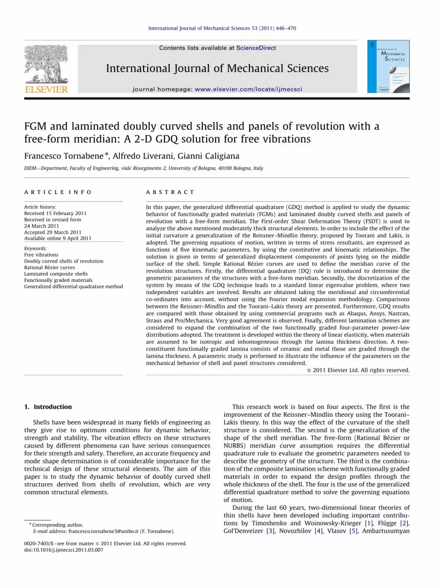
In Figs. 9–12, there are reported the first six mode shapes for

the structures with a free-form meridian considered above. In

particular, for the complete shells of revolution there are some

symmetrical mode shapes due to the symmetry of the problem

considered in 3D space. In these cases, the symmetrical mode

shapes are summarized in one figure. The mode shapes of all the

structures under discussion have been evaluated by authors.

By using the authors’ MATLAB code, these mode shapes have

been reconstructed in three-dimensional view by means of

considering the displacement field (17) after solving the eigenva-

lue problem (36).

Finally, in order to illustrate the GDQ convergence character-

istic for free-form meridian shells, the first ten frequencies of the

C–C–F–F isotropic free-form meridian panel of Table 2 are

investigated by varying the number of grid points. Results are

collected in Table 5 when the number of points of the Chebyshev–

Gauss–Lobatto grid distributions (10) and (33) is increased from

N¼M¼11 up to N¼M¼31. It can be seen that the proposed GDQ

formulation well captures the dynamic behavior of the panel by

using only 21 points in two co-ordinate directions. It can also be

seen that for the considered structure, the formulation is stable

while increasing the number of points and that the use of 21

points guarantees convergence of the procedure. Analogous and

similar convergence results can be obtained for all the shell

structures considered in this work, as shown in the Ph.D. Thesis

Table 5

First ten frequencies for the C–C–F–F isotropic free-form meridian panel of Table 2 for an increasing the number of grid points N¼M of the Chebyshev–Gauss–Lobatto

distribution.

Mode (Hz) N¼M¼11 N¼M¼15 N¼M¼17 N¼M¼21 N¼M¼25 N¼M¼29 N¼M¼31

GDQ-RM

f1 72.115 73.153 73.268 73.257 73.195 73.161 73.153

f2 95.815 96.800 97.173 97.414 97.439 97.435 97.433

f3 190.226 191.894 192.067 192.044 191.936 191.872 191.855

f4 242.855 247.103 247.722 247.979 247.909 247.845 247.826

f5 363.562 367.505 367.959 368.162 368.101 368.041 368.023

f6 424.634 431.237 432.047 432.278 432.107 431.984 431.951

f7 513.585 513.879 513.863 513.831 513.808 513.795 513.792

f8 584.260 586.074 586.372 586.479 586.430 586.392 586.381

f9 613.416 614.395 614.865 615.082 615.040 614.994 614.981

f10 640.392 638.604 639.249 639.608 639.593 639.548 639.533

GDQ-TL

f1 72.159 73.024 73.189 73.219 73.166 73.134 73.126

f2 94.487 95.761 96.126 96.360 96.383 96.380 96.379

f3 191.230 192.935 193.123 193.118 193.019 192.959 192.944

f4 243.644 248.007 248.652 248.941 248.888 248.830 248.813

f5 363.399 367.406 367.879 368.096 368.038 367.979 367.960

f6 425.686 432.336 433.160 433.417 433.261 433.146 433.114

f7 513.462 513.725 513.705 513.670 513.647 513.634 513.631

f8 584.391 586.173 586.463 586.567 586.521 586.484 586.474

f9 613.633 614.584 615.054 615.277 615.239 615.196 615.184

f10 640.595 638.810 639.454 639.815 639.803 639.759 639.744

Table 6

The first ten frequencies for the functionally graded free-form panel C–C–F–F of Table 2 (W0 ¼ 1201,h¼ 0:1m,Rb ¼ 0m) as a function of the power-law exponent

p¼ pð1Þ ¼ pð2Þ .

Mode (Hz) p¼0 p¼0.6 p¼1 p¼5 p¼20 p¼50 p¼100 p¼N

FGM1ðað1Þ ¼ 1=bð1Þ ¼ 0=cð1Þ ¼ 2=pð1Þ Þ=FGM2ðað2Þ ¼ 1=bð2Þ ¼ 0=cð2Þ ¼ 2=pð2Þ Þ power-law distribution

f1 78.170 80.625 81.175 79.788 76.097 74.553 73.922 73.219

f2 102.874 106.716 107.612 105.867 100.564 98.313 97.390 96.360

f3 206.175 210.527 211.298 207.298 199.298 195.990 194.634 193.118

f4 265.772 274.032 275.943 271.270 258.639 253.414 251.294 248.941

f5 392.983 406.716 409.887 403.116 383.520 375.249 371.867 368.096

f6 462.720 478.622 482.109 473.969 451.479 441.841 437.870 433.417

f7 548.399 547.996 546.791 534.664 521.855 517.341 515.583 513.670

f8 626.224 628.740 628.129 614.624 597.995 591.776 589.299 586.567

f9 656.875 659.473 658.396 643.927 627.483 621.015 618.332 615.277

f10 683.073 694.777 695.201 680.729 659.323 649.478 645.050 639.815

FGM2ðað1Þ ¼ 1=bð1Þ ¼ 0=cð1Þ ¼ 2=pð1Þ Þ=FGM1ðað2Þ ¼ 1=bð2Þ ¼ 0=cð2Þ ¼ 2=pð2Þ Þ power-law distribution

f1 78.170 72.837 71.322 70.552 72.263 72.814 73.013 73.219

f2 102.874 95.087 92.905 92.097 94.843 95.717 96.033 96.360

f3 206.175 194.203 190.616 188.126 191.367 192.383 192.746 193.118

f4 265.772 248.215 243.279 240.431 245.825 247.611 248.263 248.941

f5 392.983 364.631 356.697 353.166 362.729 365.816 366.935 368.096

f6 462.720 428.617 418.929 415.129 426.977 430.697 432.035 433.417

f7 548.399 532.703 527.277 516.181 514.287 513.928 513.802 513.670

f8 626.224 603.357 595.289 584.574 585.848 586.277 586.423 586.567

f9 656.875 627.086 615.850 607.459 613.555 614.659 614.982 615.277

f10 683.073 640.379 629.167 620.314 632.713 636.920 638.373 639.815


by Tornabene [59]. In addition, Hosseini-Hashemi et al. [80] (see

Table 3 of the work [80]) have compared their results obtained

with a semi analytical method with those results presented in the

article by Tornabene [51]. Since the code used to obtained the

previous results [51] is exactly the same of the code used to

obtained all the results presented in this paper, the results of the

work [80] represent another proof of the validity and the accuracy

of the present procedure. As shown, the exact results by Hosseini-

Hashemi et al. [80] are in good agreement with those reported by

Tornabene [51]. The discrepancy between results obtained from

two methods is closely zero.

Regarding the functionally graded materials, their two consti-

tuents are taken to be zirconia (ceramic) and aluminum (metal).

Young’s modulus, Poisson’s ratio and mass density for the zirconia

are EC ¼ 168GPa, nC ¼ 0:3, rC ¼ 5700kg=m3, and for the aluminum

are EM ¼ 70GPa, nM ¼ 0:3 and rM ¼ 2707kg=m3, respectively.

Tables 6–10 illustrate the first ten frequencies of different

structures with a free-form meridian. These tables show how by

varying only the power-law index p of the volume fraction Vc it is

possible to modify natural frequencies of FGM shells and panels.

For the GDQ results shown in Tables 6–10, the grid distributions

(10) and (33) with N¼M¼21 are considered. Furthermore, two

and three layered shells and panels of revolution with a free-form

meridian have been considered in order to illustrate the influence

of the volume fraction profiles shown in Figs. 5 and 6.

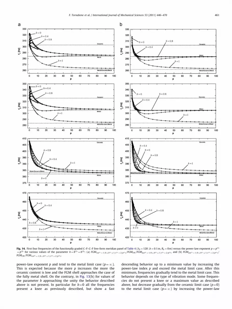
The influence of the index p on the vibration frequencies is

shown in Figs. 13–17. As can be seen from figures, natural

frequencies of FGM shells and panels often present an

Table 7

The first ten frequencies for the functionally graded free-form panel C–F–C–F of Table 4 (W0 ¼ 1201,h¼ 0:1m,Rb ¼ 0m) as a function of the power-law exponent

p¼ pð1Þ ¼ pð3Þ .


FGM1ðað1Þ ¼ 1=bð1Þ ¼ 0:5=cð1Þ ¼ 2=pð1Þ Þ=FGMCM=FGM2ðað3Þ ¼ 1=bð3Þ ¼ 0:5=cð3Þ ¼ 2=pð3Þ Þ power-law distribution

f1 302.868 307.559 309.470 305.694 291.768 287.199 285.495 283.688

f2 325.703 330.387 332.275 327.992 313.459 308.716 306.949 305.077

f3 407.901 405.629 403.909 392.648 385.643 383.621 382.868 382.069

f4 462.809 461.597 460.236 448.207 438.728 435.796 434.687 433.500

f5 581.145 580.178 578.430 562.962 551.418 547.538 546.013 544.342

f6 623.734 628.692 628.242 613.132 596.918 589.809 587.111 584.234

f7 630.423 629.451 629.878 617.256 598.165 593.781 592.179 590.500

f8 640.571 644.045 645.538 634.560 611.530 604.822 602.445 600.005

f9 671.233 667.691 665.740 649.782 634.687 631.145 629.941 628.725

f10 738.008 734.648 732.131 712.890 698.359 694.292 692.815 691.271

FGM2ðað1Þ ¼ 1=bð1Þ ¼ 0:5=cð1Þ ¼ 2=pð1Þ Þ=FGMCM=FGM1ðað3Þ ¼ 1=bð3Þ ¼ 0:5=cð3Þ ¼ 2=pð3Þ Þ power-law distribution

f1 302.868 299.911 297.810 285.463 283.171 283.403 283.533 283.688

f2 325.703 322.504 320.248 307.110 304.601 304.807 304.929 305.077

f3 407.901 403.481 400.733 387.234 383.158 382.496 382.281 382.069

f4 462.809 457.870 454.738 438.856 434.415 433.841 433.666 433.500

f5 581.145 574.996 571.054 550.668 545.248 544.665 544.498 544.342

f6 623.734 617.419 613.134 589.295 584.077 584.060 584.129 584.234

f7 630.423 623.709 619.440 597.779 591.722 590.947 590.716 590.500

f8 640.571 633.938 629.565 606.311 600.524 600.121 600.047 600.005

f9 671.233 663.927 659.411 637.531 630.695 629.498 629.109 628.725

f10 738.008 730.034 725.059 700.509 693.163 692.003 691.633 691.271

Table 8

The first ten frequencies for the functionally graded free-form panel F–F–C–C of Table 1 (W0 ¼ 1201,h¼ 0:1m,Rb ¼ 0m) as a function of the power-law exponent

p¼ p 1ð Þ ¼ p 3ð Þ .


FGM1ðað1Þ ¼ 0=bð1Þ ¼ �0:6=cð1Þ ¼ 2=pð1Þ Þ=FGMCM=FGM2ðað3Þ ¼ 0=bð3Þ ¼ �0:6=cð3Þ ¼ 2=pð3Þ Þ power-law distribution

f1 30.556 31.221 31.528 32.081 31.298 30.645 30.195 28.621

f2 83.906 85.692 86.526 88.056 85.897 84.100 82.867 78.593

f3 177.390 180.959 182.592 185.345 180.972 177.363 174.874 166.157

f4 204.823 206.327 206.993 207.267 203.188 200.211 198.257 191.853

f5 236.942 239.330 240.373 241.234 236.349 232.679 230.226 221.938

f6 290.465 296.946 300.060 306.200 298.412 291.859 287.377 272.072

f7 339.938 346.555 349.629 354.979 346.553 339.617 334.862 318.413

f8 363.542 371.615 375.425 382.635 373.089 365.072 359.563 340.522

f9 414.743 426.401 431.999 443.683 431.567 421.025 413.737 388.482

f10 465.840 472.783 475.884 479.955 469.614 461.411 455.802 436.342

FGM2ðað1Þ ¼ 0=bð1Þ ¼ �0:6=cð1Þ ¼ 2=pð1Þ Þ=FGMCM=FGM1ðað3Þ ¼ 0=bð3Þ ¼ �0:6=cð3Þ ¼ 2=pð3Þ Þ power-law distribution

f1 30.556 30.591 30.547 29.592 28.753 28.594 28.561 28.621

f2 83.906 83.985 83.861 81.256 78.981 78.543 78.447 78.592

f3 177.390 177.501 177.218 171.776 167.051 166.121 165.907 166.156

f4 204.823 204.112 203.499 198.161 194.082 192.963 192.526 191.852

f5 236.942 236.336 235.699 229.283 224.193 222.911 222.457 221.937

f6 290.465 290.811 290.412 281.305 273.357 271.839 271.514 272.070

f7 339.938 340.064 339.495 329.158 320.262 318.475 318.042 318.410

f8 363.542 363.981 363.479 352.077 342.086 340.190 339.792 340.520

f9 414.743 416.000 415.692 401.826 389.229 387.103 386.812 388.478

f10 465.840 465.366 464.359 450.934 439.750 437.268 436.540 436.340


intermediate value between the natural frequencies of the limit

cases of homogeneous shells of zirconia (p¼0) and of aluminum

(p¼N), as expected. However, natural frequencies sometimes

exceed limit cases, as can be seen from Figs. 13–17. This fact can

depend on various parameters, such as the geometry of the shell,

the boundary conditions, the power-law distribution profile, the

lamination scheme, etc. In particular, for specific values of the

four parameters a, b, c, p it is possible to exceed or approach the

ceramic limit case as shown in figures under consideration, even

if the contents of ceramic is not much. Increasing the values of the

parameter index p up to infinity reduces the contents of ceramic

and at the same time increases the percentage of metal. Thus, it is

possible to obtain dynamic characteristics similar or better than

the isotropic ceramic or metal limit case by choosing suitable

values of the four parameters a, b, c and p.

Figs. 13–17 are divided into two parts. On the left, part

(a) shows the first four frequencies versus the power-law

index p obtained using FGM1ðað1Þ=bð1Þ=cð1Þ=pð1ÞÞ=FGM2ðað2Þ=bð2Þ=cð2Þ=pð2ÞÞ

or FGM1ðað1Þ=bð1Þ=cð1Þ=pð1ÞÞ=FGMCM=FGM2ðað3Þ=bð3Þ=cð3Þ=pð3ÞÞ distributions,

while on the right, part (b) illustrates the first four frequencies

versus the power-law index p obtained using FGM2ðað1Þ=bð1Þ=cð1Þ=pð1ÞÞ=

FGM1ðað2Þ=bð2Þ=cð2Þ=pð2ÞÞ or FGM2ðað1Þ=bð1Þ=cð1Þ=pð1ÞÞ=FGMCM=FGM1ðað3Þ=bð3Þ=cð3Þ=pð3ÞÞ

distributions. The symbol FGMCM indicates that the middle ply can

be constituted by a mixture of the two constituents. If one of the

two constituents has a zero volume fraction, the isotropic mate-

rial lamina is inferred as a special case.

Fig. 13 shows the first four natural frequencies of the C–C–F–F

free-form meridian panel of Table 2 versus the power-law

index p for various values of the parameter bð1Þ ¼ bð2Þ.

Fig. 13(a) illustrates the variation of the first four frequencies

Table 9

The first ten frequencies for the functionally graded free-form panel F–C–F–C of Table 1 (W0 ¼ 1201, h¼ 0:1m, Rb ¼ 0m) as a function of the power-law exponent

p¼ p 1ð Þ ¼ p 3ð Þ .


FGM1ðað1Þ ¼ 0:6=bð1Þ ¼ 0:2=cð1Þ ¼ 3=pð1Þ Þ=FGMCM=FGM2ðað3Þ ¼ 0:6=bð3Þ ¼ 0:2=cð3Þ ¼ 3=pð3Þ Þ power-law distribution

f1 187.034 187.543 187.765 186.610 180.220 177.472 176.384 175.190

f2 214.487 214.466 214.343 211.251 205.258 202.901 201.955 200.904

f3 292.151 293.868 294.753 295.212 283.554 278.161 276.014 273.650

f4 350.950 353.713 355.147 356.987 342.061 334.858 331.952 328.725

f5 401.696 405.932 408.205 409.350 393.923 384.379 380.528 376.257

f6 411.864 412.758 413.060 413.015 396.200 390.576 388.307 385.782

f7 541.686 546.512 549.048 553.217 529.209 517.430 512.669 507.382

f8 551.139 556.695 559.563 564.397 539.605 527.113 521.987 516.237

f9 564.376 569.841 572.827 579.202 552.615 539.559 534.357 528.635

f10 635.461 637.301 638.006 633.023 612.223 603.089 599.374 595.218

FGM2ðað1Þ ¼ 0:6=bð1Þ ¼ 0:2=cð1Þ ¼ 3=pð1Þ Þ=FGMCM=FGM1ðað3Þ ¼ 0:6=bð3Þ ¼ 0:2=cð3Þ ¼ 3=pð3Þ Þ power-law distribution

f1 187.034 185.790 184.967 178.873 175.471 175.234 175.200 175.190

f2 214.487 213.063 212.130 205.370 201.513 201.101 200.995 200.904

f3 292.151 290.205 288.903 279.008 273.619 273.482 273.539 273.650

f4 350.950 348.609 347.030 334.833 328.298 328.330 328.489 328.725

f5 401.696 399.013 397.187 382.794 375.227 375.530 375.840 376.257

f6 411.864 409.126 407.316 393.950 386.466 385.916 385.826 385.782

f7 541.686 538.067 535.619 516.557 506.430 506.624 506.939 507.382

f8 551.139 547.458 544.955 525.242 514.861 515.267 515.681 516.237

f9 564.376 560.608 558.053 538.079 527.501 527.766 528.129 528.635

f10 635.461 631.233 628.432 607.598 596.008 595.294 595.217 595.218

Table 10

The first ten frequencies for the functionally graded free-form panel C–C of Table 4 (W0 ¼ 3601, h¼ 0:1m, Rb ¼ 0m) as a function of the power-law exponent p¼ p 1ð Þ ¼ p 3ð Þ .


FGM1ðað1Þ ¼ 1=bð1Þ ¼ 1=cð1Þ ¼ 5=pð1Þ Þ=FGMCM=FGM2ðað3Þ ¼ 1=bð3Þ ¼ 1=cð3Þ ¼ 5=pð3Þ Þ power

f1 503.738 500.481 498.581 488.224 481.544 479.638 478.934 478.192

f2 522.847 520.680 519.456 513.492 510.620 509.947 509.712 509.470

f3 563.237 559.685 557.616 546.405 539.265 537.243 536.499 535.714

f4 563.237 559.685 557.616 546.405 539.265 537.243 536.499 535.714

f5 577.530 575.052 573.649 566.738 563.297 562.469 562.176 561.875

f6 577.530 575.052 573.649 566.738 563.297 562.469 562.176 561.875

f7 633.303 630.408 628.758 620.451 616.022 614.893 614.488 614.066

f8 633.303 630.408 628.758 620.451 616.022 614.893 614.488 614.066

f9 660.211 655.809 653.238 639.171 630.030 627.416 626.451 625.433

f10 660.211 655.809 653.238 639.171 630.030 627.416 626.451 625.433

FGM2ðað1Þ ¼ 1=bð1Þ ¼ 1=cð1Þ ¼ 5=pð1Þ Þ=FGMCM=FGM1ðað3Þ ¼ 1=bð3Þ ¼ 1=cð3Þ ¼ 5=pð3Þ Þ power-law distribution

f1 503.738 499.180 496.620 484.618 479.784 478.829 478.510 478.192

f2 522.847 520.696 519.479 513.531 510.639 509.956 509.716 509.470

f3 563.237 558.333 555.580 542.679 537.453 536.411 536.063 535.714

f4 563.237 558.333 555.580 542.679 537.453 536.411 536.063 535.714

f5 577.530 574.976 573.534 566.530 563.197 562.422 562.152 561.875

f6 577.530 574.976 573.534 566.530 563.197 562.422 562.152 561.875

f7 633.303 630.121 628.323 619.614 615.599 614.697 614.384 614.066

f8 633.303 630.121 628.323 619.614 615.599 614.697 614.384 614.066

f9 660.211 653.958 650.452 634.085 627.561 626.283 625.858 625.433

f10 660.211 653.958 650.452 634.085 627.561 626.283 625.858 625.433


obtained using the FGM1ðað1Þ=bð1Þ=cð1Þ=pð1ÞÞ=FGM2ðað2Þ=bð2Þ=cð2Þ=pð2ÞÞ distribu-

tion, while in Fig. 13(b) the first four frequencies for the

FGM2ðað1Þ=bð1Þ=cð1Þ=pð1ÞÞ= FGM1ðað2Þ=bð2Þ=cð2Þ=pð2ÞÞ distribution are reported.

For (a, b) the same parameters að1Þ ¼ að2Þ ¼ 1,cð1Þ ¼ cð2Þ ¼ 2 are kept.

It is interesting to note that frequencies attain the value for a shell

made only of metal, due to the fact that aluminum has a much

smaller Young’s modulus than zirconia. In particular, it can be

noted that in Fig. 13(a) for low values of the parameter b the most

of frequencies exceeds the ceramic limit case (p¼0) varying the

power-law index from p¼0 to pE1, while for values of p greater

than unity frequencies decrease until a minimum value. After

the maximum, frequencies slowly decrease by increasing the

Fig. 13. First four frequencies of the functionally graded C–C–F–F free-form meridian panel of Table 2 (W0 ¼ 1201, h¼ 0:1m, Rb ¼ 0m) versus the power-law exponent

p¼ p 1ð Þ ¼ p 2ð Þ for various values of the parameter b¼ b 1ð Þ ¼ b 2ð Þ: (a) FGM1ðað1Þ ¼ 1=0rbð1Þr1=cð1Þ ¼ 2=pð1Þ Þ=FGM2ðað2Þ ¼ 1=0rbð2Þr1=cð2Þ ¼ 2=pð2Þ Þ and (b) FGM2ðað1Þ ¼ 1=0rbð1Þr1=cð1Þ ¼ 2=pð1Þ Þ=

FGM1ðað2Þ ¼ 1=0rbð2Þr1=cð2Þ ¼ 2=pð2Þ Þ .


power-law exponent p and tend to the metal limit case (p¼N).

This is expected because the more p increases the more the

ceramic content is low and the FGM shell approaches the case of

the fully metal shell. On the contrary, in Fig. 13(b) for values of

the parameter b approaching the unity the behavior described

above is not present. In particular for b¼0 all the frequencies

present a knee as previously described, but show a fast

descending behavior up to a minimum value by increasing the

power-law index p and exceed the metal limit case. After this

minimum, frequencies gradually tend to the metal limit case. This

behavior depends on the type of vibration mode. Some frequen-

cies do not present a knee or a maximum value as described

above, but decrease gradually from the ceramic limit case (p¼0)

to the metal limit case (p¼N) by increasing the power-law

Fig. 14. First four frequencies of the functionally graded C–F–C–F free-form meridian panel of Table 4 (W0 ¼ 1201,h¼ 0:1m, Rb ¼ 0m) versus the power-law exponent p¼ p 1ð Þ

¼ p 3ð Þ for various values of the parameter b¼ bð1Þ ¼ bð3Þ: (a) FGM1ðað1Þ ¼ 1=0rbð1Þr1=cð1Þ ¼ 2=pð1Þ Þ=FGMCM=FGM2ðað3Þ ¼ 1=0rbð3Þr1=cð3Þ ¼ 2=pð3Þ Þ and (b) FGM2ðað1Þ ¼ 1=0rbð1Þr1=cð1Þ ¼ 2=pð1Þ Þ=

FGMCM=FGM1ðað3Þ ¼ 1=0rbð3Þr1=cð3Þ ¼ 2=pð3Þ Þ .


exponent p. In particular, the types of vibration mode that can

present this monotone gradually decrease of frequency are tor-

sional, bending and axisymmetric mode shapes, while the cir-

cumferential and radial mode shapes are characterized by a knee

or a maximum value, as can be seen by comparing the mode

shapes represented with variations of frequencies as functions of

the power-law exponent p. However, this behavior depends on

the geometry of the shell and boundary conditions.

In the same way, Fig. 14 shows the first four natural frequen-

cies of the C–F–C–F free-form meridian panel of Table 3 versus

the power-law index p for various values of the para-

meter bð1Þ ¼ bð3Þ. Fig. 14(a) illustrates the variation of the first

Fig. 15. First four frequencies of the functionally graded F–F–C–C free-form meridian shell of Table 1 (W0 ¼ 1201, h¼ 0:1m, Rb ¼ 0m) versus the power-law exponent p¼ p 1ð Þ

¼ p 3ð Þ for various values of the parameter b¼ bð1Þ ¼ bð3Þ: (a) FGM1ðað1Þ ¼ 0=�1rbð1Þr0=cð1Þ ¼ 2=pð1Þ Þ=FGMCM=FGM2ðað3Þ ¼ 0=�1rbð3Þr0=cð3Þ ¼ 2=pð3Þ Þ and (b) FGM2ðað1Þ ¼ 0=�1rbð1Þr0=cð1Þ ¼ 2=pð1Þ Þ=

FGMCM=FGM1ðað3Þ ¼ 0=�1rbð3Þr0=cð3Þ ¼ 2=pð3Þ Þ .


four frequencies obtained using the FGM1ðað1Þ=bð1Þ=cð1Þ=pð1ÞÞ=FGMCM=

FGM2ðað3Þ=bð3Þ=cð3Þ=pð3ÞÞ distribution, while in Fig. 14(b) the first four

frequencies for the FGM2ðað1Þ=bð1Þ=cð1Þ=pð1ÞÞ=FGMCM=FGM1ðað3Þ=bð3Þ=cð3Þ=pð3ÞÞ

distribution are reported. For (a, b) the same parameters

að1Þ ¼ að3Þ ¼ 1,cð1Þ ¼ cð3Þ ¼ 2 are kept. Differently from the previous

case a new limit has been introduced. This new limit represents

the laminated shell made of three laminae: the first and the third

laminae are fully metal plies, while the middle lamina is a fully

ceramic ply. As can be seen, by varying parameters b and p

frequencies tend to different limit behaviors: ceramic, metal and

metal/ceramic/metal limit cases. b¼ b 1ð Þ ¼ b 3ð Þ is contained in the

interval [0,1] for this case.

Fig. 16. First four frequencies of the functionally graded F–C–F–C free-form meridian panel of Table 1 (W0 ¼ 1201, h¼ 0:1m, Rb ¼ 0m) versus the power-law

exponent p¼ p 1ð Þ ¼ p 3ð Þ for various values of the parameter a¼ að1Þ ¼ að3Þ: (a) FGM1ð0:2rað1Þr1:2=bð1Þ ¼ 0:2=cð1Þ ¼ 3=pð1Þ Þ=FGMCM=FGM2ð0:2rað3Þr1:2=bð3Þ ¼ 0:2=cð3Þ ¼ 3=pð3Þ Þand

(b) FGM2ð0:2rað1Þr1:2=bð1Þ ¼ 0:2=cð1Þ ¼ 3=pð1Þ Þ=FGMCM=FGM1ð0:2rað3Þr1:2=bð3Þ ¼ 0:2=cð3Þ ¼ 3=pð3Þ Þ .


Fig. 15 presents the first four natural frequencies of the F–F–C–

C free-form meridian shell of Table 1 versus the power-law index

p for various values of the parameter bð1Þ ¼ bð3Þ. As for a previous

case a three laminae shell is considered. For (a, b) the same

parameters að1Þ ¼ að3Þ ¼ 0,cð1Þ ¼ cð3Þ ¼ 2 are kept, while

b¼ bð1Þ ¼ bð3Þ is contained in the interval [�1,0]. As can be seen,

in Fig. 15(a) frequencies exceed the ceramic limit case for low

values of the power-law index p up to a maximum value and after

this maximum decrease by increasing the power-law index p. For

high value of the power-law index p frequencies slowly tend to the

metal limit case. On the contrary, different behavior can be seen in

Fig. 15(b) due to the change of the lamination scheme profile.

Fig. 17. First four frequencies of the functionally graded C–C free-form meridian shell of Table 4 (W0 ¼ 3601, h¼ 0:1m, R b ¼ 0m) versus the power-law

exponent p¼ p 1ð Þ ¼ p 3ð Þ for various values of the parameter c¼ cð1Þ ¼ cð3Þ: (a) FGM1ðað1Þ ¼ 1=bð1Þ ¼ 1=1r cð1Þr13=pð1Þ Þ=FGMCM=FGM2ðað3Þ ¼ 1=bð3Þ ¼ 1=1rcð3Þr13=pð3Þ Þ and

(b) FGM2ðað1Þ ¼ 1=bð1Þ ¼ 1=1r cð1Þr13=pð1Þ Þ=FGMCM=FGM1ðað3Þ ¼ 1=bð3Þ ¼ 1=1r cð3Þr13=pð3Þ Þ .


Moreover, the influence of the parameter a on the dynamic

vibration of the F–C–F–C free-form meridian panel of Table 1 is

investigated in Fig. 16 by considering bð1Þ ¼ bð3Þ ¼ 0:2,cð1Þ ¼ cð3Þ ¼ 3.

In this case the parameter a¼ að1Þ ¼ að3Þ varies from 0.2 to 1.2. As

can be seen, by varying parameters a and p frequencies tend to

different limit behaviors: ceramic, metal and metal/ceramic/

metal limit cases. Finally, Fig. 17 the influence of the parameter

c on the dynamic vibration of the C–C free-form meridian shell of

Table 3 is presented by considering að1Þ ¼ að3Þ ¼ 1,bð1Þ ¼ bð3Þ ¼ 1.

The parameter c¼ cð1Þ ¼ cð3Þ varies from 1 to 13. It can be noted

that the influence of the parameter c is poor and frequencies

gradually decrease by increasing the power-law exponent p and

tend to the metal/ceramic/metal limit case.

5. Conclusion remarks and summary

A generalized differential quadrature method application to

the free vibration analysis of laminated composite and function-

ally graded doubly curved shells and panels of revolution with a

free-form meridian has been presented to illustrate the versatility

and the accuracy of this methodology. The differential quadrature

rule is introduced to determine the geometric parameters of the

structures with a free-form meridian. Simple Rational Bezier

curves are used. Various lamination schemes with different layers

have been considered. New functionally graded material profiles

have been introduced. Ceramic–metal graded shells of revolution

with two four parameter power-law distributions of the volume

fraction of the constituents in the thickness direction have been

considered. Various material profiles through the functionally

graded shell thickness have been illustrated by varying the four

parameters of power-law distributions. The numerical results

have shown the influence of the power-law exponent, of the

power-law distribution choice and of the choice of the four

parameters on the free vibrations of functionally graded shells

considered. Extensive numerical results have been presented,

showing the effect of the choice of the four parameters on shell

frequencies. In general, it can be pointed out that the frequency

vibration of functionally graded shells and panels of revolution

depends on the type of vibration mode, thickness, lamination

scheme, power-law distribution, power-law exponent and the

curvature of the structure.

The adopted shell theory is the First-order Shear Deformation

Theory. In particular, the Toorani–Lakis theory has been used. By

doing so, the Reissner–Mindlin theory becomes a special case of

the Toorani–Lakis theory when the curvature coefficients are set

to zero. The motion equations have been discretized with the

GDQ method giving a standard linear eigenvalue problem. The

vibration results have been obtained without the modal expan-

sion methodology. In this way, the complete 2D differential

system, governing the structural problem has been solved. By

doing so, complete revolution shells have been obtained as special

cases of shell panels by satisfying the kinematic and physical

compatibility conditions. The examples presented show that the

generalized differential quadrature method can produce accurate

results by using a small number of sampling points. Numerical

solutions has been compared with those presented in literature

and the ones obtained using commercial programs such as

Abaqus, Ansys, Nastran, Straus and Pro/Mechanica. The compar-

isons conducted with FEM codes confirm how the GDQ simple

numerical method provides accurate and computationally low

cost results for all the structures considered. The GDQ method

provides converging results for all the cases as the number of grid

points increases. Convergence and stability have been shown.

Furthermore, discretizing and programming procedures are quite

easy. The GDQ results show to be precise and reliable. The

numerical tests demonstrate and confirm the favorable precision

of the generalized differential quadrature method.

Acknowledgments

This research was supported by the Italian Ministry for Uni-

versity and Scientific, Technological Research MIUR (40% and 60%).

Appendix

The equilibrium operators in Eq. (27) assume the following aspect:

L11 ¼1

R2j

ðA11þa1B11þa2D11þa3E11Þ@2

@j2

þ �1

R3j

@Rj

@jðA11þa1B11þa2D11þa3E11Þþ

1

R2j

B11@a1@j

þD11@a2@j

þE11@a3@j

� �

þcosj

RjR0ðA11þa1B11þa2D11þa3E11Þ

!

@

@j

þðA66þb1B66þb2D66þb3E66Þ@2

@s2þ

2A16

Rj

@2

@j@s�sinj

RjR0A12

�cos2j

R20

ðA22þb1B22þb2D22þb3E22Þ�k

R2j

ðA44þa1B44þa2D44þa3E44Þ

L12 ¼1

R2j


@j2

þ �1

R3j

@Rj


1

R2j

B16@a1@j

þD16@a2@j

þE16@a3@j

� �

þcosj

RjR0ð�A26þa1B16þa2D16þa3E16Þ

!

@

@j


@s2þ �

cosj

R0ðA66þb1B66þb2D66þb3E66þA22þb1B22þb2D22þb3E22Þ

� �

@

@s

þA12þA66

Rj

@2

@j@sþ

sinj

RjR0A16þ

cos2j

R20

ðA26þb1B26þb2D26þb3E26Þksinj

RjR0A45

L13 ¼1

R2j

ðA11þa1B11þa2D11þa3E11Þþsinj

RjR0A12þ

k

R2j


!

@

@j


þsinj

R0ðA26þb1B26þb2D26þb3E26Þþ

A16

Rjþk

A45

Rj

� �

@

@s�

1

R3j

@Rj@j


þ1

R2j

B11@a1@j

þD11@a2@j

þE11@a3@j

� �

þ �cosjsinj

R20

þcosj

RjR0

!

A12

þcosj

RjR0ðA11�A12þa1B11þa2D11þa3E11Þþ

cosjsinj

R20

ðA12�A22�b1B22�b2D22�b3E22Þ

L14 ¼1

R2j

ðB11þa1D11þa2E11þa3F11Þ@2

@j2

þ �1

R3j

@Rj@j

ðB11þa1D11þa2E11þa3F11Þþ1

R2j

D11@a1@j

þE11@a2@j

þF11@a3@j

� �

þcosj

RjR0ðB11þa1D11þa2E11þa3F11Þ

!

@

@j

þðB66þb1D66þb2E66þb3F66Þ@2

@s2þ

2B16

Rj

@2

@j@s�sinj

RjR0B12

�cos2j

R20

ðB22þb1D22þb2E22þb3F22Þþk

RjðA44þa1B44þa2D44þa3E44Þ

L15 ¼1

R2j


@j2

þ �1

R3j

@Rj@j


R2j

D16@a1@j

þE16@a2@j

þF16@a3@j

� �

þcosj

RjR0ð�B26þa1D16þa2E16þa3F16Þ

!

@

@j


@s2þ �

cosj

R0ðB66þb1D66þb2E66þb3F66þB22þb1D22þb2E22þb3F22Þ

� �

@

@s

þB12þB66

Rj

@2

@j@sþ

sinj

RjR0B16þ

cos2j

R20

ðB26þb1D26þb2E26þb3F26ÞþkA45

Rj

L21 ¼1

R2j


@j2

þ �1

R3j

@Rj@j

ðA16þa1B16þa2D16þa3E16Þþ1

R2j

B16@a1@j

þD16@a2@j

þE16@a3@j

� �

þcosj

RjR0ð2A16þA26þa1B16þa2D16þa3E16Þ

!

@

@j


@s2þ

cosj

R0ðA66þb1B66þb2D66þb3E66þA22þb1B22þb2D22þb3E22Þ

� �

@

@s

þA12þA66

Rj

@2

@j@s�sinj

RjR0A26þ

cos2j

R20

ðA26þb1B26þb2D26þb3E26Þ�ksinj

RjR0A45

L22 ¼1

R2j


@j2

þ �1

R3j

@Rj@j

ðA66þa1B66þa2D66þa3E66Þþ1

R2j

B66@a1@j

þD66@a2@j

þE66@a3@j

� �

þcosj


!

@

@j


@s2þ

2A26

Rj

@2

@j@sþ

sinj

RjR0A66

�cos2j

R20

ðA66þb1B66þb2D66þb3E66Þ�ksin2 j

R20

ðA55þb1B55þb2D55þb3E55Þ

L23 ¼1

R2j

ðA16þa1B16þa2D16þa3E16Þþsinj

RjR0A26þk

sinj

RjR0A45

!

@

@j

þsinj

R0ðA22þb1B22þb2D22þb3E22Þþ

A12

Rjþk

sinj

R0ðA55þb1B55þb2D55þb3E55Þ

� �

@

@s

�1

R3j

@Rj


1

R2j

B16@a1@j

þD16@a2@j

þE16@a3@j

� �

þ �cosjsinj

R20

þcosj

RjR0

!

A26

þcosj

RjR0ð2A16þa1B16þa2D16þa3E16Þþ

cosjsinj

R20

ð2A26þb1B26þb2D26þb3E26Þ

!

L24 ¼1

R2j


@j2

þ �1

R3j

@Rj@j


R2j

@a1@j

D16þ@a2@j

E16þ@a3@j

F16

� �

þcosj

RjR0B26þ

cosj

RjR0ð2B16þa1D16þa2E16þa3F16Þ

!


�@

@jþðB26þb1D26þb2E26þb3F26Þ

@2

@s2þ

cosj


� �

@

@s

þB12þB66

Rj

@2

@j@s�sinj

RjR0B26þ

cos2j

R20

ðB26þb1D26þb2E26þb3F26Þþksinj

R0A45

L25 ¼1

R2j


@j2

þ �1

R3j

@Rj

@jðB66þa1D66þa2E66þa3F66Þþ

1

R2j

@a1@j

D66þ@a2@j

E66þ@a3@j

F66

� �

þcosj


!

�@


@2

@s2þ

2B26

Rj

@2

@j@sþ

sinj

RjR0B66

�cos2j

R20



L31 ¼ �k

R2j

ðA44þa1B44þa2D44þa3E44Þ�1

R2j

ðA11þa1B11þa2D11þa3E11Þ�sinj

RjR0A12

!

@

@j

þ �kA45

Rj�A16

Rj�sinj


� �

@

@s

þk

R3j

@Rj@j

ðA44þa1B44þa2D44þa3E44Þ�k

R2j

@a1@j

B44þ@a2@j

D44þ@a3@j

E44

� �

�kcosj

RjR0ðA44þa1B44þa2D44þa3E44Þ�

cosj

RjR0A12�

cosjsinj

R20


L32 ¼ �ksinj

RjR0A45�

1

R2j

ðA16þa1B16þa2D16þa3E16Þ�sinj

RjR0A26

!

@

@j

þ �ksinj

R0ðA55þb1B55þb2D55þb3E55Þ�

A12

Rj�sinj


� �

@

@s

�k12cosj

RjR0A45þ

cosj

RjR0A16þ

cosjsinj

R20


L33 ¼k

R2j


@j2

þ �k

R3j

@Rj@j

ðA44þa1B44þa2D44þa3E44Þþk

R2j

@a1@j

B44þ@a2@j

D44þ@a3@j

E44

� �

þkcosj


!

@

@j

þkðA55þb1B55þb2D55þb3E55Þ@2

@s2þk

2A45

Rj

@2

@j@s�2sinj

RjR0A12

�1

R2j

ðA11þa1B11þa2D11þa3E11Þ�sin2j

R20


L34 ¼k

RjðA44þa1B44þa2D44þa3E44Þ�

1

R2j

ðB11þa1D11þa2E11þa3F11Þ�sinj

RjR0B12

!

@

@j

þ kA45�B16

Rj�sinj

R0ðB26þb1D26þb2E26þb3F26Þ

� �

@

@sþ

k

Rj

@a1@j

B44þ@a2@j

D44þ@a3@j

E44

� �

þkcosj

R0ðA44þa1B44þa2D44þa3E44Þ

�cosj

RjR0B12�

cosjsinj

R20

ðB22þb1D22þb2E22þb3F22Þ

L35 ¼ kA45

Rj�

1

R2j

ðB16þa1D16þa2E16þa3F16Þ�sinj

RjR0B26

!

@

@j

þ kðA55þb1B55þb2D55þb3E55Þ�B12

Rj�sinj

R0ðB22þb1D22þb2E22þb3F22Þ

� �

@

@s

þkcosj

R0A45þ

cosj

RjR0B16þ

cosjsinj

R20

ðB26þb1D26þb2E26þb3F26Þ

L41 ¼1

R2j


@j2

þ �1

R3j

@Rj@j


R2j

@a1@j

D11þ@a2@j

E11þ@a3@j

F11

� �

þcosj


!

@

@j



@s2þ

2B16

Rj

@2

@j@s�sinj

RjR0B12

�cos2j

R20

ðB22þb1D22þb2E22þb3F22Þþk


L42 ¼1

R2j


@j2

þ �1

R3j

@Rj


1

R2j

@a1@j

D16þ@a2@j

E16þ@a3@j

F16

� �

þcosj

RjR0ð�B26þa1D16þa2E16þa3F16Þ

!

@

@j


@s2þ �

cosj


� �

@

@s

þB12þB66

Rj

@2

@j@sþ

sinj

RjR0B16þ

cos2j

R20


R0A45

L43 ¼1

R2j

ðB11þa1D11þa2E11þa3F11Þþsinj

RjR0B12�

k


!

@

@j

þsinj

R0ðB26þb1D26þb2E26þb3F26Þþ

B16

Rj�kA45

� �

@

@s

�1

R3j

@Rj@j


R2j

@a1@j

D11þ@a2@j

E11þ@a3@j

F11

� �

þ �cosjsinj

R20

þcosj

RjR0

!

B12þcosj

RjR0ðB11�B12þa1D11þa2E11þa3F11Þþ

cosjsinj

R20

ðB12�B22�b1D22�b2E22�b3F22Þ

L44 ¼1

R2j

ðD11þa1E11þa2F11þa3H11Þ@2

@j2

þ �1

R3j

@Rj

@jðD11þa1E11þa2F11þa3H11Þþ

1

R2j

@a1@j

E11þ@a2@j

F11þ@a3@j

H11

� �

þcosj

RjR0ðD11þa1E11þa2F11þa3H11Þ

!

@

@j

þðD66þb1E66þb2F66þb3H66Þ@2

@s2þ

2D16

Rj

@2

@j@s�sinj

RjR0D12

�cos2j

R20

ðD22þb1E22þb2F22þb3H22Þ�kðA44þa1B44þa2D44þa3E44Þ

L45 ¼1

R2j


@j2

þ �1

R3j

@Rj@j

ðD16þa1E16þa2F16þa3H16Þþ1

R2j

@a1@j

E16þ@a2@j

F16þ@a3@j

H16

� �

þcosj

RjR0ð�D26þa1E16þa2F16þa3H16Þ

!

@

@j


@s2

þ �cosj

R0ðD66þb1E66þb2F66þb3H66þD22þb1E22þb2F22þb3H22Þ

� �

@

@s

þD12þD66

Rj

@2

@j@sþ

sinj

RjR0D16þ

cos2j

R20

ðD26þb1E26þb2F26þb3H26Þ�kA45

L51 ¼1

R2j


@j2

þ �1

R3j

@Rj


1

R2j

@a1@j

D16þ@a2@j

E16þ@a3@j

F16

� �

þcosj

RjR0ð2B16þB26þa1D16þa2E16þa3F16Þ

!

�@


@2

@s2

þcosj


� �

@

@s

þB12þB66

Rj

@2

@j@s�sinj

RjR0B26þ

cos2j

R20

ðB26þb1D26þb2E26þb3F26ÞþkA45

Rj

L52 ¼1

R2j


@j2

þ �1

R3j

@Rj@j


R2j

@a1@j

D66þ@a2@j

E66þ@a3@j

F66

� �

þcosj


!


�@


@2

@s2þ

2B26

Rj

@2

@j@sþ

sinj

RjR0B66

�cos2j

R20



L53 ¼1

R2j

ðB16þa1D16þa2E16þa3F16Þþsinj

RjR0B26�

k

RjA45

!

@

@j

þsinj

R0ðB22þb1D22þb2E22þb3F22Þþ

B12

Rj�kðA55þb1B55þb2D55þb3E55Þ

� �

@

@s

�1

R3j

@Rj@j


R2j

@a1@j

D16þ@a2@j

E16þ@a3@j

F16

� �

þ �cosjsinj

R20

þcosj

RjR0

!

B26þcosj

RjR0ð2B16þa1D16þa2E16þa3F16Þ

þcosjsinj

R20

ð2B26þb1D26þb2E26þb3F26Þ

L54 ¼1

R2j


@j2

þ �1

R3j

@Rj


1

R2j

@a1@j

E16þ@a2@j

F16þ@a3@j

H16

� �

þcosj

RjR0ð2D16þD26þa1E16þa2F16þa3H16Þ

!

�@

@jþðD26þb1E26þb2F26þb3H26Þ

@2

@s2þ

cosj

R0ðD22þb1E22þb2F22þb3H22þD66þb1E66þb2F66þb3H66Þ

@

@s

þD12þD66

Rj

@2

@j@s�sinj

RjR0D26þ

cos2j

R20

ðD26þb1E26þb2F26þb3H26Þ�kA45

L55 ¼1

R2j


@j2

þ �1

R3j

@Rj


1

R2j

@a1@j

E66þ@a2@j

F66þ@a3@j

H66

� �

þcosj

RjR0ðD66þa1E66þa2F66þa3H66Þ

!

@

@j


@s2þ

2D26

Rj

@2

@j@sþ

sinj

RjR0D66

�cos2j

R20

ðD66þb1E66þb2F66þb3H66Þ�kðA55þb1B55þb2D55þb3E55Þ

References

[1] Timoshenko S, Woinowsky-Krieger S. Theory of plates and shells. New York:

McGraw-Hill; 1959.

[2] Flugge W. Stresses in shells. Berlin: Springer-Verlag; 1960.

[3] Gol’Denveizer AL. Theory of elastic thin shells. Oxford: Pergamon Press;

1961.

[4] Novozhilov VV. Thin shell theory, Groningen: P. Noordhoff; 1964.

[5] Vlasov VZ. General theory of shells and its application in engineering, NASA-

TT-F-99, 1964.

[6] Ambartusumyan SA. Theory of anisotropic shells, NASA-TT-F-118, 1964.

[7] Kraus H. Thin elastic shells. New York: John Wiley & Sons; 1967.

[8] Leissa AW. Vibration of plates, NASA-SP-160, 1969.

[9] Leissa AW. Vibration of shells, NASA-SP-288, 1973.

[10] Markus S. The mechanics of vibrations of cylindrical shells. New York:

Elsevier; 1988.

[11] Ventsel E, Krauthammer T. Thin plates and shells. New York: Marcel Dekker;

2001.

[12] Soedel W. Vibrations of shells and plates. New York: Marcel Dekker; 2004.

[13] Shu C. An efficient approach for free vibration analysis of conical shells. Int J

Mech Sci 1996;38:535–49.

[14] Hua L, Lam KY. The generalized quadrature method for frequency analysis of

a rotating conical shell with initial pressure. Int J Num Methods Eng 2000;48:

1703–22.

[15] Ng TY, Li H, Lam KY. Generalized differential quadrature method for the free

vibration of rotating composite laminated conical shell with various bound-

ary conditions. Int J Mech Sci 2003;45:567–87.

[16] Redekop D. Buckling analysis of an orthotropic thin shell of revolution using

differential quadrature. Int J Pressure Ves Pip 2005;82:618–24.

[17] Zhang L, Xiang Y, Wei GW. Local adaptive differential quadrature for free

vibration analysis of cylindrical shells with various boundary conditions. Int J

Mech Sci 2006;48:1126–38.

[18] Wang X, Wang X, Shi X. Accurate buckling loads of thin rectangular platesunder parabolic edge compressions by the differential quadrature method.

Int J Mech Sci 2007;49:447–53.[19] Reissner E. The effect of transverse shear deformation on the bending of

elastic plates. J Appl Mech—Trans ASME 1945;12:66–77.[20] Gould PL. Finite element analysis of shells of revolution. Boston: Pitman

Publishing; 1984.

[21] Gould PL. Analysis of plates and shells. Upper Saddle River: Prentice-Hall;1999.

[22] Toorani MH, Lakis AA. General equations of anisotropic plates and shellsincluding transverse shear deformations, rotary inertia and initial curvatureeffects. J. Sound Vib 2000;237:561–615.

[23] Reddy JN. Mechanics of laminated composites plates and shells. New York:

CRC Press; 2003.[24] Wu CP, Tarn JQ, Tang SC. A refined asymptotic theory of dynamic analysis of

doubly curved laminated shells. Int J Solid Struct 1998;35:1953–79.[25] Wu CP, Lee CY. Differential quadrature solution for the free vibration analysis

of laminated conical shells with variable stiffness. Int J Mech Sci 2001;43:1853–69.

[26] Messina A. Free vibrations of multilayered doubly curved shells based on amixed variational approach and global piecewise-smooth functions. Int JSolid Struct 2003;40:3069–88.

[27] Viola E, Artioli E. The G.D.Q. method for the harmonic dynamic analysis ofrotational shell structural elements. Struct Eng Mech 2004;17:789–817.

[28] Artioli E, Gould P, Viola E. A differential quadrature method solution for

shear-deformable shells of revolution. Eng Struct 2005;27:1879–92.[29] Artioli E, Viola E. Static analysis of shear-deformable shells of revolution via

G.D.Q. method. Struct Eng Mech 2005;19:459–75.[30] Artioli E, Viola E. Free vibration analysis of spherical caps using a

G.D.Q. numerical solution. J Pressure Ves-Technol—Trans ASME 2006;128:

370–8.[31] Farin G. Curves and surfaces for computer aided geometric design. Boston:

Academic Press; 1990.[32] Piegl L, Tiller W. The NURBS book. Berlin: Springer; 1997.


[33] Beccari CV, Farella E, Liverani A, Morigi S, Rucci M. A fast interactive reverse-engineering system. CAD 2010;42:860–73.

[34] Amati G, Liverani A, Caligiana G. From spline to Class-A curves through multi-scale analysis filtering. Comput. Graphics 2006;30:345–52.

[35] Shu C. Differential quadrature and its application in engineering. Berlin:Springer; 2000.

[36] Yang J, Kitipornchai S, Liew KM. Large amplitude vibration of thermo-electro-mechanically stressed FGM laminated plates. Comput Methods Appl MechEng 2003;192:3861–85.

[37] Wu CP, Tsai YH. Asymptotic DQ solutions of functionally graded annularspherical shells. Eur J Mech A—Solids 2004;23:283–99.

[38] Elishakoff I, Gentilini C, Viola E. Forced vibrations of functionally gradedplates in the three-dimensional setting. AIAA J 2005;43:2000–7.

[39] Elishakoff I, Gentilini C, Viola E. Three-dimensional analysis of an all-aroundclamped plate made of functionally graded materials. Acta Mech 2005;180:21–36.

[40] Patel BP, Gupta SS, Loknath MS, Kadu CP. Free vibration analysis offunctionally graded elliptical cylindrical shells using higher-order theory.Compos Struct 2005;69:259–70.

[41] Abrate S. Free vibration, buckling, and static deflection of functionally gradedplates. Compos Sci Technol 2006;66:2383–94.

[42] Pelletier JL, Vel SS. An exact solution for the steady-state thermoelasticresponse of functionally graded orthotropic cylindrical shells. Int J SolidsStruct 2006;43:1131–58.

[43] Arciniega RA, Reddy JN. Large deformation analysis of functionally gradedshells. Int J Solids Struct 2007;44:2036–52.

[44] Roque CMC, Ferreira AJM, Jorge RMN. A radial basis function for the freevibration analysis of functionally graded plates using refined theory. J SoundVib 2007;300:1048–70.

[45] Allahverdizadeh A, Naei MH, Nikkhah Bahrami M. Vibration amplitude andthermal effects on the nonlinear behavior of thin circular functionally gradedplates. Int J Mech Sci 2008;50:445–54.

[46] Zhao X, Liew KM. Geometrically nonlinear analysis of functionally gradedshells. Int J Mech Sci 2009;51:131–44.

[47] Shen HS. Postbuckling of shear deformable FGM cylindrical shells surroundedby an elastic medium. Int J Mech Sci 2009;51:372–83.

[48] Zenkour AM. The refined sinusoidal theory for FGM plates on elasticfoundations. Int J Mech Sci 2009;51:869–80.

[49] Sobhani Aragh B, Yas MH. Three-dimensional analysis of thermal stresses infour-parameter continuous grading fiber reinforced cylindrical panels. Int JMech Sci 2010;52:1047–63.

[50] Hosseimi-Hashemi S, Fadaee M, Atashipour SR. A new exact analyticalapproach for free vibration of Reissner–Mindlin functionally graded rectan-gular plates. Int J Mech Sci 2011;53:11–22.

[51] Tornabene F. Vibration analysis of functionally graded conical, cylindrical andannular shell structures with a four-parameter power-law distribution.Comput Methods Appl Mech Eng 2009;198:2911–35.

[52] Bert C, Malik M. Differential quadrature method in computational mechanics.Appl Mech Rev 1996;49:1–27.

[53] Lam KY, Hua L. Influence of initial pressure on frequency characteristics of arotating truncated circular conical shell. Int J Mech Sci 2000;42:213–36.

[54] Liew KM, Teo TM, Han JB. Three-dimensional static solutions of rectangularplates by variant differential quadrature method. Int J Mech Sci 2001;43:1611–28.

[55] Wang X, Wang Y. Free vibration analyses of thin sector plates by the newversion of differential quadrature method. Comput Methods Appl Mech Eng2004;193:3957–71.

[56] Malekzadeh P, Karami G, Farid M. A semi-analytical DQEM for free vibrationanalysis of thick plates with two opposite edges simply supported. ComputMethods Appl Mech Eng 2004;193:4781–96.

[57] Viola E, Tornabene F. Vibration analysis of damaged circular arches withvarying cross-section. Struct Integr Durab (SID-SDHM) 2005;1:155–69.

[58] Viola E, Tornabene F. Vibration analysis of conical shell structures using GDQ

method. Far East J Appl Math 2006;25:23–39.[59] Tornabene F. Modellazione e Soluzione di Strutture a Guscio in Materiale

Anisotropo. PhD thesis, University of Bologna—DISTART Department, 2007.[60] Tornabene F, Viola E. Vibration analysis of spherical structural elements

using the GDQ method. Comput Math Appl 2007;53:1538–60.[61] Viola E, Dilena M, Tornabene F. Analytical and numerical results for vibration

analysis of multi-stepped and multi-damaged circular arches. J Sound Vib

2007;299:143–63.[62] Marzani A, Tornabene F, Viola E. Nonconservative stability problems via

generalized differential quadrature method. J Sound Vib 2008;315:176–96.[63] Tornabene F, Viola E. 2-D solution for free vibrations of parabolic shells using

generalized differential quadrature method. Eur J Mech A/Solids 2008;27:

1001–25.[64] Alibeigloo A, Modoliat R. Static analysis of cross-ply laminated plates with

integrated surface piezoelectric layers using differential quadrature. Comput

Struct 2009;88:342–53.[65] Tornabene F, Viola E. Free vibrations of four-parameter functionally graded

parabolic panels and shell of revolution. Eur J Mech A/Solids 2009;28:

991–1013.[66] Tornabene F, Viola E. Free vibration analysis of functionally graded panels

and shells of revolution. Meccanica 2009;44:255–81.[67] Tornabene F, Viola E, Inman DJ. 2-D differential quadrature solution for

vibration analysis of functionally graded conical, cylindrical and annular shell

structures. J Sound Vib 2009;328:259–90.[68] Viola E, Tornabene F. Free vibrations of three parameter functionally graded

parabolic panels of revolution. Mech Res Commun 2009;36:587–94.[69] Tornabene F, Marzani A, Viola E, Elishakoff I. Critical flow speeds of pipes

conveying fluid by the generalized differential quadrature method. Adv Theor

Appl Mech 2010;3:121–38.[70] Alibeigloo A, Nouri V. Static analysis of functionally graded cylindrical shell

with piezoelectric layers using differential quadrature method. Compos

Struct 2010;92:1775–85.[71] Andakhshideh A, Maleki S, Aghdam MM. Non-linear bending analysis of

laminated sector plates using generalized differential quadrature. Compos

Struct 2010;92:2258–64.[72] Malekzadeh P, Alibeygi Beni A. Free vibration of functionally graded arbitrary

straight-sided quadrilateral plates in thermal environment. Compos Struct

2010;92:2758–67.[73] Sepahi O, Forouzan MR, Malekzadeh P. Large deflection analysis of thermo-

mechanical loaded annular FGM plates on nonlinear elastic foundation via

DQM. Compos Struct 2010;92:2369–78.[74] Yas MH, Sobhani Aragh B. Three-dimensional analysis for thermoelastic

response of functionally graded fiber reinforced cylindrical panel. Compos

Struct 2010;92:2391–9.[75] Tornabene F. Free Vibrations of laminated composite doubly-curved shells

and panels of revolution via the GDQ method. Comput Methods Appl Mech

Eng 2011;200:931–52.[76] Tornabene F. 2-D GDQ solution for free vibrations of anisotropic doubly-

curved shells and panels of revolution. Compos Struct 2011;in press, doi:10.

1016/j.compstruct.2011.02.006.[77] Auricchio F, Sacco E. A mixed-enhanced finite-element for the analysis of

laminated composite plates. Int J Num Methods Eng 1999;44:1481–504.[78] Alfano G, Auricchio F, Rosati L, Sacco E. MITC finite elements for laminated

composite plates. Int J Num Methods Eng 2001;50:707–38.[79] Auricchio F, Sacco E. Refined first-order shear deformation theory models for

composite laminates. J Appl Mech 2003;70:381–90.[80] Hosseini-Hashemi Sh, Fadaee M, Es’haghi M. A novel approach for in-plane/

out-of-plane frequency analysis of functionally graded circular/annular

plates. Int J Mech Sci 2010;52:1025–35.


doi:10.1016/j.compstruct.2011.02.006

doi:10.1016/j.compstruct.2011.02.006

FGM and laminated doubly curved shells and panels of revolution with a free-form meridian: A 2-D GDQ...

Documents

Transcript of FGM and laminated doubly curved shells and panels of revolution with a free-form meridian: A 2-D GDQ...