Feedback linearisation control applied to the Archimedes Wave Swing

Duarte Valerio1

IDMEC / IST, TULisbonAv. Rovisco Pais 1

1049-001 Lisboa, Portugaldvalerio@dem.ist.utl.pt

Pedro Beirao2

Inst. Sup. Engenharia de CoimbraDept. Mechanical Engineering

Rua Pedro Nunes3030-199 Coimbra, Portugal

pbeirao@isec.pt

Jose Sa da CostaIDMEC / IST, TULisbon

Av. Rovisco Pais 11049-001 Lisboa, Portugalsadacosta@dem.ist.utl.pt

Abstract— Feedback linearisation control is, to the best ofthe authors’ knowledge, applied for the first time to a waveenergy converter (WEC), the Archimedes Wave Swing, a WECof which a 2 MW prototype has already been tested in Portugal.A sevenfold average increase in absorbed wave energy over thesituation without any control strategy is attained in simulations.This control strategy is thus recommendable and seems to beimportant to ensure economic viability.

I. INTRODUCTION

Environmental concerns urge humankind to find renewablesources of energy alternative to the actual options, heavilydependent on fossil fuels. The evolution of oil prices alsomakes this convenient. Solar energy and wind energy alreadypassed breakeven point. Production of electricity from seawaves, that carry enormous amounts of energy, promises todo so as soon as sufficiently efficient wave energy converters(WECs) are developed. Control engineering plays an impor-tant role towards that objective. This paper addresses thecontrol of the Archimedes Wave Swing (AWS), a WEC ofwhich is a 2 MW prototype (Fig. 1) has already been built,tested at the Portuguese northern coast during 2004, and thendecommissioned. Feedback linearisation control, a controlstrategy developed for non-linear plants, is employed, whichis (to the best of the authors’ knowledge) a novelty in whatWECs are concerned.

The paper is organised as follows: section II brieflypresents the AWS; section III introduces feedback lineari-sation control strategy for non-linear plants, of which theresults are given in section IV; conclusions are drawn insection V.

II. THE AWS

The AWS is an off-shore, fully-submerged (43 m deepunderwater), point absorber (that is to say, of neglectablesize compared to the wavelength) WEC. It consists mainlyin a bottom-fixed air-filled cylindrical chamber (the silo) anda movable upper cylinder (the floater). The latter heaves dueto the changes in wave pressure (Fig. 2): under a wave topthe floater moves down compressing the air inside the AWS;

1 Duarte Valerio was partially supported by grant SFRH/BPD/20636/2004of FCT, funded by POCI 2010, POS C, FSE and MCTES.

2 Pedro Beirao was partially supported by the “Programa do FSE-UE,PRODEP III, accao 5.3, III QCA”.

Research for this paper was partially supported by grant PTDC/EME-CRO/70341/2006 of FCT, funded by POCI 2010, POS C, FSE and MCTES.

Fig. 1. The 2 MW AWS prototype

Fig. 2. AWS working principle

under a wave trough pressure decreases and consequently theair expands and the floater moves up [1].

An electric linear generator (ELG) converts the floater’sheave motion into electricity. The AWS also has waterdampers that are actuated when the floater approaches themechanical end-stops, to reduce its velocity and avoid astrong collision. The AWS behaviour is not unlike that ofa mass-spring-damper system, though with relevant non-linearities.

A model of the AWS in the time domain is based onNewton’s law applied to the floater’s vertical acceleration ξ.The equation of motion of the floater is:

ftot = mξ ⇔

⇔ fpi − fpe − wf − fn − fv − fm − fwd − flg =

= (mf + mwt)ξ (1)

The total mass m comprises the mass of the floater mf andthe water trapped inside the floater mwt. The total force

Proceedings of the 15th Mediterranean Conference onControl & Automation, July 27 - 29, 2007, Athens - Greece

T20-001

TABLE ICHARACTERISTICS OF SEVERAL IRREGULAR WAVES ACCORDING TO ONDATLAS

Jan Feb Mar Apr May Jun Jul Aug Sep Oct Nov DecHs / m 3.2 3.0 2.6 2.5 1.8 1.7 1.5 1.6 1.9 2.3 2.8 3.1

Te,min / s 5.8 5.8 5.2 5.5 5.0 4.7 4.6 5.0 5.2 5.3 5.5 5.3Te,max / s 16.1 14.5 13.7 14.8 12.2 9.7 11.1 10.5 12.0 12.6 13.3 14.2

ftot acting on the floater is the sum of the forces due toexternal water pressure fpe, to internal air pressure fpi, tothe weight of the floater wf , to a nitrogen cylinder extantinside the AWS fn, to the hydrodynamic viscous drag fv , tomechanical friction fm, to the water dampers fwd, and to theELG flg , the last two being damping forces, and the oneswe can control. Notice that the convention of signs assumesthat positive values are given to the most natural direction—hence among all forces the only one pointing upwards isfpi.

A detailed description and complete explicit expressionsof all these terms cannot be given here for lack of space.They may be found for instance in [4], [7], [8]. A non-linear simulator of the AWS, the AWS Time Domain Model(TDM), was already developed in SIMULINK implementingthese expressions (see the references above).

III. FEEDBACK LINEARISATION CONTROL

The dynamics described by (1) are far from being linear.The expressions for nearly all the forces involved showthat they depend from variables such as floater’s verticalposition ξ, its velocity ξ, or its acceleration. Heavy non-linearities, both smooth (with continuous derivatives of anyorder) and hard (without continuous derivatives; this refersto such common non-linearities as saturations, dead zones orhysteresis), are always present.

This makes the AWS a suitable candidate for a non-linearcontrol method called feedback linearisation. Its aims areto provide a control action judiciously chosen to cancelthe non-linear dynamics of the plant, so that the closed-loop dynamics will be (as much as possible) linear [9].This method can be applied to plants that can be put intocompanion form; this is the case of (1), since it suffices tosolve it in order to ξ.

Let us call fu to the control force, that is to say,

fu = flg + fwd (2)

We will also assume that the ELG and the water dampers,which are to generate this control force, can respond imme-diately and without restrictions to any changes we want tomake in fu. This is really not the case, since both devicessaturate and have internal dynamics, but is an assumptiongood enough for our purposes. We will also decompose theexternal pressure force:

fpe = fhs + frad − fexc (3)

In (3), fexc (wave excitation force) is the force exertedon the AWS by the sea-waves assuming that the floater

0 100 200 300 400 500 6000

2

4

6

8

10

12x 106

time / s

abso

rbed

ene

rgy

/ J

Regular wave, amplitude 0.5 m, period 14 s

no control

strategy 3strategy 1strategy 2

0 100 200 300 400 500 6000

1

2

3

4

5x 107

time / s

abso

rbed

ene

rgy

/ J

Irregular wave for March

no control

strategy 3

strategy 2

strategy 1

0 100 200 300 400 500 6000

2

4

6

8

10

12

14x 106

time / s

abso

rbed

ene

rgy

/ J

Irregular wave for June

no control

strategy 3

strategy 2

strategy 1

Fig. 3. Evolution of wave energy absorption with time for three particularwaves (figurative data)

is not moving, fhs is the hydrostatic force, and frad isthe force exerted in the AWS by the wave that the floatercreates by its movement. We will assume that the forcescan be superimposed on each other; actually, when waveamplitudes are large compared with the wavelength, (3) isno longer valid and a non-linear approach must be used, butthis approximation is suitable for our case. Hence

−fu = (mf + mwt)ξ − fpi + fhs + frad

Proceedings of the 15th Mediterranean Conference onControl & Automation, July 27 - 29, 2007, Athens - Greece

T20-001

400 410 420 430 440 450−2

−1.5

−1

−0.5

0

0.5

1

1.5

2

time / s

acce

lera

tion

/ m⋅s

−2; f

orce

/ M

N

Regular wave, amplitude 0.5 m, period 14 s

fexcacceleration

400 410 420 430 440 450−2

−1.5

−1

−0.5

0

0.5

1

1.5

2

time / s

acce

lera

tion

/ m⋅s

−2; f

orce

/ M

N

Irregular wave for March

400 410 420 430 440 450−2

−1.5

−1

−0.5

0

0.5

1

1.5

2

time / s

acce

lera

tion

/ m⋅s

−2; f

orce

/ M

N

Irregular wave for June

Fig. 4. Evolution of fexc and ξ with time for three particular waves whenusing the first control strategy

− fexc + fn + fv + fm + wf (4)

Let us provide a control action given by

fu = fpi − fhs − frad − fn − fv − fm − wf + ν (5)

This is possible because there are explicit (non-linear) ex-pressions for all the forces involved in the right-hand memberof (5). Here ν is an additional term that will be chosen toprovide the desired (linear) closed-loop dynamics. Replacing(5) in (4), we will have the following dynamics:

−ν = (mf + mwt)ξ − fexc (6)

Three different values for ν were considered, each onecorresponding to a control strategy.

A. First control strategy

Letν = 0 (7)

Then, from (6),

fexc = (mf + mwt)ξ (8)

In other words, the floater’s vertical acceleration will be pro-portional to the wave excitation force, according to Newton’slaw, as though there were no other effects at all.

B. Second control strategy

Let

ν = −(mf + mwt)ξ + ξmax |fexc|

2.2(9)

Notice that the numerator of the fraction is a constant, sinceforeknowledge of fexc will be assumed. Replacing (6) weget

fexc = ξmax |fexc|

2.2⇔ ξ =

2.2

max |fexc|fexc (10)

In other words, the floater’s vertical velocity will be in phasewith the wave excitation force. In (9) and (10), constant 2.2appears because the nominal value for the floater’s verticalvelocity that the AWS should work with is 2.2 m/s [5].

This control law was chosen because it is possible to show(under some mild assumptions) that the optimum control ofan oscillating WEC is the one providing a floater’s verticalvelocity in phase with the wave excitation force. See theAppendix for more details.

C. Third control strategy

The original version of the AWS TDM was implementedtogether with a simple controller that may easily be replacedby another one to test any desired control strategy. Thisoriginal controller provides a control force given by

|fu| =∣

∣

∣ξ∣

∣

∣k

∣

∣

∣ξ − ξstp

∣

∣

∣(11)

∣

∣

∣ξstp

∣

∣

∣=

2π10 3.5

√

1 −(

ξ3.5

)2

if |ξ| < 3.5 m

0 if |ξ| ≥ 3.5 m(12)

In (11), k is the adjustable gain of a proportional controller.Constant 3.5 m shows up in (12) because it is the maximumpossible amplitude for the floater’s vertical oscillations, whileconstant 10 s shows up because it is a reasonable value forthe period of an incoming wave [4]. Suppose that we wantto follow the set point reference ξstp for the floater’s verticalvelocity, using feedback linearisation control. Then we wouldlike to have

(mf + mwt)ξ = (mf + mwt)dξstp

dt(13)

By comparison with (6), we see that we must have

ν = −(mf + mwt)dξstp

dt+ fexc (14)

Proceedings of the 15th Mediterranean Conference onControl & Automation, July 27 - 29, 2007, Athens - Greece

T20-001

400 410 420 430 440 450−2

−1.5

−1

−0.5

0

0.5

1

1.5

2

time / s

velo

city

/ m

⋅s−1

; for

ce /

MN

Regular wave, amplitude 0.5 m, period 14 s

fexcvelocity

400 410 420 430 440 450−2

−1.5

−1

−0.5

0

0.5

1

1.5

2

time / s

velo

city

/ m

⋅s−1

; for

ce /

MN

Irregular wave for March

400 410 420 430 440 450−2

−1.5

−1

−0.5

0

0.5

1

1.5

2

time / s

velo

city

/ m

⋅s−1

; for

ce /

MN

Irregular wave for June

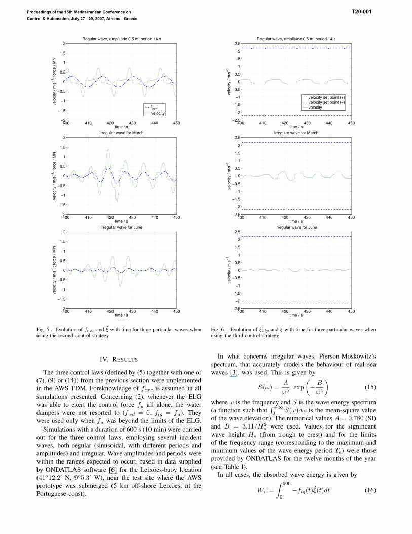
Fig. 5. Evolution of fexc and ξ with time for three particular waves whenusing the second control strategy

IV. RESULTS

The three control laws (defined by (5) together with one of(7), (9) or (14)) from the previous section were implementedin the AWS TDM. Foreknowledge of fexc is assumed in allsimulations presented. Concerning (2), whenever the ELGwas able to exert the control force fu all alone, the waterdampers were not resorted to (fwd = 0, flg = fu). Theywere used only when fu was beyond the limits of the ELG.

Simulations with a duration of 600 s (10 min) were carriedout for the three control laws, employing several incidentwaves, both regular (sinusoidal, with different periods andamplitudes) and irregular. Wave amplitudes and periods werewithin the ranges expected to occur, based in data suppliedby ONDATLAS software [6] for the Leixoes-buoy location(41o12.2′ N, 9o5.3′ W), near the test site where the AWSprototype was submerged (5 km off-shore Leixoes, at thePortuguese coast).

400 410 420 430 440 450−2.5

−2

−1.5

−1

−0.5

0

0.5

1

1.5

2

2.5

time / s

velo

city

/ m

⋅s−1

Regular wave, amplitude 0.5 m, period 14 s

velocity set point (+)velocity set point (−)velocity

400 410 420 430 440 450−2.5

−2

−1.5

−1

−0.5

0

0.5

1

1.5

2

2.5

time / s

velo

city

/ m

⋅s−1

Irregular wave for March

400 410 420 430 440 450−2.5

−2

−1.5

−1

−0.5

0

0.5

1

1.5

2

2.5

time / s

velo

city

/ m

⋅s−1Irregular wave for June

Fig. 6. Evolution of ξstp and ξ with time for three particular waves whenusing the third control strategy

In what concerns irregular waves, Pierson-Moskowitz’sspectrum, that accurately models the behaviour of real seawaves [3], was used. This is given by

S(ω) =A

ω5exp

(

−B

ω4

)

(15)

where ω is the frequency and S is the wave energy spectrum(a function such that

∫ +∞

0S(ω)dω is the mean-square value

of the wave elevation). The numerical values A = 0.780 (SI)and B = 3.11/H2

s were used. Values for the significantwave height Hs (from trough to crest) and for the limitsof the frequency range (corresponding to the maximum andminimum values of the wave energy period Te) were thoseprovided by ONDATLAS for the twelve months of the year(see Table I).

In all cases, the absorbed wave energy is given by

Wu =

∫ 600

0

−flg(t)ξ(t)dt (16)

Proceedings of the 15th Mediterranean Conference onControl & Automation, July 27 - 29, 2007, Athens - Greece

T20-001

TABLE IIPOWER IN kW OBTAINED UNDER SEVERAL REGULAR WAVES

(FIGURATIVE DATA)

Wave amplitude / m 0.5 0.75 1.0 1.25Wave period / s 14.0 12.0 10.0 8.0None 1.0 3.2 10.2 16.7First strategy: (5) and (7) 19.2 51.7 97.2 122.3% increase from no control 1820 1516 853 632Second strategy: (5) and (9) 18.5 65.5 137.3 174.5% increase from no control 1750 1947 1246 945Third strategy: (5) and (14) 20.1 45.5 71.6 72.5% increase from no control 1910 1322 602 334

From these simulations, values for the absorbed wave energy(time-averaged in the case of irregular waves) are given inTable II and in Table III; the corresponding evolution ofwave energy absorption with time is given in Fig. 3; and50 s highlights corresponding to one regular wave and twosignificant months are shown in Figures 4, 5 and 6. Forcomparison purposes, absorbed wave energy when the AWShas no control at all is also given1.

These results show, first of all, that the second controlstrategy is the best, in what wave energy absorption isconcerned.

It is also worthy of notice that wave energy absorptionincreases are very significant. Since nowadays the majorproblem of WECs is their low efficiency, these are verysatisfactory and promising results.

Such increases, however, are often achieved in spite ofthe desired linear closed-loop dynamics not being obtained.This is clear from the figures showing how acceleration andvelocity evolve with time. With the first control strategy, thefloater’s acceleration only rarely is in phase with the waveexcitation force. The second control strategy achieves betterresults in causing velocity and wave excitation force to bein phase (especially in what irregular waves are concerned),and hence the better results achieved. The set point for thevelocity employed together with the third control strategy isalways very far from being attained (consequently the waveenergy absorption improvement is not as high as with theother control strategies).

These deviations from the desired behaviour are likely toderive from the simplifications that had to be admitted whendesigning the controller, namely assuming that the actuators(the ELG and the water dampers) respond immediately andhave no saturations (when this is not the case, for eachhas its own internal dynamics, and saturation values; thisis especially the case of the water dampers, and so fwd willnot always follow its set point).

It should also be borne in mind that, while all controlstrategies are liable to have poorer performances when im-plemented in a prototype rather than simulated, feedback

1Values given in this paper for absorbed wave power when the AWS hasno control are higher than those given in [1]. This is because a residual forceexerted by the ELG that had been neglected was now taken into account,which seems to be more correct.

linearisation control is particularly prone to deteriorate itsachievements, because, in practice, non-linear forces willnever be so accurately cancelled as in simulations.

In spite of this, feedback linearisation control is stronglyrecommended, given its satisfactory results.

V. CONCLUSIONS

From the last section it is seen that among all the feed-back linearisation control strategies experimented, the secondcontrol strategy is clearly the one to choose. Simulationsshow that it achieves its aim, which was to put the floater’svertical velocity in phase with the wave excitation force.Among all control strategies, this is the one that makes moresense from the theoretical point of view (as shown in theAppendix), and thus it is no surprise that it performs best.Wave energy absorption increases (from the situation whenthere is no control applied) are very significant: a sevenfoldaverage increase is achieved over the whole year. This showsthe importance of carefully chosen control strategies for theeconomic viability of WECs.

APPENDIX

This Appendix closely follows [3].As said above in section II, the AWS is not unlike a

mass-spring-damper system. This corresponds to a dynamicbehaviour given by [2]

mξ(t) + Rξ(t) + Sξ(t) = fexc(t) (17)

R and S are both positive. This linear model can provide anapproximate description of the non-linear AWS behaviour.Defining complex-valued phasors fexc and ˆ

ξ for fexc and ξ,respectively,

fexc(t) =fexc

2eiωt +

f∗

exc

2e−iωt (18)

ξ(t) =ˆξ

2eiωt +

ˆξ∗

2e−iωt (19)

expression (17) becomes

m

(

iωˆξeiωt − iω

ˆξ∗

e−iωt

)

+ R

(

ˆξeiωt +

ˆξ∗

e−iωt

)

+S

(

1

iωˆξeiωt −

1

iωˆξ∗

e−iωt

)

=

= fexceiωt + f∗

exce−iωt ⇔

⇔ eiωt

[

fexc −

(

R + iωm +S

iω

)

ˆξ

]

+ e−iωt

[

f∗

exc −

(

R − iωm −S

iω

)

ˆξ∗]

= 0 (20)

Defining an impedance Z

Z = R + i

(

ωm −S

ω

)

(21)

expression (20) can be rewritten as

eiωt(

fexc − Zˆξ)

+ e−iωt

(

f∗

exc − Z∗ˆξ∗)

= 0 (22)

Proceedings of the 15th Mediterranean Conference onControl & Automation, July 27 - 29, 2007, Athens - Greece

T20-001

TABLE IIIPOWER IN kW OBTAINED UNDER SEVERAL IRREGULAR WAVES (FIGURATIVE DATA)

Controller Jan Feb Mar Apr May Jun Jul Aug Sep Oct Nov DecNone 14.3 11.4 9.1 7.7 4.5 4.5 3.5 3.4 4.5 6.7 9.9 13.6First strategy: (5) and (7) 85.2 69.5 47.0 43.5 14.6 10.6 7.4 9.0 17.3 31.8 56.2 75.6% increase from no control 496 509 416 465 224 135 112 164 284 374 467 456Second strategy: (5) and (9) 115.1 96.2 73.6 68.9 27.7 20.4 15.0 18.3 32.6 53.2 81.8 106.4% increase from no control 705 744 709 795 516 353 330 437 623 695 726 683Third strategy: (5) and (14) 57.1 45.0 28.4 26.2 8.0 5.7 3.9 4.8 9.6 18.5 35.1 49.0% increase from no control 300 295 212 241 77 26 11 41 112 176 254 260

For (22) to be satisfied for all values of time t, the followingcondition must be verified:

ˆξ =

fexc

Z⇒

∣

∣

∣

ˆξ∣

∣

∣=

∣

∣

∣fexc

∣

∣

∣

|Z|(23)

Expression (21) can be rewritten as Z = R + iX . The realpart R = Re[Z] is called resistance and the imaginary partX = Im[Z] = ωm− S

ωis called reactance. Suppose now that

a control force fu is applied to the AWS WEC. This will beneeded to ensure that the conditions leading to maximumwave energy absorption (or at least conditions as close aspossible to those) are met. Then

Zξ = fexc + fu ⇔

⇔ Z(ω)Ξ(ω) = Fexc(ω) + Fu(ω) (24)

(Notice that capital letters are used for variables in the fre-quency domain and lower-case letters for the correspondingvariables in the time domain.) The absorbed wave energyWu can be given by

Wu = −

∫ +∞

0

fu(t)ξ(t)dt (25)

(Notice that no decomposition of fu is assumed, unlike whatwas done in (2) or (16).) Considering that fu and ξ are realfunctions, i.e., F ∗

u (ω) = Fu(−ω) and Ξ∗(ω) = Ξ(−ω), byapplying Parseval’s theorem, Wu can be given by

Wu = −1

2π

∫ +∞

−∞

[

Fu(ω)Ξ∗(ω)]

dω (26)

Knowing that Wu is real,

Fu(ω)Ξ∗(ω) = Re[

Fu(ω)Ξ∗(ω)]

=

=1

2

[

Fu(ω)Ξ∗(ω) + F ∗

u (ω)Ξ(ω)]

(27)

expression (26) can be rewritten as

Wu =1

2π

∫ +∞

0

[

−Fu(ω)Ξ∗(ω) − F ∗

u (ω)Ξ(ω)]

dω (28)

It will be convenient to add and subtract the termFexc(ω)F∗

exc(ω)

2Rto the integrand of (28), and finally Wu is

now given by (omitting the frequency argument)

Wu =1

2π

∫ +∞

0

[

|Fexc|2

2R

−|Fexc|

2

2R− FuΞ∗ − F ∗

u Ξ

]

dω =

=1

2π

∫ +∞

0

[

|Fexc|2

2R−

α

2R

]

dω (29)

In (29) α(ω) is the so-called optimum condition coefficient,given by

α(ω) = Fexc(ω)F ∗

exc(ω)

+ 2R[

Fu(ω)Ξ∗(ω) + F ∗

u (ω)Ξ(ω)]

(30)

After some tedious manipulations, it turns out that

α =∣

∣

∣Fexc(ω) − 2RΞ(ω)

∣

∣

∣

2

≥ 0 (31)

So, it is when α(ω) = 0 that Wu is maximal. From (31) anoptimum condition can be written as

Fexc(ω) = 2RΞ(ω) (32)

This means that Ξ must be in phase with Fexc.

REFERENCES

[1] P. Beirao, D. Valerio, and J. Sa da Costa. Phase control by latchingapplied to the Archimedes Wave Swing. In Proceedings of the 7thPortuguese Conference on Automatic Control, Lisbon, 2006.

[2] P. Beirao, D. Valerio, and J. Sa da Costa. Linear model identificationof the Archimedes Wave Swing. In IEEE International Conference onPower Engineering, Energy and Electrical Drives, Setubal, 2007.

[3] J. Falnes. Ocean waves and oscillating systems. Cambridge UniversityPress, Cambridge, 2002.

[4] P. Pinto. Time domain simulation of the AWS. Master’s thesis,Technical University of Lisbon, IST, Lisbon, 2004.

[5] H. Polinder, M. Damen, and F. Gardner. Linear PM generator systemfor wave energy conversion in the AWS. IEEE Transactions on EnergyConversion, 19(3):583–589, September 2004.

[6] M. T. Pontes, R. Aguiar, and H. Oliveira Pires. A nearshore waveenergy atlas for Portugal. Journal of Offshore Mechanics and ArcticEngineering, 127:249–255, August 2005.

[7] J. Sa da Costa, P. Pinto, A. Sarmento, and F. Gardner. Modelling andsimulation of AWS: a wave energy extractor. In Proceedings of the4th IMACS Symposium on Mathematical Modelling, pages 161–170,Vienna, 2003. Agersin-Verlag.

[8] J. Sa da Costa, A. Sarmento, F. Gardner, P. Beirao, and A. Brito-Melo. Time domain model of the Archimedes Wave Swing wave energyconverter. In Proceedings of the 6th European Wave and Tidal EnergyConference, pages 91–97, Glasgow, 2005.

[9] J. Slotine and W. Li. Applied Nonlinear Control. Prentice Hall,Englewood Cliffs, 1991.

Proceedings of the 15th Mediterranean Conference onControl & Automation, July 27 - 29, 2007, Athens - Greece

T20-001