i

Feature importance recap and stacking models for forex price prediction Yunze Li, Yanan Xie, Chen Yu , Fangxing Yu, Bo Jiang and Matloob Khushi

The School of Computer Science, The University of Sydney

ABSTRACT

Forex trading is the largest market in terms of qutantitative trading.

Traditionally, traders refer to technical analysis based on the historical data to make

decisions and trade. With the development of artificial intelligent, deep learning plays

a more and more important role in forex forecasting. How to use deep learning models

to predict future price is the primary purpose of most researchers. Such prediction not

only helps investors and traders make decisions, but also can be used for auto-trading

system. In this article, we have proposed a novel approach of feature selection called

“feature importance recap” which combines the feature importance score from tree-

based model with the performance of deep learning model. A stacking model is also

developed to further improve the performance. Our results shows that proper feature

selection approach could significantly improve the model performance, and for

financial data, some features have high importance score in many models. The results

of stacking model indicate that combining the predictions of some models and feed

into a neural network can further improve the performance.

1

1. INTRODUCTION In modern quantitative trading, data analysis and modelling processes based on

statistics, databases, computer science, machine learning, and other quantitative fields

have been widely recognized and applied. Effective and accurate prediction for the

long and short-term future trends of the financial market is directly related to investors'

investment choices and returns.

In the field of data science, studies on deep neural networks have made

breakthrough progress in recent years. Deep neural network models such as CNN,

RNN, Transformers, etc., are achieving better performance than traditional machine

learning in many prediction tasks. However, due to the irregularity, uncertainty, and

instability natures of the financial market and the complexity of financial time series

data, research on DNN based financial forecasting still has room for improvement.

This project aims to develop an approach to improve the accuracy of future price

diction with feature selection and model stacking. Detailed study includes time-series

data analysis, feature engineering, DNN model development, feature selection and

model stacking.

2. RELATED LITERATURE 2.1 Background

2.1.1 Currency Exchange

Foreign Exchange Market is one of the largest financial market which is active 24/7,

and trades continuously from day and night. There are more than 170 currencies in

the world, and thousands of currency pairs can be stated in the market. Unlike other

financial markets, the foreign exchange market has no specific location and no central

transaction. Transactions can be conducted through between banks, enterprises, and

individuals. When buying and selling foreign exchange, investors can either earn the

exchange rate difference, or convert a foreign currency on hand into another foreign

currency with a higher interest rate, thereby obtaining higher interest income. For

example, if you buy GBP/USD at 1.5002. When the exchange rate rises to 1.5052, sell

the exchange held in your hand and you can make a profit of 50 points.

2.1.2 Technical Analysis and Indicators

Technical analysis is a common way to predict price movements. This analysis is based

on information stored in the market, which means that it is necessary to refer to the

past when predicting future price trends. Traders’ forecasts are based on price

movements within a certain period. This type of analysis focuses on the composition

of charts and formulas to capture major and minor trends, and to identify

buying/selling opportunities by estimating the length of the market cycle. The theory

of technical analysis is based on three assumptions[1]. Market action discounts

everything. 2. Price moves in trends. 3. History repeats itself. Depending on the time

span, traders can use intraday (every 5 minutes, every 15 minutes, hourly) technical

analysis, weekly or monthly technical analysis[2].

Technical indicators are the elements based on historical trading data such as

price, volume, and open interests, rather than the fundamental business indicators like

assets, liabilities, or equity to predict the future performance of the market. The basic

belief of technical analysis is that history repeats itself and the market movements can

be predicted with the help of reams of statistics. Compared to fundamental analysis,

technical analysis and indicators focus more on the movements of price, the trading

signals, or the changing strength of up and down. Nowadays, technical indicators are

widely implemented by investors for short-term investment assistance.

There are four types of indicators applied in our project, momentum, overlap

studies, volatility, and price transform.

Momentum Indicators measures the movement rate of rise and fall, which means the

tendency for rising asset prices to keep increasing, or for the falling ones to keep

decreasing. Here are some typical momentum indicators:

• Moving Average Convergence Divergence (MACD) [3]MACD is based on

the construction principle of moving averages, smoothing the closing price of

the gold market price, and calculating the arithmetic average value. Usually, it

utilizes two different moving averages and creates the oscillator to illustrate

the change from the short time period moving average to the longer time period

moving average. The formula for MACD:

𝑀𝐴𝐶𝐷 = shorter time period 𝐸𝑀𝐴 − longer time period EMA (1)

3

• Williams %R(WillR), shorten of the Williams Percent Range, is a momentum

indicator measuring oversold and overbought levels. It is a percentage ranging

from 0 to -100, measuring the current close price in comparison to the high-

low range over a certain time period. The formula for Williams %R is :

%𝑅 = −100 × -( Highest High − Close )

( Highest High − Lowest Low )0 (2)

When Williams %R runs up to near 0, the close price is very close to

the highest high of the certain period, which is the signal of overbought, and

that implies the price is in a strong uptrend. Whereas when Williams %R goes

down to near -100, the close price nearly reaches the lowest low in the lookback

time period. At this moment, the price is in a strong downtrend and has the

signal of oversold.

• BOP is the shorten of the Balance of Power, which is used to evaluate the

struggle between buyers and sellers. The BOP fluctuates around zero, not going

up beyond 1 and not going down beneath -1. Positive BOP value represents the

buy power is more powerful and negative BOP value implies the strong

pressure of selling. When the BOP equals to zero, the power of buyers and

sellers neutralizes each other. The formula of BOP is:

𝐵𝑂𝑃 = SMA of [ (Close − Open )/( High − Low )] (3)

Figure 1: Example of BOP [4]

Overlap studies mostly contain different kinds of moving average indicators. Moving

average is one of the most commonly used indicators in technical analysis theory. It is

mainly used to confirm, track, and judge the trends and find the buy and sell signals.

However, when the market is fluctuating, the moving average will frequently give

distorted buy and sell signals.

• Simple Moving Average (SMA) means the average mean price in a specific

period of time. The formula of SMA is:

𝑆𝑀𝐴 = [𝑃𝑟𝑖𝑐𝑒(1) + 𝑃𝑟𝑖𝑐𝑒(2) + ⋯+ 𝑃𝑟𝑖𝑐𝑒(𝑛 − 1) + 𝑃𝑟𝑖𝑐𝑒(𝑛)]/𝑛 (4)

• Exponential Moving Average (EMA) adds weights to prevent the lagging

problem in simple moving average. The formula of EMA is[4]:

𝐸𝑀𝐴 = EMA previous + 𝐾 ∗ (Price − EMA previous) (5)

Where K represents the weight calculated by K = 2 / (n + 1).

• TRIMA: Some special moving averages are also included, and we take

TRIMA as example. The Triangular Moving Average (TRIMA) is a kind of

average price replacing the middle prices of the time period. This method can

double-smooth the data using a one-half-length window of the certain time

series. The formula for TRIMA is[5]:

𝑀𝐴 =𝑆𝑀𝐴(𝑆𝑀𝐴𝑚,𝑁𝑚)

𝑁𝑚

𝑁 = Time periods + 1𝑁! = Round (𝑁/2)𝑆𝑀𝐴𝑚 = ( Sum ( Price, 𝑁𝑚))/𝑁𝑚

(6)

Volatility indicates the market's expectations and enthusiasm for the stock or the forex.

A sharp increase in volatility means that most traders are going to buy or sell during

the day, while a decrease in volatility indicates that most traders are not interested in

the market. Volatility can be used to measure the volatility of prices to help judge the

likelihood of a trend change and the trading atmosphere of the market. Volatility can

also be used to help decrease losses and profits.

• Average True Range (ATR) [6].Market technicians use the ATR to decide

whether enter or exit trades, and ATR is also a useful tool which help the users

to understand the volatility of forex of stock by using simple calculations.

5

Instead of directly indicating the price direction, the ATR can measure

volatility caused by gaps and limit up or down moves. The following formula

shows how the ATR is calculated[7]:

𝑇𝑅 = 𝑀𝑎𝑥[(𝐻 − 𝐿), 𝐴𝑏𝑠(𝐻 − 𝐶"), 𝐴𝑏𝑠(𝐿 − 𝐶")]

𝐴𝑇𝑅 = -1𝑛0M  ($)

&'(

𝑇𝑅& (7)

Price Transform There are four functions related to the price transform, mainly used

to calculate the mean value between the OHLC price：

• Average Price The average price is the simplest way to get the average value

by calculating the mean value of OHLC price.

Average Price = ( Open + High + Low + Close )/4 (8)

• Median Price The Median Price can help users have a quick understand of

prices by providing a simple average price on a timestamp. The following

formula shows how it is calculated:

Median Price = ( High + Low )/2 (9)

• Typical Price The Typical Price also called the pivot point, is the average price

of the stock or forex over the specified period. It is a substitute for the close

price, and some technical analysts prefer to use the typical price rather than the

close price as the trading price. The following formula shows how it is

calculated:

Typical Price = ( High + Low + Close )/3 (10)

Figure 2: Example of Typical Price [4]

• Weighted Close Price Similar to the median price and the typical price, the

weighted closed price is an indicator that is a mean value of each timestamp’s

price. The reason why it called “weighted close” is that it gives an extra weight

on the close price. The following formula shows how to calculate it:

𝑊𝑒𝑖𝑔ℎ𝑡𝑒𝑑𝐶𝑙𝑜𝑠𝑒𝑃𝑟𝑖𝑐𝑒 = ()*+,-∗/)01&2304+56

(11)

Figure 3: Example of Weighted Close Price [4]

2.1.3 Feature Selection

Feature selection, also known as variable selection or attribute selection. It is a way to

select subset of existing attributes for modeling. The main purpose of feature selection

is to simplify the model, shorten the training time, avoid the curse of dimensionality,

and enhance the generalization capability of the model.

In the feature selection process, if the learner (base learner) is a tree model, the

valid features can be selected according to the importance of the features. No matter

Random Forest, Gradient Boosting Decision Tree (GBDT), extreme Gradient

Boosting (XGBoost) or Light Gradient Boosting Machine (LGBM), they are all based

on decision tree models. There are two main ways to calculate the importance of

features[8]:

Calculate the importance of each feature during training. During the training

process, the importance of features was quantified by recording the total number of

splits and the total/average information gain of features. For example, in the actual

project, we will use the number of times used in the whole GBDT and XGBoost or the

total/average information gain to score the feature importance, and then sort it finally.

7

Since the Ensemble model itself has a certain randomness when choosing features for

splitting, it usually runs multiple models and then ranks them after averaging the

importance of features.

Out of Bag (OOB) data was used for calculation after training. To be specific,

the OOB data is scored using the trained model to calculate the AUC or other business

definition evaluation indicators. Then for each feature in the OOB data:(a) The value

of the current feature of random shuffle;(b) Rank the current data and calculate the

evaluation indicators;(c) Calculate the change rate of indicators. Following the above

approach, a rate of change is obtained for each feature, and the importance of the

feature is quantified by ranking the rate of change.

The calculation of feature importance of the tree-based model mentioned above

has a common shortcoming, that is, they are sensitive to collinear features. Shapley

Additive explanations(SHAP) was designed to mostly mitigate multicollinearity's

impact with a very robust statistical foundation[9].The main idea of SHAP value is

Shapley value. Shapley value is a method from Coalitional Game Theory. If Shapley

value is used to explain the prediction of machine learning, where "total expenditure"

is the predicted value of the model for a single instance of the data set. The "player" is

the eigenvalue of the instance, and the "revenue" is the actual forecast for that instance

minus the average forecast for all instances. The deep learning model itself is a black

box in calculation.

2.2 Literature Review

Nowadays, the machine learning model is widely used in the quantitative finance

industry. However, the historical financial data is noisy and may lead the machine

learning models to overfit and impact its performance. Suitable feature engineering

and effective forecast combinations can mitigate this risk[10]. Technical indicators are

commonly used as input features of the models. Shynkevich and his colleagues

elaborated on the feasibility of using technical indicators as feature engineering. They

concluded that the input window length and forecast horizon would certainly impact

financial forecasting performance[11].

Traditional regression models cannot handle the non-linearity of financial data.

Studies have shown that deep neural network methods outperform traditional

regression models (OLS, ridgeCV and Bayesian linear regression) in the financial

market[12]. Chen et al. have developed an algorithm called Filterbank CNN, which

replaces the random-generated filters with the knowledge-based filters. It has been

proved that Filterbank could improve the accuracy by up to 15% compared to the

traditional rule-based strategy[13].

Since [14] proposed the time series Autoregressive Integrated Moving Average

Models(ARIMA) model, the model has been widely used. Especially in financial data

forecasting, ARIMA has achieved great results. Based on the basic ARIMA, proposed

a fuzzy regression named fuzzy ARIMA. By predicting the historical data of the

exchange rate of the NTD and the USD, they proved that this method can not only

make better predictions, but also provide decision makers with the best and worst

possible scenarios.

Experimental results in [15] demonstrate that ANN based model can closely

forecast the forex market. In this paper, they Established and studied six different

currency pairs of Australian dollar exchange rate prediction models, namely standard

backpropagation (SBP), scaled conjugate gradient (SCG) and backpropagation with

Baysian regularization (BPR),and five moving average technical indicators are used

to build the models. The results show that all models based on neural networks are

better than ARIMA models.

[16] utilize technical indicators on LSTM to make prediction of one-day, three-

days and five-days ahead. The experiment results shows that the prediction could

generate profit for investors with proper trading strategy.

[17] develops new event-driven features through technical analysis, , which

indicate changes in trends in direction. This method largely solves the non-stationarity

and high volatility of the foreign exchange market, makes the model interpretable, and

the final experiment proves its reliability. With this event-driven method, they

implement LSTM, Bi-LSTM and GRU on predication and compared with a basic

RNN. They finally got that their best model on 15-minutes interval data for the

EUR/GBP currency achieved RMSE 1.5E-3 with a MAPE 0.12% outperforming

previous studies.

[18] trained four machine learning ensemble methods: (a) a neural network

regression ensemble;(b) a support vector regression ensemble;(c) a boosted regression

tree; and (d) a random forest regression. In addition, they established a knowledge base

9

that based on historical stock data and sentiment analysis of previous news. 19 stocks

with different trends are used as a data set. They predict the price of the stock 1-day

ahead and eventually get the MAPE≦0.75%.

Due to the interference of noise in financial data, the performance of prediction

using machine learning and deep learning models is not ideal[19]. To reduce the

impact of the noisy nature of the market, Zezheng Zhang and Matloob Khushi designed

the new trading rule features based on technical indicators and trading rules. Also, they

proposed a loss function called Sharpe and Sterling Ratio (SSR) which can reduce the

variance and the magnitude of drawdowns.

Zhiwen Zeng and Matloob Khushi found that wavelet denoising can also reduce

the influence of noise in the financial data and stabilize the data structure[20]. Besides,

they used an ARNN (Attention-based Recurrent Neural Network) model integrated

ARMIA model to make the prediction and achieved an excellent model performance.

When talking about the wavelet denoising, Yiqi Zhao and Matloob Khushi

proposed a Wavelet Denoised-ResNet[21]. And They also combine the model with the

LightGBM to get an outstanding model performance in forex price prediction.

Terry and Matloob reviewed all recent stock or forex studies using reinforcement

learning as the first deep learning method since 2015[22]. They found that most

researches had unrealistic assumptions and showed no meaningful level of

profitability. They got the conclusion that the reinforcement learning cannot work as

a mature technique utilizing into the real stock and forex market.

Tae and Matloob proposed a novel reinforcement learning model called

Deterministic Policy Gradient with 2D Relative-attentional Gated Transformer

(DPGRGT), which is a model using creative layers and new reorder methods to stable

the reinforcement learning performance[23]. They did back testing on the U.S. stock

market of the past 20 years and proved the effectiveness of this model.

[24] demonstrates the feasibility of using technical indicators as features in

machine learning to quantify transactions. In their experiment, they took the trading

data of 505 S&P 500 stocks in the United States in the past 20 years as historical data

and determined 5 technical indicators and 23 basic indicators as input characteristics

through analysis. Tests were done on 6 different models (RF,

SVM,DT,NB,CNN,KNN) to predict price changes over the next 10 days. As it turned

out, they had an overall accuracy of 83.62%, particularly with their sell signal accuracy

of 100%.

In the real financial market, the price of stock has a great relationship with

people's production activities. For almost any financial product, news can have a huge

impact on the share price. In recent years, because of the great breakthrough of natural

language processing, natural language processing has been more and more widely used

in quantitative transactions. [25] shows that the text classification in the financial field

based on StockTwits text data marked by stock price changes can effectively analyse

historical data and easily predict stock trends.

The experiment of [26]proves the reliability of deep learning in financial

prediction. They did a lot of paper comparison and analysis, and finally found that the

methods combining LSTM with other models can achieve good results.

3. PROJECT PROBLEMS

3.1 Project Aims & Objectives

This project aims to build a novel system of foreign exchange forecasting based on

machine learning and deep learning technologies. Specifically, the. objective is to

predict future highest high prices within 5 timestamps of AUD-USD and EUR-USD

currency pairs. Precise predictions of the future highest high price are expected to

support investment decisions for the greatest financial benefits. As for the innovation

of this forecasting system, we mainly focus on two aspects.

First, this project develops a “feature importance recap” approach. As important

financial forecasting tools, 71 technical analysis indicators are introduced in this

project as the input features of the forecasting models. However, not all indicators are

useful for the forecasting target, i.e., Highest price. Therefore, in this project, we

develop a feature selection approach to identify a set of most important indicators. This

method is combining the “feature importance” approaches of tree-based machine

learning models (i.e., XGBoost, Random Forest, and LightGBM) with deep learning

experiments (i.e., LSTM and GRU). For each of the 71 technical analysis indicators, a

“feature importance coefficient” is assigned.

Second, this project develops a “model stacking” approach. From the above

literature reviews, we can find that the existing machine learning and deep learning

11

technologies have made great progress in terms of minimising the losses (indicated by

RMSE, MAE, MAPE, etc.) in forex price predictions. To further improve forecasting

performance, we look forward to stacking the basic models to build a new complex

system, allowing which to learn the advantages from different models, to surpass each

single model in terms of prediction performance. Without a doubt, the input features

of the stacked models are selected based on the “feature importance recap” approach.

3.2 Project Questions

In order to achieve the above project objectives, the project needs to provide

explanations for the following questions.

• What is the data source and how to confirm its reliability?

• What data engineering work is required, in terms of the ETL process?

Specifically, how to handle missing values, how to standardise data, how to

organise data into correct formats for each forecasting model?

• What is the candidate technical analysis indicators (features of model

inputs)? How to calculate them?

• As for the tree-based models, in what criterion are the “feature importance”

determined?

• What is the threshold to determine whether a feature is important or not?

• What is the candidate forecasting models to build the stacked model?

• What optimisation approaches should be used in each model? Specifically,

how to do parameter tuning, how to save model training time?

• What evaluation metrics should be used to measure the success of the

prediction?

3.3 Project Scope

The project uses M15 history data of AUD-USD pair and EUR-USD pair to predict

the future highest high prices within 5 timestamps. We can determine the completion

of project by finalising the following tasks.

• In the “feature importance recap” approach: Fitting XGBoost, Random Forest,

and LightGBM models for prediction and calculating feature importance;

Based on the obtained feature importance, training LSTM and GRU models

and evaluating on out-of-sample data; Determining the recapped feature

importance and identifying the final important features; Training the final

LSTM and GRU models using the final important features and making

evaluation.

• In the “model stacking” approach: Selecting XGBoost, Random Forest,

LightGBM, LSTM, and GRU as candidate models; For each subset of the

candidate models, applying model stacking approach and making evaluation;

Determine the most successful subset of models as the final elements of

stacking.

In this project, the prediction loss is measured by root mean square error

(RMSE). Other evaluation metrics, i.e., mean absolute error (MAE), and mean

absolute percentage error (MAPE) are also considered.

4. METHODOLOGIES

4.1 Theory and Methods

4.1.1 Long Short Term Memory

LSTM, shorten of Long Short Term Memory, is a special RNN, mainly to solve the

problem of gradient disappearance and gradient explosion during long sequence

training. Compared to simple ordinary RNNS, LSTM can perform better in longer

sequences. LSTM is designed specifically to avoid long-term dependency problems.

The default behaviour of the LSTM is to remember the information for a long time

without the need for an extra cost.

Figure 4: The structure of LSTM [27]

13

4.1.2 Gate Recurrent Unit

GRU (Gate Recurrent Unit) is a kind of Recurrent Neural Network (RNN). Compared

to the LSTM network, the GRU has a simpler structure, and it is easier to train.

Therefore, GRU is also a popular RNN model. Similar to LSTM, GRU can also solve

the problems of gradient vanish and gradient explosion in the original RNN model.

In LSTM, three gate functions are used: input gate, forgetting gate and output

gate. The GRU model is simpler with only two gates: the update gate and the reset

gate.

Figure 5: The structure of GRU unit[28]

The GRU structure is shown in Figure 5.𝑧7and𝑟7 represent update and reset

gates, respectively. The update gate is used to control how much the state information

of the previous moment is brought into the current state. The larger the value of the

update gate, the more the state information of the previous moment is brought in. The

reset gate controls how much information from the previous state is written to the

current candidate set; the smaller the reset gate, the less information from the previous

state is written. Governing equations of a GRU[29]:

𝑧 = 𝜎Z𝑊9 ⋅ 𝑥7 + 𝑈9 ⋅ ℎ(7:() + 𝑏9]𝑟 = 𝜎Z𝑊; ⋅ 𝑥7 + 𝑈; ⋅ ℎ(7:() + 𝑏;]

ℎ̂ = tanhZ𝑊3 ⋅ 𝑥7 + 𝑟 ∗ 𝑈3 ⋅ ℎ(7:() + 𝑏9]ℎ = 𝑧 ∗ ℎ(7:() + (1 − 𝑧) ∗ ℎ̂

(12)

The current input is𝑥7 , and the hidden state delivered by the previous node

isℎ7:(, which contains information about the previous node.

By combining ℎ7:( with 𝑥7, the GRU unit can obtain the output of the current

hidden node 𝑦7, and the hidden stateℎ7 which will be delivered to the next node.

4.1.3 XGBoost

XGBoost is the shortened form of “Extreme Gradient Boosting”, which was a

scalable tree boosting algorithm published by Tianqi Chen in 2016 [30]. XGBoost

greatly improves the speed from the traditional gradient tree boosting system – up to

ten times faster than the gbm package. The basic model of XGBoost is decision tree

ensembles, which means several trees are ensembled to predict the results.

In decision tree ensembles, the objective function consists of two parts, training

loss and regularization term. The formula of objective function can be written as[31]:

obj =M $

&'(

𝑙d𝑦& , 𝑦e&(7)f +M  

7

&'(

Ω(𝑓&) (13)

In this formula, l is the loss function, and Ω is the regularization term.

The loss function is used to measure how well our predicted value fits the actual

training data, while the regularization term represents the complexity of t trees.

For boosting, one tree is added at a time. The new tree is to classify the loss

gotten from the last step. If the prediction value at step t is written as 𝑦e&(7), the formulas

for each step are:

𝑦e&(<) = 0𝑦e&(() = 𝑓((𝑥&) = 𝑦e&

(<) + 𝑓((𝑥&)

𝑦e&(/) = 𝑓((𝑥&) + 𝑓/(𝑥&) = 𝑦e&

(() + 𝑓/(𝑥&)…

𝑦e&(7) =M  

7

='(

𝑓=(𝑥&) = 𝑦e&(7:() + 𝑓7(𝑥&)

(14)

XGBoost uses the greedy algorithm to enumerate all the different tree structures.

The approach is to constantly enumerate the structure of different trees, then use the

scoring function to find a tree with the best structure, add it to the model, and repeat

the operation continuously. The advantage of XGBoost is parallel learning, in which

parameters for all leaves are independent and calculated simultaneously. This greatly

speeds up the calculation.

15

Main theories of XGBoost:

• Continuously splitting by features and adding new trees. For every step,

a new tree is added to fit the residual of the last prediction.

• When we get k trees after training, we are going to predict the score of a

sample. According to the character of this sample, every tree will fall to

a corresponding leaf, and each leaf corresponds to a score.

• Finally adding all the correspondent scores of each tree to get the

predicted value of the sample.

For every step, the algorithm chooses a new function to minimize the objective

value.

obj(7) =M  $

&'(

𝑙d𝑦& , 𝑦e&(7)f +M  

7

&'(

Ω(𝑓&)

=M  $

&'(

𝑙 d𝑦& , 𝑦e&(7:() + 𝑓7(𝑥&)f + Ω(𝑓7) + constant

(15)

The novelty of XGBoost is that it uses the second-order Taylor expansion of the

loss function to replace the objective function. Here we use Taylor’s expansion

formula to approximate the objection function:

𝑜𝑏𝑗(") =%  $

%&'

'𝑔%𝑓"(𝑥%) +12ℎ%𝑓"((𝑥%)1 + Ω(𝑓") (16)

Where 𝑔& represents the first order partial derivative of 𝑦e& , and ℎ& represents the

second order partial derivative of 𝑦e& .. The formula of 𝑔& and ℎ&:

𝑔& = ∂>?!(#$%)𝑙d𝑦& , 𝑦e&

(7:()f

ℎ& = ∂>?!(#$%)

/ 𝑙d𝑦& , 𝑦e&(7:()f

(17)

In XGboost, the tree function is defined as:

𝑓7(𝑥) = 𝑤@(A), 𝑤 ∈ 𝑅B , 𝑞: 𝑅C → {1,2,⋯ , 𝑇} (18)

Where 𝑤represents the vector scores, 𝑞 is the function to assign points to leaves, and

𝑇 is the number of leaves. And the complexity function is defined as：

Ω(𝑓) = 𝛾𝑇 +12 𝜆M  

B

D'(

𝑤D/ (19)

Let 𝐺D represents the sum of 𝑔& and 𝐻D represents the sum of ℎ&. The objection

function can re-formula to this new form:

obj(7) =M  B

D'(

y𝐺D𝑤D +12 Z𝐻D + 𝜆]𝑤D

/z + 𝛾𝑇 (20)

Since this is a quadratic function of 𝑤D, the best 𝑤D and the lowest objective reduction

can be gotten:

𝑤D∗ = −𝐺D

𝐻D + 𝜆

obj∗ = −12M  

B

D'(

𝐺D/

𝐻D + 𝜆+ 𝛾𝑇

(21)

Where 𝐺D,𝐻D, 𝜆, and 𝛾 are the parameters for the models to learn. Compared to the

traditional random forest method, the learning parameters squeeze a lot.

4.1.4 Random Forest

Random forest is a method of Bagging in ensemble learning. It is composed of

a large number of decision trees.

• The decision tree:

Each decision tree in the random forest is independent, they will use

several features in the dataset as the input of the decision tree. Commonly

used decision trees include ID4, C4.5, CART and so on. In the process

of spanning tree, which feature needs to be selected for subdivision. The

principle of selection is to improve the purity as much as possible after

separation, which can be measured by indicators such as information

gain, gain rate and Gini coefficient. If it's a tree, pruning should be

performed to avoid overfitting, removing nodes that might cause

overfitting in the validation set.

• The principle of random forest:

When the random forest algorithm is used for classification or regression,

each decision tree in the forest will be calculated independently and a

17

prediction result will be obtained. After that, the algorithm will collect

and count the prediction results of all the decision trees and select the

prediction results that appear the most times in the decision tree as the

final result.

• Advantages and disadvantages:

Random forest has many advantages, it can be used on the data with

numerous features. When using the random forest algorithm， it is

unnecessary to reduce the dimensionality of the data or do feature

selection. In addition, the random forest can also obtain the feature

importance, which is the reason that we use it in our feature importance

recap part. In addition, it is not easy to overfit, and the computational

cost is not acceptable. Random forests also have some drawbacks. It is

easy to overfit in the dataset containing noise.

• Application:

Random forest can be used in regression and classification problems, as

well as the clustering problem of unsupervised learning and outlier

detection.

Figure 6: An example of random forest [32]

4.1.5 LightGBM

LightGBM, shorten of Light Gradient Boosting Machine, is a gradient boosting

framework focusing on speeding up the training. Compared to XGBoost, Light GBM

grows leaf-wise trees and uses a technique called Gradient-based One-Side Sampling

(GOSS) to filter out the split data. As a result, Light GBM can run almost seven times

faster than XGBoost and can deal with larger datasets. Using GOSS can reduce a large

number of data instances with only small gradients, so that when calculating

information gain, only the remaining data with high gradients can be used. Compared

to XGBoost traversing all feature values, it saves a lot of time and space.

LightGBM has the following features：

• Histogram algorithm:

Compared to the pre-sorted algorithm, the memory occupation and the

data separation complexity of histogram algorithm is lower. The idea is

to discretise continuous floating-point features into k discrete values, and

construct a histogram with a width of k. Then the algorithm traverses the

training data and counts the cumulative statistics of each discrete value

in the histogram. The feature selection step is only to find the optimal

segmentation point according to the largest value of the histogram.

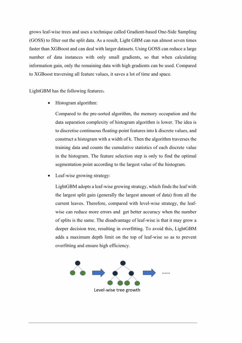
• Leaf-wise growing strategy:

LightGBM adopts a leaf-wise growing strategy, which finds the leaf with

the largest split gain (generally the largest amount of data) from all the

current leaves. Therefore, compared with level-wise strategy, the leaf-

wise can reduce more errors and get better accuracy when the number

of splits is the same. The disadvantage of leaf-wise is that it may grow a

deeper decision tree, resulting in overfitting. To avoid this, LightGBM

adds a maximum depth limit on the top of leaf-wise so as to prevent

overfitting and ensure high efficiency.

19

Figure 7: An example of LightGBM [33]

• Feature Parallelization:

LightGBM supports parallel learning, including feature parallelization

and data parallelization. The main idea of feature parallelization is to find

the optimal segmentation points on different feature sets, and then

synchronize the optimal segmentation points between the machines. Data

parallelization allows different machines to construct histograms locally,

then merge them globally, and finally find the optimal split point on the

merged histogram.

4.1.6 ARIMA

ARIMA (autoregressive integrated moving average) is a famous time series

method proposed by box and Jenkins in 1970s. It is a complex statistical model which

is the auto regression model integrated with the moving average model. And P, D, Q

are the three essential input parameters of this model. P is the number of lag orders in

the AR model. D is the degree of differencing. Q is the size of the moving average

window.

ARIMA is a generalization of the ARMA(autoregressive moving average)

model. The ARMA(p, q) model is given by[34]:

d1 − ∑  E'&'( 𝛼&𝐿&f𝑋7 = Z1 + ∑  @

&'( 𝜃&𝐿&]𝜀7 (22)

where 𝑎& are the parameters of the AR model, the 𝜃& are the parameters of MA model,

𝐿 is the operator of lag, and the 𝜀7 are the error terms.

Arima can be used when the time series data are stable. Stationary time series

represent time series without trend, one of which has constant mean value and variance

over time.

The autocorrelation function (ACF) and partial correlation function (PACF) are

used to determine the values of P and Q in autoregression (AR) and moving average

(MA), or we can use the criterion called Akaike information criterion (AIC) to make

sure the input parameters. In this project, we use AIC to calculate the appropriate input

parameters.

AIC is written as:

𝐴𝐼𝐶 = −2𝑙𝑜𝑔(𝐿) + 2(𝑝 + 𝑞 + 𝑘) (23)

where p is the order of the AR part and q is the order of the MA part, and the k is the

intercept and 𝐿 is the likelihood.

4.2 Data Processing

4.2.1 Data Collection

The forex data used in our project was extracted from Oanda.com, which is one

of the biggest forex trading brokers in the world. Moreover, the history trading prices

data was downloaded with Python code by calling the API provided by Oanda. Two

kinds of currency transactions, including AUD-USD and EUR-USD, are chosen as our

datasets, and the data fields of the datasets are timeframe and OHLC prices. These two

datasets range from June 2014 to April 2021.

4.2.2 Target Generation

Instead of predicting the close price of the next timestamp, this project aims to predict

the maximum value of the high prices on the next five timestamps, which can be called

the “highest-high” price in short. The reason why we predict the “highest-high” price,

rather than the close price, is that the prediction of the “highest-high” is more valuable

and meaningful, which can help investors estimate the upper limit of the future growth

and make a more appropriate trading strategy. The formula for calculating the

“highest-high” price is as below:

(24)

We calculate the corresponding “highest-high” value for all timestamps of the

dataset, and the “highest-high” price will be used as the label of the dataset to train the

model and get the model performance.

4.2.3 Feature Engineering

For feature engineering, we first generate technical indicators for all timestamps of the

dataset by using the TA-Lib (Technical Analysis Library) package, which is a free

21

open-source library. The reason why we generate technical indicators is that some of

them can reveal the pattern of the historical data and have a positive effect on the

prediction, so as to improve the performance of models.

We calculate 139 technical indicators from five types of functions of the TA-

Lib, including “overlap studies”, “momentum”, “volatility”, “cycle” and “pattern

recognition” for all timestamps of the dataset. However, some indicators are

meaningless and invalid for this dataset, and their values are always zero. Therefore,

we discard invalid indicators, and 71 indicators are left shown in Figure 8 as the input

features of models.

Figure 8: A technical indicators used as features

ADX - Average Directional Movement Index

BBANDS - Bollinger Bands

ADXR - Average Directional Movement Index Rating

DEMA - Double Exponential Moving Average

APO - Absolute Price Oscillator

EMA - Exponential Moving Average

AROON - Aroon

HT_TRENDLINE - Hilbert Transform - Instantaneous Trendline

AROONOSC - Aroon Oscillator

KAMA - Kaufman Adaptive Moving Average

BOP - Balance Of Power

MA - Moving average

CCI - Commodity Channel Index

MAMA - MESA Adaptive Moving Average

CMO - Chande Momentum Oscillator

MAVP - Moving average with variable period

DX - Directional Movement Index

MIDPOINT - MidPoint over period

MACD - Moving Average Convergence/Divergence

MIDPRICE - Midpoint Price over period

MACDEXT - MACD with controllable MA type

SAR - Parabolic SAR

MACDFIX - Moving Average Convergence/Divergence Fix 12/26

SAREXT - Parabolic SAR - Extended

MINUS_DI - Minus Directional Indicator

SMA - Simple Moving Average

MINUS_DM - Minus Directional Movement

T3 - Triple Exponential Moving Average (T3)

MOM - Momentum

TEMA - Triple Exponential Moving Average

PLUS_DI - Plus Directional Indicator

TRIMA - Triangular Moving Average

PLUS_DM - Plus Directional Movement

WMA - Weighted Moving Average

PPO - Percentage Price Oscillator

ATR - Average True Range

ROC - Rate of change : ((price/prevPrice)-1)*100

NATR - Normalized Average True Range

ROCP - Rate of change Percentage: (price-prevPrice)/prevPrice

TRANGE - True Range

ROCR - Rate of change ratio: (price/prevPrice)

AVGPRICE - Average Price

ROCR100 - Rate of change ratio 100 scale: (price/prevPrice)*100

MEDPRICE - Median Price

RSI - Relative Strength Index

TYPPRICE - Typical Price

STOCH - Stochastic

WCLPRICE - Weighted Close Price

STOCHF - Stochastic Fast

STOCHRSI - Stochastic Relative Strength Index

TRIX - 1-day Rate-Of-Change (ROC) of a Triple Smooth EMA

ULTOSC - Ultimate Oscillator

WILLR - Williams' %R

Momentum Overlap studies

Volatility

Price transform

NA

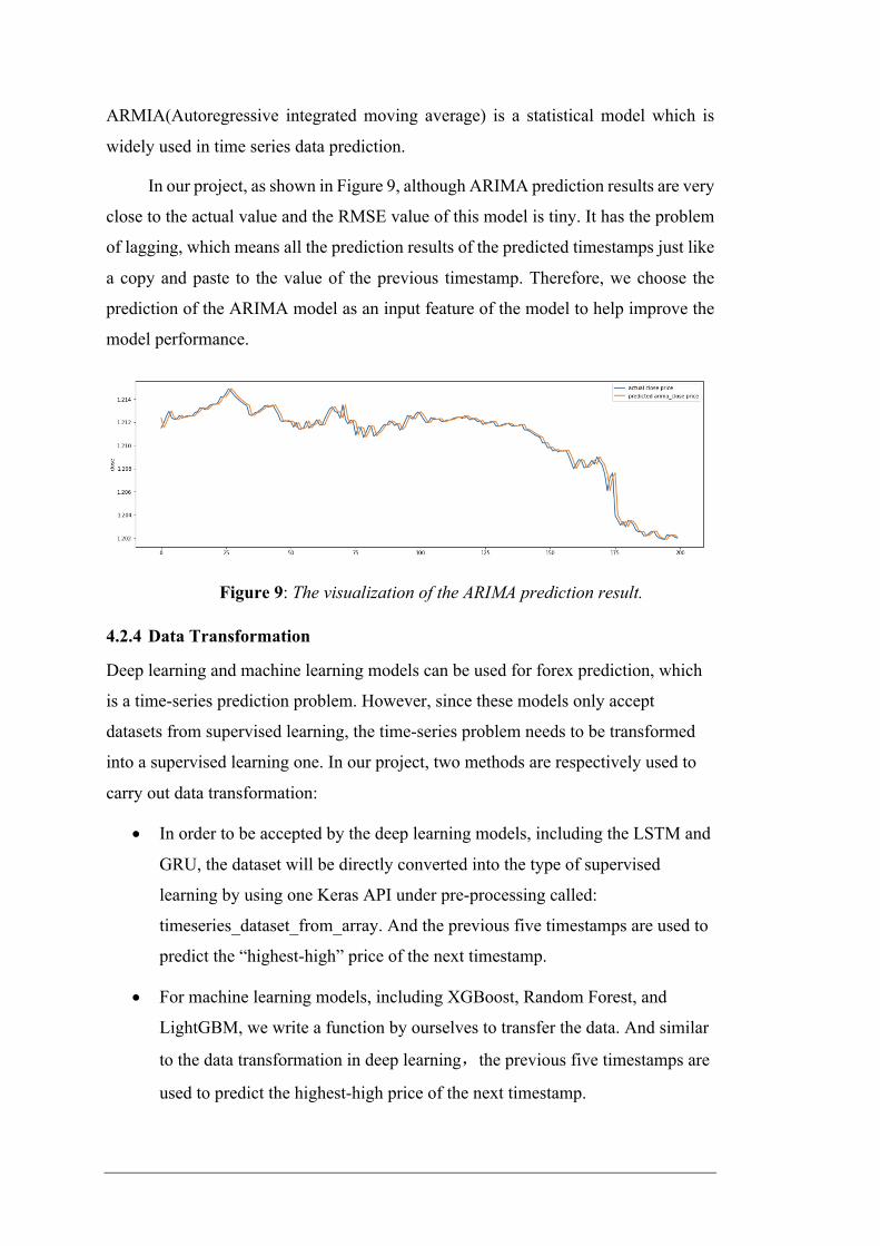
ARMIA(Autoregressive integrated moving average) is a statistical model which is

widely used in time series data prediction.

In our project, as shown in Figure 9, although ARIMA prediction results are very

close to the actual value and the RMSE value of this model is tiny. It has the problem

of lagging, which means all the prediction results of the predicted timestamps just like

a copy and paste to the value of the previous timestamp. Therefore, we choose the

prediction of the ARIMA model as an input feature of the model to help improve the

model performance.

Figure 9: The visualization of the ARIMA prediction result.

4.2.4 Data Transformation

Deep learning and machine learning models can be used for forex prediction, which

is a time-series prediction problem. However, since these models only accept

datasets from supervised learning, the time-series problem needs to be transformed

into a supervised learning one. In our project, two methods are respectively used to

carry out data transformation:

• In order to be accepted by the deep learning models, including the LSTM and

GRU, the dataset will be directly converted into the type of supervised

learning by using one Keras API under pre-processing called:

timeseries_dataset_from_array. And the previous five timestamps are used to

predict the “highest-high” price of the next timestamp.

• For machine learning models, including XGBoost, Random Forest, and

LightGBM, we write a function by ourselves to transfer the data. And similar

to the data transformation in deep learning，the previous five timestamps are

used to predict the highest-high price of the next timestamp.

23

Figure 10: The dataset after transformation for the machine learning models

These two data conversion methods are essentially the same: by using the

sliding window method, all columns of the past five timestamps are taken as the

input features of the model, and the highest high price of the timestamp is taken as

the label of the model. For example, as shown in Figure 10, if we choose the highest-

high price of timestamp “t” as the label in the model, the input features are all

columns of timestamp “t-4” combined all columns of timestamp “t-3” and all

columns of timestamp “t-2” and all columns of timestamp “t-1” and all columns of

timestamp “t”.

4.2.5 Data cleaning

In the prediction of the "highest-high" price and the generation of technical indicators,

some invalid rows in the data need to be discarded.

• In the prediction of "highest-high" price, because the last five timestamps

cannot obtain the high price of their future five timestamps, it is impossible for

them to calculate their respective "highest high" price and their corresponding

rows need to be discarded.

• In the generation of technical indicators, some indicators for the number of

rows do not exist, and the corresponding rows need to be discarded. For

example, in calculating the indicator called the moving average 10(MA10), the

MA10 value of the first nine timestamps cannot be calculated, and these rows

need to be discarded.

4.2.6 Data splitting

The entire dataset, which contains data from June 2014 to April 2021, is used in

machine learning and deep learning models and subsequent stacking systems. And the

dataset is divided into three parts: the training set, validation set, and test set. The

LabelIndex datetime open(t-4) high(t-4) low(t-4) close(t-4) upperband(t-4) ... medprice(t) typprice(t) wclprice(t) highest_high4 2014/4/1 21:45 0.92424 0.92442 0.9236 0.92386 0.924807 ... 0.92432 0.92428 0.92426 0.924615 2014/4/1 22:00 0.92387 0.92426 0.9239 0.92402 0.924375 ... 0.924355 0.924413 0.924442 0.925016 2014/4/1 22:15 0.92402 0.92405 0.9236 0.92362 0.924445 ... 0.92423 0.924147 0.924105 0.925017 2014/4/1 22:30 0.92364 0.92447 0.9236 0.92446 0.924624 ... 0.923755 0.92378 0.923792 0.925018 2014/4/1 22:45 0.92445 0.92445 0.9242 0.9242 0.924605 ... 0.92368 0.923707 0.92372 0.92501... ... ... ... ... ... ... ... ... ... ... ...124046 2019/3/31 21:45 0.71132 0.71132 0.711 0.71108 0.712408 ... 0.71077 0.710707 0.710675 0.71164124047 2019/3/31 22:00 0.71105 0.71114 0.7108 0.71094 0.711767 ... 0.71065 0.7107 0.710725 0.71164124048 2019/3/31 22:15 0.7109 0.71107 0.7108 0.71106 0.711388 ... 0.710875 0.71091 0.710927 0.71164124049 2019/3/31 22:30 0.71103 0.71117 0.711 0.71104 0.711311 ... 0.71124 0.71133 0.711375 0.71194124050 2019/3/31 22:45 0.711 0.711 0.7105 0.71058 0.711313 ... 0.711405 0.71135 0.711323 0.712

Input features

training set, which is used for model training, ranges from June 2014 to May 2019.

The validation set used for parameter tuning of models ranges from June 2019 to May

2020. The test set ranges from Jun 2020 to April 2021, and it is used for model

evaluation and also used in the subsequent stacking system. In the model evaluation,

each model uses the data from the test set to predict and obtain a prediction result with

the same row number as the test set. The prediction of each model will be used as the

input feature in the subsequent stacking system.

Figure 11: The visualization of data splitting for AUD_USD dataset

4.3 Traditional feature importance methods

The purpose of feature importance is to highlight the correlation between the features

and the target, which can help us understand the data set and the model. The

importance of a feature can be expressed by its feature importance score. The feature

importance score is usually calculated by a prediction model fitted to the data set,

providing insight into this model and how important the feature is when making

predictions. Based on the feature importance result, we can further improve the model

performance by dropping the features with low importance score. Hence, the dataset

dimension is reduced which will also speed up the training process.

For a tree-based model, the importance score measures the value of the feature

in the tree construction. The more a feature is used to build a tree in the model, the

higher its importance is. Feature importance is obtained by calculating and sorting each

feature in the data set. In a single decision tree, the feature importance is calculated by

the amount of performance improvement for each feature split point, and the weight

and frequency of making improvement is based on the node. In other words, the greater

the improvement performance of a feature on the split point (the closer it is to the root

node), the greater the weight; the more boosted trees are selected, the more important

25

the feature is. The performance measurement can be entropy gain, Gini purity,

permutation or SHAP（Shapley Additive explanation）.

In this project, we have applied built in feature importance functions for

XGBoost, Random Forest and LightGBM. For XGB, the feature importance is based

on the average gain across all splits the feature is used in. Random forest used the Gini

importance (mean decrease impurity). In random forest, the features for internal nodes

are selected by its variance reduction. The importance score is the average of how a

feature decrease the impurity over all trees in the forest. In LightGBM, the score is the

count of how many times a feature is used in splits.

4.4 Feature Importance Recap

Feature importance result from a model is for the particular model only. For

example, the same feature will have different score and rank in different models.

Therefore, we cannot simply apply the feature importance to other models without any

modification. For a tree-based model, it is easy to calculate its importance using the

methods we discussed in previous section. For deep learning model, as most of them

are block-box model, we cannot tell which feature is more importance. We could use

SHAP （Shapley Additive explanation） to explain the model. But there are several

limitations:

1. The calculation is time-consuming, its complexity is increased on an

exponential level if we add more features in the dataset. For financial data,

we could easily calculate hundreds of technical indicators as features.

2. SHAP result of a feature is not based on the performance of the model after

removing it.

3. If there are correlations between features, this perturbation-based method

may produce unrealistic data. In financial data, as the technical indicators are

calculated with financial equations, there could be features with high

correlations but still useful.

Therefore, we proposed a feature selection approach called ‘Feature importance

recap’. The main theory is that, as the tree-based model is easier to explain, we will

apply the result from these models and use the selected features as input for deep

learning model. In this project, we tested the feature importance with XGB, random

forest and LightGBM and make prediction with LSTM and GRU.

The first step is to split the training dataset into train and test dataset for feature

importance calculation. We used data from April 2014 to March 2018 as new training

set and April 2020 to April 2021 as testing set. Then we calculate the feature

importance score with XGBoost, Random Forest and LightGBM.

In the second step, we use the three feature sets from step one and apply deep

learning models to get the three RMSE result. Then we normalize the feature

importance score from step one with MinMaxScaler and divide the importance score

by the corresponding RMSE. Hence the result will represent both the importance score

and its performance in deep learning model. The final importance score is the sum of

the importance score from all three tree-based models.

Figure 12: Calculation of final feature importance score

Final feature score = SUM -𝑋𝐺𝐵 score 𝑅𝑀𝑆𝐸1 ,

𝑅𝐹 score 𝑅𝑀𝑆𝐸2 ,

𝐿𝐺𝐵𝑀 score 𝑅𝑀𝑆𝐸3 0 (25)

4.5 Model stacking

Stacking is a method from ensemble learning which can be used for both regression

and classification problems. Stacked models win most machine learning and data

science contests since the stacking system can improve the model performance to a

new level by mixing multiple existing models.

27

As shown in the stacking architecture of Figure 13, the stacking structure has

two layers. In the first layer, several different models are used to generate the

predictions. Each model's prediction is used as an input feature to form a data frame

that will be passed to the second layer of stacking. Finally, in the second layer, a model

is used to combine the results from columns of the data frame and get the final

prediction, which tends to have a better performance.

Figure 13: Stacking architecture [35]

In our project, there are five models in the first layer of the stacking system: three

of them are machine learning models, including LightGBM, Random Forest, and

XGBoost. Two are deep learning models, including LSTM and GRU. In the first layer

of stacking, five models are used respectively to predict the "highest-high" price of the

test set(June2020-April2021), and the prediction result is obtained respectively. Each

prediction result is used as a column to form a data frame, which has five columns

corresponding to the prediction results of the five models. Then put the set of the actual

"highest-high" price as the sixth column in the data frame, which is the label of the

dataset. Then, this data frame is delivered to the stacking second layer as the dataset.

In the second layer of the stacking system, a neural network model is used to

combine the results of the five models and obtain the final prediction. Before inputting

the neural network model(NN model), we first carry out data splitting on the dataset

delivered by the first layer. The dataset is divided into three parts: the training set,

validation set, and test set. The training set used for NN model training ranges from

June 2020 to October 2020. The validation which is used for parameter tuning of the

NN model ranges from November 2020 to December 2020. The test set ranges from

January 2020 to April 2021, which is used to obtain the predicted results and stacking

model evaluation.

When it comes to this NN model, it is not fixed and has 31 possible structures.

Because using all the predictions from five models as input features may not be the

optimal solution. It is possible to use the prediction results of four models as input of

the NN model to achieve better performance. Therefore, it is a combination problem

that has five candidate models.

As Figure 14 shows, there are 31 possibilities of combinations. We will compare

the performance of these 31 models and finally choose a model with the smallest

RMSE as the final NN model of the second layer of stacking. And the NN model

prediction results are the final prediction results of the stacking system.

Figure 14: 31 combinations from the five models

4.6 Evaluation

Because the primary goal of our study is to establish a model that can accurately predict

the future forex price, and it is a regression problem. Evaluation metrics of regression

models mainly include MSE, MAE, MAPE, and RMSE.

4.6.1 Mean squared error (MSE)

The mean squared error (MSE) indicates the difference of the regression predictions

with actual results. By calculating the distances from the actual points to the regression

predictions and squaring them. The range of the MSE is [0, +∞), and the lower MSE

always means a better model performance.

Xgboost Xgboost, LightGBM , RFLightGBM, Xgboost, LightGBM , LSTMRF Xgboost, LightGBM,GRULSTM Xgboost, RF,LSTMGRU Xgboost, RF,GRUXgboost, LightGBM, RF, LSTM Xgboost,LSTM,GRUXgboost, LightGBM, RF, GRU LightGBM, RF,LSTMXgboost, LightGBM, LSTM, GRU LightGBM, RF,GRUXgboost, RF, LSTM, GRU LightGBM, LSTM, GRULightGBM, RF, LSTM, GRU RF, LSTM,GRU

COMBIN(5,5) = 1 Xgboost, LightGBM, RF, LSTM, GRU

COMBIN(5,1) = 5 COMBIN(5,3) = 10

COMBIN(5,4) = 5N/A

29

𝑀𝑆𝐸 =1𝑛M  

$

&'(

(𝑦e& − 𝑦&)/ (26)

4.6.2 Root mean squared error (RMSE)

The RMSE is a measure of the differences between predicted results the values

observed. RMSE is non-negative，and the range of it is [0, +∞). When the RMSE is

equal to zero, the prediction results perfectly fit the actual data. and the lower RMSE

indicates a better model performance.

𝑅𝑀𝑆𝐸 = �1𝑛M  

$

&'(

(𝑦e& − 𝑦&)/ (27)

4.6.3 Mean absolute error (MAE)

Mean absolute error (MAE) measures errors between the predicted results and the

actual results. The MAE can avoid the problem of error cancellation, so it can

accurately reflect the actual prediction error. MAE calculates the average of the

residuals directly, while RMSE penalizes more for high differences than MAE.

𝑀𝐴𝐸 =1𝑛M  

$

&'(

|𝑦e& − 𝑦&| (28)

4.6.4 Mean Absolute Percentage Error (MAPE)

The MAPE, which is also called mean absolute percentage deviation (MAPD), is a

measure of prediction accuracy of regression in statistics.

𝑀𝐴𝑃𝐸 =100%𝑛 M  

$

&'(

�𝑦e& − 𝑦&𝑦&

� (29)

As shown in the MAPE formula, 𝑦& is the actual result of the ith sample, and

𝑦e& is the result of the ith sample predicted by the model. The range of MAPE is [0, +∞),

and when MAPE is 0, the model is the perfect one. If the MAPE value is more than 1,

it means the model performed badly. Although the concept of MAPE is intuitive and

convincing, it has a very significant disadvantage: if there is any zero-value contained

in the actual value of the dataset, the MAPE cannot be used.

5. RESULTS 5.1 Feature importance recap result

The testing dataset is from Jun 2020 to April 2021 with timeframe of 15 minutes of

AUD_USD and EUR_USD. We use the previous 5 timestamps to predict the highest

high price in the next 5 timestamps. The model performance is measured with RMSE,

MAE and MAPE. We have tested with top 20 and top 30 features. The best result for

AUD_USD is GRU with top 20 features, and for EUR_USD is LSTM with top 30

features. The result with feature importance recap is very close.

The hyperparameters are set as batch_size = 256 for timeseries dataset and

learning rate is 1E-5.

Figure 15: Test result with LSTM on AUD_USD

Figure 16: Test result with GRU on AUD_USD

Input Features RMSE（E-3） MAE（E-3） MAPE（E-3）

All features 2.1687 2.5486 3.4228XGB 20 1.4016 1.0578 1.4399

LGBM 20 1.8481 1.4253 1.9312RF 20 1.7717 1.337 1.8289

Final 20 0.8037 0.6491 0.883XGB 30 1.5245 1.169 1.5943

LGBM 30 1.2218 0.8962 1.2205RF 30 1.6558 1.2519 1.7056

Final 30 0.9482 0.6762 0.9195

Input Features RMSE（E-3） MAE（E-3） MAPE（E-3）

All features 3.1101 2.6433 3.5785XGB 20 1.0547 0.7771 1.0793

LGBM 20 1.3268 0.9391 1.3382RF 20 1.2951 0.9605 1.2946

Final 20 0.7563 0.5312 0.7223XGB 30 1.3656 1.0436 1.4417

LGBM 30 1.0056 0.7209 0.979RF 30 1.1578 0.8649 1.1754

Final 30 0.8412 0.5948 0.8065

31

Figure 17: Test result with LSTM on EUR_USD

Figure 18: Test result with GRU on EUR_USD

More experiment results with selected features please refer to the appendix and

the artifacts.

The result shows that the experiments with feature selection outperforms the

experiments fed with all features. With the feature selected with “feature importance

recap” the performance is even better.

Input Features RMSE（E-3） MAE（E-3） MAPE（E-3）

All features 2.03 1.8007 1.5104XGB 20 0.9664 0.637 0.539

LGBM 20 1.2608 1.0072 0.8457RF 20 1.1261 0.7749 0.6553

Final 20 0.8693 0.6497 0.5492XGB 30 1.7824 1.4891 1.2469

LGBM 30 1.9033 1.6794 1.4081RF 30 2.3868 2.1097 1.77

Final 30 0.7945 0.5449 0.461

Input Features RMSE（E-3） MAE（E-3） MAPE（E-3）

All features 3.1621 2.8576 2.3957XGB 20 1.97 1.7413 1.4597

LGBM 20 0.9296 0.6409 0.5402RF 20 1.5558 1.2992 1.092

Final 20 0.8824 0.7141 0.6048XGB 30 1.1294 0.8719 0.7336

LGBM 30 1.3816 1.1233 0.9436RF 30 1.1442 0.6409 0.5402

Final 30 0.9444 0.6538 0.5514

Figure 19: Selected features for LSTM on AUD_USD

By investigating the selected features, we found that some features like close,

high, price transform indicators, are selected in all experiments. Figure 19 is a sample

of selected features for LSTM on AUD_USD. As the features are selected with

supervised dataset, some features are selected twice. For example, both close(t) and

close(t-1) are selected. The timeseries dataset will use all previous values of the feature

so the selected feature set will be less than 20 or 30. The overlapping among the

selected features will be included in future research.

5.2 Model stacking result

On the unseen data set, we test the performance of stacking for two different currency

transactions, including AUD-USD and EUR-USD. By comparing the performances of

31 combinations, we choose the most suitable stacking model, which has the smallest

RMSE.

The performances of 31 stacking combinations are shown in Figure 20. The

stacking system using XGBoost, LightGBM, and GRU has the smallest RMSE overall.

The RMSE of this stacking system is 6.799e-04, which is much better than RMSE

7.563e-04 of GRU, the single best one.

Hence, in the dataset of M15 AUD-USD, we finally choose to use XGBoost,

LightGBM, and GRU in the first layer of the stacking system.

Selected features

Final 3028

['close','high','wclprice','trange','typprice','dema','upperband','atr','trima30','bop','sma10','willr','medprice','natr','fastk','plus_dm','adxr','midpoint','macdsignalfix','macdsignalext','avgprice','tema','slowd','ht','mom','minus_di','sma30','macdhistext']

RF 3019

LGBM 3027

XGB 3023

['close','high','typprice','sma10','dema','wclprice','low','tema','upperband','avgprice','arima_high','sma30','open','kama','ht','midprice','midpoint','t3','wma5','lowerband','medprice','trima30','atr']

['close','high','trange','wclprice','upperband','atr','dema','trima30','bop','willr','fastk','natr','plus_dm','medprice','adxr','macdsignalfix','midpoint','typprice','macdsignalext','tema','slowd','ht','mom','minus_di','macdhistext','sma30','fastkrsi']

['close','wclprice','high','avgprice','dema','medprice','typprice','low','open','lowerband','kama','midprice','ema','arima_close','wma5','midpoint','tema','ma','arima_high']

33

Figure 20: The RMSE of different models’ combinations on AUD_USD

Figure 21: The RMSE of different models’ combinations on EUR_USD

The performances of 31 stacking combinations are shown in Figure 21. The

stacking system using Random Forest, LSTM, and GRU has the smallest RMSE

overall. The RMSE of this stacking system is 7.2E-04, which is much better than

RMSE 7.94E-04 of LSTM, the single best one. Hence, in the dataset of M15 EUR-

USD, we finally choose to use Random Forest, LSTM, and GRU in the first layer of

the stacking system.

The result shows that the performance is improved with only certain

combinations, and overall, the combinations with both LSTM and GRU outperforms

other models.

6. DISCUSSION The forex trading market is a global speculative market. By far, it is the largest market

in terms of quantitative trading. The characteristics of forex trading distinguish it from

other quantitative trading markets. Unlike we buy stocks with money in the stock

market, what is exchanged in forex trading is the “money” itself, and the main action

is to exchange one currency to another. With its international transparency, maturity,

and standardization, it has attracted the extensive participation of banks, large

enterprises, funds, and investment institutions as well as individual investors from all

over the world.

The primary goal of this project is to predict the highest high price of the next 5

timestamps based on the historical data with machine intelligent models. We have

proposed a new feature selection approach to filter the most important features for a

deep learning model and a stacking model to combine and improve the performance

from multiple models. Both approaches significantly increased the performance.

The raw datasets are the OHLC data of a certain period downloaded from

OANDA without any other features. For feature engineering, we first calculated 139

features including overlap studies indicators, momentum indicators, volatility

indicators, price transform, cycle indicators and pattern recognition functions.

We also used the ARIMA predictions for the close and high price of next

timestamp as features. ARIMA by itself is already a mature statistical model, as AIC

function returns a q value of 0 which means we only used the AR method. So, we did

not use ARIMA as a model as it provides a lagging prediction. Instead, we keep the

ARIMA prediction as another feature. The feature importance recap result also proved

that the ARIMA prediction is vital for highest high price prediction.

We thought that since all these features are calculated based on the OHLC value,

they are all related to our target. Besides, the deep learning models already have built-

35

in mechanisms to filter the features, so we did not apply any feature selection approach.

With all these features, we applied many deep learning models including LSTM, CNN,

GRU, Transformer with LSTM, Reinforcement learning. However, these models did

not perform well on our dataset. Some model did not even converge in experiments.

We revise the processes and the model. By analyzing the features, we found that over

70 columns of cycle indicators and pattern recognition functions are 0s. These values

would make the data noisy and mislead the prediction.

Then we drop these features and retrain the model. With LSTM we got the lowest

RMSE on next timestamp close price prediction of 0.006. Although it is still high, it is

much better than our previous results.

From this experiment, we found that our dataset is too noisy, and we are not able

to get accurate results with such a combination of dataset and model. Therefore, we

decided to apply denoise and feature selection approaches to improve the performance.

For data denoise, we first did research about wavelet denoise. Most of the

experiments shows that it would improve the model performance. However, [21]

proved that wavelet denoise would lead to data leakage, it may use future data to

denoise historical data. So, we gave up wavelet denoise and turn to find a new way for

feature selection.

In previous study, we have learned the feature importance calculation in tree-

based models. Consequently, we did research about feature importance calculation in

deep learning models and tried to implement it in our experiments. We found that the

SHAP package based on the game theory could explain the importance of each feature

in the dataset. However, it has a high computational cost as it tries all combinations

among the features. With financial data, we could easily get hundreds of features by

changing the time which means that SHAP is not a valid approach. At last, we decided

to find an approach to combine the results from tree-based models and deep learning

models.

In general, we cannot apply the feature importance from on model in another as

the training process is different, which means we cannot directly apply the result from

tree-based model in deep learning model. Our experiments also proved that applying

the feature importance on other models would increase the performance, but it is not

the most suitable feature set.

To allow the feature importance score from the tree-based model carries the

performance of the selected features in deep learning model, we feed the selected

feature in deep learning and divide the feature importance score by the RMSE then

sum the importance score of each feature. The final importance will contain

information from both tree-based feature importance and deep learning model

performance. Compare with SHAP, this approach is much faster. We tested this

approach on AUD_USD and EUR_USD with both LSTM and GRU. The result shows

that the RMSE is significantly dropped.

Moreover, we found that the tree-based model also could also perform well on

the datasets, so we decided to implement a stacking model to combine the results from

five models: XGBoost, Random Forest, LightGBM, LSTM and GRU. We tried all

possible combinations, and the result is further improved.

There were four main challenges during our research and experiments:

• Lack of domain knowledge

All group members have no financial trading experience. We had to spend time to

learn the financial fundamentals regarding this project such as what is forex trading

and its characteristics, technical indicators, why we need to predict several

timestamps ahead rather than predict next one timestamp.

• Lack of timeseries data forecasting experience

All group members are major in data science but all of us do not have timeseries

data forecasting experience. In previous studies, we have learned several machine

learning models such as XGB, K-NN and some basic RNN, but each row in the

raw dataset is not related. For financial data, the previous data will impact the

future data and we had to learn how to modify the dataset so that they are in a

sequence while feeding into the models.

• Hardware infrastructure limitation

Due to the COVID-19, we cannot go to the campus and use advanced

infrastructures in the labs. Most group members can only use laptops for model

training. The limitation of computational resource makes us can only experiment

with small datasets and cannot apply grid search on hyper parameters.

• Different levels of coding experience within the team

37

All the codes of this project are in python. Some group members do not have

enough coding experience and had to spend time on practicing.

What we learned from this project:

• Always analyze the data before building model

In the first few weeks, we spend lots of time on implementing different deep

learning models. However, the performance is very bad as the data is too noisy

after we added cycle indicators and pattern recognition functions as features. Most

values of these two types of indicators are 0s and 1s, if we made detailed data

analysis, we might save these times.

• Future selection is important

After we feed the selected features using tree-based models in deep learning

models, the performance is better than feeding all features. The results from our

feature selection recap approach also proved that Propper feature selection would

benefit the model.

• Group work can improve work efficiency

Group members have different knowledge backgrounds and experience, and their

respective areas of expertise are also different. We divided the tasks for each

member so that everyone can contribute to the project. As part of the goal of this

project is to improve our understanding on AI techniques, we also helped each

other in coding.

7. LIMITATIONS AND FUTURE WORKS While the result to date shows that our approach significantly improved the

performance of highest high price prediction, there are much more we would like to

achieve. The limitation of our work is largely due to the time constraint. The project

needs to be done in 13 weeks. In the first few weeks, we spend lots of time on testing

deep learning models but did not get any acceptable results. The feature importance

recap and model stacking approaches was proposed and implemented in week 10.

Therefore, we did not have enough time to test more deep learning models and

currency pairs.

We have tested our approach with two currency pairs, two deep learning

models and stacked these two model with three tree-based models. The results proved

that our approach would improve the RMSE but to get more stable results, we need to

test with more currency pairs and models.

Moreover, this project did not involve any backtesting to test if the trading

strategy based on this prediction would make profit. This is crucial for financial data

forecasting as the purpose of price forecasting is to help the investors to make money.

The prediction with low RMSE is not guaranteed high profit margin. The prediction

accuracy is evaluated with RMSE, despite it predicted the price higher or lower, the

RMSE may stays the same. However, in financial trading, mis-predicting the increase

or decrease may lead to profit loss. Therefore, to prove our approach would benefit the

investors, we should apply back testing with some pre-defined trading strategies.

Since there are overlapping among the importance features in different models,

we could run the experiments more times to test which feature is always important and

try to predict only with these features. We can generate a solid feature set for forex

forecasting if possible. Then, when other researchers want to test a model, they can

simply feed these features.

Alternatively, we can also make predictions about the lowest low prices of

following timestamps in the future. Then design trading strategy with both highest high

and lowest low prediction. We can also compare the selected features from these two

predictions and analyse why such feature is importance from financial aspects.

Furthermore, we can extend this prediction to OHLC data, and some technical

indicators then design trading strategies with a predicted dataset and apply backtesting

to test the profitability.

For building trading strategies, rather than using rule-based trading, we can apply

reinforcement learning to further improve the strategy. Reinforcement learning will

reward the correct actions and punish actions that lost money. We can compare the

performance between the strategy from reinforcement learning and from expertise

rules.

39

8. APPENDIX

Figure 22: Stacking performance of 31 combinations on AUD_USD

Figure 23: Stacking performance of 31 combinations on EUR_USD

Error! No text of specified style in document. 41

REFERENCES

1 Murphy, J.J.: ‘John J Murphy - Technical Analysis Of The Financial Markets.pdf’, 1999 2 Julie, R.D., and Charles, D.K.: ‘When You Can Use Technical Analysis for Investing’, 2010 3 Kritzer, A.: ‘Forex for Beginners : A Comprehensive Guide to Profiting from the Global Currency Markets’ (Apress, 2012. 2012) 4 https://www.marketvolume.com/technicalanalysis/balanceofpower.asp, accessed 20 Jun 2021 5 https://www.tradingtechnologies.com/xtrader-help/x-study/technical-indicator-definitions/triangular-moving-average-trima/, accessed Jun 20 2021 6 http://www.chart-formations.com/chartists/welles-wilder.aspx, accessed Jun 20 2021 7 https://www.investopedia.com/terms/a/atr.asp, accessed Jun 20 2021 8 Murphy, K.P.: ‘Machine learning a probabilistic perspective’ (MIT Press, 2012. 2012) 9 : ‘Interpretable Machine Learning with Python’ (Packt Publishing, Limited, 2021. 2021) 10 Rasekhschaffe, K.C., and Jones, R.C.: ‘Machine Learning for Stock Selection’, Financial analysts journal, 2019, 75, (3), pp. 70-88 11 Shynkevich, Y., McGinnity, T.M., Coleman, S.A., Belatreche, A., and Li, Y.: ‘Forecasting price movements using technical indicators: Investigating the impact of varying input window length’, Neurocomputing (Amsterdam), 2017, 264, pp. 71-88 12 Wang, C., Miao, Z., Lin, Y., Jiang, H., Gao, J., Lu, J., and Shi, G.: ‘Modeling Price and Risk in Chinese Financial Derivative Market with Deep Neural Network Architectures’, in Editor (Ed.)^(Eds.): ‘Book Modeling Price and Risk in Chinese Financial Derivative Market with Deep Neural Network Architectures’ (IEEE, 2020, edn.), pp. 13-18 13 Chen, Y.-Y., Chen, W.-L., and Huang, S.-H.: ‘Developing Arbitrage Strategy in High-frequency Pairs Trading with Filterbank CNN Algorithm’, in Editor (Ed.)^(Eds.): ‘Book Developing Arbitrage Strategy in High-frequency Pairs Trading with Filterbank CNN Algorithm’ (IEEE, 2018, edn.), pp. 113-116 14 Box, G.E.P., Jenkins, G.M., Reinsel, G.C., and Ljung, G.M.: ‘Time Series Analysis : Forecasting and Control’ (Wiley, 2015, 5th edn. 2015) 15 Kamruzzaman, J., and Sarker, R.A.: ‘Forecasting of currency exchange rates using ANN: a case study’, in Editor (Ed.)^(Eds.): ‘Book Forecasting of currency exchange rates using ANN: a case study’ (IEEE, 2003, edn.), pp. 793-797 Vol.791 16 Yildirim, D.C., Toroslu, I.H., and Fiore, U.: ‘Forecasting directional movement of Forex data using LSTM with technical and macroeconomic indicators’, Financial Innovation, 2021, 7, (1), pp. 1-36 17 Qi, L., Khushi, M., and Poon, J.: ‘Event-Driven LSTM For Forex Price Prediction’, in Editor (Ed.)^(Eds.): ‘Book Event-Driven LSTM For Forex Price Prediction’ (IEEE, 2020, edn.), pp. 1-6 18 Stelmack, J.: ‘Kaizen Programming with Enhanced Feature Discovery: An Automated Approach to Feature Selection and Feature Discovery for Prediction Models’, in Editor (Ed.)^(Eds.): ‘Book Kaizen Programming with Enhanced Feature

42 Error! No text of specified style in document.

Discovery: An Automated Approach to Feature Selection and Feature Discovery for Prediction Models’ (ProQuest Dissertations Publishing, 2020, edn.), pp. 19 Zhang, Z., and Khushi, M.: ‘GA-MSSR: Genetic Algorithm Maximizing Sharpe and Sterling Ratio Method for RoboTrading’, in Editor (Ed.)^(Eds.): ‘Book GA-MSSR: Genetic Algorithm Maximizing Sharpe and Sterling Ratio Method for RoboTrading’ (IEEE, 2020, edn.), pp. 1-8 20 Zeng, Z., and Khushi, M.: ‘Wavelet Denoising and Attention-based RNN- ARIMA Model to Predict Forex Price’, in Editor (Ed.)^(Eds.): ‘Book Wavelet Denoising and Attention-based RNN- ARIMA Model to Predict Forex Price’ (IEEE, 2020, edn.), pp. 1-7 21 Zhao, Y., and Khushi, M.: ‘Wavelet Denoised-ResNet CNN and LightGBM Method to Predict Forex Rate of Change’, in Editor (Ed.)^(Eds.): ‘Book Wavelet Denoised-ResNet CNN and LightGBM Method to Predict Forex Rate of Change’ (IEEE, 2020, edn.), pp. 385-391 22 Meng, T.L., and Khushi, M.: ‘Reinforcement Learning in Financial Markets’, Data, 2019, 4, (3), pp. 110 23 Kim, T.W., and Khushi, M.: ‘Portfolio Optimization with 2D Relative-Attentional Gated Transformer’, in Editor (Ed.)^(Eds.): ‘Book Portfolio Optimization with 2D Relative-Attentional Gated Transformer’ (IEEE, 2020, edn.), pp. 1-6 24 Singh, J., and Khushi, M.: ‘Feature Learning for Stock Price Prediction Shows a Significant Role of Analyst Rating’, Applied System Innovation, 2021, 4, (1), pp. 17 25 Jaggi, M., Mandal, P., Narang, S., Naseem, U., and Khushi, M.: ‘Text Mining of Stocktwits Data for Predicting Stock Prices’, Applied System Innovation, 2021, 4, (1), pp. 13 26 Hu, Z., Zhao, Y., and Khushi, M.: ‘A Survey of Forex and Stock Price Prediction Using Deep Learning’, Applied System Innovation, 2021, 4, (1), pp. 9 27 https://colah.github.io/posts/2015-08-Understanding-LSTMs/, accessed Jun 20 2021 28 https://en.wikipedia.org/wiki/Gated_recurrent_unit, accessed Jun 20 2021 29 https://towardsdatascience.com/gate-recurrent-units-explained-using-matrices-part-1-3c781469fc18, accessed Jun 20 2021 30 Chen, T., and Guestrin, C.: ‘XGBoost: A Scalable Tree Boosting System’, in Editor (Ed.)^(Eds.): ‘Book XGBoost: A Scalable Tree Boosting System’ (ACM, 2016, edn.), pp. 785-794 31 https://xgboost.readthedocs.io/en/latest/tutorials/model.html, accessed Jun 20 2021 32 https://corporatefinanceinstitute.com/resources/knowledge/other/random-forest/, accessed Jun 20 2021 33 https://www.analyticsvidhya.com/blog/2017/06/which-algorithm-takes-the-crown-light-gbm-vs-xgboost/, accessed Jun 20 2021 34 https://en.wikipedia.org/wiki/Autoregressive_integrated_moving_average, accessed Jun 20 2021 35 https://www.geeksforgeeks.org/stacking-in-machine-learning-2/, accessed Jun 20 2021