FDTD-SUPML-ADE simulation for

Ground-Penetrating Radar modeling

Faycal Rejiba, Christian Camerlynck, and Pierre Mechler

Department of Applied Geophysics, Universite Pierre et Marie Curie, UMR 7619, Sisyphe, CNRS, Paris, France

Received 15 December 2001; revised 18 July 2002; accepted 11 September 2002; published 16 January 2003.

[1] GPR data simulations require above all an efficient forward modeling algorithm. AFinite Difference Time Domain code is presented with Simplified Unsplit PerfectMatched Layer that leads to insignificant reflections on border with few modifications ofthe core algorithm. In addition, the Auxiliary Differential Equation method allows GPRsimulations including dispersive phenomena that could not be neglected at radarfrequencies. The numerical validation is done in a classic way for amplitude/time wavepropagation and SUPML, and using the nonconventional Dispersion Analysis techniquefor physical dispersion behavior. Full 3-D and 2-D forward modeling results arefinally presented for lossy, dispersive and random media in GPR conditions. INDEX

TERMS: 0644 Electromagnetics: Numerical methods; 0689 Electromagnetics: Wave propagation (4275); 3210

Mathematical Geophysics: Modeling; 0684 Electromagnetics: Transient and time domain; KEYWORDS:

Ground-Penetrating Radar, Finite Difference-Time Domain, Perfect Matched Layer, Auxiliary Differential

Equation, physical dispersion

Citation: Rejiba, F., C. Camerlynck, and P. Mechler, FDTD-SUPML-ADE simulation for Ground-Penetrating Radar

modeling, Radio Sci., 38(1), 1005, doi:10.1029/2001RS002595, 2003.

1. Introduction

[2] Ground Penetrating Radar (GPR) is widely used inshallow geophysical exploration, in civil engineering andwater research. It is also efficient for detecting buriedobjects such as land mines [Montoya and Smith, 1999],or archeological structures and artifacts [Conyers andGoodman, 1997]. In favorable conditions, the transmis-sion of short electromagnetic pulses (few nanoseconds)allows the investigation up to several tens of meters forlow loss geological materials.[3] The simulation of GPR is generally achieved by

several techniques like Ray Tracing [Cai and McMe-chan, 1995], the Moment Method [Tabbagh, 1995;Vitebsky et al., 1997], the Spectral and Pseudo-SpectralMethods [Bitri and Grandjean, 1998; Carcione et al.,1999; Qing Huo and Guo-Xin, 1999] and FDTD method[Yee, 1966; Bourgeois and Smith, 1996; Wang and Tripp,1996; Roberts and Daniels, 1997; Teixeira et al., 1998;Bergmann et al., 1998; Chen and Huang, 1998; Gureland Ugur, 2000].[4] The FDTD method requires what is generally

called Absorbing Boundary Condition (ABC) to simulate

an open media [Mur, 1981; Mei and Fang, 1992]. Atpresent time, Berenger’s PML [Berenger, 1994; Katz etal., 1994] is by far the most interesting ABC. In thispaper, a simplified version of Unsplit PML is used[Sacks et al., 1995; Gedney, 1996; Sullivan, 1997;Teixeira et al., 1998].[5] In addition, frequency dependence of material

properties cannot be dismissed, and we count severalrealistic relaxation models for geological structures as theCole Cole relation [Xu and McMechan, 1997], theJonscher relation [Hollender and Tillard, 1998] or avisco-elastic analogy formulation [Carcione, 1996].Throughout this paper, the dispersion will refers to asimple Debye model, in addition to a static electricalconductivity term, knowing that at GPR frequencies theelectrical conductivity is frequency independent and real[Lysne, 1983].[6] Four main methods are usually used in FDTD

schemes to implement frequencies dependences: theZ-transform method [Sullivan, 1992], the AuxiliaryDifferential Equation (ADE) method [Gandhi et al.,1993], the Recursive Convolution method [Luebbers etal., 1990; Luebbers and Hunsberger, 1992] and thePiecewise Linear Recursive Convolution technique [Kel-ley and Luebbers, 1996; Teixeira et al., 1998].[7] In this paper we showed the validity of a 3-D

FDTD-SUPML-ADE implementation to simulate a

RADIO SCIENCE, VOL. 38, NO. 1, 1005, doi:10.1029/2001RS002595, 2003

Copyright 2003 by the American Geophysical Union.

0048-6604/03/2001RS002595

5 - 1

GPR acquisition in realistic media. In the followedalgorithm, the classic PML exponential functions arereplaced by simplified functions over the entire domain,that are constant in the computation domain, and hyper-bolic in the SUPML lossy domain: such an implementa-tion leads to an equivalent efficiency and avoids theheavy implementation due to the PML/computationdomain interface.[8] The propagation scheme deals with H (magnetic

field) and D (electric flux density) instead of the classicH and E (electric field) update technique, and allows aneasy implementation of the constitutive relation betweenD and E by the Auxiliary Differential Equation method.In addition to the numerical validations needed, we usein this paper, an original approach to validate thephysical dispersion that consist in a Dispersion Analysisgenerally used in acoustic wave propagation [He, 2000].

2. Simplified-UPML Formulation

[9] We start with the following transformation [Sulli-van, 1996]:

~E ¼ffiffiffiffiffie0m0

r� E ð1:1Þ

~D ¼ 1ffiffiffiffiffiffiffiffiffiffiffiffie0 � m0

p � D ð1:2Þ

Then Maxwell’s equations are

jw~D ¼ c0r� H ð1:3Þ

~D wð Þ ¼ er* wð Þ~E wð Þ ð1:4Þ

jwH ¼ �c0r� ~E ð1:5Þ

The equivalent dielectric permittivity includes a realelectric conductivity term as follows:

er* ¼ e1 þ es � e11þ j � w � t0

þ sj � w � e0

ð1:6Þ

where es, e1, c0, s, and w are respectively the staticpermittivity, the high frequency permittivity, the vacuumvelocity (m/s), the conductivity (S/m), and the pulsation(rad/s).

Figure 1. Comparison between the 3-D free space analytical solution and the FDTD-Unsplit PMLformulation. The point source is a 2 GHz Ey derived gaussian pulse (DFG) measured after 150 timesteps in the vacuum. Model discretization dx = dy = dz = 1 cm, dt = 16 ps.

5 - 2 REJIBA ET AL.: FDTD-SUPML-ADE SIMULATION

[10] The FDTD formulation consists in a generaliza-tion of the Sullivan [1997] approach for the electro-magnetic field components using dt and dx, dy, dx fortime and spatial discretization. The time step is chosenaccording the Courant stability usually used for planewave propagation:

dt ¼ 1

cffiffiffiffiffiffiffiffiffiffiffiffiffiffiffiffiffiffiffiffiffiffiffiffiffiffiffiffiffiffiffiffiffiffiffiffiffiffiffiffiffiffiffiffiffiffi1=dx2 þ 1=dy2 þ 1=dz2

p ð1:7Þ

where c is the maximum velocity encountered in themedia.[11] The SUPML are characterized by an anisotropic

implementation for each direction. In what follows, ~Dz

and ~Dx components are expressed for the x directionfrom equations (1.3) to (1.5):

jw~Dx 1þ sD xð Þjwe0

� ��1

¼ c0@Hz

@y� @Hy

@z

� �ð1:8Þ

~Dz 1þ sD xð Þjwe0

� ��1

¼ c0@Hy

@x� @Hx

@y

� �ð1:9Þ

We use a staggered grid using a Yee [1966] scheme toexpress the derivation operators. That explains the 1/2increment in the spatial coordinate and time index asfollow for ~Dz (and Hz):

~Dn

z i; j; kþ 1=2ð Þ ¼ gi3 ið Þ~Dn�1

z i; j; kþ 1=2ð Þ þ gi2 ið Þdtc0

�H

n�1=2y iþ1=2; j; kþ1=2ð Þ�H

n�1=2y i�1=2; j; kþ1=2ð Þ

dx�

Hn�1=2x i; jþ1=2; kþ1=2ð Þ�H

n�1=2x i; j�1=2; kþ1=2ð Þ

dy

0@

1A ð1:10Þ

~Dy and Hy are developed in a similar manner.

[12] Concerning ~Dx (and Hx), some algebra due to theequivalent integral operator 1

jw term gives when applied asecond order centered FDTD scheme:

@Hz

@y� @Hy

@z,

Hn�1=2z iþ1=2; jþ1=2; kð Þ�H

n�1=2z iþ1=2; j�1=2; kð Þ

dy�

Hn�1=2y iþ1=2; j; kþ1=2ð Þ�H

n�1=2y iþ1=2; j; k�1=2ð Þ

dz

24

35

� rot h

I~Dx

n iþ 1=2; j; kð Þ ¼ In�1~Dx

iþ 1=2; j; kð Þ

þ dtc0gi1 iþ 1=2ð Þrot h

~Dn

x iþ 1=2; j; kð Þ ¼ ~Dn�1

x iþ 1=2; j; kð Þ þ dtc0rot h

þ dtc0In~Dx

iþ 1=2; j; kð Þ ð1:11Þ

The specificity of the SUPML consists in simplifiedattenuation functions g(i,j,k)(1,2,3) and f(i,j,k)(1,2,3). Thosefunctions that shrink the field’s amplitude in the PML aredefined to restore the classical propagation in thecomputation domain, and range between 0 and 1:

fnc ið Þ ¼ 1

b

npml� i

npml

� �a

; i ¼ 1; . . . ; npml

f i1 ið Þ ¼ gi1 ið Þ ¼ fnc ið Þ

gi2 ið Þ ¼ f i2 ið Þ ¼ 1

1þ fnc ið Þ

gi3 ið Þ ¼ f i3 ið Þ ¼ 1� fnc ið Þ1þ fnc ið Þ ð1:12Þ

Figure 2. Snapshots of a Ey front wave propagation during 150 time steps on a 60 cm segmentlying the 40 cm thickness PML border. A 1 GHz centered DFG Ey source is emitted. Modeldiscretization dx = dy = dz = 2 cm, dt = 33 ps.

REJIBA ET AL.: FDTD-SUPML-ADE SIMULATION 5 - 3

where npml is the number of layers in the SUPML regionand (a, b) are real parameters. For other directions,equivalent formulation concerning the attenuation func-tions and field equations update are easily expressed. Thenumerical stability for the FDTD-SUPML scheme isguaranteed for b less than 3 [Sullivan, 1997], and itsvalidity is demonstrated by a simple comparison with theanalytical S free space solution (Figure 1):

S tð Þ ¼ TF�1 G3D*Jy wð Þ� �

ð1:13Þ

TF�1 is the inverse Fourier transform, and notation G3�D

is the Green function defined at the distance R from a pointsource:

G3D ¼ e�ikR

4pRð1:14Þ

The shape of the current density is a y-polarized derivedgaussian pulse (DFG):

Jy tð Þ ¼ � t

dttp

� �exp � 1þ t

dttp

� �2 !

=2

" #ð1:15Þ

where tP is the number of time step from the beginning ofthe pulse to the first maximum.[13] The geometrical model consist in dx = dy = dz = 1

cm, dt = 16 ps, and the source is 2 GHz DFG pulse. Thesource Jy is added in the FDTD scheme by the followingway:

Figure 3. (a) r values in the calculation domain including PML response in the inlet. (b) r values inthe reference domain without PML influence. (c) Evaluation of percentage of reflection followingthe (1.18) expression with a maximum average reflection of 0.8%, corresponding to the (Figure 2).

5 - 4 REJIBA ET AL.: FDTD-SUPML-ADE SIMULATION

~Dn

y i; jþ 1=2; kð Þ ¼ ~Dn

y i; jþ 1=2; kð Þ þ Jy tð Þ ð1:16Þ

3. Evaluation of SUPML

[14] PML is now well mastered, and even if SUPMLdiffers from the original formulation, it does not reallyneed any validation for plane wave propagation. Never-theless, for a point source emitted inside the computationdomain, difficulties arise due to the variation of the angleof incidence inherent to the spherical-shape of the wave.We thus consider a 1 GHz Ey DFG point source emittedin vacuum (equivalent results are obtained with otherspolarization). The simulation is made for a 2 cm isotropicdiscretization with 40 cm of SUPML which is an optimalthickness regarding the pulse width, with the followingparameters (dx = dy = dz = 2 cm, dt = 33 ps).

[15] To quantify the efficiency of the SUPML withsuch a point source, we calculate, at each time step, themean of the average �Ey of ~Ey (Figure 2) across the upperPML (60 cm � 60 cm ! 30dx � 30dy).

�Ey npml; tð Þ ¼ 1

302

Xns

x¼1

Xns

y¼1~Ey x; y; npml; tð Þ�� j

ð1:17ÞA percentage of reflection is evaluated by comparing �Ey

with what is obtained in a wider enough referencedomain in order to avoid PML interference:

Ref ¼ 100�

��Ey npml; tð Þreference domain��Ey npml; tð Þcalculation domain

Max �Ey npml; tð Þreference domain

��ð1:18Þb ¼ 5

Figure 4. (a) Dispersion model (complex dielectric permittivity) used for the dispersion analysis.It consist in a Debye pole with es = 1, e1 = 3 and t0 = 0.1 ns. (b) Corresponding phase velocitycurve vphase ¼ 1=

ffiffiffiffiffiffiffiffiereal

p.

REJIBA ET AL.: FDTD-SUPML-ADE SIMULATION 5 - 5

For our example we observe less than 0.8% of reflection(Figure 3).

4. Dispersion and Attenuation With ADE

Method

[16] The FDTD scheme is used for ~D and H update, bythis way, the ADE method looks to be particularlyadapted to take into account for physical dispersion ingeneral and so on for an equivalent Debye model. Thismethod simply consists in expressing the relationbetween the electric flux density ~D and the electric field~E thanks to following equivalences:

jwA , @A

@t¼ Anþ1 � An

dtð1:19Þ

�w2A , @2A

@t2¼ Anþ1 � 2An þ An�1

dt2ð1:20Þ

A is ~E or ~D

Let us consider for convenience the dielectric dispersivemodel (1.6) (refined model could be implemented in the

same way [Powers and Olhoeft, 1994; Xu and McMe-chan, 1997]).[17] Some algebra between (1.4) and (1.6) using (1.19)

and (1.20) lead to the following expression for the ~Ex

component:

~Enþ1

x ¼a1 ~D

nþ1

x

� �þ a2 ~D

n

x

� �þ a3 ~D

n�1

x

� �� b2~E

n

x � b3~En�1

x

� �b1

with

a1 ¼ e02dt

þ t0e0dt2

a2 ¼ � 2 � t0e0dt2

a3 ¼ � e02:dt

þ t0e0dt2

b1 ¼ ese0 þ st02dt

þ t0e1e0dt2

þ s2

Figure 5. Both traces recorded at the probes during the simulation (the geometrical model ispresented at left). The source is a Ey 10 GHz DFG emitted in the air on the Debye-like half space(Figure 4). Model discretization dx = dy = dz = 1 mm, dt = 1,6 ps.

(1.21)

5 - 6 REJIBA ET AL.: FDTD-SUPML-ADE SIMULATION

b2 ¼ � 2t0e1e0dt2

b3 ¼ � ese0 þ st02dt

þ t0e1e0dt2

þ s2

5. Validation by Dispersion Analysis

[18] The 3-D analytical validation for numerical andphysical dispersion is a tough problem for a point sourceemitted inside the computation domain. For this reason, aDispersion Analysis approach is used. A 10 GHz DFGpulse in the air and two probes are placed in a Debyedispersive half space (Figure 4) with the followingdiscretization properties: dx = dy = dz = 1 mm, dt =1.6 ps. The probes are near enough to produce less than adifference angle of p, in an interval of frequenciescorresponding to the representative spectral power ofthe source. We know that the delay between the traces iscomposed of a delay Rdt inherent to the distance Dbetween both probes, and a delay Rdp(w) that depends ofthe interspectra of both traces measured at theirrespective probe [Mari et al., 1997].

[19] Rdt is calculated by cross correlation and led tosuperimposed traces (Figure 5), while the spectrum ofrespective traces (Figure 6) is used to define the intervalof frequencies where the interpretation can be done: aminimum frequency under which there is not enoughaccuracy on phase values, and a maximum frequencyabove which the spatial discretization is no moreadapted. Rdp is evaluated thanks to the angle differencef(w) between the traces, after having shifted the latertrace by Rdt (Figure 7).

Rdp fð Þ ¼ f wð Þ2pw

ð1:22Þ

The calculated phase velocity (Figure 8) is then

V wð Þ ¼ D

Rdt þ Rdp wð Þ ð1:23Þ

6. Real Case Applications

[20] To illustrate the following implementation in anondispersive media, let us consider first a constant

Figure 6. Magnitude for both traces (Figure 5): optimal accuracy on phase velocity is obtainedbetween 500 MHz (before 500 MHz the fourier transform is badly evaluated) and 1.5 GHz (after1.5GHz the spatial discretization, 2.5 cm, becomes too coarse).

REJIBA ET AL.: FDTD-SUPML-ADE SIMULATION 5 - 7

offset acquisition with a 225MHz Pulse Ekko radar on a20/40 gravel wall buried in clay (Figure 9), with follow-ing equivalent electromagnetic parameters (the dielectricpermittivity are obtained by pointing the respectivearrivals on the real radargram): top soil: e = 10, m = m0,s = 0.02 S/m; clay: e = 16, m = m0, s = 0.1 S/m; gravelwall: e = 2.25, m = m0, s = 0.005 S/m.[21] A 3-D FDTD simulation (dx = dy = dz = 2.5 cm,

dt = 40 ps) is done on two perpendicular profiles, andshows the validity of the approach. It requires heavycomputational resources for this simple case: the profiles(Figure 10) calculated in a 200 � 200 � 140 domainduring 550 time steps require about 20 hours of con-nection on a CRAY SV1 working with four 300MHzCPUs.[22] Here a 2-D example on a realistic problem, con-

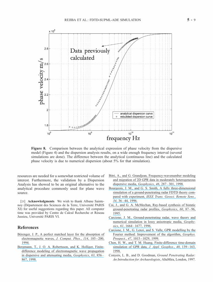
cerning pipes detection in distinct dispersive Debyemedia, for a constant offset acquisition (offset = 1 cm,spacing = 20 cm) with 100 MHz bistatic antennas(Figure 11). The TM mode simulation (point sourceEz) (Figure 12) is done on a 200 � 200 points domain(dx = dy = 10 cm) during 1000 � dt = 160 ns (dt = 0.16ns). A random distribution in material-2 is defined to adda realistic noise in the synthetic radargram.

1. The reflections are less marked in the material-3because the peak frequency is situated at a maximum ofthe imaginary part of the dielectric permittivity (Figure11), and arrive earlier because the real permittivity at thatfrequency is lower (Figure 11) than in material-4.2. Top and bottom reflections for the water filled

pipes are well distinguished thanks to a pronouncedcontrast of permittivity (the water acts like a low filterbecause the spatial discretization is no longer adapted forsuch a permittivity).3. The reflections on both interfaces between materi-

al-1/material-2 and material-2/material-3 or 4 are welldefined. Furthermore, we can see the slight separationbetween material-3 and 4, due to their respectivecharacteristic time.[23] That simulation had required 6h30 on CRAY SV1

supercomputer with four 300MHz CPUs.

7. Conclusion

[24] The FDTD-SUPML-ADE has shown to be welladapted to simulate GPR acquisition, even on highlyheterogeneous media. The possibilities for 3-D GPRsimulations are obvious, even if large computational

Figure 7. Angle difference f(w) calculated before Rdp evaluation. The range of frequency wherethe difference is calculated is determined thanks to the magnitude curve (Figure 6).

5 - 8 REJIBA ET AL.: FDTD-SUPML-ADE SIMULATION

resources are needed for a somewhat restricted volume ofinterest. Furthermore, the validation by a DispersionAnalysis has showed to be an original alternative to theanalytical procedure commonly used for plane wavesource.

[25] Acknowledgments We wish to thank Albane Sainte-noy (Departement des Sciences de la Terre, Universite PARISXI) for useful suggestions regarding this paper. All computertime was provided by Centre de Calcul Recherche et ReseauJussieu, Universite PARIS VI.

References

Berenger, J. P., A perfect matched layer for the absorption of

electromagnetic waves, J. Comput. Phys., 114, 185–200,

1994.

Bergmann, T., J. O. A. Robertsson, and K. Holliger, Finite-

difference modeling of electromagnetic wave propagation

in dispersive and attenuating media, Geophysics, 63, 856–

867, 1998.

Bitri, A., and G. Grandjean, Frequency-wavenumber modeling

and migration of 2D GPR data in moderately heterogeneous

dispersive media, Geophysics, 46, 287–301, 1998.

Bourgeois, J. M., and G. S. Smith, A fully three-dimensional

simulation of a ground-penetrating radar FDTD theory com-

pared with experiment, IEEE Trans. Geosci. Remote Sens.,

34, 36–44, 1996.

Cai, J., and G. A. McMechan, Ray-based synthesis of bistatic

ground-penetrating radar profiles, Geophysics, 60, 87–96,

1995.

Carcione, J. M., Ground-penetrating radar, wave theory and

numerical simulation in lossy anisotropic media, Geophy-

sics, 61, 1664–1677, 1996.

Carcione, J. M., G. Lenzi, and S. Valle, GPR modelling by the

Fourier method: Improvement of the algorithm, Geophys.

Prospect., 47, 1015–1029, 1999.

Chen, H. W., and T. M. Huang, Finite-difference time-domain

simulation of GPR data, J. Appl. Geophys., 40, 139–163,

1998.

Conyers, L. B., and D. Goodman, Ground Penetrating Radar:

An Introduction for Archaeologists, AltaMira, London, 1997.

Figure 8. Comparison between the analytical expression of phase velocity from the dispersivemodel (Figure 4) and the dispersion analysis results, on a wide enough frequency interval (severalsimulations are done). The difference between the analytical (continuous line) and the calculatedphase velocity is due to numerical dispersion (about 5% for that simulation).

REJIBA ET AL.: FDTD-SUPML-ADE SIMULATION 5 - 9

Gandhi, O. P., B. Q. Gao, and J. Y. Chen, A frequency depen-

dent finite difference time domain formulation for general

dispersive media, IEEE Trans. Microwave Theory Tech., 41,

792–797, 1993.

Gedney, S. D., An anisotropic PML absorbing media for the

FDTD simulation of fields in lossy and dispersive media,

Electromagnetic, 16, 399–415, 1996.

Grandjean, G., et al., Evaluation of GPR techniques for civil-

engineering applications: Study on a test site, J. Appl. Geo-

phys., 45, 141–156, 2000.

Gurel, L., and O. Ugur, Three-dimensional FDTD modeling of

a ground-penetrating radar, IEEE Trans. Geosci. Remote

Sens., 38, 1513–1521, 2000.

He, P., Measurement of acoustic dispersion using both trans-

mitted and reflected pulse, J. Acoust. Soc. Am., 107, 801–

807, 2000.

Figure 9. 225 MHz pulse Ekko radar 3-D acquisitionon a gravel wall buried in clay with 50 cm between theantennas and a spacing of 5 cm along each profile. Somesections are presented in order to situate the wall and wasused to build an equivalent model (Figure 10) from trialand errors forward modeling.

Figure 10. On top, the equivalent geometrical model(Top soil: e = 10, m = m0, s = 0.02 S/m, Clay: e = 16, m =m0, s = 0.1 S/m, Gravel wall: e = 2.25, m = m0, s = 0.005S/m). On bottom, the 3-D FDTD Unsplit PML simula-tion on two profiles, with a 225 MHz DFG Ey emitter-receiver. Model discretization dx = dy = dz = 2.5 cm, dt =40 ps.

5 - 10 REJIBA ET AL.: FDTD-SUPML-ADE SIMULATION

Hollender, F., and S. Tillard, Modeling ground-penetrating ra-

dar wave propagation and reflection with the Jonsher para-

meterization, Geophysics, 62, 1933–1942, 1998.

Katz, D. S., E. T. Thiele, and A. Taflove, Validation and exten-

sion to three dimensions of the Berenger PML absorbing

boundary condition for FD-TD meshes, IEEE Microwave

Guided Wave Lett., 4, 268–270, 1994.

Kelley, D. F., and R. J. Luebbers, Piecewise linear recursive

convolution for dispersive media using FDTD, IEEE Trans.

Antennas Propag., 44, 792–797, 1996.

Kunz, K. S., and R. J. Luebbers, The Finite Difference Time

Domain for Electromagnetic, CRC Press, Boca Raton, Fla.,

1993.

Luebbers, R. J., and F. Hunsberger, FDTD for N-th order dis-

persive media, IEEE Trans. Antennas Propag., 40, 1297–

1301, 1992.

Luebbers, R. J., F. Hunsberger, K. S. Katz, R. B. Standler, and

M. Schneider, A frequency-dependent finite-difference time-

domain formulation for dispersive materials, IEEE Trans.

Electromagn. Compat., 32, 222–227, 1990.

Lysne, P. C., A model for the high-frequency electrical response

of wet rocks, Geophysics, 48, 775–786, 1983.

Mari, J. L., F. Glangeaud, and F. Coppens, Traitement du signal

pour geologues et geophysiciens, editions technip, 460 pp.,

Inst. Fr. du Petrole, Rueil-Malmaison, France, 1997.

Mei, K. K., and J. Fang, Superabsorption—A method to im-

prove absorbing boundary conditions, IEEE Trans. Antennas

Propag., 40, 1001–1010, 1992.

Montoya, T. P., and G. S. Smith, Land mine detection using a

ground penetrating radar based on resistively loaded Vee di-

poles, IEEE Trans. Antennas Propag., 47, 1795–1806, 1999.

Mur, G., Absorbing boundary conditions for wave-like equa-

tions, IEEE Trans. Electromagn. Compat., 23, 377–382,

1981.

Powers, M. H., and G. R. Olhoeft, Modeling dispersive ground

penetrating radar data, paper presented at 5th International

Conference on Ground Penetrating Radar, Kitchener, Ont.,

Canada, 12–16 June 1994.

Qing Huo, L., and F. Guo-Xin, Simulations of GPR in disper-

sive media using a frequency dependant PSTD algorithm,

IEEE Trans. Geosci. Remote Sens., 37, 2317–2324, 1999.

Roberts, R. L., and J. J. Daniels, Modeling near-field GPR in

three dimensions using the FDTD method, Geophysics, 62,

1114–1126, 1997.

Figure 11. Debye model for material 3 and 4. For a 100 MHz peak frequency the equivalent soilproperties are: ereal = 2.5, eimaginary = 13 for material 3 (red line) and ereal = 0, eimaginary = 15 formaterial 4 (blue line).

REJIBA ET AL.: FDTD-SUPML-ADE SIMULATION 5 - 11

Sacks, Z. S., D. M. Kingsland, R. Lee, and J. F. Le, A perfectly

matched anisotropic absorber for use as an absorbing bound-

ary condition, IEEE Trans. Antennas Propag., 43, 1460–

1463, 1995.

Sullivan, D. M., Frequency-dependent FDTD metods using Z

transforms, IEEE Trans. Antennas Propag., 40, 1223–1230,

1992.

Sullivan, D. M., A simplified PML for use with the FDTD meth-

od, IEEE Microwave Guided Wave Lett., l6, 97–99, 1996.

Sullivan, D. M., An unsplit step 3D PML for use with the

FDTD method, IEEE Microwave Guided Wave Lett., 7,

184–186, 1997.

Tabbagh, A., The response of a three dimensionnal magnetic

and conductive body in shallow depth electromagnetic pro-

specting, Geophys. J. R. Astron. Soc., 81, 215–230, 1995.

Taflove, A., Computational Electromagnetic: The Finite Differ-

ence Time Domain Method, Artech House, Norwood, Mass.,

1995.

Figure 12. Model including several types of pipes used for 2-D, TM mode simulation. The sourceis a Ez 100 MHz DFG, (offset = 1 m, spacing = 5 cm). Model discretization: dx = dy = 2 cm, dt =33 ps.

5 - 12 REJIBA ET AL.: FDTD-SUPML-ADE SIMULATION

Teixeira, F. L., W. C. Chew, M. Straka, M. L. Oristaglio, and

T. Wang, Finite difference time domain simulation of ground

penetrating radar on dispersive, inhomogeneous and conduc-

tive soils, IEEE Trans. Geosci. Remote Sens., 36, 1928–

1937, 1998.

Vitebsky, S., L. Carin, M. A. Ressler, and F. H. Le, Ultra-wide-

band, short-pulse ground penetrating radar: Simulation and

measurement, IEEE Trans. Geosci. Remote Sens., 35, 762–

772, 1997.

Wang, T., and A. C. Tripp, FDTD simulation of EM wave

propagation in 3-D media, Geophysics, 61, 1097–1106,

1996.

Xu, T., and G. A. McMechan, GPR attenuation and its numer-

ical simulation in 2.5D dimensions, Geophysics, 62, 403–

414, 1997.

Yee, K. S., Numerical solution of initial boundary value pro-

blems involving Maxwell’s equation in isotropic media,

IEEE Trans. Antennas Propag., 14, 302–307, 1966.

������������C. Camerlynck, P. Mechler, and F. Rejiba, Department of

Applied Geophysics, Universite Pierre et Marie Curie, UMR

7619, Sisyphe, CNRS, Case 105, 4 Pl. Jussieu, 75252 Paris

Cedex 05, France. (rejiba@ccr.jussieu.fr)

REJIBA ET AL.: FDTD-SUPML-ADE SIMULATION 5 - 13