FCC unit modeling, identification and model predictive control, a simulation study

FCC unit modeling, identification and model predictive control, asimulation study

Chunyang Jia, Sohrab Rohani �, Arthur Jutan

Department of Chemical and Biochemical Engineering, The University of Western Ontario, London, Ont., Canada N6A 5B9

Received 15 July 2001; received in revised form 23 April 2002; accepted 23 April 2002

Abstract

The fluid catalytic cracking unit (FCCU) has a major effect on profitability of an oil refinery. The FCCU is difficult to model well,

due to significant nonlinearities and interactions. Control of the FCC is challenging and there is strong incentive to use multivariable

(MV) control schemes, such as model predictive control (MPC), which accommodate these interactions. The linear MV schemes rely

on linearized model around an operating point and therefore, it is difficult to obtain high quality control. This paper uses a singular

value decomposition method (N4SID) to obtain a state space model which is then reduced to a step model required by the MPC

algorithm. Simulations on a detailed model [Chem. Eng. Comm. 146 (1996) 163; Trans. IchemE 75 (1997) 401; A modified

integrated dynamic model of a riser type FCC unit, Master’s Thesis, University of Saskatchewan, Saskatoon (1998); Can. J. Chem.

Eng. 77 (1999) 169] show the effectiveness of this approach.

# 2002 Elsevier Science B.V. All rights reserved.

Keywords: Fluid catalytic cracking; Model predictive control; Matlab† simulation; Subspace process identification

1. Introduction

A fluidized catalytic cracking unit (FCCU) consists of

reactor-regenerator, riser reactor, main fractionator,

absorber�/stripper�/stabilizer, main air blower, wet gas

compressor, etc. The FCCU converts heavy oil into a

range of hydrocarbon products, including LPG, fuel

gas, gasoline, light diesel, aviation kerosene, slurry oil,

among which high octane number gasoline is most

valuable. But their values are all market driven, so it is

one of the control goals to maximize the production of

one or more products in different seasons. Since the

catalyst circulates through a closed loop consisting of

riser, regenerator and reactor, these three main parts are

of particular interests both in industrial and research

circles. Numerous papers have been published concern-

ing different modeling approaches and control strategies

for the FCC process, which deal with the strong

interactions and many constraints from the operating,

security and environmental point of view. The potential

of yielding more market-oriented oil products, increas-

ing production rate and stabilizing the operation

become the major incentives to search for more accurate

and practical models, high performance, and cost

effective and flexible control strategies.The methodology of model predictive control (MPC)

originated in the oil industry in the 1970s. Using a step

or impulse response model, the future dynamic response

of a process can be predicted. This prediction is

compared with a desired trajectory and by minimization

of a control objective, a manipulated variable move is

calculated to smoothly follow this trajectory while

taking into account the constraints of both the manipu-

lated and control variables. The MPC can be used for

processes with inverse response and is robust to model-

ing and measurement errors.

But progressing from theory to practice has never

been straightforward. Many petrochemical industries

have purchased commercially available MPC software

packages, but few of them have achieved the expected

economic gain. This can be attributed to different

factors. For example, imprecise process model structure,

poor data collection, improperly defined control objec-� Corresponding author. Tel.: �/519-661-4116; fax: �/519-661–3498

E-mail address: [email protected] (S. Rohani).

Chemical Engineering and Processing 42 (2003) 311�/325

www.elsevier.com/locate/cep

0255-2701/02/$ - see front matter # 2002 Elsevier Science B.V. All rights reserved.

PII: S 0 2 5 5 - 2 7 0 1 ( 0 2 ) 0 0 0 5 5 - 7

mailto:[email protected]

tives, etc. In the following paragraphs, we discuss the

simulation study of modeling and the MPC control for a

typical FCC unit.

Most of the FCC studies are based on empirical or

semi-empirical models. Such models conform quite well

the real industrial process over a small operating range.

But when the operating conditions change, their validity

can fail. Many of these models do not describe

important variables variations like pressure effects [1,2]

and use oversimplified kinetics [3�/5]. In most published

papers, the largest discrepancies appear in the modeling

of the dense bed in the regenerator. Though the

bubbling bed model of Kunii and Levenspiel [6] is often

used, due to the complexities of the proposed ap-

proaches and some lack of information, the degree of

refinement of the regenerator model very much differs

according to the authors [7,8]. There is even, disagree-

ment on the necessity of taking into account the spatial

character of the bubble phase in the dense bed [9]

though this is more realistic and considered by the more

detailed studies like McFarlane et al. [10]. The freeboard

over the dense bed is not often considered in the

modeling. Of course, these variations concerning the

FCC models have strong implications concerning the

frequently related instability issues [11�/13,7,8]. On the

other hand, a full model like the one proposed by Han

and Chung [14] probably incorporates too much com-

plexity for the objective of control studies. In particular,

partial differential equations are not always necessary

when time scales are of largely varying orders. Thus, an

adequately reduced model is crucial to meet the

objective.

A reliable model of moderate complexity model has

been proposed by Rohani and co-workers [26�/28]. A

four-lump reaction scheme [15] is used for the riser

reactions, the bubbling bed Kunii�/Levenspiel [6] for the

regenerator with ordinary differential equations for the

dense phase and spatial effects for the gaseous species in

the bubble phase, and the pressure effects have been

incorporated. The final model uses a minimum amount

of empirical expressions and retains the dominant

dynamic characteristics of the unit. This paper takes

advantage of this model and carries the study a step

further in the direction of advanced control of this

process. The simulation is conducted in the Matlab†/

Simulink† environment [16,17]. The simulation proce-

dure involves the following four major steps:

1) FCC model development in Matlab† programming

language.

2) Dynamic open loop simulations and process dataacquisition.

3) Offline model identification.

4) Real time closed loop MPC simulation in

Simulink† with an S-function as an FCC model

plant.

2. Model development of an FCC unit in MATLAB†

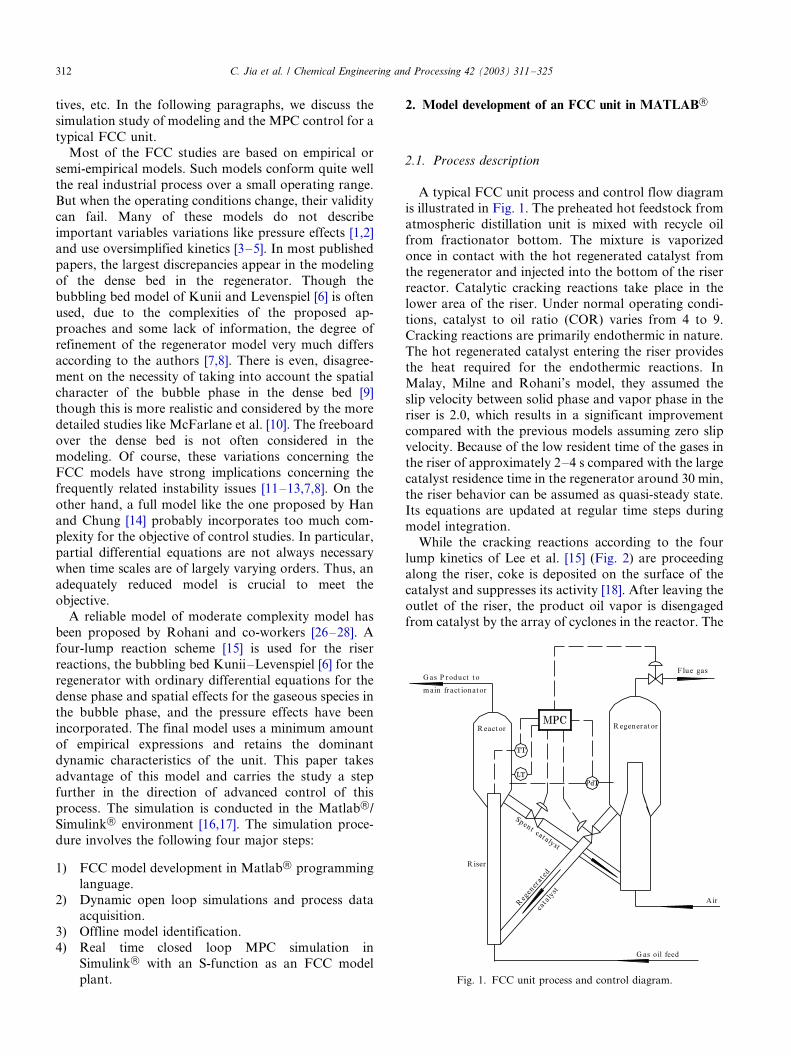
2.1. Process description

A typical FCC unit process and control flow diagram

is illustrated in Fig. 1. The preheated hot feedstock from

atmospheric distillation unit is mixed with recycle oil

from fractionator bottom. The mixture is vaporized

once in contact with the hot regenerated catalyst from

the regenerator and injected into the bottom of the riser

reactor. Catalytic cracking reactions take place in the

lower area of the riser. Under normal operating condi-

tions, catalyst to oil ratio (COR) varies from 4 to 9.

Cracking reactions are primarily endothermic in nature.

The hot regenerated catalyst entering the riser provides

the heat required for the endothermic reactions. In

Malay, Milne and Rohani’s model, they assumed the

slip velocity between solid phase and vapor phase in the

riser is 2.0, which results in a significant improvement

compared with the previous models assuming zero slipvelocity. Because of the low resident time of the gases in

the riser of approximately 2�/4 s compared with the large

catalyst residence time in the regenerator around 30 min,

the riser behavior can be assumed as quasi-steady state.

Its equations are updated at regular time steps during

model integration.

While the cracking reactions according to the four

lump kinetics of Lee et al. [15] (Fig. 2) are proceeding

along the riser, coke is deposited on the surface of the

catalyst and suppresses its activity [18]. After leaving the

outlet of the riser, the product oil vapor is disengaged

from catalyst by the array of cyclones in the reactor. The

Fig. 1. FCC unit process and control diagram.

C. Jia et al. / Chemical Engineering and Processing 42 (2003) 311�/325312

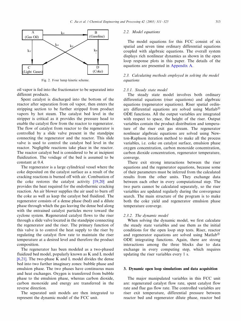
oil vapor is fed into the fractionator to be separated into

different products.

Spent catalyst is discharged into the bottom of the

reactor after separation from oil vapor, then enters the

stripping section to be further stripped from product

vapors by hot steam. The catalyst bed level in the

stripper is critical as it provides the pressure head to

enable the catalyst flow from the reactor to regenerator.

The flow of catalyst from reactor to the regenerator is

controlled by a slide valve present in the standpipe

connecting the regenerator and the reactor. This slide

valve is used to control the catalyst bed level in the

reactor. Negligible reactions take place in the reactor.

The reactor catalyst bed is considered to be at incipient

fluidization. The voidage of the bed is assumed to be

constant at 0.4.

The regenerator is a large cylindrical vessel where the

coke deposited on the catalyst surface as a result of the

cracking reactions is burned off with air. Combustion of

the coke restores the catalyst activity [19,20] and

provides the heat required for the endothermic cracking

reaction. An air blower supplies the air used to burn off

the coke as well as keep the catalyst bed fluidized. The

regenerator consists of a dense phase (bed) and a dilute

phase through which the gas leaving the dense bed along

with the entrained catalyst particles move toward the

cyclone system. Regenerated catalyst flows to the riser

through a slide valve located in the standpipe connecting

the regenerator and the riser. The primary function of

this valve is to control the heat supply to the riser by

regulating the catalyst flow rate to maintain the riser

temperature at a desired level and therefore the product

composition.

The regenerator has been modeled as a two-phased

fluidized bed model, popularly known as K and L model

[6,21]. The two-phase K and L model divides the dense

bed into two further imaginary zones: bubble phase and

emulsion phase. The two phases have continuous mass

and heat exchanges. Oxygen is transferred from bubble

phase to the emulsion phase, whereas carbon dioxide,

carbon monoxide and energy are transferred in the

reverse direction.

The separated unit models are then integrated to

represent the dynamic model of the FCC unit.

2.2. Model equations

The model equations for this FCC consist of six

spatial and seven time ordinary differential equationscoupled with algebraic equations. The overall system

displays rich nonlinear dynamics as shown in the open

loop response plots in this paper. The details of the

equations are presented in Appendix A.

2.3. Calculating methods employed in solving the model

equations

2.3.1. Steady state model

The steady state model involves both ordinary

differential equations (riser equations) and algebraic

equations (regenerator equations). Riser spatial ordin-

ary differential equations are solved using Matlab†

ODE functions. All the output variables are integrated

with respect to space, the height of the riser. Output

variables contain the product distribution and tempera-

ture of the riser exit gas stream. The regeneratornonlinear algebraic equations are solved using New-

ton-Raphson iteration method to make all the process

variables, i.e. coke on catalyst surface, emulsion phase

oxygen concentration, carbon monoxide concentration,

carbon dioxide concentration, regenerator temperature,

converge.

There exit strong interactions between the riser

equations and the regenerator equations, because someof their parameters must be inferred from the calculated

results from the other units. They exchange data

between each other in every computational step. The

two parts cannot be calculated separately, so the riser

variables are updated regularly during the convergence

search. The main structure of the program is to make

both the coke yield and regenerator emulsion phase

temperature converge.

2.3.2. The dynamic model

When solving the dynamic model, we first calculate

the steady state variables and use them as the initial

conditions for the open loop step tests. Riser, reactor

and regenerator equations are solved using Matlab†

ODE integrating functions. Again, there are strong

interactions among the three blocks due to dataexchange in every computing step, which requires

updating the riser variables every 1 s.

3. Dynamic open loop simulations and data acquisition

The major manipulated variables in this FCC unit

are: regenerated catalyst flow rate, spent catalyst flowrate and flue gas flow rate. The controlled variables are

riser exit temperature, differential pressure between

reactor bed and regenerator dilute phase, reactor bed

Fig. 2. Four lump kinetic scheme.

C. Jia et al. / Chemical Engineering and Processing 42 (2003) 311�/325 313

level. The feed oil flow rate and air flow rate are selected

as disturbances. Though many combinations for ma-

nipulated and controlled variables are possible [22], this

control scheme is consistent with most of the industrial

FCC units [23]. We can add other manipulated variables

(MVs) and controlled variables (CVs) to the MPC

control scheme according to a specific industrial prac-

tice.

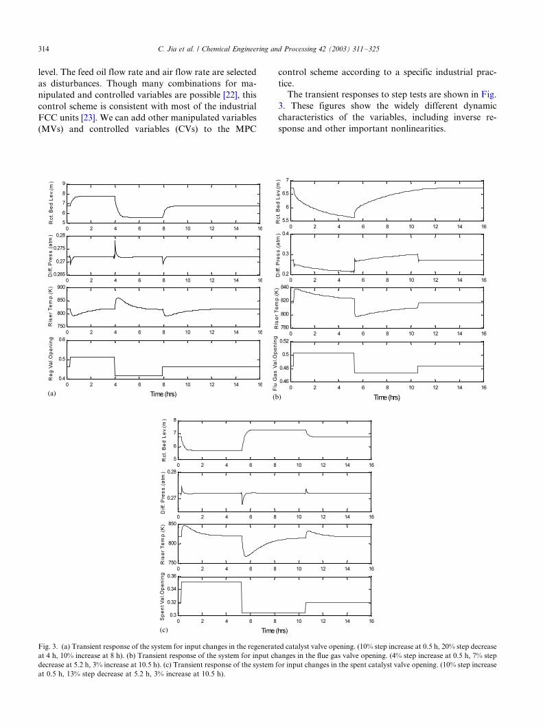
The transient responses to step tests are shown in Fig.

3. These figures show the widely different dynamic

characteristics of the variables, including inverse re-

sponse and other important nonlinearities.

Fig. 3. (a) Transient response of the system for input changes in the regenerated catalyst valve opening. (10% step increase at 0.5 h, 20% step decrease

at 4 h, 10% increase at 8 h). (b) Transient response of the system for input changes in the flue gas valve opening. (4% step increase at 0.5 h, 7% step

decrease at 5.2 h, 3% increase at 10.5 h). (c) Transient response of the system for input changes in the spent catalyst valve opening. (10% step increase

at 0.5 h, 13% step decrease at 5.2 h, 3% increase at 10.5 h).


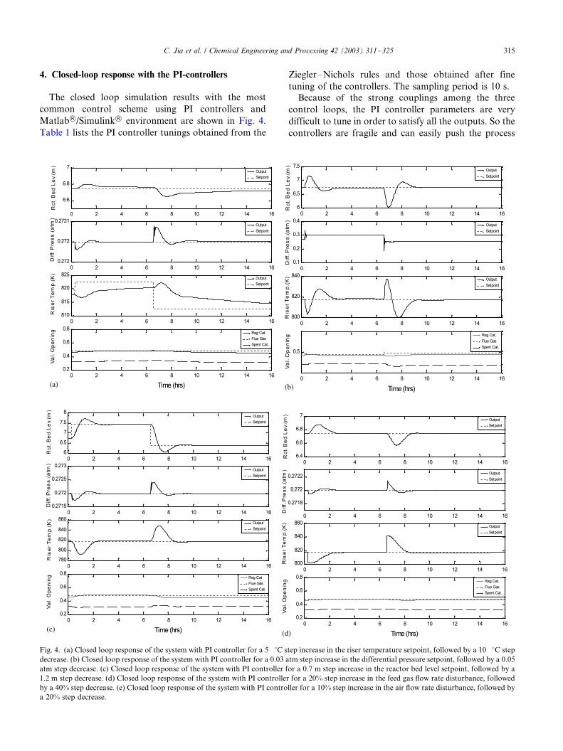
4. Closed-loop response with the PI-controllers

The closed loop simulation results with the most

common control scheme using PI controllers and

Matlab†/Simulink† environment are shown in Fig. 4.

Table 1 lists the PI controller tunings obtained from the

Ziegler�/Nichols rules and those obtained after fine

tuning of the controllers. The sampling period is 10 s.

Because of the strong couplings among the three

control loops, the PI controller parameters are very

difficult to tune in order to satisfy all the outputs. So the

controllers are fragile and can easily push the process

Fig. 4. (a) Closed loop response of the system with PI controller for a 5 8C step increase in the riser temperature setpoint, followed by a 10 8C step

decrease. (b) Closed loop response of the system with PI controller for a 0.03 atm step increase in the differential pressure setpoint, followed by a 0.05

atm step decrease. (c) Closed loop response of the system with PI controller for a 0.7 m step increase in the reactor bed level setpoint, followed by a

1.2 m step decrease. (d) Closed loop response of the system with PI controller for a 20% step increase in the feed gas flow rate disturbance, followed

by a 40% step decrease. (e) Closed loop response of the system with PI controller for a 10% step increase in the air flow rate disturbance, followed by

a 20% step decrease.


into total failure if they are not appropriately tuned.

Moreover, the responses indicate that the temperaturecontroller and bed level controller are not able to bring

these variables to their desired setpoints in some

circumstances despite the integral action. Therefore,

there is a strong incentive for a more advanced multi-

variable controller which is able to handle the strong

couplings and non-linearity inherent in the process

dynamics.

5. Offline model identification

5.1. General description

The MPC control strategy needs a model which is

used to predict the next process move and hence the

appropriate control actions to drive the process output

toward the setpoint in a satisfactory, fast and smoothmanner. However, extracting information from process

output data is not an entirely straightforward task. The

data may need to be handled carefully, and decisions

have to be made for model structure selection and

validation.

When the data are collected from a physical plant,

they are typically measured in physical units. The

magnitude of these raw inputs and outputs may not be

consistent. This will force the models to waste some

parameters correcting the levels. Therefore, it is a good

practice to subtract the mean levels from the input and

output sequences before the estimation. Depending

upon the application, interest in the model can be

focused on specific frequency bands. Filtering the data

before the estimation, through filters that enhance these

bands, improves the fit in the regions of interest.

The identification process amounts to repeatedly

selecting a model structure, computing the best model

structure, and evaluating the model properties to see if

they are satisfactory. The cycle can be itemized as

follows:

1) Design an experiment and collect input�/output

data from the process to be identified.

2) Examine the data. Polish it so as to remove trends

and outliers, select useful portions of the original

data, and apply filtering to enhance important

frequency ranges.

3) Select and define a model structure (a set of

candidate system descriptions) within which a

model is to be found.4) Compute the best model in the model structure

according to the input�/output data and a given

criterion of fit.

5) Examine the obtained model properties.

Fig. 4 (Continued)

Table 1

PI controller parameters

Controller loops Riser

temperature

Differential

pressure

Reactor

level

Ziegler�/Nichols KC 0.0052 �0.618 �0.49

t1 10.15 0.0067 0.21

Fine tuned KC 0.0019 �0.28 �0.1

t1 1.7 0.014 0.18


6) If the model is good enough quantitatively, then

stop; otherwise go back to Step 3 to try another

model set. Possibly also try other estimation meth-

ods (Step 4) or work further on the input-outputdata (Step 1 and 2).

5.2. Subspace methods and N4SID algorithm

In a common implementation of the MPC, therequired step models are obtained from plant step tests.

This approach is suitable for simple dynamics under low

noise conditions. We tried this approach and found that

only poor models emerged. This was due partly to the

severe nonlinearities in the system, but also the coupled

nature of the dynamics was hard to capture. Subspace

methods are more robust and can be used to capture the

true multivariable nature of the system and producebetter results. The N4SID [24] is briefly discussed as

follows.

The discrete time state space representation of a

MIMO system is given by:

x(k�1)�Ax(k)�Bu(k)

y(k)�Cx(k)�Du(k) (1)

where the dimension of the state x is n , dimension of y is

p , and dimension of u is m .

The subspace identification can be used to efficiently

identify the unknown description matrices A, B, C, D

and state sequence x(k ) using only the input and output

data u(k ) and y(k ).The approach is to express the input and output data

and states in an expanded space, that is:

Y�

y(0) y(1) � � � y(N�1)y(1) y(2) � � � y(N)

n n ::: ny(M�1) y(M) � � � y(N�M�2)

2664

3775 (2)

U�

u(0) u(1) � � � u(N�1)

u(1) u(2) � � � u(N)

n n ::: nu(M�1) u(M) � � � u(N�M�2)

2664

3775 (3)

X� [x(0) x(1) � � � x(N�1)] (4)

where U and Y are input and output block Hankel

matrices; N is the length of the input and output; and M

is larger than the actual space dimension n , but much

smaller than the data length N . This guarantees that the

matrices contain the state description.

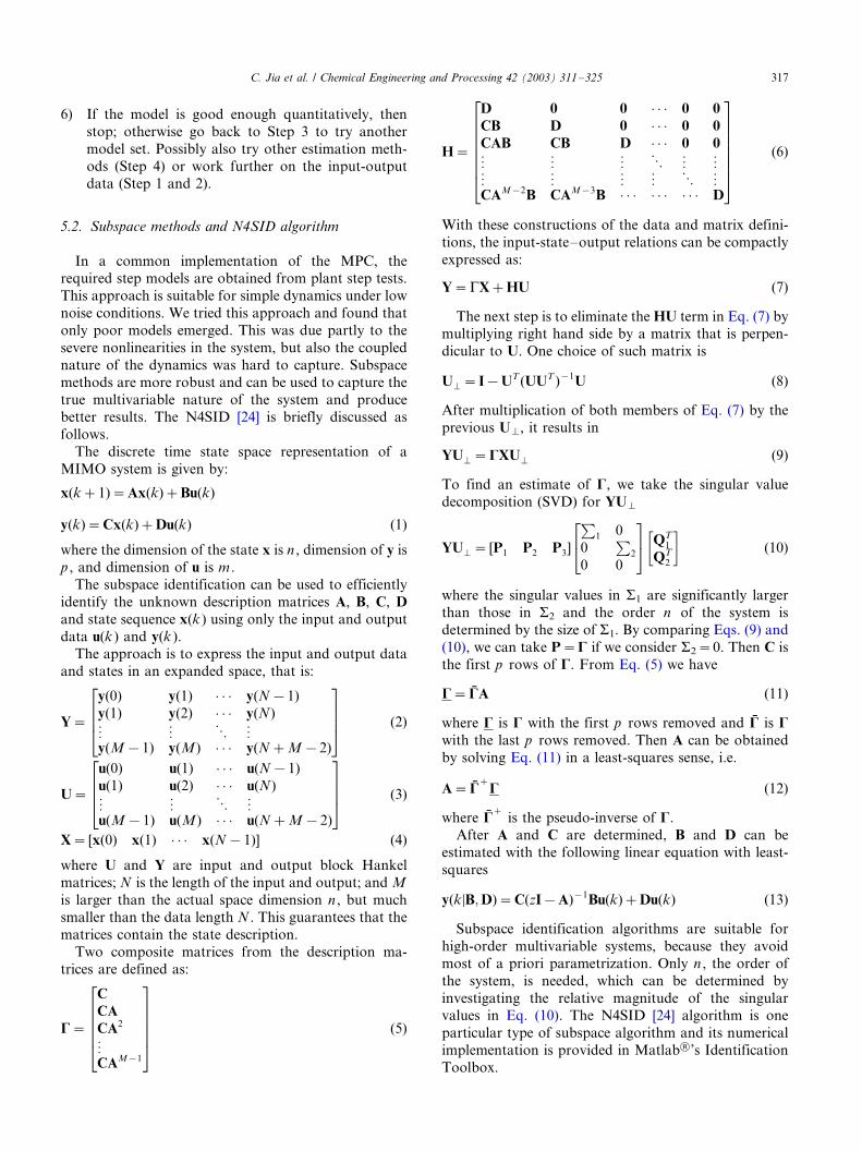
Two composite matrices from the description ma-trices are defined as:

G�

CCA

CA2

nCAM�1

266664

377775 (5)

H�

D 0 0 � � � 0 0

CB D 0 � � � 0 0

CAB CB D � � � 0 0

n n n ::: n nn n n n ::: nCAM�2B CAM�3B � � � � � � � � � D

26666664

37777775

(6)

With these constructions of the data and matrix defini-

tions, the input-state�/output relations can be compactly

expressed as:

Y�GX�HU (7)

The next step is to eliminate the HU term in Eq. (7) bymultiplying right hand side by a matrix that is perpen-

dicular to U. One choice of such matrix is

U��I�UT (UUT )�1U (8)

After multiplication of both members of Eq. (7) by the

previous U�, it results in

YU��GXU� (9)

To find an estimate of G, we take the singular value

decomposition (SVD) for YU�

YU�� [P1 P2 P3]

P1 0

0P

2

0 0

24

35 QT

1

QT2

� (10)

where the singular values in S1 are significantly larger

than those in S2 and the order n of the system is

determined by the size of S1. By comparing Eqs. (9) and

(10), we can take P�/G if we consider S2�/0. Then C is

the first p rows of G. From Eq. (5) we have

G�GA (11)

where G is G with the first p rows removed and G is G

with the last p rows removed. Then A can be obtained

by solving Eq. (11) in a least-squares sense, i.e.

A�G�

G (12)

where G�

is the pseudo-inverse of G.After A and C are determined, B and D can be

estimated with the following linear equation with least-

squares

y(k½B;D)�C(zI�A)�1Bu(k)�Du(k) (13)

Subspace identification algorithms are suitable for

high-order multivariable systems, because they avoid

most of a priori parametrization. Only n , the order of

the system, is needed, which can be determined by

investigating the relative magnitude of the singularvalues in Eq. (10). The N4SID [24] algorithm is one

particular type of subspace algorithm and its numerical

implementation is provided in Matlab†’s Identification

Toolbox.


5.3. Offline model identification procedures

If the inputs are not a white noise, a whitening

polynomial L (z ) can be determined, so that the filteredsequence

UF (t)�L(z)u(t) (14)

is approximately white, the output sequence needs to be

filtered through the same filter.

Based on the filtered data, the input covariance

function is

Ru(t)�E[u(t�t)u(t)]�l if t�0

0 t"0

(15)

Then the cross covariance function between the input

and the output is:

Ryu(t)�E[y(t�t)u(t)]�lg(t) (16)

where g (t) is the impulse response of the system that can

be estimated as:

g(t)�1

lN

XN

t�1

y(t�t)u(t) (17)

through the N4SID method. Then the system transfer

function G (z )can be obtained as:

G(z)u(t)�X�R�1

g(k)u(t�k) (18)

G(z)�X�k�1

g(k)z�k (19)

Every single-input�/single-output model should be

identified separately and then combined to render the

overall process model. Model validation should be

followed by adjustment of the model orders and other

parameters through iteration.

6. Model predictive control simulation

Once a state space model has been obtained andverified as above, it can be converted to a step response

format required by the MPC algorithm [25]. The MPC

strategy is well known, so only a statement of the main

objective is given here.

For any assumed set of present and future control

moves/Du(k); Du(k�1); . . . ; Du(k�m�1) the future

behavior of the process outputs y(k�/1jk ), y(k�/

2jk ),. . ., y(k�/p jk ) can be predicted over a horizon p .The m present and future control moves m 5/p are

computed to minimize a quadratic objective function of

the form:

minXp

l�1

½½Gyl [y(k�1½k)�r(k�1)]½½2�

Xm

l�1

½½Gul [Du(k� l�1)]½½2

Du(k) . . .Du(k�m�1)

(20)

Here Gyl and Gu

l are weighting matrices to penalize

particular components of y and u at certain future time

intervals, and r(k�/l ) is the vector of future referencevalues (setpoints). For the MPC, in general, decreasing

m relative to p makes the control action less aggressive

and tends to stabilize the system. Gul is used as a tuning

parameter. Increasing Gul always has the effect of

making the control action less aggressive.

6.1. Control problem formulation

The open loop system is modeled as follows:

y�Gu�Gdd (21)

where; u� [Fsreg Ffg Fsrct]T ; (22)

y� [Tris DP Lrct]T (23)

d� [Fgas Fair]T (24)

G is the plant model and Gd is the disturbance model.

The control objective is to maintain the controlled

variables at predetermined setpoints in the presence of

typical process disturbances while maintaining safe

plant operation, restricting the magnitude per step of

the regenerated and spent catalyst slide valves and flue

gas butterfly valve stem movements.

6.2. Closed loop simulation with the MPC

The closed loop simulation was run in Simulink† with

a nonlinear multivariable model predictive controller

and the identified linear model according to the MPC

step format and a nonlinear plant represented by a

Simulink† S-function. Many simulations were carried

out and only a representative sample is presented here:

Process sampling interval: Dt�/1s ,

Output weights: Gy �/ywt�/[1 1 1],

Input weights: Gu�/uwt�/[0 0 0],Input constraints: 05/ui 5/100%, Dui 5/0.1, i�/1, 2,

3.

Because the system is strongly nonlinear, with rapid

variations of some variables with time, if the sampling

interval is set too long, the process will be out of control

for a long time interval. In this simulation experiment,

most of the computation time is consumed in calculating

the plant model (S-function), as opposed to the calcula-

tion of the control algorithm. In an industrial situation,the sampling interval of a distributed control system

(DCS) is often set to less than 1 s. The input weights

were chosen as zero to provide more aggressive control.


This could be changed for a real process. Usually the

regulatory control system and the emergency shutdown

system are independent. So the slow response of a

control action does not imply that safety valves cannotbe shut down instantaneously in an emergency situation.

The control runs performed consisted of the following

steps:

6.2.1. Servo control

Increase the riser exit temperature setpoint by square

pulse changes from steady state value of 818�/840 K,

then drop it to 790 K, and finally back to 818 K.

Increase the differential pressure from steady state

0.272�/0.35 atm, then decrease it to 0.24 atm, and back

to 0.272 atm.

Increase the reactor bed level from steady state 6.74�/

7.5 m, then drop it to 6 m, and back to 6.74 m.

Increase or decrease all the controlled variables

randomly and simultaneously from their steady state

to different values and back to the initial steady state.

6.2.2. Disturbance rejection control

Increase the gas oil flow rate by 20% of its initial value

then decrease it by 40% then back to its initial value.

Increase air flow rate by 10% of its initial value then

decrease it by 20% then back to its initial value.

Increase both of disturbances by 20 and 5% of their

initial values, then decrease them by 40 and 10% thenback to their initial values.

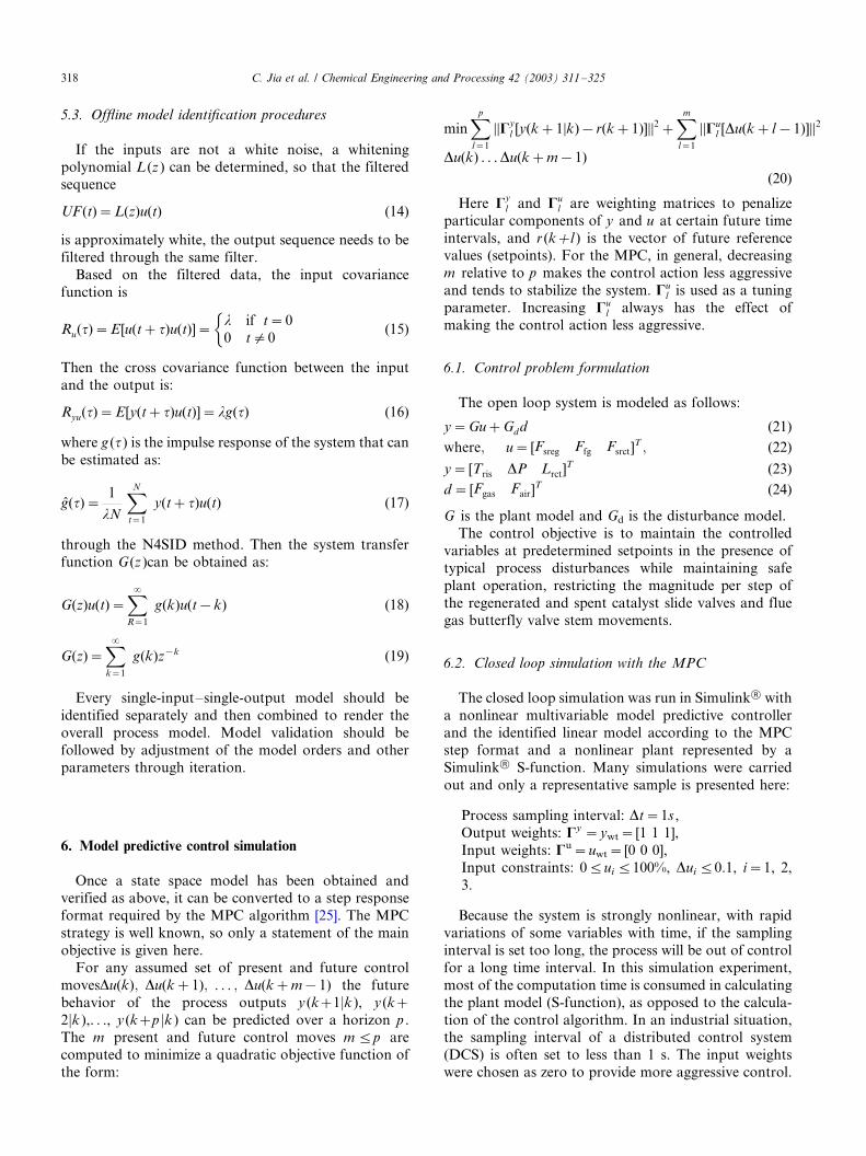
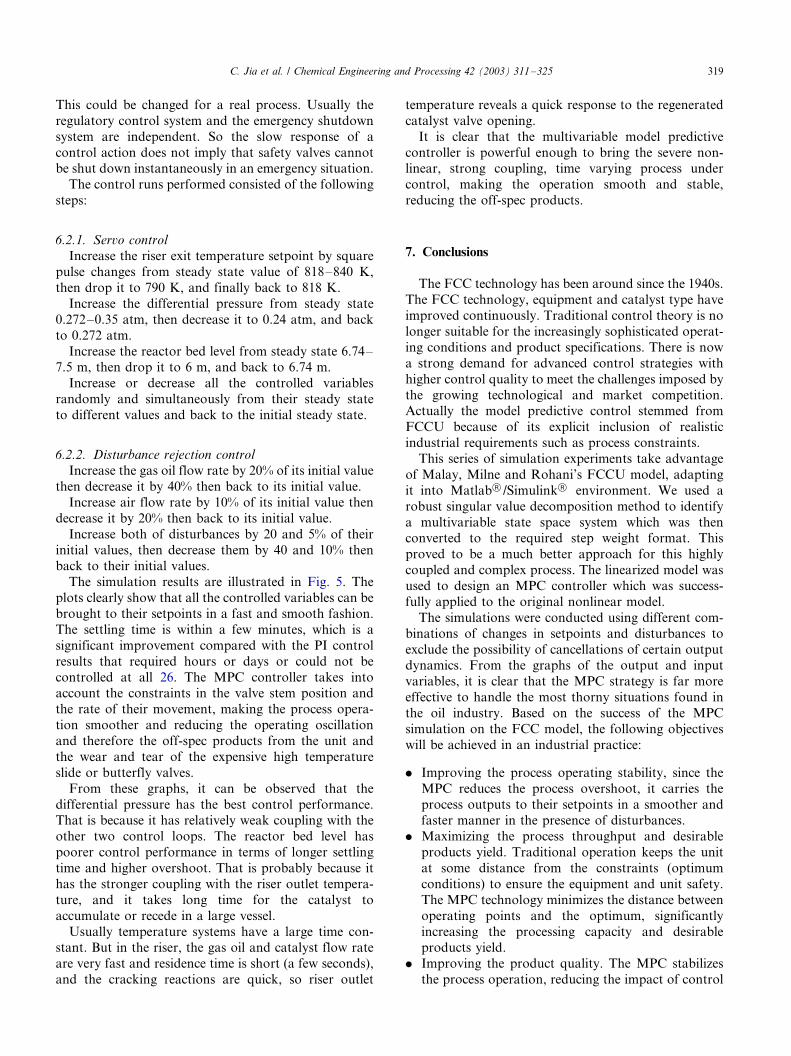
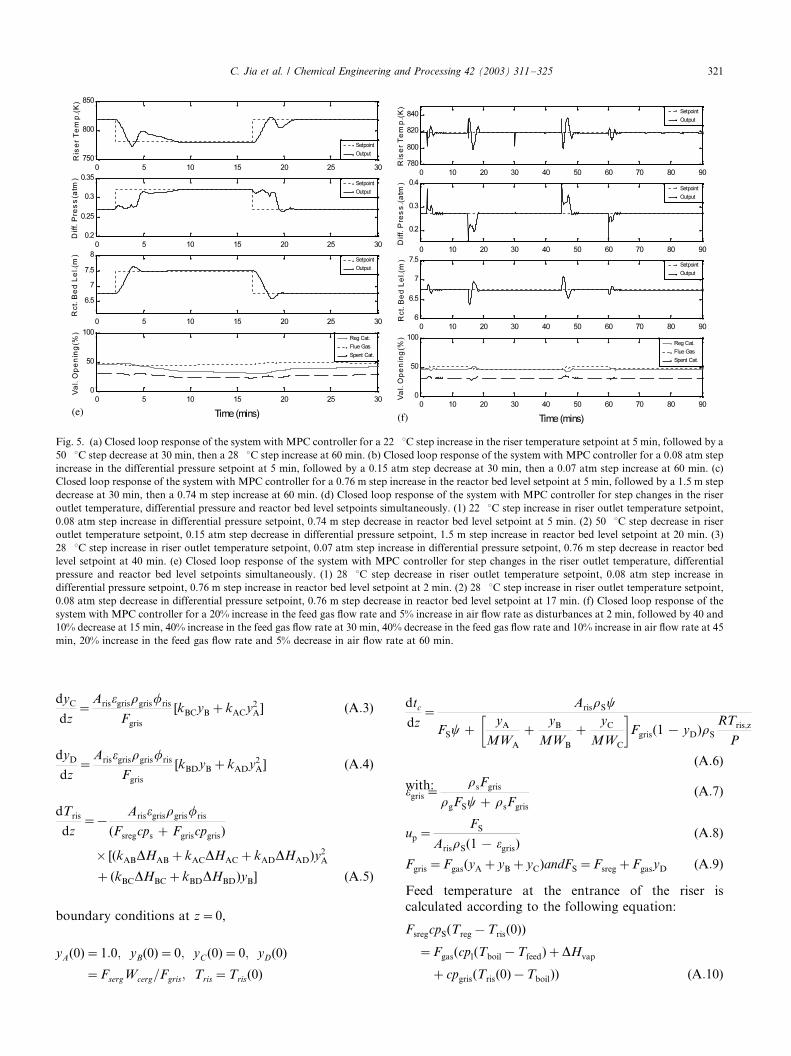
The simulation results are illustrated in Fig. 5. The

plots clearly show that all the controlled variables can be

brought to their setpoints in a fast and smooth fashion.

The settling time is within a few minutes, which is a

significant improvement compared with the PI control

results that required hours or days or could not be

controlled at all 26. The MPC controller takes intoaccount the constraints in the valve stem position and

the rate of their movement, making the process opera-

tion smoother and reducing the operating oscillation

and therefore the off-spec products from the unit and

the wear and tear of the expensive high temperature

slide or butterfly valves.

From these graphs, it can be observed that the

differential pressure has the best control performance.That is because it has relatively weak coupling with the

other two control loops. The reactor bed level has

poorer control performance in terms of longer settling

time and higher overshoot. That is probably because it

has the stronger coupling with the riser outlet tempera-

ture, and it takes long time for the catalyst to

accumulate or recede in a large vessel.

Usually temperature systems have a large time con-stant. But in the riser, the gas oil and catalyst flow rate

are very fast and residence time is short (a few seconds),

and the cracking reactions are quick, so riser outlet

temperature reveals a quick response to the regenerated

catalyst valve opening.

It is clear that the multivariable model predictive

controller is powerful enough to bring the severe non-linear, strong coupling, time varying process under

control, making the operation smooth and stable,

reducing the off-spec products.

7. Conclusions

The FCC technology has been around since the 1940s.

The FCC technology, equipment and catalyst type have

improved continuously. Traditional control theory is no

longer suitable for the increasingly sophisticated operat-

ing conditions and product specifications. There is now

a strong demand for advanced control strategies with

higher control quality to meet the challenges imposed by

the growing technological and market competition.Actually the model predictive control stemmed from

FCCU because of its explicit inclusion of realistic

industrial requirements such as process constraints.

This series of simulation experiments take advantage

of Malay, Milne and Rohani’s FCCU model, adapting

it into Matlab† /Simulink† environment. We used a

robust singular value decomposition method to identify

a multivariable state space system which was thenconverted to the required step weight format. This

proved to be a much better approach for this highly

coupled and complex process. The linearized model was

used to design an MPC controller which was success-

fully applied to the original nonlinear model.

The simulations were conducted using different com-

binations of changes in setpoints and disturbances to

exclude the possibility of cancellations of certain outputdynamics. From the graphs of the output and input

variables, it is clear that the MPC strategy is far more

effective to handle the most thorny situations found in

the oil industry. Based on the success of the MPC

simulation on the FCC model, the following objectives

will be achieved in an industrial practice:

. Improving the process operating stability, since the

MPC reduces the process overshoot, it carries the

process outputs to their setpoints in a smoother andfaster manner in the presence of disturbances.

. Maximizing the process throughput and desirable

products yield. Traditional operation keeps the unit

at some distance from the constraints (optimum

conditions) to ensure the equipment and unit safety.

The MPC technology minimizes the distance between

operating points and the optimum, significantly

increasing the processing capacity and desirableproducts yield.

. Improving the product quality. The MPC stabilizes

the process operation, reducing the impact of control


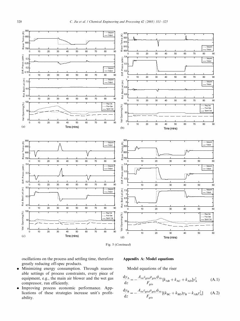
oscillations on the process and settling time, therefore

greatly reducing off-spec products.

. Minimizing energy consumption. Through reason-

able settings of process constraints, every piece of

equipment, e.g., the main air blower and the wet gas

compressor, run efficiently.

. Improving process economic performance. App-

lications of these strategies increase unit’s profit-

ability.

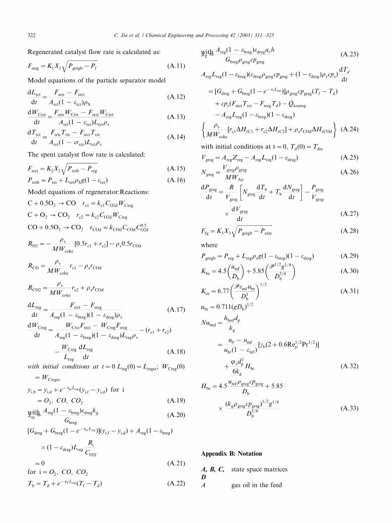
Appendix A: Model equations

Model equations of the riser

dyA

dz��

Arisogrisrgrisfris

Fgris

[kAB�kAC�kAD]y2A (A:1)

dyB

dz��

Arisogrisrgrisfris

Fgris

[(kBC�kBD)yB�kABy2A] (A:2)

Fig. 5 (Continued)


dyC

dz�

Arisogrisrgrisfris

Fgris

[kBCyB�kACy2A] (A:3)

dyD

dz�

Arisogrisrgrisfris

Fgris

[kBDyB�kADy2A] (A:4)

dTris

dz��

Arisogrisrgrisfris

(Fsregcps � Fgriscpgris)

� [(kABDHAB�kACDHAC�kADDHAD)y2A

�(kBCDHBC�kBDDHBD)yB] (A:5)

boundary conditions at z�/0,

yA(0)�1:0; yB(0)�0; yC(0)�0; yD(0)

�FsergWcerg=Fgris; Tris�Tris(0)

dtc

dz�

ArisrSc

FSc��

yA

MWA

�yB

MWB

�yC

MWC

Fgris(1 � yD)rS

RTris;z

P

(A:6)

with:ogris�rsFgris

rgFSc� rsFgris

(A:7)

up�FS

ArisrS(1 � ogris)(A:8)

Fgris�Fgas(yA�yB�yC)andFS�Fsreg�FgasyD (A:9)

Feed temperature at the entrance of the riser is

calculated according to the following equation:

FsregcpS(Treg�Tris(0))

�Fgas(cpl(Tboil�Tfeed)�DHvap

�cpgris(Tris(0)�Tboil)) (A:10)

Fig. 5. (a) Closed loop response of the system with MPC controller for a 22 8C step increase in the riser temperature setpoint at 5 min, followed by a

50 8C step decrease at 30 min, then a 28 8C step increase at 60 min. (b) Closed loop response of the system with MPC controller for a 0.08 atm step

increase in the differential pressure setpoint at 5 min, followed by a 0.15 atm step decrease at 30 min, then a 0.07 atm step increase at 60 min. (c)

Closed loop response of the system with MPC controller for a 0.76 m step increase in the reactor bed level setpoint at 5 min, followed by a 1.5 m step

decrease at 30 min, then a 0.74 m step increase at 60 min. (d) Closed loop response of the system with MPC controller for step changes in the riser

outlet temperature, differential pressure and reactor bed level setpoints simultaneously. (1) 22 8C step increase in riser outlet temperature setpoint,

0.08 atm step increase in differential pressure setpoint, 0.74 m step decrease in reactor bed level setpoint at 5 min. (2) 50 8C step decrease in riser

outlet temperature setpoint, 0.15 atm step decrease in differential pressure setpoint, 1.5 m step increase in reactor bed level setpoint at 20 min. (3)

28 8C step increase in riser outlet temperature setpoint, 0.07 atm step increase in differential pressure setpoint, 0.76 m step decrease in reactor bed

level setpoint at 40 min. (e) Closed loop response of the system with MPC controller for step changes in the riser outlet temperature, differential

pressure and reactor bed level setpoints simultaneously. (1) 28 8C step decrease in riser outlet temperature setpoint, 0.08 atm step increase in

differential pressure setpoint, 0.76 m step increase in reactor bed level setpoint at 2 min. (2) 28 8C step increase in riser outlet temperature setpoint,

0.08 atm step decrease in differential pressure setpoint, 0.76 m step decrease in reactor bed level setpoint at 17 min. (f) Closed loop response of the

system with MPC controller for a 20% increase in the feed gas flow rate and 5% increase in air flow rate as disturbances at 2 min, followed by 40 and

10% decrease at 15 min, 40% increase in the feed gas flow rate at 30 min, 40% decrease in the feed gas flow rate and 10% increase in air flow rate at 45

min, 20% increase in the feed gas flow rate and 5% decrease in air flow rate at 60 min.


Regenerated catalyst flow rate is calculated as:

Fsreg�K1X1

ffiffiffiffiffiffiffiffiffiffiffiffiffiffiffiffiffiffiffiffiffiffiPgregb�Pf

q(A:11)

Model equations of the particle separator model

dLrct

dt�

Fsris � Fsrct

Arct(1 � orct)rS

(A:12)

dWCrct

dt�

FsrisWCris � FsrctWCrct

Arct(1 � orct)Lrctrs

(A:13)

dTrct

dt�

FsrisTris � FsrctTrct

Arct(1 � orrct)Lrctrs

(A:14)

The spent catalyst flow rate is calculated:

Fsrct�K2X2

ffiffiffiffiffiffiffiffiffiffiffiffiffiffiffiffiffiffiffiffiffiffiPrctb�Preg

q(A:15)

Prctb�Prct�LrctrSg(1�orct) (A:16)

Model equations of regenerator:Reactions:

C�0:5O2 0 CO rc1�kc1CO2dWCreg

C�O2 0 CO2 rc2�kc2CO2dWCreg

CO�0:5O2 0 CO2 rCOd�kCOdCCOdC0:5O2d

RO2��rs

MWcoke

[0:5rc1�rc2]�rs0:5rCOd

RCO�rs

MWcoke

rc1�rsrCOd

RCO2�rs

MWcoke

rc2�rsrCOd

dLreg

dt�

Fsrct � Fsreg

Areg(1 � obreg)(1 � odreg)rs

(A:17)

dWCreg

dt�

WCrctFsrct � WCregFsreg

Areg(1 � obreg)(1 � odreg)Lregrs

�(rc1�rc2)

�WCreg

Lreg

dLreg

dt(A:18)

with initial conditions at t�0 Lreg(0)�Lregss; WCreg(0)

�WCregss

yi;b�yi;d�e�amLreg (yi;f �yi;d) for i

�O2; CO; CO2 (A:19)

witham�Areg(1 � obreg)odregkg

Gbreg

(A:20)

[Gdreg�Gbreg(1�e�amLreg )](yi;f �yi;d)�Areg(1�obreg)

� (1�odreg)Lreg

Ri

CO2f

�0 (A:21)

for i�O2; CO; CO2

Tb�Td�e�aTLreg (Tf �Td) (A:22)

withaT�Areg(1 � obreg)odregavh

Gbregrgregcpgreg

(A:23)

AregLreg(1�obreg)(odregrgregcpgreg�(1�odreg)rscps)dTd

dt

� [Gdreg�Gbreg(1�e�atLreg )]rgregcpgreg(Tf �Td)

�cps(FsrctTrct�FsregTd)�Qlossreg

�AregLreg(1�obreg)(1�odreg)rs

MWcoke

[rc1DHrC1�rc2DHrC2]�rsrCOdDHrCOd

�(A:24)

with initial conditions at t�/0, Td(0)�Tdss

Vgreg�AregZreg�AregLreg(1�odreg) (A:25)

Ngreg�Vgregrgreg

MWAir

(A:26)

dPgreg

dt�

R

Vgreg

�Ngreg

dTb

dt�Tb

dNgreg

dt

�

Pgreg

Vgreg

� dVgreg

dt(A:27)

Ffg�K3X3

ffiffiffiffiffiffiffiffiffiffiffiffiffiffiffiffiffiffiffiffiffiffiffiffiffiffiPgregb�Patm

q(A:28)

where

Pgregb�Preg�Lregrsg(1�obreg)(1�odreg) (A:29)

Kbc�4:5

�umf

Db

��5:85

�P1=2g1=4

D5=4

b

�(A:30)

Kce�6:77

�Pomfubr

D3b

�1=2

(A:31)

ubr�0:711(gDb)1=2

Nubed�hbeddp

kg

�u0 � umf

ubr(1 � omf )[gb(2�0:6Re1=2

p Pr1=2)]

�8 sd

2p

6kg

Hbc (A:32)

Hbc�4:5umfrgregcpgreg

Db

�5:85

� (kgrgregcpgreg)1=2g1=4

D5=4

b

(A:33)

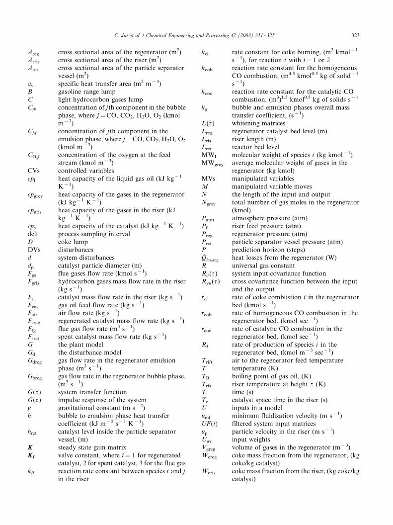
Appendix B: Notation

A, B, C,D

state space matrices

A gas oil in the feed


Areg cross sectional area of the regenerator (m2)

Arris cross sectional area of the riser (m2)

Arct cross sectional area of the particle separator

vessel (m2)av specific heat transfer area (m2 m�3)

B gasoline range lump

C light hydrocarbon gases lump

Cjb concentration of jth component in the bubble

phase, where j�/CO, CO2, H2O, O2 (kmol

m�3)

Cjd concentration of jth component in the

emulsion phase, where j�/CO, CO2, H2O, O2

(kmol m�3)

CO2f concentration of the oxygen at the feed

stream (kmol m�3)

CVs controlled variables

cpl heat capacity of the liquid gas oil (kJ kg�1

K�1)

cpgrey heat capacity of the gases in the regenerator

(kJ kg�1 K�1)cpgris heat capacity of the gases in the riser (kJ

kg�1 K�1)

cps heat capacity of the catalyst (kJ kg�1 K�1)

delt process sampling interval

D coke lump

DVs disturbances

d system disturbances

dp catalyst particle diameter (m)Fgs flue gases flow rate (kmol s�1)

Fgris hydrocarbon gases mass flow rate in the riser

(kg s�1)

Fs catalyst mass flow rate in the riser (kg s�1)

Fgas gas oil feed flow rate (kg s�1)

Fair air flow rate (kg s�1)

Fsreg regenerated catalyst mass flow rate (kg s�1)

Ffg flue gas flow rate (m3 s�1)Fsrct spent catalyst mass flow rate (kg s�1)

G the plant model

Gd the disturbance model

Gdreg gas flow rate in the regenerator emulsion

phase (m3 s�1)

Gbreg gas flow rate in the regenerator bubble phase,

(m3 s�1)

G (z) system transfer functionG (t) impulse response of the system

g gravitational constant (m s�2)

h bubble to emulsion phase heat transfer

coefficient (kJ m�2 s�1 K�1)

hrct catalyst level inside the particle separator

vessel, (m)

K steady state gain matrix

KI valve constant, where i�/ 1 for regeneratedcatalyst, 2 for spent catalyst, 3 for the flue gas

kij reaction rate constant between species i and j

in the riser

kci rate constant for coke burning, (m3 kmol�1

s�1), for reaction i with i�/1 or 2

kcob reaction rate constant for the homogeneous

CO combustion, (m4.5 kmol0.5 kg of solid�1

s�1)

kcod reaction rate constant for the catalytic CO

combustion, (m3)1.5 kmol0.5 kg of solids s�1

kg bubble and emulsion phases overall mass

transfer coefficient, (s�1)

L (z ) whitening matrices

Lreg regenerator catalyst bed level (m)

Lris riser length (m)Lrct reactor bed level

MWI molecular weight of species i (kg kmol�1)

MWgrey average molecular weight of gases in the

regenerator (kg kmol)

MVs manipulated variables

M manipulated variable moves

N the length of the input and output

Ngrey total number of gas moles in the regenerator(kmol)

Patm atmosphere pressure (atm)

Pf riser feed pressure (atm)

Preg regenerator pressure (atm)

Prct particle separator vessel pressure (atm)

P prediction horizon (steps)

/Qlossreg/ heat losses from the regenerator (W)

R universal gas constantRu(t ) system input covariance function

Ryu(t ) cross covariance function between the input

and the output

rci rate of coke combustion i in the regenerator

bed (kmol s�1)

rcob rate of homogeneous CO combustion in the

regenerator bed, (kmol sec�1)

rcod rate of catalytic CO combustion in theregenerator bed, (kmol sec�1)

RI rate of production of species i in the

regenerator bed, (kmol m�3 sec�1)

Trift air to the regenerator feed temperature

T temperature (K)

TB boiling point of gas oil, (K)

Tris riser temperature at height z (K)

T time (s)Tc catalyst space time in the riser (s)

U inputs in a model

umf minimum fluidization velocity (m s�1)

/UF (t)/ filtered system input matrices

up particle velocity in the riser (m s�1)

Uwt input weights

Vgreg volume of gases in the regenerator (m�3)

Wcreg coke mass fraction from the regenerator, (kgcoke/kg catalyst)

Wcris coke mass fraction from the riser, (kg coke/kg

catalyst)


x states in a state space model

X valve stem position

Y system outputs

ya dimensionless weight percent of the hydro-carbons in the riser, where (a�/A, B, C, D)

ywt output weights

yCG coke on regenerated catalyst/feed mass rate,

(kg coke/kg feed)

yCR coke on spent catalyst/feed mass rate, (kg

coke/kg feed)

yij dimensionless concentration of component i

in the j phase, where (i�/CO, CO2, H2O, O2)and (j�/bubble and emulsion)

yif dimensionless concentration of component i

in the feed, where (i�/CO,CO2,O2)

z axial distance in the riser (m)

z axial distance in the regenerator bed

Greek letters

a used in Eq. (A.29)DHi heat of reactions of reaction i

DHRAB heat of reaction for cracking of lump A to

lump B (kJ kg�1)

DHRC heat of reaction for coke burning (kJ

kmol�1)

DHRCO heat of reaction for CO combustion in the j

phase, (kJ kmol�1)

DP differential pressure between the regeneratorand the riser (atm)

Dt sampling interval (s)

ogris hydrocarbon gases void fraction in the riser

obreg bubbles phase void fraction in the regenera-

tor bed

odreg emulsion phase void fraction in the regen-

erator bed

omf bed voidage at minimum fluidization velocityosep bubbles phase void fraction in the separator

bed

fris catalyst activity

g unstripped hydrocarbon (kg per kg cat)

gb fraction of solids present in the bubble phase

m air viscosity (kg m�1 s�1)

8s coefficient of sphericity of the catalyst

particleskg thermal conductivity of air

m viscosity of air (kg m�1 s�1)

rb catalyst bulk density (kg m�3)

rgrey density of gas phase in the regenerator

(kg m�3)

rgris density of gas phase in the riser (kg m�3)

rs density of catalyst particles (kg m�3)

rv oil vapor density, (kg m�3)t1 controller integral time constant

(hr)

Tc catalyst residence time in the riser (s)

C ratio of velocity of gas to velocity of particles

inside the riser, feed coking tendency func-

tion

� diffusivity of O2 in airG,H composite matrices

/Gyl / weighting matrices of system output y

/Gul / weighting matrices of system input u

Subscript

A component A (gas oil)

atm atmosphere

b bubble phase in the regeneratorB component B (gasoline)

C component C (coke)

CO carbon monoxide

CO2 carbon dioxide

D component D (light hydrocarbon gases)

d emulsion phase of the regenerator

f feed

fg flue gasg gas or gaseous phase

mf minimum fluidization conditions

rct reactor or particle separator

reg regenerator

ris riser

s catalyst solid particles

ss steady state

References

[1] J.G. Balchen, S. Ljungquist Strand, State-space predictive con-

trol, Chem. Eng. Sci. 47 (4) (1992) 787�/807.

[2] M. Hovd, S. Skogestad, Procedure for regulatory control

structure selection and application to the FCC process, AIChE

J. 39 (12) (1993) 1938�/1953.

[3] P.D. Khandalekar, J.B. Riggs, Nonlinear process model based

control and optimization of a model IV FCC unit, Comp. Chem.

Eng. 19 (11) (1995) 1153�/1168.

[4] P.D. Christofides, P. Daoutidis, Robust control of multivariable

two-time scale monlinear systems, J. Proc. Cont. 7 (5) (1997) 313�/

328.

[5] R.M. Ansari, M.O. Tade, Constrained monlinear multivariable

control of a fluid catalytic cracking process, J. Proc. Cont. 10

(2000) 539�/555.

[6] D. Kunii, O. Levenspiel, Fluidization Engineering, Butterworth�/

Hienemann Publications, Massachusetts, USA, 1991.

[7] A. Arbel, Z. Huang, I.H. Rinard, R. Shinnar, Dynamic and

control of fluidized catalytic crackers. 1. Modeling of the current

generation of FCC’s, Ind. Eng. Chem. Res. 34 (1995) 1228�/1243.

[8] A. Arbel, I.H. Rinard, R. Shinnar, A.V. Sapre, Dynamic and

control of fluidized catalytic crackers. 2. Multiple steady states

and instabilities, Ind. Eng. Chem. Res. 34 (1995) 3014�/3026.

[9] H.I. De Lasa, A. Errazu, E. Barreiro, S. Solioz, Analysis of

fluidized bed catalytic cracking regenerator models in an indus-

trial scale unit, Can. J. Chem. Eng. 59 (1981) 549�/553.

[10] R.C. McFarlane, R.C. Reinemann, J.F. Bartee, C. Georgakis,

Dynamic simulator for a model IV fluid catalytic cracking unit,

Comp. Chem. Eng. 17 (1993) 275�/300.


[11] J.M. Arandes, H.I. de Lasa. Chem. Eng. Sci. Simulation and

multiplicity of steady states in fluidized FCCUs, 47 (9�/11) 2535�/

2540.

[12] S.S. Elshishini, S.S.E.H. Elnashaie, Digital simulation of indus-

trial fluid catalytic cracking units: bifurcation and its implications,

Chem. Eng. Sci. 45 (2) (1990) 553�/559.

[13] S.S.E.H. Elnashaie, S.S. Elshishini, Digital simulation of indus-

trial fluid catalytic cracking units-IV. Dynamic behavior, Chem.

Eng. Sci. 48 (3) (1993) 567�/583.

[14] I.S. Han, C.B. Chung, Dynamic modeling and simulation of a

fluidized catalytic cracking process. Part I: Process modeling. Part

II: Property estimation and simulation, Chem. Eng. Sci. 56 (2001)

1951�/1990.

[15] L.S. Lee, Y.W. Chen, T.N. Haung, W.Y. Pan, Four lump kinetic

model for fluid catalytic cracking progress, Can. J. Chem. Eng. 67

(1989) 615�/619.

[16] The Mathworks, Inc. 1994. Model predictive control toolbox,

user’s guide.

[17] The Mathworks, Inc.1995. System identification toolbox, user’s

guide.

[18] M. Larocca, S. Ng, H. de Lasa, Fast catalytic cracking of heavy

gas oils: modeling coke deactivation, Ind. Eng. Chem. Res. 29

(1990) 171�/180.

[19] K. Morley, H.I. de Lasa, On the determination of kinetic

parameters for the regeneration of cracking catalyst, Can. J.

Chem. Eng. 65 (10) (1987) 773�/777.

[20] K. Morley, H.I. de Lasa, Regeneration of cracking catalyst.

Influence of the homogeneous CO postcombustion reaction, Can.

J. Chem. Eng. 66 (6) (1988) 428�/432.

[21] L.S. Fan, L.T. Fan, Transient and steady state characteristics of a

gaseous reactant in catalytic fluidized-bed reactors, AIChE J. 26

(1) (1980) 139�/144.

[22] A. Arbel, I.H. Rinard, R. Shinnar, Dynamic and control of

fluidized catalytic crackers. 3. Designing the control system:

choice of manipulated and measured variables for partial control,

Ind. Eng. Chem. Res. 35 (1996) 2215�/2233.

[23] P. Grosdidier, A. Mason, A. Aitolahti, P. Heinonen, V. Vanha-

maki, FCC unit reactor-regenerator control, Comp. Chem. Eng.

17 (2) (1993) 165�/179.

[24] P. Van Overschee, B. De Moor, N4SID: subspace algorithms for

the identification of combined deterministic-stochastic systems,

Automatica 30 (1) (1994) 75�/93.

[25] J.M. Martin Sanchez, J. Rodellar, 1995. Adaptive Predictive

Control, Madrid, Barcelona.

[26] P. Malay, B.J. Milne, S. Rohani, The modified dynamic model of

a riser type fluid catalytic cracking unit, Can. J. Chem. Eng. 77

(1999) 169�/179.

[27] H. Ali, S. Rohani, Effect of cracking reactions kinetics on the

model predictions of an industrial fluid catalytic cracking unit,

Chem. Eng. Comm. 146 (1996) 163�/184.

[28] H. Ali, S. Rohani, J.P. Corriou, Modeling and control of a riser

type fluid catalytic cracking (FCC) unit, Trans IchemE, Part A 75

(1997) 401�/411.

[29] Malay P. 1998, A modified integrated dynamic model of a riser

type FCC unit, Master’s Thesis, University of Saskatchewan,

Saskatoon.


FCC unit modeling, identification and model predictive control, a simulation study

Documents

Transcript of FCC unit modeling, identification and model predictive control, a simulation study