1

Dissertation for the Degree in Master of Science in Economics (2013-2014)

SUPRIYA KAPOOR

13313903

kapoors@tcd.ie

EXTERNAL COMMERCIAL BORROWINGS- AN ANALYSIS

2

DECLARATION

I hereby declare that the thesis “External Commercial Borrowings- An Analysis”

which is being submitted in partial fulfillment of the requirement of the course

leading to the award of Degree in Master of Science in Economics, with Trinity

College Dublin is the result of the study carried out by me under the guidance of my

supervisor Dr. Philip Lane.

I further declare that this dissertation has not been submitted as an exercise for a

degree at this or any other University and it is entirely my own work.

I agree to deposit this thesis in the University’s open access institutional repository or

allow the library to do so on my behalf, subject to Irish Copyright Legislation and

Trinity College Library conditions of use and acknowledgement.

Supriya Kapoor

3

ACKNOWLEDGEMENT

I would like to acknowledge the help and guidance of my supervisor Dr. Philip Lane

whose unconditional and kind assistance proved to be very essential in my thesis.

I would also like to express gratitude to my teachers at Trinity College Dublin and

University of Delhi for their kind assistance.

I thank my family and friends for their patience and support throughout my college

experience.

4

SUMMARY

The first decade of the new millennium witnessed respectable growth rates till 2007

followed by anemic and uneven global financial crisis and then a sudden surge in

growth from 2012 onwards. This study provides an insight about external commercial

borrowings in India for the period 2004-2013. It uses time series data to test whether

the factors, i.e., exchange rate, interest rate differential and real domestic activity

drive the Indian corporates’ preference to borrow from overseas international capital

markets and hence analyze the external commercial borrowings pattern in the country.

These overseas borrowings are characterized by large number of companies in India,

which has led to a higher accessibility to international markets developing a more

globalized scenario in the country. It is observed that foreign borrowings by

corporates and real domestic activity share a positive relationship. The coefficient for

exchange rate revealed that an appreciation of domestic currency induces external

commercial borrowings. The demand for overseas borrowings is also predominantly

influenced by interest rate differential in most periods. The paper also provides a

description about the relationship between current account balance and capital inflows

in India.

5

CONTENTS

Declaration…………………………………………………………………………….2

Acknowledgement……………………………………………………………………..3

Summary………………………………………………………………………………4

Chapter 1: Introduction………………………………………………………………..6

Chapter 2: Theoretical Background……………………………………………….......9

Chapter 3: Literature Review………………………………………………………...13

3.1: Capital Flows and Current Account: A General Overview………........13

3.2: Relating Capital Flows to its Determinants……………………………15

3.2.1: Exchange Rates………………………………………………………15

3.2.2: Interest Rates and Interest Rate Differential…………………………17

3.2.3: Real Domestic Activity………………………………………………18

3.3: External Commercial Borrowings: The Indian Context……………….18

3.4: Mechanisms in Previous Studies………………………………………20

3.5: Potential Reasons for Corporates’ Overseas Borrowings……………...23

Chapter 4: Data Sources……………………………………………………………...25

Chapter 5: Linking Current Account with Capital Flows……………………………29

5.1: ECBs relative to debt flows…………………………………………….29

5.2: ECBs relative to total flows……………………………………………30

5.3: ECBs relative to Current Account Balance…………………………….32

Chapter 6: Method……………………………………………………………………35

Chapter 7: Results……………………………………………………………………37

7.1: Interpretation of Results………………………………………...……....37

7.1.1: Testing the equation for period 2004-13……………………………...37

7.1.2: Testing the equation for Stage 1……………………………………....43

7.1.3: Testing the equation for Stage 2………………………………………46

7.1.4: Testing the equation for Stage 3……………………………………....49

Chapter 8: Conclusion………………………………………………………….…….53

References………………………………………………………………………...….55

Appendix………………………………………………………………………..……61

6

CHAPTER 1: INTRODUCTION

The economic history estimates that capital flows lead to efficient allocation of

resources, which raise productivity and economic growth across the globe, however,

in practice it has been widely agreed and recognized that large capital flows actualize

serious challenges for policymakers, especially in emerging market economies

(EMEs). As a part of the solution, control on capital flows should be selective and

needs to be designed in such a manner that objectives are achieved. Accordingly,

many authors formalize capital account liberalization as a process and not a discrete

event (C. Rangarajan, 2000). For the period starting from mid 1990s, industrial and

import de-licensing, trade liberalization, financial sector reforms and tax reforms

define the external sector developments in India. Since then capital inflows has been a

major characteristic of the growth of Indian economy. These advancements have

provided immense amount of support to the external sector of the economy in order to

finance the current account deficit.

Capital flows have not only increased in size but also underwent compositional

changes. The determinants of capital flows that dominate the financial account are

foreign direct investment (FDI), portfolio investments, external commercial

borrowings (ECB) and non-resident deposits. Capital inflows to India are a

development of the nineties and its composition since then has changed notably

(Gopinath, 2004). A paradigm shift has been observed from official flows, i.e.,

external assistance and grants to private flows, where FDI and portfolios represent the

dominant proportion. According to the World Bank estimates, the FDI to Gross

Domestic Product (GDP) ratio increased from 0.8 percent in 1991 to 2.0 percent in

1997. Portfolio investments gained momentum after 1994. Since then equity flows

have been rising with a break in 1997-98 on account of the Asian crisis. Foreign

capital inflows were volatile in 2004-05 and afterwards. Along with them, there has

been a major surge in debt flows lately.

Focusing on the debt creating flows, it is observed that external assistance, that is, aid

flows from bilateral and multilateral sources constituted the major portion for the

period 1950s and 1960s. However, this declined steadily. Then during 1980s when

external assistance was not favored, commercial borrowings were preferred. External

7

commercial borrowings are defined as foreign currency borrowings by domestic

country from sources outside the country. These have a minimum maturity of 3 years

and they can be raised under Automatic or Approval route. ECBs continued to be

preferred in the 1990s post the break due to the aftermath of balance of payments

crisis. Lower domestic investment demand, downturn in capital flows to developing

countries and economic slowdown led to restrained commercial borrowings in early

2000s but the period 2003-04 marked their resumption. The boom and bust cycle in

external commercial borrowings continued when they underwent a sudden fall during

the global crisis in late 2008 and early 2009 and then a surge 2010 onwards.

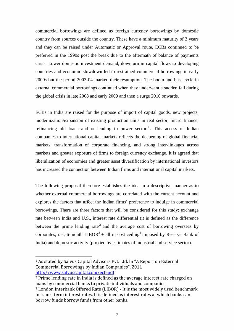
ECBs in India are raised for the purpose of import of capital goods, new projects,

modernization/expansion of existing production units in real sector, micro finance,

refinancing old loans and on-lending to power sector1

. This access of Indian

companies to international capital markets reflects the deepening of global financial

markets, transformation of corporate financing, and strong inter-linkages across

markets and greater exposure of firms to foreign currency exchange. It is agreed that

liberalization of economies and greater asset diversification by international investors

has increased the connection between Indian firms and international capital markets.

The following proposal therefore establishes the idea in a descriptive manner as to

whether external commercial borrowings are correlated with the current account and

explores the factors that affect the Indian firms’ preference to indulge in commercial

borrowings. There are three factors that will be considered for this study: exchange

rate between India and U.S., interest rate differential (it is defined as the difference

between the prime lending rate2 and the average cost of borrowing overseas by

corporates, i.e., 6-month LIBOR3 + all in cost ceiling

4 imposed by Reserve Bank of

India) and domestic activity (proxied by estimates of industrial and service sector).

1 As stated by Salvus Capital Advisors Pvt. Ltd. In “A Report on External Commercial Borrowings by Indian Companies”, 2011 http://www.salvuscapital.com/ecb.pdf 2 Prime lending rate in India is defined as the average interest rate charged on loans by commercial banks to private individuals and companies. 3 London Interbank Offered Rate (LIBOR) - It is the most widely used benchmark for short term interest rates. It is defined as interest rates at which banks can borrow funds borrow funds from other banks.

8

All the above factors are among the many factors that affect the external commercial

borrowings. The reasons for choice of these three determinants for my research are

explained in further sections. The period of study 2004-2013 is an interesting time

period for India because it is an ideal example of boom and bust where the first

decade of the millennium witnessed respectable growth rates followed by anemic and

uneven global financial crisis and then a sudden surge in growth from 2012 onwards.

The idea is further elaborated in subsequent sections: theoretical background and

literature review where the previous studies are discussed and serves as a prologue for

explicit explanation of the research questions followed by data sources,

methodological approach and results. The curiosity in exploring this topic is attributed

to the fact that in the era of financial development, the pattern of rise and fall of

external commercial borrowings have been phenomenal, but the thirst remains to

explore whether the factors assuredly affected the long run demand of Indian

corporates’ for overseas borrowings and in turn due to this, has the rise in capital

flows offset current account deficit and balanced the balance of payments.

In light of the above discussions, three hypotheses can be formed which are tested in

this thesis with regard to the variables: interest rate differential, real exchange rates

and real domestic activity.

Hypothesis 1: Increase in interest rate differential induces corporates’ to access

cheaper external commercial borrowings.

Hypothesis 2: Appreciating domestic currency induces greater external commercial

borrowings

Hypothesis 3: Greater real domestic activity implies higher external commercial

borrowings.

The chapter on data goes through the statistics for the variables used and list of

sources followed by a brief descriptive relationship among external commercial

borrowings, other components of capital flows and current account deficit. The

4 For the respective currency of borrowing or applicable benchmark

9

method will explain the regressions in detail. The thesis uses a lot of time series

regression analysis and for this purpose the software STATA is used.

CHAPTER 2: THEORETICAL BACKGROUND

This thesis observes two main questions: it elaborates the understanding of the

economy and relates to the correlation between external commercial borrowings and

current account deficit. The second question will investigate the factors that drive the

Indian corporates’ predilection to turn towards external commercial borrowings. Each

of the questions needs to be supported by theory along with the empirical tests

wherever required. The story about a country’s state of economy is often told by the

balance of payments (BoP), which constitutes the current account, financial account

and the capital account (Krugman, International Economics). This section provides

the definition and understanding of the concepts required in my thesis.

CURRENT ACCOUNT:

(1)

Where, is the trade balance of goods, services and transfers at time t and

is the net investment income at time t.

= (2)

It includes international interest and dividend payments and earnings of domestically

owned firms operating abroad. Hence, current account is defined as the sum of

balance of trade (goods and services exports minus imports), net current transfers and

net income from abroad. A current account surplus would tend to make the country a

net lender to the rest of the world, vis-à-vis. A number of factors affect the current

account balances for each country among which trade policies, exchange rates,

competitiveness and inflation are the prominent ones. A period of economic

expansion delivers a surge in imports and causes a deficit in the current account.

Consequently, we conclude that trade balance is the largest determinant of the current

account balance, either deficit or surplus. Similarly, an overvalued currency will make

exports less competitive and hence narrows down the current account surplus. In

10

contrast, an undervalued currency will boost exports, as they are cheaper thus

widening the current account surplus. It is that a chronic current account deficit leaves

the country’s currency under speculative attack, which creates a vicious circle where

the foreign reserves deplete and the trade balance is deteriorated. In such a situation, a

country often raises its interest rates or restricts capital outflows to finance its deficit

through capital inflows.

FINANCIAL ACCOUNT

(3)

Where, is the flow of assets at time t, is the flow of liabilities at

time t.

(4)

Where, FDI is foreign direct investment, PEQ is portfolio equity, PD is portfolio

derivatives, OD stands for other derivatives and RES is residents.

is the net acquisition of derivative position

(5)

This account records all the transactions of sale and purchase of financial assets. The

difference between a country’s purchase and sale of assets is called net financial

flows. The financial account also includes the capital account that constitutes

the transferring of wealth between countries. Hence, the financial account altogether

includes debt forgiveness, transfer of ownership of any financial asset, gifts and

remittances. Therefore,

(6)

Where, stands for errors and omissions. The current account is different from the

financial in a way that the former measures the difference between the sale and

purchase of goods and services, whereas the latter focuses on the difference between

acquisition of assets from the foreigners and the buildup of liabilities to them. Even

though every balance of payment credit automatically generates a counterpart debit

and vice-versa, still there is certain information regarding the debit and credit of items

that may be collected from different sources. This is shown in the errors and

omissions.

11

According to the national income accounting theory, another way to think of current

account balance is by relating it to domestic spending and investment in a way that,

(7)

Domestic savings is defined as the sum of private and government savings and

domestic investment is the investment by households and firms plus the government

investment (Higgins and Klitgaard, 1998). On the other hand, a country will invest

abroad if its domestic savings exceed domestic investment. The investment by a

lender country will be in the form of foreign direct investment, portfolio or

commercial borrowings (which is my topic of interest). The receiver country records

the capital inflow as negative net foreign assets. Consider the following:

(8)

Where, = gross national product, = consumption, = investment (private), =

government expenditure, = exports, =imports

A second equation for accounts as the sum of income received by all

individuals, i.e., (9)

Where, = private savings, = taxes and = transfers

Equating (8) and (9), we get,

(10)

Rearranging, ( ) (11)

, (12)

which means that domestic savings can be used to purchase investment, government

debt or a foreign asset.

Rearranging again ( ) (13)

Or, , which translates the current account balance into capital flows.

The above theory is supported by Milesi-Feretti and Razin (1996), where the authors

confirm that the current account deficits in early nineties characterize the imbalances

in private savings and private investment. On the capital account side, a capital

account with foreign direct investment and portfolios played an important role in

financing current account. High savings and high degree of openness was seen to

determine the sustainability of persistent current account deficits. I, in my study

would aim to study the same correlation but with a different component of capital

flows, i.e., external commercial borrowings for the period 2004-2013.

12

Considering the case of second half of 1980s in India when current account deficit

was financed by external commercial borrowings. During that time, the quantum of

external commercial borrowings rose but the debt servicing payments on those

borrowings also rose, they were so steep that by 1990-91, the net commercial

borrowings turned out to be negative, after paying the debt servicing payments. This

implies their was a net outflow from India rather than an inflow on commercial

borrowings. Hence, India was downgraded by the international credit rating agencies

and there were no new commercial borrowings. This was the time when India was in

a debt trap and it was forced to run to IMF for a loan.

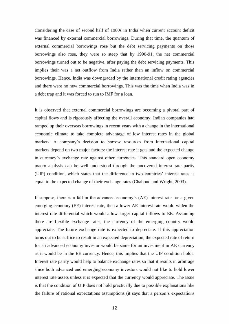
It is observed that external commercial borrowings are becoming a pivotal part of

capital flows and is rigorously affecting the overall economy. Indian companies had

ramped up their overseas borrowings in recent years with a change in the international

economic climate to take complete advantage of low interest rates in the global

markets. A company’s decision to borrow resources from international capital

markets depend on two major factors: the interest rate it gets and the expected change

in currency’s exchange rate against other currencies. This standard open economy

macro analysis can be well understood through the uncovered interest rate parity

(UIP) condition, which states that the difference in two countries’ interest rates is

equal to the expected change of their exchange rates (Chaboud and Wright, 2003).

If suppose, there is a fall in the advanced economy’s (AE) interest rate for a given

emerging economy (EE) interest rate, then a lower AE interest rate would widen the

interest rate differential which would allow larger capital inflows to EE. Assuming

there are flexible exchange rates, the currency of the emerging country would

appreciate. The future exchange rate is expected to depreciate. If this appreciation

turns out to be suffice to result in an expected depreciation, the expected rate of return

for an advanced economy investor would be same for an investment in AE currency

as it would be in the EE currency. Hence, this implies that the UIP condition holds.

Interest rate parity would help to balance exchange rates so that it results in arbitrage

since both advanced and emerging economy investors would not like to hold lower

interest rate assets unless it is expected that the currency would appreciate. The issue

is that the condition of UIP does not hold practically due to possible explanations like

the failure of rational expectations assumptions (it says that a person’s expectations

13

equal true statistical expected value), existence of time varying risk premium (Chinn

and Meredith, 2005) and investors are generally risk-averse and past literature and

proved that high interest rate countries’ currencies actually appreciate relative to

lower interest rate currencies (Aggarwal, 2013; Lothian and Wu, 2005; Chaboud and

Wright, 2003). This relates to the first two hypotheses I listed in the above section.

CHAPTER 3: LITERATURE REVIEW

I. CAPITAL FLOWS AND CURRENT ACCOUNT- A GENERAL

OVERVIEW

Total capital flows are the sum of private (foreign direct investment, portfolio

investment, liabilities to foreign banks and private transfers) and public flows (official

loans and official current transfers), as defined by the Institute of International

Finance. Since 1980s, private capital flows have escalated for many developing

countries, whereas a decline in public flows has been observed, as quoted for example

by Mody and Murshid (2005) for developing countries and Martin and Rose-Innes

(2004) for low income countries. The period of 1990s has been a boom period for

many countries in Latin America and Asia until the crisis of 1997-98, which led to a

reversal of capital flows characterized by a collapse in the asset prices and exchange

rates (Rodrik, 1999). With greater financial integration in 2000s, a massive surge in

gross capital inflows and outflows was witnessed for many developing countries as

mentioned in the report by the committee on Global Financial System, Bank for

International Settlements. Many countries have experienced rising private capital

inflows since 2000s with an unprecedented surge in 2007 until mid-2008 when the

global crisis hit the world economy. The boom and bust cycle of capital flows for

developing countries continues with the tentative recovery in mid-2009 with the help

of many developed countries’ central banks and then again a reversal in 2011, this

time due to the worsening of European debt crisis (UNCTAD, 2012). In this section, I

would hence review the extensive academic debate on capital flows and the factors

affecting them since 2000s with a deep insight on external commercial borrowings.

14

Current account imbalances are not just an element of 1990s, i.e. Mexico peso crisis

in 1995 and Asian crisis in 1997-98 but also for many countries in 1970s during the

oil price shocks (Guerin, 2012). The accretion in international capital flows has been

accompanied by the widening of current account deficits for many developing

countries. The empirical studies by Milesi-Ferretti and Razin (1996, 1998 and 1999)

suggest that major portion of current account deficits are being financed by the

inflows along with a fall in reserve accumulation. Current account balance is defined

as the difference between domestic savings and domestic investments (savings gap),

hence, the current account relates to the financial account through savings and

investment as mentioned in the above section. The disparity and unevenness between

savings and domestic investment causes current account imbalances. A boost in

capital inflows results in higher interest rates for investment. When investment rises

with the assumption that savings are unchanged, hence current account imbalances

are observed. Accordingly, reversals in capital inflows will execute reductions in

current account deficits. This descriptive mechanism illustrates the relationship

between capital flows and current account deficit; however, my main focus would be

to investigate the effect of current account deficit on ECBs.

An illustration of how current account affects capital flows is well highlighted by

Higgins and Klitgaard (1998). They assess the features and impact of U.S. current

account deficit in 1990s and how it was financed through capital inflows. The

following diagram concludes what had happened:

A study by Feldstein and Horioka (1980) concludes that perfect capital mobility is a

result of theories of current account imbalances. As stated above, a high current

account deficit is associated with higher investment spending and reduced rate of

savings, which predicts high integration of capital markets. High correlation between

savings and investment led many economists to argue that there is less than perfect

Fall in domestic investment

current account deficit as

investment > savings

a shortfall in domestic savings

Increase in investment

spending

This required the need for foreign

financing (capital inflows)

15

capital mobility. The study by Fry et al (1995) examines the Granger causality

between capital flows (mainly, foreign direct investment) and current account

balances with a sample of 46 developing countries. The paper produces diversified

results with Granger-causality running from capital to current accounts in some and

from current account to financial accounts in the others. There is also bidirectional

Granger causality found in a few with no causation at all in some countries. The paper

by Guerin (2012) is an extension to the paper by Fry et al and aims at considering the

relationship between net private capital inflows and current account in nineteen

developing and industrial countries each with the assistance of co-integration and

causality tests. The authors conclude that the net inflows and current account balances

have a long run steady state relationship. The results of causality between capital

inflows and current account vary. The authors observed that inflows do not cause

current account in industrial countries maybe because of the reason that the industrial

economies have liberalized financial accounts.

II. RELATING CAPITAL FLOWS TO ITS DETERMINANTS:

All the subsequent literature review in this sub-section relates capital flows to its

various determinants like exchange rates, interest rate differential and domestic

activity. However, the main focus of this research is on one of the components of

external commercial borrowings, which in turn is a part of capital flows. Since the

area of study is India and it has been noticed that ECBs are rising in India, hence it

would be good idea to relate the general finding in the following papers presented in

this section to my research.

1. EXCHANGE RATES

It is beneficial for the emerging economies to experience a rise in capital flows, but at

the same time it has unfavorable side effects of ‘real exchange rate appreciation’.

Regardless of the exchange rate regime a country follows, excess of capital flows

always bring with it an appreciation of the domestic currency (Jongwanich, 2010 and

Combes et al, 2011). In his study, Sebastian Edwards (2001) examines the

relationship among exchange rate, capital flows and crisis for the decade of 1990 and

draws conclusions from the lessons learnt during the Mexican, East Asian, Brazilian

and Russian crisis. A higher interest rate in domestic countries attracted a large

16

amount of capital and portfolio investments in the early 1990s in many developing

countries, which helped in financing major part of current account deficits. However,

the crisis of 1990s changed the view of many economists and researchers. In the

paper, he discusses various problems and challenges relating to exchange rate regime

and it is proposed that countries should follow one of the ‘two options’: either freely

floating exchange rates or super fixed exchange rates. Further, it is said that under

appropriate policy conditions, floating exchange rates are efficient and control of

capital inflows is an effective way of helping prevent currency crisis.

Combes et al. (2011) analyses the impact of real exchange rate on different forms of

private flows such as foreign direct investment, portfolio investments, bank loans and

private transfers. A sample of 42 developing countries was used for the period 1980-

2006 and pooled mean group estimator was applied that allowed short-run

heterogeneity while imposing long-run homogeneity on exchange rate (real) across

different countries. This indicator was introduced by Pearson, Shin and Smith (1999).

The results reveal that the effect of appreciation on private flows differ from the type

of flows, in such a way that, portfolio investments experienced the highest effect

followed by FDI and bank loans. Another important result from this research states

that a measure of exchange rate flexibility (measure used here is the de facto measure)

helps dampen real appreciation due to capital inflows and this would avoid a

significant loss of competitiveness.

In a detailed study by Dabos and Juan-Ramon (2000), they attempts to show a

relationship between real exchange rates and capital flows in Mexico for the period

1982:1- 1998:4 along with other variables such as external terms of trade and

productivity in manufacturing sector. The research was based along the lines of Khan

and Zahler (1983) who studies the analysis of short-run effects of liberalization on

both capital and current accounts. He concludes that movements in real exchange rate

in Mexico have consistently reacted to fluctuations in capital flows under different

exchange rate arrangements. The analysis also revealed the structural break in 1995

with the adoption of the floating exchange rate that led to overvaluation in peso in real

terms and post that period, the authors estimate that the appreciation in real exchange

rates became more responsive to changes in capital flows in Mexico.

17

2. INTEREST RATES AND INTEREST RATE DIFFERENTIAL

Capital flows respond to changes in interest rates. The basic theory explains that

interest rates and investment are negatively related. Investment is increased with a fall

in interest rate. Generally, an appreciation in a currency leads to increased interest rate

and a cross-border interest rate differential produces capital inflows. In most

emerging economies, the prime lending rate in domestic banks is slightly higher than

overseas interest rate. This is due to the reason that in former economies, there is

higher consumption demand that might induce double-digit inflation. Hence, to curb

this, the central banks charge a higher rate. A research by Calvo et al (1993) provides

evidence of lending and borrowing interest rates in Latin America and United States

for the period 1988-1992. He estimates that a relatively high interest rate differential

on Latin American assets during the above time period, attracted major rise in capital

flows in that region. On the other hand, in Chile there was a less pronounced impact

of inflows on the interest rate differential. Bird and Rajan (2000) studied the East

Asian case for their analysis where an interest rate advantage persisted. The authors

concluded that financial liberalization led to an increase in the domestic interest rates

and capital was ‘pulled’ and not ‘pushed’, in other words, the persistent interest rate

advantage in favor of East Asian economies was related to rising domestic interest

rates rather than falling world interest rates.

Fedderke, J.W. and W. Liu (2002) applied Autoregressive Distributed Lag (ARDL)

models to analyze the determinants of capital flows and capital flight in South Africa

for the period from 1960 to 1995. They took interest rate differential as a proxy for

rate of return and found that capital flows were responsive to changes in interest

differentials. They also determined that aggregate growth measures suggested long

run determination of capital flows. A study by Ying and Kim (2001) suggested them

to use Structural VAR to investigate the macroeconomic factors of capital flows in

Korea and Mexico for the period 1960:1 to 1996:4. They followed the push-pull

approach and took foreign output and foreign interest rates as push factors and

domestic productivity and domestic money supply as pull factors. They found that for

both countries, foreign interest rate generated only a moderate negative effect on

domestic output. The empirical results also suggested that capital flows are sensitive

to business cycles for both countries.

18

3. REAL DOMESTIC ACTIVITY

From the past two decades, domestic developments and sound economic policies have

resulted in a rise in capital inflows to developing economies, thus implying good use

of funds in the recipient countries (Reinhart, 2005). Global economy and world trade

is picking up gradually. Various push and pull factors were taken by Mody, Taylor

and Kim (2001) to forecast capital flows. Level of industrial production was a major

factor among other pull factors such as short-term domestic interest rate, consumer

price index, short term debt to forex reserve ratio, level of domestic credit, credit

rating and reserves to import ratio. Global or push factors included U.S. short-term

and long-term interest rates, Emerging Markets Bond Index (EMBI), U.S. swap rate,

U.S. output growth and risk aversion. The econometrics tool that was used was vector

error correction framework using partial derivative and integrated approach. Under

shock to global real factors like no growth in U.S. industrial production, flows to

emerging markets dropped significantly without any sign of recovery.

III. EXTERNAL COMMERCIAL BORROWINGS: THE INDIAN

CONTEXT

The volatile pattern of capital inflows from 1950s to first decade of this century

reveals an overhaul transformation from capital scarcity to surplus in India. There has

been variability with regard to changes from official flows to private flows and a shift

towards debt flows, majorly, external commercial borrowings and NRI deposits. Until

1980s, the Indian government focused on self-reliance and import-substitution. It was

only after the New Economic Policy (NEP) and opening up of capital account in

1990-91 that the surge in capital inflows to India accelerated the contribution to

exports and output growth. As per Mohan (2008), the absolute historical journey of

capital inflows in India can be branched into three phases.

Phase 1: Independence (1947) to 1980s: External flows were restricted to bilateral and

multilateral concessional finance. There was no international capital outflow or inflow

to India.

Phase 2: 1980s to 1990s: The current account deficit was externally financed through

commercial loans including short-term borrowings and NRI deposits. This resulted in

19

a significant enlargement in India’s external debt.

Phase 3: 1991 onwards: This period is marked by the balance of payments crisis in

1991. It was realized that an unstable current account deficit, inappropriate exchange

rate regime and rise in short-term debt were the causes of these crisis.

Commercial borrowings have gained momentum in the past two decades. ECBs by

the Indian corporates increased seventeen times between 1990 and 2008 (Singh,

2007). A rise in the realization of loans approved may be due to higher economic

activities domestically that led to a rise in credit demand in the domestic country or

higher interest rate differential between domestic and foreign interest rates or

favorable conditions internationally. External commercial borrowings significantly

accelerating after the balance of payments crisis constituted a large percentage of net

capital flows to India. With a slight shrink in commercial borrowings during late 90s,

the period 2003-04 marked a resumption of debt flows in India. Increased investment

demand, favorable sovereign debt rating and global liquidity conditions contribute as

the main causes of the surge in capital inflows.

Since 1980s and 1990s, a number of studies and models have been developed to

depict this existence of the trend, which is suspected to positively affect investment

demand and global liquidity conditions. In one of the very important studies in this

field, Singh (2007) concentrates on external commercial borrowings and reasons out

the main causes relating to companies’ overseas borrowings. In addition to this, he

also considers other analytical reasons that could contribute to corporates’ recourse to

international capital markets. The results reveal that Indian companies’ long run

demand for commercial loans from overseas is predominantly influenced by the

domestic activity, followed by interest rate differential and credit conditions. He tries

to intensely define every aspect of external commercial borrowings including end use

restrictions, end use pattern and ECBs through various routes. The rationale for this

research has been developed from the historical fact that ECBs, which are used as an

additional source of funding by Indian corporates’ to augment resources available

domestically, have suddenly become a major component of total capital flows to

India.

20

IV. MECHANISMS IN PREVIOUS STUDIES

The mechanisms from the previous studies are discussed below to show the different

approaches and assumptions considered by researchers in testing various determinants

of external commercial borrowings along with other proxies for capital flows. This

section is more like the framework of studies conducted earlier.

Singh (2007) estimated the determinants of external commercial borrowings in

India using co-integration and error correlation mechanism (ECM). He applied this

method to the data (quarterly) for the period 1993-2007. The determinants taken by

him were Index of Industrial Production (a proxy for real activity), interest rate

differential and broad money supply (a proxy for liquidity). It has been observed

that post-global crisis; the private sector has not been very aggressive in credit5.

There are many other determinants concerning the behavior of Indian corporates’

decisions, but data availability and resource limitations confine my present analysis

to a subset of them. He found that all the above had a statistically significant effect

on the demand for ECBs. The coefficient of error correlation revealed that there

was a complete adjustment to deviation from the long run path of external

commercial borrowings. There seemed to be a positive relation between real

activity and commercial borrowings and it was same for interest rate differential.

However, an inverse relationship was found between liquidity and ECBs. The

analysis of variance decomposition suggested that all the three determinants

together explained around three-fourth of the variation in external commercial

borrowings. Real activity was the most important variable that explained around 38

percent of variation in commercial borrowings. The contribution of interest rate

differential also explained variations in the external borrowings. As far as the

broad money supply is concerned, it gained momentum in the medium run and thus

it would be appropriate to conclude that liquidity constraint is also for corporates

when deciding upon the commercial borrowings. In recent years, the service sector

has prospered in India due to which, in my opinion, taking only IIP as the proxy for

domestic activity would not be justified.

5 This fact has been taken from Mostly economics blog: http://mostlyeconomics.wordpress.com/2010/05/06/sources-and-deployments-of-money-supply-in-india/

21

Singh (2009) also undertook the study where he analyzed the determinants of

private debt and equity flows for the time period ranging from 1950s till 2010. He

intuited that corporates’ decisions to borrow overseas is influenced by domestic real

activity, interest rate differentials and finally by the credit constraints. A high

correlation was found between ECBs and interest rate differential and a strong co-

movement was also analyzed between commercial borrowings and the real activity.

It was also shown that even though in the normal periods domestic demand shocks

predominantly influenced the commercial borrowings, in the period of crisis, it was

the credit shocks that influenced the ECBs. Singh also analyzed the behavior of

non-resident Indian (NRI) deposits by using the vector error correlation model

(VECM) for the period 1993-2009 (monthly data). These were found to be unstable

in nature as NRI deposits were statistically influenced by the determinants such as

domestic real activity, exchange rate movements and interest rate differentials.

Index of oil price was taken as the proxy for real activity in the host country. With

reference to the volatility flows, he found high co-movement in net foreign

institutional investments and stock returns. He used the Johansen’s approach to the

co-integration analysis which suggested an overall long run relationship between the

above two variables. Also, Granger causality revealed a simultaneous interaction

between portfolio flows and stock prices.

Chakrabarty (2006) contested a test of co-integration between net capital flows, real

exchange rates and interest rate differential using the data from 1993-2003. In the

post liberalization period, error correlation mechanism was operating and it related

dynamic adjustment to capital flows to the movements in interest rate differential

and real exchange rate. The paper revealed that the major changes in real exchange

rate since 1993 have been due to the intervention of Reserve Bank of India in the

foreign exchange market and these changes in turn led to changes in capital flows.

Hence, a long run relationship was experienced among net capital flows, real

exchange rate and interest rate differential.

Verma and Prakash (2011) excogitated the effects of interest rate sensitivity on four

components of capital flows using co-integration and causality analysis. The

22

components chosen for this analysis were foreign direct investment (FDI), foreign

institutional investments (FII) for the period 1998-2010, external commercial

borrowings for the period 2000-2010 and non-resident Indians deposits. It was

found that FDI was not interest rate sensitive as it is assumed to be long-term in

nature. Also, FIIs are not statistically significant to interest rate sensitivity. On the

other hand, as the author expected, ECBs and NRI deposits are found to be

statistically significant. 1 percentage point change in interest rate led to around

0.85percentage point change in ECBs and similarly 1 percentage point change in

interest rate brought 0.26percentage point change in NRI deposits. Hence, the

authors finally interpret that monetary policy takes cognizance of the fact that ECBs

and NRI deposits (debt flows) are impacted by the changes in interest rates as well

as exchange rates.

Hiroko Oura (2008) examined the firm level data on corporate financing to study

the efficiency of India’s financial system. The data on firms was for 9,000

companies out of the 10,000 listed companies in India for the fiscal years 199394-

2005/06. The majority of the firms were over 10 years old and the data included

firms from manufacturing, financial and chemical sectors. Specifically, it tries to

find whether Indian firms rely more on external funds and hence influence firm

growth. The paper also looks at corporate financing patterns and their relationship

with external finance dependence. As the results show, the author finds signs of

inefficiency in India’s financial system, which negatively affects growth

differentials of finance intensive industries but this does not quantify the impact of

inefficiency on macroeconomic growth. Also, the paper concludes that India’s

growth has been the fastest in the world despite all the inefficiencies, however, it

India could have achieved even higher growth without such burdens. It has been

suggested that the future development policy in India should involve developing

debt-financing facilities. Moreover, better financial sector reforms would open up

channels for additional efficiency gains and hence contribute to sustained

productivity growth.

Julie Jiang and Jonathan Sinton (2011) analyzed in a descriptive paper the overseas

investments by Chinese National oil companies in a descriptive manner. In the

23

recent years, many Chinese national oil companies, including the three main: China

National Petroleum Corporation (CNPC), China Petroleum & Chemical

Corporation (Sinopec) and China National Offshore Oil Corporation (CNOOC) are

doing business abroad and their actions are mainly driven by commercial incentives

to take the advantage of the global marketplace. The authors focus on understanding

the origins of the main oil companies first, where these three companies were

initially geographically divided and by 2000s these were listed in the Hong Kong

stock exchange. The reason for overseas investment by Chinese oil companies roots

from the fact that China’s oil fields are ageing and country is dependent on

international oil markets. The requirement of energy-intensive raw materials,

demand for fuel in transport goods, growing fleets of private vehicles and demand

for petrochemical feedstock led to an upward pressure oil consumption. The

Chinese companies invested in Brazil, Bolivia, Ecuador, Kazakhstan and

Venezuela. These deals were of the form loan-for-oil and loan-for-gas.

V. POTENTIAL REASONS FOR CORPORATES’ OVERSEAS BORROWINGS

The above literature tells us that exchange rates, interest rate differentials and

domestic activity have the appearance of only a few of the many reasons why Indian

companies opt for overseas financial foray. As the aim of this research is to provide a

complete assessment of external commercial borrowings, I would excogitate the other

potential arguments that consider the challenges and benefits for Indian businesses

seeking financing opportunities from international markets that have been noticed by

various researchers and authors over the years. The borrowing behavior of corporates

can be established broadly due to the ease of regulations. The Reserve Bank of India

liberalized the external borrowings norms for infrastructure and power sector up to

USD 10 billion (RBI Circular dated 23rd

September, 2011 and 20th

April, 2012). Also,

the eligible borrowers are now allowed to raise ECB under approval route from their

foreign equity holder company with minimum average maturity of 7 years for general

corporate purpose (Businesstoday.intoday.in). Consequently, there has been many

such developments which have raised capital inflows in the country through ECB

such as ECB in the aviation sector, allowing ECB funds for import of services, the

permission by RBI to convert overseas borrowings into equity through external

24

commercial borrowings and so on. Due to the collapse of Lehman Brothers during the

global financial crisis, the financial sector was reluctant to lend and the rates reached

soaring heights. At that point, RBI liberalized its policies further by expanding the list

of borrowers and easing all-in cost ceilings (Arora et al, 2010). Over the years, there

has been a shift in the purpose of loans. Towards 2003-04, the major objectives to

borrow included import of capital goods, modernization, new investments and

refinancing of existing borrowings. The idea of ‘rupee expenditure for local capital

goods’ has replaced the refinancing purpose. It has also been observed that a lot of

Indian investment abroad is being carried through Joint Venture and Wholly Owned

Subsidiaries (A report by Chartered Accountant O.P. Jagati).

A host of factors also include changes in maturity period and investor profile. This

dominant modification in the market resulted in greater confidence and willingness by

Indian firms to borrow. Corporates have started to raise large sized loans for longer

maturity, in contrast to smaller-sized in the late 1990s. Moreover, the Indian investors

have received reciprocation from international investors of the same enthusiasm. A

sea change has been noticed in the investor profile as well. A paradigm shift from

bilateral and multilateral agencies such as the Asian Development Bank (ADB) and

International Finance Corporation (IFC), who were the sole providers of overseas

credit to the major international commercial banks has been highlighted by the

Ministry of Finance, India. This upswing is due to the availability of cheaper loans

from these foreign banks. The Indian companies are growing at an unprecedented rate

due to the facility and feasibility to the international markets. It is predicted that the

companies will continue to raise large amounts of debt and equity funds in the coming

years. This motivates both the upcoming and established firms to grow in size and

ambition.

The increased credibility and reliable reputation of the Indian firms have facilitated

greater access to these markets. It has been argued that firms that engage in

borrowings from the international markets tend to obtain leverage debt maturity and

better financing opportunities (Karolyi, 1998; Miller and Puthenpurackal, 2000;

Doidge et al, 2002). These borrowings from the foreign institutions may have helped

domestic firms to manage risk through more cultivated financial instruments. Due to

risky and speculative nature of businesses, issue of IPO’s (Initial Public Offering)

25

have become uncertain and henceforth, it can serve as a reason for Indian corporates

to turn to overseas borrowings. A demand led factor, i.e., investment demand

describes the surge in ECB well (Singh, 2007). Corporate sector is witnessing robust

domestic and export demand which has aided buoyant world trade due to which

Indian companies that have become internationally competitive are now being

benefitted from the improved business environment. The investment demand for

new projects, modernization and diversification has reached dramatic levels for Indian

firms. Hence, assuming a relatively liberalized capital account regime, exchange

rates, interest rate differential and real domestic activity along with the above reasons

to some extent explore the key drivers of Indian corporates overseas borrowings.

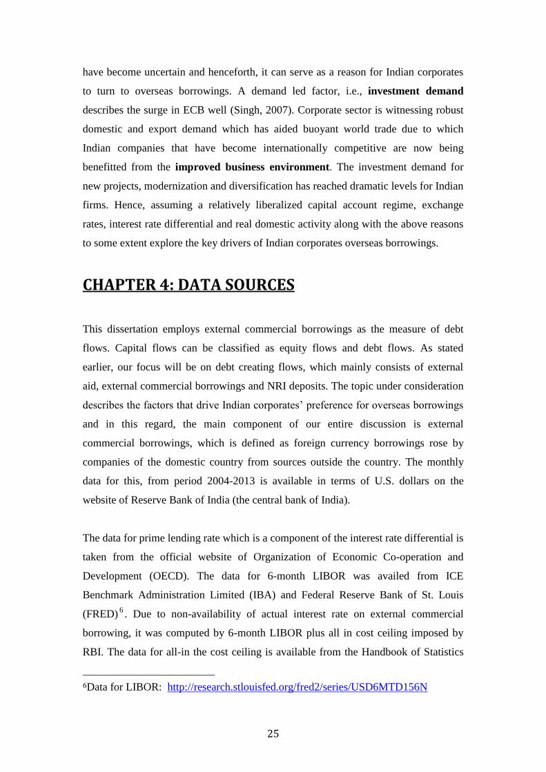
CHAPTER 4: DATA SOURCES

This dissertation employs external commercial borrowings as the measure of debt

flows. Capital flows can be classified as equity flows and debt flows. As stated

earlier, our focus will be on debt creating flows, which mainly consists of external

aid, external commercial borrowings and NRI deposits. The topic under consideration

describes the factors that drive Indian corporates’ preference for overseas borrowings

and in this regard, the main component of our entire discussion is external

commercial borrowings, which is defined as foreign currency borrowings rose by

companies of the domestic country from sources outside the country. The monthly

data for this, from period 2004-2013 is available in terms of U.S. dollars on the

website of Reserve Bank of India (the central bank of India).

The data for prime lending rate which is a component of the interest rate differential is

taken from the official website of Organization of Economic Co-operation and

Development (OECD). The data for 6-month LIBOR was availed from ICE

Benchmark Administration Limited (IBA) and Federal Reserve Bank of St. Louis

(FRED)6. Due to non-availability of actual interest rate on external commercial

borrowing, it was computed by 6-month LIBOR plus all in cost ceiling imposed by

RBI. The data for all-in the cost ceiling is available from the Handbook of Statistics

6Data for LIBOR: http://research.stlouisfed.org/fred2/series/USD6MTD156N

26

on Indian Economy from RBI’s website. As the data suggests, this value has not

changed much over the years and remains same over months in a year. For instance,

the all in cost ceiling for the year 2005-06 was 200 basis points (2 percent) if the

maturity of the loan was between 3-5 years and 350 basis points (3.5 percent) if more

than 5 years. RBI through a Master Circular, which is issued with a sunset clause of

one year and is replaced by an updated master circular the next year, releases this

value.

In my analysis, I use the grand total of external commercial borrowing for each month

and not the individual values, hence, the value of all in cost ceiling is the average of

the individual values of loan taken by any company for each month. This all-in cost

ceiling value is hence added to the LIBOR and the sum of these two is subtracted

from the lending rate, which gives the resultant interest rate differential. The reason

why interest rate differential is important for this analysis is because interest rate is

one of the main components that one considers when borrowing money. It is the

uncomplicated economic principle that investment and interest rates are negatively

related. Hence, if interest rate in domestic country is high then loans will be

purchased from outside the country and vice-versa.

The dataset for monthly values of exchange rate (Indian rupee per unit of U.S. dollar)

is obtained from Database on Indian Economy, RBI’s Data Warehouse7, the official

website of Reserve bank of India. The monthly data that has been used is the value

that prevailed during the beginning of each month. Preliminary value for the current

month is provided even if not all daily values are available for the entire month.

Exchange rates constitute as an important determinant of borrowing cost of

companies. If the domestic currency is expected to appreciate then the effective cost

of servicing the debt goes down and corporates’ tend to borrow more in international

markets.

The underlying production activities both in the industrial and service sector drive a

key issue that relates to the firms’ preferences for overseas borrowings and accessing

international markets. India is one the fastest growing developing countries since

7 Data for exchange rates: http://dbie.rbi.org.in/DBIE/dbie.rbi?site=home

27

1990s (Montek S. Ahluwalia, 2002). The reforms in the industry and trade have

improved the industrial and service sector of India. These improvements have led to

higher economic activities and in turn more funds to finance the same. Due to this

reason, the proxy for real domestic activity is taken as the sum of activities in the

manufacturing, construction, trade/hotels/transport and finance, insurance, real estate

and business services. This data is available again from the website of Reserve Bank

of India. The reason why data on Index of Industrial Production (IIP) is not taken as a

measure of domestic activity is because of the fact that since 2000s, India has

experienced major developments in the service sector with a share of 64.5 percent in

2008-09 (Das et al, 2011) and a slight decline in the industrial sector. Hence, just

taking the industrial production into account would not have been justified. The issue

with the data on estimates of industrial and service sector was that it was available in

quarterly and annual intervals, however, my research runs regression with monthly

data. Hence, quarterly data was converted into monthly data through interpolation by

assuming growth rates among quarters.

The descriptive statistic for current account deficit (CAD) is available from Reserve

Bank of India’s website under Special Data Dissemination Standards. It is a quarterly

data ranging from 2004:Q1- 2013:Q1. It is expressed in billions of U.S. dollars. The

current account deficit is defined as the sum of balance of trade (exports minus

imports of goods and services), net factor income such as in interest and dividends

and net transfer payments such as foreign aid. The data will be used to graphically

depict any correlation between ECBs and CAD.

The dissertation adopts time series analysis for India and the hypothesis are tested

through OLS regression with inclusion of all key variables. The regressions are such

that some of the variables are considered in real growth terms and this is calculated

as:

(14)

In the above equation, is the real growth in external commercial borrowings in

period ‘t’. It is appropriate to transform some variables into logarithms so that the

highly skewed variables are approximately made normal. The real growth values are

calculated in this manner for ECB as well as exchange rates and estimates of industry

and service sector.

28

The graphs below show the scatter plots of key variables with external commercial

borrowings (in log terms).

Figure 1: Scatter diagram showing

‘ecb’ and ‘exrt’

Figure 2: Scatter diagram showing ‘ecb’

and ‘ird’

Figure 3: Scatter diagram

showing ‘ecb’ and ‘gdp’

The scatter plot that represents ecb on the x-axis and the other variables on the y-axis

suggests a positive relationship between of exrt and gdp with ecb, however a negative

relation between ird and ecb. Though as per the economic theory, a wider ird tends to

induce commercial borrowings, which is in contrast to the data under study that

shows a negative correlation. The detailed regression, which would help in

interpreting the strength of the relationship through the assessment of the value of

coefficients are reported later in the thesis.

3.7

3.8

3.9

44.

14.

2

19 20 21 22 23ecb

exrt Fitted values

24

68

19 20 21 22 23ecb

IRD Fitted values

2929

.530

30.5

19 20 21 22 23ecb

gdp Fitted values

29

CHAPTER 5: LINKING CURRENT ACCOUNT WITH

CAPITAL FLOWS

5.1 ECBs relative to debt flows

India, one of the fastest emerging market economies has a robust growth, which is

becoming broad-based. Capital flow movements in India are increasing continuously

and are offsetting the impact of the current account deficits. They can be classified

into debt flows (mainly external commercial borrowings, NRI deposits and short term

loans) and non-debt/ equity flows (foreign direct investment and portfolio flows).

Starting with the analysis of debt flows in India, there is no doubt that ECBs now

constitute a major proportion. ECBs are used as an additional source of funding by

Indian corporates to augment resource available domestically and the many policy

changes in ECBs have favored Indian companies to take the advantage of global

liquidity, domestic investment demand and lower risk premia. Similarly, the NRI

deposits were introduced in 1970s. The interest rate on NRI deposits is in accordance

to LIBOR (same as ECBs). Since post-crisis (Asian crisis), this component has

undergone compositional changes like the share of foreign currency denominated

deposits in total NRI deposits had fallen from 70 percent in 1990s to 32 percent in

August 2003 (Gordon and Gupta, 2004). Short-term debt in India’s total external debt

has also increased significantly since 1980s.

According to the Economic Times Bureau and RBI’s External Debt Report end-

March 2013, the share of ECBs in 2012-13 continued to be highest at 31% of the

entire debt flows followed by 24.8% of short-term debt and 18.2% of NRI deposits.

Also, the loans under external assistance have declined by U.S. $0.6 billion. Over the

years, the external debt scenario has changed in India from aid flows to borrowings by

corporates and now even the short-term debt is rising considerably. The credit for the

rise in ECBs is given to high domestic interest rates and cheaper fund raising options

abroad. Easing of ECB norms for power, aviation and infrastructure companies,

allowing companies to convert overseas borrowings into equity via ECB and allowing

them to use ECBs for general corporate purposes are some other reasons why this

component is the most prominent one in debt flows. The prudent approach of ECBs

30

follow self-imposed ceilings on approval, careful monitoring of cost of raising funds

and their end-use, whereas, inflows in NRI deposits have exercised some specification

of interest rate ceilings and maturity requirements. Hence, I would like to conclude by

stating that debt flows in India are continuously climbing the upward ladder with the

share of ECBs at the top.

5.2 ECBs relative to total inflows

The liquidity crisis in balance of payments in 1991 in India led to significant changes

in the composition of the financial account. The financial markets react rapidly to the

policy adjustments and hence the capital account now is dominated by foreign direct

investment, portfolio flows, commercial borrowings and NRI deposits instead of

external aid and assistance in the 1980s. India adopted a gradualist approach towards

capital account convertibility, which was based on the Report on Balance of Payments

by C. Rangarajan, 1991 and the Report by the S.S. Tarapoore Committee (1997 and

2006). These reports suggested a shift from official to private flows, debt to equity

flows, institutional reforms, gradual liberalization of outflows and regulation of short-

term external commercial borrowings. The restrictions on debt flows were imposed as

these were assumed to be dangerous for the economy and a shift towards non-debt

creating flows was required. Consequently, FDI and portfolio investments had a

relatively liberal framework while ECBs were regulated. In 2000s, the bond markets

of India and other emerging economies have grown substantially with increased

efforts to develop local currency denominated bond markets (Patnaik, 2013).

On the one hand, there was significant increase in foreign participation in bond

markets in 2000s while on the other hand, the policy framework on debt flows led to

limited participation. The robust growth in the performance of Indian economy and

international investors’ confidence in India as an important investment destination has

resulted in impressive increase in FDI. Foreign Institutional Investment (FII) and

American/Global Depository Receipts (ADR/GDRs) are important segments of

portfolio investments with FII being the dominant (Dua and Garg, 2013). Post-

liberalization period, FIIs were allowed to invest in both debt and equity markets.

Ceilings on FIIs have been relaxed to great extent and equity flows have been in favor

with domestic and global developments. Along with that, FIIs registered under the

100 percent debt route can also invest in debt instruments. ADRs/GDRs are also

31

important sources of portfolio investments and the liberalization in these have

attracted corporates to access equity capital in these form.

Over the past years the global thinking has changed, which has implied a qualitative

change in India’s relationship with the world system and resurgence in debt flows,

especially ECBs, NRI deposits and short-term debt. ECBs provide flexibility to Indian

firms in borrowings and so as per the RBI reports, the debt inflows in January 2012

amounted to be U.S. $3.21 billion, which is higher than U.S. $1.7 billion of equity

flows. A major reason for this increase can be the fact that global uncertainties

recently have wiped out the risk appetite of investors and in such a risk aversion

environment, debt instruments might be considered as safe instruments. Since long,

non-debt flows (especially FDI) over debt flows are preferred but there seems to be a

sharp compositional change now. Therefore, the discussion on the components of

capital flows has made it evident that various reforms and uncertainties have led to

compositional changes.

To investigate the composition of capital flows and whether commercial borrowings

or debt flows are in correlation with equity flows, various phases can be segregated

according to the economic performance of India. Phase I: 1980-1991, when India’s

growth was based on self-reliance, phase II: 1992-2003, a time period when growth

rates ranged from a lower value to a decent one, Phase III: 2004-2008, during this

phase India recorded some of the highest growth rates and Phase IV: 2009-2012, the

recent post global crisis period (Mohanty, 2012). In phase I, the only dominant

component of capital flows was external aid. In the second phase, India reached an

average growth rate with significant rise in equity flows as stated above. On the other

hand, the third phase witnessed a moderate increase in equity flows along with a surge

in debt flows, mainly ECBs and trade credits. During the recent period, the non-debt

flows continued to grow with a slight fall in FDI but at the same time debt flows have

shown a continuous acceleration, especially ECBs. Hence, I would like to conclude

this sub-section with a view that net capital flows have accredited since the 1990s

with changes in composition.

32

5.3 ECBs relative to the Current Account Deficit

Lately, external commercial borrowings have become an important debt flow

component of financial account of the balance of payments and it may be utilized to

compensate the existing current account deficit (CAD). A current account deficit

occurs when a country is importing or consuming more than what it produces and this

is then financed by international capital flows. Consequently, it is the difference

between the inflow and outflow of foreign currency. The CAD reached historically

high levels in recent years, which posed to be the biggest risk to the economy. Hence,

this brings me to ponder upon the correlation between ECBs and CAD. India’s

current account balance has been deteriorating since the past half a decade. The

current account was found to be stable during the pre-crisis period, 2003-08 and

suddenly worsened 2009 onwards.

It is observed that on the one hand there was resurgence in ECBs with a slight

deterioration in equity flows and on the other hand, CAD has been increasing

significantly. According to the Bureau of Economic Analysis, the current account

deficit in India has risen recently mainly due to slowdown in the growth of advanced

country markets, weak exports, larger imports in gold and crude oil, deteriorating net

investment income and slowdown in the inward remittances from overseas Indians,

though they showed greater stability in recent years. The Finance Ministry of India in

January 2013 recorded that the current account deficit is a matter of worry and it

needs to be financed through international inflows, else the deficit could drain the

country’s foreign exchange reserves. As per the RBI reports, the outlook for advanced

countries remained unstable and any event shock would result in capital outflows

from emerging economies. Moreover, due to the tightening of global liquidity, the

financing of CAD exposes the economy to the risk of sudden stop or reversal of

capital flows, jeopardizing the country’s macroeconomic stability.

In his recent interview, Finance Minister P. Chidambaram suggests the three ways to

fund the CAD in India are through FDI, portfolio and ECBs. The current account

balance of any country depends on fiscal position of a country (surplus/deficit), where

fiscal means total revenue and total expenditure. Out of this total revenue if current

account transactions are taken out comprising of exports and receivables and imports

and outward remittances, the difference is either current account deficit or surplus.

33

The economy of a country depends heavily on the imports of many important items

such as crude oil in India, whose demand in the domestic market is mainly met by

importing from many countries. On the contrary, India has less foreign reserves, as

exports are not very encouraging. Thus to compensate, a regular supply of foreign

currency, capital inflow is required.

Figure 4: Depiction of ECBs and CAD

ECBs on an average have shown a rising trend. Figure 4 demonstrates the data for

external commercial borrowings and current account deficit in India. The y-axis

measures the ECB (in U.S. dollars billion) and current account balance. On critically

analyzing the graph, it is evident that ECBs are in small proportion as compared to the

entire current account balance. For instance, in July 2005, when the deficit is

approximately U.S. $8 billion, the ECBs amount a meager U.S. $0.66 billion or more

recently in July 2012, the ECBs amounted U.S. $1 billion which seems to less to

finance a current account deficit of nearly U.S. $22billion. In that situation, it is

intuitive to conclude that debt flows, or ECBs play a limited role in financing the

current account deficit for India, even though an increase has been observed

according to the above discussion. Having said that, it is interesting to note that major

current account deficit is financed in India through equity flows, FDI and portfolios.

Recent updates report that the bulk of capital inflow on the investment side was on

account of portfolio flows during 2007-08 followed by net inflow of direct investment

that amounted U.S. $3.89 billion (Reserve Bank of India, Balance of Payments’

-35.00

-30.00

-25.00

-20.00

-15.00

-10.00

-5.00

0.00

5.00

10.00

Current Account Balance(U.S. $ billion)

External CommercialBorrowings (U.S. $ billion)

34

Statistics). Due to the investor and lender confidence in the country, capital flows;

mainly non-debt flows have been in excess of India’s current account financing needs.

The average current account deficit in India from the fiscal year 2007 till 2011 has

been around -2 percent of GDP, however, in 2012 this value increased to -4.2 percent

of GDP mainly because of burgeoning of trade deficit (RBI, Current Statistics). Over

the past years capital flows have become more pronounced as there has been greater

access to debt flows by the corporate sector, however, they are not significantly

helpful in reducing the deficit. Therefore, policymakers and economists are expecting

the deficit to come down in future through reduction in imports and a simultaneous

pick up in exports. The import of gold was restricted by levying 10 percent of import

duty in 2012-13 from 4 percent in previous years. Moreover, the RBI also attempts to

boost exports by abolishing the dividend distribution tax (DDT) on special economic

zones since these are pivotal to the industrial sector (Livemint dated June 11, 2014.

Intuitively, as the above graph suggests, there is not much correlation between ECBs

and CAD. Current account over time has deteriorated and the ECBs has also

increased but that does not imply a clear relationship between the two. CAD in India

is soaring high and depreciating the currency. In such a scenario, even though ECBs

are accelerating, they are not likely to finance the deficit fully as the latter seems to be

very large in comparison. Hence, there has to be other methods to reduce the CAD,

for instance, reducing import bills and attracting more foreign currency through

Indians living abroad. Both debt and non-debt flows are indispensable components of

capital flows although, more recently risk aversion in global financial markets has

slackened the pace of capital flows to India, if the pace of FDI inflows didn’t pick up

and FII inflows revert to decreasing trend, it would be difficult to finance CAD

through debt flows.

35

CHAPTER 6: METHOD

Having gone through the results and impacts of external commercial borrowings

through previous research and literature, it can be deduced that external commercial

borrowings up to an extent are affected by the interest rate differential, real exchange

rates and real domestic activity along with many other factors. The thesis is divided

into two parts, the first phase as stated earlier focused on descriptive discussion and

intuition above. This deals with focussing on the fact, whether external commercial

borrowings and current account deficit are correlated with each other, in other words,

since the debt flows and in particular ECBs have increased in India in the previous

decade, have they been any helpful in financing the current account deficit and also

has there been a prominent shift from equity to debt flows.

The second phase uses empirical data and interprets the results. For that purpose, to

analyse the stationarity characteristics, Augmented Dickey Fuller (ADF) tests have

been used. The null hypothesis (H0) states there is a unit root at some level of

confidence. If the variables prove to be non-stationary, then I shall take out the first

difference and reckon that the variable was generated by a stationary process by

including lags. Further, I will carry out the process to find the lags according to their

Akaike and Baysian information criteria and select the most appropriate one for the

dependent variable, ECB, particularly ecb. The value of a variable might be highly

correlated with its previous value and such values occuring prior to the present ones

are called lags. Subsequently, I would perform linear regression equation (OLS) that

will be estimated with lntotalecb as the dependent variable. In the regression run for

testing the hypothesis, the real growth rate of external commercial borrowings is

regressed over the real growth rate of exchange rate, real growth rate of industry and

service sector, interest rate defferential and the lagged values. The regression equation

is as follows:

(15)

36

Here, ecb stands for first difference of (log of) external commercial borrowings, ird is

the first difference of interest rate differential, exrt is the first difference value of (log

of) exchange rate between Indian rupee and U.S. dollars, gdp stands for the first

difference (log of) value in the industrial and service sector, ecbone represents one lag

of ECB and similarly ecbtwo, ecbthree and ecbfour stands for second, third and fourth

lags respectively. This regression equation is tested over a period from 2004-2013

with monthly data.

I then attempt to break this data into three stages to check the significance, i.e., 1st

stage: 2004-06, 2nd

stage: 2007-09 and 3rd

stage: 2010-13. The division of data was

important because the entire sample chosen for the thesis witnesses two stages of

boom separated by the global crisis (2007-09), hence evaluating the effects of the

factors on the separate phases seems interesting. The regressions for that are as

follows:

(16)

(17)

(18)

Where, , , stands for first differences of interest rate differential,

exchange rate between India and U.S. and estimates of industrial and sector in stage 1

and so on for stage 2 and 3. Also, stands for the lagged values of the

dependent variable. Finally, I will test the resulting model’s residuals for serial

correlation by employing Durbin-Watson test and Durbin’s alternative test for

autocorrelation and hence apply adjustments if required. The former test is done to

check the presence of first order autocorrelation in the OLS residuals and the latter is

more general that tests for higher orders of autocorrelation with the relaxation of the

assumption that covariates in the model are strictly exogenous. The stata commands

37

for these are easy to employ and are recorded as estat dwatson and estat durbinalt

respectively.

CHAPTER 7: RESULTS

I. INTERPRETATION OF RESULTS

I.1. Testing equation for the period 2004-13:

External commercial borrowings have matured since the last decade and they have

grown at a brisk pace during 2003-04. As the data suggests, in the fiscal year 2007-

09, the ECB inflow slumped in India due to the global slowdown and risk averseness

among the foreign investors. In this phase of crisis, the economy was facing high

inflation, exchange rate crisis, discouraging investment scenario and squeezing of

liquidity conditions. However, in the following year, 2010-11, ECBs again picked up

because of international liquidity and also relaxation of ECB norms by the Reserve

Bank of India. Since the objective of this research is to analyze the performance of

ECBs depending on other variables, the relationship is deliberated in this sub-section

that presents the OLS regression results for equation (15) mentioned in the previous

chapter. The graph below displays the pattern of ECBs with the time period denoted

on the x-axis and ecb on the y-axis.

Figure 5: Pattern of

external commercial

borrowings

I start with the unit root analysis, where I first test the stationarity of the dependent

variable by using dickey-fuller test. The result gives solid evidence against unit root

and proves to be stationary as the p-value indicates significance at less than 1%. The

1920

2122

23

ecb

2004m1 2006m1 2008m1 2010m1 2012m1 2014m1month

38

augmented Dickey-Fuller (ADF) is performed following the approach from Ng and

Perron (1995). I start the ADF with a maximum lag and reduce the number of lags

until the last lagged coefficient is significant at 10% level. This lag is then the

relevant input for ADF test and the resulting test statistic gives me feedback as to

whether the series have a unit root. The test here indicates the presence of a unit root,

hence non-stationary. By taking the first difference of the dependent variable, and

again performing the ADF with different number of lags ranging from the maximum I

had set (12 was the maximum set as my thesis relates to monthly data), the test allows

me to take 4 lags, as it is significant at 10% and the approximate p-value is significant

at 1%, it is therefore concluded to be stationary. The graph below shows that the

values fluctuate around the mean and the data satisfies stationarity condition.

Figure 6: two-way graph

showing ecb as stationary

variable

It is also important to show

whether the explanatory

variables are stationary. Even

though lagged values are taken only for the dependent variable, still the reason why I

have proved the explanatory variables to be stationary relates to the famous quote by

Thomas (1994), “Experience with real world data, however, soon convinces one that

both stationarity and Gaussianity are fairy tales invented for amusement of

undergraduates”. Hence, bearing this in mind stationary condition forms the basis of

many time series models. For all the three variables, i.e., exchange rate (logs), interest

rate differential and estimates of industry and service sector (logs), the dickey fuller

test shows presence of unit root. Therefore, the series is transformed by taking first

difference of all the three variables. Next, the ADF test is performed and exrt is

stationary when 3 lags are taken, gdp satisfies the Ng and Perron condition when 8

lags are introduced and finally ird is significant at 10% when taken 3 lags and hence

proves to be stationary.

-2-1

01

2

ecb

2004m1 2006m1 2008m1 2010m1 2012m1 2014m1month

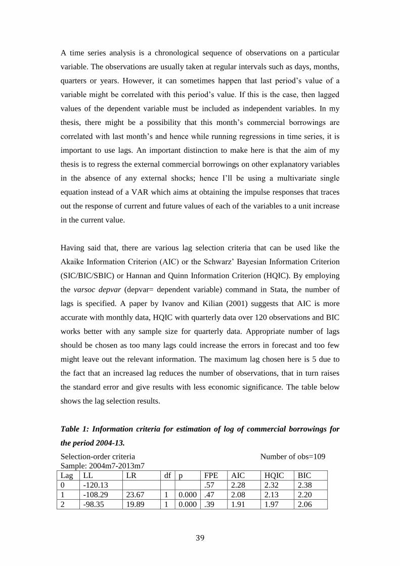
39

A time series analysis is a chronological sequence of observations on a particular

variable. The observations are usually taken at regular intervals such as days, months,

quarters or years. However, it can sometimes happen that last period’s value of a

variable might be correlated with this period’s value. If this is the case, then lagged

values of the dependent variable must be included as independent variables. In my

thesis, there might be a possibility that this month’s commercial borrowings are

correlated with last month’s and hence while running regressions in time series, it is

important to use lags. An important distinction to make here is that the aim of my

thesis is to regress the external commercial borrowings on other explanatory variables

in the absence of any external shocks; hence I’ll be using a multivariate single

equation instead of a VAR which aims at obtaining the impulse responses that traces

out the response of current and future values of each of the variables to a unit increase

in the current value.

Having said that, there are various lag selection criteria that can be used like the

Akaike Information Criterion (AIC) or the Schwarz’ Bayesian Information Criterion

(SIC/BIC/SBIC) or Hannan and Quinn Information Criterion (HQIC). By employing

the varsoc depvar (depvar= dependent variable) command in Stata, the number of

lags is specified. A paper by Ivanov and Kilian (2001) suggests that AIC is more

accurate with monthly data, HQIC with quarterly data over 120 observations and BIC

works better with any sample size for quarterly data. Appropriate number of lags

should be chosen as too many lags could increase the errors in forecast and too few

might leave out the relevant information. The maximum lag chosen here is 5 due to

the fact that an increased lag reduces the number of observations, that in turn raises

the standard error and give results with less economic significance. The table below

shows the lag selection results.

Table 1: Information criteria for estimation of log of commercial borrowings for

the period 2004-13.

Selection-order criteria Number of obs=109

Sample: 2004m7-2013m7

Lag LL LR df p FPE AIC HQIC BIC

0 -120.13 .57 2.28 2.32 2.38

1 -108.29 23.67 1 0.000 .47 2.08 2.13 2.20

2 -98.35 19.89 1 0.000 .39 1.91 1.97 2.06

40

3 -95.86 4.97 1 0.026 .39 1.89 1.96 2.06

4 -93.42 4.89* 1 0.027 .37* 1.86* 1.94* 2.06*

5 -92.81 1.23 1 0.267 1.86 1.87 1.96 2.09

Endogenous: ecb

Exogenous: ird gdp exrt _cons

From this output it is clear that the optimal number of lags is 4, so the regression

should look like:

Table 2: Basic OLS regression of ECB (logs) on explanatory variables for period

2004-13.

Standard errors in brackets *** p<0.01, ** p<0.05, * p<0.1

In the table above ecbone stands for first lagged value of log of ECB, similarly,

ecbtwo, ecbthree and ecbfour are the second, third and fourth lagged values. The most

(1) VARIABLES ecb ecbone 0.0837 (0.0989) [0.399] ecbtwo 0.0414 (0.0949) [0.663] ecbthree 0.206** (0.0935) [0.0300] ecbfour 0.104 (0.0933) [0.269] ird -0.0637* (0.0373) [0.0911] exrt -1.547* (0.807) [0.0580] gdp 0.967*** (0.345) [0.00604] Observations 111 R-squared 0.318

41

peculiar thing about co-efficient ‘β’ obtained for each variable is the sign. As results

show, the sign is positive and significant for the variable estimating real domestic

activity (gdp, proxy of estimates of industry and service sector) hence highlighting the

fact that Indian corporates’ preference to borrow overseas is positively related to

domestic activity. Result suggests 0.967 percent increase in ecb when 1 percent

change takes place in domestic economic activity. The variable is significant at 1%

level which definitely goes with the theory and literature review stated above.

Similarly, the sign is positive for the third lag of total borrowings showing statistical

significance at 5% level. It relates to the fact that 1 percent change in the previous

value of ecb would cause 0.206 percent change in borrowings today.

On the other hand, the sign is negative and significant for exrt (first difference of log

of exchange rates), describing the fact that as the domestic currency appreciates, firms

desire more overseas borrowing opportunities, however the significance is only at

10%, which is not very strong. The coefficient being -1.547 indicates the influence of

exchange rates towards ECBs. A one percent fall in the exchange rate raises total

borrowings by 1.547 percent. Exchange rate serves as a significant determinant that

drives corporates’ and business firms’ investment grade and credit rating. Due to the

vulnerability to currency shocks, the rating outlook is impacted. Depreciation of rupee

in recent history has made the repayment of interest and principal amount expensive

for the corporates. This result in the table is supported by the theory presented in

Chapter 2. Also, the sign for interest rate differential is negative and it is statistically

significant at 10% level showing a negative effect on external commercial

borrowings. The result states that a unit increase in ird will produce an expected fall

in ecb of 0.0637 units. The negative co-efficient result goes against the conclusions

provided by Singh (2007), Chakrabarty (2006) and Verma and Prakash (2011) in the

literature review above who concluded that a wider interest rate differential induces

ECB. In order to assess the model performance, we look at the R-squared value which

indicates that the model (all the three explanatory variables) explains approximately

31.8 percent of variation in total external commercial borrowings. With greater

avenues being explored by the Indian companies at home and foreign along with

easing of policies by the government, the entire mechanism has provided lower cost,

greater flexibility and the ease and comfort that international markets offer.

42

Lastly, I perform the Durbin-Watson test and the Durbin’s alternative test (H0: no

serial correlation) to check whether residuals are serially correlated from one

observation to other. This problem relates particularly to time series data and the

statistic would predict the presence of serial correlation among residuals. The null

hypothesis for this test assumes that residuals are uncorrelated. The autocorrelation of

residuals may sometimes lead to various consequences like the estimated regression

coefficient may no longer have the minimum variance or the mean square error may

underestimate the variance of error terms. After performing the Durbin-Watson test, I

obtain a value of 2.03, which indicates that residuals are uncorrelated, which is the

result that we expected. In the latter test, I reckon the p-value as 0.42, which is a large

value and thus we do not reject the null hypothesis. In order to confirm that there

exists no autocorrelation in residuals, I will scatter plot the residuals obtained from

the regression analysis above against there lagged values. The graph below

corroborates the absence of serial autocorrelation.

Figure 7: Plotting residuals with

its lagged values for the period

2004-13.

The next set of results relate to breaking down the entire dataset into three stages and

testing the explanatory variables on dependent variable (ECB).

-2-1

01

Res

idua

ls

-2 -1 0 1reslagged

43

I.2. Testing Stage 1 equation:

Starting again with a test for unit root in a time series sample, the dickey-fuller

concludes that the variable is stationary as indicated by the significant p-value at less

than 1%. The iterative ADF procedure after taking the first difference of the series

indicates the presence of unit root from lag 12 and remains until lag 2. The t-statistic

is closest to significance at 10% when lag 2 is taken. Hence at lag 2, I choose to

believe that there is no unit root in ecb for the period 2004-06. As the methodology

adopted above suggests, stationarity is to be proved for all the variables along with

commercial borrowings, hence an attempt is made and it has been ascertained that all

the three explanatory variables are required to be transformed into new series

involving the first difference and employing the ADF tests then proves ,

and stationary with 3, 8 and 1 lag respectively. The procedure of choosing the

lags is parallel to Ng and Perron method.

Again moving on to the lag selection for the dependent variable, I use the varsoc

command. The astrik in the table below tells that a lag length of 2 is picked by all the

criteria.

Table 3: Information criteria for estimation of log of commercial borrowings for

Stage1

Selection-order criteria Number of obs=30

Sample: 2004m7-2006m12

Lag LL LR df p FPE AIC HQIC BIC

0 -34.5 .76 2.56 2.62 2.75

1 -31.9 5.1 1 0.020 .68 2.45 2.53 2.69

2 -25.7 12.3* 1 0.000 .48* 2.11* 2.20* 2.39*

3 -25.7 .03 1 0.85 .52 2.18 2.28 2.50

4 -24.8 1.8 1 0.172 .52 2.18 2.30 2.55

5 -24.7 .1 1 0.706 .56 2.24 2.38 2.66

Endogenous: ecb Exogenous: ird gdp exrt _cons

44

TABLE 4: Basic OLS regression of log of ECB on explanatory variables for the

time period 2004-06.

(Stage 1)

VARIABLES ecb1

ecbone1 -0.872***

(0.179)

ecbtwo1 0.0124

(0.172)

[0.943]

ird1 1.045**

(0.461)

[0.0315]

exrt1 -4.172

(7.795)

[0.597]

gdp1 -4.342

(6.202)

[0.490]

Observations 34

R-squared 0.502

Standard errors in brackets

*** p<0.01, ** p<0.05, * p<0.1

Moving on to the impact of exchange rates, ird and domestic activity on ECB in stage

1 is described by regression equation (16) and results are shown in Table 4 above. In

the table ecbone1 and ecbtwo1 denote the first and second lagged values of the

dependent variable for stage 2 respectively. Stage 1 represents the data for the period

2004-06. In the entire model, the only variable out of the three main ones that is

significant is the ird. This very well fits into the hypothesis discussed in Chapter 1 and

states that as the ird between domestic and international markets widen, the Indian

firms are more inclined towards ECBs. A unit increase in ird produces 1.045 rise in

ecb.

The other two factors are not significant at all and moreover, the estimates of industry

and service show a negative relationship. This would imply that these two factors that

I took along with the lagged values, none affect the commercial borrowings for the 3

year period, however the above discussions concludes a surge in ECBs 2003 onwards.

Consequently, there must be other factors and reasons apart from ird that compensate

45

for this rise. I have tried to formulte certain other aspects that justify the the increase

in ECBs in the last sub-chapter of literature review. The surprising fact here is that

during 2004-06, the Indian economy was growing at approximately 8.5% which was

one of its highest8 and the results above show though an insignificant result between

ecb and gdp. For domestic activity, I have specifically taken the estimates of industry

and service sector from GDP and the survey shows a higher growth rate in

manufacturing, trade, hotels, communications and social and personal services (all

those components that constitute industry and service sector in my study). Also,

during the same period, the international credit agencies like Standard & Poor (S&P)

and Japanese Credit Rating Agency (JCRA) upgraded the credit rating for India due

to the sharp improvements in investor outlook (External Sector, Economic Survey

2004-05). The insignificance to a large extent is due to the breaking up of data and

fall in observations. Lastly, a potential reason behind the insignificance can be the

correlation between independent variables and lagged values. The value of coefficient

shall decrease when lags are taken. The first lagged value of the dependent variable is

significant at 1% level notifying that a percent increase in the previous value of

borrowings result in 0.872 decrease in it today.

The d-statistic of the Durban-Watson test does not rejects the null hypothesis which

implies that residuals are not serially correlated. The test performed gives the d-

statistic as 1.96 which is very close to 2 and hence residuals are uncorrelated. The p-

value (0.87) for the Durbin’s alternative test reflects acceptance of the null hypothesis

and hence no serial correlation. Also, I will plot the residuals against their lagged

values, which confirms

the absence of

autocorrelation.

Figure 8: Plotting

residuals with its

lagged values for Stage

1

8 The Union Budget and Economic Survey, 2004-05: http://indiabudget.nic.in/es2004-05/chapt2005/chap11.htm

-2-1

01

Res

idua

ls

-2 -1 0 1reslagged1

46

Concerning the regressions in stage 2 are denoted by the equation (17) in the previous

section and Table 6 below.

I.3 Testing Stage 2 equation:

For the period 2007-09, the dickey-fuller test for the dependent variable does not

indicate the presence of unit root and hence its stationary. Consequently, I begin to

perform the ADF test, which shows non-stationarity and therefore I proceed to take

the first difference of the (log of ) series. ADF tests on transformed series is

performed and gives the optimal lag length of 2 as t-statistic is significant at 10%

level here. Also, the p-value is significant at less than 1%. Subsequently, I check the

presence of unit root for all other variables. Converting them into first difference

series I get variables and , which stands for first difference of (log

of) exchange rate between India and U.S. for stage 2 and so on. These variables prove

to be stationary at lag 1, 8 and 1 respectively. The lag selection requires me to follow

the same procedure and results are shown in the following table below. The astrik

predict that all the criteria hint at choosing 2 lags. I now regress the dependent

variable over all the first difference values of independent variables along with the lag

values.

Table 5: Information criteria for estimation of log of commercial borrowings for

Stage 2

Selection-order criteria Number of obs=30

Sample: 2007m7-2009m12

Lag LL LR df p FPE AIC HQIC BIC

0 -31.80 .64 2.38 2.44 2.57 1 -28.24 7.12 1 0.008 .53 2.21 2.29 2.45 2 -26.19 4.09* 1 0.043 .50* 2.14* 2.23* 2.42* 3 -25.78 .822 1 0.364 .52 2.18 2.29 2.51 4 -25.43 .699 1 0.403 .55 2.22 2.34 2.60 5 -25.22 .433 1 0.510 .58 2.28 2.41 2.70 Endogenous: ecb Exogenous: ird gdp exrt _cons The results of the regression performed are shown below.

47

TABLE 6: Basic OLS regression of log of ECB on explanatory variables for the

time period 2007-09.

(1) VARIABLES ecb2

ecbone2 -0.702*** (0.187) [0.000785] ecbtwo2 0.173 (0.192) [0.377] ird2 0.0709 (0.208) [0.736] exrt2 0.198 (4.023) [0.961] gdp2 -1.286 (7.987) [0.873] Observations 34 R-squared 0.354

Standard errors in brackets *** p<0.01, ** p<0.05, * p<0.1

In the table above ecbone2 and ecbtwo2 denote the first and second lagged values of

log of the explained variable for stage 2 respectively. The analysis for evaluating the

effect of the three variables on ECB as shown by equation (17) is performed and

results are recorded in the table above. The result reveals insignificance for the three

main factors and the regression co-efficient is negative for gdp2 whereas positive for

ird2 and exrt2. Again, taking an abridged period (2007-09) has reduced the number of

observations to around 30 due to which the results found are not as expected. The

only significance in this period is shown by the first lagged value of the dependent

variable. A percent fall in ecbone2 leads to 0.702 percent fall in ecb2.

The years 2007-09 was the same period when Lehman Brothers collapsed and the

international markets raised their lending rates to soaring heights. RBI balanced this

through easing out policies and relaxation of all-in cost ceilings, but even then the

amount of ECBs dropped in 2008-09. In order to safeguard its balance sheets from

48

currency fluctuations, the firms turned to rupee financing with easy domestic liquidity

considerations (Sinha, 2010). Tightening of liquidity conditions and rise in the risk

premium added to the reduction in ECBs during the crisis. The R-squared is fairly

decent which indicates that the model explains approximately 35.4 percent of

variation in total external commercial borrowings. Unlike the results for above

regression equation, domestic activity is not significant in this case. According to the

Index of Industrial Production for the year 2008-09, the growth in the industrial sector

fell drastically this period in contrast to 2004-05 and maybe due to this there was no

effect on ECBs as far as the real domestic activity is concerned. Along with that, the

manufacturing, electricity and construction sectors also suffered.

The Durbin-Watson as mentioned earlier tests the null hypothesis that residuals from

a regression are not autocorrelated against the alternative hypothesis. After

performing the test for the period 2007-09, the d-statistic found out to be 2.06, which

predicts that the residuals to a large extent are uncorrelated. The Durbin’s alternative

test for higher orders of autocorrelation reveal that the p-value (0.70) is considerably

high and does not require rejection of the null hypothesis, which predicts no serial

autocorrelation. In order to confirm, the absence of autocorrelation, I now plot the

residuals against their fitted values and observe that there is no pattern formed. The

diagram confirms that residuals are not serially correlated.

Figure 9: Plotting

residuals with its lagged

values for Stage 2.

-1.5

-1-.5

0.5

1

Res

idua

ls

-1.5 -1 -.5 0 .5 1reslagged2

49

I.4 Testing Stage 3 equation:

The dickey-fuller test indicates that the ecb is stationary. Hence, I now turn to the

ADF test. Taking the first difference of the ecb for the period 2010-13 forms the new

transformed series. The methodology suggests taking three lags for ADF. It is quite

likely not to have any unit root here. This confirms the presence of stationarity. I also

need to test for the absence of unit root for other variables. The null hypothesis states

the occurrence of unit root. The explanatory variables were transformed into new

series by taking the first difference of each of them. I reckoned that was

stationary when taken 3 lags. Similarly, and proved to be stationary at

lags 8 and 1 respectively. Following table will determine the length of lag that needs

to be selected in order to run the regression.

Table 7: Information criteria for estimation of log of commercial borrowings for

Stage 3

Selection-order criteria Number of obs= 37

Sample: 2010m7-2013m7

Lag LL LR df p FPE AIC HQIC SBIC

0 -38.78 1 .59 2.31 2.37 2.48

1 -33.58 10.40 1 0.001 .47 2.08 2.16 2.30

2 -30.34 6.46* 1 0.011 .41 1.96 2.05 2.22*

3 -29.03 2.61 1 0.106 .41 1.94 2.05 2.25

4 -27.51 3.04 1 0.081 .40* 1.91* 2.04* 2.26

5 -26.78 1.46 1 0.226 .41 1.93 2.07 2.32

Endogenous: ecb

Exogenous: ird gdp exrt _cons

Except for SBIC, all other criteria hint at taking 4 lags. As stated above, AIC is

preferred for monthly data; hence I would finalize choosing 4 lags and carry out the

multivariate regression.

50

TABLE 8: Basic OLS regression of log of ECB on explanatory variables for the

time period 2010-13.

(1) VARIABLES ecb3

ecbone3 -1.003*** (0.173) ecbtwo3 -0.0991 (0.177) [0.579] ecbthree3 0.0932 (0.182) [0.612] ecbfour3 0.151 (0.175) [0.394] ird3 0.293* (0.166) [0.0876] exrt3 2.125 (3.258) [0.519] gdp3 0.619 (1.240) [0.621] Observations 39 R-squared 0.549

Standard errors in brackets *** p<0.01, ** p<0.05, * p<0.1

The effect on ECBs for the period 2010-13 is performed through the regression in

equation (18). This was the period when the economy started to recover and

witnessed another accretion in ECBs. The regressions are done to inspect the

significance of these three explanatory variables on ECBs. As shown in the table

above, only the is positive and significant at 10% level. It states that a unit

increase in interest rate differential raises borrowings by 0.293 units. Hence, the null

hypothesis for this variable is not rejected. The positive sign of depicts

depreciation of domestic economy induces Indian companies borrow more from

overseas which is against the theoretical concept and the hypothesis I stated. The

fairly high value of R-squared explains approximately 54.9 percent of variation in

total external commercial borrowings.

51

The insignificance in this case is due to the poor data taken with only 44 observations

(and even lesser after logs and first differences). The insignificance of these variables

along with the lagged values (except for lag 1) might be due to the poor data and the

lagged values taken as a fall in number of observations negatively impact the

significance condition of a variable. Again, one percent fall in the first lag of

dependent variable causes an increase of 1.003 percent in ECBs today. It is also to be

noted that the performance of the Indian economy during this phase was the poorest

among all the stages. Growth in manufacturing sector contracted, mining and

quarrying remained stagnant, construction sector slowed and growth in service sector

remained unchanged. I would again like concentrate on the point that these are the

same sectors taken in the estimates of industry and service. According to the

Economic Survey, 2011-12, the slowdown in the GDP was entirely due to the

weakening of the industrial growth. The adverse growth in India can also be related to

the turmoil in the euro-zone countries since 2011. Both the global and domestic

factors attributed to the slowing of the Indian economy. The deteriorated performance

of these sectors during this period justifies the insignificance on commercial

borrowings to some extent.

Carrying out the Durbin-Watson test to find out if there exists any autocorrelation

among the residuals, I obtain the d-statistic as 2.24. This is though close to 2 but does

not predict the absence of strong autocorrelation. Even the Durbin’s alternative test

for autocorrelation gives a p-value of 0,10, which is not very appealing as compared

to the above cases. In order to correct for serial correlation, I used the Prais-Winston

estimator using the prais command in stata. It uses the generalized least-squares

method to estimate parameters in the regression model (linear) where errors are

serially correlated. Employing this command gave me a corrected value of d-statistic

for AR (1) close to 2. This proves that residuals are not autocorrelated. Again, I plot

the residuals against the lagged values and observe that there is no pattern formed.

52

Figure 10: Plotting

residuals with its lagged

values for the period

It remains inconclusive overall in the regressions run for the above three stages as to

how the external commercial borrowings affected by the explanatory variables. The

prominent conclusion I can give is in the majority of stages, the interest rate

differential has been significant and positive, which reflects the fact that the

hypothesis formed was in coherence with the theory. Also, the first lagged value has

always been significant, which can too contribute as an important result. The

insignificance for other variables and lagged values might be due to the breaking up

of the data and hence reducing the number of observations. Also, there can be other

reasons that led to changes in ECBs during the various 3 periods of boom and bust.

No doubt an increase in ECBs has added onto the capital inflows in India, but that

said, there are certain implications. Due to the above reasons, firms borrow abroad to

meet their domestic expenditures and finance expansion plans, there are however,

expected dangers associated with this inclination in the near future. First, foreign

exchange earned by the country might have to be diverted to the borrowers to help

them repay their debt commitments due to the mismatch between the Indian rupee and

the currency in which the debt service commitments on external loans must be met.

This will in turn affect the trade and current account deficits and the balance of

payments. Second, if there is substantial depreciation of the domestic currency then

their debt commitments in rupee terms will rise sharply. Hence, even though they are

obtaining loans at a lower external interest rate, this behavior of the exchange rates

will neutralize the interest rate differential advantage. Moreover, the international

rates will not be low always; therefore, an increase in the external rates will tend to

expensive borrowing making the corporate firms vulnerable.

-1-.5

0.5

1

Res

idua

ls

-1 -.5 0 .5 1reslagged3

53

CHAPTER 8: CONCLUSION

It can be concluded from the results that external commercial borrowings are overall

affected by exchange rates, interest rate differentials and real domestic activity for

India for the period 2004-2013. The curiosity in exploring this topic attributed to the

fact that in the era of financial development, the pattern of rise and fall in

external commercial borrowings has been phenomenal and the data under study

very well explains that. These results can be reasoned to some important

perspectives. Firstly, due to an increasing share in the industrial and service sector of

India, the use of ECBs for overseas investments has grown significantly. Second, the

coefficients of OLS regression reveal that interest rate differential too have some

effect on the demand for ECBs. Third, exchange rate is an important variable that

explains changes in external borrowings, however there is scope to use a more

detailed approach that would help to define a clearer picture. As for the results

obtained for the three time periods (1st: 2004-06, 2

nd: 2007-09 and 3

rd: 2010-13), there

was an expectation of significant results in each stage; however, there is not much that

we can confidently interpret about the stages. There was no convincing evidence that

ECBs were affected by the explanatory variables in the three stages apart from the

significant effects of ird in two stages (10% level).

The paper also analyses the correlation between current account deficit and external

commercial borrowings along with a brief description of whether there has been a

shift from non-debt to debt flows. ECB is not a new concept and is presently playing a

vital role in the economic development of the country like India. It is a debt

component that has a long lasting role to play in the country and was introduced even

before FDI and FII. In recent years, it has been observed that a large amount of

current account deficit is being financed by ECBs. Current account deficit is not a

problem when a country faces it for one or few years, it becomes a problem when it

persistently faces one. This has been true for India and now a major part of it is being

financed through capital flows mainly, FDI, FII and ECB. The recent developments

indicate that the RBI is successful in reducing the CAD through various policies

involving high exports and reduced gold imports. Risk aversion in global financial

markets has slackened the pace of capital flows in India recently, it is expected that

54

the FDI inflows pick up pace and the FII revert to decreasing trend so that CAD is not

just majorly being financed by commercial borrowings but other components of debt

flows as well.

55

REFERENCES:

Aggarwal, S. (2013). The Uncovered Interest Rate Parity Puzzle in the Foreign

Exchange Market.

Ahluwalia, M. S. (2002). Economic reforms in India since 1991: has gradualism

worked? The Journal of Economic Perspectives, 16(3), 67-88.

Arora, D., Rathinam, F. X., & Khan, M. S. (2010). India’s Experience during Current

Global Crisis: A Capital Account Perspective. Public Policy Review, 6(5), 807-836.

Businesstoday.intoday.in. (2013). RBI eases external commercial borrowing norms -

Business Today - Business News. Retrieved 4 June 2014, from

http://businesstoday.intoday.in/story/rbi-eases-external-commercial-borrowing-

norms-sept-4-2013/1/198321.html

Calvo, G. A., Leiderman, L., & Reinhart, C. M. (1993). Capital inflows and real

exchange rate appreciation in Latin America: the role of external factors. Staff

Papers-International Monetary Fund, 108-151.

Chaboud, A. P., & Wright, J. H. (2005). Uncovered interest parity: it works, but not

for long. Journal of International Economics, 66(2), 349-362.

Chakraborty, I. (2006). Capital inflows during the post-liberalisation period.

Economic and Political Weekly, 143-150.

Chandrasekhar, C. P. (2004). Beyond the forex proposal. Economic and Political

Weekly, 5563-5565.

Chinn, M. D., & Meredith, G. (2005). Testing uncovered interest parity at short and

long horizons during the post-Bretton Woods era (No. w11077). National Bureau of

Economic Research.

56

Combes et al. (2011), “Capital flows, Exchange Rate Flexibility and Real Exchange

Rate”, International Monetary Fund Working Paper, WP/11/9.

Das, A., Banga, R., & Kumar, D. (2011). Global economic crisis: Impact and

restructuring of the services sector in India (No. 311). ADBI working paper series.

Dgff.unctad.org,. (2014). Global capital flow trends. Retrieved 29 May 2014, from

http://dgff.unctad.org/chapter1/1.2.html

Doidge, C., Karolyi, G. A., & Stulz, R. M. (2004). Why are foreign firms listed in the

US worth more?. Journal of Financial Economics, 71(2), 205-238.

Durairaj, K. (2010). Foreign Direct Investment and Exchange Rate in India. Al-

Barkaat Journal of Finance & Management, 2(2), 1-17.

Fedderke, J.W. and W. Liu (2002), “Modeling the Determinants of Capital Flows and

Capital flight: with an Application to South African data from 1960 to 1995”

Economic Modelling 19(2002) 419-444.

Feldstein, M. (1983). Domestic saving and international capital movements in the

long run and the short run. European Economic Review, 21(1), 129-151.

Fry, M. J., Claessens, C. A., Burridge, P., & Blanchet, M. C. (1995). Foreign direct

investment, other capital flows, and current account deficits: what causes what? (No.

1527). The World Bank.G.

G. Maria Milesi-Ferretti, & Razin, A. (1998). Sharp reductions in current account

deficits an empirical analysis. European Economic Review, 42(3), 897-908.

Gopinath, G. (2004). Lending booms, sharp reversals and real exchange rate

dynamics. Journal of International Economics, 62(1), 1-23.

Gordon, J. P., & Gupta, P. (2003). Portfolio Flows into India: Do Domestic

Fundamentals Matter?. International Monetary Fund.

57

Gordon, J.P. & Gupta, p. (2004). Nonresident deposits in India: In search of return?.

Vol. 4. International Monetary Fund.

Graham Bird and Ramkishen S. Rajan (2000), “Resolving the Interest Rate Premium

Puzzle: Capital Inflows and Bank Intermediation in Emerging Economies” CIES

Working Paper No. 12.

Guerin, S. (2012). The relationship between capital flows and current account:

volatility and causality. Available at SSRN 2018195.

Helpman E., and P.R. Krugman (1985), Market Structure and Foreign Trade,

Increasing Returns, Imperfect Competition and the International Economy, MIT

Press, Cambridge.

Higgins, M., & Klitgaard, T. (1998). Viewing the current account deficit as a capital

inflow. Federal Reserve Bank of New York Current Issues in Economics and Finance,

4.

Ivanov, V., & Kilian, L. (2001). A practitioner's guide to lag-order selection for

vector autoregressions (No. 2685). CEPR Discussion Papers.

`Jiang, J., & Sinton, J. (2011). overseas investments by chinese National oil

companies. International Energy Agency, February.

Jongwanich, Juthathip (2010). Capital Flows and Real Exchange Rates in Emerging

Asian Countries. Asian Development Bank, Economics Working Paper.

Juan-Ramon, V. H., & Dabós, M. P. (2000). Real Exchange Rate Response to Capital

Flows in Mexico-An Empirical Analysis. International Monetary Fund.

Karolyi, G. A. (1998). Why do companies list shares abroad?: A survey of the

evidence and its managerial implications. Financial Markets, Institutions &

Instruments, 7(1), 1-60.

58

Kaur, M., & Dhillon, S. S. (2010). Determinants of Foreign Institutional Investors’

Investment in India. Eurasian Journal of Business and Economics, 3(6), 57-70.

Khan, M. S., & Zahler, R. (1983). The Macroeconomic Effects of Changes in Barriers

to Trade and Capital Flows: A Simulation Analysis. Staff Papers-International

Monetary Fund, 223-282.

Krugman, P. R. (2006). et Obstfeld, M. (2006). International Economics.

Lothian, J.R. and Wu, L., Uncovered Interest Rate Parity over the Past Two

Centuries. Unpublished working paper, Fordham University and Baruch College,

June 2005.

Martin, M., & Rose-Innes, C. (2004). Private Capital Flows to Low-Income

Countries: Perception and Reality. Canadian Development Report 2004.

Mody, A., & Murshid, A. P. (2005). Growing up with capital flows. Journal of

International Economics, 65(1), 249-266.

Mody, A., Taylor, M. P., & Kim, J. Y. (2001). Modelling fundamentals for

forecasting capital flows to emerging markets. International Journal of Finance &

Economics, 6(3), 201-216.

Mohan, R. (2008). Capital flows to India. BIS Papers, 44, 235-263

Oura, H. (2008). Financial development and growth in India: A growing tiger in a

cage?. IMF Working Papers, 1-30.

Rangarajan, C. (2000). Capital flows: Another look. Economic and political weekly,

4421-4427.

Razin, A. (1998). International capital flows: sustainability, sudden reversals, and

market failures. International capital flows: sustainability, sudden reversals, and

market failures.

59

Rbi.org.in,. (2014). Reserve Bank of India - India's Central Bank. Retrieved 28 May

2014, from http://www.rbi.org.in

Reinhart, Carmen, (2005), “Some Perspective on Capital Flows to Emerging Market

Economies”, NBER Reporter, Summer, http://www.nber.org/

reporter/summer05/reinhart.html.

Report submitted by a Working Group established by the Committee,. (2009). Capital

flows and emerging market economies. Bank of International Settlements.

Rodrik, D., & Velasco, A. (1999). Short-term capital flows (No. w7364). National

bureau of economic research.

Sebastian, E., (2001). Exchange Rate Regimes, Capital Flows and Crisis Prevention.

NBER Working Paper No. 8529

Shah, A., & Patnaik, I. (2010). 9. Managing capital flows: the case of India.

MANAGING CAPITAL FLOWS, 239.

Singh, B. (2007). Corporate choice for overseas borrowings: The Indian evidence.

Singh, B. (2009). Changing Contours of Capital Flows to India. Economic and

Political Weekly, 58-66.

Sinha, A. (2010). Impact of the international banking crisis on the Indian financial

system. Bank of Israel Rony Hizkiyahu, 225.

Thomson, D.J. (1994). Jackknifing multiple-window spectra. In: Pro- ceedings of the

IEEE International Conference on Acoustics, Speech and Signal Processing, VI, 73-

76.

60

Verma, R., & Prakash, A. (2011). Sensitivity of Capital Flows to Interest Rate

Differentials: An Empirical Assessment for India. RBI Working Paper Series: 7/2011,

Dept. of Economic and Policy Research (DEPR), May.

Ying , Yung-Hsiang and Yoonbai Kim (2001), “An Empirical Analysis on Capital

Flows: The Case of Korea and Mexico” Southern Economic Journal, Vol. 67, No. 4

(Apr., 2001), pp. 954-968.

(2014). Retrieved from

http://www.livemint.com/Politics/fiSALCoSCEL9TgH8Y7SSqM/Govt-looks-to-

provide-fillip-to-manufacturing-exports.html

61

APPENDIX:

Important Definitions and Labels:

ecb: First difference of log of External Commercial Borrowings, where ECB

is defined as an instrument used in India to facilitate the access to foreign

money by Indian corporates.

exrt: First difference of log of exchange rates between India and U.S., where

exchange rate is defined as the price of nation’s currency in terms of another

currency.

gdp: First difference of log of estimates of industry and service sector, where

the estimates are taken as proxy for real domestic activity. Manufacturing,

Construction, trade, hotels, insurance and social and personal services

constitute the industrial and service sector in my thesis.

ird: First difference of Interest rate differential, where ird is defined as the

difference in interest rates of two distinct economic regions.

CAD: Current Account Deficit is defined as measurement of a country’s trade

in which the value of goods and services it imports exceeds the value of goods

and services it exports.