1

Exploring the ripple effect and spatial volatility

in house prices in England and Wales:

regressing interaction domain cross-correlations

against reactive statistics

Crispin Cooper, Scott Orford, Chris Webster, Christopher B. Jones

Abstract

This study conducts an exploratory spatio-temporal analysis of recent UK housing market

data 2000-2006, fine grained both in space and time. We present firstly the exploratory

technique itself, and secondly an overview of patterns found in the data set. A broadly

scoped meta-model is created which points towards fruitful avenues of further

investigation for understanding the driving forces behind price propagation in the housing

market. At the core of this model is an 8850x8850 cross-correlation matrix representing

price linkage between different areas, which is analyzed by a custom regression engine.

Hence this is the first study to unify both local and regional house price modelling, and

the first to look for a quantitative explanation of the structure of any house price

interaction matrix on a large scale. Findings corroborate existing research on the ripple

effect and spatial volatility, and point towards mechanisms through which these might

arise, as a combination of local interaction and market segmentation broken by lifecycle

migration patterns.

2

Keywords: migration, network analysis, interaction, census, house prices, time series,

cross-correlation, spatial data, regression, ripple effect.

1. Introduction

The UK’s housing market is one of the most volatile in the world and has experienced

four cycles of boom and bust since the 1970s. The most recent housing market cycle has

been the longest with the upward phase of the cycle lasting a decade from the mid-1990s

with the peak in 2006 before house prices fell and bottomed in 2008 followed by a period

of stagnation (Wong et al., 2009). However, unlike previous housing market cycles, the

last cycle has seen a move from temporal volatility to spatial volatility where house price

changes affect some regions more than others and at different times in the housing market

cycle (Ferrari and Rae, 2011). Ferrari and Rae chart the origins of this spatial volatility to

the housing market cycle of the 1980s where divergent and persistent regional variations

in house price differences first emerged in terms of both absolute prices and even more

extremely in regional house price inflation. They argue that from the 1990s up until the

peak in 2006, the temporal stability in the housing market had been at the cost of an

emergent spatial volatility which now dominates the market. Spatial differences in house

price change in the UK have long been conceptualized as a ‘ripple effect’, with London

and the South East regions leading house price changes and the northern regions of

England lagging but then catching up as the London market slows down and then

declines at the end of the cycle thus allowing the initial divergence to be corrected (eg

3

Alexander and Barrow, 1994; Meen, 1999; Wood, 2003). This conceptualization,

however, fails to acknowledge house price differentials within regions whereby local

housing market areas can exhibit high degrees of spatial divergence in prices that can be

masked by regional analysis (Gray, 2012). More importantly, it also ignores the spatial

volatility that has resulted in the decoupling of a significant number of local housing

market areas from the national market (Ferrari and Rae, 2011). In this respect, in the most

recent ‘ripple effect’ the initial divergence at the start of the cycle has not been corrected

resulting in persistent and significant local and regional differentials in house prices.

This emergent spatial volatility in house prices demands a move towards more regional

and local analysis of the UK housing market. However, a fundamental feature of UK

housing market research has been the lack of co-ordinated and integrated analysis across

different spatial and temporal scales (Meen, 2001). This has hindered the development

and validation of housing market models and, in turn, the development of housing market

theories that cover a wide range of spatial and temporal scales. As a result, a framework

that integrates housing market analysis at different scales does not currently exist.

Housing market analysis at the national level is time-series and macro-economic

orientated whilst the local level is driven by spatial, micro-economic models. Regional

level analysis sits uncomfortably between the two, both theoretically and analytically, but

has been the focus of notable research in the UK (eg MacDonald and Taylor, 1993;

Meen, 1999; Wood, 2003; Worthington & Higgs, 2003). This lack of a framework means

that important research questions on how the UK housing market functions across space

and through time are difficult to answer, leading to differing views and intellectual

4

traditions and uncertainty for policy makers. This discord has partly been due to a lack of

detailed data on housing transactions in England and Wales (Orford, 2010) resulting in an

emphasis on aggregated analysis at regional and national levels. However, since 2000,

data on individual transactions in England and Wales has been available and this has

resulted in some temporal cross-scale research on the UK housing market (e.g. Ferrari

and Rae, 2011; Gray, 2012). These studies have highlighted the importance of sub-

regional analysis of housing market data in order to better understand the connections

between local housing markets and the increasing spatial volatility between regions.

Although at a finer spatial scale than previous studies, the research is still restricted to the

district level and average quarterly and annual house prices which could mask some

important trends, particularly in times of rapid house price change and across districts

that contain a wide variation in housing stock.

This paper builds on this recent body of research by exploring a novel combination of

spatio-temporal analysis techniques applied to housing market movements. The analysis

is based on the complete individual level transaction data from 2000-2006 and intra-UK

migration and commute data taken from the 2001 census and aggregate statistics from the

same year at ward and local / unitary authority levels. The focus of the research is on

connections between local and more regional housing markets and we demonstrate the

use of massive spatial network interaction and time series data sets to reveal information

about spatial volatility in house prices in England and Wales and the importance of the

ripple effect.

5

Although exploratory in spirit, the paper is concerned with determining whether spatial

divergence in house prices has largely a reactive explanation and are caused by the

characteristics of areas, or whether they are also a result of interactive effects related to

migration flows, commuting flows and the physical distance between areas. The results

also suggest the feasibility of two simpler approaches: clustering of time series, similar to

Gary (2012) and the use of a market-leading/market-lagging framework which is briefly

explored.

Therefore, the aims of the paper are (1) to conduct an exploratory analysis of newly

available data, and (2) to document a technique for combining spatial, spatial-temporal

and interaction datasets which we believe is helpful firstly in filling the gap between

current regional and local models, and secondly in deducing the likely causes of, rather

than simply the presence of, a ripple effect.

The novelty in the paper is as follows

• Use of regression as an exploratory technique in the spatial interaction domain

• Attempting to quantitatively explain (rather than simply produce and then discuss)

patterns of inter-area correlation

• Modelling house prices within a combined local and regional framework rather

than investigating the two separately (a task requiring considerable custom

computational development)

• Formulation of the market-leading/lagging framework by summing cross-

correlations that share a common spatial endpoint

6

In the remainder of this paper we structure the research as follows. Section two explores

the background literature, while section three discusses the data used. Sections four to

six describe the methods and section seven discusses the regression results, which lead on

to an alternative analysis based on leading/lagging locations, presented in section eight

and a conclusion in section nine.

2. The ripple effect, spatial volatility and the UK housing market: an overview

Simple abstract models of individual behaviour in housing markets have no doubt guided

transactions ever since an exchange value was first assigned to a piece of land. The

extensive data drawn from modern housing markets now makes possible not just

predictions about individual behaviour, competition and the interaction of demand and

supply, but models of patterns at a scale of aggregation not normally perceptible by the

individual market participant. In this paper we concern ourselves with one such pattern:

the so-called ‘ripple effect’ of house price changes. In England and Wales for example,

market trends have typically commence in London and the South East and then

propagated to other regions (Alexander and Barrow, 1994). In relation to the current

housing market cycle, Gray (2012) concludes that in the short run, local house price

growth was locally idiosyncratic but in the medium term a pattern consistent with a ripple

passed from south to north of England, although this was not smooth with the distance

effect from London vanishing beyond the East Midlands and house prices in the north

7

appearing to jump together. As a formal model, this type of market behaviour is not well

constructed or understood. In scholarly work, the pattern has been demonstrated to exist

but a conclusive explanation for it remains to be found and this limits the degree to which

the model can be developed and used. Worthington & Higgs (2003) and MacDonald &

Taylor (1993), for example, demonstrate ripple price movements in the UK, but do not

speculate on their cause. Giussani and Hadjimatheou (1991) mention a variety of possible

explanations, including the possibility that regions react differently to external factors

such as housing stock and income. Meen (2001), studying ten UK regions, hypothesizes

that the ripple effect is generated mainly by mechanisms related to, for example, incomes

and interest rates, but also speculates that in other cases, differing economic conditions,

information dissemination through property searches and equity transfer could also cause

regularities in interregional price disparity. Gray (2012) concludes something similar,

with combinations of districts not reflecting housing markets in the sense of space

delimited by living and working but rather by buyer search/migration or information

flows. Shi et al (2009) and Pollakowski & Ray (1997) deal with similar effects in New

Zealand and the US respectively.

As Cliff & Ord (1981) noted, models of spatial processes, such as the ripple effect, rely

on “whether the levels of the process at two (neighbouring) sites reflect interaction

(between the sites) or reaction to some other variable”. Hence, Giussani and

Hadjimatheous’ proposition is a reactive explanation, although a possible interactive

explanation is also hinted at because correlations are noted between acceleration in inter-

region migration and price change, albeit aggregated to a coarse level. Meen’s (2001)

8

mechanisms are also a combination of reactive and interactive explanations although no

weighting is given to the importance of each. Further, in relation to the last housing

market cycle, Gray (2012) also observes evidence of substantial spatial volatility at odds

with the ripple effect. Here chains of districts exhibited growth patterns inconsistent with

nearby urban areas and violent switches from slow to rapidly growing districts occurred

where the dynamics were at odds with an interlocking housing market. Ferrari and Rae

(2011) explore the way in which connections and disconnections between areas might

contribute to this observed spatial volatility. They demonstrate that areas of similar levels

of deprivation remain more closely connected and that the strength of this relationship is

greater for the most and least deprived districts and that both ends of the housing market

spectrum are isolated from the rest of the market.

Crucially however, none of these studies offer a direct quantitative attempt to determine

which mechanisms are the most likely cause of observed spatially non-contiguous price

correlations, neither do they explore the structure of the pattern in any detail. The current

study attempts such an investigation by computing an interaction matrix and then

subjecting that matrix to regression analysis. This cannot of course prove causality, but

can show which variables provide a better indication of rippled market linkage than

others and also which variables are related to spatial volatility. The work is also

conducted on a finer spatial scale to any that precedes it. The house price dataset covers a

six-year time span divisible into temporal units as fine as two days, with an areal unit of

the census ward, of which there are 8,850 in England and Wales. This contrasts, for

example, with the ten regions of Mean (2001) study. Not surprisingly, there is a good

9

deal of noise in such a fine spatial model and we also report a model that more closely

fits the data, using 376 English and Wales local/unitary authorities.

3. Data description and preparation

Individual housing transactions from the England and Wales were obtained from HM

Land Registry for the period 2000-2006 representing approximately nine million records.

As this dataset does not include many housing attributes (only dwelling type, tenure and

whether the property is a new build is provided) the data were aggregated to census

Output Area level matching on postcode. As Output Areas were created with the aim of

representing a population as socially homogeneous as possible, based on tenure of

household and dwelling type (Census Geography, n.d.), constructing Output Area price

indices has the effect of incorporating basic hedonic information on the average mix of

housing in each Output Area - thereby mitigating indexing errors on short time scales

caused by the sale of particularly low- or high-valued properties. At the temporal level

the data were aggregated by averaging within successive time slices with a fixed length

chosen for each analysis.

The main analysis was conducted at the level of wards and local/unitary authorities.

These units were partly chosen because of the ready availability of census data for each

of them. In the case of wards, the aim is to conduct a fine-grained study; a finer-grained

alternative would be to analyze Output Areas, but rich socio-demographic information is

10

not provided on this scale and there are issues with disclosure control on the quality of

data. In the case of local authorities, the aim is to provide a coarse grained analysis to see

whether the different scales highlight different interactive or reactive mechanisms. We

produce ward level indices with 200-day time slices, and local/unitary authority indices

with 2-day time slices. These are chosen in order to provide as high a temporal

resolution as possible, while still remaining meaningful: on these time frames,

transactions exist in 99.9%, and 81% of time slices respectively. Where no transactions

are found in a time-slice, the index value is copied from the previous data point.

Census data are taken from the 2001 Census for England and Wales, aggregated to the

levels described. All migration, commuting and aggregate social and housing statistics

are for the year 2000-2001 only. As a full census is conducted only once every ten years,

annual data are not available to the same extent. Therefore it is necessary to assume that

data collected in 2001 is still relevant to explaining the state of the market up until 2006.

While this approach may fail to highlight factors that have caused a change in the market

over a short length of time, it still remains possible to deduce long term origins of long

term correlations.

4. Cross-correlation analysis

The case for a reactive versus interactive spatial model is rarely open and shut. This is

certainly true of the housing market. Standard reactive models tend to estimate

parameters for equations involving spatial variables, while standard interactive and mixed

11

models are likewise based on parameter estimation, but include extra terms for the target

variable at other spatial locations, weighted by an interaction matrix (e.g. Anselin 1988).

However, the necessity of pre-specifying the form of this matrix restricts the model to

representing interactions of a very specific nature, and so also runs against the spirit of

exploratory analysis.

In contrast, if sufficient data are available it should be possible to directly estimate the

interaction matrix from the data. Seemingly Unrelated Regression (Meen 2001, page

166) achieves this by treating interactions as error terms in a reactive regression. Cross-

correlation approaches, as used by Giussani & Hadjimatheou (1991) and Shi et al. (2009),

provide a more intuitive approach, looking for simple correlation between the current

growth of a region and past growth values of all other regions. We employ such an

approach in the current study, although more sophisticated techniques are noted to exist.

For example, Granger causality tests can determine whether future time series values are

better explained by auto- or cross-correlation. Vector Auto-regression (the natural

multivariate extension of Granger tests) can determine the best explanatory combination

of a number of related signals, while Johansen testing can be used to search for multiple

sets of co-integrated series. These are employed in various combinations in both of the

above citations and also in Worthington & Higgs (2003), MacDonald & Taylor (1993)

and Pollakowski & Ray (1997). None of these studies, however, analyze correlation

between more than 13 regions, in contrast to the 8,850 regions of the current study. For

this reason, cross-correlation – due to its light use of computational resources – is

considered a reasonable first approach to the problem; given that the present study is the

12

first to look for a quantitative explanation of the structure of any such house price

interaction matrix on a large scale.

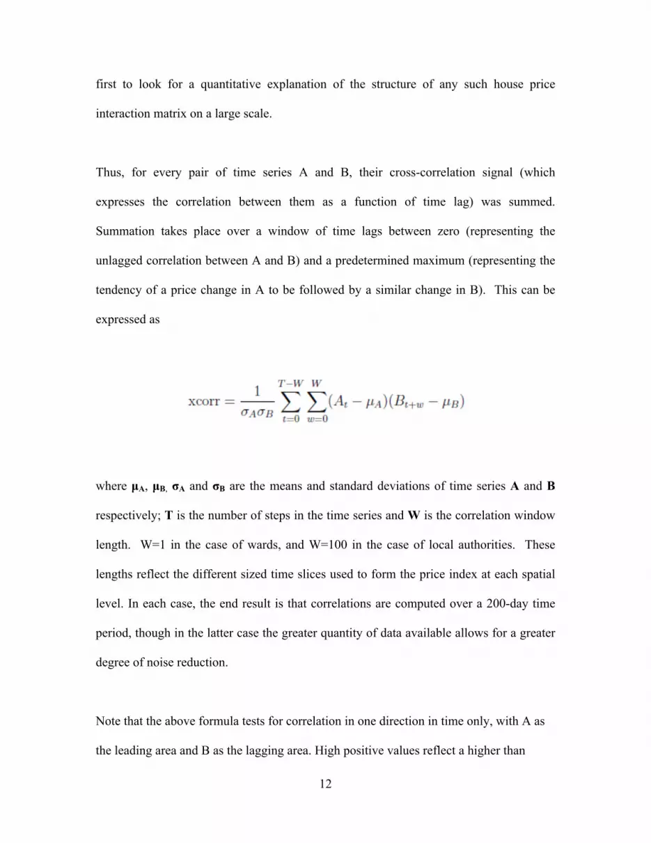
Thus, for every pair of time series A and B, their cross-correlation signal (which

expresses the correlation between them as a function of time lag) was summed.

Summation takes place over a window of time lags between zero (representing the

unlagged correlation between A and B) and a predetermined maximum (representing the

tendency of a price change in A to be followed by a similar change in B). This can be

expressed as

where µA, µB, σA and σB are the means and standard deviations of time series A and B

respectively; T is the number of steps in the time series and W is the correlation window

length. W=1 in the case of wards, and W=100 in the case of local authorities. These

lengths reflect the different sized time slices used to form the price index at each spatial

level. In each case, the end result is that correlations are computed over a 200-day time

period, though in the latter case the greater quantity of data available allows for a greater

degree of noise reduction.

Note that the above formula tests for correlation in one direction in time only, with A as

the leading area and B as the lagging area. High positive values reflect a higher than

13

average correlation between the areas. In the regression analysis (section 6), each pair of

areas is tested twice, with each member of the pair taking the place of A (LEADER) and

B (LAGGER) in turn.

Figure 1. Scatter density (2-d histogram) plot of 3-year local authority level cross-correlations

from first half of time series (2000-2003) against second half of same series (2003-2006). In the

cases where more than one data point falls on the pixel, intensity represents number of data points

The main object of analysis, then, is a cross-correlation metric, which for each pair of

areas, consists of a single figure representing the degree of forward linkage between the

pair over the entire six year time span of the data. However, it is reasonable to ask how

this metric itself would change over time. Figure 1 presents the results of a pilot study

using the local/unitary authority level data in which the data set is split into two by time

(2000-2003; 2003-2006), with each pairwise cross-correlation from the earlier half of the

time period being compared with the same metric from the latter half of the time period.

Note that there is only a weak correlation visible between past and future values of cross-

14

correlation at this level; even less correlation is visible at ward level. This limitation

probably relates both to the inherent change over time of cross-correlations, and to the

noise present in their measurement. In either case, results from this study should be

interpreted as reflecting only the state of the market at time of measurement, rather than

being universally applicable. It is however possible that analyses using a time span

greater than six years would exhibit greater stability in long-run relationships between

areas, in which case, identical techniques to those used in this paper could give rise to

stronger conclusions.

Figure 2 shows a direct pixel visualisation of the 6-year cross-correlation matrix for

local/unitary authorities, in which each pixel of the plot represents the value of cross

correlation (xcorr) for a pair of regions. Place ordering on the axis is based on the CLO-

OPT algorithm reviewed in Guo (2007), which uses clustering and linearization to order

spatial units in a single dimension. The overall effect is that points close together in

geographic space are to a reasonable extent, kept together on the 1D ordering one each

axis.

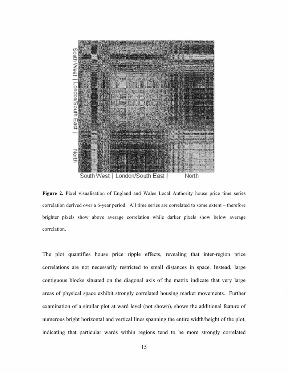
15

Figure 2. Pixel visualisation of England and Wales Local Authority house price time series

correlation derived over a 6-year period. All time series are correlated to some extent – therefore

brighter pixels show above average correlation while darker pixels show below average

correlation.

The plot quantifies house price ripple effects, revealing that inter-region price

correlations are not necessarily restricted to small distances in space. Instead, large

contiguous blocks situated on the diagonal axis of the matrix indicate that very large

areas of physical space exhibit strongly correlated housing market movements. Further

examination of a similar plot at ward level (not shown), shows the additional feature of

numerous bright horizontal and vertical lines spanning the entire width/height of the plot,

indicating that particular wards within regions tend to be more strongly correlated

16

(globally) than others. A bright horizontal or vertical line indicates that a spatial unit is

highly cross-correlated with many other non-contiguous spatial units. These points will

be returned to in Section 8.

5. Choice of regression variables

The overall aim in our exploratory variable choice is to form a meta-model which can be

used to decide which of an array of specific models is likely to have most explanatory

power.

Once time series data have been transferred to the interaction domain using cross-

correlation, it is possible to compare them to other interaction data (migration,

commuting and Euclidean distance) in order to investigate potential causes of variations

in correlated market behaviour. This is done via a regression analysis on a per-

interaction basis. However, as most existing literature on the housing market points

towards the fact that such correlations are likely explained by a reactive, rather than

interactive mechanism, reactive components should also be included in the model. If

spatial coefficient heterogeneity is to be accepted as an explanation of housing market

patterns (Meen, 2001), whereby different areas respond differently to global changes

such as the interest rate, then these differing responses will themselves have causes

related to local housing and socio-economic conditions.

17

A wide range of aggregate statistics are thus included, each in response to a prevailing

model of housing market behaviour, in order to locate the factors of greatest relevance to

spatial housing market dynamics. Life cycle models (mentioned in Meen, 2001) are

addressed by the inclusion of data on the age distribution of people living in each area.

Spatial variation in land value is addressed by the inclusion of travel-to-work distances

from the Census. Models of speculation, supply and demand suggest the inclusion of

housing stock information, initial price data taken from the year 2001, and turnover as

measured by the number of transactions between 2000-2006. Housing submarket models

(Orford, 2000) require inclusion of dwelling type and tenure type; and straight-line

distance to London from the area centriod is included to check that space itself does not

explain the ripple effect better than any of the other variables. The socio-economic class

composition of each area is also used as it is of known importance in structuring spatial

housing markets (Guerios & Le Goix, 2009).

In the case of the interaction data itself, this is included for both migration and

commuting flows, the former of which is disaggregated by social class, age (as shown to

be relevant by Dennett & Stillwell, 2008) and tenure type (shown to be relevant by

Boyle, 1993). Finally, inter-area distance from the centroids of each area is included as

an interactive statistic.

Reactive variables are converted to an interactive format through use of a

leader/lagger/squared change framework. That is to say, for every statistic X and pair of

areas A and B, the following data are included:

18

• Value of X at leading ward, XA

• Value of X at lagging ward, XB

• Squared difference in X between A and B, (XB-XA)2

These data are referred to in the results as LEADER, LAGGER and CHANGESQ

statistics respectively. As it is not known whether absolute values of a statistic (such as

number of young migrants) are more important than relative values (proportion of young

migrants), both types of data are included. Logarithms are taken of absolute values to

‘tame’ high-valued outliers, using the formula log(x+1) to allow for data values of zero.

Additionally, when regressing at ward level, data from the containing local/unitary

authorities are also included, thus enabling socio-demographic context to be captured at a

larger spatial scale reflecting wider housing market processes.

All variables are pre-normalized to zero mean and unit variance, meaning that the

estimated parameters are dimensionless and reflect only the relative importance of each

variable.

The unification of the three types of data – price time series, inter-area interaction and

individual area statistics - is summarized in Figure 3.

19

Figure 3. Data flow diagram of the interaction domain analysis

6. Regression technique

Use of regression in the manner described here is non-standard; 40 interactive and 50

reactive statistics are expanded by the processes described above, to create approximately

760 explanatory variables (for a ward level regression) and 380 variables (for a

local/unitary authority level regression), which are input to the regression engine. In a

confirmatory regression analysis, this would be considered bad practice: if a specific

hypothesis is to be tested, then only variables of relevance to that hypothesis need be

included. Furthermore, to draw confirmatory conclusions from such a regression,

20

without having a hypothesis to test in the first place, would be to commit an error of

sample selection, because the presence of a certain pattern is tested using data already

known to contain that pattern. We employ regression as an exploratory technique,

however. The deliberate intent is to search for information through use of as many

variables as possible, leaving the computer to isolate the most relevant co-variants.

However, the inclusion of so many variables entails more than purely philosophical

problems. Several assumptions of linear regression are violated: existence of a linear

model, homoscedasticity of errors, non-collinear input variables and zero spatial

autocorrelation. The last of these is exacerbated by the expansion of reactive variables

into interaction space using the leader/lagger/squared change framework described above.

At ward level, this step increases the size of the data by a factor of over 104 without

increasing the information content, so severe autocorrelation (in interaction space) and

collinearity will be present. A similar point can be made regarding the expansion of price

time series into cross-correlations, although the level of expansion is less extreme.

Two techniques are used to address these problems. Firstly, as extreme cases of

collinearity can cause overfitting of the model (resulting in a good fit but no predictive

power), the dataset is divided randomly into a training and test set. Half of the data are

then used to train the regression engine, and the other half used to check that the results

are not overfitted; the goodness-of-fit to each set being the mean squared residual and

mean squared error respectively. Secondly, as collinearity in the explanatory variables

causes unreliable estimation of regression parameters, principal component analysis

21

(PCA) is used to reduce the number of explanatory variables to a sensible quantity.

Figure 4 shows the trade-off inherent in this process, for a series of regressions using

between 40 and 380 components to represent the original 380 variables. While reducing

dimensionality causes a narrowing in the confidence intervals of parameter estimates, this

comes at a cost of increased residuals and errors. For such a large quantity of variables, it

makes for clearer analysis to discuss only the ranking of each coefficient, rather than its

absolute value – thereby considering the relative importance of different variables. By

examining the extent to which parameter confidence intervals overlap and therefore the

extent to which the given ranking is reliable, Figure 5 shows that the reliability of such

rankings is only meaningful for the 40- and 80-component regression. Thus, for

local/unitary authorities, results are presented for a regression on 80 components. At

ward level, owing to the much larger size of the data set, there is a practical limitation on

the number of components that can be used due to computation time, and this quantity is

therefore set at 40.

Owing to the size of the data set, custom parallel software was necessary to perform the

regression. This was coded in python using the mdp data processing toolkit (Zito et al.,

2009). A ward level regression (comprising analysis of circa 78 million interactions)

takes approximately 48 hours to run on a 16-core 3GHz Itanium machine. Further code

optimization would reduce this runtime considerably in future applications.

22

Figure 4. Effect of number of regression components (dimensions) used on mean parameter error

(defined as width of 99% confidence interval divided by parameter magnitude), and on accuracy

of regression (as measured by mean squared residual and error), for local authority level analysis.

0

10

20

30

40

50

60

40 80 160 240 320

Number of components used in regression

Mea

n re

lativ

e pa

ram

eter

err

of (9

9% c

onfin

t / p

aram

eter

val

ue)

0

0.1

0.2

0.3

0.4

0.5

0.6

0.7

0.8

0.9

1

Nor

mal

ized

mea

n sq

uare

resi

dual

/err

or

Mean param errorResidualError

1

51

101

151

201

251

301

351

1 51 101 151 201 251

rank of coefficient of interest

rank

of s

mal

lest

con

foun

ding

coe

ffici

ent

Ward level, d=40

d=40 d=80

d=160 d=240 d=320

23

Figure 5. Uncertainty in rank order of estimated coefficients for different values of d (the number

of principal components used in regression). Results are for local/unitary authority level except

where otherwise labelled. The rank of each parameter (ordered by magnitude) is plotted against

the rank of the smallest parameter with which its 99% confidence interval overlaps.

7. Regression diagnostics and results

At local/unitary authority level, the 80-component regression has a normalized mean

squared residual of 0.50, and a mean squared error computed from the test data of 0.50

(out of a theoretical maximum of 1.00, the error implicit in assuming all data points are

equal to the mean). Thus, a large proportion of the variability in cross-correlation is

explained by the model; also, as noted already, a lower overall error of 0.37 can be

achieved, at the cost of reduced parameter accuracy. Residuals are normally distributed.

A plot of residual against prediction shows that errors are homoscedastic for the majority

of data points; however, extreme predictions (whether high or low) have a tendency to be

greater than the actual target data, indicating that further improvement may be possible

using a nonlinear model.

At ward level, the diagnostics for the 40-component regression are similar. The rank

ordering of coefficients is more reliable due to the larger number of data points analyzed;

the mean squared residual and error are, however, much higher at 0.88. This is presumed

to be due to the extra noisiness of cross-correlation data caused by the smaller areal units

and greater expansion factors involved. However, many estimated coefficients are

24

highly significant for ward level statistics, so analysis of the results at this level is

nonetheless considered worthwhile.

Tables 1 and 2 present results for regression of cross-correlation against census statistics

for local/unitary authorities and wards respectively. For the presentation of results,

regression parameters are transformed from principal component space back to input

variable space, thus showing the total contribution of each explanatory variable to the

target prediction.

Analysis of Table 1 shows that most of the best indicators of local/unitary authority level

correlation are reactive variables, although distance between areas does indicate a

significant reduction in their market linkage. It is possible that this indicates a true

interactive mechanism in price propagation, such as information transfer through

property searches as suggested in Meen (2001). It is also possible, as with any apparent

spatial relationship, that distance is merely a proxy for other factors that determine price

linkage and have been omitted from the model. The first migration variable appears with

rank 196, and is barely statistically significant, showing its relative unimportance in

determining market correlation at local/unitary authority level.

Among the twenty most highly ranked reactive variables, commute distance, housing

stock, initial house price, population age, socio-economic class, economic activity and

housing stock are all represented. A traditional reactive model would provide more

insight into the effect of any of these variables. Many appear in squared difference form

25

with a negative impact on correlation, indicating that as these variables become less

similar between places, the movement of house prices also diverges. Hence pair-wise

local/unitary authorities that are similar in terms of the proportion of the workforce with

no fixed place of work, the proportion of vacant household spaces, the proportion of

people living in part of a converted/shared house, average 2001 house prices, and the

proportion of people in age groups 26-35 and 46-55 are also similar in their house price

changes. With the exception of the first variable, the remaining variables represent key

housing demand and supply variables (price, stock, proportions of first time buyers and

proportion of people in the age group characteristics of families with children who may

be moving due to lifestyle reasons e.g. to a bigger property). For some variables,

however, squared difference between local/unitary authorities has a positive effect on

correlation (proportion of people commuting 10-20kms or over 30kms, overall

population, proportion of people living in shared dwellings, the proportion of people in

intermediate occupations and the number of caravans/mobile homes) meaning that as

these pair-wise variables become less similar, house price movements converge. This is

probably indicative of counter-urbanisation with the commuting distances connecting

lower populated rural authorities with more highly populated urban authorities. There are

a small number of unidirectional LEADER- and LAGGER- variables that have

significant correlations with pair-wise house price movements. The proportion of people

in employment and the proportion of people in higher managerial / professional

occupations in lagger authorities have a negative effect on correlation. Conversely, the

proportions of people who are unemployed or long term unemployed or have never

worked or have an economic activity described as other in lagger authorities have a

26

positive effect on correlation. These capture authorities at either end of the deprivation

spectrum and corroborate what Ferrari and Rae (2011) concluded about areas with similar

levels of low and high deprivation having strong connections and possibly disconnected

from the rest of the housing market.

Table 2 shows that the most important indicator of a connected housing market at ward

level is the composition (rather than volume) of migration flows and commuting

distances. Wholly moving households indicate smaller than average market linkage,

while other moving groups indicate larger than average linkage. Caution should be

employed in deducing causality from this; as the pattern may be explained by the

tendency of wholly moving households to be moving as part of a lifecycle process and

thus switching between differing housing markets (e.g. city centre to suburbs to country),

in contrast to other moving groups who might have a greater tendency to move to areas

similar to those they have left. Beyond these variables, reactive effects predominate and

these relate to characteristics of the leading or lagging area, indicating that at ward level,

certain types of wards appear to have asymmetric relationships whereby one type

precedes the other in terms of price change (again this is discussed further in Section 8).

These leading wards are defined by employment characteristics of the containing

authority, and more locally, defined by the housing stock and commuting distances with

the proportion of detached housing being a particular important feature of leading wards

(and negatively correlated with lagging). The number of people aged 66-79 is also an

important authority level variable reflecting the importance of retirement age migration

on price change in certain local areas. The asymmetry at ward level is emphasized by the

27

fact that no symmetric variable appears until the first CHANGESQ type statistic in 262nd

place; hence, clustering type models are not so relevant at this level when compared to

specific trends which again suggest patterns of counter-urbanization and lifecycle

migration. The effects of commuting flows and inter-area distance are also small; in the

latter case, this is probably because inter-ward migration is a better indicator of the

practical (social and network) proximity of wards, than Euclidean distance.

Rank Census table Name Type Units Coeff 99%Conf 1 UV035 Distance to work No fixed place of work CHANGESQ proportion -1.07E-01 4.82E-03 2 n/a Distance interaction n/a -8.52E-02 4.54E-03 3 UV053 Housing Stock Vacant household space CHANGESQ proportion -7.82E-02 4.98E-03 4 n/a Log average 2001 house prices CHANGESQ n/a -7.15E-02 1.71E-03 5 UV035 Distance to work 10-20km CHANGESQ proportion 6.79E-02 5.34E-03 6 UV053 Housing Stock Vacant household space LEADER proportion -5.65E-02 3.63E-03 7 UV004 Age All people CHANGESQ count 4.69E-02 3.14E-03 8 UV004 Age 46 – 55 CHANGESQ proportion -4.29E-02 2.13E-03 9 UV055 Dwellings Shared CHANGESQ count 4.20E-02 3.00E-03 10 UV035 Distance to work Over 30km CHANGESQ proportion 4.17E-02 4.50E-03 11 UV028 Economic activity Employed LAGGER proportion -3.76E-02 1.85E-03 12 UV031 NS-SeC Never worked/Long term unemployed LAGGER proportion 3.75E-02 2.05E-03 13 UV056 Accom. Type Part of converted/shared house CHANGESQ proportion -3.65E-02 1.50E-03 14 UV028 Economic activity Other LAGGER proportion 3.64E-02 1.95E-03 15 UV031 NS-SeC Higher managerial/professional LAGGER proportion -3.60E-02 1.82E-03 16 UV031 NS-SeC Semi-routine LEADER proportion 3.60E-02 2.21E-03 17 UV031 NS-SeC Intermediate CHANGESQ proportion 3.58E-02 5.36E-03 18 UV004 Age 26-35 CHANGESQ proportion -3.56E-02 2.03E-03 19 UV056 Accom. Type Caravan/mobile/temporary structure CHANGESQ count 3.47E-02 3.62E-03 20 UV028 Economic activity Unemployed LAGGER proportion 3.32E-02 2.21E-03 … … … … … … … 196 MG201 Migrants age Under 16 interaction proportion -7.50E-03 4.98E-03 220 MG204 Migrants NS-SeC Lower managerial/professional interaction proportion 5.82E-03 4.36E-03 226 MG201 Migrants age Under 16 interaction count -5.40E-03 3.20E-03 233 MG201 Migrants age All migrants interaction count -5.01E-03 1.89E-03 347 W201 commuting All commuters interaction count -6.79E-04 1.35E-03

Table 1. Regression results for the target variable local/unitary authority level housing market cross-correlation. Top 20 variables are displayed and selected others. NS-SeC = National Statistics socio-economic classification.

28

Rank Census table Name Level Type Units Coeff 99%Conf 1 MG204 Migrants by NS-SeC Total OMG Ward interaction proportion 1.74E-03 2.10E-05 2 MG204 Migrants by NS-SeC Total WMH Ward interaction proportion -1.62E-03 1.80E-05 3 MG204 Migrants by NS-SeC Total WMH Ward interaction count -1.38E-03 1.60E-05 4 MG204 Migrants by NS-SeC Total OMG Ward interaction count 1.38E-03 1.80E-05 5 UV031 NS-SeC Small employers LA LAGGER proportion -1.23E-03 1.30E-05 6 UV055 Dwellings Shared LA LAGGER count -1.18E-03 1.10E-05 7 UV035 Distance to work 10 - 20 km LA LAGGER count -1.15E-03 1.10E-05 8 UV028 Economic activity Employed LA LAGGER count -1.13E-03 1.10E-05 9 UV031 NS-SeC Semi-routine LA LAGGER count -1.13E-03 1.10E-05 10 UV056 Accom. Type In block of flats LA LAGGER proportion -1.13E-03 1.20E-05 11 UV035 Distance to work 20 - 30 km Ward LAGGER proportion -1.13E-03 1.10E-05 12 UV004 Age 66 – 79 LA LAGGER count -1.13E-03 1.00E-05 13 UV056 Accom. Type Detached Ward LEADER proportion 1.12E-03 1.10E-05 14 MG205 Migrants by tenure Private Rented OMG Ward interaction proportion 1.11E-03 1.30E-05 15 UV035 Distance to work 10 - 20 km Ward LAGGER count -1.10E-03 1.00E-05 16 UV056 Accom. Type Detached Ward LAGGER proportion -1.08E-03 1.00E-05 17 UV031 NS-SeC Small employers LA LEADER proportion 1.07E-03 1.30E-05 18 UV035 Distance to work 20 - 30 km Ward LEADER proportion 1.07E-03 1.10E-05 19 UV035 Distance to work Working offshore LA LAGGER proportion -1.06E-03 1.00E-05 20 UV035 Distance to work 10 - 20 km LA LAGGER proportion -1.04E-03 1.00E-05 … … … … … … … … 203 W201 Commuting All commuters LA interaction count 3.06E-04 8.00E-06 262 UV053 Housing stock Second residence/holiday LA CHANGESQ count -1.78E-04 3.00E-06 390 n/a Distance Ward interaction n/a -9.50E-05 2.00E-06

Table 2. Regression results for the target variable ward level housing market cross-correlation. Top 20 variables are displayed and selected others. NS-SeC = National Statistics socio-economic classification. WMH = Wholly moving households, OMG = Other moving groups. 8. Leading/lagging wards

In this section we analyse the asymmetric relationships between wards on a market-

leading/market-lagging framework. This is presented (i) to complement our regression

analysis of cross-correlations in Section 7, (ii) to show how such a general form of

exploratory analysis can point towards more specific avenues of investigation and (iii) to

highlight the potential of the framework for further research in the field of housing.

29

Figure 6. Data flow diagram for the market-leading/market-lagging analysis.

Two metrics are defined which illustrate the leading and lagging tendencies of each

ward. These are obtained in the current case by summing the columns and rows of the

cross-correlation matrix respectively; though with more computing resources, more

sophisticated assignment of scores may be possible using iterative maximum likelihood

estimation techniques from the field of spatial interaction modelling (Fotheringham &

O’Kelly, 1989). Figure 6 gives an overview of the analysis, and figure 7 shows the

spatial distribution of the leading/lagging scores. In many cases, the strongest leading

and lagging wards tend to be located in roughly the same areas: some parts of London

and Birmingham, but principally across urban areas in the North. This is presumably

indicative of the state of the market during the years 2000-2006; during this time the

‘property bubble’ which started in the mid 1990s had already affected London, so by the

time of the study, the peripheral urban areas were experiencing the most rapid change

30

(Gray, 2012). However, if this analysis were to be conducted over a longer time span, it

is possible that the leading/lagging scores would reflect long run relationships rather than

short term market state.

Tables 3 and 4 show the results of regressions with the leading and lagging score as the

target variable respectively. As before, PCA is used to reduce the explanatory variables

to 40 components. In both cases, a key explanatory variable is market turnover, which is

positively correlated. This makes intuitive sense as it is hard to see how any area could

be said to be strongly involved in the market without exhibiting large numbers of

transactions. The remainder of the explanatory variables give a portrait of market

leading/lagging areas during the span of the study. The variables which most correlate

with a market-leading tendency are characteristic of first-time buyers; thus at ward level

population density, the proportion of people aged 26-35, the proportion of people

working in intermediate occupations and the proportion and absolute numbers of terraced

and shared houses predominate and at authority level the proportion of semi-detached

houses, houses in commercial properties and people unemployed are important and are

all indicative of urban areas. In comparison, the variables anti-correlated with market

leading behaviour are characteristic of older, wealthier buyers with families; hence at

ward level average income, the proportion of people in higher managerial / professional

occupations, and people aged 46-55 and below age 16 predominate and at authority level

the number of second homes and people aged 16-25 are also important.

31

The variables which correlate with lagging wards tend, broadly speaking, to be the same

as those which correlate with leading ones. This supports Ferrari and Rae’s (2011) recent

findings that areas that share characteristics are connected in the housing market.

Figure 7. Market-leading and market-lagging wards. Note that all wards are to some extent

correlated in price movements; therefore a negative score represents below-average interaction

rather than negative interaction.

Census table Name Level Units Coeff 99%Conf

n/a Average income Ward n/a -9.69E-02 2.79E-02

n/a Number of transactions 2000-2006 Ward n/a 8.99E-02 1.74E-02

UV031 NS-SeC Intermediate occupations Ward proportion 5.87E-02 2.17E-02

UV056 Housing type Terraced Ward proportion 5.40E-02 1.90E-02

UV056 Housing type Semi detached LA proportion 4.92E-02 2.12E-02

UV053 Housing stock Second residence/holiday LA count -4.44E-02 1.07E-02

UV056 Housing type Part of converted/shared house Ward proportion -4.42E-02 2.33E-02

UV004 Age 26 – 35 Ward proportion 4.00E-02 1.54E-02

Driving score-50000 - 00 - 1500015000 - 3000030000 - 4000040000 - 70000

Driven score-50000 - 00 - 1500015000 - 3000030000 - 4000040000 - 70000

Leading score Lagging score

32

UV004 Age 16 – 25 LA proportion -3.60E-02 2.03E-02

UV031 NS-SeC Higher managerial/professional Ward proportion -3.49E-02 1.19E-02

UV056 Housing type In commercial building LA proportion 3.40E-02 1.52E-02

UV004 Age Under 16 Ward proportion -3.39E-02 1.91E-02

UV028 Economic Activity Unemployed LA proportion 3.26E-02 1.08E-02

UV002 Population density Ward count 3.02E-02 1.27E-02

UV056 Housing type Shared Ward count 2.93E-02 2.02E-02

UV004 Age Terraced Ward count 2.89E-02 1.09E-02

UV004 Age 46 – 55 Ward proportion -2.88E-02 2.12E-02

UV031 NS-SeC Higher managerial/professional LA proportion -2.79E-02 1.02E-02

UV031 NS-SeC Intermediate occupations Ward count 2.76E-02 7.01E-03

UV004 Age 56 – 65 LA proportion 2.71E-02 1.01E-02 Table 3. Regression results for the target variable leading ward score. Top 20 variables are displayed. NS-SeC = National Statistics socio-economic classification. Census table Name Level Units Coeff 99%Conf n/a Average income Ward n/a -8.89E-02 2.78E-02 n/a Number of transactions 2000-2006 Ward n/a 7.55E-02 1.73E-02 UV031 NS-SeC Intermediate occupations Ward proportion 6.56E-02 2.16E-02 UV056 Housing type Terraced Ward proportion 5.10E-02 1.90E-02 UV056 Housing type Part of converted/shared house Ward proportion -4.95E-02 2.32E-02 UV031 NS-SeC Higher managerial/professional Ward proportion -4.42E-02 1.18E-02 UV053 Housing stock Second residence/holiday LA count -4.28E-02 1.06E-02 UV004 Age 16 – 25 LA proportion -4.16E-02 2.02E-02 UV056 Housing type In commercial building LA proportion 3.69E-02 1.51E-02 UV056 Housing type House or bungalow Ward proportion 3.58E-02 1.21E-02 UV004 Age Under 16 LA proportion 3.53E-02 2.12E-02 UV056 Housing type Flat/maisonette/apartment Ward proportion -3.53E-02 1.25E-02 UV031 NS-SeC Intermediate occupations LA proportion 3.48E-02 1.66E-02 UV056 Housing type Semi detached LA proportion 3.48E-02 2.11E-02 UV056 Housing type Shared Ward count 3.40E-02 2.01E-02 UV028 Economic Activity Unemployed LA proportion 3.33E-02 1.08E-02 UV053 Housing stock Second residence/holiday Ward count -3.22E-02 1.54E-02 UV035 Distance to work 2km - 5km Ward proportion 3.18E-02 2.26E-02 UV056 Housing type House or bungalow Ward count 3.02E-02 5.92E-03 UV002 Population density Ward count 2.95E-02 1.26E-02 Table 4. Regression results for the target variable lagging ward score. Top 20 variables are displayed. NS-SeC = National Statistics socio-economic classification. 9. Conclusion

The analysis of housing market interactions presented here has used cross-correlation and

exploratory regression in the interaction domain to reveal structure in spatial housing

market data on an unprecedented spatial and temporal scale and is the first of this kind of

33

research to be undertaken on the volume of individual level England and Wales

transaction data. From a methodological perspective, unifying three types of data (time

series, interaction and aggregate statistics), has presented a picture of the complex spatial

housing market phenomenon in greater detail than before, and the broad scope of the

model has suggested further, more specific avenues of analysis. It also moves towards a

more integrative framework for housing market analysis; one demanded by the emerging

spatial and temporal volatility of the UK housing market.

Key findings from the cross-correlation study are as follows. At local authority level,

areas with similar characteristics tend to share market behaviour, with a few exceptions

as explained in section 7. These exceptions are suggestive of asymmetry between certain

areas which tend to lead the market overall, and other areas which tend to lag it, defined

by variables which suggest a pattern of price transfer along pathways of counter-

urbanization (although this hypothesis doesn’t preclude other explanations of the

phenomenon). Within each class of area, standard reactive models – rather than

interactive mechanisms - are likely to be the most fruitful form of further study, as

indicated by the relative unimportance of interactive variables in our regression.

Depending on the level of parameter accuracy desired, this model explains 50-63% of

variability in inter-area market correlation.

The significance of physical distance as an indicator of authority level market linkage

still requires explaining, however. It is possible that the regression engine is simply using

distance as a proxy for other social or economic variables not included in the current data

34

set. If so, it is worth asking what these variables are, and if not then it is worth asking

how such physically localised price information transfer is taking place, when similar

information transfer does not occur to the same extent along common migration or

commuting pathways. Perhaps to some extent, the social expectations that affect house

pricing are formed on a local basis despite rapid propagation of information through a

nationwide market.

At ward level, inter-area correlation is explained principally by the composition of

migration flows, and asymmetries in area demographics which again suggest channels of

counter-urbanization. The unimportance of squared difference variables show that

market segmentation and clustering models are not so important at this level, a surprising

finding that deserves further study, and may again be a reflection of price expectations

being partially influenced by local activity, regardless of market segmentation.

Key findings from the direct study of leading/lagging areas (section 8) lead to similar

conclusions. Leading wards tend to be correlated with the demographic and housing

stock characteristics of first time buyers, while lagging wards tend to match older,

wealthier buyers with families.

In sum, these findings corroborate the existence of a ripple effect at broad spatial scale;

although this manifests not principally in physical space through ripples outwards from

London, but in socio-demographic space as ripples propagating mainly between classes

of areas which exhibit similar market behaviour - and occasionally, asymmetrically

35

between different classes of area. This corroborates Ferrari and Rae’s (2011) and Gray’s

(2012) analysis of spatial volatility.

We end with three points of caution, however, as is fitting. Exploratory regression results

cannot be taken as an indicator of causality. Firstly, to look for results without having a

specific hypothesis to test is a violation of scientific method. This is not considered a

problem; it is merely the distinction between exploratory and explanatory modelling.

Secondly, it is noted that the spatial correlation evident in the cross-correlation matrix

itself has yet to be fully modelled, therefore the stated confidence intervals for parameters

can be presumed to be too narrow – although by reserving 50% of the data as a test set,

we have demonstrated that our models are not over-fitted. Third, the patterns of cross-

correlation studied in the current case are not stable over time but rather indicate temporal

and spatial volatility. It may well be that a study with a longer time span will reveal more

stable correlations, in which case an identical analysis will yield stronger conclusions,

although recent research by Ferrari and Rae (ibid) and Gray (ibid) suggest that such

volatility may be an emerging feature of the UK housing market. For the time being then,

this study serves three purposes: as a demonstration of new techniques, as a pointer

towards more specific avenues of modelling which are likely to be fruitful, and as a study

restricted to the state of the market from 2000-2006 which can itself serve as a single data

point in a broader study.

From the perspective of the exploratory technique itself, several improvements may help

when embarking on exploratory approaches in future. Firstly, the remarkably different

36

behaviour of the housing market at ward and local/unitary authority level suggests that

any future exploration should be conducted using true multi-level modelling, whereby

variance in the target statistic is split to different spatial scales prior to regression. It is

noted that the transaction-based nature of house price data makes it particularly amenable

to aggregation at any spatial scale (Orford, 2000). Secondly, nonlinear regression

techniques should be used to improve model fit and ensure that the residuals from each

successive model are truly inexplicable by that model, before they are processed by

another. Third, it may be worth investigating alternatives to PCA for data reduction, as

its underlying assumption may turn out to be limiting: such use of PCA inherently

assumes that covariates which account for only a small amount of variability in the input

data, also account for only a small amount of variability in the target data. And finally,

data covering a much wider time span should be used where possible; digital land registry

records now cover the post-2006 market crash - an interesting phenomenon in itself -

while older records aggregated to the local/unitary authority level would also be of

interest for the purpose of determining which patterns of interaction are consistently

exhibited in the long term.

Notwithstanding these limitations, we have revealed a number of both expected and

unexpected trends which are ripe for further investigation by more specific models, as is

the intention of exploratory analysis.

Acknowledgements

37

Essential data for this research were supplied by HMLR, Ordnance Survey and Landmark

Information Group Ltd. Census Area Statistics and Interaction Data are taken from the

2001 UK Census under the terms of the Click-Use License. Computation was carried out

on the ARCCA (Advanced Research Computing at Cardiff) grid. The research was

funded by Cardiff University’s Richard Whipp fund and conducted as collaboration

between the Schools of City and Regional Planning and Computer Science.

Bibliography

Alexander, C. and Barrow, M. (1994) Seasonality and cointegration of regional house

prices in the UK, Urban Studies, 31, pp. 1667–1689.

 

Anselin, A. (1988), Spatial Econometrics: Methods and Models (Kluwer).

Blok, C. (2000), Monitoring change: Characteristics of dynamic geo-spatial phenomena

for visual exploration, in ‘Spatial Cognition II (LNAI 1849)’ (Springer-Verlag, Berlin) p

16.

Bourassa, S. C., Hamelink, F., Hoesli, M. & MacGregor, B. D. (1999), ‘Defining housing

submarkets’, Journal of Housing Economics 8(2), p 160.

38

Boyle, P. (1993), ‘Modelling the relationship between tenure and migration in England

and Wales’, Transactions of the Institute of British Geographers, New Series 18(3), pp

359-376.

Cai, Y., Stumpf, R., Wynne, T., Tomlinson, M., Chung, D., Boutonnier, X., Ihmig, M.,

Franco, R. & Bauernfeind, N. (2007), ‘Visual transformation for interactive

spatiotemporal data mining’, Knowledge and Information Systems 13(2), p 119.

Census Geography (n.d.), retrieved 1/12/2010, from

http://www.statistics.gov.uk/geography/census_geog.asp

Claramunt, C., Jiang, B. & Bargiela, A. (2000), ‘A new framework for the integration,

analysis and visualisation of urban traffic data within geographic information systems’,

Transportation Research C 8(1), p 167.

Cliff & Ord (1981), Spatial Processes, Models and Applications (Pion).

Demšar, U., Fotheringham, A. S. and Charlton, M. (2007), Exploring the spatio-temporal

dynamics of geographical processes with geographically weighted regression and

geovisual analytics, Information Visualization (2008) 7 pp 181-197.

Dennett, A. & Stillwell, J. (2008), Internal migration in Great Britain - a district level

analysis using 2001 census data (School of Geography, University of Leeds).

39

Ferrari, E., and Rae, A., (2011), Local housing market volatility (Joseph Rowntree

Foundation, York UK).

Fotheringham, A. S. & O’Kelly, M. E. (1989), Spatial Interaction Models: formulations

and applications (Kluwer).

Giussani, B. & Hadjimatheou, G. (1991), ‘Modeling regional house prices in the United

Kingdom’, Papers in Regional Science 70(2) pp 201-219.

Goetzmann, W. N. & Wachter, S. M. (1995), ‘Clustering methods for real estate

portfolios’, Real Estate Economics 23, p 271.

Gray, D. (2012) District House Price Movements in England and Wales 1997-2007: An

Exploratory, Spatial Data Analysis Approach, Urban Studies, 49(7) pp 1411–1434

Guerois, M. & Le Goix, R. (2009), ‘La dynamique spatio-temporelle des prix

immobiliers a differentes echelles : le cas des appartements anciens a Paris (1990-2003)’,

Cybergeo: Systemes, Modelisation, Geostatistiques p 470.

Guo, D. (2007), ‘Visual analytics of spatial interaction patterns for pandemic decision

support’, International Journal of Geographical Information Science 21(8) pp 859-877.

40

Hagerstrand, T. (1975), Space, time and human conditions., in A. E. A. Karlqvist, ed.,

‘Dynamic allocation of urban space’ (Saxon House Lexington) pp 3-14.

Kraak, M. (2001), ‘Visualize Overijssel’s past, interactive animations on the WWW’,

Kartografisch Tijdschrift 27(4), p 5.

Langran, G. (1989), ‘A review of temporal database research and its use in GIS

applications’, International Journal of Geographical Information Systems 3(3), pp 215-

232.

MacDonald, R. & Taylor, M. P. (1993), ‘Regional house prices in Britain: long-run

relationships and short-run dynamics’, Scottish Journal of Political Economy 40(1) pp

43-55.

MacQueen, J. (1967), ‘Some methods for classification and analysis of multivariate

observations.’, Proceedings of the 5th Berkeley Symposium on Mathematical Statistics

and Probability - Vol. 1 (University of California Press, Berkeley, CA) pp 281-297

Meen, G. (1999) Regional house prices and the ripple effect: a new interpretation,

Housing Studies, 14(6), pp 733–753.

Meen, G. (2001), Modelling spatial housing markets: theory, analysis and policy,

(Kluwer).

41

Openshaw, S., ed. (1995), Census Users’s Handbook.

Orford, S.(2000) Modelling Spatial Structures in Local Housing Market Dynamics: A

Multilevel Perspective. Urban Studies 37, pp 1643-1671.

Orford, S. (2010) Towards a data-rich infrastructure for housing market research:

deriving floor area estimates for individual properties from secondary data sources,

Environment and Planning B: Planning and Design 37, pp 248-264

Pollakowski, H. O. & Ray, T. S. (1997), ‘Housing price diffusion patterns at different

aggregation levels: an examination of housing market effciency’, Journal of Housing

Research 8, pp 107-124.

Shi, S., Young, M. & Hargreaves, B. (2009), ‘The ripple effect of local house price

movements in New Zealand’, Journal of Property Research 26(1) pp 1-24.

Takatsuka, M. and Gahegan, M (2002) ‘GeoVISTA Studio: A Codeless Visual

Programming Environment For Geoscientific Data Analysis and Visualization’, The

Journal of Computers & Geosciences 28(10) pp 1131-1144

Tukey, J. W. (1977), Exploratory Data Analysis (Addison Wesley).

42

Wong, C., Gibb, K., McGreal, S., Hincks, S., Kingston, R., Leishman, C., Brown, L., &

Blair, N., (2009) Housing and Neighbourhood Monitor, UK-wide Report (Joseph

Rowntree Foundation, York UK).

Wood, R. (2003) The information of regional house prices: can they be used to improve

national house price forecasts? Bank of England Quarterly Bulletin, 43(3), pp 304–314.

Worthington, A. & Higgs, H. (2003), ‘Comovement in UK regional property markets: a

multi-variate cointegration analysis’, Journal of Property Investment and Finance 21(4)

pp 326-347.

Zito, Wilbert, Wiskott & Berkes (2009), ‘Modular toolkit for data processing (mdp): a

python data processing frame work’, Front. Neuroinform. 2(8). URL: http://mdp-

toolkit.sourceforge.net