Available online at www.sciencedirect.com

ScienceDirect

Energy Procedia 00 (2013) 000–000

www.elsevier.com/locate/procedia

1876-6102 © 2013 The Authors. Published by Elsevier Ltd.

Selection and peer-review under responsibility of GHGT.

GHGT-12

Experiments and modelling of two-phase transient flow during

pipeline depressurization of CO2 with various N2 compositions

Michael Dreschera*, Kristoffer Varholm

b, Svend T. Munkejord

b, Morten Hammer

b,

Rudolf Helda,#

, Gelein de Koeijera

aStatoil ASA, Research, Development and Innovation, NO-7005 Trondheim, Norway bSINTEF Energy Research, P.O. Box 4761 Sluppen, NO-7465 Trondheim, Norway

Abstract

Pressure-release experiments of CO2 with impurity contents of 10, 20 and 30 mol% nitrogen have been executed. The

experimental investigations were performed in a 140 m long horizontal tube with an inner diameter of 10 mm. The initial

conditions of the CO2-N2 mixtures were in the supercritical region at approximately 120 bar and 20 °C. The results, which

showed a good repeatability, were then compared with numerical data from a homogeneous equilibrium model. The

investigations have concentrated on the pressure wave at the start as well as the pressure and temperature development during the

pressure release. The model, which has a certain complexity, but still contains several simplifications, gave relatively good

results for all three gas mixtures. Although the absolute values for the temperature development showed to be consistently higher

in the experimental results compared to the numerical results, the liquid dry-out points were predicted with good accuracy at all

measurement points. The numerical results of the pressure development match the experimental results very well, both regarding

the absolute and relative values. Regarding the speed of the pressure wave, the numerical results were consistently too high,

which is believed to be caused by the EOS overpredicting the speed of sound for our cases. The good results, especially for the

pressure, are promising, and further work is suggested to improve the model. © 2013 The Authors. Published by Elsevier Ltd.

Selection and peer-review under responsibility of GHGT.

Keywords: CO2 transport; Depressurization; Pressure wave; Impurities; Experiments; Model

* Corresponding author. Tel.: +47 97003339 # New affiliation: Wintershall Holding GmbH, Kassel, Germany

E-mail address: midr@statoil.com

2 Drescher et al. / Energy Procedia 00 (2013) 000–000

1. Introduction

Detailed knowledge on depressurization of CO2 pipelines has shown to be important for safe and cost-effective

design of CO2 Capture & Storage (CCS) chains. CO2 is normally transported by pipeline in a liquid, dense or

vapour-liquid phase at high pressure. Depressurizations can occur during planned operations, maintenance or

undesirable accidents. The most extreme case is a pipeline rupture due to e.g. pipeline corrosion or external force,

during which a crack will form accompanied by a sudden depressurization of CO2. If the internal pipeline pressure at

the tip of the crack is above a certain threshold, the fracture will propagate. Simultaneously, the depressurization

leads to the start of a pressure-relief front or pressure wave in the pipeline. In theory, the fracture might propagate

indefinitely if the fracture-propagation speed is faster than the pressure wave of the fluid caused by the rupture [1].

One way of preventing such a running fracture is by installing mechanical crack arrestors. However, the preferred

way is by dimensioning the pipeline with a minimum required toughness which assures shorter fracture lengths [2].

Therefore, detailed knowledge of the pressure wave is needed for safe and cost-efficient design of the pipeline.

However, CO2 from sources such as natural gas processing or flue gas of fossil-fuel power plants typically contain

impurities to a certain extent, which in turn alter the fluid properties. This will have to be accounted for by flow

models for CO2 transport [3,4]. Furthermore, such models must be able to handle two-phase flow, both for

depressurization and normal operation [5].

Fracture propagation control involves a coupled fluid-structure problem. In order to provide improved predictions

for CO2 mixtures and high-toughness steel types, coupled fluid-structure models are under development [6–11]. To

develop and verify flow models for the depressurization of CO2-rich mixtures, there is a need for experimental data.

Although data exist for natural gas [12], little has been published for CO2. In this work, therefore, pressure-release

experiments have been executed with various amounts of nitrogen as impurity. To illuminate the observed

phenomena, the data from experimental investigations are then compared with numerical data from solving a

homogeneous equilibrium model (HEM). The paper will present and discuss the measured and simulated results,

focusing on the pressure wave picked up at the start of the depressurization as well as on the pressure and

temperature development.

2. Test Facility

For executing the experimental investigations the horizontal flow circuit of the CO2 transport test facility at

Statoil’s R&D center in Trondheim, Norway was used. The horizontal flow circuit consists of a 140 m long

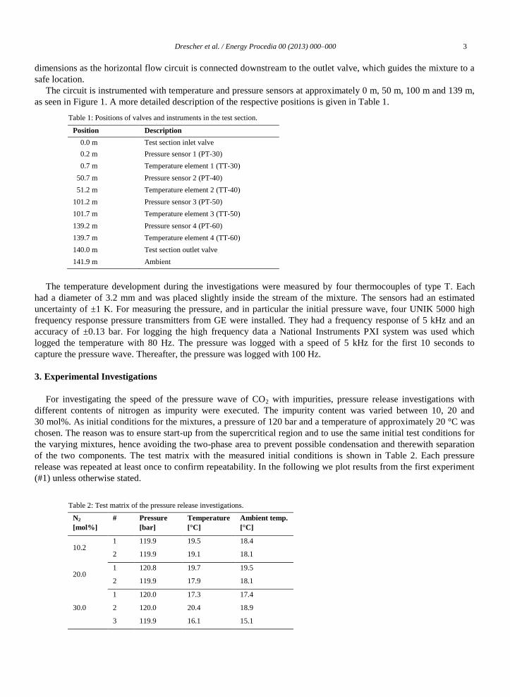
horizontal stainless steel tube with an inner diameter of 10 mm and a wall thickness of 1 mm as shown in Figure 1.

The steel has a density of 8000 kg/m3, a specific heat capacity of 485 J/(kg K) and a thermal conductivity of

14 W/(m K). Further information is found in Pettersen et al. [13] and De Koeijer et al. [14].

Figure 1: Set-up of the horizontal flow circuit.

The horizontal flow circuit is filled at the inlet valve at 0 m. At 140 m the outlet valve is situated which will be

operated during the pressure release. The outlet valve is a near full bore ball valve with an inner diameter of 9.5 mm,

which is slightly less than the horizontal flow tube. The horizontal flow circuit is located inside a container and

coiled up under the roof. During pressure-release investigations a 1.9 m long straight horizontal tube with the same

Test section

outlet valve

PT

40

TT

30

TT

40

TT

50

TT

60

Test section

inlet valve

PT

30

PT

50

PT

60

12 x 1.0 mm

0 m 50 m 100 m 139 m

Ambient

Drescher et al. / Energy Procedia 00 (2013) 000–000 3

dimensions as the horizontal flow circuit is connected downstream to the outlet valve, which guides the mixture to a

safe location.

The circuit is instrumented with temperature and pressure sensors at approximately 0 m, 50 m, 100 m and 139 m,

as seen in Figure 1. A more detailed description of the respective positions is given in Table 1.

Table 1: Positions of valves and instruments in the test section.

Position Description

0.0 m Test section inlet valve

0.2 m Pressure sensor 1 (PT-30)

0.7 m Temperature element 1 (TT-30)

50.7 m Pressure sensor 2 (PT-40)

51.2 m Temperature element 2 (TT-40)

101.2 m Pressure sensor 3 (PT-50)

101.7 m Temperature element 3 (TT-50)

139.2 m Pressure sensor 4 (PT-60)

139.7 m Temperature element 4 (TT-60)

140.0 m Test section outlet valve

141.9 m Ambient

The temperature development during the investigations were measured by four thermocouples of type T. Each

had a diameter of 3.2 mm and was placed slightly inside the stream of the mixture. The sensors had an estimated

uncertainty of ±1 K. For measuring the pressure, and in particular the initial pressure wave, four UNIK 5000 high

frequency response pressure transmitters from GE were installed. They had a frequency response of 5 kHz and an

accuracy of ±0.13 bar. For logging the high frequency data a National Instruments PXI system was used which

logged the temperature with 80 Hz. The pressure was logged with a speed of 5 kHz for the first 10 seconds to

capture the pressure wave. Thereafter, the pressure was logged with 100 Hz.

3. Experimental Investigations

For investigating the speed of the pressure wave of CO2 with impurities, pressure release investigations with

different contents of nitrogen as impurity were executed. The impurity content was varied between 10, 20 and

30 mol%. As initial conditions for the mixtures, a pressure of 120 bar and a temperature of approximately 20 °C was

chosen. The reason was to ensure start-up from the supercritical region and to use the same initial test conditions for

the varying mixtures, hence avoiding the two-phase area to prevent possible condensation and therewith separation

of the two components. The test matrix with the measured initial conditions is shown in Table 2. Each pressure

release was repeated at least once to confirm repeatability. In the following we plot results from the first experiment

(#1) unless otherwise stated.

Table 2: Test matrix of the pressure release investigations.

N2

[mol%]

# Pressure

[bar]

Temperature

[°C]

Ambient temp.

[°C]

10.2 1 119.9 19.5 18.4

2 119.9 19.1 18.1

20.0 1 120.8 19.7 19.5

2 119.9 17.9 18.1

30.0

1 120.0 17.3 17.4

2 120.0 20.4 18.9

3 119.9 16.1 15.1

4 Drescher et al. / Energy Procedia 00 (2013) 000–000

To ensure the respective gas-mixture compositions, premixed gas mixtures in gas bottles from a gas vendor were

used. The relative inaccuracy amounted to 2 % of the certified mixture. To achieve the desired test pressure, the gas

was then compressed using on oil free gas booster. The temperature of the mixture was controlled by adjusting the

ambient temperature inside the test container. After the pressure and temperature have equalized inside the test

section, the high-speed logging was started quickly followed by manually opening the test-section outlet valve.

4. Models

4.1. Flow model and thermophysical properties

The flow in the tube is modelled as one-dimensional single- or two-phase flow where there is a strong coupling

between the gas and the liquid, such that they travel at a common velocity. In addition, full equilibrium in pressure,

temperature and chemical potential is assumed. This is described by the homogeneous equilibrium model (HEM):

( ) ( ) (1)

( )

( ) ( ) (2)

[ ( )] ( ) (3)

where ρ = ρgαg + ρlαl and E = ρ (e + ½ u2) are the mixture density and total energy, respectively. Herein, α is the

volume fraction and e is the specific internal energy. Fw is the wall friction and Q is the heat-transfer rate through the

tube wall. Subscripts g and l denote the gas and liquid phase. The flow equations are advanced in time using a multi-

stage (MUSTA) finite-volume scheme [15,16] on a uniform grid. Different grids and CFL numbers have been

considered to evaluate the sensitivity. As a result, a grid of 1000 cells and a CFL number of 0.85 have been

employed in the present work.

The Peng–Robinson [17] equation of state was used. Classical Van der Waals mixing rules were applied to

account for the multicomponent fluid in the problem at hand. The TRAPP method [18,19] was used to compute the

dynamic viscosity and thermal conductivity of the fluid. The state-function-based approach of Michelsen [20] is

used to calculate pressure, temperature and phase distribution given mixture density, specific internal energy and

composition.

4.2. Friction model

The wall friction is calculated as

{

| |

( )

| |

( )

(4)

Here fj = f (Rej) is the Darcy friction factor, Rej = di/μj is the Reynolds number for phase j and is the

mass-flux density. The coefficient Φ is an empirical correlation, which is used to account for two-phase flow, and

depends on various properties of both phases. Here we have employed the Friedel [21] correlation. The details of the

calculation of the two-phase coefficient Φ, and also further discussion, can be found in Aakenes [22,23].

Drescher et al. / Energy Procedia 00 (2013) 000–000 5

4.3. Heat transfer

The steel tube has a non-negligible heat capacity which needs to be taken into account. This is done by solving

the heat equation

(

) (5)

along with the flow model, assuming radial symmetry and that axial conduction can be neglected. Herein, ρ, cp and λ

are the density, specific heat capacity and thermal conductivity, respectively, of the steel. For solving (5), ten radial

cells are employed.

For the inner heat-transfer coefficient, hi , we use the Nusselt-number correlation:

{ ⁄ ⁄ ( )

(6)

with linear interpolation in the region 2300 < Re < 3000. See e.g. Bejan [24], Chap. 6. Here Pr is the Prandtl

number:

(7)

where subscript f indicates fluid properties. The outer heat-transfer coefficient is assumed to be constant, ho = 20

W/(m2 K).

4.4. Outlet boundary conditions

Our numerical model does currently not cater for valves inside the tube. We therefore approximate the setup in

Figure 1 by simulating a tube of length 141.9 m with a valve at the end. The valve is a manually operated ball valve,

which is modelled by specifying the outlet pressure as follows:

( ) { ( ) (

)

(8)

Herein, pi is the initial tube pressure and p0 is the ambient pressure. The time to open the valve is estimated to be

tδ = 0.1 s. Due to the hyperbolic nature of the flow equations, the outlet pressure of the tube will not be the ambient

pressure, but rather a choke pressure, during much of the simulation.

5. Results & Discussion

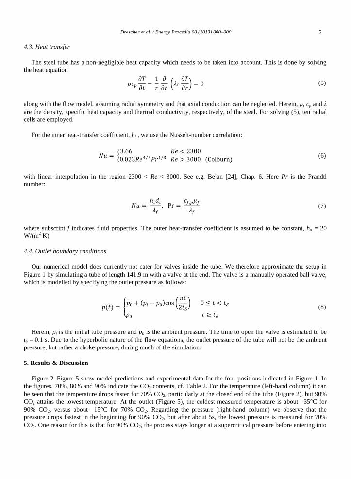
Figure 2–Figure 5 show model predictions and experimental data for the four positions indicated in Figure 1. In

the figures, 70%, 80% and 90% indicate the CO2 contents, cf. Table 2. For the temperature (left-hand column) it can

be seen that the temperature drops faster for 70% CO2, particularly at the closed end of the tube (Figure 2), but 90%

CO2 attains the lowest temperature. At the outlet (Figure 5), the coldest measured temperature is about –35°C for

90% CO2, versus about –15°C for 70% CO2. Regarding the pressure (right-hand column) we observe that the

pressure drops fastest in the beginning for 90% CO2, but after about 5s, the lowest pressure is measured for 70%

CO2. One reason for this is that for 90% CO2, the process stays longer at a supercritical pressure before entering into

6 Drescher et al. / Energy Procedia 00 (2013) 000–000

the two-phase region, at which point the mixture speed of sound drops significantly. This effect is most pronounced

near the closed end of the tube (Figure 2 and Figure 3).

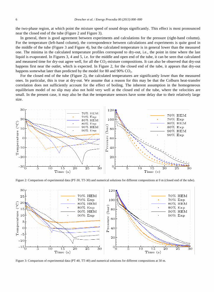
In general, there is good agreement between experiments and calculations for the pressure (right-hand column).

For the temperature (left-hand column), the correspondence between calculations and experiments is quite good in

the middle of the tube (Figure 3 and Figure 4), but the calculated temperature is in general lower than the measured

one. The minima in the calculated temperature profiles correspond to dry-out, i.e., the point in time where the last

liquid is evaporated. In Figures 3, 4 and 5, i.e. for the middle and open end of the tube, it can be seen that calculated

and measured time for dry-out agree well, for all the CO2-mixture compositions. It can also be observed that dry-out

happens first near the outlet, which is expected. In Figure 2, for the closed end of the tube, it appears that dry-out

happens somewhat later than predicted by the model for 80 and 90% CO2.

For the closed end of the tube (Figure 2), the calculated temperatures are significantly lower than the measured

ones. In particular, this is true at dry-out. We assume that a reason for this may be that the Colburn heat-transfer

correlation does not sufficiently account for the effect of boiling. The inherent assumption in the homogeneous

equilibrium model of no slip may also not hold very well at the closed end of the tube, where the velocities are

small. In the present case, it may also be that the temperature sensors have some delay due to their relatively large

size.

Figure 2: Comparison of experimental data (PT-30, TT-30) and numerical solutions for different compositions at 0 m (closed end of the tube).

Figure 3: Comparison of experimental data (PT-40, TT-40) and numerical solutions for different compositions at 50 m.

Drescher et al. / Energy Procedia 00 (2013) 000–000 7

Figure 4: Comparison of experimental data (PT-50, TT-50) and numerical solutions for different compositions at 100 m.

Figure 5: Comparison of experimental data (PT-60, TT-60) and numerical solutions for different compositions at 139 m (open end of the tube).

The calculated and measured time to dry-out at the open end of the tube for 10 and 20 % N2 are given in Table 3.

It can be seen that the agreement is good; the model predicts dry-out slightly before this is indicated by the

temperature measurements, between 5.4% and 10.2% earlier. Since the numerical model but also the experimental

data for a nitrogen composition of 30 % do not show a distinct dry-out point, this composition was omitted.

Table 3: Time to dry-out at open end of tube.

N2

[mol%]

# Experimental

[s]

Numerical

[s]

Num–Exp

[s]

10.2 1 16.88 15.97 –0.91 (–5.4%)

2 18.01 16.17 –1.84 (–10.2%)

20.0 1 8.62 8.07 –0.55 (–6.4%)

2 – – –

8 Drescher et al. / Energy Procedia 00 (2013) 000–000

60

70

80

90

100

110

120

0 0.2 0.4 0.6 0.8

Pre

ssu

re [

bar

]

Time [s]

PT-30

PT-40

PT-50

PT-60

403 ms

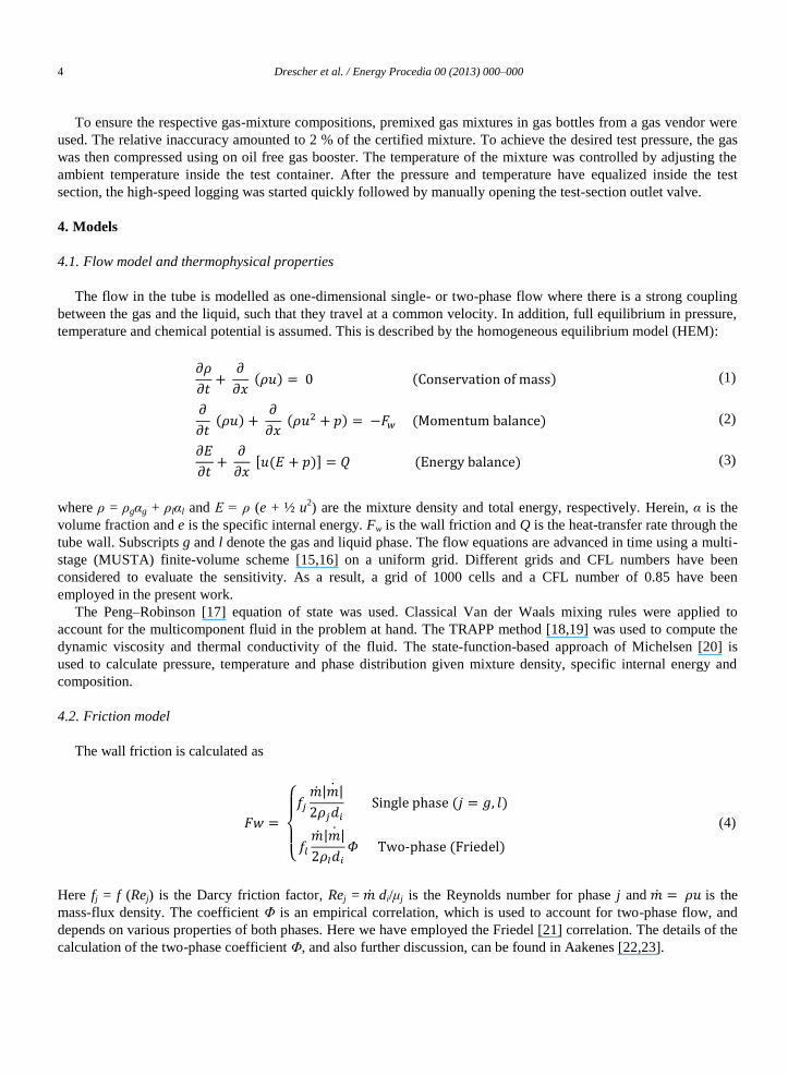
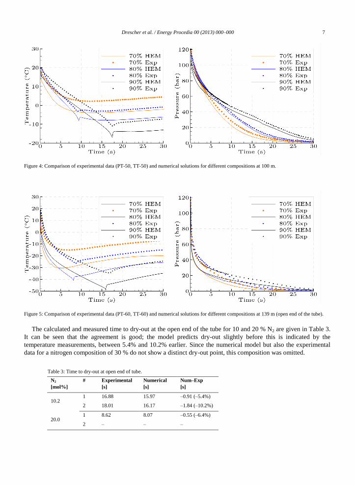
Figure 6 shows the pressure drop recorded during the first 0.8 seconds of the experimental investigations for

10% N2. The time for the pressure wave to travel from PT-60 to PT-30 amounted to 414 ms for the first test and

403 ms for the second test. Similar plots can be made for the other tests with the compositions of 20 and 30% N2.

Further, corresponding data can be extracted from the calculations. Since the fluid is initially at rest, the results can

be compared and give an indication of how well the model predicts the speed of sound. The results are shown in

Table 4. It can be seen that the experimental data are consistent, which shows a good repeatability. Furthermore, the

numerical data show that the pressure-propagation speed is overpredicted by the model, from around 10% for 10%

N2 to approximately 23% for 20% N2. The overprediction is most likely due to the use of the Peng–Robinson EOS.

Figure 6: Pressure wave recorded for the tests with 10 mol% N2 (#1 to the left and #2 to the right) as a function of time at given locations.

Table 4: Travel times for the initial pressure wave from PT-60 to PT-30.

N2

[mol%]

# Experimental

[ms]

Numerical

[ms]

Num–Exp

[ms]

10.2 1 414 368 –46 (–11.1%)

2 403 366 –37 (–9.2%)

20.0 1 565 443 –122 (–21.6%)

2 572 443 –129 (–22.6%)

30.0

1 561 467 –94 (–16.7%)

2 555 467 –88 (–15.9%)

3 561 465 –96 (–17.1%)

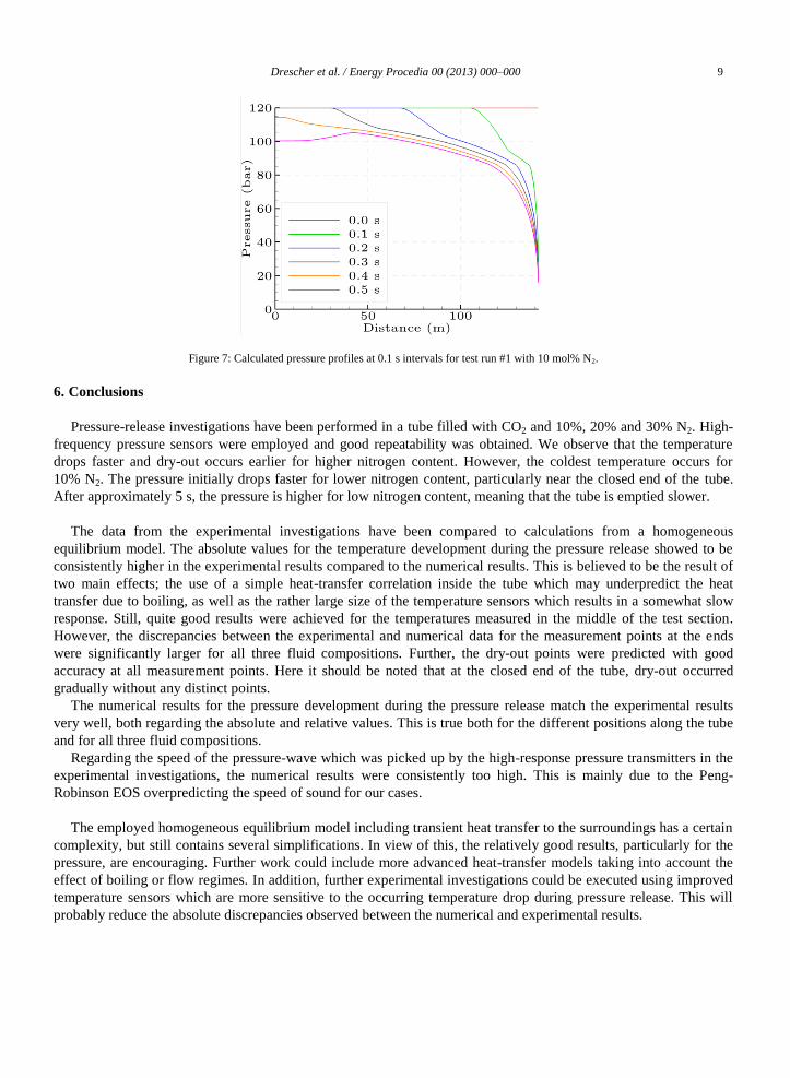
Calculated pressure profiles at 0.1 s intervals are shown in Figure 7. It illustrates the initial pressure wave

(rarefaction wave) which travels across the length of the tube, and which is reflected at the closed end. The wave

amplitude diminishes mainly due to wall friction. The figure shows that the pressure drops rapidly at first and then

levels off. This is an attribute of the drop in speed of sound when coming from the single phase region to the two-

phase region.

60

70

80

90

100

110

120

0 0.2 0.4 0.6 0.8

Pre

ssu

re [

bar

]

Time [s]

PT-30

PT-40

PT-50

PT-60

414 ms

Drescher et al. / Energy Procedia 00 (2013) 000–000 9

Figure 7: Calculated pressure profiles at 0.1 s intervals for test run #1 with 10 mol% N2.

6. Conclusions

Pressure-release investigations have been performed in a tube filled with CO2 and 10%, 20% and 30% N2. High-

frequency pressure sensors were employed and good repeatability was obtained. We observe that the temperature

drops faster and dry-out occurs earlier for higher nitrogen content. However, the coldest temperature occurs for

10% N2. The pressure initially drops faster for lower nitrogen content, particularly near the closed end of the tube.

After approximately 5 s, the pressure is higher for low nitrogen content, meaning that the tube is emptied slower.

The data from the experimental investigations have been compared to calculations from a homogeneous

equilibrium model. The absolute values for the temperature development during the pressure release showed to be

consistently higher in the experimental results compared to the numerical results. This is believed to be the result of

two main effects; the use of a simple heat-transfer correlation inside the tube which may underpredict the heat

transfer due to boiling, as well as the rather large size of the temperature sensors which results in a somewhat slow

response. Still, quite good results were achieved for the temperatures measured in the middle of the test section.

However, the discrepancies between the experimental and numerical data for the measurement points at the ends

were significantly larger for all three fluid compositions. Further, the dry-out points were predicted with good

accuracy at all measurement points. Here it should be noted that at the closed end of the tube, dry-out occurred

gradually without any distinct points.

The numerical results for the pressure development during the pressure release match the experimental results

very well, both regarding the absolute and relative values. This is true both for the different positions along the tube

and for all three fluid compositions.

Regarding the speed of the pressure-wave which was picked up by the high-response pressure transmitters in the

experimental investigations, the numerical results were consistently too high. This is mainly due to the Peng-

Robinson EOS overpredicting the speed of sound for our cases.

The employed homogeneous equilibrium model including transient heat transfer to the surroundings has a certain

complexity, but still contains several simplifications. In view of this, the relatively good results, particularly for the

pressure, are encouraging. Further work could include more advanced heat-transfer models taking into account the

effect of boiling or flow regimes. In addition, further experimental investigations could be executed using improved

temperature sensors which are more sensitive to the occurring temperature drop during pressure release. This will

probably reduce the absolute discrepancies observed between the numerical and experimental results.

10 Drescher et al. / Energy Procedia 00 (2013) 000–000

Acknowledgements

The modelling work was performed in the CO2 Dynamics project. The authors acknowledge the support from the

Research Council of Norway (189978), Gassco AS, Statoil Petroleum AS and Vattenfall AB. The experimental data

were provided by Statoil from the CO2 IT IS project funded by the Research Council of Norway (188940) and

Statoil.

References

[1] Oosterkamp, A. and Ramsen J., State-of-the-Art Overview of CO2 Pipeline Transport with relevance to offshore pipelines, Polytec Report

number: POL-O-2007-138-A, 2008

[2] Cosham A., Eiber R.J., Fracture Control in Carbon Dioxide Pipelines: The Effect of Impurities, 7th International Pipeline Conference, Vol. 3,

Calgary, Alberta, Canada, 2008

[3] Munkejord S.T., Jakobsen J.P., Austegard A. and Mølnvik M.J. Thermo- and fluid-dynamical modelling of two-phase multi-component

carbon dioxide mixtures. Int. J. Greenh. Gas Con. 2010;4:589–596.

[4] Aursand, P., Hammer, M., Munkejord, S. T. and Wilhelmsen, Ø. Pipeline transport of CO2 mixtures: Models for transient simulation. Int. J.

Greenh. Gas Con. 2013; 15:174-185.

[5] Munkejord S.T., Bernstone C., Clausen S., de Koeijer G., Mølnvik M.J. Combining thermodynamic and fluid flow modelling for CO2 flow

assurance. Energy Procedia 2013;37:2904-13

[6] Berstad, T., Dørum, C., Jakobsen, J.P., Kragset, S., Li, H., Lund, H., Morin, A., Munkejord, S.T., Mølnvik, M.J., Nordhagen, H.O. and Østby,

E. CO2 pipeline integrity: A new evaluation methodology, Energy Procedia 2011;4,:3000–3007.

[7] Nordhagen, H.O., Kragset, S., Berstad, T., Morin, A., Dørum, C. and Munkejord, S.T. A new coupled fluid-structure modelling methodology

for running ductile fracture. Comput. Struct. 2012;94–95:1006–1014.

[8] Aursand, E., Aursand P., Berstad, T., Dørum, C., Hammer, M., Munkejord, S. T. and Nordhagen, H. O. CO2 pipeline integrity: A coupled

fluid-structure model using a reference equation of state for CO2. Energy Procedia 2013; 37:3113-3122.

[9] Aursand, E., Dørum, C., Hammer, M., Morin, A., Munkejord, S. T. and Nordhagen, H. O. CO2 pipeline integrity: Comparison of a coupled

fluid-structure model and uncoupled two-curve methods. Energy Procedia 2014; 51C: 382-391.

[10] Mahgerefteh, H., Brown, S. and Denton, G. Modelling the impact of stream impurities on ductile fractures in CO2 pipelines. Chem. Eng. Sci.

2012;74:200–210.

[11] Aihara S, Misawa K. Numerical simulation of unstable crack propagation and arrest in CO2 pipelines. First International Forum on the

Transportation of CO2 by Pipeline; Gateshead, UK. 2010.

[12] Botros, K.K., Geerligs, J., Rothwell, B., Carlson, L., Fletcher, L., Venton, P. Measurements of flow parameters and decompression wave

speed following rupture of rich gas pipelines, and comparison with GASDECOM. Int. J. Pres. Ves. Pip. 2010; 87:681–695.

[13] Pettersen J., de Koeijer G., Hafner A., Construction of a CO2 pipeline test rig for R&D and operator training, GHGT-8, Norway

[14] de Koeijer G., Borch J.H., Jakobsen J., Hafner A., Experiments and modelling of CO2 pipeline depressurization – Multi-phase transient flow,

The 4th Trondheim Conference on CO2 Capture, Transport and Storage, Trondheim, Norway, 2007

[15] Toro, E.F., and Titarev, V.A. MUSTA fluxes for systems of conservation laws, J. Comput. Phys. 2006; 216, pp. 403–429.

[16] Munkejord S.T., Evje S. and Flåtten T. The multi-stage centred-scheme approach applied to a drift-flux two-phase flow model. Int. J. Numer.

Meth. Fluids 2006; 52:679–705.

[17] Peng, R.Y. and Robinson, D.B. A new two-constant equation of state. Ind. Eng. Chem. Fund. 1976; 15:59–64.

[18] Ely, J.F. and Hanley, H.J.M. Prediction of transport properties. 1. Viscosity of fluids and mixtures. Ind. Eng. Chem. Fund. 1981; 20:323–332.

[19] Ely, J.F. and Hanley, H.J.M. Prediction of transport properties. 2. Thermal conductivity of pure fluids and mixtures. Ind. Eng. Chem. Fund.

1983; 22:90–97.

[20] Michelsen, M.L. State function based flash specifications. Fluid Phase Equilib. 1999; 158-160:617-626.

[21] Friedel, L. Improved friction pressure drop correlations for horizontal and vertical two phase pipe flow, in: Proceedings, European Two

Phase Flow Group Meeting, Ispra, Italy, 1979, paper E2.

[22] Aakenes, F. Frictional pressure-drop models for steady-state and transient two-phase flow of carbon dioxide, Master’s thesis, Department of

Energy and Process Engineering, Norwegian University of Science and Technology (NTNU), 2012.

[23] Aakenes, F., Munkejord, S.T. and Drescher, M. Frictional pressure drop for two-phase flow of carbon dioxide in a tube: Comparison

between models and experimental data. Energy Procedia 2014; 51C:373–381.

[24] Bejan, A. Heat Transfer. Wiley, New York, 1993.