Experiments and Modeling of PEM FuelCells for Dead-Ended Anode Operation

by

Jason B. Siegel

A dissertation submitted in partial fulfillmentof the requirements for the degree of

Doctor of Philosophy(Electrical Engineering: Systems)

in The University of Michigan2010

Doctoral Committee:Professor James S. Freudenberg, Co-ChairProfessor Anna G. Stefanopoulou, Co-ChairProfessor Jessy W. GrizzleProfessor Jing SunProfessor Serhat Yesilyurt, Sabanci University

“Non Impediti Ratione Cogitationis”

— Click and Clack, the Tappet Brothers.

c© Jason B. Siegel

All Rights Reserved

2010

To my lovely wife Lauren and my dog Tessa, for helping me find thelight in my day.

ii

Acknowledgments

I would like to acknowledge my professors and advisors for giving me the guidance to

pursue my research; Anna Stefanopoulou, Serhat Yesilyurt, Jim Freudenberg, Stani Bo-

hac, Jesse Grizzle, and Kurt Metzger. Daniel Hussey, David Jacobson and Eli Baltic at

the National Institute for Science and Technology Center for Neutron Research provided

the expertise and patience required to collect the data making this thesis possible. My

lab-mates bestowed an excellent collaborative research environment; Denise McKay, Buz

McCain, Amey Karnik, Toyoaki Matsuura, James Marcicki, Patty Laskowsky, Jixin Chen,

and Xinfan Lin. Finally, I would like to thank my family for supporting me, listening to

my ranting, and providing inspiration.

iii

Table of Contents

Dedication . . . . . . . . . . . . . . . . . . . . . . . . . . . . . . . . . . . . . . . ii

Acknowledgments . . . . . . . . . . . . . . . . . . . . . . . . . . . . . . . . . . . iii

List of Tables . . . . . . . . . . . . . . . . . . . . . . . . . . . . . . . . . . . . . . vii

List of Figures . . . . . . . . . . . . . . . . . . . . . . . . . . . . . . . . . . . . . viii

Abstract . . . . . . . . . . . . . . . . . . . . . . . . . . . . . . . . . . . . . . . . . x

Chapter 1 Introduction . . . . . . . . . . . . . . . . . . . . . . . . . . . . . . . 11.1 PEM Fuel Cell Basics . . . . . . . . . . . . . . . . . . . . . . . . . . . . . 21.2 Fuel Cell Sub-Systems . . . . . . . . . . . . . . . . . . . . . . . . . . . . 41.3 Anode Water Management . . . . . . . . . . . . . . . . . . . . . . . . . . 61.4 Neutron Imaging to Measure Liquid Water . . . . . . . . . . . . . . . . . . 81.5 Fuel Cell Modeling . . . . . . . . . . . . . . . . . . . . . . . . . . . . . . 101.6 Thesis Organization . . . . . . . . . . . . . . . . . . . . . . . . . . . . . . 141.7 Contributions . . . . . . . . . . . . . . . . . . . . . . . . . . . . . . . . . 18

Chapter 2 Modeling PEMFC using distributed PDEs for GDL transport withlumped channels . . . . . . . . . . . . . . . . . . . . . . . . . . . . . . . . . . 202.1 Introduction . . . . . . . . . . . . . . . . . . . . . . . . . . . . . . . . . . 202.2 Experimental Hardware . . . . . . . . . . . . . . . . . . . . . . . . . . . . 232.3 Modeling of Gas and Water Dynamics . . . . . . . . . . . . . . . . . . . . 25

2.3.1 Summary of Modeling Assumptions . . . . . . . . . . . . . . . . . 272.3.2 Nomenclature . . . . . . . . . . . . . . . . . . . . . . . . . . . . . 282.3.3 Membrane Water Transport . . . . . . . . . . . . . . . . . . . . . 292.3.4 Liquid Water Capillary Transport . . . . . . . . . . . . . . . . . . 312.3.5 Gas Species Diffusion . . . . . . . . . . . . . . . . . . . . . . . . 32

2.4 Boundary Conditions . . . . . . . . . . . . . . . . . . . . . . . . . . . . . 332.4.1 Membrane Boundary Conditions . . . . . . . . . . . . . . . . . . . 332.4.2 Boundary Conditions at the Cathode Channel . . . . . . . . . . . . 372.4.3 Boundary Conditions at the Anode Channel . . . . . . . . . . . . . 39

2.5 Output Voltage Equation . . . . . . . . . . . . . . . . . . . . . . . . . . . 40

iv

2.6 Parameter Identification Approach . . . . . . . . . . . . . . . . . . .. . . 422.7 Model Calibration . . . . . . . . . . . . . . . . . . . . . . . . . . . . . . . 442.8 Model Validation and Discussion . . . . . . . . . . . . . . . . . . . . . . . 512.9 Conclusions . . . . . . . . . . . . . . . . . . . . . . . . . . . . . . . . . . 51

Chapter 3 Neutron Imaging of Liquid Water Accumulation In PEMFC . . . . 553.1 Introduction . . . . . . . . . . . . . . . . . . . . . . . . . . . . . . . . . . 553.2 Experimental Hardware . . . . . . . . . . . . . . . . . . . . . . . . . . . . 573.3 Quantification of Liquid Water Mass . . . . . . . . . . . . . . . . . . . . . 59

3.3.1 Temporal Averaging to Reduce Uncertainty . . . . . . . . . . . . . 613.3.2 Masking . . . . . . . . . . . . . . . . . . . . . . . . . . . . . . . 613.3.3 Local Spatial Averaging . . . . . . . . . . . . . . . . . . . . . . . 633.3.4 Channel Liquid Mass . . . . . . . . . . . . . . . . . . . . . . . . . 66

3.4 Results and Discussion . . . . . . . . . . . . . . . . . . . . . . . . . . . . 673.4.1 Channel Water Plugging . . . . . . . . . . . . . . . . . . . . . . . 683.4.2 Dry Anode Channel Conditions . . . . . . . . . . . . . . . . . . . 71

3.5 Flooding, Plugging and Voltage Response . . . . . . . . . . . . . . . . . . 733.5.1 Anode Nitrogen Blanketing and Voltage Response . . . . . . . . . 773.5.2 Anode Water Plugging and Voltage Response . . . . . . . . . . . . 78

3.6 Conclusion . . . . . . . . . . . . . . . . . . . . . . . . . . . . . . . . . . 83

Chapter 4 Nitrogen Front Evolution in Purged PEMFC with Dead-Ended An-ode . . . . . . . . . . . . . . . . . . . . . . . . . . . . . . . . . . . . . . . . . 854.1 Introduction . . . . . . . . . . . . . . . . . . . . . . . . . . . . . . . . . . 854.2 Experimental Setup . . . . . . . . . . . . . . . . . . . . . . . . . . . . . . 88

4.2.1 Configuration and Operating Conditions . . . . . . . . . . . . . . . 884.2.2 Gas Chromatography Setup . . . . . . . . . . . . . . . . . . . . . 894.2.3 Neutron Radiography . . . . . . . . . . . . . . . . . . . . . . . . . 90

4.3 Experimental Results . . . . . . . . . . . . . . . . . . . . . . . . . . . . . 924.3.1 Cathode Surges versus Anode Purges . . . . . . . . . . . . . . . . 944.3.2 Temperature Effects . . . . . . . . . . . . . . . . . . . . . . . . . 964.3.3 GC Sampling Effects . . . . . . . . . . . . . . . . . . . . . . . . . 984.3.4 Voltage Repeatability . . . . . . . . . . . . . . . . . . . . . . . . . 99

4.4 Modeling . . . . . . . . . . . . . . . . . . . . . . . . . . . . . . . . . . . 1004.4.1 Nitrogen Accumulation (single phase along the channel model). . . 1004.4.2 Modeling the GC Sample Location . . . . . . . . . . . . . . . . . 1044.4.3 Distributed Current Density . . . . . . . . . . . . . . . . . . . . . 1054.4.4 Nitrogen Crossover Rate . . . . . . . . . . . . . . . . . . . . . . . 109

4.5 Modeling Results . . . . . . . . . . . . . . . . . . . . . . . . . . . . . . . 1104.5.1 Effect of Operating Conditions . . . . . . . . . . . . . . . . . . . . 113

4.6 Conclusions . . . . . . . . . . . . . . . . . . . . . . . . . . . . . . . . . . 115

Chapter 5 Reduced Order Modeling of Liquid Water Fronts and NitrogenBlanketing . . . . . . . . . . . . . . . . . . . . . . . . . . . . . . . . . . . . . 1185.1 Overview of Modeling Domains . . . . . . . . . . . . . . . . . . . . . . . 118

v

5.2 GDL Fronts Simplification . . . . . . . . . . . . . . . . . . . . . . . . . . 1195.3 Modification to the GDL model for Steady State Gas Transport . . . . . . . 1215.4 Liquid Water Front Propagation in the GDL . . . . . . . . . . . . . . . . . 1215.5 Membrane Water Transport . . . . . . . . . . . . . . . . . . . . . . . . . . 124

5.5.1 Cathode Side Equations . . . . . . . . . . . . . . . . . . . . . . . 1265.6 Water Exchange With the Channel . . . . . . . . . . . . . . . . . . . . . . 126

5.6.1 Anode Channel Model . . . . . . . . . . . . . . . . . . . . . . . . 1275.6.2 Cathode Channel Model . . . . . . . . . . . . . . . . . . . . . . . 1295.6.3 Water Transport Through the Gas Diffusion Layer (GDL) . . . . . 130

5.7 Fitting Water Transport Parameters . . . . . . . . . . . . . . . . . . . . . . 1315.8 Fuel Cell Terminal Voltage . . . . . . . . . . . . . . . . . . . . . . . . . . 1325.9 Apparent Current Density and Reduced Cell Area . . . . . . . . . . . . . . 1365.10 Simulation Results . . . . . . . . . . . . . . . . . . . . . . . . . . . . . . 139

Chapter 6 Equilibrium of Nitrogen Front with DEA . . . . . . . . . . . . . . . 1436.1 Introduction . . . . . . . . . . . . . . . . . . . . . . . . . . . . . . . . . . 1436.2 Equilibrium Mechanism . . . . . . . . . . . . . . . . . . . . . . . . . . . 1456.3 Along the Channel Model . . . . . . . . . . . . . . . . . . . . . . . . . . . 1466.4 Simulation Results and Discussion . . . . . . . . . . . . . . . . . . . . . . 147

6.4.1 Influence of System Pressure . . . . . . . . . . . . . . . . . . . . . 1486.4.2 Influences of Cathode Inlet RH . . . . . . . . . . . . . . . . . . . . 1496.4.3 Influences of Cathode Stoichiometry . . . . . . . . . . . . . . . . . 1506.4.4 Evolution Toward Equilibrium . . . . . . . . . . . . . . . . . . . . 151

6.5 Experimental Results . . . . . . . . . . . . . . . . . . . . . . . . . . . . . 1526.6 Implications for Fuel Cell Design and Operation . . . . . . . . . . . . . . . 1536.7 Conclusions . . . . . . . . . . . . . . . . . . . . . . . . . . . . . . . . . . 153

Chapter 7 Conclusions. . . . . . . . . . . . . . . . . . . . . . . . . . . . . . . . 1557.1 Future Work . . . . . . . . . . . . . . . . . . . . . . . . . . . . . . . . . . 157

7.1.1 DEA Operation and Degradation Phenomena . . . . . . . . . . . . 1577.1.2 DEA Modeling . . . . . . . . . . . . . . . . . . . . . . . . . . . . 1577.1.3 DEA Control of Purging . . . . . . . . . . . . . . . . . . . . . . . 1587.1.4 Neutron Imaging . . . . . . . . . . . . . . . . . . . . . . . . . . . 158

Bibliography . . . . . . . . . . . . . . . . . . . . . . . . . . . . . . . . . . . . . . 160

vi

List of Tables

Table

1.1 Chapter-by-Chapter model highlights . . . . . . . . . . . . . . . . . . . . 17

2.1 Parameters required based on PEMFC stack specifications. . . . . . . . . . 432.2 Experimentally identified parameter values . . . . . . . . . . . . . . . . . 462.3 Parameter symbols, definitions and values. . . . . . . . . . . . . . . . . . . 54

3.1 Masks . . . . . . . . . . . . . . . . . . . . . . . . . . . . . . . . . . . . . 623.2 Cell operating conditions . . . . . . . . . . . . . . . . . . . . . . . . . . . 67

4.1 Select Cases From Data Set for Model Comparison . . . . . . . . . . . . . 944.2 Tuned Parameters . . . . . . . . . . . . . . . . . . . . . . . . . . . . . . . 1164.3 Constants . . . . . . . . . . . . . . . . . . . . . . . . . . . . . . . . . . . 116

5.1 Fuel cell water transport constants. . . . . . . . . . . . . . . . . . . . . . . 1245.2 Tuned parameters for the liquid water transport model. . . . . . . . . . . . 1315.3 Tuned Parameters in the Voltage Equation. . . . . . . . . . . . . . . . . . . 1365.4 Nomenclature and Constants . . . . . . . . . . . . . . . . . . . . . . . . . 142

6.1 Selected parameter values under equilibrium. . . . . . . . . . . . . . . . . 152

vii

List of Figures

Figure

1.1 Basic Fuel Cell structure. . . . . . . . . . . . . . . . . . . . . . . . . . . . 31.2 Fuel cell control actuators and sub-systems. . . . . . . . . . . . . . . . . . 51.3 Neutron Imaging Facility . . . . . . . . . . . . . . . . . . . . . . . . . . . 91.4 One dimensional fuel cell modeling domain. . . . . . . . . . . . . . . . . . 12

2.1 Schematic of capillary flow of liquid water through the gas diffusion layers. 212.2 Experimental hardware employed and measurement locations. . . . . . . . 242.3 Experimental data showing impact of anode purging and cathode surging . 252.4 Water transport in the GDL and membrane. . . . . . . . . . . . . . . . . . 302.5 Discretization of the gas diffusion layers. . . . . . . . . . . . . . . . . . . 342.6 Experimental measurements used for model calibration. . . . . . . . . . . . 452.7 Model calibration results. . . . . . . . . . . . . . . . . . . . . . . . . . . . 472.8 Reactant dynamics during a load change and purging event. . . . . . . . . . 492.9 Water dynamics during a load change and purging event. . . . . . . . . . . 502.10 Model validation results. . . . . . . . . . . . . . . . . . . . . . . . . . . . 52

3.1 Experimental hardware detailing sensor and actuator locations. . . . . . . . 583.2 Neutron images of the fuel cell active before and after anode purge events . 593.3 Schematic of fuel cell layers used for masking . . . . . . . . . . . . . . . . 623.4 Cathode channel mask . . . . . . . . . . . . . . . . . . . . . . . . . . . . 643.5 Average (spatial) liquid water thickness in the membrane/GDL layer . . . . 653.6 Data set #1: fully humidified cathode . . . . . . . . . . . . . . . . . . . . . 693.7 Neutron images showing water thickness (mm) . . . . . . . . . . . . . . . 703.8 Data set #2: sub-saturated cathode feed . . . . . . . . . . . . . . . . . . . 743.9 Data set #3: . . . . . . . . . . . . . . . . . . . . . . . . . . . . . . . . . . 753.10 Data set #4: . . . . . . . . . . . . . . . . . . . . . . . . . . . . . . . . . . 763.11 Voltage degradation and liquid water accumulation between anode purges . 793.12 Two-sloped voltage behavior . . . . . . . . . . . . . . . . . . . . . . . . . 813.13 Correlation between voltage and anode liquid water mass . . . . . . . . . . 82

4.1 Illustration of anode flow-field orientation and GC setup. . . . . . . . . . . 904.2 Neutron Images from sequential purge cycles . . . . . . . . . . . . . . . . 93

viii

4.3 Operating conditions and processed liquid water data from neutron images. 954.4 Selected data set 2. . . . . . . . . . . . . . . . . . . . . . . . . . . . . . . 974.5 Sequential purge cycles plotted vs. time since the previous purge. . . . . . . 994.6 One-dimensional FC modeling domain, along the channel. . . . . . . . . . 1014.7 Mapping AN CHs to an equivalent single channel. . . . . . . . . . . . . . . 1054.8 Simulation of operating condition 3 (i0.6T65 SR2RH60). . . . . . . . . . 1114.9 Along the channel distributions for operating condition 3. . . . . . . . . . . 1124.10 Simulation results for operating condition 5 (i0.4T60 SR3RH60). . . . . 1124.11 Simulation results for operating condition 6 (i0.4T50 SR3RH90). . . . . 1134.12 Along the channel distributions for operating condition 6. . . . . . . . . . . 1144.13 Model temperature effects. . . . . . . . . . . . . . . . . . . . . . . . . . . 1144.14 Model current density effects. . . . . . . . . . . . . . . . . . . . . . . . . 1154.15 GC calibration data. . . . . . . . . . . . . . . . . . . . . . . . . . . . . . . 117

5.1 Schematic diagram showing subsystem interconnections and states. . . . . 1195.2 Evolution of liquid water fronts in the GDL and channel. . . . . . . . . . . 1205.3 Two-phase water and front evolution in the anode GDL. . . . . . . . . . . . 1235.4 Diffusivity vs. membrane liquid water content at various temperatures. . . . 1275.5 Water transport as a function of current density for saturated channels. . . . 1325.6 Fuel Cell Polarization Curve. . . . . . . . . . . . . . . . . . . . . . . . . . 1355.7 Nitrogen front propagation schematic. . . . . . . . . . . . . . . . . . . . . 1385.8 Comparison of simulation versus Aug 7, 2007 Experiment at NIST. . . . . 1405.9 Zoomed plot showing model predictions vs. measured data. . . . . . . . . . 141

6.1 Equilibrium scenario in DEA operation. . . . . . . . . . . . . . . . . . . . 1446.2 Species molar fractions at equilibrium with different system pressures. . . . 1486.3 Local current densities under equilibrium with different pressures. . . . . . 1496.4 Nitrogen and oxygen distribution along the cathode channel. . . . . . . . . 1506.5 Cell voltage and species molar fractions approaching the equilibrium. . . . 1516.6 Experimental results showing time evolution and convergence to voltage

equilibrium for two different current set-points. . . . . . . . . . . . . . . . 153

ix

Abstract

This thesis develops models for the design and control of Dead-Ended Anode (DEA) fuel

cell systems. Fuel cell operation with a dead-ended systems anode reduces fuel cell system

cost, weight, and volume because the anode external humidification and recirculation hard-

ware can be eliminated. However, DEA operation presents several challenges for water

management and anode purge scheduling. Feeding dry hydrogen reduces the membrane

water content near the anode inlet. Large spatial distributions of hydrogen, nitrogen, and

water develop in the anode, affecting fuel cell durability. The water and nitrogen which

cross through the membrane accumulate in the anode during dead-ended operation. Anode

channel liquid water plugging and nitrogen blanketing can induce hydrogen starvation and,

given the right conditions, trigger cathode carbon oxidation leading to permanent loss of

active catalyst area. Additionally, the accumulation of inert gases in the anode leads to a

decrease in cell efficiency by blocking the catalyst and reducing the area available to sup-

port the reaction. Purging the anode uncovers the catalyst and recovers the available area,

but at the expense of wasting hydrogen fuel.

To understand, design, and control DEA fuel cells, various models are developed and

experimentally verified with plate-to-plate experiments using neutron radiography and gas

chromatography. The measurements are used to parameterize dynamic models of the gov-

erning two-phase (water liquid and vapor) spatially distributed transport phenomena. A

reduced order model is developed that captures the water front evolution inside the gas

diffusion layer and channels. A second model captures the nitrogen blanketing front loca-

tion along the anode channel. The reduced order models are combined to form a complete

description of the system. They require less computational effort, allow efficient parame-

terization, and provide insight for developing control laws or designing and operating DEA

fuel cells.

x

Chapter 1

Introduction

Advances in the design and control of Polymer Electrolyte Membrane (PEM) Fuel Cells

(FC)s are necessary to significantly improve durability and reduce cost for commercial ap-

plications. Degradation of the membrane and catalyst support structure has been observed

and is associated with undesired reactions which occur during load following [1] and start-

up conditions [2]. This degradation is also caused by the local build-up of liquid water

[3, 4], nitrogen, and oxygen in the anode channel. Anode channel plugging, for example,

can induce hydrogen starvation and, given the right conditions, trigger cathode carbon ox-

idation and loss of active catalyst area [5, 6, 2]. Apart from the permanent degradation,

nitrogen accumulation and blanketing in the anode channel leads to a recoverable decrease

in cell efficiency through reduction of the catalyst area available to support the reaction.

To avoid performance loss and degradation, excess water and nitrogen accumulation

in the anode channel are minimized by using high hydrogen flow rates, resulting in the

Flow-Through Anode (FTA) configuration. To increase the fuel utilization, a Re-Circulated

Anode (RCA) architecture is used. In this configuration, water is removed from the gas

stream leaving the channel and the reaming hydrogen (which is diluted with nitrogen) is

recirculated back into the stack inlet. There, the gas is combined with additional high-purity

hydrogen from the storage medium. The hydrogen rich gas is then humidified and fed to

the anode inlet. The combined water removal, recirculation, and humidification in the FTA

configuration minimizes the spatial variability in the hydrogen distribution along the an-

ode channels, but leads to higher system cost and lower power density due to the external

humidification and anode recirculation hardware. To achieve competitive cost and power

density for low temperature fuel cells Dead-Ended Anode (DEA) operation is considered

in this thesis. DEA systems can operate with dry hydrogen at low flow rates and without

external humidification, however, large variations in the spatial distributions of water (dry

inlets and flooded outlets) and nitrogen need to be addressed.

Liquid water formation can appear under various conditions leading to stationary, cy-

clostationary, or erratic patterns [3, 7]. It is therefore difficult to statistically assess or

1

physically model the impact on degradation due to lack of repeatable data. This the-

sis develops and shows plate-to-plate experiments with controlled flooding patterns [8],

which are used to parameterize models of two-phase (water liquid and vapor), dynamic

and spatially distributed transport phenomena inside a low temperature fuel cell. Detailed

experiments show that nitrogen crossover and accumulation strongly impacts the distribu-

tion of reactants and current density when operating in DEA mode. The model is then

reduced in complexity, first by deriving ordinary differential equations that capture the wa-

ter front evolution inside the FC porous media and channels. The simplification reduces

the computational effort and allows for efficient parameterization. Once parameterized, the

model can be used to study system behavior [9] and develop control laws [10, 11].

1.1 PEM Fuel Cell Basics

Proton Exchange Membrane, also called Polymer Electrolyte Membrane, Fuel Cells

(PEMFC)s are electrochemical energy conversion devices. PEMFCs produce electricity

by combining hydrogen and oxygen, typically from the air, to form water and a small

amount of heat. The heart of PEMFCs is the polymer electrolyte membrane. Two half

reactions half reactions take place at the catalyst layers on either side of the membrane as

shown in Fig. 1.1. The splitting of hydrogen into protons and electrons takes place at the

anode catalyst layer. Protons crossing the membrane combine with oxygen and electrons

at the cathode catalyst layer to generate water. The membrane provides a barrier to keep

the hydrogen and oxygen separated. It must conduct protons easily, yet be electronically

insulating to force the electrons through an external circuit and provide useful work. One

such membrane material is Nafionc© manufactured by DuPont, another competing product

is provided by Gore. These polymer membranes have low melting temperatures, which

limit operating temperature below 100C. Typical operating temperatures range from 50

to 70 C. PEMFCs have several attributes, including low operating temperature and high

efficiency (typically 50-70% for the fuel cell stack and 40-60% for the overall system),

which make them good candidates for automotive and portable power applications.

The basic structure of the PEM fuel cell is shown in Fig. 1.1. The fuel and oxygen

(air) are delivered across the active area through a series of channels. These channels are

typically machined into the backplanes which are a conductive material, allowing electron

transfer to the current collectors and completion of an electric circuit. The ratio of channel

width to rib (contact) width, and the channel flow-field pattern are important design param-

eters affecting fuel cell performance. The Gas Diffusion Layer (GDL) is a porous material

2

H2H2 H2

-

-

-

-

-

-

-

-

-

- -

-

-

-

-

- -

-

-

-

-

H2O

-

- -

-

- -

+

+

+

+ +

+

+

+

+

+

+

+

+

+

+

+

(Cross-sectional view)

Cathode

Channel

(O2 supply)

Gas

Diffusion

Layers

Anode

Channel

(H2 supply)

Catalytic

Layer Catalyst

Polymer

Electrolyte

Membrane

Chemical Reactions

Anode: H2 2H+ + 2e

-

(Oxidation)

Cathode: O2 + 4H+ + 4e

- 2H2O

(Reduction)

O2

O2

-

Figure 1.1 Basic Fuel Cell structure (not to scale) [12].

used to evenly distribute the reactant gases from the channel to the catalyst surface in the

area under the ribs and channels. The GDL is typically composed of an electrically conduc-

tive carbon paper or cloth material. It is also designed to promote the removal of product

water from the catalyst area, by treatment of the carbon with a hydrophobic coating such as

Teflon. Finally the Catalyst Layer (CL) contains platinum particles supported on a carbon

structure. The CL is where the reaction takes place inside the fuel cell. For the reaction to

take place at the cathode, all three reactants, protons, oxygen, and electrons, must be able

to reach the Platinum (Pt) particle. Protons are conducted through the Nafionc© membrane

material, electrons through the carbon support structure, and oxygen gas through the pore

space. Therefore, each Pt particle must be in contact with all three portions of the cell

[13]. A thin Micro-Porous Layer (MPL) can also be inserted between the GDL and CL

to increase the electrical contact and aid in water removal from the catalyst or membrane

hydration [14].

The membrane is a polymer that absorbs water, and the membrane water contentλmb,

defined as the number of moles of water per mole of SO3H in the membrane, is a critical

parameter for describing both proton transport and the permeation of molecular species

3

through the membrane. As the water content of the membrane increases, both the proton

conductivity and the rate of gas permeation through the membrane also increase. Increased

proton conductivity is good for fuel cell efficiency. However, increased permeability in-

creases the rate of molecular crossover through the membrane, lowering the fuel cell

efficiency, and thereby resulting in excess accumulation of water (plugging) and nitrogen

(blanketing) of the anode channels. Hydrogen is thus displaced or blocked from reaching

the catalyst sites. Modeling and managing this accumulation is the subject of this thesis.

1.2 Fuel Cell Sub-Systems

The PEMFC systems can be organized into three main categories, each of which evolves

on different time-scales, the fastest is reactant gas supply (air or oxygen and hydrogen),

followed by thermal management, then water management. Although dynamic behavior

of each sub-system is tightly coupled (for example excess reactant supply may be used to

carry heat and product water out of the cell, overlapping with the objectives of the thermal

management system), these divisions provide a useful modeling framework. This thesis

focuses on management of dead-ended anode operation. This topic has not been covered

extensively in the literature or studied by the control society. Water management is consid-

ered to be one of the main barriers to commercialization of low temperature PEMFC stacks

[15]. In this section, the overall stack management system is presented in order to provide

adequate perspective and motivate DEA operation.

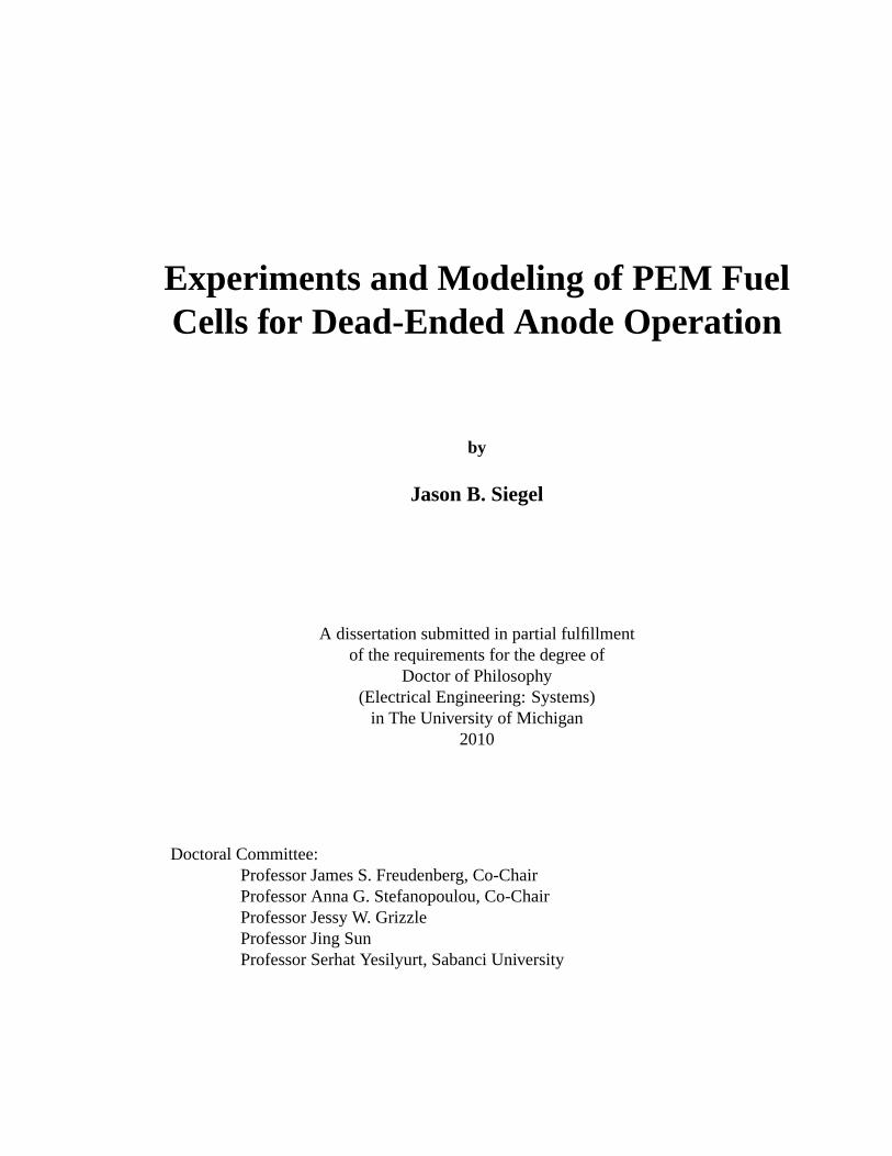
Figure 1.2a shows a basic fuel cell control architecture with many of the common con-

trol actuators for the reactant supply systems, hydrogen on the anode and air on the cathode.

Although some small portable fuel cell systems are low-pressure ambient air breathing,

which rely on free convection to deliver the oxidant, most automotive applications use

forced air. In forced air systems, a scroll or centrifugal compressor is used to increases the

oxygen partial pressure in the channels and hence the power density of the system [16]. The

actuatoru2 controls the supply rate and back-pressure of the air to the cathode side of the

fuel cell. If the compressor is driven by the fuel cell, a limit on the rate of power increase

should be used in order to prevent oxygen starvation [17]. Various control techniques have

been used to model and handle the constraints of the air compressor and manifold filling

dynamics [16, 18], including feedback linearization [19] and a reference governor [20].

In addition to buffering the fuel cell from damaging increases in load current, excess air

supplied to the cathode aids the removal of liquid water from the channels [3, 21, 22].

Since excess air is supplied, typically 2 - 3 times the amount required to support the re-

4

Fuel Cell Stack

S

Humidifier

Water SeparatorBackpressurevalve

Compressor

Water Tank

HydrogenTank

Motor

u1

u4

u3

u2

Temperature Control

Humidity Control

Hydrogen Flow /Pressure Control

Air Flow Control

Power

Conditioning

TM

u5

Power Management

u6

Traction Motor Control

Energy Storage(Battery)

Water Separator

Ejector

PHydrogen

Tank

u1

Hydrogen Purge Control

a) Re-Circulated Anode (RCA)

b) Dead-Ended Anode (DEA)

Figure 1.2 Fuel cell control actuators and sub-systems (modified from [16]). a) Dashed gray boxshows hardware required for anode re-circulation (RCA). b) Simplified hydrogen delivery systemfor pressure regulated Dead-Ended Anode (DEA), which reduces or removes the need for inlethumidification, ejector, water separator and recirculation plumbing.

action, there is a very high flow rate of gas through the cathode channels and humidification

of the incoming air is required to prevent drying the membrane. Bubblers, hotplate injec-

tion, and other novel humidifiers are employed for the inlet air humidification. The water

temperature and flow rate ( indicated by actuatoru4) through a membrane-type humidifier

may be used to control the relative humidity of the incoming air [23, 24]. This sub-system

is tightly coupled with the air flow and thermal management sub-systems [25, 26, 27], since

the coolant water exiting the stack is then fed into the humidifier. The coolant flow rate and

fan speed,u3, can be used for control of the cooling system.

The overarching difficulty in the subsystem level control paradigm is that the control of

air flow rate, cathode pressure, cathode inlet relative humidity, and stack temperature are

5

all tied to the higher level control objective of water management. Water management is a

critical issue for PEMFC operation to ensure long stack life and efficient operation. Two

of the limiting factors which prevent the mainstream adoption of PEMFCs are cost and

durability or stack lifetime [15]. One of the major culprits affecting PEMFC durability is

water, specifically the formation of liquid water inside the cell [3] and the wet-dry cycling

of the membrane [28, 29]. The formation of liquid water can block reactants from reaching

the catalyst leading to starvation and carbon corrosion [5, 30, 2], a permanent degradation

of the cathode support structure. Conversely, drying of the membrane increases protonic

resistance which yields lower cell efficiency, as illustrated in section 2.5. There needs to be

sufficient water content in the membrane, (highλmb), so that proton conduction through the

membrane is easy, however, too much water results in flooding and channel plugging. The

delicate balance between drying and flooding is called management [4, 6, 31]. Modeling

can provide the necessary tools to achieve this delicate balance in a cost-effective way.

1.3 Anode Water Management

Flow-through operation is used on both the anode and cathode of most laboratory or ex-

perimental hydrogen PEMFC systems. However, the fuel utilization of flow-through anode

(FTA) operation is too low for commercial and portable systems. Fuel utilization is the

rate of fuel consumption divided by the rate of fuel delivery,U f uel = (I f c/(nF))/vf uel [13],

whereI f c is the fuel cell current in Amperes (A),n= 2 is the number of electrons taking

part in the reaction, F=96,400 C mol−1 is Faraday’s constant andvf uel is the hydrogen de-

livery rate in mol s−1. The fuel stoichiometry,λH2 = 1/U f uel, is the inverse of utilization.

The anode reactant sub-system, shown in Fig. 1.2a, uses a re-circulation loop to re-cycle ex-

cess hydrogen back through the fuel cell stack increasing the fuel utilization. However the

RCA requires hydrogen grade plumbing and hardware such as an ejector/blower [32, 33],

water separator, and hydrogen humidification. These components add weight, volume, and

expense to the system [34, 35]. Note that the water must be removed from the gas exiting

the anode before it goes to the ejector and then the dry fuel supplied to the anode must be

re-humidified to prevent over-drying of the membrane due to the higher flow rate.

Although the RCA subsystem can remove water from the gas stream, purging is still

required to handle the nitrogen. A small amount of nitrogen crosses through the membrane,

driven by the gradient in partial pressure from the air fed in the cathode. Over time this ni-

trogen accumulates in the anode feed system, which dilutes the hydrogen fuel in the anode

[36, 37]. The dilution of H2 lowers the fuel cell terminal voltage, and hence the efficiency.

6

Therefore the anode re-circulation system needs to be purgedat certain intervals to remove

the accumulated inert gas and maximize the system efficiency.

This thesis models a Dead-Ended Anode (DEA) system fed by pure dry hydrogen,

shown in Fig. 1.2b, which is regulated to maintain anode pressure and supply exactly the

amount of hydrogen needed to support the reactionλH2 = 1. DEA operation does not have

as stringent requirements as the RCA system on hydrogen inlet humidification due to the

lower flow velocity in the channels. The water crossing through the membrane could be

enough to humidify the hydrogen fuel. The use of a pressure regulator instead of the RCA

hardware (comprised of a mass flow controller, outlet water separator, hydrogen ejectors or

blower, and inlet humidification), yield a system with lower cost and volume. In DEA oper-

ation, the binary control signal,u1 ∈ 0,1, opens the downstream solenoid valve, causing

a brief high velocity flow through the anode channel as the pressure regulator opens in

attempt to maintain the system pressure. The high velocity flow aids in the removal of

liquid water droplets [3, 22], which in the case of RCA could remain stationary due to the

lower gas velocity. Several anode configurations, and the practical aspects of purging vs.

flow-through, have been considered experimentally in [38, 39, 40].

Similar to the RCA system discussed above, nitrogen and water crossover is a concern.

In a DEA system, the nitrogen, pushed toward the end of the channel by the flow of re-

actants, accumulates. The accumulating N2 forms a blanket, which completely displaces

hydrogen from reaching the catalyst layer, effectively shutting down the power production

from the affected region of the cell [41]. Water vapor gradients between the humidified

cathode and the dry fed anode also drive excess water into the anode, which can cause sig-

nificant liquid water accumulation. Unlike water vapor whose maximum partial volume is

dictated by temperature, liquid can fill the entire free space in the channels [8]. This liquid

water accumulation in the channel water blocks the flow of reactants, which is referred to

as channel plugging, and stops the production of power in the affected regions of the cell.

The gas velocity, driven by consumption of hydrogen, pulls nitrogen and water toward

the bottom of the channel. Gravity helps stabilize the system as heavier molecules get

pushed toward the bottom. As the mass accumulation continues, a stratified pattern devel-

ops in the channel with a hydrogen rich area sitting above a hydrogen depleted region, as

shown in Fig. 1.4. The boundary between these regions is a time-varying front, which pro-

ceeds upwards toward the inlet [41]. The mass accumulation physically blocks hydrogen

gas from reaching the anode catalyst sites, which is the mechanism for the experimentally

observed and recoverable voltage degradation [8, 36, 42]. Therefore, purges of the anode

channel volume are necessary to clear the reaction product and inert gas from the chan-

nel. After the purge, the catalyst area contributing to the reaction increases and hence the

7

measured voltage increases.

To prevent confusion and clarify the observed phenomena, the termfloodingis used to

describe the accumulation of liquid water in the GDL or catalyst layer, and the termplug-

ging is used to refer to liquid water in the channels, which blocks or hinders the flow of gas

through the channels [43]. The termblanketingis used to designate N2 mass accumulation

in the AN CH, which prevents hydrogen from reaching the catalyst layer.

Understanding, modeling and predicting the front evolutions in the anode for DEA op-

eration of PEMFCs would allow a judicious choice of purging interval and duration. It

is also possible, as shown in Chapter 6. to find operating conditions with stable behavior

without purging. Using the modeling framework outlined in this thesis, one could deter-

mine an optimum schedule to reduce the H2 wasted during purges and avoid over-drying

the membrane. The advantage to developing simple models is that they can be used for

MPC [10] or observer-based feedback algorithms that provide robustness in the control

algorithm.

1.4 Neutron Imaging to Measure Liquid Water

The measurement of both water vapor and water liquid in operating PEMFCs is one of the

greatest challenges for controlling FC stack operation due to the lack of availability, and

cost, of sensors. Therefore, models which can accurately predict the amount of water in-

side the FC are important. Relative humidity (RH) sensors are expensive and saturate when

exposed to liquid water, thus making them unsuitable for controlling FC operation, except

for very dry operating conditions. The measurement of liquid water distribution inside an

operating fuel cell, needed for model validation, is often complicated by methods which

interfere with the quantity to be measured. Optical imaging of water droplets in the chan-

nels using high-speed cameras [44] requires the use of plexiglas end-plates or windows to

allow visual inspection. Unfortunately, the materials used in the construction of fuel cells

with optical viewing windows tend to have very different thermal conductivity properties,

and therefore have been shown to induce condensation and impose non-realistic operating

conditions. Magnetic Resonance Imaging (MRI) [45] is another relatively new and inter-

esting tool for investigating water behavior inside PEMFC. However, this technique also

requires the use of non-standard materials as metallic end-plates and current collectors are

incompatible with the MRI equipment. The clear advantage of neutron imaging is the abil-

ity to measure in-situ the liquid water concentration while using realistic or commercial FC

designs.

8

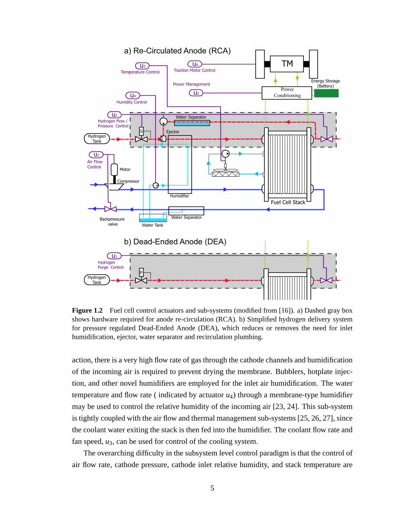
Figure 1.3 NIST Center for Neutron Research: Neutron Imaging facility [46].http://physics.nist.gov/MajResFac/Nif/

The fundamental principle of neutron imaging is based on pinhole optics. Neutrons

emitted from the reactor core escape through a small diameter (1 cm) aperture (the pin-

hole), and travel down the flight tube, as shown in Fig. 1.3. At the end of the 6 m flight

tube, the fuel cell is placed in front of a neutron sensitive detector. The intensity of the

neutron beam passing through the fuel cell is attenuated by liquid water in the fuel cell,

and then the remaining neutrons which pass through are detected by a panel array. This

produces a 2-D projection of liquid water distribution in the fuel cell. Dry images of the

fuel cell are taken as a reference, which can later be used to calculate the amount (i.e. thick-

ness) of water in the path of the neutron beam, as described in Chapter 3. Some excellent

techniques to improve resolution and reduce uncertainty in measurements using neutron

imaging can be found in [47, 48].

Beginning with [49] in 1999, many publications have utilized neutron imaging to study

the effects of liquid water accumulations and distributions on the operation of PEMFCs

[50, 7, 48, 51, 52, 53, 54, 55, 56, 57, 58, 59]. All of these publications deal with imaging

the fuel cell during steady state flow through conditions. The research presented in this

thesis is the first experimental validation of a dynamic model to predict DEA operation

using in-situ measurements of liquid water accumulation.

The capabilities of the National Institute for Standards and Technology (NIST) Neu-

tron Imaging Facility (NIF) for fuel cells are described in [46]. There are only a few other

facilities in the world which offer comparable neutron imaging capabilities, including the

Paul Scherrer Institute (PSI) [60] in Switzerland, and the International Thermonuclear Ex-

perimental Reactor (ITER) in France. There are two imaging setups available at NIST:

1) A low spatial resolution (250µm) detector with a relatively high time-resolution (for

9

fuel cell liquid water measurement), on the order of 1 s per frame. This imaging

setup was used for in-plane water distribution measurements, as described in chapter

3, where the plane is defined by the membrane.

2) A recently developed high resolution detector (10-20µm) which has poor time reso-

lution (imaging requires long exposure times,≈ 20 mins, and steady state conditions)

but can be used for through-plane (i.e.x-direction) water distribution measurements.

Modeling and measurement results from the high resolution imaging are shown in

[61].

1.5 Fuel Cell Modeling

From the simplest model, a static polarization curve, to fully dynamic 3-D multi-phase

models [62], the common objective is prediction of the fuel cell terminal voltage as a per-

formance metric. A review of fuel cell modeling approaches can be found in [63] and [64].

Modeling reactant (gas) transport from the channel, through the GDL, to the catalyst layer

at surfaces of the membrane, is critical for predicting the performance of the PEMFC, but

equally important for high power applications is the description of product water removal

from the cathode catalyst surface. Liquid water can block the catalyst surface, reducing the

number of active catalyst sites, or fill some of the pore spaces in the GDL inhibiting the

flow of reactant gas to the CL. Cathode GDL/CL flooding is the main performance limi-

tation at high current density and therefore most commonly studied in the literature. This

is considered to be a materials and design problem, since control actuators have limited

authority to impact CCL flooding without over-drying the regions near the inlet [43].

Under DEA operation, product water which diffuses through the membrane (x-

direction) back to the anode side will condense and accumulate in the anode channel (along

the y-direction), displacing hydrogen, as shown in Fig. 1.4, and preventing it from reaching

the anode catalyst layer. The prevention of hydrogen from reaching the catalyst stops the

production of power from the affected region of the cell. Observation of water accumula-

tion in DEA operation, and the voltage drop between purges motivates the development of

a model to predict the water accumulation in the GDL and channels and its impact on cell

voltage [65]. Under galvanostatic, or constant current operation, the remaining “hydrogen

rich” regions of the cell must support a larger current density (A cm−2) to account for the

area which is no longer active. Hence, the notion of apparent current density can be used to

capture this effect [41, 65] and simplify the modeling of distributed current density along

the channel (y-direction), as shown in Fig. 1.4.

10

A simple model for nitrogen accumulation in a dead-ended anode fuel cell stack was

first investigated in [41]. This model Assumes single phase, water vapor only, channel

conditions and uses the convection equation to describe the accumulation of nitrogen at

the end of the anode channel, as shown in Fig. 1.4. This model captured the correlation

between Gas Chromatography (GC) measurements, taken from the end of the channel, and

the cell voltage, but did not consider the effects of diffusion or liquid water. This previous

work motivated the investigation of simultaneous GC measurements and neutron imaging

presented in this thesis, since both nitrogen and water accumulations in the DEA contribute

to voltage loss. Chapter 4 describes the experiments that were performed and the model

developed to study the relative effects of nitrogen and water accumulation. The convection

only model is then modified to include diffusion effects using the Stefan-Maxwell modeling

framework, which better predicts the nitrogen concentration distribution (at the sampling

location) and corresponding voltage measurements. The importance of along the channel

modeling for capturing water crossover and cell performance has also been demonstrated

in [66, 67]. Although not addressed in this work, the three-dimensional (3-D) effect of lo-

cal current density distribution between the channels and ribs, resulting from gas transport

and liquid water accumulation in the GDL, is addressed in [68] where a quasi-potential

transformation was used to reduce a 2-D, GDL modeling domain down to 1-D. This type

of method can handle an-isotropic properties of the diffusion medium due to compression

of the GDL [69, 70].

The schematic representation of anode channel filling with liquid water and nitrogen is

shown in Fig. 1.4. Since water condenses in both the GDL and channels, the water transport

between the membrane and GDLs, and from the GDL to channels, determines the rate of

water accumulation in the anode. Therefore, a One-Dimensional (1-D) modeling approach

is considered, for the GDL, from channel to channel (x-direction). Calculation of the appar-

ent area, shown in Fig. 1.4, from the anode channel masses is shown in Section 5.9. Anode

purging directly impacts anode channel water accumulation, and can remove water from

the channel which may not be easily removed by conventional flow through operation, as

discussed in the previous section.

The water transport models developed in this thesis are based on previous research at

the University of Michigan Fuel Cell Control Laboratory (FCCL). A 1-D, isothermal, and

dynamic model of liquid water, water vapor, and reactant (H2 or O2), and inert (N2) gas

transport through the GDL (x-direction) was developed in [65], and reviewed in chapter 2.

Depending on the discretization level, this distributed Partial Differential Equation (PDE)

model of GDL transport can be computationally intensive. Using a three section discretiza-

tion, an ODE model is derived with 24 states, 18 of which come from the discretization of

11

Figure 1.4 The one dimensional fuel cell modeling domain, along thex-axis, which denotes thethrough membrane direction. They axis denotes the distance along the channel from inlet to outlet(not drawn to scale). This caricature shows the stratification of product water, inert nitrogen andthe displacement of hydrogen from the bottom portion of the cell. The distributed current density,i f c(y), along the channel is shown to the left of this figure; for a realistic profile (solid line), themodeled apparent current density (dashed line).

the (PDE)s describing gas and liquid water transport in the anode and cathode GDLs. The

remaining 6 states correspond to a mass balance for lumped hydrogen or oxygen, nitrogen

and water masses in the anode and cathode channels.

The GDL water transport model was derived from the steady state relationship pre-

sented in [71], where water transport is driven by the gradient in capillary pressure, de-

scribed by the Leverett J-function (2.6). The liquid water profile forms a steep front inside

the GDL as shown in Fig. 2.4. Several other, more recent, water transport models have been

developed in the literature which explain the relationship between liquid water accumula-

tion in the GDL and water flow [72, 73, 74, 75, 76, 77, 78, 79]. These models highlight the

dependence of water transport on the material properties; specifically the pore-size distri-

bution of the GDL, and % weight of hydrophobic material such as Teflon. This dissertation

focuses on the Leverett approach since there is more information readily available, how-

12

ever, it is important to note that other capillary pressure models should also exhibit a similar

behavior in the formation of a steep liquid water front and propagation mode [80]. Accu-

rate representation of the evolution of this front requires a very fine spatial discretization of

the distributed reactants, vapor and liquid water.

The first simplification used to solve the 4 coupled PDEs in the x-direction was devel-

oped by McCain et al. [81]. This approach uses a Semi-Analytic Solution (SAS) for the

water vapor, and reactant gas transport PDEs in the GDL. Since the reactant gas and vapor

diffusion in the GDL evolve with much faster time-constants than the liquid water, due to

the difference in density, the SAS uses the steady-state solution of the PDEs for the gas dis-

tributions, to propagate the concentration values in the channel through the GDL to the CL.

This reduces the number of dynamic states in the GDL model from three per discretization

slice down to one, namely liquid water. Further reduction of the number of states in the

water transport model in the GDL can be achieved using a moving front approach, which

was first introduced by Promislow et al [82, 83]. The PDEs [65, 12] describing liquid wa-

ter transport require a very fine discretization grid in order to accurately represent the front

propagation. Adaptive grids, developed to address the problem of groundwater transport

[84], have been used to handle this type of problem, but they are not well suited for a re-

duced complexity control oriented model. The nature of the sharp transition in the GDL

liquid water volume, between the wet and dry regions, can be used to simplify the model.

The two-phase front location in the GDL is defined by the point where the reduced water

saturation,S, goes to zero along thex direction, in terms of an ordinary differential equation

(ODE), similar to [80], greatly reducing the computational complexity of the 1-D 2-phase

water model.

The trade-off between model accuracy and computational complexity, 1-D versus 2-D

versus 3-D, is a difficult engineering challenge for the control of PEMFC systems. A com-

parison between 1-D and 2-D models, in terms of voltage accuracy is presented in [85],

and a review of CFD modeling for heat and mass transfer in PEMFCs can be found in

[86]. In summary, CFD models [87, 88, 62, 89, 90] are great for detailed FC modeling,

optimization, and channel design, but are very complicated to setup and require inten-

sive computational resources. Therefore, CFD models are not suitable for control oriented

applications. In order to use a fuel cell model for control design, and real-time hardware im-

plementation in an automotive grade microprocessor, development of reduced order models

is necessary.

The 1+1-D through the membrane modeling approach, presented in this thesis, is a

good compromise between model complexity and accuracy since the apparent current den-

sity, shown in Fig. 1.4, captures some of the along the channel effects without increasing

13

the computational complexity. The reduced order model developed in section 5.2 also has

another advantage over CFD models in that the water transport and voltage model can

easily be parameterized using analytical tools, as described in sections 5.7 and 2.6.

1.6 Thesis Organization

This thesis follows a chronological progression of hypothesis formulation, testing, and dis-

covery motivated by the desire to understand and model the performance and dynamics

of a PEMFC operating under DEA conditions. The second chapter is the result of a joint

research effort at the Fuel Cell Control Lab (FCCL) with Denise McKay, and represents

the fuel cell model based on the PDEs describing the distribution of water (liquid and va-

por) and reactant transport along thex-direction in the GDLs and membrane. A lumped

volume approach (also known as a stirred tank reactor or STR [91] in the field of chemical

engineering) is used for the channels. The lumped volume model constitutes a mass bal-

ance and is described in Sec. 2.4.3. Water accumulation in the GDL and channels can be

described simply by a first order integrator ODE model. The parameterization and model

tuning using stack data, based on a discretization of the PDEs describing the gas and liquid

states in the GDL coupled to a lumped channel model, was published in the Journal of

Power Sources [65]. Subsequent work, by Real et al. [92], following this approach using a

lumped channel model is shown in [92, 93, 94], where the PDEs describing reactant trans-

port in the GDLs are further simplified and approximated by a single volume each, with

the associated ODEs. Their model was tuned to represent the dynamic behavior of a Bal-

lard Nexa PEMFC stack which is auto-humidified and, as a result, also utilized a saturated

cathode feed gas supply.

In order to validate the predicted accumulation of water and avoid the issue of cell to

cell variability, single cells were built which would allow for neutron imaging. Using neu-

tron imaging, in-situ measurement of the liquid water distribution within the fuel cell was

investigated, allowing observation the otherwise immeasurable state of the system. Chapter

3 explains both the neutron imaging data and measurement uncertainty analysis from the

first round of testing at NIST. This chapter provides a basic comparison with the (slightly

modified) discretized PDE model presented in Chapter 2. The simulation results presented

in Chapter 3 include some modeling improvements beyond [65]; specifically, the inclusion

of liquid water flow through the outlet orifice. Accounting for liquid water removal dur-

ing an anode purge is necessary to predict the water balance in the fuel cell because liquid

causes plugging of the channel and outlet orifice; hence, gas cannot flow out until the liquid

14

is pushed out of the way.

Using the 1-D GDL model with lumped channels (STR), the voltage behavior can be

captured by liquid water accumulation using a thin film model for the liquid coverage

area and the notion of apparent current density. Neutron imaging shows good results with

anode channel liquid water mass accumulation, for experimental conditions which match

the assumption of uniform channel vapor distribution (i.e. saturated cathode inlets). The

observed water accumulation from neutron imaging however, does not corroborate this

predicted film thickness. Namely, the experimentally observed water coverage area was

insufficient to explain the extent of voltage deviation. The analysis of neutron imaging data

is published in the Journal of the Electrochemical Society (JES) [8]. Although the lumped

parameter channel model is able to predict the water accumulation in the GDL and anode

channel with very good accuracy for operating conditions with fully saturated cathode inlet

conditions, it is unable to adequately predict the voltage or sub-saturated (i.e. very dry)

cathode inlet conditions. Model inaccuracy for low cathode inlet RH is not surprising,

considering that the assumption of uniform/lumped channel conditions would be violated

as the vapor concentration increases along the length of the cathode channel due to the

production of water.

The inability to predict voltage for some vapor saturated cathode inlet conditions im-

plied that another un-modeled factor could be responsible. Specifically, there is a signifi-

cant voltage drop even during periods when only a small amount of liquid water build-up in

the anode channel is observed. After reviewing the literature [36, 37, 41], it was suspected

that nitrogen accumulation in the anode channel is contributing to the voltage drop during

DEA, which is recoverable by purging the anode. At first, the effects of nitrogen accumu-

lation were investigated by augmenting the lumped channel model with nitrogen crossover.

It was found that a lumped volume (STR) approach can’t predict the effect of nitrogen

accumulation in the anode channel due to the logarithmic relationship with voltage.

This motivated the development of a new distributed model to predict nitrogen dis-

tribution and blanketing effects in the anode channel. Experiments were then proposed to

measure the relative effects of nitrogen and water accumulation in the anode channel on fuel

cell voltage. Chapter 4 presents the development of a single phase along the channel model

with distributed current density to capture the nitrogen crossover and blanketing effects in

the anode channel. This chapter also details the August 2008 experiments at NIST with

simultaneous gas chromatography measurement of the nitrogen concentration and neutron

imaging, recently published in the Journal of the Electrochemical Society (JES) [95]. The

single phase nitrogen model is validated against experimental results from NIST. The neu-

tron images confirm that water accumulation in the anode channel is not significant for the

15

selected operating conditions, hence justifying the validity of the single phase model.

Since the discretized PDE model presented in Chapter 2 requires a very fine spatial

discretization to accurately predict the two phase transition between single phase and two

phase (liquid) water areas in the GDL. Therefore, an alternative representation of the GDL

water distribution and transport was considered. A reduced order method, similar to the

slowly moving, two-phase interface model presented in [80], was derived for the model,

along with the necessary tools to parameterize the membrane water transport model using

measurements from neutron imaging. Based on modeling efforts presented in Chapter 4,

a reduced order channel model to capture the N2 accumulation effect on cell voltage was

developed. The model relies on the steady state solution of the PDEs describing reactant

concentrations along the channel. Although this reduced order model is better in predict-

ing the voltage drop due to nitrogen accumulation in the anode channel, it has the same

limitations as the original lumped channel model for predicting liquid water behavior for

low cathode inlet RH. Chapter 5 details the development of a reduced order model to cap-

ture liquid water front propagation in the GDL and channel, and the nitrogen front in the

channel. This work will also be published in a forthcoming chapter of the CRC Controls

Handbook [11].

The existence of equilibrium in the nitrogen blanketing front location is predicted by

the single phase anode channel PDE equations. These equilibria, their stability and time-

constants to reach equilibrium following an anode purge are evaluated in Chapter 6. Finally,

the model predictions are verified by running experiments with DEA for extended periods

between purges.

16

CH2 1-D (through the mem-brane), 2 phase GDLmodel with lumpedchannels (BCs).

Voltage is tuned for 24 cellstack data, and thin filmmodel captures proposedrelationship between an-ode channel water accu-mulation and voltage.

Spatial discretization ofthe PDE requires highercomputational overhead,which motivates semi-analytic-solution (SAS) ofGDL [96] and CH5.

CH3 Neutron Imaging of singlecell, and comparison withslightly modified modelfrom CH2.

The model shows goodagreement with measuredwater mass accumulation,however invalidates thethin-film assumption andmotivates the investiga-tion of nitrogen effects.

The lumped channelmodel cannot predict be-havior for lower cathodeinlet RH due to spatialvariation of water contentalong the channel.

CH4 1-D (along the channel)Single phase model with0-D GDL and distributedmembrane water content,compared with simultane-ous GC and NI.

The model describes theeffect of nitrogen accumu-lation and blanketing frontevolution on cell voltage.

Single phase model is notvalid for flooding condi-tions.

CH5 1-D (through the mem-brane) reduced order GDLmodel based on liquid wa-ter front evolution in theGDL with lumped chan-nels. The effect of ni-trogen blanketing in anodechannel is augmented tothe single nitrogen massaccumulation state usingan approximation of thesteady state nitrogen pro-file observed from CH4.

This CH demonstrates pa-rameterization of watertransport, the model canbe tuned to match wateraccumulation in the an-ode channel from NI. Thecombined effects of anodeliquid water and nitrogenaccumulation on voltageare predicted well for cer-tain operating conditions.

The model has the samelimitation as originalthrough membrane model(CH2), lumped channels(and lumped membranewater content) cannotpredict the behavior forlower cathode inlet RHdue to spatial variation ofwater content along thechannel.

CH6 Equilibrium analysis of1-D along the channelmodel.

Used to determine the ef-fects of spatial variationsas compared to lumpedchannel model.

Points to validity and use-fulness of lumped channelmodel. Shows specific op-erating conditions (i,T,P),and the effect of controlinputs, CA inlet SR andRH.

Table 1.1 Chapter-by-Chapter model highlights

17

1.7 Contributions

The contributions of this dissertation are summarized here:

a) Voltage tuning algorithm: In Chapter 2, a reformulation of the voltage model is pre-

sented than can be parameterized by minimizing the prediction error using a linear

least squares cost function. The solution of the least-squares problem is then related

to the parametersK1-K4 in (2.40). The discretized GDL model presented in Chapter

2 was programmed and compared with the data.

b) Neutron imaging, data collection, and analysis:In preparation for Neutron imag-

ing experiments, the specifications for fuel cell hardware compatible with neutron

imaging was determined. The trade-off between measurement uncertainty and im-

age exposure time used to collect data suitable for analyzing transient behavior of

the PEMFC, given the constraints of the imaging system, is evaluated. Following

the experiments a method for estimating the liquid water mass in the various layers

of the fuel cell from the Neutron images was derived and programmed into image

processing routines for analysis of the data, as discussed in Chapter 3.

c) Simultaneous GC and NI measurements:Experiments were developed and per-

formed at NIST to determine the relative effects of liquid water, and nitrogen accu-

mulation in the DEA, using simultaneous measurement of liquid water accumulation

via neutron imaging and nitrogen concentration measurement via gas chromatogra-

phy. Data processing and analysis were performed to enable comparison with fuel

cell models. This research led to the publication of the first experimental results com-

paring a model with simultaneous measurement of nitrogen and water accumulation.

d) Development of an along the (anode) channel PDE model:Based on [41], but

modified to include diffusion effects and a distributed current density, a model was

developed. This model is needed to explain the two-sloped voltage behavior shown

in Fig. 4.8 and the GC measurements taken from the sampling location. A new

physics based voltage model was identified from the literature, and incorporated into

the modeling framework to account for distributed current density as described in

Chapter 4.

e) Model reduction and water fronts in the GDL: The fronts based GDL and mem-

brane model presented in Chapter 5 are derived along with a method to parameterize

the model using the quasi-steady state measured liquid water accumulation rate in

the anode channel derived from neutron imaging.

f) Improvements to the lumped channel model:Incorporation of nitrogen crossover

into the modeling framework. The channel inlet/outlet flow equations are described

18

using a model that accounts for liquid water removal from the channels, (stated as

important missing feature in A4 of [65] and in B. A. McCain’s thesis [96].)

g) Equilibrium analysis: The equilibrium that could be achieved during the dead end

anode (DEA) operations of PEM fuel cell was investigated. The simulation results

indicate that the system pressure and RH of air supply play a critical role in deter-

mining the steady state power output during DEA operation. It is shown that the

equilibrium is feasible for only small load current. Experimental validation shows

the stable voltage output under DEA conditions as predicted by the model. The re-

sults suggest that it is possible to coat only the active portion of the membrane, along

the channel length, with catalyst, hence reducing the system cost without sacrificing

catalyst utilization or durability.

19

Chapter 2

Modeling PEMFC using distributedPDEs for GDL transport with lumped

channels

This chapter describes a simple isothermal dynamic model that predicts the experimentally

observed temporal behavior of a PEMFC stack. The DEA operation of PEMFC leads to

water accumulation in the anode channel under certain operating conditions. In order to

capture the water accumulation in the channel, vapor transport, liquid water transport, and

accumulation inside the GDL needs to be considered. A reproducible methodology is pre-

sented to experimentally identify six (6) tunable physical parameters. Therefore based on

the estimation of the cell voltage, the water vapor transport through the membrane, and the

accumulation of liquid water in the gas channels. The model equations allow prediction

of the species concentrations through the gas diffusion layers, the vapor transport through

the membrane, and the degree of flooding within the cell structure. An apparent current

density is related to this flooding phenomenon and cell performance through a reduction

in the cell active area as liquid water accumulates. Despite oversimplifying some complex

phenomena, this model is a useful tool for predicting the resulting decay in cell voltage over

time after it is tuned with experimental data. The calibrated model and tuning procedure is

demonstrated with a 1.4 kW (24 cell, 300 cm2) stack. The stack is operated with pressure

regulated pure hydrogen supplied to a dead-ended anode.

2.1 Introduction

The management of water is critical for optimizing performance of a PEMFC stack be-

cause the ionic conductivity of the membrane is dependent upon its water content [97]. To

maintain membrane water content, a balance must be struck between reactant (hydrogen

and oxygen) delivery and water supply and removal. Depending upon the operating con-

20

ditions of the PEMFC stack, the flow patterns in the anode and cathode channels, and the

design of the anode gas delivery system (dead-ended or flow through), this liquid water can

accumulate within the gas diffusion layers (GDLs) and channels [56, 98, 7, 51], as shown

in Figure 2.1. Whether obstructing reactant flow or reducing the number of active catalyst

sites, the impact of flooding is a reduction in the power output of the fuel cell stack, seen

by a decrease in cell voltage [99]. Thus, a real-time estimation of the degree of flooding

within the cell structure and its impact on the cell electrical output with standard, cheap,

and reliable sensors is critical for active water management. Moreover, a low order control-

oriented model must be derived to consider such issues as identifiability, observability, and

controllability.

Channel

Anode

brane

Cathode

Gas Diffusion Layer Air

GDL

Figure 2.1 Schematic of capillary flow of liquid water through the gas diffusion layers.

To gain a better understanding of reactant and water transport within the GDL and

catalyst layers, many CFD models have been developed to approximate the two or three

dimensional flow of hydrogen, air, and water at steady-state within the cell structure

[100, 101, 102, 103, 104, 87]. Using experimental steady-state polarization (voltage versus

current) data for parameter identification, [105] and [106] investigated the sensitivity of

the cell performance to the identified parameters. Furthermore, using a model to simulate

polarization data with a given set of parameters, constrained quadratic programming was

then used to identify these given parameters [107] and address parameter identifiability and

uniqueness issues [108].

3-D CFD models are ideal for investigating two phase transport phenomena, spatial

gradients, and the influence of material properties on cell performance. Unfortunately pa-

rameter sensitivity and experimental validation of these models is still lacking. A few pub-

lications address steady-state model validation. They point to a mismatch between model

21

predictions and the spatially resolved current density data[109] indicating that different

spatial distributions can correspond to the same voltage polarization curve [109, 108].

Other work has shown good prediction of steady-state and spatially resolved current den-

sity measurements, but their tuned parameters are several orders of magnitude different

than the theoretical values [66].

Steady-state polarization measurements do not offer a conclusive data set for model

validation, however, the transient response does provide useful data for model validation

especially during unsteady operation such as flooding [110, 111]. Several transient models

have been reported to capture the relationship between critical material properties and oper-

ating conditions on the dynamic fuel cell response [112, 113, 114, 115, 116], however few

have been validated against transient experimental data and are of sufficient computational

tractability for implementation in real time control applications.

Control-oriented transient models have been developed to account for the formation of

liquid water within the gas channels [117] or within both the channels and the GDL [118],

however, they do not relate the effect of flooding to decreased cell potential. The voltage

response is a key indication of how flooding impacts cell performance. A relationship be-

tween flooding and cell performance was introduced in [111], appearing later in [92], using

the notion of apparent current density to relate the accumulation of liquid water in the gas

channels to a reduction in the cell active area, increase in the cell current density and hence

lower cell voltage.

In this chapter, a low order model of the liquid water and gas dynamics within the GDL

is presented to simulate both the effects of reactant starvation and flooding. The modeling

effort focuses on the one dimensional dynamics through the GDL thickness. It is assumed

that the two dimensional properties in the plane parallel to the membrane are invariant,

and a lumped volume is used to capture manifold filling dynamics for the gas channels,

and lumped parameter characteristics for the membrane. Lumping the GDL and channel

into a single volume, Hernandez et al. [119] experimentally validated their model for a

flow-through anode with no gas dynamics. Lumped modeling of the GDL volume was

also pursued by Real et al. [92] and validated against experimental data for a Ballardr

NEXATM system. In their approach nearly double the number of experimentally identified

parameters were used as compared to the work originally presented in [111] and used here.

The validity of the model is tested using a wider range of current densities (0-0.3

A cm−2), temperature (45-65oC) and air stoichiometries (150%-300%). These conditions

are tested while the stack operates mostly under full hydrogen utilization with intermittent

and short high hydrogen flow conditions associated with dead-ended anode operation. It is

shown that the model predicts both the fast voltage dynamics during step changes in cur-

22

rent (the gas dynamics) and the slow voltage behavior while liquid water is accumulating in

the GDL and gas channels (water dynamics), whereas [92] only predicts the slow voltage

dynamics well. Hence, the model presented here can be used for estimation and control of

fuel cell water and gas dynamics. It is important to note that the fuel cell model presented

here is not novel, except in relating cell flooding to performance. The unique contribution

lies in applying this simple isothermal model to well approximate the dynamic fuel cell

response under a range of operating conditions by leveraging standard off-the-shelf sensors

and actuators.

This chapter is organized by first presenting the experimental hardware in Section 2.2

followed by the model of gas and water dynamics in Section 2.3. The applied boundary

conditions at the gas channels and membrane surface are then presented in Section 2.4.

The impact of the liquid water on cell voltage is modeled in Section 2.5. The parameter

identification methodology is presented in Section 2.6. Finally, the model calibration and

validation results are shown in Sections 2.7 and 2.8. A list of the model parameters is given

in the Appendix.

2.2 Experimental Hardware

Experimental results are collected from a 24-cell PEMFC stack which can deliver 1.4 kW

continuous power, capable of peaking to 2.5 kW. The cell membranes are comprised of

GORETM PRIMEAr Series 5620 membrane electrode assemblies (MEAs). The MEAs

utilize 35 µm thick membranes with 0.4 mg/cm2 and 0.6 mg/cm2 Pt/C on the anode and

cathode, respectively, with a surface area of approximately 300 cm2. The GDL material,

which distributes gas from the flow fields to the active area of the membrane, consists of

double-sided, hydrophobic, version 3 ETekTM ELATsr with a thickness of 0.43 mm. The

flow fields are comprised of machined graphite plates with gas channels that are approxi-

mately 1 mm wide and 1 mm deep. The flow pattern consists of semi-serpentine passages

on the cathode (30 channels in parallel that are 16.0 cm in length with two 180o turns) and

straight passages on the anode (90 channels in parallel that are 17.1 cm in length).

The experimental hardware, designed in collaboration with the Schatz Energy Research

Center at Humboldt State University, is installed at the Fuel Cell Control Laboratory at the

University of Michigan. A schematic of the major experimental components along with the

measurement locations is depicted in Figure 2.2. A computer controlled system coordinates

air, hydrogen, cooling, and electrical subsystems to operate the PEMFC stack. Dry pure

hydrogen is pressure regulated at the anode inlet to a desired setpoint. This pressure regula-

23

tion system replenishes the hydrogen consumed in the chemical reaction. For the majority

of the operational time, the hydrogen stream is dead-ended with no flow external to the

anode. Using a purge solenoid valve, hydrogen is momentarily purged through the anode

to remove water and inert gases. Humidified air (generated using a membrane based inter-

nal humidifier) is mass flow controlled to a desired stoichiometric ratio. Deionized water

is circulated through the system to remove heat produced due to the exothermic chemical

reaction. A fan is used to thermostatically control (on-off) the stack outlet coolant to a

desired temperature. Measurements of the dry gas mass flow rates supplied to the PEMFC

stack are taken along with the temperature, pressure and relative humidity in the inlet and

outlet manifolds.

HM

Air

A

P

PS

P

HT

ResS

HX

WP

Compressor

Water

Tank

Chiller

S

S

SF

Filter

V

Hydrogen

MF

C

MF

M

Lo

ad

P

P

VF

M

PP

P P

Fuel Cell

PP

mass flow meter

volumetric flow meterVFM

MFM

HX

HT

WP

F

PS

HM

heat exchanger

heat tape

water pump

float switch

power section

humid section

measurement probe

SS solenoid valve

mass flow controllerMFC

Figure 2.2 Experimental hardware employed and measurement locations. This figure is modifiedfrom [120].

24

Due to the lack of a practical means to directly measure the accumulation of liquid

water within a multi-cell stack, consecutive anode purges and cathode surges (momentarily

increasing the gas mass flow rates) are used to indicate the presence of liquid water in either

the anode or cathode channels, as shown in Figure 2.3. At approximately 240 seconds the

cathode is surged, causing an increase in oxygen partial pressure and cell voltage. How-

ever, this momentary voltage increase is not sustained following the surge and the general

voltage decay due to flooding in the anode persists. Following an anode purge, the voltage

quickly improves and then gradually decays until the next anode purge event is initiated.

It is important to note that this gradual decay in cell voltage could be attributed to the ac-

cumulation of nitrogen in the anode which would also be expelled during and anode purge

event. However, during purge events a significant mass of liquid water can be visually de-

tected leaving the anode. Thus, this chapter focuses on the impact of anode flooding on cell

voltage and assumes nitrogen is not the culprit.

0 50 100 150 200 250 300 350 400 450 500660

670

680

690

700

710

720

Time (s)

Cell

Vo

ltag

es (

mV

)

0 50 100 150 200 250 300 350 400 450 5001.06

1.08

1.1

1.12

1.14

1.16

1.18

1.2

Time (s)

p (

bar)

P Ca In

P An In

Anode Purge

Cathode Surge

Figure 2.3 Experimental data showing impact of anode purging and cathode surging on cell volt-ages at a constant nominal current density of 0.3 A cm−2, and an operating temperature ofT=65oC.The first subplot shows the 24 individual cell voltages in thin lines along with the average cellvoltage with a thick line. The second subplot shows the anode and cathode inlet total pressures.

2.3 Modeling of Gas and Water Dynamics

The model of the reactant and water dynamics is presented in the following sections, de-

scribing the capillary transport of liquid water and the diffusion of gases within the GDL,

25

as well as the time varying boundary conditions at the membrane and gas channel inter-

faces. To approximate the spatial gradients, the gas diffusion layer is separated into discrete

volumes using standard finite difference techniques.

The anode volume contains a mixture of hydrogen and water vapor, whereas the cathode

volume contains a mixture of oxygen, nitrogen, and water vapor. The species concentra-

tions in the channel are calculated based on the conservation of mass assuming the channel

is homogeneous, lumped-parameter, and isothermal. It is assumed that product water is

formed in the vapor phase.

This product water vapor, combined with the water vapor supplied with the cathode

gas stream, is exchanged between the anode and the cathode through the hydrophilic

membrane. The protons, liberated at the anode, transport water to the cathode through

electro-osmotic drag, while back diffusion transfers vapor due to a water vapor concentra-

tion gradient across the membrane. The net flux of vapor through the membrane depends on

the relative magnitudes of these transport mechanisms. Although there are many efforts to

experimentally quantify back diffusion ([121], [122], [123], [124]), conflicting results sug-

gest an empirically data-driven identification of water vapor diffusion might be a practical

approach to this elusive subject. Constant parameters have been used to scale back diffu-

sion models for PEMFCs with different membrane materials [118] [125]. Using a similar

methodology as [118], in this chapter the membrane water transport algorithm employs a

tunable parameter to scale the membrane water diffusion model in [122].

When the production or transport of water vapor overcomes the ability of the vapor

to diffuse through the GDL to the channel, the vapor supersaturates and condenses. The

condensed liquid water accumulates in the GDL until it has surpassed the immobile sat-

uration limit, at which point capillary flow will carry the liquid water to an area of lower

capillary pressure (the GDL-channel interface). Liquid water in the GDL occupies the pore

space, reducing the diffusion of the reactant gases. However, the reduction of the reactant

concentrations due to the changes in the gas diffusivity alone is not significant enough to

degrade the voltage by the magnitude experimentally observed. Similar observations lead

to the consideration of the reactant diffusion in the catalyst layer [126].

A different approach is used in this work. Instead of adding the complexity of the

catalyst layer to the model, at low current density, channel plugging is hypothesized to im-

pact cell voltage. Water covering the GDL surface reduces the area available for diffusion

through the GDL. The water (in liquid and vapor phase) that wicks out of the hydrophobic

GDL to the channel ultimately obstructs the area that reactants can diffuse through. This

effect is not easily modeled because the GDL surface roughness makes it difficult to pre-

dict how much GDL surface area is blocked by a given volume of liquid water. For this

26

reason, it is assumed the liquid water at the GDL-channel interface forms a layer of uni-

form thickness. This water layer spreads across the surface of the GDL as the volume of

liquid water in the channel increases. The resultant reduction in surface area increases the

calculated current density, thereby lowering the cell voltage at a fixed total stack current.

In this model, the thickness of the water layer,twl, is an experimentally tuned parameter.

The estimation of the average cell voltage is a function of the reactant concentrations

at the surface of the membrane, the membrane water content, temperature, and the calcu-

lated current density based on the reduced active area, which in turn is a function of liquid

water present in the gas channel. There are four experimentally tunable voltage parame-

ters,K1−K4, which are determined using linear least squares for a given set of membrane

diffusion, αw, and water thickness,twl, parameters. By comparing the average measured

cell voltage to the model prediction, these parameters can be re-adjusted to match the rate

of decay and magnitude of the voltage degradation. This iterative process allows all six

tunable parameters to be identified.

2.3.1 Summary of Modeling Assumptions

In summary, the following assumptions are used in the model:A1 The volume of liquid water within the GDL does not restrict the volume occupied

by the gases. The authors in [127] indicated that the diffusion of gas through theGDL occurs through a hydrophobic macroporous structure, whereas the liquid watertravels through the non-wet proofed pores (a microporous structure), implying thatthe pore volume occupied by gases is fixed. Examining the time scale decompositionof the reactant and water dynamics [128], this assumption primarily influences theliquid water dynamics and, due to the relatively small change in liquid water volumebetween the GDL sections, has a negligible impact. However, if different boundaryconditions were applied which significantly modified the spatial distribution of liquidwater in the GDL sections, this assumption should be revisited.

A2 The internal cell structure (gas channel, GDL and membrane) is isothermal and equalto the time varying coolant outlet temperature. However, the gas inlet temperaturesmay vary and are used to calculate the water vapor mass flow rates entrained with thesupplied reactants. Although it is true that a multi-cell stack with a large active areawill undoubtedly have thermal gradients within the cell structure and impact watertransport [129], this assumption is adequate for estimating the temporal evolution incell voltage experimentally observed under both flooding and drying conditions, aswill be shown in Section 2.8. Accounting for dynamic thermal states within the gasdiffusion layer adds a significant degree of model complexity which, while useful fordesign, may not be appropriate for control.

A3 The gas channels are treated as homogeneous lumped parameter volumes. Addi-tionally, flow through the GDL is modeled in one dimension which neglects the

27

difference in transport mechanisms for flow under the ribs versus under the chan-nels. Although models do exist which characterize all these complex phenomena,the inclusion of this additional dimension has a significant impact on the number ofinternal states in the model.

A4 Liquid water removal from the anode channel during purging is incorporated into themodel via (5.31). It has been shown [22] that liquid water droplet instability and theresultant detachment from the GDL to the gas channel can be a significant liquid wa-ter removal mechanism at high current density (high gas velocity). Therefore, if thismodel is to be extended to high current density operation, this assumption should berevisited.

A5 All gases behave ideally. The range of system operating temperatures and pressurespermits the assumption of ideal gas behavior for the gas constituents of interest.

A6 Hydrogen and oxygen molecules, which crossover through the membrane, are as-sumed to react in the opposing CL, contributing to thei loss term in (2.37), and hencedo not accumulate in the opposing channels. Crossover of nitrogen molecules isneglected in this work, but will be addressed in chapter 4. Where there is a con-centration gradient across the membrane, nitrogen crossover can be modeled using apermeation rate [36]. The nitrogen diffusion in the GDL is not considered, becauseit is much faster than the permeation rate through the membrane.

A7 Due to the relatively small gas flux within the GDL at the current density rangeconsidered, the convective transport of gas due to bulk flow was neglected.

2.3.2 Nomenclature

This section describes the nomenclature used throughout this paper. A list of the parame-

ters is provided in the Appendix, along with values and units. Time derivatives are denoted

asd()/dt. Spatial derivatives through the GDL thickness in the membrane direction (x) are

denoted as∂ ()/∂x. In the presented model, all equations have SI units ofPa,N, m,kg,s,

andJ unless explicitly stated.

The symbola is used for water activity,c for molar concentration (mol/m3), 〈D〉 for

effective diffusivity (m2/s), Dw for water vapor diffusion coefficient (m2/s), E for the the-

oretical open circuit voltage (V),i for the nominal current density (A cm−2), iapp for the

apparent current density (A cm−2), io for the exchange current density (A cm−2), I for the

total stack current (A),Krl for relative permeability,nd for electroosmotic drag coefficient

(mol H2O/ mol H+), N for molar flux (mol/s/m2), p for pressure (Pa),psat for the water

vapor saturation pressure (Pa),Revap for the evaporation rate (mol/s m3), s for the fraction

of liquid water volume to the total volume,S for the reduced liquid water saturation,T for

temperature (K),Uact for the activation voltage loss (V),Uohmic for the ohmic voltage loss

(V), Uconc for the concentration voltage loss (V), ¯v for the measured terminal cell voltage

(V), v for the estimated terminal cell voltage (V),W for mass flow rate (kg/s),x for the mass

28

fraction, andy for the mole ratio. Greek letters are used whereε is for the GDL porosity,λfor membrane water content (molH2O/mol SO−

3 ), φ for relative humidity (0-1), andω for

humidity ratio.

The subscriptambis used to represent ambient conditions,an for anode,c for capillary,

ca for cathode,ch for channel,ct for catalyst,da for dry air,dg for dry gas,e for electrode

(an or ca), f c for fuel cell stack,H2 for hydrogen,in for the control volume inlet or input,

j as an index for gas constituents,k as an index for discretization (in time or space),l for

liquid water,mbfor membrane,N2 for nitrogen,O2 for oxygen,out for the control volume

outlet or output,p for pore,rm for return manifold,v for water vapor, andw for water (gas

and/or liquid phase).

2.3.3 Membrane Water Transport

The membrane provides a barrier to keep the hydrogen and oxygen separated. It must con-

duct protons easily, yet be electronically insulating to force the electrons though an external

circuit and provide useful work. The most common membrane material NafionR©, used in

this work, is modeled widely in the literature. The membrane water contentλmb, is defined

as the number of moles of water per mole of SO3H in the membrane.λmb, is a critical

parameter for describing both proton transport, diffusion of water, electro-osmotic drag,

and the permeation of molecular species though the membrane.

The distribution of membrane water content is described by a PDE, the divergence of

the water flux though the membrane;

∂λmb

∂ t=−EW

ρmb

∂Nw,mb

∂x, (2.1)

whereEW = 1100 g mole−1 is the equivalent weight of the membrane andρmb= 1.9685

g cm−3 is the membrane dry density. However, since the membrane is very thin,δmb =

25 µm, it can be discretized in space and represented by a single ODE.

Membrane water flux,Nw,mb (mol cm−2), from cathode to anode is calculated from the

diffusion and electro-osmotic drag terms,

Nw,mb=−Dw(λmb,T)∂λmb

∂x−nd(λmb,T)

i f c

F, (2.2)

whereDw(λmb,T) is the water diffusion coefficient for water in the membrane (5.14), and

nd(λmb) is the coefficient of electro-osmotic drag (5.17) [130]; both of which areλmb and

T dependent and increase with both membrane water content and temperature.

29

The boundary conditions complete the description of transport in the membrane, cou-

pling it with the GDL. Dirichlet boundary conditions are imposed forλmb, at the left and

right edges of the membrane, assuming the membrane is at equilibrium with the water vapor

vapor concentration in the GDL at the membrane surface,cv,an(0) andcv,ca(0). The equi-

librium value,λan, is calculated using the membrane water uptake isotherm,λT,a as shown

in (5.10) [65, 130], and the water activity at the GDL-MB interfaceaan,mb= cv,an(0)/cv,sat.

The water flux leaving the membrane,Nw,mb is the boundary condition for the GDL, as

shown in (5.37). Due to the relative thickness of the membrane (i.e. extremely thin), it

can be modeled as a resistance, and lumped into the boundary conditions of the GDL as

discussed in Sec. 2.4.1Anode GDLCathode GDL

Cathode Ch Anode ChMembrane

Figure 2.4 Water transport in the GDL and membrane. Dashed lines indicate the vapor distribu-tion in the GDL,cv, and solid blue lines represent the reduced water saturation,S. The boundaryconditions for the PDE models are shown, and arrows indicate positive x-direction in each region.The water distributions are shown for two distinct cases; saturated (bottom half) and sub-saturated(top half) anode channel conditions. In the case of sub-saturated anode channel conditions, the tran-sition between two phase (water liquid and vapor) and single phase (vapor only) is indicated by thefront location,xf r,an, as the point whereS→ 0 in the GDL along the x-direction.

30

2.3.4 Liquid Water Capillary Transport

In hydrophobic GDL material as the GDL pore spaces fill with liquid water the capillary

pressure increases causing the water to flow to adjacent pores with less water. This process

creates a flow of liquid water through the GDL, resulting in an injection of liquid into the

channel. The liquid water dynamics are calculated by applying conservation of mass to the

GDL volume,dsdt

=

(1

ρl εAf c

)∂Wl

∂x− rv(cv,an)Mv

ρl. (2.3)

where the mass of liquid water in the GDL is expressed in terms of liquid water saturation,

s, which represents the fraction of the liquid volume to the pore volume (s=Vl/Vp). Wl is

the liquid water mass flow,rv(cv,an) is the molar evaporation rate, ,Af c is the nominal fuel

cell active area,ρl is the liquid water density,Mv is the molecular weight of water, andε is

the GDL porosity.

The flow of liquid water through the GDL is a function of the capillary pressure gradient

([71, 131]) described by

Wl =−εAf cρl KKrl

µl

(∂ pc

∂S

)(∂S∂x

)

, (2.4)

where pc is the liquid water capillary pressure,K is the absolute permeability,µl is the

viscosity of liquid water, andKrl = S3 is the relative permeability of liquid water. The

relative permeability function suggests more pathways for capillary flow are available as

liquid water saturation increases, and is a function of the reduced liquid water saturation,

S, shown by

S=

s−sim

1−simfor sim < s≤ 1

0 for 0≤ s≤ sim ,(2.5)

where,sim is the value of the immobile saturation describing the point at which the liquid

water path becomes discontinuous and interrupts capillary flow. This capillary flow inter-

ruption occurs whens< sim. The results of capillary flow experiments using glass beads as

porous media show thatsim = 0.1 [71].

Capillary pressure is the surface tension of the water droplet integrated over the surface

area. The Leverett J-function describes the relationship between capillary pressure and the

reduced water saturation,S,

pc =σ cosθc√

K/ε[1.417S−2.120S2+1.263S3]︸ ︷︷ ︸

J(S)

, (2.6)

31

whereσ is the surface tension between water and air, andθc is the contact angle of the water

droplet [71]. Other, more recent, capillary pressure models can be found in [72, 73, 75].

The liquid and vapor PDEs (2.3)-(2.11) are coupled through the molar evaporation rate,

rv(cv,an) =

γ (cv,sat(T)−cv,an) for s> 0,

min0,γ(cv,sat(T)−cv,an) for s= 0(2.7)

whereγ is the volumetric condensation coefficient[71],cv,sat(T) is the vapor saturation

concentration andcv,an = pv/RT is the vapor concentration in the GDL.R is the ideal gas

constant,T is temperature, andpv is the water vapor partial pressure. When the partial

pressure of water vapor is greater than the saturation pressure,rv is negative, representing

the condensation of water. A logical constraint must be included such that if no liquid water

is present (s≤ 0)) and the saturation pressure is greater than the water vapor pressure, then

water can not be evaporated (rv = 0).

2.3.5 Gas Species Diffusion

The diffusion of gas species in the GDL is a function of the concentration gradient, trans-

ferring gas from regions of higher concentration to regions of lower concentration. The

molar concentration of gas speciesj is denotedc j and is a function of the number of moles

of gas within the pore volume,Vp, where

c j =p j

RT. (2.8)

Diffusion of hydrogen and water vapor occurs in the anode GDL and the diffusion of

oxygen and water vapor occurs in the cathode GDL. As a result, both the anode and cathode

gas diffusion can be modeled assuming binary diffusion. It is important to note that nitro-

gen gas is present in the cathode. The nitrogen concentration in the channel is modeled as

a dynamic state, however, the concentration of nitrogen in the GDL is assumed to be equal

to the channel value. A constant nitrogen profile across the GDL is reasonable since it is

not involved in the reaction at the catalyst layer. Ternary diffusion must be assumed at both

the anode and the cathode if nitrogen cross-over were to be considered. The total molar

flux is related to the concentration gradient, represented by

Nj =−〈D j〉∂c j

∂x, (2.9)

32

where〈D j〉 is the effective diffusivity of the gas constituents in the GDL,

〈D j〉= D jε(

ε −0.111−0.11

)0.785

(1−s)2 , (2.10)

for two dimensional bulk diffusion with flow perpendicular to the GDL carbon fibers, where

D j is the gas diffusion coefficient. Porosity, effective diffusivity and liquid water saturation

for carbon Torayr paper GDL, are modeled from [71].

Finally, the general temporal derivative of gas concentration as a function of the local

molar flux gradient and the local reaction rate,Rj , of the particular gas species forms a

partial differential equation (PDE),

dcj

dt=

∂Nj

∂x+Rj . (2.11)

where (2.9-2.11) are combined to yield a second order PDE.

2.4 Boundary Conditions

The membrane and gas channels serve as time-varying boundary conditions for the GDL

model. This section presents the application of mass conservation in the channel as well

as the model for the water vapor exchange between the anode and cathode through the

membrane. It is important to remember that the spatial gradients within the GDL are ap-

proximated with finite difference equations. A variable taken from a GDL section that is

adjacent to the boundary of interest will be denoted byψ(1) or ψ(L), where(L = 3) indi-

cates the section next to the gas channel and(1) indicates the section next to the membrane.

Each gas diffusion layer is separated into (L=3) discrete volumes, shown in Figure 2.5,

to approximate the solution of (2.3) and (2.11) for each of the constituents in the GDL.

Spatial discretization of the GDL yields eighteen coupled ordinary differential equations

(ODEs), describing the gas constituent concentrations and liquid water saturation, that ap-

proximate the solution of the original PDEs.

2.4.1 Membrane Boundary Conditions

The reaction at the catalyst surface of the membrane results in a loss of hydrogen and oxy-

gen at the anode and cathode, respectively. These fluxes,Nj,e(0), are used in the calculation

33

c ,chN

Anode

GDL

Cathode

GDL

Membrane

123 1 2 3

W

WW

Cathode

Channel

Anode

Channel

c

c c (3) c (2) c (1)

c (3) c (2) c (1)

s (3) s (2) s (1)

c (1) c (2) c (3)

c (1) c (2) c (3)

s (3)s (2)s (1)

an,in ca,in

ca,outWan,out

N (3)

N (2)

N (1)

N (1)

N (2)N (3)

N (3)

N (2)

N (1)

N (1)

N (2)N (3)

W (3)

W (2)

W (1)

W (1)W (2)

W (3)

c

c

Nv,mb

N (0)

N (0)N (0)

04 4

N (0)

,ch

,ch

c ,chN

,ch

,ch

Figure 2.5 Discretization of the gas diffusion layers. The direction of the assumed mass flow rateis indicated with a solid arrow. The dashed arrow is used to indicate periodic mass flow rates. Notethe swapped direction of transport for the Anode GDL and membrane from [65], to be consistentwith rest of thesis.

of the molar flux spatial gradients, described by:

Nj,e(0) =I

εAf c2ξFwith

ξ = 1 for j = H2

ξ = 2 for j = O2(2.12)

whereI is the total current drawn from the stack andF is the Faraday constant. The molar

flux of water vapor at the GDL-membrane boundary,Nv,e(0), is influenced by the gener-

ation of water vapor at the cathode membrane surface as well as the flow of water vapor

through the membrane.

Nv,an(0) =1ε

Nv,mb (2.13a)

Nv,ca(0) =1ε

(I

2FAf c+Nv,mb

)

(2.13b)

Note, a constant scaling factor of 1/ε is used here to ensure that the water vapor mass flow

rate through the membrane is equal to the mass flow rate entering the GDL at the membrane

34

boundary.

The water content of the membrane influences the membrane vapor transport which

establishes a time-varying boundary condition for both the anode and the cathode. These

membrane properties, described in [121], are assumed to be invariant across the membrane

surface. The spatial variation of water vapor throughout the membrane is neglected due to

the significant difference in thickness between the GDL (432µm) and the membrane (35

µm). It is important to note that the membrane transport properties presented in this section

are taken from experimental work conducted at steady-state. Non steady-state phenomena,

such as membrane swelling and hysteresis, could be added in the future to improve model

fidelity.

As with the other volumes, the membrane is considered to be homogeneous and lumped

parameter. The flux of water vapor through the membrane,Nv,mb, accounts for the effects

of both back-diffusion and electro-osmotic drag, suggested by [121],

Nv,mb= ndiF−αwDw

(cv,ca,mb−cv,an,mb)

tmb, (2.14)

wherei is the nominal fuel cell current density (I/Af c), nd is the electro-osmotic drag co-

efficient,Dw is the membrane water vapor diffusion coefficient, andtmb is the membrane

thickness. The parameterαw is a tunable parameter that will be identified using experi-

mental data. The convective water transport mechanisms suggested in [129, 100, 132] are

neglected due to the relatively small water pressure gradients at these operating conditions.

The electro-osmotic drag coefficient, described by [121], is calculated using:

nd =2.5λmb

22. (2.15)

where the membrane water content,λmb is defined as the ratio of water molecules to the

number of charge sites.

The water vapor concentration in the electrode at the membrane surface is:

cv,e,mb=ρmb,dry

Mmb,dryλe (2.16)

whereρmb,dry is the membrane dry density,Mmb,dry is the membrane dry equivalent weight,

andλe is the membrane water content at the surface of the membrane next to either the

anode or cathode GDL.

The water vapor diffusion coefficient for a perflourinated ionomeric membrane,

Nafionr 117, was determined at 25oC by [122] by applying a mass balance to determine

35

the water vapor flux through the membrane, resulting in

Dw = 3.5×10−6(

λmb

14

)

exp

[−2436T

]

. (2.17)

Two different cubic polynomials were presented by [121] and [133] to relate water

activity to membrane water content at 30oC and 80oC, shown as

λ 30oCj =0.043+17.81aj −39.85a2

j +36.0a3j (2.18a)

λ 80oCj =0.300+10.8aj −16.0a2

j +14.1a3j (2.18b)

wherea is the water activity and the subscriptj is used here to distinguish between the

anode or cathode membrane surface and within the membrane itself,j ∈ an, ca, mb. To

estimate the water content at intermediate temperatures and sub-saturated conditions, [134]

suggested a linear interpolation between the two uptake isotherms shown in (2.18), such

that

λ j =(

λ 80oCj −λ 30oC

j

)( T −303353−303

)

+λ 30oCj . (2.19)

It is important to note that these two uptake isotherms are applicable only when water is in

the vapor phase (aj ≤ 1).

In [121] it was shown that a membrane equilibrated with liquid water has a water

content ofλ=16.8 at 80oC, which differs from the water content when the membrane

is equilibrated with a saturated vapor. It was further indicated that the water content is

sensitive to temperature when equilibrated with liquid water, but assumed to be a linear

relationship between [λ=14,a=1] and [λ=16.8,a=3] regardless of temperature, due to a

lack of data regarding the membrane equilibration for water in both the liquid and vapor

phase. Similarly, a linear relationship is assumed between the membrane water content

when equilibrated with water vapor, shown in (2.19) fora j=1, and the value ofλ = 16.8 at

a=3 published by [121], such that

λ j =

(

16.8−λ a=1j

3−1

)

(a j −1

)+λ a=1

j (2.20)

for 1< a j < 3. Further experimental results from [135] and [133] provided data regarding

the temperature sensitivity of the membrane water content equilibrated with liquid water.

The membrane water activity is assumed to be the average between the anode and cathode

water activities (defined by the GDL sections closest to the membrane surface), described

36

by:

amb =aan(1)+aca(1)

2and ae(1) =

pv,e(1)psat

. (2.21)

wherepv,e(1) is the water vapor pressure in the GDL layer next to the membrane, calculated

using the water vapor concentrations.

It is assumed that reactant molecules do not transfer through the membrane between

the anode and the cathode. Additionally, only water vapor can penetrate the membrane, not

liquid water, implyingWl ,e(0) = 0.

In summary, the water vapor partial pressures in the GDL section closest to the mem-

brane surfaces are used to determine the water activity in the first GDL section, which

is assumed to be equal to the membrane water activity at the membrane-GDL interface.

These two membrane water activities are averaged to calculate the lumped membrane wa-

ter activity. The lumped membrane water activity is then used to calculate the diffusion

and electro-osmotic drag coefficients. Finally, the net water vapor flux is calculated, given

diffusion, drag and the water vapor concentrations at the membrane surfaces.

2.4.2 Boundary Conditions at the Cathode Channel

The concentration of oxygen and water vapor in the cathode channels,cO2,ca(L+ 1) and

cv,ca(L+1), are used for the calculation of the gas concentration gradient for the GDL sec-

tion next to the channels,∂c j,ca∂x (L). Mass conservation for the gas species in the cathode is

applied using the cathode inlet conditions as inputs, requiring measurements of the dry air

mass flow rate,Wda,ca,in, temperature,Tca,in, total gas pressure,pca,in, and humidity,φca,in,

along with the cathode outlet pressure,pca,out. After completing several experiments under

a range mass flow rates and temperatures, it was found that the cathode inlet total gas flow

was fully humidified and the cathode outlet total pressure was approximately atmospheric,

motivating the assumptions thatφca,in=1 andpca,out=patm.

The mass flow rates of the individual gas species supplied to the cathode channel are

calculated as follows:WO2,ca,in = xO2,ca,inWda,ca,in,

WN2,ca,in = xN2,ca,inWda,ca,in,

Wv,ca,in = ωca,inWda,ca,in,

(2.22)

where the humidity ratio,ω, is generally defined by

ω =Mv

Mdg

φ psat

p−φ psat(2.23)

37

for a gas-water vapor mixture, with the mass fraction of oxygen and nitrogen in the

dry air (da) defined asxO2= yO2

MO2/Mda and xN2

= (1− yO2)MN2

/Mda, whereMda =

yO2MO2

+(1−yO2)MN2

andyO2is the oxygen mole fraction in dry air.

The gas species masses in the cathode channel are balanced by applying mass continu-

ity:dmO2,ca(L+1)

dt =WO2,ca,in −WO2,ca,out+WO2,ca(L),dmN2,ca(L+1)

dt =WN2,ca,in −WN2,ca,out,dmw,ca(L+1)

dt =Wv,ca,in −Wv,ca,out+Ww,ca(L).

(2.24)

The cathode channel pressure is calculated applying Dalton’s law such that

pca(L+1) =RTVca

(

mO2,ca(L+1)

MO2

+mN2,ca(L+1)

MN2

)

︸ ︷︷ ︸

pdg,ca(L+1)

+min

[

psat,RTmw,ca(L+1)

MvVca

]

︸ ︷︷ ︸

pv,ca(L+1)

.

(2.25)

Although in the physical system the cathode air mass flow rate may be responsible for re-

moving some liquid water from the cathode channel, for modeling purposes it is assumed

that all water exiting the cathode is in the form of vapor.

The mass flow rates of the gases exiting the cathode are calculated as:

Wca,out = kca(pca(L+1)− pca,out),

Wda,ca,out = 11+ωca,out

Wca,out,

WO2,ca,out = xO2,ca,chWda,ca,out,

Wv,ca,out =Wca,out−Wa,ca,out,

WN2,ca,out = (1−xO2,ca)Wda,ca,out,

(2.26)

wherekca is an orifice constant found experimentally. Although the mole fraction of oxy-

gen at the cathode inlet is assumed to be constant,yO2,ca,in = 0.21, the mole fraction of

oxygen in the channel (driving the outlet mass flow rates) is dependent upon the oxygen

mass (pressure) state in the channel, such thatyO2,ca = pO2,ca/pca.

Finally, the oxygen and total water mass flow rates between the GDL and the channel,

WO2,ca(L) andWw,ca(L), are calculated to solve the mass conservation equations shown in

(2.24). The oxygen mass flow through the GDL-channel interface is a function of the oxy-

gen molar flux,NO2(L). The total water mass flow rate,Ww,ca(L), exchanged between the

GDL and channel is a function of the liquid water mass flow,Wl ,ca(L), and the water vapor

38

flux, Nv,ca. Both the oxygen and total water mass flow rates are described by,

WO2,ca(L) = NO2(L)MO2εAf cncells,

Ww,ca(L) =(Wl ,ca(L)+Nv,ca(L)MvεAf c

)ncells ,

(2.27)

where the assumptionSca(L+1) = 0 is employed in the calculation of the reduced water

saturation gradient to determine the liquid water mass flow rate between the GDL-channel

interface,Wl ,ca(L). Within the channel, the volume of liquid water is assumed to be negligi-

ble compared with the total channel volume, motivating this assumption thatSca(L+1)=0.

2.4.3 Boundary Conditions at the Anode Channel

Similarly to the cathode, the inputs for the anode calculations are the measured anode inlet

conditions including the dry hydrogen mass flow rate,WH2,an,in, the supply manifold tem-

perature,Tan,in, the total pressure,pan,in, and the relative humidity,φan,in. Dry hydrogen is

supplied to the anode, as a resultφan,in= 0. The resulting mass balances for hydrogen and

water aredmH2,an(L+1)

dt =WH2,an,in −WH2,an,out−WH2,an(L),dmw,an(L+1)

dt =Wv,an,in −Wv,an,out−Ww,an(L).(2.28)

The dry hydrogen inlet mass flow rate,WH2,an,in = kan,in(pan,in − pan(L+ 1)), is con-

trolled with a pressure regulator to maintain a constant anode inlet total pressure. Because

the hydrogen supplied to the anode is dry, the vapor mass flow rate is assumed to be zero

(Wv,an,in= 0). In calculating the anode total channel pressure, both the partial pressures of

hydrogen and water vapor must be estimated such that,

pan(L+1) =RT

MH2Van

mH2(L+1)

︸ ︷︷ ︸

pH2,an(L+1)

+min

[

psat,RTmw,an(L+1)

MvVan

]

︸ ︷︷ ︸

pv,an(L+1)

. (2.29)

The total mass flow rate leaving the anode channel,Wan,out, exists only during an anode

gas purge to remove both water, and unfortunately, hydrogen. The equations quantifying

the hydrogen and water vapor mass flow rates leaving the anode channel are expressed as:

Wan,out = kan,out(pan(L+1)− pan,out),

WH2,an,out = 11+ωan,out

Wan,out,

Wv,an,out =Wan,out−WH2,an,out.

(2.30)

39

Similarly to the cathode, the gas and liquid water mass flow rates between the GDL and

channel are calculated by

WH2,an(L) = NH2(L)MH2εAf cncells,

Ww,an(L) =(Wl ,an(L)+Nv,an(L)MvεAf c

)ncells.

(2.31)

where the assumptionSan(L+1) = 0 is employed in the calculation of the reduced water

saturation gradient to determine the liquid water mass flow rate between the GDL-channel

interface,Wl ,an(L).

The calculation of the mass flow rates leaving the anode channel depends on the mea-

surement of the anode outlet total pressure,pan,out, shown in (2.30). The anode outlet

pressure can also be estimated using a similar approach as presented for the anode channel

and documented in [117], whereWan,rm = kan,rm(pan,out− pamb), resulting in the addition

of two states (hydrogen and water mass in the return manifold).

2.5 Output Voltage Equation

In this section, the voltage equation is presented as a mapping from the apparent current

density, reactant concentrations, temperature and membrane humidity conditions. All units

for current density used throughout the presentation of the voltage model are given in

A cm−2 for consistency with other published models.

Once anode flooding occurs, the resulting voltage degradation is associated with the

accumulation of liquid water mass in the anode channel,

ml ,an(L+1) =max

[

0,mw,an(L+1)− psatMvVan

RT

]

, (2.32)

where the mass of water in the anode channel,mw,an(L+1), is taken from (2.28). The ac-

cumulated liquid water mass is assumed to form a thin film of thickness,twl, blocking part

of the active fuel cell area,Af c, and consequently increasing the apparent current density

[111],

iapp

(A

cm2

)

=I(A)

10000Aapp(m2), (2.33)

where the apparent fuel cell areaAapp is approximated as

Aapp= Af c−2 ml ,an(L+1)

ncells ρl twl. (2.34)

40

The scaling factor of 2 in (2.34) was used to account for the fact that one half of the sur-

face area at the GDL-channel interface is occupied by channel ribs, which reduces the area

available for the formation of a liquid water film. This methodology for relating the ac-

cumulation of the liquid water in the channel to a restricted active area was first proposed

in [111] and a similar methodology was employed by [119]. Some models that deal with

cathode flooding, however, propose an increased current density due to the water accumu-

lation in the catalyst layer at the GDL-membrane interface [136]. Ongoing experimental

work from many researchers has focused on quantifying this accumulation of liquid water

using direct visualization [137] or neutron imaging techniques [98, 99, 48].

The thickness of this water layer,twl is a tunable parameter that impacts the rate at

which the active area is reduced and in turn the rate of voltage decay as the liquid wa-

ter accumulates. Note that the notion of apparent current density, influenced bytwl in the

gas channel, is a simplification of the flooding phenomenon that nevertheless captures the

experimentally observed dynamic voltage behavior of a multi-cell stack under a range of

conditions including both flooding and non-flooding. As shown in Section 2.7, this tuned

parameter is similar to that experimentally determined in [99].

Once the apparent current density is calculated it is used, together with the partial pres-

sure of the reactants in the anode and cathode GDL sections next to the membrane, to

determine the average cell voltage. The average cell voltage,v, is equal to the theoretical

open circuit voltage,E, minus the activation,Uact, and ohmic,Uohmic, losses such that

v= E−Uact−Uohmic . (2.35)

It is assumed that the concentration voltage loss due to a mass transport limitation at high

current density is negligible as a result of operation at relatively low current densities

(i < 0.4 A cm−2).

The theoretical open circuit voltage, if the chemical reaction were a reversible process,

varies with respect to reactant partial pressures and temperature according to the change in

Gibbs free energy and the Nernst Equation [13],

E =−(

∆H2F

− T∆S2F

)

+RT2F

ln

pH2,an(1)√

pO2,ca(1)

(po)1.5

(2.36)

where∆S and∆H are the differences in entropy and enthalpy from standard state condi-

tions,po is the standard pressure, and the oxygen and hydrogen partial pressures,pO2,ca(1)

andpH2,an(1), are located in GDL Section 1 next to the membrane.

41

The activation overvoltage accounts for the energy requiredto drive the chemical reac-

tion (a deviation from equilibrium), as well as the loss current density resulting from the

transport of molecular hydrogen from the anode to the cathode through the membrane. The

total activation voltage loss was parameterized according to [138], such that

Uact = K1RTF

ln

(iapp+ i loss

io

)

, (2.37)

whereK1 is a tunable parameter representing the reciprocal of the charge transfer coeffi-

cient,i loss is the loss current density due to hydrogen crossover,iapp is the apparent current

density that is a function of the reduced active area due to the accumulation of liquid water

at the GDL-channel interface from (2.33), andio is the exchange current density which is a

function of the reactant partial pressure and temperature [138], expressed as

i0 = K2

(

pO2,ca(1)

po

)K3

exp

[

− Ec

RT

(

1− TTo

)]

, (2.38)

whereK2 andK3 are tunable parameters,Ec is the activation energy for oxygen reduction

on Pt, andTo is the reference temperature.

The ohmic voltage loss is dominated by the membrane conductivity as well as the

contact and bulk electrical resistance of the conductive materials. This loss was shown

experimentally in [121] to have the following functional form,

Uohmic= K4

[tmb

(b11λmb−b12)e−1268( 1

303− 1T )]

iapp , (2.39)

whereK4 is a tunable parameter,tmb is the membrane thickness,b11 andb12 are experi-

mentally identified parameters from [121], andλmb is the membrane water content from

(2.18-2.20).

2.6 Parameter Identification Approach

Lacking a practical experimental means to measure the spatial distribution of water mass

in the anode and cathode of a large multi-cell stack for the use of on-line control, the

lumped-parameter two-phase flow model developed here is indirectly calibrated and val-

idated through model prediction of the effects of flooding on cell voltage. A reasonably

wide variation in the experimental operating conditions has been examined, including both

flooding and non-flooding conditions, to ensure that the model adequately estimates the

42

relationship between GDL flooding and cell voltage degradation. The range of operating

conditions examined is limited due to operation with a stack, not a single cell, and the

desire to minimize cell to cell voltage variations [120].

There are two sets of model parameters which must be either calibrated or tuned. The

calibrated parameters are based on the fuel cell hardware specifications and are listed in

Table 2.1 with values provided in the Appendix. These parameters may require additional

experiments to determine, such as the orifice constants describing the back pressure flow

characteristics for each gas channel.

Table 2.1 Parameters required based on PEMFC stack specifications.

* Note: values for these parameters are provided in the Appendix.

Af c Fuel cell nominal active areaK Absolute permeabilityMm,dry Membrane dry equivalent weightn Number of cells in the stacktgdl GDL thicknesstmb Membrane thicknessVan Total anode channel volumeVca Total cathode channel volumeε GDL porosityρm,dry Membrane dry densitykan Anode orifice constantskca Cathode orifice constants

The two water related tunable parameters that require experimental identification are

the scaled “stack-level” membrane back diffusion,αw in (2.14) and thickness of liquid wa-

ter layer accumulating at the GDL-channel interface,twl in (2.34). Additionally, there are

four tunable parametersK1-K4 associated with the output voltage in (2.35-2.39). Although

the water related parameters do not appear linearly, the voltage equation can be rearranged

such that each of the tunableK’s is linear in the coefficient,

v=E−K1R TF

(

ln(iapp+ i loss)+Ec

R

(1T− 1

T0

))

+ ln(K2) K1R TF

+K3 K1RTF

ln

(

pO2,ca(1)

p0

)

−K4

[tmb

(b11λmb−b12)e−1268( 1

303− 1T )]

(iapp+ i loss) . (2.40)

Given a set of values forαw andtwl, the voltage parameters are identified using linear

43

least squares to minimize the difference between the measured average cell voltage, ¯v, and

the modeled cell voltage, ˆv,

J =∫ texp

[v(τ)− v(τ)]T [v(τ)− v(τ)]dτ , (2.41)

over the experimental testing time,texp. The statistics associated with the estimation error

are examined over a range of[αw, twl] pairs to find the locally optimal[αw, twl] combination

and the resultingK values.

Note here, there are 24 individual cell voltages being measured. The average and me-

dian cell voltages exhibit similar dynamics with a relatively small difference in voltage

between them. However, there is a significant difference in the magnitude and deviation be-

tween the minimum and maximum cell voltages. As a result, the use of either the minimum

or maximum cell voltages for parameter tuning results in an underestimation or overesti-

mation of the degree of flooding. For these reasons, the average cell voltage is used for

model tuning.

2.7 Model Calibration

Experimental calibration data are collected for a range of nominal stack current densities

from i=0-300 mA cm−2, air stoichiometries of 250% and 300%, and coolant outlet temper-

atures from 45-63oC, at an anode inlet total pressure of 1.2 bar, as shown in Figure 2.6. A

polarization curve (I-V) is conducted at approximately 70 minutes, at which time the purge

events are temporarily disabled.

The purge events were scheduled to occur every 180 seconds for a duration of 1 second.

During purge events, the purge solenoid valve is momentarily opened, exposing the anode

outlet manifold to ambient pressure. As a result of this decreased anode total pressure, the

manual pressure regulator, which tries to maintain its downstream pressure, increases the

hydrogen mass flow rate through the system. Following the closure of the purge solenoid

valve, small spikes in pressure occur as the pressure regulator readjusts its delivery pres-

sure.

As shown in Figure 2.6, the initial coolant outlet temperature setpoint is 50oC and then

changes to 60oC at approximately 185 minutes. Thermostatic controllers are used to con-

trol the heat exchanger fans to regulate the coolant outlet temperature. As these fans are

cycled, oscillations in temperature are induced.

The standard deviation in the cell voltage measurements is greater at high current den-

sity (300 mA cm−2) than at low current density [120]. This increased uncertainty at high

44

0 50 100 150 200 250600

700

800

900

1000

Time (min)C

ell

Vo

lta

ge

s (

mV

)

0 50 100 150 200 2500

0.1

0.2

0.3

Time (min)

i (A

/cm

2)

0 50 100 150 200 2501

1.05

1.1

1.15

1.2

1.25

Time (min)

p (

Ba

r)

0 50 100 150 200 25045

50

55

60

65

Time (min)

T (

C)

Ca In

An In

IV Curve

Calibration Data

Air Stoich=250% Air Stoich=300%

Setpoint T=50C

Setpoint T=60C

Figure 2.6 Experimental measurements used for model calibration. The first subplot shows the24 individual cell voltages along with black dots at 600 mV which illustrate the portions of the dataset used for calibration. The second subplot shows the nominal current density. The third subplotis the anode and cathode inlet total pressures. The fourth subplot is the temperature of the watercoolant leaving the stack.

current density, seen in Figure 2.6, is due to both the increased difference in the cell to cell

voltage variation as well as the increased excursions in cell voltage between anode purges.

45

Moreover, at high current density the cell with the minimum voltage exhibits greater volt-

age excursions between anode purges than the cell with the maximum voltage. However,

the mean and median voltages have similar dynamic and steady-state responses.

For the purposes of model calibration, a portion of the calibration data set is selected to

include a range of both transient and ”steady-state” operating conditions. This portion of

data is indicated with a blackx in the voltage plot shown in Figure 2.6. Data at open-circuit

are avoided due to the high uncertainty associated with operation at open-circuit voltage

[120]. The identified parameters resulting in the smallest mean, maximum and standard

deviation in the estimation error over the set ofαw ∈[7,12] andtwl ∈[0.12mm,0.14mm],

while still capturing the voltage response during flooding conditions, are shown in Table

2.2.Table 2.2 Experimentally identified parameter values for PEMFC stack

Parameter Tuned ValueK1 1.00K2 1.24 µ AK3 2.05K4 3.40αw 10.0twl 0.14 mm

The first tunable voltage parameter,K1, which scales the total activation overvoltage,

has a local minimum whose value is dependent ontwl, nearαw=10.5. The second and third

tunable voltage parameters,K2 andK3, influence the exchange current density and tend to

increase asαw increases ortw decreases. The fourth tunable voltage parameter,K4, scales

the ohmic overvoltage and decreases asαw increases ortw decreases.

Using the identified parameters, the model is simulated to produce voltage estima-

tions for the entire calibration data set. Figure 2.7 shows the model estimation at 300

mA cm−2 between 180-200 minutes. The second subplot compares the nominal current

density,i = I/Af c, to the apparent current density,iapp from (2.33), based on the apparent

surface area that is not blocked by the liquid water film at the GDL-channel interface.

As liquid water accumulates in the anode gas channels, the apparent area decreases,

causing an increase in the apparent current density. Following a purge, the liquid water is

removed and the apparent current density returns to the nominal value. Following some

purges, not all of the water is removed from the gas channels, causing the apparent current

density to remain greater than the nominal current density. Since the apparent current den-

sity is used to calculate the cell voltage, the estimation of cell voltage is then sensitive to the

degree of flooding in the anode gas channels and GDL. The values for the identified param-

46

180 185 190 195 200640

660

680

700

720

Cell V

olt

ag

es (

mV

)Time (min)

180 185 190 195 2000.25

0.3

0.35

i (A

/cm

2)

Time (min)

i

iapp

180 185 190 195 200

1.05

1.1

1.15

1.2

Time (min)

p (

Bar)

Ca In

An In

180 185 190 195 20050

52

54

56

58

60

62

Time (min)

T (

C)

model

data

Details in Figs 2.8-2.9

Figure 2.7 Model calibration results. The first subplot shows the 24 individual cell voltages inthin faint colored lines with the average cell voltage in a thick solid blue line and the model esti-mated average cell voltage in a thick dotted red line. The second subplot shows the nominal andapparent current densities. The third subplot is the anode and cathode inlet total pressures. Thefourth subplot is the temperature of the water coolant leaving the stack.

eters,αw andtwl influence the rate at which liquid water accumulates in the gas channels

(impacting the rate of decay in voltage between purges) as well as how much liquid water

mass accumulates in the gas channel (how much the voltage recovers following a purge).

47

When all of the liquid water is removed from the gas channels, the cell voltage returns to

approximately the same value following each purge event.

Although the voltage prediction is an indirect means for evaluating the overall predic-

tive ability of our model, voltage is a stack variable that combines the internal states of

the stack and provides an accessible, cheap, fast and accurate measurement. The model

accurately captures the trend of the voltage decay and subsequent recovery after an an-

ode purging event. Note here, for the entire calibration data set, the average estimation

error is 2.9 mV, the maximum estimation error is 42 mV and the standard deviation in the

estimation error is 3.6 mV.

In addition to adequately capturing the temporal evolution in voltage during flooding,

the model accurately estimates the reactant dynamics during load changes. The overshoot

in cell voltage during a step change up in current from 0.25 A cm−2 to 0.3 A cm−2 at ap-

proximately 183.4 minutes is shown in detail in Figure 2.8, along with subsequent purging

events near 183.7 minutes. A decrease in the partial pressure of oxygen at the cathode

membrane surface occurs due to volume filling dynamics; however, there is very little de-

viation in the hydrogen partial pressure during the load change. As a result, the reactant

starvation occurs predominantly on the cathode and not the anode under these operating

conditions. Referring back to Figure 2.7, the overshoot in cell voltage at approximately

198 minutes for a step change down in current from 0.3 A cm−2 to 0.25 A cm−2 is also

well approximated. Note here, for simulations of reactant dynamics during a load change

reported in [139] and [114], the model predictions are not compared with experimental

data.

Figure 2.9 displays the predicted water vapor partial pressures, the liquid water satura-

tion, and the mass of liquid water accumulating in the anode channel during the same load

change and subsequent purging events as described previously for Figure 2.8. The slow rise

in the water vapor partial pressure is due to the increase in the cell operating temperature.

Immediately following the purge valve opening, the mass of liquid water in the anode

channel evaporates into the bulk gas stream (due to the increased hydrogen mass flow rate

during the purge). The volumetric condensation coefficient,γ in (2.7), influences the non-

instantaneous rate of evaporation of water vapor in the GDL section allowing the water

vapor partial pressure to decrease before all of the liquid water is removed from the GDL

sections.

The liquid water saturation in the GDL section closest to the channel,san(3), decreases

most significantly during a purge. Liquid water flows from the GDL towards the channel

until the immobile saturation limit is reached,san(3)≤ sim, at which point only water va-

por enters the channel from the GDL. Liquid water does not flow from the GDL to the

48

183.2 183.4 183.6 183.8 184640

660

680

700

720

Cell V

olt

ag

es (

mV

)Time (min)

183.2 183.4 183.6 183.8 1840.25

0.3

0.35

i (A

/cm

2)

Time (min)

i

iapp

183.2 183.4 183.6 183.8 1840.05

0.1

0.15

0.2

Time (min)

pO

2 (b

ar)

4 3 2 1

183.2 183.4 183.6 183.8 1840.95

1

1.05

1.1

Time (min)

pH

2 (b

ar)

model

data

Figure 2.8 Reactant dynamics during a load change and purging event. The first row of subplotsshows the cell voltages along with the nominal and apparent current densities. The 24 individual cellvoltages are displayed in thin faint colored lines with the average cell voltage based on the measure-ments in a thick solid blue line and the estimated cell voltage in a thick dotted red line. The secondrow of subplots shows the oxygen and hydrogen partial pressures in each GDL section (1-3) as wellas in the channel (4). A load change from 0.25 A cm−2 to 0.3 A cm−2 occurs at approximately183.4 minutes followed by an anode purging event at approximately 183.7 minutes

49

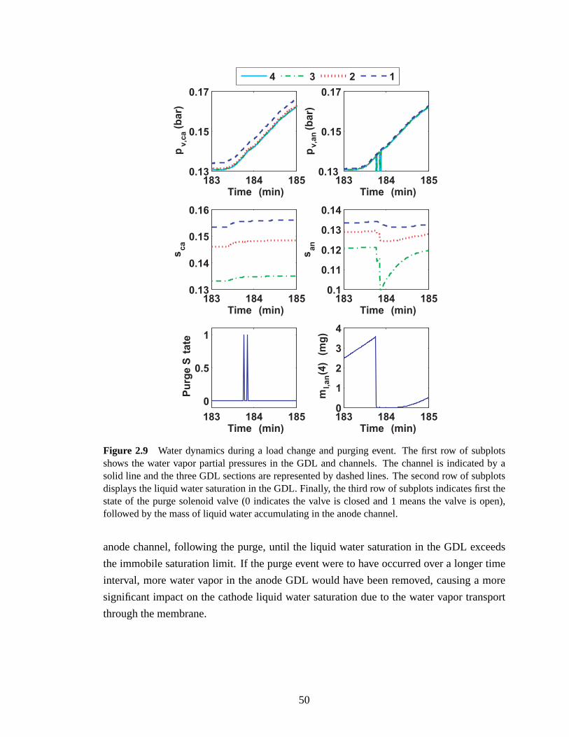
183 184 1850.13

0.15

0.17

Time (min)

pv

,ca

(ba

r)

183 184 1850.13

0.15

0.17

Time (min)

pv

,an

(ba

r)

4 3 2 1

183 184 1850.13

0.14

0.15

0.16

Time (min)

sc

a

183 184 1850.1

0.11

0.12

0.13

0.14

Time (min)s

an

183 184 185

0

0.5

1

Time (min)

Pu

rge S

tate

183 184 1850

1

2

3

4

Time (min)

ml,

an(4

) (m

g)

Figure 2.9 Water dynamics during a load change and purging event. The first row of subplotsshows the water vapor partial pressures in the GDL and channels. The channel is indicated by asolid line and the three GDL sections are represented by dashed lines. The second row of subplotsdisplays the liquid water saturation in the GDL. Finally, the third row of subplots indicates first thestate of the purge solenoid valve (0 indicates the valve is closed and 1 means the valve is open),followed by the mass of liquid water accumulating in the anode channel.

anode channel, following the purge, until the liquid water saturation in the GDL exceeds

the immobile saturation limit. If the purge event were to have occurred over a longer time

interval, more water vapor in the anode GDL would have been removed, causing a more

significant impact on the cathode liquid water saturation due to the water vapor transport

through the membrane.

50

2.8 Model Validation and Discussion

For the purposes of model validation, the calibrated model is simulated with experimen-

tal inputs that are different from the ones used in the calibration process. The resulting

model predictions are shown in Figure 2.10 and compared with the actual cell voltage mea-

surements at five different load levels. The data shown demonstrate the model predicting

capability over a range of current densities and air stoichiometries. At approximately 162

minutes, the air stoichiometry is increased from 200% to 300%, causing a more significant

increase in the voltage estimation (through the partial pressure of oxygen at the membrane

boundary) than is experimentally observed. Despite the increased error associated with the

oxygen partial pressure, the model correctly estimated the degree of anode flooding at var-

ious current densities, correctly predicting no significant flooding at low loads. As the load

level is reduced, the degree of flooding decreases, which is seen from inspection of the dif-

ference between the apparent and nominal current densities at each load level. As a result,

the deviation in voltage decreases between purges, which is experimentally confirmed.

For the entire validation data set, the average estimation error is 8.7 mV, the maximum

estimation error is 105 mV and the standard deviation in the estimation error is 11.5 mV.

Although these validation error statistics are approximately two times greater than the er-

ror statistics associated with the calibration data, at all times throughout the experiment the

estimated average cell voltage is bounded between the measured minimum and maximum

cell voltages, and the measured cell to cell variation is larger than the average estimation

error.

Although the model of the reactant and water dynamics results in an accurate estimation

of the voltage degradation between purges, it is assumed that this degradation was solely

due to the accumulation of liquid water in the gas channels. However, it is conceivable that

some of this degradation could be due to the accumulation of nitrogen on the anode as a

result of operation with air, rather than pure oxygen, or catalyst flooding. The model has

tunable parameters that can compensate for these model assumptions and simplifications,

but it is very important to check the tuned parameter values against other published values.

As Table 2.2 shows, the tunedαw andtwl, are reasonable and within the range of published

results [118, 99].

2.9 Conclusions

A two-phase isothermal one-dimensional model of reactant and water dynamics has been

developed and validated using a multi-cell stack. The lumped parameter model depends

51

150 160 170 180 190 200 210 220650

700

750

800

Cell V

olt

ag

es (

mV

)

Time (min)

150 160 170 180 190 200 210 2200

0.05

0.1

0.15

0.2

0.25

i (A

/cm

2)

Time (min)

i

iapp

150 160 170 180 190 200 210 2201

1.05

1.1

1.15

1.2

Time (min)

p (

Bar)

Ca In

An In

150 160 170 180 190 200 210 22048

50

52

54

Time (min)

T (

C)

155 160

690

700

195 205750

760

770

Air stoich from 200% to 300%

180 190

720

730

740

model

data

Figure 2.10 Model validation results. The first subplot shows the 24 individual cell voltages inthin faint colored lines with the average cell voltage based on the measurements in a thick solidblue line and the estimated cell voltage in a thick dotted red line. The second subplot shows thenominal and apparent current densities. The third subplot contains the anode and cathode inlet totalpressures. The fourth subplot is the temperature of the water coolant leaving the stack.

52

on six tunable parameters associated with the estimation of voltage, the membrane wa-

ter vapor transport and the accumulation of liquid water in the gas channels. During step

changes in load, a good voltage prediction is achieved by reproducing both the steady-

state and dynamic voltage response due to the instantaneous increase in current, as well as

the excursions in oxygen partial pressure resulting from the manifold filling dynamics, as

demonstrated. Finally, the model predicted the dynamic effect of temperature on voltage

as shown during the temperature transient from 50o to 60oC. Although simple, this model

captures the voltage dynamics observed in a fuel cell stack at low and moderate current

densities under the range of conditions tested. However, caution should be used in ex-

tending this model to conditions not examined, as this model has significant empirical and

tuned functions.

The notion of apparent current density is a means for describing the impact of water ac-

cumulation on the dynamic voltage behavior of a PEMFC. The next chapter is focused on

extending and validating this simple GDL model at higher current density, and establish-

ing the connection between the liquid water mass accumulation and voltage using neutron

imaging techniques [140].

53

Table 2.3 Parameter symbols, definitions and values.

Symbol DefinitionAf c=0.030 m2 fuel cell nominal active areab11=0.005139 [121] ohmic resistance parameterb12=0.00326 [121] ohmic resistance parameterDH2=114 mm2/s [71] hydrogen diffusion coefficientDO2=30.3 mm2/s [71] oxygen diffusion coefficientEc=66 kJ/mol [138] activation energyF=96485 C/mol e− Faraday’s constant∆H=-228,740 J/mol Enthalpy difference from STP (water in vapor phase)i loss=1 mA cm−2 [138] loss current densitykca,in=11.3e-7 m s cathode orifice constantkca,out=11.3e-7 m s cathode orifice constantkan,in=9.34e-7 m s anode orifice constantkan,out=9.34e-7 m s anode orifice constantkan,rm=11.31e-7 m s return manifold orifice constantK=2.55e-13 m2 [71] absolute permeabilityK1=1.17 tuned voltage parameterK2=4.44µA tuned voltage parameterK3=1.78 tuned voltage parameterK4=3.27 tuned voltage parameterL=3 number of GDL sectionsMH2=0.002 kg/mole hydrogen molecular weightMO2=0.032 kg/mole oxygen molecular weightMN2=0.028 kg/mole nitrogen molecular weightMH2O=0.018 kg/mole water molecular weightncells=24 cells number of cells in stackpo=1 atm standard state pressureR=8.314 J/mol K universal gas constantsim=0.1 [71] immobile saturation∆S=-44.43 J/mol K Entropy difference from STP (water in vapor phase)tgdl=0.5 mm total GDL thicknesstmb=0.038 mm PEMFC membrane thickness (includes catalyst layer)twl =0.131 mm tunable water layer thicknessTo=298.15 K standard state temperatureVp=2.5 cm3 GDL section pore volumeVca=380 cm3 cathode channel volumeVan=430 cm3 anode channel volumeVan,rm=345 cm3 anode return manifold volumeαw=11.5 tuned water vapor diffusion parameterδx=0.167 mm GDL discretization widthγ=900 s−1 [71] volumetric condensation coeff.ε=0.5 [71] material porosityθc=60 degrees [71] contact angleµ=0.405 g/m s [71] liquid water viscosityρ=997 kg/m3 liquid water densityσ=0.0644 N/m [71] surface tensionρmb,dry=1900 kg/m3 mb dry densityMmb,dry=1.0 kg/mol mb dry equivalent weight

54

Chapter 3

Neutron Imaging of Liquid WaterAccumulation In PEMFC

The operation and accumulation of liquid water within the cell structure of a polymer elec-

trolyte membrane fuel cell (PEMFC) with a dead-ended anode is observed using neutron

imaging. The measurements are performed on a single cell with 53 cm2 active area, Nafion

111-IP membrane, and carbon cloth gas diffusion layer. Even though dry hydrogen is sup-

plied to the anode via pressure regulation, accumulation of liquid water in the anode gas

distribution channels is observed in most tested conditions. Moreover, the accumulation of

liquid water in the anode channels is followed by a significant voltage drop. Anode purges

and cathode surges are also used as a diagnostic tool for differentiating between anode and

cathode water flooding. The rate of accumulation of liquid water and its impact on the rate

of cell voltage drop are shown for a range of temperature, current density, cathode inlet

relative humidity, and air stoichiometric conditions. Operating the fuel cell under dead-

ended anode conditions offers the opportunity to observe water dynamics and measured

cell voltage during large and repeatable transients.

3.1 Introduction

The electrochemical power generation of a popular category of fuel cells depends on the

proton-conducting properties of their polymer electrolyte membranes. The ability of the

membrane to conduct protons increases with increasing water content. However, polymer

electrolyte membrane fuel cells (PEMFCs) operate below the boiling point of water, caus-

ing excess water to condense and restrict gas delivery or block the catalyst active area. The

buildup of water mass, referred to as flooding, in an operating fuel cell was first observed

with neutron imaging in [49]. The impact of this flooding phenomena is a recoverable re-

duction in the power output of the fuel cell, seen by a decrease in cell voltage [99, 58], but

can also lead to irrecoverable material degradation [141, 2].

55

This chapter presents the neutron imaging of liquid water accumulation in a PEMCF

operating with a dead-ended anode. Modeling and testing for anode flooding conditions

are rare because most experimental fuel cells operate under flow-through conditions for

which anode flooding is highly unlikely. Here, a solenoid valve placed downstream from

the cell allows for an occasional purging event with high hydrogen flow rate to remove

water from the anode, preventing severe voltage drop and reactant starvation. Optimal

scheduling of purge events is necessary to prolong fuel cell life and minimize wasted hy-

drogen. An adjustable purging schedule applied to a stack with a dead-ended anode can

enable high hydrogen utilization and remove the need for costly, heavy, and bulky anode

humidification and recirculation hardware. Furthermore, understanding the water removal

with anode purging is important for designing shutdown procedures to alleviate damage

caused by freeze and thaw cycling.

Therefore, models which accurately predict the accumulation and removal of water

are necessary. If, in addition to water accumulation, the model can also predict the re-

sulting cell voltage, it could be used in combination with voltage measurement to allow

real-time adaptation of the purging events in response to component aging, environmental

changes, and system faults. Specifically, the estimated voltage is compared with the actual

voltage, and the error is used to adjust the model-based purge schedule. A similar model-

based technique was used for the estimation of hydrogen starvation [142] and control of the

hydrogen production rate from a fuel processor [143]. Hence, the experiments and exper-

imental results detailed here sought to confirm that a consistent correlation between water

accumulation and voltage degradation exists.

To this end, the experimental results offer the opportunity to observe water dynamics

and measured cell voltage during large and repeatable transients and hence, provide use-

ful data for calibrating and validating simple lumped parameter transient models [65, 140]

during anode flooding conditions. There are some limitations of the imaging system [55],

however, with careful cell design and masking the approximate location of the liquid water

within the structure can be inferred. These techniques have been applied in similar work

using neutron imaging [99, 58, 48, 98, 50, 53, 144, 57]. Neutron imaging experiments with

higher resolution in the membrane through-plane direction could provide more information

on the intrinsic mechanism of voltage degradation during anode flooding. However, higher

spatial resolution imaging requires longer exposure times [145] and hence, the method is

impractical for calibrating or validating transient models with a time resolution less than 1

min. Controlled cathode surging and anode purging events are used to distinguish anode

versus cathode channel plugging and flooding. During an anode purge, fed with dry hydro-

gen, a high gas flow rate through the cell is used to remove the liquid water stored in the

56

anode. During a cathode surge, the air flow is momentarily and abruptly increased beyond

the nominal excess ratio to remove any liquid water stored in the cathode.

It is demonstrated that liquid water accumulates in the anode gas channels, and this

buildup of liquid water is well correlated with the dynamic cell voltage response during the

majority of the experiments, as originally predicted in [146]. These data also indicate that

there is sometimes significant voltage drop, even if the mass of water does not increase in

the fuel cell. Hence, water flooding cannot be considered always responsible for the voltage

drop and nitrogen accumulation in the anode should also be considered [36, 37]. Con-

clusions about channel water mass are based on several homogeneity assumptions, which

ignore the difference in the stored liquid water mass in the Gas Diffusion Layer (GDL)

under the channels as compared to areas under lands [55, 112]. Nevertheless, the data and

data analysis provide useful new information regarding PEMFC transient behavior.

3.2 Experimental Hardware

Experiments were conducted at the Neutron Imaging Facility at the National Institute for

Standards and Technology (NIST) Center for Neutron Research [145]. The amorphous sil-

icon detector was used for its 1 Hz image acquisition rate to capture the change in mass

of liquid water over time. A 1 cm diameter aperture was used for the experiment, with a

neutron fluence rateI0 of 7.2×106 cm−2 s−1 and a neutron flight path of 6 m. In this case,

the ratio of source-to-detector distance over the source aperture diameter (L/D) is equal to

600. The width of a pixel in the image corresponds to 127µm, but the resolution of the

imaging system is about 250µm as a result of scintillator blooming [145].

The NIST test stand is used to supply a humidified gas stream to the cathode in flow-

through operation. The air is humidified using a bubbler, and it is assumed that the gas

leaving the bubbler is saturated at the water temperature. The inlet relative humidity can be

calculated at the fuel cell temperature by assuming the air has a dewpoint temperature equal

to the bubbler temperature. A portable anode purging system was constructed, which al-

lows dead-ended operation of the fuel cell. This anode purge system consists of a pressure

regulator, which supplies dry hydrogen to the anode inlet, and a solenoid valve downstream

of the anode outlet. A needle valve placed downstream from the solenoid valve is used to

set the desired flow rate during an anode purge event. The pressure drop across the nee-

dle valve is used to reduce the gas flow rate leaving the channel during an anode purge

event. This valve was adjusted prior to beginning and kept fixed for the duration of the

experiments. The anode gas flow rate during a purge is about 5 SLPM. Between purges

57

the anode is supplied with hydrogen via pressure regulation,at a stoichiometry equal to

one, as shown in Fig. 3.1. Voltage, current, pressure, temperature, and cathode flow rate

measurements are recorded continuously at 1 Hz resolution. The image data are selectively

recorded when repeatable large transients are observed. Due to the large file size, it is not

desirable to capture data for all times, creating gaps in the measured liquid water mass data.

P

P,TS

S

P,TSS

T

P,T

T

VA

Compressed

dry air

endplate

heater

Load

Pressure / Temp

Measurement

Solenoid Valve

MFC

MFC Mass Flow Controller

Heater

Fuel Cell

Bubbler

Pressure

Regulator

Hydrogen

T

Figure 3.1 Experimental hardware detailing sensor and actuator locations.

The cell is comprised of a single 53 cm2 Nafion 111-IP membrane which is 25.4µm

thick with anode and cathode catalyst layers containing a Pt areal density of 0.3 mg cm−2

purchased from Ion Power. SGL 10BB nonwoven carbon GDLs, were used, which have

an uncompressed thickness of 420µm and a porosity ofε = 0.84. The cell hardware, pur-

chased from Electrochem, consists of aluminum endplates, gold coated aluminum current

collectors, and resin-impregnated graphite flow fields. Resin-impregnated graphite is used

to prevent liquid water from accumulating inside the pore-structure of the graphite [56].

The graphite plates were thinned to 0.32 cm to reduce neutron attenuation. The anode gas

channels are straight with a channel width of 2.08 mm, depth of 1.78 mm, and land width

of 0.838 mm. A semiserpentine flow path is used on the cathode with five parallel paths,

each having a channel width of 0.686 mm, a channel depth of 0.991 mm, and a land width

of 0.762 mm. A square 45 W resistive heater, with a surface area of 58 cm2, is attached

to each end plate to ensure that uniform heating and that the desired temperature at low

58

current density is maintained.

3.3 Quantification of Liquid Water Mass

The attenuation properties of a neutron beam passing through an object can be used to

form a projected image on a detector, similar to X-ray radiography. Neutrons are strongly

scattered by hydrogen atoms and only weakly interact with the other materials used in

PEMFCs, such as aluminum and carbon. The scattering interaction is also density de-

pendent; therefore, neutron imaging is particularly sensitive to the amount of liquid water

present in the cell due to the high density of hydrogen atoms, but is unable to detect to

hydrogen gas or water vapor. This technique provides a useful tool for in-situ measurement

of liquid water content while employing commercial fuel cell materials with realistic cell

designs. The use of these materials reduces the possibility of temperature gradients induced

by selection of nonstandard materials, which would otherwise greatly impact the formation

of liquid water within the cell.

~g

Figure 3.2 Neutron images of the fuel cell active area before and after anode purge events, indi-cating the actual cell orientation. The cell is operated at 566 mA cm−2, 55C, with fully humidifiedair at a stoichiometry of 200 % for cathode and dry hydrogen supplied to anode.

Figure 3.2 shows two images collected before and after a purge event. The areas with

high liquid water accumulation are clearly visible in the top left frame, which corresponds

to a condition before an anode purge event. The second frame in Fig. 3.2 shows the drier

59

neutron image collected after the purge. The downward pointing vector~g indicates the

direction of gravity.

The image,I( j,k), formed by scattering and absorption of neutrons can be modeled by

the Beer-Lambert law

I( j,k) = I0( j,k)exp

[

−N

∑l=1

µl tl ( j,k)

]

, (3.1)

whereI0( j,k) is the incident flux rate of neutrons,N is the number of material layers in the

object,tl is the thickness of each layer, andµl is the linear attenuation coefficient of each

layer.

The thickness of liquid water is quantified by determining the amount of attenuation

which is caused by water in the image. A section of the image outside the active area, de-

fined bySp, is used to normalize each image before processing, to account for fluctuations

in the nuclear reactor power output andI0( j,k) over time, according to

Inorm( j,k) =I( j,k)

∑ j,k∈SpI( j,k)

. (3.2)

To reduce systematic error, care is taken to ensure reference images,Inormdry ( j,k), are

taken with a completely dry cell, and 1500 images are averaged to reduce noise in the im-

age. To account for the effects of thermal expansion, which cause portions of the cell to

move within the imaging frame, dry reference images are taken at 5C increments over the

operating temperature range of the fuel cell. The relative neutron transmission, found by

dividing an image by the dry reference image of the cell, can be used to calculate water

thickness, assuming that the attenuation caused by everything but liquid water remains un-

changed since the reference image was captured. A 3× 3 median filter is applied to the

images to further reduce random noise before calculating the liquid water thickness. The

thickness of the water layer is calculated using

tw( j,k) =− 1µw

ln

[

Inorm( j,k)Inormdry ( j,k)

]

, (3.3)

and the experimentally obtained attenuation coefficient,µw = 0.3708± 0.0008 mm−1

[145], which is valid for liquid water thickness less than 1 mm.

Liquid water quantification is further complicated by instrument broadening caused by

the scintillator screen, scattering of neutrons by objects in the beam and detector noise

[48, 47]. The trends in the data will still be evident without correction for these effects.

60

Quantification of the error introduced by each phenomena is currently under investigation

at NIST [145].

3.3.1 Temporal Averaging to Reduce Uncertainty

The measured uncertainty in water volume for a single pixel in the detector system sampled

at the 1 Hz rate is 0.32 x 10−6 cm3 using (L/D) = 450 [145], which is different from the

experimental setup of (L/D) = 600. The measured uncertainty can be scaled to account for

the different neutron flux used in the experiment by multiplying by the ratio of the square

root of the fluence rates, which yields a per pixel liquid water volumetric uncertainty of

0.537×10−6 cm3. This relationship can be derived from the equation for the theoretical

uncertainty [145],

δt =1µ

√

1+eµt

IoATη≈ 1

µ

√

2IoATη

, (3.4)

wheret is the water thickness,µ is the attenuation coefficient,Io is the fluence rate,A is the

area,T is the integration time, andη is the detector efficiency. Equation (3.4) also indicates

that a reduction in uncertainty of the measured liquid water volume can be achieved at the

expense of temporal resolution by averaging several frames. The uncertainty in an averaged

frame of 11 s as compared to 1 s is decreased by a factor of√

1/T ≈ 0.3. Since the time

constant associated with liquid water is on the order of 100 s [56, 147], the 11 s imaging

rate is used. The resulting liquid water volume uncertainty is 0.16× 10−6 cm3 pixel−1,

which corresponds to a water thickness of 10µm. Unfortunately, the temporal averaging

exacerbates the difficulty in tracking movement of water droplets and slugs in the channels;

liquid water droplet movement with the gas stream in the channel could be much faster than

the 1 s imaging time, and therefore, during a cathode surge or anode purge, liquid water

flow in the channels would appear blurred, even without averaging at the fastest exposure

rate of the imaging system.

3.3.2 Masking

The processed water thickness image,tw( j,k), is a two-dimensional (2-D) projection of the

liquid water inside the fuel cell. In order to infer the location of liquid water in the third

dimension, a knowledge of the physical material structure can be combined with logical ar-

guments. For example, liquid water cannot be located within an impervious solid material.

Several masking techniques have been used to analyze neutron images [99, 58, 50, 53]. A

61

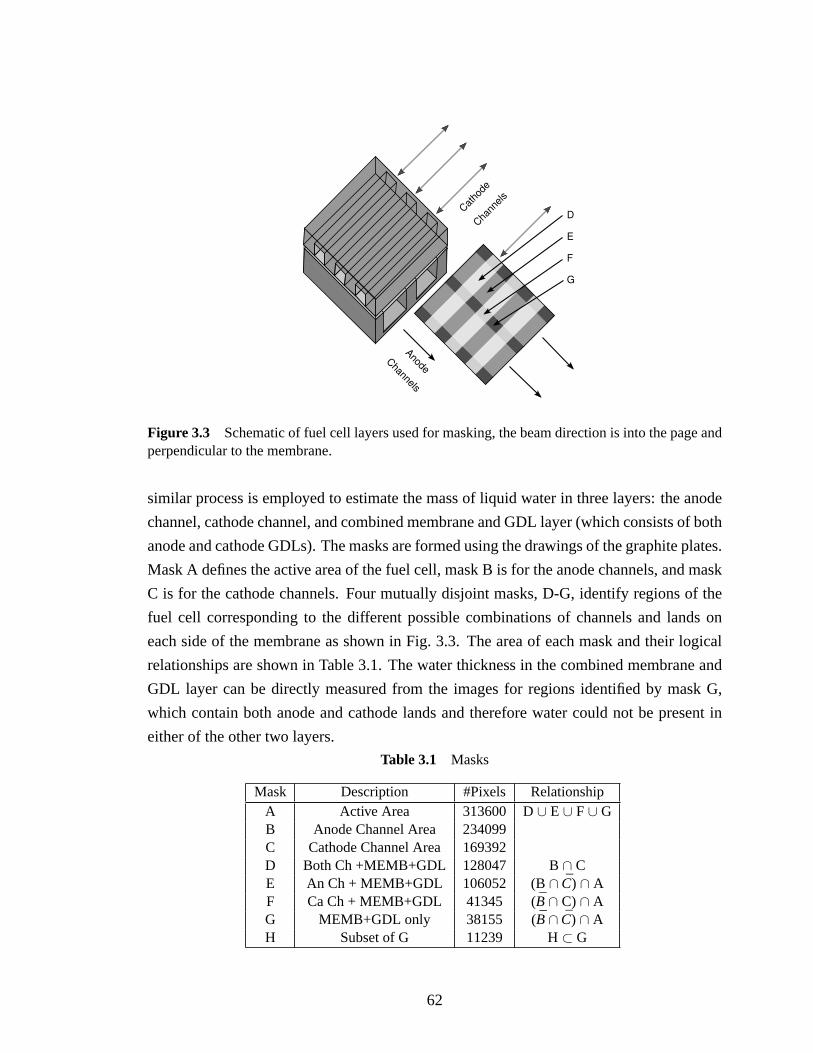
Anode

Channels

Cath

ode

Channels

D

E

F

G

Figure 3.3 Schematic of fuel cell layers used for masking, the beam direction is into the page andperpendicular to the membrane.

similar process is employed to estimate the mass of liquid water in three layers: the anode

channel, cathode channel, and combined membrane and GDL layer (which consists of both

anode and cathode GDLs). The masks are formed using the drawings of the graphite plates.

Mask A defines the active area of the fuel cell, mask B is for the anode channels, and mask

C is for the cathode channels. Four mutually disjoint masks, D-G, identify regions of the

fuel cell corresponding to the different possible combinations of channels and lands on

each side of the membrane as shown in Fig. 3.3. The area of each mask and their logical

relationships are shown in Table 3.1. The water thickness in the combined membrane and

GDL layer can be directly measured from the images for regions identified by mask G,

which contain both anode and cathode lands and therefore water could not be present in

either of the other two layers.

Table 3.1 Masks

Mask Description #Pixels RelationshipA Active Area 313600 D ∪ E∪ F ∪ GB Anode Channel Area 234099C Cathode Channel Area 169392D Both Ch +MEMB+GDL 128047 B ∩ CE An Ch + MEMB+GDL 106052 (B ∩ C) ∩ AF Ca Ch + MEMB+GDL 41345 (B∩ C) ∩ AG MEMB+GDL only 38155 (B∩ C) ∩ AH Subset of G 11239 H ⊂ G

62

3.3.3 Local Spatial Averaging

Estimation of the distribution of liquid water in the third dimension, using masking over the

entire active area, requires consideration of the significant spatial variations in the liquid

water thickness along the channels. Therefore, a local 2-D spatial average is constructed.

Specifically, the active area is partitioned into a 9×9 grid of 81 segments similar to [58].

A 9×9 grid is chosen corresponding to the nine segments of parallel cathode channels as

seen in Fig. 3.4, which is overlaid on mask C. Within each of the 81 segments, the flow of

reactant gases is in the same direction. Due to a manufacturing error the cathode inlet and

outlet manifolds were incorrectly positioned, rendering the first and last serpentine flow

pass ineffective. The cathode inlet should be located in segment 1, for proper operation,

but is instead located in segment 9 as shown in Fig. 3.4. As a result, segments 1-8 and

74-81 are not included in the cathode flow path; therefore no excess air is passed though

these segments of the cathode during normal operation of the cell. Hence, the cathode

channel exhibits an unusual accumulation of liquid water in theses segments. Due to the

orientation of the cell, prior to masking, each thickness image is rotated 44.3 to the right

using a bi-cubic interpolation method to facilitate registration with the mask. In the rotated

orientation, studies can be performed along the channels by traversing the coordinate axis

of the image. Note that segment 9, which is highlighted in Fig. 3.4, corresponds to the

upper corner of the fuel cell shown in Fig. 3.2. Segment 9 is also the location of the gas

inlets where the dry hydrogen and humidified air enter the anode and cathode channels,

respectively.

The fuel cell conditions are assumed to be uniform within each of the 81 segments. Five

image masks (D-H) are applied to each of the 81 segments individually, and the average

liquid water thickness in each of the masked regions is calculated for each segment. A

fifth mask H, which is a subset of the points in mask G not adjacent to either channel, is

used to get a more accurate estimate of the water content in the combined GDL and mem-

brane layer. This mask reduces the effects of instrument broadening and neutron scattering

when there is liquid water present in the neighboring channels [48, 145]. Since only points

near the center of the lands are counted, the effect of different gas flow distributions in the

GDL in the adjacent regions, underneath the channel as compared to the land, on liquid

accumulation may not be accurately represented.

The top subplot in Fig. 3.5 shows a comparison of the average water thickness calcu-

lated using masks G and H over the entire active area for the combined membrane and

GDL layer. If the entire active area is considered, there is little difference between the

average water thicknesses when using mask G as compared to using mask H. However,

for individual segments, a more significant difference between the applications of mask G

63

Figure 3.4 The cathode channel, mask C, is partitioned into 81 segments for the evaluation of thespatial distribution in cathode channel liquid water. Five representative segments are highlightedand shown in later analysis.

versus mask H is observed, as indicated in the remaining subplots. The largest difference

in average thicknesses is found in segment 73, located at the gas outlet near the bottom of

the cell. Due to the orientation of the cell and dead-ended anode, liquid water accumulates

in this corner of the anode channel because it is forced by the reactant gas flow and gravity.

A detailed description of the testing conditions for this experiment can be found in Fig. 3.6.

The standard deviation in water thickness for points identified by mask G, shown in

Fig. 3.5, provides a metric for how uniform the water content in the combined membrane

and GDL layer is over that segment. A large standard deviation in thickness may indicate

nonuniform conditions in the membrane and/or GDL. Scintillator blurring and/or scatter-

ing, where a significant amount of water is present in the channel, reduces the measured

standard deviation but creates a systematic uncertainty. In the limiting case, where the wa-

ter thickness is uniform, the standard deviation in measured thickness should be equal to

that of the Poisson counting process given by (3.4), which increases with increasing wa-

ter thickness. The large standard deviation measured for segment 9 between t=725 and

800 min, shown in Fig. 3.5b, is likely due to condensation and buildup of liquid water near

the cathode inlet manifold. A cathode surge conducted at around t=780 min pushes liquid

water out of segment 9, reducing the measured standard deviation in that segment. Seg-

64

ment 73 consistently contained the most water and therefore also has the highest standard

deviation.

00.10.20.3

Average Over All Sections

00.10.20.3

Average Over Section 9 (inlet)

Mask G

Mask H

std Mask H

00.10.20.3

Average Over Section 33

Wat

er T

hick

ness

(m

m)

00.10.20.3

Average Over Section 37

00.10.20.3

Average Over Section 60

700 750 800 850 900 950 1000 10500

0.2

0.4

0.6Average Over Section 73 (outlet)

Time (min)

Mask G

Mask H(a)

(b)

(c)

(d)

(e)

(f)

Figure 3.5 Average (spatial) liquid water thickness in the membrane/GDL layer. The average liq-uid water thickness for the combined membrane/GDL layer over the entire active area is shown inthe top subplot and within selected segments in subsequent subplots. Data are taken from the sameset shown in Fig 3.6.

65

3.3.4 Channel Liquid Mass

To calculate the mass of liquid water in the gas channels, assume that the water thickness

in the combined membrane and GDL layers is uniform over a segment, and then it is equal

to the averaged thickness in the region defined by mask H. In this case, the average liquid

water thickness in the anode channel can be estimated by taking the difference between av-

eraged water thickness in masked regions H (MB/GDL) and E (MB/GDL+AnCh) for each

segment. Similarly, the average cathode channel liquid water thickness can be estimated

by the difference between averaged water thickness in regions H and F. The total estimated

liquid water mass in each layer of the cell is found by summing the masses calculated for

each of the 81 segments, according to

MWGDLMB =ρl AP

81

∑i=1

NP,AA[i]H[i] , (3.5)

MWAnCh=ρl AP

81

∑i=1

NP,AnCh[i] (E[i]−H[i]) , (3.6)

MWCaCh=ρl AP

81

∑i=1

NP,CaCh[i] (F [i]−H[i]) , (3.7)

whereρl is the density of water;AP is the area of the fuel cell corresponding to a single

pixel in the detector;NP,AA[i], NP,AnCh[i], andNP,CaCh[i] are the number of pixels defining

the active area, anode channel, and cathode channel, respectively, andH[i], E[i], andF [i]

are the measured average water thickness in segmenti for each of the corresponding masks,

where the thickness is given by (3.3). The results of this image processing and data analysis

are shown in Fig. 3.6.

Three-dimensional computational models have demonstrated the possibility of a nonuni-

form liquid water distribution inside the GDL, with a buildup of water in regions underneath

channel lands [55, 112]. If the true water distribution in the GDL is concentrated under the

lands, then the previous assumptions would lead to an underestimation of the amount of

liquid water in the channel, and an overestimation of the GDL water content. Therefore

this data analysis method represents a lower bound on the mass of accumulated water in

the channels and an upper bound on the mass of water in the GDL.

Local averaging combined with masking yields more accurate results than simply aver-

aging the masked regions over the entire active area due to the nonuniform distribution of

water within the cell. The percent difference between the total liquid water mass, and the

estimated mass calculated via masked local averages,MWAnCh+ MW

CaCh+ MWGDLMB, is less

than 2%, indicating that the relative uncertainty introduced by the assumption of a uni-

66

form water thickness in the combined membrane and GDL layer for each segment is small.

Therefore, there is a high level of confidence using the locally averaged and masked data to

infer the mass of liquid water in each of the three layers: anode channel, cathode channel,

and combined membrane GDL.

3.4 Results and Discussion

The neutron imaging data were collected over 4 continuous days of testing (42 hours)

for the range of operating conditions summarized in Table 3.2 and shown in Fig. 3.6 and

Figs. 3.8- 3.10. The same cell is used throughout all the experiments, with pressure regu-

lated dry hydrogen feed at various current densities, air stoichiometric ratios, cathode inlet

relative humidities (RHs) and cell temperatures. It is assumed that the air supplied to the

cathode has a dewpoint equal to the bubbler temperature. Control of the fuel cell endplate

temperature and cathode bubbler temperature can therefore be used to achieve the desired

cathode inlet RH. Relatively low current densities are used as compared to those typically

reported in the literature. These low-to-medium current density conditions are interesting

in portable and mobile applications where the system typically idles for a significant time.

They are also conditions for which anode flooding is most predominant. However, at higher

current density electro-osmotic drag tends to dry out the anode [148].

Parameter Operating RangeAnode inlet RH 0 %

Cathode inlet RH 40 % - 100 %Anode Pressure 123.6 kPa absolute

Cathode Pressure 120 kPa-125 kPa absoluteCell Temperature 40 C, 50 C, 60C

Cell Current 0 A - 30 ACell Current density 0 mA cm−2 - 566 mA cm−2

Table 3.2 Cell operating conditions

One can notice that the operating temperature is also lower than typical. Due to the soft-

ware temperature calibration, the intended operating conditions were not attained and the

cell was operated at a temperature colder than desired. The thermocouple was re-calibrated

after the experiment, and the corrected temperature is presented in the data. As a result

of the mis-calibration, the bubbler temperature is higher than the fuel cell temperature for

some of the experiments. Therefore, the dewpoint of the air entering the cathode channel

is higher than the cell temperature, which is indicated by a calculated value of RH greater

than 1 as shown in Fig. 3.6.

67

In the two subsections below the results of the neutron image processing are presented.

The effects of the anode purge and surge events on the measured voltage is demonstrated.

Surges and purges can be used as a diagnostic tool to distinguish between operation with

anode channel water flooding (anode plugging) or cathode channel water flooding (cathode

plugging) conditions. Snapshots of the liquid water thickness images are shown to verify

the purging and surging diagnostic capability. These snapshots also clarify differences in

the 2-D flow pattern, which affects the quality or ability of the purge event to remove water

accumulated in the anode channels. Finally, note portions of the data where the water vi-

sualization indicates no anode plugging; however, repeatable voltage improvement is seen

after every purge. These data sets indicate that there is (a) an anode nitrogen blanketing

problem, and (b) a GDL water mass value below which there is no liquid water flux to the

anode channels and hence, anode water plugging is avoided. This information can be used

to tune a value for the immobile saturation of liquid water inside the GDL, which is used

in later sections to calibrate a simple model.

3.4.1 Channel Water Plugging

Figure 3.6 shows the data from one full day of testing (6 hr continuous operation), and

Fig. 3.8-3.10 shows the rest of the data collected on three other days. A detailed discussion

of the data shown in Fig. 3.6 is presented first. These data illustrate how changing the op-

erating conditions can drive the system from a state of cathode channel flooding to anode

channel flooding at low-to-medium current density. The first subplot of Fig. 3.6a shows

the mass of liquid water in each of the four mutually disjoint masked regions, described

in Sec 3.3.2, over the entire active area. The next three subplots show the estimated liquid

water mass in each of the three layers (anode channel, cathode channel, and the combined

membrane/GDL layer). The last four subplots of this figure display the important operating

conditions which are typical model inputs [65]: current density (A cm−2), end plate cell

temperature (C), cathode inlet RH and cathode stoichiometric ratio.

The cell is initially operated at low current density (Fig. 3.6f) and high cathode stoichio-

metric ratio (CA SR) (Fig. 3.6i), and heaters are used to maintain the endplate temperature

at 50C (Fig. 3.6g). Fig. 3.6h shows the estimated cathode inlet relative humidity (CA RH)

which is the ratio of the saturation pressure at the bubbler temperature over that of the

cell temperature. At t=783 min the cathode stoichiometry is decreased and water begins

to accumulate in the cell as seen in Fig. 3.6b and c. Cathode channel flooding is evident

in the neutron radiographs, which can be seen in Fig. 3.7(a) at t = 820 min, and can be

inferred by the rapid but small voltage fluctuations. This fluctuation in voltage occurs as

68

0

0.2

0.4

0

0.5

1

1.5

00.050.1

0.15

00.050.1

0.15

400

600

800

0.20.40.6

40

50

60

0.5

1

700 750 800 850 900 950 1000 1050123

Mask DMask EMask FMask G

Fig. 3.7(a)

Fig. 3.7(b)

Fig. 3.7(c) Fig. 3.7(d)M

w(g

)M

w GD

L(g

)M

w CaC

h(g

)M

w AnC

h(g

)Vo

lt(m

V)

i(A

cm−

2)

T(

C)

CA

RH

CA

SR

Time (min)

(a)

(b)

(c)

(d)

(e)

(f)

(g)

(h)

(i)

Figure 3.6 Data set 1: Measured total liquid water mass, estimated membrane/GDL and channelliquid water masses, voltage, current density, temperature, cathode inlet relative humidity (CA RH)and cathode stoichiometric ratio (CA SR); fully humidified cathode gas (air) and dry hydrogen inlet.The (red) vertical lines in the voltage subplot indicate an anode purges.

69

Inlets

Outlets(a) Cathode channel flooding at low stoichiometry ratiot = 820 min.

(b) Little channel flooding at t = 832 min.

(c) Anode channel flooding at t = 848 min.~g

(d) Both Channels Flooding at t = 883 min.

Figure 3.7 Processed neutron images showing liquid water thickness (mm) under a variety ofconditions.

the cathode channels are intermittently plugged with water, and the voltage is insensitive

to the anode purges indicating the absence of anode plugging. The the terms flooding and

plugging are used to differentiate between the accumulation of water mass in the GDL and

channel. Water accumulating in the channels forms slugs which block the flow of reactants

along the channel; hence, the adoption of the term plugging.

70

Figure 3.7(a) also shows the buildup of liquid water after the180 degree bends in the

cathode semi-serpentine flow path as observed by [7]. However, the water in the cath-

ode channel only accumulates after the 180 degree bends on the left side of the image,

which corresponds to the “downhill” turnarounds when viewed in the original orientation

as shown in Fig. 3.2. The gravity vector,~g, delineates the image rotation relative to the cell

orientation. The orientation of the cell and the effects of gravity may have a non-negligible

effect on the location of liquid water buildup within the channels [3]. This is different from

common modeling assumptions of transport in the GDL, where gravitational effects are

negligible [149].

Just before t=825 min the cathode is surged, removing liquid water from the cathode

channels, and a sustained voltage recovery of 25 mV is observed. Following the surge,

the current density and stoichiometry are both increased. The higher cathode gas veloc-

ity more readily removes liquid water from the cathode channel, as seen in Fig. 3.7(b)

at t=832 min. This new operating condition eventually leads to anode channel flooding,

shown in Fig. 3.7(c) and clearly detected by the large periodic voltage increase follow-

ing every purge. At t=858 min the cathode stoichiometry is again decreased, leading to a

condition in which both anode and cathode channel flooding occurs, as seen in Fig. 3.7(d)

and detected by the small voltage fluctuations superimposed by purge-induced voltage im-

provements.

Data at lower CA RH (70%) also resulted in anode channel flooding, shown in Fig. 3.9

near t = 3700 min. A good example of cathode channel flooding can be seen shortly after

startup in Fig. 3.8 at t = 2215 min, where a 25 mV sustained voltage recovery occurs fol-

lowing a cathode surge. Cathode flooding is also present at t = 3554 min in Fig. 3.9, under

similar conditions of low CA RH and low current density 189 mA cm−2. At the two higher

current densities which were tested, cathode surges do not provide any sustained voltage

recovery, indicating that cathode channel flooding is not a problem under these conditions.

3.4.2 Dry Anode Channel Conditions

This section discusses the limitations of the purging and surging methodology used for de-

tecting the approximate location of water in the direction perpendicular to the membrane

plane.

The first limitation is apparent where the 2-D distribution of water along the channels is

such that a purge or a surge cannot remove a significant amount of water. At lower current

density, 189 mA cm−2, the liquid water is more evenly distributed, rather than concentrated

at the end of the channel. Due to the low rate of water generation and subsequently small

71

droplet growth rate, the liquid droplets on the surface of theanode GDL did not grow large

enough, during the observed time between purges, to be pulled by the gravity to the end

of the channel. It was observed that only liquid water at the end of the anode channel is

effectively removed by purging.

This is seen in the buildup of liquid water mass in the anode channel, Fig. 3.8 between

t=2200 -2275 min and in Fig. 3.9 between t=3550 -3650 min, which is insensitive to an-

ode purges. At higher current densities, there is a greater liquid production and crossover

rate; hence, water collects near the end of the anode channels, as shown in Fig. 3.7(c), and

repeatable liquid water transients occur.

The second limitation in using the voltage-purge relation for diagnosing anode water

plugging arises from the effects of nitrogen crossover and eventual nitrogen accumulation

in the anode. In the event of nitrogen blanketing, an anode purge can also improve the cell

voltage. In the collected data, there are cases where the image processing indicates that

there is no anode water plugging; however, there is a repeatable voltage improvement after

every purge event. Specifically, Fig. 3.10 (t=5400 -5480 min) shows data at higher tempera-

ture (60C) and low CA RH (40 %), where anode channel water is no longer detected in the

neutron images. For these conditions, the total water content in the GDL decreases signif-

icantly, about half that of the case with a fully humidified cathode inlet, because the water

carrying capacity of air increases exponentially with temperature and therefore can remove

far more liquid water under these conditions [57, 150]. Dry anode channel conditions with

voltage drop between purges are also shown in Fig. 3.8 (t=2475 -2530 min) while operating

at relatively low current density (377 mA cm−2), high cathode stoichiometric ratio, high

temperature, and sub-saturated cathode inlet flow.

Dry anode channel conditions are also encountered in the first day of testing shown

in Fig. 3.6 (t=700-780 min) and (t=965-1045 min) where fully saturated air flow was fed

to the fuel cell. Some discussion of these two cases is warranted, as the membrane water

dynamics and the thermal dynamics [57] might explain why there is no water anode plug-

ging in these two cases. The period (t=700-780 min) in Fig. 3.6 was after start-up where

the membrane might not have been fully hydrated and hence, might have been absorbing

water from the surrounding GDLs. At t=925 min, a slow temperature rise of about 5C is

measured at the end plates, following the current density increase to 566 mA cm−2. It is ex-

pected that the current increase causes a large spatial gradient in temperature. The thermal

history of the membrane impacts the membrane water uptake and conductivity [151, 152].

This thermal history may account for the absence of anode flooding following the return to

lower current density and nominal temperature at t=1000 min in Fig. 3.6, conditions which

previously (t = 830 min− 850 min) exhibited anode channel water accumulation.

72

In all the cases where dry anode channel conditions are observed, except the start-up

period of Fig. 3.6 (t≤780 min), the combined GDL plus membrane water mass, estimated

through masking, is less or equal to 0.5 g. This liquid water mass is equivalent to a GDL

volume fraction ofs= 0.21. Because no liquid water is flowing to the anode channel, this

value is assumed to be equal to the immobile saturation limitsim. A linear GDL com-

pression of 20% is assumed for this calculation, which yields a compressed porosity of

ε = 0.67, and distribution of water evenly between the anode and cathode GDL layers is

also assumed.

3.5 Flooding, Plugging and Voltage Response

A consistent correlation between voltage and anode purging is observed at low-to-medium

current density under a variety of operating conditions. This relationship can be used to

establish a phenomenological model that connects the accumulation of water and nitrogen

in the channel with an apparent active area available for the reaction and hence, establish an

easily tunable model with low computational complexity for control applications [65, 140].

The hypothesis of a direct effect of anode channel water and nitrogen mass accumu-

lation on voltage is controversial, as most existing models use the decrease of reactant

pressure and the effect of liquid water accumulation in the cathode GDL-Catalyst interface

on voltage [66, 126] assuming a thin film-model which predicts the blockage of the cathode

catalyst interface [99]. A similar argument is used here to formulate an anode channel in-

terfacial blockage which leads to an apparent active area, hence an apparent current density,

and consequently a voltage degradation, as shown in Section2.5.

First, test periods are investigated where voltage decay is observed but no channel or

GDL water mass accumulation. A simple model using published membrane crossover

values for nitrogen [36] confirms the hypothesis that nitrogen crosses over from the air

supplied cathode through the membrane, accumulates in the anode, and contributes to the

measured voltage degradation. The confirmation of the hypothesis is based on the good

match between the predicted and the measured voltage degradation between purges. The

exact accumulation of nitrogen in the anode channel has to be confirmed with independent

nitrogen concentration measurements, which is the subject Chapter 4.

Second, investigation of data that show anode flooding and voltage decay are used to

demonstrate that a simple one-dimensional (1-D) (channel-to-channel through the mem-

brane), isothermal, and lumped parameter model can be used to predict the transient anode

water accumulation and voltage behavior well during anode flooding conditions under

73

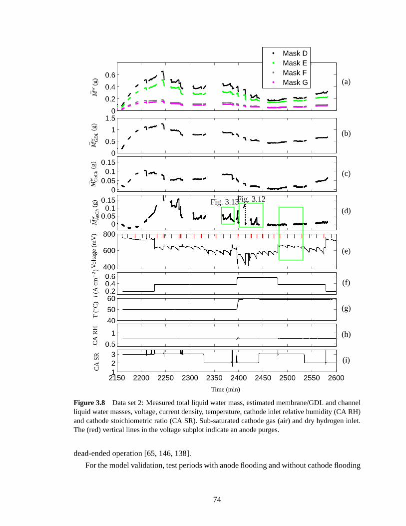
0

0.2

0.4

0.6

Mask DMask EMask FMask G

0

0.5

1

1.5

00.050.1

0.15

00.050.1

0.15

400

600

800

0.20.40.6

40

50

60

0.5

1

2150 2200 2250 2300 2350 2400 2450 2500 2550 2600123

Mw

(g)

Mw G

DL

(g)

Mw C

aCh(g

)M

w AnC

h(g

)Vo

ltage

(mV

)i(

Acm

−2 )

T(

C)

CA

RH

CA

SR

Time (min)

Fig. 3.13Fig. 3.12

(a)

(b)

(c)

(d)

(e)

(f)

(g)

(h)

(i)

Figure 3.8 Data set 2: Measured total liquid water mass, estimated membrane/GDL and channelliquid water masses, voltage, current density, temperature, cathode inlet relative humidity (CA RH)and cathode stoichiometric ratio (CA SR). Sub-saturated cathode gas (air) and dry hydrogen inlet.The (red) vertical lines in the voltage subplot indicate an anode purges.

dead-ended operation [65, 146, 138].

For the model validation, test periods with anode flooding and without cathode flooding

74

0

0.2

0.4

0.6

Mask DMask EMask FMask G

0

0.5

1

1.5

00.050.1

0.15

00.050.1

0.15

400

600

800

0.20.40.6

40

50

60

0.5

1

3500 3600 3700 3800 3900 4000123

Mw

(g)

Mw G

DL

(g)

Mw C

aCh(g

)M

w AnC

h(g

)Vo

ltage

(mV

)i(

Acm

−2 )

T(

C)

CA

RH

CA

SR

Time (min)

Fig. 3.11

(a)

(b)

(c)

(d)

(e)

(f)

(g)

(h)

(i)

Figure 3.9 Data set 3: Measured total liquid water mass, estimated membrane/GDL and channelliquid water masses, voltage, current density, temperature, cathode inlet relative humidity (CA RH)and cathode stoichiometric ratio (CA SR). Sub-saturated cathode gas (air), switching to fully hu-midified at t = 3800 min and dry hydrogen inlet. The (red) vertical lines in the voltage subplotindicates anode purge events.

are used. Another detailed graph shows a period where anode flooding and voltage decay

exhibit a characteristic two-slope behavior, corroborating the hypothesis of voltage decay

75

0

0.2

0.4

Mask DMask EMask FMask G

0

0.5

1

1.5

00.050.1

0.15

00.050.1

0.15

400

600

800

0.20.40.6

40

50

60

0.5

1

5100 5150 5200 5250 5300 5350 5400 5450 5500 5550123

Mw

(g)

Mw G

DL

(g)

Mw C

aCh(g

)M

w AnC

h(g

)Vo

ltage

(mV

)i(

Acm

−2 )

T(

C)

CA

RH

CA

SR

Time (min)

(a)

(b)

(c)

(d)

(e)

(f)

(g)

(h)

(i)

Figure 3.10 Data set 4: Measured total liquid water mass, estimated membrane/GDL and channelliquid water masses, voltage, current density, temperature, cathode inlet relative humidity (CA RH)and cathode stoichiometric ratio (CA SR). Both saturated and sub-saturated cathode gas (air) con-ditions with dry hydrogen. At t = 3800 min the bubbler is filled with colder water causing a drop ininlet CA RH. The (red) vertical lines in the voltage subplot indicates anode purge events.

due to anode plugging instead of cathode catalyst flooding. Finally, a detailed view of a

testing period with concurrent anode and cathode flooding is used for the model validation.

76

3.5.1 Anode Nitrogen Blanketing and Voltage Response

Figures 3.6, 3.8, and 3.10 contain boxes which highlight a portion of the experiments where

a small voltage degradation, 2 mV min−1, is not correlated to any liquid water accumula-

tion. As one can see, the voltage pattern is repeatable between purges despite the lack of

any similar pattern in the water observed. Portions of the experimental data indicate that

nitrogen accumulation in the anode channels should be responsible for the relatively small

(2 mV min−1) versus the larger (5 - 8 mV min−1) voltage drop that is typically observed

during anode water plugging conditions.

To investigate the effects of nitrogen, a channel-to-channel lumped parameter mass

balance can be used to calculate the rate of nitrogen accumulation using the permeation

coefficientkN2 = 10−14 mol m−1 s−1 Pa−1 [36]. At the pressure conditions highlighted in

Fig. 3.6 between t=960-1045 min, a predicted nitrogen accumulation of 0.15 mg min−1 in

the anode leads to a drop of hydrogen partial pressure of 2 kPa min−1. Assuming homoge-

neous channel conditions, the reduction in hydrogen partial pressure affects the cell voltage

through the Nernst equation (2.36), and this leads to a voltage drop of only 0.6 mV min−1

instead of 2 mV min−1 observed here. Because a large change in hydrogen partial pres-

sure alone cannot account for the significant voltage drop observed in the data, an effective

active area is modeled to represents the nonblocked (or nonblanketed) area. The effective

area can be used to calculate the apparent current density. The reduced area is caused by

displacement of hydrogen in the anode channel. Specifically, in a pressure-regulated cell

with dead-ended anode, nitrogen will be pushed by the feed gas and accumulate at the end

of the channel [36]. So if complete anode channel plugging is assumed to occur when

100% of the anode cross-sectional area has been filled with nitrogen, then the predicted

nitrogen accumulation of 0.15 mg min−1 will result in a voltage decay of 2.2 mV min−1

usingAapp from Eqn. (2.34), by replacingt∗ with the channel depth,m∗,an,ch with the anode

channel accumulated nitrogen mass, andρ∗ with nitrogen density, using the tuned voltage

model presented n Section 2.5.

In the model, the resulting voltage degradation is related to the accumulation of liquid

water mass in the anode channel,ml ,an,ch, which is assumed to form a thin film of thickness,

twl, blocking part of the active fuel cell area,Af c, to give an effective active area,Aapp in

m2,

Aapp= Af c−1.3 ml ,an,ch

ncells ρl twl− 1.3 mN2,an,ch

ncells ρN2 tch. (3.8)

The scaling factor of 1.3 is the ratio of the total active area to the anode channel area, since

only that surface area at the channel interface can be covered with liquid. In the case of

water plugging the thickness of the water layer,twl, is a tunable parameter that impacts the

77

rate of voltage decay as liquid water accumulates. A similar notion of reduced area is used

in [153] to account for the reduction in fuel cell output power when the anode is filled with

liquid water. In the case where nitrogen plugging is considered, Eq. (3.8) can also be used

to calculate effective area, but the actual channel depth is used fort∗ instead of a tunable

parameter. It is most likely that accounting for the diffusion and mixing between hydrogen

and nitrogen in the channel using an along-the-channel model will correct for the estimated

higher voltage drop. Nevertheless, the simplicity of the model provides a remarkable match

with the experimental observations of nitrogen plugging effects on voltage response.

3.5.2 Anode Water Plugging and Voltage Response

A summary of the imaging data indicates that for the majority of the tested conditions,

anode water plugging should be considered in order to model the cell performance. Ni-

trogen should clearly also be considered, but the accelerated rate of voltage decay where

water plugging is observed requires a more rapid control action and better modeling to

prevent potential damage to the cell. A model which includes the effect of both nitro-

gen and liquid water on voltage requires a more detailed channel model to determine the

reduction in active area. Standard diffusion and density values for the hydrogen and ni-

trogen gases and a simple along-the-channel model, detailed in chapter 4, indicate that the

anode constituents form stratified layers with liquid water on the bottom, followed by a

nitrogen-rich and then a hydrogen-rich area moving toward the channel inlet. The result-

ing fuel cell area, which is unavailable to support the reaction, is given by the sum of the

nitrogen-blanketed and water-covered areas. The mass of liquid water accumulated in the

anode channel is calculated using well-known equations for the membrane water trans-

port [65, 121, 133, 134] and the one-dimensional (channel-to-channel through-membrane

plane), isothermal, two-phase (liquid and vapor) flow of water through the GDL. A detailed

description of the water crossover through the membrane, the two-phase flow-through the

GDL, and the accumulation of liquid in the channel, is presented in chapters 2 and 5, and

in [65].

The neutron imaging data, with the applied masking techniques, confirm the presence

of liquid water in the anode channel, as shown in Fig. 3.11. This figure represents a typical

purge cycle and is taken from the third day of testing shown in Fig. 3.9. The red vertical

lines shown in the voltage subplot indicate anode purge events. Following an anode purge,

all of the liquid water in the anode channel is removed and then slowly accumulates until

the next purge event. Note that there is little change in the cathode channel water mass

between or during purges.

78

0

0.1

0.2

0.3

0.4

Mask DMask EMask FMask G

0.6

0.7

0.8

0

0.05

0.1

ModelData

0

0.05

0.1

550

600

650

700

3940 3945 3950 3955 3960 3965 39701

2

3

Mw(g

)M

w GD

L(g

)M

w CaC

h(g)

Mw A

nCh(

g)Vo

lt(m

V)

CA

SR

Time (min)

anode purges

cathodesurge

Figure 3.11 Measured cell voltage degradation and liquid water mass accumulation between an-ode purges, taken from the third data set. These experiments were conducted with fully humidifiedair at a current density of 378 mA cm−2, a cell operating temperature of 50C, and an air stoichiom-etry of 300 %.

79

Following the anode purge, a cathode surge is conducted at approximately 3963 min.

During the surge, the cell voltage increases due to the higher oxygen partial pressure. How-

ever, after the cathode flow rate is restored, the voltage returns to its previous value. The

mass of liquid water in the cathode channel decreases as a result of the increased water

removal rate with higher gas flow rate during the surge. In some experiments, even where

the cathode surge event occurs just preceding the anode purge event, the voltage continues

to degrade at the same rate as experienced before the cathode surge. These results indi-

cate that liquid water in cathode channel has little effect on voltage under these conditions.

In contrast, following the two anode purges at 3947 and 3962 min, the voltage recovery

is significant and sustained until liquid water begins to accumulate in the anode channel

again. There exist other operating conditions, where accumulation of water in the cathode

is detected and a sustained voltage recovery occurs following a cathode surge.

Figure 3.12, shows no liquid water accumulation in the cathode channel, with anode

channel water accumulation between purges. Following the anode purge at t=2425 min,

the imaging data shows a period with no water accumulation in the channel followed by a

linear increase with time. This distinct, two-slope behavior of liquid water accumulation

can be explained by a “strong” anode purge which removes liquid water from the GDL.

In this case, water accumulation in the channel has two modes. The first is a slow mode

which represents vapor transport through the GDL; with condensation in the GDL occur-

ring primarily near the GDL/CL interface. Once the accumulation of water in the GDL

has surpassed the immobile saturation limit [65, 146, 71] the second mode evolves, both

capillary liquid and vapor flow into the channel are present, yielding a faster rate of liq-

uid water accumulation in the channel. Hence, following an anode purge which removes

water from the GDL, it takes time before water begins to accumulate in the channel again.

The observed voltage degradation under this condition is very well correlated with the two-

slope liquid water accumulation in the anode channels and has excellent repeatability. The

simulated response using the channel-based apparent current density shows an excellent

match despite the two-slope behavior. It would be interesting to investigate whether volt-

age models that depend on catalyst flooding (water accumulation at the membrane catalyst

interface) alone can capture the observed behavior.

Figure 3.13 shows the voltage during a substantial change in liquid water mass for both

the anode and cathode channels. Specifically, the slow decay in voltage, shown in Fig. 3.13,

can be attributed to the stored anode channel water accumulation. Here the observed volt-

age clearly depends on both cathode catalyst layer and channel water mass. A cathode

surge at t=2387 min removes liquid water from the GDL and cathode channel, resulting

in voltage recovery attributed to cathode flooding, which could be caused by blockage of

80

0

0.1

0.2

0.3

0.4

0.5

0.55

0.6

0.65

0

0.05

0.1

0

0.05

0.1

450

500

550

600

2400 2410 2420 2430 2440 24501

2

3

Mask DMask EMask FMask G

ModelData

Mw(g

)M

w GD

L(g

)M

w CaC

h(g)

Mw A

nCh(

g)Vo

lt(m

V)

CA

SR

Time (min)Figure 3.12 Voltage is well correlated with anode liquid water two slope behavior at 60C,566 mA cm−2 and with a 75 % relative humidity for cathode gas stream at 200 % stoichiometry.

the catalyst or a reduction in oxygen partial pressure due to channel plugging. The simu-

lation results show that the model prediction is reasonable during these testing conditions.

Better prediction accuracy could be expected by including the membrane catalyst domain

in the modeling approach, the model employed here is simple enough to allow real-time

predictions, even in automotive microcontroller hardware [154].

81

0

0.1

0.2

0.3

0.4

Mask DMask EMask FMask G

0.7

0.8

0

0.05

0.1

ModelData

0

0.05

0.1

550

600

650

2365 2370 2375 2380 2385 2390 23951

2

3

Mw(g

)M

w GD

L(g

)M

w CaC

h(g)

Mw A

nCh(

g)Vo

lt(m

V)

CA

SR

Time (min)

cathodesurge

Figure 3.13 Voltage is well correlated with anode liquid water at 50C, 377 mA cm−2 and witha 75 % relative humidity for cathode gas stream at 200 % stoichiometry.

The data analysis and Fig.s 3.8-3.10 demonstrate that for the majority (80%) of the

tested conditions (Table 3.1) the notion of apparent current density, which relates the accu-

mulated mass of liquid water in the anode channel to voltage degradation, can be used to

82

estimate the cell voltage. This estimate agrees well with themeasured value, both between

purges as well as during purging and surging events where anode water plugging condi-

tions are observed. Fast voltage responses due to the increase in oxygen partial pressure

during surges are also estimated well due to the inclusion of the fast reactant dynamics

associated with gas concentrations. For the range of current densities tested, a fully hu-

midified cathode gas stream was sufficient to ensure anode flooding conditions, although

at higher current density this may not hold [148]. In the case where the cathode inlet gas

is fully humidified, the cathode channel always contains a saturated gas stream; therefore,

it can be assumed that there is no vapor pressure gradient along the channel, which implies

a uniform boundary condition along the cathode channel and consequently allows us to

neglect the variation along the channel and employ a 1-D (through-the-membrane) mod-

eling approach for the water dynamics. A similar argument is used in [155] to show how

uniform boundary conditions in a 2-D fuel cell model can be treated as a 1-D partial differ-

ential equation system. The model currently is not able to predict anode drying conditions

when the cathode inlet RH< 80%, because the assumption of uniform channel conditions

in the lumped model may be violated. When a sub-saturated gas stream is supplied to the

cathode, there will be a gradient in vapor concentration along the cathode channel, leading

to a time-varying and spatially varying boundary condition along the cathode channel. As

current density and air flow rate change, the point along the channel at which the gas stream

becomes fully saturated will move [57], which effects the net membrane water transport.

3.6 Conclusion

The mass of liquid water in an operating single-cell fuel cell is measured at the NIST

neutron imaging facility under dead-ended anode operation. Image masks, based on the

cell design, were employed to calculate liquid water mass in the anode versus cathode gas

channels and the combined membrane and anode-cathode GDLs. Anode purges and cath-

ode surges were conducted to remove liquid water, correlate the water removal to voltage

improvement, and visually confirm the approximate location of the accumulated liquid wa-

ter inside the fuel cell. The observed voltage recovery during these purges and surges can

be employed as a diagnostic tool indicating anode or cathode plugging and flooding.

Anode channel water plugging followed by a significant (5-8 mV min−1) voltage

decrease was observed even without cathode channel water plugging, indicating the im-

portance of anode flooding to cell performance. Further understanding the fuel cell per-

formance limitations associated with anode operating conditions is needed. The observed

83

voltage and liquid water accumulation in the anode channel exhibit a distinct and repeatable

two-slope transient behavior after an anode purge. This points to a direct phenomenolog-

ical relationship between the mass accumulated in the anode channel and the cell voltage.

Such a relation can be explained using the notion of apparent current density and a simple

1-D (through the membrane) model can capture the observed dynamic fuel cell behavior

under a wide range of operating conditions.

84

Chapter 4

Nitrogen Front Evolution in PurgedPEMFC with Dead-Ended Anode

This chapter details our August 2008 experiments1 at NIST with simultaneous GC mea-

surement and neutron imaging.

4.1 Introduction

The dynamic behavior of Fuel Cell (FC) operation under Dead-Ended Anode (DEA) con-

ditions is modeled and measured in this chapter. Although a flow-through operation is used

on both the anode and cathode of most laboratory/experimental hydrogen Proton Exchange

Membrane Fuel Cell (PEMFC) systems, the fuel utilization of the anode flow-through op-

eration is too low for commercial and portable systems. To increase the flow-through

utilization, anode recirculation is employed but the required hydrogen grade plumbing

and hardware (ejector/blower) adds weight, volume, and expense to the system [34, 35].

Additional complexity is also added to the balance of plant with the use of external humid-

ification to prevent over-drying of the membrane. However, a DEA can be fed with dry

hydrogen which is regulated to maintain anode pressure. In this configuration hydrogen is

supplied at exactly the rate needed to support the reaction. FC operation with dry hydro-

gen using a dead-ended system architecture is possible because water crossing through the

membrane is enough to humidify the fuel. The use of a pressure regulator instead of a mass

flow controller and lack of anode inlet humidification can yield a system with lower cost

and weight.

The only problem with this architecture is that nitrogen, from air fed into the cathode,

can also cross the membrane, driven by the gradient in partial pressure, creating a blanket

1Note the cathode channel end-plates have been re-machined to resolve the manufacturing defect whichwas present in the previous data set. Also a defect in the ASi detector mounting plate which caused decreasedspatial resolution was corrected since the previous data were collected.

85

of N2. The humidified cathode and the dry fed anode cause a large water vapor gradient

across the membrane. This gradient drives excess water into the anode, which can cause

significant liquid water accumulation. Unlike water vapor whose maximum partial vol-

ume is dictated by temperature, liquid can fill the entire free space and block the flow of

reactants, also known as channel plugging. The accumulation of liquid water and nitro-

gen in the anode channel (AN CH) is first observed near the outlet of the channel. Both

gravity and gas velocity driven by consumption of hydrogen pull these heavier molecules

toward the bottom of the channel. As the mass accumulation continues, a stratified pattern,

which is stabilized by the effect of gravity, develops in the channel with a hydrogen-rich

area sitting above a hydrogen depleted region. The boundary between these regions is a

time-varying front, which proceeds upward toward the inlet [41]. The mass accumulation

physically blocks hydrogen gas from reaching the anode catalyst sites, which is the mecha-

nism for the experimentally observed and recoverable voltage degradation [36, 42, 8]. The

accumulation of N2 and H2O initially leads to larger concentration losses due to decreas-

ing hydrogen concentration near the bottom of the AN CH. When a critical amount of N2

accumulates in the channel, it completely blocks H2 from reaching the catalyst, effectively

shrinking the active area of the cell, causing larger activation potential in the cathode. This

two-stage mechanism is clearly visible in all experimental conditions and scales with op-

erating conditions such as load current density, relative humidity (RH), and stoichiometric

ratio (SR) in the cathode.

Purges of the AN CH volume are necessary to clear the reaction product and inert gas

from the channel. An anode purge event consists of opening a downstream solenoid valve,

which creates a brief, high velocity flow through the anode, removing liquid water and ni-

trogen. After the purge, the catalyst area contributing to the reaction increases and, hence,

the measured voltage increases. Understanding, modeling, and predicting the front evolu-

tion and overall dynamics in DEA FC would allow judicious choice of purging interval and

duration. Better purging strategy can reduce the H2 wasted during purges and avoid over

drying the membrane. The operation of a PEMFC with hydrogen starved areas can also

lead to carbon corrosion [30, 2, 156]; therefore, the study of these operating conditions and

the derivation of controllers to schedule anode purges are critical for DEA operation and

prolonging stack life.

For a fixed purge period and duration, the FC reaches a stable cyclic behavior, typically

within a few purge periods, with both consistently repeatable voltage degradation rates be-

tween purges and voltage recovery with each purge. Repeatability of the front evolution is

verified with in-situ neutron imaging, measuring the liquid water front. Gas Chromatog-

raphy (GC) is also used to measure the hydrogen and nitrogen concentrations at a specific

86

location in the AN CH (see Fig. 4.1) which is discussed later. Gravity, buoyancy, and

channel orientation help establish these statistically repeatable and large spatiotemporal

variations with hydrogen starvation fronts. Figure 4.2 shows typical spatial and temporal

patterns of liquid water thickness and associated measurements during DEA operation with

infrequent anode purging events. The stratification of the hydrogen/nitrogen fronts and the

gravity-driven liquid water in the channels also provide a unique modeling paradigm and

distinct conditions augmenting earlier work [3, 153, 8, 22, 21, 157] that has not been studied

extensively before despite several strictly experimental results [40, 5, 39].

This chapter elucidates the DEA hydrogen PEMFC behavior, specifically by first intro-

ducing the experimental setup, examining the data, and then proposing a simple along-the-

channel model. The model is then used to explain the observed voltage behavior during

DEA operation. Because accumulation of both liquid water and nitrogen in the AN CH

of a PEMFC operating under dead ended conditions contributes to the recoverable voltage

degradation, experiments are devised to characterize the relative effects of both constituents

using simultaneous in-situ measurements of both nitrogen and liquid water. Anode purges

and cathode surges, when coupled with voltage measurement, can be used as a diagnostic

tool for determining the location of water flooding and the impact of nitrogen blanketing

in the AN CH. An anode purge, which is a short duration, high flow rate of gas though the

anode initiated by opening a downstream valve, removes both liquid water and nitrogen

gas from the AN CH and recovers the voltage drop caused by a reduced active area on

the anode side. A cathode surge is a momentary increase in the air flow rate supplied to

the cathode. The excess air increases the partial pressure of oxygen in the channel, which

leads to increased voltage for the duration of the surge. The excess air flow rate can also

remove water from the cathode channel (CA CH) and cathode GDL, which leads to an

improvement of the FC voltage after the surge relative to the value before initiating the

surge.

Finally, the data are compared with a model that captures the relative impact of each

process on the measured cell voltage. In [41], the effects of nitrogen accumulation driven

by convection are investigated. This model improves upon previous work by including

diffusive terms in the AN CH and a physics based voltage model, which accounts for mem-

brane water content with a distributed current density. The correlation of measurements of

voltage, liquid water mass, and AN CH gas concentration are used to develop and validate

a model of PEMFC under DEA operating conditions. Once properly calibrated, this model

can be used for anode purge scheduling and stack health monitoring. Snapshots of the data

are presented to demonstrate the repeatability of the observed phenomena and to provide

comparisons with the model. To prevent confusion and clarify the observed phenomena,

87

the termflooding is used to describe the accumulation of liquid water in the GDL or cat-

alyst layer, and the termplugging is used to refer to liquid water in the channels, which

blocks or hinders the flow of gas through the channels [43]. The termblanketingis used

to designate N2 mass accumulation in the AN CH, which prevents hydrogen from reaching

the catalyst layer.

4.2 Experimental Setup

A Shimadzu GC-17A gas chromatograph was used to measure the hydrogen, nitrogen,

and oxygen content of gas samples taken from the AN CH of a PEMFC during dead-ended

operation. Simultaneous measurement of the liquid water distribution inside the FC was ac-

quired via neutron imaging at the National Institute for Standards and Technology (NIST),

in Gaithersburg, MD [145, 8].

4.2.1 Configuration and Operating Conditions

The tested fuel cell has an active area of 50 cm2. The anode gas flow path consists of 25

parallel straight channels with a depth of 1.78 mm and a width of 2.08 mm. The anode

land width is 0.838 mm and the channel length is 7.3 cm. The anode channels are oriented

on a 45 angle and connected at the top and bottom of each channel by a manifold, as

shown in Fig. 4.1. A supply of dry pressure regulated hydrogen, at 4.5 psig is fed to the

dead-ended anode. As hydrogen is consumed in the reaction, the pressure regulator main-

tains constant pressure in the anode channel, effectively maintaining operation at hydrogen

utilization of one. A solenoid valve located downstream of the fuel cell anode can be peri-

odically opened to purge the anode volume, as shown in Fig. 4.1. This valve is referred to

as the Purge Valve (PV). An adjustable valve is located downstream from the anode PV to

reduce the pressure drop and flow during a purge. The valve is adjusted before starting the

experiment and remains fixed. The steady-state flow rate during purging is measured to be

1 SLPM of hydrogen. The valueNpurge listed in Table 4.3, is used to model this outlet flow.

Due to the small diameter passageway between the anode channels and the outlet manifold

of the FC, liquid water may impede the flow of gases during the initial portion of a purge.

Another solenoid valve is located downstream, connected by capillary tubing, to allow gas

sampling from the anode channel. This solenoid valve is referred to as the Sampling Valve

(SV) and is described in section 4.2.2. A micro-controller is used to actuate the solenoid

valves precisely in time and control the purge event period and duration.

88

A traditional flow-through architecture with air is used on the cathode side with a

bubbler-type humidifier. A backpressure regulator downstream from the cathode maintains

the pressure between 3.5 and 4.5 psig, depending on the flow rate. The cathode channels

have a nine-pass semi-serpentine flow path consisting of five parallel channels. Typical

cathode flow rates range from SR 1.5-3 (oxygen supplied / oxygen consumed). Due to the

use of air on the cathode, the gas velocities in the channel are much higher than a system

running on pure oxygen at the same SR. The Relative Humidity (RH) of the gas stream is

varied between 50 and 100%. Cathode surges, which are short duration (1-2 s) increases in

the air flow rate (up to SR 10), are used during the experiment to remove liquid water from

the cathode channels and to diagnose the extent of cathode channel plugging. The cath-

ode flow field is aligned perpendicular to the anode channels, but the inlets and outlets are

co-located at the upper and lower corners of the cell, respectively. As a result, the system

behavior can be approximated by an equivalent co-flow model, as discussed in Sec. 4.4.

4.2.2 Gas Chromatography Setup

The setup shown in Fig. 4.1 illustrates the interconnection of the GC equipment and fuel

cell. A heated capillary tube is inserted into the last anode channel (near the edge of the

cell), 3 cm from the bottom corner, as shown in Fig. 4.1. The 0.005 in. diameter capillary

tube is connected to an electrically actuated six-port rotational valve. A sampling valve

(SV) is placed downstream from the six-port valve which, when opened, allows for filling

of the sample loop (SL) from the fuel cell anode channel when the six-port valve is in po-

sition A. After a sample is collected in the SL and the SV is closed, the six-port valve is

rotated to position B, and the high pressure carrier gas (helium) pushes the sample into the

GC for analysis.

Ultrahigh purity helium is used as the carrier gas and supplied at a pressure of 200 kPa

gauge. This produces a steady flow of 12 ml min−1 to the GC. A Thermal Conductivity

Detector (TCD) is used for gas detection. As a result of the choice of column (Heyesep

D column Restek, 100/120 mesh, 3 m length, 1 mm inner diameter), the measurement of

water vapor is not possible due to the very long elution time for water in the column. The

difference in retention times of the GC for hydrogen and nitrogen measurement constrains

the maximum sampling rate at one sample every 40 s. The SV is opened for 1 s, during

which ≈ 300 µ l of gas is removed from the anode channel (hence, the sample volume is

less than 5% of the total anode volume). The total anode volume is 6500µ l. Only the last

5 µ l of the sample are trapped in the sample loop and then pushed into the GC when the six

port valve is rotated. The capillary tubing, six-port rotating valve, and SL are maintained

89

at a constant temperature of 110C to ensure that a consistent sample concentration is de-

livered to the GC and to prevent condensation in the tubing. Details on the GC calibration

can be found in the Appendix.

A

B

Capillary Tube

Lch −lsample

Figure 4.1 Illustration of anode flow-field orientation and GC setup. Flow through the six-portrotating valve changes based on actuator position. In position A, the flow-through of the SL is fromright to left, the FC is connected to the SL and SV, whereas the carrier gas flows to the GC. Inposition B, the flow through of the SL is from top to bottom, the carrier gas is connected to the SLand GC, whereas the FC is connected to the SV.

4.2.3 Neutron Radiography

Neutron radiography is an in situ, nondestructive test that involves placing the fuel cell in

a beam of neutrons and measuring the change in beam intensity as it passes through the

fuel cell. The decrease in beam intensity is caused primarily by neutron interaction with

liquid water in the fuel cell. By comparing the image intensity with that of a known dry

fuel cell, the two-Dimensional (2-D) distribution of liquid water thickness values in the

plane perpendicular to the beam can be calculated [8, 48]. Six of these processed images,

showing water thickness values in millimeters, are presented in Fig. 4.2, where the images

are selected from the data set shown in Fig. 4.3. Fig. 4.2(a) and Fig. 4.2(b) clearly shows

anode channel water accumulation and the effectiveness of the anode purge in removing

water from the channel. Fig. 4.2(e) and Fig. 4.2(f) shows the effect of cathode surge at re-

90

moving water from plugged cathode channels. Fig. 4.2(c) and Fig. 4.2(d) shows the small

reduction of the anode channel water plugging, which occurs during repeated anode sam-

pling. During this period, the voltage continuously improves, as shown in Fig. 4.3, which

is the combined effect of nitrogen and liquid water removal from the channel. Nitrogen

is removed with the gas sample and liquid water droplets are dislodged by the pressure

variations in the channel due to the sampling and fall to the bottom of the channel via

gravity.

The time-series sequence of neutron images is further processed in two ways so that

the amount of data is reduced and the relevant features are easier to visualize over time.

The first method of data reduction is to estimate the total liquid water mass in each of the

three layers; the Cathode Channel (CA CH), Anode Channel (AN CH), and the combined

membrane/GDL sandwich layer, by comparing the local water distributions correspond-

ing to the different combinations of channels and lands, as described in [8]. These values

are shown in the fifth and sixth subplots of Fig. 4.3 and Fig. 4.4, and help identify the

presence of GDL water flooding or channel water plugging. To make an inference about

the channel water mass from the 2-D projection of water distribution in the FC, it is as-

sumed that locally, the GDL water content is uniform in the rib and channel areas. If this

assumption is not valid, this algorithm overestimates the GDL water content (attributing

too much of the measured water mass to the GDL) and underestimates the channel water

content. Computational fluid dynamic models have demonstrated water accumulation to be

greater under the ribs [158] for single serpentine co-flow channels under certain operating

conditions. Another plausible scenario is that the high gas flow rate in the cathode channel

could have a Venturi effect, drawing liquid from the GDL, when the water saturation is

above the immobile limit, which could explain the correlation in water removal. It is not

possible to determine if the correlation (a decrease in total water masses) between the GDL

and cathode channel during a surge, as shown in Fig. 4.3 att=3400 s, is physical or an

artifact, given the present set of measurements. Future work, using neutron imaging with

the beam-direction parallel to the membrane, will be used to investigate the relationship

between GDL and channel liquid water removal. This uncertainty in the location of water

accumulation does not impact the nitrogen accumulation or voltage degradation rates mea-

sured or modeled in this chapter, and conditions with less channel water accumulation are

chosen for model validation.

The second method of analysis quantifies the fractional area coverage by liquid water

and is shown in the seventh subplot of Fig. 4.3 and Fig. 4.4. Hence, the image process-

ing provides information for (a) the total liquid water mass, which is a volume average

along the path of the beam at a specific time and (b) information about the distribution of

91

water within the FC, specifically the membrane area that is exposed to liquid water. This

additional information is important for modeling because of the difference in membrane

properties, proton conductivity and permeation rate, as a function of membrane water con-

tent. The fractional area coverage is calculated for two different water thickness values:

Water thickness values greater than 0.3 mm indicate the presence of water in the channels,

and values greater than 0.05 mm are chosen to indicate the start of GDL hydration, which

also indicates an area with higher membrane water content.

4.3 Experimental Results

The data listed in Fig. 4.3 and 4.4 represent the dynamic responses of a PEMFC; there are

changes in air flow, current density, cathode inlet RH, and temperature, as indicated in the

upper subplots of these figures. In the time period before what is shown in Fig. 4.3, the FC

was operated for several hours at 55C, with a low current density (0.2 and 0.4 A cm−2)

and a fully humidified cathode inlet. The data in Fig. 4.4 follow Fig. 4.3 after the cell was

dried at 50% cathode inlet RH for 1 h.

The repeatable and recoverable voltage decay, which is caused by mass accumulation

in the anode, can be seen in the voltage plot, with the solid line type in the fifth subplot of

Fig. 4.3 and Fig. 4.4. The anode purge events indicated by the black vertical lines in the

fourth subplot precede each of the largest voltage improvements. Cathode surges are also

correlated with voltage improvement, as discussed in the following section.

An important feature of the observed voltage dynamic is the two-sloped decay. A slow

initial decay, which can be attributed to the dilution of hydrogen in the anode, is followed

by a steeper linear decay, which marks the development of a hydrogen depleted region that

is covered by a blanketing N2 front moving upward toward the inlet. Various operating

conditions are selected to demonstrate the complex phenomena occurring during the DEA

operation.

Table 4.1 summarizes the operating conditions depicted in the following figures

and discussion. The operating conditions are described using the following notation:

(i# T# SR#RH#), where the number followingi denotes the current density in A cm−2, T

represents temperature (C), SR is the cathode stoichiometry, and RH is the cathode inlet

RH. The data sets are available on-line athttp://orion.engin.umich.edu.

Both N2 blanketing and liquid water plugging could displace H2, preventing it from

reaching the catalyst sites. To study the relative effects of both constituents, portions of

the data set corresponding to conditions with and without anode water accumulation are

92

t=56480

0 200 400 600 800

100

200

300

400

500

600

700

800 0

0.1

0.2

0.3

0.4

0.5

0.6

0.7

0.8

0.9

1

(a) Before Purge

t=56542

0 200 400 600 800

100

200

300

400

500

600

700

800 0

0.1

0.2

0.3

0.4

0.5

0.6

0.7

0.8

0.9

1

(b) After Purge

t=58452

0 200 400 600 800

100

200

300

400

500

600

700

800 0

0.1

0.2

0.3

0.4

0.5

0.6

0.7

0.8

0.9

1

(c) Low Voltage

t=59104

0 200 400 600 800

100

200

300

400

500

600

700

800 0

0.1

0.2

0.3

0.4

0.5

0.6

0.7

0.8

0.9

1

(d) Before Purge

t=59225

0 200 400 600 800

100

200

300

400

500

600

700

800 0

0.1

0.2

0.3

0.4

0.5

0.6

0.7

0.8

0.9

1

(e) After Purge / Before Surge

t=59296

0 200 400 600 800

100

200

300

400

500

600

700

800 0

0.1

0.2

0.3

0.4

0.5

0.6

0.7

0.8

0.9

1

(f) After Surge

Figure 4.2 Neutron images corresponding to the events shown in Fig. 4.3, from sequential purgecycles. Image intensity represents liquid water thickness in mm.

93

identified. In this work, lower cathode inlet RH (60%) cases areused for the investigation

of a single phase channel model; hence, the influence of N2 accumulation on voltage can

be separately identified. The lack of anode channel plugging is verified from the neutron

radiography data.

The operating conditions for case 5 are (i0.4T60 SR3RH60), as shown in Table 4.1,

which are medium current density, 60 C, and high flow rate of sub-saturated air supplied

to the cathode. This case is shown in Fig. 4.4, and is chosen to represent a single phase

condition for model comparison in section 4.5.

Table 4.1 Select Cases From Data Set for Model Comparison

T=50 C

RH \ SR Low (2) High (3) Full [1], 8 [6], (7) Mid T=6

0 C

RH \ SR Low (2) High (3) Full 11 [2], (9), [10] Mid

OPC x Current Density (x) 0.2 A cm-2 [x] 0.4 A cm-2 x 0.6 A cm-2 T=6

5 C

RH \ SR Low (2) High (3) Full Mid 3, [4] [5]

4.3.1 Cathode Surges versus Anode Purges

In the DEA operation of PEMFCs, anode purges and cathode surges, when coupled with

voltage measurement, can be used as a diagnostic tool for determining the location of wa-

ter flooding and the impact of nitrogen blanketing in the anode channel. An anode purge,

which is a short duration, high flow rate of gas through the anode initiated by opening the

PV, removes both liquid water and nitrogen gas from the anode channel and recovers the

voltage drop caused by the reduced active area on the anode side. A representative section

of the experiments is shown in Fig. 4.3. The first anode purge att=680 s removes 0.19 g

of liquid water from the anode channel and the voltage improves by 130 mV following

the anode purge, as shown in the fifth subplot of Fig. 4.3. Neutron images, from before

(Fig. 4.2(a)), and after (Fig. 4.2(b)) the purge, confirm the removal of liquid water from the

anode channel.

A cathode surge is a momentary increase in the air flow rate supplied to the cathode.

The excess air increases the partial pressure of oxygen in the channel, which leads to an

increase in the measured cell voltage for the duration of the surge. The excess air flow

rate also removes water from the cathode channel and cathode GDL, which leads to an

improvement of the fuel cell voltage after the surge relative to the value before initiating

the surge. This change in voltage should be related to the amount of water removed from

the cathode channel, GDL, or catalyst layer. Also, the resistance to O2 transport between

94

COPC3

a b c d e f

1 2 3 4

Figure 4.3 Operating conditions and processed liquid water data from neutron images. The datacorrespond to initial experiment time t0=55800s. The dashed (green) lines correspond to the axis onthe right, and solid (blue) lines use the left axis. The top subplot shows CA RH as a fraction (0-1)(solid lines) and current density (A cm−2) (dashed lines). The second subplot shows CA SR (solidlines) and cell temperature (C) (dashed lines). The third subplot shows cathode (solid lines) andanode channel pressure (kPa gauge) (dashed lines). The fourth subplot shows the mole fraction ofhydrogen and nitrogen that was measured from GC sampling, and the vertical lines indicate anodepurge events. The fifth subplot shows the cell voltage (solid lines) and the estimated mass of liquidwater in the anode channel (dashed lines). (a)-(f) indicate the times at which neutron images (a)-(f)in Fig. 4.2 were acquired. The sixth subplot shows the estimated CA CH liquid water mass (solidlines) and GDL mass (g) (dashed lines). Finally, the seventh subplot shows the fractional FC areafrom neutron imaging, with a measured liquid water thickness greater than 0.3 or 0.05 mm.

95

the channel and the cathode catalyst layer is reported to be large, especially for carbon

cloth GDLs [70], and cathode purges effectively enhance the O2 transport to those areas,

especially under the rib. Cathode surges att = 3400 s andt = 7800 s, indicated by the

short duration spikes in the Cathode Stoichiometric Ratio (CA SR) in the second subplot

of Fig. 4.3, cause a temporary increase in cathode back-pressure and voltage during the

duration of the surge, as shown in the third and fifth subplots of Fig. 4.3, respectively.

The surge att = 3700 s recovers 36 mV of voltage, and the removal of liquid water from

the cathode channel can be clearly seen by comparing Fig. 4.2(e) from before the surge to

Fig. 4.2(f) after. A larger voltage recovery from both surges and purges is expected at a

high current density (0.6 A cm−2) for two reasons. A higher amount of cathode flooding

is expected and any water accumulation has a greater effect on voltage because the higher

local current density leads to lower overall electrochemical efficiency. The fractional cov-

erage area at 0.3 mm, shown as the solid lines in the last subplot of Fig. 4.3, decreases with

both anode purges and cathode surges that remove water from the channels because water

thickness values above this threshold are attributed to channel accumulation. The estimates

of channel water mass shown in the above subplots are well correlated with the surges,

purges, and voltage recoveries.

4.3.2 Temperature Effects

The overall effect of temperature on fuel cell voltage is difficult to quantify because tem-

perature influences several competing factors. For example, an increased temperature leads

to faster reaction kinetics and increased proton conductivity, which both increase voltage.

However, the increase in vapor pressure also decreases the oxygen partial pressure, which

decreases voltage. So, the overall effect may be a decrease in voltage. Temperature also

impacts the nitrogen crossover rate though the membrane. The nitrogen permeation rate,

KN2 in (4.30), increases exponentially with temperature. Saturation pressure also increases

exponentially with temperature, so the partial pressure of water vapor is small at lower

temperatures.

The slow decrease in cathode inlet RH, shown in Fig. 4.3, fromt=200 s tot=3200 s

following the increase in current density, can be attributed to the increased heat generation

that leads to a higher cell temperature than the set point value (60 C), whereas the dew

point of the inlet air stream remains constant. This sub-saturated cathode air feed leads

to a slight recession of the two-phase front location, as shown in the seventh subplot by

the fractional coverage area. Note that the decrease in CA SR keeps the gas velocity in

the channel close to the previous value after considering the increase in current density.

96

0.55

0.60

0.65

vo

lta

ge

0.1

0.2

0.3

AN

_C

H w

ate

r (g

)

20

25

30

pre

ssu

re k

pa cathode

anode

0

0.25

0.50

0.75

mo

le f

ractio

n

H2

N2

0.25

0.50

0.75

1.00

CA

RH

0.20.40.60.81.0

cu

rre

nt

de

nsity

1.5

2.5

3.5

CA

SR

45

55

65

Te

mp

(C

)

0.1

0.3

0.5

ma

ss (

g)

0.1

0.3

0.5

0.7

0.9

CA_CH

GDL

0 1000 2000 3000 4000 5000 6000 7000 8000 90000

0.1

0.2

0.3

fra

ctio

na

l co

ve

rag

e a

rea

Time(s)

0 1000 2000 3000 4000 5000 6000 7000 8000 90000.2

0.4

0.6

0.8

1.0

at 0.3 mm

at 0.05 mm

OPC5 OPC6

ma

ss (

g)

fra

ctio

na

l co

ve

rag

e a

rea

Figure 4.4 Selected data set 2. Beginning att0=67800s, these data show the transition from sub-saturated cathode inlet conditions to fully humidified conditions and the onset of channel plugging.

Finally, the decrease in CA RH and increased cell temperature at the beginning att=3800 s

lead to a more rapid drying of the fuel cell.

The high temperature and low cathode inlet RH conditions shown in the first half of

Fig. 4.4 lead to a dry condition within the fuel cell. The total water mass is very low and

the fractional water coverage is also low, indicating that the transition from sub-saturated

97

to saturated conditions along the length of the co-flow channels is near the outlet. After the

transition to lower cell temperature att=3700 s, which increases the cathode inlet RH from

60 to 100%, the two-phase front moves back toward the inlet, as indicated by the increase in

the fractional area coverage (>0.05 mm). This leads to the onset of both AN CH plugging

and CA CH plugging. When the channels are not plugged, the cathode surge att=3500 s

has no sustained effect on voltage, but the surges following the increase to fully humidified

cathode inlet conditions att=5100 s andt=7000 s see voltage improvement that is well

correlated with the water removal from the cathode channel. Data indicate that GDL water

accumulation (data points taken from under the lands) precedes the accumulation of water

in the channels, hence liquid condensation in the GDL occurs prior to channel flooding.

4.3.3 GC Sampling Effects

The intent of GC sampling is to measure nitrogen accumulation in the anode channel. The

measurement, however, modifies the system behavior. Specifically, the effect of GC sam-

pling, that is, the removal of gas from the AN CH, can improve the FC voltage. When a

sample removes accumulated nitrogen or water from near the end of the anode channel, it

is replaced by a pure hydrogen flow from the inlet.

GC samples are initiated typically right before and after each purge event and some-

times in the middle of a purge period, as shown in the fourth subplot of Fig. 4.3. Individual

GC sampling events are correlated with the small voltage increases shown in the fifth sub-

plot of Fig. 4.3. A series of samples, betweent = 2700 and 3500 s, is taken at the fastest

sampling rate of the GC detector.

The effect of sampling has more impact on voltage with increasing time since the last

anode purge event. This can be explained by the nitrogen accumulation model presented

in Sec. 4.4. Samples taken from later in the cycle allow more nitrogen to accumulate in the

anode channel; see, for example, the sample taken att=350 s in Fig. 4.3. If nitrogen does

not have sufficient time to accumulate, the sample is removes primarily hydrogen from the

channel and no voltage improvement is observed; see, for example, the sample taken at

t=700 s immediately following an anode purge.

The continuous sampling, at one sample every 40 s, betweent = 2700 and 3500 s in

Fig. 4.3, is responsible for the voltage recovery observed over that time interval. If the sam-

pling rate is fast enough to remove more volume than the amount of nitrogen that crosses

over through the membrane in that time, then the measured voltage increases with each

subsequent sample. The fluctuations in anode pressure, due to the repeated sampling, also

enhance liquid water removal from the anode channel by allowing liquid water to escape

98

from the channel into the outlet manifold. During normal operation, the outlet manifold

is at the same pressure at the channel, so there is no flow between these volumes. This

explains the drop in AN CH liquid water mass observed between Fig. 4.2(c) and Fig. 4.2(d).

4.3.4 Voltage Repeatability

The repeatability of several purge cycles, from the end of the larger data set shown in

Fig. 4.3, can be seen by plotting each cycle vs the time since the previous purge, as show

in Fig. 4.5, creating an overlay of the voltage decays with time. The repeatability of the

voltage decay characteristics between cycles is remarkable, given the fact that some purge

cycles contain surge events. Similarly, the repeatability and consistency of the measured

mole fractions every purge cycle is very important for modeling and understanding the un-

derlying phenomena. This analysis is useful, considering the impact of GC sampling on

voltage and nitrogen distribution in the anode channel. The composition of several samples

from different points in time during the purge cycle and from different cycles allows an

accurate representation of nitrogen accumulation and voltage decay. Notice that the nitro-

gen mole fraction, shown in the bottom subplot of Fig. 4.5, saturates at around 0.8; the

remaining 20% of the gas is saturated water vapor in the AN CH.

0 100 200 300 400 500 600 700 800 900

0.4

0.45

0.5

0.55

0.6

volta

ge

0 100 200 300 400 500 600 700 800 9000

0.2

0.4

0.6

0.8

1

time (s)

mol

e fr

actio

n

H2

N2

5

5

2

3

44

Figure 4.5 Sequential purge cycles plotted vs. time since the previous purge. The data correspondto operating condition 3 from the larger data set shown in Fig. 4.3. The numbers 1-5 on the bottomsubplot indicate during which purge cycle each GC sample was taken.

99

4.4 Modeling

In this section, a one-dimensional model of nitrogen crossover and accumulation in the

AN CH of a DEA PEMFC is presented. The modeling domains for this work are the an-

ode channel and membrane. Nitrogen crossing though the membrane, into the AN CH, is

pushed to the end of the channel by the convective velocity [41]. The convective velocity

is the result of hydrogen consumption and, therefore, the velocity is greatest near the anode

inlet, decreasing along the length of the channel. Due to the high diffusivity of hydrogen in

the AN CH, the Stefan-Maxwell equation is uesd to describe the nitrogen distribution along

the channel. Modeling the influence of both convection and diffusion, is needed to com-

pare with the measured mole fractions from GC sampling. A physics-based voltage model

is used to account for the distributed current density and hydrogen consumption rate. The

voltage model includes the effect of membrane water content and proton concentration. An

isothermal modeling approach is used, where the measured cell end plate temperature is

used forT.

The important dimensions for channel modeling arex, the through membrane direc-

tion, andy, the along-the-channel direction, as shown in Fig. 4.6. For the anode, the spatial

variation of gas concentrations in thex-direction is considered, but the steady-state gas dif-

fusion profiles are calculated and used to propagate the channel values (which are modeled

as dynamic states) across the GDL to the surface of the membrane. A similar decoupling

between thex andy distributions is proposed in [83], to address the computational com-

plexity and to take advantage of the very different length scales. On the cathode, only the

steady state profiles are considered for modeling both thex- andy-dimensions. The ap-

proximation of steady-state distributions is appropriate for the cathode gas channel due to

the high gas flow rate and the large time scales over which the anode dynamics evolve.

The constants, listed in Table 4.3, and equations describing the gas constituents in the

channels are written using SI units. The exceptions are the related parameters in the voltage

model, Table 4.2 , which use A cm−2 consistent with the FC literature. In the along-the-

channel model, the fluxesN have units (mol m−2 s−1), reaction ratesr i (mol m−3 s−1), and

fluxes per unit lengthn (mol m−1 s−1).

4.4.1 Nitrogen Accumulation (single phase along the channel model).

To consider both water and nitrogen transport though the membrane, the modeling ef-

fort requires consideration of a ternary system for the anode. The Stefan-Maxwell model

100

nH2,rct

nN2,crs

∆mb

12wan,ribwan,ch

∆GDL

han,ch

Lchysample

(a)

(b)Figure 4.6 One-dimensional FC modeling domain, along the channel. In subfigure (a),y denotesthe distance along the channel from inlet to outlet (not drawn to scale). Subfigure (b) shows a viewfrom the top, indicating the FC channel dimensions.

describes convection, diffusion, and reactions in the gas-channel,

Pan

RT∂Xi

∂ t=− ∂

∂y(Ji +XiNt)+ r i , (4.1)

for i = [1,2], whereNt is the total gas flux,Ji is the diffusive flux, andr i denotes the reaction

terms. Only two of the three components are independent in this modeling framework. The

mole fractions of nitrogen,XN2 = X1, and water vapor,XH2O = X2, are chosen as dynamics

states. Because the mole fractions must sum to one,

∑Xi = 1, (4.2)

the hydrogen fraction can be calculated from the other gasesXH2(y)=1−XN2(y)−XH2O(y).

XH2O = min(X2,Psat(T)/Pan,in) is used for all the following calculations, includingJi. The

remaining water is assumed to be liquid water and is tracked separately, assuming instant

condensation/evaporation.

The convective flux,Nt , is driven by the consumption of hydrogen Eq. (4.7). In

Eq. (4.1), a constant pressure is used as an approximation because the anode volume is

101

fed via pressure regulation and the straight channel geometry introduces minimal pressure

drop along the length of the channel. Although a pressure gradient, corresponding to the

convective flux, develops along the length of the channel, the pressure drop is less than 1

Pa at 1 A cm−2, so a constant pressure is valid for calculating the concentrations. The ideal

gas law,PV = nRT or P= cRT, is used to relate pressure and mole fraction of gas species

in the channel.

A causal formulation for the diffusive fluxes is used [159]

[

J1

J2

]

=− Pan

RTφ(X)

[

D1(X1), D2(X1)

D3(X2), D4(X2)

][∂X1∂y

∂X2∂y

]

, (4.3)

whereD1(X1) = (1−X1)D13D12+X1D23D13 ,

D2(X1) =−X1(D23D12−D23D13) ,

D3(X2) =−X2(D13D12−D23D13) ,

D4(X2) = (1−X2)D23D12+X2D23D13 ,

(4.4)

and Di j are the temperature-dependent binary diffusion coefficients from [87].φ(X) is

given by

φ(X) = (D23−D12)X1+(D13−D12)X2. (4.5)

Conservation of mass allows solving of Eq. (4.1) forNt(y), assuming the outlet flow is

knownNt(L) = Nout. The equation for conservation of mass can be written as,

∂Nt

∂y= ∑ r i , (4.6)

because∑Ji = 0 by definition. Then the convective flux along the channel can be found

from Eq. (4.6) by integrating backward in space along the channel,

Nt(y) =Nt(L)+∫ L

y

(nH2,rct(y)+nN2,crs(y)+nH2O,crs(y)

wan,chhan,ch

)

dy. (4.7)

Because the anode is dead-ended,Nout = 0 unless the downstream solenoid valve is open

and the anode is purging, in which caseNout = Npurge, a constant.

The source term for nitrogen in the AN CH is membrane crossover, which is calculated

from the difference in nitrogen partial pressure across the membrane of thickness∆mb,

nN2,crs(y) =−KN2(T,λmb)(wan,ch+wan,rib)(PN2,ca,mb(y)−PN2,an,mb(y))

∆mb. (4.8)

102

It is assumed that the permeation takes place both over the ribs and channels(wan,ch+

wan,rib), where w∗ indicates the width of each. The partial pressure of nitrogen at

each membrane surface is calculated using the following expressions,PN2,an,mb(y) =

XN2(y) Pan,in and PN2,ca,mb(y) = Pca,in −Pv(T)−PO2,ca,mb(y), assuming uniform pressure

and saturated water vapor everywhere. This is reasonable, considering the water gener-

ation rate, especially when humidified inlets are used at low to mid temperatures. The

oxygen concentration at the cathode surface of the membrane,PO2,ca,mb(y), is calculated

using Eq. (4.26). The nitrogen permeation rate,KN2(T,λmb), is given by Eq. (4.30), and

depends both on temperature and membrane water content.

The hydrogen reaction rate is calculated from the local current density

nH2,rct(y) =i f c(y)

2F(wan,ch+wan,rib), (4.9)

whereF is Faraday’s constant.

The source term for water vapor in the AN CH is also membrane crossover, which is

calculated from the diffusion and electro-osmotic drag

nH2O,crs =−(

λca−λan

Rw,mb−nd(λmb)

i f c

F

)

(wan,ch+wan,rib) (4.10)

whereRw,mb is the resistance to membrane transport,

Rw,mb=∆mb

Dw(λmb,T)+

1kads

+1

kdes, (4.11)

arising from diffusion, whereDw(λmb,T) is the water diffusion coefficient for water in the

membrane [130] and interfacial mass transfer attributed to membrane adsorptionkads and

desorptionkdes [130, 160, 161]. The coefficient of electro-osmotic drag,nd(λmb), can also

be found in Rer. [130]. BothDw andnd areλmb dependent and increase with membrane

water content.

The membrane water content is the final dynamic state in the model and is calculated

from the difference between the anode and cathode equilibrium lambda values

∂λmb(y)∂ t

= Kmb(λan(y)+λca(y)−2λmb(y)) (4.12)

whereKmb= kads/∆mb= 0.25 is the membrane water uptake rate. Other, more recent mod-

els for membrane water uptake [160, 161], will be investigated in a future work but should

not impact the results for nitrogen accumulation presented here.

103

The equilibrium membrane water content is calculated from the water activity using the

uptake isotherm [130]

λan(y) = c0(T)+c1(T)aH2O,an+c2(T)a2H2O,an+c3(T)a

3H2O,an (4.13)

whereaH2O,an(y) =XH2O(y)Pan,in/Psat(T).

There exists a coupling between membrane water content,λmb(y), the current density

distribution,i f c(y), and nitrogen crossover rate,KN2(T,λmb). The nitrogen permeation rate

depends on membrane water content, and the nitrogen accumulation rate depends on both

the permeation rate and current density distribution (convective vs diffusive flow). The

current density distribution depends on nitrogen accumulation (through blanketing of H2)

and the membrane water content for proton transport losses in the membrane. Finally, the

membrane water content depends on the local current density and channel / GDL condi-

tions.

4.4.2 Modeling the GC Sample Location

The flow of gas removed from the AN CH during sampling is modeled by modifying

Eq. (4.7) to include the sample flow

Nt(y)=Nt(L)+∫ L

y

(nH2,rct(y)+nN2,crs(y)+nH2O,crs(y)

wan,chhan,ch

)

dy+

Nsample for (y≤ ysample)

0 for (y> ysample)(4.14)

whereysampleis the location of the sampling port along the equivalent channel.

Because the FC is on a 45 angle and each of the AN CHs is connected at the top

and bottom, as shown in Fig. 4.1, the N2 blanketing front propagation needs to be trans-

formed for comparison with an equivalent straight single channel. The nitrogen coverage

area, however, can be directly related to the coverage area in the single channel equivalent

model. Hence, we use the following relationship for the virtual single channel fuel cell

sampling locationysample,

(Lch−ysample)

Lch=

(Lch− lsample)2

2Af c. (4.15)

This equation relates the fractional area below the sampling location for the fuel cell placed

in the diagonal orientation (right), as shown in Fig. 4.7, to the fractional area below the

sampling location in the equivalent model (left), as shown in Fig. 4.6. The physical ni-

trogen sampling location is 3 cm from the bottom edge of the FC along the last channel,

104

−

−

Figure 4.7 Mapping AN CHs to an equivalent single channel. The path length, in the 45 orien-tation, to nitrogen front location is the same for all channels.

Lch− lsample= 0.03, as shown in Fig. 4.7.

4.4.3 Distributed Current Density

In a previous work, the voltage was calculated based on a uniform apparent current density

[65], which is related to the catalyst area with sufficient reactants to support the reac-

tion, i.e., the channel length not covered by nitrogen [41] or water [65]. In this work,

the distributed current density is considered, which is calculated directly from the reactant

concentrations. Although the apparent area modeling technique captures the correct volt-

age output behavior of the system, the full distributed current density approach is chosen

for this work to match internal model states and the measurement of nitrogen molar fraction

during sampling from the AN CH at the fixed sampling location,lsample. The diffusion of

hydrogen and nitrogen in the AN CH affects both the current density distribution and GC

measurement.

The inputs to the voltage model are: total currentI f c(A), temperatureT (K), mem-

brane water content distributionλmb(y), hydrogen partial pressure at the membrane surface

PH2,an,mb(y) = RTcH2,an,mb(y) (Pa), and oxygen partial pressure at the cathode membrane

surfacePO2,ca,mb(y) (Pa), which is calculated in Eq. (4.26). The cell terminal voltage is cal-

culated from the open-circuit potential minus the concentration, over-potential, and ohmic

105

losses

Ecell = Erev(y)−ηmb(y)−ηGDL(y)−ηact,ca(y)−ηact,an(y). (4.16)

The calculation of the FC terminal voltage and current density distribution requires the

additional computation effort to solveN+1 simultaneous non-linear algebraic constraint

equations, whereN is the number of discretized sections used to solve the partial differen-

tial equation (PDE) system. The distributed current density is resolved by solving the set

of N equations, shown in Eq. (4.16), for a uniform potentialEcell and one equation for the

conservation of currentI f c

Af c=

1Lch

∫ Lch

0i f c(y)dy. (4.17)

The reversible voltage is given by

Erev(y) =E0−RTnF

log

(

aH2O(y)

aH2(y)√

(aO2(y))

)

. (4.18)

whereE0 = 1.229−(T−T0)·2.304×10−4 [13]. The reactant and product activities are cal-

culated from the concentrationsaH2(y)=cH2,an,mb(y)/Cre f,H2, aO2(y) = cO2,ca,mb(y)/Cre f,O2

andaH2O= 1 because the liquid water product is assumed. The subscriptre f refers to the

reference quantity, and subscriptca,mbrefers to the cathode membrane surface.

To simplify the calculation of cell voltage, a hyperbolic sine function is used for the cal-

culation of over-potentials,ηact,ca andηact,an, from the exchange current density,io,ca(y)

andio,an(y)

ηact,ca(y) =RT

αc,anFasinh

(kunits i f c(y)+ i loss

2io,ca(y)

)

, (4.19)

where,kunits = 100−2 m2

cm2 is for units conversion,i f c(y) is the distributed current density

from Eq. (4.17) andi loss is the lost current density due to hydrogen crossover, a tuned pa-

rameter which is listed in Table 4.2. The hyperbolic sine is equivalent to the Butler-Volmer

equation when the forward and reverse reaction coefficients (αc,a = αc,c) are equal [162].

Although the cathode reaction depends on the oxygen concentration as well as the ac-

tivity of protons in the membrane [163], the proton activity term is typically neglected

because there are sufficiently many protons under the FC normal operation. A low hydro-

gen concentration in the anode near the end of the channel is expected, therefore, the proton

effect on the exchange current density is included

io,ca(y) = io,re f,ca

(cO2,ca,mb(y)

Cre f,O2

)γO2

(cH+

ca,mb(y)

Cre f,H+

)γH+

exp

(−Ec

R

(1T− 1

T0

))

, (4.20)

106

whereio,re f,ca is the reference current density,c is the reactant concentration,γ is the

concentration parameter, andEc in the Arrhenius term is the activation energy for hydro-

gen oxidation on platinum [138]. The cathode concentration parameter for the local proton

activity (γH+ = 0.5) is given by [164]. The inclusion of proton concentration is required

to capture the effect of nitrogen blanketing in the AN CH, which prevents hydrogen from

reaching the catalyst layer to supply protons for the reaction. The cathode exchange current

density is proportional to the square-root of the local proton activity at the cathode cata-

lyst layer. The proton activity in the cathode catalyst layer depends on the concentration

of protons dissolved in the aqueous phase in the membrane, which is proportional to the

square root of the hydrogen pressure at the anode membrane surface, for lowPH2, [165].

This relationship is approximated with a hyperbolic tangent function

( cH+ca,mb

Cre f,H+

)γH+

= KH2tanh

(

100cH2,an,mb

Cre f,H2

)

. (4.21)

The constantKH2 is absorbed into the reference current densityio,re f,ca. At the limit, where

the hydrogen concentration is zero, the proton activity at the anode drops to zero. Thus,

where the anode is subjected to local fuel starvation, the hydrogen partial pressure drops;

hence, the proton concentration in the cathode decreases. Furthermore, the membrane elec-

trolyte conductivity also decreases due to lower contribution from the proton conduction in

the bulk phase akin to increasing electrolyte resistance due to decreasing ionic concentra-

tion [163].The overall reduction of proton activity at the cathode ultimately leads to a drop

in the local current density near the dead-ended exit of the anode. For constant load current

(galvanostatic) conditions, as the power production near the outlet shuts down, the current

density increases near the anode inlet, where the membrane is relatively dry, which may

lead to higher losses and increased temperature.

Similarly, for the anode side

ηact,an(y) =RT

αa,anFasinh

(kunits i f c(y)+ i loss

2io,an(y)

)

, (4.22)

where the anode exchange current density is

io,an = io,re f,an

(cH2,an,mb

Cre f,H2

)γH2

exp

(−Ec

R

(1T− 1

T0

))

. (4.23)

The membrane resistance is calculated as follows

ηmb(y) =kunits i f c(y)∆mb

σmb(λmb,T)tanh(100cH2,an,mb/Cre f,H2

) (4.24)

107

Again, the hyperbolic tangent is used to approximate the relationship between conductivity

and proton concentration [165], and to reflect the effect of increasing electrolyte resistance

due to decreasing ion concentration [163]. The membrane conductivityσmb(λmb,T) is a

function of water content using the standard relationship from Springer et al. [121].

Finally, the GDL and contact resistances are lumped intoRGDL for the ohmic loss term

ηGDL(y) = kunits i f c(y)RGDL (4.25)

The voltage model was tuned using flow-through data from the FC, then compared

with the experimental voltage degradation rates under dead-ended operating conditions.

For model tuning with flow through data, it is assumed that the membrane is fully humidi-

fied λ (y) = λ (T,a= 1), whereλ (T,a= 1) can be found in [166], and the effects of GDL

and cathode catalyst layer flooding are ignored due to the low current density operation.

Along the Channel Distributions

The oxygen partial pressure in the cathode channel is not presently considered as one of

the dynamic states in the model, it is calculated simultaneously with the current density

distributioni f c(y) (A cm−2) from the cathode inlet pressure and SR using

PO2,ca,mb(y) =PO2,ca,in −RT4F

( i f c(y)

hm+

i f c(y)∆GDL

DO2,ef f+∫ y

0

i f c(y)

uca,inhca,chdy)(wca,ch+wca,rib)

(wca,ch)(4.26)

wherehca,ch is the CA CH height,wca,ch is the CA CH width, andwca,rib is the cathode rib

width. hm is the interfacial mass-transfer coefficient [162], anduca,in is the cathode inlet

gas velocity (assumed constant along the length of the cathode channel for simplicity)

uca,in =SRca I f c (wca,ch+wca,rib) Lca,ch(RT)

(4F)Af c PO2,ca,in (hca,chwca,ch)(4.27)

where the partial pressure of oxygen at the cathode inlet is given byPO2,ca,in =OMFca,in(Pca,in−Pv,ca,in). Pca,in is the cathode inlet pressure, andPv,ca,in is the cathode inlet vapor pressure,

andOMFca,in = 0.21 is the oxygen molar fraction.SRca is the cathode stoichiometry.

The cathode vapor pressure along the length of the channel is calculated similarly,

PH2O,ca(y)≈ min

(

Psat(T),PH2O,ca,in +RT2F

∫ y

0

i f c(y)

uca,inhca,chdy

(wca,ch+wca,rib)

(wca,ch)

)

. (4.28)

This equation actually needs+∫

nH2O,crs(y) dy to be correct, but then it becomes difficult

108

to solve for the steady-state cathode vapor distribution analytically. At high cathode SR,

this should not be a problem, but it may affect the O2 distribution in low SR; however, this

still should be a second order effect compared to variations in the anode.

The anode channel hydrogen concentration is propagated to the membrane surface as-

suming a simple diffusion model,

cH2,an,mb(y) =XH2(y)Pan,ch

(RT)− i f c(y)

2F∆GDL

DH2,ef f

(wan,ch+wan,rib)

wan,ch(4.29)

based on the effective diffusivityDH2,e f f = De f fDH2,N2 [71].

4.4.4 Nitrogen Crossover Rate

Kocha et al. [36] reported a large range of nitrogen permeability, over 1 order of magnitude.

The permeation increases with both membrane water content and temperature. Tempera-

ture has a larger effect on permeability, when the membrane is well hydrated. In this case,

the permeability can change by a factor of 2-5 over the normal range of operating temper-

atures 30-60C. The nitrogen permeation model includes the effects of membrane water

content and temperature [37]

KN2(T,λmb) = αN2(0.0295+1.21fv−1.93f 2v )×10−14exp

[EN2

R

(1

Tre f− 1

T

)]

, (4.30)

whereEN2 = 24000 J mol−1, Tre f = 303,R is the universal gas constant, andfv is the

volume fraction of water in the membrane, given by;

fv =λmbVw

Vmb+λmbVw(4.31)

whereVmb= EW/ρmb,dry is the dry membrane volume, equivalent weight divided by den-

sity, andVw is the molar volume of water.λmb is the membrane water content.

A change in permeability could account for the different nitrogen accumulation rates

observed via different voltage drop rates, assuming the voltage degradation is caused by

nitrogen accumulation. The current density would tend to shift toward the inlet, where

the membrane is dry and has lower proton conductivity; hence, there would be increased

resistive losses when N2 accumulates in the end of the channel.

109

4.5 Modeling Results

The PDE Eq. (4.1) is discretized using a central difference in space intoN = 50 sections

and solved using an ode solver. The AN CH model is solved using MATLAB “ode15s”,

which supports Differential Algebraic Equations (DAEs), of the form

Mz= f (z). (4.32)

wherez= [XN2,an,XH2O,an,λmb, i f c,Ecell]T , andM = diag(IN, IN, IN,0N,0), andIN is the

N×N identity matrix.

Three simulation plots are shown in Fig. 4.8, 4.10, and 4.11, corresponding to operating

conditions 3, 5, and 6, respectively. These portions of data are contained within the large

data sets shown in Fig. 4.3 and 4.4. The first two data sets are chosen to match the model

assumptions of humidified channel conditions but no channel liquid water plugging. The

third condition shows some flooding and hence error in the model prediction of voltage,

but the overall dynamic voltage behavior is captured quite well by the model, ignoring the

offset. The first plot in Fig. 4.8 corresponding to condition 3 shows the measured and pre-

dicted voltage in the top subplot, and the GC measurement and simulated mole fraction at

the sampling location in the bottom subplot. The model agrees very well with the data at

this operating condition because no AN CH liquid water accumulation was observed during

this period. Figure 4.9 shows the time evolution of the hydrogen mole fraction distribution

and membrane water content over a purge cycle. Three snapshots of the distributions, cor-

responding tot=1700 s,t=2000 s, andt=2400 s, from the third cycle in Fig. 4.8 are shown.

The “corner” in the voltage trace att=2000 s, where the rate of voltage degradation in-

creases, indicates that a sufficient amount of nitrogen has accumulated in the channel to

create a stratified front and a hydrogen starved region develops at the outlet. Finally, at

t=2400 s, the nitrogen front has evolved to cover nearly 20% of the anode channel. At this

time, the effect of nitrogen blanketing is clear as the current density (the dashed-dotted line

in the third subplot) is shifted.

Operating condition 5, shown in Fig. 4.10, corresponds to higher cathode stoichiome-

try and lower current density; therefore, we see slightly drier conditions along the channel

but very similar membrane water content behavior to the previous case. The corner in the

voltage model occurs too late, which indicates that either the diffusion coefficient is too

large or the nitrogen accumulation rate is too low. The membrane resistance is too high

because the voltage degradation rate after the corner point is too steep. Notice the effect

of GC sampling on voltage for the samples that occur early in the purge cycle compared to

those that occur later (larger voltage recovery), which the model accurately predicts.

110

0 500 1000 1500 2000 2500 3000 3500

0.45

0.5

0.55

0.6

Vol

tage

0 500 1000 1500 2000 2500 3000 35000

0.2

0.4

0.6

0.8

1

Time (s)

Mol

e F

ract

ion

xH2

xN2

xH2model

xN2model

xH2O model

modeldata

Figure 4.8 Simulation of operating condition 3 (i0.6T65 SR2RH60). This experiment showsvery good results with model matching because the assumption of no liquid water plugging condi-tions in the channels is satisfied.

Figure 4.11 shows a good match with the GC measurement for repeated sampling. This

data set corresponds to lower operating temperature and fully humidified cathode inlet

conditions, which exhibit both anode and cathode channel plugging, hence the discrep-

ancy between the modeled and measured voltage. The voltage matching is not very good

because the effects of flooding or plugging are not represented in the voltage model. Cath-

ode flooding and plugging are responsible for almost 20 mV of voltage loss, which can

be recovered by the cathode surges att=1000s andt=3400s. The membrane water content

distribution, shown in Fig. 4.12, is much more uniform due to the humidified cathode inlet

conditions and does not change over the purge cycle as in the previous cases.

The parametersαN2 andDH2,N2 affect the rate of nitrogen front propagation and the de-

lay before the voltage decay changes slope, as seen in Fig. 4.8. Nitrogen front propagation

is also weakly dependent on the current density distributioni f c(y), because the consump-

tion of hydrogen drives convection in the channel. The slope of voltage drop depends on

membrane/GDL resistance, the nitrogen diffusion rate, and the nitrogen front propagation

speed.

111

0 0.1 0.2 0.3 0.4 0.5 0.6 0.7 0.8 0.9 12

4

6

8

10

12

λm

b

0 0.1 0.2 0.3 0.4 0.5 0.6 0.7 0.8 0.9 10

0.5

1

xH

2

0 0.1 0.2 0.3 0.4 0.5 0.6 0.7 0.8 0.9 10

0.5

1

Fractional Channel Length

ifc

(Acm

−2)

t=1700

t=2000

t=2400

Figure 4.9 Along the channel distributions for operating condition 3. The first subplot shows asnapshot of the membrane water content along the length of the channel for three times, as shownin Fig. 4.8; after a purge, midcycle, and before the next purge. The second subplot shows the hy-drogen mole fraction along the length of the channel. The final subplot shows the current densitydistributions. The front is fully developed att=2400 s, leading to hydrogen starved region coveringnearly 20% of the channel.

0 500 1000 1500 2000 2500 3000

0.55

0.6

0.65

Vol

tage

0 500 1000 1500 2000 2500 30000

0.2

0.4

0.6

0.8

1

Time (s)

Mol

e F

ract

ion

xH2

xN2

xH2model

xN2model

xH2O model

modeldata

Figure 4.10 Simulation results for operating condition 5 (i0.4 T60 SR3RH60).

112

500 1000 1500 2000 2500 3000

0.55

0.6

0.65

Vol

tage

500 1000 1500 2000 2500 30000

0.2

0.4

0.6

0.8

1

Time (s)

Mol

e F

ract

ion

modeldata

xH2

xN2

xH2model

xN2model

xH2O model

Figure 4.11 Simulation results for operating condition 6 (i0.4 T50 SR3RH90). The model hasgood agreement with nitrogen measurement during continuous sampling, but poor voltage matchingsince flooding effects are not included.

4.5.1 Effect of Operating Conditions

Figures 4.13 and 4.14 show the effects of increasing temperature and current density, re-

spectively. Increasing temperature increases both permeation through the membrane and,

to a small extent, diffusion. The increased nitrogen permeation rate leads to both a quicker

formation of the nitrogen blanket, the time at which the voltage slope changes, and the

faster propagation of the blanketing front, which can be seen in the steeper second slope

of the voltage plot. The effect of current density is more difficult to visualize because

the voltages are very different; therefore, the deviation from the nominal voltage for each

given current density is plotted in the first subplot of Fig.4.14. The second subplot shows

the hydrogen and nitrogen mole fraction at the sampling location. Because the convective

term in Eq. (4.1) is proportional to the current density, nitrogen is pushed toward the end of

the channel more quickly with increasing current density. As a result, the blanketing front

forms much more quickly at a high current density but the propagation rate of the front

does not increase very much because the permeation rate is constant. This can be seen in

the third subplot which shows the average mole fraction of nitrogen in the anode channel,

which is nearly identical for all four cases.

113

0 0.1 0.2 0.3 0.4 0.5 0.6 0.7 0.8 0.9 16

8

10

12

λm

b

0 0.1 0.2 0.3 0.4 0.5 0.6 0.7 0.8 0.9 10

0.5

1

xH

2

0 0.1 0.2 0.3 0.4 0.5 0.6 0.7 0.8 0.9 10.1

0.2

0.3

0.4

0.5

Fractional Channel Length

ifc

(Acm

−2)

t=750

t=1300

t=1700

Figure 4.12 Along the channel distributions for operating condition 6. The first subplot showsa snapshot of the membrane water content along the length of the channel for three times shownin Fig. 4.11; after a purge (before surge), midcycle and before the next purge. The second subplotshows the hydrogen mole fraction along the length of the channel. The final subplot shows the cur-rent density distributions. Notice the different membrane profiles due to higher cathode inlet RH,and less developed nitrogen front.

100 200 300 400 500 600 700 8000.35

0.4

0.45

0.5

0.55

Voltage

100 200 300 400 500 600 700 8000

0.5

1

xN

2sa

mple

100 200 300 400 500 600 700 8000

0.1

0.2

0.3

0.4

xN

2aver

age

Time (s)

T=45T=55T=65T=75

Figure 4.13 Increasing temperature increases nitrogen permeation rate exponentially which leadsto much faster voltage decay. The conditions for simulation are (i0.6Tx S2 RH60).

114

100 200 300 400 500 600 700 800

−0.15

−0.1

−0.05

0

∆V

oltage

100 200 300 400 500 600 700 8000

0.5

1

xN

2sa

mple

100 200 300 400 500 600 700 8000

0.1

0.2

0.3

0.4

xN

2aver

age

Time (s)

i=0.2i=0.4i=0.6i=0.9

Figure 4.14 Increasing current density increases nitrogen blanket formation rate, but not the ac-cumulation rate. The conditions for simulation are (ixT65 S2 RH60).

4.6 Conclusions

The one-dimensional AN CH model presented in this chapter is able to capture and explain

the observed two-sloped voltage drop between purges in a PEMFC with DEA. The model

shows very good results when the assumption of dry conditions are met in the channels.

The evolution of a nitrogen blanketing front, which leads to a hydrogen depleted region

in the AN CH, explains the voltage loss. Although distributed current density measure-

ments [109, 167] were not acquired, the effect of mass accumulation on current density

distribution can be observed through the cell potential by measuring the terminal voltage.

Specifically, the mass accumulation affects both the rate of voltage drop and the time at

which the steeper slope begins.

The ability of the model to predict voltage is limited because the accumulation of liquid

water in the anode channel (plugging) and cathode catalyst layer (flooding) are not included

in the model, but the voltage degradation and nitrogen accumulation rates match well when

the assumption of non-flooding and non-plugging conditions are valid. Future plans in-

clude incorporating these effects into the model. The effects of nitrogen and liquid water

accumulation can be parameterized by utilizing the measurement of liquid water from neu-

tron imaging along with the GC measurements for combinations of wet and dry channel

conditions. The data set corresponding to operating condition 6, shown Fig. 4.11, could be

used for parameterizing the liquid water effect using the model of nitrogen accumulation,

115

which is calibrated for drier (non-flooding/plugging) conditions.

Appendix: Nomenclature and Constants

Table 4.2 Tuned Parameters

io,re f,ca 7E-8 (A cm−2) Cathode exchange currentio,re f,an 0.05 (A cm−2) Anode exchange current

i loss 1E-3 (A cm−2) Crossover currentDef f 0.35 Effective Diffusivity in GDLRGDL 0.275 (Ωcm2) Contract resistanceαN2 2 N2 perm scale factor

Table 4.3 Constants

EN2 24000 (J mol−1) [37]Tre f 303 (K) [37]R 8.314 Universal gas constantVw 1.81×10−5 Water Volume [130]Vmb 5.59×10−4 Membrane Volume [130]Kmb 0.25 Membrane water uptaken 2 Electron transfer #F 96485 (C mol−1) Faraday’s Constant

Cre f,O2 40.87 (molm−3)Cre f,H2 40.87 (molm−3)

Ec 66000 (J mol−1) [13]T0 298.15 (K) ref Temperature

αa,a 0.5αc,a 0.5D12 2.56 E-6 (m2 s−1) DH2O,N2 [87]D13 8.33 E-6 (m2 s−1) DH2,N2 [168]D23 9.15 E-6 (m2 s−1) DH2O,H2 [87]

wan,ch 0.0021 (m) An Ch widthwan,rib 8.38E-4 (m) An rib width∆mb 25 (µm) Membrane thickness

han,ch 0.0018 (m) An Ch heightLch 0.0727 (m) Channel length

∆GDL 3.36E-4 (m) Compressed GDL thicknessNsample 9.2e-7 (mol s−1) Sample flow rateNpurge 5e-3 (mol s−1) Purge flow rate

116

Appendix: GC Calibration

The injection port inside the GC is maintained at 100C and the column at 30C. A Ther-

mal Conductivity Detector (TCD) is used for gas detection. The TCD is operated at 100C

and 90 mA current.

Two mass flow controllers are used to create dry gas mixtures of a known (H2/N2) con-

centration in the anode channel for the calibration of the GC detector. Calibration data are

collected with the anode channel at 4.5 psig operating pressure and a nominal tempera-

ture oft=60 C. A six point calibration is used, with five samples repeated for each point.

Figure 4.15 demonstrates the linearity of the GC measurement. The detector is much more

sensitive to nitrogen, due to the choice of carrier gas. The average N2 response is 1,163,897

(area units /XN2), and the average hydrogen response is 24,416 (area units/XH2). Because

the measurement of H20 is not possible during FC operation, the concentration of vapor in

the anode is assumed equal to the saturation value and hence only temperature-dependent.

0 0.2 0.4 0.6 0.8 10

0.5

1

1.5

2

2.5

3x 10

4

Hydrogen molar fraction xH

2

H2 A

rea

Uni

ts (

−)

0 0.2 0.4 0.6 0.8 10

2

4

6

8

10

12x 10

5

Nitrogen molar fraction xN

2

N2 A

rea

Uni

ts (

−)

Figure 4.15 GC linear response, with variation in nitrogen concentration

117

Chapter 5

Reduced Order Modeling of LiquidWater Fronts and Nitrogen Blanketing

This chapter details the derivation of a fronts based, reduced order model for GDL and

anode channel water accumulation and anode channel nitrogen accumulation. The model

is parameterized using measurements of liquid water accumulation from neutron imaging

and GC sampling to characterize nitrogen crossover and the resulting voltage drop under

DEA conditions.

5.1 Overview of Modeling Domains

To capture the relevant dynamics, the fuel cell model is divided into five modeling do-

mains corresponding to the five separate regions of the fuel cell in the through membrane

direction (x): the anode channel, the cathode channel, the membrane, and the anode and

cathode GDLs. Each channel domain contains three dynamic states (the mass in the cath-

ode channel,mO2,ca,ch, mN2,ca,ch, mw,ca,ch, and in the anode channel,mH2,an,ch, mN2,an,ch,

mw,an,ch), and the remaining domains have one state each (cathode GDL liquid water front

locationxf r,ca, anode GDL front locationxf r,an, and membrane water contentλmb), for a

total of nine modeled states. Water states in the GDL and membrane are initially defined as

PDE equations in Sections 5.6.3 and 2.3.3, and further simplified to derive the statesxf r,ca,

xf r,an, andλmb in Section 5.4. Since the time constants for gas diffusion are much faster

than the liquid states in the GDL, the spatial distribution of the gas species in the GDL

can be approximated with the steady state profiles [81]. The modeling domains and the

interactions between each domain are shown schematically in Fig. 5.1. The fuel cell stack

load currentI f c is considered as a measured disturbance to the plantD1.

118

Voltage NitrogenPermeation

Rate

AnodeChannel

Anode GDL

Membrane

Cathode

Channel

Cathode GDL

Measured

Voltage

U2

U4

U1

D1

Static

WN2,crs

PN2,an,ch

c H2,an,ch

c O2,ca,ch

mH2,an,ch

mN2,an,ch

mw,an,ch

λmb˙λmb

x f r,an

x f r,ca

mO2,ca,chmN2,ca,ch

mw,ca,ch

λan

λca

Aapp

Nv,ca

λmb

Nv,an

PN2,an,ch

Nw,an

Nw,ca

cv ,ca,ch

cv ,an,ch

WO2,rct

WH2,rct

I st

Ist

Figure 5.1 Schematic diagram showing the subsystem interconnections and modeled states. Theanode channel has three states and the cathode channel has three states: for the anode GDL frontlocationxf r,an, for the cathode GDL front locationxf r,ca, and for membrane water contentλmb.

5.2 GDL Fronts Simplification

The liquid water profile forms a steep front inside the GDL. The steep drop ins at the

transition between the two-phase and single-phase water areas in the GDL is the result of

the sigmoidal function of the capillary pressure [71]. Other capillary pressure models [72],

[73], [75] should also exhibit a similar behavior in the formation of a steep liquid water

front and propagation mode [80]. The PDEs [65, 12] describing water transport require a

very fine discretization grid to represent the front propagation accurately. Adaptive grids

developed to address the problem of groundwater transport [84] have been used to handle

this type of problem, but they are not well suited for a reduced complexity control oriented

model. The nature of the sharp transition in the GDL liquid water volume is used to reduce

to complexity of the model. The two-phase front location in the GDL along thex direction

is defined in terms of an ordinary differential equation (ODE), similar to [80], thus greatly

119

x

s

a

ChGDL

x

s

b

ChGDL

x

s

c

ChGDL

y

1

Figure 5.2 Evolution of liquid water fronts in the GDL and channel. In frame (a), liquid waterfills the GDL up tos= s∗, then the two-phase front propagates toward the channel. Next in (b), theliquid begins to accumulate in the channel. Finally, in (c), once the channel section fills completely,water begins to spread back up along the channel.

reducing the computational complexity of the 1-D, two-phase water model.

It is assumed that the liquid water propagates at a constant, tunable, volume fraction,

s∗, which is slightly larger than the immobile limitsim. In [166], thesim value is estimated

using neutron imaging data of the water accumulation. The caricature is shown in Fig. 5.2,

where a square-shape, two-phase front highlights the steep transition and the front prop-

agation. Using the numerical solution of the physically-derived PDEs in [65, 12] and the

experimental observations in [8], we infer that locally, liquid water first begins to accumu-

late in the GDL as shown in frame (a). In frame (b), the liquid water front has reached

the GDL-channel boundary. Since there is little resistance to water entering the channel, it

begins to spill out of the GDL and into the channel, where it accumulates. Finally, in frame

(c), liquid water fills the anode channel section completely and begins spreading along the

y-direction, up the channel, and against gravity.

The following section introduces the ordinary differential equations that describe the

water dynamics in the membrane and the water front propagation in the GDLs. The pro-

posed GDL model uses three nonlinear states (the anode GDL liquid front location,xf r,an;

cathode,xf r,ca, GDL liquid front location; and the membrane water content,λmb) and three

inputs (the anode and cathode channel vapor concentrations, which are the states of the

channel model, and the current density which is measured) to predict the dynamically

evolving front locations in both anode and cathode side GDLs during flooding and dry-

ing, as along with the dynamic changes in membrane water content. Detailed equations

are presented only for the anode and the membrane. The modifications to these equation

necessary to describe the cathode are highlighted.

120

5.3 Modification to the GDL model for Steady State GasTransport

The steady state value can be used for the distribution of water vapor in the GDL [81],

0=∂cv,an

∂ t=

∂∂x

(

Dsimv

∂cv,an

∂x

)

+ rv(cv,an), (5.1)

whereDsimv = DVDe f f(s= sim;ε) is the diffusivity of vapor inside the GDL porous medium

whens is nearsim [81]; DV is the diffusivity of vapor in free space; andDe f f(s,ε) is the

effective diffusivity [71] correction term.

Assuming steady state conditions for the gases in the GDL [81], the hydrogen consump-

tion at the catalyst surface accounts for the flux of hydrogen leaving the anode channel into

the GDL, which is

WH2,an,GDL =−WH2,rct =− i f c

2FMH2 Af c. (5.2)

The combined liquid and vapor flux entering the GDL from the channelWw,an,GDL is found

using Eq. (5.22).

Oxygen consumption at the catalyst surface accounts for the flux of oxygen leaving the

cathode channel into the GDL,

WO2,ca,GDL =−WO2,rct =− i f c

4FMO2 Af c. (5.3)

and the nitrogen crossover rate is given by (5.27).

5.4 Liquid Water Front Propagation in the GDL

The water dynamics in the GDL-MB-GDL unit model are governed by the membrane wa-

ter content and the location of a liquid water front in the GDLs as follows. A single state

can be used to model water uptake into the membrane. Diffusion within the membrane

is fast with respect to water uptake; therefore the diffusion and osmotic drag in each half

of the membrane can be solved using (5.8) and (5.21). This approach yields a piece-wise

linear water content profile, as indicated in Fig 5.3. The average membrane water content,

λmb, is calculated from the water flux into the membrane from the cathode side,Nv,ca,mb,

and out of the membrane from the anode side,Nv,an,mb,

dλmb

dt= Kmb(Nv,ca,mb−Nv,an,mb) , (5.4)

121

whereKmb = EW/(ρmbδmb) is the membrane water uptake rate.

The location of the two-phase (liquid-vapor) water front in the anode GDL,xf r,an, is

governed by the rate of water accumulation in the GDL condensing into the liquid phase,

Nl ,an. Hence, the front propagation is given by,

dxf r,an

dt= KL

Nl ,an xf r,an < δGDL

min(0,Nl ,an) xf r,an = δGDL ,(5.5)

whereKL = Mv/(ρl s∗ ε δGDL) is a constant that accounts for the geometry and density of

liquid water in the two-phase region, assuming the front propagates with constant liquid

saturation (s= s∗), as shown in Fig. 5.3. The right hand side (RHS) of (5.5) depends on

Nl ,an, which is equal to the difference between the flux of water entering the GDL from the

membrane,Nv,an,mb, and the flux of vapor leaving the GDL and entering the channelNv,an,

Nl ,an = Nv,an,mb−Nv,an . (5.6)

These fluxes are diffusive and hence, depend on the water vapor concentration profile in

the GDL,cv,an(x), which in turn, depends on the liquid phase front location,xf r,an.

This spatially and temporally dependent coupling between the liquid and vapor phase

through the condensation and evaporation is simplified by employing two assumptions.

First, the liquid water dynamics are much slower than the gas dynamics, due to the dif-

ference in density, which is 1000 times greater. Therefore, for the purpose of tracking

the liquid front propagation in the fuel cell, the gas states are taken to be in steady state

[12, 80, 158]. Second, it is assumed that all the condensation and evaporation occurs at the

membrane-GDL interface (MB-GDL)x = 0 [158] and liquid phase front locationxf r,an.

With these assumptions, the steady-state solution of the vapor diffusion equation is a piece-

wise linear profile for the water vapor concentration, which follows the liquid water front

location, as seen in Fig. 5.3,

cv,an(x) =

min(bv,cv,sat(T)) x≤ xf r,an

mv x+bv x> xf r,an .(5.7)

The vapor profile,cv,an(x), behind the front in the two-phase regionx≤ xf r,an is equal to the

concentration at saturationcv,sat(T). In the vapor phase region, between the front location

and the channelx> xf r,an, the linear profile is the result of Fickian diffusion.

The propagation of the front location in the cathode GDL, ˙xf r,ca, is defined similarly,

whereNl ,ca is given by (5.20). For brevity, only the equations detailing the anode side will

122

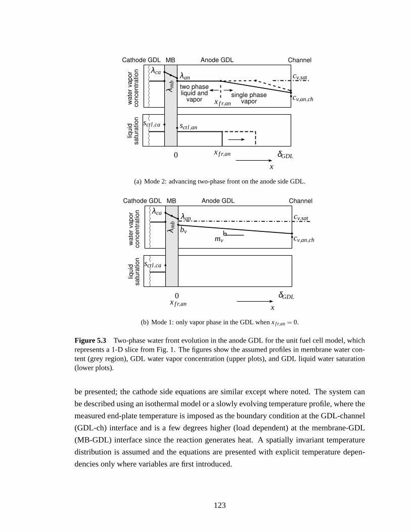
wate

r vapor

concentr

ation

liquid

satu

ration

two phaseliquid and

vaporsingle phase

vapor

MB Anode GDL ChannelCathode GDL

δGDL

xf r,an

xf r,an0

x

cv,sat

cv,an,ch

sctl,ansctl,ca

λ mb

λanλca

(a) Mode 2: advancing two-phase front on the anode side GDL.

wate

r vapor

concentr

ation

liquid

satu

ration

MB Anode GDL ChannelCathode GDL

δGDLxf r,an

0

x

cv,sat

bvmv cv,an,ch

λ mb

λanλca

sctl ,ca

(b) Mode 1: only vapor phase in the GDL whenxf r,an = 0.

Figure 5.3 Two-phase water front evolution in the anode GDL for the unit fuel cell model, whichrepresents a 1-D slice from Fig. 1. The figures show the assumed profiles in membrane water con-tent (grey region), GDL water vapor concentration (upper plots), and GDL liquid water saturation(lower plots).

be presented; the cathode side equations are similar except where noted. The system can

be described using an isothermal model or a slowly evolving temperature profile, where the

measured end-plate temperature is imposed as the boundary condition at the GDL-channel

(GDL-ch) interface and is a few degrees higher (load dependent) at the membrane-GDL

(MB-GDL) interface since the reaction generates heat. A spatially invariant temperature

distribution is assumed and the equations are presented with explicit temperature depen-

dencies only where variables are first introduced.

123

5.5 Membrane Water Transport

Diffusion and osmotic drag govern the water flux out of the membrane and into the anode

GDL,

Nv,an,mb= 2Dw(λmb,T) · (λmb−λan)

δmb− nd i f c

F. (5.8)

The first term in (5.8) describes diffusion in the membrane, which is driven by the anode

side gradient of the membrane water concentration, as shown in Fig. 5.3. The anode water

gradient is defined by the state,λmb, and the water content at the membrane interface with

the anode GDL,λan. Since the catalyst layer is very thin, its effect can be lumped intoλan.

Therefore,λan is expressed as a function of the catalyst flooding level,sctl,an, and the vapor

concentration in the GDL,cv,an(0),

λan = (1−sctl,an) λT,a+sctl,an λmax, (5.9)

whereλmax= 22 [151] is the water content of a liquid equilibrated membrane andλT,a is

the membrane water uptake isotherm [65, 130],

λT,a = c0(T)+c1(T) a+c2(T) a2+c3(T) a3, (5.10)

which is a function of the water activity,a, at the GDL-MB interface. The water activ-

ity in the GDL-MB interface is equal to the ratio of vapor concentration to the saturation

value,aan,mb= cv,an(0)/cv,sat. Theci(T), i ∈ 0,1,2,3, values are calculated by a linear

interpolation of uptake isotherms [130], which were measured at 30C and 80C,

ci(T) =(ci,353−ci,303)

50(T −303)+ci,303, (5.11)

using the values in Table 5.1.

Table 5.1 Fuel cell water transport constants.

c0,303, c1,303, c2,303, c3,303 0.043, 17.81, -39.85, 36 [121] c0,353, c1,353, c2,353, c3,353 0.3, 10.8, -16, 14.1 [133]

Dw,303, Dw,353 0.00333, 0.00259 [169]aw ( cm2 s−1) 2.72E-5 [130]cf (mol cm−3) 0.0012 [130]

Sherwood number Sh= 2.693 [149]

The dependence of membrane water content on catalyst liquid saturation is introduced

to capture the observed anode flooding behavior.sctl,an is a function of the liquid fluxNl ,an

124

as follows,

sctl ,an =max(Nl ,an,0)

NL,max, (5.12)

whereNL,max is the maximum liquid water flux the catalyst layer can handle before becom-

ing completely saturated.NL,maxshould be inversely proportional to liquid water viscosity.

The following functional form, with an exponential temperature dependence, is used to

describe the relationship,

NL,max(T) = NL0

(

exp

[

NL1

(1

303− 1

T

)])

, (5.13)

whereNL1 andNL0 are tunable parameters.

Dw(λ ,T) =

aw cf exp[2416(1/303−1/T)] Mv λmb ρmb(ρl EW+Mv λmb ρmb)

dlogambdlogλmb

, λ < λa=1(T)

Dw0(T)+Dw1(T) ·λ , λ ≥ λa=1(T)(5.14)

Dw0(T) =aw cf exp[2416(1/303−1/T)]

(ρl EW+Mv λa=1(T) ρmb)

Mv λa=1(T)2 ρmb

c1(T)+2 c2(T)+3 c3(T)−λa=1(T) Dw1(T)

(5.15)

Dw1(T) =

(

Dw,303+Dw,353−Dw,303

50(T −303)

)

aw cf exp[2416(1/303−1/T)] (5.16)

Note 1: The liquid volume fraction in the catalyst,sctl,an, represents the fraction of

the membrane in contact with liquid water. Therefore,sctl,an in (5.9) linearly interpo-

lates between the water content of a vapor equilibrated membrane,λT,a=1, and the liquid

equilibrated valueλmax= 22.

Note 2:There is no vapor gradient across the membrane when liquid is present in both

GDLs, since the vapor concentration on both sides of the membrane is equal tocv,sat. As

a result, the difference between the catalyst flooding levelssctl,an andsctl,ca drives water

transport through the membrane.

Note 3: The membrane water diffusion coefficient,Dw(λmb,T) in (5.14), has an ex-

ponential dependence on temperature, but only a linear dependence on membrane water

content for values ofλmb greater than 6 [130, 169]. Typical membrane water content, when

the cell is near flooding conditions, is in the range 9 to 14.

The second term in (5.8) describes electro-osmotic drag, which pulls water from the

anode to the cathode with the conduction of protons through the membrane, and therefore,

125

is dependent on the current density,i f c. The drag coefficient is given by,

nd =

λmb/λT,a=1 λmb< λT,a=1

Kλ ,T(λmb−λT,a=1)+1 λmb≥ λT,a=1, (5.17)

which depends on the membrane water content and temperature with,

Kλ ,T =(−1.834+0.0126T −1)

(λmax−λT,a=1), (5.18)

a linear interpolation betweennd = 1 for the vapor equilibrated membrane andnd =

−1.834+0.0126T, for the liquid equilibrated membrane [169]. The volume fraction of

water in the membrane,fv, is calculated using the following equation,

fv =λmbVw

Vmb+λmbVw, (5.19)

whereVmb= EW/ρmb is the dry membrane volume (equivalent weight divided by density)

andVw is the molar volume of water.

5.5.1 Cathode Side Equations

The same set of equations are used on the cathode, with the inclusion of generated water

and a change of sign, which accounts for the use of a different coordinate axis,

12

i f c

F−Nv,ca,mb= Nv,ca+Nl ,ca, (5.20)

Nv,ca,mb= 2Dw(λmb,T) · (λca−λmb)

δmb− nd i f c

F. (5.21)

5.6 Water Exchange With the Channel

The two-phase front location inside the GDL also determines the rate of vapor and liquid

water exchange with the channel. When the front location is inside the GDL,xf r,an< δGDL,

the water exchange with the channel is in the vapor phase only. When the front reaches the

channel,xf r,an = δGDL, the mass flow of water from the GDL into the channel is the sum

126

0 5 10 150

0.2

0.4

0.6

0.8

1

1.2

1.4

1.6x 10

−9

λmb

Diff

usio

n

Tst

=303

Tst

=313

Tst

=323

Tst

=333

Tst

=353

Figure 5.4 Diffusivity vs. membrane liquid water content at various temperatures.xs indicate thevalue of the vapor equilibrated membrane, i.e.,amb= 1.

of the liquid and vapor flux,

Ww,an,GDL = Af cMv(Nv,an+max(Nl ,an,0) if xf r,an = δGDL

)(5.22)

The max(·) function prevents liquid water in the channel from entering the GDL, since

in the model formulation,Nl ,an < 0 represents a receding two-phase front inside the GDL.

5.6.1 Anode Channel Model

The lumped volume equations constitute a mass balance for each of the three constituent

gases in the channel (H2/O2, N2, and H2O) similar to [65]. Three dynamic states are used

for the channel,dmi,an,ch

dt=Wi,an,in +Wi,an,GDL−Wi,an,out, (5.23)

wherei ∈ H2,N2,w correspond to hydrogen, nitrogen, and water.

Liquid and vapor are combined into one state in the channel, and it is assumed that they

are at a phase transition equilibrium, therefore,

mv,an,ch = min

(

mw,an,ch,Psat(T)Van,ch Mv

R T

)

(5.24)

whereMv is the molar mass of water, andPsat(T) is the temperature dependent saturated

127

vapor pressure [162]. The remaining water is considered to bein the liquid phase,

ml ,an,ch = mw,an,ch−mv,an,ch. (5.25)

The anode inlet gas flow rate is assumed to be a dry hydrogen supply, therefore,

WN2,an,in =Ww,an,in = 0 and,

WH2,an,in =Wtot,an,in. (5.26)

The total flow into the anode,Wtot,an,in, is calculated using Eq. (5.31), and the anode inlet

pressurePan,in is a constant, since it is set via a pressure regulator.

Nitrogen permeation across the membrane is a function of the channel partial pressures

of nitrogen,

WN2,an,GDL =−WN2,ca,GDL

=kN2,permMN2 Af c

δmb

(PN2,ca,ch−PN2,an,ch

).

(5.27)

The nitrogen permeation rate,kN2,perm(T,λmb), is a function of temperature and mem-

brane water content as shown in (4.30) from [36].

The partial pressures of each gas are calculated from the mass using the ideal gas law,

PN2,an,ch =mN2,an,ch R T

MN2 Van,ch, (5.28)

whereVan,ch is the anode channel volume, and the total channel pressure is given by the

sum of the partial pressures:Pan,ch = PH2,an,ch+PN2,an,ch+Pv,an,ch.

The gas flow leaving the anode channel is zero during normal operation. During an

anode purge, the gas velocity is larger, but still within the laminar flow regime.

The individual gas species flows leaving the channel are calculated from the total flow

though the outlet orifice by multiplying with the vector of mass fractions,w j ,

WH2,an,out

WN2,an,out

Ww,an,out

= w j Wtot,an,out (5.29)

whereWtot,an,out is given by Eq. (5.31) ifu1 = 1, and zero otherwise. The subscriptj = 1

corresponds to the anode channel whenP1 = Pan,ch≥ P2 = Pan,outlet, and isj = 2 otherwise,

which indicates back-flow from the outlet manifold. When liquid water is present in the

anode channel, it is assumed that it can cover the outlet orifice, and the gas mixture pa-

128

rameters are replaced with those corresponding to liquid water in equation (5.31), until the

liquid is cleared. i.e.,

w1 =

[wH2,an,ch, wN2,an,ch, wv,an,ch

]T, ml ,an,ch = 0

[0, 0, 1]T , ml ,an,ch > 0(5.30)

The density of the gas mixture is given by,ρan,ch = mtot,an,ch/Van,ch.

The total mass flow into and out of the fuel cell channel volumes is given by (5.31),

whereCturb = 0.61 is the dimensionless discharge coefficient under turbulent conditions;

Dh is the hydraulic diameter in m;A is the area of the orifice in m2; Rt=9.33 is the critical

value from [170];ρ is the density of the gas in kg m−3; ν = µ/ρ is the kinematic viscosity

in m2s−1; andP1 andP2 are the orifice upstream and downstream pressures in Pa. The dy-

namic viscosity of the gas mixtureµ is calculated from the mole fractionX of gas species

in the channel [13].

Wtot =

Aρ1

(

Cturb

√

2ρ1|P1−P2|+

(ν1 Rt

2Cturb Dh

)2− ν1 Rt

2 Dh

)

, if P1 ≥ P2

−Aρ2

(

Cturb

√

2ρ2|P1−P2|+

(ν2 Rt

2Cturb Dh

)2− ν2 Rt

2 Dh

)

, if P1 < P2

(5.31)

5.6.2 Cathode Channel Model

The control inputsu2 andu4 shown in Fig. 1.2 affect the amount of air entering the cathode

channel, the channel pressure, and the relative humidity of the supplied air. For simplicity,

these control inputs are mapped to the parameters:λO2,ca; the oxygen stoichiometry at the

cathode inlet,Ptot,ca,in; the cathode inlet pressure; andRHca,in, the relative humidity air

supplied to the cathode. In a physical system, these values would be the dynamic outputs

of the blower [16] and humidifier [23].

Three dynamic states are used for the cathode channel, corresponding to a mass balance,

dmi,ca,ch

dt=Wi,ca,in +Wi,ca,GDL−Wi,ca,out, (5.32)

wherei ∈ O2,N2,w correspond to oxygen, nitrogen, and water.

The oxygen flow into the cathode is calculated from the stoichiometric ratio,

WO2,ca,in = λO2,cai f c

4FAf c MO2. (5.33)

129

The nitrogen flow into the cathode channel,

WN2,ca,in =MN2

OMFca,in MO2

WO2,ca,in, (5.34)

can be calculated using the mole fraction of dry air,OMFca,in = 0.21. Finally, using the

vapor pressure at the cathode inlet,Pv,ca,in = RHca,in Psat(T), the flow of water vapor into

the cathode is calculated by

Wv,ca,in =Pv,ca,in Mv

OMFca,in (Ptot,ca,in −Pv,ca,in) MO2

WO2,ca,in. (5.35)

The cathode channel outlet equations are similar to the anode outlet equation and are

skipped for brevity. A fixed cathode outlet pressure is assumed.

5.6.3 Water Transport Through the Gas Diffusion Layer (GDL)

The Boundary Conditions (BCs) complete the model of GDL water accumulation and

transport. Forcv,an(x, t), Neumann type BCs are imposed at both sides. The channel (ch)

boundary condition is,

Nv,an,GDL∣∣x=δGDL

= kmt

(

cv,an,GDL∣∣x=δGDL

−cv,an,ch

)

. (5.36)

wherecv,an,ch is the vapor concentration in the channel, andkmt = Sh DV/Hch is the mass

transfer coefficient [149] related to the Sherwood numberSh, the free space diffusion co-

efficient for vapor in hydrogen,DV , and the channel height,hch, which is the characteristic

diffusion length. The water vapor flux across the membrane determines the slope of the

water vapor distribution at the membrane,

∂cv,an

∂x

∣∣∣∣x=0

=−Nw,mb

Dsimv

, (5.37)

where electro-osmotic drag and back diffusion govern the membrane water molar flux

Nw,mb [65], as shown in (2.2).

For the liquid water PDE, mixed BCs are again imposed. Specifically, water passing

into the GDL from the membrane is assumed to be in vapor form due to the presence of

a micro-porous layer; therefore,∂S∂x

∣∣x=0 = 0. The liquid water flux from the GDL into

the channel depends on the boundary condition at the GDL-channel interface. Liquid flows

130

readily when there is sufficient water to form connected pathways. The boundary condition

S(δGDL, t) = 0, (5.38)

is used to represent this behavior, similar to [80]. Other possible models include using the

liquid pressure in the channel [171] and could be considered in the future.

5.7 Fitting Water Transport Parameters

The tunable parametersNL0 and NL1 in (5.13) can be experimentally determined from

the neutron imaging data by observing the rate of liquid water accumulation in the an-

ode channel during operation of the PEMFC under DEA conditions [8].The quasi steady

state accumulation rate is calculated from the time evolution of the system and is plotted

as a function of current density,i f c, and cell temperature,T, in Figure 5.5. The fuel cell

operating conditions are chosen to maintain as close to uniform channel conditions as pos-

sible, such that the lumped channel approximation remains valid. Therefore, experimental

data with fully humidified cathode inlet gas feeds are used for the parameter identification.

Under these operating conditions, it is assumed that both the anode and cathode GDLs are

saturated,xf r,an= δGDL, when liquid water accumulation in the anode channel is observed,

and the rate of liquid water accumulation in the anode channel can be attributed to the rate

of water flux though the membrane. With these assumptions,cv,an,ch = cv,ca,ch = cv,sat(T)

andxf r,an = xf r,ca = δGDL, the equilibrium value of membrane water content,λ = λeq in

(5.39), and the resulting membrane flux into the anodeNv,an,mb,eq can be found analyti-

cally. The functionNv,an,mb,eq(T, i f c,λ = λeq,NL0,NL1), as shown in (5.40), is fit to the

measured liquid water accumulation data using the non-linear least squares fitting routine

in MATLAB c© for the parametersNL0 andNL1. An analytic expression for Jacobian matrix

is easily calculated, which speeds up the convergence of the parameter fitting. The spe-

cific functional form ofNL,max given in (5.13) is independent of the tuning procedure, and

therefore the model could easily be parameterized using another functional relationship.

Table 5.2 Tuned parameters for the liquid water transport model.

s∗ 0.37NL0 2.3434NL1 3991

λeq=4F λa=1(T)NL,max(T)−λa=1 i f c+λmaxi f c

4F NL,max(T)(5.39)

131

Nv,an,mb,eq=2 FNL,max(T)DveDw(λeq,T)(λeq−λa=1(T))− i f cδmbnd(λeq,T)

F(NL,max(T)Dveδmb+2Dve Dw(λeq,T)(λmax−λa=1(T))

) (5.40)

310 320 330 3400

1

2

3

4

5x 10

−7 ist

=0.189

310 320 330 3400

1

2

3

4

5x 10

−7 ist

=0.377

Temperature (K)

310 320 330 3400

1

2

3

4

5x 10

−7 ist

=0.566

310 320 330 3400

1

2

3

4

5x 10

−7 ist

=0.755

0 0.2 0.4 0.6 0.8 10

1

2

3

4

5x 10

−7 T=323

Nv,

an,m

b W

ater

Flu

x (m

ol c

m−2

s−1

)

Current Density (A cm −2)

0 0.2 0.4 0.6 0.8 10

1

2

3

4

5x 10

−7 T=333

y_datamodel estimate

Figure 5.5 Water transport as a function of temperature and current density for saturated channels.The fit parameters yield a model with a convex temperature relationship that is concave with currentdensity.

The tuned model shows an exponential increase in the rate of water crossover and liquid

accumulation in the anode channel with increasing temperature due to the exponential term

in the diffusion coefficient (5.14). The water crossover rate increases with current density,

as the rate of water production increases, until the osmotic drag term begins to dominate

(5.8). At this point, the water crossover rate begins to decrease with a further increase of

current density.

5.8 Fuel Cell Terminal Voltage

Fuel cell terminal voltage is the main measurable output of the system, and represents a

static, non-linear output mapping of the states and operating conditions (temperature and

load current). The electrochemical dynamics are very fast [16, 172], and can represented

by static relationships. The mass transport of reactants into the cell and the removal of

product water are responsible for the dynamic behavior observed in the measured voltage.

132

The inputs to the voltage model are: total currentI f c(A); temperatureT (K); mem-

brane water contentλmb; hydrogen partial pressure at the membrane surfacePH2,an,mb

(Pa); and oxygen partial pressure at the cathode membrane surfacePO2,ca,mb (Pa), which

is calculated in (5.54). The pressure and concentration are related by the ideal gas law

PH2,an,mb= RTcH2,an,mb, whereR is the universal gas constant. The cell terminal voltage

is calculated from the open circuit potential minus the concentration, over-potential, and

ohmic losses.

Vcell = Erev−ηact,ca−ηact,an−ηmb−ηohmic. (5.41)

The reversible voltage is given by,

Erev = E0−RTnF

log

(

aH2O

aH2√

(aO2)

)

. (5.42)

whereE0 = 1.229− (T −T0)·2.304× 10−4 [13]. The reactant and product activities are

calculated from the concentrations,aH2 = cH2,an,mb/Cre f,H2, aO2 = cO2,ca,mb/Cre f,O2, and

aH2O = 1 since liquid water product assumed. The subscriptre f refers to the reference

quantity, and the subscriptca,mbrefers to the cathode membrane surface.

To simplify the calculation of cell voltage, a hyperbolic sine function is used for the

calculation of over-potentials,ηact,ca andηact,an, from the exchange current density,io,ca

andio,an,

ηact,ca =RT

αc,anFasinh

(i f c+ i loss

2io,ca

)

, (5.43)

wherei f c =I f cAf c

is the current density andi loss is the lost current density due to hydrogen

crossover, a tuned parameter listed in Table 5.3.n= 2 is the electron transport number, and

F = 96485 C per mol of electrons is Faraday’s constant. The hyperbolic sine is equivalent to

the Butler-Volmer equation when the forward and reverse reaction coefficients (αc,a = αc,c)

are equal [162]. The following equation gives the exchange current density,

io,ca=io,re f,ca

(cO2,ca,mb

Cre f,O2

)γO2( cH+

ca,mb

Cre f,H+

)γH+

exp

(−Ec

R

(1T− 1

T0

))

, (5.44)

whereio,re f,ca is the reference current density,c∗ is the reactant concentration,γ is the con-

centration parameter, andEc in the Arrhenius term is the activation energy for hydrogen

oxidation on platinum [138]. The cathode concentration parameter for the local proton

activity, γH+ = 0.5, is given by [164]. Although the cathode reaction depends on the oxy-

gen concentration, as well as the activity of protons in the membrane [163], the proton

133

activity term is typically neglected since there are sufficient protons under normal fuel cell

operation, i.e.,(

cH+ca,mb

/Cre f,H+

)γH+

≈ 1.

Similarly for the anode side,

ηact,an =RT

αa,anFasinh

(i f c+ i loss

2io,an

)

, (5.45)

where the anode exchange current density is,

io,an = io,re f,an

(cH2,an,mb

Cre f,H2

)γH2

exp

(−Ec

R

(1T− 1

T0

))

. (5.46)

The following equation represents the potential drop due to proton conductivity losses

in the membrane,

ηmb= i f cRmb(T,λmb) (5.47)

where the membrane resistance is calculated as follows,

Rmb(T,λmb) =exp[1268

( 1T − 1

303

)]

−0.00326+0.005193λmbδmb, (5.48)

Whereδmb is the membrane thickness, and the membrane conductivity is a function of

water content and temperature using the standard relationship from Springer et al. [121].

Finally, the GDL and contact resistances are lumped intoRohmicfor the ohmic loss term,

ηohmic= i f cRohmic. (5.49)

The typical graph associated with fuel cell operation is the polarization curve shown

in Fig. 5.6, which is a plot of the terminal voltageVcell versus the applied current density

i f c. The initial drop in cell voltage for small current density is due to the activation losses,

ηact,an andηact,ca. The middle region of the polarization curve is referred to as the ohmic

region, which has a fairly lineari-v relationship. The losses for this range of current density

are primarily attributed to the ohmic termsηmb andηohmic.

The steep drop in cell voltage, shown in Fig. 5.6 at high current density, is attributed to

concentration loss at the membrane surface. This concentration loss comes from the dif-

fusion of reactants, specifically oxygen from the channel though the GDL to the CL. The

concentration value,cO2,ca,mb, represents the amount of oxygen available in the catalyst

layer, which decreases at high current density due to the finite resistance to gas transport

through the GDL. Since the diffusion is a fast process, the 1-D steady state profile can be

134

0 0.2 0.4 0.6 0.8 1 1.2 1.40

0.1

0.2

0.3

0.4

0.5

0.6

0.7

0.8

0.9

1

i (A cm−2

)

Vo

lta

ge

(V

)

Vcell

ηmb

ηGDL

ηact_ca

ηact_an

Ohmic Region

fc

Figure 5.6 Fuel Cell Polarization Curve.

considered assuming Fick’s Law in the GDL,

NO2,ca,GDL =−De f f(s,ε)DO2

∂cO2,ca,GDL

∂x(5.50)

with a Neumann boundary condition at the membrane surface where the flux is equal to the

consumption of oxygen,

NO2,ca,GDL∣∣x=0 =−NO2,rct , (5.51)

and a Neumann boundary condition at the channel, which is given by the mass transfer

coefficient,kmt [149],

NO2,ca,GDL∣∣x=δGDL

= kmt

(

cO2,ca,GDL∣∣x=δGDL

−cO2,ca,ch

)

. (5.52)

wherecO2,ca,ch is the oxygen concentration in the channel. The consumption rate of oxygen,

(mol cm−2 s−1), is given by,

NO2,rct =i f c

4F. (5.53)

The free space diffusion coefficientDO2 m2s−1 is multiplied by an effective diffusivity

coefficient,De f f(s,ε), to account for the porous structure of the GDL and the reduced vol-

135

ume due to liquid water accumulation in the diffusion medium [71]. In the case of constant

diffusivity, DsimO2

= DO2De f f(sim,ε), and this reduces to,

cO2,ca,mb= cO2,ca,GDL∣∣x=0 = cO2,ca,ch−

(

1kmt

+δGDL

DsimO2

)

NO2,rct , (5.54)

The same equation holds true for the anode, where,

NH2,rct =i f c

2F. (5.55)

For a derivation of the reactant profiles with non-constantDe f f(s(x)), see [12].

Table 5.3 Tuned Parameters in the Voltage Equation.

io,re f,ca 7E-8 (A cm−2) Cathode exchange currentio,re f,an 0.05 (A cm−2) Anode exchange current

i loss 1E-3 (A cm−2) Crossover currentDef f 0.35 Diffusivity in GDLRGDL 0.275 (Ωcm2) Contract resistance

5.9 Apparent Current Density and Reduced Cell Area

The effect of liquid water and nitrogen accumulation on the measured terminal voltage can

be captured by an apparent current density, corresponding to the area of the hydrogen rich

portion of the cell. The use of apparent current density,iapp, in place of the nominal cur-

rent density,i f c, in the above voltage model describes the resulting voltage drop from mass

accumulation in the channel.

iapp=I f c

Aapp, (5.56)

where the apparent area is calculated from the nitrogen and water mass in the channel using

the following equation,

Aapp= Af cyf r

Lch. (5.57)

whereLch is the channel length andyf r is the front location. A simple model, which consid-

ers the nominal current density, channel pressure, and temperature, can be used to translate

the mass of liquid water, and nitrogen in the dead-ended anode channel into a front location,

ml ,an,ch,mN2,an,ch 7→ yf r , (5.58)

136

based on the assumptions of saturated vapor conditions and uniform apparent current den-

sity in the region above of the front, as shown in Fig. 5.7.

yf r =

Lw mN2 ≤ mN2,critical

yf rN2 mN2 > mN2,critical, (5.59)

where the liquid water front location,Lw, is defined by the channel dimensions, liq-

uid water densityρl , and the mass of liquid water in the anode channel (5.25), using the

following equation:

Lw =

(

1− ml ,an,ch

ρlVan,ch

)

Lch. (5.60)

The nitrogen front locationyf rN2 is found by solving (5.68) and the critical nitrogen

mass at which the nitrogen front develops is given by,

mN2,critical = MN2

Vch

Lch

(Pan−Pv,sat(T))(RT)

(√2LwDN2,H2

(

1−exp(

−Kvi f cLw2DN2,H2

))

erf

(√Kvi f cLw√2DN2,H2

)√

Kvi f cπ

)

. (5.61)

This relationship is derived from steady state convection and Fickian diffusion in the

anode channel,

0=∂cN2

∂ t=

∂∂y

(

DN2,H2

∂cN2

∂y

)

−V(y)∂cN2

∂y. (5.62)

The convective velocity,V(y), (m s−1) can be calculated from the consumption of hy-

drogen, assuming the flux of N2 crossover is small relative to the reaction rate of H2. The

convective velocity is zero after the front location because no reaction occurs in this region.

V(y) =

Kvi f cyf r

(yf r −y) y≤ yf r

0 y> yf r

(5.63)

whereKv is given by the following equation,

Kv = Lch(wch+wrib)

2FRT

Pan(wchhch), (5.64)

wherePan is the anode channel pressure, andwch, hch, andwrib denote the channel width,

height, and rib width, respectively.

137

The steady state solution of (5.62), is of the form,

cN2(y)=

c1+c2erf

(√Kvi f c(y−yf rN2)√2yf rN2DN2,H2

)

y≤ yf rN2

(Pan−Pv,sat(T))/(RT) y> yf rN2

(5.65)

c1 andc2 can be solved using the boundary conditionscN2(0) = 0 (the system is fed with

dry hydrogen) andcH2(yf rN2) = 0, which impliescN2(yf rN2) = (Pan−Pv,sat(T))/(RT)

Hence, fory≤ yf rN2, the distributed nitrogen concentration is

cN2(y) =(Pan−Pv,sat(T))

(RT)

1+erf

(√Kvi f c(y−yf rN2)√2yf rN2DN2,H2

)

erf

(√Kvi f cyf rN2√2DN2,H2

)

(5.66)

Channel Length

i (A

cm

)

-2 apparent

nominal

Ve

loci

tyC

on

cen

tra

tio

n

H

N

0 ch

tail

2

2

=

Figure 5.7 Nitrogen front propagation schematic (not to scale).

The nitrogen front location,yf rN2 and the mass of nitrogen, which does not contribute

to the apparent current density,mN2,tail, can be found from the system statemN2 using the

following equation,

mN2 = mN2,tail +mN2,blanket, (5.67)

where the mass of nitrogen in the blanketed regionmN2,blanketand in the tail can be found

138

by integrating (5.65) and (5.66) along the channel to get

mN2 =MN2

Vch

Lch

(Pan−Pv,sat(T))(RT)

(

(Lw−yf rN2)+

√2yf rN2DN2,H2

(

1−exp(

−Kvi f cyf rN22DN2,H2

))

erf

(√Kvi f cyf rN2√2DN2,H2

)√

Kvi f cπ

)

,

(5.68)

which can be solved for the nitrogen blanketing front location numerically.

5.10 Simulation Results

Current densityi f c, stack temperatureT, cathode stoichiometric ratio, and cathode inlet

relative humidity (dew point temperature) are measured from the experiment and used as

the inputs for the model. Fig. 5.8 shows a simulation of the experiment at NIST [8] with a

humidified cathode inlet feed. The anode channel water vapor concentration remains near

the saturation value, decreasing only slightly during an anode purge. The membrane water

contentλmb, shown in the second subplot of Fig. 5.8, is strongly dependent on current den-

sity and temperature, increasing with current density at t=3850 (min) and decreasing with

temperature at t=3785 (min). The normalized front location is shown in the third subplot

of Fig. 5.8, and the liquid water mass in the anode channel is shown in the last subplot.

The anode purges shown in Fig. 5.9 capture the removal of liquid water from the GDL.

This can clearly be seen by the flat sections in the plot of anode channel liquid water mass.

Liquid water must re-fill the GDL before accumulation of liquid water in the anode channel

begins again following an anode purge. The duration of the flat region in the channel liquid

water trace depends on the “strength” of the anode purge, its flow rate and duration, and

the amount of liquid water present in the channel preceding the purge. The dry hydrogen

flowing through the fuel cell must first remove all of the liquid water from the channel

before causing the two-phase liquid water front location to recede in the GDL. Our model

predicts roughly a 5% change in the anode front location due to the 1 s purge, and matches

the time period before water accumulation in the channel resumes.

139

Figure 5.8 Comparison of simulation versus Aug 7, 2007 Experiment at NIST [8]. Cell tempera-ture increased from 314 (K) to 323 (K) at t=3785 (min). The model shows good agreement over therange of temperature and current density, but slightly underpredicts water transport to the anode athigher current density.

140

Figure 5.9 Zoomed plot showing model predictions vs. measured data. After an anode purge,which removes liquid water from the GDL, liquid water accumulation in the anode channel resumesonly after the liquid front reaches the channel. Experimental conditions are a fully humidified cath-ode inlet at a cell temperature of 60C. There is a change in current density, from 0.6→ 0.4 (Acm−2) and cathode stoichimetric ratio, from 3 to 4 att = 5506 min.

141

Table 5.4 Nomenclature and Constants

Catalyst layer CTLMembrane MBGas Diffusion Layer GDLMaximum liquid water flux (mol cm−2 s−1) NL,max

Anode water vapor concentration cv,an

Slope ofcv,an in single-phase region mv

Y-intercept ofcv,an in single-phase region bv

Water content of liquid equilibrated membraneλmax= 22 [151]GDL thickness (µm) δGDL = 420Membrane thickness (µm) δmb= 25Mass transfer coefficient kmt

Channel height (mm) Hch = 1Vapor flux in the anode GDL Nv,an

Liquid saturation in the two-phase region s∗Catalyst layer liquid water saturation sctl , j

Temperature (K) TWater activity a= cv/cv,sat

GDL porosity ε=0.8Vapor diffusivity (cm2 s−1) DV = 0.345Porosity corrected vapor diffusivity (cm2 s−1) Dv,e [71]Sherwood number Sh= 2.693 [149]

142

Chapter 6

Equilibrium of Nitrogen Front withDEA

This chapter investigates the equilibrium behavior during the dead-ended anode (DEA) op-

eration of a polymer electrolyte membrane fuel cell. It is shown that although nitrogen

crossover continues in the upper portion of the FC, a balancing mechanism, namely nitro-

gen back-diffusion in the lower half of the channel, brings the blanketing front to a stop.

The reduced order model was developed in Chapter 4, and 5 predicts the species molar frac-

tion of gases in the anode channel and the two-phase front locations both in the GDLs and

anode channel. Since nitrogen was shown to be the primary cause of voltage degradation

[95], the single-phase anode channel model is sufficient to investigate this phenomenon.

Although the membrane hydration model could be improved (see future work in Chap. 7),

the model predictions match reasonably well with the experiments, providing a valuable

design tool. Analysis and simulations are used to study the influence of certain control-

lable inputs and system parameters in determining a stable steady-state power output in the

DEA operation. It is shown that the equilibrium is feasible only for small load current.

Experimental validation shows the stable voltage output under DEA conditions predicted

by the model. The results suggest that it is possible to coat only the active portion of the

membrane along the channel length with a catalyst; hence, reducing the system cost with-

out sacrificing catalyst utilization or durability. Further device design based on the system

equilibria will be performed in subsequent work.

6.1 Introduction

The objective of this work is to explore the equilibrium in DEA operation and to study

the key operating parameters controlling the equilibria and outputs (fuel cell terminal volt-

age). Simulations of the dynamic models [95, 41] have indicated that such equilibria exist.

Hikita et al. [39] also showed sustained operation without purging the anode for several

143

hours. Using the previous model, it is established here that equilibria exist and the effect

of various operating conditions on the equilibrium are shown. A straightforward improve-

ment of the fuel cell design can be proposed based upon the reactant distributions in the

anode channel. The local catalyst loading could be applied non-uniformly, based on the

local hydrogen distribution in steady state, so that the catalyst could be utilized much more

efficiently in PEM fuel cells with DEAs. The partial catalyst coating can also be used to

avoid the carbon corrosion caused by the hydrogen starvation problem when operating in

DEA mode.

The dynamic model presented in Chapter 4 captures the time-evolution of gas species

concentrations, membrane water content, local current density along the channel, and cell

voltage. The model predicts anode nitrogen blanketing, a unique feature of DEA operation.

The model shows that N2 blanketing is the most significant mechanism and the primary

cause of the gradual, yet recoverable, voltage drop. The co-flow and vertical orientation

of the fuel cell channels result in the nitrogen/water accumulation at the bottom of the an-

ode channel with the front moving towards the inlet. The simplicity and predictability (no

stochastic channel water plugging causing randomly distributed phenomena) of the water

front pattern allow for model simplicity. The dynamic model has been verified by in-situ

gas chromatography measurement and neutron imaging [95]. The local difference between

anode and cathode species partial pressures drive transport through the membrane. The rate

constant for permeation depends on the membrane water content. Although the gas phase

crossover proceeds at a fairly low rate due to the low membrane permeability, the accumu-

lation effects over time have an integrator type behavior. Therefore, periodic purging of the

accumulated inert gas is required for high power operation.

Figure 6.1 Equilibrium scenario in DEA operation. (Not to scale)

144

6.2 Equilibrium Mechanism

The concept of equilibrium for nitrogen accumulation based on a single volume lumped

parameter model is easy to visualize. In the simplest form, when the purge valve is closed,

no nitrogen can enter or leave the system except to cross through the membrane; therefore,

the nitrogen accumulation is governed by the following ODE,

dPN2,an

dt= KN2

Af c

RTVan∆mb(PN2,ca−PN2,an), (6.1)

whereAf c, is the membrane area,Van is the anode volume,∆mb is the membrane thick-

ness, andKN2 is the nitrogen permeation rate through the membrane, which depends on

membrane water content and temperature. The accumulation continues until the averaged

partial pressure of N2 in the anode channel is equal to that of air in the cathode volume,

assuming uniform membrane water content, and hence uniformKN2, along the length of

the channel.

Departing from the simple lumped-volume model, the effects of convection are shown

in [41] and [173]. Convection pushes and packs the nitrogen to the bottom of the channel

and prevents hydrogen from reaching that portion of the channel. In this case, the local ni-

trogen partial pressure may easily exceed the cathode. However, if the nitrogen permeation

rate is constant along the y-direction, the average nitrogen partial pressure in the anode will

not exceed the cathode’s average (for small pressure differentials between the anode and

cathode volume). Therefore, convection driven dynamics also predict that dynamically sta-

ble equilibrium (with positive cell terminal voltage) exists at low current density, where the

active area of the fuel cell is reduced by an amount equal to the mole fraction of nitrogen

in the cathode channel (the effective area is reduced by 60 to 80%). In steady state, the

nitrogen crossover is from cathode to anode at the upper portion of the channel (negative

x-direction) and from anode to cathode in the lower region (positivex-direction), as shown

in Fig. 6.1 with the arrows of N2 flux through the membrane. In Chapter 4 and summa-

rized in (6.2), the inclusion of diffusive terms moderates the effect of nitrogen in the anode

channel by slowing the rate of formation of the nitrogen blanketing region, which is driven

by convection. Alternatively stated, the same averaged molar fraction of nitrogen in the an-

ode channel will blanket a smaller region of the fuel cell active area if diffusive effects are

included in the model. The detailed and validated model in [95] is used to investigate the

possible equilibria behavior, when the membrane water content is non-uniform. Note that

the non-uniform (along the channel) membrane water content can affect the N2 equilibrium

front location. The existence of equilibrium is established and the feasibility of operating

145

at equilibrium with respect to a reasonable power producing device is investigated, i.e., can

the equilibrium result in an acceptable voltage output.

As important prior work, Benziger and co-works [91, 174] reported the experimentally

observed equilibrium in (flow-through mode) their stirred-tank-reactor (STR) fuel cells us-

ing low humidification (RH 0.3-0.5) supplies for both fuel and air. They identify multiple

equilibria of the system using the inlet RH as a parameter and only consider the effect of

water. The STR design creates uniformity along the channel length, and hence, only the

spatial dimension considered in their model was the through-membrane (orx-direction). In

DEA operation with very long straight channels, however, the extreme spatial variations of

water and nitrogen along the anode (y-direction) require additional modeling complexity

and a PDE based model to describe the equilibrium.

6.3 Along the Channel Model

The model of Chapter 4 reported in [95] is succinctly summarized here. The major as-

sumptions in the present model are: 1) the catalyst layer is treated as an interface; 2)

the temperature is isothermal in bothx andy directions; 3) the oxygen crossover is ne-

glected since it may be completely and quickly reduced at the anode catalyst layer [175];

4) in-plane current re-distribution is neglected (due to large membrane aspect ratio) [2] and

therefore the local current density of theH2 reaction is exactly the same as the cathode

oxidization. The 1-D modeling domain (along they-direction) includes the anode channel,

membrane, and cathode channel.

The model inputs are the nominal currentI (A), the cathode inlet relative humid-

ity (RH), and the cathode inlet Stoichiometric Ratio (SR). The temperatureT and an-

ode/cathode inlet pressuresPca / Pan are fixed parameters in the model (due to the modeling

assumptions), but may be adjusted prior to simulation to capture the experimental condi-

tions. The physically measurable model output is cell voltage, but the nitrogen blanketing

front location,yN2, and the two-phase water front location,yH2O, along the length of the

anode channel are also calculated and shown as important metrics. The nitrogen blanketing

front location,yN2, is defined as the location along the anode channel at which the local hy-

drogen concentration drops below a critical value, halting the local reaction. The two-phase

front location,yH2O, is defined similarly as the point at which the vapor pressure reaches

saturation; the effects of liquid water are not considered. Due to the difference in density of

liquid water, liquid accumulation in significant quantities to block the anode channel com-

pletely occurs on a much longer time scale than with the nitrogen front evolution. However,

146

liquid water accumulation will eventually necessitate purging of the anode volume.

A brief discussion of the dynamic states follows. The state variables of interest are

the anode channel partial pressures of nitrogen and water vapor and the membrane wa-

ter contentλ . The anode nitrogen and water vapor partial pressures satisfy the following

convection-diffusion reaction PDE. To consider both water and nitrogen transport through

the membrane modeling of a ternary system for the anode is required. The Stefan-Maxwell

model describes convection, diffusion, and reactions in the gas-channel,

Pan

RT∂Xi

∂ t=− ∂

∂y(Ji +XiNt)+ r i , (6.2)

for i = [1,2] = [N2,H2O], whereNt is the total gas flux,Ji is the diffusive flux, andr i

denotes the reaction terms. Only two of the three components are independent in this mod-

eling framework. We chose to model the mole fractions of nitrogen,XN2, and water vapor,

XH2O, as our dynamics states.

The third and final dynamic state in the model is membrane water content,λ , which is

governed by diffusion, and electro-osmotic (E-O) drag.

∂λ∂ t

=∂∂x

Dw∂λ∂x

. (6.3)

whereDw is the diffusion coefficient for water in the membrane and the E-O drag term

enters the model through the boundary conditions (BCs). Due to the use of a very thin

membrane, the concentration gradient in the membrane can be approximated by a quadratic

relationship, and the membrane water-content distribution represented by a single ODE

[80]. This ODE for membrane water content is applied at each distributed y location, a

1+1-D modeling framework.

The complete description of the model includes the BCs for the above three PDEs and

the coupled algebraic equations described in Chapter 4. The algebraic equations describe

the stable and fast dynamic reaction kinetics using the Butler-Volmer equation.

6.4 Simulation Results and Discussion

Simulation of the model is performed to determine equilibrium points, where the right hand

sides of (6.2) and (6.3) are equal to zero subject to the algebraic constraints for several con-

trollable system inputs (CA RH and CA SR) and operating conditions (system pressure and

load current).

147

0 0.2 0.4 0.6 0.8 10

0.1

0.2

0.3

0.4

0.5

0.6

0.7

0.8

0.9

Fractional anode channel length

Mol

ar fr

actio

n

H2

N2

H2O

Two−phase

Fullydeactivated

(a) PCA=1.18 bar, CARH=0.6, i=0.2,CASR=2

0 0.2 0.4 0.6 0.8 10

0.1

0.2

0.3

0.4

0.5

0.6

0.7

0.8

0.9

Fractional anode channel length

Mol

ar fr

actio

n

H2

N2

H2O

Two−phase

Fullydeactivated

(b) PCA=1.38 bar, CARH=0.6,i = 0.2,CA SR=2

0 0.2 0.4 0.6 0.8 10

0.1

0.2

0.3

0.4

0.5

0.6

0.7

0.8

0.9

Fractional anode channel length

Mol

ar fr

actio

n

H2

N2

H2O

Two−phase

Fullydeactivated

(c) PCA=1.58 bar, CARH=0.6,i=0.2,CA SR=2

0 0.2 0.4 0.6 0.8 10

0.1

0.2

0.3

0.4

0.5

0.6

0.7

0.8

0.9

Fractional anode channel length

Mol

ar fr

actio

n

H2

N2

H2O

Two−phase

Fullydeactivated

(d) Species molar fractions (X) under equilib-rium with low RH (iave= 0.2 A cm−2, RHCA,in =0.1,PCA = 1.18 bar)

Figure 6.2 Species molar fractions at equilibrium with different system pressures. The systempressures are (a)PCA=1.18 bar, (b)PCA=1.38 bar, (c)PCA=1.58 bar, and (d)PCA=1.18 bar with lowRH.

6.4.1 Influence of System Pressure

To reduce membrane stress and to prevent oxygen from passing into the hydrogen rich an-

ode, for all the results shown below, the anode pressure is set 5% higher than the cathode

pressure. Since the two pressures are constrained in the system, the cathode pressure is

defined as the system pressure. The simulation conditions arei = 0.2 A cm−2 and cathode

RH=0.6, CASR=2, andT = 65C. A distinct trend observed in Fig. 6.2 is that increasing

system pressure pushes the nitrogen blanketing front towards the channel outlet. The fully

deactivated area is only 17% of the channel if the pressure can be maintained at 1.6 bar as

opposed to 27% at 1.2 bar. The location of the two-phase front along the channel at equi-

librium moves in the opposite direction (toward the channel inlet) as the system pressure

increases. This pattern can be attributed to the cathode channel vapor distribution, which is

coupled with the anode through membrane water transport. The increased system pressure

148

allows more water to be carried into the fuel cell with the humidified air at the same RH, as

pressure increases. Note that the influence of the additional cathode water on cell voltage

is not significant at low current density, and the elevated oxygen partial pressure dominates

the increased voltage performance. Fig. 6.3 shows that increasing pressure results in a more

uniform local current distribution, as the blanketing effects are also reduced.

Although beneficial, the increased system pressure in DEA operation has other system-

level issues; in particular, the anode sealing may be more likely to fail under higher

pressure. Hydrogen itself can readily diffuse into the sealing material and gradually dam-

age its original structure. In addition, simply increasing the pressure for better outputs may

not be economic overall due to the cost of pressurization in a real system and the efficiency

loss [139].

0 0.2 0.4 0.6 0.8 10

0.1

0.2

0.3

0.4

Loca

l cur

rent

den

sity

(A/c

m2 )

0 0.2 0.4 0.6 0.8 10

0.1

0.2

0.3

0.4

Fractional anode channel lengthLoca

l cur

rent

den

sity

(A/c

m2 )

CA inlet RH=0.6

CA inlet RH=0.1

P increase

P increase

Figure 6.3 Local current densities under equilibrium with different pressures. The operating con-ditions arePCA=1.18, 1.38, 1.58bar, RH=0.6 and 0.1, andiave= 0.2 A cm−2.

6.4.2 Influences of Cathode Inlet RH

The influence of cathode inlet RH can be observed by comparing Fig. 6.2(d) and Fig. 6.2(a).

As expected, the lower inlet RH pushes the two-phase front toward the end of the channel.

In the case of CA RH=0.1, the channel two-phase front is very close to the fully blanket-

ing front, indicating the presence of single-phase water along most of the active channel

region. A higher cathode inlet RH causes an increase in water in the anode channel at

equilibrium, but only if the water generation at the cathode is insufficient to humidify the

incoming air near the inlet. Once the water generation is sufficient to humidify the air near

the inlet of the cathode channel, any further increase in inlet RH has very little effect on

system performance and may lead to increased flooding at higher current. From the local

current profile (Fig. 6.3), it is shown that for RH=0.1, the current density distribution along

149

the channel exhibits non-monotonic behavior. Low current occurs near the inlet due to dry

cathode inlet conditions (higher protonic resistance in the dry membrane and lower nitro-

gen permeation). Self-humidification is achieved near the mid-channel region, which has

the highest current density. The end of the channel again has lower current density due to

nitrogen blanketing. The drier membrane conditions near the inlet could also explain the

shift in nitrogen front location at equilibrium toward the end of the anode channel; since

the nitrogen permeation decreases with membrane water content, the nitrogen flux from

cathode to anode in the upper region of the fuel cell is decreased. However, the nitrogen

crossover rate in the lower half of the cell remains unchanged as the membrane is still fully

humidified due to sufficient water generation.

6.4.3 Influences of Cathode Stoichiometry

0 0.2 0.4 0.6 0.8 10.06

0.08

0.1

0.12

0.14

0.16

0.18

Fractional cathode channel length

Mol

ar fr

actio

n of

oxy

gen

λO2

increases

λO2

=1.5, 2, 2.5, 3

(a) cathode oxygen distribution

0 0.2 0.4 0.6 0.8 10.67

0.68

0.69

0.7

0.71

0.72

0.73

0.74

Fractional cathode channel length

Mol

ar fr

actio

n of

nitr

ogen λ

O2 increases

λO2

=1.5, 2, 2.5, 3

(b) cathode nitrogen distribution

0 0.2 0.4 0.6 0.8 10

0.05

0.1

0.15

0.2

0.25

0.3

0.35

0.4

Fractional anode channel length

Loca

l cur

rent

den

sity

(A

/cm

2 )

λO2

increases

λO2

=1.5, 2, 2.5, 3

(c) current density distribution

0 0.2 0.4 0.6 0.8 10

0.1

0.2

0.3

0.4

0.5

0.6

0.7

0.8

0.9

Fractional anode channel length

Mol

ar fr

actio

ns o

f nitr

ogen

and

hyd

roge

n

λO2

increases

N2

H2

λO2

=1.5, 2, 2.5, 3

(d) anode nitrogen and hydrogen distributions

Figure 6.4 Nitrogen and oxygen distribution along the cathode channel. Note the effect of cathodeSR: low SR near 1 produces the highest nitrogen concentration at the end of the channel. Cath-ode inlet RH and temperature also affect the nitrogen distribution along the length of the cathodechannel.

150

Cathode stoichiometry plays a very limited role in determining the anode N2 distri-

bution and front location within the range of 2-3 (normal selection for PEM fuel cell

operation), as the cathode nitrogen distribution does not change significantly from the in-

let condition. If the cathode stoichiometry is further reduced near 1, the consumption of

oxygen leads to a significant increase in the partial pressure of the nitrogen at the end of

the cathode channel, as shown in Fig. 6.4(b), decreasing the flow of nitrogen from anode to

cathode in the lower half of the cell (at the end of the anode channel).

6.4.4 Evolution Toward Equilibrium

0 2000 4000 6000 80000

0.5

1

H2 M

olar

frac

tion

0 2000 4000 6000 80000

0.5

1

N2 M

olar

frac

tion

0 2000 4000 6000 80000.6

0.7

0.8

0.9

Time (s)

Cel

l vol

tage

(V

)

Entrance

MiddleEnd

Entrance

Middle

End

(a) Time evolution cell voltage and mole fractionsof H2 and N2 at three representative points alongthe channel length.

0 0.2 0.4 0.6 0.8 10

0.1

0.2

0.3

0.4

0.5

0.6

0.7

0.8

0.9

1

Fractional anode channel length

Mol

ar fr

actio

n

H2

N2

H2O

@ t=1800s, 3000s and 9900s

(b) Dynamic evolution of species molar fractiondistribution along the channel, shown at selectedtimes of 1800 s, 3000 s, and 9900 s.

Figure 6.5 Cell voltage and species molar fractions approaching the equilibrium. The simulatedoperating conditions are (PCA = 1.58 bar, RH=0.6 , CASR=2,iave= 0.2 A cm−2).

The evolution of the molar fractions along the channel is shown in Fig. 6.5(a) and

Fig. 6.5(b). The molar fractions at 10%, 50%, and 98% of the channel length are selected

to represent the conditions of the entrance, middle, and end regions of the anode channel.

Note that the cell voltage equilibrates after the species concentrations of the whole channel

have stabilized; thus, the molar fractions at the end region actually reach equilibrium much

earlier than overall equilibrium due to the slow propagation of the front.

Table 6.1 presents four important parameters under equilibrium obtained at different

average current densities and RHs but at the same pressure and temperature. The time con-

stant for cell voltageτV is defined as the time from 10% to 90% of the full voltage step.PeqN2

is the channel-averaged nitrogen partial pressure under equilibrium, andyN2 the normalized

nitrogen blanketing front location as indicated in Fig. 6.1.

Overall, high load current increases the deviation in equilibrium voltage from the ini-

151

(a) RH=0.1

iave Veqcell τV Peq

N2yN2 imax

A cm−2 V s bar A cm−2

0.1 0.78 3944 1.10 0.80 0.1230.2 0.68 4304 1.06 0.75 0.2850.3 0.57 4935 1.05 0.67 0.5000.4 0.45 5858 1.03 0.63 0.761

(b) RH=0.6

iave Veqcell τV Peq

N2yN2 imax

A cm−2 V s bar A cm−2

0.1 0.79 4150 1.08 0.86 0.1590.2 0.69 4746 1.06 0.75 0.3420.3 0.57 5023 1.04 0.63 0.5990.4 0.45 6089 1.03 0.59 0.902

Table 6.1 Selected parameter values under equilibrium. Cell operating conditions for simulationareTst=70C andPCA = 1.58 bar.

tial/maximum value following an anode purge, and results in a longer time to reach the

equilibrium voltage. Increasing RH from 0.1 to 0.6 may only give a very small perfor-

mance improvement (∼0.01V) under equilibrium; thus, the stable equilibrium output may

be more dependent on the system pressure and temperature, rather than the inlet RH of the

air supply, supporting the idea of a self-humidified high utilization fuel cell. The average

N2 partial pressure shows only a slight variation at the selected current level.

6.5 Experimental Results

Experiments were performed with the single cell to validate the calculated equilibria. Al-

though the fuel cell used for the experiment has slightly different operating conditions, the

experiment confirms the predicted results with reasonable accuracy. In Fig. 6.6, the time is

zero-referenced from each anode purge and plotted for three subsequent purge cycles. The

current density was increased after the first purge fromi = 0.2 to i = 0.3 A cm−2. The ex-

periment shows a convergence to the equilibrium voltage by 10000 s after the anode purge,

with τv = 6300 s. The erratic voltage behavior after the nitrogen front develops can be

attributed to liquid water condensation in the channel, which forms droplets that randomly

block the channel before falling to the bottom of the channel.

152

50 100 150 200 250 300 350

0.35

0.4

0.45

0.5

0.55

0.6

0.65

0.7

0.75

Vol

tage

Time (min)

Cycle 1 i=0.2 A cm−2

Cycle 2 i=0.3 A cm−2

Cycle 3 i=0.3 A cm−2

Model i=0.2 A cm−2

Model i=0.3 A cm−2

Figure 6.6 (Preliminary) Experimental results showing time evolution and convergence to voltageequilibrium for two different current set-points. (PCA= 1.18 bar,T=65C, CA RH=0.6, CASR=2.5,and iave= 0.2,0.3 A cm−2).

6.6 Implications for Fuel Cell Design and Operation

The simulation results indicate that equilibrium DEA operation has reasonable performance

even at low RH and relatively low pressure. The equilibrium is achieved with part of the

electrode region fully deactivated. Therefore, the fuel cell may be manufactured with the

MEA non-catalyzed in that deactivated region. Also, catalyst loading may be adjusted

based on the uneven local hydrogen distributions found in the simulation. The benefits of

DEA operation are the high utilization of anode fuel and the reduced requirement of hu-

midification. However, questions may arise as to whether the expected equilibrium is stable

or can be reached under certain operating conditions, such as high load current. At high

current, the cell may shutdown quickly even before the membrane becomes humidified.

As a result, low current (0.2 A cm−2) was chosen for experimental testing and parametric

studies.

6.7 Conclusions

In this work, a 1-D along-channel, isothermal, and dynamic model [95] is used to investi-

gate the existence and associated power output of equilibrium operation in a PEM fuel cell

with a DEA. The existence of stable equilibria suggests feasible operating conditions with

100% hydrogen utilization and without anode humidification. Surprisingly, low cathode

RH was found to have a weak influence on the equilibrium cell voltage, suggesting that

dead-ended operation can truly function as a self-humidifying fuel cell system. Cathode

(system) pressure influences the equilibrium voltage significantly, not only affecting the

153

kinetic but also the formation rate of the nitrogen blanketing and the two-phase fronts. Cur-

rent drawn from the cell was the most important parameter in determining the blanketing

front and the time constant for reaching an equilibrium voltage. The present model could

not examine cases with high current load, indicating cell shutdown at elevated load (higher

than 0.5 A cm−2). As expected, the DEA FC system could not support high power den-

sity, but could target low-cost / portable applications. The large variation of local current

density suggests that a spatially varying catalyst loading based on a local hydrogen profile

in equilibrium may be preferred and could improve the system power density. Future work

includes experiments to validate the stability of equilibrium and to examine the transition

between equilibria.

154

Chapter 7

Conclusions

The dead-ended anode operation of a PEMFC has several attractive qualities, such as

reduced weight, cost, and system complexity, which make it an attractive candidate for

portable power applications. However, controlling the anode purge period and duration,

along with the cathode air supply rate and humidification level are necessary to obtain good

system performance. The possibility of running for long periods without purging ultimately

will result in very high hydrogen utilization and self-humidification. This thesis shows the

important modeling domains and associated states for capturing the dynamic behavior of

PEMFCs operating with DEA. These models are important for active (automated and ro-

bust) control of purging. More importantly, the DEA conditions allow a unique perspective

in operating fuel cells under extremely varying spatiotemporal patterns of reactants and

current density.

This dissertation starts by showing how a simple voltage model using a thin film model

of the water flooding can be tuned using experimental data to predict the average voltage of

a 24-cell stack. Initial modeling attempts utilized a 1-D (through the membrane), two-phase

GDL model of the PEMFC to predict the water crossover rate and hence, anode channel

liquid water accumulation. The boundary conditions of the GDL PDE model are calcu-

lated using a lumped channel approximation and modeled as ODEs. Spatial discretization

of the PDEs requires a high computational overhead, which motivated a semi-analytic-

solution (SAS) of GDL [96] and the work pursued in Chapter 5. In this chapter a low order,

three-state, dynamic model that captures water crossover is derived.

In order to validate the water models, a set of experiments was performed. The exper-

iments conducted at the Neutron Imaging Facility at the National Institute for Standards

and Technology (NIST) Center for Neutron Research [46] allowed the measurement of

the distribution of liquid water within an operating fuel cell. The attenuation of a neutron

beam passing through the FC can be related to the water thickness along the beam path.

This technique provided a useful tool for in-situ measurement of liquid water content while

employing commercial fuel cell materials with realistic cell designs and DEA operation.

155

The parameterization of the water transport model was analyzed and it was shown that

the model could be tuned to match water accumulation in the anode channel measured by

neutron imaging. The low-order model shows good agreement with measured water mass

accumulation for most operating conditions. However, the lumped channel model cannot

predict behavior for low cathode inlet RH due to the spatial variation of water content along

the channel. These experiments also clarified that although the thin film model could be

tuned to predict the voltage behavior, the liquid water accumulation could not possibly

cause the observed voltage response. This is turn, motivated the investigation of the re-

lationship between nitrogen accumulation and voltage, shaping and focusing the research

pursued in this thesis.

To investigate nitrogen effects, another set of experiments was proposed and executed.

These experiments utilized simultaneous gas chromatography and neutron imaging to de-

termine the relative effects of nitrogen and water accumulation in the anode channel. The

distributions along the channel are important for modeling the accumulation of nitrogen

and resulting impact on cell voltage. Therefore a new 1-D (along the channel) single-phase

model with 0-D GDL and a distributed membrane water content was developed. This

model shows very good results when compared with the experiments. The model describes

the effect of nitrogen accumulation and the blanketing front evolution on cell voltage. The

1-D, AN CH model presented in this thesis is able to capture and explain the observed

two-sloped voltage drop between purges in a PEMFC with DEA. The model shows very

good results when there is no significant water plugging of the channels. Unfortunately, the

single-phase model is not valid for flooding conditions.

Motivated by the good predictability of the distributed (1-D) channel model under non-

flooding conditions, the effect of nitrogen blanketing in the anode channel is modeled by

a dynamic (evolving) nitrogen front. Using an approximation of the steady state nitrogen

profile, the front location is calculated from the nitrogen mass accumulation. This static re-

lationship between nitrogen mass and voltage, when added to the low order model, enabled

much better prediction of the output voltage.

Finally, a 1-D along-channel, isothermal, dynamic model [95] was used to investigate

the existence and associated power output of equilibrium operation in a PEM fuel cell with

a DEA. The existence of stable equilibria suggests feasible operating conditions with 100%

hydrogen utilization and without anode humidification. The model was used to determine

the effects of spatial variations as compared to the lumped channel model and points to the

validity and usefulness of the lumped channel model. Simulations show specific operating

conditions (i,T,P), and the effect of control inputs, CA inlet SR, and RH. Surprisingly, low

cathode RH was found to have a weak influence on the equilibrium cell voltage, suggesting

156

that dead-ended operation can truly function as a self-humidifying fuel cell system. Cath-

ode (system) pressure influences the equilibrium voltage significantly, not only affecting

the kinetic, but also the formation rate of the nitrogen blanketing and two-phase fronts.

The load current was the most important parameter in determining the blanketing front and

the time constant for reaching an equilibrium voltage. The large variation of local current

density suggests that spatially varying catalyst loading based on a local hydrogen profile in

equilibrium may be preferred and could improve the system power density.

7.1 Future Work

The current political administration announced a need for three miracles to realize fuel

cells: (a) durability, (b) cost, and (c) hydrogen supply infrastructure [15]. This work ad-

dresses (a) and (b); thus, pointing to very promising directions.

7.1.1 DEA Operation and Degradation Phenomena

Advancing the design and control of PEMFCs is critical for commercial automotive ap-

plications seeking to improve fuel cell durability and costs. Undesired reactions occurring

during load following and start-up conditions have been linked to degradation of both the

membrane and catalyst support structures. Degradation can affect performance and stack

life, and is accelerated when the local build-up of liquid water and nitrogen in the anode

channel causes varying spatiotemporal profiles. Anode channel plugging can induce hy-

drogen starvation and given the right conditions, trigger cathode carbon oxidation, leading

to a permanent loss of active catalyst area. Additionally, nitrogen accumulation and blan-

keting in the anode channel lead to a decrease in cell efficiency by blocking the catalyst

and by reducing the area available to support the reaction. Purging the nitrogen uncovers

the catalyst and recovers the available area but at the expense of wasting hydrogen fuel.

7.1.2 DEA Modeling

The main problem with the lumped model arises from the vapor concentration boundary

condition, which the lumped channels impose on the MEA/GDL model. Whenever liquid

water is present in either channel volume, the vapor concentration in that volume is fixed at

cv,sat, and hence, the net water transport across the membrane is insensitive to changes in

the cathode inlet relative humidity and stoichiometry. The only way the cathode inlet RH

157

can influence water transport with the lumped channel model iswhen there is no liquid;

i.e., the cathode is very dry at high temperature or very low RH<40%. To address this

issue, a 1+1-D model needs to be developed, which combines the models of water fronts in

the GDL (Chapter 5) along the channel model (or channel fronts model) to capture the low

cathode inlet relative humidity conditions in the experiments. The model reduction of the

1-D, x-distributed, GDL, and membrane water dynamics has been investigated, so that the

model could be coupled with a 1-D along the channel model, forming a 1+1-D complete

two-phase description of the fuel cell. The use of current density measurements [109, 167],

in addition to neutron imaging could provide an authoritative validation tool for the channel

distributions.

Another important topic recently proposed in the literature is the effect of thermal gra-

dients across the cell. Future work is needed to to address thermal modeling within the

current simulation framework. The “Heat-pipe effect” [61] is argued to be the main mech-

anism for water transport in the GDL, which an isothermal model cannot predict. Finally,

it would be prudent to investigate the possibility of using impedance measurements, in ad-

dition to voltage, for estimating the internal states; specifically, the membrane humidity

[176].

7.1.3 DEA Control of Purging

Understanding, modeling, and predicting the front evolutions in the anode for DEA opera-

tion of PEMFCs would allow judicious choice of purging interval and duration. Using the

modeling framework outline in this thesis, one could determine an optimum schedule to re-

duce the H2 wasted during purges and to avoid over-drying the membrane. The advantage

to developing simple models is that simulation of the system can be performed in real time,

enabling MPC [10] or observer-based feedback algorithms that provide robustness in the

control algorithm. The model can also be used to help identify and account for changes in

the FC materials over time, such as corrosion of the carbon catalyst support or deterioration

of the GDL Teflon coating, which may cause changes in the system dynamics.

7.1.4 Neutron Imaging

High-resolution, through-plane neutron imaging studies can be performed using the re-

cently developed micro-channel plate detector at NIST. This higher resolution detector

enables measurement of the water content across the membrane [177]. Through care-

ful design of the fuel cell and experiments, utilizing stroboscopic imaging techniques to

158

overcome the temporal resolution limitations of the imagingsetup, the liquid water front

propagation in the GDL can now be measured. The application of neutron radiography

to other electrochemical power devices, such as batteries, is also an important avenue for

future research. Initial experiments have shown the principle and potential of applying

radiographic techniques for measurement of the change in lithium ion concentration dis-

tribution in a pouch cell battery during charge and discharge cycling [178]. This is an

important first step in the development of this tool for validation of battery models.

159

Bibliography

[1] J. H. Ohs, U. Sauter, S. Maass, and D. Stolten, “Modeling hydrogen starvation con-ditions in proton-exchange membrane fuel cells,”J. Power Sources, vol. 196, no. 1,pp. 255 – 263, 2011.

[2] J. P. Meyers and R. M. Darling, “Model of carbon corrosion in pem fuel cells,”J.Electrochem. Soc., vol. 153, no. 8, pp. A1432–A1442, Aug. 2006.

[3] E. Kimball, T. Whitaker, Y. G. Kevrekidis, and J. B. Benziger, “Drops, slugs, andflooding in polymer electrolyte membrane fuel cells,”AIChE J., vol. 54, no. 5, pp.1313–1332, 2008.

[4] N. Yousfi-Steiner, P. Mocoteguy, D. Candusso, D. Hissel, A. Hernandez, andA. Aslanides, “A review on PEM voltage degradation associated with water man-agement: Impacts, influent factors and characterization,”J. Power Sources, vol. 183,pp. 260–274, 2008.

[5] W. Baumgartner, P. Parz, S. Fraser, E. Wallnfer, and V. Hacker, “Polarization studyof a PEMFC with four reference electrodes at hydrogen starvation conditions,”J.Power Sources, vol. 182, no. 2, pp. 413–421, Aug. 2008.

[6] W. Schmittinger and A. Vahidi, “A review of the main parameters influencing per-formance and durability of PEM fuel cells,”J. Power Sources, vol. 180, pp. 1–14,2008.

[7] N. Pekula, K. Heller, P. A. Chuang, A. Turhan, M. M. Mench, J. S. Brenizer, andK. nl, “Study of water distribution and transport in a polymer electrolyte fuel cellusing neutron imaging.”Nucl. Instrum. Methods Phys. Res., Sect. A, vol. 542, pp.134–141, 2005.

[8] J. B. Siegel, D. A. McKay, A. G. Stefanopoulou, D. S. Hussey, and D. L. Jacob-son, “Measurement of Liquid Water Accumulation in a PEMFC with Dead-EndedAnode,”J. Electrochem. Soc., vol. 155, no. 11, pp. B1168–B1178, 2008.

[9] J. Chen, J. B. Siegel, and A. G. Stefanopoulou, “Nitrogen blanketing front equilibriain dead end anode fuel cell operation,” inSubmitted to: the 2011 American ControlConference, 2011.

160

[10] G. Ripaccioli, J. B. Siegel, A. G. Stefanopoulou, and S. Di Cairano, “Derivation andsimulation results of a hybrid model predictive control for water purge scheduling ina fuel cell,” in 2nd Annual Dynamic Systems and Control Conference, Hollywood,CA, USA, October 12-14 2009.

[11] J. B. Siegel, A. G. Stefanopoulou, G. Ripaccioli, and S. Di Cairano, “Purge Schedul-ing for Dead-Ended Anode Operation of PEM Fuel Cells,” to appear inThe ControlHandbook, Second Edition: Control System Applications, Second Edition, W. S.Levine, Ed. CRC Press, 2010.

[12] B. A. McCain, A. G. Stefanopoulou, and I. V. Kolmanovsky, “On the dynamics andcontrol of through-plane water distributions in PEM fuel cells,”Chem. Eng. Sci.,vol. 63, no. 17, pp. 4418 – 4432, 2008.

[13] R. P. O’Hayre, S.-W. Cha, W. Colella, and F. B. Prinz,Fuel Cell Fundamentals.Hoboken, NJ: Wiley, 2006.

[14] A. Shah, G.-S. Kim, W. Gervais, A. Young, K. Promislow, J. Li, and S. Ye, “Theeffects of water and microstructure on the performance of polymer electrolyte fuelcells,” J. Power Sources, vol. 160, no. 2, pp. 1251–1268, Oct. 2006.

[15] DOE, “Hydrogen and fuel cell activities, progress, and plans,” DOE, Tech.Rep., 2009. [Online]. Available: http://www.hydrogen.energy.gov/pdfs/epactreport sec811.pdf

[16] J. T. Pukrushpan, A. G. Stefanopoulou, and H. Peng,Control of Fuel Cell Power Sys-tems: Principles, Modeling, Analysis and Feedback Design. New York: Springer,2000.

[17] K.-W. Suh and A. G. Stefanopoulou, “Performance limitations of air flow controlin power-autonomous fuel cell systems,”IEEE T. Contr. Syst. T., vol. 15, no. 3, pp.465–473, May 2007.

[18] A. Vahidi, A. Stefanopoulou, and H. Peng, “Current management in a hybrid fuelcell power system: A model-predictive control approach,”IEEE T. Contr. Syst. T.,vol. 14, no. 6, pp. 1047–1057, Nov. 2006.

[19] W. K. Na and B. Gou, “Feedback-linearization-based nonlinear control for pem fuelcells,” IEEE T. Energy. Conver., vol. 23, no. 1, pp. 179 –190, March 2008.

[20] A. Vahidi, I. Kolmanovsky, and A. Stefanopoulou, “Constraint handling in a fuelcell system: A fast reference governor approach,”IEEE T. Contr. Syst. T., vol. 15,no. 1, pp. 86 –98, Jan. 2007.

[21] F. Y. Zhang, X. G. Yang, and C. Y. Wang, “Liquid Water Removal from a PolymerElectrolyte Fuel Cell,”J. Electrochem. Soc., vol. 153, no. 2, pp. A225–A232, 2006.

161

[22] E. Kumbur, K. Sharp, and M. Mench, “Liquid droplet behavior and instability in apolymer electrolyte fuel cell flow channel,”J. Power Sources, vol. 161, no. 1, pp.333–345, Oct. 2006.

[23] D. A. McKay, A. G. Stefanopoulou, and J. Cook, “A membrane-type humidifierfor fuel cell applications: Controller design, analysis and implementation,”ASMEConference Proceedings, vol. 2008, no. 43181, pp. 841–850, 2008.

[24] H. P. Dongmei Chen, “Analysis of non-minimum phase behavior of pem fuel cellmembrane humidification systems,” inProceedings of the 2005 American ControlConference, June 2005, pp. 3853 – 3858 vol. 6.

[25] K. Promislow and B. Wetton, “A simple, mathematical model of thermal couplingin fuel cell stacks,”J. Power Sources, vol. 150, pp. 129–135, Oct. 2005.

[26] E. A. M’uller and A. G. Stefanopoulou, “Analysis, modeling, and validation for thethermal dynamics of a polymer electrolyte membrane fuel cell system,”Journal ofFuel Cell Science and Technology, vol. 3, no. 2, pp. 99–110, 2006.

[27] G. Vasu and A. Tangirala, “Control-orientated thermal model for proton-exchangemembrane fuel cell systems,”J. Power Sources, vol. 183, no. 1, pp. 98 – 108, 2008.

[28] X. Huang, R. Solasi, Y. Zou, M. Feshler, K. Reifsnider, D. Condit, S. Burlatsky, andT. Madden, “Mechanical endurance of polymer electrolyte membrane and PEM fuelcell durability,”Journal of Polymer Science Part B: Polymer Physics, vol. 44, no. 16,pp. 2346–2357, 2006.

[29] F. A. d. Bruijn, V. A. T. Dam, and G. J. M. Janssen, “Review: Durability and Degra-dation Issues of PEM Fuel Cell Components,”Fuel Cells, vol. 8, pp. 3 – 22, 2008.

[30] C. A. Reiser, L. Bregoli, T. W. Patterson, J. S. Yi, J. D. Yang, M. L. Perry, andT. D. Jarvi, “A Reverse-Current Decay Mechanism for Fuel Cells,”Electrochem.Solid-State Lett., vol. 8-6, pp. A273–A276, 2005.

[31] M. Schulze, N. Wagner, T. Kaz, and K. Friedrich, “Combined electrochemical andsurface analysis investigation of degradation processes in polymer electrolyte mem-brane fuel cells,”Electrochim. Acta, vol. 52, no. 6, pp. 2328–2336, Jan. 2007.

[32] A. Y. Karnik and J. Sun, “Modeling and control of an ejector based anode recir-culation system for fuel cells,” inIn: Proceedings of the third international con-ference on fuel cell science, engineering, and technology, Ypsilanti, MI., 2005, pp.FUELCELL2005–74 102.

[33] A. Y. Karnik, J. Sun, A. G. Stefanopoulou, and J. H. Buckland, “Humidity and pres-sure regulation in a pem fuel cell using a gain-scheduled static feedback controller,”IEEE T. Contr. Syst. T., vol. 17, no. 2, pp. 283–297, March 2009.

162

[34] A. Karnik, J. Sun, and J. Buckland, “Control analysis of an ejector based fuel cellanode recirculation system,” inAmerican Control Conference, 2006, June 2006, pp.6 pp.–.

[35] R. K. Ahluwalia and X. Wang, “Fuel cell systems for transportation: Status andtrends,”J. Power Sources, vol. 177, no. 1, pp. 167 – 176, 2008.

[36] S. S. Kocha, J. D. Yang, and J. S. Yi, “Characterization of gas crossover and itsimplications in PEM fuel cells,”AIChE J., vol. 52, no. 5, pp. 1916–1925, 2006.

[37] R. Ahluwalia and X. Wang, “Buildup of nitrogen in direct hydrogen polymer-electrolyte fuel cell stacks,”J. Power Sources, vol. 171, no. 1, pp. 63–71, Sep. 2007.

[38] P. Rodatz, A. Tsukada, M. Mladek, and L. Guzzella, “Efficiency Improvements byPulsed Hydrogen Supply in PEM Fuel Cell Systems,” inProceedings of IFAC 15thWorld Congress, 2002.

[39] S. Hikita, F. Nakatani, K. Yamane, and Y. Takagi, “Power-generation characteristicsof hydrogen fuel cell with dead-end system,”JSAE Review, vol. 23, pp. 177–182,2002.

[40] L. Dumercy, M.-C. Pra, R. Glises, D. Hissel, S. Hamandi, F. Badin, and J.-M. Kauff-mann, “PEFC Stack Operating in Anodic Dead End Mode,”Fuel Cells, vol. 4, pp.352 – 357, 2004.

[41] E. A. Muller, F. Kolb, L. Guzzella, A. G. Stefanopoulou, and D. A. McKay, “Corre-lating nitrogen accumulation with temporal fuel cell performance,”Journal of FuelCell Science and Technology, vol. 7, no. 2, p. 021013, 2010.

[42] A. Z. Weber, “Gas-crossover and membrane-pinhole effects in polymer-electrolytefuel cells,”J. Electrochem. Soc., vol. 155, no. 6, pp. B521–B531, 2008.

[43] H. Li, Y. Tang, Z. Wang, Z. Shi, S. Wu, D. Song, J. Zhang, K. Fatih, J. Zhang,H. Wang, Z. Liu, R. Abouatallah, and A. Mazza, “A review of water flooding issuesin the proton exchange membrane fuel cell,”J. Power Sources, vol. 178, no. 1, pp.103 – 117, 2008.

[44] S. Ge and C.-Y. Wang, “Liquid Water Formation and Transport in the PEFC Anode,”J. Electrochem. Soc., vol. 154, no. 10, pp. B998–B1005, 2007.

[45] Z. Dunbar and R. I. Masel, “Quantitative MRI study of water distribution during op-eration of a PEM fuel cell using Teflon(R) flow fields,”J. Power Sources, vol. 171,no. 2, pp. 678–687, Sep. 2007.

[46] D. S. Hussey, D. L. Jacobson, M. Arif, K. J. Coakley, and D. F. Vecchia, “In situfuel cell water metrology at the nist neutron imaging facility,”Journal of Fuel CellScience and Technology, vol. 7, no. 2, p. 021024, 2010.

163

[47] R. Hassanein, E. Lehmann, and P. Vontobel, “Methods of scattering corrections forquantitative neutron radiography,”Nucl. Instrum. Methods Phys. Res., Sect. A, vol.542, no. 1-3, pp. 353–360, Apr. 2005.

[48] D. Kramer, J. Zhang, R. Shimoi, E. Lehmann, A. Wokaun, K. Shinohara, and G. G.Scherer, “In situ diagnostic of two-phase flow phenomena in polymer electrolyte fuelcells by neutron imaging: Part A. Experimental, data treatment, and quantification,”Electrochim. Acta, vol. 50, no. 13, pp. 2603–2614, Apr. 2005.

[49] R. J. Bellows, M. Y. Lin, M. Arif, A. K. Thompson, and D. Jacobson, “NeutronImaging Technique for In Situ Measurement of Water Transport Gradients withinNafion in Polymer Electrolyte Fuel Cells,”J. Electrochem. Soc., vol. 146, no. 3, pp.1099–1103, 1999.

[50] R. Satija, D. L. Jacobson, M. Arif, and S. A. Werner, “In situ neutron imaging tech-nique for evaluation of water management systems in operating PEM fuel cells,”J.Power Sources, vol. 129, no. 2, pp. 238–245, Apr. 2004.

[51] J. Zhang, D. Kramer, R. Shimoi, Y. Ono, E. Lehmann, A. Wokaun, K. Shinohara,and G. Scherer, “In situ diagnostic of two-phase flow phenomena in polymer elec-trolyte fuel cells by neutron imaging: Part B. Material Variations,”Electrochim.Acta, vol. 51, pp. 2715–2727, 2006.

[52] D. Ludlow, C. Calebrese, S. Yu, C. Dannehy, D. Jacobson, D. Hussey, M. Arif,M. Jensen, and G. Eisman, “PEM fuel cell membrane hydration measurement byneutron imaging,”J. Power Sources, vol. 162, no. 1, pp. 271 – 278, 2006.

[53] A. Turhan, K. Heller, J. Brenizer, and M. Mench, “Quantification of liquid wateraccumulation and distribution in a polymer electrolyte fuel cell using neutron imag-ing,” J. Power Sources, vol. 160, pp. 1195–1203, 2006.

[54] J. P. Owejan, T. A. Trabold, D. L. Jacobson, D. R. Baker, D. S. Hussey, and M. Arif,“In situ investigation of water transport in an operating PEM fuel cell using neutronradiography: Part 2 -Transient water accumulation in an interdigitated cathode flowfield.” Int. J. Heat Mass Transfer, vol. 49, pp. 4721–4731., 2006.

[55] H. Ju, G. Luo, and C.-Y. Wang, “Probing Liquid Water Saturation in Diffusion Me-dia of Polymer Electrolyte Fuel Cells,”J. Electrochem. Soc., vol. 154, no. 2, pp.B218–B228, Feb. 2007.

[56] M. A. Hickner, N. P. Siegel, K. S. Chen, D. N. McBrayer, D. S. Hussey, D. L.Jacobson, and M. Arif, “Real-time imaging of liquid water in an operating protonexchange membrane fuel cell.”J. Electrochem. Soc., vol. 153, pp. A902–A908.,2006.

[57] M. A. Hickner, N. P. Siegel, K. S. Chen, D. S. Hussey, D. L. Jacobson, and M. Arif,“Understanding Liquid Water Distribution and Removal Phenomena in an Operat-ing ”PEMFC” via Neutron Radiography,”J. Electrochem. Soc., vol. 155, no. 3, pp.B294–B302, Mar. 2008.

164

[58] Y.-S. Chen, H. Peng, D. S. Hussey, D. L. Jacobson, D. T. Tran, T. Abdel-Baset,and M. Biernacki, “Water distribution measurement for a PEMFC through neutronradiography,”J. Power Sources, vol. 170, no. 2, pp. 376–386, Jul. 2007.

[59] P. Boillat, D. Kramer, B. Seyfang, G. Frei, E. Lehmann, G. Scherer, A. Wokaun,Y. Ichikawa, Y. Tasaki, and K. Shinohara, “In situ observation of the water dis-tribution across a PEFC using high resolution neutron radiography,”Electrochem.Commun., vol. 10, pp. 546–50, 2008.

[60] E. H. Lehmann, P. Vontobel, G. Frei, and C. Brnnimann, “Neutron imaging–detectoroptions and practical results,”Nucl. Instrum. Methods Phys. Res., Sect. A, vol. 531,no. 1-2, pp. 228 – 237, 2004, proceedings of the 5th International Workshop onRadiation Imaging Detectors.

[61] A. Weber and M. Hickner, “Modeling and high-resolution-imaging studies of water-content profiles in a polymer-electrolyte-fuel-cell membrane-electrode assembly,”Electrochim. Acta, vol. 53, no. 26, pp. 7668 – 7674, 2008.

[62] S. Dutta, S. Shimpalee, and J. Van Zee, “Three-dimensional numerical simulation ofstraight channel pem fuel cells,”J. Appl. Electrochem., vol. 30, no. 2, pp. 135–146,Feb. 2000.

[63] K. Haraldsson and K. Wipke, “Evaluating pem fuel cell system models,”J. PowerSources, vol. 126, no. 1-2, pp. 88 – 97, 2004.

[64] D. Cheddie and N. Munroe, “Review and comparison of approaches to proton ex-change membrane fuel cell modeling,”J. Power Sources, vol. 147, no. 1-2, pp.72–84, Sep. 2005.

[65] D. A. McKay, J. B. Siegel, W. Ott, and A. G. Stefanopoulou, “Parameterizationand prediction of temporal fuel cell voltage behavior during flooding and dryingconditions,”J. Power Sources, vol. 178, no. 1, pp. 207–222, Mar. 2008.

[66] P. Berg, K. Promislow, J. S. Pierre, J. Stumper, and B. Wetton, “Water Managementin PEM Fuel Cells,”J. Electrochem. Soc., vol. 151, no. 3, pp. A341–A353, Mar.2004.

[67] H. Dohle, A. A. Kornyshev, A. A. Kulikovsky, J. Mergel, and D. Stolten, “The cur-rent voltage plot of PEM fuel cell with long feed channels,”Electrochem. Commun.,vol. 3, no. 2, pp. 73–80, Feb. 2001.

[68] A. Z. Weber and J. Newman, “Using a quasi-potential transformation for modelingdiffusion media in polymer-electrolyte fuel cells,”SIAM Journal on Applied Mathe-matics, vol. 70, no. 2, pp. 488–509, 2009.

[69] J. T. Gostick, M. W. Fowler, M. D. Pritzker, M. A. Ioannidis, and L. M. Behra, “In-plane and through-plane gas permeability of carbon fiber electrode backing layers,”J. Power Sources, vol. 162, no. 1, pp. 228–238, Nov. 2006.

165

[70] R. Fluckiger, S. A. Freunberger, D. Kramer, A. Wokaun, G. G. Scherer, and F. N.Buchi, “Anisotropic, effective diffusivity of porous gas diffusion layer materials forPEFC,”Electrochim. Acta, vol. 54, no. 2, pp. 551–559, Dec. 2008.

[71] J. Nam and M. Kaviany, “Effective diffusivity and water-saturation distribution insingle and two-layer PEMFC diffusion medium,”Int. J. Heat Mass Transfer, vol. 46,pp. 4595–4611, 2003.

[72] J. T. Gostick, M. W. Fowler, M. A. Ioannidis, M. D. Pritzker, Y. Volfkovich, andA. Sakars, “Capillary pressure and hydrophilic porosity in gas diffusion layers forpolymer electrolyte fuel cells,”J. Power Sources, vol. 156, no. 2, pp. 375–387, Jun.2006.

[73] B. Markicevic, A. Bazylak, and N. Djilali, “Determination of transport parametersfor multiphase flow in porous gas diffusion electrodes using a capillary networkmodel,”J. Power Sources, vol. 172, p. 706 717., 2007.

[74] E. Kumbur, K. Sharp, and M. Mench, “On the effectiveness of Leverett approach fordescribing the water transport in fuel cell diffusion media,”J. Power Sources, vol.168, no. 2, pp. 356–368, Jun. 2007.

[75] E. C. Kumbur, K. V. Sharp, and M. M. Mench, “Validated leverett approach for mul-tiphase flow in PEFC diffusion media ii. compression effect,”J. Electrochem. Soc.,vol. 154, p. B1305B1314, 2007.

[76] Q. Ye and T. V. Nguyen, “Three-Dimensional Simulation of Liquid Water Distri-bution in a PEMFC with Experimentally Measured Capillary Functions,”J. Elec-trochem. Soc., vol. 154, no. 12, pp. B1242–B1251, 2007.

[77] T. V. Nguyen, G. Lin, H. Ohn, and X. Wang, “Measurement of Capillary PressureProperty of Gas Diffusion Media Used in Proton Exchange Membrane Fuel Cells,”Electrochem. Solid-State Lett., vol. 11, no. 8, pp. B127–B131, 2008.

[78] H. Ju, “Analyzing the effects of immobile liquid saturation and spatial wettabilityvariation on liquid water transport in diffusion media of polymer electrolyte fuelcells (PEFCs),”J. Power Sources, vol. 185, no. 1, pp. 55–62, Oct. 2008.

[79] J. Benziger, J. Nehlsen, D. Blackwell, T. Brennan, and J. Itescu, “Water Flow in theGas Diffusion Layer of PEM Fuel Cells,”J. Membr. Sci., vol. 261, pp. 98–106, 2005.

[80] K. Promislow, P. Chang, H. Haas, and B. Wetton, “Two-Phase Unit Cell Model forSlow Transients in Polymer Electrolyte Membrane Fuel Cells,”J. Electrochem. Soc.,vol. 155, no. 7, pp. A494–A504, 2008.

[81] A. Stefanopoulou, I. Kolmanovsky, and B. McCain, “A dynamic semi-analyticchannel-to-channel model of two-phase water distribution for a unit fuel cell,”IEEET. Contr. Syst. T., vol. 17, no. 5, pp. 1055–1068, Sept. 2009.

166

[82] J. E.-S. Chia, I. G. Kevrekidis, and J. B. Benziger, “The STR PEM Fuel Cell as aReactor Building Block,”AIChE J., vol. 52, pp. 3902–3910, 2006.

[83] P. Chang, G.-S. Kim, K. Promislow, and B. Wetton, “Reduced dimensional com-putational models of polymer electrolyte membrane fuel cell stacks,”Journal ofComputational Physics, vol. 223, no. 2, pp. 797–821, May 2007.

[84] W. Huang, L. Zheng, and X. Zhan, “Adaptive moving mesh methods for simulatingone-dimensional groundwater problems with sharp moving fronts,”InternationalJournal for Numerical Methods in Engineering, vol. 54, no. 11, pp. 1579–1603,2002.

[85] G.-S. Kim, P. Sui, A. Shah, and N. Djilali, “Reduced-dimensional models forstraight-channel proton exchange membrane fuel cells,”J. Power Sources, vol. 195,no. 10, pp. 3240 – 3249, 2010.

[86] C. Siegel, “Review of computational heat and mass transfer modeling in polymer-electrolyte-membrane (pem) fuel cells,”Energy, vol. 33, no. 9, pp. 1331 – 1352,2008.

[87] T. Berning and N. Djilali, “A 3D, Multiphase, Multicomponent Model of the Cath-ode and Anode of a PEM Fuel Cell,”J. Electrochem. Soc., vol. 150, no. 12, pp.A1589–A1598, Dec. 2003.

[88] T. Berning and N. Djilal, “Three-dimensional computational analysis of transportphenomena in a PEM Fuel Cella parametric study,”J. Power Sources, 2003.

[89] P. T. Nguyen, T. Berning, and N. Djilali, “Computational model of a PEM fuel cellwith serpentine gas flow channels,”J. Power Sources, vol. 130, no. 1-2, pp. 149–157,May 2004.

[90] K. Jiao, B. Zhou, and P. Quan, “Liquid water transport in straight micro-parallel-channels with manifolds for PEM fuel cell cathode,”J. Power Sources, vol. 157, pp.226–243, 2006.

[91] J. Benziger, E. Chia, E. Karnas, J. Moxley, C. Teuscher, and I. G. Kevrekidis, “Thestirred tank reactor Polymer Electrolyte Membrane fuel cell,”AIChE J., vol. 50, pp.1889–1900, 2004.

[92] A. J. d. Real, A. Arce, and C. Bordons, “Development and experimental validationof a PEM fuel cell dynamic model,”J. Power Sources, vol. 173, no. 1, pp. 30–324,Nov. 2007.

[93] C. Ramos-Paja, C. Bordons, A. Romero, R. Giral, and L. Martinez-Salamero, “Min-imum fuel consumption strategy for pem fuel cells,”Industrial Electronics, IEEETransactions on, vol. 56, no. 3, pp. 685 –696, March 2009.

167

[94] A. Arce, J. Del Real, C. Bordons, and R. Ramirez, “Real-time implementation ofa constrained mpc for efficient airflow control in a pem fuel cell,”IEEE T. Ind.Electron., vol. PP, no. 99, pp. 1 –1, 2009.

[95] J. B. Siegel, S. V. Bohac, A. G. Stefanopoulou, and S. Yesilyurt, “Nitrogen front evo-lution in purged polymer electrolyte membrane fuel cell with dead-ended anode,”J.Electrochem. Soc., vol. 157, no. 7, pp. B1081–B1093, 2010.

[96] B. A. McCain, “Modeling and analysis for control of reactant and water distributionsin fuel cells,” Ph.D. dissertation, The University of Michigan Dept. of MechanicalEngineering, 2008.

[97] T. Zawodzinski, C. Derouin, S. Radzinski, R. Sherman, V. Smith, T. Springer, andS. Gottesfeld, “Water Uptake by and Transport Through Nafion 117 Membranes,”J.Electrochem. Soc., vol. 140, no. 4, 1993.

[98] T. Trabold, J. Owejan, D. Jacobsen, M. Arif, and P. Huffman, “In Situ Investigationof Water Transport in an Operating PEM Fuel Cell Using Neutron Radiography:Part I-Experimental Method and Serpentine Flow Field Results,”Int. J. Heat MassTransfer, vol. 49, pp. 4712–4720, 2006.

[99] P. A. Chuang, A. Turhan, A. K. Heller, J. S. Brenizer, T. A. Trabold, and M. M.Mench, “THE NATURE OF FLOODING AND DRYING IN POLYMER ELEC-TROLYTE FUEL CELLS,” inThird International Conference on Fuel Cell Science,Engineering and Technology, 2005.

[100] J. S. Yi and T. V. Nguyen, “An along-the-channel model for proton exchange mem-brane fuel cells.”J. Electrochem. Soc., vol. 145, pp. 1149–1159, 1998.

[101] T. Fuller and J. Newman, “Water and thermal management in solid-polymer-electrolyte fuel cells,”J. Electrochem. Soc., vol. 140, no. 5, pp. 1218–1225, 1993.

[102] S. Dutta, S. Shimpalee, and J. Van Zee, “Numerical prediction of mass-exchangebetween cathode and anode channels in a PEM fuel cell,”Int. J. Heat Mass Transfer,vol. 44, pp. 2029–2042, 2001.

[103] U. Pasaogullari and C.-Y. Wang, “Two-Phase Modeling and Flooding Prediction ofPolymer Electrolyte Fuel Cells,”J. Electrochem. Soc., vol. 152, no. 2, pp. A380–A390, 2005.

[104] L. You and H. Liu, “A two-phase flow and transport model for the cathode of pemfuel cells,” International Hournal of Heat and Mass Transfer, vol. 45, pp. 2277–2287, 2002.

[105] Q. Guo, V. Sethuraman, and R. White, “Parameter Estimates for a PEMFC Cathode,”J. Electrochem. Soc., vol. 151, no. 7, pp. A983–A993, 2004.

[106] B. Carnes and N. Djilali, “Systematic Parameter Estimation for PEM Fuel Cell Mod-els,” J. Power Sources, vol. 144, pp. 83–93, 2005.

168

[107] G. Suares and K. Kosanovich, “Parameter and State Estimation of a Proton-Exchange Membrane Fuel Cell Using Sequential Quadratic Programming,”Indus-trial and Engineering Chemical Research, vol. 36, pp. 4264–4272, 1997.

[108] G. Suares and K. Hoo, “Parameter Estimation of a Proton-Exchange Membrane FuelCell Using Voltage-Current Data,”Chem. Eng. Sci., vol. 55, pp. 2237–2247, 2000.

[109] H. Ju and C. Wang, “Experimental Validation of a PEM Fuel Cell Model by CurrentDistribution Data,”J. Electrochem. Soc., vol. 151, no. 11, pp. A1954–A1960, 2004.

[110] D. Natarajan and T. V. Nguyen, “Current distribution in PEM fuel cells. Part 1:Oxygen and fuel flow rate effects,”AIChE J., vol. 51, no. 9, pp. 2587–2598, 2005.

[111] W. T. Ott, A. D. McKay, and A. Stefanopoulou, “Modeling, Parameter Identifica-tion, and Validation of Water Dynamics for a Fuel Cell Stack,” inProceedings of2005 ASME International Mechanical Engineering Congress & Exposition, 2005.

[112] D. Natarajan and T. Van Nguyen, “A Two-Dimensional, Two-Phase, Multicompo-nent, Transient Model for the Cathode of a Proton Exchange Membrane Fuel CellUsing Conventional Gas Distributors,”J. Electrochem. Soc., vol. 148, no. 12, pp.A1324–A1335, Dec. 2001.

[113] Y. Wang and C. Wang, “Transient Analysis of Polymer Electrolyte Fuel Cells,”Elec-trochim. Acta, vol. 50, pp. 1307–1315, 2005.

[114] ——, “Dynamics of Polymer Electrolyte Fuel Cells Undergoing Load Changes,”Electrochim. Acta, vol. 51, pp. 3924–3933, 2006.

[115] Y. Shan, S.-Y. Choe, and S.-H. Choi, “Unsteady 2d pem fuel cell modeling for astack emphasizing thermal effects,”J. Power Sources, vol. 165, pp. 196–209, 2007.

[116] S. Shimpalee, D. Spuckler, and J. V. Zee, “Prediction of transient response for a25-cm2 pem fuel cell,”J. Power Sources, vol. 167, pp. 130–138, 2007.

[117] J. Pukrushpan, H. Peng, and A. Stefanopoulou, “Modeling and Analysis of Fuel CellReactant Flow for Automotive Applications,”J. Dyn. Syst. Meas. Contr., vol. 126,no. 1, pp. 14–25, 2004.

[118] P. H. Rodatz, “Dynamics of the Polymer Electrolyte Fuel Cell: Experiments andModel-Based Analysis,” Ph.D. dissertation, Swiss Federal Institute of Technology,ETH, 2003.

[119] A. Hernandez, D. Hissel, and R. Outbib, “Nonlinear State Space Modeling of aPEMFC,”Fuel Cells, no. 1, pp. 38–46, 2005.

[120] A. Schilter, D. McKay, and A. Stefanopoulou, “Parameterization of Fuel Cell StackVoltage: Issues on Sensitivity, Cell-to-cell Variation, and Transient Response,”Pro-ceedings of the ASME 4th International Conference on Fuel Cell Science, Engineer-ing and Technology, vol. FUELCELL2006-97177, 2006.

169

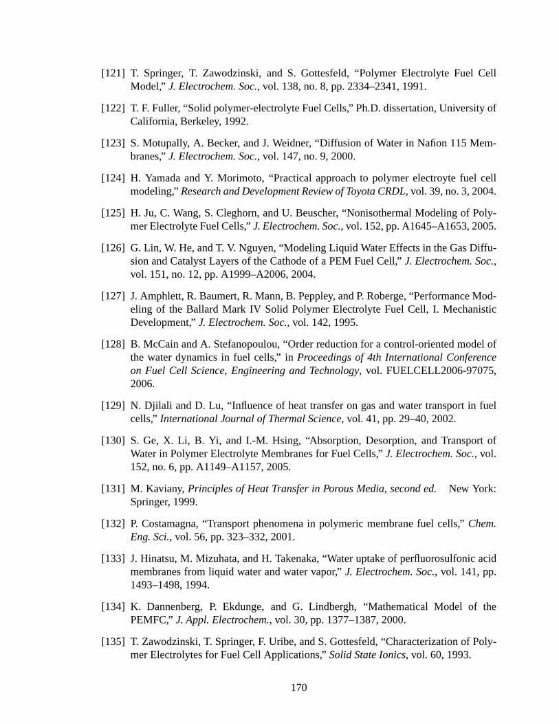
[121] T. Springer, T. Zawodzinski, and S. Gottesfeld, “Polymer Electrolyte Fuel CellModel,” J. Electrochem. Soc., vol. 138, no. 8, pp. 2334–2341, 1991.

[122] T. F. Fuller, “Solid polymer-electrolyte Fuel Cells,” Ph.D. dissertation, University ofCalifornia, Berkeley, 1992.

[123] S. Motupally, A. Becker, and J. Weidner, “Diffusion of Water in Nafion 115 Mem-branes,”J. Electrochem. Soc., vol. 147, no. 9, 2000.

[124] H. Yamada and Y. Morimoto, “Practical approach to polymer electroyte fuel cellmodeling,”Research and Development Review of Toyota CRDL, vol. 39, no. 3, 2004.

[125] H. Ju, C. Wang, S. Cleghorn, and U. Beuscher, “Nonisothermal Modeling of Poly-mer Electrolyte Fuel Cells,”J. Electrochem. Soc., vol. 152, pp. A1645–A1653, 2005.

[126] G. Lin, W. He, and T. V. Nguyen, “Modeling Liquid Water Effects in the Gas Diffu-sion and Catalyst Layers of the Cathode of a PEM Fuel Cell,”J. Electrochem. Soc.,vol. 151, no. 12, pp. A1999–A2006, 2004.

[127] J. Amphlett, R. Baumert, R. Mann, B. Peppley, and P. Roberge, “Performance Mod-eling of the Ballard Mark IV Solid Polymer Electrolyte Fuel Cell, I. MechanisticDevelopment,”J. Electrochem. Soc., vol. 142, 1995.

[128] B. McCain and A. Stefanopoulou, “Order reduction for a control-oriented model ofthe water dynamics in fuel cells,” inProceedings of 4th International Conferenceon Fuel Cell Science, Engineering and Technology, vol. FUELCELL2006-97075,2006.

[129] N. Djilali and D. Lu, “Influence of heat transfer on gas and water transport in fuelcells,” International Journal of Thermal Science, vol. 41, pp. 29–40, 2002.

[130] S. Ge, X. Li, B. Yi, and I.-M. Hsing, “Absorption, Desorption, and Transport ofWater in Polymer Electrolyte Membranes for Fuel Cells,”J. Electrochem. Soc., vol.152, no. 6, pp. A1149–A1157, 2005.

[131] M. Kaviany,Principles of Heat Transfer in Porous Media, second ed.New York:Springer, 1999.

[132] P. Costamagna, “Transport phenomena in polymeric membrane fuel cells,”Chem.Eng. Sci., vol. 56, pp. 323–332, 2001.

[133] J. Hinatsu, M. Mizuhata, and H. Takenaka, “Water uptake of perfluorosulfonic acidmembranes from liquid water and water vapor,”J. Electrochem. Soc., vol. 141, pp.1493–1498, 1994.

[134] K. Dannenberg, P. Ekdunge, and G. Lindbergh, “Mathematical Model of thePEMFC,”J. Appl. Electrochem., vol. 30, pp. 1377–1387, 2000.

[135] T. Zawodzinski, T. Springer, F. Uribe, and S. Gottesfeld, “Characterization of Poly-mer Electrolytes for Fuel Cell Applications,”Solid State Ionics, vol. 60, 1993.

170

[136] Y. Wang and C. Wang, “Two-phase Transients of Polymer Electrolyte Fuel Cells,”J.Electrochem. Soc., vol. 154, no. 7, pp. B636–B643, 2007.

[137] S. Litster, D. Sinton, and N. Djilali, “Ex situ visualization of liquid water transportin PEM fuel cell gas diffusion layers,”J. Power Sources, vol. 154, pp. 95–105, 2006.

[138] F. Barbir,PEM Fuel Cells: Theory and Practice. Burlington, Ma: Elsevier, 2005.

[139] J. T. Pukrushpan, A. G. Stefanopoulou, and H. Peng, “Control of fuel cell breathing,”IEEE Contr. Syst. Mag., vol. 24, no. 2, pp. 30–46, Apr 2004.

[140] J. B. Siegel, D. A. McKay, and A. G. Stefanopoulou, “Modeling and validation offuel cell water dynamics using neutron imaging,” inProc. American Control Con-ference, 11–13 June 2008, pp. 2573–2578.

[141] J. St-Pierre, D. P. Wilkinson, S. Knights, and M. Bos, “Relationships between wa-ter management, contamination and lifetime degradation in PEFC,”Journal of Newmaterials for Electrochemical Systems, vol. 3, pp. 99–106, 2000.

[142] M. Arcak, H. Gorgun, L. Pedersen, and S. Varigonda, “A nonlinear observer designfor fuel cell hydrogen estimation,”IEEE Trans. Control Syst. Technol., vol. 12, no. 1,pp. 101–110, 2004.

[143] J. Pukrushpan, A. Stefanopoulou, S. Varigonda, L. Pedersen, S. Ghosh, and H. Peng,“Control of natural gas catalytic partial oxidation for hydrogen generation in fuel cellapplications,”IEEE Trans. Control Syst. Technol., vol. 13, no. 1, pp. 3–14, 2005.

[144] K. Yoshizawa, K. Ikezoe, Y. Tasaki, D. Kramer, E. H. Lehmann, and G. G. Scherer,“Analysis of Gas Diffusion Layer and Flow-Field Design in a PEMFC Using Neu-tron Radiography,”J. Electrochem. Soc., vol. 155, no. 3, pp. B223–B227, Mar. 2008.

[145] D. Hussey, D. Jacobson, and M. Arif, “In situ fuel cell water metrology at the NISTneutron imaging facility,”Proceedings of the ASME International Conference onFuel Cell Science, Engineering and Technology, 2007.

[146] D. A. McKay, W. T. Ott, and A. Stefanopoulou, “Modeling, Parameter Identification,and Validation of Water Dynamics for a Fuel Cell Stack,” inProceedings of 2005ASME International Mechanical Engineering Congress & Exposition, vol. IMECE2005-81484, Nov 2005.

[147] B. A. McCain, A. G. Stefanopoulou, and I. V. Kolmanovsky, “A multi-componentspatially-distributed model of two-phase flow for estimation and control of fuel cellwater dynamics,” in2007 46th IEEE Conference on Decision and Control, 12-14Dec. 2007, pp. 584–589.

[148] A. Y. Karnik, A. G. Stefanopoulou, and J. Sun, “Water equilibria and managementusing a two-volume model of a polymer electrolyte fuel cell,”J. Power Sources, vol.164, no. 2, pp. 590 – 605, feb 2007.

171

[149] Z. H. Wang, C. Y. Wang, and K. S. Chen, “Two-phase flow and transport in the aircathode of proton exchange membrane fuel cells,”J. Power Sources, vol. 94, pp.40–50., 2001.

[150] A. Turhan, K. Heller, J. Brenizer, and M. Mench, “Passive control of liquid waterstorage and distribution in a PEFC through flow-field design,”J. Power Sources, vol.180, pp. 773–783, 2008.

[151] L. Onishi, J. Prausnitz, and J. Newman, “Water-Nafion Equilibria. Absence ofSchroeder’s Paradox,”J. Phys. Chem. B, vol. 111, no. 34, pp. 10 166–10 173, 2007.

[152] A. Weber and J. Newman, “Modeling Transport in Polymer-Electrolyte Fuel Cells,”Chemical Reviews, vol. 104, no. 10, pp. 4679–4726, 2004.

[153] C. H. Woo and J. Benziger, “PEM fuel cell current regulation by fuel feed control,”Chem. Eng. Sci., vol. 62, no. 4, pp. 957–968, Feb. 2007.

[154] B. McCain, J. Siegel, and S. A. G., “Stack-Level Validation of a Semi-AnalyticChannel-To-Channel Fuel Cell Model for Two-Phase Water Distribution BoundaryValue Control,” inAmerican Control Conference, 2008.

[155] A. Z. Weber, R. M. Darling, and J. Newman, “Modeling Two-Phase Behavior inPEFCs,”J. Electrochem. Soc., vol. 151, no. 10, pp. A1715–A1727, Oct. 2004.

[156] R. Borup, J. Meyers, B. Pivovar, Y. S. Kim, R. Mukundan, N. Garland, D. Myers,M. Wilson, F. Garzon, D. Wood, P. Zelenay, K. More, K. Stroh, T. Zawodzinski,J. Boncella, J. E. McGrath, M. Inaba, K. Miyatake, M. Hori, K. Ota, Z. Ogumi,S. Miyata, A. Nishikata, Z. Siroma, Y. Uchimoto, K. Yasuda, K.-i. Kimijima, andN. Iwashita, “Scientific Aspects of Polymer Electrolyte Fuel Cell Durability andDegradation,”Chemical Reviews, vol. 107, no. 10, pp. 3904–3951, 2007.

[157] J. Benziger, “Fan the flame with water: Current ignition, front propagation and mul-tiple steady states in polymer electrolyte membrane fuel cells,”AIChE J., vol. 55,no. 12, pp. 3034–3040, 2009.

[158] S. Basu, C.-Y. Wang, and K. S. Chen, “Phase change in a polymer electrolyte fuelcell,” J. Electrochem. Soc., vol. 156, no. 6, pp. B748–B756, 2009.

[159] N. R. Amundson, T.-W. Pan, and V. I. Paulsen, “Diffusing with stefan and maxwell,”AIChE J., vol. 49, no. 4, pp. 813–830, 2003.

[160] M. Adachi, T. Navessin, Z. Xie, B. Frisken, and S. Holdcroft, “Correlation of insitu and ex situ measurements of water permeation through nafion nre211 protonexchange membranes,”J. Electrochem. Soc., vol. 156, no. 6, pp. B782–B790, 2009.

[161] P. W. Majsztrik, M. B. Satterfield, A. B. Bocarsly, and J. B. Benziger, “Water sorp-tion, desorption and transport in Nafion membranes,”J. Membr. Sci., vol. 301, no.1-2, pp. 93–106, Sep. 2007.

172

[162] M. M. Mench,Fuel cell engines. Hoboken, N.J.: John Wiley & Sons, 2008.

[163] J. S. Newman.,Electrochemical systems, 2nd ed. Englewood Cliffs, N.J: PrenticeHall, 1991.

[164] D. M. Bernardi and M. W. Verbrugge, “A Mathematical Model of the Solid-Polymer-Electrolyte Fuel Cell,”J. Electrochem. Soc., vol. 139, no. 9, pp. 2477–2491,1992.

[165] A. Katsaounis, S. Balomenou, D. Tsiplakides, M. Tsampas, and C. Vayenas, “Therole of potential-dependent electrolyte resistance in the performance, steady-statemultiplicities and oscillations of PEM fuel cells: Experimental investigation andmacroscopic modelling,”Electrochim. Acta, vol. 50, no. 25-26, pp. 5132–5143, Sep.2005.

[166] J. B. Siegel, S. Yesilyurt, and A. G. Stefanopoulou, “Extracting Model parametersand Paradigms from Neutron Imaging of Dead-Ended Anode Operation,” inPro-ceedings of FuelCell2009 Seventh International Fuel Cell Science, Engineering andTechnology Conference, 2009, pp. 439–446.

[167] S. A. Freunberger, M. Reum, J. Evertz, A. Wokaun, and F. N. Buchi, “Measuringthe Current Distribution in PEFCs with Sub-Millimeter Resolution,”J. Electrochem.Soc., vol. 153, no. 11, pp. A2158–A2165, 2006.

[168] R. Taylor and R. Krishna,Multicomponent mass transfer. New York: Wiley, 1993.

[169] S. Ge, B. Yi, and P. Ming, “Experimental Determination of Electro-Osmotic DragCoefficient in Nafion Membrane for Fuel Cells,”J. Electrochem. Soc., vol. 153,no. 8, pp. A1443–A1450, 2006.

[170] W. Borutzky, B. Barnard, and J. Thoma, “An orifice flow model for laminar and tur-bulent conditions,”Simulation Modelling Practice and Theory, vol. 10, no. 3-4, pp.141–152, 2002.

[171] M. Grtsch and M. Mangold, “A two-phase PEMFC model for process control pur-poses,”Chem. Eng. Sci., vol. 63, pp. 434–447, 2008.

[172] J. Larminie and A. Dicks,Fuel Cell Systems Explained, 2nd ed. Hoboken, NJ:Wiley InterScience, 2003.

[173] E. Mueller, F. A. Kolb, A. G. Stefanopoulou, D. A. McKay, and L. Guzzella, “Cor-relating Nitrogen Accumulation with Temporal Fuel Cell Performance,” inProc. ofDynamic Systems and Control Conference (DSCC08), ser. , Paper TuAT5.1, 2008.

[174] W. H. Hogarth and J. B. Benziger, “Operation of polymer electrolyte membrane fuelcells with dry feeds: Design and operating strategies,”J. Power Sources, vol. 159,no. 2, pp. 968 – 978, 2006.

173

[175] J. Nam, P. Chippar, W. Kim, and H. Ju, “Numerical analysisof gas crossover effectsin polymer electrolyte fuel cells (PEFCs),”Applied Energy, vol. 87, no. 12, pp. 3699– 3709, 2010.

[176] H. Gorgun, F. Barbir, and M. Arcak, “A voltage-based observer design for mem-brane water content in pem fuel cells,” inProceedings of the 2005 American ControlConference, vol. 7, June 2005, pp. 4796 – 4801.

[177] M. A. Hickner, N. P. Siegel, K. S. Chen, D. S. Hussey, D. L. Jacobson, and M. Arif,“In Situ High-Resolution Neutron Radiography of Cross-Sectional Liquid WaterProfiles in Proton Exchange Membrane Fuel Cells,”J. Electrochem. Soc., vol. 155,pp. B427–B434, 2008.

[178] J. B. Siegel, X. Lin, A. G. Stefanopoulou, and D. Gorsich, “Neutron imaging oflithium concentration in battery pouch cells,” inSumbitted to The American ControlConference, 2011.

174