Measurement 58 (2014) 520–536

Contents lists available at ScienceDirect

Measurement

journal homepage: www.elsevier .com/ locate /measurement

Experimental investigation and performance analysisof cemented carbide inserts of different geometriesusing Taguchi based grey relational analysis

http://dx.doi.org/10.1016/j.measurement.2014.09.0250263-2241/� 2014 Elsevier Ltd. All rights reserved.

⇑ Corresponding author. Tel.: +91 44 27529247; fax: +91 44 27529094.E-mail address: nsk@adhiparasakthi.in (N. Senthilkumar).

N. Senthilkumar a,⇑, T. Tamizharasan b, V. Anandakrishnan c

a Adhiparasakthi Engineering College, Melmaruvathur 603319, Tamil Nadu, Indiab TRP Engineering College, Irungalur, Tiruchirappalli 621105, Indiac National Institute of Technology, Tiruchirappalli 620015, Tamil Nadu, India

a r t i c l e i n f o

Article history:Received 16 March 2014Received in revised form 3 September 2014Accepted 11 September 2014Available online 19 September 2014

Keywords:OptimizationHard turningTaguchi’s DoEGrey relational analysisConfidence interval

a b s t r a c t

In this work, effect of machining parameters cutting speed, feed rate and depth of cut,geometrical parameters cutting insert shape, relief angle and nose radius were investigatedand optimized using Taguchi based grey relational analysis. 18 ISO designated uncoatedcemented carbide inserts of different geometries were used to turn practically used auto-motive axles to study the influence of variation in carbide inserts geometry. Performancemeasures viz., flank wear, surface roughness and material removal rate (MRR) wereoptimized using grey relational grade, based on the experiments designed using Taguchi’sDesign of Experiments (DoE). A weighted grey relational grade is calculated to minimizeflank wear and surface roughness and to maximize MRR. Analysis of variance shows thatcutting insert shape is the prominent parameter followed by feed rate and depth of cut thatcontributes towards output responses. An experiment conducted with identified optimumcondition shows a lower flank wear and surface roughness with higher MRR. The confirma-tion results obtained are confirmed by calculating confidence interval, which lies withinthe width of the interval.

� 2014 Elsevier Ltd. All rights reserved.

1. Introduction

Machining is the process of removal of material fromrotating workpiece with the help of sharp cutting tool.Identification of cutting tools that can produce better geo-metrical and dimensional tolerance, good surface finishand the ability to serve for longer period are critical inmanufacturing industries. The cutting speed and the feedare the two most important parameters, to achieve opti-mum cutting conditions, while the depth of cut is oftenfixed. The performance of cutting tools is very dependenton their precise shape. For efficient cutting the clearance

angles, the nose radius and the sharpness of the cuttingedge are very much important. Clearance or relief angleis essential to avoid rubbing against the freshly cut surface[1]. Hard machining is defined as the machining of compo-nents with a hardness of above 45 HRC and normally theprocess is well suitable for parts having hardnesses in therange of 58–68 HRC. The workpiece materials involved inthe hard turning process include various hardened alloysteels, tool steels, case-hardened steels, superalloys,nitrided irons and hard-chrome coated steels, and heat-treated powder metallurgical parts. It is mainly a finishingor semi-finishing process where high dimensional, form,and surface finish accuracy have to be achieved. Hard turn-ing was early recognized and pioneered by the automotiveindustry as a means of improving the manufacturing of

N. Senthilkumar et al. / Measurement 58 (2014) 520–536 521

transmission components [2]. In this work severaluncoated cemented carbide cutting tool insert with differ-ent shapes, relief angles and nose radius [3] are chosen toturn practically used axle shafts of automobiles. A methodto identify surface roughness based on the measurement ofworkpiece surface temperature and root mean square forfeed vibration of the cutting tool during turning mild steelis done by Suhail et al. [4]. Investigation on machinabilitystudy of hardened steel to obtain optimum process param-eters considering MRR, surface finish, tool wear and toollife is carried out [5] for both rough and finish machiningand it is found that chipping and adhesions are the causesfor tool wear. Multi-response optimization of turningparameters and nose radius is performed [6] over surfaceroughness and power consumption and the main influenc-ing parameter is cutting speed followed by feed rate anddepth of cut. Optimization of turning parameters cuttingspeed, feed rate and depth of cut based on the Taguchimethod with grey relational analysis by determining greyrelational grade for multiple performance characteristicstool life, cutting force and surface roughness achieves bet-ter result [7]. Investigation of turning parameters forSKD11 using grey relational analysis method to minimizeaverage roughness, maximum roughness and roundnessis performed [8] and is identified that depth of cut wasinfluencing the average roughness and cutting speed isinfluencing maximum roughness and roundness. Abhangand Hameedullah [9] optimized the turning processparameters based on the multiple responses surfaceroughness and chip thickness using grey relational analysisand found that the type of lubricant has the strongesteffect on the responses followed by feed rate, cutting speedand nose radius. Effect of cutting speed, feed rate, depth ofcut and workpiece temperature is studied [10] on surfaceroughness, tool life and MRR in hot turning of stainlesssteel and found that feed rate and cutting speed are themost dominant parameters. The best process parametersfor lower cutting forces and surface roughness duringhigh-speed turning of Inconel 718 using Taguchi grey rela-tional analysis is performed [11] and found that feed ratehas the strongest correlation to cutting forces and surfaceroughness.

Tamizharasan and Senthilkumar [12] analyzed theinfluence of geometrical parameters included angle, reliefangle and nose radius over surface roughness and MRRduring turning AISI 1045 steel using Taguchi’s techniqueand ANOVA. Patil et al. [13] examined the surface integritywhile hot machining EN 36 steel using TiAlN coated car-bide tool, focusing on optimizing the surface roughness,MRR and tool wear rate and built a mathematical modelusing regression analysis between responses and processparameters. Satyanarayana et al. [14] minimized cuttingforce, surface roughness and flank wear through optimiza-tion of process parameters during turning Inconel 718using Taguchi method and GRA and found the significantparameters through ANOVA and conducted a confirmationtest with optimum conditions. Gupta and Kumar [15]investigated the effect of tool nose radius, tool rake angle,feed rate, cutting speed, cutting environment and depth ofcut during turning glass fibre reinforced plastic compositeusing Taguchi method and GRA and found that depth of cut

is the most influencing parameter on surface roughnessand MRR. Tamizharasan and Senthilkumar [16] studiedthe performances of various ISO designated cutting toolinserts having different included angle, relief angle andnose radius through finite element simulation analysisand determined the optimum geometry using Taguchi’smethod. Kolahan et al. [17] applied grey relational analysisfor multi response optimization obtained from Taguchi’smethod and developed mathematical models for it duringturning structural grade 50.2 steel and found the signifi-cant parameters through ANOVA. Tamizharasan and Sent-hilkumar [18] investigated the influence of machiningparameters and geometrical parameters during turningAISI 1045 steel with uncoated carbide inserts of varyinggeometries by finite element approach and confirmed itwith experimentation.

2. Problem identification

Manufacturing industries are more concerned with pro-ducing high quality products at lower cost due to the com-petitive global market prevailing today. One of the mostimportant factors that affect the quality of the machinedcomponent is the tool wear, since it drastically influencesthe surface finish of the machined surface and dimensionalaccuracy of finished component and increases the wear ofthe cutting tool and increases the tool changing cost.Hence much emphasis is given to tool wear [19]. At thesame time, the amount of material to be removed has tobe higher in order to achieve higher production rate.Hence, a combination of production rate and good qualityalong with reduced tool wear has to be achieved throughoptimization of cutting parameters and cutting tool geom-etry through various techniques.

From the literature review carried out, it is observedthat researches have performed hard machining using dif-ferent types of cutting tools to achieve better results [20],and to the best of our knowledge no researcher has per-formed experimental analysis combining both the machin-ing and geometrical parameters as it is chosen in thispresent work. Researchers have considered differentshapes of cutting insert having different nose radius sepa-rately or its limited combination with other parameters.But in this research work, all parameters are consideredfor performing the experimental investigation.

Cutting insert shape (included angle) is consideredsince the sharpness of the cutting edge has an effect onflank wear and surface roughness. Relative edge strengthof the cutting inserts increases with increase in theincluded angle and the tendency for chipping and breakingof inserts with various shapes increases with decrease inincluded angle of the cutting tool inserts [21].

Rubbing of flank face of the cutting tool is avoided byproviding relief angle, thereby reducing surface roughness.It is observed that if the relief angle is increased, the vol-ume of wear required to reach a particular width of flankwear land is also increased. On the other hand, with largerelief angles the mechanical strength of the cutting edgeis low and the tool is more liable to chipping or fracture.The tool wear is less at the optimum relief angle. Nose

522 N. Senthilkumar et al. / Measurement 58 (2014) 520–536

radius of cutting tool is responsible for larger area of con-tact, which removes more material from workpiece. Largernose radius gives better surface finish. On the other hand,reducing the nose to a point may make the surface finishunacceptable. Increasing the nose radius also decreasesthe tool wear so that higher cutting speed can beemployed. When the nose radius is increased excessively,cutting forces and possibility of chatter increases.

When the material hardness is more, higher flank wearoccurs; hence surface roughness will be more. Materialswith high hardness tend to increase cutting forces, cuttingtemperatures and abrasive wear [22]. Hence this parame-ter is also chosen for analysis. Along with the above param-eters, machining parameters such as cutting speed, feedrate and depth of cut also have an impact on the outputresponses. Higher cutting speed increases tool temperatureand softens the tool material. It thereby aids abrasive,adhesive and diffusional wear. The larger the feed, thegreater is the cutting force per unit area of chip-tool con-tact on the rake face and work-tool contact on the flankface and therefore cutting temperature and different typesof wear are increased. If the depth of cut is increased, thearea of the chip-tool contact increases roughly in equalproportion to the change in depth of cut. Thus, an increasein the depth of cut increases tool wear to some extent byaccelerating the abrasive adhesive and diffusional typesof tool wear.

The cause and effect diagram of turning process involv-ing various input control parameters such as cutting toolgeometries and machining parameters which have animpact on the output responses flank wear, surface rough-ness and MRR is shown in Fig. 1.

In this work, various ISO designated uncoated carbidecutting tool inserts are selected for analysis which is notpreviously considered by the researchers. Previously,researchers have performed analysis considering differentcutting insert shapes, relief angle and different nose radiusseparately or in combination of one with other. But in thisanalysis, all three geometrical parameters of the cuttingtool insert are considered along with machining parame-ters. The main objective of this work is to develop a cutting

Fig. 1. Cause and effect diagr

tool insert with a geometry that involves the shape of theinsert (included angle), relief angle and nose radius whichwill be very effective in increasing the production rate byimproving the rate of material removal, increasing thequality of the machined component by lowering the sur-face roughness at the machined surface of the workpieceand to increase the performance of the cutting tool byreducing the wear at the flank face of the cutting toolinsert.

3. Methodologies used in this analysis

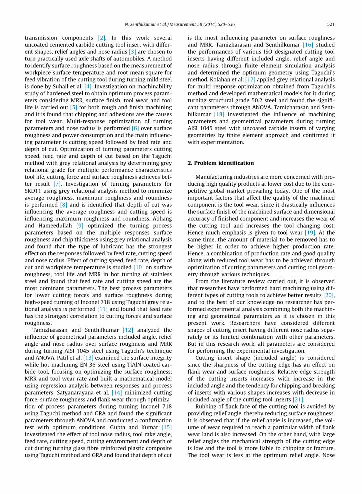
Machining of practically used automobile axles usingdifferent tool geometries [23] along with varying combina-tions of machining parameters has been selected in thiswork. The thrust activities related to the development ofcutting tool geometry that influence the scope of this workis identified for investigation and subsequently, researchmethodology has been designed. Experiments have beenconducted by applying Taguchi’s Design of Experiments(DoE) [24]. The results of the experiments are analyzedand reviewed using grey relational analysis and analysisof variance. Prediction of output responses is also per-formed by developing empirical equations with multiplelinear regression models. Confidence interval is calculatedto determine the reliability of this experimentation and theoutput obtained. The methodologies that are adopted inthis work are summarized in the flow chart shown in Fig. 2.

3.1. Material selection

The selected materials for the specimen are hardenedalloy steels, practically used for wheel axles of mediumand heavy-duty automobiles. Material ‘A’ is the real axleof Ambassador Car, Material ‘B’ is the rear axle of Standardjeep and Material ‘C’ is the rear axle of Ashok Leylandtruck. The chemical compositions and hardness values ofthe select workpiece materials are shown in Table 1.

The material of the cutting tool insert selected for thiswork is uncoated cemented carbide WIDIA make, having

am of turning process.

Fig. 2. Methodologies used in this analysis.

Table 1Chemical composition and Brinell hardness of workpiece materials.

Sl. No. Elementpresent

% of Composition

Material ‘A’ Material ‘B’ Material ‘C’

1 Carbon 0.369 0.384 0.4392 Silicon 0.212 0.253 0.1743 Manganese 1.503 1.485 0.7874 Chromium 0.000 0.109 0.1835 Nickel 0.000 0.039 0.0386 Aluminium 0.018 0.014 0.0327 Copper 0.037 0.125 0.1198 Tungsten 0.031 0.027 0.0379 Vanadium 0.001 0.003 0.00110 Phosphorous 0.020 0.027 0.02311 Sulphur 0.031 0.020 0.03312 Iron Remaining Remaining Remaining

Brinell Hardness (BHN) 512 448 522

Table 2Chemical composition and Brinell hardness of cutting tool insert.

Sl. No. Element present % of Composition

1 Tungsten carbide 96.42 Tantalum carbide 0.83 Titanium carbide 0.54 Cobalt 2.19

N. Senthilkumar et al. / Measurement 58 (2014) 520–536 523

a Brinell hardness of 1433 BHN, whose chemical composi-tion and hardness values are shown in Table 2. In order tostudy and analyze the performance of the inserts by

varying the machining and geometrical parameters,uncoated carbide cutting tool inserts are used.

Cemented carbide inserts are selected because of theirhigh hardness, keen cutting edge and red hardness proper-ties. The SEM image of uncoated carbide insert is shown inFig. 3. The micrograph shows the particles of predominantTungsten carbide which appear as light grey particles.Some voids are present during compacting. The structureis variable composition of solid solution phases of WCand TiC. The black areas are voids. The areas in betweenthe grains are cobalt solid solution.

Fig. 3. SEM image of carbide cutting insert.

524 N. Senthilkumar et al. / Measurement 58 (2014) 520–536

3.2. Experimental setup

The experiments are conducted on the CNC Turningcenter, Lokesh make 2 axis CNC TL-20, swing diameter350 mm, between centre 600 mm, spindle speed4500 rpm, main motor power of 11 kW. After performingthe machining process, the flank wear are measured byusing a Mitutoyo digital tool makers microscope of specifi-cations, eyepiece: 15�, view field diameter 13 mm, objec-tive 2�, working distance 67 mm, total magnification 30�.Surface roughness are measured by using a Kosaka Labora-tory Ltd. make Surfcorder SE1200; with a vertical measur-ing range of 520 lm, horizontal measuring range of25 mm, vertical resolution of 0.008 lm, cutoff value of0.8 mm with Gaussian filter. MRR are determined by not-ing the time and volume of material removed using the for-mula in Eq. (1).

Material removal rate

¼Volume of material removed during machiningTime taken for machining

cm3=min ð1Þ

Fig. 4. Equipments used for measurement

The measuring instruments used for measuring the out-put response parameters flank wear and surface roughnessare shown in Fig. 4.

For conducting experiments, 18 workpieces are chosenfor experiments designed using L18 Orthogonal Array, andfor each experiment an individual workpiece is allotted.Before machining, all the individual workpieces areweighed and their corresponding weights are noted down.During machining the time taken for machining the indi-vidual workpieces are noted down using a stopwatch. Afterperforming the turning operation, individual workpiecesare weighed once again and the volume of materialremoved to the machining time gives the amount of mate-rial removed during machining. Immediately after per-forming the turning operation, the surface roughness ismeasured using Surfcorder and the flank wear is measuredusing Tool maker’s microscope.

3.3. Taguchi’s Design of Experiments

Taguchi’s Design of Experiments (DoE) is a statisticaltechnique, used to study many factors simultaneouslyand most economically [25]. By studying the effects ofindividual factors on the results, the best factor combina-tion can be determined. When applied to a design, thetechnique helps to seek out the best design among themany alternatives. Taguchi’s technique is a powerful toolin quality optimization [26]. Taguchi’s technique makesuse of a special design of Orthogonal Array (OA) to examinethe quality characteristics through a minimal number ofexperiments. When applied to a design, the techniquehelps to seek out the best design among the many alterna-tives. The experimental results based on the OA are thentransformed into weighted grey relational grade to evalu-ate the performance characteristics [27,28].

Taguchi’s Design of Experiments is used to design theOrthogonal Array for the seven chosen input controlparameters such as cutting speed, feed rate, depth of cut,material hardness, cutting tool insert shape (includedangle), relief angle and nose radius. Each input parameter

of tool wear and surface roughness.

N. Senthilkumar et al. / Measurement 58 (2014) 520–536 525

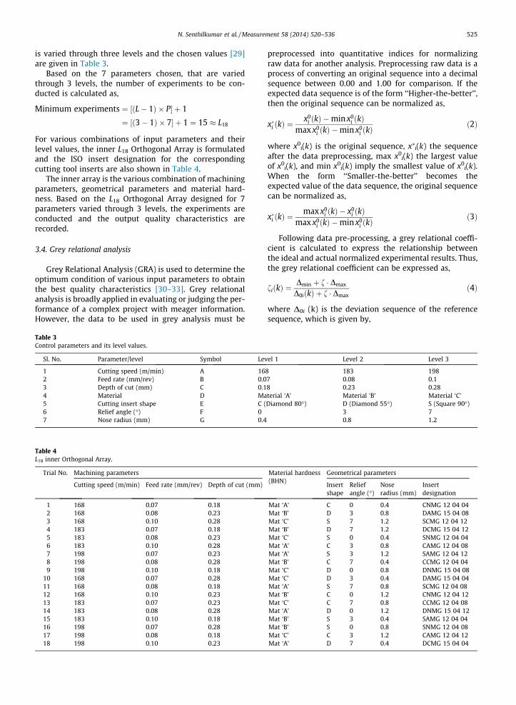
is varied through three levels and the chosen values [29]are given in Table 3.

Based on the 7 parameters chosen, that are variedthrough 3 levels, the number of experiments to be con-ducted is calculated as,

Minimum experiments ¼ ½ðL� 1Þ � P� þ 1

¼ ½ð3� 1Þ � 7� þ 1 ¼ 15 � L18

For various combinations of input parameters and theirlevel values, the inner L18 Orthogonal Array is formulatedand the ISO insert designation for the correspondingcutting tool inserts are also shown in Table 4.

The inner array is the various combination of machiningparameters, geometrical parameters and material hard-ness. Based on the L18 Orthogonal Array designed for 7parameters varied through 3 levels, the experiments areconducted and the output quality characteristics arerecorded.

3.4. Grey relational analysis

Grey Relational Analysis (GRA) is used to determine theoptimum condition of various input parameters to obtainthe best quality characteristics [30–33]. Grey relationalanalysis is broadly applied in evaluating or judging the per-formance of a complex project with meager information.However, the data to be used in grey analysis must be

Table 3Control parameters and its level values.

Sl. No. Parameter/level Symbol Lev

1 Cutting speed (m/min) A 162 Feed rate (mm/rev) B 0.03 Depth of cut (mm) C 0.14 Material D Ma5 Cutting insert shape E C (6 Relief angle (�) F 07 Nose radius (mm) G 0.4

Table 4L18 inner Orthogonal Array.

Trial No. Machining parameters

Cutting speed (m/min) Feed rate (mm/rev) Depth of cut (mm)

1 168 0.07 0.182 168 0.08 0.233 168 0.10 0.284 183 0.07 0.185 183 0.08 0.236 183 0.10 0.287 198 0.07 0.238 198 0.08 0.289 198 0.10 0.18

10 168 0.07 0.2811 168 0.08 0.1812 168 0.10 0.2313 183 0.07 0.2314 183 0.08 0.2815 183 0.10 0.1816 198 0.07 0.2817 198 0.08 0.1818 198 0.10 0.23

preprocessed into quantitative indices for normalizingraw data for another analysis. Preprocessing raw data is aprocess of converting an original sequence into a decimalsequence between 0.00 and 1.00 for comparison. If theexpected data sequence is of the form ‘‘Higher-the-better’’,then the original sequence can be normalized as,

x�i ðkÞ ¼x0

i ðkÞ �min x0i ðkÞ

max x0i ðkÞ �min x0

i ðkÞð2Þ

where x0i(k) is the original sequence, x⁄i(k) the sequence

after the data preprocessing, max x0i(k) the largest value

of x0i(k), and min x0

i(k) imply the smallest value of x0i(k).

When the form ‘‘Smaller-the-better’’ becomes theexpected value of the data sequence, the original sequencecan be normalized as,

x�i ðkÞ ¼max x0

i ðkÞ � x0i ðkÞ

max x0i ðkÞ �min x0

i ðkÞð3Þ

Following data pre-processing, a grey relational coeffi-cient is calculated to express the relationship betweenthe ideal and actual normalized experimental results. Thus,the grey relational coefficient can be expressed as,

fiðkÞ ¼Dmin þ f � Dmax

D0iðkÞ þ f � Dmaxð4Þ

where D0i (k) is the deviation sequence of the referencesequence, which is given by,

el 1 Level 2 Level 3

8 183 1987 0.08 0.18 0.23 0.28terial ‘A’ Material ‘B’ Material ‘C’Diamond 80�) D (Diamond 55�) S (Square 90�)

3 70.8 1.2

Material hardness(BHN)

Geometrical parameters

Insertshape

Reliefangle (�)

Noseradius (mm)

Insertdesignation

Mat ‘A’ C 0 0.4 CNMG 12 04 04Mat ‘B’ D 3 0.8 DAMG 15 04 08Mat ‘C’ S 7 1.2 SCMG 12 04 12Mat ‘B’ D 7 1.2 DCMG 15 04 12Mat ‘C’ S 0 0.4 SNMG 12 04 04Mat ‘A’ C 3 0.8 CAMG 12 04 08Mat ‘A’ S 3 1.2 SAMG 12 04 12Mat ‘B’ C 7 0.4 CCMG 12 04 04Mat ‘C’ D 0 0.8 DNMG 15 04 08Mat ‘C’ D 3 0.4 DAMG 15 04 04Mat ‘A’ S 7 0.8 SCMG 12 04 08Mat ‘B’ C 0 1.2 CNMG 12 04 12Mat ‘C’ C 7 0.8 CCMG 12 04 08Mat ‘A’ D 0 1.2 DNMG 15 04 12Mat ‘B’ S 3 0.4 SAMG 12 04 04Mat ‘B’ S 0 0.8 SNMG 12 04 08Mat ‘C’ C 3 1.2 CAMG 12 04 12Mat ‘A’ D 7 0.4 DCMG 15 04 04

526 N. Senthilkumar et al. / Measurement 58 (2014) 520–536

D0iðkÞ ¼ kx�0ðkÞ � x�i ðkÞk ð5Þ

Dmax ¼max8jei

max8kkx�0ðkÞ � x�j ðkÞk;

Dmin ¼min8jei

min8kkx�0ðkÞ � x�j ðkÞk

ð6Þ

f is distinguishing or identification coefficient: f e [0, 1].f = 0.5 is generally used. After obtaining the grey relationalcoefficient, normally the average of the grey relationalcoefficient is taken as the grey relational grade. The greyrelational grade is defined as,

ci ¼1n

Xn

k¼1 i

fiðkÞ ð7Þ

3.5. Multiple linear regression models

Regression is a technique for investigating functionalrelationship between output and input decision variablesof a process and may be useful for manufacturing processdata description, parameter estimation and control [34].The criteria for fitting the best line through the data in sim-ple linear regression is to minimize the sum of squares ofresiduals (Sr) between the measured values of responseand the values of response calculated with the regressionmodel. The linear fit is expressed as,

y ¼ a0 þ a1x ð8Þ

where y is the value of response and x is the value of var-iable. Multiple linear regressions are the extension of thelinear regression when the response is a linear functionof two or more independent variables. In general, theresponse variable y may be related to k regressor variables.The model in Eq. (7) is called a multiple linear regressionmodel with k regressor variables.

y ¼ b0 þ b1x1 þ b2x2 þ . . .þ bkxk þ e ð9Þ

The parameters bj, j = 0, 1, . . ., k are called the regressioncoefficients. These regression models are useful in predict-ing the response parameters with respect to the input con-trol parameters.

3.6. Analysis of variance

Analysis of Variance (ANOVA) is an important techniquefor analyzing the effect of categorical factors on a response.An ANOVA decomposes the variability in the response var-iable amongst the different factors [35]. Depending uponthe type of analysis, it may be important to determinewhich factors have a significant effect on the response,and how much of the variability in the response variableis attributable to each factor. For determining the signifi-cant factor which contributes more towards the outputresponse ANOVA is done. ANOVA is a statistical procedurethat allows us to partition (divide) the total variance mea-sured on the dependent variable in a study into its sourcesor component parts. This total measured variance is thevariance of the scores that we have obtained when partici-pants were measured on the dependent variable. Depen-dent variables or dependent measures reflect the outcome

of the study, and a useful way to conceptualize them is asoutcome variables or outcome measures. Independent vari-ables reflect the factors that may be said to influence thedependent variable; they can be conceptualized as inputfactors, treatment conditions, or treatment effects. Depen-dent and independent variables are intimately related toeach other. Dependent variables are presumed to be influ-enced or affected by independent variables.

3.7. Confidence interval

A confidence interval (CI) is a type of interval estimateof a population parameter which is used to indicate thereliability of an estimate [36]. It is an observed interval cal-culated from the observations made through experiments,in principle different from sample to sample, that fre-quently includes the parameter of interest if the experi-ment is repeated. The frequency of the observed intervalcontaining the parameter is determined by the confidencelevel or confidence coefficient. It gives an estimated rangeof values that are likely to include an unknown populationparameter and the estimated range being calculated from agiven set of sample data. The width of the confidence inter-val obtained shows how uncertain we are about theunknown parameter. A very wide interval may indicatethat more data should be collected before anything verydefinite can be said about the parameter.

4. Results and discussion

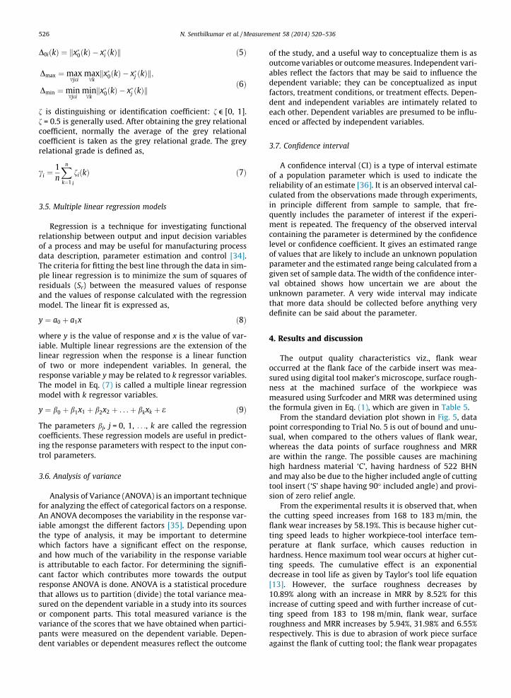
The output quality characteristics viz., flank wearoccurred at the flank face of the carbide insert was mea-sured using digital tool maker’s microscope, surface rough-ness at the machined surface of the workpiece wasmeasured using Surfcoder and MRR was determined usingthe formula given in Eq. (1), which are given in Table 5.

From the standard deviation plot shown in Fig. 5, datapoint corresponding to Trial No. 5 is out of bound and unu-sual, when compared to the others values of flank wear,whereas the data points of surface roughness and MRRare within the range. The possible causes are machininghigh hardness material ‘C’, having hardness of 522 BHNand may also be due to the higher included angle of cuttingtool insert (‘S’ shape having 90� included angle) and provi-sion of zero relief angle.

From the experimental results it is observed that, whenthe cutting speed increases from 168 to 183 m/min, theflank wear increases by 58.19%. This is because higher cut-ting speed leads to higher workpiece-tool interface tem-perature at flank surface, which causes reduction inhardness. Hence maximum tool wear occurs at higher cut-ting speeds. The cumulative effect is an exponentialdecrease in tool life as given by Taylor’s tool life equation[13]. However, the surface roughness decreases by10.89% along with an increase in MRR by 8.52% for thisincrease of cutting speed and with further increase of cut-ting speed from 183 to 198 m/min, flank wear, surfaceroughness and MRR increases by 5.94%, 31.98% and 6.55%respectively. This is due to abrasion of work piece surfaceagainst the flank of cutting tool; the flank wear propagates

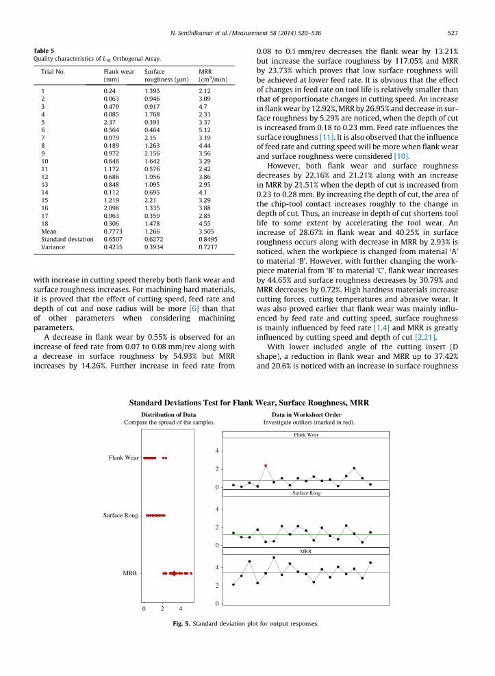
Table 5Quality characteristics of L18 Orthogonal Array.

Trial No. Flank wear(mm)

Surfaceroughness (lm)

MRR(cm3/min)

1 0.24 1.395 2.122 0.063 0.946 3.093 0.479 0.917 4.74 0.085 1.768 2.315 2.37 0.391 3.376 0.564 0.464 5.127 0.979 2.15 3.198 0.189 1.263 4.449 0.972 2.156 3.5610 0.646 1.642 3.2911 1.172 0.576 2.4212 0.686 1.956 3.8613 0.848 1.095 2.9514 0.112 0.695 4.115 1.219 2.21 3.2916 2.098 1.335 3.8817 0.963 0.359 2.8518 0.306 1.478 4.55Mean 0.7773 1.266 3.505Standard deviation 0.6507 0.6272 0.8495Variance 0.4235 0.3934 0.7217

N. Senthilkumar et al. / Measurement 58 (2014) 520–536 527

with increase in cutting speed thereby both flank wear andsurface roughness increases. For machining hard materials,it is proved that the effect of cutting speed, feed rate anddepth of cut and nose radius will be more [6] than thatof other parameters when considering machiningparameters.

A decrease in flank wear by 0.55% is observed for anincrease of feed rate from 0.07 to 0.08 mm/rev along witha decrease in surface roughness by 54.93% but MRRincreases by 14.26%. Further increase in feed rate from

MRR

Surface Roug

Flank Wear

420

4

2

0

4

2

0

4

2

0

Distribution of DataCompare the spread of the samples.

Standard Deviations Test for Flank

Fig. 5. Standard deviation plo

0.08 to 0.1 mm/rev decreases the flank wear by 13.21%but increase the surface roughness by 117.05% and MRRby 23.73% which proves that low surface roughness willbe achieved at lower feed rate. It is obvious that the effectof changes in feed rate on tool life is relatively smaller thanthat of proportionate changes in cutting speed. An increasein flank wear by 12.92%, MRR by 26.95% and decrease in sur-face roughness by 5.29% are noticed, when the depth of cutis increased from 0.18 to 0.23 mm. Feed rate influences thesurface roughness [11]. It is also observed that the influenceof feed rate and cutting speed will be more when flank wearand surface roughness were considered [10].

However, both flank wear and surface roughnessdecreases by 22.16% and 21.21% along with an increasein MRR by 21.51% when the depth of cut is increased from0.23 to 0.28 mm. By increasing the depth of cut, the area ofthe chip-tool contact increases roughly to the change indepth of cut. Thus, an increase in depth of cut shortens toollife to some extent by accelerating the tool wear. Anincrease of 28.67% in flank wear and 40.25% in surfaceroughness occurs along with decrease in MRR by 2.93% isnoticed, when the workpiece is changed from material ‘A’to material ‘B’. However, with further changing the work-piece material from ‘B’ to material ‘C’, flank wear increasesby 44.65% and surface roughness decreases by 30.79% andMRR decreases by 0.72%. High hardness materials increasecutting forces, cutting temperatures and abrasive wear. Itwas also proved earlier that flank wear was mainly influ-enced by feed rate and cutting speed, surface roughnessis mainly influenced by feed rate [1,4] and MRR is greatlyinfluenced by cutting speed and depth of cut [2,21].

With lower included angle of the cutting insert (Dshape), a reduction in flank wear and MRR up to 37.42%and 20.6% is noticed with an increase in surface roughness

Flank Wear

Surface Roug

MRR

Data in Worksheet OrderInvestigate outliers (marked in red).

Wear, Surface Roughness, MRR

t for output responses.

528 N. Senthilkumar et al. / Measurement 58 (2014) 520–536

of 32.96% since surface roughness and tool wear improveswith change in cutting tool. With further increase inincluded angle (S shape) the flank wear increases drasti-cally by 280.82% with decrease in surface roughness by12.73% and MRR by 0.24%. A decrease in flank wear andsurface roughness is observed with increase in relief angle.When the relief angle is changed from 0� to 3�, a reductionof 31.55% in flank wear, 1.98% in surface roughness and0.29% in MRR occurs. By further increasing the relief anglefrom 3� to 7�, 30.56% decrease in flank wear and 8.67%decrease in surface roughness and 2.59% increase in MRRis noticed. This is due to the prevention of rubbing actionof cutting tool on the workpiece surface by providing reliefangle to the cutting tool. Increase in flank wear by 15.03%and decrease in surface roughness by 21.57% and MRR by0.19% occurs with increase in nose radius from 0.4 to0.8 mm. Change of nose radius from 0.8 to 1.2 mm leadsto a decrease in flank wear by 42.21% and MRR by 0.05%.But, surface roughness increases by 19.37%.

When considering the geometrical parameters, theincluded angle of the carbide insert has the greater influ-ence on the flank wear, surface roughness and MRR [3], fol-lowed by nose radius rather than the relief angle, which isalso proved by numerical simulation results [16]. Flankwear and MRR were greatly influenced by included angleand nose radius [12,19], whereas surface roughness isinfluenced by nose radius and included angle [12]. It isunderstood that when MRR increases flank wear alsoincreases.

The relationship between flank wear and surface rough-ness is shown in Fig. 6. It is obvious that when the flankwear is more, surface roughness of the component pro-duced will also be more. But, it is noticed that by providing

Fig. 6. Correlation between flank w

relief angle to the cutting insert, the rubbing action of thetool with the workpiece is reduced thereby minimizing thesurface roughness.

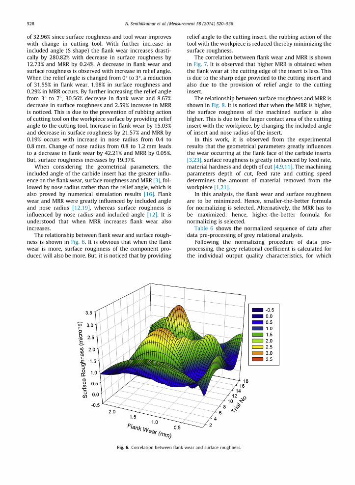
The correlation between flank wear and MRR is shownin Fig. 7. It is observed that higher MRR is obtained whenthe flank wear at the cutting edge of the insert is less. Thisis due to the sharp edge provided to the cutting insert andalso due to the provision of relief angle to the cuttinginsert.

The relationship between surface roughness and MRR isshown in Fig. 8. It is noticed that when the MRR is higher,the surface roughness of the machined surface is alsohigher. This is due to the larger contact area of the cuttinginsert with the workpiece, by changing the included angleof insert and nose radius of the insert.

In this work, it is observed from the experimentalresults that the geometrical parameters greatly influencesthe wear occurring at the flank face of the carbide inserts[3,23], surface roughness is greatly influenced by feed rate,material hardness and depth of cut [4,9,11]. The machiningparameters depth of cut, feed rate and cutting speeddetermines the amount of material removed from theworkpiece [1,21].

In this analysis, the flank wear and surface roughnessare to be minimized. Hence, smaller-the-better formulafor normalizing is selected. Alternatively, the MRR has tobe maximized; hence, higher-the-better formula fornormalizing is selected.

Table 6 shows the normalized sequence of data afterdata pre-processing of grey relational analysis.

Following the normalizing procedure of data pre-processing, the grey relational coefficient is calculated forthe individual output quality characteristics, for which

ear and surface roughness.

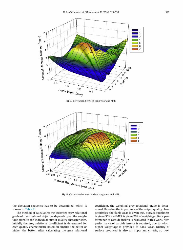
Fig. 7. Correlation between flank wear and MRR.

Fig. 8. Correlation between surface roughness and MRR.

N. Senthilkumar et al. / Measurement 58 (2014) 520–536 529

the deviation sequence has to be determined, which isshown in Table 7.

The method of calculating the weighted grey relationalgrade of the combined objective depends upon the weigh-tage given to the individual output quality characteristics.Initially the grey relational co-efficient is determined foreach quality characteristic based on smaller the better orhigher the better. After calculating the grey relational

coefficient, the weighted grey relational grade is deter-mined. Based on the importance of the output quality char-acteristics, the flank wear is given 50%, surface roughnessis given 30% and MRR is given 20% of weightage. Since per-formance of carbide inserts is evaluated in this work, highperformance of carbide inserts is required, due to whichhigher weightage is provided to flank wear. Quality ofsurface produced is also an important criteria, so next

Table 6GRA normalized sequence after data pre-processing.

Trial No. Flank wear Surface roughness MRR

1 0.923 0.440 0.0002 1.000 0.683 0.3233 0.820 0.699 0.8604 0.990 0.239 0.0635 0.000 0.983 0.4176 0.783 0.943 1.0007 0.603 0.032 0.3578 0.945 0.512 0.7739 0.606 0.029 0.480

10 0.747 0.307 0.39011 0.519 0.883 0.10012 0.730 0.137 0.58013 0.660 0.602 0.27714 0.979 0.818 0.66015 0.499 0.000 0.39016 0.118 0.473 0.58717 0.610 1.000 0.24318 0.895 0.395 0.810

Table 7Deviation sequence of GRA.

Trial No. Flank wear Surface roughness MRR

1 0.077 0.560 1.0002 0.000 0.317 0.6773 0.180 0.301 0.1404 0.010 0.761 0.9375 1.000 0.017 0.5836 0.217 0.057 0.0007 0.397 0.968 0.6438 0.055 0.488 0.2279 0.394 0.971 0.520

10 0.253 0.693 0.61011 0.481 0.117 0.90012 0.270 0.863 0.42013 0.340 0.398 0.72314 0.021 0.182 0.34015 0.501 1.000 0.61016 0.882 0.527 0.41317 0.390 0.000 0.75718 0.105 0.605 0.190

Table 8Grey relational coefficient and weighted grey relational grade.

Trial No. Grey relational coefficient Weighted greyrelational grade

Flankwear

Surfaceroughness

MRR

1 0.867 0.472 0.333 0.6422 1.000 0.612 0.425 0.7693 0.735 0.624 0.781 0.7114 0.981 0.396 0.348 0.6795 0.333 0.967 0.462 0.5496 0.697 0.898 1.000 0.8187 0.557 0.341 0.437 0.4688 0.902 0.506 0.688 0.7409 0.559 0.340 0.490 0.480

10 0.664 0.419 0.450 0.54811 0.510 0.810 0.357 0.56912 0.649 0.367 0.543 0.54313 0.595 0.557 0.409 0.54614 0.959 0.734 0.595 0.81915 0.499 0.333 0.450 0.43916 0.362 0.487 0.547 0.43717 0.562 1.000 0.398 0.66118 0.826 0.453 0.725 0.694

530 N. Senthilkumar et al. / Measurement 58 (2014) 520–536

importance is given to surface roughness of machinedsurface. Finally, the MRR is given the least weightage.The weighted grey relational grade (100%) is obtained bysumming the entire individual grey relational coefficient,which is given in Eq. (10) as,

Weighted grey relational grade ð100%Þ¼ GR Coeff � Flank wear ð50%Þ þ GR Coeff

� Surface roughness ð30%Þ þ GR Coeff

�Material removal rate ð20%Þ ð10Þ

By using smaller-the-better formula, the grey relationalcoefficient for flank wear and surface roughness are calcu-lated; hence, they have to be minimized. Higher the betteris used to determine the grey relational coefficient for MRRhence it has to be maximized. After calculating the individ-ual grey relational coefficient, the weighted grey relationalgrade is determined based on the weightages given. For

calculating the weighted grey relational grade, the testcondition No. 3 is considered.

Weighted grey relational grade

¼ ½ð0:735 � 0:5Þ þ ð0:624 � 0:3Þ þ ð0:781 � 0:2Þ� ¼ 0:711

The weighted grey relational grades are determined bycombining the entire individual grey relational coefficientvalues, as shown in Table 8.

The best levels of various parameters are identified bycalculating the average values of weighted grey relationalgrade corresponding to each level of parameters as shownin Table 9.

From the response table of weighted grey relationalgrade, the optimal parameter levels are identified as,cutting speed of 183 m/min, feed rate as 0.08 mm/rev,depth of cut as 0.28 mm, material ‘A’ of hardness 512BHN, cutting insert shape of D (Diamond 55�), relief angleof 7� and nose radius of 1.2 mm. Hence, the optimumcondition is represented as A2B2C3D1E2F3G3. From theresponse table of weighted grey relational grade, the maineffects plot of weighted grey relational grade is drawn,which is shown in Fig. 9.

The interaction or interdependence between the choseninput control parameters over weighted grey relationalgrade is shown in Fig. 10. Between cutting speed and feedrate there is no such effect since all the lines are parallel.No significant interaction is observed between cuttingspeed and depth of cut but the weighted grey relationalgrade is higher for the combination of cutting speed of183 m/min and depth of cut of 0.28 mm. The output ishigher for the material hardness of 512 BHN and cuttingspeed 183 m/min and for the other level values, no signifi-cant relationship exists. A significant relationship existsbetween the cutting insert shape and cutting speed sinceall the lines are non-parallel to each other. A considerabledependency exists between the relief angle and cuttingspeed and for level 1 value; weighted grey relational grade

Table 9Response table for weighted grey relational grade.

Parameter/level Cutting speed Feed rate Depth of cut Material hardness Insert shape Relief angle Nose radius

Level 1 0.630 0.553 0.578 0.668 0.658 0.578 0.602Level 2 0.642 0.685 0.595 0.601 0.665 0.617 0.603Level 3 0.580 0.614 0.679 0.583 0.529 0.657 0.647

198183168

0.65

0.60

0.55

0.100.080.07 0.280.230.18

Mat-'C'Mat-'B'Mat-'A'

0.65

0.60

0.55

SDC 730

1.20.80.4

0.65

0.60

0.55

Cutting Speed (m/min)

Mea

n

Feed Rate (mm/rev) Depth of Cut (mm)

Material Hardness Insert Shape Relief Angle (Degrees)

Nose Radius (mm)

Main Effects Plot for Weighted Grey Relational GradeData Means

Fig. 9. Main effects plot of weighted grey relational grade.

0.100.080.07 0.280.230.18 Mat-'C'Mat-'B'Mat-'A' SDC 730 1.20.80.4

0.8

0.6

0.40.8

0.6

0.40.8

0.6

0.40.8

0.6

0.40.8

0.6

0.40.8

0.6

0.4

Feed Rate (mm/rev)

Depth of Cut (mm)

Material Hardness

Insert Shape

Relief Angle (Degrees)

Nose Radius (mm)

168183198

SpeedCutting

168183198

(m/min)Speed

Cutting

168183198

(m/min)Speed

Cutting

168183198

(m/min)Speed

Cutting

168183198

(m/min)Speed

Cutting

168Speed

Cutting

0.070.080.10

RateFeed

0.070.080.10

(mm/rev)Feed Rate

0.070.080.10

(mm/rev)Feed Rate

0.070.080.10

(mm/rev)Feed Rate

0.070.080.10

(mm/rev)Feed Rate

0.180.230.28

of CutDepth

0.180.230.28

Cut (mm)Depth of

0.180.230.28

Cut (mm)Depth of

0.180.230.28

Cut (mm)Depth of

Mat-'A'Mat-'B'Mat-'C'

HardnessMaterial

Mat-'A'Mat-'B'Mat-'C'

HardnessMaterial

Mat-'A'Mat-'B'Mat-'C'

HardnessMaterial

CDS

ShapeInsert

CDS

ShapeInsert

Interaction Plot for Weighted Grey Relational Grade

Fig. 10. Interaction plot of weighted grey relational grade.

N. Senthilkumar et al. / Measurement 58 (2014) 520–536 531

532 N. Senthilkumar et al. / Measurement 58 (2014) 520–536

varies for different cutting speeds. A significant relationshipexists between the nose radiuses and cutting speed since alllines are non-parallel to each other and for a cutting speedof 198 m/min, a considerable change of output occurs.

The interaction effect between feed rate and depth ofcut is negligible, except for the feed rate of 0.07 mm/rev.A higher level of interdependency is observed betweenfeed rate and material hardness since all lines are non-parallel to each other. At lower feed rate, a interactionexists between feed rate and cutting insert shape and forother values of feed rate, negligible interaction exist. Aconsiderable amount of interaction exists between feedrate and relief angle, which is observed from the non-parallel lines. Except for a feed rate of 0.10 mm/rev, nointeraction exists between feed rate and nose radius.

A strong relationship exists between depth of cut andmaterial hardness, which is higher for a depth of cut of0.28 mm. For a depth of cut of 0.23 mm, a significant inter-action exists between cutting insert shape and depth ofcut, and for other values it is not significant. The relation-ship between relief angle and depth of cut is negligiblesince the lines are on the same trend. A considerable rela-tionship exists between 0.23 mm depth of cut and 1.2 mmnose radius and apart from this no significant relationexists.

Interaction is observed between material hardness andS shaped insert due to the higher included angle and forother insert shapes, no relationship exists. Material A andzero relief angle provides maximum weighted grey rela-tional grade than other level values, which is due to therubbing action of cutting tool with the hard workpiece.Higher interaction effect is observed for highest hardnessmaterial and nose radius and for other hardness, interde-pendencies is less.

A considerable inter-relationship exists between cut-ting insert shape S and relief angle, whereas for othertwo shapes, the relationship is negligible due to parallellines. A limited relationship exists between insert shape

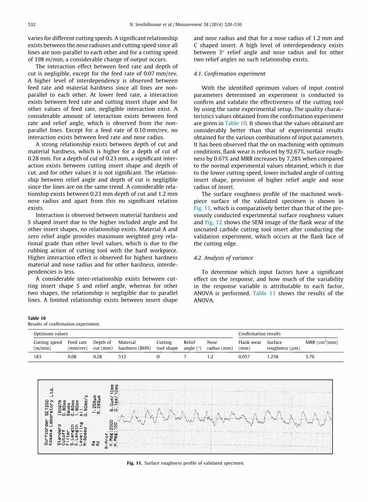
Table 10Results of confirmation experiment.

Optimum values

Cutting speed(m/min)

Feed rate(mm/rev)

Depth ofcut (mm)

Materialhardness (BHN)

Cuttingtool shape

Relieangl

183 0.08 0.28 512 D 7

Fig. 11. Surface roughness profi

and nose radius and that for a nose radius of 1.2 mm andC shaped insert. A high level of interdependency existsbetween 3� relief angle and nose radius and for othertwo relief angles no such relationship exists.

4.1. Confirmation experiment

With the identified optimum values of input controlparameters determined an experiment is conducted toconfirm and validate the effectiveness of the cutting toolby using the same experimental setup. The quality charac-teristics values obtained from the confirmation experimentare given in Table 10. It shows that the values obtained areconsiderably better than that of experimental resultsobtained for the various combinations of input parameters.It has been observed that the on machining with optimumconditions, flank wear is reduced by 92.67%, surface rough-ness by 0.67% and MRR increases by 7.28% when comparedto the normal experimental values obtained, which is dueto the lower cutting speed, lower included angle of cuttinginsert shape, provision of higher relief angle and noseradius of insert.

The surface roughness profile of the machined work-piece surface of the validated specimen is shown inFig. 11, which is comparatively better than that of the pre-viously conducted experimental surface roughness valuesand Fig. 12 shows the SEM image of the flank wear of theuncoated carbide cutting tool insert after conducting thevalidation experiment, which occurs at the flank face ofthe cutting edge.

4.2. Analysis of variance

To determine which input factors have a significanteffect on the response, and how much of the variabilityin the response variable is attributable to each factor,ANOVA is performed. Table 11 shows the results of theANOVA.

Confirmation results

fe (�)

Noseradius (mm)

Flank wear(mm)

Surfaceroughness (lm)

MRR (cm3/min)

1.2 0.057 1.258 3.76

le of validated specimen.

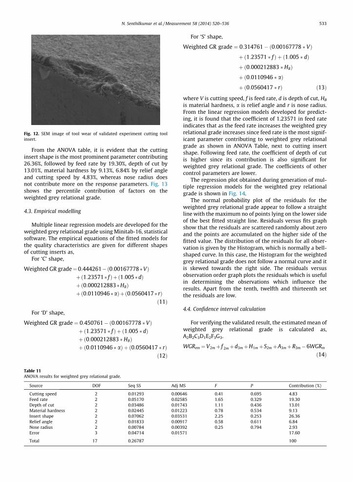
Fig. 12. SEM image of tool wear of validated experiment cutting toolinsert.

N. Senthilkumar et al. / Measurement 58 (2014) 520–536 533

From the ANOVA table, it is evident that the cuttinginsert shape is the most prominent parameter contributing26.36%, followed by feed rate by 19.30%, depth of cut by13.01%, material hardness by 9.13%, 6.84% by relief angleand cutting speed by 4.83%, whereas nose radius doesnot contribute more on the response parameters. Fig. 13shows the percentile contribution of factors on theweighted grey relational grade.

4.3. Empirical modelling

Multiple linear regression models are developed for theweighted grey relational grade using Minitab-16, statisticalsoftware. The empirical equations of the fitted models forthe quality characteristics are given for different shapesof cutting inserts as,

For ‘C’ shape,

Weighted GR grade¼ 0:444261�ð0:00167778�VÞþ ð1:23571� f Þþ ð1:005�dÞþ ð0:000212883�HBÞþ ð0:0110946�aÞþ ð0:0560417� rÞ

ð11Þ

For ‘D’ shape,

Weighted GR grade ¼ 0:450761� ð0:00167778 � VÞþ ð1:23571 � f Þ þ ð1:005 � dÞþ ð0:000212883 �HBÞþ ð0:0110946 � aÞ þ ð0:0560417 � rÞ

ð12Þ

Table 11ANOVA results for weighted grey relational grade.

Source DOF Seq SS Adj M

Cutting speed 2 0.01293 0.006Feed rate 2 0.05170 0.025Depth of cut 2 0.03486 0.017Material hardness 2 0.02445 0.012Insert shape 2 0.07062 0.035Relief angle 2 0.01833 0.009Nose radius 2 0.00784 0.003Error 3 0.04714 0.015

Total 17 0.26787

For ‘S’ shape,

Weighted GR grade ¼ 0:314761� ð0:00167778 � VÞ

þ ð1:23571 � f Þ þ ð1:005 � dÞ

þ ð0:000212883 � HBÞ

þ ð0:0110946 � aÞ

þ ð0:0560417 � rÞ ð13Þ

where V is cutting speed, f is feed rate, d is depth of cut, HB

is material hardness, a is relief angle and r is nose radius.From the linear regression models developed for predict-ing, it is found that the coefficient of 1.23571 in feed rateindicates that as the feed rate increases the weighted greyrelational grade increases since feed rate is the most signif-icant parameter contributing to weighted grey relationalgrade as shown in ANOVA Table, next to cutting insertshape. Following feed rate, the coefficient of depth of cutis higher since its contribution is also significant forweighted grey relational grade. The coefficients of othercontrol parameters are lower.

The regression plot obtained during generation of mul-tiple regression models for the weighted grey relationalgrade is shown in Fig. 14.

The normal probability plot of the residuals for theweighted grey relational grade appear to follow a straightline with the maximum no of points lying on the lower sideof the best fitted straight line. Residuals versus fits graphshow that the residuals are scattered randomly about zeroand the points are accumulated on the higher side of thefitted value. The distribution of the residuals for all obser-vation is given by the Histogram, which is normally a bell-shaped curve. In this case, the Histogram for the weightedgrey relational grade does not follow a normal curve and itis skewed towards the right side. The residuals versusobservation order graph plots the residuals which is usefulin determining the observations which influence theresults. Apart from the tenth, twelfth and thirteenth setthe residuals are low.

4.4. Confidence interval calculation

For verifying the validated result, the estimated mean ofweighted grey relational grade is calculated as,A2B2C3D1E2F3G3.

WGRem ¼V2mþ f 2mþd3mþH1mþS2mþA3mþR3m�6WGRm

ð14Þ

S F P Contribution (%)

46 0.41 0.695 4.8385 1.65 0.329 19.3043 1.11 0.436 13.0123 0.78 0.534 9.1331 2.25 0.253 26.3617 0.58 0.611 6.8492 0.25 0.794 2.9371 17.60

100

Fig. 13. Percentile contributions of factors on weighted grey relational grade.

0.20.10.0-0.1-0.2

99

90

50

10

1

Residual

Per

cent

0.70.60.5

0.1

0.0

-0.1

Fitted Value

Res

idua

l

0.100.050.00-0.05-0.10-0.15

4.8

3.6

2.4

1.2

0.0

Residual

Fre

quen

cy

18161412108642

0.1

0.0

-0.1

Observation Order

Res

idua

lNormal Probability Plot Versus Fits

Histogram Versus Order

Residual Plots for Weighted Grey Relational Grade

Fig. 14. Residual plot of weighted grey relational grade during regression modelling.

534 N. Senthilkumar et al. / Measurement 58 (2014) 520–536

where,WGRem = Estimated mean of weighted grey relationalgrade.V2m = Mean weighted grey relational gradecorresponding to cutting speed, V2.f2m = Mean weighted grey relational gradecorresponding to feed rate, f2.d3m = Mean weighted grey relational gradecorresponding to depth of cut, d3.H1m = Mean of weighted grey relational gradecorresponding to material hardness, H1.S2m = Mean weighted grey relational gradecorresponding to cutting insert shape, S2.A3m = Mean weighted grey relational gradecorresponding to relief angle, A3.

R3m = Mean weighted grey relational gradecorresponding to nose radius, R3.WGRm = Overall mean of weighted grey relational grade.

From Table 5, the mean values for the above parametersare calculated and substituting in Eq. (13).

WGRem ¼ 0:642þ 0:685þ 0:679þ 0:668þ 0:665þ 0:657þ 0:647� ð6 � 0:617Þ ¼ 0:941:

A confidence interval (CI) [20] for the prediction ofmean of weighted grey relational grade on a confirmationtest for the linear regression model is calculated as,

CI ¼

ffiffiffiffiffiffiffiffiffiffiffiffiffiffiffiffiffiffiffiffiffiffiffiffiffiffiffiffiffiffiffiffiffiffiffiffiffiffiffiffiffiffiffiffiF0:05ð3; f eÞVe

1nþ 1

R

� �sð15Þ

N. Senthilkumar et al. / Measurement 58 (2014) 520–536 535

where,

fe

Error degrees of freedom (3) fromTable 10

F0.05 (3, fe)

F ratio required for risk (3, 3) = 9.28 fromstandard ‘‘F’’ table

Ve

Error variance (0.01571) from Table 10 R Number of repetitions for confirmation

test (3)

N Total number of experiments

(nr � number of experiments)

=1 � 18 = 18 where nr � Number of replications (1)

n

Effective number of replications =N/(1 + degrees of freedom associatedwith weighted grey relational gradefrom Table 10) =18/(1 + 17) =1

From the above relations, the value of confidence interval(CI) for weighted grey relational grade of linear regressionmodel is calculated as,

CI ¼ f9:28� 0:01571½ð1=1Þ þ ð1=1Þ�g1=2 ¼ 0:54:

The 95% confidence interval of the optimal weightedgrey relational grade in confirmation test is,

ðWGRem � CIÞ < WGRcon < ðWGRem þ CIÞ ð16Þ

The result of confirmation test shows that the weightedgrey relational grade lies in between (WGRem � CI) and(WGRem + CI). (i.e., 0.757 lies in between 0.401 and1.481). The validated weighted grey relational grade is thusconfirmed by the above calculations.

5. Conclusion

The following conclusions have been made during turn-ing practically used wheel axle materials with carbideinserts having varying geometries by applying Taguchi-grey relational analysis.

1. Experimental results shows that a cutting speed of183 m/min, feed rate of 0.08 mm/rev, depth of cut of0.28 mm, material hardness of 512 BHN, cutting insertshape of ‘D’ (Diamond 55�), relief angle of 7� and noseradius of 1.2 mm provide the optimum parametric con-dition during turning automobile axles by employingmulti-criteria optimization using grey relationalanalysis.

2. Based on ANOVA results, cutting insert shape (includedangle) is the most dominant parameter contributing by26.36% while feed rate has an effect of 19.30% and depthof cut by 13.01%.

3. From the interaction plot, a considerable interactioneffect is observed between feed rate and other inputparameters and also in between depth of cut and mate-rial hardness and between other parameters the inter-action is not significant.

4. Confirmation experiment performed with the optimumconditions shows a reduction in flank wear by 92.67%,surface roughness by 0.67% with an increase in MRRby 7.28% which shows an improvement in outputresponses by varying the carbide insert geometry.

5. Prediction of weighted grey relational grade is carriedout by the developed empirical model using multiplelinear regression models for individual cemented car-bide insert shapes.

6. The reliability of the weighted grey relational grade isdetermined by calculating the confidence interval. The95% confidence interval of the weighted grey relationalgrade obtained from confirmation test is found to bewithin the limits.

Acknowledgements

The authors thank Madras Institute of Technology, AnnaUniversity –Chennai and ATC Tools Pvt. Ltd., Chennai fortheir support to carry out the research work.

References

[1] Edward Trent, Paul Wright, Metal Cutting, fourth ed., ButterworthHeinemann, USA, 2000.

[2] V.P. Astakhov, Machining of hard materials – definitions andindustrial applications, in: J. Paulo Davim (Ed.), Machining of Hardmaterials, Springer, London, Dordrecht, Heidelberg, New York, 2011,pp. 1–32.

[3] N. Senthilkumar, T. Tamizharasan, Effect of tool geometry in turningAISI 1045 steel: experimental investigation and FEM analysis, Arab. J.Sci. Eng. 39 (6) (2014) 4963–4975.

[4] Adeel H. Suhail, N. Ismail, S.V. Wong, N.A. Abdul Jalil, SurfaceRoughness Identification Using the Grey Relational Analysis withMultiple Performance Characteristics in Turning Operations, Arab. J.Sci. Eng. 37 (4) (2012) 1111–1117.

[5] Bala Murugan Gopalsamy, Biswanath Mondal, Sukamal Ghosh,Optimisation of machining parameters for hard machining: greyrelational theory approach and ANOVA, Int. J. Adv. Manuf. Technol.45 (2009) 1068–1086.

[6] C. Ahilan, S. Kumanan, N. Sivakumaran, Application of grey basedTaguchi method in multi-response optimization of turning process,Adv. Prod. Eng. Manage. 5 (3) (2010) 171–180.

[7] C.L. Lin, Use of the Taguchi method and grey relational analysis tooptimize turning operations with multiple performancecharacteristics, Mater. Manuf. Processes 19 (2) (2004) 209–220.

[8] Chorng-Jyh Tzeng, Yu-Hsin Lin, Yung-Kuang Yang, Ming-Chang Jeng,Optimization of turning operations with multiple performancecharacteristics using the Taguchi method and grey relationalanalysis, J. Mater. Process. Technol. 209 (2009) 2753–2759.

[9] L.B. Abhang, M. Hameedullah, Determination of optimum parametersfor multi-performance characteristics in turning by using greyrelational analysis, Int. J. Adv. Manuf. Technol. 63 (2012) 13–24.

[10] S. Ranganathan, T. Senthilvelan, Multi-response optimization ofmachining parameters in hot turning using grey analysis, Int. J. Adv.Manuf. Technol. 56 (2011) 455–462.

[11] Raju Shrihari Pawade, Suhas S. Joshi, Multi-objective optimization ofsurface roughness and cutting forces in high-speed turning ofInconel 718 using Taguchi grey relational analysis (TGRA), Int. J.Adv. Manuf. Technol. 56 (2011) 47–62.

[12] T. Tamizharasan, N. Senthilkumar, Analysis of surface roughness andmaterial removal rate in turning using Taguchi’s technique, in:International Conference on Advances in Engineering, Science andManagement, Nagapattinam, 2012, pp. 231–236.

[13] S. Patil, Nitin K. Kamble, S.S. Sarnobat, Multi-response optimizationof hot machining process using grey relational analysis (GRA)method, Indian J. Appl. Res. 3 (10) (2013) 1–6.

[14] B. Satyanarayana, G. Ranga Janardhana, D. Hanumantha Rao,Optimized high speed turning of Inconel 718 using Taguchimethod based grey relational analysis, Indian J. Eng. Mater. Sci. 20(2013) 269–275.

536 N. Senthilkumar et al. / Measurement 58 (2014) 520–536

[15] Meenu Gupta, Surinder Kumar, Multi-objective optimization ofcutting parameters in turning using grey relational analysis, Int. J.Ind. Eng. Comput. 4 (2013) 547–558.

[16] T. Tamizharasan, N. Senthilkumar, Optimization of cutting insertgeometry using DEFORM-3D: numerical simulation andexperimental validation, Int. J. Simul. Modell. 11 (2) (2012) 65–76.

[17] Farhad Kolahan, Reza Golmezerji, Masoud Azadi Moghaddam, MultiObjective optimization of turning process using grey relationalanalysis and simulated annealing algorithm, Appl. Mech. Mater.110–116 (2012) 2926–2932.

[18] T. Tamizharasan, N. Senthilkumar, Numerical simulation of effects ofmachining parameters and tool geometry using DEFORM-3D:optimization and experimental validation, World J. Modell. Simul.10 (1) (2014) 49–59.

[19] N. Senthilkumar, T. Tamizharasan, Experimental investigation ofcutting zone temperature and flank wear correlation in turning AISI1045 steel with different tool geometries, Indian J. Eng. Mater. Sci.21 (2) (2014) 139–148.

[20] Mohamed Elbah, Mohamed Athmane Yallese, Hamdi Aouici, TarekMabrouki, Jean-Francois Rigal, Comparative assessment of wiperand conventional ceramic tools on surface roughness in hard turningAISI 4140 steel, Measurement 46 (9) (2013) 3041–3056.

[21] Serope Kalpakjian, Steven R. Schmid, Manufacturing Engineeringand Technology, Prentice-Hall, 2001.

[22] B.L. Juneja, Nitin Seth, Fundamentals of Metal Cutting and MachineTools, New Age International (P) Limited, New Delhi, 2005.

[23] Haci Saglam, Suleyman Yaldiz, Faruk Unsacar, The effect of toolgeometry and cutting speed on main cutting force and tool tiptemperature, Mater. Des. 28 (2007) 101–111.

[24] Ilhan Asilturk, Harun Akkus, Determining the effect of cuttingparameters on surface roughness in hard turning using theTaguchi method, Measurement 44 (9) (2011) 1697–1704.

[25] Ranjit K. Roy, Design of Experiments using the Taguchi Approach: 16Steps to Product and Process Improvement, John Wiley & Sons, USA,2001.

[26] P.J. Ross, Taguchi Techniques for Quality Engineering: Loss Function,Orthogonal Experiments, Parameter and Tolerance Design, seconded., McGraw-Hill, NewYork, 1996.

[27] G. Kibria, B. Doloi, B. Bhattacharyya, Experimental investigation andmulti-objective optimization of Nd:YAG laser micro-turning processof alumina ceramic using orthogonal array and grey relationalanalysis, Opt. Laser Technol. 48 (2013) 16–27.

[28] Yigit Kazancoglu, Ugur Esme, Melih Bayramoglu, Onur Guven, SuedaOzgun, Multi-Objective optimization of the cutting forces in turningoperations using the grey-based Taguchi method, Mater. Technol. 45(2) (2011) 105–110.

[29] Ronald A. Walsh, Handbook of Machining and MetalworkingCalculations, McGraw-Hill, USA, 2001.

[30] N. Senthilkumar, T. Tamizharasan, V. Anandakrishnan, An hybridTaguchi-grey relational technique and cuckoo search algorithm formulti-criteria optimization in hard turning of AISI D3 steel, J. Adv.Eng. Res. 1 (1) (2014) 16–31.

[31] Meenu Gupta, Surinder Kumar, Multi-objective optimization ofcutting parameters in turning using grey relational analysis, Int. J.Ind. Eng. Comput. 4 (2013) 547–558.

[32] Radhakrishnan Ramanujam, Nambi Muthukrishnan, RamasamyRaju, Optimization of cutting parameters for turning Al–SiC(10p)MMC using ANOVA and grey relational analysis, Int. J. Prec. Eng.Manuf. 12 (2011) 651–656.

[33] Upinder kumar, Deepak Narang, Optimization of cutting parametersin high speed turning by grey relational analysis, Int. J. Eng. Res.Appl. 3 (1) (2013) 832–839.

[34] Douglas C. Montgomery, Design and Analysis of Experiments, eighthed., John Wiley & Sons Inc, USA, 2013.

[35] Glenn Gamst, Lawrence S. Meyers, A.J. Guarino, Analysis of VarianceDesigns – A Conceptual and Computational Approach with SPSS andSAS, Cambridge University Press, Cambridge, UK, 2008.

[36] Douglas C. Montgomery, George C. Runger, Applied Statistics andProbability for Engineers, fifth ed., John Wiley & Sons, Inc., 2011.