Experiment and simulation of micro injection molding and ...
155
HAL Id: tel-01345738 https://tel.archives-ouvertes.fr/tel-01345738 Submitted on 15 Jul 2016 HAL is a multi-disciplinary open access archive for the deposit and dissemination of sci- entific research documents, whether they are pub- lished or not. The documents may come from teaching and research institutions in France or abroad, or from public or private research centers. L’archive ouverte pluridisciplinaire HAL, est destinée au dépôt et à la diffusion de documents scientifiques de niveau recherche, publiés ou non, émanant des établissements d’enseignement et de recherche français ou étrangers, des laboratoires publics ou privés. Experiment and simulation of micro injection molding and microwave sintering Jianjun Shi To cite this version: Jianjun Shi. Experiment and simulation of micro injection molding and microwave sintering. Me- chanical engineering [physics.class-ph]. Université de Franche-Comté; Southwest Jiatong University, 2014. English. NNT : 2014BESA2064. tel-01345738
-
Upload
khangminh22 -
Category
Documents
-
view
2 -
download
0
Transcript of Experiment and simulation of micro injection molding and ...

HAL Id: tel-01345738https://tel.archives-ouvertes.fr/tel-01345738
Submitted on 15 Jul 2016
HAL is a multi-disciplinary open accessarchive for the deposit and dissemination of sci-entific research documents, whether they are pub-lished or not. The documents may come fromteaching and research institutions in France orabroad, or from public or private research centers.
L’archive ouverte pluridisciplinaire HAL, estdestinée au dépôt et à la diffusion de documentsscientifiques de niveau recherche, publiés ou non,émanant des établissements d’enseignement et derecherche français ou étrangers, des laboratoirespublics ou privés.
Experiment and simulation of micro injection moldingand microwave sintering
Jianjun Shi
To cite this version:Jianjun Shi. Experiment and simulation of micro injection molding and microwave sintering. Me-chanical engineering [physics.class-ph]. Université de Franche-Comté; Southwest Jiatong University,2014. English. NNT : 2014BESA2064. tel-01345738

Prepared and presented at
L’U.F.R. DES SCIENCES ET TECHNIQUES DE L’UNIVERSITÉ DE FRANCHE-COMTE
In order to obtain the
GRADE DE DOCTEUR DE L’UNIVERSITÉ DE FRANCHE-COMTE Spécialité: Génie Mécanique
Experiment and Simulation of Micro-Injection Molding and Microwave Sintering
Expérimentation et Simulation de Micro-Moulage par Injection et Frittage par Micro Onde
Jianjun SHI
Defence on 5 May 2014, defence committee:
Chairman X-G. ZENG Professor, Sichuan University, China Advisor J-C. GELIN Professor, Ecole Nationale Supérieure de Mécanique et des
Microtechniques, Besançon B-S. LIU Professor, Southwest Jiaotong University, China
Co-Advisor T. BARRIERE Professor, Université de Franche-Comté Z-Q. CHENG Professor, Université de Franche-Comté
Reviewers F. CHINESTA Professor, Universités à l’Ecole Centrale de Nantes J-M. BERGHEAU Professor, Ecole Nationale d’Ingénieurs de Saint Etienne
F. VALDIVIESO HDR, Ecole Nationale Supérieure des Mines de St-Etienne
Examinators Z-Q. FENG Professor, Université Evry Val d'Essonne J-H. ZHANG Professor, Sichuan University, ChinaL-X. CAI Professor, Southwest Jiaotong University, ChinaH. ZHAO Professor, Southwest Jiaotong University, China
É c o l e d o c t o r a l e s c i e n c e s p o u r l’ i n g é n i e u r e t m i c r o t e c h n i q u e s
U N I V E R S I T É D E F R A N C H E - C O M T É
Thèse de Doctorat

Classified Index: O345 U.D.C: 621
Southwest Jiaotong University & Franche-Comte University
Doctor Degree Dissertation
EXPERIMENT AND SIMULATION OF MICRO
INJECTION MOLDING AND MICROWAVE
SINTERING
Grade: 2009
Candidate: SHI Jianjun
Academic Degree Applied for: Doctor of Engineering
Speciality: Engineering Mechanics
Supervisor: LIU Baosheng, Jean-Claude GELIN
March, 2014

Université de Franche-Comté I
Declaration of initiative work for Ph.D. degree
The author hereby solemnly declares that: the present submitted doctoral thesis is the
result of researches works carried out independently under the guidance of tutors. Besides
the contents of references already mentioned, this thesis does not contain any other
individual or collective research result that has been published or authored. Individual and
collective contributions of this thesis have been clearly been mentioned in the thesis content.
The author is fully aware of the legal consequences resulting from this statement.
The main innovations of the thesis are as follows:
(1) To improve the existing filling algorithm, for modification of the untrue filling
patterns in previous in-house software and commercial software when modeling some
specific cases, a numerical algorithm similar to upwind method is proposed to strengthen the
advection effect of filling flow behind the filling front. In addition, a special algorithm is
suggested to ensure the linear filling pattern of incompressible flow when given a constant
injection velocity, by imposing reasonable outlet boundary conditions in the calculation
model.
(2) The effect of surface tension force is taken into account in micro-injection molding
simulation. Because there is no appropriate algorithm in finite element method for surface
tension calculation, a simple and systematic operation is proposed and conformed in present
thesis. The modeling results indicate that the effect of surface tension represents the
significant importance in micro-injection molding process.
(3) Experiments and discoveries of microwave sintering: Implementation of microwave
sintering experiment on 17-4PH stainless steel powder, some special results has been
detected in present thesis. The author conforms that all the superiorities of microwave
sintering relative to the traditional sintering also apply to 17-4PH stainless steel powder.
Moreover, because of its rapid heating in the internal volumetric way, microwave sintering
results in the obvious gradient in mechanic properties of the sintered material.

Université de Franche-Comté II
(4) Development of the simulation for multi-physics coupling phenomena in
microwave sintering: The sintering constitution of powder impacts is planted into the
calculation of microwave heating and heat transfer. Based on modeling and simulation of
conventional sintering, and together with the principles of electromagnetic fields,
thermodynamics and continuum mechanics, the method for multi-physics coupling
simulation is built, including the sequenced calculations from distribution of the
electromagnetic field to the densification of sintered compacts.
Signature of author: Date

Université de Franche-Comté III
Abstract
Powder Injection molding process consists of four main stages: feedstock preparation,
injection molding, debinding and sintering. The thesis presents the research on two main
aspects: micro-injection molding and microwave sintering. The main contributions can be
concluded in the following four aspects: Modification and supplement of previous algorithm
for the simulation of injection molding process; Evaluation and implementation of surface
tension effect for micro injection; Microwave sintering experiments of compacts based on
17-4PH stainless steel; Realization of the microwave sintering simulation with the coupling
of multi-physics, including the classic microwave heating, heat transfer, and the supplement
of model for sintering densification of powder impacts.
For the improvement of filling simulation, the present study modifies the explicit
vectorial algorithm for simulation of injection filling process. The wrongly directed filling
patterns in actual commercial software have been improved, by the implementation of a
suggested scheme, which is similar to upwind method. A reasonable numerical method
relative to the outlet boundary condition is suggested to overcome the untrue delay of fully
filling in the last filling stage. The results from these two modified algorithms are proved to
be optimized and more reliable.
For extending the in-house FEM software into the scope of micro injection, surface
tension effect is taken into account in the injection molding simulation. Due to the lack of
appropriate FEM method for curvature calculation, the present work proposed a systematic
algorithm for implementation of the surface tension effect in finite element method. By the
example of filling in micro channels, it indicates that the effect of surface tension shows the
importance for the projects in sub-millimeter sizes, but does not represent the significant
effect in ordinary injection molding.
For microwave sintering of 17-4PH stainless steel powder, compared to the previous
reports, some new discoveries have been found in the experiments. The author conform that
the microwave sintering process for 17-4PH stainless steel can not only shorten greatly the
sintering time, lower the peak sintering temperature, but also it provides higher sintered
density and fewer defects in micro structure. Higher Vickers-hardness of microwave sintered
compacts is also detected in the present work. Moreover, because of its rapid heating in the
internal volumetric way, microwave sintering results in the obvious gradient in mechanic
properties of the sintered material.
Microwave sintering represents the coupling of multi-physics in electro-magnetic fields,
heat generation, thermal conduction, and densification process of the powder compacts in
sintering. The existing researches focuses on the studies of microwave heating and heat

IV Université de Franche-Comté
transfer, which couples with the evaluation of electromagnetic field, but none of them
includes the densification behaviors of powder material. Bases on the sintering constitution
of powder impacts, the mathematical model and simulation method for whole of the
microwave sintering phenomena, from distribution of the electromagnetic field to the
densification of sintered compacts, are determined in the present thesis. The simulation of
microwave sintering process can be realized on the FEM platform of COMSOL
Multi-physics. This work provides a reliable way for the further investigations on microwave
sintering.
Key words Micro-Injection Molding, Microwave Sintering, surface tension effect, 17-4PH
stainless steel powder, Numerical Simulation, Multi-physics

Université de Franche-Comté V
Résumé
Procédé de moulage par injection de poudres est constitué de quatre étapes principales:
la préparation des matières premières, moulage par injection, le déliantage et le frittage.
Cette thèse présente les recherches sur deux aspects principaux: la micro-injection et frittage
par micro-ondes. Les contributions principaux peuvent être conclues dans les quatre aspects
suivants: Modification et complément de l'algorithme précédent pour la simulation du
procédé de moulage par injection; L'évaluation et la mise en oeuvre de l'effet de tension de
surface pour micro-injection; Micro-ondes expériences de frittage de compacts basés sur
l'acier inoxydable 17-4PH; Réalisation de la simulation de frittage à micro-ondes avec
couplage de la multi-physique, y compris le chauffage à micro-ondes classique, le transfert
de chaleur, et le supplément de modèle pour la densification de frittage de la poudre
compacté.
Pour l'amélioration de simulation de remplissage, l‘étude présenté a modifié
l'algorithme vectoriel explicite pour la simulation de procédés de remplissage par injection.
Les motifs de remplissage dirigés à tort dans les logiciels actuelles commerciaux ont été
améliorées, par la mise en œuvre d'un schème proposé, qui est similaire à la méthode contre
le vent. Une méthode numérique raisonnable pour la condition de limite àla sortie est
proposé. Le retard de pleine remplissage à la dernière phase d’injection est donc surmonté.
Les résultats de ces deux algorithmes modifiés sont avérés être optimisé et plus fiable.
Pour étendre le logiciel interne FEM dans le champ d'application de micro-injection,
l'effet de la tension de surface est prise en compte lors de la simulation de moulage par
injection. En raison de l'absence de méthode appropriée des éléments finis pour le calcul de
courbure, le présent travail a proposé un algorithme pour la mise en oeuvre systématique de
l'effet de tension de surface dans la méthode des éléments finis. Par l'exemple de remplissage
à micro-canaux, il indique que l'effet de la tension superficielle montre l'importance pour les
projets dans les tailles des sous-millimétriques, mais ne représente pas l'effet significatif dans
le moulage par injection ordinaire.
Pour les micro-ondes frittage de poudre d'acier inoxydable 17-4PH, par rapport aux
rapports précédents, certaines nouvelles découvertes ont été trouvées dans les expériences.
L'auteur confirme que le procédé de frittage par micro-ondes pour l'acier inoxydable 17-4PH,
peut non seulement raccourcir considérablement le temps de frittage, baisser la sommet de
temperature de frittage, mais il fournit également une densité frittée supérieure et moins de
défauts de micro structure. Supérieur Vickers dureté de comprimés micro-ondes frittés est
également détectée dans le présent ouvrage. En outre, en raison de son chauffage rapide par
un moyenne interne volumétrique, les résultats de frittage par micro-ondes internes
conduisent au gradient manifeste dans les propriétés mécaniques du matériau fritté.

VI Université de Franche-Comté
Micro-ondes frittage représente le couplage multi-physique dans les champs
électro-magnétiques, la production de chaleur, conduction thermique, et le processus de
densification des poudres en frittage. Les recherches actuelles se concentrent sur les études
de chauffage par micro-ondes et un transfert de chaleur, qui couple avec l'évaluation du
champ électromagnétique, mais aucun d'entre eux comprennent les comportements de
densification du matériau poudre. Bases sur le comportement de frittage des poudres
compactés, le modèle mathématique et méthode de la simulation pour ensemble des
phénomènes de frittage micro-ondes, depuis la distribution du champ électromagnétique et à
la densification du corps frittés, sont déterminés dans la présente thèse. La simulation de
procédé de frittage par micro-ondes peut être réalisé sur la plate-forme FEM de COMSOL
Multi-physics. Ce travail fournit un moyen fiable pour les enquêtes sur micro-ondes frittage
plus profondément.
Mots clés: La Micro-Injection, Micro-ondes Frittage, L'effet de la Tension de Surface,
Poudre d'acier Inoxydable 17-4PH, Simulation Numérique, Multi-physiques

Université de Franche-Comté VII
Glossary
CAGR: Compound Annual Growth Rate
CCIM Cemented Carbide Injection Molding
CIM Ceramic Injection Molding
CLSVOF: Coupled Level Set and Volume of Fluid
CSF: Continuum Surface Force
CRH: Conventional Resistive Heating
FEM Finite Element Method
FVM: Finite Volume Method
FDM: Finite Difference Method
FEMTO-ST: Franche-Comté Electronique Mécanique Thermique et Optique –
Sciences et Technologies
FDTD: Finite Difference Time Domain
LS: level Set
MIM: Metal Injection Molding
MEMS: Micro-Electro-Mechanical Systems
MW: Microwave
PIM Powder Injection Molding
PP: Polypropylene
PW: Paraffin Wax
PLIC: Piecewise Linear Interface Construction
SWJTU: Southwest Jiaotong University
SUPG: Streamline Upwind Petrov Galerkin
SA: Stearic Acid
VOF: Volume of Fluid
Nomenclature
A assembling operation in finite element method
B derivative matrix of interpolation function N in an element
fC coefficient of tangent viscous load
pC specific heat coefficient of the feedstock (J/m/ºC)
aC specific heat coefficient of air (J/m/ºC)
ppC heat capacity (J/kg.ºC)

VIII Université de Franche-Comté
D divergence operator of velocity field
e element
E electric field (V/m)
eE elastic modulus (Pa)
F filling state variable
iF nodal values of filling state variable
FrtF filling state variable in the filling front
lowF the lowest value for defining the range of filling front
upF the up value for defining the range of filling front
σF viscous diffusion term
extF external force vector
dF incompressibility correction term
stF surface tension force (Pa)
bF body force in a thin layer of the front (Pa)
pF a prescribed value to identify the position of filling front
f tangent viscous load (Pa)
extf surface loads converted to the nodes on boundary (Pa)
*f kinematically admissible field associated to variable
G gradient operator constructed by derivatives of interpolation functions
PG shear viscosity modulus (Pa)
g gravity vector (m/s2)
H magnetic fields (A/m)
ph heat exchange coefficients of air (W/m/ºC)
ah heat exchange coefficients of feedstock (W/m/ºC)
I second order identity tensor
Kad stiffness matrix of advection effect for filling state and temperature field
Kdf stiffness matrix of diffusion effect for filling state and temperature field

Université de Franche-Comté IX
Kadv stiffness matrix of advection effect for velocity field
Ko operator for outlet surface integration term
PK bulk viscosity modulus (Pa)
pk thermal conductivity coefficient of the feedstock (W/m/ºC)
ak thermal conductivity coefficient of air (W/m/ºC)
k the upwind-stream node number
0M lumped pseudo matrix
M mass matrix lumped into diagonal form
m node number in an element
N matrix of interpolation function
outN nodes associated to outlet surface
iN interpolation functions
outn a unit vector normal to its edge or side e
outΓ
n unit of outward normal
P injected pressure on inlet boundary (Pa)
P hydraulic pressure field (Pa)
hP heat source (J)
iP nodal pressure values (Pa)
Q heat dissipation term (W.m)
cq heat convection term (J)
T Temperature ( )
iT nodal temperature values ( )
t unit vector of local tangent
t time increment (s)
V velocity vector (m/s)
IV injected velocity on inlet boundary (m/s)
iV nodal velocity vector (m/s)

X Université de Franche-Comté
eV velocity vector at each Gauss point in an element (m/s)
FV discretized value of velocity field at each node
F
eV the column of velocity values at all nodes of an elements
e
nV velocity vector in the element associated to e
outΓ (m/s)
nV norm of velocity vector (m/s)
∗nV velocity fields of temporary middle values (m/s)
X space position
XF position of filling front
sum of space position in entire model
F filled portion in mold cavity
V void portion in mould cavity
Frt filling front region
e
outΩ elements associated to node outN
I inlet of the mold
O outlet of the mold
S intersection of filled portion and void portion
W mold walls
e
outΓ edge or side of element e
outΩ on outlet boundary
pρ density value of feedstock (kg/m3)
aρ density value of air (kg/m3)
ρ density of the materials (kg/m3)
rρ relative density (kg/m3)
coefficient of surface tension
tσ stress tensor in sintered materials (Pa)
′ deviator of Cauchy stress tensor (Pa)
p′
deviator of Cauchy stress tensor in the filled portion (Pa)
a′ deviator of Cauchy stress tensor in the void portion (Pa)

Université de Franche-Comté XI
sσ sintering stress (Pa)
ECσ electric conductivity (S)
air electric conductivity of air (S)
σtr trace of the stress tensor
p strain rate of feedstock
a strain rate of air
rε relative complex permittivity (F/m)
'rε dielectric constant (F/m)
"rε dielectric losses factor (F/m)
(tr trace of total strain rate
tensor of total strain rate
e elastic strain rate
th thermal strain rate
vp viscoplastic strain rate
Fλ dilatation coefficient in filled portion Vλ
dilatation coefficient in void portion
curvature of filling front surface
ϕ signed distance function to the interface
)(x delta function concentrated at the interface
ω angular frequency of the microwave source (rad/s)
rµ relative complex permeability (H/m)
"rµ magnetic loss factor (H/m)
k thermal conductivity (W/(m.K))
α coefficient of thermal dilatation (m/K)
ν Poisson’s ratio

XII Université de Franche-Comté
Table of Contents
Introduction .............................................................................................................................. 1
Chapter 1 State of the art .......................................................................................................... 5
1.1 Brief introduction of PIM ............................................................................................... 5
1.2 The advantages of PIM ................................................................................................. 12
1.3 PIM development and market ....................................................................................... 13
1.4 The principal research centers in PIM processing ........................................................ 15
1.5 Researches on PIM process in France and in China ..................................................... 16
Chapter 2 Developments of modified algorithms for Mold Filling Process .......................... 19
2.1 Modeling and Simulation of PIM injection .................................................................. 20
2.1.1 General Definition .................................................................................................. 20
2.1.2 Governing Equations .............................................................................................. 22
2.1.3 Explicit algorithm for simulation ........................................................................... 25
2.2 Algorithm for improvement of wrongly adverted filling profile .................................. 33
2.2.1 The source for distorted simulation results ............................................................ 37
2.2.2 Modification of the solution procedure .................................................................. 38
2.2.3 Validation of the modification scheme .................................................................. 41
2.2.4 Conclusion .............................................................................................................. 45
2.3 The outlet condition in simulation of MIM injection to track the end of filling process
............................................................................................................................................ 46
2.3.1 The inexact result at the end of filling process ....................................................... 47
2.3.2 Modification of the outlet boundary condition ...................................................... 48
2.3.3 Validation of the modified algorithm ..................................................................... 50
2.3.4 Conclusion .............................................................................................................. 52
Chapter 3 Numerical method and analysis for surface tension effects in micro-injection
process .................................................................................................................................... 53
3.1 Mechanical modeling .................................................................................................... 58
3.2 Surface tension force..................................................................................................... 61
3.3 Implementation of Surface tension in FEM .................................................................. 61
3.3.1 Surface curvature computation ............................................................................... 62

Université de Franche-Comté XIII
3.3.2 Surface tension force in computation ..................................................................... 64
3.4 Numerical investigation and discussion ....................................................................... 66
3.5 Conclusion .................................................................................................................... 74
Chapter 4 Brief Introduction and Foundational Theories for Sintering ................................. 75
4.1 Introduction of sintering ............................................................................................... 75
4.1.1 Berif introduction of sintering ................................................................................ 75
4.2 Foundational Theories for Sintering ............................................................................. 78
4.2.1 Driving Forces of Sintering .................................................................................... 78
4.2.2 Sintering Mechanisms ............................................................................................ 80
4.2.3 Stages of Sintering ................................................................................................. 81
4.3 Models and Simulations of Sintering ........................................................................... 82
4.3.1 Simulation history .................................................................................................. 82
4.3.2 Three sintering models ........................................................................................... 83
Chapter 5 Efficient sintering of 17-4PH stainless steel powder by microwave ..................... 87
5.1 Research background .................................................................................................... 88
5.2 Experimental procedure ................................................................................................ 90
5.3 Results and discussion .................................................................................................. 92
5.3.1 Specimen sizes after being injected, debinded and MW sintered .......................... 92
5.3.2 The influence factors in MW sintering process ..................................................... 93
5.3.3 Microstructure ........................................................................................................ 97
5.3.4 Distribution of the Vickers-hardness ...................................................................... 99
5.3.5 Comparison with the conventional sintering ........................................................ 101
5.3.6 Conclusions .......................................................................................................... 104
Chapter 6 Mathematical Modeling and Simulation of Microwave Sintering Process ......... 105
6.1 Research Background ................................................................................................. 105
6.2 Mathematical model of microwave sintering ............................................................. 106
6.2.1 Solve Maxwell equation to get electromagnetic fields in cavity of the furnace .. 106
6.2.2 Solve for distribution of the heat generation in process of microwave sintering . 107
6.2.3 Solution of heat transfer equation to get temperature field in the sintered body . 107

XIV Université de Franche-Comté
6.2.4 Solve the governing equations of sintering densification to get the structural
response of sintered body .............................................................................................. 108
6.2.5 Coupling of the Maxwell equation, heat transfer equation and mechanic equations
112
6.3 Numerical simulation of microwave sintering process .............................................. 112
6.3.1 Modeling of Microwave Sintering ....................................................................... 112
6.3.2 Numerical analysis ............................................................................................... 115
6.4 Conclusion and outlook .............................................................................................. 119
Chapter 7 Conclusions and Perspectives .............................................................................. 121
7.1 Conclusions................................................................................................................. 121
7.2 Future Work ................................................................................................................ 123
Acknowledgment.................................................................................................................. 126
References ............................................................................................................................ 127

Université de Franche-Comté 1
Introduction
The PIM (Powder injection molding) industry is comprised of MIM (metal injection
molding), CIM (ceramic injection molding) and CCIM (cemented carbide injection molding).
This manufacturing process is very efficient for producing small, complex and intricate
components in large batch. Excellent mechanical properties and proper geometrical accuracy
can be obtained by this newly developed technology under a cost much lower than by the
traditional ones. These notable advantages make them a strong competitiveness in the market
of alloy die cast components. It creates a new market mainly for complex miniature
components. A diverse range of PIM products are used in the chemical, textile, aerospace,
automotive, electronic, medical and communications industries. Examples of the
components resulting from PIM process are related in the Fig. 1.
Fig. 1 Examples of macro and micro components from PIM process, including the shaft, gear,
screw, pin, etc.
The PIM technology combines the well-known polymer injection molding and powder
metallurgy technology. It consists of four sequential stages: mixing of the metallic and
ceramic powders with the thermoplastic binders to get the feedstock, injection molding of
the mixtures of feedstock in the mold die cavities, debinding of green parts to mostly remove
the binder and finally sintering of brown parts by solid state diffusion to get the densified
component.
The PIM process has already been focused and developed for several decades. Now for
satisfying the market requirement, this process draws more and more attention to realize the

2 Université de Franche-Comté
manufacturing of intricate structure, advance the miniaturization and reduce the waste of
energy by improving the production efficiency. Under this condition, how to achieve the
good dimensional accuracy and the desired mechanical properties is one of the key issues to
extend the application of PIM process. It is necessary to design the injection molds and
process according to the final properties of the components. In order to solve this inverse
problem, the trial and error method is often used. But the experimental tests are very
expensive to be carried out, and the period for the determination of process parameters is
generally long for the production of new components. Alternatively, numerical simulation is
a cost-effective way to optimize the PIM process design, which is viewed as computer
experiments.
However, although PIM theory has been developed for about 40 years, the physical
modeling and numerical simulation are far behind the practices. There remain some
persistent problems in the previous developing algorithm, which results in the untrue
injection filling patterns. And there is still much work to do in physical experiment for the
calibration of sintering constitutive for powder material, spatially when using the new
sintering way by microwave heating. So to promote the application, experimental and
numerical simulation researches for micro injection molding process and microwave
sintering process are presented in the present thesis. The itinerary of the study is organized as
follows:
In chapter 1, a brief introduction is made on the process of PIM manufacture, including
relative equipment used in the sequenced stages, the advantages of PIM technology, the
development and market analysis and the relative scientific research centers for European,
Asian and America regions.
In chapter 2, the explicit algorithm with fully vectorial operations for simulation of the
injection molding stag is introduced. This vectorial method was previously developed in
research team and there remains some unfavorable problems. The work in this chapter is
going to optimize the previous algorithm and in-house software. The author improves the
untrue distortion in simulation results when some specific runners in shape ⊥ and L are
involved, by the implementation of a suggested scheme. In addition, the untrue delay of
filling process when the cavity is near fully filled has been modified. A proposed method is

Université de Franche-Comté 3
realized to complement the boundary condition on outlet in simulation of the filling
advection. It is proved that these two modification works make the results of simulation
more stable and reliable.
In chapter 3, for extending the functionality of in-house software into the problems in
micro scales, the evaluation of surface tension effect in the injection molding simulation is
implementing by a specially proposed algorithm. Through analyzing the proportion of
surface tension force to viscous force in different mold sizes, the effects of surface tension in
micro injection molding process are evaluated.
Chapter 4 turns to the investigation of another PIM stage: sintering. The diverse
sintering methods and the foundational theories for sintering are briefly introduced. The
three sintering models for numerical simulation have been shown, including models in
microscopic, mesoscopic and macroscopic.
Chapter 5 makes experiment investigation of microwave sintering. As a new developing
technology, Microwave sintering is more and more accepted for its industrial values, which
shows significant advantages against conventional sintering procedures. So the research
team expands its research topics into microwave sintering field. The densification behaviors
of 17-4PH stainless steel powder under microwave sintering are chosen for experimental
investigations, because of its sole report and unfavorable conclusion. The relationship
between processing factors and the evolution behaviors of powder material is investigated by
experiments. The experimental researches will prove the results of microwave sintering for
17-4PH stainless steel powder, under the adequate conditions. The micro structure and
mechanic properties in the sintered bodies will be investigated. The distribution of mechanic
properties is measured to evaluation the effect of microwave heating and its special outcome
on the sintered products. The influences of peak sintering temperature, holding time, heating
rate and pre-sintering stages on densification behaviors of the powder material are
investigated. The evolutions of microstructure in the sintered components under different
sintering conditions are observed by the optical microscope. The Comparison between
microwave sintering and conventional sintering is also the interest of investigation.
Chapter 6 focuses on the investigation of numerical simulation method for microwave

4 Université de Franche-Comté
sintering process. It expands the actual sintering simulation from heat generation by
microwave and temperature evolution to the coupling of multi-physics for whole process.
The modeling and simulation includes the coupling effects from distribution of the
electro-magnetic fields to the densification of the sintered material. The developed
simulation realizes the coupling of electro-magnetic fields, heat generation by microwave
effects, heat conduction, and densification process of PIM materials. The last one is based on
the sintering model developed in research team. The prediction on evolution of sintering
shrinkage and distribution of relative density is achieved based on the coupling of different
physical phenomena. This work provides a reliable frame for further investigation of the
coupling among the evolution of different material properties during the course of sintering.

Université de Franche-Comté 5
Chapter 1 State of the art
1.1 Brief introduction of PIM
The PIM (Powder Injection molding) process is somewhat similar to plastic-injection
molding. It combines the well-known polymer injection molding and powder metallurgy
process. It consists of the following stages: feedstock preparation, injection molding,
debinding of green parts and sintering of brown parts [1]. The PIM process can be stated in
Fig. 1-1.
Fig. 1-1 The sequential stages to get the final sintered components [2]. The sintering stage
may be processed by Conventional Resistive Heating or Microwave sintering ways.
As showed in Fig. 1-1, feedstock formed by metallic or ceramic powder and
thermoplastic binder are prepared and pelletized for injection. Then by using a standard
injection-molding process, the polymer-powder mixture is melted and injected into a die
cavity under pressure, where it cools and solidifies into the shape of the desired part.
Subsequent thermal, solvent or catalytic debinding processes remove the unwanted polymer
binder and get a shaped metallic component in porous state. Lastly the brown parts are
sintered to get the high-density products in pure metallic or ceramic material.
1) Feedstock preparation stage
In this preliminary state, very fine metallic or ceramic powder are mixed with

6 Université de Franche-Comté
thermoplastic polymer (known as the binder) to form a homogeneous mixture of ingredients
that is pelletized and can be fed directly into an injection molding process. This pelletized
powder-polymer mixture is known as feedstock [3]. Generally, the grain size of the powder
may vary from 2 to 20 µm with near spherical shapes. The elaboration of a successful
feedstock balances several considerations [3, 4]. It is expect that the feedstock can be as
condensed as possible to avoid a large sintering shrinkage. Formulations with high powder
contents have the advantages such as: Closer dimensional control leading to tighter
tolerances; Reduced probability of distortion during debinding; Improved handling strength
after debinding; Reduction of debinding time; Reduced grain growth; Improved structural
integrity. However, reducing the proportion of binder can also cause the difficulties. It
usually has an adverse effect on the rheology of the material being injected into the mold [5].
Most problems in PIM are caused by a poor appreciation of component-rheology and
thermal-rheology interactions. To enhance the process, the portion of powder loading must
be maximized without scarifying the rheology. PIM compositions should ideally have low
viscosity. At the meantime, it should also have low Herschel Buckley attribute yield stress
and pseudo-plastic or shear-thinning characteristics [6]. The behavior similar to that of the
toothpaste is generally desirable. The feedstock mixing equipment used in FEMTO-ST
institute in France is shown in Fig. 1-2. The one used in the lab of Southwest Jiaotong
University (SWJTU) is shown in Fig. 1-3. Both of them are using twin-screw mixer.
Fig. 1-2 Brabender® twin-screw mixer W 50 EHT, a) general view of the mixer; b) assembly
of mixing equipment; c) the two mixer blades and their counter-rotation towards each other

Université de Franche-Comté 7
a) b)
Fig. 1-3 Torque rheometer (XSS-300) used in the lab of SWJTU: a) general view of the
mixer; b) general view of the mixing chamber
The main parameters of these two mixers are indicated below:
Technical specifications Brabender® twin-screw mixer (FEMTO-ST)
Torque rheometer XSS-300 (SWJTU)
mixing temperature 20 to 500 °C 20 to 400 °C
mixing speed 0 to 120 rpm 2 to 120 rpm
maximal mixing torque 150 N.m 300 N.m
volume of mixer bowl 55 cm3 60 cm3
2) Injection molding stage
This stage includes the injection molding of feedstock and the removal of green parts
from the mold [7, 8]. A schematic cycle of the injection molding is shown in Fig. 1-4, which is
the same equipment and tooling that are used in plastic injection molding, but it needs higher
wearing resistance. In the injection molding stage, the feedstock is injected into the mold
cavities under a certain pressure about 60 MPa or more. The pressure is maintained on the
feedstock during the cooling until it solidifies at the gates. Then the component is ejected
and another new cycle can be repeated. The injection equipment used in FEMTO-ST and
SWJTU is shown in Fig. 1-5.
8 Université de Franche-Comté
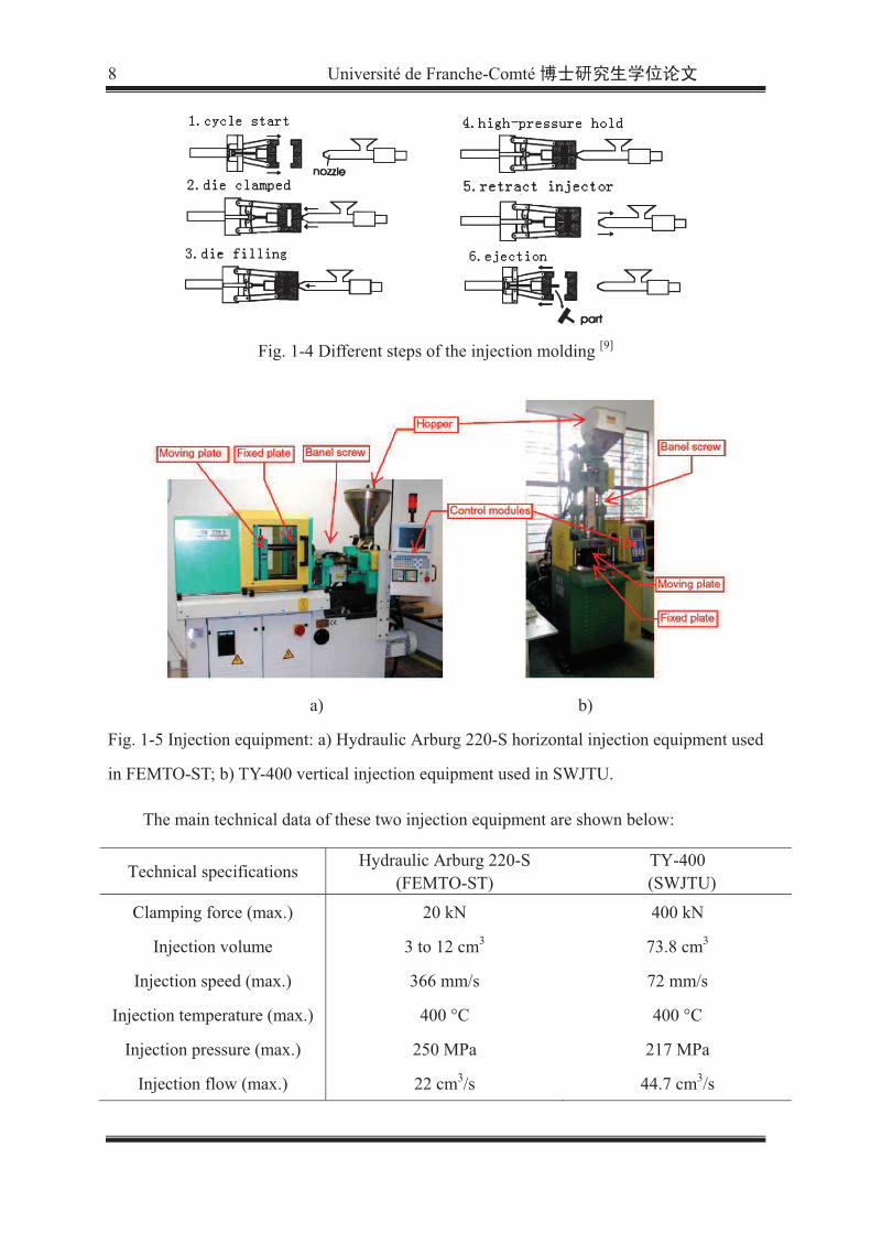
Fig. 1-4 Different steps of the injection molding [9]
a) b)
Fig. 1-5 Injection equipment: a) Hydraulic Arburg 220-S horizontal injection equipment used
in FEMTO-ST; b) TY-400 vertical injection equipment used in SWJTU.
The main technical data of these two injection equipment are shown below:
Technical specifications Hydraulic Arburg 220-S
(FEMTO-ST) TY-400
(SWJTU)
Clamping force (max.) 20 kN 400 kN
Injection volume 3 to 12 cm3 73.8 cm3
Injection speed (max.) 366 mm/s 72 mm/s
Injection temperature (max.) 400 °C 400 °C
Injection pressure (max.) 250 MPa 217 MPa
Injection flow (max.) 22 cm3/s 44.7 cm3/s

Université de Franche-Comté 9
3) Debinding of green parts
The debinding step is required to remove the binding additives from the green compacts
as a prerequisite for sintering. The thermal, solvent or catalytic debinding process is used to
get the shaped metallic components in porous state [10]. This process is a complex
combination of chemical and physical degradation of the binders under thermal conditions. It
is primarily dependent on the binder system used. In the solvent debinding process [11], the
injected components are placed in a solvent fluid or vapor to dissolve the binders. The other
debinding method is thermal debinding that removes the binders by heating the compacts [12].
In the catalytic debinding [13], the compacts are heated in atmosphere which containing
catalyst to sweep away the polymer binders. The result is known as the brown part that still
keeps its original geometry and size. For the experimental researches, the thermal debinding
device in FEMTO-ST and SWJTU is shown in Fig. 1-6.
Fig. 1-6 Thermal debinding oven used in (a) FEMTO-ST, (b)SWJTU
The principal technical specifications of these two ovens are related below:
Technical specifications (FEMTO-ST) OZE8020 (SWJTU)
Test temperature (max.) 300 °C 250 °C
Volume (max.) 27 L 24.7 L
Gas circulation air, argon air, argon, nitrogen
Gas flow (max.) 200 cm3/min 200 cm3/min

10 Université de Franche-Comté
4) Sintering of brown parts
In this process, the brown part is heated to approximately 85% of the material's melting
temperature. Sintering is often performed in a protective atmosphere or vacuum at a peak
temperature, which results in rapid elimination of the pores left by departure of the binder. It
bonds the metallic or ceramic powders together, allowing densification and shrinking of the
powders turning to a much denser solid with the elimination of pores. The sintered density is
approximately 98% of theoretical value, which ensures the proper mechanical characteristics
and corrosion properties. A shrinkage about 10~20% is obtained corresponding to the
elimination of binder and porosity, as shown in Fig. 1-7 [14]. The end result is a metal or
ceramic component in net shape or near net-shape, with properties similar to that of the bar
stocks. The sintering furnace in FEMTO-ST and SWJTU for research of the sintering cycle
is shown in Fig. 1-8.
Fig. 1-7 Remained binder in the component issued from different stages of the PIM process [14]
Fig. 1-8 Sintering furnace: (a) Conventional sintering furnace (provided by VAS®) used in
FEMTO-ST, (b) Microwave sintering furnace (HAMiLab-V1500) used in SWJTU

Université de Franche-Comté 11
The principal technical specification of the sintering furnace is given below:
Technical specifications Conventional sintering furnace
(FEMTO-ST) Microwave sintering furnace
(SWJTU)
Test temperature (max.) 2200 °C 1600
Volume (max.) 50 L 1.15 L
Atmosphere gas circulation: argon, helium; primary vacuum: 10-3 mbar, secondary vacuum: 10-5 mbar;
gas circulation: argon, heliumnitrogen or the mixture; Static vacuum: 100Pa
Heating source graphic heating elements
2.45GHz ± 25MHz MicrowaveThe Continuous adjustable output power: 0.2 1.40KW
Component holder ceramic plates Corundum mullite
In addition, some equipment for physical, rheology and mechanical analysis are needed,
as show in Fig. 1-9.
a) b)
c) d)
Fig. 1-9 The analysis equipment: a) RH2000 Capillary rheometer for the measurement of
viscosity; b) Vertical SETSYS® dilatometer used for the calibration of sintering constitutive;
c) Nikon Eclipse 55I/50I microscope used for observation of the sintered grains morphology;
d) HV-5 small load Vickers hardness tester.
12 Université de Franche-Comté
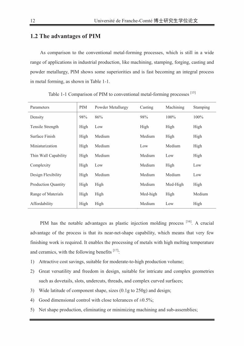
1.2 The advantages of PIM
As comparison to the conventional metal-forming processes, which is still in a wide
range of applications in industrial production, like machining, stamping, forging, casting and
powder metallurgy, PIM shows some superiorities and is fast becoming an integral process
in metal forming, as shown in Table 1-1.
Table 1-1 Comparison of PIM to conventional metal-forming processes [15]
Parameters PIM Powder Metallurgy Casting Machining Stamping
Density 98% 86% 98% 100% 100%
Tensile Strength High Low High High High
Surface Finish High Medium Medium High High
Miniaturization High Medium Low Medium High
Thin Wall Capability High Medium Medium Low High
Complexity High Low Medium High Low
Design Flexibility High Medium Medium Medium Low
Production Quantity High High Medium Med-High High
Range of Materials High High Med-high High Medium
Affordability High High Medium Low High
PIM has the notable advantages as plastic injection molding process [16]. A crucial
advantage of the process is that its near-net-shape capability, which means that very few
finishing work is required. It enables the processing of metals with high melting temperature
and ceramics, with the following benefits [17]:
1) Attractive cost savings, suitable for moderate-to-high production volume;
2) Great versatility and freedom in design, suitable for intricate and complex geometries
such as dovetails, slots, undercuts, threads, and complex curved surfaces;
3) Wide latitude of component shape, sizes (0.1g to 250g) and design;
4) Good dimensional control with close tolerances of ±0.5%;
5) Net shape production, eliminating or minimizing machining and sub-assemblies;

Université de Franche-Comté 13
6) Wide range of available alloys;
7) Capability to process the materials very hard and difficult to machine, which cannot be
produced by any other technology, such as cermets and ceramics;
8) High material density nearly 95% to 98%, approaching to wrought material properties.
1.3 PIM development and market
The appearance of PIM technology is due to the development of powder metallurgy. It
was first used in 1930s for manufacturing ceramic sheaths of spark plug insulators. The
process was adopted by the investment casting industry in which it is now still used for
manufacturing ceramic cores. However, PIM attracted little other interest until it was used
for the molding of metal powders in the mid-1970s. Before 1970, there were only 10 papers
related to Metal Injection Molding (MIM) process, even more generally in the domain of
PIM, then the number increased to 100 in 1980 and more than 1000 scientific articles were
published at the end of 1999 [18]. In the later 8 years, 3120 papers have been issued, including
1810 about MIM process. Till 2007, number of the related scientific papers raised twice [19].
Up to now, the journals related to PIM have been widely distributed, such as Powder
Metallurgy, Powder Injection Molding International, International Journal of Powder
Metallurgy, Journal of the American Ceramic Society, and Journal of the European Ceramic
Society etc. Besides, 400 patents have been registered since 1990s in USA [19]. The
researches strengthened the science and knowledge base of PIM. It is now recognized as a
sophisticated, interdisciplinary technology. This novel application will initiate the
considerable worldwide researches in the coming years.
From a market perspective, the portion of MIM in PIM is over 75%. A general resume
of the sales for PIM and MIM has been indicated in Fig. 1-10. The MIM field has exhibited
enormous growth since the first sale statistics were gathered in 1986, amounting to $9
million globally. Today, MIM is the dominant form of powder injection molding and has
sustained 14% of growth per year in recent years, regardless of a few years of drop. This plot
shows that the ceramic business contracted in recent years while MIM expanded, largely due

14 Université de Franche-Comté
to the aerospace slowdown. The segment of ceramic injection molding was most likely about
$158 million in 2012.
Fig. 1-10 Annual sales of powder injection molding (PIM) and the subset of metal injection
molding (MIM) plotted from earlist recorded values to 2012 [20].
In fact, the PIM has spread around the world, including Austria, Belgium, Brazil,
Canada, China, Czech Republic, France, Germany, Hungary, India, Ireland, Israel, Italy,
Japan, South Korea, Malaysia, Mexico, Netherlands, Singapore, South Africa, Spain,
Sweden, Switzerland, the United States and other countries and Chinese Taiwan area. By
now, the world has more than 500 companies and institutions involved in the PIM research
and development, production and consulting services.
Considering the sales of the firms identified in PIM, a survey from 1990 to 2010 gives
the variations in Fig. 1-11, according to geographical origin. The number of firms has grown
from about 50 to about 350. It can be clearly observed that China and India had rapidly
developed in the last decades and this tendency will continue in the coming years.
Fig. 1-11 Survey of the sales according to geographical regions (1990 to 2010) [21]

Université de Franche-Comté 15
The number of MIM firms has not shown much change in recent times, but the size and
sophistication have grown considerably. Various estimations have been offered for how far
and how long MIM can sustain the growth. According to a report from Global Industry
Analysts, a worldwide business strategy and market intelligence source, released in August
2011, the combined metal and ceramic injection molding market will be worth US$3.7
billion globally by 2017. Continuation of the MIM growth is strongly supported by the
economic drivers. Table 1-2 [22] from BCC-research on Metal and Ceramic Injection
Molding (AVM049B, retrieved 10/31/2012), illustrates well the projected growth rates. The
global MIM market projected to increase from US$ 985 million in 2009 to US$ 1.9 billion in
2014. It represents 14.0% of the compound annual growth rate (CAGR). The strong
technical players in MIM can expect to bring more value to customers than all of us can
imagined [23].
Table 1-2 Expected global sales of MIM components by region in 2014 [22]
2009 2014 CAGR%
Region ($ millions) (% share) ($ millions) (% share) 2009-2014
Asia 460.8 48 959.0 51 15.8
Europe 279.7 28 484.0 25 11.6
North America 231.0 23 424.0 22 12.9
Rest of the world 13.4 1 33.0 2 19.8
Total 984.9 100 1900.0 100 14.0
1.4 The principal research centers in PIM processing
In America, Prof. German and his research team have focused on the PIM process for
long time [1, 9, 10, 18, 19, 24, 25]. In Europe, there are active studies in many countries. In United
Kingdom, Prof. Ediridsinghe and his research team in Brunel university do the researches
related to the large ceramic components [26-29]. Dr. Alock [30] in University of Cranfield
mainly commits to the micro-manufacturing, which is also done by Dr. Kowalski [31] in

16 Université de Franche-Comté
University of Delft in Netherlands. In Germany, several technical research centers
concentrate on the elaboration of components by MIM process, they are Fraunhofer
(FhG-IFAM: Dr. Petzoldt [32]; FhG-IWM: Dr. Kraft [33]) and KIT Karlshuhe (Dr. Piotter [34],
Ruprecht [35]). In Switzerland, the application of NiTi shape memory materials has been
studied with powder injection molding process (Prof. Carreño-Morelli [36]). In the Swedish,
characterization of feedstock and its components is studying at Chalmers university (Prof.
Nyborg [37]). In Spain, two research groups are developing some new feedstock, especially
for M2 HSS (High Speed Steel) in University of Castilla La Mancha, large activities in PIM
are also developed by JM Torralba team (university of Madrid, Carlos ) [38]. T Vieira has
developed special coating method to improve the fluidity of the feedstock (at Coimbra
university) [39] in Portugal. In Austria, a set of modern equipment has been set to build a
large center in MIM fields, regrouping a lot of equipment providers. In Japan, several types
of very fine powders dedicated to micro-MIM or the other nanotechnology applications have
been developed. As example, iron, stainless steel, zircon, nickel and so on, have been used to
develop proper feedstock and processes for large varieties of applications [40, 41]. In Korea,
the development of MIM process with the titanium, copper, tungsten powders and several
alloys have been developed by collaborations with the research centers in USA [42, 43]. Also,
the international companies such as Parmatech and FloMet in the United States, BASF in
Germany, Pacmaco in Switzerland, AMT in Singapore are well-known in the field.
1.5 Researches on PIM process in France and in China
In France, the researches related to MIM process have been carried out since 1985;
meanwhile, the molding stage, the debinding and segregation analyses related to this process
have been studied at Ecole des Mines de Paris. Since ten years, an increasing number of
laboratories are involved in PIM activities. The ECAM laboratory developed feedstock with
biodegradable polymer for biomedical applications. BioPIM project supervised by CEA
LITEN (Grenoble, France) is going to develop some components with biodegradable
polymer. In CRITT research centers in Charleville-Mézières, a platform has been developed

Université de Franche-Comté 17
for pre-industrialization of PIM production. Since two years, POUDR'INNOV platform
starts its activities with large investments in Rhône-Alpes, in order to diffuse and promote
PIM opportunities. Since two years, almost twenty partners from industries and research
centers are participating to SF2M group in order to promote PIM potentialities for industries.
From 2010-2013, Newpim projects (FUI Newpim) have regrouped 13 partners to develop
miniature components with functional materials and the modeling and simulation of
sequential and global stages for MIM process. The projects have been managed by Alliance
and Femto-ST. A new project managed by Emetringstene and including 10 partners (Fento,
A. Raymond, Radiall, CEA, ...) begin in July 2013, for three years to develop micro
component with high accuracy for new materials. Furthermore, DMA is very active partner
in Mylisto equipex from 2011 to 2020 to develop a special platform to obtain special and
innovative equipment to elaborate micro-components with functional materials with a very
short production time by combining all stage and captive innovating process.
China began evolving in the field of PIM since the late 1980s. Central Iron & Steel
Research Institute, University of Science and Technology Beijing, Central South University,
General Research Institute for Nonferrous Metals, Guangzhou Research Institute of
Nonferrous Metals, Beijing Research Institute of Powder Metallurgy carried out successively
the PIM researches. In 1990’s, more and more universities and institutes were involved.
Several PIM Labs were established, such as the PIM Lab of Powder Metallurgy in Central
South University. Under the financial support of Nature Science Foundation of China, 863
High-tech agency of China, a lot of fundamental and applied researches have been conducted.
Many products are associated with the specific applications such as wristwatches, tungsten
penetrators, gun components. Based on these ten years research achievement, to the end of
the 90s, the institutes mastered gradually the independent PIM manufacturing technology.
Then many big enterprises emerged with capability of mass production, including the
Advanced Technology & Materials Co., Ltd. (at&m) (Beijing), Hunan Injection High
Technology Co., Ltd (HIHT) (Changsha), Jin Zhu Pang injection manufacturing co., LTD.
(Shandong), Fu Chi technology co., LTD. (Shanghai), etc.
In our laboratory at the Applied Mechanics department of FEMTO-ST institute, the

18 Université de Franche-Comté
research team managed by Professor Jean-Claude Gelin and Professor Thierry Barriere has
developed researches on micro processing and loaded polymers processing domain since
1995 [44, 45]. The conventional MIM and PIM have been carried out using various metallic or
ceramic powders. The micro-MIM and bi-material MIM have also been investigated [6, 46].
Concerning the simulation of PIM, the FeaPIM© software has been adopted, in which a
bi-phasic model was used to predict the powder segregation during the mold filling process
[47]. In the same research group, studies have also been developed on solid state sintering, the
activities have concerned experiments, modeling, simulation and optimization [48]. The
research team in SWJTU of China also has more than 20 years’ experiences in forming
processes. Based on the same research background and target, the two research team from
both French side and Chinese side began their cooperation in 1999. A chronology of the Ph.
D. theses processed in both laboratories in the last years is given in the Fig. 1-12. The names
of co-tutorial Ph. D. (Shi, Larsen, Song and Cheng) are set in the capital, bold and italic font.
Fig. 1-12 Chronology of the Ph. D. theses processed in the French and Chinese research
teams

Université de Franche-Comté 19
Chapter 2 Developments of modified algorithms for Mold
Filling Process
Powder Injection Molding is a new and advanced manufacturing technology. Numerical
simulation plays an important role in its efficient applications. The analysis of injection
molding was started by Spencer and Gilmore [49] in the early 1950s. Ballman et al [50] began
to investigate one-dimensional rectangular flow in 1959. Analytical solutions for
two-dimensional flow in a rectangular cavity were presented since the late 1970s [51-54]. Then
large amounts of research works were done in detail on fountain flow [55, 56]. The implicit
finite element method for simulation of the filling process was first tried by some authors
[57-59]. It was found that the main barrier for filling flow model is the tremendous
computational time due to the application of 3D finite element or finite difference method.
Therefore, the explicit algorithms that improve the efficiency of simulation for injection flow
model were studied and realized by Lewis and Gao, using MINI elements in 2D problems [60,
61]. The explicit algorithms with MINI element are much faster than the implicit ones. Their
validity was proven by the experiments [45, 62]. For the sake of computational cost, a new
explicit algorithm with fully vectorial operations was proposed by Liu [63]. The development
is carried out by the research work of Cheng [64, 65]. By eliminating the global solutions in the
previous explicit algorithm, it made successfully the computational cost to be about linearly
proportional to the degree of freedom number. Based on this explicit algorithm, G. Larsen et
al. [66] proposed a method combining finite element method and finite difference method for
investigating the mono-injection case.
The performance of the new explicit vectorial algorithm has been evaluated by
comparison with the results from both experiments and other numerical solvers, such as
commercial software MPI software (Autodesk(C)). The fully vectorial feature of new
algorithm provides the important advantage in computational cost for the simulation of large
scale problems in industrial application. It is easy to be parallelized for the computation on a
high performance system of multi-clusters. It was developed on the platform of Matlab (C)
software and has improved the previous in-house software for simulation of the injection
20 Université de Franche-Comté
filling process. However, it remains still some problems:
1) For some special cases when the phenomena of opposite joining and bi-pass are
involved, inside which the flow directions subject to the sudden changes during the
filling process, the present algorithm may result in untrue filling fronts. So modification
is still required to improve the simulation of injection filling at some specific filling
channels. This problem can be also seen in commercial FEM software MPI software
(Autodesk(C)).
2) The delay to fully fill the mold cavity when the filling process is close to be finished,
meanwhile the filling front approaches to the outlet boundary, is remained in the
developed solvers. This problem was mentioned in the doctoral thesis of Cheng [67], and
left unsolved because of the absence of a suitable method to complete the boundary
condition in the solution of advection equation for filling function. Also, the special
modified outlet boundary conditions are required to make the in-house software more
stable and more reliable.
3) How to extend the availability of present software into simulation of injection molding
problems in micro scales. It needs a more comprehensive consideration of the
mechanisms in mold injection. Some effects that can be ignore in macro size problems,
such as surface tension, wall slip etc., will become remarkable behaviors for problems
inmicron scales.
Work in this chapter is going to solve the first two problems mentioned above. And the
third one will be discussed in the next chapter.
2.1 Modeling and Simulation of PIM injection
2.1.1 General Definition
As usually chosen, Eulerian description is adopted for simulation of the mold filling
problems, which avoids the complicated and expensive remeshing procedures with
Lagrangian description. The general definition of mold filling problems with surface tension
is expressed as followings:

Université de Franche-Comté 21
Let ]t0[t 1,∈ be an instant in the injection course, in which 1t is the last moment f of
filling process to reach the fully filled state. The sum of position X in the whole model is
defined as set . The set in modeling of the injection molding consists of two different
portions at each instant, the portion F filled by feedstock and the remained space
V taken by the air. A field variable )( tx,F is defined to represent filling state of the
model at different instants. This field variable takes value 1 to indicate the portion filled by
feedstock and value 0 for the remained void portion, which contains in fact the atmosphere.
The physical and geometrical definition for this modeling is shown in Fig. 2-1. In which I
indicates inlet of the mold, O represents the outlet through it the air originally in the mold
can be squeezed out during the injection. S stands for intersection of subsets F and
V , which is in fact the filling front of the injection flow. IV is the injected velocity on
inlet boundary. OP is the pressure on outlet boundary, which is set to be 0 in the present
work to represent the environment pressure.
Fig. 2-1 Modeling of injection molding based on Eulerian description
The definitions for these subsets and their common surface are expressed in the
following equations:
],0[ tTt ∈∀ , ∀ ∈X
( ) ( , ) 1, ( ) ( ) t F t t t= ∈ = ∪ =F F F VX X (2-1)
( ) ( , ) 0, ( ) ( ) t F t t t= ∈ = ∪ =V V F VX X (2-2)
( ) ( ) ( ) ( )t t t t= ∈ = ∩S F S F VX (2-3)

22 Université de Franche-Comté
2.1.2 Governing Equations
To keep singleness of the solution strategy and simplicity of the software structure,
under the frame of Eulerian description, the governing equations for filling flow are chosen
the same for filled and void portion of the injection model, except that the physical
parameters are chosen differently for these two domains. In fact, the interest of simulation is
the filling flow of feedstock in mold cavity. For the portion filled by the feedstock, material
properties are the real ones. To keep good stability of the simulation process, the material
properties in void portion should to be modified to avoid too much of the difference
compared to the ones in filled portion. In fact, the result of simulation in the void portion is
not of our interest. So the parameters in the void portion can be chosen artificially to benefit
the stable simulations. Nevertheless, for the analysis of temperature in solution of the energy
conservation equation, the materials behaviors in both two portions should be the real ones,
as we need evidently the correct temperature field in the whole mold cavity. The
precondition to distinguish two different portions in the mold is to obtain the filling state
field at each instant, which indicates whether or not the position is filled by the feedstock in
the model.
2.1.2.1 Advection equation for filling state
The front position of filled domain is represented by the predefined filling state variable
)( tx,F . Some authors call it as the variable of pseudo concentration or fictive concentration
[68, 69]. At each instant t in injection course, the evolution of filling state variable is dominated
by an advection equation, driven by the velocity field.
0)(t
=•∇+∂
∂FV
F (2-4)
where V is the velocity vector, the boundary condition is 1=F on inlet of the mold. Its
initial condition is 0=F everywhere in the mold except for the inlet surface.

Université de Franche-Comté 23
2.1.2.2 Momentum conservation
Navier-Stokes equation is used to represent the momentum conservation. For two
portions filled with different materials in the mold, it is expressed as:
∀ ∈ FX , ( )p p pPt
∂ρ ρ
∂′+ • ∇ = −∇ + ∇ • +
VV V g (2-5)
∀ ∈ VX , ( )a a aPt
∂ρ ρ
∂′+ • ∇ = −∇ + ∇ • +
VV V g (2-6)
where pρ is the polymer density in the filled mold cavity, whereas aρ is the air density in
the unfilled mold cavity, P represents the hydraulic pressure field, p′ and a
′ are the
deviatoric Cauchy stress tensors in filled and void portion, g is the gravity vector.
As the flow in injection molding is often a problem with small Reynolds number,
Sometimes the influence of advection effect is negligible compared to the viscous effect in
Navier-Stokes equation. The momentum conservation can be then reduced to the solution of
two distinct Stokes equations, expressed as:
∀ ∈ FX , p p pPt
∂ρ ρ
∂′= −∇ + ∇ • +
Vg (2-7)
∀ ∈ VX , a a aPt
∂ρ ρ
∂′= −∇ + ∇ • +
Vg (2-8)
It should be mentioned that the material properties for air portion are chosen different
from their true values, for the purpose to keep numerical stability. Because of singleness of
the solution scheme for two different portions, it may result in the instability in numerical
solution if the mass and viscosity in void portion are too much different from the ones in
filled portion. However, the exact flow in void portion is not our interest. The result of such
a numerical treatment is acceptable, as our main objective is the flow of injected feedstock.
The boundary condition should be imposed for each variable in the solution process.
The mold inlet I can be specified by a prescribed velocity V or imposed pressure P .
On the mold outlet O , one needs simply to impose a zero pressure, assigned to atmosphere

24 Université de Franche-Comté
pressure. For the boundary conditions on the mold walls W , the velocity in normal
direction is always imposed to zero. A tangent viscous load f could be specified for
frictional sliding conditions. This tangential load is generally expressed in Chezy’s form as
[60]:
∀ ∈ WX , 0• =V n , 2 t tfC −= − • •f V V (2-9)
where n is the unit of outward normal, t is the unit vector of local tangent , fC is a
coefficient to be determined by experiments. For the sticking condition, the tangent velocity
is also specified to be zero as the normal one.
2.1.2.3 Incompressibility condition
Incompressibility condition should be satisfied in the portion filled by feedstock:
∀ ∈ FX , 0∇ • =V (2-10)
where V is the vector which represents the velocity field. Different from the method
developed previously in research team with MINI elements [70], incompressibility in the new
explicit algorithm [67] is to be kept only in the filled portion. The same numerical operation is
used in the void portion to keep simplicity and singleness of the solution procedure, expect
that the parameters in the void portion are not chosen attentively to maintain a strict
incompressibility. In fact, these parameters in void portion is adjusted preferably to keep
stability of the numerical solution, rather than to maintain the exact incompressibility. As
mentioned above, the result in void mold portion is not of our interest but just the need for
solution of the injection molding problems under Eulerian description.
2.1.2.4 Energy conservation
The viscous law of feedstock is strongly dependent on the local temperature values. The
variation of temperature field is very important to determine the flow of viscous feedstock
So it is necessary to evaluate the temperature field during the simulation of mold injection
filling process. Once the feedstock is considered as isotropic and the Fourier model for heat

Université de Franche-Comté 25
flux is applied, the heat transfer is governed by the following advective-diffusive equation:
∀ ∈ FX , '( ) :p p p p p
TC T k T
tρ
∂+ • ∇ = ∆ +
∂V (2-11)
∀ ∈ VX , '( ) :a a a a a
TC T k T
tρ
∂+ • ∇ = ∆ +
∂V (2-12)
where ' :p p and ' :a a stand for the dissipations associated to viscous PIM flow and
viscous air flow, T stands for the temperature field in the mold, pC and
pk are
respectively the specific heat and thermal conductivity coefficient of the feedstock, aC and
ak are respectively the specific heat and thermal conductivity coefficient of air, p and a
are the strain rate in filled and void portions. The boundary conditions are generally defined
with prescribed temperature values T T= on mold’s walls. The ambient temperature aT
may be imposed on the outlet OΓ . The convection effects can also be considered on the
mold walls of filled and void portions with relationships ( )pq h T T= − and
( )aq h T T= − , in which ph and ah are the heat transfer coefficient of feedstock and
air.
2.1.3 Explicit algorithm for simulation
The implicit algorithms are often used to solve the problems by finite element method.
But these algorithms lead to very expensive simulation even for 2D problems. The present
dissertation uses the explicit algorithm developed in research team [67, 70, 71] for simulation of
the mold filling problems with only vectorial operations in global sense. Neither the global
solution nor the construction of global matrix is required in the newly realized in-house
software. An important feature of the new algorithm is the use of elements with equal order
interpolations. The interpolations of velocity and pressure field have the same order of
interpolation, different from the traditionally used MINI elements for simulation of the
incompressible flow. Actually in the new explicit algorithm, the triangle elements in 2D case

26 Université de Franche-Comté
and tetrahedral elements in 3D case are employed, as shown in Fig. 2-2. To mesh the models
of intricate geometry, they represent less degrees of freedom and better fitness than the
quadrangle and hexahedral elements [72].
Fig. 2-2 Elements used in new algorithm
The interpolations of different variables are represented at the element level as:
1
, , , , , ,m
i i i i i
i
P F T P F T=
=V N V (2-13)
where m is the node number in such an element for different variables, iN is the
interpolation functions, iV represents the nodal vector values of velocity field. Other
notations as iP , iF and iT represent the nodal scalar values of the pressure, filling state
and temperature field.
As an explicit algorithm is used, most of the operations in fractional steps are the same
as in the previous work [70], while a special strategy is developed by Cheng [67] to verify the
incompressibility condition. This advance eliminates all the global operation in simulation.
In global sense, only the vectorial operations are performed so that high efficiency can be
achieved for further industrial application of the filling simulation. Moreover, it provides a
strong facility for computational parallelization on a multi-cluster system. The fractional
steps to solve the variable fields of filling state, velocity and temperature are performed in
the following manners, according to the dissertation of Cheng [67].
2.1.3.1 Determination of filling states
The determination of filled domain is the premise for other operations in Eulerian
description, as different material properties should be assigned in filled and void portions

Université de Franche-Comté 27
respectively. The filling state variable F defined to trace the filling front is determined by
an advection equation (Eq. 2-4). The numerical solution for the advection equation
associated to the filling state employs the same scheme as in polymer injection simulation.
For sake of the stability, the solution is based on Taylor-Galerkin method [73]. Solution
procedure of the filling state is the same as in the previous work [70]. It is then just a short
mention of the method and the necessary explanation.
The time differential of variable F in discretized form can be expressed by the
development of Taylor series:
221
2
( )( )
2n n n nF F F t F
O tt t t
+ − ∂ ∆ ∂= + + ∆
∆ ∂ ∂ (2-14)
in which nF and 1nF + represent the filling state at time step 1nt + and nt , t∆ stands for
the time increment.
The governing equation (Eq. 2-4) can lead to the follow relationship by an
approximation 1/ ( ) /n nt t+∂ ∂ = − ∆V V V :
nn
FF
t
∂= − •∇
∂V
(2-15) 2
12
( )( )n n n
n n
FF F
t t
+∂ −= •∇ •∇ − •∇
∂ ∆
V VV V
The weak form of Eq. 2-14 can be then written as:
* * *11/ 2
( )( )
2n n
n n n
F F tf d f F d f F d
t
++
Ω Ω Ω
− ∆Ω = − •∇ Ω + •∇ •∇ Ω
∆V V V (2-16)
where 1/ 2 1( ) / 2n n n+ += +V V V , *f is a kinematically admissible field associated to variable
F .
The discretized form of Eq. 2-16 by finite element method can be written as:
10 1/ 2[ ( ) ( ) ]ad dfn n
n n nt
++
−= − +
∆
F FM K V K V F (2-17)

28 Université de Franche-Comté
where 0M is a lumped pseudo matrix, ( )adK V is a stiffness matrix represents the
advection effect, while ( )dfK V is a stiffness matrix stands for diffusion effect. These terms
take respectively the following forms:
0 e
T dAΩΩ
=M N N (2-18)
1/ 2 1/ 2( )e
ad T T
n n dA+ +ΩΩ
=K V N V G (2-19)
( )2 e
df T T
n n n
tdA
ΩΩ
∆=K V G V V G
(2-20)
in above expression, A represents the assembling operation in finite element method, N
is the matrix of interpolation functions in each element for filling state variables, 1n+V and
nV are the values obtained at time step 1nt + and nt , 1/ 2 1( ) / 2n n n+ += +V V V , G is a
gradient operator constructed by derivatives of the interpolation functions:
FF G=∇ (2-21)
This solution is consisted of only local and explicit operations, so the prediction is
very efficient.
2.1.3.2 Solution of momentum conservation
Momentum conservation of the viscous flow is represented by Navier-Stokes equation
with consideration of the incompressibility condition. As an explicit algorithm, the
computation is fractionalised into three consequent steps [74]: solution for the effect of
advection, viscous diffusion and incompressibility condition, so Eq. 2-7 and Eq. 2-8 can be
decomposed into an advection equation, a viscous diffusion equation and an equation to
verify the incompressibility condition:
∀ ∈X ,( )n n
n nt
+∂ −= − • ∇
∂
V VV V (2-22)
∀ ∈ FX , ( )n n
p p pt
ρ ρ++ +∂ −′= ∇ • +
∂
V Vg (2-23)

Université de Franche-Comté 29
∀ ∈ VX , ( )n n
a a at
ρ ρ++ +∂ −′= ∇ • +
∂
V Vg (2-24)
∀ ∈ FX , 1( )n np P
tρ + ++∂ −
= −∇∂
V V (2-25)
∀ ∈ VX , 1( )n na P
tρ + ++∂ −
= −∇∂
V V (2-26)
where nV and 1n+V are the velocity fields at instant nt and 1nt + , n+V and n++V are the
intermediate velocity fields used in the fractional steps.
1) Solution of the advection effect
Generally the advection effect in Navier-Stokes equation is neglected to reduce the
equation into a Stoke one [70, 71] because the small Reynolds number in injection flow. To
solve the advection equation with a vectorial variable, it is however more complex than the
solution of advection equation for filling state variable, in which the variable is only a scalar
one. The advection effect in momentum conservation is also solved by Taylor-Galerkin
method. The time differential of velocity in discretized form can be expressed by the Taylor
series development as:
∀ ∈X , 2
212
( )( )
2n n n n n
n
n
tO t
t t t+ − ∂ ∆ ∂
= + + ∆∆ ∂ ∂
V V V V (2-27)
After discretization by finite element method, Eq. 2-22 can be written in the following
form:
∀ ∈X , 1
( )( 1 ) ( )adn n n
n n
n n
t
t t+
−
− ∆= − + •
∆ ∆
V VM K V V
11
11
)(2
)(2 −
−
−
−
•∆
∆+•
∆
∆+ nn
ad
n
nnn
ad
n
n
t
t
t
tVVKVVK
(2-28)
where M is the mass matrix lumped into diagonal form, 1nt −∆ and nt∆ are the time
increments at instant 1nt − and nt , 1n−V is the velocity fields at instant 1nt − , ( )advK V is

30 Université de Franche-Comté
a stiffness operator that represents the advection effects in Navier-Stokes equation. These
terms take respectively the follow forms:
∀ ∈ FX , ( )eF
T
p dA ρΩΩ
=M N N (2-29)
∀ ∈ VX , ( )eV
T
a dA ρΩΩ
=M N N (2-30)
∀ ∈ FX , ( ) ( ) ( )eF
adv T e
p dA ρΩΩ
=K V N G V N (2-31)
∀ ∈ VX , ( ) ( ) ( )eV
adv T e
a dA ρΩΩ
=K V N G V N (2-32)
in the above expression, A represents the assembling operation in finite element method,
eV represents the vector that contains the velocity components at all nodes in an element.
The gradient operator G should be built according to the arrangement of velocity values in
its vector eV . So at each Gauss point of the element, one has the relationship:
e∇ =V G V (2-33)
2) Solution of the viscous diffusion effect
By Galerkin method, Eq. 2-23 and 2-24 can be discretized in the following form:
∀ ∈X , ( )
( ) extn nn
t
σ++ +−= +
∆
V VM F V F (2-34)
where M is the mass matrix in the form of Eq. 2-29 and 2-30, σF is the viscous diffusion
term, extF is the load vector with gravity contribution and boundary conditions. They are
numerically defined as:
∀ ∈X , ( ) ( )e
T dAσ
ΩΩ′=F V B (2-35)
∀ ∈ FX , ( )eF
ext T ext
p dA ρΩΩ
= Ω +F N g f (2-36)
where A represents the assembling operator in finite element method, B is the matrix of
derivatives of the interpolation functions N in an element, defined to calculate the
symmetric part of velocity’s gradient e= BV , eV represents the nodal values of velocity
vectors in an element, ′ stands for the deviator of Cauchy stress tensor. This stress

Université de Franche-Comté 31
deviator should be calculated on the deviator of the strain rate, by means of different viscous
laws defined distinctly in the filled and void portion, extf stands for the surface loads
converted to the nodes on boundary. In the void portion, extF is generally set to be 0, as the
gravity effect of air can be ignored and pressure imposed on outlet is 0.
3) Incompressibility
The new strategy for verification of the incompressibility condition is the most
important feature of the newly algorithm. It eliminates the last global solution in explicit
algorithms to realize the fully vectorial computations. The incompressibility is maintained by
a feedback correction procedure, which avoids the direct evaluation of pressure fields. In the
new vectorial algorithm, Eq. 2-25 and 2-26 are replaced by the following equations for the
corrections to obtain the velocity field that satisfies the incompressibility condition.
∀ ∈ FX , 1( )[ ( ) ]Fn n
p nt
∂ρ λ
∂+ ++
++
−= −∇ • ∇ •
V VV I (2-37)
∀ ∈ VX , 1( )[ ( ) ]Vn n
a nt
∂ρ λ
∂+ ++
++
−= −∇ • ∇ •
V VV I (2-38)
Incompressibility condition 1 0n+∇ • =V , as shown in Eq. 2-10, is satisfied by a corrective
term with factor Fλ and Vλ . Such a special term is used to substitute the term of pressure
gradient in Eq. 2-25 and 2-26.
Eq. 2-25 and 2-26 can be discretized by Galerkin finite element method, which results
in the solution of velocity field 1nV + in the following form:
∀ ∈X , V,Fi∈ , 11
( )( , )d in n
n nt
λ+ +++ ++
−=
∆
V VM F V (2-39)
where M is the mass matrix in form of Eq. 2-29 and 2-30, the variables 1n+V and n++V
represent the final incompressible velocity and intermediate velocity fields, dF is the term
for correction of the incompressibility.
Determination of the coefficient Fλ , Vλ and the correction term dF will not be

32 Université de Franche-Comté
described in detail here. It belongs to the main work of Cheng [64, 67].
2.1.3.3 Calculation of heat transfer and temperature field
The heat transfer in Eq. 2-11 and 2-12 is dealt with both advection and diffusion effects.
A fractional step method proposed by Lewis [61] is used in the present work as it permits to
evaluate the temperature field explicitly. The fractional advection and diffusion steps are
written as:
∀ ∈X , ( )
•n nT TT
t+∂ −
= − ∇∂
V (2-40)
∀ ∈ FX , '1( ) 1
( : )n np n p p
p p
T Tk T
t Cρ+ +
+
−= ∆ +
∂ (2-41)
∀ ∈ VX , '1( ) 1( : )n n
a a a
a a
T Tk T
t Cρ+ +−
= ∆ +∂
(2-42)
where nT and 1nT + are the temperature fields at instant nt and 1nt + , nT + is an
intermediate temperature field used in the fractional step method.
Same as for the evaluation of filling state by Taylor-Galerkin method, Eq. 2-40 can be
discretized in following form:
∀ ∈X , 0
( )[ ( ) ( )]ad dfn n
nt
+ −= − +
∆
T TM K V K V T (2-43)
where 0M is a lumped pseudo matrix in the form of Eq. 2-18, )V(adK is a stiffness
matrix of the advection effect in the form of Eq. 2-19, while )V(dfK is a stiffness matrix of
the diffusion effect in the form of Eq. 2-20.
By Galerkin method, the solution of Eq. 2-41 and 2-42 can be written in the following
manner:
∀ ∈X , 1
0
( ) d cn nn
t+ +
+
−= + +
∆
T TM K T Q q (2-44)
where 0M takes the same form as in Eq. 2-18, dK is the thermal diffusion term, Q is

Université de Franche-Comté 33
the heat dissipation term, cq is the heat convection term. These terms can be deduced from
the following forms:
∀ ∈ FX , F
e
pd T
p p
kd
CA
ρ ΩΩ
=K G G (2-45)
∀ ∈ VX , V
e
d Ta
a a
kd
CA
ρ ΩΩ
=K G G (2-46)
∀ ∈ FX , '1
( : )F
e
T e
p p
p p
dC
Aρ Ω
Ω
=Q N (2-47)
∀ ∈ VX , '1
( : )V
e
T e
a a
a a
dC
Aρ Ω
Ω
=Q N (2-48)
∀ ∈ FX , ( )q
q
c T
p nh T T dSA +Γ
Γ
= −q N (2-49)
∀ ∈ VX , ( )q
q
c T
a nh T T dSA +Γ
Γ
= −q N (2-50)
where G is a gradient operator in the form of Eq. 2-21, '( : )e
p p and '( : )e
a a are
the values calculated at each Gauss point on the basis of obtained velocity field 1n+V and
prescribed flow behaviour in filled and void portions respectively, ph and ah are the heat
exchange coefficients of feedstock and air with the mold boundary, T is the temperature
values on the mold walls.
2.2 Algorithm for improvement of wrongly adverted filling profile
With the development of injection molding process, shape of the components is
increasingly complex [75]. Due to the constraints in physical experiments and the availability
of measurements for micro-scale factors, the accurate numerical simulation becomes more
and more important in designing and manufacturing. In general, Eulerian description is used
for simulation of the filling flow problems [76, 77]. The mold die cavity is assumed occupied

34 Université de Franche-Comté
by two different flow substances, viscous polymer in the filled portion and air in the
remained void part. A filling state variable )( tx,F is used to describe the evolution of
filling process, as the definition in section 2.1.1. The governing equation for filling state
takes the form of an advection equation (Eq. 2-4). The evolution of filling state is governed
by the velocity field in whole mold cavity.
However for some cases, it is observed that the filling patterns predicted by simulation
are not the realistic ones, especially when the phenomena of opposite joining and bi-pass are
involved. In most cases, the filling flow direction doesn’t change dramatically. The velocity
field in void portion close to filling front is similar to that of the polymer behind the filling
front. So according to the traditional mechanical model of injection filling process, as
described in chapter 2, it will often result in an accurate and realistic simulation. But it is not
so good for some special cases when the opposite joining and bi-pass are involved, such as
runners in shapes of ⊥ and L, inside which the flow directions subject to the sudden
changes in the filling runners. At this instance, the untrue results may be produced, as shown
in Fig. 2-3. The simulations are carried out using Matlab (C) software. The modeling
algorithm is based on the same principle as the previous work done by Barriere [70] and
Cheng [67, 70]. The related material properties are listed in table 2-1. These material properties
and boundary conditions are assigned just for the purpose of software validation. They do
not mean the real values obtained from experiments.
Table 2-1 Material properties and parameters used in numerical simulations
Parameter value
Feedstock: Polymer (PP)
Density: 1 g/cm3
Viscosity of the mixture: 100 Pa.s (constant viscosity)
Injection rate: 20 cm3/s
Injected velocity: 0.1 m.s-1 (constant velocity)
Boundary condition: sticky wall (no-slip on the wall)

Université de Franche-Comté 35
Fig. 2-3 Filling problems of front joining for specific die cavities in shap ⊥ and L
For the case of runner in shape ⊥ , the polymer is injected from two inlets in opposite
sides of the cavity. The same injected velocities (as inlet boundary condition) are imposed in
both inlets. The two different filling fronts with the same speed should independently
progress in the mold die cavities, and then meet to each other to reach a common outlet.
However, in Fig. 2-3, it is observed that the filling fronts get the way to bi-pass before them
merging together at the middle of bottom in ⊥ cavity. There exists an air gap between the
two evolving fluid fronts that is not completely filled at the end of simulation. For the case
of runner in shape L, after the polymer being horizontally injected into the mold die cavity, it
should arrive mainly at the right hand side wall first, and then moving into the vertical part
of the cavity. But the same untrue phenomenon happens.
As another example, the simulation result made by commercial finite element software
MPI software (Autodesk(C)) is introduced, as shown in Fig. 2-4. It uses the same material
and boundary conditions as the example in Fig. 2-3. The related material properties can be
referred to table 2-1. It can be found that in the filling of a typical runner in shape ⊥ , the
filling fronts from two opposite inlets got their own way to the middle bi-pass before they

36 Université de Franche-Comté
joined together. Evidently this result doesn’t meet the real physical phenomenon. Although
the running of software uses some strategy to modify this problem in post-processing steps,
but the filling patterns are not yet the true ones for the two opposite filling fronts to join
together.
Fig. 2-4 Simulation by MPI software (Autodesk(C)), front joining in mold cavity of shape ⊥
with opposite inlets
G. Larsen et al. [66] used the Streamline Upwind Petrov Galerkin method (SUPG) to
improve this filling problem, and confirmed that the simulation results are more close to the
real situation than the ones by Taylor-Galerkin method [67, 70, 78]. However, the real pattern of
front joining in injection molding had not been exactly predicted, as shown in Fig. 2-5.
Fig. 2-5 The improved but still untrue results by SUPG method [66]
The objective of present study is to analyze the source for the untrue simulation results
and find the effective way to settle the problem. A modified algorithm, which is similar to
upwind method, was proposed to trace the filling front. This proposed method makes the
advection of filling state be mainly affected by the filling flow behind the filling front. Based
on finite element method and the efficient vectorial explicit algorithm developed in research

Université de Franche-Comté 37
team, a systematic operation was proposed for modifying the velocity field ahead filling
front, making the advance pattern of flow front be guided more on the flow of the polymer
instead of the fictive air flow. The simulation results in shapes of ⊥ and L show that the
proposed algorithm can effectively improve the untrue filling patterns in simulation.
2.2.1 The source for distorted simulation results
The filling processes may be distorted in simulation by the following sources:
1) Differences in physical properties of the polymer and air not being taken into account in
governing equation of the filling evolution
Eulerian description is used for simulation of the injection molding process. The filling
state variable is governed by advection equation to track the filling fronts. As in Eq. 2-4, it
doesn’t distinguish the different effects of the polymer and air on advance of the filling front.
Due to extreme difference in the nature of these two substances, their effects to evolution of
the filling front are extremely different, too. In fact, as an incompressible fluid, the advance
of filling front is mainly driven by the flow of polymer behind it, and rarely guided by the air
flow ahead. But the variable of filling state F is advected by the velocity field in whole mold
cavity in simulation. It means that the velocity ahead and behind the filling front represent
the equal effect on advance of the filling front. But in fact, the gradient of pressure is
built-up mainly in the flow of polymer, rather than in the air flow. The flow of air has much
less effect on the advance of polymer filling front.
2) Artificial air properties taken in simulation
As Eulerian description is used for injection molding, a filling state variable governed
by advection equation is defined to track the filling fronts. The void portion in mold is
supposed to be filled by a fictive fluid to simplify the procedures. Under the frame of
Eulerian description and in order to keep integrity and consistency of the solution scheme,
air in the void portion is also assumed to be incompressible as the polymer. By doing this
strategy, the computation of both filled cavity and void portion can be implemented with the
unique numerical operation. However, the incompressible assumption for the air flow is not

38 Université de Franche-Comté
really consistent with its true nature. Such an assumption may affect also on the advance of
filling front, other than its virtue to simply the solution algorithm.
Besides that, the flow of materials in both filled and unfilled portions (air flow) should
satisfy the conservation of momentum. In Eq. 2-5 & 2-6, it can be noticed that in these two
parts, the same Navier-Stocks equation has been used, except that different material
parameters are assigned. The large difference in the natures of the polymer and air may result
in numerical instability. So increasing artificially the mass and viscosity of air becomes a
common practice to keep stability of the numerical simulation. Then the inaccurate air flow
may affect advance of the filling front, leading the simulation results to be distorted. It is
another factor to produce the distortion in simulation of the front tracking.
According to the analysis on the cause of distortion for front tracking, the problem is
then how to make the advection of filling state function depends more on the flow behind the
front, less on the flow of air ahead of the front.
2.2.2 Modification of the solution procedure
Based on the mechanical model and the notion of upwind method to strengthen the
influences of the polymer flow located behind the filling front, a notion similar to upwind
method was introduced. A corresponding correction method was proposed to settle the
distortion of filling front mentioned above. A feasible way to make the filling pattern more
realistic is to modify the velocity field near the filling front. Advance of the filling front can
be made to follow the guidance of polymer flow behind it, if the velocity just before the front
is set to be similar to that behind the front. By means of a systematic operation to modify the
velocity field for filling simulation, the untrue impact of air flow, represented by the velocity
field ahead of the filling fronts, can be reduced. To implement such method, there exist two
key issues to be solved:
First question: how to determine the band to be modified, ahead of the filling front?
The selection can be made by the unit of element, judging and selecting element by
element. Then the question is turned to be: which elements locate in the band close to filling
front? And what is the criterion to judge if an element is in the band?

Université de Franche-Comté 39
In fact, according to the definition of field variable )(x,tF , it takes the value F =0 to
indicate void portion while F =1 represents the filled one inside the mold cavity. Then the
nodes near filling front should represent the values between 0 and 1, note that FrtF ,
10 Frt << F . One can prescribe two values lowF and upF to define the range of band before
the front.
10 upFrtlow <<<< FFF (2-51)
By example, for the 2D triangle elements with 3 nodes, an element can be regarded in
the band if there exists at least one node for its F value to locate between lowF and upF . Let
Frt represent the band region (neighbor to the filling front). Assumed element e being
anyone in the model, i is the node number belong to this element:
e∀ , ∀i∈element e upilow FFF << )(Frt te∈ (2-52)
as shown by the gray area in Fig. 2-6.
Fig. 2-6 Schematic of the band near filling front
Question two: how to modify the velocity field for computation of the filling state?
It is evident that the modified velocity fields are used only for solution of the filling
states. The modified velocity fields should be smoothed and continuous ones. Otherwise
solution of the advection equation will become the instable one to produce the spurious
results.
A general smoothed procedure is proposed as followings
F
eT
F VdNNVe
]~
[]~
[Ω
ΩΩ= • • (2-53)
where FV is the velocity field, expressed in a discretized way at each node, for the
solution of filling state. Pay attention that it is a modified and smoothed one to make

40 Université de Franche-Comté
simulation of the front progress more realistic.
F
eV represents the column of velocity values at all nodes of an elements. It takes
initially the velocity values obtained by solution of the Stokes equations, but these values are
modified when the elements locate in the band ahead of the filling front. First, one node with
maximal F value will be determined as the upwind node, then the velocity value of the rest
nodes in the same element will be replace by the velocity value of the upwind node.
For an element in the band, element number e and the node number i:
)(Frt te∈∀ , i∀ ∈ element e
k∃ ∈element e , for Fk = (Fi)max (2-54)
where k is the upwind-stream node number, it indicates the node of maximum F value
(Fi)max in the element.
i∀ ∈ element e let ki vv = (2-55)
By this treatment to the velocity values of the elements located in the band, the velocity
in thin layer elements ahead of the filling front is modified to be the values of the elements
behind. This operation reinforces the effect of polymer behind the flow front, while reduces
the unrealistic guidance of air flow ahead of the filling front. It represents more the real
physical phenomenon. And it is more consistent with the true flow process.
For the details of different operators, let’s take the triangle element of 3 nodes as a simpler
example. This type of the elements includes 3 linear interpolation functions 1N , 2N , 3N .
The values of V at element level eV take the following form
323122211211 VVVVVVV Te = (2-56)
The matrix of interpolation function ]~
[N for velocity should be arrange in the
corresponded form as
=321
321
000
000]
~[
NNN
NNNN (2-57)

Université de Franche-Comté 41
2.2.3 Validation of the modification scheme
2.2.3.1 Simulation result of the proposed modification
This corrective strategy is also carried out based on the explicit algorithm with fully
vectorial operations, which was previously developed in the research team with
Taylor-Galerkin algorithm to solve the transport equation. For comparison, it also uses the
same material (PP) and boundary conditions as the examples in Fig. 2-3 and Fig. 2-4. The
related material properties can be referred to table 2-1.
By the proposed modification on solution algorithm, the injection filling processes in
runners of shapes ⊥ and L are represented in Fig. 2-7 and Fig. 2-8. The filling duration for
⊥ shape and L shape cavity is 0.7s and 0.8s respectively. A constant speed is imposed on the
inlet. For the injection by incompressible flow, the filling volume should be proportional to
the injection time until totally filled.
a) b)
c) d)
Fig. 2-7 Filling by two opposite inlets in cavity of shape ⊥ for different filling time: a)
0.32s, b) 0.38s, c) 0.45s, d) 0.7s.

42 Université de Franche-Comté
Fig. 2-7 shows the injection process in runner of shape ⊥ . The polymer is injected by
two opposite inlets with the same speed. The filling fronts get advanced oppositely, join at
middle of the cavity first and then go to the bi-pass together.
a) b)
c) d)
Fig. 2-8 filling process in mold cavity of shape L obtained in different filling time: a) 0.32s;
b) 0.4s; c) 0.45s; d) 0.5s.
Fig. 2-8 shows the result of runner in shape of L by modified method. The polymer is
horizontally injected into the mold cavity. It touches the wall at right end first, and then be
extruded into the vertical runner.
By comparison of the simulation results in Fig. 2-3, Fig. 2-7 and Fig. 2-8, it is observed
that the filling flows of polymer are more reasonable. They get advanced to join together, or
touch the wall in front before moving into the by-pass. The wrong guide of air flow to make
the opposite polymer flows going to bi-pass separately is largely reduced.

Université de Franche-Comté 43
2.2.3.2 Comparison with experiments
In order to show more about the validity of the above proposed method, experiment
results from G. Larsen [66] is introduced to make a comparative analysis. The specific
micro-injection molding equipment Battenfeld Microsystem 50 has been used in G. Larsen’s
work to perform the molding process. A two-plate mold has been designed and manufactured
in FEMTO-ST institute. It has the dimensions indicated Fig. 2-9(a). It is composed of three
primary entities: mold die cavity (Fig. 2-9(b)) and ejector (Fig. 2-9(c)) for mechanical
ejection of small components.
(a)
b (c)
Fig. 2-9 Detail of runners and micro-component: (a) floating die cavity insert for
micro-injection designed for Battenfeld injection equipment, (b) geometry of the ejector, (c)
injection runners and moving die mold cavity.

44 Université de Franche-Comté
Short-shots have been achieved for the injection filling process. The Polymer (PP) is
injected from the both inlets. The injection temperature is 210 °C, the injection velocity is 10
m.min-1 and the injection pressure is 35 bars. The Comparison between results from
experiment and the improved simulation are shown in table 3-1.
Table 3-1 Comparison between results from experiment and the improved simulation
Short-shot from 58 ~ 65 mm3 Simulation result
a) 58 mm3, filling state: 69% A) 0.38s, filling state: 54.3%
b) 60 mm3, filling state: 71.4% B) 0.45s, filling state: 64.3%
c) 65 mm3, filling state: 77.4% C) 0.7s, filling state: 100%

Université de Franche-Comté 45
From table 3-1, it can be seen that the track of filling flow is nearly the same as the
experiment results. No clear differences appear in the whole filling process, including the
instant when the two opposite flow merging together at the middle of bottom in ⊥ cavity.
And it can be completely filled at the end of simulation without any air gap between the two
evolving flow. It can be regarded as an effective and true simulation result.
2.2.4 Conclusion
In order to improve accuracy of the numerical simulation for injection molding process,
source of the inexact filling fronts was analyzed. As Eulerian description is generally used
for filling flow problems, the governing equation of filling state takes the form of advection
equation. The extreme difference in properties of polymer and air results in different effects
for their flows on the advance of filling front. This difference cannot be taken into accord by
the governing advection equation. The filling of polymer may be wrongly guided by the flow
of air, for some specific cases with the sudden change in flow direction of the polymer. To
settle the problem, a corrective method is proposed and implemented, by the notion similar
to upwind method. Based on the efficient explicit algorithm for PIM simulation and the FE
software developed by research team, a systematic operation is designed to modify the
velocity field of air flow close to filling front for solution of the filling advection equation.
The untrue impact of air flow, represented by the velocity field ahead of the filling fronts, is
significantly reduced. Then the advance of filling front can be mainly affected by the
polymer flow behind the filling front. The simulation results show that the corrective
algorithm can effectively improve the distorted results. The simulation of filling processes in
the complex cavities with runners in shapes ⊥ and L can be significantly improved.

46 Université de Franche-Comté
2.3 The outlet condition in simulation of MIM injection to track the
end of filling process
As a new manufacturing technology, numerical simulation plays an important role in
the efficient applications of PIM technology. As described in Section 2.1, there is a long
history in analyzing the flow behaviors of injection molding process. It existed in the early
1950s [49] , then the analysis went to one-dimensional rectangular flow in 1959 [50], and
two-dimensional flow since the late 1970s [51-54], then large amounts of research works were
done in detail on fountain flow [55, 56]. The implicit finite element method for simulation of
the filling process was firstly tried in 1990s [57-59]. It was found that the computational time
for implicit algorithm was too tremendous, then the explicit algorithms were studied and
realized to improve the efficiency [60, 61]. For further reduction in computational cost, a new
explicit algorithm with fully vectorial operations was proposed by Liu [63], then carried out
by the research work of Cheng [64, 65]. The global solutions in the previous explicit algorithm
were eliminated. The computational cost is reduced to be about linearly proportional to the
degree of freedom number.
However, there remains a persistent trouble in simulation of the filling states at the end
of injection molding. It happens in the simulations of filling process with imposed constant
velocity on inlet. As the polymer is regarded as incompressible flow, the filling ratio should
be a linear one with respect to time. But the linearity is not respected when the filling front
approaches to the outlet boundary. The cause is indicated in the Ph.D. thesis of T. Barriere [70]
in 2000, but none of the references is involved to its solution in the retrieving of available
sources. In fact, there is a lack of the integration term on the outlet boundary. This
integration is negligible when the filling front is far away from the outlet, but it becomes
significant when the front of polymer approaches. To remedy this defect, the modeling is
formulated again. An integration term on the outlet boundary is realized in solution of the
advection equation for filling state. The problem in solution of the filling process at the
ending stage is finally solved. The examples prove well validity of the proposed method.
Stability of the in-house solvers for solution of the volume fractions is improved.

Université de Franche-Comté 47
2.3.1 The inexact result at the end of filling process
Because of incompressibility of the injection flow, the filling ratio should behave
linearly versus time when constant velocity is imposed on inlet. But it did not at the ending
stage of filling process, when the modeling and simulation in laboratory is applied. There
remains a persistent trouble for simulation of the final stage of injection process, when the
filling front approaches to the outlet boundary, as shown in Fig. 2-10.
Fig. 2-10 Persistent troubles in simulation for the ending of filling process
The results reproduced accurately the real nature until the filling ratio reached to 90%,
when the filling front gets near to the outlet boundary. Then the filling of remained void
portion becomes slower than the true fact. The cause of such a trouble was indicated in the
Ph.D. thesis of T. Barriere [70]. For Eq. 2-58, which is the weak form of the advection
equation Eq. 2-4 by a Taylor-Galerkin method, the integration was supposed to take value
zero all around the boundary, while it is not true when the filling front approaches to the
outlet boundary O∈X .
ΓΩ
•∇•⋅∆
=Ω∇•⋅•∇∆
dS)(2
td])([
2
t ** nFVVfFVVf nnnnnn (2-58)
where nF and
nV represent the filling state and velocity variable at time step nt , t∆
stands for the time increment. *f is a kinematically admissible field associated to variable
F. This equation takes indeed value zero when the filling front represents the distance to
outlet boundary, when the filling ratio is smaller than 90%. But for the last duration in

48 Université de Franche-Comté
injection course, this term must be taken into account to simulate correctly the filling pass
through the outlet.
2.3.2 Modification of the outlet boundary condition
To remedy the problem mentioned above, an additional integration term should be
taken into account on outlet boundary for the last stage in injection course. The following
procedure is proposed to realize the adequate integration on outlet boundary.
The discretized form of advection equation Eq. 2-4 by finite element method should
be written as:
nnnnnnn FVFVV
FF)(])()([ 2/1
1 Odfad KKKM ++−=∆
−+
+
t (2-59)
where M is a lumped pseudo matrix constructed in a specific manner, )(VadK is a stiffness
matrix represents the advection effect while )(VdfK is a stiffness matrix stands for
diffusion effect. )( nVOK is the operator for outlet surface integration term.
Ω=ΩΩ
dAe
NNTM
Ω=Ω
+Ω
+ dAe
GVNVT
n
T
n 2/12/1 )(adK
Ω∆
=ΩΩ
dtA
eGVVGV n
T
n
T
n 2)(dfK
(2-60)
(2-61)
(2-62)
where A represents the assembling operation in finite element method. N is the matrix
of interpolation functions in each element for filling state variables F, G is a gradient
operator constructed by derivatives of these interpolation functions. 2/1+nV and nV are the
values obtained at each Gauss points.
Note outN the nodes associated to outlet surface. e
outΩ represents the elements
associated to node outN , defined as:
e
out
ee
out N Ω⊂Ω=Ω (2-63)
Let e
outΓ represent the edge or side of element e
outΩ on outlet boundary. A unit vector
outn is defined for each element e
outΩ . This vector is normal to its edge or side e
outΓ .

Université de Franche-Comté 49
The term )( nVOK in Eq. 2-59 takes the following forms:
Ω⋅∆
=Γ
dt
A GnVVNVT
out
e
n
Te
n
T
Nn
eout
out
)(2
)(OK (2-64)
where e
nV represents the velocity vector in the element associated to e
outΓ .
By investigation of the flow pattern at outlet of the mold cavity, it is realized that the
velocity vector V and outer normal n take the same direction, whereas the gradient of
variable F should exhibit the direction opposite to V and n . So on the integration of Eq.
2-58 can be simplified.
Taking into account the above mentioned features, the integration of Eq. 2-58 can be
written as:
SFVVSnFVV nnnnnO
d2
td)(f
2
t * ∇•∆
=•∇•⋅∆
ΓΓ
(2-65)
in which nV is the norm of velocity vector, it represents the value nnn VVV •= .
Then the term )( nVOK
in Eq. 2-59 takes the following forms:
Ω⋅∆
=Γ
d)(2
t)( GVVNV
Te
n
e
n
T
Nn
eout
out
AOK (2-66)
where e
nV represents the velocity vector in the element associated to e
outΓ .
This solution scheme consists of only the local and explicit operations, so the
prediction is very efficient.
A brief description on the modified algorithm relative to the outlet boundary condition
is shown in Fig. 2-11.

50 Université de Franche-Comté
Fig. 2-11 The modified explicit algorithm relative to the outlet boundary condition for
simulation of injection molding process. It is suggested to overcome the untrue delay of fully
filling in the last filling stage.
2.3.3 Validation of the modified algorithm
The modified integration term on outlet boundary in section 4 was realized on Matlab (C)
platform to focus the effort on its development and validation. As this work is based on the
previous work on explicit algorithm in laboratory [67, 70], some technical issues were taken
directly from the previous work. A simplest filling mold in shape of straight channel was
chosen to do the simulation, which was often used as the evidence of validation for a newly
developed algorithm. It was meshed with triangle elements as shown in Fig. 2-12. The
related material properties are listed in table 2-2. These material properties and boundary

Université de Franche-Comté 51
conditions are assigned just for the purpose of software validation. They do not mean the real
values obtained from experiments.
Table 2-2 Material properties and parameters used in numerical simulations
Parameter value
Feedstock: Polymer (PP)
Density: 1 g/cm3
Viscosity of the mixture: 100 Pa.s (constant viscosity)
Injection rate: 20 cm3/s
Injected velocity: 4 m/s 6 m/s and 10 m/s respectively for the
three examples (constant injected velocity)
Boundary condition: sticky wall (no-slip on the wall)
Fig. 2-12 Mesh of straight channel model
Comparison on evolution of the filling ratio versus time, obtained by previous and
modified algorithm, is shown in Fig. 2-13. It shows that the results obtained by two methods
are globally the same until the filling ratio reaches to 90%. Then the results issued of
previous algorithm show the filling rates slower than the true ones. While the filling ratio of
modified algorithm keeps nearly proportional all over the whole time, including the ending
stage. Although it presents a little deviation to the real fact when it fills up to 98%, the fully
filled pattern is soon achieved. For the approach and simulation by computation, it represents
no more a significant problem.

52 Université de Franche-Comté
Fig. 2-13 Comparison on evolution of the filling ratio versus time
2.3.4 Conclusion
The modeling of injection molding is modified to simulate correctly the ending stage of
filling process. The incorporated implementation is realized in the developed solver. The
examples with constant injection velocity on inlet are provided to validate the proposed
method. Based on the validations, one can conclude that:
(1) The modified boundary condition represents a true effect that should be taken into
account. Incompressibility of the filling flow can hence be well respected at the last
stage of filling process.
(2) The filing problems in simulation happened in the work of Dutilly [44] and Barriere [70]
can be solved by modification of the boundary condition on outlet. The opinion of
Barriere [70] was correct. Lack of the integration term on outlet boundary was the true
cause for such a problem.
(3) The persistent problem is solved successfully. The simulation of filling process is made
more reliable. Furthermore, the stability for solution of the volume fractions was
improved. The in-house solver for simulation of the injection molding was optimized.

Université de Franche-Comté 53
Chapter 3 Numerical method and analysis for surface
tension effects in micro-injection process
Micro-injection molding is one of the effective manufacturing methods in the field of
MEMS (Micro-Electro-Mechanical Systems). It is suited for the high-volume production of
very small components [79]. As the injection molding in ordinary sizes, these components
may be geometrically complex and have thin walls and structures.
Due to micro-scale factors, filling flow in micro die cavity shows the rheological
phenomena different from the conventional ones [80]. The factors such as surface tension,
wall slip, viscous dissipation and convective heat transfer, which can be not taken into
account in simulation of macro-injection molding process, will play an important role when
solving the problems in micro-scaled sizes. This chapter focuses on the proposition,
implementation and validation of a method for surface tension force in FEM simulation, and
the evaluation of surface tension effects in micro-injection filling process.
Surface tension is a contractive tendency of the liquid surface [81]. It is revealed, for
example, in the floating of some objects on the surface of water, even though they are denser
than water, and in the ability of some insects (e.g. water striders) to run on the water surface.
This property is caused by cohesion of similar molecules, and is responsible for many of the
liquid behaviors. Various inter molecular forces, such as Van der Waals forces, draw the
liquid particles together. These cohesive forces between molecules in liquid are shared with
all neighboring atoms. In the bulk of the liquid, each molecule is pulled equally in every
direction by neighboring liquid molecules, resulting in a net force of zero. The molecules at
the surface do not have the liquid molecules in outer side, and therefore exhibit stronger
attractive forces on their nearest neighbors on the surface. This enhancement of the
intermolecular attractive forces at the surface is called surface tension. Along the surface, the
particles are pulled inwards the liquid.
In the process of micro-injection molding, the feedstock is injected into the mold cavity
then air inside is squeezed out. In such a process, there exists a moving interface between the
feedstock and the air. Because of different properties of the feedstock and air, the molecules

54 Université de Franche-Comté
on interface are significantly more attracted by the molecules of feedstock than that of the air.
Then the molecules on interface subject to the resultant force directed inward of the
feedstock, as shown in Fig. 3-1.
Fig. 3-1 Illustration of surface tension force in the interface of feedstock and air
The feasibility for simulation of micro-injection molding is dependent on accuracy and
stability of the surface tension evaluation, when it is in sufficiently micro-scale [82]. Front
capturing is prerequisite for its implementation. A number of numerical methods have been
developed over the past few decades for front capturing. The well knows methods are
volume-of-fluid [83], level-set [84], phase field [85], and Smooth Volume of Fluid [86] methods.
Among them, two Eulerian-based methods, the volume-of-fluid (VOF) and level set (LS)
methods have been extensively employed.
The VOF method was proposed by Hirt and Nichols [87] in 1981, which is the simplest
treatment for controlling the numerical diffusion during advection of the VOF function. It
was later proved to be robust and relatively easy to code. It satisfies well mass conservation
while still maintaining a sharp representation of the interfaces [88]. But the overall accuracy
of this method relies heavily on the performance of its interface reconstruction scheme.
Because the VOF function is a step function and not continuous across the interface, it is
difficult to obtain the accurate calculations of normal and curvature of the interface, then
leads easily to unphysical flows around the interface. Several methods have been proposed
later to reduce these spurious currents by coupling the VOF function with smoothing kernels
[89], height-function (HF) [90], and parabolic fitting (PROST) [91]. The level-set (LS) method,
first introduced by Osher and Sethian [92], was known as a very efficient interface-capturing
method. The advantages of LS method are the fact that the curvature can be computed
accurately and the smoothness of discontinuous physical quantities near interfaces is very

Université de Franche-Comté 55
good. It suits for flows with large flow distortions and geometrical changes. However,
because the LS function is a smooth function, it produces more numerical error than VOF
method, especially when the interfaces experience severe stretching or tearing. It has been
shown in [93] that this method is subjected to significant mass loss under complicated
situations since the scheme does not explicitly impose mass conservation.
Based on the above analysis to VOF and LS methods respectively, it can be found that
they have the complementary advantages and disadvantages. So it is an inevitable trend to
develop a method combining the VOF and LS methods. That is the coupled method
(CLSVOF method), which was introduced by Bourlioux [94], and then put forward by
Sussman and Puckett [88], Son and Hur [95] and Menard et al. [96]. In the CLSVOF method, the
interface is reconstructed via a PLIC (Piecewise Linear Interface Construction) scheme from
the VOF function and the interface normal vector is computed from the LS function
/n ϕ ϕ= ∇ ∇ (where ϕ is an approximation of the signed distance function to the
interface). The principle of this coupling is to use VOF function for mass conservation, while
the interface and curvature is captured smoothly by the LS function. Curvature of the
interface is evaluated by:
nϕ
κϕ
∇= ∇⋅ = ∇⋅
∇ (3-1)
where n is the interface normal vector, ϕ is an approximation of the signed distance
function to the interface.
To solve the differential Eq. 3-1 for curvature, the approaches such as the Finite Volume
Method (FVM), Finite Difference Method (FDM) and Finite Element Method (FEM) are
widely used. It is discretized by the finite volume method on the non-staggered meshes in [97].
Sun and Tao [98] proposed an iterative geometric operation to calculate the level set function
near interfaces, which can be applied to compute the accurate curvature and smooth the
discontinuous physical quantities near interfaces. Based on FVM, it uses the high order ENO
upwind difference [99] for the convection term and the central difference for the viscous and
curvature terms. In [100], the advection equation of level set function is solved by a
second-order finite volume method. The advection of volume fraction is performed by a

56 Université de Franche-Comté
scheme based on bounded compressive normalized variable diagram (NVD). The interface is
reconstructed by both the level set and the volume fraction information. In [88], the CLSVOF
method is used but it does not smooth the curvature at all. The curvature is obtained via finite
differences of the level set function, which is derived at the previous time step by both the
level set function and volume-of-fluid function.
Compared to finite difference method, finite element method is easy to be used with a
great variety of the element types, and is thus capable of handling complex geometries and
boundary conditions. Moreover, it is very convenient to improve the finite element codes for
the solution of fluid structure interaction problems with free surface. Hysing [101] introduced a
new level set methodology for simulation of immiscible fluid flows, which essentially
combines a non-conforming finite element flow solver with a conforming level set interface
tracking method. It used a more accurate approach to reconstruct the curvature via
L2-projection and patch recovery operations. In [102], surfaces are implicitly represented by
the level set method. It studies the possibility to use the shape functions of higher order
approximation with X-FEM, when geometries include curved discontinuities. The finite
element approximation is enriched by additional functions with the notion of partition of
unity to track material interfaces. Yang et al. [103] presents an adaptive CLSVOF method for
interfacial flow simulations on unstructured triangular grids. At each time step, it evolves
both the level set function and the volume fraction. Evolution of the level set function is
governed by advection equation. A discontinuous Galerkin finite element method is used for
its solution. The advection of volume fraction is performed by a Lagrangian–Eulerian
method.
However, when dealing with the determination of front curvature according to Eq. 3-1,
it contains second derivative of the function, in the form of a Laplacian operator. As the
filling function is a scalar one while the velocity function is a vector one, the integration of
filling function in second derivative is not suitable be transformed into the boundary
integration and the integration of function in lower order derivative. It is difficult to use
ordinary integral transform to reduce the derivative order of integrated function. Some
methods were previously proposed to settle this problem. In traditional level set methods [104],
curvature is computed from the spatial derivatives of a scalar function at any instant in time,

Université de Franche-Comté 57
as ( )
2 2
3/22 2
2xx y x y xy yy x
x y
ϕ ϕ ϕ ϕ ϕ ϕ ϕϕκ
ϕ ϕ ϕ
− +∇= ∇ ⋅ =
∇ + (where is a function of the signed distance
to interface). On a Cartesian grid, this divergence is generally calculated at node points by
using a 9-point stencil with centered differences for all the partial derivatives. Ramšak and
Škerget [105] presented an efficient 3D multi-domain boundary element method (BEM) for
solving problems governed by the Laplace equation, where the domain problem is
transformed into a boundary problem. It used a multi-domain approach, also known as the
subdomain technology, very similar to FEM. Trontin et al. [106] uses markers with the
LSET-PART method to redefine the curvature. The cubic spline interpolation gives for each
marker an estimation of the local curvature of the interface. It can be evaluated exactly on
the interface without any interpolation from the Eulerian grid. Rangogni [107] dealt with the
generalized Laplace equation by coupling the boundary element method with the
perturbation method. The method requires an internal network but the unknowns are only on
the boundary. Based on the VOF method, Meier et al. [108] devised a new method, which used
empirical formulas obtained from databases that had been generated and stored in a data
bank to determine the interface curvatures. Raessi et al. [109] presents a new method for
calculating interface normal vectors and curvatures, where the interface unit normal is
advected along with whatever function represents the interface, and curvatures are calculated
directly from these advected normals.
Due to the lack of appropriated FEM method for curvature calculation, the present
investigation proposed a simpler and easier way for implementation of the surface tension
effect in finite element method. The work provided an effective method for the analysis of
capillarity-dominant free surface flows in micro-injection molding, which involves the
computation of Laplacian operation for evaluation of the curvature of filling front. It can be
used in the problems that require the integration of a scalar function (filling function) in
second derivative, but the effect is associated with the vector functions. It affords the
practical way for evaluation of the surface tension effects in viscous filling flow. The
incorporation of surface tension effect is realized under the frame of Taylor-Galerkin method,
which is used for solution of the advection equation to track the filling front. The notion of

58 Université de Franche-Comté
CLSVOF method is used. The force of surface tension is incorporated into the
Navier–Stokes equation via an individual source term. At each time step, both the level set
function and the volume fraction are evolved to update the filling front. The level set
function in advection equation is evolved by the Taylor-Galerkin method of second-order
characteristics. The interface is reconstructed based on the information of level set and
volume fraction. It provides the necessary accuracy for evaluation of the surface curvature
and the surface normal on the filling front. The present work takes the mathematic model of
surface tension force as explained by Tong and Wang [75], but the implementation is realized
in an explicit finite element solver [64] with the easy method proposed by author. The work of
Tong and Wang [75] is based on the finite difference method with the easy way to evaluate the
second derivative of level set function. The FEM explicit solver employs the simple
elements of low order interpolation functions, so no second derivative of the function can be
obtained by a direct way. The numerical implementation is clearly distinguished. The
explicit finite element solver, developed by the research team, appears to be an efficient tool
for simulation of the viscous filling flow [64]. However, the elements of low order
interpolation functions do not provide the direct way to evaluate the second derivative of
represented function. To avoid the complication in evaluation of the Laplacian operation on
filling function, a specific method is proposed to evaluate curvature of the filling front by the
simple and systematical procedures. Then the force of surface tension can be introduced
directly in solution of the Navier-Stokes equation. By comparison between the magnitudes of
surface tension force with the viscous force for a filling example in micro channels, the
effects of surface tension in micro injection molding were studied. It shows the importance
of surface tension in micro injection molding of sub-millimeter sizes, though this effect does
not represent the significance in ordinary injection molding process. These numerical results
are in close agreement with the data reported in the literature [110].
3.1Mechanical modeling
The general definition of filling process variables, boundary conditions of the injection
molding, the governing equations including advection equation, Navier-Stokes equation,

Université de Franche-Comté 59
incompressibility condition, energy conservation, and the explicit FEM algorithm for
simulation have been introduced in chapter 2, section 2.1.
In the present thesis, surface tension effect is introduced. The implementation is based
on a coupled volume-of-fluid (VOF) and level set (LS) method (CLSVOF) to track the
filling front. Based on VOF definition, the field variable )( tx,F is also defined to represent
filling state in the mold at different instants. It is used for visualization of the filling patterns
during the injection course, and the assignment of different material properties at each time
step for filled and void portion in mold cavity. This variable is governed by the advection
equation (Eq. 2-4), which is shown again by Eq. 3-2. The mechanical model of injection
flow with surface tension effect is shown in Fig. 3-2. According to the continuum surface
force (CSF) model, the surface tension force stF is handled to be a body force bF in a thin
layer of the front. The details will be discussed later in the chapter.
Fig. 3-2 Mechanical model of injection flow with surface tension effect
0)(t
=•∇+∂
∂FV
F (3-2)
For the convenience in numerical methods, the solution of above advection equation is
based on the continuous functions, and discretized at each time step. The continued function
is in fact the LS function, named by other authors [92]. It is called the filling function F, for
clearness and integrity of the presentation. It changes continuously across the filling front,
with a prescribed value to distinguish the position of filling front. The value of filling
function in mold cavity varies according to the distance from filling front. It distributes from
higher value in filled portion to lower value in void portion. The governing equation for
evolution of the filling function is expressed in the same way as shown in Eq. 3-2. The

60 Université de Franche-Comté
solution of advection equation is to determine a function F(x,t) continuous in space. Then the
filling front locates at the position XF where the filling function takes a prescribed value
between the larger value in filled portion and smaller value in void portion.
x= PF F
FX = (3-3)
where p
F is a prescribed value to identify the position of filling front according to the
distribution of filling function F. This value can be adjusted for the purpose of mass
conservation in filling process.
The continuum surface force (CSF) model [111] has been widely used to introduce the
surface tension. In the CSF model, surface tension effect is treated as a body force bF in a
thin layer of the elements that locate on the filling front. It can be added directly into the
Navier-Stokes equation (Eq. 2-5 & Eq. 2-6) as a source term. Considering surface tension
force, the equations of momentum conservation for two different portions can be expressed
as:
FΩ∈∀x , ( ) + p p p bPt
∂ρ ρ
∂′+ •∇ = −∇ + ∇ • +
VV V g F
(3-4)
VΩ∈∀x , ( )a a aPt
∂ρ ρ
∂′+ •∇ = −∇ + ∇ • +
VV V g
(3-5)
where pρ is the density of feedstock in the filled mold cavity, aρ is the air density in the
unfilled mold cavity. P represents the hydraulic pressure field, p′ and a
′ are the
deviatoric Cauchy stress tensors in filled and void portion, that is, in the feedstock and air
inside the mold cavity. g is the gravity vector. bF represents the surface tension force in
the filling front. In the modeling, the surface tension is supposed to be acted on in a thin
layer of the feedstock that locates on filling front. It should be mentioned that the material
properties for air portion are chosen different from their true values, for the purpose to keep
numerical stability. In order to keep consistency of the solution scheme for the whole model,
the same operations are carried out for both the portion filed by feedstock and the portion
that contains still the air. It may result in the instability in numerical solution if the mass and

Université de Franche-Comté 61
viscosity in void portion are too much different from the ones in filled portion. However, the
exact flow in void portion is not our interest. The result of such a numerical treatment is
acceptable, as our main objective is the flow of injected feedstock.
3.2Surface tension force
With the CSF model, surface tension effect is treated as a body force bF and added
into the Navier-Stokes equation as an external force. It is distributed within a transition
region of finite thickness at the interface, given by:
( )b n x=F (3-6)
where is the coefficient of surface tension, is the curvature of filling front surface, n is
normal vector of the surface, indicated inward the injected material. )(x is a delta function
concentrated at the interface. From the definition of filling function ),( txF , the gradient of
filling function ),( txF∇ represents a vector in inner normal direction of the filling front.
Its value in tangential direction of the interface is zero. So the following expression can be
used:
px x∀ ∈ , xx FF ∇∇= (3-7)
The above expression serves to determine unit normal of the filling front surface, no
matter how much is the value of filling function and the magnitude of its gradient.
The body force in Eq. 3-6 can also be expressed into:
( ) ( ), ,b x t x tσκ= ∇ ∇F F F (3-8)
This body force will be included into the momentum equation as a source term, as bF
in Eq. 3-4. This continuous treatment of the discontinuous change at the interface makes
easier the implementation of surface tension effect. In problems with complex topological
changes, the CSF model is superior to the conventional method in robustness and versatility.
3.3Implementation of Surface tension in FEM
From Eq. 3-8, it is evident that accuracy of the curvature estimation is the key issue in

62 Université de Franche-Comté
implementation of the surface tension.
3.3.1 Surface curvature computation
As in Eq. 3-1, normal and curvature of the filling front can be calculated by the distance
functions in LS method. In mathematics, it depends on the shape of filling front surface, no
matter value of the LS function and the magnitude of its gradient. In the present study, the
LS function is replaced by the filling function F(x, t). The expression in Eq. 3-1 then
becomes:
= nκ∇
∇ ⋅ = ∇ ⋅∇
F
F (3-9)
The filling function F(x, t) is determined by simulation of the filling state, that is, the
solution of advection equation (Eq. 3-2). Based on the filling function F at actual instant,
curvature of the filling front )(x can be determined by an explicit way, as shown in Eq. 3-
9.
For implementation of the surface tension in finite element method, it is necessary to
realize the second derivative of filling function, incorporating with the interpolation
functions of finite elements. The research in laboratory resulted in the development of an
explicit algorithm, in which the simple elements of low order interpolation functions are
used [112]. The integration of filling function in second derivative is not suitable be
transformed into the boundary integration and the integration of function in lower order
derivative, because of the difference in dimension for filling function and velocity function.
To evaluate conveniently the curvature of filling front, a simple and systematic scheme is
suggested and implemented into the explicit FEM solver. This specific scheme includes only
the vectorial operations in low cost, and is completely systematic without piecemeal
operations. In solution of the Navier-Stokes equation, the source term including field )(x
is determined by the following procedure:
1) Firstly get the gradient field at the nodes

Université de Franche-Comté 63
[ ] [ ] e
T eG dVΩ
Ω
∇ =F N F• • (3-10)
where A represents the assembling operation of finite element methods, [ ]N is the matrix
of interpolation functions for filling function. [G] is a gradient operator consists of the
derivatives of interpolation functions for filling function F. ∇F stands for the discretized
field of ∇F , represented at the nodes. eF includes the node values of F for a prescribed
element.
2) In the second steps, the Laplace of F is determined by the following way
The values determined at Gauss point can be obtained by:
][ eFDF ∇=∆= (3-11)
If the discretized values at nodes F∆ are required for next procedure of the solution, the
discretized field of Laplace F is determined by
][][ eT
e
d FVDNF ∇=∆=Ω
Ω• • (3-12)
where ][ D is a divergence operator, built based on the interpolation function for filling
function.
According to the work of Cheng [67], the elements with equal order interpolation are
adopted in the new explicit vectorial algorithm instead of the use of MINI element in mixed
interpolations. A systematic smoothing scheme is chosen to avoid the mesh lock and
numerical instability. For illustration, a simple example of triangle element with linear
interpolation is used. This type of the elements includes 3 linear interpolation functions N1,
N2, N3 for filling function F.
[ ] 1 2 3
1 2 3
N 0 N 0 N 0
0 N 0 N 0 N=N (3-13)
The nodal values of F for an element eF take the following form:
1 2 3 e T e e e=F F F F (3-14)
The discretized value of ∇F at element level is assigned in the form:

64 Université de Franche-Comté
1 1 2 2 3 3 e T e e e e e e
x y x y x y∇ = ∇ ∇ ∇ ∇ ∇ ∇F F F F F F F (3-15)
The gradient operation should be determined in the following way:
∂
∂
∂
∂
∂
∂∂
∂
∂
∂
∂
∂
=
y
N
y
N
y
Nx
N
x
N
x
N
321
321
][G (3-16)
The divergence operator is to be made in the way:
∂
∂
∂
∂
∂
∂
∂
∂
∂
∂
∂
∂=
y
N
x
N
y
N
x
N
y
N
x
N 332211][D (3-17)
3.3.2 Surface tension force in computation
In finite element method, the surface tension is implemented in a layer of the elements,
located at the positions of filling front surface. It is processed as body force acting in a thin
layer at the front. Term bF in Eq. 3-6 can be directly added into the Navier-Stokes equation,
as shown in Eq. 3-4. Based on the explicit algorithms, the evolution of velocity field is
effected by two fractional steps [64]. Effects of viscous diffusion, force loading and surface
tension are considered in the first step. The incompressibility is kept in the second step, with
the solution of pressure field. By Galerkin method [113], Navier-Stokes equation (Eq. 3-4),
including the term of surface tension, can be discretized in the following form:
Ω∈∀x next st
n
t
∗ −= + +
∆
V VM F F F (3-18)
where ∗nV is the velocity fields of temporary middle values, M is the mass matrix lumped
into diagonal form, F is the viscous diffusion term, extF is the load vector with gravity
contribution and boundary conditions. stF is the term of surface tension force.

Université de Franche-Comté 65
[ ]e
T dAσΩ
Ω
′=F B
Fext P[ ]
e
T extdAΩ
Ω
= +F g fN
( )st [ ] [ ]e e
T T
b d n x dA A δΩ Ω
Ω Ω
= =F F V VN N
[ ] ( ) ( ) [ ] e
T e ex,t x,t dAΩ
Ω
= ∇ ∇ ∇D VN F F F (3-19)
where A represents the assembling operator in finite element method, B is the matrix of
derivatives of the interpolation functions [ ]N in an element, defined to calculate the
symmetric part of velocity’s gradient e= BV , eV represents the nodal values of velocity
vectors in an element, ′ stands for the deviator of Cauchy stress tensor, extf stands for
the surface loads converted to the nodes on boundary. In the void portion, extF is generally
set to be 0, as the gravity effect of air can be ignore and pressure imposed on outlet is 0
The second fractional step is to satisfy incompressibility of the filling flow, with the
solution of pressure field. The relevant literatures can be referred for its implementation [64].
A brief description on the explicit algorithm for simulation of micro-injection molding
process, which is taking into account the surface tension effect, is shown in Fig. 3-3.

66 Université de Franche-Comté
Fig. 3-3 The explicit algorithm for simulation of micro-injection molding process with
taking into account the surface tension effect. A simple and systematic operation is proposed
for filling front curvature calculation in FEM method.
3.4Numerical investigation and discussion
In order to study the effect of surface tension in the process of micro-injection molding,
the evaluation of surface tension force in filling viscous flow is realized by simulation. The
development is made on the explicit algorithm with fully vectorial operations [64], previously
developed in research team. Based on the finite element software developed on Matlab (C)
platform, this section focuses on realization and validation of the new developed function for
surface tension.
For simplification, the injection filling in a straight channel for 2D case is often chosen
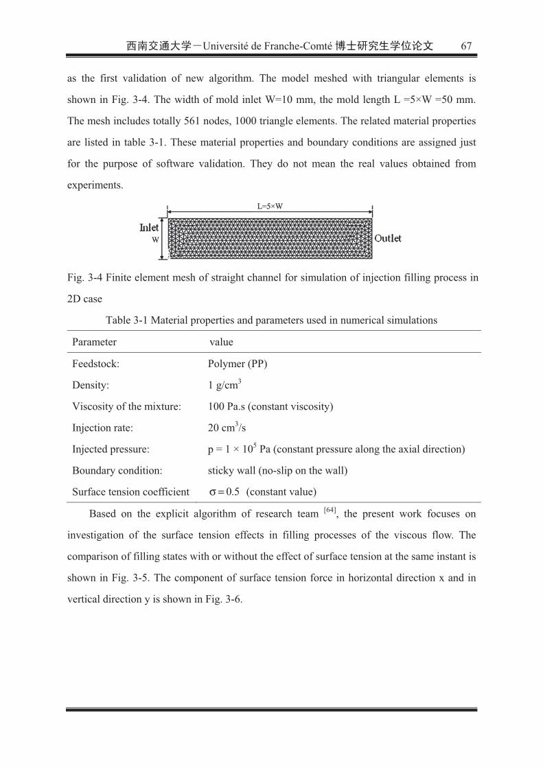
Université de Franche-Comté 67
as the first validation of new algorithm. The model meshed with triangular elements is
shown in Fig. 3-4. The width of mold inlet W=10 mm, the mold length L =5×W =50 mm.
The mesh includes totally 561 nodes, 1000 triangle elements. The related material properties
are listed in table 3-1. These material properties and boundary conditions are assigned just
for the purpose of software validation. They do not mean the real values obtained from
experiments.
Fig. 3-4 Finite element mesh of straight channel for simulation of injection filling process in
2D case
Table 3-1 Material properties and parameters used in numerical simulations
Parameter value
Feedstock: Polymer (PP)
Density: 1 g/cm3
Viscosity of the mixture: 100 Pa.s (constant viscosity)
Injection rate: 20 cm3/s
Injected pressure: p = 1 × 10⁵ Pa (constant pressure along the axial direction)
Boundary condition: sticky wall (no-slip on the wall)
Surface tension coefficient 5.0=σ (constant value)
Based on the explicit algorithm of research team [64], the present work focuses on
investigation of the surface tension effects in filling processes of the viscous flow. The
comparison of filling states with or without the effect of surface tension at the same instant is
shown in Fig. 3-5. The component of surface tension force in horizontal direction x and in
vertical direction y is shown in Fig. 3-6.

68 Université de Franche-Comté
Fig. 3-5 Comparison of the filling states with or without the effect of surface tension at the
same instant: (a) Without surface tension; (b) With surface tension effect.
Fig. 3-6 Distribution of surface tension force: (a) Component in x direction; (b) Component
in y direction
For analyzing the impacts of surface tension on molds filling of different scales, the
examples of different sizes are realized in simulation. In order to understand the variation of
surface tension effect when the geometrical scale of mold filling changes, the examples are
made under the same conditions, except for their sizes. The meshes for different models of
different sizes remain proportionally the same, except that the size of elements changes
accordantly. Then the influence of element distribution can be removed for the examples of
different sizes.

Université de Franche-Comté 69
Fig. 3-7 Results of injection filling states in molds of different sizes: (a) surface tension
ignored; (b) surface tension included.
Fig. 3-7 (including 3-7.1 ~ 3-7.5) represents variation of the simulation results for
filling state at different geometrical scales, with disregard and consideration of the surface
tension term. The comparison of two results is labeled by (a) and (b) for the simulations of
each size, respectively. The notation W and L are shown in Fig. 3-4. W is the width of mold
inlet, and L = 5W is mold length.

70 Université de Franche-Comté
Comparison of the simulation results for different sizes, shown in Fig. 3-7, provides
variation of the surface tension effect according to the change in geometrical scale. All
examples retain the same feedstock properties and same shear rate for the flow of feedstock.
The evolutions of filling state are nearly the same for the examples with and without the
surface tension term. Slight difference in curvature of the filling front surface is observed.
The smaller the example is, the more obvious for the difference in surface curvatures. It
indicates that the surface tension force impacts on the shape of filling front in injection
molding process. The surface tension increases the curvature value of filling front. The
results of simulation explain well the physics nature of surface tension, which tells that the
surface tension induces contraction of the liquid surface. But it should be noticed that the
surface tension term almost does not affect the filling of feedstock, for the size scales
investigated in the present paper. The filling ratio in mold cavity at the same instant, with or
without considering the surface tension effect, is shown in Table 3-2.
Table 3-2 Filling ratio in mold cavity at same instant with or without surface tension effect
Mold size W (/m)
F(Filled) % (without surface tension)
F1(Filled) % (with surface tension)
difference F-F1 %
0.02 42.718 42.6055 0.1125
0.01 42.994 42.8665 0.1275
0.007 43.1645 42.6422 0.5223
0.005 43.356 41.8267 1.5293
0.003 43.5102 38.8243 4.6859
The data in Table 3-2 indicates that surface tension effect has the tendency to slow down
the filling process, within the scale of simulated examples. Although the difference between
the filling ratios with or without surface tension effect is not significant for the example in
ordinary sizes, it increases obviously when the mold size is decreased. This phenomenon can
be also found in Table 3-3 and Fig. 3-8.

Université de Franche-Comté 71
Table 3-3 Relation between mold size and maximal value of surface tension force
Width of mold W (/m)
0.02 0.01 0.007 0.005 0.003
Maximal value of surface tension force
Fb_max (/N) 3.012 3.874 5.884 8.124 13.167
Fig. 3-8 Relationship of Mold width and surface tension effect
For the flow of small Reynolds number, filling front surface is governed by advection
equation, advected by velocity field. The solution of velocity field is affected by viscous
force and surface tension force. In order to evaluate and compare their effects on advance of
the filling front, 10 nodes on filling front surface were chosen to compare the values of
surface tension and viscous force. The average value of surface tension force and viscous
force at 10 nodes was used to evaluate the effect of surface tension on evolution of the filling
front surface, as shown in Table 3-4.
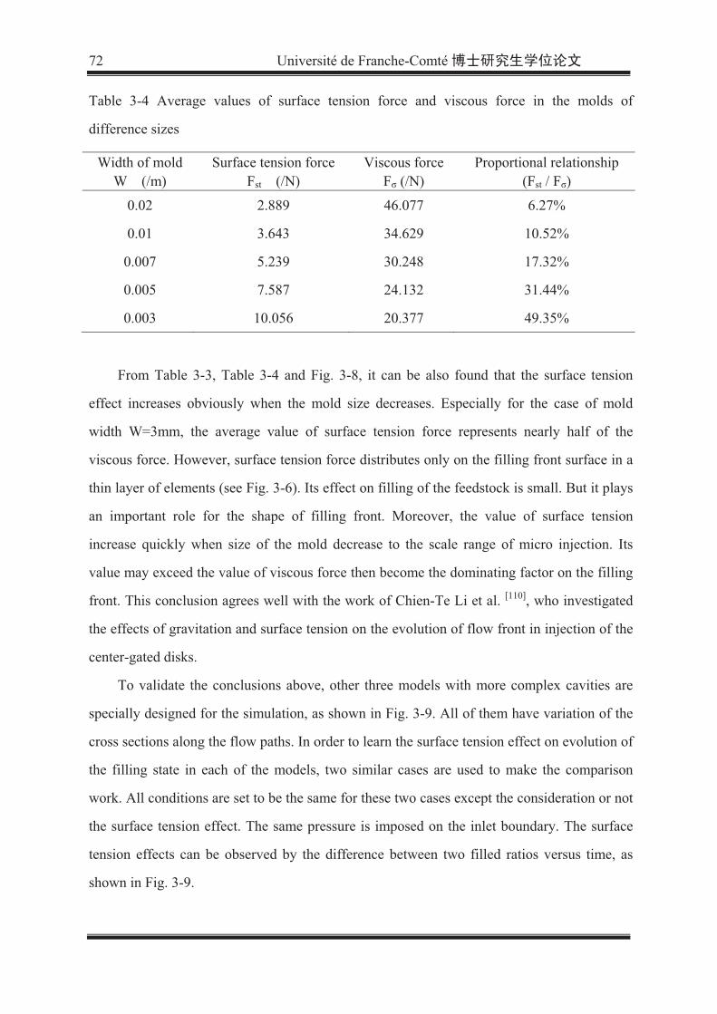
72 Université de Franche-Comté
Table 3-4 Average values of surface tension force and viscous force in the molds of
difference sizes
Width of mold W (/m)
Surface tension force Fst (/N)
Viscous force F (/N)
Proportional relationship (Fst / F )
0.02 2.889 46.077 6.27%
0.01 3.643 34.629 10.52%
0.007 5.239 30.248 17.32%
0.005 7.587 24.132 31.44%
0.003 10.056 20.377 49.35%
From Table 3-3, Table 3-4 and Fig. 3-8, it can be also found that the surface tension
effect increases obviously when the mold size decreases. Especially for the case of mold
width W=3mm, the average value of surface tension force represents nearly half of the
viscous force. However, surface tension force distributes only on the filling front surface in a
thin layer of elements (see Fig. 3-6). Its effect on filling of the feedstock is small. But it plays
an important role for the shape of filling front. Moreover, the value of surface tension
increase quickly when size of the mold decrease to the scale range of micro injection. Its
value may exceed the value of viscous force then become the dominating factor on the filling
front. This conclusion agrees well with the work of Chien-Te Li et al. [110], who investigated
the effects of gravitation and surface tension on the evolution of flow front in injection of the
center-gated disks.
To validate the conclusions above, other three models with more complex cavities are
specially designed for the simulation, as shown in Fig. 3-9. All of them have variation of the
cross sections along the flow paths. In order to learn the surface tension effect on evolution of
the filling state in each of the models, two similar cases are used to make the comparison
work. All conditions are set to be the same for these two cases except the consideration or not
the surface tension effect. The same pressure is imposed on the inlet boundary. The surface
tension effects can be observed by the difference between two filled ratios versus time, as
shown in Fig. 3-9.
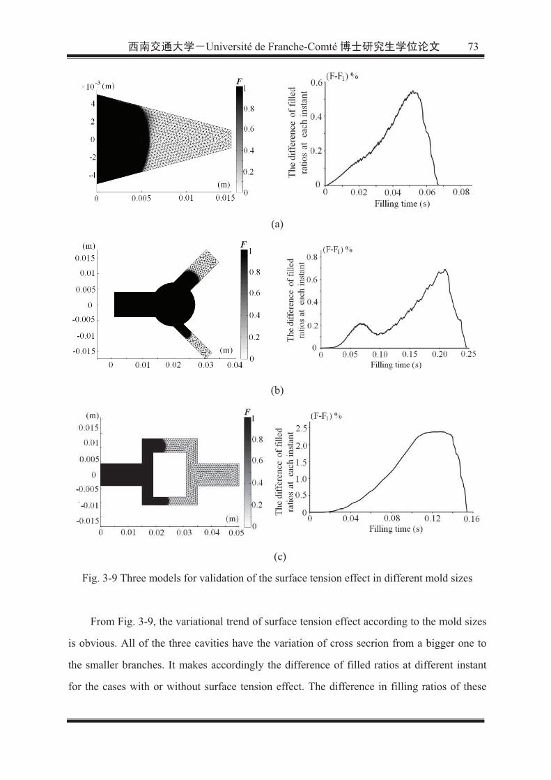
Université de Franche-Comté 73
(a)
(b)
(c)
Fig. 3-9 Three models for validation of the surface tension effect in different mold sizes
From Fig. 3-9, the variational trend of surface tension effect according to the mold sizes
is obvious. All of the three cavities have the variation of cross secrion from a bigger one to
the smaller branches. It makes accordingly the difference of filled ratios at different instant
for the cases with or without surface tension effect. The difference in filling ratios of these

74 Université de Franche-Comté
two cases is growing from a very low value to the peak value until one of them getting to the
fully filling state, then the other case continue to fill untill difference of the filling ratios
become zero. However, we should also notice that although the growing of difference is
obvious, but the magnitude of difference is small, at most 2.5%. So we can still conclude that
the surface tension effect is not so important for injection filling of the sizes in these analysis.
3.5Conclusion
In this Chapter, the effect of surface tension is implemented in an explicit finite
element solver. A simple and systematic scheme is proposed and realized to fit the
requirement of finite element methods. The Laplacian operation of filling function is realized
by a two-step vectorial procedure to evaluate curvature of the filling front. The results are
introduced directly into the source term of surface tension force in the solution of
Navier-Stokes equations. According to the continuum surface force (CSF) model [111], the
force of surface tension is distributed in a thin layer of the elements, which locates on the
filling front of injection flow. A series of the examples for filling flow at scales of different
dimensions are realized by the developed software with the ability to take into account the
effect of surface tension. These examples prove that the importance of surface tension term
increases when the mold size decreases. The surface tension can be neglected in ordinary
injection molding, but it plays the significant role for the problems in sub millimeter sizes.

Université de Franche-Comté 75
Chapter 4 Brief Introduction and Foundational Theories
for Sintering
4.1 Introduction of sintering
4.1.1 Berif introduction of sintering
Sintering is a widely used processing technology in powder metallurgy and ceramic
industries. It is a heat treatment applied to a powder compact in order to improve strength
and integrity by bonding together the particles [114]. It might best be described as the
synthetic manufacture of solid products using controlled heating of powdered raw materials.
Hausner [115] proposed the deÞnition of sintering as follows “sintering is the bonding of
particles in a mass of powders by molecular or atomic attraction in the solid state, by
application of heat, causing strengthening of the powder mass and possibly resulting in
densiÞcation and recrystallisation by transport of materials”. Kuczynski [116] deÞned
sintering as diffusional creep under action of capillary forces. According to the ISO
definition of sintering, it is the thermal treatment of a powder or compact at the temperature
below the melting point of the main constituent. The proper temperature is ordinarily 2/3 the
melting point of the particular material. For materials that have high melting points such as
molybdenum, tungsten, rhenium, tantalum, osmium and carbon, sintering is one of the few
viable manufacturing processes. During sintering the green bodies shaped by die pressing,
injection molding, slip casting, extrusion or spraying undergo the shrinkages in dimension
and the final high dense or full dense products are obtained. It is based on atomic diffusion.
The atoms in the powder particles diffuse across the boundaries of the particles, fusing the
particles together and creating one solid component, as shown in Fig. 4-1.

76 Université de Franche-Comté
Fig. 4-1 The three stages of solid state sintering: left: initial stage, centre: intermediate stage,
right: final stage (Courtesy EPMA) [117]
4.1.1.1 The history of sintering
Sintering is well established as a component fabrication approach. It has been applied to
ceramics for 26 000 years. Sinter plants were constructed for iron ore induration starting in
the 1860s. By 1871, the term showed up in archival literature with reference to bonding
minerals. Subsequently, sintering was widely used to describe ore agglomeration. Before
1900, most of the publications simply called it firing. Metal sintering was evident in the
early 1900s. For ceramics, sintering was initially reserved to describe the agglomeration of
powders. Then, sintering was used in the technical ceramics literature starting in 1939. After
the Second World War, sintering was broadly used to describe the heating of particles to
produce components. The first published reports on sintering started in 1829 for platinum.
Now, more than 20 000 archival publications are issued each year on sintered materials.
About 40% of these literatures are on iron and steel, cemented carbides or alumina based
ceramics. Engineering materials commonly processed by sintering are alumina, tool steels,
steels, cemented carbides, stainless steels, titanium, copper, silicon nitride, titanates and
zirconia. In recent years, sintering has propagated into a wide range of nanoscale powders
which extend the small device applications into the electronic and biomedical fields.
4.1.1.2 The advantages of sintering
The advantages of sintered products over stamped, forged, or molded products include
higher purity of raw materials, the maintenance of purity through the manufacturing process,
the stability of repetitive steps in manufacture, and the uniform density of the item produced.

Université de Franche-Comté 77
Obviously, advancements in technology ensure a more cost-effective manufacturing of
higher quality sintered products.
4.1.1.3 The essential sintered methods
There are two essential methods of sintered manufacturing. By mass transport
mechanisms at the atomic level, it can be devided into solid state, and liquid phase sintering
[118]. The sintering proceeded by solid-state diffusion falls into solid-state sintering. Most
polycrystalline materials are sintered by this type of the process. As similar, the liquid phase
process introduces a transient liquid phase that can improve the mass transport rate. Liquid
phase sintering is generally easier and more cost-effective than solid state.
In addition to the convenstional sintering method by resistance heating, there exist
many new sintering ways to meet the requirments of fast sintering with high heating rate and
temperature, such as Microwave Sintering [119], Selective Laser Sintering [120], Spark plasma
sintering [121] and Self-propagating Sintering [122].
Microwave sintering has emerged in recent years as a new method for sintering a
variety of materials. It has shown significant advantages against conventional sintering
procedures. It is different from the conventional methods where heat is transferred between
the objects by conduction, radiation and convection. It is a process in which the materials
couple with microwaves, absorb the electromagnetic energy volumetrically, and transform it
into heat, then sintered the powder materials. It is now widly used in sintering ceramics,
semiconductors, inorganic and polymeric materials. But there are still many unknows about
its heating principle, its reaction with sintered materials and the effects of proceeding factors
to manufacturing process. In the later research in chapter 5 and Chapter 6, we investigate
microwave sintering from both experiment and simulation aspects.
Selective Laser Sintering uses a laser to sinter powder based materials together,
layer-by-layer, to form a solid model. The system consists of a laser, component chamber,
and control system. This technology is ideal for durable, functional components with a
variety of applications and capable of producing snap fits and living hinges. It suits for
materials including: Nylon (Duraform PA), Glass-Filled Nylon (Duraform GF), Flame

78 Université de Franche-Comté
Retardant Nylon and Durable Nylon (Duraform EX).
Spark plasma sintering, also known as field assisted sintering process or pulsed electric
current sintering [123], is a sintering technology. The main characteristic of this sintering
method is that the pulsed DC current directly passes through the graphite die, as well as the
powder compact, in case of conductive samples. Therefore, the heat is generated internally,
in contrast to the conventional hot pressing, in which the heat is provided by external heating
elements. This facilitates a very high heating or cooling rate (up to 1000 K/min), hence the
sintering process is generally very fast (within a few minutes). The general rate of process
ensures its potential of densifying powders with nanosize or nanostructure, because it can
effectivlly avoid coarsening phenomenon which accompanies with standard densification
routes.
Self-propagating high-temperature synthesis is a method for producing inorganic
compounds by exothermic reactions, usually involving salts. A variant of this method is
known as solid state metathesis. Since the process occurs at high temperatures, the method is
ideally suited for the production of refractory materials with unusual properties, for example:
powders, metallic alloys, or ceramics with high purity, corrosion resistance at high
temperature or super hardnessity.
In this research work, pressureless solid-state sintering is used to densify the PIM
components. This chapter reviews the literatures on the theory of solid-state sintering.
4.2 Foundational Theories for Sintering
4.2.1 Driving Forces of Sintering
In most cases, the density of a collection of grains increases as material flows into voids,
causing the decrease in overall volume. Mass movements that occur during sintering consist
of the reduction of total porosity by repacking, followed by material transport due to
evaporation and condensation from diffusion. In the final stages, metal atoms move along
crystal boundaries to the walls of internal pores, redistributing mass from the internal bulk of

Université de Franche-Comté 79
the object and smoothing pore walls.
The driving force for densification is the impetus to reduce the free energy in particle
surfaces, the externally applied pressure and the chemical reactions [124]. In the present
research, sintering is performed without the external pressure or chemical reaction. Fig. 4-2
is the two-sphere sintering model to show the formation of interparticle bond, and the
reduction of the free solid-vapor interfaces at the contact area between the two particles. It
forms new but lower-energy solid-solid interfaces between the particles with a total decrease
in surface energy by removing the free surfaces.
Fig. 4-2 Two-sphere sintering model showing that the reduction of the free energy during
sintering by the formation of interparticle bond [14].
On the other hand, the elimination of the grain boundary area via grain growth or
coarsening can also lower the free energy of the sintering body, as shown in Fig. 4-3.
Fig. 4-3 Grain growth reduces the free energy of the sintering body by eliminating the grain
boundary area [14].

80 Université de Franche-Comté
4.2.2 Sintering Mechanisms
Sintering mechanisms have been discussed by various workers mainly under two
categories [125]:
Plastic deformation mechanism;
Diffusion mechanism.
Sintering in practice is the control of both densification and grain growth. It occurs by
diffusion of atoms through the microstructure. This diffusion is caused by a gradient of
chemical potential – atoms move from an area of higher chemical potential to an area of
lower chemical potential. The different paths the atoms take to get from one spot to another
are the sintering mechanisms. The six common mechanisms are:
• Surface diffusion – Diffusion of atoms along the surface of a particle;
• Vapor transport – Evaporation of atoms which condense on a different surface;
• Lattice diffusion from surface – atoms from surface diffuse through lattice;
• Lattice diffusion from grain boundary – atom from grain boundary diffuses through
lattice;
• Grain boundary diffusion – atoms diffuse along grain boundary;
• Plastic deformation – dislocation motion causes flow of matter.
1–3 above are non-densifying. They take atoms from the surface and rearrange them
onto another surface or part of the same surface. These coarsening mechanisms lead to neck
growth without producing the densification. They are in the form of surface diffusion,
evaporation condensation and volume diffusion from the surfaces. 4–6 above are densifying
mechanisms. Atoms are moved from the bulk to the surface of pores thereby eliminating
porosity and increasing the density of the sample. It includs grain boundary diffusion and
volume diffusion from the grain boundaries. In addiction, plastic flow occurs when the
sintering stress larger than the in-situ strength of the sintering body. It can result in the rapid
densification [126]. Fig. 4-4 shows the various mass transport paths during sinter bonding in a
three particles model.

Université de Franche-Comté 81
Fig. 4-4 Neck growth among three particles to show various mass transport paths during
sinter bonding [9].
4.2.3 Stages of Sintering
The different stages during the sintering process are sketched in Fig. 4-5.
Fig. 4-5 Illustration of the microstructure evolution during the solid state diffusion sintering
stage [9].
The debinded components are sintered by solid state diffusion. It can be divided into
three stages, based on the geometry of microstructures. There is no clear-cut distinction
between the stages, but each stage can be described by their general characters. At the
beginning of sintering, powders are in loose state. In the initial stage, the sintering necks are

82 Université de Franche-Comté
formed at the contact area and begin to growth by the diffusion process. The shrinkage
occurs during the initial stage is about 4%. In the intermediate stage, the pores are rounding
and interconnected at the grain boundaries. It undergoes rapidly the densification by
reducing the cross section of the cylindrical pores. The final stage is characterized by the
isolated pores located at the grain corners. It is also known as the grain coarsening stage.
A typical sintering cycle by solid state diffusion for stainless steel feedstock is given in
Fig. 4-6, which is composed by four main steps: thermal debinding, emergence of neck
growth, reduction of oxide diffusion and sintering.
Fig. 4-6 Typical (solid state diffusion) kinetic sintering cycle for stainless steel feedstock
with four segments [21].
4.3 Models and Simulations of Sintering
4.3.1 Simulation history
Sintering is an important process to produce the metallic and ceramic powder products.
It dominates the final dimensions and mechanical properties. On the other hand, sintering is
a complicate process that involves many physical and chemical phenomena. The
mechanisms of sintering have not been totally understood yet. The geometrical accuracy and
mechanical properties of the final components after sintering depend strongly on the choice

Université de Franche-Comté 83
of process parameters in different stages, such as heating rate, peak temperature, holding
time, sintering atmosphere and initial density. The introduction of simulation work can be
used to optimize and to understand the sintering process better and improve the quality of
sintered components. It could be a faster alternative in optimizing entire industrial processes
compared to the conventional method of trial and error. The determination and optimization
of process parameters have motivated numerous research works, as it needs deep knowledge
on different processes and accurate modeling methods for each stage.
Researches on modeling and numerical simulations of the sintering process have been
carried out for more than 50 years. The histories, development, achieved performance and
the remaining barriers of sintering simulations were reviewed by German [127]. About every
ten years the field takes a new turn, and in simple form the history of sintering simulations is
as follows:
1960 to 1970: numerical simulations of two-particle neck growth in sintering;
1970 to 1980: multiple mechanism calculations of one-dimensional shrinkage;
1980 to 1990: predictions of density including pressure-assisted sintering;
1990 to 2000: continuum mechanics and finite element simulations of shape and size;
2000 later: control programs with hybrids of simulations and artificial intelligence.
4.3.2 Three sintering models
There is no unique classification of the various established models of sintering.
According to the major approach of the modeling process, there are three kinds of
distinguish models of sintering: (i) microscopic model (physically-based), (ii) mesoscopic
model (stereological) and (iii) macroscopic model (phenomenological) [128].
4.3.2.1 Microscopic Models
The microscopic models aim to simulate the mass transport mechanisms between
several particles. Sintering is treated as a collective result of thermally activated adhesion
processes which result in the growth of contacts between particles. A number of

84 Université de Franche-Comté
micromechanical models of sintering are based on a particle representation of porous powder
material undergoing the sintering process. The most successful approaches to understand the
mechanisms of neck growth and shrinkage are the two-sphere model due to Frenkel [129] and
Kuczynski [130] for the early sintering stages (particle bonding), as shown in Fig. 4-7. The
two-particle model has been extrapolated for the intermediate shrinkage state by Kingery and
Berg [131]. Coble [132] developed a cylindrical pore model (as shown in Fig. 4-8), a spherical
pore model for the late sintering stages (as shown in Fig. 4-9) was developed by MacKenzie
and Shuttleworth [133]. More sophisticated models taking into account the superposition of
various sintering mechanisms have been developed by Ashby [134], Arzt [135], and Exner and
Arzt [136]. Until recently, simulation of microstructural evolution of large systems was not
feasible due to the computer power limitations. It is becoming increasingly possible to
simulate microstructural behavior of large systems, and this development is paving the way
for embedding microstructural evolution into macroscopic models.
Fig. 4-7 Geometries of the two-sphere model to describe the neck growth and densification
in the initial sintering stage. ( D is the diameter, X is the diameter of the neck, nr is
neck surface radius, and y is the overlap distance. ) [24]

Université de Franche-Comté 85
Fig. 4-8 The interconnected pores in cylindrical shape located on the boundaries of
tetrakaidecahedron grains in the intermediate stage of sintering [24].
Fig. 4-9 The isolated spherical pores located at the corners of boundaries of
tetrakaidecahedron grains in the final stage of sintering [24].
4.3.2.2 Mesoscopic Models
The mesoscopic models choose the representative cell or element in the sintering body,
and simulate the microstructural evolutions including densification and grain growth. The
mechanical properties of sintered components are determined by the material characters in
mesoscopic level such as grain size, pore shape and distributions. A mesoscopic model of
sintering capable of simulating large powder compacts could be a step to more realistic
macroscopic models. However, although great progress has been made in the last 50 years in
understanding microstructural evolution during sintering, current models of sintering [137-139],
still consider highly idealized geometries with limited number of circular or spherical
particles. While these models have provided much insight into the sintering process by
predicting shrinkage rates, geometric changes in the particles and other information, their

86 Université de Franche-Comté
ability to predict characteristics of a complex powder compact is limited.
4.3.2.3 Macroscopic Models
In the continuum approach, the porous powder under compaction is treated as a
continuous medium at the macro-scale. It is close to the industrial application due to its merit
in predication of the dimensional shrinkages and distortions of the sintered bodies. The
deformation behavior of sintered bodies is described by constitutive equations based on
modified theory of solids. The macroscopic behavior of sintered materials is a result of a
complex combination of elastic, viscous, plastic and thermal deformation depending on the
processes at the microscopic and atomistic levels [140]. Different mechanisms dominate the
deformation behaviors at different stages of a powder metallurgy process. Constitutive
equations of continuous media belong to the class of phenomenological models in which
model parameters are obtained by fitting experimental data. Well-known phenomenological
sintering models are those developed by Abouaf et al. [141], Duva and Crow [142], and Cocks
[143]. Phenomenological approaches have been summarized by Olevsky [114], Cocks [144] and
German [24]. Phenomenological theories do not take microstructure of the material into
consideration. More recent analytical and numerical models of sintering make fewer
assumptions. They are able to treat the details of shape change, shrinkage rate or other
characteristic more accurately in a sintering compact.
There are many achievements of each kind of the sintering models, but neither of them
is perfect. Most of the existing models are based on the spherical particle shape, cylindrical
or spherical pore shape. It is much different from the real situation in the sintering process.
Moreover, some phenomena occurring at the microstructural level and the non-thermal
mechanical factors should be considered, such as phase transition, chemical reaction,
influence of sintering atmosphere, oxidization phenomena and in-situ damage criteria etc.
The most important thing, effective links are required between the microscopic, mesoscopic
and macroscopic models.
Researches for sintering simulation are continued. The model used to simulate sintering
in this work is based on the phenomenological macroscopic model. The most widely used
linear viscoplastic constitutive law will be introduced in detail later in Chapter 6.

Université de Franche-Comté 87
Chapter 5 Efficient sintering of 17-4PH stainless steel
powder by microwave
As a new but fast developing technology, microwave sintering represents significant
theoretical and industrial values. The heating of microwave sintering is a process in which
the microwave energy is absorbed by the sintered materials. The energy is transformed into
the kinetic energy of molecules, and thermal energy in the materials. It exhibits the important
potential of rapid processing with high production efficiency [145]. Microwave heating is a
sensitive function of sintered materials. Microwave penetrates into the media in the form of
electro-magnetic waves, and results in the heating by transforming energy into heat. The heat
is generated inside the materials, together with the vibration of the microwave in high
frequency, which increase the kinetic energy of molecules and ions in the materials. The
diffusion effect of densification is then increased, too. These properties are very advantages
to improve the properties of final sintered materials in the micro and meso scales [146].
Moreover, microwave heating is selective [147] and pollutionless [148], it can be then widely
used in the actual productions.
As a combination of powder metallurgy and microwave heating technology, microwave
sintering has been extensively studied in experimental works. Takahashi et al. [149]
manufactured zirconate titanate actuator in 2001; Anjana et al. made some researches on
Ce2(WO4)3 ceramics with low temperature [150]. Since 1999, when Roy et al. [151] sintered
powdered-metals successfully in a microwave field, a wide range of standard powdered
metals have been sintered by microwave heating. Author’s teams have long-term
experiences in Micro-PIM technology, which focuses on feedstock characterization and
elaboration [152], identification of physical material parameters [153], mathematical model
proposed for bi-phase fluid flow [154] and experimental and numerical analysis on the
conventional thermal sintering [155]. For further investigation of sintering mechanism under
microwave heating, a microwave sintering furnace is equipped in the research team.
Because of its sole report and unfavorable conclusion, the study in this chapter is made
on the realization of fully densified 17-4PH stainless steel compact by hybrid microwave

88 Université de Franche-Comté
heating. The investigated factors include peak sintering temperature, holding time, heating
rate, pre-sintering stages. The results are illustrated by final size shrinkage, relative density,
hardness and microstructure. Comparative analysis is made with the sintering in conventional
resistive heating furnace. The sintering by microwave takes one tenth of the conventional
sintering time to get the better results. The optimal peak temperature is 150 ~200 lower.
It results in the better densification, more homogeneous microstructure, higher mechanical
properties, and more size shrinkage. The experiments proved a remarkable fact for
microwave sintering of the 17-4PH stainless steel powder. The heating rate must be set to an
order of 30°C/min. Lower heating rate leads to the poor results. The fast processing by
microwave results in the gradient of mechanic properties in sintered bodies. The prediction,
evaluation and purposes of the gradient properties induced by microwave leads the studies to
the more precise and profound insights.
5.1 Research background
17-4PH is a type of martensitic precipitation hardening stainless steel with high
mechanical properties [156]. By heat treatment, high yield strength up to 1100-1300 MPa
(160-190 ksi) can be achieved. Besides that, it represents excellent corrosion resistance [157].
This versatile material is then widely used in the aerospace, chemical, petrochemical, food
processing, paper and general metalworking industries [158].
Nowadays, most researches on sintering of 17-4PH stainless-steel focus on the ways by
conventional resistive heating (CRH). Sung et al. [159] studied the effect of sintering
temperature on its microstructure and mechanical properties; Ye et al. [160] investigated the
densification behavior in the temperature range of 650–1050 °C; Simchi et al. [161]
experimented with a bilayer structure and discovered that stain rate of 17-4PH were higher
than that of 316L during the course of sintering; Imgrund et al. [162] also produced
magnetic–nonmagnetic bimetals made of 316L/17-4PH and 316L/Fe powders by
micro-metal injection molding and CRH sintering process.
Microwave (MW) heating results from the absorption by molecular vibration (rotating
electric dipole/dipole reorientation) and ionic conduction of a portion of the energy

Université de Franche-Comté 89
transported by an oscillating electric field [163]. The primary advantages [164] of microwaves
sintering are (a) rapid kinetics leading to savings of time and energy [165], (b) rapid internal
heating [166], (c) lower temperature synthesis [167], (d) fine microstructures and improved
properties [168]. For MW method, many researches focused on other powder materials. Zheng
et al. [169] prepared a novel celsian/yttrium silicate coating by microwave sintering on the
surface of C/SiC composites. Chandrasekaran et al. [170] conducted microwave heating and
melting of lead, tin, aluminum and copper with the aid of square shaped silicon carbide
susceptor. Liu et al. [171] found that the addition of nanometer Al2O3 powder and MW
sintering process resulted in a synergistic effect on improvement of microstructure and
properties of alumina ceramics. Tang et al. [172] elaborated porous nickel titanium (NiTi)
shape memory alloy by microwave sintering at relatively low temperature of 850 and
short sintering time of 15 min. Mula et al. [173] investigated the applicability of microwave
sintering to produce bulk metal-based nanocomposites with blend composition of Cu99Cr1,
Cu94Cr6, Cu99Cr1– 4wt.% SiC and Cu94Cr6– 4wt.% SiC (average particle size 30 nm).
Panda et al. [174] compared the effect of heating mode on the densification, microstructure,
strength and hardness of austenitic (316L) and ferritic (434L) stainless steels. The
superiorities of MW sintering were all conformed in these works.
However, only one investigation on the microwave processing of 17-4PH
stainless-steel powder was found by the retrieves of literatures in the currently available
resources. It was a preliminary study done by Bose et al. [175]. They found that MW sintering
had not improved the mechanical properties compared to CRH sintering for 17-4PH stainless
steel.
To understand better the sintering properties of the 17-4PH stainless steel, the present
work examined the densification and microstructure evolution of 17-4PH stainless steel
powder produced by MW sintering. The injected specimens subjected to 2.45 GHz
microwaves in a mono-mode furnace. The influence factors were investigated, including the
peak sintering temperature, holding time, heating rate and pre-sintering stages in microwave
sintering process. After such a solid state sintering route [176], the evolutions of
micro-structure densification and mechanical response of the sintered specimens were

90 Université de Franche-Comté
studied. Comparison of the results between MW sintering and CRH process was also
studied.
In present research, the authors proved that the MW sintering process for 17-4PH
stainless steel provides higher sintered density and fewer defects in micro structure. Then
better mechanical properties are achieved. Meanwhile, it shortens greatly the sintering time,
lowers the peak sintering temperature. Higher Vickers-hardness of MW sintered compacts
was also detected in the present work. It is important to indicate that the mechanic properties
behave gradiently in the sintered bodies, because of the rapid processing by internal heating.
None of the specimens presents visually observable distortion.
5.2 Experimental procedure
The experimental specimens were made of 17-4PH stainless steel powder with average
size 11µm. The micrometer-scaled particles can be observed by the optical microscope as
demonstrated in Fig. 5-1. Chemical composition of 17-4PH stainless steel is shown in Table
5-1, according to standard AISI630.
Fig. 5-1 Micrographs of 17-4PH stainless steel powder (average size 11µm) used in the
subsequent tests, observed by optical microscope.
Table 5-1 Chemical composition of 17-4PH stainless steel (wt, %)
Fe Ni Cr C Cu Nb Mn S P Si
71.8~73.8 3.0~3.5 15.5~17.5 0.07 3.0~5.0 0.45 1.0 0.03 0.04 1.0
In the present analysis, specimens in 17-4PH stainless steel powders were prepared by
several processes [2] before MW sintering stage. The schematic illustration for all the steps

Université de Franche-Comté 91
from powder to sintered components is shown in Fig. 5-2. The final sintering stage is
represented by two possible ways: CRH or MW sintering. The green components, which
based on 17-4PH stainless steel powder mixing with wax-based binders, were provided by ©
Beijing Jarain Powder Injection Tech., Co. Ltd. The density of green parts was approximately
5.05 g/cm3, 64% of the density for pure 17-4PH stainless steel 7.89 g/cm3. Before sintering,
binders were burnt out in an electric thermal debinding oven. The first stage is to remove the
water vapor absorbed inside. The injected components were heated from 20 to 130
with a heating rate 55 /hour. This temperature is lower than that for decomposition of the
paraffin wax. Then the temperature was increased up to 220 with a very slow heating rate
4.5 /hour to eliminate the paraffin wax. Afterwards, the specimens were cooled for 2 hours
to reach ambient temperature. This debinding cycle was also used by Quinard et al. [153] for
the study of PIM feedstocks with 316L stainless steel powder (mean particle size 3.4 µm) to
process the micro-components. Belgacem et al. [177] made an investigation on details of the
thermal debinding process and identified the kinetic parameters for fine 316L stainless steel
feedstock. In debinding process, 6.3% of the weight was reduced for the specimens. This
preliminary debinding stage is necessary to prevent crack development in the next sintering
stage [11].
Fig. 5-2 The sequential stages to get the final sintered components [2]. The sintering stage may
be processed by CRH or MW ways.
Metal powder shows poor coupling with microwaves in low temperature stage of

92 Université de Franche-Comté
sintering [178], so a hybrid way of MW heating was used in the MW furnace
(HAMilab-V1500). A flat SiC susceptor was placed under the powder compact and some
chopped ones were put around it, according to the work of Kim-Hak et al. [179]. Surface
temperature of the specimen was continuously measured by an IR pyrometer from an outside
cavity window. In order to study the densification behavior under different heating modes,
the same debinded components were also sintered by CRH in a vertical SETSYS® evolution
dilatometer.
After sintering, size shrinkages of the sintered specimens were measured by calipers.
Bulk densities were tested according to Archimedes’ principle by immersing the samples into
an ethanol based liquid. Afterward, the sintered samples were wet polished in a manual
polisher. Then Vickers bulk hardness measurements were performed on the samples at 5 kg
load with duration 10 s. To make the measurements more reliable, the hardness values took
the averages of five readings at the spots near center of the prepared surfaces. Metallographic
processes were employed in the microstructural analyses. 4% nitric acid solution and alcohol
were used for etching the polished surface. Then optical microscope was used to observe the
microstructure on polished and chemically etched surfaces of the specimens.
5.3 Results and discussion
5.3.1 Specimen sizes after being injected, debinded and MW sintered
Specimen sizes after being injected, debinded and MW sintered were compared in Fig.
5-3. It exhibits obvious size shrinkage after sintering, about 15% along the x direction. The
polished section of the sintered component is shown in Fig. 5-4.

Université de Franche-Comté 93
Fig. 5-3 Comparison of the sizes for the specimens in 17-4PH stainless steel powder after
injection molding, thermal debinding and microwave sintering.
Fig. 5-4 Polished section of microwave sintered specimens in 17-4PH stainless steel powder
5.3.2 The influence factors in MW sintering process
5.3.2.1 Peak sintering temperature
In order to study the influence of peak temperature on sintering results, tests were
made with different peak temperatures but other processing factors remained the same.
Referring to the previous work by Quinard et al. [46] in research team on CRH sintering of
316L stainless steel, the heating processes include three steps. First the specimens were
heated to 600 , and then held the temperature for 30 minutes. Subsequently the
temperature was increased to 900 , and then held again for 30 minutes. At last the
temperature is increased to peak values of the prescribed tests, and then held the peak
temperature for 10 minutes. The same heating rate 5 /min was applied to all test processes.
The results for different peak temperatures are exhibited in Table 5-2.

94 Université de Franche-Comté
Table 5-2 Comparison of size shrinkage (along x direction in fig. 3), relative density and
Vickers-hardness obtained from specimen sintered with different peak temperatures (All
processes with heating rate: 5 /min and holding the peak temperature for 10 minutes)
Peak temperature ( ) Size shrinkage (%) Relative density (%) Vickers-hardness (HV)
1100 5.67 ±0.001 72.6 ±0.01 173 ±0.1
1140 10.29 ±0.001 90.5 ±0.01 280 ±0.1
1150 12.47 ±0.001 90.9 ±0.01 311 ±0.1
1160 9.98 ±0.001 86.7 ±0.01 235 ±0.1
1200 8.12 ±0.001 81.2 ±0.01 267 ±0.1
It shows the evidence in Table 5-2 that suitable peak temperature will result in
optimized results. For sintering of 17-4PH stainless steel powder by microwave, the optimal
peak temperature is 1150 , which results in the higher density and better mechanical
properties.
5.3.2.2 Effect of holding time
In second batch of the tests, all samples were sintered to the same peak temperature
1150 . The durations of holding time for peak temperature were varied for different tests.
Other processing factors were retained the same as illustrated in 3.2.1. The sintering results
for different holding times are shown in Table 5-3.
Table 5-3 Comparison of size shrinkage (along x direction in fig. 3), relative density and
Vickers-hardness obtained from specimens by MW sintered with different holding time in the
same peak temperature (All processes with heating rate: 5 /min and sintered to the same
peak temperature 1150 )
Holding time (min) Size shrinkage (%) Relative density (%) Vickers-hardness (HV)
5 8.81 ±0.001 85.9 ±0.01 238 ±0.1
10 12.47 ±0.001 90.9 ±0.01 311 ±0.1
15 8.32 ±0.001 84.6 ±0.01 253 ±0.1
20 8.19 ±0.001 83.4 ±0.01 277 ±0.1

Université de Franche-Comté 95
The results showed in Table 5-3 indicate that there exists an optimal heating duration
for peak temperature in microwave sintering. For the case of 17-4PH stainless steel powder,
holding 10 minutes will result in the best solution for high density and mechanical
properties.
5.3.2.3 Effects of heating rate
For third group of the tests, investigation was made by variation of the heating rates.
The peak temperature and holding time were taken to be the optimal values determined by
two above sets of tests. It represented the value 1150 for peak temperature and 10
minutes for holding time. For the purpose to focus closely our attention on heating rate, the
specimens were heating directly to peak temperature from the ambient value, and then held
it for 10 minutes. The heating rates were set for different values in different tests. The results
of MW sintering for different heating rates are shown in Table 5-4.
Table 5-4 Comparison of size shrinkage (along x direction in fig. 3), relative density and
Vickers-hardness obtained from specimen by MW sintered with different heating rates (All
processes sintered to the same peak temperature 1150 and holding it for 10 minutes)
Heating rate ( /min) Size shrinkage (%) Relative density (%) Vickers-hardness (HV)
10 11.11 ±0.001 92 ±0.01 227 ±0.1
20 15.15 ±0.001 95 ±0.01 299 ±0.1
30 16.11 ±0.001 96.6 ±0.01 316 ±0.1
40 14.90 ±0.001 93.6 ±0.01 231 ±0.1
50 Specimen damaged
From the results in Table 5-4, heating rate 50 /min leads to damage of the specimen.
The too fast heating rate results in uneven temperature distribution, which leads to the
distortion or collapse. The lower heating rate may lead to grain coarsening, which results in
lower density and lower surface hardness of the sintered products. A heating rate 30 /min
is shown to be optimal for MW sintering of 17-4PH stainless steel.

96 Université de Franche-Comté
5.3.2.4 Pre-sintering temperature
Based on the above mentioned results, specimens were heated to peak temperature
1150 with heating rate 30 /min, then holding for 10 min. Now the study on
pre-sintering stage is realized. Before the formal sintering stage, the specimens were heated
to a pre-sintering temperature, and then held for 30 min. The results for different
pre-sintering temperatures are shown in Table 5-5. A test without pre-sintering was also
realized to compare with the other processes.
Table 5-5 Comparison of size shrinkage (along x direction in fig. 3), relative density and
Vickers-hardness obtained from specimen by MW sintered with different pre-sintering
temperature (All processes heated with the same heating rate 30 /min, sintering in the same
peak temperature 1150 and holding it for 10 minutes)
Pre-sintering temperature ( )
Size shrinkage (%)
Relative density (%)
Vickers-hardness (HV)
900 9.33 ±0.001 83.7 ±0.01 182 ±0.1
600 10.12 ±0.001 87.8 ±0.01 190 ±0.1
400 12.15 ±0.001 89.9 ±0.01 207 ±0.1
270 13.94 ±0.001 93.4 ±0.01 274 ±0.1
no pre-sintering stage 16.11 ±0.001 96.6 ±0.01 316 ±0.1
In Table 5-5, it is remarkable that the best result is obtained by the process without
pre-sintering stage. If pre-sintering is really necessary for the purpose to get the initial
stiffness, the lower temperature is used, the better quality can be obtained.
A conclusion can be drawn from the facts in section 3.2. The optimal choice in
microwave sintering process for specimens in powders of 17-4PH stainless steel (powder
size 11µm) is shown in Fig. 5-5.

Université de Franche-Comté 97
Fig. 5-5 The optimal process proposed for MW sintering of specimens in 17-4PH stainless
steel powders.
5.3.3 Microstructure
The microstructure of sintered materials has been observed by optical microscope. For
the purpose of clear observation, the specimens were polished and chemically etched for the
observed areas. The sintering stage was interrupted at different temperatures, and left cooled
to have the observation on the corresponded micro structures. When the peak temperature
was reached, a holding time of 10 minutes was maintained. Evolution of the micrographs
from powders to the sintered compacts is illustrated in Fig. 5-6.

98 Université de Franche-Comté
(a) (b)
(c) (d)
(e) (f)
(g) (h)
Fig. 5-6 Micrographs of the microstructure evolution for MW sintering of the 17-4PH
stainless steel powders observed by optical microscope: (a) injected, (b) debinded, then MW
sintered at (c) 950 , (d) 1000 , (e) 1050 , (f) 1100 , (g) 1140 , (h) 1150 holding for
10 min.
Fig. 5-6 depicts well the evolution process of particle crystallization. When sintered to
950 , the as-sintered surfaces were porous and the samples exhibited small grain size. With

Université de Franche-Comté 99
the increase of sintering temperature, the number of pores decreased, and the rate of grain
growth increased apparently. From (f) and (g), the significant grain growth is obviously
observed. Most of the larger holes locate at the grain boundary. It is favorable for evacuation
of the gas entrapped in the porous powder compact and then benefit to the densification
process. When the temperature reached to 1150 (h), the big pores were almost eliminated.
This phenomenon affects directly the mechanical properties of final samples.
5.3.4 Distribution of the Vickers-hardness
In MW processing, heat is produced inside the bulk material, and sent out by radiation
and convection on outer surface of the specimens. Then it takes place the thermal gradient.
The temperature in core is higher than that on the surface. The outer surface at different
positions of the specimen subjects to different variation of temperature, because of irregular
shapes of the sintered body. The sintered material closer to the centroid is denser and
represents generally higher mechanical properties. This phenomenon can be proved by
detection of the hardness distribution over the polished cross section of the specimen.
Detection of hardness distribution on a plane section was realized by a specific scheme.
A cross section near middle plane of the specimen was prepared. On the polished section
plane, 9 small areas were arranged along a horizontal axis and a vertical axis, as shown in
Fig. 5-7. They were labeled in the sequence from x1 to x5, and from y1 to y5. In each small
area, 5 spots were tested. The average value of 5 test results was regarded as the formal
hardness of the small area.
Fig. 5-7 Distribution of the detected areas in the polished section of sintered specimen for
Vickers-hardness measurements

100 Université de Franche-Comté
Fig. 5-8 Vickers-hardness values for each detected small areas along vertical direction
Fig. 5-9 Vickers-hardness values for each detected small areas along horizontal direction
As expected, experimental results in Fig. 5-8 and Fig. 5-9 prove well the nature of MW
sintering. It is noticed that the values at symmetrical positions, said left and right, up and
down, are not symmetric. The asymmetry in the values of Vickers-hardness was induced by
the use of hybrid MW sintering. For example, the point y4, y5 in lower half were closer to
the susceptor than the ones in upper half. Their distance closer to the assist-heating materials
SiC resulted in better heating, and then greater values in Vickers-hardness.
Moreover, it is necessary to note that the difference in hardness values among these
small areas is about 20~30 Vickers units, within such a small size compact. The gradient of
mechanical property is obvious in the sintered bodies. It is due to the character of rapid
heating in MW sintering. However, there is no available way to reduce the optimal heating
rate. The lower heating rate results in the worse sintering quality, because of the grain
coarsening. Then gradient of mechanical properties can be regarded as the nature of MW
sintering. It represents the important value to study the relationship between evolution of
temperature gradient and the gradient of mechanical properties in sintered products.

Université de Franche-Comté 101
Prediction of the gradient in mechanical properties shows its potential significance in the
studies of functionally gradient materials. The research on modeling and simulation of the
property gradients in MW sintering is well expected.
It should be mentioned that none of the microwave sintered specimens exhibited the
visually observable distortion. As the shape of studied specimens was not sensitive to the
distortion, and no precise measurement was applied on their geometries, this conclusion is
just an estimated one. The influence of temperature gradient on shape distortion should be
made by specially designed specimens with the precise measurement on geometries.
5.3.5 Comparison with the conventional sintering
5.3.5.1 Sintering of 17-4PH stainless steel by conventional sintering (CRH)
In order to study and compare the densification behaviors, the same debinded
components were sintered by CRH in a vertical SETSYS® SETARAM evolution analyser,
too. These specimens were heated to peak temperature of 1350 , then holding for 2h, with
different heating rate of 5 , 10 , 20 , 30 /min respectively. According to the process
proposed by Song [48], the temperature was held for 30 min when it reached 600 and
900 to ensure homogenization of the temperature in sintered body. The kinetic size
shrinkages and shrinkage rates versus temperature are illustrated in Fig. 5-10 and Fig. 5-11.
Fig. 5-10 Size shrinkage versus temperature during sintering for the specimens in 17-4PH
stainless steel at different heating rates

102 Université de Franche-Comté
Fig. 5-11 Shrinkage rate versus temperature during sintering for the specimens in 17-4PH
stainless steel at different heating rates
Fig. 5-10 and Fig. 5-11 illustrate that (a) higher heating rate leads to greater shrinkage
rate but less shrinkage; (b) With higher heating rate, shrinkage happens at higher
temperature, and the peak of shrinkage rate happens also at higher temperature.
5.3.5.2 Comparison between MW sintering and CRH sintering
According to the results in 3.5.1, two tests were chosen to make a comparison: (1) For
CRH sintering: heated to 1350 with heating rate 5 /min then held for 2 hours. During
the heating process, the temperature is held for 30 min when it reached 600 and 900 ,
respectively. (2) For MW sintering: heated directly to 1150 by heating rate 30 /min,
then held for 10 min.
Table 5-6 Comparison of sintering time, peak temperature and final properties of the
specimens obtained by CRH sintering and MW sintering
Sintering mode
Sintering time (min)
Peak temperature
( )
Size shrinkage
(%)
Relative density
(%)
Vickers-hardness (HV)
Conventional 445 1350 14.95±0.001 95.2±0.01 284±0.1
Microwave 48 1150 16.11±0.001 96.6±0.01 316±0.1
It demonstrates in Table 5-6 that: (1) The sintering of 17-4PH stainless steel compacts
in a MW furnace represents 90% of reduction in processing time; (2) The optimal peak
temperature for MW sintering is 150 ~200 lower than that for CRH sintering; (3) The
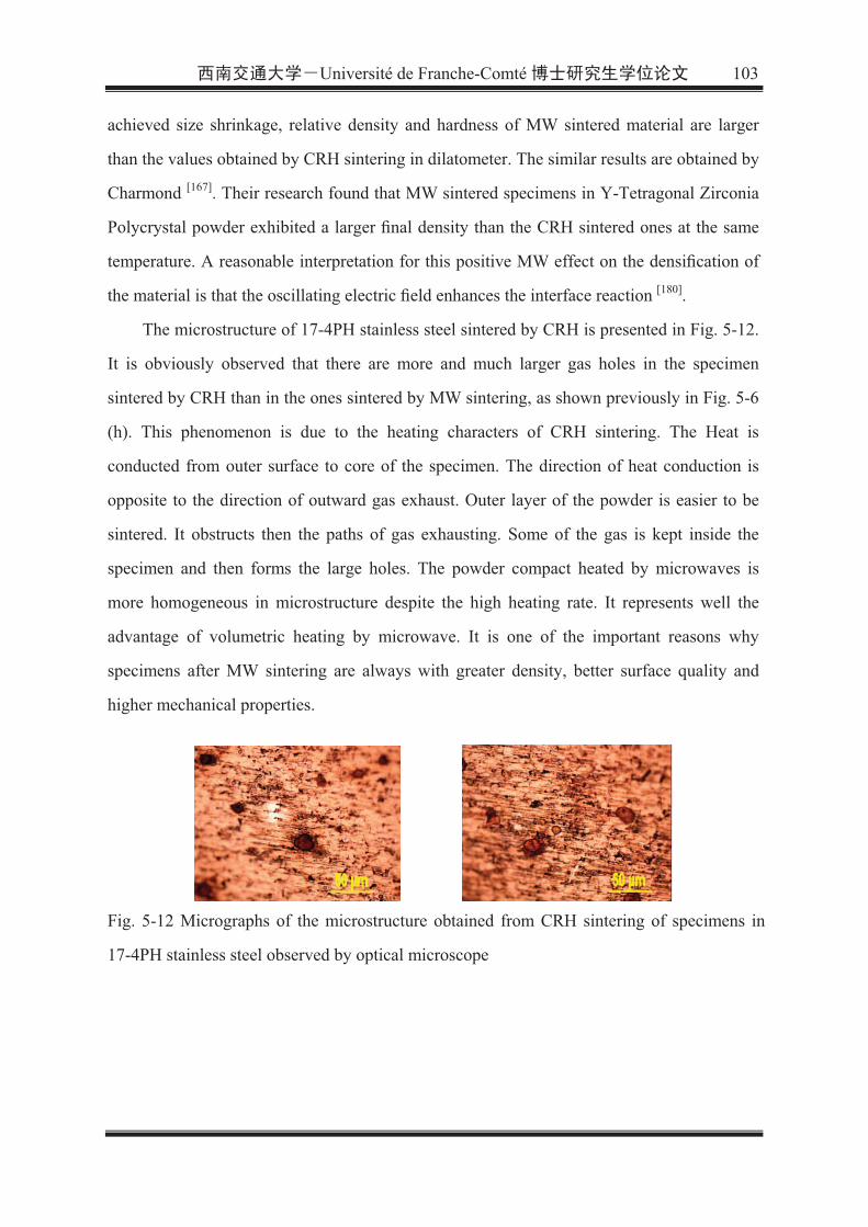
Université de Franche-Comté 103
achieved size shrinkage, relative density and hardness of MW sintered material are larger
than the values obtained by CRH sintering in dilatometer. The similar results are obtained by
Charmond [167]. Their research found that MW sintered specimens in Y-Tetragonal Zirconia
Polycrystal powder exhibited a larger Þnal density than the CRH sintered ones at the same
temperature. A reasonable interpretation for this positive MW effect on the densiÞcation of
the material is that the oscillating electric Þeld enhances the interface reaction [180].
The microstructure of 17-4PH stainless steel sintered by CRH is presented in Fig. 5-12.
It is obviously observed that there are more and much larger gas holes in the specimen
sintered by CRH than in the ones sintered by MW sintering, as shown previously in Fig. 5-6
(h). This phenomenon is due to the heating characters of CRH sintering. The Heat is
conducted from outer surface to core of the specimen. The direction of heat conduction is
opposite to the direction of outward gas exhaust. Outer layer of the powder is easier to be
sintered. It obstructs then the paths of gas exhausting. Some of the gas is kept inside the
specimen and then forms the large holes. The powder compact heated by microwaves is
more homogeneous in microstructure despite the high heating rate. It represents well the
advantage of volumetric heating by microwave. It is one of the important reasons why
specimens after MW sintering are always with greater density, better surface quality and
higher mechanical properties.
Fig. 5-12 Micrographs of the microstructure obtained from CRH sintering of specimens in
17-4PH stainless steel observed by optical microscope

104 Université de Franche-Comté
5.3.6 Conclusions
In present studies, compacts based on 17-4PH stainless steel powder were successfully
consolidated to nearly full density by hybrid MW sintering. The experiments were realized in
a furnace of mono-mode cavity. The optimal heating cycle was determined by the
experiments. The best result was obtained by heating directly from ambient temperature to
1150 with heating rate 30 /min, and then held 10 minutes. It got the specimen with
higher density (relative density: 96.6%) and better mechanical properties (Vikers-hardness:
316V). The sintering of 17-4PH stainless steel powder by MW heating represents short
processing time and lower peak temperature. It takes merely 10% of the conventional
sintering time to get the better results. The peak temperature is 150 ~200 lower than that
in the CRH sintering. Despite of high heating rates, the specimens did not display the
observable distortion or cracking. It represents the important advantage of volumetric heating
by MW. The MW sintering also represents better densification, more homogeneous
microstructure, and higher mechanical properties. As higher density is achieved, the sintering
by MW heating results in more shrinkage in size.
It is remarkable that sintering by MW heating resulted in the obvious gradient in
mechanic properties of the sintered material, because of its rapid heating in the internal
volumetric way. It is valuable to continue the studies on this nature for the application of
MW sintered products. The modeling and simulation on generation of the gradient properties
appears the significant insights for the further studies.

Université de Franche-Comté 105
Chapter 6 Mathematical Modeling and Simulation of
Microwave Sintering Process
6.1 Research Background
Microwave sintering represents the coupling phenomena of multi-physical fields. It
includes the coupling of electro-magnetic fields, thermal conduction and the densification
process of sintered powders. The true process of microwave sintering must be simulated
under the condition that these complicated coupling are taken into account. Most of the
actual literatures focus on the analysis of microwave heating. [181] utilizes FDTD method to
model the realistic sintering experiments in multimode microwave cavities; [163] develops a
simulation model for heating of the foods in microwave ovens; [182] proposes and tested
simple semi-analytical models based on a piecewise constant approximation of the material
properties; [183] develops a quasi-analytic model to examine the energy conversion during
the microwave sintering. These literatures proposed macro models that coupled the
microwave heating and thermal conduction. But none of them deals with the densification
process in microwave sintering. This chapter focuses on how to integrate such a sintering
behavior in simulation to form a complete coupling cycle of the microwave sintering. Based
on a thermo-elasto-viscoplastic model proposed by Zhang and Gisik [140], the present work
uses the previous work in research team done by Quinard, Song et al. Through studying the
sintering behaviors of compacts formed by 316L stainless steel powders [46] and alumina
powders [184] by means of dilatometer and conventional sintering furnace, a macro model
was established to describe the shrinkage phenomena of thermal sintering process. Such a
constitutive law is employed into the model of microwave sintering process in the present
work. Numerical simulation has also been realized by using the finite element solver
COMSOL Multiphysics (C) platform. It results in the 3D simulation for an example of
microwave sintering in a single mode cavity. The coupling in simulation of microwave
electric field, thermal conduction and sintering densification of the powder material is
achieved.

106 Université de Franche-Comté
6.2 Mathematical model of microwave sintering
The heating to materials by microwave is in fact dissipation of the energy for the
electro-magnetic fields in propagation. Because of its nature, the sintered bodies are heated
by the internal source produced by dissipation of the microwave energy. In order to establish
the mathematical model for microwave sintering, there exist five main aspects to be solved:
1) Solve Maxwell equation to get electromagnetic fields in cavity of the furnace;
2) Solve for distribution of the heat generation in process of microwave sintering;
3) Solution of heat transfer equation to get temperature field in the sintered body;
4) Solve the governing equations of sintering densification to get the structural response of
sintered body;
5) Coupling of the Maxwell equation, heat transfer equation and mechanic equations.
6.2.1 Solve Maxwell equation to get electromagnetic fields in cavity of the
furnace
The governing equation of electro-magnetic problems in macroscopic scale is Maxwell
equation. In the present studies, it involves the shaped components of non-ferromagnetic or
ceramic powders. The heating effect of magnetic field in microwave is then very small
compared to the effect of electric field [185]. So the effect of magnetic field is not taken into
account in the present studies. Distribution of the electric field in cavity of the furnace can be
achieved by the solution of Eq. 6-1 [185]:
0)( 21r =−×∇×∇−
EE rεωµ (6-1)
where rµ is relative complex permeability E is the strength of electric field ω is
angular frequency of the microwave source rε is relative complex permittivity:
"'r rr iεεε −= (6-2)
where 'rε is dielectric constant; "
rε is dielectric losses factor, which is an important
parameter that determines the electric field. Inside the heating chamber, the volume is

Université de Franche-Comté 107
divided into two parts: the one occupied by sintered compact and the rest space in vacuum,
with different value of rε .
During sintering process, electromagnetic parameters, such as rε and rµ etc., are the
functions of temperature and density of the sintered powder. The exact variations of these
parameters are unknown as the researches in their calibrations are still required. In
simulations, the referred values of zirconia powder are taken from the literature [186] for
approximation.
6.2.2 Solve for distribution of the heat generation in process of microwave
sintering
The resistance heat for the material to generate in electromagnetic field, or the
dissipated energy in microwave heating, can be determined by Eq. 6-3 [185]:
])[(2
1 2"2" HEP rrEC ωµωεσ ++= (6-3)
where E and H are electric and magnetic fields respectively. In the present studies, it
involves the shaped components in ceramic powder. Then the second term in right hand side
of equation (3) can be eliminated. ECσ is electric conductivity "rµ is magnetic loss factor
(the imaginary part of relative complex permeability) of the sintered materials.
6.2.3 Solution of heat transfer equation to get temperature field in the
sintered body
In principle of the microwave heating, the sintered body is regarded as dissipative
medium for transmission of the microwave. The dissipation of microwave in medium is
converted into heat. It increases the temperature in the heated body. In the heating process,
the inhomogeneity of dissipated energy is resulted by inhomogeneous distribution of the
electro-magnetic field. Then non uniform distribution of the temperature is resulted. The
process of heat transfer in microwave heating can be simulated by solution of the heat

108 Université de Franche-Comté
transfer equation (Fourier equation):
2pp h
TC k T P
tρ
∂= ∇ +
∂ (6-4)
where ρ is density of the materials ppC is its heat capacity k is thermal conductivity
T is the temperature and hP is heat source. The thermodynamic parameters such as ppC
and k depend on density of the material and its temperature. The measurements by specific
experiments are required for their calibrations. The values referred from literatures are
adopted in the present studies.
6.2.4 Solve the governing equations of sintering densification to get the
structural response of sintered body
Green components of PIM materials after injection molding and debinding are consisted
of the porous powders. The densification process during sintering is caused by grain growth
and boundary diffusion of the grains. The evolution of relative density in sintered body
during sintering process subjects to the mass conservation equation. It takes the form of Eq.
6-5:
0=⋅+ trρρ (6-5)
where ρ is density of the sintered material; (tr is the trace of total strain rate. is the
tensor of total strain rate.
Under high sintering temperature conditions, macroscopic behavior of the material can
be regarded as creep deformation [187-189]. An analogous viscoplastic constitutive law is
adopted to describe densification behaviour of the powders. In addition, the effects of
elasticity and thermal expansion are taken into account. The thermo-elasto-viscoplastic
model [190] presented in Fig. 6-1 is used in the present study.
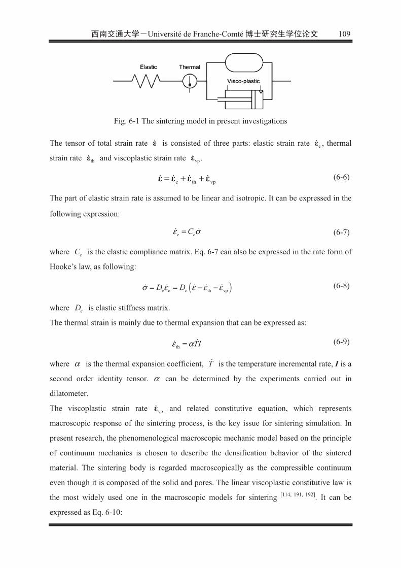
Université de Franche-Comté 109
Fig. 6-1 The sintering model in present investigations
The tensor of total strain rate is consisted of three parts: elastic strain rate e , thermal
strain rate th and viscoplastic strain rate vp .
vpthe ++= (6-6)
The part of elastic strain rate is assumed to be linear and isotropic. It can be expressed in the
following expression:
e eCε σ= (6-7)
where eC is the elastic compliance matrix. Eq. 6-7 can also be expressed in the rate form of
Hooke’s law, as following:
( )th vpe e eD Dσ ε ε ε ε= = − − (6-8)
where eD is elastic stiffness matrix.
The thermal strain is mainly due to thermal expansion that can be expressed as:
th TIε α= (6-9)
where α is the thermal expansion coefficient, T is the temperature incremental rate, I is a
second order identity tensor. α can be determined by the experiments carried out in
dilatometer.
The viscoplastic strain rate vp and related constitutive equation, which represents
macroscopic response of the sintering process, is the key issue for sintering simulation. In
present research, the phenomenological macroscopic mechanic model based on the principle
of continuum mechanics is chosen to describe the densification behavior of the sintered
material. The sintering body is regarded macroscopically as the compressible continuum
even though it is composed of the solid and pores. The linear viscoplastic constitutive law is
the most widely used one in the macroscopic models for sintering [114, 191, 192]. It can be
expressed as Eq. 6-10:

110 Université de Franche-Comté
(6-10)
where tσ is the stress tensor in sintered materials 'σ is the deviatoric stress tensor σtr
is trace of the stress tensor sσ represents the sintering stress I is second order identity
tensor. PG and PK are the shear and bulk viscosity modulus of the porous material,
respectively.
Various models have been developed to determine pG , pK and sσ in the constitutive
law. Generally they fall into three types that include the phenomenological, microstructural
and experimental ones. The elastic-viscous analogy is chosen to define the shear and bulk
viscosity modules for sintering materials, as related in equation [188]:
)1(2 vpp ν
η
+= zG
)21(3 vpp ν
η
−= zK
(6-11)
where zη and vpν are uniaxial viscosity and viscous Poisson’s ratio of the porous material.
From Eq. 6-11, it is known that PG and PK can be determined by experiments by means
of the calibration of uniaxial viscosity and viscous Poisson’s ratio. Song et al. have defined
the following relationship to define the uniaxial viscosity zη by bending tests [14, 155, 169], as
shown in Fig. 6-2 and Eq. 6-12.
Fig. 6-2 Simply supported beam model for beam-bending tests
4 3
2 3
51
32 4a s s
z
gL PL
h bh
ρη
δ= +
(6-12)
where δ is the deflection rate at center of the specimen, aρ is the apparent density, g is

Université de Franche-Comté 111
gravitational acceleration, P is the external load, sL is the distance between the two
supporting rods. b and h are width and thickness of the specimen.
The viscous Poisson’s ratio is determined from an average relationship in the following form
[188]:
1
2 3 2vp
ρν
ρ≈
−
(6-13)
where ρ is the relative density.
Sintering stress sσ should be calibrated experimentally by different heating processes.
Sintering stress sσ is the function of apparent density ρ , surface energy and particle sizes.
Its calibration is realized by sintering of small specimens in dilatometer [14, 155]. In simulation
for the process of microwave sintering, it is the function of density and temperature. The
following equation is proposed to determine the sintering stress [193]:
C
s Bσ ρ=
(6-14)
where B and C are the material parameters that should be identified from dilatometer
experiments.
The above evaluation is summarized in Fig. 6-3.
Fig. 6-3 Evaluation of the viscoplastic strain rate in the sintering model ( λ is the uniaxial
shrinkage, measured by the tests in dilatometer)

112 Université de Franche-Comté
To realize the simulation, the coefficient of thermal dilatation α for sintered material,
as well as the material parameters related to elastic deformation, are required, too. These
parameters are expressed illustratively by:
( ),Tα α ρ= , ( )TEE e ,e ρ= (6-15)
where eE is the elastic modulus of porous material.
6.2.5 Coupling of the Maxwell equation, heat transfer equation and
mechanic equations
The process of microwave sintering includes three types of the physics. One is the
transmission of microwave energy in the heating cavity. A part of the microwave energy is
converted into heat energy, because of its dissipation during the transmission. The second
one is the process of heat transfer. Because of inhomogeneous distribution of the electric
field in the heating cavity, it generates the heat not homogeneously in the sintered material,
too. Then there exists the process of heat transfer. The third one is the process of
densification during sintering. The particles and grains of PIM material connect and fuse
together. The pores among the particles reduce and disappear gradually. Macroscopically it
appears to be the shrinkage of sintered products. The volume is reduced while the density
increases. The evolution of density and temperature during sintering results in the variation
of different parameters in physical equations. It results then the complicated coupling of
different physics.
6.3 Numerical simulation of microwave sintering process
6.3.1 Modeling of Microwave Sintering
Microwave sintering is the process of microwave heating to realize the sintering
densification. It involves the solution of steady state equations for frequency domain analysis
of electro-magnetic fields and the distribution of generated heat. The distribution of

Université de Franche-Comté 113
temperature in sintered body is obtained by transient simulation of the heat transfer.
Evolution of the density and shrinkage of PIM material is achieved by mechanical
simulation of the sintering process.
The incremental algorithm is applied for integration in time of the mathematic model, in
which the processes of microwave sintering on PIM materials are described. The governing
equations for three types of the physics mentioned above are solved by the fractional steps.
In each time step, distribution of the electric field at this instant is solved by the direct
methods, while temperature field and evolution of the densification should be solved
iteratively. The coupling among three different physics is realized by increment of the time
steps. In the process of solution, the dissipated energy is introduced into the equation of heat
transfer (Eq. 6-4) as internal heating source. Then distribution of the temperature field is
solved. The temperature field is further introduced into the solution of constitutive equation
and densification equation. Their solution provides then the evolution of densification and
shape deformation during sintering of the PIM material.
Due to the variation of electromagnetic and thermal parameters according to density of
the material and temperature, the field variables are solved with the updated parameters in
the incremental solutions. The cyclic increments run forward until the prescribed sintering
process is finished. So the simulation process of microwave sintering is the cyclic solutions
of Maxwell equation, heat transfer equation, as well as the structural equilibrium equation,
material densification equation and constitutive equation, as show in Fig. 6-4.
Fig. 6-4 The coupling of multi-physics in simulation of the microwave sintering
The cavity of microwave furnace can be regarded as a metallic box. A microwave

114 Université de Franche-Comté
source of 2.45 GHz is connected with continuously adjustable output power. As the
magnetic effect is ignored in the present studies, the microwave source is set to be the
transvers electric (TE) wave. Wall surfaces of the furnace and waveguide are regarded as the
perfect electric conductor, represented by the boundary condition n × E = 0. Because of the
symmetry, half of the model is analyzed. Due to mirror symmetry of the electric field, the
plan of symmetry can be regarded as a perfect magnetic conductor, represented by the
boundary condition n × H = 0.
The shaped body in submicron ceramic powder is taken in simulation. Its physical
parameters are shown in Table 6-1. The referred values of zirconia powder in literature [186]
are taken for approximation. It should be mentioned that the experimental measurements for
these parameters are still less available. The related physical parameters, such as relative
permittivity, conductivity etc, as well as the ones in analogous viscoplastic constitutive law
for sintering, are still the current researches in material science. Their values retrieved from
literatures represent large differences, too. However, the true material parameters represent
prime importance for accurate simulation of the microwave sintering process. The present
paper focuses on the modeling and simulation method for densification process of the
microwave sintering. The really reliable parameters of sintered materials in microwave
sintering should be achieved by the experimental ways in the further works.

Université de Franche-Comté 115
Table 6-1 physical parameters of CIM component based on zirconia powder [186]
Electromagnetic parameters
Air in the cavity r_airµ = r_airε = 1;
Sintered compact: )293(0017.0r 1.010 −−= Teiε r =1
Input power of microwave source 1 KW
Heat transfer parameters
Conductivity k=30 rρ W/(mk) Density rρρ 6000= 3/ mkg
Heat capacity 900pp rC = ρ )/(kgKJ
Initial temperature kT 2930 = ( rρ is relative density)
Densification process:
Thermal expansion coefficient: α =1.2 10 2- /k; Poisson’s ratio: ν =0.33 ;
Shear viscosity modulus: PG =1 10 11 Pa; Bulk viscosity modulus PK 1 10 11 Pa;
Initial relative density 65.00 =rρ .
Note: Some of the above parameters are the initial ones. For the ones with unknown
variation, constant values are taken in the present simulation.
6.3.2 Numerical analysis
The finite element package COMSOL Multiphysics (C) is employed in the research on
simulation of microwave sintering process. In order to determine the suitable position of
sintered compact in cavity of the microwave furnace, the distribution of electric field in an
empty cavity is first analyzed. The result is shown in Fig. 6-5.
Fig. 6-5 Distribution of electric field in empty cavity

116 Université de Franche-Comté
Fig. 6-6 Placement of sintered compact
It provides the suitable placement of sintered body by investigation on distribution of
the electric field in cavity of the microwave furnace. As shown in Fig. 6-6, the sintered
compact should be placed to the position of peak electric field. Then the sintered material
absorbs as much as possible the energy of electric waves. Geometric dimensions and meshes
are shown in Fig. 6-7 and Fig. 6-8 respectively. 3D tetrahedron lagrange element has been
set as the element type. The total model includes 753 nodes, 3514 elements.
Fig. 6-7 Geometric dimensions Fig.6-8 3D Meshes in COMSOL
To simplify the model, it is assumed that the outer surface of sintered compact is
adiabatic with the environment in furnace chamber. When the solutions on evolution of heat
transfer, structural response of strain-stress and relative density are realized, it takes into
account only the region of sintered compact. The calculations for these effects are then
suppressed in void volume of cavity.

Université de Franche-Comté 117
The temperature field on a cross section inside the CIM material, after heating 1500
seconds, is shown in Fig. 6-9. The peak value of temperature reaches to about 1650 oK near
center of the sintered compact. The temperature gradient is moderate in the compact. The
displacement along x direction is shown in Fig. 6-10. The magnitude of displacement at
same time is shown in Fig. 6-11. The obvious shrinkage towards center and bottom of the
compact can be observed, which represents the effect of densification, too. The final relative
density field can be seen in Fig. 6-12.
Fig. 6-9 Temperature field at 1500s Fig. 6-10 Displacement along x-direction
Fig. 6-11 Total displacement in cross section Fig. 6-12 Final relative density
The solutions are realized by non-linear solver of the package COMSOL. It lasts 1500
seconds (25 minutes) for the whole process of microwave sintering. The results at 6 instants
are kept in simulation process for the further investigation. The 6 instants are chosen by
equal intervals for the whole process in 1500 seconds.
As relative permittivity of the material is a function of temperature, dielectric loss factor
increases with the increase of temperature. So generation of resistance heat in the material is

118 Université de Franche-Comté
very small in initial stage of the microwave heating. It heats slowly. In the first 10 minutes,
there is no obvious variation for temperature and relative density in the material. After 10
minutes, temperature increases with the strong increasing rate in the CIM material to reach
the peak value. The relative density increases continuously with the increase of temperature,
too. At last, it gets close to the fully densified material (The relative density is increasing
over 0.9). The discussed variations can be observed in Fig. 6-13 and Fig. 6-14. As the power
of microwave source is set to be a constant value 1kw, the temperature in material increases
continuously. By regulation of the input powder of microwave source, the sintering process
can be controlled to get into the holding stage, and then the cooling stage. For evaluating the
simulation result, experiment results from Charmond et al. [167] can be used to make a
comparison. Specimens made by spray-dried 2 mol% yttria-doped zirconia nanopowder have
been investigated in [167]. It concludes that the sintered material shows poor coupling with
the microwaves below 673 oK, and then the coupling effects become stronger and stronger
when the temperature is over 673 oK. This experiment phenomenon meets well with the
simulation result. With the same maximal sintering temperature at about 1633 oK, the
corresponding final relative density of conventional sintering, microwave sintering and
simulation result can be seen in Fig. 6-15. We can see that result of simulation is a little
lower than the experimental one, because the sintering model for present simulation is not a
precisely calibrated one. For some parameters with unknown variation, constant values are
taken in the present simulation. So the evolution of relative density represents only the
referential values.
Fig. 6-13 Evolution of heat generation

Université de Franche-Comté 119
Fig. 6-14 Evolution of relative density versus sintering temperature during microwave
sintering process
Fig. 6-15 Comparison between the experimental and the numerical relative density, the
experiment results are taken reference from the work of Charmond et al. [167].
6.4 Conclusion and outlook
The process of microwave sintering includes the phenomena of electromagnetism, heat
transfer and sintering densification, as well as their couplings. By analysis on the principles
of microwave sintering, the mathematic model is established. The governing equations to
describe three main physical phenomena are provided. Coupling relationships among the
main governing equations are discussed. The parameters in equations are analysed to
identify their dependence on the other factors. Discussion is made on the methods to
determine their values. The specific configuration of microwave furnace is taken into
account in the simulation. The RF module, heat transfer module, structure analysis module in

120 Université de Franche-Comté
COMSOL package is employed. The constitutive law, which describes sintering
densification of CIM materials under high temperature, is implemented into the structure
analysis. The coupling of multi-phasics in microwave sintering is realized in simulation.
Results of simulation are analysed. The work focuses on modelling of the microwave
sintering and the methods for its simulation. It provides an effective way for the further
analysis and the achievement of knowledge on microwave sintering. For more accurate
simulations, the true parameters and constitutive law of CIM materials are required. Besides
that, the external effect, such as boundary conditions, gravitation and friction, should be
taken into account. It represents the great importance to study and achieve theses parameters
and relationships by experiments.

Université de Franche-Comté 121
Chapter 7 Conclusions and Perspectives
7.1 Conclusions
The research reported in this thesis represents two main aspects for investigation of the
PIM technologies. One is the enhancement and improvement to the actual tools for
simulation of the micro filling process. The other focuses on the experiment and simulation
research of microwave sintering. Due to rarely reported, components based on 17-4PH
stainless steel powder are introduced in the experiment of microwave sintering. The
favorable results and regular gradient in sintered body are obtained and revealed, compared
to the only report of unfavorable conclusion. The simulation of microwave sintering, from
distribution of the electromagnetic fields to the densification of sintered bodies, is developed
with the coupling of multi-physics. It represents the first attempt to couple the microwave
heating and the behaviors of powder densification in simulation in our labs. The main
contributions in present thesis are detailed below:
1) For the enhancement of filling simulation, the present study in section 2.2 and
section 2.3 completed and modified the actual algorithms for simulation of the injection
filling process. In section 2.2, a modification on solution of the filling front evolution is
proposed and realized to improve the wrongly directed filling patterns in actual commercial
software and the code in research team. A modified algorithm, which is similar to upwind
method, is proposed in Section 2.2. It employs a systematic operation to modify the fluid
velocity field. Then the advection of filling state is made to be more affected by the real
filling flow behind the filling front. For validation of the new proposed method, the results
obtained by commercial software MPI software (Autodesk(C)) and the filling patterns
obtained by experimental results from G. Larsen [66] are introduced to make a comparative
analysis. It shows that this similar upwind method is valid to improve the wrongly directed
filling patterns. In section 2.3, a completion of the outlet boundary condition is added in
FEM code to overcome the delay of fully filling in the last filling stage. The filling ratio of
incompressible flow should be a linear one with respect to time when constant velocity is
imposed on inlet. But the linearity is not respected when the filling front approaches to the

122 Université de Franche-Comté
outlet boundary. To remedy this defect, the modeling is formulated again. An integration
term on the outlet boundary is realized in solution of the advection equation for filling state.
Then the incompressibility and linearity of the filling flow can hence be well respected at the
last filling stage. The results from these two modified algorithms for the simulations of mold
filling process are conformed to be optimized and more reliable. The stability for solution of
the filling state is improved.
2) In Chapter 3, for the lack of appropriated FEM method to take into account the
surface tension effect in micro injection, a specific method is proposed and implemented.
This work represents the significant importance for the analysis of capillarity dominant free
surface flows in micro-injection molding. It affords the practical way for evaluation of the
surface tension effects in viscous filling flow. However, when dealing with the determination
of front curvature, it contains a second order derivative function, in the form of a Laplacian
operator. Because the filling function is a scalar one while the velocity function is a vector
one, the integration of filling function in second derivative is not suitable be transformed into
the boundary integration and the integration of function in lower order derivative. So a new
method is proposed to evaluate the curvature of filling front by the simple and systematical
procedures. It settles down successfully the problem for calculation of the front curvature
(Eq. 3-1). By comparing the magnitudes of surface tension force with the viscous force for a
filling example in micro channels, it indicates that the effect of surface tension does not
represent the significant effect in ordinary injection molding, but shows the importance for
the micro injection molding of sub-millimeter sizes. All the works for micro injection
molding have been programmed in the C++ environment and planted into the previous
in-house solver on the platform of Matlab (C) version 7.10. The functionality of in-house
solver has been extended and become more powerful.
3) Chapter 5 is about the experiments and some new discoveries for microwave
sintering. For compacts based on 17-4PH stainless steel powder, only one investigation [175]
on the MW processing is found by the retrieves of literatures in the currently available
resources. It provided a conclusion that MW sintering has not improved the mechanical
properties compared to CRH sintering for 17-4PH stainless steel. But the results in Chapter 5
of present thesis support a different conclusion. The authors conform that the MW sintering

Université de Franche-Comté 123
process for 17-4PH stainless steel can not only shorten greatly the sintering time, lower the
peak sintering temperature, but also it provides higher sintered density and fewer defects in
micro structure. Higher Vickers-hardness of MW sintered compacts is also detected in the
present work. By a series of the experiments, the optimal microwave sintering process for
specimens based on 17-4PH stainless steel is determined. The optimal process is heating
directly from ambient temperature to 1150 with heating rate 30 /min, and then held 10
minutes. It will get the specimen with higher density (relative density: 96.6%) and better
mechanical properties (Vikers-hardness: 316V). Moreover, because of its rapid heating in the
internal volumetric way, sintering by Microwave heating resulted in the obvious gradient in
mechanic properties of the sintered material. It is due to the nature of microwave heating. In
the present thesis, none of the specimens presents visually observable distortion. The
prediction, evaluation and purposes of the gradient properties induced by microwave leads
the studies to the more precise and profound insights.
4) The mathematic model to describe Multi-physics phenomena of microwave
sintering process is established in Chapter 6. It includes the coupling of electro-magnetic
fields, thermal conduction and the densification process of sintered powders. Most of the
actual literatures propose macro models that coupled the microwave heating and thermal
conduction, but none of them deals with the densification process in microwave sintering.
The present thesis represents the first attempt to model the whole sintering process by
microwave heating. The simulation of densification is based on a thermo-elasto-viscoplastic
model [140]. It is employed into the modelling of whole microwave sintering process. Using
the finite element solver COMSOL Multi-physics, the coupling of microwave electric field,
thermal conduction and sintering densification of the powder material is realized for a 3D
example of microwave sintering in a single mode cavity. It provides an effective way for the
further analysis and the achievement of knowledge on microwave sintering.
7.2 Future Work
The presented enhancement and improvement for simulation of micro-injection molding
process, and the mathematical models for modeling the process of microwave sintering have

124 Université de Franche-Comté
proven their effectiveness in prediction of the final results. However, the works are far away
to be finished. There are still the important problems to be solved. Some of the works in the
near future can be suggested as below:
Reinforce the research on micro-injection molding in both experiment and simulation
aspect. Evaluate each of the influence factors, such as surface tension, wall slip, viscous
dissipation and convective heat transfer to the filling flow in micro cavities. Extend the
simulation of -injection to nano-injection with a lot of knowledge on the new
physical and mathematical models.
For microwave sintering experiment, the obvious gradient in mechanic properties is
found inside the sintered material. It is due to the rapid generation of heat by microwave
heating inside the sintered material. It is valuable to continue the studies on this effect
for the application of microwave sintered products. The modeling and simulation on
generation of the gradient properties represent also the significant insights for the further
studies. More physical experiments should be conducted to know the mechanical
properties. The simulation models for predicting the mechanical properties can be built
based on the experimental investigations.
For simulations of the microwave sintering process, it is actually a preliminary attempt.
There are many imperfect aspects. Chapter 6 focuses on the modeling and simulation
method for densification process of the microwave sintering. The related physical
parameters, such as relative permittivity, conductivity etc., as well as the ones in
analogous viscoplastic constitutive law for sintering, are not the really reliable
parameters of sintered materials. However, the true material parameters represent prime
importance for accurate simulation of the microwave sintering process. They should be
achieved by the new technologic and scientific development to have a specially
instrumented microwave furnace with a lot of scientific equipment (infrared camera,
pyrometers, optical measurements etc).
The sintering experiments in microwave oven for different kinds of feedstock and the
same one with various powder loadings should be carried out in future.
Combination of the simulation for injection filling stage and microwave sintering stage
is favorable for optimization of the entire PIM process. In order to simulate the sintering

Université de Franche-Comté 125
process under real conditions, the parameters such as the frictional coefficient, thermal
conductivity and heat capacity of the porous materials should be determined.
The mechanical properties of the sintered components are dependent on its
microstructures. Besides the macroscopic models, the microscopic or mesoscopic
models for sintering should also be developed. With the multi-scale modeling, the
dimensional changes and the microstructural evolutions of the sintering components can
be predicted simultaneously.

126 Université de Franche-Comté
Acknowledgment
I would like to express my sincere gratitude to my thesis supervisor, Prof. Baosheng
LIU (Southwest Jiaotong University, China) and Prof. Jean-Claude GELIN (ENSMM,
France), for their support, guidance and encouragement during the whole research course.
Their advanced knowledge and rich experiences in the field of forming manufacturing and
numerical simulation are the assurance for performing this thesis. I am also grateful to my
co-supervisor, Prof. Zhiqiang CHENG (Southwest Jiaotong University, China) and Prof.
Thierry BARRIERE (Université de Franche-Comté, France). Thanks for their working
enthusiasm and constructive opinions.
I would like to thank Université de Franche-Comté, Femto-ST institution for their
invitation and acceptance, which give me a chance to pursue my study abroad. And also
thanks to China Scholarship Council for awarding me a scholarship to stay in France.
Special thanks to engineers in Femto-ST institution, Mohamed Sahli, Gérard Michel,
Christine Millot and Vincent Placet, for their support in the experiments. I particularly
express my thankful to my friend Gang Cheng, who did me a great favor in work and daily
life when I was staying in France.
I wish to thank my colleagues and teammates Edouard Falconnet, Belgacem Mamen,
Gang Cheng, Jie Zhang, Huibin Ou in Femto-ST institute and Huiliang Luo, Yanyu Wang,
Hangzhuo Yu, Fengshun Gao, Xiangqiang Wei, Jie Chen, Lngyu Yang, Yanxin Liu and Ming
Li in Southwest Jiaotong University.
Finally, I wish to thank my grandma and my parents for providing me a lovely
environment and continuous support all through these years. I especially thank my girlfriend
Xuanyu, Yan for her fully support, encouragement and company. Je suis très heureux, Je
t'aime.

Université de Franche-Comté 127
References
[1] GERMAN R M. Powder Injection Molding [M]. Princeton: NJ, 1990.
[2] SAHLI M, MILLOT C, GELIN J C, et al. The manufacturing and replication of microfluidic mould inserts by the
hot embossing process [J]. Journal of Materials Processing Technology, 2013, 213(6): 913-25.
[3] SUPATI R, LOH N H, KHOR K A, et al. Mixing and characterization of feedstock for powder injection molding
[J]. Materials Letters, 2000, 46(2–3): 109-14.
[4] LIU Z Y, LOH N H, TOR S B, et al. Characterization of powder injection molding feedstock [J]. Materials
Characterization, 2002, 49(4): 313-20.
[5] AHN S, PARK S J, LEE S, et al. Effect of powders and binders on material properties and molding parameters
in iron and stainless steel powder injection molding process [J]. Powder Technology, 2009, 193(2): 162-9.
[6] KONG X, BARRIERE T, GELIN J C. Determination of critical and optimal powder loadings for 316L fine
stainless steel feedstocks for micro-powder injection molding [J]. Journal of Materials Processing Technology,
2012, 212(11): 2173-82.
[7] MENG J, LOH N H, FU G, et al. Micro powder injection moulding of alumina micro-channel part [J]. Journal
of the European Ceramic Society, 2011, 31(6): 1049-56.
[8] YE H, LIU X Y, HONG H. Fabrication of metal matrix composites by metal injection molding—A review [J].
Journal of Materials Processing Technology, 2008, 200(1–3): 12-24.
[9] GERMAN R M, BOSE A. Injection Molding of Metals and Ceramics [M]. Princeton, New Jersey, USA, 1997.
[10] GERMAN R M. Strength evolution during thermal debinding of injection moulded parts: (Pennsylvania
State University, USA.) [J]. Metal Powder Report, 2000, 55(9): 39.
[11] ENNETI R K, SHIVASHANKAR T S, PARK S-J, et al. Master debinding curves for solvent extraction of binders
in powder injection molding [J]. Powder Technology, 2012, 228(0): 14-7.
[12] TRUNEC M, CIHL J. Thermal debinding of injection moulded ceramics [J]. Journal of the European
Ceramic Society, 1997, 17(2–3): 203-9.
[13] WEINAND D, BLOEMACHER M. MIM feedstock for rapid catalytic debinding : (BASF AG, Ludwigshafen,
Germany) [J]. Metal Powder Report, 1994, 49(1): 39.
[14] SONG J. Experiments, Modelling and Numerical Simulation of the Sintering Process for Metallic or
Ceramic Powders [D]; University of Franche-Comté and Southwest Jiaotong University, 2007.
[15] http://www.amt-mat.com/Powder_Injection_Molding_PIM_Comparison.html.
[16] MERHAR J R. Overview of metal injection moulding [J]. Metal Powder Report, 1990, 45(5): 339-42.
[17] STEVENSON J F. Powder Metal Injection Molding [M]//MUSA R K, AVRAM L I, SHIH-JUNG LIUA2 - MUSA R.
KAMAL A L I, et al. Injection Molding. Hanser. 2009: 309-40.
[18] GERMAN R M. Research productivity and the value to the P.I.M. market [M]//GERMAN R M. PIM 2000,
Int Conference on Injection Moulding of Metals and Ceramics. Penn States University Press. 2000.
[19] GERMAN R M. Status of PIM Research and Development [M]//M.P.I.F. PIM 2007, Int Conference on
Injection Moulding of Metals and Ceramics. 2007.
[20] GERMAN R M. Powder Injection molding: Statistical trends and forward forcasts for the industry [J]. PIM
International, 2013, 7(1): No.1.
[21] KONG X J. Development and Characterization of Polymermetallic Powder Feedstocks for
Micro-injection Molding [D]; L’Université de Franche-Comté, 2011.
[22] Metal and Ceramic Injection Moulding (AVM049B) from BCC Research,
http://www.bccresearch.com/pressroom/report/code/AVM049B, retrieved 10/31/12. [M].

128 Université de Franche-Comté
[23] MACNEAL T. Growth prospects brightening for global MIM market [J]. Metal Powder Report, 2013, 68(1):
14-5.
[24] GERMAN R M. Sintering theory and practice [M]//WILEY J, SONS. 1996.
[25] GERMAN R M. Design and applications [M]. Innovation Material Solutions, 2000.
[26] EDIRISINGHE M J. Injection Molding [M]//EDITORS-IN-CHIEF: K H J B, ROBERT W C, MERTON C F, et al.
Encyclopedia of Materials: Science and Technology (Second Edition). Oxford; Elsevier. 2001: 4088-94.
[27] GUNDUZ O, AHMAD Z, STRIDE E, et al. A device for the fabrication of multifunctional particles from
microbubble suspensions [J]. Materials Science and Engineering: C, 2012, 32(4): 1005-10.
[28] SHAW H M, EDIRISINGHE M J. Porosity development during removal of organic vehicle from ceramic
injection mouldings [J]. Journal of the European Ceramic Society, 1994, 13(2): 135-42.
[29] SHAW H M, EDIRISINGHE M J. Shrinkage and particle packing during removal of organic vehicle from
ceramic injection mouldings [J]. Journal of the European Ceramic Society, 1995, 15(2): 109-16.
[30] ALCOCK J. Co-injection promises further growth for MIM [J]. Metal Powder Report, 1999, 54(6): 30-4.
[31] KOWALSKI L, DUSZCZYK J, KATGERMAN L. Thermal conductivity of metal powder-polymer feedstock for
powder injection moulding [J]. Journal of Materials Science, 1999, 34(1): 1-5.
[32] TURKER M, GODLINSKI D, PETZOLDT F. Effect of production parameters on the properties of IN 718
superalloy by three-dimensional printing [J]. Materials Characterization, 2008, 59(12): 1728-35.
[33] RADOCAJ A, WEISS T, HELSBY W I, et al. Force-Generating Cross-Bridges during Ramp-Shaped Releases:
Evidence for a New Structural State [J]. Biophysical Journal, 2009, 96(4): 1430-46.
[34] PIOTTER V, FINNAH G, HANEMANN T, et al. Micro Injection Molding [M]//MUSA R K, AVRAM L I,
SHIH-JUNG LIUA2 - MUSA R. KAMAL A L I, et al. Injection Molding. Hanser. 2009: 341-93.
[35] ZEEP B, NORAJITRA P, PIOTTER V, et al. Net shaping of tungsten components by micro powder injection
moulding [J]. Fusion Engineering and Design, 2007, 82(15–24): 2660-5.
[36] BIDAUX J E, JOCHEM A. Powder injection moulding of NiTi shape memory materials [J]. Powder Injection
Moulding International, 2008, 2(1): 59-62.
[37] NYBORG L. Interactions between surface-active additives and 316L stainless steel powder for MIM:
(Chalmers University of Technology, Sweden.) [J]. Metal Powder Report, 1998, 53(4): 38.
[38] LEVENFELD B, V REZ A, CASTRO L, et al. Processing of P/M M2 high speed steels by mould casting using
thermosetting binders [J]. Journal of Materials Processing Technology, 2001, 119(1–3): 1-6.
[39] MATOS M, CASTANHO J M, VIEIRA M T. Composite copper/stainless steel coated powders [J]. Journal of
Alloys and Compounds, 2009, 483(1–2): 460-3.
[40] LIU Z Y, LOH N H, TOR S B, et al. Micro-powder injection molding [J]. Journal of Materials Processing
Technology, 2002, 127(2): 165-8.
[41] YAMAMOTO O, SASAMOTO T, INAGAKI M. Antioxidation of carbon-carbon composites by SiC
concentration gradient and zircon overcoating [J]. Carbon, 1995, 33(4): 359-65.
[42] KANG Y, KANG S. The surface microstructure of TiC-(Ti,W)C-WC-Ni cermets sintered in a nitrogen
atmosphere [J]. Materials Science and Engineering: A, 2010, 527(27–28): 7241-6.
[43] KANG Y, KANG S. WC-reinforced (Ti,W)(CN) [J]. Journal of the European Ceramic Society, 2010, 30(3):
793-8.
[44] DUTILLY M, GHOUATI O, GELIN J C. Finite-element analysis of the debinding and densification
phenomena in the process of metal injection molding [J]. Journal of Materials Processing Technology, 1998,
83(1–3): 170-5.
[45] GELIN J C, BARRIERE T, DUTILLY M. Experiments and Computational Modeling of Metal Injection Molding
for Forming Small Parts [J]. CIRP Annals - Manufacturing Technology, 1999, 48(1): 179-82.

Université de Franche-Comté 129
[46] QUINARD C, SONG J, BARRIERE T, et al. Elaboration of PIM feedstocks with 316L fine stainless steel
powders for the processing of micro-components [J]. Powder Technology, 2011, 208(2): 383-9.
[47] BARRIERE T, GELIN J C, LIU B. Experimental and numerical investigations on properties and quality of
parts produced by MIM [J]. Powder Metallurgy, 2001, 44(3): 228-34.
[48] SONG J, GELIN J C, BARRIERE T, et al. Experiments and numerical modelling of solid state sintering for
316L stainless steel components [J]. Journal of Materials Processing Technology, 2006, 177(1–3): 352-5.
[49] SPENCER R S, GILMORE G D. Some flow phenomena in the injection molding of polystyrene [J]. Journal of
Colloid Science, 1951, 6(2): 118-32.
[50] BALIMAN R L, SHUSMAN T, TOOR H L. Injection Molding - Flow of a Molten Polymer into a Cold Cavity [J].
Industrial & Engineering Chemistry, 1959, 51(7): 847-50.
[51] KUO Y, KAMAL M R. The fluid mechanics and heat transfer of injection mold filling of thermoplastic
materials [J]. AIChE Journal, 1976, 22(4): 661-9.
[52] RYAN M E, CHUNG T S. Conformal mapping analysis of infection mold filling [J]. Polymer Engineering &
Science, 1980, 20(9): 642-51.
[53] HIEBER C A, SHEN S F. A finite-element/finite-difference simulation of the injection-molding filling
process [J]. Journal of Non-Newtonian Fluid Mechanics, 1980, 7(1): 1-32.
[54] HIEBER C A, SOCHA L S, SHEN S F, et al. Filling thin cavities of variable gap thickness: A numerical and
experimental investigation [J]. Polymer Engineering & Science, 1983, 23(1): 20-6.
[55] MAVRIDIS H, HRYMAK A N, VLACHOPOULOS J. Finite element simulation of fountain flow in injection
molding [J]. Polymer Engineering & Science, 1986, 26(7): 449-54.
[56] SATO T, RICHARDSON S M. Numerical simulation of the fountain flow problem for viscoelastic fluids [J].
Polymer Engineering & Science, 1995, 35(10): 805-12.
[57] LIN M, THOMAS HAHN H, HUH H. A finite element simulation of resin transfer molding based on partial
nodal saturation and implicit time integration [J]. Composites Part A: Applied Science and Manufacturing,
1998, 29(5–6): 541-50.
[58] SOLTANI B, MATTIASSON K, SAMUELSSON A. Implicit and dynamic explicit solutions of blade forging using
the finite element method [J]. Journal of Materials Processing Technology, 1994, 45(1–4): 69-74.
[59] SWAMINATHAN C R, VOLLER V R. A time-implicit filling algorithm [J]. Applied Mathematical Modelling,
1994, 18(2): 101-8.
[60] DHATT G, GAO D M, CHEIKH A B. A finite element simulation of metal flow in moulds [J]. International
Journal for Numerical Methods in Engineering, 1990, 30(4): 821-31.
[61] LEWIS R W, USMANI A S, CROSS J T. Efficient mould filling simulation in castings by an explicit finite
element method [J]. International Journal for Numerical Methods in Fluids, 1995, 20(6): 493-506.
[62] BARRIERE T, LIU B, GELIN J C. Determination of the optimal process parameters in metal injection
molding from experiments and numerical modeling [J]. Journal of Materials Processing Technology, 2003,
143–144(0): 636-44.
[63] LIU B S, BARRIERE T, GELIN J C. A new explicit algorithm for bi-phasic mixture flow in MIM [J]. Journal of
Southwest Jiaotong University, 2002, 10(2): 152-60.
[64] CHENG Z, BARRIERE T, LIU B, et al. A new explicit simulation for injection molding and its validation [J].
Polymer Engineering & Science, 2009, 49(6): 1243-52.
[65] CHENG Z, BARRIERE T, LIU B, et al. A fully vectorial and explicit algorithm for mould filling [J]. Journal of
Southwest Jiaotong University, 2004, 39(2): 181-4.
[66] LARSEN G, CHENG Z Q, BARRIERE T, et al. A streamline-upwind model for filling front advection in
powder injection moulding [M]. NUMIFORM 2010: Proceedings of the 10th International Conference on

130 Université de Franche-Comté
Numerical Methods in Industrial Forming Processes 2010: 545-52.
[67] CHENG Z Q. Numerical Simulation on Metal Injection Moulding [D]; Southwest Jiaotong University, 2005.
[68] HETU J F, GAO D M, GARCIA-REJON A, et al. 3D finite element method for the simulation of the filling
stage in injection molding [J]. Polymer Engineering & Science, 1998, 38(2): 223-36.
[69] PICHELIN E, COUPEZ T. Finite element solution of the 3D mold filling problem for viscous incompressible
fluid [J]. Computer Methods in Applied Mechanics and Engineering, 1998, 163(1–4): 359-71.
[70] BARRIERE T. Expérimentations, Modélisation et Simulation Numérique du Moulage par Injection de
Poudres Métalliques [D]; Université de Franche-Comté, 2000.
[71] DUTILLY M. Modélisation du Moulage par Injection de Poudres Métalliques [D]; Université de
Franche-Comté, Besancon, France, 1998.
[72] BERTRAND F H, GADBOIS M R, TANGUY P A. Tetrahedral elements for fluid flow [J]. International Journal
for Numerical Methods in Engineering, 1992, 33(6): 1251-67.
[73] ROIG B. One-step Taylor–Galerkin methods for convection–diffusion problems [J]. Journal of
Computational and Applied Mathematics, 2007, 204(1): 95-101.
[74] LAVAL H, QUARTAPELLE L. A fractional-step Taylor–Galerkin method for unsteady incompressible flows [J].
International Journal for Numerical Methods in Fluids, 1990, 11(5): 501-13.
[75] TONG A Y, WANG Z. A numerical method for capillarity-dominant free surface flows [J]. Journal of
Computational Physics, 2007, 221(2): 506-23.
[76] ROKKAM R G, FOX R O, MUHLE M E. Computational fluid dynamics and electrostatic modeling of
polymerization fluidized-bed reactors [J]. Powder Technology, 2010, 203(2): 109-24.
[77] NAGAIAH C, WARNECKE G, HEINRICH S, et al. Numerical simulation of temperature and concentration
distributions in fluidized beds with liquid injection [J]. Chemical Engineering Science, 2007, 62(6): 1567-90.
[78] JIANG C B, KAWAHARA M, KASHIYAMA K. A Taylor—Galerkin-based finite element method for turbulent
flows [J]. Fluid Dynamics Research, 1992, 9(4): 165-78.
[79] SHA B, DIMOV S, GRIFFITHS C, et al. Investigation of micro-injection moulding: Factors affecting the
replication quality [J]. Journal of Materials Processing Technology, 2007, 183(2–3): 284-96.
[80] MOHD FOUDZI F, MUHAMAD N, BAKAR SULONG A, et al. Yttria stabilized zirconia formed by micro
ceramic injection molding: Rheological properties and debinding effects on the sintered part [J]. Ceramics
International, 2013, 39(3): 2665-74.
[81] CHEN P, POLICOVA Z, PACE-ASCIAK C R, et al. Study of molecular interactions between lipids and proteins
using dynamic surface tension measurements: a review [J]. Colloids and Surfaces B: Biointerfaces, 1999,
15(3–4): 313-24.
[82] LIOVIC P, LAKEHAL D. Subgrid-scale modelling of surface tension within interface tracking-based Large
Eddy and Interface Simulation of 3D interfacial flows [J]. Computers & Fluids, 2012, 63(0): 27-46.
[83] RAESSI M, MOSTAGHIMI J, BUSSMANN M. A volume-of-fluid interfacial flow solver with advected
normals [J]. Computers & Fluids, 2010, 39(8): 1401-10.
[84] EYIYUREKLI M, BREEN D. Interactive free-form level-set surface-editing operators [J]. Computers &
Graphics, 2010, 34(5): 621-38.
[85] MOELANS N, BLANPAIN B, WOLLANTS P. An introduction to phase-field modeling of microstructure
evolution [J]. Calphad, 2008, 32(2): 268-94.
[86] PIANET G, VINCENT S, LEBOI J, et al. Simulating compressible gas bubbles with a smooth volume tracking
1-Fluid method [J]. International Journal of Multiphase Flow, 2010, 36(4): 273-83.
[87] HIRT C W, NICHOLS B D. Volume of fluid (VOF) method for the dynamics of free boundaries [J]. Journal of
Computational Physics, 1981, 39(1): 201-25.

Université de Franche-Comté 131
[88] SUSSMAN M, PUCKETT E G. A Coupled Level Set and Volume-of-Fluid Method for Computing 3D and
Axisymmetric Incompressible Two-Phase Flows [J]. Journal of Computational Physics, 2000, 162(2): 301-37.
[89] WILLIAMS M W, KOTHE D B, PUCKETT E G, et al. Fluid Dynamics at Interface; proceedings of the
Cambridge University Press,, Cambridge, F, 1999 [C].
[90] POPINET S. An accurate adaptive solver for surface-tension-driven interfacial flows [J]. Journal of
Computational Physics, 2009, 228(16): 5838-66.
[91] RENARDY Y, RENARDY M. PROST: A Parabolic Reconstruction of Surface Tension for the Volume-of-Fluid
Method [J]. Journal of Computational Physics, 2002, 183(2): 400-21.
[92] OSHER S, SETHIAN J A. Fronts propagating with curvature-dependent speed: Algorithms based on
Hamilton-Jacobi formulations [J]. Journal of Computational Physics, 1988, 79(1): 12-49.
[93] FEDKIW R P, SAPIRO G, SHU C-W. Shock capturing, level sets, and PDE based methods in computer vision
and image processing: a review of Osher’s contributions [J]. Journal of Computational Physics, 2003, 185(2):
309-41.
[94] BOURLIOUX A. Coupled level set volume of fluid algorithm for tracking material interfaces; proceedings
of the in: Proceedings of the 6th International Symposium on Computational Fluid Dynamics, , Lake Tahoe, F,
1995 [C].
[95] SON G, HUR N. A COUPLED LEVEL SET AND VOLUME-OF-FLUID METHOD FOR THE BUOYANCY-DRIVEN
MOTION OF FLUID PARTICLES [J]. Numerical Heat Transfer, Part B: Fundamentals, 2002, 42(6): 523-42.
[96] NARD M T, TANGUY S, BERLEMONT A. Coupling level set/VOF/ghost fluid methods: Validation and
application to 3D simulation of the primary break-up of a liquid jet [J]. International Journal of Multiphase
Flow, 2007, 33(5): 510-24.
[97] LI Q, OUYANG J, YANG B, et al. Numerical simulation of gas-assisted injection molding using CLSVOF
method [J]. Applied Mathematical Modelling, 2012, 36(5): 2262-74.
[98] SUN D L, TAO W Q. A coupled volume-of-fluid and level set (VOSET) method for computing
incompressible two-phase flows [J]. International Journal of Heat and Mass Transfer, 2010, 53(4): 645-55.
[99] SHU C-W, OSHER S. Efficient implementation of essentially non-oscillatory shock-capturing schemes, II [J].
Journal of Computational Physics, 1989, 83(1): 32-78.
[100] LV X, ZOU Q, ZHAO Y, et al. A novel coupled level set and volume of fluid method for sharp interface
capturing on 3D tetrahedral grids [J]. Journal of Computational Physics, 2010, 229(7): 2573-604.
[101] HYSING S. Mixed element FEM level set method for numerical simulation of immiscible fluids [J].
Journal of Computational Physics, 2012, 231(6): 2449-65.
[102] DR AU K, CHEVAUGEON N, MO S N. Studied X-FEM enrichment to handle material interfaces with
higher order finite element [J]. Computer Methods in Applied Mechanics and Engineering, 2010, 199(29–32):
1922-36.
[103] YANG X, JAMES A J, LOWENGRUB J, et al. An adaptive coupled level-set/volume-of-fluid interface
capturing method for unstructured triangular grids [J]. Journal of Computational Physics, 2006, 217(2): 364-94.
[104] MACKLIN P, LOWENGRUB J. An improved geometry-aware curvature discretization for level set
methods: Application to tumor growth [J]. Journal of Computational Physics, 2006, 215(2): 392-401.
[105] RAMŠAK M, ŠKERGET L. 3D multidomain BEM for solving the Laplace equation [J]. Engineering Analysis
with Boundary Elements, 2007, 31(6): 528-38.
[106] TRONTIN P, VINCENT S, ESTIVALEZES J L, et al. A subgrid computation of the curvature by a
particle/level-set method. Application to a front-tracking/ghost-fluid method for incompressible flows [J].
Journal of Computational Physics, 2012, 231(20): 6990-7010.
[107] RANGOGNI R. Numerical solution of the generalized Laplace equation by coupling the boundary

132 Université de Franche-Comté
element method and the perturbation method [J]. Applied Mathematical Modelling, 1986, 10(4): 266-70.
[108] MEIER M, YADIGAROGLU G, SMITH B L. A novel technique for including surface tension in PLIC-VOF
methods [J]. European Journal of Mechanics - B/Fluids, 2002, 21(1): 61-73.
[109] RAESSI M, MOSTAGHIMI J, BUSSMANN M. Advecting normal vectors: A new method for calculating
interface normals and curvatures when modeling two-phase flows [J]. Journal of Computational Physics, 2007,
226(1): 774-97.
[110] LI C-T, LAI F C. Visualization of the surface tension and gravitational effects on flow injection in
center-gated disks [J]. International Communications in Heat and Mass Transfer, 2010, 37(3): 230-3.
[111] BRACKBILL J U, KOTHE D B, ZEMACH C. A continuum method for modeling surface tension [J]. Journal of
Computational Physics, 1992, 100(2): 335-54.
[112] CHENG Z, BARRIERE T, LIU B, et al. A vectorial algorithm with finite element method for prediction of
powder segregation in metal injection molding [J]. International Journal for Numerical Methods in Fluids, 2012,
70(10): 1290-304.
[113] DA , CANõVAR A, AHIN A. Taylor–Galerkin and Taylor-collocation methods for the numerical solutions
of Burgers’ equation using B-splines [J]. Communications in Nonlinear Science and Numerical Simulation, 2011,
16(7): 2696-708.
[114] OLEVSKY E A. Theory of sintering: from discrete to continuum [J]. Materials Science and Engineering: R:
Reports, 1998, 23(2): 41-100.
[115] HAUSNER H H. //RISTIC M M. Sintering New Developments. Elsevier, Amsterdam. 1979: 3.
[116] KUCZYNSKI G C. //RISTIC M M. Sintering New Developments. Elsevier, Amsterdam. 1979: 245.
[117] http://wwwipmdnet/Introduction_to_powder_metallurgy/Sintering.
[118] MANESHIAN M H, SIMCHI A. Solid state and liquid phase sintering of mechanically activated
W–20 wt.% Cu powder mixture [J]. Journal of Alloys and Compounds, 2008, 463(1–2): 153-9.
[119] LEE Y-C, YEH Y-Y, TSAI P-R. Effect of microwave sintering on the microstructure and electric properties of
(Zn,Mg)TiO3-based multilayer ceramic capacitors [J]. Journal of the European Ceramic Society, 2012, 32(8):
1725-32.
[120] OLAKANMI E O. Selective laser sintering/melting (SLS/SLM) of pure Al, Al–Mg, and Al–Si powders:
Effect of processing conditions and powder properties [J]. Journal of Materials Processing Technology, 2013,
213(8): 1387-405.
[121] WANG L, ZHANG J, JIANG W. Recent development in reactive synthesis of nanostructured bulk
materials by spark plasma sintering [J]. International Journal of Refractory Metals and Hard Materials, 2013,
39(0): 103-12.
[122] PERSSON P, JARFORS A E W, SAVAGE S. Self-propagating high-temperature synthesis and liquid-phase
sintering of TiC/Fe composites [J]. Journal of Materials Processing Technology, 2002, 127(2): 131-9.
[123] HULBERT D M, ANDERS A, DUDINA D V, et al. The absence of plasma in “spark plasma sintering” [J].
Journal of Applied Physics, 2008, 104(033305-7
[124] RAHAMAN M N. Ceramic Processing and Sintering [M]. 2nd ed, Marcel Dekker Inc. New York, USA.
2003.
[125] UPADHYAYA G S. Some issues in sintering science and technology [J]. Materials Chemistry and Physics,
2001, 67(1–3): 1-5.
[126] GERMAN R M. Powder injection molding - design and applications [M]. Pennsylvania, USA, 2003.
[127] GERMAN R M. Computer modeling of sintering processes [J]. International Journal of Powder
Metallurgy, 2001, 38(2): 48-66.
[128] ZHANG R. Numerical simulation of solid-state sintering of metal powder compact dominated by grain

Université de Franche-Comté 133
boundary diffusion [D]; The Pennsylvania State University, 2005.
[129] FRENKEL J. Viscous flow of crystalline bodies under the action of surface tension [J]. Journal of Physics
(USSR), 1945, 9(5): 385–91.
[130] KUCZYNSKI G C. Self diffusion in sintering of metallic particles [J]. Metals Transactions, 1949,
185(169-78.
[131] KINGERY W D, BERG M. Study of the initial stages of sintering of solids by viscous flow, evaporation
condensation and self-diffusion [J]. Journal of Applied Physics, 1955, 26(10): 1205-12.
[132] COBLE R L. Sintering of crystalline solids. I. Intermediate and final state diffusion models [J]. Journal of
Applied Physics, 1961, 32(5): 787-92.
[133] MACKENZIE J K, SHUTTLEWORTH R. A Phenomenological Theory of Sintering [J]. Proceedings of The
Physical Society Section B, 1949, 62(12): 833-52.
[134] ASHBY M F. A first report on sintering diagrams [J]. Acta Metallurgica, 1974, 22(3): 275-89.
[135] ARLT E. The influence of an increasing particle coordination on the densification of spherical polders [J].
Acta Metallurgica, 1982, 30(10): 1883-90.
[136] EXNER H E, ARZT E. Sintering processes [M]//CAHN R W, HAASEN P. Physical Metallurgy, 30,
Elsevier Science. 1996: 2628–62.
[137] ZENG P, ZAJAC S, CLAPP P C, et al. Nanoparticle sintering simulations [J]. Materials Science and
Engineering: A, 1998, 252(2): 301-6.
[138] PAN J, LE H, KUCHERENKO S, et al. A model for the sintering of spherical particles of different sizes by
solid state diffusion [J]. Acta Materialia, 1998, 46(13): 4671-90.
[139] ZHANG W, SCHNEIBEL J H. The sintering of two particles by surface and grain boundary diffusion—a
two-dimensional numerical study [J]. Acta Metallurgica et Materialia, 1995, 43(12): 4377-86.
[140] ZHANG B, GASIK M M. Stress evolution in graded materials during densification by sintering processes
[J]. Computational Materials Science, 2002, 25(1–2): 264-71.
[141] ABOUAF M, CHENOT J L, RAISSON G, et al. Finite element simulation of hot isostatic pressing of metal
powders [J]. International Journal for Numerical Methods in Engineering, 1988, 26(1): 191–212.
[142] DUVA J M, CROW P D. The densification of powders by power-law creep during hot isostatic pressing [J].
Acta Metallurgica et Materialia, 1992, 40(1): 31-5.
[143] COCKS A C F. Inelastic deformation of porous materials [J]. Journal of the Mechanics and Physics of
Solids, 1989, 37(6): 693-715.
[144] COCKS A C F, SINKA I C. Constitutive modelling of powder compaction – I. Theoretical concepts [J].
Mechanics of Materials, 2007, 39(4): 392-403.
[145] OGHBAEI M, MIRZAEE O. Microwave versus conventional sintering: A review of fundamentals,
advantages and applications [J]. Journal of Alloys and Compounds, 2010, 494(1–2): 175-89.
[146] GUO Y, YI J, LUO S, et al. Fabrication of W–Cu composites by microwave infiltration [J]. Journal of Alloys
and Compounds, 2010, 492(1–2): L75-L8.
[147] DEMIRSKYI D, RAGULYA A, AGRAWAL D. Initial stage sintering of binderless tungsten carbide powder
under microwave radiation [J]. Ceramics International, 2011, 37(2): 505-12.
[148] TOMPSETT G A, CONNER W C, YNGVESSON K S. Microwave synthesis of nanoporous materials [J].
Chemphyschem 2006, 7(2): 296-319.
[149] TAKAHASHI H, KATO K, JINHAO Q, et al. Property of lead zirconate titanate actuator manufactured with
microwave sintering process [J]. Japanese Journal of Applied Physics, 2001, 40(2A): 724-7.
[150] HUANG G, ZHOU D, XU J, et al. Low-temperature sintering and microwave dielectric properties of
(Zr,Sn)TiO4 ceramics [J]. Materials Science and Engineering: B, 2003, 99(1–3): 416-20.
134 Université de Franche-Comté
[151] ROY R, AGRAWAL D, CHENG J, et al. Full sintering of powdered-metal bodies in a microwave field [J].
Nature, 1999, 399(6737): 668-70.
[152] KONG X, QUINARD C, BARRIERE T, et al. Mixing and Characterisation of stainless steel 316L feedstock [J].
Int J Mater Form, 2009, 2(1): 709-12.
[153] QUINARD C, BARRIERE T, GELIN J C. Development and property identification of 316L stainless steel
feedstock for PIM and µPIM [J]. Powder Technology, 2009, 190(1–2): 123-8.
[154] LARSEN G, CHENG Z Q, BARRIERE T, et al. Modelling and numerical simulation of biphasic fluid flow [J].
Steel Research International, 2010, 81(9): 1458-61.
[155] SONG J, BARRIERE T, LIU B, et al. Experimental and numerical analysis on the sintering behaviours of
injection moulded components in 316L stainless steel powder [J]. Powder Metallurgy, 2010, 53(4): 295-304.
[156] RACK H J, KALISH D. The strength, fracture toughness, and low cycle fatigue behavior of 17-4 PH
stainless steel [J]. MT, 1974, 5(7): 1595-605.
[157] ZAKERI M, BAHRAMI A, MOUSAVI ANIJDAN S H. Using genetic algorithm in heat treatment optimization
of 17-4PH stainless steel [J]. Materials & Design, 2007, 28(7): 2034-9.
[158] LIN X, CAO Y, WU X, et al. Microstructure and mechanical properties of laser forming repaired 17-4PH
stainless steel [J]. Materials Science and Engineering: A, 2012, 553(0): 80-8.
[159] SUNG H-J, HA T K, AHN S, et al. Powder injection molding of a 17-4 PH stainless steel and the effect of
sintering temperature on its microstructure and mechanical properties [J]. Journal of Materials Processing
Technology, 2002, 130–131(0): 321-7.
[160] YE H, LIU X Y, HONG H. Sintering of 17-4PH stainless steel feedstock for metal injection molding [J].
Materials Letters, 2008, 62(19): 3334-6.
[161] SIMCHI A, ROTA A, IMGRUND P. An investigation on the sintering behavior of 316L and 17-4PH stainless
steel powders for graded composites [J]. Materials Science and Engineering: A, 2006, 424(1–2): 282-9.
[162] IMGRUND P, ROTA A, SIMCHI A. Microinjection moulding of 316L/17-4PH and 316L/Fe powders for
fabrication of magnetic–nonmagnetic bimetals [J]. Journal of Materials Processing Technology, 2008, 200(1–3):
259-64.
[163] CAMPA ONE L, PAOLA C, MASCHERONI R. Modeling and Simulation of Microwave Heating of Foods
Under Different Process Schedules [J]. Food Bioprocess Technol, 2012, 5(2): 738-49.
[164] CLARK D E, FOLZ D C, WEST J K. Processing materials with microwave energy [J]. Materials Science and
Engineering: A, 2000, 287(2): 153-8.
[165] LEONELLI C, VERONESI P, DENTI L, et al. Microwave assisted sintering of green metal parts [J]. Journal of
Materials Processing Technology, 2008, 205(1–3): 489-96.
[166] PRABHU G, CHAKRABORTY A, SARMA B. Microwave sintering of tungsten [J]. International Journal of
Refractory Metals and Hard Materials, 2009, 27(3): 545-8.
[167] CHARMOND S, CARRY C P, BOUVARD D. Densification and microstructure evolution of Y-Tetragonal
Zirconia Polycrystal powder during direct and hybrid microwave sintering in a single-mode cavity [J]. Journal of
the European Ceramic Society, 2010, 30(6): 1211-21.
[168] WU Q, ZHANG X, WU B, et al. Effects of microwave sintering on the properties of porous hydroxyapatite
scaffolds [J]. Ceramics International, 2013, 39(3): 2389-95.
[169] ZHENG X, DU Y, XIAO J, et al. Celsian/yttrium silicate protective coating prepared by microwave
sintering for C/SiC composites against oxidation [J]. Materials Science and Engineering: A, 2009, 505(1–2):
187-90.
[170] CHANDRASEKARAN S, BASAK T, RAMANATHAN S. Experimental and theoretical investigation on
microwave melting of metals [J]. Journal of Materials Processing Technology, 2011, 211(3): 482-7.

Université de Franche-Comté 135
[171] LIU Y, MIN F-F, ZHU J-B, et al. Effect of nanometer Al2O3 powder on microstructure and properties of
alumina ceramics by microwave sintering [J]. Materials Science and Engineering: A, 2012, 546(0): 328-31.
[172] TANG C Y, ZHANG L N, WONG C T, et al. Fabrication and characteristics of porous NiTi shape memory
alloy synthesized by microwave sintering [J]. Materials Science and Engineering: A, 2011, 528(18): 6006-11.
[173] MULA S, SAHANI P, PRATIHAR S K, et al. Mechanical properties and electrical conductivity of Cu–Cr and
Cu–Cr–4% SiC nanocomposites for thermo-electric applications [J]. Materials Science and Engineering: A, 2011,
528(13–14): 4348-56.
[174] PANDA S S, SINGH V, UPADHYAYA A, et al. Sintering response of austenitic (316L) and ferritic (434L)
stainless steel consolidated in conventional and microwave furnaces [J]. Scripta Materialia, 2006, 54(12):
2179-83.
[175] BOSE A, AGRAWAL D, DOWDING. R J. Preliminary Investigations into Microwave Processing of Powder
Injection Molded 17-4 PH Stainless Steel [J]. International Conference on Powder Metallurgy and Particulate
Materials, 2004, 53.
[176] SAPTONO R. Solid State Sintering of Nanostructured Ceramics [J]. Procedia Engineering, 2012, 50(0):
369-80.
[177] BELGACEM M, THIERRY B, JEAN-CLAUDE G. Investigations on thermal debinding process for fine 316L
stainless steel feedstocks and identification of kinetic parameters from coupling experiments and finite
element simulations [J]. Powder Technology, 2013, 235(0): 192-202.
[178] MENEZES R R, SOUTO P M, KIMINAMI R H G A. Microwave hybrid fast sintering of porcelain bodies [J].
Journal of Materials Processing Technology, 2007, 190(1–3): 223-9.
[179] KIM-HAK O, SOULIER M, SZKUTNIK P-D, et al. Microwave sintering and thermoelectric properties of
p-type (Bi0.2Sb0.8)2Te3 powder [J]. Powder Technology, 2012, 226(0): 231-4.
[180] BERNARD-GRANGER G, GUIZARD C. Apparent Activation Energy for the Densification of a Commercially
Available Granulated Zirconia Powder [J]. Journal of the American Ceramic Society, 2007, 90(4): 1246-50.
[181] ISKANDER M D, ANDRADE A O N M. FDTD simulation of microwave sintering of ceramics in multimode
cavities [J]. EEE Trans Microwave Theory and Techniques, 1994, 42(1): 793-9.
[182] KOZLOV P V, RAFATOV I R, KULUMBAEV E B, et al. On modeling of microwave heating of a ceramic
material [J]. Journal of physics D: Applied Physics, 2007, 40(9): 2927-35.
[183] LASRI J, RAMESH P D, SCH CHTER L. Energy Conversion during Microwave Sintering of a Multiphase
Ceramic Surrounded by a Susceptor [J]. Journal of the American Ceramic Society, 2000, 83(6): 1465-8.
[184] SONG J, BARRIERE T, GELIN J C, et al. Powder injection molding of metallic and ceramic hip implants [J].
International Journal of Powder Metallurgy, 2009, 45(3): 25-34.
[185] SANTOS T, VALENTE M A, MONTEIRO J, et al. Electromagnetic and thermal history during microwave
heating [J]. Applied Thermal Engineering, 2011, 31(16): 3255-61.
[186] BOUVARD D, CHARMOND S, CARRY C P. Mutiphysics Simulation of Microwave Sintering in a Monomode
Cavity [M]. 12 Seminar Computer Modeling in Microwave Engineering & Applications. Grenoble, France. 2010.
[187] COBLE R L. A model for boundary diffusion controlled creep in polycrystalline materials [J]. Journal of
Applied Physics, 1963, 34(6): 1679-82.
[188] BORDIA R K, SCHERER G W. On constrained sintering-I Constitutive model for a sintering body [J]. Acta
Materialia, 1988, 36(9): 2393-7.
[189] NABARRO F R N. Creep at very Low Rates [J]. Metallurgical and Materials Transactions A, 2002,
33A(153): 213-8.
[190] GASIK M, ZHANG B. A constitutive model and FE simulation for the sintering process of powder
compacts [J]. Computational Materials Science, 2000, 18(1): 93-101.

136 Université de Franche-Comté
[191] R.K B, SCHERER G W. On constrained sintering-I Constitutive model for a sintering body [J]. Acta
Metallurgica, 1988, 36(9): 2393-7.
[192] KRAFT T, RIEDEL H. Numerical simulation of solid state sintering; model and application [J]. Journal of
the European Ceramic Society, 2004, 24(2): 345-61.
[193] PETERSSON A, ÅGREN J. Constitutive behaviour of WC–Co materials with different grain size sintered
under load [J]. Acta Materialia, 2004, 52(7): 1847-58.

Université de Franche-Comté 137
Publications
Published papers
[1] , , . . [J], Vol.27, No.4, 2010, 723-727. Jianjun SHI, Zhiqiang CHENG, Baosheng LIU. Numerical Analysis to Surface Tension Effects of Micro-Injection Molding [J]. Chinese Journal of Applied Mechanics, 2010, 27(4):723-727.
[2] , , . . [J], Vol.47, No.6, 2012, 962-967. EI, DOI: 10.3969/j.issn.0258-2724.2012.06.009 Jianjun SHI, Zhiqiang CHENG, Baosheng LIU. Modified Algorithm for Simulation of Injection Molding Process [J]. Journal of Southwest Jiaotong University, 2012, 47(6): 962-967. EI, DOI: 10.3969/j.issn.0258-2724.2012.06.009
[3] Jianjun SHI, Zhiqiang CHENG, Jean-Claude GELIN, Baosheng LIU, Thierry BARRIERE. Modified method for simulation of the filling states at the end of injection molding process, The 2nd International Conference on Advances in Computational Modeling and Simulation. Applied Mechanics and Materials [J]. 2013, 444-445:1042-1049. (EI, DOI: 10.4028/www.scientific.net/ AMM.444-445.1042)
[4] , , J.C. Gelin, . , [J]. ( ) Jianjun SHI, Zhiqiang CHENG, Jean-Claude GELIN, Baosheng LIU, Thierry BARRIERE. Modeling and simulation on process of microwave sintering, Materials for Mechanical Engineering [J]. (Accepted)
[5] , , J.C. Gelin, . , 2013, http://www.paper.edu.cn.
Jianjun SHI, Zhiqiang CHENG, Jean-Claude GELIN, Baosheng LIU, Thierry BARRIERE. Numerical Simulation Method on Multi-physics Coupling Process of Microwave Sintering. Chinese Sciencepaper Online, 2013, http://www.paper.edu.cn.
Manuscript under review
[6] Jianjun SHI, Zhiqiang CHENG, Jean-Claude GELIN, Baosheng LIU, Thierry BARRIERE. Efficient sintering of 17-4PH stainless steel powder by microwave and gradient in mechanic properties. Materials Design [J].
[7] Jianjun SHI, Zhiqiang CHENG, Jean-Claude GELIN, Baosheng LIU, Thierry BARRIERE. A simple and systematic scheme implemented in explicit FEM solver for surface tension effects in micro-injection molding. Journal of Computational Physics [J].

Modélisation physique, simulation
numérique et investigation expérimentale
de l’estampage à chaud des polymères
thermoplastiques amorphes
Gang CHENG
Abstrat :
Powder Injection molding process consists off our main stages: feedstock preparation, injection
molding, debinding and sintering. The thesis presents the research on two main aspects: micro-
injection molding and microwave sintering. The main contributions can be concluded in the
following four aspects: Modification and supplement of previous algorithm for the simulation of
injection molding process; Evaluation and implementation of surface tension effect in simulation
for micro injection; Microwave sintering experiments of compacts based on 17-4PH stainless
steel; Realization of the microwave sintering simulation with the coupling of multi-physics,
including the classic microwave heating, heat transfer, and the supplement of model for
sintering densification of powder impacts
Key words
Micro-Injection Molding, Microwave Sintering, surface tension effect, 17-4PH stainless steel
powder, Numerical Simulation, Multi-physics
Résumé :
Procédé de moulage par injection de poudres est constitué de quatre étapes principales: la
préparation des matières premières, moulage par injection, le déliantage et le frittage. Cette
thèse présente les recherches sur deux aspects principaux: la micro-injection et frittage par
micro-ondes. Les contributions principaux peuvent être conclues dans les quatre aspects
suivants: Modification et complément de l'algorithme précédent pour la simulation du procédé
de moulage par injection; L'évaluation et la mise en oeuvre de l'effet de tension de surface en
simulation pour micro-injection; Micro-ondes expériences de frittage de compacts basés sur
l'acier inoxydable 17-4PH; Réalisation de la simulation de frittage à micro-ondes avec couplage
de la multi-physique, y compris le chauffage à micro-ondes classique, le transfert de chaleur, et
le supplément de modèle pour la densification de frittage de la poudre compacté.
Mots clés:
La Micro-Injection, Micro-ondes Frittage, L'effet de la Tension de Surface, Poudre d'acier
Inoxydable17-4PH, Simulation Numérique, Multi-physiques