Auburn University

Department of Economics

Working Paper Series

Examining the Evidence of Purchasing Power

Parity by Recursive Mean Adjustment

Hyeongwoo Kima and Young-Kyu Mohb

aAuburn University; bTexas Tech University

AUWP 2010-08

This paper can be downloaded without charge from:

http://media.cla.auburn.edu/economics/workingpapers/

http://econpapers.repec.org/paper/abnwpaper/

Examining the Evidence of Purchasing Power Parity by

Recursive Mean Adjustment

Hyeongwoo Kim∗ and Young-Kyu Moh†

Auburn University and Texas Tech University

December 2010

Abstract

This paper revisits the empirical evidence of purchasing power parity under the current float

by recursive mean adjustment (RMA) proposed by So and Shin (1999). We first report superior

power of the RMA-based unit root test in finite samples relative to the conventional augmented

Dickey-Fuller (ADF) test via Monte Carlo experiments for 16 linear and nonlinear autoregressive

data generating processes. We find that the more powerful RMA-based unit root test rejects

the null hypothesis of a unit root for 16 out of 20 current float real exchange rates relative to

the US dollar, while the ADF test rejects only 5 at the 10% significance level. We also find

that the computationally simple RMA-based asymptotic confidence interval can provide useful

information regarding the half-life of the real exchange rate.

Keywords: Recursive Mean Adjustment, Finite Sample Performance, Purchasing Power Parity,

Half-Life

JEL Classification: C12, C22, F31

∗Department of Economics, Auburn University, 339 Haley Center, Auburn, AL 36849. Tel: 334-844-2928. Fax:334-844-4615. Email: gmmkim@gmail.com

†Department of Economics, Texas Tech University, Lubbock, TX 79409. Tel: 806-742-2466 ext.225. Fax: 806-742-1137. Email: young-kyu.moh@ttu.edu

1

1 Introduction

Purchasing power parity (PPP) asserts that the real exchange rate is a mean reverting stochastic

process around its long-run equilibrium level. PPP serves as a key building block for many open

economy macro models. Despite its popularity and extensive research, empirical validity of PPP

remains inconclusive due to the mixed empirical evidence.

Testing for long-run PPP is typically carried out by implementing unit root tests for real

exchange rates. Studies employing conventional augmented Dickey-Fuller (ADF) tests find very

little evidence of PPP with the current float (post Bretton Woods system) real exchange rates. It

is well known that the ADF test has low power when the time span of the data is relatively short.

Indeed, empirical studies that use long-horizon data, rather than using the current float data, find

more favorable evidence for PPP (A. Taylor, 2002, among others).1 In an effort to overcome the

power problem, an array of research employed panel unit-root tests for the current float data and

report evidence in favor of PPP. It should be noted, however, that (first-generation) panel unit-root

tests may be oversized (Phillips and Sul, 2003).2 Therefore, it is not clear that panel approaches

using the current float data solve the power problem.

Another important issue we note is the following. It is a well-known statistical fact that the

least squares (LS) estimator for autoregressive (AR) processes suffers from serious small-sample

bias when the stochastic process includes a non-zero intercept and/or deterministic time trend.

The bias can be substantial especially when the process is highly persistent (Andrews, 1993).

Since the pioneering work of Kendall (1954), many bias-correction methods have been devel-

oped. Andrews (1993) proposed a method to obtain the exactly median-unbiased estimator for

AR(1) process with normal errors. Andrews and Chen (1994) extend the work of Andrews (1993)

and develop the approximately median-unbiased estimator for AR(p) processes. Hansen (1999) de-

veloped a nonparametric bias correction method of grid bootstrap that is robust to distributional

assumptions.

Murray and Papell (2002) employ methods proposed by Andrews(1993) and Andrews and Chen

1See Rogoff (1996) for a survey.2Phillips and Sul (2003) show that conventional panel unit-root tests tend to reject the null of unit root too

often in presence of cross-section dependence. O’Connell (1998) finds much weaker evidence for PPP controlling forcross-section dependence.

2

(1994) to correct for the downward median-bias in the persistence parameter estimates and find that

confidence intervals for the half-lives of most current float real exchange rates extend to positive

infinity. Based on this, they conclude that the univariate estimation methods provides no useful

information on the real exchange rate dynamics. Similar evidence is reported by Rossi (2005).

We revisit these issues by employing an alternative method, recursive mean adjustment (RMA)

by So and Shin (1999), that belongs to a class of (approximately) mean-unbiased estimators. The

RMA estimator is computationally convenient to implement yet powerful and has been employed

in various studies. For instance, Choi et al. (2010) develop an RMA-based bias-reduction method

for dynamic panel data models. Sul et al. (2005) employ RMA to mitigate prewhitening bias in

heteroskedasticity and autocorrelation consistent estimation. R. Taylor (2002) employs RMA for

a seasonal unit root test and found superior size and power properties. Cook (2002) applied RMA

to correct a severe oversize problem of the Dicky-Fuller test in the presence of level break. Kim et

al. (2010) compare RMA with Hansen’s (1999) grid bootstrap method for estimating the half-life

of international relative equity prices.

We first demonstrate superior finite sample performance (in terms of power) of the RMA-

based unit root test over the ADF test by Monte Carlo experiments for 16 linear and nonlinear

autoregressive data generating processes.3 We also show that, unlike the LS-based methods, a

simple RMA asymptotic confidence interval can provide good coverage properties.

To evaluate its practical usefulness, we test the null hypothesis of unit root for 20 current float

quarterly real exchange rates relative to the US dollar. We note that the more powerful RMA-based

unit root test rejects the null for 16 countries while the conventional ADF test rejects the null only

for 5 countries at the 10% significance level. Second, unlike Murray and Papell (2002) and Rossi

(2005), we obtain compact confidence intervals for the half-lives for those countries that pass the

RMA-based unit root test.

The remainder of the paper is organized as follows. Section 2 describes So and Shin’s (1999)

RMA and three alternative methods to construct confidence intervals for the persistence parameter

estimate. In Section 3, we present Monte Carlo simulation results to evaluate the finite sample

3Shin and So (2001) show that the RMA-based unit root test is asymptotically more power than the LS-basedtest.

3

performance of the unit root test with RMA. Section 4 reports our main empirical results with the

current float exchange rate data. Concluding remarks follow in the last section.

2 The Methodology

2.1 Recursive Mean Adjustment

Let pt be the domestic price level, p∗t be the foreign price level, and et be the nominal exchange

rate as the unit price of the foreign currency in terms of the home currency. All variables are

expressed in natural logarithms and are integrated processes of order 1. When PPP holds, there

exists a cointegrating vector [1 1 − 1]′ for the vector [p∗t et pt]′, the log real exchange rate,

st = p∗t + et − pt, can be represented by a stationary AR process such as,

st = c+ ut, (1)

ut =

p∑

j=1

ρjut−j + εt,

where ρ =∑pj=1 ρj is less than one in absolute value (|ρ| < 1) and εt is a mean-zero white noise

process. Equivalently, the AR model (1) can be alternatively represented by,

st = c(1− ρ) +

p∑

j=1

ρjst−j + εt, (2)

which implies the following augmented Dickey-Fuller form,

st = (1− ρ)c+ ρst−1 +k∑

j=1

βj∆st−j + εt, (3)

where k = p− 1, βj = −∑ps=j+1 ρs, and ρ =

∑pj=1 ρj as previously defined.

Assuming that PPP holds, the persistence parameter ρ can be estimated by the conventional

LS estimator. When p = 1, (1) can be written as,

st = (1− ρ)c+ ρst−1 + εt (4)

4

By the Frisch-Waugh-Lovell theorem, (4) can be equivalently estimated by,

st − s = ρ(st−1 − s) + ηt, (5)

where s = T−1∑Ti=1 si is a sample mean and ηt = εt − (1 − ρ)c − (1 − ρ)s. Note that εt, and

thus ηt, is correlated with the demeaned regressor (st−1 − s) because εt is correlated with si for

i = t, t+ 1, · · · , T , which is embedded in the regressor (st−1 − s) through s. Since the exogeneity

assumption fails, the LS estimator, ρLS , is biased. The bias has an analytical representation and one

can obtain the exactly mean-unbiased estimate by using a formula developed by Kendall (1954).4

This paper corrects for the bias by employing an alternative method, the recursive mean ad-

justment (RMA), proposed by So and Shin (1999). The RMA method is computationally simple

yet powerful and flexible enough to deal with higher order AR models. For this, rewrite (4) as,

st − st−1 = ρ(st−1 − st−1) + ξt, (6)

where st−1 = (t−1)−1∑t−1i=1 si is the recursive mean and ξt = εt− (1−ρ)c− (1−ρ)st−1. Since εt is

orthogonal to the adjusted regressor (st−1− st−1), the RMA estimator ρRMA substantially reduces

the bias.

When p = k + 1 > 2, we follow a single-equation version of Choi et al.’s (2010) method. That

is, we first estimate (3) by the LS and construct the following.

s+t = (1− ρ)c+ ρst−1 + ε+t , (7)

where s+t = st −∑kj=1 ρj,LS∆st−j and ε

+t = εt −

∑kj=1(ρj,LS − ρj)∆st−j. Then, we apply RMA to

(7),

s+t − st−1 = ρ(st−1 − st−1) + νt, (8)

4Tanaka (1984) and Shaman and Stine (1988) extend Kendall’s exact mean-bias correction method to AR(p)models. However, their methods are computationally complicated when the lag order is large.

5

where νt = ε+t + (1− ρ)c− (1− ρ)st−1. Finally, the RMA estimator ρRMA is obtained by,

ρRMA =

∑Ti=2(st−1 − st−1)(s

+t − st−1)∑T

i=2(st−1 − st−1)2

(9)

After estimating ρRMA and its associated standard error, one can use the RMA-based ADF

t-statistic to test the null hypothesis of a unit-root (H0 : ρ = 1). As shown by Shin and So (2001),

the RMA-based unit root test possesses greater power asymptotically than the LS-based ADF unit

root test. Due to reduced-bias estimation, the left pth percentile of the null distribution of the

test statistic shifts to the right, while asymptotic distributions of the RMA and LS estimators are

identical under the alternative. This leads to an improvement in power over the LS-based unit root

test.

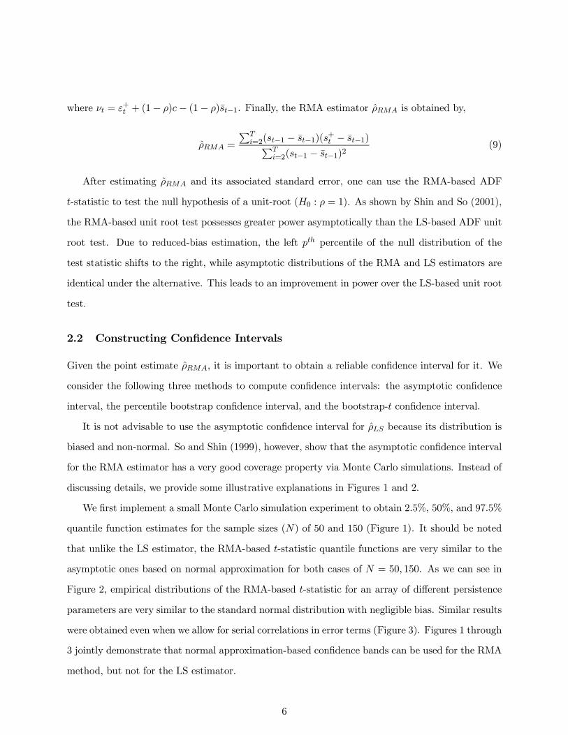
2.2 Constructing Confidence Intervals

Given the point estimate ρRMA, it is important to obtain a reliable confidence interval for it. We

consider the following three methods to compute confidence intervals: the asymptotic confidence

interval, the percentile bootstrap confidence interval, and the bootstrap-t confidence interval.

It is not advisable to use the asymptotic confidence interval for ρLS because its distribution is

biased and non-normal. So and Shin (1999), however, show that the asymptotic confidence interval

for the RMA estimator has a very good coverage property via Monte Carlo simulations. Instead of

discussing details, we provide some illustrative explanations in Figures 1 and 2.

We first implement a small Monte Carlo simulation experiment to obtain 2.5%, 50%, and 97.5%

quantile function estimates for the sample sizes (N) of 50 and 150 (Figure 1). It should be noted

that unlike the LS estimator, the RMA-based t-statistic quantile functions are very similar to the

asymptotic ones based on normal approximation for both cases of N = 50, 150. As we can see in

Figure 2, empirical distributions of the RMA-based t-statistic for an array of different persistence

parameters are very similar to the standard normal distribution with negligible bias. Similar results

were obtained even when we allow for serial correlations in error terms (Figure 3). Figures 1 through

3 jointly demonstrate that normal approximation-based confidence bands can be used for the RMA

method, but not for the LS estimator.

6

>>> Figures 1 and 2 <<<

The 90% asymptotic confidence interval for ρRMA is,

[ρRMA − 1.645 · se(ρRMA), ρRMA − 1.645 · se(ρRMA)] , (10)

where se(ρRMA) = σ(ρRMA)/[∑T

i=2(st−1 − st−1)2

]1/2and σ(ρRMA) is the estimated standard

error.

For the (nonparametric) percentile bootstrap confidence interval, let F be the empirical cumu-

lative distribution function of ρRMA obtained from nonparametric bootstrap simulations. The 90%

confidence interval is,[F−10.05, F

−10.95

]= [ρRMA,0.05, ρRMA,0.95] , (11)

where F−1α is the α percentile of the bootstrap distribution.

Finally, the bootstrap-t confidence interval (Efron and Tibshirani, 1993) is obtained as follows.

Denote Z as the empirical cumulative distribution function of,

zi =ρiRMA − ρRMAse(ρiRMA)

, (12)

where ρiRMA and se(ρiRMA) are the RMA point estimate and the standard error from the ith

bootstrap sample. The 90% confidence interval is then obtained by,

[ρRMA − z0.95 · se(ρRMA), ρRMA − z0.05 · se(ρRMA)] , (13)

where zα is the α percentile of the bootstrap distribution Z.

3 Finite Sample Performance

We conduct simulation experiments to explore finite sample performance of the unit-root test with

RMA for 16 linear and nonlinear data generating processes (DGP). The DGPs are summarized

7

in Table 1.5 The DGPs consist of various AR models (DGPs 1 to 7) such as AR(1), generalized

AR(1), bilinear, non-linear AR, squared relation, exponential relation, and binary neural network.

The next group of DGPs are endogenous and exogenous regime switching models (DGPs 8 to

13). They are self-exciting threshold autoregressive (SETAR), equilibrium TAR (EQ-TAR), band

TAR, exponential smooth transition AR (ESTAR), and logistic smooth transition AR (LSTAR).

We also consider three structural break models (DGPs 14 to 16). These various DGPs can cover

many common linear and nonlinear models that are employed in empirical work. We consider

sample sizes of T ∈ {50, 100, 200, 500} and each simulation run consists of 5,000 replications. Each

replication generates T +500 observations and then discards the first 500 observations to minimize

start up effects. We set the values for the associated autoregressive parameter (ρ and ρ1) to be

identical for all the stationary DGPs and consider two different values for ρ (0.5 and 0.9) to gauge

the effect of the associated AR parameter on power of the test.

>>> Table 1 <<<

Table 2 presents the rejection rates of each unit root test at the 10% significance level. As Choi

and Moh (2007) find that the ADFLS test shows satisfactory power performance against the unit

root null when T is sufficiently large. If not, the test suffers from low power when the stochastic

process is persistent (ρ is high).

The Monte Carlo experiments show that the ADF test with RMA (ADFRMA) provides substan-

tial power improvement over the LS-based ADF test (ADFLS). This superior discriminatory power

of ADFRMA against the unit root null stands out for all sample sizes and values of ρ. Also the

power improvement occurs more often as the sample size becomes larger. Through their simulation

experiments, Choi and Moh (2007) find that the ADFLS test stands out among five tests they

compared when the sample size is relatively small for majority of DGPs.6 However, our simulation

experiments clearly demonstrate that the ADFLS test cannot outperform the ADFRMA for most

5See Choi and Moh (2007) for more detail.6The five tests they compared are the ADF test, the momentum-threshold autoregressive (M-TAR) test, the sign

test, the KSS test, and the inf-t test. See Choi and Moh (2007) for more detail.

8

cases. Armed with the superior performance of the RMA, we next carry out empirical application

of the RMA to the real exchange rate dynamics.

>>> Table 2 <<<

4 Empirical Application

We consider CPI based real exchange rates for 21 industrialized countries. Our data set consists

of quarterly observations from 1974:Q1 to 1998:Q4 for Eurozone countries and from 1974:Q1 to

2005:Q4 for non-Eurozone countries. The US is taken as the numeraire (home) country and nominal

exchange rates and CPIs are from the International Financial Statistics.

We start with the conventional ADF test for the real exchange rates. We select the number

of lags (k) by the General-to-Specific rule as recommended by Ng and Perron (2001) for the ADF

test. The test results are presented in Table 4. As can be seen from the table, the ADF test with

the LS estimator (without bias correction) rejects the null of unit root for only 5 out of 20 countries

at the 10% significance level. However, when we apply RMA-based test, the test results change

dramatically. The null of unit root is now rejected for 16 out of 20 countries at the 10% significance

level, which may be due to superior power of the test in finite samples as we demonstrate in previous

section.

>>> Table 3 <<<

So and Shin (1999) and Shin and So (2001) show that the RMA estimator is powerful and

provides an excellent coverage property yet is computationally simple to obtain. Table 5 reports

our estimates for the persistence parameter. To examine the performance of the RMA estimator

(ρRMA), we also report the LS estimator (ρLS). We first note from the Table 5 that the RMA

estimator yields significant bias-corrections. For all real exchange rates, persistence parameter

estimates become greater with RMA. For example, the persistence parameter estimate increases

9

from 0.920 (LS) to 0.940 (RMA) for the UK. The RMA estimator delivers effective bias correction

that ranges from 0.009 (Canada) to 0.02 (UK) which is far from negligible.

Given the point estimate ρRMA, it is important to obtain a reliable confidence interval for

the estimate. Particularly for the case of highly persistent stochastic processes, more compact

confidence intervals (high precision) may provide useful information in exploring the dynamics

of the time-series of interest. It is well-known that the asymptotic confidence interval for ρLS

performs very poorly (see Hansen 1999, for example). So and Shin (1999), however, using Monte

Carlo simulations, show that the asymptotic confidence interval for the RMA estimator exhibits

a very good coverage property. To gauge the effectiveness of bias correction attained by the RMA

estimator, we consider three alternative ways to compute confidence intervals. They are asymptotic

confidence interval (CIA) with RMA, the percentile bootstrap confidence interval (CIρ), and the

bootstrap-t confidence interval (CIt).

>>> Table 4 <<<

The 90% confidence intervals we derived from the percentile bootstrapping are narrow but upper

bounds for the persistence parameter estimates are less than unity for all 21 countries. This does

not conform to the results of unit-root tests with RMA since the upper bounds are too low with

the percentile methods even for the countries where our unit-root test fails to reject the null. By

contrast, the bootstrap-t method returns higher lower bounds for the parameter estimates but now

the upper bounds reach unity for almost all the countries. Only 2 out of 21 countries show less

than unity as upper bounds at the 90% confidence intervals with the bootstrap-t method and the

results are not consistent with the unit-root test results in Table 4.

However, we obtain the compact 90% asymptotic confidence intervals for ρRMA for 16 out of 20

countries. These confidence intervals are also consistent with the results of the unit-root tests with

RMA that appear in Table 4. It seems that the asymptotic confidence interval performs reasonably

well in terms of both parsimony and efficiency even though it is computationally simple.

Murray and Papell (2002) claim that univariate approaches provide virtually no useful informa-

tion on the size of real exchange rate half-lives since the confidence intervals for the point estimates

10

are too wide and often the upper bounds are infinite. However, when we apply RMA to correct

for the bias in the LS estimates in univariate ADF regressions, we obtain much tighter confidence

intervals for the persistence parameter estimates with upper bounds that are less than unity. That

is, by stark contrast to Murray and Papell (2002), our findings suggest that the univariate methods

can provide useful information regarding the size of real exchange rate half-lives using the more

powerful but straightforward bias correction method of RMA.

5 Concluding Remarks

This paper revisits the empirical evidence on real exchange rate dynamics with the recently de-

veloped RMA method. We demonstrate superior finite sample performance of the RMA-based

unit root test via Monte Carlo simulations experiments for 16 linear and nonlinear autoregressive

models. We also show that the normal approximation-based confidence interval can be used for

the RMA method but not for the LS estimator. Using the current float quarterly real exchange

rate data we find that the unit-root test with the RMA estimator rejects the null of a unit root for

16 out of 20 industrialized countries while the conventional ADF tests rejects the null for only 5

countries. By stark contrast to Murray and Papell’s (2002) and Rossi’s (2005) results, we find that

the simple asymptotic confidence interval can provide useful information regarding the half-life of

the real exchange rate.

11

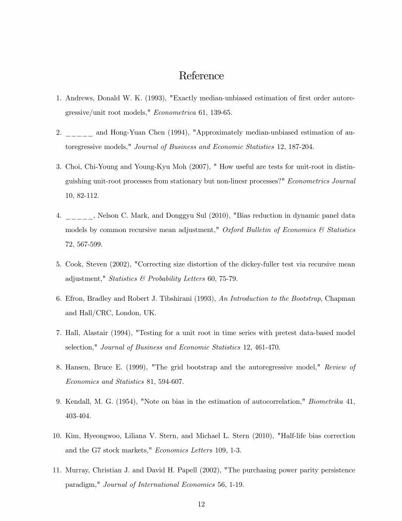
Reference

1. Andrews, Donald W. K. (1993), "Exactly median-unbiased estimation of first order autore-

gressive/unit root models," Econometrica 61, 139-65.

2. _____ and Hong-Yuan Chen (1994), "Approximately median-unbiased estimation of au-

toregressive models," Journal of Business and Economic Statistics 12, 187-204.

3. Choi, Chi-Young and Young-Kyu Moh (2007), " How useful are tests for unit-root in distin-

guishing unit-root processes from stationary but non-linesr processes?" Econometrics Journal

10, 82-112.

4. _____, Nelson C. Mark, and Donggyu Sul (2010), "Bias reduction in dynamic panel data

models by common recursive mean adjustment," Oxford Bulletin of Economics & Statistics

72, 567-599.

5. Cook, Steven (2002), "Correcting size distortion of the dickey-fuller test via recursive mean

adjustment," Statistics & Probability Letters 60, 75-79.

6. Efron, Bradley and Robert J. Tibshirani (1993), An Introduction to the Bootstrap, Chapman

and Hall/CRC, London, UK.

7. Hall, Alastair (1994), "Testing for a unit root in time series with pretest data-based model

selection," Journal of Business and Economic Statistics 12, 461-470.

8. Hansen, Bruce E. (1999), "The grid bootstrap and the autoregressive model," Review of

Economics and Statistics 81, 594-607.

9. Kendall, M. G. (1954), "Note on bias in the estimation of autocorrelation," Biometrika 41,

403-404.

10. Kim, Hyeongwoo, Liliana V. Stern, and Michael L. Stern (2010), "Half-life bias correction

and the G7 stock markets," Economics Letters 109, 1-3.

11. Murray, Christian J. and David H. Papell (2002), "The purchasing power parity persistence

paradigm," Journal of International Economics 56, 1-19.

12

12. Ng, Serena and Pierre Perron (2001), "Lag length selection and the construction of unit root

tests with good size and power," Econometrica 69, 1519-1554.

13. O’Connell, Paul G. J. (1998), "The overvaluation of purchasing power parity," Journal of

International Economics 44, 1-19.

14. Phillips, Peter C. B. and Donggyu Sul (2003), "Dynamic panel estimation and homogeneity

testing under cross section dependence," Econometrics Journal 6, 217-260.

15. Rogoff, Kenneth (1996), "The purchasing power parity puzzle," Journal of Economic Litera-

ture 34, 647-668.

16. Rossi, Barbara (2005), “Confidence intervals for half-life deviations from purchasing power

parity,” Journal of Business and Economic Statistics 23, 432-442.

17. Shaman, Paul and Robert A. Stine (1988), "The bias of autoregressive coefficient estimators,"

Journal of the American Statistical Association 83, 842-848.

18. Shin, Dong Wan and Beong Soo So (2001), "Recursive mean adjustment for unit root tests,"

Journal of Time Series Analysis 22, 595-612.

19. So, Beong Soo and Dong Wan Shin (1999), "Recursive mean adjustment in time-series infer-

ences," Statistics & Probability Letters 43, 65-73.

20. Sul, Donggyu, Peter C. B. Phillips, and Chi-Young Choi (2005), "Prewhitening bias in HAC

estimation," Oxford Bulletin of Economics & Statistics 67, 517-546.

21. Tanaka, Katsuto (1984), "An asymptotic expansion associated with the maximum likelihood

estimators in ARMA models," Journal of the Royal Statistical Society, Ser. B 46, 58-67.

22. Taylor, Alan M. (2002), "A century of purchasing power parity," Review of Economics and

Statistics 84, 139—150.

23. Taylor, Robert (2002), "Regression-based unit root tests with recursive mean adjustment

for seasonal and nonseasonal time series," Journal of Business and Economic Statistics 20,

269-281.

13

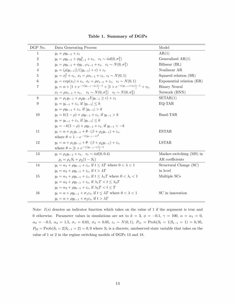
Table 1. Summary of DGPs

DGP No. Data Generating Process Model

1 yt = ρyt−1 + εt AR(1)

2 yt = ρyt−1 + φy2t−1 + et, et ∼ iid(0, σ21) Generalized AR(1)

3 yt = ρyt−1 + φyt−1et−1 + et, et ∼ N(0, σ21) Bilinear (BL)

4 yt = (ρ|yt−1|)/(|yt−1|+ c) + εt Nonlinear AR

5 yt = x2t + t, xt = ρxt−1 + εt, t ∼ N(0, 1) Squared relation (SR)

6 yt = exp(xt) + t, xt = ρxt−1 + εt, t ∼ N(0, 1) Exponential relation (ER)

7 yt = α+ [1 + e−γ(yt−1−xt)]−1 + [1 + e−γ(yt−1+xt)]−1 + vt, Binary Neural

xt = ρxt−1 + et, vt ∼ N(0, σ21) et ∼ N(0, σ22) Network (BNN)

8 yt = ρ1yt−1 + ρ2yt−1I(yt−1 ≥ c) + εt SETAR(1)

9 yt = yt−1 + εt, if |yt−1| ≤ k EQ-TAR

yt = ρyt−1 + εt, if |yt−1| > k

10 yt = k(1− ρ) + ρyt−1 + εt, if yt−1 > k Band-TAR

yt = yt−1 + εt, if |yt−1| ≤ k

yt = −k(1− ρ) + ρyt−1 + εt, if yt−1 < −k11 yt = α+ ρ1yt−1 + θ · (β + ρ2yt−1) + εt, ESTAR

where θ = 1− e−γ(yt−1−c)2

12 yt = α+ ρ1yt−1 + θ · (β + ρ2yt−1) + εt, LSTAR

where θ = [1 + e−γ(yt−1−c)]−1

13 yt = ρtyt−1 + et, et ∼ iid(0, 0.4) Markov-switching (MS) in

ρt = ρ1St + ρ2(1− St) AR coefficients

14 yt = α1 + ρyt−1 + εt, if t ≤ λT where 0 < λ < 1 Structural Change (SC)

yt = α2 + ρyt−1 + εt, if t > λT in level

15 yt = α1 + ρyt−1 + εt, if t ≤ λ1T where 0 < λi < 1 Multiple SCs

yt = α2 + ρyt−1 + εt, if λ1T < t ≤ λ2T

yt = α3 + ρyt−1 + εt, if λ2T < t ≤ T

16 yt = α+ ρyt−1 + σ1εt, if t ≤ λT where 0 < λ < 1 SC in innovation

yt = α+ ρyt−1 + σ2εt, if t > λT

Note: I(s) denotes an indicator function which takes on the value of 1 if the argument is true and

0 otherwise. Parameter values in simulations are set to k = 3, φ = −0.1, γ = 100, α = α1 = 0,

α2 = −0.5, α3 = 1.5, σ1 = 0.01, σ2 = 0.05, εt ∼ N(0, 1), P11 = Prob(St = 1|St−1 = 1) = 0, 95,

P22 = Prob(St = 2|St−1 = 2) = 0, 9 where St is a discrete, unobserved state variable that takes on thevalue of 1 or 2 in the regime switching models of DGPs 13 and 18.

14

Table 2. Rejection Rates at 10% Significance Level

DGP/ ADFLS ADFRMA

T/ 50 100 200 500 50 100 200 500

ρ = ρ1 = 0.5; ρ2 = 0.05

1 0.96 1.00 1.00 1.00 1.00 1.00 1.00 1.002 0.96 1.00 1.00 1.00 1.00 1.00 1.00 1.003 0.96 1.00 1.00 1.00 1.00 1.00 1.00 1.004 1.00 1.00 1.00 1.00 1.00 1.00 1.00 1.005 1.00 1.00 1.00 1.00 1.00 1.00 1.00 1.006 0.98 1.00 1.00 1.00 0.99 1.00 1.00 1.007 1.00 1.00 1.00 1.00 1.00 1.00 1.00 1.008 0.95 1.00 1.00 1.00 1.00 1.00 1.00 1.009 0.34 0.83 1.00 1.00 0.62 0.98 1.00 1.0010 0.22 0.33 0.84 1.00 0.34 0.56 0.98 1.0011 0.92 1.00 1.00 1.00 0.99 1.00 1.00 1.0012 0.99 1.00 1.00 1.00 1.00 1.00 1.00 1.0013 0.99 1.00 1.00 1.00 1.00 1.00 1.00 1.0014 0.84 1.00 1.00 1.00 0.98 1.00 1.00 1.0015 0.08 0.57 1.00 1.00 0.46 0.97 1.00 1.0016 0.90 1.00 1.00 1.00 1.00 1.00 1.00 1.00

ρ = ρ1 = 0.9; ρ2 = 0.05

1 0.23 0.50 0.94 1.00 0.40 0.73 0.99 1.002 0.23 0.50 0.94 1.00 0.40 0.73 0.99 1.003 0.23 0.50 0.94 1.00 0.40 0.73 0.99 1.004 1.00 1.00 1.00 1.00 1.00 1.00 1.00 1.005 0.63 0.91 0.99 1.00 0.82 0.96 1.00 1.006 0.79 0.96 0.99 1.00 0.87 0.95 0.98 1.007 1.00 1.00 1.00 1.00 1.00 1.00 1.00 1.008 0.18 0.32 0.71 1.00 0.30 0.51 0.89 1.009 0.19 0.30 0.75 1.00 0.31 0.50 0.94 1.0010 0.15 0.20 0.31 0.96 0.23 0.29 0.50 1.0011 0.15 0.24 0.51 0.99 0.25 0.37 0.72 1.0012 0.44 0.84 1.00 1.00 0.67 0.96 1.00 1.0013 0.81 0.97 1.00 1.00 0.90 0.99 1.00 1.0014 0.07 0.09 0.25 0.99 0.11 0.17 0.57 1.0015 0.00 0.00 0.00 0.00 0.00 0.00 0.00 0.00

16 0.23 0.48 0.87 1.00 0.57 0.82 0.99 1.00

Note: Entries represent the fraction of times when the null hypothesis is rejected out of 5,000 replica-

tions. Numbers in bold face indicate dominance.

15

Table 3. Rejection Rates at 10% Significance Level with Serially Correlated Errors

DGP/ ADFLS ADFRMA

T/ 50 100 200 500 50 100 200 500

ρ = ρ1 = 0.5; ρ2 = 0.05

1 0.79 1.00 1.00 1.00 0.94 1.00 1.00 1.002 0.79 1.00 1.00 1.00 0.94 1.00 1.00 1.003 0.79 1.00 1.00 1.00 0.94 1.00 1.00 1.004 0.96 1.00 1.00 1.00 1.00 1.00 1.00 1.005 0.96 1.00 1.00 1.00 0.98 1.00 1.00 1.006 0.92 0.99 1.00 1.00 0.95 0.99 1.00 1.007 0.96 1.00 1.00 1.00 1.00 1.00 1.00 1.008 0.77 1.00 1.00 1.00 0.93 1.00 1.00 1.009 0.33 0.84 1.00 1.00 0.56 0.97 1.00 1.0010 0.26 0.56 0.99 1.00 0.39 0.77 1.00 1.0011 0.74 0.99 1.00 1.00 0.90 1.00 1.00 1.0012 0.86 1.00 1.00 1.00 0.97 1.00 1.00 1.0013 0.90 1.00 1.00 1.00 0.98 1.00 1.00 1.0014 0.72 0.99 1.00 1.00 0.90 1.00 1.00 1.0015 0.21 0.65 1.00 1.00 0.48 0.93 1.00 1.0016 0.70 0.98 1.00 1.00 0.95 1.00 1.00 1.00

ρ = ρ1 = 0.9; ρ2 = 0.05

1 0.22 0.44 0.89 1.00 0.32 0.63 0.97 1.002 0.22 0.44 0.89 1.00 0.32 0.63 0.97 1.003 0.22 0.44 0.89 1.00 0.32 0.63 0.97 1.004 0.96 1.00 1.00 1.00 1.00 1.00 1.00 1.005 0.56 0.85 0.99 1.00 0.69 0.91 0.99 1.006 0.81 0.96 0.98 1.00 0.83 0.93 0.97 0.997 0.96 1.00 1.00 1.00 1.00 1.00 1.00 1.008 0.18 0.30 0.66 1.00 0.25 0.44 0.83 1.009 0.20 0.39 0.85 1.00 0.29 0.57 0.96 1.0010 0.17 0.23 0.53 1.00 0.22 0.35 0.75 1.0011 0.15 0.22 0.47 0.98 0.20 0.32 0.66 1.0012 0.29 0.59 0.95 1.00 0.41 0.77 0.99 1.0013 0.70 0.91 0.99 1.00 0.80 0.93 1.00 1.0014 0.15 0.27 0.67 1.00 0.22 0.42 0.87 1.0015 0.00 0.00 0.00 0.00 0.01 0.00 0.00 0.1116 0.21 0.42 0.81 1.00 0.49 0.76 0.97 1.00

Note: Entries represent the fraction of times when the null hypothesis is rejected out of 5,000 replica-

tions. Numbers in bold face indicate dominance.

16

Table 4. Unit Root Tests: Short-Horizon Quarterly Real Exchange Rates

Country Lag ADFLS ADFRMA

Australia 3 -2.525 -1.672∗

Austria 3 -2.273 -1.856∗

Belgium 3 -2.312 -1.827∗

Canada 3 -2.023 -1.333

Denmark 3 -2.582∗ -2.191†

Finland 3 -2.740∗ -2.502†

France 1 -2.329 -1.749∗

Germany 4 -2.596∗ -2.285†

Greece 4 -2.233 -1.753∗

Ireland 1 -2.467 -2.016†

Italy 3 -2.467 -2.202†

Japan 3 -2.263 -1.496

Netherlands 3 -2.367 -1.955†

New Zealand 3 -3.154† -2.829‡

Norway 1 -2.297 -1.819∗

Portugal 3 -1.682 -1.137

Spain 1 -1.955 -1.304

Sweden 3 -2.292 -1.813∗

Switzerland 3 -2.832∗ -2.353†

UK 1 -2.382 -1.788∗

Note: i) Sample periods are 1973Q1-1998Q4 for the Euro-zone countries and 1973Q1-2004Q4 for the

non Euro-zone countries. ii) ADFLS and ADFRMA refer to the augmented Dickey-Fuller unit root

t-test with LS and RMA estimator, respectively, when an intercept is included. iii) The number of

lags was chosen by the general-to-specific rule (Hall, 1994). iv) The asymptotic critical values for the

ADFRMA test were obtained from Shin and Soh (2001). v) ∗, †, and ‡ refer the cases that the null ofunit root is rejected at the 10%, 5%, and 1% significance level.

17

Table 5. Recursive Mean Adjustment Estimates and Alternative Confidence Intervals

Country Lag ρLS ρRMA CIA CIρ CItAustralia 3 0.945 0.964 [0.929,0.999]∗ [0.877,0.979]∗ [0.949,1.000]

Austria 3 0.933 0.947 [0.901,0.994]∗ [0.852,0.975]∗ [0.916,1.000]

Belgium 3 0.938 0.953 [0.911,0.995]∗ [0.866,0.976]∗ [0.926,1.000]

Canada 3 0.973 0.982 [0.960,1.000] [0.925,0.992]∗ [0.971,1.000]

Denmark 3 0.930 0.943 [0.901,0.986]∗ [0.863,0.969]∗ [0.913,1.000]

Finland 3 0.908 0.921 [0.869,0.973]∗ [0.826,0.959]∗ [0.878,0.991]∗

France 1 0.930 0.947 [0.898,0.997]∗ [0.847,0.972]∗ [0.918,1.000]

Germany 4 0.900 0.918 [0.860,0.977]∗ [0.798,0.958]∗ [0.873,1.000]

Greece 4 0.932 0.949 [0.902,0.997]∗ [0.843,0.977]∗ [0.919,1.000]

Ireland 1 0.905 0.923 [0.860,0.986]∗ [0.804,0.959]∗ [0.881,1.000]

Italy 3 0.918 0.931 [0.880,0.983]∗ [0.833,0.966]∗ [0.892,1.000]

Japan 3 0.950 0.967 [0.932,1.000] [0.881,0.983]∗ [0.951,1.000]

Netherlands 3 0.924 0.940 [0.890,0.991]∗ [0.839,0.970]∗ [0.906,1.000]

New Zealand 3 0.913 0.927 [0.885,0.969]∗ [0.852,0.955]∗ [0.896,0.985]∗

Norway 1 0.933 0.947 [0.899,0.995]∗ [0.854,0.972]∗ [0.917,1.000]

Portugal 3 0.958 0.972 [0.932,1.000] [0.871,0.990]∗ [0.952,1.000]

Spain 1 0.951 0.967 [0.926,1.000] [0.872,0.986]∗ [0.947,1.000]

Sweden 3 0.953 0.964 [0.931,0.997]∗ [0.895,0.982]∗ [0.943,1.000]

Switzerland 3 0.915 0.932 [0.885,0.980]∗ [0.842,0.960]∗ [0.901,1.000]

UK 1 0.920 0.940 [0.885,0.995]∗ [0.838,0.964]∗ [0.911,1.000]

Note: i) Sample periods are 1973Q1-1998Q4 for the Euro-zone countries and 1973Q1-2004Q4 for

the non Euro-zone countries. ii) The number of lags is chosen by the general-to-specific rule (Hall,

1994). iii) ρLS and ρRMA refer to the least squares and the recursive mean adjustment ρ estimate,

respectively. iv) For each real exchange rate, the 95% nonparametric bootstrap confidence interval

was obtained from 2.5% and 97.5% percentile estimates from 10,000 bootstrap replications from the

empirical distribution at the least squares point estimates (Efron and Tibshirani, 1993). v) * denotes

a finite confidence interval.

18

Figure 1. Quantitle Function Estimates of t-Statistics by the LS and the RMA Methods

(i) Number of Observations = 50

19

Figure 1. Continued

(ii) Number of Observations = 150

Note: 2.5%, 50%, and 97.5% quantile function estimates of the t-statistics from 10,000 Monte Carlo

simulations with Gaussian errors are reported.

20

Figure 2. Empirical Distributions of t-Statistics by the LS and the RMA Methods

(i) Number of Observations = 50

21

Figure 2. Continued

(ii) Number of Observations = 150

Note: The distributions of the t-statistics from the LS and the RMA method are obtained from 10,000

Monte Carlo simulations with Gaussian errors.

22

Figure 3. Empirical Distributions of t-Statistics by the LS and the RMA Methods:Serially Correlated Errors

(i) Number of Observations = 50

23

Figure 3. Continued

(ii) Number of Observations = 150

Note: The distributions of the t-statistics from the LS and the RMA method are obtained from

10,000 Monte Carlo simulations with Gaussian errors. The error term obeys AR(1) process with 0.9

persistence parameter.

24