Evidence-driven Testing and Debugging of Software Systems
200
Evidence-driven Testing and Debugging of Software Systems by Ezekiel Olamide Soremekun A dissertation submitted towards the degree Doctor of Engineering (Dr.-Ing.) of the Faculty of Mathematics and Computer Science of Saarland University Saarbrücken 2021
-
Upload
khangminh22 -
Category
Documents
-
view
0 -
download
0
Transcript of Evidence-driven Testing and Debugging of Software Systems

Evidence-driven Testing and Debuggingof Software Systems
by
Ezekiel Olamide Soremekun
A dissertation submitted towards the degreeDoctor of Engineering (Dr.-Ing.)
of the Faculty of Mathematics and Computer Scienceof Saarland University
Saarbrücken
2021
Evidence-driven Testing and Debugging of Software SystemsDissertation from Ezekiel Olamide SoremekunSaarbrückenApril 2021
Day of Colloquium: April 8th, 2021Dean of the Faculty Univ.-Prof. Dr. Thomas Schuster
Chair of the Committee: Prof. Dr. Christian RossowReportersFirst reviewer: Prof. Dr. Andreas ZellerSecond reviewer: Dr. Marcel BöhmeThird reviewer: Prof. Dr. Lars GrunskeAcademic Assistant: Dr. Rafael Dutra

Abstract
Program debugging is the process of testing, exposing, reproducing, diagnosing and fixingsoftware bugs. Many techniques have been proposed to aid developers during software testing anddebugging. However, researchers have found that developers hardly use or adopt the proposedtechniques in software practice. Evidently, this is because there is a gap between proposed methodsand the state of software practice. Most methods fail to address the actual needs of softwaredevelopers. In this dissertation, we pose the following scientific question: How can we bridge thegap between software practice and the state-of-the-art automated testing and debugging techniques?
To address this challenge, we put forward the following thesis: Software testing and debuggingshould be driven by empirical evidence collected from software practice. In particular, we positthat the feedback from software practice should shape and guide (the automation) of testing anddebugging activities. In this thesis, we focus on gathering evidence from software practice byconducting several empirical studies on software testing and debugging activities in the real-world.We then build tools and methods that are well-grounded and driven by the empirical evidenceobtained from these experiments.
Firstly, we conduct an empirical study on the state of debugging in practice using a surveyand a human study. In this study, we ask developers about their debugging needs and observethe tools and strategies employed by developers while testing, diagnosing and repairing real bugs.Secondly, we evaluate the effectiveness of the state-of-the-art automated fault localization (AFL)methods on real bugs and programs. Thirdly, we conducted an experiment to evaluate the causesof invalid inputs in software practice. Lastly, we study how to learn input distributions fromreal-world sample inputs, using probabilistic grammars.
To bridge the gap between software practice and the state of the art in software testing anddebugging, we proffer the following empirical results and techniques: (1) We collect evidence onthe state of practice in program debugging and indeed, we found that there is a chasm between(available) debugging tools and developer needs. We elicit the actual needs and concerns ofdevelopers when testing and diagnosing real faults and provide a benchmark (called DbgBench)to aid the automated evaluation of debugging and repair tools. (2) We provide empirical evidenceon the effectiveness of several state-of-the-art AFL techniques (such as statistical debuggingformulas and dynamic slicing). Building on the obtained empirical evidence, we provide a hybridapproach that outperforms the state-of-the-art AFL techniques. (3) We evaluate the prevalenceand causes of invalid inputs in software practice, and we build on the lessons learned from this

experiment to build a general-purpose algorithm (called ddmax ) that automatically diagnosesand repairs real-world invalid inputs. (4) We provide a method to learn the distribution of inputelements in software practice using probabilistic grammars and we further employ the learneddistribution to drive the test generation of inputs that are similar (or dissimilar) to sample inputsfound in the wild.
In summary, we propose an evidence-driven approach to software testing and debugging,which is based on collecting empirical evidence from software practice to guide and direct softwaretesting and debugging. In our evaluation, we found that our approach is effective in improving theeffectiveness of several debugging activities in practice. In particular, using our evidence-drivenapproach, we elicit the actual debugging needs of developers, improve the effectiveness of severalautomated fault localization techniques, effectively debug and repair invalid inputs, and generatetest inputs that are (dis)similar to real-world inputs. Our proposed methods are built on empiricalevidence and they improve over the state-of-the-art techniques in testing and debugging.
Keywords : Software Testing, Automated Debugging, Automated Fault Localization, InputDebugging, Grammar-based Test generation

Zusammenfassung
Software-Debugging bezeichnet das Testen, Aufspüren, Reproduzieren, Diagnostizieren und dasBeheben von Fehlern in Programmen. Es wurden bereits viele Debugging-Techniken vorgestellt,die Softwareentwicklern beim Testen und Debuggen unterstützen. Dennoch hat sich in derForschung gezeigt, dass Entwickler diese Techniken in der Praxis kaum anwenden oder adaptieren.Das könnte daran liegen, dass es einen großen Abstand zwischen den vorgestellten und in derPraxis tatsächlich genutzten Techniken gibt. Die meisten Techniken genügen den Anforderungender Entwickler nicht. In dieser Dissertation stellen wir die folgende wissenschaftliche Frage: Wiekönnen wir die Kluft zwischen Software-Praxis und den aktuellen wissenschaftlichen Technikenfür automatisiertes Testen und Debugging schließen?
Um diese Herausforderung anzugehen, stellen wir die folgende These auf: Das Testen undDebuggen von Software sollte von empirischen Daten, die in der Software-Praxis gesammeltwurden, vorangetrieben werden. Genauer gesagt postulieren wir, dass das Feedback aus derSoftware-Praxis die Automation des Testens und Debuggens formen und bestimmen sollte. Indieser Arbeit fokussieren wir uns auf das Sammeln von Daten aus der Software-Praxis, indemwir einige empirische Studien über das Testen und Debuggen von Software in der echten Weltdurchführen. Auf Basis der gesammelten Daten entwickeln wir dann Werkzeuge, die sich auf dieDaten der durchgeführten Experimente stützen.
Als erstes führen wir eine empirische Studie über den Stand des Debuggens in der Praxisdurch, wobei wir eine Umfrage und eine Humanstudie nutzen. In dieser Studie befragen wirEntwickler zu ihren Bedürfnissen, die sie beim Debuggen haben und beobachten die Werkzeugeund Strategien, die sie beim Diagnostizieren, Testen und Aufspüren echter Fehler einsetzen.Als nächstes bewerten wir die Effektivität der aktuellen Automated Fault Localization (AFL)-Methoden zum automatischen Aufspüren von echten Fehlern in echten Programmen. Unserdritter Schritt ist ein Experiment, um die Ursachen von defekten Eingaben in der Software-Praxiszu ermitteln. Zuletzt erforschen wir, wie Häufigkeitsverteilungen von Teileingaben mithilfe einerGrammatik von echten Beispiel-Eingaben aus der Praxis gelernt werden können.
Um die Lücke zwischen Software-Praxis und der aktuellen Forschung über Testen und Debuggenvon Software zu schließen, bieten wir die folgenden empirischen Ergebnisse und Techniken: (1)Wir sammeln aktuelle Forschungsergebnisse zum Stand des Software-Debuggens und finden in derTat eine Diskrepanz zwischen (vorhandenen) Debugging-Werkzeugen und dem, was der Entwicklertatsächlich benötigt. Wir sammeln die tatsächlichen Bedürfnisse von Entwicklern beim Testen und

Debuggen von Fehlern aus der echten Welt und entwickeln einen Benchmark (DbgBench), umdas automatische Evaluieren von Debugging-Werkzeugen zu erleichtern. (2) Wir stellen empirischeDaten zur Effektivität einiger aktueller AFL-Techniken vor (z.B. Statistical Debugging-Formelnund Dynamic Slicing). Auf diese Daten aufbauend, stellen wir einen hybriden Algorithmus vor,der die Leistung der aktuellen AFL-Techniken übertrifft. (3) Wir evaluieren die Häufigkeit undUrsachen von ungültigen Eingaben in der Softwarepraxis und stellen einen auf diesen Datenaufbauenden universell einsetzbaren Algorithmus (ddmax ) vor, der automatisch defekte Eingabendiagnostiziert und behebt. (4) Wir stellen eine Methode vor, die Verteilung von Schnipseln vonEingaben in der Software-Praxis zu lernen, indem wir Grammatiken mit Wahrscheinlichkeitennutzen. Die gelernten Verteilungen benutzen wir dann, um den Beispiel-Eingaben ähnliche (oderverschiedene) Eingaben zu erzeugen.
Zusammenfassend stellen wir einen auf der Praxis beruhenden Ansatz zum Testen undDebuggen von Software vor, welcher auf empirischen Daten aus der Software-Praxis basiert, umdas Testen und Debuggen zu unterstützen. In unserer Evaluierung haben wir festgestellt, dassunser Ansatz effektiv viele Debugging-Disziplinen in der Praxis verbessert. Genauer gesagt findenwir mit unserem Ansatz die genauen Bedürfnisse von Entwicklern, verbessern die Effektivitätvieler AFL-Techniken, debuggen und beheben effektiv fehlerhafte Eingaben und generierenTest-Eingaben, die (un)ähnlich zu Eingaben aus der echten Welt sind. Unsere vorgestelltenMethoden basieren auf empirischen Daten und verbessern die aktuellen Techniken des Testensund Debuggens.
Schlüsselwörter : Testen, Automatisches Debuggen, Automatisches Finden von Fehlern,Eingabeberichtigung, Grammatikbasiertes Testen

Dedication
To God and my loving parents.


Acknowledgment
Firstly, I want to appreciate my advisor, Prof. Dr. Andreas Zeller. You have been an excellentmentor; your research ideas, guidance, communication skills and passion for good research havebeen a major motivation to me. It has been a great opportunity to work with you in the last fewyears. More importantly, I am thankful that beyond work, you paid attention to my welfare.
I am grateful to the members of the thesis committee (Prof. Dr. Lars Grunske and Dr. MarcelBöhme) for accepting to review this thesis. I appreciate the contribution of close collaborators(Lukas Kirschner, Marcel, Lars, Dr. Esteban Pavese, Nikolas Havrikov, Emamurho Ugherughe, Dr.Sudipta Chattopadhyay), thank you for your contributions to this body of work, I am grateful forthe interesting research endeavors. To my office mates over the years – Björn Mathis, AlexanderKampmann, Nikolas Havrikov, Matthias Höschele and Clemens Hammacher, I am thankful for thedaily conversations and your help with ideas and technical issues. Notably, I want to appreciateBjörn and Michaël Mera, for constructive feedback on research projects and papers. I am alsothankful for the Dagstuhl trips, and lunch break discussions with my colleagues (Nataniel Borges,Konstantin Kuznetsov, Andreas Rau, Jenny Rau and Sascha Just) and Post Docs (Alessio Gambi,Rahul Gopinath and María Gómez Lacruz) in the software engineering group. I want to alsoappreciate my first research mentors and advisers (Sudipta and Marcel), I learned a lot workingand interacting with both of you. I am particularly grateful to Marcel for introducing me tosoftware engineering (SE) research by advising my research immersion on automated debugging.I am also grateful for the research internship with Sudipta, it was an interesting introduction toresearch in the intersection of machine learning (ML) and SE. I want to appreciate Sakshi Udeshifor making my Singapore research trip fun and for the interesting weekly research discussions.
To my closest friends in Nigeria – Isa, Kunle, Biodun and Toye. Thank you for always makingmy Nigerian holidays a good break from the continuous grind of research. To my Nigerian friendsin Germany (the Ratata family, especially Onyi, Bright, Emamurho, Eustace, David, Olachi,Tejumade, Chinyere, Anita, Bobo, Mark, Yakubu and Fuji), thank you for the frequent Jollof riceand game nights. To Ufuoma Bright Ighoroje, for encouraging me to apply for this PhD program,and ensuring I applied on the very last day of the deadline. Thank you for always being a mentorin many ways than one. To Bobo and Mark, thank you for the (online) FIFA game nights. Tomy closest friends from the graduate school (Marko, Apratim, Kireeti, Shweta and Dajana), I amgrateful I met you all, you made my weekends enjoyable. I would not forget all the Europeantrips, bar visits and nerdy arguments. To my best friend (Onyi) and her husband (Bryan), thank

you for your support since my first day in Saarbrücken.I am thankful to God for my family, my partner (Matilda), my sisters (Grace and Helen) and
my parents (Samuel and Christianah). I can not over-emphasize the importance of the emotionalsupport and understanding of my sisters, thank you for bringing sunshine to my life, especiallyon my very few Christmas trips. To my partner – Matilda, for always being there for me, forthe love and support. Thank you for keeping me focused on writing this thesis and tracking myprogress, since I am always distracted by the next research project. This process would have beenmuch harder without you.
I dedicate this thesis to God and my parents. To God, without whom I will not have madeit this far, I am grateful for the favor, grace and endless mercies. To my parents, Samuel andChristianah, for their love, trust and patience, as well as your time and financial investmentsin my education and upbringing. Daddy (Samuel), thank you for being a good example. Youtaught me to be focused, generous, happy and humble. You have taught me to always focus firston the most important things in life, and to always invest my energy and time (in your words)in “certainties” rather than “uncertainties”. Thank you for teaching me the discipline to not bedriven by money, time and location. Mom (Christianah), you have taught me patience, calmnessand perseverance. I appreciate your love and the privileges you afford me, you are a source of joy.This PhD program would have been significantly difficult without your support and trust.

Contents
1 Introduction 11.1 Thesis Statement . . . . . . . . . . . . . . . . . . . . . . . . . . . . . . . . . . . . 21.2 Publications . . . . . . . . . . . . . . . . . . . . . . . . . . . . . . . . . . . . . . . 31.3 Dissertation Outline . . . . . . . . . . . . . . . . . . . . . . . . . . . . . . . . . . 4
2 Background 52.1 Software Failures . . . . . . . . . . . . . . . . . . . . . . . . . . . . . . . . . . . . 52.2 Problem Statement . . . . . . . . . . . . . . . . . . . . . . . . . . . . . . . . . . . 62.3 Debugging Process . . . . . . . . . . . . . . . . . . . . . . . . . . . . . . . . . . . 72.4 Debugging Challenges . . . . . . . . . . . . . . . . . . . . . . . . . . . . . . . . . 8
2.4.1 Debugging in Software Practice . . . . . . . . . . . . . . . . . . . . . . . . 82.4.2 Fault Localization . . . . . . . . . . . . . . . . . . . . . . . . . . . . . . . 82.4.3 Input Debugging . . . . . . . . . . . . . . . . . . . . . . . . . . . . . . . . 132.4.4 Test Generation . . . . . . . . . . . . . . . . . . . . . . . . . . . . . . . . 14
3 Debugging in Practice: An Empirical Study 173.1 Introduction . . . . . . . . . . . . . . . . . . . . . . . . . . . . . . . . . . . . . . . 173.2 Survey . . . . . . . . . . . . . . . . . . . . . . . . . . . . . . . . . . . . . . . . . . 19
3.2.1 Study Design . . . . . . . . . . . . . . . . . . . . . . . . . . . . . . . . . . 193.2.2 Study Results . . . . . . . . . . . . . . . . . . . . . . . . . . . . . . . . . . 23
3.3 Observational Study . . . . . . . . . . . . . . . . . . . . . . . . . . . . . . . . . . 333.3.1 Study Design . . . . . . . . . . . . . . . . . . . . . . . . . . . . . . . . . . 343.3.2 Study Results . . . . . . . . . . . . . . . . . . . . . . . . . . . . . . . . . . 40
3.4 A Benchmark for Debugging Tools . . . . . . . . . . . . . . . . . . . . . . . . . . 483.5 Limitations and Threats to Validity . . . . . . . . . . . . . . . . . . . . . . . . . . 523.6 Related Work . . . . . . . . . . . . . . . . . . . . . . . . . . . . . . . . . . . . . . 543.7 Discussions and Future Work . . . . . . . . . . . . . . . . . . . . . . . . . . . . . 56
4 Locating Faults with Program Slicing: An Empirical Analysis 614.1 Introduction . . . . . . . . . . . . . . . . . . . . . . . . . . . . . . . . . . . . . . . 614.2 A Hybrid Approach . . . . . . . . . . . . . . . . . . . . . . . . . . . . . . . . . . 65
i

Contents
4.3 Evaluation Setup . . . . . . . . . . . . . . . . . . . . . . . . . . . . . . . . . . . . 674.3.1 Implementation . . . . . . . . . . . . . . . . . . . . . . . . . . . . . . . . . 684.3.2 Metrics and Measures . . . . . . . . . . . . . . . . . . . . . . . . . . . . . 694.3.3 Objects of Empirical Analysis . . . . . . . . . . . . . . . . . . . . . . . . . 714.3.4 Measure of Localization Effectiveness . . . . . . . . . . . . . . . . . . . . . 73
4.4 Experimental Results . . . . . . . . . . . . . . . . . . . . . . . . . . . . . . . . . . 764.5 Threats to Validity . . . . . . . . . . . . . . . . . . . . . . . . . . . . . . . . . . . 914.6 Related Work . . . . . . . . . . . . . . . . . . . . . . . . . . . . . . . . . . . . . . 924.7 Discussions and Future Work . . . . . . . . . . . . . . . . . . . . . . . . . . . . . 94
5 Debugging Failure-Inducing Inputs 975.1 Introduction . . . . . . . . . . . . . . . . . . . . . . . . . . . . . . . . . . . . . . . 975.2 Prevalence of Invalid Inputs . . . . . . . . . . . . . . . . . . . . . . . . . . . . . . 995.3 Lexical Repair . . . . . . . . . . . . . . . . . . . . . . . . . . . . . . . . . . . . . 1025.4 Syntactic Repair . . . . . . . . . . . . . . . . . . . . . . . . . . . . . . . . . . . . 1105.5 Diagnostic Quality . . . . . . . . . . . . . . . . . . . . . . . . . . . . . . . . . . . 1145.6 Threats to Validity . . . . . . . . . . . . . . . . . . . . . . . . . . . . . . . . . . . 1165.7 Limitations . . . . . . . . . . . . . . . . . . . . . . . . . . . . . . . . . . . . . . . 1165.8 Related Work . . . . . . . . . . . . . . . . . . . . . . . . . . . . . . . . . . . . . . 1175.9 Discussions and Future Work . . . . . . . . . . . . . . . . . . . . . . . . . . . . . 118
6 Learning Input Distributions for Grammar-Based Test Generation 1216.1 Introduction . . . . . . . . . . . . . . . . . . . . . . . . . . . . . . . . . . . . . . . 1216.2 Overview . . . . . . . . . . . . . . . . . . . . . . . . . . . . . . . . . . . . . . . . 1236.3 Approach . . . . . . . . . . . . . . . . . . . . . . . . . . . . . . . . . . . . . . . . 126
6.3.1 Probabilistic Grammars . . . . . . . . . . . . . . . . . . . . . . . . . . . . 1266.3.2 Learning Probabilities . . . . . . . . . . . . . . . . . . . . . . . . . . . . . 1276.3.3 Inverting Probabilities . . . . . . . . . . . . . . . . . . . . . . . . . . . . . 1276.3.4 Producing Inputs from a Grammar . . . . . . . . . . . . . . . . . . . . . . 1286.3.5 Implementation . . . . . . . . . . . . . . . . . . . . . . . . . . . . . . . . . 129
6.4 Experimental Evaluation . . . . . . . . . . . . . . . . . . . . . . . . . . . . . . . . 1306.4.1 Evaluation Setup . . . . . . . . . . . . . . . . . . . . . . . . . . . . . . . . 1316.4.2 Experimental Results . . . . . . . . . . . . . . . . . . . . . . . . . . . . . 135
6.5 Threats to Validity . . . . . . . . . . . . . . . . . . . . . . . . . . . . . . . . . . . 1456.6 Limitations . . . . . . . . . . . . . . . . . . . . . . . . . . . . . . . . . . . . . . . 1466.7 Related Work . . . . . . . . . . . . . . . . . . . . . . . . . . . . . . . . . . . . . . 1466.8 Discussions and Future Work . . . . . . . . . . . . . . . . . . . . . . . . . . . . . 148
7 Conclusion 1517.1 Summary . . . . . . . . . . . . . . . . . . . . . . . . . . . . . . . . . . . . . . . . 1517.2 Contributions . . . . . . . . . . . . . . . . . . . . . . . . . . . . . . . . . . . . . . 1527.3 Future Work . . . . . . . . . . . . . . . . . . . . . . . . . . . . . . . . . . . . . . 153
ii

Contents
Bibliography 157
Appendices 181
List of Figures 183
List of Tables 187
iii

Chapter 1
Introduction
“Beware of bugs in the above code;I have only proved it correct, not tried it.”
— Donald E. Knuth
Programs often fail. Frequently, programs contain bugs that cause failures and unexpectedbehaviors. When a program fails, software developers are saddled with the task of exposing,reproducing, diagnosing and repairing the bug. Developers first have to test the program withsuitable inputs, then diagnose and fix the failure. Testing is the process of writing or generatinginputs that executes the program code, in order to expose (or reproduce) bugs. Meanwhile,debugging is the process of diagnosing and fixing such bugs. Both testing and debugging arearduous tasks, that consume a lot of time and resources.
Several methods have been developed to support developers in software testing and debug-ging [1, 2, 3, 4, 5, 6, 7, 8]. However, there is a gap between proposed methods and the actualstate of software practice. Most methods lack strong empirical support; they either do not haveany empirical validation at all or have weak evaluations with unrealistic assumptions [9, 10].Often, researchers have found evidence of assumptions, tools and techniques that do not applyin practice [11, 12, 13, 14, 15]. This lack of empirical support can be attributed to the cost anddifficulty of experimentation [16, 17, 18].
Consequently, this chasm has created a gap between the state of the art tools and how developersactually test and debug programs. For instance, a recent survey on debugging cites more than400 publications on fault localization techniques [1]. However, most developers have never usedan automated fault localization tool in practice [19]. Likewise, many test generation methodsdo not generate test inputs that are similar to those written by developers or end-users of thesoftware [20]. Notably, current approaches ignore how proposed tools address real-world needs.We know very little about how developers test and debug; we also lack the data and methods tocheck (proposed) tools against practitioner’s needs.
How can we bridge this gap? In this thesis, we conduct several empirical studies to gatherevidence from software practice, in order to effectively guide and automate software testing anddebugging. We put forward the thesis that testing and debugging should be driven by empiricalevidence collected from software practice. We posit that the feedback from software practice
1

1. Introduction
should shape and guide software testing and debugging. Thus, we focus on building tools andmethods that are driven by empirical evidence collected from software practice.
1.1 Thesis Statement
In this dissertation, we designed and conducted several experiments to empirically test our thesisstatement. Then, we collect empirical evidence from these experiments to build novel methods fortesting and debugging. We analyze the results of our experiments in order to support the thesis,we discuss the implications of these experiments and we introduce novel testing and debuggingmethods that are built on empirical evidence from software practice.
The rest of this dissertation builds on different aspects of this thesis statement:
Software testing and debugging should be drivenby empirical evidence collected from software practice.
Firstly, we evaluate the state of debugging in practice (Chapter 3). In particular, we evaluatehow developers diagnose and repair bugs in practice. We conducted a retrospective study withhundreds of developers and an observational study with 12 practitioners, in order to collectempirical evidence on the state-of-the-practice in debugging. We investigate how developers spendtheir time diagnosing and fixing bugs. We also examine the tools and strategies employed bydevelopers while debugging. Our findings reveal the need for automated assistance to evaluateand develop realistic debugging aids. Subsequently, we apply the evidence gathered from theseempirical studies to facilitate and guide future research. In particular, we provide DbgBench, ahighly usable debugging benchmark that provides fault locations, patches and explanations forcommon bugs as provided by practitioners.
Secondly, we evaluate the effectiveness of the state-of-the-art fault localization methods (Chap-ter 4). Specifically, we compare the effectiveness of several statistical fault localization methodsagainst dynamic program slicing in a large study of over 706 faults in 46 open source C programs.Our findings reveal that dynamic slicing was more effective than the best performing statisticaldebugging formula. For most bugs, dynamic slicing will find the fault earlier than the bestperforming statistical debugging formula. Consequently, we apply this empirical evidence todevelop a hybrid approach. The hybrid approach leverages the strengths of both dynamic slicingand statistical fault localization to achieve the best results. Programmers using the hybridapproach will need to examine fewer lines of code to locate faults.
Thirdly, we evaluate how to debug invalid inputs that occur in software practice (Chapter 5).We first evaluate the prevalence of invalid inputs in practice, and we found that four percent ofinputs in the wild are invalid. We then build on this empirical evidence to develop a method todebug inputs — that is, identify which parts of the input data prevent processing, and recover asmuch of the (valuable) input data as possible. We present a general-purpose algorithm calledddmax that addresses these problems automatically, via numerous experiments that maximizesthe subset of the input that can still be processed by the program. Particularly, this is the firstapproach that fixes faults in the input data without requiring program analysis.
Lastly, we propose an approach that generates structured inputs that are (dis)similar to real-world inputs found in the wild (Chapter 6). We first learn the distribution of input elements in
2

1.2. Publications
real-world sample inputs using a probabilistic grammar. We then apply the learned probabilisticgrammar to generate inputs that are similar to the sample. We also generate inputs thatare dissimilar to the sample by inverting the learned probabilities. In addition, this approachallows to reproduce (or avoid) program failures by learning the distribution of input elements infailure-inducing inputs.
1.2 Publications
This dissertation builds on the following papers (in chronological order):
• Ezekiel Soremekun. Debugging with probabilistic event structures. In 2017 IEEE/ACM39th International Conference on Software Engineering Companion (ICSE-C), pages 437–440.IEEE, 2017.
• Marcel Böhme, Ezekiel Soremekun, Sudipta Chattopadhyay, Emamurho Ugherughe,and Andreas Zeller. Wo ist der fehler und wie wird er behoben? ein experiment mitsoftwareentwicklern. Software Engineering und Software Management (SESWM), 2018.
• Marcel Böhme, Ezekiel Soremekun, Sudipta Chattopadhyay, Emamurho Juliet Ugherughe,and Andreas Zeller. How developers debug software —the dbgbench dataset. In 2017IEEE/ACM 39th International Conference on Software Engineering Companion (ICSE-C),pages 244–246. IEEE, 2017.
• Marcel Böhme, Ezekiel Soremekun, Sudipta Chattopadhyay, Emamurho Ugherughe, andAndreas Zeller. Where is the bug and how is it fixed? an experiment with practitioners.In Proceedings of the 2017 11th Joint Meeting on Foundations of Software Engineering(ESEC/FSE), pages 117–128, 2017.
• Ezekiel Soremekun, Lukas Kirschner, Marcel Böhme, and Andreas Zeller. Locating faultswith program slicing: An empirical analysis. Empirical Software Engineering (EMSE) 26,51 (2021).
• Lukas Kirschner, Ezekiel Soremekun, and Andreas Zeller. Debugging inputs. In 2020IEEE/ACM 42nd International Conference on Software Engineering (ICSE). IEEE, 2020.
• Ezekiel Soremekun, Esteban Pavese, Nikolas Havrikov, Lars Grunske, and AndreasZeller. Inputs from hell: Learning input distributions for grammar-based test generation.Transaction on Software Engineering (TSE), 2020.
The author of this dissertation has also co-authored the following papers, these papers do notcontribute to this dissertation:
• Rahul Gopinath, Alexander Kampmann, Nicolas Havrikov, Ezekiel Soremekun andAndreas Zeller. Abstracting Failure-Inducing Inputs. In 2020 ACM SIGSOFT InternationalSymposium on Software Testing and Analysis (ISSTA), 2020. ACM Distinguished Award.
3

1. Introduction
• Alexander Kampmann, Nicolas Havrikov, Ezekiel Soremekun and Andreas Zeller. Whendoes my Program do this? Learning Circumstances of Software Behavior. In Proceedingsof the 2020 ACM Joint European Software Engineering Conference and Symposium on theFoundations of Software Engineering (ESEC/FSE), 2020.
• Björn Mathis, Vitalii Avdiienko, Ezekiel Soremekun, Marcel Böhme, and Andreas Zeller.Detecting information flow by mutating input data. In 2017 32nd IEEE/ACM InternationalConference on Automated Software Engineering (ASE), pp. 263-273. IEEE, 2017.
1.3 Dissertation Outline
The rest of this dissertation is organized as follows: First, in Chapter 2, we provide backgroundon the main areas of software testing and debugging that are addressed by this dissertation. Inparticular, we discuss the state of the art in program debugging, automated fault localization, inputdebugging and grammar-based test generation. In Chapter 3, we present an empirical study ondebugging in practice in which we investigate how developers diagnose and fix real bugs. Wepresent key findings on the tools and strategies used by developers in practice. We also provideDbgBench— a benchmark providing empirical data on debugging in practice, in order to aidfuture research. Chapter 4 introduces an empirical study of the effectiveness of the state-of-the-artautomated fault localization techniques, in particular, program slicing and several statistical faultlocalization methods. We also present a hybrid approach that outperforms the state-of-the-art.Chapter 5 presents an empirical study of invalid inputs in the wild, where we present key insightson the prevalence and sources of input invalidity in software practice. Building on this evidence,we present a black-box approach that repairs and debugs invalid inputs using a maximizing variantof the delta debugging algorithm. In Chapter 6, we present a grammar-based probabilistic testgeneration approach, that allows to generate inputs that are (dis)similar to sample inputs writtenby end-users or developers. We further illustrate how our approach allows to generate inputsthat reproduce (or avoid) failures. Finally, we conclude this dissertation with a discussion of thecontributions and future directions in Chapter 7.
4
Chapter 2
Background
This chapter is taken, directly or with minor modifications, from our 2017 ICSE paper Debuggingwith probabilistic event structures [21] and our 2018 SE paper Wo ist der Fehler und wie wirder behoben? Ein Experiment mit Softwareentwicklern [22]. My contribution in this work is asfollows: (I) original idea; (II) partial implementation; (III) evaluation.
“If I have seen further, it is by standing on the shoulders of giants.”— Sir Isaac Newton
2.1 Software Failures
When a program fails, we say the program is buggy. A program can be buggy by construction (e.g.due to omission errors) or because it contains defects. Invariably, for a software to be consideredbuggy, the execution of the software has to result in unexpected behavior(s).
Exposing bugs in programs is non-trivial and determining the presence of a bug is difficult.In software development, bugs are typically revealed via software testing. Developers have toconstruct test input(s) that expose and reproduce the observed unexpected behavior (e.g. afailure, crash or wrong output). A bug is found or exposed, when a program fails when fed witha valid test input. The failing test execution confirms that the program is buggy. Test inputs thatcause a program to fail are referred to as failure-inducing input. These failure-inducing inputsallow developers to reproduce and diagnose the bug.
When a bug is found in a software, developers have to debug the software, i.e. understand,diagnose and fix the bug. The process of bug diagnosis and fixing is called debugging. Debuggingis a tedious task that involves analyzing the failing program execution(s). When debugging,developers often employ techniques that aid program understanding, bug analysis and testexecution.
Terminology
In the following, we explain the main debugging terminologies used in this dissertation basedon the IEEE Glossary [23]. We define an error as incorrect program behavior or result, forinstance, when the program prints 0 when it is expected to print 1. A fault is the defect in the
5
2. Background
source code that causes an error, like a missing increment. A bug may be any of the above. Anerror’s symptom is the observed unexpected behavior, for instance, the program unexpectedlyprinting 0. A failing test case is an input and an assertion of the expected output that fails in thepresence of an error. Debugging is a “post-mortem” activity that follows once an error has beenfound and reported, for instance, via testing or by a user. Debugging is the task of identifyingthe fault and removing the error completely without introducing new errors. We distinguishfour distinct sub-tasks during debugging: Bug reproduction is the task of reproducing the buglocally by constructing a test case that fails because of the bug. Bug diagnosis is the task ofunderstanding and explaining the run-time actions causing the symptom. Fault localization isthe task of identifying the faulty code locations, i.e. the statements responsible for the bug and(potentially) have to be changed to fix it. Finally, bug fixing or repair is the task of removing theerror by changing the source code.
2.2 Problem Statement
Several techniques have been proposed to support developers during debugging activities [1].However, evidence has shown that most of these techniques are not widely adopted by developersin practice [11]. More importantly, the state-of-the-art approaches do not meet the real-worldneeds of developers [12]. In this dissertation, we ask the following fundamental question: Howcan we bridge the gap between the state-of-the-art debugging methods and the state of debuggingin practice?
Indeed, addressing this question requires analyzing the state of debugging in practice andthe performance of the state-of-the-art debuggers. On one hand, it is pertinent to conductempirical studies that sheds light on the nature of debugging and the needs of developers. Theempirical study should address questions such as: How do developers debug programs? And whatdo developers need when debugging in practice? The results of the study should provide thedebugging requirements of developers and serve as a baseline to design and evaluate debuggingaids. On the other hand, one needs to evaluate the performance of the state-of-the-art debuggingtools in real world setting. In this context, one needs to address the following fundamentalquestion: What is the most effective fault localization method on real faults? Subsequently, onecan build methods that address the needs and concerns of developers elicited in the first step, inorder to improve the performance of the state-of-the-art debugging tools in practical settings.
The main goal of this work is to provide methods that meet the actual needs of developerswhen debugging in practice. To achieve this goal, we employ an evidence-based approach todevelop techniques which support developers during debugging activities. This is a two-stepapproach that proceeds for a debugging challenge or activity as follows: First, 1) conduct realisticempirical studies that elicit the nature and requirements of the debugging activity in practice,then 2) develop methods and tools that are based on the evidence (i.e. requirements) gatheredfrom the empirical studies (in step one). In this dissertation, all empirical studies are based onthe first step (1) of this approach, and all proposed methods in this dissertation are results of thesecond step (2) of the evidence-based approach.
6

2.3. Debugging Process
2.3 Debugging Process
The main goal of automated debugging is to support developers during debugging activities.Debuggers are designed to improve developer’s effectiveness during bug diagnosis and fixing. Theusefulness and applicability of debuggers is vital, considering that about a third of developmenttime is spent on debugging activities [1]. Thus, software developers can benefit significantly fromtechniques that improve productivity during debugging.
Typically, to effectively debug a program, a developer needs to 1) expose or reproduce the bug(via testing), 2) understand the unexpected program behavior (called bug diagnosis), 3) determinethe fault locations responsible for the observed failing behavior (called fault localization) and (4.)repair or fix the bug (called program repair). In the following, we discuss these debugging steps:
1. Bug Reproduction: When debugging, developers must first expose or reproduce the failure,in order to observe the unexpected behavior. This may involve running existing tests orconstructing new tests that reproduce the failure. These tests are expected to accurately andreliably reveal the unexpected software behavior, this is necessary to establish the presenceof a bug in the software.
2. Bug Diagnosis: Secondly, the developer has to diagnose the bug or failure. The goal ofthis step is to comprehend the conditions under which the bug can be observed. Thisinvolves program comprehension (i.e. understanding the program behavior) and analyzingtest executions, for instance, comparing failing and passing executions. Other bug diagnosisapproaches include (dynamic) program analysis, i.e. analyzing program executions in orderto diagnose the conditions (e.g. data or control flow paths) under which the failing behaviorcan (not) be observed.
3. Fault Localization: In this step, the developer analyzes the program to determine the faultycode locations. The fault locations are the program features (e.g. statements or lines ofcode) that explains the bug, such features may need to be modified to fix the bug. Thisstep is often achieved by analyzing the code locations that are executed in the failing (andpassing) execution(s), in order to determine the code point(s) where the executions divergedfrom the expected behavior. Fault Localization is a prerequisite step to fix a bug, thus, it isthe first step of most APR tools. Examples of prominent AFL techniques include statisticaldebugging, program slicing and mutational AFL.
4. Program Repair: Finally, the developer (or an APR tool) fixes the bug by modifying theprogram. This process patches the faulty program (e.g. by removing the error), in orderto ensure that the program behavior matches the expected behavior. However, to makesure the fix is correct, it is important to ensure that 1) the failing test(s) no longer leads toa failure in the fixed program (called patch plausibility), 2) the fix is complete, it actuallyfixes the bug and not a symptom of the bug (called patch completeness) and 3) the fix (orprogram change) does not introduce a new bug or a regression bug that cause other tests tofail, this step is called regression testing.
7

2. Background
2.4 Debugging Challenges
Let us provide relevant background on the challenges in the major areas of software testing anddebugging that are investigated in this thesis. In particular, we discuss the state of the art inprogram debugging, automated fault localization, input debugging and test generation.
2.4.1 Debugging in Software Practice
In 1997, Liebermann introduced the CACM special section on “The Debugging Scandal and Whatto Do About It" with the words “debugging is still as it was 30 years ago, largely a matter of trialand error” [24]. Researchers argue that debugging in practice is an art more than a science [25],nothing but trial-and-error [24]. Others have gone as far as modelling the way how programmersdebug as a predator that is following scent to find prey [26]. Except, debugging does not need tobe an unpremeditated activity. Today, automated debugging tools hold the promise of providingguidance during debugging, of an increase of productivity, and of a significant reduction of timeand money spent on debugging; all by the push of a button.
The “debugging scandal” is definitely not due to the lack of tools produced in the outstandingresearch of automated software debugging. Researchers have developed tools that can identifypotential fault locations [27, 28], potential fix locations [29, 30], failure-inducing modifications inupdates [31], the chain of events leading up to the error [32], and even potential software patches[33, 34, 35, 36]. However, empirical evidence shows that most developers have never used anautomated debugging tool [19].
Why would a rational developer forgo the promises of automation in the face of the tediousnessof the manual debugging activity? Andrew Ko writes about his experience as a CTO of a companyand his attempts to bring software engineering research into practice that “most of what I presentjust isn’t relevant, isn’t believed, or isn’t ready; honestly, many of our engineering problemssimply aren’t the problems that software engineering researchers are investigating” [37]. LionelBriand adds that “the research community had a rather superficial understanding of the problemsfacing practitioners while debugging” [38].
In this thesis, we asked ourselves: what is the state of debugging in practice (see Chapter 3)?Which problems do practitioners have? What do they want? What do practitioners find relevant?Why do they reject debugging automation? In addition, we collected empirical data from hundredsof hours of debugging sessions of professional developers: We investigated how developers debugand repair real software bugs, the tools and strategies applied, the time taken and the bugdiagnoses and patches they provided.
2.4.2 Fault Localization
This section sheds light on the details of automated fault localization (AFL) techniques. AFLrefers to methods that automatically identify the root cause(s) of a bug, i.e. the faulty programlocations (e.g. statements or methods) that triggered an observed failing behavior. The aimof AFL approaches is to provide developers (and automated tools) with faulty code locations,in order to aid bug diagnoses and program repair. AFL is an important software engineeringresearch area, which has provided a wealth of automated tools. Wong et al. [39] surveyed more
8
2.4. Debugging Challenges
than 60 AFL tools and list 29 as publicly available (e.g., as Eclipse plugin [40]). A recent surveyfinds that the majority1 of practitioners considers research on AFL as essential or worthwhile [41].
In this dissertation, we investigate the efficacy of AFL approaches (see Chapter 4). There aretwo main AFL approaches, namely program slicing and statistical debugging [39]. In the rest ofthis section, we provide background on program slicing and statistical debugging.
Program Slicing
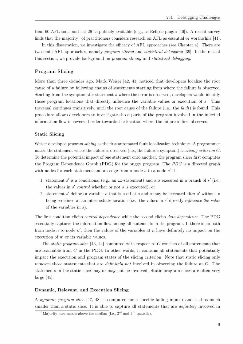
More than three decades ago, Mark Weiser [42, 43] noticed that developers localize the rootcause of a failure by following chains of statements starting from where the failure is observed.Starting from the symptomatic statement s where the error is observed, developers would identifythose program locations that directly influence the variable values or execution of s. Thistraversal continues transitively, until the root cause of the failure (i.e., the fault) is found. Thisprocedure allows developers to investigate those parts of the program involved in the infectedinformation-flow in reversed order towards the location where the failure is first observed.
Static Slicing
Weiser developed program slicing as the first automated fault localization technique. A programmermarks the statement where the failure is observed (i.e., the failure’s symptom) as slicing criterion C.To determine the potential impact of one statement onto another, the program slicer first computesthe Program Dependence Graph (PDG) for the buggy program. The PDG is a directed graphwith nodes for each statement and an edge from a node s to a node s
0 if
1. statement s0 is a conditional (e.g., an if-statement) and s is executed in a branch of s
0 (i.e.,the values in s
0 control whether or not s is executed), or2. statement s
0 defines a variable v that is used at s and s may be executed after s0 without v
being redefined at an intermediate location (i.e., the values in s0 directly influence the value
of the variables in s).
The first condition elicits control dependence while the second elicits data dependence. The PDGessentially captures the information-flow among all statements in the program. If there is no pathfrom node n to node n
0, then the values of the variables at n have definitely no impact on theexecution of n
0 or its variable values.The static program slice [43, 44] computed with respect to C consists of all statements that
are reachable from C in the PDG. In other words, it contains all statements that potentiallyimpact the execution and program states of the slicing criterion. Note that static slicing onlyremoves those statements that are definitely not involved in observing the failure at C. Thestatements in the static slice may or may not be involved. Static program slices are often verylarge [45].
Dynamic, Relevant, and Execution Slicing
A dynamic program slice [47, 48] is computed for a specific failing input t and is thus muchsmaller than a static slice. It is able to capture all statements that are definitely involved in
1Majority here means above the median (i.e., 3rd and 4th quartile).
9
2. Background
Fault Localization Should Use Slices
Ezekiel SoremekunSoftware Engineering Chair
Saarland UniversitySaarbrücken, Germany
Marcel BöhmeSchool of Computing
National University of SingaporeSingapore
Andreas ZellerSoftware Engineering Chair
Saarland UniversitySaarbrücken, Germany
ABSTRACTIf programmers follow dynamic backward dependencies from thefailing output, they will find the fault much quicker than if theyexamine locations whose execution correlates with failure. In ourstudy of XXX real bugs, fault localization along dynamic depen-dences required programmers to examine on average N% of thecode; whereas statistical debugging techniques required NN%. Thisstudy is the first to compare the fault localization effectiveness ofstatistical debugging and dynamic dependencies, although both havebeen around for more than 15 years.
CCS Concepts•General and reference � General conference proceedings; Gen-eral literature; •Software and its engineering � Software testingand debugging; Search-based software engineering;
KeywordsACM proceedings
1. INTRODUCTIONIn the past 20 years, the field of automated fault localization has
found considerable interest among researchers in Software Engi-neering. Given a program failure, the aim of fault localization isto suggest locations in the program code where a fault in the codecauses the failure at hand. Locating a fault is an obvious prerequi-site for removing and fixing it; and thus, automated fault localiza-tion brings the promise of supporting programmers during arduousdebugging tasks. Fault localization is also an important prerequisitefor automated program repair, as the locations suggested by faultlocalization would serve as candidates where to apply synthesizedfixes.
The large majority of today’s publications on automated faultlocalization fall into the category of Statistical Debugging, an ap-proach pioneered more than 15 years ago by both Liblit [?] as wellas Jones, Stasko, and Harrold [?]. Today, a recent survey by Wonget al. [?] lists more than 100 publications on statistical debuggingin the past 15 years.
Permission to make digital or hard copies of all or part of this work for personal orclassroom use is granted without fee provided that copies are not made or distributedfor profit or commercial advantage and that copies bear this notice and the full cita-tion on the first page. Copyrights for components of this work owned by others thanACM must be honored. Abstracting with credit is permitted. To copy otherwise, or re-publish, to post on servers or to redistribute to lists, requires prior specific permissionand/or a fee. Request permissions from [email protected] 2016 Singaporec� 2016 ACM. ISBN 978-1-4503-2138-9.
DOI: 10.1145/1235
⌅: covered statements x 3 1 3 5 5 21 int middle(x, y, z) { y 3 2 2 5 3 12 int x, y, z; z 5 3 1 5 4 33 int m = z; ⌅ ⌅ ⌅ ⌅ ⌅ ⌅ 34 if (y < z) { ⌅ ⌅ ⌅ ⌅ ⌅ ⌅ 45 if (x < y) � ⌅ � � � � 56 m = y; � ⌅ � � � � 67 else if (x < z) ⌅ � � � ⌅ ⌅ 78 m = y; ⌅ � � � � ⌅ 89 } else { ⌅ � ⌅ ⌅ � � 9
10 if (x > y) � � ⌅ � � � 1011 m = y; � � ⌅ � � � 1112 else if (x > z) � � � � � � 1213 m = x; � � � � � � 1314 } � � � � � � 1415 return m; ⌅ ⌅ ⌅ ⌅ ⌅ ⌅ 1516 } 4 4 4 4 4 8
Figure 1: Statistical Debugging illustrated [?]: The middlefunction takes three values and returns the middle one; how-ever, on the input (2, 1, 3), it returns 1 rather than 2. Statis-tical Debugging reports the faulty Line 8 as the most suspi-cious one, since the correlation of its execution with failure isthe strongest.
The core idea of statistical debugging is to take a set of passingand failing runs, and to record which program lines would be exe-cuted (“covered”) in these runs. If there is a correlation between theexecution of a line and failure (say, because this line is only exe-cuted in failing runs, and never in passing runs), then the line wouldbe flagged as “suspicious”; and the stronger the correlation and thehigher the support, the more suspicious a line would become.
To illustrate Statistical Debugging, let us have a look at the middlefunction, pioneered in [?] to introduce the technique. middlecomputes the middle of three numbers x, y, z; ?? shows its sourcecode as well as a few sample inputs. On most inputs, middleworks as advertised; but when fed with x = 2, y = 1, and z = 3,it returns 1 rather than the middle value 2. Given the runs and thelines covered in each, Statistical Debugging now determines statis-tical correlations between each line being executed and the programfailing. This correlation is the strongest in Line 8, which also hap-pens to be the fault location.
Statistical Debugging, however, is not the first technique to auto-mate fault, localization. In his seminal paper of 1985 “Program-mers use slicing when debugging”, Mark Weiser introduced theconcept of a program slice composed of data and control dependen-cies in the program, and argued that during debugging, program-mers would start from a faulty value, and then proceed backwards
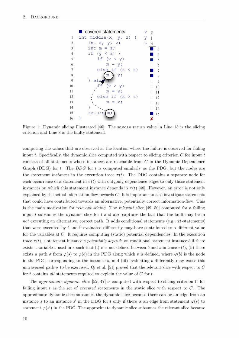
Figure 1: Dynamic slicing illustrated [46]: The middle return value in Line 15 is the slicingcriterion and Line 8 is the faulty statement.
computing the values that are observed at the location where the failure is observed for failinginput t. Specifically, the dynamic slice computed with respect to slicing criterion C for input t
consists of all statements whose instances are reachable from C in the Dynamic DependenceGraph (DDG) for t. The DDG for t is computed similarly as the PDG, but the nodes arethe statement instances in the execution trace ⇡(t). The DDG contains a separate node foreach occurrence of a statement in ⇡(t) with outgoing dependence edges to only those statementinstances on which this statement instance depends in ⇡(t) [48]. However, an error is not onlyexplained by the actual information-flow towards C. It is important to also investigate statementsthat could have contributed towards an alternative, potentially correct information-flow. Thisis the main motivation for relevant slicing. The relevant slice [49, 50] computed for a failinginput t subsumes the dynamic slice for t and also captures the fact that the fault may be innot executing an alternative, correct path. It adds conditional statements (e.g., if-statements)that were executed by t and if evaluated differently may have contributed to a different valuefor the variables at C. It requires computing (static) potential dependencies. In the executiontrace ⇡(t), a statement instance s potentially depends on conditional statement instance b if thereexists a variable v used in s such that (i) v is not defined between b and s in trace ⇡(t), (ii) thereexists a path � from '(s) to '(b) in the PDG along which v is defined, where '(b) is the nodein the PDG corresponding to the instance b, and (iii) evaluating b differently may cause thisuntraversed path � to be exercised. Qi et al. [51] proved that the relevant slice with respect to C
for t contains all statements required to explain the value of C for t.
The approximate dynamic slice [52, 47] is computed with respect to slicing criterion C forfailing input t as the set of executed statements in the static slice with respect to C. Theapproximate dynamic slice subsumes the dynamic slice because there can be an edge from aninstance s to an instance s
0 in the DDG for t only if there is an edge from statement '(s) tostatement '(s0) in the PDG. The approximate dynamic slice subsumes the relevant slice because
10
2.4. Debugging Challenges
8 6
15
11 13
12
10
7
5
4
2
8
15
7
5
4
2
(a) Static Slice (b) Dynamic Slice
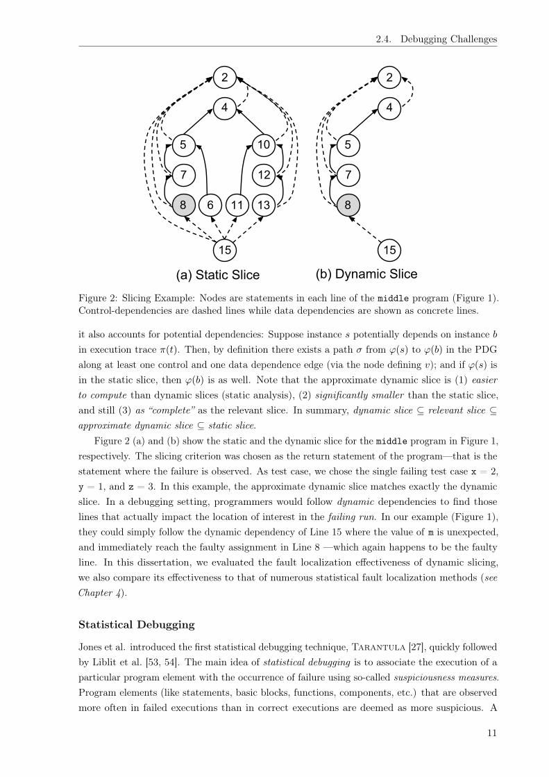
Figure 2: Slicing Example: Nodes are statements in each line of the middle program (Figure 1).Control-dependencies are dashed lines while data dependencies are shown as concrete lines.
it also accounts for potential dependencies: Suppose instance s potentially depends on instance b
in execution trace ⇡(t). Then, by definition there exists a path � from '(s) to '(b) in the PDGalong at least one control and one data dependence edge (via the node defining v); and if '(s) isin the static slice, then '(b) is as well. Note that the approximate dynamic slice is (1) easierto compute than dynamic slices (static analysis), (2) significantly smaller than the static slice,and still (3) as “complete” as the relevant slice. In summary, dynamic slice ✓ relevant slice ✓approximate dynamic slice ✓ static slice.
Figure 2 (a) and (b) show the static and the dynamic slice for the middle program in Figure 1,respectively. The slicing criterion was chosen as the return statement of the program—that is thestatement where the failure is observed. As test case, we chose the single failing test case x = 2,y = 1, and z = 3. In this example, the approximate dynamic slice matches exactly the dynamicslice. In a debugging setting, programmers would follow dynamic dependencies to find thoselines that actually impact the location of interest in the failing run. In our example (Figure 1),they could simply follow the dynamic dependency of Line 15 where the value of m is unexpected,and immediately reach the faulty assignment in Line 8 —which again happens to be the faultyline. In this dissertation, we evaluated the fault localization effectiveness of dynamic slicing,we also compare its effectiveness to that of numerous statistical fault localization methods (seeChapter 4).
Statistical Debugging
Jones et al. introduced the first statistical debugging technique, Tarantula [27], quickly followedby Liblit et al. [53, 54]. The main idea of statistical debugging is to associate the execution of aparticular program element with the occurrence of failure using so-called suspiciousness measures.Program elements (like statements, basic blocks, functions, components, etc.) that are observedmore often in failed executions than in correct executions are deemed as more suspicious. A
11

2. Background
1 int middle(x, y, z) { Tarantula Ochiai Naish2
2 int x, y, z; 0.500 0.408 0.1673 int m = z; 0.500 0.408 0.1674 if (y < z) { 0.500 0.408 0.1675 if (x < y) 0.625 0.500 0.5006 m = y; 0.000 0.000 �0.1677 else if (x < z) 0.714 0.578 0.6678 m = y; 0.833 0.707 0.833
9 } else { 0.000 0.000 �0.33310 if (x > y) 0.000 0.000 �0.33311 m = y; 0.000 0.000 �0.16712 else if (x > z) 0.000 0.000 �0.16713 m = x; 0.000 0.000 0.00014 } 0.000 0.000 0.00015 return m; 0.500 0.408 0.16716 }
Figure 3: Statistical Fault Localization Example: The faulty line 8 and its scores are in bold red
program element with a high suspiciousness score is more likely to be related to the root causeof the failure. When Tarantula was first introduced, the authors envisioned an integrateddevelopment environment where more suspicious code regions are colored in different shades ofred while less suspicious code regions are colored in shades of green. After the execution of thetest suite, at first glance, the developer can identify likely code regions where the fault mighthide.
An important property of statistical debugging is that apart from measuring coverage, itrequires no specific static or dynamic program analysis. This makes it easy to implement anddeploy, in particular as part of automated program repair. In fact, most popular automatedrepair techniques use statistical fault localization to automatically decide where to attempt thepatch [33, 35, 55, 56]. Instead of a visualization that is presented to the developer, statistical faultlocalization provides a ranking that is presented to the automated repair technique. The highestranked, most suspicious element is considered first as patch location. Using a more effectivedebugging technique thus directly increases the effectiveness of any repair technique.
Figure 3 shows the scores computed for the executable lines in our motivating example(Figure 1). The statement in Line 8 is incorrect and should read m = x; instead. This statementis also the most suspicious according to all three statistical fault localization techniques in theexample. Notice that only twelve (12) lines are actually executable. Evidently, in this examplefrom Jones and Harrold [46], the faulty statement is also the most suspicious for these threestatistical fault localization techniques.2
In this dissertation, we investigate the effectiveness of the main families of statistical measuresusing 18 statistical fault localization formulas in total. There are four main families of statisticaldebugging formulas, namely human-generated optimal measures, most popular measures, geneticprogramming (GP) evolved measures and measures targeted at single bug optimality.
2The scores for the faulty statement in Line 8 are tarantula(s8) = 11/
�11 + 1
5
�, ochiai(s8) = 1p
1(1+1), and
naish2(s8) = 1 � 11+4+1 .
12

2.4. Debugging Challenges
2.4.3 Input Debugging
Although there are hundreds of automatic fault localization (AFL) and repair techniques [1];all of these techniques focus on program code, attempting to identify possible fault locations inthe code and synthesizing fixes for this code. However, when a program fails on some input,it need not be the program code that is at fault. Often, the input may be invalid, e.g. due tohardware failures, hardware aging, transmission errors that corrupt input data. Input data canalso be corrupted through software bugs, with the processing software writing out malformed orincomplete data. General-purpose automated debugging techniques (such as AFL) are not usefulto debug inputs, since they focus on faults in code, they would regularly identify the input parserand its error-handling code as being associated with the fault.
In this dissertation, we investigate the problem of input debugging, i.e. isolating faults ininputs and recovering as much data as possible from the existing input (see Chapter 5). Theaim is to recover maximal valid data from the failure-inducing input, as well as provide a precisediagnosis or root cause of the input invalidity. The rest of this section provides background oninput debugging, we discuss the state-of-the-art techniques for identifying or fixing faults ininputs.
Input Minimization
We discuss the state of the art in input reduction. These techniques aim to produce a subsetof the input that still produces the failure. These approaches isolate the faults in invalid orfailure-inducing inputs, in order to obtain the minimal subset that reproduces a failure.
Researchers have proposed several methods to automatically identify failure causes in input [57,58, 59, 60]. The Delta Debugging algorithm ddmin [57] reduces inputs by repeatedly removingparts of the input (first larger ones, then smaller ones) and testing whether running the programwith the reduced input still produces the failure. The result is a so-called 1-minimal input inwhich every single element (character) of the input is relevant for producing the failure. Someapproaches employ the input structure to simplify inputs [59] (HDD) and [60]. In particular,[60] applies the syntactic structure of Java programs to simplify buggy Java programs [60].Meanwhile, HDD [59] uses an hierarchical input minimization algorithm based on ddmin.
In this dissertation, we propose a maximizing variant of the delta debugging algorithm toprovide precise diagnosis of failure-inducing inputs. Our algorithm works at both the lexical andsyntactic levels of the input. In addition, we compare the performance of our proposed algorithm(ddmax ) to that of ddmin.
Input Repair
The problem of repairing inputs is the inverse of input minimzation. Rather than minimizingfailure-inducing inputs (the reduction problem), users would be interested in maximizing non-failure-inducing inputs, i.e. recover as much data as possible from the input at hand.
There are a few approaches for repairing failure-inducing inputs. In security-critical applica-tions, input rectification is employed to transform potentially malicious inputs, in order to ensurethey behave safely. Input rectifiers [61, 62] address this problem by learning a set of constraints
13

2. Background
from typical inputs, then transforming a malicious input into a benign input that satisfies thelearned constraints. Other approaches apply program analysis to repair failure inducing inputs.In particular, Docovery [63] and S-DAGS [64] are white-box techniques for fixing broken inputdocuments. Docovery [63] uses symbolic execution to manipulate corrupted input documentsin a manner that forces the program to follow an alternative error-free path. S-DAGS [64] isa semi-automatic technique that enforces formal (semantic) consistency constraints on inputsdocuments in a collaborative document editing scenario. Likewise, data diversity [65] appliesprogram analysis to transform an invalid input into a valid input that generates an equivalentresult, in order to improve software reliability. This is achieved by finding the regions of the inputspace that causes a fault, and re-expressing a failing input to avoid the faulty input regions.
Unlike the aforementioned approaches, in this dissertation, we propose a black-box genericinput repair approach that recovers the maximal passing input data, and provides the minimalinput diagnoses using several test experiments (see Chapter 5).
2.4.4 Test Generation
Generating valid inputs is a challenging testing problem. Software testing aims to generate inputsthat cover program behavior and expose faults. Typical (random) test generation approachesoften produce invalid inputs, such inputs require further input repair before they can be processedby the intended program. To generate valid inputs and avoid input repair, test generation methodsneed to produce valid inputs. Besides, executing the program logic requires valid inputs that passthe input validation step of the program, since most programs expect structured inputs that meetspecific input specifications (e.g. JSON and JavaScript).
Grammar-based test generation addresses this problem by using input grammars to guide thegeneration of valid inputs. This section highlights the state of the art in (grammar-based) testgeneration. This lays the foundation for our work on generating inputs that are (dis)similar tocommon inputs in the wild (see Chapter 6). In this dissertation, we apply probabilistic grammarsto generate valid software tests. Thus, we also present the background on the interplay ofgrammar-based testing and probabilistic grammars.
Generating software tests.
The aim of software test generation is to find a sample of inputs that induce executions thatsufficiently cover the possible behaviors of the program—including undesired behavior. Modernsoftware test generation relies, as surveyed by Anand et al. [66] on symbolic code analysis tosolve the path conditions leading to uncovered code [67, 68, 69, 70, 71, 72, 73, 74], search-basedapproaches to systematically evolve a population of inputs towards the desired goal [75, 76, 77, 78],random inputs to programs and functions [79, 80] or a combination of these techniques [81,82, 83, 84, 85]. Additionally, machine learning techniques can also be applied to create testsequences [86, 87]. All these approaches have in common that they do not require an additionalmodel or annotations to constrain the set of generated inputs; this makes them very versatile,but brings the risk of producing false alarms—failing executions that cannot be obtained throughlegal inputs.
14
2.4. Debugging Challenges
Grammar-based test generation.
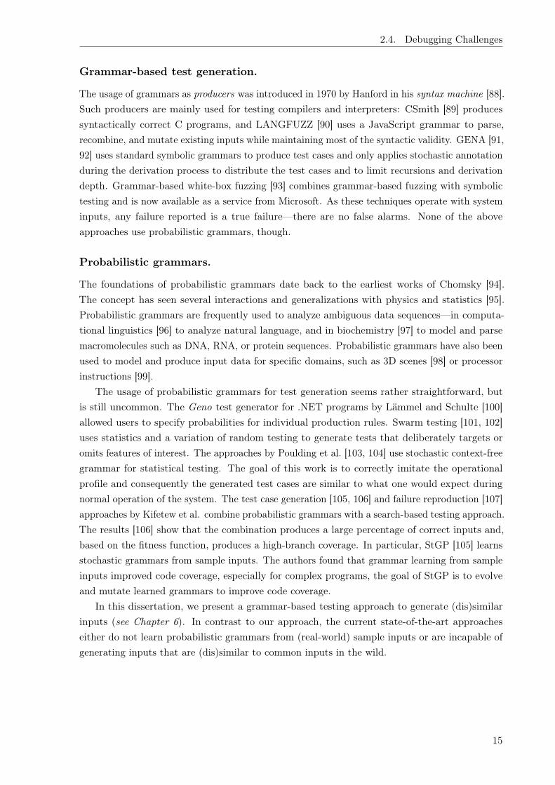
The usage of grammars as producers was introduced in 1970 by Hanford in his syntax machine [88].Such producers are mainly used for testing compilers and interpreters: CSmith [89] producessyntactically correct C programs, and LANGFUZZ [90] uses a JavaScript grammar to parse,recombine, and mutate existing inputs while maintaining most of the syntactic validity. GENA [91,92] uses standard symbolic grammars to produce test cases and only applies stochastic annotationduring the derivation process to distribute the test cases and to limit recursions and derivationdepth. Grammar-based white-box fuzzing [93] combines grammar-based fuzzing with symbolictesting and is now available as a service from Microsoft. As these techniques operate with systeminputs, any failure reported is a true failure—there are no false alarms. None of the aboveapproaches use probabilistic grammars, though.
Probabilistic grammars.
The foundations of probabilistic grammars date back to the earliest works of Chomsky [94].The concept has seen several interactions and generalizations with physics and statistics [95].Probabilistic grammars are frequently used to analyze ambiguous data sequences—in computa-tional linguistics [96] to analyze natural language, and in biochemistry [97] to model and parsemacromolecules such as DNA, RNA, or protein sequences. Probabilistic grammars have also beenused to model and produce input data for specific domains, such as 3D scenes [98] or processorinstructions [99].
The usage of probabilistic grammars for test generation seems rather straightforward, butis still uncommon. The Geno test generator for .NET programs by Lämmel and Schulte [100]allowed users to specify probabilities for individual production rules. Swarm testing [101, 102]uses statistics and a variation of random testing to generate tests that deliberately targets oromits features of interest. The approaches by Poulding et al. [103, 104] use stochastic context-freegrammar for statistical testing. The goal of this work is to correctly imitate the operationalprofile and consequently the generated test cases are similar to what one would expect duringnormal operation of the system. The test case generation [105, 106] and failure reproduction [107]approaches by Kifetew et al. combine probabilistic grammars with a search-based testing approach.The results [106] show that the combination produces a large percentage of correct inputs and,based on the fitness function, produces a high-branch coverage. In particular, StGP [105] learnsstochastic grammars from sample inputs. The authors found that grammar learning from sampleinputs improved code coverage, especially for complex programs, the goal of StGP is to evolveand mutate learned grammars to improve code coverage.
In this dissertation, we present a grammar-based testing approach to generate (dis)similarinputs (see Chapter 6). In contrast to our approach, the current state-of-the-art approacheseither do not learn probabilistic grammars from (real-world) sample inputs or are incapable ofgenerating inputs that are (dis)similar to common inputs in the wild.
15


Chapter 3
Debugging in Practice: An EmpiricalStudy
This chapter is taken, directly or with minor modifications, from our 2017 ICSE paper HowDevelopers Debug Software—The DBGBENCH Dataset [108] and our 2017 ESEC/FSE paperWhere is the bug and how is it fixed? an experiment with practitioners [109]. My contribution inthis work is as follows: (I) original idea; (II) partial implementation; (III) evaluation.
“The fundamental principle of science, the definition almost, is this:the sole test of the validity of any idea is experiment.”
— Richard P. Feynman
3.1 Introduction
Research has produced a multitude of automated approaches for fault localization, debugging, andrepair. A recent survey of Wong et al. [39] cites more than 400 publications on fault localizationtechniques. Hundreds of approaches have also been proposed for automatic program repair [3].Besides, several benchmarks have become available for the empirical evaluation of such approaches.For instance, CoREBench [14] and Defects4J [110] contain a large number of real errors for Cand Java, together with developer-provided test suites and bug fixes. Using such benchmarks,researchers can make empirical claims about the efficacy of their tools and techniques. Forinstance, an effective fault localization technique would rank very high a statement that waschanged in the bug fix [39]. The assumption is that practitioners would identify the samestatement as the fault. Likewise, an effective auto-generated bug fix would pass all test cases [33],under the assumption that practitioners would accept such fixes.
Unfortunately, debugging is not that simple, particularly not for humans. Recently, severalresearch assumptions have turned out to be unrealistic [11, 12, 13, 14, 15]. In empirical studies,the human factor is naturally somewhat left behind. For instance, despite the hundreds ofproposed fault localization techniques [39], most practitioners have never used an automatedfault localization tool [19]. Why is that, and do we really understand how our tools can addressthe real-world debugging needs of software engineering professionals at work?
17

3. Debugging in Practice: An Empirical Study
Do proposed debugging approaches relate to the way practitioners actually locate, understand,and fix bugs? Given the complexity of the debugging process, one might assume that it would bestandard practice to evaluate novel techniques by means of user studies [111]: Does the tool fitinto the process? Does it provide value? How? Yet, how humans actually debug is still not reallywell explored. Between 1981 and 2010, Parnin and Orso [112] identified only a handful of articlesthat presented the results of a user study—none of which involved actual practitioners and realerrors. Since the end of 2010 till 2016, we could identify only three (3) papers that evaluated newdebugging approaches with actual practitioners and real errors [113, 114, 115].3
To address this problem, we collect empirical evidence on every-day debugging experienceof software developers. First, we conducted a retrospective survey on debugging practice withhundreds of developers. Secondly, we conducted an observational study with developers diagnosingand fixing real bugs, from which we collected empirical data from hundreds of hours of debuggingsessions. Then, we provide another kind of benchmark — DbgBench; one that allows realitychecks for novel automated debugging and repair techniques.
In our retrospective survey, we examine the state-of-the-practice regarding how developersdiagnose and repair bugs in the real world. First, we take stock of the state-of-the-practice byinvestigating the nature of debugging in practice. Then, we ask what practitioners want thatwould make debugging easier for them, we analyze their responses and determine the propertiesof debugging tools and auto-generated patches that practitioners find important to consideradoption. We also identify several reasons in favor and against the automation of bug diagnosisand repair. We then discuss implications of these findings for debugging research and training.
In our observational study, we find the first evidence that debugging can actually be automatedand is no subjective endeavor. In our experiment, different practitioners provide essentially thesame fault locations and the same bug diagnosis for the same error. If humans disagreed, howcould a machine ever produce the “correct” fault locations, or the “correct” bug diagnosis? Since,there is a consensus on bug diagnoses and patching, we collected the data from this observationalstudy to support the automatic evaluation of debugging and repair tools. We provide these dataand findings as a benchmark called DbgBench.
Our benchmark — DbgBench allows for realistic evaluation of debugging and repair tools.Since participants agree on essential bug features, it is fair to treat their findings as ground truth.We have compiled our study data for all 27 bugs into a benchmark named DbgBench [116],which is the third central contribution of this study. DbgBench can be used in cost-effective userstudies to investigate how debugging time, debugging difficulty, and patch correctness improvewith the novel debugging/repair aid. DbgBench can be used to evaluate without a user studyhow well novel automated tools perform against professional software developers in the tasks offault localization, debugging, and repair.
The remainder of this chapter is organized as follows: First, we present a retrospective studyinvestigating the state-of-the-art in debugging practice in Section 3.2. In Section 3.3, we present
3We surveyed the following conference proceedings: ACM International Conference on Software Engineering(ICSE’11–16), ACM SIGSOFT Foundations of Software Engineering (FSE’11–16), ACM SIGSOFT InternationalSymposium on Software Testing and Analysis (ISSTA’11–16), IEEE/ACM International Conference on AutomatedSoftware Engineering (ASE’11–16), and International Conference on Software Testing, Verification and Validation(ICST’11–16) and identified 82 papers on automated debugging or software repair only 11 of which conducted userstudies. From these only three (3) involved software engineering professionals and real errors.
18

3.2. Survey
an observational study evaluating how developers debug and fix real bugs. Section 3.4 describesDbgBench— a benchmark for evaluating automated debugging and automated program repairtools. We present the limitations of our work in Section 3.5 and closely related work in Section 3.6.Finally, we close with our interpretation of the results and their implications in Section 3.7.
3.2 Survey
In a survey that ran over 14 months, we collected empirical evidence on the state of debugging inpractice from 212 software engineering professionals in 41 countries. We asked questions abouttheir present every-day debugging experience and their expectations and beliefs regarding thefuture of debugging. We make the questionnaire and response data available on our webpage[116]. Our insights go a long way towards addressing unwarranted beliefs, building tools thatsolve problems that practitioners actually have, and better educating future software engineeringprofessionals about the pitfalls of manual debugging and about actionable opportunities to makedebugging a more efficient and systematic activity. Specifically, we investigate the following aboutdebugging practice, what tools do practitioners use?, what tools do practitioners want? and whatdo practitioners believe about debugging automation?
This section is structured according to the guidelines for empirical research in softwareengineering [117]. After this survey introduction, in Section 3.3.1, we introduce the researchquestions, the population and how it was sampled plus which parameters we measured as studydesign. The collected data is analyzed and presented in Section 3.3.2 as study results.
3.2.1 Study Design
The study design describes the population of interest, how it was sampled, and demographicattributes of that sample. The study design also describes the variables of interest and how theyare measured. The goal of the study design is to ensure that the design is appropriate for theobjectives of the study. Since our study is explorative in nature many questions are qualitativeand open-ended. We leverage the standard measures such as the Likert-scale to analyze qualitativeattributes, and grounded theory, specifically open-card sort, as systematic methodology to analyzethe responses to open-ended questions. To assess the reliability of the conclusions drawn from theself-reports, we measure inter-rater agreement.
Research Questions
The main objective of the survey is to review the state-of-the-practice in debugging and elicitthe expectations and beliefs of software engineering professionals about the automation of theirdebugging activities. Thus, we pose the following research questions:
RQ1 How do developers debug? How much time do practitioners spend trying to reproduce,diagnose, and fix bugs; how familiar are they with the source code? Which debugging toolsand techniques do practitioners use and would they classify their strategy as systematic ortrial-and-error?
19

3. Debugging in Practice: An Empirical Study
RQ2 What do they want? Given an error and possibly a failing test case, which output dopractitioners expect of an automated bug diagnosis tool that should aid in understandinghow the error comes about? Which criteria do practitioners expect to be satisfied to accepta patch that is generated by an automated bug fixing tool?
RQ3 Why do they reject automation? Do practitioners believe that the chain of run-timeevents leading to the observed error can ever be explained intuitively by the push of a button?Do practitioners believe that bugs can ever be fixed reliably by the push of a button? Whydo they believe so?
Our insights go a long way towards addressing unwarranted beliefs, building tools that solveproblems that practitioners actually have, and better educating future software engineeringprofessionals about the pitfalls of manual debugging and actionable opportunities of debuggingautomation. We hope that the results of our survey will inspire more research that is groundedin practice.
Questionnaire and Respondents
Recruitment. We set out to examine broadly all software engineering professionals at any levelof experience that are involved in the development and debugging of industrial-scale softwareproducts. We designed an online questionnaire and sent the link to developers that shared theiremail address on the source-code repository platform Github. We also posted the link to severalsoftware development user groups at Meetup.com, on freelancer platforms, such as Freelancer,Upwork, and Guru, and on social media platforms as well as professional networks, such asFacebook and LinkedIn. We started three advertisement campaigns in August 2015, March 2016,and July 2016 following which we had the highest response rate lasting for about one month each.We received the first response in August 2015 and the most recent response more than one yearlater in October 2016.
Questionnaire. The questionnaire takes about 10 minutes to fill and is strictly anonymous.4
It begins with a consent form informing respondents about the goals of our study and somebasic terminology. We assure that all responses are treated as confidential, and in no case willresponses from individual participants be identified; rather, all data will be pooled and publishedin aggregate form only. Respondents start by answering a series of simple demographic questionsabout occupation, experience, and level of skill as software developers. After that follows a seriesof technical questions which investigate our study objectives. The questionnaire is available athttp://bit.do/dbg and on our webpage [116].
Demographics. The questionnaire was filled by 212 respondents. The majority5 of respon-dents are professional software developers from all over the world with seven (7) years or moreexperience in software development rating their level of skill as advanced or expert. 706 candidatesopened the link either directly or from 35 distinct referrer webpages.6 Figure 4 shows the 41 home
4Participation is strictly anonymous if the respondent so wishes. However, we do offer the opportunity toleave their email address in case they want to be informed about the study outcome or participate in a follow-uphands-on experiment.
5Majority here means above the median (i.e., 3rd and 4th quartile).6Statistics are as of 07th Jan’17 and provided at http://bit.do/dbg-. From 706 distinct IP addresses, 14 are
from robots, like the Google web crawler.
20
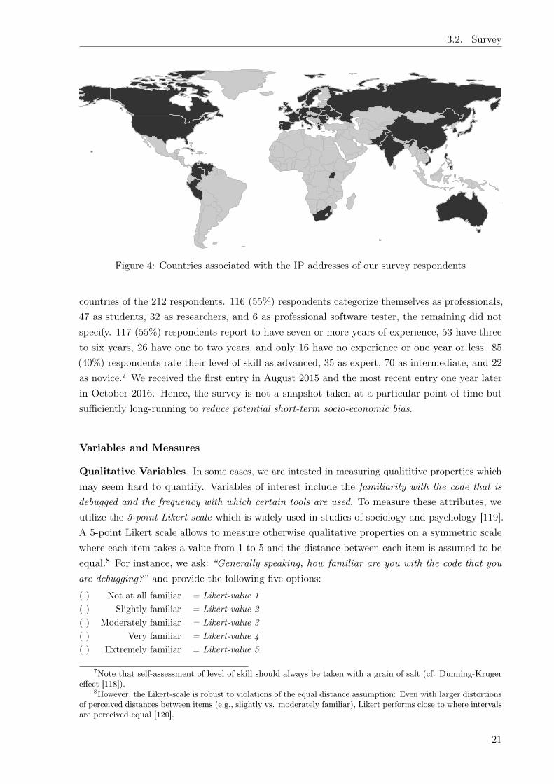
3.2. Survey
V2
Figure 4: Countries associated with the IP addresses of our survey respondents
countries of the 212 respondents. 116 (55%) respondents categorize themselves as professionals,47 as students, 32 as researchers, and 6 as professional software tester, the remaining did notspecify. 117 (55%) respondents report to have seven or more years of experience, 53 have threeto six years, 26 have one to two years, and only 16 have no experience or one year or less. 85(40%) respondents rate their level of skill as advanced, 35 as expert, 70 as intermediate, and 22as novice.7 We received the first entry in August 2015 and the most recent entry one year laterin October 2016. Hence, the survey is not a snapshot taken at a particular point of time butsufficiently long-running to reduce potential short-term socio-economic bias.
Variables and Measures
Qualitative Variables. In some cases, we are intested in measuring qualititive properties whichmay seem hard to quantify. Variables of interest include the familiarity with the code that isdebugged and the frequency with which certain tools are used. To measure these attributes, weutilize the 5-point Likert scale which is widely used in studies of sociology and psychology [119].A 5-point Likert scale allows to measure otherwise qualitative properties on a symmetric scalewhere each item takes a value from 1 to 5 and the distance between each item is assumed to beequal.8 For instance, we ask: “Generally speaking, how familiar are you with the code that youare debugging?” and provide the following five options:( ) Not at all familiar = Likert-value 1
( ) Slightly familiar = Likert-value 2
( ) Moderately familiar = Likert-value 3
( ) Very familiar = Likert-value 4
( ) Extremely familiar = Likert-value 5
7Note that self-assessment of level of skill should always be taken with a grain of salt (cf. Dunning-Krugereffect [118]).
8However, the Likert-scale is robust to violations of the equal distance assumption: Even with larger distortionsof perceived distances between items (e.g., slightly vs. moderately familiar), Likert performs close to where intervalsare perceived equal [120].
21

3. Debugging in Practice: An Empirical Study
An average code familiarity of 4.7 would indicate that most respondents report to be very toextremely familiar with the code and only very few report to be not at all familiar. However,conclusions from such data can be trusted only after demonstrating their reliability. To assessthe reliability of the resulting findings, we measure inter-rater agreement and specifically Fleiss’kappa [121]. If respondents are in complete agreement, then = 1. If there is no agreementother than what would be expected by chance, then 0.
Time. We are interested in the time that practitioners spend debugging, and the time thatpractitioners spend with each of the three sub-tasks of debugging: bug reproduction, diagnosis,and fixing. We measure debugging time relative to the work time and the time spent on eachsub-task relative to the debugging time spent. We measure time on an interval scale from 0% -100% in ten percent intervals that is finer-grained on either side (five percent intervals).
Tools and Techniques. We ask respondents about the following set of tools and techniques:[ ] Trace-based Debugging (using printing; e.g., println, log4c)[ ] Interactive/Online Debugging (using breakpoints; e.g., gdb, jdb)[ ] Post-Mortem/Offline Debugging (using core dumps, stack traces)
[ ] Regression Debugging to find faulty changes (e.g., git bisect)
[ ] Statistical/Spectrum-based Debugging to find faulty statements
(e.g., Tarantula)
[ ] Program Slicing (e.g., Frama-C, CodeSurfer)
[ ] Time Travel or Reversible Debugging (e.g., UndoDB)
[ ] Algorithmic or Declarative Debugging (e.g., JavaDD)
Open-ended Questions. Most questions about beliefs and expectations (RQ2, RQ3)are open-ended in the sense that respondents are asked to fill a text field instead of settingcheckmarks on pre-specified answers. This reduces experimenter bias. To analyze replies, weborrow a methodology from grounded theory called coding [122]. In the context of softwareengineering [123, 124], this methodology is also referred to as open card sort [125]. To derive thegeneral categories from the responses and sort the responses to these categories, we used thefollowing coding protocol :
1. Researcher #1 went through all responses and came up with an inital draft of the coding.The coding comprised of a set of labels that are attached to the responses and a policy thatspecifies when to apply which label.
2. Researchers #1, #2, and #3 discussed and amended labels and policy but not the codingdraft by Researcher #1.
3. Researchers #1, #2 and #3 independently produced their own codings according to policy(Researcher #1 repeated with the updated policy).
4. Researchers #1, #2, and #3 compared their codings and resolve any contention to producethe final coding.
Notice that the labels had not been predefined but emerged during coding. Independent codingreduces potential bias. The coding allows to quantify the prevalence of certain “categories” ofresponses. The authors spent about half a day in meetings to discuss and amend labels and
22

3.2. Survey
●● ●
● ●●●●●●●● ●
%D
evelopment Tim
e%
Debugging Tim
e
0% 25% 50% 75% 100%
Debugging
Diagnosis
Patching
Reproduction
Figure 5: Boxplots of the time spent reproducing, diagnosing, and fixing bugs. The boxplot atthe top shows the reported time spent debugging as a percentage of the development time. Theboxplots below show the reported time spent on each subtask as a percentage of debugging time.
policy (Step-2) and three days resolving contentions (Step-4) in addition to the actual coding(Step-1&3).
Redundant Questions. Due to the self-reporting nature of a questionnaire it is customaryto reduce cognitive bias with an empirical assessment tool called subject triangulation [126]. Weask separate questions about the same subject and check the consistency of the replies to assessthe validity of our insights. For instance, we ask how familiar the developers are generally with thecode they debug on a 5-point Likert scale. Several questions later, we ask how often they debugother peoples code on a 5-point Likert scale. If developers generally feel slightly or moderatelyfamiliar, they should also debug other peoples’ code moderately or very often.
Bias Mitigation. In summary, we use several empirical devices to mitigate sources ofcognitive bias in our self-reporting study. We ask redundant questions for subject triangulation[126]. We avoid leading questions. We ask many open-ended questions, which allows respondentsto express themselves more holistically than if we used pre-specified answers. We use standardmeasures of qualititive attributes [119] and leverage a systematic methodology from groundedtheory to analyze the open-ended questions [122]. To assess the reliability of our conclusions fromthis survey data, we leverage a measure of inter-rater agreement [121].
3.2.2 Study Results
The survey ran over 14 months and gathered 212 responses. For the 3392 ratings on all 16multiple-choice questions, we measure a reasonable, fair agreement amongst the respondentsabove the level of agreement expected by chance (Fleiss’ = 0.301). This suggests reliability ofour conclusions from the self-reported data.
23
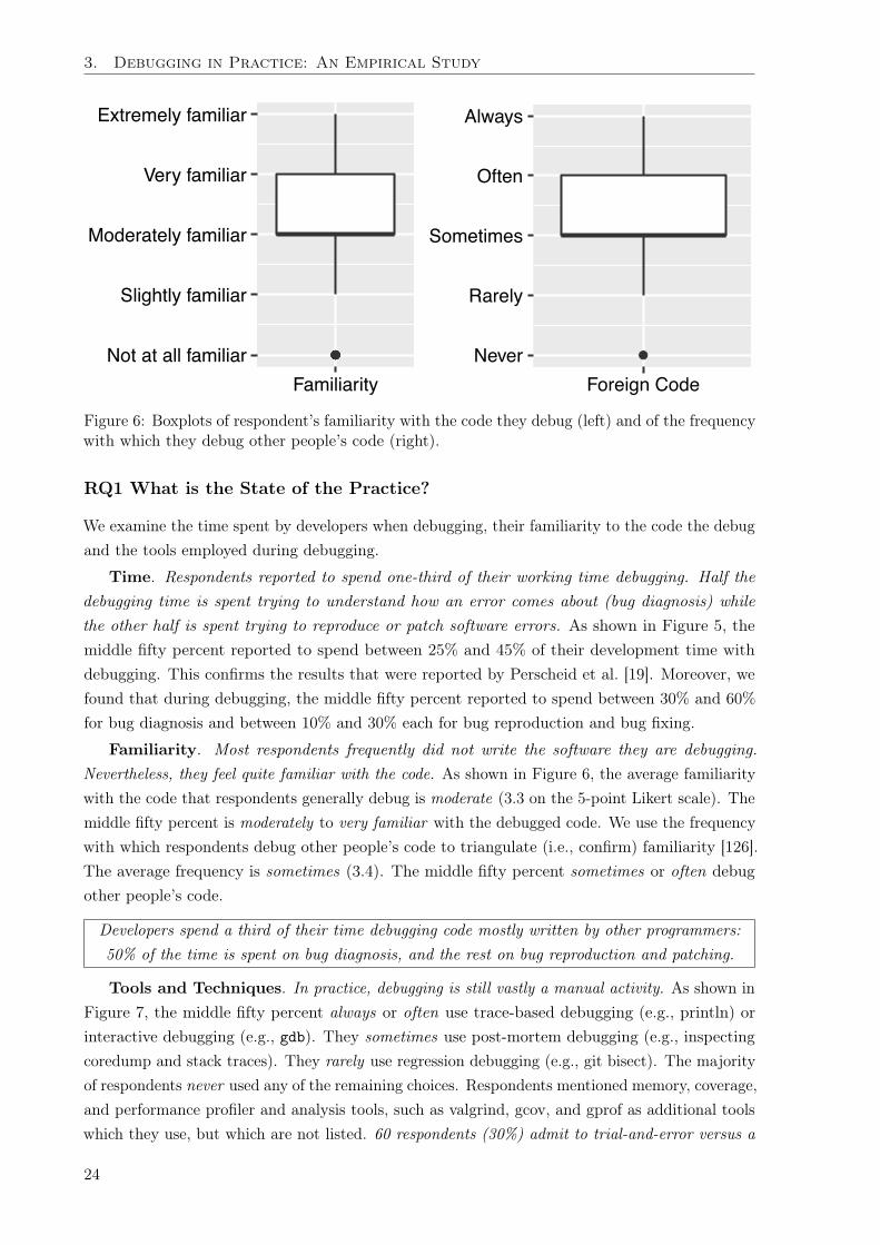
3. Debugging in Practice: An Empirical Study
●●●●●●Not at all familiar
Slightly familiar
Moderately familiar
Very familiar
Extremely familiar
Familiarity●Never
Rarely
Sometimes
Often
Always
Foreign Code
Figure 6: Boxplots of respondent’s familiarity with the code they debug (left) and of the frequencywith which they debug other people’s code (right).
RQ1 What is the State of the Practice?
We examine the time spent by developers when debugging, their familiarity to the code the debugand the tools employed during debugging.
Time. Respondents reported to spend one-third of their working time debugging. Half thedebugging time is spent trying to understand how an error comes about (bug diagnosis) whilethe other half is spent trying to reproduce or patch software errors. As shown in Figure 5, themiddle fifty percent reported to spend between 25% and 45% of their development time withdebugging. This confirms the results that were reported by Perscheid et al. [19]. Moreover, wefound that during debugging, the middle fifty percent reported to spend between 30% and 60%for bug diagnosis and between 10% and 30% each for bug reproduction and bug fixing.
Familiarity. Most respondents frequently did not write the software they are debugging.Nevertheless, they feel quite familiar with the code. As shown in Figure 6, the average familiaritywith the code that respondents generally debug is moderate (3.3 on the 5-point Likert scale). Themiddle fifty percent is moderately to very familiar with the debugged code. We use the frequencywith which respondents debug other people’s code to triangulate (i.e., confirm) familiarity [126].The average frequency is sometimes (3.4). The middle fifty percent sometimes or often debugother people’s code.
Developers spend a third of their time debugging code mostly written by other programmers:50% of the time is spent on bug diagnosis, and the rest on bug reproduction and patching.
Tools and Techniques. In practice, debugging is still vastly a manual activity. As shown inFigure 7, the middle fifty percent always or often use trace-based debugging (e.g., println) orinteractive debugging (e.g., gdb). They sometimes use post-mortem debugging (e.g., inspectingcoredump and stack traces). They rarely use regression debugging (e.g., git bisect). The majorityof respondents never used any of the remaining choices. Respondents mentioned memory, coverage,and performance profiler and analysis tools, such as valgrind, gcov, and gprof as additional toolswhich they use, but which are not listed. 60 respondents (30%) admit to trial-and-error versus a
24
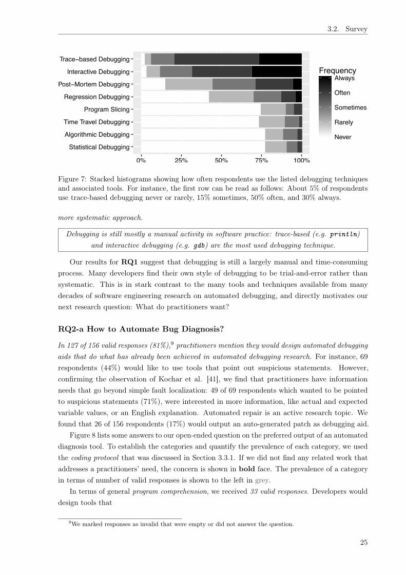
3.2. Survey
Statistical Debugging
Algorithmic Debugging
Time Travel Debugging
Program Slicing
Regression Debugging
Post−Mortem Debugging
Interactive Debugging
Trace−based Debugging
0% 25% 50% 75% 100%
Never
Rarely
Sometimes
Often
AlwaysFrequency
Figure 7: Stacked histograms showing how often respondents use the listed debugging techniquesand associated tools. For instance, the first row can be read as follows: About 5% of respondentsuse trace-based debugging never or rarely, 15% sometimes, 50% often, and 30% always.
more systematic approach.
Debugging is still mostly a manual activity in software practice: trace-based (e.g. println)and interactive debugging (e.g. gdb) are the most used debugging technique.
Our results for RQ1 suggest that debugging is still a largely manual and time-consumingprocess. Many developers find their own style of debugging to be trial-and-error rather thansystematic. This is in stark contrast to the many tools and techniques available from manydecades of software engineering research on automated debugging, and directly motivates ournext research question: What do practitioners want?
RQ2-a How to Automate Bug Diagnosis?
In 127 of 156 valid responses (81%),9 practitioners mention they would design automated debuggingaids that do what has already been achieved in automated debugging research. For instance, 69respondents (44%) would like to use tools that point out suspicious statements. However,confirming the observation of Kochar et al. [41], we find that practitioners have informationneeds that go beyond simple fault localization: 49 of 69 respondents which wanted to be pointedto suspicious statements (71%), were interested in more information, like actual and expectedvariable values, or an English explanation. Automated repair is an active research topic. Wefound that 26 of 156 respondents (17%) would output an auto-generated patch as debugging aid.
Figure 8 lists some answers to our open-ended question on the preferred output of an automateddiagnosis tool. To establish the categories and quantify the prevalence of each category, we usedthe coding protocol that was discussed in Section 3.3.1. If we did not find any related work thataddresses a practitioners’ need, the concern is shown in bold face. The prevalence of a categoryin terms of number of valid responses is shown to the left in grey.
In terms of general program comprehension, we received 33 valid responses. Developers woulddesign tools that
9We marked responses as invalid that were empty or did not answer the question.
25
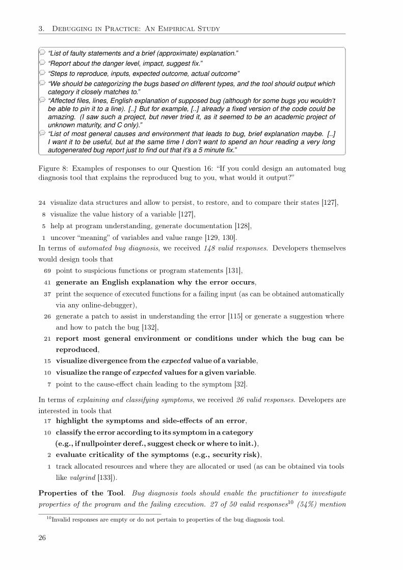
3. Debugging in Practice: An Empirical Study
“List of faulty statements and a brief (approximate) explanation.”“Report about the danger level, impact, suggest fix.”“Steps to reproduce, inputs, expected outcome, actual outcome”“We should be categorizing the bugs based on different types, and the tool should output whichcategory it closely matches to.”“Affected files, lines, English explanation of supposed bug (although for some bugs you wouldn’tbe able to pin it to a line). [..] But for example, [..] already a fixed version of the code could beamazing. (I saw such a project, but never tried it, as it seemed to be an academic project ofunknown maturity, and C only).”“List of most general causes and environment that leads to bug, brief explanation maybe. [..]I want it to be useful, but at the same time I don’t want to spend an hour reading a very longautogenerated bug report just to find out that it’s a 5 minute fix.”
Figure 8: Examples of responses to our Question 16: “If you could design an automated bugdiagnosis tool that explains the reproduced bug to you, what would it output?”
24 visualize data structures and allow to persist, to restore, and to compare their states [127],8 visualize the value history of a variable [127],5 help at program understanding, generate documentation [128],1 uncover “meaning” of variables and value range [129, 130].
In terms of automated bug diagnosis, we received 148 valid responses. Developers themselveswould design tools that
69 point to suspicious functions or program statements [131],41 generate an English explanation why the error occurs,37 print the sequence of executed functions for a failing input (as can be obtained automatically
via any online-debugger),26 generate a patch to assist in understanding the error [115] or generate a suggestion where
and how to patch the bug [132],21 report most general environment or conditions under which the bug can be
reproduced,15 visualize divergence from the expected value of a variable,10 visualize the range of expected values for a given variable.7 point to the cause-effect chain leading to the symptom [32].
In terms of explaining and classifying symptoms, we received 26 valid responses. Developers areinterested in tools that
17 highlight the symptoms and side-effects of an error,10 classify the error according to its symptom in a category
(e.g., if nullpointer deref., suggest check or where to init.),2 evaluate criticality of the symptoms (e.g., security risk),1 track allocated resources and where they are allocated or used (as can be obtained via tools
like valgrind [133]).
Properties of the Tool. Bug diagnosis tools should enable the practitioner to investigateproperties of the program and the failing execution. 27 of 50 valid responses10 (54%) mention
10Invalid responses are empty or do not pertain to properties of the bug diagnosis tool.
26
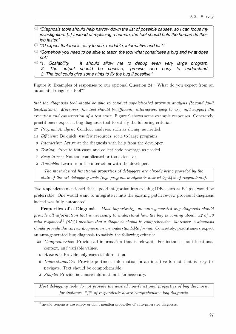
3.2. Survey
“Diagnosis tools should help narrow down the list of possible causes, so I can focus myinvestigation. [..] Instead of replacing a human, the tool should help the human do theirjob faster.”“I’d expect that tool is easy to use, readable, informative and fast.”“Somehow you need to be able to teach the tool what constitutes a bug and what doesnot.”“1. Scalability. It should allow me to debug even very large program.2. The output should be concise, precise and easy to understand.3. The tool could give some hints to fix the bug if possible.”
Figure 9: Examples of responses to our optional Question 24: ”What do you expect from anautomated diagnosis tool?”
that the diagnosis tool should be able to conduct sophisticated program analysis (beyond faultlocalization). Moreover, the tool should be efficient, interactive, easy to use, and support theexecution and construction of a test suite. Figure 9 shows some example responses. Concretely,practitioners expect a bug diagnosis tool to satisfy the following criteria:27 Program Analysis: Conduct analyses, such as slicing, as needed.14 Efficient : Be quick, use few resources, scale to large programs.8 Interactive: Arrive at the diagnosis with help from the developer.8 Testing : Execute test cases and collect code coverage as needed.7 Easy to use: Not too complicated or too extensive.2 Trainable: Learn from the interaction with the developer.
The most desired functional properties of debuggers are already being provided by thestate-of-the-art debugging tools (e.g. program analysis is desired by 54% of respondents).
Two respondents mentioned that a good integration into existing IDEs, such as Eclipse, would bepreferrable. One would want to integrate it into the existing patch review process if diagnosisindeed was fully automated.
Properties of a Diagnosis. Most importantly, an auto-generated bug diagnosis shouldprovide all information that is necessary to understand how the bug is coming about. 32 of 50valid responses11 (64%) mention that a diagnosis should be comprehensive. Moreover, a diagnosisshould provide the correct diagnosis in an understandable format. Concretely, practitioners expectan auto-generated bug diagnosis to satisfy the following criteria:
32 Comprehensive: Provide all information that is relevant. For instance, fault locations,context, and variable values.
16 Accurate: Provide only correct information.9 Understandable: Provide pertinent information in an intuitive format that is easy to
navigate. Text should be comprehensible.3 Simple: Provide not more information than necessary.
Most debugging tools do not provide the desired non-functional properties of bug diagnosis:for instance, 64% of respondents desire comprehensive bug diagnosis.
11Invalid responses are empty or don’t mention properties of auto-generated diagnoses.
27
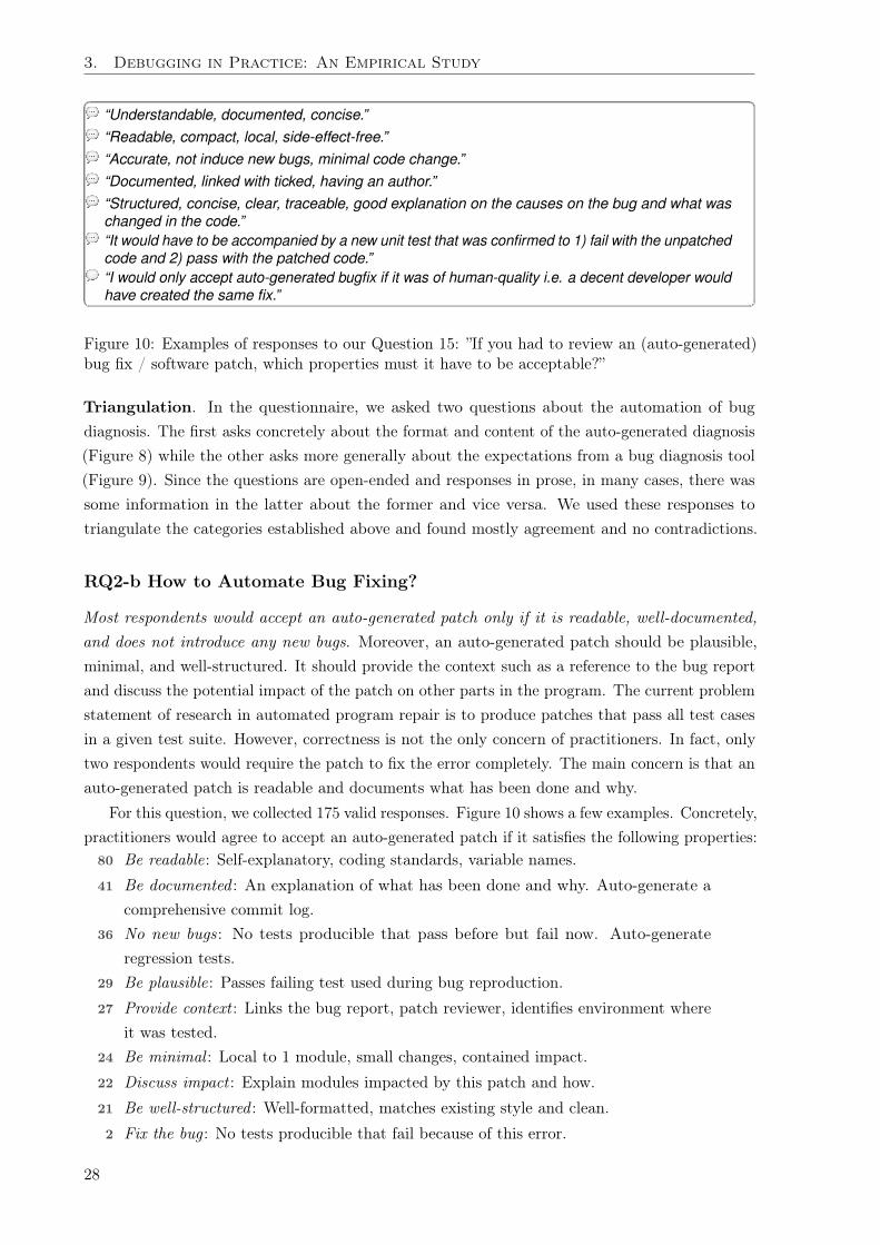
3. Debugging in Practice: An Empirical Study
“Understandable, documented, concise.”“Readable, compact, local, side-effect-free.”“Accurate, not induce new bugs, minimal code change.”“Documented, linked with ticked, having an author.”“Structured, concise, clear, traceable, good explanation on the causes on the bug and what waschanged in the code.”“It would have to be accompanied by a new unit test that was confirmed to 1) fail with the unpatchedcode and 2) pass with the patched code.”“I would only accept auto-generated bugfix if it was of human-quality i.e. a decent developer wouldhave created the same fix.”
Figure 10: Examples of responses to our Question 15: ”If you had to review an (auto-generated)bug fix / software patch, which properties must it have to be acceptable?”
Triangulation. In the questionnaire, we asked two questions about the automation of bugdiagnosis. The first asks concretely about the format and content of the auto-generated diagnosis(Figure 8) while the other asks more generally about the expectations from a bug diagnosis tool(Figure 9). Since the questions are open-ended and responses in prose, in many cases, there wassome information in the latter about the former and vice versa. We used these responses totriangulate the categories established above and found mostly agreement and no contradictions.
RQ2-b How to Automate Bug Fixing?
Most respondents would accept an auto-generated patch only if it is readable, well-documented,and does not introduce any new bugs. Moreover, an auto-generated patch should be plausible,minimal, and well-structured. It should provide the context such as a reference to the bug reportand discuss the potential impact of the patch on other parts in the program. The current problemstatement of research in automated program repair is to produce patches that pass all test casesin a given test suite. However, correctness is not the only concern of practitioners. In fact, onlytwo respondents would require the patch to fix the error completely. The main concern is that anauto-generated patch is readable and documents what has been done and why.
For this question, we collected 175 valid responses. Figure 10 shows a few examples. Concretely,practitioners would agree to accept an auto-generated patch if it satisfies the following properties:
80 Be readable: Self-explanatory, coding standards, variable names.41 Be documented : An explanation of what has been done and why. Auto-generate a
comprehensive commit log.36 No new bugs: No tests producible that pass before but fail now. Auto-generate
regression tests.29 Be plausible: Passes failing test used during bug reproduction.27 Provide context : Links the bug report, patch reviewer, identifies environment where
it was tested.24 Be minimal : Local to 1 module, small changes, contained impact.22 Discuss impact : Explain modules impacted by this patch and how.21 Be well-structured : Well-formatted, matches existing style and clean.2 Fix the bug : No tests producible that fail because of this error.
28

3.2. Survey
“Clear indication that the fix correctly accomplishes intended transformation of buggy code withouterror or side-effect.”“Such a tool should never modify my existing code. [Instead it would] allow me to audit the changesbefore applying them.”“[..] find the smallest acceptable modification to the codebase that would make all the providedtests green.”“Very verbose information about the fix, and the details of the bug itself. How this won’t causeissues elsewhere.”“The tool should give some reason why the fix is generated, [..] generate a test suite to show thatthe fix still keeps original functionality of the program and all errors caused by the bug are gone,[..] provide some fixes so the developer can choose the best one.”
Figure 11: Examples of responses to our Question 25: ”What do you expect from an automatedbug fixing tool?”
Properties of the Tool. On the one hand, 26 of 64 respondents (41%) would not like thetool to fix a program fully automatically and instead intervene whenever necessary or select froma ranked choice of patches. On the other hand, 19 respondents (30%) say that such tool wouldneed to fix a bug on its own. However, most respondents (63%) would like the tool to providea proof of correctness (22), an explanation of how the bug is fixed (13), or at least guaranteecorrectness (18).12
For this optional question, we collected 64 valid responses. A few examples are shown inFigure 11. Concretely, practitioners would agree to use an auto-repair tool if it satisfies thefollowing criteria. The tool should be:
26 Interactive: Arrive at the correct fix with help from developer. For instance, produce severalpatches rank in order of quality.
19 Fully automated : Produce and apply bug fix fully automatically.22 Provide proof of correctness: Generate regression test cases. Show that error was really
fixed and no new errors are introduced.18 Correct : Does not produce incorrect patches.13 Provide rationale: Explain the bug and how it is fixed now.7 Decide degree of automation based on bug type: Some errors may need almost no intervention
and can be auto-corrected.4 Be efficient : Be quick, use few resources, scale to large programs.1 Be open-source: So that developers can inspect how it works.
Beyond patch correctness, the most desirable properties of repair tools (e.g. fix explanation andcorrectness guarantee) are not provided by the current state-of-the-art repair tools.
Triangulation. In the questionnaire, we asked two questions about the automation of bugfixing. The first asks concretely about properties of auto-generated patches that are required toaccept the patch (Figure 10) while the other asks more generally about the expectations from anautomated bug fixing tool (Figure 11). We used these responses to triangulate the categoriesestablished above and found mostly agreement and no contradictions.
12Note that a response can be assigned multiple labels.
29

3. Debugging in Practice: An Empirical Study
No auto-diagnosis —– Neither —– No auto-repair
All respondents
Figure 12: Venn Diagram showing the set of respondents which oppose the full automation ofeither bug diagnosis (no auto-diagnosis) or bug fixing (no auto-repair).
RQ3 Why Accept/Reject Automated Debugging?
Most surveyed practitioners do not believe that debugging will ever be fully automated. The Venndiagram in Figure 12 provides more details. 116 respondents (55%) believe that neither bugdiagnosis nor program repair will ever be fully automated. 165 (78%) believe that bugs willnever be fixed reliably by a machine while 124 respondents (58%) believe that bugs will never beexplained intuitively.Points in favor of Automation. 33 of 96 proponents13 provide a rationale in favour of theautomation of bug diagnosis, repair, or both. The most prevalent responses cite recent advancesin artificial intelligence as reason why debugging might be fully automated in the future. Othersmention that existing techniques do not sufficiently leverage information that is available, in theprogram itself or in lessons-learned from earlier debugging sessions.
Concretely, 33 practitioners explained that debugging might be automated at some point inthe future for the following reasons:14 Advances in AI : Given the progress of Artificial Intelligence (AI) in other areas, it
may soon also be able to auto-repair programs.9 Information from program: Stack traces and source code can be mined via program
analysis for information on a bug fix.5 Information from history : Repositories of human-generated bug reports and patches
can be mined for information on a patch.3 Information from specifications : Adequate test suites or formal specifications should
contain enough information to fix a bug.2 Advances in Self-Healing : In future, a software system may test and heal itself and
automatically recover from runtime errors.2 Advances in Optimisation Algorithms : Genetic algorithms have shown promise, taking
inspiration from natural evolution.2 Advances in Program Synthesis: If programs are generated from specifications, then
bugs are fixed by changing the specification.
A third of developers (34%) believe in the (future) automation of debugging or repairbecause of advances in artificial intelligence (AI) and program analysis.
13We call as proponent a respondent who believes that diagnosis, repair, or both will be automated at somepoint of time in the future (white area in Figure 12). In other words, even if the respondent believes that one task,e.g., diagnosis, will never be automated, she is still classified as a proponent. Only 32 of 212 respondents (15%)believe that both, diagnosis and patching may be automated in the future (13 provide a rationale).
30
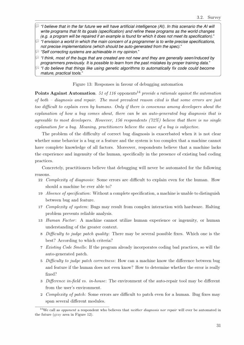
3.2. Survey
“I believe that in the far future we will have artificial intelligence (AI). In this scenario the AI willwrite programs that fit its goals (specification) and refine these programs as the world changes(e.g. a program will be repaired if an example is found for which it does not meet its specification).”“I envision a world in which the main concern of a programmer is to write precise specifications,not precise implementations (which should be auto-generated from the spec).”“Self correcting systems are achievable in my opinion.”“I think, most of the bugs that are created are not new and they are generally seen/induced byprogrammers previously. It is possible to learn from the past mistakes by proper training data.”“I do believe that things like using genetic algorithms to automatically fix code could becomemature, practical tools.”
Figure 13: Responses in favour of debugging automation
Points Against Automation. 51 of 116 opponents14 provide a rationale against the automationof both – diagnosis and repair. The most prevalent reason cited is that some errors are justtoo difficult to explain even by humans. Only if there is consensus among developers about theexplanation of how a bug comes about, there can be an auto-generated bug diagnosis that isagreeable to most developers. However, 156 respondents (72%) believe that there is no singleexplanation for a bug. Meaning, practitioners believe the cause of a bug is subjective.
The problem of the difficulty of correct bug diagnosis is exacerbated when it is not clearwhether some behavior is a bug or a feature and the system is too complex that a machine cannothave complete knowledge of all factors. Moreover, respondents believe that a machine lacksthe experience and ingenuity of the human, specifically in the presence of existing bad codingpractices.
Concretely, practitioners believe that debugging will never be automated for the followingreasons.
22 Complexity of diagnosis: Some errors are difficult to explain even for the human. Howshould a machine be ever able to?
19 Absence of specification: Without a complete specification, a machine is unable to distinguishbetween bug and feature.
17 Complexity of system: Bugs may result from complex interaction with hardware. Haltingproblem prevents reliable analysis.
13 Human Factor : A machine cannot utilize human experience or ingenuity, or humanunderstanding of the greater context.
8 Difficulty to judge patch quality : There may be several possible fixes. Which one is thebest? According to which criteria?
7 Existing Code Smells: If the program already incorporates coding bad practices, so will theauto-generated patch.
5 Difficulty to judge patch correctness: How can a machine know the difference between bugand feature if the human does not even know? How to determine whether the error is reallyfixed?
3 Difference in-field vs. in-house: The environment of the auto-repair tool may be differentfrom the user’s environment.
2 Complexity of patch: Some errors are difficult to patch even for a human. Bug fixes mayspan several different modules.
14We call as opponent a respondent who believes that neither diagnosis nor repair will ever be automated inthe future (gray area in Figure 12).
31
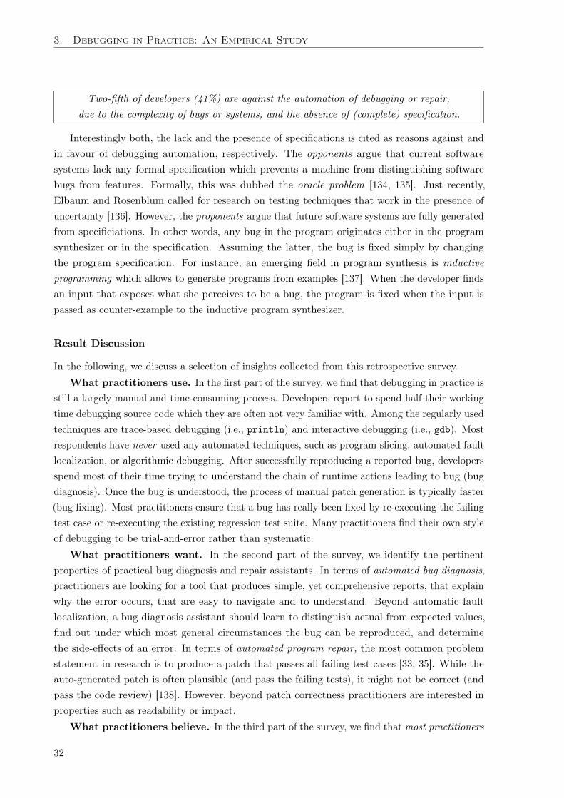
3. Debugging in Practice: An Empirical Study
Two-fifth of developers (41%) are against the automation of debugging or repair,due to the complexity of bugs or systems, and the absence of (complete) specification.
Interestingly both, the lack and the presence of specifications is cited as reasons against andin favour of debugging automation, respectively. The opponents argue that current softwaresystems lack any formal specification which prevents a machine from distinguishing softwarebugs from features. Formally, this was dubbed the oracle problem [134, 135]. Just recently,Elbaum and Rosenblum called for research on testing techniques that work in the presence ofuncertainty [136]. However, the proponents argue that future software systems are fully generatedfrom specificiations. In other words, any bug in the program originates either in the programsynthesizer or in the specification. Assuming the latter, the bug is fixed simply by changingthe program specification. For instance, an emerging field in program synthesis is inductiveprogramming which allows to generate programs from examples [137]. When the developer findsan input that exposes what she perceives to be a bug, the program is fixed when the input ispassed as counter-example to the inductive program synthesizer.
Result Discussion
In the following, we discuss a selection of insights collected from this retrospective survey.What practitioners use. In the first part of the survey, we find that debugging in practice is
still a largely manual and time-consuming process. Developers report to spend half their workingtime debugging source code which they are often not very familiar with. Among the regularly usedtechniques are trace-based debugging (i.e., println) and interactive debugging (i.e., gdb). Mostrespondents have never used any automated techniques, such as program slicing, automated faultlocalization, or algorithmic debugging. After successfully reproducing a reported bug, developersspend most of their time trying to understand the chain of runtime actions leading to bug (bugdiagnosis). Once the bug is understood, the process of manual patch generation is typically faster(bug fixing). Most practitioners ensure that a bug has really been fixed by re-executing the failingtest case or re-executing the existing regression test suite. Many practitioners find their own styleof debugging to be trial-and-error rather than systematic.
What practitioners want. In the second part of the survey, we identify the pertinentproperties of practical bug diagnosis and repair assistants. In terms of automated bug diagnosis,practitioners are looking for a tool that produces simple, yet comprehensive reports, that explainwhy the error occurs, that are easy to navigate and to understand. Beyond automatic faultlocalization, a bug diagnosis assistant should learn to distinguish actual from expected values,find out under which most general circumstances the bug can be reproduced, and determinethe side-effects of an error. In terms of automated program repair, the most common problemstatement in research is to produce a patch that passes all failing test cases [33, 35]. While theauto-generated patch is often plausible (and pass the failing tests), it might not be correct (andpass the code review) [138]. However, beyond patch correctness practitioners are interested inproperties such as readability or impact.
What practitioners believe. In the third part of the survey, we find that most practitioners
32
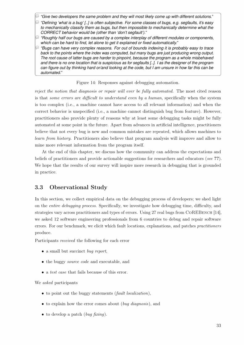
3.3. Observational Study“Give two developers the same problem and they will most likely come up with different solutions.”“Defining ’what is a bug’ [..] is often subjective. For some classes of bugs, e.g. segfaults, it’s easyto mechanically classify them as bugs, but then impossible to mechanically determine what theCORRECT behavior would be (other than ‘don’t segfault’).”“Roughly half our bugs are caused by a complex interplay of different modules or components,which can be hard to find, let alone to get it explained or fixed automatically.”“Bugs can have very complex reasons. For out of bounds indexing it is probably easy to traceback to the points where the index was computed, but many bugs are just producing wrong output.The root cause of latter bugs are harder to pinpoint, because the program as a whole misbehavedand there is no one location that is suspicious as for segfaults [..]. I as the designer of the programcan figure out by thinking hard or/and looking at the code, but I am unsure in how far this can beautomated.”
Figure 14: Responses against debugging automation.
reject the notion that diagnosis or repair will ever be fully automated. The most cited reasonis that some errors are difficult to understand even by a human, specifically when the systemis too complex (i.e., a machine cannot have access to all relevant information) and when thecorrect behavior is unspecified (i.e., a machine cannot distinguish bug from feature). However,practitioners also provide plenty of reasons why at least some debugging tasks might be fullyautomated at some point in the future. Apart from advances in artificial intelligence, practitionersbelieve that not every bug is new and common mistakes are repeated, which allows machines tolearn from history. Practitioners also believe that program analysis will improve and allow tomine more relevant information from the program itself.
At the end of this chapter, we discuss how the community can address the expectations andbeliefs of practitioners and provide actionable suggestions for researchers and educators (see ??).We hope that the results of our survey will inspire more research in debugging that is groundedin practice.
3.3 Observational Study
In this section, we collect empirical data on the debugging process of developers; we shed lighton the entire debugging process. Specifically, we investigate how debugging time, difficulty, andstrategies vary across practitioners and types of errors. Using 27 real bugs from CoREBench [14],we asked 12 software engineering professionals from 6 countries to debug and repair softwareerrors. For our benchmark, we elicit which fault locations, explanations, and patches practitionersproduce.
Participants received the following for each error
• a small but succinct bug report,
• the buggy source code and executable, and
• a test case that fails because of this error.
We asked participants
• to point out the buggy statements (fault localization),
• to explain how the error comes about (bug diagnosis), and
• to develop a patch (bug fixing).
33
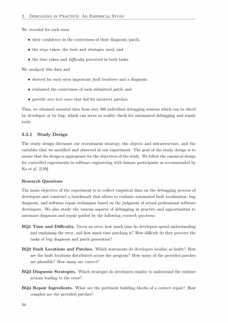
3. Debugging in Practice: An Empirical Study
We recorded for each error
• their confidence in the correctness of their diagnosis/patch,
• the steps taken, the tools and strategies used, and
• the time taken and difficulty perceived in both tasks.
We analyzed this data and
• derived for each error important fault locations and a diagnosis
• evaluated the correctness of each submitted patch, and
• provide new test cases that fail for incorrect patches.
Thus, we obtained essential data from over 300 individual debugging sessions which can be slicedby developer or by bug, which can serve as reality check for automated debugging and repairtools.
3.3.1 Study Design
The study design discusses our recruitment strategy, the objects and infrastructure, and thevariables that we modified and observed in our experiment. The goal of the study design is toensure that the design is appropriate for the objectives of the study. We follow the canonical designfor controlled experiments in software engineering with human participants as recommended byKo et al. [139].
Research Questions
The main objective of the experiment is to collect empirical data on the debugging process ofdevelopers and construct a benchmark that allows to evaluate automated fault localization, bugdiagnosis, and software repair techniques based on the judgment of actual professional softwaredevelopers. We also study the various aspects of debugging in practice and opportunities toautomate diagnosis and repair guided by the following research questions.
RQ1 Time and Difficulty. Given an error, how much time do developers spend understandingand explaining the error, and how much time patching it? How difficult do they perceive thetasks of bug diagnosis and patch generation?
RQ2 Fault Locations and Patches. Which statements do developers localize as faulty? Howare the fault locations distributed across the program? How many of the provided patchesare plausible? How many are correct?
RQ3 Diagnosis Strategies. Which strategies do developers employ to understand the runtimeactions leading to the error?
RQ4 Repair Ingredients. What are the pertinent building blocks of a correct repair? Howcomplex are the provided patches?
34
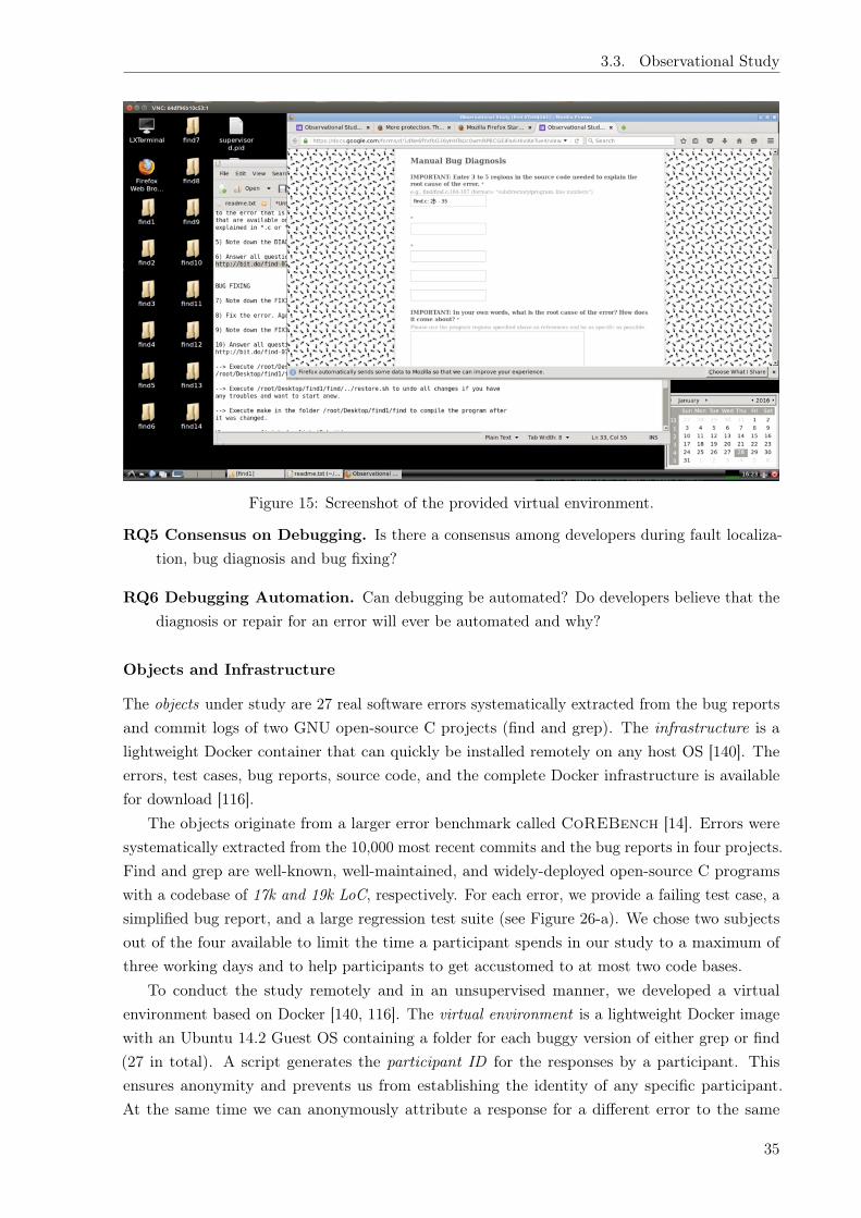
3.3. Observational Study
Figure 15: Screenshot of the provided virtual environment.
RQ5 Consensus on Debugging. Is there a consensus among developers during fault localiza-tion, bug diagnosis and bug fixing?
RQ6 Debugging Automation. Can debugging be automated? Do developers believe that thediagnosis or repair for an error will ever be automated and why?
Objects and Infrastructure
The objects under study are 27 real software errors systematically extracted from the bug reportsand commit logs of two GNU open-source C projects (find and grep). The infrastructure is alightweight Docker container that can quickly be installed remotely on any host OS [140]. Theerrors, test cases, bug reports, source code, and the complete Docker infrastructure is availablefor download [116].
The objects originate from a larger error benchmark called CoREBench [14]. Errors weresystematically extracted from the 10,000 most recent commits and the bug reports in four projects.Find and grep are well-known, well-maintained, and widely-deployed open-source C programswith a codebase of 17k and 19k LoC, respectively. For each error, we provide a failing test case, asimplified bug report, and a large regression test suite (see Figure 26-a). We chose two subjectsout of the four available to limit the time a participant spends in our study to a maximum ofthree working days and to help participants to get accustomed to at most two code bases.
To conduct the study remotely and in an unsupervised manner, we developed a virtualenvironment based on Docker [140, 116]. The virtual environment is a lightweight Docker imagewith an Ubuntu 14.2 Guest OS containing a folder for each buggy version of either grep or find(27 in total). A script generates the participant ID for the responses by a participant. Thisensures anonymity and prevents us from establishing the identity of any specific participant.At the same time we can anonymously attribute a response for a different error to the same
35

3. Debugging in Practice: An Empirical Study
participant to measure, for instance, how code familiarity increases over time. The same scriptdoes some folder scrambling to randomize the order in which participants debug the providederrors: The first error for one participant might be the last error for another. The scramblingcontrols for learning effects. For instance, if every participant would start with the same error,this error might incorrectly be classified as very difficult. The docker image contains the mostcommon development and debugging tools for C, including gdb, vim, and Eclipse. Participantswere encouraged to install their own tools and copy the created folders onto their own machine.A screenshot of the docker image desktop is shown in Figure 15.
Pilot Studies: Researchers and Students
Ko et al. [139] note that the design of a study with human participants is necessarily an iterativeprocess. Therefore, a critical step in preparing an experiment is to run pilot studies. Hence, wefirst evaluated our design and infrastructure in a sandbox pilot where we, the researchers, werethe participants. This allowed us to quickly catch the most obvious of problems at no extracost. Thereupon, we sought to recruit several graduate students from Saarland University forthe pilot study. We advertised the study in lectures, pasted posters on public bulletin boards,and sent emails to potentially interested students. From 10 interested students, we selected five(5) that consider their own level of skill in the programming with C as advanced or experts.15
We conducted the pilot study as supervised, observational study in-house, in our computer lab.After filling the consent form and answering demographic questions, we introduced the errors andinfrastructure in a small hands-on tutorial that lasted about 30 minutes. Then, the students hadeight (8) hours, including a one hour lunch break, to debug as many errors as they could. Werecorded the screen of each student using a screen capturing tool. Independent of the outcome,all participants received EUR 50 as monetary compensation. While none of the data collected inthe pilot studies was used for the final results, the pilot studies helped us to improve our studydesign in several ways:
1) No Students. For the main study, we would use only software engineering professionals. Inseven hours our student participants submitted only a sum total of five patches. On average, astudent fixed one (1) error in eight (8) hours (while in the main study a professional fixed 27errors in 21.5 hours). The feedback from students was that they under-estimated the requiredeffort and over-estimated their own level of skill.
2) No Screen Capturing. The video of only a single participant would take several Gigabyteof storage and it needs to be transferred online to a central storage. This was deemed notviable.
3) Good Infrastructure. The setup, infrastructure, and training material was deemed appro-priate.
15Note that self-assessment of level of skill should always be taken with a grain of salt (cf. Dunning-Krugereffect [118]).
36
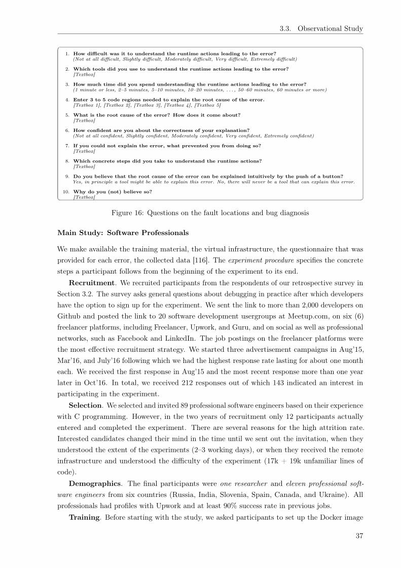
3.3. Observational Study
1. How difficult was it to understand the runtime actions leading to the error?(Not at all difficult, Slightly difficult, Moderately difficult, Very difficult, Extremely difficult)
2. Which tools did you use to understand the runtime actions leading to the error?[Textbox]
3. How much time did you spend understanding the runtime actions leading to the error?(1 minute or less, 2–5 minutes, 5–10 minutes, 10–20 minutes, . . . , 50–60 minutes, 60 minutes or more)
4. Enter 3 to 5 code regions needed to explain the root cause of the error.[Textbox 1], [Textbox 2], [Textbox 3], [Textbox 4], [Textbox 5]
5. What is the root cause of the error? How does it come about?[Textbox]
6. How confident are you about the correctness of your explanation?(Not at all confident, Slightly confident, Moderately confident, Very confident, Extremely confident)
7. If you could not explain the error, what prevented you from doing so?[Textbox]
8. Which concrete steps did you take to understand the runtime actions?[Textbox]
9. Do you believe that the root cause of the error can be explained intuitively by the push of a button?Yes, in principle a tool might be able to explain this error. No, there will never be a tool that can explain this error.
10. Why do you (not) believe so?[Textbox]
Figure 16: Questions on the fault locations and bug diagnosis
Main Study: Software Professionals
We make available the training material, the virtual infrastructure, the questionnaire that wasprovided for each error, the collected data [116]. The experiment procedure specifies the concretesteps a participant follows from the beginning of the experiment to its end.
Recruitment. We recruited participants from the respondents of our retrospective survey inSection 3.2. The survey asks general questions about debugging in practice after which developershave the option to sign up for the experiment. We sent the link to more than 2,000 developers onGithub and posted the link to 20 software development usergroups at Meetup.com, on six (6)freelancer platforms, including Freelancer, Upwork, and Guru, and on social as well as professionalnetworks, such as Facebook and LinkedIn. The job postings on the freelancer platforms werethe most effective recruitment strategy. We started three advertisement campaigns in Aug’15,Mar’16, and July’16 following which we had the highest response rate lasting for about one montheach. We received the first response in Aug’15 and the most recent response more than one yearlater in Oct’16. In total, we received 212 responses out of which 143 indicated an interest inparticipating in the experiment.
Selection. We selected and invited 89 professional software engineers based on their experiencewith C programming. However, in the two years of recruitment only 12 participants actuallyentered and completed the experiment. There are several reasons for the high attrition rate.Interested candidates changed their mind in the time until we sent out the invitation, when theyunderstood the extent of the experiments (2–3 working days), or when they received the remoteinfrastructure and understood the difficulty of the experiment (17k + 19k unfamiliar lines ofcode).
Demographics. The final participants were one researcher and eleven professional soft-ware engineers from six countries (Russia, India, Slovenia, Spain, Canada, and Ukraine). Allprofessionals had profiles with Upwork and at least 90% success rate in previous jobs.
Training. Before starting with the study, we asked participants to set up the Docker image
37
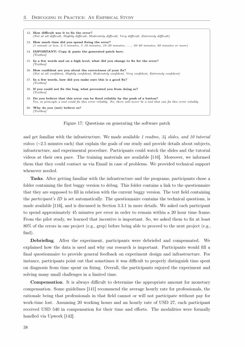
3. Debugging in Practice: An Empirical Study
12. How difficult was it to fix the error?(Not at all difficult, Slightly difficult, Moderately difficult, Very difficult, Extremely difficult)
13. How much time did you spend fixing the error?(1 minute or less, 2–5 minutes, 5–10 minutes, 10–20 minutes, . . . , 50–60 minutes, 60 minutes or more)
14. IMPORTANT: Copy & paste the generated patch here.[Textbox]
15. In a few words and on a high level, what did you change to fix for the error?[Textbox]
16. How confident are you about the correctness of your fix?(Not at all confident, Slightly confident, Moderately confident, Very confident, Extremely confident)
17. In a few words, how did you make sure this is a good fix?[Textbox]
18. If you could not fix the bug, what prevented you from doing so?[Textbox]
19. Do you believe that this error can be fixed reliably by the push of a button?Yes, in principle a tool could fix this error reliably. No, there will never be a tool that can fix this error reliably.
20. Why do you (not) believe so?[Textbox]
Figure 17: Questions on generating the software patch
and get familiar with the infrastructure. We made available 1 readme, 34 slides, and 10 tutorialvideos (⇠2.5 minutes each) that explain the goals of our study and provide details about subjects,infrastructure, and experimental procedure. Participants could watch the slides and the tutorialvideos at their own pace. The training materials are available [116]. Moreover, we informedthem that they could contact us via Email in case of problems. We provided technical supportwhenever needed.
Tasks. After getting familiar with the infrastructure and the programs, participants chose afolder containing the first buggy version to debug. This folder contains a link to the questionnairethat they are supposed to fill in relation with the current buggy version. The text field containingthe participant’s ID is set automatically. The questionnaire contains the technical questions, ismade available [116], and is discussed in Section 3.3.1 in more details. We asked each participantto spend approximately 45 minutes per error in order to remain within a 20 hour time frame.From the pilot study, we learned that incentive is important. So, we asked them to fix at least80% of the errors in one project (e.g., grep) before being able to proceed to the next project (e.g.,find).
Debriefing. After the experiment, participants were debriefed and compensated. Weexplained how the data is used and why our research is important. Participants would fill afinal questionnaire to provide general feedback on experiment design and infrastructure. Forinstance, participants point out that sometimes it was difficult to properly distinguish time spenton diagnosis from time spent on fixing. Overall, the participants enjoyed the experiment andsolving many small challenges in a limited time.
Compensation. It is always difficult to determine the appropriate amount for monetarycompensation. Some guidelines [141] recommend the average hourly rate for professionals, therationale being that professionals in that field cannot or will not participate without pay forwork-time lost. Assuming 20 working hours and an hourly rate of USD 27, each participantreceived USD 540 in compensation for their time and efforts. The modalities were formallyhandled via Upwork [142].
38
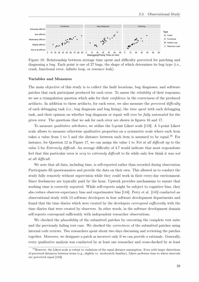
3.3. Observational Study
●
●
●●
●
●
●●
●
●
●
●
●
●●
●●
●
●●
●
Combined Bug Diagnosis Patching
Not at all difficult
Slightly difficult
Moderately difficult
Very difficult
Extremely difficult
0 10 20 30 40 50 60 70 80 90 0 10 20 30 40 50 60 0 10 20 30 40 50 60Debugging/Fixing Time (in min)
Type● Crash
Functional
Infinite Loop
Resource Leak
Figure 18: Relationship between average time spent and difficulty perceived for patching anddiagnosing a bug. Each point is one of 27 bugs, the shape of which determines its bug type (i.e.,crash, functional error, infinite loop, or resource leak).
Variables and Measures
The main objective of this study is to collect the fault locations, bug diagnoses, and softwarepatches that each participant produced for each error. To assess the reliability of their responses,we use a triangulation question which asks for their confidence in the correctness of the producedartifacts. In addition to these artifacts, for each error, we also measure the perceived difficultyof each debugging task (i.e., bug diagnosis and bug fixing), the time spent with each debuggingtask, and their opinion on whether bug diagnosis or repair will ever be fully automated for thegiven error. The questions that we ask for each error are shown in figures 16 and 17.
To measure qualitative attributes, we utilize the 5-point Likert scale [119]. A 5-point Likertscale allows to measure otherwise qualitative properties on a symmetric scale where each itemtakes a value from 1 to 5 and the distance between each item is assumed to be equal.16 Forinstance, for Question 12 in Figure 17, we can assign the value 1 to Not at all difficult up to thevalue 5 for Extremely difficult. An average difficulty of 4.7 would indicate that most respondentsfeel that this particular error is very to extremely difficult to fix while only few think it was notat all difficult.
We note that all data, including time, is self-reported rather than recorded during observation.Participants fill questionnaires and provide the data on their own. This allowed us to conduct thestudy fully remotely without supervision while they could work in their every-day environment.Since freelancers are typically paid by the hour, Upwork provides mechanisms to ensure thatworking time is correctly reported. While self-reports might be subject to cognitive bias, theyalso reduce observer-expectancy bias and experimenter bias [144]. Perry et al. [145] conducted anobservational study with 13 software developers in four software development departments andfound that the time diaries which were created by the developers correspond sufficiently with thetime diaries that were created by observers. In other words, in the software development domainself-reports correspond sufficiently with independent researcher observations.
We checked the plausibility of the submitted patches by executing the complete test suiteand the previously failing test case. We checked the correctness of the submitted patches usinginternal code reviews. Two researchers spent about two days discussing and reviewing the patchestogether. Moreover, we designate a patch as incorrect only if we can provide a rationale. Generally,every qualitative analysis was conducted by at least one researcher and cross-checked by at least
16However, the Likert-scale is robust to violations of the equal distance assumption: Even with larger distortionsof perceived distances between items (e.g., slightly vs. moderately familiar), Likert performs close to where intervalsare perceived equal [143].
39

3. Debugging in Practice: An Empirical Study
●
●
●●
●
●
●
●●
●●
●
●●
●
●●
●●
●●
●
●
●
Regions per Error Statements per Error Statements per Region
2
4
6
02468
101214161820222426283032343638404244464850525456
02468
1012141618202224262830
Loca
tions
Figure 19: Boxplots showing the number of contiguous regions per bug diagnosis (left), thenumber of statements per diagnosis (middle), and the number of statements per contiguous region(right). For example, file.c:12-16,20 specifies six statements in two contiguous regions.
one other researcher.
3.3.2 Study Results
Overall, 27 real errors in 2 open-source C programs were diagnosed and patched by 12 participantswho together spent 29 working days.
RQ1 Time and Difficulty
Our data on debugging time and difficulty can be used in cost-effective user-studies that set outto show how a novel debugging aid improves the debugging process in practice. We also elicitcauses of difficulties during the manual debugging process.
Time and Difficulty. On average, participants rated an error as moderately difficult toexplain (2.8) and slightly difficult to patch (2.3). On average, participants spent 32 and 16 minuteson diagnosing and patching an error, respectively. There is a linear and positive relationshipbetween perceived difficulty and the time spent debugging. As we can see in Figure 18, participantsperceived four errors to be very difficult to diagnose. These are three functional errors andone crash. Participants spent about 55 minutes diagnosing the error that was most difficult todiagnose. However, there are also nine errors perceived to be slightly difficult to diagnose withthe main cluster situated between 15 and 20 minutes of diagnosis time. Participants perceivedone (functional) error as very difficult to patch and spent about 40 minutes patching it. However,there are also two bugs perceived to be not at all difficult to patch and took about five minutes.
Bug diagnosis is twice as time-consuming as bug fixing; participants spent two-third of theirtime diagnosing the bug and only a third of the time to patch.
Why are some errors very difficult? There are four errors rated as very difficult todiagnose. In many cases, missing documentation for certain functions, flags, or data structureswere mentioned as reasons for such difficulty. Other times, developers start out with an incorrecthypothesis before moving on to the correct one. For instance, the crash in grep.3c3bdace is caused
40

3.3. Observational Study
by a corrupted heap, but the crash location is very distant from the location where the heap iscorrupted. The crash and another functional error are caused by a simple operator fault. Threeof the four bugs which are very difficult to diagnose are actually fixed in a single line. For the onlyerror that is both very difficult to diagnose and patch, the developer-provided patch is actuallyvery complex, involving 80 added and 30 deleted lines of code. Only one participant provided acorrect patch.
Developers perceived bug diagnosis to be difficult due to poor codedocumentation and incorrect (root cause) hypothesis.
RQ2 Fault Locations and Patches
Our data on those program locations which practitioners need to explain how an error comes about(i.e., fault locations) can be used for a more realistic evaluation of automated fault localization,and motivates the development of techniques that point out multiple pertinent fault locations.Our data on multiple patches for the same error can be used to evaluate auto-repair techniques,and motivates research in automated repair and its integration with automated regression testgeneration to circumvent the considerable human error.
Fault Locations. The middle 50% of consolidated bug diagnoses references three to fourcontiguous code regions, many of which can appear in different functions or files. In other words,practitioners often reference multiple statements to explain an error. A contiguous code regionis a consecutive sequence of program statements. In most cases, the regions for one error arelocalized in different functions and files. As shown in Figure 19, the majority of contiguous regions(below the median) contain only a single statement, the middle 50% contains between 1 and 3statements. A typical bug diagnosis references 10 statements.
Developers reference multiple (10) statements and multiple(three to four) code regions to explain an error.
Patches. While 282 out of 290 (97%) of the submitted patches are plausible and pass theprovided test case, only 182 patches (63%) are actually correct and pass our code review.17 Acorrect patch does not introduce new errors and does not allow to provide other test cases that faildue to the same error. We determined correctness by code review and plausibility by executingthe failing test case. For each incorrect patch, we also give a reason as to why it is incorrectand whether the test case passes. DbgBench provides several examples of correct and incorrectpatches for an error and a high-level description of the changes done to the code. An example isshown in Figure 26-c.
Figure 20 shows that the median proportional plausibility is 100%, meaning that for themajority of errors (above the median), all patches that participants submit pass the providedtest case. Even for the middle 50% of errors, more than 90% of patches are plausible. However,the median proportional correctness is 69%, meaning that for the majority of errors (above themedian), only 69% of patches submitted by participants pass our code review. For the middle50% of errors only between 45% and 82% of patches are actually correct.
17Note that participants were asked to ensure the plausibility of their submitted patch by passing the provided
41
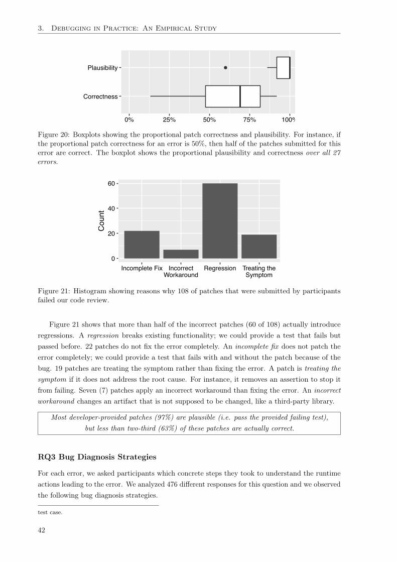
3. Debugging in Practice: An Empirical Study
●
Correctness
Plausibility
0% 25% 50% 75% 100%
Figure 20: Boxplots showing the proportional patch correctness and plausibility. For instance, ifthe proportional patch correctness for an error is 50%, then half of the patches submitted for thiserror are correct. The boxplot shows the proportional plausibility and correctness over all 27errors.
0
20
40
60
Incomplete Fix IncorrectWorkaround
Regression Treating theSymptom
Cou
nt
Figure 21: Histogram showing reasons why 108 of patches that were submitted by participantsfailed our code review.
Figure 21 shows that more than half of the incorrect patches (60 of 108) actually introduceregressions. A regression breaks existing functionality; we could provide a test that fails butpassed before. 22 patches do not fix the error completely. An incomplete fix does not patch theerror completely; we could provide a test that fails with and without the patch because of thebug. 19 patches are treating the symptom rather than fixing the error. A patch is treating thesymptom if it does not address the root cause. For instance, it removes an assertion to stop itfrom failing. Seven (7) patches apply an incorrect workaround than fixing the error. An incorrectworkaround changes an artifact that is not supposed to be changed, like a third-party library.
Most developer-provided patches (97%) are plausible (i.e. pass the provided failing test),but less than two-third (63%) of these patches are actually correct.
RQ3 Bug Diagnosis Strategies
For each error, we asked participants which concrete steps they took to understand the runtimeactions leading to the error. We analyzed 476 different responses for this question and we observedthe following bug diagnosis strategies.
test case.
42

3.3. Observational Study
0
20
40
60
80
100
120
BR CC FR IM OA IT#tim
es th
e di
agno
sis
stra
tegy
was
use
d
Diagnosis strategy
Diagnosis strategies used w.r.t. a bug type
crashresource leak
functionalinfinite loop
Figure 22: Diagnosis strategies for different error types.
Classification. We extend the bug diagnosis strategies that have been identified by Romeroand colleagues [146, 147]:
• (FR) Forward Reasoning. Programmers follow each computational step in the execution of the failing
test.
• (BR) Backward Reasoning. Programmers start from the unexpected output following backwards to
the origin.
• (CC) Code Comprehension. Programmers read the code to understand it and build a mental
representation.
• (IM) Input Manipulation. Programmers construct a similar test case to compare the behavior and
execution.
• (OA) Offline analysis. Programmers analyze an error trace or a coredump (e.g. via valgrind, strace).
• (IT) Intuition. Developer uses her experience from a previous patch.
Specifically, we identified the Input Manipulation (IM) bug diagnosis strategy. Developerswould first modify the failing test case to construct a passing one. This gives insight into thecircumstances required to observe the error. Next, they would compare the program states inboth executions. IM is reminiscent of classic work on automated debugging [148], which mightagain reflect the potential lack of knowledge about automated techniques that have been availablefrom the research community for over a decade.
Frequency. We discovered that forward reasoning and code comprehension (FR+CC) arethe most commonly used diagnosis strategies in our study. The number of usage of differentbug diagnosis strategies is shown in Figure 22 for the different error types. We observe thatpast experience (IT) is used least frequently. Many participants used input modification (IM)as diagnosis strategy. Therefore, the integration of automated techniques that implement IM(e.g. [148]) into mainstream debugger will help improve debugger productivity.
43

3. Debugging in Practice: An Empirical Study
Forward reasoning and code comprehension (FR+CC) arethe most commonly used bug diagnosis strategies among developers.
Error Type. We observe that forward reasoning (FR) is the most commonly used diagnosisstrategy for bugs reflecting infinite loops (26 out of a total 45 responses). Intuitively, there is nolast executed statement which can be used to reason backwards from. Out of a total 137 responsesfor crash-related bugs, we found that backward reasoning (BR) was used 55 times. Intuitively, thecrash location is most often a good starting point to understand how the crash came about. Forfunctional errors, 112 responses, out of a total 270 responses, reflect forward reasoning (FR). If thesymptom is an unexpected output, the actual fault location can be very far from print statementresponsible for the unexpected output. It may be better to start stepping from a location wherethe state is not infected, yet. Finally, we observed that input modification (IM) strategy wasused for 31 out of 270 scenarios to diagnose functional errors. This was to understand whatdistinguishes the failing from a passing execution.
The choice of diagnosis strategy depends on the error type, for instance,forward reasoning (FR) was mostly employed to diagnose functional errors and infinite loops.
Tools. Every participant used a combination of trace-based and interactive debugging. Forresource leaks, participants further used tools such as valgrind and strace. We also observed thatparticipants use bug diagnosis techniques that have been automated previously [148], albeit withmanual effort, to narrow down the pertinent sequence of events.
Developers mostly used interactive or trace-based debuggers (e.g. gdb),but often used specialized tools (e.g. valgrind) for specific errors (e.g. memory leaks).
RQ4 Repair Ingredients
Out of 290 submitted patches, 100 (34%) exclusively affect the control flow, 87 (30%) exclusivelyaffect the data flow, while the remaining 103 patches (36%) affect both, control and data flow.
Control Flow. In automated repair research, the patching of control flow is consideredtractable because of the significantly reduced search space [149]: Either a set of statements isexecuted or not. The frequency with which participants fix the control flow may provide someinsight about the effectiveness of such an approach for the errors provided with DbgBench. Thecontrol flow is modified by 200 patches (69%). Specifically, a branch condition is changed by 126patches and the loop or function flow is modified by 38 patches.18 A new if-branch is added by86 patches whereupon, in many cases, an existing statement is then moved into the new branchor a new function call is added.19
Data Flow. The data flow is modified by 187 of 290 submitted patches (64%). Specifically,57 patches modify a variable value or function parameter. GenProg [33] copies, moves, or deletesexisting program statements, effectively relying on the Plastic Surgery Hypothesis (PSH) [150].In our study, the PSH seems to hold. 44 patches move existing statements while 29 patches deleteexisting statements. However, 73 patches add new variable assignments while 40 patches add new
18Examples of changing the loop or function flow are adding a return, exit, continue, or goto statement.19Note that one patch can modify several statements!
44

3.3. Observational Study
● ●
●
●
●
●
●
●
●
●
●
●
●
●
●
●
●
●
● ●
●
●
●
●
●
●
●
● ●
●
● ●
●
● ●
●
●
●
●
●
●
●
●
●
0%
25%
50%
75%
100%
Location 1 Location 2 Location 3
● find
grep
Figure 23: Proportional agreement on Top-3 most suspicious fault locations showing box plotswith jitter overlay (each shape is one of 27 errors).
function calls, for instance to report an error or to release resources. A completely new variable isdeclared in 27 patches. Only 8 patches introduce complex functions that need to be synthesized.
A third (36%) of submitted patches affect both data and control flow, while another thirdexclusively affect data flow (30%) or control flow (34%), respectively.
Patch Complexity. On average, a submitted patch contained six (6) Changed Lines ofCode (CLoC). The median patch contained 3 CLoC. The mean being to the far right of themedian points to a skewed distribution. Indeed, many patches are not very complex but thereare a few that require more than 50 CLoC.
Most bug fixes are not very complex, most patches contain three to six CLoC.
RQ5 Consensus on Debugging
We investigate whether there is consensus among the developers during fault localization, diagnosisand fixing. Suppose, there is not. Then, how should there ever be consensus on whether anautomated debugging technique has produced the correct fault locations, the correct bug diagnosis,or the correct patch for an error?
Consensus on Fault Locations. For most errors (above the median), more than 75%of participants independently localize the same location as pertinent to explain the error (Lo-cation 1). For each error, we count the proportion of participants independently reporting afault location. Sorted by proportion, we get the top-most, 2nd-most, and 3rd-most suspiciouslocations (Location 1–3). For the middle 50% of errors, between half and two third of participantsindependently report the same 2nd-most suspicious location while between one third and halfof participants still independently report the same 3rd-most suspicious location. However, notethat a participant might mention less or more than three locations. The consensus of professionalsoftware developers on the fault locations suggests that every bug in DbgBench is correctlylocalized by at least two (2) specific statements. These locations can serve as ground truth for theevaluation of automated fault localization tools.
Consensus on Bug Diagnosis. 10 of 12 participants (85%) give essentially the same
45
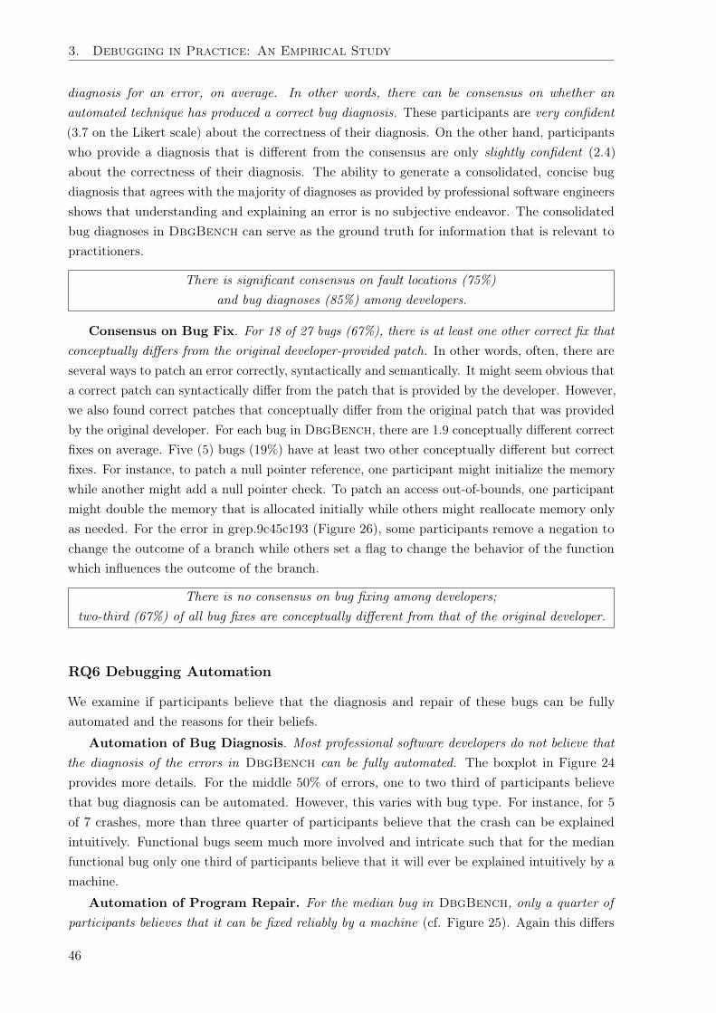
3. Debugging in Practice: An Empirical Study
diagnosis for an error, on average. In other words, there can be consensus on whether anautomated technique has produced a correct bug diagnosis. These participants are very confident(3.7 on the Likert scale) about the correctness of their diagnosis. On the other hand, participantswho provide a diagnosis that is different from the consensus are only slightly confident (2.4)about the correctness of their diagnosis. The ability to generate a consolidated, concise bugdiagnosis that agrees with the majority of diagnoses as provided by professional software engineersshows that understanding and explaining an error is no subjective endeavor. The consolidatedbug diagnoses in DbgBench can serve as the ground truth for information that is relevant topractitioners.
There is significant consensus on fault locations (75%)and bug diagnoses (85%) among developers.
Consensus on Bug Fix. For 18 of 27 bugs (67%), there is at least one other correct fix thatconceptually differs from the original developer-provided patch. In other words, often, there areseveral ways to patch an error correctly, syntactically and semantically. It might seem obvious thata correct patch can syntactically differ from the patch that is provided by the developer. However,we also found correct patches that conceptually differ from the original patch that was providedby the original developer. For each bug in DbgBench, there are 1.9 conceptually different correctfixes on average. Five (5) bugs (19%) have at least two other conceptually different but correctfixes. For instance, to patch a null pointer reference, one participant might initialize the memorywhile another might add a null pointer check. To patch an access out-of-bounds, one participantmight double the memory that is allocated initially while others might reallocate memory onlyas needed. For the error in grep.9c45c193 (Figure 26), some participants remove a negation tochange the outcome of a branch while others set a flag to change the behavior of the functionwhich influences the outcome of the branch.
There is no consensus on bug fixing among developers;two-third (67%) of all bug fixes are conceptually different from that of the original developer.
RQ6 Debugging Automation
We examine if participants believe that the diagnosis and repair of these bugs can be fullyautomated and the reasons for their beliefs.
Automation of Bug Diagnosis. Most professional software developers do not believe thatthe diagnosis of the errors in DbgBench can be fully automated. The boxplot in Figure 24provides more details. For the middle 50% of errors, one to two third of participants believethat bug diagnosis can be automated. However, this varies with bug type. For instance, for 5of 7 crashes, more than three quarter of participants believe that the crash can be explainedintuitively. Functional bugs seem much more involved and intricate such that for the medianfunctional bug only one third of participants believe that it will ever be explained intuitively by amachine.
Automation of Program Repair. For the median bug in DbgBench, only a quarter ofparticipants believes that it can be fixed reliably by a machine (cf. Figure 25). Again this differs
46
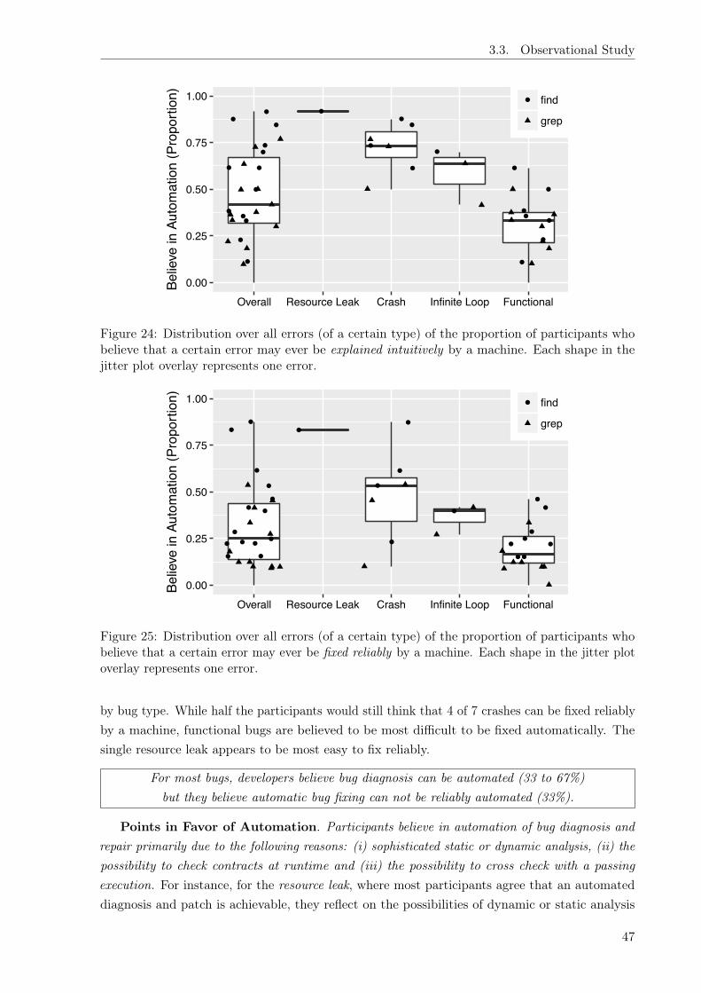
3.3. Observational Study
●
●
●
●
●
●
●
●
●●
●
●
●●
●
●
●
●
●
●
●
●●
●
●
●
0.00
0.25
0.50
0.75
1.00
Overall Resource Leak Crash Infinite Loop Functional
Belie
ve in
Aut
omat
ion
(Pro
porti
on) Subject
● find
grep
Figure 24: Distribution over all errors (of a certain type) of the proportion of participants whobelieve that a certain error may ever be explained intuitively by a machine. Each shape in thejitter plot overlay represents one error.
●
●
●
●
●
●
●
●
●
●
●
●
●
●
●
●
●
●
●
●
●
●
●
●
●
●
●
●
0.00
0.25
0.50
0.75
1.00
Overall Resource Leak Crash Infinite Loop Functional
Belie
ve in
Aut
omat
ion
(Pro
porti
on) Subject
● find
grep
Figure 25: Distribution over all errors (of a certain type) of the proportion of participants whobelieve that a certain error may ever be fixed reliably by a machine. Each shape in the jitter plotoverlay represents one error.
by bug type. While half the participants would still think that 4 of 7 crashes can be fixed reliablyby a machine, functional bugs are believed to be most difficult to be fixed automatically. Thesingle resource leak appears to be most easy to fix reliably.
For most bugs, developers believe bug diagnosis can be automated (33 to 67%)but they believe automatic bug fixing can not be reliably automated (33%).
Points in Favor of Automation. Participants believe in automation of bug diagnosis andrepair primarily due to the following reasons: (i) sophisticated static or dynamic analysis, (ii) thepossibility to check contracts at runtime and (iii) the possibility to cross check with a passingexecution. For instance, for the resource leak, where most participants agree that an automateddiagnosis and patch is achievable, they reflect on the possibilities of dynamic or static analysis
47
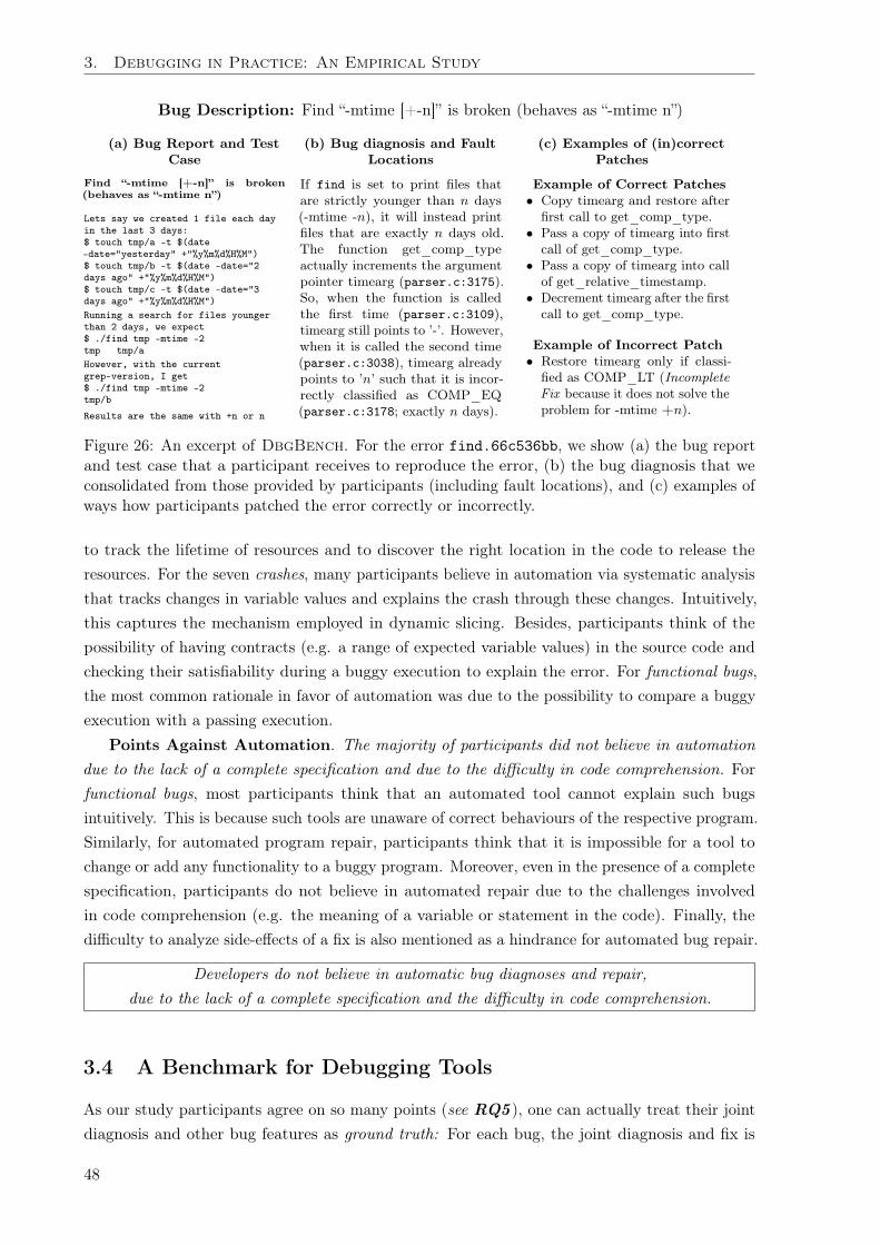
3. Debugging in Practice: An Empirical Study
Bug Description: Find “-mtime [+-n]” is broken (behaves as “-mtime n”)
(a) Bug Report and Test
Case
Find “-mtime [+-n]” is broken(behaves as “-mtime n”)
Lets say we created 1 file each day
in the last 3 days:
$ touch tmp/a -t $(date
–date="yesterday" +"%y%m%d%H%M")
$ touch tmp/b -t $(date –date="2
days ago" +"%y%m%d%H%M")
$ touch tmp/c -t $(date –date="3
days ago" +"%y%m%d%H%M")
Running a search for files younger
than 2 days, we expect
$ ./find tmp -mtime -2
tmp tmp/a
However, with the current
grep-version, I get
$ ./find tmp -mtime -2
tmp/b
Results are the same with +n or n
(b) Bug diagnosis and Fault
Locations
If find is set to print files thatare strictly younger than n days(-mtime -n), it will instead printfiles that are exactly n days old.The function get_comp_typeactually increments the argumentpointer timearg (parser.c:3175).So, when the function is calledthe first time (parser.c:3109),timearg still points to ’-’. However,when it is called the second time(parser.c:3038), timearg alreadypoints to ’n’ such that it is incor-rectly classified as COMP_EQ(parser.c:3178; exactly n days).
(c) Examples of (in)correct
Patches
Example of Correct Patches
• Copy timearg and restore afterfirst call to get_comp_type.
• Pass a copy of timearg into firstcall of get_comp_type.
• Pass a copy of timearg into callof get_relative_timestamp.
• Decrement timearg after the firstcall to get_comp_type.
Example of Incorrect Patch
• Restore timearg only if classi-fied as COMP_LT (IncompleteFix because it does not solve theproblem for -mtime +n).
Figure 26: An excerpt of DbgBench. For the error find.66c536bb, we show (a) the bug reportand test case that a participant receives to reproduce the error, (b) the bug diagnosis that weconsolidated from those provided by participants (including fault locations), and (c) examples ofways how participants patched the error correctly or incorrectly.
to track the lifetime of resources and to discover the right location in the code to release theresources. For the seven crashes, many participants believe in automation via systematic analysisthat tracks changes in variable values and explains the crash through these changes. Intuitively,this captures the mechanism employed in dynamic slicing. Besides, participants think of thepossibility of having contracts (e.g. a range of expected variable values) in the source code andchecking their satisfiability during a buggy execution to explain the error. For functional bugs,the most common rationale in favor of automation was due to the possibility to compare a buggyexecution with a passing execution.
Points Against Automation. The majority of participants did not believe in automationdue to the lack of a complete specification and due to the difficulty in code comprehension. Forfunctional bugs, most participants think that an automated tool cannot explain such bugsintuitively. This is because such tools are unaware of correct behaviours of the respective program.Similarly, for automated program repair, participants think that it is impossible for a tool tochange or add any functionality to a buggy program. Moreover, even in the presence of a completespecification, participants do not believe in automated repair due to the challenges involvedin code comprehension (e.g. the meaning of a variable or statement in the code). Finally, thedifficulty to analyze side-effects of a fix is also mentioned as a hindrance for automated bug repair.
Developers do not believe in automatic bug diagnoses and repair,due to the lack of a complete specification and the difficulty in code comprehension.
3.4 A Benchmark for Debugging Tools
As our study participants agree on so many points (see RQ5 ), one can actually treat their jointdiagnosis and other bug features as ground truth: For each bug, the joint diagnosis and fix is
48
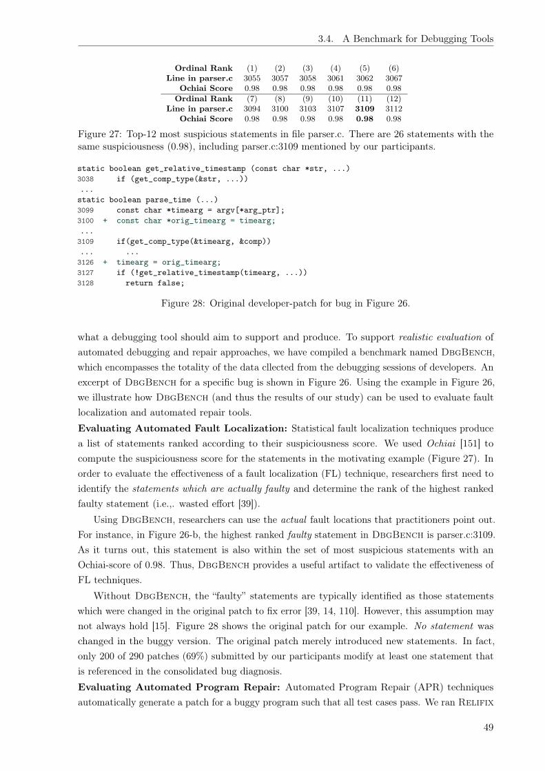
3.4. A Benchmark for Debugging Tools
Ordinal Rank (1) (2) (3) (4) (5) (6)Line in parser.c 3055 3057 3058 3061 3062 3067
Ochiai Score 0.98 0.98 0.98 0.98 0.98 0.98Ordinal Rank (7) (8) (9) (10) (11) (12)
Line in parser.c 3094 3100 3103 3107 3109 3112Ochiai Score 0.98 0.98 0.98 0.98 0.98 0.98
Figure 27: Top-12 most suspicious statements in file parser.c. There are 26 statements with thesame suspiciousness (0.98), including parser.c:3109 mentioned by our participants.
static boolean get_relative_timestamp (const char *str, ...)3038 if (get_comp_type(&str, ...))...static boolean parse_time (...)3099 const char *timearg = argv[*arg_ptr];3100 + const char *orig_timearg = timearg;...3109 if(get_comp_type(&timearg, &comp))... ...3126 + timearg = orig_timearg;3127 if (!get_relative_timestamp(timearg, ...))3128 return false;
Figure 28: Original developer-patch for bug in Figure 26.
what a debugging tool should aim to support and produce. To support realistic evaluation ofautomated debugging and repair approaches, we have compiled a benchmark named DbgBench,which encompasses the totality of the data cllected from the debugging sessions of developers. Anexcerpt of DbgBench for a specific bug is shown in Figure 26. Using the example in Figure 26,we illustrate how DbgBench (and thus the results of our study) can be used to evaluate faultlocalization and automated repair tools.Evaluating Automated Fault Localization: Statistical fault localization techniques producea list of statements ranked according to their suspiciousness score. We used Ochiai [151] tocompute the suspiciousness score for the statements in the motivating example (Figure 27). Inorder to evaluate the effectiveness of a fault localization (FL) technique, researchers first need toidentify the statements which are actually faulty and determine the rank of the highest rankedfaulty statement (i.e.,. wasted effort [39]).
Using DbgBench, researchers can use the actual fault locations that practitioners point out.For instance, in Figure 26-b, the highest ranked faulty statement in DbgBench is parser.c:3109.As it turns out, this statement is also within the set of most suspicious statements with anOchiai-score of 0.98. Thus, DbgBench provides a useful artifact to validate the effectiveness ofFL techniques.
Without DbgBench, the “faulty” statements are typically identified as those statementswhich were changed in the original patch to fix error [39, 14, 110]. However, this assumption maynot always hold [15]. Figure 28 shows the original patch for our example. No statement waschanged in the buggy version. The original patch merely introduced new statements. In fact,only 200 of 290 patches (69%) submitted by our participants modify at least one statement thatis referenced in the consolidated bug diagnosis.Evaluating Automated Program Repair: Automated Program Repair (APR) techniquesautomatically generate a patch for a buggy program such that all test cases pass. We ran Relifix
49
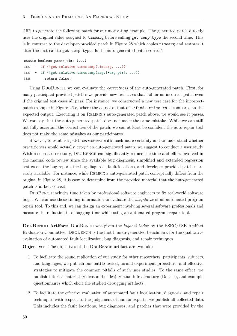
3. Debugging in Practice: An Empirical Study
[152] to generate the following patch for our motivating example. The generated patch directlyuses the original value assigned to timearg before calling get_comp_type the second time. Thisis in contrast to the developer-provided patch in Figure 28 which copies timearg and restores itafter the first call to get_comp_type. Is the auto-generated patch correct?
static boolean parse_time (...)3127 - if (!get_relative_timestamp(timearg, ...))3127 + if (!get_relative_timestamp(argv[*arg_ptr], ...))3128 return false;
Using DbgBench, we can evaluate the correctness of the auto-generated patch. First, formany participant-provided patches we provide new test cases that fail for an incorrect patch evenif the original test cases all pass. For instance, we constructed a new test case for the incorrect-patch-example in Figure 26-c, where the actual output of ./find -mtime +n is compared to theexpected output. Executing it on Relifix’s auto-generated patch above, we would see it passes.We can say that the auto-generated patch does not make the same mistake. While we can stillnot fully ascertain the correctness of the patch, we can at least be confident the auto-repair tooldoes not make the same mistakes as our participants.
However, to establish patch correctness with much more certainty and to understand whetherpractitioners would actually accept an auto-generated patch, we suggest to conduct a user study.Within such a user study, DbgBench can significantly reduce the time and effort involved inthe manual code review since the available bug diagnosis, simplified and extended regressiontest cases, the bug report, the bug diagnosis, fault locations, and developer-provided patches areeasily available. For instance, while Relifix’s auto-generated patch conceptually differs from theoriginal in Figure 28, it is easy to determine from the provided material that the auto-generatedpatch is in fact correct.
DbgBench includes time taken by professional software engineers to fix real-world softwarebugs. We can use these timing information to evaluate the usefulness of an automated programrepair tool. To this end, we can design an experiment involving several software professionals andmeasure the reduction in debugging time while using an automated program repair tool.
DbgBench Artifact: DbgBench was given the highest badge by the ESEC/FSE ArtifactEvaluation Committee. DbgBench is the first human-generated benchmark for the qualitativeevaluation of automated fault localization, bug diagnosis, and repair techniques.
Objectives. The objectives of the DbgBench artifact are two-fold:
1. To facilitate the sound replication of our study for other researchers, participants, subjects,and languages, we publish our battle-tested, formal experiment procedure, and effectivestrategies to mitigate the common pitfalls of such user studies. To the same effect, wepublish tutorial material (videos and slides), virtual infrastructure (Docker), and examplequestionnaires which elicit the studied debugging artifacts.
2. To facilitate the effective evaluation of automated fault localization, diagnosis, and repairtechniques with respect to the judgement of human experts, we publish all collected data.This includes the fault locations, bug diagnoses, and patches that were provided by the
50

3.4. A Benchmark for Debugging Tools
practitioners. For each error, it also includes the error-introducing commit, the original anda simplified bug report, a test case failing because of the error, and the developer-providedpatch. Moreover, this artifact contains our reconciled bug diagnoses, our classification ofthe patches as correct and incorrect together with the general fixing strategies, and whichrationale we have to classify a patch as incorrect.
Provided data. Specifically, we make the following data available:
• The benchmark summary containing the complete list of errors, their average debuggingtime, difficulty, and patch correctness, human-generated explanations of the runtime actionsleading to the error, and examples of correct and incorrect fixes, sorted according to averagedebugging time.
• The complete raw data containing the responses to the questions in Figure 16 and Figure 17for each debugging session:
– the error ID to identify error,
– the participant ID to identify participant,
– the timestamp to follow participants accross errors,
– fault Locations, bug diagnosis, and patches,
– the confidence in the correctness of their diagnosis or patch,
– the difficulty to diagnose or patch the error,
– the time taken to diagnose or patch the error,
– what would have helped reducing diagnosis or patch time,
– the steps taken to arrive at the diagnosis or patch,
– the tools used to arrive at the diagnosis or patch,
– the problems if they could not diagnose or patch the error,
– whether he/she believes that generating the diagnosis or patch for this error wouldever be automated,
– why he/she believes so,
– the code familiarity as it increases over time,
– the diagnosis techniques used, and
– how he/she ensured the correctness of the submitted patch,
• The complete cleaned data containing for each error:
– the regression-introducing commit,
– the simplified and original bug reports,
– the important fault locations,
– the reconciled bug diagnosis,
51
3. Debugging in Practice: An Empirical Study
– the original, developer-provided patch,
– the patches submitted by participants,
– our classification of patches as correct or incorrect,
– our rationale of classifying a patch as incorrect, and
– test cases that expose an incorrect patch.
• An example questionnaire to elicit the raw data above.
• The Docker virtual infrastructure and instructions how to use it.
• The tutorial material, incl. slides, videos, and readme files.
Disclaimer DbgBench is a first milestone towards the realistic evaluation of tools in softwareengineering that is grounded in practice. DbgBench can thus be used as necessary reality checkfor in-depth studies. When conducting user studies, DbgBench can significantly reduce the timeand cost that is inherent in large user studies involving professional software engineers. In theabsence of user studies, DbgBench allows in-depth evaluations while minimizing the number ofpotentially unrealistic assumptions. For example, we found a high consensus among participantson the location of the faults. They would often point out several contiguous code regions ratherthan a single statement. We also found no overlap of fault locations with fix locations. Existingerror-benchmarks might assume that an artificially injected fault (i.e., a single mutated statement)or fix locations (i.e., those statements changed in the original patch) are representative of realisticfault locations. DbgBench dispenses with such assumptions and directly provides those faultlocations that practitioners would point out with high consensus. DbgBench allows the realisticevaluation of automated debugging techniques that is grounded in practice.
However, we would strongly suggest to also utilize other benchmarks, such as CoREBench[14] or Defects4J [110], for the empirical evaluation. Only an empirical evaluation, the use ofa sufficiently large representative set of subjects, allows to make empirical claims about theefficacy of an automated debugging technique. Going forward, we hope that more researcherswill produce similar realistic benchmarks which take the practitioner into account. To this end,we also publish our battle-tested, formal experiment procedure, effective strategies to mitigatecommon pitfalls, and all our material. We believe that no single research team can realisticallyproduce a benchmark that is both representative and reflects the realities of debugging in practice.Hence, we propose that similar benchmarks be constructed alongside with user studies. Softwareengineering research, including debugging research, must serve the needs of users and developers.User studies are essential to properly evaluate techniques that are supposed to automate tasksthat are otherwise manual and executed by a software professional. Constructing new benchmarksas artifacts during user studies would allow to build an empirical body of knowledge and at thesame time minimize the cost and effort involved in user studies.
3.5 Limitations and Threats to Validity
Generalizability of Findings. For the results of our experiment we do not claim generalizabilityof the findings. We decided on two subjects to limit the time a participant spends in our study
52
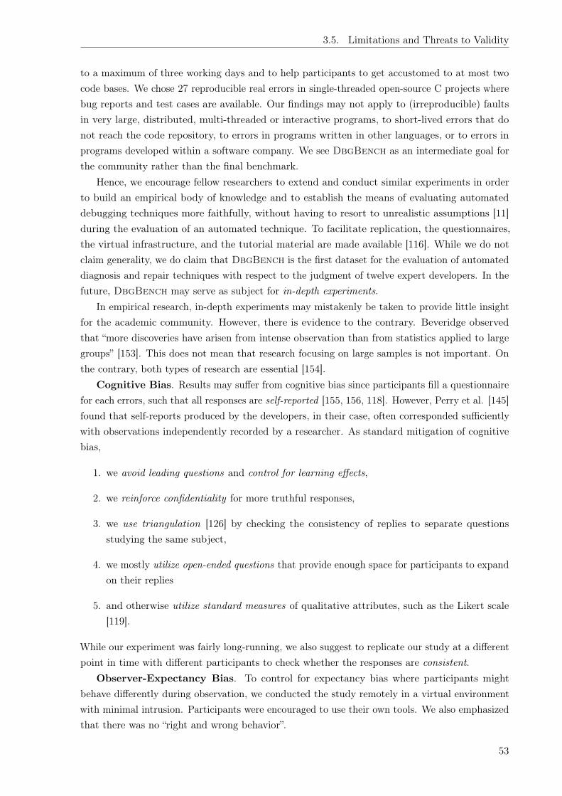
3.5. Limitations and Threats to Validity
to a maximum of three working days and to help participants to get accustomed to at most twocode bases. We chose 27 reproducible real errors in single-threaded open-source C projects wherebug reports and test cases are available. Our findings may not apply to (irreproducible) faultsin very large, distributed, multi-threaded or interactive programs, to short-lived errors that donot reach the code repository, to errors in programs written in other languages, or to errors inprograms developed within a software company. We see DbgBench as an intermediate goal forthe community rather than the final benchmark.
Hence, we encourage fellow researchers to extend and conduct similar experiments in orderto build an empirical body of knowledge and to establish the means of evaluating automateddebugging techniques more faithfully, without having to resort to unrealistic assumptions [11]during the evaluation of an automated technique. To facilitate replication, the questionnaires,the virtual infrastructure, and the tutorial material are made available [116]. While we do notclaim generality, we do claim that DbgBench is the first dataset for the evaluation of automateddiagnosis and repair techniques with respect to the judgment of twelve expert developers. In thefuture, DbgBench may serve as subject for in-depth experiments.
In empirical research, in-depth experiments may mistakenly be taken to provide little insightfor the academic community. However, there is evidence to the contrary. Beveridge observedthat “more discoveries have arisen from intense observation than from statistics applied to largegroups” [153]. This does not mean that research focusing on large samples is not important. Onthe contrary, both types of research are essential [154].
Cognitive Bias. Results may suffer from cognitive bias since participants fill a questionnairefor each errors, such that all responses are self-reported [155, 156, 118]. However, Perry et al. [145]found that self-reports produced by the developers, in their case, often corresponded sufficientlywith observations independently recorded by a researcher. As standard mitigation of cognitivebias,
1. we avoid leading questions and control for learning effects,
2. we reinforce confidentiality for more truthful responses,
3. we use triangulation [126] by checking the consistency of replies to separate questionsstudying the same subject,
4. we mostly utilize open-ended questions that provide enough space for participants to expandon their replies
5. and otherwise utilize standard measures of qualitative attributes, such as the Likert scale[119].
While our experiment was fairly long-running, we also suggest to replicate our study at a differentpoint in time with different participants to check whether the responses are consistent.
Observer-Expectancy Bias. To control for expectancy bias where participants mightbehave differently during observation, we conducted the study remotely in a virtual environmentwith minimal intrusion. Participants were encouraged to use their own tools. We also emphasizedthat there was no “right and wrong behavior”.
53

3. Debugging in Practice: An Empirical Study
Imposed Time Bound. We suggested the participants to complete an error in 45 minutesso as to remain within a 20 hours time frame. Some errors would take much more time. So, givenmore time, the participants might form a better understanding of the runtime actions leadingto the error and produce a larger percentage of correct patches. However, participants told usthat they felt comfortable to diagnose and patch each error within the stipulated time-bound.They tended to stretch the bounds whenever necessary, taking time from errors that were quicklydiagnosed and patched.
3.6 Related Work
There are several articles exploring the opinions of practitioners on research in automated softwareengineering. However, to the best of our knowledge none explores the rationale why practitionersdo not wish to adopt automated debugging techniques, which capabilities an automated bugdiagnosis tool should have beyond simple fault localization, or which qualities an auto-generatedpatch must have so that developers would actually accept it.
In 2015, Perscheid et al. [19] set out to determine whether the state-of-practice has sinceimproved, and conducted a survey involving 303 practitioners to study time spent and tools usedin debugging practice. The middle fifty percent of their respondents spend 20% to 40% of theirwork time for debugging while the next largest group reported 40% to 60%. Like our study, mostpractitioners reported to only use trace-based (e.g., printf) or interactive debugging (e.g., gdb)regularly. The authors also find that most respondents have never used any automated techniquesuch as fault localization, slicing, or likely invariants. However, Perscheid et al. note that thesample might not be representative to allow a general conclusion whence (as is customary in theempirical sciences) we replicate and extend their study as part of our larger study.
Begel and Zimmermann [124] conducted a prospective study that investigates potential softwareengineering research problems that practitioners find interesting. The authors published 145questions ranked in the order of importance that professional software engineers would like toask a data scientist. These questions were mostly about software users, engineers, processes, andpractices. For instance, the question perceived as most important was: “How do users typicallyuse my application?” Lo et al. [123] conducted a retrospective study that explores how developersrate the relevance of 517 actual software engineering research papers. The authors elicite reasonsas to why developers consider certain research as “unwise”: Researchers might overestimate therelevance of a problem, or fail to consider the cost, side effects, or actionability of a solution. Thus,it is important to explore practitioners’ expectations and beliefs before attempting to automate amanual activity.
The bulk of automated debugging research is on Automated Fault Localization (AFL), that is,techniques that produce a ranked list of suspicious locations in the program. A recent surveycites more than 400 publications on AFL [39]. This is in stark contrast to the finding of Perscheidet al. [19] that most practitioners have never used an AFL tool. Parnin and Orso [112] shedlight on this dichotomy and conducted a small user study with an AFL tool. Even when thefault was ranked artificially high, participants did not find the tool more effective than traditionaldebugging. After inspecting the fault in the list of suspicious locations, 9 of 10 participants wouldstill spend another 10 minutes before stopping to provide a diagnosis. The authors found that
54

3.6. Related Work
beyond AFL, developers wanted the relevant context and variable values. More recently, Kochharet al. [41] investigated the necessary capababilities of an AFL tool such that practitioners wouldconsider its adoption. Three quarter of surveyed practitioners would investigate no more thanthe Top-5 ranked statements — which should contain the faulty statement at least three out offour times and take less than one minute to compute.20 Most practitioners find it crucial thatthe AFL tool explains the rationale why the user should consider a suspicious location.
Previous work established that practitioners are interested in automated diagnosis tools withcapabilities that go beyond simple AFL [112, 41]. In this work, we follow up and explore whichcapabilities both, automated bug diagnosis and repair tools should have. In contrast to previouswork, we want to shed light on Lieberman’s debugging scandal without limiting ourselves toAFL. We find out exactly what practitioners want that would improve their debugging experience.We find that most practitioners do not believe that debugging will ever be fully automated andprovide their rationales.
In 2015, Perscheid et al. [19] set out to determine whether the state-of-the-practice had sinceimproved and could only answer in the negative: Debugging remains what it was 50 years ago,largely manual, time-consuming, and a matter of trial-and-error rather than automated, efficient,and systematic. We believe that, at least in part, the debugging scandal is brought about by theabsence of user studies and the assumptions that researchers had to make when evaluating theoutput of a machine without involving the human. Only recently, several studies have uncoveredthat many of these assumptions are not based upon empirical foundations [11, 12, 13, 14, 15]. Inthis work, we attempt to remedy this very problem.
While several researchers investigated debugging strategies that developers generally employin practice, it remains unclear whether developers who independently debug the same erroressentially localize the same faulty statements, provide the same explanation (i.e., diagnosis) andgenerate the same patch. Perscheid et al. [19] visited four companies in Germany and conductedthink-aloud experiments with a total of eight developers during their normal work. While nonewas formally trained in debugging, all participants used a simplified, implicit form of ScientificDebugging [157]: They mentally formulated hypotheses and performed simple experiments toverify them. Katz and Anderson [147] classify bug diagnosis strategies broadly into forwardreasoning where the programmer forms an understanding of what the code should do comparedto what it actually does, and backward reasoning where the programmer reasons backwardsstarting from the location where the bug is observed (e.g., [158]). Romero et al. [146] explorethe impact of graphical literacy on the choice of strategy. Lawrance et al. [26] model debuggingas a predator following scent to find prey. The authors argue that a theory of navigation holdsmore practical value for tool builders than theories that rely on mental constructs. Gilmore etal. [159] studied different models of debugging and their assumptions. The authors argue thatthe success of experts at debugging is not attributed to better debugging skills, but to bettercomprehension. Our evaluation of the impact of “Code Comprehension” in this study furthervalidates these findings.
Several colleagues have investigated debugging as a human activity. Ko et al. [160] observedhow 10 developers understand and debug unfamiliar code. The authors found that developers
20Supposing a tool must have a minimum satisfaction rate of 80%.
55
3. Debugging in Practice: An Empirical Study
interleaved three activities while debugging, namely, code search, dependency analysis and relevantinformation gathering. Layman et al. [161] investigated how developers use information and toolsto debug, by interviewing 15 professional software engineers at Microsoft. The authors found thatthe interaction of hypothesis instrumentation and software environment is a source of difficultywhen debugging. Parnin and Orso [112] also conducted an empirical study to investigate howdevelopers use and benefit from automated debugging tools. The authors found that severalassumptions made by automated debugging techniques do not hold in practice. While thesepapers provide insights on debugging as a human activity, none of these studies provides the dataand methods that would allow researchers to evaluate debugging tools against fault locations,bug diagnosis, and patches provided by actual software engineering professionals.
Many researchers have proposed numerous tools to support developers when debugging, butonly a few have evaluated these tools with user studies, using real bugs and professional developers.For instance, between 1981 and 2010, Parnin and Orso [112] identified only a handful of articles[162, 163, 164, 165, 166, 167] that presented the results of a user study: Unlike this study, none ofthese studies involved actual practitioners and real errors. In our own literature survey, studyingwhether the state-of-the-research has since improved, we could identify only three (3) papers thatconduct user studies with actual practitioners and real errors in the last five years.21 Two articlesemployed user studies to evaluate the acceptability of the auto-generated patches [114, 113] whileone had practitioners to evaluate the effectiveness of an auto-generated bug diagnosis [115].22 Webelieve that this general absence of user studies is symptomatic of the difficulty, expense, andtime spent conducting user studies. This is the problem we address with DbgBench.
3.7 Discussions and Future Work
In this chapter, we provide empirical evidence on program debugging in software practice, ourevaluation results overwhelmingly reveal that debugging in practice is (still) a largely manualand time-consuming process. Developers spend half of their working time debugging source codewhich they are often not very familiar with. After successfully reproducing a reported bug,developers spend most of their time trying to understand the chain of runtime actions leadingto bug. Many practitioners find their own style of debugging to be trial-and-error rather thansystematic. Twenty years after “The Debugging Scandal” [24], debugging in practice is still whatit was five decades ago.
The state-of-the-practice is in stark contrast to the many tools and techniques that have beendeveloped in several decades of software engineering research on automated debugging. For bugdiagnosis, we find that many capabilities that practitioners expect of an automated tool havebeen addressed and well-researched by the software engineering research community. For instance,most practitioners would like a tool that can localize the fault while automated fault localization
21We surveyed the following conference proceedings: ACM International Conference on Software Engineering(ICSE’11–16), ACM SIGSOFT Foundations of Software Engineering (FSE’11–16), ACM SIGSOFT InternationalSymposium on Software Testing and Analysis (ISSTA’11–16), IEEE/ACM International Conference on AutomatedSoftware Engineering (ASE’11–16), and International Conference on Software Testing, Verification and Validation(ICST’11–16) and identified 82 papers on automated debugging or software repair only 11 of which conducted userstudies. From these only three (3) involved software engineering professionals and real errors.
22Tao et al. [115] measured debugging time and the percentage of correct repairs provided by the participants,after they had received an auto-generated patch as bug diagnosis
56
3.7. Discussions and Future Work
is also the most popular and a long-standing topic in research of automated debugging [39]. Then,why is there little or no adoption of automated debugging and repair tools?
The empirical evidence from out study suggests that most practitioners reject the notion thatbug diagnosis or repair will ever be fully automated. The most cited reason is that some errorsare difficult to understand even by a human, specifically when the system is too complex and themachine cannot access all relevant information or when the correct behavior is unspecified andthe machine cannot distinguish bug from feature. For instance, if your mobile’s GPS is off by5km and after debugging it is off by 5m, has the bug really been fixed?
Building on these empirical evidence, we see five clear directions to address the concernsof practitioners: 1) to assume full automation only for certain types of bugs, 2) to allow moreinteraction with the developer, 3) to provide some proof of correctness for the provided diagnosisor patch, 4) to develop techniques that account for the presence of uncertainty, and 5) to introduceand improve systematic training in debugging.
Do not Assume Full Automation: Our first recommendation is that researchers shouldassume full automation only for certain types of bugs. To this end, researchers could develop anontology for prevalent classes of software errors and an automated scheme that classifies an erroras easy or difficult to diagnose or patch with existing debugging tools.
Practitioners accept that certain bugs can be fully automatically diagnosed or fixed. Forinstance, if the program crashes because an array is accessed out of bounds, developers wouldallow a tool to automatically introduce the required bounds check. Syntactic errors might beauto-corrected similar to spelling errors on the phone. For other (difficult) errors, more interactionor some proof of correctness is needed.
Despite their wariness for full automation, practitioners also provide plenty of reasons why atleast some debugging tasks might be fully automated at some point in the future. Apart fromadvances in artificial intelligence, practitioners believe that not every bug is new and commonmistakes are repeated, which allows machines to learn from history. Practitioners also believethat program analysis will improve and allow to mine more relevant information from the faultyprogram.
Allow for More Interaction: As our second recommendation, we state that researchers shouldinvestigate how automated debugging tools can interact with the user to access information thatis otherwise inaccessible, such as the developer’s experience with similar bugs, or which programbehavior would be expected. Practitioners would like interactive debugging assistants that renderthe developer more efficient in solving a bug, instead of debugging automatons that seek tosubstitute the developer, or assistants that slow down the developer with too many false positivesor too much irrelevant information. The most prominent work in this direction is Ko and Meyer’sWhyLine [163]. Beyond WhyLine, such interaction could enable the assistant to learn fromcommon bugs and mistakes in earlier debugging sessions.
To support practitioners further, future research thus could investigate intuitive visualizationsof relevant information that can be easily navigated; researchers might want to develop techniquesthat produce a natural language explanation (e.g. in English) of pertinent program information toimprove the automation of bug diagnosis; researchers could investigate how a tool can analyticallydetermine the expected value of a variable (some information should be present in the test suite,
57

3. Debugging in Practice: An Empirical Study
other could be requested from the user); and researchers should develop techniques that candetermine the most general environment or conditions under which the error can be reproduced.
Context, Rationales, and Correctness: Our third recommendation is that researchers shoulddevelop techniques that explain the process which leads an automated debugging or repair tool tothe specific diagnosis or patch that is provided. They also should integrate automated repair andregression testing techniques to provide some proof that the patch did not introduce new errors(e.g., [168, 169]). In general, practitioners would like some evidence that the produced diagnosisor patch is correct, including simple, yet comprehensive reports, that explain why the error occurs,that are easy to navigate and to understand.
A deeper understanding of the process that underlies the automated debugging tool and of its“rationale” would build trust in the correctness of the produced output. Otherwise, practitionerseven explicitly ask for auto-generated test cases that exercise the patch and pass after the patch,in order to convince the user that the auto-generated patch does not introduce any new bugs.
In terms of automated program repair, a common problem statement in research is to producea patch that passes the failing test suite. While the auto-generated patch is plausible, it mightnot be correct [138]. However, practitioners are interested in properties of auto-generated patchesbeyond patch correctness. In fact, a property that was mentioned twice as often as correctnesswas patch readability: An auto-generated patch should appeal to the human, be well-documented,well-structured, easy to understand, and minimal. As mentioned before, practitioners want someevidence that the patch really fixes the bug and that it does not introduce new bugs. A bugfixing tool should document how it fixes the bug, the potential impact of the patch, and relevantcontext information.
To further improve automated repair techniques, researchers could investigate a wider varietyof properties of auto-generated diagnoses and patches to increase adoption in the industry. Forinstance, researchers could leverage search algorithms from multi-objective search-based softwareengineering (e.g., [170]) to produce patches that are not only correct (i.e., pass all test cases)but also are readable, minimal, and adhere to the existing coding standards. Beyond faultlocalization and repair, an automated bug diagnosis tool should be able to distinguish actual fromexpected values, find out under which most general circumstances the bug can be reproduced,and determine the side-effects of an error.
Account for Uncertainty: In our study, developers highlight the frequent absence of speci-fications and complexity of the system to be debugged as reasons why they do not believe inautomated debugging. This is in contrast to research of automated debugging, where we oftenassume 1) access to the complete state of a buggy system and 2) that the test suite or specificationis complete with respect to the buggy behavior. In practice, neither assumption may ever hold.
As our fourth recommendation, we thus state that researchers should investigate automateddebugging in the presence of uncertainty. This is along the lines of the recent work by Elbaum andRosenblum, who called for testing techniques that can work in the presence of uncertainty [136].Our study shows that we may just as well extend this call to the debugging community [21].
Teach Debugging: Finally, our study shows that much more training for systematic debuggingis required: Educators and trainers should teach systematic methods for debugging. Our studyreaffirms that one third of software development time is spent on debugging; yet, the amount of
58

3.7. Discussions and Future Work
space spent on debugging in courses or textbooks is a much lesser fraction, if not zero. Developersshould be formally trained in systematic debugging processes [157] as well as the principles of themost important debugging and analysis techniques, such that they can deploy them as needed.This calls for better abstractions and descriptions of debugging processes, as well as evaluatingthese with students and practitioners.
Note, though, that better debugging is not just a matter of productivity, it is also a matterof risk. In our study, 30% of respondents admit to “trial and error” debugging. This effectivelymeans that they neither understand how the code works nor how the bug came to be. If 30%of programmers were to confess that they program by trial and error—imagine the uproar thiswould cause. Yet, in the end, debugging a program always means to (re)write a program—andthus, trial-and-error debugging is the same as trial-and-error programming, with all the risks thatfollow.
In summary, this study suggests that debugging in practice is still in a deplorable state.Given how much time practitioners spend on debugging, it is surprising how little we know aboutdebugging [38]. This study shows that the realities of debugging and the needs of practitionersare far more complex and fine-grained than what a convenient abstraction (or benchmark) wouldcover. With our study, we hope to have shed some light into this under-researched area. Thisstudy provides some insights on what practitioners need and what they believe, we encourageresearchers to investigate and fulfill these needs, in order to challenge these beliefs. With ourDbgBench benchmark, we hope to contribute some ground truth to guide the development andevaluation of future debugging tools towards the needs and strategies of professional developers.We encourage researchers to challenge and refine our findings, and possibly repeat and extendthis study as desired. The DbgBench benchmark as well as all other study data is available atour project site:
https://dbgbench.github.io
59


Chapter 4
Locating Faults with Program Slicing:An Empirical Analysis
This chapter is taken, directly or with minor modifications, from our 2021 EMSE paper LocatingFaults with Program Slicing: An Empirical Analysis [171]. My contribution in this work is asfollows: (I) original idea; (II) partial implementation; (III) evaluation.
“Synergy: The combined effect of individuals in collaborationthat exceeds the sum of their individual effects.”
— Stephen Covey
4.1 Introduction
In the past 20 years, the field of automated fault localization (AFL) has found considerable interestamong researchers in Software Engineering. Given a program failure, the aim of fault localizationis to suggest locations in the program code where a fault in the code causes the failure at hand.Locating a fault is an obvious prerequisite for removing and fixing it; and thus, automated faultlocalization brings the promise of supporting programmers during arduous debugging tasks. Faultlocalization is also an important prerequisite for automated program repair, where the identifiedfault locations serve as candidates for applying the computer-generated patches [33, 35, 55, 56].
The large majority of recent publications on automated fault localization fall into the cate-gory of statistical debugging (also called spectrum-based fault localization (SBFL)), an approachpioneered 15 years ago [27, 54, 53]. A recent survey [172] lists more than 100 publications onstatistical debugging in the past 15 years. The core idea of statistical debugging is to take a setof passing and failing runs, and to record the program lines which are executed (“covered”) inthese runs. The stronger the correlation between the execution of a line and failure (say, becausethe line is executed only in failing runs, and never in passing runs), the more we consider the lineas “suspicious”.
As an example, let us have a look at the function middle, used in [27] to introduce thetechnique (see Figure 29). The middle function computes the middle of three numbers x, y, z;Figure 29 shows its source code as well as statement coverage for few sample inputs. On most
61

4. Locating Faults with Program Slicing: An Empirical Analysis
⌅: covered statements x 3 1 3 5 5 2
1 int middle(x, y, z) { y 3 2 2 5 3 1
2 int x, y, z; z 5 3 1 5 4 3
3 int m = z; ⌅ ⌅ ⌅ ⌅ ⌅ ⌅ 3
4 if (y < z) { ⌅ ⌅ ⌅ ⌅ ⌅ ⌅ 4
5 if (x < y) ⌅ ⌅ ⇤ ⇤ ⌅ ⌅ 5
6 m = y; ⇤ ⌅ ⇤ ⇤ ⇤ ⇤ 6
7 else if (x < z) ⌅ ⇤ ⇤ ⇤ ⌅ ⌅ 7
8 m = y; ⌅ ⇤ ⇤ ⇤ ⇤ ⌅ 8
9 } else { ⇤ ⇤ ⌅ ⌅ ⇤ ⇤ 9
10 if (x > y) ⇤ ⇤ ⌅ ⌅ ⇤ ⇤ 10
11 m = y; ⇤ ⇤ ⌅ ⇤ ⇤ ⇤ 11
12 else if (x > z) ⇤ ⇤ ⇤ ⌅ ⇤ ⇤ 12
13 m = x; ⇤ ⇤ ⇤ ⇤ ⇤ ⇤ 13
14 } ⇤ ⇤ ⇤ ⇤ ⇤ ⇤ 14
15 return m; ⌅ ⌅ ⌅ ⌅ ⌅ ⌅ 15
16 } 4 4 4 4 4 8
Figure 29: Statistical debugging illustrated [46]: The middle function takes three values andreturns that value which is greater than or equals the smallest and less than or equals the biggestvalue; however, on the input (2, 1, 3), it returns 1 rather than 2. Statistical debugging reportsthe faulty Line 8 (in bold red) as the most suspicious one, since the correlation of its executionwith failure is the strongest.
inputs, middle works as advertised; but when fed with x = 2, y = 1, and z = 3, it returns 1rather than the middle value 2. Note that the statement in Line 8 is incorrect and should read m= x. Given the runs and the lines covered in them, statistical debugging assigns a suspiciousnessscore to each program statement—a function on the number of times it is (not) executed bypassing and failing test cases. The precise function it uses differs for each statistical debuggingtechnique. Since the statement in Line 8 is executed most often by the failing test case and leastoften by any passing test case, it is reported as most suspicious fault location.
Statistical debugging, however, is not the first technique to automate fault localization. In hisseminal paper titled “Programmers use slices when debugging” [42], Mark Weiser introduced theconcept of a program slice composed of data and control dependencies in the program. Weiserargued that during debugging, programmers would start from the location where the error isobserved, and then proceed backwards along these dependencies to find the fault. In a debuggingsetting, programmers would follow dynamic dependencies to find those lines that actually impactthe location of interest in the failing run. In our example (Figure 30), they could simply followthe dynamic dependency of Line 15 where the value of m is unexpected, and immediately reachthe faulty assignment in Line 8. Consequently, on the example originally introduced to show theeffectiveness of statistical debugging (Figure 29), the older technique of dynamic slicing is just aseffective (see Figure 30).
Thus, in this chapter, we investigate the fault localization effectiveness of the most effectivestatistical debugging formulas against dynamic program slicing (both introduced in Chapter 2).A few researchers have empirically evaluated the fault localization effectiveness of different slicingalgorithms [173, 174]. However, they did not compare the effectiveness of slicing to that ofstatistical debugging. To the best of our knowledge, this is the first empirical study to evaluate
62

4.1. Introduction
Fault Localization Should Use Slices
Ezekiel SoremekunSoftware Engineering Chair
Saarland UniversitySaarbrücken, Germany
Marcel BöhmeSchool of Computing
National University of SingaporeSingapore
Andreas ZellerSoftware Engineering Chair
Saarland UniversitySaarbrücken, Germany
ABSTRACTIf programmers follow dynamic backward dependencies from thefailing output, they will find the fault much quicker than if theyexamine locations whose execution correlates with failure. In ourstudy of XXX real bugs, fault localization along dynamic depen-dences required programmers to examine on average N% of thecode; whereas statistical debugging techniques required NN%. Thisstudy is the first to compare the fault localization effectiveness ofstatistical debugging and dynamic dependencies, although both havebeen around for more than 15 years.
CCS Concepts•General and reference � General conference proceedings; Gen-eral literature; •Software and its engineering � Software testingand debugging; Search-based software engineering;
KeywordsACM proceedings
1. INTRODUCTIONIn the past 20 years, the field of automated fault localization has
found considerable interest among researchers in Software Engi-neering. Given a program failure, the aim of fault localization isto suggest locations in the program code where a fault in the codecauses the failure at hand. Locating a fault is an obvious prerequi-site for removing and fixing it; and thus, automated fault localiza-tion brings the promise of supporting programmers during arduousdebugging tasks. Fault localization is also an important prerequisitefor automated program repair, as the locations suggested by faultlocalization would serve as candidates where to apply synthesizedfixes.
The large majority of today’s publications on automated faultlocalization fall into the category of Statistical Debugging, an ap-proach pioneered more than 15 years ago by both Liblit [?] as wellas Jones, Stasko, and Harrold [?]. Today, a recent survey by Wonget al. [?] lists more than 100 publications on statistical debuggingin the past 15 years.
Permission to make digital or hard copies of all or part of this work for personal orclassroom use is granted without fee provided that copies are not made or distributedfor profit or commercial advantage and that copies bear this notice and the full cita-tion on the first page. Copyrights for components of this work owned by others thanACM must be honored. Abstracting with credit is permitted. To copy otherwise, or re-publish, to post on servers or to redistribute to lists, requires prior specific permissionand/or a fee. Request permissions from [email protected] 2016 Singaporec� 2016 ACM. ISBN 978-1-4503-2138-9.
DOI: 10.1145/1235
⌅: covered statements x 3 1 3 5 5 21 int middle(x, y, z) { y 3 2 2 5 3 12 int x, y, z; z 5 3 1 5 4 33 int m = z; ⌅ ⌅ ⌅ ⌅ ⌅ ⌅ 34 if (y < z) { ⌅ ⌅ ⌅ ⌅ ⌅ ⌅ 45 if (x < y) � ⌅ � � � � 56 m = y; � ⌅ � � � � 67 else if (x < z) ⌅ � � � ⌅ ⌅ 78 m = y; ⌅ � � � � ⌅ 89 } else { ⌅ � ⌅ ⌅ � � 9
10 if (x > y) � � ⌅ � � � 1011 m = y; � � ⌅ � � � 1112 else if (x > z) � � � � � � 1213 m = x; � � � � � � 1314 } � � � � � � 1415 return m; ⌅ ⌅ ⌅ ⌅ ⌅ ⌅ 1516 } 4 4 4 4 4 8
Figure 1: Statistical Debugging illustrated [?]: The middlefunction takes three values and returns the middle one; how-ever, on the input (2, 1, 3), it returns 1 rather than 2. Statis-tical Debugging reports the faulty Line 8 as the most suspi-cious one, since the correlation of its execution with failure isthe strongest.
The core idea of statistical debugging is to take a set of passingand failing runs, and to record which program lines would be exe-cuted (“covered”) in these runs. If there is a correlation between theexecution of a line and failure (say, because this line is only exe-cuted in failing runs, and never in passing runs), then the line wouldbe flagged as “suspicious”; and the stronger the correlation and thehigher the support, the more suspicious a line would become.
To illustrate Statistical Debugging, let us have a look at the middlefunction, pioneered in [?] to introduce the technique. middlecomputes the middle of three numbers x, y, z; ?? shows its sourcecode as well as a few sample inputs. On most inputs, middleworks as advertised; but when fed with x = 2, y = 1, and z = 3,it returns 1 rather than the middle value 2. Given the runs and thelines covered in each, Statistical Debugging now determines statis-tical correlations between each line being executed and the programfailing. This correlation is the strongest in Line 8, which also hap-pens to be the fault location.
Statistical Debugging, however, is not the first technique to auto-mate fault, localization. In his seminal paper of 1985 “Program-mers use slicing when debugging”, Mark Weiser introduced theconcept of a program slice composed of data and control dependen-cies in the program, and argued that during debugging, program-mers would start from a faulty value, and then proceed backwards
Figure 30: Dynamic slicing illustrated [46]: The middle return value in Line 15 can stem fromany of the assignments to m, but only those in Lines 3 and 8 are executed in the failing run.Following back the dynamic dependency immediately gets the programmer to Line 8, the faultyone.
the fault localization effectiveness of program slicing versus (one of) the most effective statisticaldebugging formulas. This is also one of the largest empirical studies of fault localization techniques,evaluating hundreds of faults (706) in C programs.
To ascertain the fault localization effectiveness of these AFL techniques (program slicing andstatistical debugging), firstly, we conducted an evaluation using 457 bugs from four benchmarks.We collect empirical evidence from the performance of both techniques using real world programsand faults. Secondly, using the evidence from this evaluation, we proposed a hybrid strategy whereprogrammers first examine the top (five) most suspicious locations from statistical debugging,and then switch to dynamic slices. Next, we evaluate the effectiveness of the hybrid approach, aswell as the influence of other factors such as error type and the number of faults on the faultlocalization effectiveness of all three techniques. In our evaluation, we use four benchmarks with35 tools, 46 programs and 457 bugs to compare fault localization techniques against each other.This set of bugs comprises of 295 real single faults, 74 injected single faults, and 88 injectedmultiple faults containing about four faults per program, on average. In total, we had 709 programfaults. Our takeaway findings are as follows:
1. Top ranked locations in statistical debugging can pinpoint the fault. If one is onlyinterested in a small set of candidate locations, statistical debugging frequently pinpointsthe faults, it correctly localizes 33% of faults after inspecting only the single most suspiciouscode location. It outperforms dynamic slicing in the top 5% of the most suspicious locations,by localizing faults in twice as many buggy programs as dynamic slicing. In our experiments,looking at only the top 5% of the most suspicious code locations, statistical debuggingwould reveal faults for 6% of all buggy programs, twice as many as slicing (3% of buggyprograms). This result is important for automatic program repair (APR) techniques, as thesearch for possible repairs can only consider a limited set of candidate locations; also, the
63

4. Locating Faults with Program Slicing: An Empirical Analysis
repair attempt is not necessarily expected to succeed.
2. If one must fix a (single-fault) bug, dynamic slicing is more effective.23 In ourexperiments, dynamic slicing is 62% more likely to find the fault location earlierthan statistical debugging, for single faults. In absolute terms, locating faults alongdynamic dependencies requires programmers to examine on average 21% of the code (40LoC); whereas the most effective statistical debugging techniques require 26% (51 LoC).Not only is the average better; the effectiveness of dynamic slicing also has a much lowerstandard deviation and thus is more predictable. Both features are important for humandebuggers, as they eventually must find and fix the fault: If they follow the dynamic slicefrom the failing output, they will find the fault quicker than if they examine locations whoseexecution correlates with failure. Moreover, dynamic slicing needs only the failing run,whereas statistical debugging additionally requires multiple similar passing runs. Althoughdynamic slicing is more effective on single faults, statistical debugging performs better onmultiple faults (see RQ7 ).
3. Programmers can start with statistical debugging, but should quickly switchto dynamic slicing after a few locations. In our experiments, it is a hybrid strategythat works best: First consider the top locations of statistical debugging (if applicable),and then proceed along the dynamic slice. In our experiments, the hybrid approach issignificantly more effective than both slicing and statistical debugging. For most errors (98%),the hybrid approach localizes the fault within the top-20 most suspicious statements, incontrast, both slicing and statistical debugging will localize faults for most errors (98%) afterinspecting about five times as many statements (100 LoC). Notably, the hybrid approach ismore effective than statistical debugging and dynamic slicing, regardless of the error type(real/artificial) and the number of faults (single/multiple) in a buggy program, (see RQ6and RQ7 ).
The remainder of this chapter is organized as follows:
1. Section 4.2 presents an approach that merges both dynamic slicing and statistical debugginginto a hybrid strategy, where the developer switches to slicing after investigating a handfulof the most suspicious statements reported by statistical debugging.
2. We describe our evaluation setup (see Section 4.3) and empirically evaluate the faultlocalization effectiveness of dynamic slicing, statistical debugging and our hybrid approach(RQ1 to RQ5 in Section 4.4).
3. We conduct an empirical study on the effect of error type and the number of faults on theeffectiveness of AFL techniques. We examine the difference between evaluating an AFLtechnique on real vs. artificial faults (RQ6 in Section 4.4), as well as single vs. multiplefaults (RQ7 in Section 4.4).
23In our evaluation, dynamic slicing is more effective than SBFL for single faults. However, other factorssuch as multiple faults (see RQ7), test generation [175], test reduction [176] and program sizes may influence itseffectiveness (see Section 4.5).
64

4.2. A Hybrid Approach
In Section 4.5, we discuss the limitations and threats to the validity of this work. Section 4.6presents closely related work. Finally, Section 4.7 closes with consequences and future researchdirections.
The contributions and findings of this chapter are important for debugging and programrepair stakeholders. Programmers, debugging tools and automated program repair (APR) toolsneed effective fault localization techniques, in order to reduce the amount of time and effortspent (automatically) diagnosing and fixing errors. In particular, these findings enable APR tools,debuggers and programmers to be effective and efficient in bug diagnosis and bug fixing.
4.2 A Hybrid Approach
Even though dynamic slicing is generally more effective than statistical debugging, we observethat statistical debugging can be highly effective for some bugs, especially when inspecting onlythe top most suspicious statements. For instance, statistical debugging can pinpoint a singlefaulty statement as the most suspicious statement for about 40% of the errors in IntroClass andSIR, i.e. a developer can find a faulty statement after inspecting only one suspicious statement(see Figure 36). This is further illustrated by the clustering of some points in the rightmost cornerbelow the diagonal line of the comparison charts (see Figure 35).
In this work, we assume that a programmer in the end has to fix a bug, and a viable “alternative”method is following the dependencies by (dynamic) slicing. To this end, we investigate a hybridfault localization approach which leverages the strengths of both dynamic slicing and statisticaldebugging. The goal is to improve on the effectiveness of both approaches by harnessing thepower of statistical correlation and dynamic program analysis. The hybrid approach first reportsthe top most suspicious statements (e.g. top five statements) before it reports the statements inthe dynamic slice computed w.r.t. the symptomatic statement.
The concept of examining only the top most suspicious statements is also backed by userstudies on statistical fault localization. In a recent survey [177], Kochhar et al. found that threequarter of surveyed practitioners would investigate no more than the top-5 ranked statements—which should contain the faulty statement at least three out of four times—before switching toalternative methods. This is also confirmed by the study of Parnin and Orso [178], who observedthat programmers tend to transition to traditional debugging (i.e., finding those statements thatimpact the value of the symptomatic statement) after failing to locate the fault within the first N
top-ranked most suspicious statements. This transition is exactly what the hybrid approachprovides.
Specifically, the hybrid approach proceeds in two phases. In the first phase, it reports the topN (e.g. N = 5) most suspicious statements, obtained from the ordinal ranking24 of a statisticalfault localization technique. Then, if the fault is not found, it proceeds to the second phase whereit reports the symptom’s dynamic backward dependencies. In the second phase, we only reportstatements that have not already been reported in the first phase.25
Weakness of Statistical Debugging: The hybrid approach is capable of overcoming theweaknesses of statistical debugging. Statistical fault localization techniques are sensitive to the
24In ordinal ranking, lines with the same score are ranked by line number.25This is to avoid duplication of inspected statements, i.e. avoid double inspection.
65

4. Locating Faults with Program Slicing: An Empirical Analysis
⌅: covered statements x 3 2
1 int middle(x, y, z) { y 3 1
2 int x, y, z; z 5 3 Tarantula Ochiai Naish2
3 int m = z; ⌅ ⌅ 0.500 0.707 0.500
4 if (y < z) { ⌅ ⌅ 0.500 0.707 0.500
5 if (x < y) ⌅ ⌅ 0.500 0.707 0.500
6 m = y; ⇤ ⇤ 0.000 0.000 0.000
7 else if (x < z) ⌅ ⌅ 0.500 0.707 0.500
8 m = y; ⌅ ⌅ 0.500 0.707 0.500
9 } else { ⇤ ⇤ 0.000 0.000 0.000
10 if (x > y) ⇤ ⇤ 0.000 0.000 0.000
11 m = y; ⇤ ⇤ 0.000 0.000 0.000
12 else if (x > z) ⇤ ⇤ 0.000 0.000 0.000
13 m = x; ⇤ ⇤ 0.000 0.000 0.000
14 } ⇤ ⇤ 0.000 0.000 0.000
15 return m; ⌅ ⌅ 0.500 0.707 0.500
16 } 4 8
Figure 31: Test suite sensitivity of statistical debugging. Let us consider the middle functionwith fault in line 8 (in bold red), given a small test suite containing two test cases (3, 3, 5) and(2, 1, 3). Then, statistical debugging reports all executed lines 3, 4, 5, 7, 8, and 15 as the “most”suspicious statements, since they are all strongly correlated to the failure.
size and variance of the accompanying test suites [179]. Statistical debugging is less efficientwhen the accompanying test suite is small or achieves low or similar coverage. To reduce thetime wasted in search of the fault in these cases, the hybrid approach reports only the Top-Nmost suspicious statements, then proceeds to dynamic slicing. For instance, Figure 31 depictsfor our motivating example how the effectiveness of statistical fault localization depends on theprovided test suite. Given one passing and one failing test case, statistical debugging correlatesall six executed statements for the failing test case (2, 3, 4, 7, 8, 15), as the most suspicious rankedstatements. Conservatively, the programmer needs to inspect half the program statements beforefinding the fault. Although a large test suite and high coverage is desirable for statistical faultlocalization, for real programs this is not always available. Often only one or two failing testcases are actually available [14].
Meanwhile, the hybrid approach with the same test suite improves the programmer’s effec-tiveness. Assuming N = 2, the programmer inspects the first two statements before followingthe dependency from the symptomatic statement in Line 15. She finds the fault after inspectingonly three statements. In contrast, using statistical debugging she would find the fault afterinvestigating five statements (using ordinal ranking).
Weakness of Dynamic Slicing: Program slices can become very large [45]. Generally, pro-grammers using dynamic slicing become ineffective when the fault is located relatively far awayfrom the symptomatic statement. However, our proposed hybrid approach can overcome thislimitation by leveraging statistical debugging which can point to any statement in the programhowever far from the symptomatic statement. This improves the chances of finding the faultquickly by first applying statistical correlation before dynamic analysis.
Figure 32 illustrates this weakness. This modified variant of the middle function containsanother fault (in Line 5) which is exposed by the same test suite. Since the return value for thefailing test case (1,2,3) is unexpected, we mark Line 15 as the slicing criterion. In this example,the operator fault is located relatively far from the slicing criterion. The programmer followingbackward dependencies from the symptom has to inspect three statements (lines 8, 7, and 5) in
66
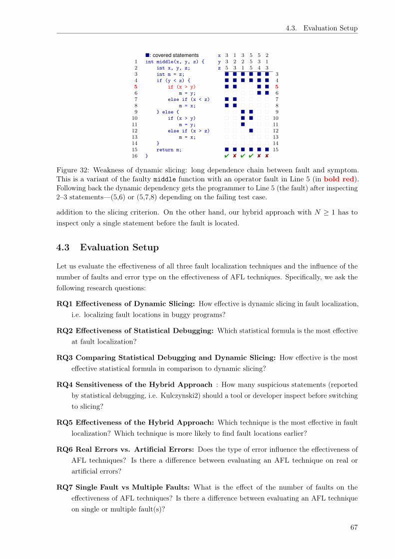
4.3. Evaluation Setup
⌅: covered statements x 3 1 3 5 5 2
1 int middle(x, y, z) { y 3 2 2 5 3 1
2 int x, y, z; z 5 3 1 5 4 3
3 int m = z; ⌅ ⌅ ⌅ ⌅ ⌅ ⌅ 3
4 if (y < z) { ⌅ ⌅ ⌅ ⌅ ⌅ ⌅ 4
5 if (x > y) ⌅ ⌅ ⇤ ⇤ ⌅ ⌅ 5
6 m = y; ⇤ ⇤ ⇤ ⇤ ⌅ ⌅ 6
7 else if (x < z) ⌅ ⌅ ⇤ ⇤ ⇤ ⇤ 7
8 m = x; ⌅ ⌅ ⇤ ⇤ ⇤ ⇤ 8
9 } else { ⇤ ⇤ ⌅ ⌅ ⇤ ⇤ 9
10 if (x > y) ⇤ ⇤ ⌅ ⌅ ⇤ ⇤ 10
11 m = y; ⇤ ⇤ ⌅ ⇤ ⇤ ⇤ 11
12 else if (x > z) ⇤ ⇤ ⇤ ⌅ ⇤ ⇤ 12
13 m = x; ⇤ ⇤ ⇤ ⇤ ⇤ ⇤ 13
14 } ⇤ ⇤ ⇤ ⇤ ⇤ ⇤ 14
15 return m; ⌅ ⌅ ⌅ ⌅ ⌅ ⌅ 15
16 } 4 8 4 4 8 8
Figure 32: Weakness of dynamic slicing: long dependence chain between fault and symptom.This is a variant of the faulty middle function with an operator fault in Line 5 (in bold red).Following back the dynamic dependency gets the programmer to Line 5 (the fault) after inspecting2–3 statements—(5,6) or (5,7,8) depending on the failing test case.
addition to the slicing criterion. On the other hand, our hybrid approach with N � 1 has toinspect only a single statement before the fault is located.
4.3 Evaluation Setup
Let us evaluate the effectiveness of all three fault localization techniques and the influence of thenumber of faults and error type on the effectiveness of AFL techniques. Specifically, we ask thefollowing research questions:
RQ1 Effectiveness of Dynamic Slicing: How effective is dynamic slicing in fault localization,i.e. localizing fault locations in buggy programs?
RQ2 Effectiveness of Statistical Debugging: Which statistical formula is the most effectiveat fault localization?
RQ3 Comparing Statistical Debugging and Dynamic Slicing: How effective is the mosteffective statistical formula in comparison to dynamic slicing?
RQ4 Sensitiveness of the Hybrid Approach : How many suspicious statements (reportedby statistical debugging, i.e. Kulczynski2) should a tool or developer inspect before switchingto slicing?
RQ5 Effectiveness of the Hybrid Approach: Which technique is the most effective in faultlocalization? Which technique is more likely to find fault locations earlier?
RQ6 Real Errors vs. Artificial Errors: Does the type of error influence the effectiveness ofAFL techniques? Is there a difference between evaluating an AFL technique on real orartificial errors?
RQ7 Single Fault vs Multiple Faults: What is the effect of the number of faults on theeffectiveness of AFL techniques? Is there a difference between evaluating an AFL techniqueon single or multiple fault(s)?
67

4. Locating Faults with Program Slicing: An Empirical Analysis
In this chapter, we evaluate the performance of statistical debugging, dynamic slicing andthe hybrid approach in the framework of Steimann, Frenkel, and Abreu [180] where we fix thegranularity of fault localization at statement level and the fault localization mode at one-at-a-time (except for multiple faults in RQ7). In this setting with real errors and real test suites,the provided test suites may not be coverage adequate, e.g. they may not execute all programstatements. Fault localization effectiveness is evaluated as relative wasted effort based on theranking of units in the order they are suggested to be examined (see Section 4.3.4 for moredetails).
4.3.1 Implementation
Let us provide implementation details for each AFL technique.Dynamic Slicing Implementation: The approximate dynamic slice is computed using Frama-C,26
gcov, git-diff, gdb, and several Python libraries. Given the preprocessed source files of a Cprogram, Frama-C computes the static slices for each function and their call graphs as DOT files.The gcov-tool determines the executed/covered statements in the program. The git-diff-tooldetermines the changed statements in the patch and thus the faulty statements in the program.The gdb-tool allows to derive coverage information even for crashing inputs and to determine theslicing criterion as the last executed statement. Our Python script intersects the statements inthe static slice and the set of executed statements to derive the approximate dynamic slice. Weuse the Python libraries pygraphviz27, networkx,28 and matplotlib29 to process the DOT filesand compute the score for the approximate dynamic slice.Statistical Debugging Implementation: The statistical debugging tool was implementedusing two bash scripts with several standard command line tools, notably gcov,30 git-diff31
and gdb32. The differencing tool git-diff identifies those lines in the buggy program that werechanged in the patch. If the patch only added statements, we cannot determine a correspondingfaulty line. Some errors were thus excluded from the evaluation. The code coverage tool, gcovidentifies those lines in the buggy program that are covered by an executed test case. When theprogram crashes, gcov does not emit any coverage information. If the crash is not caused by aninfinite loop, it is sufficient to run the program under test in gdb and force-call the gcov-functionfrom gdb to write the coverage information once the segmentation fault is triggered. This wasautomated as well. However, for some cases, no coverage information could be generated due toinfinite recursion. Gcov also gives the number of executable statements in the buggy program(i.e., |P |).33 Finally, our Python implementation of the scores is used to compute the faultlocalization effectiveness.Hybrid Approach Implementation: The hybrid approach is implemented simply as a com-bination of both tools. If the top-N most suspicious statements do not contain the fault, the
26http://frama-c.com/27https://pygraphviz.github.io/28https://networkx.github.io/29http://matplotlib.org/30https://gcc.gnu.org/onlinedocs/gcc/Gcov.html31https://git-scm.com/docs/git-diff32https://www.gnu.org/software/gdb/documentation/33The executable statements refers to statements for which coverage information are obtainable by Gcov, in
particular, all program statements except spaces, blanks and comments.
68

4.3. Evaluation Setup
dynamic slicing component is informed about the set of statements already inspected in the firstphase. Given the unranked suspiciousness score of every executable statement in the program,the hybrid fault localizer performs an ordinal ranking of all statements. It then determinesthe proportion of the top N rank of suspicious statements, based on the N value of the hybridapproach. For instance, an hybrid approach with N = 5 takes the five topmost suspiciousstatements. Then, it determines the highest ranked faulty statement in the rank of all suspiciousstatements. If the faulty statement is in the top N suspicious positions (e.g. third position), thenit reports the number of statements in the top ranked positions up till the faulty statement, as aproportion of all executable program statements.
In the case that the suspicious statement is not in the top N suspicious positions (e.g. seventhposition), then it proceeds to slicing and reports the cardinality of the set union of all N topranked statements and the number of inspected statements in the slice before the first faultystatement.
4.3.2 Metrics and Measures
Odds Ratio . To establish the superiority of one technique A over another technique B, it iscommon to measure the effect size of A w.r.t. B. A standard measure of effect size and widelyused is the odds ratio [181]. It “is a measure of how many times greater the odds are that amember of a certain population will fall into a certain category than the odds are that a memberof another population will fall into that category” [181]. In our case, let “A is successful ” meanthat fault localization technique A is more effective than fault localization technique B and let a
be the number of successes for A, b the number of successes for B, and n = a+ b the total numberof successes. Then, the odds ratio is calculated as
=
a + ⇢
n + ⇢� a
!, b + ⇢
n + ⇢� b
!
where ⇢ is an arbitrary positive constant (e.g., ⇢ = 0.5) used to avoid problems with zero successes.There is no difference between the two algorithms when = 1, while > 1 indicates thattechnique A has higher chances of success. For example, an odds ratio of five means that faultlocalization technique A is five times more likely to be successful (i.e., more effective as comparedto B) at fault localization than B.
The Mann-Whitney U -test is used to show whether there is a statistical difference betweentwo techniques [182]. In general, it is a non-parametric test of the null hypothesis that twosamples come from the same population against an alternative hypothesis, especially that aparticular population tends to have larger values than the other. Unlike the t-test it does notrequire the assumption that the data is normally distributed. More specifically, it shows whetherthe difference in performance of two techniques is actually statistically significant.
A cumulative frequency curve is a running total of frequencies. We use such curves to showthe percentage of errors that require examining up to a certain number of program locations.The number of code locations examined is plotted on a log-scale because the difference betweenexamining 5 to 10 locations is more important than difference between examining 1005 to 1010locations.
69

4. Locating Faults with Program Slicing: An Empirical Analysis
Table 1: Details of Subject Programs
Benchmark Tool Avg. Size #Errors #Failing #Passing(Error Type) (Program) (LoC) Tests Tests
SIR(Artificial)
tcas 65.1 37 1356 58140print_tokens 199 3 184 12206print_tokens2 199.5 8 2031 30889tot_info 125 18 1528 17408schedule 160.5 4 690 9910schedule2 139.2 4 116 10724
IntroClass(Real;
Students)
checksum 11.3 3 7 41digits 17.4 3 16 32grade 16.1 8 30 114median 13.5 2 8 18smallest 13.2 2 16 16syllables 11.6 2 12 20
Codeflaws(Real;
Competitions)
WTLW (71A) 10.3 11 60 61HQ9+ (133A) 10.9 18 270 1260AG (144A) 24.5 13 302 202IB (478A) 8.6 20 31 329TN (535A) 61.2 9 118 778Exam (534A) 17.5 12 108 68Holidays (670A) 12.8 9 662 1118DC (495A) 14.5 13 96 279VBT(336A) 13.6 14 108 309PP(509B) 21.2 16 84 98DHHF (515B) 29.5 15 127 707HVW2 (143A) 17.5 16 124 707Ball Game (46A) 10 8 114 148WE (31A) 14.4 14 187 200LM (146B) 29.5 11 116 355SG (570B) 7.5 11 69 531WD (168A) 7.7 9 132 254Football (417C) 13.2 13 64 352MS (218A) 16.5 10 156 156Joysticks (651A) 12.6 8 66 246
CoREBench(Real;
Developers)
core. (cut) 306 4 4 6core. (rm) 110 1 1 63core. (ls) 1605.5 2 2 73core. (du) 315 1 1 28core. (seq) 219.7 3 3 5core. (expr) 321 1 1 1core. (copy) 897 1 1 59find (parser) 119.3 3 3 286find (ftsfind) 211.5 2 2 183find (pred) 825 2 2 235grep (dfasearch) 181.5 2 2 46grep (savedir) 64 1 1 15grep (kwsearch) 77 2 2 46grep (main) 853.5 2 2 45
Total 35 (46) 369 9012 148767
70
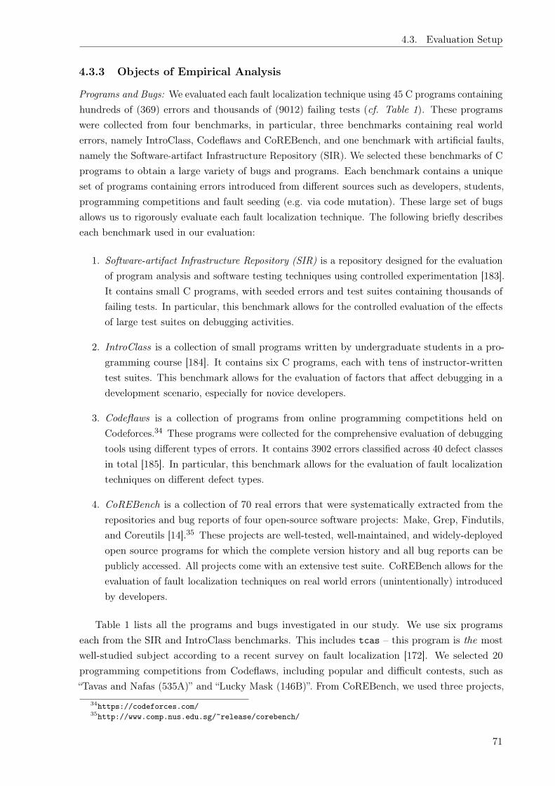
4.3. Evaluation Setup
4.3.3 Objects of Empirical Analysis
Programs and Bugs: We evaluated each fault localization technique using 45 C programs containinghundreds of (369) errors and thousands of (9012) failing tests (cf. Table 1). These programswere collected from four benchmarks, in particular, three benchmarks containing real worlderrors, namely IntroClass, Codeflaws and CoREBench, and one benchmark with artificial faults,namely the Software-artifact Infrastructure Repository (SIR). We selected these benchmarks of Cprograms to obtain a large variety of bugs and programs. Each benchmark contains a uniqueset of programs containing errors introduced from different sources such as developers, students,programming competitions and fault seeding (e.g. via code mutation). These large set of bugsallows us to rigorously evaluate each fault localization technique. The following briefly describeseach benchmark used in our evaluation:
1. Software-artifact Infrastructure Repository (SIR) is a repository designed for the evaluationof program analysis and software testing techniques using controlled experimentation [183].It contains small C programs, with seeded errors and test suites containing thousands offailing tests. In particular, this benchmark allows for the controlled evaluation of the effectsof large test suites on debugging activities.
2. IntroClass is a collection of small programs written by undergraduate students in a pro-gramming course [184]. It contains six C programs, each with tens of instructor-writtentest suites. This benchmark allows for the evaluation of factors that affect debugging in adevelopment scenario, especially for novice developers.
3. Codeflaws is a collection of programs from online programming competitions held onCodeforces.34 These programs were collected for the comprehensive evaluation of debuggingtools using different types of errors. It contains 3902 errors classified across 40 defect classesin total [185]. In particular, this benchmark allows for the evaluation of fault localizationtechniques on different defect types.
4. CoREBench is a collection of 70 real errors that were systematically extracted from therepositories and bug reports of four open-source software projects: Make, Grep, Findutils,and Coreutils [14].35 These projects are well-tested, well-maintained, and widely-deployedopen source programs for which the complete version history and all bug reports can bepublicly accessed. All projects come with an extensive test suite. CoREBench allows for theevaluation of fault localization techniques on real world errors (unintentionally) introducedby developers.
Table 1 lists all the programs and bugs investigated in our study. We use six programseach from the SIR and IntroClass benchmarks. This includes tcas – this program is the mostwell-studied subject according to a recent survey on fault localization [172]. We selected 20programming competitions from Codeflaws, including popular and difficult contests, such as“Tavas and Nafas (535A)” and “Lucky Mask (146B)”. From CoREBench, we used three projects,
34https://codeforces.com/35http://www.comp.nus.edu.sg/~release/corebench/
71

4. Locating Faults with Program Slicing: An Empirical Analysis
Table 2: Details of Multiple Faults
Benchmark Tool # Buggy #Faults #Failing #Passing(Error Type) Programs Tests Tests
SIR(Mutated)
tcas 37 144 19973 39523print_tokens 3 11 12074 316print_tokens2 8 28 27630 5290tot_info 18 64 16667 2269schedule 4 17 9673 927schedule2 4 16 8616 2224
IntroClass(Mutated)
checksum 1 4 15 1digits 2 7 30 2grade 5 22 67 23median 2 8 13 13smallest 1 4 8 8syllables 3 13 34 14
Total 88 338 94800 50610
namely the Coreutils, Grep and Find project. Notably, all projects in CoREBench come fromthe GNU open source C programs, in particular, these three projects contain a total of 103 tools.Due to code modularity, the program size for a single tool (e.g. cut in coreutils) contain afew hundred LoC (about 306 LoC), however, the entire code base for CoREBench is fairly large.For instance, Coreutils, Grep and Find have 83k, 18k and 11k LoC, respectively [14]. For eachbenchmark, we exempted programs where Frama-C could not construct the Program DependenceGraph (PDG). For instance, because it cannot handle some recursive or variadic method calls. Inaddition, we excluded an error if no coverage information could be generated (e.g., infinite loops)or the faulty statement could not be identified (e.g., omission faults where the patch only addedstatements).
Single Faults: For our evaluation (all RQs except RQ7), we used buggy programs collectedfrom benchmarks where each program contained only a single fault, for most programs. Todetermine single faults in our bug dataset, for each program, we executed all tests available for aproject on the fixed version of the program, in order to determine if there are any failing testcases that are unrelated to the bug at hand. Our evaluation revealed that our dataset containedmostly single bugs (368/369=99.7%). Almost all buggy program versions had exactly one fault,except for a single program – Codeflaws version DC 495A. For all benchmarks, only this programcontained multiple faults, i.e. more than one fault. This distribution of single faults portrays thehigh prevalence of single faults and single-fault fixes in the wild [186].
Multiple Faults: To evaluate the effectiveness of all three fault localization techniques onmultiple faults (see RQ7), we automatically curated a set of multiple faults using mutation-basedfault injection, in line with the evaluation of multiple bugs in previous works [187, 188, 189, 190,191].36 We automatically mutated the original passing version of each program until we have abuggy version containing between three to five faults. In particular, we performed logical andarithmetic operator mutation on each passing version of the programs contained in the SIR andIntroClass benchmarks. Table 2 provides details of the buggy programs with multiple faults,the number of faults, as well as the number of failing and passing test cases. For each fault
36To the best of our knowledge, there is no known benchmark of real-world multiple bugs.
72
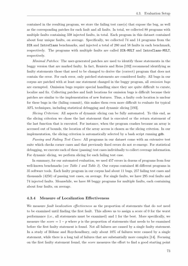
4.3. Evaluation Setup
contained in the resulting program, we store the failing test case(s) that expose the bug, as wellas the corresponding patches for each fault and all faults. In total, we collected 88 programs withmultiple faults containing 338 injected faults, in total. Each program in this dataset containedabout four unique faults, on average. Specifically, we collected 74 and 14 programs from theSIR and IntroClass benchmarks, and injected a total of 280 and 58 faults in each benchmark,respectively. The programs with multiple faults are called SIR-MULT and IntroClass-MULT,respectively.
Minimal Patches: The user-generated patches are used to identify those statements in thebuggy version that are marked faulty. In fact, Renieris and Reiss [192] recommend identifying asfaulty statements those that need to be changed to derive the (correct) program that does notcontain the error. For each error, only patched statements are considered faulty. All bugs in ourcorpus are patched with at least one statement changed in the buggy program, all omission bugsare exempted. Omission bugs require special handling since they are quite difficult to curate,localize and fix. Collecting patches and fault locations for omission bugs is difficult because theirpatches are similar to the implementation of new features. Thus, a faulty code location is unclearfor these bugs in the (failing commit), this makes them even more difficult to evaluate for typicalAFL techniques, including statistical debugging and dynamic slicing [193].
Slicing Criterion: All aspects of dynamic slicing can be fully automated. To this end, asthe slicing criterion we chose the last statement that is executed or the return statement ofthe last function that is executed. For instance, when the program crashes because an array isaccessed out of bounds, the location of the array access is chosen as the slicing criterion. In ourimplementation, the slicing criterion is automatically selected by a bash script running gdb.
Passing and Failing Test Cases: All programs in our dataset come with an extensive testsuite which checks corner cases and that previously fixed errors do not re-emerge. For statisticaldebugging, we execute each of these (passing) test cases individually to collect coverage information.For dynamic slicing, we perform slicing for each failing test case.
In summary, for our automated evaluation, we used 457 errors in dozens of programs from fourwell-known benchmarks (see Table 1 and Table 2). Our corpus contained 46 different programs in35 software tools. Each faulty program in our corpus had about 11 bugs, 257 failing test cases andthousands (4250) of passing test cases, on average. For single faults, we have 295 real faults and74 injected faults. Meanwhile, we have 88 buggy programs for multiple faults, each containingabout four faults, on average.
4.3.4 Measure of Localization Effectiveness
We measure fault localization effectiveness as the proportion of statements that do not needto be examined until finding the first fault. This allows us to assign a score of 0 for the worstperformance (i.e., all statements must be examined) and 1 for the best. More specifically, wemeasure the score = 1 � p where p is the proportion of statements that needs to be examinedbefore the first faulty statement is found. Not all failures are caused by a single faulty statement.In a study of Böhme and Roychoudhury, only about 10% of failures were caused by a singlestatement, while there is a long tail of failures that are substantially more complex [14]. Focusingon the first faulty statement found, the score measures the effort to find a good starting point
73

4. Locating Faults with Program Slicing: An Empirical Analysis
to initiate the bug-fixing process rather than to provide the complete set of code that must bemodified, deleted, or added to fix the failure. [172] motivates this measure of effectiveness andpresents an overview of other measures.General Measures
Ranking. All three fault localization techniques presented in this chapter produce a ranking.The developer starts examining the highest ranked statement and goes down the list until reachingthe first faulty statement. To generate the ranking for statistical debugging, we list all statementsin the order of their suspiciousness (as determined by the technique), most suspicious first. Togenerate the ranking for approximate dynamic slicing, given the statement c where the failureis observed, we rank first those statements in the slice that can be reached from c along onebackward dependency edge. Then, we rank those statements that can be reached from c alongtwo backward dependency edges, and so on. Generally, for all techniques, the score is computedas
score = 1 � |S||P |
where S are all statements with the same rank or less as the highest ranked faulty statementand P is the set of all statements in the program. So, S represents the statements a developerneeds to examine until finding the first faulty one.37.
Multiple Statements, Same Rank. In most cases there are several statements that have thesame rank as the faulty statement. For all our evaluations, we employ ordinal ranking, in order toeffectively determine the top N most suspicious statements for each technique. This is necessaryto evaluate the fault localization effectiveness of each technique, if a developer is only willing toinspect N most suspicious statements [177]. In ordinal ranking, lines with the same score arere-ranked by line numbers.38 This is in agreement with evaluations of fault localization techniquesin previous work [172, 194, 177].
Multiple Faults, Expense Score. For multiple faults, we measure fault localization effectivenessusing the expense score [176]. The expense score is the percentage of the program (statements)that must be examined to find the first fault, in particular, the first faulty statement in the firstlocalized fault using the ranking given by the fault localization technique. It is similar to the scoreemployed for single faults, and it has been employed in previous evaluations of multiple faults,such as [191, 190]. Formally:
expense score =|S||P | ⇤ 100
where S are all statements with the same rank or less as the highest ranked faulty statement forthe first fault found and P is the set of all executable statements in the program. So, S representsthe statements a developer needs to examine until finding the first faulty statement, for the firstlocalized fault. The assumption is that it is the first fault that the developer would begin fixing,thus, finding the first statement suffices for the diagnosis of all faults [176]. In our evaluation ofmultiple faults, the fault localization effectiveness score is computed similarly to single faults as
scoremult = 1 � (expense score/100)
37Note that all executable program statements are ranked in the suspiciousness rank, executable statementsthat are not contained in the dynamic slice are ranked lowest.
38Ranking ties are broken in ascending order, i.e. if both lines 10 and 50 have the same score, then line number10 is ranked above line number 50.
74
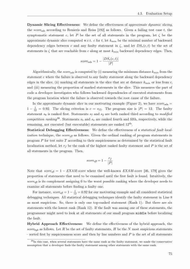
4.3. Evaluation Setup
Dynamic Slicing Effectiveness: We define the effectiveness of approximate dynamic slicing,the scoreads according to Renieris and Reiss [192] as follows. Given a failing test case t, thesymptomatic statement c, let P be the set of all statements in the program, let ⇣ be theapproximate dynamic slice computed w.r.t. c for t, let kmin be the minimal number of backwarddependency edges between c and any faulty statement in ⇣, and let DS⇤(c, t) be the set ofstatements in ⇣ that are reachable from c along at most kmin backward dependency edges. Then,
scoreads = 1 � |DS⇤(c, t)||P |
Algorithmically, the scoreads is computed by (i) measuring the minimum distance kmin from thestatement c where the failure is observed to any faulty statement along the backward dependencyedges in the slice, (ii) marking all statements in the slice that are at distance kmin or less from c,and (iii) measuring the proportion of marked statements in the slice. This measures the part ofcode a developer investigates who follows backward dependencies of executed statements fromthe program location where the failure is observed towards the root cause of the failure.
In the approximate dynamic slice in our motivating example (Figure 2), we have scoreads =
1 � 112 = 0.92. The slicing criterion is c = s15. The program size is |P | = 12. The faulty
statement s8 is ranked first. Statements s7 and s2 are both ranked third according to modifiedcompetition ranking39. Statements s5 and s4 are ranked fourth and fifth, respectively, while theremaining, not executed (but executable) statements are ranked 12th.Statistical Debugging Effectiveness: We define the effectiveness of a statistical fault local-ization technique, the scoresfl as follows. Given the ordinal ranking of program statements inprogram P for test suite T according to their suspiciousness as determined by the statistical faultlocalization method, let rf be the rank of the highest ranked faulty statement and P is the set ofall statements in the program. Then,
scoresfl = 1 �rf
|P |
Note that scoresfl = 1 � EXAM-score where the well-known EXAM-score [46, 179] gives theproportion of statements that need to be examined until the first fault is found. Intuitively, thescoresfl is its complement assigning 0 to the worst possible ranking where the developer needs toexamine all statements before finding a faulty one.
For instance, scoresfl = 1� 112 = 0.92 for our motivating example and all considered statistical
debugging techniques. All statistical debugging techniques identify the faulty statement in Line 8as most suspicious. So, there is only one top-ranked statement (Rank 1). But there are sixstatements with the lowest rank (Rank 12). If the fault was among one of these statements, theprogrammer might need to look at all statements of our small program middle before localizingthe fault.Hybrid Approach Effectiveness: We define the effectiveness of the hybrid approach, thescorehyb as follows. Let R be the set of faulty statements, H be the N most suspicious statements– sorted first by suspiciousness score and then by line numbers and P is the set of all statements
39In this case, when several statements have the same rank as the faulty statement, we made the conservativeassumption that a developer finds the faulty statement among other statements with the same rank.
75
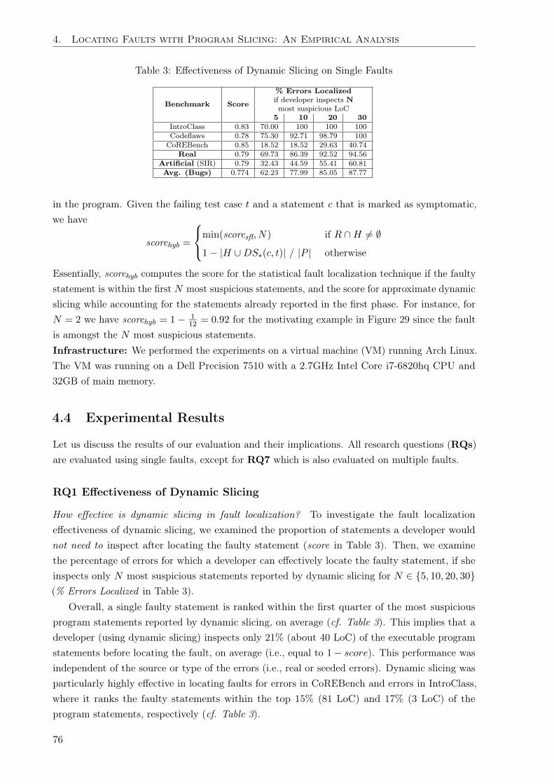
4. Locating Faults with Program Slicing: An Empirical Analysis
Table 3: Effectiveness of Dynamic Slicing on Single Faults
Benchmark Score
% Errors Localized
if developer inspects N
most suspicious LoC
5 10 20 30
IntroClass 0.83 70.00 100 100 100
Codeflaws 0.78 75.30 92.71 98.79 100
CoREBench 0.85 18.52 18.52 29.63 40.74
Real 0.79 69.73 86.39 92.52 94.56
Artificial (SIR) 0.79 32.43 44.59 55.41 60.81
Avg. (Bugs) 0.774 62.23 77.99 85.05 87.77
in the program. Given the failing test case t and a statement c that is marked as symptomatic,we have
scorehyb =
8<
:min(scoresfl, N) if R \ H 6= ;
1 � |H [ DS⇤(c, t)| / |P | otherwise
Essentially, scorehyb computes the score for the statistical fault localization technique if the faultystatement is within the first N most suspicious statements, and the score for approximate dynamicslicing while accounting for the statements already reported in the first phase. For instance, forN = 2 we have scorehyb = 1 � 1
12 = 0.92 for the motivating example in Figure 29 since the faultis amongst the N most suspicious statements.Infrastructure: We performed the experiments on a virtual machine (VM) running Arch Linux.The VM was running on a Dell Precision 7510 with a 2.7GHz Intel Core i7-6820hq CPU and32GB of main memory.
4.4 Experimental Results
Let us discuss the results of our evaluation and their implications. All research questions (RQs)are evaluated using single faults, except for RQ7 which is also evaluated on multiple faults.
RQ1 Effectiveness of Dynamic Slicing
How effective is dynamic slicing in fault localization? To investigate the fault localizationeffectiveness of dynamic slicing, we examined the proportion of statements a developer wouldnot need to inspect after locating the faulty statement (score in Table 3). Then, we examinethe percentage of errors for which a developer can effectively locate the faulty statement, if sheinspects only N most suspicious statements reported by dynamic slicing for N 2 {5, 10, 20, 30}(% Errors Localized in Table 3).
Overall, a single faulty statement is ranked within the first quarter of the most suspiciousprogram statements reported by dynamic slicing, on average (cf. Table 3). This implies that adeveloper (using dynamic slicing) inspects only 21% (about 40 LoC) of the executable programstatements before locating the fault, on average (i.e., equal to 1 � score). This performance wasindependent of the source or type of the errors (i.e., real or seeded errors). Dynamic slicing wasparticularly highly effective in locating faults for errors in CoREBench and errors in IntroClass,where it ranks the faulty statements within the top 15% (81 LoC) and 17% (3 LoC) of theprogram statements, respectively (cf. Table 3).
76
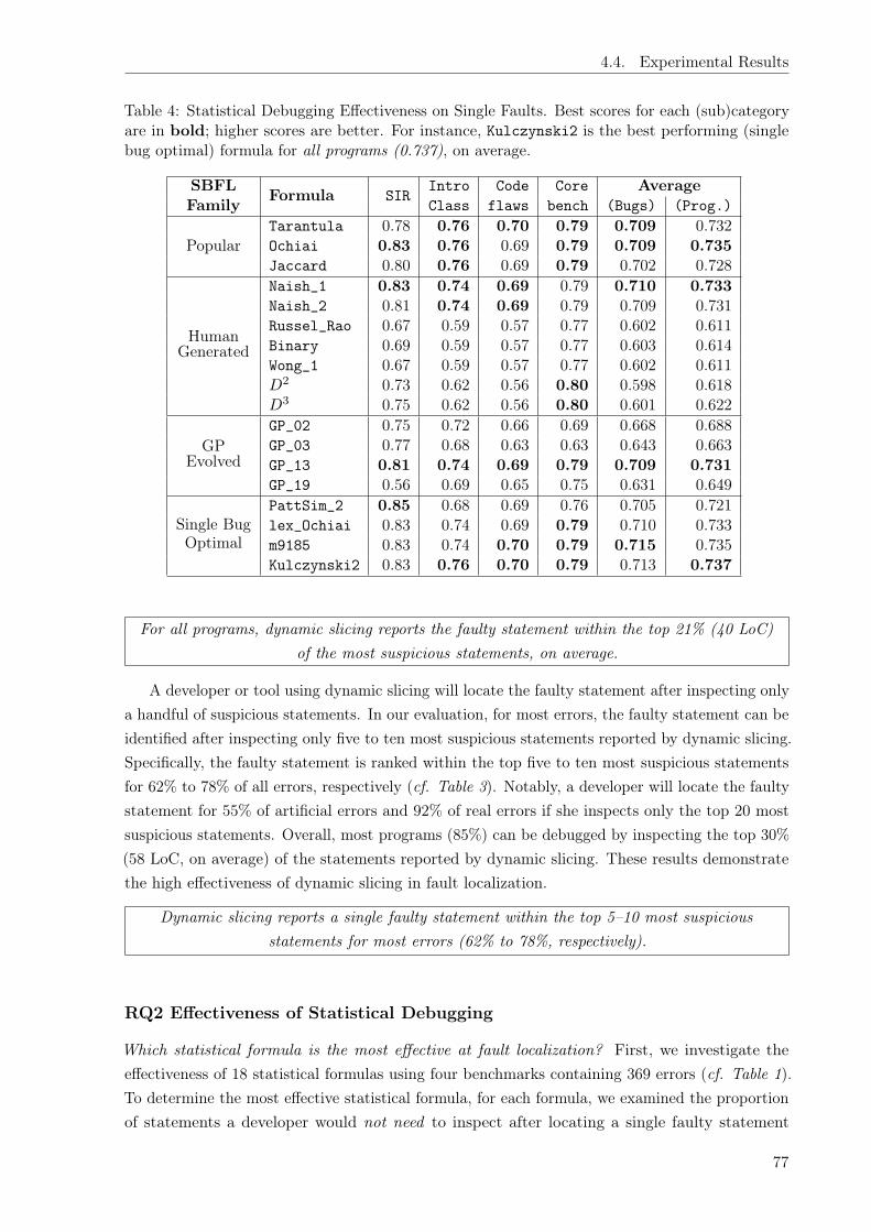
4.4. Experimental Results
Table 4: Statistical Debugging Effectiveness on Single Faults. Best scores for each (sub)categoryare in bold; higher scores are better. For instance, Kulczynski2 is the best performing (singlebug optimal) formula for all programs (0.737), on average.
SBFL Formula SIRIntro Code Core Average
Family Class flaws bench (Bugs) (Prog.)
PopularTarantula 0.78 0.76 0.70 0.79 0.709 0.732Ochiai 0.83 0.76 0.69 0.79 0.709 0.735Jaccard 0.80 0.76 0.69 0.79 0.702 0.728
HumanGenerated
Naish_1 0.83 0.74 0.69 0.79 0.710 0.733Naish_2 0.81 0.74 0.69 0.79 0.709 0.731Russel_Rao 0.67 0.59 0.57 0.77 0.602 0.611Binary 0.69 0.59 0.57 0.77 0.603 0.614Wong_1 0.67 0.59 0.57 0.77 0.602 0.611D
2 0.73 0.62 0.56 0.80 0.598 0.618D
3 0.75 0.62 0.56 0.80 0.601 0.622
GPEvolved
GP_02 0.75 0.72 0.66 0.69 0.668 0.688GP_03 0.77 0.68 0.63 0.63 0.643 0.663GP_13 0.81 0.74 0.69 0.79 0.709 0.731GP_19 0.56 0.69 0.65 0.75 0.631 0.649
Single BugOptimal
PattSim_2 0.85 0.68 0.69 0.76 0.705 0.721lex_Ochiai 0.83 0.74 0.69 0.79 0.710 0.733m9185 0.83 0.74 0.70 0.79 0.715 0.735Kulczynski2 0.83 0.76 0.70 0.79 0.713 0.737
For all programs, dynamic slicing reports the faulty statement within the top 21% (40 LoC)of the most suspicious statements, on average.
A developer or tool using dynamic slicing will locate the faulty statement after inspecting onlya handful of suspicious statements. In our evaluation, for most errors, the faulty statement can beidentified after inspecting only five to ten most suspicious statements reported by dynamic slicing.Specifically, the faulty statement is ranked within the top five to ten most suspicious statementsfor 62% to 78% of all errors, respectively (cf. Table 3). Notably, a developer will locate the faultystatement for 55% of artificial errors and 92% of real errors if she inspects only the top 20 mostsuspicious statements. Overall, most programs (85%) can be debugged by inspecting the top 30%(58 LoC, on average) of the statements reported by dynamic slicing. These results demonstratethe high effectiveness of dynamic slicing in fault localization.
Dynamic slicing reports a single faulty statement within the top 5–10 most suspiciousstatements for most errors (62% to 78%, respectively).
RQ2 Effectiveness of Statistical Debugging
Which statistical formula is the most effective at fault localization? First, we investigate theeffectiveness of 18 statistical formulas using four benchmarks containing 369 errors (cf. Table 1).To determine the most effective statistical formula, for each formula, we examined the proportionof statements a developer would not need to inspect after locating a single faulty statement
77

4. Locating Faults with Program Slicing: An Empirical Analysis
DSta
r2
DSta
r3
Won
g1
Russ
elR
aoB
inar
yN
aish
1N
aish
2
Tar
antu
laO
chia
iJa
ccar
d
GP
02G
P03
GP
13G
P19
m91
85K
ulc
zynsk
i2le
xO
chia
iPat
tSim
20.4
0.5
0.6
0.7
0.8
0.9
Sco
re
E�ectiveness of all statistical formulas
SIR IntroClass Codeflaws CorebenchD
Sta
r2
DSta
r3
Won
g1
Russ
elR
aoB
inar
yN
aish
1N
aish
2
Tar
antu
laO
chia
iJa
ccar
d
GP
02G
P03
GP
13G
P19
m91
85K
ulc
zynsk
i2le
xO
chia
iPat
tSim
2
0.0
0.5
1.0
1.5
2.0
2.5
3.0
Sco
re
E�ectiveness of all statistical formulas
SIR IntroClass Codeflaws Corebench
(a) Each Benchmark (b) All Benchmarks
Figure 33: Effectiveness of each statistical debugging formula: (a) results are grouped into barsfor each family, and (b) cumulative results for all benchmarks (stacked for all families)
SIR IntroClass Codeflaws Corebench0.5
0.6
0.7
0.8
0.9
1.0
Sco
re
E�ectiveness of the most e�ective statistical formula
Ochiai Naish 1 GP 13 Kulczynski2
Ochiai Naish 1 GP 13 Kulczynski20.70
0.71
0.72
0.73
0.74
0.75
0.76
Sco
re
0.7350.733
0.731
0.737
Average over programs for the best-performing formulas
All
(a) Each Benchmark (b) All Benchmarks
Figure 34: Effectiveness of the most effective statistical formula in (a) each family and (b) theoverall average
78

4.4. Experimental Results
Table 5: Effectiveness of Kulczynski2 on single faults, i.e. the most effective statistical formula
Benchmark Score
% Errors Localized
if developer inspects N
most suspicious LoC
5 10 20 30
IntroClass 0.76 80.00 85.00 100 100
Codeflaws 0.69 64.37 86.23 97.57 99.19
CoREBench 0.79 22.22 25.93 37.04 48.15
Real 0.72 61.56 80.61 92.18 94.56
Artificial (SIR) 0.83 35.14 41.89 68.92 71.62
Avg. (Bugs) 0.713 56.25 72.83 87.50 89.95
(score in Table 4). Figure 33 (a) and (b) further illustrate the effectiveness of the SBFL formulas.Then, for the best performing statistical formula, we inspected the percentage of errors for whicha developer can effectively locate the faulty statement, if she inspects only N most suspiciousstatements for N 2 {5, 10, 20, 30} (% Errors Localized in Table 5).
Overall, the single bug optimal formulas are the most effective family of statistical formulas,they are the best performing formulas across all errors and programs. In particular, on average,PattSim2 performed best for injected errors (i.e. SIR), while Kulczynski2 outperformed all otherformulas for real errors, especially for IntroClass (cf. Table 4). Bold values in Table 4 indicatethe best performing formula for each family and (sub)category. For instance, Kulczynski2 isthe best performing (single bug optimal) formula for all programs (0.737). The performance ofsingle-bug optimal formulas supports the results obtained in previous works [195]. This family ofstatistical formulas are particularly effective because they are optimized for programs containinga single bug; based on the observation that if a program contains only a single bug, then allfailing traces cover that bug [196].
The single bug optimal statistical formulas outperformed all other SBFL formulas,for both injected and real errors, on average.
The most effective statistical formula is Kulczynski2, it outperformed all other formulas inour evaluation (see Table 4 and Figure 33 (a) and (b)). The most effective statistical formulafor each family are Ochiai, Naish_1, GP_13 and Kulczynski2 for the popular, human-generated,genetically-evolved and single bug optimal families, respectively. Figure 34 (a) and (b) comparesthe performance of the most effective formula in each family. For instance, in the popularstatistical family, Ochiai is the best performing formula, both for all errors (0.709) and allprograms (0.735) (cf. Table 4). Meanwhile, in the single bug optimal family, Kulczynski2 is thebest performing formula for all programs (0.737) (cf. Table 4).
Indeed, a developer using Kulczynski2 will inspect the least number of suspicious programstatements before finding the faulty statement. On average, Kulczynski2 required a developer toinspect about 26% (51 LoC) of the program code before finding the faulty statement. Among allstatistical formulas, it has the highest suspiciousness rank for 40% (14 out of 35) of the programsand 72% (265 out of 369) of all errors. It is also the most effective statistical formula for localizingreal errors.40
40Further evaluations in this chapter use Kulczynski2 as the default “statistical debugging” formula.
79

4. Locating Faults with Program Slicing: An Empirical Analysis
0.0 0.2 0.4 0.6 0.8 1.0
Statistical Debugging E�ectiveness
0.0
0.2
0.4
0.6
0.8
1.0
Slici
ng
E�ec
tive
nes
s
SIR
0.0 0.2 0.4 0.6 0.8 1.0
Statistical Debugging E�ectiveness
0.0
0.2
0.4
0.6
0.8
1.0
Slici
ng
E�ec
tive
nes
s
IntroClass
(a) SIR (b) IntroClass
0.0 0.2 0.4 0.6 0.8 1.0
Statistical Debugging E�ectiveness
0.0
0.2
0.4
0.6
0.8
1.0
Slici
ng
E�ec
tive
nes
s
Codeflaws
0.0 0.2 0.4 0.6 0.8 1.0
Statistical Debugging E�ectiveness
0.0
0.2
0.4
0.6
0.8
1.0
Slici
ng
E�ec
tive
nes
s
Corebench
(c.) Codeflaws (d.) CoREBench
Figure 35: Direct comparison of fault localization effectiveness between statistical debugging(Kulczynski2) and dynamic slicing (on single faults) in each benchmark
Kulczynski2 is the most effective statistical formula, on average, requiring a developer toinspect only 26% (51 LoC) before finding the fault.
A tool or developer using Kulczynski2 will locate the faulty statement after inspecting fiveto ten most suspicious statements. The faulty statement is ranked within the top five to ten mostsuspicious statements for most errors, i.e. 56% to 73% of all errors, respectively (cf. Table 5).Overall, most programs (60%) can be debugged by inspecting the top 30% (58 LoC) of thesuspicious statements reported by Kulczynski2.
Kulczynski2 reports the faulty statements within the top 5–10 most suspicious statements for56% to 72% of all errors, respectively.
Is the difference in the performance of Kulczynski2 statistically significant, in comparison tothe best performing formula for each statistical debugging family? In our evaluation, the differencein the performance of Kulczynski2 (i.e. the best performing formula) is not statistically significant.Table 6 highlights the statistical tests comparing Kulczynski2 to the best performing statisticalformula in each family, i.e. Kulczynski2 vs. {Ochiai, Naish1, GP13}. Notably, the performance
80

4.4. Experimental Results
Table 6: Statistical Tests for the most effective Statistical Debugging Formulas; Odds ratio (allratios are statistically significant Mann-Whitney U -test< 0.05 for all tests)
Odds Ratio (Mann Whitney test score U)Benchmark Kulczynski2 Kulczynski2 Kulczynski2
vs. Ochiai vs. Naish1 vs. GP_13SIR 0.2985 (0.0002) 0.0004 (0) 0.0004 (0)
IntroClass 0.0006 (0) 0.0183 (0) 0.0059 (0)Codeflaws 0.0013 (0) 0.0005 (0) 0.0002 (0)CoREBench 0.0003 (0) 0.0003 (0) 0.0003 (0)All Bugs 0.0106 (0) 0.0006 (0) 0.0002 (0)
of Kulczynski2 is not statistically significant, in comparison to the the best statistical formulafor each family. This is evident from the fact that the odds ratio is less than one ( < 1) for alltest comparisons (see Table 6). This suggests that Kulczynski2 has no statistically significantadvantage over the best performing statistical formulas in each family; despite the fact that, inabsolute terms, Kulczynski2 outperforms the best formula in each family.
Kulczynski2 has no statistically significant advantage over the best formula in other SBFLfamilies (i.e., Ochiai, Naish1 and GP13).
RQ3 Comparing Statistical Debugging and Dynamic Slicing
How effective is the most effective statistical formula in comparison to dynamic slicing? Wecompare the performance of the most effective statistical formula (Kulczynski2) to that ofdynamic slicing (cf. Figure 35 and Figure 36).
We find that on average, dynamic slicing is more effective than statistical debugging at faultlocalization. Slicing is about eight percentage points more effective than the best performingstatistical formula for all programs in our evaluation (cf. Figure 36, Table 3 and Table 5). For allerrors in our study, a programmer using dynamic slicing needs to examine about three-quarters(78%) of those statements that she would need to examine if she used statistical debugging.41
This result is independent of the type of errors or program. Figure 36 shows that dynamicslicing consistently outperforms statistical debugging for each benchmark, with slicing consistentlylocalizing all faults ahead of statistical debugging.
Overall, dynamic slicing was eight percentage points more effective than the best performingstatistical debugging formula, i.e. Kulczynski2.
For two-third of bugs (66%, 243 out of 369 errors), dynamic slicing will find the fault earlierthan the best performing statistical debugging formula. Figure 35 shows a direct comparisonof the scores computed for slicing and statistical debugging. Each scatter plot shows for eacherror the effectiveness score of statistical debugging on the x-axis and the effectiveness score ofslicing on the y-axis. Errors plotted above the diagonal line are better localized using dynamicslicing. For all benchmarks, the majority of the points are above the diagonal line which indicates
41Percentage improvement is measured as 1�0.7941�0.737 . Note that score by itself gives the number of statements
that need not be examined.
81

4. Locating Faults with Program Slicing: An Empirical Analysis
1 2 5 10 20 50 100 200
Locations examined to find fault location
0%
20%
40%
60%
80%
100%
Err
ors
loca
lize
d
Locations to be examined for SIR
Slicing Stat.Dbg Hybrid 5 Hybrid 2
1 2 5 10 20 50 100 200
Locations examined to find fault location
0%
20%
40%
60%
80%
100%
Err
ors
loca
lize
d
Locations to be examined for IntroClass
Slicing Stat.Dbg Hybrid 5 Hybrid 2
(a) SIR (b) IntroClass
1 2 5 10 20 50 100 200
Locations examined to find fault location
0%
20%
40%
60%
80%
100%
Err
ors
loca
lize
d
Locations to be examined for Codeflaws
Slicing Stat.Dbg Hybrid 5 Hybrid 2
1 2 5 10 20 50 100 200
Locations examined to find fault location
0%
20%
40%
60%
80%
100%
Err
ors
loca
lize
d
Locations to be examined for Corebench
Slicing Stat.Dbg Hybrid 5 Hybrid 2
(c.) Codeflaws (d.) CoREBench
Figure 36: Cumulative frequency of the locations to be examined, for dynamic slicing vs. statisticaldebugging vs. the hybrid approach (on single faults) in each benchmark
that slicing outperforms statistical debugging in most cases. We can see that dynamic slicingconsistently outperforms statistical debugging across all benchmarks.
For two-third (66%) of bugs, dynamic slicing locates the fault earlier than the best performingstatistical debugging formula, i.e. Kulczynski2.
To compare the significance of dynamic slicing and statistical debugging, we compute theodds ratio and conduct a Mann-Whitney U -test (cf. Slicing vs. Kulczynski2 in Table 7). Theodds ratio is in favor of dynamic slicing ( > 1) for all projects. In particular, slicing is 62%more likely to find a faulty statement earlier than statistical debugging, this likelihood is alsostatistically significant according to the Mann-Whitney test. The statistically significant oddsratio is explained by slicing being more effective than statistical debugging in most cases. Forinstance, slicing is more effective than statistical debugging for 50 out of 74 bugs in the SIRbenchmark and for 18 out of 27 bugs in CoREBench.
Dynamic slicing is significantly more likely to find a faulty statementearlier than statistical debugging.
82
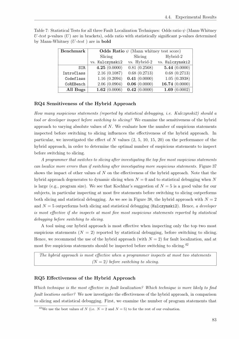
4.4. Experimental Results
Table 7: Statistical Tests for all three Fault Localization Techniques: Odds ratio (Mann-WhitneyU -test p-values (U) are in brackets), odds ratio with statistically significant p-values determinedby Mann-Whitney (U -test ) are in bold
Benchmark Odds Ratio (Mann whitney test score)Slicing Slicing Hybrid-2
vs. Kulczynski2 vs. Hybrid-2 vs. Kulczynski2SIR 4.25 (0.0000) 0.81 (0.2568) 5.44 (0.0000)
IntroClass 2.16 (0.1087) 0.68 (0.2713) 0.68 (0.2713)Codeflaws 1.16 (0.2094) 0.41 (0.0000) 1.05 (0.3938)CoREBench 2.06 (0.0904) 0.06 (0.0000) 16.74 (0.0000)All Bugs 1.62 (0.0006) 0.42 (0.0000) 1.69 (0.0002)
RQ4 Sensitiveness of the Hybrid Approach
How many suspicious statements (reported by statistical debugging, i.e. Kulczynski2) should atool or developer inspect before switching to slicing? We examine the sensitiveness of the hybridapproach to varying absolute values of N . We evaluate how the number of suspicious statementsinspected before switching to slicing influences the effectiveness of the hybrid approach. Inparticular, we investigated the effect of N values (2, 5, 10, 15, 20) on the performance of thehybrid approach, in order to determine the optimal number of suspicious statements to inspectbefore switching to slicing.
A programmer that switches to slicing after investigating the top five most suspicious statementscan localize more errors than if switching after investigating more suspicious statements. Figure 37shows the impact of other values of N on the effectiveness of the hybrid approach. Note that thehybrid approach degenerates to dynamic slicing when N = 0 and to statistical debugging when N
is large (e.g., program size). We see that Kochhar’s suggestion of N = 5 is a good value for oursubjects, in particular inspecting at most five statements before switching to slicing outperformsboth slicing and statistical debugging. As we see in Figure 38, the hybrid approach with N = 2
and N = 5 outperforms both slicing and statistical debugging (Kulczynski2). Hence, a developeris most effective if she inspects at most five most suspicious statements reported by statisticaldebugging before switching to slicing.
A tool using our hybrid approach is most effective when inspecting only the top two mostsuspicious statements (N = 2) reported by statistical debugging, before switching to slicing.Hence, we recommend the use of the hybrid approach (with N = 2) for fault localization, and atmost five suspicious statements should be inspected before switching to slicing.42
The hybrid approach is most effective when a programmer inspects at most two statements(N = 2) before switching to slicing.
RQ5 Effectiveness of the Hybrid Approach
Which technique is the most effective in fault localization? Which technique is more likely to findfault locations earlier? We now investigate the effectiveness of the hybrid approach, in comparisonto slicing and statistical debugging. First, we examine the number of program statements that
42We use the best values of N (i.e. N = 2 and N = 5) to for the rest of our evaluation.
83
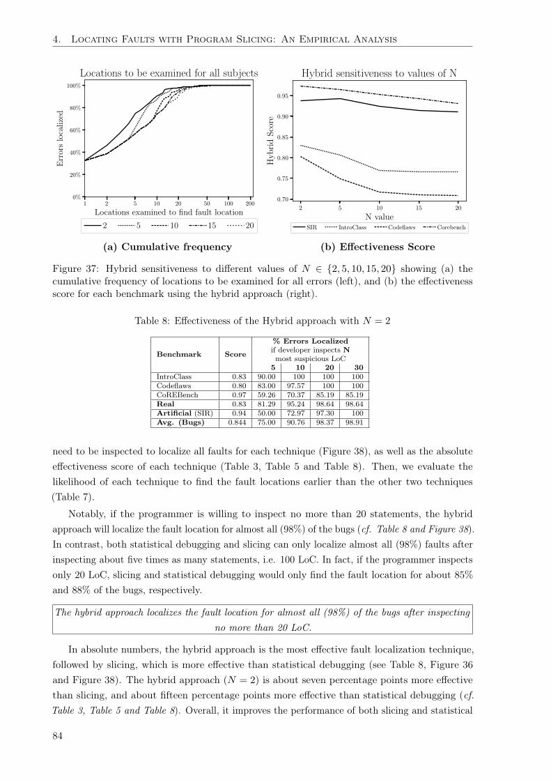
4. Locating Faults with Program Slicing: An Empirical Analysis
1 2 5 10 20 50 100 200
Locations examined to find fault location
0%
20%
40%
60%
80%
100%
Err
ors
loca
lize
d
Locations to be examined for all subjects
2 5 10 15 20
2 5 10 15 20
N value
0.70
0.75
0.80
0.85
0.90
0.95
Hyb
rid
Sco
re
Hybrid sensitiveness to values of N
SIR IntroClass Codeflaws Corebench
(a) Cumulative frequency (b) Effectiveness Score
Figure 37: Hybrid sensitiveness to different values of N 2 {2, 5, 10, 15, 20} showing (a) thecumulative frequency of locations to be examined for all errors (left), and (b) the effectivenessscore for each benchmark using the hybrid approach (right).
Table 8: Effectiveness of the Hybrid approach with N = 2
Benchmark Score
% Errors Localized
if developer inspects N
most suspicious LoC
5 10 20 30
IntroClass 0.83 90.00 100 100 100
Codeflaws 0.80 83.00 97.57 100 100
CoREBench 0.97 59.26 70.37 85.19 85.19
Real 0.83 81.29 95.24 98.64 98.64
Artificial (SIR) 0.94 50.00 72.97 97.30 100
Avg. (Bugs) 0.844 75.00 90.76 98.37 98.91
need to be inspected to localize all faults for each technique (Figure 38), as well as the absoluteeffectiveness score of each technique (Table 3, Table 5 and Table 8). Then, we evaluate thelikelihood of each technique to find the fault locations earlier than the other two techniques(Table 7).
Notably, if the programmer is willing to inspect no more than 20 statements, the hybridapproach will localize the fault location for almost all (98%) of the bugs (cf. Table 8 and Figure 38).In contrast, both statistical debugging and slicing can only localize almost all (98%) faults afterinspecting about five times as many statements, i.e. 100 LoC. In fact, if the programmer inspectsonly 20 LoC, slicing and statistical debugging would only find the fault location for about 85%and 88% of the bugs, respectively.
The hybrid approach localizes the fault location for almost all (98%) of the bugs after inspectingno more than 20 LoC.
In absolute numbers, the hybrid approach is the most effective fault localization technique,followed by slicing, which is more effective than statistical debugging (see Table 8, Figure 36and Figure 38). The hybrid approach (N = 2) is about seven percentage points more effectivethan slicing, and about fifteen percentage points more effective than statistical debugging (cf.Table 3, Table 5 and Table 8). Overall, it improves the performance of both slicing and statistical
84

4.4. Experimental Results
debugging. For instance, a programmer using the hybrid approach needs to examine only abouthalf (58%) and three-quarter (75%) of those statements that she would need to examine if sheused slicing and statistical debugging, respectively.
The hybrid approach is significantly more effective than slicing and statistical debugging,respectively.
We compute the odds ratio and conduct a Mann-Whitney U -test, in order to determine thesignificance of the hybrid approach. The odds ratio for all projects is strictly in favor of thehybrid approach ( > 1 in Table 7). Specifically, the hybrid approach is (69%) more likely to finda faulty statement earlier than statistical debugging (cf. “Hybrid-2 vs. Kulczynski2” in Table 7).Moreover, a programmer is (42%) less likely to find the fault location early if she localizes withdynamic slicing instead of the hybrid approach (cf. “Slicing vs. Hybrid-2” in Table 7).
The statistically significant odds ratio is explained by the hybrid approach being more effectivethan slicing and statistical debugging in most cases. The majority of bugs is best localized bythe hybrid approach. For more than half of the bugs (56%, 208 out of 369 errors), the hybridapproach will find the fault earlier than both slicing and statistical debugging. In particular, forCoREBench, the hybrid approach is more effective than both techniques for 19 out of 27 bugs, aswell as for 33 out of 74 bugs in SIR.
The hybrid approach is significantly more likely to find a faulty statement earlier than dynamicslicing and statistical debugging.
RQ6 Real Errors vs. Artificial Errors
In this section, we evaluate the effect of error type on the effectiveness of an AFL technique, inparticular, the difference between evaluating AFL techniques on artificial errors (i.e., SIR43) versusreal errors (i.e., IntroClass, Codeflaws and CoREBench). We examine the performance of eachtechnique on each error type and portray the bias and differences in such evaluations. Figure 35and Figure 36 highlight the difference between evaluating a fault localization technique on real orartificial errors. Table 9 summarizes the difference in the effectiveness of each AFL techniquewhen using real or artificial faults. Table 3, Table 5 and Table 8 also quantify the difference inthe effectiveness of all three AFL techniques (i.e., dynamic slicing, statistical debugging and thehybrid approach, respectively) on real and artificial faults.
What is the most effective statistical debugging formula for artificial or real faults? In ourevaluation, the error type influences the effectiveness of a statistical debugging formula. PattSim_2is the most effective statistical formula for artificial faults (score=0.85 ), this is closely followedby Ochiai and Naish_1 with score = 0.83 (see Table 4). Meanwhile, for real faults, the mosteffective statistical formulas are Kulczynski2 and Tarantula with scores 0.76, 0.70 and 0.79 forIntroClass, Codeflaws and CoREBench, respectively (see Table 4).44Notably, the most effective
43The SIR benchmark is the most used subject for the evaluation of AFL techniques, especially statistical faultlocalization [172].
44Even among real faults, the most effective formula depends on the benchmark. For instance the DStar algorithmslightly outperforms Kulczynski2 and Tarantula on CoREBench, despite performing worse on IntroClass andCodeflaws.
85
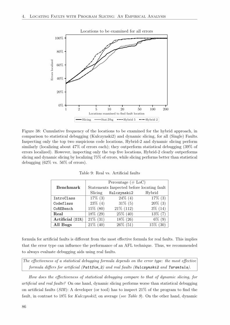
4. Locating Faults with Program Slicing: An Empirical Analysis
1 2 5 10 20 50 100 200Locations examined to find fault location
0%
20%
40%
60%
80%
100%
Err
ors
loca
lize
d
Locations to be examined for all errors
Slicing Stat.Dbg Hybrid 5 Hybrid 2
Figure 38: Cumulative frequency of the locations to be examined for the hybrid approach, incomparison to statistical debugging (Kulczynski2) and dynamic slicing, for all (Single) Faults.Inspecting only the top two suspicious code locations, Hybrid-2 and dynamic slicing performsimilarly (localizing about 47% of errors each); they outperform statistical debugging (39% oferrors localized). However, inspecting only the top five locations, Hybrid-2 clearly outperformsslicing and dynamic slicing by localizing 75% of errors, while slicing performs better than statisticaldebugging (62% vs. 56% of errors).
Table 9: Real vs. Artificial faults
Percentage (# LoC)Benchmark Statements Inspected before locating fault
Slicing Kulczynski2 HybridIntroClass 17% (3) 24% (4) 17% (3)Codeflaws 23% (4) 31% (5) 20% (3)CoREBench 15% (80) 21% (112) 3% (14)Real 18% (29) 25% (40) 13% (7)Artificial (SIR) 21% (31) 18% (26) 6% (9)All Bugs 21% (40) 26% (51) 15% (30)
formula for artificial faults is different from the most effective formula for real faults. This impliesthat the error type can influence the performance of an AFL technique. Thus, we recommendedto always evaluate debugging aids using real faults.
The effectiveness of a statistical debugging formula depends on the error type: the most effectiveformula differs for artificial (PattSim_2) and real faults (Kulczynski2 and Tarantula).
How does the effectiveness of statistical debugging compare to that of dynamic slicing, forartificial and real faults? On one hand, dynamic slicing performs worse than statistical debuggingon artificial faults (SIR): A developer (or tool) has to inspect 21% of the program to find thefault, in contrast to 18% for Kulczynski2, on average (see Table 9). On the other hand, dynamic
86

4.4. Experimental Results
1 2 5 10 20 50 100 200Locations examined to find fault location
0%
20%
40%
60%
80%
100%E
rror
slo
calize
d
Locations examined for all single-fault SIR and IntroClass versions
Slicing Kulczynski2 Tarantula Hybrid 5 Hybrid 2
1 2 5 10 20 50 100 200Locations examined to find fault location
0%
20%
40%
60%
80%
100%
Err
ors
loca
lize
d
Locations examined for all multiple-fault SIR and IntroClass versions
Slicing Kulczynski2 Tarantula Hybrid 5 Hybrid 2
(a) Single Faults (b) Multiple Faults
Figure 39: Cumulative frequency of the locations to be examined for (a) single-fault and (b)multiple-fault versions of the SIR and IntroClass, using the hybrid approach, statistical debugging(Kulczynski2 and Tarantula) and dynamic slicing
slicing performs better than statistical debugging on real faults (i.e., IntroClass, Codeflaws andCoREBench). For real errors, a developer has to inspect (7%) less statements when using dynamicslicing (18%) compared to slicing (25%). Again, this shows that the error type has a significantinfluence on the effectiveness of an AFL technique.
Statistical debugging performs better on artificial faults, while dynamic slicing performs betteron real faults.
What is the most effective AFL approach on artificial and real faults? The hybrid approach isthe most effective AFL approach, outperforming both dynamic slicing and statistical debugging(see Table 9). In particular, depending on the error type, a developer or tool using the hybridapproach inspects only one-third to less than three-quarter (0.3 to 0.7) of the statements inspectedwhen using dynamic slicing or statistical debugging. This shows that the effectiveness of thehybrid approach is independent of error type.
The hybrid approach is the most effective approach, regardless of error type, i.e. artificial or realfaults.
We observed that fault localization effectiveness on artificial errors does not predict results onreal faults. In our evaluation, the performance of dynamic slicing and statistical debugging aredifferent depending on the error type. For instance, Table 9 clearly shows that dynamic slicingperforms better on real faults, while statistical debugging performs better on artificial faults. Thisresult illustrates that the performance of an AFL technique on artificial faults is not predictiveof its performance in practice. Hence, it is pertinent to evaluate AFL techniques on real faultsrather than artificial faults, this is in line with the findings of previous studies [194].
The effectiveness of an AFL technique on artificial faults does not predict its effectiveness onreal faults.
87

4. Locating Faults with Program Slicing: An Empirical Analysis
Table 10: Effectiveness of all AFL techniques on Single and Multiple Faults for SIR and IntroClassbenchmarks. Single Fault Scores are in italics and bracketed, i.e. (Single), while Multiple FaultScores are in normal text. For multiple faults, the best scores for each (sub)category are in bold;higher scores are better. For instance, Tarantula is the best performing (popular) statisticaldebugging formula for all programs with multiple faults with score 0.8269, on average.
AFL Formula/Approach
SIRMULT (Single)
IntroClassMULT (Single)
AverageTechnique (Prog.) (Vers.)
PopularSBFL
Tarantula0.8214 0.8324 0.8269 0.7878(0.6907 ) (0.7464 ) (0.7186 ) (0.6266 )
Ochiai0.7796 0.7747 0.7772 0.7560
(0.7337 ) (0.7464 ) (0.7401 ) (0.6514 )
Jaccard0.7720 0.7747 0.7734 0.7532
(0.7029 ) (0.7464 ) (0.7247 ) (0.6342 )
HumanGenerated
SBFL
Naish_10.7215 0.7638 0.7426 0.7136
(0.7399 ) (0.7448 ) (0.7423 ) (0.6682 )
Naish_20.7484 0.7747 0.7615 0.7404
(0.7207 ) (0.7464 ) (0.7336 ) (0.6596 )
Russel_Rao0.7350 0.7586 0.7468 0.7185
(0.6088 ) (0.6394 ) (0.6241 ) (0.6051 )
Binary0.7125 0.7553 0.7339 0.6975
(0.6283 ) (0.6378 ) (0.633 ) (0.6129 )
Wong_10.7350 0.7586 0.7468 0.7185
(0.6088 ) (0.6394 ) (0.6241 ) (0.6051 )
D2 0.7718 0.7747 0.7732 0.7553
(0.7345 ) (0.7464 ) (0.7404 ) (0.6523 )
D3 0.7680 0.7747 0.7714 0.7553
(0.7484 ) (0.7464 ) (0.7474 ) (0.6611 )
GPEvolvedSBFL
GP_020.7633 0.7747 0.7690 0.7498(0.6725 ) (0.7157 ) (0.6941 ) (0.6133 )
GP_030.7473 0.7747 0.7610 0.7402
(0.6813 ) (0.6169 ) (0.6491 ) (0.6285 )
GP_130.7456 0.7747 0.7602 0.7398
(0.7211 ) (0.7464 ) (0.7338 ) (0.6606 )
GP_190.7629 0.7558 0.7593 0.7279
(0.4673 ) (0.6237 ) (0.5455 ) (0.4876 )
Single BugOptimalSBFL
PattSim_20.7608 0.7747 0.7677 0.7301
(0.7537 ) (0.6544 ) (0.704 ) (0.6506 )
lex_Ochiai0.7532 0.7747 0.7640 0.7396
(0.7356 ) (0.7464 ) (0.741 ) (0.6646 )
m91850.8183 0.8315 0.8249 0.7664(0.7570 ) (0.7225 ) (0.7397 ) (0.6646 )
Kulczynski20.7885 0.7747 0.7816 0.7588
(0.7572 ) (0.7464 ) (0.7518 ) (0.6689 )ProgramSlicing
DynamicSlicing
0.8357 0.5487 0.6922 0.7840(0.7935 ) (0.8602 ) (0.8269 ) (0.7535 )
HybridApproach
Hybrid-20.9627 0.9057 0.9342 0.9457(0.9358 ) (0.888 ) (0.9119 ) (0.9237 )
Hybrid-50.9505 0.8406 0.8955 0.9206
(0.9397 ) (0.814 ) (0.8768 ) (0.8974 )
88

4.4. Experimental Results
Slicing Kulczynski2 Tarantula Hybrid0.5
0.6
0.7
0.8
0.9
1.0Sco
re
E�ectiveness of the best-performing techniques
SIR single-fault
SIR multi-fault
IntroClass single-fault
IntroClass multi-fault
Slicing Kulczynski2 Tarantula Hybrid0.0
0.5
1.0
1.5
2.0
2.5
3.0
3.5
4.0
Sco
re
E�ectiveness single vs. multiple faults
SIR single-fault
SIR multi-fault
IntroClass single-fault
IntroClass multi-fault
(a) Each Benchmark (b) Cumulative Score
Figure 40: Effectiveness of each technique for Single and Multiple Fault(s) in SIR and IntroClass:(a) Scores for each benchmark and (b) Scores for both benchmarks
RQ7 Single Fault vs. Multiple Faults
In this section, we compare the effectiveness of all three AFL techniques on programs with multiplefaults. Then, we examine the effect of multiple faults on the performance of each technique and thedifference between evaluating an AFL technique on single or multiple fault(s). In this experiment,we employ the original single-fault versions of the SIR and IntroClass benchmarks, as wellas the multiple-fault versions of the same benchmarks, called SIR-MULT and IntroClass-MULT,respectively. Table 10 highlights the results for single and multiple fault(s) for all AFL techniques,including statistical debugging, hybrid and dynamic slicing. Figure 39, Figure 40 and Figure 41illustrate the difference in the performance of each technique when given programs with a singlefault or multiple faults.
What is the most effective statistical debugging formula for multiple faults? In our evaluation,the most effective statistical debugging formula for multiple faults is Tarantula (0.8269), from thepopular statistical debugging family. It outperforms the other statistical debugging formulas (cf.Table 10 and Figure 40). For the other statistical debugging families, the most effective formulafor multiple faults are DStar (D2 and D
3), GP02 and m9185 for the popular, human-generated andgenetically evolved families, respectively (cf. Table 10). The performance of Tarantula is closelyfollowed by that of the single-bug optimal formulas m9185 (0.8249). However, the difference inthe performance of m9185 and Tarantula is not statistically significant, i.e. < 1 (odds ratio = 0.14, Mann-Whitney U -test p-value U = 0). Notably, the most effective single-bug optimalformulas (i.e. m9185) outperformed the human-generated and genetically evolved formulas (cf.Table 10). This illustrates that single bug optimal formulas are also effective for multiple faults,despite being specialized for single faults.
Tarantula is the most effective statistical debugging formula for multiple faults;it outperforms all other statistical debugging formulas.
89
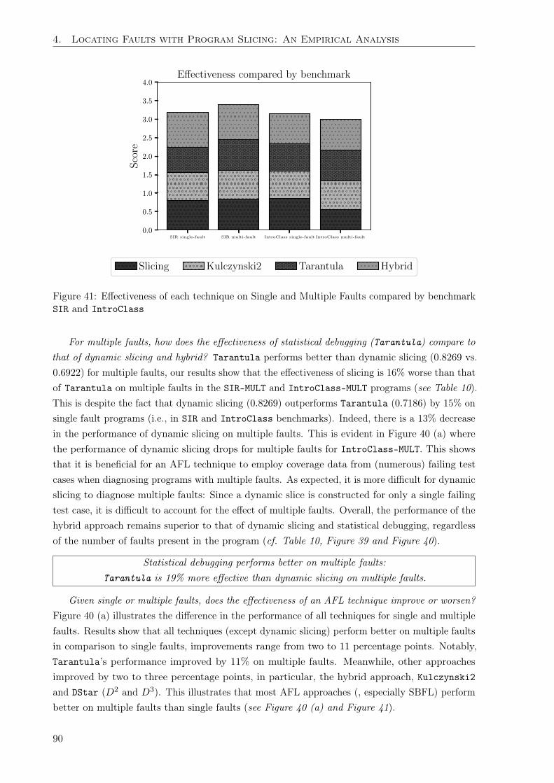
4. Locating Faults with Program Slicing: An Empirical Analysis
SIR single-fault SIR multi-fault IntroClass single-fault IntroClass multi-fault
0.0
0.5
1.0
1.5
2.0
2.5
3.0
3.5
4.0
Sco
re
E�ectiveness compared by benchmark
Slicing Kulczynski2 Tarantula Hybrid
Figure 41: Effectiveness of each technique on Single and Multiple Faults compared by benchmarkSIR and IntroClass
For multiple faults, how does the effectiveness of statistical debugging (Tarantula) compare tothat of dynamic slicing and hybrid? Tarantula performs better than dynamic slicing (0.8269 vs.0.6922) for multiple faults, our results show that the effectiveness of slicing is 16% worse than thatof Tarantula on multiple faults in the SIR-MULT and IntroClass-MULT programs (see Table 10).This is despite the fact that dynamic slicing (0.8269) outperforms Tarantula (0.7186) by 15% onsingle fault programs (i.e., in SIR and IntroClass benchmarks). Indeed, there is a 13% decreasein the performance of dynamic slicing on multiple faults. This is evident in Figure 40 (a) wherethe performance of dynamic slicing drops for multiple faults for IntroClass-MULT. This showsthat it is beneficial for an AFL technique to employ coverage data from (numerous) failing testcases when diagnosing programs with multiple faults. As expected, it is more difficult for dynamicslicing to diagnose multiple faults: Since a dynamic slice is constructed for only a single failingtest case, it is difficult to account for the effect of multiple faults. Overall, the performance of thehybrid approach remains superior to that of dynamic slicing and statistical debugging, regardlessof the number of faults present in the program (cf. Table 10, Figure 39 and Figure 40).
Statistical debugging performs better on multiple faults:Tarantula is 19% more effective than dynamic slicing on multiple faults.
Given single or multiple faults, does the effectiveness of an AFL technique improve or worsen?Figure 40 (a) illustrates the difference in the performance of all techniques for single and multiplefaults. Results show that all techniques (except dynamic slicing) perform better on multiple faultsin comparison to single faults, improvements range from two to 11 percentage points. Notably,Tarantula’s performance improved by 11% on multiple faults. Meanwhile, other approachesimproved by two to three percentage points, in particular, the hybrid approach, Kulczynski2and DStar (D2 and D
3). This illustrates that most AFL approaches (, especially SBFL) performbetter on multiple faults than single faults (see Figure 40 (a) and Figure 41).
90
4.5. Threats to Validity
Statistical debugging is better suited for diagnosing multiple faults,while dynamic slicing is more effective at localizing single faults.
Generally, we found that the performance of a technique on programs containing singlefaults does not predict its performance on multiple faults. For instance, although Kulczynski2outperformed the other statistical formulas for single faults (0.7518), it is outperformed by m9185for multiple faults (0.7816 vs. 0.8249) (cf. Table 10). This result is also evident from Figure 40(a) and Table 10, where dynamic slicing outperforms statistical debugging (Kulczynski2) forSIR single faults (0.8269 vs. 0.7518), but statistical debugging (m9185 and Kulczynski2) clearlyoutperform dynamic slicing for multiple faults. These results suggest that the number of faults inthe program influences the effectiveness of an AFL technique.
The effectiveness of an AFL technique on single faults does notpredict its effectiveness on multiple faults.
4.5 Threats to Validity
We discuss the threats to validity for this fault localization study within the framework of [180].External Validity: refers to the extent to which the reported results can be generalized to otherobjects which are not included in the study. The most immediate threats to external validity arethe following:
• EV.1) Heterogeneity of Probands. The quality of the test suites provided by the object ofanalysis may vary greatly which hampers the assessment of accuracy for practical purposes.However, in our study the test suites are well-stocked and maintained. All projects areopen source C programs which are subject to common measures of quality control, such ascode review and providing a test case with bug fixes and feature additions.
• EV.2) Faulty Versions and Fault Injection. For studies involving artificially injected faults,it is important to control the type and number of injected faults. Test cases become subjectto accidental fault injection. Some failures may be spurious. However, in our study we alsouse real errors that were introduced (unintentionally) by real developers. Failing test casesare guaranteed to fail because of the error.
• EV.3) Language Idiosyncrasies. Indeed, our objects contain well-maintained open-source Cprojects with real errors typical for such projects. However, for instance errors in projectswritten in other languages, like Java, or in commercially developed software may be ofdifferent kind and complexity. Hence, we cannot claim generality for all languages andsuggest reproducing our experiments for real errors in projects written in other languagesas well.
• EV.4) Test Suites. The size of a test suite can influence the performance of an AFLtechnique. Testing strategies that reduce or increase test suite size such as test reductionor test generation methods (i.e. removing tests or generating new tests) have been shownto improve the performance of some AFL techniques [175, 176]. We mitigate the effect of
91
4. Locating Faults with Program Slicing: An Empirical Analysis
test suite size by employing projects with varying test suite sizes (ranging from tens totens of thousands of test cases) as provided by our subject programs. In our evaluation, wedo not generate additional tests or remove any tests from the test suite provided by thebenchmarks, in order to simulate the typical debugging scenario for the software project.
• EV.5) Missing Statements in Slices. Although, there is a risk of discarding faulty state-ments during program slicing, dynamic slicing rarely miss faulty statements during faultlocalization [197]. [197] found that dynamic slicing reports the faulty statement in thetop-ten most suspicious statement 91% of the time. We further mitigate this risk by firstinspecting statements in the dynamic slice before inspecting other executable statements.Thus, dynamic slicing (eventually) finds the faulty statement for all bugs in our evaluation.
Construct Validity: refers to the degree to which a test measures what it claims to be measuring.The most immediate threats to construct validity are the following:
• CV.1) Measure of Effectiveness. Conforming to the standard [172], we measure faultlocalization effectiveness as ranking-based relative wasted effort. The technique thatranks the faulty statement higher is considered more effective. Parnin and Orso find that“programmers will stop inspecting statements, and transition to traditional debugging,if they do not get promising results within the first few statements they inspect” [178].However, [180] insist that one may question the usefulness of fault locators, but measures ofranking-based relative wasted effort are certainly necessary for evaluating their performance,particularly in the absence of the subjective user as the evaluator.
• CV.2) Implementation Flaws. Tools that we used for the evaluation process may beinaccurate. Despite all care taken, our implementation of the 18 studied statistical faultlocalization techniques, or of approximate dynamic slicing, or of the empirical evaluationmay be flawed or subject to random factors. However, we make all implementations andexperimental results available online for public scrutiny.
4.6 Related Work
Evaluation of Fault Localization Techniques: The effectiveness of various fault localizationapproaches have been studied by several colleagues, see Wong et al. [172]. Most papers investigatedthe effects of program, test and bug features on the effectiveness of statistical debugging. Abreuet al. [179] examined the effects of the number of passing and failing test cases on the effectivenessof statistical debugging, they established that the suspiciousness scores stabilize starting from anaverage six (6) failing and twenty (20) passing test cases. [194] evaluated the difference betweenevaluating fault localization techniques on real faults versus artificial faults, using two maintechniques, namely statistical debugging and mutation-based fault localization. Notably, theirevaluation results shows that results on artificial faults do not predict results on real faults forboth techniques, and a hybrid technique is significantly better than both techniques. Keller etal. [198] and Heiden et al. [199] evaluated the effectiveness of statistical fault localization on realworld large-scale software systems. The authors found that, for realistic large-scale programs,the accuracy of statistical debugging is not suitable for human developers. In fact, the authors
92
4.6. Related Work
emphasize the obvious need to improve statistical debugging with contextual information suchas information from the bug report or from version history of the code lines. In contrast to ourwork, none of these papers evaluated the fault localization effectiveness of program slicing, norcompare the effectiveness of slicing to that of statistical debugging.
A few approaches have evaluated the effectiveness of dynamic slices in fault localization [173,174]. In particular, Zhang et al. [174] evaluated the effectiveness of three variants of dynamicslicing algorithms, namely data slicing, full (dynamic) slicing, and relevant slicing. Like ourstudy, the authors found that slicing considerably reduces the number of program statementsthat need to be examined to locate faulty statements. In contrast to our study, the authors havenot empirically compared the performance of slicing to that of statistical debugging.
Improvements of Statistical Fault Localization: Several authors have proposed approachesto improve statistical fault localization (SBFL). Most approaches are focused on reducing theprogram spectra (i.e. the code coverage information) fed to statistical debugging, sometimesby using delta debugging [200], program slicing [201, 202, 203], test generation [204], testprioritization [205] or machine learning [206, 207]. In particular, some techniques apply programslicing to reduce the program spectra fed to statistical debugging formulas [208, 201, 209, 201, 202,203]. The popular page rank algorithm has been used to boost statistical debugging effectivenessby estimating the contributions of different tests to re-compute program spectral [205]. Machinelearning algorithms (such as learning to rank) also improves the effectiveness of statisticaldebugging [207, 206]. In addition, BARINEL employs a combination of bayesian reasoning andstatistical debugging to improve fault localization effectiveness, especially for programs withmultiple faults [187]. BARINEL combines statistical debugging and model-based diagnosis (MBD),i.e., logic reasoning over a behavioral model to deduce multiple-fault candidates: The goal is toovercome the high computational complexity of typical MBD. Search-based test generation hasalso been combined with SBFL, in order to improve the performance of statistical debuggingfor Simulink models [204]. However, none of these papers localize faults by following controland data dependencies in the program, i.e. they do not directly use program slicing as a faultlocalization technique.
Zou et al. [206] found that the combination of fault localization techniques improves overindividual techniques, the authors recommend that future fault localization techniques shouldbe evaluated in the combined setting. For instance, slicing hitting set computation (SHSC) isa combination of model-based debugging and program slicing that has been applied for faultlocalization [210]. In contrast to our work, SHSC combines slices of faulty variables, which causesundesirable high ranking of statements executed in many test cases [211]. To address this, Hoferand Wotawa also proposed SENDYS – a combination of statistical debugging and SHSC toimprove the ranking of faulty statements [211]. The focus of this work is to provide fault locationsat a finer granularity than program blocks. In contrast to typical dynamic slicing, SENDYSanalyzes the execution information from both passing and failing test cases and uses statisticaldebugging results as a-priori fault probabilities of single statements in SHSC [211].
93
4. Locating Faults with Program Slicing: An Empirical Analysis
4.7 Discussions and Future Work
The empirical results from this chapter shows that dynamic slicing remains the technique of choicefor programmers and debuggers. Suspicious statements, as produced by statistical debugging,can provide good starting points for an investigation; but beyond the top-ranked statements,following dependencies is much more likely to be effective. We therefore recommend that followingdependencies should remain the primary method of fault localization—it is a safe and robusttechnique that will get programmers towards the goal.
Dynamic slicing as a fault localization technique can be further improved, in order make itmore effective and efficient in software practice. Building on the empirical results from our study(in Chapter 4), we consider the following improvements:
Cognitive load. In our investigation, we did not consider or model the cognitive load it takesto understand the role of individual statements in context. Since following dependenciesin a program is much more likely to stay within same or similar contexts than statisticaldebugging, where the ranked suspicious lines can be strewn arbitrarily over the code, we wouldexpect dependency-based techniques to take a lead here. The seminal study of Parnin andOrso [178] found that ranked lists of statements are hardly helping human programmers—letus find out which techniques work best for humans.
Alternate search techniques. There are other search strategies along program dependencies(for instance, starting with the input, and progressing forward through a program; startingat some suspicious or recently changed location; or moving along coarse-grained functionsfirst, and fine-grained lines later) that may be even more efficient both in terms of nodesvisited as well as from the assumed cognitive load. Again, this calls for more human studiesin debugging.
Experimental techniques. For instance, input minimization techniques (such as delta debug-ging [212]) offer another means to reduce the cognitive load—by systematically narrowingdown the conditions under which a failure occurs. The work of Burger and Zeller [213] onminimization of calling sequences with delta debugging showed dramatic improvements overdynamic slicing, reducing “the search space to 13.7% of the dynamic slice or 0.22% of thesource code”. In a recent human study, delta debugging “significantly increased programmersefficiency in failure detection, fault localization and fault correction.” [214].
Symbolic techniques. Finally, following dependencies is still one of the simplest methods toexploit program semantics. Applying symbolic execution and constraint solving would narrowdown the set of possible faults. Model-based debugging [215] was one of the first to applythis idea in practice; the more recent bugassist work of Jose and Majumdar “quickly andprecisely isolates a few lines of code whose change eliminates the error.” [216].
To summarize, the fault localization techniques proposed for future work can profit fromwider evaluations and assessments. In addition, they can also be joined and combined similarlyto our hybrid approach (in Section 4.2). For instance, one could start with suspicious statementsas indicated by statistical fault localization, follow dependencies from there, and skip influences
94

4.7. Discussions and Future Work
deemed impossible by symbolic analysis. The key challenge of automated fault localization willbe to bring the best of the available techniques together in ways that are applicable to a widerange of programs and useful for real programmers, who must fix their bugs by the end of theday. Finally, we encourage the use of true defects to compare AFL techniques and a willingnessto actually compare to the state of the art techniques, as we do in this work. All of our scripts,tools, benchmarks and results are freely available to support scrutiny, evaluation, reproductionand extension:
https://tinyurl.com/HybridFaultLocalization
95


Chapter 5
Debugging Failure-Inducing Inputs
This chapter is taken, directly or with minor modifications, from our 2020 ICSE paper De-bugging Inputs [217]. My contribution in this work is as follows: (I) original idea; (II) partialimplementation; (III) evaluation.
“Every failure carries with it the seed of an equal or greater benefit.”— Napoleon Hill
5.1 Introduction
In the last decade, techniques for automated debugging and repair have seen great interestin research and practice. A recent survey [1] lists more than 100 papers on automatic faultlocalization and repair. Recently, social networking giant Facebook provided developers withautomatically generated repair suggestions for every failure report of its apps [218]. Almost all ofthese techniques focus on program code, attempting to identify possible fault locations in the codeand synthesizing fixes for this code. However, when a program fails on some input, it need not bethe program code that is at fault. Hardware failures, hardware aging, transmission errors may allcause data to get corrupted. In computer hardware, radiation can impact memory cells, leadingto bit flips and again data corruption. And finally, data can be corrupted through software bugs,with the processing software writing out malformed or incomplete data. If data is corrupted, theeasiest remedy is to use a backup. But if a backup does not exist (or is too old, or fails to beprocessed), one may want to recover as much data as possible from the existing data—or in otherwords, debug the data.
Some programs come with application-specific means to recover data. Input parsers canrecover from syntactical errors by applying sophisticated recovery strategies; in a programminglanguage, this may involve skipping the current statement or function and resuming with the nextone [219]. When detecting a corrupted or incomplete file, Microsoft Office programs may attemptto recover from the error, using a number of undisclosed approaches [220]. When a programdoes not implement a good recovery strategy, though, users are left to their own devices, usinggeneral-purpose editors to identify file contents and possible corrupted parts.
As listed above, general-purpose automated debugging techniques focus on faults in code anddo not provide much help in such situations, as they would regularly identify the input parser
97

5. Debugging Failure-Inducing Inputs
{ "item": "Apple", "price": **3.45 }
Figure 42: Failing JSON input
{
Figure 43: Failing input reduced with ddmin
{ "item": "Apple", "price": 3.45 }
Figure 44: Failing input repaired with ddmax
and its error-handling code as being associated with the fault. The delta debugging (ddmin)algorithm [57], however, focuses on identifying error causes in the input; in repeated runs withreduced inputs, it simplifies a failure-inducing input down to a minimum that reproduces theerror. Unfortunately, delta debugging is not a good fit: applied to invalid inputs, it produces thesmallest subset of the input that also produces an input error—typically a single character. Asan example, consider Figure 42, a JSON input with a syntax error; ddmin produces the reducedinput in Figure 43, consisting of a single { character, which also produces a syntax error. This isneither helpful for diagnosis nor a basis for data recovery.
In this chapter, we first investigate the relevance of invalid inputs in software practice andcollect empirical evidence on the prevalence and causes of invalid inputs. Secondly, we introducea generic input repair method that automatically (1) identifies which parts of the input dataprevent processing, and (2) recovers as much of the (valuable) input data as possible. Likeddmin, our approach runs the program under test repeatedly with different subsets of the input,assessing whether the subset can be processed or not. Also, it does not need any kind of programanalysis and can thus be used in a wide range of settings. Unlike ddmin, however, which aims atminimizing the failure-inducing input, our ddmax algorithm aims at maximizing the passing input.Its result is a subset of the input that (1) can be successfully processed and (2) is 1-maximal: nofurther element from the failing input can be added without causing the input to become invalidagain.
Applied on our example from Figure 42, ddmax produces the “repaired” (passing) input subsetin Figure 44, in which the confounding ** characters (and nothing else) are removed. Thedifference between the original input (Figure 42) and the repaired input (Figure 44), listed inFigure 45, actually makes a precise diagnosis of the failure cause and can be given to developersfor further debugging steps.
Note that while ddmax recovers a maximum of data, it does not recover a maximum ofinformation; in our example, we do not know whether 3.45 actually is the correct price. However,the repaired input can now be read and processed by the program at hand, enabling humans toread and check their document and engage into additional recovery steps.
Although, many applications produce error messages when processing invalid inputs, mosterror mesages are vague. Often, applications simply report that an input is corrupted, withoutrepairing the input or providing the reason for the invalidity. However, ddmax identifies theinvalid input fragment quickly (for debuggers) while also preserving a maximum of content (for
98
5.2. Prevalence of Invalid Inputs
**
Figure 45: Difference between failing and repaired input
end users).The remainder of this chapter makes the following contributions:
An empirical study of invalid inputs in practice. We evaluate the prevalence of invalidinput in the wild (Section 5.2). We crawled thousands of input files from github anddetermine the set of valid and invalid files. We find that invalid inputs are common inpractice, about four percent (295 files) of all input files (7835 files) crawled from github wereinvalid.
Generic input repair with minimal data loss. We introduce the ddmax algorithm, auto-matically recovering a maximum of data from a given failure-inducing input (Section 5.3).To the best of our knowledge, ddmax is the first input repair technique that can be appliedto arbitrary inputs and programs without additional knowledge on input formats or programcode. In its evaluation on eight subjects and three input formats, using real-world invalidinputs as well as synthetic corruptions, we find that ddmax is effective: It repairs 69% ofcorrupted inputs and recovers about 78% of data, within a time budget of one minute perinput.
An efficient syntactical input repair technique. We introduce a variant of ddmax thatmakes use of a grammar to parse inputs into derivation trees and to maximize inputs bypruning parts of the tree that could not be read (Section 5.4); this vastly speeds up inputrepair. In its evaluation, syntactic ddmax is faster and more efficient than the lexical variant.
Identifying faults in input data. The difference between the “repaired” input by ddmax andthe original input contains all parts of the input that prevented the data from being processedin the first place. Section 5.5 shows that this difference precisely characterizes the fault inthe input.
After discussing the threats to validity (Section 5.6) and limitations (Section 5.7), we discussclosely related work (Section 5.8). Lastly, we close with discussions and future work (Section 5.9).
5.2 Prevalence of Invalid Inputs
Before we start repairing inputs, let us first answer the question of how relevant the problem is.Is it actually possible that some application cannot open or process a data file? And would therebe files claiming to adhere to some format if in fact, they are not? To answer such questions, wemine some invalid inputs from the wild.
Evaluation Setup
Subject Programs
In this study, we use eight programs as test subjects, namely Blender [221], Assimp [222],Appleseed [223], JQ [224], JSON-Simple [225], Minimal-JSON [226], Graphviz [227], and finally
99

5. Debugging Failure-Inducing Inputs
Table 11: Subject Programs
Subject Input Prog. Size MaturityProgram Format Lang. (in KLoC) (1st Commit)Blender OBJ C/C++ 1800 Jan. 1994Assimp OBJ C++ 88.9 July 2002Appleseed OBJ C++ 600.1 May 2009JQ JSON C 20.2 July 2012JSONSimple JSON Java 2.6 Nov. 2008Minimal-JSON JSON Java 6.4 Feb. 2013Graphviz DOT C 1140 Sep. 1991Gephi DOT Java 166.1 July 2008
Table 12: Input Grammar Details
Grammar Size (LoC) #ParserRules #LexerRulesJSON 79 5 9
Wave. OBJ 271 13 42DOT 181 14 15
Gephi [228]. Each input format was evaluated with three subjects, except for DOT which wasevaluated with two programs. All our subject programs are open source C, C++ or Java programs.On average, these programs have 478 KLoC and a maturity of over 14 years. Table 11 highlightsthe properties of our subject programs.
Grammars
We have collected the grammars for our subjects from the ANTLR Grammar repository [229].We chose complex and large grammars for data-rich input formats used in two popular domains,namely graphics domain (i.e. Wavefront OBJ (OBJ) and DOT) and data exchange domain (i.e.JSON). To ensure the grammars were sound, we tested them with 50 valid crawled files for eachinput format. We modified the Wavefront OBJ grammar since its ANTLR grammar was only asubset of the official Wavefront OBJ specificiation [230]. The JSON and DOT grammars were usedunmodified since they matched the official specifications [231, 232]. On average, the grammarsare written in 177 LoC, with 11 parser rules and 22 lexer rules (cf. Table 12).
Mining and Filtering Input Files.
Table 13 highlights the details of the input files in our corpus. We crawled for a specific file formatusing the file extension (e.g. “.json” for the JSON input format). In total, we collected a corpus of9544 input files (cf. #Crawled Files in Table 13) using the Github API for crawling [233]. Then,we deleted all files that are empty or duplicated, as well as the input files that have a different inputformat despite having the intended file name suffix (e.g. a Wavefront OBJ file has the same suffix(“.obj”) as a binary OBJ file that was created by a compiler). This resulted in 7835 unique inputfiles (cf. #Unique files). We also separated files that contain unsupported grammar extensions.In particular, for JSON and DOT, we removed 166 input files (cf. #Files Rejected by A) that
100

5.2. Prevalence of Invalid Inputs
Table 13: Details of Mined Input Files. We report the cause of input invalidity by showing thenumber of files rejected by (A) the input grammar, (B) at least one subject program and (C) allsubject programs
Input #Crawled #Unique #Valid #Invalid #Files Rejected by Mean File Size (KiB)Format Files Files Files Files A B C Valid Invalid
JSON 8654 7006 6948 222 164 58 52 12.84 0.78OBJ 509 480 455 25 0 25 0 401.57 64.15DOT 381 349 303 48 2 46 4 4.74 2.88
only contain literals like a number or a string (e.g. which are invalid JSON [231]) and JSON filesthat contain multiple JSON files appended to each other, as written by some programs.
To determine actual invalid input files (cf. #Invalid), we filter out the valid input filesfrom the set of unique files by checking that (1) the file does not lead to a lexing/parsing errorwhen parsed by ANTLR and (2) the file was successfully opened by all subject programs (ofthe input format) without crashing (using the test oracle in Section 5.2). In total, 7702 inputfiles (cf. #Valid Files) passed the check of the filtering process and the remaining 295 input filesrepresent our set of real-world invalid files (cf. #Invalid Files). Exactly 166 inputs were rejectedby ANTLR, this is shown in Table 3 (cf. #Files Rejected by A).
In the set of invalid input files, 129 input files specifically failed to be processed by at leastone of the subject programs (cf. #Files Rejected by B), while 56 input files failed for all subjectprograms (cf. #Files Rejected by C ). In addition, we modified all valid files by removing additionalwhite spaces in each, in order to accurately determine the data loss incurred by our approachesduring evaluation.
Test Oracle
In our setup, the test oracle for ddmax is a crashing oracle. An input is treated as invalid if itcrashes the subject program, or the result of the subject is empty, or the subject takes more than10 seconds to process the input45. A program run is considered a crash if the subject programreturns a non-zero exit value. Even if a subject reports an error, it is only considered a crash if italso returns a non-zero exit value. Opening a valid file, however, produces a non-empty outputafter 10 seconds and does not crash the subject program. The test oracle does not use ANTLR asan invalidity criterium for (lexical) ddmax , because the goal is to repair an input with feedbackfrom a subject program, without the knowledge of the input grammar. Although, syntactic ddmaxemploys ANTLR to build its initial AST, it does not obtain feedback from ANTLR during repair,i.e. when the AST is being modified.
To automate tests, we ensure that all subject programs have a full command-line interface(CLI) support or a Java/Python API. The test oracle was implemented in 890 LoC of Java and412 LoC of Python code.
45This execution time of 10 seconds was determined as a maximum opening time to successfully process allvalid input files in our evaluation corpus.
101

5. Debugging Failure-Inducing Inputs
Experimental Results
RQ1: How prevalent are invalid inputs in practice?
Invalid input files are common. About four percent of all inputs in our corpus (295 files) wereinvalid (cf. Table 13); they were either rejected by subject program(s) or the input grammar.Specifically, about two percent of the input files (129 files) in our sample were rejected by at leastone subject program; however, less than 1% (56 files) were rejected by all subject programs inour evaluation setup.
A common cause of invalidity is wrong syntax, missing or non-conforming elements. Manyinput files were invalid because of single character errors, such as a deleted character, a missingcharacter or an extraneous character. For instance, some JSON inputs were invalid due todeletions of characters such as quotes, parentheses and braces. These errors are difficult to findbecause they are often hidden in large documents. For example, our set of crawled OBJ filescontained many files of about 300KiB with one corrupted line (e.g. an invalid character inside a“usemtl” statement). To fix such an error by hand, one would have to scroll through thousandsof lines of code and find this single corrupted character. Other sources of invalidity include theaddition of elements that do not conform with the input specification. Some JSON files containedcomments that begin with the "$" character. Comments are not permitted in JSON, however,this was common practice in some JSON files and a few parsers support comments (e.g. GoogleGson).
In our sample of GitHub files, four percent could not be processed either bythe input grammar or at least one subject program.
5.3 Lexical Repair
Now that we have established that there are actually files that cannot be properly parsed oropened, let us introduce the ddmax algorithm for recovering and repairing invalid input. Thisvariant of ddmax works on a character-by-character basis; we thus call it lexical ddmax .
Delta Debugging
Our ddmax technique can be seen as a variation on the minimizing delta debugging algorithm, atechnique for automatically reducing failure-inducing inputs by means of systematic tests. Thereduction problem is modeled as follows: Configurations consisting of individual (input) elementswhich may or may not be present. There are two configurations: a passing configuration c4 anda failing configuration c8. The passing configuration c4 typically stands for an empty or trivialinput (c4 = ;), and the failing configuration c8 � c4 stands for the failure-inducing input inquestion. In our example from Section 5.1, the failing configuration would be
c8 = { "item": "Apple", "price": **3.45 } (1)
Zeller et al. [57] define the ddmin algorithm as follows. ddmin produces one set c08 with
c4 ⇢ c08 ✓ c8, where c
08 has a minimal size overall. It works by testing sets c
0 that lie between c4
102

5.3. Lexical Repair
Maximizing Delta Debugging Algorithm
Let test and c8 be given such that test(;) = 4 ^ test(c8) = 8 hold.The goal is to find c
04 = ddmax(c8) such that c
04 ⇢ c8, test(c04) = 4,
and � = c8 � c04 is 1-minimal.
The maximizing Delta Debugging algorithm ddmax(c) is
ddmax(c8) = ddmax2(;, 2) where
ddmax2(c04, n) =
8>>>>>>>>>>><
>>>>>>>>>>>:
ddmax2(c8 � �i, 2) if 9i 2 {1, . . . , n} · test(c8 � �i) = 4
(“increase to complement”)ddmax2
�c04 [ �i, max(n � 1, 2)
�else if 9i 2 {1, . . . , n} · test(c04 [ �i) = 4
(“increase to subset”)ddmax2
�c04, min(|c8|, 2n)
�else if n < |c8 � c
04|
(“increase granularity”)c04 otherwise (“done”).
where � = c8 � c04 = �1 [ �2 [ · · · [ �n, all �i are pairwise disjoint,
and 8�i · |�i| ⇡ |c8 � c04|/n holds.
The recursion invariant (and thus precondition) for ddmax2 is test(c04) = 4 ^ n |�|.
Figure 46: Maximizing Lexical Delta Debugging algorithm
and c8 (i.e., c4 ✓ c0 ✓ c8). A test involves running the original program on the newly synthesized
input c0. The outcome test(c0) of the test—either 4 (passing), 8 (failing), or (unresolved)—
determines algorithm progress: Whenever a subset c0 ✓ c8 fails (test(c0) = 8), ddmin further
narrows down the difference between c0 and c4. In our example from Section 5.1, Figure 43 shows
a typical ddmin output c08: The one character in the input suffices to cause the (syntax) error.
When choosing a new candidate c0, ddmin initially splits the sets to be tested in half; as
long as tests always pass or fail, this is as efficient as a binary search. If tests are unresolved(say, because the input is invalid), ddmin resorts to cutting quarters, eighths, sixteenths of theinput (ddmin). Eventually, ddmin tests each remaining element (character) for its relevance inproducing the failure.
The ddmax Algorithm
Our definition of ddmax is shown in Figure 46. ddmax uses the same setting as ddmin; however,rather than minimizing the failure-inducing input c8, it starts with a passing input c
04 = c4;
like ddmin, it assumes for simplicity that c4 = ; holds. It then maximizes c04, systematically
minimizing the difference between c04 and c8 using the same techniques as ddmin (first progressing
with large differences, then smaller and smaller differences), until every remaining differencewould cause c
04 to fail. This makes ddmax act in exact symmetry to ddmin, and complements the
original definitions of dd and ddmin [57].
103

5. Debugging Failure-Inducing Inputs
A ddmax Example
How does ddmax work? Let us illustrate it on the example from Section 5.1. We have c8 definedas in Equation (1), above, and evaluate ddmax(c8) to obtain c
04, the maximal subset of c8 that
passes the test (i.e., that can be still be processed by our JSON application at hand). We nowinvoke ddmax(c8) and get ddmax2(;, 2)—that is, c
04 = ; and n = 2. The set c
04 will continually
hold more and more characters, and n will hold the current granularity.ddmax2 determines � = c8 � c
04 = c8 � ; = c8, and splits it into two parts �1 [ �2 = �:
�1 = "price": **3.45 }
�2 = { "item": "Apple",
As part of “increase to complement”, ddmax2 first tests c8��1 (which is �2) and then c8 = �2
(which is �1). Neither of both is a valid JSON input, hence the tests do not pass. In “increaseto subset”, the sets to be tested are c
04 [ �1 = (; [ �1) = �1 and c
04 [ �2 = (; [ �2) = �2;
we already know that these tests do not pass. Hence, we “increase granularity” and double n ton = 4.
With n = 4, we now split � into four parts �1 [ · · · [ �4 = �:
�1 = { "item": �2 = "Apple",
�3 = "price": �4 = **3.45 }
In “increase to complement”, the tests run on the failing set c8 without the individual �i—that is:
c8 � �1 = "Apple", "price": **3.45 }
c8 � �2 = { "item": "price": **3.45 }
c8 � �3 = { "item": "Apple", **3.45 }
c8 � �4 = { "item": "Apple", "price":
None of these inputs is syntactically valid JSON, and no test passes; so ddmax further increasesgranularity to n = 8. In this round, again none of the �i pass; but one of the complements does:
c8 � �6 = { "item": "Apple", "price":45 }
with �6 = **3.
The set c8 ��6 is indeed a syntactically valid JSON input, and test(c8 ��6) passes (“increaseto complement”). At this point, we have recovered 31
36 = 86% of the input data already.Can we add more characters? Following the ddmax definition, we reinvoke ddmax2 with
c04 = c8 � �6. Now, the remaining difference between c
04 and c8 is �6 as above. We restart with
n = 2 and decompose the remaining � = c8 � c04 = �6 into �61 and �62 :
�61 = ** �62 = 3.
104
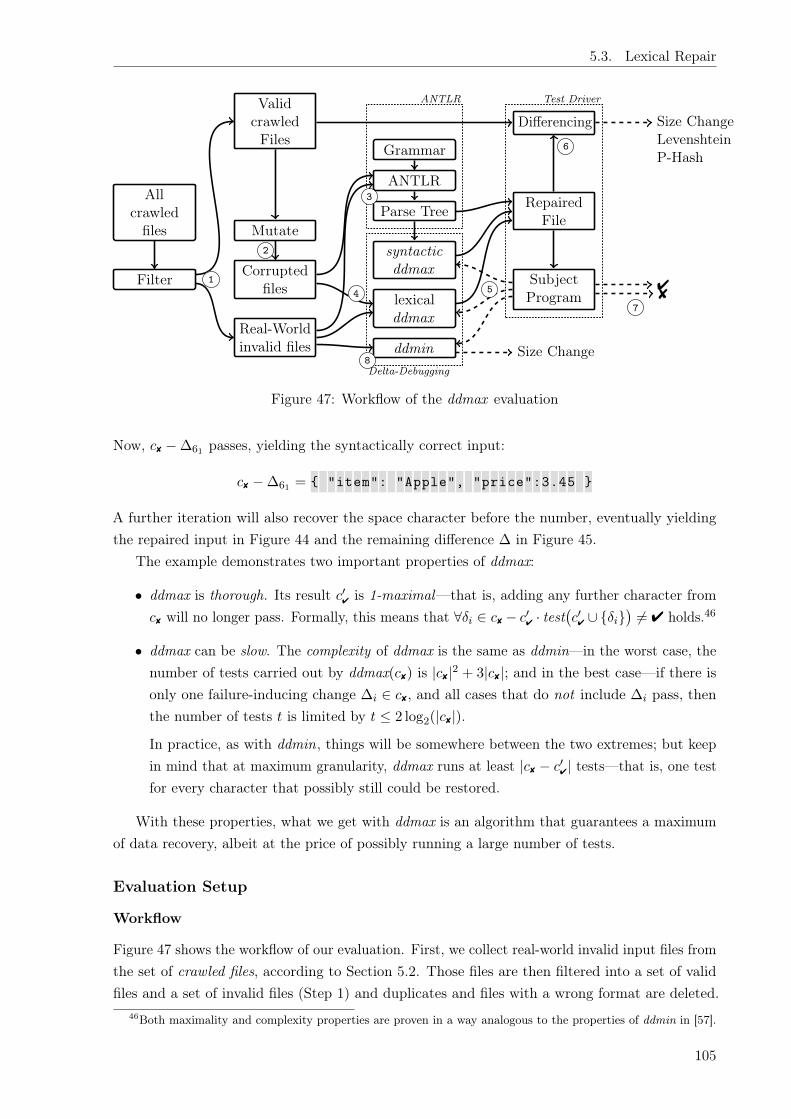
5.3. Lexical Repair
Corruptedfiles
syntacticddmax
lexicalddmax
Parse Tree
ANTLR
Grammar
RepairedFile
SubjectProgram
48
Differencing Size ChangeLevenshteinP-Hash
Mutate
ValidcrawledFiles
ddminReal-Worldinvalid files Size Change
Filter
Allcrawled
files
Test Driver
Delta-Debugging
ANTLR
2
3
45
6
7
8
1
Figure 47: Workflow of the ddmax evaluation
Now, c8 � �61 passes, yielding the syntactically correct input:
c8 � �61 = { "item": "Apple", "price":3.45 }
A further iteration will also recover the space character before the number, eventually yieldingthe repaired input in Figure 44 and the remaining difference � in Figure 45.
The example demonstrates two important properties of ddmax:
• ddmax is thorough. Its result c04 is 1-maximal—that is, adding any further character from
c8 will no longer pass. Formally, this means that 8�i 2 c8 � c04 · test
�c04 [ {�i}
�6= 4 holds.46
• ddmax can be slow. The complexity of ddmax is the same as ddmin—in the worst case, thenumber of tests carried out by ddmax(c8) is |c8|2 + 3|c8|; and in the best case—if there isonly one failure-inducing change �i 2 c8, and all cases that do not include �i pass, thenthe number of tests t is limited by t 2 log2(|c8|).
In practice, as with ddmin, things will be somewhere between the two extremes; but keepin mind that at maximum granularity, ddmax runs at least |c8 � c
04| tests—that is, one test
for every character that possibly still could be restored.
With these properties, what we get with ddmax is an algorithm that guarantees a maximumof data recovery, albeit at the price of possibly running a large number of tests.
Evaluation Setup
Workflow
Figure 47 shows the workflow of our evaluation. First, we collect real-world invalid input files fromthe set of crawled files, according to Section 5.2. Those files are then filtered into a set of validfiles and a set of invalid files (Step 1) and duplicates and files with a wrong format are deleted.
46Both maximality and complexity properties are proven in a way analogous to the properties of ddmin in [57].
105

5. Debugging Failure-Inducing Inputs
Secondly, we select and mutate 50 valid crawled files to produce an additional set of corruptedinput files (Step 2). Then, we feed a invalid file to each subject program, and the ANTLR parserframework (Step 3). ANTLR executes its default error recovery strategy while generating aparse tree for the input. Next, we feed the invalid file to lexical ddmax (Step 4). Lexical ddmaxtests the input under repair repeatedly using the feedback from the subject program (Step 5).Then, we feed the original crawled files and the resulting repaired file from each technique to thedifferencing framework (Step 6), which computes the change in file size, Levenshtein distanceand perceptive hash value for both files. We save the feedback from our subject program (Step 7).Finally, to ensure the quality of our approach, we also execute ddmin on the real-world invalidinputs (Step 8) and report the content and size of the result.
Lexical ddmax was implemented in 595 LoC of Java code. ANTLR also implements aninbuilt error recovery strategy which is designed to recover from lexing or parsing errors (e.g.missing/wrong tokens or incomplete parse trees) [234].
Mutations
In addition to the real-world invalid inputs (cf. Section 5.2), we also simulate real-world datacorruption by applying byte-level mutations on valid input files. These mutations were chosenbecause they are similar to the corruptions observed in real-world invalid files (see Section 5.2 andSection 5.5). We perform the following mutations at a random position in each valid input file:byte insertion, byte deletion and byte flip. To simulate single data corruption, we randomly chooseone of these mutations and apply it once on the valid input file. For multiple data corruptions,we perform up to 16 random mutations on each input file. A mutation is only successful (for aninput format), if at least one of the subject programs (that passes before) fails after the mutation.These criteria is similar to how we collected invalid input files in the wild.
Metrics and Measures
In order to determine the quality of ddmax repair, we use the following metrics and tools:
1. File Size: We measure the file size of the inputs recovered by ddmax and the difference infile size between the original valid input and the repaired file. We use these measurementsto account for the amount of data recovered by ddmax as well as the amount of data lossincurred.
2. Levenshtein Distance: Additionally, we measure data loss using the Levenshtein distancemetric [235], measuring the edit distance between valid input and repaired file.
3. Perceptive Image Difference: In order to measure the (semantic) information lossincurred by ddmax , we calculate the hash value of our 3D images, i.e. Wavefront OBJformat. We compute the image distance of our 3D image files by rendering both therepaired image and the original valid image into several 2D images from three differentcamera angles and three scales, then measuring the 2D image distance of all nine images.We compare these images using the Python ImageHash library [236] in order to obtaina good approximation of the real image difference between those two 3D models as a
106
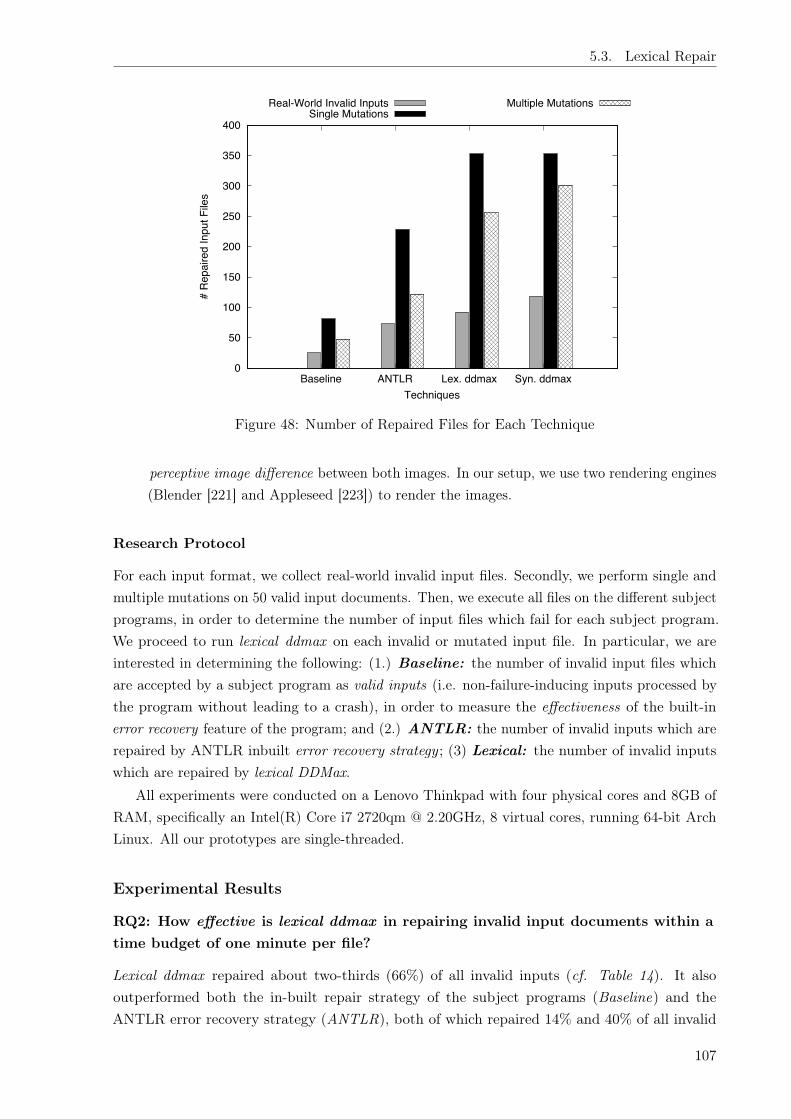
5.3. Lexical Repair
0
50
100
150
200
250
300
350
400
Baseline ANTLR Lex. ddmax Syn. ddmax
# R
epai
red
Inpu
t File
s
Techniques
Real-World Invalid InputsSingle Mutations
Multiple Mutations
Figure 48: Number of Repaired Files for Each Technique
perceptive image difference between both images. In our setup, we use two rendering engines(Blender [221] and Appleseed [223]) to render the images.
Research Protocol
For each input format, we collect real-world invalid input files. Secondly, we perform single andmultiple mutations on 50 valid input documents. Then, we execute all files on the different subjectprograms, in order to determine the number of input files which fail for each subject program.We proceed to run lexical ddmax on each invalid or mutated input file. In particular, we areinterested in determining the following: (1.) Baseline: the number of invalid input files whichare accepted by a subject program as valid inputs (i.e. non-failure-inducing inputs processed bythe program without leading to a crash), in order to measure the effectiveness of the built-inerror recovery feature of the program; and (2.) ANTLR: the number of invalid inputs which arerepaired by ANTLR inbuilt error recovery strategy ; (3) Lexical: the number of invalid inputswhich are repaired by lexical DDMax.
All experiments were conducted on a Lenovo Thinkpad with four physical cores and 8GB ofRAM, specifically an Intel(R) Core i7 2720qm @ 2.20GHz, 8 virtual cores, running 64-bit ArchLinux. All our prototypes are single-threaded.
Experimental Results
RQ2: How effective is lexical ddmax in repairing invalid input documents within atime budget of one minute per file?
Lexical ddmax repaired about two-thirds (66%) of all invalid inputs (cf. Table 14). It alsooutperformed both the in-built repair strategy of the subject programs (Baseline) and theANTLR error recovery strategy (ANTLR), both of which repaired 14% and 40% of all invalid
107
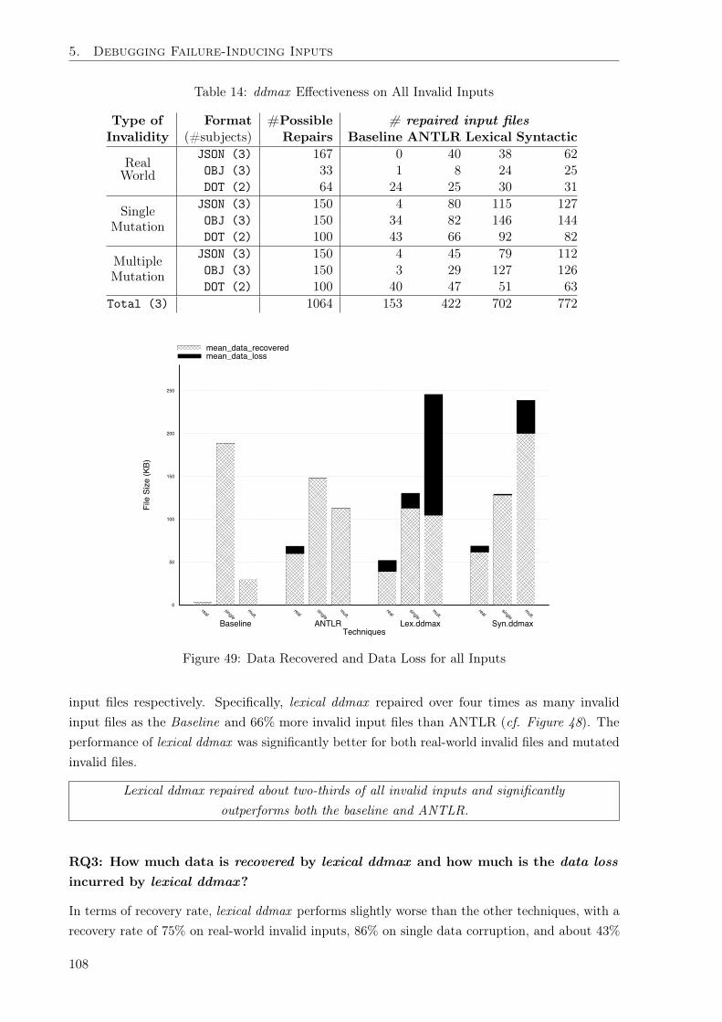
5. Debugging Failure-Inducing Inputs
Table 14: ddmax Effectiveness on All Invalid Inputs
Type of Format #Possible # repaired input filesInvalidity (#subjects) Repairs Baseline ANTLR Lexical Syntactic
RealWorld
JSON (3) 167 0 40 38 62OBJ (3) 33 1 8 24 25DOT (2) 64 24 25 30 31
SingleMutation
JSON (3) 150 4 80 115 127OBJ (3) 150 34 82 146 144DOT (2) 100 43 66 92 82
MultipleMutation
JSON (3) 150 4 45 79 112OBJ (3) 150 3 29 127 126DOT (2) 100 40 47 51 63
Total (3) 1064 153 422 702 772
0
50
100
150
200
250
realsingle
mult.real
singlemult.
realsingle
mult.real
singlemult.
File
Siz
e (K
B)
Techniques
mean_data_recoveredmean_data_loss
Syn.ddmaxLex.ddmaxANTLRBaseline
Figure 49: Data Recovered and Data Loss for all Inputs
input files respectively. Specifically, lexical ddmax repaired over four times as many invalidinput files as the Baseline and 66% more invalid input files than ANTLR (cf. Figure 48). Theperformance of lexical ddmax was significantly better for both real-world invalid files and mutatedinvalid files.
Lexical ddmax repaired about two-thirds of all invalid inputs and significantlyoutperforms both the baseline and ANTLR.
RQ3: How much data is recovered by lexical ddmax and how much is the data lossincurred by lexical ddmax?
In terms of recovery rate, lexical ddmax performs slightly worse than the other techniques, with arecovery rate of 75% on real-world invalid inputs, 86% on single data corruption, and about 43%
108
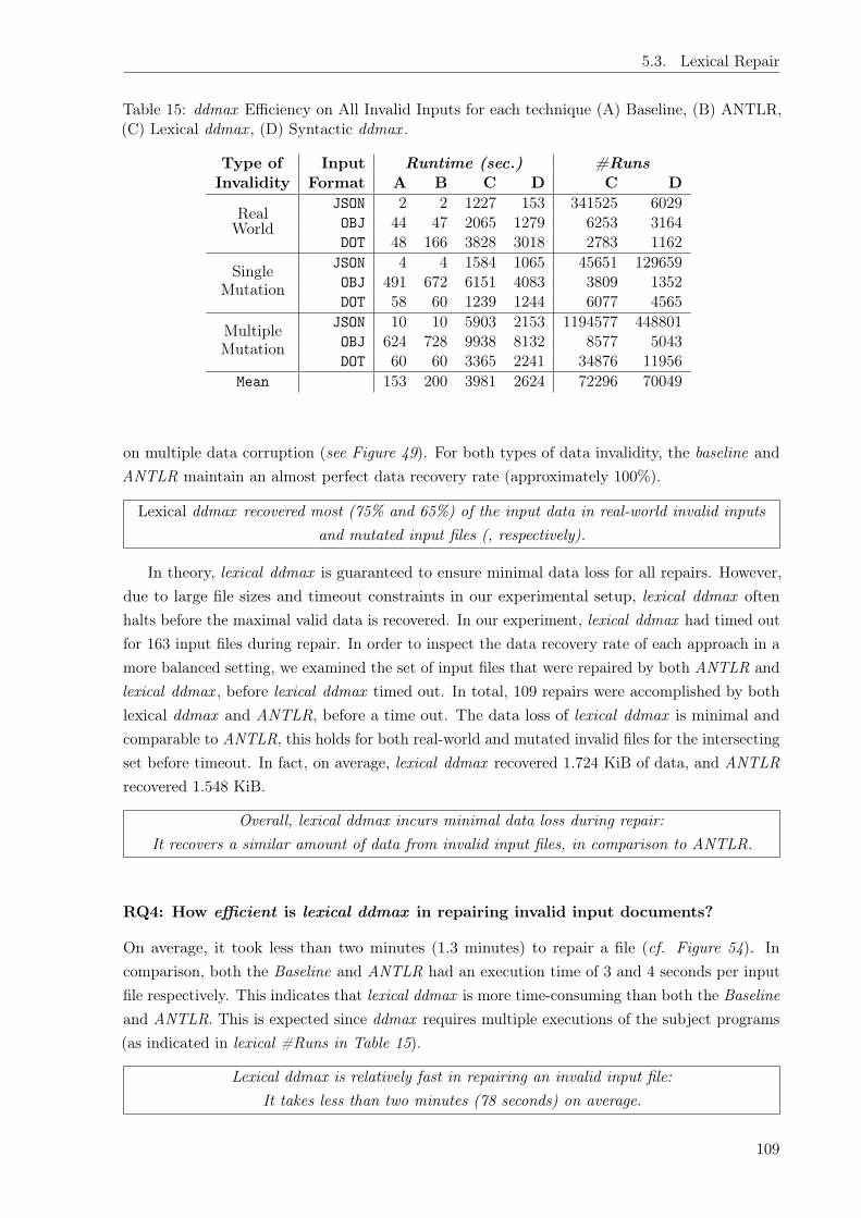
5.3. Lexical Repair
Table 15: ddmax Efficiency on All Invalid Inputs for each technique (A) Baseline, (B) ANTLR,(C) Lexical ddmax , (D) Syntactic ddmax .
Type of Input Runtime (sec.) #RunsInvalidity Format A B C D C D
RealWorld
JSON 2 2 1227 153 341525 6029OBJ 44 47 2065 1279 6253 3164DOT 48 166 3828 3018 2783 1162
SingleMutation
JSON 4 4 1584 1065 45651 129659OBJ 491 672 6151 4083 3809 1352DOT 58 60 1239 1244 6077 4565
MultipleMutation
JSON 10 10 5903 2153 1194577 448801OBJ 624 728 9938 8132 8577 5043DOT 60 60 3365 2241 34876 11956
Mean 153 200 3981 2624 72296 70049
on multiple data corruption (see Figure 49). For both types of data invalidity, the baseline andANTLR maintain an almost perfect data recovery rate (approximately 100%).
Lexical ddmax recovered most (75% and 65%) of the input data in real-world invalid inputsand mutated input files (, respectively).
In theory, lexical ddmax is guaranteed to ensure minimal data loss for all repairs. However,due to large file sizes and timeout constraints in our experimental setup, lexical ddmax oftenhalts before the maximal valid data is recovered. In our experiment, lexical ddmax had timed outfor 163 input files during repair. In order to inspect the data recovery rate of each approach in amore balanced setting, we examined the set of input files that were repaired by both ANTLR andlexical ddmax , before lexical ddmax timed out. In total, 109 repairs were accomplished by bothlexical ddmax and ANTLR, before a time out. The data loss of lexical ddmax is minimal andcomparable to ANTLR, this holds for both real-world and mutated invalid files for the intersectingset before timeout. In fact, on average, lexical ddmax recovered 1.724 KiB of data, and ANTLRrecovered 1.548 KiB.
Overall, lexical ddmax incurs minimal data loss during repair:It recovers a similar amount of data from invalid input files, in comparison to ANTLR.
RQ4: How efficient is lexical ddmax in repairing invalid input documents?
On average, it took less than two minutes (1.3 minutes) to repair a file (cf. Figure 54). Incomparison, both the Baseline and ANTLR had an execution time of 3 and 4 seconds per inputfile respectively. This indicates that lexical ddmax is more time-consuming than both the Baselineand ANTLR. This is expected since ddmax requires multiple executions of the subject programs(as indicated in lexical #Runs in Table 15).
Lexical ddmax is relatively fast in repairing an invalid input file:It takes less than two minutes (78 seconds) on average.
109

5. Debugging Failure-Inducing Inputs
{ "item": "Apple", "price" 3.45 }
Figure 50: Failing JSON input with missing colon
{ "item": "Apple" }
Figure 51: Repaired JSON input by ddmax
5.4 Syntactic Repair
We have seen that ddmax is general, but also slow: If one wants to recover a maximum of data,it runs a single test for every candidate character that can be recovered. Is it possible to speedthings up, possibly by leveraging information on the input format? To this end, we introduce thesyntactic ddmax algorithm, which improves the performance of ddmax using the knowledge ofthe input grammar.
The key insight is to execute ddmax on the parse tree of the input, instead of the inputcharacters. Here, we analyze the input at the syntactical level, rather than the lexical level. Thisimproves the runtime and general performance of the ddmax algorithm. The main benefit ofthe approach is that it enables ddmax to reason at a more coarse-grained level by testing on theinput structure. Lexical ddmax may take thousands of test runs, depending on the size of theinput, in fact its number of runs is bound to the number of characters in the input. However,syntactic ddmax is bound to the number of terminal nodes in the parse tree, which is typicallysmaller than the number of characters in the input. Thus, syntactic ddmax can easily excludecorrupted parse tree nodes or subtrees during test runs. Additionally, the knowledge of the inputstructure ensures that the resulting recovered inputs are syntactically valid. This helps in thecase of syntax errors, large corrupted input region(s) and multiple data corruptions on the input(structure).
Specifically, the syntactic ddmax algorithm takes as input a parse tree for the corrupted inputfile (see Figure 52) and obtains a pre-order list of terminals in the parse tree. For instance,consider the corrupted JSON input in Figure 50. Repairing this input using the lexical ddmaxalgorithm results in the JSON input in Figure 51, which would take over 100 test runs. Even forthis small example, syntactic ddmax enhances the performance of ddmax with the input grammar,reducing the number of test runs of ddmax to nine (9) and improving performance by ten fold(10x).
To repair the input (cf. Figure 50), syntactic ddmax first parses the input into a parse tree47,shown in Figure 52. Next, we run the ddmax algorithm on the parse tree, removing terminalnodes (instead of single characters) in each iteration of ddmax 48. We define c8 as our failingconfiguration, which contains the terminal nodes of the parse tree from Figure 52.
Let us run the ddmax algorithm on our example terminal nodes. We invoke ddmax(c8) whichresults in ddmax2(;, 2), so inside ddmax2, we have c
04 = ; and n = 2. At first, our � is split into
47ANTLR is capable of generating a parse tree for corrupted input files, it summarizes syntactically wrongsymbols or trees into error nodes (similar to Figure 52).
48Removing only the error node in the parse tree does not necessarily result in a non-failure-inducing input.
110

5.4. Syntactic Repair
hJSONi
{ hdicti
hstringi
"item" : "Apple"
, Error
}
Figure 52: Parse tree of Figure 50
two parts49:
�1 = { "item" : "Apple"
�2 = , Error }
Running test(c8 � �1) and test(c8 � �2) both fail (= 8). We are at the first run, so with c08 = ;,
c04 [ �1 = c8 � �2 and c
04 [ �2 = c8 � �1 which also both fail in the “increase to subset” step.
Next, we set n = 4 and restart ddmax2(c04, n).With n = 4, in the “increase to complement” and “increase to subset” steps, we get
�1 = { "item" �2 = : "Apple"
�3 = , Error �4 = }
In the “increase to complement” step, we find that test(c8 � �3) = 4, so we repeat ouralgorithm with c
04 = c8 � �3 and n = 2, getting
�1 = , �2 = Error
Since neither test(c8 � �i) nor test(c04 [ �i) passes for any i and n = |c8 � c04| = 2, we are done
and end up with the remaining input seen in Figure 51. For this example, the syntactic ddmaxrun needed only 9 test runs of the subject program to repair the faulty input.
Let us now take a look at the complexity of our algorithm. As mentioned in Section 5.3,ddmax has a worst-case complexity of t = |c8|2 + 3|c8| test runs and a best-case complexity oft 2 log2(|c8|). Intuitively, the complexity of syntactic ddmax is similar to the complexity ofddmax, except that it is bounded by the number of terminal nodes instead of the number ofcharacters. In the worst case, an input’s parse tree has as many terminal nodes as characters.However, real-world input formats have keywords, data types and character classes to aggregrategroup of characters into terminals (e.g. string and integers). This reduces the number of terminalnodes and the required number of test runs for syntactic ddmax . It therefore speeds up ddmax bydecreasing the number of elements to maximize with ddmax . Consider the example in Figure 50,there are 33 single characters to search with lexical ddmax , which are parsed into 7 terminalnodes for syntactic ddmax . In general, we can assume that with an average terminal node length
49Note that checking for only syntactically valid subsets of the programs (e.g. using the grammar only) is notsufficient to repair the input. We leverage the application, since the semantics and intended use of the input fileare encoded in the logic of the applcation.
111

5. Debugging Failure-Inducing Inputs
of n characters, we have a worst-case complexity of⇣|c8|n
⌘2+ 3 |c8|
n test runs and a best-case
complexity of t 2 log2(|c8|n ) test runs.
Evaluation Setup
Implementation
Syntactic ddmax was implemented in 1084 LoC of Java code, this implementation is built ontop of the ANTLR 4.5 parser generator framework [237] for each input grammar. Overall, theimplementation of syntactic ddmax differs from that of lexical ddmax in Section 5.3, because ofits use of the input grammar and parse tree. Specifically, Syntactic ddmax uses the ANTLR parsetree (from Step 3 in Figure 47) to repair invalid inputs. In our evaluation, we feed the invalidreal-world files into our syntactic ddmax, we proceed to run syntactic ddmax on each invalidinput file and evaluate the change in file size (i.e. the data loss on byte-level). Syntactic ddmaxtests the input under repair repeatedly using the feedback from the subject program (Step 5). Inaddition to the research protocol in Section 5.3, we feed all invalid input files to syntactic ddmaxand measure the number of invalid files which are repaired by our syntactic DDMax using theinput grammar, this measure is termed Syntactic.
Experimental Results
RQ5: How effective is syntactic ddmax in repairing invalid input documents withina time budget of one minute per file?
Syntactic ddmax repaired about three-quarters (73%) of all invalid inputs in our evaluation,within a time budget of one minute per input (cf. Table 14). Overall, it is about 10% moreeffective than lexical ddmax (cf. Figure 48). It significantly outperformed both the built-in repairstrategies of the subject programs and ANTLR, it repaired five times as many files as the subjectprograms, and almost twice as many files as ANTLR (cf. Table 14). This confirms our hypothesis(in RQ2 ) that ddmax can benefit from the knowledge of the input grammar.
Syntactic ddmax repaired about three-quarters of all invalid inputs (within one minute per input)and it is more effective than lexical ddmax, for all invalid inputs.
RQ6: How much data is recovered by syntactic ddmax and how much is the dataloss incurred by syntactic ddmax ?
On average, syntactic ddmax (89%) has a higher data recovery rate in comparison to lexicalddmax (58%) for all invalid inputs. For single data corruption, the data recovery rate of syntacticddmax is similar to that of ANTLR and the baseline, when using mean file size as a metric. Onmultiple data corruption, syntactic ddmax recovered about 84% of the data in the input files(cf. Figure 49). For all invalid inputs, the baseline and ANTLR maintain an almost perfect datarecovery rate (approximately 100%). Evidently, the data loss incurred by both ANTLR and thebaseline is negligible.
112

5.4. Syntactic Repair
0
50
100
150
200
Baseline ANTLR Lex. ddmax Syn. ddmax
Dat
a Lo
ss
Techniques
Mean Difference in File Size (KB)Mean Levenshtein Distance
Mean Perceptive Image Difference (PHASH)
Figure 53: Data Loss Incurred for Invalid Files
Syntactic ddmax has a high data recovery rate,recovering most (89%) of the data in invalid input files.
The data loss incurred by syntactic ddmax is very low, in terms of the edit distance betweenthe recovered file and the valid file. For all invalid inputs, it is less than 50% worse off thanANTLR, as captured by the Levenshtein distance (cf. Figure 53). In particular, the meanedit distance of the repaired file and the originally valid input file is less than four for thebaseline and about 24 for ANTLR. As expected, the Levenshtein distance is lower (21–28) forsingle data corruptions for lexical and syntactical ddmax respectively, and higher for multiplecorruptions (76–77). On inspection, we found that the high loss of ddmax is due to early timeoutsfor large input files, indeed, ddmax finds a valid subset, but times out before the maximal subsetis reached. For Wavefront OBJ files, the perceptive image difference shows us similar scalingresult as the Levenshtein distance. While it shows small results for Baseline and ANTLR (0.1and 29.7, respectively), the results for lexical and syntactical ddmax are higher (76.4 and 51.9),thus the difference between the unmodified image and the repaired image is larger.
We conduct our evaluation of minimal data loss similarly to the setting in RQ3 (cf. Section 5.3).As expected, syntactic ddmax recovered slightly less data than lexical ddmax , exactly 1.720 KiBon average. This is because syntactic ddmax removes terminal nodes, a terminal node may containmore characters than the number of mutated characters in the node. In summary, with a highenough timeout lexical ddmax is guaranteed to achieve minimal data loss, this guarantee doesnot hold for syntactic ddmax , since it operates at the parse tree level rather than the byte level.
Syntactic ddmax incurs comparativelysimilar data loss during repair as lexical ddmax.
113

5. Debugging Failure-Inducing Inputs
0.1
1
10
100
1000
10000
100000
1x10⁶
1x10⁷
Baseline ANTLR Lex. ddmax Syn. ddmax
Run
time
(ms)
Techniques
Mean runtime per repaired input file
1443.5 1882.7
37997.8 25153.9
Figure 54: Mean Runtime per Input File for Each Technique
RQ7: How efficient is syntactic ddmax in repairing invalid input documents?
Syntactic ddmax improves over the runtime performance of lexical ddmax (cf. RQ4 Section 5.3).It improves over lexical ddmax by 34%, its execution time is about two-third of the running timeof lexical ddmax. Specifically, syntactic ddmax is quicker, it took approximately one minute torepair a single file, but requires a grammar and a parse tree50.
Syntactic ddmax is faster in repairing an invalid input file:It takes less than one minute to repair a file on average.
5.5 Diagnostic Quality
Even though ddmax is primarily meant for repairing data, its maximized input can also be usefulfor diagnostics and debugging. In particular, ddmax diagnosis is the difference (�) between thefailing and maximal passing input. This is a minimal failure cause, which is necessary to debugthe input. Most notably, the � from ddmax includes all input characters that are failure-inducing,whereas ddmin include only a minimal subset.
Evaluation Setup
To evaluate the diagnostic utility of ddmax , we compare ddmax diagnoses to the establishedstate of the art input diagnosis approach ddmin. In our evaluation, we compare ddmax diagnosisto that of ddmin, we do not compare to the general delta debugging (DD) algorithm. This isbecause DD is not suited for repairing inputs. Although, DD would produce a passing and afailing input with a minimal difference between them. This DD difference could be as small as
50Depending on the grammar and on the input file size, generating a parse tree should take less than a second.
114

5.5. Diagnostic Quality
Table 16: Diagnostic Quality on Real-World Invalid Inputs for A○ ddmin and B○ ddmax diagnoses,and C○ ddmax repair.
Format Diagnosis (B) Repair (B) Intersection (%)(#inputs) A B C A \ B A \ CJSON (21) 2.909 19.095 103.476 13.88 23.18OBJ (18) 2.722 1.000 189.000 18.03 11.46DOT (27) 376.654 1.115 675.346 5.76 54.64Mean 155.754 6.804 360.747 11.69 32.85
the ddmax difference between the maximal passing input and the original failing input, and havesimilar diagnostic quality; also, DD would likely be faster. However, DD does not have the goalof minimizing data loss, and thus the passing input resulting from general DD may actually beclose to a minimal input cutting away all the original context.
By construction, DD (and ddmin) can minimize (and thus lose) all the context of the originalfailure. For instance, if there is a flag in the input that activates the faulty function, and DD(and ddmin) will remove that flag, causing the program to pass, then this single flag will endup as failure-inducing input. On the other hand, ddmax would preserve as much of the originalcontext as possible by construction. It is these experiences that have driven us to experimentwith DD alternatives such as ddmax and ddmin.
We implemented a ddmin algorithm following the delta debugging algorithm in [57] in 450LoC of Java code. Our ddmin implementation uses both the subject program and ANTLR asoracles to minimize an invalid input, in order to ensure that ddmin diagnosis is syntacticallyvalid. This ensures that ddmin does not report a valid subset that may trigger a failure due tosyntactic invalidity (e.g. in cf. Figure 43 in Section 5.1), since ANTLR can parse the ddmindiagnosis, but the subject program crashes. Then, we feed the real-world invalid files into ourddmin implementation (as seen in Figure 47 Step 8) and compare the diagnosis generated byddmin to that of ddmax .
We are interested in evaluating the soundness and completeness of ddmin diagnosis, usingddmax diagnoses as the “ground truth”. To be fair to both approaches, we consider the intersectionof the diagnoses for both ddmin and ddmax that finished execution before a time-out, this a setof 66 input files in total (cf. Table 16).
Experimental Results
RQ8: How effective is ddmax in diagnosing the root cause of invalid inputs,especially in comparison to ddmin?
Given that ddmax was completely executed without a timeout, the repair of ddmax is the maximalpassing input and ddmax diagnosis is the minimal failure cause. As expected ddmin diagnosis issignificantly larger (21 times more) than the ddmax diagnosis, hence, it contains a significantamount (33%) of the maximal passing input, which is considered noise in the diagnosis (cf. A\ C in Table 16). Additionally, ddmin diagnosis only contains a small portion (12%) of theminimal failure cause required to diagnose the input invalidity (cf. A \ B in Table 16). This
115
5. Debugging Failure-Inducing Inputs
result shows that ddmax diagnosis is more effective for input debugging in comparison to thestate of the art, ddmin.
Only one-eighth (12%) of a ddmin diagnosis contains the minimal failure cause and aboutone-third (33%) of ddmin diagnosis contains the maximal passing input, on average.
5.6 Threats to Validity
Our evaluation is limited to the following threats to validity:
External validity refers to the generalizability of our approach and results. We have evaluatedour approach on a small set of applications and input grammars. There is a threat thatddmax does not generalize to other applications and grammars. However, we have mitigatedthis threat by evaluating ddmax using mature subject programs with varying input sizes.Our subjects have 478 KLoC and 14 years maturity, on average, making us confident thatour approach will work on a large variety of applications and invalid inputs.
Internal validity is threatened by incorrectness of our implementation, specifically whetherwe have correctly adapted ddmin to ddmax for input repair. We mitigate this threat bytesting our implementation on smaller inputs and simpler grammars, in order to ensure ourimplementation works as expected.
Construct validity is threatened by our test oracle, and consequently the error-handling im-plementation of the subject. For instance, an application which silently handles exceptionswould not provide ddmax with useful feedback during test runs. We checked that therendered input produced by the subject is non-empty, after a 10 second timeout, which wassufficient to identify failure-inducing inputs.
5.7 Limitations
Both ddmax variants are limited in the following ways:
Repair to subsets only. Both ddmax variants will return a strict lexical or syntactical subset ofthe original failure-inducing input. The assumption is that only data should be restored thatalready is there (rather than synthesizing new data, for instance). If the input format hasseveral context-sensitive dependencies, such as checksums, hashes, encryption, or references,a strict lexical or syntactical subset might be small to the point of being useless.
Data repair, not information repair. Both ddmax variants are set to recover as much dataas possible, but not necessarily information. Even though the repaired input may be lexicallyor syntactically close to the (presumed) original input, it can have very different semantics.Users therefore are advised to thoroughly check the repaired input for inconsistencies; thegoal of this work is to enable users to load the input into their program such that they canengage in this task.
116

5.8. Related Work
Input Semantics. Although, ddmax obtains some “semantic” information from the feedback ofthe subject program itself, this feedback is limited to failure characteristics, i.e. “pass” or“fail”. However, it is possible to extend ddmax to include (domain-specific) semantic checks,which could either be defined as the execution of specific program artifacts such as a specificbranch, or programmatically defined by a developer (e.g. as an expected program output).
Multiple errors and multiple repairs. If there are multiple errors in an input, ddmax willproduce a maximum input that repairs all of them. However, if there are multiple waysto repair the input, ddmax will produce only one of them. This property is shared withdelta debugging and its variants, which also pick a local minimum rather than searching fora global one. However, it would be easy to modify ddmax to assess all alternative repairsrather than the first repair.
5.8 Related Work
There is a large body of work concerning the interplay of program, inputs, and faults. We discussthe most important related works.
Document Recovery attempts to fix broken input documents. Docovery [63] uses symbolicexecution to manipulate corrupted input documents in a manner that forces the program tofollow an alternative error-free path. In contrast to ddmax , this is a white-box approachthat analyzes the program paths executed by the failure-inducing inputs. S-DAGS [64] is asemi-automatic technique that enforces formal (semantic) consistency constraints on inputsdocuments in a collaborative document editing scenario. Both of these approaches requireprogram analysis.
Input Rectification aims at transforming invalid inputs into inputs that behave acceptably.Input rectifiers [61, 62] address this problem by learning a set of constraints from typicalinputs, then transforming a malicious input into a benign input that satisfies the learnedconstraints. In contrast, ddmax does not learn constraints but rather employs the feedbackfrom the program’s execution (and a grammar) to determine an acceptable subset of theinput. In comparison to security-critical rectification, its goal is maximal data recovery.
Input Minimization Numerous researchers have examined the problem of simplifying failure-inducing inputs [57, 58, 59, 60]. In particular, [59] (HDD) and [60] are closely related toddmax . Both approaches use the input structure to simplify inputs, albeit without an inputgrammar. Unlike ddmax , these approaches do not recover maximal valid data from thefailure-inducing input, but rather minimize the input like ddmin.
Data Diversity [65] transforms an invalid input into a valid input that generates an equivalentresult, in order to improve software reliability. This is achieved by finding the regions of theinput space that causes a fault, and re-expressing a failing input to avoid the faulty inputregions. In contrast, ddmax does not require program analysis; it only needs a means toassess whether the program can process the input or not.
117

5. Debugging Failure-Inducing Inputs
Data Structure Repair iteratively fixes corrupted data structures by enforcing that they con-form to consistency constraints [238, 239, 240, 241]. These constraints can be extracted,specified and enforced with predicates [242], model-based systems [238], goal-directed rea-soning [239], dynamic symbolic execution [240] or invariants [241]. On the one hand, thegoal of data structure repair is to ensure a program executes safely and acceptably, despitedata structure corruption. On the other hand, the goal of ddmax is to repair the input inorder to avoid the corruption of the program’s internal data structure.
Syntactic Error Recovery. Parsers and compilers implement numerous syntax error recoveryschemes [219, 243]. Most approaches involve a plethora of operations including insertion,deletion and replacement of symbols [244, 245, 246], extending forward or backwards from aparser error [247, 248], or more general methods of recovery and diagnosis [249, 250]. Unlikeddmax , these schemes ensure the compiler does not halt while parsing, however, the invalidinput is not automatically fixed.
Data Cleaning and Repair. Several researchers have addressed the problem of data cleaningof database systems. Most approaches automatically analyse the database to remove noisydata or fill in missing data [251, 252]. Other approaches allow developers to write and applylogical rules on the database [253, 254, 255, 256, 257, 258]. In contrast to ddmax , all of theseapproaches repair database systems, not raw user inputs.
Data Testing and Debugging aims to identify system errors caused by well-formed but in-correct data while a user modifies a database [259]. For instance, continuous data testing(CDT) [260] identfies likely data errors by continuously executing domain-specfic test queries,in order to warn users of test failures. DATAXRAY [261] also investigates the underlyingconditions that cause data bugs, it reveals hidden connections and common properties amongdata errors. In contrast to ddmax , these approaches aim to guard data from new errors bydetecting data errors in database systems during modification.
5.9 Discussions and Future Work
This chapter has provided empirical evidence on the relevance, causes and prevalence of invalidinputs in software practice. For instance, we found that four (4) percent of inputs in the wildare invalid. Evidently, debugging and repairing invalid inputs is a relevant and challengingproblem. Thus, with ddmax , we have presented the first generic technique for automaticallyrepairing failure-inducing inputs—that is, recovering a maximal subset of the input that can stillbe processed by the program at hand. Our approach (i.e. ddmax) is a variant of delta debuggingthat maximizes the passing input, both at a lexical and a syntactical level; it requires nothingmore than the ability to automatically run the program with a given input. In our evaluation,we find that ddmax fully repairs 79% of invalid input files, within a one (1) minute time budget.Both variants of ddmax can be easily implemented and deployed in a large variety of contexts asthey do not require any kind of program analysis.
This work opens the door for a number of exciting research opportunities, our future workwill focus on the following issues:
118

5.9. Discussions and Future Work
Synthesizing input structures. Going for a strict lexical or syntactical subset of the failure-inducing input is a conservative strategy; yet, there can be cases where adding a smallamount of lexical or syntactical elements can help to recover even more information. We areinvestigating appropriate grammar-based production strategies as well as hybrid strategiesthat leverage both syntactical and lexical progression.
Learned grammars. Right now, our syntactical variant of ddmax requires an input grammarto start with. We are investigating whether such a grammar can also be inferred fromthe program at hand [262, 263], thus freeing users or developers from having to provide agrammar.
From input repair to code repair. A minimal difference (�) between a maximized passingand a full failure-inducing input also brings great opportunities for fault localization andrepair. For instance, what is the code executed by the failure-inducing input, but not by themaximized passing input? What are the differences in variable values? Such differences inexecution can help developers to further narrow down failure causes as well as synthesizingcode repairs.
End-user debugging. Our input repair technique needs no specific knowledge on program code,and could thus also be applied by end users. We are investigating appropriate strategies tocommunicate the results of our repair and information about conflicting document parts toend users, such that they can fix the problem without having to fix the program.
Hybrid repair. Lexical and syntactic ddmax can be combined such that after syntactic ddmaxis executed on the parse tree, lexical ddmax further repairs the text in the faulty nodes.This combination reduces the number of iterations and the execution time, in comparison tolexical ddmax . Moreover, it improves on the effectiveness of syntactic ddmax .
Semantic Input Repair. It is possible to extend the ddmax test oracle to include checks fordesirable “semantic” properties other than failure characteristics (i.e. pass or fail). Forinstance, the test oracle can be extedned to check if some function is triggered or somespecific output is produced, such “semantic” checks would ensure that the resulting maximizedpassing input is semantically similar to the original input and avoids the failure.
Fuzzing. Both variants of ddmax can be applied to improve software fuzzing. For instance,mutational fuzzing techniques often modify seed inputs to find bugs in the program. Often,these inputs become malformed after mutation, ddmax can be applied to repair such inputs,in order to ensure that they are valid, and consequently, cover program logic.
The implementation of ddmax and the experimental data are available as a replication package:
https://tinyurl.com/debugging-inputs-icse-2020
119


Chapter 6
Learning Input Distributions forGrammar-Based Test Generation
This chapter is taken, directly or with minor modifications, from our 2020 TSE paper Inputs fromHell: Learning Input Distributions for Grammar-Based Test Generation [20]. My contributionin this work is as follows: (I) original idea; (II) partial implementation; (III) evaluation.
“A pinch of probability is worth a pound of perhaps.”— James Thurber
6.1 Introduction
During the process of software testing, software engineers typically attempt to satisfy three goals:
1. First, the software should work well on common inputs, such that the software delivers itspromise on the vast majority of cases that will be seen in typical operation. To cover suchbehavior, one typically has a set of dedicated tests (manually written or generated).
2. Second, the software should work well on uncommon inputs. The rationale for this is thatsuch inputs would exercise code that is less frequently used in production, possibly lesstested, and possibly less understood [70].
3. Third, the software should work well on inputs that previously caused failures, such that itis clear that previous bugs have been fixed. Again, these would be covered via specific tests.
How can engineers obtain such inputs? In this chapter, we propose an approach that learnsthe distribution of input elements from typical inputs found in software practice, in order to drivetest generation. Firstly, our approach learns the distribution of input elements from a set ofsample inputs found in software practice. The learned input distribution is then used to drivethe generation of new test inputs. Specifically, we introduce a novel test generation method thatproduce additional inputs that are markedly similar or dissimilar to the sample. By learningfrom past failure-inducing inputs, we can create inputs with similar features; by learning fromcommon inputs, we can create uncommon inputs with dissimilar features not seen in the sample.
121

6. Learning Input Distributions for Grammar-Based Test Generation
The key ingredient to our approach is a context-free grammar that describes the inputlanguage to a program. Using such a grammar, we can parse existing input samples and counthow frequently specific elements occur in these samples. Armed with these numbers, we canenrich the grammar to become a probabilistic grammar, in which production alternatives carrydifferent likelihoods. Since these probabilities come from the samples used for the quantification,such a grammar captures properties of these samples, and producing from such a grammarshould produce inputs that are similar to the sample. Furthermore, we can invert the learnedprobabilities in order to obtain a second probabilistic grammar, whose production would produceinputs that are dissimilar to the sample. We thus can produce three kinds of inputs, covering thethree testing goals listed above:
1. “Common inputs”. By learning from common samples, we obtain a “common” probabilitydistribution, which allows us to produce more “common” inputs. This is useful for regressiontesting.
2. “Uncommon inputs”. Learning from common samples, the resulting inverted grammardescribes in turn the distribution of valid, but uncommon inputs. This is useful forcompleting test suites by testing uncommon features.
3. “Failure-inducing inputs”. By learning from samples that caused failures in the past, wecan produce similar inputs that test the surroundings of the original inputs. This is usefulfor testing the completeness of fixes.
Both the “uncommon inputs” and “failure-inducing inputs” strategies have high chances oftriggering failures. Since they combine features rarely seen or having caused issues in the past,we gave them the nickname “inputs from hell”. As an example, consider the following JavaScriptinput generated by focusing on uncommon features:
var { a: {} = ’b’ } = {};
This snippet is valid JavaScript code, but causes the Mozilla Rhino 1.7.7.2 JavaScript engineto crash during interpretation.51 This input makes use of so-called destructuring assignments : InJavaScript, one can have several variables on the left hand side of an assignment or initialization.In such a case, each gets assigned a part of the structure on the right hand side, as in
var [one , two , three] = [1, 2, 3];
where the variable one is assigned a value of 1, two a value of 2, and so on. Such destructuringassignments, although useful in some contexts, are rarely found in JavaScript programs and tests.It is thus precisely the aim of our approach to generate such uncommon “inputs from hell”.
This chapter makes the following contributions:
1. We use context-free grammars to determine production probabilities from a given set ofinput samples.
51We have reported this snippet as Rhino issue #385 and it has been fixed by the developers.
122
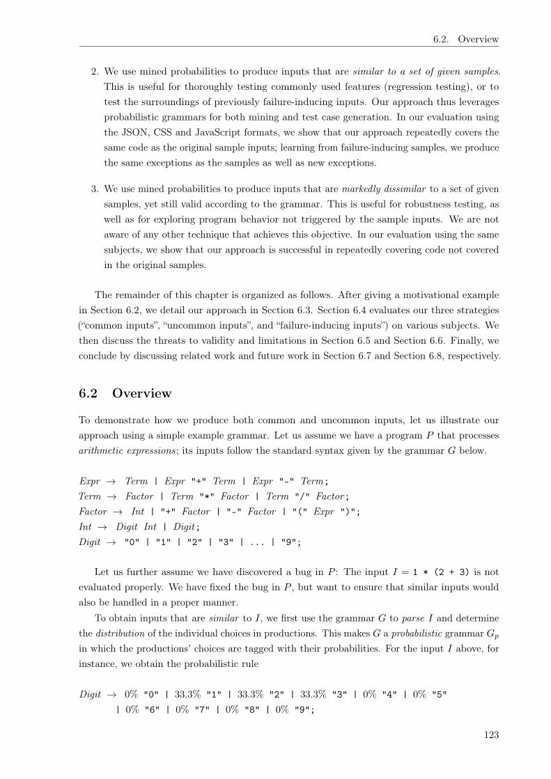
6.2. Overview
2. We use mined probabilities to produce inputs that are similar to a set of given samples.This is useful for thoroughly testing commonly used features (regression testing), or totest the surroundings of previously failure-inducing inputs. Our approach thus leveragesprobabilistic grammars for both mining and test case generation. In our evaluation usingthe JSON, CSS and JavaScript formats, we show that our approach repeatedly covers thesame code as the original sample inputs; learning from failure-inducing samples, we producethe same exceptions as the samples as well as new exceptions.
3. We use mined probabilities to produce inputs that are markedly dissimilar to a set of givensamples, yet still valid according to the grammar. This is useful for robustness testing, aswell as for exploring program behavior not triggered by the sample inputs. We are notaware of any other technique that achieves this objective. In our evaluation using the samesubjects, we show that our approach is successful in repeatedly covering code not coveredin the original samples.
The remainder of this chapter is organized as follows. After giving a motivational examplein Section 6.2, we detail our approach in Section 6.3. Section 6.4 evaluates our three strategies(“common inputs”, “uncommon inputs”, and “failure-inducing inputs”) on various subjects. Wethen discuss the threats to validity and limitations in Section 6.5 and Section 6.6. Finally, weconclude by discussing related work and future work in Section 6.7 and Section 6.8, respectively.
6.2 Overview
To demonstrate how we produce both common and uncommon inputs, let us illustrate ourapproach using a simple example grammar. Let us assume we have a program P that processesarithmetic expressions ; its inputs follow the standard syntax given by the grammar G below.
Expr ! Term | Expr "+" Term | Expr "-" Term;Term ! Factor | Term "*" Factor | Term "/" Factor;Factor ! Int | "+" Factor | "-" Factor | "(" Expr ")";Int ! Digit Int | Digit;Digit ! "0" | "1" | "2" | "3" | ... | "9";
Let us further assume we have discovered a bug in P : The input I = 1 * (2 + 3) is notevaluated properly. We have fixed the bug in P , but want to ensure that similar inputs wouldalso be handled in a proper manner.
To obtain inputs that are similar to I, we first use the grammar G to parse I and determinethe distribution of the individual choices in productions. This makes G a probabilistic grammar Gp
in which the productions’ choices are tagged with their probabilities. For the input I above, forinstance, we obtain the probabilistic rule
Digit ! 0% "0" | 33.3% "1" | 33.3% "2" | 33.3% "3" | 0% "4" | 0% "5"| 0% "6" | 0% "7" | 0% "8" | 0% "9";
123

6. Learning Input Distributions for Grammar-Based Test Generation
Expr
Term
Factor
")"Expr
Term
Factor
Int
Digit
"3"
"*"Term
Factor
Int
Digit
"2"
"("
"+"Expr
Term
Factor
Int
Digit
"1"
Figure 55: Derivation tree representing "1 + (2 * 3)"
Expr ! 66.7% Term | 33.3% Expr "+" Term | 0% Expr "-" Term;Term ! 75% Factor | 25% Term "*" Factor | 0% Term "/" Factor;Factor ! 75% Int | 0% "+" Factor | 0% "-" Factor | 25% "(" Expr ")";Int ! 0% Digit Int | 100% Digit;Digit ! 0% "0" | 33.3% "1" | 33.3% "2" | 33.3% "3" | 0% "4" | 0% "5"
| 0% "6" | 0% "7" | 0% "8" | 0% "9";
Figure 56: Probabilistic grammar Gp, expanding G
(2 * 3)2 + 2 + 1 * (1) + 2((3 * 3))3 * (((3 + 3 + 3) * (2 * 3 + 3))) * (3)3 * 1 * 3((3) + 2 + 2 * 1) * (1)1((2)) + 3
Figure 57: Inputs generated from Gp in Figure 56
124
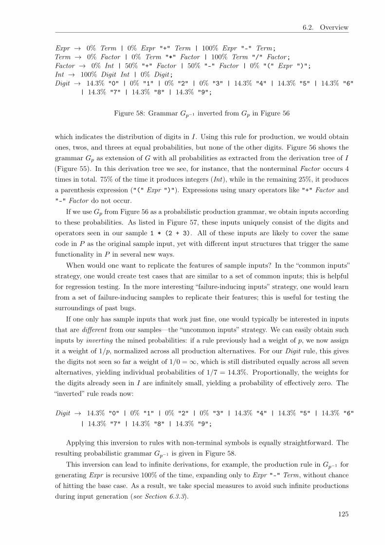
6.2. Overview
Expr ! 0% Term | 0% Expr "+" Term | 100% Expr "-" Term;Term ! 0% Factor | 0% Term "*" Factor | 100% Term "/" Factor;Factor ! 0% Int | 50% "+" Factor | 50% "-" Factor | 0% "(" Expr ")";Int ! 100% Digit Int | 0% Digit;Digit ! 14.3% "0" | 0% "1" | 0% "2" | 0% "3" | 14.3% "4" | 14.3% "5" | 14.3% "6"
| 14.3% "7" | 14.3% "8" | 14.3% "9";
Figure 58: Grammar Gp�1 inverted from Gp in Figure 56
which indicates the distribution of digits in I. Using this rule for production, we would obtainones, twos, and threes at equal probabilities, but none of the other digits. Figure 56 shows thegrammar Gp as extension of G with all probabilities as extracted from the derivation tree of I
(Figure 55). In this derivation tree we see, for instance, that the nonterminal Factor occurs 4times in total. 75% of the time it produces integers (Int), while in the remaining 25%, it producesa parenthesis expression ("(" Expr ")"). Expressions using unary operators like "+" Factor and"-" Factor do not occur.
If we use Gp from Figure 56 as a probabilistic production grammar, we obtain inputs accordingto these probabilities. As listed in Figure 57, these inputs uniquely consist of the digits andoperators seen in our sample 1 * (2 + 3). All of these inputs are likely to cover the samecode in P as the original sample input, yet with different input structures that trigger the samefunctionality in P in several new ways.
When would one want to replicate the features of sample inputs? In the “common inputs”strategy, one would create test cases that are similar to a set of common inputs; this is helpfulfor regression testing. In the more interesting “failure-inducing inputs” strategy, one would learnfrom a set of failure-inducing samples to replicate their features; this is useful for testing thesurroundings of past bugs.
If one only has sample inputs that work just fine, one would typically be interested in inputsthat are different from our samples—the “uncommon inputs” strategy. We can easily obtain suchinputs by inverting the mined probabilities: if a rule previously had a weight of p, we now assignit a weight of 1/p, normalized across all production alternatives. For our Digit rule, this givesthe digits not seen so far a weight of 1/0 = 1, which is still distributed equally across all sevenalternatives, yielding individual probabilities of 1/7 = 14.3%. Proportionally, the weights forthe digits already seen in I are infinitely small, yielding a probability of effectively zero. The“inverted” rule reads now:
Digit ! 14.3% "0" | 0% "1" | 0% "2" | 0% "3" | 14.3% "4" | 14.3% "5" | 14.3% "6"| 14.3% "7" | 14.3% "8" | 14.3% "9";
Applying this inversion to rules with non-terminal symbols is equally straightforward. Theresulting probabilistic grammar Gp�1 is given in Figure 58.
This inversion can lead to infinite derivations, for example, the production rule in Gp�1 forgenerating Expr is recursive 100% of the time, expanding only to Expr "-" Term, without chanceof hitting the base case. As a result, we take special measures to avoid such infinite productionsduring input generation (see Section 6.3.3).
125

6. Learning Input Distributions for Grammar-Based Test Generation
+5 / -5 / 7 - +0 / 6 / 6 - 6 / 8 - 5 - 4-4 / +7 / 5 - 4 / 7 / 4 - 6 / 0 - 5 - 0+5 / ++4 / 4 - 8 / 8 - 4 / 8 / 7 - 8 - 9-6 / 9 / 5 / 8 - +7 / -9 / 6 - 4 - 4 - 6+8 / ++8 / 5 / 4 / 0 - 5 - 4 / 8 - 8 - 8-9 / -5 / 9 / 4 - -9 / 0 / 5 - 8 / 4 - 6++7 / 9 / 5 - +8 / +9 / 7 / 7 - 6 - 8 - 4-+6 / -8 / 9 / 6 - 5 / 0 - 5 - 8 - 0 - 5
Figure 59: Inputs generated from Gp�1 from Figure 58
If we use Gp�1 as a production grammar—and avoiding infinite production—we obtain inputsas shown in Figure 59. These inputs now focus on operators like subtraction or division orunary operators not seen in our input samples. Likewise, the newly generated digits cover thecomplement of those digits previously seen. Yet, all inputs are syntactically valid according tothe grammar.
In summary, with common inputs as produced by Gp, we can expect to have a good set ofregression tests—or a set replicating the features of failure-inducing inputs when learning fromfailure-inducing samples. In contrast, uncommon inputs as produced by Gp�1 would producefeatures rarely found in samples, and thus cover complementary functionality.
6.3 Approach
In order to explain our approach in detail, we start with introducing basic notions of probabilisticgrammars.
6.3.1 Probabilistic Grammars
The probabilistic grammars that we employ in this chapter are based on the well-known context-free grammars (CFGs) [264].
Definition 1 (Context-free grammar). A context-free grammar is a 4-tuple (V, T, P, S0), whereV is the set of non-terminal symbols, T the terminals, P : V ! (V [ T )⇤ the set of productions,and S0 2 V the start symbol.
In a non-probabilistic grammar, rules for a non-terminal symbol S provide n alternatives Ai
for expansion:S ! A1 | A2 | . . . | An (2)
In a probabilistic context-free grammar (PCFG), each of the alternatives Ai in Equation (2) isaugmented with a probability pi, where
Pni=1 pi = 1 holds:
S ! p1 A1 | p2 A2 | . . . | pn An (3)
If we are using these grammars for generation of a sentence of the language described by thegrammar, each alternative Ai has a probability of pi to be selected when expanding S.
126
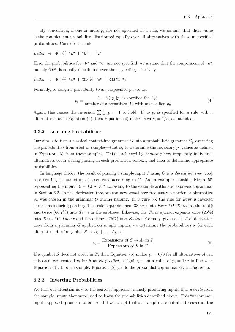
6.3. Approach
By convention, if one or more pi are not specified in a rule, we assume that their valueis the complement probability, distributed equally over all alternatives with these unspecifiedprobabilities. Consider the rule
Letter ! 40.0% "a" | "b" | "c"
Here, the probabilities for "b" and "c" are not specified; we assume that the complement of "a",namely 60%, is equally distributed over them, yielding effectively
Letter ! 40.0% "a" | 30.0% "b" | 30.0% "c"
Formally, to assign a probability to an unspecified pi, we use
pi =1 �
P{pj |pj is specified for Aj}
number of alternatives Ak with unspecified pk(4)
Again, this causes the invariantPn
i=1 pi = 1 to hold. If no pi is specified for a rule with n
alternatives, as in Equation (2), then Equation (4) makes each pi = 1/n, as intended.
6.3.2 Learning Probabilities
Our aim is to turn a classical context-free grammar G into a probabilistic grammar Gp capturingthe probabilities from a set of samples—that is, to determine the necessary pi values as definedin Equation (3) from these samples. This is achieved by counting how frequently individualalternatives occur during parsing in each production context, and then to determine appropriateprobabilities.
In language theory, the result of parsing a sample input I using G is a derivation tree [265],representing the structure of a sentence according to G. As an example, consider Figure 55,representing the input "1 + (2 * 3)" according to the example arithmetic expression grammarin Section 6.2. In this derivation tree, we can now count how frequently a particular alternativeAi was chosen in the grammar G during parsing. In Figure 55, the rule for Expr is invokedthree times during parsing. This rule expands once (33.3%) into Expr "+" Term (at the root);and twice (66.7%) into Term in the subtrees. Likewise, the Term symbol expands once (25%)into Term "*" Factor and three times (75%) into Factor . Formally, given a set T of derivationtrees from a grammar G applied on sample inputs, we determine the probabilities pi for eachalternative Ai of a symbol S ! A1 | . . . | An as
pi =Expansions of S ! Ai in T
Expansions of S in T(5)
If a symbol S does not occur in T , then Equation (5) makes pi = 0/0 for all alternatives Ai; inthis case, we treat all pi for S as unspecified, assigning them a value of pi = 1/n in line withEquation (4). In our example, Equation (5) yields the probabilistic grammar Gp in Figure 56.
6.3.3 Inverting Probabilities
We turn our attention now to the converse approach; namely producing inputs that deviate fromthe sample inputs that were used to learn the probabilities described above. This “uncommoninput” approach promises to be useful if we accept that our samples are not able to cover all the
127
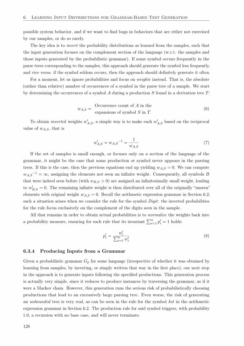
6. Learning Input Distributions for Grammar-Based Test Generation
possible system behavior, and if we want to find bugs in behaviors that are either not exercisedby our samples, or do so rarely.
The key idea is to invert the probability distributions as learned from the samples, such thatthe input generation focuses on the complement section of the language (w.r.t. the samples andthose inputs generated by the probabilistic grammar). If some symbol occurs frequently in theparse trees corresponding to the samples, this approach should generate the symbol less frequently,and vice versa: if the symbol seldom occurs, then the approach should definitely generate it often.
For a moment, let us ignore probabilities and focus on weights instead. That is, the absolute(rather than relative) number of occurrences of a symbol in the parse tree of a sample. We startby determining the occurrences of a symbol A during a production S found in a derivation tree T :
wA,S =Occurrence count of A in theexpansions of symbol S in T
(6)
To obtain inverted weights w0A,S , a simple way is to make each w
0A,S based on the reciprocal
value of wA,S , that is
w0A,S = wA,S
�1 =1
wA,S(7)
If the set of samples is small enough, or focuses only on a section of the language of thegrammar, it might be the case that some production or symbol never appears in the parsingtrees. If this is the case, then the previous equations end up yielding wA,S = 0. We can computewA,S
�1 = 1, assigning the elements not seen an infinite weight. Consequently, all symbols B
that were indeed seen before (with wB,S > 0) are assigned an infinitesimally small weight, leadingto w
0B,S = 0. The remaining infinite weight is then distributed over all of the originally “unseen”
elements with original weight wA,S = 0. Recall the arithmetic expression grammar in Section 6.2;such a situation arises when we consider the rule for the symbol Digit : the inverted probabilitiesfor the rule focus exclusively on the complement of the digits seen in the sample.
All that remains in order to obtain actual probabilities is to normalize the weights back intoa probability measure, ensuring for each rule that its invariant
Pni=1 p
0i = 1 holds:
p0i =
w0iPn
i=1 w0i
(8)
6.3.4 Producing Inputs from a Grammar
Given a probabilistic grammar Gp for some language (irrespective of whether it was obtained bylearning from samples, by inverting, or simply written that way in the first place), our next stepin the approach is to generate inputs following the specified productions. This generation processis actually very simple, since it reduces to produce instances by traversing the grammar, as if itwere a Markov chain. However, this generation runs the serious risk of probabilistically choosingproductions that lead to an excessively large parsing tree. Even worse, the risk of generatingan unbounded tree is very real, as can be seen in the rule for the symbol Int in the arithmeticexpression grammar in Section 6.2. The production rule for said symbol triggers, with probability1.0, a recursion with no base case, and will never terminate.
128
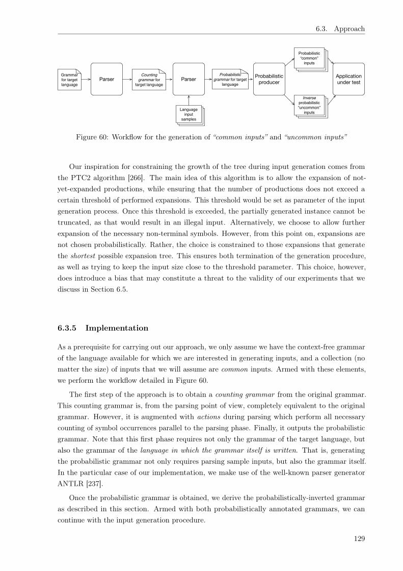
6.3. Approach
ParserGrammar for target language
Counting grammar for
target languageParser
Language input
samples
Probabilistic grammar for target
language
Probabilistic producer
Probabilistic“common”
inputs
Inverse probabilistic “uncommon”
inputs
Application under test
Figure 60: Workflow for the generation of “common inputs” and “uncommon inputs”
Our inspiration for constraining the growth of the tree during input generation comes fromthe PTC2 algorithm [266]. The main idea of this algorithm is to allow the expansion of not-yet-expanded productions, while ensuring that the number of productions does not exceed acertain threshold of performed expansions. This threshold would be set as parameter of the inputgeneration process. Once this threshold is exceeded, the partially generated instance cannot betruncated, as that would result in an illegal input. Alternatively, we choose to allow furtherexpansion of the necessary non-terminal symbols. However, from this point on, expansions arenot chosen probabilistically. Rather, the choice is constrained to those expansions that generatethe shortest possible expansion tree. This ensures both termination of the generation procedure,as well as trying to keep the input size close to the threshold parameter. This choice, however,does introduce a bias that may constitute a threat to the validity of our experiments that wediscuss in Section 6.5.
6.3.5 Implementation
As a prerequisite for carrying out our approach, we only assume we have the context-free grammarof the language available for which we are interested in generating inputs, and a collection (nomatter the size) of inputs that we will assume are common inputs. Armed with these elements,we perform the workflow detailed in Figure 60.
The first step of the approach is to obtain a counting grammar from the original grammar.This counting grammar is, from the parsing point of view, completely equivalent to the originalgrammar. However, it is augmented with actions during parsing which perform all necessarycounting of symbol occurrences parallel to the parsing phase. Finally, it outputs the probabilisticgrammar. Note that this first phase requires not only the grammar of the target language, butalso the grammar of the language in which the grammar itself is written. That is, generatingthe probabilistic grammar not only requires parsing sample inputs, but also the grammar itself.In the particular case of our implementation, we make use of the well-known parser generatorANTLR [237].
Once the probabilistic grammar is obtained, we derive the probabilistically-inverted grammaras described in this section. Armed with both probabilistically annotated grammars, we cancontinue with the input generation procedure.
129

6. Learning Input Distributions for Grammar-Based Test Generation
Table 17: Depth and size of derivation trees for “common inputs” (PROB) and “uncommon inputs”(INV)
Grammar Mode Depth of derivation tree Nodesmin max avg. median avg.
JSON PROB 14 2867 96 63 3058INV 5 37 23 37 68
JavaScript PROB 1 79 19 8 400INV 1 38 19 1 11,061
CSS PROB 3 44 41 44 19,380INV 9 30 29 30 11,269
6.4 Experimental Evaluation
In this section we evaluate our approach by applying the technique in several case studies. Inparticular, we ask the following research questions:
• RQ1 (“Common inputs”). Can a learned grammar be used to generate inputs thatresemble those that were employed during the grammar training?
• RQ2 (“Uncommon inputs”). Can a learned grammar be modified so it can generateinputs that, opposed to RQ1, are in contrast to those employed during the grammartraining?
• RQ3 (“Sensitivity to training set variance”). Is our approach sensitive to variance inthe initial samples?
• RQ4 (“Sensitivity to size of training set”). Is our approach sensitive to the size of theinitial samples?
• RQ5 (“Bugs found”). What kind of crashes (exceptions) do we trigger in RQ1 andRQ2?
• RQ6 (“Failure-inducing inputs”). Can a learned grammar be used to generate inputsthat reproduce failure-inducing behavior?
To answer RQ1 and RQ2, we need to compare inputs in order to decide whether these inputsare “similar” or “contrasting”. In the scope of this evaluation, we will use the method coverageand call sequences as measures of input similarity. We will define these measures later in thissection, and we will discuss their usefulness. We address RQ3 by comparing the method callsand call sequences induced for three randomly selected training sets, each containing five inputs.Likewise, we evaluate RQ4 by comparing the method calls and call sequences induced for fourrandomly selected training sets, each containing N sample inputs, where N 2 {1, 5, 10, 50}. Weassess RQ5 by categorizing, inspecting and reporting all exceptions triggered by our test suites inRQ1 and RQ2. Finally, we address RQ6 by investigating if the “(un)common inputs” strategycan reproduce (or avoid) a failure and explore the surroundings of the buggy behavior.
130
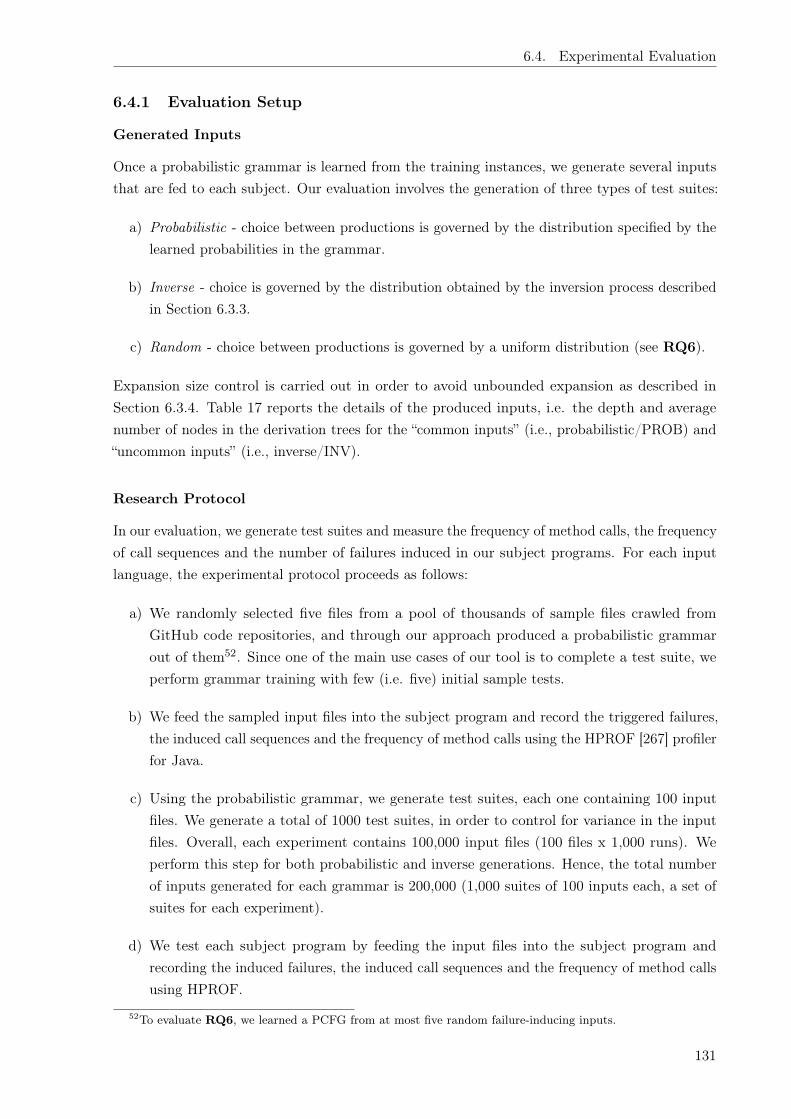
6.4. Experimental Evaluation
6.4.1 Evaluation Setup
Generated Inputs
Once a probabilistic grammar is learned from the training instances, we generate several inputsthat are fed to each subject. Our evaluation involves the generation of three types of test suites:
a) Probabilistic - choice between productions is governed by the distribution specified by thelearned probabilities in the grammar.
b) Inverse - choice is governed by the distribution obtained by the inversion process describedin Section 6.3.3.
c) Random - choice between productions is governed by a uniform distribution (see RQ6).
Expansion size control is carried out in order to avoid unbounded expansion as described inSection 6.3.4. Table 17 reports the details of the produced inputs, i.e. the depth and averagenumber of nodes in the derivation trees for the “common inputs” (i.e., probabilistic/PROB) and“uncommon inputs” (i.e., inverse/INV).
Research Protocol
In our evaluation, we generate test suites and measure the frequency of method calls, the frequencyof call sequences and the number of failures induced in our subject programs. For each inputlanguage, the experimental protocol proceeds as follows:
a) We randomly selected five files from a pool of thousands of sample files crawled fromGitHub code repositories, and through our approach produced a probabilistic grammarout of them52. Since one of the main use cases of our tool is to complete a test suite, weperform grammar training with few (i.e. five) initial sample tests.
b) We feed the sampled input files into the subject program and record the triggered failures,the induced call sequences and the frequency of method calls using the HPROF [267] profilerfor Java.
c) Using the probabilistic grammar, we generate test suites, each one containing 100 inputfiles. We generate a total of 1000 test suites, in order to control for variance in the inputfiles. Overall, each experiment contains 100,000 input files (100 files x 1,000 runs). Weperform this step for both probabilistic and inverse generations. Hence, the total numberof inputs generated for each grammar is 200,000 (1,000 suites of 100 inputs each, a set ofsuites for each experiment).
d) We test each subject program by feeding the input files into the subject program andrecording the induced failures, the induced call sequences and the frequency of method callsusing HPROF.
52To evaluate RQ6, we learned a PCFG from at most five random failure-inducing inputs.
131

6. Learning Input Distributions for Grammar-Based Test Generation
Table 18: Subject details
Input Format Subject Version #Methods LOC
JSON
Argo 5.4 523 8,265Genson 1.4 1,182 18,780Gson 2.8.5 793 25,172
JSONJava 20180130 202 3,742Jackson 2.9.0 5,378 117,108
JsonToJava 1880978 294 5,131MinimalJson 0.9.5 224 6,350
Pojo 0.5.1 445 18,492json-simple a8b94b7 63 2,432cliftonlabs 3.0.2 183 2,668fastjson 1.2.51 2,294 166,761json2flat 1.0.3 37 659
json-flattener 0.6.0 138 1,522
JavaScript Rhino 1.7.7 4873 100,234rhino-sandbox 0.0.10 49 529
CSS3
CSSValidator 1.0.4 7774 120,838flute 1.3 368 8,250
jstyleparser 3.2 2,589 26,287cssparser 0.9.27 2,014 18,465
closure-style 0.9.27 3,029 35,401
All experiments were conducted on a server with 64 cores and 126 GB of RAM; more specificallyan Intel Xeon CPU E5-2683 v4 @ 2.10GHz with 64 virtual cores (Intel Hyperthreading), runningDebian 9.5 Linux.
Subject Programs
We evaluated our approach by generating inputs and feeding them to a variety of Java applications.All these applications are open source programs using three different input formats, namely JSON,JavaScript and CSS3. Table 18 summarizes the subjects to be analyzed, their input format andthe number of methods in each implementation.
The initial, unquantified grammars for the input subjects were adapted from those in therepository of the well-known parser generator ANTLR [237]. We handle grammar ambiguity thatmay affect learning probabilities by ensuring every input has only one parse tree. Specifically, weadapt the input grammars by (re-)writing lexer modes for the grammars, shortening lexer tokensand re-writing parser rules. Training samples were obtained by scraping GitHub repositories forthe required format files. The probabilistic grammars developed from the original ones, as well asthe obtained training samples can be found in our replication package.
Measuring (Dis)similarity
Questions RQ1 and RQ2 refer to a notion of similarity between inputs. Although white-boxapproaches exist that aim to measure test-case similarity and dissimilarity [268, 269], applyingthem to complex grammar-based inputs is not straightforward. However, in this work, since weare dealing with evaluating the behavior of a certain piece of software, it makes sense to aim for
132

6.4. Experimental Evaluation
(a) PROB vs. SAMP vs. INV
(b) PROB (c) SAMP (d) INV
Figure 61: Frequency analysis of call sequences for json-flattener (length=2)
a notion of semantic similarity. In this sense, two inputs are semantically similar if they incitesimilar behaviors in the software that processes them. In order to achieve this, we define twomeasures of input similarity based on structural and non-structural program coverage metrics.The non-structural measure of input similarity is the frequency of method calls induced in theprograms. The structural measure is the frequency of call sequences induced in the program, asimilar measure was used in [270]. Thus, we will say two inputs are similar if they induce similar(distribution of) method call frequencies for the same program. The frequency of call sequencesrefers to the number of times a specific method call sequence is triggered by an input, for aprogram. For this measure, we say two inputs are similar if they trigger a similar distributionin the frequency with which the method sequences are called, for the same program. Thesenotions allow for a great variance drift if we were to compare only two inputs. Therefore, weperform these comparisons on test suites as a whole to dampen the effect of this variance. Usingthese measures, we aim at answering RQ1 and RQ2. RQ1 will be answered satisfactorily ifthe (distribution of) call frequencies and sequences induced by the “common inputs” strategy is
133
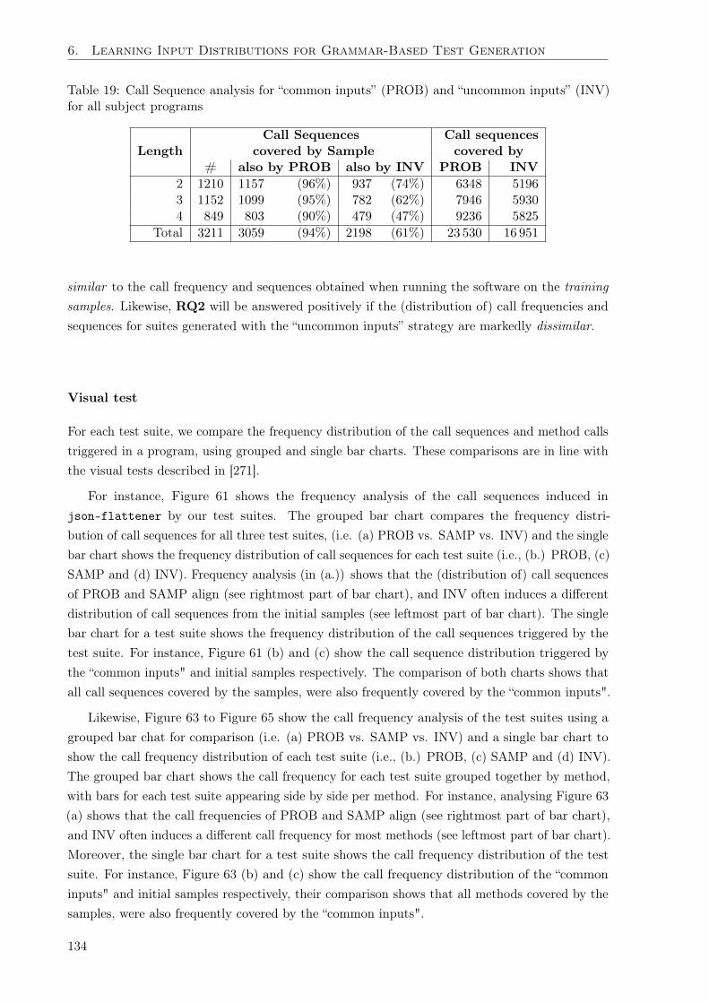
6. Learning Input Distributions for Grammar-Based Test Generation
Table 19: Call Sequence analysis for “common inputs” (PROB) and “uncommon inputs” (INV)for all subject programs
LengthCall Sequences Call sequences
covered by Sample covered by# also by PROB also by INV PROB INV
2 1210 1157 (96%) 937 (74%) 6348 51963 1152 1099 (95%) 782 (62%) 7946 59304 849 803 (90%) 479 (47%) 9236 5825
Total 3211 3059 (94%) 2198 (61%) 23 530 16 951
similar to the call frequency and sequences obtained when running the software on the trainingsamples. Likewise, RQ2 will be answered positively if the (distribution of) call frequencies andsequences for suites generated with the “uncommon inputs” strategy are markedly dissimilar.
Visual test
For each test suite, we compare the frequency distribution of the call sequences and method callstriggered in a program, using grouped and single bar charts. These comparisons are in line withthe visual tests described in [271].
For instance, Figure 61 shows the frequency analysis of the call sequences induced injson-flattener by our test suites. The grouped bar chart compares the frequency distri-bution of call sequences for all three test suites, (i.e. (a) PROB vs. SAMP vs. INV) and the singlebar chart shows the frequency distribution of call sequences for each test suite (i.e., (b.) PROB, (c)SAMP and (d) INV). Frequency analysis (in (a.)) shows that the (distribution of) call sequencesof PROB and SAMP align (see rightmost part of bar chart), and INV often induces a differentdistribution of call sequences from the initial samples (see leftmost part of bar chart). The singlebar chart for a test suite shows the frequency distribution of the call sequences triggered by thetest suite. For instance, Figure 61 (b) and (c) show the call sequence distribution triggered bythe “common inputs" and initial samples respectively. The comparison of both charts shows thatall call sequences covered by the samples, were also frequently covered by the “common inputs".
Likewise, Figure 63 to Figure 65 show the call frequency analysis of the test suites using agrouped bar chat for comparison (i.e. (a) PROB vs. SAMP vs. INV) and a single bar chart toshow the call frequency distribution of each test suite (i.e., (b.) PROB, (c) SAMP and (d) INV).The grouped bar chart shows the call frequency for each test suite grouped together by method,with bars for each test suite appearing side by side per method. For instance, analysing Figure 63(a) shows that the call frequencies of PROB and SAMP align (see rightmost part of bar chart),and INV often induces a different call frequency for most methods (see leftmost part of bar chart).Moreover, the single bar chart for a test suite shows the call frequency distribution of the testsuite. For instance, Figure 63 (b) and (c) show the call frequency distribution of the “commoninputs" and initial samples respectively, their comparison shows that all methods covered by thesamples, were also frequently covered by the “common inputs".
134

6.4. Experimental Evaluation
0
20
40
60
80
100
Length=2 Length=3 Length=4 All
Sequ
ence
s co
vere
d by
Sam
ple
(%)
Sequence of Method Calls
Sequence of Method Calls covered by Sample: PROB vs INV
Common Inputs (PROB)Uncommon Inputs (INV)
Figure 62: Call sequences covered by Sample for “common inputs” (PROB) and “uncommoninputs” (INV)
Collecting failure-inducing inputs
For each input file in our Github corpus, we fed it to every subject program of the input languageand observe if the subject program crashes, i.e. the output status code is non-zero after execution.Then, we collect such inputs as failure-inducing inputs for the subject program and parse thestandard output for the raised exception. In total, we fed 10,853 files to the subject programs,1,000 each for CSS and JavaScript, and 8853 for JSON. Exceptions were triggered for two inputlanguages, namely JavaScript and JSON, no exception was triggered for CSS. In total, we collected15 exceptions in seven subject programs (see Table 26).
6.4.2 Experimental Results
In Figure 63 to Figure 65, we show a representative selection of our results53. For each subject,we constructed a chart that represents the absolute call frequency of each method in the subject.The horizontal axis (which is otherwise unlabelled) represents the set of methods in the subject,ordered by the frequency of calls in the experiment on probabilistic inputs.
53The full range of charts is omitted for space reasons. However, all charts, as well as the raw data, are availableas part of the artifact package. Moreover, the charts shown here have been selected so that they are representativeof the whole set; that is, the omitted charts do not deviate significantly.
135
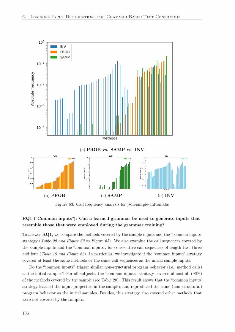
6. Learning Input Distributions for Grammar-Based Test Generation
(a) PROB vs. SAMP vs. INV
(b) PROB (c) SAMP (d) INV
Figure 63: Call frequency analysis for json-simple-cliftonlabs
RQ1 (“Common inputs”): Can a learned grammar be used to generate inputs thatresemble those that were employed during the grammar training?
To answer RQ1, we compare the methods covered by the sample inputs and the “common inputs”strategy (Table 20 and Figure 63 to Figure 65). We also examine the call sequences covered bythe sample inputs and the “common inputs”, for consecutive call sequences of length two, threeand four (Table 19 and Figure 62). In particular, we investigate if the “common inputs” strategycovered at least the same methods or the same call sequences as the initial sample inputs.
Do the “common inputs” trigger similar non-structural program behavior (i.e., method calls)as the initial samples? For all subjects, the “common inputs” strategy covered almost all (96%)of the methods covered by the sample (see Table 20). This result shows that the “common inputs”strategy learned the input properties in the samples and reproduced the same (non-structural)program behavior as the initial samples. Besides, this strategy also covered other methods thatwere not covered by the samples.
136

6.4. Experimental Evaluation
Table 20: Method coverage for “common inputs” (PROB) and “uncommon inputs” (INV)
Methods covered by sample Methods Kolmogorov-Smirnov (KS) test of
Subject # also by covered by SAMP vs. PROB SAMP vs. INV
PROB INV PROB INV D-stat(p-value) D-stat(p-value)
Argo 52 52 (100%) 32 (62%) 256 165 0.28 (1.11E�9) 0.50 (1.84E�30)
Genson 12 12 (100%) 10 (83%) 218 188 0.25 (3.46E�7) 0.73 (5.88E�64)
Gson 24 24 (100%) 14 (58%) 287 239 0.52 (1.09E�40) 0.25 (1.94E�9)
JSONJava 29 29 (100%) 23 (79%) 51 42 0.08 (0.99) 0.63 (3.45E�11)
Jackson 2 2 (100%) 1 (50%) 957 732 N/A N/A
JsonToJava 29 29 (100%) 9 (31%) 82 33 0.25 (8.48E�3) 0.24 (1.38E�2)
MinimalJson 24 24 (100%) 18 (75%) 110 100 0.34 (2.36E�6) 0.83 (5.39E�42)
Pojo 23 23 (100%) 7 (30%) 159 93 0.19 (1.81E�3) 0.29 (1.04E�7)
json-simple 11 11 (100%) 10 (91%) 26 24 0.35 (0.09) 0.46 (7.13E�3)
cliftonlabs 23 23 (100%) 23 (100%) 48 48 0.21 (0.25) 0.54 (8.29E�7)
fastjson 70 70 (100%) 62 (89%) 245 231 0.37 (3.07E�15) 0.41 (8.84E�19)
json2flat 6 6 (100%) 5 (83%) 17 14 0.35 (0.24) 0.65 (1.15E�3)
json-flattener 36 36 (100%) 32 (89%) 83 81 0.15 (0.29) 0.15 (0.29)
Rhino 23 6 (26%) 23 (100%) 107 201 0.34 (3.18E�12) 0.45 (6.48E�21)
rhino-sandbox 3 3 (100%) 3 (100%) 17 17 0.47 (0.04) 0.53 (0.02)
CSSValidator 10 10 (100%) 10 (100%) 97 124 0.42 ( 1.20E�10) 0.38 (7.95E�9)
flute 58 57 (98%) 51 (88%) 148 131 0.29 (3.35E�6) 0.50 (7.34E�18)
jstyleparser 75 74 (99%) 59 (79%) 183 169 0.34 (1.53E�13) 0.38 (1.83E�17)
cssparser 71 71 (100%) 66 (93%) 177 152 0.36 (2.91E�12) 0.62 (4.21E�37)
closure-style 104 95 (91%) 103 (99%) 229 238 0.16 (2.03E�6) 0.09 (3.34E�2)
Total 685 657 (96%) 561 (82%) 3,497 3,022
The “common inputs” strategy triggered almost all methods (96%)called by the initial sample inputs.
Do the “common inputs” also trigger similar structural program behavior (i.e., sequences ofmethod calls)? In our evaluation, the “common inputs” strategy covered most of the call sequencesthat were covered by the initial samples. For instance, Figure 61 shows that the call sequencescovered by the samples were also frequently covered by the “common inputs", for json-flattener.Overall, the “common inputs” strategy covered 94% of the method call sequences induced by thesample (see Table 19 and Figure 62). For all call sequences, the “common inputs” strategy alsocovered 90% to 96% of the method call sequences covered by the samples. This result showsthat the ‘common inputs” strategy triggers the same structural program behavior as the initialsamples.
The “common inputs” strategy triggered most call sequences (94%)covered by the initial sample inputs.
Additionally, we compare the statistical distributions resulting from our strategies. We needto be able to see a pattern in frequency calls such that the frequency curves for the sample runsand the probabilistic runs match as described in the visual test (see Section 6.4.1). Figure 63 toFigure 65 show that this match does hold for all subjects.
For all subjects, the method call frequency curves for the sample runsand the probabilistic runs match.
We also perform a statistical analysis on the distributions to increase the confidence in ourconclusion. We performed a distribution fitness test (KS - Kolmogorov-Smirnov) on the samplevs. the probabilistic call distribution; and on the sample vs. the inverse probabilistic distribution.It must be noted that the KS test aims at determining whether the distributions are exactly the
137

6. Learning Input Distributions for Grammar-Based Test Generation
(a) PROB vs. SAMP vs. INV
(b) PROB (c) SAMP (d) INV
Figure 64: Call frequency analysis for JSONJava
same, whereas we want to ascertain if they are similar or dissimilar. KS tests are very sensitiveto small variations in data, which makes it, in principle, inadequate for this objective. In thiswork, we employ the approach used by Fan [272]—we first estimate the kernel density functionsof the data distributions, which smoothen the estimated distribution. Then, we bootstrap andresample new data on the kernel density estimates, and perform the KS test on the bootstrappeddata.
The KS test confirms the results from the the visual inspection, the distribution of the methodcall frequency of “common inputs” matches the distribution in the sample (see Table 20), forsome subjects. However, there are also subjects, where the hypothesis is rejected (p < 0.05)that method call frequency distributions (sample and “common inputs”) come from the samedistribution, which is indicated by the blue entries. In the case of the Jackson subject, frequenciesfor the sample calls are all close to zero, which makes the data inadequate for the KS test.
138

6.4. Experimental Evaluation
(a) PROB vs. SAMP vs. INV
(b) PROB (c) SAMP (d) INV
Figure 65: Call frequency analysis for json-simple
RQ2 (“Uncommon inputs”): Can a learned grammar be modified such it cangenerate inputs that, opposed to RQ1, are in contrast to those employed duringthe grammar training?
For all subjects, the “uncommon inputs” produced by inverting probabilities covered markedlyfewer (82%) of the methods covered by the sample (see Table 20). This result shows that the“uncommon inputs” strategy learned the input properties in the samples and produced inputsthat avoid several methods covered by the samples.
The “uncommon inputs” strategy triggered markedly fewer methods (82%)called by the initial sample inputs.
Do the “uncommon inputs” trigger fewer of the call sequences covered by the initial samples?Table 19 shows that the “uncommon inputs” strategy triggered significantly fewer (61%) of thecall sequences covered by the samples. The number of call sequences induced by the uncommon
139

6. Learning Input Distributions for Grammar-Based Test Generation
Table 21: Sensitivity to training set variance using three different sets (S 2 {1, 2, 3}) of initialsamples containing five inputs each
Methods covered by Sample Methods Call Seq. covered by Sample Call Seq.
Salso by covered by also by covered by
# PROB INV PROB INV # PROB INV PROB INV
1 685 657 (96%) 561 (82%) 3,497 3,022 3,211 3,059 (94%) 2,198 (61%) 23,530 16,951
2 2,963 2,924 (97%) 2,764 (85%) 8,623 8,246 6,044 5,643 (93%) 4,110 (68%) 22,531 19,896
3 2,656 2,639 (100%) 2,516 (87%) 8,655 8,165 5,005 4,915 (98%) 3,306 (66%) 20,792 19,892
Table 22: Sensitivity to the size of the training set using initial sample size N 2 {1, 5, 10, 50}
Methods covered by Sample Methods Call Seq. covered by Sample Call Seq.
Nalso by covered by also by covered by
# PROB INV PROB INV # PROB INV PROB INV
1 1,496 1,490 (100%) 1,352 (79%) 8,715 7,954 1,955 1,942 (99%) 1,135 (58%) 21,279 15,341
5 685 657 (96%) 561 (82%) 3,497 3,022 3,211 3,059 (94%) 2,198 (61%) 23,530 16,951
10 3,546 3,517 (100%) 3,339 (89%) 9,388 11,497 6,297 6,105 (97%) 4,474 (71%) 26,575 21,214
50 5,347 5,313 (100%) 4,961 (89%) 8,950 8,217 9,389 9,076 (97%) 7,421 (79%) 23,512 18,391
inputs decreases significantly as the length of the call sequence increases (see Figure 62). Forinstance, comparing frequency charts of call sequences in Figure 61 ((a), (c) and (d)) also showthat “uncommon inputs” frequently avoided inducing the call sequences triggered by the initialsamples. Notably, for sequences of four consecutive method calls, the “uncommon inputs” strategycovered only 47% of the sequences covered by the initial samples (see Table 19). Overall, the“uncommon inputs” avoided inducing the call sequences that were triggered by the initial samples.
The “uncommon inputs” strategy induced significantly fewer call sequences (61%)covered by the initial samples.
Do the “uncommon inputs” only cover fewer, or also different methods? We perform a visualtest to examine if we see a markedly different call frequency between the samples and the inputsgenerated by the “uncommon inputs” strategy. In almost all charts this is the case (see Figure 63to Figure 65). The only exception is the CSSValidator subject.
For all subjects (except CSSValidator), the method call frequency curves for the sampleruns and “uncommon inputs" runs are markedly different.
Besides, we examine if the frequency of distribution of method calls for the samples and the“uncommon inputs” are significantly dissimilar. In particular, the KS tests shows that for allsubjects (except json-flattener) the distributions of method calls in the sample and the “uncommoninputs” are significantly different (p < 0.05, see sample vs. INV in Table 20).
RQ3 (“Sensitivity to training set variance”): Is our approach sensitive to variancein the initial samples?
We examine the sensitivity of our approach to the variance in the training set. We randomlyselected three distinct training sets, each containing five inputs. Then, for each set, we comparethe methods and call sequences covered by the samples to those induced by the generated inputs(Table 21).
Our evaluation showed that our approach is not sensitive to training set variance. In particular,for all training sets, the “common inputs” strategy covered most of the methods and call sequences
140

6.4. Experimental Evaluation
Crawled PROB
INV
9 32
31 1
4
Figure 66: Number of exceptions triggered by the test suites
induced by the initial sample inputs. Table 21 shows that the “common inputs” (PROB)consistently covered almost all call sequences (93 to 98%) covered by the initial samples, while“uncommon inputs” (INV) covered significantly fewer call sequences (61 to 68%). Likewise, the“common inputs” consistently covered almost all methods (96 to 100%) covered by the initialsamples, while “uncommon inputs” covered fewer methods (82 to 87%) (cf. Table 21).
Both strategies, the “common inputs” and the “uncommon inputs”,are insensitive to training set variance.
RQ4 (“Sensitivity to the size of training set”): Is our approach sensitive to the sizeof the initial samples?
We evaluate the sensitivity of our approach to the size of the training set. For each inputformat, we randomly selected four distinct training sets containing N sample inputs, whereN 2 {1, 5, 10, 50}. Then, for each set, we compare the methods and call sequences induced bythe samples to those induced by the generated inputs (Table 22).
Regardless of the size of the training set, the “common inputs” strategy consistently coveredmost of the methods and call sequences covered by the initial samples. Specifically, for all sizes,the “common inputs” covered almost all (94 to 99%) of the call sequences covered by the initialsamples, while “uncommon inputs” covered significantly fewer call sequences (58 to 79%). In thesame vein, the “common inputs” consistently covered almost all methods (96 to 100%) covered bythe initial samples, while “uncommon inputs” covered fewer methods (79 to 89%) (cf. Table 22).These results demonstrates that the effectiveness of our approach is independent of the size ofthe training set.
The effectiveness of our approach is independent of the sizeof the training set used for grammar training.
RQ5 (“Bugs found”): What kind of crashes (exceptions) do we trigger?
To address RQ5, we examine all of the exceptions triggered by our test suites. We inspectthe exceptions triggered during our evaluation of the “common inputs” strategy (in RQ1) and
141

6. Learning Input Distributions for Grammar-Based Test Generation
Table 23: Exception details
Input #Exceptions #SubjectsAverage subject crash rate
(All) (Crashed)
SAMP 3 1 0.05263 1
PROB 9 4 0.05999 0.28493
INV 9 7 0.03139 0.08521
the “uncommon inputs” strategy (in RQ2). To evaluate if our approach is capable of findingreal-world bugs, we compare the exceptions triggered in both RQ1 and RQ2 to the exceptionstriggered by the input files crawled from Github (using the setup described in Section 6.4.1).
Both of our strategies triggered 40% of the exceptions triggered by the crawled files, i.e. six(out of 15) exceptions causing thousands of crashes in four subjects (cf. Table 23 and Table 24).Half (three) of these exceptions had no samples of failure-inducing inputs in their grammartraining. This indicates that, even without failure-inducing input samples during grammartraining, our approach is able to trigger common buggy behaviors in the wild, i.e. bugs triggeredby the crawled input samples. Exceptions were triggered for JSON and JavaScript input formats,however, no exception was triggered for CSS.
Probabilistic grammar-based testing induced two fifths of all exceptionstriggered by the crawled files.
Our strategies were able to trigger eight other exceptions that could not be found by thecrawled files (cf. Figure 66). This result shows the utility of our approach in finding rare buggybehaviors, i.e. uncommon bugs in the crawled input samples. Besides, all of these exceptions weretriggered despite a lack of “failure-inducing input” samples in the grammar training. In particular,both strategies triggered nine exceptions each, three and four of which were triggered only by the“common inputs” and only by the “uncommon inputs”, respectively.
Probabilistic grammar-based testing induced eight new exceptionsthat were not triggered by the crawled files.
The “common inputs” strategy triggered all of the exceptions triggered by the original sampleinputs used in grammar training. Three exceptions were triggered by the sample inputs andall three exceptions were triggered by the “common inputs” strategy, while “uncommon inputs”triggered only two of these exceptions (cf. Table 23 and Table 24). Again, this result confirmsthat our grammar training approach can learn the input properties that characterize specificprogram behaviors.
The “common inputs” induced all of the exceptions triggered by the original sample inputs.
Overall, 14 exceptions in seven subject programs were found in our experiments (see Table 23and Table 24). On inspection, six of these exceptions affecting five subject programs have beenreported to developers as severe bugs. These exceptions have been extensively discussed in thebug repository of each subject program. This result reveals that our approach can generate inputsthat reveal real-world buggy behaviors. Additionally, from the evaluation of crawled files, 15exceptions in five subjects were found. In particular, one exception (Rhino issue #385, which isalso reproducible with our approach) has been confirmed and fixed by the developers.
142

6.4. Experimental Evaluation
Table 24: Exceptions induced by “Common Inputs” (PROB), and “Uncommon Inputs” (INV)
Input
FormatSubject Exception
#Failure- Occurrence rate in
inducing PROB INV Crawled
samples Files
CSS No exceptions triggered
JSON
Gson java.lang.NullPointer 0 0 0.0001 0Pojo java.lang.StringIndexOutOfBounds 0 0.0259 0 0.0024Pojo java.lang.NumberFormat 0 0 0.0001 0Argo argo.saj.InvalidSyntax 0 0 0.0023 0.0225JSONToJava org.json.JSON 0 0.0200 0.0200 0.0223json2flat com.fasterxml.jackson.core.JsonParse 0 0 0.0013 0json-flattener com.eclipsesource.json.Parse 0 0 0.0013 0json-flattener java.lang.UnsupportedOperation 0 0.2981 0 0json-flattener java.lang.IllegalArgument 0 0.2554 0 0json-flattener java.lang.NullPointer 0 0.0398 0 0json-flattener java.lang.NumberFormat 0 0.0028 0.0745 0
Java-
Script
rhino-sandbox org.mozilla.javascript.Evaluator 3 0.4905 0.4469 0.5290rhino-sandbox java.lang.IllegalState 1 0.0016 0 0.0010rhino-sandbox org.mozilla.javascript.EcmaError 1 0.0058 0.0500 0.3740
RQ6 (“Failure-inducing inputs”): Can a learned grammar be used to generateinputs that reproduce failure-inducing behavior?
Let us now investigate if our approach can learn a PCFG from failure-inducing samples andreproduce the failure.
For each exception triggered by the crawled files (in Section 6.4.1), we learned a PCFG fromat most five failure-inducing inputs that trigger the exception. Then, we run our PROB approachon the PCFG, using the protocol setting in Section 6.4.1. The goal is to demonstrate that thePCFG learns the input properties of the “failure-inducing inputs”, i.e. inputs generated via PROBshould trigger the same exception as the failure-inducing samples. This is useful for exploring thesurroundings of a bug.
In addition, for each exception, we run the inverse of “failure-inducing inputs" (i.e., INV), inorder to evaluate if the “uncommon inputs” avoid reproducing the failures. In contrast, for eachexception, we run the random generator (RAND) on the CFG (according to Section 6.4.1), in orderto evaluate the probability of randomly triggering (these) exceptions without a (learned) PCFG.In the random configuration (RAND), production choices have equal probability of generation.
In Table 25, we have summarized the number of reproduced exceptions. We see that proba-bilistic generation (PROB) reproduced all (15) failure-inducing inputs collected in our corpus.This shows that the grammar training approach effectively captured the distribution of inputproperties in the failure-inducing inputs. Moreso, it reproduced the program behavior using thelearned PCFG.
Learning probabilities from failure-inducing inputs strategy reproduces100% of the exceptions in our corpus.
For the inverse of “failure-inducing inputs", our evaluation showed that the “uncommon inputs”strategy could avoid reproducing the learned failure-inducing behavior for most (10 out of 15) ofthe exceptions (cf . Table 25 and Table 26).
The “uncommon inputs” strategy could avoid reproducing the learned program behaviorfor two-thirds of the exceptions.
143
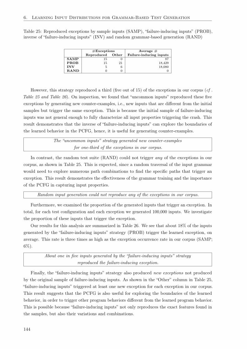
6. Learning Input Distributions for Grammar-Based Test Generation
Table 25: Reproduced exceptions by sample inputs (SAMP), “failure-inducing inputs” (PROB),inverse of “failure-inducing inputs” (INV) and random grammar-based generation (RAND)
#Exceptions Average #
Reproduced Other Failure-inducing inputs
SAMP 15 0 87
PROB 15 21 18,429
INV 5 6 18,080
RAND 0 0 0
However, this strategy reproduced a third (five out of 15) of the exceptions in our corpus (cf .Table 25 and Table 26). On inspection, we found that “uncommon inputs” reproduced these fiveexceptions by generating new counter-examples, i.e., new inputs that are different from the initialsamples but trigger the same exception. This is because the initial sample of failure-inducinginputs was not general enough to fully characterize all input properties triggering the crash. Thisresult demonstrates that the inverse of “failure-inducing inputs” can explore the boundaries ofthe learned behavior in the PCFG, hence, it is useful for generating counter-examples.
The “uncommon inputs” strategy generated new counter-examplesfor one-third of the exceptions in our corpus.
In contrast, the random test suite (RAND) could not trigger any of the exceptions in ourcorpus, as shown in Table 25. This is expected, since a random traversal of the input grammarwould need to explore numerous path combinations to find the specific paths that trigger anexception. This result demonstrates the effectiveness of the grammar training and the importanceof the PCFG in capturing input properties.
Random input generation could not reproduce any of the exceptions in our corpus.
Furthermore, we examined the proportion of the generated inputs that trigger an exception. Intotal, for each test configuration and each exception we generated 100,000 inputs. We investigatethe proportion of these inputs that trigger the exception.
Our results for this analysis are summarized in Table 26. We see that about 18% of the inputsgenerated by the “failure-inducing inputs” strategy (PROB) trigger the learned exception, onaverage. This rate is three times as high as the exception occurrence rate in our corpus (SAMP;6%).
About one in five inputs generated by the “failure-inducing inputs” strategyreproduced the failure-inducing exception.
Finally, the “failure-inducing inputs” strategy also produced new exceptions not producedby the original sample of failure-inducing inputs. As shown in the “Other” column in Table 25,“failure-inducing inputs” triggered at least one new exception for each exception in our corpus.This result suggests that the PCFG is also useful for exploring the boundaries of the learnedbehavior, in order to trigger other program behaviors different from the learned program behavior.This is possible because “failure-inducing inputs” not only reproduces the exact features found inthe samples, but also their variations and combinations.
144
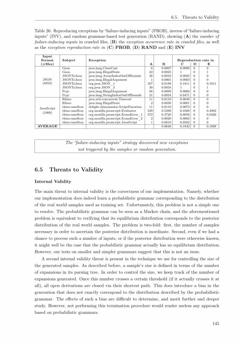
6.5. Threats to Validity
Table 26: Reproducing exceptions by “failure-inducing inputs” (PROB), inverse of “failure-inducinginputs” (INV), and random grammar-based test generation (RAND), showing (A) the number offailure-inducing inputs in crawled files, (B) the exception occurrence rate in crawled files, as wellas the exception reproduction rate in (C) PROB, (D) RAND and (E) INV
Input
Subject ExceptionFormat Reproduction rate in
(#files) A B C D E
JSON
(8853)
Gson java.lang.ClassCast 6 0.0007 0.0090 0 0Gson java.lang.IllegalState 22 0.0025 1 0 1JSONToJava java.lang.ArrayIndexOutOfBounds 38 0.0043 0.0025 0 0JSONToJava java.lang.IllegalArgument 1 0.0001 0.0003 0 0JSONToJava org.json.JSON_1 167 0.0189 0.1811 0 0.1811JSONToJava org.json.JSON_2 30 0.0034 1 0 1Pojo java.lang.IllegalArgument 88 0.0099 0.0002 0 0Pojo java.lang.StringIndexOutOfBounds 21 0.0024 0.0471 0 0
JavaScript
(1000)
Rhino java.util.concurrent.Timeout 11 0.0110 0.0048 0 0Rhino java.lang.IllegalState 2 0.0030 0.0001 0 0rhino-sandbox delight.rhinosandox.ScriptDuration 11 0.0110 0.0073 0 0rhino-sandbox org.mozilla.javascript.Evaluator 529 0.5290 0.4560 0 0.4982rhino-sandbox org.mozilla.javascript.EcmaError_1 372 0.3720 0.0056 0 0.0326rhino-sandbox org.mozilla.javascript.EcmaError_2 2 0.0020 0.0002 0 0rhino-sandbox org.mozilla.javascript.JavaScript 1 0.0010 0.0502 0 0
AVERAGE 0.0646 0.1842 0 0.1808
The “failure-inducing inputs” strategy discovered new exceptionsnot triggered by the samples or random generation.
6.5 Threats to Validity
Internal Validity
The main threat to internal validity is the correctness of our implementation. Namely, whetherour implementation does indeed learn a probabilistic grammar corresponding to the distributionof the real world samples used as training set. Unfortunately, this problem is not a simple oneto resolve. The probabilistic grammar can be seen as a Markov chain, and the aforementionedproblem is equivalent to verifying that its equilibrium distribution corresponds to the posteriordistribution of the real world samples. The problem is two-fold: first, the number of samplesnecessary in order to ascertain the posterior distribution is inordinate. Second, even if we had achance to process such a number of inputs, or if the posterior distribution were otherwise known,it might well be the case that the probabilistic grammar actually has no equilibrium distribution.However, our tests on smaller and simpler grammars suggest that this is not an issue.
A second internal validity threat is present in the technique we use for controlling the size ofthe generated samples. As described before, a sample’s size is defined in terms of the numberof expansions in its parsing tree. In order to control the size, we keep track of the number ofexpansions generated. Once this number crosses a certain threshold (if it actually crosses it atall), all open derivations are closed via their shortest path. This does introduce a bias in thegeneration that does not exactly correspond to the distribution described by the probabilisticgrammar. The effects of such a bias are difficult to determine, and merit further and deeperstudy. However, not performing this termination procedure would render useless any approachbased on probabilistic grammars.
145
6. Learning Input Distributions for Grammar-Based Test Generation
External Validity
Threats to external validity relate to the generalizability of the experimental results. In our case,this is specifically related to the subjects used in the experiments. We acknowledge that wehave only experimented with a limited number of input grammars. However, we have selectedthe subjects with the intention to test our approach on practically relevant input grammarswith different complexities, from small to medium size grammars like JSON; and rather complexgrammars like JavaScript and CSS. As a result, we are confident that our approach will also workon inputs that can be characterized by context-free grammars with a wide range of complexity.However, we do have evidence that the approach does not seem to be generalizable to combinationsof grammars and samples such that they induce the learning of an almost-uniform probabilisticgrammar.
Construct Validity
The main threat to construct validity is the metric we use to evaluate the similarity between testsuites, namely method call frequency. While the uses of coverage metrics as adequacy criteriais extensively discussed by the community [66, 273, 274], their binary nature (that is, we caneither report covered or not covered) makes them too shallow to differentiate for behavior. Thevariance intrinsic to the probabilistic generation makes it very likely that at least one samplewill cover parts of the code unrelated to those covered by the rest of the suite. Besides, methodcall frequency is considered a non-structural coverage metric. To mitigate this threat, we alsoevaluate our test suites using a structural metric, in particular, (frequency of) call sequences.
6.6 Limitations
Context sensitivity: Although, our probabilistic grammar learning approach captures thedistribution of input properties, the learned input distribution is limited to production choices atthe syntactic level. This approach does not handle context-sensitive dependencies such as theorder, sequences or repetitions of specific input elements. However, our approach can be extendedto learn contextual dependencies, e.g. by learning sequences of elements using N-grams [275] orhierarchies of elements using k-paths [276].Input Constraints: Beyond lexical and syntactical validity, structured inputs often containinput semantics such as checksums, hashes, encryption, or references. Context-free grammars,as applied in this work, do not capture such complex input constraints. Automatically learningsuch input constraints for test generation is a challenging task [277]. In the future, we plan toautomatically learn input constraints to drive test generation, e.g. using attribute grammars.
6.7 Related Work
Generating software tests. The aim of software test generation is to find a sample of inputs thatinduce executions that sufficiently cover the possible behaviors of the program—including undesiredbehavior. Modern software test generation relies, as surveyed by Anand et al. [66] on symboliccode analysis to solve the path conditions leading to uncovered code [67, 68, 69, 70, 71, 72, 73, 74],
146

6.7. Related Work
search-based approaches to systematically evolve a population of inputs towards the desiredgoal [75, 76, 77, 78], random inputs to programs and functions [79, 80] or a combination of thesetechniques [81, 82, 83, 84, 85]. Additionally, machine learning techniques can also be applied tocreate test sequences [86, 87]. All these approaches have in common that they do not requirean additional model or annotations to constrain the set of generated inputs; this makes themvery versatile, but brings the risk of producing false alarms—failing executions that cannot beobtained through legal inputs.
Grammar-based test generation. The usage of grammars as producers was introduced in1970 by Hanford in his syntax machine [88]. Such producers are mainly used for testing compilersand interpreters: CSmith [89] produces syntactically correct C programs, and LANGFUZZ [90]uses a JavaScript grammar to parse, recombine, and mutate existing inputs while maintaining mostof the syntactic validity. GENA [91, 92] uses standard symbolic grammars to produce test casesand only applies stochastic annotation during the derivation process to distribute the test casesand to limit recursions and derivation depth. Grammar-based white-box fuzzing [93] combinesgrammar-based fuzzing with symbolic testing and is now available as a service from Microsoft.As these techniques operate with system inputs, any failure reported is a true failure—there areno false alarms. None of the above approaches use probabilistic grammars, though.
Probabilistic grammars. The foundations of probabilistic grammars date back to theearliest works of Chomsky [94]. The concept has seen several interactions and generalizationswith physics and statistics; we recommend the very nice article by Geman and Johnson [95]as an introduction. Probabilistic grammars are frequently used to analyze ambiguous datasequences—in computational linguistics [96] to analyze natural language, and in biochemistry [97]to model and parse macromolecules such as DNA, RNA, or protein sequences. Probabilisticgrammars have been used also to model and produce input data for specific domains, such as3D scenes [98] or processor instructions [99].
The usage of probabilistic grammars for test generation seems rather straightforward, butis still uncommon. The Geno test generator for .NET programs by Lämmel and Schulte [100]allowed users to specify probabilities for individual production rules. Swarm testing [101, 102]uses statistics and a variation of random testing to generate tests that deliberately targets or omitsfeatures of interest. These approaches, in contrast to the one we present in this chapter, does notuse existing samples to learn or estimate probabilities. The approach by Poulding et al. [103, 104]uses a stochastic context-free grammar for statistical testing. The goal of this work is to correctlyimitate the operational profile and consequently the generated test cases are similar to what onewould expect during normal operation of the system. The test case generation [105, 106] andfailure reproduction [107] approaches by Kifetew et al. combine probabilistic grammars with asearch-based testing approach. In particular, like our work, StGP [105] also learns stochasticgrammars from sample inputs.
Our approach aims to generate inputs that induce (dis)similar program behaviors as thesample inputs. In contrast to our work, StGP [105] is focused on evolving and mutating thelearned grammars to improve code coverage. Although, StGP’s goal of generating realistic inputsis very similar to our "common inputs" strategy (see RQ1 ), our approach can further generaterealistic inputs that are dissimilar to the sample inputs (see RQ2 ). Meanwhile, StGP is not
147
6. Learning Input Distributions for Grammar-Based Test Generation
capable of generating dissimilar inputs.Mining probabilities. Related to our work are approaches that mine grammar rules and
probabilities from existing samples. Patra and Pradel [278] use a given parser to mine probabilitiesfor subsequent fuzz testing and to reduce tree-based inputs for debugging [279]. Their aim, however,is not to produce inputs that would be similar or dissimilar to existing inputs, but rather toproduce inputs that have a higher likelihood to be syntactically correct. This aim is also sharedby two mining approaches: GLADE [280] and Learn&Fuzz [281], which learn producers fromlarge sets of input samples even without a given grammar.
All these approaches, however, share the problem of producing only “common inputs”—theycan only focus on common features rather than uncommon features, creating a general “tensionbetween conflicting learning and fuzzing goals” [281]. In contrast, our work can specifically focuson “uncommon inputs”—that is, the complement of what has been learned.
Like us, the Skyfire approach [282] aims at also leveraging “uncommon inputs” for probabilisticfuzzing. Their idea is to learn a probabilistic distribution from a set of samples and use thisdistribution to generate seeds for a standard fuzzing tool, namely AFL [283]. Here, favoringlow probability rules is one of many heuristics applied besides low frequency, low complexity, orproduction limits. Although the tool has shown good results for XML-like languages, results forother, general grammar formats such as JavaScript are marked as “preliminary” only, though.
Mining grammars. Our approach requires a grammar that can be used both for parsing andproducing inputs. While engineering such a grammar may well pay off in terms of better testing,it is still a significant investment in the case of specific domain inputs where such a grammarmight not be immediately available. Mining input structures [284], as exemplified using the aboveGLADE [280] and Learn&Fuzz [281] approaches, may assist in this task. AUTOGRAM [285]and MIMID [286] mine human-readable input grammars exploiting structure and identifiers of aprogram processing the input, which makes them particularly promising.
6.8 Discussions and Future Work
This chapter empirically show that learning input distribution from sample inputs in the wild isuseful to drive test generation. We have presented an approach that allows engineers, using agrammar and a set of input samples, to generate instances that are either similar or dissimilar tothese samples. Similar samples are useful, for instance, when learning from failure-inducing inputs;while dissimilar samples could be used to leverage the testing approach to explore previouslyuncovered code. Our approach provides a simple, general, and cost-effective means to generatetest cases that can then be targeted to the commonly used portions of the software, or to therarely used features.
Despite their usefulness for test case generation, grammars (including probabilistic grammars)still have a lot of potential to explore in research, and a lot of ground to cover in practice. In thefuture, we plan to investigate the following topics:
Deep models. At this point, our approach captures probabilistic distributions only at the levelof individual rules. However, probabilistic distributions could also capture the occurrenceof elements in particular contexts, and differentiate between them. For instance, if a "+"
148
6.8. Discussions and Future Work
symbol rarely occurs within parentheses, yet frequently outside of them, this differencewould, depending on how the grammar is structured, not be caught by our approach. Thedomain of computational linguistics [96] has introduced a number of models that take contextinto account. In our future work, we shall experiment with deeper context models, anddetermining their effect on capturing common and uncommon input features.
Grammar learning. The big cost of our approach is the necessity of a formal grammar forboth parsing and producing—a cost that can boil down to 1–2 programmer days if a formalgrammar is already part of the system (say, as an input file for parser generators), but alsoextend to weeks if it is not. In the future, we will be experimenting with approaches thatmine grammars from input samples and programs [285, 286] with the goal of extending theresulting grammars with probabilities for probabilistic fuzzing.
Debugging. Mined probabilistic grammars could be used to characterize the features of failure-inducing inputs, separating them from those of passing inputs. Statistical fault localizationtechniques [1], for instance, could then identify input elements most likely associated witha failure. Generating “common inputs”, as in this work, and testing whether they causefailures, could further strengthen correlations between input patterns and failures, as well asnarrow down the circumstances under which the failure occurs.
We provide the source code of our parsers, production tools, the raw input samples, as well as allobtained data and processed charts as a replication package:
https://tinyurl.com/inputs-from-hell
149


Chapter 7
Conclusion
In this thesis, we propose an evidence-driven approach to address challenges in software testingand debugging. The main idea of this approach is to gather empirical evidence from softwarepractice to guide and support the debugging activities of software developers. We conclude thisdissertation with a summary of our work and its contributions. We also discuss future researchopportunities and elicit on possible directions for further improvement and investigation.
7.1 Summary
We provide a summary of the challenges addressed in this work with respect to the thesis statement:“Software testing and debugging should be driven by empirical evidence collected from softwarepractice". Specifically, to evaluate this thesis statement, we pose these scientific questions:
1. How do developers debug and repair software bugs? We have conducted an empiricalstudy to collect data on the tools and strategies employed by developers while debuggingreal faults. Our study includes a survey of over 200 developers and a human study where weobserve 12 developers while they debug 27 real bugs. In this study, we collected data on thedebugging needs of developers and the reasons for developers (non-)adoption of debuggingaids. Indeed, we have found that there is a gap between the needs of developers and thetools provided by researchers.
2. What is the most effective automated fault localization (AFL) technique? We haveevaluated the effectiveness of the state-of-the-art fault localization techniques using hundredsof real faults. In particular, we evaluated the performance of 18 most effective statisticaldebugging formulas against program slicing. We also evaluate the impact of error type(artificial or real faults) and the number of faults (single or multiple faults) on the effectivenessof these AFL methods. In our evaluation, we found that dynamic slicing is best suited fordiagnosing single faults, while, statistical debugging performs better on multiple faults.
3. How can we automatically debug and repair real-world invalid inputs? In the con-text of input debugging, we evaluate the prevalence and causes of invalidity in inputs, usingthousands of real-world input files. In our evaluation, we found that four percent of inputfiles in the wild are invalid, they were either rejected by at least one subject program or their
151

7. Conclusion
input grammar. We have also identified a number of causes of input invalidity, such as wrongsyntax and missing or nonconforming elements. Many inputs were invalid because of singlecharacter errors, such as a deleted character, a missing character or an extraneous character.
4. Can we leverage real-world sample inputs to guide test generation? We provide anapproach to automatically learn the distribution of input elements from sample inputs foundin the wild. Our approach employs probabilistic grammars to learn input distribution andapplies the learned grammars to generate inputs that are similar or dissimilar to the the initialsamples. In our evaluation, our approach effectively generates inputs that reproduce/avoidfailures and tests for neighboring program behaviors. During debugging, this is useful forbug reproduction and testing the completeness of bug fixes.
7.2 Contributions
This thesis answers the aforementioned scientific questions and provides a number of tools andmethods to aid developers during debugging activities as well as researchers in evaluating debuggingand repair tools. Specifically, this dissertation makes the following technical contributions:
DbgBench. In our empirical study on debugging in practice, we have collected hundreds ofreal world fault locations and patches provided by 12 developers while debugging 27 realbugs. We provide the empirical data from this study as a benchmark called DbgBench.DbgBench provides details on the debugging needs of developers, as well as the tools andstrategies employed by developers when debugging real faults. In addition, it is useful forthe automatic evaluation of debuggers and automated repair tools. Our evaluation setup,empirical data and experimental results are available at: https://dbgbench.github.io
Hybrid Fault Localization. We have proposed a hybrid approach that synergistically combinesthe strengths of both dynamic slicing and statistical debugging, our hybrid approach buildson the empirical evidence from our study on the effectiveness of AFL techniques. Thishybrid approach combines the contextual information provided by dynamic slicing andthe fault correlation analysis performed by statistical debugging to effectively diagnosefaults. Our evaluation showed that our hybrid strategy overcomes the weaknesses of bothslicing and statistical fault localization. In our evaluation with hundreds of faults, thebest fault localization approach is the hybrid strategy, regardless of the number or type ofprogram faults. The empirical data and results obtained in this evaluation can be foundhere: https://tinyurl.com/HybridFaultLocalization
Maximizing Delta Debugging (ddmax). Building on the empirical results from our study onthe causes of input invalidity, we provide a black-box technique for automatically diagnosingand repairing invalid inputs via several test experiments. Our maximizing delta debuggingalgorithm (ddmax ) (1) identifies which parts of the input data prevent processing, and (2)recover as much of the (valuable) input data as possible. Through experiments, ddmaxmaximizes the subset of the input that can still be processed by the program, thus recoveringand repairing as much data as possible. The difference between the original failing input
152

7.3. Future Work
and the “maximized” passing input includes all input fragments that could not be processed.We provide our tool and findings in an artifact package, the artifact is available at: https://tinyurl.com/debugging-inputs-icse-2020
Probabilistic Test Generation (Inputs From Hell). Applying probabilistic grammars asinput parsers, we show how to learn input distributions from input samples, allowing tocreate inputs that are (dis)similar to the sample. Among many use cases, this method allowsfor the generation of failure-inducing inputs – learning from inputs that caused failures inthe past gives us inputs that share similar features and thus also have a high chance oftriggering bugs. This is useful for bug reproduction and testing the completeness of bugfixes. Our evaluation shows that learning from failure-inducing sample inputs effectivelyreproduces the same failure and also reveal new failures. The experimental setup, evaluationdata and results are available at: https://tinyurl.com/inputs-from-hell
7.3 Future Work
This dissertation opens the door for a number of exciting future research opportunities. There arestill lots of open problems and research challenges to address in the interplay of software practiceand automated debugging. Our future work will focus on the following issues:
Multiple Fault Locations. In contrast to the assumptions of typical debugging and repairtools, most real-world bugs can not be explained, localized or patched by finding one faultlocation [287, 112]. In the context of automated debugging, this assumption is called perfectbug understanding. It is the assumption that finding and examining a single faulty statementin the program is sufficient to detect, understand, explain and fix the bug [178]. A fewresearchers have shown that this assumption does not hold in software practice [112], infact it has been shown to impede the effectiveness of debugging aids and automated repairtechniques [287]. The results from our empirical study on debugging practice (in Chapter 3)also show that the perfect bug understanding assumption does not hold in reality. Indeed, formost bugs, developers provided bug diagnoses and fixes that span more than one contiguousfault location. For instance, we found that most (over 50% of) developer-provided diagnosesspan multiple (three to four) contiguous code locations and multiple (10 statements) faultyLoC (, on average). This result has major implications for debuggers and repair tools inpractice, since most tools assume perfect bug understanding.
To address this problem, we plan to conduct an empirical study to investigate the impact ofmulti-line faults and multiple (contiguous) fault locations on the productivity of developersand the effectiveness of debugging techniques. It is pertinent to examine the impact of theperfect bug understanding assumption on the effectiveness of debugging aids and its cost interms of developer productivity and time. Besides, this assumption has serious implicationsfor the (previous) evaluation of debugging and repair tools. We plan to first empiricallyinvestigate the impact of this assumption in realistic debugging settings with developers,using real-world bugs with multi-line faults and multiple contiguous fault locations. We
153

7. Conclusion
would then employ the empirical evidence collected from this study to build tools thataddress this challenge in practical debugging and repair settings.
Advanced Input Debugging. We are investigating a number of open problems in input de-bugging, in particular, how to leverage program features to improve input repair. To addressthis problem, we plan to develop a white-box input repair approach. The goal is to leverageprogram semantics to improve input diagnosis and repair.
First, we plan to empirically investigate the presence of program invariants that correlateswith input (in)validity in software practice, using a number of subject programs and thousandsof inputs. Applying the lessons learned from this investigation, we would develop a white-boxinput repair algorithm that automatically learns program invariants (e.g. coverage-basedmetrics) that correlates with input (in)validity. One can employ such invariants as semanticchecks for input diagnosis and repair, for instance, via test oracle checks for the coverage oferror-handling method calls. White-box input repair is important to effectively repair invalidinputs for programs that silently handle failures, e.g. without triggering a program crash.
154

Bibliography
[1] W Eric Wong, Ruizhi Gao, Yihao Li, Rui Abreu, and Franz Wotawa. A survey on softwarefault localization. IEEE Transactions on Software Engineering, 42(8):707–740, 2016.
[2] Baowen Xu, Ju Qian, Xiaofang Zhang, Zhongqiang Wu, and Lin Chen. A brief survey ofprogram slicing. ACM SIGSOFT Software Engineering Notes, 30(2):1–36, 2005.
[3] Luca Gazzola, Daniela Micucci, and Leonardo Mariani. Automatic software repair: Asurvey. IEEE Transactions on Software Engineering, 45(1):34–67, 2017.
[4] Josep Silva. A survey on algorithmic debugging strategies. Advances in engineering software,42(11):976–991, 2011.
[5] Richard Torkar and Stefan Mankefors. A survey on testing and reuse. In Proceedings 2003Symposium on Security and Privacy, pages 164–173. IEEE, 2003.
[6] Mats Grindal, Jeff Offutt, and Sten F Andler. Combination testing strategies: a survey.Software Testing, Verification and Reliability, 15(3):167–199, 2005.
[7] Per Runeson. A survey of unit testing practices. IEEE software, 23(4):22–29, 2006.
[8] Robert V Binder. Testing object-oriented software: a survey. Software Testing, Verificationand Reliability, 6(3-4):125–252, 1996.
[9] Heiko Koziolek. The role of experimentation in software engineering. 2006.
[10] Walter F Tichy, Paul Lukowicz, Lutz Prechelt, and Ernst A Heinz. Experimental evaluationin computer science: A quantitative study. Journal of Systems and Software, 28(1):9–18,1995.
[11] Spencer Pearson, José Campos, René Just, Gordon Fraser, Rui Abreu, Michael D. Ernst,Deric Pang, and Benjamin Keller. Evaluating & improving fault localization techniques. InProceedings of the 39th International Conference on Software Engineering, ICSE 2017, 2017.
[12] Friedrich Steimann, Marcus Frenkel, and Rui Abreu. Threats to the validity and value ofempirical assessments of the accuracy of coverage-based fault locators. In Proceedings ofthe 2013 International Symposium on Software Testing and Analysis, ISSTA 2013, pages314–324, 2013.
157
Bibliography
[13] Hao Zhong and Zhendong Su. An empirical study on real bug fixes. In Proceedings of the37th International Conference on Software Engineering, ICSE’15, pages 913–923, 2015.
[14] Marcel Böhme and Abhik Roychoudhury. Corebench: Studying complexity of regressionerrors. In Proceedings of the 23rd ACM/SIGSOFT International Symposium on SoftwareTesting and Analysis, ISSTA, pages 105–115, 2014.
[15] Qianqian Wang, Chris Parnin, and Alessandro Orso. Evaluating the usefulness of ir-basedfault localization techniques. In Proceedings of the 2015 International Symposium onSoftware Testing and Analysis, pages 1–11. ACM, 2015.
[16] Walter F Tichy. Should computer scientists experiment more? Computer, 31(5):32–40,1998.
[17] Marvin V Zelkowitz and Dolores R. Wallace. Experimental models for validating technology.Computer, 31(5):23–31, 1998.
[18] Victor R Basili. The role of experimentation in software engineering: past, current, andfuture. In Proceedings of IEEE 18th International Conference on Software Engineering,pages 442–449. IEEE, 1996.
[19] Michael Perscheid, Benjamin Siegmund, Marcel Taeumel, and Robert Hirschfeld. Studyingthe advancement in debugging practice of professional software developers. Software QualityJournal, pages 1–28, 2016.
[20] Ezekiel Soremekun, Esteban Pavese, Nikolas Havrikov, Lars Grunske, and Andreas Zeller. In-puts from hell: Learning input distributions for grammar-based test generation. Transactionon Software Engineering (TSE), 2020.
[21] Ezekiel O Soremekun. Debugging with probabilistic event structures. In 2017 IEEE/ACM39th International Conference on Software Engineering Companion (ICSE-C), pages 437–440.IEEE, 2017.
[22] Marcel Böhme, Ezekiel Olamide Soremekun, Sudipta Chattopadhyay, Emamurho Ugherughe,and Andreas Zeller. Wo ist der fehler und wie wird er behoben? ein experiment mitsoftwareentwicklern. Software Engineering und Software Management (SE) 2018, 2018.
[23] IEEE. IEEE Standard Glossary of Software Engineering Terminology. IEEE Std 610.12-1990,pages 1–84, Dec 1990.
[24] Henry Lieberman. The debugging scandal and what to do about it (introduction to thespecial section). Communications of the ACM, 40(4):26–29, 1997.
[25] Abhik Roychoudhury. Debugging as a science, that too, when your program is changing.Electronic Notes in Theoretical Computer Science, 266:3–15, 2010.
[26] J. Lawrance, C. Bogart, M. Burnett, R. Bellamy, K. Rector, and S. D. Fleming. How pro-grammers debug, revisited: An information foraging theory perspective. IEEE Transactionson Software Engineering, 39(2):197–215, Feb 2013.
158

Bibliography
[27] James A. Jones, Mary Jean Harrold, and John Stasko. Visualization of test information toassist fault localization. In Proceedings of the 24th International Conference on SoftwareEngineering, ICSE ’02, pages 467–477, 2002.
[28] Ben Liblit, Mayur Naik, Alice X. Zheng, Alex Aiken, and Michael I. Jordan. Scalable statis-tical bug isolation. In Proceedings of the 2005 ACM SIGPLAN Conference on ProgrammingLanguage Design and Implementation, PLDI ’05, pages 15–26, 2005.
[29] Manu Jose and Rupak Majumdar. Cause clue clauses: Error localization using maximumsatisfiability. In Proceedings of the 32Nd ACM SIGPLAN Conference on ProgrammingLanguage Design and Implementation, PLDI ’11, pages 437–446, 2011.
[30] Dawei Qi, Abhik Roychoudhury, Zhenkai Liang, and Kapil Vaswani. Darwin: An approach todebugging evolving programs. ACM Transactions on Software Engineering and Methodology,21(3):19:1–19:29, July 2012.
[31] Andreas Zeller. Yesterday, my program worked. today, it does not. why? In Proceedings ofthe 7th European Software Engineering Conference Held Jointly with the 7th ACM SIGSOFTInternational Symposium on Foundations of Software Engineering, ESEC/FSE-7, pages253–267, 1999.
[32] Andreas Zeller. Isolating cause-effect chains from computer programs. In Proceedings ofthe 10th ACM SIGSOFT Symposium on Foundations of Software Engineering, SIGSOFT’02/FSE-10, pages 1–10, 2002.
[33] Claire Le Goues, ThanhVu Nguyen, Stephanie Forrest, and Westley Weimer. Genprog: Ageneric method for automatic software repair. IEEE Transactions on Software Engineering,38(1):54–72, January 2012.
[34] Stelios Sidiroglou-Douskos, Eric Lahtinen, Fan Long, and Martin Rinard. Automatic errorelimination by horizontal code transfer across multiple applications. In Proceedings of the36th ACM SIGPLAN Conference on Programming Language Design and Implementation,PLDI ’15, pages 43–54, 2015.
[35] Hoang Duong Thien Nguyen, Dawei Qi, Abhik Roychoudhury, and Satish Chandra. Semfix:Program repair via semantic analysis. In Proceedings of the 2013 International Conferenceon Software Engineering, ICSE ’13, pages 772–781, 2013.
[36] Earl T. Barr, Mark Harman, Yue Jia, Alexandru Marginean, and Justyna Petke. Automatedsoftware transplantation. In Proceedings of the 2015 International Symposium on SoftwareTesting and Analysis, ISSTA 2015, pages 257–269, 2015.
[37] Andrew Ko. The black hole of software engineering research. https://blogs.uw.edu/ajko/2015/10/05/the-black-hole-of-software-engineering-research/, Oct. 2015.Accessed: 2017-01-12.
[38] L. Briand. Embracing the engineering side of software engineering. IEEE Software, 29(4):96–96, July 2012.
159

Bibliography
[39] W. Eric Wong, Ruizhi Gao, Yihao Li, Rui Abreu, and Franz Wotawa. A survey on softwarefault localization. IEEE Transactions on Software Engineering, 42(8):707–740, August 2016.
[40] Valentin Dallmeier, Christian Lindig, and Andreas Zeller. Lightweight defect localizationfor java. In Proceedings of the 19th European Conference on Object-Oriented Programming,ECOOP’05, pages 528–550, 2005.
[41] Pavneet Singh Kochhar, Xin Xia, David Lo, and Shanping Li. Practitioners’ expectationson automated fault localization. In Proceedings of the 25th International Symposium onSoftware Testing and Analysis, ISSTA 2016, pages 165–176, 2016.
[42] Mark Weiser. Programmers use slices when debugging. Communications of the ACM,25(7):446–452, July 1982.
[43] Mark Weiser. Program slicing. In Proceedings of the 5th International Conference onSoftware Engineering, ICSE ’81, pages 439–449, 1981.
[44] Frank Tip. A survey of program slicing techniques. Journal of programming languages,3(3):121–189, 1995.
[45] David Binkley, Nicolas Gold, and Mark Harman. An empirical study of static program slicesize. ACM Trans. Softw. Eng. Methodol., 16(2), April 2007.
[46] James A. Jones and Mary Jean Harrold. Empirical evaluation of the tarantula automaticfault-localization technique. In Proceedings of the 20th IEEE/ACM International Conferenceon Automated Software Engineering, ASE ’05, pages 273–282, 2005.
[47] B. Korel and J. Laski. Dynamic program slicing. Inf. Process. Lett., 29(3):155–163, October1988.
[48] Hiralal Agrawal and Joseph R. Horgan. Dynamic program slicing. In Proceedings of theACM SIGPLAN 1990 Conference on Programming Language Design and Implementation,PLDI ’90, pages 246–256, 1990.
[49] Hiralal Agrawal, Joseph R. Horgan, Edward W. Krauser, and Saul London. Incrementalregression testing. In Proceedings of the Conference on Software Maintenance, ICSM ’93,pages 348–357, 1993.
[50] Tibor Gyimóthy, Árpád Beszédes, and Istán Forgács. An efficient relevant slicing methodfor debugging. In Proceedings of the 7th European Software Engineering Conference HeldJointly with the 7th ACM SIGSOFT International Symposium on Foundations of SoftwareEngineering, ESEC/FSE-7, pages 303–321, 1999.
[51] Dawei Qi, Hoang D. T. Nguyen, and Abhik Roychoudhury. Path exploration based onsymbolic output. ACM Trans. Softw. Eng. Methodol., 22(4):32:1–32:41, October 2013.
[52] Hiralal Agrawal, Richard A DeMillo, and Eugene H Spafford. Efficient debugging withslicing and backtracking. Technical report, Purdue University, 1990.
160

Bibliography
[53] Ben Liblit, Mayur Naik, Alice X. Zheng, Alex Aiken, and Michael I. Jordan. Scalable statis-tical bug isolation. In Proceedings of the 2005 ACM SIGPLAN Conference on ProgrammingLanguage Design and Implementation, PLDI ’05, pages 15–26, 2005.
[54] Alice X Zheng, Michael I Jordan, Ben Liblit, and Alex Aiken. Statistical debugging ofsampled programs. In Advances in Neural Information Processing Systems, pages 9–11,2003.
[55] Dongsun Kim, Jaechang Nam, Jaewoo Song, and Sunghun Kim. Automatic patch generationlearned from human-written patches. In Proceedings of the 2013 International Conferenceon Software Engineering, ICSE ’13, pages 802–811, 2013.
[56] Yuhua Qi, Xiaoguang Mao, Yan Lei, Ziying Dai, and Chengsong Wang. The strength ofrandom search on automated program repair. In Proceedings of the 36th InternationalConference on Software Engineering, ICSE 2014, pages 254–265, 2014.
[57] Andreas Zeller and Ralf Hildebrandt. Simplifying and isolating failure-inducing input. IEEETrans. Softw. Eng., 28(2):183–200, February 2002.
[58] James Clause and Alessandro Orso. Penumbra: Automatically identifying failure-relevantinputs using dynamic tainting. In Proceedings of the eighteenth international symposium onSoftware testing and analysis, pages 249–260. ACM, 2009.
[59] Ghassan Misherghi and Zhendong Su. HDD: Hierarchical delta debugging. In Proceedingsof the 28th international conference on Software engineering, pages 142–151. ACM, 2006.
[60] Chad D. Sterling and Ronald A. Olsson. Automated bug isolation via program chipping.Software: Practice and Experience, 37(10):1061–1086, 2007.
[61] Martin C. Rinard. Living in the comfort zone. In Proceedings of the 22Nd Annual ACMSIGPLAN Conference on Object-oriented Programming Systems and Applications, OOPSLA’07, pages 611–622, New York, NY, USA, 2007. ACM.
[62] Fan Long, Vijay Ganesh, Michael Carbin, Stelios Sidiroglou, and Martin Rinard. Auto-matic input rectification. In Proceedings of the 34th International Conference on SoftwareEngineering, ICSE ’12, pages 80–90, Piscataway, NJ, USA, 2012. IEEE Press.
[63] Tomasz Kuchta, Cristian Cadar, Miguel Castro, and Manuel Costa. Docovery: Towardgeneric automatic document recovery. In International Conference on Automated SoftwareEngineering (ASE 2014), pages 563–574, 9 2014.
[64] Jan Scheffczyk, Uwe M Borghoff, Peter Rödig, and Lothar Schmitz. S-dags: Towards efficientdocument repair generation. In Proc. of the 2nd Int. Conf. on Computing, Communicationsand Control Technologies, volume 2, pages 308–313, 2004.
[65] Paul Eric Ammann and John C Knight. Data diversity: An approach to software faulttolerance. Ieee transactions on computers, (4):418–425, 1988.
161
Bibliography
[66] Saswat Anand, Edmund K. Burke, Tsong Yueh Chen, John A. Clark, Myra B. Cohen,Wolfgang Grieskamp, Mark Harman, Mary Jean Harrold, and Phil McMinn. An orchestratedsurvey of methodologies for automated software test case generation. Journal of Systemsand Software, 86(8):1978–2001, 2013.
[67] Willem Visser, Corina S. Pasareanu, and Sarfraz Khurshid. Test input generation withJava PathFinder. In Proceedings of the 2004 ACM SIGSOFT International Symposium onSoftware Testing and Analysis, ISSTA ’04, pages 97–107, New York, NY, USA, 2004. ACM.
[68] Marcel Böhme, Van-Thuan Pham, Manh-Dung Nguyen, and Abhik Roychoudhury. Di-rected greybox fuzzing. In Bhavani M. Thuraisingham, David Evans, Tal Malkin, andDongyan Xu, editors, Proceedings of the 2017 ACM SIGSAC Conference on Computer andCommunications Security, CCS 2017, Dallas, TX, USA, October 30 - November 03, 2017,pages 2329–2344. ACM, 2017.
[69] Cristian Cadar, Daniel Dunbar, and Dawson Engler. KLEE: unassisted and automaticgeneration of high-coverage tests for complex systems programs. In Proceedings of the 8thUSENIX Conference on Operating Systems Design and Implementation, OSDI’08, pages209–224, Berkeley, CA, USA, 2008. USENIX Association.
[70] Cristian Cadar, Vijay Ganesh, Peter M. Pawlowski, David L. Dill, and Dawson R. Engler.EXE: automatically generating inputs of death. ACM Trans. Inf. Syst. Secur., 12(2):10:1–10:38, 2008.
[71] Sarfraz Khurshid, Corina S. Pasareanu, and Willem Visser. Generalized symbolic executionfor model checking and testing. In Hubert Garavel and John Hatcliff, editors, Tools andAlgorithms for the Construction and Analysis of Systems, 9th International Conference,TACAS 2003, volume 2619 of Lecture Notes in Computer Science, pages 553–568. Springer,2003.
[72] You Li, Zhendong Su, Linzhang Wang, and Xuandong Li. Steering symbolic execution to lesstraveled paths. In Antony L. Hosking, Patrick Th. Eugster, and Cristina V. Lopes, editors,Proceedings of the 2013 ACM SIGPLAN International Conference on Object OrientedProgramming Systems Languages & Applications, OOPSLA 2013, part of SPLASH 2013,Indianapolis, IN, USA, October 26-31, 2013, pages 19–32. ACM, 2013.
[73] Maria Christakis, Peter Müller, and Valentin Wüstholz. Guiding dynamic symbolic executiontoward unverified program executions. In Laura K. Dillon, Willem Visser, and LaurieWilliams, editors, Proceedings of the 38th International Conference on Software Engineering,ICSE 2016, Austin, TX, USA, May 14-22, 2016, pages 144–155. ACM, 2016.
[74] Nikolai Tillmann and Jonathan de Halleux. Pex—white box test generation for .NET.In Bernhard Beckert and Reiner Hähnle, editors, Tests and Proofs, Second InternationalConference, TAP 2008, Prato, Italy, April 9-11, 2008. Proceedings, volume 4966 of LectureNotes in Computer Science, pages 134–153. Springer, 2008.
162

Bibliography
[75] Phil McMinn. Search-based software testing: Past, present and future. In Proceedingsof the 2011 IEEE Fourth International Conference on Software Testing, Verification andValidation Workshops, ICSTW ’11, pages 153–163, Washington, DC, USA, 2011. IEEEComputer Society.
[76] Gordon Fraser and Andrea Arcuri. EvoSuite: Automatic test suite generation for object-oriented software. In Proceedings of the 19th ACM SIGSOFT Symposium and the 13thEuropean Conference on Foundations of Software Engineering, ESEC/FSE ’11, pages416–419, New York, NY, USA, 2011. ACM.
[77] A. Panichella, F. M. Kifetew, and P. Tonella. Automated test case generation as a many-objective optimisation problem with dynamic selection of the targets. IEEE Transactionson Software Engineering, 44(2):122–158, Feb 2018.
[78] Ke Mao, Mark Harman, and Yue Jia. Sapienz: multi-objective automated testing forandroid applications. In Andreas Zeller and Abhik Roychoudhury, editors, Proceedings ofthe 25th International Symposium on Software Testing and Analysis, ISSTA 2016, pages94–105. ACM, 2016.
[79] Carlos Pacheco, Shuvendu K. Lahiri, Michael D. Ernst, and Thomas Ball. Feedback-directedrandom test generation. In Proceedings of the 29th International Conference on SoftwareEngineering, ICSE ’07, pages 75–84, Washington, DC, USA, 2007. IEEE Computer Society.
[80] Barton P. Miller, Louis Fredriksen, and Bryan So. An empirical study of the reliability ofunix utilities. Commun. ACM, 33(12):32–44, December 1990.
[81] Patrice Godefroid, Nils Klarlund, and Koushik Sen. DART: directed automated randomtesting. In Proceedings of the 2005 ACM SIGPLAN Conference on Programming LanguageDesign and Implementation, PLDI ’05, pages 213–223, New York, NY, USA, 2005. ACM.
[82] Koushik Sen, Darko Marinov, and Gul Agha. CUTE: a concolic unit testing engine for c.In Proceedings of the 10th European Software Engineering Conference Held Jointly with13th ACM SIGSOFT International Symposium on Foundations of Software Engineering,ESEC/FSE-13, pages 263–272, New York, NY, USA, 2005. ACM.
[83] Marcel Böhme, Van-Thuan Pham, Manh-Dung Nguyen, and Abhik Roychoudhury. Di-rected greybox fuzzing. In Bhavani M. Thuraisingham, David Evans, Tal Malkin, andDongyan Xu, editors, Proceedings of the 2017 ACM SIGSAC Conference on Computer andCommunications Security, CCS 2017, Dallas, TX, USA, October 30 - November 03, 2017,pages 2329–2344. ACM, 2017.
[84] Sanjay Rawat, Vivek Jain, Ashish Kumar, Lucian Cojocar, Cristiano Giuffrida, and HerbertBos. Vuzzer: Application-aware evolutionary fuzzing. In 24th Annual Network andDistributed System Security Symposium, NDSS 2017, San Diego, California, USA, February26 - March 1, 2017. The Internet Society, 2017.
163

Bibliography
[85] Luca Della Toffola, Cristian-Alexandru Staicu, and Michael Pradel. Saying ’hi!’ is notenough: mining inputs for effective test generation. In Grigore Rosu, Massimiliano DiPenta, and Tien N. Nguyen, editors, Proceedings of the 32nd IEEE/ACM InternationalConference on Automated Software Engineering, ASE 2017, Urbana, IL, USA, October 30 -November 03, 2017, pages 44–49. IEEE Computer Society, 2017.
[86] Peng Liu, Xiangyu Zhang, Marco Pistoia, Yunhui Zheng, Manoel Marques, and LingfeiZeng. Automatic text input generation for mobile testing. In Sebastián Uchitel, AlessandroOrso, and Martin P. Robillard, editors, Proceedings of the 39th International Conference onSoftware Engineering, ICSE 2017, pages 643–653. IEEE / ACM, 2017.
[87] Ting Su, Guozhu Meng, Yuting Chen, Ke Wu, Weiming Yang, Yao Yao, Geguang Pu, YangLiu, and Zhendong Su. Guided, stochastic model-based GUI testing of Android apps. InEric Bodden, Wilhelm Schäfer, Arie van Deursen, and Andrea Zisman, editors, Proceedingsof the 2017 11th Joint Meeting on Foundations of Software Engineering, ESEC/FSE 2017,pages 245–256. ACM, 2017.
[88] Kenneth V. Hanford. Automatic generation of test cases. IBM Systems Journal, 9(4):242–257, 1970.
[89] Xuejun Yang, Yang Chen, Eric Eide, and John Regehr. Finding and understanding bugsin c compilers. In Proceedings of the 32Nd ACM SIGPLAN Conference on ProgrammingLanguage Design and Implementation, PLDI ’11, pages 283–294, New York, NY, USA, 2011.ACM.
[90] Christian Holler, Kim Herzig, and Andreas Zeller. Fuzzing with code fragments. In Presentedas part of the 21st USENIX Security Symposium (USENIX Security 12), pages 445–458,Bellevue, WA, 2012. USENIX.
[91] Hai-Feng Guo and Zongyan Qiu. Automatic grammar-based test generation. In HüsnüYenigün, Cemal Yilmaz, and Andreas Ulrich, editors, Testing Software and Systems - 25thIFIP WG 6.1 International Conference, ICTSS 2013, Istanbul, Turkey, November 13-15,2013, Proceedings, volume 8254 of Lecture Notes in Computer Science, pages 17–32. Springer,2013.
[92] Hai-Feng Guo and Zongyan Qiu. A dynamic stochastic model for automatic grammar-basedtest generation. Softw., Pract. Exper., 45(11):1519–1547, 2015.
[93] Patrice Godefroid, Adam Kiezun, and Michael Y. Levin. Grammar-based whitebox fuzzing.In Proceedings of the 29th ACM SIGPLAN Conference on Programming Language Designand Implementation, PLDI ’08, pages 206–215, New York, NY, USA, 2008. ACM.
[94] Noam Chomsky. Syntactic structures. Mouton, 1957.
[95] Stuart Geman and Mark Johnson. Probabilistic grammars and their applications. In InInternational Encyclopedia of the Social & Behavioral Sciences. N.J. Smelser and P.B,pages 12075–12082, 2000.
164
Bibliography
[96] Christopher D. Manning and Hinrich Schütze. Foundations of Statistical Natural LanguageProcessing. MIT Press, Cambridge, MA, USA, 1999.
[97] Yasubumi Sakakibara, Michael Brown, Richard Hughey, I. Saira Mian, Kimmen Sjölander,Rebecca C. Underwood, and David Haussler. Stochastic context-free grammers for tRNAmodeling. Nucleic Acids Research, 22(23):5112–5120, 1994.
[98] Tianqiang Liu, Siddhartha Chaudhuri, Vladimir G. Kim, Qixing Huang, Niloy J. Mitra,and Thomas Funkhouser. Creating consistent scene graphs using a probabilistic grammar.ACM Trans. Graph., 33(6):211:1–211:12, November 2014.
[99] O. Cekan and Z. Kotasek. A probabilistic context-free grammar based random test programgeneration. In 2017 Euromicro Conference on Digital System Design (DSD), pages 356–359,Aug 2017.
[100] Ralf Lämmel and Wolfram Schulte. Controllable combinatorial coverage in grammar-based testing. In M. Ümit Uyar, Ali Y. Duale, and Mariusz A. Fecko, editors, Testing ofCommunicating Systems, pages 19–38, Berlin, Heidelberg, 2006. Springer Berlin Heidelberg.
[101] Alex Groce, Chaoqiang Zhang, Eric Eide, Yang Chen, and John Regehr. Swarm testing. InProceedings of the 2012 International Symposium on Software Testing and Analysis, pages78–88, 2012.
[102] Mohammad Amin Alipour, Alex Groce, Rahul Gopinath, and Arpit Christi. Generatingfocused random tests using directed swarm testing. In Proceedings of the 25th InternationalSymposium on Software Testing and Analysis, pages 70–81, 2016.
[103] Robert Feldt and Simon M. Poulding. Finding test data with specific properties viametaheuristic search. In IEEE 24th International Symposium on Software ReliabilityEngineering, ISSRE 2013, Pasadena, CA, USA, November 4-7, 2013, pages 350–359. IEEEComputer Society, 2013.
[104] Simon M. Poulding, Robert Alexander, John A. Clark, and Mark J. Hadley. The optimisationof stochastic grammars to enable cost-effective probabilistic structural testing. Journal ofSystems and Software, 103:296–310, 2015.
[105] Fitsum Meshesha Kifetew, Roberto Tiella, and Paolo Tonella. Combining stochasticgrammars and genetic programming for coverage testing at the system level. In Claire LeGoues and Shin Yoo, editors, Search-Based Software Engineering - 6th InternationalSymposium, SSBSE 2014, Fortaleza, Brazil, August 26-29, 2014. Proceedings, volume 8636of Lecture Notes in Computer Science, pages 138–152. Springer, 2014.
[106] Fitsum Meshesha Kifetew, Roberto Tiella, and Paolo Tonella. Generating valid grammar-based test inputs by means of genetic programming and annotated grammars. EmpiricalSoftware Engineering, 22(2):928–961, 2017.
[107] Fitsum Meshesha Kifetew, Wei Jin, Roberto Tiella, Alessandro Orso, and Paolo Tonella.Reproducing field failures for programs with complex grammar-based input. In Seventh
165
Bibliography
IEEE International Conference on Software Testing, Verification and Validation, ICST2014, March 31 2014-April 4, 2014, Cleveland, Ohio, USA, pages 163–172. IEEE ComputerSociety, 2014.
[108] Marcel Böhme, Ezekiel Olamide Soremekun, Sudipta Chattopadhyay, Emamurho JulietUgherughe, and Andreas Zeller. How developers debug software—the dbgbench dataset.In 2017 IEEE/ACM 39th International Conference on Software Engineering Companion(ICSE-C), pages 244–246. IEEE, 2017.
[109] Marcel Böhme, Ezekiel O Soremekun, Sudipta Chattopadhyay, Emamurho Ugherughe, andAndreas Zeller. Where is the bug and how is it fixed? an experiment with practitioners.In Proceedings of the 2017 11th Joint Meeting on Foundations of Software Engineering(ESEC/FSE), pages 117–128, 2017.
[110] René Just, Darioush Jalali, and Michael D. Ernst. Defects4j: A database of existing faults toenable controlled testing studies for java programs. In Proceedings of the 2014 InternationalSymposium on Software Testing and Analysis, ISSTA 2014, pages 437–440, 2014.
[111] Thomas D. LaToza and Brad A. Myers. Designing useful tools for developers. In Proceedingsof the 3rd ACM SIGPLAN Workshop on Evaluation and Usability of Programming Languagesand Tools, PLATEAU ’11, pages 45–50, 2011.
[112] Chris Parnin and Alessandro Orso. Are automated debugging techniques actually helpingprogrammers? In Proceedings of the 20th International Symposium on Software Testingand Analysis, ISSTA, pages 199–209, 2011.
[113] Dongsun Kim, Jaechang Nam, Jaewoo Song, and Sunghun Kim. Automatic patch generationlearned from human-written patches. In Proceedings of the 2013 International Conferenceon Software Engineering, ICSE ’13, pages 802–811, 2013.
[114] Wensheng Dou, Shing-Chi Cheung, and Jun Wei. Is spreadsheet ambiguity harmful?detecting and repairing spreadsheet smells due to ambiguous computation. In Proceedingsof the 36th International Conference on Software Engineering, ICSE 2014, pages 848–858,2014.
[115] Yida Tao, Jindae Kim, Sunghun Kim, and Chang Xu. Automatically generated patches asdebugging aids: A human study. In Proceedings of the 22nd ACM SIGSOFT InternationalSymposium on Foundations of Software Engineering, FSE 2014, pages 64–74, 2014.
[116] Website. Dbgbench: From practitioners for researchers. https://dbgbench.github.io,2017. Accessed: 2017-06-30.
[117] Barbara A. Kitchenham, Shari Lawrence Pfleeger, Lesley M. Pickard, Peter W. Jones,David C. Hoaglin, Khaled El Emam, and Jarrett Rosenberg. Preliminary guidelines forempirical research in software engineering. IEEE Transactions on Software Engineering,28(8):721–734, August 2002.
166

Bibliography
[118] Justin Kruger and David Dunning. Unskilled and unaware of it: How difficulties inrecognizing one’s own incompetence lead to inflated self-assessments. Journal of Personalityand Social Psychology, 77(6):1121–1134, 1999.
[119] Rensis Likert. A technique for the measurement of attitudes. Archives of psychology, 1932.
[120] Sanford Labovitz. Some observations on measurement and statistics. Social Forces, pages151–160, 1967.
[121] J. L. Fleiss. Measuring nominal scale agreement among many raters. Psychological Bulletin,76(5):378–382, 1971.
[122] Kathy Charmaz. Constructing grounded theory : a practical guide through qualitativeanalysis. Sage Publications, London; Thousand Oaks, Calif., 2006.
[123] David Lo, Nachiappan Nagappan, and Thomas Zimmermann. How practitioners perceivethe relevance of software engineering research. In Proceedings of the 2015 10th Joint Meetingon Foundations of Software Engineering, ESEC/FSE 2015, pages 415–425, 2015.
[124] Andrew Begel and Thomas Zimmermann. Analyze this! 145 questions for data scientistsin software engineering. In Proceedings of the 36th International Conference on SoftwareEngineering, ICSE 2014, pages 12–23, 2014.
[125] Wilhelm Hudson. Card Sorting. 2013.
[126] Paulette Rothbauer. Triangulation, pages 892–894. The SAGE Encyclopedia of QualitativeResearch Methods, 2008.
[127] Philip J. Guo. Online python tutor: Embeddable web-based program visualization for cseducation. In Proceeding of the 44th ACM Technical Symposium on Computer ScienceEducation, SIGCSE ’13, pages 579–584, 2013.
[128] Giriprasad Sridhara, Emily Hill, Divya Muppaneni, Lori Pollock, and K. Vijay-Shanker.Towards automatically generating summary comments for Java methods. In Proceedings ofthe IEEE/ACM International Conference on Automated Software Engineering, ASE ’10,pages 43–52, 2010.
[129] Michael D. Ernst, Jeff H. Perkins, Philip J. Guo, Stephen McCamant, Carlos Pacheco,Matthew S. Tschantz, and Chen Xiao. The daikon system for dynamic detection of likelyinvariants. Science of Computer Programming, 69(1-3):35–45, December 2007.
[130] Veselin Raychev, Martin Vechev, and Andreas Krause. Predicting program properties from"big code". In Proceedings of the 42nd Annual ACM SIGPLAN-SIGACT Symposium onPrinciples of Programming Languages, POPL ’15, pages 111–124, 2015.
[131] Alice X. Zheng, Michael I. Jordan, Ben Liblit, and Alexander Aiken. Statistical debuggingof sampled programs. In Proceedings of the Advances in Neural Information ProcessingSystems 16, NIPS’03, pages 603–610, 2003.
167
Bibliography
[132] Shalini Kaleeswaran, Varun Tulsian, Aditya Kanade, and Alessandro Orso. Minthint:Automated synthesis of repair hints. In Proceedings of the 36th International Conferenceon Software Engineering, ICSE 2014, pages 266–276, 2014.
[133] Website. Valgrind instrumentation framework. http://valgrind.org, 2017. Accessed:2017-06-30.
[134] Elaine J. Weyuker. On Testing Non-Testable Programs. The Computer Journal, 25(4):465–470, November 1982.
[135] E. T. Barr, M. Harman, P. McMinn, M. Shahbaz, and S. Yoo. The oracle problem insoftware testing: A survey. IEEE Transactions on Software Engineering, 41(5):507–525,May 2015.
[136] Sebastian Elbaum and David S. Rosenblum. Known unknowns: Testing in the presenceof uncertainty. In Proceedings of the 22Nd ACM SIGSOFT International Symposium onFoundations of Software Engineering, FSE ’14, pages 833–836, 2014.
[137] Emanuel Kitzelmann. Inductive Programming: A Survey of Program Synthesis Techniques,pages 50–73. Springer Berlin Heidelberg, Berlin, Heidelberg, 2010.
[138] Zichao Qi, Fan Long, Sara Achour, and Martin Rinard. An analysis of patch plausibilityand correctness for generate-and-validate patch generation systems. In Proceedings of the2015 International Symposium on Software Testing and Analysis, ISSTA 2015, pages 24–36,2015.
[139] Andrew J. Ko, Thomas D. Latoza, and Margaret M. Burnett. A practical guide to controlledexperiments of software engineering tools with human participants. Empirical SoftwareEngineering, 20(1):110–141, February 2015.
[140] Website. Docker infrastructure – homepage. http://docker.com/, 2017. Accessed: 2017-06-30.
[141] Research Ethics Policy and Advisory Committee, University of Toronto. Guidelines forcompensation and reimbursement of research participants, 2017.
[142] Website. Upwork - hire freelancers and post programming jobs. https://www.upwork.com/,2017. Accessed: 2017-06-30.
[143] Sanford Labovitz. Some observations on measurement and statistics. Social Forces, 46(2):151–160, 1967.
[144] Jerald Greenberg and Robert Folger. Experimenter Bias, pages 121–138. Springer NewYork, 1988.
[145] Dewayne E. Perry, Nancy Staudenmayer, and Lawrence G. Votta. People, organizations,and process improvement. IEEE Software, 11(4):36–45, July 1994.
168

Bibliography
[146] Pablo Romero, Benedict du Boulay, Richard Cox, Rudi Lutz, and Sallyann Bryant. Debug-ging strategies and tactics in a multi-representation software environment. InternationalJournal of Human-Computer Studies, 65(12):992 – 1009, 2007.
[147] Irvin R. Katz and John R. Anderson. Debugging: An analysis of bug-location strategies.International Journal of Human–Computer Interaction, 3(4):351–399, December 1987.
[148] Andreas Zeller and Ralf Hildebrandt. Simplifying and isolating failure-inducing input. IEEETransactions on Software Engineering, 28(2):183–200, 2002.
[149] J. Xuan, M. Martinez, F. DeMarco, M. Clement, S. Lamelas Marcote, T. Durieux, D. LeBerre, and M. Monperrus. Nopol: Automatic repair of conditional statement bugs in Javaprograms. IEEE Transactions on Software Engineering, PP(99):1–1, 2016.
[150] Earl T. Barr, Yuriy Brun, Premkumar Devanbu, Mark Harman, and Federica Sarro. Theplastic surgery hypothesis. In Proceedings of the 22Nd ACM SIGSOFT InternationalSymposium on Foundations of Software Engineering, FSE 2014, pages 306–317, 2014.
[151] R. Abreu, P. Zoeteweij, and A. J. c. Van Gemund. An evaluation of similarity coefficients forsoftware fault localization. In Proceedings of the 12th Pacific Rim International Symposiumon Dependable Computing, PRDC’06, pages 39–46, 2006.
[152] Shin Hwei Tan and Abhik Roychoudhury. Relifix: Automated repair of software regressions.In Proceedings of the 37th International Conference on Software Engineering - Volume 1,ICSE ’15, pages 471–482, 2015.
[153] Adam Kuper and Jessica Kuper. The Social Science Encyclopedia. Routledge, 1985.
[154] Barbara A. Kitchenham and Shari L. Pfleeger. Personal Opinion Surveys, pages 63–92.Springer London, London, 2008.
[155] Elizabeth J. Austin, Ian J. Deary, Gavin J. Gibson, Murray J. McGregor, and J.Barry Dent.Individual response spread in self-report scales: personality correlations and consequences.Personality and Individual Differences, 24(3):421 – 438, 1998.
[156] Xitao Fan, Brent C. Miller, Kyung-Eun Park, Bryan W. Winward, Mathew Christensen,Harold D. Grotevant, and Robert H. Tai. An exploratory study about inaccuracy andinvalidity in adolescent self-report surveys. Field Methods, 18(3):223–244, 2006.
[157] Andreas Zeller. Why Programs Fail: A Guide to Systematic Debugging. Morgan KaufmannPublishers Inc., San Francisco, CA, USA, 2005.
[158] Mark Weiser. Programmers use slices when debugging. Communications of the ACM,25(7):446–452, July 1982.
[159] David J Gilmore. Models of debugging. Acta psychologica, 78(1):151–172, 1991.
[160] Andrew J Ko, Brad A Myers, Michael J Coblenz, and Htet Htet Aung. An exploratory studyof how developers seek, relate, and collect relevant information during software maintenancetasks. IEEE Transactions on software engineering, 32(12), 2006.
169

Bibliography
[161] Lucas Layman, Madeline Diep, Meiyappan Nagappan, Janice Singer, Robert DeLine,and Gina Venolia. Debugging revisited: Toward understanding the debugging needs ofcontemporary software developers. In Empirical Software Engineering and Measurement,2013 ACM/IEEE International Symposium on, pages 383–392. IEEE, 2013.
[162] Margaret Ann Francel and Spencer Rugaber. The value of slicing while debugging. Scienceof Computer Programming, 40(2-3):151–169, 2001.
[163] Andrew J. Ko and Brad A. Myers. Designing the whyline: A debugging interface for askingquestions about program behavior. In Proceedings of the SIGCHI Conference on HumanFactors in Computing Systems, CHI ’04, pages 151–158, 2004.
[164] Shinji Kusumoto, Akira Nishimatsu, Keisuke Nishie, and Katsuro Inoue. Experimentalevaluation of program slicing for fault localization. Empirical Software Engineering, 7(1):49–76, 2002.
[165] Jonathan Sillito, Kris De Voider, Brian Fisher, and Gail Murphy. Managing software changetasks: An exploratory study. In Empirical Software Engineering, 2005. 2005 InternationalSymposium on, pages 10–pp. IEEE, 2005.
[166] Mark Weiser and Jim Lyle. Experiments on slicing-based debugging aids. In Paperspresented at the first workshop on empirical studies of programmers on Empirical studies ofprogrammers, pages 187–197. Ablex Publishing Corp., 1986.
[167] Mark Weiser. Program slicing. In Proceedings of the 5th International Conference onSoftware Engineering, ICSE ’81, pages 439–449, 1981.
[168] Paul Dan Marinescu and Cristian Cadar. Katch: High-coverage testing of software patches.In Proceedings of the 2013 9th Joint Meeting on Foundations of Software Engineering,ESEC/FSE 2013, pages 235–245, 2013.
[169] Marcel Böhme, Bruno C. d. S. Oliveira, and Abhik Roychoudhury. Regression tests to exposechange interaction errors. In Proceedings of the 2013 9th Joint Meeting on Foundations ofSoftware Engineering, ESEC/FSE 2013, pages 334–344, 2013.
[170] Kiran Lakhotia, Mark Harman, and Phil McMinn. A multi-objective approach to search-based test data generation. In Proceedings of the 9th Annual Conference on Genetic andEvolutionary Computation, GECCO ’07, pages 1098–1105, 2007.
[171] Ezekiel Soremekun, Lukas Kirschner, Marcel Böhme, and Andreas Zeller. Locating faultswith program slicing: An empirical analysis. Empirical Software Engineering (EMSE),2021.
[172] W. Eric Wong, Ruizhi Gao, Yihao Li, Rui Abreu, and Franz Wotawa. A survey on softwarefault localization. IEEE Transactions on Software Engineering, page preprint, 2016.
[173] Xiangyu Zhang, Neelam Gupta, and Rajiv Gupta. A study of effectiveness of dynamicslicing in locating real faults. Empirical Software Engineering, 12(2):143–160, 2007.
170

Bibliography
[174] Xiangyu Zhang, Haifeng He, Neelam Gupta, and Rajiv Gupta. Experimental evaluation ofusing dynamic slices for fault location. In Proceedings of the sixth international symposiumon Automated analysis-driven debugging, pages 33–42, 2005.
[175] Jinqiu Yang, Alexey Zhikhartsev, Yuefei Liu, and Lin Tan. Better test cases for betterautomated program repair. In Proceedings of the 2017 11th Joint Meeting on Foundationsof Software Engineering, pages 831–841, 2017.
[176] Yanbing Yu, James Jones, and Mary Jean Harrold. An empirical study of the effects oftest-suite reduction on fault localization. In 2008 ACM/IEEE 30th International Conferenceon Software Engineering, pages 201–210. IEEE, 2008.
[177] Pavneet Singh Kochhar, Xin Xia, David Lo, and Shanping Li. Practitioners’ expectationson automated fault localization. In Proceedings of the 25th International Symposium onSoftware Testing and Analysis, pages 165–176. ACM, 2016.
[178] Chris Parnin and Alessandro Orso. Are automated debugging techniques actually helpingprogrammers? In Proceedings of the 2011 International Symposium on Software Testingand Analysis, ISSTA ’11, pages 199–209, New York, NY, USA, 2011. ACM.
[179] Rui Abreu, Peter Zoeteweij, Rob Golsteijn, and Arjan J. C. van Gemund. A practicalevaluation of spectrum-based fault localization. J. Syst. Softw., 82(11):1780–1792, November2009.
[180] Friedrich Steimann, Marcus Frenkel, and Rui Abreu. Threats to the validity and value ofempirical assessments of the accuracy of coverage-based fault locators. In Proceedings ofthe 2013 International Symposium on Software Testing and Analysis, ISSTA 2013, pages314–324, 2013.
[181] R. Grissom and J. Kim. Effect sizes for research: A broad practical approach. LawrenceErlbaum, 2005.
[182] Henry B Mann and Donald R Whitney. On a test of whether one of two random variablesis stochastically larger than the other. The annals of mathematical statistics, pages 50–60,1947.
[183] Monica Hutchins, Herb Foster, Tarak Goradia, and Thomas Ostrand. Experiments on theeffectiveness of dataflow-and control-flow-based test adequacy criteria. In Proceedings of16th International conference on Software engineering, pages 191–200. IEEE, 1994.
[184] Claire Le Goues, Neal Holtschulte, Edward K Smith, Yuriy Brun, Premkumar Devanbu,Stephanie Forrest, and Westley Weimer. The manybugs and introclass benchmarks forautomated repair of c programs. IEEE Transactions on Software Engineering, 41(12):1236–1256, 2015.
[185] Shin Hwei Tan, Jooyong Yi, Sergey Mechtaev, Abhik Roychoudhury, et al. Codeflaws:a programming competition benchmark for evaluating automated program repair tools.
171

Bibliography
In 2017 IEEE/ACM 39th International Conference on Software Engineering Companion(ICSE-C), pages 180–182. IEEE, 2017.
[186] Alexandre Perez, Rui Abreu, and Marcelo d’Amorim. Prevalence of single-fault fixes and itsimpact on fault localization. In 2017 IEEE International Conference on Software Testing,Verification and Validation (ICST), pages 12–22. IEEE, 2017.
[187] Rui Abreu, Peter Zoeteweij, and Arjan JC Van Gemund. Spectrum-based multiple faultlocalization. In 2009 IEEE/ACM International Conference on Automated Software Engi-neering, pages 88–99. IEEE, 2009.
[188] Alice X Zheng, Michael I Jordan, Ben Liblit, Mayur Naik, and Alex Aiken. Statistical debug-ging: simultaneous identification of multiple bugs. In Proceedings of the 23rd internationalconference on Machine learning, pages 1105–1112, 2006.
[189] Nicholas DiGiuseppe and James A Jones. On the influence of multiple faults on coverage-based fault localization. In Proceedings of the 2011 international symposium on softwaretesting and analysis, pages 210–220, 2011.
[190] W Eric Wong, Vidroha Debroy, Ruizhi Gao, and Yihao Li. The dstar method for effectivesoftware fault localization. IEEE Transactions on Reliability, 63(1):290–308, 2013.
[191] W Eric Wong, Vidroha Debroy, Yihao Li, and Ruizhi Gao. Software fault localizationusing dstar (d*). In 2012 IEEE Sixth International Conference on Software Security andReliability, pages 21–30. IEEE, 2012.
[192] Manos Renieris and Steven P Reiss. Fault localization with nearest neighbor queries. InProceedings of the 18th IEEE International Conference on Automated Software Engineering,pages 30–39. IEEE, 2003.
[193] Yun Lin, Jun Sun, Lyly Tran, Guangdong Bai, Haijun Wang, and Jinsong Dong. Break thedead end of dynamic slicing: localizing data and control omission bug. In Proceedings ofthe 33rd ACM/IEEE International Conference on Automated Software Engineering, pages509–519, 2018.
[194] Spencer Pearson, José Campos, René Just, Gordon Fraser, Rui Abreu, Michael D Ernst,Deric Pang, and Benjamin Keller. Evaluating and improving fault localization. In 2017IEEE/ACM 39th International Conference on Software Engineering (ICSE), pages 609–620.IEEE, 2017.
[195] David Landsberg. Methods and measures for statistical fault localisation. PhD thesis,University of Oxford, 2016.
[196] Lee Naish and Hua Jie Lee. Duals in spectral fault localization. In 2013 22nd AustralianSoftware Engineering Conference, pages 51–59. IEEE, 2013.
[197] Sofia Reis, Rui Abreu, and Marcelo d’Amorim. Demystifying the combination of dynamicslicing and spectrum-based fault localization. In IJCAI, pages 4760–4766, 2019.
172
Bibliography
[198] Fabian Keller, Lars Grunske, Simon Heiden, Antonio Filieri, Andre van Hoorn, and DavidLo. A critical evaluation of spectrum-based fault localization techniques on a large-scalesoftware system. In 2017 IEEE International Conference on Software Quality, Reliabilityand Security (QRS), pages 114–125. IEEE, 2017.
[199] Simon Heiden, Lars Grunske, Timo Kehrer, Fabian Keller, Andre van Hoorn, AntonioFilieri, and David Lo. An evaluation of pure spectrum-based fault localization techniquesfor large-scale software systems. Software: Practice and Experience, 49(8):1197–1224, 2019.
[200] Arpit Christi, Matthew Lyle Olson, Mohammad Amin Alipour, and Alex Groce. Reducebefore you localize: Delta-debugging and spectrum-based fault localization. In 2018 IEEEInternational Symposium on Software Reliability Engineering Workshops (ISSREW), pages184–191. IEEE, 2018.
[201] Elton Alves, Milos Gligoric, Vilas Jagannath, and Marcelo d’Amorim. Fault-localizationusing dynamic slicing and change impact analysis. In 2011 26th IEEE/ACM InternationalConference on Automated Software Engineering (ASE 2011), pages 520–523. IEEE, 2011.
[202] Yan Lei, Xiaoguang Mao, Ziying Dai, and Chengsong Wang. Effective statistical faultlocalization using program slices. In 2012 IEEE 36th Annual Computer Software andApplications Conference, pages 1–10. IEEE, 2012.
[203] Anbang Guo, Xiaoguang Mao, Deheng Yang, and Shangwen Wang. An empirical studyon the effect of dynamic slicing on automated program repair efficiency. In 2018 IEEEInternational Conference on Software Maintenance and Evolution (ICSME), pages 554–558.IEEE, 2018.
[204] Bing Liu, Shiva Nejati, Lionel C Briand, et al. Improving fault localization for simulinkmodels using search-based testing and prediction models. In 2017 IEEE 24th InternationalConference on Software Analysis, Evolution and Reengineering (SANER), pages 359–370.IEEE, 2017.
[205] Mengshi Zhang, Xia Li, Lingming Zhang, and Sarfraz Khurshid. Boosting spectrum-basedfault localization using pagerank. In Proceedings of the 26th ACM SIGSOFT InternationalSymposium on Software Testing and Analysis, pages 261–272, 2017.
[206] Daming Zou, Jingjing Liang, Yingfei Xiong, Michael D Ernst, and Lu Zhang. An empiricalstudy of fault localization families and their combinations. IEEE Transactions on SoftwareEngineering, 2019.
[207] Tien-Duy B. Le, David Lo, Claire Le Goues, and Lars Grunske. A learning-to-rank basedfault localization approach using likely invariants. In Proceedings of the 25th InternationalSymposium on Software Testing and Analysis, pages 177–188, 2016.
[208] Ting Shu, Lei Wang, and Jinsong Xia. Fault localization using a failed execution slice. In2017 International Conference on Software Analysis, Testing and Evolution (SATE), pages37–44. IEEE, 2017.
173

Bibliography
[209] Bing Liu, Lucia, Shiva Nejati, Lionel C Briand, and Thomas Bruckmann. Simulink faultlocalization: an iterative statistical debugging approach. Software Testing, Verification andReliability, 26(6):431–459, 2016.
[210] Franz Wotawa. Fault localization based on dynamic slicing and hitting-set computation. In2010 10th International Conference on Quality Software, pages 161–170. IEEE, 2010.
[211] Birgit Hofer and Franz Wotawa. Spectrum enhanced dynamic slicing for better faultlocalization. In ECAI, volume 12, pages 420–425, 2012.
[212] Andreas Zeller and Ralf Hildebrandt. Simplifying and isolating failure-inducing input. IEEETrans. Softw. Eng., 28(2):183–200, February 2002.
[213] Martin Burger and Andreas Zeller. Minimizing reproduction of software failures. InProceedings of the 2011 International Symposium on Software Testing and Analysis, ISSTA’11, pages 221–231, 2011.
[214] Mouna Hammoudi, Brian Burg, Gigon Bae, and Gregg Rothermel. On the use of DeltaDebugging to reduce recordings and facilitate debugging of web applications. In Proceedingsof the 2015 10th Joint Meeting on Foundations of Software Engineering, ESEC/FSE 2015,pages 333–344, New York, NY, USA, 2015. ACM.
[215] Franz Wotawa, Markus Stumptner, and Wolfgang Mayer. Model-based debugging or howto diagnose programs automatically. In Proceedings of the 15th International Conferenceon Industrial and Engineering Applications of Artificial Intelligence and Expert Systems:Developments in Applied Artificial Intelligence, IEA/AIE ’02, pages 746–757, London, UK,UK, 2002. Springer-Verlag.
[216] Manu Jose and Rupak Majumdar. Cause clue clauses: Error localization using maximumsatisfiability. In Proceedings of the 32Nd ACM SIGPLAN Conference on ProgrammingLanguage Design and Implementation, PLDI ’11, pages 437–446, New York, NY, USA, 2011.ACM.
[217] Lukas Kirschner, Ezekiel Soremekun, and Andreas Zeller. Debugging inputs. In 2020IEEE/ACM 42nd International Conference on Software Engineering (ICSE). IEEE, 2020.
[218] Alexandru Marginean, Johannes Bader, Satish Chandra, Mark Harman, Yue Jia, Ke Mao,Alexander Mols, and Andrew Scott. Sapfix: Automated end-to-end repair at scale. In Pro-ceedings of the 41st International Conference on Software Engineering: Software Engineeringin Practice, pages 269–278. IEEE Press, 2019.
[219] K Hammond and Victor J. Rayward-Smith. A survey on syntactic error recovery and repair.Computer Languages, 9(1):51–67, 1984.
[220] Microsoft Support. How to recover a lost word document, 2018.
[221] Blender Foundation. blender.org - home of the blender project - free and open 3d creationsoftware, 2018.
174
Bibliography
[222] assimp team. The open-asset-importer-lib, 2018.
[223] The appleseedHQ Organization. appleseed - a modern, open-source production renderer,2018.
[224] Stephen Dolan. Command-line json processor, 2018.
[225] json simple. A simple java toolkit for JSON, 2018.
[226] Ralf Sternberg. minimal-json - a fast and small json parser and writer for java, 2018.
[227] AT&T Labs Research. Graphviz - graph visualization software, 2018.
[228] Gephi. The open graph viz platform, 2018.
[229] GitHub. Grammars written for ANTLR v4, 2018.
[230] University of Utah. Wavefront obj specification, 2003.
[231] Douglas Crockford. Ecma-404 the json data interchange standard, 2017.
[232] Eleftherios Koutsofios, Stephen North, et al. Drawing graphs with dot. Technical report,Technical Report 910904-59113-08TM, AT&T Bell Laboratories, Murray Hill, NJ, 1991.
[233] GitHub Inc. Rest api v3, 2018.
[234] ANTLR 4.7.1 API JavaDocs. Class defaulterrorstrategy, 2018.
[235] Vladimir I. Levenshtein. Binary codes capable of correcting deletions, insertions, andreversals. In Soviet physics doklady, volume 10, pages 707–710, 1966.
[236] Johannes Buchner. Imagehash 4.0, 2017.
[237] Terence Parr. The Definitive ANTLR 4 Reference. Pragmatic Bookshelf, 2nd edition, 2013.
[238] Brian Demsky and Martin Rinard. Automatic detection and repair of errors in datastructures. SIGPLAN Not., 38(11):78–95, October 2003.
[239] B. Demsky and M. Rinard. Data structure repair using goal-directed reasoning. InProceedings. 27th International Conference on Software Engineering, 2005. ICSE 2005.,pages 176–185, May 2005.
[240] Ishtiaque Hussain and Christoph Csallner. Dynamic symbolic data structure repair. InSoftware Engineering, 2010 ACM/IEEE 32nd International Conference on, volume 2, pages215–218. IEEE, 2010.
[241] Brian Demsky, Michael D. Ernst, Philip J. Guo, Stephen McCamant, Jeff H. Perkins, andMartin Rinard. Inference and enforcement of data structure consistency specifications. InProceedings of the 2006 International Symposium on Software Testing and Analysis, ISSTA’06, pages 233–244, New York, NY, USA, 2006. ACM.
175

Bibliography
[242] Bassem Elkarablieh and Sarfraz Khurshid. Juzi: A tool for repairing complex data structures.In Proceedings of the 30th international conference on Software engineering, pages 855–858.ACM, 2008.
[243] Roland C Backhouse. Syntax of programming languages: theory and practice. Prentice-Hall,Inc., 1979.
[244] S. O. Anderson and Roland Carl Backhouse. Locally least-cost error recovery in earley’salgorithm. ACM Transactions on Programming Languages and Systems (TOPLAS), 3(3):318–347, 1981.
[245] Carl Cerecke. Locally least-cost error repair in LR parsers. 2003.
[246] S. O. Anderson, Roland Carl Backhouse, E. H. Bugge, and CP Stirling. An assessment oflocally least-cost error recovery. The Computer Journal, 26(1):15–24, 1983.
[247] Michael Burke and Gerald A. Fisher Jr. A practical method for syntactic error diagnosisand recovery, volume 17. ACM, 1982.
[248] Jon Mauney and Charles N. Fischer. A forward move algorithm for LL and LR parsers.ACM SIGPLAN Notices, 17(6):79–87, 1982.
[249] Tomasz Krawczyk. Error correction by mutational grammars. Information ProcessingLetters, 11(1):9–15, 1980.
[250] Alfred V Aho and Thomas G Peterson. A minimum distance error-correcting parser forcontext-free languages. SIAM Journal on Computing, 1(4):305–312, 1972.
[251] Hui Xiong, Gaurav Pandey, Michael Steinbach, and Vipin Kumar. Enhancing data analysiswith noise removal. IEEE Transactions on Knowledge and Data Engineering, 18(3):304–319,2006.
[252] Mauricio A Hernández and Salvatore J Stolfo. The merge/purge problem for large databases.ACM Sigmod Record, 24(2):127–138, 1995.
[253] Ravali Pochampally, Anish Das Sarma, Xin Luna Dong, Alexandra Meliou, and DiveshSrivastava. Fusing data with correlations. In Proceedings of the 2014 ACM SIGMODinternational conference on Management of data, pages 433–444, 2014.
[254] Helena Galhardas, Daniela Florescu, Dennis Shasha, and Eric Simon. Ajax: An extensibledata cleaning tool. ACM Sigmod Record, 29(2):590, 2000.
[255] Lukasz Golab, Howard Karloff, Flip Korn, and Divesh Srivastava. Data auditor: Exploringdata quality and semantics using pattern tableaux. Proceedings of the VLDB Endowment,3(1-2):1641–1644, 2010.
[256] Shawn R Jeffery, Gustavo Alonso, Michael J Franklin, Wei Hong, and Jennifer Widom.A pipelined framework for online cleaning of sensor data streams. In 22nd InternationalConference on Data Engineering (ICDE’06), pages 140–140. IEEE, 2006.
176

Bibliography
[257] Vijayshankar Raman and Joseph M Hellerstein. Potter’s wheel: An interactive data cleaningsystem. In VLDB, volume 1, pages 381–390, 2001.
[258] Dominik Luebbers, Udo Grimmer, and Matthias Jarke. Systematic development of datamining-based data quality tools. In Proceedings 2003 VLDB Conference, pages 548–559.Elsevier, 2003.
[259] Kıvanç Muşlu, Yuriy Brun, and Alexandra Meliou. Data debugging with continuous testing.In Proceedings of the 2013 9th Joint Meeting on Foundations of Software Engineering, pages631–634, 2013.
[260] Kıvanç Muşlu, Yuriy Brun, and Alexandra Meliou. Preventing data errors with continuoustesting. In Proceedings of the 2015 International Symposium on Software Testing andAnalysis, pages 373–384, 2015.
[261] Xiaolan Wang, Mary Feng, Yue Wang, Xin Luna Dong, and Alexandra Meliou. Er-ror diagnosis and data profiling with data x-ray. Proceedings of the VLDB Endowment,8(12):1984–1987, 2015.
[262] Matthias Höschele and Andreas Zeller. Mining input grammars with autogram. In Pro-ceedings of the 39th International Conference on Software Engineering Companion, pages31–34. IEEE Press, 2017.
[263] Rahul Gopinath, Björn Mathis, Mathias Höschele, Alexander Kampmann, and AndreasZeller. Sample-free learning of input grammars for comprehensive software fuzzing. arXivpreprint arXiv:1810.08289, 2018.
[264] John E Hopcroft, Rajeev Motwani, and Jeffrey D Ullman. Introduction to automata theory,languages, and computation. Acm Sigact News, 32(1):60–65, 2001.
[265] Alfred V. Aho, Monica S. Lam, Ravi Sethi, and Jeffrey D. Ullman. Compilers: Principles,Techniques, and Tools (2Nd Edition). Addison-Wesley Longman Publishing Co., Inc.,Boston, MA, USA, 2006.
[266] S. Luke. Two fast tree-creation algorithms for genetic programming. IEEE Transactions onEvolutionary Computation, 4(3):274–283, Sep 2000.
[267] Kelly O’Hair. HPROF: a Heap/CPU profiling tool in J2SE 5.0. Sun Developer Network,Developer Technical Articles & Tips, 28, 2004.
[268] Robert Feldt, Richard Torkar, Tony Gorschek, and Wasif Afzal. Searching for cognitivelydiverse tests: Towards universal test diversity metrics. In First International Conference onSoftware Testing Verification and Validation, ICST 2008, pages 178–186. IEEE ComputerSociety, 2008.
[269] Qingkai Shi, Zhenyu Chen, Chunrong Fang, Yang Feng, and Baowen Xu. Measuring thediversity of a test set with distance entropy. IEEE Trans. Reliability, 65(1):19–27, 2016.
177

Bibliography
[270] Wei Jin and Alessandro Orso. Bugredux: reproducing field failures for in-house debugging.In 2012 34th International Conference on Software Engineering (ICSE), pages 474–484.IEEE, 2012.
[271] Andreas Buja, Dianne Cook, Heike Hofmann, Michael Lawrence, Eun-Kyung Lee, Deborah FSwayne, and Hadley Wickham. Statistical inference for exploratory data analysis and modeldiagnostics. Philosophical Transactions of the Royal Society of London A: Mathematical,Physical and Engineering Sciences, 367(1906):4361–4383, 2009.
[272] Yanqin Fan. Testing the goodness of fit of a parametric density function by kernel method.Econometric Theory, 10(2):316–356, 1994.
[273] Antonia Bertolino. Software testing research: Achievements, challenges, dreams. In Lionel C.Briand and Alexander L. Wolf, editors, International Conference on Software Engineering,ISCE 2007, Workshop on the Future of Software Engineering, FOSE 2007, May 23-25, 2007,Minneapolis, MN, USA, pages 85–103. IEEE Computer Society, 2007.
[274] Hong Zhu, Patrick A. V. Hall, and John H. R. May. Software unit test coverage andadequacy. ACM Comput. Surv., 29(4):366–427, 1997.
[275] Marc Damashek. Gauging similarity with n-grams: Language-independent categorizationof text. Science, 267(5199):843–848, 1995.
[276] Nikolas Havrikov and Andreas Zeller. Systematically covering input structure. In Proceedingsof the 34th IEEE/ACM International Conference on Automated Software Engineering, ASE’19, page 189–199. IEEE Press, 2019.
[277] Michaël Mera. Mining constraints for grammar fuzzing. In Proceedings of the 28th ACMSIGSOFT International Symposium on Software Testing and Analysis, pages 415–418, 2019.
[278] Jibesh Patra and Michael Pradel. Learning to fuzz: Application-independent fuzz testingwith probabilistic, generative models of input data. Technical Report TUD-CS-2016-14664,Technical University of Darmstadt, November 2016.
[279] Satia Herfert, Jibesh Patra, and Michael Pradel. Automatically reducing tree-structured testinputs. In Grigore Rosu, Massimiliano Di Penta, and Tien N. Nguyen, editors, Proceedingsof the 32nd IEEE/ACM International Conference on Automated Software Engineering, ASE2017, Urbana, IL, USA, October 30 - November 03, 2017, pages 861–871. IEEE ComputerSociety, 2017.
[280] Osbert Bastani, Rahul Sharma, Alex Aiken, and Percy Liang. Synthesizing programinput grammars. In Proceedings of the 38th ACM SIGPLAN Conference on ProgrammingLanguage Design and Implementation, PLDI 2017, pages 95–110, New York, NY, USA,2017. ACM.
[281] Patrice Godefroid, Hila Peleg, and Rishabh Singh. Learn&fuzz: Machine learning for inputfuzzing. In Proceedings of the 32nd IEEE/ACM International Conference on AutomatedSoftware Engineering, ASE 2017, pages 50–59, Piscataway, NJ, USA, 2017. IEEE Press.
178
Bibliography
[282] Junjie Wang, Bihuan Chen, Lei Wei, and Yang Liu. Skyfire: Data-driven seed generationfor fuzzing. In 2017 IEEE Symposium on Security and Privacy, SP 2017, pages 579–594.IEEE Computer Society, 2017.
[283] Michal Zalewski. American fuzzy lop. http://lcamtuf.coredump.cx/afl/, 2018. Accessed:2018-01-28.
[284] Zhiqiang Lin and Xiangyu Zhang. Deriving input syntactic structure from execution. InMary Jean Harrold and Gail C. Murphy, editors, Proceedings of the 16th ACM SIGSOFTInternational Symposium on Foundations of Software Engineering, 2008, Atlanta, Georgia,USA, November 9-14, 2008, pages 83–93. ACM, 2008.
[285] Matthias Höschele and Andreas Zeller. Mining input grammars from dynamic taints.In Proceedings of the 31st IEEE/ACM International Conference on Automated SoftwareEngineering, ASE 2016, pages 720–725, New York, NY, USA, 2016. ACM.
[286] Rahul Gopinath, Björn Mathis, and Andreas Zeller. Mining input grammars from dynamiccontrol flow. In Proceedings of the ACM Joint European Software Engineering Conferenceand Symposium on the Foundations of Software Engineering (ESEC/FSE) 2020, 2020.
[287] Sergey Mechtaev, Jooyong Yi, and Abhik Roychoudhury. Angelix: Scalable multilineprogram patch synthesis via symbolic analysis. In Proceedings of the 38th InternationalConference on Software Engineering, ICSE ’16, pages 691–701, 2016.
179


Appendices
181


List of Figures
1 Dynamic slicing illustrated [46]: The middle return value in Line 15 is the slicingcriterion and Line 8 is the faulty statement. . . . . . . . . . . . . . . . . . . . . . . . 10
2 Slicing Example: Nodes are statements in each line of the middle program (Figure 1).Control-dependencies are dashed lines while data dependencies are shown as concretelines. . . . . . . . . . . . . . . . . . . . . . . . . . . . . . . . . . . . . . . . . . . . . . 11
3 Statistical Fault Localization Example: The faulty line 8 and its scores are in bold red 12
4 Countries associated with the IP addresses of our survey respondents . . . . . . . . . 215 Boxplots of the time spent reproducing, diagnosing, and fixing bugs. The boxplot at
the top shows the reported time spent debugging as a percentage of the developmenttime. The boxplots below show the reported time spent on each subtask as a percentageof debugging time. . . . . . . . . . . . . . . . . . . . . . . . . . . . . . . . . . . . . . 23
6 Boxplots of respondent’s familiarity with the code they debug (left) and of the frequencywith which they debug other people’s code (right). . . . . . . . . . . . . . . . . . . . 24
7 Stacked histograms showing how often respondents use the listed debugging techniquesand associated tools. For instance, the first row can be read as follows: About 5% ofrespondents use trace-based debugging never or rarely, 15% sometimes, 50% often,and 30% always. . . . . . . . . . . . . . . . . . . . . . . . . . . . . . . . . . . . . . . 25
8 Examples of responses to our Question 16: “If you could design an automated bugdiagnosis tool that explains the reproduced bug to you, what would it output?” . . . 26
9 Examples of responses to our optional Question 24: ”What do you expect from anautomated diagnosis tool?” . . . . . . . . . . . . . . . . . . . . . . . . . . . . . . . . 27
10 Examples of responses to our Question 15: ”If you had to review an (auto-generated)bug fix / software patch, which properties must it have to be acceptable?” . . . . . . 28
11 Examples of responses to our Question 25: ”What do you expect from an automatedbug fixing tool?” . . . . . . . . . . . . . . . . . . . . . . . . . . . . . . . . . . . . . . 29
12 Venn Diagram showing the set of respondents which oppose the full automation ofeither bug diagnosis (no auto-diagnosis) or bug fixing (no auto-repair). . . . . . . . . 30
13 Responses in favour of debugging automation . . . . . . . . . . . . . . . . . . . . . . 3114 Responses against debugging automation. . . . . . . . . . . . . . . . . . . . . . . . . 3315 Screenshot of the provided virtual environment. . . . . . . . . . . . . . . . . . . . . . 3516 Questions on the fault locations and bug diagnosis . . . . . . . . . . . . . . . . . . . 3717 Questions on generating the software patch . . . . . . . . . . . . . . . . . . . . . . . 38
183

List of Figures
18 Relationship between average time spent and difficulty perceived for patching anddiagnosing a bug. Each point is one of 27 bugs, the shape of which determines its bugtype (i.e., crash, functional error, infinite loop, or resource leak). . . . . . . . . . . . 39
19 Boxplots showing the number of contiguous regions per bug diagnosis (left), the numberof statements per diagnosis (middle), and the number of statements per contiguousregion (right). For example, file.c:12-16,20 specifies six statements in two contiguousregions. . . . . . . . . . . . . . . . . . . . . . . . . . . . . . . . . . . . . . . . . . . . 40
20 Boxplots showing the proportional patch correctness and plausibility. For instance,if the proportional patch correctness for an error is 50%, then half of the patchessubmitted for this error are correct. The boxplot shows the proportional plausibilityand correctness over all 27 errors. . . . . . . . . . . . . . . . . . . . . . . . . . . . . 42
21 Histogram showing reasons why 108 of patches that were submitted by participantsfailed our code review. . . . . . . . . . . . . . . . . . . . . . . . . . . . . . . . . . . . 42
22 Diagnosis strategies for different error types. . . . . . . . . . . . . . . . . . . . . . . . 43
23 Proportional agreement on Top-3 most suspicious fault locations showing box plotswith jitter overlay (each shape is one of 27 errors). . . . . . . . . . . . . . . . . . . . 45
24 Distribution over all errors (of a certain type) of the proportion of participants whobelieve that a certain error may ever be explained intuitively by a machine. Eachshape in the jitter plot overlay represents one error. . . . . . . . . . . . . . . . . . . . 47
25 Distribution over all errors (of a certain type) of the proportion of participants whobelieve that a certain error may ever be fixed reliably by a machine. Each shape inthe jitter plot overlay represents one error. . . . . . . . . . . . . . . . . . . . . . . . . 47
26 An excerpt of DbgBench. For the error find.66c536bb, we show (a) the bug reportand test case that a participant receives to reproduce the error, (b) the bug diagnosisthat we consolidated from those provided by participants (including fault locations),and (c) examples of ways how participants patched the error correctly or incorrectly. 48
27 Top-12 most suspicious statements in file parser.c. There are 26 statements with thesame suspiciousness (0.98), including parser.c:3109 mentioned by our participants. . 49
28 Original developer-patch for bug in Figure 26. . . . . . . . . . . . . . . . . . . . . . . 49
29 Statistical debugging illustrated [46]: The middle function takes three values andreturns that value which is greater than or equals the smallest and less than or equalsthe biggest value; however, on the input (2, 1, 3), it returns 1 rather than 2. Statisticaldebugging reports the faulty Line 8 (in bold red) as the most suspicious one, sincethe correlation of its execution with failure is the strongest. . . . . . . . . . . . . . . 62
30 Dynamic slicing illustrated [46]: The middle return value in Line 15 can stem fromany of the assignments to m, but only those in Lines 3 and 8 are executed in the failingrun. Following back the dynamic dependency immediately gets the programmer toLine 8, the faulty one. . . . . . . . . . . . . . . . . . . . . . . . . . . . . . . . . . . . 63
184

List of Figures
31 Test suite sensitivity of statistical debugging. Let us consider the middle functionwith fault in line 8 (in bold red), given a small test suite containing two test cases(3, 3, 5) and (2, 1, 3). Then, statistical debugging reports all executed lines 3, 4, 5, 7,8, and 15 as the “most” suspicious statements, since they are all strongly correlated tothe failure. . . . . . . . . . . . . . . . . . . . . . . . . . . . . . . . . . . . . . . . . . 66
32 Weakness of dynamic slicing: long dependence chain between fault and symptom.This is a variant of the faulty middle function with an operator fault in Line 5 (inbold red). Following back the dynamic dependency gets the programmer to Line 5(the fault) after inspecting 2–3 statements—(5,6) or (5,7,8) depending on the failingtest case. . . . . . . . . . . . . . . . . . . . . . . . . . . . . . . . . . . . . . . . . . . 67
33 Effectiveness of each statistical debugging formula: (a) results are grouped into barsfor each family, and (b) cumulative results for all benchmarks (stacked for all families) 78
34 Effectiveness of the most effective statistical formula in (a) each family and (b) theoverall average . . . . . . . . . . . . . . . . . . . . . . . . . . . . . . . . . . . . . . . 78
35 Direct comparison of fault localization effectiveness between statistical debugging(Kulczynski2) and dynamic slicing (on single faults) in each benchmark . . . . . . . . 80
36 Cumulative frequency of the locations to be examined, for dynamic slicing vs. statisticaldebugging vs. the hybrid approach (on single faults) in each benchmark . . . . . . . 82
37 Hybrid sensitiveness to different values of N 2 {2, 5, 10, 15, 20} showing (a) thecumulative frequency of locations to be examined for all errors (left), and (b) theeffectiveness score for each benchmark using the hybrid approach (right). . . . . . . . 84
38 Cumulative frequency of the locations to be examined for the hybrid approach, incomparison to statistical debugging (Kulczynski2) and dynamic slicing, for all (Single)Faults. Inspecting only the top two suspicious code locations, Hybrid-2 and dynamicslicing perform similarly (localizing about 47% of errors each); they outperformstatistical debugging (39% of errors localized). However, inspecting only the top fivelocations, Hybrid-2 clearly outperforms slicing and dynamic slicing by localizing 75%of errors, while slicing performs better than statistical debugging (62% vs. 56% oferrors). . . . . . . . . . . . . . . . . . . . . . . . . . . . . . . . . . . . . . . . . . . . 86
39 Cumulative frequency of the locations to be examined for (a) single-fault and (b)multiple-fault versions of the SIR and IntroClass, using the hybrid approach, statis-tical debugging (Kulczynski2 and Tarantula) and dynamic slicing . . . . . . . . . . 87
40 Effectiveness of each technique for Single and Multiple Fault(s) in SIR and IntroClass:(a) Scores for each benchmark and (b) Scores for both benchmarks . . . . . . . . . . 89
41 Effectiveness of each technique on Single and Multiple Faults compared by benchmarkSIR and IntroClass . . . . . . . . . . . . . . . . . . . . . . . . . . . . . . . . . . . . 90
42 Failing JSON input . . . . . . . . . . . . . . . . . . . . . . . . . . . . . . . . . . . . . 9843 Failing input reduced with ddmin . . . . . . . . . . . . . . . . . . . . . . . . . . . . 9844 Failing input repaired with ddmax . . . . . . . . . . . . . . . . . . . . . . . . . . . . 9845 Difference between failing and repaired input . . . . . . . . . . . . . . . . . . . . . . 9946 Maximizing Lexical Delta Debugging algorithm . . . . . . . . . . . . . . . . . . . . . 10347 Workflow of the ddmax evaluation . . . . . . . . . . . . . . . . . . . . . . . . . . . . 105
185
List of Figures
48 Number of Repaired Files for Each Technique . . . . . . . . . . . . . . . . . . . . . . 10749 Data Recovered and Data Loss for all Inputs . . . . . . . . . . . . . . . . . . . . . . 10850 Failing JSON input with missing colon . . . . . . . . . . . . . . . . . . . . . . . . . . 11051 Repaired JSON input by ddmax . . . . . . . . . . . . . . . . . . . . . . . . . . . . . 11052 Parse tree of Figure 50 . . . . . . . . . . . . . . . . . . . . . . . . . . . . . . . . . . . 11153 Data Loss Incurred for Invalid Files . . . . . . . . . . . . . . . . . . . . . . . . . . . . 11354 Mean Runtime per Input File for Each Technique . . . . . . . . . . . . . . . . . . . . 114
55 Derivation tree representing "1 + (2 * 3)" . . . . . . . . . . . . . . . . . . . . . . . 12456 Probabilistic grammar Gp, expanding G . . . . . . . . . . . . . . . . . . . . . . . . . 12457 Inputs generated from Gp in Figure 56 . . . . . . . . . . . . . . . . . . . . . . . . . . 12458 Grammar Gp�1 inverted from Gp in Figure 56 . . . . . . . . . . . . . . . . . . . . . . 12559 Inputs generated from Gp�1 from Figure 58 . . . . . . . . . . . . . . . . . . . . . . . 12660 Workflow for the generation of “common inputs” and “uncommon inputs” . . . . . . . 12961 Frequency analysis of call sequences for json-flattener (length=2) . . . . . . . . . . . 13362 Call sequences covered by Sample for “common inputs” (PROB) and “uncommon
inputs” (INV) . . . . . . . . . . . . . . . . . . . . . . . . . . . . . . . . . . . . . . . . 13563 Call frequency analysis for json-simple-cliftonlabs . . . . . . . . . . . . . . . . . . . . 13664 Call frequency analysis for JSONJava . . . . . . . . . . . . . . . . . . . . . . . . . . 13865 Call frequency analysis for json-simple . . . . . . . . . . . . . . . . . . . . . . . . . . 13966 Number of exceptions triggered by the test suites . . . . . . . . . . . . . . . . . . . . 141
186

List of Tables
1 Details of Subject Programs . . . . . . . . . . . . . . . . . . . . . . . . . . . . . . . 702 Details of Multiple Faults . . . . . . . . . . . . . . . . . . . . . . . . . . . . . . . . . 723 Effectiveness of Dynamic Slicing on Single Faults . . . . . . . . . . . . . . . . . . . . 764 Statistical Debugging Effectiveness on Single Faults. Best scores for each (sub)category
are in bold; higher scores are better. For instance, Kulczynski2 is the best performing(single bug optimal) formula for all programs (0.737), on average. . . . . . . . . . . . 77
5 Effectiveness of Kulczynski2 on single faults, i.e. the most effective statistical formula 796 Statistical Tests for the most effective Statistical Debugging Formulas; Odds ratio
(all ratios are statistically significant Mann-Whitney U -test< 0.05 for all tests) . . . 817 Statistical Tests for all three Fault Localization Techniques: Odds ratio (Mann-
Whitney U -test p-values (U) are in brackets), odds ratio with statistically significantp-values determined by Mann-Whitney (U -test ) are in bold . . . . . . . . . . . . . 83
8 Effectiveness of the Hybrid approach with N = 2 . . . . . . . . . . . . . . . . . . . . 849 Real vs. Artificial faults . . . . . . . . . . . . . . . . . . . . . . . . . . . . . . . . . . 8610 Effectiveness of all AFL techniques on Single and Multiple Faults for SIR and
IntroClass benchmarks. Single Fault Scores are in italics and bracketed, i.e. (Single),while Multiple Fault Scores are in normal text. For multiple faults, the best scoresfor each (sub)category are in bold; higher scores are better. For instance, Tarantulais the best performing (popular) statistical debugging formula for all programs withmultiple faults with score 0.8269, on average. . . . . . . . . . . . . . . . . . . . . . . 88
11 Subject Programs . . . . . . . . . . . . . . . . . . . . . . . . . . . . . . . . . . . . . . 10012 Input Grammar Details . . . . . . . . . . . . . . . . . . . . . . . . . . . . . . . . . . 10013 Details of Mined Input Files. We report the cause of input invalidity by showing the
number of files rejected by (A) the input grammar, (B) at least one subject programand (C) all subject programs . . . . . . . . . . . . . . . . . . . . . . . . . . . . . . . . 101
14 ddmax Effectiveness on All Invalid Inputs . . . . . . . . . . . . . . . . . . . . . . . . 10815 ddmax Efficiency on All Invalid Inputs for each technique (A) Baseline, (B) ANTLR,
(C) Lexical ddmax , (D) Syntactic ddmax . . . . . . . . . . . . . . . . . . . . . . . . . 10916 Diagnostic Quality on Real-World Invalid Inputs for A○ ddmin and B○ ddmax diag-
noses, and C○ ddmax repair. . . . . . . . . . . . . . . . . . . . . . . . . . . . . . . . 115
187
List of Tables
17 Depth and size of derivation trees for “common inputs” (PROB) and “uncommoninputs” (INV) . . . . . . . . . . . . . . . . . . . . . . . . . . . . . . . . . . . . . . . . 130
18 Subject details . . . . . . . . . . . . . . . . . . . . . . . . . . . . . . . . . . . . . . . 13219 Call Sequence analysis for “common inputs” (PROB) and “uncommon inputs” (INV)
for all subject programs . . . . . . . . . . . . . . . . . . . . . . . . . . . . . . . . . . 13420 Method coverage for “common inputs” (PROB) and “uncommon inputs” (INV) . . . 13721 Sensitivity to training set variance using three different sets (S 2 {1, 2, 3}) of initial
samples containing five inputs each . . . . . . . . . . . . . . . . . . . . . . . . . . . . 14022 Sensitivity to the size of the training set using initial sample size N 2 {1, 5, 10, 50} . 14023 Exception details . . . . . . . . . . . . . . . . . . . . . . . . . . . . . . . . . . . . . . 14224 Exceptions induced by “Common Inputs” (PROB), and “Uncommon Inputs” (INV) . 14325 Reproduced exceptions by sample inputs (SAMP), “failure-inducing inputs” (PROB),
inverse of “failure-inducing inputs” (INV) and random grammar-based generation(RAND) . . . . . . . . . . . . . . . . . . . . . . . . . . . . . . . . . . . . . . . . . . . 144
26 Reproducing exceptions by “failure-inducing inputs” (PROB), inverse of “failure-inducing inputs” (INV), and random grammar-based test generation (RAND), showing(A) the number of failure-inducing inputs in crawled files, (B) the exception occurrencerate in crawled files, as well as the exception reproduction rate in (C) PROB, (D)RAND and (E) INV . . . . . . . . . . . . . . . . . . . . . . . . . . . . . . . . . . . 145
188