Evaluation of using absolute vs. relative base level ... - DiVA

Evaluation of using absolute vs. relative base level

when analyzing brain activation images

using the scale-space primal sketch�

Mikael Rosbacke1, Tony Lindeberg1 and Per E. Roland2

1Computational Vision and Active Perception Laboratory (CVAP)Dept. of Numerical Analysis and Computing Science (NADA)

KTH (Royal Institute of Technology)S-100 44 Stockholm, Sweden{rosbacke, tony}@nada.kth.se

2Division of Human Brain ResearchDepartment of Neuroscience

Karolinska Institutet, S-171 77 Solna, [email protected]

Abstract

A dominant approach to brain mapping is to de�ne functional regions in the

brain by analyzing images of brain activation obtained from positron emission to-

mography (PET) and functional magnetic resonance imaging (fMRI). This paper

presents an evaluation of using one such tool, called the scale-space primal sketch,

for brain activation analysis. A comparison is made concerning two possible def-

initions of the scale-space signi�cance measure, where local contrast is measured

either relative to a local or global reference level.

Experiments on real brain data show that the global approach with absolute

base level gives a higher signi�cance to small blobs superimposed on larger scale

structures, than a local approach with relative base level, whereas the signi�cance

of isolated blobs largely remains una�ected. The global approach also has a higher

degree of correspondence to a traditional statistical method.

Relative to previously reported works, the following two technical improve-

ments are also presented: (i) A post-processing tool is introduced for merging

multiple blob responses to similar image structures. This simpli�es automated

analysis from the scale-space primal sketch. (ii) A new approach is introduced

for scale-space normalization of the signi�cance measure, by collecting reference

statistics of residual noise images obtained from the general linear model.

Keywords: brain activation, brain mapping, functional region, scale-space, primal

sketch

�

We would like to thank Eva Björkman for her assistance when generating residual noise images

and matching scale-space primal sketch representations, as well as Anders Ledberg for his support

with the general linear model and for giving us access to previously unpublished experimental data.

The support from the Swedish Foundation for Strategic Research (SSF) and the Swedish Research

Council for Engineering Sciences (TFR) is gratefully acknowledged.

1

Scale-space analysis of brain activations 2

1 Introduction

In functional brain imaging, one studies neuronal activity of the brain when subjects

perform di�erent tasks. A main purpose is to characterize functional regions activated

in the cerebral cortex. Two main goals in this context are to localize the regions

of interest and to measure the level of activity. The underlying hypothesis to this

approach is that neurons are activated in large populations, also known as the cortical

�eld activation hypothesis (Roland, 1993). The two most common imaging techniques

used today are PET and fMRI, and a large number of techniques have been developed

to analyze such data. In this paper, we focus mainly on images derived from PET

studies, where one relies on the tight spatial coupling between neuronal activity and

local cerebral blood �ow.

Previous works on detecting functional regions have been done with di�erent sta-

tistical approaches. (Friston et al., 1991), (Friston et al., 1994), (Worsley et al., 1992),

(Worsley et al., 1996b) use the theory of Gaussian random �elds to derive a prob-

ability measure of the activations in PET images. (Holmes et al., 1996) suggest a

non-parametric approach with permutations in the ordering of PET images to derive

a probability measure. (Poline and Mazoyer, 1993), (Roland et al., 1993), (Ledberg

et al., 1999) uses noise images from PET experiments to generate synthetic noise im-

ages, to derive a probability distribution in a Monte Carlo fashion.

In this paper, we will use a tool from the computer vision community, called the

scale-space primal sketch. It is based on scale-space theory (Witkin, 1983), (Koenderink,

1984), (Lindeberg, 1994), (Florack, 1997) and has been proposed as a method for PET

image analysis by (Lidberg et al., 1996), (Coulon et al., 1996), (Coulon et al., 1997)

and (Lindeberg et al., 1999). Some attractive properties of this method are that it only

makes few assumptions on the data, there is no need for determining the amount of

spatial �ltering and the process for extracting regions of interest is fully automatic.

Aim of paper. The aim of this paper is to investigate a modi�cation of the scale-

space primal sketch approach. In the original method, the regions of interest were

ranked according to signi�cance by measuring the volumes that certain primitives,

called scale-space blobs, occupy in scale-space. These scale-space blobs do not con-

stitute a signi�cance measure in the statistical sense, since no p-value is attached to

each scale-space blob. In the following, the term signi�cance will mean the scale-space

primal sketch signi�cance unless otherwise stated.

The scale-space primal sketch was originally developed to deal with natural images,

in which brightness variations are judged from relative comparisons and for which

there is no absolute reference level to which intensity di�erences can be related. This

made it natural to base the signi�cance measure on a relative base level, measuring

the intensities of the blobs from the base level of a so-called delimiting saddle point

of the blob (de�ned in section 2.3). On the other hand, when analyzing statistical

contrast images, as obtained by �tting a general linear model to the data, there is a

preferred statistically determined absolute zero level. For this reason, one may consider

an alternative approach of de�ning the local contrast of blobs relative to an absolute

base level (see section 2.3.2).

In our method, the PET images are realigned, reformatted to standard anatomical

format (Roland et al., 1994) and a general linear model is used. From the linear

model, student-t test images are derived from contrast images, which represent the

contrast between two experimental conditions. Since the mean value of a voxel across

all the PET images is excluded from the contrast, the global zero-level of the contrast

signi�es a border between the two included test conditions. All values above the zero


level represent a higher activation in the �rst condition and values below zero a higher

activation in the second condition. This paper will investigate the e�ect of using an

absolute base level in the scale-space primal sketch, in order to relate the volume of

the scale-space blobs to a global zero level.

Merging of multiple responses. During the work with the scale-space primal

sketch it has been noted that several blobs may be extracted corresponding to the

same underlying activation. The division of the activation among several scale-space

blobs has the e�ect of dividing the signi�cance measure among these blobs and the

ranking will not re�ect the underlying strength of the activation. To reduce this e�ect,

a method will be proposed to identify this type of scale-space blob fragmentation and

to merge these scale-space blobs together to form a new blob, which better represents

the underlying activation (see section 3.2).

Estimation of statistical properties from blobs using residual noise. The

scale-space primal sketch needs an estimation of the statistical distribution of grey-

level blobs across scales in order to properly assign signi�cance measures to the brain

activations. In previous works, this statistics has been collected from reference im-

ages, which have been either generated from white noise images (Lindeberg 1993) or

di�erence images, alternatively student-t images, from PET experiments.

In this work, we will also make use of a new approach for generating reference

statistics for scale normalization. The idea is to use residual images as obtained from

the general linear model used as a pre-processing stage to the scale-space analysis. Pre-

liminary results by (Björkman et al., 1999) demonstrate that this model has attractive

properties for separating blobs representing brain activations in PET images from blobs

extracted from noise patterns.

2 Theory

The scale-space primal sketch is a representation developed to extract blob structures

in image data. In this section, we will give a brief review of the theory of the general

linear model, scale-space representation and the scale-space primal sketch.

2.1 Brief review of the general linear model

The general linear model (Searle, 1971) is used for inter-subject averaging and decom-

position of the images into di�erent test conditions. This is done by applying a linear

model for every voxel. Each PET-image is usually classi�ed according to which test

subject it represents and which test condition was performed during the image acqui-

sition. Each subject and each condition in the experiment is assigned an unknown

parameter in the experiment and an additional parameter is assigned for the mean

value of each voxel. The parameters are connected to the PET images by a set of ex-

planatory variables, which indicate when a PET image belongs to a certain test subject

and test condition.

Let vn(x) denote the voxel intensity of PET image n 2 [1; N ] at position x =

(x1; x2; x3)T . The di�erent test subjects and test conditions are assigned unknown

parameters �j(x) where j 2 [1; J ] and �0(x) is the mean intensity value at every voxel

x over the PET images. Let zjn 2 f0; 1g be the explanatory variables which connect

PET image n to the unknown parameter �j . Every PET image is usually connected to

one test subject and one test condition and zjn is set to 1 at these positions, otherwise

0. (The rest condition is considered a test condition in this context.) The vector z0n


has the value 1 for n 2 [1; N ] such that �0(x) represents the mean value of voxel x and

the remaining residual noise in the model is modeled by "n (x). The model can then

be written in matrix form as

V (x) = Z�(x) + "(x) (1)

where V (x) = [v1(x); :::; vn(x)]T ; �(x) = [�0(x); :::; �J(x)]

T , "(x) = ["1(x); :::; "n(x)]T

and Z is a design matrix of size N � (J + 1). This model is applied for every voxel x

in the PET-images and is solved for the unknowns �(x).

This model is generally overdetermined, and the solution is obtained by minimiz-

ing of the squared residual sum "(x)T "(x) of the model, also known as a least square

�t of the model. If the design matrix Z is of full rank, this is done by the solu-

tion �(x) = (ZTZ)�1ZTV (x) of the normal equation. However, the design matrix of

PET experiments is usually not of full rank and a generalized inverse C which satis�es

(ZTZ)C(ZTZ) = ZTZ, is used for the solution. A linear subspace remains undeter-

mined by this approach and we arbitrarily choose one instance of the free subspace and

the solution, denoted by

�(x) = CZTV (x) (2)

To perform a test on the data, a contrast image is derived from the �(x) parameters.

A column vector w of length (J + 1) is constructed to represent this contrast in such

a way that the contrast image is not dependent on the free subspace. A safe way to

construct the w vector is to decompose it into three blocks corresponding to the mean

value, the test conditions and the test subjects. If the sum of the components in each

block of w is zero, then it is properly constructed. The contrast image c(u) is then

derived from w by

c(x) = wT�(x) 8x (3)

The student-t statistical image used for the actual test is formed by the contrast image

according to

f(x) =c(x)p

var[c(x)](4)

where the variance var[c(x)] is computed as

var[c(x)] = wTCZTZCTw�2 (5)

where �2 is the variance of the noise estimated as

�2 =1

vV T

(x)(I � ZCZT)V (x) (6)

and v = N � rank(Z) is the number of degrees of freedom of the test. These are

the image data that will be analyzed by the scale-space analysis described in the next

section.

2.2 Scale-space representation

The scale-space representation L : RD�R+ ! R for a D-dimensional image f : RD !

R is constructed by adding one dimension representing scale changes. L is de�ned such

that the original image corresponds to the zero level in the scale-space representation

L(�; 0) = f(�) (7)

and coarser scale representations for t > 0 are obtained by convolution

L(�; t) = g(�; t) ? f(�) (8)


with the Gaussian kernel

g(x; t) =1

(2�t)D=2e�x

Tx=2t (9)

As the scale parameter increases, the images at the corresponding scale are smoothed

and structures with size corresponding to the smoothing kernel may be detected at

that scale level. The choice of the Gaussian kernel can be shown to be unique, given

natural symmetry requirements referred to as scale-space axioms. For a more thorough

discussion of scale-space theory, see (Witkin, 1983), (Koenderink, 1984), (Lindeberg,

1994) or (Florack, 1997).

2.3 The scale-space primal sketch

The scale-space primal sketch is a representation which makes an explicit description

of an image in scale-space, in terms of extremum points and their surroundings, also

referred to as grey-level blobs. The grey-level blobs impose a boundary between regions

of interest and background and are linked across scales in a hierarchical fashion to form

a hierarchy of scale-space blobs. We will here give a brief review. For a more thorough

description, see (Lindeberg, 1993), (Lindeberg et al., 1999).

2.3.1 Grey-level blobs

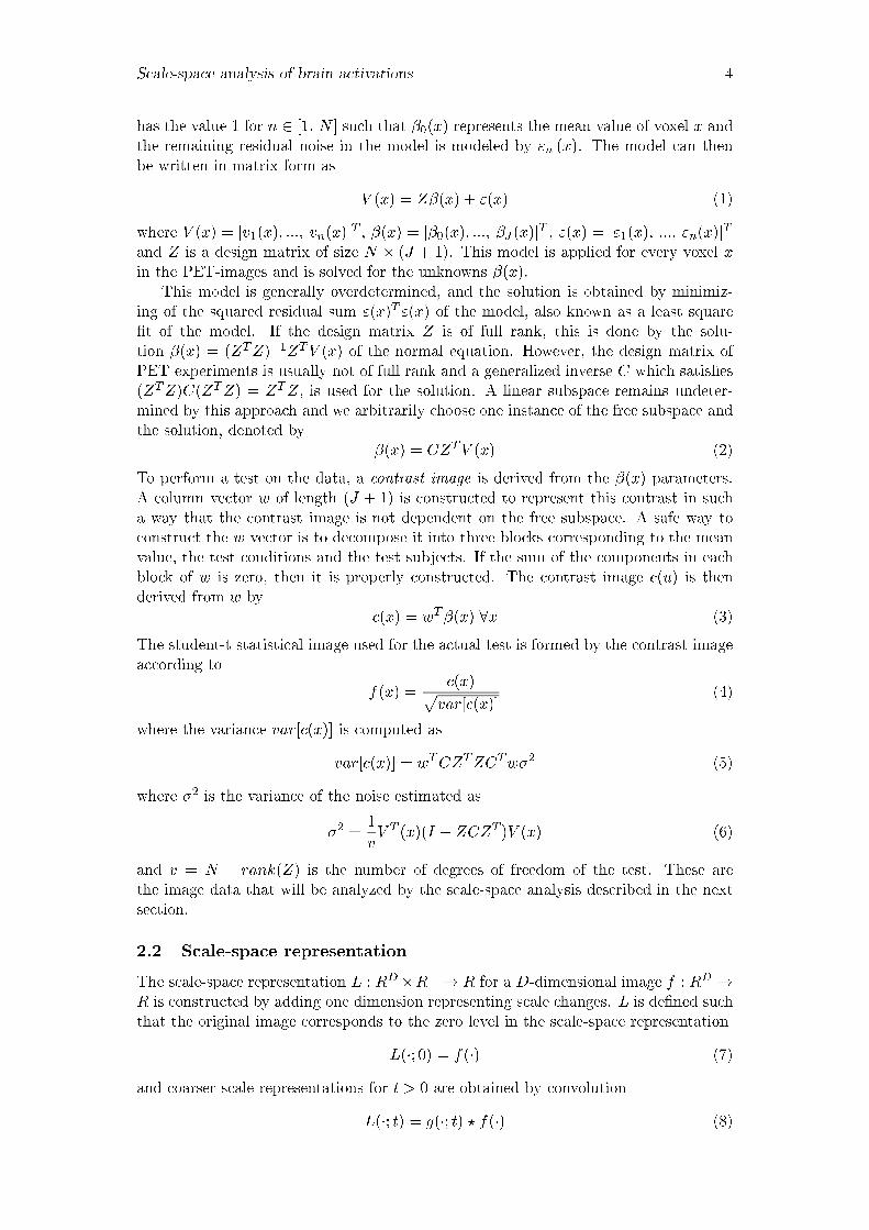
A grey-level blob is de�ned at a single scale and represents a local intensity extremum

point Pe at a given scale t with a surrounding spatial support region, delimited by an

intensity level curve through the delimiting saddle point Psaddle of the grey level blob.

For bright blobs, the extremum point is a local maximum and the delimiting saddle

point is the highest possible point, where a path can be traced to both the local max-

imum belonging to the blob, and another local maximum, without descending below

the saddle point. The support region GR of the blob is the set of points inside the

delimiting level curve, that have an intensity value greater than the intensity of the

level curve (see �gure 1).

The volume Gvol�rel of the grey-level blob at scale t with original relative base level

is de�ned as

Gvol�rel =

ZGR

L(x; t)� L(Psaddle; t) dx (10)

Later, this entity will be used when formulating a quantitative measure of the signi�-

cance of the grey-level blob.

Figure 1: De�nition of the grey-level blob in the two-dimensional case. The intensity is along

the Z-axis.


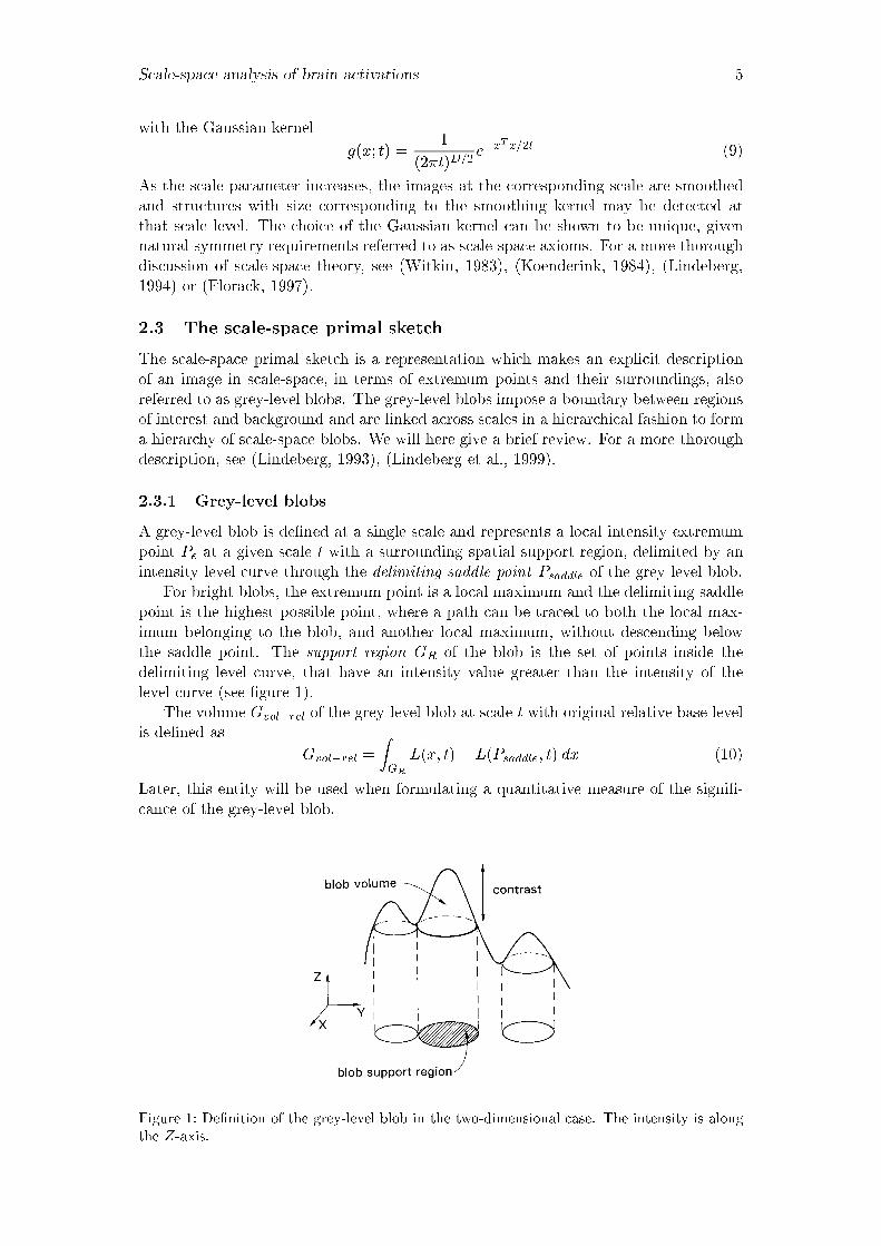
2.3.2 Grey-level blobs with absolute base level

An alternative approach for measuring the grey-level blob volume is to use an absolute

base level. The motivation for the relative base level is that in intensity images there

is no absolute reference level to relate the intensity measurements to. When analyzing

data with an absolute reference level, such as those produced by the general linear

model, one may consider the approach of de�ning the grey-level blob volume relative

to this reference level. Thus, the grey-level blob volume with absolute base-level is

de�ned by

Gvol�abs =

( RGR

L(x; t) dx if L(Psaddle; t) � 0RGR

L(x; t)� L(Psaddle; t) dx if L(Psaddle; t) < 0(11)

where GR is the support region and Psaddle is the position of the delimiting saddle point

for this grey-level blob. This relates the blob volumes to the absolute zero base level

suitable for PET images. To have a graceful transition for blobs with a negative saddle

point intensity, the calculation of the volumes for these blobs uses the intensity of the

saddle point as the base-level. This de�nition is illustrated in �gure 2.

��

��

��

��

��

��

��

��

��

��

��

Absolute base levelRelative base level

Figure 2: The de�nition of grey-level blob volume using a relative base level is based on local

contrasts measured relative to the delimiting saddle point of the grey-level blob, while de�nition

of grey-level blob volume using absolute base level is based on contrasts relative to a zero base

level. For blobs that contain negative intensity values, however, we always use the de�nition

in term of relative base level.

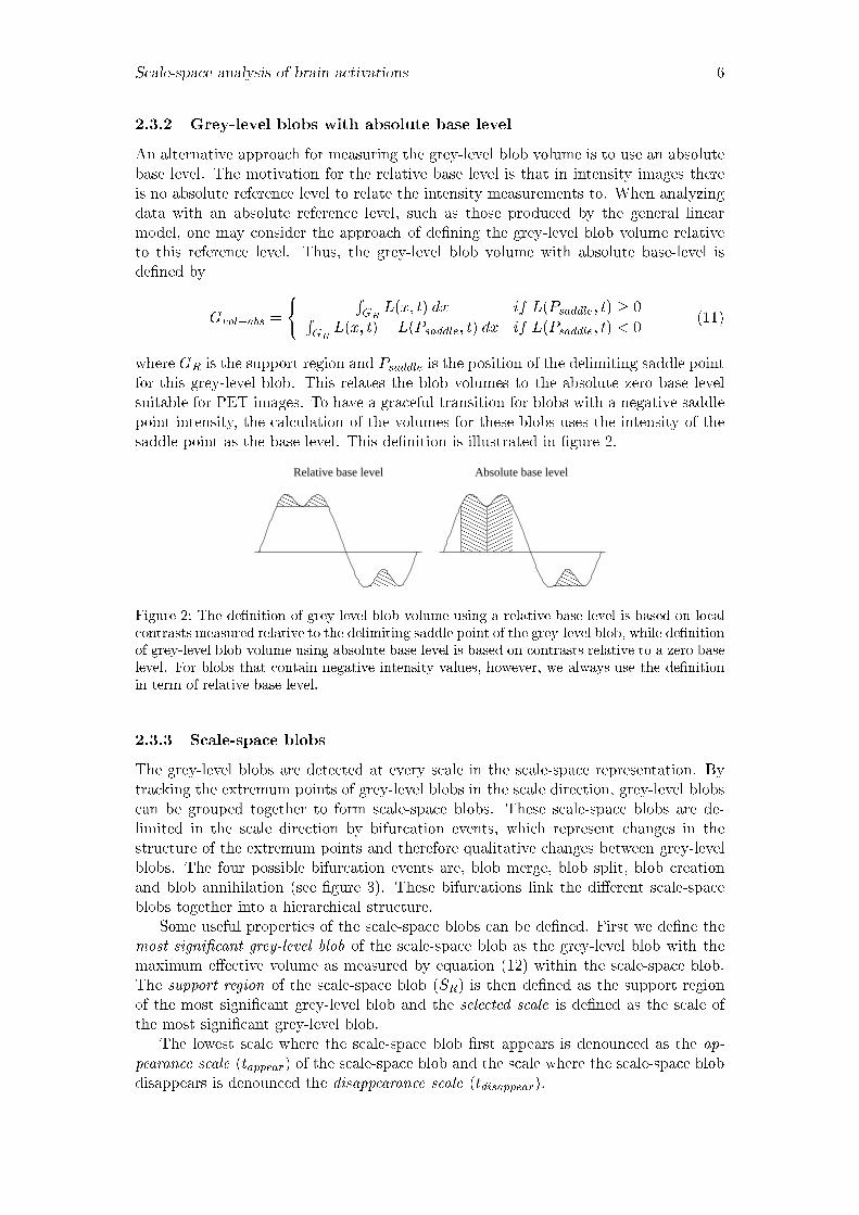
2.3.3 Scale-space blobs

The grey-level blobs are detected at every scale in the scale-space representation. By

tracking the extremum points of grey-level blobs in the scale direction, grey-level blobs

can be grouped together to form scale-space blobs. These scale-space blobs are de-

limited in the scale direction by bifurcation events, which represent changes in the

structure of the extremum points and therefore qualitative changes between grey-level

blobs. The four possible bifurcation events are, blob merge, blob split, blob creation

and blob annihilation (see �gure 3). These bifurcations link the di�erent scale-space

blobs together into a hierarchical structure.

Some useful properties of the scale-space blobs can be de�ned. First we de�ne the

most signi�cant grey-level blob of the scale-space blob as the grey-level blob with the

maximum e�ective volume as measured by equation (12) within the scale-space blob.

The support region of the scale-space blob (SR) is then de�ned as the support region

of the most signi�cant grey-level blob and the selected scale is de�ned as the scale of

the most signi�cant grey-level blob.

The lowest scale where the scale-space blob �rst appears is denounced as the ap-

pearance scale (tappear) of the scale-space blob and the scale where the scale-space blob

disappears is denounced the disappearance scale (tdisappear).


d)c)b)

a)

Figure 3: Generic blob events in the scale-space (a) annihilation, (b) merge, (c) split, (d)

creation. Here, the scale parameter is along the vertical axis.

2.3.4 Signi�cance of scale-space blobs

The signi�cance measure of the scale-space blobs should be a measure of the underlying

structure of the activations in the image. A more signi�cant activation should result in

a higher signi�cance measure and noise should give scale-space blobs with lower signif-

icance measures. As argued in (Lindeberg, 1993), the following following components

are natural to include in a signi�cance measure:

� spatial extent x: A grey-level blob having large spatial extent, may be treated as

more signi�cant than a smaller grey-level blob.

� contrast z: A grey-level blob with a high contrast value may be treated as more

signi�cant than a similar grey-level blob with a lower contrast.

� lifetime � : A grey-level blob with a long lifetime in scale-space, may be treated

as more signi�cant than a similar grey-level blob with a shorter lifetime.

Measuring spatial extent and contrast. When measuring spatial extent and con-

trast, a natural requirement is to allow for comparison of grey-level blob volumes across

scales. This is done by normalizing the grey-level blob volume Gvol by

Vprel =Gvol � Vm(t)

V�(t)(12)

where Vm(t) is the mean and V�(t) the standard deviation of grey-level blob volumes

at the scale t. The Vm(t) and V�(t) functions are estimated from statistics reference

noise images. (see section 3.1)

The entity Vprel is, however, not suitable for scale integration, since it can assume

negative values. A normalization that empirically has given reasonable results is

Veff =

(1 + Vprel when Vprel � 0;

eVprel when Vprel < 0:(13)

Measuring scale lifetime. When measuring scale lifetime it is natural to require

that the expected lifetime of a scale space blob should not vary over scales. This leads

to a transformation function of the form

�eff (t) = C1 + C2 log(p(t)) (14)

where p(t) is the expected density of extrema at scale t and C1 and C2 are constants,

where C1 without loss of generality can be set to zero. In our case, �eff (t) is calculated

as

�eff (t) = log

pref(0)

pref (t)

!(15)

where pref(t) denotes the average density of local extrema as a function of scale t.


Computing the scale space volume. Finally, given the transformed entities �effand Veff , the scale-space blob volume is then de�ned by

Svol =

Z tdisappear

tappear

Veff (t)d�eff (t) (16)

where tappear is the appearance scale of the scale-space blob, tdisappear is the disap-

pearance scale of the scale-space blob. The entity Svol will be used as the signi�cance

measure for the scale-space blob, and thus for ranking brain activations in order of

signi�cance.

3 Methods

3.1 Collecting reference statistics

The de�nition of the scale-space blob volume according to (16) as a signi�cance mea-

sure for ranking blobs in order of signi�cance relies on the the accumulation of reference

statistics of the behavior of blob descriptors in scale-space, in order to allow for the

comparison between image structures at di�erent scales. The idea is that reference

statistics of Vm(t), V�(t) and pref(t) in (12) and (15) should be collected for repre-

sentative image data containing noise with similar characteristics at the PET images,

however, disregarding the e�ect of coarser scale brain activations.

In the original work on the scale-space primal sketch for computer vision ap-

plications, white noise was used for this normalization purpose. The idea behind

this choice was to estimate to what extent accidental groupings occur in scale-space

(Lindeberg, 1993). Later, also self-similar noise patterns have been considered for scale

normalization (Lindeberg, 1998). When analyzing PET images, however, the imaging

and reconstruction procedures lead to a preferred inner scale of the data, which we want

to capture in order to avoid an unnecessary bias to image structures corresponding to

these artifacts related to the imaging procedure. For these reasons, di�erence images

between di�erent PET experiments as well as student-t images from PET experiments

were used for scale normalization (Lindeberg et al., 1999).

In this work, we will use an extension of these ideas, by taking the detailed structure

of the pre-processing stages to the scale-space analysis into account. We propose that

the residual noise images "(x) obtained from the general linear model (1) are ideally

suited for the collection of reference statistics for scale normalization. The idea behind

this choice is that the general linear model applied to the composed PET experiment

should capture the overall brain activations in the data, and that image structures that

are not captured by this model could be regarded as a reasonable estimate of the noise

characteristics. Preliminary results by (Björkman et al., 1999) demonstrate that this

model has attractive properties for separating blobs representing brain activations in

PET images from blobs extracted from noise patterns.

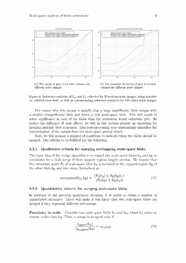
Figure 4 shows reference statistics of Vm(t), V�(t) collected in this way for 30 images,

using relative base level as well as absolute base level. For comparison, corresponding

results of using white noise normalization are also shown.

3.2 Merging of multiple responses

When using the scale-space primal sketch in practice, it sometimes occurs that an

activation in the image is represented by multiple blobs in the scale-space primal sketch,

although we from an intuitive viewpoint would regard the these blobs as corresponding

to the same image structure. (For one example, see �gure 5 on page 12.)


10−1

100

101

102

100

101

102

Mean grey level blob volume

White Gaussian noise imagesResidual noise images using absolute base levelResidual noise images using relative base level

(a) The mean of grey level blob volumes for

di�erent noise images.

10−1

100

101

102

100

101

102

103

Standard deviation of grey level blob volumes

White Gaussian noise imagesResidual noise images using absolute base levelResidual noise images using relative base level

(b) The standard deviation of grey level blob

volumes for di�erent noise images.

Figure 4: Reference statistics of Vm and V� collected for 30 residual noise images, using absolute

vs. relative base level, as well as corresponding reference statistics for 100 white noise images.

The reason why this occurs is usually that a large (signi�cant) blob merges with

a smaller (insigni�cant) blob and forms a new scale-space blob. This will result in

lower signi�cance in each of the blobs than the activation would otherwise give. To

reduce the in�uence of such e�ects, we will in this section present an algorithm for

merging multiple blob responses. This post-processing step substantially simpli�es the

interpretation of the output from the scale-space primal sketch.

Next, we will propose a number of conditions to indicate when two blobs should be

merged. The criteria to be ful�lled are the following:

3.2.1 Qualitative criteria for merging overlapping scale-space blobs

The basic idea of the merge algorithm is to regard two scale-space blobs bA and bB as

candidates for a blob merge if their support regions largely overlap. We require that

the extremum point Pe of scale-space blob bA is included in the support-region SR of

the other blob bB and vice versa, formalized as:

mergecand(bA; bB) =(Pe(bA) 2 SR(bB)) ^

(Pe(bB) 2 SR(bA))(17)

3.2.2 Quantitative criteria for merging scale-space blobs

In addition to the previous qualitative criterion, it is useful to de�ne a number of

quantitative measures. These will make it less likely that two scale-space blobs are

merged if they represent di�erent activations.

Proximity in scale. Consider two scale-space blobs bA and bB, where bA exists at

coarser scales than bB . Then, a merge is accepted only if

tappear(bA)

tdisappear(bB)< streshold (18)


Similarity in the size of the support region. A merge between two scale-space

blobs bA and bB is accepted only if the size of the support region is similar. That is, if

��log size[SR(bA)]size[SR(bB)]

�� < vtreshold (19)

3.2.3 Merging order

Two scale-space blobs bA and bB are considered for a merge only if all the previous

conditions are satis�ed. After establishing that two blobs could be merged, one has to

establish in which order the merging should occur. In this application, we �rst group

all blobs that are related according to the abovementioned criteria into groups. Then,

within each group, we �rst merge the two blobs that are nearest to each other in the

scale direction.

Here, distances in the scale direction are measured as relative variations. For two

scale-space blobs bA and bB, where bA exists at coarser scales than bB , the distance

d(A;B) between these blobs is de�ned as

d(bA; bB) = dAB = logtappear(bA)

tdisappear(bB)(20)

3.3 Merging of blobs

When merging two scale-space blobs, there are two natural ways to compute the signif-

icance value of the new blob. One approach is to just add the scale-space blob volumes

of the scale-space blobs. This is clearly a conservative approach. Another approach

is to extend the extent of the scale-space blob over the entire scale range of the two

primitive scale-space blobs, and to �ll in the scale interval in between. The signi�cance

value of the merged scale-space blob will then be composed of both the sum of the two

primitive scale-space blob volumes, incremented by the result of interpolating grey-level

blob volumes in the scale interval in between. Here, the latter approach is chosen.

3.4 Composed scale-space blob merging algorithm

In summary, the blob merging algorithm consist of the following steps. Let the set

of all scale-space blobs in the image be denoted by B. Each blob in B is denoted by

bi, where 1 � i � n and n is the number of blobs. If the conditions (17), (18) and

(19) in sections 3.2.1 and 3.2.2 are satis�ed, then we say that the blob merge criterion

C(bi; bj) = cij is true. Since this relationship is symmetric, it follows that cij = cji.

1. For each blob bi, select the subset M(bi) that consist of all blobs bj that satisfy

cij = true.

2. All blobs with empty subsets M(bi) are moved to a set F . These blobs do not

need further processing.

3. Within each subset M(bi), compute the distances dij in the scale direction ac-

cording to equation (20) between all pairs (bi; bj) of blobs in this subset.

4. For each subset M(bi), determine the blob bmin(bi) with the minimum distance

dmin(bi) where

dmin(bi) = minfj:cij=trueg

d(bi; bj) (21)


5. If a pair of blobs (bj ; bk) satis�es (bmin(bj) = bk) ^ (bmin(bk) = bj), then these

blobs are merged to a new blob bl. All relevant descriptors for bl are computed.

All blobs in the subsets M(bj) and M(bk) are tested according to the blob merge

criteria against bl and possibly included in subset M(bl). Finally, the blobs bjand bk are removed.

6. Continue with step 2-5 until there is no non-empty subset M(bi).

3.5 Parameter setting of merging algorithm

There are two free parameters in the algorithm, streshold in equation (18) and vtresholdin equation (19):

� vtreshold is a threshold determining when two scale-space blobs are su�ciently

similar in size. Here, we use log 2D, where D is the dimensionality of the data.

� streshold is a threshold determining when two blobs are su�ciently close enough

in scale direction. Here, we use streshold = 22.

These parameter settings have been demonstrated to give reasonable results in our

experiments, and are kept constant.

3.6 Measure of signi�cance change

To quantify how much the signi�cance values are a�ected by measuring the grey-level

blob volumes using an absolute base level compared to a relative base-level, we intro-

duce a measure of signi�cance change in the following way:

First, a regression model is computed between the scale-space blob volumes Svol�reliusing relative base level and the scale-space blob volumes Svol�absi using absolute base

level. In other words, a constant c is �tted from a least squares �t of

log10 Svol�absi = log10 Svol�reli + log10 c (22)

over a range of blobs, where we have introduced a logarithmic transformation to em-

phasize the impact of relative variations. Then, a local descriptor Di of how much the

signi�cance value has changed for a single blob is de�ned as

Di = log10 Svol�absi � log10 Svol�reli � log10 c (23)

This local descriptor gives us an indication of how much the signi�cance have changed

in comparison to other blobs in the same image when changing the signi�cance measure.

4 Experiments

4.1 Blob merging on synthetic images with noise

To evaluate the behavior of the merging algorithm, we shall �rst investigate its behavior

on synthetic images consisting of randomly positioned Gaussian peaks with added white

Gaussian noise.


(a) Original image with 10 Gaussian peaks

and white Gaussian noise.

(b) The 50 most signi�cant scale-space blobs,

detected from the grey-level image

(c) Blob support regions after merging.

0 50 100 150 200 2500

50

100

150

200

250

1

2

3

4

5

6

7

8

9

10 11

12

13

14

1516

17

18

19

20

21

(d) Ranking of the blobs after merging, over-

layed on blob boundaries.

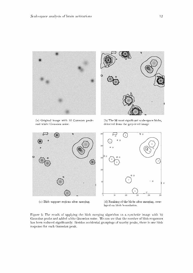
Figure 5: The result of applying the blob merging algorithm to a synthetic image with 10

Gaussian peaks and added white Gaussian noise. We can see that the number of blob responses

has been reduced signi�cantly. Besides accidental groupings of nearby peaks, there is one blob

response for each Gaussian peak.


Experimental setup. Ten Gaussian peaks, all with the same integral mass of 20,

and randomly selected standard deviations � in [3; 10] were randomly positioned in

a 256x256 image. White Gaussian noise with standard deviation of 0:01 was added

to the signal (�gure 5(a)). The noise level was selected to induce the e�ect of high

blob fragmentation. The scale-space primal sketch was applied to this image, and the

50 most signi�cant blobs were selected (�gure 5(b)). Originally there were about 104

scale-space blobs in the data.

Evaluation of blob merging. As can be seen from the results in �gure 5(b), some

of the Gaussian peaks give rise to multiple blob responses. Figure 5(c) shows the

results after blob merging, using the algorithm in section 3.4. As can be seen, the

results are intuitively very reasonable. For most of the Gaussian peaks, there is a

unique corresponding scale-space blob and this blob has a high signi�cance value. For

three nearby blobs in the upper right corner, the algorithm in addition �nds blobs

corresponding to the union of two or more nearby blobs. These blobs correspond to

hierarchical grouping of the blobs, and should not be merged by the algorithm.

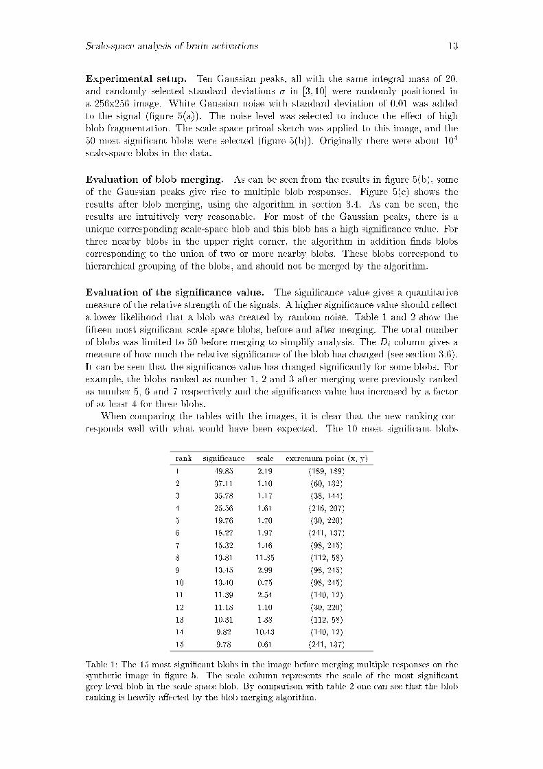
Evaluation of the signi�cance value. The signi�cance value gives a quantitative

measure of the relative strength of the signals. A higher signi�cance value should re�ect

a lower likelihood that a blob was created by random noise. Table 1 and 2 show the

�fteen most signi�cant scale-space blobs, before and after merging. The total number

of blobs was limited to 50 before merging to simplify analysis. The Di column gives a

measure of how much the relative signi�cance of the blob has changed (see section 3.6).

It can be seen that the signi�cance value has changed signi�cantly for some blobs. For

example, the blobs ranked as number 1, 2 and 3 after merging were previously ranked

as number 5, 6 and 7 respectively and the signi�cance value has increased by a factor

of at least 4 for these blobs.

When comparing the tables with the images, it is clear that the new ranking cor-

responds well with what would have been expected. The 10 most signi�cant blobs

rank signi�cance scale extremum point (x, y)

1 49.85 2.19 (189, 189)

2 37.11 1.10 (60, 132)

3 35.78 1.17 (38, 144)

4 25.56 1.61 (216, 207)

5 19.76 1.70 (30, 220)

6 18.27 1.97 (241, 137)

7 15.32 1.46 (98, 245)

8 13.81 11.85 (112, 58)

9 13.45 2.99 (98, 245)

10 13.40 0.75 (98, 245)

11 11.39 2.54 (140, 12)

12 11.18 1.10 (30, 220)

13 10.31 1.38 (112, 58)

14 9.82 10.43 (140, 12)

15 9.78 0.61 (241, 137)

Table 1: The 15 most signi�cant blobs in the image before merging multiple responses on the

synthetic image in �gure 5. The scale column represents the scale of the most signi�cant

grey-level blob in the scale-space blob. By comparison with table 2 one can see that the blob

ranking is heavily a�ected by the blob merging algorithm.


rank signi�cance scale extremum point (x, y) blobs before merge Di

1 71.03 0.61 (30, 220) 5, 12, 17, 21, 27, 29, 36, 39 0.4064

2 65.32 0.61 (241, 137) 6, 15, 22, 25, 26, 33 0.4040

3 64.52 0.75 (98, 245) 7, 9, 10, 18, 32, 50 0.4751

4 59.51 1.70 (189, 189) 1, 16 -0.0724

5 50.37 1.03 (140, 13) 11, 14, 19, 20, 35, 38 0.4963

6 47.65 0.89 (59, 132) 2, 28, 49 -0.0408

7 44.92 1.38 (112, 58) 8, 13, 23, 30 0.3631

8 40.91 1.17 (38, 144) 3, 34 -0.0911

9 25.56 1.61 (216, 207) 4 -0.1493

10 6.10 0.54 (189, 189) 24 -0.1493

11 4.87 108.64 (193, 186) 31 -0.1493

12 4.07 31.38 (255, 45) 37 -0.1493

13 3.90 1.31 (4, 159) 40 -0.1493

14 3.75 1.61 (32, 195) 41 -0.1493

15 3.63 1.17 (162, 251) 42 -0.1493

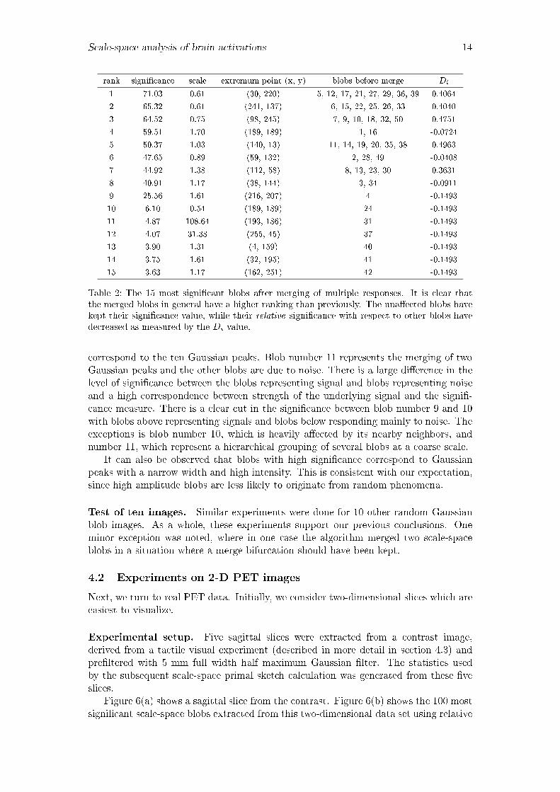
Table 2: The 15 most signi�cant blobs after merging of multiple responses. It is clear that

the merged blobs in general have a higher ranking than previously. The una�ected blobs have

kept their signi�cance value, while their relative signi�cance with respect to other blobs have

decreased as measured by the Di value.

correspond to the ten Gaussian peaks. Blob number 11 represents the merging of two

Gaussian peaks and the other blobs are due to noise. There is a large di�erence in the

level of signi�cance between the blobs representing signal and blobs representing noise

and a high correspondence between strength of the underlying signal and the signi�-

cance measure. There is a clear cut in the signi�cance between blob number 9 and 10

with blobs above representing signals and blobs below responding mainly to noise. The

exceptions is blob number 10, which is heavily a�ected by its nearby neighbors, and

number 11, which represent a hierarchical grouping of several blobs at a coarse scale.

It can also be observed that blobs with high signi�cance correspond to Gaussian

peaks with a narrow width and high intensity. This is consistent with our expectation,

since high amplitude blobs are less likely to originate from random phenomena.

Test of ten images. Similar experiments were done for 10 other random Gaussian

blob images. As a whole, these experiments support our previous conclusions. One

minor exception was noted, where in one case the algorithm merged two scale-space

blobs in a situation where a merge bifurcation should have been kept.

4.2 Experiments on 2-D PET images

Next, we turn to real PET data. Initially, we consider two-dimensional slices which are

easiest to visualize.

Experimental setup. Five sagittal slices were extracted from a contrast image,

derived from a tactile visual experiment (described in more detail in section 4.3) and

pre�ltered with 5 mm full width half maximum Gaussian �lter. The statistics used

by the subsequent scale-space primal sketch calculation was generated from these �ve

slices.

Figure 6(a) shows a sagittal slice from the contrast. Figure 6(b) shows the 100 most

signi�cant scale-space blobs extracted from this two-dimensional data set using relative


Index_abs Sign_abs Scale_abs Index_rel Sign_rel Scale_rel Di

1 15.53 8.43 1 14.24 8.43 -0.0112

2 14.44 1.32 12 3.11 1.32 0.6186

3 10.21 0.00 10 3.61 0.00 0.4029

4 6.73 0.00 4 5.64 0.00 0.0277

5 5.79 0.00 3 7.75 0.00 -0.1751

6 5.34 0.00 17 2.18 0.00 0.3412

7 5.22 0.28 2 8.15 0.28 -0.2420

8 4.31 7.11 7 5.05 7.11 -0.1173

9 4.02 0.00 8 4.42 0.65 -0.0905

10 3.76 0.17 6 5.21 0.17 -0.1904

11 3.68 0.00 5 5.60 0.00 -0.2310

12 2.97 0.00 18 2.16 0.00 0.0886

13 2.97 0.00 9 3.65 0.00 -0.1391

14 2.54 0.17 16 2.31 0.17 -0.0082

15 2.52 0.65 14 2.67 0.65 -0.0741

16 2.48 0.28 20 1.72 0.28 0.1094

17 2.39 0.00 13 2.82 0.00 -0.1217

18 2.38 0.00 11 3.40 0.00 -0.2042

19 2.27 0.00 15 2.37 0.00 -0.0667

20 2.17 0.00 21 1.60 0.00 0.0829

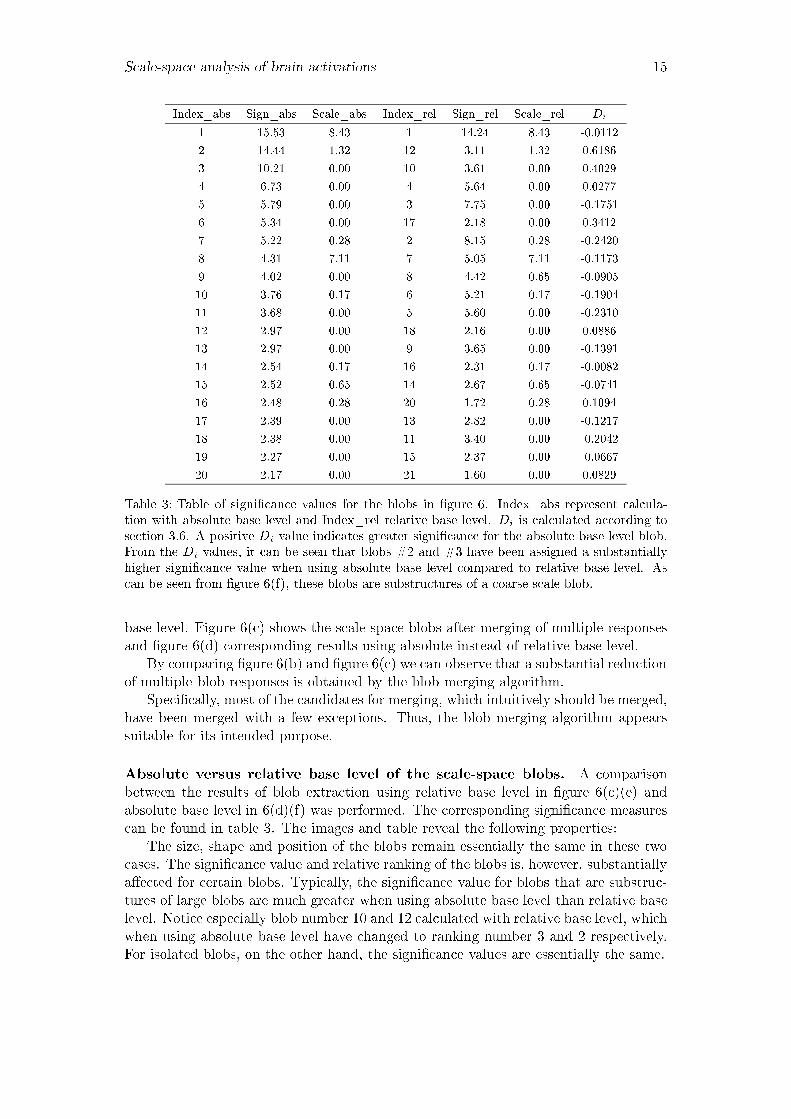
Table 3: Table of signi�cance values for the blobs in �gure 6. Index_abs represent calcula-

tion with absolute base level and Index_rel relative base level. Di is calculated according to

section 3.6. A positive Di value indicates greater signi�cance for the absolute base level blob.

From the Di values, it can be seen that blobs #2 and #3 have been assigned a substantially

higher signi�cance value when using absolute base level compared to relative base level. As

can be seen from �gure 6(f), these blobs are substructures of a coarse scale blob.

base level. Figure 6(c) shows the scale-space blobs after merging of multiple responses

and �gure 6(d) corresponding results using absolute instead of relative base level.

By comparing �gure 6(b) and �gure 6(c) we can observe that a substantial reduction

of multiple blob responses is obtained by the blob merging algorithm.

Speci�cally, most of the candidates for merging, which intuitively should be merged,

have been merged with a few exceptions. Thus, the blob merging algorithm appears

suitable for its intended purpose.

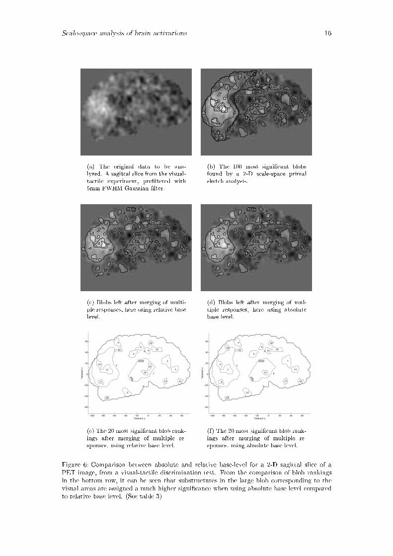
Absolute versus relative base level of the scale-space blobs. A comparison

between the results of blob extraction using relative base level in �gure 6(c)(e) and

absolute base level in 6(d)(f) was performed. The corresponding signi�cance measures

can be found in table 3. The images and table reveal the following properties:

The size, shape and position of the blobs remain essentially the same in these two

cases. The signi�cance value and relative ranking of the blobs is, however, substantially

a�ected for certain blobs. Typically, the signi�cance value for blobs that are substruc-

tures of large blobs are much greater when using absolute base level than relative base

level. Notice especially blob number 10 and 12 calculated with relative base level, which

when using absolute base level have changed to ranking number 3 and 2 respectively.

For isolated blobs, on the other hand, the signi�cance values are essentially the same.


(a) The original data to be ana-

lyzed. A sagittal slice from the visual-

tactile experiment, pre�ltered with

5mm FWHM Gaussian �lter.

(b) The 100 most signi�cant blobs

found by a 2-D scale-space primal

sketch analysis.

(c) Blobs left after merging of multi-

ple responses, here using relative base

level.

(d) Blobs left after merging of mul-

tiple responses, here using absolute

base level.

−100 −80 −60 −40 −20 0 20 40 60

−60

−40

−20

0

20

40

60

Talairach y

Tal

aira

ch z

1

2

3

4

5

6

7

8

9

10

11

12

13

14

15

16

17

18

19

20

(e) The 20 most signi�cant blob rank-

ings after merging of multiple re-

sponses, using relative base level.

−100 −80 −60 −40 −20 0 20 40 60

−60

−40

−20

0

20

40

60

Talairach y

Tal

aira

ch z

1

2

3

4

5

6

7

8

9

10

1112

13

14

1516

17 18

19

20

(f) The 20 most signi�cant blob rank-

ings after merging of multiple re-

sponses, using absolute base level.

Figure 6: Comparison between absolute and relative base-level for a 2-D sagittal slice of a

PET image, from a visual-tactile discrimination test. From the comparison of blob rankings

in the bottom row, it can be seen that substructures in the large blob corresponding to the

visual areas are assigned a much higher signi�cance when using absolute base level compared

to relative base level. (See table 3)


4.3 Experiments on 3-D PET images

A study has been performed to evaluate the e�ect of using absolute base level instead

of relative base level on real 3-D PET data. Two di�erent PET experiments were used

for this evaluation. One study involved a tactile-visual contrast where the subject had

an ellipsoid in their hand and was supposed to match it to visually presented ellipsoids

of di�erent shapes. The second study was a forced choice discrimination test, where

the subject was to choose which one of two parallellepipeda had the most oblong shape.

Tactile visual experiment. This study, originally described in (Hadjikhani and

Roland, 1998), consists of eight test subjects, performing four di�erent test conditions

with three repetitions of every test condition. Some PET-images were excluded due to

artifacts and the total number of images used in the study was 93. The test conditions

consisted of matching between di�erent ellipsoids, presented visually and tactically, to

the subjects. The four test-conditions were, tactile-tactile matching (TT), tactile-visual

matching (TV), visual-visual matching (VV) and a motor control resting condition

(rest).

The PET images were realigned within subjects to compensate for movements be-

tween acquisitions, and reformatted to standard form using the human brain atlas

of (Roland et al., 1994). There was no pre�ltering of the data at this stage. These

preprocessed images formed the input data to the general linear model, described in

section 2.1. Thirteen parameters were used in the model: one for the mean, four for

the di�erent test-conditions and eight for the test subjects.

The residual noise "i(x) in the general linear model was used for estimating the

noise in the PET-images. From the "i(x) images, a number of synthetic random noise

images were derived through a process described in (Ledberg, 1999). The synthetic

random noise images were used to estimate Vm(t), V�(t) and �eff (t) in the scale-space

primal sketch.

The contrast derived from the GLM model was the tactile-visual contrast with

all the subjects and repetitions in it. This is the same contrast as in (Lindeberg

et al., 1999). The contrast image was analyzed in 3-D with the scale-space primal

sketch. Multiple responses were merged and a mask was applied to remove scale-space

blobs outside the brain.

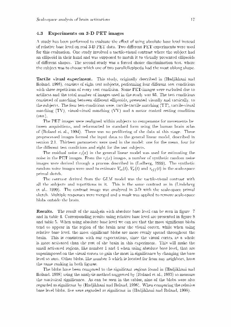
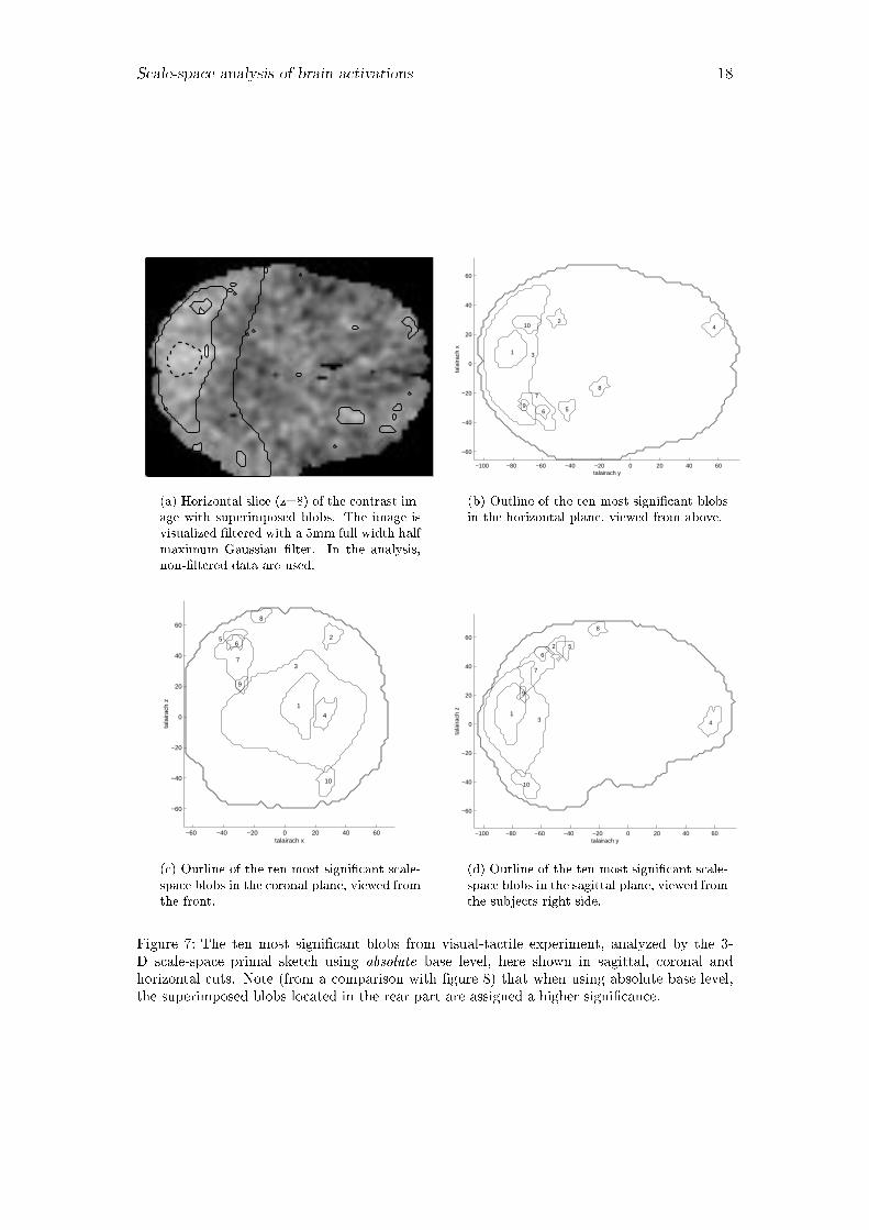
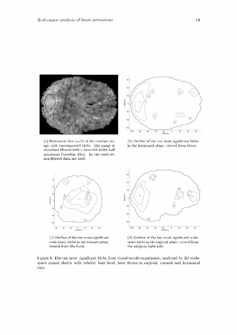
Results. The result of the analysis with absolute base level can be seen in �gure 7

and in table 4. Corresponding results using relative base level are presented in �gure 8

and table 5. When using absolute base level we can see that the most signi�cant blobs

tend to appear in the region of the brain near the visual cortex, while when using

relative base level, the most signi�cant blobs are more evenly spread throughout the

brain. This is consistent with our expectations, since the visual cortex as a whole

is more activated than the rest of the brain in this experiment. This will make the

small activated regions, like number 1 and 4 when using absolute base level, that are

superimposed on the visual cortex to gain the most in signi�cance by changing the base

level to zero. Other blobs, like number 5 which is located far from any neighbors, have

the same ranking in both �gures.

The blobs have been compared to the signi�cant regions found in (Hadjikhani and

Roland, 1998) using the analysis method suggested by (Roland et al., 1993) to measure

the statistical signi�cance. As can be seen in the tables, nine of the blobs were also

regarded as signi�cant by (Hadjikhani and Roland, 1998). When comparing the relative

base level blobs, �ve were regarded as signi�cant in (Hadjikhani and Roland, 1998).


(a) Horizontal slice (z=8) of the contrast im-

age with superimposed blobs. The image is

visualized �ltered with a 5mm full width half

maximum Gaussian �lter. In the analysis,

non-�ltered data are used.

−100 −80 −60 −40 −20 0 20 40 60

−60

−40

−20

0

20

40

60

talairach y

tala

irach

x

1

2

3

4

56

78

9

10

(b) Outline of the ten most signi�cant blobs

in the horizontal plane, viewed from above.

−60 −40 −20 0 20 40 60

−60

−40

−20

0

20

40

60

talairach x

tala

irach

z

1

2

3

4

56

7

8

9

10

(c) Outline of the ten most signi�cant scale-

space blobs in the coronal plane, viewed from

the front.

−100 −80 −60 −40 −20 0 20 40 60

−60

−40

−20

0

20

40

60

talairach y

tala

irach

z

1

2

3 4

56

7

8

9

10

(d) Outline of the ten most signi�cant scale-

space blobs in the sagittal plane, viewed from

the subjects right side.

Figure 7: The ten most signi�cant blobs from visual-tactile experiment, analyzed by the 3-

D scale-space primal sketch using absolute base level, here shown in sagittal, coronal and

horizontal cuts. Note (from a comparison with �gure 8) that when using absolute base level,

the superimposed blobs located in the rear part are assigned a higher signi�cance.


(a) Horizontal slice (z=8) of the contrast im-

age with superimposed blobs. The image is

visualized �ltered with a 5mm full width half

maximum Gaussian �lter. In the analysis,

non-�ltered data are used.

−100 −80 −60 −40 −20 0 20 40 60

−60

−40

−20

0

20

40

60

talairach y

tala

irach

x

1

2 3

4

56

7

8

9

10

(b) Outline of the ten most signi�cant blobs

in the horizontal plane, viewed from above.

−60 −40 −20 0 20 40 60

−60

−40

−20

0

20

40

60

talairach x

tala

irach

z

1

2

34

5

6

7

8

9

10

(c) Outline of the ten most signi�cant

scale-space blobs in the coronal plane,

viewed from the front.

−100 −80 −60 −40 −20 0 20 40 60

−60

−40

−20

0

20

40

60

talairach y

tala

irach

z

1

2

34

5

67

8

9

10




Figure 8: The ten most signi�cant blobs from visual-tactile experiment, analyzed by 3D scale-

space primal sketch with relative base level, here shown in sagittal, coronal and horizontal

cuts.


Indexabs

Sign

Scale

Position

Volmm3

Prev.sig

Indexrel

Signrel

Di

Regionname

1

71.67

5.92

(8,-82,8)

8672

yes

4

31.99

0.1170

visualcortex(V1,V2)

2

69.89

0.80

(34,-48,54)

736

yes

2

58.28

-0.1544

somatosensoryassociationcortex

3

59.89

20.57

(10,-82,8)

114704

yes

1

70.98

-0.3071

visualcortex

4

47.67

1.65

(26,57,-1)

1392

yes

34

10.19

0.4366

sulcusfrontalissup.sin.

5

39.32

1.25

(-31,-44,54)

776

yes

5

24.65

-0.0307

lobuspareitalissup.dxt.

6

28.55

0.86

(-33,-62,-52)

336

yes

12

15.10

0.0434

lobuspareitalissup.post.dxt.

7

27.58

6.36

(-31,-60,46)

5816

yes

23

12.37

0.1147

sulcusintraparetalisdxt.

8

25.25

1.51

(-19,-22,68)

656

yes

25

12.21

0.0824

premotorcortexdxt.

9

24.35

0.42

(-27,-72,20)

248

yes

14

14.74

-0.0152

visualcortexlobusoccipitalis

10

21.91

2.31

(28,-70,-41)

1496

no

21

12.59

0.0073

lobuspost.sin.cerebellum

11

21.82

0.70

(22,-56,-53)

256

no

8

16.91

-0.1224

lobuspost.dxt.

12

21.69

2.94

(4,-58,54)

1936

yes

13

14.76

-0.0661

precuneussin.

13

19,42

2.49

(-13,-88,1)

1048

yes

93

6.43

0.2465

visualcortex(V1,V2)

14

18.94

0.19

(34,-62,52)

168

yes

24

12.34

-0.0473

sulcusintrapareitalissin.

15

18.69

0.59

(54,-54,12)

368

no

33

10.26

0.0274

gyrustemp.sup.sin.

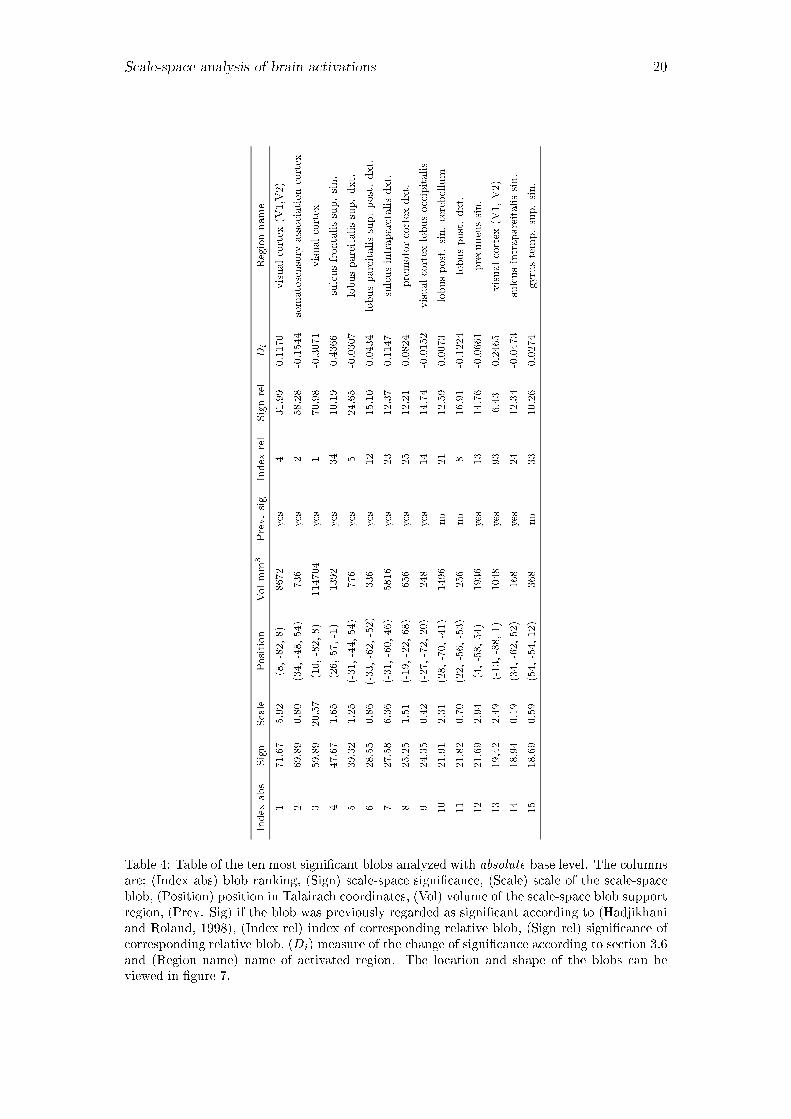
Table 4: Table of the ten most signi�cant blobs analyzed with absolute base level. The columns

are; (Index abs) blob ranking, (Sign) scale-space signi�cance, (Scale) scale of the scale-space

blob, (Position) position in Talairach coordinates, (Vol) volume of the scale-space blob support

region, (Prev. Sig) if the blob was previously regarded as signi�cant according to (Hadjikhani

and Roland, 1998), (Index rel) index of corresponding relative blob, (Sign rel) signi�cance of

corresponding relative blob, (Di) measure of the change of signi�cance according to section 3.6

and (Region name) name of activated region. The location and shape of the blobs can be

viewed in �gure 7.


Indexrel

Sign

Scale

Position

Volmm3

Prev.sig

Indexabs

Signabs

Di

Regionname

1

70.98

20.58

(10,-82,8)

114704

yes

3

59.89

0.0941

visualcortex

2

58.28

0.80

(34,-48,54)

736

yes

2

69.89

-0.0586

somatosensoryassociationcortex

3

53.44

2.94

(26,59,-1)

4120

yes

4

47.67

0.0699

sulcusfrontalissup.sin.

4

31.99

12.14

(10,-82,10)

22120

yes

1

71.67

-0.3301

visualcortex(V1,V2)

5

24.66

1.25

(-31,-44,54)

776

yes

5

39.32

-0.1823

lobuspareitalissup.dxt.

6

23.15

0.43

(-37,49,12)

392

no

25

14.26

0.2307

sulcusfrontalissup.dxt.

7

17.36

2.31

(-29,19,4)

2072

no

22

15.63

0.0659

insulaanteriordxt.

8

16.91

0.70

(22,-56,-53)

256

no

11

21.82

-0.0906

lobusposteriorsin.cerebellum

9

16.27

0.37

(-47,7,-19)

184

no

68

8.29

0.3132

polustemporalisdxt.

10

15.99

2.94

(30,21,14)

1560

no

61

9.03

0.2687

insulaanteriorsin.

11

15.29

0.86

(34,-15,-15)

424

no

44

10.44

0.1860

amygdalasin.

12

15.10

0.86

(-33,-62,52)

336

yes

6

28.55

-0.2565

lobuspareitalissup.post.dxt.

13

14.76

2.94

(4,-58,54)

1936

yes

12

21.69

-0.1469

precuneussin.

14

14.74

0.43

(-27,-72,20)

248

yes

9

24.35

-0.1979

visualcortexlobusoccipitalis

15

14.45

0.19

(-43,-5,-33)

80

no

69

8.23

0.2527

polustemporalisdxt.

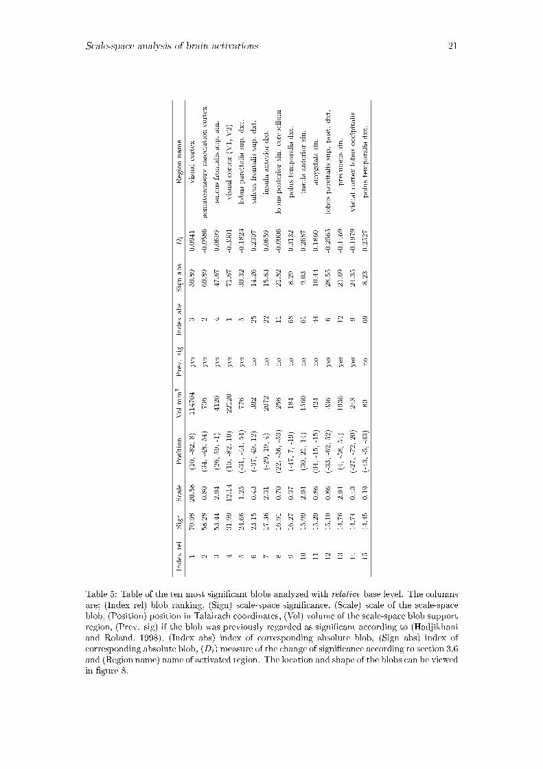
Table 5: Table of the ten most signi�cant blobs analyzed with relative base level. The columns

are; (Index rel) blob ranking, (Sign) scale-space signi�cance, (Scale) scale of the scale-space

blob, (Position) position in Talairach coordinates, (Vol) volume of the scale-space blob support

region, (Prev. sig) if the blob was previously regarded as signi�cant according to (Hadjikhani

and Roland, 1998), (Index abs) index of corresponding absolute blob, (Sign abs) index of

corresponding absolute blob, (Di) measure of the change of signi�cance according to section 3.6

and (Region name) name of activated region. The location and shape of the blobs can be viewed

in �gure 8.


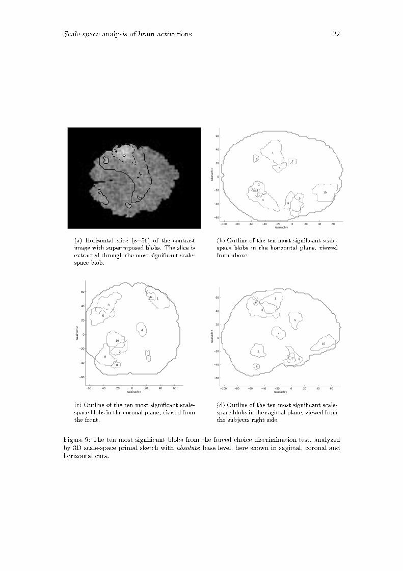
(a) Horizontal slice (z=56) of the contrast

image with superimposed blobs. The slice is

extracted through the most signi�cant scale-

space blob.

−100 −80 −60 −40 −20 0 20 40 60

−60

−40

−20

0

20

40

60

talairach y

tala

irach

x

1

2

3

4

5

67

8

9

10

(b) Outline of the ten most signi�cant scale-

space blobs in the horizontal plane, viewed

from above.

−60 −40 −20 0 20 40 60

−60

−40

−20

0

20

40

60

talairach x

tala

irach

z

1

2

3

4

5

6

7

8

9

10



the front.

−100 −80 −60 −40 −20 0 20 40 60

−60

−40

−20

0

20

40

60

talairach y

tala

irach

z

1

2

3

4

5

6

7

8

9

10




Figure 9: The ten most signi�cant blobs from the forced choice discrimination test, analyzed

by 3D scale-space primal sketch with absolute base level, here shown in sagittal, coronal and

horizontal cuts.


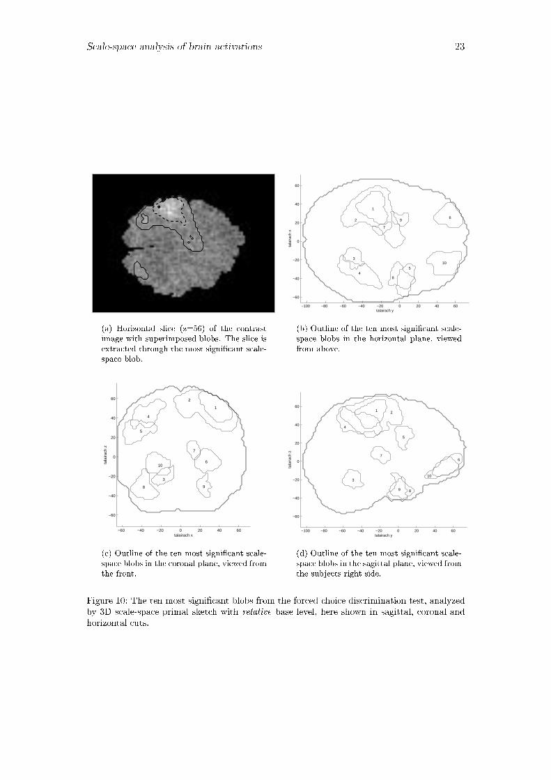
(a) Horizontal slice (z=56) of the contrast

image with superimposed blobs. The slice is

extracted through the most signi�cant scale-

space blob.

−100 −80 −60 −40 −20 0 20 40 60

−60

−40

−20

0

20

40

60

talairach y

tala

irach

x

1

2

3

45

6

7

8

9

10

(b) Outline of the ten most signi�cant scale-

space blobs in the horizontal plane, viewed

from above.

−60 −40 −20 0 20 40 60

−60

−40

−20

0

20

40

60

talairach x

tala

irach

z

1

2

3

4

5

6

7

8 9

10



the front.

−100 −80 −60 −40 −20 0 20 40 60

−60

−40

−20

0

20

40

60

talairach y

tala

irach

z

1 2

3

4

5

67

89

10




Figure 10: The ten most signi�cant blobs from the forced choice discrimination test, analyzed

by 3D scale-space primal sketch with relative base level, here shown in sagittal, coronal and

horizontal cuts.


Indexabs

Sign

Scale

Position

Volmm3

Prev.sig

Indexrel

Signrel

Di

Regionname

1

1214.42

1.65

(36,-28,56)

12016

yes

1

1450.10

-0.0747

Lsomatosensoryandmotorcortex

2

221.06

1.65

(-15,-52,-19)

3736

yes

3

224.18

-0.0037

Rlobusanteriorcerebellum

3

102.17

4.37

(-33,-42,44)

11896

yes

4

102.67

0.0002

Rinterpareitalsulcus

4

81.34

1.95

(12,-20,10)

2000

yes

7

73.38

0.0471

Lventrolateralthalamus

5

61.10

2.49

(-49,5,30)

5992

yes

5

90.08

-0.1662

Rmiddlefrontalgyrus

6

57.50

0.42

(26,-54,56)

408

yes

11

32.01

0.2567

Lsup.pareitallobe

7

52.71

0.80

(22,3,-29)

624

yes

9

62.72

-0.0732

Ltemporalpole

8

48.63

0.42

(-19,-54,-43)

368

yes

12

26.79

0.2613

Rlobusposteriorcerebellum

9

40.40

3.44

(-43,3,-33)

5592

yes

8

65.34

-0.2064

Rtemporalpole

10

32.35

4.71

(-27,55,-5)

6184

no

10

49.32

-0.1808

Rsuperiorfrontalsulcus

11

32.28

3.44

(30,53,-5)

5776

-

6

75.95

-0.3692

Lsuperiorfrontalsulcus

12

31.73

1.08

(-19,-20,64)

408

-

32

14.30

0.3485

Lgyrusprecentralis.

13

31.43

3.16

(22,-48,-23)

3176

-

27

15.34

0.3139

Llobusant.cerebelli

14

29.09

1.02

(8,-54,48)

552

-

15

22.45

0.1148

Lsup.parietalsulcus

15

25.89

1.45

(-35,-42,46)

488

-

59

9.86

0.4216

Rintraparietalsulcus

Table 6: Table of the the �fteen most signi�cant blobs from the forced choice discrimination

test analyzed with absolute base level. The columns are; (Index abs) blob ranking, (Sign)

scale-space signi�cance, (Scale) scale of the scale-space blob, (Position) position in Talairach

coordinates, (Vol) volume of the scale-space blob support region, (Prev. Sig) if the blob

was previously regarded as signi�cant according to (Roland et al., 1993), (Index rel) index of

corresponding relative blob, (Sign rel) signi�cance of corresponding relative blob, (Di) measure

of the change of signi�cance according to section 3.6 and (Region name) name of activated

region. The location and shape of the blobs can be viewed in �gure 9. (The dashes '�' in

rows 11-15 in column 'Prev sig.' indicate that these data are not available to us. (unpublished))


Indexrel

Sign

Scale

Position

Volmm3

Prev.sig

Indexabs

Signabs

Di

Regionname

1

1450.10

1.65

(36,-28,56)

12016

yes

1

1214.41

-0.0496

Lsomatosensoryandmotorcortex

2

512.79

10.25

(38,-28,54)

49680

yes

16

25.10

1.1836

Lsup-pre-motorandsom-sensorycor.

3

224.18

1.65

(-15,-52,-19)

3736

yes

2

221.06

-0.1205

Rlobusanteriorcerebellum

4

102.67

4.37

(-33,-42,44)

11896

yes

3

102.17

-0.1245

Rinterpareitalsulcus

5

90.08

2.49

(-49,5,30)

5992

yes

5

61.10

0.0420

Rmiddlefrontalgyrus

6

75.95

3.44

(30,53,-5)

5776

no

11

32.28

0.2451

Lsuperiorfrontalsulcus

7

73.38

1.95

(12,-20,10)

2000

yes

4

81.34

-0.1713

Lventrolateralthalamus

8

65.34

3.44

(-43,3,-33)

5592

yes

9

40.40

0.0821

Rtemporalpole

9

62.72

2.22

(22,3,-29)

2176

yes

7

52.71

-0.0511

Ltemporalpole

10

49.32

4.71

(-27,55,-5)

6184

no

10

32.35

0.0565

Rsuperiorfrontalsulcus

11

32.01

0.42

(26,-54,56)

408

-

6

57.50

-0.3810

Lsup.parietallobe

12

26.79

0.42

(-19,-54,-43)

368

-

8

48.63

-0.3856

Rlobusposteriorcerebellum

13

26.40

2.31

(48,-62,2)

2416

-

17

23.92

-0.0838

Linferiortemporalgyrus

14

23.19

0.86

(46,39,-11)

560

-

30

15.88

0.0378

Linferiortemporalgyrus

15

22.45

1.02

(8,-54,48)

552

-

14

29.09

-0.2392

Lsup.parietalsulcus

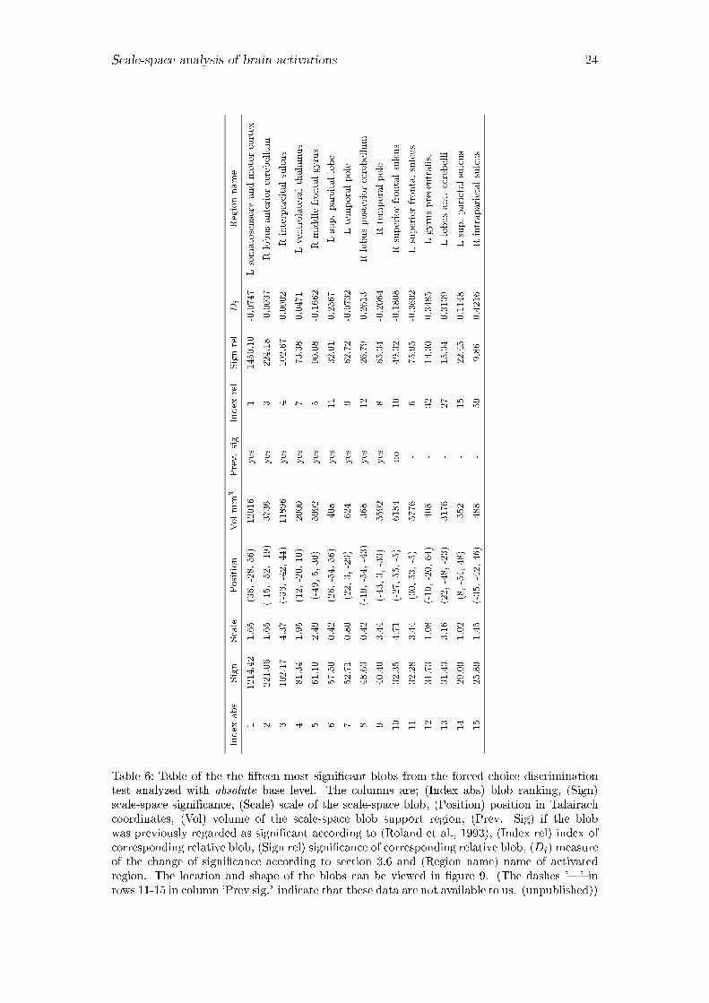
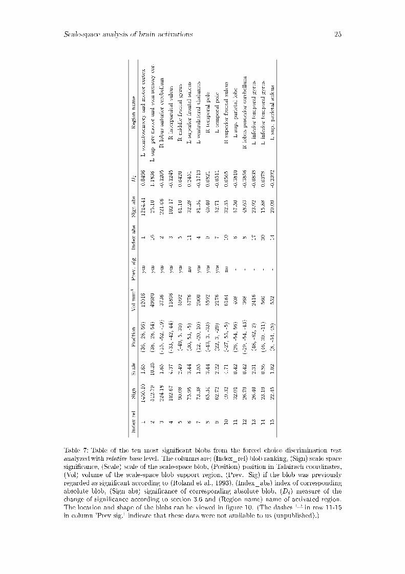
Table 7: Table of the ten most signi�cant blobs from the forced choice discrimination test

analyzed with relative base level. The columns are; (Index_rel) blob ranking, (Sign) scale-space

signi�cance, (Scale) scale of the scale-space blob, (Position) position in Talairach coordinates,

(Vol) volume of the scale-space blob support region, (Prev. Sig) if the blob was previously

regarded as signi�cant according to (Roland et al., 1993), (Index_abs) index of corresponding

absolute blob, (Sign abs) signi�cance of corresponding absolute blob, (Di) measure of the

change of signi�cance according to section 3.6 and (Region name) name of activated region.

The location and shape of the blobs can be viewed in �gure 10. (The dashes '�' in row 11-15

in column 'Prev sig.' indicate that these data were not available to us (unpublished).)


Forced choice discrimination experiment. This experiment was previously re-

ported in (Ledberg et al., 1999). The study consists of six test subjects, performing

one test condition and one rest condition with four repetitions of every condition. The

test condition consisted of discrimination between objects of oblonged shape.

The PET images were realigned within subjects and reformatted to standard format

using the human brain atlas of (Roland et al., 1994). There was no pre�ltering of the

data. These preprocessed images formed the input data to the general linear model,

described in section 2.1. Nine parameters were used in the model: one for the mean,

two for the di�erent test conditions and six for the test subjects.

The residual noise from the tactile visual experiment was used for estimating the

noise in the PET-images. From the "i(x) images, a number of synthetic noise images

were derived through a process described in (Ledberg, 1999). The synthetic noise

images were used to estimate Vm(t), V�(t) and �eff (t) in the scale-space primal sketch.

The contrast derived from the GLM model was the test condition contrasted against

the rest condition. The contrast image was analyzed in 3-D with the scale-space primal

sketch. Multiple responses were merged and a mask was applied to remove blobs outside

the brain.

Results. The result of the analysis when using an absolute base level can be seen

in �gure 9 and in table 6. For corresponding results using a relative base level, see

�gure 10 and table 7. With a relative base level, all the top ten ranked blobs have

a larger support volume than 2000 mm3 compared to using an absolute base level

where blobs number 6 to 8 have a support volume of less than 1000 mm3. Also, the

blob ranked as number 2 when using relative base level with a support volume of 49680

mm3 is not among the 15 most signi�cant blobs when using an absolute base level. The

matches between the support regions were perfect in all cases except one, where the

support regions overlapped but had di�erent spatial extent. The matching was done

with the 100 most signi�cant scale-space blobs in both the absolute and the relative

cases and the match is the best possible among those.

The blobs have been compared to the signi�cant regions found when using the

method described in (Roland et al., 1993). When using absolute base level, blob number

10 was not regarded as signi�cant. When using relative base level, blobs number 6 and

10 were not regarded as signi�cant.

5 Summary and discussion

We have presented a comparison of using two di�erent signi�cance measures in the

scale-space primal sketch applied on functional brain images. The original approach

of using a relative base level was compared to new proposed absolute base level, and

the purpose of this study was to investigate how this change a�ects the scale-space

blob signi�cance on PET contrast images as well as to what extent this in�uences the

relative ranking of the blobs.

The experiments indicate that an absolute base level gives a higher degree of cor-

respondence to an existing statistical method than using the relative base level. The

statistical method uses the existence of a global zero level, which is one assumption

underlying the argument for an absolute base level in the scale-space primal sketch. On

the other hand, this imposes a stronger assumption about stationarity of the signal,

which would be weaker when using a relative base level. In general the scale-space

primal sketch gives biologically meaningful responses when the position of the blobs

were compared to previously published brain activations in identical test setups (Seitz


et al., 1991), (Hadjikhani and Roland, 1998).

In the experiment in section 4.2 and the �rst experiment presented in section 4.3,

it was noted that small blobs superimposed on the visual cortex were assigned a higher

signi�cance when using an absolute base level. Since the blobs were superimposed

on larger activations they gained signi�cance by adding the intensity of the larger

activation to their signi�cance values. In the forced choice experiment presented in

section 4.3, it was noted that the absolute base level emphasizes small scale-space

blobs, while the relative base emphasizes large scale-space blobs in term of size of

support-region. It is a common phenomenon that small activations are superimposed

on larger ones. These small activations gain more signi�cance by using absolute base

level than larger sized activations. Thus, changing the base level to an absolute will in

general give a greater emphasis to smaller blobs relative to larger ones.

We have also presented a post-processing tool to the scale-space primal sketch for

merging multiple scale-space responses corresponding to the same activation. This tool

has been useful to give a better correspondence between activation strength and the

signi�cance of the scale-space blobs. This tool removes the need for choosing a scale-

space blob to represent an activation when multiple scale-space blob represent the same

activation and it also gives a more distinct di�erence between the signi�cance of blobs

corresponding to an activation and blobs corresponding to noise.

Moreover, we presented a new approach for collecting reference statistics for scale

normalization, using residual noise images from the general linear model.

References

Björkman, E., Lindeberg, T. and Roland, P. E. (1999). In preparation.

Coulon, O., Bloch, I., Frouin, V., and Mangin, J.-F. (1996). The structure of PET activation

maps, Proc. 3rd International Conference on Functional Mapping of the Human Brain,

Copenhagen, Denmark. Neuroimage vol. 5 no. 4 p 391, 1997.

Coulon, O., Bloch, I., Frouin, V. and Mangin, J.-F. (1997). Multi-scale measures in linear scale-

space for characterizing cerebral functional activations in 3D PET di�erence images, in

B. M. ter Haar Romeny, L. M. J. Florack, J. J. Koenderink and M. A. Viergever (eds),

Scale-Space Theory in Computer Vision: Proc. First Int. Conf. Scale-Space'97, Vol. 1252

of Springer verlag LNCS, Utrecht, The Netherlands, pp. 188�199.

Florack, L. M. J. (1997). Image Structure, Series in Mathematical Imaging and Vision, Kluwer

Academic Publishers, Dordrecht, Netherlands.

Friston, K. J., Frith, C. D., Liddle and Frackowiak, R. S. J. (1991). Comparing functional PET

images: The assessment of signi�cant change, J Cereb Blood Flow Metab 11: 81�95.

Friston, K. J., Worsley, K. J., Frackowiak, R. S. J., Mazziotta and Evans, A. C. (1994).

Assessing the signi�cance of focal activations using their spatial extent, Human Brain

Mapping 1: 210�220.

Hadjikhani, N. and Roland, P. (1998). Cross-modal transfer of information between the tactile

and the visual representations in the human brain � A PET study, J. of Neuroscience

18: 1072�1084.

Holmes, A. P., Blair, R. C., Watson, J. D. G. and Ford, I. (1996). Non-parametric analysis

of statistical images from functional mapping experiments, J Cereb Blood Flow Metab

16: 7�22.

Koenderink, J. J. (1984). The structure of images, Biological Cybernetics 50: 363�370.

Ledberg, A. (1999). Robust estimation of the probabilities of 3D clusters in functional brain

images: Application to PET data, Human Brain Mapping . in press.


Ledberg, A., Åkerman, S. and Roland, P. (1999). Estimation of the probabilities of 3-D clusters

in functional brain images, NeuroImage 8: 113�128.

Lidberg, P., Lindeberg, T. and Roland, P. (1996). Analysis of brain activation patterns using a

3-D scale-space primal sketch, Proc. 3rd International Conference on Functional Mapping

of the Human Brain, Copenhagen, Denmark, p. 393. Neuroimage vol. 5 no. 4 p 393, 1997.

Lindeberg, T. (1993). Detecting salient blob-like image structures and their scales with a scale-

space primal sketch: A method for focus-of-attention, International Journal of Computer

Vision 11(3): 283�318.

Lindeberg, T. (1994). Scale-Space Theory in Computer Vision, The Kluwer International

Series in Engineering and Computer Science, Kluwer Academic Publishers, Dordrecht,

the Netherlands.

Lindeberg, T. (1998). Feature detection with automatic scale selection, International Journal

of Computer Vision 30(2): 77�116.

Lindeberg, T., Lidberg, P. and Roland, P. (1999). Analysis of brain activation patterns using

a 3-D scale-space primal sketch, Human Brain Mapping 7(3): 166�194.

Poline, J.-B. and Mazoyer, B. (1993). Cluster analysis in individual functional brain images:

Some new techniques to enhance the sensitivity of activation detection methods, J Cereb

Blood Flow Metab 13: 425�437.

Roland, P. E. (1993). Brain Activation, John Wiley and Sons, New York.

Roland, P. E., Graufelds, J., Wåhlin, J., Ingelman, L., Andersson, M., Ledberg, A., Pedersen,

J., Åkerman, S., Dabringhaus, A. and Zilles, K. (1994). Human brain atlas: For high-

resolution functional and anatomical mapping, Human Brain Mapping 1: 173�184.

Roland, P. E., Levin, B., Kawashima, R. and Åkerman, S. (1993). Three-dimensional analysis

of clustered voxels in 15O-butanol brain activation images, Human Brain Mapping 1: 3�19.

Searle, S. (1971). Linear models, Wiley, New York.

Seitz, R., Roland, P., Bohm, C., Greitz, T. and Stone-Elander, S. (1991). Somatosensory dis-

crimination of shape-tactile exploration and cerebral activation, Eur. J. Neurosci. 3: 481�

492.

Witkin, A. P. (1983). Scale-space �ltering, Proc. 8th Int. Joint Conf. Art. Intell., Karlsruhe,

West Germany, pp. 1019�1022.

Worsley, K. J., Evans, A. C., Marrett, S. and Nelin (1992). A three-dimensional analysis for

CBF activation studies in human brain, J. Cereb. Blood Flow Metab. 12: 900�918.

Worsley, K. J., Marret, S., Neelin, P. and Evans, A. C. (1996b). Searching scale space for

activation in PET images, Human Brain Mapping 4: 74�90.

Evaluation of using absolute vs. relative base level ... - DiVA

Documents

Transcript of Evaluation of using absolute vs. relative base level ... - DiVA